Uniform confidence bands for pricing kernels - Statistik - Humboldt
45
Uniform confidence bands for pricing kernels 1 Wolfgang Karl H¨ ardle † , Yarema Okhrin ‡ 2 , Weining Wang § †Humboldt-Universit¨ at zu Berlin, CASE - Center for Applied Statistics and Economics, D-10178 Berlin, Germany. Email:[email protected] ‡University of Augsburg, Department of Statistics, D-86159 Augsburg, Germany. Email:[email protected] §Hermann Otto Hirschfeld Junior Professor at the Ladislaus von Bortkiewicz chair of statistics and C.A.S.E., Humboldt-Universit¨ at zu Berlin, Spandauer Straße 1, 10178 Berlin, Germany. Email:[email protected] 1 The financial support from the Deutsche Forschungsgemeinschaft via SFB 649 “ ¨ Okonomisches Risiko”, Humboldt-Universit¨ at zu Berlin is gratefully acknowledged. 2 Corresponding author. 1
Transcript of Uniform confidence bands for pricing kernels - Statistik - Humboldt

Uniform confidence bands for pricing kernels1
Wolfgang Karl Hardle†, Yarema Okhrin‡2, Weining Wang§
†Humboldt-Universitat zu Berlin, CASE - Center for Applied Statistics and Economics,
D-10178 Berlin, Germany. Email:[email protected]
‡University of Augsburg, Department of Statistics, D-86159 Augsburg, Germany.
Email:[email protected]
§Hermann Otto Hirschfeld Junior Professor at the Ladislaus von Bortkiewicz chair of statistics
and C.A.S.E., Humboldt-Universitat zu Berlin, Spandauer Straße 1, 10178 Berlin, Germany.
Email:[email protected]
1The financial support from the Deutsche Forschungsgemeinschaft via SFB 649 “Okonomisches
Risiko”, Humboldt-Universitat zu Berlin is gratefully acknowledged.2Corresponding author.
1

Abstract
Pricing kernels implicit in option prices play a key role in assessing the risk
aversion over equity returns. We deal with nonparametric estimation of the pricing
kernel (PK) given by the ratio of the risk-neutral density estimator and the histor-
ical density (HD). The former density can be represented as the second derivative
w.r.t. the European call option price function, which we estimate by nonparametric
regression. HD is estimated nonparametrically too. In this framework, we develop
the asymptotic distribution theory of the Empirical Pricing Kernel (EPK) in the
L∞ sense. Particularly, to evaluate the overall variation of the pricing kernel, we
develop a uniform confidence band of the EPK. Furthermore, as an alternative to
the asymptotic approach, we propose a bootstrap confidence band. The developed
theory is helpful for testing parametric specifications of pricing kernels and has a
direct extension to estimating risk aversion patterns. The established results are
assessed and compared in a Monte-Carlo study. As a real application, we test risk
aversion over time induced by the EPK.
Keywords: Empirical Pricing Kernel; Confidence Band; Bootstrap; Kernel Smooth-
ing; Nonparametric Fitting
JEL classification: C00; C14; J01; J31
1 Introduction
A challenging task in financial econometrics is to understand investors’ attitudes towards
market risk in its evolution over time. Such a study naturally involves stochastic discount
factors, empirical pricing kernels (EPK) and state price densities, see Cochrane (2001).
Asset pricing kernels (PKs) summarize investors’ risk preferences and the so called “EPK
paradox” exhibits when PKs are estimated from data, as several studies including Aıt-
Sahalia and Lo (2000), Rosenberg and Engle (2002), Brown and Jackwerth (2004) have
shown. Although in all these studies the EPK paradox (non-monotonicity) became evi-
dent, a test for the non-monotone behavior of the pricing kernel has not been devised yet.
2

A uniform confidence band is a very simple tool for such shape inspection. Confidence
bands drawn around an EPK based on asymptotic theory and bootstrap is the subject of
our paper. In addition, we relate critical values of our test to changing market conditions
given by exogenous time series.
The common difficulty is that the investors’ preference is implicit in the goods traded in
the market and thus can not be directly observed from the path of returns. A profound
martingale based pricing theory provides us one approach to tackle the problem from a
probabilistic perspective. An important concept involved is the State Price Density (SPD)
or Arrow-Debreu prices reflecting fair prices of one unit gain or loss for the whole market.
Under no arbitrage assumption, there exists at least one SPD, and when a market is
complete, this SPD is unique. Assuming a market is complete, pricing is done by taking
expected payoff under the risk neutral measure, which is related to the pdf of the historical
measure by multiplying with a stochastic discount factor, see Section 2 for a detailed
illustration. From an economic perspective, the price is formed according to the utility
maximization theory, which admits that the risk preference of consumers is connected to
the shape of utility functions. Specifically, a concave, convex or linear utility function
describes the risk averse, risk seeking or risk neutral behavior. Importantly, a stochastic
discount factor can be expressed via a utility function (Marginal Rate of Substitution),
which links the shape of pricing kernel to the risk patterns of investors, see Kahneman
and Tversky (1979), Jackwerth (2000), Rosenberg and Engle (2002) and others.
The above mentioned theory allows us to relate price processes of assets to risk preference
of investors. This amounts to fitting a flexible model and making inference on the dynam-
ics of EPKs over time. A well-known but restrictive approach is to assume the underlying
following a geometric Brownian motion. In this setting, SPDs and HDs are log normal
distributions with different drifts, and the parametrization of PK coincides with the con-
ditional expectation of marginal utilities when assuming a power utility function. Thus
it is decreasing in return and implies overall risk-averse behavior. However, across differ-
ent markets, one observes quite often a non-decreasing pattern for EPKs, a phenomenon
called the EPK paradox, see Chabi-Yo, Garcia and Renault (2008), Christoffersen, Heston
3

0.95 1 1.05 1.10
0.5
1
1.5
2
2.5
3
3.5
4
4.5
Figure 1: Examples of estimated inter-temporal pricing kernels (as functions of money-
ness) with fixed maturity 0.00833 (3 days) in years respectively on 17-Jan-2006 (blue),
18-Apr-2006 (red), 16-May-2006 (magenta), 13-June-2006 (violet), see Grith, Hardle and
Park (2013).
and Jacobs (2011).
Two plots of pricing kernels are shown in Figure 1 and Figure 2. Figure 1 depicts inter-
temporal pricing kernels with fixed maturity, while Figure 2 depicts pricing kernels with
two different maturities and their confidence bands. The figures are shown on return scale.
The curves present a bump in the middle and a switch from convexity to concavity in all
cases. Especially, this shows that very unlikely the bands contain a monotone decreasing
curve.
Besides the shape of the confidence bands, the time varying coverage probability of a
uniform confidence band has implications on risk attitudes of investors. At a fixed point
in time, it helps us to test against alternatives for a PK and thus yields insights into time
varying risk patterns. The extracted time varying parameter, realized either from a low
dimensional model for PKs or given by the coverage probability, may thus be econom-
ically analyzed in connection with exogenous macroeconomic business cycle indicators,
4

0.96 0.98 1 1.02 1.04 1.06−8
−6
−4
−2
0
2
4
6
8
10
Figure 2: Examples of estimated inter-temporal pricing kernels with various maturities
in years: 0.02222 (8 days, red) 0.1 (36 days, black) on 12-Jan-2006 and their confidence
bands.
e.g. credit spread, yield curve, etc., see also Grith, Hardle and Park (2013).
To our knowledge, there are no comparable approaches developed for uniform testing
of the shape of EPK or of any continuous transformations of it. Golubev, Hardle and
Timofeev (2012) suggest a test of monotonicity of the PK, while other literature on
testing PKs, for example, Jagannathan and Wang (1996), Wang (2002), Wang (2003),
serves different purposes like verifying the significance of pricing errors. In contrary to
these papers we do not address the issue of mispricing, but provide a solid statistical tool
to testing the validity of any parametric shape of the PK.
Several econometric studies are concerned with estimating PKs by estimating a SPD and
HD separately. See section 2 for details. It is stressed in Aıt-Sahalia and Lo (1998) that
nonparametric inference from pricing kernels gives unbiased insights into the properties of
asset markets. The stochastic fluctuation of EPK as measured by the maximum deviation
has not been studied yet. Nevertheless, the asymptotic distribution of the maximum
deviation and the uniform confidence band linked to it are very useful for model check.
5

Uniform confidence bands for smooth curves have first been developed for kernel density
estimators by Bickel and Rosenblatt (1973), extension to regression smoothing can be
found in Liero (1982) and Hardle (1989). But only recently, the results have been carried
over to derivative smoothing by Claeskens and Van Keilegom (2003). Our theoretical path
follows largely their results, but our results are applied to a ratio estimator instead of a
local polynomial estimator. Also we have a realistic data situation that relates coverage
to economic indicators. In addition we perform the smoothing in an implied volatility
space which brings by itself an interesting modification of the results of that paper.
The paper is organized as follows: In Section 2, we describe the theoretical connection
between utility functions and pricing kernels. In Section 3, we present a nonparametric
framework for the estimation of both the HD and the SPD and derive the asymptotic
distribution of the maximum deviation. In Section 4, we simulate the asymptotic behavior
of the uniform confidence band and compare it with the bootstrap method. Moreover, we
also compare the results with other parametric estimation procedures. In Section 5, we
conclude and discuss our results.
2 Empirical Pricing Kernel Estimation
Consider an arbitrary risky financial security with the price process {St}t∈[0,T ]. The
interest rate process r is deterministic. We assume that the market is complete, so there
exists a unique risk neutral measure. By the change-of-measure argument the price at
time t for the nonnegative payoff ψ(ST ) is
Ptdef= EQ
[e−rτψ(ST )
]= E
[e−rτψ(ST )K(ST )
], (1)
where K(ST ) is defined as the pricing kernel or stochastic discount factor at time t, E is the
expectation under the historical measure PST |St(x) and EQ is the expectation under the
risk neutral measure QST |St(x), τ is the time to maturity. Thus the price of the security
at time point t equals the expected net present value of its future payoffs, computed with
6
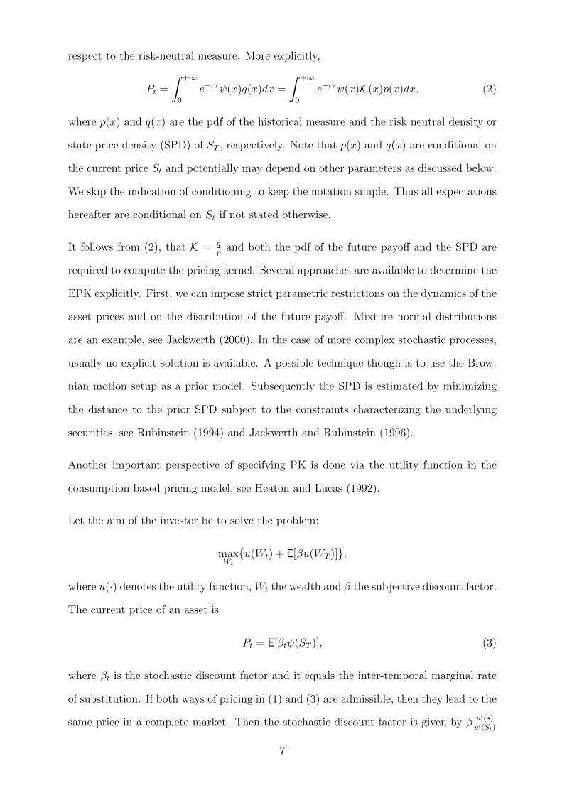
respect to the risk-neutral measure. More explicitly,
Pt =
∫ +∞
0
e−rτψ(x)q(x)dx =
∫ +∞
0
e−rτψ(x)K(x)p(x)dx, (2)
where p(x) and q(x) are the pdf of the historical measure and the risk neutral density or
state price density (SPD) of ST , respectively. Note that p(x) and q(x) are conditional on
the current price St and potentially may depend on other parameters as discussed below.
We skip the indication of conditioning to keep the notation simple. Thus all expectations
hereafter are conditional on St if not stated otherwise.
It follows from (2), that K = qp
and both the pdf of the future payoff and the SPD are
required to compute the pricing kernel. Several approaches are available to determine the
EPK explicitly. First, we can impose strict parametric restrictions on the dynamics of the
asset prices and on the distribution of the future payoff. Mixture normal distributions
are an example, see Jackwerth (2000). In the case of more complex stochastic processes,
usually no explicit solution is available. A possible technique though is to use the Brow-
nian motion setup as a prior model. Subsequently the SPD is estimated by minimizing
the distance to the prior SPD subject to the constraints characterizing the underlying
securities, see Rubinstein (1994) and Jackwerth and Rubinstein (1996).
Another important perspective of specifying PK is done via the utility function in the
consumption based pricing model, see Heaton and Lucas (1992).
Let the aim of the investor be to solve the problem:
maxWt
{u(Wt) + E[βu(WT )]},
where u(·) denotes the utility function, Wt the wealth and β the subjective discount factor.
The current price of an asset is
Pt = E[βtψ(ST )], (3)
where βt is the stochastic discount factor and it equals the inter-temporal marginal rate
of substitution. If both ways of pricing in (1) and (3) are admissible, then they lead to the
same price in a complete market. Then the stochastic discount factor is given by β u′(s)u′(St)
7

and is proportional to the PK. This implies that by fixing the utility of the investor we can
determine the PK, which is related to the standard risk aversion measures. In practice,
however, usually the opposite procedure is applied. The PK is estimated via a ratio of
q and p and used to determine the utility function or the risk aversion coefficient of the
investor. Assessment of the temporal dynamics of the latter allows for inferences on the
market risk behavior.
2.1 EPK and option pricing
EPK is calibrated from the data via an estimation of the ratio of the SPD q and the
HD p respectively. In this section we describe the details for this calibration. The latter
can easily be estimated either parametrically or nonparametrically from the time series
of payoffs. On the contrary, the SPD depends on risk preferences and therefore the past
observed stock price time series do not contain enough information. Option prices do
reflect preferences and, therefore, can be used to estimate the SPD q. Let C(St, X, τ, r, σ2)
denote the European call-option price as a function of the strike price X, price St, maturity
τ , interest rate r and volatility σ. Following Breeden and Litzenberger (1978) the SPD
can be determined from the pricing equation by
q(ST ) = erτ∂2C
∂X2
∣∣∣X=ST
. (4)
This result is very general and is valid for all European call options with the payoff
function (ST−X)+ and with the single assumption that the price is twice differentiable. No
additional restrictions on the stochastic process for the underlying or on the preferences of
market participants are needed. In a Black-Scholes (BS) framework, where the underlying
asset price St follows a geometric Brownian motion, the European options are priced via:
C(St, X, τ, r, σ2) = StΦ(d1)−XerτΦ(d2),
where d1 and d2 are known functions of σ2, τ , X and St. This implies that both q(ST )
and p(ST ) are the densities of lognormal distributions:
q(ST ) =1
ST√
2πσ2τexp
[−{log(ST/St)− (r − σ2/2)τ}2
2σ2τ
](5)
8

and p(ST ) with µ replacing r in (5).
The restrictive parametric form of BS model may often induce modeling bias when fitted
to the data, especially it is not possible to reflect the implicit volatility smile (surface) as a
function of X and τ via (5), see Renault (1997). The latter may be derived in a stochastic
volatility model, such as those of Heston or Bates type. In order to study unbiased risk
patterns, we need to guarantee models for the pricing kernel that are rich enough to reflect
local risk aversion in time and space. This leads naturally to a smoothing approach.
We now describe how to estimate q(·) nonparametrically. Consider call options with ma-
turity τ . We consider the following heteroscedastic nonparametric model for the observed
option prices Yi
Yi = Cτ (Xi) + σ(Xi)εi, i = 1, . . . , nq, (6)
where Yi denotes the observed option price, Xi the strike price and Cτ (·) is a smooth
function of the strike price. For simplicity of notation, we write C(·) for Cτ (·). The
informational content of the model is similar to that of Yuan (2009). We argue that
the perceived errors are due to neglected heterogeneity factors, rather than mispricings
exploited by arbitrage strategies, see Renault (1997). Thus the pricing errors εi are
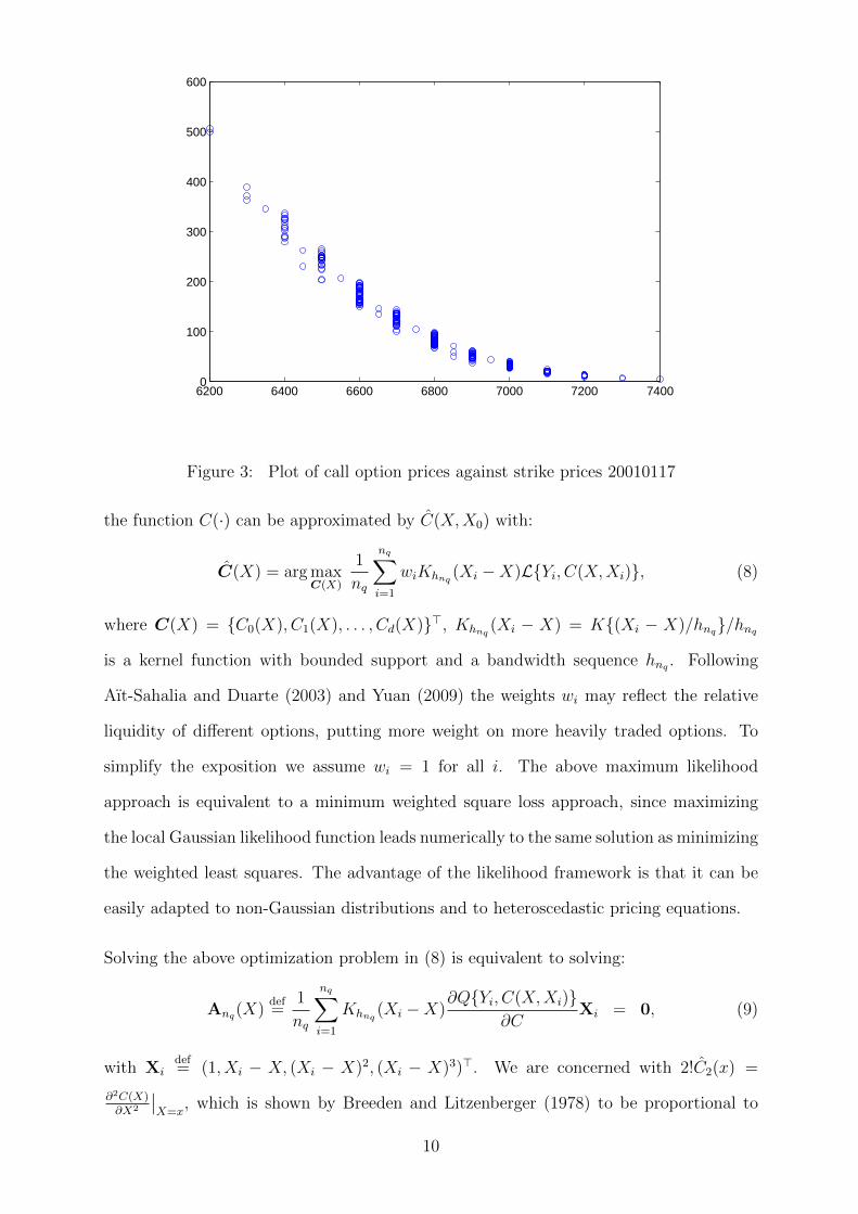
assumed to be i.i.d. in the cross section. Figure 3 depicts the call option prices used to
calculate a SPD. The observations are distributed, with different variances, at discrete
grid points of strike prices.
As from (4), estimation of q(·) boils down to the estimation of the second derivative
of C(·). The following local polynomial approach allows us to estimate C(·) and the
derivatives of C(·) simultaneously. Assuming that C(X) is continuously differentiable of
order d = 3, it can be locally approximated by
C(X,X0) =d∑j=0
Cj(X0)(X0 −X)j, (7)
where Cj(X) = C(j)(X)/j!, j = 0, . . . , d. See Cleveland (1979), Fan (1992), Fan (1993),
Ruppert and Wand (1994) for more details. By assuming a local Gaussian quasi-likelihood
model with L{Y,C(X)} = {Y − C(X)}2/{2σ2(X)} and maximizing the local likelihood,
9
6200 6400 6600 6800 7000 7200 74000
100
200
300
400
500
600
Figure 3: Plot of call option prices against strike prices 20010117
the function C(·) can be approximated by C(X,X0) with:
C(X) = arg maxC(X)
1
nq
nq∑i=1
wiKhnq(Xi −X)L{Yi, C(X,Xi)}, (8)
where C(X) = {C0(X), C1(X), . . . , Cd(X)}>, Khnq(Xi − X) = K{(Xi − X)/hnq}/hnq
is a kernel function with bounded support and a bandwidth sequence hnq . Following
Aıt-Sahalia and Duarte (2003) and Yuan (2009) the weights wi may reflect the relative
liquidity of different options, putting more weight on more heavily traded options. To
simplify the exposition we assume wi = 1 for all i. The above maximum likelihood
approach is equivalent to a minimum weighted square loss approach, since maximizing
the local Gaussian likelihood function leads numerically to the same solution as minimizing
the weighted least squares. The advantage of the likelihood framework is that it can be
easily adapted to non-Gaussian distributions and to heteroscedastic pricing equations.
Solving the above optimization problem in (8) is equivalent to solving:
Anq(X)def=
1
nq
nq∑i=1
Khnq(Xi −X)
∂Q{Yi, C(X,Xi)}∂C
Xi = 0, (9)
with Xidef= (1, Xi − X, (Xi − X)2, (Xi − X)3)>. We are concerned with 2!C2(x) =
∂2C(X)∂X2
∣∣X=x
, which is shown by Breeden and Litzenberger (1978) to be proportional to
10

q(x). Note that the described procedure does not guarantee the feasibility of the estima-
tor as a density. The constrained estimator of Aıt-Sahalia and Duarte (2003) makes the
large sample results below invalid. Therefore, we rely on the consistency and asymptotic
validity of q as a density estimator. This approach is justified by large samples avail-
able in financial applications. A multiplicative renormalizing of the estimator will shift
the EPK curve and the corresponding confidence bands, while keeping the results of the
monotonicity test unchanged. Furthermore, the renormalization introduces a bias, which
is difficult to tackle analytically. Additional improvement of the estimator is elaborated
in Section 3.1.
Note that we assume the parameter C(·) and σ(·) to be orthogonal to each other. Thus we
can estimate them separately as in a single parameter case. The following lemma states
the results on the existence of the solution and its consistency.
Lemma 1. Under conditions (A1) − (A7), there exists a sequence of solutions to the
equations
Anq(x) = 0,
with x being an element of a compact set E, such that
supx∈E|q(x)− q(x)| = O
[h−2nq{log nq/(nqhnq)}1/2 + h2nq
]a.s.
Proof. The statement follows from Theorem 2.1 of Claeskens and Van Keilegom (2003).
The HD p(x) can be estimated separately from the SPD using historical prices St, . . . , St+np+τ−1
(t+ np + τ − 1 < T ) of the underlying asset. The nonparametric kernel estimator of p(x)
is given similarly to Aıt-Sahalia and Lo (2000) by
preturn(x) = n−1p
np−1∑j=0
Khnp{x− log(St+j+τ/St+j)} ,
where Khnpis a kernel function with bounded support and the bandwidth hnp . This kernel
should necessarily coincide with the kernel for estimating SPD q(·). Also as in Aıt-Sahalia
11

and Lo (2000), the density of log-returns can be estimated as:
preturn(x) = St exp(x)p{St exp(x)}.
Alternatively, to eliminate the impact of serial dependence of overlapping returns over τ
periods, we can simulate independent pathes of the price process and use it to estimate
the density of ST , then np will become the number of paths simulated for the time T .
Under assumption (A5), we know that
supx∈E|p(x)− p(x)| = O{(nphnp/ log np)
−1/2 + h2np} a.s. (10)
Remark The uniform convergence results for estimation of HD in the i.i.d case follows
from Bickel and Rosenblatt (1973), and recently extended by Liu and Wu (2010) (Theorem
2.3) to the serial dependent data case.
The EPK is then given by the ratio of the estimated SPD and the HD p(x) i.e. K(x) =
q(x)/p(x). The next lemma provides the linearization of the ratio, which is important for
further statements about the uniform confidence band of the EPK.
Lemma 2. Under conditions (A1)− (A7) it holds
supx∈E|K(x)−K(x)|
= supx∈E
∣∣ q(x)− q(x)
p(x)− p(x)− p(x)
p(x)· q(x)
p(x)− {q(x)− q(x)}{p(x)− p(x)}
p2(x)
∣∣+O[max{(nphnp/ log np)
−1/2 + h2np, h−2nq{nqhnq/ log nq}−1/2 + h2nq
}] a.s.. (11)
This lemma implies that the stochastic deviation of K from K can be linearized into a
stochastic part containing the estimator of the SPD and a deterministic part containing
E[p(x)]. The uniform convergence can be proved by dealing separately with the two
parts. The convergence of the deterministic part is shown by imposing mild smoothness
conditions, while the convergence of the stochastic part is proved by following the approach
of Claeskens and Van Keilegom (2003). Theorem 1 formalizes this uniform convergence
of the EPK.
Theorem 1. Under conditions (A1)− (A7), it holds
supx∈E|K(x)−K(x)| = O[max{(nphnp/ log np)
−1/2+h2np, h−2nq{nqhnq/ log nq}−1/2+h2nq
}] a.s.
12

The proof is given in the appendix. The theoretical optimal rate of bandwidth follows by
minimizing the bias and variance term together in Theorem 1 leading to (nq log nq)−1/9. In
our simulation and applications, we use the bandwidth sequence which minimizes coverage
error by performing a grid search, see Claeskens and Van Keilegom (2003).
3 Confidence intervals and confidence bands
Confidence intervals characterize the precision of the EPK for a given fixed value of the
payoff. This allows to make inference about the PK at each particular strike price, but does
not allow conclusions about the global shape. The confidence bands, however, characterize
the whole EPK curve and offer therefore the possibility to test for shape characteristics.
In particular, it is a way to check the persistence of the bump as observed. Given a certain
shape, one may verify the restriction imposed by the power utility and obtain insights
on the market risk aversion. In addition, the confidence bands can be used to measure
the global variability of the EPK. Also, the proportion of the BS-based EPK covered
in nonparametric bands can be used as a measure of global risk aversion. The global
variability is measured by the variance function of EPK and the BS-based EPK means
the parametric fitting achieved by assuming that the underlying follows the geometric
Brownian motion.
A confidence interval for the EPK at a fixed value x requires the asymptotic distribution of
p(x) and q(x). Hereafter, we use L to denote the convergence in law. Under (A1)− (A7):
√nphnp{p(x)− p(x)} L−→ N{0, p(x)
∫K2(u)du} (12)
and √nqh5nq
{q(x)− q(x)} L−→ N{0, σ2q (x)}, (13)
where σ2q (x) = [B(x)−1L−1TL−1](3,3), with B(x) equal to the product of the density fX(x)
of the strike price and the local Fisher information matrix I{C(x)}. The matrices L and
T are given by Ldef= [∫ui+jK(u)du]i,j and T
def= [∫ui+jK2(u)du]i,j with i, j = 0, . . . , 3.
13
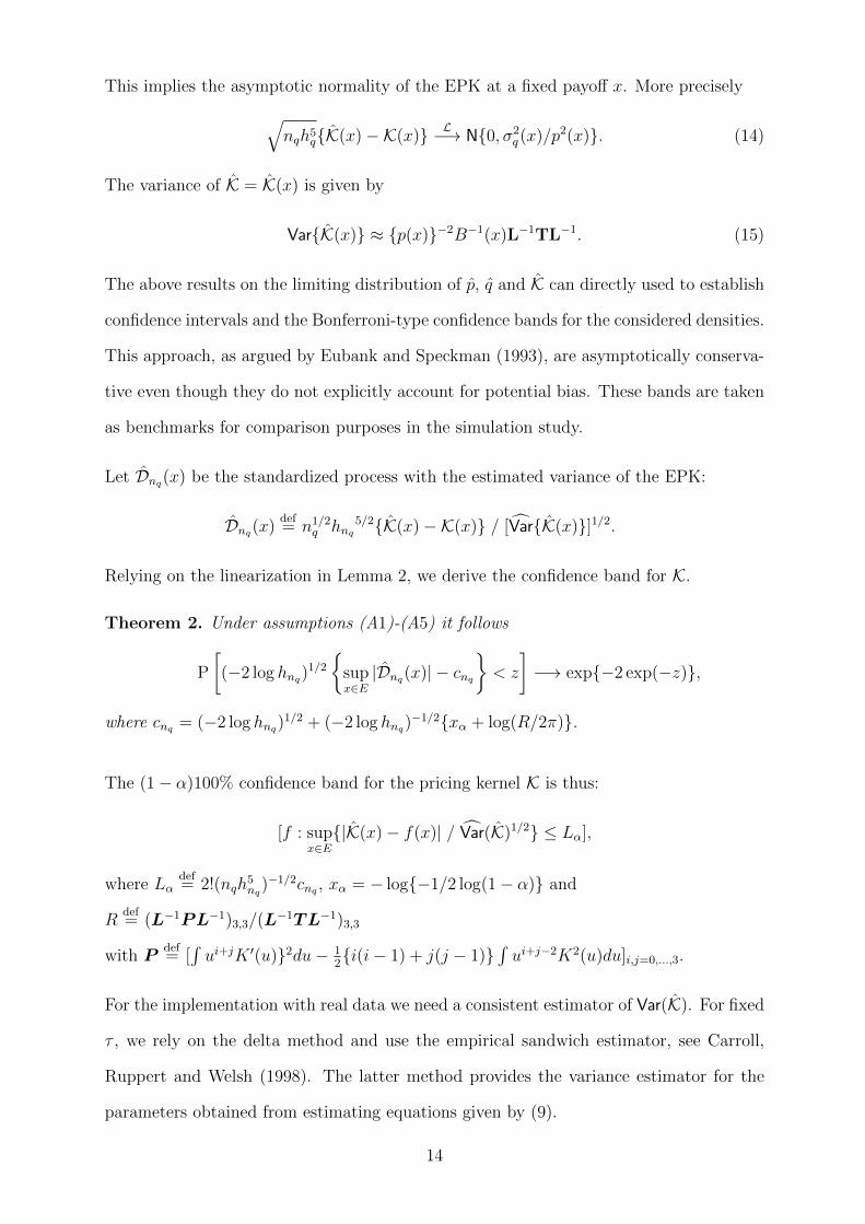
This implies the asymptotic normality of the EPK at a fixed payoff x. More precisely√nqh5q{K(x)−K(x)} L−→ N{0, σ2
q (x)/p2(x)}. (14)
The variance of K = K(x) is given by
Var{K(x)} ≈ {p(x)}−2B−1(x)L−1TL−1. (15)
The above results on the limiting distribution of p, q and K can directly used to establish
confidence intervals and the Bonferroni-type confidence bands for the considered densities.
This approach, as argued by Eubank and Speckman (1993), are asymptotically conserva-
tive even though they do not explicitly account for potential bias. These bands are taken
as benchmarks for comparison purposes in the simulation study.
Let Dnq(x) be the standardized process with the estimated variance of the EPK:
Dnq(x)def= n1/2
q hnq
5/2{K(x)−K(x)} / [Var{K(x)}]1/2.
Relying on the linearization in Lemma 2, we derive the confidence band for K.
Theorem 2. Under assumptions (A1)-(A5) it follows
P
[(−2 log hnq)
1/2
{supx∈E|Dnq(x)| − cnq
}< z
]−→ exp{−2 exp(−z)},
where cnq = (−2 log hnq)1/2 + (−2 log hnq)
−1/2{xα + log(R/2π)}.
The (1− α)100% confidence band for the pricing kernel K is thus:
[f : supx∈E{|K(x)− f(x)| / Var(K)1/2} ≤ Lα],
where Lαdef= 2!(nqh
5nq
)−1/2cnq , xα = − log{−1/2 log(1− α)} and
Rdef= (L−1PL−1)3,3/(L
−1TL−1)3,3
with Pdef= [∫ui+jK ′(u)}2du− 1
2{i(i− 1) + j(j − 1)}
∫ui+j−2K2(u)du]i,j=0,...,3.
For the implementation with real data we need a consistent estimator of Var(K). For fixed
τ , we rely on the delta method and use the empirical sandwich estimator, see Carroll,
Ruppert and Welsh (1998). The latter method provides the variance estimator for the
parameters obtained from estimating equations given by (9).
14

To estimate the variance function of the EPK we consider time series of the option prices
and the corresponding strike prices, (Xit, Yit), i = 1, · · · , nq; t = t + 1, · · · , t + τ , we
have
Var{K(x)} = {p(x)}−2V (x)−1U(x)V (x)−1, (16)
where
V (x)def=
1
nqτ
nq∑i=1
t+τ∑j=t+1
K2hnq
(Xij − x)
[∂
∂CQ{Yij ; C(x,Xij)}
]2(H−1nq
Xij)(H−1nq
Xij)>,(17)
U(x)def=
1
nqτ
nq∑i=1
t+τ∑j=t+1
K2hnq
(Xij − x)
[∂2
∂2CQ{Yij ; C(x,Xij)}
](H−1nq
Xij)(H−1nq
Xij)>,(18)
where Xijdef= (1, · · · , (Xij − x)3)> and Hnq
def= diag{1, . . . , h3nq
}. The estimator is consis-
tent in our setup as motivated in Appendix A.2 of Carroll et al. (1998).
It is important to note that the nonparametric estimators are biased, which leads to
potentially wrongly centered confidence bands and misleading coverages.
To overcome this problem we deploy the bias-correcting technique of Xia (1998), which
is based on the local polynomial estimation. It is used to correct the bias in estimated
SPD, while the bias in the HD is corrected using the additive bias correction method
mentioned in Jones, Linton and Nielsen (1995). In the next step we correct the bias in
the EPK using the linearization in Lemma 2. The estimated leading term bias for EPK
consists of the estimated bias of q(x) and of p(x) with a bigger bandwidth than what used
in estimation. This is the oversmoothing idea proposed by Eubank and Speckman (1993).
3.1 Bootstrap confidence bands
In this subsection, we discuss a bootstrap version of the confidence band to obtain possi-
bly better finite sample performance. The slow rate of convergence is known to us by Hall
(1991), who showed that for density estimators, the supremum of {q(x)− q(x)} converges
at the slow rate (log nq)−1 to the Gumbel extreme value distribution. Therefore the con-
fidence band may exhibit poor performance in finite samples. An alternative approach is
to use the bootstrap method. Claeskens and Van Keilegom (2003) used smooth bootstrap
15

for the numerical approximation to the critical value. Here we consider the bootstrap
technique of the leading term in Lemma 2
supx∈E| q(x)− q(x)
p(x)|.
We resample data from the smoothed bivariate distribution of (X, Y ) with the density
estimator given by estimator is:
f(x, y) =σX
nqhnqhnq σY
nq∑i=1
K{Xi − x
hnq
,(Yi − y)σXhnq σY
},
where σX and σY are the estimated standard deviations of the distributions of X and
Y . The motivation of using the smooth bootstrap procedure is that the Rosenblatt
transformation requires the resampled data (X∗, Y ∗) to be continuously distributed.
From the re-sampled data sets, we calculate the bootstrap analogue of the leading term
in Lemma 2:
supx∈E| q∗(x)− q(x)
p(x)|.
One may argue that this resampling technique does not correctly reflect the bias arising in
estimating q. Therefore, Hardle and Marron (1991) use therefore a resampling procedure
based on a larger bandwidth. This refined bias correcting bootstrap method does not
need to be applied in our case, since our bandwidth conditions ensure a negligible bias.
Correspondingly, we define the one-step estimator for the stochastic deviation:
h2nq{K∗(x)− K(x)} = −{p(x)}−2 {U ∗(x)−1H−1
nqA∗nq
(x)}3,3,
with U ∗(x) and A∗nq(x) as U(x) and Anq(x) defined previously with bootstrap data
(X∗i , Y∗i ) and the variance given by:
Var{K(x)} ≈ {p(x)}−2B(x)−1L−1PL−1, (19)
where B(x) is defined after equation (13).
Corollary 1. Assume conditions (A1)-(A7), a (1−α)100% bootstrap confidence band for
the EPK K(x) is:
[f(x) : supx∈E{|K(x)− f(x)|V ar(K)−1/2} ≤ L∗α],
16

where the bound L∗α satisfies
P∗[−{U(x)−1H−1nq
A∗nq(x)}3,3/{B(x)−1L−1PL−1}3,3 ≤ L∗α] = 1− α.
The estimator V ar(K) is computed in a similar fashion as in the previous section.
3.2 Confidence bands based on smoothing implied volatility
Although the nonparametric estimator of the PK is reasonable in theoretical sense, it
often fails to provide stable and economically treatable estimators with real data. One
way to stabilizing the empirical SPD is the use of data-driven local bandwidths (see Vieu
(1993)) or a multiple-testing-type adaptive technique of Lepski and Spokoiny (1997).
These alternative methods are tools of general purpose and address the bias-variance
trade-off locally. They are known to be either asymptotically optimal or to have a near
oracle property. Although the adaptive bandwidth provides us with optimal estimators,
it is still possible that the noise is too large and the algorithm fails to provide a curve with
a small bias and easy interpretation. This point is stressed in Rookley (1997): “implied
volatilities on the other hand tend to be less volatile and differences in implied volatilities
convey much more economic information than option prices alone, as implied volatilities
already embed much of the fundamental information available”.
We follow, however, an alternative approach and stabilize the empirical SPD by a two-
step procedure as in Rookley (1997) and Fengler (2005). At the first step, we estimate
the implied volatility (IV) function by a local polynomial regression. At the second step,
we plug the smoothed IV into the BS formula to obtain a semiparametric estimator of
the option price. This approach relies on a bijective transformation of the call prices
to the IV space and reflects the tendency of investors to quote the options in terms of
IV. Aıt-Sahalia and Lo (1998) used a similar semiparametric technique for dimension
reduction purposes. Note that the procedure does not require the BS model to hold, but
leads to finite sample improvements, while being asymptotically equivalent to the original
estimator (see Theorem 3). Thus we impose more assumptions on the functional form
17

of the call price function and focus only on the nonparametric structure of the volatility
surface. Thus the noise is relevant only in the estimation of the volatility surface. However,
it is well recognized that the volatility is less noisy and its shape is more tractable and
easy to interpret economically. Moreover, we can improve our two-step procedure further
by adopting adaptive techniques for the volatility surface.
Formally we smooth the IV using a local polynomial regression in moneyness M , with
the implicit assumption on the pricing formula is homogenous of degree 1 w.r.t. the asset
price and the strike price as proved in Renault (1997). In the absence of dividends, the
moneyness is defined at time t as Mit = St/Xi. The heteroscedastic model for the IV is
given by:
σi = σ(Mit) +√η(Mit)υi, i = 1, . . . , nq, (20)
where υi are the i.i.d. errors with zero mean, unit variance and η(·) is the volatility
function. We make the same assumptions about the implied volatility σ(·) as we did for
the option prices C(·) in Section 2.1.
Defining the rescaled call option price c(Mit) = C(Xi)/St, we obtain from the BS formula
c(Mit) = c{Mit;σ(Mit)} = Φ{d1(Mit)} −e−rτΦ{d2(Mit)}
Mit
,
where
d1(Mit) =log(Mit) +
{r + 1
2σ(Mit)
2}τ
σ(Mit)√τ
, d2(Mit) = d1(Mit)− σ(Mit)√τ .
Combining the result of Breeden and Litzenberger (1978) with the expression for c(Mit)
leads to the SPD
q(x) = erτ∂2C
∂X2
∣∣∣X=x
= erτSt∂2c
∂X2
∣∣∣X=x
(21)
with
∂2c
∂X2=
d2c
dM2
(M
X
)2
+ 2dc
dM
M
X2. (22)
As it is shown in the appendix the derivatives in the last expression can be determined
explicitly and are functions of Vdef= σ(M), V ′
def= ∂σ(M)/∂M and V ′′
def= ∂2σ(M)/∂M2.
18

We estimate the latter quantities by the nonparametric local polynomial regression for
the IV of the from
σ(Mit) ≈ V (M) + V ′(M)(Mit −M) +1
2V ′′(M)(Mit −M)2,
for M near Mit. The respective estimators are denoted by V , V ′ and V ′′. Plugging the
results into (21)-(22) we obtain the estimator of SPD in the smoothed IV space. Assuming
that the IV process fulfills the (A1)− (A7) in the appendix instead of C(·), we conclude
that Theorem 2.1 of Claeskens and Van Keilegom (2003) holds also for V , V ′ and V ′′.
Note that the convergence rate of V and V ′ is lower than of V ′′. Relying on this fact, we
state the asymptotic behavior of q(x)− q(x) in the next theorem.
Theorem 3. Let σ(·) satisfy the assumptions (A1)-(A7). Then with M = St/x it holds√nqh5nq
{q(x)− q(x)} L−→ N{0, r(M)2σ2V (M)}, (23)
where
r(M)def= erτSt
M2
x2
[ϕ{d1(M)}
{√τ/2− log(M) + rτ
V (M)2√τ
}− e−rτϕ{d2(M)}
{−√τ/2− log(M) + rτ
V (M)2√τ
}/M]
and σ2V (M)
def= [BV (M)−1L−1TL−1](3,3), with σ2
V (M) defined as in (15).
Proof. The proof is given in the appendix.
Theorem 3 allows us to construct the confidence bands of the SPD estimated semipara-
metrically using the confidence bands for the IV. The variance of the estimator is obtained
by the delta method in the following way
Var{q(x)− q(x)} =( ∂q
∂V ′′
)2Var{V ′′(M)− V ′′(M)}.
The variance Var{V ′′(M) − V ′′(M)} is estimated using a sandwich estimator similarly
to (16), and ∂q∂V ′′
= erτStM2
x2
[ϕ{d1(M)}
{√τ/2 − log(M)+rτ
V (M)2√τ
}− e−rτϕ{d2(M)}
{−√τ/2 −
log(M)+rτV (M)2
√τ
}/M]. Here we have proved that it is sufficient to consider only the variance of
the second derivative of V , as the other terms involved are of higher order.
19

3.3 Extension to dependent data
In the previous sections we have assumed independent data in the estimation of both the
historical density and the SPD. Violation of this assumption may lead to misspecified
asymptotic results and wrong confidence bands. The assumption is, however, feasible
in our study for both densities. The confidence bands for a simple density estimator of
time series data are analysed by Liu and Wu (2010, see Section 2.1) and can be directly
transferred to the historical density in our setup. Note however, that the impact of these
results on the confidence bands for the EPK is flattened by the higher convergence rate
of the historical density. Regarding the SPD note that assuming sufficient liquidity we
can use options only with a given maturity traded on a single day. This implies that the
data used to estimate SPD is not a time series data and there is no need to take the serial
correlation into account.
Nevertheless, to serve a general purpose estimation, it is still interesting to generalize our
theoretical results to dependent data. Liu and Wu (2010) developed uniform confidence
bands for kernel density estimators and Nadaraya-Watson estimation for a general class
of time series models. In this section we adopt their approach to our problem. We extend
the setup to time dependence and consider the model as in (6)
Yi = C(Xi) + σ(Xi)εi, i = 1, · · · , nq,
with the strike prices being a causal stationary process Xi = G(· · · , ηi−1, ηi), ηi are i.i.d.
and independent with εi.
We focus on the estimation of C(·) as in (8) and keep σ(·) known for the derivations in
this subsection. The physical dependence measure θ(i,γ)def= ‖Xi−X ′i‖γ = (E |Xi−X ′i|γ)1/γ,
where X ′i is a coupled process of Xi with η0 is replaced by an i.i.d. copy of η′0, i.e. X ′i =
G(η′0, · · · , ηi−1, ηi). Additionally define the dependence measure with coupled whole past
as Ψi,γdef= ‖G(η0, · · · , ηi−1, ηi)−G(η′0, · · · , η′i−1, η′i)‖γ. Suppose that ||Xi||κ ≤ ∞ for some
κ > 0. Let κ′ = min(κ, 2) such that Θnq =∑nq
i=1 θκ′/2(i,κ′). Define Znq
def=∑∞
k=−nq(Θnq+k −
Θk)2 and ξi
def= (· · · , εi−1, εi, · · · , ηi−1, ηi).
20
(A8) Assume (||Xi||κ ≤ ∞ for κ > 0. The density of ηi is positive and uniformly bounded
over its whole support up to the third derivative. There exists a constant M < ∞
such that sup[|fXnq |ξnq−1(x)| + |f ′
Xnq |ξnq−1(x)| + |f ′′
Xnq |ξnq−1(x)|] ≤ M almost surely. εi has
bounded fourth moments. Ψnq ,γ = O(n−rq ) for some γ and r > δ1/(1− δ1), 0 < δ1 < 1/4.
There exists a constant δ such that 0 < δ ≤ δ1 < 1 and hnq = O(n−δq ), n−δq = O(hnq).
Furthermore θ(nq ,κ) = O(ρnq) for some κ > 0 and 0 < ρ < 1.
Let Fnq(x) be the standardized process:
Fnq(x)def= n1/2
q hnq
5/2{q(x)− q(x)} / [σq(x)]1/2.
Theorem 4. Under assumptions (A1)-(A6), (A8), hnq = O{(nq log nq)−1/9}, Znqh
3nq
=
O(nq log nq), it follows
P
[(−2 log hnq)
1/2
{supx∈E|Fnq(x)| − cnq
}< z
]−→ exp{−2 exp(−z)},
where cnq = (−2 log hnq)1/2 + (−2 log hnq)
−1/2{xα + log(R/2π)}.
Liu and Wu (2010) note an interesting dichotomy phenomenon, where the rate of conver-
gence is the consequence of an interplay between the strength of dependency and the band-
width hnq . Accordingly, we suggest to undersmooth as a smaller bandwidth would both
reduce the bias and the effect of dependency. The rate of hnq is set to O{(nq log nq)−1/9}.
4 Monte-Carlo study
The practical performance of the above theoretical considerations is investigated via two
Monto-Carlo studies. The first simulation aims at evaluating the performance under the
BS hypothesis, while the second simulation setup does the same under a realistically
calibrated surface. The confidence bands are applied to DAX index options. We first
study the confidence bands under a BS null model (Section 4.1). Naturally, without
volatility smile, both the BS estimator and nonparametric estimator are expected to be
covered by the bands. While in the presence of volatility smile (Section 4.2), we expect
our tests to reject the BS hypothesis in most cases.
21

4.1 How well is the BS model covered?
In the first setting, we calibrate a BS model on day 20010117 with the interest rate set
equal to the short rate r = 0.0481, S0 = 6500, strike prices in the interval [6000, 7400].
We refer to Aıt-Sahalia and Duarte (2003) on the sources of the noise and use an identical
simulation setting, with the noise being uniformly distributed in the interval [0, 6]. Figure
4 is a scatter plot of generated observations of European call option prices against strikes,
the data is clustered in discrete values of the strike price. Recall that bandwidths in the
following context are all selected to minimize pricing error using a leave-one-out approach
on the bivariate grid [1/np; 1]× [1/nq; 1].
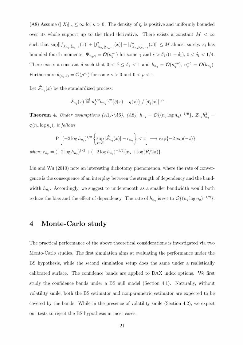
Figure 5 shows a nonparametric estimator for the SPD and a parametric BS estimator.
The two estimators roughly coincide except for a small wiggle, thus the bands drawn
around the nonparametric curve also fully cover the parametric one. The accuracy is
evaluated by calculating the coverage probabilities and average area within the bands,
see Table 1(see the rows labeled “null”). The coverage probabilities is determined via 500
simulations, whenever the hypothesized curve calculated on a grid of 100. The coverage
probability approaches its nominal level with increasing sample size, but never reaches
it. This may well be attributed to the above mentioned poor convergence of Gaussian
maxima to the Gumbel distribution. The area within the bands reflects the stability of
the estimation procedure. The bands get narrower with increasing sample size.
The bias correction for the SPD follows the approach of Xia (1998). The HD is corrected
as in Jones et al. (1995). The bias correction for EPK relies on the linear term from
Lemma 2. The correction of the bands mimics the Bonferroni correction in Eubank and
Speckman (1993) and is based on the asymptotic confidence intervals in (13) and (14). We
conclude that the bias correction approach and the Bonferroni correction are not better
than the proposed method for all sample sizes.
HDs are estimated from simulated stock prices following geometric Brownian motion with
µ = 0.23. A BS EPK estimator could be tested using the above procedure. Due to bound-
ary effects, we concentrate on moneyness (Mt = St/X) in [0.95, 1.1]. Figure 6 displays
22

Level Maturity Method nq = 300 450 600
5% (null) 3M EPK 0.782(2.54) 0.798(2.49) 0.802(2.38)
EPK (bias) 0.798(2.51) 0.800(2.43) 0.802(2.31)
EPK (Bonfer.) 0.673(2.98) 0.697(2.88) 0.754(2.76)
SPD 0.906(2.40) 0.914(2.20) 0.923(1.99)
SPD (Bonfer.) 0.873(2.68) 0.924(2.57) 0.929(2.44)
6M EPK 0.860(2.50) 0.875(2.43) 0.890(2.41)
EPK (bias) 0.862(2.53) 0.883(2.41) 0.899(2.42)
EPK (Bonfer.) 0.785(2.90) 0.801(2.67) 0.824(2.74)
SPD 0.896(2.44) 0.906(2.13) 0.920(2.07)
SPD (Bonfer.) 0.883(2.73) 0.894(2.69) 0.903(2.52)
10%(null) 3M EPK 0.706(2.47) 0.736(2.34) 0.762(2.23)
EPK (bias) 0.712(2.45) 0.737(2.33) 0.771(2.23)
EPK (Bonfer.) 0.673(2.33) 0.686(2.12) 0.734(2.01)
SPD 0.795(2.17) 0.812(2.06) 0.853(1.88)
SPD (Bonfer.) 0.764(2.12) 0.801(2.00) 0.833(1.98)
6M EPK 0.729(2.50) 0.774(2.23) 0.829(2.31)
EPK (bias) 0.713(2.47) 0.753(2.26) 0.835(2.30)
EPK (Bonfer.) 0.671(2.86) 0.745(2.88) 0.798(2.72)
SPD 0.800(2.34) 0.814(2.08) 0.860(1.94)
SPD (Bonfer.) 0.763(2.55) 0.800(2.46) 0.847(2.36)
5% (alter.) 3M EPK 0.512(2.43) 0.178(2.23) 0.050(2.02)
EPK (bias) 0.543(2.42) 0.235(2.27) 0.145(1.99)
EPK (Bonfer.) 0.372(2.51) 0.239(2.37) 0.099(2.12)
6M EPK 0.592(2.53) 0.410(2.17) 0.178(2.02)
EPK (bias) 0.541(2.49) 0.349(2.12) 0.251(2.01)
EPK (Bonfer.) 0.331(2.34) 0.136(2.16) 0.150(2.15)
10% (alter.) 3M EPK 0.258(2.12) 0.050(2.04) 0.030(2.01)
EPK (bias) 0.268(2.13) 0.043(2.01) 0.001(2.00)
EPK (Bonfer.) 0.148(2.78) 0.030(2.61) 0.001(2.54)
6M EPK 0.375(2.22) 0.410(2.13) 0.178(2.00)
EPK (bias) 0.362(2.21) 0.432(2.13) 0.176(2.01)
EPK (Bonfer.) 0.231(2.46) 0.221(2.35) 0.110(2.25)
Table 1: Averaged, coverage probability (area) of the uniform confidence band over 500
simulations in different cases. (bias) means bias correction, (Bonfer.) means Bonferoni
correction.
23

6000 6200 6400 6600 6800 7000 7200 74000
100
200
300
400
500
600
700
Figure 4: Generated noisy BS call option prices against strike prices.
the nonparametric EPK with confidence band and the BS EPK covered in the band. We
observe that the BS EPK is strictly monotonically decreasing. The summary statistics
are given in Table 1, due to the additional source of randomness introduced through
the estimation of p(x), the coverage probabilities are less precise than the corresponding
coverage probabilities for SPD. Nevertheless, the probabilities are getting closer to their
nominal values and the bands get narrower when the sample size increases.
4.2 How well is the band in reality?
Section 4.1 studied the performance of the bands under the null hypothesis with BS
assumption, while this section is designed to investigate the performance of the bands
when the null hypothesis is violated by a realistic volatility smile observed in the market.
Keeping the parameters identical to the setup of the first study, we generated the data
with a smoothed volatility function based on data for or options traded on 20010117 with
τ = 3M,6M to maturity.
Figure 7 and 8 report the estimators for SPD and EPK. The bands do not cover the BS
24
0.9 0.95 1 1.05 1.1 1.15−20
−15
−10
−5
0
5
10
15
20SPD and its uniform confidence band
Figure 5: Estimation of SPD (red), bands (black) and the BS SPD (blue), with hnq =
0.085, α = 0.05, nq = 300.
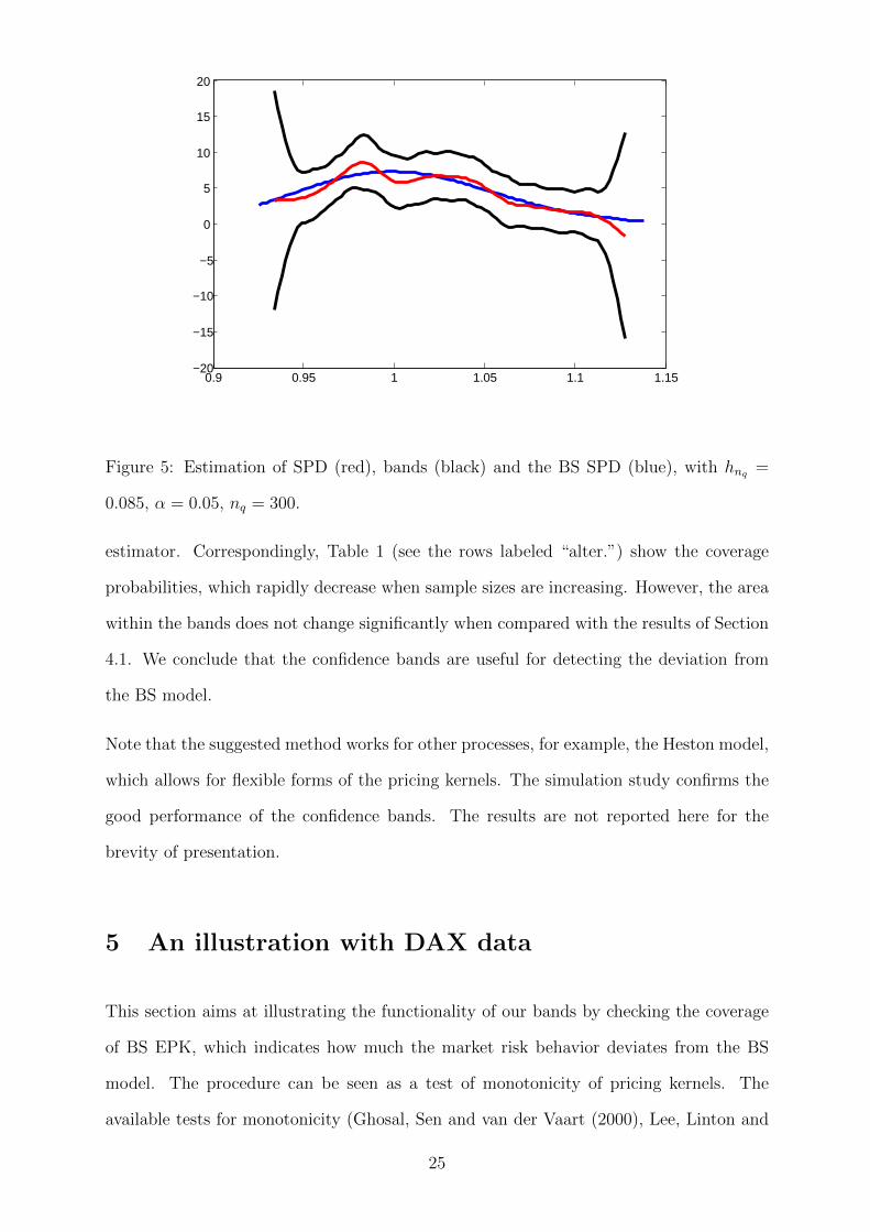
estimator. Correspondingly, Table 1 (see the rows labeled “alter.”) show the coverage
probabilities, which rapidly decrease when sample sizes are increasing. However, the area
within the bands does not change significantly when compared with the results of Section
4.1. We conclude that the confidence bands are useful for detecting the deviation from
the BS model.
Note that the suggested method works for other processes, for example, the Heston model,
which allows for flexible forms of the pricing kernels. The simulation study confirms the
good performance of the confidence bands. The results are not reported here for the
brevity of presentation.
5 An illustration with DAX data
This section aims at illustrating the functionality of our bands by checking the coverage
of BS EPK, which indicates how much the market risk behavior deviates from the BS
model. The procedure can be seen as a test of monotonicity of pricing kernels. The
available tests for monotonicity (Ghosal, Sen and van der Vaart (2000), Lee, Linton and
25

0.9 0.95 1 1.05 1.1 1.15−0.5
0
0.5
1
1.5
2
2.5
3
Figure 6: Estimation of EPK (red), bands (black) and the BS EPK (blue), with hnq =
0.085, hnp = 0.060 and α = 0.05, np = 2000, nq = 300.
Whang (2009), Chetverikov (2012)) work for (regression) functions and not for derivative
estimation as required here. We take a dynamic point of view by considering the EPK
estimated at different dates.
5.1 Data
In contrast to previous studies that are mainly based on S&P500 data, we focus on
intraday European options on the DAX options. The source is the European Exchange
EUREX and data available by C.A.S.E., RDC SFB 649 (http://sfb649.wiwi.hu-berlin.de)
in Berlin. The extracted observations for our analysis cover the period between 1998 and
2008. The smoothing in volatility approach described in Section 3.2 is applied to estimate
the EPK (denoted as Rookley method). As we cannot find traded options with the same
maturity on each day, we consider options with maturity 15 days (10 trading days) across
several years. Specifically, we extract a time series of options for every month from Jan
2001 to Dec 2006; this adds up to 63 days.
26

0.9 0.95 1 1.05 1.1 1.15-4
-2
0
2
4
6
8
Figure 7: Plot of confidence bands (black), nonparametrically estimated SPD (red), the
fitted BS (blue) SPD with simulated volatility smile, nq = 300, hnq = 0.066, α = 0.05.
To make sure that the data correctly represents the market conditions, we use several
cleaning criteria. In our sample, we eliminate the observations with τ < 1D and IV > 0.7.
Also, we skip the option quotes violating general no-arbitrage condition i.e. S > C >
max{0, S − Xe−rτ}. Due to the put-call parity, both out-of-the-money call options and
in-the-money puts are used to compute the smoothed volatility surface. The median of
intra day stock prices is used to compute the SPD. We use a window of 500 returns for
nonparametric kernel density estimators of HD.
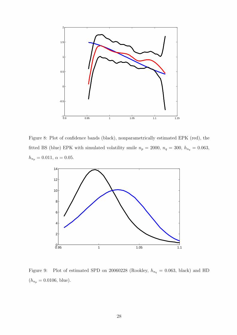
Figure 9 describes the relative position of the HD and SPD on a specific day, the EPK
peak is apparently created through the different probability mass contributions at different
moneyness states.
27
0.9 0.95 1 1.05 1.1 1.15-1
-0.5
0
0.5
1
1.5
2
Figure 8: Plot of confidence bands (black), nonparametrically estimated EPK (red), the
fitted BS (blue) EPK with simulated volatility smile np = 2000, nq = 300, hnq = 0.063,
hnp = 0.011, α = 0.05.
0.95 1 1.05 1.10
2
4
6
8
10
12
14
Figure 9: Plot of estimated SPD on 20060228 (Rookley, hnq = 0.063, black) and HD
(hnp = 0.0106, blue).
28
5.2 Estimation of DAX EPK and its uniform confidence band
0.95 1 1.05 1.1−6
−4
−2
0
2
4
6
8
10
12
(a) 060214, τ = 13D
0.95 1 1.05 1.1−1
0
1
2
3
4
5
(b) 060301, τ = 27D
0.95 1 1.05 1.1−2
−1
0
1
2
3
4
5
6
7
8
(c) 060305, τ = 20D
0.95 1 1.05 1.1−1
0
1
2
3
4
5
6
(d) 060417, τ = 27D
0.95 1 1.05 1.1−6
−4
−2
0
2
4
6
(e) 060419, τ = 13D
0.95 1 1.05 1.1−2
−1
0
1
2
3
4
5
(f) 060512, τ = 20D
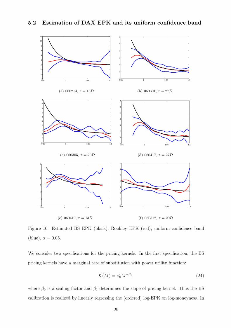
Figure 10: Estimated BS EPK (black), Rookley EPK (red), uniform confidence band
(blue), α = 0.05.
We consider two specifications for the pricing kernels. In the first specification, the BS
pricing kernels have a marginal rate of substitution with power utility function:
K(M) = β0M−β1 , (24)
where β0 is a scaling factor and β1 determines the slope of pricing kernel. Thus the BS
calibration is realized by linearly regressing the (ordered) log-EPK on log-moneyness. In
29

the second specification, we construct the nonparametric confidence bands as described
in Section 3.2. A sequence of EPKs and corresponding bands are shown in Figure 10. In
most of the cases, the BS EPKs are rejected via the confidence bands. The amount of
deviation from the hypothesized BS specification though provides us valuable information
about how risk hungry investors are. Besides, the area of between the bands varies over
time, which gives us insights into the variabilities of the prevailing risk patterns. In sum,
the bands do not only provide a simple test for hypothesizes EPKs, but also help us to
study the dynamics of risk patterns over time.
200101 200112 200208 200302 200411 200509 2006110
0.1
0.2
0.3
0.4
0.5
0.6
0.7
0.8
0.9
1
Figure 11: Coverage probability (α = 0.05) estimated at 63 trading days and the DAX
index ( rescale to [0, 1]), τ = 3M .
5.3 Linking economic conditions to EPK dynamics
We use two different indicators for the deviation from a simple BS model. As an approxi-
mation to the coverage probability, we calculate the proportion of grid points of the band
which covers the BS EPK. As a second measure, we introduce the average width of the
confidence bands over the moneyness interval [0.95, 1.1] as a proxy for the area between
the confidence bands. This provides us with a measure of variability, see also Theorem 2.
The first risk pattern time series is given in Figure 11, where we display the DAX index
30

200101 200112 200208 200302 200411 200509 200611−3
−2
−1
0
1
2
3
Figure 12: First difference of Coverage probability and the DAX index return (standard-
ized).
(scaled to [0, 1]) together with the coverage probability. We discover that the coverage
probability becomes less volatile when the DAX index level is high. Figure 12 shows the
differenced time series. From a simple correlation analysis, we argue that the change in
coverage probability and DAX return (with a lag of 3M) are highly negatively correlated
(correlation −0.3543) when the DAX index goes down (200101-200302). On the contrary,
in the period when the DAX goes up, one observes a large positive correlation (0.3151).
What does this mean economically? This implies in a period of worsening economic
condition, a positive part of the monthly DAX returns induces a greater hunger for risk in
a delay horizon of 3 months. Positive returns have just the opposite effects. With boosting
and bullish markets, the positive correlation indicates a 3-month horizon of decreasing
risk aversion. The exercise we have done so far support these economic reasoning. Risk
aversion seems to be higher in recessions and lower in boom times. This corresponds to
the findings in the economics literature. Economic agents (e.g., corporate firms, banks,
households) with higher risk aversion tend to hold more liquid assets, driving down the
interest rate. At the same time, the higher risk aversion calls for a higher rate of return
on risky assets. A lower interest rate and a higher rate on risky assets generate a higher
risk premium, Gilchrist and Zakrajek (2012).
31

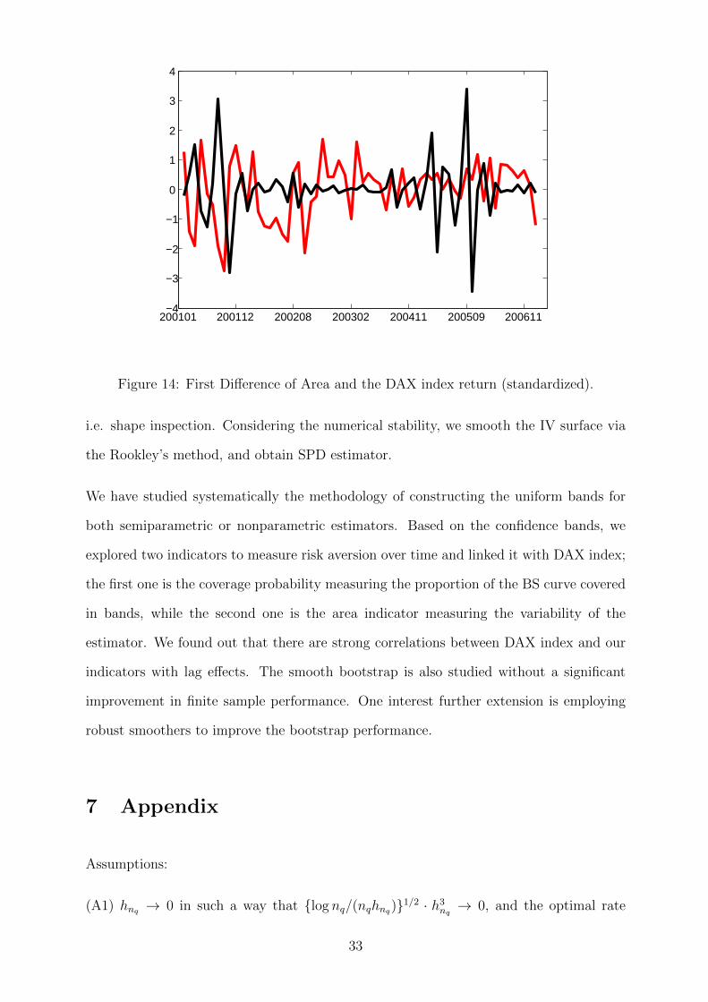
As far as the average width of the bands is concerned, we may conclude from Figure 13
and Figure 14 that in periods of clearly bullish or bearish momentum, the volatility of
the width of the confidence band is higher. This may be caused by the uncertainty of
the market participants about the long-term persistence of the trend. The lag effect on
risk hunger is also detectable for this constructed indicator. Over the whole observation
interval, the correlation between the monthly DAX return and the change in the average
width is −0.3230 for a 1M lag and −0.2717 for 3M.
200101 200112 200208 200302 200411 200509 2006110
0.2
0.4
0.6
0.8
1
Figure 13: Area of the confidence bands (α = 0.05) estimated at 63 trading days and the
DAX index (rescaled to [0, 1]).
6 Conclusions
Pricing Kernels are important elements in understanding investment behavior since they
reflect the relative weights given by investors’ states of nature (Arrow-Debreu securities).
Pricing kernels may be deduced in either parametric or nonparametric approaches. Para-
metric approaches like a simple BS model are too restrictive to account for the dynamics
of the risk patterns, which induces the well-known EPK paradox. Nonparametric ap-
proaches allow more flexibility and reduce the modeling bias. Simple tools like uniform
confidence bands help us to conduct tests against any parametric assumption of the EPKs
32
200101 200112 200208 200302 200411 200509 200611−4
−3
−2
−1
0
1
2
3
4
Figure 14: First Difference of Area and the DAX index return (standardized).
i.e. shape inspection. Considering the numerical stability, we smooth the IV surface via
the Rookley’s method, and obtain SPD estimator.
We have studied systematically the methodology of constructing the uniform bands for
both semiparametric or nonparametric estimators. Based on the confidence bands, we
explored two indicators to measure risk aversion over time and linked it with DAX index;
the first one is the coverage probability measuring the proportion of the BS curve covered
in bands, while the second one is the area indicator measuring the variability of the
estimator. We found out that there are strong correlations between DAX index and our
indicators with lag effects. The smooth bootstrap is also studied without a significant
improvement in finite sample performance. One interest further extension is employing
robust smoothers to improve the bootstrap performance.
7 Appendix
Assumptions:
(A1) hnq → 0 in such a way that {log nq/(nqhnq)}1/2 · h3nq→ 0, and the optimal rate
33

bandwidth, to guarantee undersmoothing, would be O{(log nq · nq)−1/9}.
(A2) The kernel functions K ∈ C(1)[−1, 1] (adopted for estimating both HD p(x) and
SPD q(x)) are symmetric and takes value 0 on the boundary.
(A3) For the likelihood function L ∈ C(1)(E) it holds that infx∈E L(x) > 0. C(x) ∈
C(4)(E). Additionally the third partial derivatives of L(Y,C) with respect to C exists
and is continuous in C for every y. The Fisher information I(C(x)) has a continuous
derivative and infx∈E I{C(x)} > 0.
(A4) There exists a neighborhood N(C(x)) such that
maxk=1,2
supx∈E|| supC∈N{C(x)}
∂k
∂CkL(y;C)||λ <∞
for some λ ∈ (2,∞]. Furthermore
supx∈E
E[ supC∈N{C(x)}
| ∂3
∂C3L(y;C)|] <∞.
(A5) The HD of underlying p(x) is three times continuously differentiable and is bounded
by a positive constant from below on the compact set E.
(A6) Let anp = (nphnp/ log np)−1/2 + h2np
from (10) and bnq = h−2nq(nqhnq/ log nq)
−1/2 + h2nq
from Lemma 1. We assume that nq/np = O(1), h5nq/hnp = O(1).
(A7) The pricing errors εi are independent and identically distributed random variables.
(A1) is a bandwidth assumption for estimating SPD. We can undersmooth to reduce
the bias. (A2) is the assumption on kernel function which facilitates the derivation of
results. In a typical setting, hnq is chosen to be as in (A1), while hnp is chosen to
be O(n−1/5p ), and hnq is larger than hnp . (A4) contains moment conditions defined via
likelihood functions. (A5) is an assumption imposed on the smoothness of p(x). In
our empirical setting, nq = 715, np = 200, thus for a typical data situations, (A6) is
reasonable. The assumptions (A1) and (A2) ensure anp/bnq = O(1).
34

7.1 Proof of Lemma 2
Recall from Lemma 1 and (10) that
supx∈E|p(x)− p(x)| = O{{log nq/(nqhnq)}1/2 + h2np
} = O(anp),
supx∈E|q(x)− q(x)| = O[h−2nq
{log nq/(nqhnq)}1/2 + h2nq] = O(bnq).
To determine the order of the EPK we linearize the ratio q(x)/p(x).
K(x)−K(x) =q(x)
p(x)− q(x)
p(x)=q(x)p(x)− p(x)q(x)
p2(x)· 1
1 + p(x)−p(x)p(x)
. (25)
We decompose the first factor as q(x)p(x) − p(x)q(x) = {q(x) − q(x)}p(x) − {p(x) −
p(x)}q(x), while for the second factor we use the first order Taylor expansion. Putting
together we obtain
supx∈E|K(x)−K(x)| = sup
x∈E| q(x)− q(x)
p(x)− p(x)− p(x)
p(x)· q(x)
p(x)
−{q(x)− q(x)}{p(x)− p(x)}p2(x)
+{p(x)− p(x)}2
p2(x)· q(x)
p(x)|.
The first two elements are of order O(bnq) and O(anp) respectively, while the last element
is of order O(anp). Summarizing we conclude that
supx∈E|K(x)−K(x)| = O[max{anp , bnq}].
7.2 Proof of Theorem 2
The basic idea of the proof is to approximate the process
Dnq(x) = n1/2q h5/2nq
{K(x)−K(x)}/[Var{K(x)}]1/2
by a process with non-stochastic variance term, which will then be further approximated
by a process that can be treated with the tools of Claeskens and Van Keilegom (2003).
Here we have dropped for the simplicity of notation the q in nq and the nq in hnq . More
precisely, we define, as first approximation,
D(1)n (x)
def= n1/2h5/2{K(x)−K(x)}/{Var{K(x)}}1/2,
35
where Var{K(x)} is given in (15). Lemma 2 ensures that the approximation by
n1/2h5/2{q(x)− q(x)}/{p(x)Var{K(x)}1/2} (26)
is uniformly of order Op{(log n)−1/2}. The process in equation (26) can be approximated
as in Claeskens and Van Keilegom (2003) by
2! exp(rτ)h2fX(x)−1/2 Var{K(x)}−1/2I{C(x)}−1/23∑i=0
fX(x)−1/2I{C(x)}−1/2{L−1}3,i+1An,i(x)
(27)
For the definition of the local Fisher information, I{C(x)}, the matrix L and the process
Ani(x), we refer to section 3, and section 7. Define
Zni(x)def= (nh)1/2h−i[I{C(x)}fX(x)]−1/2Ani(x).
Then equation (27) can be written as
Fn(x)def= 2! exp(rτ)h2{fX(x)}−1/2 Var{K(x)}−1/2I{C(x)}−1/2
3∑i=0
hi{L−1}3,i+1Zni(x)
Please note that L is not a function of x as Claeskens and Van Keilegom (2003) erroneously
write. Following their line of thoughts, we replace Zni(x) (uniformly) by
Z ′ni(x) = h1/2∫Kh(z − x)
(z − xh
)dz
In order to apply corollary A1 of (Bickel and Rosenblatt, 1973), define the covariance
function r(x) of the Gaussian process Fnq(x), and we know that
r(x) = Cov(Z ′nj(x), Z ′nj(0))
= C1 − C2|x|2 + O(|x|2),
for x ∈ E, where C1 and C2 are two constants, so the regularity conditions satisfies, the
result follows.
Finally, we have to show that supx∈E |Var{K(x)} − Var{K(x)}| = Op(1).
supx∈E|Var{K(x)} − Var{K(x)}|
= supx∈E|Var
{ q(x)− q(x)
p(x)
}− Var
{ q(x)− q(x)
p(x)
}|+ Op{(nh)−(1/2+α)(log n)1+α},
36

where 0 < α < 1.
According to corollary 2.1 in Claeskens and Van Keilegom (2003), for j = 3, k = 3,
supx∈E|Var{q(x)} − Var{q(x)}| = Op{(nh log n)−1/2}.
So we have,
supx∈E|Var{K(x)} − Var{K(x)}| = Op(1).
7.3 Expressions for the semiparametric estimator of SPD and
proof of Theorem 3
To proof the statement we show that√nqhnq(q(x) − q(x)) has asymptotically the same
distribution as√nqhnq{V ′′(M)−V ′′(M)} with proper scaling. Thus we drive the following
equation.
q(x)− q(x) = erτStM2
x2
[ϕ{d1(M)}
{√τ/2− log(M) + rτ
V (M)2√τ
}(28)
−e−rτϕ{d2(M)}{−√τ/2− log(M) + rτ
V (M)2√τ
}/M]{V ′′(M)− V ′′(M)}
+O{V ′′(M)− V ′′(M)}, (29)
where di and c are the terms defined in Section 3.2 with V (M) replaced by the true
function. We now describe how to derive (29) Taking the derivatives of c(Mit) with
respect to moneyness (M) and noting that both d1(Mit) and d2(Mit) depend on Mit we
obtain
dc
dM= ϕ(d1)
dd1dM− e−rτ ϕ(d2)
M
dd2dM
+ e−rτΦ(d2)
M2,
d2c
dM2= ϕ(d1)
{ d2d1dM2
− d1(
dd1dM
)2}−e−rτϕ(d2)
M
{ d2d2dM2
− 2
M
dd2dM− d2
(dd2dM
)2}− 2e−rτΦ(d2)
M3
Computing the first and second order differentials for d1 and d2 using the notation V =
σ(M), V ′ = ∂σ(M)/∂M and V ′′ = ∂2σ(M)/∂M2, we obtain
37

dd1dM
=1
MV√τ
+{− log(M) + rτ
V 2√τ
+√τ/2}V ′,
dd2dM
=1
MV√τ
+{− log(M) + rτ
V 2√τ
−√τ/2}V ′,
d2d1dM2
= − 1
MV√τ
{ 1
M+V ′
V
}+ V ′′
{√τ2− log(M) + rτ
V 2√τ
}+V ′
{2V ′
log(M) + rτ
V 3√τ
− 1
MV 2√τ
},
d2d2dM2
= − 1
MV√τ
{ 1
M+V ′
V
}+ V ′′
{−√τ
2− log(M) + rτ
V 2√τ
}+V ′
{2V ′
log(M) + rτ
V 3√τ
− 1
MV 2√τ
}.
To prove (29), we know from (22) and (21) that
q(x)− q(x) =
(d2c
dM2− d2c
dM2
)(M
X
)2
+ 2
(dc
dM
M
X2− dc
dM
M
X2
). (30)
The stochastic terms involved are
d2c
dM2− d2c
dM2={ϕ(d1)
d2d1dM2
− ϕ(d1)d2d1dM2
}−{ϕ(d1)d1
(dd1dM
)2
− ϕ(d1)d1
(dd1dM
)2}−{e−rτϕ(d2)
M
d2d2dM2
− e−rτϕ(d2)
M
d2d2dM2
}+{e−rτϕ(d2)
M
2
M
dd2dM− e−rτϕ(d2)
M
2
M
dd2dM
}+{e−rτϕ(d2)
Md2
(dd2dM
)2
− e−rτϕ(d2)
Md2
(dd2dM
)2}−{2e−rτΦ(d2)
M3− 2e−rτΦ(d2)
M3
}def= gt1 − gt2 − gt3 + gt4 + gt5 − gt6
and
dc
dM− dc
dM=
{ϕ(d1)
dd1dM− ϕ(d1)
dd1dM
}−{e−rτ
ϕ(d2)
M
dd2dM− e−rτ ϕ(d2)
M
dd2dM
}+{e−rτ
Φ(d2)
M2− e−rτ Φ(d2)
M2
}def= g′t1 − g′t2 + g′t3.
Now we analyze each term obtaining,
gt1 =d2d1dM2
{ϕ(d1)− ϕ(d1)
}− ϕ(d1)
{ d2d1dM2
− d2d1dM2
}gt2 = d1
(dd1dM
)2{ϕ(d1)− ϕ(d1)
}+
(dd1dM
)2
ϕ(d1){d1 − d1
}+d1ϕ(d1)
{( dd1dM
)2
−(
dd1dM
)2},
38

and similarly for gt3, gt4, gt5, gt6, g′t1, g
′t2, g
′t3. The further analysis of the rate boils down to
the analysis of the rates for dd1dM− dd1
dM, d
2d1dM2 − d2d1
dM2 , d1− d1, Φ(d1)−Φ(d1) and similar terms
for d2, as d2(M) = d1(M)− σ(M))√τ .
By the mean value theorem
Φ(d1)− Φ(d1) = ϕ(d0)(d1 − d1)
d1 − d1 ={log(M) + rtτ}(V − V )
V V√τ
+√τ(V − V )/2
dd1dM− dd1
dM=
V − VMV V
√τ
+{(log(M) + rτ)(V 2 − V 2)
V 2V 2√τ
+√τ/2}V ′
+{(log(M) + rτ)
V 2√τ
+√τ/2}
(V ′ − V ′),
= O({(log(M) + rτ)
V 2√τ
+√τ/2}
(V ′ − V ′))
d2d1dM2
− d2d1dM2
= −{ 1
M√τ
V − VV V
1
M+
1
M
V − VV V√τ
V ′
V+
1
MV√τ
V ′(V − V ) + V (V ′ − V ′)V V M
}+{V ′′ − V ′′
}{√τ2− log(M) + rτ
V 2√τ
}+ V ′′
{− (log(M) + rτ)(V 2 − V 2)
V 2V 2√τ
}+2V 3{V ′2 − V ′2} log(M) + rτ
V 3V 3√τ
+ 2V ′2{V 3 − V 3} log(M) + rτ
V 3V 3√τ
−{V 2(V ′ − V ′) 1
MV 2V 2√τ
+ V ′(V 2 − V 2)1
MV 2V 2√τ
}= O(
{V ′′ − V ′′
}{√τ2− log(M) + rτ
V 2√τ
}).
So the dominant term in the equation (30) is Sterτ
(d2cdM2 − d2c
dM2
)(MX
)2
and this term is
dominated by gt1 and gt3.
q(x)− q(x) = O(Sterτ
(M
X
)2{ϕ(d1)
d2d1dM2
− ϕ(d1)d2d1dM2
}−(M
X
)2
Sterτ{e−rτϕ(d2)
M
d2d2dM2
− e−rτϕ(d2)
M
d2d2dM2
})
= O(−Sterτ(M
X
)2
ϕ(d1){ d2d1
dM2− d2d1
dM2
}+Ste
rτe−rτ(M
X
)2
ϕ(d2)/M{ d2d2
dM2− d2d2
dM2
})
= O(−Sterτ(M
X
)2
ϕ(d1){V ′′ − V ′′
}{√τ2− log(M) + rτ
V 2√τ
}+St
(M
X
)2
ϕ(d2)/M{V ′′ − V ′′
}{−√τ2− log(M) + rτ
V 2√τ
}).
39

7.4 Proof of Theorem 4
Firstly, the expansion under (A8) in Corollary 2.1 in Claeskens and Van Keilegom (2003)
is still valid with remainder term,
Hnq{C(x)−C(x)} = J(x)−1H−1nqAnq(x) + Rnq(x), (31)
where using I{C(x)}, L defined in Section 3,
J(x)def= fX(x)I{C(x)}L (32)
and
Rnq(x) = −B−1nq(x)J−1(x){J(x) + Bnq(x)}H−1nq
Anq(x) (33)
+{B−1nq(x)J−1(x)Bnq(x)− J−1(x)}H−1nq
Anq(x)−B−1nq(x)Dnq(x). (34)
Define
Dnq(x)def=
1
2nq
nq∑i=1
Khnq(Xi − x)
∂3
∂C3log f{Yi; ξ(x,Xi)}(C(x)−C(x))
X>i Xi(C(x)−C(x))H−1nqXi
Bnq(x)def=
1
nq
nq∑i=1
Khnq(Xi − x)
∂2
∂C2log f{Yi;C(x,Xi)}H−1nq
Xi(H−1nq
Xi)>.
where ξ(x,Xi) is in between C(x,Xi) and C(x,Xi). Masry (1996) proved that the remain-
der term is theoretically ignorable uniformly under strong mixing conditions and under
(A8) it can be shown that
supx∈E
Rnqj(x) = Op((hnq log nq/nq)1/2). (35)
Thus we concentrate on the scaled first order term
Snjdef= (nqhnq)
1/2h−jnq{g(x)}−1/2Anqj(x)
with g(x)def= I(C(x))fX(x).
Recall that with a Gaussian likelihood, the components involved in J(x)−1H−1n An(x) are
Snqj = −(nq)−1/2h1/2nq
(g(x))−1/2nq∑i=1
Kh(Xi − x){(Xi − x)j/hjnq}{Yi − C(x,Xi)}/σ2(x)
= Tnq1(x) + Tnq2(x), j = 0, . . . , d,
40

where
Tnq1def= −(nq)
−1/2h1/2nqg(x)−1/2
nq∑i=1
Khnq(Xi − x){(Xi − x)j/hjnq
}(C(x)− C(x,Xi))/σ2(x),
Tnq2def= −(nq)
−1/2h1/2nqg(x)−1/2
nq∑i=1
Khnq(Xi − x){(Xi − x)j/hjnq
}(σ(Xi)εi)/σ2(x).
Then we rely on an easy modification of Theorem 2.4 in Liu and Wu (2010), which implies
supx∈E|Tnq1(x)| = Op
(hnq
√log nq +
Z1/2nq h
3/2nq
n1/2q
), (36)
supx∈E|Tnq2(x)− h
1/2nq
(nqfX(x))1/2
nq∑i=1
Khnq(Xi − x)(Xi − x)jεi/h
jnq| = Op(hnq
√log nq).(37)
We need a linear combination of the component Snqj to analyze q(x)− q(x), in particular∑pj=0 L−13,j+1Snqj.
The rest of the proof then follows from the modification of the proof of Proposition 2.1
in Liu and Wu (2010) and is similar to Theorems 4 and 5 in Zhao and Wu (2008).
References
Aıt-Sahalia, Y. and Duarte, J. (2003). Nonparametric option pricing under shape restric-
tions, Journal of Econometrics 116: 9–47.
Aıt-Sahalia, Y. and Lo, A. W. (1998). Nonparametric estimation of state-price densities
implicit in financial asset prices, The Journal of Finance 53: 499–547.
Aıt-Sahalia, Y. and Lo, A. W. (2000). Nonparametric risk management and implied risk
aversion, Journal of Econometrics 94: 9–51.
Bickel, P. J. and Rosenblatt, M. (1973). On some global measures of the deviations of
density function estimates, The Annals of Statistics 1: 1071–1095.
Breeden, D. and Litzenberger, R. (1978). Prices of state-contingent claims implicit in
options prices, The Journal of Business 51: 621–651.
41
Brown, D. P. and Jackwerth, J. C. (2004). The pricing kernel puzzle: Reconciling index
option data and economic theory, Manuscript .
Carroll, R., Ruppert, D. and Welsh, A. (1998). Local estimating equations, Journal of
American Statistical Association 93: 214–227.
Chabi-Yo, Y., Garcia, R. and Renault, E. (2008). State dependence can explain the risk
aversion puzzle, Review of Financial Studies 21: 973–1011.
Chetverikov, D. (2012). Testing regression monotonicity in econometric models, Technical
report, MIT.
Christoffersen, P., Heston, S. and Jacobs, K. (2011). A GARCH option model with
variance-dependent pricing kernel, Technical report, University of Maryland.
Claeskens, G. and Van Keilegom, I. (2003). Bootstrap confidence bands for regression
curves and their derivatives, The Annals of Statistics 31: 1852–1884.
Cleveland, W. (1979). Robust locally weighted regression and smoothing scatterplots,
Journal of the American Statistical Association 74: 829–836.
Cochrane, J. H. (2001). Asset pricing, Princeton University Press.
Eubank, R. L. and Speckman, P. L. (1993). Confidence bands in nonparametric regression,
Journal of the American Statistical Association 88: 1287–1301.
Fan, J. (1992). Design-adaptive nonparametric regression, Journal of the American Sta-
tistical Association 87: 998–1004.
Fan, J. (1993). Local linear regression smoothers and their minimax efficiencies, The
Annals of Statistics 21: 196–216.
Fengler, M. (2005). Semiparametric modeling of implied volatility, Springer Verlag.
Ghosal, S., Sen, A. and van der Vaart, A. (2000). Testing monotonicity of a regression
function, The Annals of Statistics 28: 1054–1082.
42

Gilchrist, S. and Zakrajek, E. (2012). Credit spreads and business cycle fluctuations,
American Economic Review 102: 1692–1720.
Golubev, Y., Hardle, W. and Timofeev, R. (2012). Testing monotonicity of pricing kernels,
J. Appl. Econometrics, invited resubmission, 01.10.2010 .
Grith, M., Hardle, W. and Park, J. (2013). Shape invariant modelling pricing kernels and
risk aversion, Journal of Financial Econometrics 11: 370–399.
Hall, P. (1991). Edgeworth expansions for nonparametric density estimators, with appli-
cations, Vol. 22, New York: Academic Press.
Hardle, W. (1989). Asymptotic maximal deviation of M -smoothers, Journal of Multivari-
ate Analysis 29: 163–179.
Hardle, W. and Marron, J. (1991). Bootstrap simultaneous error bars for nonparametric
regression, The Annals of Statistics 19: 778–796.
Heaton, J. and Lucas, D. (1992). The effects of incomplete insurance markets and trading
costs in a consumption-based asset pricing model, Journal of Economic Dynamics
and Control 16: 601–620.
Jackwerth, J. (2000). Recovering risk aversion from option prices and realized returns,
Review of Financial Studies 13: 433–451.
Jackwerth, J. and Rubinstein, M. (1996). Recovering probability distributions from option
prices, Journal of Finance 51: 1611–1631.
Jagannathan, R. and Wang, Z. (1996). The conditional CAPM and the cross-section of
expected returns, Journal of Finance 51: 3–53.
Jones, M. C., Linton, O. and Nielsen, J. P. (1995). A simple bias reduction method for
density estimations, Biometrika 82: 327–38.
Kahneman, D. and Tversky, A. (1979). Prospect theory: an analysis of decision under
risk, Econometrica 47: 263–291.
43
Lee, S., Linton, O. and Whang, Y. (2009). Testing for stochastic monotonicity, Econo-
metrica 77: 585–602.
Lepski, O. V. and Spokoiny, V. G. (1997). Optimal pointwise adaptive methods in non-
parametric estimation, The Annals of Statistics 25: 2512–2546.
Liero, H. (1982). On the maximal deviation of the kernel regression function estimate,
Mathematische Operationsforschung und Statistik, Serie Statistics 13: 171–182.
Liu, W. and Wu, W. (2010). Simultaneous nonparametric inference of time series, The
Annals of Statistics 38: 2388–2421.
Masry, E. (1996). Multivariate local polynomial regression for time series: Uniform strong
consistency and rates, Journal of Time Series Analysis 17: 571–599.
Renault, E. (1997). Econometric models of option pricing errors, in D. M. Kreps and
K. F.Wallis (eds), Proceedings the Seventh World Congress of the Econometric
Society, Econometric Society Monographs, London: Cambridge University Press,
pp. 223–278.
Rookley, C. (1997). Fully exploiting the information content of intra day option quotes:
Applications in option pricing and risk management, Manuscript .
Rosenberg, J. and Engle, R. F. (2002). Empirical pricing kernels, Journal of Financial
Economics 64: 341–372.
Rubinstein, M. (1994). Implied binomial trees, Journal of Finance 49: 771–818.
Ruppert, D. and Wand, M. (1994). Multivariate locally weighted least squares regression,
The Annals of Statistics 22: 1346–1370.
Vieu, P. (1993). Nonparametric regression: optimal local bandwidth choice, Journal of
the Royal Statistical Society, Series B 53: 453–464.
Wang, K. (2002). Nonparametric tests of conditional mean-variance efficiency of a bench-
mark portfolio, Journal of Empirical Finance 9: 133–169.
44

Wang, K. (2003). Asset pricing with conditioning information: a new test, Journal of
Finance 58: 161–196.
Xia, Y. (1998). Bias-corrected confidence bands in nonparametric regression, Journal of
the Royal Statistical Society: Series B 4: 797–811.
Yuan, M. (2009). State price density estimation via nonparametric mixtures, Journal of
Applied Statistics 3: 963–984.
Zhao, Z. and Wu, W. (2008). Confidence bands in nonparametric time series regression,
The Annals of Statistics 36: 1854–1878.
45