Uni�ed Performance-Based Design of RC DualsystemDURGA MIBANG  ( durgamibang28@gmail.com )

National Institute of Technology Silchar https://orcid.org/0000-0002-2794-6483Satyabrata Choudhury 

National Institute of Technology Silchar

Research Article

Keywords: Dual system, Performance-Based Design, Uni�ed Performance-Based Design, Layered shellelement, Drift, Performance level.

Posted Date: June 2nd, 2021

DOI: https://doi.org/10.21203/rs.3.rs-566220/v1

License: This work is licensed under a Creative Commons Attribution 4.0 International License.  Read Full License

1

UNIFIED PERFORMANCE-BASED DESIGN OF RC DUAL SYSTEM

ABSTRACT

A dual system building is comprised of frames and shear walls. In dual system the shear wall

predominantly carries the lateral loads arising out of earthquake or wind. Frame is primarily

designed for vertical load along with a fraction of lateral load. The force-based method of

design or codal design method can hardly design building for pre-defined target objectives.

The alternative method of design is displacement-based design (DBD). Available

displacement-based design, like, Direct Displacement-Based design (DDBD) had been

applied to dual system. However, DDBD method satisfied only drift criteria and was silent

about the performance level. Also, the member sizes had to be obtained through iterations.

Unified Performance-Based Design (UPBD) method can accommodate both drift and

performance level as target design criteria. In the present study the theoretical background of

UPBD method for dual system has been explained and detailed design steps have been

highlighted. The method has been validated through several dual system buildings with

different target design criteria. Dual system buildings have been designed using UPBD

method for target objectives of (i) Immediate Occupancy performance level (PL) with drift

1%, (ii) life Safety PL with drift 2% and, (iii) Collapse Prevention PL with drift 3%. The

nonlinear evaluation of the designed buildings shows that in all the cases the target design

criteria have been fulfilled. The UPBD method of dual system also gives the member sizes in

the beginning of the design and thus avoids iteration in design.

KEYWORDS Dual system, Performance-Based Design, Unified Performance-Based Design, Layered shell

element, Drift, Performance level.

1. INTRODUCTION

A dual system building, also known as frame-shear wall building, is very efficient in carrying

lateral load arising out of earthquake or wind. Shear wall resists the lateral loads through in-

plane action. Frame primarily takes vertical load along with a fraction of the lateral load.

Shear wall also dissipates a large amount of energy absorbed from the ground motion,

through hysteresis. Shear wall can be modeled as mid-pier element, large column element as

well as element with shell (Harman and Henderson 1985, Kalkan and Chopra 2011, Looi et

al. 2017). Clough et al. (1964) proposed 2D model frame termed as wide column analogy

2

that gained popularity. Further, Akis et al. (2018) proposed two different 3D models of shear

wall which were with open and closed sections; but it could not give accurate behavior of a

shear wall. The importance of proper modeling of shear wall for both linear and nonlinear

analysis was highlighted (Ozkula et al. 2019, Pejovic et.al 2018). A recently developed model

of shear wall is layered shear wall (Kubin et al. 2008, Fahjan 2010). The benefit of modeling

shear wall as layered shell elements is that it can tackle shear wall of large size in 3D models.

As far as position of the shear walls in plan is concerned, the position in the mid-length of

plan dimension was found to decrease the displacement and increase the performance

(Chandurkar et al. 2013, Tarigan et al. 2018) and therefore layered shell elements have been

used in the present study. Conventional codal method of design of dual system is essentially

force-based, that is, it involves computing base shear compatible to the design spectrum and

distributing the base shear over floors and then designing the system for these distributed

forces. No attention is given to performance of the system in terms of drift or performance

level. In fact, designing the system for a given target performance through codal method is

almost impossible (possible through large numbers of trials). The alternative method of

design is displacement-based design (DBD) or performance-based design (PBD) which can

accommodate target design criteria in the design process. Direct Displacement-Based Design

(DDBD) for reinforced concrete (RC) frame buildings (Pettinga and Priestley 2005) and dual

system (Sullivan et al. 2006) are easy to use and effective in satisfying target criterion. But

the limitation of the DDBD method is that it can fulfil only one target criterion, namely,

design drift. The performance level (PL), which is equally important design criterion, is not

addressed in this design approach. UPBD method for RC frame buildings was developed by

Choudhury and Singh (2013). In the UPBD design, member sizes are obtained in the

beginning of the design by satisfying target criteria of both drift and performance level (in

relation to plastic rotation in designated members) simultaneously. Das and Choudhury

(2019) investigated the effect of effective stiffness in RC frame buildings designed using

UPBD method and found that gross stiffness or FEMA-specified stiffness are inadequate in

capturing true dynamic response of such buildings. In the current study, the applicability of

the UPBD method for dual system for different target performance objectives has been

explored. In the present study dual system buildings of 2 plans and 4 height categories (8-,

10-, 12- and 15-storey) have been considered with target design criteria as (i) Immediate

Occupancy (IO) PL with 1% drift, (ii) Life Safety (LS) PL with 2% drift and, (iii) Collapse

Prevention (CP) PL with 3% drift. These drift limits have been assumed as per FEMA-356

(2000, Table C1-3). The design as well as nonlinear evaluation of buildings has been carried

out separately in two major directions of each plan. The nonlinear hinge properties have been

used as per ASCE 41-13 (2014), Performance-Based Design (PBD) is damage-based design

and hence MCE level of seismicity is taken in PBD for design and analysis. The considered

buildings have been designed using UPBD method with EC-8 (2004) design spectrum at

0.45g seismicity level and type B soil condition. The designed buildings have been evaluated

through nonlinear analyses under spectrum compatible ground motions (SCGM)

corresponding to the same design spectrum. For the generation of SCGMs, five background

earthquakes have been selected based on magnitude range of 4.9 to 7.9 (Peer 2015-11,

Kalkan and Chopra 2011). The SCGMs have been generated using the software developed

by Kumar (Kumar 2004).

2. DESIGN PHILOSOPHY IN UPBD METHOD FOR FRAME- SHEAR WALL

BUILDINGS

3

The force-based design (FBD) method or codal design method considers the force as the core

design parameter. In FBD it is difficult to achieve any target design criteria (like drift, plastic

rotation and crack width) without going through large number of iterations, as member sizes

are unknown in the beginning of the design. Displacement-based design (DBD) and PBD are

the alternative methods of design approach which can address the target design criteria. The

available DDBD method for RC frame buildings (Pettinga and Priestley 2005) and DDBD

method for dual system (Sullivan et al. 2006) can address only drift as single design criterion.

These two methods are silent about member PL. Also the member sizes are obtained through

iteration. UPBD method on the other hand can take care of two performance criteria, namely,

drift and performance level (in terms of plastic rotation in members). In addition to this

UPBD method also gives member sizes in the beginning of the design so that iteration is

avoided. The sizes of beams are obtained as per Choudhury and Singh (2013) and length of

shear wall and thickness of shear wall are obtained through a formulation as discussed in

section 2.1.

2.1 Computation of wall length and wall thickness

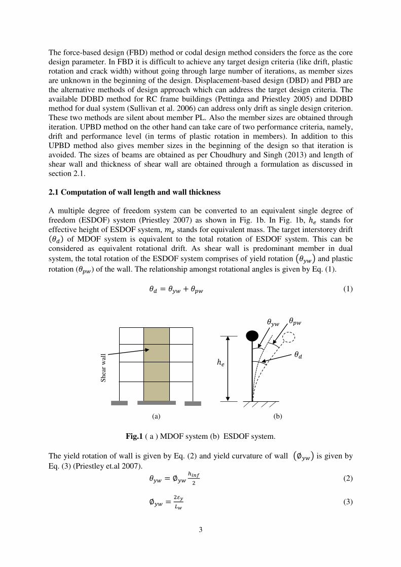
A multiple degree of freedom system can be converted to an equivalent single degree of

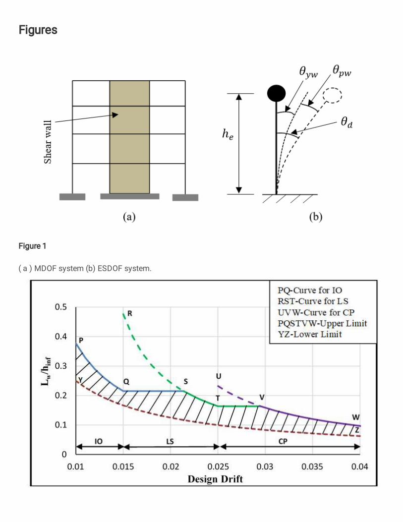
freedom (ESDOF) system (Priestley 2007) as shown in Fig. 1b. In Fig. 1b, ℎ𝑒 stands for

effective height of ESDOF system, 𝑚𝑒 stands for equivalent mass. The target interstorey drift (𝜃𝑑) of MDOF system is equivalent to the total rotation of ESDOF system. This can be

considered as equivalent rotational drift. As shear wall is predominant member in dual

system, the total rotation of the ESDOF system comprises of yield rotation (𝜃𝑦𝑤) and plastic

rotation (𝜃𝑝𝑤) of the wall. The relationship amongst rotational angles is given by Eq. (1).

𝜃𝑑 = 𝜃𝑦𝑤 + 𝜃𝑝𝑤 (1)

Fig.1 ( a ) MDOF system (b) ESDOF system.

The yield rotation of wall is given by Eq. (2) and yield curvature of wall (∅𝑦𝑤) is given by

Eq. (3) (Priestley et.al 2007). 𝜃𝑦𝑤 = ∅𝑦𝑤 ℎ𝑖𝑛𝑓2 (2)

∅𝑦𝑤 = 2𝜀𝑦𝐿𝑤 (3)

𝜃𝑦𝑤

𝜃𝑑

𝜃𝑝𝑤

ℎ𝑒

(a) (b)

Sh

ear

wal

l

4

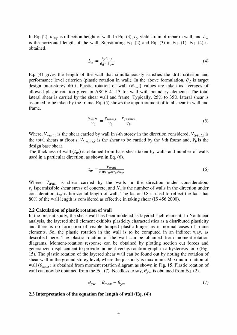
In Eq. (2), ℎ𝑖𝑛𝑓 is inflection height of wall. In Eq. (3), 𝜀𝑦 yield strain of rebar in wall, and 𝐿𝑤

is the horizontal length of the wall. Substituting Eq. (2) and Eq. (3) in Eq. (1), Eq. (4) is

obtained.

𝐿𝑤 = 𝜀𝑦ℎ𝑖𝑛𝑓𝜃𝑑− 𝜃𝑝𝑤 (4)

Eq. (4) gives the length of the wall that simultaneously satisfies the drift criterion and

performance level criterion (plastic rotation in wall). In the above formulation, 𝜃𝑑 is target

design inter-storey drift. Plastic rotation of wall (𝜃𝑝𝑤 ) values are taken as averages of

allowed plastic rotation given in ASCE 41-13 for wall with boundary elements. The total

lateral shear is carried by the shear wall and frame. Typically, 25% to 35% lateral shear is

assumed to be taken by the frame. Eq. (5) shows the apportionment of total shear in wall and

frame.

𝑉𝑤𝑎𝑙𝑙,𝑖𝑉𝑏 = 𝑉𝑡𝑜𝑡𝑎𝑙,𝑖𝑉𝑏 − 𝑉𝑓𝑟𝑎𝑚𝑒,𝑖𝑉𝑏 (5)

Where, 𝑉𝑤𝑎𝑙𝑙,𝑖 is the shear carried by wall in i-th storey in the direction considered, 𝑉𝑡𝑜𝑡𝑎𝑙,𝑖 is

the total shears at floor i, 𝑉𝑓𝑟𝑎𝑚𝑒,𝑖 is the shear to be carried by the i-th frame and, 𝑉𝑏 is the

design base shear.

The thickness of wall (𝑡𝑤) is obtained from base shear taken by walls and number of walls

used in a particular direction, as shown in Eq. (6).

𝑡𝑤 = 𝑉𝑊𝑎𝑙𝑙0.8×𝐿𝑤×𝜏𝑐×𝑁𝑤 (6)

Where, 𝑉𝑊𝑎𝑙𝑙 is shear carried by the walls in the direction under consideration, 𝜏𝑐 ispermissible shear stress of concrete, and 𝑁𝑤is the number of walls in the direction under

consideration, 𝐿𝑤 is horizontal length of wall. The factor 0.8 is used to reflect the fact that

80% of the wall length is considered as effective in taking shear (IS 456 2000).

2.2 Calculation of plastic rotation of wall

In the present study, the shear wall has been modeled as layered shell element. In Nonlinear

analysis, the layered shell element exhibits plasticity characteristics as a distributed plasticity

and there is no formation of visible lumped plastic hinges as in normal cases of frame

elements. So, the plastic rotation in the wall is to be computed in an indirect way, as

described here. The plastic rotation of the wall can be obtained from moment-rotation

diagrams. Moment-rotation response can be obtained by plotting section cut forces and

generalized displacement to provide moment versus rotation graph in a hysteresis loop (Fig.

15). The plastic rotation of the layered shear wall can be found out by noting the rotation of

shear wall in the ground storey level, where the plasticity is maximum. Maximum rotation of

wall (𝜃𝑚𝑎𝑥) is obtained from moment rotation diagram as shown in Fig. 15. Plastic rotation of

wall can now be obtained from the Eq. (7). Needless to say, 𝜃𝑦𝑤 is obtained from Eq. (2).

𝜃𝑝𝑤 = 𝜃𝑚𝑎𝑥 − 𝜃𝑦𝑤 (7)

2.3 Interpretation of the equation for length of wall (Eq. (4))

5

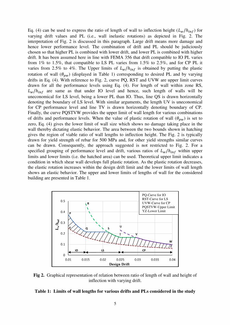
Eq. (4) can be used to express the ratio of length of wall to inflection height (𝐿𝑤/ℎ𝑖𝑛𝑓) for

varying drift values and PL (i.e., wall inelastic rotations) as depicted in Fig. 2. The

interpretation of Fig. 2 is discussed in this paragraph. Large drift means more damage and

hence lower performance level. The combination of drift and PL should be judiciously

chosen so that higher PL is combined with lower drift, and lower PL is combined with higher

drift. It has been assumed here in line with FEMA 356 that drift compatible to IO PL varies

from 1% to 1.5%, that compatible to LS PL varies from 1.5% to 2.5%, and for CP PL it

varies from 2.5% to 4%. The Upper limits of 𝐿𝑤/ℎ𝑖𝑛𝑓 is obtained by putting the plastic

rotation of wall (𝜃𝑝𝑤) (displayed in Table 1) corresponding to desired PL and by varying

drifts in Eq. (4). With reference to Fig. 2, curve PQ, RST and UVW are upper limit curves

drawn for all the performance levels using Eq. (4). For length of wall within zone RS, 𝐿𝑤/ℎ𝑖𝑛𝑓 are same as that under IO level and hence, such length of walls will be

uneconomical for LS level, being a lower PL than IO. Thus, line QS is drawn horizontally

denoting the boundary of LS level. With similar arguments, the length UV is uneconomical

for CP performance level and line TV is drawn horizontally denoting boundary of CP.

Finally, the curve PQSTVW provides the upper limit of wall length for various combinations

of drifts and performance levels. When the value of plastic rotation of wall (𝜃𝑝𝑤) is set to

zero, Eq. (4) gives the lower limit of wall size which shows no damage taking place in the

wall thereby dictating elastic behavior. The area between the two bounds shown in hatching

gives the region of viable ratio of wall lengths to inflection height. The Fig. 2 is typically

drawn for yield strength of rebar for 500 MPa and, for other yield strengths similar curves

can be drawn. Consequently, the approach suggested is not restricted to Fig. 2. For a

specified grouping of performance level and drift, various ratios of 𝐿𝑤/ℎ𝑖𝑛𝑓 within upper

limits and lower limits (i.e. the hatched area) can be used. Theoretical upper limit indicates a

condition in which shear wall develops full plastic rotation. As the plastic rotation decreases,

the elastic rotation increases within the design drift limit and the lower limits of wall length

shows an elastic behavior. The upper and lower limits of lengths of wall for the considered

building are presented in Table 1.

Fig 2. Graphical representation of relation between ratio of length of wall and height of

inflection with varying drift.

Table 1: Limits of wall lengths for various drifts and PLs considered in the study

PQ-Curve for IO RST-Curve for LS

UVW-Curve for CP

PQSTVW-Upper Limit

YZ-Lower Limit

Y

6

3. DESIGN PROCEDURE AS PER UPBD METHOD

The step wise procedure for designing frame-shear wall building using UPBD method is

given below.

Step 1: Computation of member sizes

The design target drift (𝜃𝑑) and performance level (in terms of plastic rotation of wall and

beam) are decided. The hazard level is considered. Inflection height is computed. The wall

length satisfying the target criteria is given by Eq. (4) which is repeated as Eq. (8) here.

Alternatively, 𝐿𝑤ℎ𝑖𝑛𝑓 ratio can be obtained from graph shown in Fig. 2, and Lw can be computed

knowing the value of ℎ𝑖𝑛𝑓.

𝐿𝑤 = 𝜀𝑦ℎ𝑖𝑛𝑓𝜃𝑑−𝜃𝑝𝑤 (8)

The beam depth satisfying the target criteria is given by Eq. (9) (Choudhury and Singh,

2013).

ℎ𝑏 = 0.5𝜀𝑦𝑙𝑏𝜃𝑑−𝜃𝑝𝑏 (9)

In Eq. (9), 𝑙𝑏 is length of beam in the direction of seismic action, 𝜃𝑝𝑏 is allowable plastic

rotation of beam for the PL considered (available from ASCE-SEI-41-13 and FEMA-356).

The width of beam is taken as half to two-third of beam depth as per common practice.

Column size is found out by trial so that the column steel remains in the range 3% to 4% of

the gross sectional area of column. This is the practical range of steel in column avoiding

over-crowding of bars. Alternatively, the column size can be obtained after (Mayengbam and

Choudhury 2014).

Step 2: Computation of ESDOF system properties

Length of wall for building

Target

design

drift

(𝜃𝑑)

%

Target

PL

Average

Plastic

rotation

of wall

(𝜃𝑝𝑤)

rad

(ASCE-

SEI-41-

13)

𝐿𝑤/ℎ𝑖𝑛𝑓

8-storey

(ℎ𝑖𝑛𝑓 =19.63 m)

mm

for 10-storey

(ℎ𝑖𝑛𝑓=23.6 m)

mm

12-storey

(ℎ𝑖𝑛𝑓=27.53 m)

mm

Length of wall

for 15-storey

building

(ℎ𝑖𝑛𝑓=27.53 m)

mm

Upper

limit

Lowe

r limit

Upper

limit

Lower

limit

Upper

limit

Lower

limit

Upper

limit

Lower

limit

Upper

limit

Lower

limit

1 IO 0.00337

5 0.377 0.25 7407 4907 8905 5900 10388 6882 12716 8425

2 LS 0.00975

0 0.204 0.113 3091 2453 3716 2950 4335 3441 5307 4212

3 CP 0.01425 0.169 0.083 1717 1635 2064 1966 2408 2294 2948 2808

7

The MDOF building is converted to ESDOF system using formulae given as Eq. (10) to (13)

(Sullivan et al. 2006). ∆𝑑= ∑ 𝑚𝑖∆𝑖2𝑁𝑖=1∑ 𝑚𝑖𝑛𝑖=1 ∆𝑖 (10)

𝑚𝑒 = ∑ 𝑚𝑖∆𝑖𝑁𝑖=1∆𝑑 (11)

ℎ𝑒 = ∑ 𝑚𝑖∆𝑖ℎ𝑖𝑁𝑖=1∑ 𝑚𝑖𝑛𝑖=1 ∆𝑖 (12)

∆𝑖= ∆𝑖𝑦𝑤 + (𝜃𝑑 − 𝜙𝑦𝑤ℎ𝑖𝑛𝑓/2)ℎ𝑖 (13)

Where, ∆𝑑is the design displacement, 𝑚𝑒is the effective mass, ℎ𝑒 is the equivalent height of

the ESDOF system; 𝑚𝑖 is the mass of i-th storey, ∆𝑖𝑦𝑤 is the yield displacements of wall in i-

th storey, ℎ𝑖 is the height of i-th floor from the base of the building, ∆𝑖 is the profile

displacement in the i-th floor and, N is the number of storey in the building. The yield

displacement profile of wall is obtained using Eq. (14).

∆𝑖𝑦𝑤= ∅𝑦𝑤ℎ𝑖ℎ𝑖𝑛𝑓2 − ∅𝑦𝑤ℎ𝑖𝑛𝑓26 , when ℎ𝑖 ≥ ℎ𝑖𝑛𝑓 (14a)

∆𝑖𝑦𝑤= ∅𝑦𝑤ℎ𝑖22 − ∅𝑦𝑤ℎ𝑖36ℎ𝑖𝑛𝑓 , when ℎ𝑖 ≤ ℎ𝑖𝑛𝑓 (14b) ∅𝑦𝑤 = 2𝜀𝑦𝐿𝑤 (14c)

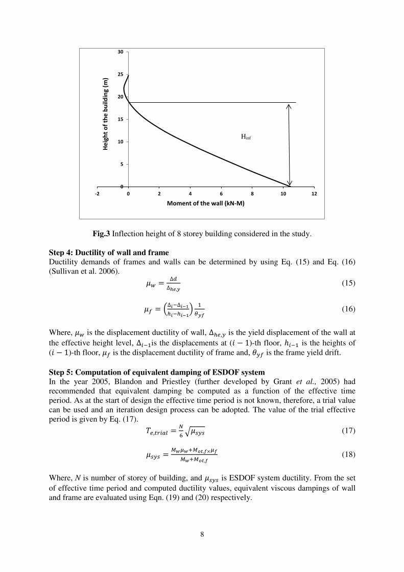
Step 3: Computation of height of inflection of wall

The height of the inflection (ℎ𝑖𝑛𝑓) is a design parameter in dual system design. Inflection

point is where the curvature of the building reverses due to frame-shear wall interaction. The

height of inflection of frame shear wall can be determined by identifying the moments that

are borne by shear wall. The vertical distribution of the moment of the wall is determined by

subtracting the frame moments from the total moments. The detailed process can be seen in

(Priestley et. al.2007). A typical drawing for inflection height is shown in Fig. 3.

8

Fig.3 Inflection height of 8 storey building considered in the study.

Step 4: Ductility of wall and frame Ductility demands of frames and walls can be determined by using Eq. (15) and Eq. (16)

(Sullivan et al. 2006). 𝜇𝑤 = ∆𝑑∆ℎ𝑒,𝑦 (15)

𝜇𝑓 = (∆𝑖−∆𝑖−1ℎ𝑖−ℎ𝑖−1) 1𝜃𝑦𝑓 (16)

Where, 𝜇𝑤 is the displacement ductility of wall, ∆ℎ𝑒,𝑦 is the yield displacement of the wall at

the effective height level, ∆𝑖−1is the displacements at (𝑖 − 1)-th floor, ℎ𝑖−1 is the heights of

(𝑖 − 1)-th floor, 𝜇𝑓 is the displacement ductility of frame and, 𝜃𝑦𝑓 is the frame yield drift.

Step 5: Computation of equivalent damping of ESDOF system

In the year 2005, Blandon and Priestley (further developed by Grant et al., 2005) had

recommended that equivalent damping be computed as a function of the effective time

period. As at the start of design the effective time period is not known, therefore, a trial value

can be used and an iteration design process can be adopted. The value of the trial effective

period is given by Eq. (17). 𝑇𝑒,𝑡𝑟𝑖𝑎𝑙 = 𝑁6 √𝜇𝑠𝑦𝑠 (17)

𝜇𝑠𝑦𝑠 = 𝑀𝑤𝜇𝑤+𝑀𝑜𝑡,𝑓×𝜇𝑓𝑀𝑤+𝑀𝑜𝑡,𝑓 (18)

Where, N is number of storey of building, and 𝜇𝑠𝑦𝑠 is ESDOF system ductility. From the set

of effective time period and computed ductility values, equivalent viscous dampings of wall

and frame are evaluated using Eqn. (19) and (20) respectively.

0

5

10

15

20

25

30

-2 0 2 4 6 8 10 12

He

igh

t o

f th

e b

uil

din

g (

m)

Moment of the wall (kN-M)

Hinf

9

𝜉𝑤 = 951.3𝜋 (1 − 𝜇𝑤−0.5 − 0.1 × 𝑟 × 𝜇𝑤) ( 1( 𝑇𝑒,𝑡𝑟𝑖𝑎𝑙+0.85)4) (19)

𝜉𝑓 = 1201.3𝜋 (1 − 𝜇𝑤−0.5 − 0.1 × 𝑟 × 𝜇𝑓) (1 + 1( 𝑇𝑒,𝑡𝑟𝑖𝑎𝑙+0.85)4) (20)

The equivalent damping of ESDOF system is obtained from Eq. (21).

𝜉𝑆𝐷𝑜𝐹 = 𝑀𝑤𝜉𝑤+𝑀𝑜𝑡,𝑓 𝜉𝑓𝑀𝑤+ 𝑀𝑜𝑡,𝑓 (21)

Here, 𝑀𝑤 is wall moment, 𝜉𝑤 is wall damping, 𝑀𝑜𝑡,𝑓 is overturning moment of frames, 𝜉𝑓 is

frame damping, 𝑇𝑒,𝑡𝑟𝑖𝑎𝑙 is trial effective time period, and 𝑟 is the post yield stiffness ratio,

generally taken as 0.05 for new RC structures.

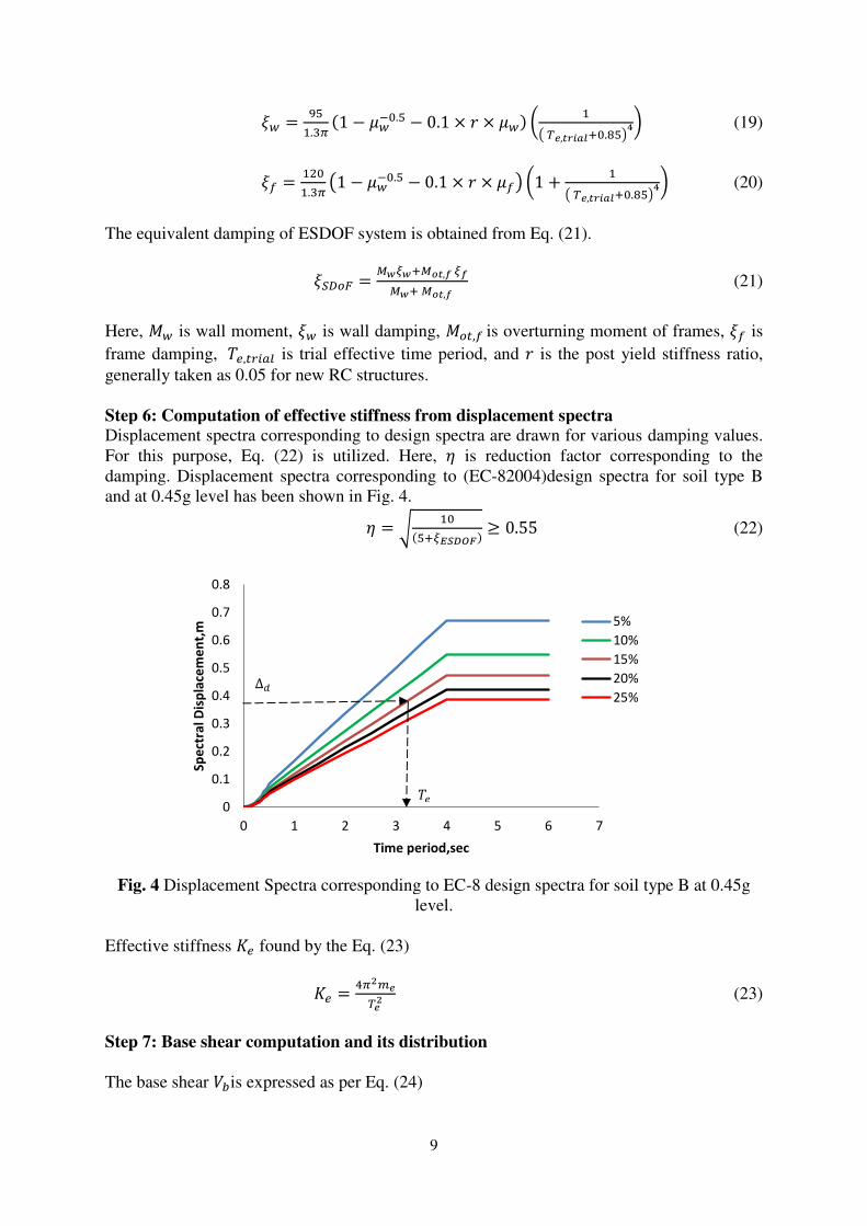
Step 6: Computation of effective stiffness from displacement spectra

Displacement spectra corresponding to design spectra are drawn for various damping values.

For this purpose, Eq. (22) is utilized. Here, 𝜂 is reduction factor corresponding to the

damping. Displacement spectra corresponding to (EC-82004)design spectra for soil type B

and at 0.45g level has been shown in Fig. 4. 𝜂 = √ 10(5+𝜉𝐸𝑆𝐷𝑂𝐹) ≥ 0.55 (22)

Fig. 4 Displacement Spectra corresponding to EC-8 design spectra for soil type B at 0.45g

level.

Effective stiffness 𝐾𝑒 found by the Eq. (23)

𝐾𝑒 = 4𝜋2𝑚𝑒𝑇𝑒2 (23)

Step 7: Base shear computation and its distribution

The base shear 𝑉𝑏is expressed as per Eq. (24)

0

0.1

0.2

0.3

0.4

0.5

0.6

0.7

0.8

0 1 2 3 4 5 6 7

Sp

ect

ral

Dis

pla

cem

en

t,m

Time period,sec

5%

10%

15%

20%

25%Δ𝑑

𝑇𝑒

10

𝑉𝑏 = 𝐾𝑒∆𝑑 (24)

The computed base shear is distributed to different floors as per Eq. (25) 𝐹𝑖 = 𝑉𝑏 𝑚𝑖∆𝑖∑ 𝑚𝑖∆𝑖𝑛𝑖=1 (25)

Where, Fi is the force applied to different floors of the buildings. The base shear computation

and its distribution shall be done in both the mutually perpendicular directions of the plan of

the building. The Eq. (25) is valid upto 10-storey high buildings. For buildings taller than ten

storey, 90% of base shear is distributed in all floors including the roof level as per Eq. (25);

the remaining 10% of base shear is put at roof level. This is done to take care of higher mode

effects in tall buildings.

Step 8: Load combination and design

The combinations of load used for design are:

𝐷𝐿 + 𝐿𝐿 𝐷𝐿 + 𝐿𝐿 ± 𝐹𝑥 𝐷𝐿 + 𝐿𝐿 ± 𝐹𝑦

Where 𝐷𝐿, 𝐿𝐿, 𝐹𝑥, 𝐹𝑦stand for dead load, live load, earthquake load in x direction and

earthquake load in y direction respectively. It may be noted that DDBD or UPBD method of

design are damaged based design. As such partial safety factor as used in limit state design

are not applicable. For the same reason expected strength of materials are used. Capacity

design is carried out so that column to beam capacity ratio is more than 1.4 (IS 13920-2016;

this is 1.3 as per EC-8).

4. MODELING ASPECTS

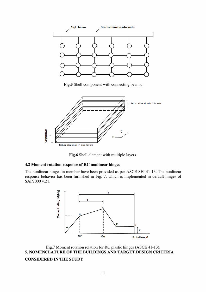
4.1 Shear wall modeling

The shear wall has been modeled as layered shell element. In shell element the steel bar can

provided in either one layer or two layers. Rigid beam elements are assumed in the beam

level. There is a tendency of normal beams embedded within shear wall get damaged thereby

distorting the normal shear wall behavior. The rigid beam element prevents this unwanted

behavior of wall. The purpose of rigid element is also to reduce the mesh resistance

formulations. It also gives proper connection with adjacent beams and columns. These

aspects are shown in Fig. 5 and 6. The modulus of elasticity of rigid beams is taken about 10

times the modulus of elasticity of concrete (Kubin et al. 2008, Fahjan et al. 2010). ASCE-

SEI-41-13 gives the plastic rotation of shear wall for various performance levels. Debnath

and Choudhury (2017) performed a nonlinear shell element component study and attempted

to understand its performance for LS buildings.

11

Fig.5 Shell component with connecting beams.

Fig.6 Shell element with multiple layers.

4.2 Moment rotation response of RC nonlinear hinges

The nonlinear hinges in member have been provided as per ASCE-SEI-41-13. The nonlinear

response behavior has been furnished in Fig. 7, which is implemented in default hinges of

SAP2000 v.21.

Fig.7 Moment rotation relation for RC plastic hinges (ASCE 41-13).

5. NOMENCLATURE OF THE BUILDINGS AND TARGET DESIGN CRITERIA

CONSIDERED IN THE STUDY

12

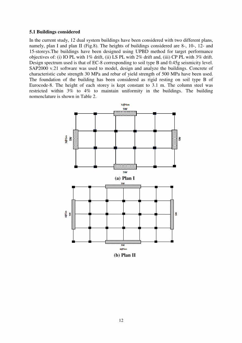
5.1 Buildings considered

In the current study, 12 dual system buildings have been considered with two different plans,

namely, plan I and plan II (Fig.8). The heights of buildings considered are 8-, 10-, 12- and

15-storeys.The buildings have been designed using UPBD method for target performance

objectives of: (i) IO PL with 1% drift, (ii) LS PL with 2% drift and, (iii) CP PL with 3% drift.

Design spectrum used is that of EC-8 corresponding to soil type B and 0.45g seismicity level.

SAP2000 v.21 software was used to model, design and analyze the buildings. Concrete of

characteristic cube strength 30 MPa and rebar of yield strength of 500 MPa have been used.

The foundation of the building has been considered as rigid resting on soil type B of

Eurocode-8. The height of each storey is kept constant to 3.1 m. The column steel was

restricted within 3% to 4% to maintain uniformity in the buildings. The building

nomenclature is shown in Table 2.

(a) Plan I

(b) Plan II

13

(c) Typical elevation

Fig.8 Building model considered in the study: (a) Plan I (b) Plan II (c) typical elevation [SW

indicates shear wall].

Building name starts with ‘B’ and contains number of storey and PL (IO, LS or CP). The sizes of member used in buildings have been given in Table 3. As an example, for the

building B-15-CP length of wall has taken as 12 m, which lies between the upper limit and

lower limits (Table 1). To show any length of wall within this limit works, the length of wall

for building B-12-CP have been taken as 10 m. Likewise, the length of wall of other

buildings has been taken within limits of Table 1. The computed ESDOF system properties

are given in Table 4. As per FEMA-356, the expected strength of concrete is taken as 1.5

times the characteristics strength, and, expected strength of rebar is taken as 1.25 times the

yield strength of rebar.

Table 2: Nomenclature of the buildings and target design criteria considered

Sl No. Plan of the

Building

Nomenclature

of Buildings

Target

performance

level

Target

drift

1 I B-8-IO

IO 1% 2 I B-10-IO 3 I B-12-IO 4 I B-15-IO

5 I B-8-LS

LS 2% 6 II B-10-LS 7 II B-12-LS

8 II B-15-LS

9 II B-8-CP

CP 3% 10 II B-10-CP 11 II B-12-CP

12 II B-15-CP

14

Table 3: Dimensions of members of the buildings considered

Building name Column sizes (mm)

Beam size (mm) Shear wall thickness

(mm)

Length of wall

(mm) Inner

Column

Outer

column

B-8-IO 800 × 800 900 × 900 500 × 1000 150 3000

850 × 850

800 ×800

B-10-IO 600 × 600 700×700 350 × 500 300 3500

650×650

600×600

B-12-IO 600 ×600 700×700 400 × 600 300 4000

650×650

600×600

B-15-IO 800 × 800 800×800 500 × 1000 300 5000

850×850

900×900

B-8-LS 700 × 700 800×800 450 × 700 150 5000

750×750

700×700

B-10-LS 550 × 550 650×650 400 × 700 300 6000

600×600

550×550

B-12-LS 650 ×650 750×750 450 × 900 300 7000

700×700

650×650

B-15-LS 700 × 700 800×800 350 × 600 300 8000

750×750

730×730

B-8-CP 600 × 600 700×700 350 × 500 150 7000

650×650

600×600

B-10-CP 600 × 600 700×700 350 × 500 200 8000

650×650

600×600

B-12-CP 600 × 600 700×700 450 × 650 200 10000

650×650

600×600

B-15-CP 730 × 730 780×780 500 × 750 300 12000

750×750

730×730

Table 4: ESDOF system properties for buildings designed

Buildings ∆d

m

me

kg he

ξw

%

ξf

%

μ Te

sec

Ke

kN/m

Vb

kN wall frame

B-8-IO

B-10-IO

B-12-IO

B-15-IO

0.247

0.400

0.557

0.733

2109150

3340535

3149765

6874082

17.669

23.137

25.835

32.198

8.16

9.29

10.67

11.71

17.15

10.35

7.06

9.50

2.377

2.776

3.419

4.097

6.71

2.46

1.77

2.24

2.9

2.6

2.9

3.8

9890787

19488960

14770714

18774433

2447

7799

8229

13770

B-8-LS

B-10-LS

B-12-LS

B-15-LS

0.283

0.322

0.424

0.610

3108391

3774809

6659832

7705276

17.209

21.220

25.532

40.301

9.69

9.33

8.96

8.54

7.77

8.63

7.83

7.34

2.944

2.792

2.652

2.502

1.89

2.05

1.9

1.81

2.9

2.6

2.9

3.6

14576692

22022553

31231051

23447823

4127

7093

13249

14318

B-8-CP

B-10-CP

B-12-CP

B-15-CP

0.314

0.366

0.439

0.556

2358018

3961201

5912479

13898194

17.929

21.089

25.351

31.589

12.08

9.674

9.303

10.05

3.56

9.37

7.42

9.50

4.347

2.935

2.781

3.109

1.31

2.20

1.82

2.24

2.9

2.6

2.9

3.8

11057844

23109979

27726365

37958626

3482

8474

12199

21125

15

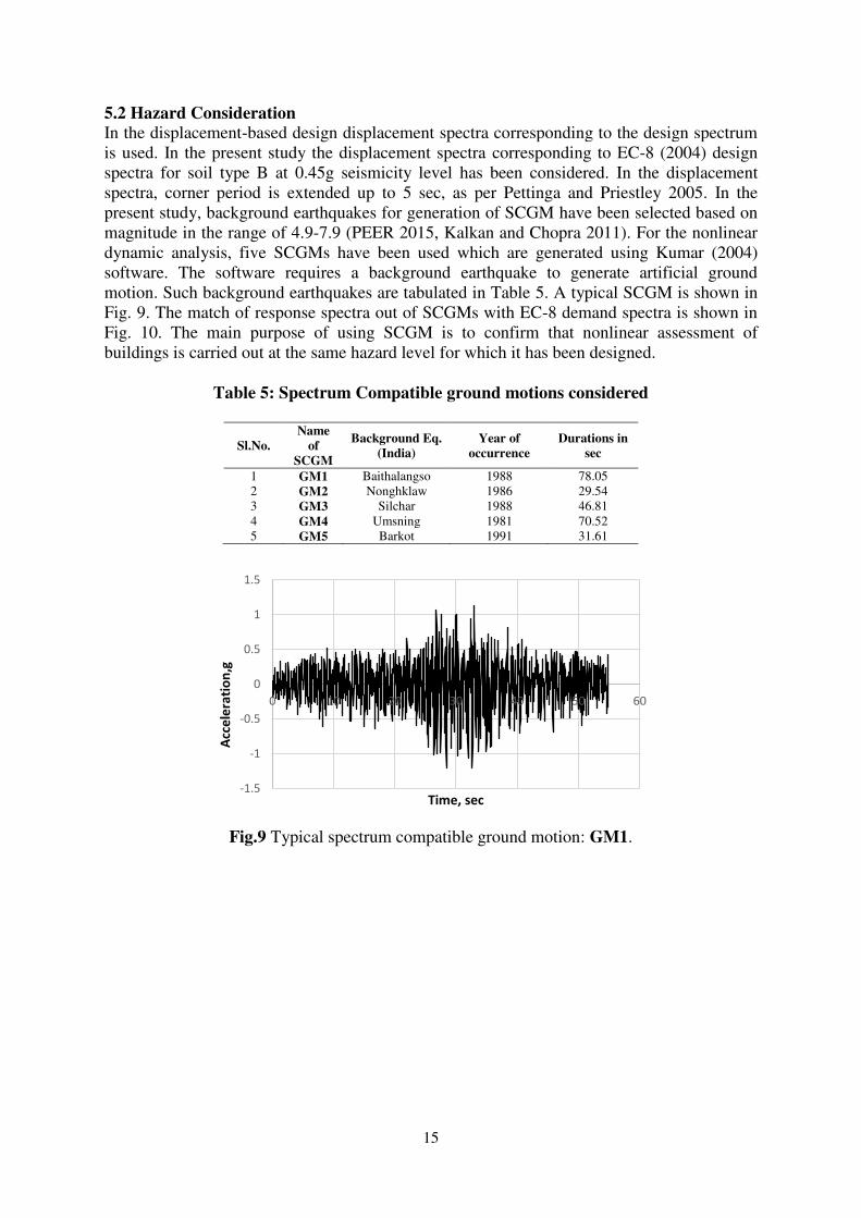
5.2 Hazard Consideration

In the displacement-based design displacement spectra corresponding to the design spectrum

is used. In the present study the displacement spectra corresponding to EC-8 (2004) design

spectra for soil type B at 0.45g seismicity level has been considered. In the displacement

spectra, corner period is extended up to 5 sec, as per Pettinga and Priestley 2005. In the

present study, background earthquakes for generation of SCGM have been selected based on

magnitude in the range of 4.9-7.9 (PEER 2015, Kalkan and Chopra 2011). For the nonlinear

dynamic analysis, five SCGMs have been used which are generated using Kumar (2004)

software. The software requires a background earthquake to generate artificial ground

motion. Such background earthquakes are tabulated in Table 5. A typical SCGM is shown in

Fig. 9. The match of response spectra out of SCGMs with EC-8 demand spectra is shown in

Fig. 10. The main purpose of using SCGM is to confirm that nonlinear assessment of

buildings is carried out at the same hazard level for which it has been designed.

Table 5: Spectrum Compatible ground motions considered

Sl.No.

Name

of

SCGM

Background Eq.

(India)

Year of

occurrence

Durations in

sec

1 GM1 Baithalangso 1988 78.05

2 GM2 Nonghklaw 1986 29.54

3 GM3 Silchar 1988 46.81

4 GM4 Umsning 1981 70.52

5 GM5 Barkot 1991 31.61

Fig.9 Typical spectrum compatible ground motion: GM1.

-1.5

-1

-0.5

0

0.5

1

1.5

0 10 20 30 40 50 60

Acc

ele

rati

on

,g

Time, sec

16

Fig. 10 Match of response spectra of SCGMs with EC-8 design spectrum.

6. RESULTS AND DISCUSSIONS

Plastic rotations of the frame members are checked by observing the hinge patterns. In

SAP2000 v.21 software, the frame member’s show lumped plastic hinges and the

performance level of the hinges can be identified by the color of the hinges. As shown in

Table 3, total 12 frame-shear wall buildings have been designed in this study using UPBD

method, and evaluated through nonlinear analyses.The hinge formation at MCE level in

frame elements for typical frames are shown in Fig. 11. The hinge patterns show that the

target performance levels for respective buildings have been achieved.

B-8-IO Short-Direction

B-8-IO Long-Direction

0

0.5

1

1.5

2

2.5

3

3.5

0 1 2 3 4 5

Sa

/g

Period (sec)

EC-8

GM1

GM2

GM3

GM4

GM5

17

B-10-LS Short-Direction

B-10-LS Long-Direction

Fig.11 Plastic hinges for typical building frames at end of time history analysis.

The performance level for the buildings can also be read out from the pushover analysis. The

performance point encompassed by a nearest performance level designator in the capacity

curve gives the performance level of the building. In Fig. 12, the typical pushover curves

have been presented. The pushover curves show that the target performance level of IO and

LS have been achieved in the respective buildings.

0

2000

4000

6000

8000

10000

12000

0 0.1 0.2 0.3 0.4

Ba

se s

he

ar

(kN

)

Displacement (m)

B-12-IO

Mode Pushover

Uniform Pushover

IO

LS

CP

PP

0

4000

8000

12000

16000

20000

0 0.1 0.2 0.3 0.4

Ba

se s

hea

r (k

N)

Displacement (m)

B-15-IO

18

Fig.12 Pushover curves of typical buildings at the end of time history analysis.

The inter-storey drift ratio (IDR) can be obtained from displacement time histories of floors.

In Fig. 13 the IDR diagram for typical buildings are presented. From the figures it is clear

that the target drifts have been achieved with marginal deviation.

0

3000

6000

9000

0 0.2 0.4 0.6 0.8 1

Ba

se s

he

ar

(kN

)

Displacement (m)

B-8-LS

0

8000

16000

24000

32000

40000

0 0.1 0.2 0.3

Ba

se

she

ar

(kN

)

Displacement (m)

B-12-LS

0

3000

6000

9000

12000

15000

18000

0 0.2 0.4 0.6

Ba

se s

he

ar

(kN

)

Displacement (m)

B-12-CP

0

5000

10000

15000

20000

25000

30000

0 0.2 0.4 0.6 0.8

Ba

se s

he

ar

(kN

)

Displacement (m)

B-15-CP

0

1

2

3

4

5

6

7

8

9

0 1 2

Sto

rey

Hei

gh

t

IDR%

B-8-IO short-direction

PGA 1

PGA 2

PGA 3

PGA 4

PGA 5

1% DRIFT

0

1

2

3

4

5

6

7

8

9

0 1 2

Sto

rey

Hei

gh

t

IDR%

B-8-IO long-direction

0

2

4

6

8

10

12

14

0 2 4

Sto

rey

Hei

gh

t

IDR%

B-12-LS short-direction

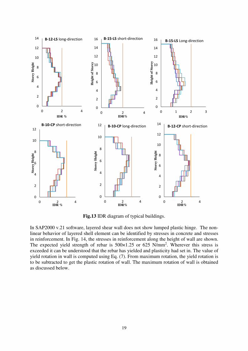
19

Fig.13 IDR diagram of typical buildings.

In SAP2000 v.21 software, layered shear wall does not show lumped plastic hinge. The non-

linear behavior of layered shell element can be identified by stresses in concrete and stresses

in reinforcement. In Fig. 14, the stresses in reinforcement along the height of wall are shown.

The expected yield strength of rebar is 500×1.25 or 625 N/mm2. Wherever this stress is

exceeded it can be understood that the rebar has yielded and plasticity had set in. The value of

yield rotation in wall is computed using Eq. (7). From maximum rotation, the yield rotation is

to be subtracted to get the plastic rotation of wall. The maximum rotation of wall is obtained

as discussed below.

0

2

4

6

8

10

12

14

0 2 4

Sto

rey

Hei

gh

t

IDR %

B-12-LS long-direction

0

2

4

6

8

10

12

14

16

0 2 4

Hei

gh

t o

f S

tore

y

IDR%

B-15-LS short-direction

0

2

4

6

8

10

12

14

16

0 1 2 3

Hei

gh

t o

f S

tore

y

IDR%

B-15-LS Long-direction

0

2

4

6

8

10

12

0 2 4

Sto

rey

Hei

gh

t

IDR %

B-10-CP short-direction

0

2

4

6

8

10

12

0 2 4

Sto

rey

Hei

gh

t

IDR%

B-10-CP long-direction

0

2

4

6

8

10

12

14

0 2 4

Sto

rey

Hei

gh

t

IDR%

B-12-CP short-direction

20

Fig.14 Stress diagrams of layered shear wall for typical walls.

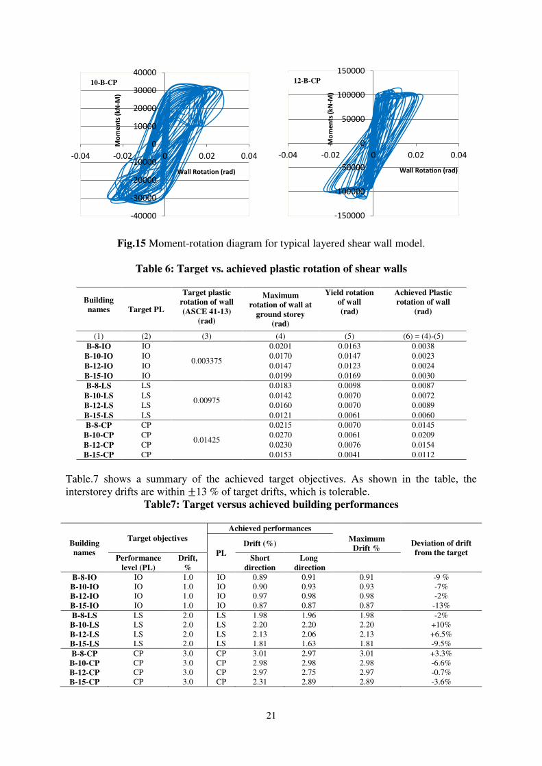
The maximum rotation in shear wall can be determined by plotting section cut forces and

generalized displacements which in turn provides the moment versus rotation graph in a

hysteresis loop as shown in Fig.15. From these graphs the maximum rotation of wall can be

determined. The plastic rotation is obtained by subtracting the yield rotation from total

rotation. Table 6 shows the computed plastic rotation of shear walls of different buildings and

also it shows that the actual plastic rotations are within the limits of target values.

-30000

-20000

-10000

0

10000

20000

30000

-0.03 -0.02 -0.01 0 0.01 0.02

Mo

me

nts

(kN

-M)

Wall Rotation(rad)

-60000

-40000

-20000

0

20000

40000

60000

-4.00E-02 -2.00E-02 0.00E+00 2.00E-02

Mo

me

nts

(k

N-M

)

Wall Rotation (rad)

B-8-IO B-12-IO B-10-CP

8-B-LS 12-B-LS

21

Fig.15 Moment-rotation diagram for typical layered shear wall model.

Table 6: Target vs. achieved plastic rotation of shear walls

Building

names

Target PL

Target plastic

rotation of wall

(ASCE 41-13)

(rad)

Maximum

rotation of wall at

ground storey

(rad)

Yield rotation

of wall

(rad)

Achieved Plastic

rotation of wall

(rad)

(1) (2) (3) (4) (5) (6) = (4)-(5)

B-8-IO IO

0.003375

0.0201 0.0163 0.0038

B-10-IO IO 0.0170 0.0147 0.0023

B-12-IO IO 0.0147 0.0123 0.0024

B-15-IO IO 0.0199 0.0169 0.0030

B-8-LS LS

0.00975

0.0183 0.0098 0.0087

B-10-LS LS 0.0142 0.0070 0.0072

B-12-LS LS 0.0160 0.0070 0.0089

B-15-LS LS 0.0121 0.0061 0.0060

B-8-CP CP

0.01425

0.0215 0.0070 0.0145

B-10-CP CP 0.0270 0.0061 0.0209

B-12-CP CP 0.0230 0.0076 0.0154

B-15-CP CP 0.0153 0.0041 0.0112

Table.7 shows a summary of the achieved target objectives. As shown in the table, the

interstorey drifts are within ±13 % of target drifts, which is tolerable.

Table7: Target versus achieved building performances

Building

names

Target objectives

Achieved performances

Deviation of drift

from the target PL

Drift (%) Maximum

Drift %

Performance

level (PL)

Drift,

%

Short

direction

Long

direction

B-8-IO IO 1.0 IO 0.89 0.91 0.91 -9 %

B-10-IO IO 1.0 IO 0.90 0.93 0.93 -7%

B-12-IO IO 1.0 IO 0.97 0.98 0.98 -2%

B-15-IO IO 1.0 IO 0.87 0.87 0.87 -13%

B-8-LS LS 2.0 LS 1.98 1.96 1.98 -2%

B-10-LS LS 2.0 LS 2.20 2.20 2.20 +10%

B-12-LS LS 2.0 LS 2.13 2.06 2.13 +6.5%

B-15-LS LS 2.0 LS 1.81 1.63 1.81 -9.5%

B-8-CP CP 3.0 CP 3.01 2.97 3.01 +3.3%

B-10-CP CP 3.0 CP 2.98 2.98 2.98 -6.6%

B-12-CP CP 3.0 CP 2.97 2.75 2.97 -0.7%

B-15-CP CP 3.0 CP 2.31 2.89 2.89 -3.6%

-40000

-30000

-20000

-10000

0

10000

20000

30000

40000

-0.04 -0.02 0 0.02 0.04

Mo

me

nts

(k

N-M

)

Wall Rotation (rad)

-150000

-100000

-50000

0

50000

100000

150000

-0.04 -0.02 0 0.02 0.04

Mo

me

nts

(k

N-M

)

Wall Rotation (rad)

10-B-CP 12-B-CP

22

7. CONCLUSIONS

The theoretical background of the UPBD method for dual system has been highlighted. This

method of design can accommodate both drift and performance level as the target design

objectives. The method also gives member sizes in the beginning of design. The UPBD

method has been applied to design of 12 numbers of dual system buildings of two plans and

height categories of 8-, 10-, 12- and 15-storey heights and for various combinations of drifts

and performance levels. The drifts and performance levels considered are: IO with 1% drift,

LS with 2% drift and, CP with 3% drift. Layered shear wall shell elements have been used in

modeling the shear wall. Displacement spectra corresponding to EC-8 design spectra for B

type soil and seismicity level of 0.45g has been used. However, the design philosophy shall

work at any other seismicity level. Default hinges of SAP2000 v.21 software for frame

elements have been used as per ASCE-SEI 13. After the design for various target objectives,

the buildings have been subjected to nonlinear pushover analysis and time history analysis

under 5 spectrum compatible ground motions. The effectiveness of the UPBD method has

been verified along both the directions of plan of the buildings considered. Fig. 11 and Fig.

12 along with Table 6 show that the target performance levels have been achieved in all

cases. Fig. 13 and Table 7 show that the target drifts have been achieved to satisfactory

tolerance limit. From the discussions on the results obtained, it is found that the UPBD

method for dual system works well in satisfying target design objectives in terms of drift and

performance level, under any specific hazard level. The advantage of the UPBD method lies

in the fact that the target performance level and the target drift can be accommodated

simultaneously in design and, member sizes are obtained at the beginning of design thus,

avoiding iteration.

REFERENCES

[1] AkisT, Tokdemir T, Yilmaz C. (2018) Modeling of Asymmetric Shear Wall-Frame

Building Structures. Journal of Asian Architecture and Building Engineering 8 (2):531-538.

[2] ASCE/SEI 41-13(2014) (American Society of Civil Engineers Seismic Evaluation and

Retrofit of Existing Buildings).

[3] Blandon, C. A. and Priestley, M. J. N. (2005) “Equivalent viscous damping equations

for direct displacement based design,” Journal of Earthquake Engineering 9 (Special

Issue 2), 257–278.

[4] Choudhury S, Singh S.M. (2013) A Unified Approach to Performance-Based Design of

RC Frame Buildings. Journal of the Institution of Engineers (India); Series A 94(2):73-82.

[5] Clough, R.W, King, I.P.Wilson, E.L. (1964) Structural analysis of multistory buildings.

Journal of the Structural Division. 90 (19):19-34

[6] Chandurkar P. P., Pajgade P. S. (2013) Seismic Analysis of RCC Building with and

Without Shear Wall, International Journal of Modern Engineering Research. 3(3): 1805-

1810.

[7] Das S, Choudhury S. (2019) Influence of effective stiffness on the performance of RC

frame buildings designed using displacement-based method and evaluation of column

effective stiffness using ANN. Engineering Structures 197.

[8] Debnath P.P, Choudhury S. (2017) Nonlinear Analysis of Shear Wall in Unified

Performance Based Seismic Design of Buildings. Asian Journal of Civil Engineering

(BHRC) 18(4): 633-642.

[9] Eurocode 8 (2004) Design of Structures for Earthquake Resistance, Part 1: General Rules,

Seismic Actions and Rules for Buildings Comite European de Normalization, Brussels.

23

[10] FEMA-356 (2000) Pre-standard and commentary for the seismic rehabilitation of

building.

[11] Fahjan Y.M, Kubin J, Tan M.T.(2010) Non-linear analysis methods for reinforced

concrete buildings with shear walls. 14 European Conference on Earthquake Engineering 1-

8.

[12] Grant, D. N., Blandon, C. A. and Priestley, M. J. N. (2005) Modelling Inelastic Response

in Direct-Displacement Based Design, Research Report ROSE – 2005/3, IUSS Press,

Pavia, Italy.

[13]Harman D. J, and Henderson P. W. (1985) Analysis of interconnected shear walls using

wide column analogy. Canadian Journal of Civil Engineering. 12(2) 362-369.

[14] IS 13920 (2016) ductiledesigns and detailing of reinforced concrete structure subjected

to seismic force. Bureau of Indian Standards New Delhi, India.

[15] IS 456 (2000) Plain and reinforced concrete code of practice, Bureau of Indian Standards

New Delhi India.

[16] IS 1893(2016) PART-1 Criteria for earthquake resistant design of structure general

provisions and buildings, sixth revision, Bureau of Indian Standard New Delhi, India.

[17] Kumar A (2004), Generation of spectrum compatible ground motion13th World

Conference of Earthquake Engineering Canada.

[18] Kubin J, Fahjan Y. M, Tan M. T. (2008) Comparison of practical approaches for

modelling shear walls in structural analyses of buildings. The 14th World Conference on

Earthquake Engineering.

[19] Kwan A. K. H. (1993) Improved wide-column-frame analogy for shear/core wall

analysis. Journals of Structural Engineering. 119(2):420-437.

[20] Kalkan E and Chopra A. K. (2011) Practical Guidelines to Select and Scale Earthquake

Records for Nonlinear Response History Analysis of Structures. Earthquake Engineering

Research Institute.

[21] Looi D.T.W, Su R.K.L, Cheng B, Tsang H.H. (2017) Effects of axial load on seismic

performance of reinforced concrete walls with short shear span, Engineering Structures. 151:

pp. 312-326.

[22] Mayengbam S. and Choudhury S. (2014) Determination of column size for

displacement-based design of reinforced concrete frame buildings. Journal of Earthquake

Engineering and Structural Dynamics 43(8): 1149-1172.

[23] Ozkula T. A, Kurtbeyoglub A, Borekcic M, Zengind B, Kocakc A.(2019) Effect of shear

wall on seismic performance of RC frame buildings. Engineering Failure Analysis 100:60-

75.

[24] Pettinga J.D, Priestley M.J.N. (2005) Dynamic behaviour of reinforced concrete frames

designed with direct displacement-based design. Journal of Earthquake Engineering 9

(Special Issue 2):309-330.

[25] Priestley MJN, (2003) Myths and fallacies in Earthquake engineering, Revisited the

ninth mallet Milne lecture.

[26] Priestley MJN, Calvi GM, Kowalaski MJ. (2007) Displacement based seismic design of

structures. Pavia, ItalyIUSS Press.

[27] Pejovic J, Serdar N, Pejovic R, Jankovic S. (2018) Shear force magnification in

reinforced concrete walls of high-rise buildings designed according to Eurocode 8.

Engineering Structures 200.

[28] SAP2000v21, Structural analysis programme. Berkley, CA, USA: Computer and

Structures Inc.

[29] Sullivan T.J, Priestley M.J.N., Calvi G.M.(2006) Direct Displacement-Based Design of

Frame-Wall Structures. Journal of Earthquake Engineering.10 (Special Issue 1): 91-124.

24

[30] Tarigan J, Manggala J, Sitorus T. (2018) The effect of shear wall location in resisting

earthquake. IOP conference series: Materials Science and Engineering. 309:1-6.

Figures

Figure 1

( a ) MDOF system (b) ESDOF system.

Figure 2

Graphical representation of relation between ratio of length of wall and height of in�ection with varyingdrift.

Figure 3

In�ection height of 8 storey building considered in the study.

Figure 4

Displacement Spectra corresponding to EC-8 design spectra for soil type B at 0.45g level.

Figure 5

Shell component with connecting beams.

Figure 6

Shell element with multiple layers.

Figure 7

Moment rotation relation for RC plastic hinges (ASCE 41-13).

Figure 8

Building model considered in the study: (a) Plan I (b) Plan II (c) typical elevation [SW indicates shearwall].

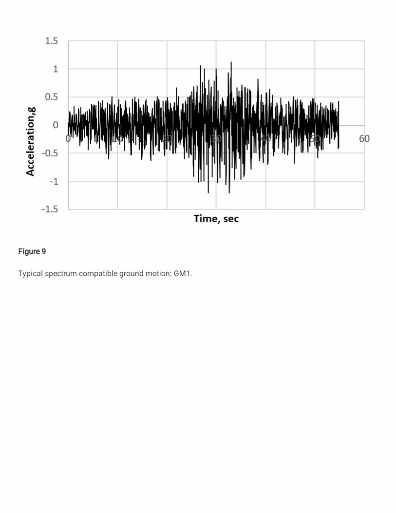
Figure 9

Typical spectrum compatible ground motion: GM1.

Figure 10

Match of response spectra of SCGMs with EC-8 design spectrum.

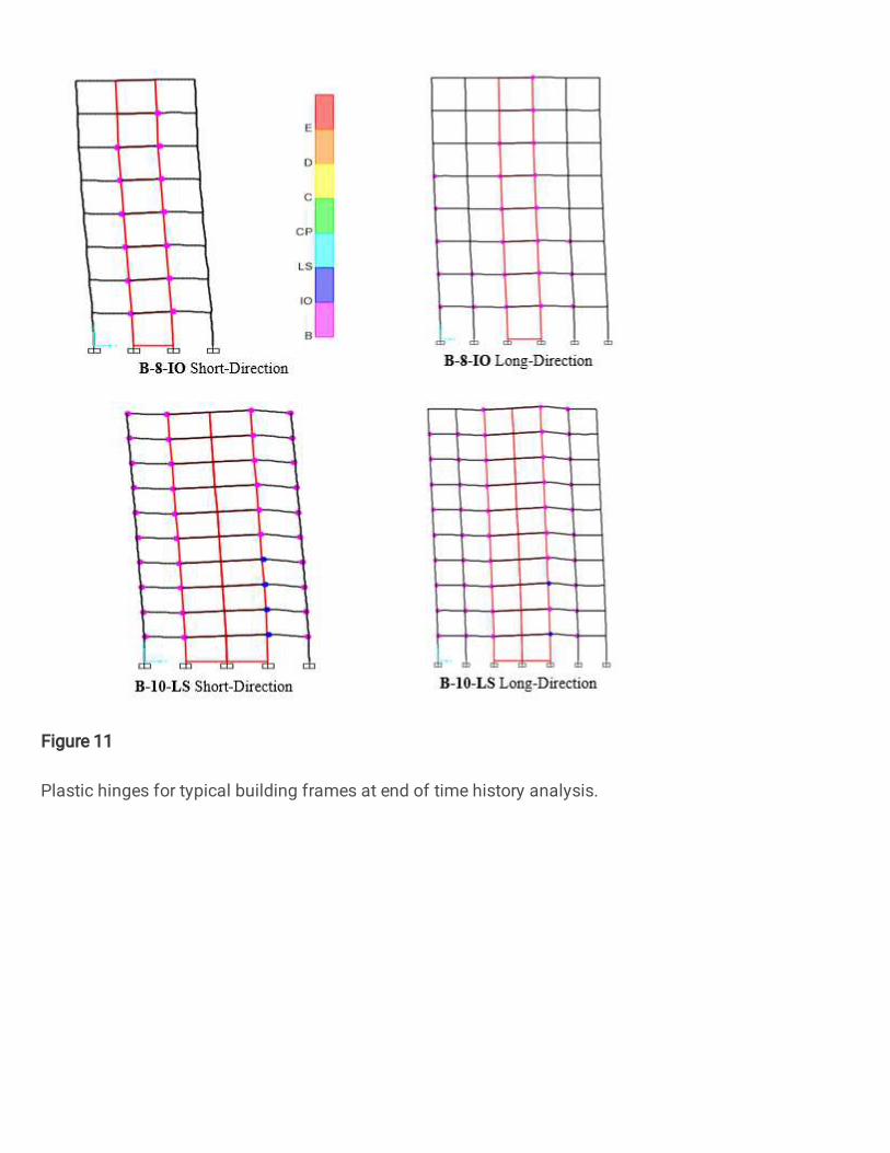
Figure 11

Plastic hinges for typical building frames at end of time history analysis.

Figure 12

Pushover curves of typical buildings at the end of time history analysis.

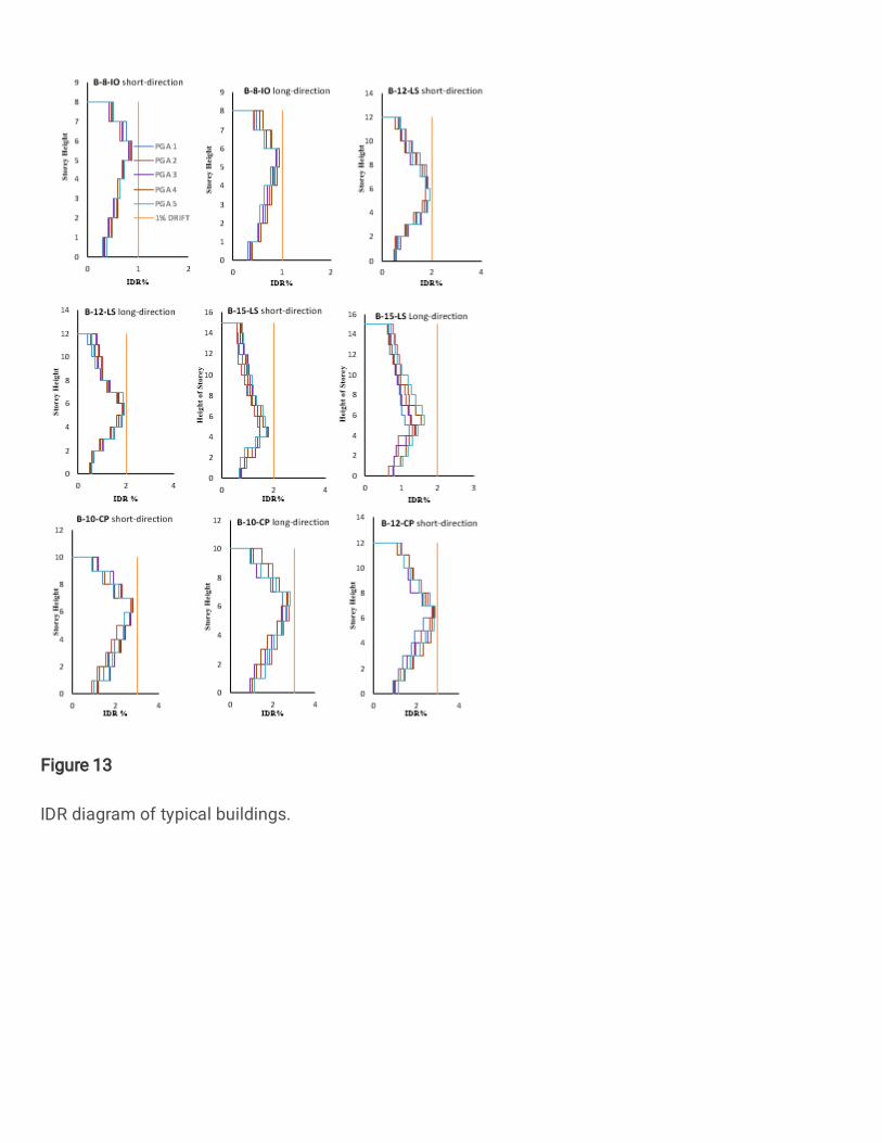
Figure 13

IDR diagram of typical buildings.

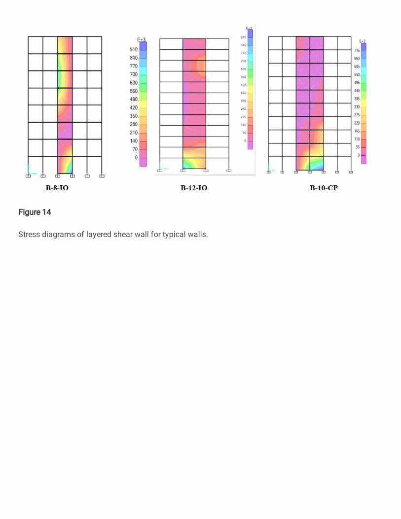
Figure 14

Stress diagrams of layered shear wall for typical walls.

Figure 15

Moment-rotation diagram for typical layered shear wall model.