UNDERSTANDING UNIT COSTS OF HOUSING PROVIDERS – REGRESSION ... · PDF fileUnderstanding...

UNDERSTANDING UNIT COSTS OF HOUSING PROVIDERS – REGRESSION ANALYSIS Technical Report July 2012

1

Understanding unit costs of housing providers – regression analysis

Technical report

Contents

Introduction 3

Regression analysis – outline 4

Cost data – headlines and trends 11

Explanatory variables – overview 17

Results of regression analysis 25

Extensions of the model 39

Annex A – Additional detail of modelling 48

2

Introduction and analytical framework

Introduction

Understanding how different factors influence the costs of providing social housing is an important aspect of the regulator’s role.

Costs of social housing providers are driven by a number of factors. Without controlling for a sufficient range of factors, simple comparisons of costs across groups of providers are unlikely to be meaningful. Regression analysis is a statistical method that overcomes this: it allows one to isolate the effects of a particular factor on costs, holding all other factors constant.

The regulator has conducted a full regression analysis to estimate the effect of different cost drivers for providers1. This is a more extensive exercise than those previously commissioned for the sector2, incorporating over 170,000 data points from 2005 to 2011. It draws together data gathered by the regulator (Accounts Returns, RSR) and also from national datasets (e.g. CORE lettings data, regional wages, deprivation, rural areas). It has been informed by a practical understanding of social housing and the data on which analysis is based. It is focused on understanding sector-wide cost drivers rather than the costs of individual providers.

The analysis represents the outcome of careful and extensive testing. This technical paper sets out the detail of this process and is intended for a more technical audience than that included in the accompanying summary report. This represents an update and extension of analysis published with the 2010 Global Accounts.

The analysis aims to strengthen the evidence base on important sector-wide issues. For example:

Controlling for all other factors (e.g. Decent Homes Programme, shared ownership, growing size of providers and increased rationalisation), how have underlying costs in social housing changed over time?

Do mergers, or group structures, appear to generate lower costs?

To what extent is rationalisation of stock, or contracting out of management services, associated with reduced costs?

How much do activities such as anti-social behaviour interventions, Decent Homes investment, new construction and choice-based lettings cost on average?

How much variation in costs is there between providers? How much of this variation can be explained by differences in fundamental cost drivers?

1 All registered providers with over 1,000 social housing units.

2 Indepen’s Operating Cost Index (OCI) study conducted for the Housing Corporation.

3

Regression analysis – outline Regression analysis is a statistical technique that tests the relationship between a dependent variable and one or more independent variables. More specifically, regression analysis is used to estimate how the typical value of the dependent variable changes when any one of the independent variables is varied, while the other independent variables are held fixed.

The dependent variable here is annual registered provider costs. All other variables are independent variables – those variables thought to affect cost. Regression analysis tests the relationship between costs and each independent variable holding all other independent variables constant.

Where there are only two variables being analysed, regression can be summarised graphically. Regression analysis will mathematically determine the line of best fit through a scatter plot of observations with two variables. The standard regression tool is Ordinary Least Squares (OLS). This plots the line of best fit by minimising the sum of squared residuals – that is the square of the distance between each scatter plot and the line (illustrated as ‘distance x’ and ‘distance y’ for two observations below).

Comparison with Operating Cost Index (OCI)

The analysis presented employs the same statistical technique as used in what became known as the Operating Cost Index (OCI). This work was conducted by external consultants (Indepen Ltd) for the Housing Corporation. Similarly, this was a regression analysis of unit costs for registered providers. However, the process, scope and focus of this work differs from the OCI in several important respects:

Focus on understanding sector costs: The OCI was used to estimate ‘efficiency’ at the level of individual providers. The focus of this analysis has been to understand what drives costs at a sector level.

Larger data set: seven years’ of data has been compiled for providers, and over 70 initial control variables. In total there are 1,600 observations and around 170,000 data points to input into the regression. This makes this work potentially more powerful than previous analysis, which extended at most over three years, with greater scope to estimate dynamic effects.

New control factors: a range of new control factors have been introduced – notably reductions in non-decent homes, deprivation and a range of geographical dispersal measures which have all proved important in explaining cost difference.

Greater internal input and control: Bringing the work in-house has given analysts and regulators greater opportunity to understand and shape the analysis as it evolves.

4

Figure 1: Example of regression analysis for two variables

Unit costs

Independent variable

Line of best fit

Distance y

Distance x

Intercept

Outlier

Regression analysis is used to derive the following results:

Determining whether there is significant evidence3 of a relationship between each independent variable and costs across the sector.

Estimating the magnitude of the relationship between each independent variable and costs (e.g. additional costs associated, on average, with each home made decent).

The amount of variation in costs that can be explained by the independent variables.

3 Typically at a 95% level of probability.

5

Regression analysis – terminology

Coefficient: the coefficient on each independent variable is the estimate of the relationship between the independent variable and the dependent variable. In the example above, it is equal to the slope of the line of best fit.

Intercept: this is the estimate of the value of the dependent variable when all independent variables are set to zero. In the example above, it is the value of the line of best fit where it crosses the x-axis.

Dummy variable: a variable – either taking the value of zero or one – which indicates a category. For example, the dummy variable for an LSVT would be one for all stock transfer organisations and zero for traditional organisations.

Outlier: an outlier is a single observation that has an actual or observed dependent variable with an ‘extreme’ value for some variables. It can have a marked effect on a regression coefficient. It often has a cost measure very different from that predicted by the regression. In the figure above it will appear a long way from the line of best fit and, necessarily, from most other observations. Because OLS is based on the squared value of the distance between the regression line and a value, outliers often have a large effect on a regression line.

P-value: it is possible to test the probability that each coefficient is different to zero (if the coefficient is zero, the regression line in the figure overleaf will be a horizontal line). This is analogous to testing whether an independent variable – controlling for all others – has any effect on the dependent variable.

R-squared value: this measures the amount of variation in the independent variable which is explained by the dependent variables collectively (between 0% and 100%). It should be noted the R-squared value cannot fall as more independent variables are added to a regression.

Adjusted R-squared value: akin to the R-squared value but can fall when more independent variables are added.

Cross-sectional data: data derived from a sample of a population at any time period.

Panel data: a dataset constructed from repeated cross-sections over time. With a balanced panel the same units (providers) appear in each period. With an unbalanced panel some units (providers) do not appear in all periods.

Standard Ordinary Least Squares (OLS): the standard general-purpose regression model. This can be employed for regression on a single year’s data but not for a full panel.

Fixed Effects Model: regression model which uses the change rather than levels in each variable over time to estimate relationships. This is called a time-demeaned model and is used for panel data.

Random Effects Model: regression model which is based partly on changes in each variable over time and partly on cross-sectional data in any year. It is a quasi-time demeaned model that can be used for panel data. Where there is limited variation in variables over time, it offers more power than the Fixed Effects Model. However, its validity depends on certain assumptions being satisfied

4. This can limit its applicability in practice.

4 Specifically the unobserved and non-random cost differential associated with each provider

over time is uncorrelated with all independent variables.

6

Regression analysis is not without difficulties or limits. Fortunately, there are ways in which most of the statistical difficulties can be addressed. This typically involves a mixture of statistical testing and informed reasoning. Key difficulties that should be understood are as follows:

Missing independent variables: Data limitations inevitably mean it is not possible to include all factors that influence provider costs. This is not necessarily a problem – all econometric analysis on real-world data has this issue to some degree. It can be more problematic when a missing variable is correlated with an independent variable: the estimate of the coefficient will be biased since it picks up the effect of the missing variable. Where this is an issue, and the missing variable cannot be estimated, the independent variable needs to either be understood as a proxy or dropped from the analysis altogether.

Multi-colinearity: Describes a high degree of (linear) correlation between two or more independent variables. While not necessarily a problem, especially with a large sample, it means the accuracy of the estimate of each coefficient falls (and p-value rises). Where it presents a serious problem, it may be necessary to choose between two related variables.

Over-controlling: Occurs when there are two or more variables measuring the same factor in a regression. Because each coefficient is the effect on costs of changing some independent variable, holding all other variables constant, interpretation becomes difficult where there are two or more variables measuring the same factor. Such variables are often linearly related (multi-colinearity). It is often necessary to select the single variable that best represents the explanatory factor being modelled.

Correctly dealing with panel data: Panel data generates a more powerful model than data for a single year since there are more observations. However, often in panel data values of some variables are related to previous data e.g. costs in 2010 may be as much related to costs in 2009 as to explanatory factors. This creates statistical complexities and potential biased estimators. Special tools are needed to deal with these issues in panel data: Fixed Effects and Random Effects Models. The Fixed Effects Models only look at changes in all dependent and independent variables over time and ignore cross-sectional differences. The Random Effects Model is more powerful, since it incorporates both changes and cross-sectional differences. However, the validity of its results depends critically on certain statistical conditions being satisfied5. Ensuring these conditions are met can reduce the scope of the Random Effects Model that can be run in practice. This is explored in the results section.

The work presented here is the result of several iterations to address these issues. Initial outputs from the analysis have been reviewed and sense-checked by financial analysts and DCLG analysts. They have been presented to an internal steering group made up of senior regulators and business analysts as a reality check of the data. This has led to further refinements of the model.

5 Specifically the unobserved and non-random cost differential associated with each provider

over time is uncorrelated with all independent variables.

7

Regression model: hypotheses

In building a regression model, it is important to begin with a set of hypotheses. This means identifying the factors expected to determine costs of providers, and the particular cost measures to be included. This is summarised in the figure and set out in more detail below.

Figure 2: Summary of regression model

Main model

•Type of units (General Needs, Housing for Older People,

Supported Housing, Shared Ownership, Non-Social)

•Scale of provider i.e. total units by type

•Group membership (parent & subsidiary)

•Stock transfers (LSVT)

•Non-decent homes - reduction & residual

•Regional wages*

•Neighbourhood-level deprivation (IMD rank)*

Costs per social housing unit owned or

managed, as follows:

1) Operating costs

2) Operating cost plus – operating costs plus

capitalised improvement spend.

3) Social housing costs – social housing

lettings costs plus social housing non lettings

costs.

All three measures do not include cost of

sales, depreciation, impairment and lease

costs.

Explanatory Factors Tested Cost Measures

Data compiled for c. 320 housing

associations for each year

between 2005 to 2011.

Balanced panel comprises 227

providers where data is complete

every year (excluding Supported

Housing specialists).

Tested but not included in main model

•Geographical dispersal of stock

•Scale of stock growth, acquisition and construction *

•Rent levels *

•Rural stock *

•Contracting out (by type) °

•Size of units (bedrooms) °

•Properties repaired °

•Anti-social behaviour activity (ASBOs & ASBIs issued) °

•Void & lettings rates °

* New or revised data for 2011 Global Accounts

° Tested on 2005-10 Global Accounts data and not re-tested

First, costs are defined so as to explore the actual costs of delivering social housing and strip out ‘noise’. Operating costs are explored gross and net of capitalised improvement spend to existing stock. In addition, the narrower measure of social housing lettings costs is included. Depreciation, impairment and lease costs are removed from all measures. Social housing units used as a denominator equal self-contained units plus bedspaces in non-self-contained units6.

Second, the following explanatory factors are expected to drive provider costs:

Supported housing (SH) or housing for older people (HOP) as a proportion of total stock: operating costs will tend to be greater where wrap-around services are more intensive.

Shared ownership, leasehold and non-social housing as a proportion of total stock: the costs of shared ownership stock to providers is expected to be lower than General Needs, although there may be some additional costs of marketing and processing shared ownership sales. While leasehold and non-social housing are not included in the sum of total social housing used to

6 This is the same figure as that termed ‘stock’ below.

8

generate unit costs, the extent to which they are associated with extra costs is tested.

Scale of provider: larger organisations may be better able to achieve economies of scale which may be reflected in lower unit costs. While the focus is on General Needs stock, unit cost differences will be tested for all main types of stock separately to examine any distinct effects.

Group structures: membership of a group structure may offer the opportunity to realise savings through sharing of back office functions or services for example. The effects of membership of group structure may differ depending on whether a provider is registered as a group parent or subsidiary. Administratively some costs may be recharged to the parent organisation. Alternatively, some parents who target growth may incur costs to achieve this.

Scale of stock growth, acquisition and construction: stock acquisition, new construction or growth by other means may lead to additional costs. To capture these effects through time, effects of average growth over three and seven years as a proportion of total stock are included.

Stock transfers: stock transfers (LSVTs) may have different cost structures to traditional (non-LSVT) providers.

Unbundling of management services: Unbundling is understood as management, repairs and other services being contracted out by the owner to other organisations. The Cave Review of Social Housing Regulation7 identified unbundling as one of the possible means by which cost-effective delivery of social housing could be promoted. From RSR returns, it is possible to estimate the proportion of stock for which management services are contracted out.

Bedroom size of units: larger units may exhibit slight differences in repair costs. However, it is more likely that any effects may be due to bedroom size proxying the type or age of property. For example, 1-bed units are likely to be flats, which involve the expense of maintaining shared facilities (e.g. lifts).

Properties repaired: significant repair programmes are likely to involve direct maintenance and repair costs as well as additional administrative costs.

Decent Homes: bringing homes up to DHS may be an especially costly form of repair. Costs incurred are tested by the reduction in non-decent homes since the previous year. Achieving the DHS may involve a series of repairs and expenditure over time. The number of non-decent homes may be an indicator of the scale of the current or pipeline major repair programme at any point in time.

Regional wage index: high general wage rates in certain regions (e.g. London and the South East) are likely to make running housing services in these regions relatively expensive.

Rent levels: instead of wages affecting provider’s costs, the rent they charge tenants may be a better determinant. This tested the extent to which provider rental income has a power to explain costs over and above the cost drivers in the model.

Neighbourhood-level deprivation: higher levels of neighbourhood deprivation, holding all other factors constant, may make housing management and overheads more expensive. This may be due to more intensive housing

7 Communities and Local Government (2007).

9

management, involvement in wider neighbourhood management or regeneration initiatives.

Geographical dispersal of stock: a stock pattern which is very geographically dispersed may be more expensive to manage effectively, because of the lack of local economies of scale and increased travel by housing officers for example. However, the precise relationship between dispersal and costs is largely an empirical question. The significance of both composite measures (e.g. Herfindahl Index) and the amount of stock held in dispersed pockets below certain cut-off points at a local authority and sub-regional level are tested.

Rurality of stock: operating in more rural and remote areas maybe more costly to manage, due to greater travel costs and poorer accessibility of bought-in services for example.

The following section outlines the data used to populate this model.

10

Cost data – headlines and trends This section outlines the data drawn together to run the regression analysis. It includes a description and key statistics for explanatory variables included, and provides an analysis of trends for costs.

Overview

A panel dataset has been compiled from 2005 to 2011 inclusive. This is complete for the vast majority of providers (measured at an entity level) with at least 1,000 units in management operating over this period. This is much more extensive than previous datasets constructed and is potentially a very powerful analytical tool.

Significant value has been derived from the datasets collected by the regulator to date: the Regulatory and Statistical Return survey (RSR), Continuous Recording of Lettings and Sales in Social Housing in England (CORE), and electronic accounts of providers. These have been supplemented with national published data, including the Annual Survey of Hours and Earnings (ASHE)8 for regional wages, the Index of Multiple Deprivation (IMD)9 for neighbourhood deprivation, and ONS categorisation of rural districts and neighbourhoods.

Data is complete for 2,398 observations between 2005 and 2011, which represents approximately 343 registered providers per annum on average – 90%10 of the total possible observations over this period. Once outliers are removed from the analysis11 the number of complete observation falls to 2,359. This forms the unbalanced panel of data since not all observations represent providers which have data for all seven years.

The balanced panel comprises all those complete observations which appear in all seven years. It tracks 227 providers over seven years. Therefore by using a balanced rather than an unbalanced panel, excluding those providers which do not appear in all seven years, the sample drops by 33%12. The balanced panel has the advantage of controlling for potential biases brought about through the addition of new organisations to the sample over time. Given it does this with only modest loss in overall sample size, it is chosen as the default basis for analysis. The robustness of the main results has been tested for the larger unbalanced panel.

8 Office of National Statistics, 2009.

9 Communities and Local Government, 2007.

10 Based on the 2,665 observations over this period where providers own at least 1,000 social

housing units.

11 Providers who hold over 70% of their stock in Supported Housing are identified as outliers.

These outliers are removed because they display uncommon characteristics, which will skew the results of the analysis.

12 The balanced panel contains 1,589 observations in total over seven years.

11

Cost data

The data used for unit costs is derived from the electronic accounts data returns database from the period year ending March 2005 to year ending March 2011. This is the same database the regulator uses to develop the annual Global Accounts report. All the cost measures are presented in 2011 prices, adjusted using the Consumer Price Index (CPI)13. The cost measures were also divided by total social housing stock14 to give per unit cost measures and aid comparability across providers of different sizes.

The three main cost measures selected are as follows:

1. Operating cost (net) – all operating costs less depreciation, impairment and lease costs15.

2. Operating cost plus (net) – all operating costs plus capitalised major repairs spend on existing stock, less depreciation, impairment and lease costs.

3. Social housing lettings costs (net) for all types (including Low Cost Home Ownership), less depreciation, impairment and lease costs.

These are selected because they are considered to be robust measures of overall operating costs – including and excluding capitalised improvement spend to existing stock.

Total costs for all providers (with more than 1,000 units) are set out in the table opposite. Total operating costs (net) were £8.7bn in 2011, or £3,441 per social housing unit; operating costs plus (net) were £3,937 per unit.

Because they exclude lease charges, depreciation and impairment, the costs used in the analysis here are around 10% lower than the headline costs in Global Accounts. Average net unit costs for the balanced panel of providers used in this regression is close to the averages for the sector as a whole (drawn from the Global Accounts). Figure 3 shows the rate of growth of net costs from both sources – the balanced panel is a reasonable approximation to trends in the sector as a whole.

13

Based on the percentage increase in the financial year (Office of National Statistics, 2011). Stability of coefficients is more likely once the effect of basic price inflation has been removed.

14 Averaged over the current and previous year. Stock is self-contained units plus bedspaces

in non-self-contained units.

15 Headline operating costs and social housing lettings costs in the TSA Global Accounts

include depreciation, impairment and lease costs. Therefore there is a small difference (c. 10%) between the costs presented here and headline Global Accounts costs.

Table 1: Registered provider costs (2011, £) £ 000s Per Unit

(£) Management 2,206,308

Service Costs 1,129,432

Care/Support Costs 198,490

Routine Maintenance 1,670,903

Planned Maintenance 879,530

Major Repairs 1,010,649

Bad Debts 68,265

Other 56,772

Social Housing Lettings Costs (net)

7,220,348 2,857

Expenditure on other social housing & non-social housing activities (net of costs of sales)

1,476,270

Operating costs (net) 8,696,618 3,441

Capitalised Major Repairs 1,253,717

Operating costs plus (net) 9,950,335 3,937

Social housing costs netted from all three measures

Lease Charges 220,152

Depreciation of Housing props. 651,646

Impairment of Housing props. 642

Total 872,439

Operating costs plus (gross) 10,822,774 4,283

Operating costs (gross) 9,569,057 3,787

Source: TSA Global Accounts 2011. For all registered providers with at least 1,000 units in management.

12

Figure 3: Net unit costs for providers over time (Source: Global Accounts and balanced panel data 2005 – 2011, £k current prices)

2.50

2.70

2.90

3.10

3.30

3.50

3.70

3.90

4.10

4.30

2005 2006 2007 2008 2009 2010 2011

Co

sts

per

so

cia

l h

ou

sin

g u

nit

(£k)

Social housing lettings costs (net, Global Accounts)Social housing lettings costs (net, balanced panel)Operating costs (net, Global Accounts)Operating costs (net, balanced panel)Operating costs plus (net, Global Accounts)Operating costs plus (net, balanced panel)

□ Global Accounts data

● Balanced panel data

All three measures of costs for providers grew significantly above inflation over the four years to 2008-09, before reducing in the subsequent two years. In nominal terms16, operating costs (gross) for the sector as a whole grew by 2.4% per annum over this period from £3,280 per unit in 2005 to £3,790 in 2011. Operating costs plus (gross) rose 3.0% per annum and social housing lettings costs (gross) by 2.0% per annum over the same period. Overall, the balanced panel data used in this regression underestimates rate of growth in operating costs plus per unit, however the other two cost measures are approximately estimated. This should be considered when considering conclusions on cost inflation17.

Table 2: Change in unit costs (2005 – 2011, £k current prices)

2005 2011

Avg annual growth rate (%)

Social housing lettings costs (gross, Global Accounts) 2.84 3.20 2.0%

Social housing lettings costs (net, Global Accounts) 2.54 2.86 2.0%

Social housing lettings costs (net, balanced panel) 2.58 2.91 2.0%

Operating costs (gross, Global Accounts) 3.28 3.79 2.4%

Operating costs (net, Global Accounts) 2.98 3.44 2.4%

Operating costs (net, balanced panel) 3.00 3.50 2.6%

Operating costs plus (gross, Global Accounts) 3.58 4.28 3.0%

Operating costs plus (net, Global Accounts) 3.28 3.94 3.1%

Operating costs plus (net, balanced panel) 3.30 3.86 2.6%

16

i.e. Current prices, not adjusted for inflation.

17 It reinforces the finding that changes in underlying factors modelled here do not seem to

account for cost inflation between 2005 and 2011.

13

Adjusting for inflation, there has been little increase in average real unit costs between 2005 and 2011. On average, Consumer Price Inflation (CPI) was 2.9% between 2005 and 2011. Average increase in unit costs for providers was either at or slightly below this level. The graph below shows average unit costs between 2005 and 2011, with prices 2005-10 inflated to be expressed in 2011 prices. It shows costs in 2011, in real terms (i.e. controlling for inflation) are approximately the same level as in 2005.

Figure 4: Net unit costs for providers over time (Source: Global Accounts and balanced panel data 2005 – 2011, £k constant 2011 prices)

2.50

3.00

3.50

4.00

4.50

5.00

2005 2006 2007 2008 2009 2010 2011

Co

sts

per

so

cia

l h

ou

sin

g u

nit

(£k)

Social housing lettings costs (net, Global Accounts)Social housing lettings costs (net, balanced panel)Operating costs (net, Global Accounts)Operating costs (net, balanced panel)Operating costs plus (net, Global Accounts)Operating costs plus (net, balanced panel)

□ Global Accounts data

● Balanced panel data

There is a large variation in costs within the registered provider sector. The average operating cost (net) per unit over the seven years was £3,93718. Costs vary considerably and are up to £20,000 per unit for some providers. Highest costs are likely to be accounted for in part by organisations specialising in intensive Supported Housing.

The scatterplot at fig. 6 shows there is much more extreme variation for the smallest providers in the sample, that is those with less than 2,000 units under management. For two thirds of providers operating costs per unit are between £1,200 and £6,80019. The standard deviation – the average variance from the mean – is £2,600 per registered provider across all years. One of the aims of this regression analysis is to test how much of this variation can be explained by measured cost drivers.

18

In 2011 prices.

19 The standard deviation is £2,760. The standard deviation is of the average variation from

the mean. The range given is dependent on the operating cost data exhibiting a normal distribution (bell-shaped distribution); there is evidence of such a distribution although there is a positive skew in the data.

14

Figure 5: Histogram of operating cost per unit (Source: TSA Global Accounts 2005 -2011, unbalanced panel20)

20

Specialist SH providers are also included.

15

Figure 6: Operating costs per unit and size of provider (GN stock) (unbalanced panel21, a representative year)

21

Specialist SH providers are also included.

16

Explanatory variables – overview This section sets out some of the principle explanatory factors used in the final sets of models. Additional variables were used in the initial analysis but later omitted from analysis. These are detailed in the Appendix.

Rural stock

Five explanatory variables were created to measure the degree to which each provider operates in rural areas. These are generated from ONS classification of local authorities (LA) and neighbourhoods (Lower Super Output Areas, LSOA) by rurality combined with RSR data on stock holdings (at an LA level) and CORE lettings data (at LSOA level).

At the LA level, the categories used follow the three ONS categories for rural stock at a local level: ‘rural-80’, ‘rural-50’ and ‘significant rural,’ with rural-80 being the most rural22. The regression analysis names these ‘very very rural’ (rural-80), ‘very rural’ (rural-50 and rural-80) and rural (significant rural LAs).

At a LSOA level (approximately the area of 1,500 households) the categories follow the ONS ‘rural,’ and ‘village and dispersed’ categories, with village and dispersed being the most rural category. The regression analysis names these ‘very rural’ (village and dispersed) and ‘rural’ (rural).

Information at an LSOA level is only available from the CORE dataset, so GN lettings by LSOA 23 have been used as a proxy for each provider’s GN stock. The amount and proportion24 of GN lettings in rural categories was counted for each provider. This was then multiplied by the provider’s share of GN stock25. In the few instances where values are missing, because the provider registered no GN lettings in the year26, the proportion of GN lettings was set to the average in the dataset and this figure was then multiplied by the proportion of GN stock.

There is less GN stock in rural neighbourhoods than rural districts – typically social housing is in urban parts of otherwise rural areas. The average proportion of providers stock in rural LAs is 33% in 2010-11, with an average of 11% of stock in ‘very very rural’ LAs. Defined on a neighbourhood basis, on average 12% of stock is in rural LSOAs and 5% in very rural LSOAs (2010-11 data).

The figures below show the average figures mask a U-shaped distribution for providers holding rural stock. It is not common for providers to operate in rural areas – however a small number of providers that operate in predominantly rural areas

22

‘Rural-80’ refers to districts with at least 80% of their population in rural settlements and larger market towns. ‘Rural-50’ refers to districts with 50%-80% of their population in rural settlements and larger market towns. (Defra). ‘Significant Rural’ refers to districts with more than 26% of their population in rural settlements and larger market towns.

23 General Needs has been used because it’s the main type of stock.

24 The proportion is calculated with total GN lettings as the denominator.

25 The share of GN stock is averaged over the current and previous year.

26 CORE records new or re-let lettings, so no recordings of GN lettings may be because there

was no new or re-let GN lettings, which would be probable for providers with minimal GN stock, or because there is missing data in CORE.

17

push the mean value up. The distribution of rural variables by LSOA has a stronger positive skew27, with most providers having 10% or less of letting in rural LSOAs.

Table 3: Average proportion of provider’s lettings in rural areas (CORE & ONS 2005-2011, balanced panel)

28

Year

Proportion of GN lettings in: 2005 2006 2007 2008 2009 2010 2011

Rural LAs 32% 29% 29% 29% 28% 29% 33%

Very rural LAs 21% 19% 19% 19% 18% 19% 23%

Very very rural LAs 12% 11% 11% 11% 11% 11% 11%

Rural LSOA 14% 12% 13% 12% 12% 12% 12%

Very rural LSOA 5% 5% 5% 5% 5% 5% 5%

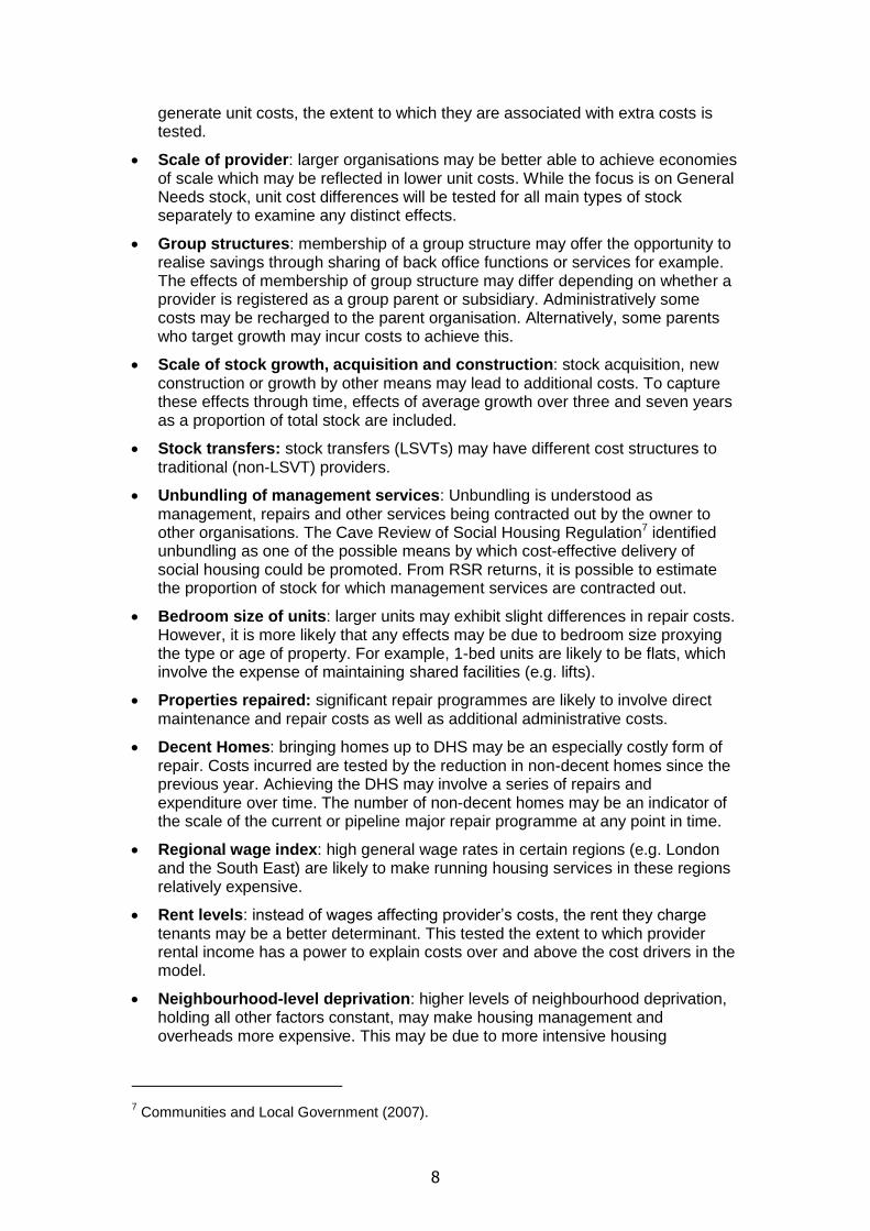
Figure 7: Histogram of provider's proportion of lettings in rural area by LA (Source: CORE & ONS 2005-2011, balanced panel)

27

The skewness for the proportion of rural lettings by LA variable is 0.52, whilst for the proportion of rural lettings by LSOA variable it is 1.46.

28 The figures shown in the table and rest of this section refer to the proportion of rural lettings

before the variable is multiplied by the provider’s proportion of GN stock.

18

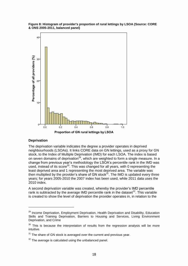
Figure 8: Histogram of provider's proportion of rural lettings by LSOA (Source: CORE & ONS 2005-2011, balanced panel)

Deprivation

The deprivation variable indicates the degree a provider operates in deprived neighbourhoods (LSOAs). It links CORE data on GN lettings, used as a proxy for GN stock, to the Index of Multiple Deprivation (IMD) for each LSOA. The index is based

on seven domains of deprivation29, which are weighted to form a single measure. In a change from previous year’s methodology the LSOA’s percentile rank in the IMD was used, instead of its score30. This was changed for all years, with 0 representing the least deprived area and 1 representing the most deprived area. The variable was then multiplied by the provider’s share of GN stock31. The IMD is updated every three years; for years 2005-2010 the 2007 index has been used, while 2011 data uses the 2010 index.

A second deprivation variable was created, whereby the provider’s IMD percentile rank is subtracted by the average IMD percentile rank in the dataset32. This variable is created to show the level of deprivation the provider operates in, in relation to the

29

Income Deprivation, Employment Deprivation, Health Deprivation and Disability, Education Skills and Training Deprivation, Barriers to Housing and Services, Living Environment Deprivation, and Crime

30 This is because the interpretation of results from the regression analysis will be more

intuitive.

31 The share of GN stock is averaged over the current and previous year.

32 The average is calculated using the unbalanced panel.

19

private registered provider sector. This variable is then multiplied by the percentage of GN stock, averaged over the current and previous year.

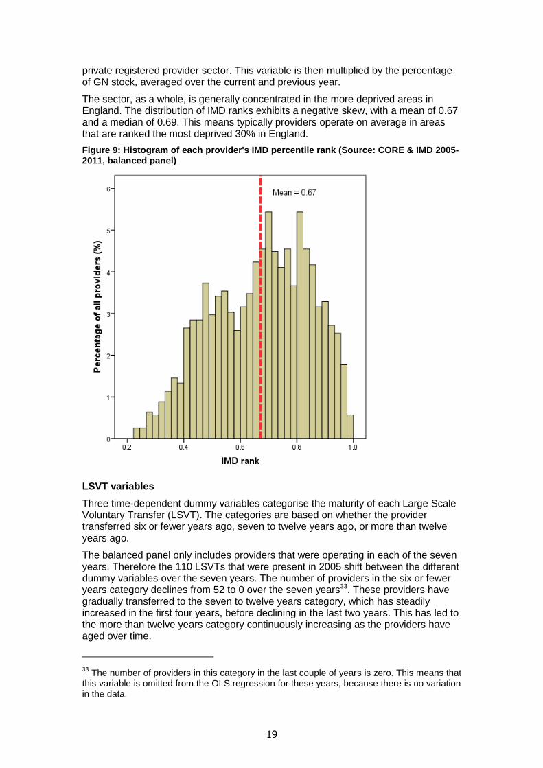
The sector, as a whole, is generally concentrated in the more deprived areas in England. The distribution of IMD ranks exhibits a negative skew, with a mean of 0.67 and a median of 0.69. This means typically providers operate on average in areas that are ranked the most deprived 30% in England.

Figure 9: Histogram of each provider's IMD percentile rank (Source: CORE & IMD 2005-2011, balanced panel)

LSVT variables

Three time-dependent dummy variables categorise the maturity of each Large Scale Voluntary Transfer (LSVT). The categories are based on whether the provider transferred six or fewer years ago, seven to twelve years ago, or more than twelve years ago.

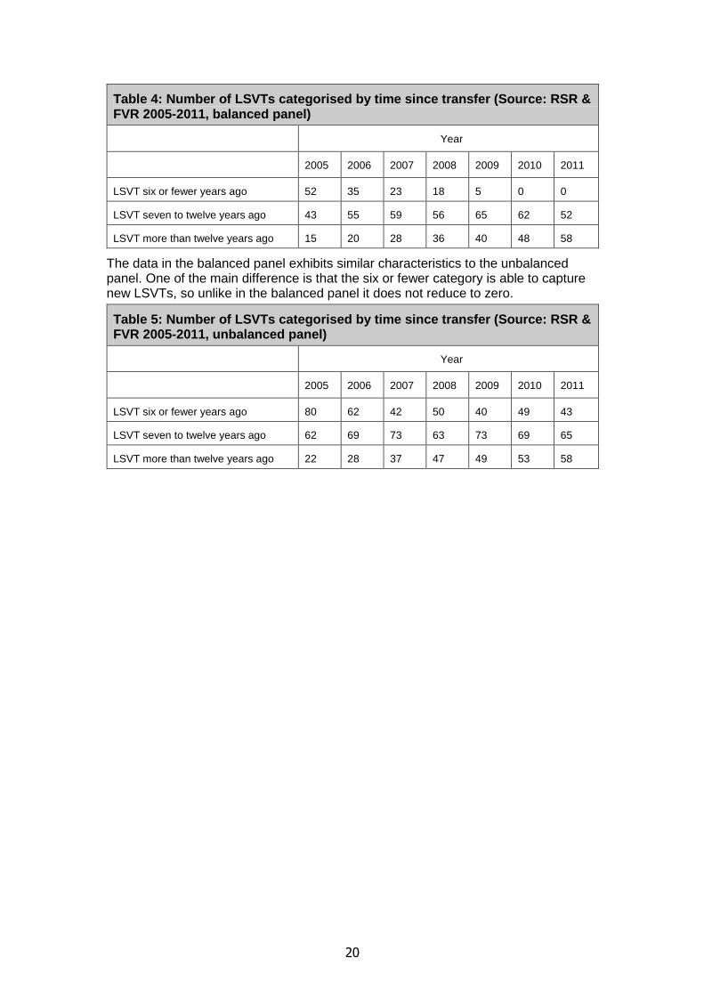
The balanced panel only includes providers that were operating in each of the seven years. Therefore the 110 LSVTs that were present in 2005 shift between the different dummy variables over the seven years. The number of providers in the six or fewer years category declines from 52 to 0 over the seven years33. These providers have gradually transferred to the seven to twelve years category, which has steadily increased in the first four years, before declining in the last two years. This has led to the more than twelve years category continuously increasing as the providers have aged over time.

33

The number of providers in this category in the last couple of years is zero. This means that this variable is omitted from the OLS regression for these years, because there is no variation in the data.

20

Table 4: Number of LSVTs categorised by time since transfer (Source: RSR & FVR 2005-2011, balanced panel)

Year

2005 2006 2007 2008 2009 2010 2011

LSVT six or fewer years ago 52 35 23 18 5 0 0

LSVT seven to twelve years ago 43 55 59 56 65 62 52

LSVT more than twelve years ago 15 20 28 36 40 48 58

The data in the balanced panel exhibits similar characteristics to the unbalanced panel. One of the main difference is that the six or fewer category is able to capture new LSVTs, so unlike in the balanced panel it does not reduce to zero.

Table 5: Number of LSVTs categorised by time since transfer (Source: RSR & FVR 2005-2011, unbalanced panel)

Year

2005 2006 2007 2008 2009 2010 2011

LSVT six or fewer years ago 80 62 42 50 40 49 43

LSVT seven to twelve years ago 62 69 73 63 73 69 65

LSVT more than twelve years ago 22 28 37 47 49 53 58

21

Table 6: Definitions of independent variables used in regression model Proportion of GN General Needs (GN) units owned or managed, averaged over the current and previous year, as a

proportion of average total social housing stock owned or managed in the current and previous year.

Proportion of GN squared The squared term of the proportion of general needs. The squared term is included to test if there are economies or diseconomies to specialisation with regard to the supply of GN housing.

Proportion of HOP Supported housing units for older people (HOP) owned or managed, averaged over the current and previous year, as a proportion of average total social housing stock owned or managed in the current and previous year.

Proportion of HOP squared

The squared term of the proportion of supported housing for older people. The squared term is included to test if there are economies or diseconomies to specialisation with regard to the supply of HOP housing.

Proportion of SH Supported housing (SH) units (excluding housing for older people) owned or managed, averaged over the current and previous year, as a proportion of average total social housing stock owned and managed in the current and previous year.

Proportion of SH squared The squared term of the proportion of supported housing excluding older people. The squared term is included to test if there are economies or diseconomies to specialisation with regard to the supply of supported housing (excluding older people).

Proportion of shared ownership

Total shared ownership stock and other stock which is <100% leasehold (excluding housing for older people), as a proportion of total social housing stock which is owned or managed.

Proportion of non-social housing

Total non-social housing which is owned or managed as a proportion of total social housing stock which is owned or managed.

Proportion of reduction in non-decent stock

Reduction in non-decent stock owned since the previous year, as a proportion of total social housing stock. This is a proxy for major repairs. Therefore all recorded increases in non-decent stock owned by a provider during a year – due to transfers of stock from local authorities for example – are excluded.

Proportion of non-decent stock

Units of stock which are non-decent at the end of the year, as a proportion of total social housing stock owned or managed.

Proportion of change in stock

Change in social housing stock owned or managed since the previous year, as a proportion of total social housing stock owned & managed.

Proportion of change in stock t-1

The proportion of change in total social housing stock from the previous year. For 2005, 0 is given for all cases.

Proportion of change in stock in the past 3 years

Total change in stock over the past three years as a percentage of total social housing stock owned & managed in the past three years. In instances of missing data, the numerator and denominator have been both been set to 0 for that year's data.

Proportion of change in stock in the past 7 years

Total change in stock during the last seven years as a percentage of total social housing stock owned & managed in the last seven years. In instances of missing data, the numerator and denominator have been both been set to 0 for that year's data.

Proportion of change in stock in the current, past and future years

Total change in stock during the current, previous and future years, as a percentage of total social housing stock owned & managed in the last seven years. In instances of missing data, the numerator and denominator have been both been set to 0 for that year's data.

Proportion of stock acquired in the past 3 years

Total stock acquired during the past three years as a percentage of total social housing stock owned & managed in the past three years. In instances of missing data, the numerator and denominator have been both been set to 0 for that year's data.

Proportion of stock acquired in the past 7 years

Total stock acquired during the past seven years as a percentage of total social housing stock owned & managed in the past seven years. In instances of missing data, the numerator and denominator have been both been set to 0 for that year's data.

Proportion of stock acquired in the current, past and future years

Total stock acquired during the current, previous and future years, as a percentage of total social housing stock owned & managed in the last seven years. In instances of missing data, the numerator and denominator have been both been set to 0 for that year's data.

Proportion of new built stock in the past 3 years

Total new built stock during the last three years as a percentage of total social housing stock owned & managed in the last three years. In instances of missing data, the numerator and denominator have been both been set to 0 for that year's data.

Proportion of new built stock in the past 7 years

Total new built stock during the last seven years as a percentage of total social housing stock owned & managed in the last seven years. In instances of missing data, the numerator and denominator have been both been set to 0 for that year's data.

Proportion of new built stock in the current, past and future years

Total new built stock during the current, previous and future years, as a percentage of total social housing stock owned & managed in the last seven years. In instances of missing data, the numerator and denominator have been both been set to 0 for that year's data.

22

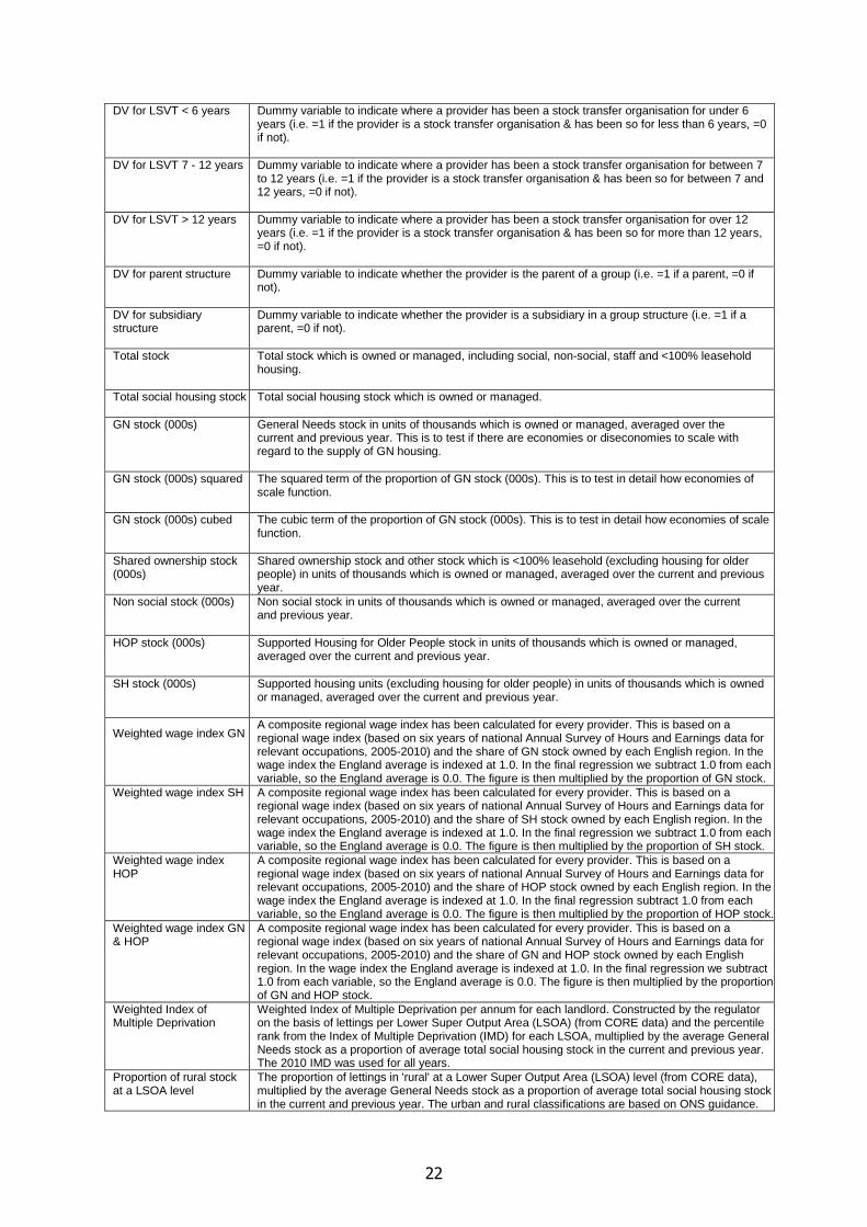
DV for LSVT < 6 years Dummy variable to indicate where a provider has been a stock transfer organisation for under 6 years (i.e. =1 if the provider is a stock transfer organisation & has been so for less than 6 years, =0 if not).

DV for LSVT 7 - 12 years Dummy variable to indicate where a provider has been a stock transfer organisation for between 7 to 12 years (i.e. =1 if the provider is a stock transfer organisation & has been so for between 7 and 12 years, =0 if not).

DV for LSVT > 12 years Dummy variable to indicate where a provider has been a stock transfer organisation for over 12 years (i.e. =1 if the provider is a stock transfer organisation & has been so for more than 12 years, =0 if not).

DV for parent structure Dummy variable to indicate whether the provider is the parent of a group (i.e. =1 if a parent, =0 if not).

DV for subsidiary structure

Dummy variable to indicate whether the provider is a subsidiary in a group structure (i.e. =1 if a parent, =0 if not).

Total stock Total stock which is owned or managed, including social, non-social, staff and <100% leasehold housing.

Total social housing stock Total social housing stock which is owned or managed.

GN stock (000s) General Needs stock in units of thousands which is owned or managed, averaged over the current and previous year. This is to test if there are economies or diseconomies to scale with regard to the supply of GN housing.

GN stock (000s) squared The squared term of the proportion of GN stock (000s). This is to test in detail how economies of scale function.

GN stock (000s) cubed The cubic term of the proportion of GN stock (000s). This is to test in detail how economies of scale function.

Shared ownership stock (000s)

Shared ownership stock and other stock which is <100% leasehold (excluding housing for older people) in units of thousands which is owned or managed, averaged over the current and previous year.

Non social stock (000s) Non social stock in units of thousands which is owned or managed, averaged over the current and previous year.

HOP stock (000s) Supported Housing for Older People stock in units of thousands which is owned or managed, averaged over the current and previous year.

SH stock (000s) Supported housing units (excluding housing for older people) in units of thousands which is owned or managed, averaged over the current and previous year.

Weighted wage index GN

A composite regional wage index has been calculated for every provider. This is based on a regional wage index (based on six years of national Annual Survey of Hours and Earnings data for relevant occupations, 2005-2010) and the share of GN stock owned by each English region. In the wage index the England average is indexed at 1.0. In the final regression we subtract 1.0 from each variable, so the England average is 0.0. The figure is then multiplied by the proportion of GN stock.

Weighted wage index SH A composite regional wage index has been calculated for every provider. This is based on a regional wage index (based on six years of national Annual Survey of Hours and Earnings data for relevant occupations, 2005-2010) and the share of SH stock owned by each English region. In the wage index the England average is indexed at 1.0. In the final regression we subtract 1.0 from each variable, so the England average is 0.0. The figure is then multiplied by the proportion of SH stock.

Weighted wage index HOP

A composite regional wage index has been calculated for every provider. This is based on a regional wage index (based on six years of national Annual Survey of Hours and Earnings data for relevant occupations, 2005-2010) and the share of HOP stock owned by each English region. In the wage index the England average is indexed at 1.0. In the final regression subtract 1.0 from each variable, so the England average is 0.0. The figure is then multiplied by the proportion of HOP stock.

Weighted wage index GN & HOP

A composite regional wage index has been calculated for every provider. This is based on a regional wage index (based on six years of national Annual Survey of Hours and Earnings data for relevant occupations, 2005-2010) and the share of GN and HOP stock owned by each English region. In the wage index the England average is indexed at 1.0. In the final regression we subtract 1.0 from each variable, so the England average is 0.0. The figure is then multiplied by the proportion of GN and HOP stock.

Weighted Index of Multiple Deprivation

Weighted Index of Multiple Deprivation per annum for each landlord. Constructed by the regulator on the basis of lettings per Lower Super Output Area (LSOA) (from CORE data) and the percentile rank from the Index of Multiple Deprivation (IMD) for each LSOA, multiplied by the average General Needs stock as a proportion of average total social housing stock in the current and previous year. The 2010 IMD was used for all years.

Proportion of rural stock at a LSOA level

The proportion of lettings in 'rural' at a Lower Super Output Area (LSOA) level (from CORE data), multiplied by the average General Needs stock as a proportion of average total social housing stock in the current and previous year. The urban and rural classifications are based on ONS guidance.

23

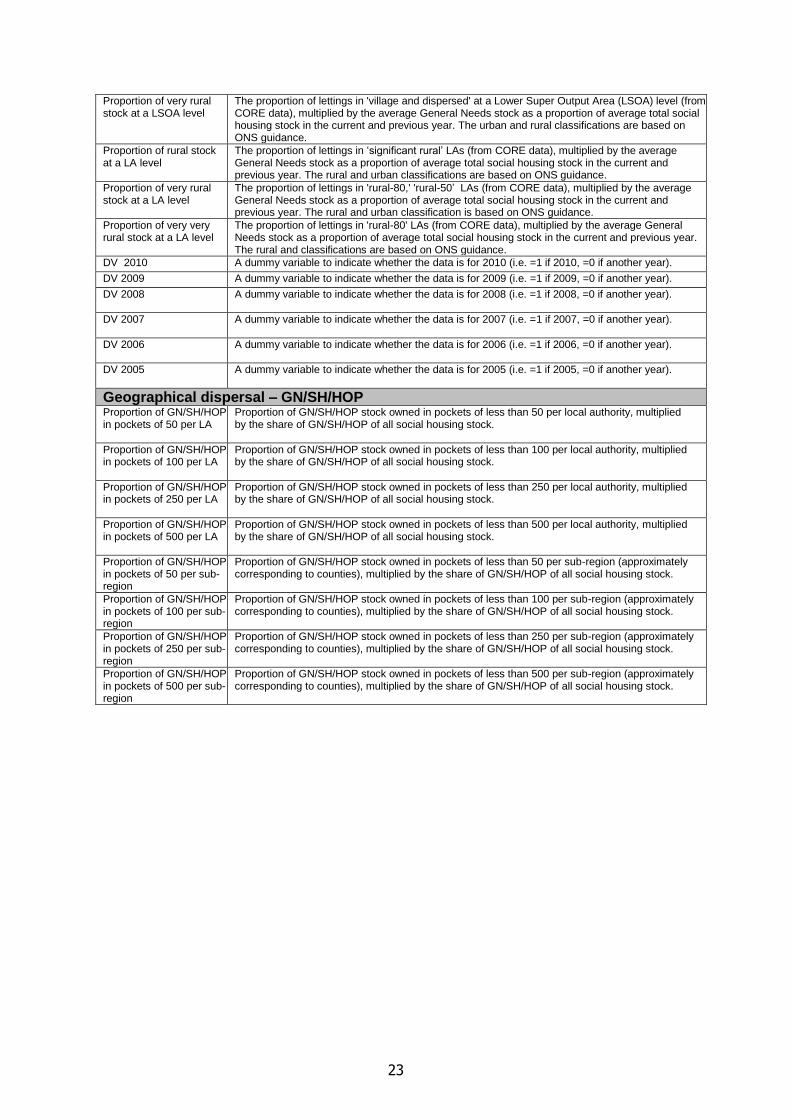
Proportion of very rural stock at a LSOA level

The proportion of lettings in 'village and dispersed' at a Lower Super Output Area (LSOA) level (from CORE data), multiplied by the average General Needs stock as a proportion of average total social housing stock in the current and previous year. The urban and rural classifications are based on ONS guidance.

Proportion of rural stock at a LA level

The proportion of lettings in ‘significant rural’ LAs (from CORE data), multiplied by the average General Needs stock as a proportion of average total social housing stock in the current and previous year. The rural and urban classifications are based on ONS guidance.

Proportion of very rural stock at a LA level

The proportion of lettings in 'rural-80,' 'rural-50’ LAs (from CORE data), multiplied by the average General Needs stock as a proportion of average total social housing stock in the current and previous year. The rural and urban classification is based on ONS guidance.

Proportion of very very rural stock at a LA level

The proportion of lettings in 'rural-80' LAs (from CORE data), multiplied by the average General Needs stock as a proportion of average total social housing stock in the current and previous year. The rural and classifications are based on ONS guidance.

DV 2010 A dummy variable to indicate whether the data is for 2010 (i.e. =1 if 2010, =0 if another year).






Geographical dispersal – GN/SH/HOP Proportion of GN/SH/HOP in pockets of 50 per LA

Proportion of GN/SH/HOP stock owned in pockets of less than 50 per local authority, multiplied by the share of GN/SH/HOP of all social housing stock.

Proportion of GN/SH/HOP in pockets of 100 per LA






Proportion of GN/SH/HOP in pockets of 50 per sub-region

Proportion of GN/SH/HOP stock owned in pockets of less than 50 per sub-region (approximately corresponding to counties), multiplied by the share of GN/SH/HOP of all social housing stock.







24

Results of regression analysis

This section summarises the results of the regression analysis of social housing costs for providers (entity level). The headline results presented here have been derived from careful testing of a range of explanatory factors, and are based on the three main unit cost measures on a regression of 19 explanatory variables. The process of selected these 19 variables, from a long list of over seventy, is detailed below.

Overview of results

All three main models outlined in the introduction have been employed to run the regression on the balanced panel of providers (2005-11 inclusive):

Standard ordinary least squares (OLS) on cross-sectional data (full model, one year at a time): standard OLS can only be applied on each year individually, which reduces the power of the regression considerably. However, it is a statistically robust way to examine the cross-sectional effects each year.

Fixed Effects Model (full model): this model estimates the relationship between changes in independent variables and changes in costs over time. It is limited in that it does not pick up static cross-sectional differences in data and therefore its power is limited where variance is minimal over time. However, it is statistically robust and incorporates all independent variables.

Random Effects Model (smaller model): this model is potentially more powerful than the OLS or Fixed Effects Model because it combines data on changes in variables over time with cross-sectional observations. However, it depends critically on a statistical condition34 which is not met for all variables in the full model. Because they cause the statistical conditions to be violated, measures of scale could not be supported within the Random Effects framework and are removed in the model presented here. Even then the model can only serve to estimate social housing lettings costs. It still provides a useful benchmark for many findings.

All three models have validity in explaining the costs of social housing providers. Where there is significant variability for individual providers over time, such as for the Decent Homes Programme for example, the Fixed Effects Model is likely to perform well. The findings of the report are derived from inspecting the results of all models collectively.

1) Standard OLS

The results of the OLS model, run each year with 227 observations for each cost measure, are summarised overleaf. The coefficient shows how much a unit change is associated with a unit change in costs (£000 per unit). Where there is statistically significant evidence of a relationship cells are shaded, depending on the degree of significance (80%, 90% or 95%).

34

Each observation deviates to some degree from the ‘true’ model of costs that is being estimated – one part of which is a random error term, the other is the unobserved error linked to a particular provider (e.g. higher or lower costs through all time periods). The Random Effects Model requires that this unobserved error is uncorrelated with all independent variables. However, this condition turns out to be violated for some independent variables. The Hausman Test is used to test whether this condition is satisfied.

25

Table 7: OLS Model – effect of each explanatory factor on the three cost measures for each year (balanced panel, 2005 – 2011)

Operating costs (£000s) Operating costs plus (£000s) Soc. housing lettings costs (£000s)

‘11 ‘10 ‘09 ‘08 ‘07 ‘06 ‘05 ‘11 ‘10 ‘09 ‘08 ‘07 ‘06 ‘05 ‘11 ‘10 ‘09 ‘08 ‘07 ‘06 ‘05

Intercept 2.87 2.56 2.74 1.71 1.81 1.93 2.22 3.08 2.61 2.73 1.75 1.84 2.09 2.20 2.76 2.79 2.47 2.53 2.34 2.57 2.63

% Housing for Older People .89 1.01 0.81 1.22 1.00 .62 -.01 .33 .73 .60 1.05 0.73 0.16 -1.23 1.18 .85 1.51 .82 .91 .66 .34

% Supported housing 10.82 12.74 14.88 14.24 13.25 13.34 12.76 9.77 11.86 14.49 13.67 12.88 11.66 11.25 6.14 5.92 7.25 7.07 6.85 6.66 6.66

% Shared ownership 6.73 8.02 8.23 12.45 11.4 12.59 11.88 5.43 7.09 8.06 12.1 10.7 11.98 11.7 .47 1.62 1.78 -.58 -.72 -.73 -1.07

% Non-social 1.06 .79 .24 .95 .90 1.31 2.08 1.72 1.44 .78 1.24 1.20 1.46 1.87 .65 .47 .12 .40 .63 .38 -.05

% Reduction non-decent 6.86 2.15 2.93 1.71 .46 1.83 2.58 11.03 3.34 4.96 2.51 1.50 6.16 2.83 3.04 2.23 2.11 -.39 .75 1.43 1.92

% Residual non-decent .52 2.00 .13 .19 -.27 .36 .83 5.96 4.90 .09 0.38 -0.52 0.02 1.53 1.47 1.03 -.86 .26 -.11 .25 .54

LSVT < 7 years (DV) .41 1.06 1.23 1.02 .99 .40 1.40 1.90 1.62 1.50 .63 1.13 .93 .88 0.73

LSVT 7 – 12 years (DV) .15 .32 .42 .36 .54 .50 .48 0.26 .39 .53 0.40 0.65 0.72 0.65 0.10 .21 .37 .19 .18 .18 .11

LSVT> 12 years (DV) .02 .04 .11 .16 .20 .14 .28 -0.11 -.05 .05 0.08 0.13 0.17 0.33 -0.03 -.02 .10 .04 -.05 -.24 -.05

Group parent (DV) .10 .36 .27 .13 -.08 .07 .17 0.14 .46 .41 0.15 0.27 0.21 0.26 -0.17 -.06 -.08 -.07 -.24 -.09 -.25

Group subsidiary (DV) -.43 -.17 -.10 -.08 -.20 -.17 -.32 -0.38 -.16 -.06 -0.07 -0.09 -0.17 -0.22 -0.28 -.20 -.12 -.04 -.06 .05 -.16

Regional wage index (GN) 3.85 4.23 5.54 4.91 4.52 3.67 3.40 6.33 7.10 9.02 7.77 7.58 9.46 6.26 3.93 3.58 4.60 4.83 4.07 2.97 2.26

Regional wage index (SH) 9.16 15.86 -12.06 12.83 7.86 -2.08 4.91 -0.77 1.65 -28.11 3.87 -6.83 -27.86 -7.43 2.55 3.22 -1.86 -4.32 -5.67 -1.20 1.40

Index of Multiple Deprivation (% rank) .18 .33 .07 1.10 1.18 .63 .15 0.53 .87 .74 1.62 1.67 1.15 0.87 0.10 -.04 .17 .32 .55 -.04 -.18

GN stock (000s) -.04 -.03 -.03 .03 .00 .03 -.03 -0.04 -.02 -.04 0.02 -0.01 -0.01 -0.10 -0.02 .00 .02 .00 .01 .03 .00

GN stock (000s) squared .00 .00 .00 .00 .00 .00 .00 0.00 .00 .00 0.00 0.00 0.00 0.00 0.00 .00 .00 .00 .00 .00 .00

HOP stock (000s) -.01 .04 .08 .12 .13 .16 .13 0.04 .07 .11 0.15 0.13 0.19 0.31 -0.05 .02 .01 .05 .07 .05 .05

Supported Housing (000s) -.07 -.24 -.47 -.31 -.08 -.04 .03 -0.04 -.14 -.42 -0.20 -0.02 0.14 0.22 -0.08 -.14 -.14 -.25 -.18 -.04 .01

Shared ownership (000s) -.48 -.56 -.47 -1.28 -1.04 -1.46 -1.31 -0.43 -0.57 -.53 -1.21 -0.99 -1.36 -1.25 -0.22 -.42 -.43 -.23 -.18 -.34 -.19

N (total observations) 227 227 227 227 227 227 227 227 227 227 227 227 227 227 227 227 227 227 227 227 227

Mean of cost measure 3.50 3.70 3.86 3.72 3.67 3.69 3.56 3.86 4.06 4.22 4.07 4.03 4.13 3.93 2.91 3.05 3.14 3.11 3.10 3.18 3.07

Standard deviation of costs 1.32 1.36 1.49 1.45 1.43 1.49 1.46 1.42 1.48 1.66 1.54 1.55 1.71 1.61 .84 .82 .93 .96 1.02 1.05 1.00

Standard error of regression 1.03 1.06 1.20 1.00 1.02 1.06 .99 1.09 1.12 1.32 1.05 1.10 1.23 1.15 .69 .71 .80 .80 .87 .89 .82

R-squared .45 .44 .41 .57 .54 .53 .58 .46 .47 .42 .58 .54 .53 .53 .39 .32 .32 .37 .34 .34 .39

Adjusted R-squared .40 .39 .36 .53 .49 .49 .54 .42 .42 .37 .54 .50 .48 .49 .34 .26 .26 .31 .27 .28 .34

Note: * and green shading denotes coefficients with p values of less than 0.05, i.e. there is evidence at a 95% confidence level that the coefficient is non-zero. Amber shading denotes a p value of between 0.05 and 0.1 and yellow between 0.1 and 0.2. Unless indicated otherwise, figures presented in the main body of the table are the regression coefficients. Data on LSVTs<7 years omitted for 2010 and 2011 due to no associations falling into these categorise (and needing to avoid perfect multicolinearity).

26

Table 8: Fixed effects model – effects of changes in each explanatory factor on the three main cost measures (balanced panel, 2005-11 data)

Dependent cost variable Operating costs (£000s)

Operating costs plus (£000s)

Social housing lettings costs (£000s)

Intercept 3.20 2.88 2.85

% Housing for Older People -.63 .45 -.01

% Supported housing 4.86 3.72 7.34

% Shared ownership 3.78 2.89 -1.98

% Non-social 2.38 2.35 .22

% Reduction non-decent 1.99 3.29 1.45

% Residual non-decent .50 .97 .35

LSVT < 7 years (DV) .54 .63 .64

LSVT 7 – 12 years (DV) .05 .02 .05

Group parent (DV) .04 .09 -.02

Group subsidiary (DV) -.18 -.09 -.19

Regional wage index (GN) 13.85 20.86 12.53

Regional wage index (SH) 25.52 28.68 20.66

Index of Multiple Deprivation (% rank) .98 1.95 .74

GN stock (000s) -.15 -.08 -.14

GN stock (000s) squared .00 .00 .00

HOP stock (000s) -.15 -.23 -.10

Supported Housing (000s) -.05 -.01 -.24

Shared ownership (000s) .08 .21 .32

2010 (DV) .19 .19 .13

2009 (DV) .33 .35 .19

2009 (DV) .10 .07 .07

2007 (DV) .01 -.01 -.03

2006 (DV) -.02 .04 -.01

2005 (DV) -.23 -.34 -.21

% GN in pockets <250 units per LA .27 -.09 .78

N (total observations) 1,589 1,589 1,589

Mean of cost measure 3.67 4.04 3.08

Standard Deviation of cost measure 1.43 1.57 .96

Standard error of regression .53 .67 .41 Note: green shading denotes coefficients with p values of less than 0.05, i.e. there is evidence at a 95% confidence level that the coefficient is non-zero. Amber shading denotes a p value of between 0.05 and 0.1 and yellow between 0.1 and 0.2. Unless indicated otherwise, figures presented in the main body of the table are the regression coefficients. In order to derive this regression, a range of variables are also included to control for dispersal of SH and HOP stock – these are not reported here for brevity.

27

2) Fixed effects model

The results of the Fixed Effects Model are set out in table 8. The coefficient shows how much a change in each independent variable affects unit costs (£000s) on average. The standard error is an estimate of the standard deviation of each coefficient35 and allows one to state the level of statistical confidence that the coefficient is non-zero i.e. the probability that there is a relationship. Coefficients where there is evidence of a relationship at a 95% and 90% level of confidence are flagged and shaded in green and amber. Coefficients that are non-zero at 80% confidence bounds are shaded yellow, although in general 90% is considered the minimum level of confidence for robust statistical analysis. The regression is based on 1,589 observations over seven years.

3) Random effects model

Satisfying a statistical test called the Hausman Test is generally considered a necessary condition for the Random Effects Model to be valid. The Hausman Test only has a p-value greater than 0.1 for social housing lettings costs (i.e. the test does not reject at a 90% confidence level), and only then are measures of scale removed. This means there is potential for missing variable bias, to the extent that remaining independent variables are correlated with either of these omitted variables. However, even given this, the results of the model form a useful cross-reference for OLS and Fixed Effects Model results.

35

There is a subtle difference between standard deviation and standard error of a coefficient. Standard deviation of the coefficient is the population or ‘true’ value of standard deviation of a coefficient in the full population. It cannot be known with 100% accuracy from a sample. Standard error is an estimate of this, derived from a sample from this population. Standard deviation is a measure of average deviation from the mean.

Table 9: Random effects model – Social housing lettings costs (balanced panel, 2005-11 data)

Dependent cost variable

Social housing lettings costs

(£000s)

Coefficient

Intercept 2.55 *

% Housing for Older People .74 *

% Supported Housing 6.91 *

% Shared ownership -1.72 *

% Non-social .32

% Reduction non-decent 1.42 *

% Residual non-decent .07

LSVT < 7 years (DV) .74 *

LSVT 7 - 12 years (DV) .11 *

Group parent -.01

Group subsidiary -.17 *

Regional wage index (GN) 3.12 *

Regional wage index (SH) 5.21

Index of Multiple Deprivation (% rank) .24

2010 (DV) .12 *

2009 (DV) .18 *

2008 (DV) .09 *

2007 (DV) .01

2006 (DV) .04

2005 (DV) -.17 *

N (total observations) 1,589

Mean of cost measure 3.08

Standard Deviation of cost measure .96

Standard error of regression 0.80

Hausman p-value 0.20

Note: * and green shading denotes coefficients with p values of less than 0.05, i.e. there is evidence at a 95% confidence level that the coefficient is nonzero. Amber shading denotes a p value of between 0.05 and 0.1 and yellow between 0.1 and 0.2. Unless indicated otherwise, figures presented in the main body of the table are the regression coefficients.

28

What does this data mean?

Regional wage differences

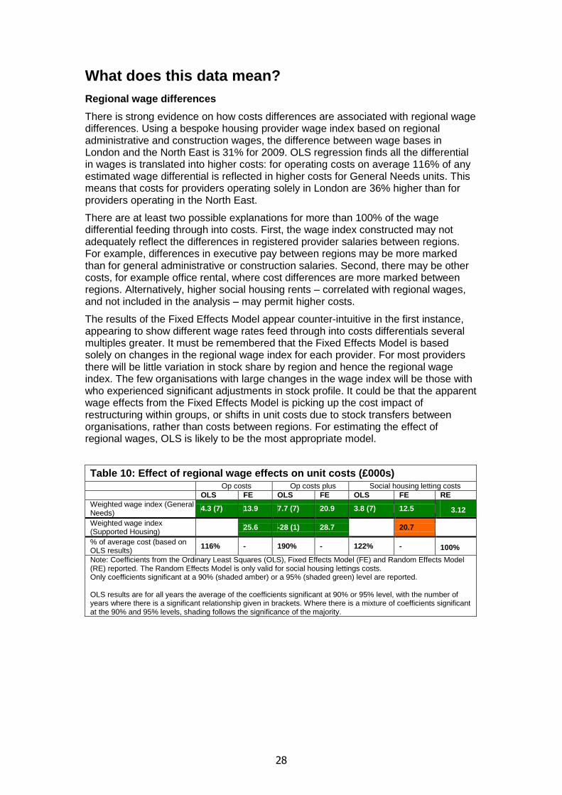
There is strong evidence on how costs differences are associated with regional wage differences. Using a bespoke housing provider wage index based on regional administrative and construction wages, the difference between wage bases in London and the North East is 31% for 2009. OLS regression finds all the differential in wages is translated into higher costs: for operating costs on average 116% of any estimated wage differential is reflected in higher costs for General Needs units. This means that costs for providers operating solely in London are 36% higher than for providers operating in the North East.

There are at least two possible explanations for more than 100% of the wage differential feeding through into costs. First, the wage index constructed may not adequately reflect the differences in registered provider salaries between regions. For example, differences in executive pay between regions may be more marked than for general administrative or construction salaries. Second, there may be other costs, for example office rental, where cost differences are more marked between regions. Alternatively, higher social housing rents – correlated with regional wages, and not included in the analysis – may permit higher costs.

The results of the Fixed Effects Model appear counter-intuitive in the first instance, appearing to show different wage rates feed through into costs differentials several multiples greater. It must be remembered that the Fixed Effects Model is based solely on changes in the regional wage index for each provider. For most providers there will be little variation in stock share by region and hence the regional wage index. The few organisations with large changes in the wage index will be those with who experienced significant adjustments in stock profile. It could be that the apparent wage effects from the Fixed Effects Model is picking up the cost impact of restructuring within groups, or shifts in unit costs due to stock transfers between organisations, rather than costs between regions. For estimating the effect of regional wages, OLS is likely to be the most appropriate model.

Table 10: Effect of regional wage effects on unit costs (£000s)

Op costs Op costs plus Social housing letting costs

OLS FE OLS FE OLS FE RE

Weighted wage index (General Needs)

4.3 (7) 13.9 7.7 (7) 20.9 3.8 (7) 12.5 3.12

Weighted wage index (Supported Housing)

25.6 -28 (1) 28.7 20.7

% of average cost (based on OLS results)

116% - 190% - 122% - 100%

Note: Coefficients from the Ordinary Least Squares (OLS), Fixed Effects Model (FE) and Random Effects Model (RE) reported. The Random Effects Model is only valid for social housing lettings costs. Only coefficients significant at a 90% (shaded amber) or a 95% (shaded green) level are reported. OLS results are for all years the average of the coefficients significant at 90% or 95% level, with the number of years where there is a significant relationship given in brackets. Where there is a mixture of coefficients significant at the 90% and 95% levels, shading follows the significance of the majority.

29

Deprivation

A deprivation index has been calculated annually for every provider. This is the weighted average Index of Multiple Deprivation (IMD) rank for all Lower Super Output Areas (LSOAs) where new General Needs lettings are registered. The IMD rank ranges from 0%, for the least deprived neighbourhood in England to 100% for the most deprived. Moving from the provider operating in neighbourhood ranked as having an average level of deprivation (50% IMD) to one operating in the most deprived areas (99% IMD) is associated with increased operating costs plus of around £750 per unit (19%).

Almost certainly deprivation is picking up a range of factors associated with increased costs: more intensive housing management and anti-social behaviour activities, increased letting costs through faster stock turnover, regeneration initiatives and in all probability older stock.

Table 11: Effect of deprivation on unit costs (£000s)



Index of Multiple Deprivation (% rank)

1.1 (2) 1.0 1.5 (3) 2.0 0.7


Economies of scale

One of the key issues motivating this piece of research is the desire to understand the relationship between costs and size of provider – more specifically the extent to which the sector exhibits economies of scale which feed through to lower costs, controlling for all other factors. A manual inspection of the data, set out on costs and size, does not immediately indicate any simple relationship. Moreover, the higher costs of many smaller providers are likely to be due to specialisation in SH. It is necessary to control for such factors to understand any economies of scale.

Potential mathematical forms of the relationship between size and costs have been explored as extensions to the model set out here. The following models were tested:

1. Total stock (000s) in absolute terms.

2. Natural logarithm of total stock (000s), to allow for equal percentage changes in stock to generate an equal increase or decrease in unit costs.

3. Total stock (000s), with squared and cubed functions added in turn.

4. General Needs stock (000s).

5. General Needs stock (000s), with squared and cubic functions in turn.

6. Natural logarithm of general needs stock, SH, HOP, shared ownership and non-social housing.

7. General Needs stock (000s), along with absolute stock (000s) for SH, HOP, shared ownership, and non-social housing (to test any effects of these alternative kinds of stock on cost36). Squared and cubic terms were added for General Needs stock.

36

Shared ownership is included in the total stock figures. Non-social housing is not included.

30

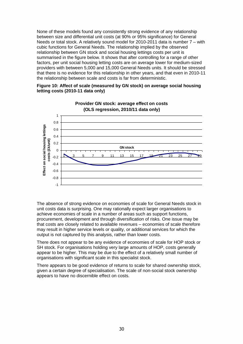
None of these models found any consistently strong evidence of any relationship between size and differential unit costs (at 90% or 95% significance) for General Needs or total stock. A relatively sound model for 2010-2011 data is number 7 – with cubic functions for General Needs. The relationship implied by the observed relationship between GN stock and social housing lettings costs per unit is summarised in the figure below. It shows that after controlling for a range of other factors, per unit social housing letting costs are on average lower for medium-sized providers with between 5,000 and 15,000 General Needs units. It should be stressed that there is no evidence for this relationship in other years, and that even in 2010-11 the relationship between scale and costs is far from deterministic.

Figure 10: Affect of scale (measured by GN stock) on average social housing letting costs (2010-11 data only)

Provider GN stock: average effect on costs

(OLS regression, 2010/11 data only)

-1

-0.8

-0.6

-0.4

-0.2

0

0.2

0.4

0.6

0.8

1

1 3 5 7 9 11 13 15 17 19 21 23 25 27 29

GN stock

Eff

ec

t o

n s

oc

ial h

ou

sin

g le

ttin

gs

co

sts

(£

k/u

nit

)

The absence of strong evidence on economies of scale for General Needs stock in unit costs data is surprising. One may rationally expect larger organisations to achieve economies of scale in a number of areas such as support functions, procurement, development and through diversification of risks. One issue may be that costs are closely related to available revenues – economies of scale therefore may result in higher service levels or quality, or additional services for which the output is not captured by this analysis, rather than lower costs.

There does not appear to be any evidence of economies of scale for HOP stock or SH stock. For organisations holding very large amounts of HOP, costs generally appear to be higher. This may be due to the effect of a relatively small number of organisations with significant scale in this specialist stock.

There appears to be good evidence of returns to scale for shared ownership stock, given a certain degree of specialisation. The scale of non-social stock ownership appears to have no discernible effect on costs.

31

Table 12: Effects of scale on unit costs (£000s)



GN stock (000s) - 0.15 - 0.1 (1) -0.14

GN stock (000s) squared 0.00 (1) 0.00 (1) 0.00

HOP stock (000s) 0.13 (2) 0.19 (4) -0.23

SH stock (000s)

Shared ownership stock (000s) -0.94 (7) -0.98 (6) -0.39 (3) 0.32

Non social stock (000s)

Note: Coefficients from the Ordinary Least Squares (OLS), Fixed Effects Model (FE) and Random Effects Model (RE) reported. The Random Effects Model is only valid for social housing lettings costs. Only coefficients significant at a 90% (shaded amber) or a 95% (shaded green) level are reported. Economies of scale for General Needs stock have been investigated further by adding different mathematical forms to the model. This is summarised above and set out in the annex. OLS results are for all years the average of the coefficients significant at 90% or 95% level, with the number of years where there is a significant relationship given in brackets. Where there is a mixture of coefficients significant at the 90% and 95% levels, shading follows the significance of the majority.

Non-standard units: supported housing, housing for older people, shared ownership and non-social housing

Higher shares of supported housing (SH) and housing for older people (HOP) may lead to higher costs of a provider on average. However, the extra costs generated are not necessarily the same for all providers. Costs may depend on the overall scale of SH or HOP holdings. Absolute SH and HOP stock holdings are included to test for economies of scale – the extent to which costs vary with the scale of stock holdings. These results are summarised in Table 1237.

For the average provider each unit of SH adds c. £7,000 to social housing lettings costs and is associated with an increased operating costs plus of £12,000. It should be noted that Supported Housing specialists – providers where Supported Housing is at least 70% of total stock – have been removed from the balanced panel. Therefore, in general, these are the costs for providers who hold at least some General Needs stock. This is likely to account for the increase in the average costs of Supported Housing. Many of the additional costs on top of social housing letting costs may be associated with wider services or campaign work carried out by providers with large amounts of Supported Housing, and may not necessarily be directly linked to these units. There is no evidence of economies to specialisation for more specialist SH providers. This may be due to more specialist providers providing more intensive types of social housing or providing wider services.

There is relatively weak evidence that HOP is associated with additional costs. Where there is evidence for social housing lettings costs, it suggests each unit of HOP is associated with costs of £1,400 (40%) on top of a typical General Needs unit. There are no evident economies to scale.

It appears that for the average housing provider across the balanced panel, each unit of shared ownership adds significant operating costs (c. £4,000) over and above the

37

Previous analysis set out in the 2010 Global Accounts tested for economies of specialisation by including quadratic terms of the proportion of SH and HOP stock held. Given lack of any positive evidence for 2005-10, the approach here has been simplified and such quadratic terms have been removed.

32

General Needs property. This follows from the mean shared ownership stock holding of 4.4% of total stock or 280 units per provider over the balanced panel. The finding is perhaps counter-intuitive since it would be expected that costs would be considerably lower than General Needs. However, significant economies of scale are evident meaning providers that hold larger amounts of shared ownership properties will see costs fall towards those for General Needs units. As one might expect, additional costs associated with shared ownership units are associated with wider operating costs rather than social housing lettings costs.

It appears that each unit of non-social property has associated operating costs and operating costs plus of £1,400 - £1,900 on average38. This is likely to reflect a mix of properties constituting non-social properties, which may include small numbers of properties with significant support attached (but not categorised as SH).

Table 13: Net effect of specialisation and scale effects for shared ownership over General Needs costs

Operating costs Operating costs plus

Social housing letting costs

Average (balanced panel, 2005-11)

Shared ownership

Shared ownership (% total) (coefficient) 10.2 (7) 10.3 (6) -1.1 (1) 4.4%

Shared ownership (000s) (coefficient) -0.9 (7) -1.0 (6) -0.4 (3) .28

Average net effect per unit 4.5 4.0 -3.5 -

Note: Avg effects based on the mean for each value from the balanced panel (2005-11) and coefficients derived from the mean of significant coefficients from OLS analysis. Net effects combine scale and specialisation effects.

Table 14: Effect of share of SH, HOP, social housing & non-social units on unit costs (£000s)


OLS* FE OLS* FE OLS* FE RE

% Housing for Older People 1.4 (2) .74

HOP stock (000s) .1 (2) .2 (4) -.2 n/a

% Supported Housing 13.2 (7) 12.2 (7) 6.7 (7) 7.3 6.9

Supported Housing (000s) n/a

% Shared ownership 10.2 (7) 3.8 10.3 (7) 2.9 -1.0 (1) -2.0 -1.7

Shared ownership (000s) -.9 (7) -1.0 (6) -.4 (3) 0.3 n/a

% Non-social 1.3 (4) 2.4 1.5 (6) 2.4 .6 (1)


38

It should be noted non-social stock is not included in the measure of total stock.

33

Growth in stock – dynamic effects

Different types of stock growth, tested over several time periods, were not found to have significant impacts on costs. Extending the analysis set out in the 2010 Global Accounts, growth in stock was tested over a longer period of the past seven years, the past three years and the current, previous and future year. These time frames were used for three measures: stock change, stock acquired and new build stock. Even over these longer time periods there was limited evidence that growth in stock affected short-term costs. These conclusions were based using the OLS model on the three most recent years using all three costs measures.

Table 15: Effect of growth in stock on unit costs (£000s) (balanced panel, 2011)


OLS OLS OLS

% change in stock in past, future & current year

% change in stock in past 7 years

-5.42 (one year only)

% change in stock in past 3 years

% stock acquired in past, future & current year

% stock acquired in past 7 years

% stock acquired in past 3 years

% new build stock in past, future & current year

% new build stock in past 7 years

% new build stock in past 3 years

Note: Coefficients from the Ordinary Least Squares (OLS). Only coefficients significant at a 90% (shaded amber) or a 95% (shaded green) level are reported. Results shown are of a representative year (2011)

Group structures

While the entity level analysis suggests group structures are associated with lower cost, analysis of consolidated group accounts suggests this is due to costs of non-registered group parents (or other entities not included in the analysis39). The entity-level analysis suggests strong evidence for lower costs for group subsidiaries, and no increase in costs for group parents. This finding was presented in the analysis in the 2010 Global Accounts with the proviso that group-level accounts data would need to be investigated to establish the robustness of this finding. Analysis of group-level accounts yielded no evidence to suggest providers in group structures have lower costs than those not in groups, controlling for other factors. This group-level accounts analysis is set out later in this paper as an extension to the main model.

Stock transfers (LSVTs)

Stock transfer providers (LSVTs), controlling for other measured factors considered here, are more expensive than traditional providers in their early years. For LSVTs in their first six years, operating costs plus on average £1,600 per unit (36%) higher than units in similar traditional providers. This is likely to be the result of significant

39

Costs associated with registered entities with less than 1,000 units, which could include group parents, could generate apparent savings from group subsidiaries.

34

regeneration and community engagement programmes in the first few years of operation, not captured in the model here. LSVTs older than six years but younger than twelve years have higher operating costs plus of £600 per unit (14%) on average. Beyond twelve years, there is no evidence of a difference in costs between LSVTs and similar non-LSVTs.

Table 16: Unit costs for stock transfers (£000s)


OLS* FE OLS* FE OLS* FE RE

LSVT < 7 years (DV) 1.1 (4) 0.5 1.6 (4) 0.6 0.9 (4) 0.6 0.7

LSVT 7 - 12 years (DV) 0.5 (5) 0.6 (5) 0.3 (2) 0.1

LSVT > 12 years (DV) n/a n/a n/a n/a

Notes: Coefficients from the Ordinary Least Squares (OLS), Fixed Effects Model (FE) and Random Effects Model (RE) reported. The Random Effects Model is only valid for social housing lettings costs. Only coefficients significant at a 90% (shaded amber) or a 95% (shaded green) level are reported. Because of near perfect multicolinearity it is not possible to include LSVT>12 years in the Fixed Effects and Random Effects models. OLS results are for all years the average of the coefficients significant at 90% or 95% level, with the number of years where there is a significant relationship given in brackets. Where there is a mixture of coefficients significant at the 90% and 95% levels, shading follows the significance of the majority.

Decent Homes Programme

The reduction in non-decent homes held by each provider over the course of each year has been tracked (excluding those cases where there is significant stock acquisition or disposal). Given there have been significant changes in the scale of providers’ Decent Homes Programmes over time, the Fixed Effects Model – focusing on changes for each provider – is likely to be a robust model to estimate the associated costs of the Programme.

From the Fixed Effects Model, operating costs plus associated with each home made decent in a given year is £3,300. However, works are likely to be required over several years on a home before the standard is met – evidence that residual non-decent stock each year is associated with higher costs points to this. On average, each non-decent unit each year is associated with additional operating costs plus of £1,500. These costs recur each year until a stock is made decent.

The best estimate of the costs of associated with achieving DHS is operating costs plus of £11,900 per unit made decent, a cost that typically accrues over several years. This is derived from data over seven years, and requires some modelling and certain assumptions. In particular, it assumes that the costs associated with residual non-decent homes in each year is expenditure on homes where decency was achieved by 2011. This is not too much of a heroic assumption, given that mean non-decent stock per provider fell from 13% to 0.6% for the balanced panel over the period, although it will tend to slightly overstate costs. On the other hand, some of the costs of achieving decency standards in 2005 and 2011 will have been incurred before 2005 and will not be captured in this analysis making it an underestimate. These effects counteract each other to some degree.

It appears the last units to achieve DHS have higher associated costs than other units. Costs of achieving decency standards per unit rose in 2010-2011 compared to earlier years. For example, the Fixed Effects Model show operating costs plus associated with each home made decent are £3,300 on average for 2005-11 compared to £2,900 for 2005-1040. While part of this increase is due to the additional

40

Stated in 2011 prices. The regression results for 2005-10, presented in March 2010 Global Accounts had a 2009 price basis. The Fixed Effect Model coefficient for homes made decent

35

year improving modelling accuracy41, the majority is likely to be associated with higher per unit costs of achieving Decent Homes in 2010-11, in many cases associated with the ‘hardest to address’ stock.

Table 17: Effect of Decent Homes Programme on unit costs (£000s)



% reduction in non-decent stock

4.7 (2) 2.0 6.2 (4) 3.3 1.9 (1) 1.5 1.4

% residual non-decent stock 4.1 (3) 1.0 1.4 (1)


presented in March 2010 (£2,700) has been inflated into an equivalent figure in 2011 prices (£2,900).

41 It was noted in Global Accounts 2010 that the large amount of units achieving Decent

Homes standards in 2005 and 2006 is likely to make overall costs an underestimate on balance. Adding an additional year reduces this element of underestimation.

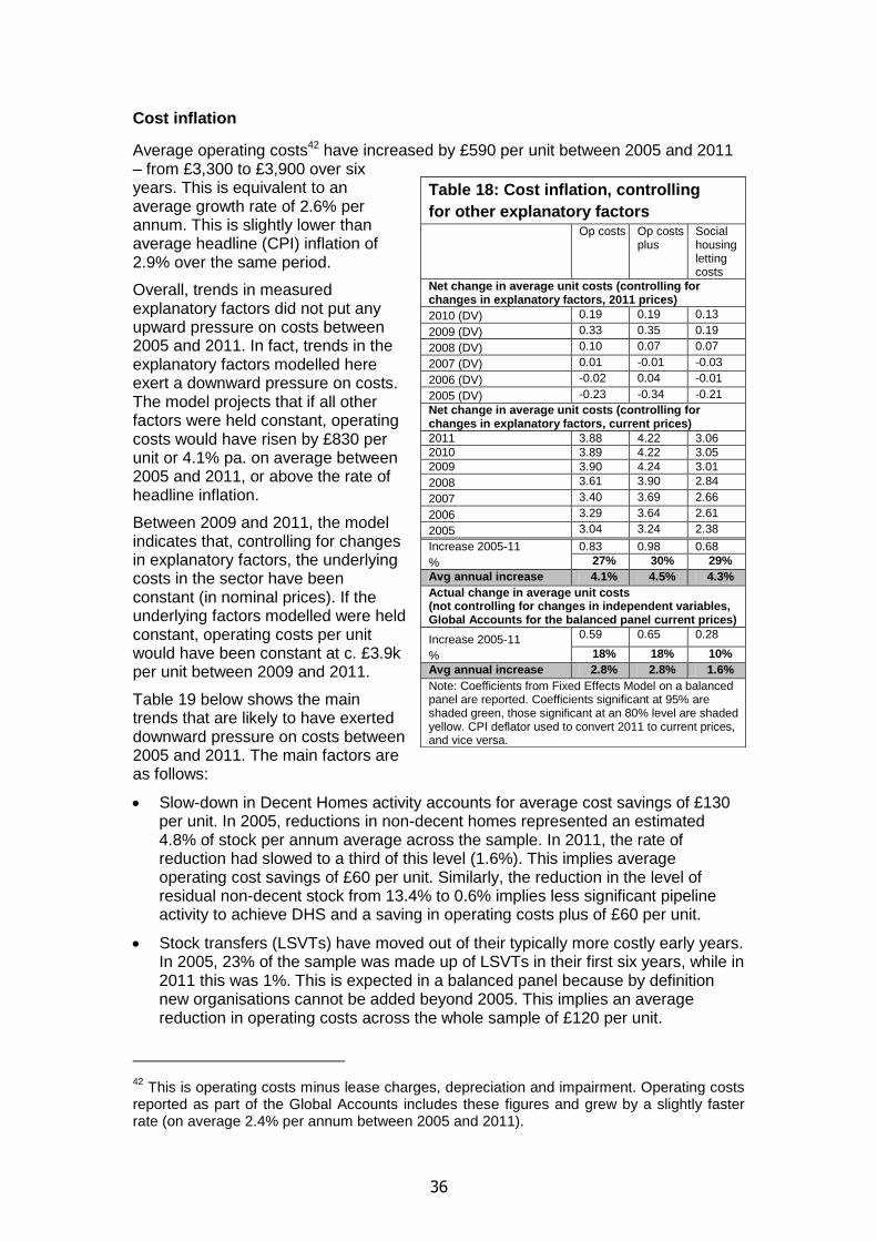
36

Cost inflation

Average operating costs42 have increased by £590 per unit between 2005 and 2011 – from £3,300 to £3,900 over six years. This is equivalent to an average growth rate of 2.6% per annum. This is slightly lower than average headline (CPI) inflation of 2.9% over the same period.

Overall, trends in measured explanatory factors did not put any upward pressure on costs between 2005 and 2011. In fact, trends in the explanatory factors modelled here exert a downward pressure on costs. The model projects that if all other factors were held constant, operating costs would have risen by £830 per unit or 4.1% pa. on average between 2005 and 2011, or above the rate of headline inflation.

Between 2009 and 2011, the model indicates that, controlling for changes in explanatory factors, the underlying costs in the sector have been constant (in nominal prices). If the underlying factors modelled were held constant, operating costs per unit would have been constant at c. £3.9k per unit between 2009 and 2011.

Table 19 below shows the main trends that are likely to have exerted downward pressure on costs between 2005 and 2011. The main factors are as follows:

Slow-down in Decent Homes activity accounts for average cost savings of £130 per unit. In 2005, reductions in non-decent homes represented an estimated 4.8% of stock per annum average across the sample. In 2011, the rate of reduction had slowed to a third of this level (1.6%). This implies average operating cost savings of £60 per unit. Similarly, the reduction in the level of residual non-decent stock from 13.4% to 0.6% implies less significant pipeline activity to achieve DHS and a saving in operating costs plus of £60 per unit.

Stock transfers (LSVTs) have moved out of their typically more costly early years. In 2005, 23% of the sample was made up of LSVTs in their first six years, while in 2011 this was 1%. This is expected in a balanced panel because by definition new organisations cannot be added beyond 2005. This implies an average reduction in operating costs across the whole sample of £120 per unit.

42

This is operating costs minus lease charges, depreciation and impairment. Operating costs reported as part of the Global Accounts includes these figures and grew by a slightly faster rate (on average 2.4% per annum between 2005 and 2011).

Table 18: Cost inflation, controlling

for other explanatory factors

Op costs Op costs plus


Net change in average unit costs (controlling for changes in explanatory factors, 2011 prices)

2010 (DV) 0.19 0.19 0.13

2009 (DV) 0.33 0.35 0.19

2008 (DV) 0.10 0.07 0.07

2007 (DV) 0.01 -0.01 -0.03

2006 (DV) -0.02 0.04 -0.01

2005 (DV) -0.23 -0.34 -0.21

Net change in average unit costs (controlling for changes in explanatory factors, current prices)

2011 3.88 4.22 3.06

2010 3.89 4.22 3.05

2009 3.90 4.24 3.01

2008 3.61 3.90 2.84

2007 3.40 3.69 2.66

2006 3.29 3.64 2.61

2005 3.04 3.24 2.38

Increase 2005-11 0.83 0.98 0.68

% 27% 30% 29%

Avg annual increase 4.1% 4.5% 4.3%

Actual change in average unit costs (not controlling for changes in independent variables, Global Accounts for the balanced panel current prices)

Increase 2005-11 0.59 0.65 0.28

% 18% 18% 10%

Avg annual increase 2.8% 2.8% 1.6%

Note: Coefficients from Fixed Effects Model on a balanced panel are reported. Coefficients significant at 95% are shaded green, those significant at an 80% level are shaded yellow. CPI deflator used to convert 2011 to current prices, and vice versa.

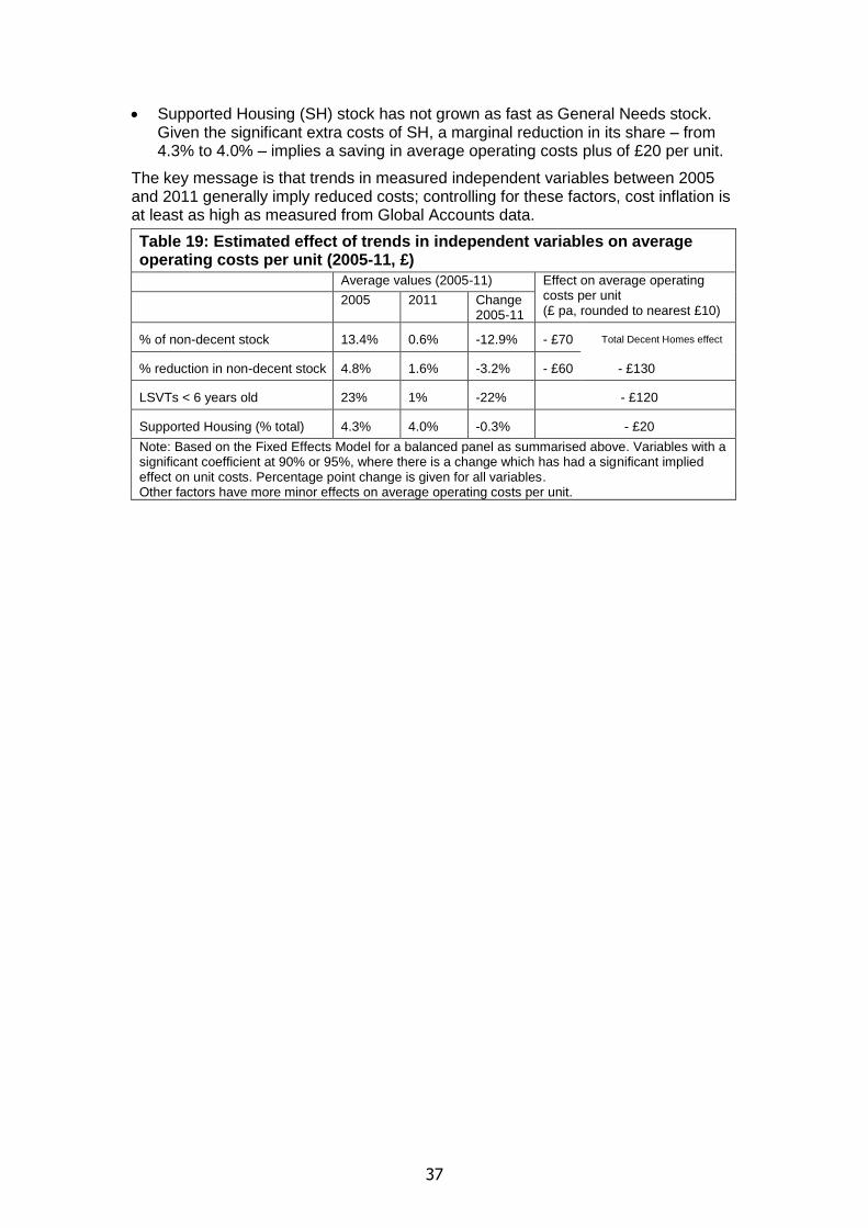
37

Supported Housing (SH) stock has not grown as fast as General Needs stock. Given the significant extra costs of SH, a marginal reduction in its share – from 4.3% to 4.0% – implies a saving in average operating costs plus of £20 per unit.

The key message is that trends in measured independent variables between 2005 and 2011 generally imply reduced costs; controlling for these factors, cost inflation is at least as high as measured from Global Accounts data.

Table 19: Estimated effect of trends in independent variables on average operating costs per unit (2005-11, £)

Average values (2005-11) Effect on average operating costs per unit (£ pa, rounded to nearest £10)

2005 2011 Change 2005-11

% of non-decent stock 13.4% 0.6% -12.9% - £70 Total Decent Homes effect

% reduction in non-decent stock 4.8% 1.6% -3.2% - £60 - £130

LSVTs < 6 years old 23% 1% -22% - £120

Supported Housing (% total) 4.3% 4.0% -0.3% - £20

Note: Based on the Fixed Effects Model for a balanced panel as summarised above. Variables with a significant coefficient at 90% or 95%, where there is a change which has had a significant implied effect on unit costs. Percentage point change is given for all variables. Other factors have more minor effects on average operating costs per unit.

38

Extensions of the model There are a number of ways in which the model above has been extended to test the impact of other independent variables. In some cases, such as geographical dispersal, the number of control factors needed make the other aspects of the core model less easy to grasp intuitively (e.g. additional costs associated with SH need to factor in the average effect of ten relevant dispersal measures, the effects of rents on top of regional wages). Other variables, such as voids or size of property, are too closely linked to variables included in the analysis. These issues are explored below.

Geographical dispersal

An important extension of the main model is examining the effect of geographical dispersal of General Needs stock on costs. Eight measures of dispersal were tested in the work presented with the 2010 Global Accounts:

Proportion of General Needs stock held in pockets of less than 50, 100, 250 or 500 per local authority area.

Proportion of General Needs stock held in pockets of less than 50, 100, 250 or 500 per sub-region.

2009-10 analysis found evidence that GN stock held in isolated pockets of less than 50 or 100 per local authority or sub-region are associated with significantly increased costs. Evidence was typically stronger for social housing lettings costs and operating costs than operating costs plus. 2009-10 analysis found no evidence that dispersed GN stock measured by the Herfindahl Index or the Entropy Index has an impact on costs.

General Needs stock held in pockets of less than 100 per local authority was used as the principle indicator for the analysis presented here. A full set of dispersal measures have been calculated for SH and HOP. SH costs in particular are much greater than General Needs on average, and are highly variable depending on the nature of the service offered. Given the relatively small numbers of units involved, the costs of dispersed specialist units tends to follow the particular type of service offered rather than measure the costs of dispersal. For this reason, the costs of dispersed stock for SH or HOP are not estimated.

However, data analysis shows there is a clear correlation between dispersal of General Needs and other types of stock: providers with large amounts of HOP and SH stock held in small pockets tend to have dispersed General Needs holdings, typically held in slightly bigger pockets. This correlation means that it is necessary to include the SH and HOP dispersal measures in the regression in order to accurately capture the effect of dispersal of General Needs stock. Otherwise there would be a powerful bias introduced through missing variables.

Overall there is mixed evidence of a relationship between dispersed GN stock and costs. In the balanced panel, there was no evidence of such a relationship. The table below shows with the wider unbalanced panel model there is significant evidence for higher social housing lettings and operating costs in three out of seven years. Increased costs associated with this stock are £1,400 per unit or c. 40% higher than typical costs for General Needs. These findings only hold for the unbalanced panel and are no significant results occur in any year in the balanced panel.

The Fixed Effects Model yields no clear evidence of a relationship between dispersal of GN stock and costs. However, it is likely that there have not been sufficient variability in holdings of stock within providers across the panel to have a significant effect on costs.

39

Table 20: Effect of GN dispersal (100 LA) on unit costs (£000s) (balanced panel, 2005-2011)



Proportion of GN in pockets of 100 LA

n/a

Note: Coefficients from the Ordinary Least Squares (OLS), Fixed Effects Model (FE) and Random Effects Model (RE) reported. The Random Effects Model was not valid for social housing lettings once dispersal measures were added. Only coefficients significant at a 90% (shaded amber) or a 95% (shaded green) level are reported. No coefficients were significant and hence the table is blank. The regressions tested included the 19 explanatory variables set out in the main model, plus proportion of GN in pockets of less than 100 per local authority, plus a range of dispersal measures for Supported Housing and Housing for Older People. OLS results are for all years the average of the coefficients significant at 90% or 95% level, with the number of years where there is a significant relationship given in brackets. Where there is a mixture of coefficients significant at the 90% and 95% levels, shading follows the significance of the majority.

Table 21: Effect of GN dispersal (100 LA) on unit costs (£000s) (unbalanced panel, 2005-2011)


OLS OLS OLS


1.57 (4) 1.36 (3)

Note: Coefficients from the Ordinary Least Squares (OLS), Fixed Effects Model (FE) and Random Effects Model (RE) reported. The Random Effects Model was not valid for social housing lettings once dispersal measures were added. Only coefficients significant at a 90% (shaded amber) or a 95% (shaded green) level are reported. The regressions tested were the 19 explanatory variables set out in the main model, plus proportion of GN in pockets of less than 100 per local authority, plus a range of dispersal measures for Supported Housing and Housing for Older People. OLS results are for all years the average of the coefficients significant at 90% or 95% level, with the number of years where there is a significant relationship given in brackets. Where there is a mixture of coefficients significant at the 90% and 95% levels, shading follows the significance of the majority.

40

Rural stock

The five rural stock measures were added to the model in turn and each of them had no significant effect on costs. This analysis was done on the social housing lettings costs using the balanced panel (shown below), while further OLS analysis using the unbalanced panel supported these findings of no effects.

Table 22: Effect of rural stock variables on unit costs (£000s) (social housing letting costs, balanced panel, 2005-2011)


OLS FE RE

Stock in rural neighbourhoods (LSOA)

Proportion of rural stock at LSOA level n/a

Proportion of very rural stock at LSOA level

n/a

Stock in rural local authorities

Proportion of rural stock at LA level n/a

Proportion of very rural stock at LA level

n/a

Proportion of very very rural stock at LA level

n/a

Note: Coefficients from the Ordinary Least Squares (OLS), Fixed Effects Model (FE) and Random Effects Model (RE) reported. The Random Effects Model was not valid for social housing lettings once dispersal measures were added. There are no coefficients significant at a 90% (shaded amber) or a 95% (shaded green) level are reported, hence no data is displayed on the table above The dispersal measures are included because of their correlation with the rural stock measures. *OLS results are for all years the average of the coefficients significant at 90% or 95% level, with the number of years where there is a significant relationship given in brackets. Where there is a mixture of coefficients significant at the 90% and 95% levels, shading follows the significance of the majority.

Extensions of the model in previous years

Other extensions of the model were conducted on the analysis presented with the 2010 Global Accounts and were found to have little power to explain provider costs. These extensions were not repeated for 2010-11 data. These extensions are as follows:

Contracting out of management services – there was little clear evidence of savings from contracting out of management for GN stock.

Repairs – there was no clear evidence of costs associated with properties repaired (as recorded in the RSR). Recorded Decent Homes activity was a much better predictor of costs.

Choice-based lettings – there was little evidence of increased costs from choice-based lettings.

Voids, lettings, anti-social behaviour, size of properties – there were significant inter-linkages between all of these measures as well as with deprivation. For example, new social housing constructed in recent years has been predominantly two-bed properties, while the profile of older social housing estates tends to be skewed towards larger properties. Moreover, newer properties tend to be constructed in relatively less deprived neighbourhoods than existing social housing on average, as indicated by the shifting IMD index as well as other research. Therefore, the bedroom size of properties may proxy a range of issues around age of property and additional management and repair costs tend to be associated with significant neighbourhood deprivation, rather than actually measuring the effect of the size of a property. There are similar issues involved in including voids, lettings or ASB activities as indicators. To mitigate

41

against multi-colinearity and over-controlling, the general level of neighbourhood deprivation was incorporated as a broad indicator for these factors.

Testing robustness of approach

In order to test the robustness of the approach presented with the 2010 Global Accounts, regression analysis was extended in several important directions. The idea was to test the extent to which the main findings of the work are robust to viable alternate approaches. The main regression model was run with the following modifications:

Different functional forms: the same variable can be employed in the model in a number of mathematical forms. In particular, the results of running a regression with dependent (cost) variable in a logarithmic rather than an absolute form43 were compared.

Quantile regression: estimators being based on median values rather than the standard mean values. This is a non-standard approach that could arguably be more applicable to provider data here where there are outlying values for unit costs for example.

Unbalanced panel: the main regression for an unbalanced rather than balanced panel, incorporating a larger number of providers each year.

Different inflation rates: costs were adjusted by the Average Earnings Index rather than the Consumer Price Index (CPI). This is because it is likely that provider costs will follow wage costs more closely than general prices, and hence coefficients are likely to be more stable across the panel.

Testing the effect of the above approaches involved running the main regression under different assumptions. Testing was originally conducted on data for 2005-09 and not all have been re-run for all the tests for the additional years of data (2010 or 2011). In the analysis presented here, the results have been tested for the unbalanced as well as the balanced panel. Overall, there was little evidence to suggest that the main results set out here are critically sensitive to the approach taken.

Residual analysis: how much cost variation can be explained?

Residuals are the difference between actual and predicted unit costs. They can be thought of as the amount of variation in costs left over after the regression analysis. The standard deviation of operating costs per unit, before any regression, is £1,43044. That is, on average, costs were £1,430 above or below the mean. The standard error of the regression – the amount by which unit costs vary from those predicted – is around £1,000. Therefore, there is still considerable variability in costs – on average 29% above or below the mean45 – which cannot be explained by the factors considered here.

One measure of the explanatory power of the regression is the R-squared measure. On average for each year between 2005 and 2011, R-squared for operating costs is

43

The test involves using the log-model to derive a predicted value for absolute costs for each observation. These predicted values of absolute costs (from the log model) are compared against observed costs and an R-squared value is derived. This can be directly compared with the R-squared value from the linear model.

44 For all years in the balanced panel, excluding specialist organisations and organisations

with accounts not based on 12 months.

45 Based on mean operating costs per unit of £3,500 for 2011 (balanced panel).

42

0.50 – this can be interpreted saying the regression can explain 50% of variability in observed unit costs. The R-squared value is similar for operating costs plus (51%) and slightly lower for social housing letting costs (36%).

It is possible to test the correlation between certain variables and residuals. The figure below shows the variation between unexplained cost variation and size of provider, measured by GN stock. It is clear that there is no simple deterministic relationship between residual costs and size of provider. The regression line runs along the x-axis in the diagram below.

However, there is a clear relationship between variability of unexplained costs and size. Regression analysis on residuals squared and size yields the relationship set out in the figure below. This shows that the variability in the residual applies more for smaller landlords and declines sharply as size increases. More variability for the smallest landlords compared to the largest is not surprising, since the largest have greater diversification which allows them to absorb shocks to costs e.g. major repair requirements for a larger landlord with a diverse portfolio of stock is likely to be smoother over time. However, it is perhaps surprising that there is still significant variability for medium-sized landlords with around 10,000 units. The distance (negative or positive) between actual and predicted costs for these landlords is around £800, only slightly lower than the level for the smallest landlords in the sample (£1,200). However, average variability is marginal for landlords with at least 20,000 GN units.

The relationship between variability and other factors such as LSVTs or specialist organisations may be worthy of further investigation.

43

Figure 11: Residual values (difference between predicted and actual costs, £000s) and size of provider (GN units, 000s) (balanced panel, an illustrative year)

Figure 12: Average variability in residuals (square root of residuals squared) by size of provider (GN units, 000s) (balanced panel, an illustrative year)

0

0.2

0.4

0.6

0.8

1

1.2

1.4

1 2 3 4 5 6 7 8 9 10 11 12 13 14 15 16 17

GN stock (000s)

Sq

uare

ro

ot

of

resid

uals

sq

uare

d

44

Analysis of consolidated group accounts

In order to check the robustness of the results from entity-level analysis, a similar analysis was conducted on consolidated group accounts (2009-10 data). A full set of data on costs and explanatory factors was collated for 128 groups for 2009-10. Cost data was from published group-level accounts and explanatory variables from amalgamated entity-level data. Together with existing data for 85 organisations not in group structures, this gave a total sample size of 213 organisations for 2009-10 (89% of the 240 provider structures with over 1,000 units).

The main hypothesis to be tested from group-level analysis is whether group structures appeared to have lower costs. In the entity level analysis, there are apparent savings from group structures. However, only registered entities with more than 1,000 units are included. Group parents or other entities without this level of stock holdings may incur some costs for common functions that are not fully charged to their larger registered subsidiaries and hence indicate apparent savings from group structures. However group-level accounts data typically picks up the costs of these unregistered components.

Detailed results of group-level analysis

The same regression model as used in the previous entity-level analysis published with the 2010 Global Accounts was used to test the effect of explanatory factors or group-level costs. Due to availability of group-level accounts data, it was only possible to run the analysis for one year. Hence overall evidence is weaker than the entity level analysis based on seven years’ data.

The results of the OLS model, run for 2009-10 for 213 observations, are summarised in the table below. The coefficient shows how much a unit change is associated with a unit change in costs (£000/unit). Where there is statistically significant evidence of a relationship cells are shaded, depending on the degree of significance (80%, 90% or 95%).

Conclusions from group-level analysis

Group-level analysis showed, when costs are measured at a consolidated-group level, there is no significant evidence that group structures achieved any lower costs than equivalent stand-alone organisations. Group-level analysis also supports a range of findings from the entity-level analysis: for example for costs associated with Supported Housing, regional wages, Decent Homes activity and neighbourhood deprivation. There was no evidence for economies to scale.

45

Table 23: Effect of changes in each explanatory factor on three main cost measures (unbalanced panel, 2009-2010 data using consolidated group accounts for entities in group structures)

Dependent cost variable Operating costs

(£000s) Operating costs plus

(£000s) Social housing lettings

costs (£000s)

Coefficient SE Coefficient SE Coefficient SE

Intercept 3.05 * 0.48 3.93 * 0.49 2.81 * 0.45

Housing for older people (% total) 1.44 2.13 0.96 2.15 1.81 1.75

% HOP squared 0.65 2.00 0.32 2.03 0.13 1.68

Supported Housing (% total) 11.02 4.63 8.22 4.82 5.79 4.29

% of SH squared 6.61 6.60 8.34 6.70 7.30 5.22

Shared ownership (% total) 0.81 4.72 -1.22 4.61 -1.49 4.63

Non-social housing (% total) 1.93 1.47 2.04 1.35 1.04 0.90

% reduction in non-decent stock 2.18 2.86 4.96 * 1.97 2.90 2.98

% of non-decent stock -0.73 1.45 1.34 2.28 -0.38 1.54

% change in stock -3.88 2.64 -3.92 2.55 -3.97 * 1.81

% change in stock t-1 -1.09 1.49 -1.18 1.58 -0.69 1.24

LSVT < 7 years (DV) -0.44 0.33 0.46 0.89 -0.37 0.30

LSVT 7 - 12 years (DV) -0.18 0.20 -0.42 0.22 -0.13 0.20

LSVT > 12 years (DV) -0.29 0.26 -0.60 * 0.28 -0.24 0.21

Group structure (DV) -0.07 0.25 -0.08 0.27 0.00 0.20

Weighted wage index 4.97 * 1.25 6.69 * 1.91 4.99 * 1.12

Weighted Index of Deprivation 0.02 * 0.01 0.01 0.01 0.02 * 0.01

GN stock (000s) 0.02 0.02 -0.01 0.03 0.00 0.02

HOP stock (000s) -0.08 0.11 -0.02 0.11 -0.07 0.09

SH stock (000s) -0.26 0.28 -0.14 0.29 0.00 0.25

Shared ownership stock (000s) -0.14 0.21 -0.15 0.22 0.03 0.21

Non social stock (000s) 0.05 0.10 0.07 0.10 -0.02 0.08

N (total observations) 213 213 213

Mean of cost measure 3.99 4.51 3.52

Standard Deviation of cost measure 2.77 2.85 2.20

Standard error of regression 1.48 1.64 1.29

Note: * and green shading denotes coefficients with p values of less than 0.05, i.e. there is evidence at a 95% confidence level that the coefficient is nonzero. Amber shading denotes a p value of between 0.05 and 0.1 and yellow between 0.1 and 0.2. Unless indicated otherwise, figures presented in the main body of the table are the regression coefficients.

46

Scope for further analysis

This work should not be seen as the final destination for regression analysis on social housing costs. The outputs to date have involved detailed exploration of a range of issues. It is likely that this regression model would be periodically refreshed with new data, and enhanced analysis. Many of the potential extensions to the model previously identified – the effect of rents, rural stock, etc. – have been introduced as new factors here. There are a number of additional ways in which the analysis can be usefully extended:

Examining the power of regressions for certain sub-groups. For example, it is possible to test regressions including and excluding certain sub-groups such as LSVTs or specialist providers. Excluding certain sub-groups may increase the power of the main regression.

Test the robustness of findings to a range of outlying variables in more detail. Outlying variables can be defined as those that have a very strong influence on regression results. They do not necessarily have very large residuals overall. There are a range of statistical techniques that can be employed.

Examining in more detail how economies of scale and specialisation for different types of specialist units work in practice. This means examining the implications of the analysis in the context of the holdings of selected providers.

Focusing on the costs associated with different types of Supported Housing.

Exploring the concept of economies of scale for shared ownership stock in more detail, potentially linking economies of scale with the degree of specialisation.

Investigating the effect of rents as an explanatory factor on costs in more detail, and potentially its combination with other factors in the model.

47

Annex A – Additional detail of modelling This Annex details some of the detailed modelling that was involved in the constructing of the regression model of unit costs in social housing. The process of preparing the data for the analysis is outlined, in terms of cleaning data and selecting a balanced panel. Some of the statistical and econometric testing is outlined, which includes the process of selecting the best estimators. A range of testing was originally conducted on data for 2005-09. Not all these tests have been re-run for the additional sixth and seventh years of data (2010 & 2011) and hence some results below are for 2005-09 only. This is followed by descriptive statistics for the data included in the model.

Data preparation

Missing data

Regression analysis cannot be reliably run with missing data. Where any data-point is missing for a certain landlord, the options are to either make an estimate of the value of this data-point or to exclude the landlord from the analysis altogether.

Where data has been missing from the RSR, the regulator has sought to understand the reasons for this, and amend the data accordingly. For many measures where positive responses are generally low – such as numbers of Anti-Social Behaviour Orders served – the missing values have been changed to zero.

Additional questions were added to the RSR in 2005. This means that all data for certain fields were missing for 2004. The intention was originally to include the data for 2004 in the regression along with data for 2005 – 2011 inclusive. However, the decision was made to exclude this data. Where cost data (the dependent variable) was missing, the observation was excluded from the data.

There may be features of the annual cost data for any given provider that mean it is not particularly representative of providers at large. For example, a new provider created on a date other than 31 March is likely to report costs for their first (or second) year which are not based on a 12 month period. The regulator holds information on the number of months cost information pertains to: organisations where the cost information is not based on 12 months were excluded from the analysis.

Outliers

Outliers are observations which have ‘extreme’ characteristics which can affect the analysis and give mis-leading results. Providers that specialise in Supported Housing46 tend to exhibit these characteristics, as their stock profile is different to most providers and they tend to have higher costs per unit47. Therefore these providers have been removed from the analysis; in the balanced panel this results in three providers being removed in every year (in the unbalanced panel there are slightly more).

Balanced panel

Over the seven years there were 2,668 observations, however not all of these observations had complete data (10%). Once these observations and the outliers

46

Defined these as providers with over 70% of stock in SH.

47 Operating costs per unit over £20,000.

48

were removed, 2,359 usable observations were left. Given the dynamic nature of the social housing market, several providers left and entered the market over the seven years, which meant that not all of the 2,359 observations were involved in every year. When this occurs, the 2,359 observations are termed an ‘unbalanced panel’, while the observations that have data for all the years are termed a ‘balanced panel.’ The balanced panel constitutes 1,589 observations or 227 providers over seven years, and was the main sample used in the regression analysis.

The table below summarises the number of observations removed from the original database through removing cost data which is not on the basis of a 12 month period, missing data that could not be modified and through selecting a balanced panel.

Table 24: Summary of observations – before and after cleaning of data

2005 2006 2007 2008 2009 2010 2011 Total

Original observations 388 381 381 390 386 378 364 2,668

Observations removed from analysis

Non-12 month cost data 5 11 27 15 12 3 3 76

Missing data 17 24 21 31 37 36 28 194

Specialist SH providers 7 6 6 6 6 5 3 39

Observations used in the panel

Unbalanced panel (N) 359 340 327 338 331 334 330 2,359

Balanced panel (N) 227 227 227 227 227 227 227 1,589

Econometric testing

An extensive and iterative process of refining and testing the model was carried out. This process provides greater assurance that any inference from the model is robust and that the model is correctly specified48.

Excluded variables

An initial long-list of variables was tested but many variables were excluded from the final regression. The majority of variables were excluded because multiple variables were used to proxy a single factor which influenced costs. To avoid over-controlling in such instances, each variable was tested in separate models and the best estimator was selected49. To avoid multi-colinearity the correlation of all the independent variables was checked. This highlighted some unintentional correlations; for example, the size of properties was correlated with deprivation measures, which made it necessary to select a best estimator from the subset of size of properties and deprivation measures. The table below outlines the variables not included in the final regression.

Table 25: Variables not included in the final regression

48

Given the variables tested. The regulator acknowledges there maybe other variables that influence cost that have not been included in the model.

49 The basis for selecting the best estimator was: the significance of the variable’s effect on

cost (the lowest p-value), and in the model’s ability to explain the variation in costs (the highest adjusted R-squared value).

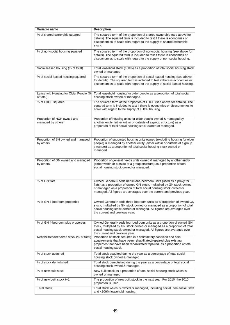
49

Variable name Description

% of shared ownership squared The squared term of the proportion of shared ownership (see above for details). The squared term is included to test if there is economies or diseconomies to scale with regard to the supply of shared ownership stock.

% of non-social housing squared The squared term of the proportion of non-social housing (see above for details). The squared term is included to test if there is economies or diseconomies to scale with regard to the supply of non-social housing.

Social leased housing (% of total) Total leasehold stock (100%) as a proportion of total social housing stock owned or managed.

% of social leased housing squared The squared term of the proportion of social leased housing (see above for details). The squared term is included to test if there is economies or diseconomies to scale with regard to the supply of social leased housing.

Leasehold Housing for Older People (% of total)

Total leasehold housing for older people as a proportion of total social housing stock owned or managed.

% of LHOP squared The squared term of the proportion of LHOP (see above for details). The squared term is included to test if there is economies or diseconomies to scale with regard to the supply of LHOP housing.

Proportion of HOP owned and managed by others

Proportion of housing units for older people owned & managed by another entity (either within or outside of a group structure) as a proportion of total social housing stock owned or managed.

Proportion of SH owned and managed by others

Proportion of supported housing units owned (excluding housing for older people) & managed by another entity (either within or outside of a group structure) as a proportion of total social housing stock owned or managed.

Proportion of GN owned and managed by others

Proportion of general needs units owned & managed by another entity (either within or outside of a group structure) as a proportion of total social housing stock owned or managed.

% of GN flats Owned General Needs bedsit/one-bedroom units (used as a proxy for flats) as a proportion of owned GN stock, multiplied by GN stock owned or managed as a proportion of total social housing stock owned or managed. All figures are averages over the current and previous year.

% of GN 3-bedroom properties Owned General Needs three-bedroom units as a proportion of owned GN stock, multiplied by GN stock owned or managed as a proportion of total social housing stock owned or managed. All figures are averages over the current and previous year.

% of GN 4-bedroom plus properties Owned General Needs four-bedroom units as a proportion of owned GN stock, multiplied by GN stock owned or managed as a proportion of total social housing stock owned or managed. All figures are averages over the current and previous year.

Rehabilitated/repaired stock (% of total) Proportion of stock acquired in a satisfactory condition and also acquirements that have been rehabilitated/repaired plus existing properties that have been rehabilitated/repaired, as a proportion of total social housing stock.

% of stock acquired Total stock acquired during the year as a percentage of total social housing stock owned & managed.

% of stock demolished Total stock demolished during the year as a percentage of total social housing stock owned & managed.

% of new built stock New built stock as a proportion of total social housing stock which is owned or managed.

% of new built stock t+1 The proportion of new built stock in the next year. For 2010, the 2010 proportion is used.

Total stock Total stock which is owned or managed, including social, non-social, staff and <100% leasehold housing.

50

Total social housing stock Total social housing stock which is owned or managed.

GN stock (000s) squared The squared term of the proportion of GN stock (000s). The squared term is included to test if there is economies or diseconomies to scale with regard to the supply of GN housing.

GN stock (000s) cubed The cubic term of the proportion of GN stock (000s). The cubic term is included to test if there is a cubic relation with regard to the supply of GN housing and the dependent variable.

LN Total social housing stock The natural log of total stock. The natural log function of total stock is included to test how unit costs change given a proportional change in stock.

LN GN stock The natural log of GN stock which is owned or managed. The natural log function of total stock is included to test how unit costs change given a proportional change in stock.

LN HOP stock The natural log of supported housing stock which is owned or managed. The natural log function of total stock is included to test how unit costs change given a proportional change in stock.

LN SH stock The natural log of supported housing stock (excl. older people) which is owned or managed. The natural log function of total stock is included to test how unit costs change given a proportional change in stock.

LN Shared ownership The natural log of shared ownership stock and other stock which is <100% leasehold (excluding housing for older people). A natural log function of stock is included to test how unit costs change given a proportional change in stock.

LN Non-social The natural log of non-social stock. A natural log function of stock is included to test how unit costs change given a proportional change in stock.

LN wage The natural log of the weighted wage index. A natural log function of stock is included to test how unit costs change given a proportional change in wage costs.

Proportion of unavailable voids Self-contained vacant but unavailable units as a proportion of total social housing stock owned or managed in the current and previous year.

% of unavailable voids squared The squared term of the proportion of unavailable voids. The squared term is included to test if there is economies or diseconomies to scale with regard to the effect of unavailable voids on the dependent variable.

% of available voids Self-contained vacant but available units as a proportion of total social housing stock owned or managed in the current and previous year.

% of available voids squared The squared term of the proportion of unavailable voids. The squared term is included to test if there is economies or diseconomies to scale with regard to the effect of available voids on the dependent variable.

% of voids All self-contained vacant units as a proportion of total social housing stock owned or managed in the current and previous year.

% of voids squared The squared term of the proportion of voids. The squared term is included to test if there is economies or diseconomies to scale with regard to the effect of voids on the dependent variable.

% of GN lettings General Needs lettings per annum, as a proportion of general needs stock, multiplied by share of General Needs of all stock.

% of employed tenants Average employment rate of new General Needs tenants at the time of lettings (from CORE data). This is whether either the main tenant or any partner is in full-time or part-time employment. Multiplied by share of General Needs of all stock. This is a proxy of deprivation and challenging socio-economic background of tenants.

51

Choice-based lettings (DV) Dummy variable to indicate whether the provider states they operate choice-based lettings (i.e. =1 if yes, =0 if no). Since it is assumed this is more likely to apply to General Needs stock, multiplied by the share of average General Needs of average total social housing stock for the current and previous year.

ASBO & ASBI per 10,000 GN Anti-Social Behaviour Orders and Injunctions (ASBOs & ASBIs) per 10,000 General Needs properties, multiplied by the average General Needs stock as a proportion of average total social housing stock in the current and previous year.

Weighted Index of Deprivation Score (deviation from the mean)

Weighted Index of Multiple Deprivation per annum for each landlord. Constructed by the regulator on the basis of lettings per Lower Super Output Area (LSOA) (from CORE data) and the percentile rank from the Index of Multiple Deprivation (IMD) for each LSOA subtracted by the IMD percentile rank in the dataset, multiplied by the average General Needs stock as a proportion of average total social housing stock in the current and previous year. The 2010 IMD was used for all years.

Herfindahl GN/SH/HOP One minus the Herfindahl Index for GN/SH/HOP stock owned at a local authority level, multiplied by GN/SH/HOP stock as a proportion of all stock. The Herfindahl Index is a measure of concentration where 1 is the maximum and 0 is the minimum level of concentration. Formally it is the sum of squares of each proportionate share of stock in each geography. Therefore one minus the index means a higher number indicates greater geographical dispersal. The cost impacts of a given level of dispersal are likely to depend on the amount of GN/SH/HOP stock, hence it is weighed by the share of GN/SH/HOP of total social housing stock.

Entropy GN/SH/HOP Entropy Index for GN/SH/HOP stock owned at a local authority level, multiplied by GN/SH/HOP stock as a proportion of all social housing stock. The Entropy Index is a measure of dispersal (from science) where a higher number indicates greater dispersal. It differs from the Herfindahl Index by placing greater weight on dispersal (i.e. small numbers of stock per local authority) rather than concentration. The cost impacts of a given level of dispersal are likely to depend on the amount of GN/SH/HOP stock, hence it is weighed by the share of GN/SH/HOP of total social housing stock.

Economies of scale testing

To test for an affect of economies of scale on costs a number of different functional forms and stock measures were experimented with. Total stock was used to test for a relationship between overall size and cost. In addition, stock was split into GN, HOP, SH, shared ownership and non-social to test for an effect for these particular types of stock. Experimentation with the functional form included using the natural log of the stock measure and also testing for a linear, squared and cubic relationship for total and GN stock measures. The stock measures chosen in the final regression were based on the R-squared value and the significance of the economies of scale variables. An illustrative example of the testing is given in the table below.

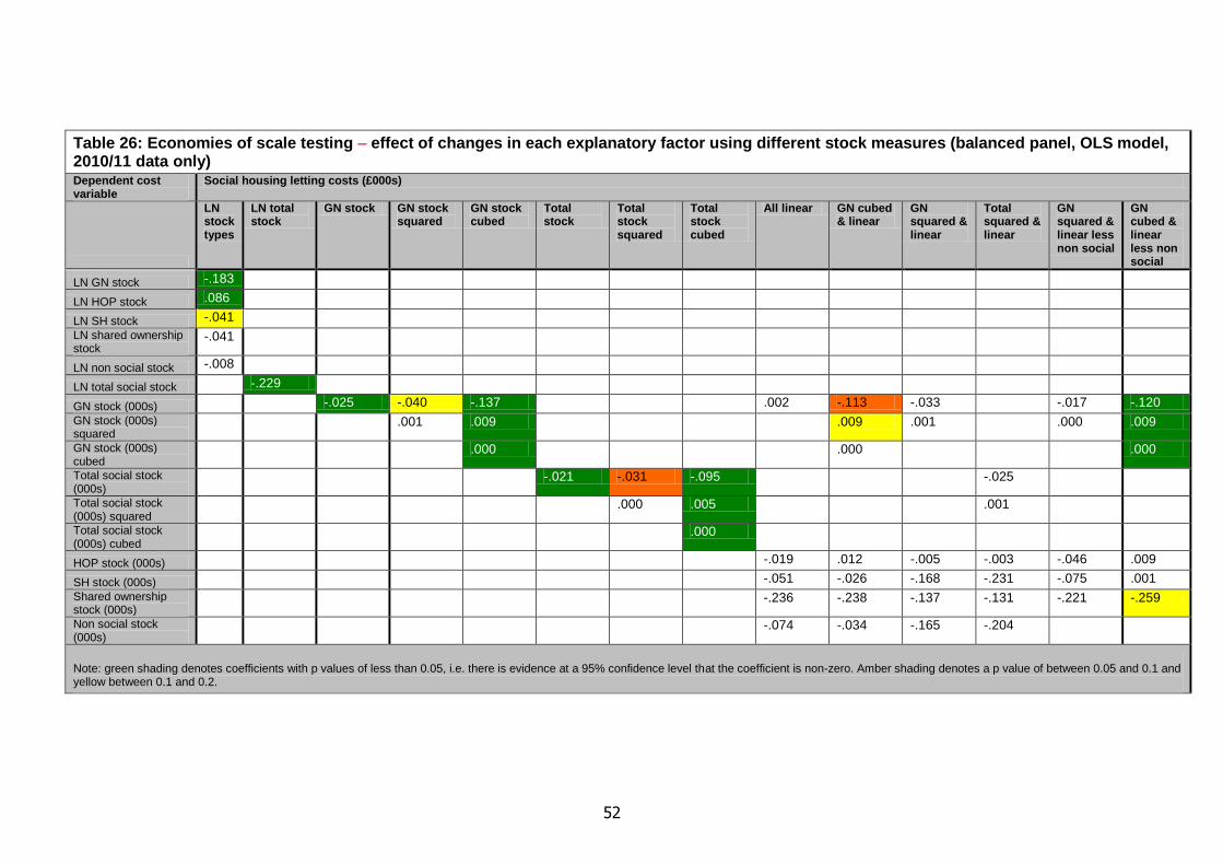
52

Table 26: Economies of scale testing – effect of changes in each explanatory factor using different stock measures (balanced panel, OLS model, 2010/11 data only) Dependent cost variable

Social housing letting costs (£000s)

LN stock types

LN total stock

GN stock GN stock squared

GN stock cubed

Total stock

Total stock squared

Total stock cubed

All linear GN cubed & linear

GN squared & linear

Total squared & linear

GN squared & linear less non social

GN cubed & linear less non social

LN GN stock -.183

LN HOP stock .086

LN SH stock -.041

LN shared ownership stock

-.041

LN non social stock -.008

LN total social stock -.229

GN stock (000s) -.025 -.040 -.137 .002 -.113 -.033 -.017 -.120

GN stock (000s) squared

.001 .009 .009 .001 .000 .009

GN stock (000s) cubed

.000 .000 .000

Total social stock (000s)

-.021 -.031 -.095 -.025

Total social stock (000s) squared

.000 .005 .001

Total social stock (000s) cubed

.000

HOP stock (000s) -.019 .012 -.005 -.003 -.046 .009

SH stock (000s) -.051 -.026 -.168 -.231 -.075 .001


-.236 -.238 -.137 -.131 -.221 -.259

Non social stock (000s)

-.074 -.034 -.165 -.204

Note: green shading denotes coefficients with p values of less than 0.05, i.e. there is evidence at a 95% confidence level that the coefficient is non-zero. Amber shading denotes a p value of between 0.05 and 0.1 and yellow between 0.1 and 0.2.

53

Heteroskedasticity

Heteroskedasticity is where the average variance of the error terms is non-constant over different segments of the population of providers. This does not mean that the estimates of each coefficient are biased, or that the R-squared values are invalid. However, heteroskedasticity can mean that the standard T-tests and F-tests of statistical significance of coefficients are invalid, even with large sample sizes.

Running the Breusch-Pagan Test on initial regressions yielded evidence of heteroskedasticity at a 5% significance level. The presence of heteroskedasticity did not present a problem in testing, as heteroskedastic-robust standard errors have been calculated for all coefficients. This meant that all inferences were reliable and accounted for the non-constant variance of the error term.

Descriptive statistics

The tables below set out standard descriptive statistics – mean, standard deviation – for all independent and dependent variables included in the modelling process. An indication of variation over time has been included, since this determines the power of the Fixed Effects Model rather than the standard OLS model. Since they are material in considering issues of multi-colinearity and over-controlling, a table of simple correlations between each explanatory variables is set out.

Table 27: Descriptive statistics, including variance in variables (balanced panel, 2005-2011)

Mean Standard deviation

Change in average 2005 - 11

Standard deviation of average annual difference from mean

Operating costs per unit

3.673 1.433 -0.061 0.115

Operating cost plus per unit

4.044 1.570 -0.065 0.120

Social housing lettings cost per unit

3.078 0.952 -0.159 0.087

Housing for Older People (% total)

0.134 0.129 -0.007 0.005

% of HOP squared 0.035 0.095 0.000 0.002

Supported Housing (% total)

0.042 0.068 -0.003 0.002

% of SH squared 0.006 0.028 -0.002 0.001

Shared ownership (% total)

0.044 0.074 0.021 0.008

Non-social housing (% total)

0.030 0.104 0.003 0.003


0.029 0.051 -0.032 0.011

% of non-decent stock

0.064 0.092 -0.129 0.047

54

% stock acquired in the current, past and future years

0.031 0.055 -0.034 0.012

% stock acquired in the past 3 years

0.027 0.048 -0.003 0.002

% stock acquired in the past 7 years

0.028 0.045 -0.001 0.001

% change in stock 0.025 0.090 0.002 0.006

% change in stock t-1

0.022 0.085 0.021 0.011

% change in stock in the current, past and future years

0.028 0.063 -0.006 0.003

% change in stock in the past 3 years

0.028 0.068 0.007 0.003

% change in stock in the past 7 years

0.028 0.063 0.008 0.004

% of new built stock 0.015 0.021 0.001 0.001

% new built stock in the current, past and future years

0.018 0.026 -0.016 0.006

% new built stock in the past 3 years

0.015 0.020 0.002 0.001

% new built stock in the past 7 years

0.015 0.020 0.001 0.000

LSVT < 7 years (DV) 0.084 0.277 -0.229 0.086

LSVT 7 - 12 years (DV)

0.247 0.431 0.040 0.032

LSVT > 12 years (DV)

0.154 0.361 0.189 0.067

Group parent (DV) 0.231 0.422 0.106 0.056

Group subsidiary (DV)

0.425 0.494 0.172 0.069

Weighted wage index GN

-0.008 0.075 0.000 0.000

Weighted wage index SH

0.000 0.007 0.000 0.000

Weighted wage index HOP

-0.005 0.011 0.001 0.001

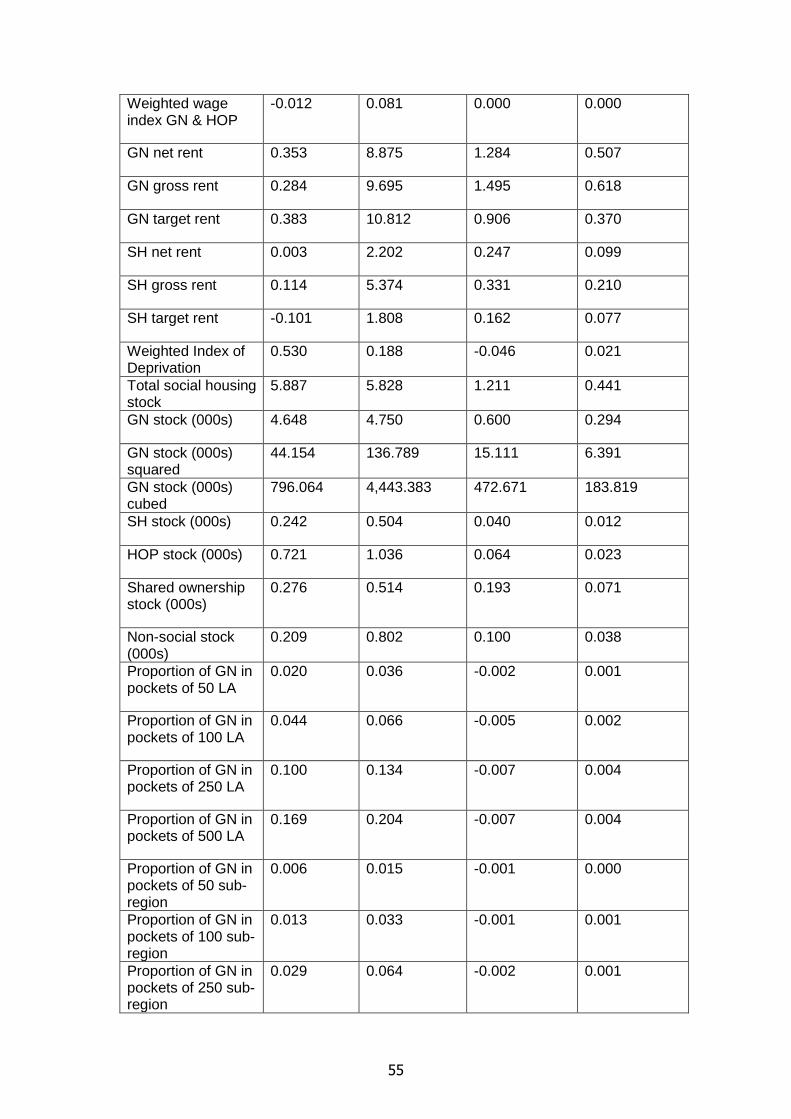
55

Weighted wage index GN & HOP

-0.012 0.081 0.000 0.000

GN net rent 0.353 8.875 1.284 0.507

GN gross rent 0.284 9.695 1.495 0.618

GN target rent 0.383 10.812 0.906 0.370

SH net rent 0.003 2.202 0.247 0.099

SH gross rent 0.114 5.374 0.331 0.210

SH target rent -0.101 1.808 0.162 0.077

Weighted Index of Deprivation

0.530 0.188 -0.046 0.021

Total social housing stock

5.887 5.828 1.211 0.441

GN stock (000s) 4.648 4.750 0.600 0.294

GN stock (000s) squared

44.154 136.789 15.111 6.391

GN stock (000s) cubed

796.064 4,443.383 472.671 183.819

SH stock (000s) 0.242 0.504 0.040 0.012

HOP stock (000s) 0.721 1.036 0.064 0.023


0.276 0.514 0.193 0.071

Non-social stock (000s)

0.209 0.802 0.100 0.038


0.020 0.036 -0.002 0.001


0.044 0.066 -0.005 0.002


0.100 0.134 -0.007 0.004


0.169 0.204 -0.007 0.004

Proportion of GN in pockets of 50 sub-region

0.006 0.015 -0.001 0.000


0.013 0.033 -0.001 0.001


0.029 0.064 -0.002 0.001

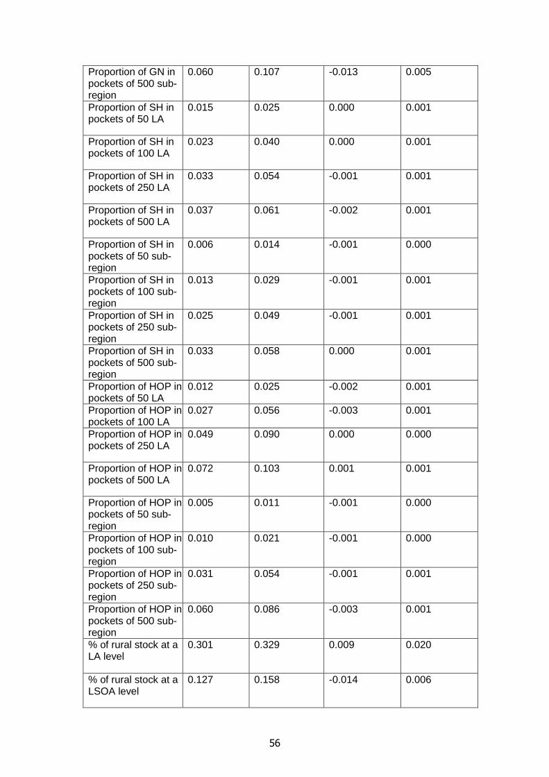
56


0.060 0.107 -0.013 0.005

Proportion of SH in pockets of 50 LA

0.015 0.025 0.000 0.001


0.023 0.040 0.000 0.001


0.033 0.054 -0.001 0.001


0.037 0.061 -0.002 0.001

Proportion of SH in pockets of 50 sub-region

0.006 0.014 -0.001 0.000


0.013 0.029 -0.001 0.001


0.025 0.049 -0.001 0.001


0.033 0.058 0.000 0.001

Proportion of HOP in pockets of 50 LA

0.012 0.025 -0.002 0.001


0.027 0.056 -0.003 0.001


0.049 0.090 0.000 0.000


0.072 0.103 0.001 0.001

Proportion of HOP in pockets of 50 sub-region

0.005 0.011 -0.001 0.000


0.010 0.021 -0.001 0.000


0.031 0.054 -0.001 0.001


0.060 0.086 -0.003 0.001

% of rural stock at a LA level

0.301 0.329 0.009 0.020

% of rural stock at a LSOA level

0.127 0.158 -0.014 0.006

57

% of very rural stock at a LA level

0.201 0.295 0.015 0.017

% of very rural stock at a LSOA level

0.048 0.068 -0.003 0.001

% of very very rural stock at a LA level

0.108 0.229 -0.002 0.006

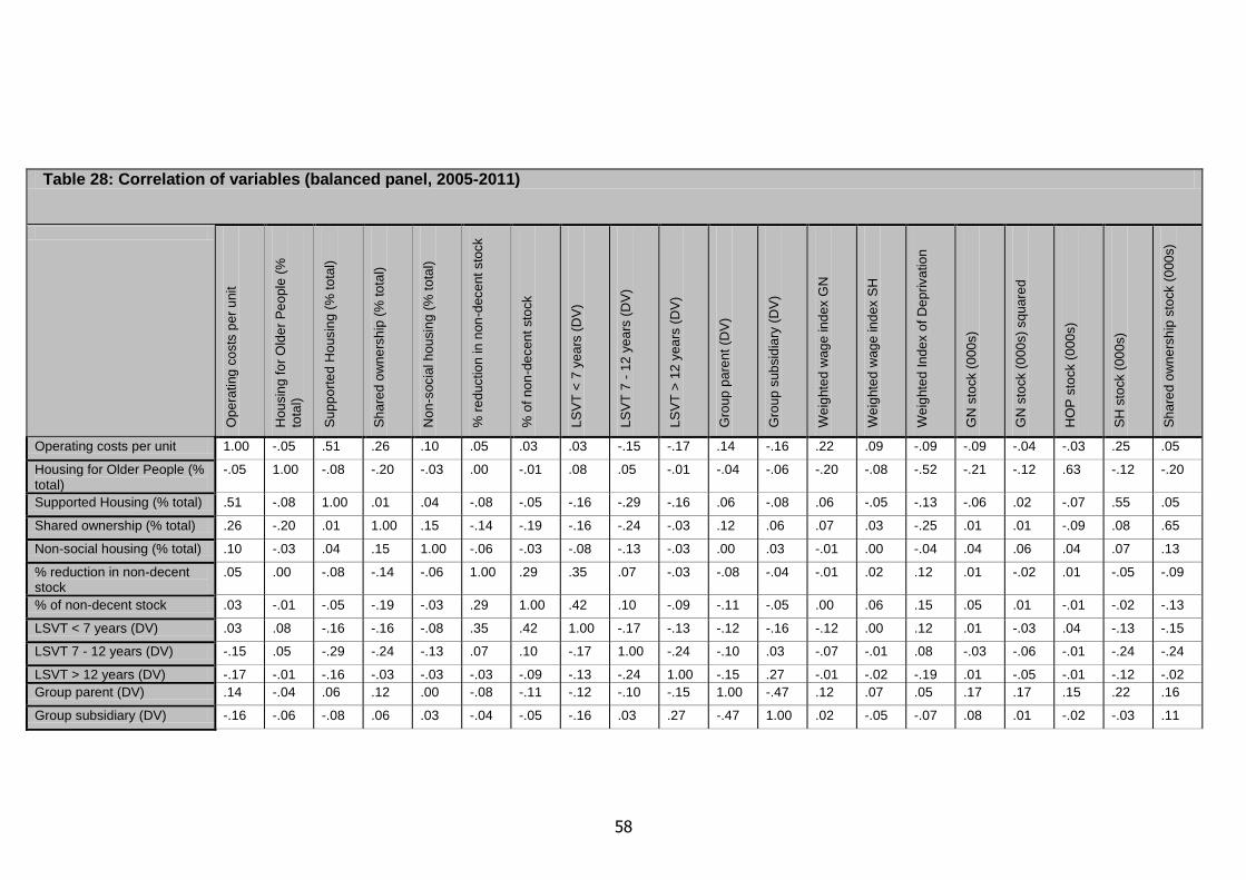
58

Table 28: Correlation of variables (balanced panel, 2005-2011)

O

pe

rating

co

sts

pe

r u

nit

Hou

sin

g f

or

Old

er

Pe

ople

(%

tota

l)

Su

pp

ort

ed

Ho

usin

g (

% to

tal)

Sh

are

d o

wne

rsh

ip (

% to

tal)

Non

-socia

l h

ou

sin

g (

% t

ota

l)

% r

ed

uctio

n in

non

-dece

nt

sto

ck

% o

f no

n-d

ecen

t sto

ck

LS

VT

< 7

ye

ars

(D

V)

LS

VT

7 -

12

ye

ars

(D

V)

LS

VT

> 1

2 y

ea

rs (

DV

)

Gro

up

pa

ren

t (D

V)

Gro

up

sub

sid

iary

(D

V)

We

ighte

d w

ag

e in

dex G

N

We

ighte

d w

ag

e in

dex S

H

We

ighte

d In

dex o

f D

ep

riva

tio

n

GN

sto

ck (

000

s)

GN

sto

ck (

000

s)

sq

ua

red

HO

P s

tock (

000

s)

SH

sto

ck (

00

0s)

Sh

are

d o

wne

rsh

ip s

tock (

000

s)

Operating costs per unit 1.00 -.05 .51 .26 .10 .05 .03 .03 -.15 -.17 .14 -.16 .22 .09 -.09 -.09 -.04 -.03 .25 .05

Housing for Older People (% total)

-.05 1.00 -.08 -.20 -.03 .00 -.01 .08 .05 -.01 -.04 -.06 -.20 -.08 -.52 -.21 -.12 .63 -.12 -.20

Supported Housing (% total) .51 -.08 1.00 .01 .04 -.08 -.05 -.16 -.29 -.16 .06 -.08 .06 -.05 -.13 -.06 .02 -.07 .55 .05

Shared ownership (% total) .26 -.20 .01 1.00 .15 -.14 -.19 -.16 -.24 -.03 .12 .06 .07 .03 -.25 .01 .01 -.09 .08 .65

Non-social housing (% total) .10 -.03 .04 .15 1.00 -.06 -.03 -.08 -.13 -.03 .00 .03 -.01 .00 -.04 .04 .06 .04 .07 .13


.05 .00 -.08 -.14 -.06 1.00 .29 .35 .07 -.03 -.08 -.04 -.01 .02 .12 .01 -.02 .01 -.05 -.09

% of non-decent stock .03 -.01 -.05 -.19 -.03 .29 1.00 .42 .10 -.09 -.11 -.05 .00 .06 .15 .05 .01 -.01 -.02 -.13

LSVT < 7 years (DV) .03 .08 -.16 -.16 -.08 .35 .42 1.00 -.17 -.13 -.12 -.16 -.12 .00 .12 .01 -.03 .04 -.13 -.15

LSVT 7 - 12 years (DV) -.15 .05 -.29 -.24 -.13 .07 .10 -.17 1.00 -.24 -.10 .03 -.07 -.01 .08 -.03 -.06 -.01 -.24 -.24

LSVT > 12 years (DV) -.17 -.01 -.16 -.03 -.03 -.03 -.09 -.13 -.24 1.00 -.15 .27 -.01 -.02 -.19 .01 -.05 -.01 -.12 -.02

Group parent (DV) .14 -.04 .06 .12 .00 -.08 -.11 -.12 -.10 -.15 1.00 -.47 .12 .07 .05 .17 .17 .15 .22 .16

Group subsidiary (DV) -.16 -.06 -.08 .06 .03 -.04 -.05 -.16 .03 .27 -.47 1.00 .02 -.05 -.07 .08 .01 -.02 -.03 .11

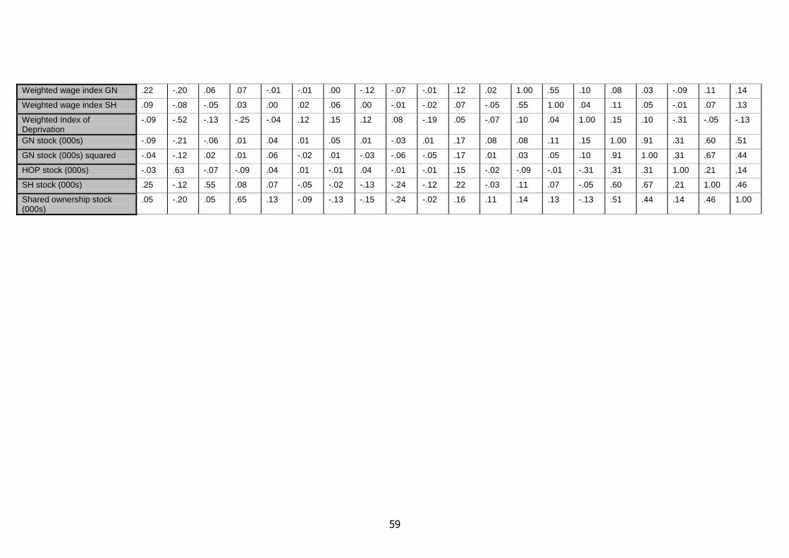
59

Weighted wage index GN .22 -.20 .06 .07 -.01 -.01 .00 -.12 -.07 -.01 .12 .02 1.00 .55 .10 .08 .03 -.09 .11 .14

Weighted wage index SH .09 -.08 -.05 .03 .00 .02 .06 .00 -.01 -.02 .07 -.05 .55 1.00 .04 .11 .05 -.01 .07 .13

Weighted Index of Deprivation

-.09 -.52 -.13 -.25 -.04 .12 .15 .12 .08 -.19 .05 -.07 .10 .04 1.00 .15 .10 -.31 -.05 -.13

GN stock (000s) -.09 -.21 -.06 .01 .04 .01 .05 .01 -.03 .01 .17 .08 .08 .11 .15 1.00 .91 .31 .60 .51

GN stock (000s) squared -.04 -.12 .02 .01 .06 -.02 .01 -.03 -.06 -.05 .17 .01 .03 .05 .10 .91 1.00 .31 .67 .44

HOP stock (000s) -.03 .63 -.07 -.09 .04 .01 -.01 .04 -.01 -.01 .15 -.02 -.09 -.01 -.31 .31 .31 1.00 .21 .14

SH stock (000s) .25 -.12 .55 .08 .07 -.05 -.02 -.13 -.24 -.12 .22 -.03 .11 .07 -.05 .60 .67 .21 1.00 .46


.05 -.20 .05 .65 .13 -.09 -.13 -.15 -.24 -.02 .16 .11 .14 .13 -.13 .51 .44 .14 .46 1.00

Homes and Communities Agency 7th Floor Maple House 149 Tottenham Court Road London W1T 7BN [email protected]

Publication date: July 2012

UNDERSTANDING UNIT COSTS OF HOUSING PROVIDERS – REGRESSION ... · PDF fileUnderstanding...

Documents

Transcript of UNDERSTANDING UNIT COSTS OF HOUSING PROVIDERS – REGRESSION ... · PDF fileUnderstanding...