Understanding the Time-Lapse Microgravity Response due to ...

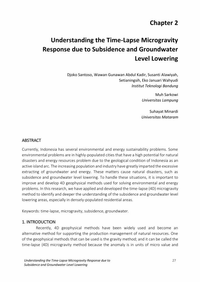
Understanding the Time-Lapse Microgravity Response due to 27 Subsidence and Groundwater Level Lowering

Chapter 2

Understanding the Time-Lapse Microgravity

Response due to Subsidence and Groundwater

Level Lowering

Djoko Santoso, Wawan Gunawan Abdul Kadir, Susanti Alawiyah,

Setianingsih, Eko Januari Wahyudi

lnstitut Teknologi Bandung

Muh Sarkowi

Universitas Lampung

Suhayat Minardi

Universitas Mataram

ABSTRACT

Currently, Indonesia has several environmental and energy sustainability problems. Some

environmental problems are in highly-populated cities that have a high potential for natural

disasters and energy resources problem due to the geological condition of Indonesia as an

active island arc. The increasing population and industry have greatly imparted the excessive

extracting of groundwater and energy. These matters cause natural disasters, such as

subsidence and groundwater level lowering. To handle these situations, it is important to

improve and develop 4D geophysical methods used for solving environmental and energy

problems. In this research, we have applied and developed the time-lapse (4D) microgravity

method to identify and deeper the understanding of the subsidence and groundwater level

lowering areas, especially in densely-populated residential areas.

Keywords: time-lapse, microgravity, subsidence, groundwater.

1. INTRODUCTION

Recently, 4D geophysical methods have been widely used and become an

alternative method for supporting the production management of natural resources. One

of the geophysical methods that can be used is the gravity method; and it can be called the

time-lapse {4D) microgravity method because the anomaly is in units of micro value and

28 Understanding the Time-Lapse Microgravity Response due to Subsidence and Groundwater Level Lowering

time as the fourth dimension. Time-lapse microgravity is the development of the gravity

method which is characterized by the repealed gravity measurements at certain time

periods. The changes in time-lapse microgravity responses are relatively small therefore,

these values must be detected using the equipment capable of detecting anomalies up 'to

level of microGal.

The development of the gravity method in various aspects of applications resulted

in increasingly widespread uses of' this method in geophysical exploration. The development

in data acquisition techniques and gravity instruments allows this method to be used for

hydrocarbon and gas monitoring as well as for monitoring the land subsidence and

groundwater level changes. In this research, the time-lapse microgravity method was

chosen to handle environmental and energy problems because highly-populated cities are

mostly located in or close to residential areas, therefore, we need a method which uses

handy equipment (movable), is easily moved from station to station, does not cause

environmental damage, requires minimal 'electricity support', only needs a small team, and

does not cause social conflict.

Time-lapse microgravity anomaly reflects several sources, such as station elevation

change, fluid movement and physical properties (density) change in the subsurface. Based

on the relationship, the use of the time-lapse microgravity method has been widely applied

for monitoring oil and gas reservoirs (Hare et al., 1999; Santoso et al., 2004; Santoso et al.

2007; Kadir et al., 2008; Kadir, 2009; Ferguson et al., 2008; Hare et al., 2008), geothermal

reservoirs (Allis and Hunt, 1986; Fujimitsu et al., 2000; Zaenudin et al., 2008; Sugihara and.

Ishida, 2008), groundwater reservoirs (Santoso et al., 2006; Sarkowl, 2007; Pool, 2008; Davis

et al., 2008; Getting et al., 2008; Chapman et al., 2008), land subsidence and groundwater

level change (Branston and Styles, 2000; Kadir et al., 2004; Kadir et al., 2007; and Santoso

et; al., 2006), etc.

Researchers know that a gravity anomaly in the surface is a superposition of all

possible sources; and the best way to split out each anomaly has been a common problem

in interpretation. In the tine-lapse microgravity anomaly. The source of anomaly comes from

the surface source [vertical ground movement) and from the subsurface sources (fluid

movement and density change in the reservoir). A similar response of the time-lapse

microgravity anomaly valve between subsidence (vertical ground movement/ and ·the

subsurface density increase, as well as between groundwater level lowering and subsurface

density decrease, have been another problem with the geophysical interpretation

technique. Therefore, we will present how to understand and identify the time-lapse

microgravity response due to subsidence and groundwater level lowering. In this research,

we have improved the time-lapse microgravity processing technique that can be used to

separate- these anomalies in order to reduce ambiguity. Using a striping filter (model-based

filler), we can extract the anomalies, which is caused by subsidence, and combine them with

groundwater level changes data, so that we will get the subsidence value based on its

sources such as groundwater withdrawal and other sources. To support this analysis,

application of the method in a residential area of Jakarta that has a highly significant


subsidence and groundwater level lowering rate will be shown as an example study. Based

on the time-lapse microgravity data and groundwater level changes data, we can analyses

the source of subsidence in all parts of Jakarta.

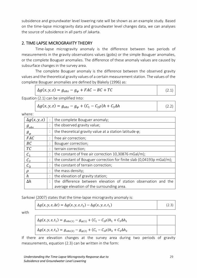
2. TIME·LAPSE MICROGRAVITY THEORY

Time-lapse microgravity anomaly is the difference between two periods of

measurements in the gravity observations values (gobs) or the simple Bouguer anomalies,

or the complete Bouguer anomalies. The difference of these anomaly values are caused by

subsurface changes in the survey area.

The complete Bouguer anomaly is the difference between the observed gravity

values and the theoretical gravity values of a certain measurement station. The values of the

complete Bouguer anomalies are defined by Blakely (1996) as:

∆𝑔(𝑥, 𝑦, 𝑧) = 𝑔𝑜𝑏𝑠 − 𝑔𝜑 + 𝐹𝐴𝐶 − 𝐵𝐶 + 𝑇𝐶 (2.1)

Equation (2.1) can be simplified Into:

∆𝑔(𝑥, 𝑦, 𝑧) = 𝑔𝑜𝑏𝑠 − 𝑔𝜑 + (𝐶1 − 𝐶2𝜌)ℎ + 𝐶3∆ℎ (2.2)

where:

∆𝑔(𝑥, 𝑦, 𝑧) : the complete Bouguer anomaly;

𝑔𝑜𝑏𝑠

: the observed gravity value;

𝑔𝜑

: the theoretical gravity value at a station latitude ;

𝐹𝐴𝐶 : free air correction;

𝐵𝐶 : Bouguer correction;

𝑇𝐶 : terrain correction;

𝐶1 : the constant of free air correction 10,30876 mGal/m);

𝐶2 : the constant of Bouguer correction for finite slab (0,04193p mGal/m);

𝐶3 : the constant of terrain correction;

𝜌 : the mass density;

ℎ : the elevation of gravity station;

∆ℎ : the difference between elevation of station observation and the average elevation of the surrounding area.

Sarkowi {2007) states that the time-lapse microgravity anomaly is:

∆𝑔(𝑥, 𝑦, 𝑧, ∆𝑡) = ∆𝑔(𝑥, 𝑦, 𝑧, 𝑡2) − ∆𝑔(𝑥, 𝑦, 𝑧, 𝑡1) (2.3)

with

∆𝑔(𝑥, 𝑦, 𝑧, 𝑡1) = 𝑔𝑜𝑏𝑠(1) − 𝑔𝜑(1) + (𝐶1 − 𝐶2𝜌)ℎ1 + 𝐶3∆ℎ1

∆𝑔(𝑥, 𝑦, 𝑧, 𝑡2) = 𝑔𝑜𝑏𝑠(2) − 𝑔𝜑(2) + (𝐶1 − 𝐶2𝜌)ℎ2 + 𝐶3∆ℎ2

If there are elevation changes at the survey area during two periods of gravity

measurements, equation (2.3) can be written in the form:


∆𝑔(𝑥, 𝑦, 𝑧, ∆𝑡) = (𝑔𝑜𝑏𝑠(2) − 𝑔𝑜𝑏𝑠(1)) − (𝑔𝜑(2) − 𝑔𝜑(1))

+ (𝐶1 − 𝐶2𝜌)(ℎ2 − ℎ1) + 𝐶3(∆ℎ2 − ∆ℎ1) (2.4)

where:

∆𝑔(𝑥, 𝑦, 𝑧, ∆𝑡) : the time-lapse microgravltv anomaly; ∆𝑔(𝑥, 𝑦, 𝑧, 𝑡1) the complete Bouguer anomaly from the first gravity measurement ∆𝑔(𝑥, 𝑦, 𝑧, 𝑡2) the complete Bouguer anomaly from the second gravity

measurement

𝑔𝑜𝑏𝑠(1)

: the observed gravity value in the first gravity measurement

𝑔𝑜𝑏𝑠(2)

the observed gravity value in the second gravity measurement

𝑔𝜑(1)

: the theoretical gravity value at a station latitude in the first gravity measurement

𝑔𝜑(2)

the theoretical gravity value at a station latitude in the second gravity measurement

ℎ1 : the elevation of gravity station in the first gravity measurement;

ℎ2 : the elevation of gravity station in the second gravity measurement;

∆ℎ1 : the difference between elevation of station observation and the average elevation of the surrounding area in the first measurement:

∆ℎ2 : the difference between elevation of station observation and the average elevation of the surrounding area in the second measurement:

If there is not the displacement of gravity stations in the horizontal direction during

two periods of gravity measurements (𝜑1 = 𝜑2) equation (2.4} can be simplified into:

∆𝑔(𝑥, 𝑦, 𝑧, ∆𝑡) = (𝑔𝑜𝑏𝑠(2) − 𝑔𝑜𝑏𝑠(1)) + (𝐶1 − 𝐶2𝜌)(ℎ2 − ℎ1) + 𝐶3(∆ℎ2 − ∆ℎ1) (2.5)

Or

(𝑔𝑜𝑏𝑠(2) − 𝑔𝑜𝑏𝑠(1)) = ∆𝑔(𝑥, 𝑦, 𝑧, ∆𝑡) − (𝐶1 − 𝐶2𝜌)(ℎ2 − ℎ1)

−𝐶3(∆ℎ2 − ∆ℎ1) (2.6)

For the 30 causative body with density distribution p(, , ), the time-lapse

microgravity anomaly at a certain measurement station P(x, y, z) on the surface can be

expressed by the equation (Kadir, 1999):

∆𝑔(𝑥, 𝑦, 𝑧, ∆𝑡) = ∫ ∫ ∫𝐺∆𝜌(𝛼, 𝛽, 𝛾, ∆𝑡)(𝑧 − 𝛾)

[(𝑥 − 𝛼)2 + (𝑦 − 𝛽)2 + (𝑧 − 𝛾)2]3 2⁄ 𝑑𝛼𝑑𝛽𝑑𝛾

∞

−∞

∞

−∞

∞

0

(2.7)


Based on equation (26) and equation (2. 7), it can be obtained:

(𝑔𝑜𝑏𝑠(2) − 𝑔𝑜𝑏𝑠(1))

= ∫ ∫ ∫𝐺∆𝜌(𝛼, 𝛽, 𝛾, ∆𝑡)(𝑧 − 𝛾)

[(𝑥 − 𝛼)2 + (𝑦 − 𝛽)2 + (𝑧 − 𝛾)2]3 2⁄ 𝑑𝛼𝑑𝛽𝑑𝛾

∞

−∞

∞

−∞

∞

0

− (𝐶1 − 𝐶2𝜌)(ℎ2 − ℎ1) − 𝐶3(∆ℎ2 − ∆ℎ1)

(2.8)

Based on the results of mathematical modeling and· simulation using synthetic data,

It can be shown that the time-lapse microgravity anomaly will be not be influenced by the

topography effect. In addition, the soil consolidation which causes subsidence will not

decrease the density of soil, therefore, the Bouguer correction can be neglected. Therefore,

equation (2.8) can be simplified into:

(𝑔𝑜𝑏𝑠(2) − 𝑔𝑜𝑏𝑠(1))

= ∫ ∫ ∫𝐺∆𝜌(𝛼, 𝛽, 𝛾, ∆𝑡)(𝑧 − 𝛾)

[(𝑥 − 𝛼)2 + (𝑦 − 𝛽)2 + (𝑧 − 𝛾)2]3 2⁄ 𝑑𝛼𝑑𝛽𝑑𝛾

∞

−∞

∞

−∞

∞

0

− (𝐶1)(ℎ2 − ℎ1)

(2.9)

The equation (2.9} shows the difference of the observed gravity values from the first

and second gravity measurements which are caused by the subsurface density changes

(relating to groundwater level changes) and subsidence.

The appropriate method to split-out time-lapse microgravity responses due to

subsidence and groundwater level lowering is being considered in this research. Here, we

have developed a stripping filter using a model-based filter (MBF). The main part of MBF

development is forward modeling used to calculate gravity responses from the surface

sources {subsidence) and the subsurface sources (subsurface density changes). In this

forward modeling, a mass distribution is considered a finite collection of mass elements

dm = p(, , ) dV with a continuous mass distribution where p represents mass density and

(, , ) is mass coordinate. According to Blakely (1996), a mass can be approximated

geometrically by the prism model as shown in Figure 2.1.

Figure.2.1- Geometric approximation of

a mass using the prism model (Blakely, 1996).


The gravitational potential (U) and the gravitational acceleration (g) at the point P

which is caused by an object's mass with the mass density is: 𝑔(𝑃) = ∇𝑈

= −G ∫�̅�

𝑟2𝑉

𝑑𝑉 (2.10)

From equation (2.10), it can be obtained

𝑔(𝑥, 𝑦, 𝑧) =∂𝑈

𝜕𝑧

= −G ∫ ∫ ∫ 𝜌(𝛼, 𝛽, 𝛾)(𝑧 − 𝛾)

𝑟3𝛼𝛽𝛾

𝑑𝛼𝑑𝛽𝛾 (2.11)

Where 𝑟 = √(𝑥 − 𝛼)2 + (𝑦 − 𝛽)2 + (𝑧 − 𝛾)2

Equation (2.11) can be written more simply as:

𝑔(𝑥, 𝑦, 𝑧) = ∫ ∫ ∫ 𝜌(𝛼, 𝛽, 𝛾)(𝑧 − 𝛾)

𝑟3𝛼𝛽

𝐾(𝑥 − 𝛼, 𝑦 − 𝛽, 𝑧 − 𝛾)𝛾

𝑑𝛼𝑑𝛽𝛾

(2.12)

Where 𝐾(𝑥, 𝑦, 𝑧) = −𝐺𝑧

(𝑥2+𝑦2+𝑧2) is Green function.

A mass distribution is considered as a finite collection of mass elements {cells). And

the gravity anomalies which are caused by a mass distribution are the superposition of

gravity responses from these mass elements. The model .approximation, of a mass

distribution is shown in Figure 2.2.

Figure 2.2 -Model approximation of a mass distribution

composed of a set of prism cells (Blakely, 1996).

The values of gravity responses of each vertical prism cells are calculated by an integration

of an equation (2.12) that correspond to its boundary condition. If the vertical prism cells

have mass density p with boundary condition 𝑥1 ≤ 𝑥 ≤ 𝑥2 , 𝑦1 ≤ 𝑦 ≤ 𝑦2, 𝑧 1 ≤ 𝑧 ≤ 𝑧2 the

values of gravity responses can be calculated by:


𝑔 = 𝐺𝜌 ∫ ∫ ∫𝛾

(𝛼2 + 𝛽2 + 𝛾2)𝛼𝛽𝛾

𝑑𝛼𝑑𝛽𝛾 (2.13)

For each vertical prism cells with homogen mass density as shown in Figure 2.2., equation

(2.13} is expressed by Plouff {1976) as:

𝑔 = 𝐺𝜌 ∑ ∑ ∑ 𝜇𝑖,𝑗,𝑘 [𝑧𝑘𝑎𝑟𝑐𝑡𝑎𝑛𝑥𝑖𝑦𝑖

𝑧𝑘𝑟𝑖,𝑗,𝑘

− 𝑥𝑖 log(𝑅𝑖,𝑗,𝑘 + 𝑦𝑖) − 𝑦𝑖log (𝑅𝑖,𝑗,𝑘 + 𝑥𝑖)] (2.14)

with𝑅𝑖,𝑗,𝑘 = √𝑥𝑖2 + 𝑦𝑗

2 + 𝑧𝑘2 and 𝜇𝑖,𝑗,𝑘 = (−1)𝑖(−1)𝑗(−1)𝑘

3. GRAVITY RESPONSES DUE TO A VARIETY OF ANOMALY SOURCES

3.1 Time-lapse Microgravity Responses due to Subsidence

One factor that can affect the gravity response is the difference of elevation

between the measurement point and the average compartment of the surrounding area.

This factor needs to be corrected by terrain correction using a cylindrical coordinate system

of the Bouguer plate as shown in Figure 2.3 (Telford et al., 1990). The calculation of terrain

correction has been formulated by Hammer (1939) which uses a model approach of

cylindrical object with height h relative to the measurement point and the surrounding area.

The calculation of terrain correction is divided into several concentric circular zones with

each zone divided into sever at sectors, and the average elevation is estimated from a

topographic map. The total effect of gravity responses due to all of these zones, whether

due to the negative height difference (valley) or the positive height difference (hill), it is

called as terrain correction.

Figure 2.3. The cylindrical coordinate system of the Bouguer plate used to

calculate terrain correction (Telford et al., 1990).

The calculation of gravity responses over a sector can be done using the equation

proposed by Telford et al. (1990).

𝑔𝑇𝐶 = 𝜌𝐺𝜃 [(𝑟2 − 𝑟1) + √𝑟12 + ∆ℎ2 − √𝑟2

2 + ∆ℎ2] (2.15)

where:

𝑔𝑇𝐶

: the gravity responses due to topographic changes;

𝜌 : the mass density; 𝐺 : the universal gravity constant;


𝜃 : the sector angle (radian)

𝑟1 𝑎𝑛𝑑 𝑟2 : the inner and outer radius; ∆ℎ : the difference of elevation between the measurement point and the

surrounding area.

If within a certain time interval subsidence occurs at the measurement point. The

difference of elevation between, the measurement point and the surrounding area will

change. To model the changes in topography before and after the subsidence at the

measurement point, Supriyadi (2008) has described the model as shown in Figure 2.4. It is

assumed that before subsidence (t0) the difference of elevation between the measurement

point and the surrounding area is h. If there is subsidence of z, the difference of elevation

between the measurement point and the surrounding area will be h+z.

Figure 2.4. The model of topographic changes before subsidence at t0 and after

subsidence at t1 (Supriyadi, 2.008).

The modeling results of terrain correction due to topographic changes are shown in

Figure 2.5 and Figure 2.6. Based on these figures, it can be shown the changes of terrain

correction increase with decreasing the inner radius, and the value is relatively constant with

increasing the outer radius. However, the value of terrain correction will increase with

increasing the elevation changes of the measurement point.

Figure 2.5. The changes of terrain correction due to topographic changes

with a variation of the inner radius r, and constant outer radius r, 1000 m (Minardi, 2010).


Figure 2.6. The changes of terrain correction due to topographic changes

with the variation of the outer radius r, and constant inner radius r1 20 m (Minardi, 2010).

Subsidence is a process of shifts downward in a surface which results in a decrease in

distance between the measurement point and the centre of the Earth. The causes of

subsidence are the compaction in one subsurface layer as a natural process or due to human

activities. Decrease in the elevation of the measurement point will result in changes in the

time-lapse microgravity response as shown in Figure 2. 7.

Figure 2.7. The result of time-lapse microgravity responses modeling

due to decrease in the elevation of the measurement point (Minardi, 2010).

The results of gravity modeling used to calculate the response due to compaction,

which occurs in one layer of the Earth, show that the gravity responses of the initial

conditions (at t0) until there is a compaction of 2 meters (at t1) coincide as shown In Figure

2.3 and visualized in figure 2.9. Based on modeling results, it can be shown that compaction

does not result in mass loss because the volume reduction due· to compaction will be

compensated by the increasing mass density in the compacting rock layer.


Figure 2.8 · Gravity responses due to compaction

in one subsurface layer (Minardi, 2010).

Figure 2.9. Gravity responses and visualization

of the compacting rock layer (Minardi, 2010).

3.2. Time-lapse Microgravity Responses due to Groundwater Level

lowering

As explained previously, in order to identify the lime-lapse microgravity response due

to subsidence and groundwater level lowering, we have developed a stripping filter using a

model-based filter. To develop the filter as a tool to separate the sources of the anomalies

from surface and subsurface, it needs to build a model describing density change occurring

in the surface and the aquifer. The model of rock layer should be based on the aquifer data

of the area studied. For example, Table 2.1 shows the 3D modeling results used to compute

the time-lapse microgravity responses due to groundwater level changes using the

assumption of a finite slab anomaly body with a fluid mass density of 1 gram/cc and the

porosity of the reservoir at 30%.


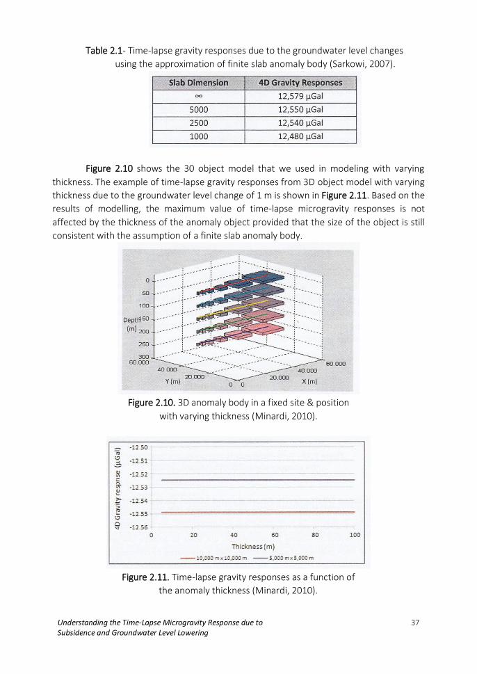
Table 2.1- Time-lapse gravity responses due to the groundwater level changes

using the approximation of finite slab anomaly body (Sarkowi, 2007).

Figure 2.10 shows the 30 object model that we used in modeling with varying

thickness. The example of time-lapse gravity responses from 3D object model with varying

thickness due to the groundwater level change of 1 m is shown in Figure 2.11. Based on the

results of modelling, the maximum value of time-lapse microgravity responses is not

affected by the thickness of the anomaly object provided that the size of the object is still

consistent with the assumption of a finite slab anomaly body.

Figure 2.10. 3D anomaly body in a fixed site & position

with varying thickness (Minardi, 2010).

Figure 2.11. Time-lapse gravity responses as a function of

the anomaly thickness (Minardi, 2010).


Next, the goal in using the modeling results is to know the time-lapse microgravity

responses due to the influence of the site and the depth of the anomaly object. Figure 2.12

shows the 3D object model that we used in modeling w.th varying size and depth. The

example of time-lapse gravity responses from 3D object model with varying size and depth

is shown in figure 2.13. Based on the results of modeling, there are the variation of

timelapse microgravity responses as a function of the anomaly size and depth.

Figure 2.12. 3D anomaly body with varying size and depth (Minardi, 2010).

Figure 2.13. Time-lapse gravity responses as a function of

the anomaly size and depth (Minardi, 2010).

3.3 Time-lapse Microgravity Anomaly and Model-Based Filter

To develop a model-based filter, Fourier transformation is performed on synthetic

data of the time-lapse gravity responses due to subsidence and subsurface mass density

changes. The results of Fourier transformation are used to analyze the amplitude and

frequency of each anomaly. If each anomaly that is generated by different sources have

different amplitude and frequency, the separation of anomaly sources can be performed


using a specific filter. The scheme of the filtering process in spatial and frequency domain is

described as follows:

Figure 2.14. Scheme of filtering process in spatial and frequency domain

(modified from Widianto, 2008).

Based on Figure 2.14, the relationship between input function, transfer systems, and output

function in spatial and frequency domain can be formulated as:

𝑠(𝑠) ∗ ℎ(𝑥) = 𝑦(𝑥) (2.16)

𝑆(𝑓) ∙ 𝐻(𝑓) = 𝑌(𝑓) (2.17)

𝐻(𝑓) =𝑌(𝑓)

𝑆(𝑓) (2.18)

where s(x) and S{f) are input functions; y(x) and Y(f) are output functions; h(x) and H(f) are

linear transfer function;. To determine an output function directly in the spatial domain

requires the convolution process of the input function with the transfer function and is

usually more difficult than simply multiplying two functions in the frequency domain.

The application of equation (2.17) and equation (2.18) for this case study is the input

of anomalies spectrum due to subsidence and subsurface mass density changes.

𝑆(𝑓)𝑠𝑢𝑏𝑠𝑖𝑑𝑒𝑛𝑐𝑒+𝑔𝑟𝑜𝑢𝑛𝑑𝑤𝑎𝑡𝑒𝑟 ∙ 𝐻(𝑓) = 𝑌(𝑓)𝑠𝑢𝑏𝑠𝑖𝑑𝑒𝑛𝑐𝑒 (2.19)

𝐻(𝑓) =𝑌(𝑓)𝑠𝑢𝑏𝑠𝑖𝑑𝑒𝑛𝑐𝑒

𝑆(𝑓)𝑠𝑢𝑏𝑠𝑖𝑑𝑒𝑛𝑐𝑒+𝑔𝑟𝑜𝑢𝑛𝑑𝑤𝑎𝑡𝑒𝑟 (2.20)

𝑆(𝑓)𝑠𝑢𝑏𝑠𝑖𝑑𝑒𝑛𝑐𝑒+𝑔𝑟𝑜𝑢𝑛𝑑𝑤𝑎𝑡𝑒𝑟 ∙ 𝐻(𝑓) = 𝑌(𝑓)𝑔𝑟𝑜𝑢𝑛𝑑𝑤𝑎𝑡𝑒𝑟 (2.21)

𝐻(𝑓) =𝑌(𝑓)𝑔𝑟𝑜𝑢𝑛𝑑𝑤𝑎𝑡𝑒𝑟

𝑆(𝑓)𝑠𝑢𝑏𝑠𝑖𝑑𝑒𝑛𝑐𝑒+𝑔𝑟𝑜𝑢𝑛𝑑𝑤𝑎𝑡𝑒𝑟 (2.22)

Based on equation (2.20) and equation (2.22), input function is the combination of

an anomalies spectrum due to subsidence and groundwater level changes which is:

operated by the output transfer function to generate the anomalies spectrum due to

subsidence in equation (2.20) and the anomalies spectrum due to subsurface mass density

changes in equation (2.22).


The model-based filter developed in this research is a model-based filter that

doesn't depend on the wavelength of the anomaly. To obtain the most effective model-

based filter that can separate the sources of time-lapse gravity anomalies, we have to

conduct modeling for various sizes of anomaly object. The results of modeling should not be

affected by the vertical position of model (anomaly depth).

4. CASE STUDIES

4-1 Subsidence and Groundwater Level Changes in Jakarta

The increasing population and Industry resulting from urban development in

Jakarta will lead to the exacerbation of environmental and energy problems. These

matters cause natural disasters such as subsidence and groundwater level lowering.

Land subsidence in several places in Jakarta have been measured. Since the early

1980's using several techniques. Rate of land subsidence which were measured using

several techniques are given in Table 2.2 (Abidin et al., 2009).

Table 2.2 Land subsidence rate of several places in Jakarta which were measured

using several techniques (Abidin et al, 2009).

The increasing population and 'the development of industry in Jakarta have

increased the water demand in this area. Since the drinking water supplied by

surface water only covers 30% of the water demand, people are harvesting the

available groundwater in the basin. In the Jakarta groundwater Basin, the use of

groundwater has greatly accelerated corresponding to the rise of Jakarta's

population and the development of the industrial sector, which consumes a

relatively huge amount of water (Delinom, 2008).

In order to control extraction of groundwater from the reservoir, Jakarta

Mining Agency and BPLHD have measured the groundwater level at several places

in Jakarta. The result of the measurement shows that groundwater levels in Jakarta

has decreased in several places and increased in other places but the decreasing

groundwater level is dominant. Groundwater level changes during the time period

1007 - 7008 is given at Figure 2.l5.


Figure 2.15 - Groundwater level changes in Jakarta during

the time period 2007 -2008 (Minardi et al., 2010).

Many researchers have investigated the causes of subsidence in Jakarta.

Rismianto and Mak (1993) and Murdohardono and Tirtomihardjo (1993) concluded

that the main source of subsidence in Jakarta is groundwater withdrawal. Abidin et

al. (2001) has compared subsidence and hydrogeology data and concluded that

subsidence has a strong relationship with and is often caused by groundwater

withdrawal. Maathuis et al. (1996) found an inconsistency in groundwater level

lowering and changes in the benchmark elevation pattern and concluded that

settlement caused by natural compaction and infrastructure loading is also a source

of subsidence. Purnomo et. al., (1999) interpreted subsidence and groundwater

level maps and found that while groundwater withdrawal was significant source or

subsidence in many areas, in other areas it was not significant.

4.2 Microgravity Measurements To understand sources of subsidence in Jakarta, especially which are caused by

groundwater withdrawal, microgravity measurements have been conducted during two

time periods, September 2007 and July 2008. Measurement; were conducted during the


same season to minimize the effect of rain fall, The result of gravity measurements of

.Jakarta in 2007 and 200R are given in Figure 2.16.

Figure 2.16 - Gravity observation map of Jakarta in 2007 and 2008

(Minardi et al., 2010).

The main cause of gravity changes at the same observation point between surveys

are vertical ground movements and subsurface changes (Allis and Hunt, 1986). Subsurface

change factors that affect the gravity differences are the changes in the groundwater level,

changes in saturation (soil moisture content). In the vadose zone, changes in rainfall

(seasons), and other fluid changes in the subsurface. Local topographic changes, horizontal

ground movements, and changes in gravity at the base station are other factors causing

gravity changes.

The gravity effects of groundwater movements and changes in subsurface mass

density are obtained by correcting the measured gravity anomalies for the gravitational

effect of vertical ground movements (subsidence) and changes in base value, if any. For

convention, a decrease in gravity is referred to as a negative change (groundwater level

lowering) and an increase (groundwater level upheaval) as a positive value. A negative

change value implies groundwater withdrawal {discharge) and a positive value implies a

groundwater increase (recharge).

Gravity correction for elevation changes can be calculated using the following

equation (Telford et. al, 1990):

𝑔(𝜑) = [1 + (5

2𝑚 − 𝑓 −

17

14𝑚𝑓) 𝑠𝑖𝑛2𝜑 + (

𝑓2

8−

5

8𝑚𝑓) 𝑠𝑖𝑛22𝜑] (2.23)


𝜕𝑔𝜑

𝜕ℎ= −

2𝑔𝜑

𝑎(1 + 𝑚 + 𝑓 − 2𝑓𝑠𝑖𝑛2𝜑) (2.24)

𝜕𝑔𝜑

𝜕ℎ= −3,0876 𝜇𝐺𝑎𝑙/𝑐𝑚 (2.25)

where 𝑔(𝜑), ℎ, 𝑎, 𝑓, 𝑚, 𝜑,𝜕𝑔𝜑

𝜕ℎ are theoretical gravity at latitude 𝜑, altitude , axis minor of .-

the earth; the Earth flattening; Clairaut constant; latitude and gradient vertical gravity

respectively.

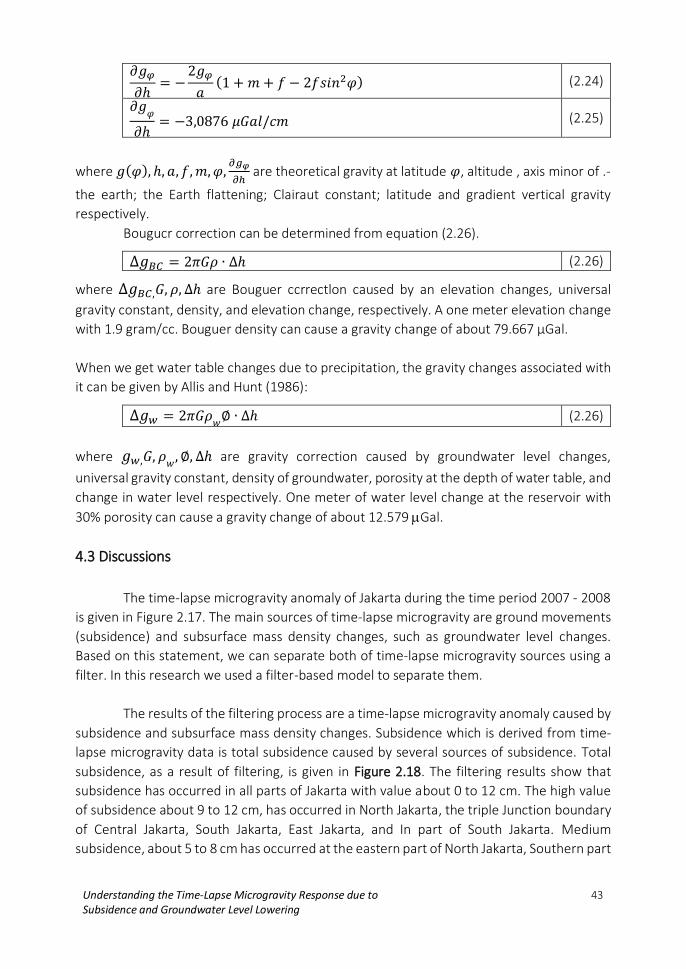
Bougucr correction can be determined from equation (2.26).

∆𝑔𝐵𝐶 = 2𝜋𝐺𝜌 ∙ ∆ℎ (2.26)

where ∆𝑔𝐵𝐶,𝐺, 𝜌, ∆ℎ are Bouguer ccrrectlon caused by an elevation changes, universal

gravity constant, density, and elevation change, respectively. A one meter elevation change

with 1.9 gram/cc. Bouguer density can cause a gravity change of about 79.667 µGal.

When we get water table changes due to precipitation, the gravity changes associated with

it can be given by Allis and Hunt (1986):

∆𝑔𝑤 = 2𝜋𝐺𝜌𝑤

∅ ∙ ∆ℎ (2.26)

where 𝑔𝑤,𝐺, 𝜌𝑤

, ∅, ∆ℎ are gravity correction caused by groundwater level changes,

universal gravity constant, density of groundwater, porosity at the depth of water table, and

change in water level respectively. One meter of water level change at the reservoir with

30% porosity can cause a gravity change of about 12.579 Gal.

4.3 Discussions

The time-lapse microgravity anomaly of Jakarta during the time period 2007 - 2008

is given in Figure 2.17. The main sources of time-lapse microgravity are ground movements

(subsidence) and subsurface mass density changes, such as groundwater level changes.

Based on this statement, we can separate both of time-lapse microgravity sources using a

filter. In this research we used a filter-based model to separate them.

The results of the filtering process are a time-lapse microgravity anomaly caused by

subsidence and subsurface mass density changes. Subsidence which is derived from time-

lapse microgravity data is total subsidence caused by several sources of subsidence. Total

subsidence, as a result of filtering, is given in Figure 2.18. The filtering results show that

subsidence has occurred in all parts of Jakarta with value about 0 to 12 cm. The high value

of subsidence about 9 to 12 cm, has occurred in North Jakarta, the triple Junction boundary

of Central Jakarta, South Jakarta, East Jakarta, and In part of South Jakarta. Medium

subsidence, about 5 to 8 cm has occurred at the eastern part of North Jakarta, Southern part


of West Jakarta, south western part of South Jakarta, and eastern part of East Jakarta. A low

value of subsidence, 0 to 4 cm, has occurred at the northwestern part of West Jakarta and

North Jakarta, southern part of South Jakarta, northeastern part of East Jakarta, and eastern

part of North Jakarta.

Figure 2.17 - Time-lapse microgravity anomaly of Jakarta during

the time period 2007 - 2008 (Minardi et al., 2010) .

Figure 2.18 - Subsidence derived from time-lapse microgravity data

of Jakarta during the time period -2007- 2008 (Minardi et al., 2010).


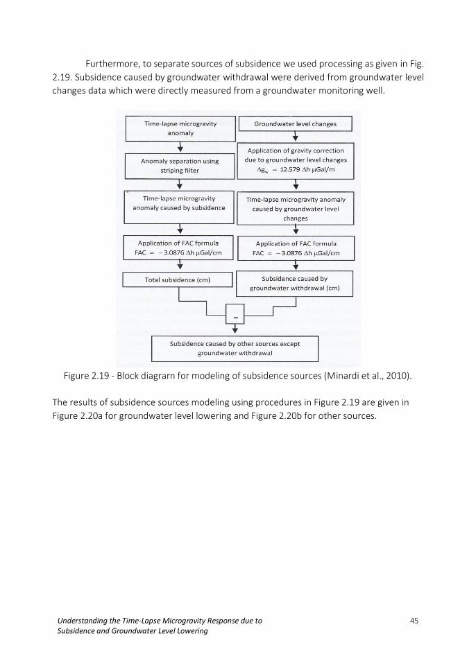
Furthermore, to separate sources of subsidence we used processing as given in Fig.

2.19. Subsidence caused by groundwater withdrawal were derived from groundwater level

changes data which were directly measured from a groundwater monitoring well.

Figure 2.19 - Block diagrarn for modeling of subsidence sources (Minardi et al., 2010).

The results of subsidence sources modeling using procedures in Figure 2.19 are given in

Figure 2.20a for groundwater level lowering and Figure 2.20b for other sources.


Figure 2.20 Subsidence derived from time-lapse microgravity data of Jakarta during the

time period 2007-2008 caused by (a) groundwater level lowering and (b) sources except

groundwater level lowering (Minardi et al., 2010).

Groundwater level lowering as an impact of groundwater withdrawal, as given in

Figure 2.20a has caused subsidence in Jakarta of about O to 9 cm. The highest impact of

groundwater withdrawal on subsidence has happened in the northwestern part of East

Jakarta.

According to Figure 2.20b, subsidence which are caused by other sources, except

groundwater withdrawal, has a value of about 0 to 12 cm. The highest value has occurred in

the eastern part of North Jakarta. a large part of East Jakarta, and West Jakarta. During the

short period of one year from 2007 to 2008, the most possible source is the load from

buildings and infrastructure,

Based on the results of subsidence source analyzes, we concluded that:

- In North Jakarta most of the subsidence were caused by the load of buildings and

infrastructure

- In East, Jakarta most of the subsidence were caused by the load of buildings and

infrastructure, but in a few parts of East Jakarta groundwater withdrawal significantly

influenced the potential for subsidence

- In South Jakarta most of the subsidence were caused by groundwater withdrawal.

- In West Jakarta most of the subsidence were caused by the load of buildings and

infrastructure.

- In Central Jakarta groundwater withdrawal had the same influence as infrastructure on

subsidence.

REFERENCES Abidin, H. Z., Djaja, R., Darmawan, O., Hadi, S., Akbar, A., Rajiyowiryono, H., Sudibyo, Y., Meilano,

I., Kusuma, M. A., Kahar, J., Subarya, C., 2001, Land subsidence of Jakarta (lndonesia) and


Its Geodetlc-Based Monitoring System, .Journal of The Jnternational Society of the

Preventation and Mitigation of Natural Hazards. Vol. 23, No. 2/3. March, pp. 365 -387,

Abidin, H. Z., Andreas. H., Gumilar, I., GamaI, M., Fukuda, Y., and Deguchi, T., 2009, Land

Subsidence and Urban Development in Jakarta (Indonesia), 7th FIG Regional Conference

Spatial Data Serving People: Land Governance and the Environment - Building the

Capacity Hanoi, October 19·22, Vietnam.

Allis, R. C. and Hunt, T.M., 1986, Analysis of Exploitation Induced Gravity Changes at Wairakei

Geothermat Field, Geophysics, 51; pp. 1641 - 1660.

Blackely, R. J., 1996, Potential Theory in Gravity and Magnetics Applications, Cambridge

University Press.

Branston , M. W. and Sty!es, P., 2000, The Use of Time-lapse Microgravity to Investigate and

Monitor An Area Undergoing Surface Subsidence; A Case Study, www.esci-

keele.ac.uk/geophysics.

Chapman, D.S., Sahm, E., and Gettings, P., 2008, Monitoring Aquifer Recharge using Repeated

High Precision Gravity Measurement: A Pilot Study in South weber, Utah, Geophysics, 73,

pp. WAB3-WA93.

Davis, K., Li, Y., and Batzle, M., 2008, Time-lapse Gravity Monitoring: A Systematic 4D Approach

with Application to Aquifer Storage and Recovery, Geophysics, 73, pp. WA61-WA69.

Delinom. R. M., 2008, Groundwater Management Issues in the Greater Jakarta Area, Indonesia,

Proceedings of· International Workshop on Integrated Watershed Management for

Sustainable Water Use in a Humid Tropical Region, JSPS-DGHE Joint Research Project,

Tsukuba, October 2007, Bull. TERC, Univ. Tsukuba, No. 8 Supplement, no. 2,

Ferguson. J. F., Klopping, F.J., Chen, T., Siebert, J, E., Hare, J. L., and Brady, J. L., 2008, The 4D

Microgravity Method for Water flood Surveillance: Part 3 – 4D Absolute Surveys at Prudhoe Bay,

Alaska, Geophysics, 73, pp. WA163-WA171.

Fujimitsu, Y., Nishijima, J., Shimosako, N., Ehara, S., and Ikeda, K., 2000, Reservoir Monitoring by

Repeat Gravity Measurements at the Takigami Geothermal Field, Central Kyushu, Japan,

Proceeding World Geothermal Congress, 573-577.

Gettings, P., Chapman, D. S., and Allis, R., 2008, Techniques, Analysis, and Noise in a Salt Lake

Valley 4D Gravity Experiment, Geophysics, 73, pp. WA7l-WA82.

Hammer, S., 1939, Terrain Correction for Stations, Geophysics, 4, pp. 181 -191.

Hare, J. L., Ferguson,, J. F., Aiken, C. L. V., and Bradly, J. L., 1999. The: 4-D Microgravity Method

for Water-flood Surveillance: a Model Study for the Prudhoe Bay Reservoir. Alaska,

Geophysics, 64, pp. 78-87.

Hare, J. L, Ferguson, J. F., Brady, J. L, 2008, The 4D Microgravity Method for Water flood

Surveillance: Part IV - Modeling and Interpretation of Early Epoch 4D Gravity Surveys at

Prudhoe Bay, Alaska. Geophysics, 73, pp. WA173-WA180.

Kadir, W. G. A., 2009, Harga Anomaly Gayaberat Mikro 'Time-Lapse' Rendah dan Hubungannya

dengan Pergerakan Fluida dalam Reservoir sebagai lndikasi Prospek Hidrokarbon, Contoh

Kasus : Lapangan Tambun dan Minas, Proceeding 34th HAGI Annual Convention,

Exhibition and Geophysics Education Meeting, Jogjakarta.

Kadir, W. G. A, Santcso, D., and Sarkowi, 2004, Time-lapse Vertical Gradient Microgravity

Measurement for Subsurface Mass Change and Vertical Ground Movement (Subsidence)


Identification, Case Study: Semarang Alluvial Plain, Central Java, Indonesia. Proc. of 7th

SEGJ international Symposium.

Kadir. W. G. A., Santoso, D., and Alawiyah, S., 2007, Principle and Application of 4D Microgravity

Survey for Engineering Purpose: Case Study for Groundwater Level Lowering and

Subsidence in Residential Area, Jakarta, Proc. of 20th SAGEEP international Symposium,

Denver, Colorado.

Kadir. W. G. A., Dahrin, D,, Benyamin, M., Alawiyah, S., and Setianingsih, 2008, Time-lapse

Microgravity Anomaly of carbonate Reservoir and Its correlation with Physical Properties

of the Reservoir. Case Study: Carbonate Reservoir of Baturaja Formation at X field. South

Sumatra, Indonesia, Journal of Geofisika, Edition of 2008, No. 1, pp. 13-22.

Maathuis, H., 1996, Development of Groundwater Management Strategic in Coastal Region of

Jakarta, Indonesia, Final Report. BPPT and IDRC, Jakarta.

Minardi, S., 2010, Pengembangan Filter Berbasis Model dengan Banyak Masukan (Multi Input)

pada Data Gayaberat Mlkro Antar waktu untuk Pemantauan Amblesan (Studl Kasus: DKI

Jakarta), Disertasi Program Doktor, Institut Teknologi Bandung

Minardi, S., Santoso, D., Kadir, W.G.A., and Notosiswoyo, S., 2010, Analysis of Subsidence Source

in Jakarta using Time-lapse Microgravity, International Geosciences Conference and

Exposition, July 19-22, Bali, Indonesia.

Murdohardono, D., and Tirtomihardjo, H., 1993, Penurunan Tanah di Jakarta dan Rencana

Pemantauannva, Proceeding 22nd, Annual Convention of The Indonesian Association of

Geologists, December 29, Bandung. Volume I, pp. 346-354

Plouff, D., 1976, Gravity and Magnetic Field of Polygonal Prisms and Application to Magnetic

Terrain Correction, Geophysics, 41, pp. 727-741

Pool. D. R, 2008, The Utility of Gravity and Water - level Monitoring at Alluvial Aquifer Wells in

Southern Arizona, Geophysics, 73, pp. WA49-WA59.

Purnomo, H., Murdohardono, D., Pindratmo, M. H., 1999, Land Subsidence Study in Jakarta,

Proceedings 28th Annual Convention of the lndonesian Associotion of Geologists,

November 30 - December 1, Jakarta, Indonesia, pp. 53-72.

Rismianto, D. and Mak, W., 1993, Environmental Aspects of Groundwater Abstraction in DKI

Jakarta: Changing Views. Proceeding 22nd Annual Convention of the lndonesian

Associotion of Geologist, December 6-9, Bandung, Volume I, pp. 327-345.

Santoso, D., Gunawan. W., Syarkowi, Adriyansyah, and Waluyo, 2004, Time-lapse Microgravity

study to Injection Water Monitoring of Talang Jimar Field, Proc. of 7th SEGJ International

Symposium.

Santoso, D., Sarkowi, and Kadir. W. G. A., 2006, Determination of Negative Groundwater

Withdrawal in Semarang City Arc.1 using Time-lapse Microgravity Analysis, Proc. of 8th

SEGJ International Symposium.

Santoso, D., Kadir, W. G. A., Sarkowi, M., Adriansyah, and Waluyo, 2007, Time-lapse Microgravity

Study for Injection Water Monitoring of Talang Jimar field, Preview, Issue No. 126,

February.

Sarkowi. M., 2007, Gayaberat Mikro antar waktu untuk Analisis Perubahan Kedalaman Muka Air

Tanah (Studi Kasus Dataran Aluvial Semarang), Disertasi Program Doktor, Institut

Teknologi Bandung.


Sugihara, M. and lshido, T., 2008, Geothermal Reservoir Monitoring with a Combination of

Absolute and Relative Gravimetry, Geophysics, 73, pp. WA37-WA47.

Supriyadi, 2008, Pemisahan AnomaIi Gayaberat akibat Amblesan dan akibat Penurunan Muka Air

Tanah Berdasarkan Data Gayaberat Mikro antar Waktu Menggunakan Model Based Filter

(Studi Kasus Dataran Alluvial Semaranz), Disertasi Program Doktor, Institut Teknologi

Bandung.

Telford, W. M., Geldart, L. P., and Sheriff, R. P., 1990, Applied Geophysics -2nd ed., Cambridge

University Press.

Widianto, E., 2008, Penentuan Konfigurasi Struktur Batuan Dasar dan Jenis Cekungan dengan

Data Gayaberat serta lmplikasinya pada Target Eksp!orasi Minyak dan G3s Bumi di Pulau

Jawa, Disertasi Program Doktor, Institut Teknologi Bandung.

Zaenudin, A., Sarkowi, M., Kadir, W. G. A., and Santoso, D., 2008, Identification Reservoir Mass

Change in Kamojang Geothermal Field Using, Time-lapse Microgravity Analysis,

Proceeding 33th HAGI Annual Convention and Exhibition, Bandung.

Understanding the Time-Lapse Microgravity Response due to ...

Documents

Transcript of Understanding the Time-Lapse Microgravity Response due to ...