ACCOUNTING WORKSHOP

Understanding the “Numbers Game”

By

Andrew Bird

Steven A. Karolyi *

Thomas G. Ruchti

Tepper School of Business

Carnegie Mellon University

Thursday, March 1st, 2018 1:20 – 2:50 p.m.

Room C06 *Speaker Paper Available in Room 447

Understanding the “Numbers Game”

Andrew Bird, Stephen A. Karolyi, and Thomas G. Ruchti

Tepper School of Business

Carnegie Mellon University

January 30, 2018

Abstract

We model the earnings management decision as the manager’s tradeoff between thecosts and capital market benefits of meeting earnings benchmarks. Using a regressiondiscontinuity design, we estimate these benefits and the realized earnings distributionas model inputs. Estimated model parameters yield the percentage of manipulatingfirms, magnitude of manipulation, noise in manipulation, and sufficient statistics toevaluate proxies for “suspect” firms. Finally, we use SOX as a policy experiment andfind that, by increasing costs, it reduced earnings management by 36%. This occurreddespite an increase in benefits, as the market rationally became less skeptical of firmsjust-meeting benchmarks.

We thank David Aboody, Brian Akins, Phil Berger, Pietro Bonaldi, Brian Bushee, Judson Caskey,Nicholas Chen, Si Cheng, Alan Crane, Kevin Crotty, David De Angelis, Karl Diether (discussant), PaulFischer, Henry Friedman, Zhenyu Gao, Joseph Gerakos, Matthew Gustafson, Luzi Hail, Sam Hartzmark(discussant), Mirko Heinle, Burton Hollifield, Bob Holthausen, Jack Hughes, Peter Iliev, Andy Koch, KalinKolev, Jason Kotter, Rick Lambert, Alina Lerman, Marios Panayides, K. Ramesh, Shiva Sivaramakrishnan,Chester Spatt, Shyam Sunder, Chris Telmer, Jake Thomas, Shawn Thomas, Yizhou Xiao, Frank Zhang,and Frank Zhou (discussant) for helpful comments and discussion and participants at the FARS MidyearMeetings, First Annual CMU-Pitt-PSU Finance Conference, Computing in Economics and Finance AnnualConference, Northern Finance Association Conference, Stanford, UCLA, University of Washington SummerFinance Conference, and Yale. We also thank the Tepper School of Business at Carnegie Mellon Universityfor financial support.

1 Introduction

In his 1998 speech titled “The Numbers Game,” former Securities and Exchange Commission

(SEC) chairman Arthur Levitt said, “I recently read of one major U.S. company that failed

to meet its so-called ‘numbers’ by one penny, and lost six percent of its stock value in one

day.” These “numbers” are earnings-per-share (EPS) and the game is played by equity

analysts, corporate executives, and investors. This game is complex because the objectives,

constraints, and often the actions of the players are uncertain or unobservable.

Earnings management, or the practice of intentionally distorting earnings-per-share to

meet benchmarks set by equity analysts, has become the focal point of an important and

growing finance and accounting literature. Dichev et al. [2016] reports that the nearly 400

CFOs they survey believe that one-fifth of companies in a given fiscal quarter are intention-

ally managing earnings and that the distortion in earnings may be as large as 10% of the

realized earnings. The surveyed CFOs further report that the top motivations for earnings

management are “to influence stock price” and “the pressure to hit benchmarks.”

In this paper, we develop and estimate a structural model to connect two well-known

stylized facts from the earnings management literature. First, firms manipulate earnings to

meet short-term performance benchmarks (Brown and Caylor [2005]; Dechow et al. [2003];

Degeorge et al. [1999]; Burgstahler and Dichev [1997]; Hayn [1995]). Second, investors signif-

icantly reward firms for meeting their short-term earnings benchmarks (Payne and Thomas

[2011]; Keung et al. [2010]; Bhojraj et al. [2009]; Kasznik and McNichols [2002]). To update,

confirm, and generalize existing evidence on the benefits and presence of earnings manage-

ment, we use tools from the regression discontinuity design literature (McCrary [2008]; Hahn

et al. [2001]). This approach places fewer restrictions on the economic behavior of managers,

analysts, and investors. At the discontinuity between meeting and missing these perfor-

mance benchmarks, investors reward firms that just-meet with 1.5 percentage points higher

cumulative market-adjusted returns.1 These significant benefits and observed manipulation

1Practitioners and academics have recognized the existence of short-term benefits of earnings management,

1

behavior leave us with a puzzle: why do so many firms just barely miss their performance

benchmarks?

To investigate this puzzle, we use these regression discontinuity estimates as inputs for

our new structural approach to uncover the unobservable cost of earnings management. Our

findings link manipulation behavior and capital market benefits using an economic model of

the trade off of these observable benefits against some unobservable costs of manipulation.

To estimate these unobservable costs, we contribute new methodological insights that can be

broadly applied to other contexts where only the distribution of equilibrium outcomes and

either the benefits or costs are observed. Additionally, our method highlights a new avenue

for future research on the key economic tradeoff that firms face in reporting earnings in the

presence of conflicts between shareholders, management, and analysts.

In the earnings manipulation context, we use this methodology to understand features of

the marginal cost curve that give rise to equilibrium earnings management and to understand

how counterfactual cost functions would affect this equilibrium. We then derive implications

for the commonly-used empirical proxies for identifying “suspect” firms—those likely to have

managed earnings—and produce a new measure of the probability of earnings manipulation

based on our structural estimates. Finally, we use the Sarbanes-Oxley Act (SOX) as an

experimental setting to understand how the regulation and enforcement of financial reporting

changes the costs, benefits, and prevalence of earnings management. Our results suggest that

SOX succeeded in curtailing the frequency and severity of manipulation by increasing the

cost of earnings management, but also that investors rationally conditioned on this shock

and so increased the reward to meeting earnings benchmarks.

Our economic model studies firms’ use of costly manipulation to achieve capital market

rewards (Bartov et al. [2002]; Edmans et al. [2016]; Matsunaga and Park [2001]). Previ-

ous work has suggested that firms artificially meet earnings benchmarks by (i) managing

analysts’ expectations (e.g. Cotter et al. [2006]), (ii) manipulating accounting information

and have even suggested explanations of this potentially suboptimal behavior (Zang [2011]; Cohen et al.[2010]; Caylor [2010]; Roychowdhury [2006]; Graham et al. [2005]; Jensen [2005]).

2

via accruals (e.g. Burgstahler and Dichev [1997]), revenue recognition (Caylor [2010]) or

classification shifting (McVay [2006]), and (iii) altering real operating activities, including

investment, R&D, discretionary expenses, or product characteristics (Ertan [2015]; Cohen

et al. [2010]; Roychowdhury [2006]). Since the literature documents the substitutability of

these tools (Zang [2011]), our modeling approach is consistent with managers using a port-

folio of manipulation tools, starting with the least costly, which would naturally lead to a

convex cost function.2

Our model incorporates four parameters in the manipulation cost function: the marginal

cost of earnings manipulation, the slope of the cost of earnings management, noise of manip-

ulation, and heteroskedasticity. This cost function therefore allows for variation in the cost

of a single cent of manipulation, the increase in costs for additional earnings management,

the degree to which earnings manipulation is noisy (if it is noisy at all), and how that noise

increases with increasing manipulation, respectively. We estimate these parameters using

simulated method of moments in a four step procedure. First, we pick candidate parameters

for the cost function. Second, given these candidate parameters, we model optimal manipu-

lation behavior. Third, starting with the empirical earnings surprise distribution, we invert

optimal manipulation behavior to obtain a candidate latent distribution of unmanipulated

earnings. Fourth, among all candidate parameters and latent distributions, we identify our

parameter estimates using the particular candidate latent distribution that is the smoothest

curve approximating the empirical earnings surprise distribution.

We find that the median marginal cost of earnings management is 161 basis points per

cent manipulated for manipulating firms,3 and that the slope of the cost function is relatively

2Unlike other papers that focus on proxies of analyst, accounting, or operating behavior, our estimationdoes not rely on observing cross-sectional variation in accounting or operating characteristics that may bethe source of the friction. Because our estimation is agnostic about the source of the friction, it allows for allpotential sources to be valued on the same scale, so unobservable opportunity costs that may not materializeuntil some future date, like the net present value of cutting R&D or investment, can be compared directlywith presently realized costs.

3Note that the median firm does not manipulate earnings. The marginal cost of the marginal manipulatingfirm is 104 basis points. This is less than the marginal benefit because of the effect of estimated noise—somefirms that pay the cost to manipulate may not receive the benefit.

3

convex, with an exponential parameter of 2.08. This upward slope is consistent with an op-

timally chosen portfolio of manipulation strategies underlying the cost function. Further,

we find that manipulation is uncertain, and that the variance of earnings manipulation is

roughly 0.8 cent, and that the heteroskedasticity of earnings management increases nearly

four-fold per additional cent of manipulation. These parameters lead to our finding that

2.62% of firms manipulate earnings over our sample. Conditional upon manipulating earn-

ings, firms manipulate by 1.21 cents, on average, and 59.6% of these manipulating firms fail

to hit their manipulation targets, either up or down. These estimates are precise primarily

due to our large sample size and that we estimate a relatively small number of parameters.

Despite the apparent ability to manipulate earnings, a significant fraction, 6.1%, of firms

just-miss their earnings benchmarks. Via counterfactual simulations, our structural esti-

mates provide intuition for this surprising fact. The marginal cost and noise parameters of

the cost function drive this behavior. The marginal cost parameter has straightforward con-

sequences; as the marginal cost of manipulation increases, the optimal strategy of managers

shifts toward avoiding manipulation. The noise parameter changes optimal manipulation in

two ways. The optimal strategy for managers with low costs that expect to significantly miss

earnings may be to manipulate up in the hopes of getting shocked into meeting the bench-

mark. Reducing noise decreases the expected payoff of this strategy. Also, negative noise

forces firms that expect to just-meet to just-miss, so reducing noise increases the expected

payoff of manipulating just above zero earnings surprise.

Analysts’ forecasts may be biased due to managers issuing negative earnings guidance or

strategic forecasting behavior to curry favor with managers (Kross et al. [2011]; Chan et al.

[2007]; Burgstahler and Eames [2006]; Cotter et al. [2006]). Our estimation produces a latent

distribution of unmanaged earnings surprise, which, if analysts’ objectives are to minimize

forecast error, should be symmetrically distributed around zero earnings surprise. Instead,

54.7% of our estimated latent distribution has a positive earnings surprise, which is similar

to 57.0% of the empirical distribution. From this asymmetry, we can infer the presence of

4

analyst bias that is not directly induced by the manager and quantify its contribution to the

discontinuity in unmanaged earnings. Although we do not explicitly model the behavior of

analysts, our approach is consistent with the idea that while analysts may understand and

anticipate reporting bias, they may not fully undo it, as a means of catering to management

(Brown et al. [2015]).

Workhorse empirical proxies for earnings management depend on the relative number of

just-meet firms and the number of just-miss firms (e.g. Bhojraj et al. [2009]). From our

structural estimates, we uncover the proportion of firms in each cent bin that are manipula-

tors, leading to a more continuous proxy for suspect firms that is grounded in theory. This

distribution of manipulation naturally produces a means to evaluate the commonly-used

“suspect” bin empirical proxies for earnings management based on type 1 and type 2 errors.

Sarbanes-Oxley provides an important shift in the regulation and attention paid to ac-

counting information. Whether or not this increased attention led to greater costs of earn-

ings management remains unclear. We implement our estimation to the pre- (1999-2001)

and post-SOX (2002-2004) periods, and compare estimates to uncover the effects of the

regulation. We find that while the regression discontinuity estimates of the equity return

benefits to just meeting or beating earnings increased between these periods, the marginal

costs of manipulation, and particularly the incremental costs of earnings management, in-

creased even more. This had strong effects on the incentives to manage earnings—namely,

the number of manipulating firms decreased by 36% following SOX.

The rest of the paper proceeds as follows: Section 2 formally describes and discusses our

estimation of the benefits of earnings management, Section 3 presents our approach and es-

timation of the empirical distribution of earnings surprise, Section 4 describes our structural

model, identification, and estimates, and Section 5 presents a series of consequences of our

structural estimates, including counterfactual exercises and implications for future research

on earnings management, and Section 6 concludes.

5

2 The Benefits of Earnings Management

An entire literature in finance and accounting has concerned itself with explaining phenomena

related to short-term and long-term stock returns around earnings announcements (Bernard

and Thomas [1989]; Bernard and Thomas [1990]; Frazzini and Lamont [2007]; Barber et al.

[2013]; Foster et al. [1984]; So and Wang [2014]). A growing component of this literature

focuses on the role of short-term performance benchmarks, including analyst earnings-per-

share (EPS) forecasts, lagged EPS, and zero earnings, in determining these stock returns

(Athanasakou et al. [2011]; Bhojraj et al. [2009]; Bartov et al. [2002]). In particular, this

literature has identified several means by which managers may use discretion in accounting

or operations to generate a positive earnings surprise, which is defined as the difference

between realized EPS and analysts’ consensus EPS forecast (Edmans et al. [2016]). These

papers, including survey evidence from Graham et al. [2005], suggest that managers’ myopic

incentives are to blame (Roychowdhury [2006]; Baber et al. [1991]; Jensen [2005]).

In this paper, we take market reactions and firm outcomes as given and estimate the

unobservable cost function to learn about the tradeoff firms face in managing earnings. For

this approach, we must accurately quantify the difference in short-term market reactions for

firms that beat and miss their EPS benchmarks. Before we discuss our specific empirical

strategy, it is first useful to clarify the assumptions underlying this kind of investigation.

There is limited evidence in the literature that the existence of a benefit to earnings man-

agement depends on how those reported earnings were achieved (Bartov et al. [2002]; Bhojraj

et al. [2009]). For this reason, we take the perspective that the problem facing the market

in valuation is assessing the aggregate likelihood of manipulation for each level of earnings

surprise. It is then an empirical question whether and how much the market rewards firms

just meeting the analyst consensus. Presumably, the market trades off a desire to reward

“true” performance against the cost of rewarding manipulated performance, although this

approach is consistent with a variety of models of investor behavior, including partial or

complete fixation on accounting earnings. A key implication of this idea is that any indi-

6

vidual firm cannot affect this aggregate tradeoff and so would rationally take the observed

benefit as given.4 For this reason, it is only the equilibrium reward offered by markets that

matters in our empirical setting, rather than the particular theoretical model that generates

this market equilibrium.

Empirically, papers that document the benefits of beating earnings benchmarks typically

focus on the well-known difference in cumulative market-adjusted stock returns around earn-

ings announcements between firms that just-miss and firms that just-meet their analysts’

consensus EPS forecast. Methodologically, these papers typically compare two subsamples

of firms—those that just-miss have an earnings surprise between -1 and 0 cents or between

-2 and 0 cents, and firms that just-meet have an earnings surprise between 0 and 1 cents or

between 0 and 2 cents.5

These tests of differences in means across two subsamples are useful and convincing es-

timators, but may not provide quantitatively accurate estimates of the benefits of beating

earnings benchmarks. In particular, by focusing on two subsamples that make up approxi-

mately 14% of firm-year observations in a typical year, they eliminate almost all variation in

earnings surprise, which means that they ignore potential trends in the conditional expec-

tation function of market reaction given earnings surprise. For example, if market reactions

have, on average, a positive linear relationship with earnings surprise, then the strategy of

comparing just-miss firms with just-meet firms will overstate the benefits of beating ana-

lysts’ consensus EPS forecasts because they do not control for this trend. Nonlinearities in

the conditional expectation function of market reaction given earnings surprise could lead to

additional bias. As shown in Figure 1, the true conditional expectation function of market

4Another implication of this framework is that heterogeneity in benefits should not have a first orderimpact on firm behavior. In particular, uncertainty ex ante about benefits would not affect the tradeofffaced by a risk neutral manager. In Section 4.4, we allow for heterogeneity in benefits and verify thistheoretical argument. We also extend our analysis to allow for benefits and costs to be arbitrarily correlatedat the firm level.

5Keung et al. [2010] show that the market is becoming increasingly skeptical of firms in the [0,1) centbin, with earnings response coefficients in that bin being much lower than those in adjacent bins. Consistentwith Bhojraj et al. [2009], skepticism is warranted because earnings surprises in the [0,1) bin are relativelyless predictive of future earnings surprises.

7

reaction given earnings surprise is nonlinear and may even have different functional forms

on either side of the zero earnings surprise.

The applied microeconometrics literature on regression discontinuity designs provides

a solution for this problem. To estimate the difference in cumulative three day market-

adjusted earnings announcement returns (CMAR) just-above and just-below the cutoff of

zero earnings surprise, we implement two standard regression discontinuity estimators. These

estimators split firm-year observations into earnings surprise bins (as EPS is denoted in

cents, we use conventional one cent bins), calculate the average CMAR for each bin, and

estimate the conditional expectation function of CMAR given earnings surprise using either

(i) global polynomial control functions over the full support of earnings surprise (Hahn

et al. [2001]), or (ii) local polynomial/linear control functions within some bandwidth of the

zero earnings surprise cutoff (Lee and Lemieux [2010]). Because each of these regression

discontinuity estimators yields conditional expectation functions of CMAR given earnings

surprise on either side of the zero earnings surprise cutoff, the difference in the two functions

at the cutoff is an unbiased estimate of the “discontinuity” in CMAR, or benefits, that a

firm receives by just-beating its analysts’ consensus EPS forecast relative to just-missing.

Because semiparametric control functions are flexible and can be estimated using the full

distribution of firm-years, our estimators are not only statistically powerful and robust, but

also provide unbiased estimates of the discontinuity in benefits at the zero earnings surprise

cutoff (Hahn et al. [2001]; Lee and Lemieux [2010]).

Using either global polynomial or local linear control functions, we estimate the following

generalized regression discontinuity estimator:

CMARit = a+ B ·MBEit + fk(Surpriseit) + gj(MBE × Surpriseit) + eit (1)

Here, CMARit is the cumulative three day market-adjusted earnings announcement re-

turns for firm i in year t, Surpriseit is the difference between firm i’s realized EPS and

8

its analysts’ consensus EPS forecast in year t, MBEit is an indicator that equals one if

firm i has a nonnegative earnings surprise in year t, fk(·) and gj(·) are order-k and order-j

flexible polynomial functions of Surpriseit on each side of the zero earnings surprise cut-

off, and B represents the discontinuity in capital market benefits of just-meeting analysts’

consensus EPS forecast at the zero earnings surprise cutoff. We choose k and j using the

Akaike Information Criterion and Bayesian Information Criterion (Hahn et al. [2001]), but

we report results where k = j and range from 0 to 3. Like the extant literature, we measure

earnings surprise in cents per share since analysts’ EPS forecasts are widely reported and

disseminated in cents and also because managers claim analysts’ consensus EPS forecasts as

their most important earnings management target (Graham et al. [2005]). Data on analysts’

EPS forecasts and firms’ realized EPS come from I/B/E/S and Compustat, and daily stock

returns data from which we calculate CMAR comes from CRSP.6 Our sample period spans

1994 to 2014.

We present estimates of B from equation (1) in Table 2 for k = j = 0, 1, 2, 3. Panel A

presents estimates using global polynomial control functions (Hahn et al. [2001]) and Panel

B presents estimates using local linear control functions and bandwidth restrictions (Lee

and Lemieux [2010]). In Panel A, these estimates range from 1.17% to 2.68%. Columns (2),

(4), (6), and (8) include firm and year-quarter fixed effects to account for unobservable fixed

cross-sectional differences and aggregate time-varying differences in earnings surprise and

CMAR. These fixed effects estimates are consistent with estimates that use cross-sectional

and time series variation in earnings surprise and CMAR. This suggests that the fundamen-

tal observation that investors reward firms for meeting or beating short-term performance

benchmarks is not a fixed firm characteristic or a result of outlier years. Our preferred speci-

fication is in column (3) of Panel A, which suggests a discontinuity in the benefits of beating

earnings benchmarks of 1.45%, because our model selection criteria (i.e., the AIC and BIC)

choose k = j = 2.

6We use raw forecast data unadjusted for stock splits to correct the ex-post performance bias fromexcessive rounding in the standard I/B/E/S database (see Diether et al. [2002]).

9

The results in Panel B are consistent with those in Panel A, which means that our

methodological choice of global polynomial control functions is not critical to identifying

the discontinuity in benefits. Furthermore, it is encouraging that our estimates of B are

qualitatively similar across specifications within Panel A and consistent with differences-

in-means estimates from the existing literature (Payne and Thomas [2011]; Keung et al.

[2010]; Bhojraj et al. [2009]; Kasznik and McNichols [2002]). Thus, our novel approach to

identifying the discontinuity in the benefits of beating earnings benchmarks incorporates

variation from the broader earnings surprise distribution and relaxes restrictive assumptions

about the relationship between earnings surprise and the corresponding market reaction,

but yields the same general conclusion that investors reward firms for meeting or beating

short-term earnings benchmarks.

A point of clarification is that our objective is not to make causal inference about the

discontinuity of benefits around the analyst benchmark. Rather, we seek to study endoge-

nous manipulation behavior, which is a function of the tradeoff between these observable

benefits and some unobservable costs. Our use of regression discontinuity design tests and

tools should simply be viewed as a technically rigorous and modern methodology for estimat-

ing the capital markets benefits of meeting earnings benchmarks and earnings management

around earnings benchmarks, which have been studied for decades in accounting research

(see Dechow et al. [2010] for a review).

3 Detecting Manipulation

A large literature in finance and accounting has focused on identifying the presence and con-

sequences of earnings management (see Healy and Wahlen [1999] for a review). Of course,

because manipulation is not observed ex ante or, more importantly, ex post, identifying

manipulation or the effects of manipulation relies on the use of proxies for manipulation,

statistical tests of manipulation, or combinations of the two. These statistical tests of ma-

10

nipulation often follow those used to measure the benefits of beating earnings benchmarks:

they compare the frequency of firms that just-miss to firms that just-meet their analysts’

consensus EPS forecast (Brown and Caylor [2005]; Dechow et al. [2003]; Degeorge et al.

[1999]; Burgstahler and Dichev [1997]; Hayn [1995]; Gilliam et al. [2015]; Brown and Pinello

[2007]; Jacob and Jorgensen [2007]).

For these tests of differences in proportions to be valid tests of manipulation, one must

assume that (i) the counterfactual frequencies of firms that just-miss and just-meet are equal,

(ii) firms have perfect control over earnings surprise, and (iii) the counterfactual earnings

surprise for firms that just-miss and just-meet are to switch to just-meet and just-miss,

respectively. These assumptions would be violated under mild conditions. For example,

these assumptions would not hold if managers faced noise in their ability to manipulate

earnings or if analysts exhibited strategic forecasting behavior. Our estimation relaxes these

assumptions.

The challenge of identifying manipulation around financial reporting benchmarks is not

unique to the earnings management literature (e.g., Berg et al. [2013]; Howell [2015]). Again,

we diverge from the extant literature on earnings management and turn to the applied

econometrics literature on regression discontinuity designs for methodological insight. In

typical regression discontinuity designs, establishing quasi-random variation in treatment

around the cutoff depends on rejecting that agents have precise control over which side of

the cutoff on which they land. McCrary [2008] derives a formal test of manipulation around

cutoffs to support or reject causal interpretation. We aim to document and rigorously analyze

the endogenous equilibrium behavior of managers facing both benefits and costs of earnings

management. Therefore, rather than use the McCrary [2008] approach to reject precise

control, we employ this regression discontinuity estimator as a parsimonious way to estimate

the discontinuity while incorporating all of the information in the distribution of earnings

surprise. An additional benefit of this formal procedure is that the existence of such a

discontinuity is a useful diagnostic test for the presence of manipulation. This can be seen

11

in Figure 2.

We estimate the following generalized regression discontinuity estimator:

Frequencyb = a+ ∆ ·MBEb + fk(Surpriseb) + gj(MBE × Surpriseb) + eb (2)

Here, Frequencyb is the proportion of firm-year observations in earnings surprise bin b,

Surpriseb is the earnings surprise in bin b, MBEb is an indicator that equals one if bin

b’s earnings surprise is positive, fk(·) and gj(·) are order-k and order-j flexible polynomial

functions of Surpriseb, and ∆ represents the discontinuity in frequencies at the zero earnings

surprise cutoff. We choose k and j using the Akaike Information Criterion and Bayesian

Information Criterion (Hahn et al. [2001]), but we report results where k = j and range

from 0 to 10.

We present estimates of ∆ in Table 3. As in Table 2, Panel A presents global polynomial

control function estimates with polynomials ranging in degree from 0 to 10, and Panel

B presents local linear control function estimates with bandwidths ranging from 5 to 20

cents per share. In Panel A, these estimates range from 0.44% to 3.09%. Our preferred

specification is in column (3), which estimates a discontinuity in the distribution of 2.63%,

because our model selection criteria (i.e., the AIC and BIC) choose k = j = 6. This is

also the specification that we use in the next section to characterize the earnings surprise

distribution in our cost estimation.

We are encouraged that these estimates produce an economically and statistically sig-

nificant discontinuity in the earnings surprise distribution at zero cents per share, which,

following McCrary [2008] is statistical evidence of earnings manipulation. In fact, even re-

strictive specifications that are unlikely to fit the earnings surprise distribution, like the ones

with global linear control functions in column (2), produce a discontinuity. This evidence

is broadly consistent with differences-in-proportions estimates from the existing literature

and suggests that firms manipulate earnings to meet or beat short-term performance bench-

12

marks, but our estimation allows for more general assumptions about the economic behavior

of managers, analysts, and investors.

In the previous section, we discussed the potential capital market benefits to beating the

analyst benchmark; in this section, we presented diagnostic evidence of manipulation using

the distribution of firms around the same benchmark. In the remainder of the paper, our

objective is to connect these two findings using an economic model of optimal manipulation.

4 Costs of Managing Earnings

The goal of our structural model is to rationalize the empirical distribution from Section 3

with the estimated benefits from Section 2. These costs are natural to study for at least three

reasons. First, if the market cannot perfectly observe manipulation, then the heterogeneity

in firm behavior must be driven by heterogeneity on the firm side in costs. Second, because

firms are unable to affect the aggregate distribution of capital market benefits, a value-

maximizing firm would take these benefits as given and trade them off against manipulation

costs. Third, learning about the manipulation cost function provides an avenue to learn

much more about the economics of strategic disclosure. Placing theoretical restrictions on

the cost function allows us to learn about the firm’s reporting technology.

4.1 Model of Earnings Management

A manager receives an interim signal about her firm’s earnings per share, e, with respect

to analyst forecasts. For example, earnings of e = 0 means that the firm just-meets the

analysts’ consensus EPS forecast. The manager can then choose to manipulate earnings or

not,7 trading off the capital market benefits of meeting the analyst benchmark and the costs

of earnings management.8 However, there may be a difference between the strategy of the

7Because earnings announcements and the analyst benchmark are measured in cents per share, the ma-nipulation decision is also based on cents per share.

8These costs could be due to inducing bias in analyst forecasts, manipulating accounting information,and altering real operating activities. Manipulation decisions are potentially dynamic. Our model inherently

13

firm (desired manipulation), and the outcome (reported earnings).9 We capture potential

uncertainty in manipulation with a noise parameter. Note that we abstract away from

principal-agent problems, so that optimal behavior is determined by the benefits and costs

to the firm—the objective is firm value maximization. We therefore use the terms manager

and firm interchangeably in the model discussion. The result of earnings manipulation leads

to the following report,

Reported Earnings per Share = Interim Earnings per Share + Manipulation + Noise

—or—

R = e+m+ ε (3)

where R is reported earnings per share, e is the interim signal, m is the desired manipulation,

and ε is noise, ε ∼ N(0, σ2) where σ2 = 1m6=0 · (1 + ζ(m − 1))ψ2, making noise a function

of the level of desired manipulation. The ζ parameter captures the possibility that more

manipulation leads to more uncertainty in reported earnings. Further, the indicator func-

tion demonstrates that unless the firm decides to manage earnings, the firm simply reports

underlying earnings e. Without manipulating, there is no uncertainty for the firm. Because

the capital market observes reported earnings, the benefit is B(R), where B(·) is the return

for a particular level of reported earnings, relative to the analyst benchmark.10

The cost of earnings management is as follows:

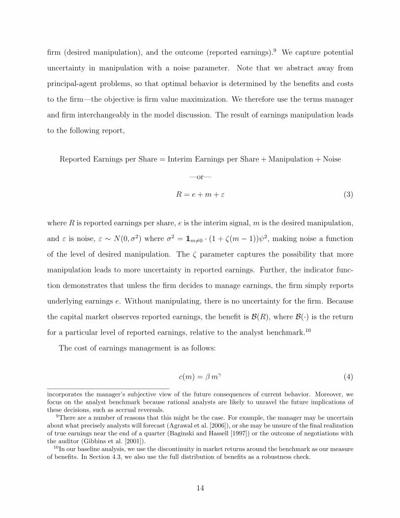
c(m) = β mγ (4)

incorporates the manager’s subjective view of the future consequences of current behavior. Moreover, wefocus on the analyst benchmark because rational analysts are likely to unravel the future implications ofthese decisions, such as accrual reversals.

9There are a number of reasons that this might be the case. For example, the manager may be uncertainabout what precisely analysts will forecast (Agrawal et al. [2006]), or she may be unsure of the final realizationof true earnings near the end of a quarter (Baginski and Hassell [1997]) or the outcome of negotiations withthe auditor (Gibbins et al. [2001]).

10In our baseline analysis, we use the discontinuity in market returns around the benchmark as our measureof benefits. In Section 4.3, we also use the full distribution of benefits as a robustness check.

14

where m is the desired manipulation, β ∼ U [0, 2η] is the linear cost of manipulation, and γ is

the exponential curvature of the cost of manipulation function. Therefore, given parameters

θ = η, γ, ψ2, ζ, the utility of the manager is,

u(e,m, θ) =

∫ ∞−∞

φm,θ(ε)B(e+m+ ε)dε− β mγ (5)

where φm,θ(ε) is the normal pdf with mean zero and variance (1+ζ(m−1))ψ2. The manager

therefore chooses m such that utility is maximized,

m∗e = arg maxm

u(e,m, θ) (6)

4.2 Simulated Method of Moments

Our modeling procedure is illustrated in the figure below. We use the empirical earnings

surprise distribution and the estimated capital market benefits from a regression disconti-

nuity design. We then employ a model of earnings manipulation to back out the shape of

the cost function. We implement our procedure using the simulated method of moments

(McFadden [1989] and Pakes and Pollard [1989]). We pick candidate parameters for the cost

function, model optimal behavior given these parameters and estimated benefits, and invert

this optimal behavior to obtain a candidate latent distribution of earnings surprise. We

repeat these three steps until we find the smoothest curve that approximates the empirical

earnings surprise distribution.

Our estimates arise from the cost parameters that produce optimal behavior that can

be inverted to best describe the latent earnings distribution. We are therefore interested in

measuring the cost function that best rationalizes the empirical earnings surprise distribution

given the observed benefits. From these estimated parameters, we are able to perform several

diagnostics tests and simulations, and explore a policy experiment using Sarbanes-Oxley. The

following discussion illustrates our empirical approach and our use of the simulated method

15

of moments. Interested readers can find further detail and proofs in Appendix A.

Estimation Method

empirical earnings surprisedistribution

estimated benefits

Estimation (SMM)

1. pick candidate parameters

2. model optimal behavior

3. invert optimal behavior–obtain candidate latent distribution–

4. smoothest curve that approximatesempirical earnings surprise distribu-

tion

repeat

Estimateslearn about the costs ofearnings manipulation

Diagnostic Tests

% manipulators

E(manipulation)

% noise

Simulations

who manipulates

manipulation proxiesPolicy Experiment

Sarbanes-Oxley

We first choose candidate cost function parameters. As in equation (6), firms take into

account the expected benefits and the costs of manipulation when deciding the number of

cents to manipulate earnings. Given the estimated benefits from our regression discontinuity

design and our candidate cost function parameters, we next obtain the optimal behavior for

each firm, from its starting bin, to its manipulated bin. These transitions from one bin to

another are affected by both costs and uncertainty. If there is uncertainty, then this affects

the outcomes for firms. If we consider π the vector representing the empirical earnings

surprise distribution, x the latent distribution of earnings, and P the transitions from one

16

bin to another, then in matrix notation,

P · x = π (7)

—or—

(Manipulation, bin to bin) ∗ (latent earnings) = empirical earnings

Using this equation, our third step is to invert optimal behavior by firms to obtain a candidate

latent distribution of earnings. We do this using matrix algebra, x = P−1 · π.

The latent distribution of earnings should be similar to the empirical earnings surprise

distribution, but it should also satisfy other properties motivated by theory. The second

key criterion we that we use to evaluate candidate latent distributions is smoothness. We

operationalize this using bin-to-bin differences in frequencies, as in Burgstahler and Dichev

[1997] and the subsequent literature. Smoothness means that, on average, bin-to-bin differ-

ences should be small. Smoothness would reduce bunching at the discontinuity, the peak of

the discontinuity itself, and would even out the distribution in general. These properties are

all reasonable assumptions given an underlying distribution of earnings that comes from a

continuous distribution.

Assuming that the underlying distribution follows some parametric form, such as normal,

would put a restriction on behavior of firms that is atheoretical.11 This is a primary concern

when applying an economic model to data—we wish to avoid assuming our result through

the imposition of arbitrary parametric restrictions. Our approach is to let the data speak

for itself. Thus, the fourth step in our procedure is selecting, from the set of candidate

latent distributions, the smoothest curve that approximates the empirical earnings surprise

distribution.12 This gives us our fitted parameters. Of course, this final step could be

altered or supplemented to include any desired distributional characteristics, parametric or

11Inspection of either the empirical or candidate latent distributions does not reveal any obvious parametricfit, nor does the literature give us any insight into what that parametric fit should be.

12In our baseline approach, we give equal weight to each of these criteria. In Section 4.3, we show thatshifting the weight towards either criterion yields similar estimates.

17

otherwise. The method is therefore general to a variety of criteria regarding the underlying

earnings distribution.

We are interested in inverting the optimal behavior of firms to find the latent distribu-

tion that strikes a balance between smoothness and fitting the empirical earnings surprise

distribution. The granularity of the partition potentially affects our estimates. In particu-

lar, if data were sufficiently granular, then the “smoothed” curve would coincide with the

empirical earnings surprise distribution. Earnings surprise, firm by firm, is measured in cent

granularity for a variety of reasons, but particularly because earnings per share disclosures

in earnings announcements are disclosed in cents, and because analysts forecast earnings

per share in cents, meaning that the earnings surprise distribution is measured in cents.

Moreover, the literature that follows Burgstahler and Dichev [1997] uses differences across

bins according to this partition. Our “smoothness” criteria maps directly to the difference

across bins metric studied in this literature.

With our fitted parameters, we simulate the model to perform diagnostic tests to better

understand the number of firms that manipulate earnings, the number that experience noisy

outcomes, and the mean manipulation decision made by firms. Further, we can uncover

which types of firms manipulate (i.e., from which bins), and to where they manipulate

(i.e., to which bins). This provides us with empirical proxies in various bins to the number

of manipulators expected to be in each bin. Finally, our estimation procedure allows us

to evaluate equilibrium behavior before and after Sarbanes-Oxley, in order to investigate

whether the regulation had an effect on the costs of earnings management.

An alternative estimation approach might begin with a latent distribution of earnings,

and then simulated optimal behavior by firms from that distribution of earnings. The main

obstacle in this alternative approach is that we do not observe the unmanaged distribution

of earnings surprise. Without this distribution, to which we would add the optimal earnings

manipulation, we would not have anything to compare to the empirical distribution, and

it is exactly this kind of comparison of distributions which we use to fit the model. In

18

principle, this approach is feasible with additional assumptions. For example, if one were

willing to pick a particular functional form for the latent distribution as well as make some

assumptions about where manipulation is happening (such as, for example, dropping the

bins around the benchmark), then it would be possible to estimate the latent distribution

as a first step. While the intuition for such a procedure is mathematically similar, it is not

internally consistent. Instead, we allow the model to inform us about where manipulation is

taking place.

4.3 Results

Table 5 presents estimates of the model. The parameters we estimate are η, the marginal

cost; γ, the exponential slope of the cost curve; ψ2, the noisiness of earnings manipulation;

and ζ, the heteroskedasticity of earnings manipulation noise. We find that marginal costs,

η, are 161 basis points. We find that the slope of the cost function is reasonably convex,

with costs increasing with exponent 2.08. However, we find that earnings management is

not certain, and that manipulation has a 0.82 cent variance (outcomes can deviate from

planned), increasing nearly fourfold (heteroskedasticity of 3.71) for each additional cent of

manipulation. Figure 3 shows the empirical and latent distributions, as estimated by the

model.

The marginal benefit of meeting the analyst benchmark to firms is 145 basis points, which

is less than the marginal cost for the median firm. Also, noise in manipulation means that

some firms in the [-1,0) bin that choose to manipulate up will miss their target, meaning

the expected marginal benefit of manipulating is even lower. We calculate that the marginal

cost of the marginal manipulator is 104 basis points, meaning that the median firm in the

[-1,0) bin does not manipulate earnings. Further, the average marginal cost of manipulation

for manipulating firms, is 37 basis points. This is less than half of the marginal cost of the

marginal manipulator, which reflects the fact that some manipulators are manipulating up

by more than one bin.

19

Given these estimates, we can simulate the model to calculate the proportion of firms

that manipulate their earnings. Namely, we find that 2.62% of firms in our sample ma-

nipulate earnings. This is remarkably close to 2.63%, the magnitude of the discontinuity

in the distribution of firms by earnings surprise estimated in Section 3. This similarity is

notable because our structural approach does not directly target the discontinuity, it does

not impose any polynomial restrictions on the data, and it allows for a much broader range

of manipulation strategies than just moving from just to the left of the threshold to just to

the right.

We also show that manipulating firms do so by 1.21 cents on average. Because of stochas-

ticity in manipulation, 59.6% of firms do not hit their intended targets, missing either above

or below. Figure 4 illustrates the effect of the equilibrium manipulation strategy on the

proportion of firms in each surprise bin. Panel A shows the fraction of manipulators in each

earnings surprise bin, categorized by the amount of manipulation. While most firms do not

manipulate at all, a nontrivial fraction of firms manipulate from one up to five cents. In

Panel B, we normalize the mass of firms in each bin to one, to better illustrate the different

strategies by bin.

In the remaining rows of Table 5, we show that our results are not only robust to model

specification, but also sensitive to salient features of the empirical distribution. We use bins

from [-20,-19) to [20,21) cents in our main estimates, but most of the manipulating firms are

in bins much closer to the discontinuity. As such, it is important to show that reducing the

number of bins we use to fit our model does not meaningfully change our results. When we

estimate our model on data from the [-15,-14) to [15,16) cent bins, or further reducing to the

[-10,-9) to [10,11) bins, or the [-5,-4) to [5,6) bins, our results are similar. This is particularly

true for important parameters η, which varies from 154 to 167 basis points (vs. a baseline of

161) and ψ2, which varies from 0.76 to 0.79 (vs. a baseline of 0.82). In addition, %manip is

relatively unchanged, varying from 2.56% to 2.84% (vs. a baseline of 2.62%), as is %noise,

varying from 55.7% to 60.0% (vs. a baseline of 59.6%).

20

Our estimation equally weights similarity to the empirical distribution and smoothness as

qualities of the latent unmanaged earnings surprise distribution. We therefore reestimate our

model overweighting empirical similarity by 10% and then run it again instead overweighting

smoothness by 10%. We find that our results do not significantly change, and cost parameters

and manipulation move in the direction one would expect. Namely, costs go up (170 vs.

161 basis points) and manipulation goes down (2.45% vs. 2.62% of firms manipulate) when

empirical sameness is emphasized, whereas costs go down (146 basis points) and manipulation

goes up (3.11% of firms manipulate) when smoothness is emphasized, which is intuitive given

that more manipulation smooths the discontinuity. Comparing across these three different

weighting schemes, we are comforted by the fact that our preferred, equal weighting yields

a propensity to manipulate almost exactly equal to that of a simple, theory-free, regression

discontinuity design. This is our preferred weighting because we want to avoid baking in

higher manipulation through imposing too much smoothing.

Because ζ has the greatest standard error and plays the smallest role in our model, we

also estimate the model without ζ (setting ζ = 0). Our estimates change the most in this

robustness check. While ζ does not have large effects on equilibrium behavior, we can see

from its effect on other parameters that it is an important feature of the model.

We next investigate whether our approach is sensitive to features of the empirical dis-

tribution by mechanically changing the empirical distribution of earnings. First, we reduce

the peak found in the [0,1) cent bin, halving its size relative to the [1,2) cent bin. Using this

Reduce peak empirical distribution of earnings, the implied marginal costs increase by 27%,

while the slope increases by only 5%. If we remove the peak entirely, making the [0,1) cent

bin equal to the [1,2) cent bin, then the slope remains unchanged, but marginal costs in-

crease by 70% relative to the baseline. Further, reducing the peak cuts down on the implied

number of manipulators, down to 1.91% and 1.36% of firms, respectively. These alternative

estimates demonstrate that our results are sensitive to earnings surprise discontinuities, and

that removing the discontinuity yields much lower levels of manipulation, via higher cost

21

parameters.

In untabulated results, we employ the full distribution of capital markets benefits for

different levels of earnings relative to the benchmark. As shown in Figure 1, the main

difference is the existence of small, but positive, marginal benefits of moving rightward from

the benchmark. When we estimate the model, we obtain similar parameter estimates for the

cost function, though because of the increased benefits, this cost function yields somewhat

higher levels of manipulation.

4.4 Benefits Heterogeneity

So far we have assumed that the benefits to manipulating earnings are known and fixed. In

this subsection, we extend our model to consider the possibility of heterogeneity in benefits.

Importantly, for this heterogeneity to have an effect on the firm’s problem, it must be

known before the reporting decision is made. While there is likely significant variation ex

post in benefits, this variation is not behavior relevant—the firm can only act on its ex

ante expectation of benefits. To study this issue, we incorporate cross-firm variation in

expected benefits, using the estimated dispersion (standard error) in our estimated benefit

parameter. This problem is reasonably straightforward, as after the firms draw their benefits,

the structure of the tradeoff underlying manipulation is the same as in our base model.

We present several parameterizations of benefits heterogeneity in Table 6. In the first

row, before making the reporting decision, firms draw a benefit from a normal distribution

with mean and standard deviation as in column 5, Panel A, of Table 2, our preferred model

for estimating benefits. We alternatively allow for the distribution of benefits to come from a

Bernoulli distribution (with the same underlying mean and standard deviation) in the third

row, where the idea is that firms either get a “large” benefit or no benefit at all. In either

case, our estimates are essentially the same as in our baseline model with no heterogeneity.

In the second and fourth rows, we magnify the variation (increasing the standard deviations

by a factor of five, well beyond any of our estimates in Table 2) as a robustness check and

22

to get a better sense of how this new feature affects our estimation. Our estimates are again

in line with the baseline. We conclude from this investigation that heterogeneity in benefits

is not an important feature of the firm’s problem in practice.

The economics of heterogeneity become much more interesting, at least in theory, if firm-

specific benefits are correlated with firm-specific costs. This kind of a correlation broadly

allows for a relaxation of the assumption that manipulation (or firm-side heterogeneity) is not

observable by investors making valuation decisions. With a non-zero correlation, investors

can go some way towards tailoring the market reward to different earnings surprise bins

across firms. To study this issue, and get a sense of its empirical importance, we augment

the above analysis of unconditional benefits heterogeneity to allow for a correlation between

the firm’s benefits draw and its cost draw. In particular, we take the normal distribution

and incorporate correlations of 0.5 and -0.5; these large correlations imply that the market

gets a strong signal about individual firms and their likelihood of engaging in manipulation.

This structure can capture a variety of particular economic models of investor behavior.

For example, the positive correlation has a natural interpretation as the market wanting to

reward good performance but not manipulated performance. When investors see high costs

(or a signal of high costs), they would rationally infer that, all else equal, firms are less likely

to manipulate. This would mean that firms meeting the analyst benchmark are more likely

to have gotten there based on real performance and so would warrant a larger valuation

premium. On the other hand, one would get a negative correlation out of a model where low

costs and thus the capacity to manipulate earnings are a positive signal, perhaps indicating

financial flexibility or a sophisticated understanding of the business on the part of managers.

Then investors would see low costs, and rationally pay a relatively high premium for meeting

the analyst benchmark since such firms are of better quality along some relevant dimension.

While the extant earnings management literature has studied such issues (and might come

out more on the side of a positive correlation), our goal in the new analysis is simply to get

an idea of whether these kinds of mechanisms are empirically significant.

23

The fifth and seventh rows of Table 6 present the 0.5 and -0.5 correlation models, re-

spectively. Our inferences are essentially unchanged. As we did above, we also re-estimate

the models with these correlations for the inflated variation (again a factor of five). The

estimates are again similar. Especially in light of the results with implausibly high benefits

variability, we conclude that allowing for an empirically-driven relationship between benefits

and costs at the firm-level does not have a meaningful impact on our understanding of the

firm’s manipulation decision. This finding has two important implications. First, identi-

fication of a correlation parameter is not really feasible in our setting because even wide

variation in this parameter has limited effect on the fit of the model. More importantly, we

believe that this new set of findings supports our overall approach of focusing on the firm’s

problem, which takes the capital market benefits as given.

4.5 Identification

In estimating models of this type, it is important that we demonstrate the role the param-

eters in our model play in generating the empirical earnings surprise distribution from the

latent earnings surprise distribution. Table 7 shows how the manipulation strategy varies

while altering each parameter, in turn, by reducing it to 10% of our estimated level. For

example, we estimate a marginal cost of 161 basis points, but here ask what equilibrium

earnings management behavior we would observe if firms instead faced average marginal

costs of 16 basis points. By reducing the marginal cost parameter, we see that the number

of manipulating firms increases to 12.6%, roughly five times our estimated 2.62%. We also

find that mean manipulation increases to 1.92 cents, which is significantly larger than our

estimate of 1.21 cents. Similarly, decreasing the slope of the cost curve increases the number

of manipulating firms to 9.45% and mean manipulation to 10.16 cents, which is more than

eight times larger than our estimates. There is also an increase to 78.4% (vs. 59.6% esti-

mated) of firms missing their target, either above or below, due to heteroskedasticity. If we

decrease the noise parameter, we see a large reduction in missing manipulation targets, and

24

only a modest increase in the number of manipulators (3.22%) and mean manipulation (1.23

cents). Altering the heterskedasticity parameter has negligible effects, pointing to the fact

that heteroskedasticity, while likely present, is not a crucial component in modeling noise in

earnings management.

Figure 5 provides further intuition for how the parameters are estimated by showing

how the empirical distribution would differ according to each of the piecemeal parameter

reductions discussed above. The curves shown in red represent the empirical distribution

and the curves shown in blue are the counterfactual empirical distributions. Specifically, we

see that the marginal cost parameter, η, is the most important for identifying manipulation

close to the discontinuity, as reducing the marginal costs induces larger jumps out of the

[-2,-1) and [-1,0) cent bins.

However, the slope parameter, γ, is associated with the degree to which firms from farther

away from the discontinuity manipulate. This can be seen by the greater participation in

manipulation by firms from -20 cents to -5 cents. If we reduce the noise parameter, ψ2, to

10% of its estimated value, a divot appears in the [-1,0) cent bin, implying that noise corrects

for the discontinuous nature of manipulation, smoothing both the benefits of manipulation

as well as the outcomes of manipulation itself. This parameter reflects the uncertainty

inherent in manipulation. Consistent with the results presented in Table 8, we see that

the heteroskedasticity parameter, ζ, has small effects on manipulation. While it allows for

greater manipulation from farther away from the discontinuity, as well as more manipulation

beyond the discontinuity, this type of distributional smoothing is only marginally important

to the overall fit of the model.

5 Consequences

An understanding of the costs of earnings management has many implications for how we

interpret firm behavior and for the validity of measures employed in the literature to identify

25

earnings management. In this section, we discuss a number of applications of the results

described above.

5.1 Why do so few firms manage earnings?

Given the significant benefit to meeting earnings benchmarks and the results of surveying

managers themselves (Dichev et al. [2016]), our estimated fraction of firms managing earnings

is perhaps surprisingly low. Of particular interest are firms in the [-1,0) earnings surprise

bin, since these are the ones with the most potential to take advantage of the discontinuity

in capital market responses to earnings announcements. The counterfactual simulations

discussed above can help in understanding why so many firms remain below, and yet very

close to, the benchmark.

Two of the parameters in the cost function appear to drive this behavior—the marginal

cost parameter, η, and the noise parameter, ψ2. In the latent distribution, 6.1% of firms are

in the [-1,0) cent bin. Cutting η to 10% of its estimated level, as in Table 7, reduces this

fraction by 3.1%. This reduction is a straightforward consequence of decreasing the marginal

cost of manipulation. If ψ2 is simultaneously cut to 10% of its estimated level, only 0.9% of

firms remain in the negative one bin. Reducing the magnitude of noise has two key effects.

The optimal strategy for managers with relatively low costs in bins farther away from the

benchmark may be to manipulate up to negative one in the hopes of getting shocked into

meeting the benchmark13—reducing noise decreases the expected payoff of this strategy.

The second effect is mechanical: negative noise drops firms from meeting the benchmark

(the most likely target) into the negative one bin.

The results of the counterfactuals show that both the marginal cost effect and the noise

effect are economically significant explanations for the relative lack of manipulation out of

13Although managers are risk neutral (so that noise is not necessarily harmful), there is an asymmetryto the effect of noise on the manager’s objective function. From the [0,1) cent bin, which is the most likelytarget for managers, a negative shock hurts the manager much more than she is helped by a positive shock,because of the nature of the discontinuity in benefits. From the [-1,0) bin, the asymmetry is reversed, withthe expected benefit of noise becoming positive.

26

the negative one bin. Determining the exact contribution of the two forces is complicated

by the fact that there is an interaction between the two. As marginal costs decrease, more

firms target just-meeting the benchmark, but the mechanical effect of noise means that a

higher noise parameter shocks more of these firms back down into the negative one cent

bin. However, this interaction accounts for only nine percent of the overall effect of the

counterfactual.

5.2 Identifying “suspicious” firms

Our model estimates reveal the incidence (and amount) of manipulation in each earnings

surprise bin. This is of interest given the prevalent use of proxy measures of manipulation

based on whether a firm ends up in the [0,1) cent bin or not (e.g., Bhojraj et al. [2009], Cohen

et al. [2008], Roychowdhury [2006]). Table 8 quantifies how well a variety of definitions of

“suspicious” firms fare in accurately identifying manipulation. The first row shows the

percentage of firms in each surprise bin that manipulated to get there and the second row

captures the percentage of all manipulators from the sample that ended up in that surprise

bin. The third and fourth rows replicate the first and second, respectively, while weighting

the manipulating firm observations according to the mean level of manipulation in each

surprise bin (e.g. the firm counts twice if it manipulated up two cents).

The first column of Table 8 describes the firms captured by the typically used [0,1)

“suspicious” bin. Of the firms in this bin, 11% manipulated to get there, which is perhaps

surprisingly low, but in line with our overall estimates of the extent of manipulation in

aggregate. This subset covers 53.1% of all manipulators in the sample. On these two metrics,

this bin performs the best at identifying manipulation, restricting to single bin measures.

The next best bin to add to the measure would be [1,2), which reduces accuracy to 9.9% but

then accounts for 80.9% of the total manipulators. Given the salience of the discontinuity

in the capital market response to earnings surprise, it is interesting that the bin with the

third most manipulators is the [-1,0) bin; as in the previous subsection, this is because the

27

possibility of a positive shock makes manipulating into this bin the optimal strategy for some

firms with an intermediate level of costs. If the priority were to account for nearly all of

the manipulators, the [-1,3) range may be desirable in that 97.4% of manipulators fall into

this range and the accuracy falls only to 7.3%. Relative to the [0,1) bin, this reflects an

83% increase in the fraction of all manipulators included, at the cost of reducing accuracy

by 34%.

Turning to the third and fourth rows of Table 8, we find a similar pattern of results,

though with a clear tendency toward improvement from including more bins. This results

from bins farther away from the benchmark having higher expected manipulation, condi-

tional on manipulating at all, relative to bins closer to the benchmark. For example, in this

case, the [0,2) range performs better than [0,1) on both margins, increasing the weighted

fraction of manipulators and significantly increasing the fraction of total manipulation cov-

ered. Extending to [-1,3) yields an even larger increase in coverage and reduces accuracy by

only 13% relative to the [0,2) range.

Overall, Table 8 shows how different definitions of “suspicious” bins trade off Type 1 and

Type 2 errors and can help guide this measurement choice in a variety of contexts. Further,

it may be preferred for some applications to use a continuous measure of the probability of

manipulation by bin, which naturally places more weight on bins close to the benchmark

and less on those farther away, rather than making a discrete choice of which bins to include

in the measure and which to exclude.

5.3 Do analysts bias their forecasts?

So far, we have studied the management of earnings towards a particular benchmark, which

we assume to be known at the time the managers make their manipulation decisions. How-

ever, it is well known in the literature (Kross et al. [2011]; Chan et al. [2007]; Burgstahler

and Eames [2006]; Cotter et al. [2006]) that the benchmark itself is subject to manipulation.

This can be accomplished by managers through negative earnings guidance, which indirectly

28

affects the analyst’s choice of benchmark, or may directly reflect the strategy of analysts,

who would like to curry favor with managers. Indeed, Burgstahler and Eames [2006] show

evidence that firms avoid negative earnings surprise through downward management of an-

alysts’ forecasts, incremental to their management of the underlying earnings number.

One of the outputs of our estimation process, as described above, is the unmanaged

distribution of earnings. If the benchmark is chosen by analysts with the objective of min-

imizing forecast error, one would expect this distribution to be symmetric, with an equal

probability of positive and negative errors, especially in the neighborhood of the benchmark.

Interestingly, this is not the case—the asymmetry is reduced in the latent distribution rela-

tive to the empirical distribution but is not eliminated.14 Specifically, we find that 57.0% of

observations are on the positive side of our window in the empirical distribution; this falls to

54.7% in the latent distribution. We can infer from this asymmetry the presence of analyst

bias, and can quantify the contribution of this bias to the discontinuity in earnings relative

to that of short-term earnings management. The remaining bias is striking because analysts

themselves should be able to understand the potential for manipulation and so might be ex-

pected to remove the effects of bias from their forecasts, leading to a distribution symmetric

around this forecast. We therefore interpret the remaining asymmetry as the analysts’ own

preference to bias forecasts, in the absence of active managerial intervention, consistent with

findings in the literature (Brown et al. [2015]; Richardson et al. [2004]).

Our broad approach to analyst behavior is that analysts either anticipate manipulation

and fail to undo it, or fail to anticipate manipulation. Either alternative is consistent with

our approach and with the literature on analyst behavior. To this end, Abarbanell and

Lehavy [2003] find evidence “consistent with a growing body of literature that finds analysts

either cannot anticipate or are not motivated to anticipate completely in their forecasts firms

efforts to manage earnings.” Burgstahler and Eames [2003] show that analysts are unable to

14Brown [2001] shows that there was a shift in the distribution of earnings surprise rightward from 1984-1999. Our data, which mostly come from years after this period, confirm the observation that the medianearnings surprise is a small positive number.

29

consistently identify specific firms that engage in “small” amounts of earnings management,

consistent with the magnitude of earnings management we estimate.

5.4 Sarbanes-Oxley and the cost of earnings management

After a string of accounting scandals in the late 1990s and early 2000s, including Enron

and Worldcom, the Sarbanes-Oxley Act (SOX) was enacted in 2002. In line with the SEC’s

stated objective of protecting investors, SOX initiated broad changes in corporate disclosures,

with the goal of improving the reliability of financial information disclosed in company

reports. SOX consisted of three main regulatory changes. First, it established the Public

Company Accounting Oversight Board (PCAOB) to set rules on auditing, quality control,

and independence. Second, it provided for greater auditor independence by requiring that

independent directors sit on audit committees and that firms rotate audit partners at least

every five years. Third, it produced a code of ethics for senior financial officers and required

chief executive and financial officers to certify and take personal responsibility for public

financial statements and to forfeit bonus compensation upon accounting restatements. Along

with the other eleven sections of the bill, these provisions were intended to provide enforceable

rules and penalty-based incentives for managers to engage in reliable financial reporting

behavior.

Our methodology can be used to uncover the effects of such regulation on earnings man-

agement by exploiting time series variation in the empirical earnings surprise distribution

and the benefits of meeting earnings benchmarks. SOX provides an ideal setting for such

an analysis because the effects of SOX have been of great interest to practitioners and in

the academic literature. Cohen et al. [2008] and Bartov and Cohen [2009] find that earnings

management declined after the introduction of SOX, and attribute this decline particularly to

reduced accruals-based earnings management (as well as a decline in downwards expectation

management using negative managerial guidance). Cohen et al. [2008] note that the three

years prior to SOX were characterized by an abnormal increase in earnings management

30

relative to earlier in the 1990s.

To investigate the effects of SOX using our methodology, we look at subsamples of the

three years before SOX (1999-2001) and the three years after SOX (2002-2004).15 Table 9

presents estimates from these two subsamples. Consistent with the work discussed above,

our diagnostic test statistic of the extent of manipulation, the discontinuity in the earnings

distribution (∆), falls post-SOX. The benefit of meeting the benchmark (B) increases after

SOX by 80 basis points. Together, these two findings suggest that SOX had its intended

effect of improving the quality of financial reporting and that capital markets responded with

larger rewards for meeting the benchmark. This is likely due to an increased willingness by

markets to attribute the meeting of earnings benchmarks to true performance rather than

manipulation.

Next, we use our structural model to estimate the consequences of these changes for the

costs of earnings management as well as the extent of manipulation. As expected, we find

significant increases in costs. Table 9 shows that both the marginal cost parameter and the

slope parameter increase significantly. This suggests that both the cost of the first cent of

managed earnings and the cost of incremental manipulation both increased, consistent with

the goals of the reform.16 Earnings management also became much less noisy after SOX—

we conjecture that this is due to a switch away from riskier, less certain strategies, towards

more conservative use of discretion.17 In aggregate, manipulation fell from 4.05% of firms to

2.61%, a 36% reduction, evidence that SOX had its desired effect on financial reporting and

earnings management.

15Our results are not sensitive to these specific definitions of the pre- and post-SOX periods. For example,dropping either 2001 or 2002 yields similar estimates.

16There are a number of mechanisms through which the costs could have increased. For example, auditorslikely increased their scrutiny of reported earnings both because of increased regulation on their behavior,and as a rational response to the increased risk to their survival made evident by the collapse of ArthurAndersen.

17The fact that we estimate a relatively small noise parameter post-SOX is also reassuring with regardto our main results. One could have been concerned that the role of noise was confounded with modelmisspecification in some other dimension. The post-SOX partition shows that our approach can indeedproduce significant variation in the importance of noise, suggesting that the higher noise parameter weestimate for the full sample is indeed indicative of uncertainty in earnings manipulation.

31

6 Conclusion

Two distinct literatures in accounting and finance have pursued estimates of the capital

market benefits of meeting earnings benchmarks, and statistical evidence of earnings ma-

nipulation around earnings benchmarks. In this paper, we connect these findings using an

economic model of firm behavior where there is a tradeoff between observable capital mar-

ket benefits and unobservable costs of earnings manipulation. The cost function which we

recover using this structural approach provides numerous insights about firm behavior and

can be used, for example, to assess the validity of identifying manipulation using a “suspi-

cious” earnings surprise bin and also to estimate the effect of SOX on the financial reporting

process. In future research, we plan to study more broadly how costs change over time and

whether they vary according to the benchmark and to the characteristics of the firm and the

incentives of its managers.

32

References

Jeffery Abarbanell and Reuven Lehavy. Biased forecasts or biased earnings? The role ofreported earnings in explaining apparent bias and over/underreaction in analysts earningsforecasts. Journal of Accounting and Economics, 36(1):105–146, 2003.

Anup Agrawal, Sahiba Chadha, and Mark A. Chen. Who is afraid of reg FD? The behaviorand performance of sell-side analysts following the SECs fair disclosure rules. The Journalof Business, 79(6):2811–2834, 2006.

Vasiliki Athanasakou, Norman C. Strong, and Martin Walker. The market reward for achiev-ing analyst earnings expectations: does managing expectations or earnings matter? Jour-nal of Business Finance & Accounting, 38(1-2):58–94, 2011.

William R. Baber, Patricia M. Fairfield, and James A. Haggard. The effect of concernabout reported income on discretionary spending decisions: The case of research anddevelopment. The Accounting Review, 66(4):818–829, 1991.

Stephen P. Baginski and John M. Hassell. Determinants of management forecast precision.The Accounting Review, pages 303–312, 1997.

Brad M. Barber, Emmanuel T. De George, Reuven Lehavy, and Brett Trueman. The earningsannouncement premium around the globe. Journal of Financial Economics, 108(1):118–138, 2013.

Eli Bartov and Daniel A. Cohen. The “Numbers Game” in the pre-and post-Sarbanes-Oxleyeras. Journal of Accounting, Auditing & Finance, 24(4):505–534, 2009.

Eli Bartov, Dan Givoly, and Carla Hayn. The rewards to meeting or beating earningsexpectations. Journal of Accounting and Economics, 33(2):173–204, 2002.

Tobias Berg, Manju Puri, and Jorg Rocholl. Loan officer incentives and the limits of hardinformation. Working paper, 2013.

Victor L. Bernard and Jacob K. Thomas. Post-earnings-announcement drift: Delayed priceresponse or risk premium? Journal of Accounting Research, 27:1–36, 1989.

Victor L. Bernard and Jacob K. Thomas. Evidence that stock prices do not fully reflect theimplications of current earnings for future earnings. Journal of Accounting and Economics,13(4):305–340, 1990.

Sanjeev Bhojraj, Paul Hribar, Marc Picconi, and John McInnis. Making sense of cents:An examination of firms that marginally miss or beat analyst forecasts. The Journal ofFinance, 64(5):2361–2388, 2009.

Lawrence D. Brown. A temporal analysis of earnings surprises: Profits versus losses. Journalof Accounting Research, 39(2):221–241, 2001.

33

Lawrence D. Brown and Marcus L. Caylor. A temporal analysis of quarterly earnings thresh-olds: Propensities and valuation consequences. The Accounting Review, 80(2):423–440,2005.

Lawrence D. Brown and Arianna Spina Pinello. To what extent does the financial reportingprocess curb earnings surprise games? Journal of Accounting Research, 45(5):947–981,2007.

Lawrence D. Brown, Andrew C. Call, Michael B. Clement, and Nathan Y. Sharp. Insidethe“black box” of sell-side financial analysts. Journal of Accounting Research, 53(1):1–47,2015.

David Burgstahler and Ilia Dichev. Earnings management to avoid earnings decreases andlosses. Journal of Accounting and Economics, 24(1):99–126, 1997.

David Burgstahler and Michael Eames. Management of earnings and analysts’ forecaststo achieve zero and small positive earnings surprises. Journal of Business Finance &Accounting, 33(5-6):633–652, 2006.

David C. Burgstahler and Michael J. Eames. Earnings management to avoid losses andearnings decreases: Are analysts fooled? Contemporary Accounting Research, 20(2):253–294, 2003.

Marcus L. Caylor. Strategic revenue recognition to achieve earnings benchmarks. Journalof Accounting and Public Policy, 29(1):82–95, 2010.

Louis K.C. Chan, Jason Karceski, and Josef Lakonishok. Analysts’ conflicts of interestand biases in earnings forecasts. Journal of Financial and Quantitative Analysis, 42(04):893–913, 2007.

Daniel Cohen, Raj Mashruwala, and Tzachi Zach. The use of advertising activities to meetearnings benchmarks: Evidence from monthly data. Review of Accounting Studies, 15(4):808–832, 2010.

Daniel A. Cohen, Aiyesha Dey, and Thomas Z. Lys. Real and accrual-based earnings manage-ment in the pre-and post-Sarbanes-Oxley periods. The Accounting Review, 83(3):757–787,2008.

Julie Cotter, Irem Tuna, and Peter D. Wysocki. Expectations management and beatabletargets: How do analysts react to explicit earnings guidance? Contemporary AccountingResearch, 23(3):593–624, 2006.

Patricia Dechow, Weili Ge, and Catherine Schrand. Understanding earnings quality: Areview of the proxies, their determinants and their consequences. Journal of Accountingand Economics, 50(2):344–401, 2010.

Patricia M. Dechow, Scott A. Richardson, and Irem Tuna. Why are earnings kinky? Anexamination of the earnings management explanation. Review of Accounting Studies, 8(2-3):355–384, 2003.

34

Francois Degeorge, Jayendu Patel, and Richard Zeckhauser. Earnings management to exceedthresholds. The Journal of Business, 72(1):1–33, 1999.

Ilia Dichev, John Graham, Campbell R. Harvey, and Shiva Rajgopal. The misrepresentationof earnings. Financial Analysts Journal, 72(1):22–35, 2016.

Karl B. Diether, Christopher J. Malloy, and Anna Scherbina. Differences of opinion and thecross section of stock returns. The Journal of Finance, 57(5):2113–2141, 2002.

Alex Edmans, Vivian W. Fang, and Katharina A. Lewellen. Equity vesting and managerialmyopia. Working paper, 2016.

Aytekin Ertan. Real earnings management in the financial industry. Working paper, 2015.

George Foster, Chris Olsen, and Terry Shevlin. Earnings releases, anomalies, and the be-havior of security returns. The Accounting Review, 59(4):574–603, 1984.

Andrea Frazzini and Owen Lamont. The earnings announcement premium and tradingvolume. Working paper, 2007.

Michael Gibbins, Steven Salterio, and Alan Webb. Evidence about auditor–client manage-ment negotiation concerning clients financial reporting. Journal of Accounting Research,39(3):535–563, 2001.

Thomas A. Gilliam, Frank Heflin, and Jeffrey S. Paterson. Evidence that the zero-earningsdiscontinuity has disappeared. Journal of Accounting and Economics, 60(1):117–132, 2015.

John R. Graham, Campbell R. Harvey, and Shiva Rajgopal. The economic implications ofcorporate financial reporting. Journal of Accounting and Economics, 40(1):3–73, 2005.

Jinyong Hahn, Petra Todd, and Wilbert Van der Klaauw. Identification and estimationof treatment effects with a regression-discontinuity design. Econometrica, 69(1):201–209,2001.

Carla Hayn. The information content of losses. Journal of Accounting and Economics, 20(2):125–153, 1995.

Paul M. Healy and James M. Wahlen. A review of the earnings management literature andits implications for standard setting. Accounting Horizons, 13(4):365–383, 1999.

Sabrina T. Howell. Financing constraints as barriers to innovation: Evidence from R&Dgrants to energy startups. Working paper, 2015.

John Jacob and Bjorn N. Jorgensen. Earnings management and accounting income aggre-gation. Journal of Accounting and Economics, 43(2):369–390, 2007.

Michael C. Jensen. Agency costs of overvalued equity. Financial Management, 34(1):5–19,2005.

35

Ron Kasznik and Maureen F. McNichols. Does meeting earnings expectations matter? Ev-idence from analyst forecast revisions and share prices. Journal of Accounting Research,40(3):727–759, 2002.

Edmund Keung, Zhi-Xing Lin, and Michael Shih. Does the stock market see a zero or smallpositive earnings surprise as a red flag? Journal of Accounting Research, 48(1):91–121,2010.

William J. Kross, Byung T. Ro, and Inho Suk. Consistency in meeting or beating earningsexpectations and management earnings forecasts. Journal of Accounting and Economics,51(1):37–57, 2011.

David S. Lee and Thomas Lemieux. Regression discontinuity designs in economics. Journalof Economic Literature, 48:281–355, 2010.

Steven R. Matsunaga and Chul W. Park. The effect of missing a quarterly earnings bench-mark on the CEO’s annual bonus. The Accounting Review, 76(3):313–332, 2001.

Justin McCrary. Manipulation of the running variable in the regression discontinuity design:A density test. Journal of Econometrics, 142(2):698–714, 2008.

Daniel McFadden. A method of simulated moments for estimation of discrete responsemodels without numerical integration. Econometrica, 57(5):995–1026, 1989.

Sarah E. McVay. Earnings management using classification shifting: An examination of coreearnings and special items. The Accounting Review, 81(3):501–531, 2006.

Ariel Pakes and David Pollard. Simulation and the asymptotics of optimization estimators.Econometrica, 57(5):1027–1057, 1989.

Jeff L. Payne and Wayne B. Thomas. The torpedo effect: Myth or reality? Journal ofAccounting, Auditing & Finance, 26(2):255–278, 2011.

Scott Richardson, Siew Hong Teoh, and Peter D. Wysocki. The walk-down to beatableanalyst forecasts: The role of equity issuance and insider trading incentives. ContemporaryAccounting Research, 21(4):885–924, 2004.

Sugata Roychowdhury. Earnings management through real activities manipulation. Journalof Accounting and Economics, 42(3):335–370, 2006.

Eric C. So and Sean Wang. News-driven return reversals: Liquidity provision ahead ofearnings announcements. Journal of Financial Economics, 114(1):20–35, 2014.

Amy Y. Zang. Evidence on the trade-off between real activities manipulation and accrual-based earnings management. The Accounting Review, 87(2):675–703, 2011.

36

A Estimating Equations

There exists an empirical distribution of earnings surprise from [−20, 20] cents per share,

in one cent increments. Let π be the vector representing the number of firms with each

per share earnings surprise. We index π1 as the number of firms that have −20 cents in

per share earnings surprise, and πi the number of firms that have −21 + i cents in per

share earnings surprise, such that π41 is the number of firms that have 20 cents in per share

earnings surprise.

We assume that the empirical distribution is the result of a latent distribution of unman-

aged earnings surprise plus the effect of manipulation, or earnings management, on the part

of each firm. While many firms go without managing earnings, some do so, which results in

higher earnings surprise. The latent distribution of earnings surprise represents the number

of firms that fall into each cent bin of earnings surprise before engaging in earnings man-

agement. Let x be the model-implied latent distribution of earnings, indexed in a similar

fashion, x1, x2, . . . , x41, to π. We identify costs by the proportion of firms, in each cent bin,

that manipulate earnings, and tie this to the properties of the latent distribution of earnings

surprise that we find.

Say we examine the -20 cents bin, which represents earnings surprise in the [-20,-19)

cents interval. Firms in this bin could have only one potential simulated latent earnings

surprise, and that is -20 cents. A proportion of those firms chose not to manipulate their

earnings numbers, and so landed in the -20 cents bin. We call the transition probability

from bin i to bin j ≥ i, pi,j. Therefore, we have π1 = p1,1x1, or the number of -20 cents bin

firms that did not manage earnings, and instead reported latent earnings, is equal to the

transition probability from the -20 cents bin to the -20 cents bin multiplied by the latent

number of -20 cents bin earners. Similarly, for the number of realized -19 cents bin firms,

we have π2 = p1,2x1 + p2,2x2, or equal to the number manipulating from latent -20 cents bin,

and those that chose not to manipulate from -19 cents bin. We can see this below,

π1 = p1,1x1

π2 = p1,2x1 + p2,2x2

π3 = p1,3x1 + p2,3x2 + p3,3x3

...

In matrix form we get,

37

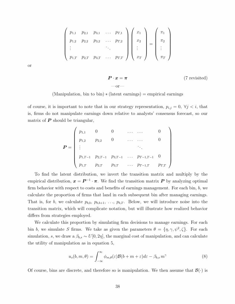
p1,1 p2,1 p3,1 . . . pT,1

p1,2 p2,2 p3,2 . . . pT,2...

. . .

p1,T p2,T p3,T . . . pT,T

x1

x2

...

xT

=

π1

π2

...

πT

or

P · x = π (7 revisited)

—or—

(Manipulation, bin to bin) ∗ (latent earnings) = empirical earnings

of course, it is important to note that in our strategy representation, pi,j = 0, ∀j < i, that

is, firms do not manipulate earnings down relative to analysts’ consensus forecast, so our

matrix of P should be triangular,

P =

p1,1 0 0 . . . . . . 0

p1,2 p2,2 0 . . . . . . 0...

. . .

p1,T−1 p2,T−1 p3,T−1 . . . pT−1,T−1 0

p1,T p2,T p3,T . . . pT−1,T pT,T

To find the latent distribution, we invert the transition matrix and multiply by the

empirical distribution, x = P−1 · π. We find the transition matrix P by analyzing optimal

firm behavior with respect to costs and benefits of earnings management. For each bin, b, we

calculate the proportion of firms that land in each subsequent bin after managing earnings.

That is, for b, we calculate pb,b, pb,b+1, . . ., pb,T . Below, we will introduce noise into the

transition matrix, which will complicate notation, but will illustrate how realized behavior

differs from strategies employed.

We calculate this proportion by simulating firm decisions to manage earnings. For each

bin b, we simulate S firms. We take as given the parameters θ = η, γ, ψ2, ζ. For each

simulation, s, we draw a βb,s ∼ U [0, 2η], the marginal cost of manipulation, and can calculate

the utility of manipulation as in equation 5,

us(b,m, θ) =

∫ ∞−∞

φm,θ(ε)B(b+m+ ε)dε− βb,smγ (8)

Of course, bins are discrete, and therefore so is manipulation. We then assume that B(·) is

38

a vector, and that m is a whole number choice, making utility,

us, Discrete(b,m, θ) =20∑−20

φm,θ(ε)B(b+m+ ε)dε− βb,smγ (9)

where φm,θ(ε) provides the discrete approximation of the continuous normal pdf with mean

0, and variance 1m6=0 · (1 + ζ(m − 1))ψ2. For various values of m, in whole cents from 0 to

T − b, we find the optimal earnings management,

m∗b,s(θ) = arg maxm∈[0,T−b]

u(b,m, θ) (10)

From this we calculate the strategy taken by each firm, from each bin b to a weakly higher

bin j ≥ b,

pstrategyb,j,S (θ) =

S∑s=1

1m∗b,s(θ)=j−b

S, ∀b, and ∀j ≥ b

0, otherwise

.

However, because firms may face noise in their decisions, then noise would affect transitions

accordingly,

pb,j,S(θ) =

S∑s=1

T−j∑k=0

1m∗b,s(θ)=j+k−b · 1εs(m∗

b,s(θ),θ)=−k

S, ∀b, j

.

where εs(m, θ) is a simulated outcome for a random variable following a discrete approx-

imation of the normal distribution, φm,θ(·), where the mean is 0, and the variance is

1m6=0 · (1 + ζ(m− 1))ψ2, and in equilibrium, ∀s, q < 0, m∗b,s(θ) 6= q.

For non-zero ψ2, the matrix is technically—though, in probability, not effectively—fully

populated,

PS(θ) =

p1,1,S(θ) p2,1,S(θ) p3,1,S(θ) . . . pT,1,S(θ)

p1,2,S(θ) p2,2,S(θ) p3,2,S(θ) . . . pT,2,S(θ)...

. . .

p1,T,S(θ) p2,T,S(θ) p3,T,S(θ) . . . pT,T,S(θ)

Claim 1. If K is the true transition matrix from the latent distribution to the realized

distribution of earnings surprise per share,

plimS→∞

PS(θ0) = K (11)

39

Proof. For each bin, i, we know firms behave optimally. Therefore, for each j ≥ i, we can

calculate, for S, the number of firms that manipulate to j, and divide that by S to find

pi,j,S(θ), for some θ. If θ0 is the true set of parameters, then as S → ∞, pi,j,S(θ0) should

approach Ki,j for all j, and then for all i, by the law of large numbers.

We assume this is the unique set of parameters that generates this transition matrix, or

A 1. θ0 ≡ arg minθ∈Θ

(PS(θ)−K)2

We call the true distribution of earnings surprise `∗ = `∗1, `∗2, . . . , `

∗T , which represents

earnings, before manipulation. We define the latent earnings surprise distribution

K · `∗ = π

so,

`∗ = K−1π (12)

as the smoothest curve (as measured by the differences between bins) that is close to the

realized empirical earnings distribution, as follows,

A 2. `∗ ≡

arg min`∈R+

>0

π

`(2,...,T )

− `

`(1,...,T−1)

′Ω π

`(2,...,T )

− `

`(1,...,T−1)

with the constraint that the mass under `∗ is equal to the mass under π.

Further, let

xS(θ) ≡ PS(θ)−1 · π (13)

Our SMM estimator finds the true parameters when the simulated distribution of latent

earnings coincides with the true distribution of earnings surprise. From equations 12 and

13, using these T moments, we propose our second stage estimator,

θST , 2-stage ≡ arg minθ∈Θ

[`∗ − xS(θ)]′Ω [`∗ − xS(θ)] (14)

Proposition 2. plimS→∞

θST , 2-stage = θ0

40

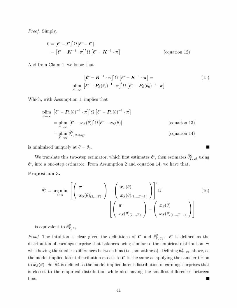
Proof. Simply,

0 = [`∗ − `∗]′Ω [`∗ − `∗]

=[`∗ −K−1 · π

]′Ω[`∗ −K−1 · π

](equation 12)

And from Claim 1, we know that

[`∗ −K−1 · π

]′Ω[`∗ −K−1 · π

]= (15)

plimS→∞

[`∗ − PS(θ0)−1 · π

]′Ω[`∗ − PS(θ0)−1 · π

]Which, with Assumption 1, implies that

plimS→∞

[`∗ − PS(θ)−1 · π

]′Ω[`∗ − PS(θ)−1 · π

]= plim

S→∞[`∗ − xS(θ)]′Ω [`∗ − xS(θ)] (equation 13)

= plimS→∞

θST , 2-stage (equation 14)

is minimized uniquely at θ = θ0.

We translate this two-step estimator, which first estimates `∗, then estimates θST , 2S using

`∗, into a one-step estimator. From Assumption 2 and equation 14, we have that,

Proposition 3.

θST ≡ arg minθ∈Θ

π

xS(θ)(2,...,T )

− xS(θ)

xS(θ)(1,...,T−1)

′Ω (16)

π

xS(θ)(2,...,T )

− xS(θ)

xS(θ)(1,...,T−1)

is equivalent to θST , 2S

Proof. The intuition is clear given the definitions of `∗ and θST , 2S. `∗ is defined as the

distribution of earnings surprise that balances being similar to the empirical distribution, π

with having the smallest differences between bins (i.e., smoothness). Defining θST , 2S, above, as

the model-implied latent distribution closest to `∗ is the same as applying the same criterion

to xS(θ). So, θST is defined as the model-implied latent distribution of earnings surprises that

is closest to the empirical distribution while also having the smallest differences between

bins.

41

Figure 1: Benefits of Earnings Surprise

This figure presents a regression discontinuity plot of cumulative earnings announcement returns aroundEPS surprise. The running variable is EPS Surprise, which is defined as realized earnings-per-share (EPS)minus analysts’ consensus EPS forecast, and the dependent variable is CMAR3 day, which is defined asthree day cumulative market-adjusted returns. The scatterplot presents dots that correspond to the av-erage CMAR3 day within each EPS Surprise bin and two fitted polynomials in grey, which represent thebest-fitting (both second degree) polynomials on either side of the EPS surprise cutoff of zero cents. Theintersection of the fitted polynomials at EPS Surprise = 0 represents our preferred discontinuity estimateof the benefits of meeting analysts’ consensus EPS forecast.

-.02

-.01

0.0

1.0

2.0

33-

day

Cum

ulat

ive

Abn

orm

al R

etur

n

-20 -15 -10 -5 0 5 10 15 20EPS Surprise (cents)

42

Figure 2: Fitted EPS Surprise Frequencies

This figure presents a regression discontinuity plot that corresponds to a McCrary [2008] test of manipu-lation of earnings-per-share (EPS) around analysts’ consensus earnings forecasts. The running variable isEPS Surprise, which is defined as reported earnings minus analysts’ consensus earnings forecast, and thedependent variable is the frequency of firm-quarter observations in each earnings surprise bin. The scatter-plot presents dots that correspond to the frequency of observations within each EPS Surprise bin and twofitted polynomials in grey, which represent the best-fitting (both sixth degree) polynomials on either sideof the EPS surprise cutoff of zero cents. The intersection of the fitted polynomials at EPS Surprise = 0represents our preferred diagnostic test statistic of the prevalence of earnings management around the zeroearnings surprise cutoff.

0.0

2.0

4.0

6.0

8.1

Fre

quen

cy

-20 -15 -10 -5 0 5 10 15 20

EPS Surprise (cents)

43

Figure 3: Latent and Empirical Distributions

This figure presents the empirical and latent distributions of earnings surprise, which is defined as therealized earnings-per-share (EPS) minus analysts’ consensus EPS forecast. The empirical distribution isestimated using a regression discontinuity approach (McCrary [2008]) which allows for a discontinuity in thefrequencies of observations around the zero earnings surprise cutoff. The latent distribution is an output ofour structural estimation that accounts for managers’ optimal manipulation decisions and trades off distanceto the empirical distribution with smoothness. Panel A presents these distributions from -20 to 20 cents ofearnings surprise, whereas Panel B presents them from -5 to 5 cents of earnings surprise.

(a) -20 to 20 cents

Latent

Empirical

−20 −15 −10 −5 0 5 10 15 20

0

2

4

6

8

Earnings Surprise

Per

cent

offi

rms

(b) -5 to 5 cent bins

Latent

Empirical

−5 −4 −3 −2 −1 0 1 2 3 4 5

0

2

4

6

8

Earnings Surprise

Per

cent

of

firm

s

44

Figure 4: Cent Manipulation

This figure presents the empirical distribution of earnings surprise, which is defined as the realized earnings-per-share (EPS) minus analysts’ consensus EPS forecast, between -5 and 5 cents of earnings surprise. Thefigures highlight the fraction of manipulating firms in each earnings surprise bin and the mean amount ofmanipulation that the manipulating firms choose in shades of red. Panel A presents manipulation acrossthe empirical distribution manipulation and Panel B normalizes the empirical distribution to highlight theprevalence and amount of manipulation in each surprise bin.

(a) Manipulation by Bin

−5 −4 −3 −2 −1 0 1 2 3 4 5

0

2

4

6

8

Earnings Surprise

Per

cent

offi

rms

no change1 cent change2 cents change3 cents change4 cents change

(b) Normalized Manipulation by Bin

−5 −4 −3 −2 −1 0 1 2 3 4 5

0.85

0.9

0.95

1

Earnings Surprise

Fra

ctio

nof

firm

sin

each

bin

no change1 cent change2 cents change3 cents change4 cents change

45

Figure 5: Counterfactual Parameters

This figure contrasts the empirical distribution of earnings surprise, which is defined as the realized earnings-per-share (EPS) minus analysts’ consensusEPS forecast, between -20 and 20 cents of earnings surprise with counterfactual distributions of earnings surprise that arise by cutting each estimatedstructural parameter to 10% of its estimated value and then recalculating optimal manipulation. The dashed blue lines represent counterfactualempirical distributions and the solid red lines represent the empirical distribution. These counterfactuals provide intuition for the role of each costfunction parameter in shaping earnings manipulation behavior. Panel A, B, C, and D present the counterfactuals of setting η, γ, ψ2, and ζ to 10%of estimated values, respectively.

(a) η at 10% (b) γ at 10%

−20 −15 −10 −5 0 5 10 15 20

0

2

4

6

8

10

12

Earnings Surprise

Per

cent

offi

rms

−20 −15 −10 −5 0 5 10 15 20

0

2

4

6

8

10

12

Earnings Surprise

Per

cent

offi

rms

(c) ψ2 at 10% (d) ζ at 10%

−20 −15 −10 −5 0 5 10 15 20

0

2

4

6

8

10

12

Earnings Surprise

Per

cent

offi

rms

Counterfactual

Empirical

−20 −15 −10 −5 0 5 10 15 20

0

2

4

6

8

10

12

Earnings Surprise

Per

cent

offi

rms

46

Table 1: Summary Statistics

This table presents summary statistics (i.e., mean, standard deviation, 25th percentile, median, and 75thpercentile) of key characteristics used in our regression discontinuity tests to follow.

Mean SD 25% Median 75%

EPS Surprise -0.236 7.521 -4 0 3

EPS Surprise ≥ 0 58.40% - - - -

CMAR3 day 0.552 8.327 -2.797 0.457 3.811

47

Table 2: The Benefits of Beating Earnings Benchmarks

This table presents regression discontinuity tests of three day cumulative earnings announcement returns around earnings benchmarks. The runningvariable is EPS Surprise, which is defined as realized earnings-per-share (EPS) minus analysts’ consensus EPS forecast, and the dependent variableis CMAR3 day, which is defined as three day cumulative market-adjusted returns. We estimate the discontinuity in CMAR3 day at the cutoffEPS Surprise = 0. Panel A uses global polynomial controls. Panel B uses local linear controls with bandwidth restrictions. Robust standard errorsare clustered at the firm level and are reported in parentheses. ***,**,* represent statistical significance at the 1%, 5%, and 10% levels, respectively.

Panel A. Benefits test - Global Polynomial Controls

Dependent variable: CMAR3 day

(1) (2) (3) (4) (5) (6) (7) (8)

EPS Surprise ≥ 0 2.494*** 2.678*** 1.815*** 2.006* 1.447** 1.514*** 1.173*** 1.300***

(0.083) (0.099) (0.120) (0.144) (0.168) (0.198) (0.228) (0.271)

Fixed effects :

Firm X X X X

Y ear − quarter X X X X

Polynomial degree 0 0 1 1 2 2 3 3

R2 0.0210 0.2235 0.0233 0.2254 0.0241 0.2260 0.0242 0.2261

Observations 103,819

Bins 41

48

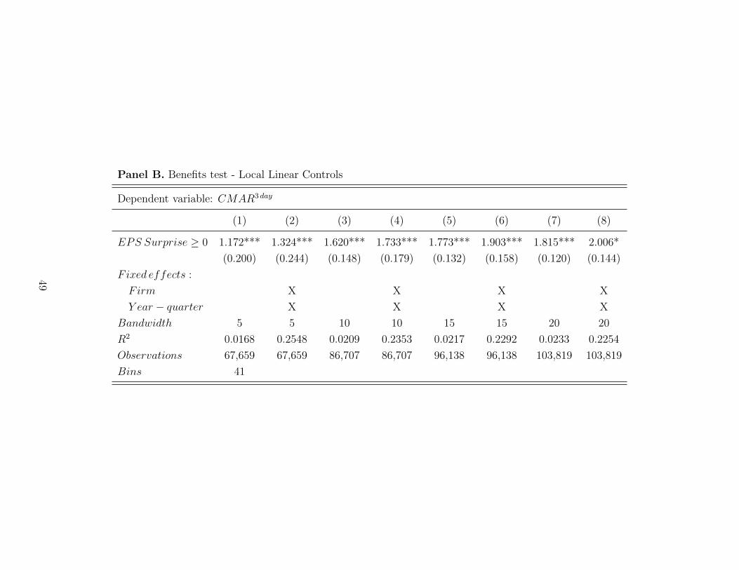
Panel B. Benefits test - Local Linear Controls

Dependent variable: CMAR3 day

(1) (2) (3) (4) (5) (6) (7) (8)

EPS Surprise ≥ 0 1.172*** 1.324*** 1.620*** 1.733*** 1.773*** 1.903*** 1.815*** 2.006*

(0.200) (0.244) (0.148) (0.179) (0.132) (0.158) (0.120) (0.144)

Fixed effects :

Firm X X X X

Y ear − quarter X X X X

Bandwidth 5 5 10 10 15 15 20 20

R2 0.0168 0.2548 0.0209 0.2353 0.0217 0.2292 0.0233 0.2254

Observations 67,659 67,659 86,707 86,707 96,138 96,138 103,819 103,819

Bins 41

49

Table 3: Distributional Evidence of Manipulation Around Earnings Benchmarks

This table presents McCrary [2008] tests of manipulation of earnings-per-share (EPS) around analysts’ consensus earnings forecasts. The runningvariable is EPS Surprise, which is defined as reported earnings minus analysts’ consensus earnings forecast, and the dependent variable is thefrequency of firm-quarter observations in each earnings surprise bin. We estimate the discontinuity in πi at the cutoff EPS Surprise = 0. Panel Auses global polynomial controls. Panel B uses local linear controls with bandwidth restrictions. Robust standard errors are presented in parentheses.***,**,* represent statistical significance at the 1%, 5%, and 10% levels, respectively.

Panel A. Manipulation test - EPS Surprise - Global Polynomial Controls

Dependent variable: πi

(1) (2) (3) (4) (5) (6) (7) (8) (9) (10) (11)

EPS Surprise ≥ 0 0.438 1.614* 2.416*** 2.775*** 2.818*** 2.625*** 2.631*** 3.093*** 1.789* 2.901 2.728**

(0.553) (0.939) (0.884) (0.697) (0.474) (0.371) (0.555) (0.610) (1.080) (2.435) (1.055)

Polynomial degree 0 1 2 3 4 5 6 7 8 9 10*

R2 0.4324 0.6987 0.9186 0.9720 0.9854 0.9886 0.9899 0.9902 0.9914 0.9917 0.9913

Observations 103,819

Bins 41

*k = 10 and j = 8 due to degrees of freedom restriction.

50

Panel B. Manipulation Test - EPS Surprise - Local Linear Controls

Dependent variable: πi

(1) (2) (3) (4)

EPS Surprise ≥ 0 2.752** 2.322*** 1.831* 1.614*

(0.896) (0.992) (0.964) (0.939)

Bandwidth 5 10 15 20

R2 0.9248 0.8378 0.7793 0.6987

Observations 103,819

Bins 41

51

Table 4: Variable Definitions

This table presents definitions of variables and parameters used in estimation of the model.

Notation Definition

B Estimated capital market benefit of just-meeting the earn-ings benchmark (in equity market returns)

∆ Estimated discontinuity in the earnings distribution (in %of firms)

η Firm marginal cost to manage earnings (in equity marketreturns)

γ Exponential slope parameter for cost to manage earnings(> 1 implies increasing costs of earnings managment)

ψ2 Stochastic noise of earnings management (in cents)

ζ Heteroskedasticity of earnings management noise (increasesnoise with greater manipulation)

52

Table 5: Structural Estimates

This table presents our structural estimates as well as statistics regarding the percentage of manipulators,the expected amount of manipulation by manipulators and the fraction of manipulators shocked out of theirtarget bin by noise.

η γ ψ2 ζ %manip manip %noise

Baseline 0.0161 2.0817 0.8201 3.7105 2.62% 1.21 59.6%

(0.0004) (0.0517) (0.0236) (0.0941)

robustness

-15 to 15 cents 0.0157 2.2398 0.7761 3.8515 2.71% 1.15 55.7%

-10 to 10 cents 0.0154 1.9381 0.7942 3.9199 2.84% 1.27 60.0%

-5 to 5 cents 0.0167 2.0950 0.7599 4.1904 2.56% 1.19 57.3%

Overweight empirical 0.0170 2.2847 0.7992 2.6322 2.45% 1.15 57.3%

Overweight smoothness 0.0146 1.8871 0.7901 2.5761 3.11% 1.31 58.9%

ζ = 0 0.0211 2.0907 0.2983 0 2.29% 1.29 26.4%

alternate distributions

Reduce peak 0.0205 2.1867 0.8178 2.2439 1.91% 1.17 73.5%

Kill peak 0.0273 2.0523 1.1699 0.9738 1.36% 1.20 64.3%

53

Table 6: Benefits Heterogeneity

This table presents our robustness estimates as well as statistics regarding the percentage of manipulators,the expected amount of manipulation by manipulators and the fraction of manipulators shocked out of theirtarget bin by noise. In the first set of alternative tests, we allow for heterogeneity in benefits. For the Normalrows, we assume that firms draw a random benefit that is normally distributed according to the mean andstandard deviation of our preferred benefit estimate (Table 2, Panel A, Column 5). For the Bernoulli rows,we assume that firms draw a random benefit that is either “high” or zero, with standard error as before. Inthe second row for each distribution, we multiply standard errors on benefits by a factor of five. In the lastfour rows, we use the normally distributed benefits and allow for a correlation with costs of either 0.5 or -0.5(and again with alternate specifications using inflated standard deviations).

η γ ψ2 ζ %manip manip %noise

Baseline 0.0161 2.0817 0.8201 3.7105 2.62% 1.21 59.6%

heterogeneity in benefits

Normal 0.0148 2.1297 0.7600 4.5100 2.88% 1.19 57.5%

Normal (x5 std. err.) 0.0152 1.9273 0.8068 4.4838 2.85% 1.31 59.7%

Bernoulli 0.0153 1.9731 0.8045 3.4927 2.81% 1.27 60.1%

Bernoulli (x5 std. err.) 0.0151 2.0110 0.8004 3.0636 2.83% 1.28 59.6%

correlated heterogeneity

0.5 correlation 0.0153 2.0135 0.7930 4.4206 2.84% 1.23 59.3%

0.5 correlation (x5 std. err.) 0.0141 1.9505 0.8178 4.6580 3.20% 1.31 59.7%

-0.5 correlation 0.0160 2.2237 0.7945 3.5933 2.64% 1.16 58.9%

-0.5 correlation (x5 std. err.) 0.0173 2.1715 0.7854 4.2884 2.45% 1.19 58.8%

54

Table 7: Counterfactuals

This table shows parameter estimates and statistics based on counterfactual simulations. These simulationsinvolve, one at a time, reducing the value of each parameter to 10% of its estimated value. The first rowreproduces the baseline estimates for comparison purposes.

η γ ψ2 ζ %manip manip %noise

Baseline 0.0161 2.0817 0.8201 3.7105 2.62% 1.21 59.6%

η at 10% 0.0016 2.0817 0.8201 3.7105 12.6% 1.92 64.3%

γ at 10% 0.0161 0.2082 0.8201 3.7105 9.45% 10.16 78.4%

ψ2 at 10% 0.0161 2.0817 0.0820 3.7105 3.22% 1.23 6.9%

ζ at 10% 0.0161 2.0817 0.8201 0.3711 2.56% 1.29 57.8%

55

Table 8: Identifying Manipulators by Earnings Surprise Bins

This table illustrates the performance of various definitions of “suspect” bins on identifying manipulation.The second set of percentages weights manipulation by the amount of manipulation, i.e. a firm manipulatingtwo cents gets twice the weight of a firm only manipulating one cent.

[0,1) [0, 2) [0, 3) [−1, 1) [−1, 2) [−1, 3)

% Manipulating 11.0% 9.9% 8.1% 8.7% 8.5% 7.3%

% of Manipulators 53.1% 80.9% 86.4% 64.2% 92.0% 97.4%

% Manipulating (weighted) 12.8% 14.2% 12.4% 10.2% 12.1% 11.1%

% of Manipulators (weighted) 39.6% 77.3% 88.3% 48.3% 86.0% 97.0%

56

Table 9: SOX and the Cost of Earnings Management

This table shows how the costs of earnings management changed around SOX. The pre-SOX period is 1999-2001 and the post-SOX period is 2002-2004. ∆ is the estimated discontinuity in the earnings distribution,estimated as in Table 3. B is the benefit to meeting the analyst benchmark, estimated as in Table 2. η,γ, ψ2 and ζ are the estimated parameters of the cost function. The final three rows describe the estimatedequilibrium manipulation in each period.

Pre-SOX Post-SOX Diff. p-value

∆ 4.196 3.012 -1.184 0.008

B 1.229 2.027 0.798 0.034

η 0.0097 0.0278 0.0181 <0.0001

γ 1.942 2.808 0.865 <0.0001

ψ2 0.646 0.202 -0.444 <0.0001

ζ 3.040 1.316 -1.724 <0.0001

%manip 4.05% 2.61% -1.44% -

manip 1.29 1.06 -0.23 -

%noise 54.2% 16.0% -38.1% -

57