Understanding the Dynamic Process of Dissolution Using In ...

Seton Hall UniversityeRepository @ Seton HallSeton Hall University Dissertations and Theses(ETDs) Seton Hall University Dissertations and Theses

Spring 5-15-2017

Understanding the Dynamic Process ofDissolution Using In-situ FT-IR SpectroscopyVrushali M. [email protected]

Follow this and additional works at: https://scholarship.shu.edu/dissertations

Part of the Medicinal-Pharmaceutical Chemistry Commons

Recommended CitationBhawtankar, Vrushali M., "Understanding the Dynamic Process of Dissolution Using In-situ FT-IR Spectroscopy" (2017). Seton HallUniversity Dissertations and Theses (ETDs). 2294.https://scholarship.shu.edu/dissertations/2294

https://scholarship.shu.edu?utm_source=scholarship.shu.edu%2Fdissertations%2F2294&utm_medium=PDF&utm_campaign=PDFCoverPages

https://scholarship.shu.edu/dissertations?utm_source=scholarship.shu.edu%2Fdissertations%2F2294&utm_medium=PDF&utm_campaign=PDFCoverPages


https://scholarship.shu.edu/etds?utm_source=scholarship.shu.edu%2Fdissertations%2F2294&utm_medium=PDF&utm_campaign=PDFCoverPages


http://network.bepress.com/hgg/discipline/136?utm_source=scholarship.shu.edu%2Fdissertations%2F2294&utm_medium=PDF&utm_campaign=PDFCoverPages

https://scholarship.shu.edu/dissertations/2294?utm_source=scholarship.shu.edu%2Fdissertations%2F2294&utm_medium=PDF&utm_campaign=PDFCoverPages

i

Understanding the Dynamic Process of Dissolution

Using In-situ FT-IR Spectroscopy

By

Vrushali M. Bhawtankar

Ph.D. Dissertation

Submitted in partial fulfillment of the requirements for the degree of Doctor of Philosophy in the

Department of Chemistry and Biochemistry of Seton Hall University

May, 2017

South Orange, New Jersey

ii

©2017 Vrushali M. Bhawtankar

yatt R. r;fu'rph ,Ph.D.

ember of Dissertation Committee, Seton Hall University

Dissertation Committee Approvals

We certify that we have read this thesis and that in our opinion it is sufficient in scientific scope

and quality as a dissertation for the degree of Doctor of Philosophy

APPROVED BY:

Nicholas H. Snow, Ph.D.

Advisor, Seton Hall University

e:::2&v cJ,be-ur. Stephen Kelty, Ph.D.

Member of Dissertation Committee, Seton Hall University

C4 7J;~uL<'Dr. Cecilia Marzabadi, Ph.D.

Chair, Department of Chemistry and Biochemistry, Seton Hall University

Dissertation Committee Approvals We certify that we have read this thesis and that in our opinion it is sufficient in scientific scope

and quality as a dissertation for the degree of Doctor of Philosophy

APPROVED BY:

Nicholas H. Snow, Ph.D.

Advisor, Seton Hall University

yatt R. �rph/, Ph.D. ember of Dissertation Committee, Seton Hall University

-�>I:t1 «'=\,� ( ---- . ·- ----·nr. Stephen Kelty, Ph.D.

Member of Dissertation Committee, Seton Hall University

(l4 na�-z,th, ,/',

Dr. Cecilia Marzabadi, Ph.D.

Chair, Department of Chemistry and Biochemistry, Seton Hall University

..

iv

Dedicated to my dear husband Mangesh for his encouragement and support

to pursue higher education.

v

Abstract

Dissolution studies provide valuable and critical drug release information (in vitro) that are

important for quality control drug development. Using in-situ FT-IR spectroscopy methods has

been developed for analyzing and monitoring dissolutions of pharmaceutical APIs. The accuracy

of this technique was found to be ± 3% relative to HPLC and UV/Vis Spectroscopy. A dynamic

analysis of the dissolution and subsequent hydrolysis of aspirin has been determined by in-situ FT-

IR. This technique allows real-time analysis of the behavior of aspirin under simulated

physiological conditions (pH 1.2, 4.5, 6.8) as aspirin (1205 cm-1) and salicylic acid (1388 cm-1)

are detected as separate and distinct peaks in the in-situ FT-IR.

For this study, 325 mg Bayer aspirin tablet was used. The data shows dissolution of aspirin with

the hydrolysis profile and the formation of salicylic acid. Comparison of the dissolution behavior

of generic brands of aspirin has been performed. The formulations contain the same amount of

drug substance as present in Bayer aspirin. Dissolution and hydrolysis of enteric coated aspirin

tablets has been performed, and compared with the Bayer aspirin tablets. The dissolution was

carried out as per the USP procedure.

This technique indicates a future potential for real-time studies of dissolution and hydrolysis of

other prodrugs such as Loratadine. The in-situ FT-IR system is extremely capable of measuring

low concentrations (0.03 mg/ml) and for distinguishing separate components of a multiple

component systems without requiring manual sampling. Specifically, the unique fingerprint region

of the in-situ FT-IR spectra provides detailed information about the release profile of the drug.

One more demonstration of the in-situ FT-IR novel technique is the dissolution study of Loratadine

vi

(hydrolysis of Loratadine), a pro-drug that has a tendency to hydrolyze to an active compound

desloratadine.

In addition, research on the acetaminophen dissolution observed on extra strength Tylenol and on

Tylenol Arthritis has been validated by UV/Vis spectroscopy and HPLC. In this study the non-

linear behavior of Beer-Lamberts’s law was observed. The hypothesis has been established that

the acetaminophen forms dimer at higher concentrations. The investigation was carried out by

NMR and FTIR Spectroscopy and by measuring colligative properties such as vapor pressure

osmometer and freezing point depression.

In-situ FT-IR spectroscopy is a novel technique used for monitoring the dissolution testing. The

fingerprint region of the in-situ FT-IR has great potential for studying dissolution kinetics as well

as hydrolysis kinetics for aspirin. A separate peak for aspirin as well as salicylic acid has been

observed. This technique has excellent potential for the dissolution studies of tablets without

disturbing the dissolution media.

vii

Acknowledgement

During my graduate career at Seton Hall University, I have had the privilege and opportunity to

develop myself as a research scientist. First and foremost, I would like to thank Dr. Nicholas Snow

for adopting me into his research group. His constant support, motivation, and enthusiasm were

irreplaceable and greatly appreciated. I would like to express my sincere gratitude to my advisor

for his patient guidance, encouragement and generous advice he has provided and inspiring me to

become better.

I would like to give special thanks to my former research advisor Dr. John R. Sowa, Jr. for the

continuous support, valuable guidance, expertise, encouragement of my Ph.D. study and research.

I will be forever grateful for his motivation, enthusiasm, and assistance. I would like to

acknowledge Wes Walker and Jane Riley from Mettler-Toledo for technical support for the iC10IR

Instrument.

Specifically, I would like to give a special appreciation of my thesis committee to Dr. Wyatt

Murphy and Dr. Stephen Kelty for their scientific advice, knowledge and many insightful

suggestions with encouraging, motivating and supporting my research ambitions. I would also like

to acknowledge Dr. Cecilia Marzabadi, Dr. Yufeng Wei, Dr. Yuri Kazakevich Dr. James Hanson,

Dr. Alexander Fadeev, Dr. Rosario Lobrutto. Dr. David Sabatino and Dr. Sergiu Gorun for their

guidance and mentoring throughout my studies. I will forever be indebted to those who have

supported me through the years in this endeavor. It is with great appreciation that I offer my

gratitude to all.

viii

I would also like to acknowledge separation science group and Dr. Sowa’s research group for

motivating me as well as the faculty members of the Department of Chemistry and Biochemistry

and all my friends at Seton Hall University.

A great deal of credit goes to my husband, Mangesh for his sacrifice over past few years. I would

like to especially thank him for encouraging me in all of my pursuits and inspiring me to follow

my dreams by the emotional and financial support. I offer my acknowledgement to my mom, dad

and my in-laws for their unequivocal and unconditional love and support throughout my life.

ix

Table of Contents

Abstract ........................................................................................................................................... v

Acknowledgement ........................................................................................................................ vii

List of Figures ............................................................................................................................... xv

List of Tables ............................................................................................................................... xix

CHAPTER 1 ................................................................................................................................... 1

INTRODUCTION .......................................................................................................................... 1

1.1 Introduction .................................................................................................................. 1

1.2 Dissolution Models and Theories ................................................................................. 3

1.3 Mathematical Models of Dissolution ........................................................................... 8

1.4 USP Dissolution Information ..................................................................................... 13

1.5 Infrared Spectroscopy ................................................................................................. 22

1.5.1 Attenuated Total Reflectance-Infrared (ATR-IR) spectroscopy ............................. 24

1.6 Drugs used in this Research ........................................................................................ 30

1.6.1 Acetaminophen ....................................................................................................... 30

1.6.2 Aspirin and Salicylic Acid ...................................................................................... 34

CHAPTER– 2 ............................................................................................................................... 42

DISSOLUTION AND NONLINEAR BEHAVIOR OF ACETAMINOPHEN ........................... 42

x

2.1 Introduction ................................................................................................................ 42

2.2 Experimental Section .................................................................................................. 42

2.2.1 Chemicals and materials ......................................................................................... 42

2.2.2 Instrumentation ....................................................................................................... 43

2.2.3 Potassium phosphate buffer (pH 5.8)...................................................................... 44

2.2.4 Acetaminophen solutions for calibration ................................................................ 44

2.2.5 Standard solutions ................................................................................................... 44

2.2.6 Dissolution of acetaminophen (Extra Strength Tylenol) ........................................ 44

2.2.7 Dissolution of acetaminophen (Arthritis Tylenol) .................................................. 45

2.2.8 In-situ FT-IR analysis ............................................................................................. 45

2.2.9 HPLC analysis ........................................................................................................ 45

2.3 Results and Discussion ............................................................................................... 46

2.3.1 Calibration of acetaminophen ................................................................................. 46

2.3.2 Dissolution of Extra Strength Tylenol .................................................................... 49

2.3.3 Dissolution of Tylenol (Arthritis Pain) ................................................................... 52

2.4 Non-Linear behavior of Acetaminophen .................................................................... 54

2.5 Conclusion .................................................................................................................. 59

CHAPTER - 3 ............................................................................................................................... 60

DISSOLUTION AND HYDROLYSIS STUDY OF ASPIRIN ................................................... 60

xi

3.1 Introduction ................................................................................................................ 60

3.2 Experimental Section .................................................................................................. 61

3.2.1 Chemicals and materials ............................................................................................. 61

3.2.2 Instrumentation ....................................................................................................... 62

3.2.3 Simulated gastric fluid ............................................................................................ 62

3.2.4 Sodium acetate buffer ............................................................................................. 62

3.2.5 Potassium phosphate buffer .................................................................................... 63

3.2.6 Aspirin solution for calibration ............................................................................... 63

3.2.7 Salicylic acid solution for calibration ..................................................................... 64

3.2.8 Hydrolysis of aspirin to salicylic acid in test tubes................................................. 64

3.2.9 Standard solutions ................................................................................................... 65

3.2.10 Dissolution and hydrolysis of aspirin ..................................................................... 65

3.2.11 In-situ FT-IR Analysis ............................................................................................ 65

3.2.11.1 Aspirin analysis ............................................................................................... 65

3.2.11.2 Salicylic acid analysis ...................................................................................... 66

3.2.11.3 Dissolution and hydrolysis of aspirin tablet .................................................... 66

3.2.12 HPLC analysis ........................................................................................................ 67

3.3 Results and Discussion ............................................................................................... 68

3.3.1 Calibration of aspirin .............................................................................................. 68

3.3.2 Calibration of salicylic acid .................................................................................... 69

xii

3.3.3 Hydrolysis of aspirin to salicylic acid in test tube ................................................. 76

3.3.4 Dissolution and hydrolysis of aspirin tablet in simulated gastric fluid pH 1.2 ...... 78

3.3.5 Dissolution and hydrolysis of aspirin tablet in sodium acetate buffer pH 4.5........ 84

3.3.6 Dissolution and hydrolysis of aspirin tablet in potassium phosphate buffer pH 6.8

………………………………………………………………………………………90

3.3.7 Kinetic study ........................................................................................................... 96

3.4 Conclusion ................................................................................................................ 101

CHAPTER – 4 ............................................................................................................................ 103

HYDROLYSIS STUDY OF ASPIRIN ...................................................................................... 103

4.1 Introduction .............................................................................................................. 103

4.2 Experimental Section ................................................................................................ 104

4.2.1 Chemicals and materials ....................................................................................... 104

4.2.2 Instrumentation ..................................................................................................... 105

4.2.3 Simulated gastric fluid .......................................................................................... 106

4.2.4 Sodium acetate buffer ........................................................................................... 106

4.2.5 Potassium phosphate buffer .................................................................................. 106

4.2.6 Standard solutions ................................................................................................. 107

4.2.7 Dissolution and hydrolysis of all brands of aspirin tablets ................................... 107

4.2.8 In-situ FT-IR analysis ........................................................................................... 107

xiii

4.3 Results and Discussion ............................................................................................. 108

4.3.1 Comparison between Bayer aspirin and Bayer advanced aspirin tablets ............. 108

4.3.2 Comparison between Bayer aspirin and generic aspirin tablets ........................... 110

4.3.3 Dissolution of enteric-coated tablets ..................................................................... 114

4.3.4 Kinetic study ............................................................................................................. 118

4.4 Conclusion ................................................................................................................ 120

CHAPTER - 5 ............................................................................................................................. 121

DISSOLUTION OF LORATADINE ......................................................................................... 121

5.1 Introduction ........................................................................................................................... 121

5.2 Experimental Section ................................................................................................ 122

5.2.1 Chemicals and materials ....................................................................................... 122

5.2.2 Instrumentation ..................................................................................................... 123

5.2.3 0.1 N hydrochloric acid......................................................................................... 123

5.2.4 Loratadine solution for calibration ........................................................................ 123

5.2.5 Standard solutions ................................................................................................. 124

5.2.6 Dissolution of loratadine ....................................................................................... 124

5.2.7 In-situ FT-IR analysis ........................................................................................... 124

5.3 Results and Discussion ............................................................................................. 127

5.3.1 Calibration of loratadine ....................................................................................... 127

xiv

5.3.2. Dissolution of loratadine ....................................................................................... 127

5.4 Conclusion ................................................................................................................ 130

Research Summary ..................................................................................................................... 131

References ................................................................................................................................... 133

Appendix 150

Standard Operating Procedure for ReactIR ................................................................................ 150

xv

List of Figures

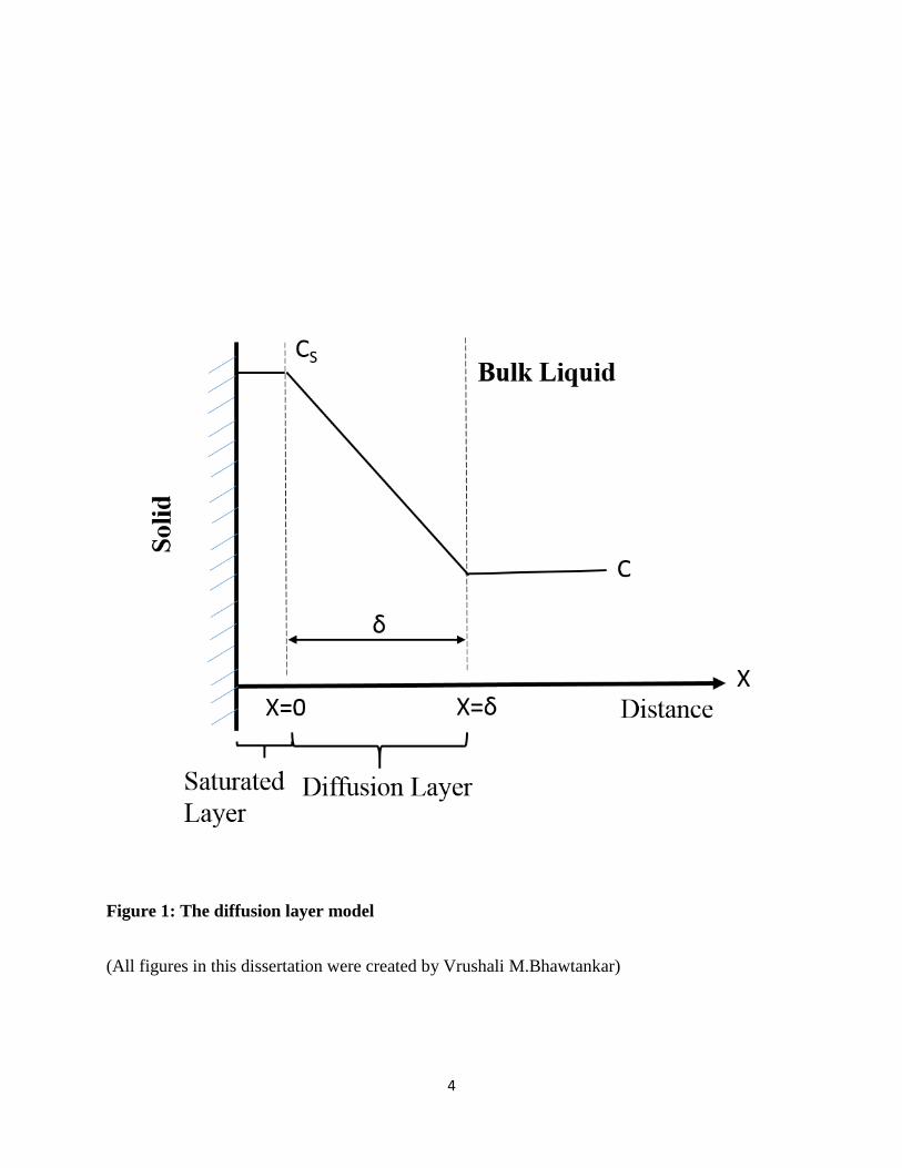
Figure 1: The diffusion layer model ............................................................................................... 4

Figure 2: The interfacial barrier model ........................................................................................... 6

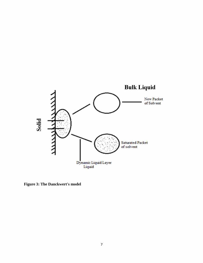
Figure 3: The Danckwert's model ................................................................................................... 7

Figure 4: Schematic illustration of apparatus 1 and apparatus 2 .................................................. 16

Figure 5: USP apparatus 1 basket stirring elements (© 104 U.S. Pharmacopeial Convention,

Used with Permission) .................................................................................................................. 18

Figure 6: USP apparatus 2 specifications (© 104 U.S. Pharmacopeial Convention, Used with

Permission) ................................................................................................................................... 19

Figure 7: Schematic diagram of flow-through cell apparatus-4 ................................................... 21

Figure 8: FT-IR schematic diagram .............................................................................................. 23

Figure 9: A multiple reflection ATR system ................................................................................ 26

Figure 10: A representation of ATR with in-situ FT-IR ............................................................... 27

Figure 11: Structures of drugs used in this research ..................................................................... 31

Figure 12: In-situ FT-IR spectra of acetaminophen ...................................................................... 32

Figure 13: IR spectra of acetaminophen from SDBS database [45] ............................................. 33

Figure 14: Synthesis of aspirin in 1800’s [48] .............................................................................. 35

Figure 15: Acid-catalyzed aspirin hydrolysis ............................................................................... 37

Figure 16: Base-catalyzed aspirin hydrolysis ............................................................................... 38

Figure 17: In-situ FT-IR spectra of aspirin and salicylic acid ...................................................... 39

Figure 18: IR spectra of aspirin from SDBS database [51] .......................................................... 40

Figure 19: IR spectra of salicylic acid from SDBS database [51] ................................................ 41

Figure 20: Non-linear graph for different levels of acetaminophen reference standards ............. 47

xvi

Figure 21: Linear calibration graph of acetaminophen at low concentrations.............................. 48

Figure 22: Dissolution of acetaminophen ..................................................................................... 50

Figure 23: Dissolution of acetaminophen after polynomial calculations ..................................... 51

Figure 24: Dissolution data of acetaminophen (Arthritis pain) .................................................... 53

Figure 25: Calibration graph of aspirin in simulated gastric fluid (pH 1.2) ................................. 70

Figure 26: Calibration of aspirin in sodium acetate buffer (pH 4.5) ............................................ 71

Figure 27: Calibration of aspirin in potassium phosphate buffer (pH 6.8) ................................... 72

Figure 28: Calibration graph of salicylic acid in simulated gastric fluid (pH 1.2) ....................... 73

Figure 29: Calibration graph of salicylic acid sodium acetate buffer (pH 4.5) ............................ 74

Figure 30: Calibration graph of salicylic acid potassium phosphate buffer (pH 6.8) in [mM] .... 75

Figure 31: Ferric chloride color test on standard solutions and on samples in the flask. ............. 77

Figure 32: Dissolution and hydrolysis of data in simulated gastric fluid (pH 1.2): in-situ FT-IR

vs. HPLC ....................................................................................................................................... 80

Figure 33: Dissolution and hydrolysis of data in simulated gastric fluid (pH 1.2): in-situ FT-IR,

Overlay .......................................................................................................................................... 81

Figure 34: Dissolution and hydrolysis of data in simulated gastric fluid (pH 1.2): in-situ FT-IR,

Combined study ............................................................................................................................ 82

Figure 35: Dissolution and hydrolysis of data in sodium acetate buffer (pH 4.5): in-situ FT-IR vs.

HPLC ............................................................................................................................................ 86

Figure 36: Dissolution and hydrolysis of data in sodium acetate buffer (pH 4.5): in-situ FT-IR,

overlay........................................................................................................................................... 87

Figure 37: Dissolution and hydrolysis of data in sodium acetate buffer (pH 4.5): in-situ FT-IR,

combined study ............................................................................................................................. 88

xvii

Figure 38: Dissolution and hydrolysis of data in potassium phosphate buffer (pH 6.8): in-situ FT-

IR vs. HPLC .................................................................................................................................. 92

Figure 39: Dissolution and hydrolysis of data in potassium phosphate buffer (pH 6.8): in situ,

overlay........................................................................................................................................... 93

Figure 40: Dissolution and hydrolysis of data in potassium phosphate buffer (pH 6.8): in-situ FT-

IR, combined study ....................................................................................................................... 94

Figure 41: Comparison of dissolution and hydrolysis of Bayer aspirin tablet and Bayer advanced

aspirin tablet by In-situ FT-IR in SGF ........................................................................................ 109

Figure 42: Comparison of dissolution and hydrolysis of all brands of aspirin tablets by in-situ

FT-IR in simulated gastric fluid .................................................................................................. 111


FT-IR in sodium acetate buffer ................................................................................................... 112


FT-IR in phosphate buffer .......................................................................................................... 113

Figure 45: Dissolution and hydrolysis of Ecospirin-150 tablet by in-situ compared with Bayer

aspirin in Phosphate buffer ......................................................................................................... 116

Figure 46: Dissolution and hydrolysis of Delisprin-150 tablet by in-situ FT-IR compared with

Bayer aspirin tablet in Phosphate buffer ..................................................................................... 117

Figure 47: Loratadine in-situ FT-IR peak at 1246 cm-1 for calibration ...................................... 126

Figure 48: Calibration graph of loratadine.................................................................................. 128

Figure 49: Dissolution of loratadine-combined (n=3) ................................................................ 129

Figure 50: ReactIR nozzle for liquid nitrogen ............................................................................ 150

Figure 51: ReactIR nozzle with funnel ....................................................................................... 151

xviii

Figure 52: Screenshot shows iC IR 4.0software icon ................................................................. 151

Figure 53: Screenshot of start page of ReactIR software ........................................................... 152

Figure 54: Experimental section of iC IR software .................................................................... 152

Figure 55: Screenshot of iC IR software and configuration window ......................................... 153

Figure 56: Enlarge view of configuration window ..................................................................... 154

Figure 57: Configure hardware and software setting .................................................................. 155

Figure 58: Detector settings ........................................................................................................ 155

Figure 59: Probe hardware settings............................................................................................. 156

Figure 60: Different type of IR Probes ....................................................................................... 156

Figure 61: Probe hardware settings for different types of probe ................................................ 157

Figure 62: Probe acquisition Settings ......................................................................................... 158

Figure 63: Position of the probe.................................................................................................. 158

Figure 64: Align probe window .................................................................................................. 159

Figure 65: Collect background window ...................................................................................... 160

Figure 66: Collect water vapor sample window ......................................................................... 161

Figure 67: Name experiment file ................................................................................................ 162

Figure 68: Experiment duration window .................................................................................... 163

Figure 69: Reference spectra window ......................................................................................... 164

Figure 70: Position of the probe.................................................................................................. 165

Figure 71: Clean probe window .................................................................................................. 166

Figure 72: Collect background window ...................................................................................... 167

Figure 73: Collect reference window .......................................................................................... 168

Figure 74: Edit reference window ............................................................................................... 169

xix

List of Tables

Table 1: List of dissolution apparatus as per USP [20] ................................................................ 15

Table 2: Dissolution and hydrolysis data of aspirin tablet in simulated gastric fluid ................... 83

Table 3: Dissolution and hydrolysis data of aspirin tablet in sodium acetate buffer .................... 89

Table 4: Dissolution and hydrolysis data of aspirin tablet in potassium phosphate buffer (pH 6.8)

....................................................................................................................................................... 95

Table 5: Rate of dissolution and hydrolysis in simulated gastric fluid (pH 1.2) .......................... 98

Table 6: Rate of dissolution and hydrolysis in sodium acetate buffer (pH 4.5) ........................... 99

Table 7: Rate of dissolution and hydrolysis study in potassium phosphate buffer (pH 6.8) ...... 100

Table 8: Kinetic data of all brands of aspirin tablets .................................................................. 119

xx

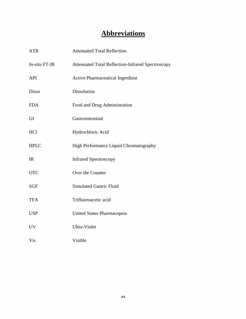
Abbreviations

ATR Attenuated Total Reflection

In-situ FT-IR Attenuated Total Reflection-Infrared Spectroscopy

API Active Pharmaceutical Ingredient

Disso Dissolution

FDA Food and Drug Administration

GI Gastrointestinal

HCl Hydrochloric Acid

HPLC High Performance Liquid Chromatography

IR Infrared Spectroscopy

OTC Over the Counter

SGF Simulated Gastric Fluid

TFA Trifluoroacetic acid

USP United States Pharmacopeia

UV Ultra-Violet

Vis Visible

1

CHAPTER 1

INTRODUCTION

1.1 Introduction

Dissolution of solids has been studied for many decades and applied to many industrial fields for

various chemical or physical applications, for example, food and pharmaceutical products.

Dissolution is the process by which a solid substance enters the solvent phase yielding a solution.

[1] In the past few years, the importance of dissolution testing has increased substantially, as seen

by the high level of regulations imposed on the pharmaceutical industry by various health agencies

around the world. Dissolution testing is critical for measuring the performance of a pharmaceutical

formulation. For a solid dosage from, it will be disintegrated into small granules then dissolution

process of the granules can be studied and its outcomes such as solubility can be obtained.

Dissolution testing plays several important roles in the pharmaceutical industry. First, the

dissolution test is a quality control tool that measures the change in stability of the formulation.

Some of the relevant changes that dissolution testing is able to detect include changes caused by

temperature, humidity, and photosensitivity. Second, the dissolution testing is also important for

formulation development. During development of a drug product, the formulators use dissolution

testing to distinguish between different variations of the drug product. The physical characteristics

of particles applied in dissolution studies are normally pointed as its objective properties. The

physical properties of particles are related to its size, shape, surface and structure. In the

pharmaceutical industry, it is important to develop with several variations of the drug product since

these are needed to access the drug’s performance in clinical trials. From the clinical trials, the

2

efficacy of the variants is distinguished and obtained. Third, once in vivo (clinical trials) data has

been established for the drug product, a correlation between in vivo (human blood data)/ in vitro

(lab dissolution results) is attempted. [2] [3] Fourth, dissolution testing is used for the development

of the quality control specifications for the manufacturing process, such as compression and

binding agents in tablets and other parameters for other dosage forms. [4] With this, dissolution

plays a very important role for measuring the stability of the investigational product. In the

manufacturing industry, another application of dissolution testing is to assess the batch-to-batch

consistency preferably in solid dosage forms. Finally, the Food and Drug Administration (FDA)

requires dissolution testing in regulatory filings for all oral dosage forms and many other dosage

forms as well.

Dissolution is the process by which a solid dosage form enters in the dissolution media to yield a

solution. It is simply a process by which a solid dosage form dissolves. It is controlled by the

affinity between the molecules comprising the solid substance and the solvent. Moreover, the

dissolution rate plays an important role in the understanding of dissolution chemistry. The

dissolution rate is defined as the amount of drug substance that goes into solution per unit time

under standardized conditions of liquid/solid interface, temperature and solvent composition.

Dissolution testing can be performed using different types of testing apparatus for pharmaceutical

dosage forms. Even though there is increased research interest in this area, the techniques used for

studying dissolution rates remain constant. In fact, there are only a few instruments used to analyze

and understand the dissolution rates of drugs. This chapter discusses the current techniques used

for dissolution testing. Additionally, a detailed literature review into the use of in-situ FT-IR

spectroscopy in general and as a dissolution technique has been made and is discussed in this

chapter. [5]

3

1.2 Dissolution Models and Theories

In the dissolution research, Higuchi provided fundamental contributions to the development of

dissolution theory. [6] According to Higuchi’s research, there are three basic models used alone or

in combination to describe the dissolution process and mechanisms. These three models are;

diffusion layer, interfacial barrier and Danckwerts.

The diffusion layer model was simply used for a crystal solid to describe the dissolution process

in the pure solvent without any reactive actions. This model was once expressed by Nernst. [7]

According to the diffusion layer model as shown in Figure 1, it is assumed that there is a saturated

layer of solvent Cs around the solid surface and equilibrium conditions occur on the surface. Then

the dissolution process is driven by the diffusion movement of molecules in the diffusion layer, δ

cm in thickness. Therefore the dissolution process can be expressed such that the first step of solid

forming an interface in the solvent is very rapid. This leads to the formation of a saturated stagnant

layer around the surface. Then slow diffusion occurs from the surface into the bulk solution

through the diffusion layer. The rate of dissolution is entirely based on the diffusion of the solid

molecule from the diffusion layer to bulk liquid.

4

Figure 1: The diffusion layer model

(All figures in this dissertation were created by Vrushali M.Bhawtankar)

5

The interfacial barrier model assumes that there is a high activation energy to promote the

interfacial transport process. [8] According to this model as shown in Figure 2, a free energy barrier

surmounts before the solid can dissolve. The surface of the solid is continually exposed to the

solvent and equilibrium is assumed at the solute-solvent interface Cs. The solute then diffuses from

free energy barrier and is carried into the solvent under the agitation. This leads to the formation

of a saturated stagnant layer around the surface. Then slow diffusion occurs from the surface into

the bulk solution through the diffusion layer. Therefore there is no layer around the surface and

the surface is continually replaced by the solvent medium.

The Danckwerts model assumes that the macroscopic packets of solvent reach the solute-solvent

interface first by eddy diffusion in some random fashion [9] as explained in Figure 3. At the

interface, the packet is able to absorb solute according to the laws of diffusion and then replaced

by new packets. This process continually occurs and the surface is continually replaced by the new

packets of solvent. Therefore the surface renewal process can be related to the solute transport

process.

These three models explain the mechanism of the drug dissolution testing, where solid drug reacts

with the fluid of dissolution medium. This reaction takes place at the solid-liquid interface.

Therefore dissolution kinetics are dependent on three things-the flow rate of the dissolution

medium towards the solid-liquid interface, the reaction rate at the interface and the diffusion of the

dissolved drug molecules from the interface towards a bulk solution. The most commonly used

model is diffusion layer model.

6

Figure 2: The interfacial barrier model

7

Figure 3: The Danckwert's model

8

1.3 Mathematical Models of Dissolution

The in vitro dissolution has been recognized as an important testing in the drug development. There

are several mathematical and kinetic models for dissolution testing are greatly developed and

explained. These models describe drug dissolution from immediate and sustained release dosage

forms. There are several models represents the drug dissolution profile, which is a function of

time-related to the amount of drug released from the pharmaceutical dosage form. [10] This section

covers a brief information about each model with the final derived equation.

There are many fundamental mathematical models based on the Noyes-Whitney equation and on

Nernst-Brunner film theory on dissolution kinetics which can be expressed as statistical methods.

These include the exploratory data analysis method, repeated measures design and multivariate

approach. Model dependent methods including the zero-order model, first-order model, Higuchi

model, Hixson-Crowell model, Baker-Lonsdale model, Korsmeyer-Peppas model and Weibull

model have been developed. Model independent methods including difference factor and

similarity factor also have been used.

The first equation for dissolution kinetics was described by Noyes and Whitney in 1897 with the

equation. [11]

𝑑𝑀

𝑑𝑡 = 𝑘𝑆( 𝐶𝑠 − 𝐶𝑡)

(1)

Where M is the is the dissolved mass, t is the dissolution time, S is the surface area of particles,

CS is the equilibrium solubility at the temperature, Ct is the concentration in solution at the time

and k is the dissolution rate constant.

9

This Noyes-Whitney law was developed from observing the dissolution of two different materials

dissolving in water. With this equation, the dissolution could be assumed to be driven by the

difference between the concentrations at the particle surface, which can be regarded as the

equilibrium solubility with the concentration in the bulk. Therefore the dissolution process was

controlled by the mass transfer from the surface of the particle to bulk.

Then, the dissolution mathematical model was greatly developed by Brunner and Nernst. In their

studies, a relationship between diffusion coefficient and the concentration in bulk was explained.

The equation to describe this theory is expressed by Nernst and Brunner as

𝑘 =

𝐷𝑆

𝑣ℎ

(2)

Where D is the diffusion coefficient, h is the diffusion layer thickness, is the volume of solution,

S is the surface area of particles and k is constant. With this model, Nernst and Brunner stated that

the dissolution process could be proposed in two steps. They assumed that the fluid in the diffusion

layer was stagnant. Furthermore, this theory also assumed that the dissolution process at the

surface of the particle is much faster than the mass transfer process and a linear concentration

gradient happens in the particle surface layer. However, this ideal condition assumption may never

occur because the surface area of the particle changes permanently with the dissolution process.

Exploratory data analysis

This method is used to understand and compare the dissolution data with a controlled dissolution

process. [12] The comparison can be achieved with dissolution data in graphical and numerical

methods. The dissolution data can be plotted for every formulation with one or two error bars at

each dissolution time point. Therefore the dissolution data can be summarized numerically and the

differences between every dissolution data profile can be compared at each dissolution time point.

10

Multivariate approach

The multivariate analysis of variance (MANOVA) is a statistical method, based on the repeated

measurements designs where the percent dissolved material is depended with the repeated factor

of time. With the repeated measurements, the factors are measured repeatedly with more than two

levels. [13] The data were collected with repeated measurements over time on the same

experimental instrument. These are compound symmetry assumptions and the assumptions of

spherocity, it refers to the condition where the variances of the differences between all possible

pairs of within subject conditions are equal. Because of these assumptions, MANOVA approach

to repeated measures has gained popularity in recent years.

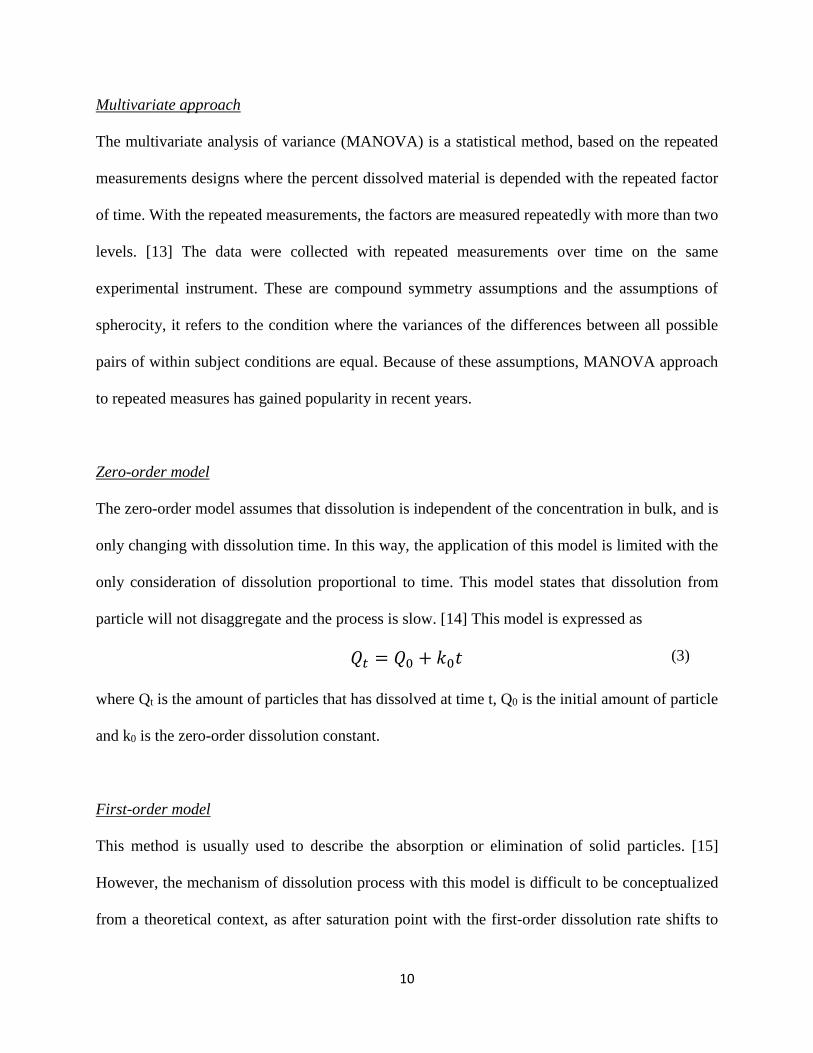
Zero-order model

The zero-order model assumes that dissolution is independent of the concentration in bulk, and is

only changing with dissolution time. In this way, the application of this model is limited with the

only consideration of dissolution proportional to time. This model states that dissolution from

particle will not disaggregate and the process is slow. [14] This model is expressed as

𝑄𝑡 = 𝑄0 + 𝑘0𝑡 (3)

where Qt is the amount of particles that has dissolved at time t, Q0 is the initial amount of particle

and k0 is the zero-order dissolution constant.

First-order model

This method is usually used to describe the absorption or elimination of solid particles. [15]

However, the mechanism of dissolution process with this model is difficult to be conceptualized

from a theoretical context, as after saturation point with the first-order dissolution rate shifts to

11

zero order. Because of this scenario, it is also called mixed-order kinetics. The first order kinetics

can be represented as follows, where dC is the change in concentration, dt is the change in time, C

is the concentration and kf is the first-order dissolution rate constant.

−

𝑑𝐶

𝑑𝑡 = 𝑘𝑓 𝐶

(4)

Higuchi model

This model was firstly expressed by Higuchi to describe drug release from a matrix system. The

assumption of this model can be described that the initial concentration should be higher than

solubility, and the diffusion occurs only in one dimension, the drug particles are much smaller than

diffusion layer thickness. [16] The model can be expressed as

𝑄 = 𝐴√𝐷(2𝐶0 − 𝐶𝑠)𝐶𝑠𝑡 (5)

where Q is amount of dissolved particles in area A at time t, C0 is the initial concentration, CS is

the solubility of particles and D is the diffusion coefficient of particle molecules. The common

application of this equation is the simplified equation where kH is the Higuchi dissolution rate

constant.

𝑄 = 𝑘𝐻𝑡1/2 (6)

The application of the Higuchi model is for the drug release from the dispersed matrices to particles

of general shape using the pseudo-steady-state approximation of Higuchi. [17]

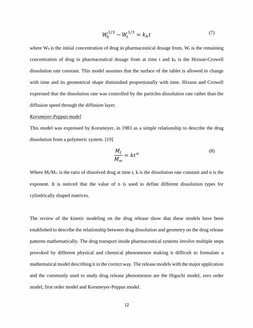
Hixson-Crowell model

This mathematical model was first expressed by Hixson and Crowell as the particle regular area is

proportional to the cube root of the volume. [18] The equation can be described as

12

𝑊01/3

− 𝑊𝑡1/3

= 𝑘ℎ𝑡 (7)

where W0 is the initial concentration of drug in pharmaceutical dosage from, Wt is the remaining

concentration of drug in pharmaceutical dosage from at time t and kh is the Hixson-Crowell

dissolution rate constant. This model assumes that the surface of the tablet is allowed to change

with time and its geometrical shape diminished proportionally with time. Hixson and Crowell

expressed that the dissolution rate was controlled by the particles dissolution rate rather than the

diffusion speed through the diffusion layer.

Korsmeyer-Peppas model

This model was expressed by Korsmeyer, in 1983 as a simple relationship to describe the drug

dissolution from a polymeric system. [19]

𝑀𝑡

𝑀∞= 𝑘𝑡𝑛

(8)

Where Mt/M is the ratio of dissolved drug at time t, k is the dissolution rate constant and n is the

exponent. It is noticed that the value of n is used to define different dissolution types for

cylindrically shaped matrices.

The review of the kinetic modeling on the drug release show that these models have been

established to describe the relationship between drug dissolution and geometry on the drug release

patterns mathematically. The drug transport inside pharmaceutical systems involve multiple steps

provoked by different physical and chemical phenomenon making it difficult to formulate a

mathematical model describing it in the correct way. The release models with the major application

and the commonly used to study drug release phenomenon are the Higuchi model, zero order

model, first order model and Korsmeyer-Peppas model.

13

1.4 USP Dissolution Information

In the history of dissolution the results reveled in late 1800’s to the mid-1900’s, the first official

dissolution testing method appeared in United States of Pharmacopeia XVIII in 1970. The United

States Pharmacopeia or USP is a non-government, official public standards–setting authority for

prescription and over-the-counter medicines and other healthcare products manufactured or sold

in the United States. [20] The USP also sets widely recognized standards for food ingredients and

dietary supplements. The USP sets standards for the quality, purity, strength, and consistency of

these products which are critical to the public health. Increased interest in dissolution regulations

continued to grow well into the 1970’s.

In 1978 the Food and Drug Administration (FDA) published the document entitled, “Guidelines

for Dissolution Testing.” [21] The intention behind this publication was to harmonize and

streamline the systems and processes of different laboratories. This was due to the fact that

dissolution results were observed to have high variability. There are minor changes in the

equipment parameters which causes higher variability. The FDA realized that more controls on

the tolerances of the dissolution equipment were needed so that results would be more

reproducible. Additionally, the FDA along with USP introduced the idea of calibrator tablets.

In 1978 the USP launched three calibrator tablets; prednisone, salicylic Acid and nitrofurantoin.

These calibrator tablets were used during the calibration of the instrument to validate the

dissolution testing system. The calibrator tablets have known specification limits and the

calibrations of the instruments have to be within those limits. To have an appreciation of the

14

complexity of the dissolution system and equipment parameters, an overview of the technology

will be given in the next section.

In 1995, the USP assigned unique numbers to the different dissolution apparatus that were

available to the scientific community. All dissolution testing apparatus are listed in Table 1. There

are seven different types of dissolution equipment that are available to the dissolution chemist. The

most widely used dissolution apparatus in the pharmaceutical industry are apparatus I, II and IV.

The use of apparatus IV has been developed more importance in recent years.

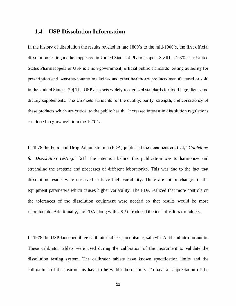
Apparatus 1 and 2 are most widely used in the pharmaceutical industry. As shown in Table 1,

Apparatus 1 uses baskets while Apparatus 2 uses paddles. Figure 4, shown below, is a schematic

and brief illustration of these two apparatuses and more precise dissolution testing vessels. The

apparatuses are comprised of a covered vessel which is cylindrical with hemispherical bottom with

capacity of minimal 1 liter, a metallic drive shaft which rotates smoothly that could affect the

results, a motor to spin the shaft, a cylindrical basket (Apparatus 1) or a paddle (Apparatus 2)

which are explained in detail in figure 5 and 6 respectively and dissolution medium.

The dissolution testing apparatus comprised a water bath or heated jacket capable of maintaining

the temperature of the vessels at 37°C ± 0.5°C. The dissolution testing apparatus is connected to

the auto sampler and if not then need to collect aliquots manually at the particular time point.

Although the figure below appears simple in design, there are strict regulations for the

specifications of each component of the apparatus and tolerances for each component are specified

by USP General Chapter Dissolution <711>. [22]

15

Table 1: List of dissolution apparatus as per USP [20]

APPARATUS NAME DRUG PRODUCT

Apparatus 1 Rotating basket Tablets, Capsules

Apparatus 2 Paddle Tablets, capsules, modified drug products

Apparatus 3 Reciprocating cylinder Extended-release drug products, Beads

Apparatus 4 Flow through cell Drug products containing low-water-soluble drug

Apparatus 5 Paddle over-disk

Transdermal drug products, Ointments, Gels,

Emulsion

Apparatus 6 Rotating Cylinder

Transdermal drug products, Ointments, Gels,

Emulsion

Apparatus 7 Reciprocating holder

Extended-release drug products, Transdermal

Patches, Ointments, Gels, Emulsion

16

Figure 4: Schematic illustration of apparatus 1 and apparatus 2

17

Figure 5 shows the stirring basket elements of dissolution apparatus 1. The apparatus has a basket

on the bottom of the shaft with 37 ±3 mm, made of stainless steel. At the bottom of the basket a

mesh with 25 ±3 mm diameter. The figure shows the dimensions of the each part of the shaft and

basket and the position of the each stirring elements. These are the USP requirements for the

instrumentation of the dissolution apparatus 1. A dosage unit is placed in a dry basket at the

beginning of the test. The distance between the bottom of vessel and bottom of the flask is 25 ± 2

mm is required.

Figure 6 shows the stirring for schematic diagrams of dissolution apparatus 2. This apparatus is

similar to the apparatus 1, as the only difference is a paddle used instead of a basket. This apparatus

is the most widely used to develop a dissolution method in the pharmaceutical industry. The

specifications of the shaft and the paddle are mentioned in detail in the figure. The distance

between the bottom of paddle and bottom of the flask is 25 ± 2 mm is required. The total length of

the paddle is required to be 74-75 mm with a thickness of 4 ± 1 mm.

The specifications of other USP apparatus are specified in general chapter Drug Release<724>.

[23] The general chapter <1092> the dissolution of Procedure: Development and Validation were

published in 2001. The authors proposed that the chapter contains detailed information not only

on the development of dissolution tests to supplement the information that was in <1088> but also

on the validation procedures particular to dissolution testing. [24] As a result of these regulations

of the past fifty years, the number of USP monographs has exponentially increased. In 1970 there

were only twelve monographs. [25] In 2011 there were 740 dissolution USP monographs and in

the recently updated version of USP has 4900 USP monographs.

18

Figure 5: USP apparatus 1 basket stirring elements (© 104 U.S. Pharmacopeial

Convention, Used with Permission)

19

Figure 6: USP apparatus 2 specifications (© 104 U.S. Pharmacopeial Convention, Used

with Permission)

20

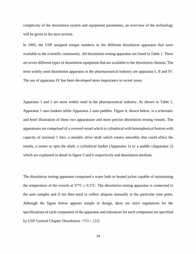
Another most widely used dissolution apparatus in the pharmaceutical industry is USP Apparatus

4, Flow-through cell. It was first appeared in 1957 and developed by FDA. [26] The method was

adapted by USP, European Pharmacopeia, and Japanese Pharmacopeia, and the flow through cell

became an official apparatus as USP apparatus-4. The system consists of a reservoir containing

dissolution medium, a pump that forces the medium upwards through the vertically positioned

flow-cell and a water bath to control the temperature in the cell. Different types of cells are

available for testing different dosage forms. Usually, bottom cone of the cell is filled with small

glass beads (about 1 mm diameter) and the dosage unit is placed on top of the beads. Peristaltic or

pulsating pistons are used in the pumps.

Dissolution testing using apparatus 4 continues to grow in popularity. Many pharmaceutical

companies in the United States and throughout the world are currently developing new methods

utilizing apparatus 4 and become more widespread. In the dissolution method development

different variations such as the size of the cell, flow rate, filter size and media with pH change can

be varied with difficulty in apparatus 1 and 2. This technique is useful for the low solubility and

rapidly degrading drugs. [27] Two different types of configurations can be used: an open loop or

closed loop where dissolution media is circulating through drug sample. In the open loop method,

the dissolution media flows through a cell containing the drug sample and goes into the waste after

sampling as it flows in one direction only. [28]

Figure 7 shows all parts of the dissolution apparatus 4. The dissolution medium is placed in a

covered flask from where the medium passes to the cell with the help of a pump. The flow is in

the upward direction, so a pump is required. The cell contains the dosage unit, through which

dissolution media flows and passes through the filtration unit which is placed on the top of the cell

and finally collected in a waste flask or circulates again for a closed system.

21

Figure 7: Schematic diagram of flow-through cell apparatus-4

22

1.5 Infrared Spectroscopy

Infrared spectroscopy (IR) is performed using wavelengths, 4000 cm-1 to 400 cm-1, of the

electromagnetic spectrum. Additionally, the IR portion of the electromagnetic spectrum is divided

into three regions; near-infrared, mid-infrared and far-infrared. The near-infrared energy is

approximately in the region between 14000 to 4000 cm-1 and can excite overtone or harmonic

vibrations. The mid-infrared energy is approximately in the region between 4000 (2500 nm) to

400 cm-1 (2500 nm) and can be used to study the fundamental vibrations of structures. The far-

infrared region is approximately in the region between 400 to 10 cm-1 and can be used to study to

rotations of structures. [29] [30] With IR spectroscopy, different functional groups absorb at

different IR bands or regions. Thus, this technique can help identify and even quantify organic and

inorganic molecules.

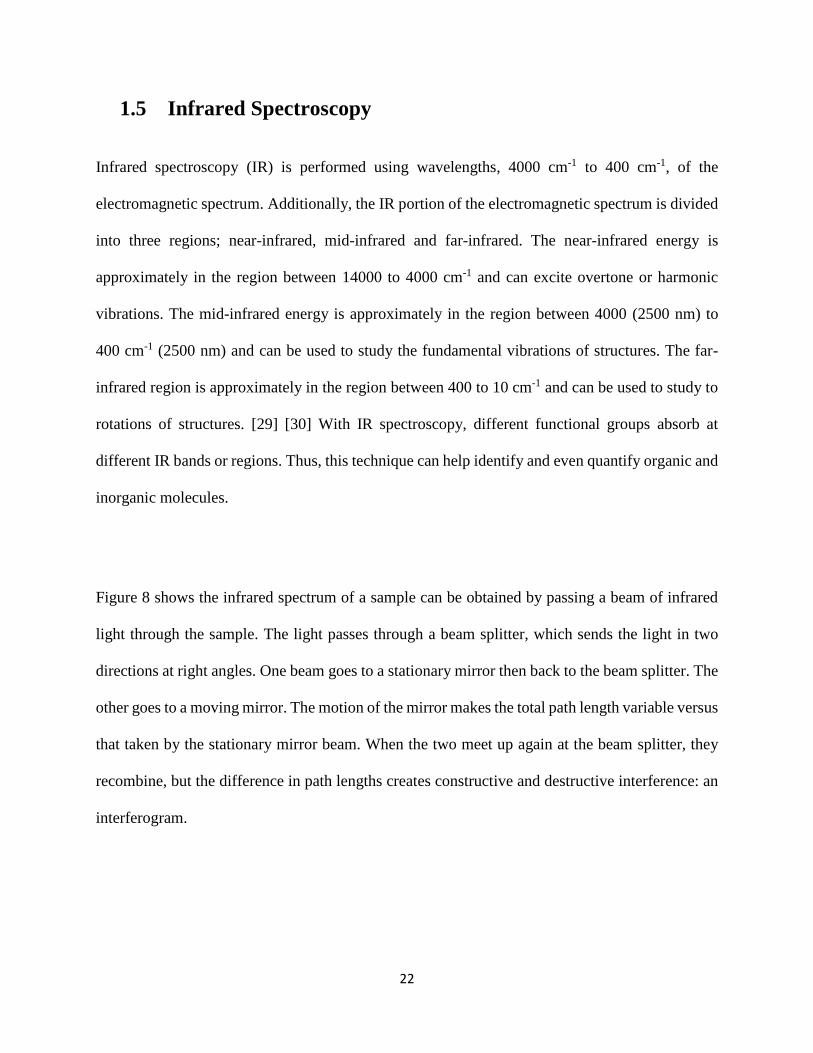
Figure 8 shows the infrared spectrum of a sample can be obtained by passing a beam of infrared

light through the sample. The light passes through a beam splitter, which sends the light in two

directions at right angles. One beam goes to a stationary mirror then back to the beam splitter. The

other goes to a moving mirror. The motion of the mirror makes the total path length variable versus

that taken by the stationary mirror beam. When the two meet up again at the beam splitter, they

recombine, but the difference in path lengths creates constructive and destructive interference: an

interferogram.

23

Figure 8: FT-IR schematic diagram

24

A Fourier transform instrument can be used to measure how much energy was absorbed by the

sample over the entire wavelength range. [31] The interferogram represents the light output as a

function of mirror position. The FT-IR raw data is processed to give the actual spectrum of light

output as a function of wavenumber. The FT-IR system can produce both transmittance and

absorbance spectrum. Molecules absorb IR radiation and excite to higher energy states. The IR

frequency matches with the natural vibrational frequencies of the molecule. Only those bonds that

have a dipole moment are capable of absorbing IR radiation. Symmetric bond such as those of H2

or Cl2 don does not absorb IR radiation. [32]

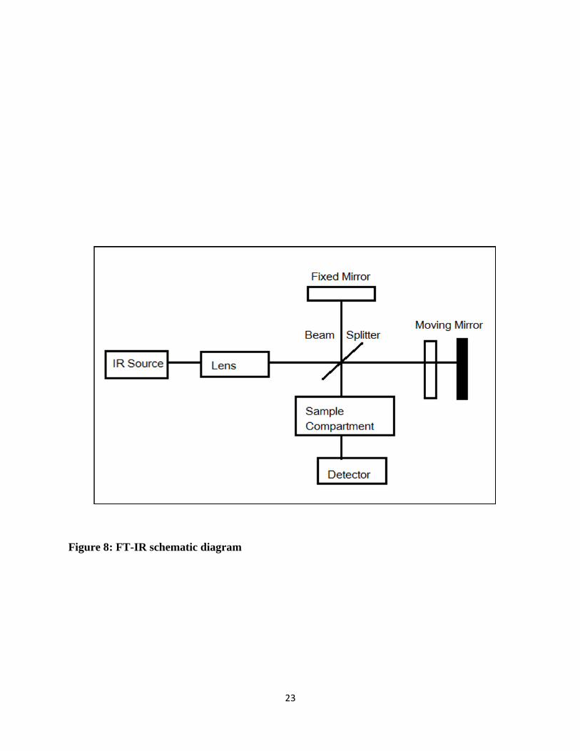
1.5.1 Attenuated Total Reflectance-Infrared (ATR-IR) spectroscopy

Attenuated Total Reflectance generally allows qualitative or quantitative analysis of solid and

liquid samples with little or no sample preparation, greatly improves the rate of analysis. The main

benefit of ATR sampling comes from the very thin sampling path length or depth of penetration

of the IR beam into the sample. This is in contrast to traditional FT-IR sampling by transmission

where most of the time the sample must be diluted with an IR transparent salt (e.g. KBr), pressed

into a pellet or pressed to a thin film, prior to analysis to minimize absorption and reflection by the

sample. [33]

In ATR a beam of infrared light is allowed to interact with the sample and the beam gets internally

reflected as it bounces through a crystal, changes relative to a background signal are recorded by

the instrument. An optically dense crystal (e.g. Diamond, Zinc selenide or Germanium) with a

high refractive index (typically refractive index values between 2.38 and 4.01) is used and the

infrared beam is allowed to impact at a certain angle. The most frequently used small crystal in

ATR is diamond, because it has the best durability and chemical inertness.

25

Figure 9 shows that a beam of infrared light is directed onto a crystal with a high refractive index

at a certain angle. An evanescent wave is formed due to the internal reflectance which penetrates

out of the crystal and passes through the sample which is in contact with the crystal. However, the

evanescent wave moves only 0.5 µ to 5 µ out of the crystal making it mandatory for the sample to

be in very good contact with the crystal. The evanescent wave is attenuated in the regions where

the sample absorbs energy and the altered wave is reflected back to the IR beam, which then exits

the opposite end of the crystal and is sent to the detector of the spectrometer which ultimately gives

an IR spectrum after processing.

The following experimental factors that affect the quality of final spectrum are the refractive

indices of the ATR crystal, the angle of incidence of the IR beam, the depth of penetration, the

wavelength of the IR beam, the number of reflections and ATR crystal characteristics. ATR

provides excellent quality data in conjunction with the best possible reproducibility of any IR

sampling technique. ATR allows faster sampling, improved sample to sample reproducibility and

minimizing user to user spectral variation.

Figure 10 shows the in-situ FT-IR instrument on which the research has been done. The FT-IR

instrument is the ReactIRTM iC10, from the Mettler Toledo. The FiberConduit™ is comprised of

flexible IR transparent silver chloride/silver bromide optical fibers. The fiber optic probe interface

(AgX 9.5 mm x 1.5 m fiber (Silver Halide)) contains a diamond tip-DiComp ATR crystal. The

enlarged view of the tip of the probe, works with ATR technique.

26

Figure 9: A multiple reflection ATR system

27

Figure 10: A representation of ATR with in-situ FT-IR (Adopted from Mettler Toledo)

28

Recent use and application of the ATR-IR spectroscopy has increased in pharmaceutical industry,

especially in the region of the Mid-IR and the Near-IR. [34] Near-IR spectroscopy has gained

acceptance in the pharmaceutical industry for analysis of incoming raw materials and finished

dosage forms in the last century. [35] The determination of the multiple parameters from a single

near-IR spectrum is the most valuable attribute. One recent application of near-IR is in the

prediction of dissolution behavior of pharmaceutical tablets with near-IR imaging. [36] Wendy

and Zhuangji described detection and quantitation of volatile organic contaminants in water using

ATR-IR technique. [37]

The FT-IR Imaging technique was first introduced in 1997. The technique has been applied to

study many different systems from all facets of science, from areas such as polymer diffusion and

dissolution. [38] Van der Weerd and his colleagues described the design and implementation of a

new cell, which allows the study of drug release from tablets by macro-FT-IR ATR imaging with

a diamond ATR accessory. Tablet formulation can be impacted directly on the ATR crystal. The

authors explain that various components in the tablet can be determined FT-IR imaging. [39] Wray

and his colleagues explored the novel application of FT-IR imaging to study the dissolution of

delayed release and pH resistant compressed coating pharmaceutical tablets. It was used to

accurately determine the swelling of the hydroxypropyl cellulose core and its relation the rate of

water ingress.

29

In the pharmaceutical industry, there are two main solid oral dosage forms: tablets and capsules

and others as well. The tablets or capsules are immersed in an aqueous solution for dissolution

testing, and the concentration of the active ingredient is monitored as a function of time.

Dissolution testing alone provides limited information on chemical processes that take place within

a dissolution vessel, because of the limited capabilities of the techniques that are used during

dissolution. Most dissolution analysis is carried out using ultra-violet and visible spectroscopy

which only gives concentration as a function of time. high-performance liquid chromatography is

used to separate multi-component drugs but still utilizes UV/Vis detection. [40]

One of the challenges in the industry is faced with is to increase an understanding of the

mechanisms governing dissolution. The current approach relies heavily on a data-driven approach.

To have a better understanding of dissolution, dissolution chemists need to explore other

applications that could give insight into what is happening inside of the vessel. This research

focuses on using ATR mid-infrared spectroscopy as an in situ technique to monitor and study the

dissolution of pharmaceutical tablets. The fiber-optic probes for reaction monitoring and

spectroscopy have been used as an important device in research. The flexible fiber optical probes

and spectroscopic software have enhanced the development of real-time applications. However,

recently, on-line methodologies have been used for obtaining accurate data during the dissolution

process.

30

1.6 Drugs used in this Research

As discussed earlier, this research is conducted using in situ FT-IR technique to monitor the

dissolution process. For this research, solid dosage form such as tablets were selected which were

available over the counter and easily available, these are acetaminophen, aspirin, salicylic acid and

Loratadine which are shown in Figure 11.

1.6.1 Acetaminophen

Acetaminophen (paracetamol) has been widely used for nearly a century and is currently one of

the most commonly used medications in the United States. Acetaminophen is an effective and

well-tolerated analgesic and antipyretic agent when used as indicated. [41] Acetaminophen is a

synthetic, nonopiate, centrally acting analgesic derived from p-aminophenol and it is also a

degradation product. It is reported to have significant nephrotoxic and teratogenic effects, therefore

its dosage should be strictly controlled. [42] [43] Drug metabolism plays a key role in

acetaminophen-induced hepatotoxicity. Acetaminophen metabolism occurs primarily in the liver,

where the drug undergoes glucuronidation sulfation by UDP-glucuronosyltransferases and

sulfotransferases, respectively.

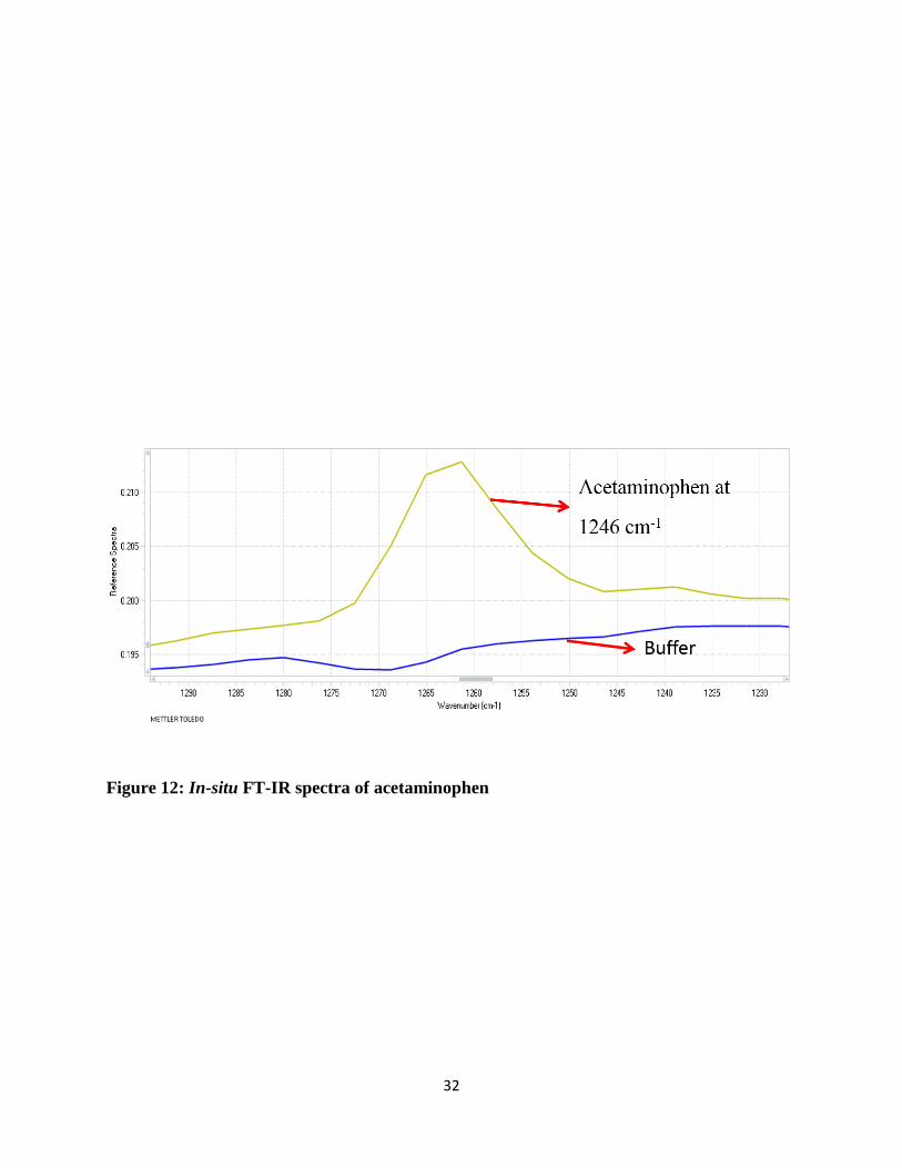
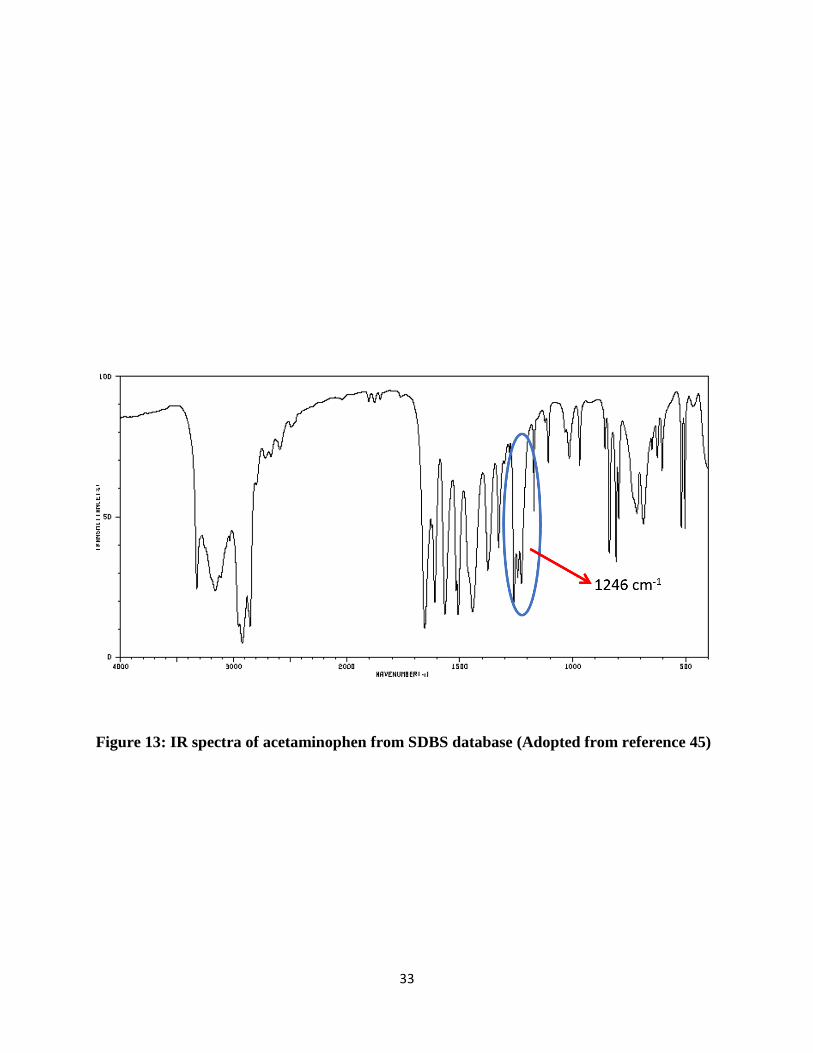
Figure 12 shows the FT-IR spectra of a standard solution of acetaminophen and phosphate buffer.

The blue line is for the buffer and the yellow line is for acetaminophen which shows peak at 1246

cm-1 for the analysis, corresponding to C-N stretch. For the research, the standard IR spectra of

acetaminophen collected via FT-IR were confirmed and compared with standard spectra, which is

collected from SDBS database for acetaminophen shown in Figure 13. [44] One more confirmation

test has been performed by studying calibration of acetaminophen using different concentrations.

31

Figure 11: Structures of drugs used in this research

32

Figure 12: In-situ FT-IR spectra of acetaminophen

33

Figure 13: IR spectra of acetaminophen from SDBS database (Adopted from reference 45)

34

1.6.2 Aspirin and Salicylic Acid

Aspirin is unique in its history and has many important roles in drug therapy. Aspirin is a pro-drug

and known to decrease pain. It fights pain and inflammation by blocking the action of an enzyme

called cyclooxygenase which inhibits the formation of prostaglandins, [45] which signal an injury

and trigger pain. Aspirin also inhibits the formation of prostaglandins. This results in the inhibition

of blood clots which could cause a heart attack or stroke. Aspirin was first synthesized by the

German chemist Felix Hoffmann (1868-1946) in the laboratories of Farbenfabriken Bayer,

Elberfeld, Germany in 1897. [46] Salicylic acid was used prior to aspirin, has several bad flaws as

a medicine. It has a bad taste, cause stomach irritation and presents other side effects spurred

researchers to look for other derivatives. The intent was to keep salicylic acid efficacy without the

disadvantages it posed. Acetylation of the hydroxyl group was one of the logical modifications.

This eventually led to the synthesis and discovery of aspirin.

Felix Hoffman used acetic anhydride for preparation of aspirin. Figure 14 shows the formation of

aspirin from salicylic acid and acetic anhydride. Salicylic acid can react with ethenone and acetyl

chloride to form aspirin. This is the general synthesis pathways for the formation of salicylic acid

that were investigated back in the late 1800’s. [47]

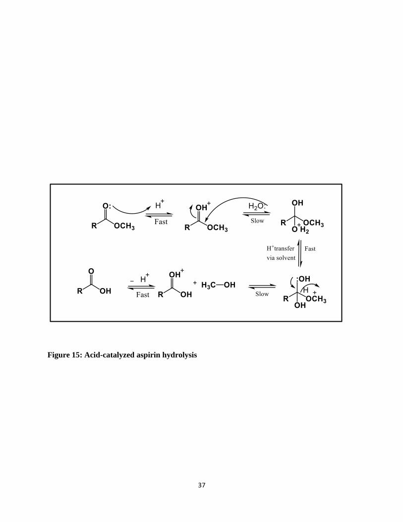
A chemical reaction of particular relevance to aspirin’s stability in biological fluids is hydrolysis.

There are two types of hydrolysis which are based on the pH. Figure 15 shows the acid catalyzed

mechanism, if the proton source is hydronium (H3O+), the catalysis is termed specifically acid

catalysis. The source of the proton is a dissociated acid and the substrate (the ester) is already

protonated in the rate-limiting (slow) step of the reaction.

35

Figure 14: Synthesis of aspirin in 1800’s [48]

36

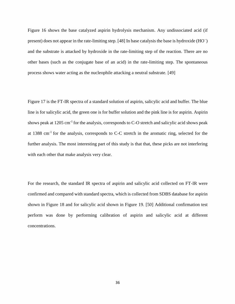
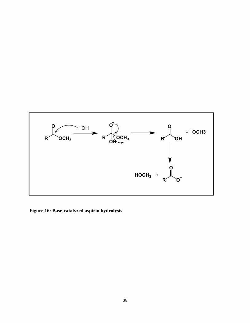
Figure 16 shows the base catalyzed aspirin hydrolysis mechanism. Any undissociated acid (if

present) does not appear in the rate-limiting step. [48] In base catalysis the base is hydroxide (HO−)

and the substrate is attacked by hydroxide in the rate-limiting step of the reaction. There are no

other bases (such as the conjugate base of an acid) in the rate-limiting step. The spontaneous

process shows water acting as the nucleophile attacking a neutral substrate. [49]

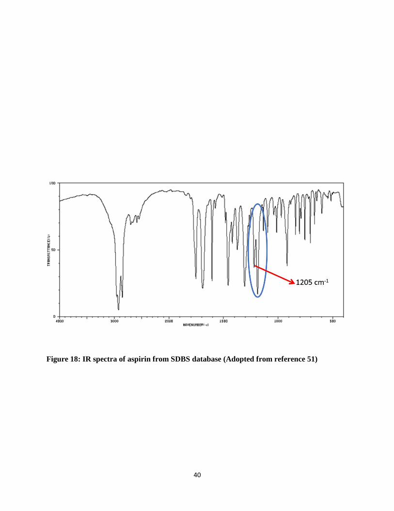
Figure 17 is the FT-IR spectra of a standard solution of aspirin, salicylic acid and buffer. The blue

line is for salicylic acid, the green one is for buffer solution and the pink line is for aspirin. Aspirin

shows peak at 1205 cm-1 for the analysis, corresponds to C-O stretch and salicylic acid shows peak

at 1388 cm-1 for the analysis, corresponds to C-C stretch in the aromatic ring, selected for the

further analysis. The most interesting part of this study is that that, these picks are not interfering

with each other that make analysis very clear.

For the research, the standard IR spectra of aspirin and salicylic acid collected on FT-IR were

confirmed and compared with standard spectra, which is collected from SDBS database for aspirin

shown in Figure 18 and for salicylic acid shown in Figure 19. [50] Additional confirmation test

perform was done by performing calibration of aspirin and salicylic acid at different

concentrations.

37

Figure 15: Acid-catalyzed aspirin hydrolysis

38

Figure 16: Base-catalyzed aspirin hydrolysis

39

Figure 17: In-situ FT-IR spectra of aspirin and salicylic acid

40

Figure 18: IR spectra of aspirin from SDBS database (Adopted from reference 51)

41

Figure 19: IR spectra of salicylic acid from SDBS database (Adopted from reference 51)

1388 cm-1

42

CHAPTER– 2

DISSOLUTION AND NONLINEAR BEHAVIOR OF

ACETAMINOPHEN

2.1 Introduction

Dissolution testing can give an in-vitro snapshot of how the drug product may behave in-vivo. As

a result, the number of dissolution methods in the United States Pharmacopeia has grown

substantially. [51] The potential impact of a new analytical technique that permits in-situ analysis

of multiple active ingredients during dissolution testing is profound.

This section focuses on the dissolution of over-the-counter acetaminophen tablets. The study of

the dissolution of acetaminophen was done earlier by conventional methods. [52] These

conventional methods need manual sampling which disturbs the dissolution process during

analysis by the traditional way using UV or HPLC. [53] The main purpose of this study is to

perform dissolution and analysis of acetaminophen tablet by a novel technique using in-situ FT-

IR which is compared to UV and HPLC.

2.2 Experimental Section

2.2.1 Chemicals and materials

Acetaminophen reference material used in this study (batch no. 104K0154) was purchased from

Sigma-Aldrich (St. Louis, MO). Acetaminophen tablets (Tylenol extra strength batch no. SLA175)

were purchased from a local pharmacy. Acetaminophen extended release tablets (Tylenol Arthritis

Pain batch no. 09FMC085) were purchased from a local pharmacy. Methanol, acetone and

acetonitrile (HPLC grades) were purchased from Pharmaco-Aaper (Brookfield, CT). Sodium

43

hydroxide (batch no. 064214BH), used to prepare the pH buffered solutions, was purchased from

Sigma-Aldrich (St. Louis, MO). Potassium phosphate monobasic (batch no. 103K0060), used to

prepare the pH buffered solutions, was purchased from Sigma-Aldrich (St. Louis, MO). Sodium

chloride crystals (batch no. J39602) was purchased from Mallinckrodt Chemicals (England, UK).

All solutions were prepared using water treated by a Milli-Q plus Millipore purification system

(Milford, MA). All purified water aliquots have a resistivity of not less than 18 MOhm-cm-1.

2.2.2 Instrumentation

All chemicals were weighed on a Mettler Toledo balance (Washington Crossing, PA) PB303

Delta-Range® and AG204 Delta-Range®. The pH of the buffer was measured on pH meter by

VWR SympHony (Radnor, PA) SB70P. Dissolutions were carried out on the Easy MaxTM 102 by

Mettler Toledo. HPLC analysis was performed on a Hewlett-Packard 1050 HPLC, with Chem

Station software. All UV measurements were carried out using a Hewlett-Packard UV instrument

(model no. 8452A diode array). The UV instrument was operated using Olis Spectralworks. All

manual dissolutions were tested using a Van-kel Dissolution Bath (model no. 700 and serial no.

31-214-1296).

In-situ FT-IR analysis was performed on a Mettler Toledo iC 10 ReactIR, with iCIR versions 3.0

and 4.0 software. The ReactIR™ iC10 FTIR instrument is composed of a Mercury Cadmium

Telluride detector (liquid nitrogen cooled) and a FiberConduit™. The FiberConduit™ is

comprised of flexible IR transparent silver chloride/silver bromide optical fibers. The fiber optic

probe interface (AgX 9.5 mm x 1.5 m Fiber (Silver Halide)) contains a diamond tip-DiComp ATR

crystal. The resolution was set to 8 wavenumbers. The optical range used by the system is: 1900

cm-1 to 650 cm-1. The gain adjustment was set to normal (1x) and the apodization method was set

44

to Happ-Genzel. The system uses compressed air (house air, filtered and dehumidified) to purge

the optics.

2.2.3 Potassium phosphate buffer (pH 5.8)

Potassium phosphate buffer (0.2 M) was prepared as per the USP procedures of buffer solutions.

[54] For 200 mL of buffer 50 mL of 0.2 M potassium phosphate monobasic solution and 3.6 mL

of 0.2 M sodium hydroxide solution were used. The volume was made up with deionized water to

200 mL and then the pH was measured.

2.2.4 Acetaminophen solutions for calibration

For the calibration study, 137.5 mg of acetaminophen (99 %) was weighed and dissolved in 100

mL of phosphate buffer pH 5.8 and used as stock solution. Then 14 dilutions were made using the

stock solution. For dilution added 0.5, 1, 1.5, 2, 3, 4, 5, 6, 7, 8, 9, 10, 11 and 12 mL stock solution

by using volumetric pipettes in each 25 mL volumetric flask and made volume with phosphate

buffer pH 5.8, then concentration of each flask was 0.0275, 0.055, 0.0825, 0.110, 0.165, 0.220,

0.275, 0.330, 0.385, 0.440, 0.495, 0.550, 0.605 and 0.660 mg/mL respectively analyzed samples

on UV spectroscopy and in-situ FT-IR.

2.2.5 Standard solutions

The standard solution of acetaminophen was prepared by weighing 55 mg of acetaminophen and

dissolved in 100 mL of phosphate buffer pH 5.8 resulting concentration 0.55 mg/mL.

2.2.6 Dissolution of acetaminophen (Extra Strength Tylenol)

Tylenol tablets 500 mg of acetaminophen (Label Claim) were tested in pH 5.8 phosphate buffer as

per acetaminophen USP monograph. [55] Dissolutions were conducted using vessel volumes of

45

900 mL and at 37.0 °C on Van-kel dissolution bath. All dissolutions were conducted using USP

Apparatus Type II (paddles) with an agitation speed of 50 rpm.

2.2.7 Dissolution of acetaminophen (Arthritis Tylenol)

Tylenol (Arthritis Pain) tablets 650 mg of acetaminophen (Label Claim) were tested in pH 5.8

phosphate buffer 64 mins. Dissolutions were conducted using vessel volumes of 900 mL and at

37.0 °C on Van-kel dissolution bath. All dissolutions were conducted using USP Apparatus Type

II (paddles) with an agitation speed of 50 rpm.

2.2.8 In-situ FT-IR analysis

For the calibration as well as the dissolution of acetaminophen experiments, data treatment was

carried out using the following methodology: The data was first subjected to baseline correction.

The absorption band at 1246 cm-1 (corresponding to the C-N stretch) was selected for

acetaminophen. The peak area was calculated using a two-point baseline correction set at 1265

cm-1 and 1230 cm-1. The ATR-IR system was configured to collect spectra every two minutes at

room temperature.

2.2.9 HPLC analysis

1.0 mL aliquots were collected during dissolution testing after a time interval (2, 4, 8, 16, 32 and

64 mins) and filtered using a syringe filter (0.45 µm). The column used was Phenomenex Luna

5µm Phenyl-Hexyl column (4.6 x 150 mm), with mobile phase 70/30/1

(methanol/water/trifluoroacetic acid). The flow rate was set 0.5 mL/min, isocratic mode, with an

injection volume 10 µL and the absorbance set at 296 nm.

46

2.3 Results and Discussion

2.3.1 Calibration of acetaminophen

The USP monograph specifies the pH 5.8 phosphate buffer as the medium of choice for

acetaminophen dissolution. Hence all standard diluted solutions were prepared in phosphate buffer

pH 5.8. Based on the in-situ FT-IR spectra and UV/Vis data obtained for acetaminophen, at low

concentrations (≤ 0.11 mg/ml), the relationship between absorbance and concentration is

effectively linear (r2= 0.9967). However, non-linear behavior was observed for both IR (r2=

0.9985) and UV-Vis (r2= 0.9981) methods at higher concentrations.

Figure 20 shows the calibration data of acetaminophen standard solutions. The calibration was run

from 0.05 to 0.66 mg/mL concentration of acetaminophen. 2nd order polynomial curve with r2=

0.999 was observed for both FT-IR as well as UV/Vis spectroscopy.

Figure 21 shows the calibration data of acetaminophen low standard solutions. The calibration data

was from 0.05 to 0.11 mg/mL concentration of acetaminophen. The calibration is a linear, which

ran on the UV/Vis spectroscopy with r2= 0.997.

Both methods can be modeled using second-order polynomial equations and has been confirmed

after multiple replications. [56] The hypothesis has established that it is because of the dimerization

of the acetaminophen. The proposed statement is that in the higher concentrations the

acetaminophen molecules form dimers. The detailed experimentation is discussed in the later part

of this section.

47

Figure 20: Non-linear graph for different levels of acetaminophen reference standards

48

Figure 21: Linear calibration graph of acetaminophen at low concentrations

y = 2.1924x + 0.0122R² = 0.9967

0

0.05

0.1

0.15

0.2

0.25

0.3

0 0.02 0.04 0.06 0.08 0.1 0.12

Ab

sorb

an

ce(A

U)

Concentration(mg/mL)

Acetaminophen reference standards in 5.8 phosphate buffer,

UV/Vis absorbance at 296 nm, 5-20% dilutions

Abs

Linear (Abs)

49

2.3.2 Dissolution of Extra Strength Tylenol

At the initial stage of the research, dissolution of extra strength Tylenol was performed using

UV/Vis spectroscopy to understand the dissolution procedure and analysis. As per the procedure

which is discussed in the experimental section, dissolution was performed three times using 5

vessels with a Van-Kel dissolution bath. Aliquots were collected for UV/Vis analysis after 2, 4, 8,

16, 32 and 64 mins respectively. The percent dissolution was calculated by using following

formula.

% Dissolution =

Absorbance of Sample

Absorbance of Standard×

Standard Mass

Standard Volume

×Vessel Volume

Potency× Standard Purity × 100

(9)

Figure 22 shows the dissolution of extra strength Tylenol. The tablets were dissolved in 15-20

mins and all vessel data overlapped as per expectations. Maximum drug dissolved after 60 mins

were 91%.

It is noticed that percent dissolution observed during this study is slightly lower than percent

dissolution observed during other experiments carried out with Extra strength Tylenol in last few

decades. This observation could be due to the hypothesis of the calibration of acetaminophen

which showed polynomial curve at increased concentration.

Figure 23 shows that recalculated percent dissolution of acetaminophen by using polynomial

equation from the calibration graph and observed that the percentage of dissolution has increased

to 96%. Based on these calculations and results, it confirmed the hypothesis at higher

concentrations acetaminophen molecules form dimers.

50

Figure 22: Dissolution of acetaminophen

0.0

10.0

20.0

30.0

40.0

50.0

60.0

70.0

80.0

90.0

100.0

0 20 40 60 80

% D

isso

lved

Time in minutes

Dissolution data 5 vessles of Acetaminophen in 5.8 phosphate

buffer, UV/Vis absorbance at 296 nm

% D (1)

% D (2)

% D (3)

% D (4)

% D (5)

% D (6)

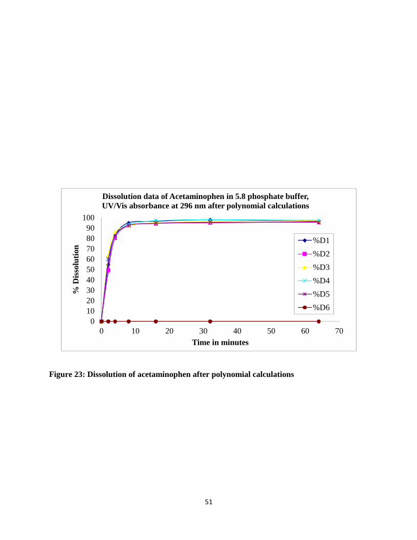
51

Figure 23: Dissolution of acetaminophen after polynomial calculations

0

10

20

30

40

50

60

70

80

90

100

0 10 20 30 40 50 60 70

% D

isso

luti

on

Time in minutes

Dissolution data of Acetaminophen in 5.8 phosphate buffer,

UV/Vis absorbance at 296 nm after polynomial calculations

%D1

%D2

%D3

%D4

%D5

%D6

52

2.3.3 Dissolution of Tylenol (Arthritis Pain)

After studying the UV/Vis analysis and dissolution procedures, the research was extended towards

the main goal of the thesis which was the in-situ FT-IR dissolution and its comparison with HPLC.

Tylenol has a long lasting effect on the arthritis pain and hence the dissolution was performed for

8 Hrs. Aliquots were taken throughout the experiment and analyzed to compare the in situ FT-IR

method with HPLC and UV/Vis methods.

The results from the in situ FT-IR, UV/Vis and HPLC systems are overlaid as shown in Figure 24.

An excellent correlation was observed between these three methods. The amount of released

acetaminophen by HPLC (yellow Line) and UV/Vis (green Line) is little higher than the in-situ

FT-IR (Orange line) in the early part of the dissolution from 30 mins to 2 hr. This might be because

of the dissolution-in-dissolution concept which happens in the HPLC and UV/Vis vials; fine

particles of acetaminophen can appear after filtration in the vial was dissolved again in the

dissolution media upon storage of sample for the analysis and showed higher concentration than

the in-situ FT-IR. This shows the advantage of the novel technique in-situ FT-IR, which avoids

further dissolution of the drug in the sample vial upon wait time for analysis.

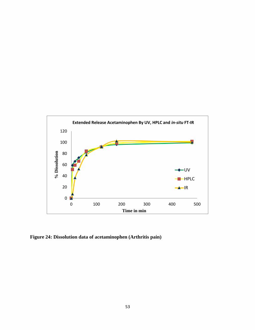
53

Figure 24: Dissolution data of acetaminophen (Arthritis pain)

0

20

40

60

80

100

120

0 100 200 300 400 500

% D

isso

luti

on

Time in min

Extended Release Acetaminophen By UV, HPLC and in-situ FT-IR

UV

HPLC

IR

54

2.4 Non-Linear behavior of Acetaminophen

In acetaminophen research, it has been observed from the calibration data that acetaminophen has

a non-linear behavior. The calibration study was done by UV-vis spectroscopy and in-situ FT-IR

from concentration ranges from 0.005 mg/mL to 0.66 mg/mL. At the lower concentration the

calibration showed a linear graph in Figure 21, but at higher concentrations, it is non-linear as

shown in Figure 20. On searching for literature explaining this behavior specifically for

acetaminophen, it was found that acetaminophen has a tendency to form dimer with respect to pH

of the solution. [57] [58] The polymorphism study of acetaminophen showed that the interplay of

molecular flexibility and hydrogen bonding manifested in the monoclinic and orthorhombic

polymorphs of acetaminophen and with the X-ray crystallographic study has confirmed. [59] [60]

There is evidence about the formation of acetaminophen hemi adducts due to the formation of

chains for acetaminophen molecule linked via OH…O=C interaction or NH….O=C interaction.

[61]

In this research, the acetaminophen was in solution form, where it was dissolved in phosphate

buffer pH 5.8. There is no evidence which claiming the formation of a dimer in these conditions.

Because of the importance of acetaminophen as medicine, there is a need to better understand this

unusual behavior of acetaminophen. Based on the observed results, the hypothesis was proposed

that the non-linear behavior is because of the dimerization showed in reaction 1 or aggregation of

the acetaminophen molecules showed in reaction 2.

55

Reaction 1

Reaction 2

The main focus is to study the non-linear behavior of acetaminophen by different instrumental

techniques and by studying colligative properties to calculate the number of moles of

acetaminophen in the buffer solution.

Investigation of the dimerization of acetaminophen has been performed by different techniques,

Infrared spectroscopy (IR), Nuclear Magnetic Resonance spectroscopy (NMR) and colligative

properties in that by vapor pressure osmometry and freezing point depression.

Investigation of dimerization of acetaminophen is possible by IR spectroscopy. It can identify

interactions that occur as a result of hydrogen bonding which leads to dimeric and oligomeric

structures shown in Reaction 1 and Reaction 2. The carbonyl group present is around 1600-1700

cm-1 wave numbers. There is literature, which describes the use of IR spectroscopy to detect

56

dimerization of carboxylic acid structures. This suggests that this technique can be used to study

acetaminophen in nonpolar solvents. [62] [63] [64] Literature gave evidence that, because of

formation of dimer, which creates a new hydrogen bond and shows a new broad peak for the dimer

in the region of 3300 cm-1-3700cm-1. [65] IR Spectroscopy has been used to identify the phosphoric

acid dimerization a well-known example of dimerization. [66] [67]

Another common example for the study of the nonlinear behavior is benzoic acid which is shown

in reaction 3.

Reaction 3

The investigation of the benzoic acid dimer was done by IR spectroscopy. They observed a

broadening and shift of the carbonyl stretching frequency. [68] Literature studies provide evidence

about the benzoic acid dimer study. [69] [70] [71] Literature study of dimerization shows the IR

spectroscopy study will be useful for investigation and confirmation.

The non-linear behavior of acetaminophen which is because of the aggregation or dimerization of

molecules can be investigated by NMR. That gives the information about the chemical shift of

hydrogen and carbon peak which moves to downfield. [72] The proton transfer in the benzoic acid

dimer was measured by the NMR. [73] The literature showed that the study of dimerization and

the oligomerization can be analyzed by NMR, even quantitative analysis can be done by NMR.

57

[74] [75] [76] Literature suggested another way to determine the dimer formation of

acetaminophen in phosphate buffer by NMR analysis.

The presence of one or more solutes alters the ability of the solvent molecules to interact, reducing

their freedom of movement, thus the ability to move from liquid to solid is altered. These changes,

which collectively are referred to as colligative properties, are dependent on the total number of

particles present in the solution. [77] One of the colligative property, osmotic pressure a direct

measurement of the molar concentration of total solutes in an aqueous solution. Osmotic pressure

is defined as the force which would be required to resist movement of solvent across a membrane

which is permeable to the solvent but not to the solute molecules. A solute particle can be a

molecule or an ion or an aggregated species such as dimer that can exist discretely in solution.

Since osmotic pressure is directly related to the total molar concentration of solute, there is a direct

and linear relationship between osmotic pressure. [78] [79]

Another excellent way to determine the molecular weight of dissolved acetaminophen is by

measuring the vapor pressure of the solution. By osmometry, one can measure the vapor pressure

of the acetaminophen solution and can calculate the molecular weight and then moles of the

solution.

Thus, if acetaminophen dimerizes or oligomerizes, the measured molar mass will be larger than

the molar mass of the monomer of 151.16 g/mol. However, it is expected that the measured molar

mass will be a weighted average of monomer, dimer and oligomer species that will be present.

Thus M = x (monomer) + y (dimer) + z (trimer) + zz (tetramer +…. Robert performed some

58

forensic laboratory experiments to calculate the weights of drugs and diluents by osmometry,

which gave the motivation of performing the experiments to calculate the moles of acetaminophen.

[80]

A solution freezes at a lower temperature than does the pure solvent. This phenomenon is called

freezing point depression. The freezing point depression of a solution is a colligative property of

the solution which is dependent upon the number of dissolved particles in the solution. The higher

the solute concentration, the greater the freezing point depression of the solution. [81] The freezing

point values are determined from the cooling curves obtained by recording the temperature as a

function of time. [82] Another application of this method is mainly in the food industry to study

the thermodynamic properties of frozen food and fruits. [83] [84] Freezing point depression is used

to determine the molecular mass of polyols which avoids the interference by water, by using

acetophenone as a solvent having freezing point depression 20oC. [85]

After reviewing all this literature performed the different experiments on IR, NMR and for

colligative properties such as vapor pressure osmometer and Freezing point depression as well.

The results from these experiments could not support the hypothesis that at higher concentrations

acetaminophen molecules form dimer. There is a lack of any evidence to explain or confirm the

dimerization of acetaminophen as per the proposed hypothesis.

59

2.5 Conclusion

The in-situ infrared spectroscopy is a viable alternative for measuring dissolution profiles of

pharmaceutical tablets. The in-situ FT-IR system was found to be impressive and validated by

comparing dissolution profile using UV/Vis and HPLC. The method was calibrated with

acetaminophen standard solutions ranging from 0.05 mg/mL to 0.66 mg/mL, with r2=0.998. The

percent dissolution of acetaminophen was found in the range of 95-97 % by all three techniques.

The in-situ FT-IR has great advantage of minimizing the manual efforts required for manual

sampling of dissolution. On the contrary, UV/Vis and HPLC methods require laborious manual

sampling. With the current configuration of the in-situ FT-IR instrument, this analysis is limited

by the sensitivity and wavelength range of the in-situ fiber optic probe. However, since this chapter

successfully demonstrates the versatility of this novel application of in-situ FT-IR spectroscopy.

Unsatisfactory results were observed for the hypothesis of the dimerization of acetaminophen. As

part of this study, multiple experiments were designed and performed on the respective instruments

(IR, NMR and using colligative properties such as vapor pressure osmometer and freezing point

depression) for the dimerization study of acetaminophen. But still, there is a lack of evidence to

support the proposed dimerization hypothesis.

60

CHAPTER - 3

DISSOLUTION AND HYDROLYSIS STUDY OF ASPIRIN

3.1 Introduction

This section focuses on monitoring the dissolution and hydrolysis of over the counter tablet

acetylsalicylic acid (aspirin) under acidic conditions by In-situ FT-IR spectroscopy using

attenuated total reflectance infrared probe (ReactIR). The acetylsalicylic acid undergoes hydrolysis

to form salicylic acid and acetic acid. [86] The equation of aspirin hydrolysis is written as

mentioned below.

Reaction 4

The majority of the methods for monitoring dissolution utilize UV/Vis spectroscopy. For example,

aliquots are manually withdrawn and analyzed by UV/Vis spectroscopy or HPLC with ultraviolet

detection. However, the sampling process is disruptive to the dissolution profile since the removal

of aliquots from the vessel disturbs the solution. In addition, there are instruments that allow real-

time analysis using in-situ UV/Vis probes. For example, fiber optic dissolution testing is used in

the pharmaceutical industry to monitor drug product release. Fiber optic dissolution is also used

for formulation development. [87] Formulators are using these in-situ UV/Vis systems to profile

61

and develop drugs faster, instead of conventional techniques where dissolutions are conducted

manually and analyzed offline. The advantage of the fiber optic system is that it allows real-time

data analysis. But the major disadvantage of UV/Vis system is a small range of the analysis that is

200-400 nm, in the case of aspirin and salicylic acid study both peaks overlap of the main maxima

and limits the analysis which needs additional determination for methods. [88]

There is an interest to develop new methods that do not require manual sampling. The use of in-

situ FT-IR for analyzing aqueous samples is limited by the relatively high concentration of analyte

required for detection. [89] Hence this research investigated the use of in-situ FT-IR spectroscopy

as a potential technique for monitoring and understanding dissolution. The research showed that

dissolution using in-situ FT-IR spectroscopy for the single component as well as multi-component

formulations is useful for monitoring the release profile of each active pharmaceutical ingredient

(API). [90] Thus, there is also an interest in the development of hydrolysis of a prodrug aspirin

while performing dissolution and study kinetics of that process.



Acetylsalicylic acid (aspirin) reference material (batch no. 016K0131) was purchased from Sigma-

Aldrich (St. Louis, MO). Salicylic acid reference material (batch no. 04708HE) was purchased

from Sigma-Aldrich (St. Louis, MO). Acetylsalicylic acid 325 mg tablets (Genuine Bayer batch

no. 219050N) were purchased from a local pharmacy. Methanol, acetone and acetonitrile (HPLC

grades) were purchased from Pharmaco-Aaper (Brookfield, CT). Sodium chloride crystals (batch

no. J39602) was purchased from Mallinckrodt Chemicals (England, UK). Hydrochloric acid (batch

no. H44032) was purchased from J.T. Baker (Central Valley, PA). Sodium acetate crystals (batch

62

no.05816HD, potassium phosphate monobasic (batch no. 103K0060) and sodium hydroxide

(batch no. 06414BH) were purchased from Sigma-Aldrich Chemicals (St. Louis, MO). Glacial

acetic acid (batch no. 971666) was purchased from Fisher Chemicals (Waltham, MA). All

solutions were prepared using water treated by a Milli-Q plus Millipore purification system

(Milford, MA). All purified water aliquots have a resistivity of not less than 18 MOhm-cm-1.



Delta-Range® and AG204 Delta-Range®. The pH of the buffer was measured on a VWR

SympHony (Radnor, PA) SB70P pH meter. Dissolutions were carried out on the Easy MaxTM 102

by Mettler Toledo. HPLC analysis was performed on a Hewlett-Packard 1050 HPLC, with Chem

Station software. In-situ FT-IR analysis was carried on a Mettler Toledo iC 10 ReactIR, with iCIR

versions 3.0 and 4.0 software.

3.2.3 Simulated gastric fluid

Simulated gastric fluid was prepared with hydrochloric acid and sodium chloride as per USP buffer

procedure. [91] 2 g of sodium chloride was dissolved in 100 mL of deionized water, in that 7 mL

HCl was added and then volume made up to 1000 mL by adding deionized water, and then

measured pH of that solution and was adjusted to 1.2.

3.2.4 Sodium acetate buffer

Sodium acetate buffer was prepared with glacial acetic acid and sodium acetate anhydrous as per

the USP buffer procedures. [92] 2.99 g of sodium acetate was dissolved in 100 mL of deionized

water, in that 1.66 mL glacial acetic acid was added and then volume made up to1000 mL by

adding deionized water and then measured pH of that solution and was adjusted to 4.5.

63

3.2.5 Potassium phosphate buffer

Potassium phosphate buffer (0.2 M) was prepared with monobasic potassium phosphate and

sodium hydroxide as per the USP buffer procedures. [93] First potassium phosphate solution was

prepared by weighing 27.22 g of monobasic potassium phosphate and dissolved in 100 mL of

deionized water and diluted with up to 1000 mL. Next sodium hydroxide solution was prepared

by weighing 8 g of sodium hydroxide dissolved in water and made volume up to 100 mL. For

phosphate buffer added 50 mL of monobasic potassium phosphate solution in a 200 mL volumetric

flask then added 22.4 mL of sodium hydroxide solution and then added water to make a volume.

Finally measured the pH of this solution and was adjusted to 6.8.

3.2.6 Aspirin solution for calibration

Aspirin stock solution was prepared by dissolving 500 mg of aspirin in 100 mL of simulated gastric

fluid (pH 1.2), sodium acetate buffer (pH 4.5) and phosphate buffer (pH 6.8). To prepare a

calibration curve, nine dilutions were made by using this stock solution by adding 1.00, 2.00, 3.00,

4.00, 5.00, 6.00, 7.00, 8.00 and 9.00 mL to 10.00 mL volumetric flasks respectively and diluting

to volume with respective buffer solution. The concentration of aspirin in each flask was 0.500,

1.00, 1.50, 2.00, 2.50, 3.00, 3.50, 4.00 and 4.50 mg/mL as well as 3.62, 7.24, 10.9, 14.5, 18.1, 21.7,

25.3, 28.9 and 32.6 mM respectively. Aspirin starts hydrolyzing as it goes into solution, to avoid

or to slow down that process; solutions were placed into an ice bath immediately after the

preparation. As soon as solutions were ready, they were scanned by in-situ FT-IR for the

calibration study at room temperature.

64

3.2.7 Salicylic acid solution for calibration

A stock solution of salicylic acid was made by dissolving 500 mg of salicylic acid in 100.00 mL

of simulated gastric fluid (pH 1.2), sodium acetate buffer (pH 4.5) and phosphate buffer (pH 6.8).

To prepare a calibration curve, nine dilutions were made by using this stock solution by adding

1.00, 2.00, 3.00, 4.00, 5.00, 6.00, 7.00, 8.00 and 9.00 mL to 10.00 mL volumetric flasks

respectively and diluting to volume with respective buffer solution. The concentration of salicylic

acid in each flask was 0.500, 1.00, 1.50, 2.00, 2.50, 3.00, 3.50, 4.00 and 4.50 mg/mL as well as

2.78, 5.55, 8.33, 11.1, 13.9, 16.7, 19.4, 22.2 and 25.0 mM respectively.

3.2.8 Hydrolysis of aspirin to salicylic acid in test tubes

Prior to the hydrolysis experiments, a qualitative measurement was investigated for determining

the presence of salicylic acid in solution. Acetylsalicylic acid hydrolyzes to salicylic acid in the of

acidic medium. Ferric chloride test was found to be a good qualitative test for phenols. Ferric

chloride in solution gives colors with a number of organic derivatives. The common ones are

phenols, enols, oximes, hydroxamic acids, and some carboxylic acids. It will, however, react with

salicylic acid, which is used to synthesize aspirin, forming an iron-phenol complex. [94] [95] Thus,

adding an aqueous ferric chloride solution to an aspirin solution is a good way to see if there is any

salicylic acid present. The ferric chloride color test is shown below. A small experiment was

performed in that used three vials containing simulated gastric fluid (vial C) as control, aspirin

solution (vial A) and salicylic acid solution (vial S).

65


The standard solutions were prepared by weighing 325 mg of aspirin and 325 mg salicylic acid

and dissolved in 100 mL of simulated gastric fluid, sodium acetate buffer and potassium phosphate

respectively and obtained concentration 3.25 mg/mL.

3.2.10 Dissolution and hydrolysis of aspirin

Bayer Aspirin tablets 325 mg of aspirin (Label Claim) were measured in pH 1.2 simulated gastric

fluid solutions for 1.5 hr., pH 4.5 sodium acetate buffer for 24 hr and potassium phosphate buffer

for 24 hr. Dissolutions were conducted using vessel volumes of 100 mL at 37.0 °C. All dissolutions

were conducted using USP Apparatus Type II (paddles) with an agitation speed of 100 rpm as per

the USP procedure and collected samples for HPLC as well.

3.2.11 In-situ FT-IR Analysis

3.2.11.1 Aspirin analysis

A distinct peak for aspirin without interference was observed. Calibration of aspirin with standard

diluted solutions as discussed in experimental section. For the calibration of aspirin experiments,

data treatment was carried out using the following methodology: The data was first subjected to

baseline correction. The absorption band at 1205 cm-1 (corresponding to the C-O stretch) was

selected for acetylsalicylic acid. The study was done by using three different body pHs such as

simulated gastric fluid (pH 1.2), sodium acetate buffer (pH 4.5) and phosphate buffer (pH 6.8)

which depicts stomach, duodenum and small intestine pHs respectively.

66

3.2.11.2 Salicylic acid analysis

A distinct peak for salicylic acid without interference was observed which is shown in Figure 17,

then performed calibration of salicylic acid with standard diluted solutions as discussed in

experimental section. For the calibration of salicylic acid experiments, data treatment was carried

out using the following methodology: The data was first subjected to baseline correction. The

absorption band at 1488 cm-1 (corresponding to the C-C stretch in the aromatic ring) was selected

for salicylic acid. Although a unique absorption at 1161 cm-1 (corresponding to the C-O stretch)

was observed for salicylic acid, 1488 cm-1 was chosen for further analysis because of its higher

intensity. The study was done by using three different body pHs such as, simulated gastric fluid

(pH 1.2), sodium acetate buffer (pH 4.5) and phosphate buffer (pH 6.8) which depicts stomach,

duodenum and small intestine pHs respectively.

3.2.11.3 Dissolution and hydrolysis of aspirin tablet

The dissolution testing was carried out as discussed in the experiment section. The in-situ FT-IR

fiber optic probe collected baseline spectra (blank medium) for the first 30 minutes. A single 325

mg Bayer aspirin tablet was dropped into the vessel containing 100 mL of buffer solution

(simulated gastric fluid pH 1.2, sodium acetate buffer pH 4.5 and potassium phosphate buffer pH

6.8) and the dissolution profiles were collected using in-situ FT-IR spectroscopy. Standard spectra

of pure aspirin and salicylic acid were collected prior to running the dissolutions. These standards

were used to identify the unique peaks of interests for these active drugs. For the aspirin tablet

analysis, the same steps as discussed in calibration analysis were followed.

67

For this experiment, data processing is critical to obtain well-resolved spectra. For all in-situ FT-

IR experiments, 256 scans were collected and co-added for each spectral point and each data point

took about two minutes to complete. The peak of interest was identified (1205 cm-1) and the area

was calculated using a two-point baseline correction. A trend analysis was performed using the

iCIR software on this peak. This provided a plot of absorbance vs. time. This plot was subjected

to smoothing using a 25 point smoothing parameter. After smoothing, and while still in the trend

analysis, the baseline correct routine was performed. Then, the data were exported to Excel.

Further data processing in Excel involved the subtraction of solvent spectra background. A 30 min

set of spectra at the beginning of the experiment were obtained before aspirin pill was added. These

spectra were subtracted from the spectra taken after the pill was dropped to give the final set of

data. Within the final set of data, the area of the 1205 cm-1 peak was calculated at each time point.

Then the plot of area vs. time was performed to give rate information. In addition, using a

calibration curve, peak areas were converted to concentration to provide concentration vs. time

plots.

3.2.12 HPLC analysis

The dissolution aliquots (1.0 mL) were collected after a certain time interval and filtered using

syringe filter (0.45 µm) transferred to an ice bath to prevent further hydrolysis. The column was

used is Phenomenex C18 5 µm Luna column (4.6 x 150 mm), with mobile phase 60/40/1

(methanol/water/trifluoroacetic acid) with 13 min run time. The flow rate was set to 0.5 mL/min,

isocratic mode, with an injection volume 10 µL and absorbance was measured at 300 nm.

68


3.3.1 Calibration of aspirin

Based on the IR spectra obtained, aspirin has unique IR bands at 1205 cm-1. Linear regression for

aspirin was calculated by using the area under curve (AUC) calculations of the IR absorption band

at 1205 cm-1. The analysis was performed as discussed in the experimental section and by plotting

the concentration vs Intensity of AUC of the peak, it was determined that aspirin had a linear

correlation.

Figure 25 shows the calibration data of aspirin with different concentrations of standard aspirin

solution. The concentrations range from 3 mM to 33 mM with r2= 0.9922 of AUC of aspirin IR

peak vs. concentration in simulated gastric fluid (pH 1.2).



peak vs. concentration in sodium acetate buffer (pH 4.5).



peak vs. concentration in potassium phosphate buffer (pH 6.8).

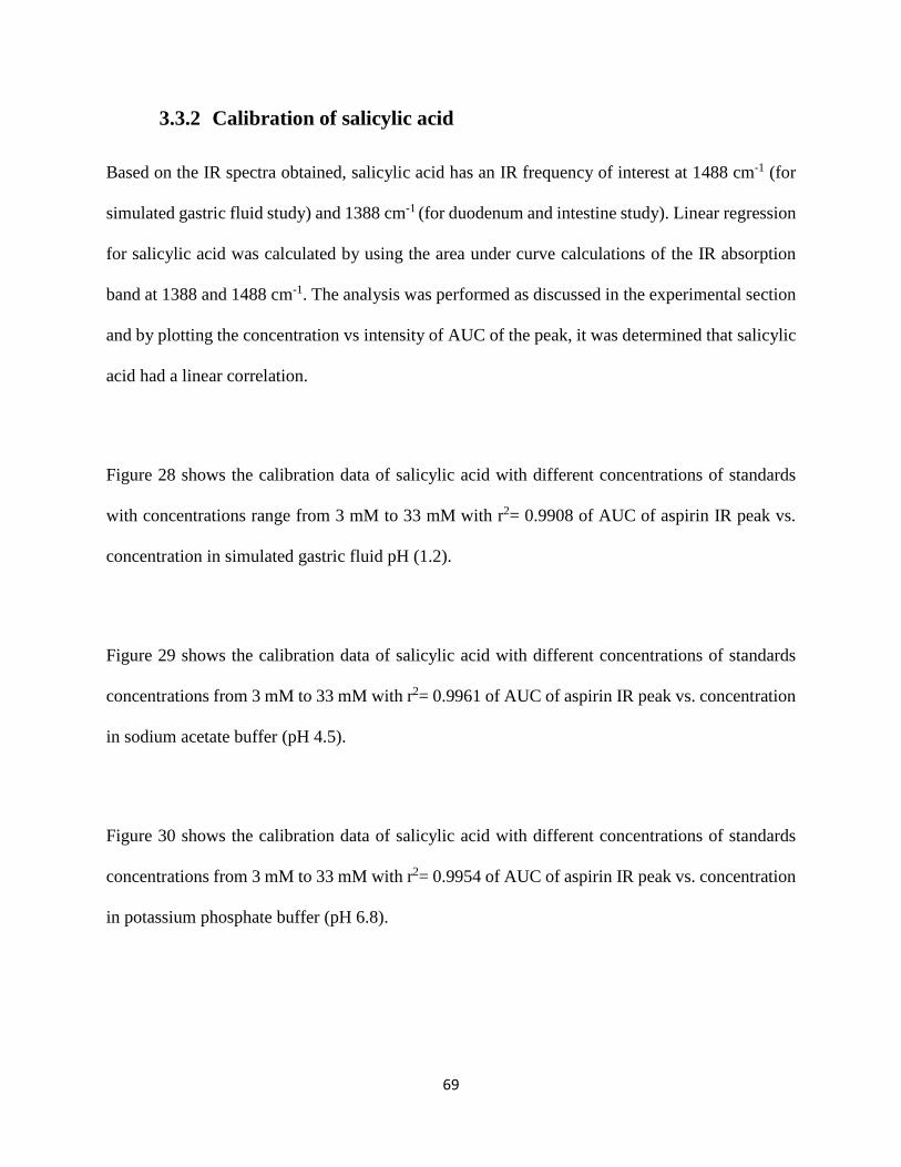
69

3.3.2 Calibration of salicylic acid

Based on the IR spectra obtained, salicylic acid has an IR frequency of interest at 1488 cm-1 (for

simulated gastric fluid study) and 1388 cm-1 (for duodenum and intestine study). Linear regression

for salicylic acid was calculated by using the area under curve calculations of the IR absorption

band at 1388 and 1488 cm-1. The analysis was performed as discussed in the experimental section

and by plotting the concentration vs intensity of AUC of the peak, it was determined that salicylic

acid had a linear correlation.

Figure 28 shows the calibration data of salicylic acid with different concentrations of standards

with concentrations range from 3 mM to 33 mM with r2= 0.9908 of AUC of aspirin IR peak vs.

concentration in simulated gastric fluid pH (1.2).


concentrations from 3 mM to 33 mM with r2= 0.9961 of AUC of aspirin IR peak vs. concentration

in sodium acetate buffer (pH 4.5).


concentrations from 3 mM to 33 mM with r2= 0.9954 of AUC of aspirin IR peak vs. concentration

in potassium phosphate buffer (pH 6.8).

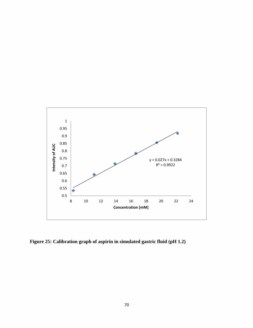
70

Figure 25: Calibration graph of aspirin in simulated gastric fluid (pH 1.2)

y = 0.027x + 0.3284R² = 0.9922

0.5

0.55

0.6

0.65

0.7

0.75

0.8

0.85

0.9

0.95

1

8 10 12 14 16 18 20 22 24

Inte

nsi

ty o

f A

UC

Concentration [mM]

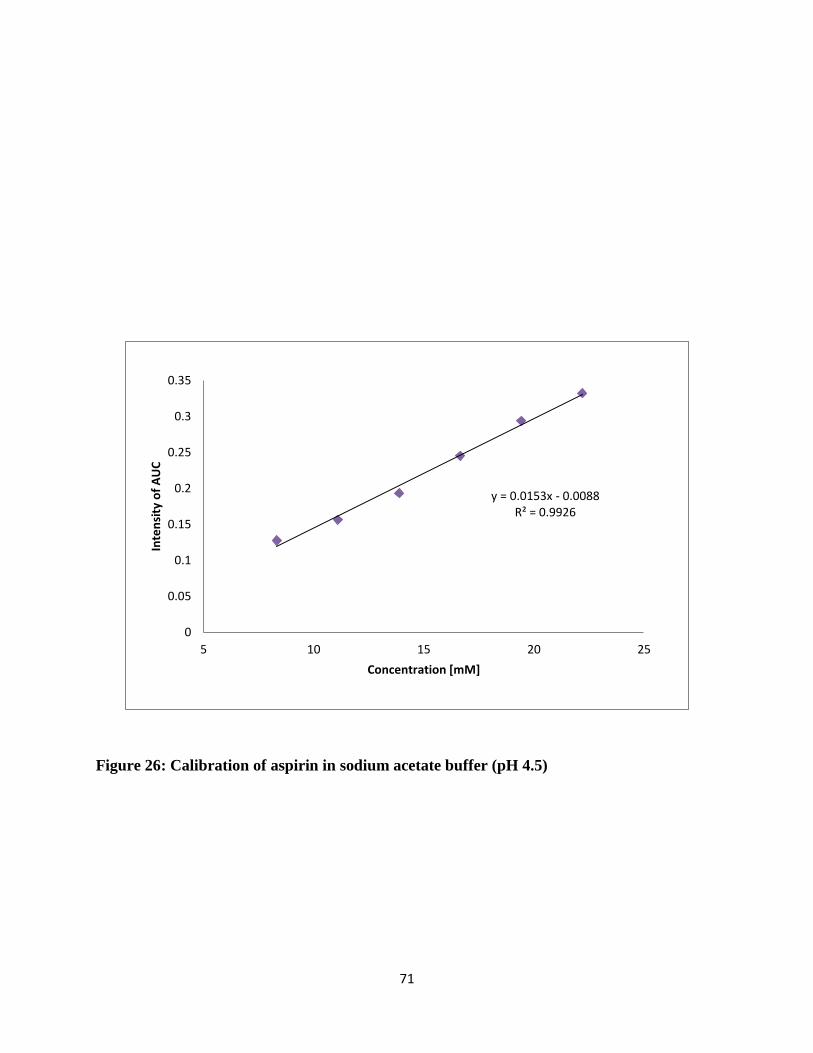
71

Figure 26: Calibration of aspirin in sodium acetate buffer (pH 4.5)

y = 0.0153x - 0.0088R² = 0.9926

0

0.05

0.1

0.15

0.2

0.25

0.3

0.35

5 10 15 20 25

Inte

nsi

ty o

f A

UC

Concentration [mM]

72

Figure 27: Calibration of aspirin in potassium phosphate buffer (pH 6.8)

y = 0.0088x + 0.0296R² = 0.9979

0.0000

0.0500

0.1000

0.1500

0.2000

0.2500

0.3000

0.00 5.00 10.00 15.00 20.00 25.00 30.00

Inte

nsi

ty o

f A

UC

Concentration [mM]

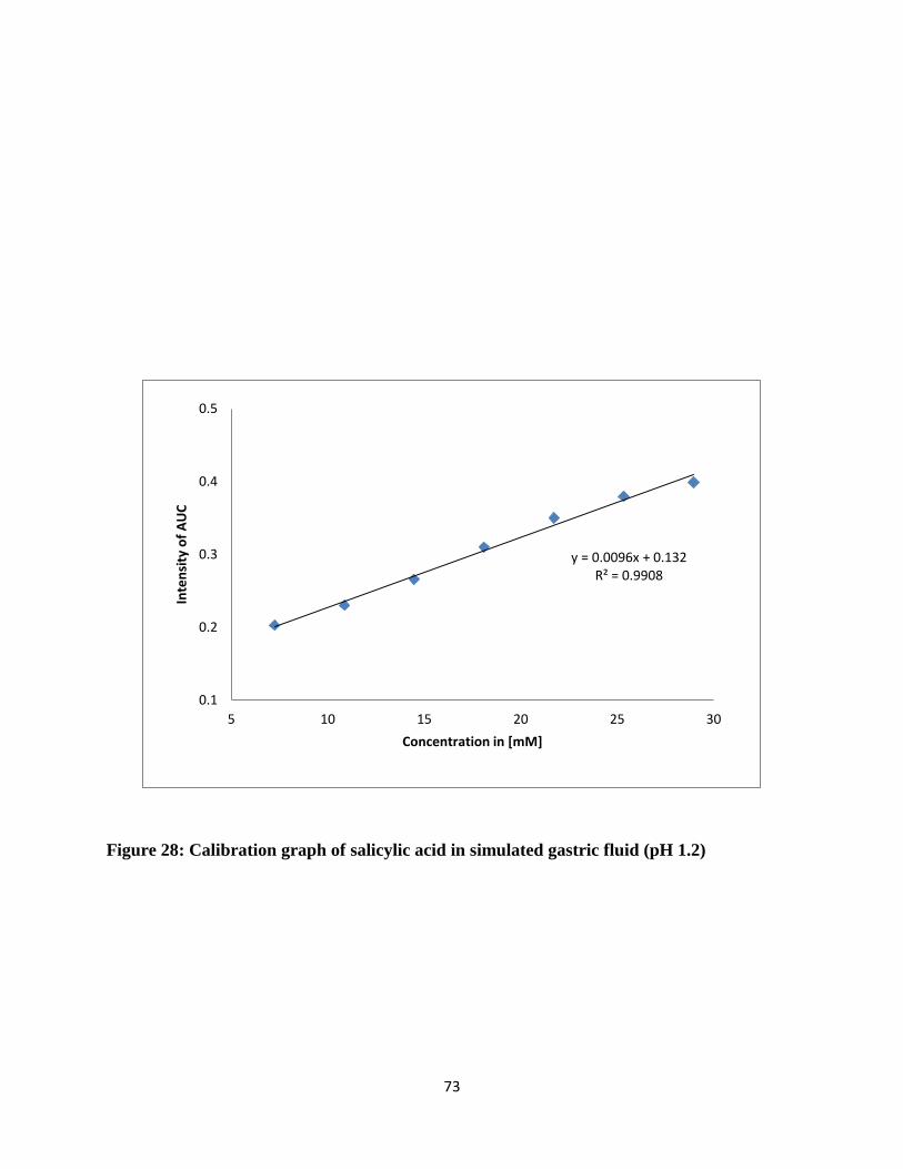
73

Figure 28: Calibration graph of salicylic acid in simulated gastric fluid (pH 1.2)

y = 0.0096x + 0.132R² = 0.9908

0.1

0.2

0.3

0.4

0.5

5 10 15 20 25 30

Inte

nsi

ty o

f A

UC

Concentration in [mM]

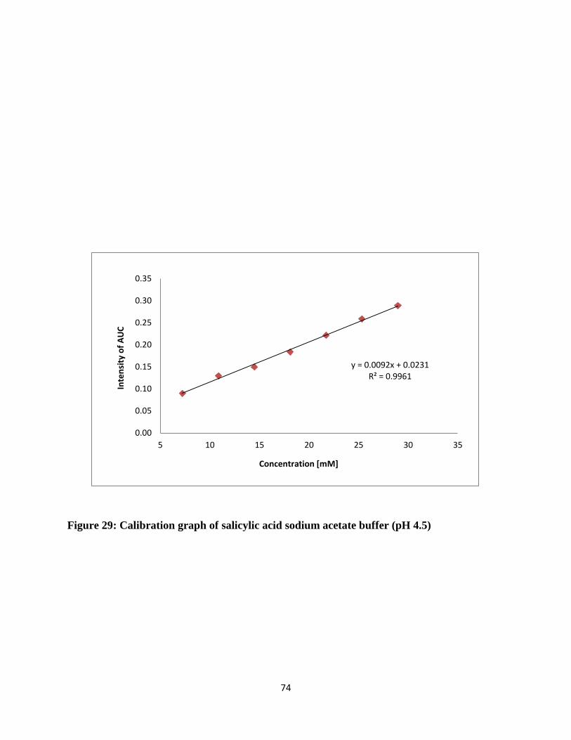
74

Figure 29: Calibration graph of salicylic acid sodium acetate buffer (pH 4.5)

y = 0.0092x + 0.0231R² = 0.9961

0.00

0.05

0.10

0.15

0.20

0.25

0.30

0.35

5 10 15 20 25 30 35

Inte

nsi

ty o

f A

UC

Concentration [mM]

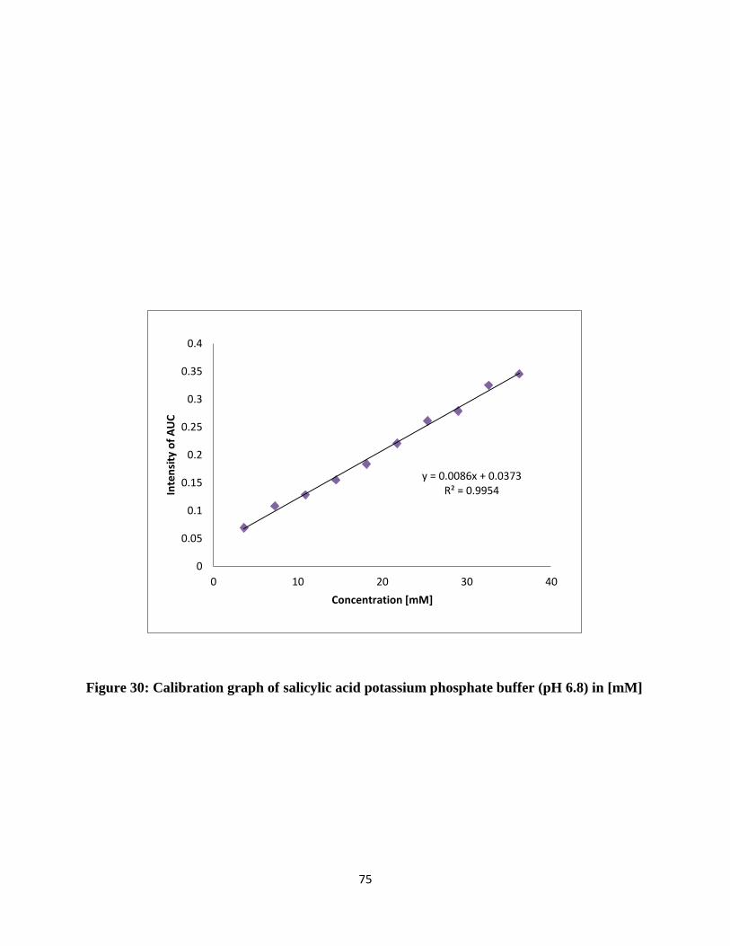
75

Figure 30: Calibration graph of salicylic acid potassium phosphate buffer (pH 6.8) in [mM]

y = 0.0086x + 0.0373R² = 0.9954

0

0.05

0.1

0.15

0.2

0.25

0.3

0.35

0.4

0 10 20 30 40

Inte

nsi

ty o

f A

UC

Concentration [mM]

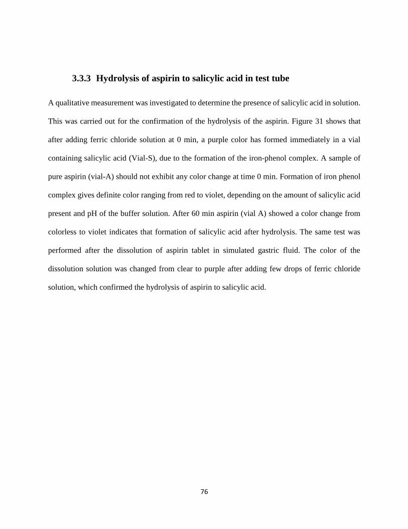
76

3.3.3 Hydrolysis of aspirin to salicylic acid in test tube

A qualitative measurement was investigated to determine the presence of salicylic acid in solution.

This was carried out for the confirmation of the hydrolysis of the aspirin. Figure 31 shows that

after adding ferric chloride solution at 0 min, a purple color has formed immediately in a vial

containing salicylic acid (Vial-S), due to the formation of the iron-phenol complex. A sample of

pure aspirin (vial-A) should not exhibit any color change at time 0 min. Formation of iron phenol

complex gives definite color ranging from red to violet, depending on the amount of salicylic acid

present and pH of the buffer solution. After 60 min aspirin (vial A) showed a color change from

colorless to violet indicates that formation of salicylic acid after hydrolysis. The same test was

performed after the dissolution of aspirin tablet in simulated gastric fluid. The color of the

dissolution solution was changed from clear to purple after adding few drops of ferric chloride

solution, which confirmed the hydrolysis of aspirin to salicylic acid.

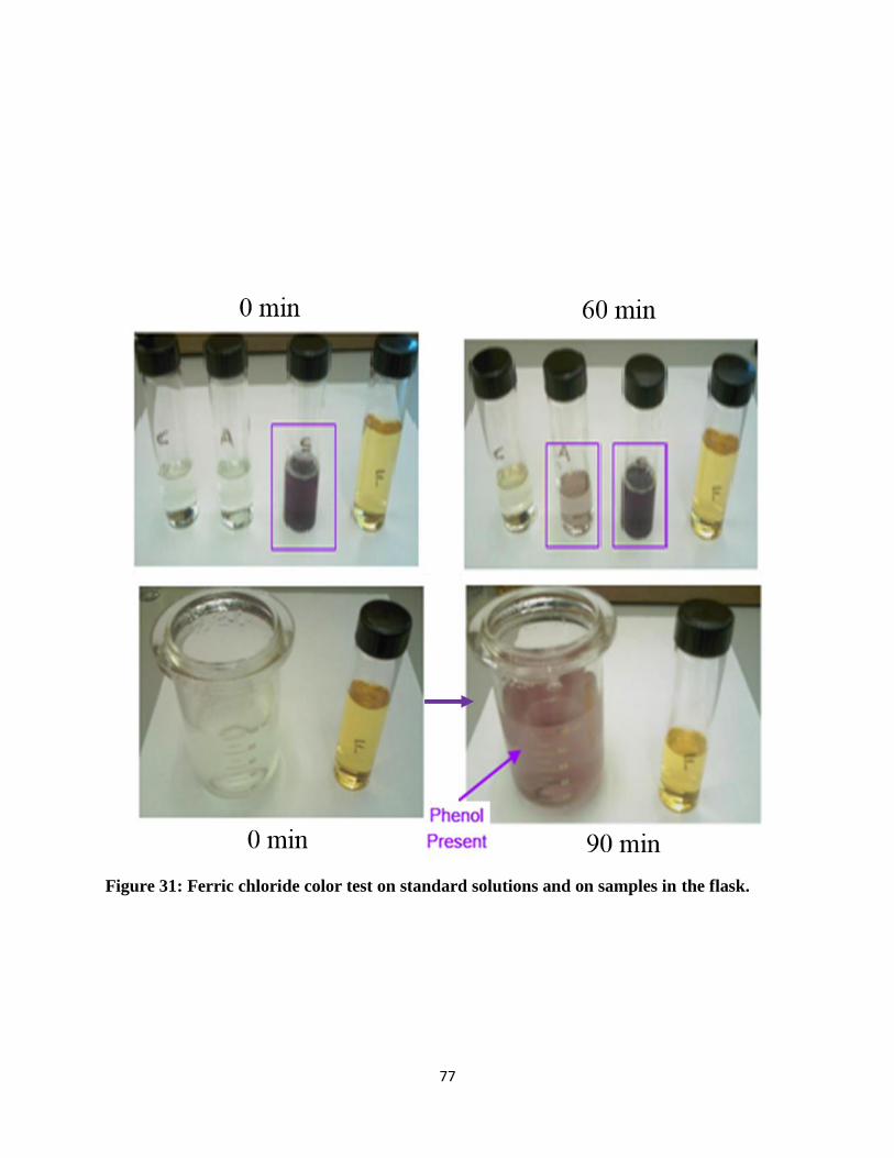
77

Figure 31: Ferric chloride color test on standard solutions and on samples in the flask.

78

3.3.4 Dissolution and hydrolysis of aspirin tablet in simulated gastric

fluid pH 1.2

This study was focused on performing dissolution, simultaneously observing hydrolysis of aspirin

by in-situ FT-IR in simulated gastric fluid. Figure 32 shows the dissolution and hydrolysis of

aspirin and formation of salicylic acid with time. The dissolution profile was monitored by in-situ

FT-IR and confirmed by HPLC analysis. The graph for both methods showed overlapping data

which gives the authentication of the in-situ FT-IR method. The graph has two lines, a brown line

depicts the dissolution of aspirin and a blue line depicts the formation of salicylic acid. A brown

line with steep upward trend indicates dissolution of aspirin in first 20 mins followed by downward

trend indicating hydrolysis of aspirin after 20 min. The blue line indicates the formation of salicylic

acid during this process. At initial stage of dissolution, small amount of salicylic acid was detected.

This might be because of the salicylic acid produced by aspirin in the process of manufacturing or

hydrolysis of aspirin can occurred upon storage. It is observed that the rate of dissolution is faster

at pH 1.2 compared to other pHs. The rate of dissolution is 1.706 mM/min in simulated gastric

fluid. Almost 90% of the aspirin was dissolved in first 15-20 min in simulated gastric fluid pH 1.2,

which indicates that stomach is the best place for the dissolution of the aspirin tablet. It was

observed that the rate of the dissolution rate of hydrolysis also faster than other pHs.

79

After the dissolution and hydrolysis study was confirmed, a replicate study with the same

experimental conditions was performed as shown in Figure 33. During the replicate study, the

result of dissolution and hydrolysis of aspirin and formation of salicylic acid overlapped with the

initial study which confirmed the method.

Figure 34 shows the combined study of all dissolutions and hydrolysis of aspirin from all the

experiments. Data from all these experiments were combined to calculate standard deviation,

which is shown in the form of error bars within the range of 4-5%.

Table 2 shows the amount of aspirin and salicylic acid by in-situ FT-IR and HPLC methods. In

this table, the quantities are mentioned in the mM concentration instead of percent dissolution. The

Bayer aspirin tablet contains 325 mg of aspirin, was converted into millimolar concentration of

18.03 mM. The percent dissolution and hydrolysis of aspirin and formation of salicylic acid was

also converted to mM.

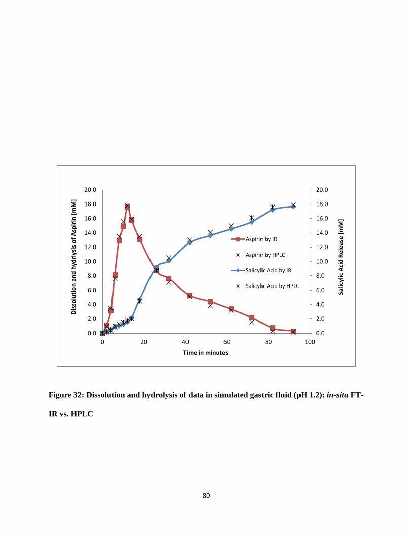
80

Figure 32: Dissolution and hydrolysis of data in simulated gastric fluid (pH 1.2): in-situ FT-

IR vs. HPLC

0.0

2.0

4.0

6.0

8.0

10.0

12.0

14.0

16.0

18.0

20.0

0.0

2.0

4.0

6.0

8.0

10.0

12.0

14.0

16.0

18.0

20.0

0 20 40 60 80 100Sa

licyl

ic A

cid

Re

leas

e [

mM

]

Dis

solu

tio

n a

nd

hyd

rlys

is o

f A

spir

in [

mM

]

Time in minutes

Aspirin by IR

Aspirin by HPLC

Salicylic Acid by IR

Salicylic Acid by HPLC

81


IR, Overlay

0.0

2.0

4.0

6.0

8.0

10.0

12.0

14.0

16.0

18.0

20.0

0.0

2.0

4.0

6.0

8.0

10.0

12.0

14.0

16.0

18.0

20.0

0 20 40 60 80 100Sa

licyl

ic A

cid

Re

leas

e [

mM

]

Dis

solu

tio

n a

nd

Hyd

roly

sis

of

Asp

irin

[m

M]

Time in minutes

Aspirin by IR Aspirin by IR


Aspirin by IR Salicylic Acid by IR

Salicylic Acid by IR Salicylic Acid by IR


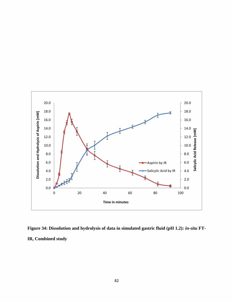
82


IR, Combined study

0.0

2.0

4.0

6.0

8.0

10.0

12.0

14.0

16.0

18.0

20.0

0.0

2.0

4.0

6.0

8.0

10.0

12.0

14.0

16.0

18.0

20.0

0 20 40 60 80 100Sa

licyl

ic A

cid

Re

leas

e [

mM

]

Dis

solu

tio

n a

nd

Hyd

roly

sis

of

Asp

irin

[m

M]

Time in minutes

Aspirin by IR


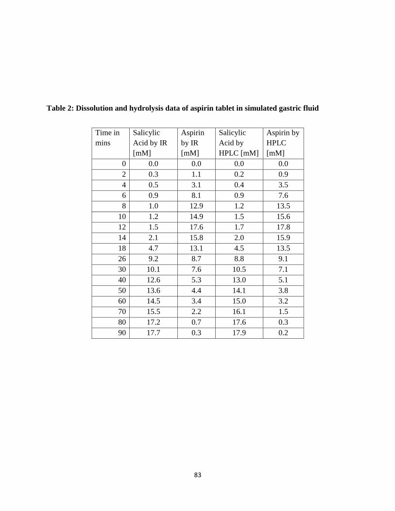
83

Table 2: Dissolution and hydrolysis data of aspirin tablet in simulated gastric fluid

Time in

mins

Salicylic

Acid by IR

[mM]

Aspirin

by IR

[mM]

Salicylic

Acid by

HPLC [mM]

Aspirin by

HPLC

[mM]

0 0.0 0.0 0.0 0.0

2 0.3 1.1 0.2 0.9

4 0.5 3.1 0.4 3.5

6 0.9 8.1 0.9 7.6

8 1.0 12.9 1.2 13.5

10 1.2 14.9 1.5 15.6

12 1.5 17.6 1.7 17.8

14 2.1 15.8 2.0 15.9

18 4.7 13.1 4.5 13.5

26 9.2 8.7 8.8 9.1

30 10.1 7.6 10.5 7.1

40 12.6 5.3 13.0 5.1

50 13.6 4.4 14.1 3.8

60 14.5 3.4 15.0 3.2

70 15.5 2.2 16.1 1.5

80 17.2 0.7 17.6 0.3

90 17.7 0.3 17.9 0.2

84

3.3.5 Dissolution and hydrolysis of aspirin tablet in sodium acetate

buffer pH 4.5

In the method development of dissolution, it is a good practice to perform the dissolutions in

different body pHs and study the dissolution pattern. After gastric simulated fluid tablet moves to

the duodenum, another place where a tablet can dissolve in the body. This set of experiments

performed dissolution and simultaneously observed hydrolysis of aspirin by in-situ FT-IR in

sodium acetate buffer having pH 4.5 depicts duodenum pH and compared with HPLC.

Figure 35 shows the dissolution and hydrolysis of aspirin and formation of salicylic acid with time.

The dissolution profile was monitored by in-situ FT-IR and confirmed by HPLC analysis. The

graph for both methods showed overlapping data which gives the authentication of the in-situ FT-

IR method. The graph has two lines, a brown line depicts the dissolution of aspirin and a blue line

depicts the formation of salicylic acid. A brown line with steep upward trend indicates dissolution

of aspirin in first 3-4 hrs followed by downward trend indicating hydrolysis of aspirin after 3-4

hrs. The blue line indicates the formation of salicylic acid during this process. Thus the dissolution

and the hydrolysis of aspirin and at the same time formation of the salicylic acid was observed. At

initial stage of dissolution, small amount of salicylic acid was detected. This might be because of

the salicylic acid produced by aspirin in the process of manufacturing or hydrolysis of aspirin can

occurred upon storage. It was observed that the rate of dissolution is slower in pH 4.5 sodium

acetate buffer compared to simulated gastric fluid pH 1.2. The rate is affected on the basis of

acidity of dissolution medium that is 0.545 mM/min. The dissolution and hydrolysis of aspirin

85

with the comparison of HPLC data and confirmed by this method. It was observed that the rate of

the dissolution rate of hydrolysis was slower than simulated gastric fluid pH 1.2.

After the dissolution and hydrolysis study was confirmed, a replicate study with the same

experimental conditions was performed as shown in Figure 36. During the replicate study, the

result of dissolution and hydrolysis of aspirin and formation of salicylic acid are overlapped with

the initial study which confirmed the method.





this table, the quantities are mentioned in the mM concentration instead of percent dissolution. The



also converted to mM

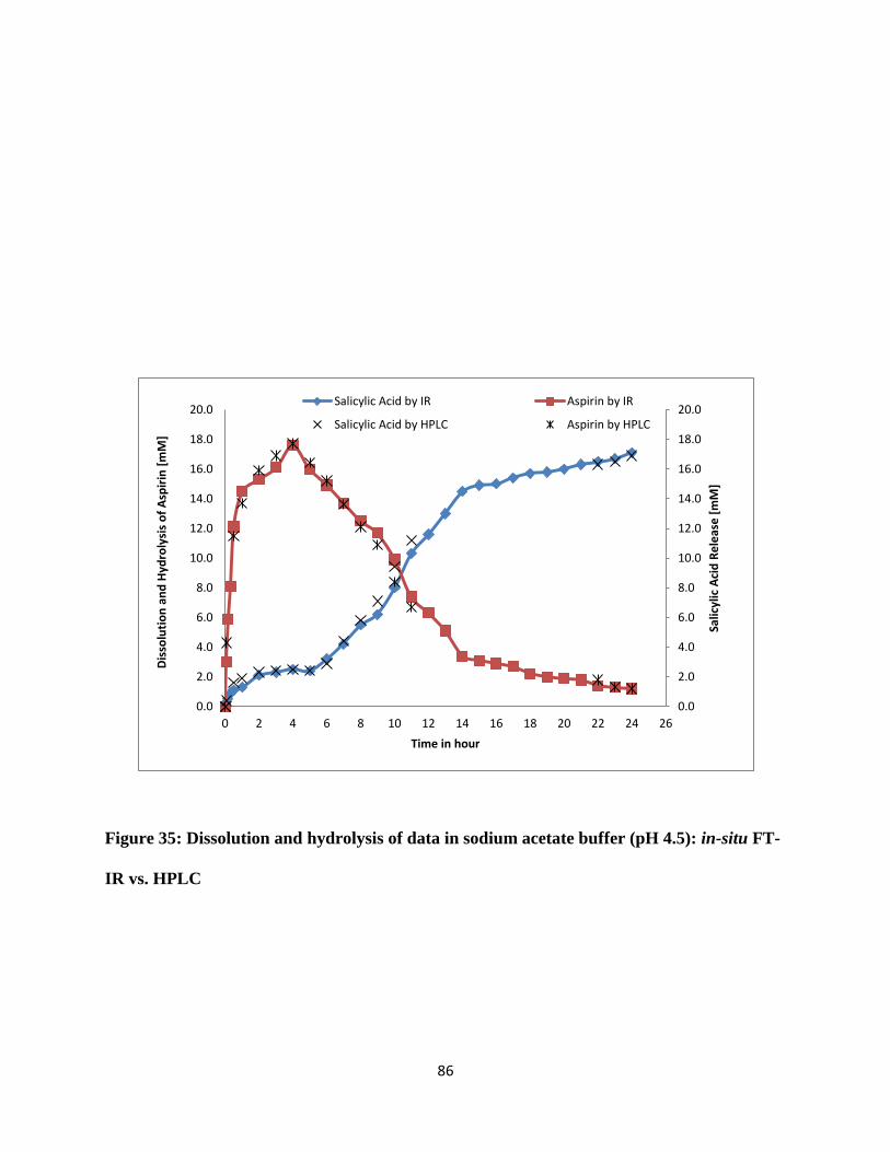
86

Figure 35: Dissolution and hydrolysis of data in sodium acetate buffer (pH 4.5): in-situ FT-

IR vs. HPLC

0.0

2.0

4.0

6.0

8.0

10.0

12.0

14.0

16.0

18.0

20.0

0.0

2.0

4.0

6.0

8.0

10.0

12.0

14.0

16.0

18.0

20.0

0 2 4 6 8 10 12 14 16 18 20 22 24 26Sa

licyl

ic A

cid

Re

leas

e [

mM

]

Dis

solu

tio

n a

nd

Hyd

roly

sis

of

Asp

irin

[m

M]

Time in hour

Salicylic Acid by IR Aspirin by IR

Salicylic Acid by HPLC Aspirin by HPLC

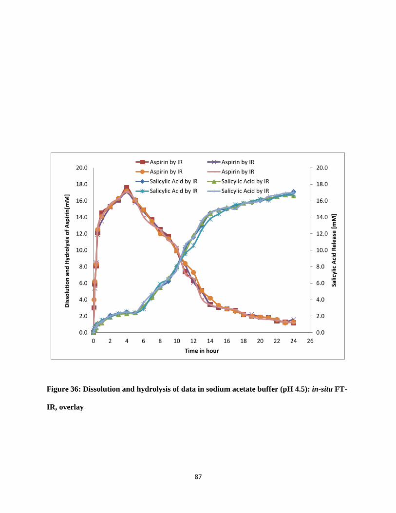
87


IR, overlay

0.0

2.0

4.0

6.0

8.0

10.0

12.0

14.0

16.0

18.0

20.0

0.0

2.0

4.0

6.0

8.0

10.0

12.0

14.0

16.0

18.0

20.0

0 2 4 6 8 10 12 14 16 18 20 22 24 26Sa

licyl

ic A

cid

Re

leas

e [

mM

]

Dis

solu

tio

n a

nd

Hyd

roly

sis

of

Asp

irin

[mM

]

Time in hour





88


IR, combined study

0.0

2.0

4.0

6.0

8.0

10.0

12.0

14.0

16.0

18.0

20.0

0.0

2.0

4.0

6.0

8.0

10.0

12.0

14.0

16.0

18.0

20.0

0 2 4 6 8 10 12 14 16 18 20 22 24 26Sa

licyl

ic A

cid

Re

leas

e [

mM

]

Dis

solu

tio

n a

nd

Hyd

roly

sis

of

asp

irin

[m

M]

Time in hour

Aspirin by IR


89

Table 3: Dissolution and hydrolysis data of aspirin tablet in sodium acetate buffer

Time

in hrs.

Salicylic

Acid by

IR [mM]

Aspirin

by IR

[mM]

Salicylic

Acid by

HPLC [mM]

Aspirin by

HPLC

[mM]

0 0.0 0.0 0.0 0.0

0.08 0.3 3.0 0.4 4.3

0.16 0.5 5.9 - -

0.33 0.9 8.1 - -

0.50 1.1 12.1 1.6 11.5

1 1.3 14.5 1.9 13.7

2 2.1 15.3 2.3 15.9

3 2.3 16.1 2.4 16.9

4 2.5 17.6 2.5 17.7

5 2.4 16.0 2.4 16.4

6 3.2 14.9 2.9 15.2

7 4.2 13.7 4.4 13.6

8 5.5 12.5 5.8 12.1

9 6.2 11.7 7.1 10.9

10 8.0 9.9 9.4 8.4

11 10.3 7.4 11.2 6.7

12 11.6 6.3 - -

13 13.0 5.1 - -

14 14.5 3.4 - -

15 14.9 3.1 - -

16 15.0 2.9 - -

17 15.4 2.7 - -

18 15.7 2.2 - -

19 15.8 2.0 - -

20 16.0 1.9 - -

21 16.3 1.8 - -

22 16.5 1.4 16.3 1.8

23 16.7 1.3 16.5 1.3

24 17.1 1.2 16.9 1.2

90

3.3.6 Dissolution and hydrolysis of aspirin tablet in potassium phosphate

buffer pH 6.8

As per the physiological conditions, finally tablet reaches to the small intestine another place for

dissolution of pharmaceutical dosage forms. In this set of experiments were performed dissolution

and simultaneously observed hydrolysis of aspirin by in-situ FT-IR in phosphate buffer having pH

6.8 depicts small intestine pH and compared with HPLC.

Figure 38 shows the dissolution and hydrolysis of aspirin and formation of salicylic acid with time.

The dissolution profile was monitored by in-situ FT-IR and confirmed by HPLC analysis. The

graph for both methods showed overlapping data which gives the authentication of the in-situ FT-

IR method. The graph has two lines, a brown line depicts the dissolution of aspirin and a blue line

depicts the formation of salicylic acid. A brown line with steep upward trend indicates dissolution

of aspirin in first 7-8 hrs followed by downward trend indicating hydrolysis of aspirin after 7-8

hrs. The blue line indicates the formation of salicylic acid during this process. Thus the dissolution

and the hydrolysis of aspirin and at the same time formation of the salicylic acid was observed. At

initial stage of dissolution, small amount of salicylic acid was detected. This might be because of

the salicylic acid produced by aspirin in the process of manufacturing or hydrolysis of aspirin can

occurred upon storage. It was observed that the rate of dissolution is slowest in potassium

phosphate buffer pH 6.8 compared to other two pHs is 0.085mM/min. The dissolution and

hydrolysis of aspirin with the comparison of HPLC data and confirmed by this method. It was

observed that the rate of dissolution and hydrolysis was slowest than other pHs.

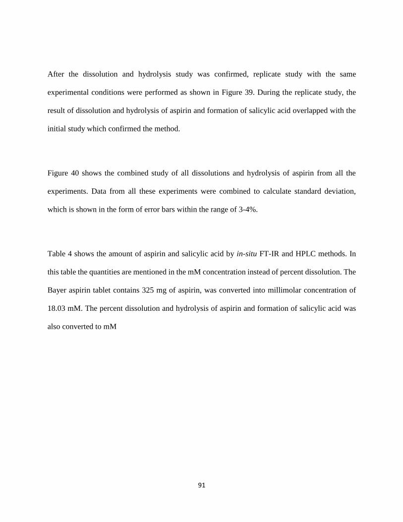
91

After the dissolution and hydrolysis study was confirmed, replicate study with the same

experimental conditions were performed as shown in Figure 39. During the replicate study, the

result of dissolution and hydrolysis of aspirin and formation of salicylic acid overlapped with the

initial study which confirmed the method.





this table the quantities are mentioned in the mM concentration instead of percent dissolution. The



also converted to mM

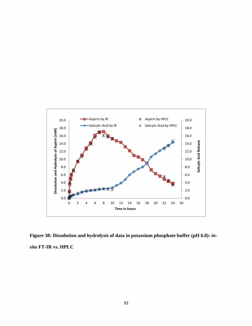
92

Figure 38: Dissolution and hydrolysis of data in potassium phosphate buffer (pH 6.8): in-

situ FT-IR vs. HPLC

0.0

2.0

4.0

6.0

8.0

10.0

12.0

14.0

16.0

18.0

20.0

0.0

2.0

4.0

6.0

8.0

10.0

12.0

14.0

16.0

18.0

20.0

0 2 4 6 8 10 12 14 16 18 20 22 24 26

Salic

ylic

Aci

d R

ele

ase

Dis

solu

tio

n a

nd

Hyd

roly

sis

of

Asp

irin

[m

M]

Time in hours

Aspirin by IR Aspirin by HPLC

Salicylic Acid by IR Salicylic Acid by HPLC

93

Figure 39: Dissolution and hydrolysis of data in potassium phosphate buffer (pH 6.8): in situ,

overlay

0.0

2.0

4.0

6.0

8.0

10.0

12.0

14.0

16.0

18.0

20.0

0.0

2.0

4.0

6.0

8.0

10.0

12.0

14.0

16.0

18.0

20.0

0 2 4 6 8 10 12 14 16 18 20 22 24 26Sa

licyl

ic A

cid

Re

leas

e [

mM

]

Dis

solu

tio

n a

nd

Hyd

roly

sis

of

Asp

irin

[m

M]

Time in hour





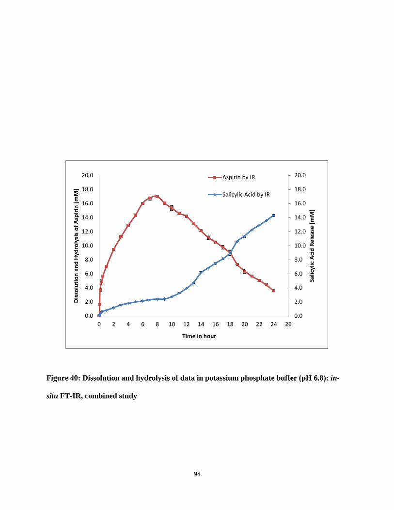
94

Figure 40: Dissolution and hydrolysis of data in potassium phosphate buffer (pH 6.8): in-

situ FT-IR, combined study

0.0

2.0

4.0

6.0

8.0

10.0

12.0

14.0

16.0

18.0

20.0

0.0

2.0

4.0

6.0

8.0

10.0

12.0

14.0

16.0

18.0

20.0

0 2 4 6 8 10 12 14 16 18 20 22 24 26

Salic

ylic

Aci

d R

ele

ase

[m

M]

Dis

solu

tio

n a

nd

Hyd

roly

sis

of

Asp

irin

[m

M]

Time in hour

Aspirin by IR


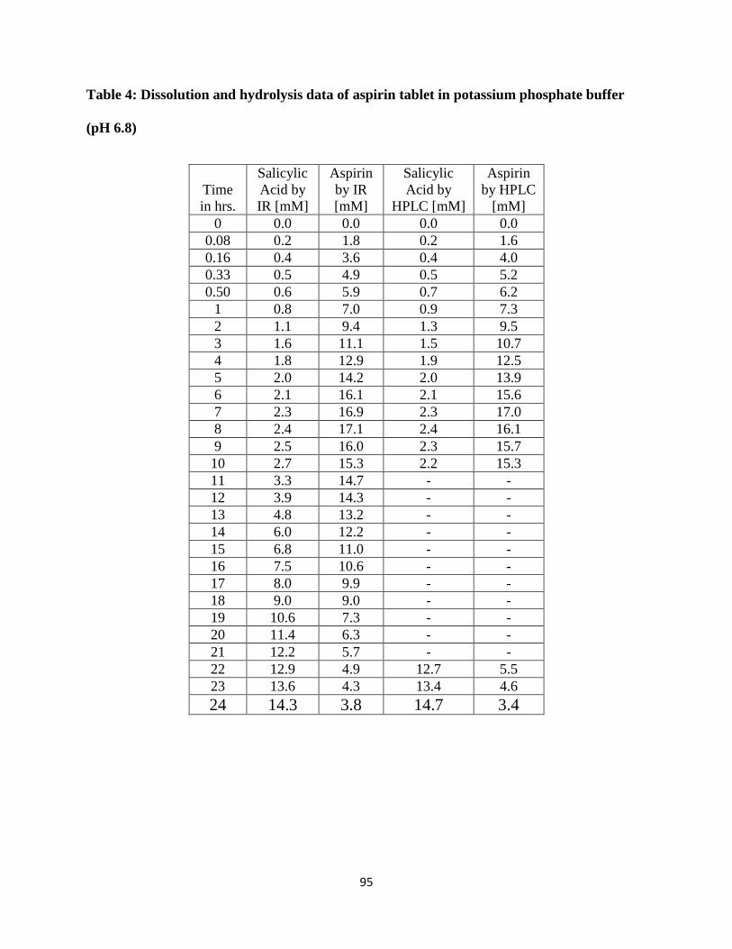
95

Table 4: Dissolution and hydrolysis data of aspirin tablet in potassium phosphate buffer

(pH 6.8)

Time

in hrs.

Salicylic

Acid by

IR [mM]

Aspirin

by IR

[mM]

Salicylic

Acid by

HPLC [mM]

Aspirin

by HPLC

[mM]

0 0.0 0.0 0.0 0.0

0.08 0.2 1.8 0.2 1.6

0.16 0.4 3.6 0.4 4.0

0.33 0.5 4.9 0.5 5.2

0.50 0.6 5.9 0.7 6.2

1 0.8 7.0 0.9 7.3

2 1.1 9.4 1.3 9.5

3 1.6 11.1 1.5 10.7

4 1.8 12.9 1.9 12.5

5 2.0 14.2 2.0 13.9

6 2.1 16.1 2.1 15.6

7 2.3 16.9 2.3 17.0

8 2.4 17.1 2.4 16.1

9 2.5 16.0 2.3 15.7

10 2.7 15.3 2.2 15.3

11 3.3 14.7 - -

12 3.9 14.3 - -

13 4.8 13.2 - -

14 6.0 12.2 - -

15 6.8 11.0 - -

16 7.5 10.6 - -

17 8.0 9.9 - -

18 9.0 9.0 - -

19 10.6 7.3 - -

20 11.4 6.3 - -

21 12.2 5.7 - -

22 12.9 4.9 12.7 5.5

23 13.6 4.3 13.4 4.6

24 14.3 3.8 14.7 3.4

96

3.3.7 Kinetic study

The kinetic rates were also determined for the experiments discussed earlier. The kinetics of the

dissolution and hydrolysis is based on the concentration of aspirin, so it is a first order reaction.

[96] Kinetic study was determined by using the slope of the line and by using following formula

to study rate of dissolution and rate of hydrolysis.

ln[𝐴] = −𝑘𝑡 + ln[𝐴]0 (10)

The rates are compared to literature research [97] [98] [99]and were found dissolution rate to be

equivalent. The literature data shows the rate of hydrolysis of aspirin has a specific pH rate profile.

[100] The experimental values showed comparable rate profile. In this study, the rate of hydrolysis

of aspirin after dissolution is completely depends on the rate of dissolution. The main goal of this

is to monitor dissolution and hydrolysis of aspirin tablet. For the hydrolysis reaction, there must

be free aspirin present in the solution, which will be available after the dissolution of the tablet. So

as the rate of dissolution is slow with a change in the pH, hydrolysis is also slow.

The rates of the reactions were determined from the dissolution plots. In order to calculate the rates

using the plot, the following procedure was implemented. First, a plot log of percent dissolved vs.

time is obtained which was shown in the initial part of result section. Next, a straight line is drawn

over the area of the dissolution curve where dissolution starts to occur (middle area in this case).

Furthermore, the rate of hydrolysis is also calculated with the same method using the graph where

the hydrolysis starts, showed in the hydrolysis that is disappearance curve.

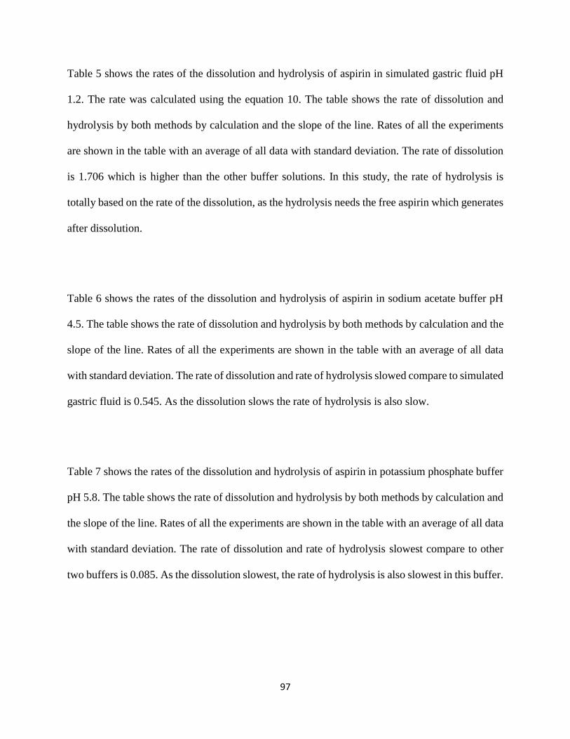
97

Table 5 shows the rates of the dissolution and hydrolysis of aspirin in simulated gastric fluid pH

1.2. The rate was calculated using the equation 10. The table shows the rate of dissolution and

hydrolysis by both methods by calculation and the slope of the line. Rates of all the experiments

are shown in the table with an average of all data with standard deviation. The rate of dissolution

is 1.706 which is higher than the other buffer solutions. In this study, the rate of hydrolysis is

totally based on the rate of the dissolution, as the hydrolysis needs the free aspirin which generates

after dissolution.

Table 6 shows the rates of the dissolution and hydrolysis of aspirin in sodium acetate buffer pH

4.5. The table shows the rate of dissolution and hydrolysis by both methods by calculation and the

slope of the line. Rates of all the experiments are shown in the table with an average of all data

with standard deviation. The rate of dissolution and rate of hydrolysis slowed compare to simulated

gastric fluid is 0.545. As the dissolution slows the rate of hydrolysis is also slow.

Table 7 shows the rates of the dissolution and hydrolysis of aspirin in potassium phosphate buffer

pH 5.8. The table shows the rate of dissolution and hydrolysis by both methods by calculation and

the slope of the line. Rates of all the experiments are shown in the table with an average of all data

with standard deviation. The rate of dissolution and rate of hydrolysis slowest compare to other

two buffers is 0.085. As the dissolution slowest, the rate of hydrolysis is also slowest in this buffer.

98

Table 5: Rate of dissolution and hydrolysis in simulated gastric fluid (pH 1.2)

By Calculations By Slope

Exp

Rate of Dissolution

(mM/min)

Rate of Hydrolysis

(mM/min)

Rate of Dissolution

(mM/min)

Rate of Hydrolysis

(mM/min)

1 1.500 0.675 1.283 0.586

2 1.766 0.775 1.415 0.454

3 1.733 0.650 1.387 0.465

4 1.866 0.275 1.322 0.586

5 1.667 0.675 1.283 0.586

Avg 1.706 0.610 1.338 0.535

S. dev 0.136 0.193 0.061 0.069

99

Table 6: Rate of dissolution and hydrolysis in sodium acetate buffer (pH 4.5)


Exp

Rate of Dissolution

(mM/min)

Rate of Hydrolysis

(mM/min)

Rate of Dissolution

(mM/min)

Rate of Hydrolysis

(mM/min)

1 0.540 0.033 0.561 0.024

2 0.580 0.018 0.559 0.024

3 0.480 0.022 0.561 0.023

4 0.580 0.020 0.559 0.022

Avg 0.545 0.023 0.560 0.023

S. dev 0.047 0.007 0.002 0.001

100

Table 7: Rate of dissolution and hydrolysis study in potassium phosphate buffer (pH 6.8)


Exp

Rate of Dissolution

(mM/min)

Rate of Hydrolysis

(mM/min)

Rate of Dissolution

(mM/min)

Rate of Hydrolysis

(mM/min)

1 0.110 0.012 0.306 0.015

2 0.100 0.010 0.339 0.015

3 0.040 0.010 0.357 0.014

4 0.090 0.018 0.341 0.015

Avg 0.085 0.013 0.336 0.015

S. dev 0.031 0.004 0.022 0.000

101

3.4 Conclusion

The USP monograph of dissolution of aspirin explains about the conventional methods that are

UV/Vis and HPLC analysis, but the importance of this study is to perform the dissolution by FT-

IR in real time. The in-situ FT-IR measures the vibrations of a molecule in the fingerprint region,

which is important for the analyst, because each molecule has its own specific spectrum. Aspirin

has the tendency to hydrolyze and to form salicylic acid and acetic acid when it dissolves. So the

advantage of the in-situ FT-IR is to monitor dissolution as well as the hydrolysis of aspirin, which

is very difficult by UV/Vis and HPLC, because of the overlapping of these two peaks.

When the aspirin tablet was dropped into the dissolution medium, it starts to dissolve and slowly

hydrolyze into salicylic acid and acetic acid. The dissolution was performed on three different

body pHs and compared with HPLC. The results of the dissolution and hydrolysis study by both

methods are comparable, and this gives the validation of the new in-situ FT-IR technique. The

dissolution and hydrolysis of aspirin was monitored, in which two trends of the data was observed.

First trend explains about the dissolution of aspirin and followed by hydrolysis, so intensity if the

peak decreases gradually. The second trend is the formation of salicylic acid where the gradual

increase in the peak intensity was observed, based on the rate of hydrolysis. The rate of hydrolysis

and rate of formation of salicylic acid is based on the dissolution of the tablet. Once the tablet

dissolves, then the free aspirin will be available for the hydrolysis and as hydrolysis proceeds

formation of salicylic acid. So the rate of the reaction depends on the concentration as well as the

dissolution. This research was possible because of the versatility of the in-situ FT-IR system.

102

This study demonstrated that in situ infrared spectroscopy is a viable technique for detecting and

measuring the hydrolysis of aspirin at different body pH. The in-situ FT-IR system was found to

be impressive in its capability of measuring low concentrations and was able to distinguish

separate components of a multiple component hydrolysis systems without requiring manual

sampling.

This versatility is demonstrated by observing the simultaneous dissolution and then elimination of

the acetylsalicylic acid component while monitoring the formation of the salicylic acid component

as acetylsalicylic acid undergoes hydrolysis. Specifically, the unique fingerprint region of the IR

spectra gave detailed information about the release profile of the drug. Conventional methods

would only show the release profile of one component. Moreover, the hydrolysis and

transformation of the drug from one form to another is missed with conventional techniques.

However, in-situ FT-IR captures those minor details and displays them in the fingerprint region,

as shown earlier. Furthermore, since this chapter successfully demonstrates the versatility of this

novel application of in-situ FT-IR spectroscopy, it suggests that the method has excellent potential

for the study of the dissolution and hydrolysis kinetics of pro-drug formulations.

103

CHAPTER – 4

HYDROLYSIS STUDY OF ASPIRIN

4.1 Introduction

This chapter focuses on performing the dissolution and hydrolysis of different generic brands of

over the counter aspirin tablets with brand Bayer aspirin tablet by in situ FT-IR. As discussed

earlier aspirin undergoes hydrolysis to form salicylic acid and acetic acid. To perform dissolution

and hydrolysis of the different generic aspirin tablets were bought from Rite-Aid, Walgreen, CVS

pharmacies and Bayer aspirin with two different lot numbers. Two different brands of enteric

coated aspirin tablets are bought from India. The enteric coating prevents the dissolution of tablet

in acidic medium such as stomach and duodenum, tablet should dissolve in small intestine and

slowly release drug from pharmaceutical dosage form.

The comparison study of dissolution helps in the drug development of pharmaceutical dosage

forms. Fawzia and his group performed the comparison study of in vitro dissolution testing for

commercial available aspirin tablets, they observed similar dissolution profile for all brands of

aspirin. [101] Literature showed that comparison study of the dissolution with different brands has

been carried out. [102] Author compared the dissolution study with 23 generic tablets of

Levofloxacin with one branded tablet in Japan. Another study was on the design of the sustained

release tablets with different polymers and theirs quality control test to check the polymer effect

on the quality. [103] Clement and his group have compared the dissolution profile of 7 immediate-

release metformin 500 mg tablets. This study compared other characteristics such as weight

variation and drug content. The dissolution was carried on USP-II and they observed only one

formulation showed <85 % drug release in 15 min. [104] Issa and group have performed the

104

comparative study of chlorpheniramine maleate orally disintegrating tablets. They have prepared

the different formulations by using different diluents and different disintegrating agents by direct

compression method. The formulation contains glucose crospovidone showed faster dissolution

as it disintegrates at faster rate compare to other formulations. [105] Ozkan and his group have

performed the comparison of dissolution on different designed and formulated salbutamol tablets.

This study was carried out using USP-I and USP-II. They observed the commercial formulation

showed the faster release of salbutamol. [106]

Literature study explains about the importance of the comparison study of dissolution and

developed motivation for this study. Thus interest has created to perform the dissolution of

different generic brands of aspirin tablets and compare with Bayer aspirin tablet. The different

generic brands of aspirin tablets were compared with Bayer aspirin tablet with same strength by

using in-situ FT-IR spectroscopy. The comparison of Bayer aspirin has performed with the enteric

coated tablets as well. The enteric coated tablets has a coating so that these tablets could not

dissolve in the stomach and duodenum.



Acetylsalicylic acid (aspirin) reference material (batch no. 016K0131) was purchased from Sigma-

Aldrich. Salicylic acid reference material (batch no. 04708HE) was purchased from Sigma-

Aldrich. Acetylsalicylic acid 325 mg tablets (Genuine Bayer batch no. 219050N) were purchased

from a local pharmacy. Another acetylsalicylic acid 325 mg tablets (Genuine Bayer batch no.

NAA01N9), Rite-Aid Pain relief Aspirin 325 mg tablets (batch no. 4125), CVS Genuine Aspirin

105

325 mg tablets (batch no. 4200), Walgreen Regular strength Aspirin 325 mg tablets (batch

no.4148) and Bayer Advanced aspirin 500 mg tablets (batch no. 231051E) were purchased from

local Pharmacy store. Ecosprin 150 mg (batch no. 04005074) and Delisprin 150 mg (batch no.

M109M032) tablets were purchased from a local pharmacy from India. Methanol, acetone and

acetonitrile (HPLC grades) were purchased from Pharmaco-Aaper (Brookfield, CT). Sodium

chloride crystals (batch no. J39602) was purchased from Mallinckrodt Chemicals (England, UK).

Hydrochloric acid (batch no. H44032) was purchased from J.T. Baker (Central Valley, PA).

Sodium acetate crystals (batch no.05816HD, potassium phosphate monobasic (batch no.

103K0060) and sodium hydroxide (batch no. 06414BH) were purchased from Sigma-Aldrich

Chemicals (St. Louis, MO). Glacial acetic acid (batch no. 971666) was purchased from Fisher

Chemicals (Waltham, MA). All solutions were prepared using water treated by a Milli-Q plus

Millipore purification system (Milford, MA). All purified water aliquots have resistivity of not

less than 18 MOhm-cm-1.





by Mettler Toledo. HPLC analysis was performed on a Hewlett-Packard 1050 HPLC, with Chem

Station software. In-situ FT-IR analysis was carried on a Mettler Toledo iC 10 ReactIR, with iCIR

versions 3.0 and 4.0 software.

106

4.2.3 Simulated gastric fluid

Simulated gastric fluid was prepared with hydrochloric acid and sodium chloride as per USP

procedure for buffers. 2 g of sodium chloride was dissolved in 100 mL of deionized amount of

water, in that 7 mL HCl was added and then volume made up to 1000 mL by adding deionized

water, and then measured pH of that solution and adjusted to 1.2.

4.2.4 Sodium acetate buffer

Sodium acetate buffer was prepared with glacial acetic acid and sodium acetate anhydrous as per

the USP procedures for buffers. 2.99 g of sodium acetate was dissolved in 100 mL of deionized of

water, in that 1.66 mL glacial acetic acid was added and then volume made up to1000 mL by

adding deionized water and then measured pH of that solution and adjusted to 4.5.

4.2.5 Potassium phosphate buffer

Potassium phosphate buffer (0.2 M) was prepared with monobasic potassium phosphate and

sodium hydroxide as per the USP buffer procedures. First potassium phosphate solution was

prepared by weighing 27.22 g of monobasic potassium phosphate and dissolved in 100 mL of

deionized water and diluted with up to 1000 mL. Next sodium hydroxide solution was prepared

by weighing 8 g of sodium hydroxide dissolved in water and made volume up to 100 mL. For

phosphate buffer added 50 mL of monobasic potassium phosphate solution in a 200 mL volumetric

flask then added 22.4 mL of sodium hydroxide solution and then added water to make a volume.

Finally measured the pH of this solution and was adjusted to 6.8.

107


For standard solutions weighed 325 mg of aspirin and salicylic acid and dissolved in 100 mL of

simulated gastric fluid, sodium acetate buffer and potassium phosphate and made concentration

3.25 mg/mL.

4.2.7 Dissolution and hydrolysis of all brands of aspirin tablets

All aspirin tablets were measured in pH 1.2 simulated gastric fluid solutions for 1.5 hr., pH 4.5

sodium acetate buffer for 24 hr and potassium phosphate buffer for 24 hr. Dissolutions were

conducted using vessel volumes of 100 mL and at 37.0 °C. All dissolutions were conducted using

USP Apparatus Type II (paddles) with an agitation speed of 100 rpm as per USP specifications.


The set for dissolution testing was carried out as discussed in the experiment section. The in-situ

FT-IR fiber optic probe has collected baseline spectra (blank medium) for the first 30 minutes. A

single 325 mg Bayer aspirin tablet was dropped into the vessel containing 100 mL of buffer

solution (simulated gastric fluid pH 1.2, sodium acetate buffer pH 4.5 and potassium phosphate

buffer pH 6.8) and the dissolution profiles were collected using in-situ FT-IR spectroscopy.

Standard spectra of pure aspirin and salicylic acid were collected prior to running the dissolutions.

These standards were used to identify the unique peaks of interests for these active drugs. For the

aspirin tablet analysis, the same steps as discussed in calibration analysis were followed. The data

processing was carried out as mentioned in the previous chapter

108


This study was focused to perform dissolution and simultaneously observation of hydrolysis of

different generic brands of aspirin with Bayer aspirin tablet by in-situ FT-IR in simulated gastric

fluid pH 1.2, sodium acetate buffer pH 4.5 and phosphate buffer pH 5.8.

4.3.1 Comparison between Bayer aspirin and Bayer advanced aspirin

tablets

Two separate dissolutionss were conducted by the procedure as mentioned in experimental section

on Bayer aspirin and Bayer Advanced aspirin tablet. This study was focused on performing

dissolution and simultaneously observe hydrolysis of aspirin by in-situ FT-IR in simulated gastric

fluid which depicts stomach environment having pH 1.2.

Figure 41 shows the dissolution profile of aspirin as per time with simultaneous hydrolysis of

aspirin and formation of salicylic acid of both the tablets. The dissolution profile was monitored

by in-situ FT-IR. The graph showed that the Bayer Advanced tablet showed the higher dissolution

than the Bayer aspirin tablet, as that tablet is immediate release tablet. In pH 1.2 gastric fluid the

rate of the dissolution is faster with Advanced Bayer aspirin tablet. Almost 90% dissolution of the

aspirin was observed in first 15-20 mins. which indicates that stomach is the best place for the

dissolution of the aspirin tablet. The Advanced Bayer aspirin tablet is an immediate release tablet

so it dissolves in the stomach at a high rate. The brown line in the graph represents Advanced

Bayer aspirin tablet and blue line represents Bayer aspirin tablet.

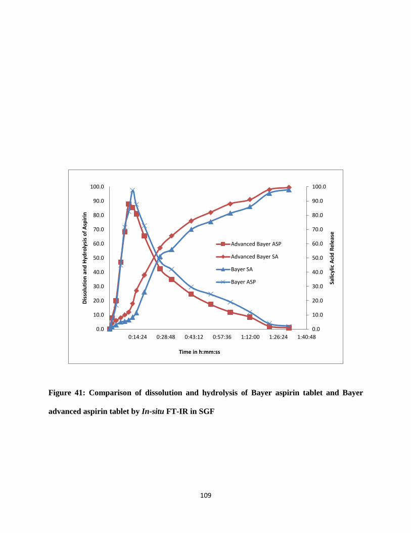
109

Figure 41: Comparison of dissolution and hydrolysis of Bayer aspirin tablet and Bayer

advanced aspirin tablet by In-situ FT-IR in SGF

0.0

10.0

20.0

30.0

40.0

50.0

60.0

70.0

80.0

90.0

100.0

0.0

10.0

20.0

30.0

40.0

50.0

60.0

70.0

80.0

90.0

100.0

0:14:24 0:28:48 0:43:12 0:57:36 1:12:00 1:26:24 1:40:48Sa

licyl

ic A

cid

Re

leas

e

Dis

solu

tio

n a

nd

Hyd

roly

sis

of

Asp

irin

Time in h:mm:ss

Advanced Bayer ASP

Advanced Bayer SA

Bayer SA

Bayer ASP

110

4.3.2 Comparison between Bayer aspirin and generic aspirin tablets

This set of experiments performed dissolution and simultaneously observed hydrolysis of aspirin

by in-situ FT-IR in simulated gastric acid pH 1.2, sodium acetate buffer having pH 4.5 and

phosphate buffer pH 6.8 on Bayer aspirin tablets and other generic aspirin tablets. Each dissolution

was performed separately with same dissolution conditions and gone through the data treatment

on in-situ FT-IR.

Figure 42 shows the overlay plot of the dissolution profile of aspirin as per time, simultaneous

hydrolysis of aspirin and formation of salicylic acid in simulated gastric fluid pH 1.2. The plot

showed the dissolution and the hydrolysis data of 5 types of aspirin tablets which are mentioned

in the experimental section. All these tablets showed a similar trend for dissolution plot, then

aspirin peak intensity has decreased and at the same time formation of salicylic trend starts

increasing. The aspirin trend line has decreased shows the hydrolysis of aspirin. The dissolution

and hydrolysis all brands of aspirin tablets are similar to each other and they overlapped.


hydrolysis of aspirin and formation of salicylic acid in sodium acetate buffer pH 4.5. The plot

showed the dissolution and the hydrolysis data of 5 types of aspirin tablets which are mentioned

in the experimental section. All these tablets showed a similar trend for dissolution plot, then

aspirin peak intensity has decreased and at the same time formation of salicylic trend starts


and hydrolysis all brands of aspirin tablets are similar to each other and overlapped.

111

Figure 42: Comparison of dissolution and hydrolysis of all brands of aspirin tablets by in-

situ FT-IR in simulated gastric fluid

0.0

2.0

4.0

6.0

8.0

10.0

12.0

14.0

16.0

18.0

20.0

0.0

2.0

4.0

6.0

8.0

10.0

12.0

14.0

16.0

18.0

20.0

0 20 40 60 80 100Sa

licyl

ic A

cid

Re

leas

e [

mM

]

Dis

solu

tio

n a

nd

Hyd

roly

sis

of

Asp

irin

[m

M]

Time in minutes

Bayer SA Bayer AspirinNew B SA New B AspirinCVS SA CVS AspirinRite aid SA Rite aid AspirinWalgreen SA Walgreen Aspirin

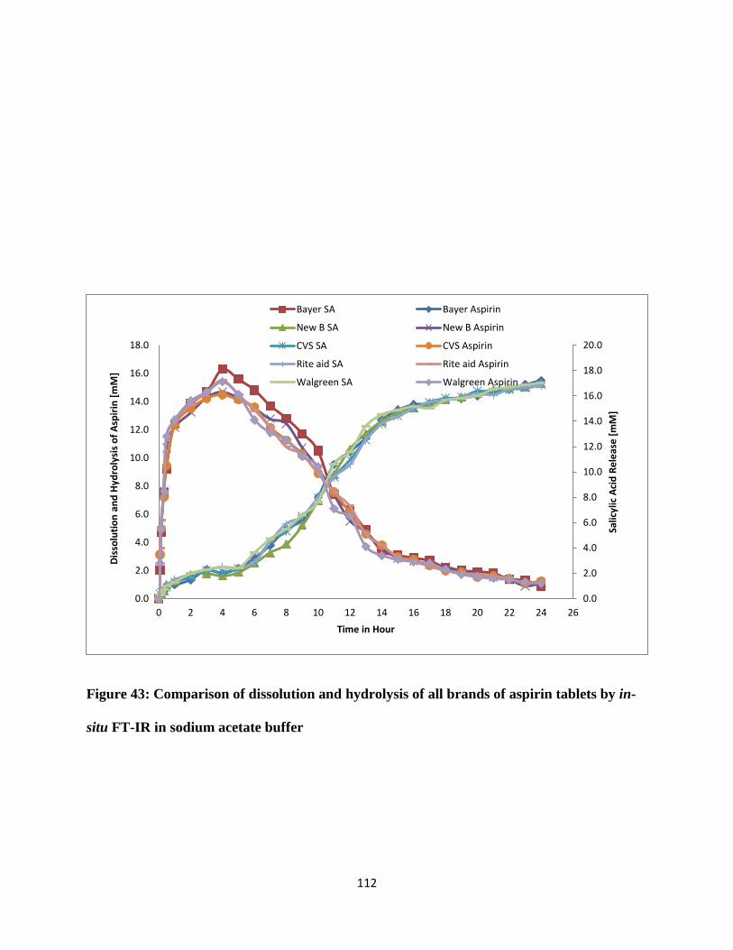
112


situ FT-IR in sodium acetate buffer

0.0

2.0

4.0

6.0

8.0

10.0

12.0

14.0

16.0

18.0

20.0

0.0

2.0

4.0

6.0

8.0

10.0

12.0

14.0

16.0

18.0

0 2 4 6 8 10 12 14 16 18 20 22 24 26Sa

licyl

ic A

cid

Re

leas

e [

mM

]

Dis

solu

tio

n a

nd

Hyd

roly

sis

of

Asp

irin

[m

M]

Time in Hour

Bayer SA Bayer Aspirin

New B SA New B Aspirin

CVS SA CVS Aspirin

Rite aid SA Rite aid Aspirin

Walgreen SA Walgreen Aspirin

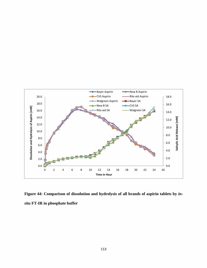
113


situ FT-IR in phosphate buffer

0.0

2.0

4.0

6.0

8.0

10.0

12.0

14.0

16.0

18.0

0.0

2.0

4.0

6.0

8.0

10.0

12.0

14.0

16.0

18.0

20.0

0 2 4 6 8 10 12 14 16 18 20 22 24 26

Salic

ylic

Aci

d R

ele

ase

[m

M]

Dis

solu

tio

n a

nd

Hyd

roly

sis

of

Asp

irin

[m

M]

Time in Hour

Bayer Aspirin New B Aspirin

CVS Aspirin Rite aid Aspirin

Walgreen Aspirin Bayer SA

New B SA CVS SA

Rite aid SA Walgreen SA

114


hydrolysis of aspirin and formation of salicylic acid in potassium phosphate buffer pH 5.8. The

plot showed the dissolution and the hydrolysis data of 5 types of aspirin tablets which are

mentioned in the experimental section. All these tablets showed a similar trend for dissolution plot,

then aspirin peak intensity has decreased and at the same time formation of salicylic trend starts


and hydrolysis all brands of aspirin tablets are similar to each other and overlapped on.

4.3.3 Dissolution of enteric-coated tablets

The next step of the comparison study of dissolution and hydrolysis of aspirin is to perform the

the dissolution of enteric coated aspirin tablets. The enteric coated means, that the tablet is coated

with a material to prevent the dissolution process in the stomach and in duodenum but allow

dissolution in the small intestine. The advantage of this coating is to avoid dissolution of those

compounds which creates stomach irritations. The Ecospirin-150 and Delisiprin-150 tablets were

selected for this study. The dissolution of these tablets was carried out in simulated gastric fluid

pH 1.2 and sodium acetate buffer pH 4.5 up to 24 hrs. for the confirmation of the enteric coating

and observed that both tablets showed no dissolution in both buffers. At the end of 24 hrs. tablets

were present in the dissolution media in its initial form. However, the dissolution of these tablets

were performed in phosphate buffer pH 6.8 and observed the dissolution of aspirin followed by

hydrolysis.

115

The dissolution of Ecospirin-150 was carried as per the procedure mentioned in the experimental

section. Figure 45 shows the comparison of dissolution and hydrolysis data of aspirin. The similar

profile was observed as discussed earlier. The dissolution of aspirin plot was increased as per the

time and after dissolution, simultaneous hydrolysis of aspirin was observed. With this formation

of salicylic acid was also observed in potassium phosphate buffer pH 6.8.The dissolution was

compared with Bayer aspirin tablet. The data was overlapped.

The dissolution of Delisprin-150 was carried as per the procedure mentioned in the experimental

section. Figure 46 shows the comparison of dissolution and hydrolysis data of aspirin. The similar

profile was observed as discussed earlier. The dissolution of aspirin plot was increased as per the

time and after dissolution, simultaneous hydrolysis of aspirin was observed. With this formation

of salicylic acid was also observed in potassium phosphate buffer pH 6.8.The dissolution was

compared with Bayer aspirin tablet. The data was overlapped.

116

Figure 45: Dissolution and hydrolysis of Ecospirin-150 tablet by in-situ compared with Bayer

aspirin in Phosphate buffer

0.0

2.0

4.0

6.0

8.0

10.0

12.0

14.0

16.0

18.0

0.0

2.0

4.0

6.0

8.0

10.0

12.0

14.0

16.0

18.0

20.0

0 2 4 6 8 10 12 14 16 18 20 22 24 26

Salic

ylic

Aci

s R

elea

se [

mM

]

Dis

solu

tio

n a

nd

Hyd

roly

sis

of

Asp

irin

in [

mM

]

TIme in Hour

Bayer Aspirin Bayer SA

Ecospirin SA Ecospirin Asp

117

Figure 46: Dissolution and hydrolysis of Delisprin-150 tablet by in-situ FT-IR compared with

Bayer aspirin tablet in Phosphate buffer

0.0

2.0

4.0

6.0

8.0

10.0

12.0

14.0

16.0

18.0

0.0

2.0

4.0

6.0

8.0

10.0

12.0

14.0

16.0

18.0

0 2 4 6 8 10 12 14 16 18 20 22 24 26Sa

licyl

ic A

cid

Rel

ease

[m

M]

Dis

solu

tio

n a

nd

Hyd

roly

sis

of

Ap

irin

[m

M]

Time in Hour

Bayer Aspirin Bayer SA

Delisprin ASP Delisprin SA

118

4.3.4 Kinetic study

The kinetic study was determined by using the slope of the line and by using following formula

calculated the rate of dissolution and rate of hydrolysis.

ln[𝐴] = −𝑘𝑡 + ln[𝐴]0 (11)

The rates of the reactions were determined from the dissolution plots. In order to calculate the rates

using the plot, the following procedure was implemented. First, a plot log of percent dissolved vs.

time is obtained which was shown in the initial part of result section. Next, a straight line is drawn

over the area of the dissolution curve where dissolution starts to occur (middle area in this case).

Furthermore, the rate of hydrolysis is also calculated with the same method using the graph where

the hydrolysis starts, showed in the hydrolysis that is disappearance curve.

As the main goal is to study the dissolution of an aspirin tablet and with that monitoring hydrolysis

of aspirin. For the hydrolysis reaction, there must be free aspirin present in the solution, which will

come after the dissolution of the tablet. So as the rate of dissolution is slow with a change in the

pH, hydrolysis is also slow.

Table 8 shows the rate of dissolution and rate of hydrolysis of all dissolutions data. The list of

brands of aspirin tablets and their dissolution and hydrolysis rates has shown in the table. The

kinetic data is similar with Bayer aspirin tablet.

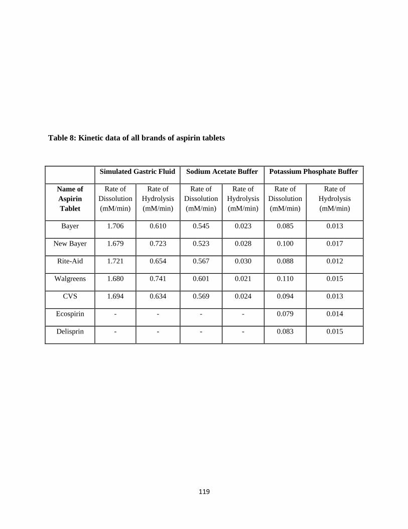
119

Table 8: Kinetic data of all brands of aspirin tablets

Simulated Gastric Fluid Sodium Acetate Buffer Potassium Phosphate Buffer

Name of

Aspirin

Tablet

Rate of

Dissolution

(mM/min)

Rate of

Hydrolysis

(mM/min)

Rate of

Dissolution

(mM/min)

Rate of

Hydrolysis

(mM/min)

Rate of

Dissolution

(mM/min)

Rate of

Hydrolysis

(mM/min)

Bayer 1.706 0.610 0.545 0.023 0.085 0.013

New Bayer 1.679 0.723 0.523 0.028 0.100 0.017

Rite-Aid 1.721 0.654 0.567 0.030 0.088 0.012

Walgreens 1.680 0.741 0.601 0.021 0.110 0.015

CVS 1.694 0.634 0.569 0.024 0.094 0.013

Ecospirin - - - - 0.079 0.014

Delisprin - - - - 0.083 0.015

120

4.4 Conclusion

The in-situ FT-IR records vibrations in the fingerprint region, which is important for the analyst,

because each molecule has its own specific spectrum. Aspirin has the tendency to hydrolyze and

to form salicylic acid and acetic acid when it dissolves. So the advantage of the in-situ FT-IR is to

monitor dissolution as well as the hydrolysis of aspirin, which is very difficult by UV/Vis and

HPLC, because of the overlapping of these two peaks. As the aspirin tablet dropped into the

dissolution medium, it starts to dissolve and slowly hydrolyzes into salicylic acid and acetic acid.

The dissolution was performed on three different body pHs and compared with HPLC in the

previous chapter and validated.

The dissolution and hydrolysis of Bayer aspirin tablets were monitored and compared with the

generic aspirin tablet and enteric coated aspirin tablet. The profile showed the two trends of the

data has been seen in all the tablets. The first trend explains about the dissolution of aspirin and

followed by hydrolysis so intensity if the peak decreases gradually. The second trend is the

formation of salicylic acid where the gradual increase in the peak intensity can has seen, based on

the rate of hydrolysis. The enteric coated tablets dissolution and hydrolysis has compared with

Bayer aspirin tablet. This research was possible because of the versatility of the in-situ FT-IR

system.

121

CHAPTER - 5

DISSOLUTION OF LORATADINE

5.1 Introduction

In the previous sections, the versatility of in-situ FT-IR which is dissolution and hydrolysis study

of aspirin and dissolution of acetaminophen were discussed in detail. Another over-the-counter

antihistaminic drug, loratadine has been chosen for the further confirmation of the new in-situ

analysis technique to monitor dissolution. [107]

Loratadine is a second-generation antihistamine antagonist drug used to treat allergies. The FDA

approved Loratadine in 1993. Loratadine is effective for both nasal and eye symptoms: sneezing,

runny nose, and itchy or burning eyes. [108] Loratadine could be also used to treat mild to

moderate pain from headaches. The mechanism of action of loratadine is a tricyclic antihistamine

which acts as a selective inverse agonist of peripheral histamine H1-receptors. Histamine is

responsible for many features of allergic reactions. Loratadine is metabolized by cytochrome P450,

primarily by CYP3A4 and CYP2D6 isozymes. [109] Loratadine is a prodrug which hydrolyzes

into descarboethoxy loratadine also known as desloratadine. [110] [111]There are recent studies

of dissolution of loratadine and the formulation with different dosage forms by different drug

delivery system are found in the literature. [112]

Mondal and Islam have prepared loratadine formulations based on Self Emulsifying Drug Delivery

System (SEDDS). They used oleic acid and cremophore EL surfactant with different

concentrations and performed the dissolution study by using USP-II. They observed the rate of

drug release has increased with increased amount of cremophor EL surfactant in the formulation.

http://en.wikipedia.org/wiki/Inverse_agonist

http://en.wikipedia.org/wiki/Histamine

http://en.wikipedia.org/wiki/Histamine_H1_receptor

122

[113] Borgaonkar and group have studied the dissolution of loratadine buccal tables to enhance

the bioavailability and to minimize the first pass metabolism, they prepared loratadine tablets using

different polymers. They finalized that the hydroxypropylmethylcellulose is good for the

dissolution study as they found 99% in-vitro drug release in 8 hr. with satisfactory mucoadhesion

strength. [114]

Soni and Sagar designed the quick dissolving loratadine tablets by compression method. The

dissolution of the formulation is used for the stability study. [115] Qadir and group have formulated

fast dissolving films of loratadine for sublingual use. They performed the dissolution of loratadine

films by USP-II with the observation that with increased content of PVP, the rate and extent of

drug release was faster. [116] Another study was carried out to enhance the solubility if loratadine

by using cyclodextrin binary system. [117]

The novelty of this study is to perform the dissolution by in-situ FT-IR, without manual sampling

and disturbing dissolution process. The dissolution data



Loratadine reference material used in this study is CAS # 79794-75-5. Claritin 10 mg tablets which

contains loratadine was purchased with (lot number 2RXF523) from a Rit-Aid pharmacy.

Methanol, acetone and acetonitrile (HPLC grades) were purchased from Pharmaco-Aaper

(Brookfield, CT). Hydrochloric acid (batch no. H44032) was purchased from J.T. Baker (Central

Valley, PA). Solutions were prepared using water treated by a Milli-Q Millipore purification

system (Milford, MA). All purified water aliquots have resistivity of not less than 18 MOhm-cm-

1.

123





by Mettler Toledo. In-situ FT-IR analysis was carried on a Mettler Toledo iC 10 ReactIR, with

iCIR versions 3.0 and 4.0 software.

5.2.3 0.1 N hydrochloric acid

0.1 N HCl was prepared as per the USP procedure for buffers. [118] 8.5 mL of concentrated HCl

was diluted with 1000 mL of deionized water for the analysis.

5.2.4 Loratadine solution for calibration

Loratadine stock solution of concentration 10 mg/mL was prepared by dissolving 500 mg of

loratadine in 50 mL of 0.1 N HCl. Nine dilutions were prepared by adding 1.00, 2.00, 3.00, 4.00,

5.00, 6.00, 7.00, 8.00 and 9.00 mL of this stock solution respectively to 10.00 mL volumetric flasks

respectively and diluting to volume with 0.1 N HCl for the calibration curve. The concentration of

loratadine in each flask was 1.00, 1.50, 2.00, 2.50, 3.00, 3.50, 4.00, 4.50 and 5.00 mg/mL

respectively. Loratadine has a tendency to hydrolyze as it goes into solution. Solutions were placed

into an ice bath immediately after the preparation to slow down the hydrolysis process. As soon as

solutions were ready, they were scanned by in-situ FT-IR for the calibration study at room

temperature.

124


The standard solutions of concentration 0.1 mg/mL was prepared using 10 mg of loratadine was

dissolved in 100 mL of 0.1 N HCl.

5.2.6 Dissolution of loratadine

Claritin tablet 10 mg of loratadine (label claim) were tested in pH 0.1N HCl solutions for 2 hr.

Dissolutions were conducted using vessel volumes of 100 mL and at 37.0 °C. All dissolutions

were conducted using USP-II (paddles) with an agitation speed of 50 rpm as per the USP

monograph of loratadine. [119]


For the calibration of aspirin experiments, data treatment was carried out using the following

methodology: The data was first subjected to baseline correction. The absorption band at 1246

cm-1 (corresponding to the C-N stretch) was selected for loratadine as shown in Figure 47 with the

calibration study. [120] The figure is the overlay calibration data of the loratadine from the in-situ

FT-IR software in 0.1 N HCl. A distinct peak for loratadine without any interfering peak was

observed. The peak at 1246 cm-1 has increased intensity with increased concentration. The

different concentration of loratadine solution also ran three times and the spectra overlapped on

each other. The peak area was calculated using a two-point baseline correction set at 1265 cm-1

and 1230 cm-1. The in-situ FT-IR system was configured to collect spectra every two minutes at

room temperature.

125

For this experiment, data processing is critical to obtain well-resolved spectra. Here is how the

data is processed. For all in-situ FT-IR experiments, 256 scans were collected and co-added for

each spectral point on average and each data point took about two minutes to complete. First, the

peak of interest was identified (1246 cm-1) and the area was calculated using a two-point baseline

correction. Next, a trend analysis was performed using the iCIR software on this peak. This

provided a plot of absorbance vs. time. This plot was subjected to smoothing using a 25 point

smoothing parameter. After smoothing, and while still in the trend analysis, the baseline correct

routine was performed. Then, the data were exported to Excel. Further data processing in Excel

involved the subtraction of solvent spectra from reaction spectra. To perform this, a 30 min set of

spectra at the beginning of the experiment, before claritin pill was added, was selected. These

spectra were subtracted from the spectra taken after the pill was dropped to give the final set of

data. Within the final set of data, the area of the 1246 cm-1 peak was calculated at each time point.

Then the plot of area vs. time was performed to give rate information. In addition, using a

calibration curve, peak areas were converted to concentration to provide concentration vs. time

plots.

126

Figure 47: Loratadine in-situ FT-IR peak at 1246 cm-1 for calibration

127


5.3.1 Calibration of loratadine

Based on the in-situ FT-IR spectra obtained, loratadine has an IR frequency of interest at 1246 cm-

1. Based on the analysis, it was determined that loratadine had excellent linear correlation using IR

spectroscopy with a 0.9951 in 0.1 N HCl correlation coefficient (r2) and shown in Figure 48. Linear

regression for loratadine was calculated by using the area under curve calculations of the IR

absorption bands.

5.3.2. Dissolution of loratadine

The data was compared to reference standards measurements collected prior to the start of the

linearity and dissolution experiment. Dissolution data was plotted vs. time. Figure 49 shows the

dissolution profiles of loratadine by the in-situ FT-IR instrument software. Experiment and the

dissolution media was equilibrated for first 30 mins and then dropped the tablet in the dissolution

vessel. The dissolution performed for longer time to check the stagnant line after complete

dissolution. Figure 49 showed the dissolution profile of loratadine per time, within 15-20 min 50%

of loratadine dissolved. Once the dissolution study has confirmed, performed a replicate study with

the same experimental conditions.

128

Figure 48: Calibration graph of loratadine

y = 0.1373x - 0.0545R² = 0.9951

0

0.05

0.1

0.15

0.2

0.25

0.3

0.35

0.4

0.45

0.5 1 1.5 2 2.5 3 3.5 4

Inte

nsi

ty o

f A

UC

Concentration in mg/mL

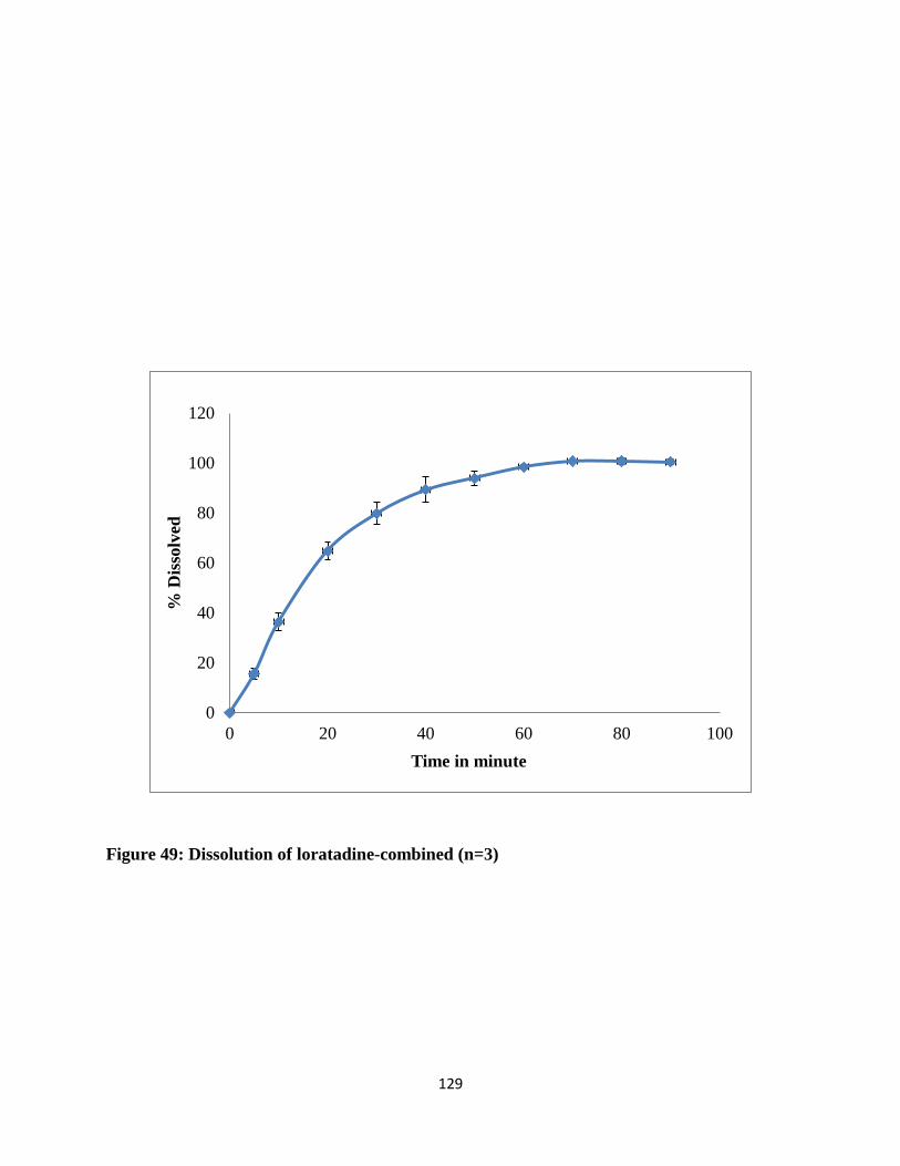
129

Figure 49: Dissolution of loratadine-combined (n=3)

0

20

40

60

80

100

120

0 20 40 60 80 100

% D

isso

lved

Time in minute

130

5.4 Conclusion

The dissolution loratadine was performed successfully by using in-situ FT-IR spectroscopy. The

calibration of the loratadine from 1 mg/mL to 5 mg/mL was carried out and showed liner

correlation with r2 value 0.9951. The dissolution was performed successfully, in first 40 mins more

than 80% of loratadine has dissolved. This study demonstrated and confirmed that in situ FT-IR is

a viable technique for monitoring the dissolution of the pharmaceutical dosage form. The in situ

FT-IR system was found to be impressive in its capability of measuring low concentrations without

requiring manual sampling.

This versatility has demonstrated by observing the simultaneous dissolution and then hydrolysis

of prodrug such as aspirin. Specifically, the unique fingerprint region of the IR spectra gave

detailed information about the release profile of the drug.

As future work of this study is to monitor the hydrolysis of loratadine as it is a prodrug. The active

metabolite of loratadine metabolism is after hydrolysis, which has more pharmacological potencies

than the parent drug. As per the conventional methods, it is very difficult to analyze these

components. By this technique, these two components can find distinct separate peaks for

loratadine and desloratadine as like the aspirin and salicylic acid. By this method, the dissolution

of loratadine can monitor with the transformation of loratadine to desloratadine which is difficult

in the conventional method.

131

Research Summary

Dissolution studies are critical tests for measuring the performance of a drug product. In this

dissertation, a new technique, in-situ attenuated total reflection infrared spectroscopy (in-situ FT-

IR), has been developed to monitor dissolutions of pharmaceutical drug formulations. The

accuracy of this technique was determined to be relative to HPLC. Three over-the-counter (OTC)

active drugs (i.e., acetaminophen, acetylsalicylic acid and loratadine) were tested during the

research. Moreover, these drug formulations were tested and the individual components were

identified by in-situ FT-IR spectroscopy.

Very first project in this research is dissolution of acetaminophen, the potential of the in-situ FT-

IR spectroscopy for the quantitative analysis such as monitor the dissolution was observed. During

these experimentation, the non-linear Beer-Lambert’s behavior was observed, the hypothesis

behind this behavior was proposed due to the dimerization of the acetaminophen molecules. As

per the literature, for the confirmation of the dimerization studies were performed on the NMR,

FT-IR, Osmometry and freezing point depression. But, there was a lack of any evidence to confirm

the hypothesis of dimerization of acetaminophen.

Furthermore, the system has the capability of monitoring drug transformations during dissolution.

For instance, using this technique the hydrolysis of aspirin to salicylic acid was monitored.

Moreover, the simultaneous dissolution and elimination of aspirin has been monitored and at the

same time the formation of salicylic acid in solution has been monitored. The dissolution

monitored on the three different body pHs, that is stomach pH 1.2, duodenal pH 4.5 and last

intestinal pH 6.8 and the kinetics of the dissolution as well as hydrolysis were performed. However,

the stomach pH is the best dissolution media where the rate of dissolution and hydrolysis is fast.

132

As the rate of hydrolysis is based on the dissolution of aspirin because it needs free aspirin in the

media, then aspirin transforms into salicylic acid, which observed slow in higher pHs as aspirin

dissolves slowly.

Dissolution and hydrolysis of aspirin study was performed using in-situ FT-IR spectroscopy and

compared with HPLC on Bayer aspirin tablet. In-situ FT-IR spectroscopy was compared with

different brands of generic aspirin tablets with the same strength. The rate of dissolution and

hydrolysis of all these brands are similar to Bayer aspirin. Dissolution of the enteric coated aspirin

tablet were performed, which dissolved in intestinal pH and used for the delayed release.

Loratadine was another pro-drug selected for the dissolution and hydrolysis study. This thesis

explains about the dissolution of loratadine and hydrolysis can be a study for future work.

The in-situ FT-IR system was found to have very good sensitivity for monitoring dissolution test.

The in-situ FT-IR has great potential for use in studies of dissolution of drugs and monitoring

competing for reactions such as hydrolysis of prodrugs in pharmaceutical development,

formulation and quality assurance without disturbing dissolution system as well as manual

sampling.

133

References

[1] D. Jennifer and K. Johannes, Pharmaceutical Dissolution Testing, New York: Taylor and

Frencis Group, 2005.

[2] f. I. Guidance, "Extended Release Oral Dosage Forms: Development, Evaluation, and

Application of In Vitro/In Vivo Correlations," 1997.

[3] f. I. Guidance, "Waiver of In Vivo Bioavailability and Bioequivalence Studies for

Immediate-Release Solid Oral Dosage Forms Based on a Biopharmaceutics Classification

System," 2000.

[4] f. I. Guidance, "Q8(R2) Pharmaceutical Development.," 2009.

[5] H. R and G. V., Handbook of Dissolution testing, 3rd edition, Hockessin: Dissolution

Technologies, Incorporated, 2004.

[6] W. I. Higuchi, "Diffusional models useful in bio pharmaceutics drug release rate processes,"

Journal of Pharmaceutical Sciences, vol. 56, no. 3, pp. 315-324, 1967.

[7] W. Nernst, "Theory of reaction velocity in heterogenous systems," Zeit. physikal. Chem,

vol. 47, pp. 52-55, 1904.

[8] T. Higuchi, "Rate of release of medicaments from ointment bases containing drugs in

suspension," Journal of pharmaceutical sciences, vol. 50, no. 10, pp. 874-875, 1961.

134

[9] S. Gautam and S. Mahaveer, "Review: In-Vitro Drug Release Characterization Models,"

International Journal of Pharmaceutaical Studies and Research, pp. 77-84, 2011.

[10] U. Riaz, S. Nadia and S. Kumar BIshwajit, "Dissolution and Dissolution Apparatus: A

Review," International journal of Current Biomedical and Pharmaceutical Research, vol.

1, no. 4, pp. 201-207, 2011.

[11] A. A. Noyes and W. R. Whitney, "The rate of solution of solid substances in their own

solutions," Journal of the American Chemical Society, vol. 19, no. 12, pp. 930-934, 1897.

[12] T. O'hara, A. Dunne, J. Butler and J. Devane, "A review of methods used to compare

dissolution profile data.," Pharmaceutical Science & Technology Today, vol. 1, no. 5, pp.

214-223, 1998.

[13] S. Dash, P. N. Murthy, L. Nath and P. Chowdhury, "Kinetic modeling on drug release from

controlled drug delivery systems.," Acta Poloniae Pharmaceutica, vol. 67, no. 3, pp. 217-

223, 2010.

[14] C. Paulo and M. Jose, "Modeling and Comparison of Dissolution Profiles," European

Journal of Pharmaceutical Sciences , vol. 13, pp. 123-133, 2001.

[15] S. N. Bhattachar, J. A. Wesley, A. Fioritto, P. J. Martin and S. R. Babu, "Dissolution testing

of a poorly soluble compound using the flow-through cell dissolution apparatus,"

International journal of pharmaceutics, vol. 236, no. 1, pp. 135-143, 2002.

135

[16] J. Siepmann and N. Peppas, "Higuchi Equation:Derivation, Application, Use and misuse,"

International Journal of Pharmaceutics, vol. 418, pp. 6-12, 2011.

[17] M.R.Brophy and P.B.Deasy, "The application of the Higuchi model is for the drug release

from the dispersed matrices to particles of general shape," International Journal of

Pharmaceutics, vol. 37, pp. 41-47, 1987.

[18] T. P. Kravtchenko, J. Renoir, A. Parker and G. Brigand, "A novel method for determining

the dissolution kinetics of hydrocolloid powders.," Food Hydrocolloids, vol. 3, no. 3, pp.

219-225, 1999.

[19] R. W. Korsmeyer, R. Gurny, E. B. P. Doelker and N. A. Peppas, "Mechanisms of solute

release from porous hydrophilic polymers," International Journal of Pharmaceutics, vol.

15, no. 1, pp. 25-35, 1983.

[20] "United States Pharmacopeia Home Page," in USP, Rockville, 1990.

[21] FDA, "Dissolution Testing of Immediate Release Solid Oral Dosage Forms," in Guidance

for Industry: , U.S. Department of Health and Human Services, 1997.

[22] "USP General Chapter <711>: Dissolution,," in US Pharmacopoeia & National Formulary.

[23] "USP General Chapter <724> Drug Release," in US Pharmacopoeia & National

Formulary- .

[24] B. M. M. William, "USP and Dissolution-20 years of Progress," Dissolution Technologies,

vol. 21, no. 3, pp. 24-27, 2014.

136

[25] J. Cohen, B. Hubert, L. Leeson, C. Rhodes, J. Robinson, T. Roseman and E. Shefter, "The

Devlopment of USP Dissolution and Drug Release Standards," Pharmaceutical Research,

vol. 7, no. 10, pp. 983-987, 1990.

[26] N. Fotaki, "Flow-through Cell Apparatus (USP Apparatus 4): Operation and Features,"

Dissolution Technologies, pp. 46-49, 2011.

[27] L. Terry, "USP apparatus 4 [Flow-Through Method] Primer," Dissolution Technologies,

1996.

[28] G. Zongming, "In Vitro Dissolution Testing with Flow through Method: A Technical Note,"

Pharma Sci Tech, vol. 10, no. 4, pp. 1401-1405, 2009.

[29] C. P. Sherman, "Chapter-5, Infrared Specrtoscopy," in Handbook of Instrumental

Techniques for Analytical Chemistry, pp. 247-283.

[30] D. Skoog, J. Holler and S. Crouch, "Applications of Infrared Spectroecopy," in Principles

of Instrumental Analysis, Thomson Books,, 2007, pp. 505-532.

[31] B. Smith, "Chapter 4," in Fundamentals of Fourier Transform Infrared Spectroscopy,

London, CRC Press, 1996.

[32] P. Donald, L. Gary and K. George, "CHapter-2 Infrared Spectroscopy," in Intoduction of

Spcetroscopy, Kundli, Sanat Printers, 2007, pp. 13-101.

[33] "FT-IR Specrtoscopy, Attenuated Total Reflectance (ATR), Technical Report".

137

[34] K. Sergei and W. Patrick, "Appilcations of FTIR Spectroscopic Imaging in Pharmaceutical

Sciences," FTIR Imaging of Pharmaceuticals.

[35] K. John and J. Drennen, "Dtermination of film-coated tablet Paramters near-infrared

Spectroscopy," Journal of Pharmaceutical and Biomedical Analysis, vol. 13, pp. 1273-

1281, 1995.

[36] Y. Ketsia, A. Nicolas, B. Bernard, G. Ryan, T. Sharkwi, S. Jean-Sebastien and C. Antoine,

"Predicting the dissolution behavior of Pharmaceutical tabltes with NIR chemiacl imaging,"

International Journal of Pharmaceutics, vol. 486, pp. 242-251, 2015.

[37] L. Wendy and L. Zhuangji, "Detection and quantitation of trace Organic Contaminants in

water using the FT-IR Attenuated Total Reflectance technique.," Anal. Chem., vol. 82, no.

2, pp. 505-515, 2010.

[38] J. Van der Weerd and S. G. Kazarian, "Combined approach of FTIR imaging and

conventional dissolution tests applied to drug release," Journal of Controlled Release , vol.

98, pp. 295-305, 2004.

[39] J. Van der Weerd, K. L. A. Chan and S. Kazarian, "An innovative design of compaction cell

for in situ FT-IR imaging of tablet dissolution," Vibrational Spectroscopy, vol. 35, no. 1-2,

pp. 9-13, 2004.

[40] M. A. and B. C., "CE versus HPLC for the dissoltuion test in a pharmaceutical formulation

containing actaminophen, phenylephrine and chlorpheniramine," Journal of

Pharmaceutical and Biomedical Analysis, vol. 35, pp. 769-777, 2004.

138

[41] C. Sarah, K. Amber and v. d. A. John, "Simultaneous quantification of Acetaminophen and

five acetaminophen metabolitesin human plasma and urine by HPLC-electrospray

ionization-tandem mass spectrometry; Method Validation and application to a neonatal

pharmacokinetics study," Journal of Chromatography B, vol. 1007, pp. 30-42, 2015.

[42] N. Tamas, J. Peter, J. Nemeth-Palotas and K.-S. Hilda, "Determination of paracetamol and

its main impurity 4-aminophenol in analgesic preparations by micellar electrokinetic

chromatography," Journal of Pharmaceutical and Biomedical Analysis, vol. 47, pp. 746-

749, 2008.

[43] Q. Xiangjun, L. Dan, S. Ding, L. Zebin, G. Pengtao and Z. Nan-sheng, "Simultaneous

dtermination of Acetaminophen and dihyrocodeine in human plasma by UPLC-MS/MS; Its

pharmacokinetics application," Journal of Chromatography B, vol. 992, pp. 91-95, 2015.

[44] "SDBS," [Online]. Available: http://sdbs.db.aist.go.jp/sdbs/cgi-bin/direct_frame_top.cgi.

[Accessed 25 August 2009].

[45] D. Pavia, G. Lapman, G. Kriz and R. Engel, "Aspirin," in Introduction to Organic

Laboratory Techniques, a microscale approach, Belmont, Brooks/Cole Cengage Learning,

2007, pp. 61-67.

[46] F. Klaus, "Aspirin," in Analytical Profiles of Drug Substances,8, 1979, pp. 1-46.

[47] F. Hoffmann, "U.S. Patent C44077 of February 27, 1900.".

139

[48] M. Peter, "Class Projects in Physical Organic Chemistry: The Hydrolysis of Aspirin,"

Journal of Chemical Education, vol. 81, no. 6, pp. 870-873, 2004.

[49] C. Sosale and K. Honnaiah Vijay, "The reaction of Aspirin with Base," Tetrahedron Letters,

vol. 52, pp. 3561-3564, 2011.

[50] "SDBS," [Online]. Available: http://sdbs.db.aist.go.jp/sdbs/cgi-bin/direct_frame_top.cgi.

[Accessed 17 May 2010].

[51] "United States Food and Drug Administration Home Page.," in http://www.fda.gov/.

[52] O. Yalcin, O. Yildiz, A. Savaser and O. and Sibel, "compartive dissolution testingof

Paracetamolcommercial tabletdosage forms," Acta Poloniac Pharmaceutic-Drug Research,

vol. 57, no. 1, pp. 33-41, 2000.

[53] S. Ravishankar, M. Vasudevan, M. Gandhimathi and B. Suresh, "Resversed phase HPLE

method for the estimation of acetamniophen, ibuprofen and chlorzoxazone in formulation,"

Talanta, vol. 46, pp. 1577-1581, 1998.

[54] "USP," in US Pharmacopoeia & National Formulary, Monograph: Acetaminophen Tablets

& Dissolution Chapter, USP22-NF27, Rockville, United States Pharmacopeial Convention

Inc., 1990, p. 1787.

[55] "USP," in US Pharmacopoeia & National Formulary USP22-NF27, Rockville, United

States Pharmacopeial Convention Inc., 1990, pp. 14-15.

140

[56] B. Dejaegher, M. Bloomfield, J. Smeyers-Verbeke and Y. Heyden, "Validation of a

fluorimetric assay for 4-aminophenol in paracetamol formulations," Talanta, vol. 75, p.

258–265, 2008.

[57] D. Nematollahi, H. Shayani-Jam, M. Alimoradi and S. Niroomand, "Electrochemical

oxidation of Acetamionphen in aqueous solutions: Kinetic evaluation of hydrolysis,

hydroxylation and dimerization processes," Electrochimica Acta, vol. 54, pp. 7407-7415,

2009.

[58] H. Barry, G. David, M. Paul and G. Daniel, "Crystallisation of paracetamol (acetaminophen)

in the presence of structurally related substances," Journal of Crystal Growth, vol. 183, pp.

629-640, 1998.

[59] N. Tsapatsaris, B. Kolesov, J. Fischer, E. Boldyreva, L. Daemen, J. Eckert and H. Bordallo,

"Plymorphism of Paracetamol: Anew Understanding of Molecular Flexibility through Local

Methyl Dynamics," Molecular Pharmaceutics, vol. 11, no. 3, pp. 1032-41, 2014 .

[60] W. Jean and M. Gregory, "X-Ray Powder Data for Actaminophen (C8H9NO2)," Powder

Diffraction, vol. 3, no. 2, pp. 102-103, 1988.

[61] I. Oswald, D. Allan, P. McGregor, W. Motherwell, S. Parsons and C. Pulham, "The

formation of paracetamol (acetaminophen) adducts with hydrogen-bond acceptors.," Acta

Crystallographica Section B, vol. 58, no. 6, pp. 1057-66, 2002 .

[62] C. Jenn-Shing, W. Cheng-Chang and K. Dah-Yu, "New approach to IR study of monomer–

dimer self-association: 2,2-dimethyl-3-ethyl-3-pentanol in tetrachloroethylene as an

141

example," Spectrochimica Acta Part A: Molecular and Biomolecular Spectroscopy, vol. 60,

no. 10, p. 2287–2293, 2004.

[63] B. Michael and M. Frank-Olaf, "Dimerization of Acrylic Acid and of Methacrylic Acid in

Supercritical Ethylene," The Journal of Supercritical Fluids, vol. 8, pp. 119-126, 1995.

[64] W. Gallagher, "FTIR Anlaysisof Protein Structure," in Chemistry Manual, University of

Wisconsin, 2005.

[65] J.-S. Chen and D.-Y. Kao, "Accurate Determination of Dimerization Constants from IR

Study of Monomer-Dimer Self-Association: 3-Ethyl-2-Methyl-3-Pentanol in Carbon

Tetrachloride as an Example," Journal of the Chinese Chemical Society, vol. 51, pp. 881-

888, 2004.

[66] R. E. Aslin, G. S. Denisov, D. N. Poplevchenkov, K. Tokbadze and T. Y.Velikanova, "IR

v(OH) Band and Dimerization of Phosphorus Acids in the Gas Phase and Solid State,"

Polish J. Chern, vol. 76, pp. 1223-1231, 2002.

[67] D. Joshua, C. Felya and A. Eric, "Dimerization Constants for Phosphoric Acid DIesters,"

Tetrahydron Letters, vol. 37, no. 12, pp. 1925-1928, 1996.

[68] M. Dias, S. L. Raghavan and J. Hadgraft, "ATR-FTIR spectroscopic investigation on the

effect of solvents on the permeation of benzoic acid and salicylic acid through silicon

membrane," International Journal of Pharmaceutics, vol. 216 , pp. 51-59, 2001.

142

[69] T. Hiroyuki, Y. Yasuhiko, I. Hiroshi and S. Shozaburo, "Dimerization of Benzoic Acid in

Saturated Solution of Supercritical Carbon Dioxide," Journal of Chemical Engineering of

Japan, vol. 25 , no. 3, pp. 351-353 , 1992 .

[70] Y. Hiromichi, Y. Kyoko, W. Hiroko and N. Genkichi, "Effect of Solvation on Partition and

Dimerization of Benzoic Acid in Mixed Solvent Systems," Talanta, vol. 42, no. 6, pp. 789-

795, 1995.

[71] R. Jorgen, O. Ole and B. Thor, "Acta Chem. Scand.," Rates of Dimerization of Substituted

Benzoic Acid, vol. 21, no. 6, pp. 1443-1448, 1967.

[72] A. Shinji, A. Isao, S. Akira and T. Ozaki, "Intermolecular Hydrogen-Bonding Effect on 13C

NMR Chemical shifs of Glycine Residue Carbonyl Carbons of Peptides in the Solid State,"

Journal of American Chemical Society , vol. 110, no. 11, pp. 3380-3386, 1988.

[73] S. Nagaoka, T. Tero, F. Imashiro, A. Saika, N. HIrota and S. Hayashi, "A study of the proton

Transfer in the Benzoic Acid Dimer by 13C High-Resolution Solid Stae NMPR and

PRonton T1 Measuremnt," Chemical Physics Letter , vol. 80, no. 3, pp. 580-584, 1981.

[74] C. Roumestand, V. Louisa, A. Aumelasa, G. Grassya, B. Calasb and A. Chavanieub,

"Oligomerization of protegrin-1 in the presence of DPC micelles. A proton high-resolution

NMR study," FEBS Letters, vol. 421, no. 3, pp. 263-267, 1998.

[75] W. Smith, "Quantitaive Analysis Using NMR," Journal of Cheimcal Education, vol. 41, no.

2, pp. 97-99, 1964.

143

[76] K. Haushalter, J. Lau and J. Roberts, "An NMR Investigation of the Effect of Hydrogen

Bonding on the Rates of Rotation about the C-N Bonds in Urea and Thiourea," Journal of

American Chemical Society , vol. 118, no. 37, pp. 8891-8896, 1996.

[77] N. Allen, "For Water-Electrolyter balance Experiments in the instructional Laboratoy," in

Using Osmometry, pp. 1-13.

[78] "US Pharmacopoeia & National Formulary,USP28-NF23," in USP, Rockville, United


[79] S. Eugene, "Intermolecular Association by Vapor Pressure Osmometer," Journal of

Chemical Education, vol. 45, no. 3, pp. 176-180, 1968.

[80] R. Robert, "A Forensic Science Laboratory Experiment: Molcular weights of Drugs and

Diluents by Osmometry," Journal of Chimcal Education, vol. 59, no. 8, pp. 672-673, 1982.

[81] "Freezing Point of Solutions.," in LAHC, pp. 1-3.

[82] H. James, "Freezing POnt Measuremnet," Journal of Chemical Education, vol. 37, no. 3,

pp. 146-147, 1960.

[83] G. Nejib, A.-S. Ghalib Said, R. Mohammad, B. Salwa and A. A.-A. Ahmed, "State

Diagramof dates: Glass transition, Freezing curve and maximal-freeze-conecntration

condition," Journal of Food Engineering, vol. 99, pp. 92-97, 2010.

[84] R. M., G. N., A.-K. M., A.-H. S., A.-M. S. and A.-H. K., "Analysis of cooling curve to

determine the end point of freeing," Food Hydrocolloids, vol. 16, pp. 653-659, 2002.

144

[85] H. Klara and P. Maria, "Dtermination of Average Molecular Mass of Polyols by Freezing

Point Depression: Method to avoid Interference by Water," Cellular Polymers, vol. 5, pp.

357-367, 1986.

[86] L. L. Borer, "Experiments with Aspirin," Journal of Chemincal Education, vol. 77, no. 3,

pp. 354-355, March 2000.

[87] T. Mirza, Q. Liu, R. Vivilecchia and Y. Joshi, "Comprehensive validation scheme for in situ

fiber optics dissolution method for pharmaceutical drug product testing," Journal

Pharmaceutical Science, vol. 98, pp. 1086-1094 , 2009.

[88] Zenon Kokot and Kinga Burda, " Simultaneous determination of salicylic acid and

acetylsalicylic acid in aspirin delayed-release tablet formulations by second-derivative UV

spectrophotometry," Journal of Pharmaceutical and Biomedical Analysis, vol. 18, p. 871–

875, 1998.

[89] F. Regan, M. Meaney, J. G. Vos, B. D. Maccraith and J. E. Walsh, "Determination of

pesticides in water using ATR-FTIR spectroscopy on PVC/chloroparaffin coatings,"

Analytical Chimica Acta , vol. 334, pp. 85-92, 1996.

[90] A. Kassis, V. Bhawtankar and J. Sowa, "Attenuated total reflection infrared spectroscopy

(ATR-IR) as an in situ technique for dissolution studies," Journal of Pharmaceutical and

Biomedical Analysis , vol. 53, pp. 269-273, 2010.

[91] in US Pharmacopoeia & National Formulary solutions, USP22-NF27, Rockville, United

States Pharmacopeial Convention Inc., 1990, p. 1788.

145

[92] "USP," in US Pharmacopoeia & National Formulary, solutions, USP28-NF23, Rockville,

United States Pharmacopeial Convention Inc., 2005, p. 1238.

[93] "USP," in US Pharmacopoeia & National Formulary, solutions, USP22-NF27, Rockville ,


[94] S. Saul and W. Samuel, "Improved Ferric Chloride Test for Phenols," Analytical Chemistry,

vol. 24, no. 6, pp. 979-983, 1952.

[95] K.-W. Cha and K.-W. Park, "Determination of iron (III) with salicylic acid by fluorescence

quenching method," Talanta, vol. 46, no. 6, pp. 1567-1571, 1998.

[96] G. Alibrandi, s. Coppolino, N. Micali and a. A. Vilari, "Varivale pH Kinetics: An Easy

Dtermination of pH-Rate profile," Journal of Pharmaceutical Science, vol. 90, no. 3, pp.

270-274, 2000.

[97] L. J. Edward, "The Hydrolysis of Aspirin," Transaction of the Faraday Society, vol. 46, pp.

723-735, 1950.

[98] M. Habib and J. Rogers, "Kinetics of hydrolysis and stabilization of acetylsalicylic acid in

liposome formulations," International Journal of Pharmaceutics, vol. 44, pp. 235-241,

1998,.

[99] James J. Zimmerman and Alan S. Kirschner, " A student Experiment in Pharmaceutics: The

pH stability profile of Aspirin," American Journal of Pharmaceutical Education, pp. 609-

614.

146

[100] J. Blanch and A. Finch, "A student experiment in chemical kinetics: The hydrolysis of

aspirin," American Journal of Pharmaceutical Education, pp. 191-195.

[101] K. Fawzia, L. Mingzhong and S. Walkiria, "Comparison of in vitro Dissolution test for

commerically available Aspirin Tablets," Dissolution Technologies, pp. 48-58, 2013.

[102] M. Kayoko, Y. Ryo, T. Tomoko, K. Junko and H. Seiji, "Dissolution Profile of 24

Levofloxacin (100 mg) tablets," J. Infect Chemother, vol. 19, pp. 996-998, 2013.

[103] S. Ahmed, A. A. Ahmed, M. A. Ali and H. O. , "Design and in vitro/in vivo evaluation of

sustained-release floating tablets of itopride hydrochloride," Drug Design, Development

and Therapy , vol. 10, p. 4061—4071, 2016.

[104] A. Stuart, Y. Clement, P. Seal, R. LObenberg, L. MOntane-Jaime, R. Maharaj and A.

Maxwell, "Comparing the Dissolution Profile of 7 Metformin Formulations in Simulated

Intestinal Fluid," Dissolution Technologies, vol. 22, no. 1, pp. 17-21, 2015.

[105] A. I. O. Mansour and T. Hammad, "Comparative Study of Different Formulations of

Chlorpheniramine Maleate Orally," International Journal of Pharmaceutical Sciences

Review and Research, vol. 28, no. 2, pp. 24-239, 2014.

[106] Y. Ozkan, A. Savaser, Y. Ozalp and A. Isimer, "Dissolution Properties of differnt designed

and formulated Salbutamol tablet dosage forms," Acta Poloniac Pharmaceutica, vol. 57,

no. 4, pp. 271-276, 2000.

147

[107] Mayer, B. Testa and a. J. M., "Loratadine," in Hydrolysis in Drug and Prodrug Metabolism,

Wiley-VcH, pp. 391-392.

[108] K. Kathiresan, P. Vijin, C. Moorthi and a. R. Manavalan, "Formulation and evaluation of

Loratadine chewable tablets," Research Journal of Pharmaceutical Biological and

Chemical Sciences, vol. 1, no. 4, pp. 763-774, 2010.

[109] Y.-F. Zhang, X.-Y. Chen, D.-F. Zhong and Y.-M. and Dong, "Pharmacokinetics of

Loratadine and its active metabolite descarboethoxyloratadine in healthy Chinese subjects,"

Acta Pharmacol Sin, vol. 24, no. 7, pp. 715-718, 2003.

[110] I. P. Veronez, J. S. P. Daniel, J. S. Garcia and a. M. G.Trevisan, "Characterization and

compatibility study of desloratadine," Journal of Thermal Analysis and Calorimetry, vol.

115, no. 3, pp. 2407-2414, 2014.

[111] J. Gibbons, D. Sardella, D.Duncan and R. Pike, "Degradation product of Loratadine,"

Journal of pharmaceutical and biomedical analysis, vol. 43, pp. 1191-1192, 2007.

[112] N. Kolasinac, K. Kachrimanis, J. Djuris, I. Homsek, B. Grujic and a. S. Ibric, "Spray coating

as a powerful technique in perparation of solid dispersions with enhanceddesloratadine

dissolution rate," Drug Development and Industrial Pharmacy, vol. 39, no. 7, pp. 1020-

1027, 2013.

[113] M. S. Mondal, M. T. Islam, M. S. Rahman and a. M. A. Islam, "Dissolution Enhancement

of Loratadine by Formulating Oleic acid and Cremophor EL based Self Emulsifying Drug

148

Delivery System (SEDDS)," Journal of applied Pharmaceutical Sciences, vol. 3, no. 7, pp.

64-67, 2013.

[114] P. Borgonkar, T. VIrsen, R. Haripras anna and M. Najmuddin, "Formulation and In-Vitro

Evaluation of Buccal Tablets of loratadinefor Effective Treatment of Allergy," International

journal of Research in Pharmacy and Chemistry, vol. 1, no. 3, pp. 551-559, 2011.

[115] S. Rajeev and V. S. Gali, "Design an Development of Quick Dissolving Tablet Contianing

Loratadineby Direct Compression method," International Journal of Pharmaceutical,

Chemical and Biological Sciences, vol. 3, no. 3, pp. 771-800, 2013.

[116] Q. Khanusiya, R. N. Charyulu, P. Prabhu, S. Bhatt and C. S. Shastry, "Formulation and

Evaluation of Fast Dissolving Films of Loratadine for Sublingual use," International

Research Journal of Pharmacy, vol. 3, no. 7, pp. 157-161, 2012.

[117] P. Singh, M. Bajpai and S. Shrivatava, "Physicochemical Characterization and dissolution

enhancement of Loratadine-Hydrozyprpyl-B-cyclodextrin binary syatem," Journal of

Pharmaceutical Sciences and Research , vol. 3, no. 4, pp. 1170-1175, 2011.





149

[120] N. A. E. Ragehy, A. M. Badawey and S. Z. E. Khateeb, "Satbility indicating methods for

the dtermination of loratadine in the persence of its degradation product," Journal of

Pharmaceutical and Biomedical Analysis, vol. 28, pp. 1041-1053, 2002.

[121]

[122] W. Nernst and E. Brunner, "Velocity of Reaction in Non-Homogeneous System," Physical

Chemistry, vol. 47, pp. 56-102, 1904.

[123] "USP," in US Pharmacopoeia & National FormularyUSP28-NF23, Rockville, United


[124] M. Charles and C. Marie, "Convenient Freezing Point Depression Apparatus," Journal of

Chemical Education, vol. 32, p. 650, 1980.

[125] S. Charles, S. Judy and J. Ronald, "A convenient Melting/Freezing Point Depression

Apparatus," Journal of Chemical Education, vol. 59, no. 8, p. 682, 1982.

150

Appendix

Standard Operating Procedure for ReactIR

This chapter explains the detail and stepwise standard operating procedure.

Starting Instrument:

1. Verify whether the instrument is on or off. (Usually, instrument is kept on. Please do an

additional check).

2. Fill in the liquid nitrogen through the funnel shown in Figure 50 and wait for 45 mins for

cooling the detector. To filling the liquid nitrogen, remove the nozzle and fit in the funnel,

then pour the liquid nitrogen with the help of the liquid nitrogen container in the funnel.

Stop pouring the liquid nitrogen in the funnel, after it starts overflowing.

3. Turn on the computer.

Figure 50: ReactIR nozzle for liquid nitrogen

Remove nozzle to fill

the liquid nitrogen

151

Figure 51: ReactIR nozzle with funnel

Starting Software:

1. The ReactIR uses iC IR 4.0 for analysis. On the desktop, the iC IR 4.0 icon is highlighted

with purple color. To start the software double-clicks the icon, which would bring up the

software window shown in Figure 52.

Figure 52: Screenshot shows iC IR 4.0software icon

iC IR Software

4.0

Funnel to fill

liquid nitrogen

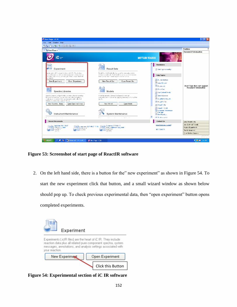
152

Figure 53: Screenshot of start page of ReactIR software

2. On the left hand side, there is a button for the” new experiment” as shown in Figure 54. To

start the new experiment click that button, and a small wizard window as shown below

should pop up. To check previous experimental data, then “open experiment” button opens

completed experiments.

Figure 54: Experimental section of iC IR software

Click this Button

153

Figure 55: Screenshot of iC IR software and configuration window

3. Before starting any experiment, it’s a good practice to configure instrument. To configure

the instrument, click the configure instrument button, which is located on the bottom left of

the new experiment window.

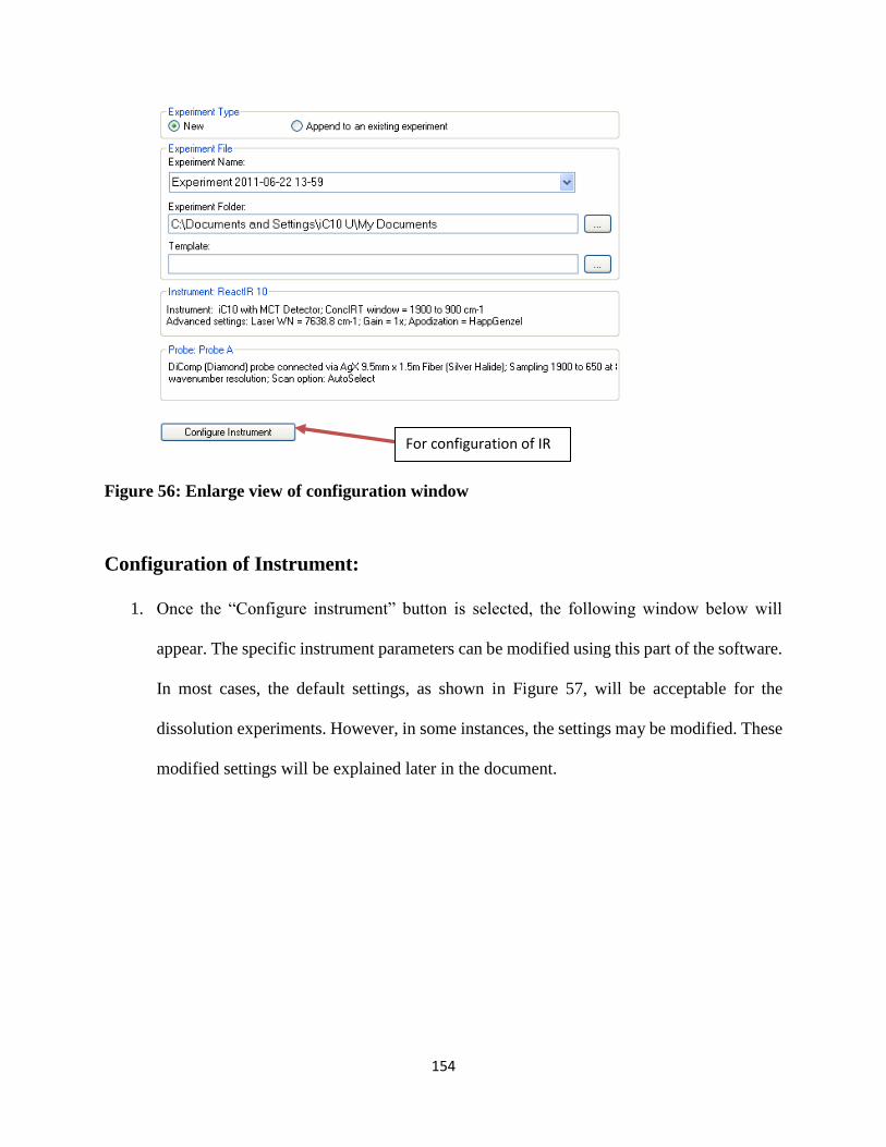
154

Figure 56: Enlarge view of configuration window

Configuration of Instrument:

1. Once the “Configure instrument” button is selected, the following window below will

appear. The specific instrument parameters can be modified using this part of the software.

In most cases, the default settings, as shown in Figure 57, will be acceptable for the

dissolution experiments. However, in some instances, the settings may be modified. These

modified settings will be explained later in the document.

For configuration of IR

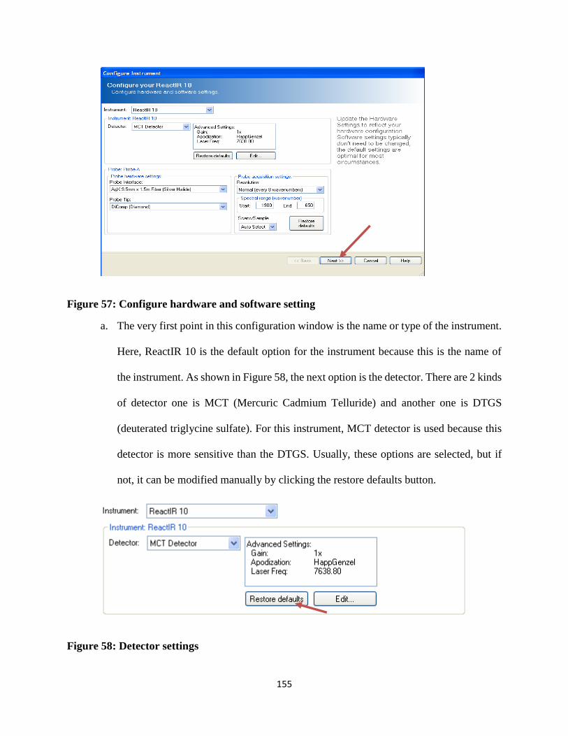
155

Figure 57: Configure hardware and software setting

a. The very first point in this configuration window is the name or type of the instrument.

Here, ReactIR 10 is the default option for the instrument because this is the name of

the instrument. As shown in Figure 58, the next option is the detector. There are 2 kinds

of detector one is MCT (Mercuric Cadmium Telluride) and another one is DTGS

(deuterated triglycine sulfate). For this instrument, MCT detector is used because this

detector is more sensitive than the DTGS. Usually, these options are selected, but if

not, it can be modified manually by clicking the restore defaults button.

Figure 58: Detector settings

156

b. The next part in this window is the “Probe Hardware settings”. Since the instrument

contains a 9.5 mm x 1.5 m silver halide probe with a covered diamond tip, the following

parameters need to be selected as shown in Figure 59. There are numerous probe

settings available in the system. These can be found by selecting the drop down arrow

as shown below. So that it creates the facility to change the probe.

Figure 59: Probe hardware settings

c. This instrument software can allow other kinds of the probe as shown in Figure 26.

Once the probe has changed, it’s mandatory to change the probe hardware setting in

the configuration window, such as in probe interface K4 conduit and in probe tip

SiComp (Silicon) option by using the drop-down arrow as shown in Figure 60. These

three probes below can be used for this instrument and software also.

Figure 60: Different type of IR Probes

Dropdown

Arrow

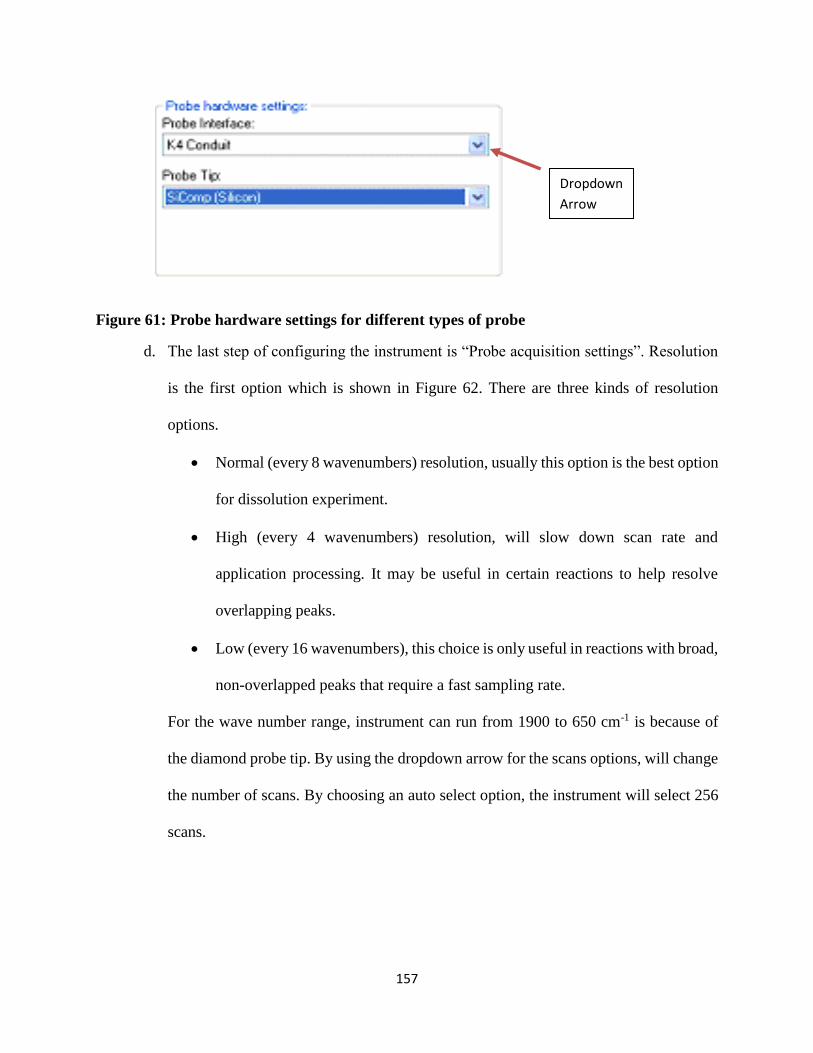
157

Figure 61: Probe hardware settings for different types of probe

d. The last step of configuring the instrument is “Probe acquisition settings”. Resolution

is the first option which is shown in Figure 62. There are three kinds of resolution

options.

Normal (every 8 wavenumbers) resolution, usually this option is the best option

for dissolution experiment.

High (every 4 wavenumbers) resolution, will slow down scan rate and

application processing. It may be useful in certain reactions to help resolve

overlapping peaks.

Low (every 16 wavenumbers), this choice is only useful in reactions with broad,

non-overlapped peaks that require a fast sampling rate.

For the wave number range, instrument can run from 1900 to 650 cm-1 is because of

the diamond probe tip. By using the dropdown arrow for the scans options, will change

the number of scans. By choosing an auto select option, the instrument will select 256

scans.

Dropdown

Arrow

158

Figure 62: Probe acquisition Settings

2. Once finished with all modifications in parameters for the configuration of the instrument,

it’s time to move to the next step. Click the “Next” button. The next window will appear

as shown in Figure 65, with the picture of the instrument and the probe. Click “Next” button

to move further.

Figure 63: Position of the probe

159

3. The pop-up window as shown in Figure 64 seen on the screen, which explains about the

alignment of the probe. For the alignment of the probe, Peak Height should be more than

18,000 and less than 28,000 and Contrast should be more than 10.00. If peak height and

contrast is more than these mentioned values, the two bars will change into green. If peak

height and contrast is less than these values, the bars are in red color and length is also less

compare to green bars. Once the bars turns to green, then press the “Next” button.

Figure 64: Align probe window

160

4. The window shown in Figure 65 is used to collect the background. Here is the option for

the scans, from the drop-down list, the values for the number of scans can be changed.

Then click the “Collect Background” button. To collect the background normally takes 1-

2 min, but it also depends on the number of scans option. After collection of the background

click the “Next” button.

Figure 65: Collect background window

161

5. Then “collect water vapor sample” window will open. This page of the wizard is used to

collect a reference spectrum of water vapor. This reference spectrum is used for subtracting

out water vapor from a data set. It is not intended to be a replacement for an effective dry

air or nitrogen purge. The water vapor reference spectrum is simply a convenient way to

remove small amounts of water vapor which may enter or leave the instrument over a long

reaction period. After collection of the water vapor click the “Finish” button for completion

of the configuration of the instrument.

Figure 66: Collect water vapor sample window

For Collection

For completion of

Configuration

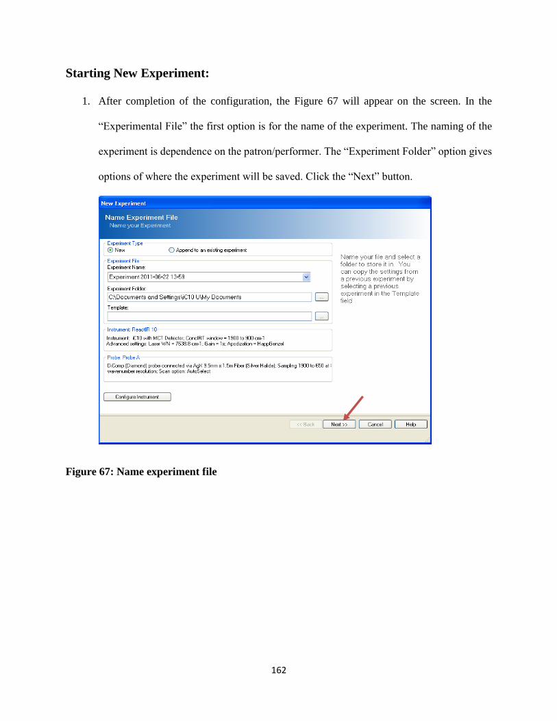
162

Starting New Experiment:

1. After completion of the configuration, the Figure 67 will appear on the screen. In the

“Experimental File” the first option is for the name of the experiment. The naming of the

experiment is dependence on the patron/performer. The “Experiment Folder” option gives

options of where the experiment will be saved. Click the “Next” button.

Figure 67: Name experiment file

163

2. This window gives the choice to set the time for the experiment and give the interval time

for the scans. As per the mentioned experiment time and interval time, the software will

show the total number of samples. Then click the “Next” button for next step.

Figure 68: Experiment duration window

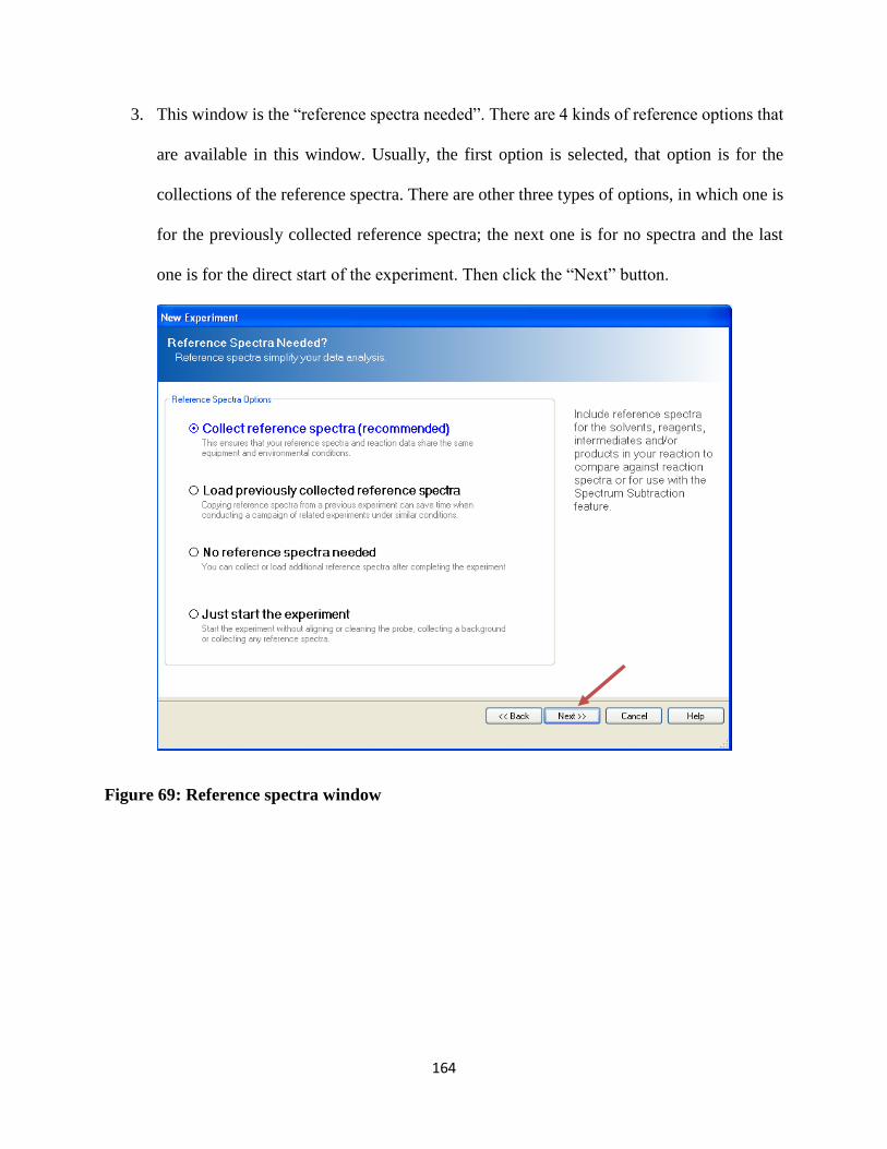
164

3. This window is the “reference spectra needed”. There are 4 kinds of reference options that

are available in this window. Usually, the first option is selected, that option is for the

collections of the reference spectra. There are other three types of options, in which one is

for the previously collected reference spectra; the next one is for no spectra and the last

one is for the direct start of the experiment. Then click the “Next” button.

Figure 69: Reference spectra window

165

4. The next window again will show the picture of the instrument and the probe. The picture

will appear as below. Then click the “Next” button.

Figure 70: Position of the probe

166

5. The align probe window will appear as shown in Figure 64. The position of the probe and

mirror should be aligned and if it is aligned then the bars will turn into the green color.

Otherwise, it will remain red. Click the “Next” Button.

6. In the next window, which is for the cleaning of the probe, there are two bars, one is for

the purging and one is for cleaning the probe. If purging and cleaning are proper then these

bars are green as shown below. The deionized water is the best solvent, for the cleaning of

the probe, also use acetone and 0.2 N hydrochloric acid (very very dilute). So that all small

traces of the previous experiment will dissolve in these solvents and the probe will be clean.

Click the “Next” button.

Figure 71: Clean probe window

167

7. The “collect background” window will open.The main purpose of this window is to collect

the air background. The number of scans option can be chosen from the drop-down arrow

list or the default option is 256 scans. Then click the “Collect Background” button. The

collection of the background normally takes 1-2 min, but it also depends on the number of

scan options. Once the background is collected, click the “Next” button.

Figure 72: Collect background window

To collect

background

For next Window

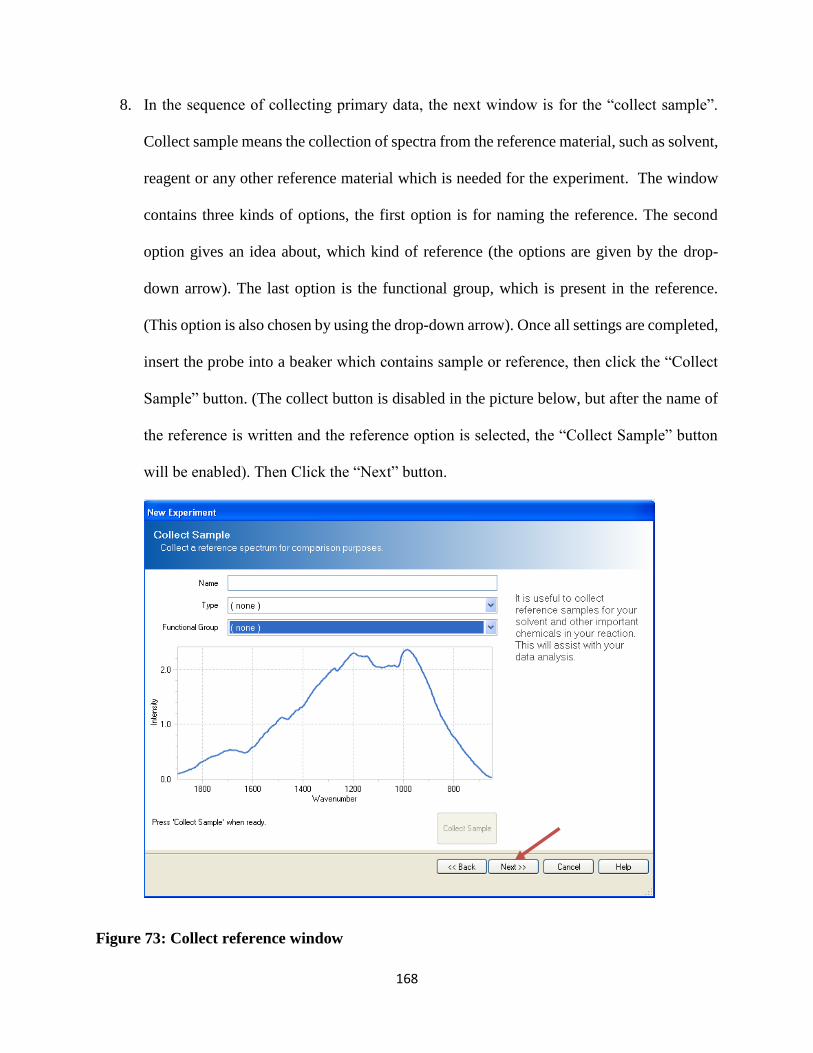
168

8. In the sequence of collecting primary data, the next window is for the “collect sample”.

Collect sample means the collection of spectra from the reference material, such as solvent,

reagent or any other reference material which is needed for the experiment. The window

contains three kinds of options, the first option is for naming the reference. The second

option gives an idea about, which kind of reference (the options are given by the drop-

down arrow). The last option is the functional group, which is present in the reference.

(This option is also chosen by using the drop-down arrow). Once all settings are completed,

insert the probe into a beaker which contains sample or reference, then click the “Collect

Sample” button. (The collect button is disabled in the picture below, but after the name of

the reference is written and the reference option is selected, the “Collect Sample” button

will be enabled). Then Click the “Next” button.

Figure 73: Collect reference window

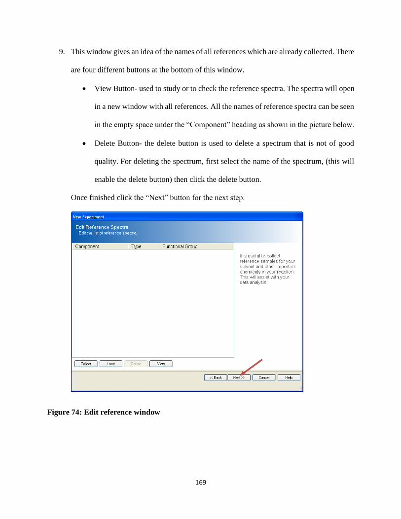
169

9. This window gives an idea of the names of all references which are already collected. There

are four different buttons at the bottom of this window.

View Button- used to study or to check the reference spectra. The spectra will open

in a new window with all references. All the names of reference spectra can be seen

in the empty space under the “Component” heading as shown in the picture below.

Delete Button- the delete button is used to delete a spectrum that is not of good

quality. For deleting the spectrum, first select the name of the spectrum, (this will

enable the delete button) then click the delete button.

Once finished click the “Next” button for the next step.

Figure 74: Edit reference window

170

10. After collecting the reference spectra, the instrument will show the clean probe window

again as shown in Figure 71. It means that before starting the experiment, the probe should

be clean. Whatever traces from the reference material which is present on the probe must

be removed by cleaning. The clean probe window will appear as shown below. Once the

probe is cleaned two green bars will appear showed as below will appear on the screen.

Click the “Next” button.

11. In front of the screen should be a “Collection Background” window as shown in Figure 72.

The main importance of collecting background is, the instrument can start its new

experiment with a fresh setting for the better results and good quality of spectra. Then click

the “Finish” button which is at the bottom of this window. After this step all the preliminary

requirements are finished, it will open a new experiment window.

Understanding the Dynamic Process of Dissolution Using In ...

Documents

Transcript of Understanding the Dynamic Process of Dissolution Using In ...