UNDERSTANDING STATISTICS - Northern Arizona …jan.ucc.nau.edu/~pms/cj355/readings/patten.pdfPART F...

PART F

UNDERSTANDING STATISTICS

In this part, we'll begin by examining the differences between the two majorbranches of statistics — descriptive statistics, which help us summarize and de-scribe data that we've collected, and inferential statistics, which help us make in-ferences from samples to the populations from which they were drawn. Then wewill consider basic statistical techniques used in analyzing the results of research.

Because this part is designed to prepare you to comprehend statistics re-ported in research reports, the emphasis is on understanding their meanings—noton computations. Thus, we will take a conceptual look at statistics and considercomputations only when they are needed to help you understand concepts.

Important NoteThe topics in this part are highly interrelated; in many topics, Ihave assumed that you have mastered material in the earlier topics.Thus, you are strongly advised to read the topics in the orderpresented.

89

TOPIC 37 DESCRIPTIVE AND INFERENTIAL STATISTICS

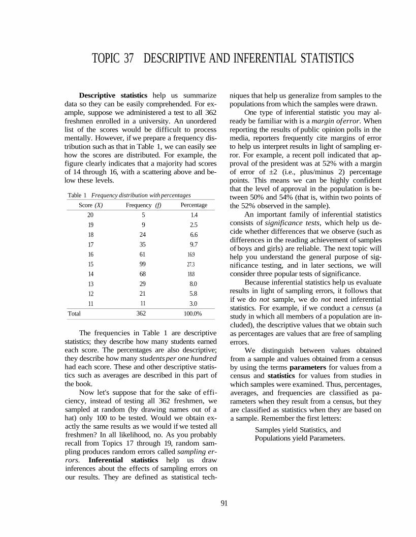
Descriptive statistics help us summarizedata so they can be easily comprehended. For ex-ample, suppose we administered a test to all 362freshmen enrolled in a university. An unorderedlist of the scores would be difficult to processmentally. However, if we prepare a frequency dis-tribution such as that in Table 1, we can easily seehow the scores are distributed. For example, thefigure clearly indicates that a majority had scoresof 14 through 16, with a scattering above and be-low these levels.

Table 1 Frequency distribution with percentages

Score (X)

20

19

18

17

16

15

14

13

12

11

Total

Frequency (f)

5

9

24

35

61

99

68

29

21

11

362

Percentage

1.4

2.5

6.6

9.7

16.9

27.3

18.8

8.0

5.8

3.0

100.0%

The frequencies in Table 1 are descriptivestatistics; they describe how many students earnedeach score. The percentages are also descriptive;they describe how many students per one hundredhad each score. These and other descriptive statis-tics such as averages are described in this part ofthe book.

Now let's suppose that for the sake of effi-ciency, instead of testing all 362 freshmen, wesampled at random (by drawing names out of ahat) only 100 to be tested. Would we obtain ex-actly the same results as we would if we tested allfreshmen? In all likelihood, no. As you probablyrecall from Topics 17 through 19, random sam-pling produces random errors called sampling er-rors. Inferential statistics help us drawinferences about the effects of sampling errors onour results. They are defined as statistical tech-

niques that help us generalize from samples to thepopulations from which the samples were drawn.

One type of inferential statistic you may al-ready be familiar with is a margin of error. Whenreporting the results of public opinion polls in themedia, reporters frequently cite margins of errorto help us interpret results in light of sampling er-ror. For example, a recent poll indicated that ap-proval of the president was at 52% with a marginof error of ±2 (i.e., plus/minus 2) percentagepoints. This means we can be highly confidentthat the level of approval in the population is be-tween 50% and 54% (that is, within two points ofthe 52% observed in the sample).

An important family of inferential statisticsconsists of significance tests, which help us de-cide whether differences that we observe (such asdifferences in the reading achievement of samplesof boys and girls) are reliable. The next topic willhelp you understand the general purpose of sig-nificance testing, and in later sections, we willconsider three popular tests of significance.

Because inferential statistics help us evaluateresults in light of sampling errors, it follows thatif we do not sample, we do not need inferentialstatistics. For example, if we conduct a census (astudy in which all members of a population are in-cluded), the descriptive values that we obtain suchas percentages are values that are free of samplingerrors.

We distinguish between values obtainedfrom a sample and values obtained from a censusby using the terms parameters for values from acensus and statistics for values from studies inwhich samples were examined. Thus, percentages,averages, and frequencies are classified as pa-rameters when they result from a census, but theyare classified as statistics when they are based ona sample. Remember the first letters:

Samples yield Statistics, andPopulations yield Parameters.

91

EXERCISE ON TOPIC 37

1. Which branch of statistics helps us summarize data so they can be easily comprehended?

2. According to Figure 1 in this topic, how many subjects had a score of 19?

3. What is the name of the statistic that describes how many subjects per 100 have a certaincharacteristic?

4. Which branch of statistics helps us draw inferences about the effects of sampling errors on our results?

5. If we test a random sample instead of all members of a population, is it likely that the sample resultswill be the same as the results we would have obtained by testing the population?

6. Is a margin of error a descriptive or an inferential statistic?

7. Do we perform significance tests with inferential or descriptive statistics?

8. By studying populations, do we obtain statistics or parameters?

9. By studying samples, do we obtain statistics or parameters?

Question for Discussion

10. Keep your eye out for a report of a poll in which a margin of error is reported. Copy the exact wordsand bring it to class for discussion.

For Students Who Are Planning Research

11. Will you be reporting descriptive statistics? (Note that statistics often are not reported in qualitative re-search. See Topics 9 and 10.)

12. Will you be reporting inferential statistics? (Note that they are needed only if you have sampled.)

92

TOPIC 3 8 INTRODUCTION TO THE NULL HYPOTHESIS

Suppose we drew random samples of engi-neers and psychologists, administered a self-report measure of sociability, and computed themean (the most commonly used average) for eachgroup. Furthermore, suppose the mean for engi-neers is 65.00 and the mean for psychologists is70.00. Where did the five-point difference comefrom? There are three possible explanations:

1. Perhaps the population of psychologists istruly more sociable than the population ofengineers, and our samples correctly identi-fied the difference. (In fact, our researchhypothesis may have been that psycholo-gists are more sociable than engineers—which now appears to be supported by thedata.)

2. Perhaps there was a bias in procedures. Byusing random sampling, we have ruled outsampling bias, but other procedures such asmeasurement may be biased. For example,maybe the psychologists were contactedduring December, when many social eventstake place and the engineers were contactedduring a gloomy February. The only way torule out bias as an explanation is to takephysical steps to prevent it. In this case, wewould want to make sure that the sociabilityof both groups was measured in the sameway at the same time.

3. Perhaps the populations of psychologistsand engineers are the same but the samplesare unrepresentative of their populations be-cause of random sampling errors. For in-stance, the random draw may have given usa sample of psychologists who are more so-ciable, on the average, than their population.

The third explanation has a name — it is the nullhypothesis. The general form in which it is statedvaries from researcher to researcher. Here arethree versions, all of which are consistent witheach other:

Version A of the null hypothesis:The observed difference was created by sam-pling error. (Note that the term sampling error

refers only to random errors—not errorscreated by a bias.)

Version B of the null hypothesis:There is no true difference between the twogroups. (The term true difference refers to thedifference we would find in a census of thepopulations, that is, the difference we wouldfind if there were no sampling errors.)

Version C of the null hypothesis:The true difference between the two groups iszero.

Significance tests determine the probabilitythat the null hypothesis is true. (We will be con-sidering the use of specific significance tests inTopics 41—42 and 48-50.) Suppose for our exam-ple we use a significance test and find that theprobability that the null hypothesis is true is lessthan 5 in 100; this would be stated as p < .05,where p obviously stands for probability. Ofcourse, if the chances that something is true is lessthan 5 in 100, it's a good bet that it's not true. Ifit's probably not true, we reject the null hypothe-sis, leaving us with only the first two explanationsthat we started with as viable explanations for thedifference.

There is no rule of nature that dictates atwhat probability level the null hypothesis shouldbe rejected. However, conventional wisdom sug-gests that .05 or less (such as .01 or .001) is rea-sonable. Of course, researchers should state intheir reports the probability level they used to de-termine whether to reject the null hypothesis.

Note that when we fail to reject the null hy-pothesis because the probability is greater than.05, we do just that: We "fail to reject" the nullhypothesis and it stays on our list of possible ex-planations; we never "accept" the null hypothesisas the only explanation—remember, there arethree possible explanations and failing to rejectone of them does not mean that you are acceptingit as the only explanation.

An alternative way to say that we have re-jected the null hypothesis is to state that the dif-ference is statistically significant. Thus, if westate that a difference is statistically significant at

93

the .05 level (meaning .05 or less), it is equivalentto stating that the null hypothesis has been re-jected at that level.

When you read research reported in aca-demic journals, you will find that the null hy-pothesis is seldom stated by researchers, whoassume that you know that the sole purpose of asignificance test is to test a null hypothesis. In-stead, researchers tell you which differences weretested for significance, which significance testthey used, and which differences were found to bestatistically significant. It is more common to find

null hypotheses stated in theses and dissertationssince committee members may wish to make surethat the students they are supervising understandthe reason they have conducted a significance test.

As we consider specific significance tests inthe next three parts of this book, we'll examinethe null hypothesis in more detail.


1. How many explanations were there for the difference in sociability between psychologists and engi-neers in the example in this topic?

2. What does the null hypothesis say about sampling error?

3. Does the term sampling error refer to random errors or to bias?

4. The null hypothesis says that the true difference equals what value?

5. What is used to determine the probabilities that null hypotheses are true?

6. For what does p < .05 stand?

7. Do we reject the null hypothesis when the probability of its truth is high or when it is low?

8. What do we do if the probability is greater than .05?

9. What is an alternative way of saying that we have rejected the null hypothesis?

10. Are you more likely to find a null hypothesis stated in a journal article or in a thesis?


11. We all use probabilities in everyday activities to make decisions. For example, before we cross a busystreet, we estimate the odds that we will get across the street safely. Briefly describe one other specificuse of probability in everyday decision making.


12. Will you need to test the null hypothesis in your research? Explain.

94

TOPIC 39 SCALES OF MEASUREMENT

There are four scales (or levels) at which wemeasure. The lowest level is the nominal scale.This may be thought of as the "naming" level. Forexample, when we ask subjects to name theirmarital status, they will respond with words—notnumbers—that describe their status such as "mar-ried," "single," "divorced," etc. Notice that nomi-nal data do not put subjects in any particularorder. There is no logical basis for saying that onecategory such as "single" is higher or lower thanany other.

The next level is ordinal. At this level, weput subjects in order from high to low. For in-stance, an employer might rank order applicantsfor a job on their professional appearance. Tradi-tionally, we give a rank of 1 to the subject who ishighest, 2 to the next highest, and so on. It is im-portant to note that ranks do not tell us by howmuch subjects differ. If we are told that Janet hasa rank of 1 and Frank has a rank of 2, we do notknow if Janet's appearance is greatly superior toFrank's or only slightly superior. To measure theamount of difference among subjects, we use thenext levels of measurement.

Measurements at the interval and ratio lev-els have equal distances among the scores theyyield. For example, when we say that Jill weighs120 pounds and Sally weighs 130 pounds, weknow by how much the two subjects differ. Also,note that a 10-pound difference represents thesame amount regardless of where we are on thescale. For instance, the difference between 120and 130 pounds is the same as the difference be-tween 220 and 230 pounds.

The ratio scale is at a higher level than the in-terval scale because the ratio has an absolute zeropoint that we know how to measure. Thus, weightis an example of the ratio scale because it has anabsolute zero that we can measure.

The interval scale, while having equal inter-vals like the ratio scale, does not have an absolutezero. The most common examples of intervalscales are scores obtained using objective testssuch as multiple-choice tests of achievement. It iswidely assumed that each multiple-choice testitem measures a single point's worth of the trait

being measured and that all points are equal to allother points—making it an interval scale (just asall pounds are equal to all other pounds ofweight). However, such tests do not measure atthe ratio level because the zero on such tests is ar-bitrary—not absolute. To see this, consider some-one who gets a zero on a multiple-choice finalexamination. Does the zero mean that the studenthas absolutely no knowledge of or skills in thesubject area? Probably not. He or she probablyhas some knowledge of simple facts, definitions,and concepts, but the test was not designed tomeasure at the skill level at which the student isoperating. Thus, a score of zero indicates only thatthe student knows nothing on that test—not thatthe student has zero knowledge of the contentdomain.

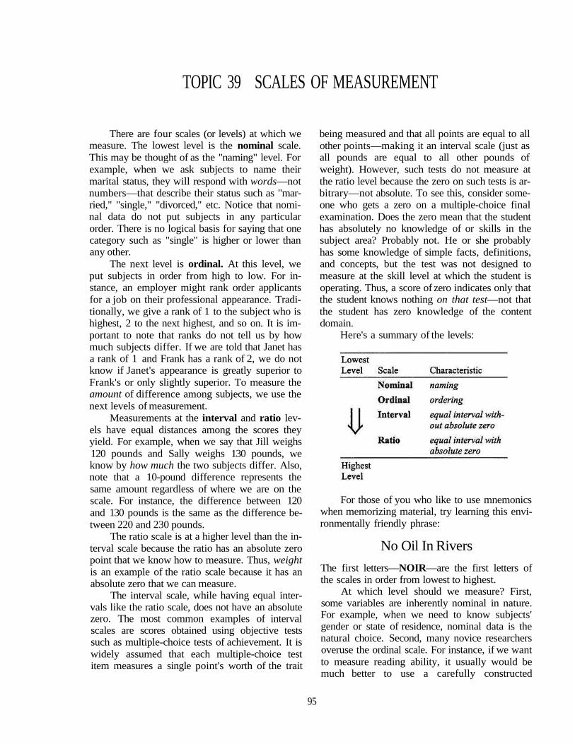
Here's a summary of the levels:

For those of you who like to use mnemonicswhen memorizing material, try learning this envi-ronmentally friendly phrase:

No Oil In Rivers

The first letters—NOIR—are the first letters ofthe scales in order from lowest to highest.

At which level should we measure? First,some variables are inherently nominal in nature.For example, when we need to know subjects'gender or state of residence, nominal data is thenatural choice. Second, many novice researchersoveruse the ordinal scale. For instance, if we wantto measure reading ability, it usually would bemuch better to use a carefully constructed

95

standardized test (which measures at the intervallevel) than having teachers rank order students interms of their reading ability. Remember, measur-ing at the interval level gives you more informa-tion because it tells you by how much studentsdiffer. Also, as you will learn when we explorestatistics, you can do more interesting and power-ful types of analyses when you measure at the in-terval rather than the ordinal level. Thus, whenplanning instruments for a research project, if youare thinking in terms of having subjects ranked(for ordinal measurement), you would be well ad-

vised to consider whether there is an alternative atthe interval level.

The choice between interval and ratio de-pends solely on whether it is possible to measurewith an absolute zero. When it is possible, weusually do so. For the purposes of statisticalanalysis, interval and ratio data are treated in thesame way.

The level at which we measure has importantimplications for data analysis, so you will findreferences to scales of measurement throughoutour discussion of statistics.


1. If we ask subjects to name the country in which they were bom, we are using what scale ofmeasurement?

2. Which two scales of measurement have equal distances among the scores they yield?

3. If we have a teacher rank students according to their oral language skills, we are using which scaleof measurement?

4. Which scale of measurement has an absolute zero that is measured?

5. Which scale of measurement is at the lowest level?

6. Objective, multiple-choice achievement tests are usually assumed to measure at what level?

7. If we measure in such a way that we find out which subject is most honest, which is the next mosthonest, and so on, we are measuring at what scale of measurement?

8. The number of minutes of overtime work that employees perform is an example of what scale ofmeasurement?

9. Weight measured in pounds is an example of which scale of measurement?


10. Name a trait that inherently lends itself to nominal measurement. Explain your answer.


11. List the measures you will be using, and name the scale of measurement for each one.

96

TOPIC 40 DESCRIPTIONS OF NOMINAL DATA

We obtain nominal data when we classifysubjects according to names (words) instead ofquantities. For example, suppose we asked apopulation of 540 teachers which candidate theyeach prefer for a school board vacancy and foundthat 258 preferred Smith and 282 preferred Jones.The 258 and 282 are frequencies, whose symbolis /; we can also refer to them as numbers ofcases, whose symbol is N.

We can convert the numbers of cases intopercentages by dividing the number who prefereach candidate by the number in the populationand multiplying by 100. Thus, for Smith, the cal-culations are:

When reporting percentages, it's a good idea toalso report the underlying numbers of cases,which is done in Table 1.

Table 1 is an example of univariate analysis.We are analyzing how people vary (hence, we usethe root variate) on only one variable (hence, weuse the prefix uni-).

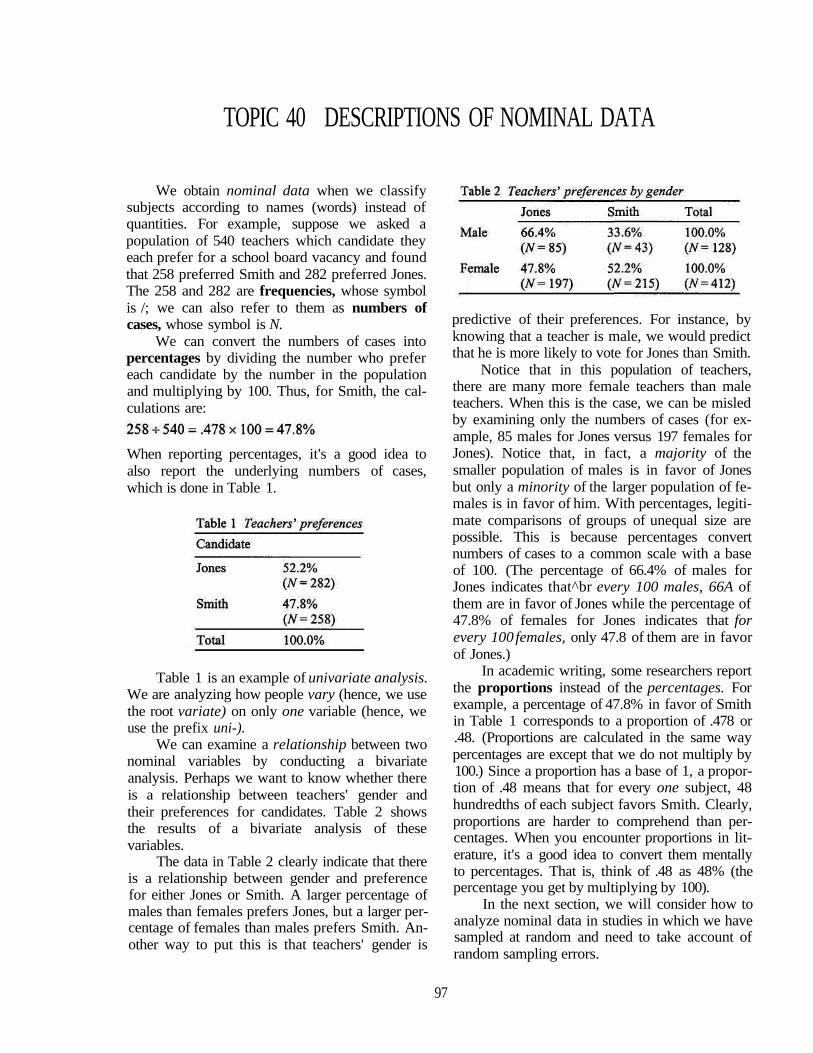
We can examine a relationship between twonominal variables by conducting a bivariateanalysis. Perhaps we want to know whether thereis a relationship between teachers' gender andtheir preferences for candidates. Table 2 showsthe results of a bivariate analysis of thesevariables.

The data in Table 2 clearly indicate that thereis a relationship between gender and preferencefor either Jones or Smith. A larger percentage ofmales than females prefers Jones, but a larger per-centage of females than males prefers Smith. An-other way to put this is that teachers' gender is

predictive of their preferences. For instance, byknowing that a teacher is male, we would predictthat he is more likely to vote for Jones than Smith.

Notice that in this population of teachers,there are many more female teachers than maleteachers. When this is the case, we can be misledby examining only the numbers of cases (for ex-ample, 85 males for Jones versus 197 females forJones). Notice that, in fact, a majority of thesmaller population of males is in favor of Jonesbut only a minority of the larger population of fe-males is in favor of him. With percentages, legiti-mate comparisons of groups of unequal size arepossible. This is because percentages convertnumbers of cases to a common scale with a baseof 100. (The percentage of 66.4% of males forJones indicates that^br every 100 males, 66A ofthem are in favor of Jones while the percentage of47.8% of females for Jones indicates that forevery 100 females, only 47.8 of them are in favorof Jones.)

In academic writing, some researchers reportthe proportions instead of the percentages. Forexample, a percentage of 47.8% in favor of Smithin Table 1 corresponds to a proportion of .478 or.48. (Proportions are calculated in the same waypercentages are except that we do not multiply by100.) Since a proportion has a base of 1, a propor-tion of .48 means that for every one subject, 48hundredths of each subject favors Smith. Clearly,proportions are harder to comprehend than per-centages. When you encounter proportions in lit-erature, it's a good idea to convert them mentallyto percentages. That is, think of .48 as 48% (thepercentage you get by multiplying by 100).

In the next section, we will consider how toanalyze nominal data in studies in which we havesampled at random and need to take account ofrandom sampling errors.

97


1. If 400 people in a population of 1,000 are Democrats, what percentage are Democrats?

2. When reporting a percentage, is it a good idea to also report the underlying number of cases?

3. Do we use univariate or bivariate analyses to examine relationships among nominal variables?

4. Percentages convert numbers of cases to a common scale with what base?

5. What is the base for a proportion?

6. Are percentages or proportions easier for most people to comprehend?


7. Be on the lookout for a report in the popular press in which percentages are reported. Bring a copy toclass. Be prepared to discuss whether the frequencies are also reported and whether it is a univariateor bivariate analysis.


8. Will you be measuring anything at the nominal level? Explain.

9. Will you be reporting percentages? Will you do a univariate analysis? A bivariate analysis? Explain.

98

TOPIC 41 INTRODUCTION TO THE CHI SQUARE TEST

Suppose we drew at random a sample of 200members of a professional association of sociolo-gists and asked them whether they were in favorof a proposed change to their bylaws. The resultsare shown in Table 1. But do these observed re-sults reflect the true results that we would haveobtained if we had questioned the entire popula-tion? Remember that the null hypothesis (seeTopic 38) says that the observed difference wascreated by random sampling errors; that is, in thepopulation, the true difference is zero. Put anotherway, the observed difference (n = 120 vs. n = 80)is an illusion created by chance errors.

The usual test of the null hypothesis when weare considering frequencies (that is, number ofcases or n) is chi square, whose symbol is:

It turns out that after doing some computa-tions, which are beyond the scope of this book, forthe data in Table 1, the results are:

What does this mean for a consumer of researchwho sees this in a report? The values of chi squareand degrees of freedom (df) were calculated sole-ly to obtain the probability that the null hypothesisis correct. That is, chi square and degrees of free-dom are not descriptive statistics that you shouldattempt to interpret. Rather, think of them as sub-steps in the mathematical procedure for obtainingthe value of p. Thus, the consumer of researchshould concentrate on the fact that p is less than

.05. As you probably recall from Topic 38, whenthe probability (p) that the null hypothesis is cor-rect is .05 or less, we reject the null hypothesis.(Remember, when the probability that somethingis true is less than 5 in 100—a low probability—conventional wisdom suggests that we should re-ject it as being true.) Thus, the difference we ob-serve in Table 1 was probably not created byrandom sampling errors; therefore, we can saythat the difference is statistically significant at the.05 level.

So far, we have concluded that the differencewe observed in the sample was probably not cre-ated by sampling errors. So where did the differ-ence come from? Two possibilities remain:

1. Perhaps there was a bias in procedures suchas the person asking the question in the sur-vey leading the respondents by talking en-thusiastically about the proposed change inthe bylaws. If we are convinced that ade-quate measures were taken to prevent proce-dural bias, we are left with only the nextpossibility as a viable explanation.

2. Perhaps the population of sociologists is, infact, in favor of the proposed change, andthis fact is correctly identified by studyingthe random sample.

Now let's consider some results from a sur-vey in which the null hypothesis was not rejected.Table 2 shows the numbers and percentages ofsubjects in a random sample from a population ofteachers who prefer each of three methods forteaching reading. In the table, there are three dif-ferences (30 for A versus 27 for B, 30 for A ver-

sus 22 for C, and 27 for B versus 22 for C). Thenull hypothesis says that this set of differenceswas created by random sampling errors; in other

*We are using the term true results here to stand for the results of a census of the entire population. The results of acensus are true in the sense that they are free of sampling errors. Of course, there may also be measurement errors,which we are not considering here.

99

words, it says that there is no true difference inthe population; we have observed a differenceonly because of sampling errors. The results ofthe chi square test for the data in Table 2 are:

Using the decision rule that p must be equal to orless than .05 to reject the null hypothesis, we failto reject the null hypothesis, which is called a sta-tistically insignificant result. In other words, thenull hypothesis must remain on our list as a viable

explanation for the set of differences we observedby studying a sample.

In this topic, we have considered the use ofchi square in a univariate analysis in which weclassify each subject in only one way (such aswhich candidate each prefers). In the next topic,we'll consider its use in bivariate analysis inwhich we classify each subject in two ways (suchas which candidate each prefers and the gender ofeach) in order to examine a relationship betweenthe two.


1. When we study a sample, are the results called the true results or the observed results'!

2. According to the null hypothesis, what created the difference in Table 1 in this topic?

3. What is the name of the test of the null hypothesis used when we are analyzing frequencies?

4. As a consumer of research, should you try to interpret the value of dfl

5. What is the symbol for probability1?

6. If you read that a chi square test of a difference yielded up of less than 5 in 100, what should you con-clude about the null hypothesis on the basis of conventional wisdom?

7. Does;? < .05 or/> > .05 usually lead a researcher to declare a difference to be statistically significant?

8. If we fail to reject a null hypothesis, is the difference in question statistically significant?

9. If we have a statistically insignificant result, does the null hypothesis remain on our list of viablehypotheses?


10. Briefly describe a hypothetical study in which it would be appropriate to conduct a chi square test forunivariate data.


11. Will you be conducting a chi square test? Explain.

i

100

TOPIC 42 A CLOSER LOOK AT THE CHI SQUARE TEST

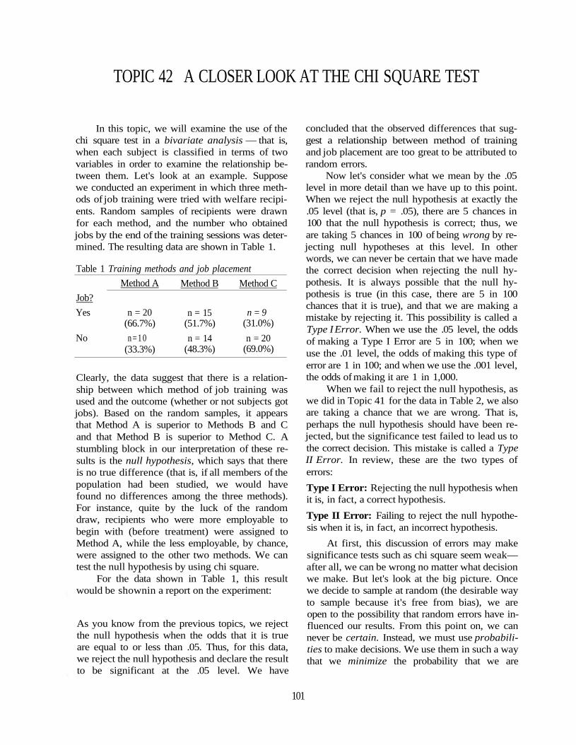
In this topic, we will examine the use of thechi square test in a bivariate analysis — that is,when each subject is classified in terms of twovariables in order to examine the relationship be-tween them. Let's look at an example. Supposewe conducted an experiment in which three meth-ods of job training were tried with welfare recipi-ents. Random samples of recipients were drawnfor each method, and the number who obtainedjobs by the end of the training sessions was deter-mined. The resulting data are shown in Table 1.

Table 1 Training methods and job placement

Job?

Yes

No

Method A

n = 20(66.7%)

n = 1 0(33.3%)

Method B

n = 15(51.7%)

n = 14(48.3%)

Method C

n = 9(31.0%)

n = 20(69.0%)

Clearly, the data suggest that there is a relation-ship between which method of job training wasused and the outcome (whether or not subjects gotjobs). Based on the random samples, it appearsthat Method A is superior to Methods B and Cand that Method B is superior to Method C. Astumbling block in our interpretation of these re-sults is the null hypothesis, which says that thereis no true difference (that is, if all members of thepopulation had been studied, we would havefound no differences among the three methods).For instance, quite by the luck of the randomdraw, recipients who were more employable tobegin with (before treatment) were assigned toMethod A, while the less employable, by chance,were assigned to the other two methods. We cantest the null hypothesis by using chi square.

For the data shown in Table 1, this resultwould be shownin a report on the experiment:

As you know from the previous topics, we rejectthe null hypothesis when the odds that it is trueare equal to or less than .05. Thus, for this data,we reject the null hypothesis and declare the resultto be significant at the .05 level. We have

concluded that the observed differences that sug-gest a relationship between method of trainingand job placement are too great to be attributed torandom errors.

Now let's consider what we mean by the .05level in more detail than we have up to this point.When we reject the null hypothesis at exactly the.05 level (that is, p = .05), there are 5 chances in100 that the null hypothesis is correct; thus, weare taking 5 chances in 100 of being wrong by re-jecting null hypotheses at this level. In otherwords, we can never be certain that we have madethe correct decision when rejecting the null hy-pothesis. It is always possible that the null hy-pothesis is true (in this case, there are 5 in 100chances that it is true), and that we are making amistake by rejecting it. This possibility is called aType I Error. When we use the .05 level, the oddsof making a Type I Error are 5 in 100; when weuse the .01 level, the odds of making this type oferror are 1 in 100; and when we use the .001 level,the odds of making it are 1 in 1,000.

When we fail to reject the null hypothesis, aswe did in Topic 41 for the data in Table 2, we alsoare taking a chance that we are wrong. That is,perhaps the null hypothesis should have been re-jected, but the significance test failed to lead us tothe correct decision. This mistake is called a TypeII Error. In review, these are the two types oferrors:

Type I Error: Rejecting the null hypothesis whenit is, in fact, a correct hypothesis.

Type II Error: Failing to reject the null hypothe-sis when it is, in fact, an incorrect hypothesis.

At first, this discussion of errors may makesignificance tests such as chi square seem weak—after all, we can be wrong no matter what decisionwe make. But let's look at the big picture. Oncewe decide to sample at random (the desirable wayto sample because it's free from bias), we areopen to the possibility that random errors have in-fluenced our results. From this point on, we cannever be certain. Instead, we must use probabili-ties to make decisions. We use them in such a waythat we minimize the probability that we are

101

wrong. To do this, we usually emphasize mini-mizing the probability of a Type I error by using alow probability such as .05 or less. By using a lowprobability, we will infrequently be wrong in re-jecting the null hypothesis.


1. What is the name of the type of analysis when each subject is classified in terms of two variables inorder to examine the relationship between them?

2. What decision have we made about the null hypothesis if a chi square test leads us to the conclusionthat the observed differences that suggest a relationship between two variables are too great to be at-tributed to random errors?

3. If p = .05 for a chi square test, chances are how many in 100 that the null hypothesis is true?

4. When we use the .01 level, what are the odds of making a Type I error?

5. What is the name for the error we make when we fail to reject the null hypothesis when it is, in fact,an incorrect hypothesis?

6. What is the name for the error we make when we reject the null hypothesis when it is, in fact, a cor-rect hypothesis?

7. Why is random sampling desirable even though it creates errors?

Questions for Discussion

8. Are both of the variables in Table 1 in this topic nominal? Explain.

9. Briefly describe a hypothetical study in which it would be appropriate to conduct a chi square test onbivariate data.


10. Will you be using a chi square test in a bivariate analysis? Explain.

102

TOPIC 43 SHAPES OF DISTRIBUTIONS

One way to describe quantitative data is toprepare a frequency distribution such as thatshown in Topic 37 (see page 91). It is easier to seethe shape of the distribution if we prepare a figurecalled a frequency polygon. This figure is a fre-quency polygon for the data in Topic 37:

ScoresFigure 1 Frequency polygon for data on page 91

A frequency polygon is easy to read. For example,a score of 20 has a frequency (/) of 5, which iswhy the curve is low at a score of 20. A score of15 has a frequency of 99, which is why the curveis high at 15.

Notice that the curve in Figure 1 is fairlysymmetrical with a high point in the middle anddropping off on the right and left. When verylarge samples are used, the curve often takes onan even smoother shape, such as the one shown inFigure 2.

The smooth, bell-shaped curve in Figure 2 has aspecial name; it is the normal curve. As the name"normal" suggests, it is the common shape that isregularly observed. Many things in nature are nor-mally distributed—the weights of grains of sandon a beach, the heights of women (or men), theannual amounts of rainfall in most areas, and soon. The list is almost limitless. Many social andbehavioral scientists also believe that mental traitsof humans probably are also normally distri-buted.1

Some distributions are skewed—that is, theyhave a tail to the left or right. Figure 3 shows adistribution that is skewed to the right (that is , thetail is to the right); it is said to have a positiveskew. An example of a distribution with a positiveskew is income. Most people earn relatively smallamounts, so the curve is high on the left. Smallnumbers of rich and very rich people create a tailto the right.

Figure 3 A distribution with a positive skew

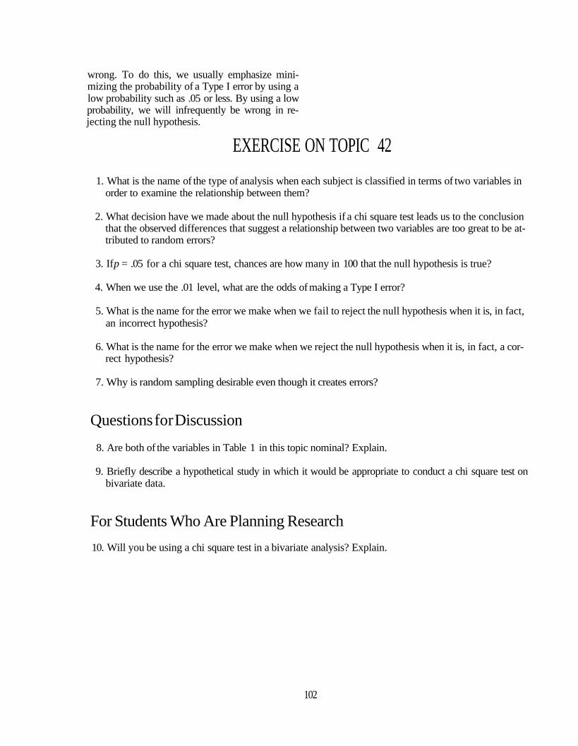
Figure 4 is skewed to the left; it has a nega-tive skew. We would get a negative skew, for ex-ample, if we administered a test of basic mathskills to a large sample of college seniors. Mostwould do very well and get almost perfect scores,but a small scattering will get lower scores for avariety of reasons such as misunderstanding thedirections for marking their answers, not feelingwell the day the test was administered, and so on.

'Because measures of mental traits are far from perfect, it is difficult to show conclusively that mental traits arenormally distributed. However, many norm-referenced tests do yield normal distributions when large representativenational samples are tested.

103

While there are other shapes, the three shownhere are the ones you are most likely to encounter.Whether a distribution is basically normal orskewed affects how quantitative data at the inter-val and ratio levels are analyzed, which we willconsider in the next topic.


1. According to Figure 1, about how many subjects had a score of 14?

2. In Figure 1, are the frequencies on the vertical or horizontal axis?

3. Which of the curves discussed in this topic is symmetrical?

4. If a distribution has some extreme scores on the right (but not on the left) it is said to have what type ofskew?

5. If a distribution is skewed to the left, does it have a positive or negative skew?

6. In most populations, income has what type of skew?

7. Does a distribution with a tail to the right have a positive or negative skew?


8. Name a population and a variable that might be measured. Speculate on whether the distribution wouldbe normal or skewed.


9. Do you anticipate that any of your distributions will be highly skewed? Explain.

104

TOPIC 44 THE MEAN, MEDIAN, AND MODE

The most frequently used average is themean, which is the balance point in a distribution.Its computation is simple—just sum (add up) thescores and divide by the number of scores. Themost common symbol for the mean in academicjournals is M (for the mean of a population) or m(for the mean of a sample). The symbol preferredby statisticians is

X which is pronounced "X-bar."Because the mean is very frequently used as

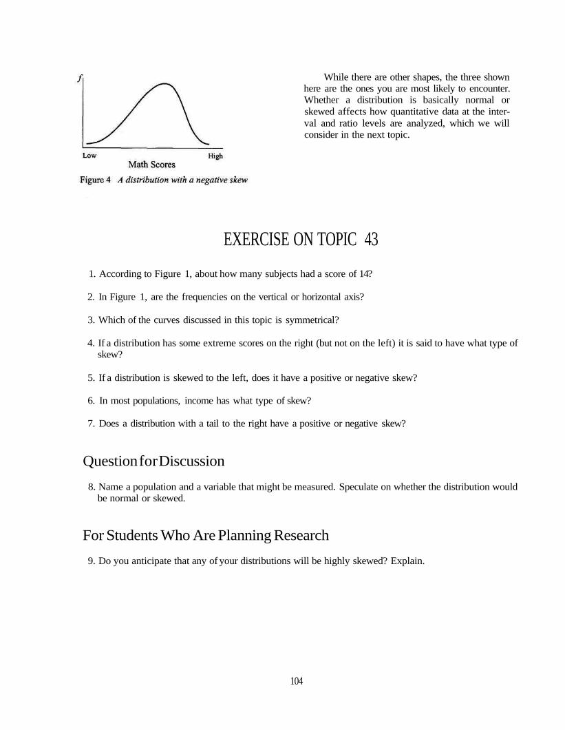
the average, let's consider its formal definition,which is the value around which the deviationssum to zero. You can see what this means by con-sidering the scores in Table 1. When we subtractthe mean of the scores (which is 4.0) from each ofthe other scores, we get the deviations (whosesymbol is x). If we sum the deviations, we getzero, as shown in Table 1.

Table 1 Scores and deviation scores

Note that if you take any set of scores, com-pute their mean, and follow the steps in Table 1,the sum of the deviations will always equal zero.1

Considering the formal definition, you cansee why we also informally define the mean as thebalance point in a distribution. The positive andnegative deviations balance each other out.

A major drawback of the mean is that it isdrawn in the direction of extreme scores. Considerthe following two sets of scores and their means.

Scores for Group A: 1,1,1, 2, 3, 6, 7, 8, 8M-4.ll

Scores for Group B: 1, 2, 2, 3, 4, 7, 9, 25, 32Mf=9.44

Notice that in both sets there are nine scores andthe two distributions are very similar except forthe scores of 25 and 32 in Group B, which aremuch higher than the others and, thus, create askewed distribution. (To review skewed distribu-tions, see Topic 43.) Notice that the two very highscores have greatly pulled up the mean for GroupB; in fact, the mean for Group B is more thantwice as high as the mean for Group A because ofthe two high scores.

When a distribution is highly skewed, we usea different average, the median, which is definedas the middle score. To get an approximate me-dian, put the scores in order from low to high asthey are for Groups A and B above, and thencount to the middle. Since there are nine scores inGroup A, the median (middle score) is 3 (fivescores up from the bottom). For Group B, the me-dian (middle score) is 4 (five scores up from thebottom), which is more representative of the cen-ter of this skewed distribution than the mean,which we noted was 9.44. Thus, one use of themedian is to describe the average of skewed dis-tributions. Another use is to describe the averageof ordinal data, which we'll explore in Topic 46.

A third average, the mode, is simply the mostfrequently occurring score. For Group B, there aremore scores of 2 than any other score; thus, 2 isthe mode. The mode is sometimes used in infor-mal reporting but is very seldom used in formalreports of research.

Because there is more than one type of aver-age, it is vague to make a statement such as, "Theaverage is 4.11." Rather, we should indicate thespecific type of average being reported with state-ments such as, "The mean is 4.11."

'it might be slightly off from zero if you use a rounded mean such as using 20.33 as the mean when its precise valueis 20.3333333333.

105

Note that a synonym for the term averages ismeasures of central tendency. Although the lat-ter is seldom used in reports of scientific research,you may encounter it in other research and statis-tics textbooks.


1. Which average is defined as the most frequently occurring score!

2. Which average is defined as the balance point in a distribution?

3. Which average is defined as the middle score?

4. What is the formal definition of the mean?

5. How is the mean calculated?

6. Should the mean be used for highly skewed distributions?

7. Should the median be used for highly skewed distributions?

8. What is a synonym for the term averages?


9. Suppose a fellow student gave a report in class and said, "The average was 25.88." For what additionalinformation should you ask? Why?


10. Do you anticipate calculating measure(s) of central tendency? If so, which one(s) are you likely to use?Explain your choice(s).

106

TOPIC 45 THE MEAN AND STANDARD DEVIATION

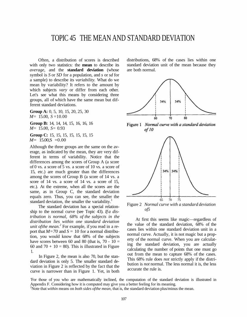
Often, a distribution of scores is describedwith only two statistics: the mean to describe itsaverage, and the standard deviation (whosesymbol is S or SD for a population, and s or sd fora sample) to describe its variability. What do wemean by variability? It refers to the amount bywhich subjects vary or differ from each other.Let's see what this means by considering threegroups, all of which have the same mean but dif-ferent standard deviations.

Group A: 0, 5, 10, 15, 20, 25, 30M= 15.00, S =10.00

Group B: 14, 14, 14, 15, 16, 16, 16M= 15.00, S= 0.93

Group C: 15, 15, 15, 15, 15, 15, 15M= 15.00,S =0.00

Although the three groups are the same on the av-erage, as indicated by the mean, they are very dif-ferent in terms of variability. Notice that thedifferences among the scores of Group A (a scoreof 0 vs. a score of 5 vs. a score of 10 vs. a score of15, etc.) are much greater than the differencesamong the scores of Group B (a score of 14 vs. ascore of 14 vs. a score of 14 vs. a score of 15,etc.). At the extreme, when all the scores are thesame, as in Group C, the standard deviationequals zero. Thus, you can see, the smaller thestandard deviation, the smaller the variability.1

The standard deviation has a special relation-ship to the normal curve (see Topic 43). If a dis-tribution is normal, 68% of the subjects in thedistribution lies within one standard deviationunit of the mean.2 For example, if you read in a re-port that M=70 and S = 10 for a normal distribu-tion, you would know that 68% of the subjectshave scores between 60 and 80 (that is, 70 - 10 =60 and 70 + 10 = 80). This is illustrated in Figure1.

In Figure 2, the mean is also 70, but the stan-dard deviation is only 5. The smaller standard de-viation in Figure 2 is reflected by the fact that thecurve is narrower than in Figure 1. Yet, in both

distributions, 68% of the cases lies within onestandard deviation unit of the mean because theyare both normal.

65 70 75

Figure 2 Normal curve with a standard deviationof5

At first this seems like magic—regardless ofthe value of the standard deviation, 68% of thecases lies within one standard deviation unit in anormal curve. Actually, it is not magic but a prop-erty of the normal curve. When you are calculat-ing the standard deviation, you are actuallycalculating the number of points that one must goout from the mean to capture 68% of the cases.This 68% rule does not strictly apply if the distri-bution is not normal. The less normal it is, the lessaccurate the rule is.

'For those of you who are mathematically inclined, the computation of the standard deviation is illustrated inAppendix F. Considering how it is computed may give you a better feeling for its meaning.2Note that within means on both sides of the mean, that is, the standard deviation plus/minus the mean.

107


1. Which average is usually reported when the standard deviation is reported?

2. What is meant by the term variability!

3. Is it possible for two groups to have the same mean but different standard deviations?

4. If everyone in a group has the same score, what is the value of the standard deviation for the scores?

5. What percentage of the subjects lies within one standard deviation unit of the mean in a normaldistribution?

6. The middle 68% of the subjects in a normal distribution has scores between what two values if themean equals 100 and the standard deviation equals 15?

7. If the mean of a normal distribution equals 50 and the standard deviation equals 5, what percentage ofthe subjects has scores between 45 and 50?

8. Does the 68% rule strictly apply if a distribution is not normal?

9. If the standard deviation for Group X is 14.55 and the standard deviation for Group Y is 20.99, whichgroup has less variability in their scores?

10. Which group in question 9 has a narrower curve?


11. Examine a journal article in which a mean and standard deviation are reported. Does the author indicatewhether the distribution is normal in shape? Does the 68% rule strictly apply? Explain.


12. Will you be reporting means and standard deviations? Explain.

108

TOPIC 46 THE MEDIAN AND INTERQUARTILE RANGE

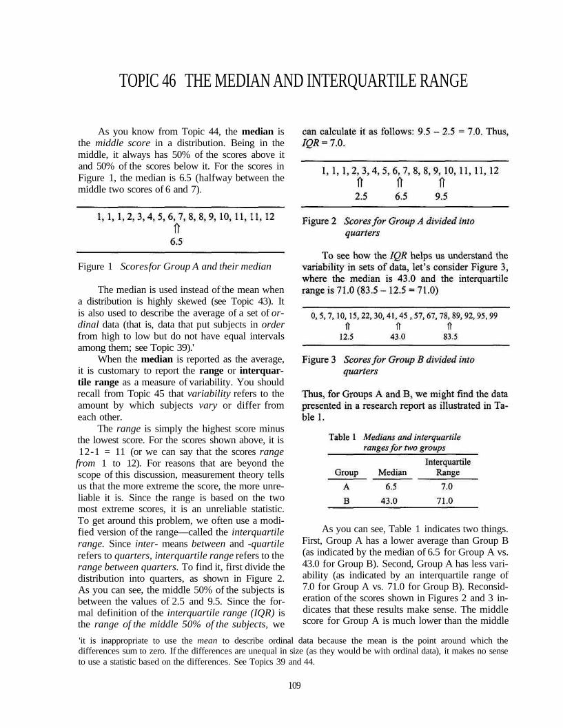
As you know from Topic 44, the median isthe middle score in a distribution. Being in themiddle, it always has 50% of the scores above itand 50% of the scores below it. For the scores inFigure 1, the median is 6.5 (halfway between themiddle two scores of 6 and 7).

Figure 1 Scores for Group A and their median

The median is used instead of the mean whena distribution is highly skewed (see Topic 43). Itis also used to describe the average of a set of or-dinal data (that is, data that put subjects in orderfrom high to low but do not have equal intervalsamong them; see Topic 39).'

When the median is reported as the average,it is customary to report the range or interquar-tile range as a measure of variability. You shouldrecall from Topic 45 that variability refers to theamount by which subjects vary or differ fromeach other.

The range is simply the highest score minusthe lowest score. For the scores shown above, it is12-1 = 11 (or we can say that the scores range

from 1 to 12). For reasons that are beyond thescope of this discussion, measurement theory tellsus that the more extreme the score, the more unre-liable it is. Since the range is based on the twomost extreme scores, it is an unreliable statistic.To get around this problem, we often use a modi-fied version of the range—called the interquartilerange. Since inter- means between and -quartilerefers to quarters, interquartile range refers to therange between quarters. To find it, first divide thedistribution into quarters, as shown in Figure 2.As you can see, the middle 50% of the subjects isbetween the values of 2.5 and 9.5. Since the for-mal definition of the interquartile range (IQR) isthe range of the middle 50% of the subjects, we

As you can see, Table 1 indicates two things.First, Group A has a lower average than Group B(as indicated by the median of 6.5 for Group A vs.43.0 for Group B). Second, Group A has less vari-ability (as indicated by an interquartile range of7.0 for Group A vs. 71.0 for Group B). Reconsid-eration of the scores shown in Figures 2 and 3 in-dicates that these results make sense. The middlescore for Group A is much lower than the middle

'it is inappropriate to use the mean to describe ordinal data because the mean is the point around which thedifferences sum to zero. If the differences are unequal in size (as they would be with ordinal data), it makes no senseto use a statistic based on the differences. See Topics 39 and 44.

109

score for Group B, and the differences among the scores for Group B (0 vs. 5 vs. 7 vs. 10 vs. 15,scores for Group A (1 vs. 1 vs. 1 vs. 1 vs. 2, etc.) etc.)—indicating less variability in Group A thanare much smaller than the differences among the Group B.


1. If the median for a group of subjects is 34.00, what percentage of the subjects has scores below a scoreof 34?

2. Should the mean or median be used with ordinal data?

3. How do you calculate the range of a set of scores?

4. Is the range or the interquartile range a more reliable statistic?

5. What is the definition of the interquartile range!

6. Suppose you read that for Group X, the median equals 55.1 and the IQR equals 30.0, while for GroupY, the median equals 62.9 and the IQR equals 25.0. Which group has the higher average score?

7. Based on the information in question 6, the scores for which group are more variable?

8. Which two statistics discussed in this topic are measures of variability?

9. Which two statistics mentioned in this topic are measures of central tendency (that is, are averages)?


10. Name two circumstances under which the median is preferable to the mean.


11. Do you anticipate reporting medians and interquartile ranges? Explain.

110

TOPIC 47 THE PEARSON CORRELATION COEFFICIENT

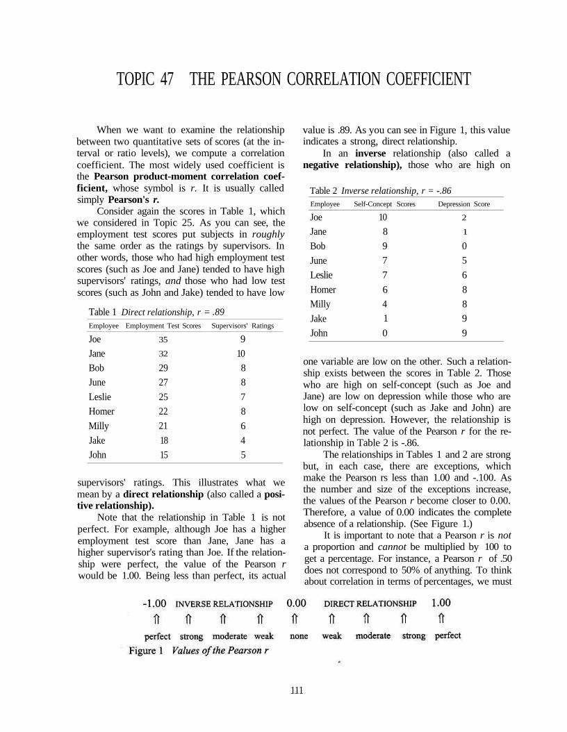
When we want to examine the relationshipbetween two quantitative sets of scores (at the in-terval or ratio levels), we compute a correlationcoefficient. The most widely used coefficient isthe Pearson product-moment correlation coef-ficient, whose symbol is r. It is usually calledsimply Pearson's r.

Consider again the scores in Table 1, whichwe considered in Topic 25. As you can see, theemployment test scores put subjects in roughlythe same order as the ratings by supervisors. Inother words, those who had high employment testscores (such as Joe and Jane) tended to have highsupervisors' ratings, and those who had low testscores (such as John and Jake) tended to have low

Table 1Employee

Joe

JaneBob

June

LeslieHomer

MillyJakeJohn

Direct relationship, rEmployment Test Scores

35

32

29

27

25

22

21

18

15

= .89Supervisors' Ratings

9

10

8

8

7

8

6

4

5

supervisors' ratings. This illustrates what wemean by a direct relationship (also called a posi-tive relationship).

Note that the relationship in Table 1 is notperfect. For example, although Joe has a higheremployment test score than Jane, Jane has ahigher supervisor's rating than Joe. If the relation-ship were perfect, the value of the Pearson rwould be 1.00. Being less than perfect, its actual

value is .89. As you can see in Figure 1, this valueindicates a strong, direct relationship.

In an inverse relationship (also called anegative relationship), those who are high on

Table 2 Inverse relationship, r = -.86Employee

Joe

JaneBob

JuneLeslie

HomerMilly

JakeJohn

Self-Concept Scores

10

8

9

7

7

6

4

1

0

Depression Score

2

1

0

5

6

8

8

9

9

one variable are low on the other. Such a relation-ship exists between the scores in Table 2. Thosewho are high on self-concept (such as Joe andJane) are low on depression while those who arelow on self-concept (such as Jake and John) arehigh on depression. However, the relationship isnot perfect. The value of the Pearson r for the re-lationship in Table 2 is -.86.

The relationships in Tables 1 and 2 are strongbut, in each case, there are exceptions, whichmake the Pearson rs less than 1.00 and -.100. Asthe number and size of the exceptions increase,the values of the Pearson r become closer to 0.00.Therefore, a value of 0.00 indicates the completeabsence of a relationship. (See Figure 1.)

It is important to note that a Pearson r is nota proportion and cannot be multiplied by 100 toget a percentage. For instance, a Pearson r of .50does not correspond to 50% of anything. To thinkabout correlation in terms of percentages, we must

111

convert Pearson rs to another statistic, the coeffi-cient of determination, whose symbol is r2,which indicates how to compute it—simplysquare r. Thus, for an r of .50, r2 equals .25. If wemultiply .25 by 100, we get 25%. What does thismean? Simply this: A Pearson r of .50 is 25% bet-ter than a Pearson r of 0.00. Table 3 shows se-lected values of r, r1, and the percentages youshould think about when interpreting an r.'

Table 3 Selected values ofr and r2

r.90.50

.25

-.25

-.50

-.90

r2 Percentage better than zero1

.81

.25

.06

.06

.25

.81

81%

25%

6%

6%

25%

81%

Also called percentage of variance accounted for orpercentage of explained variance.


1. "Pearson r" stands for what words?

2. When the relationship between two variables is perfect and inverse, what is the value ofr?

3. Is it possible for a negative relationship to be strong?

4. Is an r of -.90 stronger than an r of .50?

5. Is a relationship direct or inverse when those with high scores on one variable have high scores on theother and those with low scores on one variable have low scores on the other?

6. What does an r of 1.00 indicate?

7. For a Pearson r of .60, what is the value of the coefficient of determination?

8. What do we do to a coefficient of determination to get a percentage?

9. A Pearson r of .70 is what percentage better than a Pearson r of 0.00?


10. Name two variables between which you would expect to get a strong, positive value of r.


11. Will you be reporting Pearson rs? If so, name the two variables that will be correlated for eachvalue ofr.

'Note that the procedure for computing a Pearson r is beyond the scope of this book.

112

TOPIC 48 THE t TEST

Suppose we have a research hypothesis thatsays "homicide investigators who take a shortcourse on the causes of HIV will be less fearful ofthe disease than investigators who have not takenthe course," and test it by conducting an experi-ment in which a random sample of investigators isassigned to take the course and another randomsample is designated as the control group.1 Let'ssuppose that at the end of the experiment the ex-perimental group gets a mean of 16.61 on a fear ofHIV scale and the control group gets a mean of29.67 (where the higher the score, the greater thefear of HIV). These means support our researchhypothesis. But can we be certain that our re-search hypothesis is correct? If you've been read-ing the topics on statistics in order from thebeginning, you already know that the answer is"no" because of the null hypothesis, which saysthat there is no true difference between the means;that is, the difference was created merely by thechance errors created by random sampling. (Theseerrors are known as sampling errors) Put anotherway, unrepresentative groups may have been as-signed to the two conditions quite at random.

The t test is often used to test the null hy-pothesis regarding the observed difference be-tween two means.2 For the example we areconsidering, a series of computations (which arebeyond the scope of this book) would be per-formed to obtain a value of t (which, in this case,is 5.38) and a value of degrees of freedom (which,in this case, is df= 179). These values are not ofany special interest to us except that they are usedto get the probability (p) that the null hypothesisis true. In this particular case, p is less than .05.Thus, in a research report, you may read a state-ment such as this:

The difference between the means is statisti-cally significant (t = 5.38, df= 179,p< .05).3

As you know from Topic 38, the term statisticallysignificant indicates that the null hypothesis hasbeen rejected. You should recall that when theprobability that the null hypothesis is true is .05 orless (such as .01 or .001), we reject the null hy-pothesis. (When something is unlikely to be truebecause it has a low probability of being true, wereject it.)

Having rejected the null hypothesis, we arein a position to assert that our research hypothesisprobably is true (assuming no procedural bias wasallowed to affect the results, such as testing thecontrol group immediately after a major newsstory on a famous person with AIDS, while test-ing the experimental group at an earlier time).

What leads a t test to give us a low probabil-ity? Three things:

1. Sample size. The larger the sample, theless likely that an observed difference isdue to sampling errors. (You should recallfrom the sections on sampling that largersamples provide more precise informa-tion.) Thus, when the sample is large, weare more likely to reject the null hypothe-sis than when the sample is small.

2. The size of the difference between means.The larger the difference, the less likelythat the difference is due to sampling er-rors. Thus, when the difference betweenthe means is large, we are more likely toreject the null hypothesis than when thedifference is small.

3. The amount of variation in the population.You should recall from Topic 22 thatwhen a population is very heterogeneous(has much variability) there is more poten-tial for sampling error. Thus, when there islittle variation (as indicated by the stan-dard deviations of the sample), we are

'You probably recall that we prefer random sampling because it precludes any bias in the assignment of subjects tothe groups and because we can test for the effect of random errors with significance tests; we cannot test for theeffects of bias.To test the null hypothesis between two medians, the median test is used; it is a specialized form of the chi square

test, whose results you already know how to interpret.3Sometimes researchers leave out the abbreviation df and present the result as f(179) = 5.38, p < .05.

113

j

more likely to reject the null hypothesisthan when there is much variation.

A special type of t test is also applied to cor-relation coefficients. Suppose we drew a randomsample of 50 students and correlated their handsize with their GPAs and got an r of .19. The nullhypothesis says that the true correlation in thepopulation is 0.00—that we got .19 merely as theresult of sampling errors. For this example, the ttest indicates that p > .05. Since the probability

that the null hypothesis is true is greater than 5 in100, we do not reject the null hypothesis; we havea statistically insignificant correlation coefficient.(In other words, for n = 50, an r of .19 is not sig-nificantly different from an r of 0.00.) When re-porting the results of the t test for the significanceof a correlation coefficient, it is conventional notto mention the value of t. Rather, researchers usu-ally indicate only whether or not the correlation issignificant at a given probability level.


1. What does the null hypothesis say about the difference between two sample means?

2. Is the value of t usually of any special interest to consumers of research?

3. Suppose you read that for the difference between two means, t = 2.000, df = 20, p > .05. Using conven-tional standards, should you conclude that the null hypothesis should be rejected?

4. Suppose you read that for the difference between two means, t = 2.859, df= 40, p < .01. Using conven-tional standards, should you conclude that the null hypothesis should be rejected?

5. Based on the information in question 4, should you conclude that the difference between the means isstatistically significant?

6. When we use a large sample, are we more or less likely to reject the null hypothesis than when we use asmall sample?

7. When the size of the difference between means is large, are we more or less likely to reject the null hy-pothesis than when the size of the difference is small?

8. If we read that for a sample of 92 subjects, r = .41, p < .001, should we reject the null hypothesis?

9. Is the value of r in question 8 statistically significant?


10. Of the three things that lead to a low probability, which one is most directly under the control of aresearcher?


11. Will you be conducting t tests? Explain.

114

UNDERSTANDING STATISTICS - Northern Arizona …jan.ucc.nau.edu/~pms/cj355/readings/patten.pdfPART F...

Documents

Transcript of UNDERSTANDING STATISTICS - Northern Arizona …jan.ucc.nau.edu/~pms/cj355/readings/patten.pdfPART F...