Understanding Sectoral Labor Market Dynamics: AnEquilibrium Analysis of the Oil and Gas Field Services

Industry�

Patrick KlineUC Berkeley

pkline@econ.berkeley.edu

Nov 15th, 2008

Abstract

This paper examines the response of employment and wages in the US oil and gas�eld services industry to changes in the price of crude petroleum using a time seriesof quarterly data spanning the period 1972-2002. I �nd that labor quickly reallocatesacross sectors in response to price shocks but that substantial wage premia are nec-essary to induce such reallocation. The timing of these premia is at odds with thepredictions of standard models� wage premia emerge quite slowly, peaking only aslabor adjustment ends and then slowly dissipating. I develop and estimate the pa-rameters of a dynamic equilibrium model capable of rationalizing these phenomena.Impulse responses generated from the estimated model closely match the empiricalpatterns found in the data. Auxiliary evidence is provided corroborating the implieddynamics of some of the model�s key unobserved variables. I conclude with implicationsfor future research.

�I am grateful to John Bound, Charlie Brown, Matias Busso, David Card, Kerwin Charles, MichaelElsby, Chris House, Ben Keys, Justin McCrary, Enrico Moretti, Matthew Shapiro, Gary Solon, and RobertWillis for useful discussions and suggestions. This paper bene�tted greatly from the comments of seminarparticipants at Berkeley, Boston University, Brown, Chicago, Duke, Harvard, Michigan, MIT, Northwestern,Princeton, San Diego, Stanford, Yale, and Wharton. All errors are my own.

1

1 Introduction

Economists have long been interested in understanding the process by which markets are

able to reallocate factors of production between sectors in response to changes in tastes

and technology. The traditional thinking, motivated by classical general equilibrium theory,

is that prices serve to coordinate the investment decisions of otherwise unrelated agents,

providing important signals of economy-wide needs through the decentralized process of

market clearing.

In the case of the labor market, wages are thought to compel workers to enter sectors

where their services are in greatest demand and to leave sectors with labor surpluses. This

view enjoys great popularity in both labor and macro- economics, forming the foundation of

canonical equilibrium models of both geographic (Blanchard and Katz, 1992) and sectoral

(Lucas and Prescott, 1974; Rogerson, 1987) employment and wage dynamics.

Yet a common �nding in empirical analyses of the adjustment process is that wage changes

lag, rather than lead, employment changes, seemingly calling into question their role as an

important allocative signal.1 Attention has not focused on these anomalies since it is often

thought that many sectors of the US labor market di¤er from the standard neoclassical spot

market that traditional models assume, being characterized instead by speci�c training,

career concerns, or even unionization.

This paper examines the dynamic response of wages and employment in the U.S. Oil

and Gas Field Services (OGFS) industry to changes in the price of crude petroleum using

quarterly data from 1972 to 2002. The oil industry provides an important case study for a

number of reasons. First, much has been made of the supposition that shifts in the sectoral

composition of demand are capable of lowering aggregate output via costly reallocation of

capital and labor.2 In a series of in�uential papers, Hamilton (1983, 1988, 2003) has argued

that major oil shocks have caused recessions through such a mechanism, while others (Barsky

and Kilian, 2002, 2004) have questioned this view. Given the debate over the potential

macroeconomic e¤ects of oil, it is of considerable interest to investigate the allocative e¤ects

of oil price changes on the labor market to which it is most directly tied.3

1See for example Blanchard and Katz (1992) and Carrington (1996).2See, for example, Lilien (1983), Abraham and Katz (1986), Bresnahan and Ramey (1993), Davis (1987),Brainard and Cutler (1993), and Ramey and Shapiro (1998).3The existing empirical work that examines the labor market response to oil shocks either ignores wages(Davis and Haltiwanger, 2001) or relies upon relatively short panels incapable of identifying detailed dynamicresponses to shocks (Keane and Prasad, 1995).

2

Second, OGFS is a non-unionized high-turnover industry, employing relatively homoge-

nous production workers with little formal training. In this sense, it approximates the

neoclassical spot market for labor assumed in traditional models. As a result, the patterns

of wage and employment dynamics found in this industry are substantially less likely to be

confounded by the conventional obstacles to market clearing discussed in the literature.

Finally, the immense changes in the price of crude petroleum over the time period in

question provide ample exogenous variation in labor demand with which to examine the

performance of standard models of adjustment. The fact that oil prices are well measured,

volatile, and di¢ cult to forecast makes them ideal for investigating labor market dynamics

since they provide the rare opportunity to trace how well-de�ned demand shocks propagate

throughout a labor market at high frequencies. If dynamic market clearing models are to have

any empirical content, they must be capable of explaining the basic stylized facts uncovered

in this analysis.

Using a simple econometric speci�cation, I �nd that labor quickly reallocates across

sectors in response to price shocks, but that substantial wage premia are necessary to induce

such reallocation. These wage premia emerge quite slowly, peaking only as labor adjustment

ends and then slowly dissipating. This pro�le of wage e¤ects is inconsistent with traditional

market clearing models which predict that wages should jump on news of a price change

only to be dissipated away by �ows of workers into the sector.

After considering and discarding stories involving contracting and composition bias, I

argue that a dynamic market clearing model with sluggish movements in industry-wide

labor demand is, in fact, capable of rationalizing the joint response of industry employment

and wages to oil price shocks. The key insight is that forward looking workers will use

information over and above current wages to make sectoral choice decisions. In such an

environment increases in the current price of oil signal future increases in the demand for oil

workers which may lead workers to �ow into the sector in anticipation of future wage premia

and thereby depress current wages.4

To assess the quantitative plausibility of this story, I construct a parameterized dynamic

stochastic general equilibrium (DSGE) model capable of generating simulated impulse re-

sponses to oil price shocks. The labor supply decisions of workers are microfounded as a

dynamic discrete choice problem with costly mobility between sectors. Heterogeneity across

workers in the form of unanticipated taste shocks smooths out aggregate labor supply be-

havior and generates di¤erentiable closed form expressions characterizing the dynamics of4That wages might actually fall in response to anticipated shocks was �rst conjectured by Topel (1986).

3

sectoral worker �ows. The labor market is assumed to be competitive but labor demand

adjusts slowly in response to shocks due to employment adjustment rigidities among �rms

and sluggish downstream linkages between the oil extraction industry and the OGFS sector.

The equilibrium behavior of the economy is disciplined by the assumption that �rms and

workers share rational expectations, though I experiment with speci�cations where workers

are substantially less forward looking than �rms.

I develop a generalized method of moments (GMM) based procedure for estimating the

model�s parameters using data on oil prices and OGFS employment and wages. The proce-

dure involves computing nonlinear approximations to the model�s solution by making use of

recently developed perturbation based algorithms (Collard and Juillard, 2001a, 2001b). The

estimates indicate that outside workers face costs of entering the OGFS industry equal to

roughly two months worth of steady state earnings while OGFS �rms face relatively modest

costs of adjusting employment. I demonstrate by means of simulations that the estimated

model matches key features of the labor market�s reduced form dynamics including the �nd-

ing that wage changes lag employment changes. These conclusions are shown to be robust

to alternative calibrations where workers are substantially less forward looking than �rms.

I also show that the model yields accurate predictions about the evolution of sectoral un-

employment and OGFS output prices in response to oil price shocks despite the fact that

neither series was used in the estimation process.

The contribution of the paper is threefold. First, I provide the most credible evidence

to date on the dynamic e¤ects of well-measured demand shocks on the equilibrium behavior

of a relatively homogeneous and competitive sectoral labor market of the sort described in

undergraduate textbooks. The analysis reveals that even in a very �exible labor market

demand shocks can have persistent e¤ects on wages suggesting that sectoral shocks may

have protracted e¤ects on the welfare and decision-making of workers and �rms. I also

document that demand induced wage premia substantially lag employment adjustment at

quarterly frequencies, a fact one would have di¢ culty uncovering or interpreting without

observable exogenous demand shifters. Second, I build a formal dynamic general equilibrium

model illustrating that market clearing behavior is qualitatively consistent with the sort of

dynamics uncovered in the empirical work once one allows for forward looking behavior

and adjustment rigidities in labor demand. Finally, by estimating the model, I show that

reasonable parameters can quantitatively match the dynamic patterns in the data and that

these parameter estimates yield accurate predictions about other moments not used to �t

the model.

The next section provides an overview of the Oil and Gas Field Services Industry. Section

4

3 describes the data used in the analysis, while Section 4 describes the reduced form empirical

results. Section 5 considers various explanations of the estimated dynamics. Section 6 lays

out a dynamic market clearing model of sectoral reallocation. Section 7 describes the methods

used to estimate the model and discusses the parameter estimates and simulated impulse

responses. Section 8 concludes with a discussion of the generalizability of the results and

implications for future work.

2 A Brief Overview of the U.S. Oil and Gas Field Ser-

vices Industry

The Oil and Gas Field Services industry (SIC 138) performs drilling, exploration, and main-

tenance services on a contract basis for large oil companies. Over the period 1968-2002, oil

and gas �eld services employed, on average, 65% of the production workers in the larger

oil and gas extraction industry (SIC 13).5 The main distinction in the industry is between

exploration and extraction. Using increasingly sophisticated methods, small crews of spe-

cialized workers search for geological formations likely to contain oil or gas. Upon discovery

of oil, an oil company will install a steel structure known as a derrick to support the drilling

equipment and dig for oil. If the site is o¤ shore, the company will install a �oating rig to

support the drilling operation.

The bulk of OGFS employment is in extraction. According to the 1992 Economic Census

drilling and maintenance activities account for approximately 90% of total production worker

employment in the industry. Tasks undertaken by maintenance crews (the largest group)

include excavating slush pits and cellars, building foundations at well locations, surveying

wells, running, cutting, and pulling casings tubes, cementing wells, shooting wells, perfo-

rating well casings, acidizing and chemically treating wells, and cleaning out, bailing, and

swabbing wells. These tasks involve some skill but are primarily manual in nature. Little

formal education is required and most training occurs on the job.

The industry employs a variety of occupations in many di¤erent work environments.

While roustabouts and construction workers perform physical tasks in rugged outdoor en-

vironments, there are a number of executives and clerical workers whose work is performed

indoors. Geologists, petroleum engineers, and managers frequently split their time between

the o¢ ce and the �eld.5Oil and gas �eld services encompasses the same tasks (e.g. drilling, exploration, and well maintenance) asthe general oil and gas extraction industry. The distinction is that the work in SIC 138 is done on a contractbasis usually for large oil companies.

5

According to the 1999 Occupational Employment Statistics published by the Bureau of

Labor Statistics, �Construction and Extraction Occupations�constitute the largest occupa-

tional group representing 41% of total OGFS employment. Among these workers the most

common occupation is the roustabout� a handyman who repairs equipment and performs

generalized physical tasks.6 Petroleum engineers, while common in the broader oil extrac-

tion industry, constitute less than 1% of employment in OGFS. Engineering occupations in

general are uncommon, making up less than 5% of total employment. Finally, �O¢ ce and

Administrative Support Occupations�make up around 10% of total employment.

Employment in the U.S. oil industry is concentrated in a few states. In decreasing

order of importance they are: Texas, Louisiana, Oklahoma, and California. Over the 1968-

2002 period approximately 40% of industry employment was in Texas. The industry is not

unionized. Only 4% of workers in the broader oil extraction industry report being union

members in the March Current Population Survey. The OGFS industry consists primarily

of small and medium size �rms. Most maintenance workers are employed in �rms with less

than 50 employees and most workers in the drilling subindustry work in �rms with less than

250 employees.

2.1 The Market for Oil and Gas

The U.S. oil and gas industries are regulated by state agencies, the most important of which

is the Texas Railroad Commission (TRC). Since 1919, the TRC has had the authority to set

allowable oil and gas production levels and to grant drilling rights. The mission of TRC�s Oil

and Gas Division is to �prevent waste of the state�s natural resources�but its practical role

has been to stabilize the price of oil by adjusting supply in response to projected changes in

demand. Prior to 1972, allowable production levels were set such that the U.S. oil industry

operated substantially below capacity, ensuring a high but stable price. By April 1972,

demand outstripped supply and the industry began operating at full capacity, e¤ectively

ending the rationing of oil. Also by this time net imports of oil and gas had risen to 27.6%

of total production signifying an important dependence on foreign oil supplies.

On October 17, 1973 the OPEC embargo was announced. With domestic suppliers

already operating at peak capacity prices rose dramatically. From this point on, international

�uctuations in supply and demand became the primary drivers of the price of oil and gas.7

While there is debate about whether the proximate causes of oil price shocks have been

6Roustabouts represent 10.4% of total employment in OGFS and a quarter of employment among theConstruction and Extraction Occupations which are likely to constitute the bulk of production workers.7See Hamilton (1985) for an excellent overview of the historical determinants of oil prices.

6

geopolitical events or shifts in global demand,8 it seems clear that oil prices are not being

driven by idiosyncratic labor supply shocks to the U.S. oil industry. Accordingly, variation

in the price of crude oil provides an ideal opportunity to examine the response of a well

de�ned industrial labor market to exogenous changes in output price and consequently labor

demand.

3 Data

I measure employment and wages in the oil extraction industry using the Current Employ-

ment Survey (CES), which is a monthly survey of establishments conducted by the Bureau

of Labor Statistics (BLS). The CES reports information on the total hours worked, average

weekly earnings, and average weekly hours of production workers as reported by employers.

The earnings concept includes overtime pay and bonuses while the hours variable includes

overtime and sick days. Average hourly wages are measured as average weekly earnings

divided by average weekly hours.9 The CES employment data are benchmarked annually to

the ES-202 series, which contains information on earnings and employment for all establish-

ments covered by unemployment insurance laws. The primary advantages of the CES data

over the ES-202 data are that they contain information on hours worked and are publicly

available over a longer period of time.10

Because oil shocks in�uence in�ation and other macroeconomic variables, it is useful to

focus on wages relative to the outside world rather than nominal wages. For this reason

I use the nonmetallic mining industry (SIC 14) as a control group in order to �lter out

macroeconomic disturbances. Workers in nonmetallic mining perform tasks similar to oil

workers, have similar skills, and work in roughly comparable physical environments.11 Rel-

ative wages are measured as the di¤erence in log average hourly wages between the OGFS

and nonmetallic mining industries. Prior to the large disruptions in the price of oil beginning

in 1972, wages in OGFS and nonmetallic mining were nearly identical. Since wages re�ect

the quality of the workers employed in an industry, this �nding reinforces the notion that

workers in the two industries are comparable. There are no large shifts in employment in

8See Barsky and Kilian (2002, 2004) and Hamilton (2001).9Note that this implicitly weights average wages by hours worked.10The ES-202 series is publicly available back to 1975.11Workers in this industry extract sand, stone, granite and other minerals from quarries. The tasks performedby production workers are remarkably similar to those in OGFS as they involve drilling, transporting,and processing raw materials. Unlike coal and metal mining, SIC 14 employment is not geographicallyconcentrated as most states have deposits of stone, clay, and sand. Employment is highest in California,Texas, and Georgia. Like in the OGFS industry most workers are employed in medium and small �rms.

7

nonmetallic mining during the sample period, and, because it employs similar workers, the

nonmetallic mining industry is likely to share much of the secular variation in labor supply

conditions experienced by the oil industry.

Monthly data on oil prices are from the Producer Price Index series for Crude Petro-

leum.12 This series corresponds closely to annual data from the Department of Energy on

the domestic �rst purchase price of crude oil. I de�ate the price data by the CPI-U since

�rms should be interested in maximizing real pro�ts. Because oil prices are not good indi-

cators of domestic demand during the period of regulation by the TRC, I start my analysis

with data from the �rst quarter of 1972. The analysis is conducted at quarterly frequencies.

I use the middle month of each quarter in constructing each series.

4 Empirical Dynamics

Figure 1 shows log employment and relative wages in the oil industry versus log oil prices.

Table 1 shows the �rst 30 autocorrelations of the �rst di¤erences of oil prices, employment,

and relative wages. The oil price series seems well approximated by a pure random walk.

Dickey Fuller GLS tests (Elliott et al., 1996) cannot reject the null that the series contains

a unit root against the alternative that it is mean stationary at the 10% level.13 Moreover,

it is not possible to reject the null that price changes are mean zero white noise.14 This

implies that, to �rst order, oil prices, at least at the quarterly frequencies examined, are

a martingale, exhibiting no forecastable short or medium run dynamics. Employment and

wages also appear to contain a unit root component, but they all have important short run

dynamics as well.15 This di¤erential property of the time series of oil prices is notable, for

any theory purporting to explain the dynamics of wages and employment as a function of

oil price shocks must generate short run dynamics on its own.

Clearly, the three series in Figure 1 track each other very closely.16 Note that employment

seems responsive both to price increases and decreases, suggesting that the oil industry is

12BLS Commodity Series WPU056113Unit root tests are conducted using the lag length selection procedure of Ng and Perron (2001).14A portmanteau Q test using 40 lags has a p-value of .6. The lowest p-value across all lags between 1 and40 is .094. The mean log price change over the sample period is on the order of 10�7.15DFGLS tests cannot reject the presence of a unit root against the alternative of trend stationarity at the10% level for either variable, but portmanteau tests easily reject that the changes in the series are whitenoise at the 1% level.16The correlation between the employment and oil price variables is .78, while the correlation between relativewages and oil prices is .6 after correcting for a linear trend.

8

able to end employment relationships fairly quickly.17 The relative wage series is roughly

centered around zero, as we would expect given a good measure of the outside wage, but

contains a noticeable downward trend which I correct for in the regressions to come. Like

the employment series, relative wages are strongly correlated with oil prices. Restricting

attention to the massive price buildup from 1972-1981 we see that employment increased

by approximately 370%, while relative wages (after detrending) increased by approximately

18%. Thus, if we were to interpret this behavior as representing shifts along a stable supply

curve, we would get a back-of-the-envelope elasticity of about 20.

Though the �gures reveal an obvious long run relationship between log employment,

relative wages, and oil prices, it is of interest to investigate the dynamics of the relationship

between these variables more carefully. I consider simple distributed lag speci�cations of the

form:18

yt = �+24Xk=0

�kpt�k + �t+ �qt + "t (1)

where yt denotes the outcome of interest (log employment, relative wages, or log hours), the

pt�k are lags of log oil prices, t is a linear time trend, the �qt are quarter e¤ects, and "t is

a serially correlated error term. Assuming that oil prices are exogenous, the �k coe¢ cients

give the e¤ect of a 1 unit change in log oil prices k periods in the past. The speci�cation

imposes that the adjustment process concludes after 6 years.19

In light of the aforementioned persistence of oil prices, it is more informative to estimate

the dynamic response of the yt�s to a permanent change in prices since that is the sort of

shock the oil industry seems to be faced with in practice. Denote the partial sum of the

distributed lag coe¢ cients by the symbol �k =kPj=0

�j. The �k�s give the e¤ect of a permanent

1 unit change in log oil prices after k periods. We can reparameterize the above equation to

estimate the �k�s directly:

yt = �+23Xk=0

�k�pt�k + �24pt�24 + �t+ �qt + "t (2)

Since oil prices are non-stationary and the error term is serially correlated, I estimate equa-

tion (2) in �rst di¤erences and use Newey-West standard errors for inference.

17It could also be that many �rms go out of business during this period. I lack the data necessary todistinguish between the two hypotheses.18Appropriately parameterized vector autoregressive and autoregressive distributed lag speci�cations yieldvirtually identical results.19The results are robust to the inclusion of additional terms.

9

Figure 2 plots the estimated �k�s for employment, relative wages, and hours along with

95% con�dence intervals. The estimated instantaneous e¤ect of a permanent 10% increase

in oil prices is a 1.5% increase in employment. This instantaneous e¤ect is followed by

approximately four more quarters of employment increases after which time hiring slows

down and employment levels out at a new equilibrium approximately 7% higher than the

old steady state. Unlike employment, wages do not respond instantaneously to oil price

changes. In fact, the point estimate for the instantaneous e¤ect of oil prices on wages is

negative. Wages grow slowly over the next six quarters, after which they plateau at a peak

of approximately 1% above steady state. They remain at this level for approximately two

years and then slowly begin to fall back to parity with the outside world. Hours per worker

jump immediately by approximately 1% in response to price shocks and then slowly decline.

The estimates in Figure 2 are somewhat heavily parameterized. Figure 3 constrains the

�k�s to lie on a 5th order polynomial. This reduces the standard errors and eases visual

interpretation of the results. The same pattern emerges. Wages move slowly, rising only

as hiring slows down and dissipating only some time after the industry labor market has

stopped growing. Hours jump immediately and remain high until employment adjustment

is complete. These regularities constitute the set of stylized facts that the next section seeks

to explain.

5 Discussion

The dynamics estimated thus far are puzzling for conventional models of labor market dy-

namics. The sizable and immediate response of employment to oil price changes suggests

that labor demand responds instantaneously to oil price shocks, yet wages do not increase

for several quarters. If the demand for workers moves instantaneously in response to price

changes, one would expect wages to also move instantaneously when labor is supplied in-

elastically to the sector. Indeed, one usually thinks of the wage premia as the primary

market signal motivating the in�ow of workers. These wage premia should dissipate slowly

as workers arbitrage wage di¤erentials across sectors until the marginal revenue product of

labor is equalized across industries. Once employment adjustment is complete, wages should

have returned to steady state. In practice, however, wages seem to peak when employment

adjustment ends. This behavior is all the more puzzling given that hours respond to shocks

immediately and wage data should re�ect overtime payments.

Several alternative rationalizations of the facts seem possible. An obvious one is that

contracts prevent �rms from moving wages rapidly. However there is good reason to believe

10

that contracting is not the culprit in this case. As mentioned previously, the industry is not

unionized. Table 2 shows that monthly separation and accession rates in the oil and gas �eld

services industry are both on the order of 10% in the years for which data is available. Note

that this rate is substantially higher than in the crude petroleum, natural gas, and natural

gas liquids industry which was also witnessing a dramatic expansion during this time period.

This is attributable to the di¤erent skill and occupation composition of the two industries.

As their title suggests, roustabouts, the backbone of the oil and gas �eld services industry,

do not enter their profession in order to hold down stable jobs. With turnover rates of this

magnitude, formal contracting is likely to be costly and ine¢ cient. And though workers and

�rms would like to share risk, there is little chance for implicit contracts to emerge in an

environment where the employment relationship is so likely to be short.20

One might still suspect that �rms are unable to adjust wages in the short run for other

reasons, such as administrative costs. However, inspection of the raw time series of relative

wages in Figure 1 indicates that wages often do adjust very quickly. For example, starting

in the �rst quarter of 1983, after employment had reached its peak, wages in the oil indus-

try began to plummet precipitously. Likewise wages were able to spike immediately after

the onset of the �rst OPEC crisis in the last quarter of 1973. Thus, wage rigidity of the

conventional sort does not seem to provide a satisfying explanation of the patterns in the

data.

Furthermore, data from the Quarterly Census of Employment and Wages indicate that

the number of OGFS establishments increased by 250% between 1975 and 1980 and then

fell by a quarter over the next 5 years. If a substantial part of the changes in industry

employment involve the entry or exit of �rms (or even establishments), it seems unlikely

that contracts or administrative costs would be capable of preventing wages from adjusting.

Another explanation might involve composition bias. If lower quality workers are hired

in times of high demand this might depress the observed wage even though the real wage has

increased. There are two reasons to suspect this is not what is going on. First, this would

require very large short run hiring elasticities. Say for example that new hires are only half

as productive as experienced workers and that this is re�ected in their wages.21 Then we

can write mean observed wages as:

w = [s+ 2 (1� s)]w020The contracting story also raises the question of how the industry manages to attract so many workers soquickly without o¤ering higher wages. And, if it can do so, why it eventually does raise wages after havingalready hired them.21This could be expected to occur if new workers require a period of on-the-job training.

11

where w is the observed average wage, s is the share of workers that are new and w0 is the

wage of an inexperienced worker. Logarithmically di¤erentiating this equation with respect

to oil prices yields: ew = ew0 � s

2� seswhere variables with a tilde above them are elasticities. Thus observed wage elasticities equal

real wage elasticities minus a component due to increases in the fraction of inexperienced

workers. The magnitude of this latter component is increasing in the fraction of workers

who are inexperienced. To �x things, say, in keeping with the data in Table 1, that s = :25

and ew0 = :5. Then in order for wages not to move es would need to equal 3.5 �i.e. a 1%increase in oil prices would need to result in a 3.5% increase in the employment share of

inexperienced workers.

To get a sense of the magnitude of this number, write s = ITwhere I is the number of

inexperienced workers and T is the total number of workers. If we assume that no experienced

workers leave in times of hiring and that no inexperienced workers become experienced,22

we get the following relationship: es = �1� ss

� eTThe regression estimates indicated that a 10% increase in price yields an instantaneous 2%

increase in employment (eT = :2). Hence with s = :25 we would only expect es = :6, far belowthe level necessary to prevent wages from moving in this example.

Second, even if one thought that composition biases were large enough to prevent wages

from moving instantaneously, it would still be di¢ cult to rationalize the rest of the dynamics

found in the previous section. If hiring slows down rapidly and workers only require one

period of training then wages could rise slowly in subsequent periods as the fraction of new

workers fall. But why should wages remain high for several quarters after hiring has slowed

down and industry employment has reached a new steady state? By this time adjustment

should be complete and w0 should have returned to steady state, implying that, if anything,

we should expect composition biases to yield a w slightly below steady state after a period

of expansion.

5.1 A Forward Looking Alternative22Relaxing these assumptions will only reinforce the conclusion that composition bias is incapable of explain-ing the results.

12

Suppose that potential oil workers are aware of the statistical relationship between oil prices,

oil sector employment, and wages. In such a case workers may be willing to switch into the

industry when oil prices increase based upon expectations of future wage increases and job

openings even if current wages do not move. This shift in the sectoral labor supply curve

could in turn put su¢ cient downward pressure on wages to prevent them from rising in the

immediate wake of an oil price increase.

Would such behavior constitute an equilibrium? In the absence of demand side frictions,

it would not, for in such a case wages must rise on impact if they are to rise at all. However,

if the adjustment of labor demand is sluggish, large preemptive shifts in labor supply may

temporarily outweigh the contemporaneous shift in labor demand keeping wages low despite

rapid rates of hiring. As adjustment continues, however, the number of workers available to

work in the industry is drawn down and demand begins to outstrip supply over the medium

run, leading wages to eventually rise. But such premia cannot persist inde�nitely. Because

the outside world is large relative to the oil industry, long run labor supply to the sector is

highly elastic. Thus, in the long run, any wage premia will eventually be arbitraged away.

Two features of this story are worth pointing out here. First, the usual dichotomy between

supply and demand shifters has broken down. Innovations to oil prices shift the contem-

poraneous labor supply curve because they slowly shift the labor demand curve. Workers

need not be aware of the manner in which demand moves, only the resulting reduced form

statistical relationship between employment, wages, and prices.

Second, the belief by agents that oil price innovations will result in future wage premia

is part of why the premium is delayed. Were agents totally myopic or ignorant of the

relationship between oil prices and wages, the supply curve would not shift out on impact,

and wages would inevitably rise. Thus, the beliefs about delayed compensation are self-

con�rming.

One naturally wonders whether such a story could be quantitatively plausible. How

large of a future premium would agents need to expect in order for wages not to move on

impact? How predictable would demand need to be? In the next section I lay out a dynamic

structural model of sectoral reallocation that can be used to help answer these questions.

6 An Equilibrium Model of Sectoral Reallocation

The previous section argued that the slow response of wages and quick response of employ-

ment in the oil industry to oil price shocks may be the result of rational forward looking

13

behavior on the part of workers and adjustment rigidities on the part of �rms. This section

formalizes a dynamic market clearing model of sectoral choice in the spirit of Lucas and

Prescott (1974) capable of recreating dynamics of the sort previously discussed.23

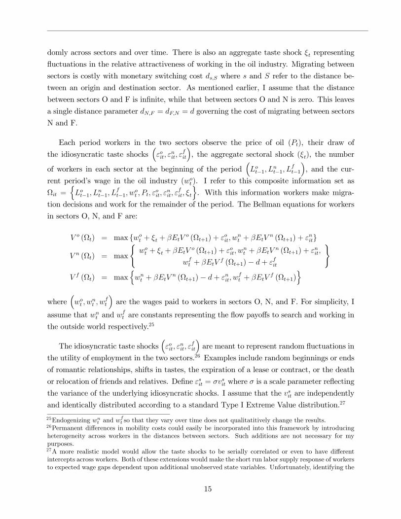
Workers can reside in one of three sectors: the oil industry (O), a nearby sector (N),

or the "far away" outside world (F). Let the symbols Lot ; Lnt ; and L

ft represent the number

of workers in a given period employed in the oil industry, the nearby sector, and the far

away sector respectively. One can think of the nearby sector as a reduced form for search

behavior. It is the number of workers capable of entering the oil industry in the next period

with minimal cost. Most such workers are likely unemployed, though there are also probably

some workers who currently have jobs capable of entering the oil industry on short notice.

The number of workers in the nearby sector will adjust based upon how attractive sector O is

at any given time relative to the rest of the economy. Workers in the rest of the economy face

costs that make it infeasible to enter the oil industry immediately. Thus, I require workers

in sector F to enter sector N before being able to enter sector O. For simplicity I also require

workers in sector O to enter sector N before entering sector F, though the model changes

little when this assumption is relaxed. Figure 4 illustrates the relationship between the three

sectors and the aggregate worker �ows between them.

Switching from sector F to sector N (and vice versa) is costly, which makes the migration

decision an investment problem as in classic human capital models of migration (Sjaastad,

1962). Workers in sector F will consider not just the �ow payo¤ to entering sector N but the

continuation value of residence in sector N, a quantity which will be heavily in�uenced by

the option value of moving to sector O. Mobility between sectors O and N has no pecuniary

cost, but entails an opportunity cost since a worker moving from sector N to O forfeits the

option to work in sector F.24 Thus a worker in sector N has reason to consider the future

payo¤s associated with residence in sector O when considering a switch into the oil industry.

Each period�s payo¤s are determined in equilibrium as wages adjust to equate the factor

demands of forward looking �rms with the supply decisions of workers.

6.1 Labor Supply

The labor supply decisions of agents are modeled as a dynamic discrete choice problem.

Workers have utility that is linear in wages and a random taste shock "st which varies ran-

23Other multi-sector labor market models in this tradition include Rogerson (1987), Chan (1996), and Phelanand Trejos (2000).24Such an opportunity cost would still be present if workers could move from sector O to F, if the trip fromO to F is more costly than a trip from N to F.

14

domly across sectors and over time. There is also an aggregate taste shock �t representing

�uctuations in the relative attractiveness of working in the oil industry. Migrating between

sectors is costly with monetary switching cost ds;S where s and S refer to the distance be-

tween an origin and destination sector. As mentioned earlier, I assume that the distance

between sectors O and F is in�nite, while that between sectors O and N is zero. This leaves

a single distance parameter dN;F = dF;N = d governing the cost of migrating between sectors

N and F.

Each period workers in the two sectors observe the price of oil (Pt), their draw of

the idiosyncratic taste shocks�"oit; "

nit; "

fit

�, the aggregate sectoral shock (�t), the number

of workers in each sector at the beginning of the period�Lot�1; L

nt�1; L

ft�1

�, and the cur-

rent period�s wage in the oil industry (wot ). I refer to this composite information set as

it =nLot�1; L

nt�1; L

ft�1; w

ot ; Pt; "

oit; "

nit; "

fit; �t

o. With this information workers make migra-

tion decisions and work for the remainder of the period. The Bellman equations for workers

in sectors O, N, and F are:

V o (t) = max fwot + �t + �EtV o (t+1) + "oit; wnt + �EtV n (t+1) + "nitg

V n (t) = max

(wot + �t + �EtV

o (t+1) + "oit; w

nt + �EtV

n (t+1) + "nit;

wft + �EtVf (t+1)� d+ "fit

)V f (t) = max

nwnt + �EtV

n (t+1)� d+ "nit; wft + �EtV

f (t+1)o

where�wot ; w

nt ; w

ft

�are the wages paid to workers in sectors O, N, and F. For simplicity, I

assume that wnt and wft are constants representing the �ow payo¤s to search and working in

the outside world respectively.25

The idiosyncratic taste shocks�"oit; "

nit; "

fit

�are meant to represent random �uctuations in

the utility of employment in the two sectors.26 Examples include random beginnings or ends

of romantic relationships, shifts in tastes, the expiration of a lease or contract, or the death

or relocation of friends and relatives. De�ne "sit = �vsit where � is a scale parameter re�ecting

the variance of the underlying idiosyncratic shocks. I assume that the vsit are independently

and identically distributed according to a standard Type I Extreme Value distribution.27

25Endogenizing wnt and wft so that they vary over time does not qualitatitively change the results.

26Permanent di¤erences in mobility costs could easily be incorporated into this framework by introducingheterogeneity across workers in the distances between sectors. Such additions are not necessary for mypurposes.27A more realistic model would allow the taste shocks to be serially correlated or even to have di¤erentintercepts across workers. Both of these extensions would make the short run labor supply response of workersto expected wage gaps dependent upon additional unobserved state variables. Unfortunately, identifying the

15

The assumptions made so far are su¢ cient to derive labor supply functions with very

convenient analytical properties. Consider a worker starting the period in sector N. Such a

worker will choose to move from sector N to sector O if and only if the following conditions

hold:

wot + �t + �EtVo (t+1) + "

oit > wn + �EtV

n (t+1) + "nit

wot + �t + �EtVo (t+1) + "

oit > wf + �EtV

F (t+1)� d+ "nit

or equivalently when:

voit � vnit > � (wot + �t � wn + �Et [V o (t+1)� V n (t+1)]) =�voit � v

fit > �

�wot + �t �

�wf � d

�+ �Et

�V o (t+1)� V f (t+1)

��=�

De�ne a selection variable Ds;St = 1 if a worker moves from sector s to sector S in period

t. Then, given our distributional assumptions on vit, it follows from standard results (e.g.

McFadden, 1974) that the probability of switching from sector N to sector O can be written

in logit form as:

pn;ot � P (Dn;ot = 1)

=

"1 + exp (� (wot + �t � wn + �Et [V o (t+1)� V n (t+1)]) =�)

+ exp���wot + �t �

�wf � d

�+ �Et

�V o (t+1)� V f (t+1)

��=�� #�1 (3)

while the probabilities of switching between the other feasible sector pairs may be written:

pn;ft � P (Dn;ft = 1)

=

"1 + exp

���wf � wn + �Et

�V f (t+1)� V n (t+1)

��=��

+exp���wf � wot � �t + �Et

�V f (t+1)� V o (t+1)

�� d�=�� #�1

pf;nt � P (Df;nt = 1)

=�1 + exp

���wn � wf + �Et

�V n (t+1)� V f (t+1)

��=����1

po;nt � P (Do;nt = 1)

= [1 + exp (� (wn � wot � �t + �Et [V n (t+1)� V o (t+1)]) =�)]�1

parameters governing these additional forms of state dependence is infeasible without longitudinal microdata.

16

The parameter � governs the responsiveness of migration behavior to di¤erences in sectoral

payo¤s. When � is small, minute di¤erences in the attractiveness of sectors can yield large

migration responses. When � is very large, the probability of migrating to a sector becomes

nearly independent of the sectoral payo¤s.

Note that the migration probabilities depend upon the equilibrium distribution of sector

continuation values V o (t+1) ; V n (t+1) ; and V f (t+1). Making use of the properties of

Extreme Value distributions documented in McFadden (1978) and Rust (1987) we can sim-

plify the expressions for the expectations of these values by integrating out the idiosyncratic

taste shocks as follows:

EtVn (t+1) = Etmax

8><>:wot+1 + �t+1 + �Et+1V

o (t+2) + "oit+1;

wn + �Et+1Vn (t+2) + "

nit+1;

wf � d+ �Et+1V f (t+2) + "fit+1

9>=>;= �Etmax

8><>:�wot+1 + �t+1 + �Et+1V

o (t+2)�=� + voit+1;

(wn + �Et+1Vn (t+2)) =� + v

nit+1;�

wf + �Et+1Vf (t+2)� d

�=� + vfit+1

9>=>;= �Et

264Evit+1 max8><>:�wot+1 + �t+1 + �Et+1V

o (t+2)�=� + voit+1;

(wn + �Et+1Vn (t+2)) =� + v

nit+1;�

wf + �Et+1Vf (t+2)� d

�=� + vfit+1

9>=>;375

= �Et

264 + ln0B@ exp

��wot+1 + �t+1 + �Et+1V

o (t+2)�=��

+exp ((wn + �Et+1Vn (t+2)) =�)

+ exp��wf + �Et+1V

f (t+2)� d�=��1CA375 (4)

where � :5772 is Euler�s constant (the mean of the extreme value distribution) and Evt+1denotes the expectation with respect to the fundamental taste shocks

�voit+1; v

nit+1; v

fit+1

�next period. Equivalent arguments yield:

EtVo (t+1) = �Et

" + ln

exp

��wot+1 + �t+1 + �Et+1V

o (t+2)�=��

+exp ((wn � d+ �Et+1V n (t+2)) =�)

!#

EtVf (t+1) = �Et

" + ln

exp

��wf + �Et+1V

f (t+2)�=��

+exp ((wn � d+ �Et+1V n (t+2)) =�)

!#

Thus, the addition of taste shocks to the worker�s problem yields expected continuation

values that are recursive and di¤erentiable in their future expected values, a feature which

facilitates computation of smooth approximations to the worker�s decision rules. Moreover,

these analytical expressions are convenient for developing insight into the sectoral labor

17

supply decision.

Note that if mobility were possible between all sectors at zero cost, the expected contin-

uation values would all be equal and switching decisions would depend only upon current

returns. In the current setup, with mobility costs between sectors N and F and no mobility

between O and F, the expected continuation values will in general di¤er from one another,

making future payo¤s important for current migration decisions. The fact that mobility is

restricted between sectors O and F provides sector N with an advantage as a gateway sector,

which is re�ected in the fact that the expression for EtV n (t+1) has three terms instead

of two. Another way of seeing the option value associated with residence in sector N is to

rearrange the expression for the continuation value as follows:

EtVn (t+1) = � + w

n + �EtVn (t+2)� �Et ln

�1� pn;ot+1 � p

n;ft+1

�Interpretation of this equation is straightforward. The expected value of residence in

sector N next period is the expected return to remaining in the sector next period plus the ex-

pected option value associated with switching sectors next period: ��Et ln�1� pn;ot+1 � p

n;ft+1

�.

A �rst order logarithmic expansion of this last term is illustrative:

�Et ln�1� pn;ot+1 � p

n;ft+1

�� Et

"epn;ot+1 pn;ot+1

1� pn;ot+1 � pn;ft+1

+ epn;ft+1 pn;ft+1

1� pn;ot+1 � pn;ft+1

#

= Et

"epn;ot+1 exp

wot+1 + �t+1 � wn

+�Et+1 [Vo (t+2)� V n (t+2)]

!=�

!#

+E

"epn;ft+1 exp

wf � wn � d+�Et+1

�V f (t+2)� V n (t+2)

� ! =�!#

where ep = dpp. So a proportional increase in the probability of switching from sector N

to another sector yields an increase in option value roughly equal to the exponentiated

di¤erence in expected payo¤s between sectors. Analogous expressions hold for the other

sectors�continuation values which each have only a single migration probability. Thus, a

worker in sector F may be enticed to enter sector N this period because �ows from sector

N to sector O are expected to increase next period. This creates the potential for rich

intertemporal responses to sectorally biased demand shocks.

The migration probabilities in (3) map into aggregate migration �ows by means of the

following identity:

ms;St = ps;St L

st�1 (5)

18

The laws of motion characterizing the evolution of sector sizes are:

Lot = Lot�1 +mn;o �mo;n (6)

Lnt = Lnt�1 +mo;n �mn;o +mf;n �mn;f

Lft = T � Lot � Lnt

where T is the total size of the economy. To ensure that the long run wage e¤ects of an oil

price increase are minimal T must be chosen to be a large number, guaranteeing that ample

outside workers are available to arbitrage any persistent wage premia.

6.2 Labor Demand

We turn now to specifying the demand side of the model. Firms are assumed to be price

takers on the input market. Because in such an environment wages are determined only by

industry-wide demand, I will not attempt to model the microeconomic details of oil pro-

duction nor the attendant heterogeneity across �rms in productivity, resources, or stocks of

labor and capital. The key idea for the current discussion is that sectoral labor demand

should respond sluggishly to shocks. This could be accomplished by means of interindustry

linkages between the oil extraction and OGFS industries, capital adjustment costs, employ-

ment adjustment costs, gross hiring costs, risk aversion, learning, or any other number of

familiar stories.

I focus on two mechanisms: sluggishness in the demand for OGFS output and employment

adjustment costs.28 The �rst mechanism is meant to capture the fact that the OGFS industry

does not actually produce oil, but rather oil and gas �eld services. Thus, the demand for

OGFS output is likely to lag behind oil price innovations if oil extraction �rms, who hire

OGFS �rms, have rigidities of their own. The second mechanism, employment adjustment

costs, captures rigidities within OGFS �rms and provides a reason for them to be forward

looking with respect to their employment adjustment decisions.

I use a standard representative �rm framework to capture the behavior of industry-wide

movements in the demand for oil production workers.29 The �rm produces output using a

28In a previous version of this paper, I included capital in the production function and found qualitativelysimilar results. Without time series data on capital adjustment, such additions add little to the empiricalwork.29While it is by now well recognized that the microeconomic details of the adjustment costs faced by �rms canin�uence the aggregate dynamics of factor demand (Caballero et al. 1993, 1997) , the gains from modelingsuch processes are likely to be small in this situation.

19

production technology with quadratic labor adjustment costs.30 The pro�t function is given

by

�(t) = bPtAtF (Lot )� wotLot � �2 �Lot � Lot�1�2 + �Et�(t+1)where bPt is the price of the �rm�s output, � is the �rm�s discount rate, � is a parametergoverning the cost of adjusting the size of the �rm�s workforce, and At is the productivity

level of the industry which is allowed to vary across time.

To capture sluggishness in the demand for OGFS output I assume it takes a period for

the price of OGFS output to respond to the price of oil after which time the relationship

between the two prices follows a simple �rst order autoregressive relationship given by the

following equation:

ln bPt = � ln bPt�1 + (1� �) lnPt�1 (7)

where Pt is the price of oil. The parameter � determines how quickly OGFS demand responds

to oil price innovation. When � = 0 adjustment is instantaneous after a one period lag, while

when its value is near one adjustment is very slow.31

The �rst order condition for employment is

wt = bPtAtF 0 (Lot )� � �Lot � Lot�1�+ ��Et �Lot+1 � Lot �A useful alternative representation of this labor demand curve is the following

Lot � Lot�1 =1

��t (8)

�t = bPtAtF 0 (Lot )� wot + �Et [�t+1]In words, the desired change in employment is proportional to the discounted stream of gross

marginal pro�ts (�t) expected to be earned by permanently increasing the size of the �rm�s

workforce.32 Without adjustment costs employment would be set so that �t always equals

zero. With adjustment costs �t only equals zero in steady state.

Note that the absence of adjustment costs would also make �rms unresponsive to expected

changes in bPt (and wt). With adjustment costs, if demand for output is expected to increase,30Classic examples of the use of quadratic labor adjustment costs under rational expectations include Sargent(1978) and Shapiro (1986).31The above speci�cation constrains the long run OGFS - oil price elasticity to equal one. This is done merelyfor convenience since identifying the long run elasticity would require direct measures of OGFS output.32This representation of dynamic labor demand is similar to the q-theory representation of investment asexpounded in, for example, Hayashi (1982).

20

the �rm will hire workers now in order to avoid incurring large adjustment costs when

demand actually does increase. Larger values of � will magnify the size of this response.

Thus � > 0 implies that oil price innovations will lead to instantaneous increases in labor

demand even though the innovations are assumed to take a period to begin propagating into

OGFS demand.

A parametric form for the production function remains to be chosen. The distributed

lags in Figure 3 indicate a long run employment price elasticity of around .75. A suitable

production function would be capable of accommodating this behavior. Steady state wages

are:

wo = bPAF 0 (Lo)Totally di¤erentiating the above and imposing long run wage equalization yields a long

run employment price elasticity of

�l;p = �F 0 (Lo)

F 00 (Lo)Lo

which for the case of a Cobb-Douglas production function of the form F (L) = L� can be

shown to equal 11�� . Because this elasticity is bounded below by one for a > 0; it will not

do for this analysis. Instead, I use the following "isoelastic" generalization of a single input

Cobb-Douglas function capable of exhibiting su¢ cient concavity to yield long run elasticities

below one:

F (L) = C � L��

�(9)

where C is a positive constant and � is allowed to vary over the entire real line.33 It is

straightforward to show that this function exhibits a long run elasticity of 11+�

which will lie

below unity for � > 0 and exceed it for � < 0. The parameter C, which is necessary only to

ensure that output is positive at all employment levels, falls out of the �rst order conditions

for employment since the marginal product of labor is simply F 0 (L) = L�(1+a).

6.3 Equilibrium

Having laid out the equations governing labor supply and demand we now attempt to describe

the resulting equilibrium behavior of the system. The migration probabilities expressed in

(3) make clear that the �ows between sectors are a function of both current and future wage

premia. The upper panel of Figure 5 illustrates gross �ows into (mno) and out of (mon) the

33By L�Hopital�s rule, as � approaches zero, L��

� approaches -ln (L). Values of � above zero are more concavethan a simple logarithm, while values below zero are less concave.

21

oil industry as a function of the current oil wage conditional on beliefs about the future path

of wages. Each �ow curve has a logistic shape re�ecting the functional form of the choice

probabilities. The particular shape and position of each curve depends upon the number

of workers in the originating sector and the scale � of the taste shocks. Flow curves from

large sectors will have shapes that appear to be stretched horizontally, since small changes

in probability will yield large changes in �ows. In steady state, the two curves will cross at

the steady state wage wo, at which point net �ows will be zero. In Figure 5, wo is greater

than wn, the wage in the nearby sector, which can occur when sector O is larger than sector

N.

In the wake of an oil price increase EtV o (t+1) will rise relative to EtV n (t+1) on

expectations of future changes in the oil wage. This will lead the in�ows curve to shift to

the right and the out�ows curve to shift to the left, thereby motivating large net �ows into

the oil sector equal to the horizontal distance between the two curves at the going wage.

This increase in the size of sector O has important feedback e¤ects on the system. First,

net in-migration will put downward pressure on wages as the marginal product of labor is

gradually reduced. Second, as sector O expands, the base population at risk of emigrating

from sector O increases, shifting the out-migration curve to the right. Finally, the realized

wage increases eventually cause sector N to grow thereby o¤setting the e¤ects on the in-

migration curve of the decreases in wages. The new steady state equilibrium illustrated

in the bottom panel of Figure 5 has larger gross �ows in both directions, larger sectoral

workforces, and wages equal to their original steady state level.

It is convenient to illustrate the dynamics of the equilibrium in terms of the behavior of

net �ows �Lot to the oil industry since we may also graphically represent demand in such

a space by means of equation (8). A key feature of this model is that the gross migration

curves and consequently Lot depend upon expectations of future changes in demand. If labor

demand were expected to increase in the future but for some reason had not yet shifted, we

would actually expect to see wages decrease in response to a price shock.34 Even if demand

did shift contemporaneously, if the future changes in demand were expected to result in

substantial wage premia, the supply curve might shift enough for wages to fall on impact.

Figure 6 illustrates such a case graphically. Here we graph the supply and demand for

net migration to the oil industry in wage quantity space. We start at the steady state where

wages are such that�Lot = 0meaning that gross out-migration equals gross in-migration. Oil

34Topel (1986) �nds an analogous result in his analysis of the migratory response to predictable changes inlocal labor market conditions.

22

prices increase raising the expected continuation value of being in sector O and causing both

the supply and demand curves to shift out to S�and D�. This leads wages to fall very slightly

but results in large �ows into the sector. As the sector grows, the demand for additional

hires falls and the demand curve shifts to the left. However, the supply curve of net migrants

also shifts to the left. This happens for two reasons. One is that the number of workers in

nearby sector N is drawn down causing the in-migration curvemn;o to shift leftward. Second,

as sector O grows, out-migration becomes more common since more workers are at risk of

emigrating. This serves to diminish net �ows into the sector and consequently for demand

to outstrip supply and for wages to rise. Labor demand continues to ratchet to the left as �tis driven down by increases in Lot and the demand curve approaches its steady state. Labor

supply also continues to shift to the left as the temporary wage changes are realized leading

the expected continuation value of residence in sector O to fall. These shifts lead wages

to settle down to an equilibrium near their old level. The next section asks what sort of

parameter values are necessary to rationalize this behavior.

7 Estimation

After specifying a stochastic process for the model�s exogenous variables (Pt; At; and �t), the

equations in (3), (4), (5), (6), (7), and (8) collectively characterize the dynamic stochastic

process generating the labor market variables. To solve the system I use Dynare++ 1.3.7,

which is a C++ routine for numerically simulating Dynamic Stochastic General Equilibrium

(DSGE) models via perturbation methods.35 Policy functions are obtained by calculating

Taylor series approximations to the decision rules implied by the model equations. Because

these approximations are made around a deterministic steady state I specify log oil prices

to be a near unit root so that a proper steady state can be said to exist.36 The speci�cation

used is

ln (Pt) = :001�+ :999 ln (Pt�1) + ut (10)

where � = 3:91 is the log de�ated value of the crude oil PPI in the �rst quarter of 1972. The

simulations assume that � is a normally distributed i.i.d. shock with variance equal to 0.02,

the empirical variance of the log oil price changes.

The taste shock �t and the logarithm of the productivity shock At are each assumed to

35For details see Juillard (1996) and Collard and Juillard (2001a, 2001b).36In fact, it is hard to believe that oil prices, even in logarithms, follow a pure random walk. It is wellacknowledged that the best forecast for oil prices over the very long run is somewhere near the historicalmean of approximately 20 dollars a barrel.

23

follow �rst order autoregressive processes:

ln (At) = (1� �A) ln (A) + �A ln (At�1) + �t

�t = �� ln��t�1

�+ �t

where it is assumed that (�t; �t) � N (0;�) with � ="�2� ���

��� �2�

#. The potential for con-

temporaneous correlation between taste and productivity shocks highlights the importance

of having a powerful exogenous demand shifter like oil prices for identifying the model�s

parameters.

There are sixteen parameters in the system: �; wn; wf ; �; �; d; A; �; �; �; T; �A; ��; �2� ; �

2� ; ��� .

To reduce the number of free parameters, I start by assuming that �rms and workers share

common discount rates � = � = :95 and that the number of workers in the economy (T )

equals ten million (about 100 times the size of the OGFS industry). I also impose three

restrictions which allow me to calibrate the parameters A;wn; and wf . First, I impose that

steady state wages in the oil industry wo equal their 1972 value of $8.86/hr. Second, I

choose steady state employment in the oil industry to equal 99.6 thousand, its value in the

�rst quarter of 1972, which is roughly the modal size of the oil workforce experienced over

the sample period. Finally, in keeping with the turnover data in Table 2, I also impose that

the steady state probability of migrating from O to N is .25. I use a numerical solver to

recover the values of A;wn; and wf implied by these restrictions conditional on the rest of

the parameter vector.

This leaves �ve "deep" structural parameters (�; �; �; d; �) for estimation along with the

�ve stochastic parameters��A; ��; �

2� ; �

2� ; ���

�. To understand the estimation strategy note

�rst from equation (3) that pn;o is monotonically increasing in �t which suggests that supply

shocks to the oil industry increase employment at �xed wages, which, by virtue of the struc-

ture of demand, will lead to reductions in wages for �xed productivity level At. Conversely,

from equation (8) we see that productivity shocks (innovations to At) monotonically raise

wages and employment for �xed values of �t.

The �rst step of the estimation strategy then, is to recover the vector of structural shocks

(�t; �t) implied by the time series of oil sector wages and employment. This is done by solving

the model numerically conditional upon a hypothesized parameter vector � which yields a

function F (st; !t; �) mapping the state vector st =hLot�1; L

nt�1; L

ft�1; Pt�1; bPt�1; At�1; �t�1i

and the structural shocks !t = [ut; �t; �t] into the next period�s state st+1 and control vector

24

ct = [wot ;mt;pt;Vt] where mt is the vector of gross migration �ows, pt the corresponding

vector of migration probabilities, and Vt the vector of sector values.37 I assume the market

is in its (deterministic) steady state in the �rst quarter of 197238 and then solve numerically

for the values of �t and �t implied by each subsequent change in oil prices and (detrended)

employment and wages.39 See the Appendix for details.

I then use these shocks, in conjunction with oil price changes (ut) to form a set of moment

conditions for use in estimating the model. The moment conditions, which are listed in the

Appendix, are of three varieties. The �rst set of conditions impose that the productivity and

taste shocks are orthogonal to contemporaneous oil price innovations and two lags of those

innovations. The second set of conditions impose that the shocks are serially uncorrelated

up to second order. And the �nal set of conditions de�ne method of moments estimators of

the variance and contemporaneous correlation of the shocks. In total this yields seventeen

moment conditions with which to estimate the ten parameters, providing a reasonable degree

of overidenti�cation.

To perform the actual estimation, I choose parameters b� to minimize the quadratic formQCUGMM (�) = g (�)

0W (�) g (�)

where g (�) = 1T

Xt

gt (�) is a 17x1 vector of moments and W =

1

T�1

Xt

gt (�) gt (�)0

!�1is a 17x17 matrix which weights each moment by an estimate of the inverse of its variance.

This is the "continuously updated" GMM estimator of Hansen, Heaton and Yaron (1996)

which has been shown theoretically to possess a variety of desirable properties including

higher order improvements in asymptotic bias (Newey and Smith, 2004).

Although the model implies that the vector gt (�) should be serially uncorrelated, I use a

heteroscedasticity and autocorrelation consistent (HAC) estimate bV of the long run varianceof gt (�) when making inferences. This is analogous to performing robust inference in a

quasi-maximum likelihood setting.40 Chi-squared goodness of �t tests are calculated by

37I use a third order polynomial approximation to the policy function.38Recall that prior to 1972 oil prices were regulated by the TRC which substantially muted volatility in thismarket.39I project employment and relative wages o¤ of a linear trend prior to solving for the shocks. Ideally, onewould allow the structural shocks themselves to contain a trend. Unfortunately, the nonlinear nature of themodel substantially complicates the process of theoretically detrending the model. One cannot use simplenormalizations of the sort found in traditional growth models to obtain a stationary representation of thedetrended system capable of being solved numerically.40I eschew using the HAC covariance estimator to weight the moments in the estimation process because of

25

computing QCUGMM

�b�� using W = bV �1. The Appendix provides further details on theestimation methods and construction of the standard errors.

7.1 Parameter Estimates

The estimated structural parameter values and standard errors for the model are given in

Table 3a. All of the parameters are estimated quite precisely. The second row of the Table

also shows results from a myopic version of the model where agents are assumed to be

substantially less forward looking than �rms, having quarterly discount rates (�) of only

0.75 (or equivalently annual discount rates of 0.32). In both speci�cations, the chi-squared

goodness-of-�t tests which have �ve degrees of freedom, easily reject the null hypothesis

that the deviations of the sample moments from zero are due to chance. The smaller chi-

squared value for the myopic speci�cation is more an artifact of the greater imprecision of

that speci�cation than a sign of improved �t. The �t of the two models will be discussed

further in the next section.

Turning now to the parameters, the fundamental metric of costs in this setup is quarterly

dollars per hour. For example, in the baseline estimates with � = :95 moving from sector

F to N yields an estimated mobility cost d equal to approximately $6.95/hr. in wages paid

over the duration of a quarter or, roughly, ten weeks worth of steady state earnings in the

oil sector.41 The standard deviation of the taste shocks can be shown to be �p6� and is

also measured in quarterly dollars per hour. The baseline estimate of � = 1:24 implies that

the standard deviation of the transitory taste shocks is equivalent to $1.59/hr. in quarterly

wages or about two weeks worth of steady state earnings.

The adjustment cost parameter � measures the marginal cost to the �rm in quarterly

dollars per hour of expanding the workforce by 1,000 laborers. The baseline estimated value

of � = 0:36 implies that the 1,000th worker hired costs the �rm $0.36/hr. for a quarter, equal

to around half a week worth of that worker�s earnings in steady state. If the average worker

works forty �ve hours a week and thirteen weeks a quarter this means the total dollar value

of the adjustment cost is 45�13� :36 = $210:60. The average per capita cost of hiring 1,000workers is half this amount. These numbers are relatively small and indicate that sluggish

output prices are doing most of the work of matching the slow rampup of employment.

concerns that it is substantially less precise than the simple variance estimator W . One could impose evenmore structure on the weighting matrix by imposing the restrictions implied by joint normality of the errorsand using the estimated elements of the covariance matrix

X. My approach is intermediate between these

two extremes, allowing for heteroscedasticity, but not autocorrelation.41Steady state wages are $8.86/hr. Assume 13 weeks in a quarter. 6:95=8:86� 13 � 10.

26

The baseline estimated value of � is 0:5 which indicates moderate sluggishness in OGFS

demand. The emphasis on sluggish output demand derives from the fact that employment

adjustment costs yield current responses to future expected demand shifts. Given � > 0, too

large of an adjustment cost would yield enough of a contemporaneous shift in labor demand

to raise wages immediately. Small adjustment costs yield enough anticipatory hiring to

match the early employment responses, but not so much as to cause a jump in the wage or

to substantially slow down later hiring.

The parameter � is a measure of the concavity of the representative �rm�s production

function. Recall from earlier that the long run employment price elasticity of this production

technology is �l;p = 11+�. Because the empirical value of �l;p � :75 one would expect that

any attempt to match the long run behavior of the distributed lags would require � � 1=3.The baseline estimated value of � is slightly below this value at .22 which implies a long

run elasticity �l;p of approximately :82. A logarithmic speci�cation with unitary output

elasticities cannot be rejected for either speci�cation of the model.

The myopic model yields parameter values broadly similar to those found in the baseline

speci�cation except that the estimated switching costs and the standard deviation of the taste

shocks are both substantially smaller. This re�ects the fact that if workers are less forward

looking, they e¤ectively have fewer periods over which to accrue the gains of switching

sectors, thereby lowering the requisite switching cost necessary to rationalize their behavior.

They likewise need to be more sensitive to nominal di¤erences in expected payo¤s across

sectors since the scale of the continuation values has been reduced. It is worth pointing out

that even the myopic estimates yield plausible switching costs equal to around six weeks of

steady state earnings. Thus, although the model is predicated upon forward looking behavior

on the part of agents, the conclusion that reasonable parameters can rationalize the observed

data is not contingent upon oil roustabouts being terribly prescient.

Table 3b describes the stochastic properties of the structural shocks. Both shocks are

estimated to be moderately persistent with autoregressive coe¢ cients ranging from 0.52 to

0.82. Both speci�cations also �nd substantial positive correlation between productivity and

taste shocks, suggesting that the observational covariances between employment changes and

wages re�ect innovations to both supply and demand conditions.

Figure 7 plots the two sets of shocks for the baseline and myopic models. Despite a few

outliers in the immediate aftermath of the collapse of OPEC, the baseline estimated shocks

are very well behaved, centered around zero, and roughly serially uncorrelated suggesting

27

that the model is reasonably well speci�ed.42 The myopic model has two very large taste

shocks around the time of the second OPEC shock. These outliers substantially increase

the HAC estimate of the variance of the model�s parameters and are the reason for that

speci�cation�s relatively low chi-squared statistic.43

7.2 Impulse Responses

At least as interesting as the estimated parameters are the impulse responses they imply.

Figure 8 plots the simulated responses of oil sector wages and employment to a permanent

price shock at the estimated parameter values against the reduced form estimates of the

response. The log price innovation is one standard deviation in magnitude and the impulse

responses are in logarithmic deviations from steady state scaled by the size of the shock so

they may be read as elasticities.

The simulated responses match the behavior of the distributed lag coe¢ cients reasonably

well. Wages exhibit little response to oil price innovations on impact but then steadily begin

to rise, peaking roughly a year after the shock and then slowly declining. Employment jumps

on impact and proceeds to ramp up rapidly towards its new steady state level. Although

simulated wages peak slightly earlier than in the estimated distributed lags, the largest

systematic discrepancy comes from the failure of simulated employment to adjust to steady

state as quickly as in the distributed lags. This occurs not because adjustment costs are

prohibitively high or OGFS demand too sluggish, but rather because the eventual decreases

in the wage lead to increases in the quantity of labor demanded by �rms making it di¢ cult

for employment to level out after two years. The autoregressive structure of OGFS prices

and the quadratic speci�cation of the adjustment costs both imply geometric adjustment

which require adjustment to be slow early if it is to be slow later on. More �exible functional

form assumptions on the adjustment costs or the relationship between bP and P would likelydo a better job matching the early employment coe¢ cients and perhaps improve the �t to

wages as well.

Because the model is nonlinear, the impulse responses depend upon the state of the labor

market. If the labor market is tight, as it will be after a long period of expansion, spot wages

will be more sensitive to shocks. If, on the other hand, the market is slack, as it will be after

several consecutive oil price declines, the e¤ect of a positive demand shock on oil wages will

42A Box-Ljung test rejects the null hypothesis that the shocks are martingale di¤erences after four lags inboth models. However, the estimated autocovariances tend to be very small and follow no consistent pattern.43Dummying out or downweighting those taste shocks substantially improves the estimated precision of theparameters in the Myopic speci�cation.

28

be attenuated. Figure 9 illustrates these phenomena by plotting impulse responses under two

di¤erent scenarios. The �rst is the e¤ect of an oil price increase after three prior consecutive

oil price increases (of one standard deviation each) starting from steady state. The second is

the e¤ect of an increase after three prior consecutive oil price decreases starting from steady

state.

The heterogeneity in responses is rather stark. In the baseline model, an oil price increase

in a tight labor market yields an immediate spike in wages that eventually dissipates, while

an equivalent increase in a slack market yields a small wage decline followed by gradual

and muted increases. In the myopic model, wages exhibit a hump shaped response under

both scenarios, but the magnitude of the response is much larger when the labor market has

already grown tight.

As already discussed, net changes in sectoral employment are the sum of the gross mi-

gration �ows between sectors. The upper panel of Figure 10 illustrates the response of gross

�ows between sectors O, N, and F to an oil shock. Flows from sector F to N jump on impact,

intensify for two periods, and then smoothly ratchet down, while �ows from sector N to F do

the opposite. Flows from sector N to O exhibit more erratic behavior, jumping on impact,

intensifying next quarter when OGFS demand begins to shift out, and then falling as the

number of workers in the nearby sector begins to be depleted. Eventually enough workers

from the outside world come in to replenish the size of sector N and �ows to sector O reach

a new higher steady state. Flows from sector O to sector N fall on news of the price shock

and continue to fall as the large wage increases grow nearer. As the wage premia dissipate

and the value of residence in sectors O and N converges back towards parity out�ows reach

their new higher steady state attributable to the new larger size of sector O.

The bottom panel of Figure 10 shows the simulated response of the log value of residence

in sectors O, N, and F to an oil price shock. The values of being in sectors O and N each

jump on news of the price shock. The value of sector O residence jumps by slightly more

than sector N because of the opportunity cost associated with switching from sector N to O,

while the value of being in sector F is virtually una¤ected because of its large size. In the

periods after the shock hits the value premia associated with sectors O and N each intensify

as the largest wage premia draw closer. The sector values eventually begin to dissipate as

wages, of which they are a forward moving average, begin to mean revert.

The sector values are measured in quarterly dollars per hour scaled by the size of the

shock. The instantaneous impacts imply that sector values rise by about a week�s worth of

steady state earnings in response to a one standard deviation increase in oil prices. Assuming

29

the average worker works 45 hours a week this translates into an approximate $400 increase

in the expected value of residence in the oil sector in response to a typical oil price increase.

Expected returns of this magnitude seem large enough to plausibly motivate substantial �ows

of potential workers to search for oil jobs even if oil wages have not yet risen dramatically.

7.3 Auxiliary Evidence

We have seen that a forward looking model of sectoral migrations with slow moving demand

can recreate the qualitative features of wages and employment we initially set out to explain.

We ask now whether any auxiliary evidence can be brought to bear on the mechanisms

generating the employment and wage dynamics in the model. Fluctuations in the wage

are ultimately driven by the dynamic scarcity of labor. Wages rise because at some point

insu¢ ciently many cheap workers are available. This mechanism was particularly evident

in Figure 9, which demonstrated that the wage and employment dynamics strongly depend

upon the preexisting state of the labor market. The structural model allows us to simulate

the dynamics of labor scarcity by examining the response of the size of sector N to shocks.

When Lnt is below steady state, the labor market will be tight and it will be hard to attract

large numbers of workers without wage premia.

A key question then is whether Lnt has any empirical analogue. The traditional measure

of market tightness is the unemployment rate. Since in this model sector N is meant to

represent some notion of the number of workers engaged in (directed) search, unemployment

may not be a bad proxy for Lnt . I use the basic monthly CPS �les to compute the number of

unemployed workers who list their previous industry of employment as "oil and gas extrac-

tion" in each month from 1976-2002. Using the middle month of each quarter I estimate a

distributed lag of the response of the log number of unemployed oil workers to innovations in

oil prices. These coe¢ cients are not directly comparable to the IRF of Lnt since, according

to the model, some of the workers in Lnt came not from the oil industry but from the outside

world. To deal with this, I introduce a new variable Ut =�1� pn;ot � pn;ft

�Ut�1+m

ont to the

model which measures the number of workers residing in sector N whose most recent sector

of employment was in sector O (as opposed to sector F).44

Figure 11 compares the distributed lag coe¢ cients to the simulated impulse response of

Ut generated by the model.45 Given that none of the parameters used in the simulations

were estimated taking these distributed lags into account, the similarity between these plots

44In practice the IRF of Ut is extremely similar to that of Lnt .45Because the distributed lags are quite noisy, 90% con�dence intervals are presented.

30

is remarkable. While the distributed lags are noisy, the point estimates track the simulated

path of Ut extremely closely, exhibiting a U-shaped response to the shock which bottoms

out approximately six quarters after the shock, which is also approximately the time that

wages peak. After reaching a shared nadir both the estimated and simulated IRFs exhibit

steady sustained increases in unemployment culminating in overshooting of approximately

40% relative to steady state.

Another key unobservable used by the model to rationalize the behavior of wage and

employment is sluggishness in the price of OGFS output� bPt�. The Bureau of Labor Sta-

tistics reports industry based Producer Price Indices (PPIs) for a variety of mining support

services back to 1985. I create a proxy for OGFS output prices by averaging the indices for

NAICS industries 213111 "drilling oil and gas wells" and 213112 "support activities for oil

and gas wells". After de�ating the composite index by the CPI, I compute distributed lag

estimates of the response of the log of the de�ated index to oil price changes.

Figure 12 compares the estimated distributed lags to the predictions from the model.

Recall that in the model the long run elasticity of OGFS prices with respect to oil prices

was normalized to one. Thus, a comparison of the distributed lags to the model requires a

rescaling factor, which I estimate by regressing the estimated distributed lag coe¢ cients on

the simulated impulse response coe¢ cients without a constant. These coe¢ cients were used

to rescale the simulations.46 The concordance between the simulated IRFs and the estimated

distributed lag is striking. It appears that the estimated value of � comes extremely close

to providing the best approximation to the distributed lag coe¢ cients possible with a single

autoregressive coe¢ cient. Again, this is quite surprising given that this data was not used

in the estimation.

Clearly neither of these out of sample tests con�rms the assumptions underlying the

model. The CPS measure of OGFS unemployment is coarse and noisy and many of the

workers considering entering the oil industry are probably employed in other sectors. Like-

wise, the constructed PPI is an imperfect measure of OGFS demand. What this exercise

reveals however is that the dynamic relationship between a broad measure of sectoral un-

employment, the OGFS PPIs, and oil prices follows just the pattern necessary to rationalize

the empirical response of oil industry wages and employment to price shocks through the

model. This is a provocative �nding and one that ought to warrant further investigation of

this class of dynamic equilibrium models.

46The rescaling factor is :330 for the baseline model and :336 for the myopic model.

31

8 Conclusion

This paper has investigated the dynamics of a single sectoral labor market. The empirical

�nding that, on average, wages lag employment in response to exogenous shocks to labor

demand is at odds with the predictions of conventional market clearing models. I have shown

that a forward looking model of sectoral reallocation with standard adjustment rigidities can

rationalize this behavior with sensible parameter values.

An obvious question is the extent to which such a model might generalize to other indus-

tries or environments. The recipe for equilibrium behavior of the sort under study is clear:

an industry should be subject to large and recurrent shocks to product demand, �rms in

the industry should face substantial adjustment rigidities, and there should exist a pool of

low cost workers capable of entering the industry in the short run. Whether large segments

of the U.S. economy meet these criteria is an open question. In manufacturing industries

other factors such as unionization are likely to complicate the wage setting process, while in

higher skilled industries such as engineering, lags in the training of workers are likely to add

additional dynamics to the labor supply decision.

Caveats aside, there is evidence of similar employment and wage dynamics in a few

important settings. The �rst is Carrington�s (1996) study of the building of the Alaskan

pipeline, which found a slow increase in the earnings of workers in construction and related

industries which eventually reverted to trend.47 Second, Blanchard and Katz (1992) �nd

hump shaped wage responses to seemingly permanent labor demand shocks in panels of U.S.

states. In both papers most of the employment adjustment seems to occur before wages

peak. Finally, in a closely related paper, Topel (1986) �nds evidence of state level wages

falling in response to predictable changes in local labor demand. The evidence in these

papers raises the possibility that labor market dynamics of the sort modeled here may be

found in settings more general than the oil industry.

A few additional points are worth taking away from this exercise. First, the labor market

under study is extremely �exible. Between 1978 and 1982 employment in oil and gas �eld

services doubled while over the next four years employment fell back to its 1978 level. These

adjustments highlight the ability of well functioning markets to e¤ectively match workers to

jobs. However, a well functioning matching process does not imply that reallocations are

costless. The behavior of wages over the course of these dramatic shifts in labor demand

suggests that sectoral �ows impose substantial costs on both workers and �rms. A researcher

47See �gs. 3,7, 8 and especially �g. 9 in that paper.

32

armed with detailed longitudinal microdata might take seriously the task of estimating the

social costs associated with such high frequency intersector reallocations.48

Second, despite the �exibility of the oil labor market, permanent demand shocks appear

to be associated with wage premia that persist for several years, even when the system is

begun in steady state. A series of persistent shocks such as those experienced by the oil

industry can keep wages out of steady state for decades at a time. To the extent that these

sorts of persistent expansions and contractions are present in other industries, an important

component of sectoral choice is likely to involve market conditions. More work is needed

linking standard models of sectoral choice with dynamic market models.49 Particularly

fertile ground for research may be found in developing countries heavily invested in exporting

commodities subject to large persistent price risks. Labor supply decisions in such countries

are likely to be fundamentally in�uenced by expectations and uncertainty regarding the

future path of commodity prices. Learning more about the dynamics of these decisions

and how they interact with individual heterogeneity may provide important insights for the

crafting of e¤ective industrial and labor market policies.

Finally, the model presented here is applicable to labor markets de�ned in spaces more

general than output sectors. A natural parallel is to local and regional labor markets. As

in Topel (1986), the analysis presented here has been one of spatial equilibrium. But unlike

with Topel�s model, the implication has been that the dynamic linkages between markets are

governed in part by the "distance" separating them. Thinking carefully about networks of

local labor markets that are (perhaps unequally) dynamically interrelated holds the promise

of revealing deeper insights into how labor markets adjust to shocks.

48Lee and Wolpin (2006) provide a detailed analysis of the social costs of the long run reallocation of laborbetween the service and manufacturing sectors.49The literature on sectoral and occupational choice is too large to document here. Starting with Roy�soriginal (1951) contribution there have been several notable attempts to estimate models of selection inthe labor market. Famous examples include Willis and Rosen (1979) and Heckman and Sedlacek (1985,1990). One of the great challenges in linking selection models with dynamic market models is disentanglingheterogeneity and dynamics. Recent advances in statistical modeling and data availability may soon yieldgreat progress in this area.

33

References1. Abraham, Katherine, James Spletzer, and Jay Stewart. 1998. �Divergent Trends

in Alternative Wage Series.�Labor Statistics Measurement Issues, eds. Haltiwanger,

Manser, and Topel. Chicago: University of Chicago Press.

2. Barsky, Robert and Lutz Kilian. 2002. �Do We Really Know That Oil Caused the

Great Stag�ation? A Monetary Alternative.�NBER Macroeconomics Annual 16:137-

183.

3. Barsky, Robert and Lutz Kilian. 2004. �Oil and the Macroeconomy Since the 1970s.�

Journal of Economic Perspectives 18(4):115-134.

4. Bartik, Timothy. 1991. Who Bene�ts From State and Local Economic Development

Policies? Kalamazoo, MI: W.E. Upjohn Institute for Employment Research.

5. Blanchard, Olivier and Lawrence Katz. 1992. �Regional Evolutions.�Brookings Papers

on Economic Activity 1992(1):1-75.

6. Bound, John and Harry Holzer. 2000. �Demand Shifts, Population Adjustments, and

Labor Market Outcomes during the 1980s.�Journal of Labor Economics 18(1):20-54.

7. Brainard, Lael S. and David M. Cutler. 1993. �Sectoral Shifts and Cyclical Unem-

ployment Reconsidered.�Quarterly Journal of Economics 108(1):219-243

8. Bresnahan, Timothy and Valerie A. Ramey. 1993. �Segment Shifts and Capacity

Utilization in the U.S. Automobile Industry.�American Economic Review Papers &

Proceedings 83(2):213-218.

9. Bureau of Labor Statistics. 2005. �Career Guide to Industries: Oil and Gas Extrac-

tion�obtained online at: http://www.bls.gov/oco/cg/cgs005.htm.

10. Caballero, Ricardo, Eduardo Engel, and John Haltiwanger. 1997. �Aggregate Em-

ployment Dynamics: Building from Microeconomics.� American Economic Review

87(1):115-137.

11. Caballero, Ricardo and Eduardo Engel. 1993. �Microeconomic Adjustment Hazards

and Aggregate Dynamics.�Quarterly Journal of Economics 108(2):359-383.

12. Carrington, William J. 1996. �The Alaskan Labor Market During the Pipeline Era.�

Journal of Political Economy 104(1):186-218.

34

13. Chan, William. 1996. �Intersectoral Mobility and Short Run Labor Market Adjust-

ments.�Journal of Labor Economics 14(3):454-471.

14. Collard, Fabrice and Michel Juillard. 2001a. "A Higher-Order Taylor Expansion Ap-

proach to Simulation of Stochastic Forward-Looking Models with an Application to a

Non-Linear Phillips Curve." Computational Economics 17(2):125-139.

15. Collard, Fabrice and Michel Juillard. 2001b. "Accuracy of Stochastic Perturbation

Methods: The Case of Asset Pricing Models." Journal of Economic Dynamics and

Control 25(7):979-999.

16. Davis, Steven J. 1987. �Fluctuations in the Pace of Labor Reallocation.�Carnegie-

Rochester Conference Series on Public Policy 27:335-402.

17. Davis, Steven and John Haltiwanger. 2001. �Sectoral Job Creation and Destruction

Responses to Oil Price Changes.�Journal of Monetary Economics 48(3):465-512.

18. Elliott, Graham, Thomas Rothenberg and James Stock. 1996. �E¢ cient Tests for an

Autoregressive Unit Root.�Econometrica 64(4):813-836.

19. Hamilton, James D. 1983. �Oil and the Macroeconomy Since World War II.�Journal

of Political Economy 91(2):228-248.

20. Hamilton, James D. 1985. �Historical Causes of Postwar Oil Shocks and Recessions.�

The Energy Journal 6(1):97-116.

21. Hamilton, James D. 1988. �A Neoclassical Model of Unemployment and the Business

Cycle.�Journal of Political Economy 96(3):593-617.

22. Hamilton, James D. 2003. �What is an Oil Shock?�Journal of Econometrics 113:363-

398.

23. Hayashi, Fumio. 1982. "Tobin�s Marginal q and Average q: A Neoclassical Interpre-

tation." Econometrica 50(1):214-224.

24. Heckman, James J. and Guilherme L. Sedlacek. 1985. �Heterogeneity, Aggregation,

and Market Wage Functions: An Empirical Model of Self-Selection in the Labor Mar-

ket.�Journal of Political Economy 93(6):1077-1125.

25. Heckman, James J. and Guilherme L. Sedlacek. 1990. �Self-Selection and the Distri-

bution of Hourly Wages.�Journal of Labor Economics 8(1):S329-S363.

35

26. Juillard, Michel. 1996. "DYNARE: A Program for the Resolution and Simulation of

Dynamic Models with Forward Variables through the Use of a Relaxation Algorithm."

CEPREMAP, Couverture Orange No. 9602.

27. Keane, Michael and Eswar Prasad. 1996. �The Employment and Wage E¤ects of Oil

Price Changes: A Sectoral Analysis.�Review of Economics and Statistics 78(3):389-

400.

28. Lee, Donghoon and Kenneth Wolpin. 2006. "Intersectoral Labor Mobility and the

Growth of the Service Sector." Econometrica 47(1):1-46.

29. Lucas, Robert E. and Edward C. Prescott. 1974. �Equilibrium Search and Unemploy-

ment.�Journal of Economic Theory 7(2):188-209.

30. McFadden, Daniel. 1974. "Conditional Logit Analysis of Qualitative Choice Behavior",

in P. Zarembka, ed., Frontiers in Econometrics, Academic Press, New York, pp. 105�

142.

31. McFadden, Daniel. 1978. "Modeling the Choice of Residential Location." in Spa-

tial Interaction Theory and Planning Models ed. Karlqvist, Lundqvist, Snickars, and

Weibull. Amsterdam: North Holland.

32. Newey, Whitney and Kenneth West. 1994. "Automatic Lag Selection in Covariance

Matrix Estimation." Review of Economic Studies 61(4):631-653.

33. Newey, Whitney and Richard Smith. 2004. "Higher Order Properties of GMM and

Generalized Empirical Likelihood Estimators." Econometrica 72(1):219-255.

34. Ng, Serena and Pierre Perron. 2001. �Lag Length Selection and the Construction of

Unit Root Tests with Good Size and Power.�Econometrica 69(6):1519-1554.

35. Phelan, Christopher and Alberto Trejos. 2000. �The Aggregate E¤ects of Sectoral

Reallocations.�Journal of Monetary Economics 45(2):249-268.

36. Ramey, Valerie and Matthew Shapiro. 1998. �Costly Capital Reallocation and the

E¤ects of Government Spending.� Carnegie-Rochester Conference Series on Public

Policy 48:145-194.

37. Ramey, Valerie andMatthew Shapiro. 2001. �Displaced Capital: A Study of Aerospace

Plant Closings.�Journal of Political Economy 109(5):958-992.

36

38. Rogerson, Richard. 1987. �An Equilibrium Model of Sectoral Reallocation.�Journal

of Political Economy 95(4):824-834.

39. Roy, A.D. 1951. �Some Thoughts on the Distribution of Earnings.�Oxford Economic

Papers 3(2):135-146.

40. Rust, John. 1987. "Optimal Replacement of GMC Bus Engines: An Empirical Model

of Harold Zurcher." Econometrica 55(5):999-1033.

41. Sargent, Thomas. 1978. "Estimation of Dynamic Labor Demand Schedules Under

Rational Expectations." Journal of Political Economy 86(6):1009-1044.

42. Sjaastad, Larry A. 1962. "The Costs and Returns of Human Migration" Journal of

Political Economy 70:80-89.

43. Shapiro, Matthew. 1986. "The Dynamic Demand for Capital and Labor." Quarterly

Journal of Economics 101(3):513-542.

44. Topel, Robert. 1986. �Local Labor Markets.�Journal of Political Economy 94(3):S111-

S143.

45. Willis, Robert and Sherwin Rosen. 1979. �Education and Self-Selection.�Journal of

Political Economy 87(5):S7-S36.

37

Appendix

Model Solution

I use Dynare++ 1.3.7 for solving the model and generating an approximation to the function

F (st; !t). A third order approximation was taken around the deterministic steady state of

the model. Higher order approximations yielded similar results at a wide range of parameter

values.

Recovering the Shocks

Let the function eF (st; !t) map the state and shock vectors into employment and wages.Then the process of recovering the shocks amounts to solving the following pair of nonlinear

equations "Lot

wot

#= eF (st; !t) (A1)

for (�t; �t) each period subject to the constraint that [st+1; ct]0 = F (st; !t), [s1; c1]

0 =

F (s1; 0) ; and that ut = lnPt � :999 lnPt�1. Were the function eF (st; !t) linear, this wouldamount to sequentially solving the linear system

"Lot

wot

#= Ast+But+C

"�t

�t

#, for

"�t

�t

#where A is a 2x7 matrix, B is a 2x1 matrix, and C is a 2x2. matrix. A unique solution to

this problem would be guaranteed whenever the matrix C is of full rank which is a directly

veri�able condition since the elements of the three matrices are computable functions of the

structural parameters.50

In order to capture the model�s nonlinearities, however, eF (st; !t) was approximated bya third order multivariate Taylor expansion around the deterministic steady state. This

raises two potential problems. The �rst is that the polynomial approximation raises the

possibility that for some parameter values several real solutions to (A1) may exist. The

practical importance of this indeterminacy is di¢ cult to assess. The estimated shocks do

not change dramatically when a linear policy rule is used and I use the shocks from the

linear rule as starting values in searching for the roots to the nonlinear policy function. In

some cases I have been able to �nd multiple roots, but in such cases it was always clear that

only one of the roots was legitimate, as the others tended to be unreasonably large. After

50In practice I have been unable to �nd any parameter values that yield a de�cient rank for C in the casewhere the model is solved linearly.

38

extensive experimentation I have found no evidence that such errant roots are relevant for

any of my estimates.

A second di¢ culty with the polynomial approximation is that it raises the possibility that,

for some parameter values, no solutions exist to (A1), meaning that no sequence of structural

shocks is capable of rationalizing the observed data. I have veri�ed that this sometimes occurs

for certain extreme regions of the parameter space. The problem appears to be an artifact of

the polynomial basis, which cannot enforce global monotonicity of eF (st; !t) with respect tothe shocks. As a result, the model sometimes has di¢ culty rationalizing very large changes

in the observed states such as the collapse of employment in the wake of the OPEC collapse.

The parameter values for which this problem occurs are not in the neighborhood of my

estimates.

Estimation and Inference

The moment conditions imposed in the estimation process were as follows:

E

""�t

�t

#��I2

hut ut�1 ut�2

i�#= 0

E��t�t�1

�= 0; E

��t�t�2

�= 0; E [�t�t�1] = 0; E [�t�t�2] = 0; E [�t�t�1] = 0; E [�t�t�2] = 0

E�(�t � E [�t])

2� = �2� ; E �(�t � E [�t])2� = �2�; E [�t�t] = ���Minimization of the CUGMM objective function was conducted by alternating between

a Quasi-Newton method and a derivative free downhill simplex method. The minimization

algorithm converges to the same solution from many di¤erent starting values. I found that

the minimization process (and the associated standard errors) were adversely a¤ected by two

large outliers in the productivity shocks �t occuring during the time of the OPEC collapse.

To deal with this, I made those two shock values parameters, e¤ectively "dummying" them

out (though they are included in Figure 7). It is for this reason that the minimized criterion

values are distributed with only 5 degrees of freedom despite the fact that there are seventeen

moment conditions and ten parameters.

The variance-covariance matrix of the parameters was computed via the formula ~V =1T(G0WG)�1

�G0WV̂ �1WG

�(G0WG)�1, where G = @

@�g (�) is the numerical gradient of the

39

moments with respect to the structural parameters, V̂ is a HAC covariance estimate com-

puted with a Bartlett kernel using a bandwidth of four quarters51, and W is the weighting

matrix described in the text. Some of the parameters were transformed prior to the min-

imization process in order to improve the performance of the Quasi-Newton method. The

Delta method was used to construct standard errors for the untransformed values reported

in Table 3.

51This bandwidth was chosen via the procedure of Newey and West (1994).

40

41

Table 1: Correlation Structure of First Differences of Oil Prices, Wages,

and Employment

lag AC Q p‐value AC Q p‐value AC Q p‐value

1 0.084 0.895 0.344 ‐0.077 0.741 0.389 0.488 30.055 0.000

2 ‐0.084 1.787 0.409 ‐0.160 3.988 0.136 0.154 33.050 0.000

3 0.060 2.253 0.522 0.085 4.913 0.178 0.161 36.377 0.000

4 ‐0.063 2.764 0.598 0.189 9.505 0.050 0.180 40.575 0.000

5 ‐0.226 9.410 0.094 ‐0.059 9.952 0.077 ‐0.152 43.580 0.000

6 0.077 10.198 0.117 ‐0.289 20.910 0.002 ‐0.295 55.017 0.000

7 ‐0.068 10.813 0.147 ‐0.155 24.097 0.001 ‐0.093 56.167 0.000

8 ‐0.138 13.358 0.100 0.330 38.638 0.000 0.106 57.665 0.000

9 ‐0.046 13.644 0.136 ‐0.085 39.607 0.000 ‐0.048 57.979 0.000

10 0.061 14.145 0.167 ‐0.140 42.278 0.000 ‐0.031 58.112 0.000

11 ‐0.028 14.251 0.219 0.004 42.281 0.000 0.179 62.512 0.000

12 0.093 15.454 0.218 0.213 48.534 0.000 0.347 79.172 0.000

13 ‐0.007 15.461 0.279 0.000 48.534 0.000 0.169 83.177 0.000

14 0.043 15.722 0.331 ‐0.106 50.115 0.000 0.081 84.091 0.000

15 0.030 15.848 0.392 ‐0.171 54.254 0.000 0.236 92.042 0.000

16 ‐0.018 15.895 0.460 0.207 60.419 0.000 0.209 98.312 0.000

17 ‐0.107 17.540 0.418 ‐0.017 60.459 0.000 ‐0.107 99.961 0.000

18 0.024 17.623 0.481 ‐0.202 66.424 0.000 ‐0.231 107.780 0.000

19 0.051 18.011 0.522 0.052 66.817 0.000 ‐0.095 109.100 0.000

20 0.039 18.238 0.572 0.139 69.695 0.000 0.016 109.140 0.000

21 ‐0.066 18.902 0.591 ‐0.015 69.727 0.000 ‐0.092 110.420 0.000

22 0.051 19.298 0.627 ‐0.090 70.968 0.000 ‐0.115 112.450 0.000

23 ‐0.051 19.692 0.660 ‐0.051 71.374 0.000 0.065 113.090 0.000

24 0.057 20.199 0.685 0.127 73.860 0.000 0.132 115.770 0.000

25 0.032 20.360 0.728 0.011 73.878 0.000 ‐0.019 115.830 0.000

26 ‐0.086 21.544 0.713 ‐0.156 77.739 0.000 ‐0.077 116.760 0.000

27 ‐0.105 23.313 0.668 0.057 78.252 0.000 0.065 117.430 0.000

28 0.163 27.589 0.486 0.022 78.327 0.000 0.109 119.340 0.000

29 0.028 27.720 0.533 ‐0.040 78.595 0.000 ‐0.091 120.680 0.000

30 ‐0.016 27.764 0.583 ‐0.065 79.286 0.000 ‐0.096 122.200 0.000

Oil Prices Relative Wages Employment

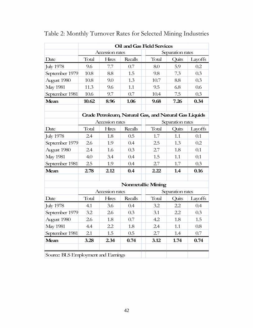
42

Table 2: Monthly Turnover Rates for Selected Mining Industries

Date Total Hires Recalls Total Quits LayoffsJuly 1978 9.6 7.7 0.7 8.0 5.9 0.2September 1979 10.8 8.8 1.5 9.8 7.3 0.3August 1980 10.8 9.0 1.3 10.7 8.8 0.3May 1981 11.3 9.6 1.1 9.5 6.8 0.6September 1981 10.6 9.7 0.7 10.4 7.5 0.3Mean 10.62 8.96 1.06 9.68 7.26 0.34

Date Total Hires Recalls Total Quits LayoffsJuly 1978 2.4 1.8 0.5 1.7 1.1 0.1September 1979 2.6 1.9 0.4 2.5 1.3 0.2August 1980 2.4 1.6 0.3 2.7 1.8 0.1May 1981 4.0 3.4 0.4 1.5 1.1 0.1September 1981 2.5 1.9 0.4 2.7 1.7 0.3Mean 2.78 2.12 0.4 2.22 1.4 0.16

Date Total Hires Recalls Total Quits LayoffsJuly 1978 4.1 3.6 0.4 3.2 2.2 0.4September 1979 3.2 2.6 0.3 3.1 2.2 0.3August 1980 2.6 1.8 0.7 4.2 1.8 1.5May 1981 4.4 2.2 1.8 2.4 1.1 0.8September 1981 2.1 1.5 0.5 2.7 1.4 0.7Mean 3.28 2.34 0.74 3.12 1.74 0.74

Source: BLS Employment and Earnings

Oil and Gas Field Services

Nonmetallic MiningAccession rates Separation rates

Accession rates Separation rates

Accession rates Separation ratesCrude Petroleum, Natural Gas, and Natural Gas Liquids

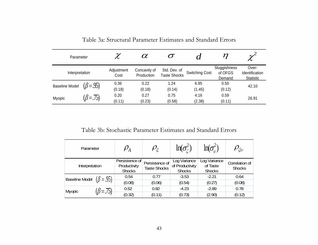
43

Table 3a: Structural Parameter Estimates and Standard Errors

Parameter

Interpretation Adjustment Cost

Concavity of Production

Std. Dev. of Taste Shocks Switching Cost

Sluggishness of OFGS Demand

Over-Identification

Statistic0.36 0.22 1.24 6.95 0.50(0.18) (0.18) (0.14) (1.45) (0.12)0.20 0.27 0.75 4.16 0.59(0.11) (0.23) (0.58) (2.38) (0.11)

Baseline Model 42.10

Myopic 26.91

2d

( .95) ( .75)

Table 3b: Stochastic Parameter Estimates and Standard Errors

Parameter

InterpretationPersistence of Productivity

Shocks

Persistence of Taste Shocks

Log Variance of Productivity

Shocks

Log Variance of Taste Shocks

Correlation of Shocks

0.54 0.77 -3.53 -2.21 0.64(0.08) (0.06) (0.54) (0.27) (0.08)0.52 0.82 -4.23 -2.89 0.78(0.32) (0.11) (0.73) (2.90) (0.12)

Myopic

Baseline Model

( .75)

2ln( )2ln( )A

( .95)

44

Figure 1: Employment, Relative Wages, and the Price of Oil

4.5

55.

56

Log

Pro

duct

ion

Wor

kers

1970 1975 1980 1985 1990 1995 2000 2005

Employment

-.1-.0

50

.05

.1R

elat

ive

Wag

es

1970 1975 1980 1985 1990 1995 2000 2005

Relative Wages

2.5

33.

54

4.5

5Lo

g D

efla

ted

PPI

Cru

de O

il

1970 1975 1980 1985 1990 1995 2000 2005

Price of Oil

Note: Relative wages are the log of the ratio of average production wages in the oil industry to average production wages in" "nonmetallic mining. Oil prices are deflated using the CPI-U series.

45

Figure 2: Estimated Response to a Permanent Unit Log Increase in Oil Prices (Unrestricted Distributed Lag)

0.5

11.

5

0 2 4 6 8 10 12 14 16 18 20 22 24

Employment

-.1-.0

50

.05

.1.1

5

0 2 4 6 8 10 12 14 16 18 20 22 24

Relative Wages

-.2-.1

0.1

.2

0 2 4 6 8 10 12 14 16 18 20 22 24

Hours per Worker

Quarters After Shock

Note: shaded areas are 95% confidence intervals computed via Newey-West HAC estimator.

46

Figure 3: Estimated Response to a Permanent Unit Log Increase in Oil Prices (5th Order Polynomial Distributed Lag)

0.2

.4.6

.81

1.2

0 2 4 6 8 10 12 14 16 18 20 22 24

Employment

-.05

0.0

5.1

.15

0 2 4 6 8 10 12 14 16 18 20 22 24

Relative Wages

-.15

-.1-.0

50

.05

.1.1

5

0 2 4 6 8 10 12 14 16 18 20 22 24

Hours per Worker

Quarters After Shock

Note: shaded areas are 95% confidence intervals computed via Newey-West HAC estimator.

47

Figure 4: Gross Flows Between Sectors

mcf

mfc

moc

mco

O

N

F

48

Figure 5: Gross and Net Migration Curves

ow nw

IN

OUT’

OUT IN’

Flow

otw

ow

IN OUT

OUT*

IN*

Flow

otw

49

Figure 6: Equilibrium Response to an Increase in the Price of Oil

o

tw

ow

0

S S’

D D’ D’’

S’’

otL

50

Figure 7: Structural Shocks

-2-1

01

2Ta

ste

Sho

cks

-1.5

-1-.5

0.5

11.

5P

rodu

ctiv

ity S

hock

s

1970 1975 1980 1985 1990 1995 2000 2005

Productivity Shocks Taste Shocks

Baseline Model

-2-1

01

2Ta

ste

Sho

cks

-1.5

-1-.5

0.5

11.

5P

rodu

ctiv

ity S

hock

s

1970 1975 1980 1985 1990 1995 2000 2005

Productivity Shocks Taste Shocks

Myopic

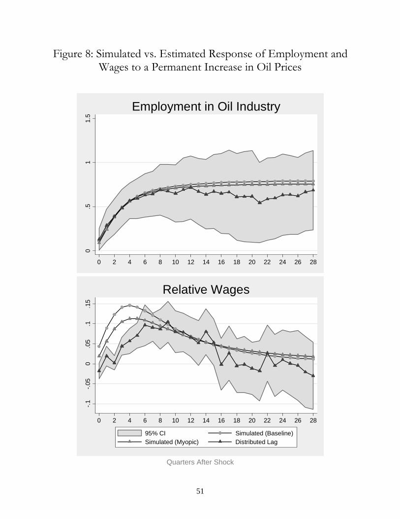
51

Figure 8: Simulated vs. Estimated Response of Employment and Wages to a Permanent Increase in Oil Prices

0.5

11.

5

0 2 4 6 8 10 12 14 16 18 20 22 24 26 28

Employment in Oil Industry

-.1-.0

50

.05

.1.1

5

0 2 4 6 8 10 12 14 16 18 20 22 24 26 28

95% CI Simulated (Baseline)Simulated (Myopic) Distributed Lag

Relative Wages

Quarters After Shock

52

Figure 9: State Dependence in Impulse Response Functions

0.5

11.

5

0 2 4 6 8 10 12 14 16 18 20 22 24 26 28

Employment in Oil Industry

-.1-.0

50

.05

.1.1

5

0 2 4 6 8 10 12 14 16 18 20 22 24 26 28

95% CI Distributed LagSimulated (Tight) Simulated (Slack)Simulated (Tight, Myopic) Simulated (Slack, Myopic)

Relative Wages

Quarters After Shock

53

Figure 10: Simulated Response of Gross Migrations and Sector Values to a Permanent Increase in Oil Prices

-4

-20

24

0 2 4 6 8 10 12 14 16 18 20 22 24 26 28

mon mnomnf mfn

Gross Flows

02

46

0 2 4 6 8 10 12 14 16 18 20 22 24

Vo VnVf

Sector Values

Quarters After Shock

54

Figure 11: Estimated/Simulated Response of Log Oil Unemployment to a Permanent Increase in Oil Prices

-10

-50

510

0 2 4 6 8 10 12 14 16 18 20 22 24 26 28

90% CI Simulated (Baseline)Simulation (Myopic) Distributed Lag

Quarters After Shock

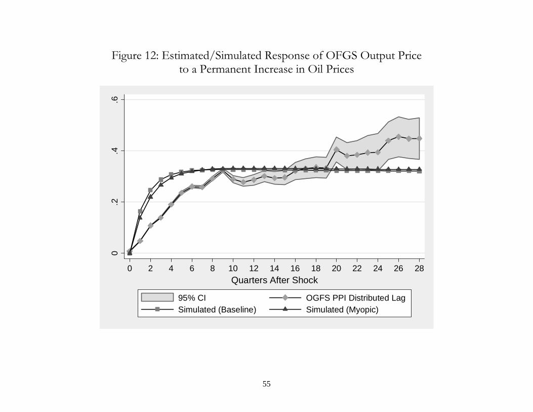
55

Figure 12: Estimated/Simulated Response of OFGS Output Price to a Permanent Increase in Oil Prices

0.2

.4.6

0 2 4 6 8 10 12 14 16 18 20 22 24 26 28

95% CI OGFS PPI Distributed LagSimulated (Baseline) Simulated (Myopic)

Quarters After Shock