Understanding Recursion /1 Powerful computing/problem-solving

techniques Examples

• Factorial: • f(n) = 1, if n = 1

• f(n) = f(n-1) * n, if n ≥ 1

• Quick sort:• Sort([x]) = [x]

• Sort([x1, …, pivot, … xn]) = sort[ys] ++ sort[zs]), where

ys = [ x | x in xi, x ≤ pivot ]

zs = [ x | x <- xi, x > pivot ]18/04/23 1

f(0) = 0! = ???f(0) = 0! = ???

List comprehension in Haskell or python

List comprehension in Haskell or python

Understanding Recursion /2 Let C(n, m) be the number of ways to select m balls from n

numbered balls Show that C(n, m) = C(n-1, m-1) + C(n-1, m)

Example: m = 3, n = 5 Consider any ball in the 5 balls, e.g., ‘d’

18/04/23 2

entire solution space

?1 ?2 ?3

d ?1 ?2 ?1 (not d) ?2 ?3

a b c d e?i in { }

Key Points Sub-problems need to be “smaller”, so that a

simple/trivial boundary case can be reached Divide-and-conquer

• There may be multiple ways the entire solution space can be divided into disjoint sub-spaces, each of which can be conquered recursively.

18/04/23 3

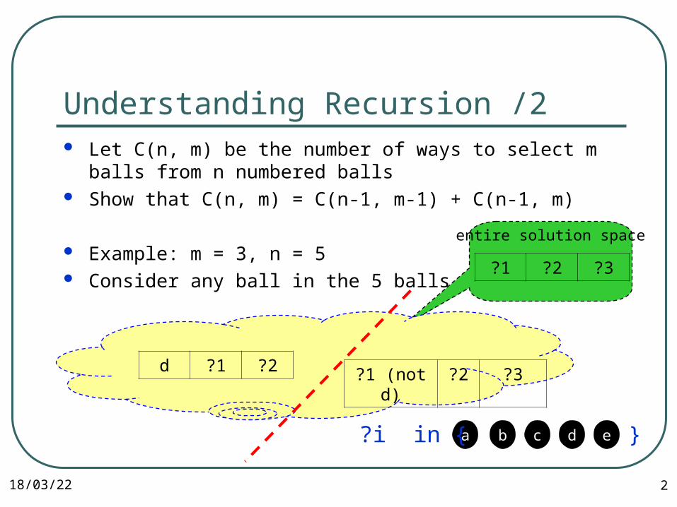
Outline

We offer two ways to derive/interpret a BUC-like algorithm• Slides 5-8:

• Slides 9-11: geometric derivation

Slides 12-17:• Simplified pseudo-code of BUC

• Misc stuffs

• Example

18/04/23 4

Naïve Relational Cubing Method /1

All tuples in the cube has the format

• (ai, bj, ck, …, Ml)

• ai must be one of the values on dim A observed from the base cuboid + * (i.e. ALL) collectively denoted as Dom*(A)

Cubing R ABC =

• foreach (ai, bj, ck) in Dom*(A) X Dom*(B) X Dom*(C)

• return ( ai, bj, ck, aggregate(R, (ai, bj, ck)) ) 18/04/23 5

i.e., Cubing(R, ABC). We omit () for clarity. No confusion as Cubing(., .) always takes 2 parametersi.e., Cubing(R, ABC). We omit () for clarity. No confusion as Cubing(., .) always takes 2 parameters

Naïve Relational Cubing Method /2

Rather than hardcode 3 nested loops, use recursion

Cubing R ABC =

• [Cubing R aiBC | ai in Dom*(A)]

• Cubing R aiBC = [ai] ⨉ Cubing R BC

• ⨉ is the Cartesian product; effectively prepending ai to every tuple from the recursion call

Assertion (which is easy to prove):• Cubing(.,.) returns the (almost) correct cube from

R wrt the given set of dimensions18/04/23 6

Boundary case omitted. Try to write it by yourself.Boundary case omitted. Try to write it by yourself.

Improved Relational Cubing Method /1 Cubing R ABC =

• [ [ai] ⨉ Cubing R BC | ai in Dom*(A)]

Problem: may generate non-observed dimension value combinations.

• The choice of bj should depend on ai

• Fix: • (1) pass tuples with A = ai to recursive calls

• (2) take bj values from those observed in the set of tuples passed in.

18/04/237

[1] ⨉[1] ⨉[2] ⨉[2] ⨉[*] ⨉[*] ⨉

(1, 1, *, 0) is spurious(1, 1, *, 0) is spurious

Improved Relational Cubing Method /2 Cubing R ABC =

• [ [ai] ⨉ Cubing ∏BCσA=ai(R) BC

| ai in Dom*(R.A) ]

18/04/238

[1] ⨉[1] ⨉[2] ⨉[2] ⨉[*] ⨉[*] ⨉

Reduce Cube(in 2D) to Cube(in 1D)

18/04/23 9

Geometric Interpretation /1

M11 M12 M13 [Step 1]

M21 M22 M23 [Step 1]

[Step 2] [Step 2] [Step 2] [Step 3]

a1

a2

b1 b2 b3

M11 M12 M13 [Step 1]b1 b2 b3

M21 M22 M23 [Step 1]

[Step 2] [Step 2] [Step 2] [Step 3]

[a1] ⨉[a1] ⨉[a2] ⨉[a2] ⨉[a*] ⨉[a*] ⨉

Reduce Cube(in 3D) to Cube(in 2D)

18/04/23 10

Geometric Interpretation /2

Reduce Cube(in 3D) to Cube(in 2D)

18/04/23 11

Geometric Interpretation /3

12

Scaffolding BUC

Alg: BottomUpCube(input, d)

BUC (Scaffolded) Explained

Essentially the same as the improved recursive cubing algorithm• Some recursion manually unfolded

• Computes coarse aggregation first (Line 1), mainly for iceberg cube computation

Computes aggregates from cuboids interleavingly and in the order shown on the right

18/04/23 13

Our: ABC, AB, AC, A, BC, B, C, ɸ

BUC: ɸ, A, AB, ABC, AC, B, BC, C

Cuboid AB = GROUP BY A, B = (ai, bj, [….])Cuboid AB = GROUP BY A, B = (ai, bj, [….])

An Alternative View of BUC’s Algorithm

Divide the solution space (all tuples in the cube) in the following manner:

• A=ai

• A=*, B=bj

• A=*, B=*, C=ck

• … …

• ???

18/04/23 14

disjoint & complete(why? write out the last bullet)

Compute (d-1) dim cube

Compute (d-2) dim cube

…

???

15

Additional Advantage of Divide and Conquer: Locality of Access Increasingly important when dealing with large

datasets, residing• on disk (disk is slower than memory)

• in the memory (memory is slower than L2/1 cache; TLB misses)

Each chunk of data is loaded once into the memory, and then we perform all the computation depending on it• If (1, _, _ …) fits in the memory

• Compute all (1, _, _, …) without additional I/O cost

• Write out (*, _, _, …)

• No longer needed afterwardsc.f., external memory sort

18/04/23 16

BUC Example

50112

40131

30121

20211

10111

MCBA

ABC

AB AC BC

A B C

(*, *, *) = 150

A B C

(1, *, *) (2, *, *)

AB

(1, 1, *) (1, 2, *) (1, 3, *)

AB

ABC

(1, 1, 1)

ABC

(1, 2, 1)

ABC

(1, 3, 1)

(2, 1, *)

ABC

(2, 1, 1)

AC

(1, *, 1) (1, *, 2)

AC

(2, *, 1)

(1, 1, 2)

18/04/23 17

BUC Example

(*, *, *) = 150

B C

(*, 1, *)

BC

(*, 1, 1) (*, 1, 2)

5011

4013

3012

2021

1011

MCB

(*, 2, *)

BC

(*, 2, 1)

(*, 3, *)

BC

(*, 3, 1)

(*, *, 1) (*, *, 2)

ABC

AB AC BC

A B C

A

ABC

AB AC

Note: strictly speaking, BUC uses depth-first traversal order and it is slightly different from what is shown in the animation here. E.g., when partitioning on B, it discovers three partitions, and will delve into the first partition (and calculate (*,1,*)); it will only access and perform computation for other partitions after all the (recursive) computation of the first partition is completed.