Understanding Monte Carlo Simulation -

W E A L T H C A R E C A P I T A L M A N A G E M E N T : w h i t e p a p e r

600 east Main Street, richmond, Va 23219 p 804.644.4711 f 804.644.4759 www.wealthcarecapital.com

Understanding Monte Carlo Simulation

DAvID B. LoEPER, CIM A ®, CIMC ® ChairMan/CeO

W E A L T H C A R E C A P I T A L M A N A G E M E N T

Whether you call it Monte Carlo Simulation, Stochastic Modeling, or Probability Analysis, there exists among advisors and their clients a fair amount of mystery about what exactly this analysis is and how it works. When such modeling methods are exploited to help clients make the best choices about their life, as in our Wealthcare Process or Wachovia Securities’ EnvisionSM process, it really isn’t necessary to explain how the watch works to know what time it is, but; because many advisors are gaining access to the meth-odology without a process to support its use, it may be helpful to understand why it is gaining popularity, what problems it might help us solve, how it works and what it shows and perhaps more importantly, what it cannot show. The objective of this paper is to clarify these questions in layman’s terms.

what is it?

Monte Carlo (the city - not the method) is known for gaming and there is good reason this mathematical methodology was named for it. In general, gambling has uncertainty associated with it and there is risk that one might lose a little or a lot, and there is a chance one might win, a little or even win a lot. The games in casinos have random outcomes...they are uncertain. Dice rolled at a craps table do not remem-ber how they previously fell. The little ball rolling around the roulette wheel has no memory either and will randomly fall in any of 38 spaces (37 in the city of Monte Carlo and most of Europe’s casinos; they have only one green “0” as opposed to American’s additional green “00”.) The effect of this randomness means that there are many different potential outcomes with both winners and losers. The odds are tilted towards the casino of course, but that doesn’t mean it isn’t possible to win on any particular trip, or even series of trips at the expense of the casino. All it means is that the Casino will end up with a profit (“take”) if enough people gamble enough times with enough money.

If one thinks about the capital markets, there is obviously a lot of uncertainty in how they will perform and we generally consider this uncertainty as investment risk. Like the bankrolls of all the gamblers in a casino (and therefore also the casino’s profit for any given night or month), bonds and stocks both go up and down in varying amounts from year to year. Like investment asset classes (stocks and bonds for example), the casino in the long run makes more money on some games than others (for example, roulette has around a 5% “take” while craps and blackjack when played properly generally have less than a 1% “take”), but that doesn’t mean the roulette table produces more profits every night. Some nights a casino will lose on all of their games, sometimes they will win on all of them, and sometimes they will win on most of them but lose so much at one game that it erodes the profits for the night from all of the others.

Doesn’t the nightly uncertainty for the casino feel a bit like yearly investment returns? When you are investing, you are the casino with a long run advantage (expected return) and a short term risk (uncertainty). In the long run we expect a profit when investing for accepting investment risk, just like the casino profits in the long run for the risk it takes. But, just like the casino’s uncertainty on any night for any particular game, we have asset class “games” that have varying amounts of uncertainty. Do we not experience losses in stocks more frequently and more severely than bonds? Do we not have years where our stock losses exceed the gains we have in cash and in bonds? Are there not occasionally years where both stocks and bonds are both down or both up for that matter?

Monte Carlo simulation has rapidly gained adoption by financial advisors because it corrects a material flaw we had been making (until Monte Carlo tools were available for financial advisors we couldn’t practi-cally correct for it). A person’s life has a lot of uncertainty associated with it, and we attempted to comfort clients about the uncertainty of the future by planning their financial future for them. By identifying how much money one has, how much one was saving, when one would retire, how much one would spend, etc. and combining this assumed “life plan” with an assumed return (i.e. their long run investing “take”) based on their risk tolerance, we thought in theory we were mapping out whether the client would meet their goals. The problem with how we were doing this was that we made the assumption that there were

Understanding Monte Carlo Simulation February 23, 2005 © wealthcare Capital Management all rights reserved PAGE 2


no uncertainties about investment returns. If a client’s risk tolerance pointed to a 7% return (“take”) assumption, while we identified their risk tolerance to determine what the long run return assump-tion might be, when it came time to plan their future, the best practice of the industry was to assume that risk we identified somehow evaporated and they could plan their lives around 7% every year...no uncertainty...no standard deviation...never a loss...or...the exact same “take” every night at the casino.

Imagine a casino capitalizing itself with this assumption. Since they have a 5% take in the long run at rou-lette, they could just assume they would profit every night (just as we planned investors’ financial future with 7% profits every year) and they wouldn’t need any capital. of course, casinos know what their risks are (and yes, they run Monte Carlo simulations to estimate their capital needs) for the risk of losing games, losing nights and even losing months.

on the surface, it might appear as though ignoring the year to year gyrations of the markets wouldn’t be all that bad because in the long run the investor should average a return somewhere near our assumed return. This is a bad assumption.

The first problem that Monte Carlo simulation helps us understand is the risk that even over long peri-ods of time, the capital markets are uncertain. Take your typical 65 year old client who just recently retired. They might live to age 95 or so, a 30-year planning horizon. The worst historical 30-year com-pound return for large cap stocks (based on CRSP data from 1926-2004) ranged from a low of 7.17% to a high of 14.29%. For 10-year treasury bonds, the range was from 2.25% to 9.02%. For a 60/40 blend of the two, the range was 6.79% to 12.43%. With such wide spreads even over 30 years, we see that any assumed compound return could be significantly off target. Monte Carlo simulations, with reasoned inputs, helps us understand how wide this spread might be, and the odds of any particular 30 year result being above or below any specific return.

While some are somewhat surprised by the wide range of outcomes for such long time periods, it isn’t the whole story behind what Monte Carlo simulation can help us understand about investment risk. This is because the goals a client might confidently exceed are spent with dollars, and not percentage returns. We often make the erroneous assumption that a higher average return (“take”) will produce more dol-lars for a client...but what we are ignoring in this is the varying amounts of capital the client will have exposed to returns throughout their life. Test yourself on this a bit to see if you might understand why when a client gets a return might make a bigger difference than what the average return is over the long run. Think about what happens to a casino’s take for a night if the high rollers were luckier than run of the mill gamblers.

Imagine the 65 year old recently retired client mentioned above with a 30 year planning horizon and for purposes of this exercise, let’s assume we have a special investment that behaves almost identically to how we have planned in the past...that is, it produces a 7% return each and every year, except for two years to introduce just a tiny bit of uncertainty. In one of those two deviating years, the investor will get a “bonus” return of 21%, and in the other, he will have a negative 7% return. Unlike the uncertainty of real portfolios though, this special investment permits the investor to actually pick which year he gets the bonus return and which year he will suffer the losing year. As his advisor, he asks you for advice about this...what would be your answer? Which year should he choose to take the “bonus” 21% return and which year should he suffer the loss of 7%? Does it make any difference?

table 1 shows that the result for a $100 investment in this special investment over the next thirty years is completed unaffected by which year is selected for the bonus return or the negative return.



obviously what is important for this investor is not the timing of the returns, but instead what the aver-age return is. However, how many retired people do you know that do not plan on spending any of their money? What goals that do NoT require money are we trying to comfort our client about by going through a planning exercise? Have you ever met a retired person that had a goal of not dipping into their capital but producing a continuous stream of income over their life? If all that matters is the aver-age return in the long run, and since we already have seen in table 1 that when the return occurs makes no difference, shouldn’t the assumed long run average be close enough?

In table 2 we see the same first year versus last year timing contrast again with one 21% bonus return and one negative 7% return in the context of an investor that wants to withdraw $7 a year from his $100 portfolio and does not want to dip into principal.


Table 1- The ending portfolio value is the same regardless of whether the 21% return occurs in the first year (left) or the last year (right) if there are no contributions or withdrawals.

YearReturn in

%Return

in $Contribution (Withdrawal)

Portfolio Value Year

Return in %

Return in $

Contribution (Withdrawal)

Portfolio Value

$100 $1001 21% $21 -$ $121 1 -7% ($7) -$ $932 7% $8 -$ $129 2 7% $7 -$ $1003 7% $9 -$ $139 3 7% $7 -$ $1064 7% $10 -$ $148 4 7% $7 -$ $1145 7% $10 -$ $159 5 7% $8 -$ $1226 7% $11 -$ $170 6 7% $9 -$ $1307 7% $12 -$ $182 7 7% $9 -$ $1408 7% $13 -$ $194 8 7% $10 -$ $1499 7% $14 -$ $208 9 7% $10 -$ $16010 7% $15 -$ $222 10 7% $11 -$ $17111 7% $16 -$ $238 11 7% $12 -$ $18312 7% $17 -$ $255 12 7% $13 -$ $19613 7% $18 -$ $273 13 7% $14 -$ $20914 7% $19 -$ $292 14 7% $15 -$ $22415 7% $20 -$ $312 15 7% $16 -$ $24016 7% $22 -$ $334 16 7% $17 -$ $25717 7% $23 -$ $357 17 7% $18 -$ $27518 7% $25 -$ $382 18 7% $19 -$ $29419 7% $27 -$ $409 19 7% $21 -$ $31420 7% $29 -$ $438 20 7% $22 -$ $33621 7% $31 -$ $468 21 7% $24 -$ $36022 7% $33 -$ $501 22 7% $25 -$ $38523 7% $35 -$ $536 23 7% $27 -$ $41224 7% $38 -$ $574 24 7% $29 -$ $44125 7% $40 -$ $614 25 7% $31 -$ $47226 7% $43 -$ $657 26 7% $33 -$ $50527 7% $46 -$ $703 27 7% $35 -$ $54028 7% $49 -$ $752 28 7% $38 -$ $57829 7% $53 -$ $805 29 7% $40 -$ $61830 -7% ($56) -$ $748 30 21% $130 -$ $748

7% Average 7% Average


As we can see in table 2, having the bonus return come early not only enabled the client to achieve both their income goal and not dip into principal, but also ended up with 73% more (as a percentage of the original investment) as a bonus that could have been spent without sacrificing their estate goal. Experiencing the loss in the first year and the bonus return at the end had them completely depleting their principal.

This is perhaps a bit more intuitive for some because we know the concept of the “time value of money.” Perhaps for you, this might be a bit more intuitive than the first example that proved in the absence of contributions or withdrawals (goals) it made no difference when the bonus return and negative return occurred. However, each investor is unique and has different goals and so there are cases where the reverse will be true. For example, what if our retired client had deferred compensation plan that was going to produce $6 a year more than they needed to live on for the first 10 years of retirement and then when that was done, they would start taking withdrawals from their portfolio? table 3 shows that for this investor, they are actually slightly better off by taking the loss in the first year and waiting to the last year to get the bonus return, the exact opposite of what one would assume when thinking about the time value of money.


Table 2 - The timing of the bonus return and negative return have a huge impact when we include a goal of an income stream and not dipping into principal.

YearReturn in

%Return



Return in %

Return in $


Portfolio Value

$100 $1001 21% $21 (7)$ $114 1 -7% ($7) (7)$ $862 7% $8 (7)$ $115 2 7% $6 (7)$ $853 7% $8 (7)$ $116 3 7% $6 (7)$ $844 7% $8 (7)$ $117 4 7% $6 (7)$ $835 7% $8 (7)$ $118 5 7% $6 (7)$ $826 7% $8 (7)$ $120 6 7% $6 (7)$ $807 7% $8 (7)$ $121 7 7% $6 (7)$ $798 7% $8 (7)$ $122 8 7% $6 (7)$ $789 7% $9 (7)$ $124 9 7% $5 (7)$ $7610 7% $9 (7)$ $126 10 7% $5 (7)$ $7411 7% $9 (7)$ $128 11 7% $5 (7)$ $7212 7% $9 (7)$ $129 12 7% $5 (7)$ $7113 7% $9 (7)$ $132 13 7% $5 (7)$ $6814 7% $9 (7)$ $134 14 7% $5 (7)$ $6615 7% $9 (7)$ $136 15 7% $5 (7)$ $6416 7% $10 (7)$ $139 16 7% $4 (7)$ $6117 7% $10 (7)$ $141 17 7% $4 (7)$ $5918 7% $10 (7)$ $144 18 7% $4 (7)$ $5619 7% $10 (7)$ $147 19 7% $4 (7)$ $5320 7% $10 (7)$ $151 20 7% $4 (7)$ $4921 7% $11 (7)$ $154 21 7% $3 (7)$ $4622 7% $11 (7)$ $158 22 7% $3 (7)$ $4223 7% $11 (7)$ $162 23 7% $3 (7)$ $3824 7% $11 (7)$ $166 24 7% $3 (7)$ $3425 7% $12 (7)$ $171 25 7% $2 (7)$ $2926 7% $12 (7)$ $176 26 7% $2 (7)$ $2427 7% $12 (7)$ $181 27 7% $2 (7)$ $1928 7% $13 (7)$ $187 28 7% $1 (7)$ $1329 7% $13 (7)$ $193 29 7% $1 (7)$ $730 -7% ($14) (7)$ $173 30 21% $1 (7)$ $1



Because this investor has unique goals (like all investors), there are even better or worse choices as to when they receive the bonus, or negative return. With this investor accumulating money for a period (sound like someone nearing retirement?) and then living off the portfolio thereafter, moving the bonus and negative returns to this sensitive date makes an $84 difference (84% of their starting portfolio value) over the life of the plan as is highlighted in table 4.


Table 3 - For some investor’s goals, getting the loss early and the gain later actually improves the result.

YearReturn in

%Return



Return in %

Return in $


Portfolio Value

$100 $1001 21% $21 6$ $127 1 -7% ($7) 6$ $992 7% $9 6$ $142 2 7% $7 6$ $1123 7% $10 6$ $158 3 7% $8 6$ $1264 7% $11 6$ $175 4 7% $9 6$ $1415 7% $12 6$ $193 5 7% $10 6$ $1566 7% $14 6$ $213 6 7% $11 6$ $1737 7% $15 6$ $234 7 7% $12 6$ $1918 7% $16 6$ $256 8 7% $13 6$ $2119 7% $18 6$ $280 9 7% $15 6$ $23210 7% $20 6$ $305 10 7% $16 6$ $25411 7% $21 (7)$ $320 11 7% $18 (7)$ $26512 7% $22 (7)$ $335 12 7% $19 (7)$ $27613 7% $23 (7)$ $352 13 7% $19 (7)$ $28914 7% $25 (7)$ $369 14 7% $20 (7)$ $30215 7% $26 (7)$ $388 15 7% $21 (7)$ $31616 7% $27 (7)$ $408 16 7% $22 (7)$ $33117 7% $29 (7)$ $430 17 7% $23 (7)$ $34718 7% $30 (7)$ $453 18 7% $24 (7)$ $36419 7% $32 (7)$ $478 19 7% $26 (7)$ $38320 7% $33 (7)$ $504 20 7% $27 (7)$ $40321 7% $35 (7)$ $532 21 7% $28 (7)$ $42422 7% $37 (7)$ $562 22 7% $30 (7)$ $44723 7% $39 (7)$ $595 23 7% $31 (7)$ $47124 7% $42 (7)$ $630 24 7% $33 (7)$ $49725 7% $44 (7)$ $667 25 7% $35 (7)$ $52526 7% $47 (7)$ $706 26 7% $37 (7)$ $55427 7% $49 (7)$ $749 27 7% $39 (7)$ $58628 7% $52 (7)$ $794 28 7% $41 (7)$ $62029 7% $56 (7)$ $843 29 7% $43 (7)$ $65630 -7% ($59) (7)$ $777 30 21% $138 (7)$ $787



The answer to our original question as to when the investor should elect to receive the bonus and nega-tive returns has only one correct answer...that is...it depends on what the investor wishes to achieve. It is insufficient to answer that question with a simple “I want to make the most money possible” because it depends on when and how much they are contributing to the portfolio and withdrawing from it. And, as was demonstrated in table 1, in the absence of any contributions or withdrawals (goals), while there was a correct answer, that answer was it makes no difference if you have no other goals!

Before we start to examine how Monte Carlo simulation might help us model more realistic portfolios that have uncertainty every year, there is one other important concept to understand and that is the effect of the uncertainty in timing of various returns, contributions and goals can have far more impact than the average return or even the risk of the portfolio.

For this we are going to play a little game and since we are dealing with fantasy portfolios that have very little uncertainty, we are going to pretend that past performance actually is an indication of future results. Pretend for a moment that you have the choice of two investments for our typical retired client that wants to avoid dipping into their capital and also to produce a continuous stream of income.

Even though past performance IS NoT an indication of future results, in this fantasy game we are going to assume that there is complete certainty that our investments will produce the exact same results over the next thirty years as they had over the last thirty. You might think that knowing this information in


Table 4 - Which year the bonus and negative return happen can make a bigger difference in the middle of the plan if the investor is accumulating for a period and then begins distributions later.

YearReturn in

%Return



Return in %

Return in $


Portfolio Value

$100 $1001 21% $21 6$ $127 1 -7% ($7) 6$ $992 7% $9 6$ $142 2 7% $7 6$ $1123 7% $10 6$ $158 3 7% $8 6$ $1264 7% $11 6$ $175 4 7% $9 6$ $1415 7% $12 6$ $193 5 7% $10 6$ $1566 7% $14 6$ $213 6 7% $11 6$ $1737 7% $15 6$ $234 7 7% $12 6$ $1918 7% $16 6$ $256 8 7% $13 6$ $2119 7% $18 6$ $280 9 7% $15 6$ $23210 7% $20 6$ $305 10 7% $16 6$ $25411 -7% ($21) (7)$ $277 11 21% $53 (7)$ $30012 7% $19 (7)$ $289 12 7% $21 (7)$ $31413 7% $20 (7)$ $303 13 7% $22 (7)$ $32914 7% $21 (7)$ $317 14 7% $23 (7)$ $34515 7% $22 (7)$ $332 15 7% $24 (7)$ $36216 7% $23 (7)$ $348 16 7% $25 (7)$ $38117 7% $24 (7)$ $366 17 7% $27 (7)$ $40018 7% $26 (7)$ $384 18 7% $28 (7)$ $42119 7% $27 (7)$ $404 19 7% $30 (7)$ $44420 7% $28 (7)$ $425 20 7% $31 (7)$ $46821 7% $30 (7)$ $448 21 7% $33 (7)$ $49422 7% $31 (7)$ $473 22 7% $35 (7)$ $52123 7% $33 (7)$ $499 23 7% $36 (7)$ $55124 7% $35 (7)$ $526 24 7% $39 (7)$ $58225 7% $37 (7)$ $556 25 7% $41 (7)$ $61626 7% $39 (7)$ $588 26 7% $43 (7)$ $65227 7% $41 (7)$ $622 27 7% $46 (7)$ $69128 7% $44 (7)$ $659 28 7% $48 (7)$ $73229 7% $46 (7)$ $698 29 7% $51 (7)$ $77730 7% $49 (7)$ $740 30 7% $54 (7)$ $824



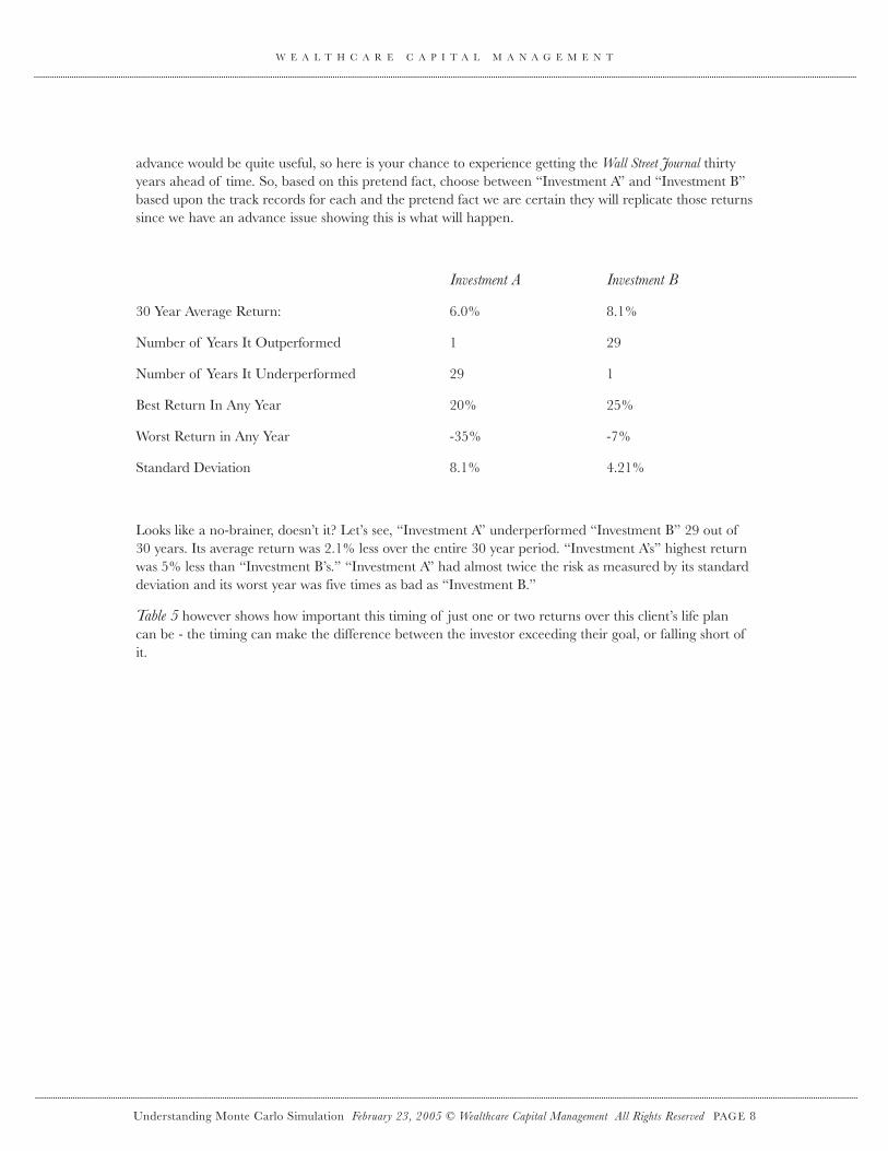
advance would be quite useful, so here is your chance to experience getting the wall Street Journal thirty years ahead of time. So, based on this pretend fact, choose between “Investment A” and “Investment B” based upon the track records for each and the pretend fact we are certain they will replicate those returns since we have an advance issue showing this is what will happen.

investment a investment B

30 Year Average Return: 6.0% 8.1%

Number of Years It outperformed 1 29

Number of Years It Underperformed 29 1

Best Return In Any Year 20% 25%

Worst Return in Any Year -35% -7%

Standard Deviation 8.1% 4.21%

Looks like a no-brainer, doesn’t it? Let’s see, “Investment A” underperformed “Investment B” 29 out of 30 years. Its average return was 2.1% less over the entire 30 year period. “Investment A’s” highest return was 5% less than “Investment B’s.” “Investment A” had almost twice the risk as measured by its standard deviation and its worst year was five times as bad as “Investment B.”

table 5 however shows how important this timing of just one or two returns over this client’s life plan can be - the timing can make the difference between the investor exceeding their goal, or falling short of it.



Think about this example the next time you attempt to pick a superior investment. Which one of these two outcomes do you think the client would prefer? How valuable was your superior selection to this cli-ent?

So far, each of these examples showed us that even just a small amount of uncertainty (only two of thirty years) can have a tremendous impact on the ultimate result for the client, as long as there are either con-tributions (savings) or withdrawals (goals). In the past, (before Monte Carlo simulation was available) we assumed there was no uncertainty and we would plan the client’s life - completely ignoring the impact of the obvious risk that the returns received will not be identical each year. But, if the timing of just two returns out of thirty years produces either 73% more capital or has the client completely depleting their capital despite producing the same average return (table 2), or if the timing of just two years out of thirty can have an investment with a consistently lower return and higher risk exceed the dollar result (the client spends dollars and not percentage returns) of a higher returning portfolio with less risk (table 5), we clearly see we were in need of a better means of modeling our client’s future.


Table 5 - Despite the terrible track record of “Investment A” with consistently lower returns and more risk, it actually exceeded this investor’s goals while unfortunate timing of one return for the far superior “Investment B” had the client consistently falling short of their goal of not dipping into principal in all but the first year.

"Investment A" "Investment B"

YearReturn in

%Return



Return in %

Return in $


Portfolio Value

$100 $1001 7% $7 (7)$ $100 1 8% $8 (7)$ $1012 20% $20 (7)$ $113 2 -7% ($7) (7)$ $873 7% $8 (7)$ $114 3 8% $7 (7)$ $874 7% $8 (7)$ $115 4 8% $7 (7)$ $875 7% $8 (7)$ $116 5 8% $7 (7)$ $876 7% $8 (7)$ $117 6 8% $7 (7)$ $877 7% $8 (7)$ $118 7 8% $7 (7)$ $878 7% $8 (7)$ $120 8 8% $7 (7)$ $879 7% $8 (7)$ $121 9 8% $7 (7)$ $8710 7% $8 (7)$ $122 10 8% $7 (7)$ $8611 7% $9 (7)$ $124 11 8% $7 (7)$ $8612 7% $9 (7)$ $126 12 8% $7 (7)$ $8613 7% $9 (7)$ $127 13 8% $7 (7)$ $8614 7% $9 (7)$ $129 14 8% $7 (7)$ $8615 7% $9 (7)$ $131 15 8% $7 (7)$ $8616 7% $9 (7)$ $134 16 8% $7 (7)$ $8617 7% $9 (7)$ $136 17 8% $7 (7)$ $8618 7% $10 (7)$ $138 18 8% $7 (7)$ $8619 7% $10 (7)$ $141 19 8% $7 (7)$ $8520 7% $10 (7)$ $144 20 8% $7 (7)$ $8521 7% $10 (7)$ $147 21 8% $7 (7)$ $8522 7% $10 (7)$ $150 22 8% $7 (7)$ $8523 7% $11 (7)$ $154 23 8% $7 (7)$ $8524 7% $11 (7)$ $158 24 8% $7 (7)$ $8425 7% $11 (7)$ $162 25 8% $7 (7)$ $8426 7% $11 (7)$ $166 26 8% $7 (7)$ $8427 7% $12 (7)$ $171 27 8% $7 (7)$ $8428 7% $12 (7)$ $175 28 8% $7 (7)$ $8329 7% $12 (7)$ $181 29 8% $7 (7)$ $8330 -35% ($63) (7)$ $111 30 25% $21 (7)$ $97

6.0% Average 8.1%

8.10%-35%20%

4.21%-7%25%

Standard DeviationWorst YearBest Year


Average


Now if just two years of uncertainty had this wide ranging impact to the client’s lifestyle, imagine how wide the range of results might be if each year the return was uncertain, as it is in reality.

But, how could one model this uncertainty? Let’s pretend we are back in the early 1990’s (before there were Monte Carlo simulation tools available for financial advisors) and you are an advisor that wants to consider this uncertainty when planning your clients’ future. Just as I had manually input the starting capital, contributions, withdrawals and returns in a spreadsheet, you could do the same. But, to model the uncertainty in each year I would need a better way model the randomness of what the returns might be in each year than just picking one or two years to see the impact.

So, I take a bowl and fill it with slips of paper, and each slip of paper has a historical return of the markets written on it. Like a raffle, I shake the bowl and draw a slip with a return on it, record it in my spread sheet as the return in the first year, but unlike a raffle, I the return the paper to the bowl, shake it and draw another slip for year two...and so on. (If I’m simulating randomness I MUST return each slip to the bowl, because just like the dice not remembering that a seven was rolled in craps, or the roulette ball not remembering that it fell on “00”, if I didn’t return the paper to the bowl the future outcomes would exclude each slip as I withdrew it, in essence modeling no chance from that point forward that return could occur again.)

If I repeated this exercise for all thirty years, I would have one potential result or what is known as a “trial.” The average return and risk of thirty “draws” would vary each time I repeated the exercise and could be higher than the average of all the numbers in the bowl (depending on if I were lucky and drew a disproportionate amount of high returns), or lower than the average (if I were unlucky and drew an excessive number of low returns.) Also, like the example in table 5, there would be some outcomes that might average a higher than normal result but bad timing of when I draw a slip of paper might cause an unpleasant outcome, or I might have a lower than average result with fortunate timing that ends up exceeding the client’s goals none-the-less. table 6 shows an example of doing just such an exercise twice, or pulling 60 slips of paper from the bowl filled with market returns to produce two 30-year trials.



In these two sample “trials” that each model one potential way the returns might fall for the investor, we see the average returns and risks are different and yet another example of how fortunate timing for an inferior average result still had the client meeting their goals (it obviously doesn’t always work that way). Now that I have these two results, do I have a better sense of how confident the client can be of meet-ing their goals? Not really, because there are so many other potential ways the numbers might fall. This would obviously be pretty time consuming as well.

To really get a sense of confidence, or the client’s odds (chances) of exceeding their goals (that is what is happening in any number of trials, the client ends up with more than they were planning around, not merely achieving their goal), I would need to do this exercise many, many times. If I had the patience to draw the numbers for 500 or 1000 trials (drawing 15,000 or 30,000 slips- one slip for each year of each 30 year trial), I would have a better understanding of how confident the client could be. Clearly with that many samples, odds are that I would have drawn Great Depression types of results, back to back with the bear market of ‘73-’74 and probably the bear market of ‘00-’02 too.

From a very simplistic standpoint, this is what Monte Carlo simulation is doing. It just does it a lot faster. However, because there is also a chance that the market may not have had its worst year we could see (or best for that matter), instead of filling the bowl with only actual market returns, we could fill the bowl


Table 6 – Manually modeling the impact of the uncertainty of market returns by drawing numbers from a bowl sixty times to produce two thirty-year “trials”.

Trial 1 Trial 2

YearReturn in

%Return



Return in %

Return in $


Portfolio Value

$100 $1001 23% $23 (7)$ $116 1 6% $6 (7)$ $992 -9% ($10) (7)$ $99 2 23% $23 (7)$ $1153 -8% ($8) (7)$ $84 3 -1% ($1) (7)$ $1074 -25% ($21) (7)$ $56 4 -9% ($10) (7)$ $905 38% $21 (7)$ $70 5 26% $23 (7)$ $1066 9% $6 (7)$ $69 6 -8% ($9) (7)$ $917 14% $10 (7)$ $72 7 -18% ($16) (7)$ $688 -1% ($1) (7)$ $64 8 -18% ($12) (7)$ $489 22% $14 (7)$ $71 9 13% $6 (7)$ $4810 28% $20 (7)$ $84 10 38% $18 (7)$ $5911 3% $3 (7)$ $80 11 18% $11 (7)$ $6212 8% $6 (7)$ $79 12 9% $6 (7)$ $6113 45% $36 (7)$ $108 13 18% $11 (7)$ $6514 11% $12 (7)$ $113 14 14% $9 (7)$ $6715 7% $8 (7)$ $114 15 -7% ($5) (7)$ $5516 -14% ($16) (7)$ $91 16 -1% ($1) (7)$ $4817 9% $8 (7)$ $92 17 5% $2 (7)$ $4318 24% $22 (7)$ $107 18 22% $10 (7)$ $4619 6% $6 (7)$ $106 19 22% $10 (7)$ $4920 17% $18 (7)$ $117 20 28% $14 (7)$ $5521 7% $8 (7)$ $119 21 27% $15 (7)$ $6322 5% $6 (7)$ $118 22 3% $2 (7)$ $5823 -7% ($8) (7)$ $102 23 32% $19 (7)$ $7024 -18% ($18) (7)$ $77 24 8% $6 (7)$ $6925 36% $28 (7)$ $98 25 18% $12 (7)$ $7426 13% $13 (7)$ $103 26 32% $24 (7)$ $9127 9% $9 (7)$ $106 27 9% $8 (7)$ $9228 26% $27 (7)$ $126 28 11% $10 (7)$ $9529 -1% ($1) (7)$ $118 29 -14% ($13) (7)$ $7530 6% $7 (7)$ $118 30 7% $5 (7)$ $73

9.4% 10.4%


AverageStandard DeviationWorst YearBest Year

Average16.37%

-25%45%

15.26%-18%38%


with statistically “possible” results which would include the actual market returns. By doing this we would be able to measure not only the uncertainty of historical returns but also potential returns. This additional step helps us to make sure we are not ignoring the chance that we have not yet seen the worst (or the best) of what the markets might produce.

So, by drawing these slips of paper from the bowl filled with both actual and even potential market returns, we can start to understand how confident the client can be of exceeding their goals considering the uncertainty of market returns...or can we?

What if I filled the bowl with numbers that looked like the last 25 years instead of going back to 1926? That’s still a pretty long time period...would my confidence level change? The 25 years ending in 2003 produced a compound return that fell in the top 16% of all historical 25 year periods. While there would be a lot of trials that still produced poor results, half of the trials would exceed the top 16% of all his-torical 25 year periods. In essence I would be telling the client that from now on there is a 50% chance the markets will do better than most historical periods. The reverse could be true as well, if for example I used just the last five years that was dominated by a bear market. If I filled the bowl with numbers like those, I would be simulating half of all the trials doing worse than the bottom 10% of all five year peri-ods.

For the confidence number to have any really useful meaning, the returns that fill the bowl (or are requested from the computer’s random number generator) must not be overly optimistic, or overly pes-simistic relative to the nature of the markets. To control this and make the confidence result materially meaningful, a great deal of diligence therefore must go into figuring out how many slips of paper have what numbers on them (or in the case of a computer, the mean, standard deviation and shape of the distribution we are asking the random number generator to create for us.) A confidence number of exceeding the client’s goals in only 50% of the trials might be a good result if we used the last five years as an input, because our population of numbers that filled the bowl (or came from the random number generator) was loaded with numbers that fell in the bottom of market results. Likewise, an 80% confi-dence number may not be very good if we used the last 25 years to fill the bowl since nearly half of the numbers in the bowl fell near the best results the market ever had.

These inputs (known as “Capital Market Assumptions” or “CMAs”) are just as critical as modeling the uncertainty of returns because if they are overly biased one way or the other we are either misrepresent-ing how confident the client can be, or, being overly conservative causing the client to needlessly sacrifice their lifestyle.

However, assuming we have well thought out CMAs, we understand the client’s goals and planned contributions, assuming we have a reasonable method of modeling the taxes that might be confiscated from the client along the way and assuming our random number generator is producing a population of returns shaped similarly to potential behavior of the markets, we can then get a sense of how confident the client can be of exceeding their goals. or can we?

Is it really the client’s goals we are measuring the confidence of exceeding or is it a merely a set of potential goals the client might choose? The answer to this question is dependent upon whether the advisor has a discipline or a process that can discern between the two.

Unfortunately for clients, most advisors that have begun to use Monte Carlo simulation are still applying the exact same advice discipline they applied in the past before they had access to the information Monte Carlo simulation can provide. They view MCS as another arrow in their quiver, an evolution of their existing discipline. That is, they ask the client how much they are currently saving, what their assets are



invested in, their risk tolerance, a desired age of retirement and a retirement income goal. Just as they plugged these figures into their old fashioned tools that assumed no market uncertainty, they plug them into their new Monte Carlo tools and provide the client with either a “better” portfolio allocation or indicate how much savings shortfall the client must make up, to “get to the highest possible confidence of achieving their goals.” THIS IS AN ABUSE oF CLIENTS.

If we ignore for a moment the wide range of absurd Capital Market Assumptions (CMAs) that are often haphazardly input into such tools and assume for a moment they are all well reasoned with a distribution that is shaped similarly to markets’ behaviors, the notion of getting to the highest confidence level pos-sible makes the analysis of no practical use.

Think about how we manually drew numbers from a bowl that contained only actual market returns and how if we did it enough times we would certainly end up with some trials that started with a Great Depression, followed by a ‘73-’74 bear market and then drew from the bowl yet another Great Depression (you remember the numbers are returned to bowl after they were drawn to ensure random-ness.)

The odds of such a string of returns are certainly fairly low but with the number of times we are draw-ing numbers it is actual fairly likely that we would end up drawing such a string of returns. If we seek the highest possible confidence level (or chances/odds of “achieving” the client’s goals) we would be con-straining the client’s lifestyle to plan around such environments. While on the surface it might be nice to feel that confident, or nearly certain, that level of confidence comes at a very high price most advisors are ignoring and their clients end up needlessly paying.

You will observe I chose slightly different words when describing the results of a simulation in the context of how many advisors are using (misusing?) Monte Carlo. Most advisors misuse MCS in an attempt to give the client the highest possible probability to “achieve” clients’ goals instead of “exceeding” sacrificed goals as I used elsewhere in this paper.

If I run 1000 trials and in 20 of them the uncertainty of potential capital market results showed insuf-ficient capital to fund all of the client’s goals (as presently known) including the terminal value of their estate at their death, how many results did we model? We modeled 1000, but by overly simplifying these 1000 results into a simple binary “achieved” or “failed”, we are misleading the client and needlessly sacrificing their lifestyle. What happened in the other 980 trials? Did any of them have extra money? The reality of this “98% confidence” level is that in at least 979 of the trials the client left money in his estate he could have spent. In fact, it might be in 900 of the trials he left an estate more than three times more than he wanted to leave behind, or in 750 he left more than six times his estate goal. When we start looking toward the middle of the results, we might find that a “98% chance of achieving “his” goals” (as sacrificed to produce absurd confidence) left him with a 50% chance of leaving an estate behind that is TWENTY TIMES the estate goal he desired. Put yourself in the shoes of a client and think about this. Do you really want an advisor who coerces you to sacrifice the only life you have so you can die on a death bed stuffed with money you wished you would have spent?

It gets worse the way some advisors abuse MCS. one of the most useful aspects of MCS is for iden-tifying that there is a shortage of goals (choices) for the super wealthy that they should consider. Instead, many advisors focus on how MCS can model the odds of “running out of money” as if a client who planned twenty years ago to spend $100,000 a year and has been experiencing one of those truly severe market environments will just keep right on spending the same $100,000 until their money is gone.

For nearly any client, there will be a wide range of outcomes from such simulations, based on oNLY the



uncertainty in the capital markets and a completely CERTAIN AND UNCHANGING set of goals and priorities for the client throughout their life.

Casinos do not capitalize themselves based on every possible outcome, because they have choices of how to respond if rare extremes present themselves (i.e. changing table limits and rules, etc.) and the amount of capital required to deal with every potential outcome guarantees nothing more than a poor return on capital. In essence, why measure the odds? We could simply plan on losing 10% every year and we don’t need a simulation method to plan around that whether we are a casino, or an investor. The price of excessive conservatism to the casino is a low return on capital and likewise the price to the investor is a sacrificed lifestyle or goals. Clients have choices as well if things do not go exactly as hoped and they might delay retirement a year or two, move up the risk scale a notch, or delay a major purchase. If you have a 75-90% chance of not needing to make such compromises, why would you plan on making them now just in case?

This balance, and the CHoICES one makes between keeping the odds tilted sufficiently in our favor to avoid too much uncertainty versus the price of nearly certain sacrifice is what advisors can provide as their value proposition for their clients. It requires a lot more than just the mathematical methodology, reasoned inputs and tools to calculate the odds. It also requires us to give advice about a lot more than portfolios and savings but all of those other choices that have as much impact or more that our tradi-tional financial advising services failed to contemplate.

In the past, our value proposition for clients was focused around portfolios and beating markets. table 5 clearly demonstrated however that even with certainty of performance replicating over time, whether a client gets a value from that certainty is itself uncertain.

In the past, we expected clients to “know” with clairvoyance what their goals would be throughout their life and it wasn’t our job to advise them about those choices in their life. Instead we made it our job to be right about where a client might fall in what was in reality a vastly uncertain and wide range of thou-sands of potential outcomes. Then, as we continued the relationship, our job changed into coercing cli-ents to “stick with the long term plan” about decisions they made years ago, regardless of whether those choices were what the client currently valued.

In the past, our ongoing service (in addition to coercing clients to hold steadfast to old decisions) was focused on what the performance had been, and not what it meant to the client’s lifestyle, as if we could change what already happened.

For most users of Monte Carlo simulations, none of these things have changed. For an elite few of enlightened thinkers, they have questioned what they were doing and discovered a new way of advising clients. This discovery wasn’t in what the “tool” did for them, but instead what they could do for their clients in using their skills with such tools.

It is funny how financial advisors undersell their skills (except in out-smarting markets) and instead sell their tools as being more valuable than their skills. It is like choosing a carpenter based on the brand of hammer they swing.

These enlightened advisors do not make misleading misrepresentations to clients, because they do not need to. They don’t tell clients their MCS tool will get them to the highest possible probability of meeting their goals, because they know that there are higher probabilities possible and it is no client’s goal to needlessly sacrifice their lifestyle.

These advisors don’t tell clients that their MCS model measures the risk of running out of money, because they know if such terrible markets happen, they will alter (that’s right...change the plan instead



of sticking with it) their advice to make the best choices the client has going forward because of what happened, long before they are broke.

They do not expect clients to be clairvoyant about their goals, and instead willingly encourage clients to be uncertain and let them dream so what is defined is ranges of what is ideal and what is accept-able as well as the priorities among them. Such advisors, without needlessly having the client constrain their goals to specifics in the absence of choices or an unknown restriction of “realism” are often able to find ways to achieve not only the client’s goals and priorities, but also “frivolous dreams” other advisors ignore.

Finally, such advisors' ongoing service and advice is about tomorrow and not yesterday. They understand their value is greater if they are advising about tomorrow rather than merely reporting something that already happened and cannot be changed. These advisors not only recognize clients are not clairvoyant about their future goals, but also, their goals and priorities change throughout their life...an uncertainty we have not yet discovered a means of modeling effectively. None-the-less, they view it as their job to help the client make the best decisions in their life, regardless of how their lives, or the markets unfold.

While new tools can solve past problems like Monte Carlo simulation has done in solving our problem of ignoring uncertainty of market returns, sometimes these new tools enable advisors to go far beyond merely correcting a past mistake. For some advisors, that is all they are getting from MCS, and frankly, some of them are reversing the situation and actually creating new problems while attempting only to correct past mistakes.

other advisors though, see the value not in the tool, but in what they can create with it for their clients. If you are one of these advisors, one that can understand that while MCS does nothing without you, but instead enables you to create advice for clients that simply makes the most of the one life they have, well, then you understand why this is the future of financial advising.


Understanding Monte Carlo Simulation -

Documents

Transcript of Understanding Monte Carlo Simulation -