Understanding Map ProjectionsThe flattening is the difference in length between the two axes...
120
GIS by ESRI ® Understanding Map Projections
Transcript of Understanding Map ProjectionsThe flattening is the difference in length between the two axes...
GIS by ESRI®
Understanding Map Projections
���������� ���������������������������������������� ��� ��! ����"���#�$���%"�
&��� #��$"�� %� "� ��� �����%'$� �����(%�'������������#�����&���)��*������%��' ���! ����"��%��������")" ������ �� "�� "�%���������"���" �%� �� �� ��+��"��#���)��*$"�,�������'%�����" �$���� " �#��$��,�" �$�" �����%�� �%��$�%�" �%"��� %�'�� �����%���� �" ���%���� ����,�" �� #��$"�� ���"����������"�����$��(%��"��(����������$���� )��� �,�����������-'������'��,��� ��� �� .�� �"%�/" "����������0�+�)1��*���������" ����� ��2�30����!���
&��� #��$"�� %� "� ��� �����%'$� ���',4�%�%�" ��)���' ��%��
���������������� ������ � ���� ����
� ���#)"�����%'$� "�� �" �5���""�������������' ������',4�%�����$��#��6�%� �������$� �� ���� ��"����!���7���� $� "%-'������"���" ���&���&�856�/�&�8��79&���"$� �$'$�'����'���%"�� ������%���'��,���!���7���� $� ���',4�%������%�� �"���#���� :��;<����23������ "�������" ����=>!+� 02?@:��;<����23� =>!+� 02?" �5��:��;������5������=��$$��%�"�&�%� �%"�8""5��$�'����#)"��?@" �8:���;�<����232��<=+AB� <?=&�%� �%"�8""?" �5��8:���;��2�2���=��$�'����#)"��?�"�"����%",����� �"%��5/" '#"%'�����������0�+�)1��*���������" ����� ��2�30����!���
�������%7�������%7���������%� #����%7��,��" �)))������%�$"���"��$"�*������������"��$"�*���������%�$"�*��#����� ��! ����"������'����" ��$$' �����%��"� ����4'�����%�� ��
&�� "$�� �# ���� %�$�" ��� " � ����'%� ����� "�� �"��$"�*� �� ��������� �"��$"�*� �# ���� �����%����"��$"�*C�) ����
attribution.pmd 02/11/2004, 3:09 PM1
Contents
CHAPTER 1: GEOGRAPHIC COORDINATE SYSTEMS......................... 1
Geographic coordinate systems .................................................................................... 2
Spheroids and spheres .................................................................................................. 4
Datums ....................................................................................................................... 6
North American datums .............................................................................................. 7
CHAPTER 2: PROJECTED COORDINATE SYSTEMS ............................ 9
Projected coordinate systems ..................................................................................... 10
What is a map projection? .......................................................................................... 11
Projection types ........................................................................................................ 13
Other projections ...................................................................................................... 19
Projection parameters ................................................................................................ 20
CHAPTER 3: GEOGRAPHIC TRANSFORMATIONS............................. 23
Geographic transformation methods .......................................................................... 24
Equation-based methods ........................................................................................... 25
Grid-based methods .................................................................................................. 27
CHAPTER 4: SUPPORTED MAP PROJECTIONS ................................. 29
List of supported map projections ............................................................................. 30
Aitoff ....................................................................................................................... 34
Alaska Grid ............................................................................................................... 35
Alaska Series E .......................................................................................................... 36
Albers Equal Area Conic ............................................................................................ 37
Azimuthal Equidistant .............................................................................................. 38
Behrmann Equal Area Cylindrical .............................................................................. 39
Bipolar Oblique Conformal Conic .............................................................................. 40
Bonne ....................................................................................................................... 41
Cassini–Soldner ......................................................................................................... 42
Chamberlin Trimetric ................................................................................................. 43
Craster Parabolic ....................................................................................................... 44
Cube ......................................................................................................................... 45
Cylindrical Equal Area ............................................................................................... 46
Double Stereographic ................................................................................................ 47
TOC.pmd 02/11/2004, 3:10 PM3
iv • Understanding Map Projections
Eckert I .................................................................................................................... 48
Eckert II ................................................................................................................... 49
Eckert III .................................................................................................................. 50
Eckert IV .................................................................................................................. 51
Eckert V ................................................................................................................... 52
Eckert VI .................................................................................................................. 53
Equidistant Conic ..................................................................................................... 54
Equidistant Cylindrical .............................................................................................. 55
Equirectangular ......................................................................................................... 56
Fuller ........................................................................................................................ 57
Gall’s Stereographic ................................................................................................... 58
Gauss–Krüger ........................................................................................................... 59
Geocentric Coordinate System ................................................................................... 60
Geographic Coordinate System .................................................................................. 61
Gnomonic ................................................................................................................. 62
Great Britain National Grid ....................................................................................... 63
Hammer–Aitoff ........................................................................................................ 64
Hotine Oblique Mercator .......................................................................................... 65
Krovak ..................................................................................................................... 66
Lambert Azimuthal Equal Area ................................................................................. 67
Lambert Conformal Conic ......................................................................................... 68
Local Cartesian Projection ......................................................................................... 69
Loximuthal ............................................................................................................... 70
McBryde–Thomas Flat-Polar Quartic ......................................................................... 71
Mercator ................................................................................................................... 72
Miller Cylindrical ....................................................................................................... 73
Mollweide ................................................................................................................. 74
New Zealand National Grid ...................................................................................... 75
Orthographic ............................................................................................................ 76
Perspective ............................................................................................................... 77
Plate Carrée .............................................................................................................. 78
Polar Stereographic ................................................................................................... 79
Polyconic .................................................................................................................. 80
Quartic Authalic ....................................................................................................... 81
Rectified Skewed Orthomorphic ............................................................................... 82
Robinson .................................................................................................................. 83
Simple Conic ............................................................................................................. 84
TOC.pmd 02/11/2004, 3:10 PM4
Contents • v
Sinusoidal ................................................................................................................. 85
Space Oblique Mercator ............................................................................................ 86
State Plane Coordinate System ................................................................................... 87
Stereographic ............................................................................................................ 89
Times ........................................................................................................................ 90
Transverse Mercator .................................................................................................. 91
Two-Point Equidistant .............................................................................................. 93
Universal Polar Stereographic .................................................................................... 94
Universal Transverse Mercator ................................................................................... 95
Van Der Grinten I ..................................................................................................... 96
Vertical Near-Side Perspective ................................................................................... 97
Winkel I ................................................................................................................... 98
Winkel II .................................................................................................................. 99
Winkel Tripel .......................................................................................................... 100
SELECTED REFERENCES ...................................................................... 101
GLOSSARY ............................................................................................... 103
INDEX ...................................................................................................... 109
TOC.pmd 02/11/2004, 3:10 PM5

TOC.pmd 02/11/2004, 3:10 PM6
1
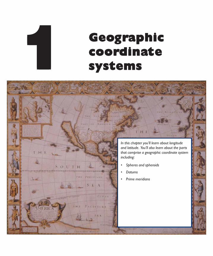
11111 GeoGeoGeoGeoGeogrgrgrgrgraphicaphicaphicaphicaphiccoorcoorcoorcoorcoordinadinadinadinadinatetetetetesystemssystemssystemssystemssystems
In this chapter you’ll learn about longitudeand latitude. You’ll also learn about the partsthat comprise a geographic coordinate systemincluding:
• Spheres and spheroids
• Datums
• Prime meridians
2 • Understanding Map Projections
GEOGRAPHIC COORDINATE SYSTEMS
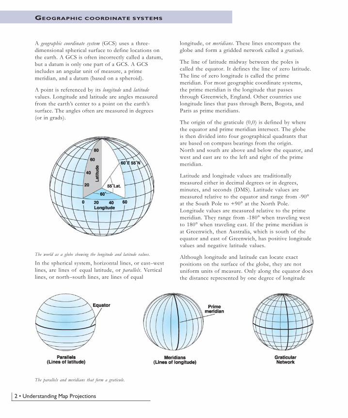
A geographic coordinate system (GCS) uses a three-dimensional spherical surface to define locations onthe earth. A GCS is often incorrectly called a datum,but a datum is only one part of a GCS. A GCSincludes an angular unit of measure, a primemeridian, and a datum (based on a spheroid).
A point is referenced by its longitude and latitudevalues. Longitude and latitude are angles measuredfrom the earth’s center to a point on the earth’ssurface. The angles often are measured in degrees(or in grads).
The world as a globe showing the longitude and latitude values.
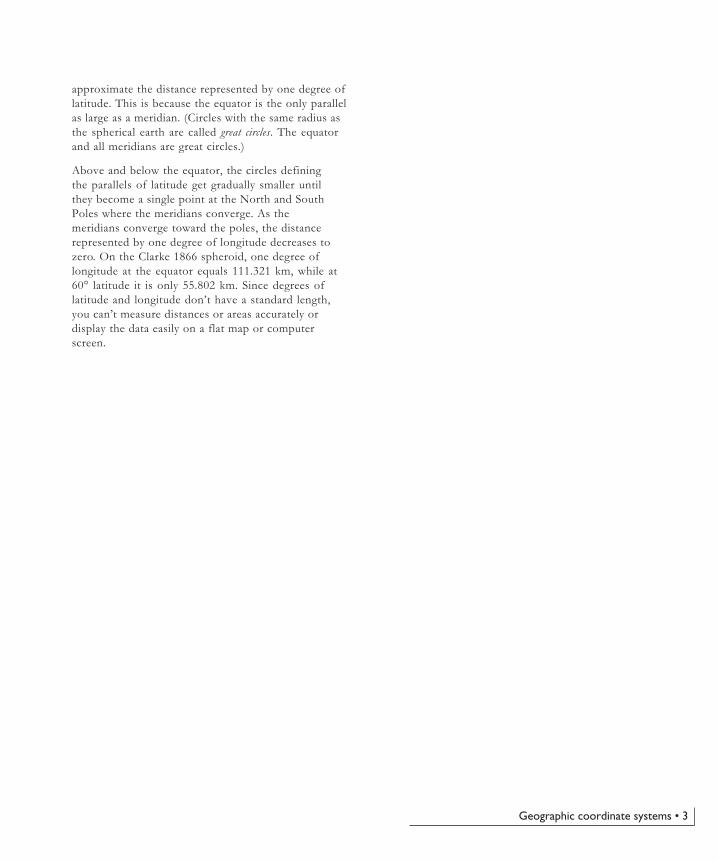
In the spherical system, horizontal lines, or east–westlines, are lines of equal latitude, or parallels. Verticallines, or north–south lines, are lines of equal
longitude, or meridians. These lines encompass theglobe and form a gridded network called a graticule.
The line of latitude midway between the poles iscalled the equator. It defines the line of zero latitude.The line of zero longitude is called the primemeridian. For most geographic coordinate systems,the prime meridian is the longitude that passesthrough Greenwich, England. Other countries uselongitude lines that pass through Bern, Bogota, andParis as prime meridians.
The origin of the graticule (0,0) is defined by wherethe equator and prime meridian intersect. The globeis then divided into four geographical quadrants thatare based on compass bearings from the origin.North and south are above and below the equator, andwest and east are to the left and right of the primemeridian.
Latitude and longitude values are traditionallymeasured either in decimal degrees or in degrees,minutes, and seconds (DMS). Latitude values aremeasured relative to the equator and range from -90°at the South Pole to +90° at the North Pole.Longitude values are measured relative to the primemeridian. They range from -180° when traveling westto 180° when traveling east. If the prime meridian isat Greenwich, then Australia, which is south of theequator and east of Greenwich, has positive longitudevalues and negative latitude values.
Although longitude and latitude can locate exactpositions on the surface of the globe, they are notuniform units of measure. Only along the equator doesthe distance represented by one degree of longitude
The parallels and meridians that form a graticule.
Geographic coordinate systems • 3
approximate the distance represented by one degree oflatitude. This is because the equator is the only parallelas large as a meridian. (Circles with the same radius asthe spherical earth are called great circles. The equatorand all meridians are great circles.)
Above and below the equator, the circles definingthe parallels of latitude get gradually smaller untilthey become a single point at the North and SouthPoles where the meridians converge. As themeridians converge toward the poles, the distancerepresented by one degree of longitude decreases tozero. On the Clarke 1866 spheroid, one degree oflongitude at the equator equals 111.321 km, while at60° latitude it is only 55.802 km. Since degrees oflatitude and longitude don’t have a standard length,you can’t measure distances or areas accurately ordisplay the data easily on a flat map or computerscreen.
4 • Understanding Map Projections
SPHEROIDS AND SPHERES
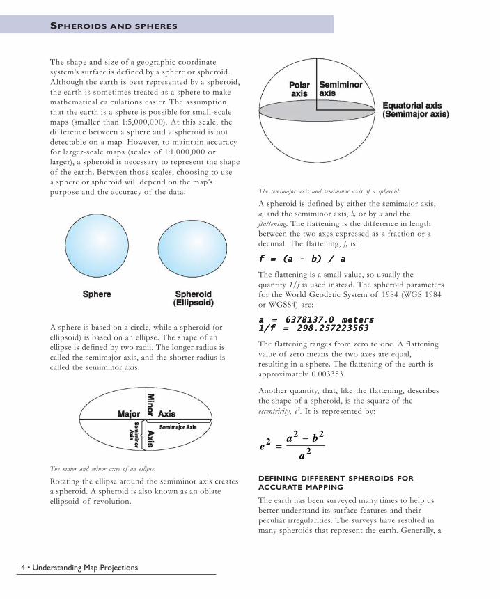
The shape and size of a geographic coordinatesystem’s surface is defined by a sphere or spheroid.Although the earth is best represented by a spheroid,the earth is sometimes treated as a sphere to makemathematical calculations easier. The assumptionthat the earth is a sphere is possible for small-scalemaps (smaller than 1:5,000,000). At this scale, thedifference between a sphere and a spheroid is notdetectable on a map. However, to maintain accuracyfor larger-scale maps (scales of 1:1,000,000 orlarger), a spheroid is necessary to represent the shapeof the earth. Between those scales, choosing to usea sphere or spheroid will depend on the map’spurpose and the accuracy of the data.
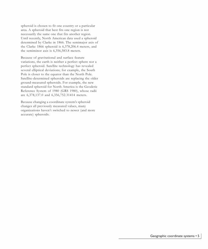
A sphere is based on a circle, while a spheroid (orellipsoid) is based on an ellipse. The shape of anellipse is defined by two radii. The longer radius iscalled the semimajor axis, and the shorter radius iscalled the semiminor axis.
The major and minor axes of an ellipse.
Rotating the ellipse around the semiminor axis createsa spheroid. A spheroid is also known as an oblateellipsoid of revolution.
The semimajor axis and semiminor axis of a spheroid.
A spheroid is defined by either the semimajor axis,a, and the semiminor axis, b, or by a and theflattening. The flattening is the difference in lengthbetween the two axes expressed as a fraction or adecimal. The flattening, f, is:
f = (a - b) / af = (a - b) / af = (a - b) / af = (a - b) / af = (a - b) / a
The flattening is a small value, so usually thequantity 1/f is used instead. The spheroid parametersfor the World Geodetic System of 1984 (WGS 1984or WGS84) are:
a = 6378137.0 metersa = 6378137.0 metersa = 6378137.0 metersa = 6378137.0 metersa = 6378137.0 meters1/f = 298.2572235631/f = 298.2572235631/f = 298.2572235631/f = 298.2572235631/f = 298.257223563
The flattening ranges from zero to one. A flatteningvalue of zero means the two axes are equal,resulting in a sphere. The flattening of the earth isapproximately 0.003353.
Another quantity, that, like the flattening, describesthe shape of a spheroid, is the square of theeccentricity, e2. It is represented by:
ea b
a2
2 2
2=−
DEFINING DIFFERENT SPHEROIDS FORACCURATE MAPPING
The earth has been surveyed many times to help usbetter understand its surface features and theirpeculiar irregularities. The surveys have resulted inmany spheroids that represent the earth. Generally, a
Geographic coordinate systems • 5
spheroid is chosen to fit one country or a particulararea. A spheroid that best fits one region is notnecessarily the same one that fits another region.Until recently, North American data used a spheroiddetermined by Clarke in 1866. The semimajor axis ofthe Clarke 1866 spheroid is 6,378,206.4 meters, andthe semiminor axis is 6,356,583.8 meters.
Because of gravitational and surface featurevariations, the earth is neither a perfect sphere nor aperfect spheroid. Satellite technology has revealedseveral elliptical deviations; for example, the SouthPole is closer to the equator than the North Pole.Satellite-determined spheroids are replacing the olderground-measured spheroids. For example, the newstandard spheroid for North America is the GeodeticReference System of 1980 (GRS 1980), whose radiiare 6,378,137.0 and 6,356,752.31414 meters.
Because changing a coordinate system’s spheroidchanges all previously measured values, manyorganizations haven’t switched to newer (and moreaccurate) spheroids.
6 • Understanding Map Projections
DATUMS
While a spheroid approximates the shape of theearth, a datum defines the position of the spheroidrelative to the center of the earth. A datum providesa frame of reference for measuring locations on thesurface of the earth. It defines the origin andorientation of latitude and longitude lines.
Whenever you change the datum, or more correctly,the geographic coordinate system, the coordinatevalues of your data will change. Here’s the coordinates in DMS of a control point in Redlands,California, on the North American Datum of 1983(NAD 1983 or NAD83).
-117 12 57.75961 34 01 43.77884
Here’s the same point on the North American Datumof 1927 (NAD 1927 or NAD27).
-117 12 54.61539 34 01 43.72995
The longitude value differs by about three seconds,while the latitude value differs by about0.05 seconds.
In the last 15 years, satellite data has providedgeodesists with new measurements to define thebest earth-fitting spheroid, which relates coordinatesto the earth’s center of mass. An earth-centered, orgeocentric, datum uses the earth’s center of mass asthe origin. The most recently developed and widelyused datum is WGS 1984. It serves as the frameworkfor locational measurement worldwide.
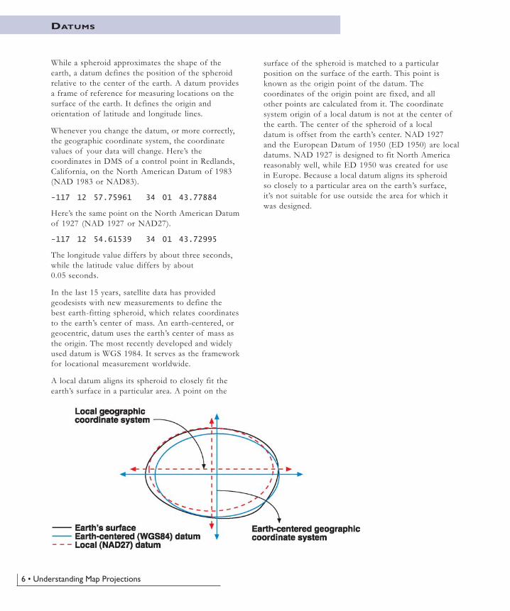
A local datum aligns its spheroid to closely fit theearth’s surface in a particular area. A point on the
surface of the spheroid is matched to a particularposition on the surface of the earth. This point isknown as the origin point of the datum. Thecoordinates of the origin point are fixed, and allother points are calculated from it. The coordinatesystem origin of a local datum is not at the center ofthe earth. The center of the spheroid of a localdatum is offset from the earth’s center. NAD 1927and the European Datum of 1950 (ED 1950) are localdatums. NAD 1927 is designed to fit North Americareasonably well, while ED 1950 was created for usein Europe. Because a local datum aligns its spheroidso closely to a particular area on the earth’s surface,it’s not suitable for use outside the area for which itwas designed.
Geographic Coordinate Systems • 7
The two horizontal datums used almost exclusivelyin North America are NAD 1927 and NAD 1983.
NAD 1927
NAD 1927 uses the Clarke 1866 spheroid torepresent the shape of the earth. The origin of thisdatum is a point on the earth referred to as MeadesRanch in Kansas. Many NAD 1927 control pointswere calculated from observations taken in the1800s. These calculations were done manually and insections over many years. Therefore, errors variedfrom station to station.
NAD 1983
Many technological advances in surveying andgeodesy—electronic theodolites, Global PositioningSystem (GPS) satellites, Very Long BaselineInterferometry, and Doppler systems—revealedweaknesses in the existing network of control points.Differences became particularly noticeable whenlinking existing control with newly establishedsurveys. The establishment of a new datum alloweda single datum to cover consistently North Americaand surrounding areas.
The North American Datum of 1983 is based on bothearth and satellite observations, using the GRS 1980spheroid. The origin for this datum is the earth’scenter of mass. This affects the surface location of alllongitude–latitude values enough to cause locationsof previous control points in North America to shift,sometimes as much as 500 feet. A 10-yearmultinational effort tied together a network ofcontrol points for the United States, Canada, Mexico,Greenland, Central America, and the Caribbean.
The GRS 1980 spheroid is almost identical to theWGS 1984 spheroid. The WGS 1984 and NAD 1983coordinate systems are both earth-centered. Becauseboth are so close, NAD 1983 is compatible with GPSdata. The raw GPS data is actually reported in theWGS 1984 coordinate system.
HARN OR HPGN
There is an ongoing effort at the state level toreadjust the NAD 1983 datum to a higher level ofaccuracy using state-of-the-art surveying techniquesthat were not widely available when the NAD 1983datum was being developed. This effort, known as
NORTH AMERICAN DATUMS
the High Accuracy Reference Network (HARN), orHigh Precision Geodetic Network (HPGN), is acooperative project between the National GeodeticSurvey and the individual states.
Currently, all states have been resurveyed, but not allof the data has been released to the public. As ofSeptember 2000, the grids for 44 states and twoterritories have been published.
OTHER UNITED STATES DATUMS
Alaska, Hawaii, Puerto Rico and the Virgin Islands,and some Alaskan islands have used other datumsbesides NAD 1927. See Chapter 3, ‘Geographictransformations’, for more information. New data isreferenced to NAD 1983.

9
22222 PrPrPrPrProjectedojectedojectedojectedojectedcoorcoorcoorcoorcoordinadinadinadinadinatetetetetesystemssystemssystemssystemssystems
Projected coordinate systems are anycoordinate system designed for a flat surface,such as a printed map or a computer screen.Topics in this chapter include:
• Characteristics and types of mapprojection
• Different parameter types
• Customizing a map projection through itsparameters
• Common projected coordinate systems
10 • Understanding Map Projections
PROJECTED COORDINATE SYSTEMS
A projected coordinate system is defined on a flat, two-dimensional surface. Unlike a geographic coordinatesystem, a projected coordinate system has constant lengths,angles, and areas across the two dimensions. A projectedcoordinate system is always based on a geographiccoordinate system that is based on a sphere or spheroid.
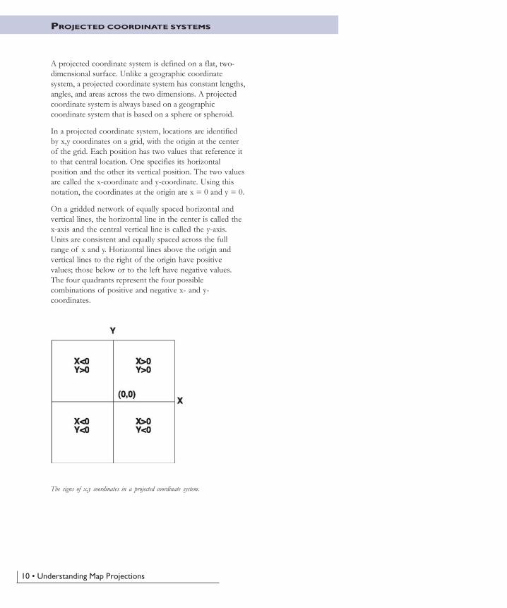
In a projected coordinate system, locations are identifiedby x,y coordinates on a grid, with the origin at the centerof the grid. Each position has two values that reference itto that central location. One specifies its horizontalposition and the other its vertical position. The two valuesare called the x-coordinate and y-coordinate. Using thisnotation, the coordinates at the origin are x = 0 and y = 0.
On a gridded network of equally spaced horizontal andvertical lines, the horizontal line in the center is called thex-axis and the central vertical line is called the y-axis.Units are consistent and equally spaced across the fullrange of x and y. Horizontal lines above the origin andvertical lines to the right of the origin have positivevalues; those below or to the left have negative values.The four quadrants represent the four possiblecombinations of positive and negative x- and y-coordinates.
The signs of x,y coordinates in a projected coordinate system.
Projected coordinate systems • 11
WHAT IS A MAP PROJECTION?
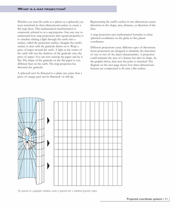
Whether you treat the earth as a sphere or a spheroid, youmust transform its three-dimensional surface to create aflat map sheet. This mathematical transformation iscommonly referred to as a map projection. One easy way tounderstand how map projections alter spatial properties isto visualize shining a light through the earth onto asurface, called the projection surface. Imagine the earth’ssurface is clear with the graticule drawn on it. Wrap apiece of paper around the earth. A light at the center ofthe earth will cast the shadows of the graticule onto thepiece of paper. You can now unwrap the paper and lay itflat. The shape of the graticule on the flat paper is verydifferent than on the earth. The map projection hasdistorted the graticule.
A spheroid can’t be flattened to a plane any easier than apiece of orange peel can be flattened—it will rip.
Representing the earth’s surface in two dimensions causesdistortion in the shape, area, distance, or direction of thedata.
A map projection uses mathematical formulas to relatespherical coordinates on the globe to flat, planarcoordinates.
Different projections cause different types of distortions.Some projections are designed to minimize the distortionof one or two of the data’s characteristics. A projectioncould maintain the area of a feature but alter its shape. Inthe graphic below, data near the poles is stretched. Thediagram on the next page shows how three-dimensionalfeatures are compressed to fit onto a flat surface.
The graticule of a geographic coordinate system is projected onto a cylindrical projection surface.
12 • Understanding Map Projections
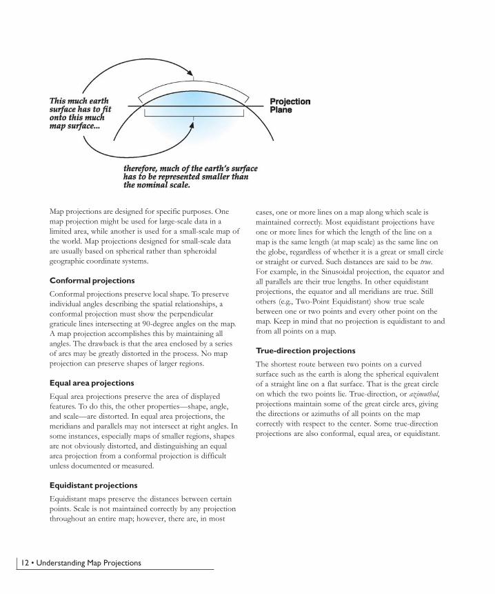
Map projections are designed for specific purposes. Onemap projection might be used for large-scale data in alimited area, while another is used for a small-scale map ofthe world. Map projections designed for small-scale dataare usually based on spherical rather than spheroidalgeographic coordinate systems.
Conformal projections
Conformal projections preserve local shape. To preserveindividual angles describing the spatial relationships, aconformal projection must show the perpendiculargraticule lines intersecting at 90-degree angles on the map.A map projection accomplishes this by maintaining allangles. The drawback is that the area enclosed by a seriesof arcs may be greatly distorted in the process. No mapprojection can preserve shapes of larger regions.
Equal area projections
Equal area projections preserve the area of displayedfeatures. To do this, the other properties—shape, angle,and scale—are distorted. In equal area projections, themeridians and parallels may not intersect at right angles. Insome instances, especially maps of smaller regions, shapesare not obviously distorted, and distinguishing an equalarea projection from a conformal projection is difficultunless documented or measured.
Equidistant projections
Equidistant maps preserve the distances between certainpoints. Scale is not maintained correctly by any projectionthroughout an entire map; however, there are, in most
cases, one or more lines on a map along which scale ismaintained correctly. Most equidistant projections haveone or more lines for which the length of the line on amap is the same length (at map scale) as the same line onthe globe, regardless of whether it is a great or small circleor straight or curved. Such distances are said to be true.For example, in the Sinusoidal projection, the equator andall parallels are their true lengths. In other equidistantprojections, the equator and all meridians are true. Stillothers (e.g., Two-Point Equidistant) show true scalebetween one or two points and every other point on themap. Keep in mind that no projection is equidistant to andfrom all points on a map.
True-direction projections
The shortest route between two points on a curvedsurface such as the earth is along the spherical equivalentof a straight line on a flat surface. That is the great circleon which the two points lie. True-direction, or azimuthal,projections maintain some of the great circle arcs, givingthe directions or azimuths of all points on the mapcorrectly with respect to the center. Some true-directionprojections are also conformal, equal area, or equidistant.
Projected coordinate systems • 13
PROJECTION TYPES
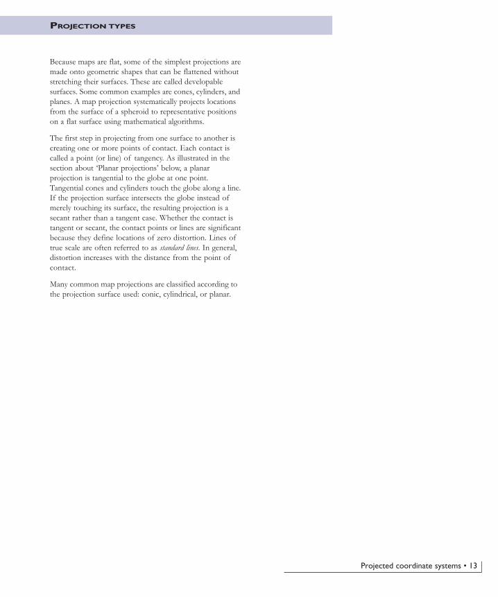
Because maps are flat, some of the simplest projections aremade onto geometric shapes that can be flattened withoutstretching their surfaces. These are called developablesurfaces. Some common examples are cones, cylinders, andplanes. A map projection systematically projects locationsfrom the surface of a spheroid to representative positionson a flat surface using mathematical algorithms.
The first step in projecting from one surface to another iscreating one or more points of contact. Each contact iscalled a point (or line) of tangency. As illustrated in thesection about ‘Planar projections’ below, a planarprojection is tangential to the globe at one point.Tangential cones and cylinders touch the globe along a line.If the projection surface intersects the globe instead ofmerely touching its surface, the resulting projection is asecant rather than a tangent case. Whether the contact istangent or secant, the contact points or lines are significantbecause they define locations of zero distortion. Lines oftrue scale are often referred to as standard lines. In general,distortion increases with the distance from the point ofcontact.
Many common map projections are classified according tothe projection surface used: conic, cylindrical, or planar.
14 • Understanding Map Projections
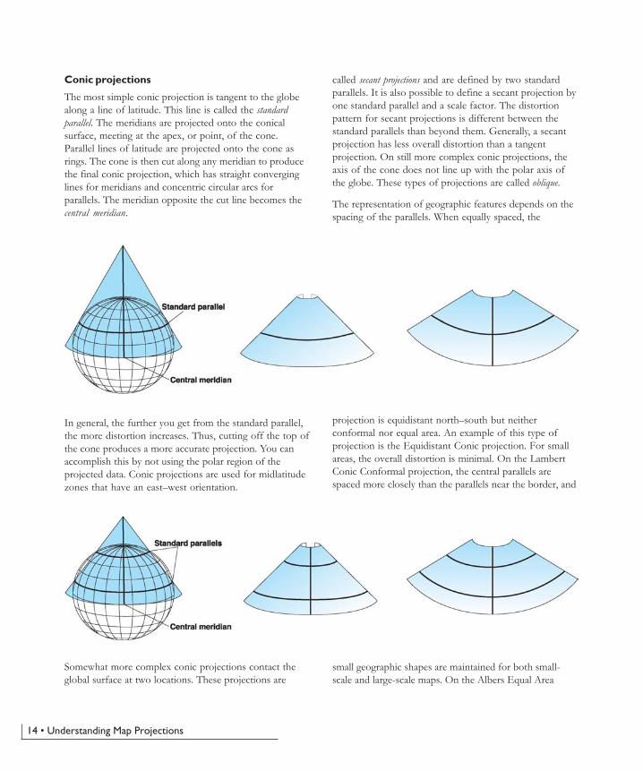
Conic projections
The most simple conic projection is tangent to the globealong a line of latitude. This line is called the standardparallel. The meridians are projected onto the conicalsurface, meeting at the apex, or point, of the cone.Parallel lines of latitude are projected onto the cone asrings. The cone is then cut along any meridian to producethe final conic projection, which has straight converginglines for meridians and concentric circular arcs forparallels. The meridian opposite the cut line becomes thecentral meridian.
In general, the further you get from the standard parallel,the more distortion increases. Thus, cutting off the top ofthe cone produces a more accurate projection. You canaccomplish this by not using the polar region of theprojected data. Conic projections are used for midlatitudezones that have an east–west orientation.
Somewhat more complex conic projections contact theglobal surface at two locations. These projections are
called secant projections and are defined by two standardparallels. It is also possible to define a secant projection byone standard parallel and a scale factor. The distortionpattern for secant projections is different between thestandard parallels than beyond them. Generally, a secantprojection has less overall distortion than a tangentprojection. On still more complex conic projections, theaxis of the cone does not line up with the polar axis ofthe globe. These types of projections are called oblique.
The representation of geographic features depends on thespacing of the parallels. When equally spaced, the
projection is equidistant north–south but neitherconformal nor equal area. An example of this type ofprojection is the Equidistant Conic projection. For smallareas, the overall distortion is minimal. On the LambertConic Conformal projection, the central parallels arespaced more closely than the parallels near the border, and
small geographic shapes are maintained for both small-scale and large-scale maps. On the Albers Equal Area
Projected coordinate systems • 15
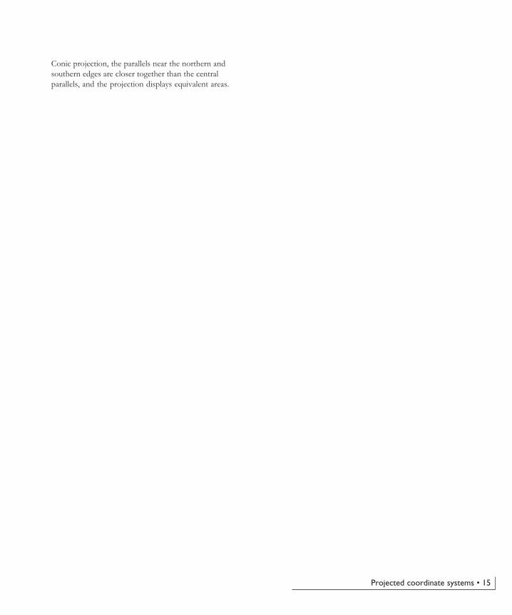
Conic projection, the parallels near the northern andsouthern edges are closer together than the centralparallels, and the projection displays equivalent areas.
16 • Understanding Map Projections
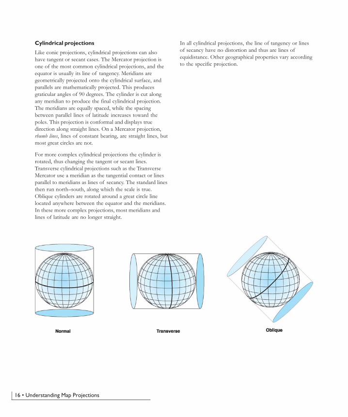
Cylindrical projections
Like conic projections, cylindrical projections can alsohave tangent or secant cases. The Mercator projection isone of the most common cylindrical projections, and theequator is usually its line of tangency. Meridians aregeometrically projected onto the cylindrical surface, andparallels are mathematically projected. This producesgraticular angles of 90 degrees. The cylinder is cut alongany meridian to produce the final cylindrical projection.The meridians are equally spaced, while the spacingbetween parallel lines of latitude increases toward thepoles. This projection is conformal and displays truedirection along straight lines. On a Mercator projection,rhumb lines, lines of constant bearing, are straight lines, butmost great circles are not.
For more complex cylindrical projections the cylinder isrotated, thus changing the tangent or secant lines.Transverse cylindrical projections such as the TransverseMercator use a meridian as the tangential contact or linesparallel to meridians as lines of secancy. The standard linesthen run north–south, along which the scale is true.Oblique cylinders are rotated around a great circle linelocated anywhere between the equator and the meridians.In these more complex projections, most meridians andlines of latitude are no longer straight.
In all cylindrical projections, the line of tangency or linesof secancy have no distortion and thus are lines ofequidistance. Other geographical properties vary accordingto the specific projection.
Projected coordinate systems • 17
Planar projections
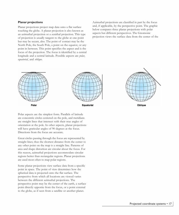
Planar projections project map data onto a flat surfacetouching the globe. A planar projection is also known asan azimuthal projection or a zenithal projection. This typeof projection is usually tangent to the globe at one pointbut may be secant, also. The point of contact may be theNorth Pole, the South Pole, a point on the equator, or anypoint in between. This point specifies the aspect and is thefocus of the projection. The focus is identified by a centrallongitude and a central latitude. Possible aspects are polar,equatorial, and oblique.
Polar aspects are the simplest form. Parallels of latitudeare concentric circles centered on the pole, and meridiansare straight lines that intersect with their true angles oforientation at the pole. In other aspects, planar projectionswill have graticular angles of 90 degrees at the focus.Directions from the focus are accurate.
Great circles passing through the focus are represented bystraight lines; thus the shortest distance from the center toany other point on the map is a straight line. Patterns ofarea and shape distortion are circular about the focus. Forthis reason, azimuthal projections accommodate circularregions better than rectangular regions. Planar projectionsare used most often to map polar regions.
Some planar projections view surface data from a specificpoint in space. The point of view determines how thespherical data is projected onto the flat surface. Theperspective from which all locations are viewed variesbetween the different azimuthal projections. Theperspective point may be the center of the earth, a surfacepoint directly opposite from the focus, or a point externalto the globe, as if seen from a satellite or another planet.
Azimuthal projections are classified in part by the focusand, if applicable, by the perspective point. The graphicbelow compares three planar projections with polaraspects but different perspectives. The Gnomonicprojection views the surface data from the center of the
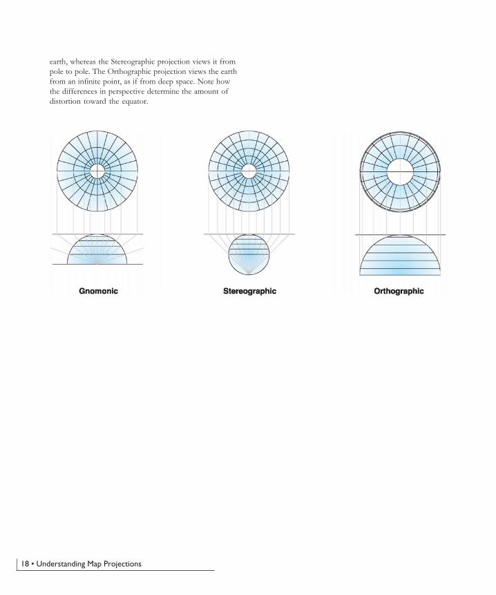
18 • Understanding Map Projections
earth, whereas the Stereographic projection views it frompole to pole. The Orthographic projection views the earthfrom an infinite point, as if from deep space. Note howthe differences in perspective determine the amount ofdistortion toward the equator.
Projected coordinate systems • 19
The projections discussed previously are conceptuallycreated by projecting from one geometric shape (a sphere)onto another (a cone, cylinder, or plane). Many projectionsare not related as easily to a cone, cylinder, or plane.
Modified projections are altered versions of otherprojections (e.g., the Space Oblique Mercator is amodification of the Mercator projection). Thesemodifications are made to reduce distortion, often byincluding additional standard lines or changing thedistortion pattern.
Pseudo projections have some of the characteristics ofanother class of projection. For example, the Sinusoidal iscalled a pseudocylindrical projection because all lines oflatitude are straight and parallel and all meridians areequally spaced. However, it is not truly a cylindricalprojection because all meridians except the centralmeridian are curved. This results in a map of the earthhaving an oval shape instead of a rectangular shape.
Other projections are assigned to special groups, such ascircular or star.
OTHER PROJECTIONS
20 • Understanding Map Projections
PROJECTION PARAMETERS
A map projection by itself isn’t enough to define aprojected coordinate system. You can state that a dataset isin Transverse Mercator, but that’s not enough information.Where is the center of the projection? Was a scale factorused? Without knowing the exact values for the projectionparameters, the dataset can’t be reprojected.
You can also get some idea of the amount of distortionthe projection has added to the data. If you’re interestedin Australia but you know that a dataset’s projection iscentered at 0,0, the intersection of the equator and theGreenwich prime meridian, you might want to thinkabout changing the center of the projection.
Each map projection has a set of parameters that youmust define. The parameters specify the origin andcustomize a projection for your area of interest. Angularparameters use the geographic coordinate system units,while linear parameters use the projected coordinatesystem units.
Linear parameters
False easting—A linear value applied to the origin of thex-coordinates.
False northing—A linear value applied to the origin of they-coordinates.
False easting and northing values are usually applied toensure that all x or y values are positive. You can also usethe false easting and northing parameters to reduce therange of the x- or y-coordinate values. For example, ifyou know all y values are greater than five million meters,you could apply a false northing of -5,000,000.
Height—Defines the point of perspective above thesurface of the sphere or spheroid for the Vertical Near-side Perspective projection.
Angular parameters
Azimuth—Defines the center line of a projection. Therotation angle measures east from north. Used with theAzimuth cases of the Hotine Oblique Mercatorprojection.
Central meridian—Defines the origin of thex-coordinates.
Longitude of origin—Defines the origin of thex-coordinates. The central meridian and longitude oforigin parameters are synonymous.
Central parallel—Defines the origin of they-coordinates.
Latitude of origin—Defines the origin of they-coordinates. This parameter may not be located at thecenter of the projection. In particular, conic projectionsuse this parameter to set the origin of the y-coordinatesbelow the area of the interest. In that instance, you don'tneed to set a false northing parameter to ensure that all y-coordinates are positive.
Longitude of center—Used with the Hotine ObliqueMercator Center (both Two-Point and Azimuth) cases todefine the origin of the x-coordinates. Usuallysynonymous with the longitude of origin and centralmeridian parameters.
Latitude of center—Used with the Hotine ObliqueMercator Center (both Two-Point and Azimuth) cases todefine the origin of the y-coordinates. It is almost alwaysthe center of the projection.
Standard parallel 1 and standard parallel 2—Used withconic projections to define the latitude lines where thescale is 1.0. When defining a Lambert Conformal Conicprojection with one standard parallel, the first standardparallel defines the origin of the y-coordinates.
For other conic cases, the y-coordinate origin is defined bythe latitude of origin parameter.
Longitude of first pointLatitude of first pointLongitude of second pointLatitude of second point
The four parameters above are used with the Two-PointEquidistant and Hotine Oblique Mercator projections.They specify two geographic points that define the centeraxis of a projection.
Pseudo standard parallel 1—Used in the Krovakprojection to define the oblique cone’s standard parallel.
XY plane rotation—Along with the X scale and Y scaleparameters, defines the orientation of the Krovakprojection.
Projected coordinate systems • 21
Unitless parameters
Scale factor—A unitless value applied to the center pointor line of a map projection.
The scale factor is usually slightly less than one. The UTMcoordinate system, which uses the Transverse Mercatorprojection, has a scale factor of 0.9996. Rather than 1.0,the scale along the central meridian of the projection is0.9996. This creates two almost parallel linesapproximately 180 kilometers away, where the scale is 1.0.The scale factor reduces the overall distortion of theprojection in the area of interest.
X scale—Used in the Krovak projection to orient theaxes.
Y scale—Used in the Krovak projection to orient theaxes.
Option—Used in the Cube and Fuller projections. In theCube projection, option defines the location of the polarfacets. An option of 0 in the Fuller projection will displayall 20 facets. Specifying an option value between 1–20will display a single facet.

23
33333 GeoGeoGeoGeoGeogrgrgrgrgraphicaphicaphicaphicaphictrtrtrtrtransfansfansfansfansformaormaormaormaormationstionstionstionstions
This chapter discusses the various datumtransformation methods including:
• Geocentric Translation
• Coordinate Frame and Position Vector
• Molodensky and Abridged Molodensky
• NADCON and HARN
• National Transformation version 2 (NTv2)
24 • Understanding Map Projections
GEOGRAPHIC TRANSFORMATION METHODS
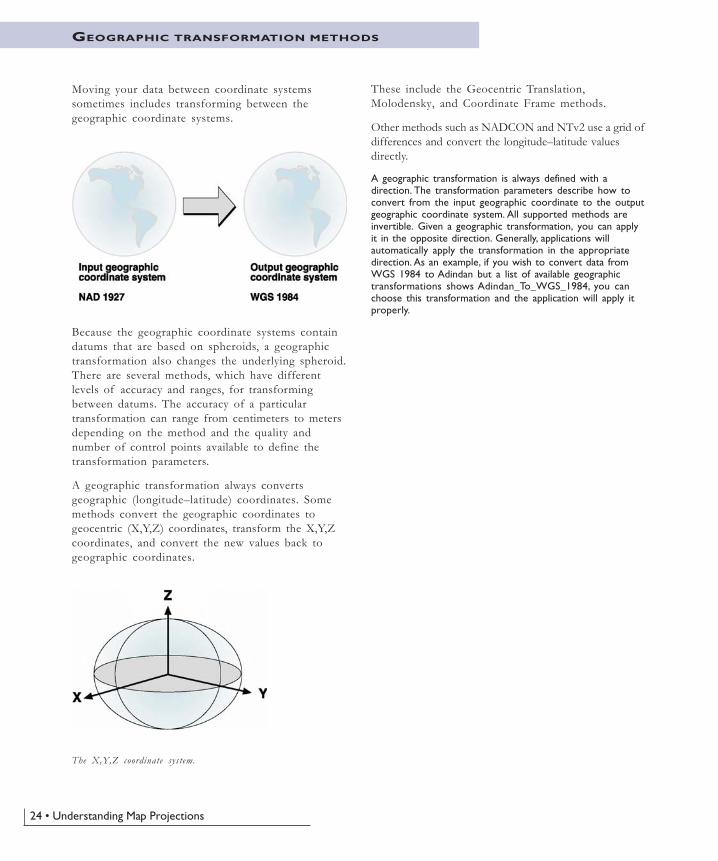
Moving your data between coordinate systemssometimes includes transforming between thegeographic coordinate systems.
Because the geographic coordinate systems containdatums that are based on spheroids, a geographictransformation also changes the underlying spheroid.There are several methods, which have differentlevels of accuracy and ranges, for transformingbetween datums. The accuracy of a particulartransformation can range from centimeters to metersdepending on the method and the quality andnumber of control points available to define thetransformation parameters.
A geographic transformation always convertsgeographic (longitude–latitude) coordinates. Somemethods convert the geographic coordinates togeocentric (X,Y,Z) coordinates, transform the X,Y,Zcoordinates, and convert the new values back togeographic coordinates.
The X,Y,Z coordinate system.
These include the Geocentric Translation,Molodensky, and Coordinate Frame methods.
Other methods such as NADCON and NTv2 use a grid ofdifferences and convert the longitude–latitude valuesdirectly.
A geographic transformation is always defined with adirection. The transformation parameters describe how toconvert from the input geographic coordinate to the outputgeographic coordinate system. All supported methods areinvertible. Given a geographic transformation, you can applyit in the opposite direction. Generally, applications willautomatically apply the transformation in the appropriatedirection. As an example, if you wish to convert data fromWGS 1984 to Adindan but a list of available geographictransformations shows Adindan_To_WGS_1984, you canchoose this transformation and the application will apply itproperly.
Geographic transformations • 25
EQUATION-BASED METHODS
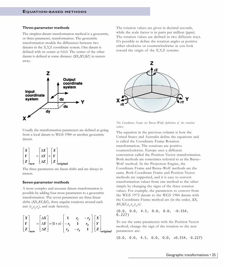
Three-parameter methods
The simplest datum transformation method is a geocentric,or three-parameter, transformation. The geocentrictransformation models the differences between twodatums in the X,Y,Z coordinate system. One datum isdefined with its center at 0,0,0. The center of the otherdatum is defined at some distance (∆X,∆Y,∆Z) in metersaway.
Usually the transformation parameters are defined as goingfrom a local datum to WGS 1984 or another geocentricdatum.
The three parameters are linear shifts and are always inmeters.
Seven-parameter methods
A more complex and accurate datum transformation ispossible by adding four more parameters to a geocentrictransformation. The seven parameters are three linearshifts (∆X,∆Y,∆Z), three angular rotations around eachaxis (rx,ry,rz), and scale factor(s).
( )X
Y
Z
X
Y
Z
s
r r
r r
r r
X
Y
Znew
z y
z x
y x original
�
�
���
�
�
���
=�
�
���
�
�
���
+ + ⋅−
−−
�
�
���
�
�
���
⋅�
�
���
�
�
���
∆∆∆
1
1
1
1
The rotation values are given in decimal seconds,while the scale factor is in parts per million (ppm).The rotation values are defined in two different ways.It’s possible to define the rotation angles as positiveeither clockwise or counterclockwise as you looktoward the origin of the X,Y,Z systems.
The Coordinate Frame (or Bursa–Wolf) definition of the rotationvalues.
The equation in the previous column is how theUnited States and Australia define the equations andis called the Coordinate Frame Rotationtransformation. The rotations are positivecounterclockwise. Europe uses a differentconvention called the Position Vector transformation.Both methods are sometimes referred to as the Bursa–Wolf method. In the Projection Engine, theCoordinate Frame and Bursa–Wolf methods are thesame. Both Coordinate Frame and Position Vectormethods are supported, and it is easy to converttransformation values from one method to the othersimply by changing the signs of the three rotationvalues. For example, the parameters to convert fromthe WGS 1972 datum to the WGS 1984 datum withthe Coordinate Frame method are (in the order, ∆X,∆Y,∆Z,rx,ry,rz,s):
(0.0, 0.0, 4.5, 0.0, 0.0, -0.554,0.227)
To use the same parameters with the Position Vectormethod, change the sign of the rotation so the newparameters are:
(0.0, 0.0, 4.5, 0.0, 0.0, +0.554, 0.227)
X
Y
Z
X
Y
Z
X
Y
Znew original
�
�
���
�
�
���
=�
�
���
�
�
���
+�
�
���
�
�
���
∆∆∆
26 • Understanding Map Projections
Unless explicitly stated, it’s impossible to tell fromthe parameters alone which convention is beingused. If you use the wrong method, your results canreturn inaccurate coordinates. The only way todetermine how the parameters are defined is bychecking a control point whose coordinates areknown in the two systems.
Molodensky method
The Molodensky method converts directly betweentwo geographic coordinate systems without actuallyconverting to an X,Y,Z system. The Molodenskymethod requires three shifts (∆X,∆Y,∆Z) and thedifferences between the semimajor axes (∆a) and theflattenings (∆f) of the two spheroids. The ProjectionEngine automatically calculates the spheroiddifferences according to the datums involved.
fa
bN
b
aM
ae
eZ
YXhM
∆++
∆−
+∆+
∆−∆−=∆+
)(cossin
)sin1(
cossincos
sinsincossin)(
2/122
2
ϕϕ
ϕϕϕϕ
λϕλϕϕ
YXhN ∆+∆−=∆+ λλλϕ cossincos)(
fe
fa
aeZ
YXh
∆−
−+
∆−−∆+
∆+∆=∆
ϕϕ
ϕϕλϕλϕ
2
2/122
2/122
sin)sin1(
)1(
)sin1(sin
sincoscoscos
h ellipsoid height (meters)ϕ latitudeλ longitudea semimajor axis of the spheroid (meters)b semiminor axis of the spheroid (meters)f flattening of the spheroide eccentricity of the spheroid
M and N are the meridional and prime vertical radiiof curvature, respectively, at a given latitude. Theequations for M and N are:
2/322
2
)sin1(
)1(
ϕe
eaM
−−=
2/122 )sin1( ϕe
aN
−=
You solve for ∆λ and ∆ϕ. The amounts are addedautomatically by the Projection Engine.
Abridged Molodensky method
The Abridged Molodensky method is a simplifiedversion of the Molodensky method. The equationsare:
ϕϕϕλϕλϕϕ
cossin2)(cos
sinsincossin
⋅∆+∆+∆+∆−∆−=∆
affaZ
YXM
YXN ∆+∆−=∆ λλλϕ cossincos
aaffaZ
YXh
∆−∆+∆+∆+
∆+∆=∆
ϕϕλϕλϕ
2sin)(sin
sincoscoscos
Geographic transformations • 27
GRID-BASED METHODS
NADCON and HARN methods
The United States uses a grid-based method to convertbetween geographic coordinate systems. Grid-basedmethods allow you to model the differences between thesystems and are potentially the most accurate method. Thearea of interest is divided into cells. The NationalGeodetic Survey (NGS) publishes grids to convertbetween NAD 1927 and other older geographiccoordinate systems and NAD 1983. We group thesetransformations into the NADCON method. The mainNADCON grid, CONUS, converts the contiguous 48states. The other NADCON grids convert older geographiccoordinate systems to NAD 1983 for
• Alaska
• Hawaiian islands
• Puerto Rico and Virgin Islands
• St. George, St. Lawrence, and St. Paul Islands inAlaska
The accuracy is around 0.15 meters for thecontiguous states, 0.50 for Alaska and its islands,0.20 for Hawaii, and 0.05 for Puerto Rico and theVirgin Islands. Accuracies can vary depending onhow good the geodetic data in the area was whenthe grids were computed (NADCON, 1999).
The Hawaiian islands were never on NAD 1927.They were mapped using several datums that arecollectively known as the Old Hawaiian datums.
New surveying and satellite measuring techniques haveallowed NGS and the states to update the geodetic controlpoint networks. As each state is finished, the NGSpublishes a grid that converts between NAD 1983 and themore accurate control point coordinates. Originally, thiseffort was called the High Precision Geodetic Network(HPGN). It is now called the High Accuracy ReferenceNetwork (HARN). More than 40 states have publishedHARN grids as of September 2000. HARNtransformations have an accuracy around 0.05 meters(NADCON, 2000).
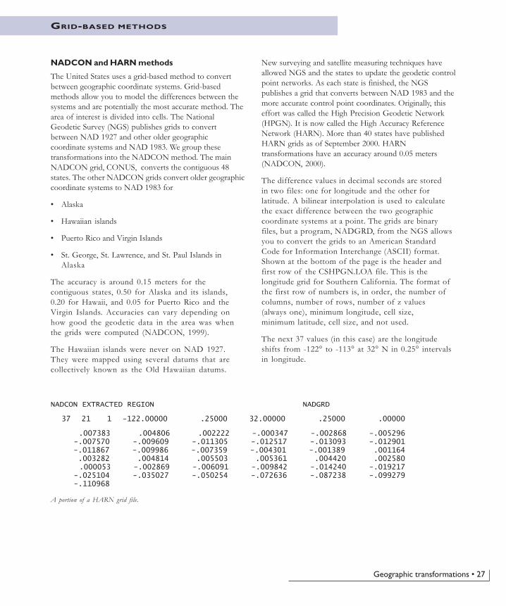
The difference values in decimal seconds are storedin two files: one for longitude and the other forlatitude. A bilinear interpolation is used to calculatethe exact difference between the two geographiccoordinate systems at a point. The grids are binaryfiles, but a program, NADGRD, from the NGS allowsyou to convert the grids to an American StandardCode for Information Interchange (ASCII) format.Shown at the bottom of the page is the header andfirst row of the CSHPGN.LOA file. This is thelongitude grid for Southern California. The format ofthe first row of numbers is, in order, the number ofcolumns, number of rows, number of z values(always one), minimum longitude, cell size,minimum latitude, cell size, and not used.
The next 37 values (in this case) are the longitudeshifts from -122° to -113° at 32° N in 0.25° intervalsin longitude.
NADCON EXTRACTED REGION NADGRD
37 21 1 -122.00000 .25000 32.00000 .25000 .00000
.007383 .004806 .002222 -.000347 -.002868 -.005296 -.007570 -.009609 -.011305 -.012517 -.013093 -.012901 -.011867 -.009986 -.007359 -.004301 -.001389 .001164 .003282 .004814 .005503 .005361 .004420 .002580 .000053 -.002869 -.006091 -.009842 -.014240 -.019217 -.025104 -.035027 -.050254 -.072636 -.087238 -.099279 -.110968
A portion of a HARN grid file.
28 • Understanding Map Projections
National Transformation version 2
Like the United States, Canada uses a grid-basedmethod to convert between NAD 1927 and NAD1983. The National Transformation version 2 (NTv2)method is quite similar to NADCON. A set of binaryfiles contains the differences between the twogeographic coordinate systems. A bilinearinterpolation is used to calculate the exact values fora point.
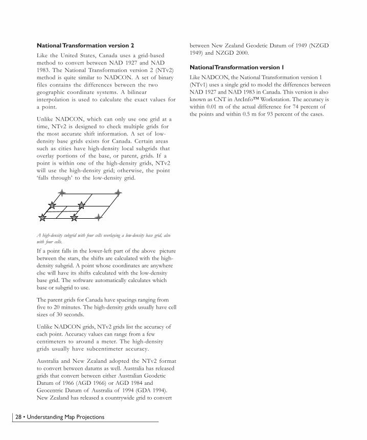
Unlike NADCON, which can only use one grid at atime, NTv2 is designed to check multiple grids forthe most accurate shift information. A set of low-density base grids exists for Canada. Certain areassuch as cities have high-density local subgrids thatoverlay portions of the base, or parent, grids. If apoint is within one of the high-density grids, NTv2will use the high-density grid; otherwise, the point‘falls through’ to the low-density grid.
A high-density subgrid with four cells overlaying a low-density base grid, alsowith four cells.
If a point falls in the lower-left part of the above picturebetween the stars, the shifts are calculated with the high-density subgrid. A point whose coordinates are anywhereelse will have its shifts calculated with the low-densitybase grid. The software automatically calculates whichbase or subgrid to use.
The parent grids for Canada have spacings ranging fromfive to 20 minutes. The high-density grids usually have cellsizes of 30 seconds.
Unlike NADCON grids, NTv2 grids list the accuracy ofeach point. Accuracy values can range from a fewcentimeters to around a meter. The high-densitygrids usually have subcentimeter accuracy.
Australia and New Zealand adopted the NTv2 formatto convert between datums as well. Australia has releasedgrids that convert between either Australian GeodeticDatum of 1966 (AGD 1966) or AGD 1984 andGeocentric Datum of Australia of 1994 (GDA 1994).New Zealand has released a countrywide grid to convert
between New Zealand Geodetic Datum of 1949 (NZGD1949) and NZGD 2000.
National Transformation version 1
Like NADCON, the National Transformation version 1(NTv1) uses a single grid to model the differences betweenNAD 1927 and NAD 1983 in Canada. This version is alsoknown as CNT in ArcInfo™ Workstation. The accuracy iswithin 0.01 m of the actual difference for 74 percent ofthe points and within 0.5 m for 93 percent of the cases.
29
A map projection converts data from theround earth onto a flat plane. Each mapprojection is designed for a specific purposeand distorts the data differently. This chapterwill describe each projection including:
• Method
• Linear graticules
• Limitations
• Uses and applications
• Parameters
44444 SupporSupporSupporSupporSupportedtedtedtedtedmapmapmapmapmapprprprprprojectionsojectionsojectionsojectionsojections
30 • Understanding Map Projections
LIST OF SUPPORTED MAP PROJECTIONS
Aitoff A compromise projection developed in 1889 and used for world maps.
Alaska Grid This projection was developed to provide a conformal map of Alaska withless scale distortion than other conformal projections.
Alaska Series E Developed in 1972 by the United States Geological Survey (USGS) topublish a map of Alaska at 1:2,500,000 scale.
Albers Equal Area Conic This conic projection uses two standard parallels to reduce some of thedistortion of a projection with one standard parallel. Shape and linear scaledistortion are minimized between the standard parallels.
Azimuthal Equidistant The most significant characteristic of this projection is that both distanceand direction are accurate from the central point.
Behrmann Equal Area Cylindrical This projection is an equal-area cylindrical projection suitable for worldmapping.
Bipolar Oblique Conformal Conic This projection was developed specifically for mapping North and SouthAmerica and maintains conformality.
Bonne This equal-area projection has true scale along the central meridian and allparallels.
Cassini–Soldner This transverse cylindrical projection maintains scale along the centralmeridian and all lines parallel to it. This projection is neither equal area norconformal.
Chamberlin Trimetric This projection was developed and used by the National Geographic Societyfor continental mapping. The distance from three input points to any otherpoint is approximately correct.
Craster Parabolic This pseudocylindrical equal-area projection is primarily used for thematicmaps of the world.
Cube Projects the world to a box that is then unfolded into a plane.
Cylindrical Equal Area Lambert first described this equal-area projection in 1772. It is usedinfrequently.
Double Stereographic This azimuthal projection is conformal.
Eckert I This pseudocylindrical projection is used primarily as a novelty map.
Eckert II A pseudocylindrical equal-area projection.
Eckert III This pseudocylindrical projection is used primarily for world maps.
Eckert IV This equal-area projection is used primarily for world maps.
Eckert V This pseudocylindrical projection is used primarily for world maps.
Eckert VI This equal-area projection is used primarily for world maps.
Supported map projections • 31
Equidistant Conic This conic projection can be based on one or two standard parallels. As thename implies, all circular parallels are spaced evenly along the meridians.
Equidistant Cylindrical One of the easiest projections to construct because it forms a grid of equalrectangles.
Equirectangular This projection is very simple to construct because it forms a grid of equalrectangles.
Fuller The Fuller projection was created by Buckminster Fuller in 1954. Using anicosahedron, the shape is flattened so that the land masses are notinterrupted.
Gall’s Stereographic The Gall’s Stereographic projection is a cylindrical projection designedaround 1855 with two standard parallels at latitudes 45° N and 45° S.
Gauss–Krüger This projection is similar to the Mercator except that the cylinder is tangentalong a meridian instead of the equator. The result is a conformal projectionthat does not maintain true directions.
Geocentric Coordinate System The geocentric coordinate system is not a map projection. The earth ismodeled as a sphere or spheroid in a right-handed X,Y,Z system.
Geographic Coordinate System The geographic coordinate system is not a map projection. The earth ismodeled as a sphere or spheroid.
Gnomonic This azimuthal projection uses the center of the earth as its perspectivepoint.
Great Britain National Grid This coordinate system uses a Transverse Mercator projected on the Airyspheroid. The central meridian is scaled to 0.9996. The origin is 49° N and2° W.
Hammer–Aitoff The Hammer–Aitoff projection is a modification of the Lambert AzimuthalEqual Area projection.
Hotine Oblique Mercator This is an oblique rotation of the Mercator projection. Developed forconformal mapping of areas that do not follow a north–south or east–westorientation but are obliquely oriented.
Krovak The Krovak projection is an oblique Lambert conformal conic projectiondesigned for the former Czechoslovakia.
Lambert Azimuthal Equal Area This projection preserves the area of individual polygons whilesimultaneously maintaining true directions from the center.
Lambert Conformal Conic This projection is one of the best for middle latitudes. It is similar to theAlbers Conic Equal Area projection except that the Lambert ConformalConic projection portrays shape more accurately than area.
Local Cartesian Projection This is a specialized map projection that does not take into account thecurvature of the earth.
32 • Understanding Map Projections
Loximuthal This projection shows loxodromes, or rhumb lines, as straight lines with thecorrect azimuth and scale from the intersection of the central meridian andthe central parallel.
McBryde–Thomas Flat-Polar Quartic This equal-area projection is primarily used for world maps.
Mercator Originally created to display accurate compass bearings for sea travel. Anadditional feature of this projection is that all local shapes are accurate andclearly defined.
Miller Cylindrical This projection is similar to the Mercator projection except that the polarregions are not as areally distorted.
Mollweide Carl B. Mollweide created this pseudocylindrical projection in 1805. It is anequal-area projection designed for small-scale maps.
New Zealand National Grid This is the standard projection for large-scale maps of New Zealand.
Orthographic This perspective projection views the globe from an infinite distance. Thisgives the illusion of a three-dimensional globe.
Perspective This projection is similar to the Orthographic projection in that itsperspective is from space. In this projection, the perspective point is not aninfinite distance away; instead, you can specify the distance.
Plate Carrée This projection is very simple to construct because it forms a grid of equalrectangles.
Polar Stereographic The projection is equivalent to the polar aspect of the Stereographicprojection on a spheroid. The central point is either the North Pole or theSouth Pole.
Polyconic The name of this projection translates into ‘many cones’ and refers to theprojection methodology.
Quartic Authalic This pseudocylindrical equal-area projection is primarily used for thematicmaps of the world.
Rectified Skewed Orthomorphic This oblique cylindrical projection is provided with two options for thenational coordinate systems of Malaysia and Brunei.
Robinson A compromise projection used for world maps.
Simple Conic This conic projection can be based on one or two standard parallels.
Sinusoidal As a world map, this projection maintains equal area despite conformaldistortion.
Space Oblique Mercator This projection is nearly conformal and has little scale distortion within thesensing range of an orbiting mapping satellite such as Landsat.
State Plane Coordinate System (SPCS) The State Plane Coordinate System is not a projection. It is a coordinatesystem that divides the 50 states of the United States, Puerto Rico, and theU.S. Virgin Islands into more than 120 numbered sections, referred to aszones.
Supported map projections • 33
Stereographic This azimuthal projection is conformal.
Times The Times projection was developed by Moir in 1965 for BartholomewLtd., a British mapmaking company. It is a modified Gall’s Stereographic,but the Times has curved meridians.
Transverse Mercator Similar to the Mercator except that the cylinder is tangent along a meridianinstead of the equator. The result is a conformal projection that does notmaintain true directions.
Two-Point Equidistant This modified planar projection shows the true distance from either of twochosen points to any other point on a map.
Universal Polar Stereographic (UPS) This form of the Polar Stereographic maps areas north of 84° N and southof 80° S that are not included in the UTM Coordinate System. Theprojection is equivalent to the polar aspect of the Stereographic projectionof the spheroid with specific parameters.
Universal Transverse Mercator (UTM) The Universal Transverse Mercator coordinate system is a specializedapplication of the Transverse Mercator projection. The globe is divided into60 zones, each spanning six degrees of longitude.
Van Der Grinten I This projection is similar to the Mercator projection except that it portraysthe world as a circle with a curved graticule.
Vertical Near-Side Perspective Unlike the Orthographic projection, this perspective projection views theglobe from a finite distance. This perspective gives the overall effect of theview from a satellite.
Winkel I A pseudocylindrical projection used for world maps that averages thecoordinates from the Equirectangular (Equidistant Cylindrical) andSinusoidal projections.
Winkel II A pseudocylindrical projection that averages the coordinates from theEquirectangular and Mollweide projections.
Winkel Tripel A compromise projection used for world maps that averages the coordinatesfrom the Equirectangular (Equidistant Cylindrical) and Aitoff projections.

34 • Understanding Map Projections
AITOFF
DESCRIPTION
A compromise projection developed in 1889 and for usewith world maps.
PROJECTION METHOD
Modified azimuthal. Meridians are equally spaced andconcave toward the central meridian. The central meridianis a straight line and half the length of the equator.Parallels are equally spaced curves, concave toward thepoles.
LINEAR GRATICULES
The equator and the central meridian.
PROPERTIES
Shape
Distortion is moderate.
Area
Moderate distortion.
Direction
Generally distorted.
Distance
The equator and central meridian are at true scale.
LIMITATIONS
Neither conformal nor equal area. Useful only for worldmaps.
The central meridian is 0°.
USES AND APPLICATIONS
Developed for use in general world maps.
Used for the Winkel Tripel projection.
Supported map projections • 35
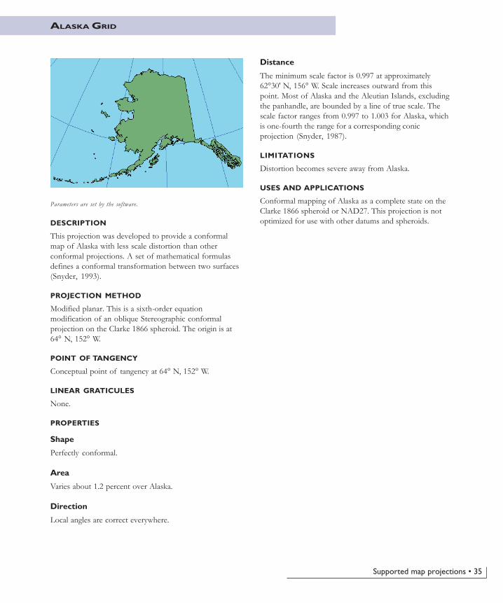
ALASKA GRID
DESCRIPTION
This projection was developed to provide a conformalmap of Alaska with less scale distortion than otherconformal projections. A set of mathematical formulasdefines a conformal transformation between two surfaces(Snyder, 1993).
PROJECTION METHOD
Modified planar. This is a sixth-order equationmodification of an oblique Stereographic conformalprojection on the Clarke 1866 spheroid. The origin is at64° N, 152° W.
POINT OF TANGENCY
Conceptual point of tangency at 64° N, 152° W.
LINEAR GRATICULES
None.
PROPERTIES
Shape
Perfectly conformal.
Area
Varies about 1.2 percent over Alaska.
Direction
Local angles are correct everywhere.
Distance
The minimum scale factor is 0.997 at approximately62°30' N, 156° W. Scale increases outward from thispoint. Most of Alaska and the Aleutian Islands, excludingthe panhandle, are bounded by a line of true scale. Thescale factor ranges from 0.997 to 1.003 for Alaska, whichis one-fourth the range for a corresponding conicprojection (Snyder, 1987).
LIMITATIONS
Distortion becomes severe away from Alaska.
USES AND APPLICATIONS
Conformal mapping of Alaska as a complete state on theClarke 1866 spheroid or NAD27. This projection is notoptimized for use with other datums and spheroids.
Parameters are set by the software.
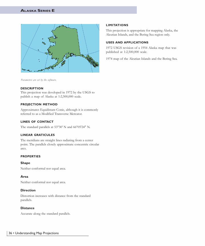
36 • Understanding Map Projections
DESCRIPTIONThis projection was developed in 1972 by the USGS topublish a map of Alaska at 1:2,500,000 scale.
PROJECTION METHOD
Approximates Equidistant Conic, although it is commonlyreferred to as a Modified Transverse Mercator.
LINES OF CONTACT
The standard parallels at 53°30' N and 66°05'24" N.
LINEAR GRATICULES
The meridians are straight lines radiating from a centerpoint. The parallels closely approximate concentric circulararcs.
PROPERTIES
Shape
Neither conformal nor equal area.
Area
Neither conformal nor equal area.
Direction
Distortion increases with distance from the standardparallels.
Distance
Accurate along the standard parallels.
ALASKA SERIES E
Parameters are set by the software.
LIMITATIONS
This projection is appropriate for mapping Alaska, theAleutian Islands, and the Bering Sea region only.
USES AND APPLICATIONS
1972 USGS revision of a 1954 Alaska map that waspublished at 1:2,500,000 scale.
1974 map of the Aleutian Islands and the Bering Sea.
Supported map projections • 37
ALBERS EQUAL AREA CONIC
DESCRIPTION
This conic projection uses two standard parallels to reducesome of the distortion of a projection with one standardparallel. Although neither shape nor linear scale is trulycorrect, the distortion of these properties is minimized inthe region between the standard parallels. This projectionis best suited for land masses extending in an east-to-westorientation rather than those lying north to south.
PROJECTION METHOD
Conic. The meridians are equally spaced straight linesconverging to a common point. Poles are represented asarcs rather than as single points. Parallels are unequallyspaced concentric circles whose spacing decreases towardthe poles.
LINES OF CONTACT
Two lines, the standard parallels, defined by degreeslatitude.
LINEAR GRATICULES
All meridians.
PROPERTIES
Shape
Shape along the standard parallels is accurate andminimally distorted in the region between the standardparallels and those regions just beyond. The 90 degreeangles between meridians and parallels are preserved, but
because the scale along the lines of longitude does notmatch the scale along the lines of latitude, the finalprojection is not conformal.
Area
All areas are proportional to the same areas on the earth.
Direction
Locally true along the standard parallels.
Distance
Distances are most accurate in the middle latitudes. Alongparallels, scale is reduced between the standard parallelsand increased beyond them. Along meridians, scale followsan opposite pattern.
LIMITATIONS
Best results for regions predominantly east–west inorientation and located in the middle latitudes. Total rangein latitude from north to south should not exceed 30–35degrees. No limitations on the east–west range.
USES AND APPLICATIONS
Used for small regions or countries but not for continents.
Used for the conterminous United States, normally using29°30' and 45°30' as the two standard parallels. For thisprojection, the maximum scale distortion for the 48 statesis 1.25 percent.
One method to calculate the standard parallels is bydetermining the range in latitude in degrees north to southand dividing this range by six. The ‘One-Sixth Rule’ placesthe first standard parallel at one-sixth the range above thesouthern boundary and the second standard parallel minusone-sixth the range below the northern limit. There areother possible approaches.
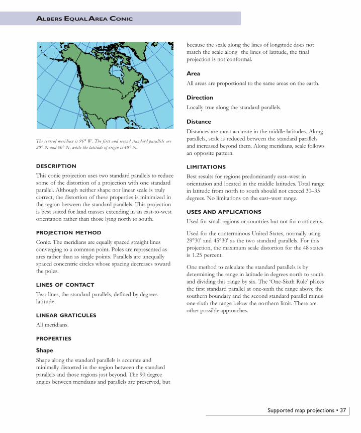
The central meridian is 96° W. The first and second standard parallels are20° N and 60° N, while the latitude of origin is 40° N.
38 • Understanding Map Projections
AZIMUTHAL EQUIDISTANT
DESCRIPTION
The most significant characteristic is that both distanceand direction are accurate from the central point. Thisprojection can accommodate all aspects: equatorial, polar,and oblique.
PROJECTION METHOD
Planar. The world is projected onto a flat surface from anypoint on the globe. Although all aspects are possible, theone used most commonly is the polar aspect, in which allmeridians and parallels are divided equally to maintain theequidistant property. Oblique aspects centered on a cityare also common.
POINT OF TANGENCY
A single point, usually the North or the South Pole,defined by degrees of latitude and longitude.
LINEAR GRATICULES
Polar—Straight meridians are divided equally byconcentric circles of latitude.
Equatorial—The equator and the projection’s centralmeridian are linear and meet at a 90-degree angle.
Oblique—The central meridian is straight, but there are no90-degree intersections except along the central meridian.
PROPERTIES
Shape
Except at the center, all shapes are distorted. Distortionincreases from the center.
Area
Distortion increases outward from the center point.
Direction
True directions from the center outward.
Distance
Distances for all aspects are accurate from the center pointoutward. For the polar aspect, the distances along themeridians are accurate, but there is a pattern of increasingdistortion along the circles of latitude, outward from thecenter.
LIMITATIONS
Usually limited to 90 degrees from the center, although itcan project the entire globe. Polar-aspect projections arebest for regions within a 30 degree radius because there isonly minimal distortion.
Degrees from center:15 30 45 60 90
Scale distortion in percent along parallels:1.2 4.7 11.1 20.9 57
USES AND APPLICATIONS
Routes of air and sea navigation. These maps will focus onan important location as their central point and use anappropriate aspect.
Polar aspect—Polar regions and polar navigation.
Equatorial aspect—Locations on or near the equator, suchas Singapore.
Oblique aspect—Locations between the poles and theequator; for example, large-scale mapping of Micronesia.
If this projection is used on the entire globe, theimmediate hemisphere can be recognized and resemblesthe Lambert Azimuthal projection. The outer hemispheregreatly distorts shapes and areas. In the extreme, a polar-aspect projection centered on the North Pole willrepresent the South Pole as its largest outermost circle.The function of this extreme projection is that, regardlessof the conformal and area distortion, an accuratepresentation of distance and direction from the centerpoint is maintained.
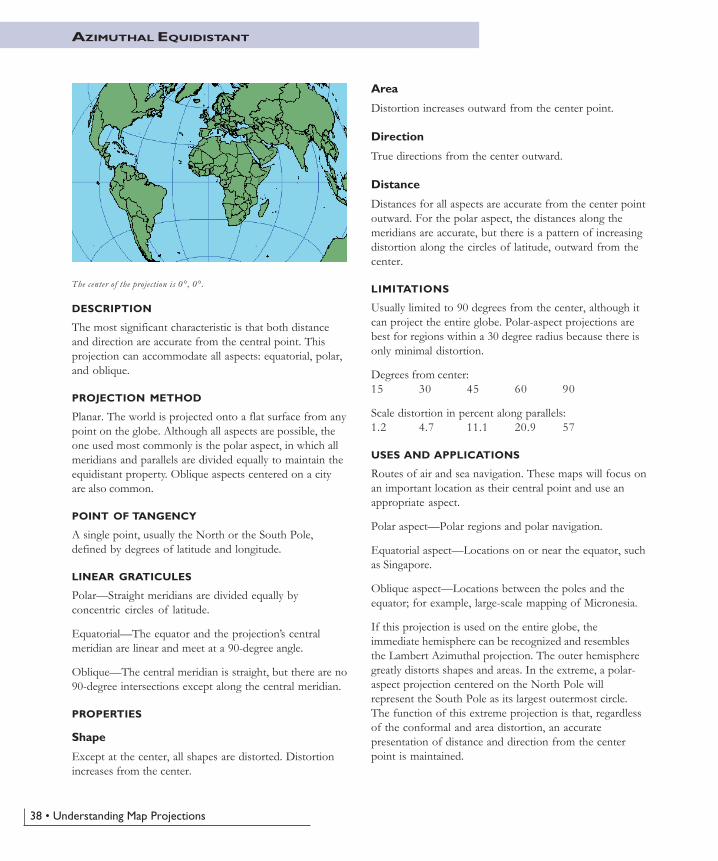
The center of the projection is 0°, 0°.
Supported map projections • 39
BEHRMANN EQUAL AREA CYLINDRICAL
DESCRIPTION
This projection is an equal-area cylindrical projectionsuitable for world mapping.
PROJECTION METHOD
Cylindrical. Standard parallels are at 30° N and S. A caseof Cylindrical Equal Area.
LINES OF CONTACT
The two parallels at 30° N and S.
LINEAR GRATICULES
Meridians and parallels are linear.
PROPERTIES
Shape
Shape distortion is minimized near the standard parallels.Shapes are distorted north–south between the standardparallels and distorted east–west above 30° N and below30° S.
Area
Area is maintained.
Direction
Directions are generally distorted.
Distance
Directions are generally distorted except along theequator.
LIMITATIONS
Useful for world maps only.
USES AND APPLICATIONS
Only useful for world maps.
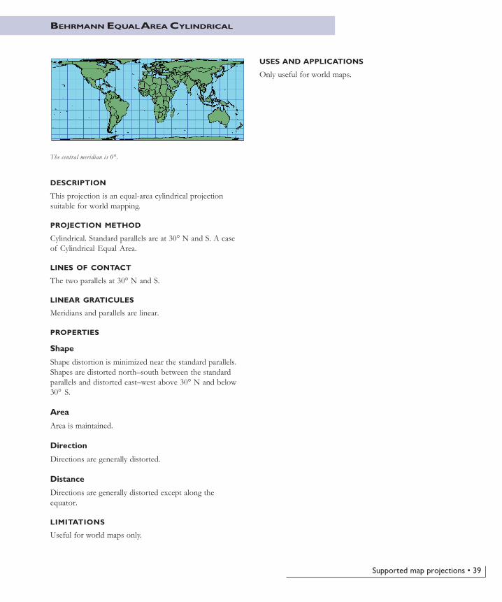
The central meridian is 0°.
40 • Understanding Map Projections
BIPOLAR OBLIQUE CONFORMAL CONIC
DESCRIPTION
This projection was developed specifically for mappingNorth and South America. It maintains conformality. It isbased on the Lambert Conformal Conic, using two obliqueconic projections side by side.
PROJECTION METHOD
Two oblique conics are joined with the poles 104 degreesapart. A great circle arc 104 degrees long begins at 20° Sand 110° W, cuts through Central America, and terminatesat 45° N and approximately 19°59'36" W. The scale of themap is then increased by approximately 3.5 percent. Theorigin of the coordinates is 17°15' N, 73°02' W(Snyder, 1993).
LINES OF CONTACT
The two oblique cones are each conceptually secant. Thesestandard lines do not follow any single parallel ormeridian.
LINEAR GRATICULES
Only from each transformed pole to the nearest actualpole.
PROPERTIES
Shape
Conformality is maintained except for a slight discrepancyat the juncture of the two conic projections.
Area
Minimal distortion near the standard lines, increasing withdistance.
Direction
Local directions are accurate because of conformality.
Distance
True along standard lines.
LIMITATIONS
Specialized for displaying North and South America only,together. The Bipolar Oblique projection will displayNorth America and South America only. If havingproblems, check all feature types—particularly annotationand tics—and remove any features that are beyond therange of the projection.
USES AND APPLICATIONS
Developed in 1941 by the American Geographical Societyas a low-error single map of North and South America.
Conformal mapping of North and South America as acontiguous unit.
Used by USGS for geologic mapping of North Americauntil it was replaced in 1979 by the Transverse Mercatorprojection.
Supported map projections • 41
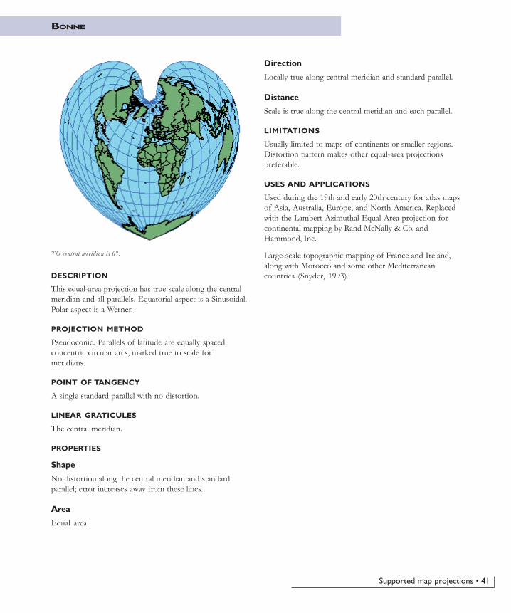
DESCRIPTION
This equal-area projection has true scale along the centralmeridian and all parallels. Equatorial aspect is a Sinusoidal.Polar aspect is a Werner.
PROJECTION METHOD
Pseudoconic. Parallels of latitude are equally spacedconcentric circular arcs, marked true to scale formeridians.
POINT OF TANGENCY
A single standard parallel with no distortion.
LINEAR GRATICULES
The central meridian.
PROPERTIES
Shape
No distortion along the central meridian and standardparallel; error increases away from these lines.
Area
Equal area.
BONNE
Direction
Locally true along central meridian and standard parallel.
Distance
Scale is true along the central meridian and each parallel.
LIMITATIONS
Usually limited to maps of continents or smaller regions.Distortion pattern makes other equal-area projectionspreferable.
USES AND APPLICATIONS
Used during the 19th and early 20th century for atlas mapsof Asia, Australia, Europe, and North America. Replacedwith the Lambert Azimuthal Equal Area projection forcontinental mapping by Rand McNally & Co. andHammond, Inc.
Large-scale topographic mapping of France and Ireland,along with Morocco and some other Mediterraneancountries (Snyder, 1993).
The central meridian is 0°.
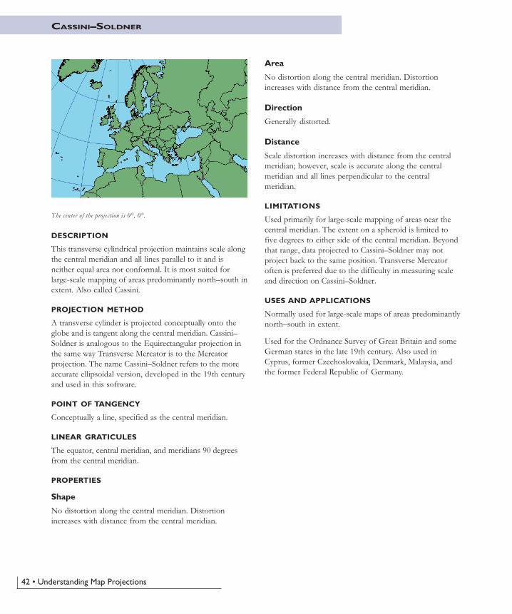
42 • Understanding Map Projections
CASSINI–SOLDNER
DESCRIPTION
This transverse cylindrical projection maintains scale alongthe central meridian and all lines parallel to it and isneither equal area nor conformal. It is most suited forlarge-scale mapping of areas predominantly north–south inextent. Also called Cassini.
PROJECTION METHOD
A transverse cylinder is projected conceptually onto theglobe and is tangent along the central meridian. Cassini–Soldner is analogous to the Equirectangular projection inthe same way Transverse Mercator is to the Mercatorprojection. The name Cassini–Soldner refers to the moreaccurate ellipsoidal version, developed in the 19th centuryand used in this software.
POINT OF TANGENCY
Conceptually a line, specified as the central meridian.
LINEAR GRATICULES
The equator, central meridian, and meridians 90 degreesfrom the central meridian.
PROPERTIES
Shape
No distortion along the central meridian. Distortionincreases with distance from the central meridian.
Area
No distortion along the central meridian. Distortionincreases with distance from the central meridian.
Direction
Generally distorted.
Distance
Scale distortion increases with distance from the centralmeridian; however, scale is accurate along the centralmeridian and all lines perpendicular to the centralmeridian.
LIMITATIONS
Used primarily for large-scale mapping of areas near thecentral meridian. The extent on a spheroid is limited tofive degrees to either side of the central meridian. Beyondthat range, data projected to Cassini–Soldner may notproject back to the same position. Transverse Mercatoroften is preferred due to the difficulty in measuring scaleand direction on Cassini–Soldner.
USES AND APPLICATIONS
Normally used for large-scale maps of areas predominantlynorth–south in extent.
Used for the Ordnance Survey of Great Britain and someGerman states in the late 19th century. Also used inCyprus, former Czechoslovakia, Denmark, Malaysia, andthe former Federal Republic of Germany.
The center of the projection is 0°, 0°.
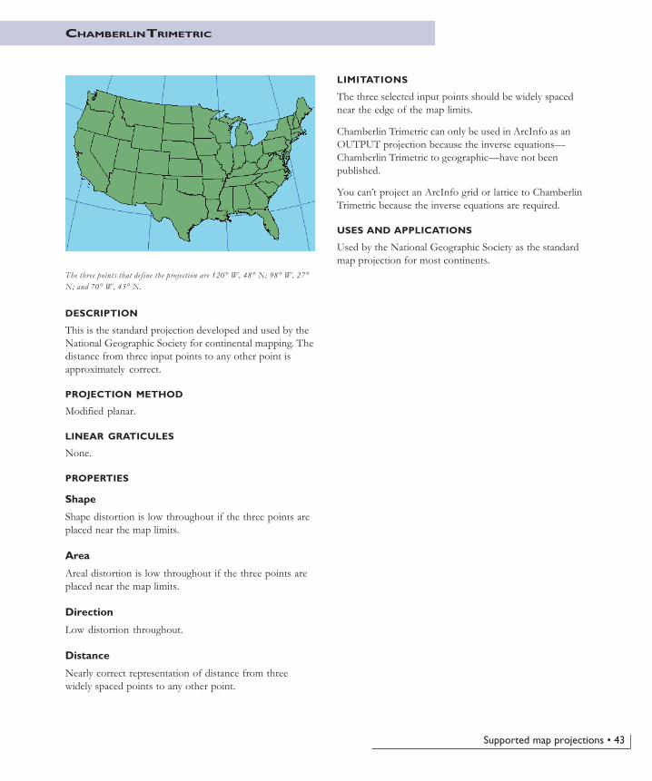
Supported map projections • 43
DESCRIPTION
This is the standard projection developed and used by theNational Geographic Society for continental mapping. Thedistance from three input points to any other point isapproximately correct.
PROJECTION METHOD
Modified planar.
LINEAR GRATICULES
None.
PROPERTIES
Shape
Shape distortion is low throughout if the three points areplaced near the map limits.
Area
Areal distortion is low throughout if the three points areplaced near the map limits.
Direction
Low distortion throughout.
Distance
Nearly correct representation of distance from threewidely spaced points to any other point.
LIMITATIONS
The three selected input points should be widely spacednear the edge of the map limits.
Chamberlin Trimetric can only be used in ArcInfo as anOUTPUT projection because the inverse equations—Chamberlin Trimetric to geographic—have not beenpublished.
You can’t project an ArcInfo grid or lattice to ChamberlinTrimetric because the inverse equations are required.
USES AND APPLICATIONS
Used by the National Geographic Society as the standardmap projection for most continents.
CHAMBERLIN TRIMETRIC
The three points that define the projection are 120° W, 48° N; 98° W, 27°N; and 70° W, 45° N.
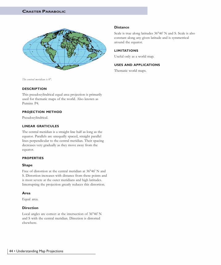
44 • Understanding Map Projections
DESCRIPTION
This pseudocylindrical equal area projection is primarilyused for thematic maps of the world. Also known asPutnins P4.
PROJECTION METHOD
Pseudocylindrical.
LINEAR GRATICULES
The central meridian is a straight line half as long as theequator. Parallels are unequally spaced, straight parallellines perpendicular to the central meridian. Their spacingdecreases very gradually as they move away from theequator.
PROPERTIES
Shape
Free of distortion at the central meridian at 36°46' N andS. Distortion increases with distance from these points andis most severe at the outer meridians and high latitudes.Interrupting the projection greatly reduces this distortion.
Area
Equal area.
Direction
Local angles are correct at the intersection of 36°46' Nand S with the central meridian. Direction is distortedelsewhere.
CRASTER PARABOLIC
Distance
Scale is true along latitudes 36°46' N and S. Scale is alsoconstant along any given latitude and is symmetricalaround the equator.
LIMITATIONS
Useful only as a world map.
USES AND APPLICATIONS
Thematic world maps.
The central meridian is 0°.
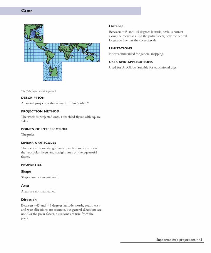
Supported map projections • 45
CUBE
The Cube projection with option 1.
DESCRIPTION
A faceted projection that is used for ArcGlobe™.
PROJECTION METHOD
The world is projected onto a six-sided figure with squaresides.
POINTS OF INTERSECTION
The poles.
LINEAR GRATICULES
The meridians are straight lines. Parallels are squares onthe two polar facets and straight lines on the equatorialfacets.
PROPERTIES
Shape
Shapes are not maintained.
Area
Areas are not maintained.
Direction
Between +45 and -45 degrees latitude, north, south, east,and west directions are accurate, but general directions arenot. On the polar facets, directions are true from thepoles.
Distance
Between +45 and -45 degrees latitude, scale is correctalong the meridians. On the polar facets, only the centrallongitude line has the correct scale.
LIMITATIONS
Not recommended for general mapping.
USES AND APPLICATIONS
Used for ArcGlobe. Suitable for educational uses.
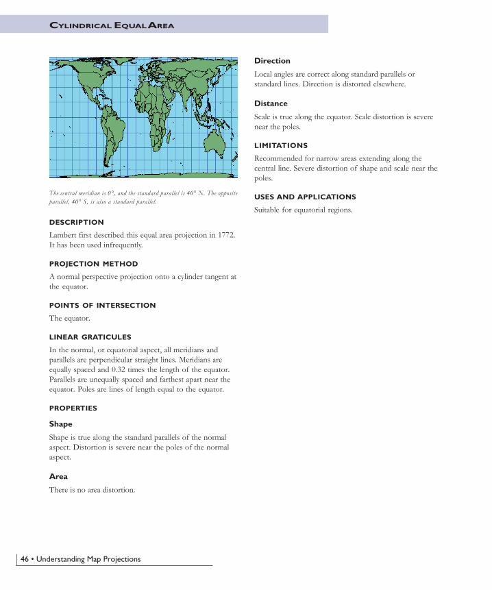
46 • Understanding Map Projections
CYLINDRICAL EQUAL AREA
DESCRIPTION
Lambert first described this equal area projection in 1772.It has been used infrequently.
PROJECTION METHOD
A normal perspective projection onto a cylinder tangent atthe equator.
POINTS OF INTERSECTION
The equator.
LINEAR GRATICULES
In the normal, or equatorial aspect, all meridians andparallels are perpendicular straight lines. Meridians areequally spaced and 0.32 times the length of the equator.Parallels are unequally spaced and farthest apart near theequator. Poles are lines of length equal to the equator.
PROPERTIES
Shape
Shape is true along the standard parallels of the normalaspect. Distortion is severe near the poles of the normalaspect.
Area
There is no area distortion.
Direction
Local angles are correct along standard parallels orstandard lines. Direction is distorted elsewhere.
Distance
Scale is true along the equator. Scale distortion is severenear the poles.
LIMITATIONS
Recommended for narrow areas extending along thecentral line. Severe distortion of shape and scale near thepoles.
USES AND APPLICATIONS
Suitable for equatorial regions.
The central meridian is 0°, and the standard parallel is 40° N. The oppositeparallel, 40° S, is also a standard parallel.
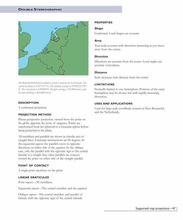
Supported map projections • 47
DOUBLE STEREOGRAPHIC
DESCRIPTION
A conformal projection.
PROJECTION METHOD
Planar perspective projection, viewed from the point onthe globe opposite the point of tangency. Points aretransformed from the spheroid to a Gaussian sphere beforebeing projected to the plane.
All meridians and parallels are shown as circular arcs orstraight lines. Graticular intersections are 90 degrees. Inthe equatorial aspect, the parallels curve in oppositedirections on either side of the equator. In the obliquecase, only the parallel with the opposite sign to the centrallatitude is a straight line; other parallels are concavetoward the poles on either side of the straight parallel.
POINT OF CONTACT
A single point anywhere on the globe.
LINEAR GRATICULES
Polar aspect—All meridians.
Equatorial aspect—The central meridian and the equator.
Oblique aspect—The central meridian and parallel oflatitude with the opposite sign of the central latitude.
PROPERTIES
Shape
Conformal. Local shapes are accurate.
Area
True scale at center with distortion increasing as you moveaway from the center.
Direction
Directions are accurate from the center. Local angles areaccurate everywhere.
Distance
Scale increases with distance from the center.
LIMITATIONS
Normally limited to one hemisphere. Portions of the outerhemisphere may be shown, but with rapidly increasingdistortion.
USES AND APPLICATIONS
Used for large-scale coordinate systems in New Brunswickand the Netherlands.
The Rijksdriehoekstelsel coordinate system is used in the Netherlands. Thecentral meridian is 5°23'15.5" E. The latitude of origin is 52°09'22.178"N. The scale factor is 0.9999079. The false easting is 155,000 meters, andthe false northing is 463,000 meters.
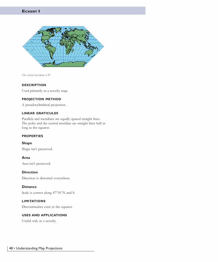
48 • Understanding Map Projections
DESCRIPTION
Used primarily as a novelty map.
PROJECTION METHOD
A pseudocylindrical projection.
LINEAR GRATICULES
Parallels and meridians are equally spaced straight lines.The poles and the central meridian are straight lines half aslong as the equator.
PROPERTIES
Shape
Shape isn’t preserved.
Area
Area isn’t preserved.
Direction
Direction is distorted everywhere.
Distance
Scale is correct along 47°10' N and S.
LIMITATIONS
Discontinuities exist at the equator.
USES AND APPLICATIONS
Useful only as a novelty.
ECKERT I
The central meridian is 0°.
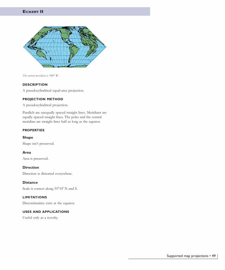
Supported map projections • 49
DESCRIPTION
A pseudocylindrical equal-area projection.
PROJECTION METHOD
A pseudocylindrical projection.
Parallels are unequally spaced straight lines. Meridians areequally spaced straight lines. The poles and the centralmeridian are straight lines half as long as the equator.
PROPERTIES
Shape
Shape isn’t preserved.
Area
Area is preserved.
Direction
Direction is distorted everywhere.
Distance
Scale is correct along 55°10' N and S.
LIMITATIONS
Discontinuities exist at the equator.
USES AND APPLICATIONS
Useful only as a novelty.
ECKERT II
The central meridian is 100° W.
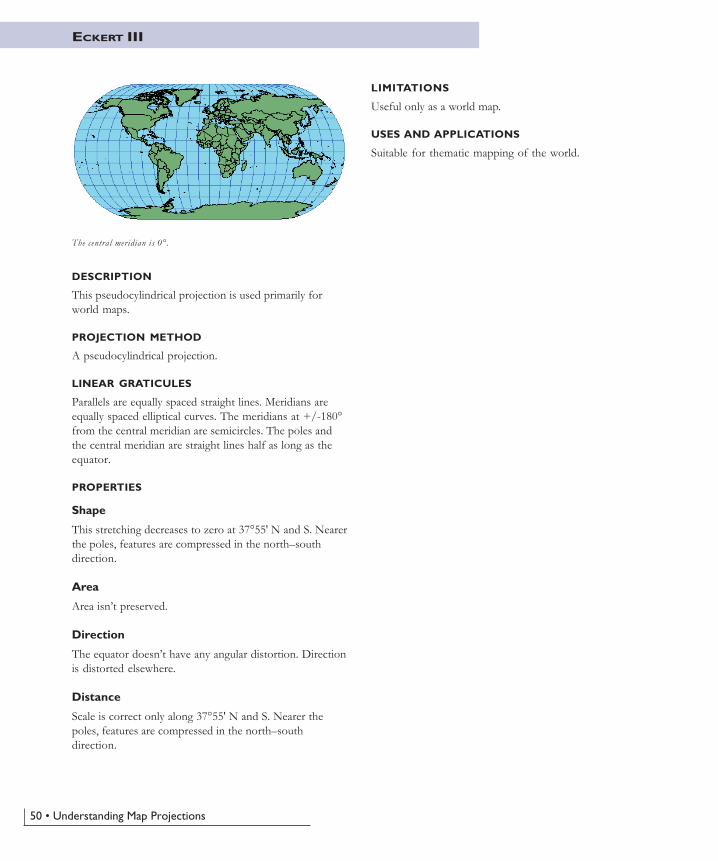
50 • Understanding Map Projections
DESCRIPTION
This pseudocylindrical projection is used primarily forworld maps.
PROJECTION METHOD
A pseudocylindrical projection.
LINEAR GRATICULES
Parallels are equally spaced straight lines. Meridians areequally spaced elliptical curves. The meridians at +/-180°from the central meridian are semicircles. The poles andthe central meridian are straight lines half as long as theequator.
PROPERTIES
Shape
This stretching decreases to zero at 37°55' N and S. Nearerthe poles, features are compressed in the north–southdirection.
Area
Area isn’t preserved.
Direction
The equator doesn’t have any angular distortion. Directionis distorted elsewhere.
Distance
Scale is correct only along 37°55' N and S. Nearer thepoles, features are compressed in the north–southdirection.
ECKERT III
The central meridian is 0°.
LIMITATIONS
Useful only as a world map.
USES AND APPLICATIONS
Suitable for thematic mapping of the world.

Supported map projections • 51
ECKERT IV
DESCRIPTION
This equal area projection is used primarily for worldmaps.
PROJECTION METHOD
A pseudocylindrical equal-area projection.
LINEAR GRATICULES
Parallels are unequally spaced straight lines, closer togetherat the poles. Meridians are equally spaced elliptical arcs.The poles and the central meridian are straight lines half aslong as the equator.
PROPERTIES
Shape
Shapes are stretched north–south 40 percent along theequator, relative to the east–west dimension. Thisstretching decreases to zero at 40°30' N and S at thecentral meridian. Nearer the poles, features are compressedin the north–south direction.
Area
Equivalent.
Direction
Local angles are correct at the intersections of 40°30' Nand S with the central meridian. Direction is distortedelsewhere.
Distance
Scale is distorted north–south 40 percent along theequator relative to the east–west dimension. Thisdistortion decreases to zero at 40°30' N and S at thecentral meridian. Scale is correct only along these parallels.
Nearer the poles, features are compressed in the north–south direction.
LIMITATIONS
Useful only as a world map.
USES AND APPLICATIONS
Thematic maps of the world such as climate.
The central meridian is 0°.
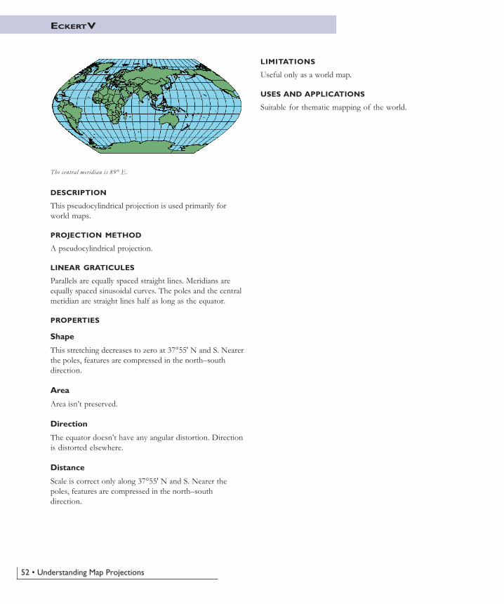
52 • Understanding Map Projections
ECKERT V
DESCRIPTION
This pseudocylindrical projection is used primarily forworld maps.
PROJECTION METHOD
A pseudocylindrical projection.
LINEAR GRATICULES
Parallels are equally spaced straight lines. Meridians areequally spaced sinusoidal curves. The poles and the centralmeridian are straight lines half as long as the equator.
PROPERTIES
Shape
This stretching decreases to zero at 37°55' N and S. Nearerthe poles, features are compressed in the north–southdirection.
Area
Area isn’t preserved.
Direction
The equator doesn’t have any angular distortion. Directionis distorted elsewhere.
Distance
Scale is correct only along 37°55' N and S. Nearer thepoles, features are compressed in the north–southdirection.
LIMITATIONS
Useful only as a world map.
USES AND APPLICATIONS
Suitable for thematic mapping of the world.
The central meridian is 89° E.
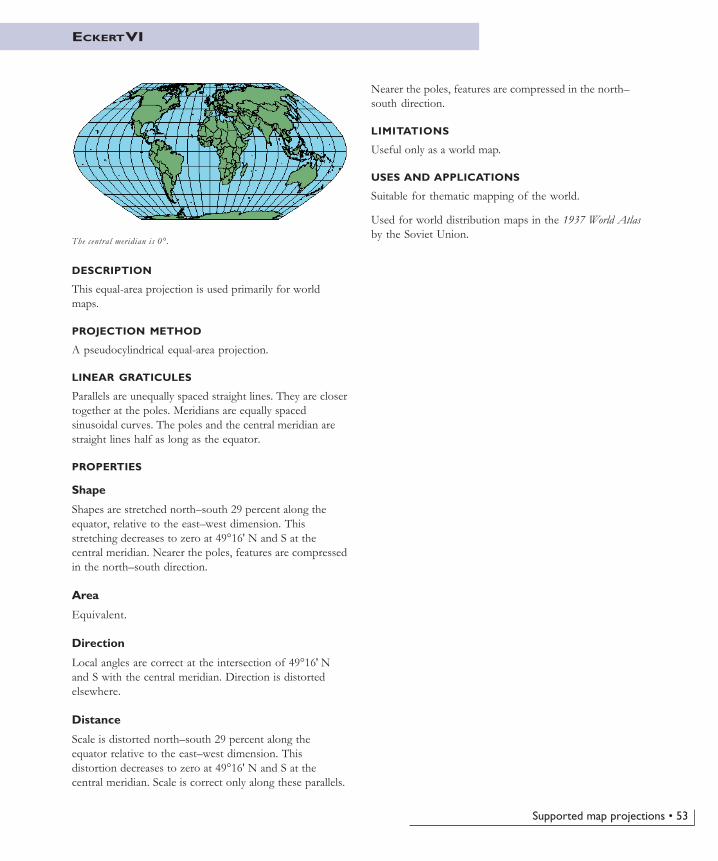
Supported map projections • 53
ECKERT VI
DESCRIPTION
This equal-area projection is used primarily for worldmaps.
PROJECTION METHOD
A pseudocylindrical equal-area projection.
LINEAR GRATICULES
Parallels are unequally spaced straight lines. They are closertogether at the poles. Meridians are equally spacedsinusoidal curves. The poles and the central meridian arestraight lines half as long as the equator.
PROPERTIES
Shape
Shapes are stretched north–south 29 percent along theequator, relative to the east–west dimension. Thisstretching decreases to zero at 49°16' N and S at thecentral meridian. Nearer the poles, features are compressedin the north–south direction.
Area
Equivalent.
Direction
Local angles are correct at the intersection of 49°16' Nand S with the central meridian. Direction is distortedelsewhere.
Distance
Scale is distorted north–south 29 percent along theequator relative to the east–west dimension. Thisdistortion decreases to zero at 49°16' N and S at thecentral meridian. Scale is correct only along these parallels.
Nearer the poles, features are compressed in the north–south direction.
LIMITATIONS
Useful only as a world map.
USES AND APPLICATIONS
Suitable for thematic mapping of the world.
Used for world distribution maps in the 1937 World Atlasby the Soviet Union.
The central meridian is 0°.
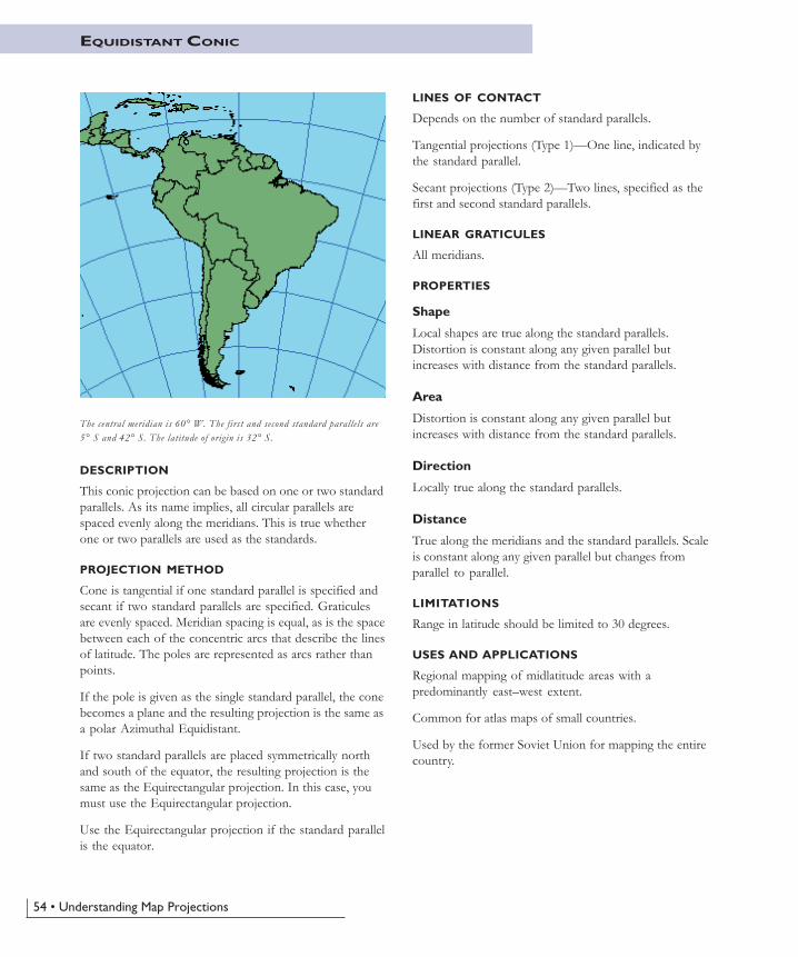
54 • Understanding Map Projections
EQUIDISTANT CONIC
DESCRIPTION
This conic projection can be based on one or two standardparallels. As its name implies, all circular parallels arespaced evenly along the meridians. This is true whetherone or two parallels are used as the standards.
PROJECTION METHOD
Cone is tangential if one standard parallel is specified andsecant if two standard parallels are specified. Graticulesare evenly spaced. Meridian spacing is equal, as is the spacebetween each of the concentric arcs that describe the linesof latitude. The poles are represented as arcs rather thanpoints.
If the pole is given as the single standard parallel, the conebecomes a plane and the resulting projection is the same asa polar Azimuthal Equidistant.
If two standard parallels are placed symmetrically northand south of the equator, the resulting projection is thesame as the Equirectangular projection. In this case, youmust use the Equirectangular projection.
Use the Equirectangular projection if the standard parallelis the equator.
LINES OF CONTACT
Depends on the number of standard parallels.
Tangential projections (Type 1)—One line, indicated bythe standard parallel.
Secant projections (Type 2)—Two lines, specified as thefirst and second standard parallels.
LINEAR GRATICULES
All meridians.
PROPERTIES
Shape
Local shapes are true along the standard parallels.Distortion is constant along any given parallel butincreases with distance from the standard parallels.
Area
Distortion is constant along any given parallel butincreases with distance from the standard parallels.
Direction
Locally true along the standard parallels.
Distance
True along the meridians and the standard parallels. Scaleis constant along any given parallel but changes fromparallel to parallel.
LIMITATIONS
Range in latitude should be limited to 30 degrees.
USES AND APPLICATIONS
Regional mapping of midlatitude areas with apredominantly east–west extent.
Common for atlas maps of small countries.
Used by the former Soviet Union for mapping the entirecountry.
The central meridian is 60° W. The first and second standard parallels are5° S and 42° S. The latitude of origin is 32° S.
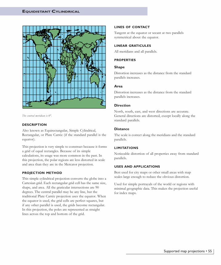
Supported map projections • 55
EQUIDISTANT CYLINDRICAL
DESCRIPTION
Also known as Equirectangular, Simple Cylindrical,Rectangular, or Plate Carrée (if the standard parallel is theequator).
This projection is very simple to construct because it formsa grid of equal rectangles. Because of its simplecalculations, its usage was more common in the past. Inthis projection, the polar regions are less distorted in scaleand area than they are in the Mercator projection.
PROJECTION METHOD
This simple cylindrical projection converts the globe into aCartesian grid. Each rectangular grid cell has the same size,shape, and area. All the graticular intersections are 90degrees. The central parallel may be any line, but thetraditional Plate Carrée projection uses the equator. Whenthe equator is used, the grid cells are perfect squares, butif any other parallel is used, the grids become rectangular.In this projection, the poles are represented as straightlines across the top and bottom of the grid.
LINES OF CONTACT
Tangent at the equator or secant at two parallelssymmetrical about the equator.
LINEAR GRATICULES
All meridians and all parallels.
PROPERTIES
Shape
Distortion increases as the distance from the standardparallels increases.
Area
Distortion increases as the distance from the standardparallels increases.
Direction
North, south, east, and west directions are accurate.General directions are distorted, except locally along thestandard parallels.
Distance
The scale is correct along the meridians and the standardparallels.
LIMITATIONS
Noticeable distortion of all properties away from standardparallels.
USES AND APPLICATIONS
Best used for city maps or other small areas with mapscales large enough to reduce the obvious distortion.
Used for simple portrayals of the world or regions withminimal geographic data. This makes the projection usefulfor index maps.
The central meridian is 0°.
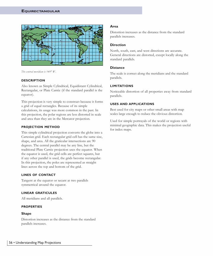
56 • Understanding Map Projections
EQUIRECTANGULAR
DESCRIPTION
Also known as Simple Cylindrical, Equidistant Cylindrical,Rectangular, or Plate Carrée (if the standard parallel is theequator).
This projection is very simple to construct because it formsa grid of equal rectangles. Because of its simplecalculations, its usage was more common in the past. Inthis projection, the polar regions are less distorted in scaleand area than they are in the Mercator projection.
PROJECTION METHOD
This simple cylindrical projection converts the globe into aCartesian grid. Each rectangular grid cell has the same size,shape, and area. All the graticular intersections are 90degrees. The central parallel may be any line, but thetraditional Plate Carrée projection uses the equator. Whenthe equator is used, the grid cells are perfect squares, butif any other parallel is used, the grids become rectangular.In this projection, the poles are represented as straightlines across the top and bottom of the grid.
LINES OF CONTACT
Tangent at the equator or secant at two parallelssymmetrical around the equator.
LINEAR GRATICULES
All meridians and all parallels.
PROPERTIES
Shape
Distortion increases as the distance from the standardparallels increases.
Area
Distortion increases as the distance from the standardparallels increases.
Direction
North, south, east, and west directions are accurate.General directions are distorted, except locally along thestandard parallels.
Distance
The scale is correct along the meridians and the standardparallels.
LIMITATIONS
Noticeable distortion of all properties away from standardparallels.
USES AND APPLICATIONS
Best used for city maps or other small areas with mapscales large enough to reduce the obvious distortion.
Used for simple portrayals of the world or regions withminimal geographic data. This makes the projection usefulfor index maps.
The central meridian is 149° W.
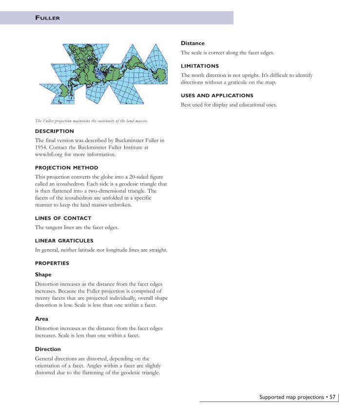
Supported map projections • 57
FULLER
The Fuller projection maintains the cootinuity of the land masses.
DESCRIPTION
The final version was described by Buckminster Fuller in1954. Contact the Buckminster Fuller Institute atwww.bfi.org for more information.
PROJECTION METHOD
This projection converts the globe into a 20-sided figurecalled an icosahedron. Each side is a geodesic triangle thatis then flattened into a two-dimensional triangle. Thefacets of the icosahedron are unfolded in a specificmanner to keep the land masses unbroken.
LINES OF CONTACT
The tangent lines are the facet edges.
LINEAR GRATICULES
In general, neither latitude nor longitude lines are straight.
PROPERTIES
Shape
Distortion increases as the distance from the facet edgesincreases. Because the Fuller projection is comprised oftwenty facets that are projected individually, overall shapedistortion is low. Scale is less than one within a facet.
Area
Distortion increases as the distance from the facet edgesincreases. Scale is less than one within a facet.
Direction
General directions are distorted, depending on theorientation of a facet. Angles within a facet are slightlydistorted due to the flattening of the geodesic triangle.
Distance
The scale is correct along the facet edges.
LIMITATIONS
The north direction is not upright. It’s difficult to identifydirections without a graticule on the map.
USES AND APPLICATIONS
Best used for display and educational uses.
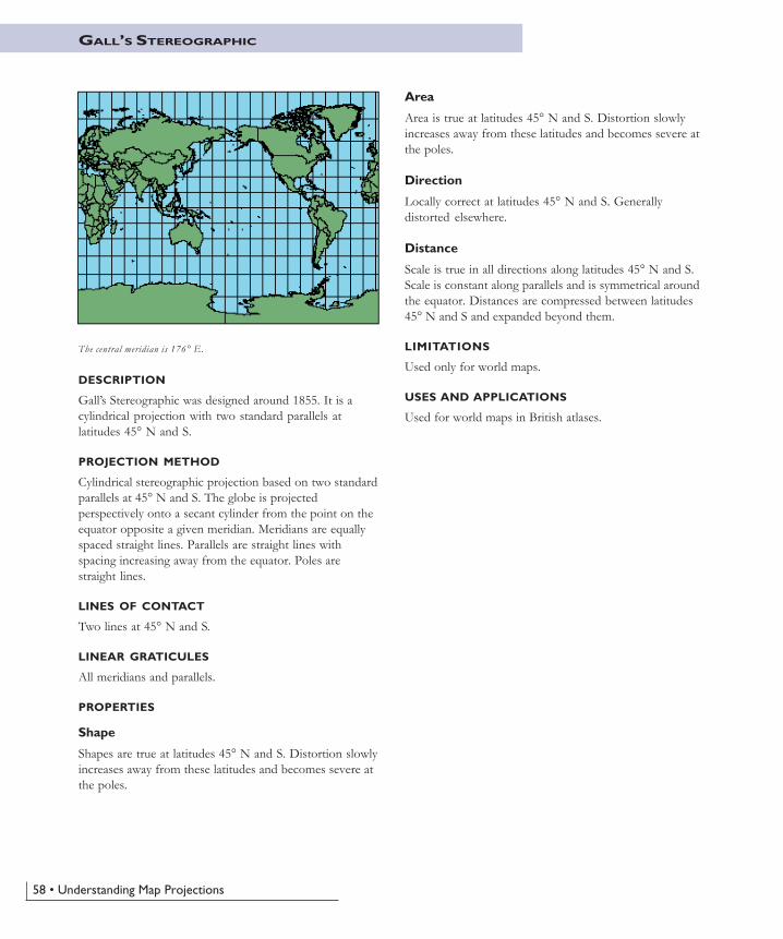
58 • Understanding Map Projections
GALL’S STEREOGRAPHIC
DESCRIPTION
Gall’s Stereographic was designed around 1855. It is acylindrical projection with two standard parallels atlatitudes 45° N and S.
PROJECTION METHOD
Cylindrical stereographic projection based on two standardparallels at 45° N and S. The globe is projectedperspectively onto a secant cylinder from the point on theequator opposite a given meridian. Meridians are equallyspaced straight lines. Parallels are straight lines withspacing increasing away from the equator. Poles arestraight lines.
LINES OF CONTACT
Two lines at 45° N and S.
LINEAR GRATICULES
All meridians and parallels.
PROPERTIES
Shape
Shapes are true at latitudes 45° N and S. Distortion slowlyincreases away from these latitudes and becomes severe atthe poles.
Area
Area is true at latitudes 45° N and S. Distortion slowlyincreases away from these latitudes and becomes severe atthe poles.
Direction
Locally correct at latitudes 45° N and S. Generallydistorted elsewhere.
Distance
Scale is true in all directions along latitudes 45° N and S.Scale is constant along parallels and is symmetrical aroundthe equator. Distances are compressed between latitudes45° N and S and expanded beyond them.
LIMITATIONS
Used only for world maps.
USES AND APPLICATIONS
Used for world maps in British atlases.
The central meridian is 176° E.
Supported map projections • 59
DESCRIPTION
Also known as Transverse Mercator.
This projection is similar to the Mercator except that thecylinder is longitudinal along a meridian instead of theequator. The result is a conformal projection that does notmaintain true directions. The central meridian is placed onthe region to be highlighted. This centering minimizesdistortion of all properties in that region. This projectionis best suited for land masses that stretch north–south. TheGauss–Krüger (GK) coordinate system is based on theGauss–Krüger projection.
PROJECTION METHOD
Cylindrical projection with central meridian placed in aparticular region.
LINES OF CONTACT
Any single meridian for the tangent projection. For thesecant projection, two parallel lines equidistant from thecentral meridian.
LINEAR GRATICULES
The equator and the central meridian.
PROPERTIES
Shape
Conformal. Small shapes are maintained. Shapes of largerregions are increasingly distorted away from the centralmeridian.
Area
Distortion increases with distance from the centralmeridian.
Direction
Local angles are accurate everywhere.
Distance
Accurate scale along the central meridian if the scalefactor is 1.0. If it is less than 1.0, then there are twostraight lines having an accurate scale, equidistant fromand on each side of the central meridian.
LIMITATIONS
Data on a spheroid or an ellipsoid cannot be projectedbeyond 90 degrees from the central meridian. In fact, theextent on a spheroid or ellipsoid should be limited to 10 to12 degrees on both sides of the central meridian. Beyondthat range, data projected may not project back to thesame position. Data on a sphere does not have theselimitations.
USES AND APPLICATIONS
Gauss–Krüger coordinate system. Gauss–Krüger dividesthe world into zones six degrees wide. Each zone has ascale factor of 1.0 and a false easting of 500,000 meters.The central meridian of zone 1 is at 3° E. Some placesalso add the zone number times one million to the500,000 false easting value. GK zone 5 could have a falseeasting value of 500,000 or 5,500,000 meters.
The UTM system is very similar. The scale factor is0.9996, and the central meridian of UTM zone 1 is at177° W. The false easting value is 500,000 meters, andsouthern hemisphere zones also have a false northing of10,000,000.
GAUSS–KRÜGER
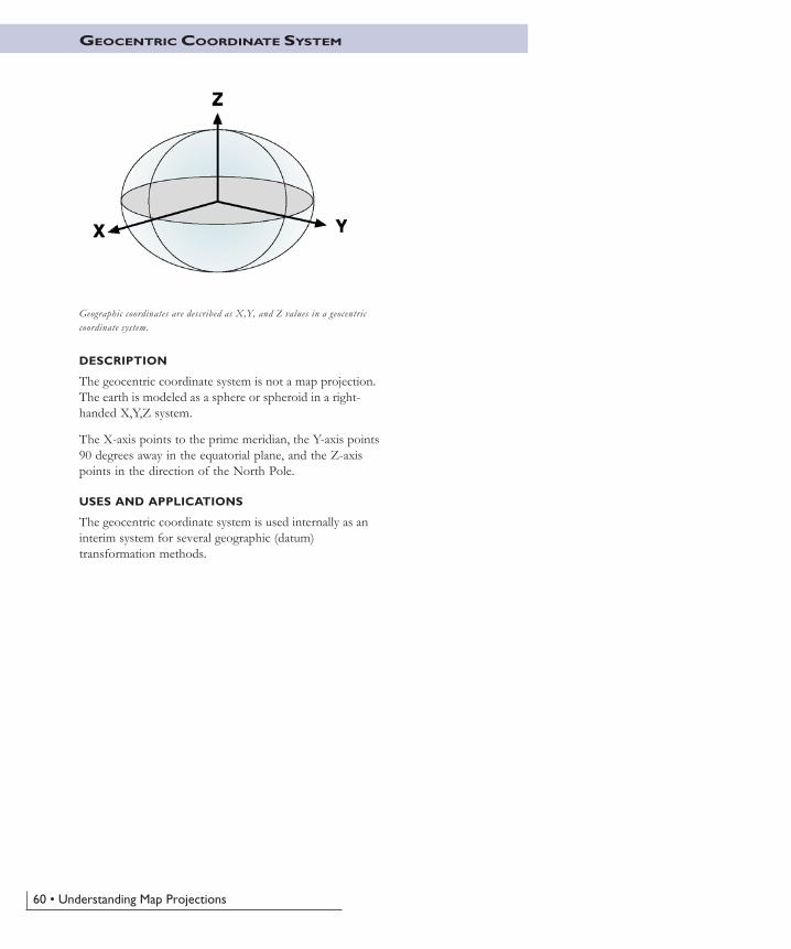
60 • Understanding Map Projections
GEOCENTRIC COORDINATE SYSTEM
DESCRIPTION
The geocentric coordinate system is not a map projection.The earth is modeled as a sphere or spheroid in a right-handed X,Y,Z system.
The X-axis points to the prime meridian, the Y-axis points90 degrees away in the equatorial plane, and the Z-axispoints in the direction of the North Pole.
USES AND APPLICATIONS
The geocentric coordinate system is used internally as aninterim system for several geographic (datum)transformation methods.
Geographic coordinates are described as X,Y, and Z values in a geocentriccoordinate system.
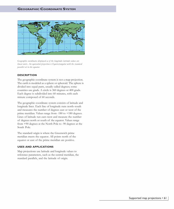
Supported map projections • 61
GEOGRAPHIC COORDINATE SYSTEM
DESCRIPTION
The geographic coordinate system is not a map projection.The earth is modeled as a sphere or spheroid. The sphere isdivided into equal parts, usually called degrees; somecountries use grads. A circle is 360 degrees or 400 grads.Each degree is subdivided into 60 minutes, with eachminute composed of 60 seconds.
The geographic coordinate system consists of latitude andlongitude lines. Each line of longitude runs north–southand measures the number of degrees east or west of theprime meridian. Values range from -180 to +180 degrees.Lines of latitude run east–west and measure the numberof degrees north or south of the equator. Values rangefrom +90 degrees at the North Pole to -90 degrees at theSouth Pole.
The standard origin is where the Greenwich primemeridian meets the equator. All points north of theequator or east of the prime meridian are positive.
USES AND APPLICATIONS
Map projections use latitude and longitude values toreference parameters, such as the central meridian, thestandard parallels, and the latitude of origin.
Geographic coordinates displayed as if the longitude–latitude values arelinear units. An equivalent projection is Equirectangular with the standardparallel set to the equator.
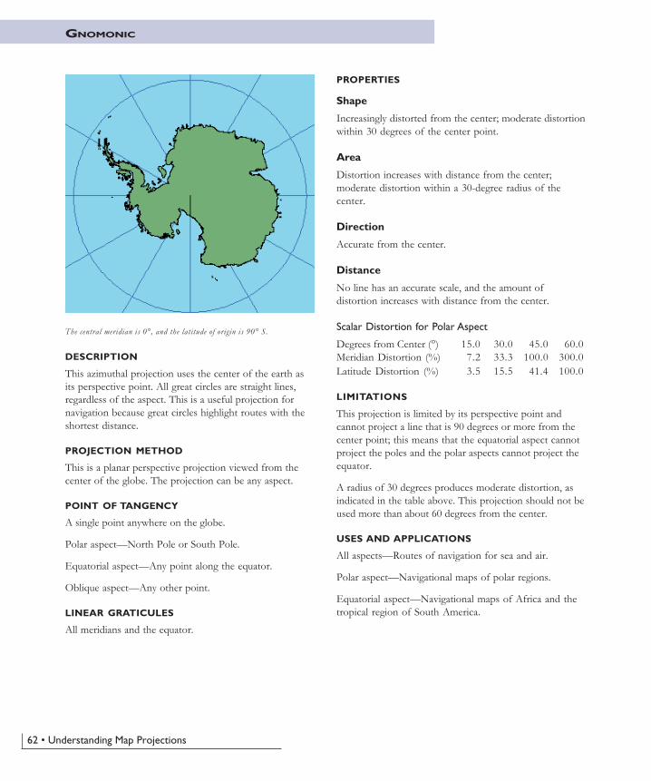
62 • Understanding Map Projections
GNOMONIC
DESCRIPTION
This azimuthal projection uses the center of the earth asits perspective point. All great circles are straight lines,regardless of the aspect. This is a useful projection fornavigation because great circles highlight routes with theshortest distance.
PROJECTION METHOD
This is a planar perspective projection viewed from thecenter of the globe. The projection can be any aspect.
POINT OF TANGENCY
A single point anywhere on the globe.
Polar aspect—North Pole or South Pole.
Equatorial aspect—Any point along the equator.
Oblique aspect—Any other point.
LINEAR GRATICULES
All meridians and the equator.
PROPERTIES
Shape
Increasingly distorted from the center; moderate distortionwithin 30 degrees of the center point.
Area
Distortion increases with distance from the center;moderate distortion within a 30-degree radius of thecenter.
Direction
Accurate from the center.
Distance
No line has an accurate scale, and the amount ofdistortion increases with distance from the center.
Scalar Distortion for Polar Aspect
Degrees from Center (°) 15.0 30.0 45.0 60.0Meridian Distortion (%) 7.2 33.3 100.0 300.0Latitude Distortion (%) 3.5 15.5 41.4 100.0
LIMITATIONS
This projection is limited by its perspective point andcannot project a line that is 90 degrees or more from thecenter point; this means that the equatorial aspect cannotproject the poles and the polar aspects cannot project theequator.
A radius of 30 degrees produces moderate distortion, asindicated in the table above. This projection should not beused more than about 60 degrees from the center.
USES AND APPLICATIONS
All aspects—Routes of navigation for sea and air.
Polar aspect—Navigational maps of polar regions.
Equatorial aspect—Navigational maps of Africa and thetropical region of South America.
The central meridian is 0°, and the latitude of origin is 90° S.
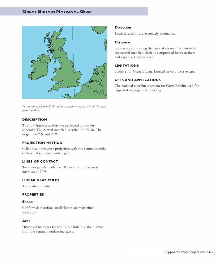
Supported map projections • 63
GREAT BRITAIN NATIONAL GRID
DESCRIPTION
This is a Transverse Mercator projected on the Airyspheroid. The central meridian is scaled to 0.9996. Theorigin is 49° N and 2° W.
PROJECTION METHOD
Cylindrical, transverse projection with the central meridiancentered along a particular region.
LINES OF CONTACT
Two lines parallel with and 180 km from the centralmeridian at 2° W.
LINEAR GRATICULES
The central meridian.
PROPERTIES
Shape
Conformal; therefore, small shapes are maintainedaccurately.
Area
Distortion increases beyond Great Britain as the distancefrom the central meridian increases.
Direction
Local directions are accurately maintained.
Distance
Scale is accurate along the lines of secancy 180 km fromthe central meridian. Scale is compressed between themand expanded beyond them.
LIMITATIONS
Suitable for Great Britain. Limited in east–west extent.
USES AND APPLICATIONS
The national coordinate system for Great Britain; used forlarge-scale topographic mapping.
The central meridian is 2° W, and the latitude of origin is 49° N. The scalefactor is 0.9996.
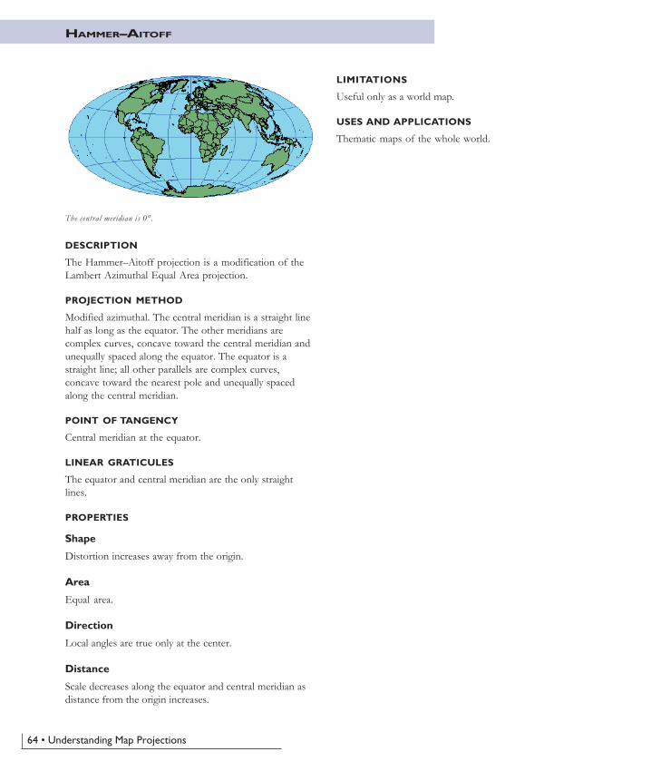
64 • Understanding Map Projections
HAMMER–AITOFF
DESCRIPTION
The Hammer–Aitoff projection is a modification of theLambert Azimuthal Equal Area projection.
PROJECTION METHOD
Modified azimuthal. The central meridian is a straight linehalf as long as the equator. The other meridians arecomplex curves, concave toward the central meridian andunequally spaced along the equator. The equator is astraight line; all other parallels are complex curves,concave toward the nearest pole and unequally spacedalong the central meridian.
POINT OF TANGENCY
Central meridian at the equator.
LINEAR GRATICULES
The equator and central meridian are the only straightlines.
PROPERTIES
Shape
Distortion increases away from the origin.
Area
Equal area.
Direction
Local angles are true only at the center.
Distance
Scale decreases along the equator and central meridian asdistance from the origin increases.
The central meridian is 0°.
LIMITATIONS
Useful only as a world map.
USES AND APPLICATIONS
Thematic maps of the whole world.
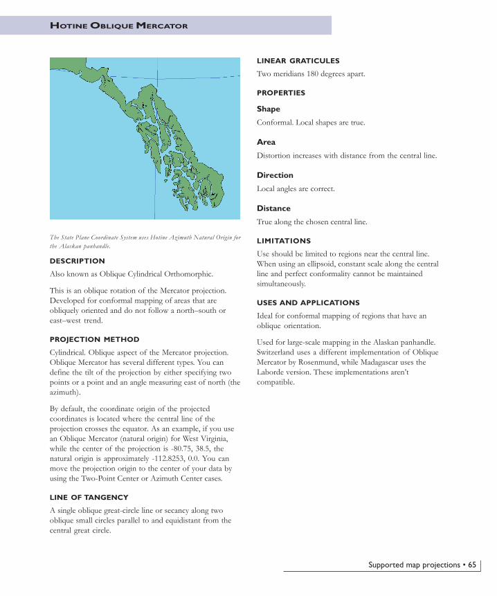
Supported map projections • 65
HOTINE OBLIQUE MERCATOR
The State Plane Coordinate System uses Hotine Azimuth Natural Origin forthe Alaskan panhandle.
DESCRIPTION
Also known as Oblique Cylindrical Orthomorphic.
This is an oblique rotation of the Mercator projection.Developed for conformal mapping of areas that areobliquely oriented and do not follow a north–south oreast–west trend.
PROJECTION METHOD
Cylindrical. Oblique aspect of the Mercator projection.Oblique Mercator has several different types. You candefine the tilt of the projection by either specifying twopoints or a point and an angle measuring east of north (theazimuth).
By default, the coordinate origin of the projectedcoordinates is located where the central line of theprojection crosses the equator. As an example, if you usean Oblique Mercator (natural origin) for West Virginia,while the center of the projection is -80.75, 38.5, thenatural origin is approximately -112.8253, 0.0. You canmove the projection origin to the center of your data byusing the Two-Point Center or Azimuth Center cases.
LINE OF TANGENCY
A single oblique great-circle line or secancy along twooblique small circles parallel to and equidistant from thecentral great circle.
LINEAR GRATICULES
Two meridians 180 degrees apart.
PROPERTIES
Shape
Conformal. Local shapes are true.
Area
Distortion increases with distance from the central line.
Direction
Local angles are correct.
Distance
True along the chosen central line.
LIMITATIONS
Use should be limited to regions near the central line.When using an ellipsoid, constant scale along the centralline and perfect conformality cannot be maintainedsimultaneously.
USES AND APPLICATIONS
Ideal for conformal mapping of regions that have anoblique orientation.
Used for large-scale mapping in the Alaskan panhandle.Switzerland uses a different implementation of ObliqueMercator by Rosenmund, while Madagascar uses theLaborde version. These implementations aren’tcompatible.
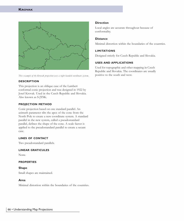
66 • Understanding Map Projections
This example of the Krovak projection uses a right-handed coordinate system.
DESCRIPTION
This projection is an oblique case of the Lambertconformal conic projection and was designed in 1922 byJosef Krovak. Used in the Czech Republic and Slovakia.Also known as S-JTSK.
PROJECTION METHOD
Conic projection based on one standard parallel. Anazimuth parameter tilts the apex of the cone from theNorth Pole to create a new coordinate system. A standardparallel in the new system, called a pseudostandardparallel, defines the shape of the cone. A scale factor isapplied to the pseudostandard parallel to create a secantcase.
LINES OF CONTACT
Two pseudostandard parallels.
LINEAR GRATICULES
None.
PROPERTIES
Shape
Small shapes are maintained.
Area
Minimal distortion within the boundaries of the countries.
KROVAK
Direction
Local angles are accurate throughout because ofconformality.
Distance
Minimal distortion within the boundaries of the countries.
LIMITATIONS
Designed strictly for Czech Republic and Slovakia.
USES AND APPLICATIONS
Used for topographic and other mapping in CzechRepublic and Slovakia. The coordinates are usuallypositive to the south and west.
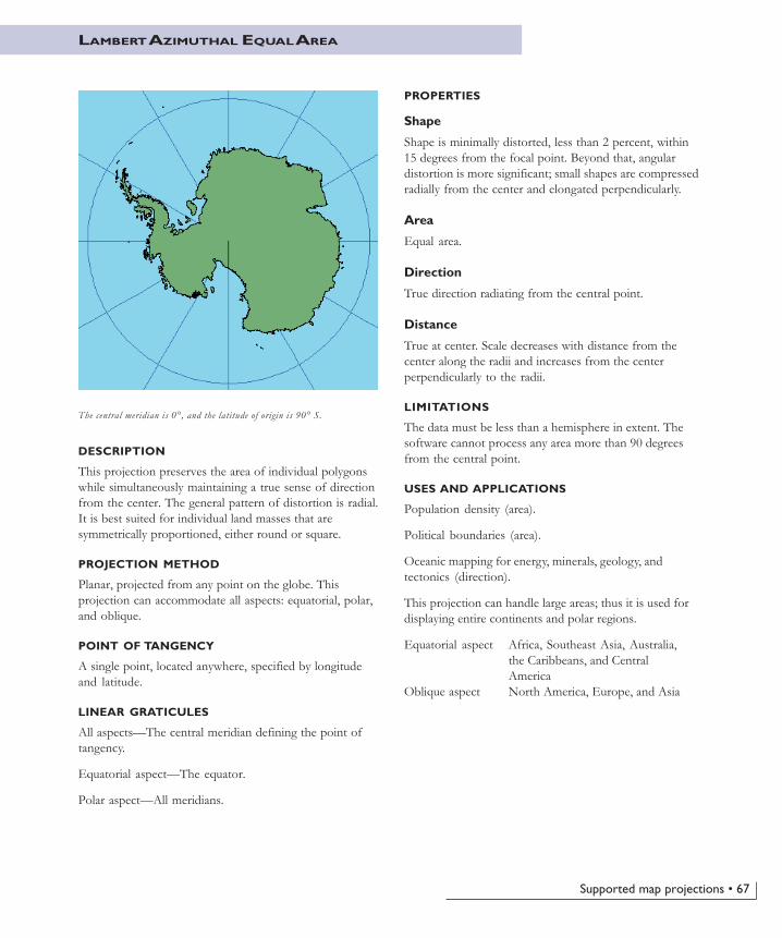
Supported map projections • 67
LAMBERT AZIMUTHAL EQUAL AREA
DESCRIPTION
This projection preserves the area of individual polygonswhile simultaneously maintaining a true sense of directionfrom the center. The general pattern of distortion is radial.It is best suited for individual land masses that aresymmetrically proportioned, either round or square.
PROJECTION METHOD
Planar, projected from any point on the globe. Thisprojection can accommodate all aspects: equatorial, polar,and oblique.
POINT OF TANGENCY
A single point, located anywhere, specified by longitudeand latitude.
LINEAR GRATICULES
All aspects—The central meridian defining the point oftangency.
Equatorial aspect—The equator.
Polar aspect—All meridians.
PROPERTIES
Shape
Shape is minimally distorted, less than 2 percent, within15 degrees from the focal point. Beyond that, angulardistortion is more significant; small shapes are compressedradially from the center and elongated perpendicularly.
Area
Equal area.
Direction
True direction radiating from the central point.
Distance
True at center. Scale decreases with distance from thecenter along the radii and increases from the centerperpendicularly to the radii.
LIMITATIONS
The data must be less than a hemisphere in extent. Thesoftware cannot process any area more than 90 degreesfrom the central point.
USES AND APPLICATIONS
Population density (area).
Political boundaries (area).
Oceanic mapping for energy, minerals, geology, andtectonics (direction).
This projection can handle large areas; thus it is used fordisplaying entire continents and polar regions.
Equatorial aspect Africa, Southeast Asia, Australia,the Caribbeans, and CentralAmerica
Oblique aspect North America, Europe, and Asia
The central meridian is 0°, and the latitude of origin is 90° S.
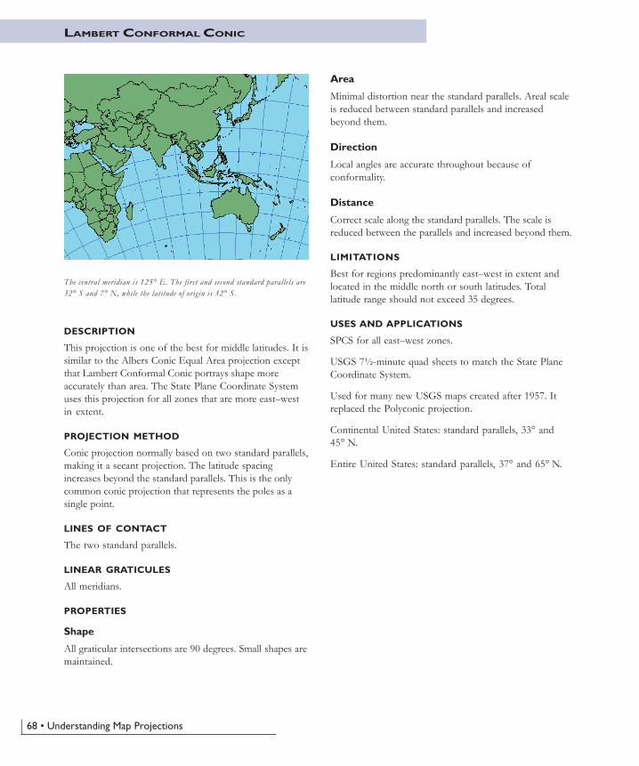
68 • Understanding Map Projections
LAMBERT CONFORMAL CONIC
DESCRIPTION
This projection is one of the best for middle latitudes. It issimilar to the Albers Conic Equal Area projection exceptthat Lambert Conformal Conic portrays shape moreaccurately than area. The State Plane Coordinate Systemuses this projection for all zones that are more east–westin extent.
PROJECTION METHOD
Conic projection normally based on two standard parallels,making it a secant projection. The latitude spacingincreases beyond the standard parallels. This is the onlycommon conic projection that represents the poles as asingle point.
LINES OF CONTACT
The two standard parallels.
LINEAR GRATICULES
All meridians.
PROPERTIES
Shape
All graticular intersections are 90 degrees. Small shapes aremaintained.
Area
Minimal distortion near the standard parallels. Areal scaleis reduced between standard parallels and increasedbeyond them.
Direction
Local angles are accurate throughout because ofconformality.
Distance
Correct scale along the standard parallels. The scale isreduced between the parallels and increased beyond them.
LIMITATIONS
Best for regions predominantly east–west in extent andlocated in the middle north or south latitudes. Totallatitude range should not exceed 35 degrees.
USES AND APPLICATIONS
SPCS for all east–west zones.
USGS 7½-minute quad sheets to match the State PlaneCoordinate System.
Used for many new USGS maps created after 1957. Itreplaced the Polyconic projection.
Continental United States: standard parallels, 33° and45° N.
Entire United States: standard parallels, 37° and 65° N.
The central meridian is 125° E. The first and second standard parallels are32° S and 7° N, while the latitude of origin is 32° S.
Supported map projections • 69
LOCAL CARTESIAN PROJECTION
DESCRIPTION
This is a specialized map projection that does not take intoaccount the curvature of the earth. It’s designed for verylarge-scale mapping applications. This projection is actuallythe Orthographic projection based on a spheroid.
PROJECTION METHOD
The coordinates of the center of the area of interestdefine the origin of the local coordinate system. The planeis tangent to the spheroid at that point, and the differencesin z values are negligible between corresponding points onthe spheroid and the plane. Because the differences in zvalues are ignored, distortions will greatly increase beyondroughly one degree from the origin.
USES AND APPLICATIONS
Large-scale mapping. In ArcInfo Workstation it should notbe used for areas greater than one degree from the origin.
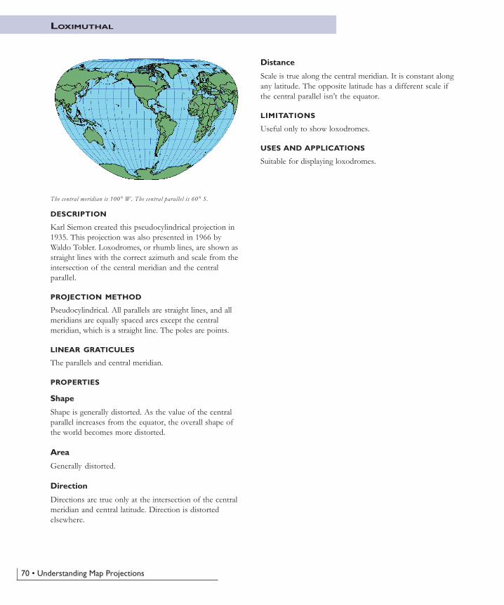
70 • Understanding Map Projections
LOXIMUTHAL
The central meridian is 100° W. The central parallel is 60° S.
DESCRIPTION
Karl Siemon created this pseudocylindrical projection in1935. This projection was also presented in 1966 byWaldo Tobler. Loxodromes, or rhumb lines, are shown asstraight lines with the correct azimuth and scale from theintersection of the central meridian and the centralparallel.
PROJECTION METHOD
Pseudocylindrical. All parallels are straight lines, and allmeridians are equally spaced arcs except the centralmeridian, which is a straight line. The poles are points.
LINEAR GRATICULES
The parallels and central meridian.
PROPERTIES
Shape
Shape is generally distorted. As the value of the centralparallel increases from the equator, the overall shape ofthe world becomes more distorted.
Area
Generally distorted.
Direction
Directions are true only at the intersection of the centralmeridian and central latitude. Direction is distortedelsewhere.
Distance
Scale is true along the central meridian. It is constant alongany latitude. The opposite latitude has a different scale ifthe central parallel isn’t the equator.
LIMITATIONS
Useful only to show loxodromes.
USES AND APPLICATIONS
Suitable for displaying loxodromes.
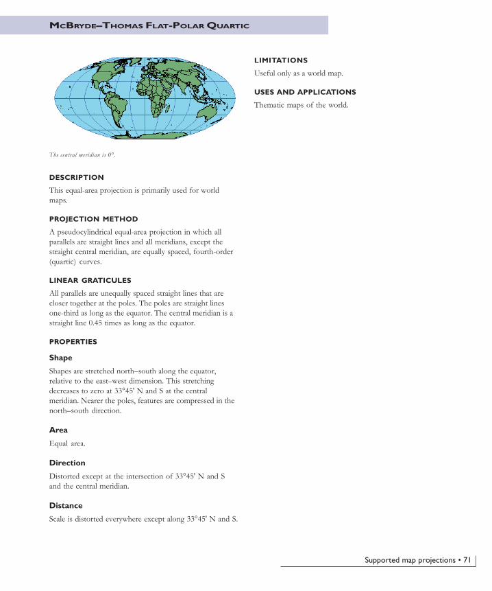
Supported map projections • 71
MCBRYDE–THOMAS FLAT-POLAR QUARTIC
DESCRIPTION
This equal-area projection is primarily used for worldmaps.
PROJECTION METHOD
A pseudocylindrical equal-area projection in which allparallels are straight lines and all meridians, except thestraight central meridian, are equally spaced, fourth-order(quartic) curves.
LINEAR GRATICULES
All parallels are unequally spaced straight lines that arecloser together at the poles. The poles are straight linesone-third as long as the equator. The central meridian is astraight line 0.45 times as long as the equator.
PROPERTIES
Shape
Shapes are stretched north–south along the equator,relative to the east–west dimension. This stretchingdecreases to zero at 33°45' N and S at the centralmeridian. Nearer the poles, features are compressed in thenorth–south direction.
Area
Equal area.
Direction
Distorted except at the intersection of 33°45' N and Sand the central meridian.
Distance
Scale is distorted everywhere except along 33°45' N and S.
The central meridian is 0°.
LIMITATIONS
Useful only as a world map.
USES AND APPLICATIONS
Thematic maps of the world.
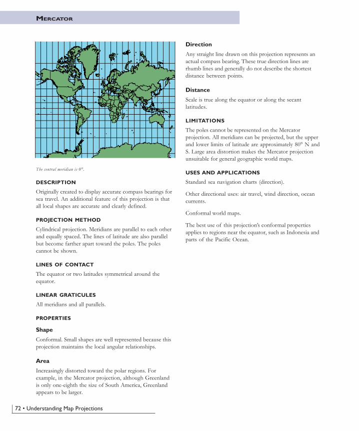
72 • Understanding Map Projections
MERCATOR
DESCRIPTION
Originally created to display accurate compass bearings forsea travel. An additional feature of this projection is thatall local shapes are accurate and clearly defined.
PROJECTION METHOD
Cylindrical projection. Meridians are parallel to each otherand equally spaced. The lines of latitude are also parallelbut become farther apart toward the poles. The polescannot be shown.
LINES OF CONTACT
The equator or two latitudes symmetrical around theequator.
LINEAR GRATICULES
All meridians and all parallels.
PROPERTIES
Shape
Conformal. Small shapes are well represented because thisprojection maintains the local angular relationships.
Area
Increasingly distorted toward the polar regions. Forexample, in the Mercator projection, although Greenlandis only one-eighth the size of South America, Greenlandappears to be larger.
Direction
Any straight line drawn on this projection represents anactual compass bearing. These true direction lines arerhumb lines and generally do not describe the shortestdistance between points.
Distance
Scale is true along the equator or along the secantlatitudes.
LIMITATIONS
The poles cannot be represented on the Mercatorprojection. All meridians can be projected, but the upperand lower limits of latitude are approximately 80° N andS. Large area distortion makes the Mercator projectionunsuitable for general geographic world maps.
USES AND APPLICATIONS
Standard sea navigation charts (direction).
Other directional uses: air travel, wind direction, oceancurrents.
Conformal world maps.
The best use of this projection’s conformal propertiesapplies to regions near the equator, such as Indonesia andparts of the Pacific Ocean.
The central meridian is 0°.
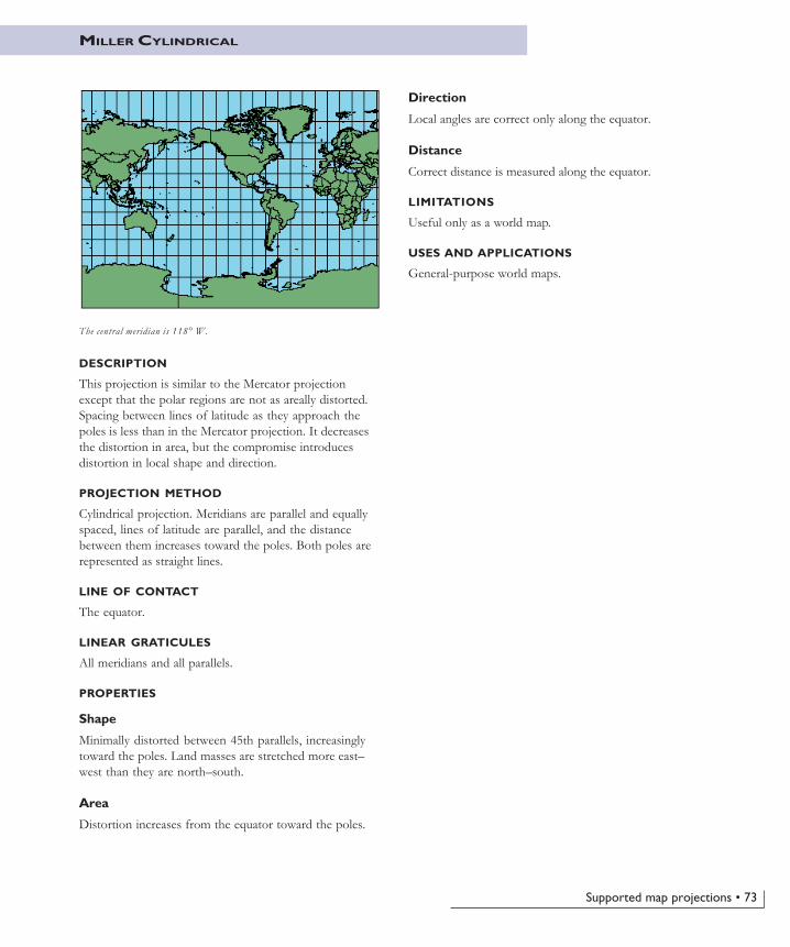
Supported map projections • 73
MILLER CYLINDRICAL
DESCRIPTION
This projection is similar to the Mercator projectionexcept that the polar regions are not as areally distorted.Spacing between lines of latitude as they approach thepoles is less than in the Mercator projection. It decreasesthe distortion in area, but the compromise introducesdistortion in local shape and direction.
PROJECTION METHOD
Cylindrical projection. Meridians are parallel and equallyspaced, lines of latitude are parallel, and the distancebetween them increases toward the poles. Both poles arerepresented as straight lines.
LINE OF CONTACT
The equator.
LINEAR GRATICULES
All meridians and all parallels.
PROPERTIES
Shape
Minimally distorted between 45th parallels, increasinglytoward the poles. Land masses are stretched more east–west than they are north–south.
Area
Distortion increases from the equator toward the poles.
Direction
Local angles are correct only along the equator.
Distance
Correct distance is measured along the equator.
LIMITATIONS
Useful only as a world map.
USES AND APPLICATIONS
General-purpose world maps.
The central meridian is 118° W.
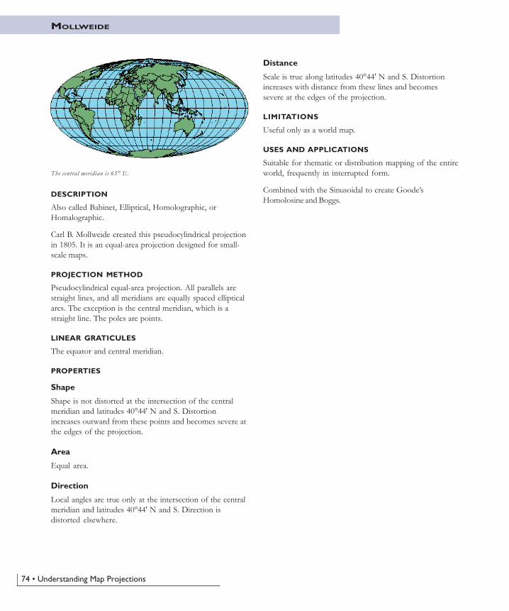
74 • Understanding Map Projections
MOLLWEIDE
DESCRIPTION
Also called Babinet, Elliptical, Homolographic, orHomalographic.
Carl B. Mollweide created this pseudocylindrical projectionin 1805. It is an equal-area projection designed for small-scale maps.
PROJECTION METHOD
Pseudocylindrical equal-area projection. All parallels arestraight lines, and all meridians are equally spaced ellipticalarcs. The exception is the central meridian, which is astraight line. The poles are points.
LINEAR GRATICULES
The equator and central meridian.
PROPERTIES
Shape
Shape is not distorted at the intersection of the centralmeridian and latitudes 40°44' N and S. Distortionincreases outward from these points and becomes severe atthe edges of the projection.
Area
Equal area.
Direction
Local angles are true only at the intersection of the centralmeridian and latitudes 40°44' N and S. Direction isdistorted elsewhere.
Distance
Scale is true along latitudes 40°44' N and S. Distortionincreases with distance from these lines and becomessevere at the edges of the projection.
LIMITATIONS
Useful only as a world map.
USES AND APPLICATIONS
Suitable for thematic or distribution mapping of the entireworld, frequently in interrupted form.
Combined with the Sinusoidal to create Goode’sHomolosine and Boggs.
The central meridian is 65° E.
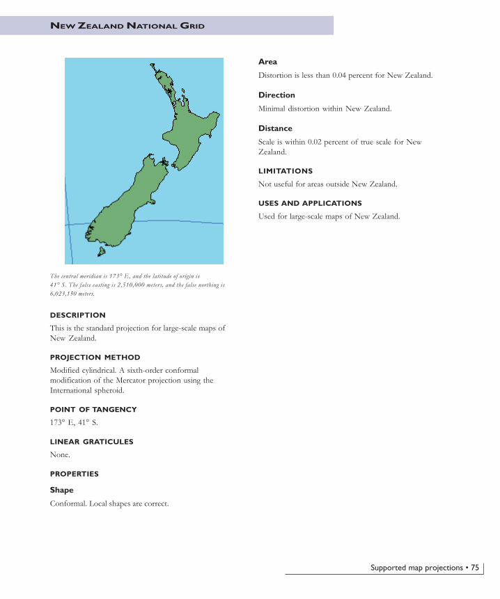
Supported map projections • 75
NEW ZEALAND NATIONAL GRID
DESCRIPTION
This is the standard projection for large-scale maps ofNew Zealand.
PROJECTION METHOD
Modified cylindrical. A sixth-order conformalmodification of the Mercator projection using theInternational spheroid.
POINT OF TANGENCY
173° E, 41° S.
LINEAR GRATICULES
None.
PROPERTIES
Shape
Conformal. Local shapes are correct.
Area
Distortion is less than 0.04 percent for New Zealand.
Direction
Minimal distortion within New Zealand.
Distance
Scale is within 0.02 percent of true scale for NewZealand.
LIMITATIONS
Not useful for areas outside New Zealand.
USES AND APPLICATIONS
Used for large-scale maps of New Zealand.
The central meridian is 173° E, and the latitude of origin is41° S. The false easting is 2,510,000 meters, and the false northing is6,023,150 meters.
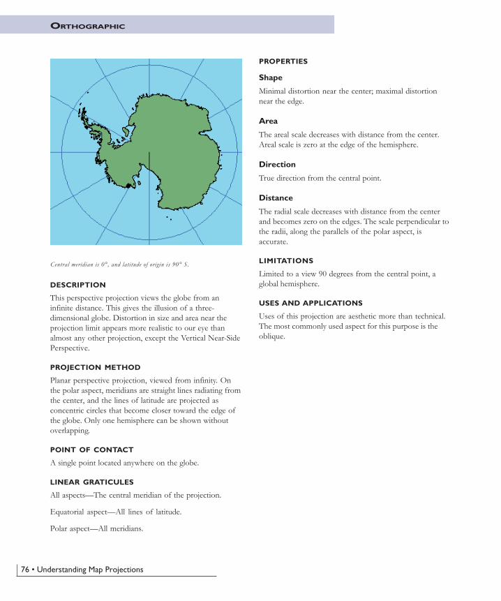
76 • Understanding Map Projections
ORTHOGRAPHIC
DESCRIPTION
This perspective projection views the globe from aninfinite distance. This gives the illusion of a three-dimensional globe. Distortion in size and area near theprojection limit appears more realistic to our eye thanalmost any other projection, except the Vertical Near-SidePerspective.
PROJECTION METHOD
Planar perspective projection, viewed from infinity. Onthe polar aspect, meridians are straight lines radiating fromthe center, and the lines of latitude are projected asconcentric circles that become closer toward the edge ofthe globe. Only one hemisphere can be shown withoutoverlapping.
POINT OF CONTACT
A single point located anywhere on the globe.
LINEAR GRATICULES
All aspects—The central meridian of the projection.
Equatorial aspect—All lines of latitude.
Polar aspect—All meridians.
PROPERTIES
Shape
Minimal distortion near the center; maximal distortionnear the edge.
Area
The areal scale decreases with distance from the center.Areal scale is zero at the edge of the hemisphere.
Direction
True direction from the central point.
Distance
The radial scale decreases with distance from the centerand becomes zero on the edges. The scale perpendicular tothe radii, along the parallels of the polar aspect, isaccurate.
LIMITATIONS
Limited to a view 90 degrees from the central point, aglobal hemisphere.
USES AND APPLICATIONS
Uses of this projection are aesthetic more than technical.The most commonly used aspect for this purpose is theoblique.
Central meridian is 0°, and latitude of origin is 90° S.
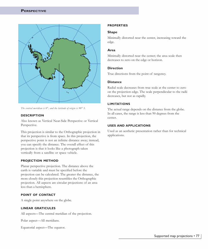
Supported map projections • 77
PERSPECTIVE
DESCRIPTION
Also known as Vertical Near-Side Perspective or VerticalPerspective.
This projection is similar to the Orthographic projection inthat its perspective is from space. In this projection, theperspective point is not an infinite distance away; instead,you can specify the distance. The overall effect of thisprojection is that it looks like a photograph takenvertically from a satellite or space vehicle.
PROJECTION METHOD
Planar perspective projection. The distance above theearth is variable and must be specified before theprojection can be calculated. The greater the distance, themore closely this projection resembles the Orthographicprojection. All aspects are circular projections of an arealess than a hemisphere.
POINT OF CONTACT
A single point anywhere on the globe.
LINEAR GRATICULES
All aspects—The central meridian of the projection.
Polar aspect—All meridians.
Equatorial aspect—The equator.
PROPERTIES
Shape
Minimally distorted near the center, increasing toward theedge.
Area
Minimally distorted near the center; the area scale thendecreases to zero on the edge or horizon.
Direction
True directions from the point of tangency.
Distance
Radial scale decreases from true scale at the center to zeroon the projection edge. The scale perpendicular to the radiidecreases, but not as rapidly.
LIMITATIONS
The actual range depends on the distance from the globe.In all cases, the range is less than 90 degrees from thecenter.
USES AND APPLICATIONS
Used as an aesthetic presentation rather than for technicalapplications.
The central meridian is 0°, and the latitude of origin is 90° S.
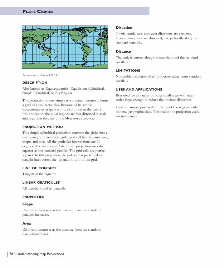
78 • Understanding Map Projections
DESCRIPTION
Also known as Equirectangular, Equidistant Cylindrical,Simple Cylindrical, or Rectangular.
This projection is very simple to construct because it formsa grid of equal rectangles. Because of its simplecalculations, its usage was more common in the past. Inthis projection, the polar regions are less distorted in scaleand area than they are in the Mercator projection.
PROJECTION METHOD
This simple cylindrical projection converts the globe into aCartesian grid. Each rectangular grid cell has the same size,shape, and area. All the graticular intersections are 90degrees. The traditional Plate Carrée projection uses theequator as the standard parallel. The grid cells are perfectsquares. In this projection, the poles are represented asstraight lines across the top and bottom of the grid.
LINE OF CONTACT
Tangent at the equator.
LINEAR GRATICULES
All meridians and all parallels.
PROPERTIES
Shape
Distortion increases as the distance from the standardparallels increases.
Area
Distortion increases as the distance from the standardparallels increases.
PLATE CARRÉE
Direction
North, south, east, and west directions are accurate.General directions are distorted, except locally along thestandard parallels.
Distance
The scale is correct along the meridians and the standardparallels.
LIMITATIONS
Noticeable distortion of all properties away from standardparallels.
USES AND APPLICATIONS
Best used for city maps or other small areas with mapscales large enough to reduce the obvious distortion.
Used for simple portrayals of the world or regions withminimal geographic data. This makes the projection usefulfor index maps.
The central meridian is 149° W.
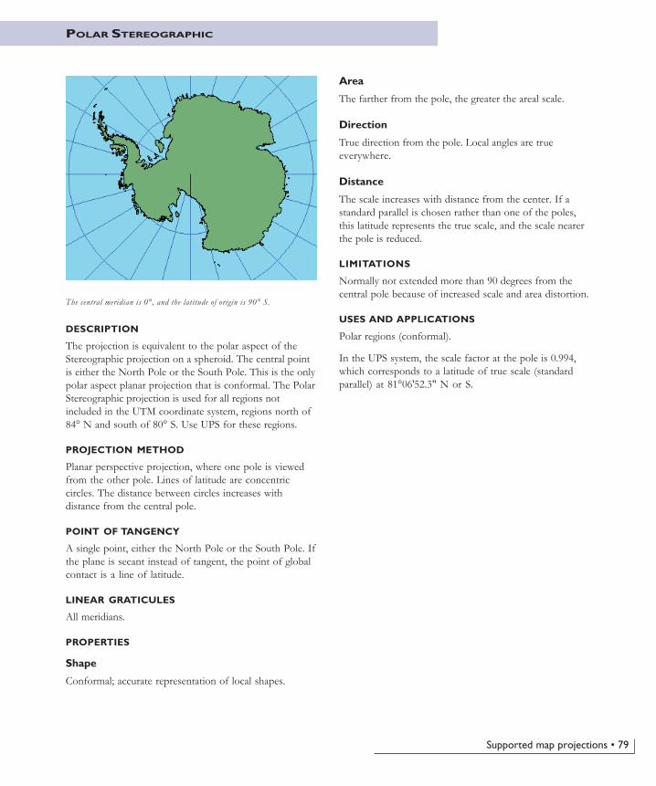
Supported map projections • 79
POLAR STEREOGRAPHIC
DESCRIPTION
The projection is equivalent to the polar aspect of theStereographic projection on a spheroid. The central pointis either the North Pole or the South Pole. This is the onlypolar aspect planar projection that is conformal. The PolarStereographic projection is used for all regions notincluded in the UTM coordinate system, regions north of84° N and south of 80° S. Use UPS for these regions.
PROJECTION METHOD
Planar perspective projection, where one pole is viewedfrom the other pole. Lines of latitude are concentriccircles. The distance between circles increases withdistance from the central pole.
POINT OF TANGENCY
A single point, either the North Pole or the South Pole. Ifthe plane is secant instead of tangent, the point of globalcontact is a line of latitude.
LINEAR GRATICULES
All meridians.
PROPERTIES
Shape
Conformal; accurate representation of local shapes.
Area
The farther from the pole, the greater the areal scale.
Direction
True direction from the pole. Local angles are trueeverywhere.
Distance
The scale increases with distance from the center. If astandard parallel is chosen rather than one of the poles,this latitude represents the true scale, and the scale nearerthe pole is reduced.
LIMITATIONS
Normally not extended more than 90 degrees from thecentral pole because of increased scale and area distortion.
USES AND APPLICATIONS
Polar regions (conformal).
In the UPS system, the scale factor at the pole is 0.994,which corresponds to a latitude of true scale (standardparallel) at 81°06'52.3" N or S.
The central meridian is 0°, and the latitude of origin is 90° S.
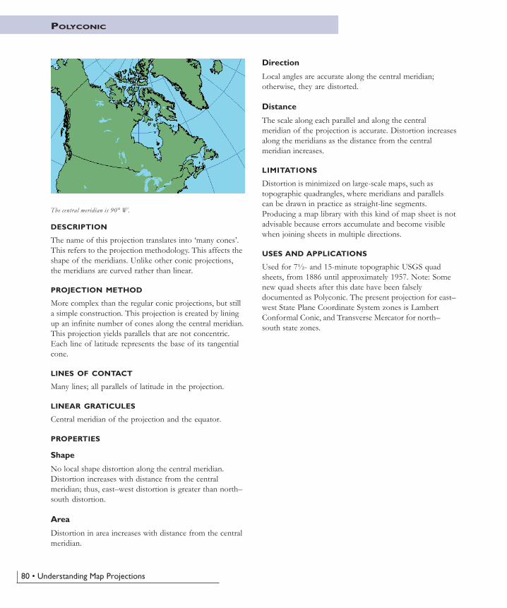
80 • Understanding Map Projections
POLYCONIC
DESCRIPTION
The name of this projection translates into ‘many cones’.This refers to the projection methodology. This affects theshape of the meridians. Unlike other conic projections,the meridians are curved rather than linear.
PROJECTION METHOD
More complex than the regular conic projections, but stilla simple construction. This projection is created by liningup an infinite number of cones along the central meridian.This projection yields parallels that are not concentric.Each line of latitude represents the base of its tangentialcone.
LINES OF CONTACT
Many lines; all parallels of latitude in the projection.
LINEAR GRATICULES
Central meridian of the projection and the equator.
PROPERTIES
Shape
No local shape distortion along the central meridian.Distortion increases with distance from the centralmeridian; thus, east–west distortion is greater than north–south distortion.
Area
Distortion in area increases with distance from the centralmeridian.
Direction
Local angles are accurate along the central meridian;otherwise, they are distorted.
Distance
The scale along each parallel and along the centralmeridian of the projection is accurate. Distortion increasesalong the meridians as the distance from the centralmeridian increases.
LIMITATIONS
Distortion is minimized on large-scale maps, such astopographic quadrangles, where meridians and parallelscan be drawn in practice as straight-line segments.Producing a map library with this kind of map sheet is notadvisable because errors accumulate and become visiblewhen joining sheets in multiple directions.
USES AND APPLICATIONS
Used for 7½- and 15-minute topographic USGS quadsheets, from 1886 until approximately 1957. Note: Somenew quad sheets after this date have been falselydocumented as Polyconic. The present projection for east–west State Plane Coordinate System zones is LambertConformal Conic, and Transverse Mercator for north–south state zones.
The central meridian is 90° W.
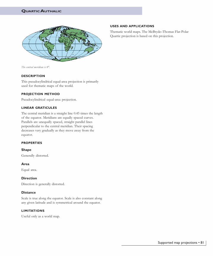
Supported map projections • 81
QUARTIC AUTHALIC
DESCRIPTION
This pseudocylindrical equal-area projection is primarilyused for thematic maps of the world.
PROJECTION METHOD
Pseudocylindrical equal-area projection.
LINEAR GRATICULES
The central meridian is a straight line 0.45 times the lengthof the equator. Meridians are equally spaced curves.Parallels are unequally spaced, straight parallel linesperpendicular to the central meridian. Their spacingdecreases very gradually as they move away from theequator.
PROPERTIES
Shape
Generally distorted.
Area
Equal area.
Direction
Direction is generally distorted.
Distance
Scale is true along the equator. Scale is also constant alongany given latitude and is symmetrical around the equator.
LIMITATIONS
Useful only as a world map.
USES AND APPLICATIONS
Thematic world maps. The McBryde–Thomas Flat-PolarQuartic projection is based on this projection.
The central meridian is 0°.
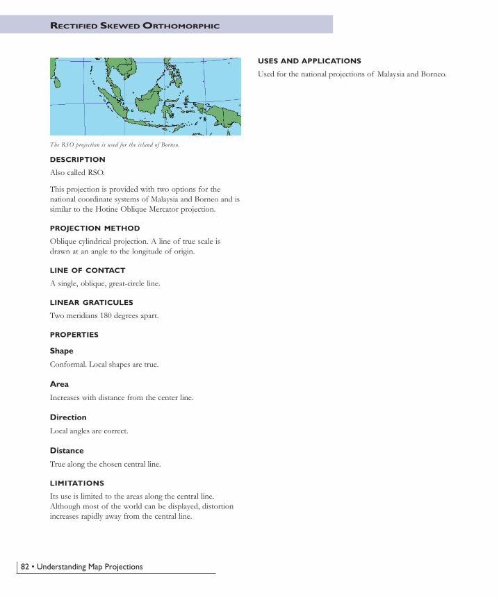
82 • Understanding Map Projections
RECTIFIED SKEWED ORTHOMORPHIC
The RSO projection is used for the island of Borneo.
DESCRIPTION
Also called RSO.
This projection is provided with two options for thenational coordinate systems of Malaysia and Borneo and issimilar to the Hotine Oblique Mercator projection.
PROJECTION METHOD
Oblique cylindrical projection. A line of true scale isdrawn at an angle to the longitude of origin.
LINE OF CONTACT
A single, oblique, great-circle line.
LINEAR GRATICULES
Two meridians 180 degrees apart.
PROPERTIES
Shape
Conformal. Local shapes are true.
Area
Increases with distance from the center line.
Direction
Local angles are correct.
Distance
True along the chosen central line.
LIMITATIONS
Its use is limited to the areas along the central line.Although most of the world can be displayed, distortionincreases rapidly away from the central line.
USES AND APPLICATIONS
Used for the national projections of Malaysia and Borneo.
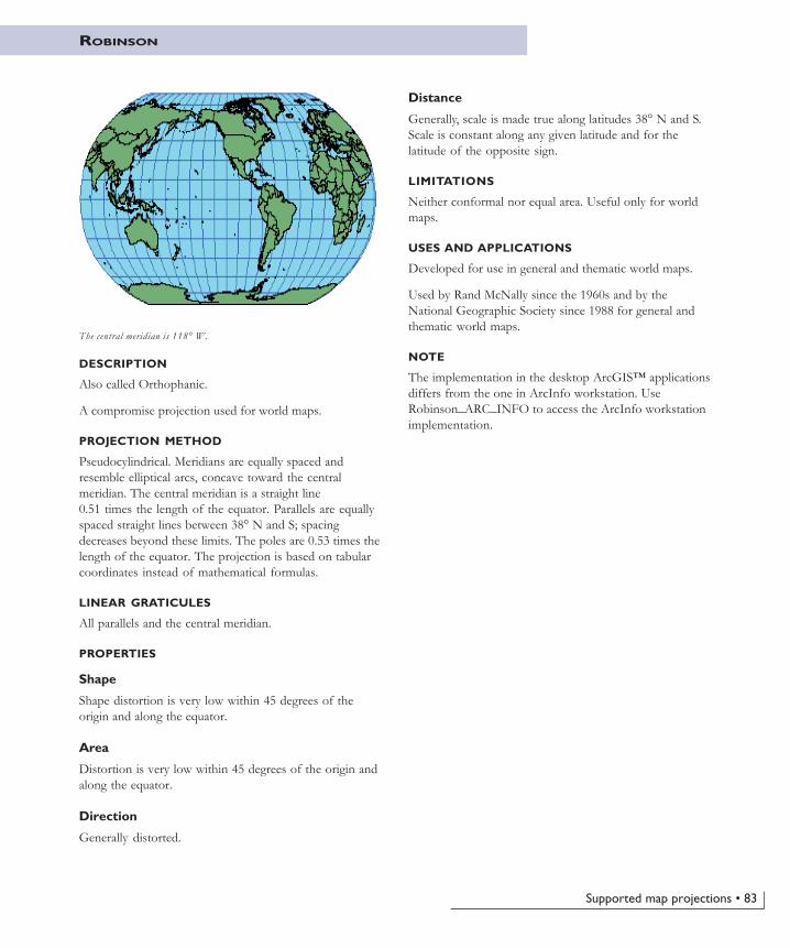
Supported map projections • 83
ROBINSON
DESCRIPTION
Also called Orthophanic.
A compromise projection used for world maps.
PROJECTION METHOD
Pseudocylindrical. Meridians are equally spaced andresemble elliptical arcs, concave toward the centralmeridian. The central meridian is a straight line0.51 times the length of the equator. Parallels are equallyspaced straight lines between 38° N and S; spacingdecreases beyond these limits. The poles are 0.53 times thelength of the equator. The projection is based on tabularcoordinates instead of mathematical formulas.
LINEAR GRATICULES
All parallels and the central meridian.
PROPERTIES
Shape
Shape distortion is very low within 45 degrees of theorigin and along the equator.
Area
Distortion is very low within 45 degrees of the origin andalong the equator.
Direction
Generally distorted.
Distance
Generally, scale is made true along latitudes 38° N and S.Scale is constant along any given latitude and for thelatitude of the opposite sign.
LIMITATIONS
Neither conformal nor equal area. Useful only for worldmaps.
USES AND APPLICATIONS
Developed for use in general and thematic world maps.
Used by Rand McNally since the 1960s and by theNational Geographic Society since 1988 for general andthematic world maps.
NOTE
The implementation in the desktop ArcGIS™ applicationsdiffers from the one in ArcInfo workstation. UseRobinson_ARC_INFO to access the ArcInfo workstationimplementation.
The central meridian is 118° W.
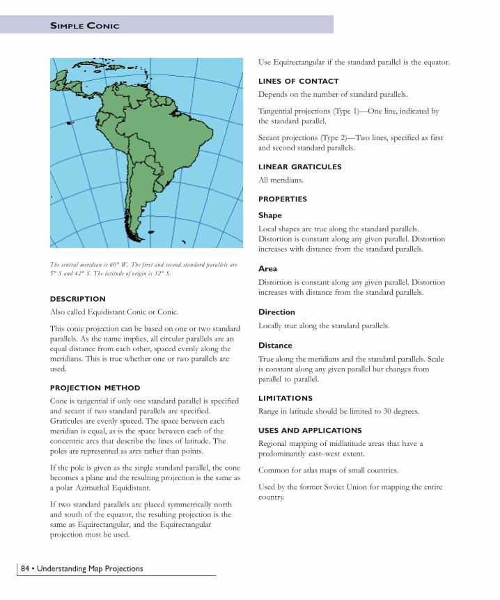
84 • Understanding Map Projections
SIMPLE CONIC
DESCRIPTION
Also called Equidistant Conic or Conic.
This conic projection can be based on one or two standardparallels. As the name implies, all circular parallels are anequal distance from each other, spaced evenly along themeridians. This is true whether one or two parallels areused.
PROJECTION METHOD
Cone is tangential if only one standard parallel is specifiedand secant if two standard parallels are specified.Graticules are evenly spaced. The space between eachmeridian is equal, as is the space between each of theconcentric arcs that describe the lines of latitude. Thepoles are represented as arcs rather than points.
If the pole is given as the single standard parallel, the conebecomes a plane and the resulting projection is the same asa polar Azimuthal Equidistant.
If two standard parallels are placed symmetrically northand south of the equator, the resulting projection is thesame as Equirectangular, and the Equirectangularprojection must be used.
Use Equirectangular if the standard parallel is the equator.
LINES OF CONTACT
Depends on the number of standard parallels.
Tangential projections (Type 1)—One line, indicated bythe standard parallel.
Secant projections (Type 2)—Two lines, specified as firstand second standard parallels.
LINEAR GRATICULES
All meridians.
PROPERTIES
Shape
Local shapes are true along the standard parallels.Distortion is constant along any given parallel. Distortionincreases with distance from the standard parallels.
Area
Distortion is constant along any given parallel. Distortionincreases with distance from the standard parallels.
Direction
Locally true along the standard parallels.
Distance
True along the meridians and the standard parallels. Scaleis constant along any given parallel but changes fromparallel to parallel.
LIMITATIONS
Range in latitude should be limited to 30 degrees.
USES AND APPLICATIONS
Regional mapping of midlatitude areas that have apredominantly east–west extent.
Common for atlas maps of small countries.
Used by the former Soviet Union for mapping the entirecountry.
The central meridian is 60° W. The first and second standard parallels are5° S and 42° S. The latitude of origin is 32° S.
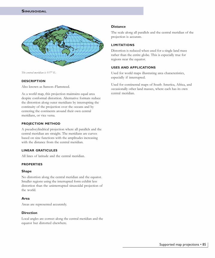
Supported map projections • 85
SINUSOIDAL
DESCRIPTION
Also known as Sanson–Flamsteed.
As a world map, this projection maintains equal areadespite conformal distortion. Alternative formats reducethe distortion along outer meridians by interrupting thecontinuity of the projection over the oceans and bycentering the continents around their own centralmeridians, or vice versa.
PROJECTION METHOD
A pseudocylindrical projection where all parallels and thecentral meridian are straight. The meridians are curvesbased on sine functions with the amplitudes increasingwith the distance from the central meridian.
LINEAR GRATICULES
All lines of latitude and the central meridian.
PROPERTIES
Shape
No distortion along the central meridian and the equator.Smaller regions using the interrupted form exhibit lessdistortion than the uninterrupted sinusoidal projection ofthe world.
Area
Areas are represented accurately.
Direction
Local angles are correct along the central meridian and theequator but distorted elsewhere.
Distance
The scale along all parallels and the central meridian of theprojection is accurate.
LIMITATIONS
Distortion is reduced when used for a single land massrather than the entire globe. This is especially true forregions near the equator.
USES AND APPLICATIONS
Used for world maps illustrating area characteristics,especially if interrupted.
Used for continental maps of South America, Africa, andoccasionally other land masses, where each has its owncentral meridian.
The central meridian is 117° E.
86 • Understanding Map Projections
SPACE OBLIQUE MERCATOR
DESCRIPTION
This projection is nearly conformal and has little scaledistortion within the sensing range of an orbiting mappingsatellite such as Landsat. This is the first projection toincorporate the earth’s rotation with respect to theorbiting satellite. For Landsat 1, 2, and 3, the path range isfrom 1 to 251. For Landsat 4 and 5, the path range is from1 to 233.
PROJECTION METHOD
Modified cylindrical, for which the central line is curvedand defined by the ground track of the orbit of thesatellite.
LINE OF TANGENCY
Conceptual.
LINEAR GRATICULES
None.
PROPERTIES
Shape
Shape is correct within a few parts per million for thesensing range of the satellite.
Area
Varies by less than 0.02 percent for the sensing range ofthe satellite.
Direction
Minimal distortion within the sensing range.
Distance
Scale is true along the ground track and variesapproximately 0.01 percent within the sensing range.
LIMITATIONS
Plots for adjacent paths do not match withouttransformation.
USES AND APPLICATIONS
Specifically designed to minimize distortion within thesensing range of a mapping satellite as it orbits the rotatingearth.
Used to tie satellite imagery to a ground-based planarcoordinate system and for continuous mapping of satelliteimagery.
Standard format used for data from Landsat 4 and 5.
Supported map projections • 87
STATE PLANE COORDINATE SYSTEM
DESCRIPTION
Also known as SPCS, SPC, State Plane, and State.
The State Plane Coordinate System is not a projection. Itis a coordinate system that divides the 50 states of theUnited States, Puerto Rico, and the U.S. Virgin Islandsinto more than 120 numbered sections, referred to aszones. Each zone has an assigned code number that definesthe projection parameters for the region.
PROJECTION METHOD
Projection may be cylindrical or conic. See LambertConformal Conic, Transverse Mercator, and HotineOblique Mercator for methodology and properties.
WHY USE STATE PLANE
Governmental organizations and groups who work withthem primarily use the State Plane Coordinate System.Most often, these are county or municipal databases. Theadvantage of using SPCS is that your data is in a commoncoordinate system with other databases covering the samearea.
WHAT IS STATE PLANE
The State Plane Coordinate System was designed for large-scale mapping in the United States. It was developed inthe 1930s by the U.S. Coast and Geodetic Survey toprovide a common reference system to surveyors andmappers. The goal was to design a conformal mappingsystem for the country with a maximum scale distortionof one part in 10,000, then considered the limit ofsurveying accuracy.
Three conformal projections were chosen: the LambertConformal Conic for states that are longer east–west, suchas Tennessee and Kentucky; the Transverse Mercatorprojection for states that are longer north–south, such asIllinois and Vermont; and the Oblique Mercator projectionfor the panhandle of Alaska, because it lays at an angle.
To maintain an accuracy of one part in 10,000, it wasnecessary to divide many states into zones. Each zone hasits own central meridian or standard parallels to maintainthe desired level of accuracy. The boundaries of thesezones follow county boundaries. Smaller states such asConnecticut require only one zone, while Alaska iscomposed of 10 zones and uses all three projections.
This coordinate system is referred to here as the StatePlane Coordinate System of 1927 (SPCS 27). It is basedon a network of geodetic control points referred to as theNorth American Datum of 1927 (NAD 1927 or NAD27).
STATE PLANE AND THE NORTH AMERICANDATUM
Technological advancements of the last 50 years have ledto improvements in the measurement of distances, angles,and the earth’s size and shape. This, combined withmoving the origin of the datum from Meades Ranch inKansas to the earth’s center of mass for compatibility withsatellite systems, made it necessary to redefine SPCS 27.The redefined and updated system is called the State PlaneCoordinate System of 1983 (SPCS 83). The coordinatesfor points are different for SPCS 27 and SPCS 83. Thereare several reasons for this. For SPCS 83, all State Planecoordinates published by NGS are in metric units, theshape of the spheroid of the earth is slightly different,some states have changed the definition of their zones,and values of longitude and latitude are slightly changed.
Officially, SPCS zones are identified by their NGS code.When ESRI® implemented the NGS codes, they were partof a proposed Federal Information Processing Standard(FIPS). For that reason, ESRI identifies the NGS zones asFIPS zones. That proposed standard was withdrawn, butESRI maintains the FIPS name for continuity.
Sometimes people use an older Bureau of LandManagement (BLM) system. The BLM system is outdatedand doesn’t include codes for some of the new zones. Thevalues also overlap. You should always use the NGS/FIPScodes.
The following zone changes were made from SPCS 27 toSPCS 83. The zone numbers listed below are FIPS zonenumbers. In addition, false easting and northing, or origin,of most zones has changed.
California—California zone 7, SPCS 27 FIPS zone 0407,was eliminated and included in California zone 5, SPCS 83FIPS zone 0405.
Montana—The three zones for Montana, SPCS 27 FIPSzones 2501, 2502, and 2503, were eliminated and replacedby a single zone, SPCS 83 FIPS zone 2500.
Nebraska—The two zones for Nebraska, SPCS 27 FIPSzones 2601 and 2602, were eliminated and replaced by asingle zone, SPCS 83 FIPS zone 2600.
88 • Understanding Map Projections
South Carolina—The two zones for South Carolina, SPCS27 FIPS zones 3901 and 3902, were eliminated andreplaced by a single zone, SPCS 83 FIPSzone 3900.
Puerto Rico and Virgin Islands—The two zones forPuerto Rico and the Virgin Islands, St. Thomas, St. John,and St. Croix, SPCS 27 FIPS zones 5201 and 5202, wereeliminated and replaced by a single zone, SPCS 83 FIPSzone 5200.
UNIT OF LENGTH
The standard unit of measure for SPCS 27 is the U.S.Survey foot. For SPCS 83, the most common unit ofmeasure is the meter. Those states that support both feetand meters have legislated which feet-to-metersconversion they use. The difference between the two isonly two parts in one million, but that can becomenoticeable when datasets are stored in double precision.The U.S. Survey foot equals 1,200/3,937 m, or0.3048006096 m.
EXAMPLES OF ZONE DEFINITIONS
Here are two examples of SPCS 83 parameters:
State Alabama East TennesseeZONE 3 1 0 1 5 3 0 1FIPS Zone 0 1 0 1 4 1 0 0Projection Transverse LambertStandard Parallels 35°15'
36°25'Central Meridian -85°50' -86°00'Scale Factor Reduction at Central Meridian1 :25 ,000 1 : 15 ,000Latitude of Origin 30°30' 34°20'Longitude of Origin -85°50' -86°00'False Easting 200 ,000 600 ,000False Northing 0 0
USES AND APPLICATIONS
Used for standard USGS 7½- and 15-minute quad sheets.
Used for most federal, state, and local large-scale mappingprojects in the United States.
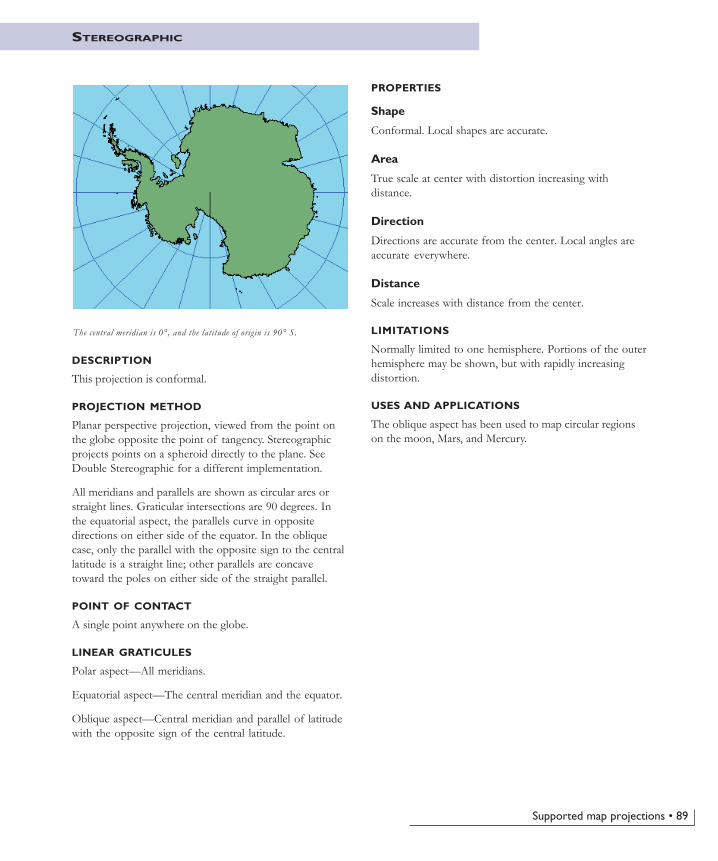
Supported map projections • 89
STEREOGRAPHIC
DESCRIPTION
This projection is conformal.
PROJECTION METHOD
Planar perspective projection, viewed from the point onthe globe opposite the point of tangency. Stereographicprojects points on a spheroid directly to the plane. SeeDouble Stereographic for a different implementation.
All meridians and parallels are shown as circular arcs orstraight lines. Graticular intersections are 90 degrees. Inthe equatorial aspect, the parallels curve in oppositedirections on either side of the equator. In the obliquecase, only the parallel with the opposite sign to the centrallatitude is a straight line; other parallels are concavetoward the poles on either side of the straight parallel.
POINT OF CONTACT
A single point anywhere on the globe.
LINEAR GRATICULES
Polar aspect—All meridians.
Equatorial aspect—The central meridian and the equator.
Oblique aspect—Central meridian and parallel of latitudewith the opposite sign of the central latitude.
PROPERTIES
Shape
Conformal. Local shapes are accurate.
Area
True scale at center with distortion increasing withdistance.
Direction
Directions are accurate from the center. Local angles areaccurate everywhere.
Distance
Scale increases with distance from the center.
LIMITATIONS
Normally limited to one hemisphere. Portions of the outerhemisphere may be shown, but with rapidly increasingdistortion.
USES AND APPLICATIONS
The oblique aspect has been used to map circular regionson the moon, Mars, and Mercury.
The central meridian is 0°, and the latitude of origin is 90° S.
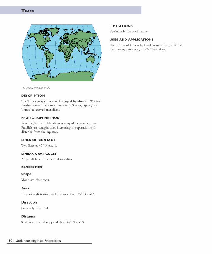
90 • Understanding Map Projections
TIMES
DESCRIPTION
The Times projection was developed by Moir in 1965 forBartholomew. It is a modified Gall’s Stereographic, butTimes has curved meridians.
PROJECTION METHOD
Pseudocylindrical. Meridians are equally spaced curves.Parallels are straight lines increasing in separation withdistance from the equator.
LINES OF CONTACT
Two lines at 45° N and S.
LINEAR GRATICULES
All parallels and the central meridian.
PROPERTIES
Shape
Moderate distortion.
Area
Increasing distortion with distance from 45° N and S.
Direction
Generally distorted.
Distance
Scale is correct along parallels at 45° N and S.
The central meridian is 0°.
LIMITATIONS
Useful only for world maps.
USES AND APPLICATIONS
Used for world maps by Bartholomew Ltd., a Britishmapmaking company, in The Times Atlas.
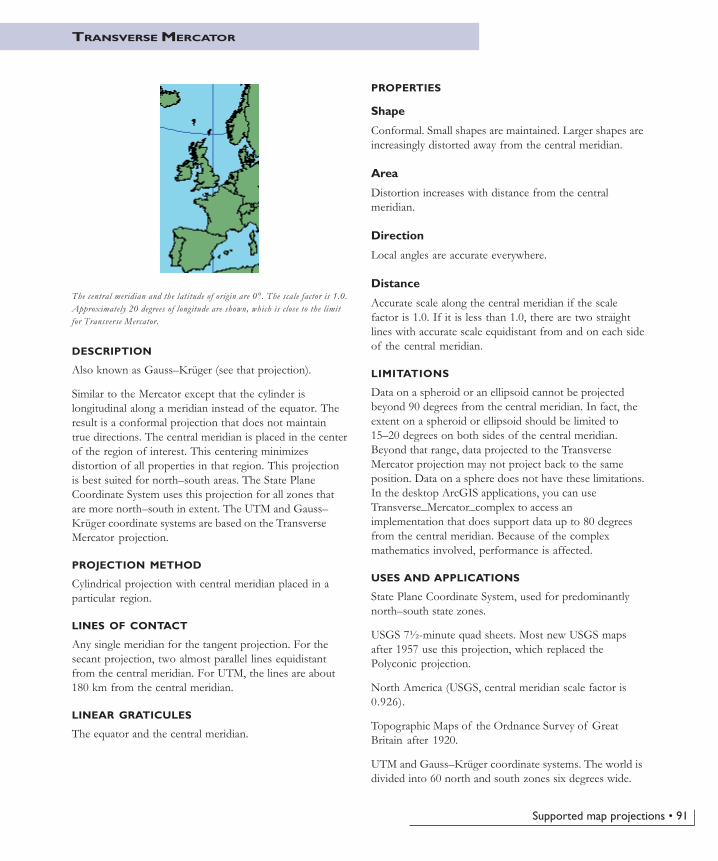
Supported map projections • 91
TRANSVERSE MERCATOR
DESCRIPTION
Also known as Gauss–Krüger (see that projection).
Similar to the Mercator except that the cylinder islongitudinal along a meridian instead of the equator. Theresult is a conformal projection that does not maintaintrue directions. The central meridian is placed in the centerof the region of interest. This centering minimizesdistortion of all properties in that region. This projectionis best suited for north–south areas. The State PlaneCoordinate System uses this projection for all zones thatare more north–south in extent. The UTM and Gauss–Krüger coordinate systems are based on the TransverseMercator projection.
PROJECTION METHOD
Cylindrical projection with central meridian placed in aparticular region.
LINES OF CONTACT
Any single meridian for the tangent projection. For thesecant projection, two almost parallel lines equidistantfrom the central meridian. For UTM, the lines are about180 km from the central meridian.
LINEAR GRATICULES
The equator and the central meridian.
PROPERTIES
Shape
Conformal. Small shapes are maintained. Larger shapes areincreasingly distorted away from the central meridian.
Area
Distortion increases with distance from the centralmeridian.
Direction
Local angles are accurate everywhere.
Distance
Accurate scale along the central meridian if the scalefactor is 1.0. If it is less than 1.0, there are two straightlines with accurate scale equidistant from and on each sideof the central meridian.
LIMITATIONS
Data on a spheroid or an ellipsoid cannot be projectedbeyond 90 degrees from the central meridian. In fact, theextent on a spheroid or ellipsoid should be limited to15–20 degrees on both sides of the central meridian.Beyond that range, data projected to the TransverseMercator projection may not project back to the sameposition. Data on a sphere does not have these limitations.In the desktop ArcGIS applications, you can useTransverse_Mercator_complex to access animplementation that does support data up to 80 degreesfrom the central meridian. Because of the complexmathematics involved, performance is affected.
USES AND APPLICATIONS
State Plane Coordinate System, used for predominantlynorth–south state zones.
USGS 7½-minute quad sheets. Most new USGS mapsafter 1957 use this projection, which replaced thePolyconic projection.
North America (USGS, central meridian scale factor is0.926).
Topographic Maps of the Ordnance Survey of GreatBritain after 1920.
UTM and Gauss–Krüger coordinate systems. The world isdivided into 60 north and south zones six degrees wide.
The central meridian and the latitude of origin are 0°. The scale factor is 1.0.Approximately 20 degrees of longitude are shown, which is close to the limitfor Transverse Mercator.
92 • Understanding Map Projections
Each zone has a scale factor of 0.9996 and a false eastingof 500,000 meters. Zones south of the equator have afalse northing of 10,000,000 meters to ensure that all yvalues are positive. Zone 1 is at 177° W.
The Gauss–Krüger coordinate system is very similar to theUTM coordinate system. Europe is divided into zones sixdegrees wide with the central meridian of zone 1 equal to3° E. The parameters are the same as UTM except for thescale factor, which is equal to 1.000 rather than 0.9996.Some places also add the zone number times one millionto the 500,000 false easting value. GK zone 5 could havefalse easting values of 500,000 or 5,500,000 meters.
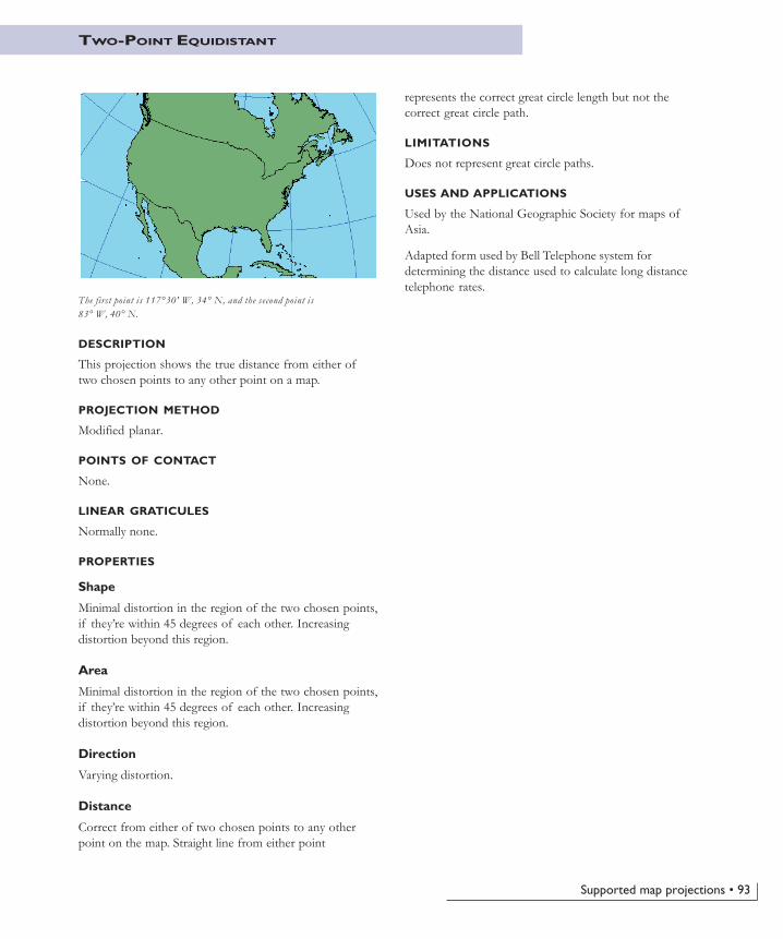
Supported map projections • 93
TWO-POINT EQUIDISTANT
DESCRIPTION
This projection shows the true distance from either oftwo chosen points to any other point on a map.
PROJECTION METHOD
Modified planar.
POINTS OF CONTACT
None.
LINEAR GRATICULES
Normally none.
PROPERTIES
Shape
Minimal distortion in the region of the two chosen points,if they’re within 45 degrees of each other. Increasingdistortion beyond this region.
Area
Minimal distortion in the region of the two chosen points,if they’re within 45 degrees of each other. Increasingdistortion beyond this region.
Direction
Varying distortion.
Distance
Correct from either of two chosen points to any otherpoint on the map. Straight line from either point
represents the correct great circle length but not thecorrect great circle path.
LIMITATIONS
Does not represent great circle paths.
USES AND APPLICATIONS
Used by the National Geographic Society for maps ofAsia.
Adapted form used by Bell Telephone system fordetermining the distance used to calculate long distancetelephone rates.
The first point is 117°30' W, 34° N, and the second point is83° W, 40° N.
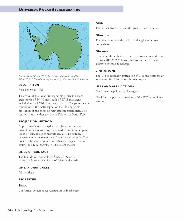
94 • Understanding Map Projections
The central meridian is 90° S. The latitude of standard parallel is81°06'52.3" S. The false easting and northing values are 2,000,000 meters.
DESCRIPTION
Also known as UPS.
This form of the Polar Stereographic projection mapsareas north of 84° N and south of 80° S that aren’tincluded in the UTM Coordinate System. The projection isequivalent to the polar aspect of the Stereographicprojection of the spheroid with specific parameters. Thecentral point is either the North Pole or the South Pole.
PROJECTION METHOD
Approximately (for the spheroid) planar perspectiveprojection, where one pole is viewed from the other pole.Lines of latitude are concentric circles. The distancebetween circles increases away from the central pole. Theorigin at the intersection of meridians is assigned a falseeasting and false northing of 2,000,000 meters.
LINES OF CONTACT
The latitude of true scale, 81°06'52.3" N or S,corresponds to a scale factor of 0.994 at the pole.
LINEAR GRATICULES
All meridians.
PROPERTIES
Shape
Conformal. Accurate representation of local shape.
Area
The farther from the pole, the greater the area scale.
Direction
True direction from the pole. Local angles are correcteverywhere.
Distance
In general, the scale increases with distance from the pole.Latitude 81°06'52.3" N or S has true scale. The scalecloser to the pole is reduced.
LIMITATIONS
The UPS is normally limited to 84° N in the north polaraspect and 80° S in the south polar aspect.
USES AND APPLICATIONS
Conformal mapping of polar regions.
Used for mapping polar regions of the UTM coordinatesystem.
UNIVERSAL POLAR STEREOGRAPHIC
Supported map projections • 95
UNIVERSAL TRANSVERSE MERCATOR
DESCRIPTION
Also known as UTM.
The Universal Transverse Mercator system is a specializedapplication of the Transverse Mercator projection. Theglobe is divided into 60 north and south zones, eachspanning six degrees of longitude. Each zone has its owncentral meridian. Zones 1N and 1S start at -180° W. Thelimits of each zone are 84° N and 80° S, with the divisionbetween north and south zones occurring at the equator.The polar regions use the Universal Polar Stereographiccoordinate system.
The origin for each zone is its central meridian and theequator. To eliminate negative coordinates, the coordinatesystem alters the coordinate values at the origin. The valuegiven to the central meridian is the false easting, and thevalue assigned to the equator is the false northing. A falseeasting of 500,000 meters is applied. A north zone has afalse northing of zero, while a south zone has a falsenorthing of 10,000,000 meters.
PROJECTION METHOD
Cylindrical projection. See the Transverse Mercatorprojection for the methodology.
LINES OF CONTACT
Two lines parallel to and approximately 180 km to eachside of the central meridian of the UTM zone.
LINEAR GRATICULES
The central meridian and the equator.
PROPERTIES
Shape
Conformal. Accurate representation of small shapes.Minimal distortion of larger shapes within the zone.
Area
Minimal distortion within each UTM zone.
Direction
Local angles are true.
Distance
Scale is constant along the central meridian but at a scalefactor of 0.9996 to reduce lateral distortion within eachzone. With this scale factor, lines lying 180 km east andwest of and parallel to the central meridian have a scalefactor of one.
LIMITATIONS
Designed for a scale error not exceeding 0.1 percentwithin each zone. Error and distortion increase for regionsthat span more than one UTM zone. UTM is not designedfor areas that span more than a few zones.
Data on a spheroid or an ellipsoid cannot be projectedbeyond 90 degrees from the central meridian. In fact, theextent on a spheroid or ellipsoid should be limited to15–20 degrees on both sides of the central meridian.Beyond that range, data projected to the TransverseMercator projection may not project back to the sameposition. Data on a sphere does not have these limitations.
USES AND APPLICATION
Used for United States topographic quadrangles,1:100,000 scale.
Many countries use local UTM zones based on the officialgeographic coordinate systems in use.
Large-scale topographic mapping of the former SovietUnion.
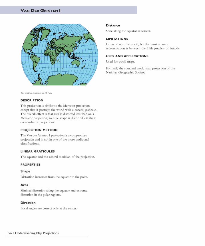
96 • Understanding Map Projections
VAN DER GRINTEN I
DESCRIPTION
This projection is similar to the Mercator projectionexcept that it portrays the world with a curved graticule.The overall effect is that area is distorted less than on aMercator projection, and the shape is distorted less thanon equal-area projections.
PROJECTION METHOD
The Van der Grinten I projection is a compromiseprojection and is not in one of the more traditionalclassifications.
LINEAR GRATICULES
The equator and the central meridian of the projection.
PROPERTIES
Shape
Distortion increases from the equator to the poles.
Area
Minimal distortion along the equator and extremedistortion in the polar regions.
Direction
Local angles are correct only at the center.
Distance
Scale along the equator is correct.
LIMITATIONS
Can represent the world, but the most accuraterepresentation is between the 75th parallels of latitude.
USES AND APPLICATIONS
Used for world maps.
Formerly the standard world map projection of theNational Geographic Society.
The central meridian is 56° E.
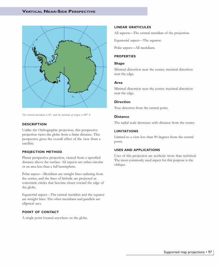
Supported map projections • 97
VERTICAL NEAR-SIDE PERSPECTIVE
DESCRIPTION
Unlike the Orthographic projection, this perspectiveprojection views the globe from a finite distance. Thisperspective gives the overall effect of the view from asatellite.
PROJECTION METHOD
Planar perspective projection, viewed from a specifieddistance above the surface. All aspects are either circularor an area less than a full hemisphere.
Polar aspect—Meridians are straight lines radiating fromthe center, and the lines of latitude are projected asconcentric circles that become closer toward the edge ofthe globe.
Equatorial aspect—The central meridian and the equatorare straight lines. The other meridians and parallels areelliptical arcs.
POINT OF CONTACT
A single point located anywhere on the globe.
LINEAR GRATICULES
All aspects—The central meridian of the projection.
Equatorial aspect—The equator.
Polar aspect—All meridians.
PROPERTIES
Shape
Minimal distortion near the center; maximal distortionnear the edge.
Area
Minimal distortion near the center; maximal distortionnear the edge.
Direction
True direction from the central point.
Distance
The radial scale decreases with distance from the center.
LIMITATIONS
Limited to a view less than 90 degrees from the centralpoint.
USES AND APPLICATIONS
Uses of this projection are aesthetic more than technical.The most commonly used aspect for this purpose is theoblique.
The central meridian is 0°, and the latitude of origin is 90° S.
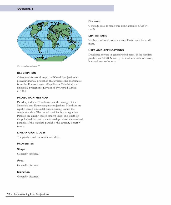
98 • Understanding Map Projections
DESCRIPTION
Often used for world maps, the Winkel I projection is apseudocylindrical projection that averages the coordinatesfrom the Equirectangular (Equidistant Cylindrical) andSinusoidal projections. Developed by Oswald Winkelin 1914.
PROJECTION METHOD
Pseudocylindrical. Coordinates are the average of theSinusoidal and Equirectangular projections. Meridians areequally spaced sinusoidal curves curving toward thecentral meridian. The central meridian is a straight line.Parallels are equally spaced straight lines. The length ofthe poles and the central meridian depends on the standardparallels. If the standard parallel is the equator, Eckert Vresults.
LINEAR GRATICULES
The parallels and the central meridian.
PROPERTIES
Shape
Generally distorted.
Area
Generally distorted.
Direction
Generally distorted.
WINKEL I
Distance
Generally, scale is made true along latitudes 50°28' Nand S.
LIMITATIONS
Neither conformal nor equal area. Useful only for worldmaps.
USES AND APPLICATIONS
Developed for use in general world maps. If the standardparallels are 50°28' N and S, the total area scale is correct,but local area scales vary.
The central meridian is 0°.
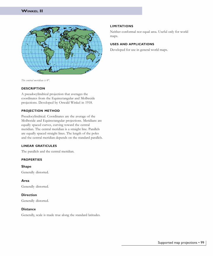
Supported map projections • 99
DESCRIPTION
A pseudocylindrical projection that averages thecoordinates from the Equirectangular and Mollweideprojections. Developed by Oswald Winkel in 1918.
PROJECTION METHOD
Pseudocylindrical. Coordinates are the average of theMollweide and Equirectangular projections. Meridians areequally spaced curves, curving toward the centralmeridian. The central meridian is a straight line. Parallelsare equally spaced straight lines. The length of the polesand the central meridian depends on the standard parallels.
LINEAR GRATICULES
The parallels and the central meridian.
PROPERTIES
Shape
Generally distorted.
Area
Generally distorted.
Direction
Generally distorted.
Distance
Generally, scale is made true along the standard latitudes.
WINKEL II
LIMITATIONS
Neither conformal nor equal area. Useful only for worldmaps.
USES AND APPLICATIONS
Developed for use in general world maps.
The central meridian is 0°.
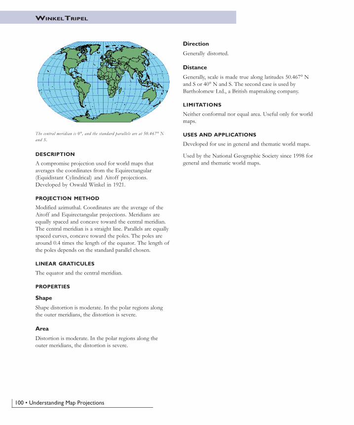
100 • Understanding Map Projections
WINKEL TRIPEL
DESCRIPTION
A compromise projection used for world maps thataverages the coordinates from the Equirectangular(Equidistant Cylindrical) and Aitoff projections.Developed by Oswald Winkel in 1921.
PROJECTION METHOD
Modified azimuthal. Coordinates are the average of theAitoff and Equirectangular projections. Meridians areequally spaced and concave toward the central meridian.The central meridian is a straight line. Parallels are equallyspaced curves, concave toward the poles. The poles arearound 0.4 times the length of the equator. The length ofthe poles depends on the standard parallel chosen.
LINEAR GRATICULES
The equator and the central meridian.
PROPERTIES
Shape
Shape distortion is moderate. In the polar regions alongthe outer meridians, the distortion is severe.
Area
Distortion is moderate. In the polar regions along theouter meridians, the distortion is severe.
Direction
Generally distorted.
Distance
Generally, scale is made true along latitudes 50.467° Nand S or 40° N and S. The second case is used byBartholomew Ltd., a British mapmaking company.
LIMITATIONS
Neither conformal nor equal area. Useful only for worldmaps.
USES AND APPLICATIONS
Developed for use in general and thematic world maps.
Used by the National Geographic Society since 1998 forgeneral and thematic world maps.
The central meridian is 0°, and the standard parallels are at 50.467° Nand S.
101
Datums, Ellipsoids, Grids and Grid Reference Systems.Washington, D.C.: NIMA, 1990. Technical Manual 8358.1,www.nima.mil/GandG/pubs.html.
Department of Defense World Geodetic System 1984.Third Edition. Washington, D.C.: NIMA, 1997. TechnicalReport 8350.2, www.nima.mil/GandG/pubs.html.
European Petroleum Survey Group, EPSG GeodesyParameters, v6.3. www.epsg.org, 2003.
European Petroleum Survey Group, POSC LiteraturePertaining to Coordinate Convresions and Transformationsincluding Formulas. 2002. Guidance Note Number 7.
Geodesy for the Layman. Fourth Edition. Washington, D.C.:NIMA, 1984. Technical Report 80-003,www.nima.mil/GandG/pubs.html.
Hooijberg, Maarten, Practical Geodesy: Using Computers.Berlin: Springer–Verlag, 1997.
Junkins, D.R., and S.A. Farley, NTv2 Developer’s Guide.Geodetic Survey Division, Natural Resources Canada,1995.
Junkins, D.R., and S.A. Farley, NTv2 User’s Guide.Geodetic Survey Division, Natural Resources Canada,1995.
Maling, D.H., Coordinate Systems and Map Projections. SecondEdition. Oxford: Pergamon Press, 1993.
National Geodetic Survey, NADCON Release Notes,README file accompanying NADCON Version 2.1.NOAA/NGS, July 2000.
Rapp, Richard H., Geometric Geodesy: Part I. Department ofGeodetic Science and Surveying, Ohio State University,April 1991.
Rapp, Richard H., Geometric Geodesy: Part II. Departmentof Geodetic Science and Surveying, Ohio State University,March 1993.
Snyder, John P., Map Projections: A Working Manual. USGSProfessional Paper 1395. Washington, D.C.: USGS, 1993.
Snyder, John P., and Philip M. Voxland, An Album of MapProjections. USGS Professional Paper 1453. Washington,D.C.: USGS, 1989.
Soler, T., and L.D. Hothem (1989), “ImportantParameters Used in Geodetic Transformations.” Journal ofSurveying Engineering 112(4):414–417, November 1989.
Torge, Wolfgang, Geodesy. Second Edition. New York: deGruyter, 1991.
Vanicek, Petr, and Edward J. Krakiwsky, Geodesy: TheConcepts. Amsterdam: North-Holland Publishing Company,1982.
Voser, Stefan A., MapRef: The Collection of Map Projectionsand Reference Systems for Europe. www.mapref.org, 2002.
Selected References

103
angular unitsThe unit of measurement on a sphere or a spheroid;usually degrees. Some map projection parameters, such asthe central meridian and standard parallel, are defined inangular units.
aspectThe conceptual center of a projection system. See alsoequatorial, oblique, and polar aspect.
azimuthThe angle, measured in degrees, between a baseline drawnfrom a center point and another line drawn from the samepoint. Normally, the baseline points true north and theangle is measured clockwise from the baseline. Often usedto define an oblique cylindrical map projection or theangle of a geodesic between two points.
azimuthal projectionA form of map projection in which the earth is projectedonto a conceptual tangent or secant plane. Azimuthalprojections are characterized by the fact that the azimuth,or direction, from the center of the projection to everyother point on the map is shown correctly. Therefore theshortest route from the center point to any other point isshown as a straight line. See planar projection.
central meridianThe line of longitude that defines the center and often thex origin of a projected coordinate system. In planarrectangular coordinate systems of limited extent, such asstate plane, grid north coincides with true north at thecentral meridian.
circleA two-dimensional geometric shape for which the distancefrom the center to any point on the edge is equal; theclosed plane curve defining such a shape or the surfacebounded by such a curve.
conformal projectionA projection that preserves the correct shapes of smallareas. Graticule lines intersect at 90-degree angles, and atany point on the map the scale is the same in all directions.A conformal projection maintains all angles at each point,including those between the intersections of arcs;therefore the size of areas enclosed by many arcs may begreatly distorted. No map projection can preserve theshapes of larger regions. Also called an orthomorphicprojection (Snyder and Voxland, 1989).
conic projectionA projection made by projecting geographic features ofthe earth onto a tangent or secant cone that is wrappedaround the globe in the manner of a party hat. The cone isthen cut lengthwise and unrolled into a flat map.
coordinate systemA fixed reference framework superimposed onto thesurface of an area to designate the position of a pointwithin it; a reference system consisting of a set of points,lines and/or surfaces, and a set of rules, used to define thepositions of points in space in either two or threedimensions. The Cartesian coordinate system and thegeographic coordinate system used on the Earth’s surfaceare common examples of coordinate systems.
cylindrical projectionA projection resulting from the conceptual projection ofthe earth’s geographic features onto a tangent or secantcylinder wrapped around the globe. The cylinder is thencut and unrolled into a flat map (Snyder and Voxland,1989).
datumIn the most general sense, any set of numeric or geometricconstants from which other quantities, such as coordinatesystems, can be defined. A datum defines a referencesurface. There are many types of datums, but most fallinto two categories: horizontal and vertical.
Glossary
104 • Understanding Map Projections
datum transformationSee geographic transformation.
eccentricityA measure of how much an ellipse deviates from a circle,expressed as the ratio of the distance between the centerand one focus of an ellipsoid to the length of itssemimajor axis. The square of the eccentricity, e2, iscommonly used with the semimajor axis a to define aspheroid in map projection equations.
ellipseA closed plane curve section of a right circular cone.
ellipsoid1. A three-dimensional, closed geometric shape, all planar
sections of which are ellipses or circles. An ellipsoidhas three independent axes, and is usually specified bythe lengths a,b,c of the three semi-axes. If an ellipsoidis made by rotating an ellipse about one of its axes,then two axes of the ellipsoid are the same, and it iscalled an ellipsoid of revolution, or spheroid. If thelengths of all three of its axes are the same, it is asphere.
2. When used to represent the earth, an oblate ellipsoidof revolution, made by rotating an ellipse about itsminor axis.
ellipticitySee eccentricity. See also flattening.
equal-area projectionA projection in which the whole of the map as well aseach part has the same proportional area as thecorresponding part of the earth. An equal area projectionmay distort shape, angle, scale, or any combination thereof(Snyder and Voxland, 1989). No flat map can be bothequal area and conformal. Also known as an equivalentprojection.
equatorThe parallel of reference that is equidistant from the polesand defines the origin of latitude values as 0° north orsouth.
equatorial aspectA planar—or azimuthal—projection with its central pointlocated at the equator.
equidistant projectionA projection that maintains scale along one or more lines,or from one or two points to all other points on the map.Lines along which scale (distance) is correct are the sameproportional length as the lines they reference on theglobe. In the sinusoidal projections, for example, thecentral meridian and all parallels are their true lengths. Anazimuthal equidistant projection centered on Chicagoshows the correct distance between Chicago and any otherpoint on the projection, but not between any other twopoints.
equivalent projectionSee equal area projection.
false eastingThe linear value added to all x-coordinates of a mapprojection so that none of the values in the geographicregion being mapped are negative. See also false northing.
false northingThe linear value added to all y-coordinates of a mapprojection so that none of the values in the geographicregion being mapped are negative. See false easting.
flatteningA measure of how much a spheroid differs from a sphere.The flattening is the ratio of the semimajor axis minus thesemiminor axis to the semimajor axis.
Gauss–KrügerA projected coordinate system that uses the TransverseMercator projection to divide the world into standardzones six degrees wide. Used mainly in Europe and Asia,the Gauss-Krüger coordinate system is similar to theUniversal Transverse Mercator (UTM) coordinate system.
geocentric coordinate systemA three-dimensional, earth-centered reference system inwhich locations are identified by their x, y, and z-values.The x axis is in the equatorial plane and intersects theprime meridian—usually Greenwich. The y axis is also inthe equatorial plane and intersects the +90° meridian. Thez axis coincides with the polar axis and is positive towardsthe north pole.
geocentric latitudeThe angle between the equatorial plane and a line from apoint on the surface to the center of the sphere or
Glossary • 105
spheroid. On a sphere, all latitudes are geocentric. Theunqualified term latitude generally refers to geographic, orgeodetic, latitude.
geodesicThe shortest distance between two points on the surfaceof a spheroid. Any two points along a meridian form ageodesic.
geodetic datumA datum designed to best fit all or part of the geoid,defined by the origin of an initial point—its latitude,longitude, and according to some authors, its elevation—the orientation of the network—the azimuth of a linefrom the origin—and two constants that define thereference spheroid. More recent definitions express theposition and orientation of the datum as functions of thedeviations in the meridian and in the prime vertical, thegeoid-ellipsoid separation, and the parameters of areference ellipsoid.
geodetic latitudeThe angle that a line drawn perpendicular to the surfacethrough a point on a spheroid makes with the equatorialplane.
geographic coordinate systemA reference system using latitude and longitude to definethe locations of points on the surface of a sphere orspheroid.
geographic coordinatesA measurement of a location on the earth’s surfaceexpressed in degrees of latitude and longitude. See alsogeographic coordinate system.
geographic transformationA method of converting data between two geographiccoordinate systems (datums). Also known as a datumtransformation.
global positioning system (GPS)A constellation of 24 radio-emitting satellites deployed bythe U.S. Department of Defense and used to determinelocation on the earth’s surface. The orbiting satellitestransmit signals that allow a GPS receiver anywhere onearth to calculate its own location through triangulation.The system is used in navigation, mapping, surveying, andother applications where precise positioning is necessary.
GPSSee global positioning system (GPS).
graticuleA network of longitude and latitude lines on a map orchart that relates points on a map to their true locationson the earth. (Snyder and Voxland, 1989).
great circleAny circle or near circle produced by the intersection of asphere and a flat plane that passes through the center ofthe sphere. The equator and all lines of longitude are greatcircles. Great circles are used in navigation, since theshortest path between any two points on the earth’ssurface lies on a great circle (Snyder and Voxland, 1989).
Greenwich prime meridianThe meridian adopted by international agreement in 1884as the 0-degree meridian from which all other longitudesare calculated. The Greenwich prime meridian runsthrough the Royal Observatory in Greenwich, England.
gridIn cartography, any network of parallel and perpendicularlines superimposed on a map and used for reference. Thesegrids are usually named after the map’s projection; forexample, Lambert grid and transverse Mercator grid.
HARNSee High Accuracy Reference Network (HARN).
High Accuracy Reference Network (HARN)A resurvey of NAD 1983 control points using GPStechniques. The resurvey date is often included as part ofthe datum name—NAD 1983 (1991) or NAD91.
High Precision Geodetic (or GPS) NetworkA resurvey of NAD 1983 control points using GPStechniques. The resurvey date is often included as part ofthe datum name—NAD 1983 (1991) or NAD91.
HPGNSee High Precision Geodetic (or GPS) Network.
international meridianSee Greenwich prime meridian.
106 • Understanding Map Projections
interrupted projectionDiscontinuities and gaps are added to a map to decreasethe overall distortion. The world is divided, usually alongcertain meridians, into sections, or gores. Each section hasits own projection origin.
latitudeThe angular distance—usually measured in degrees—northor south of the equator. Lines of latitude are also calledparallels. See geodetic latitude and geocentric latitude.
latitude of centerThe latitude value that defines the center—and sometimesorigin—of a projection.
latitude of originThe latitude value that defines the origin of they-coordinate values for a projection.
linear unitsThe unit of measurement on a plane or a projectedcoordinate system, often meters or feet. Map projectionparameters, such as the false easting and false northing, aredefined in linear units.
longitudeThe angular distance—usually measured in degrees—eastor west of a prime meridian.
longitude of centerThe longitude value that defines the center—andsometimes origin—of a projection.
longitude of originThe longitude value that defines the origin of thex-coordinate values for a projection.
loxodromeSee rhumb line.
major axisThe longer axis of an ellipse or spheroid.
map projectionSee projection.
map scaleSee scale.
meridianA great circle on the earth that passes through the poles,often used synonymously with longitude. Meridians runnorth-south between the poles. From a prime meridian or0 degrees longitude—usually the Greenwich primemeridian—measures of longitude are negative to the westand positive to the east, where they meet halfway aroundthe globe at the line of 180 degrees longitude.
minor axisThe shorter axis of an ellipse or spheroid.
NAD 1927North American Datum of 1927; also known as NAD27.The primary local geodetic datum and geographiccoordinate system used to map the United States duringthe middle part of the 20th century, referenced to theClarke spheroid of 1866 and an initial point at MeadesRanch, Kansas. Features on USGS topographic maps,including the corners of 7.5-minute quadrangle maps, arereferenced to NAD27. It is gradually being replaced bythe North American Datum of 1983. See also NAD1983.
NAD 1983North American Datum of 1983, also known as NAD83.A geocentric datum and graphic coordinate system basedon the Geodetic Reference System 1980 ellipsoid(GRS80). Mainly used in North America, itsmeasurements are obtained from both terrestrial andsatellite data. See also NAD 1927.
oblate ellipsoidAn ellipsoid created by rotating an ellipse around its minoraxis. The shape of the earth approximates an oblateellipsoid with a flattening of one part in 298.257. Seealso ellipsoid, spheroid.
oblique aspectSee oblique projection.
oblate spheroidSee oblate ellipsoid.
oblique projection1. A planar or cylindrical projection whose point of
tangency is neither on the equator nor at a pole.
2. A conic projection whose axis does not line up withthe polar axis of the globe.
Glossary • 107
3. A cylindrical projection whose lines of tangency orsecancy follow neither the equator nor a meridian.
orthomorphic projectionSee conformal projection.
parallelAn imaginary east–west line encircling the earth, parallelto the equator and connecting all points of equal latitude.Also, the representation of this line on a globe or map.
parameter1. A variable that determines the outcome of a function
or operation.
2. In a map projection, a group of parameters define aspecific instance of a projection. Parameters differ foreach projection and can include central meridian,standard parallel, scale factor, or latitude of origin.
planar coordinate systemA two-dimensional measurement system that locatesfeatures on a map based on their distance from an origin(0,0) along two axes, a horizontal x-axis representingeast–west and a vertical y-axis representing north–south.
planar projectionA projection resulting from the conceptual projection ofthe earth onto a tangent or secant plane. Usually, a planarprojection is the same as an azimuthal or zenithalprojection, because it shows true direction (Snyder andVoxland, 1989).
polar aspectA planar projection with its central point located at eitherthe North or South Pole.
polar flatteningSee flattening.
prime meridianSee Greenwich prime meridian.
projected coordinate systemA reference system used to locate x,y and z positions ofpoint, line, and area features in two or three dimensions. Aprojected coordinate system is defined by a geographiccoordinate system, a map projection, any parametersneeded by the map projection, and a linear unit ofmeasure.
projectionA method by which the curved surface of the earth isportrayed on a flat surface. This generally requires asystematic mathematical transformation of the earth’sgraticule of lines of longitude and latitude onto a plane. Itcan be visualized as a transparent globe with a light bulb atits center, casting lines of latitude and longitude onto asheet of paper. Generally, the paper is either flat andplaced tangent to the globe—a planar or azimuthalprojection—or formed into a cone or cylinder and placedover the globe—cylindrical and conical projections. Everymap projection distorts distance, area, shape, direction, orsome combination thereof.
radiusThe distance from the center to the outer edge of a circleor circular curve.
reference ellipsoidSee ellipsoid.
rhumb lineA complex curve on the earth’s surface that crosses everymeridian at the same oblique angle. A rhumb line pathfollows a single compass bearing; it is a straight line on aMercator projection, or a logarithmic spiral on a polarprojection. A rhumb line is not the shortest distancebetween two points on a sphere (Snyder and Voxland,1989). See also great circle, sphere.
scaleThe ratio or relationship between a distance or area on amap and on the corresponding distance or area on theground, commonly expressed as a fraction or ratio. A mapscale of 1/100,000 or 1:100,000 means that one unit ofmeasure on the map equals 100,000 of the same unit onthe earth.
scale factorIn a coordinate system, a value, usually less than one, thatconverts a tangent projection to a secant projection.Represented by ‘k0’ or ‘k’. If a projected coordinatesystem doesn’t have a scale factor, the standard lines ofthe projection have a scale of 1.0. Other points on themap have scales greater or less than 1.0. If a projectedcoordinate system has a scale factor, the definingparameters no longer have a scale of 1.0.
108 • Understanding Map Projections
secant projectionA projection whose surface intersects the surface of theearth. A secant conic or cylindrical projection, forexample, is recessed into the globe, intersecting it at twocircles. At the lines of intersection the projection is freefrom distortion.
semimajor axisThe equatorial radius of a spheroid. Often known as ‘a’.
semiminor axisThe polar radius of a spheroid. Often known as ‘b’.
sphereA three-dimensional shape whose center is equidistantfrom every point on its surface, made by revolving a circlearound its diameter.
spherical coordinate systemA reference system using positions of latitude andlongitude to define the locations of points on the surfaceof a sphere or spheroid.
spheroidWhen representing the earth, the three-dimensional shapeobtained by rotating an ellipse about its minor axis. This isan oblate ellipsoid of revolution, also called an ellipsoid.
standard lineA line on a sphere or spheroid that has no lengthcompression or expansion after being projected.Commonly, a standard parallel or central meridian.
standard parallelThe line of latitude where the projection surface touchesthe surface. A tangent conic or cylindrical projection hasone standard parallel, while a secant conic or cylindricalprojection has two. A standard parallel has no distortion.
State Plane Coordinate SystemA projected coordinate system used in the United Statesthat divides each state into one or more zones to minimizedistortion caused by the map projection. Also known asSPCS and SPC.
tangent projectionA projection whose surface touches the earth’s withoutpiercing it. A tangent planar projection touches the globeat one point, while tangent conic and cylindrical
projections touch the globe along a line. At the point orline of tangency the projection is free from distortion.
true-direction projectionSee azimuthal projection.
unit of measureA standard quantity used for measurements, such aslength, area, and height. See also angular units or linearunits.
Universal Transverse MercatorUTM.
UTMUniversal Transverse Mercator. A projected coordinatesystem that divides the world into 60 north and southzones, six degrees wide.
WGS 1984World Geodetic System of 1984. A geocentric datum andgeographic coordinate system created by the United Statesmilitary. Also known as WGS84.
Index
A
Abridged Molodensky method 26Aitoff 34Alaska Grid 35Alaska Series E 36Albers 37Angular parameters
azimuth 20central meridian 20central parallel 20defined 20latitude of center 20latitude of first point 20latitude of origin 20latitude of second point 20longitude of center 20longitude of first point 20longitude of origin 20longitude of second point 20standard parallel 1 20standard parallel 2 20
Angular unitsdefined 103
Aspectdefined 103
Azimuth 20defined 103
Azimuthal Equidistant 38Azimuthal projections
defined 12, 103Double Stereographic 47equidistant 38Lambert Azimuthal Equal Area
67Orthographic 76Perspective 77Polar Stereographic 79Stereographic 97Universal Polar Stereographic 94
B
Behrmann 39Bipolar Oblique 40Bonne 41Bursa–Wolf method 25
C
Cassini–Soldner 42Central meridian 14, 20
defined 103Central parallel 20Chamberlin Trimetric 43Circle
defined 103Clarke 1866 spheroid 5Conformal projections
Bipolar Oblique 40defined 12, 103Double Stereographic 47Gauss–Krüger 59, 104Hotine 65Krovak 66Lambert Conformal Conic 68Mercator 72Stereographic 89Transverse Mercator 91UTM 108
Conic projectionsAlbers 37Bipolar Oblique 40defined 14, 103Equidistant Conic 54Krovak 66Lambert Conformal Conic 68Polyconic 80Simple Conic 84
Coordinate Frame method 25Coordinate systems
defined 103geographic 105projected 107spherical 108
Coordinatesin different datums 6
Craster Parabolic 44
Cube 45Cylindrical Equal Area 46Cylindrical projections
Behrmann 39Cassini–Soldner 42Cylindrical Equal Area 46defined 16, 103Equidistant Cylindrical 55Equirectangular 56Gall’s Stereographic 58Gauss–Krüger 59, 104Hotine 65Mercator 72Miller 73Plate Carrée 78Transverse Mercator 91UTM 108
D
Datumdefined 103
Datum transformations. SeeGeographic transformations
defined 104Datums
coordinatees in different 6definition 6earth-centered 6local 6NAD 1927 106NAD 1983 106origin point 6transforming 24versus geographic coordinate
systems 2WGS 1984
defined 108Degrees 2Degrees-minutes-seconds 2Developable surfaces 13Distortions
and map projections 11DMS. See Degrees-minutes-secondsDouble Stereographic 47
110 • Understanding Map Projections
E
Earthas a sphere 4as a spheroid 4
Earth-centered datums 6Eccentricity
defined 104Eckert I 48Eckert II 49Eckert III 50Eckert IV 51Eckert V 52Eckert VI 53ED 1950 6Ellipse
defined 104Ellipsoids
defined 104eccentricity 104ellipticity 104flattening 104major axis 106minor axis 106semimajor axis 108semiminor axis 108
Ellipticitydefined 104
Equal-area projectionsAlbers 37Behrmann 39Bonne 41Craster Parabolic 44Cylindrical Equal Area 46defined 12, 104Eckert II 49Eckert IV 51Eckert VI 53Lambert Azimuthal Equal Area
67McBryde–Thomas Flat-Polar
Quartic 71Mollweide 74Quartic Authalic 81Sinusoidal 85
Equation-based methods 25Equator
defined 104
Equatorial aspectdefined 104
Equidistant Conic 54Equidistant Cylindrical 55Equidistant projections
Azimuthal 38defined 12, 104Equidistant Conic 54Equidistant Cylindrical 55Simple Conic 84Two-Point Equidistant 93
Equirectangular 56Equivalent projection
defined 104European Datum of 1950 6
F
Facets 45, 57False easting 20
defined 104False northing 20
defined 104Flat-Polar Quartic 71Flattening 4
defined 104Fuller 57
G
Gall’s Stereographic 58Gauss–Krüger 59
defined 104Geocentric Coordinate System 60Geocentric coordinate systems
defined 104Geocentric latitude
defined 104Geocentric Translation method 25Geodesic
defined 105Geodetic datum
defined 105Geodetic latitude
defined 105Geographic Coordinate System 61
Geographic coordinate systemsdefined 2, 105parts of 2size and shape 4sphere-based 4spheroid-based 4transforming 24
Geographic coordinatesdefined 105
Geographic transformationsAbridged Molodensky 26Bursa–Wolf 25Coordinate Frame 25defined 105Geocentric Translation 25HARN 27HARN method 105HPGN 27Molodensky 26NADCON 27NTv1 28NTv2 28Position Vector 25seven-parameter 25three-parameter 25
GK. See Gauss–KrügerGlobal positioning system (GPS)
defined 105Gnomonic 62GPS (global positioning system)
defined 105Graticule
defined 105Graticules 2Great Britain National Grid 63Great circle
defined 105Great circles 3Greenwich prime meridian 2
defined 105Grid
defined 105Grid-based methods 27GRS 1980 5GRS80 5
Index • 111
H
Hammer–Aitoff 64HARN. See High Accuracy
Reference NetworkHARN (High Accuracy Reference
Networkdefined 105
High Accuracy Reference Network7, 27
High Accuracy Reference Network(HARN)
defined 105High Precision Geodetic (or GPS)
Networkdefined 105
High Precision Geodetic Network7, 27
Hotine Oblique Mercator 65HPGN. See High Precision Geodetic
Networkdefined 105
I
Icosahedron 57International meridian
defined 105Interrupted projection
defined 106
K
Krovak 66
L
Lambert Azimuthal Equal Area 67Lambert Conformal Conic 68Latitude 2
defined 106Latitude of center 20
defined 106Latitude of first point 20Latitude of origin 20
defined 106Latitude of second point 20
Latitude range 2Latitudes
geocentric 104geodetic 105
Linear parametersdefined 20false easting 20false northing 20
Linear unitsdefined 106
Local Cartesian Projection 69Local datums 6Longitude 2
defined 106Longitude length 3Longitude of center 20
defined 106Longitude of first point 20Longitude of origin 20
defined 106Longitude of second point 20Longitude range 2Loximuthal 70Loxodrome
defined 106
M
Major axisdefined 106
Map projectionsdefined 11, 106
Map scaledefined 106
McBryde–Thomas Flat-Polar Quartic71
Mercator 16, 72Meridians 2
defined 106Meridional convergence 3Miller Cylindrical 73Minor axis
defined 106Mollweide 74Molodensky method 26
N
NAD 1927 6, 7, 27, 28defined 106
NAD 1983 27, 28defined 106
NAD 1983 and WGS 1984 7NAD27 7NAD83 7NADCON method 27National Transformation version 1
28National Transformation version 2
28New Zealand National Grid 75North American Datum of 1927 7North American Datum of 1983 7NTv2. See National Transformation
version 2
O
Oblate ellipsoiddefined 106
Oblate spheroiddefined 106
Oblique aspectdefined 106
Oblique Mercator 65Oblique projections
Azimuthal Equidistant 38Bipolar 40defined 106Double Stereographic 47Hotine 65Krovak 66Lambert Azimuthal Equal Area
67Orthographic 76Polar Stereographic 79Stereographic 89Vertical Near-Side Perspective 97
Old Hawaiian datum 27Option 21Origin point 6Orthographic 18, 76Orthomorphic projection
defined 107
112 • Understanding Map Projections
P
Parallels 2defined 107
Parametersangular 20azimuth 103central meridian 103defined 107false easting 104false northing 104latitude of center 106latitude of origin 106linear 20longitude of center 106longitude of origin 106option 21pseudo standard parallel 1 20scale factor 107standard line 108standard parallel 108X scale 21XY plane rotation 20Y scale 21
Perspective 77Planar coordinate system
defined 107Planar projections
Azimuthal Equidistant 38defined 17, 107Double Stereographic 47Gnomonic 62Orthographic 76Perspective 77Polar Stereographic 79Stereographic 89Vertical Near-Side Perspective
77, 97Plate Carrée 78Polar aspect
defined 107Polar flattening
defined 107Polar Stereographic 79Polyconic 80Position Vector method 25Prime meridians 2
defined 107Greenwich 105
Projected coordinate systemsand geographic coordinate systems
10defined 10, 107units 10x-axis 10y-axis 10
Projection parametersazimuth 20central meridian 20central parallel 20defined 20false easting 20false northing 20latitude of center 20latitude of first point 20latitude of origin 20latitude of second point 20longitude of center 20longitude of first point 20longitude of origin 20longitude of second point 20option 21pseudo standard parallel 1 20standard parallel 1 20standard parallel 2 20X scale 21XY plane rotation 20Y scale 21
Projection surfaces 11Projection types 13Projections
azimuthal 17, 103conformal 12, 103conic 14, 103cylindrical 16, 103defined 107distortions 11equal-area 12, 104equidistant 12, 104equivalent 104planar 17, 107secant 108tangent 108true-direction 12, 108
Pseudo standard parallel 1 20
Q
Quartic Authalic 81
R
Radiusdefined 107
Rectified Skewed Orthomorphic 82Reference ellipsoids. See Ellipsoids
defined 107Rhumb lines 16
defined 107Robinson 83RSO. See Rectified Skewed
Orthomorphic
S
Sanson–Flamsteed 85Scale
defined 107Scale factor
defined 107Secant projections 13, 14
defined 108Semimajor axis 4
defined 108Semiminor axis 4
defined 108Seven-parameter method 25Simple Conic 84Sinusoidal 85Space Oblique Mercator 86SPCS. See State Plane Coordinate
SystemSphere
defined 108Spherical coordinate system
defined 108Spheroids
defined 108discussion 4eccentricity 104ellipticity 104flattening 4, 104major axis 106minor axis 106
Index • 113
Spheroids (continued)semimajor axis 4, 108semiminor axis 4, 108using different 4
Standard lines 13defined 108
Standard paralleldefined 108
Standard parallel 1 20Standard parallel 2 20Standard parallels 14State Plane Coordinate System 87
defined 108Stereographic 89
Polar case 79
T
Tangent projections 13defined 108
Three-parameter method 25Times 90Transformations
datum 104Transverse Mercator 16, 91Transverse projections 16True-direction projections
defined 12, 108Two-Point Equidistant 93
U
Units of measureangular 103defined 108linear 106
Universal Polar Stereographic 94Universal Transverse Mercator 95
defined 108UPS 94UTM 95
defined 108
V
Van Der Grinten I 96Vertical Near-Side Perspective
77, 97
W
WGS 1984defined 108
WGS 1984 and NAD 1983 7Winkel I 98Winkel II 99Winkel Tripel 100
X
X scale 21X-axis 10XY plane rotation 20XYZ coordinate systems 24
Y
Y scale 21Y-axis 10