Understanding diffraction grating behavior: including ...

$: Understanding diffraction grating behavior: including ...$
Understanding diffraction gratingbehavior: including conical diffractionand Rayleigh anomalies fromtransmission gratings

James E. HarveyRichard N. Pfisterer

James E. Harvey, Richard N. Pfisterer, “Understanding diffraction grating behavior: including conicaldiffraction and Rayleigh anomalies from transmission gratings,” Opt. Eng. 58(8), 087105 (2019),doi: 10.1117/1.OE.58.8.087105.

Downloaded From: https://www.spiedigitallibrary.org/journals/Optical-Engineering on 24 Mar 2022Terms of Use: https://www.spiedigitallibrary.org/terms-of-use

Understanding diffraction grating behavior: includingconical diffraction and Rayleigh anomalies fromtransmission gratings

James E. Harvey* and Richard N. PfistererPhoton Engineering, LLC, Tucson, Arizona, United States

Abstract. With the wide-spread availability of rigorous electromagnetic (vector) analysis codes for describingthe diffraction of electromagnetic waves by specific periodic grating structures, the insight and understanding ofnonparaxial parametric diffraction grating behavior afforded by approximate methods (i.e., scalar diffractiontheory) is being ignored in the education of most optical engineers today. Elementary diffraction grating behavioris reviewed, the importance of maintaining consistency in the sign convention for the planar diffraction gratingequation is emphasized, and the advantages of discussing “conical” diffraction grating behavior in terms of thedirection cosines of the incident and diffracted angles are demonstrated. Paraxial grating behavior for coarsegratings (d ≫ λ) is then derived and displayed graphically for five elementary grating types: sinusoidal amplitudegratings, square-wave amplitude gratings, sinusoidal phase gratings, square-wave phase gratings, and classicalblazed gratings. Paraxial diffraction efficiencies are calculated, tabulated, and compared for these five elemen-tary grating types. Since much of the grating community erroneously believes that scalar diffraction theory is onlyvalid in the paraxial regime, the recently developed linear systems formulation of nonparaxial scalar diffractiontheory is briefly reviewed, then used to predict the nonparaxial behavior (for transverse electric polarization) ofboth the sinusoidal and the square-wave amplitude gratings when the þ1 diffracted order is maintained in theLittrow condition. This nonparaxial behavior includes the well-known Rayleigh (Wood’s) anomaly effects that areusually thought to only be predicted by rigorous (vector) electromagnetic theory. © The Authors. Published by SPIE under aCreative Commons Attribution 4.0 Unported License. Distribution or reproduction of this work in whole or in part requires full attribution of the originalpublication, including its DOI. [DOI: 10.1117/1.OE.58.8.087105]

Keywords: paraxial and nonparaxial diffraction grating behavior; “conical” diffraction in direction cosine space; Rayleigh (Wood’s)anomalies from sinusoidal and square-wave amplitude gratings.

Paper 190651 received May 14, 2019; accepted for publication Jul. 29, 2019; published online Aug. 28, 2019.

1 IntroductionThe fundamental diffraction problem consists of two parts:(i) determining the effects of introducing the diffractingaperture (or grating) upon the field immediately behind thescreen and (ii) determining how it affects the field down-stream from the diffracting screen (i.e., what is the fieldimmediately behind the grating and how does it propagate).

A “diffraction grating” is an optical element that imposesa “periodic” variation in the amplitude and/or phase ofan incident electromagnetic wave.1 It thus produces, throughconstructive interference, a number of discrete diffractedorders (or waves) which exhibit dispersion upon propaga-tion. Diffraction gratings are thus widely used as dispersiveelements in spectrographic instruments,2–5 although they canalso be used as beam splitters or beam combiners in variouslaser devices or interferometers. Other applications includeacousto-optic modulators or scanners.6

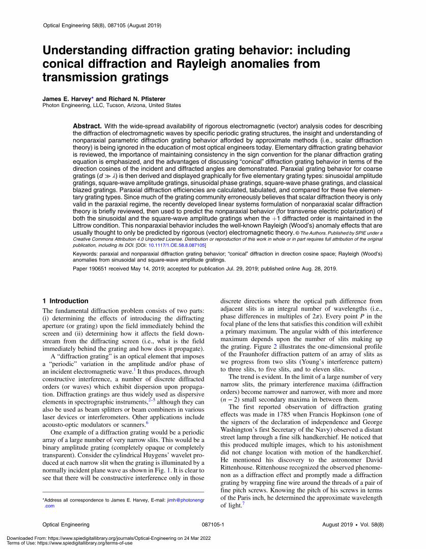
One example of a diffraction grating would be a periodicarray of a large number of very narrow slits. This would be abinary amplitude grating (completely opaque or completelytransparent). Consider the cylindrical Huygens’ wavelet pro-duced at each narrow slit when the grating is illuminated by anormally incident plane wave as shown in Fig. 1. It is clear tosee that there will be constructive interference only in those

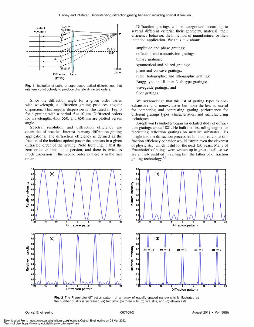
discrete directions where the optical path difference fromadjacent slits is an integral number of wavelengths (i.e.,phase differences in multiples of 2π). Every point P in thefocal plane of the lens that satisfies this condition will exhibita primary maximum. The angular width of this interferencemaximum depends upon the number of slits making upthe grating. Figure 2 illustrates the one-dimensional profileof the Fraunhofer diffraction pattern of an array of slits aswe progress from two slits (Young’s interference pattern)to three slits, to five slits, and to eleven slits.

The trend is evident. In the limit of a large number of verynarrow slits, the primary interference maxima (diffractionorders) become narrower and narrower, with more and more(n − 2) small secondary maxima in between them.

The first reported observation of diffraction gratingeffects was made in 1785 when Francis Hopkinson (one ofthe signers of the declaration of independence and GeorgeWashington’s first Secretary of the Navy) observed a distantstreet lamp through a fine silk handkerchief. He noticed thatthis produced multiple images, which to his astonishmentdid not change location with motion of the handkerchief.He mentioned his discovery to the astronomer DavidRittenhouse. Rittenhouse recognized the observed phenome-non as a diffraction effect and promptly made a diffractiongrating by wrapping fine wire around the threads of a pair offine pitch screws. Knowing the pitch of his screws in termsof the Paris inch, he determined the approximate wavelengthof light.7

*Address all correspondence to James E. Harvey, E-mail: [email protected]

Optical Engineering 087105-1 August 2019 • Vol. 58(8)

Optical Engineering 58(8), 087105 (August 2019)


https://doi.org/10.1117/1.OE.58.8.087105

https://doi.org/10.1117/1.OE.58.8.087105

https://doi.org/10.1117/1.OE.58.8.087105

https://doi.org/10.1117/1.OE.58.8.087105

https://doi.org/10.1117/1.OE.58.8.087105

https://doi.org/10.1117/1.OE.58.8.087105

mailto:[email protected]

mailto:[email protected]

Since the diffraction angle for a given order varieswith wavelength, a diffraction grating produces angulardispersion. This angular dispersion is illustrated in Fig. 3for a grating with a period d ¼ 10 μm. Diffracted ordersfor wavelengths 450, 550, and 650 nm are plotted versusangle.

Spectral resolution and diffraction efficiency arequantities of practical interest in many diffraction gratingapplications. The diffraction efficiency is defined as thefraction of the incident optical power that appears in a givendiffracted order of the grating. Note from Fig. 3 that thezero order exhibits no dispersion, and there is twice asmuch dispersion in the second order as there is in the firstorder.

Diffraction gratings can be categorized according toseveral different criteria: their geometry, material, theirefficiency behavior, their method of manufacture, or theirintended application. We thus talk about:

amplitude and phase gratings;reflection and transmission gratings;binary gratings;symmetrical and blazed gratings;plane and concave gratings;ruled, holographic, and lithographic gratings;

Bragg type and Raman-Nath type gratings;waveguide gratings; andfiber gratings.

We acknowledge that this list of grating types is non-exhaustive and nonexclusive but none-the-less is usefulfor comparing and contrasting grating performance fordifferent gratings types, characteristics, and manufacturingtechniques.

Joseph von Fraunhofer began his detailed study of diffrac-tion gratings about 1821. He built the first ruling engine forfabricating reflection gratings on metallic substrates. Hisinsight into the diffraction process led him to predict that dif-fraction efficiency behavior would “strain even the cleverestof physicists,” which it did for the next 150 years. Many ofFraunhofer’s findings were written up in great detail, so weare entirely justified in calling him the father of diffractiongrating technology.8,9

Fig. 1 Illustration of paths of superposed optical disturbances thatinterfere constructively to produce discrete diffracted orders.

Fig. 2 The Fraunhofer diffraction pattern of an array of equally spaced narrow slits is illustrated asthe number of slits is increased: (a) two slits, (b) three slits, (c) five slits, and (d) eleven slits.


Harvey and Pfisterer: Understanding diffraction grating behavior: including conical diffraction. . .


A whole new era of spectral analysis opened up withRowland’s famous paper in 1882. He constructed sophisti-cated ruling engines and invented the “concave grating,”a device of spectacular value to modern spectroscopists.10

John Strong, quoting G. R. Harrison, stated in a JOSAarticle in 1960—It is difficult to point to another singledevice that has brought more important experimental infor-mation to every field of science than the diffraction grating.The physicist, the astronomer, the chemist, the biologist, themetallurgist, all use it as a routine tool of unsurpassed accu-racy and precision, as a detector of atomic species to deter-mine the characteristics of heavenly bodies and the presenceof atmospheres in the planets, to study the structures of mol-ecules and atoms, and to obtain a thousand and one items ofinformation without which modern science would be greatlyhandicapped.”11

A troublesome aspect of the multiple order behavior ofdiffraction gratings is that adjacent higher order spectra fre-quently overlap. In fact, in Fig. 3, one can see the third-orderprinciple maximum for blue light almost overlapping thesecond-order red principle maximum. One can readily showthat the second order for wavelengths 100, 200, and 300 nmis diffracted into the same directions as the first order forwavelengths 200, 400, and 600 nm.

Two generalizations to the behavior of gratings must nowbe discussed. First, if the individual slits making up the gra-ting have significant width (in order to transmit more light),the Fraunhofer diffraction pattern of an individual slit willform an envelope function modulating the strength of thediscrete diffracted orders.12–15 For the case illustrated inFig. 4, we have chosen the width of the slits to be one-thirdof the slit separation. You will note that every third diffracted

Fig. 3 Illustration of angular dispersion produced by a diffraction grating.

Fig. 4 The Fraunhofer diffraction pattern of an array of eleven equally spaced slits whose width is one-third of their spacing.




order is absent. This is caused by the envelope functiongoing to zero at those locations.

The second generalization includes the situation wherethe light is incident upon the grating at an arbitrary angleθi rather than normal incidence. This situation will be takencare of by including the incident angle in the grating equationdiscussed in Sec. 2, where we will review the planar gratingequation and the sign convention for numbering the variousdiffracted orders.

The more general phenomenon of “conical” diffractionthat occurs with large obliquely incident angles will be dis-cussed in Sec. 3 and the parametric behavior will be shown tobe particularly simple and intuitive when formulated and dis-played in terms of the direction cosines of the incident anddiffracted angles. In Sec. 4, we will use the remarkably intui-tive direction cosine diagram to portray the conical gratingbehavior exhibited in the presence of large obliquely incidentbeams and arbitrary orientation of the grating. Section 5examines the paraxial diffraction efficiency behavior ofseveral elementary grating types. Section 6 will review theunderlying concepts of nonparaxial scalar diffraction theoryand apply them to the sinusoidal and square-wave amplitudegratings when the þ1 diffracted order is maintained in the“Littrow condition.” This nonparaxial behavior includesthe well-known Rayleigh (Wood’s) anomaly effects that areusually thought to only be predicted by rigorous (vector)electromagnetic theory.16

A summary, statement of conclusions, and an extensiveset of references will then complete this paper.

2 Planar Grating Equation and Sign ConventionMonochromatic light of wavelength λ incident upon a refrac-tive transmission grating (interface between two dielectricmedia exhibiting a periodic surface relief pattern) of spatialperiod d at an angle of incidence θi will be diffracted into thediscrete angles θm according to the following (planar) gratingequation:3,4,16–18

EQ-TARGET;temp:intralink-;e001;63;344n 0 sin θm − n sin θi ¼ −mλ∕d; m ¼ 0;�1;�2;�3;

(1)

where n is the refractive index of the media on the incidentside of the diffracting surface, n 0 is the refractive index ofthe media containing transmitted diffracted light, and m isan integer called the order of diffraction. The sign of m isarbitrary and determines the sign convention for labelingdiffracted orders.

The equation for a reflection grating can be obtained bysetting n 0 ¼ −n, just as we do when tracing rays froma reflecting surface:4

EQ-TARGET;temp:intralink-;e002;326;653 sin θm þ sin θi ¼ mλ∕nd; m ¼ 0;�1;�2;�3: (2)

Note that setting m ¼ 0 in Eq. (1) results in θ0 having thesame sign as θi. Likewise, setting m ¼ 0 in Eq. (2) results inθ0 having the opposite sign as θi . We have thus adopted asign convention that conforms to that used in geometricaloptics whereby all angles are directional quantities measuredfrom optical axes or surface normals to refracted or reflectedrays. These directional angles are “positive if counterclock-wise,” and “negative if clockwise.” An “angle” here is thesmaller of the two angles that a ray forms with the axis orsurface normal.

For a thin diffraction grating in air, we thus haven ¼ n 0 ¼ 1, and the two grating equations can be combinedto yield

EQ-TARGET;temp:intralink-;e003;326;479 sin θm∓ sin θi ¼ ∓mλ∕d; m ¼ 0;�1;�2;�3: (3)

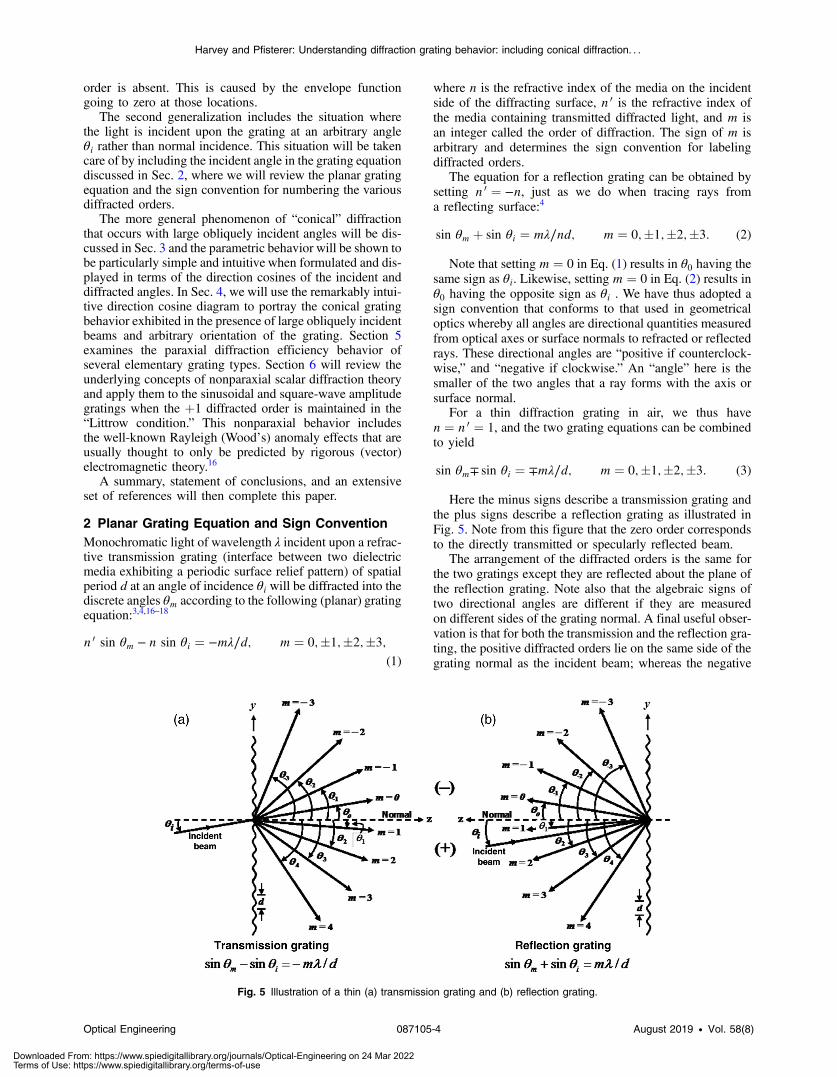
Here the minus signs describe a transmission grating andthe plus signs describe a reflection grating as illustrated inFig. 5. Note from this figure that the zero order correspondsto the directly transmitted or specularly reflected beam.

The arrangement of the diffracted orders is the same forthe two gratings except they are reflected about the plane ofthe reflection grating. Note also that the algebraic signs oftwo directional angles are different if they are measuredon different sides of the grating normal. A final useful obser-vation is that for both the transmission and the reflection gra-ting, the positive diffracted orders lie on the same side of thegrating normal as the incident beam; whereas the negative

Fig. 5 Illustration of a thin (a) transmission grating and (b) reflection grating.




diffracted orders lie on the opposite side of the gratingnormal from the incident beam. A “plus” sign has thus beenplaced on the lower side of the grating normal in Fig. 5 anda “minus” sign has been placed on the upper side of thegrating normal as an indicator of our sign convention. Someauthors absorb the minus sign on the right side of Eq. (3)into the m, thus achieving a seemingly simpler equation.However, this results in a different sign convention for label-ing the diffracted orders.

We have specifically chosen the form of Eq. (3) not onlyto maintain the sign convention for directional angles usedalmost exclusively in geometrical optics and optical designray trace codes (positive if counterclockwise and negativeif clockwise), but also to be consistent with the sign conven-tion for labeling diffraction grating order numbers used bythe popular Diffraction Grating Handbook published anddistributed free by the Newport Corporation (formerlyRichardson Grating Laboratory).19

The above grating equations are restricted to the specialcase where the grating grooves/lines are oriented perpendic-ular to the plane of incidence, i.e., the plane containingthe incident beam and the normal to the grating surface. Forthis situation, all of the diffracted orders lie in the plane ofincidence.

The more general phenomenon of conical diffractionthat occurs with large obliquely incident angles is rarelydiscussed in elementary optics or physics text books.However, the formulation of a nonparaxial scalar diffractiontheory20–23 provides a simple and intuitive means of gainingadditional insight into this nonparaxial diffraction gratingbehavior.

3 Conical Diffraction in Direction Cosine SpaceConsider diffraction from a conventional linear reflectiongrating. However, suppose the incident light strikes the gra-ting at a large oblique angle (represented by direction cosinesαi and βi) as illustrated in Fig. 6. The resulting diffractionbehavior is described by the following grating equationwritten in terms of the direction cosines of the propagation

vectors of the incident beam and the diffracted orders (thegrooves are assumed to be parallel to the y axis):24

EQ-TARGET;temp:intralink-;e004;326;730αm þ αi ¼ mλ∕d; βm þ βi ¼ 0; (4)

whereEQ-TARGET;temp:intralink-;e005;326;688

αm ¼ sin θm cos ϕo; αi ¼ − sin θo cos ϕo; βi ¼ − sin ϕo:

(5)

The diffracted orders now propagate along the surface ofa cone and will strike the observation hemisphere in a crosssection that is not a great circle, but instead a latitude sliceas illustrated for a reflection grating in Fig. 6. Note thatthe direction cosines are obtained by merely projecting therespective points on the hemisphere down onto the plane ofthe aperture and normalizing to a unit radius. Even for largeangles of incidence and large diffracted angles, the variousdiffracted orders are equally spaced and lie on a straight lineonly in the direction cosine space.

This behavior is even more evident in Fig. 7, in which thelocation of the incident beam and the diffracted orders aredisplayed in direction cosine space for a reflection gratingwhose grooves are parallel to the y or β axis. The diffractedorders are always exactly equally spaced in direction cosinespace and lie in a straight line perpendicular to the orienta-tion of the grating grooves. From Eq. (4), this equidistantspacing of diffracted orders is readily shown to be equalto the nondimensional quantity λ∕d. The diffracted ordersthat lie inside the unit circle are real and propagate, and thediffracted orders that lie outside the unit circle are evanescent(and thus do not propagate).

For a reflection grating, the undiffracted zero orderalways lies diametrically opposite the origin of the α − βcoordinate system from the incident beam. As the incidentangle is varied, the diffraction pattern (size, shape, separa-tion, and orientation of diffracted orders) remains unchangedbut merely shifts its position maintaining the above relation-ship between the zero order and the incident beam. Note alsothat when the plane of incidence is perpendicular to the

Fig. 6 Illustration of the position of the diffracted orders in real spaceand direction cosine space for an arbitrary (skew) obliquely incidentbeam.

Fig. 7 Relative position of diffracted orders and incident beam indirection cosine space for a reflection grating. Diffracted ordersoutside the unit circle are evanescent.




grating grooves (ϕ0 ¼ 0), Eq. (4) reduces to the familiargrating equation presented in Eq. (3).

For a transmission grating, with our sign convention, thediffraction angle for the zero order is equal to the incidentangle (θ0 ¼ θi). Thus the coordinates of the location in thedirection cosine diagram representing the zero order andthe incident beam are superposed as illustrated as shown inFig. 8.

As with the case of the reflection grating, the diffractedorders remain equally spaced and in a straight line as theincident angle is changed, i.e., the size, shape, separation, andorientation of diffracted orders again remains unchanged,merely shifting its position such that the zero order remainssuperposed upon the incident beam.

Figure 9 illustrates the propagating diffracted orders thatwould exist if a beam were normally incident upon a trans-mission diffraction grating with λ∕d ¼ 0.08333. There wouldbe precisely 25 propagating diffracted orders including thetwo at �90 deg. The uniform diffracted order spacing indirection cosine space Δβ is contrasted with the increasingangular spacing Δθ , and the even more rapidly increasinglinear spacing Δx, when the diffracted orders are projectedupon a plane observation screen.

For normal incidence, the diffraction grating equationyields

EQ-TARGET;temp:intralink-;e006;326;631m ¼ dλ

sin θm; thusdmdθm

¼ dλ

cos θm: (6)

Taking the reciprocal of this derivative and writing it asa ratio of differences, we have

EQ-TARGET;temp:intralink-;e007;326;566

ΔθmΔm

¼ λ

d cos θm: (7)

Setting Δm equal to unity, we obtain the followingexpression for the angular spacing of “adjacent” diffractedorders as a function of diffracted angle:

EQ-TARGET;temp:intralink-;e008;326;490Δθm ¼ λ

d cos θm: (8)

Similarly, from Fig. 9, we can see that

EQ-TARGET;temp:intralink-;e009;326;435xm ¼ L tan θm; (9)

where L is the distance between the grating and the obser-vation screen.

Taking the derivative of xm with respect to m, we obtain


ΔxmΔm

¼ dxmdm

¼ dxmdθm

dθmdm

¼ λ

dL

�1

cos θmþ sin2 θm

cos3 θm

�: (10)

Again setting Δm equal to unity yields an expression forthe linear spacing of adjacent diffracted orders projectedupon a plane observation screen as a function of diffractedangle

EQ-TARGET;temp:intralink-;e011;326;282Δxm ¼ λ

dL

�1

cos θmþ sin2 θm

cos3 θm

�: (11)

Plotting the expressions provided by Eqs. (8) and (11)provides a graphical comparison of the relative spacingbetween adjacent diffracted orders Δx, Δθ, and Δβ.

Figure 10 indicates that both Δx and Δθ asymptoticallyapproaches infinity for diffracted angles of 90 deg, whereasΔβ remains constant for all diffracted angles. When pro-jected upon a plane screen, the spacing of adjacent diffractedorders increases by a factor of two (100% increase) ata diffraction angle of merely 38 deg. The angular spacingof adjacent diffracted orders increases by a factor of twoat a diffraction angle of 60 deg. If only a 5% increase inΔx were allowed, the diffraction angle would have to beheld below 10 deg. For Δθ, a 5% increase is observed ata diffraction angle of 18 deg.

Fig. 8 Relative position of diffracted orders and incident beam indirection cosine space for a transmission grating. The zero order andincident beam are superposed.

Fig. 9 Graphical illustration of the relationship between Δθ, Δx ,and Δβ.




4 General Grating Equation and the DirectionCosine Diagram

For obliquely incident beams and arbitrarily oriented gra-tings, a complicated three-dimensional diagram is requiredto depict the diffraction behavior in real space.25 However,the direction cosine diagram provides a simple and intuitivemeans of determining the diffraction grating behavior evenfor these general cases. The general grating equation for

a reflection grating with arbitrarily oriented lines (grooves)is given by24

EQ-TARGET;temp:intralink-;e012;326;467αm þ αi ¼�mλ

d

�sin ψ βm þ βi ¼

�mλ

d

�cos ψ ; (12)

where ψ is the angle between the direction of the gratinggrooves and the α axis. Note that Eq. (12) still reduces to

Fig. 10 Graphical illustration of the relative spacing between adjacent diffracted orders Δx , Δθ, and Δβ .

Fig. 11 Direction cosine diagrams for four orientations of a grating with period d ¼ 3λ illuminated with anobliquely incident beam (αi ¼ −0.3 and βi ¼ −0.4): (a) ψ ¼ 90 deg, (b) ψ ¼ 60 deg, ψ ¼ 30 deg,ψ ¼ 0 deg.




Eq. (3) when ψ ¼ 90 deg. Figure 11 illustrates the directioncosine diagram for a beam obliquely incident (αi ¼ −0.3 andβi ¼ −0.4) upon the same reflection grating discussed above(d ¼ 3λ) for different orientations of the grating.

Note that in all cases, the zero order is diametrically oppo-site to the origin from the incident beam and the diffractedorders remain equally spaced in a straight line. However, thisline is rotated about the zero order such that it is alwaysperpendicular to the grating grooves. This simple behaviorof conical diffraction from linear gratings when expressedin direction cosine space provides understanding and insightnot provided by most textbook treatments. It is interesting tonote that Rowland expressed the grating equation in terms ofdirection cosines in a paper published over 125 years ago.26

We have demonstrated that when the grating equation isexpressed in terms of the direction cosines of the propagationvectors of the incident beam and the diffracted orders, evenwide-angle diffraction phenomena (including conical dif-fraction from arbitrarily oriented gratings) is shift invariantwith respect to variations in the incident angle. New insightand an intuitive understanding of diffraction behavior forarbitrary grating orientation were then shown to result fromthe use of a simple direction cosine diagram.

5 Paraxial Grating Behavior (Coarse Gratings)In this section, we discuss the paraxial predictions of diffrac-tion efficiency for five basic types of diffraction gratings:sinusoidal amplitude gratings, square-wave amplitude gra-tings, sinusoidal phase gratings, square-wave phase gratings,and the classical blazed grating (sawtooth groove profile).The paraxial diffraction efficiencies of various diffractedorders will then be tabulated and compared for these fiveelementary grating types. For all cases, transverse electric(TE) polarization for the incident beam has been assumed.

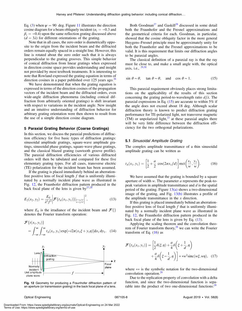
If the grating is placed immediately behind an aberration-free positive lens of focal length f that is uniformly illumi-nated by a normally incident plane wave as illustrated inFig. 12, the Fraunhofer diffraction pattern produced in theback focal plane of the lens is given by27,28

EQ-TARGET;temp:intralink-;e013;63;322E2ðx2; y2Þ ¼E0

λ2f2

��FftAðx1; y1Þgjξ¼x2∕λfη¼y2∕λf

��2; (13)

where E0 is the irradiance of the incident beam and Ffgdenotes the Fourier transform operation:EQ-TARGET;temp:intralink-;e014;63;256

Fftðx1; y1Þg

¼Z

∞

−∞

Z∞

−∞tAðx1; y1Þ exp½−i2πðx1ξþ y1ηÞ�dx1 dy1: (14)

Both Goodman27 and Gaskill28 discussed in some detailboth the Fraunhofer and the Fresnel approximations andthe geometrical criteria for each. Goodman, in particular,showed that the cosine obliquity factor in the more generalHuygens–Fresnel principle must be approximately unity forboth the Fraunhofer and the Fresnel approximations to bevalid. It is this requirement that limits our diffraction anglesto be paraxial angles.

The classical definition of a paraxial ray is that the raymust lie close to, and make a small angle with, the opticalaxis, i.e., 29,30

EQ-TARGET;temp:intralink-;e015;326;631 sin θ ∼ θ; tan θ ∼ θ; and cos θ ∼ 1: (15)

This paraxial requirement obviously places strong limita-tions on the applicability of the results of this sectionconcerning the grating period-to-wavelength ratio d∕λ. Theparaxial expressions in Eq. (15) are accurate to within 5% ifthe angle does not exceed about 18 deg. Although scalardiffraction theory is known to predict diffraction gratingperformance for TE-polarized light, not transverse magnetic(TM) or unpolarized light,22 at these paraxial angles therewill be very little difference between the diffraction effi-ciency for the two orthogonal polarizations.

5.1 Sinusoidal Amplitude Grating

The complex amplitude transmittance of a thin sinusoidalamplitude grating can be written as

EQ-TARGET;temp:intralink-;e016;326;441tAðx1; y1Þ ¼�1

2þ a

2cosð2πx1∕dÞ

�rect

�x1w;y1w

�: (16)

We have assumed that the grating is bounded by a squareaperture of width w. The parameter a represents the peak-to-peak variation in amplitude transmittance and d is the spatialperiod of the grating. Figure 13(a) shows a two-dimensionalimage of the grating, and Fig. 13(b) illustrates a profile ofthe amplitude transmittance in the x direction.

If this grating is placed immediately behind an aberration-free positive lens of focal length f that is uniformly illumi-nated by a normally incident plane wave as illustrated inFig. 12, the Fraunhofer diffraction pattern produced in theback focal plane of the lens is given by Eq. (13).

Applying the scaling theorem and the convolution theo-rem of Fourier transform theory,28 we can write the Fouriertransform of Eq. (16) as


FftAðx1; y1Þg ¼�1

2δðξ;ηÞ þ a

4δ

�ξþ 1

d;η

�

þ a4δ

�ξ−

1

d;η

�� w2sincðwξ;wηÞ; (17)

where �� is the symbolic notation for the two-dimensionalconvolution operation.28

Due to the replication property of convolution with a deltafunction, and since the two-dimensional function is sepa-rable into the product of two one-dimensional functions:28

Fig. 12 Geometry for producing a Fraunhofer diffraction pattern ofan aperture (or transmission grating) in the back focal plane of a lens.





FftAðx1; y1Þgjξ¼x2∕λfη¼y2∕λf

¼ w2 sinc

�y2

λf∕w

��1

2sinc

�x2

λf∕w

�

þ a4sinc

�x2 þ λf∕dλf∕w

�

þ a4sinc

�x2 − λf∕dλf∕w

��: (18)

If there are many grating periods within the aperture,then w ≫ d, and there will be negligible overlap betweenthe three sinc functions; hence, there will be no cross termsin the squared modulus of this sum. Substituting this intoEq. (13) thus yields the diffracted irradiance distribution inthe focal plane of the lens:

EQ-TARGET;temp:intralink-;e019;63;296Eðx2; y2Þ ¼E0w4

λ2f2sinc2

�y2

λf∕w

��1

4sinc2

�x2

λf∕w

�|fflfflfflfflfflfflfflfflfflfflfflffl{zfflfflfflfflfflfflfflfflfflfflfflffl}

m¼0

þ a2

16sinc2

�x2 þ λf∕dλf∕w

�|fflfflfflfflfflfflfflfflfflfflfflfflfflfflfflfflfflffl{zfflfflfflfflfflfflfflfflfflfflfflfflfflfflfflfflfflffl}

m¼þ1

þ a2

16sinc2

�x2 − λf∕dλf∕w

�|fflfflfflfflfflfflfflfflfflfflfflfflfflfflfflfflfflffl{zfflfflfflfflfflfflfflfflfflfflfflfflfflfflfflfflfflffl}

m¼−1

�: (19)

We thus have three discrete diffracted waves or “orders,”each of which is a scaled replica of the Fraunhofer diffractionpattern of the square aperture bounding the grating. Thecentral diffraction lobe is called the “zero order,” and thetwo side lobes are called the plus and minus “first orders.”The spatial separation of the first orders from the zero orderis λf∕d, whereas the width of the main lobe of all orders is2λf∕w as shown in Fig. 14.

The diffraction efficiency is defined as the fraction ofthe incident optical power that appears in a given diffractedorder (usually the þ1 order) of the grating. Integratingthe irradiance distribution representing a given diffractedorder and dividing by the incident optical power Po ¼ E0w2

gives the diffracted efficiency for that order. Since, for anyb and xo


Z∞

−∞

Z∞

−∞

1

b2sinc2

�x − xob

;yb

�¼ 1; (20)

it is clear that the efficiencies are just the coefficients ofthe three sinc2 terms in the curly brackets of Eq. (18). Theseefficiencies are tabulated in Table 1.

Theþ1 diffracted order thus contains at most (if the quan-tity a is equal to unity) 6.25% of the optical power incidentupon a sinusoidal amplitude grating. This very low diffrac-tion efficiency is not adequate for many applications. As seenin Table 1, the sum of the efficiencies of all three orders isonly equal to 1∕4þ a2∕8. The rest of the incident opticalpower is lost through absorption by the grating.

We will find later in Sec. 6 that a nonparaxial analysisindicates somewhat better performance for certain combina-tions of grating period and incident angle.

Fig. 13 (a) Two-dimensional image of sinusoidal amplitude grating and (b) profile of amplitude trans-mittance in the x direction.

Fig. 14 Irradiance profile of the Fraunhofer diffraction pattern produced by a thin sinusoidal amplitudegrating.

Table 1 Diffraction efficiencies for Fig. 14.

Order # Efficiency

0 0.25

þ1 a2∕16

−1 a2∕16




5.2 Square-Wave Amplitude Grating

The complex amplitude transmittance of a thin square-waveamplitude grating can be written asEQ-TARGET;temp:intralink-;e021;63;581

tAðx1; y1Þ ¼�rect

�x1b

�ð1Þ

� � 1dcomb

�x1d

�δðy1Þ

�rect

�x1w;y1w

�; (21)

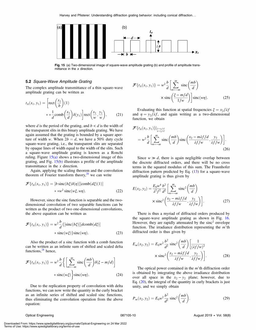
where d is the period of the grating, and b < d is the width ofthe transparent slits in this binary amplitude grating. We haveagain assumed that the grating is bounded by a square aper-ture of width w. When 2b ¼ d, we have a 50% duty cyclesquare-wave grating, i.e., the transparent slits are separatedby opaque lines of width equal to the width of the slits. Sucha square-wave amplitude grating is known as a Ronchiruling. Figure 15(a) shows a two-dimensional image of thisgrating, and Fig. 15(b) illustrates a profile of the amplitudetransmittance in the x direction.

Again, applying the scaling theorem and the convolutiontheorem of Fourier transform theory,28 we can write

EQ-TARGET;temp:intralink-;e022;63;377FftAðx1; y1Þg ¼ ½b sincðbξÞδðηÞ�½combðdξÞð1Þ�� w2 sincðwξ; wηÞ: (22)

However, since the sinc function is separable and the two-dimensional convolution of two separable functions can bewritten as the product of two one-dimensional convolutions,the above equation can be written as

EQ-TARGET;temp:intralink-;e023;63;282FftAðx1; y1Þg ¼ w2bdf½sincðbξÞ�½dcombðdξÞ�

� sincðwξÞgsincðwηÞ: (23)

Also the product of a sinc function with a comb functioncan be written as an infinite sum of shifted and scaled deltafunctions,28 hence,EQ-TARGET;temp:intralink-;e024;63;190

FftAðx1; y1Þg ¼ w2bd

�� X∞m¼−∞

sinc

�mbd

�δðξ −m∕dÞ

�

� sincðwξÞsincðwηÞ: (24)

Due to the replication property of convolution with deltafunctions, we can now write the quantity in the curly bracketas an infinite series of shifted and scaled sinc functions,thus eliminating the convolution operation from the aboveequation:


FftAðx1; y1Þg ¼ w2bd

� X∞m¼−∞

sinc

�mbd

�

× sinc

�ξ −m∕d1∕w

��sincðwηÞ: (25)

Evaluating this function at spatial frequencies ξ ¼ x2∕λfand η ¼ y2∕λf, and again writing as a two-dimensionalfunction, we obtain

EQ-TARGET;temp:intralink-;e026;326;516FftAðx1; y1Þgjξ¼x2∕λfη¼y2∕λf

¼ w2bd

� X∞m¼−∞

sinc

�mbd

�sinc

�x2 −mλf∕d

λf∕w;

y2λf∕w

��:

(26)

Since w ≫ d, there is again negligible overlap betweenthe discrete diffracted orders, and there will be no crossterms in the squared modulus of this sum. The Fraunhoferdiffraction pattern predicted by Eq. (13) for a square-waveamplitude grating is thus given by


Eðx2; y2Þ ¼E0w4

λ2f2b2

d2

� X∞m¼−∞

sinc2�mbd

�

× sinc2�x2 −mλf∕d

λf∕w;

y2λf∕w

��: (27)

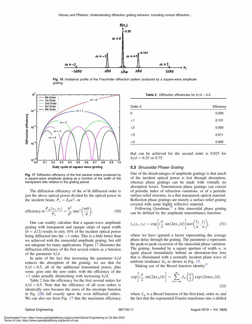
There is thus a myriad of diffracted orders produced bythe square-wave amplitude grating as shown in Fig. 16.However, they are rapidly attenuated by the sinc2 envelopefunction. The irradiance distribution representing the m’thdiffracted order is thus given by


Emðx2; y2Þ ¼ E0w2b2

d2sinc2

�mbd

��1

ðλf∕wÞ2


λf∕w;

y2λf∕w

��: (28)

The optical power contained in the m’th diffraction orderis obtained by integrating the above irradiance distributionover all space in the x2 − y2 plane; however, due toEq. (20), the integral of the quantity in curly brackets is justunity, and we simply obtain

EQ-TARGET;temp:intralink-;e029;326;107Pmðx2; y2Þ ¼ E0w2b2

d2sinc2

�mbd

�: (29)

Fig. 15 (a) Two-dimensional image of square-wave amplitude grating (b) and profile of amplitude trans-mittance in the x direction.




The diffraction efficiency of the m’th diffracted order isjust the above optical power divided by the optical power inthe incident beam, Po ¼ E0w2, or

EQ-TARGET;temp:intralink-;e030;63;307efficiency ≡Pmðx2; y2Þ

Po¼ b2

d2sinc2

�mbd

�: (30)

One can readily calculate that a square-wave amplitudegrating with transparent and opaque strips of equal width(b ¼ d∕2) results in only 10% of the incident optical powerbeing diffracted into the þ1 order. This is a little better thanwe achieved with the sinusoidal amplitude grating, but stillnot adequate for many applications. Figure 17 illustrates thediffraction efficiency of the first several orders as a functionof the parameter b∕d.

In spite of the fact that increasing the parameter b∕dreduces the absorption of the grating, we see that forb∕d > 0.5, all of the additional transmitted power, plussome, goes into the zero order, with the efficiency of theþ1 order actually diminishing with increasing b∕d.

Table 2 lists the efficiency for the first several orders forb∕d ¼ 0.5. Note that the efficiency of all even orders isidentically zero because the zeros of the envelope functionin Eq. (28) fall exactly upon the even diffracted orders.We can also see from Fig. 17 that the maximum efficiency

that can be achieved for the second order is 0.025 forb∕d ¼ 0.25 or 0.75.

5.3 Sinusoidal Phase Grating

One of the disadvantages of amplitude gratings is that muchof the incident optical power is lost through absorption,whereas phase gratings can be made with virtually noabsorption losses. Transmission phase gratings can consistof periodic index of refraction variations, or of a periodicsurface relief structure, in a thin transparent optical material.Reflection phase gratings are merely a surface relief gratingcovered with some highly reflective material.

Following Goodman,27 a thin sinusoidal phase gratingcan be defined by the amplitude transmittance function:

EQ-TARGET;temp:intralink-;e031;326;275tAðx1; y1Þ ¼ exp

�ia2

sinð2πx1∕dÞ�rect

�x1w;y1w

�; (31)

where we have ignored a factor representing the averagephase delay through the grating. The parameter a representsthe peak-to-peak excursion of the sinusoidal phase variation.The grating, bounded by a square aperture of width w, isagain placed immediately behind an aberration-free lensthat is illuminated with a normally incident plane wave ofuniform irradiance E0 as shown in Fig. 13.

Making use of the Bessel function identity27

EQ-TARGET;temp:intralink-;e032;326;142 exp

�ia2

sinð2πx1∕dÞ�¼

X∞m¼−∞

Jm

�a2

�expði2πmx1∕dÞ;

(32)

where Jm is a Bessel function of the first kind, order m, andthe fact that the exponential Fourier transforms into a shifted

Fig. 16 Irradiance profile of the Fraunhofer diffraction pattern produced by a square-wave amplitudegrating.

Fig. 17 Diffraction efficiency of the first several orders produced bya square-wave amplitude grating as a function of the width of thetransparent slits relative to the grating period.

Table 2 Diffraction efficiencies for b∕d ¼ 0.5.

Order # Efficiency

0 0.250

�1 0.101

�2 0.000

�3 0.011

�4 0.000




delta function,28 it is readily shown that, within the paraxiallimitation, the irradiance distribution in the back focal planeof the lens is given byEQ-TARGET;temp:intralink-;e033;63;719

Eðx2; y2Þ ¼ E0w2

� X∞m¼−∞

J2m

�a2

��1

ðλf∕wÞ2


λf∕w;

y2λf∕w

��; (33)

and the diffraction efficiency of the m’th diffracted order ofa perfectly conducting sinusoidal phase grating is given bythe following well-known expression:1,22,27,31,32


Po¼ J2m

�a2

�; (34)

where a ¼ 4πh∕λ and h is the peak to peak groove depth ofthe sinusoidal reflection grating.

The conservation of energy is easily shown for thisperfectly conducting paraxial (d ≫ λ) reflection grating atnormal incidence because the sum over m from −∞ to ∞ ofthe squared Bessel function in Eq. (33) is equal to unity.

Since the Fraunhofer diffraction integral implicitly con-tains the paraxial approximation, the diffraction angle isproportional to displacement on the focal plane containingthe Fraunhofer diffraction patterns

EQ-TARGET;temp:intralink-;e035;63;457θx ¼ tan−1ðx2∕fÞ ≈ x2∕f; θy ¼ tan−1ðy2∕fÞ ≈ y2∕f:(35)

Recalling our definitions of radiometric quantities, it isclear that the diffracted intensity distribution (radiant powerper unit solid angle) emanating from the grating is thusproportional to the diffracted irradiance distribution (radiantpower per unit area) incident upon the focal plane as given byEq. (33):EQ-TARGET;temp:intralink-;e036;63;345

Iðθx; θyÞ ¼ I0X∞

m¼−∞J2m

�a2

��1

ðλf∕wÞ2


λf∕w;

y2λf∕w

��: (36)

Figure 18 illustrates the diffracted intensity distributionas a function of diffraction angle θx and groove depth h,for a sinusoidal “reflection” grating with period d ¼ 20λoperating at normal incidence.

The maximum value of J21ða∕2Þ is 0.3386 and occurs fora ¼ 3.68, corresponding to a groove depth of h ¼ 0.293λ .The diffraction efficiency of the first few orders for this valueof a is tabulated in Table 3. Note that the energy falls offrapidly, with 99.88% of the diffracted radiant power con-tained in diffracted orders jmj ≤ 3. This paraxial model isaccurate only for very coarse gratings (d ≫ λ).

The paraxial behavior described by Eq. (36) above leadsto the common misconception that it is impossible to getmore than 33.86% of the incident energy into the first dif-fracted order with a sinusoidal phase grating. “Nothing couldbe further from the truth!” In fact, if you decrease the gratingperiod, the diffracted angles increase and the higher orderseventually go evanescent. When only the zero and �1 dif-fracted orders remain, changing the incident angle will cause

the −1 order to go evanescent. Then one can vary the groovedepth to squelch the energy in the zero order. For a perfectlyconducting sinusoidal reflectance grating, we can thus get100% of the incident energy in the þ1 diffracted order!33

In addition to being a paraxial (d ≫ λ) grating, if thesinusoidal reflection grating is also shallow (i.e., the groovedepth is much less than a wavelength of the incident light),then the diffraction efficiency of the first orders of the sinus-oidal reflection grating can be approximated by

EQ-TARGET;temp:intralink-;e037;326;291efficiency ≡ J21ða∕2Þ ≈ a2∕16: (37)

Figure 19 compares the predicted diffraction efficiency ofthis approximation with the results of Eq. (34) for a perfectly

Fig. 18 Diffracted intensity distribution as predicted by the aboveparaxial model for a sinusoidal reflection grating of period d ¼ 20λoperating at normal incidence.

Table 3 Diffraction efficiencies for a ¼ 3.68, corresponding toh ¼ 0.293λ.

Order # Efficiency

0 1.003 × 10−1

�1 3.386 × 10−1

�2 9.970 × 10−2

�3 1.093 × 10−2

�4 6.320 × 10−4

Fig. 19 Comparison of diffracted efficiency of a sinusoidal phasegrating as predicted by Eq. (34) and the common approximation forshallow (smooth) gratings expressed in Eq. (37).




conducting surface (R ¼ 1) and illustrates how shallow thegrating must be to satisfy various error tolerances. Note thatthe above approximation exhibits only a 1% error in the pre-diction of diffraction efficiency of the þ1 diffracted order ath ¼ 0.0318λ, a 5% error at h ¼ 0.0702λ, and a 10% errorat h ¼ 0.098λ.

5.4 Square-Wave Phase Grating

Let us first look at a special case of a rectangular phasegrating where the peak-to-peak phase step is equal to π (thisshould result in zero efficiency for the zero diffracted order)and a duty cycle of b∕d ¼ 0.5 as illustrated in Fig. 20. FromEuler’s equation

EQ-TARGET;temp:intralink-;e038;63;604 expðiϕÞ ¼ cosðϕÞ þ i sinðϕÞ; (38)

we readily see that expðiϕÞ is equal to −1 when ϕ ¼ π andþ1 when ϕ ¼ 0 as illustrated in Fig. 21. The complex ampli-tude transmittance of this rectangular phase grating boundedby a square aperture of width w thus can be written asEQ-TARGET;temp:intralink-;e039;63;529

tAðx1; y1Þ ¼��

2 rect

�x1d∕2

�ð1Þ � � 1

dcomb

�x1d

�δðy1Þ�− 1

× rect

�x1w;y1w

�: (39)

Following the discussion of the square-wave amplitudegrating, we obtain a Fraunhofer diffraction pattern given byEQ-TARGET;temp:intralink-;e040;63;434

Eðx2; y2Þ ¼E0w4

λ2f2

� X∞m¼−∞

sinc2�m2

�


λf∕w;

y2λf∕w

��; (40)

except that the zero diffracted order is absent. Continuing,we obtain


Po¼ sinc2

�m2

�for m ≠ 0: (41)

Table 4 thus lists the efficiency for the first several ordersfor this special case of a rectangular phase grating. Notethat the π phase step has eliminated the zero order, and theefficiency of all other even orders is identically zero becausethe zeros in the envelope function in Eq. (40) fall exactlyupon the even diffracted orders. This thus maximizes theefficiency of the remaining orders.

We have thus seen that the maximum efficiency of theþ1 diffracted order (in the paraxial limit) increases from0.0625 for a sinusoidal amplitude grating, to 0.1013 fora rectangular amplitude grating, to 0.3386 for a sinusoidalphase grating, and to 0.4053 for a rectangular phase grating.

Before we proceed to discuss the classical blazed grating,we want to derive the general solution for the diffractionbehavior of an “arbitrary rectangular phase grating.” Thisderivation will lay the groundwork for studying the behaviorof diffraction gratings with “arbitrary groove shapes.”

For a rectangular phase grating with an arbitrary phasestep, the complex amplitude transmittance can be written as

EQ-TARGET;temp:intralink-;e042;326;370tAðx1; y1Þ ¼ exp½iϕðx1Þ�; (42)

where the phase variation is given by

EQ-TARGET;temp:intralink-;e043;326;332φðx1Þ ¼ a rectx1b

�ð1Þ � � 1

dcomb

x1d

�δðy1Þ: (43)

This phase variation is illustrated graphically in Fig. 22.Since this is an even function, it can be decomposed into a

discrete cosine Fourier series. The Fourier series coefficientsfor the above periodic function can be shown to be given by

EQ-TARGET;temp:intralink-;e044;326;251cn ¼ 2abdsinc

nbd

�; (44)

thus

EQ-TARGET;temp:intralink-;e045;326;200ϕðx1Þ ¼a2þX∞n¼1

cn cosð2πnx1∕dÞ: (45)Fig. 20 Phase variation for a special case of a rectangular phase gra-ting with a peak-to-peak phase step of π and a 50% duty cycle.

Fig. 21 Complex amplitude for a rectangular phase grating witha peak-to-peak phase step of π and a 50% duty cycle.

Table 4 Diffraction efficiencies for a square-wave phase grating witha π phase step.

Order # Efficiency

0 0.000

�1 4.053 × 10−1

�2 0.000

�3 4.503 × 10−2

�4 0.000

�5 1.621 × 10−2

Fig. 22 Phase variation for a rectangular phase grating.




However, we can ignore the constant term resulting fromthe fact that ϕðx1Þ as illustrated above does not have a zeromean. The rectangular phase variation is thus represented asa superposition of cosinusoidal phase variations:

EQ-TARGET;temp:intralink-;e046;63;708ϕðx1Þ ¼X∞n¼1

cn cosð2πnx1∕dÞ: (46)

A thin rectangular phase grating can thus be defined bythe amplitude transmittance function:

EQ-TARGET;temp:intralink-;e047;63;638tAðx1; y1Þ ¼ exp

�iX∞n¼1

cn cosð2πnx1∕dÞ�: (47)

But this can be written as the infinite product:

EQ-TARGET;temp:intralink-;e048;63;579tAðx1; y1Þ ¼Y∞n¼1

fexp½icn cosð2πnx1∕dÞ�g: (48)

Making use of the Bessel function identity34

EQ-TARGET;temp:intralink-;e049;63;520 exp½iz cosðθÞ� ¼X∞

m¼−∞imJmðzÞ expðimθÞ; (49)

we have an infinite product of infinite sums, which uponFourier transforming results in an infinite array of convolu-tions of infinite sums of delta functions:


FftAðx1; y1Þg ¼�� X∞

m¼−∞JmðcnÞδðξ − nm∕dÞ

�n¼1

�� X∞m¼−∞

JmðcnÞδðξ − nm∕dÞ�n¼2

�� X∞m¼−∞

JmðcnÞδðξ − nm∕dÞ�n¼3

� · · · �� X∞m¼−∞

JmðcnÞδðξ − nm∕dÞ�n¼∞

:

(50)

Although the above expression might at first appear to berather unwieldy, it is rather easily solved numerically withthe array operations provided with the MATLAB softwarepackage. In fact, the above operation results in an array ofdelta functions that represents the diffracted orders producedby the rectangular phase grating. The squared moduli ofthe coefficients of those terms are the efficiencies of the dif-fracted orders.

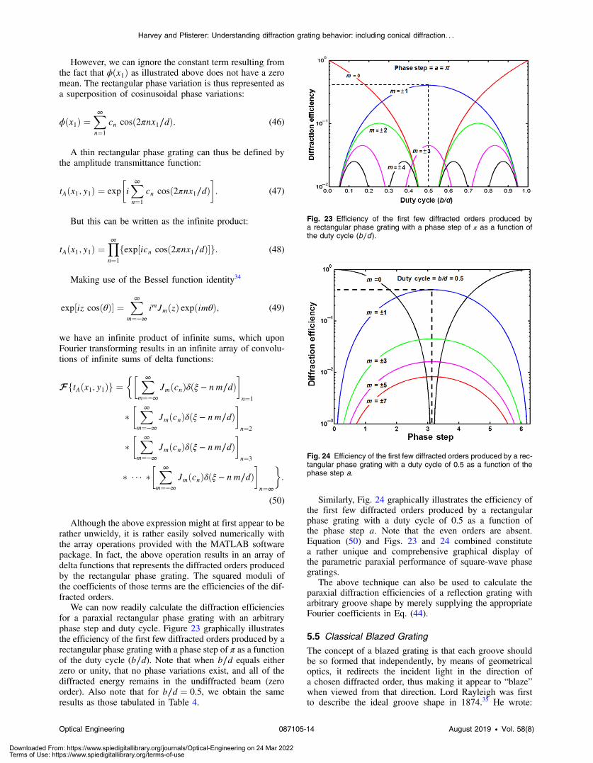
We can now readily calculate the diffraction efficienciesfor a paraxial rectangular phase grating with an arbitraryphase step and duty cycle. Figure 23 graphically illustratesthe efficiency of the first few diffracted orders produced by arectangular phase grating with a phase step of π as a functionof the duty cycle (b∕d). Note that when b∕d equals eitherzero or unity, that no phase variations exist, and all of thediffracted energy remains in the undiffracted beam (zeroorder). Also note that for b∕d ¼ 0.5, we obtain the sameresults as those tabulated in Table 4.

Similarly, Fig. 24 graphically illustrates the efficiency ofthe first few diffracted orders produced by a rectangularphase grating with a duty cycle of 0.5 as a function ofthe phase step a. Note that the even orders are absent.Equation (50) and Figs. 23 and 24 combined constitutea rather unique and comprehensive graphical display ofthe parametric paraxial performance of square-wave phasegratings.

The above technique can also be used to calculate theparaxial diffraction efficiencies of a reflection grating witharbitrary groove shape by merely supplying the appropriateFourier coefficients in Eq. (44).

5.5 Classical Blazed Grating

The concept of a blazed grating is that each groove shouldbe so formed that independently, by means of geometricaloptics, it redirects the incident light in the direction ofa chosen diffracted order, thus making it appear to “blaze”when viewed from that direction. Lord Rayleigh was firstto describe the ideal groove shape in 1874.35 He wrote:

Fig. 23 Efficiency of the first few diffracted orders produced bya rectangular phase grating with a phase step of π as a function ofthe duty cycle (b∕d ).

Fig. 24 Efficiency of the first few diffracted orders produced by a rec-tangular phase grating with a duty cycle of 0.5 as a function of thephase step a.




“. . . the retardation should gradually alter by a wavelength inpassing over each element of the grating and then fall backto its previous value, thus springing suddenly over a wave-length.” He was not very optimistic about achieving suchgeometry, but 36 years later, in 1910, Wood36 producedthe first grating that we would call “blazed” for use in theinfrared. He did this with a tool of carborundum, ruled intocopper.

A missing insight that we now take for granted was pro-vided by John Anderson in 1916 while working at the Mt.Wilson Observatory. He demonstrated that superior gratingscould be produced by “burnishing” (plastic deformationof the surface) rather than cutting the grooves into thesubstrate.37 The material thus had to be soft enough to acceptlocal deformation and at the same time be highly polished.

The classical blazed grating is thus a reflection gratingwith a sawtooth groove profile as shown in Fig. 25. Suchgratings have been manufactured for over 150 years by scrib-ing, or burnishing, a series of grooves upon a good opticalsurface. Originally, this surface was one of highly polishedspeculum metal.

A major advance in the development of diffraction gra-tings was the discovery by John Strong in 1936 that vacuumdeposited aluminum on glass is a far superior medium intowhich to rule grating grooves than speculum metal, whichhad been almost universally used for nearly a century.38

Therefore, in recent times, diffraction gratings have beenruled in thin layers of aluminum or gold deposited upona glass substrate.

Blazed gratings can be designed for a particular wave-length, incident angle, and diffracted order. The blaze angleθB of the grating is given by

EQ-TARGET;temp:intralink-;e051;63;400θB ¼ tan−1ðh∕dÞ; (51)

where h is the groove depth and d is the grating period.For a paraxial grating designed to operate at normal inci-

dence, the groove depth must be equal to

EQ-TARGET;temp:intralink-;e052;63;336h ¼ nBλB∕2; (52)

where nB is the blaze (or design) order and λB is the blaze(or design) wavelength.

The specularly reflected plane wavefront segments willthen be out of phase by precisely 2π, thus producingconstructive interference for that wavelength and diffractedorder. Stated another way, the reflected phase variation overone period of the above grating can be written as

EQ-TARGET;temp:intralink-;e053;63;228ϕðx1Þ ¼2π

λOPDðx1Þ ¼

2π

λ2h

x1d

¼ 2πnBλBx1∕ðλdÞ: (53)

Making use of the replication properties of convolutionwith a comb function, the complex amplitude transmittance(or reflectance in this case) of a grating blazed for the n’thorder and operating at the blaze wavelength can thus bewritten as

EQ-TARGET;temp:intralink-;e054;326;697tAðx1Þ ¼ rect

�x1d

�expð−i2πnBλBx1∕λdÞ �

1

dcomb

�x1d

�:

(54)

Using the scaling theorem and the convolution theorem ofFourier transform theory, we can write

EQ-TARGET;temp:intralink-;e055;326;617FftAðx1Þg ¼ sinc½dðξ − nBλB∕λdÞ�½d combðdξÞ�: (55)

The irradiance of the Fraunhofer diffraction pattern in thex2 − y2 observation plane a distance z from the grating isproportional to the squared modulus of the Fourier transformof the complex amplitude distribution emerging from thegrating:

EQ-TARGET;temp:intralink-;e056;326;531E2ðx2Þ ∝1

λzjFftAðx1Þgjξ¼x2∕λzj2; (56)

EQ-TARGET;temp:intralink-;e057;326;479E2ðx2Þ ∝ sinc2�x2 − ðnBλB∕λÞλz∕d

λz∕d

�1

λz∕dcomb

�x2

λz∕d

�:

(57)

When operating at the blaze wavelength λ ¼ λB, the peakof the sinc2 function is centered on the nB’th diffracted orderand all of the other delta functions (diffracted orders) fall onthe zeros of the sinc2 function. All of the reflected energy isthus diffracted into the nB’th diffracted order. Figure 26shows a plot of diffraction efficiency versus x2 × λz∕d fora coarse grating blazed to operate in the second order atnormal incidence for a wavelength of 550 nm. If d ≫ nBλB,we can be assured, from the planar grating equation, Eq. (3),that the nB’th order will be diffracted at a paraxial angle andthis predicted behavior will be accurate.

If the incident angle is nonzero, there would be an addi-tional linear phase variation over the entire grating (not eachfacet individually). Equation (54) describing the complexamplitude distribution emerging from the reflecting blazedgrating would thus have to be modified as follows:

Fig. 25 Classical reflection blazed grating with normally incident light.

Fig. 26 Illustration of the 100% efficiency achieved by a perfectlyreflecting blazed grating designed to operate at normal incidencein the second diffracted order.




EQ-TARGET;temp:intralink-;e058;63;752tAðx1Þ ¼�rect

�x1d

�expð−i2πnBλBx1∕λdÞ

� 1

dcomb

�x1d

��exp

�−i2π

θ0λx1

�; (58)

where the diffraction angle of the zero order (angle ofreflection) is merely the negative of the incident angle, i.e.,θ0 ¼ −θi. Again, using the scaling theorem and the convo-lution theorem of Fourier transform theory, we obtain

EQ-TARGET;temp:intralink-;e059;63;643FftAðx1Þg ¼ fsinc½dðξ − nBλB∕λdÞ�½dcombðdξÞ�g� δðξ − θ0∕λÞ: (59)

Evaluating at ξ ¼ x2∕λz and substituting into Eq. (56)yields the following expression for the diffraction patternprojected onto a screen at a distance z from the grating:


E2ðx2Þ∝ sinc2

24x2−

nBλBλ þ θ0d

λ

�λzd

λzd

35 1

λzd

comb

24x2 −

θ0dλ

�λzd

λzd

35:

(60)

Introducing an arbitrary incident angle will thus shift boththe sinc2 envelope function and the diffracted orders by pre-cisely the same amount. Therefore, under “paraxial” condi-tions, the diffraction efficiency does not change with incidentangle. For example, if we illuminate the above grating blazedfor the second order with an incident angle equal to the blazeangle ðθi ¼ θBÞ, the incident beam will strike the individualfacets at normal incidence and the second order will be ret-roreflected as illustrated in Fig. 27. This situation ðθi ¼ θ2Þis referred to as the Littrow condition for the second order,19

and the efficiency will remain at 100% as shown in Fig. 28.The zero order will of course be specularly reflected fromthe plane of the grating, and the þ1 order will be diffractednormal to the plane of the grating.

The product of a sinc2 function with a comb function canbe written as an infinite sum of shifted and scaled delta func-tions,28 each of which represents a different diffracted order.Equation (60) can, therefore, be rewritten asEQ-TARGET;temp:intralink-;e061;63;279

E2ðx2Þ ∝X∞

m¼−∞sinc2

�m − ðnBλB∕λþ θ0d∕λÞλz∕d

λz∕d

�

× δðx2 − ðθ0d∕λÞλz∕dÞ: (61)

For polychromatic light, we can represent the resultingdiffracted orders with a summation over the discretediffracted orders of an integral over some spectral bandΔλ ¼ λ2 − λ1:


E2ðx2Þ ∝X∞

m¼−∞

Zλ2

λ1

sinc2�m − ðnBλB∕λþ θ0d∕λÞλz∕d

λz∕d

�

× δ½x2 − ðθ0d∕λÞλz∕d�: (62)

Figure 29 schematically illustrates the dispersive behaviorover the visible spectrum of a grating blazed for the firstorder at a wavelength 500 nm. The seven classical discretecolors: red (λ1 ¼ 650 nm), orange (λ2 ¼ 600 nm), yellow(λ3 ¼ 550 nm), green (λ4 ¼ 500 nm), blue (λ5 ¼ 450 nm),indigo (λ6 ¼ 400 nm), and violet (λ7 ¼ 350 nm) areobtained by replacing the integral in the above equationby a discrete summation:


E2ðx2Þ ∝X∞

m¼−∞

Xλ7λ¼λ1

sinc2�m − ðnBλB∕λþ θ0d∕λÞλz∕d

λz∕d

�

× δ½x2 − ðθ0d∕λÞλz∕d�: (63)

Figure 30 illustrates that the dispersion is indeed doubledif the grating is blazed for the second diffracted order. Note

Fig. 27 Blazed grating satisfying the Littrow condition for the secondorder.

Fig. 28 Illustration of the 100% efficiency achieved by a perfectlyreflecting blazed grating satisfying the Littrow condition for the seconddiffracted order.

Fig. 29 Illustration of the dispersion produced over the visible spec-trum by a grating blazed for a wavelength of 500 nm in the firstdiffractive order.




also that the diffraction efficiency is substantially reduced forall wavelengths other than the blaze wavelength.

In this section, we have systematically described in detailthe paraxial behavior of five different classical grating types:the sinusoidal amplitude grating, the square-wave amplitudegrating, the sinusoidal phase grating, the square-wave phasegrating, and the blazed reflection grating (sawtooth profile).The result of the paraxial diffraction efficiency analyses ofthese five grating types is summarized in Table 5.

6 Nonparaxial Scalar Diffraction TheoryAs discussed briefly in Sec. 1–Sec. 5, it is well-known thatthe paraxial irradiance distribution on a plane in the farfield (Fraunhofer region) of a diffracting aperture is givenby the squared modulus of the Fourier transform of the com-plex amplitude distribution emerging from the diffractingaperture.27,28 A slight variation of Eq. (13), without the pres-ence of the lens, can be written as

EQ-TARGET;temp:intralink-;e064;63;375Eðx2; y2Þ ¼E0

λ2z2

��FfUþo ðx1; y1Þg

��ξ¼x2

λz;η¼y2λz

��2: (64)

Here Uþo ðx1; y1Þ ¼ U−

o ðx1; y1Þt1ðx1; y1Þ is the complexamplitude distribution emerging from the diffracting apertureof complex amplitude transmittance t1ðx1; y1Þ, andU−

o ðx1; y1Þis the complex amplitude incident upon the lens.

The spatial frequencies ξ and η are the reciprocal variablesin Fourier transform space. Also the Fresnel diffraction inte-gral is given by the Fourier transform of the product of theaperture function with a quadratic phase factor.27,28 Implicitin both the Fresnel and the Fraunhofer approximation is a“paraxial limitation” that restricts their use to small diffrac-tion angles and small angles of incidence.27,28 This paraxiallimitation severely restricts the conditions under which thisconventional linear systems formulation of scalar diffractiontheory adequately describes real diffraction phenomena.

A linear systems approach to modeling nonparaxial scalardiffraction phenomena has been developed by normalizingthe spatial variables by the wavelength of light:20–23

EQ-TARGET;temp:intralink-;e065;326;445x ¼ x∕λ; y ¼ y∕λ; z ¼ z∕λ; etc: (65)

The reciprocal variables in Fourier transform spacebecome the “direction cosines” of the propagation vectors ofthe plane wave components in the angular spectrum of planewaves discussed by Ratcliff,39 Goodman,27 and Gaskill:28

EQ-TARGET;temp:intralink-;e066;326;370α ¼ x∕r; β ¼ y∕r; and γ ¼ z∕r: (66)

By incorporating sound radiometric principles into scalardiffraction theory, it becomes evident that the squaredmodulus of the Fourier transform of the complex amplitudedistribution emerging from the diffracting aperture yields“diffracted radiance (not irradiance or intensity)20–23:”


L 0ðα; β − β0Þ ¼ K λ2

AsjFfU 0

oðx; y; 0Þ expði2πβ0yÞgj2 for α2 þ β2 ≤ 1

L 0ðα; β − β0Þ ¼ 0 for α2 þ β2 > 1:(67)

For large incident and/or diffracted angles, the diffractedradiance distribution function will be truncated by the unitcircle in direction cosine space. Evanescent waves are thenproduced and the equation for diffracted radiance must berenormalized. The renormalization factor in Eq. (67) is givenby20–23

EQ-TARGET;temp:intralink-;e068;63;159K ¼R∞α¼−∞

R∞β¼−∞ Lðα; β − β0Þdα dβR

1α¼−1

R ffiffiffiffiffiffiffiffi1−α2

p

β¼−ffiffiffiffiffiffiffiffi1−α2

p Lðα; β − β0Þdα dβ(68)

and only differs from unity if the diffracted radiance distri-bution function extends beyond the unit circle in directioncosine space (i.e., only if evanescent waves are produced).

In spite of the fact that it is almost universally believedthat—“in no way can scalar theory deal with cut-offanomalies,”40 the renormalization factor K in Eq. (67) anddefined by Eq. (68) enables this linear systems formulationof nonparaxial scalar diffraction theory to predict and modelthe well-known Wood’s (Rayleigh) anomalies16 that occur indiffraction efficiency behavior for simple cases of amplitudetransmission gratings discussed in the following two sectionsof this paper.

This renormalization process is also consistent with thelaw of conservation of energy. However, it is significant thatthis linear systems formulation of nonparaxial scalar diffrac-tion theory has been derived by the application of Parseval’stheorem and not by merely heuristically imposing the law ofconservation of energy.20–23

Fig. 30 Illustration that the dispersion is proportional to the diffractedorder number.

Table 5 Paraxial efficiencies of various grating types (optimized forþ1 order).

Grating typeZeroorder

Firstorder

Secondorder

Thirdorder

Fourthorder

Sinusoidal amplitude 0.250 0.0625 N/A N/A N/A

Square-wave amplitude 0.250 0.101 0.000 0.011 0.000

Sinusoidal phase 0.1003 0.3386 0.0997 0.0109 0.0006

Square-wave phase 0.0000 0.4053 0.0000 0.0450 0.0000

Classical blazed 0.0000 1.0000 0.0000 0.0000 0.0000




6.1 Rayleigh Anomalies from Sinusoidal AmplitudeTransmission Gratings

Since many individual measurements are required tocompletely characterize the efficiency behavior of a givengrating, it has become commonplace to make diffractionefficiency measurements with a given diffracted order inthe Littrow condition.19 For transmission gratings, a givendiffracted order satisfies the Littrow condition if θm ¼ −θi.For reflection gratings, the Littrow condition is satisfied ifthe given diffracted order is antiparallel to the incident beam,i.e., θm ¼ θi. This allows the experimenter to leave the detec-tor and the source in a fixed location and merely rotate thegrating between measurements.

As previously shown in Table 1 of Sec. 5.1, for a narrowbeam normally incident upon a paraxial sinusoidal amplitudegrating with modulation of unity, five-eighths of the incidentenergy is absorbed and three-eights of it is transmitted.Twenty-five percent of the total incident energy is containedin the zero order and six and one-quarter percent is containedin both the þ1 and the −1 orders.

If the þ1 diffracted order is in the Littrow condition(θ1 ¼ −θi) as shown in Fig. 31, the grating equationexpressed in Eq. (3) results in the following expression forthe incident angle

EQ-TARGET;temp:intralink-;e069;63;484θi ¼ sin−1ð0.5λ∕dÞ: (69)

Substituting Eq. (69) into Eq. (3) yields

EQ-TARGET;temp:intralink-;e070;63;442 sin θm ¼ −�m −

1

2

�λ

d: (70)

Hence, the þ1 and −1 diffracted orders produced by asinusoidal amplitude grating propagate at angles:

EQ-TARGET;temp:intralink-;e071;63;375θ1 ¼ −sin−1�1

2

λ

d

�and θ−1 ¼ sin−1

�3

2

λ

d

�: (71)

Note that the sign of these two angles are consistent withthe sign convention previously illustrated in Fig. 5. Figure 31illustrates this situation for λ∕d ¼ 0.4.

As the grating is rotated to increase λ∕d, both the angle ofincidence and the diffraction angles increase. If we useEq. (71) to calculate at what value of λ∕d the −1 diffractedorder goes evanescent, θ−1 ¼ π∕2, we obtain

EQ-TARGET;temp:intralink-;e072;63;253λ∕d ¼ 2∕3 ¼ 0.667: (72)

Clearly, the total amount of energy transmitted throughthis thin grating does not vary as the angle of incidence of

the narrow beam is increased. Thus when the −1 diffractedorder goes evanescent, the energy that was contained in it(6.25% of the incident energy) is redistributed into thetwo remaining propagating orders (the Rayleigh anomalyphenomenon).

According to Eq. (68), the renormalization constant K isequal to

EQ-TARGET;temp:intralink-;e073;326;483K ¼ η−1 þ η0 þ η1η0 þ η1

¼ 0.0625þ 0.25þ 0.0625

0.25þ 0.0625¼ 1.2;

(73)

where ηm is the diffraction efficiency of the m’th diffractedorder. The diffraction efficiency of a sinusoidal amplitudediffraction grating is plotted versus λ∕d in Fig. 32.

Note the 20% increase in diffraction efficiency of boththe zero and the þ1 diffracted order at λ∕d > 0.667.41

It is thus possible to get a maximum diffraction efficiency of0.075 for the þ1 order with a sinusoidal amplitude grating.In spite of this increase over the paraxial prediction ofSec. 5.1, this low diffraction efficiency combined with thefact that precision sinusoidal amplitude gratings are difficultto fabricate explains why they are rarely used for practicalapplications.

6.2 Rayleigh Anomalies from Square-WaveAmplitude Gratings

The paraxial behavior of the square-wave amplitude gratingwas discussed in detail in Sec. 5.2. Equation (28) indicatedthat there is a myriad of diffracted orders produced; however,they are rapidly attenuated by a sinc2 envelope function. Fora 50% duty cycle square-wave amplitude grating (d ¼ 2b),the zeros of the envelope function fall precisely on the evendiffraction orders as illustrated in Fig. 33. We see fromEq. (28) and Fig. 33 that the diffraction efficiency of them’thdiffracted order is given by

EQ-TARGET;temp:intralink-;e074;326;157ηm ¼ 1

4sinc2

�m2

�: (74)

The paraxial diffraction efficiencies of the first 19diffracted orders of a square-wave amplitude grating witha 50% duty cycle are listed in Table 6. Note that 25% ofthe incident energy is contained in the zero diffracted order,

Fig. 31 Diffraction configuration for a sinusoidal amplitude transmis-sion grating with theþ1 diffracted order satisfying the Littrow conditionwhen λ∕d ¼ 0.4.

Fig. 32 Illustration of Rayleigh anomalies from a sinusoidal amplitudetransmission grating with the þ1 diffracted order satisfying the Littrowcondition.




all even orders are identically zero, and the remaining dif-fracted orders contain another 25%. The remaining 50% ofthe energy in the incident beam is absorbed by the opaquestrips making up the square-wave amplitude grating.

When operating in the Littrow condition, the diffractedorders are distributed symmetrically about the grating normalas shown in Fig. 34. For small λ∕d, there are many diffractedorders, but they all have small diffraction angles. As λ∕d isincreased, both the angle of incidence and the diffractionangles increase, and the higher diffracted orders start goingevanescent.

Since the diffracted orders are distributed symmetricallyabout the grating normal, a positive and a negative order alwaysgo evanescent simultaneously. Figure 34 illustrates the situationfor a transmission grating with λ∕d ¼ 0.25 and the þ1 dif-fracted order satisfying the Littrow condition (θ1 ¼ −θi).

Using Eq. (69) to calculate at what value of λ∕d the þ2diffracted order goes evanescent, we obtain

EQ-TARGET;temp:intralink-;e075;63;104 sinð−π∕2Þ ¼ −1 ¼ −�2 −

1

2

�λ

dor λ∕d ¼ 2∕3: (75)

Similarly, the −1 order goes evanescent when

EQ-TARGET;temp:intralink-;e076;326;294 sinðπ∕2Þ ¼ 1 ¼ −�−1 −

1

2

�λ

dor λ∕d ¼ 2∕3: (76)

We likewise discover that the −2 and þ3 diffractedorders go evanescent when λ∕d ¼ 2∕5, and the −3 and þ4diffracted orders go evanescent when λ∕d ¼ 2∕7, etc.

Hence, when plotting diffraction efficiency versus λ∕d,there can be at most only two propagating orders (the zeroorder and the þ1 that is being maintained in the Littrow con-dition) for λ∕d > 2∕3. All other orders are evanescent.

As with the sinusoidal amplitude grating, the total amountof energy transmitted through a square-wave amplitude gra-ting does not vary as the angle of the incident beam isincreased. Thus as each pair of diffracted orders goes evan-escent, the energy that was contained by them is redistributedinto the remaining propagating orders (again the Rayleighgrating anomaly phenomenon) according to the nonparaxialscalar diffraction theory summarized earlier in this section.The renormalization constant K is equal to

Fig. 33 Schematic illustration of diffraction orders for a 50% duty cycle square-wave amplitude grating.Note that all even orders are absent.

Table 6 Diffraction Efficiencies for the 1st 19 diffracted orders of asquare-wave amplitude grating with b∕d ¼ 0.5.

Order # Efficiency

0 0.2500

�1 0.1013

�2 0.0000

�3 0.0113

�4 0.0000

�5 0.0041

�6 0.0000

�7 0.0021

�8 0.0000

�9 0.0013Fig. 34 Illustration of diffraction orders for a transmission grating withλ∕d ¼ 0.25 and theþ1 diffracted order satisfying the Littrow condition.




EQ-TARGET;temp:intralink-;e077;63;564K ¼P∞

m¼−∞ ηmPprop:orders

ηm¼ 0.5P

prop:ordersηm; (77)

where ηm is the diffraction efficiency of the m’th diffractedorder.

The diffraction efficiency of the zero order and the þ1order which is maintained in the Littrow condition for asquare-wave amplitude diffraction grating is plotted versusλ∕d in Fig. 35.

Note in Fig. 35, the incremental increase in diffractionefficiency of both the zero and the þ1 diffracted orderas successive pairs of diffracted orders go evanescent.41

A major increase is observed at λ∕d > 0.667 when the −1order goes evanescent, after which the renormalization factorhas a value of

EQ-TARGET;temp:intralink-;e078;63;388K ¼ 0.5

η0 þ η1¼ 0.5

0.25þ 0.1013¼ 1.4233: (78)

It is thus possible to get a maximum diffraction efficiencyof 0.1442 for the þ1 order with a square-wave amplitudegrating. This is a 42.3% increase over the paraxial value of0.1013.

7 Summary and ConclusionsElementary diffraction grating behavior (including diffrac-tion efficiency and dispersion) was reviewed and early chal-lenges in the development of diffraction grating fabricationtechnology were discussed. The importance of maintainingconsistency in the sign convention for the planar diffractiongrating equation was emphasized. The advantages of discus-sing conical diffraction grating behavior in terms of thedirection cosines of the incident and diffracted angles weredemonstrated, particularly for oblique incident angles andarbitrary grating orientation.

The paraxial grating behavior for coarse gratings (d ≫ λ)was derived and displayed graphically for five elementarygrating types: the sinusoidal amplitude grating, the square-wave amplitude grating, the sinusoidal phase grating, thesquare-wave phase grating, and the classical blazed grating(sawtooth groove profile). Paraxial diffraction efficienciesfor various diffracted orders were calculated, tabulated, andcompared for these five elementary grating types.

Since much of the grating community erroneouslybelieves that scalar diffraction theory is only valid in the par-axial regime (d ≫ λ), it was emphasized that this limitationis due to an “unnecessary” paraxial approximation in the tra-ditional Fourier treatment of scalar diffraction theory, nota limitation of scalar theory itself. The development of alinear systems formulation of “nonparaxial scalar diffractiontheory”20–23 was thus briefly reviewed, then used to predictthe nonparaxial behavior of both the sinusoidal and thesquare-wave amplitude transmission gratings when the þ1diffracted order is maintained in the Littrow condition. Thisnonparaxial behavior included the well-known Rayleighanomaly effects that are usually thought to require rigorous(vector) electromagnetic theory.

A companion paper, Understanding Diffraction GratingBehavior, Part II is currently in progress and will discuss indetail the limits of applicability of nonparaxial scalar diffrac-tion theory to sinusoidal reflection (holographic) gratings asa function of the grating period to wavelength ratio.

References

1. M. Born and E. Wolf, Principles of Optics, 6th ed., p. 401, 598,Pergamon Press, Oxford (1980).

2. M. C. Hutley, Diffraction Gratings, p. 57, Academic Press, Inc., NewYork (1982).

3. D. J. Schroeder, Astronomical Optics, Academic Press, San Diego,California (1987).

4. D. Malacara, Geometrical and Instrumental Optics, p. 210, AcademicPress, Inc., San Diego, California (1988).

5. W. L. Wolfe, Introduction to Grating Spectrometers, p. 55, SPIE Press,Bellingham, Washington (1997).

6. B. E. A. Saleh and M. C. Teich, Fundamentals of Photonics, 2nd ed.,p. 804, Wiley Interscience, Hoboken, New Jersey (2012).

7. D. Rittenhouse, “An optical problem proposed by F. Hopkinson andsolved,” Trans. Am. Phil. Soc. 2, 202–206 (1786).

8. J. Fraunhofer, “Kurtzer Bericht von the Resultaten neuerer Versucheuber die Gesetze des Lichtes, und die Theorie derselbem,” Gilbert’sAnn. Phys. 74, 337–378 (1823).

9. J. Fraunhofer, “Uber dieBrechbarkeit des Electrishen Lichtes,” K. Acad.D. Wiss. Zu Munchen, pp. 61–62 (1824).

10. H. Rowland, “Preliminary notice of results accomplished in the manu-facture and theory of gratings for optical purposes,” Philos. Mag. 13,469–474 (1882).

11. J. Strong, “The John Hopkins University and diffraction gratings,”J. Opt Soc. Am. 50, 1148–1152 (1960).

12. R. S. Longhurst, Geometrical and Physical Optics, John Wiley andSons, New York (1957).

13. F. A. Jenkins and H. E. White, Fundamentals of Optics, McGraw-HillBook Co., New York (1957).

14. M. V. Klein, Optics, John Wiley and Sons, Inc., New York (1970).15. E. Hecht, Optics, 2nd ed., Addison Wesley Publishing Co., Reading,

Massachusetts (1987).16. R. W. Wood, “On a remarkable case of uneven distribution of light in

a diffraction grating spectrum,” Philos. Mag. 4, 396–402 (1902).17. P. Mouralous and J. McDonald, Geometrical Optics and Optical

Design, Oxford University Press, New York (1997).18. K. Moore, ZEMAX Optical Design Program User’s Guide, Version 9.0,

Focus Software, Inc. (2000).19. C. Palmer and E. Loewen, Diffraction Grating Handbook, 7th ed.,

Newport Corp., Rochester, New York (2005).20. J. E. Harvey et al., “Diffracted radiance: a fundamental quantity in

a non-paraxial scalar diffraction theory,” Appl. Opt. 38, 6469–6481(1999).

21. J. E. Harvey et al., “Diffracted radiance: a fundamental quantity ina non-paraxial scalar diffraction theory: errata,” Appl. Opt. 39, 6374–6375 (2000).

22. J. E. Harvey, A. Krywonos, and D. Bogunovic, “Non-paraxial scalartreatment of sinusoidal phase gratings,” J. Opt. Soc. Am. A 23, 858–865 (2006).

23. A. Krywonos, “Predicting surface scatter using a linear systems formu-lation of non-paraxial scalar diffraction,” PhD Dissertation, Universityof Central Florida (2006).

24. J. E. Harvey and C. L. Vernold, “Description of diffraction gratingbehavior in direction cosine space,” Appl. Opt. 37, 8158–8160 (1998).

25. M. G. Moharam and T. K. Gaylord, “Three-dimensional vector coupled-wave analysis of planar-grating diffraction,” J. Opt. Soc. Am. 73, 1105–1112 (1983).

Fig. 35 Illustration of Rayleigh anomalies from a square-wave ampli-tude transmission grating with the þ1 order satisfying the Littrowcondition.




https://doi.org/10.1002/(ISSN)1521-3889

https://doi.org/10.1002/(ISSN)1521-3889

https://doi.org/10.1080/14786448208627217

https://doi.org/10.1364/JOSA.50.001148

https://doi.org/10.1080/14786440209462857

https://doi.org/10.1364/AO.38.006469

https://doi.org/10.1364/AO.39.006374

https://doi.org/10.1364/JOSAA.23.000858

https://doi.org/10.1364/AO.37.008158


26. H. A. Rowland, “XXXIX. Gratings in theory and practice,” Philos.Mag. 35(216), 397–419 (1893).

27. J. W. Goodman, Introduction to Fourier Optics, McGraw-Hill, NewYork (1968).

28. J. D. Gaskill, Linear Systems, Fourier Transforms, and Optics, Wiley,New York (1978).

29. R. Kingslake, Optical System Design, p. 32, Academic Press, Inc.,Orlando, Florida (1983).

30. W. J. Smith,Modern Optical Engineering, 2nd ed., p. 32, McGraw-Hill,Inc., New York (1990).

31. T. K. Gaylord and M. G. Moharam, “Analysis and applications ofoptical diffraction by gratings,” Proc. IEEE 73, 894–937 (1985).

32. C. V. Raman and N. S. N. Nath, “The diffraction of light by highfrequency sound waves,” Proc. Indian Acad. Sci. A 2, 406–412(1935).

33. J. E. Harvey and R. N. Pfisterer, “Parametric diffraction efficiencyof non-paraxial sinusoidal reflection gratings,” Proc. SPIE 10375,103750B (2017).

34. I. S. Gradshteyn and I. M. Ryzhik, Tables of Integrals Series andProducts, p. 973, Academic Press, New York (1965).

35. J. W. Strutt (Lord Rayleigh), “XII. On the manufacture and theory ofdiffraction gratings,” Philos. Mag. 47, 81–93 (1874).

36. R. Wood, “LXXXV. The Echelette Grating for the Infra-red,” Philos.Mag. 20, 770–778 (1910).

37. H. D. Babcock, “Bright diffraction gratings,” J. Opt. Soc. Am. 34, 1–5(1944).

38. J. Strong, “The evaporation process and its application to the aluminiz-ing of large telescope mirrors,” Astrophys. J. 83, 401–423 (1936).

39. J. A. Ratcliff, “Some aspects of diffraction theory and their applicationto the ionosphere,” Rep. Prog. Phys. 19, 188–267 (1956).

40. E. G. Loewen and E. Popov, Diffraction Gratings and Applications,p. 376, Marcel Dekker, New York (1997).

41. D. Bogunovic, “Non-paraxial scalar treatment of diffraction gratingbehavior,” MS Thesis, University of Central Florida (2002).

James E. Harvey received his PhD in optical sciences from theUniversity of Arizona. He is a retired associate professor fromCREOL at the College of Optics and Photonics of the University ofCentral Florida, and currently a senior optical engineer with PhotonEngineering, LLC, Tucson, Arizona, USA. He is credited with morethan 220 publications and conference presentations in diverse areasof applied optics. He is a member of OSA and a fellow and past boardmember of SPIE.

Richard N. Pfisterer received his bachelor’s and master’s degrees inoptical engineering from the Institute of Optics at the University ofRochester in 1979 and 1980, respectively. He is a co-founder anda president of Photon Engineering at LLC. Previously, he was thehead of optical design at TRW (now Northup-Grumman) and a senioroptical engineer at Breault Research Organization. He is credited withmore than 20 articles and conference presentations in the areasof optical design, stray light analysis, and phenomenology. He isa member of OSA and SPIE.




https://doi.org/10.1080/14786449308620425

https://doi.org/10.1080/14786449308620425

https://doi.org/10.1109/PROC.1985.13220

https://doi.org/10.1007/BF03035840

https://doi.org/10.1117/12.2286703

https://doi.org/10.1080/14786447408640996

https://doi.org/10.1080/14786441008636964

https://doi.org/10.1080/14786441008636964


https://doi.org/10.1086/143734

https://doi.org/10.1088/0034-4885/19/1/306

Understanding diffraction grating behavior: including ...

Documents

Transcript of Understanding diffraction grating behavior: including ...