Understanding Declining Fluidity in the U.S. Labor Market · MOLLOY, SMITH, TREZZI, and WOZNIAK 185...
77
183 RAVEN MOLLOY RICCARDO TREZZI Federal Reserve Board Federal Reserve Board CHRISTOPHER L. SMITH ABIGAIL WOZNIAK Federal Reserve Board University of Notre Dame Understanding Declining Fluidity in the U.S. Labor Market ABSTRACT In this paper, we first document a clear, downward trend in labor market fluidity that is common across a variety of measures of worker and job turnover. This trend began in the early 1980s, if not somewhat earlier. Next, we present evidence for a variety of hypotheses that might explain this downward trend, which is only partly related to population demographics and is not due to the secular shift in industrial composition. Moreover, this decline in labor market fluidity seems unlikely to have been caused by an improvement in worker–firm matching or by mounting regulatory strictness in the labor or housing markets. Plausible avenues for further exploration include changes in the worker–firm relationship, particularly with regard to compensation adjust- ment; changes in firm characteristics, such as firm size and age; and a decline in social trust, which may have increased the cost of job searches or made both parties in the hiring process more risk averse. T here is mounting evidence that the U.S. labor market has experienced marked declines in fluidity along a variety of dimensions. Exam- ples include the rate of job-to-job transitions (Bjelland and others 2011; Molloy, Smith, and Wozniak 2014), the formation of new firms (Davis and Haltiwanger 2014), hires and separations (Hyatt and Spletzer 2013), and geographic movement across labor markets (Kaplan and Schulhofer- Wohl 2012; Molloy, Smith, and Wozniak 2014). This emerging consensus centering on a general set of concurrent trends raises obvious questions about whether these trends are related and what is causing them. More- over, these trends could have substantial implications for the performance of the aggregate economy. On one hand, the declines in labor market fluid- ity could signal a rise in the costs of making labor market transitions, which
Transcript of Understanding Declining Fluidity in the U.S. Labor Market · MOLLOY, SMITH, TREZZI, and WOZNIAK 185...

183
RAVEN MOLLOY RICCARDO TREZZIFederal Reserve Board Federal Reserve Board
CHRISTOPHER L. SMITH ABIGAIL WOZNIAKFederal Reserve Board University of Notre Dame
Understanding Declining Fluidity in the U.S. Labor Market
ABSTRACT In this paper, we first document a clear, downward trend in labor market fluidity that is common across a variety of measures of worker and job turnover. This trend began in the early 1980s, if not somewhat earlier. Next, we present evidence for a variety of hypotheses that might explain this downward trend, which is only partly related to population demographics and is not due to the secular shift in industrial composition. Moreover, this decline in labor market fluidity seems unlikely to have been caused by an improvement in worker–firm matching or by mounting regulatory strictness in the labor or housing markets. Plausible avenues for further exploration include changes in the worker–firm relationship, particularly with regard to compensation adjust-ment; changes in firm characteristics, such as firm size and age; and a decline in social trust, which may have increased the cost of job searches or made both parties in the hiring process more risk averse.
There is mounting evidence that the U.S. labor market has experienced marked declines in fluidity along a variety of dimensions. Exam-
ples include the rate of job-to-job transitions (Bjelland and others 2011; Molloy, Smith, and Wozniak 2014), the formation of new firms (Davis and Haltiwanger 2014), hires and separations (Hyatt and Spletzer 2013), and geographic movement across labor markets (Kaplan and Schulhofer-Wohl 2012; Molloy, Smith, and Wozniak 2014). This emerging consensus centering on a general set of concurrent trends raises obvious questions about whether these trends are related and what is causing them. More-over, these trends could have substantial implications for the performance of the aggregate economy. On one hand, the declines in labor market fluid-ity could signal a rise in the costs of making labor market transitions, which
184 Brookings Papers on Economic Activity, Spring 2016
are likely to have negative effects on aggregate productivity and economic performance. On the other hand, lower labor market fluidity could be a sign that there is less need to make such transitions, in which case the implica-tion for aggregate economic performance may well be positive. The goals of this paper are to determine whether the trends in various measures of labor market fluidity are related, to establish when this fluidity began to decline, and to make progress in understanding the likely causes of this decline.
Because we seek to determine the date of the beginning of the decline in fluidity, we need to examine patterns of labor market fluidity that extend for a lengthy period of time, during the past several decades at a minimum. Consequently, our analysis focuses on data series that are available since at least the early 1980s. We combine information on labor market flows as measured from the perspective of workers (transitions into and out of employment and job-to-job transitions), flows as measured from the per-spective of firms ( job creation and job destruction), and flows as measured using interstate migration, a transition that is frequently associated with a job change or a change in labor force participation. Bringing together evidence from a variety of sources and methods of measurement is helpful because it reduces the influence of factors that might be idiosyncratic to a particular measure of fluidity and also smooths measurement error that might be specific to a particular data source.
A related body of literature on business dynamism documents that the formation of new firms, or start-ups, has declined for several decades, and that the reallocation of jobs across firms and establishments has declined during a similar period (Davis and others 2007; Davis, Faberman, and Haltiwanger 2012; Davis and Haltiwanger 2014; Karahan, Pugsley, and Sahin 2015). Our research complements this literature by exploring declines in transitions from the worker perspective, focusing on workers’ labor market transitions such as changes in employers and changes in labor force participation. By examining how the propensity of workers to alter their employment situations has changed during the last several decades, we can gain new insights into the decline in business dynamism. Although it is possible that the decline in firm-side dynamism might explain the general decline in transitions among U.S. workers, our worker-side focus allows us to consider a number of other explanations as well.1
1. Davis and others (2010) demonstrate a link between declining job reallocation rates at the state level and worker flows into and out of unemployment. Davis, Faberman, and Haltiwanger (2012) show that hires and separations are linked to job creation and destruction at the establishment level.

MOLLOY, SMITH, TREZZI, and WOZNIAK 185
We begin with an analysis of trends in aggregate data. Using time series techniques, we isolate the low-frequency movements in each of eight labor market flows. Most of these trends present a clear, downward trajectory. Moreover, these downward trends appear to be related; using principal component analysis, we identify a single component that explains a large portion of the variation of the low-frequency movements of these series and puts a positive weight on all of them. The downward trajectory seems to have begun at least in the 1980s, and possibly earlier. Thus, the downward trend in fluidity predates the early 1990s, which highlights an important limitation of analyses of the fluidity trends that are based on data sources only available starting in the 1990s. Using our unified measure, labor mar-ket fluidity decreased by 10 to 15 percent during the period that we are studying. However, this single measure smooths changes across several separate measures of fluidity, which individually decline by as much as 25 percent. A decline of this magnitude implies a marked change in the labor market, and suggests that the effects of the trend in fluidity could be substantial.
Having established that the decline in labor market fluidity is sizable and appears to be a phenomenon that has been ongoing for three to four decades, we next turn to the question of why. This analysis is composed of three main sections. First, we examine the role of population demo-graphics to see if changes in the distribution of worker characteristics can explain the declines or if the downward trends are concentrated among certain types of workers. Previous research has shown that shifts in the age distribution of the population, as well as other characteristics of workers—including health care–related job lock among those covered by employer-provided insurance—do not explain a substantial portion of the decline in various measures of fluidity (Kaplan and Schulhofer-Wohl 2012; Molloy, Smith, and Wozniak 2014). Other research has ruled out a compositional role for some firm characteristics (Decker and others 2014a; Hyatt and Spletzer 2013). Similarly, we find that changes in the distribu-tion of age, sex, and marital status explain no more than half the trends in labor market flows as measured from the worker perspective. Trends in transitions into and out of employment appear to mirror trends in labor force participation. Thus, demographic groups with a secular increase in labor force participation (such as prime-age women) have experienced larger declines in transitions out of employment and increases in transi-tions into employment, whereas the reverse has been true for demographic groups with a secular decrease in labor force participation. Meanwhile, trends in job-to-job flows and interstate migration are similar for most

186 Brookings Papers on Economic Activity, Spring 2016
demographic groups. Putting this all together, although demographics go some way toward explaining some labor market flows, they do not seem to account for the bulk of the decline in transitions that is common across all measures. Therefore, explanations for the general downward trend should apply to a wide range of workers.
Our second method of narrowing down explanations is to examine state-level trends in labor market fluidity. Local labor markets vary along many dimensions, so it seems natural to expect whatever is causing the aggregate decline in fluidity to have a larger influence in some locations relative to others. Following a strategy similar to the one we used for the aggregate data, we create a measure of general decline in labor market fluidity for each state that is based on both worker and job reallocation. Although labor market fluidity has decreased in all states, it has fallen much more in some states than others. There is a clear geographic pattern, in that fluidity has declined more in the Mountain and Pacific census divisions than in other locations. Surprisingly, this geographic pattern persists even after we con-trol for a wide array of state characteristics, indicating that it is not related to the standard observable attributes of the population or to the industrial composition of firms. It is not obvious to us what might be driving this result, and we think it is worth exploring in future research.
Another outcome of the state-level analysis is that states with a larger share of workers in administrative support occupations and machine oper-ators in the late 1970s experienced smaller subsequent declines in labor market fluidity. Workers in these occupations were particularly hard-hit by the secular decline in demand for workers who perform routine-intensive tasks, so their labor market transition rates may have been boosted as they left old jobs and searched for new ones. Thus, these results suggest that the decrease in fluidity would have been larger absent the secular decline in demand for middle-skilled workers. It therefore seems unlikely that the secular change in demand for skills and the accompanying widening of wage inequality could have caused the decline in labor market fluidity.
Finally, we directly assess a variety of specific theories for the decline in labor market fluidity by assembling evidence from existing research as well as new analysis. As we consider these hypotheses, we find it helpful to divide them into two general categories: those that have benign implica-tions for general economic activity, and those with less benign implica-tions. The benign explanations imply a reduced need for reallocation, such as reasons for improved worker–firm matches. The less benign explana-tions generally involve an increase in some cost that has caused labor mar-ket transitions to become more difficult.

MOLLOY, SMITH, TREZZI, and WOZNIAK 187
Regarding the benign explanations, one hypothesis is that the match quality between workers and firms has improved. This trend would likely result in either larger returns to staying in the firm, or higher wages in the initial match. Using three cohorts from the National Longitudinal Surveys (NLS), we show that after controlling for returns to industry and occupa-tion tenure, returns to employer tenure are small and have not changed noticeably from the late 1960s to the late 2000s. We also examine long-run trends in starting wages in the NLS and the Panel Study of Income Dynamics (PSID), and we find no evidence of a secular increase in match quality as reflected in higher initial wages. Consequently, it seems unlikely that the decline in labor market fluidity can be explained by better matching between workers and firms. A related hypothesis that could explain less labor market fluidity is that workers and firms have been investing more in job-specific training, since this type of investment is associated with reduced separations from employers (Cairó and Cajner 2014). Research on the long-run trends in this type of firm-specific training has had mixed results, and more studies on this topic would be helpful. Finally, a decrease in worker turnover might result from a greater ability of compensation to adjust to changes in the productivity of the worker–firm match. Again, evi-dence supporting this theory is rather mixed, but further investigation, par-ticularly using matched employer-employee data, seems worthwhile.
Turning to the less benign explanations, we consider a number of factors that may have caused changes in the labor market to become more costly: a general decrease in the liquidity of the labor market resulting from a reduc-tion of young workers; a decrease in job searches or willingness to take new jobs arising from decreases in social capital; and increased regulations in the housing or labor markets that inhibit labor market transitions. We find little support for any of these hypotheses, with the exception of the social capital channel, where we find weakly suggestive evidence of a role for declining trust. In particular, states with larger declines in the fraction of people who think that strangers are trustworthy have also experienced larger declines in labor market fluidity. This correlation is provocative, and more research is needed to explore the mechanism.
In the final portion of our analysis, we discuss the potential implications of the decline in labor market transitions. With fewer workers making these transitions, we might expect firms and workers to renegotiate wages less frequently. We find that in the 1980s and 1990s, wages were most strongly correlated with the best labor market conditions since the worker-employer relationship began, suggesting that wages were renegotiated when outside labor market conditions improved. In the 2000s, wages have become more

188 Brookings Papers on Economic Activity, Spring 2016
closely tied to conditions in the worker’s first year of employment. Thus, workers appear to be renegotiating wages less frequently.
I. Time Series Analysis
The goals of this section are (i) to identify long-run trends in various mea-sures of labor market fluidity; (ii) to determine whether these trends are related; and finally (iii) to determine when declines in fluidity began. To do this, we identify eight aggregate time series on flows in the labor market and use time series techniques to estimate low-frequency trends in each of these series. We then assess the comovement of these low-frequency trends and discuss what these trends suggest about the magnitude and timing of declining fluidity.
Labor market flows can be measured from the perspective of workers making a transition or from the perspective of firms changing the number or composition of their employees. For example, the new employees at a firm must consist of workers who were formerly unemployed (coded UE), out of the labor force (NE), or working for another firm (JtJ). Simi-larly, workers flow out of a firm by transitioning to unemployment (EU), leaving the labor force (EN), or leaving to work for a different firm (JtJ). These worker flows are sometimes grouped into “hires” and “separations,” defined as follows:
Hires NE UE JtJ( ) = + +1 ,
Separations EU EN JtJ= + +(2) .
These transitions are gross flows, in that someone moving directly from one firm to another will be counted both as a separation (from the old firm) and a hire (to the new firm). Meanwhile, job flows (from firms’ perspec-tives) are usually measured as a net flow. Specifically, job creation is usu-ally defined as the net new jobs in new firms and expanding firms, whereas job destruction is usually defined as the net job loss from contracting firms and firms that have shut down. Notably, the sum of aggregate job creation and job destruction is much lower than the sum of aggregate hires and separations because many transitions do not necessarily lead to a change in the number of filled jobs (Davis and Haltiwanger 2014; Hyatt and Spletzer 2013; Fallick and Fleischman 2004).
In our analysis, we simultaneously consider flows as measured from both the worker and firm perspectives because both sets of variables are

MOLLOY, SMITH, TREZZI, and WOZNIAK 189
measured with error and are subject to idiosyncratic influences that are unrelated to the secular decline in fluidity. By combining them, we think we are more likely to identify a common component that accurately reflects general changes in labor market fluidity.
We start our analysis by considering EU, UE, NE, and EN, because these four flows are available at a quarterly frequency over a span of more than 40 years. Relative to annual data, the quarterly frequency makes it easier to isolate business cycle fluctuations from those located at lower-than-business-cycle frequencies. The long time series is essential for determin-ing when the low-frequency movements began to turn down. Following the analysis of these four quarterly series, we extend the analysis to include job-to-job flows in order to complete the picture of reallocation from the worker’s perspective. Doing so requires switching to an annual frequency and considering a shorter time period. Finally, we add in three additional annual series: job creation (JC), job destruction (JD), and interstate migra-tion (IM). Although IM does not measure labor market flows directly, more than half of all interstate migrants report having moved for a reason related to the labor market.2 Also, because we measure IM using a separate data source from the other worker flows, we think that including this measure helps to mitigate concerns that the measured declines in fluidity are due to mismeasurement in a particular data source.
In our time series analysis, we adopt a two-step procedure. First, we esti-mate the (smooth) low-frequency movement of the series, using a biweight filter.3 As James Stock and Mark Watson (2012) point out, the local means estimated using the biweight kernel are approximately the same as those computed as the average of the series over a centered moving window, except that the biweight filter means are less noisy because they avoid the sharp cutoff of a moving window. Endpoints are handled by truncating the kernel and renormalizing the truncated weights to sum to 1.4 The resulting low-frequency trends capture the long-run fluctuations of the series. In the
2. Our calculations are based on data from the Current Population Survey’s Annual Social and Economic Supplement from 1999 to 2015.
3. For the quarterly series we use a 90-quarter window. This corresponds to about 46 quar-
ters (90/1.93) for an equal-weighted moving average, where the value = −
−
1.93 14
30
1 2
comes from finding the width of the kernel when its unnormalized value is 1/2.4. This approach has the advantage that it makes no assumption about reversion of the
local mean. By contrast, the standard approach imposes mean reversion by using a stationary time series model to pad the series with forecasts and backcasts.

190 Brookings Papers on Economic Activity, Spring 2016
second step, we run a principal component analysis (PCA) on the esti-mated low-frequency series. PCA is a statistical method that uses orthogo-nal transformation to convert a set of possibly correlated variables (in our case, time series) into a set of linearly uncorrelated variables called prin-cipal components. The idea is to identify one or more components that explain the largest possible portion of the variance of the underlying series. If a single component is associated with an eigenvalue greater than 1 and explains a large fraction of the underlying variance, this component can be interpreted as a common factor driving variation in all series. In our case, we interpret the first principal component as a measure of the long-run decline in labor market fluidity. With an estimate of the long-run trend in labor market fluidity in hand, we can then assess the magnitude of this decline and when it began.
An alternative, more formal approach would require testing each series for a unit root and, conditional on finding that the series are nonstationary, testing for a “common trend” among them (that is, cointegration). How-ever, each series that we examine consists of rates, and because they are naturally bounded between 0 and 1, they are stationary by definition. More-over, owing to the small number of observations—especially when consid-ering annual series—unit root and cointegration tests would have very low power. A second alternative could be to test for a common cyclical com-ponent, assuming that each series contains two cycles—one at a business cycle frequency, and the other a lower frequency. However, once again the small number of observations and the use of annual series prevents us from taking this approach. Consequently, we prefer to first isolate the trend in each series and then use PCA to consider how they are related. We use PCA for several reasons. First, PCA provides a statistically based way to combine worker flows and job flows into a single measure of fluidity. Because worker flows are gross flows but job flows are net flows, adding or averaging these flows is not appropriate. Second, PCA gives equal weight to each series. Another way to combine the worker flows would be to add up the number of individuals making each transition and divide by total employment—a measure called “worker reallocation” by Steven Davis and John Haltiwanger (1999). This method, although appropriate for quantify-ing aggregate reallocation patterns, heavily weights NE and EN transitions because these flows are about twice larger in magnitude than EU and UE flows. Because our purpose is to search for a trend that is common across all types of transitions, we prefer a method that does not weight some flows more than others a priori.

MOLLOY, SMITH, TREZZI, and WOZNIAK 191
I.A. The Data Series
The four quarterly series reflecting transitions into and out of employ-ment (EU, UE, EN, and NE) are derived from the Current Population Survey (CPS), and are available from 1967:Q2 to 2015:Q3, for a total of 194 observations.5 All flows are expressed as a share of persons in the initial labor market state (for example, EN shows the number of transitions from employment to not in the labor force as a share of employment).6
Regarding the annual series, we calculate aggregate job-to-job transi-tions from micro data for the Current Population Survey’s Annual Social and Economic Supplement (CPS-ASEC), as provided by the Unicon Research Corporation.7 Specifically, we calculate these transitions as the fraction of employed workers who report having had more than one employer in the previous year (respondents are explicitly instructed not to count multiple jobs held at the same time). We use data from 1975 to 2012 as provided by the Unicon Research Corporation, and extend through 2014 using data from the Integrated Public Use Microdata Series (IPUMS) (Ruggles and others 2015), for a total of 40 annual observations. Although this measure is a count of job transitions within a year, and therefore is
5. Data since 2012 are available from the Bureau of Labor Statistics’ gross flows statis-tics. Data through 2012 are from Elsby, Michaels, and Ratner (2015). Their data are derived from three sources. The data for June 1967 to December 1975 were tabulated by Joe Ritter and are available from Hoyt Bleakley. The data for January 1976 through January 1990 were constructed by Robert Shimer (2012), and are available on his website (https://sites.google.com/site/robertshimer/research/flows). The data for February 1990 until 2015 are available from the Bureau of Labor Statistics’ gross flows statistics. Later in our analysis, we estimate gross flows by demographic characteristics, which we calculate using monthly CPS data matched with the codes that Robert Shimer provides on his website.
6. The Job Openings and Labor Turnover Survey (JOLTS) from the Bureau of Labor Statistics provides alternative measures of worker-level transitions. However, JOLTS data only begin in 2001, and therefore do not provide a long enough period for our primary analysis. Appendix figure A.1 compares our CPS-based measures of labor market transitions to JOLTS-based measures, although the measures from these two sources are not entirely comparable because JOLTS-based measures include job-to-job transitions, whereas the CPS-based measures do not. Even so, the trend in the job finding rate looks similar in JOLTS and CPS data. The job separation rate looks rather flat in the CPS data since the mid-1990s, while it has fallen in the JOLTS data. Disaggregating further, the JOLTS layoff rate is very similar to the CPS EU flows (both are roughly flat, on net, during the 2000s); it is the JOLTS quit rate that has been falling more than the CPS EN rate. This difference is likely because job-to-job transitions have been declining (see panel D of appendix figure A.1). The online appendixes for this and all other papers in this volume may be found at the Brookings Papers web page, www.brookings.edu/bpea, under “Past Editions.”
7. The Unicon Research Corporation has ceased providing CPS data. The data used by the authors for this portion of the analysis are available upon request.

192 Brookings Papers on Economic Activity, Spring 2016
not conceptually identical to more common measures of month-to-month transitions, it is highly correlated with measures created by matching CPS cross sections across months (Fallick and Fleischman 2004), which can be calculated from 1994 onward, as well as with job-to-job flows, as measured in the Quarterly Workforce Indicators published by the Census Bureau, which are available from 2000 onward.8 Interstate migration from 1975 to 2010 is from the Internal Revenue Service’s (IRS) migration data. Because the methodology for measuring migration changed in 2011, we extend the IRS data post-2010 with growth rates of migration rates from the American Community Survey (ACS).9 Finally, the job creation and job destruction data are from the Census Bureau’s Business Dynamics Statistics, recorded from 1977 to 2013, for a total of 37 observations.
I.B. Results
Figure 1 shows the four quarterly series (EU, UE, EN, and NE) and the extracted low-frequency components, and figure 2 shows the series recorded at annual frequency (JtJ, IM, JD, and JC) and the extracted trends.10 All four annual series show clear evidence of downward trends during the sample period. UE also declines for most of its (somewhat longer) sample period. EU increases from the mid-1960s to mid-1980s, but then falls for much of the remaining period. EN falls from the mid-1960s to the late 1990s, and then flattens out. Finally, of all these mea-sures, NE shows the least evidence of a downward trend—although, as described in the next section, this is because declines for prime-age men and younger persons are offset by a rise in NE for prime-age females, con-sistent with trends in labor force participation for these groups. Broadly, the evidence emerging from figures 1 and 2 suggests a long-run decline in fluidity, with all trends at the end of the sample being below or well below their levels in 1975.
Because the series in figures 1 and 2 have different scales, it is hard to compare the magnitude of the declines. In table 1, therefore, for the low-frequency component of each series we report the sample mean, the sam-ple standard deviation, the minimum and the year in which it occurred, and the maximum and the year in which it occurred. In each case, the
8. See panel D of appendix figure A.1. The correlation of our estimate with each of these other estimates is .97.
9. For the years that the IRS and ACS data overlap, the level and changes in aggregate migration are quite similar (Molloy, Smith, and Wozniak 2011).
10. For the quarterly series, we use a 90-quarter window; for the annual series, we use a 30-year window.

MOLLOY, SMITH, TREZZI, and WOZNIAK 193
minimum is located at the very end of the series, whereas the maximum is at the beginning of the sample period (with the exception of NE, for which it is in the middle). On average, the size of the decline in fluidity measures is substantial. If we compare the deviation between maximum and minimum, the drop amounts to almost a fourth of the initial level for JtJ and to about 20 percent for IM, EN, and JC, whereas it is smaller for EU and NE. Also, these long-run fluctuations seem to be highly correlated. In table 2, we report the pairwise correlation coefficients among the eight estimated trends. Although these correlations are computed from a rela-tively small number of observations (37 annual data points), the evidence
Figure 1. Labor Market Fluidity: Quarterly Series and Estimated Low-Frequency Trends, 1967–2015a
Sources: Bureau of Labor Statistics; Elsby, Michaels, and Ratner (2015). Data for June 1967 to December 1975 were tabulated by Joe Ritter and made available by Hoyt Bleakley. Data for January 1976 through January 1990 were constructed by Robert Shimer (2012), and are available on his website (https://sites.google.com/site/robertshimer/research/flows). Data for February 1990 until 2015 are available from the Bureau of Labor Statistics’ gross flows statistics.
a. Dashed lines are the estimated low-frequency trends using a biweight filter with a bandwidth of 90 quarters.
1970 1980 1990 2000 2010
1970 1980 1990 2000 2010
1970 1980 1990YearYear
YearYear
2000 2010
1970 1980 1990 2000 2010
Employment to unemployment (EU) Unemployment to employment (UE)
Employment to not in labor force (EN) Not in labor force to employment (NE)
Share of employed Share of unemployed
Share of employed Share of not in labor force
0.01
0.015
0.02
0.2
0.25
0.35
0.3
0.04
0.045
0.055
0.05
0.03
0.025
0.035
0.04
Sources: Current Population Survey, Annual Social and Economic Supplement, as provided by Unicon Research Corporation and Ruggles and others (2015); Business Dynamics Statistics; American Community Survey; Internal Revenue Service migration data.
a. Dashed lines are the estimated low-frequency trends using a biweight filter with a bandwidth of 30 years. b. Share of average employment between current and previous period. Data are from 1977 to 2013.
1980 1990 2000 2010
1980 1990 2000 2010
Year
Year
Job-to-job transitions (JtJ) Interstate migration (IM)
Job destruction (JD) Job creation (JC)
Share of employed Share of population
Share of employedb Share of employedb
0.025
0.03
0.14
0.12
0.16
0.2
0.18
1980 1990Year
2000 2010
0.12
0.1
0.14
0.16
Year1980 1990 2000 2010
0.16
0.14
0.12
0.18
Figure 2. Labor Market Fluidity: Annual Series and Extracted Trends, 1975–2014a
Table 1. Descriptive Statistics for Low-Frequency Flow Components, Annual Series, 1975–2014a
Variable Mean Std. Dev.
Minimum Maximum
Value Year Value Year
EU 0.014 0.001 0.014 2014 0.015 1978UE 0.259 0.008 0.242 2014 0.271 1975EN 0.029 0.001 0.027 2014 0.032 1975NE 0.047 0.001 0.047 2014 0.047 1995JtJ 0.139 0.010 0.119 2014 0.154 1975IM 0.026 0.001 0.024 2014 0.028 1975JD 0.149 0.004 0.142 2013 0.156 1977JC 0.169 0.001 0.154 2013 0.183 1977
Sources: See sources for figures 1 and 2.a. Low-frequency flow components are extracted using a biweight filter with a window of 30 years. All
series are recorded at annual frequency. For JD and JC, the latest observation in the sample is 2013. See the notes to figures 1 and 2 for the units of each flow component.

MOLLOY, SMITH, TREZZI, and WOZNIAK 195
emerging from table 2 suggests a high degree of comovement across the low-frequency components of these labor market fluidity measures, with the exception of NE, which appears less correlated with the other trends.
Next, we formalize these correlations using PCA. Table 3 reports results from three distinct PCAs: one using the trends based on the four quarterly flows, one using the trends in the five annual measures of worker flows, and one using the trends in all eight annual series. In all cases, the first principal component explains the majority of the variance of the underlying series: 52 percent in the first case (when considering only EU, UE, EN, and NE), 77 percent in the second case, and 86 percent of the total variance when running the PCA including all series. For this reason, we focus on the first component as our common component of interest. As the right-hand side of table 3 shows, the PCAs put a positive weight on nearly every variable in the analysis (again, NE is the exception), indicating that the common component identifies a factor that is positively correlated with seven of the eight flows. Finally, we plot the first components of the three PCAs in figure 3. These three measures convey the same message: There is a clear, downward, long-run trend that is common across virtually all measures of labor market fluidity. Because the components generated by PCA are normalized to have a mean equal to 0 and a variance equal to 1, the result does not give much insight into the magnitude of the decline in fluidity.
Table 2. Correlation between Low-Frequency Flow Components, Annual Series, 1977–2013a
EU UE EN NE JtJ IM JD
UE .95[0.00]
EN .82 .92[0.00] [0.00]
NE -.07 -.15 -.48[0.61] [0.28] [0.00]
JtJ .99 .99 .93 .04[0.00] [0.00] [0.00] [0.76]
IM .97 .98 .97 -.09 .98[0.00] [0.00] [0.00] [0.56] [0.00]
JD .99 .99 .94 .03 .99 .99[0.00] [0.00] [0.00] [0.83] [0.00] [0.00]
JC .98 .99 .96 -.02 .99 .98 .99[0.00] [0.00] [0.00] [0.87] [0.00] [0.00] [0.00]
Sources: See sources for figures 1 and 2.a. Low-frequency flow components are extracted using a biweight filter with a window of 30 years. All
series are recorded at annual frequency. Significance levels are reported in square brackets.

196 Brookings Papers on Economic Activity, Spring 2016
Taking a simple average of the eight individual long-run trends suggests that general labor market fluidity decreased by 10 to 15 percent during the period that we examine.11
Finally, we address the timing of the decline in labor market fluidity. Although various idiosyncratic factors may have caused each series to have peaks in different time periods, the PCAs shown in figure 3 suggest that the decline in labor market fluidity began at least in the early 1980s. Notably, these declines appear to be fairly constant for most of the period we are considering. To a large extent, we obtain this result because we choose trends that filter out all but the very low-frequency movements in each
11. A simple average is not a bad approximation since the PCA assigns roughly equal weights to most series. Using the factor loadings from the PCA as weights also yields a weighted average decline of about 13 percent.
Table 3. Principal Component Analysisa
Eigenvaluesb Eigenvectorsc
(1)d (2)e (3)f (1)d (2)e (3)f
Component 1 2.08 3.87 6.88 EU 0.49 0.50 0.38[0.52] [0.77] [0.86]
Component 2 1.33 1.10 1.10 UE 0.62 0.50 0.38[0.33] [0.22] [0.13]
Component 3 0.57 0.01 0.01 EN 0.60 0.48 0.37[0.14] [0.00] [0.00]
Component 4 0.01 0.00 0.00 NE -0.02 -0.01 0.00[0.00] [0.00] [0.00]
Component 5 — 0.00 0.00 JtJ — 0.50 0.38— [0.00] [0.00]
Component 6 — — 0.00 IM — — 0.38— — [0.00]
Component 7 — — 0.00 JD — — 0.38— — [0.00]
Component 8 — — 0.00 JC — — 0.38— — [0.00]
Sources: See sources for figures 1 and 2.a. Low-frequency flow components are extracted using a biweight filter with a window of 30 years. The
PCA is run three times, corresponding to the three columns on each side of the table.b. The left-hand panel reports the eigenvalues of the PCA, with the fraction of total variance explained
by each component in square brackets.c. The right-hand panel shows the entries of the eigenvector associated with the first component of the PCA.d. The PCA is run on EU, UE, EN, and NE, recorded at quarterly frequency, from 1967 to 2015.e. The PCA is run on EU, UE, EN, and NE, annualized, plus JtJ, from 1975 to 2014.f. The PCA is run on EU, UE, EN, and NE, annualized, plus JtJ, IM, JD, and JC, from 1977 to 2013.

MOLLOY, SMITH, TREZZI, and WOZNIAK 197
series. Filters that allow for higher-frequency movements, such as using a 60-quarter window for the quarterly series, are more difficult to interpret because they tend to be correlated with the severe business cycles of the early 1980s and the late 2000s. Thus, it is difficult to distinguish possible changes in the long-run trend from the fact that there were two severe busi-ness cycles toward the beginning and end of the period. Consequently, we focus on the lowest-possible frequency movements in labor market fluidity, smoothing through possible inflection points in the data.12
All this evidence is robust to a large set of robustness checks (shown in appendix A). As mentioned above, methods that include higher-frequency
12. Decker and others (2014b, 2016) emphasize that the decline in job creation and job destruction appears to have accelerated in about 2000 in some industries. Although an analy-sis of the inflection points in specific industries is undoubtedly valuable in shedding light on the specific factors affecting labor market flows in these industries, we choose to focus on common trends that persist over the entire 30 to 40 years in hopes of shedding light on contributors to the decline in labor market fluidity that are broad-based across industries and pertain to a long period of time.
Sources: See the sources for figures 1 and 2. a. Principal components are normalized to have a mean equal to 0 and variance equal to 1.b. The PCA is run on EU, UE, EN, and NE, annualized, plus JtJ, from 1975 to 2014.c. The PCA is run on EU, UE, EN, and NE, annualized, plus JtJ, IM, JD, and JC, from 1977 to 2013.d. The PCA is run on EU, UE, EN, and NE, recorded at quarterly frequency, from 1967 to 2015.
1
–1
0
First principal componenta
Year1970 1980 1990 2000 2010
Four variablesd
Five variablesb
Eight variablesc
Figure 3. Principal Component Analysis: First Component, 1967–2015

198 Brookings Papers on Economic Activity, Spring 2016
movements lead to qualitatively similar results, but they are more difficult to interpret because they pick up the severe recessions of the early 1980s and late 2000s. We also tried a wider window, and we obtained almost iden-tical results compared with the baseline.13 Second, results are similar when we use two alternative filters to estimate the low frequency movements: (i) the low-pass version of the band pass filter developed by Lawrence Christiano and Terry Fitzgerald (2003), and (ii) the low-frequency cosine projection method suggested by Ulrich Müller and Watson (2015).14 As a final check, we also reversed the order of our two-step procedure, running the PCA first on the raw series and then estimating the low-frequency trend of the first principal component. In this case, we obtained similar results to the baseline—although, without first smoothing out the cyclical fluctua-tions in these series, it is more difficult to identify a component that has a positive weight on all measures of fluidity.
Overall, these robustness checks largely confirm the baseline evidence of a long-run decline in fluidity that tends to be positively related to virtu-ally all separate transition measures.
II. Worker Demographics and the Decline in Mobility
Declines in labor market fluidity during the past three to four decades coincide with other demographic and economic trends that seem, on their face, like logical explanations for a substantial portion of the secular decline in fluidity. Examples include the aging of the population and rising female labor force participation. Previous research has found that these demographic shifts account for only a little of the secular decline in some measures of fluidity. For example, Greg Kaplan and Sam Schulhofer-Wohl (2012) show that changes in the age distribution, changes in the types of occupations and industries, rising income inequality, and increased num-bers of dual-earning households only explain a small amount of the decline in cross-state migration. In Molloy, Smith, and Wozniak (2014), we show that, in addition to being unable to explain much of the decline in inter-state migration, shifts in these and other demographic factors (for example, education and geography) cannot explain much of decline in employment transitions across firms, occupations, or industries.
13. Given the number of observations in our sample, the maximum number of smoothing quarters allowed by the biweight filter is 97.
14. The parameters of the Christiano and Fitzgerald (2003) filter are set to retrieve cycles longer than 30 years. For the cosine projection method, we use two cosine functions.

MOLLOY, SMITH, TREZZI, and WOZNIAK 199
Similarly, Henry Hyatt and James Spletzer (2013) show that changes in a variety of worker characteristics (for example, age, gender, and educa-tion), and firm characteristics (for example, size and age) explain only a small fraction of the changes in worker flows, including job-to-job transi-tions, hiring rates, and separation rates. Regarding flows measured from the firm’s perspective, Ryan Decker and others (2014a) find that the shift in the age distribution of firms (toward older firms) can account for no more than a third of the decline in job creation and destruction since the late 1980s.
In this section, we revisit these questions, using the labor market transi-tions that make up our fluidity measure. We assess how much of the aggre-gate change in fluidity can be explained by changes in the distribution of demographic characteristics (for example, aging of the population), and we identify important differences in fluidity across demographic groups. For ease of exposition, we examine job finding rates (UE and NE transitions as a share of nonemployment), job separation rates (EU and EN as a share of employment), and job-to-job transitions (as a share of employment), although we also note where findings are different for the separate UE, NE, EU, and EN flows.
Demographic shifts should affect movements in labor market fluidity to the extent that average levels of fluidity vary across demographic groups. Indeed, figure 4 reveals a number of important demographic differences in job finding and separation rates, as well as demographic differences in job-to-job transitions and interstate migration (as measured in the CPS-ASEC). Job separation rates tend to be higher for younger workers (ages 16–24). Job finding rates and job-to-job transitions are higher than average for younger workers and lower than average for workers nearer retirement age (ages 55 and older). Migration rates are also higher for younger persons, and lower for older persons. Because age appears to be an important determinant of the level of many of these measures, the gradual aging of the labor force offers one potential, cohesive explanation for the decline in these measures of fluidity.
II.A. The Role of Changes in Demographics
To assess the contribution of shifts in the distribution of characteris-tics to the aggregate movement in these measures of fluidity, we estimate the following regression, which follows the approach of Robert Moffitt (2012):
y Xikt ikt k t ikt= β + β + Θ + ε(3) .0

200 Brookings Papers on Economic Activity, Spring 2016
Here, k is an age–sex–education–marital status category. For ease of com-putation, we collapse the data to k-level cells by age, sex, four education groups, and marital status, by year.15 Included covariates are, depending on the specification, a full set of age dummies, sex dummies, education group dummies (no high school degree, high school degree, some college but less than a 4-year degree, 4-year degree or more), and marital status dummies (ever married or not). When we only include year fixed effects in the regres-sion, the fixed effects estimate the average fluidity in each year. When other demographic controls are included, the year fixed effects represent the annual average fluidity in each year after controlling for the included demo-graphic controls. We then normalize the year fixed effects to 0 in the start of the sample (1976 for labor market flows, and 1981 for interstate migration).
Figure 5 plots these fixed effects for job finding and job separation rates, job-to-job transitions, and interstate migration. The solid line plots year fixed effects without controlling for any demographics; the trends in these series correspond to the aggregate trends shown in figures 1 and 2. The dashed line plots the year fixed effects after controlling for age, sex, and marital status. The dotted line shows the year fixed effects after also con-trolling for education, another characteristic of the workforce that has dis-played a considerable secular change during the past four decades.
For all series, the first set of demographic controls explains at most half the decline in all measures of fluidity during this period. When we include education, we can overexplain the decline in job separations. Mechanically, persons without a high school degree tend to have high job separation rates, and persons with a 4-year degree or more have low job separation rates; these differences are so big that the secular rise in educational attainment would be expected to reduce job separation rates by even more than actu-ally occurred, all else being equal. Meanwhile, shifts in the distribution of education do not do much to help explain any of the movements in job finding rates, job-to-job transitions, and migration.16
These figures may be somewhat misleading in that the dashed and dot-ted lines (fixed effects with demographic or education controls) are nota-bly above the solid lines (fixed effects with no controls) at the end of the sample. However, in most cases the divergence between these lines occurs during the late 1980s or early 1990s, and the subsequent trends in the lines
15. We estimate the regressions with weighted least squares, weighting by the size of each cell.
16. As shown in appendix figure A.3, aging can explain about half of the decline in EN, EU, and NE, but none of the variation in UE. Adding in education also helps explain more of the decline in EN, EU, and NE, but also provides no additional contribution to UE.

MOLLOY, SMITH, TREZZI, and WOZNIAK 201
Source: Current Population Survey, monthly data as provided by the Bureau of Labor Statistics, and annual data from the Annual Social and Economic Supplement, as provided by Unicon Research Corporation.
a. Flows by demographic characteristics are estimated from matched CPS monthly data. b. Sample begins in 1981.
1980 1990 2000 2010
1980 1990 2000 2010
Year
Year
Job separation (EN and EU) Job finding (NE and UE)
Job-to-job transitions (JtJ) Interstate migration (IM)b
Share of employment Share of nonemployment
Share of employment Share of population
1980 1990Year
2000 2010
Year1980 1990 2000 2010
0.04
0.02
0.06
0.08
0.1
0.05
0.1
0.15
0.1
0.2
0.3
0.02
0.04
0.03
0.01
0.05
All
Ages 16–24
Ages 55and older
Males, ages 25–34
Females, ages 25–34
Figure 4. Labor Market Fluidity by Demographics, 1976–2014a

202 Brookings Papers on Economic Activity, Spring 2016
Source: Current Population Survey, monthly data as provided by the Bureau of Labor Statistics, and annual data from the Annual Social and Economic Supplement, as provided by Unicon Research Corporation.
a. Labor market fluidity is estimated as the year fixed effect from equation 3, with or without various other controls. Values are normalized to the start of the sample.
b. Sample begins in 1981. c. Demographic controls include age, sex, and marital status.
1980 1990 2000 2010
1980 1990 2000 2010
Year
Year
Job separation (EN and EU) Job finding (NE and UE)
Job-to-job transitions (JtJ) Interstate migration (IM)b
Share of employment, normalized Share of nonemployment, normalized
Share of employment, normalized Share of population, normalized
Year1980 1990 2000 2010
–0.01
0
0.02
–0.02
–0.04
–0.005
1980 1990Year
2000 2010
0
0
0.005
0.01
–0.005
–0.01
0
0.005
–0.015
–0.01
–0.005
No controlsControlling for demographicsc
Controlling for demographics, educationc
Figure 5. Estimated Labor Market Fluidity, Controlling for Demographics, 1976–2014a

MOLLOY, SMITH, TREZZI, and WOZNIAK 203
are similar. Appendix table A.1 shows the percent of the change in each fluidity measure (since the early 1980s or early 1990s) that is explained by the age-gender distribution as estimated by this regression-based approach. (This is calculated as the change in the dashed lines as a share of the solid lines.) The lower panel of table A.1 shows that for all measures but EN and EU, little of the change in fluidity since the early 1990s can be explained by changes in the age-gender distribution.
We also estimate the contribution of demographics with a traditional “shift-share” analysis; that is, we hold demographic shares fixed for a particular period and allow fluidity measures within demographic cells to evolve as they did (Moffitt 2012; Aaronson and others 2014). Appendix table A.1 shows results for changes since the early 1980s and early 1990s. For the most part, these findings are broadly consistent with our regression-based approach; changes in the age-sex distribution can explain no more than half the decline in UE, NE, JtJ, or IM, but can explain a good bit more of the decline in EN and EU.
II.B. Changes in Fluidity for Particular Demographic Groups
As shown above, demographic shifts appear to explain some, but not all, of the secular decline in fluidity. To understand what may be respon-sible for the remainder, it is useful to consider differences in fluidity trends across demographic groups.
Returning to figure 4, declines in the job finding rates have been much steeper for prime-age males and younger persons; job finding rates for prime-age females rose for much of this sample period. By contrast, separation rates fell more for older workers and prime-age females. The demographic differences in these trends mirror well-documented differ-ences in labor force participation (Aaronson and others 2014; Council of Economic Advisers 2014). Female labor force participation rates rose steadily through the late 1990s, reflecting changes in social and workplace norms and increased job opportunities for women. This pattern likely con-tributed to the secular increase in job finding rates and secular decline in job separation rates for prime-age women. Meanwhile, participation rates for prime-age men have been in a prolonged decline, likely in part due to technology- and globalization-driven shifts in labor demand away from male-dominated occupations and industries. This decline in participation is consistent with the secular decline in job finding rates and rise in job sepa-ration rates for this group. Participation rates for older persons have also risen as retirement ages have increased, and consequently their job separa-tion rate has fallen. Finally, the decline in the job finding rate of younger

204 Brookings Papers on Economic Activity, Spring 2016
persons is consistent with the decline in participation rates for this group, likely reflecting increased rates of college enrollment.17
Trends in job-to-job transitions and interstate migration are much more similar across groups than job finding and separation rates (figure 4). In particular, job-to-job transitions have declined for all groups except those ages 55 and older, and interstate migration rates have declined for all groups.
To summarize, there are important differences in labor market fluidity across groups of workers according to sex and age, which in many cases reflect secular trends in labor force attachment during this period. Shifts in the composition of the population toward groups that tend to make labor market transitions less often explain some, but no more than half, of the aggregate trends in fluidity. Thus, although demographic shifts clearly matter, there remains considerable room for other explanations.
III. State-Level Differences in Labor Market Fluidity
As is true for any large country, the U.S. labor market is a collection of smaller, local labor markets that differ along many dimensions. Geographic movement of workers and firms helps to integrate these markets, although this integration is far from perfect because long-distance migration is costly. The decline in the national average of labor market fluidity that we have documented thus far must therefore also occur at the local level, but perhaps to varying degrees across states.18 In this section, we ana-lyze variation in trends in labor market fluidity across states in hopes of shedding light on the factors that are behind the decline in the national average. State-level trends in fluidity are likely similar to those at finer levels, making them a useful approximation of subnational labor markets (Molloy, Smith, and Wozniak 2011). Moreover, data concerns are also rel-evant: Publicly available data sets with annual data on labor market transi-tions are too small to be able to identify geographic areas any smaller than states. For this analysis, we create state-level measures of fluidity using the same eight measures that we used in the aggregate analysis. Most measures
17. Demographic differences in the various component flows of job finding and job sepa-ration rates are consistent with explanations related to labor force participation (appendix figure A.4). For younger workers and prime-age males, NE flows have declined notably. For prime-age women, EN flows have fallen somewhat and NE flows had risen through 2006 or so before dropping back during and after the recession. For persons ages 55 and older, EN flows have also fallen, likely reflecting later retirement ages. Also, and less likely to be related to labor participation decisions, EU flows have fallen a bit for most demographic groups.
18. Davis and Haltiwanger (2014) use variation in worker and job reallocation across states to examine the effects of reallocation on employment rates.

MOLLOY, SMITH, TREZZI, and WOZNIAK 205
are from the CPS: flows from employment to unemployment (EU), flows from employment to not in the labor force (EN), flows from unemploy-ment to employment (UE), flows from not in the labor force to employment (NE), job-to-job transition rates (JtJ), and interstate migration rates (IM). Data on job creation (JC) and job destruction (JD) are from the Business Dynamics Statistics produced by the Census Bureau. Due to the availabil-ity of the migration and job creation and destruction variables, the eight measures combined are available from 1980 to 2013.19 We focus on annual rather than quarterly data because we are concerned that many states are too small to reliably estimate labor market flows at a higher frequency.
Our state-level analysis follows the same two-step procedure we use with the aggregate data. We start by estimating a state-level trend for each measure of labor market fluidity. With only 34 annual observations for each state, it is not possible to employ our time series techniques to estimate these trends. Instead, for each state we estimate a linear time trend from an ordinary least squares regression that includes a trend and the state unemployment rate (contemporaneous and one-period lag). The coefficient on the linear trend reflects the average decline in each measure by state, after (roughly) accounting for the business cycle.
One concern with this method is that the linear trend assumes that declines in fluidity have been constant over time. To assess this assump-tion, we interact the linear trend with an indicator for the second half of the sample (post-1996). Because we estimate separate regressions for each state and each measure of labor market fluidity, this exercise yields 408 estimates (51 states times 8 measures) of trend breaks. In only about one-quarter of cases does the estimated trend change by more than 20 per-cent from the first half to the second half of the sample, with the difference being statistically significant at the 5 percent level or less.20 Consequently, although there are clearly cases where the trend has not been constant dur-ing this 34-year sample period, we conclude that characterizing the general pattern with a linear trend is a reasonable approximation.
In the second step, we combine the data for all states and use PCA to identify the first principal component among all the eight measures of fluid-ity. Because we include the trends for all states in a single PCA, this method uses variation across states to determine the common patterns among the
19. All the results reported below are robust to measuring migration using IRS data rather than CPS data; we prefer CPS data for this purpose because IRS data are not available for the District of Columbia, Alaska, and Hawaii.
20. Trend breaks appear to be more common for job destruction, job-to-job transitions, and flows from employment to not in the labor force.

206 Brookings Papers on Economic Activity, Spring 2016
eight variables. The first principal component explains 70 percent of the variation among these eight trends and has a positive factor loading on each one. Thus, we use this component as the average decline in labor market fluidity by state.
Figure 6 reports the trend in labor market fluidity for each state.21 The first point to take away from the figure is that the estimated trend is
Sources: Current Population Survey, monthly data as provided by the Bureau of Labor Statistics, and annual data from the Annual Social and Economic Supplement, as provided by Unicon Research Corporation; Business Dynamics Statistics.
a. Trend in labor market fluidity is the first component from a PCA of linear trends of the following annual variables: EU, UE, EN, NE, JtJ, IM, JC, and JD. Linear trends are estimated from a state-specific regression for each variable on a linear trend and the state’s unemployment rate (contemporaneous and one-period lag) from 1980 to 2013.
b. Weighted average of the state-specific trends, where the weights are the average state populations from 1980 to 2013.
Trend in labor market fluidity
–0.005
–0.015
–0.01
–0.02
State
National averageb
AKID
MTSD
WVNM
WAWY
ORNH
HIIA
LARI
ALVT
MEMS
CONE
MNAZ
ARMO
NDOK
KYKS
UTCA
WITX
TNNV
FLMA
MDPA
VADC
INMI
DEGA
OHIL
NJNY
CTSC
NC
Figure 6. Trend in Labor Market Fluidity by State, 1980–2013a
21. These estimates are not dissimilar to those shown by Davis and Haltiwanger (2014), who calculate trends for all 51 states as the difference in average job reallocation from 1988–90 to 2008–10. The correlation of our estimates with theirs is .64. Differences between the two sets of estimates are due to a number of methodological differences: We include a wider range of measures of labor market fluidity, our sample period is longer, we control for the business cycle, and we estimate trends using all annual data points rather than taking the difference of the end points.

MOLLOY, SMITH, TREZZI, and WOZNIAK 207
negative in all states. Nevertheless, there is a substantial amount of varia-tion in declines in fluidity across states. Declines are relatively mild in a number of eastern states like North Carolina and Connecticut, averaging about 0.5 percent of the initial level of fluidity per year, whereas they average more than 1.5 percent per year in western states like New Mexico and Montana.22
The geographic pattern of declines in labor market fluidity is intriguing because states in the West differ from states in the East along a number of demographic and economic dimensions. With only 51 states and state-level characteristics that are highly correlated with one another, it is extremely difficult to tease out which state-level characteristics are robustly correlated with the decline in labor market fluidity. Nevertheless, as an attempt to examine this question, we estimate a series of regressions with the decline in labor market fluidity as the dependent variable and various sets of state-level characteristics as independent variables.23 We consider the following sets of characteristics: population age, educational attainment, marital sta-tus, homeownership, industry, occupation, union membership, and class of worker (private, self-employed, or government).24 For each set of variables, we consider correlations with the average level from 1977 to 1979, as well as the trend from 1980 to 2013. These trends are estimated using the same methodology as was used for estimating trends in labor market fluidity. The dependent and independent variables are all scaled to have a mean of 0 and a standard deviation of 1, so that the magnitudes of the coefficients can be interpreted in terms of standard deviations. For most sets of characteristics, one or two appear to be at least moderately correlated with the trend in labor market fluidity. One notable exception is homeownership—neither the initial level nor trend is correlated with the trend in fluidity—suggesting that changes in the cost of homeownership or the rise in homeownership are unlikely to explain the decline in fluidity. The remaining correlations
22. In order to interpret the first principal component as an average percent change, we calculate the weighted average of the eight trends in the individual fluidity measures and divide by the weighted average of the initial levels of these measures in 1980. In both cases, the weights used are those on the first principal component of the PCA.
23. We do not have enough observations to consider all potential state-level character-istics in a single regression. Although we could regress fluidity on each state characteris-tic individually, doing so would likely lead to a large number of spurious results because many state-level characteristics are mechanically correlated with other characteristics; for example, states with a large fraction of young people also have a small fraction of old people.
24. All state characteristics except union membership are from the CPS-ASEC. Union membership was calculated from the monthly CPS and the Directory of National Unions and Employee Associations by Hirsch, Macpherson, and Vroman (2001).

208 Brookings Papers on Economic Activity, Spring 2016
are fairly difficult to distill into any clear explanations for the decline in fluidity, so we combine all the variables that appeared to be meaningful into a single regression and drop variables that do not maintain a significant coefficient with a magnitude of at least 0.1 (that is, a change of 1 standard deviation in the variable is associated with a change of at least 0.1 stan-dard deviation in the trend in fluidity). Table 4 reports the results of this exercise. The coefficients for the full sets of variables are reported in appendix table A.6.
Four interesting patterns emerge. First, declines in fluidity are smaller in states with larger initial shares of workers in administrative support and
Table 4. Correlations between State-Level Trends in Labor Market Fluidity and Selected State Characteristicsa
Characteristic All states
All states, excluding
Alaska
Percent administrative support occupations, average level, 1977–79b
0.29** 0.33**(0.07) (0.06)
Percent operator occupations, average level, 1977–79b
0.33** 0.38**(0.08) (0.07)
Percent union member, trend, 1980–2013c -0.18** -0.13*(0.07) (0.06)
Percent ages 35–44, trend, 1980–2013c 0.34** 0.06(0.08) (0.09)
Middle Atlantic 0.57 0.49*(0.28) (0.24)
Mountain -0.92** -0.92**(0.21) (0.17)
Pacific -0.99** -0.91**(0.25) (0.21)
Constant 0.21* 0.26**(0.08) (0.07)
No. of observations 51 50Adjusted R2 0.80 0.79
Sources: Current Population Survey, Annual Social and Economic Supplement, as provided by the Bureau of Labor Statistics, Unicon Research Corporation, and Ruggles and others (2015); Hirsch, Macpherson, and Vroman (2001).
a. Reports the results of regressing the trend in labor market fluidity in each state on selected state characteristics (for the coefficients using the full set of characteristics, see appendix table A.6). The trend in labor market fluidity is the first component from a PCA of linear trends of the following annual vari-ables: EU, UE, EN, NE, JtJ, IM, JC, and JD. Standard errors are in parentheses. Statistical significance is indicated at the **1 percent and *5 percent levels.
b. Defined by the variable occ1990 from IPUMS.c. Estimated from a state-specific regression on a linear trend and the state unemployment rate (contem-
poraneous and one-period lag) from 1980 to 2013.
MOLLOY, SMITH, TREZZI, and WOZNIAK 209
operator or fabricator occupations.25 This correlation is likely related to the secular decline in demand for middle-skilled workers, which was par-ticularly prevalent for workers in these categories (Autor 2011).26 The dis-placement of middle-skilled workers may generally contribute to additional churn in the labor market as these workers leave their old jobs and search for new jobs. It is worth noting that when we consider industry alone, we also find that declines in fluidity were smaller in states with a higher initial manufacturing share, a sector where the change in demand for skill was more pronounced.27 However, this result disappears once we control for the occupation shares. In general, these relationships suggest that the dis-placement of middle-skilled workers has partly offset the general decline in fluidity in states with concentrated employment in routine-intensive jobs. However, they do not explain why the general decline occurred. In fact, they suggest that the decline in fluidity would have been more severe in the absence of the change in the demand for certain types of skill.
A second interesting correlation is that declines in labor market fluidity are marginally smaller in states with a larger decline in union member-ship, which is consistent with the notion that the decline of unions has reduced the frictions associated with hiring and firing workers. A third point to draw from table 4 is that accounting for these state characteristics reduces the coefficients on the census division indicators somewhat, but differences in the Middle Atlantic, Mountain, and Pacific divisions are still material. These regional differences also persist after controlling for state population growth from 1960 to 2010, or the change in population growth from 1960–70 to 2000–10.28 Thus, the geographic patterns are not largely attributable to the wide array of observable state characteristics that we are considering here.
Finally, neither the levels nor trends of the states’ distributions of age or education are related to the subsequent decline in labor market fluidity. Although we do find a positive correlation between the trend in the popu-lation ages 35 to 44 and the trend in fluidity, this result is entirely driven
25. Occupations are defined using the 1990 categorization from IPUMS (Ruggles and others 2015).
26. We obtain similar results when only the trends in the shares of these occupations are included. However, when both the levels and trends are included, the estimated correlations with the trends become small and insignificant, likely because the correlations of the trends with the initial levels are greater than .9 for both variables.
27. Decker and others (2014b) find that the trend decline in job reallocation (defined as job creation plus job destruction) is less steep in the manufacturing sector than in some other industries, like retail and services.
28. These results are available upon request.

210 Brookings Papers on Economic Activity, Spring 2016
by the fact that declines in labor market fluidity were largest in Alaska, and this state also experienced the largest decrease in the population share for this age group. Thus, although these demographic factors were impor-tant in explaining the downward trends in some individual measures of flu-idity, the result does not hold when combining all measures together. This difference makes sense because these demographics had opposite effects on different flows; for example, the rise in the labor force participation of older workers reduces job separation rates but contributes positively to job finding rates. Combining these flows and focusing on the first principal component across all measures of fluidity reduces the roles of such demo-graphic effects.
IV. Why Is Fluidity Declining? Benign and Less Benign Explanations
In this section, we consider two classes of explanations for the decline in labor market fluidity: some that are not likely to imply adverse conse-quences for workers or economic activity, which we call “benign”; and some that are more likely to imply adverse consequences, which we call “less benign.” By bringing together results from the literature and perform-ing additional analyses, we assess several explanations in both categories.
IV.A. Benign Explanations
Reduced transitions may reflect improvements in the worker–firm rela-tionship, and thus less need for workers to change jobs. A major source of such improvement may be better matching between workers and firms. As matching improves, it becomes less likely that another job exists where a worker would be more productive, and thus transitions in the labor market decline. A related but separate cause of improvements in the worker–firm relationship could be if firms are investing more in their workers through increased training, thereby strengthening workers’ ties to their firms. Finally, compensation may have become more responsive to changes in produc-tivity, reducing the need for the worker–firm match to dissolve in order for compensation to adjust. Although a full welfare analysis is outside the scope of this paper, all three of these explanations seem likely to be benign, if not beneficial, for the overall functioning of the economy.
EVIDENCE ON IMPROVED MATCHING If matching has improved and wages reflect match quality, then a worker’s wage will be more closely aligned with his or her best possible match quality over the course of his or her career. We cannot directly test for changes in match quality because it is

MOLLOY, SMITH, TREZZI, and WOZNIAK 211
unobservable. However, if wages proxy for realized match quality, then trends in wages can provide some insight into the plausibility of the improved matching hypothesis.
To fix ideas, define match quality, d, in the following way. Let QF be the set of all firms and QW be the set of all workers. For simplicity of notation, assume that firms have only one worker. M(QF, QW) is a one-to-one alloca-tion of workers to firms.
A role for match quality implies the existence of an allocation M*, such that there is no Pareto-improving switch of workers across firms that would raise or hold constant match quality for all firms.
Specifically, under M*, there is no change in worker–firm matches k, j, such that
wkfj
wjfj
wjfk
wkfkδ > δ δ ≥ δ(4) and ,
where d fjwk is the match quality generated when worker k matches with firm j,
and so on for the other terms. We define improved match quality to mean that the labor market has moved closer to M*. More firms employ their M* worker, and more workers are employed at their M* firm.
To consider the impact of improved matching on wages, assume that wages, w, equal match quality plus a base equal to the average level of human capital among workers, h
–, which we assume can be deployed for
the same return in any firm:
(5) .h Mw wf( )ω = + δ
When matching falls short of M*, swapping workers can result in Pareto improvements in match quality that raise wages for some without lower-ing wages for others. Improvements in matching should therefore result in higher average wages (all else being constant), given that these matches are more frequently made. To put it another way, under a better-matched allocation, more workers are employed by firms at which, if they were to change employment, the match quality for themselves, their replacement, or both would be lower.
The incidence of these higher wages over the course of a worker’s career depends on when match quality is revealed in the worker–firm relationship. If match quality is revealed before starting employment, and if match qual-ity is rising, then we should observe starting wages rising over time. Hyatt and Spletzer (2016) find no evidence that starting wages increased during the 1996–2014 period in the CPS or during the 1998–2008 period in the Longitudinal Employer-Household Dynamics.

212 Brookings Papers on Economic Activity, Spring 2016
To investigate further, we look at initial wages at a job in three cohorts from the National Longitudinal Surveys that span the years from the late 1960s to the present. Specifically, these data come from the young men’s cohort of the National Longitudinal Survey of Older and Young Men (NLSM), the National Longitudinal Survey of Youth 1979 (NLSY79), and the National Longitudinal Survey of Youth 1997 (NLSY97). We focus on results for men because the labor force participation of women changed markedly during these decades, so the types of women starting jobs in recent years are likely quite different from the types of women starting jobs in the 1960s and 1970s.29 Because respondents in the latest waves of the NLSY97 are still young, we restrict each sample to respondents ages 22 to 33 to maintain comparability across the samples.
To calculate starting wages, we regress the real wage of young male workers who have less than one year of tenure at their current employer on indicators for age, race, education, and year. The regression is estimated separately for three cohorts during the periods 1966–81, 1979–94, and 2002–13. The constant of this regression reveals the average starting real wage in each period. Table 5 shows that in these cohorts, starting wages rose somewhat from the first period to the second, but then decreased in
Table 5. Average Hourly Wage for Jobs Held for Less Than One Year for Men Ages 22–33a
NLSM NLSY79 NLSY97
Average wage 10.5 11.6 10.6(0.42) (0.56) (0.48)
Average wage in low-education subsample
11.2 12.2 10.3(0.50) (0.62) (0.53)
Average wage in high-education subsample
13.0 15.2 14.6(0.67) (0.97) (0.69)
No. of observations 3,165 5,450 4,756Observation years 1966–71, 1973,
1975–76, 1978, 1980–81
1979–94 2002–13
Sources: National Longitudinal Survey of Older and Young Men, young men’s cohort (NLSM); National Longitudinal Survey of Youth 1979 (NLSY79); National Longitudinal Survey of Youth 1997 (NLSY97).
a. Average wages are computed as the constant term in a regression of real wages on controls for age, race, education, and the national unemployment rate, using the National Longitudinal Survey sample indicated in the column headings. Samples are restricted to those with less than one year of tenure at their main job. Standard errors are in parentheses.
29. This sample is similar to the one we constructed for Molloy, Smith, and Wozniak (2014), but we have made it publicly accessible by omitting use of restricted geocoded vari-ables. We have also updated the data construction in a number of other ways. The details of the data assembly are available upon request.

MOLLOY, SMITH, TREZZI, and WOZNIAK 213
the third period. If average starting wages constructed in this way reflect average match quality, this pattern suggests that matching was better in the 1980s and early 1990s than in more recent years, a result that is incon-sistent with a rise in match quality.30 The same pattern holds within broad skill groups, suggesting no trend improvement in initial match quality even among more educated workers, who faced rising demand for their skills during this period. We find similar results in the PSID, for which we can look at older workers as well as younger workers, but only from 1976 onward (see appendix figure A.5). One concern with interpreting the trends in starting wages as evidence of an initial match quality is that workers’ bargaining power may have declined over time, putting downward pres-sure on wages even as match quality improves. Indeed, labor’s share of income has fallen substantially since the early 1980s. Nevertheless, given that aggregate productivity has been rising over time, changes in bargaining power would need to have been substantial to entirely offset these gains.
If match quality is only revealed after a worker has been with a firm for some amount of time, the quality of retained matches should rise across cohorts, even though the quality of new matches would not improve. As long as wages reflect match quality, returns to tenure with an employer should rise across cohorts of workers. We also test this hypothesis empiri-cally using our panel of young workers from the three cohorts of NLS respondents. To examine changes in returns to employer tenure across cohorts, we estimate the following regression equation:
y indten indten occten occten
jobten jobten X
it it it it it
it it it t i it
= β + β + β + β + β
+ β + β + θ + Θ + Θ + ε
(6)
.
0 1 22
3 42
5 62
The dependent variable is log real hourly wages for respondent i at the main job in survey year t. The hourly wage is the “hourly rate of pay” variable constructed for each reported job by NLS administrators. Xit is a set of addi-tional background controls that includes age, age squared, and educational attainment dummies (high school dropout, high school graduate, 1–3 years of college, 4 or more years of college). Qt is a set of survey-year dummies.
30. The estimation controls for year effects within each cohort, but not across cohorts of the NLS, so one may still worry about cyclical differences across the three NLS cohorts. However, the average unemployment rate was 4.3 percent in the first period, 7.0 percent in the second period, and 6.5 percent in the third period. Therefore, it is unlikely that changes in the cyclical position of the economy over these three cohorts are obscuring a secular increase in starting wages.

214 Brookings Papers on Economic Activity, Spring 2016
Qi is a set of person fixed effects, which are included to mitigate the con-cern that higher-quality workers may stay longer with an employer, biasing up the estimated return to tenure. It is worth emphasizing that the regres-sion includes controls for occupation and industry tenure, so the estimated return to employer tenure does not include returns to more general human capital that workers can take with them when they change employers.
We estimate this equation separately for each of our NLS cohorts. The results are reported in table 6, which shows estimates of the returns to a third year of tenure with an employer. We focus on the third year of expe-rience because average tenure in each sample is about two to three years. Returns to employer tenure are economically small and insignificant for all three cohorts, providing no evidence for rising returns to employer tenure over time.31
CHANGES IN EMPLOYER-PROVIDED TRAINING Isabel Cairó (2013) and Cairó and Tomaz Cajner (2014) develop models in which job-related training reduces the propensity of workers to separate from employers. Thus, an increase in training requirements for broad groups of workers could con-tribute to the secular decline in labor market fluidity. Based on a model
Table 6. Implied Returns to a Third Year of Employer Tenure for Men Ages 22–33a
NLSM NLSY79 NLSY97
Industry tenure 0.016** 0.015** 0.005(0.006) (0.005) (0.007)
Occupation tenure 0.015** 0.016*** 0.012(0.006) (0.004) (0.007)
Employer tenure -0.012 0.002 0.0005(0.006) (0.006) (0.008)
No. of observations 11,466 19,363 15,842Observation years 1966–71, 1973,
1975–76, 1978, 1980–81
1979–94 2002–13
Sources: National Longitudinal Survey of Older and Young Men, young men’s cohort (NLSM); National Longitudinal Survey of Youth 1979 (NLSY79); and National Longitudinal Survey of Youth 1997 (NLSY97).
a. Cells show implied returns to three years of tenure in the designated category, holding other charac-teristics constant. Returns are calculated from estimates of equation 6, using the National Longitudinal Survey sample indicated in the column headings. Standard errors are in parentheses. Statistical significance is indicated at the ***0.1 percent, **1 percent, and *5 percent levels.
31. Our estimated returns to tenure are smaller than many others in the literature (Topel 1991; Buchinsky and others 2005) because we are controlling for occupation and industry tenure (Parent 2000). Our estimates are similar in magnitude to those reported by Altonji, Smith, and Vidangos (2013), who model wages, employment transitions, and hours jointly for men in the PSID from 1975 to 1996.

MOLLOY, SMITH, TREZZI, and WOZNIAK 215
simulation, Cairó (2013) concludes that rising training requirements can account for about one-third of the decline in job creation and destruc-tion from 1993 to 2011. A related hypothesis is that skills have begun to decay at a faster rate, as might be the case with firm- or job-specific skills. Shigeru Fujita (2015) proposes a model in which there is a secular increase in the risk of experience depreciation during an unemployment spell for all workers in an economy. Workers therefore become increasingly reluctant to separate from their firms and risk the loss of skills that would result from a failed transition to a new job. He argues that such a model can recon-cile declining labor market turnover with stagnant wages and rising public anxiety about job security.
A challenge for the view that the decline in fluidity can be explained by an increase in job-related training is that evidence for a sustained increase in such training is limited. Cairó (2013) finds that the share of workers employed in occupations that require relatively more specific training, as classified by the Dictionary of Occupational Titles, increased from 1970 to 2005. Moreover, an update to the Dictionary’s classification system reveals an increase in training requirements within occupations from 1977 to 1991 (Cairó 2013). Conversely, several studies that use direct evidence on the provision of training by employers find no evidence of a sustained upward trend. In fact, it appears to have declined after peaking in the mid-1990s, a period when policymakers were calling for increased training, and firms were providing it (Lerman, McKernan, and Riegg 2004). This evidence is reviewed by Peter Cappelli (2015) and the White House (2015). Cairó and Cajner (2014) also find that the incidence of formal on-the-job training was fairly flat, on net, from 1987 to 2007. Finally, it seems likely to us that a greater incidence of on-the-job training should result in greater returns to employer-specific tenure, for which we found no evidence in our analysis above.
ENHANCED COMPENSATION FLEXIBILITY A third benign possibility that we consider is that reduced transitions reflect fewer frictions from wage or compensation adjustment. If firms are able to adjust compensation to reflect changes in productivity, this could reduce the need for layoffs as well as decrease voluntary separations, whereby workers leave a job in search of a larger wage adjustment.32
32. The implications of more frequent wage adjustment may not be viewed by workers as entirely benign if they dislike compensation volatility. The negative effects of greater compensation flexibility seem unlikely to outweigh the benefits of preserving a good match and reducing turnover costs, but a full welfare accounting of this channel is beyond the scope of this paper.

216 Brookings Papers on Economic Activity, Spring 2016
There is some evidence for this kind of enhanced compensation flexibil-ity in the literature. Peter Gottschalk and Moffitt (1994, 2002) demonstrate that the transitory component of men’s earnings rose between the late 1970s and the late 1980s. They argue that enhanced compensation flexibility—perhaps arising from changes in worker protections or regulation, or from a more competitive product market—may have led to more rapid shifts in wages. Diego Comin, Erica Groshen, and Bess Rabin (2009) use Compustat data to test for an increasing correlation between firm-level volatility in total sales and firm average compensation over time. They find that firms with higher sales volatility also exhibit higher average wage volatility, and that this relationship became much stronger after 1980. They argue that this change over time reflects an enhanced pass-through of productivity fluctuations to worker wages. They further show that the compensation–sales volatility relationship is strongest in large firms. With a secular shift of employment toward larger firms, as documented by Davis and others (2007), one would expect the average pass-through of productivity to wage volatility to have increased.
However, other evidence raises questions about the potential for an increase in compensation flexibility to explain declining fluidity. First, there is little evidence of a sustained rise in the variance of transitory earn-ings. More recent analyses show a large increase in about the late 1970s and early 1980s, followed by a long, stable period and possibly even by a reversal, before it rose again into the 2000s and particularly in the Great Recession (Gottschalk and Moffitt 2009; Shin and Solon 2011; Koo 2016). One recent view holds that the increase in earnings volatility among men is related to severe recessions (Koo 2016), and is driven in large part by spells of unemployment (Ziliak, Hardy, and Bollinger 2011; Koo 2016). Additionally, any increase in earnings volatility is confined to male work-ers, given that earnings volatility has trended down for women since 1970 (Dynan, Elmendorf, and Sichel 2012).
IV.B. Less Benign Explanations
Another class of explanations associates declines in fluidity with an increase in some cost of making an employment transition. In general, we think that rising costs are unlikely to be benign in their overall impact on the economy. Not only does a cost require resources to surmount, but a rise in transition costs and the consequent reduction in reallocation will result in a less optimal allocation of resources.
THE ROLE OF AN AGING WORKFORCE REVISITED We begin by exploring the possibility that an aging workforce has led to fewer transitions in the labor

MOLLOY, SMITH, TREZZI, and WOZNIAK 217
market. Above, we showed that changes in the age composition of the pop-ulation can explain a portion of the declines in some labor market flows—particularly those related to labor force participation—but that the age distribution alone could account for less than half of the general decline in fluidity. However, simple decompositions might not yield the entire effect of the age distribution, because if an aging workforce has broader general equilibrium effects on fluidity in the labor market, then aging could cause declines in fluidity even for older workers. For example, Robert Shimer (2001) develops a model in which a larger fraction of young workers gen-erates more churning in the labor market, and older workers benefit from this churning as well. Similarly, Fatih Karahan and Serena Rhee (2014) develop a model in which an increase in the fraction of workers with higher moving costs (that is, older workers) causes firms to hire more local work-ers, reducing the migration rates of all types.
To evaluate the likelihood of such general equilibrium effects, we look to see whether states with a larger decline in the fraction of young people have also experienced a larger decline in the labor market fluidity of older workers. Although we found little evidence of this correlation in section III after controlling for other state characteristics, that analysis did not directly address the correlation of the youth share with the fluidity of older workers. Consequently, we slightly alter the method described in section III to mea-sure declines in fluidity for older workers. We calculate state-level fluidity measures only for 35- to 64-year-olds, excluding job creation and destruc-tion, given that those two variables are not available by age of worker. Next, we calculate the trends in these six measures using the same regres-sion method described above, and then we combine the six trends using PCA. The results of the PCA are similar, in that all the variables have a positive loading and the first principal component explains a large fraction of the variation in the data.
Figure 7 graphs the estimated declines in youth share against the esti-mated decline in labor market fluidity among older workers. The correla-tion is very weak. And the correlations are similarly weak when we control for the state characteristics that were found to matter in section III, as well as when we examine each measure of labor market fluidity separately.33 This evidence casts doubt on the idea that the decline in the population of young workers has had a general equilibrium effect on the labor market transition rate of older workers.
33. These results are available upon request.

218 Brookings Papers on Economic Activity, Spring 2016
DECLINING SOCIAL CAPITAL Social institutions, and social capital in par-ticular, are positively related to economic performance (Knack and Keefer 1997).34 Recent research argues that this relationship is causal, with greater aggregate social capital leading to improved long-run growth at the coun-try level (Algan and Cahuc 2010). It is also possible that social capital is important for job and worker searches, as there is evidence that jobs are often found through personal networks (Bayer, Ross, and Topa 2008; Hellerstein, McInerney, and Neumark 2011; Hellerstein, Kutzbach, and Neumark 2014). Two major social capital measures for the United States, both taken from the General Social Survey (GSS), have been declining for the last several decades (Glaeser, Laibson, and Sacerdote 2002). Declines
Source: Current Population Survey, monthly data as provided by the Bureau of Labor Statistics, and annual data from the Annual Social and Economic Supplement, as provided by Unicon Research Corporation.
a. Trend in labor market fluidity is the first component from a PCA of linear trends of the following annual variables: EU, UE, EN, NE, JtJ, and IM. Linear trends are estimated from a state-specific regression for each variable on a linear trend and the state’s unemployment rate (contemporaneous and one-period lag) from 1980 to 2013.
b. Trend in age is estimated from a state-specific regression of the fraction of a state’s population ages 23 to 34 on a linear trend and the state’s unemployment rate (contemporaneous and one-period lag) from 1980 to 2013.
Trend in labor market fluidity for persons ages 35–64
Trend in share of population ages 23–34b
0
–0.01
–0.005
0.005
0.01
–0.002 –0.001 0
AL
AK
AZAR
CA
CO
CT
DEDC
FL
GA
HI
ID
IL
IN
IAKS
KY
LA
ME
MD
MA MIMN MS
MO
MT
NENV
NH
NJ
NM
NY
NC
ND
OH
OK
OR
PARI
SC
SD
TN
TXUT
VT VA
WA
WV
WI
WY
Figure 7. State-Level Correlation between the Trends in Labor Market Fluidity of Older Workers and the Youth Share of the Population, 1980–2013a
34. Social capital refers to the density of positive interpersonal relationships (connec-tions) between members of a group.

MOLLOY, SMITH, TREZZI, and WOZNIAK 219
in social capital—particularly the extent and strength of social networks—may raise the cost of job searches by forcing workers to rely on more for-mal channels with less detailed information on the types of jobs available and the associated firm environments. In addition, reduced social capital may increase the cost of new hires because managers have less information about potential workers.
We use restricted-use GSS data with state identifiers to test for a relation-ship between social capital and fluidity in our state-level framework. The GSS has been widely used to measure social capital in the United States. Of several such measures that can be constructed, the indicator variable for agreement with the statement “Most people can be trusted” is available during the longest period, for almost all the years from 1972 to 2014.35 As shown in figure 8, the fraction of respondents who agree that most people can be trusted has declined markedly during the past three decades.
35. The complete text of this and other GSS questions may be viewed in the “General Social Surveys, 1972–2014: Cumulative Codebook,” made available by the National Opin-ion Research Center at http://gss.norc.org/documents/codebook/GSS_Codebook.pdf. This survey question appears there on p. 335, coded with the variable called TRUST. Note that the wording for many questions varies slightly across the years.
Source: General Social Survey.
Share of respondents saying “Most people can be trusted”
0.45
0.35
0.4
Year1975 1980 1990 20001985 1995 2005 2010
Figure 8. Social Capital as Measured by Trust, 1972–2014

220 Brookings Papers on Economic Activity, Spring 2016
According to Edward Glaeser, David Laibson, and Bruce Sacerdote (2002), this is a useful measure of aggregate social capital, for it indicates whether a community has a large share of members who are likely to behave in a trusting manner in their transactions. A second common mea-sure of social capital from the GSS is the number of different types of membership organizations to which a respondent belongs. We focus on the trust measure because the memberships variable is not reported after 2004 and was not asked about consistently in the years before that, but the results given in figure 8 are broadly similar for the two measures.
Figure 9 shows the relationship between a state’s trend in fluidity and its trend in social capital as measured by the trust share shown in figure 8.36
Sources: Bureau of Labor Statistics and General Social Survey (sensitive data files).a. Trend in labor market fluidity is the first component from a PCA of linear trends of the following annual
variables: EU, UE, EN, NE, JtJ, IM, JC, and JD. Linear trends are estimated from a state-specific regression for each variable on a linear trend and the state’s unemployment rate (contemporaneous and one-period lag) from 1980 to 2013. The regression coefficient is 0.06, with a standard error of 0.12.
1
–1
0
Trend in labor market fluidity
Trend in trust–1 0 1 2 3
Figure 9. State-Level Correlation between Trends in Labor Market Fluidity and Social Capital as Measured by Trust, 1980–2013a
36. The trend in fluidity is the same as the one created in section III. The trend in trust is constructed using the same method as the trend in fluidity: the coefficient on a linear time trend in a regression controlling for the state’s unemployment rate and its one-year lag.

MOLLOY, SMITH, TREZZI, and WOZNIAK 221
Due to gaps in state coverage in the GSS from year to year, we can only reliably estimate trends for 41 states. Nevertheless, the figure shows a roughly positive relationship between changes in a state’s social capital and its change in fluidity. A regression using these 41 points shows that this relationship is not statistically significant and is small in magnitude. In particular, a more negative trend in trust of 1 standard deviation is associ-ated with a larger decline in labor market fluidity of only 0.06 standard deviation. However, this correlation more than doubles, to 0.15, when two outliers where trust increased substantially are excluded. It is also worth noting that some of the states with the largest declines in trust were in the Western census region—the part of the country where declines in fluidity have been unusually large. The positive correlation between the trend in trust and the trend in fluidity is robust to controlling for the state character-istics that were found to matter in table 4.37 Thus, this evidence is weakly suggestive that institutional changes, particularly a decline in social trust, may accompany the decline in fluidity. It is impossible to tell whether this reflects the role of a third factor vis-à-vis both trust and fluidity, or whether it reflects a causal relationship, but this question deserves further consider-ation by researchers.
REGULATION OF LAND USE AND BUSINESS PRACTICES A third candidate expla-nation we consider is regulations on businesses and land use. Specifically, we examine whether the regulation of land use, which restricts housing supply, or regulatory practices that affect the costs of hiring or firing workers are associated with declining fluidity. Restrictive land use regu-lations may be preventing the geographic reallocation of workers, and thus reducing labor market fluidity more generally (Ganong and Shoag 2015). Although this hypothesis may seem unlikely given that labor market fluidity has also declined substantially for transitions that do not require a change in residential location (Molloy, Smith, and Wozniak 2014), it is possible that it could be relevant if geographic reallocation is important for overall economic growth, as argued by Chang-Tai Hsieh and Enrico Moretti (2015).
Figure 10 displays the correlation of state-level declines in labor market fluidity with the average degree of regulation, as measured by the Wharton Residential Land Use Regulatory Index (Gyourko, Saiz, and Summers 2008), which is based on a survey conducted in the early 2000s. The figure shows no support for the hypothesis that declines in labor market fluidity are more concentrated in states with tighter land use regulation.
37. These results are available upon request.

222 Brookings Papers on Economic Activity, Spring 2016
Regarding regulations that might affect labor market transitions more directly, Nathan Goldschlag and Alexander Tabarrok (2015) show that job creation and job destruction are not, in fact, lower in industries with a higher degree of federal regulation—including, but not limited to, labor regulations—in a panel of industries from 1999 to 2011. Moreover, federal regulation has been rising faster for manufacturing than for other broad industry categories since 1975, whereas fluidity has been declining by less in this sector (Decker and others 2014b). Meanwhile, in Molloy, Smith, and Wozniak (2015), we find no evidence that occupational licensing require-ments, which have become considerably more common since the 1950s, have contributed to the secular decline in geographic or labor market tran-sitions. Finally, we consider the role of the formalization of hiring practices using data on membership from the Society for Human Resource Man-agement (SHRM), the major professional organization for human resource
Sources: Bureau of Labor Statistics; Gyourko, Saiz, and Summers (2008).a. Trend in labor market fluidity is the first component from a PCA of linear trends of the following annual
variables: EU, UE, EN, NE, JtJ, IM, JC, and JD. Linear trends are estimated from a state-specific regression for each variable on a linear trend and the state’s unemployment rate (contemporaneous and one-period lag) from 1980 to 2013.
b. Land use regulation is the state average of the Wharton Residential Land Use Regulation Index.
Trend in labor market fluidity
–0.01
–0.02
–0.015
–0.005
Land use regulationb
–1 0 1 2
AL
AK
AZARCA
CO
CT
DEFL
GA
HI
ID
ILIN
IA
KS KY
LAME
MD MAMI
MNMSMO
MT
NE
NV
NH
NJ
NM
NY
NC
ND
OH
OK
OR
PA
RI
SC
SD
TN TX UT
VT
VA
WAWV
WI
WY
Figure 10. State-Level Correlation between Trend in Labor Market Fluidity and Land Use Regulation, 1980–2013a

MOLLOY, SMITH, TREZZI, and WOZNIAK 223
workers in the United States. Although the fraction of the labor force who are SHRM members has risen substantially since 1950 (see figure 11), those states that had larger increases in SHRM membership after 1998 (the earliest available year for state-level data) did not experience larger declines in labor market fluidity (figure 12). In sum, it seems unlikely that changes in regulatory practices that affect the housing and labor markets have been the primary driver of the secular decline in labor market fluidity.
IV.C. Implications of Declining Fluidity
Regardless of the cause, less fluidity in the labor market leads to fewer opportunities for workers to renegotiate their current employment arrange-ments using outside options as leverage.38 In a key paper, Paul Beaudry and John DiNardo (1991) argue that we can observe the results of such renegotiations by testing for the impact of labor market conditions on wages over the course of a worker’s employment with a firm. To paraphrase their
Sources: Society for Human Resource Management; Bureau of Labor Statistics.
Share of labor force
0.0015
0.0005
0.001
Year1970 1980 1990 2000 2010
Figure 11. Share of the U.S. Labor Force That Belongs to the Society for Human Resource Management, 1964–2014
38. This holds even under the benign scenarios, as better matching or enhanced com-pensation adjustments make it less likely that workers obtain a credible outside option with which to bargain.

224 Brookings Papers on Economic Activity, Spring 2016
central claim: If broader market conditions at a given point in time affect a worker’s wages, then the worker must have had an outside option that he or she could credibly threaten to accept at that time. Thus, they argue that in a spot market for labor, wages should be related to contempora-neous labor market conditions. Conversely, if wages are determined by long-term implicit contracts between workers and firms, then contem-poraneous conditions should have little effect. Rather, the relationship between wages and labor market conditions should depend on workers’ opportunities or ability to move across firms. If workers have limited mobility across firms, then wages are set at the start of a new worker-firm relationship, and wages should reflect labor market conditions at the time the worker was hired. By contrast, if workers have perfect mobility
Sources: Society for Human Resource Management; Bureau of Labor Statistics. a. Trend in labor market fluidity is the first component from a PCA of linear trends of the following annual
variables: EU, UE, EN, NE, JtJ, IM, JC, and JD. Linear trends are estimated from a state-specific regression for each variable on a linear trend and the state’s unemployment rate (contemporaneous and one-period lag) from 1998 to 2013.
b. Trend in Society for Human Resource Management membership is estimated from a state-specific regression of the fraction of the state’s labor force who are members of the Society of Human Resource Manage-ment on a linear trend and the state’s unemployment rate (contemporaneous and one-period lag) from 1998 to 2013.
Trend in labor market fluidity
Trend in SHRM membershipb
–0.01
–0.005
0
0.005
–0.015
0.00005 0.00007 0.00009
AL
AK
AZ
AR
CA CO
CTDE
FL
GA
HI
ID
IL
IN
IA
KS
KY
LA
ME
MD
MA
MI
MN
MS
MO
MT
NE
NV NH
NJNMNY
NC
ND
OH
OK
OR
PA
RISC
SD
TN
TXUT
VT
VA
WA
WV
WI
WY
Figure 12. State-Level Correlation between the Trends in Labor Market Fluidity and Membership in the Society for Human Resource Management, 1998–2013a

MOLLOY, SMITH, TREZZI, and WOZNIAK 225
across firms, then the contract is reset whenever workers receive a better outside option, in which case wages should be related to the best labor market conditions since the worker was hired.
Using data from the PSID and CPS in the late 1970s and early 1980s, Beaudry and DiNardo (1991) find the strongest support for the implicit contract model with perfect worker mobility. Darren Grant (2003) finds similar results using the original cohorts of the National Longitudinal Surveys and the NLSY79. We build on these studies by examining how these relationships have changed during the past three decades. In par-ticular, we estimate a log wage equation that includes labor market con-ditions at three points in time: contemporaneous conditions, conditions at the time a worker started his or her current job, and the most favorable conditions that obtained from the time the job started to the present. We use the annual national unemployment rate for all individuals ages 16 and older as our measure of labor market conditions.39 Other controls include age, age squared, employer tenure, and employer tenure squared. We esti-mate the model in the PSID, the NLSY, and the CPS (surveys that include the tenure supplement). The PSID and NLSY specifications also include individual fixed effects, whereas the CPS specification includes educa-tional attainment, indicators for nonwhite and ever married, and industry and region fixed effects. The one notable difference between our specifica-tion and that in Beaudry and DiNardo (1991) is that our samples are long enough to include a quadratic time trend, so that our results are not driven by trends in unemployment and wages.
We find evidence that the role of external labor market conditions in wage setting has changed, at least since the 1990s. As shown in table 7, as in the earlier two papers, we find that the minimum unemployment rate after a worker was hired had a large impact on wages in the 1980s and into the 1990s. However, in the 2000s the connection between wages and the minimum unemployment rate is much weaker.40 At the same time, ini-tial conditions seem to have become more important for wages, although this correlation is not significant in our smaller data samples (NLSY97,
39. The results are similar if we use state-level labor market conditions, allowing us to include year fixed effects in the regression. However, we prefer the specification that uses national conditions because wage offers can come from outside of one’s state of residence.
40. In the PSID, when the 2007–09 recession and postrecession years are excluded, the coefficient on the minimum unemployment rate in the 2000s falls to -0.017 and is insignifi-cantly different from 0. Otherwise, all estimates in table 7 are robust to excluding that reces-sion, as well as to omitting individuals whose current job has lasted less than one year (for whom initial conditions, best conditions, and contemporaneous conditions are all the same).

226 Brookings Papers on Economic Activity, Spring 2016
Table 7. Nested Tests of Contracting Modelsa
PSIDb,c PSIDb,c CPS c,d CPS c,d NLSY79b,e NLSY97b
Ages 21–64 22–33 21–64 22–33 22–33 22–33Years 1981–2013 1981–2013 1979–2012 1979–2012 1979–94 2002–13Current unemployment ratef
1980s 0.017** 0.013* 0.007** 0.022** 0.003(0.003) (0.005) (0.002) (0.006) (0.003)
1990s 0.005 0.010 0.026** -0.060*(0.003) (0.007) (0.009) (0.024)
2000s -0.004 -0.013** 0.008* 0.000 -0.003(0.002) (0.004) (0.003) (0.007) (0.006)
Initial unemployment rateg
1980s 0.010 0.011 0.000 0.005 -0.000(0.006) (0.007) (0.004) (0.008) (0.005)
1990s -0.001 -0.009 0.007 -0.003(0.004) (0.008) (0.006) (0.013)
2000s -0.018** -0.017 -0.013** -0.040* -0.010(0.005) (0.010) (0.004) (0.016) (0.018)
Minimum unemployment rateh
1980s -0.044** -0.035** -0.007 -0.035** -0.031**(0.007) (0.011) (0.005) (0.013) (0.007)
1990s -0.060** -0.045** -0.047** 0.043(0.007) (0.013) (0.011) (0.025)
2000s 0.002 0.010 -0.005 0.024 -0.017(0.007) (0.012) (0.006) (0.019) (0.027)
No. of observations 37,769 14,657 73,416 16,610 19,628 7,853
a. This table is an updated version of table 11 in Molloy, Smith, and Wozniak (2014). Standard errors are in parentheses, clustered by individual for the PSID and NLSY; robust standard errors are in parentheses for the CPS. Statistical significance is indicated at the **1 percent and *5 percent levels.
b. Regressions include a quadric time trend, individual fixed effects, employer tenure, employer tenure squared, age, and age squared.
c. Estimates by decade are estimated from a single regression with decade dummies and interactions of decade dummies with labor market conditions.
d. Regressions include a quadratic time trend, employer tenure, employer tenure squared, age, age squared, a dummy for having been married, a dummy for being nonwhite, and dummies for educational status, industry, and region.
e. Although the results are shown in the 1980s row, note that the results actually span parts of both the 1980s and the 1990s.
f. National unemployment rate for all workers ages 16 and up in the current survey year for the NLSY or the past calendar year for the PSID and CPS.
g. National unemployment rate in the calendar year when the job began.h. Minimum of national unemployment rates from the year when the job began to the current survey year for the
NLSY or the past calendar year for the PSID and CPS.
14384-04a_Molloy-4thPgs.indd 226 8/5/16 10:51 AM

MOLLOY, SMITH, TREZZI, and WOZNIAK 227
or young workers in the PSID). Thus, it seems that in the 2000s, workers and employers renegotiated wage contracts less frequently with improving market conditions than they did in the 1980s and 1990s, a result that is consistent with the secular decline in labor market fluidity.41 The question of when and by how much worker compensation adjustments happen is a key area for future research that we take up below.
Declining fluidity may have other effects as well. For example, Davis and Haltiwanger (2014) find that declining worker and job reallocation has reduced the employment rates of some groups, perhaps because labor market fluidity and job reallocation are associated with career advance-ment and productivity growth. Another possibility is that declining fluidity could make workers reluctant to separate voluntarily, leading to “precau-tionary” job holding, as the likelihood of finding another job within a given time frame is reduced. In this case, the fraction of separations that are voluntary should fall, and, correspondingly, the fraction that are invol-untary should rise. To investigate this possibility, we use the same state panel trend regression approach from previous sections and regress the cycle-adjusted state trend in the share of the unemployed who report that their separations were involuntary (“involuntary unemployment”) on the state trend in fluidity.42 We find that states with larger declines in fluidity saw higher shares of their unemployed who reported an involuntary sepa-ration was behind their unemployment. The relationship is substantial: A decrease in fluidity of 1 standard deviation is associated with an increase of 0.33 standard deviation in involuntary shares of unemployment. This result suggests that the effect of fluidity on precautionary job holding should be explored further—although, alternatively, this result may be due to a compositional effect if voluntary separations have fallen more than involuntary separations for other reasons.
V. Concluding Discussion: What Have We Learned, and What Should Future Research Tackle Next?
Is the U.S. labor market becoming less fluid? An accumulation of evidence on declines in assorted worker transition rates, as well as declining turnover within firms, has led economists to ask if these separate findings represent
41. If compensation has become more flexible, then wages with the current employer may adjust more frequently than at the business cycle level. This could explain the decreas-ing importance of the minimum unemployment rate for wages, but it is difficult to reconcile with a greater role for the initial unemployment rate.
42. Involuntary unemployment was measured using the variable WHYUNEMP in the CPS monthly data available from IPUMS for 1976 to 2015 (Ruggles and others 2015).

228 Brookings Papers on Economic Activity, Spring 2016
a more general shift toward fewer transitions within the U.S. labor mar-ket. Motivated by this question, we first seek to demonstrate a statistical connection between various measures of labor market transitions. To this end, we construct a unique measure of the trend in labor market fluidity by combining trends on the major flows into and out of employment with job-to-job transitions, interstate migration, and job creation and destruc-tion. Our analysis suggests that labor market fluidity has declined 10 to 15 percent during the past three to four decades, indicating that this trend has been sizable.
One advantage of our measure of labor market fluidity is that it extends over a long period, from the late 1960s to the present in its longest version, which allows us to investigate when the decline in fluidity began. The data suggest that the declines began at least in the early 1980s, and perhaps in the 1970s. The result—that this trend has persisted for at least three decades—suggests that the causes of this trend also must have persisted for a long period.
We devote the remainder of the paper to trying to understand the cause or causes of the decline in labor market fluidity. Although we are ultimately unable to identify a clear reason for the decline, we make progress along several key dimensions. We first verify that demographic changes can only explain a limited portion of the general decline. Changes in labor force par-ticipation and educational attainment are relevant for some types of transi-tions and some demographic groups, but overall, the general patterns are similar for most types of workers that we examine.
Next, using state-level variation in trends in labor market fluidity, we find that fluidity is unrelated to most worker characteristics in the state as well as to the industrial composition of the state. One interesting exception is that states in the Mountain and Pacific census divisions have experienced larger declines in fluidity, even conditional on a wide variety of state char-acteristics. We also find that declines have been smaller in states with larger initial shares of middle-skill jobs. It seems possible that the displacement of routine-intensive jobs may have increased labor market transitions for these workers, dampening the general decline in fluidity.
Finally, we consider a number of concrete explanations for declining labor market fluidity, grouped into explanations with benign implications for the aggregate economy and explanations with less benign implications. The benign explanations that we consider are improved matches between workers and firms; enhanced flexibility in compensation that ties com-pensation more directly to productivity; and more intensive employer- provided training. The less benign explanations that we consider are

MOLLOY, SMITH, TREZZI, and WOZNIAK 229
sclerosis, as a shrinking fraction of young workers reduces the liquidity of the labor market for workers of all ages; declines in social capital that make hiring and job searches more difficult; and an increase in regulatory barriers to labor market transitions. Although our approach to assessing these explanations is descriptive and, in some cases, relies on the previous literature, we conclude that most of these potential channels are unlikely to explain the decline in fluidity. One exception is that states with a larger decrease in the fraction of people who report that strangers can be trusted tend to have experienced larger declines in labor market fluidity, suggesting that explanations related to social capital and networks are worth exploring in future research. We also believe the question of whether compensation adjustment within and across jobs has changed deserves more attention.
Although the evidence on potential explanations in this paper is far from definitive, in general we find little role for explanations that are related solely to worker characteristics or to general labor market institutions. Consequently, research into the connection between firm characteristics and declining labor market fluidity seems like a promising avenue for future research. We can rule out the simple effect of industrial composi-tion, and other studies have found a limited role for industrial composi-tion, including Hyatt and Spletzer (2013) and Decker and others (2014a). However, there are many other firm characteristics that we are unable to explore with our data. For example, Decker and others (2014a) and Davis and Haltiwanger (2014) show that the secular decline in job creation and destruction is at least partly related to a decline in the number of smaller and younger firms. Research on the role that firm size and age may play in declining fluidity measures has so far focused on compositional effects, which may not account for all the ways in which these characteristics affect job turnover. The decline in new firm formation dates from the 1970s (Pugsley and Sahin 2015), which aligns well with the timing of the downward trend in fluidity. Therefore, a more detailed examination of changes in how firms and workers interact—particularly across firm size and age groups—would be quite valuable.
Getting inside the black box of the employment relationship also seems likely to be helpful. A series of recent papers document the important role of firms in rising earnings inequality (Card, Heining, and Kline 2013; Barth and others 2014; Song and others 2015). Namely, a substantial portion of the widening in earnings inequality during the last several decades has been due to a growing dispersion of earnings across firms, rather than increases in dispersion within firms. This trend could contribute to declining labor market fluidity if rising disparity in pay across firms extends workers’ job

230 Brookings Papers on Economic Activity, Spring 2016
Table 8. Geographic Dimension of Rising Firm-Level Inequality
Census division
Percent change in 90/10 ratio of establishment
compensation, 1982–90 to 2007–15
New England (CT, ME, MA, NH, RI, VT) 37Middle Atlantic (NJ, NY, PA) 31East North Central (IL, IN, MI, OH, WI) 7West North Central (IA, KS, MN, MO, NE, ND, SD) 7South Atlantic (DE, DC, FL, GA, MD, NC, SC, VA, WV) 40East South Central (AL, KY, MI, TN) -1West South Central (AR, LA, OK, TX) 31Mountain (AZ, CO, ID, MT, NV, NM, UT, WY) 14Pacific (AK, CA, HI, OR, WA) 34
Source: Bureau of Labor Statistics, Office of Compensation and Working Conditions, unpublished statistics tabulated by Brooks Pierce and Jesus Ranon.
search time. However, the evidence assembled so far suggests that the rise in earnings inequality is unlikely to be behind the decline in fluidity. First, the secular rise in earnings inequality has been linked to the decline in demand for middle-skilled workers, and if anything it seems as if the changes in demand for skills have dampened the long-run decline in labor market fluidity.
To further examine this relationship, we requested special tabulations of establishment-level total compensation inequality from the Office of Compensation and Working Conditions at the Bureau of Labor Statistics.43 As summarized in table 8, the rise in the 90/10 differential in average compensation across establishments (a proxy for firms) is largely a coastal story, with noncoastal census divisions having experienced little increase in establishment-level pay inequality. This pattern does not align well with the geographic pattern that we observe in labor market fluidity. Thus, an increase in firm heterogeneity seems unlikely to explain declining fluidity, although it is possible that more research could be done here. But a more promising avenue would be an exploration of the wage and compensa-tion changes that workers experience both within and across firms. Simply robustly documenting these changes over time would be a helpful step, because there has been very little research in this area.
43. We thank Brooks Pierce and Jesus Ranon of the Office of Compensation and Work-ing Conditions at the Bureau of Labor Statistics for tabulating these data for us.

MOLLOY, SMITH, TREZZI, and WOZNIAK 231
Such an analysis would allow a cleaner assessment of whether within-firm earnings volatility has increased, possibly signaling the stronger connection between compensation and productivity discussed above. It would also allow for an examination of whether the return to chang-ing employers has fallen, which might have occurred if large firms have offered a less variable set of contracts to a given worker.44 Enhanced infor-mation about firms would also allow an exploration of how firm output volatility relates to hiring and separation, and whether these relationships have changed over time.
Most publicly available data sets are unsuitable for examining wage or compensation changes within firms. The use of matched employer-employee data, which tend to be large and of high quality, would be an appropriate resource to explore. Although it is also often the case that demographic information is more limited in these data sets, our analysis suggests that demographics can largely be set aside. Conversely, many such data sets are only available for recent decades, so one would need to extrapolate from this evidence to the entire three to four decades dur-ing which labor market fluidity has been declining.
Another potentially fruitful direction for future research would be to explore secular changes in terms of employment, such as information on screening and hiring practices, as well as firm-provided training. And enhanced matching across administrative data sets might help us under-stand more about how firms use firing versus other types of separations.
Finally, another important topic for future research is to pursue a clearer understanding of the effects of the secular decline in labor market fluidity. We have shown that this trend appears to have coincided with a reduced frequency of wage renegotiations between employers and workers, which might signal additional rigidities in the compensation-setting process, or a diminished need to renegotiate. In addition, states with larger declines in labor market fluidity have experienced an increase in the fraction of invol-untary separations. Davis and Haltiwanger (2014) show that decreases in worker and job reallocation are associated with lower employment rates, especially of the young and less educated. Taken all together, this evidence strongly suggests that the first-order effect of the aggregate decline in fluid-ity is unlikely to be benign, at least not for workers.
44. Cannon and others (2001) find that compensation differences across firms but within occupation groups declined from the early 1980s to the late 1990s. However, they only examine average compensation differences, not changes in the compensation received by workers that change employers.

232 Brookings Papers on Economic Activity, Spring 2016
Although this paper has raised at least as many questions as it has answered, we hope that it has made a few things clear: Labor market fluidity has been declining since at least the 1980s, and it has been fairly broad-based across types of workers and broad industrial sectors. Never-theless, there are marked geographic differences in the extent of declines in fluidity that are not easily explained by the standard demographic or socioeconomic characteristics of the people who live there. Because this trend has persisted for so long and touches on so many types of workers and firms, more research on the causes and consequences of this trend would be extremely valuable.
ACKNOWLEDGMENTS We are grateful to Stephanie Aaronson, Josh Gallin, and Andrea Stella for helpful comments; to our discussants, Erica Groshen and John Haltiwanger; and to our editor, James Stock. For providing research data, we thank Frank Limehouse of the Chicago Census Research Data Center, Jaesok Son of the National Opinion Research Center, and Brooks Pierce and Jesus Ranon of the Office of Compensation and Working Condi-tions at the Bureau of Labor Statistics. For helpful research assistance, we thank Ning Jia. All errors and omissions remain ours. The views expressed in this paper are those of the authors and do not necessarily reflect those of the Board of Governors or the Federal Reserve System.

MOLLOY, SMITH, TREZZI, and WOZNIAK 233
References
Aaronson, Stephanie, Tomaz Cajner, Bruce Fallick, Felix Galbis-Reig, Christopher Smith, and William Wascher. 2014. “Labor Force Participation: Recent Devel-opments and Future Prospects.” Brookings Papers on Economic Activity, Fall: 197–255.
Algan, Yann, and Pierre Cahuc. 2010. “Inherited Trust and Growth.” American Economic Review 100, no. 5: 2060–92.
Altonji, Joseph G., Anthony A. Smith, and Ivan Vidangos. 2013. “Modeling Earn-ings Dynamics.” Econometrica 81, no. 4: 1395–54.
Autor, David. 2011. “The Polarization of Job Opportunities in the U.S. Labor Mar-ket: Implications for Employment and Earnings.” Community Investments 23, no. 2: 11–16.
Barth, Erling, Alex Bryson, James C. Davis, and Richard Freeman. 2014. “It’s Where You Work: Increases in Earnings Dispersion across Establishments and Individuals in the U.S.” Working Paper no. 20447. Cambridge, Mass.: National Bureau of Economic Research.
Bayer, Patrick, Stephen L. Ross, and Giorgio Topa. 2008. “Place of Work and Place of Residence: Informal Hiring Networks and Labor Market Outcomes.” Journal of Political Economy 116, no. 6: 1150–96.
Beaudry, Paul, and John DiNardo. 1991. “The Effect of Implicit Contracts on the Movement of Wages over the Business Cycle: Evidence from Micro Data.” Journal of Political Economy 99, no. 4: 665–88.
Bjelland, Melissa, Bruce Fallick, John Haltiwanger, and Erika McEntarfer. 2011. “Employer-to-Employer Flows in the United States: Estimates Using Linked Employer-Employee Data.” Journal of Business & Economic Statistics 29, no. 4: 493–505.
Buchinsky, Moshe, Denis Fougère, Francis Kramarz, and Rusty Tchernis. 2005. “Interfirm Mobility, Wages, and the Returns to Seniority and Experience in the U.S.” Discussion Paper no. 1521. Bonn: Institute for the Study of Labor (IZA).
Cairó, Isabel. 2013. “The Slowdown in Business Employment Dynamics: The Role of Changing Skill Demands.” Job Market Paper. Barcelona: Universitat Pompeu Fabra, Department of Economics and Business. www.econ.upf.edu/gpefm/jm/pdf/paper/JMP%20Cairo.pdf
Cairó, Isabel, and Tomaz Cajner. 2014. “Human Capital and Unemployment Dynamics: Why More Educated Workers Enjoy Greater Employment Stability.” Finance and Economics Discussion Series no. 2014-09. Washington: Board of Governors of the Federal Reserve System.
Cannon, Sandra A., Bruce Fallick, Michael Lettau, and Raven Saks. 2001. “Has Compensation Become More Flexible?” In Worker Wellbeing in a Changing Labor Market, edited by Solomon W. Polachek. Greenwich, Conn.: JAI Press.
Cappelli, Peter. 2015. “Skill Gaps, Skill Shortages, and Skill Mismatches: Evi-dence and Arguments for the United States.” Industrial and Labor Relations Review 68, no. 2: 251–91.

234 Brookings Papers on Economic Activity, Spring 2016
Card, David, Jörg Heining, and Patrick Kline. 2013. “Workplace Heterogeneity and the Rise of West German Wage Inequality.” Quarterly Journal of Economics 128, no. 3: 967–1015.
Council of Economic Advisers. 2014. “The Labor Force Participation Rate since 2007: Causes and Policy Implications.” Washington. www.whitehouse.gov/sites/default/files/docs/labor_force_participation_report.pdf
Christiano, Lawrence J., and Terry J. Fitzgerald. 2003. “The Band Pass Filter.” International Economic Review 44, no. 2: 435–65.
Comin, Diego, Erica L. Groshen, and Bess Rabin. 2009. “Turbulent Firms, Turbu-lent Wages?” Journal of Monetary Economics 56, no. 1: 109–33.
Davis, Steven J., R. Jason Faberman, and John Haltiwanger. 2012. “Labor Market Flows in the Cross Section and over Time.” Journal of Monetary Economics 59, no. 1: 1–18.
Davis, Steven J., R. Jason Faberman, John Haltiwanger, Ron Jarmin, and Javier Miranda. 2010. “Business Volatility, Job Destruction, and Unemployment.” American Economic Journal: Macroeconomics 2, no. 2: 259–87.
Davis, Steven J., and John Haltiwanger. 1999. “On the Driving Forces behind Cyclical Movement in Employment and Job Reallocation.” American Eco-nomic Review 89, no. 5: 1234–58.
———. 2014. “Labor Market Fluidity and Economic Performance.” Working Paper no. 20479. Cambridge, Mass.: National Bureau of Economic Research.
Davis, Steven J., John Haltiwanger, Ron Jarmin, and Javier Miranda. 2007. “Volatility and Dispersion in Business Growth Rates: Publicly Traded versus Privately Held Firms.” NBER Macroeconomics Annual 21: 107–56.
Decker, Ryan, John Haltiwanger, Ron Jarmin, and Javier Miranda. 2014a. “The Role of Entrepreneurship in U.S. Job Creation and Economic Dynamism.” Journal of Economic Perspectives 28, no. 3: 3–24.
———. 2014b. “The Secular Decline in Business Dynamism in the U.S.” Working paper. http://www.rdecker.net/research
———. 2016. “Changing Business Dynamism: Volatility of Shocks vs. Respon-siveness to Shocks?” Working paper. http://www.rdecker.net/research
Dynan, Karen, Douglas Elmendorf, and Daniel Sichel. 2012. “The Evolution of Household Income Volatility.” B.E. Journal of Economic Analysis & Policy 12, no. 2: article 3.
Elsby, Michael W. L., Ryan Michaels, and David Ratner. 2015. “The Beveridge Curve: A Survey.” Journal of Economic Literature 53, no. 3: 571–630.
Fallick, Bruce, and Charles A. Fleischman. 2004. “Employer-to-Employer Flows in the U.S. Labor Market: The Complete Picture of Gross Worker Flows.” Finance and Economics Discussion Series no. 2004-34. Washington: Board of Governors of the Federal Reserve System.
Fujita, Shigeru. 2015. “Declining Labor Turnover and Turbulence.” Working Paper no. 15-29. Federal Reserve Bank of Philadelphia.

MOLLOY, SMITH, TREZZI, and WOZNIAK 235
Ganong, Peter, and Daniel Shoag. 2015. “Why Has Regional Convergence in the U.S. Stopped?” Working paper. http://scholar.harvard.edu/files/shoag/files/why_has_regional_income_convergence_in_the_us_declined_01.pdf
Glaeser, Edward L., David Laibson, and Bruce Sacerdote. 2002. “An Economic Approach to Social Capital.” Economic Journal 112, no. 483: F437–F458.
Goldschlag, Nathan, and Alexander T. Tabarrok. 2015. “Is Regulation to Blame for the Decline in American Entrepreneurship?” Working Paper in Economics no. 15-11. Fairfax, Va.: George Mason University.
Gottschalk, Peter, and Robert Moffitt. 1994. “The Growth of Earnings Instabil-ity in the U.S. Labor Market.” Brookings Papers on Economic Activity, no. 2: 217–54.
———. 2002. “Trends in the Transitory Variance of Earnings in the United States.” Economic Journal 112, no. 478: C68–C73.
———. 2009. “The Rising Instability of U.S. Earnings.” Journal of Economic Perspectives 23, no. 4: 3–24.
Grant, Darren. 2003. “The Effect of Implicit Contracts on the Movement of Wages over the Business Cycle: Evidence from the National Longitudinal Surveys.” Industrial and Labor Relations Review 56, no. 3: 393–408.
Gyourko, Joseph, Albert Saiz, and Anita Summers. 2008. “A New Measure of the Local Regulatory Environment for Housing Markets: The Wharton Residential Land Use Regulatory Index.” Urban Studies 45, no. 3: 693–729.
Hellerstein, Judith K., Mark J. Kutzbach, and David Neumark. 2014. “Do Labor Market Networks Have an Important Spatial Dimension?” Journal of Urban Economics 79: 39–58.
Hellerstein, Judith K., Melissa McInerney, and David Neumark. 2011. “Neigh-bors and Coworkers: The Importance of Residential Labor Market Networks.” Journal of Labor Economics 29, no. 4: 659–95.
Hirsch, Barry T., David A. Macpherson, and Wayne G. Vroman. 2001. “Estimates of Union Density by State.” Monthly Labor Review 124, no. 7: 51–55.
Hsieh, Chang-Tai, and Enrico Moretti. 2015. “Why Do Cities Matter? Local Growth and Aggregate Growth.” Working Paper no. 21154. Cambridge, Mass.: National Bureau of Economic Research.
Hyatt, Henry R., and James R. Spletzer. 2013. “The Recent Decline in Employ-ment Dynamics.” IZA Journal of Labor Economics 2: article 5.
———. 2016. “The Shifting Job Tenure Distribution.” Working Paper no. 16-12. Washington: U.S. Census Bureau, Center for Economic Studies.
Kaplan, Greg, and Sam Schulhofer-Wohl. 2012. “Understanding the Long-Run Decline in Interstate Migration.” Working Paper no. 18507. Cambridge, Mass.: National Bureau of Economic Research.
Karahan, Fatih, Benjamin Pugsley, and Aysegül Sahin. 2015. “Understanding the 30-Year Decline in Business Dynamism: A General Equilibrium Approach.” Annual Meeting Paper no. 1333. Warsaw: Society for Economic Dynamics. www.economicdynamics.org/meetpapers/2015/paper_1333.pdf

236 Brookings Papers on Economic Activity, Spring 2016
Karahan, Fatih, and Serena Rhee. 2014. “Population Aging, Migration Spillovers, and the Decline in Interstate Migration.” Staff Report no. 699. Federal Reserve Bank of New York.
Knack, Stephen, and Philip Keefer. 1997. “Does Social Capital Have an Economic Payoff? A Cross-Country Investigation.” Quarterly Journal of Economics 112, no. 4: 1251–88.
Koo, Kyong Hyun. 2016. “The Evolution of Earnings Volatility during and after the Great Recession.” Industrial Relations: A Journal of Economy and Society 55, no. 4.
Lerman, Robert I., Signe-Mary McKernan, and Stephanie Riegg. 2004. “The Scope of Employer-Provided Training in the United States: Who, What, Where, and How Much?” In Job Training Policy in the United States, edited by Christopher J. O’Leary, Robert A. Straits, and Stephen A. Wandner. Kalamazoo: W. E. Upjohn Institute for Employment Research.
Moffitt, Robert A. 2012. “The Reversal of the Employment-Population Ratio in the 2000s: Facts and Explanations.” Brookings Papers on Economic Activity, Fall: 201–50.
Molloy, Raven, Christopher L. Smith, and Abigail Wozniak. 2011. “Internal Migration in the United States.” Journal of Economic Perspectives 25, no. 3: 173–96.
———. 2014. “Declining Migration within the U.S.: The Role of the Labor Market.” Working Paper no. 20065. Cambridge, Mass.: National Bureau of Economic Research.
———. 2015. “The Puzzling Decline in Long-Distance Migration within the U.S.” Working paper.
Müller, Ulrich K., and Mark W. Watson. 2015. “Low-Frequency Econometrics.” Working Paper no. 21564. Cambridge, Mass.: National Bureau of Economic Research.
Parent, Daniel. 2000. “Industry-Specific Capital and the Wage Profile: Evidence from the National Longitudinal Survey of Youth and the Panel Study of Income Dynamics.” Journal of Labor Economics 18, no. 2: 306–23.
Pugsley, Benjamin, and Aysegül Sahin. 2015. “Grown-Up Business Cycles.” Staff Report no. 707. Federal Reserve Bank of New York.
Ruggles, Steven, Katie Genadek, Ronald Goeken, Josiah Grover, and Matthew Sobek. 2015. Integrated Public Use Microdata Series: Version 6.0 [Machine-readable database]. Minneapolis: University of Minnesota.
Shimer, Robert. 2001. “The Impact of Young Workers on the Aggregate Labor Market.” Quarterly Journal of Economics 116, no. 3: 969–1007.
———. 2012. “Reassessing the Ins and Outs of Unemployment.” Review of Eco-nomic Dynamics 15, no. 2: 127–48.
Shin, Donggyun, and Gary Solon. 2011. “Trends in Men’s Earnings Volatility: What Does the Panel Study of Income Dynamics Show?” Journal of Public Economics 95, nos. 7–8: 973–82.

MOLLOY, SMITH, TREZZI, and WOZNIAK 237
Song, Jae, David J. Price, Fatih Guvenen, Nicholas Bloom, and Till von Wachter. 2015. “Firming Up Inequality.” Working Paper no. 21199. Cambridge, Mass.: National Bureau of Economic Research.
Stock, James H., and Mark W. Watson. 2012. “Disentangling the Channels of the 2007–09 Recession.” Brookings Papers on Economic Activity, Spring: 81–135.
Topel, Robert. 1991. “Specific Capital, Mobility, and Wages: Wages Rise with Job Seniority.” Journal of Political Economy 99, no. 1: 145–76.
White House. 2015. “White House Report: President Obama’s Upskill Initiative.” www.whitehouse.gov/sites/default/files/docs/150423_upskill_report_final_3.pdf
Ziliak, James P., Bradley Hardy, and Christopher Bollinger. 2011. “Earnings Volatility in America: Evidence from Matched CPS.” Labour Economics 18, no. 6: 54.
238
Comments and Discussion
COMMENT BYERICA L. GROSHEN This ambitious paper by Raven Molloy, Christo-pher Smith, Riccardo Trezzi, and Abigail Wozniak explores an important topic: the apparent decline in labor market fluidity over time. The authors look at a variety of flows—those between the various labor market states, job cre-ation and destruction, job-to-job transitions, and interstate migration. By estab-lishing a common trend among a variety of worker and job flows, they test a number of hypotheses to try to find one explanation for the decline in fluidity.
Their findings are intriguing. Although, in the authors’ own words, “this paper has raised at least as many questions as it has answered,” it makes a valuable contribution to the literature. And it is a fine demonstration of the value of having multiple, high-quality data series that can each provide a unique perspective on an important phenomenon.
My comments are organized into six topics, each with some points about the paper and some suggestions for future research.
To begin with, it would be helpful to have a clear theoretical motivation for why we should expect that the same factors that explain the decline in fluidity among worker flows would also explain the decline in the fluidity of job flows. It seems that there should be different hypotheses for these two types of flows. And if this is true, how and when should the decline in worker flows lead to a decline in job flows, and vice versa? One might also expect different causal factors behind the decline in fluidity among the various worker flows. Thus, can the theories be differentiated more clearly as to whether worker or job flows are directly affected, and which type of flow in particular—NE, EN, EU, UE, JtJ, quits, layoffs, births, deaths, by demographics, industry, state, and so on?
Second, the authors readily acknowledge that though not explaining the entire decline in fluidity, demographics do appear to play a substantial role.

COMMENTS and DISCUSSION 239
Further exploration of the role of demographics would seem to be a topic for future investigation.
To this end, it might be useful to break down the worker flows into specific demographic groups, and to do the same time series detrending technique already used in the paper. This would give additional flows to test the robustness of the common component that the authors find in the eight flows they currently use. If the common component disappears when breaking down worker flows by demographics, that would actu-ally be strong evidence that demographics explain a major portion of the decline in fluidity. This analysis would help in explaining the importance of demographics and seeing how much of the decline in fluidity remains to be explained after we consider certain key demographic changes over this period (baby boomers retiring, women’s stronger attachment to the labor force, and so on).
Third, most of the hypotheses tested in the paper seem to focus on try-ing to explain worker flows, with little attention to explaining job flows. There is little discussion about how changes in firm structure might be an important explanation for the job flows.
For instance, there may be reason to think that increasing vertical dis-integration over time (that is, more complex production networks) would lead to a decline in volatility in purchasing industries, which could explain some of the declining fluidity in job flows. Consider a temporary help agency that supplies workers to companies in a town in order to meet uncorrelated transient demand shifts. Compared with the case where the customers each hired and fired workers as needed, using a temporary help agency would decrease the fluidity of the labor market. Though Vasco Carvalho (2014) emphasizes that big sectoral hubs can lead to aggregate fluctuations, he notes that other network patterns can dampen idiosyncratic movements.
A potentially related question is how this decline in fluidity relates to the previous literature on the “Great Moderation” begun by Margaret McConnell and Gabriel Perez-Quiros (2000). This line of thought and subsequent work on the impact of just-in-time inventory management suggests that job flows warrant further exploration. Job creation and destruction could be broken down by industry to add even more flows to the time series detrending exer-cise at the beginning of the paper. It would be interesting to see how much of the common component remains when considering industries separately, and perhaps it would illuminate some new explanations for the decline.
One possibility for future work is to use input–output tables to test hypotheses about changes in industries and vertical integration over

240 Brookings Papers on Economic Activity, Spring 2016
time. An examination of input and output patterns with reference to net-work theory predictions would seem potentially fruitful for pursuing an explanation.
Fourth, as the authors note, removing the effects of the business cycle is not easy. Future research will no doubt delve further into the special importance of the choice of bandwidths in the time series analysis, which determines the degree of smoothing.
In addition, I cannot help but wonder if it would be helpful to distin-guish between trends before and after the Great Recession. In particular, the fall in flows from not in the labor force to employment seems to have primarily occurred during the Great Recession. Given the possible con-cern about a finite sample, repeating the analysis both with and without the Great Recession would be a good robustness check.
Fifth, I raise a puzzle posed by the National Longitudinal Surveys of Youth (NLSY) data. In NLSY97, individuals on average held more jobs from age 18 through 26 than had been observed over the same age range in NLSY79. This may be worth exploring further; on the surface at least, this observation would seem to be evidence against the declining fluidity story.
Sixth and finally, I offer two more institutional changes that likely con-tributed to declining fluidity—for future study. The institution of expe-rience rating for unemployment insurance in the 1980s was intended to reduce the overuse of temporary layoffs by employers. To the extent that it succeeded, we would see a decline in fluidity. In addition, tighter bank-ruptcy laws would reduce fluidity over time, as they reduced the number of business deaths and, therefore, births.
All told, I agree with the authors on the value of reaching across data series to see if a common trend exists, organizing the explanations to bring them to the data, and considering implications. This paper advances the discussion in all three ways. The multitude of remaining questions raised by this work are hardly a sign of failure. I look forward to further research on this topic from this team and others.
REFERENCES FOR THE GROSHEN COMMENT
Carvalho, Vasco M. 2014. “From Micro to Macro via Production Networks.” Jour-nal of Economic Perspectives 28, no. 4: 23–48.
McConnell, Margaret M., and Gabriel Perez-Quiros. 2000. “Output Fluctuations in the United States: What Has Changed since the Early 1980’s?” American Economic Review 90, no. 5: 1464–76.

COMMENTS and DISCUSSION 241
COMMENT BYJOHN HALTIWANGER Raven Molloy, Christopher Smith, Riccardo Trezzi, and Abigail Wozniak have written an interesting and informa-tive paper about the changing patterns of labor market fluidity in the U.S. economy. Consistent with the burgeoning recent literature on this topic, this paper confirms a decline in indicators of labor market fluidity during the last several decades. The contributions of this paper to this recent liter-ature are multifold. First, the authors use the Current Population Survey’s (CPS) gross flows data to quantify some of the important components of the indicators of labor market fluidity going back to the late 1960s. Sec-ond, they focus much of their attention on possible factors underlying the changes in labor market fluidity and possible implications. They conduct a number of interesting exercises to explore possible sources of the decline.
I am very sympathetic to the broad themes of the paper, and also value the contribution of using the CPS gross flows to shed additional light on the issues that have arisen regarding indicators of declining labor market fluid-ity. For economy-wide measures of worker reallocation (defined as hires plus separations), recent research has been restricted to indicators starting in 1990 (Davis and Haltiwanger 2014). For job reallocation (defined as job creation plus job destruction), measures at the economy-wide level are available starting in the late 1970s and back to 1947 for the manufacturing sector (Davis, Faberman, and Haltiwanger 2006). As discussed below in more detail, job reallocation only captures a portion of the overall pace of worker reallocation (defined as hires plus separations). A welcome addition to the literature in this paper is the authors’ use of the CPS gross flows as a potential source of economy-wide measures of worker reallocation starting in 1967. However, the CPS gross flows are missing job-to-job flows—a key aspect of worker reallocation until the 1990s. But one interesting find-ing from the CPS gross flows is that at least some components of worker reallocation have been declining since the late 1960s. Taken at face value, this is an important finding for the literature because it suggests that the underlying factors accounting for the declining indicators of labor market fluidity may date back to the late 1960s.
It turns out, however, that comparisons of the CPS gross flows–based measures do not exhibit the same patterns of declining fluidity in the post-1990 period from the survey and administrative sources that are available starting in that period. This raises questions about how to interpret the main findings of this paper, as well as the paper’s exercises focusing on the pos-sible sources and implications of declining fluidity that depend on using the spatial variation in declining trends in the CPS gross flows.

242 Brookings Papers on Economic Activity, Spring 2016
To understand the comparisons with other sources, it is helpful to take a step back to consider concepts and definitions. A useful starting point is the identities in the authors’ equations 1 and 2, which relate total hires to the flows of workers from nonemployment (unemployment plus those not in the labor force) plus job-to-job flows, and total separations to the flows of workers to nonemployment plus job-to-job flows. The CPS gross flows permit measuring the flows to and from nonemployment (the NE, UE, EN, and EU terms in the authors’ equations 1 and 2) from the late 1960s to the present. Direct measures of job-to-job flows from the CPS only become available starting in 1994, with the CPS redesign (Fallick and Fleischman 2004). These measures are available on a monthly basis but, as is common in the literature, Molloy, Smith, Trezzi, and Wozniak focus on cumulative monthly values at a quarterly frequency, given that the CPS-based flows are quite noisy.
These identities are useful for relating the CPS gross flows–based measures of hires and separations to alternative sources. Starting in the 1990s, the Quarterly Workforce Indicators (QWI), published by the Census Bureau, yield quarterly measures of total hires and separations for the U.S. private sector. In addition, the Longitudinal Employer-Household Dynam-ics (LEHD) program at the Census Bureau has recently released a decom-position of the hires and separations into those that involve job-to-job flows and those that reflect hires from nonemployment and separations to non-employment (Haltiwanger, Hyatt, and McEntarfer 2015). The QWI and the LEHD job-to-job flows data are based on comprehensive, longitudinal, matched employer–employee data from administrative sources.
In addition, since 2001 the monthly, establishment-level Job Open-ings and Labor Turnover Survey (JOLTS) has provided monthly data on hires and separations (along with a breakdown of the latter into quits and layoffs). Steven Davis, Jason Farberman, and I (2012) have developed methods using the integration of the JOLTS micro data with the Business Employment Dynamics (BED) micro data at the Bureau of Labor Statistics (BLS) to construct backcasted measures of hires, separations, quits, and layoffs that date back to the second quarter of 1990. I refer to these as the JOLTS+BED estimates in what follows. The integrated JOLTS+BED data cover the U.S. private, nonfarm sector.
The BED is one of two administrative data–based sources of job cre-ation and job destruction measures. The BED provides quarterly measures from the early 1990s to the present and is based on comprehensive admin-istrative data covering more than 6 million establishments every quarter. Molloy, Smith, Trezzi, and Wozniak use the other primary administrative

COMMENTS and DISCUSSION 243
data–based source for job creation and job destruction from the Busi-ness Dynamics Statistics (BDS), which provides annual job creation and destruction series from the late 1970s to the present. The BDS covers the U.S. private, nonfarm sector.
This brief review of the alternative sources is relevant here because, as noted above, this enables comparisons of the CPS gross flows–based mea-sures with these alternative sources. Molloy, Smith, Trezzi, and Wozniak conduct some of these comparisons in their paper’s online appendix, but it is instructive to make detailed comparisons to draw out the relevant con-ceptual and measurement issues.
In the main body of their paper, Molloy, Smith, Trezzi, and Wozniak do not, for the most part, formally exploit the identities in their equations 1 and 2. I think this is unfortunate for a number of reasons. First, as dis-cussed in detail below, this makes it difficult to compare the findings in this paper with alternative sources and with the findings using these sources in the recent literature. Second, their approach, which uses principal compo-nents analysis, involves standardizing the various components of the flows (which they measure as a mix of hazards and flows as a percent of employ-ment), so there are no longer any natural units. But the identities in the authors’ equations 1 and 2 make transparent the fact that there are natural units in this setting—the flow of the number of workers. It is common in the literature to use the natural units of the flow of the number of work-ers and to express each of the components as a percent of total employ-ment. This has the advantage of yielding indicators of labor market fluidity with exact decompositions into the components from the identities in the authors’ equations 1 and 2, as well as accompanying related decomposi-tions. Moreover, the components of the decomposition are weighted appro-priately. In terms of indicators of fluidity, if there are a greater number of workers flowing from one labor market state to another, we want to take this into account for measuring fluidity. My comments focus on what we can learn from these exact decompositions.
As a starting point, my figure 1 shows the hires from nonemployment (the sum of NE and UE) and separations to nonemployment (the sum of EN and EU) from the CPS gross flows as a percent of employment from 1967:Q3 to 2016:Q1.1 These series are constructed directly from the same
1. Constructing the series in my figure 1 from 1990 forward is straightforward, because the BLS has produced internally consistent stocks and flows since 1990. Before 1990, con-verting the CPS hazard rates to the percent of employment requires combining the CPS gross flows with the CPS stocks. Though this is more problematic, it is not critical for the issues raised in this paper, given that much of the focus of my comments is on the post-1990 period.

244 Brookings Papers on Economic Activity, Spring 2016
CPS gross flows series used by Molloy, Smith, Trezzi, and Wozniak. Inter-estingly, and consistent with one of the authors’ main findings, these com-ponents of total hires and total separations exhibit a pronounced decline from the late 1960s to the present. However, observe that the declining trend in these indicators is entirely from the 1960s to the early 1990s. Fit-ting a simple linear trend for the period from 1990 to 2016 yields no evi-dence of a statistically significant trend. Starting in 1990, there is a modest decline in these indicators through the mid-1990s, but then there is a mod-est offsetting positive trend from 1996 to the present. For those who are active participants in this literature, this is a puzzle, because alternative survey and administrative sources show signs of a pronounced downward trend in measures of fluidity starting in 1990 that, if anything, accelerates in the post-2000 period.
In terms of their principal component analysis, Molloy, Smith, Trezzi, and Wozniak supplement these measures of hires and separations with job
Figure 1. Hires from Nonemployment and Separations to Nonemployment from the Current Population Survey’s Gross Flows, 1967–2016
Source: U.S. Bureau of Labor Statistics, Current Population Survey.
Percent of employed
Hires
Separations
16
14
12
1970 1976 1982 1988Year
1994 2000 2006 2012

COMMENTS and DISCUSSION 245
flows from the BDS and a proxy for job-to-job flows from the CPS.2 They combine all these measures together with their standardization and princi-pal component analysis. Given that these supplemental measures exhibit downward trends in the post-1990 period and that the standardization inherent in the process weights all components equally, the principal com-ponent analysis yields a downward trend in the first principal component in the post-1990 period. For the reasons discussed above, it is difficult to interpret these patterns, given the standardization of the flows. Moreover, the components they add to their principal component analysis are subcom-ponents of the hires and separations measures they are using. This implies that there is some double counting that also makes it difficult to interpret the principal component analysis.
Focusing on measures that permit exact decompositions in natural units, my figure 2 shows the pace of worker reallocation (hires plus separations) that emerges from the CPS and the measure that emerges from the inte-grated survey and administrative data (JOLTS+BED). The CPS-based mea-sure in my figure 2 makes use of the identities in the authors’ equations 1 and 2, along with both the CPS gross flows–based hires and separations from and to nonemployment, and also the CPS-based job-to-job flow series starting in 1996.
Conceptually, total worker reallocation reflects the total flow of workers changing labor market states between employment and nonemployment plus the flow of workers who change employers. Total worker reallocation has the desirable feature that it can be exactly decomposed into the terms in the authors’ equations 1 and 2. It is a measure that has been used frequently in the literature as a summary measure of labor market fluidity (Davis and Haltiwanger 2014). In my figure 2, these measures are reported as a percent of employment.
My figure 2 suggests, at least at first glance, that the CPS and JOLTS+BED worker reallocation measures are closely related. Although there is a level difference, the correlation is quite high (.94). Moreover, both series show evident declines in the pace of worker reallocation in the post-2000 period. How do we reconcile my figures 1 and 2? The compo-nent of total worker reallocation in the CPS-based measure in my figure 2
2. Instead of using the direct measure based on Fallick and Fleischman (2004), Molloy, Smith, Trezzi, and Wozniak use an alternative measure based on a question in the annual March supplement that asks about the number of employers in the prior year. It turns out that it is highly correlated with the direct measure. I use the direct measure in my comments, because it enables exact decompositions of the authors’ equations 1 and 2.
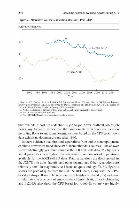
246 Brookings Papers on Economic Activity, Spring 2016
that exhibits a post-1996 decline is job-to-job flows. Without job-to-job flows, my figure 1 shows that the components of worker reallocation involving flows to and from nonemployment based on the CPS gross flows data exhibit no downward trend after 1990.
Is there evidence that hires and separations from and to nonemployment exhibit a downward trend since 1990 from other data sources? The answer is overwhelmingly yes. One source is the JOLTS+BED data. My figures 3 and 4 present evidence about the alternative components of separations available for the JOLTS+BED data. Total separations are decomposed in the JOLTS into quits, layoffs, and other separations. Other separations are relatively small in magnitude, so I focus on quits and layoffs. My figure 3 shows the pace of quits from the JOLTS+BED data, along with the CPS-based job-to-job flows. The series are very highly correlated (.95) and have similar rates (as a percent of employment). Henry Hyatt, Erika McEntarfer, and I (2015) also show the CPS-based job-to-job flows are very highly
Figure 2. Alternative Worker Reallocation Measures, 1990–2015a
Sources: U.S. Bureau of Labor Statistics, Job Openings and Labor Turnover Survey (JOLTS) and Business Employment Dynamics (BED), as integrated by Davis, Faberman, and Haltiwanger (2012); U.S. Bureau of Labor Statistics, Current Population Survey (CPS) gross flows.
a. Worker reallocation is the sum of total hires and separations as a percent of employment. b. The CPS covers the entire economy. c. The JOLTS+BED data cover the private, nonfarm sector.
Percent of employed
CPS gross flowsc
JOLTS+BEDb
35
40
30
25
1992 1994 1996 1998 2000 2002 2004 2006 2008 2010 2012 2014Year

COMMENTS and DISCUSSION 247
correlated with the new LEHD-based job-to-job flows (correlation of .96). Three inferences emerge. First, the CPS-based job-to-job flows have prop-erties that match alternative administrative data of the same concept. Sec-ond, the quits measure from the JOLTS+BED data is a first approximation of a proxy for job-to-job flows. This implies that the layoffs measure from the JOLTS+BED data is a proxy for separations to nonemployment. Third, all the alternative sources of job-to-job flows show a pronounced down-ward trend during the post-2000 period.
My figure 4 shows the CPS gross flows–based measure of separations to nonemployment, the layoffs series from the JOLTS+BED data, and the job destruction series from the BED for the 1990–2015 period. Davis, Faberman, and I (2012) highlight the very tight link between layoffs and job destruction at the quarterly frequency. For current purposes, the primary issue is the relationship between the trends in the three measures in my figure 4. Fitting a simple linear trend from 1990 to 2015 (using quarterly
Figure 3. Quits and Job-to-Job Flows, 1990–2016
Sources: U.S. Bureau of Labor Statistics, Job Openings and Labor Turnover Survey (JOLTS) and Business Employment Dynamics (BED), as integrated by Davis, Faberman, and Haltiwanger (2012); U.S. Bureau of Labor Statistics, Current Population Survey (CPS) gross flows.
a. Quits are from the JOLTS+BED data, which cover the private, nonfarm sector. b. Job-to-job flows are from the CPS, which covers the entire economy.
Percent of employed
Quitsa
Job-to-job flowsb
7
8
6
5
1992 1994 1996 1998 2000 2002 2004 2006 2008 2010 2012 2014Year

248 Brookings Papers on Economic Activity, Spring 2016
data), there is a substantial and statistically significant negative trend in layoffs and job destruction during this period. In contrast, there is no sta-tistically significant trend in the CPS gross flows–based separations to nonemployment over this period. The simple linear trends used here are limited relative to the time series methods used by Molloy, Smith, Trezzi, and Wozniak. But the main point made here is that the CPS gross flows–based measures have different properties than other sources.
The new LEHD job-to-job flows series can be combined with the QWI to generate administrative-based hires from nonemployment and separations to nonemployment, which I refer to as LEHD+QWI. Hyatt, McEntarfer, and I (2015) show these series from 1998:Q2 to 2011:Q4 in that paper’s figure 3. Consistent with my figure 4, the LEHD+QWI–based series show a pronounced downward trend in separations to nonemployment during this period. In addition, the hires from nonemployment from the LEHD+QWI
Figure 4. Job Destruction, Layoffs, and Separations to Nonemployment, 1990–2016
Sources: U.S. Bureau of Labor Statistics, Job Openings and Labor Turnover Survey (JOLTS) and Business Employment Dynamics (BED), as integrated by Davis, Faberman, and Haltiwanger (2012); U.S. Bureau of Labor Statistics, Current Population Survey (CPS) gross flows.
a. Separations to nonemployment are from the CPS, which covers the entire economy. b. Job destruction is from the BED data, which cover the private, nonfarm sector. c. Layoffs are from the JOLTS+BED data, which cover the private, nonfarm sector.
Percent of employed
Layoffsc
Job destructionb
Separations to nonemploymenta
10
12
8
6
1992 1994 1996 1998 2000 2002 2004 2006 2008 2010 2012 2014Year

COMMENTS and DISCUSSION 249
data exhibit a similar downward trend. Fitting a simple linear trend yields a statistically significant negative trend from 1998:Q2 to 2011:Q4 for both series, while the CPS-based series from my figure 1 yields a positive and statistically significant trend during this period.
Taking stock, multiple data sources other than the CPS all show a pronounced and accelerating downward trend in measures of hires from nonemployment and separations to nonemployment during the post-1990 period. The CPS gross flows–based series show no such downward trends. The CPS gross flows are the outlier here. The CPS gross flows are arguably based on data and a methodology that is subject to much more sampling and nonsampling error than the series from other sources. As such, this raises questions about inferences from the CPS gross flows vis-à-vis trends during the post-1990 period. Many of the empirical exercises conducted by Molloy, Smith, Trezzi, and Wozniak rely on samples starting in 1980 or at some point in the 1990s for analyses of the possible sources of the changes in the decline in fluidity. Given that this is the period when the CPS gross flows appear to be anomalous, this raises questions about how to interpret these results. For the measurement community, attention needs to be given to why the CPS gross flows yield such different patterns from the alterna-tive sources of hires from and separations to nonemployment.
Beyond these measurement concerns, a limitation of the principal com-ponent analysis, with its standardization of series and focus on the first principal component, is that it misses patterns in the different components of the flows that have the potential to shed light on the underlying causes of the decline in fluidity. My figure 5 depicts an exact decomposition of total worker reallocation into job reallocation and churning that has been actively used in the literature (Davis, Haltiwanger, and Schuh 1996; Burgess, Lane, and Stevens 2000; Hyatt and Spletzer 2013; Davis and Haltiwanger 2014). Conceptually, these different components of worker reallocation depicted in my figure 5 are potentially driven by quite different forces.
Job reallocation reflects the expansion, contraction, opening, and clos-ing down of establishments. In this respect, variation in job reallocation is inherently linked to models of firm dynamics. Such models characterize firm dynamics resulting from the interaction of the evolution of the distri-bution of idiosyncratic, firm-level shocks and the responses of firms to such shocks. The latter reflect potential frictions and distortions not only in labor markets but also in capital adjustment, product markets, and credit markets. The impact of globalization and information technology on how firms are organized internally potentially plays a role in these firm dynamics and is the subject of active research in the firm dynamics literature (Decker and
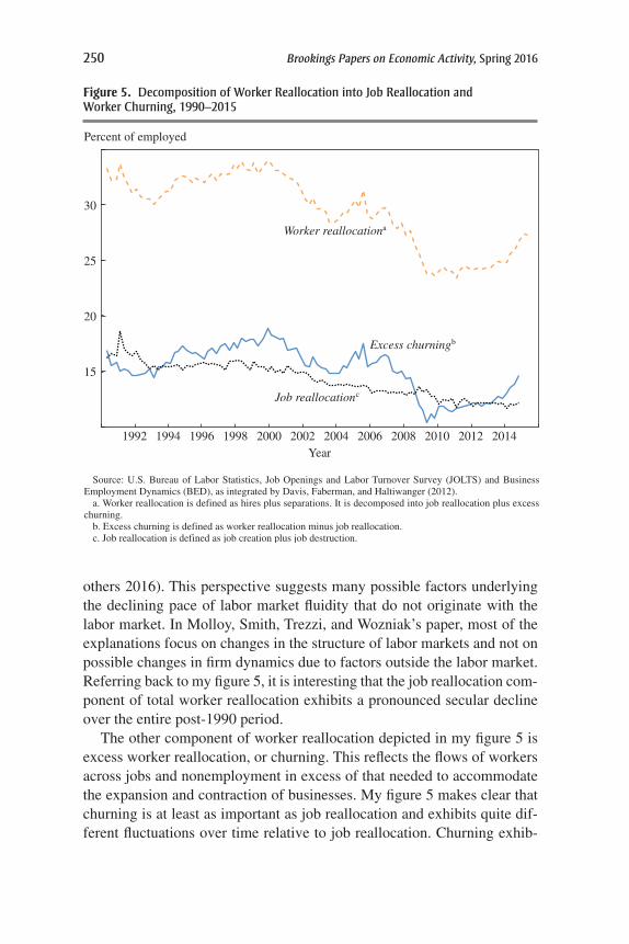
250 Brookings Papers on Economic Activity, Spring 2016
others 2016). This perspective suggests many possible factors underlying the declining pace of labor market fluidity that do not originate with the labor market. In Molloy, Smith, Trezzi, and Wozniak’s paper, most of the explanations focus on changes in the structure of labor markets and not on possible changes in firm dynamics due to factors outside the labor market. Referring back to my figure 5, it is interesting that the job reallocation com-ponent of total worker reallocation exhibits a pronounced secular decline over the entire post-1990 period.
The other component of worker reallocation depicted in my figure 5 is excess worker reallocation, or churning. This reflects the flows of workers across jobs and nonemployment in excess of that needed to accommodate the expansion and contraction of businesses. My figure 5 makes clear that churning is at least as important as job reallocation and exhibits quite dif-ferent fluctuations over time relative to job reallocation. Churning exhib-
Figure 5. Decomposition of Worker Reallocation into Job Reallocation and Worker Churning, 1990–2015
Source: U.S. Bureau of Labor Statistics, Job Openings and Labor Turnover Survey (JOLTS) and Business Employment Dynamics (BED), as integrated by Davis, Faberman, and Haltiwanger (2012).
a. Worker reallocation is defined as hires plus separations. It is decomposed into job reallocation plus excess churning.
b. Excess churning is defined as worker reallocation minus job reallocation.c. Job reallocation is defined as job creation plus job destruction.
Percent of employed
25
30
20
15
1992 1994 1996 1998 2000 2002 2004 2006 2008 2010 2012 2014Year
Worker reallocationa
Job reallocationc
Excess churningb

COMMENTS and DISCUSSION 251
its cyclical fluctuations throughout the 1990s, but it then declines sharply after the 2001 recession and does not recover. It declines further during the Great Recession and again does not recover. The pattern of decline for churning is quite different from job reallocation.
Changing frictions in the labor market (for example, regulations and flexibility of wages) are likely to influence both the job reallocation and churning components of worker reallocation. However, as discussed above, job reallocation is likely to reflect many factors above and beyond frictions in the labor market. Though my figure 5 yields no immediate inferences about these possible alternative factors, the different patterns across these different components suggest that this decomposition is likely to be useful for future research.
Even with the measurement and conceptual issues raised above, I think this paper by Molloy, Smith, Trezzi, and Wozniak makes a valuable con-tribution to the literature with the articulation, investigation, and summary of what we know so far about a number of interesting hypotheses. From their approach and perspective, they confirm what others have found in terms of the declining labor market fluidity not being driven simply by a changing composition of firms and workers in observable characteristics. In addition, they usefully investigate a number of possible benign and less benign factors that may underlie the decline in labor market fluidity. For example, they explore, in a similar manner to Hyatt and Spletzer (2013), the hypothesis that the decline in fluidity might reflect improved matching in the labor market. This would be a benign factor that might reflect, for example, improved information in the labor market, given the information technology revolution. They find little evidence to support this hypothe-sis. Although I am sympathetic to this conclusion, this inference is mostly based on exploiting aggregate time series variation in the starting wages for new workers. Many omitted factors may be changing at the aggregate level, such as productivity and the relationship between productivity and wages (an interesting topic in and of itself). Molloy, Smith, Trezzi, and Wozniak recognize these limitations, but this situation highlights the iden-tification challenges that are present in this literature.
To conclude, the final section of Molloy, Smith, Trezzi, and Wozniak’s paper has a very useful discussion and summary of directions for future research. Pursuing these topics should have a high priority. As the authors and the recent literature highlight, benign factors may underlie at least some components (or sectors) of the decline in fluidity. However, there is accumulating evidence in this study and the recent literature that there are likely adverse implications for workers. Moreover, there is also much need
252 Brookings Papers on Economic Activity, Spring 2016
for further investigation into the productivity effects of reduced fluidity. An open and interesting question is whether the anemic performance of U.S. productivity growth in the post-2000 period is linked to the decline in fluidity.
REFERENCES FOR THE HALTIWANGER COMMENT
Burgess, Simon, Julia Lane, and David Stevens. 2000. “Job Flows, Worker Flows, and Churning.” Journal of Labor Economics 18, no. 3: 473–502.
Davis, Steven J., R. Jason Faberman, and John Haltiwanger. 2012. “Labor Market Flows in the Cross Section and over Time.” Journal of Monetary Economics 59, no. 1: 1–18.
Davis, Steven J., and John Haltiwanger. 2014. “Labor Market Fluidity and Economic Performance.” In Economic Policy Symposium Proceedings: Re-Evaluating Labor Market Dynamics. Jackson Hole, Wyo.: Federal Reserve Bank of Kansas City.
Davis, Steven J., John C. Haltiwanger, and Scott Schuh. 1996. Job Creation and Destruction. MIT Press.
Decker, Ryan, John Haltiwanger, Ron Jarmin, and Javier Miranda. 2016. “Chang-ing Business Dynamism: Volatility of Shocks vs. Responsiveness to Shocks?” Working paper. http://www.rdecker.net/research
Fallick, Bruce, and Charles A. Fleischman. 2004. “Employer-to-Employer Flows in the U.S. Labor Market: The Complete Picture of Gross Worker Flows.” Finance and Economics Discussion Series no. 2004-34. Washington: Board of Governors of the Federal Reserve System.
Haltiwanger, John, Henry Hyatt, and Erika McEntarfer. 2015. “Cyclical Reallo-cation of Workers across Employers by Firm Size and Firm Wage.” Working Paper no. 21235. Cambridge, Mass.: National Bureau of Economic Research.
Hyatt, Henry R., and James R. Spletzer. 2013. “The Recent Decline in Employ-ment Dynamics.” IZA Journal of Labor Economics 2: article 5.
GENERAL DISCUSSION Robert Hall spoke first about what he believed to be one of the most important components of labor market flu-idity: the prevalence of extremely short-term jobs, which is a topic studied extensively by Henry Hyatt and James Spletzer. In his own recent work, Hall noted that by observing the distribution of the number of W-2s filed by year across workers, one can observe a decline in the number of work-ers who file many W-2s in a single year—that is, in the number who hold multiple short-term jobs in a single year. This trend in very short-term job losses is likely an important component of the decline in labor market flu-
COMMENTS and DISCUSSION 253
idity. And Hall commended the present paper for not focusing exclusively on month-to-month changes, as many authors have.
The main story of the paper, Hall asserted, was the big decline in match-ing efficiency in unemployment. A natural question to ask is: If it has become harder and harder to match workers, why is unemployment not rising? The answer, according to Hall, is that entry rates to employment are declining along very much the same trend, and the result is that they exactly offset each other. Unemployment today is exactly the same as it was in 1948, despite matching efficiency being much lower, something he called “an amazing fact.”
Hall agreed with discussant John Haltiwanger that the role of large employers in reducing turnover, rationalizing the labor market, and inci-dentally reducing fluidity is a good thing. Lower labor market fluidity implies lower job turnover, and large employers are able to achieve lower turnover because they have many tools and are efficient at managing it. “Fluidity is a bad thing,” he said, “so it is a good thing to reduce it.” He concluded that declining job turnover—now interestingly labeled declining labor market fluidity—is very much a fact. The Bureau of Labor Statistics, for instance, has published turnover rates from the Current Population Sur-vey (CPS) all the way back to 1948, and tabulations support the notion that labor market fluidity has been declining for a long time.
Richard Cooper proposed that two changes in the character of the labor force might explain the trends in declining labor market fluidity, and won-dered if they might be quantitatively important. The first related to service in the armed forces, which he noted has been a big source of job mobility in the United States over the years. He listed a number of factors related to service in the armed forces that might be relevant, including service mem-bers’ frequent changing of geographic location and their training in certain skills, as well as the fact that the size of the armed forces has fluctuated considerably over time, particularly after the end of the draft in the 1970s. Second, Cooper wondered how the issue of immigration was treated. He noted that there have been big changes in both the number of immigrants and the treatment of immigrants, in particular the legalizing of a large num-ber of formerly undocumented immigrants. Might these features have any influence on the authors’ findings?
Robert Moffitt encouraged the authors to look around in the literature to see what it says on turnover at longer durations than a quarterly or annual period. As an algebraic matter, one could have declining transition rates in short durations and increasing exit rates at somewhat longer durations, and

254 Brookings Papers on Economic Activity, Spring 2016
that would be something interesting to know. He suggested that the decline in job-to-job flows might be explained using a Jovanovic-style learning model, in which both parties form a match, but it takes a while for them to each learn whether it is a good match or not.1 In addition, he noted that there appears to be some very casual evidence that the amount of uncer-tainty employers have about whether a match is good or not does not rely as heavily as it once did on the usual indicators, such as education, age, and past employment history. Thus, it might take a while longer for employers to learn whether a match is good or not.
However, Moffitt argued that the job-to-job flow component is more important than the not-in-the-labor-force component. He recalled a paper presented at the Fall 1991 Brookings Papers meeting in which Kevin Murphy and Robert Topel documented an increase in the length of time that less educated men were spending completely out of the labor force and simply not working for an extended period.2 Consequently, this leads to fewer entrants into unemployment. He noted that there was an observable decline in labor force participation starting in about 2000, during which both men and women began spending more and lengthier times completely out of the labor force. Perhaps this fact could shed a somewhat different light on how to interpret turnover in the labor market.
Matthew Shapiro wondered if the authors’ analysis could shed light on whether the trend of increasing occupational regulation and licensing is an important factor when it comes to job-to-job flows. He noted that it might be interesting to know whether the decline in labor market fluidity is within industry or between industry, or similarly with occupation. He believed the question could be addressed using the authors’ framework, and that it might point to one of their hypotheses.
David Romer had two brief comments. First, he suggested that it might be useful for the authors to calibrate their analysis against other countries, such as those in Europe. He recalled from a Fall 2011 paper by Michael Elsby, Bart Hobijn, Aysegül Sahin, and Robert Valletta that at the height of the Great Recession, the job-finding rate for long-term unemployed work-ers in the United States was higher than for unemployed workers in France
1. See for example, Boyan Jovanovic and Yaw Nyarko, “A Bayesian Learning Model Fitted to a Variety of Empirical Learning Curves,” Brookings Papers on Economic Activity: Microeconomics, 1995: 247–99.
2. Chinhui Juhn, Kevin M. Murphy, and Robert H. Topel, “Why Has the Natural Rate of Unemployment Increased over Time?” Brookings Papers on Economic Activity, no. 2 (1991): 75–126.

COMMENTS and DISCUSSION 255
under normal times.3 This comparison suggests that despite the recent declines in fluidity, the U.S. labor market remains extremely dynamic rela-tive to those of other countries and is very far from exhibiting sclerosis. Second, Romer wondered about the issue of the job market becoming more formal or litigious. He thought that the small amount of evidence the paper provides on this issue is interesting but far from definitive, and that casual empiricism suggests that increased litigiousness might be a nontrivial fac-tor in declining fluidity. As an example, he recalled a conversation he had with a lawyer who represents firms in employment litigation; the lawyer reported that, in California, if an employer fires someone without good cause, the employer would almost certainly be sued.
Valerie Ramey wondered if one possible explanation for the longer-term decline in labor market fluidity was the rise of two-career couples, to the extent that there is now a joint location problem for many people. She suggested that this might explain the decrease in geographic mobility that one sees in the data, along with the decreasing fluidity. In her own work, Ramey had noticed a decline in the marital wage premium for men, which would be consistent with people being stuck in their same jobs because of the joint location problem.
Karen Dynan wondered if the authors could say more about the hous-ing market and its relationship to labor market fluidity. She noted that at least one of the authors (Raven Molloy) is an expert on the housing mar-ket, so she suspected that they had probably thought a lot about it. Dynan recalled that in the paper, the authors mentioned having looked at land use regulations, but that they did not find much evidence of a connection to declining labor market fluidity. She noted that land use regulation is an incomplete measure of the elasticity of housing supply, and wondered if the authors had looked at more direct measures. She suggested that the level of home prices might be a more direct indicator of the frictions associated with moving; the higher the level, the more costly it would be to move. Additionally, higher home prices might mean that homeowners have more wealth tied up in housing, which would explain the relationship to the pro-pensity to start new businesses.
Gabriel Chodorow-Reich mentioned some joint work with Johannes Wieland in which he and Wieland play with a model that has both worker
3. Michael W. L. Elsby, Bart Hobijn, Aysegül Sahin, and Robert G. Valletta, “The Labor Market in the Great Recession—An Update to September 2011,” Brookings Papers on Eco-nomic Activity, Fall 2011: 353–71.

256 Brookings Papers on Economic Activity, Spring 2016
shocks and job shocks.4 In a frictional labor market, it is easier to accom-modate job shocks that shift the distribution of labor demand across firms or across industries without increasing aggregate unemployment if gross worker flows are higher. This interaction between changes in the distri-bution of labor demand and worker fluidity, Chodorow-Reich concluded, suggests that more weight might need to be put on the less benign interpre-tation of the decline in worker flows.
Discussant Erica Groshen had suggested that the authors consider shorter-duration series, since much of the “light” on the causality from job flows to workers flows will probably be found there. Abigail Wozniak responded with a reminder of what the authors believed they were accom-plishing in the paper: They felt it was important to go back as far as pos-sible in order to get a handle on the underlying, long-term factors of labor market fluidity. She agreed with Groshen that much of the “light” is in fact with the shorter-duration series, but that the present analysis seeks to accomplish something different. In response to a question raised by mod-erator James Stock about the seemingly small role of demographics in their analysis, Wozniak explained that one of the helpful pieces of their approach was the ruling out of the demographics story a bit, so that when they did turn to shorter-duration series—which do not have detailed demographics attached to them—the authors could go forward with confidence.
In response to a point made by Haltiwanger about the CPS and what it shows, Wozniak noted that this was not the first time the authors had run into questions about how the CPS measures job transition. She noted that when it comes to migration declines, the CPS actually shows more pro-nounced declines than other series, like the American Community Survey, during the same period. Wozniak added that there are probably really impor-tant questions about how the CPS picks up job transitions, and whether that technique is changing over time. Nonetheless, she concluded that it would probably not change much about the paper’s overall story.
Adding on to comments made about the length of the series, Raven Molloy noted that the authors began by trying to think about whether there was a single explanation for the entire 30- to 35-year period; when a decline is observed over such a long period, it is natural to start by ask-ing if there is one thing that can explain the entire decline. She agreed that there are probably many things going on, and different explanations could
4. Gabriel Chodorow-Reich and Johannes Wieland, “Secular Labor Reallocation and Business Cycles,” Working Paper no. 21864 (Cambridge, Mass.: National Bureau of Eco-nomic Research, 2016).

COMMENTS and DISCUSSION 257
be more important for some periods than others, but given that the decline looks pretty steady for the entire period, perhaps there was an explanation that made sense for the entire period. Similarly, the authors thought it was natural to try to find an explanation that could make sense for an entire set of different types of workers and industries. Although it is true that there is interesting variation across different types of workers and industries, it is still the case that declines are observed for many different types of workers and industries, which again suggests that some broad-based explanation might be affecting all workers and industries.
On the question of housing, brought up by Dynan, Molloy stated that it was something the authors had thought a lot about, and she would have loved to have found an explanation for the declines in labor market fluid-ity related to the housing market. In the end, Molloy could not convince herself that there was a housing story, partly because many declines in job transitions are observed within geographic labor markets. The authors tried to look at job-to-job flows for people who stay within the same state or stay within the same metropolitan area, and they observed that there are also big declines in labor market fluidity in those flows. It is hard to reconcile why there is such a big decline observed in migration rates for these types of people, and even to a greater extent in other kinds of job transitions as well. And in response to a question posed by Ramey, Molloy added that the same thing is true of two-career couples. The authors spent a lot of time in another paper they wrote trying to see if these kinds of explanations could apply to the long-run decline in migration, and again could not really find much evidence. This is partly because the increase in two-career couples was just much too small by the measures that the authors could find in the CPS to really explain much of the decline in migration, and partly because, again, it was a more broad-based phenomenon; there are lots of declines in migration and labor market flows for people who are not married, for example.
Christopher Smith responded to some of the questions related to the data. During her remarks, Groshen had suggested that perhaps when the authors were thinking about explanations, they should think about what explanations have implications for which measures of fluidity, and that there were some other questions about how declines in labor force par-ticipation might tie into some of these flows. Smith noted that the authors actually mention this in the paper, and it turns out that when one looks at some of the labor market flows individually, one sees declines that seem as if they are related to the secular declines in participation for particu-lar demographic groups. In particular, the job-finding rates for younger

258 Brookings Papers on Economic Activity, Spring 2016
workers and for prime-aged men have both been declining since the mid-1980s, which lines up with their secular declines in participation. On the other hand, the job separation rate for prime-aged women has been falling over this period, which also reflects the rise in participation. When looking at any one measure in isolation, Smith noted, there are going to be idiosyn-cratic factors or things related to, say, secular declines in participation that might affect that particular measure. But the goal of the paper, he insisted, was to look at a variety of measures in hopes of finding common factors that were running under all of them.
On the question of what the CPS shows about job-to-job transitions since its major redesign in 1994, Smith noted that one can in fact con-struct a measure using the CPS, referring to it as the Fallick–Fleischman measure.5 One question in the CPS asks whether you were working for the same employer in the previous month or not, which has been the industry-standard measure for estimating job-to-job transitions from one month to the next. Smith believed that one of the innovations of the present paper was that the authors in a way extend something that looks like that series backward by considering a question from the March CPS that asks respon-dents about the number of employers where they have worked in the last year, which could also be considered a measure of job-to-job transitions; this trend, he noted, looks virtually identical to the more traditional mea-sures. Extending this series back, one interesting thing that pops out is that from this longer measure of job-to-job transitions, it is pretty much flat until the mid-1990s, which is when the decline begins to be observed. The traditional measure, on the other hand, would not necessarily pick up this clear flatness followed by the decline.
Riccardo Trezzi added a few final points about the authors’ time series analysis. Regarding concerns raised about the authors’ specific data set and trending methods, Trezzi noted that the paper does contain some robustness checks, in the sense that the biweight filter is not the only filter used in the analysis; the authors also check their results using the Christiano–Fitzgerald band pass filter6 and the Müller–Watson cosine projection method.7 Finally,
5. See for example, Bruce Fallick and Charles A. Fleischman, “Employer-to-Employer Flows in the U.S. Labor Market: The Complete Picture of Gross Worker Flows,” Finance and Economics Discussion Series no. 2004-34 (Washington: Board of Governors of the Federal Reserve System, 2004).
6. Lawrence J. Christiano and Terry J. Fitzgerald, “The Band Pass Filter,” International Economic Review 44, no. 2 (2003): 435–65.
7. Ulrich K. Müller and Mark W. Watson, “Low-Frequency Econometrics,” Working Paper no. 21564 (Cambridge, Mass.: National Bureau of Economic Research, 2015).

COMMENTS and DISCUSSION 259
Trezzi added that the reason the authors chose the particular analysis period was that they wanted to get at underlying trends, and did not want to pick up business cycle movements. In order to do this, one has to work on the low-frequency side of the spectrum—and significantly so— otherwise the analysis will tend to pick up some business cycle move-ments, especially because the Great Recession is at the end of the sample, which generates additional issues.