Understanding contrasts - University of Edinburgh · Understanding contrasts Dr. Martyn McFarquhar...
53
Understanding contrasts Dr. Martyn McFarquhar Division of Neuroscience & Experimental Psychology The University of Manchester Edinburgh SPM course, 2017 1
Transcript of Understanding contrasts - University of Edinburgh · Understanding contrasts Dr. Martyn McFarquhar...

Understanding contrastsDr. Martyn McFarquhar
Division of Neuroscience & Experimental Psychology The University of Manchester
Edinburgh SPM course, 20171

What are contrasts?Informally, a contrast is a method of asking a question about your model in mathematical terms
As the parameters represent the relationship between the predictors and the outcome, their estimated values are the part of the model that we are most interested in
The GLM partitions the data into model and error
The model is the typical value of the data for given values of the predictor variables
This is formed via a linear combination of known predictor variables and unknown parameters
Y = X�|{z}model
+ ✏|{z}error
2
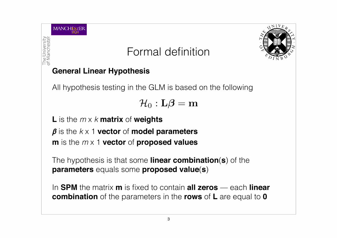
General Linear Hypothesis
Formal definition
H0 : L� = m
In SPM the matrix m is fixed to contain all zeros — each linear combination of the parameters in the rows of L are equal to 0
All hypothesis testing in the GLM is based on the following
L is the m x k matrix of weights𝞫 is the k x 1 vector of model parametersm is the m x 1 vector of proposed values
The hypothesis is that some linear combination(s) of the parameters equals some proposed value(s)
3

H0 :⇥1 0
⇤ �1
�2
�= 0
H0 :
1 00 1
� �1
�2
�=
00
�
H0 :⇥1 �1
⇤ �1
�2
�= 0
H0 :⇥12
12
⇤ �1
�2
�= 0
General Linear Hypothesis
Formal definition
H0 : L� = m
This is a very flexible system
All hypothesis testing in the GLM is based on the following
β1 is equal to 0
β1 or β2 is equal to 0
the difference between β1 and β2 is 0
the average of β1 and β2 is 0
4

Parameters and interpretationAs contrasts are linear combinations of parameters, their interpretation depends on understanding the parameters
1st-level
0 50 100 150-2
-1
0
1
2
3
4
5
0 50 100 150-2
-1
0
1
2
3
4
5
The parameters scale the predicted shape of the response to best fit the data
Their values tell us about the magnitude and direction of the average change from baseline in each experimental condition
Estimation
5

Parameters and interpretation
2nd-levelIndicator variables
• Contain only 1 or 0 to model a factor • Parameters are cell means
Continuous covariates • Contain any value within a range • Parameters are regression slopes
Comparing cell means is sensible, but comparing regression slopes only makes sense if the predictors are scaled identically
μ1 μ2 β0 β1 β2
As contrasts are linear combinations of parameters, their interpretation depends on understanding the parameters
6

Parameters and interpretation
outcome
predictor1
predictor 2
outcome
predictor 2
Effect of predictor 1
VS
For multiple predictor variables, tests on each parameter is interpreted as testing the unique variability explained after adjusting for all other variables
7

predictor 2
outcome
predictor1
Parameters and interpretation
Effect of predictor 2
VSpredictor
1
outcome
For multiple predictor variables, tests on each parameter is interpreted as testing the unique variability explained after adjusting for all other variables
8

Parameters and interpretationFor multiple predictor variables, tests on each parameter is interpreted as testing the unique variability explained after adjusting for all other variables
For contrasts, this means that even if a parameter is given a weight of 0, the other parameters are still adjusted for its presence
L =⇥1 0 0
⇤
ANCOVA
The individual cell means are still adjusted for the covariate
The value of the parameter estimates depends on other variables in the model
Contrasts ask questions about the model — they do not alter the model
9

Parameters and interpretationParameters are estimated using
� = (X0X)�1X0Y
Important consequences 1. The estimates depend on the scaling of the columns of X2. If X is rank deficient (contains redundant columns) then there
are an infinite number of solutions
If X is rank deficient then (XʹX)-1 does not exist
Notice that this depends on the design matrix
We can still find a solution using a pseudo-inverse — creates complications in specifying and interpreting contrasts
10

Estimable functions
L = TX
An estimable contrast is also one that can be expressed as a linear combination of the model estimates
An L matrix defines an estimable function of the model parameters if it can be expressed as
Our contrast is only meaningful if it is formed from a linear combination of the rows of the design matrix
c = L�
= TX�
= TY
The model estimates dictate how meaningful values are formed from combining the predictors and the parameters
A question is only meaningful if it respects this combination
11
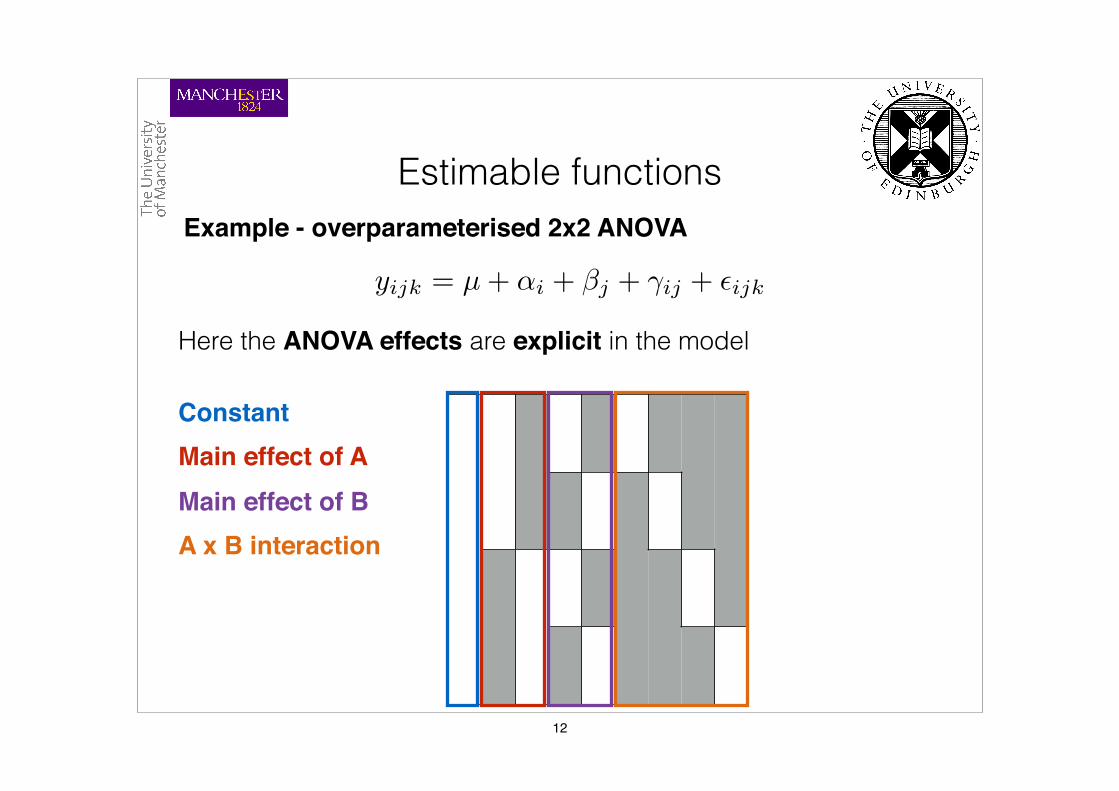
Estimable functionsExample - overparameterised 2x2 ANOVA
ConstantMain effect of AMain effect of BA x B interaction
Here the ANOVA effects are explicit in the model
yijk = µ+ ↵i + �j + �ij + ✏ijk
12
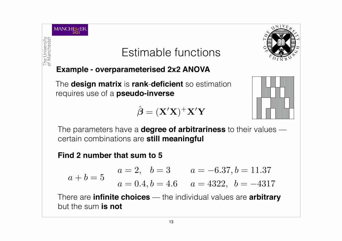
Estimable functionsExample - overparameterised 2x2 ANOVA
The design matrix is rank-deficient so estimation requires use of a pseudo-inverse
� = (X0X)+X0Y
The parameters have a degree of arbitrariness to their values — certain combinations are still meaningful
Find 2 number that sum to 5
There are infinite choices — the individual values are arbitrary but the sum is not
a+ b = 5a = 2, b = 3
a = 0.4, b = 4.6
a = �6.37, b = 11.37
a = 4322, b = �4317
13

Estimable functionsExample - overparameterised 2x2 ANOVA
Contrasts must respect the meaningful combinations of parameters given by the rows of X
Main effect of A?
L =⇥0 1 �1 0 0 0 0 0 0
⇤
LA1B1 =⇥1 1 0 1 0 1 0 0 0
⇤
LA1B2 =⇥1 1 0 0 1 0 1 0 0
⇤
LA2B1 =⇥1 0 1 1 0 0 0 1 0
⇤
LA2B2 =⇥1 0 1 0 1 0 0 0 1
⇤
LA1 =⇥1 1 0 0.5 0.5 0.5 0.5 0 0
⇤
LA2 =⇥1 0 1 0.5 0.5 0 0 0.5 0.5
⇤
LA1�A2 =⇥0 1 �1 0 0 0.5 0.5 �0.5 �0.5
⇤
}
Correct main effect of A
}
❌
✔
14

Estimable functionsEstimable functions in SPM
Non-estimable parameters are indicated by a grey box below the associated column
15

Estimable functionsEstimable functions in SPM
To make sure that the contrast we are testing is estimable, SPM will perform an estimability test
This ensures that we are testing combinations that do not depend on the solution for the parameters (see McFarquhar, 2016)
16
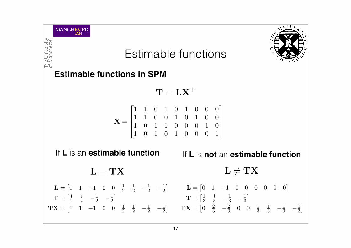
Estimable functionsEstimable functions in SPM
T = LX+
If L is an estimable function
L = TX
If L is not an estimable function
L 6= TX
L =⇥0 1 �1 0 0 0 0 0 0
⇤
T =⇥13
13 � 1
3 � 13
⇤
TX =⇥0 2
3 � 23 0 0 1
313 � 1
3 � 13
⇤
L =⇥0 1 �1 0 0 1
212 � 1
2 � 12
⇤
T =⇥12
12 � 1
2 � 12
⇤
TX =⇥0 1 �1 0 0 1
212 � 1
2 � 12
⇤
X =
2
664
1 1 0 1 0 1 0 0 01 1 0 0 1 0 1 0 01 0 1 1 0 0 0 1 01 0 1 0 1 0 0 0 1
3
775
17

Contrast interpretationMost of the time we work with well parameterised models and so do not have to worry about estimability — check the grey boxes!
Despite this, a contrast can be estimable but misinterpreted
This largely comes down to 1. Understanding what the parameters mean 2. Making sure that the contrast is testing what you think it is
You should always ensure that you are clear how to interpret the parameters and contrasts from your model
How can you know what your results mean of you don’t understand what the model is telling you, or what your questions are?
18

Contrast interpretation1st-level example — baselines
Model 1(A, B, rest, const.)
Model 2(A, B, const.)
LA�B =⇥1 �1 0
⇤
LA�R =⇥1 0 0
⇤
LB�R =⇥0 1 0
⇤
LA =⇥1 0 1
⇤
LB =⇥0 1 1
⇤
LA�B =⇥1 �1 0 0
⇤
LA�R =⇥1 0 �1 0
⇤
LB�R =⇥0 1 �1 0
⇤
LA =⇥1 0 0 1
⇤
LB =⇥0 1 0 1
⇤
An explicit baseline over an implicit baseline alters the interpretation of the parameters and the contrasts
19

Contrast interpretation2nd-level example — t-test
Model 1(A, B, const.)
Model 2(A, const.)
Model 3(A, B)
LA�B =⇥1 �1 0
⇤
LA =⇥1 0 1
⇤
LB =⇥0 1 1
⇤
Lmean =⇥0.5 0.5 1
⇤
LA�B =⇥1 0
⇤
LA =⇥1 1
⇤
LB =⇥0 1
⇤
Lmean =⇥0.5 1
⇤
LA�B =⇥1 �1
⇤
LA =⇥1 0
⇤
LB =⇥0 1
⇤
Lmean =⇥0.5 0.5
⇤
Different parameterisations lead to the same predicted values, but change the meaning of the parameters
Need to be clear on what the parameters mean in order to correctly interpret a contrast
20

Test statisticsAssuming our contrast is estimable and we are clear on what it means we can test the estimated value against a proposed population value by forming a test statistic
In SPM we have two options for how to test our contrast value — as a t-contrast or an F-contrast
Each type is used in different contexts and it is important to understand their differences, and similarities, to ensure you use the most appropriate method for your questions
21

t-contrastsIn SPM a t-contrast is defined by
• An L matrix with a single row • Hypothesis testing using a t-statistic • One-tailed p-values
t =L� �m
�p
L(X0X)�1L0
Notice that L appears in the numerator and denominator — scaling of L does not matter
All lead to the same t-statistic:
L =⇥1 �1
⇤L =
⇥2 �2
⇤L =
⇥1000 �1000
⇤
22

t-contrastsIn SPM a t-contrast is defined by
• An L matrix with a single row • Hypothesis testing using a t-statistic • One-tailed p-values
The p-values are upper-tail values — you will only see results for positive t-statistics
-3 -2 -1 0 1 2 3
0.0
0.1
0.2
0.3
0.4
Normal Distribution: Mean=0, Standard deviation=1
x
Density
-3-2-10123
0.0
0.1
0.2
0.3
0.4
Normal Distribution: Mean=0, Standard deviation=1
x
Density
0-1.24 1.24
Upper-tail p for -1.24 = 0.920
23

t-contrastsIn SPM a t-contrast is defined by
• An L matrix with a single row • Hypothesis testing using a t-statistic • One-tailed p-values
The p-values are upper-tail values — you will only see results for positive t-statistics
-3 -2 -1 0 1 2 3
0.0
0.1
0.2
0.3
0.4
Normal Distribution: Mean=0, Standard deviation=1
x
Density
-3-2-10123
0.0
0.1
0.2
0.3
0.4
Normal Distribution: Mean=0, Standard deviation=1
x
Density
0-1.24 1.24
Upper-tail p for 1.24 = 0.08
Upper-tail p for -1.24 = 0.920
24

t-contrastsIn SPM a t-contrast is defined by
• An L matrix with a single row • Hypothesis testing using a t-statistic • One-tailed p-values
The p-values are upper-tail values — you will only see results for positive t-statistics
A positive t-statistic occurs when the direction of the effect matches the direction of the contrast
L =⇥�1 0
⇤Only see positive effectsOnly see negative effects
One-tailed p-values only suitable for strong directional hypotheses
L =⇥
1 0⇤
25

In SPM a F-contrast is defined by • An L matrix with multiple rows • Hypothesis testing using an F-statistic • Two-tailed p-values
F-contrasts
An F-contrast with a single row is the same as t2 — in SPM this allows for a two-tailed alternative to a t-contrast
The numerator forms a sum-of-squares — divided by r to form a mean square
Multiple rows can be thought of as an OR question
F =(L� �m)0(L(X0X)�1L0)�1(L� �m)
r�2
26

F-contrastsSimple example: 1-way ANOVA with a 3-level factor
L =
1 �1 00 1 �1
�
The weights for an F-contrast testing the main effect of the factor are:
L =
2
41 �1 00 1 �11 0 �1
3
5
Should it not be?Does this seem odd at all?
27

L =
2
41 �1 00 1 �11 0 �1
3
5
F-contrastsSimple example: 1-way ANOVA with a 3-level factor
Should it not be?
This last row is the sum of the other rows — value from this row is not independent of the other rows
� =
2
4101512
3
5 L� =
2
4�53
�2
3
5
The last row provides no more information — connection with numerator degrees of freedom
This row is redundant
(�5) + 3 = �2
28
Do the weights have to sum to zero?
A potential source of confusion relates to wether the weights of the contrast must sum to zero
Distinction between a linear combination and a contrast: • A contrast is specifically about comparing parameters • A linear combination is more general e.g. averaging,
summing etc.
In SPM the term contrast is used generically for either
In the statistics literature a contrast has the additional requirement that the weights sum to zero — not necessary for a linear combination
29

Do the weights have to sum to zero?
H0 : �1 � �2 = 0
L =⇥1 �1
⇤
L =⇥2 �2
⇤ L =⇥1 �2
⇤✔✔
❌
H0 : (�1 + �2)/2� �3 = 0
L =⇥0.5 0.5 �1
⇤L =
⇥1 1 �1
⇤L =
⇥1 1 �2
⇤ ✔
✔❌
Xli = 0
Xli = 0
Xli = �1
Xli = 0
Xli = 0
Xli = 1
In both cases we are looking at differences of parameters — these are true contrasts
30

The alternative is when we look at individual parameters or averages of parameters
If the parameters are estimable then these are all valid
Interpretation must be done with care — depends on how the model is parameterised (e.g. implicit vs explicit baselines)
Do the weights have to sum to zero?
H0 : �1 = 0
L =⇥1 0
⇤ Xli = 1 ✔
L =⇥0.5 0.5
⇤L =
⇥1 1
⇤Xli = 1
Xli = 2✔ ✔
H0 : (�1 + �2)/2 = 0
31

SPM defaults to a cell means ANOVA rather than an overparameterised ANOVA — no need to worry about estimability
Basic contrasts in ANOVA modelsOften, it is the group-level where our hypotheses are focussed
Typically, data collected from factorial designs will be analysed using an ANalysis Of VAriance model
For designs with >2 factors, the ANOVA model has a number of effects that we may be interested in — main effects, interactions, simple effects
Important to understand how these are tested using contrasts
32

Basic contrasts in ANOVA models
Factor A
1 2
Factor B1 μ11 μ21 μ.1
2 μ12 μ22 μ.2
μ1. μ2.
Cell means are the means from the intersection of the factors and the marginal means are the means from across a factor
2 x 2 ANOVA
Cell means
Marginal means for Factor A
Marginal means for Factor B
The dot notation indicates a subscript averaged over
33

Basic contrasts in ANOVA models2 x 2 ANOVA
yijk = µij + ✏ijk
The simplest model is the cell means model
Here the parameters are the cell means of design
The ANOVA effects are then formed using contrasts of the cell means
L =⇥1 1 �1 �1
⇤
L =⇥1 �1 1 �1
⇤
L =⇥1 �1 �1 1
⇤
Main effect of A
Main effect of B
A x B interaction
34

Basic contrasts in ANOVA models2 x 2 ANOVA
We are looking for a difference of two differences
A⇥ B = (A1B1�A2B1)� (A1B2�A2B2)
Effect of A at the first level of B
Effect of A at the second level of B
The interaction contrast
35

A⇥ B = (µ11 � µ21)� (µ12 � µ22)
Basic contrasts in ANOVA models2 x 2 ANOVA
We are looking for a difference of two differences
The interaction contrast
µ11 µ21 µ12 µ22
36

A⇥ B = (µ11 � µ21)� (µ12 � µ22)
Basic contrasts in ANOVA models2 x 2 ANOVA
We are looking for a difference of two differences
The interaction contrast
µ11 µ21 µ12 µ22
1 �1 0 00 0 1 �1
L =⇥1 �1 �1 1
⇤
The weights for the interaction come from subtracting the weights for the simple effects
37
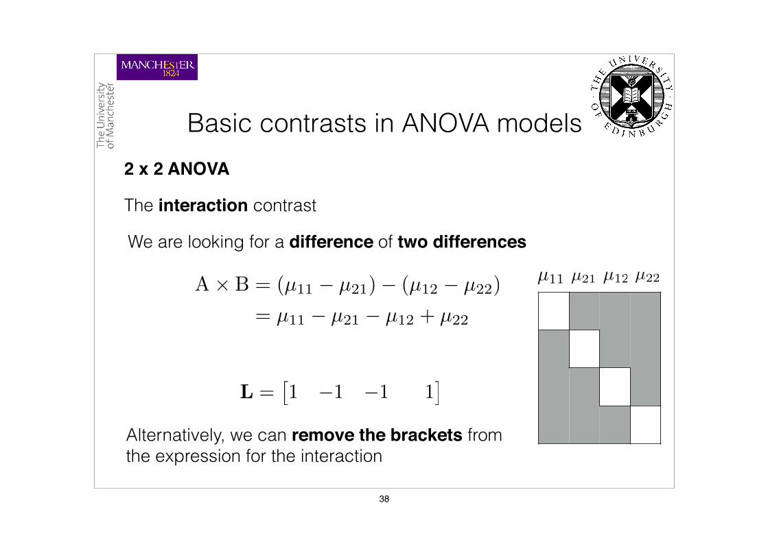
A⇥ B = (µ11 � µ21)� (µ12 � µ22)
= µ11 � µ21 � µ12 + µ22
Basic contrasts in ANOVA models2 x 2 ANOVA
We are looking for a difference of two differences
The interaction contrast
µ11 µ21 µ12 µ22
L =⇥1 �1 �1 1
⇤
Alternatively, we can remove the brackets from the expression for the interaction
38

A⇥ B = (µ11 � µ21)� (µ12 � µ22)
= µ11 � µ21 � µ12 + µ22
Basic contrasts in ANOVA models2 x 2 ANOVA
We are looking for a difference of two differences
The interaction contrast
µ11 µ21 µ12 µ22
L =⇥1 �1 �1 1
⇤
Alternatively, we can remove the brackets from the expression for the interaction
39
Unbalanced designs
Advanced contrasts in ANOVA models
In other statistical packages, we have a choice of sums-of-squares when dealing with unbalanced ANOVA designs with >2 factors — Type I, Type II and Type III
The equally weighted means contrasts we use in SPM are equivalent to Type III sums-of-squares
There is debate about how sensible the Type III tests are — some authors suggest we should be using Type II instead (e.g. Venables, 1998; Langsrud, 2003; Fox, 2008; Fox and Weisberg, 2011)
40

Advanced contrasts in ANOVA models
Type ISequential sums of squares where each effect is tested after adding to the model
Type IIRespects the principle of marginality where main effects are tested assuming any interaction is 0
Type IIIIgnores the principle of marginality so main effects are tested after correcting for interactions
yijk = µ+ ✏ijk
yijk = µ+ ↵i + ✏ijk
yijk = µ+ �j + ✏ijk
yijk = µ+ ↵i + �j + ✏ijk
yijk = µ+ �j + (↵�)ij + ✏ijk
yijk = µ+ ↵i + �j + (↵�)ij + ✏ijk
41

Implementation using contrasts
Advanced contrasts in ANOVA models
Both Type I and Type II are tricky to calculate weights for — no facility in SPM to do this for us
See McFarquhar (2016) for MATLAB code and more detailed discussion on these approaches
LI =⇥0 1 �1 �0.167 0.167 0.5 0.5 �0.667 0.333
⇤
LII =⇥0 1 �1 0 0 0.6 0.4 �0.6 �0.4
⇤
LIII =⇥0 1 �1 0 0 0.5 0.5 �0.5 �0.5
⇤
Not particularly intuitive when written down — both Type I and Type II weights depend on the number of subjects in each cell
42

Other uses of contrastsContrasts are generic methods of selecting linear combinations of the model parameters
Contrasts are also used in SPM for • Selecting parameters to plot in bar charts • Partitioning the model to plot only effects of interest
Understanding how this works is crucial to getting the most out of the SPM plotting facilities
43
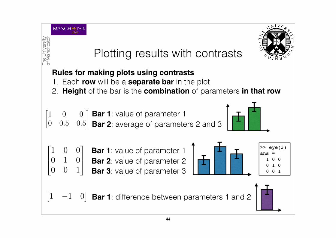
Rules for making plots using contrasts 1. Each row will be a separate bar in the plot 2. Height of the bar is the combination of parameters in that row
Plotting results with contrasts
1 0 00 0.5 0.5
�Bar 1: value of parameter 1Bar 2: average of parameters 2 and 3
2
41 0 00 1 00 0 1
3
5Bar 1: value of parameter 1Bar 2: value of parameter 2Bar 3: value of parameter 3
⇥1 �1 0
⇤Bar 1: difference between parameters 1 and 2
>> eye(3)ans = 1 0 0 0 1 0 0 0 1
44

Plotting results with contrasts2 x 2 ANOVAAge (older/younger) x Diagnosis (control/depressed)
To plot the interaction we want to select each cell mean
Plot A⇥ B =
2
664
1 0 0 0
0 1 0 0
0 0 1 0
0 0 0 1
3
775
4 bars for the cell means
OlderControl
OlderDepressed
YoungerControl
YoungerDepressed
45

Plotting results with contrasts2 x 2 ANOVAAge (older/younger) x Diagnosis (control/depressed)
Plot Age =
0.5 0.5 0 0
0 0 0.5 0.5
�
2 bars each averaged across Diagnosis
Older Younger
To plot the main effects we average over the cells of the other factor to form the marginal means
46
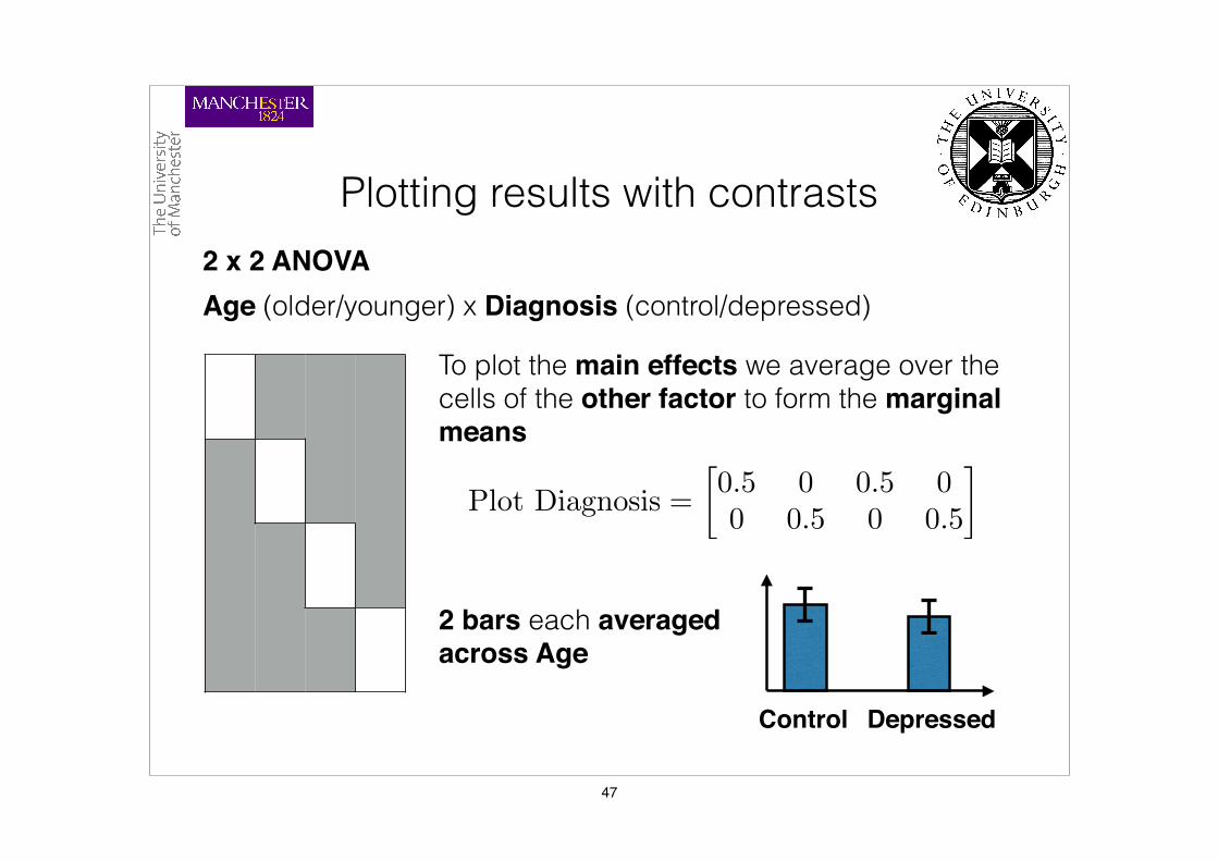
Plotting results with contrasts2 x 2 ANOVAAge (older/younger) x Diagnosis (control/depressed)
Control Depressed
Plot Diagnosis =
0.5 0 0.5 0
0 0.5 0 0.5
�
To plot the main effects we average over the cells of the other factor to form the marginal means
2 bars each averaged across Age
47
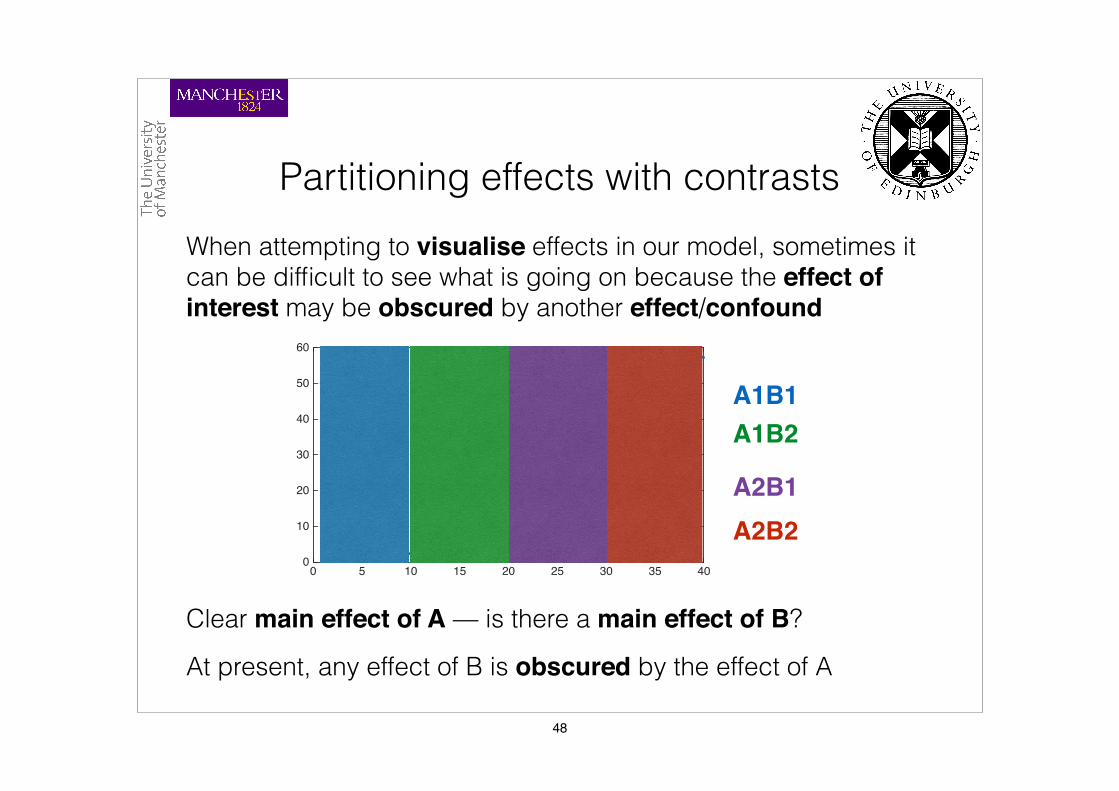
Partitioning effects with contrastsWhen attempting to visualise effects in our model, sometimes it can be difficult to see what is going on because the effect of interest may be obscured by another effect/confound
0 5 10 15 20 25 30 35 400
10
20
30
40
50
60
Clear main effect of A — is there a main effect of B?
At present, any effect of B is obscured by the effect of A
A1B1A1B2
A2B1A2B2
48
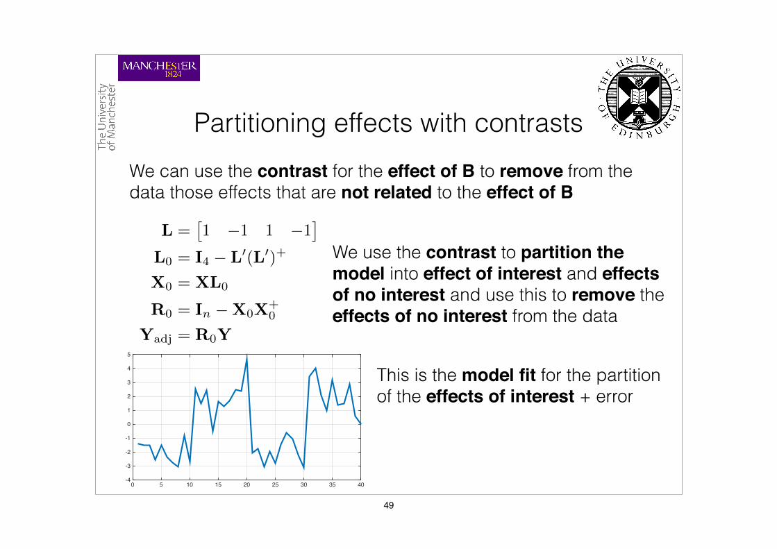
Partitioning effects with contrastsWe can use the contrast for the effect of B to remove from the data those effects that are not related to the effect of B
L =⇥1 �1 1 �1
⇤
L0 = I4 � L0(L0)+
X0 = XL0
R0 = In �X0X+0
Yadj = R0Y
We use the contrast to partition the model into effect of interest and effects of no interest and use this to remove the effects of no interest from the data
This is the model fit for the partition of the effects of interest + error
0 5 10 15 20 25 30 35 40-4
-3
-2
-1
0
1
2
3
4
5
49
0 5 10 15 20 25 30 35 40-4
-3
-2
-1
0
1
2
3
4
5
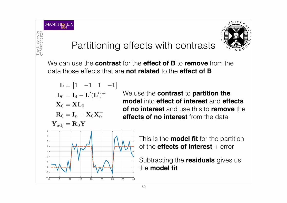
Partitioning effects with contrastsWe can use the contrast for the effect of B to remove from the data those effects that are not related to the effect of B
L =⇥1 �1 1 �1
⇤
L0 = I4 � L0(L0)+
X0 = XL0
R0 = In �X0X+0
Yadj = R0Y
We use the contrast to partition the model into effect of interest and effects of no interest and use this to remove the effects of no interest from the data
This is the model fit for the partition of the effects of interest + error
Subtracting the residuals gives us the model fit
50
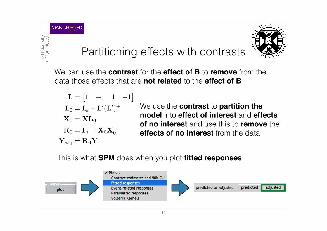
Partitioning effects with contrastsWe can use the contrast for the effect of B to remove from the data those effects that are not related to the effect of B
L =⇥1 �1 1 �1
⇤
L0 = I4 � L0(L0)+
X0 = XL0
R0 = In �X0X+0
Yadj = R0Y
We use the contrast to partition the model into effect of interest and effects of no interest and use this to remove the effects of no interest from the data
This is what SPM does when you plot fitted responses
51

SummaryThe use of contrast weights allows us to defining linear combinations of the parameters estimates
Contrasts must respect the meaningful combinations of parameters dictated by the rows of X — only an issue with rank-deficient designs
Contrasts are flexible as they can • Provide alternative means of testing hypotheses in
unbalanced designs • Select parameters for plotting • Partition the design into effects of interest/no interest
Typically this is used to define a hypothesis about the parameters — important to understand what the parameters mean
52

References
McFarquhar, M. (2016) Testable Hypotheses for Unbalanced Neuroimaging Data. Frontiers in Neuroscience: Brain Imaging Methods, 10, 270.
Poline, J-B., Kherif, F., Pallier, C. & Penny, W. (2007) Contrasts and classical inference. In Friston, K.J. et al. (Eds.) Statistical Parametric Mapping: The Analysis of Functional Brain Images. London: Academic Press.
Poline, J-B., Brett, M. (2012). The general linear model and fMRI: does love last forever? NeuroImage, 62, 871-80.
53