Understanding Calculus is Largely

Locally Linear

Dan KennedyPearson Author

If you zoom in on the graph of y = 6 4x at the point (1, 2), it comes to resemble a line. Graph the function in the ZDecimal window, trace to (1, 2), and zoom in repeatedly until this happens. Then use your calculator to find the equation of this "line."

My Class’s First Problem of the Day:

Point-Slope Equation of a Line:

1 1( )y y m x x Linearization of f at x = a:

( ) ( )( )y f a f a x a or

( ) ( )( )y f a f a x a

This simple equation is the basis for:

Instantaneous rate of change

Differentials

Linear approximations

Newton’s Method for Finding Roots

Rules for Differentiation

Slope Fields

Euler’s Method

L’Hopital’s Rule

What is Instantaneous Rate of Change?

If a rock falls 20 feet in 2 seconds, its average velocity during that time period is easily measured:

20 feet10 ft/sec

2 sec

But what if we capture that rock at a moment in time and ask for its instantaneous velocity at that single moment? What is the logical reply?

0 feet 0 ft/sec

0 sec 0

Obviously, traditional algebra fails us when it comes to instantaneous rate of change.

feet

seconds

But if we graph the rock’s position as a function of time, we see that velocity is the same as slope. Instantaneous velocity is just the slope of the zoomed-in picture – which is linear!

That’s what differentials are all about. Since the derivative is the slope of the curve at a point, there is no true Δy or Δx…but there is a slope. So we write:

0limx

y dy

x dx

If we zoom in on a differentiable curve, because it is locally linear, Δy/ Δx is essentially constant. That makes dy/dx defensible as something other than 0/0.

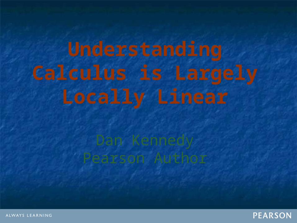
If we zoom in at a point (a, f(a)):

0lim ( )x

yf a

x

So… if (x, y) is close to (a, f(a)),

( )( ) ( ) ( )( )

y f af a y f a f a x a

x a

There’s that equation again!

This is the basis for linear approximations. For example, here is Problem of the Day #23:

Find the linearization of ( )f x x at x = 100 and use

it to approximate 101 . Use f to predict whether the approximation will be slightly smaller or slightly larger than the actual value.

1100 100

2 1001

10 101 100 10.0520

y x

y y

The Good News: Modern students can check how close this approximation is by using a calculator.

The Bad News: Modern students do not appreciate how much these approximation tricks meant to their ancestors.

Another such method is Newton’s Method for approximating roots. Here is Problem of the Day #22:

The line shown is tangent to the graph of y = f(x) at the point (a, f(a)).

(a, f(a))

(a) Find an equation of the line. (b) Find the x-intercept of this line in terms of a.

( ) ( )( )

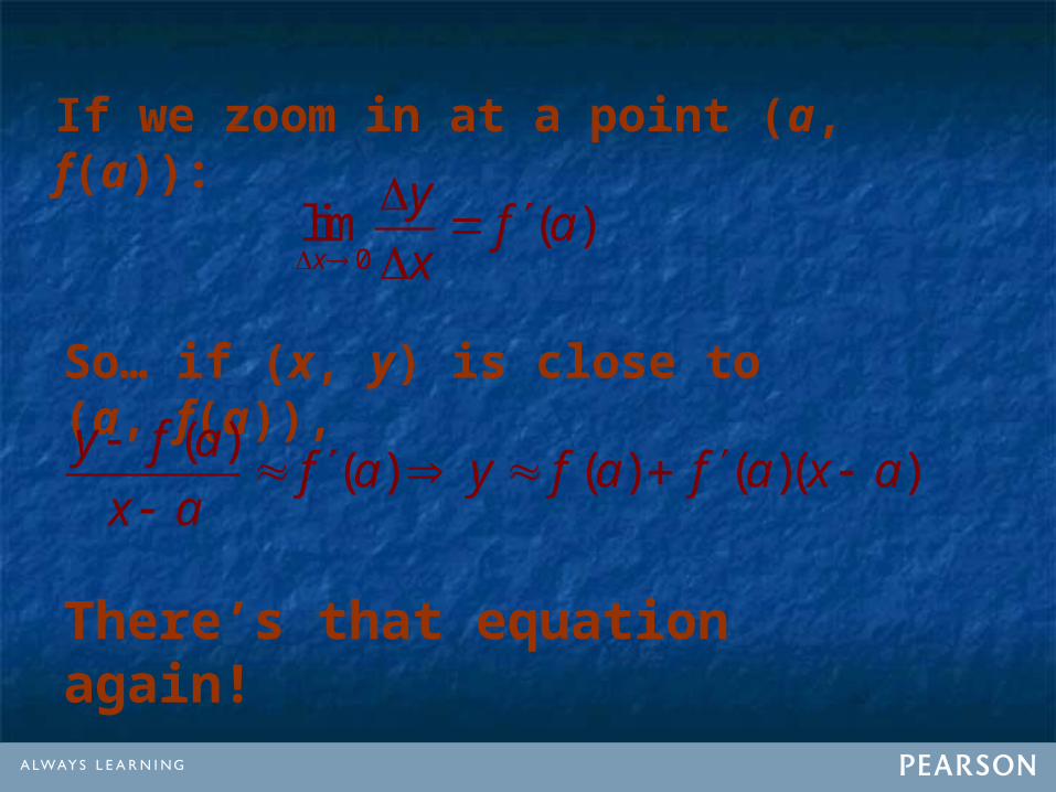
0 ( ) ( )( )

( )

( )

y f a f a x a

f a f a x a

f ax a

f a

Then we name this x-intercept b. Using (b, f(b)) as the new point, I have them repeat the process. Clever students quickly write:

( )

( )

f bx b

f b

(a, f(a))

Eventually this process will zoom in on an x-intercept of the curve. This is Newton’s Method for approximating roots of equations.

For example, let us find a root of the equation sin x = 0. Start with a guess of a = 2.

2

sintan

cos

ax a a a

a

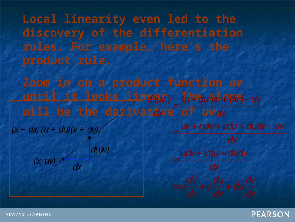
Local linearity even led to the discovery of the differentiation rules. For example, here’s the product rule.

Zoom in on a product function uv until it looks linear. The slope will be the derivative of uv.

(x + dx, (u + du)(v + dv))

(x, uv)dx

d(uv)

( ) ( )( )d uv u du v dv uv

dx dxuv udv vdu dudv uv

dxudv vdu dudv

dxdv du dv

u v dudx dx dx

A slope field is all about local linearity.

At each point (x, y) the differential equation determines a slope. This is the very essence of point-slope!

dyx y

dx

Here is Problem of the Day #37: Suppose y = f(x) satisfies the differential equation dy

x ydx

. Find the linearization of f at the point (1, 1)

and use it to approximate f(1.1). Then use the linearization at the new point to approximate f(1.2).

( , )x x y y

x

dyy x

dx

(x, y)

Slope dy

dx This is Euler’s

Method. The picture at the right shows how it works.

You start with a point on the curve. Find the slope, dy/dx. Now move horizontally by Δx. Move vertically by Δy = (dy/dx) Δx.This gives you a new point (x + Δx, y + Δy).Repeat the process.

I like to use a table.

((xx, , yy)) dy/dxdy/dx ΔΔxx ΔΔyy ((xx + + ΔΔx, yx, y + + ΔΔyy))((xx, , yy)) dy/dxdy/dx ΔΔxx ΔΔyy ((xx + + ΔΔx, yx, y + + ΔΔyy))

(1, 1)(1, 1)

((xx, , yy)) dy/dxdy/dx ΔΔxx ΔΔyy ((xx + + ΔΔx, yx, y + + ΔΔyy))

(1, 1)(1, 1) 22

((xx, , yy)) dy/dxdy/dx ΔΔxx ΔΔyy ((xx + + ΔΔx, yx, y + + ΔΔyy))

(1, 1)(1, 1) 22 0.10.1

((xx, , yy)) dy/dxdy/dx ΔΔxx ΔΔyy ((xx + + ΔΔx, yx, y + + ΔΔyy))

(1, 1)(1, 1) 22 0.10.1 0.20.2

((xx, , yy)) dy/dxdy/dx ΔΔxx ΔΔyy ((xx + + ΔΔx, yx, y + + ΔΔyy))

(1, 1)(1, 1) 22 0.10.1 0.20.2 (1.1, 1.2)(1.1, 1.2)

((xx, , yy)) dy/dxdy/dx ΔΔxx ΔΔyy ((xx + + ΔΔx, yx, y + + ΔΔyy))

(1, 1)(1, 1) 22 0.10.1 0.20.2 (1.1, 1.2)(1.1, 1.2)

(1.1, 1.2)(1.1, 1.2)

((xx, , yy)) dy/dxdy/dx ΔΔxx ΔΔyy ((xx + + ΔΔx, yx, y + + ΔΔyy))

(1, 1)(1, 1) 22 0.10.1 0.20.2 (1.1, 1.2)(1.1, 1.2)

(1.1, 1.2)(1.1, 1.2) 2.32.3

((xx, , yy)) dy/dxdy/dx ΔΔxx ΔΔyy ((xx + + ΔΔx, yx, y + + ΔΔyy))

(1, 1)(1, 1) 22 0.10.1 0.20.2 (1.1, 1.2)(1.1, 1.2)

(1.1, 2.2)(1.1, 2.2) 2.32.3 0.10.1

((xx, , yy)) dy/dxdy/dx ΔΔxx ΔΔyy ((xx + + ΔΔx, yx, y + + ΔΔyy))

(1, 1)(1, 1) 22 0.10.1 0.20.2 (1.1, 2.2)(1.1, 2.2)

(1.1, 1.2)(1.1, 1.2) 2.32.3 0.10.1 0.230.23

((xx, , yy)) dy/dxdy/dx ΔΔxx ΔΔyy ((xx + + ΔΔx, yx, y + + ΔΔyy))

(1, 1)(1, 1) 22 0.10.1 0.20.2 (1.1, 1.2)(1.1, 1.2)

(1.1, 1.2)(1.1, 1.2) 2.32.3 0.10.1 0.230.23 (1.2, 1.43)(1.2, 1.43)

Problem of the Day #53: The graphs of two differentiable functions f and g cross the x-axis at x = a, as shown:

a

When we zoom in at (a, 0), the graphs will resemble their

linearizations. Find a formula for ( )

lim( )x a

f x

g x by replacing f(x) and g(x)

by their linearizations and simplifying.

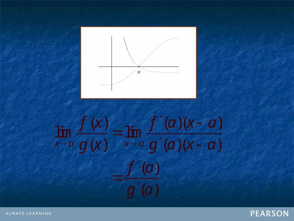
( ) ( )( )lim lim

( ) ( )( )

( )

( )

x a x a

f x f a x a

g x g a x a

f a

g a

And now for something completely different…

The Top Ten Student Errors on

the AP Calculus Examination

…according to Dan Kennedy

Error #10: Mishandling the Chain Rule

Error #9: Universal Logarithmic Antidifferentiation

Error #8: Not Showing the Pre-calculator Step

You can evaluate a definite integral on your calculator, but you must show the integral first.

You can solve an equation on your calculator, but you must show the equation first.

Error #7: Using Ambiguous References

Avoid statements like:"The graph of the derivative is increasing, so the graph must be concave up."

Use statements like:"The graph of f ' is increasing, so the graph of f must be concave up."

Error #6: Omitting the Constant of Integration

This can be a very costly error if you are solving a differential equation with an initial condition, like:

Error #5: Not Separating the Variables

This can be a much more costly error if you are solving a separable differential equation like:

Error #4: The Bad Washer Formula

R

Good:

Bad:

/4 2 2

0cos sinx x dx

/4 2

0cos sinx x dx

Error #3: Messing up Average Rate of Change

Remember: A derivative is the instantaneous rate of change. It's a calculus concept.

Average rate of change is just . It's an algebra concept.

Δy

Δx

Error #2: Justifying Maxima and Minima

Remember: Showing that f ' = 0 is only a start.

For local extrema, show how f ' changes sign, or check concavity using the sign of f ''.

For absolute extrema, give a global argument on the entire domain, including endpoints if relevant.

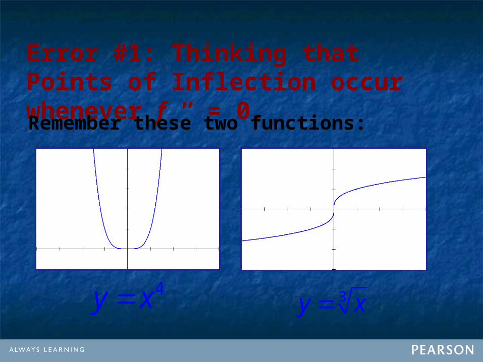
Error #1: Thinking that Points of Inflection occur whenever f '' = 0.

Remember these two functions:

4y x 3y x

And now, ladies and gentlemen, a word from our sponsor…

While you’re here, be sure to check out:

FDWK4“…the only book that could possibly follow FDWK3…”

New Features

•All answers in back of the TE

•Improved slope fields, series, etc.

•Guidance on calculator usage

•More AP® Quick Quizzes

New Features

•New “More Derivatives” chapter

•Updated data problems

•Better answers and solutions

•Better Teacher Edition stuff

And what about the State Common Core Standards?

Prentice Hall textbooks either have the content now or will make it available with website supplements – even if authors question whether it is appropriate. Some of it is quite ambitious.

We must all become statistics teachers.

The trickiest part for many teachers will be the mathematical practices. We have been writing textbooks with those in mind for about fifteen years!

•Make sense of problems and persevere in solving them

•Reason abstractly and quantitatively

•Construct viable arguments and critique the reasoning of others

•Model with mathematics

•Use appropriate tools strategically

•Attend to precision

•Look for and make use of structure

•Look for and express regularity in repeated reasoning

If we can survive a few years of transition, common state standards can be a great thing for American mathematics education.

After all, the common curriculum is one of the main reason that AP Calculus works so well!

On the other hand, we may see fewer students taking AP in the future.

It will no longer be possible to rush through the pre-calculus curriculum.

There will be a lot more to be learned, and the expectation is that students will learn it.

And much of it will not specifically relate to calculus preparation!

dkennedy@baylorschool.org