UNDERSTANDING BIOMECHANICAL DIFFERENCES IN …

UNDERSTANDING BIOMECHANICAL DIFFERENCES IN TECHNIQUE BETWEEN PHASES OF A SPRINT

HANS CHRISTIAN VON LIERES UND WILKAU A thesis submitted for the degree of Doctor of Philosophy

Cardiff Metropolitan University December 2017

Director of Studies: Dr Ian N. Bezodis

Supervisory team: Professor Gareth Irwin Dr Neil E. Bezodis

Scott Simpson

COPYRIGHT Attention is drawn to the fact that copyright of this thesis rests with its author. This

copy of the thesis has been supplied on condition that anyone who consults it is

understood to recognise that its copyright rests with the author and that no quotation

from the thesis and no information derived from it may be published without the prior

written consent of the author.

© Hans Christian von Lieres und Wilkau, 2017

I

Declaration

This work has not previously been accepted in substance for any degree and is

not being concurrently submitted in candidature for any degree.

Signed……………....................................................... (Candidate)

Date........................................................................

STATEMENT ONE

This thesis is the result of my own investigations, except where otherwise stated.

Where correction services have been used, the extent and nature of the correction

is clearly marked in a footnote(s). Other sources are acknowledged by footnotes

giving explicit references. A bibliography is appended.


Date........................................................................

STATEMENT TWO

I hereby give consent for my thesis, if accepted, to be available for photocopying

and for inter-library loan, and for the title and summary to be made available to

outside organisations.


Date........................................................................

II

Abstract UNDERSTANDING BIOMECHANICAL DIFFERENCES IN TECHNIQUE

BETWEEN PHASES OF A SPRINT Hans C. von Lieres und Wilkau, Cardiff Metropolitan University, Cardiff

Sprinting requires the rapid development of velocity while technique changes across

multiple steps. Research Themes (Phase analysis, Technique analysis and Induced

acceleration analysis) were formulated to investigate and understand the

biomechanical differences in technique between the initial acceleration, transition

and maximal velocity phases of a sprint.

Theme 1 (Phase analysis) revealed relatively large changes in touchdown variables

(e.g. centre of mass height, touchdown distances, shank angles) during the initial

acceleration phase. This likely reflects an increasing need to generate larger vertical

forces early during stance as a sprint progresses. At toe-off, smaller yet progressive

changes in variables (e.g. trunk angles and centre of mass height) across the initial

acceleration and transition phases reflect a constraint determining decreases in

propulsive forces during a sprint. Theme 2 (Technique analysis) revealed a trend

linking smaller horizontal foot velocities and touchdown distances with smaller

braking impulses during the transition and maximal velocity phases. Furthermore,

moderate to large increases in negative work by the ankle plantar flexors and knee

extensors suggests an increased contribution to absorb forces at those joints and

maintain the height of the centre of mass as a sprint progresses.

Finally, theme 3 (Induced acceleration analysis) revealed that the braking impulses

relative to body mass (expressed in m·s-1) due to the accelerations at contact point,

which largely resulted from the foot being decelerated at touchdown, increased from

-0.01 ± 0.01 m·s-1 to -0.08 ± 0.02 m·s-1 between steps three to 19 of a sprint. The

ankle moment provided the largest contributions to centre of mass acceleration

throughout stance with the changing orientation of the ground reaction force vector

ultimately determined by the increasing foot, shank and trunk angles as the sprint

progressed. This thesis developed the conceptual understanding of the technical

differences between different phases of sprinting. It will contribute to the

development and evaluation of sprinting technical models associated with different

phases of the event and provide a greater understanding of key contributors to

performance. As a sprint progresses, sprinters should emphasise the development

of the leg mechanics during the terminal swing and early stance phases to ensure

step-to-step changes in braking impulses are managed.

III

Publications

Conference Presentations: International conference abstracts von Lieres und Wilkau, H., Irwin, G., Bezodis, N., Simpson, S., & Bezodis, I.N. (June, 2017). Contributions to braking impulse during initial acceleration, transition and maximal velocity in sprinting. In: Proceedings of the 35rd International Conference on Biomechanics in Sports. Cologne, Germany. von Lieres und Wilkau, H., Irwin, G., Bezodis, N., Simpson, S., & Bezodis, I.N. (July, 2016). Support leg joint contributions to center of mass acceleration during three phases of maximal sprinting. In: M. Ae, Y. Enomoto, N. Fujii & H. Takagi (eds.). Proceedings of the 34rd International Conference on Biomechanics in Sports. Tsukuba, Japan, pp. 1097-1100. von Lieres und Wilkau, H., Irwin, G., Simpson, S. Elias, M., & Bezodis, I.N. (June, 2015). A comparison of different methods for identifying transition steps in the acceleration phase of sprint running. In: F. Colloud, M. Domolain and T. Monnet (Eds.), Proceedings of the 33rd International Conference on Biomechanics in Sports. Poitiers, France, pp. 106 – 109. National conference abstracts von Lieres und Wilkau, H., Irwin, G., Bezodis, N., Simpson, S., & Bezodis, I.N. (April, 2017). Differences in contributions to braking impulse between phases of maximal sprinting. In: 1st Pan-Wales Postgraduate Conference, Swansea, Wales. von Lieres und Wilkau, H., Irwin, G., Bezodis, N., Simpson, & Bezodis, I.N. (2016). Influence of the foot model on the results of an induced acceleration analysis in maximal sprinting. In: Program and Abstract Book of the 31st Annual British Association of Sport and Exercise Sciences Biomechanics Interest Group (Ed. M. Robinson), Liverpool John Moores University, UK, 23. von Lieres und Wilkau, H., Irwin, G., Simpson, & Bezodis, I.N. (April, 2015). A case study of changes in transition steps and performance measures in sprint acceleration. In: Program and Abstract Book of the 30th Annual British Association of Sport and Exercise Sciences Biomechanics Interest Group (Ed. C. Diss), University of Roehampton, UK, 32.

IV

Acknowledgements

I would like to express my thanks to everyone that has been part of my journey to

achieve my PhD.

To my supervisors, Dr Ian Bezodis, Prof Gareth Irwin, Dr Neil Bezodis and Scott

Simpson. Thank you for all the support, guidance and advice you have given me

throughout my PhD.

To Welsh Athletics, Sport Wales and the Cardiff Metropolitan University for

providing the funding for this PhD

To the coaches and athletes who willingly gave their time to participate and make

this research possible.

To the Biomechanics technicians Laurie Needham, Melanie Golding and Mike

Long for your technical assistance when planning and running my data collections.

Also, thank you to Ed Thompson for helping me prepare the testing area prior to

data collections.

To the NIAC facilities and CSS staff for their assistance over the years with

booking the space necessary for the data collections. Furthermore, thank you to

the catering team at Bench for providing the cakes and coffees to keep me going.

To my fellow Post grad students for all your help and support over the years.

Especially thank you to Adam Brazil and Laurie Needham for all the help and

discussions over the years.

To my family and friends who have offered continued support throughout my

academic career.

To Rachel Spittle for your endless love and support. Thank you for always

providing the necessary distraction.

V

Table of Contents Declaration ............................................................................................................... I Abstract ................................................................................................................... II Publications............................................................................................................ III Acknowledgements ................................................................................................IV

Table of Contents ................................................................................................... V

List of Figures ........................................................................................................ X

List of Tables...................................................................................................... XVII List of Equations .................................................................................................. XX

Nomenclature and definitions............................................................................. XXII Chapter 1 – Introduction ......................................................................................... 1

1.1. Research overview ..................................................................................... 1

1.2. Research aim and purpose ........................................................................ 4

1.2.1. Development of Research Themes ............................................................... 5

1.3. Organisation of Chapters ........................................................................... 8

1.3.1. Chapter 2: Review of literature ...................................................................... 8

1.3.2 Chapter 3: Phase analysis: Phases in maximal sprinting ............................... 8

1.3.3 Chapter 4: Technique analysis: Changing joint kinematics and kinetics between different phases in maximal sprinting ....................................................... 9

1.3.4 Chapter 5: Induced acceleration analysis: Changes in contributions to performance between different phases in maximal sprinting .................................. 9

1.3.5 Chapter 6: General discussion ....................................................................... 9

Chapter 2 - Review of Literature ........................................................................... 11

2.1 Introduction ................................................................................................ 11

2.2 Description of Phases ............................................................................... 11

2.2.1. Description of Phases summary ................................................................. 16

2.3 Sprint Technique ....................................................................................... 17

2.3.1 Step Characteristics ..................................................................................... 17

2.3.1.1 Step Length and Step Frequency ............................................................. 17

2.3.1.2 Components of step length ....................................................................... 20

2.3.1.3 Components of step frequency ................................................................. 21

2.3.1.4 Summary of step characteristics ............................................................... 23

2.3.2 Segment and Joint kinematics ..................................................................... 23

2.3.2.1 Summary of segment and joint kinematics ................................................ 29

2.3.3 External Kinetics .......................................................................................... 29

2.3.3.1 Summary of external kinetics .................................................................... 36

VI 2.3.3 Musculoskeletal aspects of technique .......................................................... 37

2.3.3.1 Joint Kinetics ............................................................................................. 37

2.3.3.2 Theoretical investigations into sprinting technique .................................... 43

2.3.3.3 Summary of musculoskeletal aspects of technique .................................. 45

2.4 Methodological considerations ................................................................ 46

2.4.1 Methods of Data collection ........................................................................... 46

2.4.1.1 Video based motion analysis .................................................................... 46

2.4.1.2 Ground reaction forces.............................................................................. 46

2.4.2 Signal Processing ........................................................................................ 48

2.4.2.1 Coordinate Reconstruction ........................................................................ 48

2.4.2.2 Noise Reduction ........................................................................................ 48

2.4.3 Computational methods in biomechanics..................................................... 50

2.4.3.1 Inverse dynamic analysis .......................................................................... 50

2.4.3.2 Induced acceleration analysis ................................................................... 52

2.4.3.3 Induced power analysis ............................................................................. 55

2.4.4 Models used in biomechanics ...................................................................... 55

2.4.4.1 Kinematic models ...................................................................................... 55

2.4.4.2 Foot-floor contact models .......................................................................... 57

2.4.4.3 Inertia models ........................................................................................... 58

2.4.5 Statistical analysis approaches .................................................................... 59

2.4.5.1 Inferential statistics ................................................................................... 59

2.4.6 Summary of methodological considerations ................................................. 61

2.5 Chapter summary ...................................................................................... 61

Chapter 3 - Phase analysis: Phases in maximal sprinting .................................... 63

3.1 Introduction ................................................................................................ 63

3.2 Methods ...................................................................................................... 65

3.2.1 Participants .................................................................................................. 65

3.2.2 Protocol ........................................................................................................ 65

3.2.3 Data Collection ............................................................................................. 66

3.2.4 Data Reduction ............................................................................................ 67

3.2.5 Data synchronisation ................................................................................... 68

3.2.7 Data Processing ........................................................................................... 69

3.2.8 Identifying the initial acceleration, transition and maximal velocity phases .. 71

3.2.9 Data smoothing ............................................................................................ 73

3.2.10 Reliability and Objectivity of digitising ........................................................ 74

3.2.11 Data Analysis ............................................................................................. 74

VII

3.3 Results ........................................................................................................ 75

3.3.1 Trial times, Tstart, MVstart and CT≤FT ............................................................ 76

3.3.3 Changes in step characteristics, spatiotemporal and kinematic variables ... 77

3.4 Discussion ................................................................................................. 83

3.4.1 Comparison of measures used to identify the acceleration phases ............. 83

3.4.2 Changes in step characteristics, spatiotemporal and kinematic variables ... 86

3.4.3 Practical Implications ................................................................................... 92

3.5 Conclusions ............................................................................................... 93

3.6 Chapter summary ...................................................................................... 95

Chapter 4 - Technique analysis: Changes in joint kinematics and kinetics between different phases of a sprint .................................................................................... 97

4.1 Introduction ................................................................................................ 97

4.2 Methods ...................................................................................................... 98

4.2.1 Participants .................................................................................................. 98

4.2.2 Protocol ........................................................................................................ 99

4.2.3 Data Collection ............................................................................................. 99

4.2.4 Data Processing ......................................................................................... 100

4.2.4.1 Inverse dynamics analysis ...................................................................... 104

4.2.5 Data normalisation ..................................................................................... 108

4.2.6 Data presentation ....................................................................................... 108

4.2.7 Data analysis ............................................................................................. 108

4.3 Results ...................................................................................................... 109

4.3.1 Kinematic variables .................................................................................... 109

4.3.2 GRF variables ............................................................................................ 110

4.3.3 Joint kinematics and kinetics ...................................................................... 113

4.3.3.1 MTP Joint ................................................................................................ 113

4.3.3.2 Ankle Joint .............................................................................................. 115

4.3.3.3 Knee Joint ............................................................................................... 118

4.3.3.4 Hip Joint .................................................................................................. 121

4.3.4 Segment angles and angular velocities ..................................................... 124

4.4 Discussion ............................................................................................... 126

4.4.1 Ground reaction force and impulse ............................................................ 127

4.4.2 Joint kinematics and kinetics ...................................................................... 130

4.4.2.1 MTP Joint ................................................................................................ 130

4.4.2.2 Ankle Joint .............................................................................................. 131

4.4.2.3 Knee Joint ............................................................................................... 134

4.4.2.4 Hip Joint .................................................................................................. 138

VIII 4.4.3 Segment angles and angular velocities ..................................................... 141

4.4.4 Practical Implications ................................................................................. 142

4.5 Conclusion ............................................................................................... 144

4.6 Chapter summary .................................................................................... 145

Chapter 5 – Induced acceleration analysis: Changes in contributions to performance ........................................................................................................ 147

5.1 Introduction .............................................................................................. 147

5.2 Methods .................................................................................................... 149

5.2.1 Data Processing ......................................................................................... 149

5.2.1.1 Induced acceleration analysis ................................................................. 149

5.2.1.2 Contact model ......................................................................................... 151

5.2.1.3 Performing the IAA .................................................................................. 153

5.2.1.4 Induced power analysis ........................................................................... 154

5.2.2 Data presentation ....................................................................................... 154

5.2.2.1 Force events ........................................................................................... 155

5.2.3 Data analysis ............................................................................................. 157

5.3 Results ...................................................................................................... 157

5.3.1 Accuracy .................................................................................................... 157

5.3.2 Induced CM accelerations.......................................................................... 157

5.3.3 Contribution by joint moments .................................................................... 160

5.3.3.1 Foot complex .......................................................................................... 160

5.3.3.3 Knee........................................................................................................ 161

5.3.3.4 Hip .......................................................................................................... 162

5.3.4 Induced accelerations at the peak force events ......................................... 164

4.3.4.1 Peak braking force event ........................................................................ 165

4.3.4.2 Peak vertical force event ......................................................................... 167

4.3.4.3 Peak propulsive force event .................................................................... 169

5.4 Discussion ............................................................................................... 171

5.4.1 Induced centre of mass acceleration ......................................................... 171

5.4.1. Induced accelerations due to accelerations at the foot-floor interface ...... 174

5.4.3 Joint moment induced accelerations .......................................................... 175

5.4.3.1 Foot complex (FC) .................................................................................. 177

5.4.3.2 Knee........................................................................................................ 180

5.4.3.3 Hip moment ............................................................................................. 182

5.4.4 Practical Implications ................................................................................. 183

5.5 Conclusions ............................................................................................. 186

5.6 Chapter Summary .................................................................................... 187

IX Chapter 6 - General Discussion .......................................................................... 189

6.1 Introduction .............................................................................................. 189

6.2 Addressing the Research Themes ......................................................... 189

6.3 Discussion of Methodology .................................................................... 203

6.3.1 Assessment of data collection methods ..................................................... 203

6.3.2 Study design .............................................................................................. 204

6.3.3 Determination of phases in maximal sprinting ............................................ 206

6.3.3 Induced acceleration analysis .................................................................... 206

6.4 Novel contributions to knowledge and practical implications ............ 208

6.5 Directions of future research .................................................................. 213

6.7 Thesis Conclusion ................................................................................... 216

References.......................................................................................................... 218

Appendix A - Overview ....................................................................................... 243

- Reliability and objectivity of digitising ............................ 244

- Individual Tstart, MVstart and Vmax variables .................... 248

- CM angle ...................................................................... 251

- Accuracy and reliability of joint kinematics and kinetics 252

- Components of IAA ....................................................... 255

- Foot-floor models in maximal sprinting ......................... 261

- Induced segment accelerations at the peak braking, vertical and propulsive force events ....................................................... 266

- Example Participant information sheets and written informed consent form ........................................................................... 269

X

List of Figures Chapter 1: Figure 1.1. A diagram representing the framework of this thesis highlighting the aims, key themes and research questions of each chapter. ................................. 10 Chapter 2:

Figure 2.1. Measures previously used to sub-divide the acceleration phase in sprinting. The different colour arrows indicate the different phases identified. Above each arrow is the distance/step number and associated discriminating variable, which the phase is based on. The block phase was not included. ........................ 13 Figure 2.2. Initial acceleration, transition and maximal velocity phases according to the British Athletics coaching literature (Crick, 2013a). ......................................... 16 Figure 2.3. Contact (×) and flight times () during the initial acceleration, transition and maximal velocity phases from previous research in sprinting. Only studies that presented both flight and contact times were included. ........................................ 21 Chapter 3: Figure 3.1. Camera and synch light set-up (not to scale). Direction of travel from left to right. .................................................................................................................. 66 Figure 3.2. The 17 points digitised around touchdown and toe-off (see text for details). ................................................................................................................. 68 Figure 3.3. Schematic representation of the sub-division of the acceleration phase. The black line represents the initial acceleration phase, the blue line represents the transition phase and the red line represents the maximal velocity phase. ............ 71 Figure 3.4. Example detection of Tstart using multiple first order polynomials. The open circles represent the relative CM-h at each touchdown. The red and black lines represents two of the eight first order polynomials used to detect Tstart. The grey diamonds represent the difference between the residuals of adjacent approximations. The vertical dotted line indicates the step (Tstart) which corresponds to the maximal difference of the residuals. ............................................................ 72 Figure 3.5. Example breakpoint detection of MVstart using two straight-line approximations. The open circles represent the relative CM-h at each touchdown. Relative CM-h was plotted against touchdown times. The two black lines on the figure represent the two first order polynomials to detect MVstart. The grey diamonds represent the collective RMSD for each set of approximations. The vertical dotted line indicates the step (MVstart) which corresponds to the minimal difference of the residuals. .............................................................................................................. 73

XI Figure 3.6. Tstart and MVstart steps of the participant’s best trial from day 1 (x) and day 2 (+). The grey columns highlight the initial acceleration, transition and maximal velocity phase steps that lie outside the range (best trials) of Tstart and MVstart steps. .............................................................................................................................. 78 Figure 3.7. Step-to-step profiles for (a) step velocity, (b) step length and (c) step frequency over the first 25 steps of the participants best 50 m sprint from day 1 (black) and day 2 (grey). The grey columns highlight the initial acceleration, transition and maximal velocity phase steps that lie outside the range (best trials) of Tstart and MVstart steps. .......................................................................................... 79 Figure 3.8. a) Touchdown CM-h and b) step-to-step changes in CM-h step over the first 25 steps of the participants best 50 m sprint from day 1 (black) and day 2 (grey). The grey columns highlight the initial acceleration, transition and maximal velocity phase steps that lie outside the range (best trials) of Tstart and MVstart steps. ....... 80 Figure 3.9. Step-to-step contact times (a), flight times (b), contact distance (c), flight distance (d), touchdown distance (e) and toe-off distances profile over 25 steps of the participants best 50 m sprint from day 1 (black) and day 2 (grey). Grey columns highlight the initial acceleration, transition and maximal velocity phase steps that lie outside the range (best trials) of Tstart and MVstart steps. ....................................... 81 Figure 3.10. Step-to-step trunk (a-c), thigh (d-f) and shank (g–i) angle and ranges of motion profiles over the first 25 steps of the participants best 50 m sprint from day 1 (black) and day 2 (grey). The grey columns highlight the initial acceleration, transition and maximal velocity phase steps that lie outside the range (best trials) of Tstart and MVstart steps. .......................................................................................... 82 Chapter 4 Figure 4.1. Similar to figure 3.6 shows the steps that occurred in the initial acceleration, transition and maximal velocity phases (shaded areas) as identified in Chapter 3. The coloured arrows identify the steps investigated in the current Chapter. ................................................................................................................ 98 Figure 4.2. Set-up. ............................................................................................. 100 Figure 4.3. Convention used to describe positive changes (extension) in joint kinematic and kinetics. ........................................................................................ 102 Figure 4.4. Free body diagram illustrating the forces acting on the ith segment. 105 Figure 4.5. Free body diagram illustrating the forces and moments acting on the ith segment. ............................................................................................................. 106 Figure 4.6. Definition of the power phases for the MTP, ankle and hip joints. .... 107 Figure 4.7. Definition of the power phases for the knee during steps three, nine and 19. ....................................................................................................................... 107

XII Figure 4.8. Mean ± SD time-histories of horizontal (a) and vertical (b) ground reaction force data for step three (black), step nine (blue) and step 19 (red). The tables below the respective figures show the descriptive results of the MBI analysis of the differences between the three steps. For each comparison, there is a qualitative description of the probability of the standardised differences being larger than 0.02 which is followed by the size (standardised effect) and direction of the differences. ......................................................................................................... 111 Figure 4.9. Scatter-plots and trend lines for steps three (black), nine (blue) and 19 (red) for a) foot touchdown velocity and b) touchdown distance against relative the relative braking impulse. ..................................................................................... 113 Figure 4.10. Mean ± SD MTP angle (a), normalised MTP angular velocity (b), normalised MTP moment (c) and normalised power between steps three (black), nine (blue) and 19 (red). The tables below the respective figures show the descriptive results of the results of the MBI analysis of the differences between the three steps. For each comparison, there is a qualitative description of the probability of the standardised differences being larger than 0.02 which is followed by the size (standardised effect) and direction of the differences.. ....................................... 114 Figure 4.11. Mean ± SD normalised negative (MTP-) and positive (MTP+) MTP work for steps three (black), nine (blue) and 19 (red). The table shows the results of the MBI analysis of the differences between the three steps. For each comparison, there is a qualitative description of the probability of the standardised differences being larger than 0.02 which is followed by the size (standardised effect) and direction of the differences. ................................................................................. 115 Figure 4.12. Mean ± SD ankle angle (a), normalised ankle angular velocity (b), normalised ankle moment (c) and normalised ankle power between steps three (black), nine (blue) and 19 (red). The tables below the respective figures show the descriptive results of the results of the MBI analysis of the differences between the three steps. For each comparison, there is a qualitative description of the probability of the standardised differences being larger than 0.02 which is followed by the size (standardised effect) and direction of the differences. ........................................ 116 Figure 4.13. Mean ± SD normalised negative (A-) and positive (A+) ankle work for steps three (black), nine (blue) and 19 (red). The table shows the results of the MBI analysis of the differences between the three steps. For each comparison, there is a qualitative description of the probability of the standardised differences being larger than 0.02 which is followed by the size (standardised effect) and direction of the differences………………………………………………………………………….117 Figure 4.14. Mean ± SD knee angle (a), normalised Knee angular velocity (b), normalised Knee moment (c) and normalised knee power between steps three (black), nine (blue) and 19 (red). The tables below the respective figures show the descriptive results of the results of the MBI analysis of the differences between the three steps. For each comparison, there is a qualitative description of the probability

XIII of the standardised differences being larger than 0.02 which is followed by the size (standardised effect) and direction of the differences. ........................................ 119 Figure 4.15. Mean ± SD positive and negative knee work for steps three (black), nine (blue) and 19 (red). From left to right, the each cluster of bars represent knee flexor power generation (Kf+), knee extensor power absorption (Ke-), knee extensor power generation (Ke+) and knee flexor power absorption (Kf-). The table shows the results of the MBI analysis of the differences between the three steps. For each comparison, there is a qualitative description of the probability of the standardised differences being larger than 0.02 which is followed by the size (standardised effect) and direction of the differences. .......................................................................... 121 Figure 4.16. Mean ± SD hip angle (a), normalised Hip angular velocity (b), normalised hip moment (c) and normalised hip power between steps three (black), nine (blue) and 19 (red). The tables below the respective figures show the descriptive results of the results of the MBI analysis of the differences between the three steps. For each comparison, there is a qualitative description of the probability of the standardised differences being larger than 0.02 which is followed by the size (standardised effect) and direction of the differences. ........................................ 122 Figure 4.17. Mean ± SD normalised positive (H+) and negative (H-) hip work for steps three (black), nine (blue) and 19 (red). The table shows the results of the MBI analysis. The table shows the results of the MBI analysis of the differences between the three steps. For each comparison, there is a qualitative description of the probability of the standardised differences being larger than 0.02 which is followed by the size (standardised effect) and direction of the differences ....................... 123 Figure 4.18. Mean segment angles across stance phases of steps three, nine and 19 (left) and mean segments angular velocities across steps three (black), nine (blue) and 19 (red). ............................................................................................. 125 Chapter 5: Figure 5.1. Orienation of the fore foot, rear foot, shank, thigh and HAT at the instants of peak braking force during step 19. The arrows indicate the contribution of the MTP and ankle (purple), knee (blue), hip (red) and total (black) joint moments on segment accelerations during steps three, nine and 19. The induced CM acceleration is represented by the light grey arrow. Below the figures, the joint moments, induced CM accelerations and segment orientations corresponding to the peak braking force event percentage of stance shown top left corner of each figure). The segments, coloured arrows and ground reaction force vectors are to scale. See text boxes for a description of the figure/table..................................................... 156 Figure 5.2. The horizontal and vertical induced GRF due to the joint moments (round dot line), gravity (square dot line), joint centripetal acceleration (CA; dashed line), foot-floor accelerations (dash dot line) and the contralateral leg (long dash line). The total calculated (sum of all inputs; solid line) and measured GRF (grey shaded area) are also presented. Data for step three (a & b), nine (c & d) and 19 (e & f) is presented. ................................................................................................. 159

XIV Figure 5.3. Total and individual induced horizontal and vertical ground reaction forces due the joint moments. The measured ground reaction forces (shaded area) is also presented as a reference. Data for step three (a & b), nine (c & d) and 19 (e & f) is presented. ................................................................................................. 161 Figure 5.4. Stance average induced a) resultant, b) horizontal and c) vertical CM accelerations due to the total joint moments (Total_JM) and the individual joint moments of the MTP, ankle, knee and hip. Step three is represented by the black bars, step nine is presented by the blue bars and step 19 is represented by the red bars. The tables below the respective figures show the descriptive results of the results of the MBI analysis of the differences between the three steps. For each comparison, there is a qualitative description of the probability of the standardised differences being larger than 0.02, followed by the size (standardised effect) and direction of the differences.. ................................................................................ 163 Figure 5.5. Joint moment and induced acceleration data at the instantaneous peak braking (a & d), peak propulsive (b & e) and peak vertical (c & f) force event for steps three (black), nine (blue) and 19 (red). Figures a to c show the joint moments at the events. Figures d and f show the horizontal induced accelerations and figure e shows the vertical induced accelerations. ........................................................... 164 Figure 5.6. Fore foot, rear foot, shank, thigh and HAT positions and orientation at the instants of peak braking force. The arrows indicate the contribution of the FC (MTP and ankle (purple)), knee (blue), hip (red) and total (black) joint moments on segment accelerations during steps three, nine and 19. The induced CM acceleration is represented by the grey arrow. Below the figures, the joint moments, induced CM accelerations and segment orientations corresponding to the peak braking force event are shown. The segments, coloured arrows and ground reaction force vectors are to scale. The results of the induced power (IP) analysis shows whether a joint moments increased (+) or decreased (-) the energy of either the LEG or HAT. The segments, coloured arrows and grand reaction force vectors are to scale. .................................................................................................................. 166 Figure 5.7. Fore foot, rear foot, shank, thigh and HAT positions and orienation at the instants of peak braking force. The arrows indicate the contribution of the FC (MTP and ankle (purple)), knee (blue), hip (red) and total (black) joint moments on segment accelerations during steps three, nine and 19. The induced CM acceleration is represented by the grey arrow. Below the figures, the joint moments, induced CM accelerations and segment orientations corresponding to the peak vertical force event are shown. The segments, coloured arrows and ground reaction force vectors are to scale. The results of the induced power (IP) analysis shows whether a joint moments increased (+) or decreased (-) the energy of either the LEG or HAT. The segments, coloured arrows and grand reaction force vectors are to scale. .................................................................................................................. 168

XV Figure 5.8. Fore foot, rear foot, shank, thigh and HAT positions and orientation at the instants of peak braking force. The arrows indicate the contribution of the FC (MTP and ankle (purple)), knee (blue), hip (red) and total (black) joint moments on segment accelerations during steps three, nine and 19. The induced CM acceleration is represented by the grey arrow. Below the figures, the joint moments, induced CM accelerations and segment orientations corresponding to the peak propulsive force event are shown. The segments, coloured arrows and ground reaction force vectors are to scale. The results of the induced power (IP) analysis shows whether a joint moments increased (+) or decreased (-) the energy of either the LEG or HAT. The segments, coloured arrows and grand reaction force vectors are to scale. ........................................................................................................ 170

Appendix A: Figure A1.1. Re-digitised step-to-step a) CM-h, b) shank angles, c) trunk angles and d) touchdown and toe-off distance profiles. Each figure contains the three digitisations by digitiser 1 (solid black lines) and digistiser 2 (dashed grey lines). ............................................................................................................................ 247 Figure A3.1. a) Touchdown CM angle and b) toe-off CM angle. ........................ 251 Figure A4.1. Mean (-) and individual () horizontal and vertical reconstruction errors. ............................................................................................................................ 252 Figure A4.2. Continuous time-history joint angle, joint angular velocity, joint moment and joint power data obtained from the re-digitised step three (black), nine (blue) and 19 (red) trial………………………………………………………………………..254 Figure A5.1. Components of matrix A. Matrix A is a square matrix with 27 rows and 27 columns.......................................................................................................... 255 Figure A5.2. Full matrix A used for the IAA adapted from (Hof & Otten, 2005). Rows 1 to 10 contain the coefficients for the equations of linear acceleration (equations 5.10). Rows 11 to 18 contain the coefficients for the constraint equations (equations 5.13). Rows 19 to 20 are the coefficients for the equations of angular acceleration (equation 5.17). Rows 24 to 27 contain the coefficients for the constraint equations with the ground. It is important to remind the reader at this point that two contact models were used. At the beginning and end of ground contact when the one-point contact model applied, contact was modelled either between the fore foot (yellow shaded) or rear foot (red shading). This was dependent on the location of the COP relative to the MTP joint. For example, when the COP was behind the MTP joint, all the inputs in red text were removed from the matrix and replaced by zeros. During the stationary fore foot phase of ground contact, the two-point contact model was used (see 5.2.1.2 Contact model). Rows 24 to 27 and columns 24 to 27 were filled cording to the red text. In this case contact coefficients describing contact at the projected MTP location are added to rows and columns 24 to 25, while the coefficients describing contact at the projected TOE location are added to rows and columns 26 to 27. ................................................................................................ 258

XVI Figure A5.3. Variables contained within the column vector c adapted from (Hof & Otten, 2003). When the COP was behind the MTP joint, all the inputs in red were removed from the matrix and replaced by zeros. Variables in red are replaced by zeros when the COP was behind the MTP joint. ................................................. 259 Figure A6.1. Three ground contact models used in the current study. The contact model in a) involves a 1 segment foot where contact is modelled between the foot and the ground via the COP (1SegFoot_ COP). The contact model in b) involves a two-segment foot where contact with the ground is modelled between the COP and the distal segment (2SegFoot_ COP). The contact model in c) involves a two-segment foot and used the COP at the beginning and end of ground contact and the MTP joint and toe when the forefoot was stationary on the ground (2SegFoot_TwoPoint). ........................................................................................ 262 Figure A6.2. The relative RMSD between the measured anterior-posterior ( ), vertical ( ) and resultant ( ) accelerations between the calculated and the total calculated induced CM accelerations for steps three (left), nine (middle) and 19 (right). The three foot-ground models are a) 1segment foot model connected to the floor at the COP, b) 2segment foot model connected to the floor at the COP, c) 2segment foot multi-contact point model. ........................................................... 263

XVII

List of Tables Chapter 2: Table 2.1. Change in touchdown distance throughout a sprint. .......................... 20 Table 2.2. Kinematic characteristics during the stance phases of the initial acceleration, transition and maximum Velocity Phases. ....................................... 26 Table 2.3. External kinetics during initial acceleration, transition and maximal velocity. ................................................................................................................. 31 Chapter 3: Table 3.1. Participant Characteristics. .................................................................. 65 Table 3.2. Measures used to sub-divide the acceleration phase in sprinting, the event these measures identify and the study that used the measure. .................. 71 Table 3.3. Mean () ± SD 50 m time from the March and May 2014 data collection as well as each participant’s range across the trials. ............................................ 76 Table 3.4. Group mean () ± SD using all available trials, ranges across all trials and ranges across the best trials for Tstart steps (CM-h, shank angles (θshank) and CT≤FT) and MVstart steps (CM-h and trunk angles (θtrunk)). Also presented are the CM height, θshank and θtrunk at their respective Tstart and MVstart steps. ................. 76 Table 3.5. Group mean () ± SD of Vmax steps as well as the ranges (all trials and best trials) for Vmax steps. Group mean () ± SD and ranges (all trials and best trials) of step velocity (SV), CM-h and trunk angle (θtrunk) corresponding to the Vmax step are also presented. ............................................................................................... 77 Table 3.6. Individual RMSD between Tstart steps identified either using CM-h, shank angles or the CT≤FT step and the RMSD between MVstart steps identified using either CM-h or trunk angles. These RMSD values were calculated using all trials for each participant. .................................................................................................... 77 Chapter 4: Table 4.1. Participant Characteristics. .................................................................. 99 Table 4.2. Mean ± SD values for selected step characteristics, performance and temporal variables for steps three, nine and 19 across all participants. .............. 109 Table 4.3. Mean ± SD of touchdown CM-h, trunk and shank angles for steps three, nine and 19 ......................................................................................................... 110 Table 4.4. Mean ± SD horizontal and vertical foot velocity and touchdown and toe-off distances during steps three, nine and 19. .................................................... 110

XVIII Table 4.5. Mean ± SD of stance mean and maximum resultant GRF from steps three, nine and 19. .............................................................................................. 111 Table 4.6. Mean ± SD changes in vertical, net horizontal velocity as well as the mean ± SD horizontal velocity decrease and increase during steps three, nine and 19 across all participants. ................................................................................... 112

Chapter 5: Table 5.1. Absolute and relative RMSD between the measured vertical and horizontal forces and the sum vertical and horizontal induced ground reaction forces calculated from all inputs. ................................................................................... 157 Table 5.2. Mean ± SD peak accelerations and relative impulses induced by the joint moments. ............................................................................................................ 158 Table 5.3. Group mean ± SD relative impulses induced by each of the joint moments. ............................................................................................................ 162

Appendix A: Table A1.1. Reliability and objectivity of digitising. The values represent the absolute and relative differences between digitised trials of the same digitiser (reliability) and between digitised trials of different digitisers (objectivity). .......... 245 Table A2.1. Participant mean (SD) as well as across participant mean (SD) and range of Tstart steps, CM-h, shank angles, step velocities and relative step velocities for each participant. ............................................................................................ 248 Table A2.2. Participant mean (SD) as well as across participant mean (SD) and range of MVstart steps, CM-h, shank angles, step velocities and relative step velocities for each participant. ............................................................................. 249 Table A2.3. Participant mean (SD) as well as across participant mean (SD) and range of CT≤FT and Vmax steps, absolute and relative step velocity at those steps and trunk angle at Vmax. ...................................................................................... 250 Table A4.1. Absolute and relative RMSD between re-digitised trials for step 3. . 253 Table A4.2. Absolute and relative RMSD between re-digitised trials for step 9. 253 Table A4.3. Absolute and relative RMSD between re-digitised trials for step 19. ............................................................................................................................ 253 Table A6.1. Average ± SD MTP, ankle, FC, knee and hip moment contributions to CM acceleration using the three foot-ground models during steps 3, 9 and 19. . 264

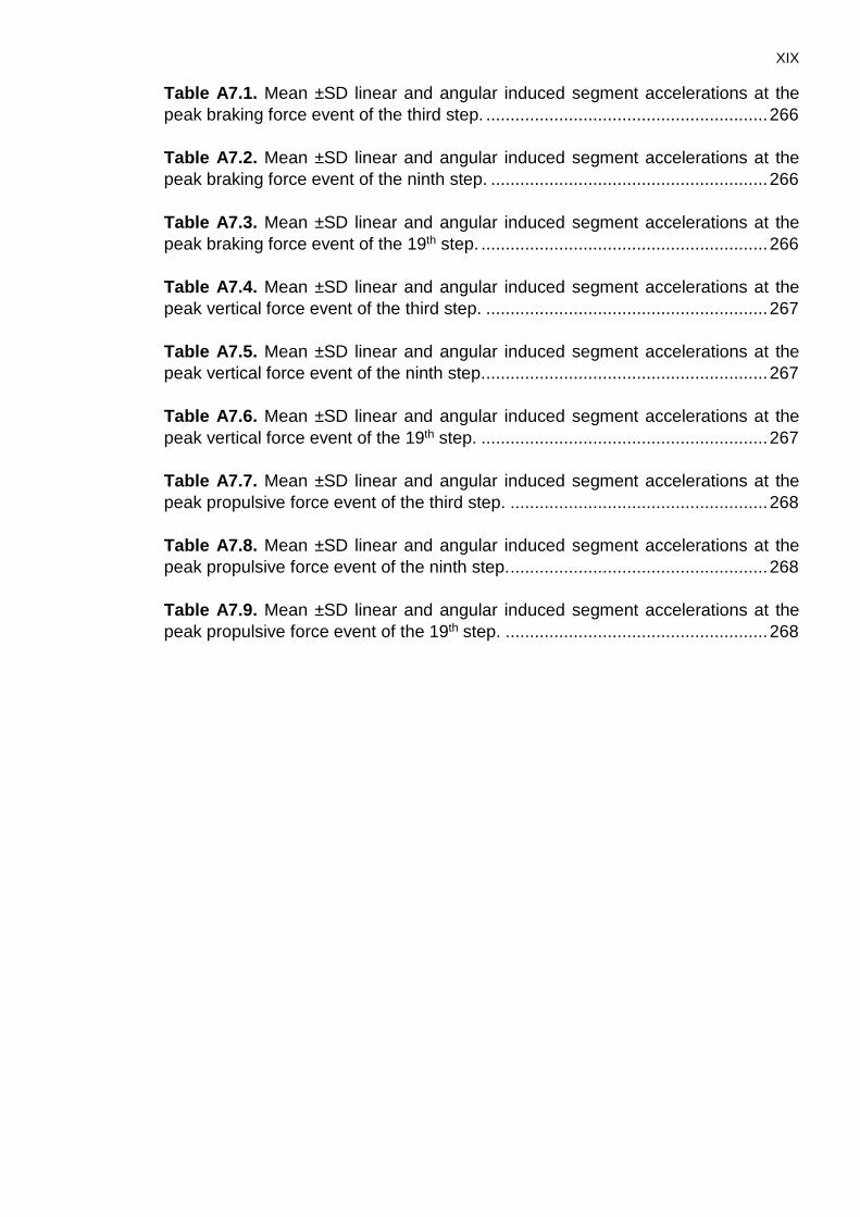
XIX Table A7.1. Mean ±SD linear and angular induced segment accelerations at the peak braking force event of the third step. .......................................................... 266 Table A7.2. Mean ±SD linear and angular induced segment accelerations at the peak braking force event of the ninth step. ......................................................... 266 Table A7.3. Mean ±SD linear and angular induced segment accelerations at the peak braking force event of the 19th step. ........................................................... 266 Table A7.4. Mean ±SD linear and angular induced segment accelerations at the peak vertical force event of the third step. .......................................................... 267 Table A7.5. Mean ±SD linear and angular induced segment accelerations at the peak vertical force event of the ninth step. .......................................................... 267 Table A7.6. Mean ±SD linear and angular induced segment accelerations at the peak vertical force event of the 19th step. ........................................................... 267 Table A7.7. Mean ±SD linear and angular induced segment accelerations at the peak propulsive force event of the third step. ..................................................... 268 Table A7.8. Mean ±SD linear and angular induced segment accelerations at the peak propulsive force event of the ninth step. ..................................................... 268 Table A7.9. Mean ±SD linear and angular induced segment accelerations at the peak propulsive force event of the 19th step. ...................................................... 268

XX

List of Equations Chapter 2:

M(θ)θ̈ = JMi + V�θ, θ̇�i

+ G(θ)i ………………………………..……………………….53

M11(θ)θ̈1 + M12(θ)θ̈2 = JM1 + V�θ, θ̇�11

+ V�θ, θ̇�12

+ G(θ)11……………………….53

M21(θ)θ̈1 + M22(θ)θ̈2 = JM2 + V�θ, θ̇�21

+ V�θ, θ̇�22

+ G(θ)21 ……………….……..53

�M11(θ) M12(θ)M21(θ) M22(θ)� �

θ̈1θ̈2� = �τ1τ2�+ �V�θ,θ̇�11

V�θ,θ̇�21� + �G(θ)11

G(θ)21� ................................................... 53

θ̈ = M−1(θ) �JMi + G(θ)i + V�θ, θ̇�i�………… ........................................................ 53

Pi = Mi(θ)θı̈ × θı̇ …….. ........................................................................................... 55

Chapter 3: yi = 0.25 ∗ xi−1 + 0.5 ∗ xi + 0.25 ∗ xi+1 ; i = 2 to (N− 1) ......................................... 74

Chapter 4:

∑Fi = mi × ai 40TU………………… ............................................................................ 105

Fyi = mi × ayi − Fyi−1 40TU…….……………………… ................................................. 105

Fzi = mi × azi − mi × g − Fzi−1 40TU……..…………. ................................................... 105

∑ Mi = Ii × αi…………… ..................................................................................... 106

Mpi = (Fzi × ripy) + (Fyi × ripz) + (Fzi−1 × ridy) + (Fyi−1 × ridz) + (Ii × αi) − Mdi

............................................................................................................................ 106

JPi = Mpi .ωi ………………………………….…………………………………….106

Wnj = ∫ JPidtt1t2 40TU………… ...................................................................................... 106

Chapter 5: A × x = c40TU…….. .................................................................................................... 150

Fi − Fi+1 + mig = miai ......................................................................................... 150

a�⃗ cmi + �θ̈i × r⃗pi� − (θ̇i2 × r⃗pi) = a�⃗ cm(i+1) + �θ̈(i+1) × r⃗d(i+1)� − (θ̇(i+1)2 × r⃗d(i+1)).. . 150

(Fdi × rdi) − �Fpi × rpi�+ Mdj − Mpj = Ii × θ̈i …................................................... 150

ac = acm1 + θ̈1(rd1) − θ̇12(rd1)… .......................................................................... 151

x = A−1 × c… ...................................................................................................... 151

XXI Appendix A:

Fi − Fi+1 + mig = miai ......................................................................................... 255

Fi − Fi+1 − miai = −mig ...................................................................................... 255

a�⃗ ji = a�⃗ i + �θ̈i × r⃗ji� − (θ̇i2 × r⃗ji) ............................................................................. 256

a�⃗ pi = a�⃗ d(i+1) ......................................................................................................... 256

a�⃗ pi + �θ̈i × r⃗pi� − (θ̇i2 × r⃗pi) = a�⃗ d(i+1) + �θ̈d(i+1) × r⃗d(i+1)� − (θ̇d(i+1)2 × r⃗d(i+1)) .... 256

a�⃗ 2i − a�⃗ (i+1) + �θ̈i × r⃗pi� − �θ̈(i+1) × r⃗d(i+1)� = −(θ̇(i+1)2 × r⃗d(i+1)) + (θ̇i2 × r⃗pi) ........ 256

(Fdi × rdi) − �Fpi × rpi�+ Mdi − Mpi = Ii × θ̈i ........................................................ 256

−(Fdi × rdi) + �Fpi × rpi� − Ii × θ̈i = −Mdi + Mpi ............................................. 256

a�⃗ p1 = a�⃗ d0 = 0 ...................................................................................................... 257

a�⃗ 1 + �θ̈1 × r⃗1� − (θ̇12 × r⃗1) = 0 .............................................................................. 257

XXII

Nomenclature and definitions

Symbols used to represent variables in equations throughout the thesis

F Force 𝑎𝑎 Acceleration

g Acceleration due to gravity

m Mass

CM Centre of mass

𝐹𝐹𝑦𝑦𝑖𝑖 Horizontal joint reaction force at the proximal endpoint of the ith

segment

𝐹𝐹𝑧𝑧𝑖𝑖 Vertical joint reaction force at the proximal endpoint of the ith

segment

𝑎𝑎𝑦𝑦𝑖𝑖 Horizontal acceleration of the ith segment

𝑎𝑎𝑧𝑧𝑖𝑖 Vertical acceleration of the ith segment

𝐹𝐹𝑦𝑦𝑖𝑖−1 Horizontal joint reaction force at the distal endpoint of the ith

segment

𝐹𝐹𝑧𝑧𝑖𝑖−1 Vertical joint reaction force at the distal endpoint of the ith segment

𝑀𝑀 Moment

𝐼𝐼𝑖𝑖 Moment of inertia of the ith segment

𝛼𝛼𝑖𝑖 Angular acceleration of the ith segment

𝑀𝑀𝑝𝑝𝑖𝑖 Moment acting on the proximal endpoint of the ith segment

𝑀𝑀𝑑𝑑𝑖𝑖 Moment acting on the distal endpoint of the ith segment

𝑟𝑟𝑝𝑝𝑖𝑖 Position vector of CM of segment i relative to proximal joint

𝑟𝑟𝑑𝑑𝑖𝑖 Position vector of CM of segment i relative to distal joint

𝐽𝐽𝑃𝑃𝑗𝑗 Joint power of the jth joint

𝜔𝜔𝑗𝑗 Angular velocity of the jth joint

𝑊𝑊𝑛𝑛𝑗𝑗 Joint work of the nth power phase of joint j

𝐽𝐽𝑃𝑃𝑗𝑗 Joint power of the ith joint

t1 Start of power phase

t2 End of power phase

∑ Sum of

A Matrix of equations of motions (also see Appendix A1)

x Vector of unknowns (also see Appendix A3)

c Vector of known variables (also see Appendix A2)

𝐹𝐹𝑝𝑝𝑖𝑖 Force at joint (at proximal joint of segment i)

XXIII 𝐹𝐹𝑑𝑑𝑖𝑖 Force at joint (at distal joint of segment i)

𝑚𝑚𝑖𝑖 Mass of ith segment

𝑎𝑎𝑐𝑐𝑐𝑐𝑖𝑖 Acceleration of centre of mass of ith segment

𝑎𝑎𝑐𝑐𝑐𝑐 Acceleration at the foot-floor contact point

𝑀𝑀𝑝𝑝𝑖𝑖 Joint moment (at proximal joint of segment i)

𝑀𝑀𝑑𝑑𝑖𝑖 Joint moment (at distal joint of segment i)

�̈�𝜃𝑖𝑖 Angular acceleration of ith segment

�̇�𝜃𝑖𝑖 Angular velocity of ith segment

y Anterior-posterior horizontal axis

z Vertical axis

N Number of values in the sample

Definition of the power phases at each stance leg joint quantified using the inverse

dynamics analysis

MTP+ / A+ / H+ The positive power phase of the MTP joint during stance.

The (+) is representative of a positive power phase while

the (-) represents a negative power phase. The same

convention is used for the ankle (A) and hip (H) joints.

Kf+/ Ke-/ Ke+/Kf- Four power phases were identified at the knee (K). The

letter after the K denotes whether the moment is flexor (Kf)

or extensor (Ke) dominant. The positive or negative sign

denotes whether the joint moment is absorbing (-) or

generating (+) energy.

Abbreviations used for terminology throughout the thesis

DLT Direct linear transformation

2D two-dimensional

m Metres

s Seconds

LED Light emitting diode

C7 Seventh cervical vertebra

MTP Metatarsal-phalangeal

CM Centre of mass

CM-h Centre of mass height

XXIV Tstart Step the defines the start of the transition phase

MVstart Step the defines the start of the maximal velocity phase

CT≤FT The step when flight time equals or exceeds the contact time

θshank Shank angle

θthigh Thigh angle

θtrunk Trunk angle

TD Touchdown

TO Toe-off

Vmax Maximal running velocity

SV Step velocity

SL Step length

SF Step frequency

GRF Ground reaction force

CM angle Angle between the vector connecting the CM to the contact

point relative to the ground

Symbols used to abbreviate statistical terminology throughout the thesis

Mean

SD Standard deviation

RMSD Root mean squared difference

% Percentage

Definitions of key terms used throughout the thesis

Sprint A track and field event contested over distances up to 400 m where the aim is to cover the desired distance in the shortest time possible.

Technique A movement sequence used to execute a specific task. Technique is a collective term that includes both kinematic (posture) and kinetic (e.g. joint moments, joint power, joint work) aspects of movement.

Posture A collective term used to describe the orientation of the segments that dictate the orientation of the athlete relative to the ground.

Performance A measure of the success associated with executing a task.

XXV

Phase

A distinct period of a movement or task that describes a specific aspect of the task.

Acceleration phase The first phase in the sprint events, which defines a period during which the horizontal velocity of sprinters increases.

Initial acceleration phase

The first phase of sprint acceleration characterised by a forward orientated posture and relatively large step-to-step increases in horizontal velocity.

Transition phase

The second phase of sprint acceleration characterised by a more inclined posture and small step-to-step increases in horizontal velocity compared to the initial acceleration phase.

Maximal velocity phase

The phase in a sprint when the sprinter has an upright posture and maintains their running velocity above 95% of their maximal velocity.

Step An event lasting from the instant of touchdown of one foot to the subsequent touchdown on the contralateral foot.

Step velocity The mean velocity of the centre of mass across a step.

Step frequency The number of steps a sprinter takes per second.

Step length Horizontal displacement of the centre of mass across a step.

Flight phase

The period of the step when the sprinter is in the air.

Ground contact phase

The period of the step when one foot is on the ground.

Touchdown Distance

The horizontal distance between the contact point and the CM at the instant of touchdown. For consistency throughout the thesis, the horizontal location of the MTP was used as the contact point.

Toe-off Distance

The horizontal distance between the contact point and the CM at the instant of toe-off. For consistency throughout the thesis, the horizontal location of the toe location was used as the contact point.

Segment angles All segment angles are relative to the right forward horizontal.

XXVI

Inclined Refers to the angular deviation from the right forward horizontal.

Braking phase

The period of the ground contact phase when the sprinter is generating a negative anterior-posterior GRF.

Propulsive phase

The period of the ground contact phase when the sprinter is generating a positive anterior-posterior GRF.

Breakpoint A sudden deviation in the progression of a variable over time.

Clockwise/anti-clockwise rotations

Throughout this Thesis the mention of clockwise and anti-clockwise rotations are always in references to the running motion viewed from left to right.

External Validity

Describes the applicability of the data to real-world settings.

Accuracy Describes the degree to which a measure represents the true value.

Reliability Describes the degree to which a measure is repeatable.

Objectivity Describes the bias within a certain measure.

Empirical research

Generation of knowledge by means direct measurement or observation.

1

Chapter 1 – Introduction 1.1. Research overview The main aim of the sprint events is to cover a predefined distance in as short a time

as possible, with hundredths of a second often being the difference between first

and second place. Based on velocity-time profiles, the sprint events can be divided

into a reaction, acceleration, maximal velocity and deceleration phase (Bartonietz &

Güllich, 1992; Mero, Komi & Gregor, 1992; Delecluse, Van Coppenolle, Willems,

Diels, Goris, Van Leemputte & Vuylsteke, 1995). While the maximal velocity

sprinters achieve is important to the final time (Moravec, Ruzicka, Susanka, Dostal,

Kodejs & Nosek, 1988; Fuchs & Lames, 1990; Maćkala, 2007), the acceleration

phase ultimately determines the velocity that sprinters can achieve (Bartonietz &

Güllich, 1992). Depending on the ability level of the sprinters, the maximal velocity

is generally achieved between 30 to 60 m with elite sprinters achieving their maximal

velocity further into the sprint (Moravec et al., 1988). However, the maximum

velocity achieved is dependent on their ability to maximally accelerate during the

sprinter’s whole acceleration phase (Bartonietz & Güllich, 1992) with the length of

the acceleration is dependent on the ability of the sprinter (Delecluse, 1997).

To facilitate a more in-depth analysis and understanding of the acceleration phase,

which would allow for a more manageable approach to preparing sprinters for the

event, previous literature has proposed the sub-division of the acceleration phase

into two phases (Seagrave, 1991; Bartonietz & Güllich, 1992; Delecluse et al., 1995;

Qing & Kruger, 1995; Čoh, Tomažin & Štuhec, 2006; Nagahara, Matsubayashi,

Matsuo & Zushi, 2014; Crick, 2013a). Using a factor analysis on multiple

velocity-time curves, Delecluse et al. (1995) identified two phases within sprint

acceleration. The first phase or initial acceleration phase was associated with a high

acceleration over the first 10 m. The second phase or transition phase was related

to the ability to achieve a high maximal velocity up to 36 m (Delecluse et al., 1995).

While this structure could be generalised across all sprinters it does not provide

information on technical changes that occur during the acceleration phase. With the

acceleration phase characterised by continuous changes in kinematics, a more

in-depth understanding of these changes and their influence on the sprinter’s

performance may by facilitated by a more sensitive method of identifying the

different phases within the acceleration phase of maximal sprinting.

2 It has been suggested that sudden changes in in the step-to-step progression of

segment orientations occur between specific consecutive steps (i.e. breakpoint

steps) during the acceleration phase (Bosch & Klomp, 2005). These breakpoint

steps could therefore be identified to sub-divide the acceleration (e.g. Nagahara,

Matsubayashi et al., 2014). Nagahara, Matsubayashi et al. (2014) identified

breakpoints in the step-to-step increases in the height of the centre of mass (CM-h)

which allowed the authors to sub-divide the 50 m sprint trial into three phases. Other

studies have defined phases within sprint acceleration by identifying specific events.

These events, which were based on contact and flight times, include the step when

decreases in contact times plateau (Qing & Krüger, 1995), or when flight times equal

or exceed contact times (Čoh et al., 2006). Furthermore, British Athletics coaching

literature suggested that changes in step-to-step progressions of shank and trunk

angles could be used to identify the start of the transition and maximal velocity

phases respectively (Crick, 2013a). Although these different measures have been

successfully implemented to identify abrupt changes in kinematics, it is unclear how

the steps identified by different measures compare. In addition, the appropriateness

of the measures used previously to identify the breakpoint steps are still unclear.

Throughout the acceleration phase in sprinting, step characteristics and kinematic

variables change (Maćkala, 2007; Debaere, Jonkers & Delecluse, 2013; Nagahara,

Naito, Morin & Zushi, 2014; Nagahara, Matsubayashi et al., 2014). Nagahara,

Matsubayashi et al. (2014) identified two breakpoints during maximal 50 m

accelerations and reported abrupt changes in kinematics as sprinters crossed these

breakpoints. Although changes in upper body kinematics and velocity contributions

across multiple steps throughout a 50 m sprint have previously been reported by

Nagahara, Matsubayashi et al. (2014) it is still unclear how the how the kinematics

of the stance leg change throughout the acceleration phase. As the segments of the

leg play an important role in influencing CM variables (e.g. CM-h, touchdown and

toe-off distances) knowledge of these changes will build on the study of Nagahara,

Matsubayashi et al. (2014). This will increase understanding of variables that are

more visually accessible and therefore could assist coaches and sport scientists to

better interpret the technical changes that occur during maximal sprinting.

It is well known from Newton’s second law of motion that forces determine motion

(i.e. ∑F = m × a). Recent studies have shown that world class sprinters have a better

3 technical ability to direct their resultant ground reaction force (GRF) vector more

horizontally throughout the acceleration phase compared to athletes with similar

physical capabilities (Morin, Edouard & Samozino, 2011; Rabita, Dorel, Slawinski,

Sàez-de-Villarreal, Couturier, Samozino & Morin, 2015). As sprinters accelerate

from low to high velocities, performance is influenced by their ability to continue to

produce a net horizontal propulsive force (Rabita et al., 2015) while producing

sufficiently large vertical forces to provide an appropriate flight time to allow them to

prepare for the next stance phase (Hunter et al., 2005). However, in light of the

decreasing ground contact times as running velocities increase, there is an

increasing demand to generate the larger vertical ground reaction forces required

to maximise running velocities (Weyand et al., 2000). Since the GRFs ultimately

determine the acceleration of the sprinter’s CM, knowledge of changes in the

horizontal and vertical components of the GRF between consecutive steps is

important to understand the demands of sprinting.

Previous research has generally aimed to understand the causes of motion through

a description of the joint kinetics of the sprint by focusing in on a specific step or

phase of the sprint. These include the block phase (Mero, Kuitunen, Harland,

Kyröläinen & Komi, 2006; Brazil, Exell, Wilson, Willwacher, Bezodis & Irwin, 2016),

first contact (Charalambous, Irwin, Bezodis & Kerwin, 2012; Debaere, Delecluse,

Aerenhouts, Hagman & Jonkers, 2013, Bezodis, Salo, & Trewartha 2014), second

contact (Jacobs & van Ingen Schenau, 1992; Debaere, Delecluse et al., 2013),

transition (Johnson & Buckley, 2001: ~14 m; Hunter et al., 2004c: ~16 m; Yu, Sun,

Yang, Wang, Yin, Herzog and Liu, 2016: ~12 m) and maximal velocity phase

(Bezodis et al., 2008; Yu et al., 2016). The few studies that have reported joint kinetic

data across multiple steps indicated some important changes in the energy

absorption and generation strategies (Ito, Saito, Fuchimoto & Kaneko, 1992;

Braunstein, Goldmann, Albracht, Sanno, Willwacher, Heinrich and Brüggemann,

2013) and joint moments (Yu et al., 2016) at the ankle and knee. However, these

multi-step studies have either only focused on joint powers or work (e.g. Ito et al.,

1992; Braunstein et al., 2013), joint moments (Yu et al., 2016) or have only reported

their results in abstract form (e.g. Ito et al., 1992; Braunstein et al., 2013). Since the

kinematic changes associated with the acceleration phase in sprinting are likely

driven by the work done at the joints, a detailed analysis of the changes in joint

kinematics and joint moments and powers between initial acceleration, transition

4 and maximal velocity phases will add to the understanding of technical changes

during maximal sprinting. The GRFs and resulting motion of the sprinter are largely

determined by the forces exerted by muscles at the joints of the stance leg. It can

therefore be speculated that changes in external ground reaction forces result from

changes in joint kinetics.

While knowledge of the changes in joint kinematic and kinetic aspects of technique

in sprinting provide insights into the musculoskeletal demands, the multi-segment

nature of the body makes it difficult to intuitively predict their specific influence on

the acceleration of the sprinter. An induced acceleration analysis (IAA; Zajac,

Neptune & Kautz, 2002) allows the quantification of the contributions to whole-body

and segmental CM accelerations generated by different forces (e.g. joint moments)

acting on a multi-articulated body (Robertson et al., 2013). Although previous

studies have reported the contributions to CM accelerations, these were either in

abstract form (e.g. Cabral, Kepple, Moniz-Pereira, João & Veloso, 2013; Debaere

et al., 2015; Koike & Nagai, 2015) or reported on contributions during a single phase

in sprinting (Debaere, Delecluse, Aerenhouts, Hagman & Jonkers, 2015). It is

therefore still unclear whether these contributions change during a maximal sprint

and, if so, how they change. Since CM accelerations are dependent on the

orientation of the segments and the magnitudes of the joint moments (Hoff & Otten,

2005), changes in either of those variables will result in changes in CM acceleration.

Knowledge of these specific changes in contributions to whole-body and segmental

accelerations will increase understanding of how performance changes during a

maximal sprint.

Based on the theory that optimal performance in the sprint events is based on the

acceleration phase, which is characterised by changes in kinematics and GRFs, an

overall research aim was generated to understand the changes associated with

maximal sprinting. To address the aim of this thesis, a thematic approach was taken

based on the aim and purpose of this thesis.

1.2. Research aim and purpose There is currently a limited understanding of the biomechanical changes that occur

during the acceleration phase in sprinting. As such the aim of this thesis was to

investigate and understand biomechanical differences in technique between the

5 initial acceleration, transition and maximal velocity phases of a sprint. The overall

purpose of this thesis was to increase the conceptual understanding of the

biomechanical changes in technique as a sprint progresses, and help develop

coaching knowledge of biomechanical differences between the initial acceleration,

transition and maximal velocity phases. This will increase understanding of the

acceleration phase and provide valuable insights which can be used by coaches

and sport scientists to develop their conceptual understanding of the technical

changes as a sprint progresses and help to develop and evaluate training drills

which specifically develop different aspects of changing acceleration technique. To

address the overall aim of the thesis, a thematic approach was used based on three

key research themes that emerged from the literature. These included: phase

analysis; technique analysis; and an Induced acceleration analysis (Figure 1.1).

1.2.1. Development of Research Themes

Theme 1: Phase analysis: Phases in maximal sprinting have previously been

described in scientific (e.g. Delecluse, 1995; Čoh et al., 2006; Debaere, Jonkers &

Delecluse, 2013; Nagahara, Matsubayashi et al., 2014) and coaching literature (e.g.

Seagrave, 1992; Crick, 2013a). However, these studies have either suggested or

used different measures. Knowledge of the most appropriate measure to sub-divide

the acceleration phase in sprinting is necessary. This informed the development of

the first research question of Theme 1:

Research question (i) - How comparable are the breakpoints separating the initial acceleration, transition and maximal velocity phases when identified using different measures?

The measure which was identified to appropriately detect the breakpoints during

maximal sprinting was used to sub-divide the acceleration phase of the participants

and allow the description of the initial acceleration, transition and maximal velocity

phases. It is known from previous literature (e.g. Nagahara, Matsubayashi et al.,

2014) that step characteristics and kinematic variables change during the whole

acceleration phase in sprinting. However, it is still unclear whether step-to-step

changes are characteristic of the different phases of sprint acceleration and how

stance leg kinematics change during different phases in sprinting. Research

question ii was therefore formulated:

6

Research question (ii) - How do step-to-step changes of step characteristics and kinematics differ between the initial acceleration phase, transition phase and maximal velocity phase?

Through a phase analysis, the aim of Theme 1 was to investigate differences in

step-to-step changes in step characteristics and kinematic variables between the

initial acceleration, transition and maximal velocity phases. The overall purpose of

was to increase knowledge of the initial acceleration, transition and maximal velocity

phases and assist with the development of technical models for different phases of

sprinting. This will improve understanding of how variables that are more easily

accessible to coaches and sport scientists in applied settings change within the

phases of sprint acceleration.

Since the kinematic changes identified in Theme 1 are caused by kinetics and

therefore largely driven by the work done at the joints, a detailed analysis of the

differences in joint kinematics and kinetics between steps in the initial acceleration,

transition and maximal velocity phases will add to the understanding of the technical

changes during maximal sprinting.

Theme 2: Technique analysis: Joint kinetics have been widely reported in

sprinting, however the majority of studies focused on single steps within specific

phases of the sprint (e.g. Mann & Sprague, 1980; Johnson & Buckley, 2001;

Bezodis et al., 2008; Bezodis et al., 2014). Although some studies have investigated

differences in joint kinetics across multiple steps (Ito et al., 1992; Braunstein et al.,

2013; Yu et al., 2016), these have focused either on joint moments or joint powers

and therefore only offer an incomplete picture of the changes in joint kinetics during

maximal sprinting. Theme 2 builds on the insights gained from the results of Theme

1 by providing a deeper level of understanding associated with changes in technique

during maximal sprinting. An inverse dynamics analysis was employed to

investigate the changes in joint kinematics and kinetic between steps three, nine

and 19 and address research question iii:

Research question (iii) - How do the joint kinematics and kinetics change between the initial acceleration, transition and maximal velocity phases?

7

Through a technique analysis, the aim of Theme 2 was to investigate the changes

in joint kinetics between the initial acceleration, transition and maximal velocity

phases. The purpose was to provide a new understanding of the changes in

musculoskeletal characteristics as a sprint progresses, which will add valuable novel

information to the body of knowledge of maximal sprinting. Furthermore, the

knowledge gained will assist with the appraisal of training drills and exercises

against the specific needs of the acceleration phase they are aimed at developing.

World-class sprinters are better able to maintain a relatively large ratio of

anterior-posterior to resultant force compared to sub-elite sprinters (Morin et al.,

2011; Rabita et al., 2015). While the results of Themes 1 and 2 could offer some

new insights into maximal sprinting through the initial acceleration, transition and

maximal velocity phases, it is still unclear how these kinematic and kinetic changes

influence the changes in the acceleration of the CM.

Theme 3: Induced acceleration analysis: The contributions to CM acceleration

are dependent on both the magnitude of the forces acting on the multi-segment

system and the orientation of the segments (Hof & Otten, 2005). Theme 3 will build

on the novel insights gained from Themes 1 and 2 by investigating how the

kinematic and kinetic changes between the initial acceleration, transition and

maximal velocity phases influence the contributions to vertical and horizontal CM

acceleration quantified via an IAA (Zajac et al., 2002) and therefore address

research question iv:

Research question iv – What are the primary contributors to the acceleration of the CM during the initial acceleration, transition and maximal velocity phases?

The acceleration of the whole-body CM is influenced by the acceleration of

individual segments. Therefore, knowledge of segmental induced accelerations

would allow the identification of important interactions between different joint

moments (Zajac, Neptune & Kautz, 2003) that are necessary for the execution of

the ground contact phase in sprinting. The results of the IAA analysis allowed

research question v to be addressed:

8

Research question v - How do the segmental accelerations induced by the different joint moments change between the initial acceleration, transition and maximal velocity phases?

Using an Induced acceleration analysis, the aim of Theme 3 was to investigate the

effects different forces (joint moments and non-muscular) acting on a sprinter have

on the sagittal plane acceleration of the sprinter during steps from different phases

of a sprint. The purpose was to build on the knowledge gained from Themes 1 and

2 and develop a greater depth of knowledge regarding the underlying mechanisms

by which sprinters accelerate their CM during steps from different phases of a sprint.

Furthermore, this knowledge can assist with the evaluation of the effect technical

and physical changes may have on the performance of the sprinter.

Overall, three studies were designed to address the three themes and their

respective research questions. This provided the basis to address the aim of this

thesis.

1.3. Organisation of Chapters 1.3.1. Chapter 2: Review of literature

In Chapter 2, a review of the relevant sprinting literature is presented. This includes

literature regarding phases within maximal sprinting, kinematic and kinetics during

various steps and phases of sprinting and theoretical methods previously used in

sprinting research. Selected literature concerned with relevant methodological

approaches used in biomechanical analysis are also discussed.

1.3.2 Chapter 3: Phase analysis: Phases in maximal sprinting

Theme 1 of this thesis, focusing on an increased understanding of the differences

between the initial acceleration, transition and maximal velocity phases, is

addressed in Chapter 3. This includes a comparison of the different measures

previously used to sub-divide the acceleration phase in sprinting. The most

appropriate measure was identified and this was then applied to sub-divide the

acceleration phase in order to identify the delimiting steps for the initial acceleration,

transition and maximal velocity phases. This is followed by a description of the step

characteristics and kinematic changes associated with those phases. The findings

9 of this chapter also informed the selection of the steps which were investigated in

more detail in Chapters 4 and 5.

1.3.3 Chapter 4: Technique analysis: Changing joint kinematics and kinetics

between different phases in maximal sprinting

Theme 2, focusing on the changes in joint kinematic and kinetics between steps

form the initial acceleration, transition and maximal velocity phases, is addressed in

Chapter 4. An inverse dynamics analysis (Winter, 2009) was used to investigate the

differing musculoskeletal demands between the initial acceleration, transition and

maximal velocity phases.

1.3.4 Chapter 5: Induced acceleration analysis: Changes in contributions to

performance between different phases in maximal sprinting

Theme 3, focusing on the contributions to performance, is addressed in Chapter 5.

This chapter builds on the knowledge gained from Themes 1 and 2 by the changes

in contributions to CM acceleration between the initial acceleration, transition and

maximal velocity phase. This will be discussed in the context of the changes in

kinematic and kinetic characteristics identified in Chapter 4 (Theme 2). Furthermore,

the accelerations induced on different segments of the body were investigated. This

revealed important interactions between the different joint moments that are

necessary to transfer forces to the ground.

1.3.5 Chapter 6: General discussion

The findings of the three themes and their corresponding research questions, which

are addressed by the investigations outlined in Chapters 3 to 5 are discussed in

Chapter 6. Additionally, the appropriateness of the methodology used in this thesis

and the novel contributions to knowledge, including practical implications, will be

discussed. Finally, potential future investigations will be suggested.

10

Figure 1.1. A diagram representing the framework of this thesis highlighting the aims, key themes and research questions of each chapter.

11

Chapter 2 - Review of Literature 2.1 Introduction Sprint events are one of the most popular events in athletics. The ‘stade’ was part

of the ancient Olympics where the athletes sprinted over a distance of 192 m (IAAF,

n.d.). The 100 m sprint has been part of the modern Olympics since 1896 (IAAF,

n.d.) and the winner of this race is considered the fastest man or women in the world.

2.2 Description of Phases Based on the velocity profile, the sprint can be divided into an acceleration phase,

maximal velocity phase and deceleration phase (Volkov & Lapin 1979, Mero, Komi

& Gregor, 1992, Delecluse, Van Copenolle, Willems, Diels, Goris, Van Leemputte

and Vuylsteke, 1995; Seagrave, 1996; Jones, Bezodis & Thompson, 2009; Crick,

2013a). During the 100 m sprint event, the race time is strongly correlated with the

maximal velocity achieved (Maćkala, 2007, Fuchs & Lames, 1990). However, the

maximal velocity achieved is dependent on the preceding acceleration phase, since

sprinters can only run a velocity to which they have previously accelerated.

During the acceleration phase, sprinters exhibit an initial low drive out of the blocks

(Jones et al., 2009), where acceleration is achieved through extension of the knee

and hip joints (Bezodis et al., 2014), to an upright running position (Jones et al.,

2009) characterised by a cyclical action of the leg about the hip joint (Debaere,

Jonkers & Delecluse, 2013). Due to the dynamic nature of the acceleration phase,

the technique of the sprinter changes constantly. Depending on the length of the

sprint (e.g. 60 m or 100 m) and ability level of the sprinter, the acceleration phase

can last between 30-60 m (Mero et al., 1992; Crick, 2013a) with faster sprinters

reaching their maximal velocity later in the race (Ae, Ito & Suzuki, 1992). Once

changes in posture have plateaued, the British Athletics coaching literature

suggests that sprinters have started their maximal velocity phase (Crick, 2013a).

During the deceleration phase, sprinters try to minimise the slowing down due to

fatigue by altering their step characteristics (Bezodis, Irwin, Kuntze & Kerwin, 2011).

The deceleration phase has been shown to start anywhere from 50 m onwards

(Gajer, Thépaut-Mathieu & Lehénaff, 1999).

12 Due to the relatively large technical changes that occur during the acceleration

phase in sprinting, describing acceleration as a single phase may be too simplistic

to facilitate a deeper understanding of the technical changes that occur during sprint

acceleration. In the sprint coaching literature, Dick (1987) was one of the first to

sub-divide the acceleration phase into smaller phases. He coined the term ‘pick-up

acceleration’ to describe the link between early acceleration and maximal velocity

(Schiffer, 2009). Since then scientific (Bartonietz & Güllich, 1992; Delecluse et al.,

1997; Debaere, Jonkers & Delecluse, 2013; Nagahara, Matsubayashi et al., 2014)

and coaching literature (Seagrave, 1996; Mann, 2007; Crick, 2013a) have

sub-divided the acceleration phase of sprinting to better analyse the mechanics

adopted by sprinters. However, there is ambiguity in the sprint literature on how to

best sub-divide the acceleration phase. One reason for this could be the dynamic

nature of the acceleration phase, which makes it difficult to identify consistent

technical patterns. In addition, various measures have previously been used to

identify phases within sprint acceleration (Figure 2.1) and these are discussed next.

Based on an analysis of velocity curves from 171 physical education students,

Delecluse et al. (1995) identified two phases associated with the acceleration phase

of a 100 m sprint. The first phase is characterised by the sprinters’ ability to perform

a high acceleration over the first 10 m of the race. The second performance phase

was characterised by the sprinters’ ability to achieve high maximal running velocities

between 10 and 36 metres. The instrumentation used in this study was unique and

allowed velocity to be calculated for every 0.1 m of distance covered. The velocity

patterns of the participants in this study were found to be similar to that of sprinters

in higher performance levels although some adjustments of the duration of the two

phases would have to be made for highly skilled sprinters (Delecluse, 1997).

Similarly, Mann (2007) used velocity to identify sub-phases within sprint

acceleration. The initial acceleration phase was defined as the block phase and the

first two steps. Steps three until the sprinter reached 80% of maximal velocity was

defined as the transition phase. According to Mann (2007), the transition phase

should be completed by step 11. Following that, Mann (2007) split the maximum

velocity phase into two sections: the velocity achievement phase during which the

sprinters continues to accelerate from 80% to 100% of their maximum velocity and

the velocity maintenance phase then lasts from 100% of maximal velocity until the

end of the race.

13

Discriminating variable Phases

↑: increase (↑↑ = specifies greater increase compared to ↑); ↓: decrease; → (plateau); %: percentage of maximal velocity; CT: contact time; FT: flight time; SL: step length; SF: step frequency; CM-h: Centre of mass height; θshank: Shank angle; θ trunk: Trunk angle

Figure 2.1. Measures previously used to sub-divide the acceleration phase in sprinting. The different colour arrows indicate the different phases identified. Above each arrow is the distance/step number and associated discriminating variable, which the phase is based on. The block phase was not included.

14

While the definitions of Delecluse et al. (1995) and Mann (2007) are able to

sub-divide the acceleration phase of a sprint, they do not take into consideration the

technical changes that occur during the acceleration phase as velocity could

increase smoothly irrespective of the underlying technical changes. It has been

suggested that “abrupt changes in body posture” (Bosch & Klomp, 2005, p. 172)

occur between consecutive steps during the acceleration phase. These abrupt

changes could be identified as breakpoint steps (i.e. where the step-to-step

progression curve of a variable defines a sudden change) and have previously been

reported using step-to-step changes in CM-h (Nagahara, Matsubayashi et al.,

2014). Few studies have attempted to identify breakpoint steps during the

acceleration phase based on step-to-step changes in either temporal (e.g. Qing &

Krüger, 1995; Čoh et al., 2006: contact and flight times) or postural (e.g. Nagahara,

Matsubayashi et al., 2014: CM-h) measures. Furthermore, the British Athletics

coaching literature suggests that changes in the step-to-step progression of shank

and trunk angles can be used to identify the phases (Crick, 2013a).

Two authors have previously used temporal variables to sub-divide the acceleration

phase. Qing and Krüger (1995) identified two sections in sprint acceleration based

on the identification of a breakpoint, which defines the step when the sprinters

moved from the first acceleration phase to the second acceleration phase. This

breakpoint was based on the step when contact times reached a plateau. In their

study, this occurred between steps 9 - 11 or between 12 - 17.5 m. It is however

unclear precisely how they defined the plateau in contact times. Nonetheless, Qing

and Krüger (1995) reported that during their first phase of acceleration, contact

times decreased rapidly, trunk angle increased step-to-step and no knee flexion was

observed during ground contact in this phase. During the second part of the

acceleration phase: ground contact time and trunk angle remained stable. Čoh et

al. (2006) identified a similar step. In their study, step 9 was identified as the

breakpoint step between the initial acceleration phase and transition phase. Here,

the breakpoint step was defined as the step where contact time became shorter

than the flight time. The results of Čoh et al. (2006) are however based on one

athlete, and it is unclear how this applies to different athletes.

15

With the aim to confirm kinematic changes during the acceleration phase of

sprinting, Nagahara, Matsubayashi et al. (2014) identified two breakpoints in the

step-to-step change of the average CM-h during ground contact. The first transition

step occurred between steps 3 and 6 while the second transition step occurred

between steps 10 to 20. Based upon this premise, the whole sprint acceleration

phase was separated into three sections. The first section was characterised by a

high rate of acceleration, rapid increase in step frequency, rapid decrease in contact

times and no knee flexion during ground contact. During the middle section of

acceleration, step frequency stabilised, step length continued to increase and knee

flexion was visible during stance. Nagahara, Matsubayashi et al. (2014) found that

after the first transition step, trunk angles were still increasing. The third acceleration

sector identified by Nagahara, Matsubayashi et al. (2014) which could coincide with

the second acceleration phase identified by Qing and Krüger (1995) was

characterised by a plateau in the step-to-step changes in contact times and trunk

angles.

The British Athletics coaching literature has previously proposed that the initial

acceleration phase ends when the shank is vertical at touchdown (Crick, 2013e) and

the transition phase ends when the trunk angle at touchdown is vertical (Crick,

2013f). For well-trained sprinters, the initial acceleration phase is proposed to end

after five to seven steps by which time sprinters will have reached around 80% of

their maximal velocity (Crick, 2013e). The transition phase ends at approximately

step 17 at which point sprinters will have reached around 95% of their maximal

velocity (Crick, 2013f). These phase identifications are based on the idea that the

there is a trade-off between anterior-posterior and vertical force production. The less

inclined shank and trunk during the initial acceleration phase facilitate propulsive

force production. During the transition phase, the vertical shank at touchdown is

suggested to facilitate vertical force production while the less inclined trunk allows

sprinters to retain some anterior-posterior force component during the latter half of

stance (Crick, 2013e). While an ‘upright’ posture during the maximal velocity phase,

emphasises vertical force production allowing sprinters to maximise running

velocities (Crick, 2013f).

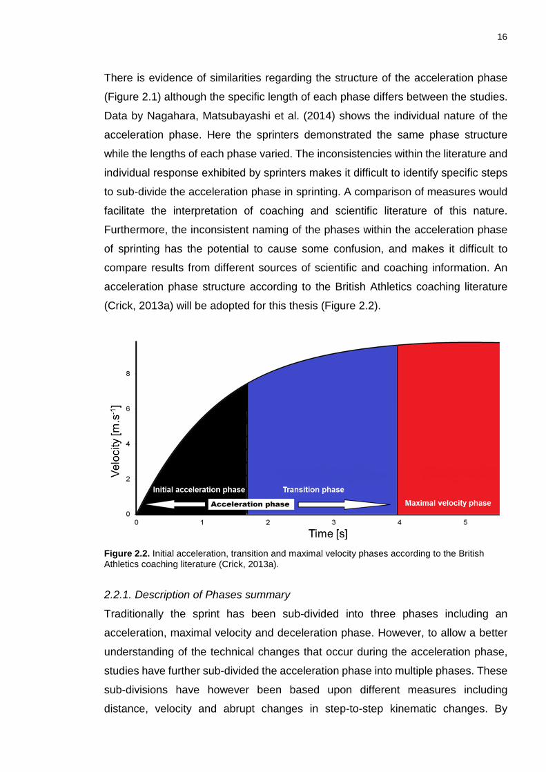
16

There is evidence of similarities regarding the structure of the acceleration phase

(Figure 2.1) although the specific length of each phase differs between the studies.

Data by Nagahara, Matsubayashi et al. (2014) shows the individual nature of the

acceleration phase. Here the sprinters demonstrated the same phase structure

while the lengths of each phase varied. The inconsistencies within the literature and

individual response exhibited by sprinters makes it difficult to identify specific steps

to sub-divide the acceleration phase in sprinting. A comparison of measures would

facilitate the interpretation of coaching and scientific literature of this nature.

Furthermore, the inconsistent naming of the phases within the acceleration phase

of sprinting has the potential to cause some confusion, and makes it difficult to

compare results from different sources of scientific and coaching information. An

acceleration phase structure according to the British Athletics coaching literature

(Crick, 2013a) will be adopted for this thesis (Figure 2.2).

Figure 2.2. Initial acceleration, transition and maximal velocity phases according to the British Athletics coaching literature (Crick, 2013a).

2.2.1. Description of Phases summary

Traditionally the sprint has been sub-divided into three phases including an

acceleration, maximal velocity and deceleration phase. However, to allow a better

understanding of the technical changes that occur during the acceleration phase,

studies have further sub-divided the acceleration phase into multiple phases. These

sub-divisions have however been based upon different measures including

distance, velocity and abrupt changes in step-to-step kinematic changes. By

Initial acceleration phase

Transition phase Maximal velocity phase

17

identifying abrupt changes in kinematics (i.e. breakpoint steps), the delimiting steps

of the initial acceleration, transition and maximal velocity phases can be determined

(Nagahara, Matsubayashi et al., 2014). However, there is still much uncertainty

regarding the appropriateness of the kinematic measures used in previous literature.

2.3 Sprint Technique Following is a review of the technique associated with sprinting. While the sprint

start must be considered an important factor contributing to the overall sprint (Jones

et al., 2009), the remainder of this review and thesis will only consider the portion

from block exit until maximal velocity.

2.3.1 Step Characteristics

2.3.1.1 Step Length and Step Frequency

Running velocity in sprinting is the product of step length and step frequency (Hay,

1994; Hunter, Marshall & McNair, 2004a) and the ratio between these vary between

the phases in sprinting and between individuals (Dyson, 1962). During the

acceleration phase, both step length and step frequency increase with increasing

running velocity (Cronin & Hansen, 2006; Maćkala, 2007). However, while step

frequency reaches a maximal value relatively quickly following block exit (Maćkala

2007; Debaere, Jonkers & Delecluse, 2013; Nagahara, Naito, Morin & Zushi, 2014;

Rabita et al., 2015), step length continues to increase during the transition, maximal

velocity and deceleration phases (Ae et al., 1992). During the deceleration phase,

Bezodis et al., (2011) found that the fastest sprinters of the sample tended to

increase step length while decreasing step frequency in an attempt to maintain their

step velocity. The relationship between step length and step frequency has been

described by many authors across an entire 100 m sprint (Salo et al., 2011), during

the acceleration phase (Hunter et al., 2004a; Maćkala, 2007; Nagahara, Naito,

Morin & Zushi, 2014; Debaere, Jonkers & Delecluse, 2013) and maximal velocity

phase (e.g. Gajer et al., 1999; Kuitunen, Komi & Kyröläinen, 2002; Bezodis, 2006).

There are some conflicting views of the relative importance of step length and step

frequency during the different phases of sprinting. Debaere, Jonkers & Delecluse

(2013) reported that with a homogenous group of high-level Belgian sprinters,

neither step length nor step frequency were found to be most influential to

18

acceleration in the initial acceleration and transition phases in sprinting. On the other

hand, when investigating the acceleration performance of participants ranging from

physical education students to elite sprinters, Morin, Bourdin, Eduard, Peyrot,

Samozino and Lacour (2012) reported that step frequency was significantly

correlated to acceleration performance. During maximal velocity sprinting, previous

studies have either identified step length (Gajer et al., 1999), step frequency

(Kuitunen et al., 2002) or neither (Debaere, Jonkers & Delecluse, 2013) as the most

influential variable on running velocity. Kuitunen et al. (2002) showed that when

increasing velocity from 70% to 100%, step frequency was the dominant factor,

while Gajer et al. (1999) found that once sprinters reach a certain level of proficiency,

step length was more important to further improve performance. These conflicting

results may be related to the level of participants in each study (e.g. Debaere et al.,

2013; Morin et al., 2012), or the grouping of the sprinters used in the studies (Salo

et al., 2011). Hunter et al. (2004a) also showed the influence of groupings on the

outcome of the investigation. The authors reported that on a group level, step length

was the determining variable while within individual differences showed step

frequency was higher during faster trials. This suggests the importance for

considering individual strategies during sprinting (Dufek, Bates, Stergiou & James,

1995).

Analysing the variation of step characteristics of elite male sprinters, Salo et al.

(2011) found that in a group of elite sprinters, athletes achieved their performance

via varying combinations of step length and step frequency. Furthermore, the

authors identified the reliance of some sprinters on either step length or step

frequency. This step characteristic reliance has since been suggested by other

research (e.g. Naito, Kariyama, Miyashiro, Yamamoto & Tanigawa, 2013;

Charalambous, Kerwin, Irwin, Bezodis & Hailes, 2011). Naito et al. (2013) analysed

the type-specific characteristics between sprinters during the acceleration phase of

sprinting. A cluster analysis was used to classify the participants as either step

length or step frequency reliant based on the ratio of step length and step frequency

during their maximal velocity phase (30-60 m). Although, 100 m performance did

not differ between the groups, the authors reported that throughout the acceleration

phase, step length reliant sprinters had significantly higher step lengths compared

to the step frequency reliant sprinters. Similarly, the step frequency reliant group

19

showed higher step frequencies throughout the sprint compared to the step length

reliant sprinters. Furthermore, the authors reported that within the step length and

step frequency reliant groups, the fastest sprinters within each of the groups showed

a higher step length or step frequency respectively, after the seventh step. They

concluded that the seventh step might represent an important breakpoint step in the

acceleration phase. Although reliance on either step length or step frequency was

previously found to be highly individual (Salo et al., 2011), the study by Naito et al.

(2013) suggests that this reliance is visible throughout the sprint. The step

characteristic reliance may have some important implications for training as

Charalambous et al. (2011) reported that developing athletes showed the largest

development of the step characteristic that they relied on when they started their

training block.

Previous studies have generally attempted to associate absolute step length and

frequency to sprinting performance. Recently, Nagahara et al. (2014a) studied the

association between acceleration and rates of change in step length and step

frequency in 21 male sprinters over 60 m. Nagahara et al. (2014a) found positive

correlations between acceleration and rates of change in step frequency up to step

two (r = 0.51–0.63). Between steps five to 19, acceleration was significantly

correlated to rate of change in step length (r = 0.45-0.72). Contrary to Debaere,

Jonkers & Delecluse (2013), who investigated the association between average

step length and step frequency to acceleration during the initial acceleration and

transition phase, Nagahara et al. (2014a) investigated the association between step-

to-step changes in step characteristics and acceleration. This may have contributed

to some of the different outcomes between the two studies. Nonetheless, Nagahara

and his colleagues concluded that the acceleration phase could be divided into three

phases based on the importance of step-to-step changes in either step frequency

or step length to the acceleration of the sprinters.

A negative interaction has previously been described between step length and step

frequency (Hunter et al., 2004a; Salo et al., 2011; Debaere, Jonkers & Delecluse,

2013; Nagahara, Naito, Morin & Zushi, 2014) where an increase in one variable

could negatively influence the development of the other variable. This is believed to

be due to the opposing mechanical requirements needed to develop each measure

20

(Hunter et al., 2004a). It is therefore important to consider the development of the

components of either step length or step frequency during the initial acceleration,

transition and maximal velocity phases of sprinting.

2.3.1.2 Components of step length

Step length can be considered the sum of three separate components (Hay, 1994).

These include the toe-off distance (the anterior-posterior distance between the

contact point and CM at toe-off), the flight distance (the anterior-posterior distance

the CM travel during flight) and touchdown distance (the anterior-posterior distance

between the contact point and the CM at touchdown). Together, the touchdown

distances and toe-off distances determine the contact length, which represents the

distance that the sprinters’ CM travels while in contact with the ground. The initial

acceleration phase is characterised by a negative contact distance as the foot

contacts the ground behind the CM (Mero et al., 1992; Nagahara, Matsubayashi et

al., 2014). During this phase, both touchdown distance and contact length have

been shown to increase relatively quickly compared to the transition phase

(Nagahara, Matsubayashi et al., 2014). During the transition phase, touchdown

distances continue to increase; however with smaller increments relative to the initial

acceleration phase (Table 2.1) while contact lengths plateaued (Nagahara,

Matsubayashi et al., 2014). During their maximal velocity phase, touchdown

distances started to plateau (Nagahara, Matsubayashi et al., 2014). Mann (2007)

reported that elite male and female sprinters tended to have a smaller touchdown

distance during maximal velocity (0.195 - 0.201 m) compared to average sprinters

(0.238 - 0.244 m).

Table 2.1. Change in touchdown distance throughout a sprint. Step Source Touchdown distance [m]

1 Mero et al., 1992 -0.13 2 Mero et al., 1992 -0.04 3 Mero et al., 1992 0.05

16 m Hunter et al., 2005 0.25 15 m Naito et al., 2015 0.20 60 m Ito, Fukada and Kijima, 2007 0.31

Maximal velocity Mann (2007) 0.195 -0.244

Less is known about the step-to-step changes of the toe-off distances. However this

variable is influenced by the inclination of the body and it is therefore expected that

toe-off distance decreases as the body becomes more upright (Hay, 1994). Flight

21

length, which during the maximal velocity phase contributes the largest portion to

step length (Hay, 1994), is expected to increase during each step following block

exit as CM height, running velocity and flight times increase (Hunter et al., 2004a).

Hunter et al. (2005) reported that minimising touchdown distance (contacting the

foot closer to the CM) leads to lower braking forces. As this variable increases during

the acceleration phase, it could be speculated that better performance during the

transition and maximal velocity phases could be achieved by minimising step-to-

step increases in touchdown distances.

2.3.1.3 Components of step frequency

Step frequency, which is the inverse of the step time, is composed of flight time and

contact time (Mann, 2007; Salo et al, 2011). Since step frequency reaches a plateau

early on following the start (Salo et al., 2011; Debaere, Jonkers & Delecluse, 2013),

total step time also does not change much during each step following the start

(Mann, 2007; Salo, et al., 2011). However, the components that make up step time

(i.e. flight and contact time; Figure 2.3) vary greatly during the sprint (Dyson, 1962;

Mann, 2007; Čoh & Tomazin, 2006).

Atwater (1982) 100m PB: 10.79 ± 0.21 s

Salo et al. (2005) 100m PB: 10.82 s

Čoh et al. (2006) 100m PB: 10.14 s

Slawinski et al. (2010) 100m PB: 10.27 ± 0.14 s

Slawinski et al. (2010) 100m PB: 11.31 ± 0.28 s

Hunter et al. (2004) (sprinters and team sports)

Mero and Komi (1987) PB: 10.62 ± 0.04

Kuitunen et al. (2002) PB: 10.91 ± 0.39 s

Figure 2.3. Contact (×) and flight times () during the initial acceleration, transition and maximal velocity phases from previous research in sprinting. Only studies that presented both flight and contact times were included.

Step 1 Step 2 Step 3 Step 4 Transition Max Vel0.02

0.06

0.10

0.14

0.18

0.22

Step

Tim

e [s

]

22

Previous published data shows that during the initial steps following block exit, step

times are dominated by contact times (Dyson, 1962; Salo, Keränen & Viitasalo,

2005; Mann, 2007; Čoh & Tomazin, 2006, Atwater, 1982). Čoh and Tomazin (2006)

reported that during the first and second step, contact time comprised 77.4% and

65.8% of the total step time. Between the eighth to the tenth step, flight times

equalled or exceeded contact times (Čoh & Tomazin, 2006). These results were

however based on a single sprinter and it is unclear how this relates to different

sprinters across different performance levels. As sprinters continue to progress

towards their maximal velocity, contact times decrease while flight times increase

(Qing and Krüger, 1995; Čoh & Tomazin, 2006; Debaere, Jonkers & Delecluse,

2013). Ballreich (1969) found that contact time decreased independent of sprinting

ability in the first 12 to 15 steps after which contact times stabilised. During maximal

velocity sprinting, contact times have plateaued (Atwater, 1982; Mero et al., 1992;

Debaere, Jonkers & Delecluse, 2013, Kuitunen et al., 2002; Mann & Herman, 1985;

Mann, 2007), but flight times continue to increase as step velocity increases

(Nagahara, Matsubayashi et al., 2014).

Theoretically, maximising propulsive impulses while minimising contact time could

be considered desirable (Charalambous, 2012). The longer contact times during the

initial portion of the race could allow sprinters to take advantage of their strength

capabilities (Mann, 2007) and produce a large propulsive impulse during ground

contact. This would benefit the development of the sprinters’ contact length, as a

longer contact time would allow the sprinters’ CM to travel further during ground

contact. This is partly supported by Kugler and Janshen (2010), who reported that

during the first step faster athletes exhibited a strategy involving a longer contact

time. This allowed their CM more time to move farther forward relative to their

contact point and therefore generate higher propulsive forces (Kugler & Janshen,

2010). Therefore, it might seem advantageous to maximise performance by

increasing contact times and minimising flight times as this could allow a sprinter

greater opportunity to accelerate during the initial acceleration phase. However,

given the negative interaction between step length and step frequency (e.g.

Debaere, Jonkers & Delecluse, 2013) and the influence of the step-to-step changes

in step frequency on the acceleration of the sprinter over the first three steps

23

(Nagahara et al, 2014a), the strategy of maximising performance by increasing

contact times may be detrimental to performance across multiple steps.

Performance during the transition and maximal velocity phases and across the

whole sprint was previously associated with lower ground contact times (Weyand et

al., 2000; Morin et al., 2012; Debaere, Jonkers & Delecluse, 2013). Nagahara et al.

(2014a) reported that the rate of decrease of contact times between steps 11 and

16 and the rate of increase in flight times between steps 8 to 10 were associated

with larger acceleration performances. While the decreasing contact time influenced

the contact length of the sprinter, the increasing flight times during the transition

phase would benefit the continued increase in step length by increasing the flight

length component of step length.

2.3.1.4 Summary of step characteristics

The step velocity of a sprinter is dependent on the step length and the step

frequency. However, these two components of running velocity are negatively

related due to the different mechanisms required to develop them (Hunter et al.,

2004a). While step frequency increases relatively quickly over the first couple of

steps (e.g. Debaere, Jonkers & Delecluse, 2013) and then plateaus during the

transition and maximal velocity phases, step length has been shown to increase

throughout the different phases of a sprint (Ae et al., 1992). These patterns can be

better understood when investigating the changes in the components underlying

step length (i.e. contact length and flight length) and step frequency (i.e. contact

time and flight time).

2.3.2 Segment and Joint kinematics

The orientation of the CM relative to the ground plays an important role in sprinting

(di Prampero, Fusi, Sepulcri, Morin, Belli & Antonutto, 2005). Di Prampero et al.

(2005) showed that the angle between the line connecting the ground contact point

and the CM relative to the ground (CM_angle) is dependent on the anterior-posterior

and vertical acceleration of the sprinter. Furthermore, Kugler and Janshen (2010)

reported that faster sprinters achieved superior acceleration performances by

achieving a lower CM angle during stance (i.e. less inclined). Since the angle of the

CM depends on the position of the different segments, changing segment

24

orientations therefore play an important role in influencing step-to-step changes in

external ground reaction forces during sprinting.

During any running action, each leg cycles though a stance and a swing phase. The

function of the swing phase is to reposition the limbs so that force can effectively be

applied during the subsequent stance phase (Crick, 2013c). Although this thesis will

focus mainly on the stance phase in sprinting, a short description of the swing phase

is presented next. Regarding the mechanics of the swing phase, most of the

literature exists within coaching texts and education resources. The swing phase

can be sub-divided into a residual phase, recovery phase and the ground

preparation phase (Crick, 2013c). The residual phase is defined as the time between

toe-off and when the thigh begins to move forwards relative to the CM. The recovery

phase starts when the thigh starts to move forward until maximum hip flexion is

reached, while the ground preparation phase starts after maximum hip flexion is

achieved and ends at touchdown (Crick, 2013c). The whole recovery action is

initially characterised by a low repositioning of the leg (measured by the height of

the foot relative to the ground) during the initial acceleration phase. Throughout the

acceleration phase, the foot and thigh are gradually recovered higher (increase foot

ground distances and smaller hip flexion angles and the end of the recovery phase)

with each successive step (Crick, 2013e). The majority of previous research tended

to agree that during the maximal velocity phase, faster sprinters exhibited increased

knee flexion as the swing leg thigh passed the midline of the body during recovery

(Mann & Herman, 1985; Mann, 2007; Ito et al., 2007). Furthermore, sprinters

generally achieve a higher knee elevation at the end of the recovery phase (Mann,

2007; Crick, 2013c). This is thought to aid the sprinter in accelerating the foot down

and backwards relative to the CM during the ground preparation phase (Mann,

2007; Crick, 2013c). A high knee lift at the end of the recovery phase is however not

a precursor to a fast swing back velocity of the leg relative to the CM prior to ground

contact. Ae et al. (1992) reported that two elite sprinters achieved a similar swing

back velocity although one achieved a knee lift comparable to those of university

level sprinters.

During the ground preparation phase, previous studies show that faster sprinters

are able to sufficiently minimise the forward velocity of the foot prior to touchdown

25

(i.e. generate a larger negative forward foot velocity relative to the CM) (Mann &

Herman, 1985; Ae, Ito & Suzuki, 1992; Hunter et al., 2005; Mann, 2007). Further,

well-trained sprinters are able to better accelerate the foot down into the ground at

higher velocities (Clark, Laurence, Ryan & Weyand, 2014). The anterior-posterior

and vertical foot velocity prior to touchdown have previously been linked to braking

(Hay, 1994; Hunter, Marshall & McNair, 2005) and vertical (Clark et al., 2014a) force

production following touchdown. This will be discussed in more detail within section

2.3.3.

Throughout the initial acceleration, transition and maximal velocity phases, large

changes in kinematics have previously been observed (Table 2.2). These changes

are characterised by sprinters gradually becoming upright and contacting the ground

further ahead of their CM (Mann, 2007; Debaere, Jonkers & Delecluse, 2013;

Nagahara, Matsubayashi et al., 2014; Crick, 2013a). During the initial acceleration

phase, relatively large increases in CM velocity occur with each touchdown

compared to the transition and maximal velocity phases (Delecluse et al., 1995). As

sprinters approach the end of initial acceleration phase, they will have reached

about 80% of their maximal velocity (Crick, 2013e) and by the end of the transition

phase, the sprinters should have reached 95% of their maximal velocity (Crick,

2013f). The relatively large step-to-step increase in velocity during the initial

acceleration phase is aided by the less inclined posture resulting in a smaller CM

angle. Theoretically, this would therefore require larger forward acceleration of the

CM to maintain postural equilibrium (di Prampero et al., 2005).

The position of the CM relative to the foot is determined by the orientations of the

segments of the limbs and the trunk. The British Athletics coaching literature

suggests that during the initial acceleration phase, the shank exhibits angles less

than 90° at touchdown (Crick, 2013a) and increases between 6 to 8° per step (Crick,

2013e). While Crick (2013e) suggests that the smaller shank and CM angles during

the initial acceleration phase are important to generate large propulsive forces, large

step-to-step increases step-to-step increases in shank angles may reflect and

increasing need to generate larger vertical forces and facilitate increases in flight

times (Crick, 2013e). However, large step-to-step increases (i.e. >8° per step) in

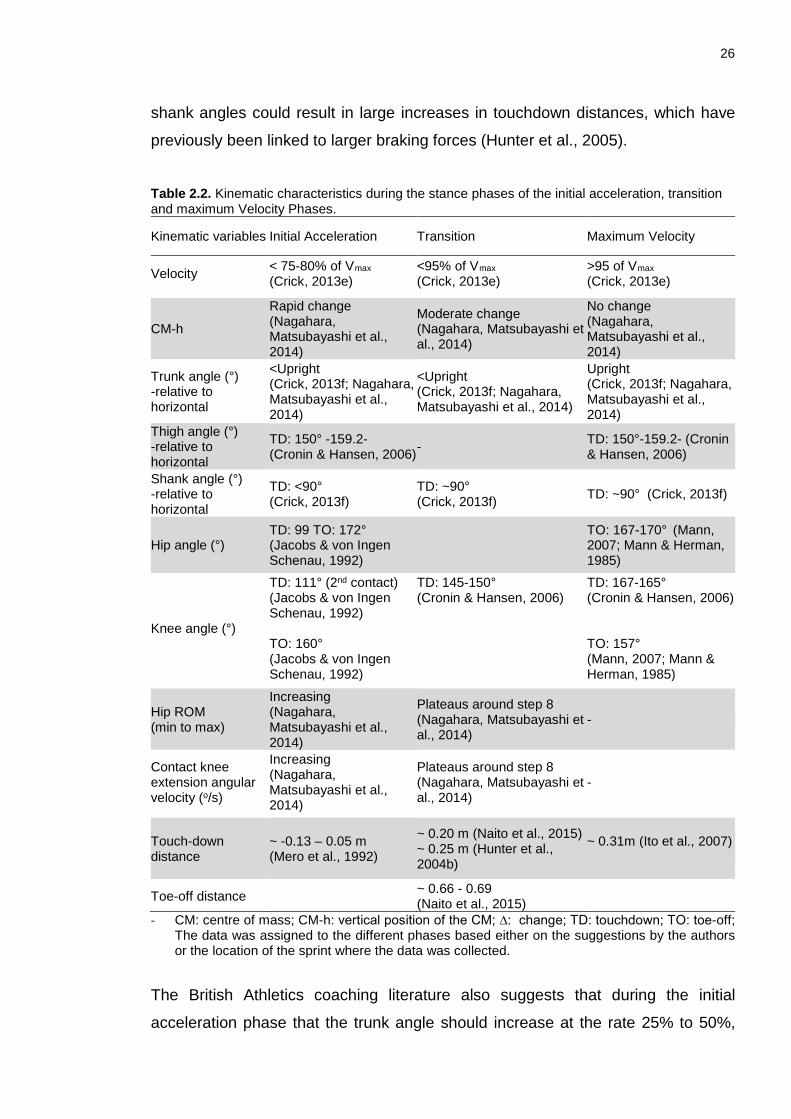
26

shank angles could result in large increases in touchdown distances, which have

previously been linked to larger braking forces (Hunter et al., 2005).

Table 2.2. Kinematic characteristics during the stance phases of the initial acceleration, transition and maximum Velocity Phases.

Kinematic variables Initial Acceleration Transition Maximum Velocity

Velocity < 75-80% of Vmax (Crick, 2013e)

<95% of Vmax (Crick, 2013e)

>95 of Vmax (Crick, 2013e)

CM-h

Rapid change (Nagahara, Matsubayashi et al., 2014)

Moderate change (Nagahara, Matsubayashi et al., 2014)

No change (Nagahara, Matsubayashi et al., 2014)

Trunk angle (°) -relative to horizontal

<Upright (Crick, 2013f; Nagahara, Matsubayashi et al., 2014)

<Upright (Crick, 2013f; Nagahara, Matsubayashi et al., 2014)

Upright (Crick, 2013f; Nagahara, Matsubayashi et al., 2014)

Thigh angle (°) -relative to horizontal

TD: 150° -159.2- (Cronin & Hansen, 2006) -

TD: 150°-159.2- (Cronin & Hansen, 2006)

Shank angle (°) -relative to horizontal

TD: <90° (Crick, 2013f)

TD: ~90° (Crick, 2013f) TD: ~90° (Crick, 2013f)

Hip angle (°) TD: 99 TO: 172° (Jacobs & von Ingen Schenau, 1992)

TO: 167-170° (Mann, 2007; Mann & Herman, 1985)

Knee angle (°)

TD: 111° (2nd contact) (Jacobs & von Ingen Schenau, 1992) TO: 160° (Jacobs & von Ingen Schenau, 1992)

TD: 145-150° (Cronin & Hansen, 2006)

TD: 167-165° (Cronin & Hansen, 2006) TO: 157° (Mann, 2007; Mann & Herman, 1985)

Hip ROM (min to max)

Increasing (Nagahara, Matsubayashi et al., 2014)

Plateaus around step 8 (Nagahara, Matsubayashi et al., 2014)

-

Contact knee extension angular velocity (o/s)

Increasing (Nagahara, Matsubayashi et al., 2014)

Plateaus around step 8 (Nagahara, Matsubayashi et al., 2014)

-

Touch-down distance

~ -0.13 – 0.05 m (Mero et al., 1992)

~ 0.20 m (Naito et al., 2015) ~ 0.25 m (Hunter et al., 2004b)

~ 0.31m (Ito et al., 2007)

Toe-off distance ~ 0.66 - 0.69 (Naito et al., 2015)

- CM: centre of mass; CM-h: vertical position of the CM; ∆: change; TD: touchdown; TO: toe-off; The data was assigned to the different phases based either on the suggestions by the authors or the location of the sprint where the data was collected.

The British Athletics coaching literature also suggests that during the initial

acceleration phase that the trunk angle should increase at the rate 25% to 50%,

27

slower than that of the shank angle (Crick, 2013e), so that the trunk angle of 45° to

55° degrees by the end of the initial acceleration phase (Crick, 2013e). The

step-to-step changes in the orientations of the segments of the stance leg at

touchdown and toe-off during the initial acceleration, transition and maximal velocity

phases within a group of sprinters have however not yet been quantified.

The initial acceleration phase is also characterised by relatively large step-to-step

increases in vertical position of the CM-h compared to the transition phase

(Nagahara, Matsubayashi et al., 2014). This increase during the initial acceleration

phase can be attributed to increases in hip height as stance limb mechanics change

(Nagahara, Matsubayashi et al., 2014). Further increases in CM-h during the

transition phase are attributed to continued step-to-step increases in trunk and head

angles (Nagahara, Matsubayashi et al., 2014). Once an upright posture is reached,

which is characteristic of the maximal velocity phase (Crick, 2013f; Nagahara,

Matsubayashi et al., 2014), changes in CM-h, trunk angle and head angle plateau.

Apart from influencing the position of the CM, the orientation of the segments play

an important role in their potential to contribute to the anterior-posterior velocity of

the CM. The contribution of the rotational kinematics of segments to linear velocity

of the CM are governed by geometrical constraints (van Ingen Schenau, Bobbert &

Rozendal, 1987; Bobbert & van Ingen Schenau, 1988). The contribution of a

segments angular motion to the translation of the CM depends on the segments

angular velocity and orientation (Jacobs & van Ingen Schenau, 1992). The proximal

to distal sequencing would ensure that maximum joint angular velocities are reached

as their respective segments approach a vertical orientation, therefore maximising

the contribution to the anterior-posterior translation of the CM (Jacobs & von Ingen

Schenau, 1992).

Based the geometric constraint theory (van Ingen Schenau et al., 1987), Nagahara,

Matsubayashi et al. (2014) calculated the contributions to CM velocity by the relative

anterior-posterior velocity of the segments. The relative anterior-posterior segment

velocity was calculated by subtracting the distal anterior-posterior velocity of the

foot, shank and thigh from the proximal anterior-posterior velocity of the respective

segment. The authors reported that, step-to-step increases in the relative anterior-

28

posterior velocity of the thigh and shank contributed to the relatively large increases

in CM velocity associated with the initial acceleration phase (Nagahara,

Matsubayashi et al., 2014). Throughout the transition phase, step-to-step increases

in CM velocity were supported by the step-to-step increases in the relative anterior-

posterior velocity of the thigh, shank and foot (Nagahara, Matsubayashi et al., 2014).

During the maximal velocity phase, further increases in the relative anterior-

posterior velocity of the foot and shank contributed to the relatively small increases

in CM velocity (Nagahara, Matsubayashi et al., 2014). Nagahara, Matsubayashi et

al. (2014) concluded that these results suggest a change in acceleration strategy

throughout the acceleration phase in sprinting.

During all stance phases in sprinting, consistent ankle and hip joint kinematic

patterns have been observed (Jacobs & van Ingen Schenau, 1992; Charalambous

et al., 2012; Bezodis, Salo & Trewartha, 2014; Nagahara, Matsubayashi et al.,

2014). At the knee joint, an extension pattern was exhibited throughout stance

during the initial acceleration phase (Charalambous et al., 2012; Bezodis et al.,

2014; Nagahara, Matsubayashi et al., 2014). This changed to a flexion-extension

pattern during the transition and maximal velocity phases (Hunter et al., 2004c;

Johnson & Buckley, 2001; Bezodis et al., 2008; Nagahara, Matsubayashi et al.,

2014). The flexion to extension pattern at the knee has recently been shown to occur

from step four onwards (Nagahara, Matsubayashi et al., 2014).

Regarding joint angular velocities, a proximal to distal sequencing of the lower limb

joint angular velocities has generally been reported throughout the sprint (Johnson

& Buckley, 2001; Hunter et al., 2004c; Bezodis et al., 2008; Charalambous et al.,

2012) where peak extension angular velocity is reached by the hip first followed by

the knee and finally the ankle joint. Ae et al. (1992) and Ito, Fukuda and Kijima

(2007) found that faster sprinters displayed higher hip extension velocities (r=0.284,

p<0.05, Ito et al., 2007). Mann and Herman (1985) reported a similar trend in hip

extension velocities during the final of the 200 m of the 1984 Summer Olympics.

They reported that the gold and silver medallist displayed higher hip extension

velocities during ground contact than the 8th place finisher. Regarding knee

extension velocities, Ito et al. (2007) reported that faster sprinters tended towards

lower knee extension velocities (r = -0.407, p<0.1) while some even exhibited a knee

29

flexor angular velocity throughout stance. Ito et al. (2007) suggested that if the knee

remains fixed during stance, 100% of the hip extension could be converted to a

clockwise rotation of the leg. However, if the knee flexes during stance (as the case

with some elite sprinters) the velocity transferred down the leg could exceed the

velocity created by the hip extension alone. In this case, the clockwise angular

velocity of the thigh generated by the hip musculature and the clockwise angular

velocity of the shank will result in an increased clockwise rotation of the whole leg.

2.3.2.1 Summary of segment and joint kinematics

The orientation of the segments not only dictate the CM angle which is

mathematically linked to CM acceleration (di Prampero, 2005), but also influence

the conversion of angular segmental motion to the translation of the CM (van Ingen

Schenau et al., 1987). Due to the dynamic nature of the acceleration phase in

sprinting, relatively large changes in segment orientation can be expected to occur.

Although studies exist describing kinematic changes (e.g. Nagahara, Matsubayashi

et al., 2014) across multiple steps within the acceleration phase, a detailed

description of the step-to-step changes in segment orientations (especially of the

stance leg) is still lacking. This would complement the work of Nagahara,

Matsubayashi et al. (2014) and provide coaches and applied scientists a better

understanding of how variables that are more visually accessible change during the

initial acceleration, transition and maximal velocity phases.

2.3.3 External Kinetics

Hunter et al. (2005) suggested that for analysis purposes, the GRF can be broken

down into its three orthogonal components (vertical, anterior-posterior and

medio-lateral). The anterior-posterior component has been further sub-divided into

braking and a propulsive force. During the braking phase, the body’s CM velocity

decreases due to the negative anterior-posterior ground reaction force applied to

the sprinter’s foot by the ground (Hay, 1994). The velocity of the CM then increases

again during the subsequent propulsive phase. Although many studies have

reported ground reaction forces in sprinting, these have generally focused on single

or multiple steps from the initial acceleration phase, transition phase or maximal

velocity phase (Table 2.3). This makes it difficult to identify changes between steps

from different phases in maximal sprinting. Few studies have reported multiple steps

30

from different phases. Yu, Sun, Chen Yang, Wang, Yin, Herzog and Liu (2016)

reported external kinetics from one step from the transition and maximal velocity

phases. Rabita et al. (2015) investigated the determinants of maximal sprinting

acceleration over multiple steps of a 40 m ‘virtual’ sprint. Furthermore, a recent pilot

study was publish in abstract form that detailed external kinetics over 25 successive

steps (Nagahara, Mizutani & Matsuo, 2016).

From the literature, the braking phase as a proportion of the whole contact changes

increased as the sprint progressed. During the initial acceleration phase previous

studies reported braking phases lasting 6 -13% of ground contact (Mero et al., 1992;

Salo et al., 2005). This increased to 32% during the transition phase (Yu et al., 2016)

and 40 – 48% during maximal velocity (Mero & Komi, 1988; Bezodis, 2006; Yu et

al., 2016). The peak braking forces expressed in body weights also increased from

the initial acceleration phase (~ -0.06 to -0.71 BW; Mero 1987; Bezodis et al., 2014)

to the transition (~ -0.67 ± 0.25 BW; Yu et al., 2016) and maximal velocity phases

(~ -0.91 to -1.30 BW; Bezodis, 2006; Yu et al., 2016).

When comparing propulsive forces reported in previous literature, it appears that

peak forces decrease from the initial acceleration, transition and maximal velocity

phase (Table 2.3). During the first step, propulsive forces were previously measured

at 1.04 -1.31 BW (Bezodis et al., 2014). By the time sprinters reached their maximal

velocity, propulsive forces decreased to 0.68 – 0.91 BW (Bezodis, 2006).

Interestingly, Yu et al. (2016) found no significant (p=0.063) differences between the

peak forces generated during a step from the transition (0.90 ± 0.11 BW) and

maximal velocity (0.88 ± 0.13 BW) phases.

31

Table 2.3. External kinetics during initial acceleration, transition and maximal velocity. Kinetics Initial Acceleration Transition Maximum Velocity

Braking phase

Duration: ~11% (Mero, 1988)

Duration: 32 ± 8% (Yu et al., 2016)

Duration: ~43 - 44% (Mero et al., 1987)

~40 – 48% (Bezodis, 2006)

43 ± 3% (Yu et al., 2016)

Peak force: -0.6 BW (Mero, 1988)

-0.1 to - 1.2 BW (Bezodis et al., 2014)

Peak force:

-0.7 ± 0.3 BW (Yu et al., 2016)

Peak force: -0.9 to -1.3 BW (Bezodis, 2006)

-1.3 ± 0.2 BW (Yu et al., 2016)

∆ velocity: -0.04 m·s-1 (Mero, 1988)

-0.02-0.06 m·s-1 (Salo et al., 2005)

∆ velocity: -0.10 m·s-1 (Hunter et al, 2005)

-0.09 m·s-1 (Yu et al., 2016)

∆ velocity:

-0.19 m·s-1

(Yu et al., 2016)

Propulsion phase

Duration: ~ 89% (Mero et al., 1987)

Duration: 68 ± 8 % (Yu et al., 2016)

Duration: 56 – 57 % (Mero et al., 1987)

52 - 60% (Bezodis, 2006)

57 ± 3% (Yu et al., 2016)

Peak forces: 1.0 -1.3 BW (Bezodis et al., 2014)

Peak forces: 0.90 ± 0.11BW (Yu et al., 2016)

Peak forces: 0.42 BW (Mero et al., 1992)

0.68 – 0.91 BW (Bezodis, 2006)

0.88 ± 0.13 BW (Yu et al., 2016)

∆ velocity: 1.16-0.56m·s-1 (Salo et al., 2005)

∆ velocity: 0.25 m·s-1 (Hunter et al., 2005)

0.41 m·s-1 (Yu et al., 2016)

∆ velocity:

0.29 m·s-1 (Yu et al., 2016)

Vertical

Peak force: 1.1 BW (Mero, 1988)

1.9 -2.3 BW (Bezodis et al., 2014)

Peak force:

3.3 ± 0.5 BW (Yu et al., 2016)

Peak force: 3.6 – 4.4 BW (Bezodis, 2006)

4.0 ± 0.5 BW (Yu et al., 2016)

- ∆ velocity: 0.99 m·s-1

(Hunter et al., 2005)

∆ velocity: 1.11 - 1.27 m·s-1 (Bezodis, 2006)

- ∆: change in; The data in this table was taken from various sources. When not presented in the format used in this thesis the values were adjusted based on the participants mass. The Yu et al. (2016) data is the only direct comparison between phases from the same study.

32

The sum of the impulses (force × time) created by these braking and propulsive

forces determine the change in velocity of the CM. In the first four steps of a sprint,

Salo et al (2005) reported that net anterior-posterior impulses decreased from about

92 Ns (or a 1.16 m·s-1 increase in velocity) to 44 Ns (0.56 m·s-1) between step one

and four. Around the 14 m mark, Johnson and Buckley (2001) reported a net

anterior-posterior impulse of 19.5 Ns (0.28 m·s-1) while Hunter et al. (2005) reported

that net anterior-posterior impulse was about 18 Ns (0.25 m·s-1) 16 m from the start.

During the maximal velocity phase, the net anterior-posterior impulse was previously

reported as 3.9 to 10.8 Ns or 0.06 to 0.13 m·s-1 (Bezodis, 2006). Morin, Slawinski,

Dorel, de Villareal, Courtier, Samozino, Brughelli and Rabita, (2015) reported that

the mean anterior-posterior impulse between 0 to 20 m was 64.1 ± 9.03 Ns (0.805

± 0.061 m·s-1). Between 20 to 40 m, the mean anterior-posterior impulse decreased

to 10.6 ± 2.9 Ns (0.132 ± 0.030 m·s-1) (Morin et al., 2015). Nagahara et al., (2016)

showed that while decreasing propulsive and increasing braking impulse

contributed to decreasing net anterior-posterior impulses up to around step 15 of a

maximal sprint that increases in braking impulses after step 15 were the main factor

resulting in a decreased anterior-posterior impulse.

The sprint literature agrees that a sprinters’ performance during the initial

acceleration and transition phase is determined by the net anterior-posterior and

propulsive impulses applied during ground contact (Mero, 1987; Hunter et al., 2005;

Kawamori, Nosaka & Newton, 2013; Morin et al., 2015). Furthermore, the authors

generally reported that braking impulses were not significantly correlated to

performance (Hunter et al., 2005; Kawamori et al., 2013 Morin et al., 2015).

However, when performing a multiple regression analysis, Hunter et al. (2005)

reported that although propulsive impulses accounted for 57% of the differences

they observed, a small amount (7%) was attributed to the differences in braking

impulses, although the authors could not rule out whether faster sprinters decreased

braking forces.

Morin et al. (2015) distinguished between braking and propulsive impulses over

multiple steps. This study was an extension of the Rabita et al. (2015) study

(discussed later) to investigate the relationship between net anterior-posterior,

braking, propulsive and vertical impulses over multiple steps to acceleration

33

performance (i.e. mean 40 m velocity). The authors reported that net anterior-

posterior impulse and propulsive impulse were significantly correlated to the 40 m

velocity (r= 0.868, p<0.01 and r=0.802, P<0.01) while braking impulse was not. They

also found that when splitting the 40 m sprint into two sections (i.e. 0-20m and

20-40 m), that average propulsive impulses over 0-20 m were significantly

correlated (r = 0.833, P<0.02) with 40 m performance while 20-40 m data was not.

The authors concluded that these result shows that faster sprinters had larger

propulsive impulses but not necessarily lower braking impulses than slower ones.

Furthermore, the fact that the mean data over the 0-20 m distance correlated

strongly with performance while the data over the 20-40 m distance did not show

the importance of generating as much anterior-posterior impulse as possible during

the initial steps a sprint (Morin et al., 2015). While the study did not find any

significant correlations between the performance variable and braking forces, the

study highlighted that step-to-step decreases in net anterior-posterior impulse over

the first six to seven steps were mainly due to decreases in the propulsive impulse,

while between steps nine to 11 braking impulses were responsible for the larger

decreases in net anterior-posterior impulse. This conclusion was recently supported

by Nagahara, Mizutani, Matsuo, Kanehisa & Fukunaga (2017a) who reported that

larger propulsive impulses provided a significant contribution to acceleration

performance between 55% to 95% of maximal velocity while smaller braking

impulses significantly influenced acceleration performance between 75% to 95% of

maximal velocity (from 7.5 ± 0.6 m into a sprint). This may suggest that during the

acceleration phase sprinters should attempt to maximise propulsive impulses during

the initial acceleration phase and then focus on minimising braking impulses during

the transition and maximal velocity phases.

The results of Hunter et al. (2005) and Kawamori et al. (2013) suggest that during

the early steps of a sprint, braking and vertical impulse generated are not as

influential to performance compared to the net anterior-posterior or propulsive

forces. The studies by Morin et al. (2015), Yu et al. (2016), Nagahara et al. (2016)

and Nagahara, Naito, Morin & Zushi, 2014 however suggest that braking impulse

may present a limiting factor to further increases in velocities at higher running

velocities. Furthermore, although it has been accepted that braking forces are

necessary in sprinting (e.g. storage of elastic energy) (Cavagna, Komarek &

34

Mazzoleni, 1971; Hunter et al., 2005), various authors have suggested that these

forces should be minimised to improve sprint performance (Mero et al., 1992; Hay,

1994; Hunter et al., 2005). Previous literature has suggested that the anterior-

posterior foot velocity prior to touchdown is the main contributor to the braking forces

(Hay, 1994) and it is suggested that sprinters should aim to minimise the forward

velocity of the foot immediately prior to touchdown (Mann & Sprague, 1983). Hunter

et al. (2005) showed that during the transition phase in sprinting, smaller forward

velocities of the foot prior to touchdown were associated with lower braking forces.

While even world-class sprinters have some amount of forward foot velocity (Mann,

2007) faster sprinters are generally able to reduce the forward foot velocities more

than slower sprinters (Ae et al., 1992; Mann, 2007). There is however still a lack of

evidence linking the velocity of the foot prior to touchdown to braking forces.

Although previous studies only found weak (Hunter et al., 2005) or non-significant

(Kawamori et al., 2013; Morin et al., 2015) relationships between vertical impulse

and sprint performance during the acceleration phase. Interestingly, Nagahara et al.

(2017a) reported that during the acceleration phase (<95% maximal velocity)

smaller vertical impulses were associated with better acceleration performances.

These results further support the suggestion by Hunter et al. (2005) that sprinters

need to apply the necessary vertical impulse to overcome gravity and prepare for

the next flight phase, with larger vertical impulses leading to longer flight times and

therefore lower step frequencies (Nagahara, Mizutani, Matsuo, Kanehisa &

Fukunaga, 2017a). The ever-decreasing contact times as running velocities,

increase means that there is an increased demand to generate higher magnitudes

of vertical ground reaction forces (Weyand et al., 2000; Weyand et al., 2010

Nagahara et al., 2017a). Nagahara et al., (2017a) showed that although vertical

impulses did not change much during the acceleration phase, the mean vertical

force applied during ground contact increased throughout the acceleration phase.

Although producing relatively high levels of anterior-posterior force as velocities

increase is essential to continue to increase running velocity (Rabita et al., 2015),

the requirement to produce larger ground reaction forces during short contact times

may represent a further limiting factor for some sprinters to maximise their running

velocities (Weyand et al., 2000; Weyand et al., 2010). Furthermore, sprinters have

unique GRF profiles compared to non-sprinters (Clark & Weyand, 2014). Clark and

35

Weyand (2014) found that sprinters attained higher maximal velocities by applying

significantly greater vertical forces during the first half of stance (2.65 ± 0.05 BW vs.

2.21 ± 0.05 BW) while there were no differences during the second half of stance

(1.71 ± 0.04 BW vs. 1.73 ± 0.04 BW). This could be attributed to their ability to

produce higher downward foot velocities prior to touchdown (Clark & Weyand,

2014). This is possibly aided by the higher knee lift generally achieved by better

sprinters at the end of the recovery phase of swing (Mann, 2007).

To quantify a sprinter’s ability to orientate ground reaction forces more horizontally,

Morin, Eduard and Samozino (2011) proposed a measure quantifying the ratio of

force application (RF) as the ratio of the anterior-posterior to resultant force during

ground contact. Later, Morin et al. (2012) reported that a sprinter’s dominance

during sprint acceleration is not necessarily a result of the magnitude of the forces

they can apply but rather a technical ability to properly direct forces during ground

contact. The authors found that athletes with better acceleration ability produced

more horizontally directed force with respect to the resultant force (larger RF) during

a maximal sprint acceleration on a motorised treadmill. The mean RF value obtained

from the treadmill was also a stronger determinant of the athletes’ 100 m

performance while the magnitudes of either vertical or resultant ground reaction

forces were not. Rabita et al. (2015) later confirmed these results when investigating

the mechanics of over ground maximal sprinting by constructing a virtual 40 m sprint

by combining data from steps collected over multiple trials.

Morin et al., (2012) also suggested an index of force application technique (DRF).

This was based on the slope created by individual RF values plotted over time. A

steep slope or high DRF means that a desired RF was not maintained while a flat

RF-velocity relationship or small DRF indicates a technical ability to maintain a

desired RF ratio. This DRF index revealed a further characteristic of world-class

sprinters. It was reported that world-class sprinters have the ability to apply greater

anterior-posterior forces at higher velocities (Morin et al., 2012; Rabita et al., 2015).

This increased ability to produce greater anterior-posterior forces during higher

sprinting velocities was found to be significantly correlated to their technical ability

(a high RF) to direct the resultant ground reaction force vector more horizontally

(Morin et al., 2012; Rabita et al., 2015).

36

Force application ability has been highlighted as an important characteristic of elite

sprinters (e.g. Morin et al., 2012; Rabita et al., 2015). It was speculated that an

increased hip extension and the ankle plantar flexors are important contributors to

a better orientation of the resultant GRF vector (Rabita et al., 2015). Furthermore,

various authors (e.g. Mann & Sprague, 1980; Wiemann & Tidow, 1995) proposed

the theory that a clockwise rotation of the thigh generated by powerful hip extension

is an important contributor to large anterior-posterior GRF production. The “hip

extension theory” (Hunter et al., 2004c, p. 1445) could however not be supported by

work from Hunter et al. (2004c) and Kugler and Janshen (2010). While Hunter et al.

(2004c) showed that during the first half of stance, the hip extensor moment was the

main contributor to the clockwise rotation of the thigh. Anterior-posterior ground

reaction forces during this time were however generally low (Hunter et al., 2004c).

Kugler and Janshen (2010) reported that at similar CM angles, faster sprinters did

not generate larger propulsive forces than slower sprinters. This may be linked to a

constraint that requires the sum of the moments about the CM to be zero, therefore

ensuring postural stability throughout ground contact (Kugler & Janshen, 2010).

Faster sprinters were able to achieve small CM angles and therefore larger

anterior-posterior forces towards toe-off (Kugler & Janshen, 2010). This finding by

Kugler and Janshen (2010) aligns with the mechanical relationship between CM

acceleration and CM angle described by di Prampero et al. (2005). These results

suggest the importance of the orientation of the body in sprinting.

2.3.3.1 Summary of external kinetics

The net anterior-posterior and propulsive impulse are the main determinants of

acceleration ability during the initial acceleration and transition phases. Recent

studies have shown that world class sprinters have a better technical ability to

maintain a higher ratio of anterior-posterior to vertical ground reaction force

throughout the acceleration phase compared to athletes with similar physical

capabilities (Morin et al., 2011; Rabita et al., 2015). As sprinters accelerate from

lower velocities to higher velocities, performance is influenced by the sprinters’

ability to continue to produce a net anterior-posterior propulsive force (Rabita et al.,

2015) while producing sufficiently large vertical forces to provide an appropriate

flight time to allow the sprinter to prepare for the next stance phase (Hunter et al.,

2005). However, vertical force production at higher velocities could be considered a

37

limiting factor as sprinters need to be able to generate sufficiently large vertical

impulse during short ground contact times in order to maximise running velocities

(Weyand et al., 2000). Evidence from recent literature suggests that the orientation

of the body plays an important role in the performance of a sprinter during the

acceleration phase in sporting.

2.3.3 Musculoskeletal aspects of technique

2.3.3.1 Joint Kinetics

So far, the literature review has presented kinematic and external kinetic data of the

initial acceleration phase, transition phase and maximal velocity phase of a sprint.

While this provides a description of the motion of a sprinter, the translation of the

CM is ultimately driven by forces acting around the joints of the body (Jacobs & van

Ingen Schenau, 1992). A joint kinetic analysis has the potential to provide a more

in-depth understanding of muscle actions across a joint (Winter, 2009). Joint kinetics

have previously been presented for step one (Charalambous et al., 2012; Debaere,

Delecluse et al., 2013; Bezodis et al., 2014; Brazil, Exell, Wilson, Willwacher,

Bezodis & Irwin, 2016), step two (Jacobs & von Ingen Schenau, 1992; Debaere,

Delecluse et al., 2013), 12 m (Yu et al., 2016), ~ 14 m (Hunter et al., 2004c; Yu),

~35 m (Johnson & Buckley, 2001) and the maximal velocity phase (Bezodis et al.,

2008; Yu et al., 2016). The following section will provide a review of the current

literature regarding joint kinetics in sprinting. The first joint that will be discussed is

the metatarsophalangeal (MTP) joint, followed by the ankle, knee and hip joints.

However, since not all previous research have presented their data using the same

units, the joint moment and joint power data from previous studies were adjusted to

dimensionless values according to methods outlines by Hof (1996) and Bezodis,

Salo & Trewartha (2010). This was achieved by using the mean participant height

and mass data presented in each individual study.

With the MTP being closest joint to the ground it is exposed to large external forces

and is therefore be considered an important contributor to the overall power output

of the leg (Stefanyshyn & Nigg, 1997). Despite this few authors (Elftman, 1940;

Stefanyshyn & Nigg, 1997; Smith, Lake & Lees, 2014; Bezodis et al., 2014) have

investigated the joint kinetics of the MTP joint in sprinting. Generally, a plantar flexor

moment has been observed at this joint during the first step of a sprint (Bezodis et

38

al., 2012; Bezodis et al., 2014) and 15 m to 20 m into an acceleration phase

(Stefanyshyn & Nigg, 1997; Smith et al., 2014). These studies have reported

relatively large plantar flexor moments of 0.07 – 0.16 during the first stance (Bezodis

et al., 2012) and 0.09 at a distance of 15 to 20 m into a sprint (Stefanyshyn & Nigg,

1997). Although a plantar flexor moment was present throughout stance, this joint

acts predominantly as a power absorber for the majority of stance with magnitudes

up to 12 to 35 times larger than power generation (Stefanyshyn & Nigg, 1997). It

must be acknowledged that the specific source of the MTP joint moment cannot be

isolated with standard inverse dynamics analysis and the joint moment observed at

this joint are possibly due to a combination of flexor muscle, passive biological

structures (e.g. fascia) and non-biological structures (e.g. sprint shoe stiffness)

(Bezodis et al., 2014; Smith et al., 2014).

A period of dorsiflexion followed by plantar flexion was observed at the ankle during

various steps throughout a sprint (Charalambous et al., 2012; Hunter et al., 2004c;

Bezodis et al., 2008). This dorsiflexion range of motion was reported to increase

between the initial acceleration and maximal velocity phases (Braunstein,

Goldmann, Albracht, Sanno, Willwacher, Heinrich, & Brüggemann, 2013). Similar to

the MTP joint moment, a plantar flexor moment is observed thorough stance. Plantar

flexor moments previously reported at the ankle joint were 0.20 to 0.24 (Bezodis et

al., 2012) and 0.24 ± 0.01 (Charalambous et. al., 2011) on step one, 0.17 for step

two (Jacobs & van Ingen Schenau, 1992), 0.27 (Johnson & Buckley, 2001) and 0.17

(Yu et al., 2016) from the transition phase (mid-acceleration) and 0.19 (Yu et al.,

2016) to 0.25 (Bezodis et al., 2008) for the maximal velocity phase.

A recent study by Kulmala, Korhonen, Ruggiero, Kuitunen, Suominen, Heinonen,

Mikkola & Avela (2016) compared how close to their maximal capacity the muscles

surrounding the ankle and knee joint function during walking (1.6 m·s-1), running

(4.1 m·s-1) and sprinting (9.3 m·s-1). They presented the calculated joint moment

during the different forms of locomotion relative to the joint moments calculated

during a reference hopping test. The authors reported that during sprinting the joint

moments calculated at the ankle functioned at a larger relative effort compared to

the knee joint moment (96% vs. 76%) when compared to their respective joint

moments in the hopping test. Furthermore, the relative effort at which the ankle joint

39

functioned increased between walking (35 ± 6%), running (84 ± 12%) and sprinting

(96 ± 11%) when compared to the reference hopping test. This supports the

importance of the ankle moment to contributing to the forward and upward

acceleration of the CM during sprinting (e.g. Cabral, Kepple, Moniz-Pereira, João &

Veloso, 2013; Debaere et al., 2015; Koike & Nagai, 2015).

Across the various steps previously investigated, the negative ankle power phase

ranged from the first 30% of stance during step one (Charalambous et al., 2012) to

60% of stance during maximal velocity phase (Bezodis et al., 2008). Unlike the MTP

joint, the ankle joint generated 3.3 to 4.0 times more energy during the first step than

it absorbed (Bezodis et al., 2014). Bezodis et al. (2014) reported magnitudes of

energy absorption between -0.041 and -0.067 and energy generated between 0.163

and 0.223. However, during the maximal velocity phase, Bezodis et al. (2008)

reported that energy absorbed (-0.093) at the ankle outweighed energy generated

(0.053). These contradictory findings are likely due to the differences in the absolute

durations of the negative and positive power phases, joint angular velocities and

joint moments between different steps during sprinting. Nonetheless, these findings

across different studies suggest that there may be an increased requirement to

absorb energy at the ankle and maintain the height of the centre of mass following

touchdown. Interestingly, a study comparing the positive and negative work done at

the ankle between acceleration and steady state running within the same

participants reported that negative and positive work done at the ankle joint did not

significantly change between the two conditions (Williams III, Cole & Powell, 2017).

This may suggest that the ankle joint is not an important contributor to acceleration

performance (Williams III et al., 2017). However, the protocol used involved

sub-maximal steady state and accelerated running. It is therefore unclear if a

maximal acceleration and steady state running task will show similar results.

Although the knee joint moment time-histories have shown inconsistencies in the

previous literature, lower knee moments were generally reported relative to ankle

and hip moments (Charalambous et al., 2012; Bezodis et al., 2008). These

differences in knee moment patterns are characterised by high frequency

fluctuations between a knee flexor and knee extensor moment soon after touchdown

(Johnson & Buckley, 2001; Hunter et al., 2004c; Bezodis et al., 2008; Yu et al.,

40

2016). The high frequency fluctuation soon after touchdown may have been

influenced by the filtering methods used when calculating the joint kinetics (Bisseling

& Hof, 2006; Bezodis et al., 2013). This makes it difficult to compare the results of

different studies. The different methods of filtering kinematic and kinetic data for joint

kinetic calculations will be discussed in section 2.4.3.1.

Immediately following touchdown, a knee flexor joint moment was typically reported

in most studies in sprinting (e.g. Mann & Sprague, 1980; Jacobs & van Ingen

Schenau, 1992; Johnson & Buckley, 2001; Bezodis et al., 2008; Charalambous et

al., 2012; Bezodis et al., 2014; Yu et al., 2016). These knee flexion moments

immediately following touchdown were generally larger during the transition

(Johnson & Buckley, 2001; Hunter et al., 2004c; Yu et al., 2016) and maximal

velocity (Bezodis et al., 2014; Yu et al., 2016) phases compared to the first few steps

of a sprint (Jacobs & van Ingen Schenau, 1992; Charalambous et al., 2011; Bezodis

et al., 2014; Brazil et al., 2016). This knee flexor moment following touchdown was

previously associated with the action of attempting to decrease the influence of

braking forces (Mann & Sprague, 1980; Mann, 1981) and therefore the knee flexor

moment may increase with increasing touchdown distances.

Ignoring any fluctuations in the knee moment time-histories following touchdown,

previously reported peak resultant knee extension moments were 0.05 to 0.25

(Bezodis et al., 2014) and 0.33 ± 0.07 (Brazil et al., 2016) for step one, 0.10 for step


(Yu et al., 2016) from the transition phase and 0.09 (Bezodis et al., 2008) and 0.12

(Yu et al., 2016) for the maximal velocity phase. Furthermore, Yu et al. (2016)

reported that within the same group of participants, that the peak knee extensor

moment significantly increased between the transition and maximal velocity phases

(p = 0.001). The knee joint has been suggested to play a potentially important role

in generating anterior-posterior and vertical velocity during the initial acceleration

phase (Charalambous et al., 2012b; Debaere, Delecluse et al., 2013; Bezodis et al.,

2014). During the transition and maximal velocity phases the knee joint and muscles

surrounding the knee are thought to play more of a supportive role assisting with the

transfer of energy to the more distal joints (Bezodis et al., 2008; Johnson & Buckley,

2001).

41

These different functional roles of the knee joint moment could be further highlighted

by relatively large positive power phases reported at the knee between the initial

acceleration, transition and maximal velocity phases. The large positive power

phases reported during the first few steps of the sprint highlights the knee joint

moments’ importance to accelerating the sprinter (Bezodis et al., 2014). On the

other hand, a negative power phase followed by a positive power phase has been

reported at the knee during the transition and maximal velocity phases (Johnson &

Buckley, 2001; Hunter et al., 2004c; Bezodis et al., 2008), which suggests that the

knee extensor moment is important to slow the downward velocity of the CM

following touchdown before accelerating the sprinter into the next flight phase

(Mann, 1981). This supports the proposal that during the transition and maximal

velocity phases, the knee extensor moment plays a role in maintaining the height of

the CM during ground contact (Johnson & Buckley, 2001).

The action of the hip extensor muscles around the hip are often thought to be

performance determining in the sprint (Hunter et al., 2004c) with the “hip extension

theory” (Hunter et al., 2004c; p.1445) describing the importance of the hip in

generating propulsive GRF during ground contact (Mann & Sprague, 1980;

Wiemann & Tidow, 1995; Hunter et al., 2004c). Across the initial acceleration,

transition and maximal velocity phases a resultant extension moment was observed

at the hip during first two thirds of stance (Johnson & Buckley, 2001; Hunter et al.,

2004c; Bezodis et al., 2008; Charalambous et al., 2012; Bezodis et al., 2014) after

which a resultant hip flexor moment was observed. Peak hip extension moment

values were previously reported for the first step (0.20 ± 0.01: Charalambous et al.,

2012; 0.13 to 0.17: Bezodis et al., 2014), steps of the transition phase (0.24: Yu et

al., 2016; 0.31: Johnson & Buckley, 2001) and the maximal velocity phase (0.19;

Bezodis et al., 2008; 0.26: Yu et al., 2016). Since the hip extends throughout stance,

the hip power patterns mimics that of the hip moment pattern. This resulted in a

large power generation phase during the first two thirds of stance followed by a

power absorption phase during the last third of stance, which likely acts to slow the

clockwise rotation of the thigh and prepare for the upcoming swing phase

(Charalambous et al., 2012). During the first stance, around 4.5 times more energy

was generated than absorbed (Bezodis et al., 2014). During maximal velocity phase

only about 1.5 times more energy was generated at the hip than was absorbed

42

(Bezodis et al., 2008). Williams III et al. (2017) recently reported this decrease in

positive work at the hip within the same group of participants. The authors reported

that the positive work done at the hip decreased between an accelerated (0.06 ±

0.02) running task and a steady state running task (0.04 ± 0.02) (Williams III et al.,

2017). The authors suggested that a focus on hip extension strength may be

important to improve performance during accelerating running tasks, but this was

not specific to a maximal sprint acceleration.

Previously, some studies (e.g. Belli, Kyröläinen & Komi, 2001; Kyröläinen, Belli &

Komi, 2001; Kuitunen, Komi & Kyröläinen, 2002; Schache, Blanch, Dorn, Brown,

Rosemond & Pandy, 2011) reported changes in joint kinetics over a range of steady

state running velocities. While these studies are not representative of a maximal

sprint acceleration, they could offer some insights into the musculoskeletal

requirements of running at progressively higher velocities. Generally, there was an

increase in work done at the ankle joint (Belli et al., 2001; Schache et al., 2011) and

knee joint (Belli et al., 2001) during the stance phases as velocity increased.

However, only the results from Schache et al. (2011) showed that this was

accompanied by an increase in ankle moments at lower velocities (e.g. 3.50 ± 0.04

m·s-1 to 5.02 ± 0.10 m·s-1). This may be due to differences in the sub-maximal

running velocities and differences in running techniques of the participants used in

different studies. Belli et al. (2001) suggested that the increased work at the ankle

and knee as velocities increased may have been important to increase joint stiffness

at the knee and ankle with increasing steady state running velocities. This increased

lower body stiffness would have facilitated the application of large vertical GRFs

immediately following touchdown (Clark & Weyand, 2014) and shortened ground

contact times to facilitate larger running velocities (Kuitunen et al., 2002). At the hip,

increases in hip extensor moments following touchdown increased as steady state

running velocities increased (Belli et al., 2001; Kuitunen et al., 2002; Schache et al.,

2011). This has been interpreted as showing the importance of the hip extensors as

the primary forward movers during sprinting (Belli et al., 2001; Kuitunen et al., 2002).

However, it is unclear whether the results from these studies can be directly

transferred to sprinting tasks where the participants are accelerating maximally. For

example, while running at lower steady state running velocities could represent a

controlled sub maximal activity to achieve the desired running velocity, maximal

43

accelerated sprinting requires maximal effort to maximise the change in centre of

mass velocity. Changes in joint kinetics during maximal accelerated sprinting

therefore requires further investigation.

2.3.3.2 Theoretical investigations into sprinting technique

Theoretical investigations have previously been used to further understanding of

kinematic and kinetic aspects of sprinting mechanics. Generally, these have been

developed using empirical data (e.g. Bezodis, Trewartha & Salo, 2015; Debaere,

Delecluse, Aerenhouts, Hagman & Jonkers, 2015) and have investigated the

influence or contribution of kinematic and joint kinetic variables in sprinting. By

developing a simulation model, Bezodis et al. (2015) examined how manipulations

of certain kinematic variables previously reported in empirical research (e.g. Bezodis

et al., 2008; Kugler & Janshen, 2010; Charalambous et. al., 2012; Bezodis et al.,

2014) influence performance during the first stance phase in sprinting. The variables

that were manipulated included touchdown distances and ankle joint dorsiflexion

during early stance (Bezodis et al., 2015). Specifically, the study by Bezodis et al.

(2015) provided evidence for the beneficial effect of decreasing touchdown

distances (i.e. foot placed further backwards relative to CM) and decreasing the

ankle dorsiflexion range of motion during the first stance in sprinting. However, limits

to increases in performance resulting from too large a decrease touchdown

distances were found (Bezodis et al., 2015). Through the development and

application of a simulation model in sprinting Bezodis et al. (2015) provided a more

in depth understanding of the influence of kinematic features on sprint performance.

Although kinematics play an important role in sprinting, the forces and joint moments

acting on the body ultimately generate angular motion of the segments and

accelerate the centre of mass of the sprinter. The contributions by joint moments to

CM acceleration in sprinting have previously been reported for the stance phase

(e.g. Cabral, Kepple, Moniz-Pereira, João & Veloso, 2013; Debaere et al., 2015;

Koike & Nagai, 2015) and swing phase (e.g. Koike & Sudo, 2015) of sprinting. The

majority of these studies (i.e. Cabral, Kepple, Moniz-Pereira, João and Veloso,

2013; Koike & Nagai, 2015; Koike & Sudo, 2015) have however only presented

limited data in abstract form. Furthermore, studies that have investigated the

contributions to CM acceleration during the stance phase of sprinting have generally

44

focused on the contributions to the whole-body CM during the initial acceleration

phase in sprinting. Nevertheless, these studies are generally in agreement that the

plantar flexor joint moments at the ankle induces the largest forward (Cabral et al.,

2013; Debaere et al., 2015; Koike & Nagai, 2015) and upward (Cabral et al., 2013;

Debaere et al., 2015) accelerations on the CM.

The contributions to CM accelerations by the hip and knee were relatively small

compared to those of the ankle (Cabral et al., 2013; Debaere et al., 2015; Koike &

Nagai, 2015). However, Debaere et al. (2015) did report larger vertical and anterior-

posterior contributions by the hip and knee during the first stance phase compared

to the second stance phase in sprinting. This may have been influenced by the

changes in posture between steps one and two (Debaere et al., 2015) and suggests

that the hip extensors may be better able to contribute to the anterior-posterior

acceleration of the CM during the early steps in sprinting when the body is in a less

inclined position compared to maximal velocity sprinting.

The ability of the proximal hip and knee joint moments to accelerate the CM is likely

determined by the distal ankle moment. Cabral et al. (2013) identified that the

contribution by the hip joint moment during early stance increased when they limited

the position of the foot relative to the ground. The authors concluded that the plantar

flexors at the ankle are crucial to performance during the first step in sprinting as

they directly accelerate the CM while also playing a stabilising role at the foot,

therefore providing a stable base for the more proximal joint moments to act on

(Cabral et al. 2013). Koike and Nagai (2015) reported that the hip extensors and to

a lesser degree the knee extensors contributed to the ankle joint moment during the

ankles’ negative power phase.

The ability of the hip and knee to contribute to the forward acceleration of the CM

therefore appears to be linked to the posture (Debaere et al., 2015) of the sprinter

and the ability of the plantar flexors at the ankle to transfer forces to the ground

(Cabral et al. 2013; Koike & Nagai, 2015). While the joint moments have generally

been reported as the main contributors to CM acceleration during stance, Koike and

Sudo (2015) identified the motion dependent term (i.e. product sum of the segment

angular velocities) as the main contributor to knee joint angular velocity. The motion

45

dependent term has also previously been identified as an important contributor to

performance where end-point velocity (i.e. tennis, baseball pitching) is of importance

(e.g. Koike & Harada, 2014; Hirashima, 2011). This variable may therefore play an

important role during the late swing phase, when the backward velocity of the foot

relative to the CM is maximised prior to touchdown. The joint moments, however

indirectly, contribute to high end-point accelerations by contributing to the motion

dependent term (Koike & Harada, 2014).

2.3.3.3 Summary of musculoskeletal aspects of technique

Previous research investigating the musculoskeletal demands of sprinting have

generally focused on a specific step or phase of the sprint. The few studies that

have reported joint kinetics data across multiple steps of a maximal accelerated

sprint have indicated some important changes in the energy absorption and

generation strategies (Ito et al., 1992; Braunstein et al., 2013) and joint moments

(Yu et al., 2016) at the ankle and knee. The results presented in these studies

suggest that as sprinters progress towards maximal velocity, a pattern of increased

energy absorption and decreased energy generation appears to emerge. However,

these multi-step studies have either only reported general trends in abstract form

(e.g. Ito et al., 1992; Braunstein et al., 2013) or only focused on net joint moments

(Yu et al., 2016). The data presented thus far have provided an invaluable insight

into the demands of sprinting during individual steps, but it is difficult to identify any

patterns of changing initial acceleration phase, transition phase and maximal

velocity phase joint kinetics. With the performance of a sprinter is largely determined

by the work done at the joint of the stance limb, a better understanding of the

changes in joint kinematic and kinetics will add valuable knowledge to better

understanding the challenges sprinters face during maximal sprinting.

Some studies have directly quantified the influence of kinematics and joint kinetics

of technique on performance. Although these studies have reported data from single

steps or from steps within the initial acceleration phase of sprinting, they have

increased understanding of the contributing factors to performance. However it is

not known how musculoskeletal demands and the contributions to performance

change across a sprint. Knowledge of these changes will provide new insight into

the acceleration phase during maximal sprinting.

46

2.4 Methodological considerations 2.4.1 Methods of Data collection

2.4.1.1 Video based motion analysis

Video has traditionally been one of the most popular measurement techniques for

the analysis of human motion (Payton, 2008). Manual video analysis involves the

recording of motion trials without the need to attach markers to the participants.

Despite being time consuming to the researcher, manual video analysis offers an

unobtrusive and externally valid method to collect motion data from well-trained

athletes. In sprinting, manual digitising has been a widely used data collection

procedure (e.g. Mann & Sprague, 1980; Mann & Herman, 1985; Johnson & Buckley,

2001; Bezodis et al., 2008; Bezodis et al., 2014). Ultimately, it is important that

motion analysis needs to provide an accurate estimation of position data (Brewin &

Kerwin, 2003). The accuracy of a system is generally assessed by comparing the

estimated coordinate to known locations (Challis & Kerwin, 1992). The set-up of the

camera plays an important role in ensuring that accurate and valid data is collected.

Generally, the distance between the camera and the performer needs to be

maximised and the camera needs to be set-up orthogonal to the path of the

movement being recorded. This will ensure that perspective error is minimised

(Payton, 2008). Furthermore, the field of view needs to be adapted to capture the

full range of motion with the addition of a few extra frames before and after the skill

(Robertson & Caldwell, 2014). With the image of the performer as large as possible

within the field of view, care should also be taken not to digitise too close to the

edges of the fields of view as this can result in distorted image data (Robertson &

Caldwell, 2014).

2.4.1.2 Ground reaction forces

Force at the foot-ground interface can be either estimated using kinematic data and

complex mathematical formulae or directly measured using force plates imbedded

in the ground (Lees & Lake, 2008). Data from force plates have played an important

role in furthering understanding of the interaction between the athlete and external

environment and facilitating the calculation of joint kinetics using inverse dynamics

(Exell, Gittoes, Irwin & Kerwin, 2012). A difficulty with collecting ground reaction

force data using force plates is the need for foot contact to occur within the relatively

small area of the force plate (typically 0.90 × 0.60 m). With the typical dimensions

47

of a force plate shorter than the average step length and only about twice the width

of the steps previously reported during the initial acceleration phase (~0.3 – 0.4 m;

Ito, Ichikawa, Isoletho & Komi, 2006), occurrence of foot contacts outside of the

boundaries of the force plates can lead to rejected trials (Johnson & Buckley, 2001).

This can affect the number of trials needed to collect sufficient data and therefore

fatigue could start to influence the data if a lot of trials are required. Even if ground

contact occurred within the boundaries of the forces plate, errors in the calculation

of the centre of pressure (COP), which is a variable needed for the calculation of the

joint kinetics, increases as contacts occur towards the corners of the force plate and

outside the force sensors (Bobbert & Schamhardt, 1990).

Using two force plates mounted end-to-end, Exell et al., (2012) reported that the trial

success rate increased to 87% compared to 35% when only one force plate was

used. Furthermore, Exell et al. (2012) reported that errors in COP calculations

associated with foot contacts that occurred across two force plates were within

0.003 ± 0.002 m of a control. The authors noted that these errors are acceptably

small and that trials where foot contact occurred across two plates could and should

be included in inverse dynamics calculations.

Intentionally altering step parameters to ensure contact is made with the forces

plates has previously been shown to influence the timing and magnitudes of ground

reaction force variable (Challis, 2001). To overcome the effect of force plate

targeting, previous studies have used trials were sprinters did not noticeably alter

their step characteristics whilst approaching the force plates (Johnson & Buckley,

2001; Hunter et al., 2004a; Bezodis et al., 2008). Another approach used previously

was to place a check mark before the sprinter enters the data collection zone (Mann,

1981; Bezodis et al., 2008). Mann (1981) found that this increased the number of

successful contacts on the force plate. The occurrence of successful trials can

therefore be increased by using two force plates in sequence and ensuring the

participants start their sprints at an appropriate distance from the force plates

depending on the step required for investigation.

48

2.4.2 Signal Processing

2.4.2.1 Coordinate Reconstruction

After collecting and digitising image data (in pixels), these data need to be

transformed into real-world locations (e.g. in metres). Two methods used to

transform image data to real-world locations are scaling and direct linear

transformation (Brewin & Kerwin, 2003). Due to the planar nature of sprinting, some

studies have applied scaling techniques (e.g. Johnson & van Ingen Schenau, 1992;

Johnson & Buckley, 2001; Bezodis et al., 2014). Advantages of scaling are the

simplicity of use and uncomplicated mathematical procedure (Brewin & Kerwin,

2003). This method however has the potential to result in larger errors in data

reconstruction when cameras are not set-up exactly level and perpendicular to the

plane of motion (Brewin & Kerwin, 2003).

Direct linear transformation (DLT) is another method that is commonly used in video

analysis. DLT allows greater flexibility in camera set-up and has been shown to offer

greater accuracies in coordinate reconstruction (Brewin & Kerwin, 2003). A modified

two-dimensional direct linear transformation (2D-DLT) (Walton, 1981) can be used

to reconstruct motion occurring in a single plane. The method uses a minimum of

eight parameters, which are used to transform the digitised image coordinates into

real-world coordinates. A minimum of four calibration points are required to calculate

these eight parameters, although increasing the number of points has been shown

to increase the reconstruction accuracy (Mclean, Vint, Hinrichs, DeWitt, Morrison &

Mitchell, 2004). Further, reconstruction accuracies are greater if the reconstructed

points lie within the area defined by the calibration points (Challis & Kerwin, 1992).

It is therefore necessary to ensure that the calibration point are evenly spread

throughout the field of view of the camera. Brewin and Kerwin (2003) demonstrated

greater errors for reconstructed points which lie outside the calibration points. To

further enhance reconstruction accuracy and account for the image distortion due

to the curvature of the lens (Brewin & Kerwin, 2003) a ninth parameter can be

calculated (Walton, 1981).

2.4.2.2 Noise Reduction

Kinematic and kinetic data is composed of the true signal and noise (Challis, 1999).

The noise in the data, which could be influenced by the spatial precision of the

49

digitising system, incorrect digitisation, lighting, electrical interference, or artefacts

from moving wires has different characteristics from the signal (Derrick, 2014).

When differentiating the signal, the noise contained within the signal is amplified

and even minimal noise contained within the displacement data can have a large

effect on velocity and acceleration data (Wood, 1982). Because the noise is

nondeterministic, has a lower amplitude and often has a different frequency range

compared to the true signal it can be minimised within the data (Derrick, 2014). The

techniques used for smoothing data include polynomial smoothing, splines, Fourier

smoothing, moving average, digital filtering and generalised cross-validation

(Derrick, 2014).

Digital filters are often used on biomechanical data. This type of filter allows the

selective attenuation of noise at certain frequencies (Winter, 2009). Since most of

the noise in biomechanical analysis is high frequency in nature the low-pass

Butterworth filter is commonly used in biomechanical data analysis (Derrick, 2014).

This type of filter allows low frequency data to pass through the filter unchanged.

Data is usually passed bi-directionally through the filter, so any time shift created by

the first pass is removed (Derrick, 2014). Digital filters generally distort the data at

the beginning and end of the data set. This can be minimised by ensuring that extra

data is collected at the start and end of the trial or the ends are padded with data

(Derrick, 2014). Furthermore, using a low pass filter in combination with data

differentiation via a central differences method offers an appropriate solution to

approximating an acceleration trace from displacement data (Wood, 1982).

When using digital filters, the selection of the optimal cut-off frequency is important

since noise should be attenuated whilst minimising distortion of the true signal. To

determine the optimal cut-off frequency, various methods have previously been

suggested including residual analysis (Winter, 2009) and autocorrelation analysis

(Challis, 1999). Residual analysis determines the optimal cut-off frequency by

calculating the root-mean squared difference between filtered and unfiltered signals

over a range of frequencies (Winter, 2009). While being widely used, this method

can be quite labour intensive and subjective as it requires residual plots to be

visually assessed which could lead to a lack of repeatability (Challis, 1999). The

autocorrelation method, which is based on the autocorrelation function, varies the

50

cut-off frequencies until a signal representing the difference between the filtered and

unfiltered data represents the best approximation of white noise (Challis, 1999).

While it is unclear whether different methods to identify optimal cut-off frequencies

are superior, the auto correlation method proposed by Challis (1999) provides a

more objective and repeatable method of determining the cut-off frequencies of

multiple data sets however the filtered data should be investigated to identify any

anomalies introduced during the filtering process (Challis, 1999).

2.4.3 Computational methods in biomechanics

2.4.3.1 Inverse dynamic analysis

The computation of internal joint forces, moments and joint powers is important to

investigate the loading participants experience when executing their task. An

inverse dynamics analysis (IDA) is an unobtrusive means to approximate the net

moments, net powers and work at a joint using known inertial properties, kinematics

and external ground reaction forces (Whittlesey & Robertson, 2014). Using

Newton’s second and third laws of motion, the forces and moments acting on the

segments are calculated. An inverse dynamics analysis involves a process of

working from known to unknown. Starting with the most distal segment (e.g. Foot

segment), the inertial properties of that segment, known segmental accelerations

and measured forces acting on the segment are combined to calculate the forces

and moments acting at the proximal endpoint of the segment (Winter, 2009). This

process is aided by the representation of the human body as a linked segment

system. However, the choice of model playing an important role in the analysis

(Hatze, 2000). This will be discussed in more detail in section 2.4.4.1.

The uncertainties associated with an IDA have been well documented in previous

research (e.g. Challis & Kerwin, 1996; Holden & Stanhope, 1998; Hatze, 2000;

Riemer, Hsiao-Wecksler & Zhang, 2007; Bezodis, Salo & Trewartha, 2013;

Whittlesey & Robertson, 2014). These uncertainties are influenced by the accuracy

of the inputs and data treatment techniques (e.g. filter) used to generate the data

needed to perform an IDA. Generally, uncertainties in IDA are linked to errors

contained within the ground reaction forces, centre of pressure, joint centre

locations, segment inertial properties and accelerations (Hatze, 2000; Whittlesey &

Robertson, 2014) as well as the techniques used to process the data prior to

51

performing the IDA (Bezodis et al., 2013). However, it has been suggested that

some inputs (e.g. kinematics) have a larger influence on the uncertainties

associated with IDA calculations than others do (e.g. GRF, segment inertial

properties) (Challis & Kerwin, 1996; Riemer et al., 2007; Whittlesey & Robertson,

2014). Regarding the influence of the kinematic inputs on the uncertainty of the IDA

data, joint centre locations (Challis & Kerwin, 1996) and the accelerations derived

from the displacement data (Bezodis et al., 2013) are suggested to be the main

sources of uncertainty.

The locations of joint centre are important for the IDA as they define the point at

which the resultant joint forces and moments act. However, during motion analysis,

the resulting motion of the segments may result in a variation of the instantaneous

joint centre locations (Challis & Kerwin, 1996). Holden and Stanhope (1998)

investigated the influence of knee joint location variation on the resulting joint

moments. The authors reported that this variation was more influential during slower

walking trials than faster walking trials. The authors concluded that during slower

walking, when the knee joint moments were relatively small (i.e. smaller than the

variation in the knee joint centre location), a confident interpretation of the knee

moment as flexor or extensor dominant was not possible. The influence of walking

speed as reported by Holden and Stanhope (1998) may be related to the

magnitudes of the external ground reaction forces during these tasks. Whittlesey &

Robertson (2014) noted that during the stance phases of locomotion, the GRF

dominate the joint moment calculations and are therefore likely to be less influenced

by uncertainties in the kinematic data. An accurate measurement of GRF is

therefore essential to ensuring accurate IDA during ground contact. This is different

to the swing phases, where the lack of external GRF means that the kinematic inputs

have a larger effect on the IDA results (Whittlesey & Robertson, 2014).

When differentiating displacement data, the noise contained within these data are

amplified resulting in noisy velocity and acceleration data (Winter, 2009). Data

treatment (i.e. filtering) is therefore an important consideration to ensuring that the

noise is sufficiently attenuated therefore decreasing the influence of noise in the

acceleration data on the IDA uncertainties (see section 2.4.2.2). When performing

an IDA the cut-off frequency used to filter the kinematic and kinetic data requires

52

careful consideration. Previous authors have investigated the influence of using

varying cut-off frequencies to filter the kinematic and GRF data used during the IDA

(Bisseling & Hof, 2006; Kristianslund, Krosshaug & van den Bogert, 2012; Bezodis

et al., 2013). Bezodis et al. (2013) noted that when filtering the kinematic data at

lower cut-off frequencies compared to the kinetic data, that excessive high

frequency artefacts in the knee joint moments were observed following touchdown.

The lower cut-off frequencies used for the kinematic data likely attenuated the true

accelerations at the lower limb around touchdown resulting in the creation of a large

internal joint force to counter the higher frequency GRF data (Bezodis et al., 2013).

Bisseling and Hof (2006), Kristianslund et al. (2012) and Bezodis et al. (2013)

recommended filtering the GRF and kinematic data using the same cut-off

frequency when used for an IDA. Although the cut-off frequency should be kept as

high as possible to maintain as much of the impact GRFs as possible, the cut-off

frequency ultimately depends on the quality of the kinematic data (Bezodis et al.,

2013).

One limitation of IDA is that individual muscle activity cannot be determined

(Whittlesey & Robertson, 2014). This is due to the indeterminacy problem were

there are more muscle and forces than equations to solve for the unknowns

(Whittlesey & Robertson, 2014). When interested in muscle actions, further

methodologies are needed to decompose the joint moments and joint forces into

individual muscle moments and forces (Whittlesey & Robertson, 2014).

Furthermore, forces and joint moments acting on a segment within multi-articulated

systems have the ability to accelerate not just the segments on which they are acting

but all segments within a system (Zajac & Gordon, 1989). This makes the direct

contributions by a force or joint moment to acceleration of the segments or the

whole-body CM difficult to understand.

2.4.3.2 Induced acceleration analysis

Due to the dynamic coupling associated with the multi-articulated systems, forces

and joint moments acting on one segment will induce joint reaction forces at each

joint in the system (Zajac & Gordon, 1989). Mathematically, the equations of motion

for a multi-articular body are coupled and as such, the accelerations resulting from

distant forces can be determined (Zajac & Gordon, 1989). The equation of motion

53

that governs a multi segment system is generally written as (Zajac & Gordon, 1989;

Zatsiorsky, 2002a; Selbie, Hamill & Kepple, 2014):

𝑴𝑴(𝜽𝜽)�̈�𝜽 = 𝑱𝑱𝑴𝑴𝒊𝒊 + 𝑽𝑽�𝜽𝜽, �̇�𝜽�

𝒊𝒊+ 𝑮𝑮(𝜽𝜽)𝒊𝒊 [Equation 2.1]

where 𝜃𝜃, �̇�𝜃, �̈�𝜃 represent generalised coordinates, velocities and accelerations of the

segments; M (θ) represents mass matrix of the system; 𝐽𝐽𝑀𝑀𝑖𝑖 is the vector of net joint

moments; (𝐺𝐺(𝜃𝜃)𝑖𝑖 + 𝑉𝑉�𝜃𝜃, �̇�𝜃�𝑖𝑖) represent gravity and velocity dependent terms and i

represents the joint. Equation 2.1 can be expanded to describe a two segment

system:

𝑴𝑴𝟏𝟏𝟏𝟏(𝜽𝜽)�̈�𝜽𝟏𝟏 + 𝑴𝑴𝟏𝟏𝟏𝟏(𝜽𝜽)�̈�𝜽𝟏𝟏 = 𝑱𝑱𝑴𝑴𝟏𝟏 + 𝑽𝑽�𝜽𝜽, �̇�𝜽�𝟏𝟏𝟏𝟏

+ 𝑽𝑽�𝜽𝜽, �̇�𝜽�𝟏𝟏𝟏𝟏

+ 𝑮𝑮(𝜽𝜽)𝟏𝟏𝟏𝟏 [Equation 2.2] 𝑴𝑴𝟏𝟏𝟏𝟏(𝜽𝜽)�̈�𝜽𝟏𝟏 + 𝑴𝑴𝟏𝟏𝟏𝟏(𝜽𝜽)�̈�𝜽𝟏𝟏 = 𝑱𝑱𝑴𝑴𝟏𝟏 + 𝑽𝑽�𝜽𝜽, �̇�𝜽�

𝟏𝟏𝟏𝟏+ 𝑽𝑽�𝜽𝜽, �̇�𝜽�

𝟏𝟏𝟏𝟏+ 𝑮𝑮(𝜽𝜽)𝟏𝟏𝟏𝟏 [Equation 2.3]

Because equation 2.2 and equation 2.3 both contain acceleration components for

both segments (i.e. �̈�𝜃1𝑎𝑎𝑎𝑎𝑎𝑎 �̈�𝜃2), they need to be solved in matrix form.

�𝑴𝑴𝟏𝟏𝟏𝟏(𝜽𝜽) 𝑴𝑴𝟏𝟏𝟏𝟏(𝜽𝜽)𝑴𝑴𝟏𝟏𝟏𝟏(𝜽𝜽) 𝑴𝑴𝟏𝟏𝟏𝟏(𝜽𝜽)� �

�̈�𝜽𝟏𝟏�̈�𝜽𝟏𝟏� = �𝝉𝝉𝟏𝟏𝝉𝝉𝟏𝟏� + �𝑽𝑽�𝜽𝜽,�̇�𝜽�𝟏𝟏𝟏𝟏

𝑽𝑽�𝜽𝜽,�̇�𝜽�𝟏𝟏𝟏𝟏� + �𝑮𝑮(𝜽𝜽)𝟏𝟏𝟏𝟏

𝑮𝑮(𝜽𝜽)𝟏𝟏𝟏𝟏� [Equation 2.4]

Equation 2.1 can be solved for accelerations (�̈�𝜃) by inverting the mass matrix (𝑀𝑀(𝜃𝜃)):

�̈�𝜽 = 𝑴𝑴−𝟏𝟏(𝜽𝜽) [𝑱𝑱𝑴𝑴𝒊𝒊 + 𝑮𝑮(𝜽𝜽)𝒊𝒊 + 𝑽𝑽�𝜽𝜽, �̇�𝜽�

𝒊𝒊] [Equation 2.5]

Since Equation 2.5 represents a linear equation (i.e. A × x = c), the induced

acceleration due to any input (i.e. 𝐽𝐽𝑀𝑀𝑖𝑖 ,𝐺𝐺(𝜃𝜃)𝑖𝑖,𝑉𝑉�𝜃𝜃, �̇�𝜃�𝑖𝑖) can be solved at any instance

in time. Furthermore, the above equations for a planar two segment system should

demonstrate two important characteristics that underpin induced acceleration

analysis. Firstly, the equations of motion for multiple segments are coupled and any

force causing motion of one segment in a system will simultaneously accelerate all

other segments within that system (Zajac & Gordon, 1989). The ability of force to

accelerate remote segments is due to interaction forces which occur between all

segments of a system when forces act on a system (Hirashima, 2011). Secondly,

the accelerations produced by a force depend on the configuration (θ) of the system

(Hirashima, 2011). In other words, the same force can cause different accelerations

throughout the segments depending on how the segments are orientated relative to

54

each other. Therefore, while the magnitudes of the joint moments will influence the

magnitude of the resulting accelerations, the pose of the system will influence the

direction of the resulting accelerations (Hof & Otten, 2005). This method therefore

has the potential to offer valuable insights into how joint moments and segment

orientations contribute to CM acceleration in maximal sprinting.

Identifying these contributions to CM acceleration is known as an induced

acceleration analysis (IAA) (Selbie et al., 2014). IAA is based on the dynamic

coupling associated with multi-articulated bodies (Zajac & Gordon, 1989), and lies

between the field of inverse dynamics and forward dynamics, since it can be used

to interpret experimental or simulated data (Selbie et al., 2014). Because this

method uses existing data to compute the induced accelerations, an IAA is easier

to implement than a forward dynamics model but also allows the calculation of

instantaneous induced accelerations. These induced accelerations fall into two

categories. Firstly, the instantaneous effects which include all joint moment and

gravity related accelerations at a particular instant and secondly the cumulative

effects which include all induced accelerations due the velocity dependent forces

(Hirashima, 2011). In tasks where the end-point velocity is high (e.g. baseball

pitching, Hirashima, 2011) it is more difficult to identify the role of joint moments or

gravity to the system’s motion. This is because at each instant in time, joint moments

and gravity not only induce instantaneous accelerations on the system, but also

influence the system by contributing to the velocity dependent term (Hirashima,

2011).

While an IAA can provide an objective breakdown of movement dynamics, various

authors have raised the issue that induced accelerations are sensitive to the

modelling details (e.g. Chen, 2006; Patel, Talaty & Õunpuu, 2007) as well as

modelling error associated with variations in segment lengths, joint axis fluctuation

and errors in body segment parameters (Koike, Nakaya, Mori, Ishikawa& Willmott,

2017). This further extends into how the interaction between the model and the

external world is described, as this has been previously shown to have an effect on

the resulting whole-body induced acceleration results (Dorn, Lin & Pandy, 2010).

Finally, it is important not just to consider the induced accelerations due to individual

55

forces, but rather the knowledge gained from studying the effects of individual forces

should be combined to understand how they function as a unit (Chen, 2004).

2.4.3.3 Induced power analysis

The accelerations induced on a segments have the potential to change the energy

of the segment. A muscle can influence the energy of a segment irrespective of

whether it is performing a concentric, eccentric or isometric action (Zajac, Neptune

& Kautz, 2002). Furthermore, due to dynamic coupling of multi-articulated systems,

the energy of a segment can be increased or decreased by a joint moment acting

on distant segments (Selbie et al., 2014). This is due to interaction forces between

segments (Fregly & Zajac, 1996). The contribution of a joint moment or force to the

energy of segments can be determined at each instant from the current state of the

system (i.e. segment masses, segment velocities) and the induced segment

accelerations due to the joint moments or other forces (Equation 2.6).

𝑷𝑷𝒊𝒊 = 𝑴𝑴𝒊𝒊(𝜽𝜽)𝜽𝜽𝒊𝒊̈ × 𝜽𝜽𝒊𝒊̇ [Equation 2.6]

This is known as an induced power analysis (IPA) and provides a clear interpretation

of how joint moments or other forces increase or decrease the energy of a segment

(Zajac et al., 2002). If the current state of the system ( �̇�𝜃𝑖𝑖) is known, equation 2.6

defines the relationship between any force in the model and the power it contributes

(positive or negative) to any segment (Fregly & Zajac, 1996).

2.4.4 Models used in biomechanics Whether using inverse dynamics or forward dynamics analysis of human motion, a

representative model of the musculoskeletal system must be used. These describe

the spatial characteristics of the segments which make up the musculoskeletal

system, the contact of the body with the ground and the inertial properties of the

different segments within the musculoskeletal system.

2.4.4.1 Kinematic models

Kinematic models which represent “an abstract representation of selected attributes

of a real object, event, or process’’ (Hatze, 2000, p. 110) are essential in

biomechanics. While complex models are not very economical, the models used in

biomechanics tend to be simplified to include the segments and joint deemed

56

important for the skill under investigation (Bezodis, Salo & Trewartha, 2012).

However, Hatze (2000) warned that oversimplification could lead to inaccurate

results with “valid simplifications” necessary (Hatze, 2002, p. 110) to preserve the

predictive, structural and replicative validity of the models. Biomechanical

investigations in sprinting have generally modelled the stance leg as three rigid

segments (e.g. Mann & Sprague, 1980; Jacobs & van Ingen Schenau, 1992;

Johnson & Buckley, 2001; Hunter et al., 2004c; Bezodis et al., 2008; Charalambous

et al., 2012), including a thigh, shank and foot segment. Although joint moments are

generally calculated from distal to proximal joints (Winter, 2009), Bezodis et al.

(2013) showed that the inclusion of MTP joint in the joint kinetic calculations had a

negligible impact on the ankle, knee and hip joint moments. Bezodis et al. (2013)

however reported that the end-point definitions of the segments play an important

role in the calculations of joint powers and work at the ankle. A three segment model

of the leg was shown to be sufficient to represent the joint kinetics of the ankle, knee

and hip if the distal end-point of the foot is defined by the location of the MTP joint

(Bezodis et al., 2013).

When performing an IAA, Chen (2005) and Patel et al. (2007) showed that the

complexity of the kinematic model plays an important role in the outcome of an IAA.

Chen (2006) reported the inclusion of distal degrees of freedom in the model had

an important effect of the resulting contributions to CM accelerations. This suggests

that the use of a three segment leg (i.e. one segment foot) versus four segment leg

(i.e. two segment foot) will have an important effect on the results of an IAA and

therefore needs to be considered. Similarly, Patel et al. (2007) reported some

differences in the results relating to the contributions of the hip moment when

comparing results between kinematic models that defined the pelvis and trunk as a

single segment versus combining them as two separate segments. Patel et al.

(2007) showed that the analysis using the combined pelvis and trunk segments

underestimated the magnitudes of vertical accelerations induced on the upper body

by the hip extensor moment. It is important that kinematic models should poses

sufficient replicative validity to replicate the behaviour of the system being

investigated (Zeigler, Kim & Praehofer, 2000). Ultimately, the complexity of the

model used will be dependent on the aim of the research and the methods used to

collect and process the data. As a rule, the models should be as simple as possible

57

while being sufficient complexity to address the research questions (Yeadon & King,

2008).

2.4.4.2 Foot-floor contact models

The effects joint moments and forces have on the motion of multi-articulated body

is influenced by the contact with the ground (Kuo, 2001). This is because the ground

constrains the achievable motion of the system (Kuo, 2001). When preforming an

IAA where the goal is to identify the accelerations induced on the CM during stance,

the definition of how the foot interacts with the ground contact can have an important

influence on the results (Dorn et al., 2010). In IAA literature involving a range of gait

modalities (i.e. from walking to running and sprinting), ground contact models have

generally involved rigid kinematic constraints applied at discrete points (e.g. Kepple

et al., 1997; Hof & Otten, 2005; Hamner et al., 2010; Dorn et al., 2012; Cabral et.

al., 2013; Koike & Nagai, 2016). These constraints ensure that accelerations at the

contact points are zero (Heitmann, Ferns & Breakspear, 2012). The contributions to

CM acceleration by a single joint moment therefore equals the acceleration needed

to reduce the contact point acceleration to zero (Wang, 2012). In the literature, the

number and location of these discrete points has varied between a single point

located at the centre of pressure (e.g. Kepple et al., 1997; Hof & Otten, 2005; Cabral

et al., 2013; Koike & Nagai, 2016) or multiple points located at various point across

the sole of the foot (Lin, Kim and Pandy, 2011; Dorn et al., 2012).

The studies that have defined ground contact at a single discrete point during

ground contact have generally also employed a single segment foot model (e.g.

Kepple et al., 1997; Hof & Otten, 2005; Cabral et al., 2013; Koike & Nagai, 2016;

Koike et al., 2017). These studies have generally modelled ground contact at the

instantaneous COP. This could however lead to errors in IAA results due large

fluctuations in the COP position relative to the foot (Koike et al., 2017). This could

be especially problematic during initial contact when the GRFs are low (Smith et al.,

2014). Studies that have used more complex foot models (e.g. multi-segment foot)

have used multiple contact points have modelled the foot using multiple segments

(e.g. Lin et al., 2011; Dorn et al., 2012; Koike, Ishikawa & Ae, 2010). Furthermore,

Bezodis et al. (2015) found that when creating a simulation model of the first stance

phase of sprinting, that a two-point contact model at the MTP and distal hallux

58

resulted in the most representative GRF data. Thus, while using only a single

contact point might be sufficient when using a one-segment foot model, using

multiple contact points to model ground contact may be necessary to model ground

contact using multi-segment foot models. Finally, multiple contact points may also

provide an effective method for reducing errors associated with COP fluctuations

during ground contact (Koike et al., 2017). This may be especially problematic if the

moment arm between the CM of the Foot and the COP is relatively small.

2.4.4.3 Inertia models

Knowledge of mass distributions, mass centres, and moments of inertia of segments

are important aspects influencing kinematic and kinetic analyses in biomechanics

(Winter, 2009). Body segment inertial properties (BSIP) define characteristics of the

kinematic models used which are important inputs to IDA and IAA calculations.

There are four methods are generally used to determine the BSIP. The first method

involves ratio and regression equations based on the results from cadaver studies

(e.g. Dempster, 1955; Clauser, McConville & Young, 1969; Chandler, Clauser,

McConville, Reynolds & Young, 1975). These should however be taken with caution

as it may be questionable to extrapolate the data to healthy athlete populations

(Yeadon, 1990). The second method is based on mathematical models (e.g.

Hanavan, 1964; Hatze, 1980; Yeadon, 1990) that determine the BSIP by

approximating the body using geometric shapes (Robertson, 2014). This method

has generally been shown to predict body mass to within 2.3% (Yeadon, 1990), yet

they do however require specific measurements to be taken from the participants.

The third method (e.g. Zatsiorsky & Seluyanov, 1983) is based on scanning and

imaging techniques (e.g. Gamma-mass scanning) to estimate the BSIP. Although

the equipment needed for these measurements are relatively expensive, Zatsiorsky

and Seluyanov (1983) used this method to develop regression equations using data

collected from an athletic population. This allows customised BSIP to be calculated

for other participants. These data were later adjusted by de Leva (1996) to align with

segment end-point definitions commonly used in biomechanics. The final method

involves kinematic measures (e.g. kinematic measures of oscillating segments) to

indirectly quantify BSIPs (Robertson, 2014). As this method generally requires the

oscillating segments, it can only be used for distal segments (Robertson, 2014).

59

Ultimately, the choice of model will depend on various factors including the accuracy

of the model, time to perform the necessary measurements and the characteristics

of the participants to be investigated. The methods’ ability to define the BSIPs of the

body is important to many biomechanical investigations. Studies that have

investigated the accuracy of different BSIP models have generally compared the

calculated acceleration and CM location during free fall to gravitational acceleration

and known CM locations. Bezodis (2006) compared the mathematical model of

Yeadon (1990) to that of Zatsiorsky and Seluyanov (1983) and the adjusted model

by de Leva (1996) for the calculation of gravitational acceleration and location of the

CM during different body orientations during free fall. The author noted that although

the differences between the methods were small, differences were more

pronounced in movements associated with larger thigh ranges of motion. These

may have been influenced by the differences in segmental mass distribution

associated with the different models (Bezodis, 2006). Nonetheless, uncertainties

associated with the inertial model used were previously found to be smaller than

uncertainties associated with the kinematic data (Bezodis, 2006; Manning, 2014).

Bezodis (2006) concluded that while all three methods could be used to determine

the BSIP for trained athletes, using the adjusted Zatsiorsky and Seluyanov (1983)

model provided by de Leva (1996) can provide a means to unobtrusively determine

BSIP during testing sessions.

2.4.5 Statistical analysis approaches

2.4.5.1 Inferential statistics

Generally, making inferences about an effect involves significance testing of a null

hypothesis (Mullineaux, 2007). This involves calculating the probability (p value) that

the observed differences are representative of the true differences if the

null-hypothesis were true (Vincent & Weir, 2012). However, while statistical

significance testing of a null-hypothesis has traditionally been widely used in sport

science research, the information gained merely provides a ‘yes’ or ‘no’ to the

question of whether the observed differences were significant or not (Vincent &

Weir, 2012; Winter, Abt & Nevill, 2014). Furthermore, null-hypothesis testing does

not provide an indication of the magnitude of the effect, which is often what matters

(Cohen, 1994). Confidence intervals can represent an alternative or addition to

traditional null-hypothesis testing (Batterham & Hopkins, 2006; Vincent & Weir,

60

2012). A confidence interval represents the range within which the true population

value is expected to fall (Batterham & Hopkins, 2006). When used in conjunction

with null-hypothesis testing, confidence intervals can provide additional information

about the size and direction (i.e. negative or positive) of the differences tested using

null-hypothesis testing. When used on their own, confidence intervals can be used

to makes inferences about the significance of differences by providing knowledge

about whether the observed differences is significant (i.e. if the confidence interval

of the difference does not cross zero) (Batterham & Hopkins, 2006). However, null-

hypothesis testing, confidence intervals, or a combination of both, do not provide

information about whether significant differences between two samples are

important (Batterham & Hopkins, 2006). As Batterham & Hopkins (2006) warned,

significant differences (as identified using either null-hypothesis testing or

confidence intervals) can exist, but be too small to be considered important. This

has clear implications for applied sport settings where coaches are often interested

in the size of any differences or changes.

Magnitude based inferences (MBI; Batterham & Hopkins, 2006) offer an alternative

method to make inferences about the mechanistic (i.e. positive, trivial or negative)

or practical (i.e. harmful, trivial or beneficial) meaningfulness of an effect. With MBI,

inferences about meaningful outcomes are based on probabilities that the true value

is larger than a predefined smallest worthwhile change (SWC). When assessing the

effectiveness of interventions, the SWC is generally variable dependent (Buchheit,

2016) and can be based on a subjective assessment of what would be considered

the smallest change that is necessary for an intervention or differences between two

samples to be considered a meaningful effect. However, this can often be difficult

to determine, and therefore a smallest (standardised) effect of 0.2 is commonly

adopted as the SWC (Winter et al., 2014). This means that a difference or change

between two samples is only considered meaningful when it surpasses and effect

size of 0.2. Furthermore, different magnitudes of effects can then be described in

terms of Cohen’s levels for effect sizes (e.g. small, moderate, large) to provide an

enhanced level of interpretation of the mean effect (Batterham & Hopkins, 2006;

Buchheit, 2016). MBI can also be used to describe the probabilities that the

observed changes or differences are real (Batterham & Hopkins, 2006), where

61

probabilities are presented using both qualitative (e.g. very likely) and quantitative

(e.g. 90%) descriptors. These probabilities represent an assessment of the

uncertainty of the observed effect and are assessed based on the confidence

interval around the mean effect relative to the SWC.

2.4.6 Summary of methodological considerations

This review of the methodologies shows that there are a number of considerations

necessary when selecting the appropriate means to collect data. Ultimately, while

the choice of methods used to collect the data depend on the research questions to

be addressed, it is important to ensure that the data obtained from the data collection

methods are accurate. Furthermore, when processing the data, the different options

available to reduce the noise in the data, and the kinematic and inertial models used

to define the body of the participants need to be considered to ensure that valid

results are obtained to address the specific research questions. Ultimately, the

research questions, availability of facilities and equipment and sample population

will influence the choice of methods used to address the aim of this thesis.

2.5 Chapter summary The relevant literature relating to the biomechanics of sprinting was discussed.

Furthermore, methods and equipment used to collect accurate data and the

methods used to process the data were discussed. From the review of literature, the

overall aim of the thesis: to understand biomechanical differences in technique

between the initial acceleration, transition and maximal velocity phases of a sprint,

was developed. Three key Themes were developed to address the aim of the thesis

(Figure 1.1). The Themes and relevant research questions were address in three

studies (Chapters 3 to 5).

The majority of research in sprinting has generally focused on understanding the

mechanics of a single steps or phase in sprinting. However, less is known about the

mechanical changes in the sprinters technique between different phases in

sprinting. Since the acceleration phase in sprinting is key to the maximum velocity

that a sprinter can achieve, a phase analysis (Theme 1) will provide an

understanding of differences in the step-to-step changes in step characteristics and

kinematics between the initial acceleration, transition and maximal velocity phases

62

in sprinting. This could ultimately provide a greater understanding of how variables

that are more visually accessible (e.g. segment angles) changes during and

between these phases.

The performance of sprinter throughout the initial acceleration, transition and

maximal velocity phases is ultimately dependent on the work done by the muscles

surrounding the joints of the stance leg. Theme 2 (Technique analysis) investigates

the changes in joint kinematics and kinetics between the three phases. With

previous research generally focussing on a singles step, there is still lack of

understanding relating to the changes across different phases in maximal sprinting.

Especially during sprint acceleration where running velocity increases step-to-step,

knowledge of the changing joint kinetics can provide important information on the

conditioning and technical needs of sprinters, which will undoubtedly aid coaches

and sport scientists in the preparation of athletes for the sprint events.

The Induced acceleration analysis (Theme 3) will investigate contribution to CM

acceleration due to different forces acting on the sprinters. Theme 3 will aim to build

on the knowledge gained by Themes 1 and 2 by providing a better understanding

of the influence that changes in kinematics and joint kinetics have on the

performance of the sprinter. In the following chapters, empirical and theoretical

analyses are presented to address the three research Themes of this thesis.

63

Chapter 3 - Phase analysis: Phases in maximal sprinting 3.1 Introduction In a 100 m sprint, the maximum velocity athletes achieve is closely associated with

the official race time (Moravec et al., 1988; Fuchs & Lames, 1990) and is dependent

on their ability to accelerate (Morin, Edouard & Samozino, 2013). The acceleration

phase is characterised by changes in body posture (Crick, 2013a; Nagahara,

Matsubayashi et al., 2014), step characteristics, and contact and flight times (Čoh

et al., 2006; Debaere, Jonkers & Delecluse, 2013; Nagahara, Naito, Morin & Zushi,

2014; Nagahara, Matsubayashi et al., 2014). The scientific and coaching literature

have both proposed that the acceleration phase can be sub-divided into two phases

(Delecluse et al., 1995; Seagrave, 1996; Crick, 2013a).

Different kinematic measures have previously been used to sub-divide the

acceleration phase in sprinting. This was done by identifying breakpoint steps (i.e.

a step where the step-to-step progressions of a measure shows a clear change) or

a step when a measure crosses a pre-defined threshold or event. These steps were

then used to sub-divide the acceleration phase into the initial acceleration and

transition phases. The variables previously used include the height of the centre of

mass (CM-h; Nagahara, Naito, Morin & Zushi, 2014), the intersection between

contact and flight times (Čoh et al., 2006) and the point when contact times start to

plateau (Qing & Krüger, 1995). Coaching literature has proposed that the initial

acceleration phase ends when the shank at touchdown becomes vertical, after

which step-to-step changes in touchdown shank angles terminate (Crick, 2013e).

Furthermore, the coaching literature suggests that the transition phase ends when

step-to-step changes in the angle of the trunk at touchdown has terminated, after

which sprinters are described as having an ‘upright’ posture (Crick, 2013f). This

suggests that changes in the step-to-step progressions of shank and trunk angles

could be adopted to sub-divide the acceleration phase. It is, however, unclear

whether there is parity between the phases of sprint acceleration, which are

identified using these different measures.

Throughout the acceleration phase in sprinting, step characteristics (Maćkala, 2007;

Debaere, Jonkers & Delecluse, 2013; Nagahara, Naito, Morin & Zushi, 2014) and

64

kinematic variables change (Nagahara, Matsubayashi et al., 2014). While the

horizontal velocity of a sprinter can be expressed in terms of step length and step

frequency, the forces generated during ground contact ultimately determine an

athlete’s acceleration (Rabita et al., 2015). Since measuring forces may not always

be practical in an applied setting, knowledge of how kinematic variables link to force

application is important. One such variable is the angle between the vector

connecting the centre of mass (CM) to the point of force application and the ground

during ground contact (CM angle; di Prampero et al., 2005). The CM angle can be

calculated from the vertical and anterior-posterior distances between CM and point

of force application. Both of these have previously been shown to change during the

acceleration phases (Nagahara et al., 204b). However, the multi-segment body

means that the position of individual segments (e.g. shank, thigh and trunk position)

influences the vertical and horizontal distances between the point of force

application and the CM and therefore ultimately influences the CM angle. Since the

CM angle is mechanically relevant to the acceleration performance of the athlete,

knowledge of how the components of the CM angle during the phases of sprinting

will be practically relevant to the understanding of the initial acceleration and

transition phases in sprinting.

The aim of this chapter was to investigate differences in step-to-step changes in

step characteristics and kinematic variables between the initial acceleration,

transition and maximal velocity phases. To achieve this aim, the research question

i - ‘How comparable are the breakpoints separating the initial acceleration, transition

and maximal velocity phases when identified using different measures?’ was

addressed first. This will provide a better understanding of the appropriateness of

measures previously used in research (e.g. CM-h or contact and flight times) to sub-

divide the acceleration phase versus using shank and trunk angles which were

identified from the coaching literature. Furthermore, this will provide the necessary

data to objectively sub-divide the acceleration phase into the initial acceleration and

transition phases and address research question ii - ‘How do step-to-step changes

of step characteristics and kinematics differ between the initial acceleration phase,

transition phase and maximal velocity phase?’. Such data would develop knowledge

of the characteristics of the initial acceleration, transition and maximal velocity

phases in sprinting.

65

Through a phase analysis of sprinting (Theme 1), the overall purpose of this chapter

was to increase knowledge of the initial acceleration, transition and maximal velocity

phases and assist with the development of technical models for different phases of

sprinting. This will improve understanding of how variables that are more easily

accessible to coaches and sport scientists in applied settings change within the

phases of sprint acceleration.

3.2 Methods 3.2.1 Participants

To ensure that the identified sprint phases are representative across sprinters, male

and female participants were recruited for this study. Five nationally competitive

sprinters (Table 3.1) gave written informed consent to participate in the study after

ethical approval was obtained from the university’s Research Ethics Committee. The

participants were injury free prior to and for the duration of data collection.

Table 3.1. Participant Characteristics. ID Age Gender Height [m] Body Mass [kg] 60 m/100 m PB [s]

P01 27 Male 1.89 89.1 6.99/10.87 P02 20 Male 1.79 73.5 6.80/10.64 P03 19 Male 1.79 72.0 6.86/10.71 P04 20 Female 1.76 69.4 7.65/12.34 P05 25 Female 1.71 63.3 7.61/11.90

3.2.2 Protocol

Data were collected on two separate days at the National Indoor Athletics Centre in

Cardiff. The first data collection took place in March 2014 (which was after the

participants had completed their indoor season). The second data collection was

undertaken in May 2014 (eight weeks after the first session and early in the outdoor

season). Immediately prior to the data collection, the participants’ height and body

mass were measured. For later inertial calculations, the mass of each participant’s

sprint shoes were measured using a standard (kitchen) scale (Salter, London). The

participants were then instructed to complete their normal sprint specific warm-ups.

Following their warm-up, each participant performed five maximal effort sprints over

50 m from starting blocks at each collection, with the exception of participant P03,

who only completed three trials at the second data collection. Participants had a

minimum of five minutes rest between each trial to ensure full recovery.

66

3.2.3 Data Collection

At both collections, five HDV digital cameras (camera 1: Sony Z5; cameras 2 and 3:

Sony Z1; cameras 4 and 5: Sony A1E), each with a 12 m horizontal and 9 m vertical

field of view, were set up 19 m from the running lane (Figure 3.1).

Figure 3.1. Camera and synch light set-up (not to scale). Direction of travel from left to right.

The cameras recorded in HD (1440 × 1080) at 50 Hz with an open iris and a shutter

speed of 1/600 s. There was a 2 m overlap between the cameras around the 10 m,

20 m, 30 m and 40 m marks. A sixth camera (Sony Z5) was set up perpendicular to

the 25 m mark elevated 5 m above the track and 40 m away from the centre of the

lane. This camera was used as a panning camera to identify touchdown and toe-off

events. It recorded in HD (1440 × 1080) at 200 Hz with an open iris and a shutter

speed of 1/600 s.

To obtain the data required for calibration, a calibration pole with three spherical

control points (diameter of 0.100 m) was moved sequentially through known

positions throughout the field of view. The calibration videos from each day allowed

a 10.000 m × 2.170 m plane to be calibrated for each camera, which when all

cameras were combined allowed a 50.000 × 2.170 m plane to be created. To assess

the accuracy of reconstruction, a pole with six points of known location was placed

and recorded at various points along the plane. Two sets of 20 sequentially

67

illuminating LEDs (Wee Beastie Electronics, Loughborough, Leicestershire, UK),

which were visible in cameras 1 to 4, were used to identify the starting signal and

synchronise the cameras. This allowed the cameras to be synchronised to the

nearest 0.001 s (Irwin & Kerwin, 2006). The illumination of the lights was

synchronised with an audible starting noise, which was used to start the participants.

3.2.4 Data Reduction

The videos were extracted from the camera tapes using Dartfish Team Pro 6.0

(Dartfish) and then converted to .avi format and de-interlaced in VLC 2.1.3

(VideoLan, France). The videos were then digitised in Matlab (The MathWorks Inc.,

USA, version R2014a) using an open source digitising package (DLTdv5.m,

Hedrick, 2008, http://unc.edu/~thedrick/software1.html). Digitising was completed at

a 2× zoom and quarter-pixel accuracy, providing a resolution of measurement of

0.002 m for the current analysis. To reconstruct the digitised coordinates, an open

source 8 parameter 2D DLT camera calibration and point reconstruct code (Woltring

& Huiskes, 1985; Meershoek, 1997; http://isbweb.org/software/) was edited to

include a ninth parameter. The inclusion of the ninth parameter allowed for the

correction of lens distortion (Walton, 1981).

The calibration data was acquired by digitising by the centroids of each of the

spherical calibration points. This allowed the calculation of the nine DLT parameters

needed to convert the digitised data from pixel coordinates to real world coordinates

(i.e. meters). To determine the spatial reconstruction accuracy, the accuracy points

which were included in the calibration videos were digitised and re-constructed. The

accuracy of spatial data reconstruction was then assessed by calculating the

horizontal and vertical RMSD between reconstructed and known locations.

Following visual identification, two frames around each touchdown (last frame

before and first frame of ground contact; Bezodis, 2006) and toe-off (last frame

before and first frame of flight) were digitised. Sixteen specific points were digitised:

vertex and seventh cervical vertebra (C7), then both hips, shoulder, elbow, wrist,

knee, ankle and MTP joint centres (Figure 3.2). A 17th point was included which was

used to digitise the toe of the foot on the ground.

http://unc.edu/%7Ethedrick/software1.html

http://isbweb.org/software/

68

Figure 3.2. The 17 points digitised around touchdown and toe-off (see text for details).

Using the panning camera videos, touchdown and toe-off events were identified by

marking the relevant frames using the DLTdv5 digitising package. Here, touchdown

was defined as the first frame when the foot was visibly on the ground while toe-off

was defined as the first frame when the foot was visibly in the air following stance.

The process of identifying touchdown and toe-off was repeated three times with at

least five days between repeat intervals. The touchdown and toe-off events

identified consistently in at least two of the three repeats were used for further

processing. The identified frames were processed in Matlab to calculate touchdown

event times as well as contact time, flight time and step time.

3.2.5 Data synchronisation

Cameras 1 to 4 and the panning camera were synchronised using the

synchronisation lights described in section 3.2.3. Camera 5 was subsequently

synchronised to cameras 1 to 4 based on a calculated time offset, which was

calculated from touchdown and toe-off data obtained from cameras 4 and 5. The

time offset was calculated by estimating the CM position of the participant in camera

5 relative to participant’s same position in camera 4.

Due to the limitation of 50 Hz video regarding temporal variables (Salo, Grimshaw

& Marar, 1997) and since touchdown and toe-off events do not necessarily occur

halfway between the two frames that were digitised around touchdown and toe-off,

the event times from the panning camera were synchronised to each of the static

cameras. This was done in one of two ways:

69

• The first method involved using the triggering of the LED synch lights, which

triggered an event that was visible in cameras 1 to 4 and the panning camera.

• The second method was used when the triggering of the LED lights was not

captured on the panning video. This method involved fitting the touchdown

and toe-off events identified in the panning camera to those of the static

cameras using a least squares approach.

After synchronising the 50 Hz data with the 200 Hz touchdown and toe-off data, the

coordinate positions of each of the digitised points (excluding the toe point) at the

touchdown and toe-off events were then calculated via linear interpolation between

the two frames digitised around touchdown and toe-off using a custom written

Matlab script.

3.2.7 Data Processing

After determining the coordinate positions at touchdown and toe-off, a custom

written Matlab script was used to calculate the variables of interest. The whole-body

CM was calculated based on the summation of the segmental moment approach

(Winter, 2009). This was based on the inertia data from de Leva (1996) apart from

the foot segment for which Winter’s (2009) data were used with the added mass of

each athlete’s running shoe. The event times and corresponding horizontal and

vertical CM (CM-h) locations, segment CM locations and joint centre locations were

then used to calculate the following variables:

50 m times [s]: Time at 50 m minus reaction time. Reaction time was determined by

identifying the first movement of the athlete in the blocks using the 200 Hz panning

camera video. This data were used to identify each participant’s quickest time at

each data collection.

Step velocity [m·s-1]: The mean velocity during a step, calculated as the horizontal

displacement of the CM between two consecutive touchdowns divided by the time

between the touchdown events.

70

Step length [m]: The horizontal distance covered by the CM between two

consecutive touchdowns (Nagahara, Matsubayashi et al., 2014).

Step frequency [Hz]: Defined as the rate at which steps were taken and was

calculated as the inverse of step time (sum of contact and flight times) which was

determined from the panning camera.

Contact time [s]: The duration the foot was in contact with the ground, calculated by

subtracting the touchdown event time from the subsequent toe-off event time.

Flight time [s]: The duration between ground contacts, calculated by subtracting the

toe-off event time from the subsequent touchdown event time.

Contact distance [m]: The horizontal distance the CM travelled during ground

contact.

Flight distance [m]: The horizontal distance the CM travelled during the flight phase.

Touchdown distance (TDdistance) [m]: The horizontal distance between the MTP

marker and the CM at touchdown. Negative values indicate that the MTP marker

was behind the CM at touchdown.

Toe-off distance (TOdistance) [m]: The horizontal distance between the CM at toe-off

and the average toe position during touchdown. Negative values indicate that the

toe marker was behind the CM at toe-off.

Segment angles were calculated as the angle between the horizontal forward line

and the vector created from the segment end-points using the inverse tangent.

Trunk (θtrunk), thigh (θthigh) and shank (θshank) angles at touchdown and toe-off were

calculated. The touchdown and toe-off segment angles were then used to calculate

the range of motion of the segments during ground contact.

Data from each camera were then combined to provide data for the full 50 m sprint

trial. Only complete contact data (i.e. touchdown and toe-off data) that occurred

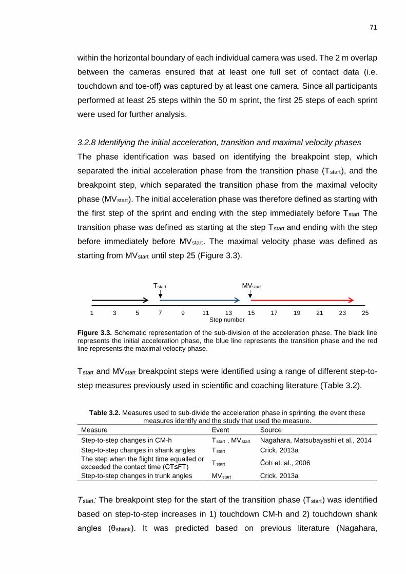
71

within the horizontal boundary of each individual camera was used. The 2 m overlap

between the cameras ensured that at least one full set of contact data (i.e.

touchdown and toe-off) was captured by at least one camera. Since all participants

performed at least 25 steps within the 50 m sprint, the first 25 steps of each sprint

were used for further analysis.

3.2.8 Identifying the initial acceleration, transition and maximal velocity phases

The phase identification was based on identifying the breakpoint step, which

separated the initial acceleration phase from the transition phase (Tstart), and the

breakpoint step, which separated the transition phase from the maximal velocity

phase (MVstart). The initial acceleration phase was therefore defined as starting with

the first step of the sprint and ending with the step immediately before Tstart. The

transition phase was defined as starting at the step Tstart and ending with the step

before immediately before MVstart. The maximal velocity phase was defined as

starting from MVstart until step 25 (Figure 3.3).

Figure 3.3. Schematic representation of the sub-division of the acceleration phase. The black line represents the initial acceleration phase, the blue line represents the transition phase and the red line represents the maximal velocity phase.

Tstart and MVstart breakpoint steps were identified using a range of different step-to-

step measures previously used in scientific and coaching literature (Table 3.2).

Table 3.2. Measures used to sub-divide the acceleration phase in sprinting, the event these

measures identify and the study that used the measure. Measure Event Source Step-to-step changes in CM-h Tstart , MVstart Nagahara, Matsubayashi et al., 2014 Step-to-step changes in shank angles Tstart Crick, 2013a The step when the flight time equalled or exceeded the contact time (CT≤FT) Tstart Čoh et. al., 2006

Step-to-step changes in trunk angles MVstart Crick, 2013a

Tstart: The breakpoint step for the start of the transition phase (Tstart) was identified

based on step-to-step increases in 1) touchdown CM-h and 2) touchdown shank

angles (θshank). It was predicted based on previous literature (Nagahara,

1 3 5 7 9 11 13 15 17 19 21 23 25Step number

Tstart MVstart

72

Matsubayashi et al., 2014; Crick, 2013e; Delecluse et al., 1995) that Tstart would

occur within the first 10 steps. Therefore, to remove the possible effect of the data

towards the latter end of the 50 m, only the first 10 steps of the full 25 step data set

was used. To identify this step, a method involving multiple straight-line

approximation (Neder & Stein, 2006; Nagahara, Matsubayashi et al., 2014) was

used. Firstly, step-to-step changes in CM-h and θshank were approximated using

multiple first order polynomials where the first approximation included the first three

touchdowns, the second approximation included the first four touchdowns and so

on. With each subsequent approximation the number of touchdowns used was

increased by one until the first 10 touchdowns were included in the approximation.

Then, for each approximation, a residual score was calculated based on the RMSD

between the raw and approximated data points. The differences between the

residuals of adjacent approximations were then calculated where the first difference

of residuals corresponded to step three, the second difference of residuals to step

four, and so on. Finally, Tstart was identified as the step corresponding to the maximal

difference between the residuals. The method described above was used to detect

Tstart from both CM-h and shank angles at touchdown (Figure 3.4).

Tstart

Touchdown time [s]

Figure 3.4. Example detection of Tstart using multiple first order polynomials. The open circles represent the relative CM-h at each touchdown. The red and black lines represents two of the eight first order polynomials used to detect Tstart. The grey diamonds represent the difference between the residuals of adjacent approximations. The vertical dotted line indicates the step (Tstart) which corresponds to the maximal difference of the residuals.

A third measure was identified as a possible way to identify Tstart. This measure was

identified as the step when flight time equalled or exceeded contact time (CT≤FT)

during the acceleration phase. This measure, which was previously used by Čoh et

al. (2006) and will be compared to the Tstart steps, which were identified using both

the CM-h and shank angles.

0.0

0.2

0.4

0.6

40

45

50

55

0.3 0.6 0.9 1.2 1.5 1.8 2.1 2.4 2.7

Res

idua

l diff

eren

ces

[%]

Rel

ativ

e C

M h

eigh

t [%

]

73

MVstart: The breakpoint step for the start of the maximal velocity phase (MVstart) was

identified based on step-to-step increases in 1) touchdown CM-h and 2) touchdown

trunk angles (θtrunk). Data from step eight onwards were used to detect this step. A

method using two first order polynomials (Schneider, Phillips, & Stoffolano, 1993;

Nagahara, Matsubayashi et al., 2014) was used to identify MVstart as follows. Firstly,

the data (steps 8 to 25) were divided into two sections (Nagahara, Matsubayashi et

al., 2014). The first section included steps eight to ten while the second section

included steps ten to 25. Then, a first order polynomial was fit to each of the sections

and an overall RMSD residual between the raw data and the approximated data

was calculated. The step linking the two sections (initially step 10) was then moved

sequentially through the data set up to the third to last step (23rd touchdown). Each

time the linking step was moved the new sections were approximated using two new

first order polynomials and an overall RMSD residual between the raw data and the

approximated data and was calculated for the new approximation. The linking step

that corresponded to the minimum RMSD residual was adopted as MVstart. The

method described above was used to detect MVstart using both CM-h and trunk

angles at touchdown (Figure 3.5).

MVstart

Touchdown time [s] Figure 3.5. Example breakpoint detection of MVstart using two straight-line approximations. The open circles represent the relative CM-h at each touchdown. Relative CM-h was plotted against touchdown times. The two black lines on the figure represent the two first order polynomials to detect MVstart. The grey diamonds represent the collective RMSD for each set of approximations. The vertical dotted line indicates the step (MVstart) which corresponds to the minimal difference of the residuals.

3.2.9 Data smoothing

Following the identification of the Tstart and MVstart the step-to-step data was then

smoothed to remove the effects of any bilateral differences, as well as potential

noise due to the data collection and processing procedures. Data were smoothed

using the Hanning moving averages algorithm (Equation 3.1 ; Grimshaw, Fowler,

0.0

0.3

0.6

0.9

1.2

1.5

40

45

50

55

60

0 1 2 3 4 5 6

Residual differences [%

]Rel

ativ

e C

M h

eigh

t [%

]

74

Lees & Burden, 2004). This algorithm was selected as it places a greater weighting

factor on the point being smoothed instead of a standard moving average algorithm

were all the points have an equal weighting. It was assumed that the data was

evenly spaced (i.e. step one, step two, step three etc.).

𝒚𝒚𝒊𝒊 = 𝟎𝟎.𝟏𝟏𝟐𝟐 ∗ 𝒙𝒙𝒊𝒊−𝟏𝟏 + 𝟎𝟎.𝟐𝟐 ∗ 𝒙𝒙𝒊𝒊 + 𝟎𝟎.𝟏𝟏𝟐𝟐 ∗ 𝒙𝒙𝒊𝒊+𝟏𝟏 ; 𝒊𝒊 = 𝟏𝟏 𝒕𝒕𝒕𝒕 (𝑵𝑵− 𝟏𝟏) [Equation 3.1]

𝑦𝑦𝑖𝑖 = newly calculated ‘smooth’ value 𝑥𝑥𝑖𝑖 = original data i = touchdown or toe-off point being smoothed N = number of steps

3.2.10 Reliability and Objectivity of digitising

To assess reliability and objectivity of digitising, two experienced digitisers each

digitised one trial three times. Each re-digitisation included the identification of the

touchdown and toe-off events in the panning videos and digitising two frames

around touchdown and toe-off in the static videos. Data from this was then used to

calculate the within-digitiser (reliability) and between-digitiser (objectivity)

differences in the variables identified in section 3.2.5. These results are discussed

in appendix A1.

3.2.11 Data Analysis

To address the first research question, which involves the measures used to identify

the breakpoint during the acceleration phase in sprinting, all three to five trials from

the participants from each day where used. All the trials were included to allow a

more robust and thorough comparison of the different measures that are used to

sub-divide the acceleration phase in sprinting. The mean and standard deviations

(SD) of the detected Tstart, MVstart, CT≤FT and the step at which the participants

achieved their maximal step velocity (Vmax) was calculated across each participant

and the group. Furthermore, a mean and SD of the relative CM-h (% of stature),

shank angles (θshank), trunk angles (θtrunk) and step velocities (absolute and relative

to the maximal velocity) corresponding to the Tstart, MVstart, CT≤FT and Vmax steps

were calculated. The differences in the Tstart steps, which were identified using the

measures CM-h, shank angles and CT≤FT, were quantified by calculating an

individual and group RMSD between each of the measures for each day. The same

75

was done to quantify the differences between the MVstart steps which were identified

using either CM-h or trunk angles.

To address the second research question, each participant’s best trials from days

one and two were selected for further analysis. This selection was based on the

fastest 50 m sprint times. This allowed the investigation of the step-to-step changes

in step characteristics and kinematics associated with the participant’s best

performance on each day. To identify the steps occurring in the initial acceleration,

transition and maximal velocity phases, the range of Tstart (CM-h) and MVstart (CM-h)

steps identified from those best trials was used to sub-divide the trials. Finally, the

smoothed step characteristic, spatiotemporal and kinematic data of each

participant’s best trial on each day was presented to investigate the differences

between the initial acceleration, transition and maximal velocity phases.

Step-to-step changes in the variables during the initial acceleration, transition and

maximal velocity phases were qualitatively described as showing a steep rise (or

decline), a less step rise (or decline) or plateau. A plateau is defined as a period of

unclear step-to-step increases or decreases in a variable.

3.3 Results Reconstruction errors ranged from 0.003 to 0.005 m horizontally and 0.002 to 0.004

m vertically. The within-digitiser differences for the step characteristics (step

velocity, step length) were below 1% of their respective range across the first 25

steps while the between digitiser differences were 0.033 m for step length and 0.07

Hz for step frequency. Within and between digitiser differences for segment angles

were ≤ 3° or 4% of the variable’s respective range. Within and between digitiser

uncertainties for CM-h were below ≤ 0.5% of stature or 5% of the variable’s range

over the first 25 steps of the sprint. Within-digitiser uncertainties in contact distances

were 0.010 m or 4% of the variables range while between-digitiser differences in

contact distances were 0.035 m or 13% of the range. The larger between digitiser

differences for step length, step frequency and contact distances were due to the

between-digitiser differences in touchdown and toe-off events. Touchdown and

toe-off events were identified to the same frame 67% of the time, with one frame

difference (0.005 s) 31% of the time and with a two frame difference (0.010 s) 2%

76

of the time. See Appendix A1 for a more complete discussion of reliability and

objectivity results.

3.3.1 Trial times, Tstart, MVstart and CT≤FT

Participant P02, who at the time of testing had the best 100 m personal best of the

male participants, ran the fastest 50 m overall on day 1 with a time of 5.86 s (Table

3.3). Out of the two female participants, P05 ran the fastest 50 m on both days with

6.63 s and 6.75 s on days 1 and 2, respectively (Table 3.3). Only participant P01

improved on their best performance from day 1 to day 2 (6.13 to 6.07 s).

Table 3.3. Mean () ± SD 50 m time from the March and May 2014 data

collection as well as each participant’s range across the trials. Day 1 Day 2

Participants Range [s] Range [s] P01 6.13 – 6.21 6.07 – 6.15 P02 5.86 – 5.94 5.98 – 6.01 P03 5.90 – 5.96 5.89 – 5.94 P04 6.78 – 6.90 6.83 – 7.06 P05 6.63 – 6.75 6.75 – 6.78

Ranges of Tstart steps identified using either CM-h or shank angles were consistent

between the two days (Table 3.4). Across both days, Tstart was detected between

steps 3 - 7 when using touchdown CM-h and between steps 3 - 6 when using

touchdown shank angles (Table 3.4). The shank reached a 90 ± 2° touchdown

position between steps 5 - 15. For the individual data for each participant, see

Appendix A2. Table 3.4. Group mean () ± SD using all available trials, ranges across all trials and ranges across the best trials for Tstart steps (CM-h, shank angles (θshank) and CT≤FT) and MVstart steps (CM-h and trunk angles (θ trunk)). Also presented are the CM height, θshank and θ trunk at their respective Tstart and

MVstart steps. Tstart MVstart CM-h θshank CT≤FT CM-h θ trunk Day Step Height

[%] Step Angle

[°] Step Step Height

[%] Step Angle

[°] ± SD

(all trials) 1 4.5 ±1.3 51 ±1 4.8 ±1.0 78 ±8 13.2 ±2.4 15.0 ±1.2 56 ±1 16.0 ±1.4 82 ±4 2 4.7 ±1.0 51 ±1 4.7 ±1.0 76 ±5 11.5 ±1.6 14.8 ±1.5 56 ±1 15.2 ±1.5 82 ±3

Range (all trials)

1 3 - 7 48 -53 3 - 6 57 -90 9 -16 12 - 17 54 -57 13 - 18 75 -88 2 3 - 7 49 -53 3 - 6 65 -85 8 -15 13 - 17 54 -57 12 - 19 77 -86

Range (Best trials)

1 4 - 6 49 -52 4 - 6 69 -85 9 -16 14 - 16 55 -56 14 - 17 75 -88 2 4 - 6 51 -53 4 - 6 67 -85 10 -15 14 - 17 55 -56 15 - 17 79 -86

The range of CT≤FT steps was smaller on day two and generally occurred earlier

across all participants (Table 3.4). Across both days, the maximal step velocity was

77

reached between steps 18 to 25 where the participants achieved 8.56 - 10.76 m·s-1

(Table 3.5).

Table 3.5. Group mean () ± SD of Vmax steps as well as the ranges (all trials and best trials) for Vmax steps. Group mean () ± SD and ranges (all trials and best trials) of step

velocity (SV), CM-h and trunk angle (θ trunk) corresponding to the Vmax step are also presented.

Vmax Day Step SV [m·s-1] CM-h [%] θ trunk [°]

± SD (all trials)

1 23.3 ± 2.1 9.81 ± 0.74 56 ± 1 84 ± 3 2 22.9 ± 1.4 9.74 ± 0.74 56 ± 1 84 ± 2

Range (all trials)

1 18 - 25 8.83 - 10.76 53 - 58 79 - 89 2 19 - 25 8.56 - 10.63 54 - 57 81 - 90

Range (Best trials)

1 23 - 25 9.04 - 10.73 55 - 57 79 - 87 2 22 - 24 8.86 - 10.63 55 - 57 82 - 90

To make the comparison between Tstart and MVstart steps identified using different

measures more robust, all trials were included in this analysis. The RMSD between

Tstart steps identified using either CM-h or shank angles, ranged between 0.8 – 2.1

steps (Table 3.6). The RMSD between Tstart steps identified using the CT≤FT step

or either CM-h and shank angles ranged from 5.9 - 12.2 steps. The RMSD between

MVstart steps identified using CM-h or trunk angles were between 1.3 - 2.3 steps

(Table 3.6).

Table 3.6. Individual RMSD between Tstart steps identified either using CM-h, shank angles or the CT≤FT step and the RMSD between MVstart steps identified using either CM-h or trunk

angles. These RMSD values were calculated using all trials for each participant. Tstart MVstart

Participant Day CM-h vs. θshank CM-h vs. CT≤FT θshank vs. CT≤FT CM-h vs. θ trunk

P01 1 1.6 8.0 9.4 1.3 2 1.5 7.9 7.2 1.4

P02 1 1.2 6.0 5.7 1.6 2 0.8 6.4 6.2 2.0

P03 1 2.1 12.2 10.7 2.3 2 1.3 7.7 7.4 1.3

P04 1 1.1 10.1 9.3 1.6 2 1.1 7.6 8.3 1.7

P05 1 1.1 8.3 7.8 2.0 2 0.9 5.9 6.5 1.7

CM-h: centre of mass height (%); θshank: shank angle (º); θtrunk: trunk angle (º); CT≤FT:flight time exceeds contact time

3.3.3 Changes in step characteristics, spatiotemporal and kinematic variables

To investigate the step characteristics and kinematics associated with the

participant’s best performance on each day, only data from each participant’s best

trial based on the 50 m times was used. After identifying the best trials, the ranges

78

of Tstart and MVstart steps from those trials were used to sub-divide the whole 50 m

sprint trial into three phases (shaded areas; Figure 3.6).

Tstart MVstart

Figure 3.6. Tstart and MVstart steps of the participant’s best trial from day 1 (x) and day 2 (+). The grey columns highlight the initial acceleration, transition and maximal velocity phase steps that lie outside the range (best trials) of Tstart and MVstart steps.

Steps one to three were always part of the initial acceleration phase, steps six to 13

were always within the transition phase and steps 17 onwards always fell into the

maximal velocity phase. When using each participant’s best trial from each day,

Tstart using CM-h was associated with step velocities of 6.06 to 7.83 m·s-1 or 65 to

77 % of Vmax, while MVstart was associated with step velocities of 8.19 to 10.07 m·s-1

or 92 to 98% of Vmax. Over the 25 steps, the largest changes in step characteristics

(Figure 3.7) occurred during the initial acceleration phase (i.e. steps 1 to 3).

During the initial acceleration phase, step velocity, step length and step frequency

showed a steep increase (Figure 3.7), while during the transition phase, the step

velocity and step length curves became less steep showing that step-to-step

increases continued at a slower rate relative to the initial acceleration phase. The

maximal velocity phase was characterised by small step-to-step increases in step

velocity and step length.

0

1

2

3

4

5

1 3 5 7 9 11 13 15 17 19 21 23 25

Part

icip

ants

Steps

Initi

al a

ccel

erat

ion

phas

e

Transition phase Maximal velocity

phase

79

Steps Figure 3.7. Step-to-step profiles for (a) step velocity, (b) step length and (c) step frequency over the first 25 steps of the participants best 50 m sprint from day 1 (black) and day 2 (grey). The grey columns highlight the initial acceleration, transition and maximal velocity phase steps that lie outside the range (best trials) of Tstart and MVstart steps.

Figure 3.8 shows the step-to-step pattern of CM-h and step-to-step changes of

CM-h. The initial acceleration phase was characterised by a steep rise in the height

3

4

5

6

7

8

9

10

11

1 3 5 7 9 11 13 15 17 19 21 23 25

Step

vel

ocity

[m·s

-1]

0.7

1.0

1.3

1.6

1.9

2.2

2.5

1 3 5 7 9 11 13 15 17 19 21 23 25

Step

leng

th [m

]

3.0

3.5

4.0

4.5

5.0

1 3 5 7 9 11 13 15 17 19 21 23 25

Step

freq

eunc

y [s

teps

·s-1

]

a

b

c

80

of the CM. During the transition phase, the CM-h curve became less steep,

characterised by a step-to-step CM-h changes between 0.0 -1.0% of stature.

Figure 3.8. a) Touchdown CM-h and b) step-to-step changes in CM-h step over the first 25 steps of the participants best 50 m sprint from day 1 (black) and day 2 (grey). The grey columns highlight the initial acceleration, transition and maximal velocity phase steps that lie outside the range (best trials) of Tstart and MVstart steps.

The initial acceleration phase was characterised by a steep rise in flight time, contact

distance, flight distance and touchdown distance while contact times showed a

steep decline (Figure 3.9). During the transition phase, the flight time and contact

time curves became less steep showing a decrease in the magnitude of step-to-step

changes. In addition, during the transition phase, the contact distance curves started

to plateau. This was associated with a slowing down of the step-to-step increases

in touchdown distance when compared with the initial acceleration phase.

Throughout the initial acceleration and transition phases, flight distance and toe-off

distances showed relatively consistent step-to-step changes. During the maximal

velocity phase, contact times, contact distances, touchdown and toe-off distances

had plateaued while flight time and flight distance continued to show small step-to-

step increases.

Steps Steps

40

45

50

55

60

1 3 5 7 9 11 13 15 17 19 21 23 25

CM

-h [%

of s

tatu

re]

-1.0-0.50.00.51.01.52.02.53.03.54.0

1 3 5 7 9 11 13 15 17 19 21 23 25

Cha

nge

in C

M-h

[% o

f sta

ture

] b a

81

Steps Steps

Figure 3.9. Step-to-step contact times (a), flight times (b), contact distance (c), flight distance (d), touchdown distance (e) and toe-off distances profile over 25 steps of the participants best 50 m sprint from day 1 (black) and day 2 (grey). Grey columns highlight the initial acceleration, transition and maximal velocity phase steps that lie outside the range (best trials) of Tstart and MVstart steps.

The touchdown angle and range of motion of the shank (Figure 3.10 g & i) showed

a steep step-to-step increase during the initial acceleration phase. During the

transition phase, shank angles showed a less steep step-to-step increase before

reaching a plateau during the maximal velocity phase. Touchdown angle and range

of motion of the thigh (Figure 3.10 d & f) increased early in the initial acceleration

phase, and then decreased during the transition phase before plateauing during the

maximal velocity phase. Trunk angles at touchdown and toe-off increased

throughout the initial acceleration and transition phases (Figure 3.10 a & b).

0.02

0.06

0.10

0.14

0.18

0.22

0.26

1 3 5 7 9 11 13 15 17 19 21 23 25

Con

tact

Tim

e [s

]

0.02

0.06

0.10

0.14

0.18

0.22

0.26

1 3 5 7 9 11 13 15 17 19 21 23 25

Flig

ht T

ime

[s]

0.1

0.3

0.5

0.7

0.9

1.1

1.3

1.5

1 3 5 7 9 11 13 15 17 19 21 23 25

Con

tact

dis

tanc

e [m

]

0.1

0.3

0.5

0.7

0.9

1.1

1.3

1.5

1 3 5 7 9 11 13 15 17 19 21 23 25

Flig

ht d

ista

nce

[m]

-0.4

-0.2

0.0

0.2

0.4

0.6

1 3 5 7 9 11 13 15 17 19 21 23 25

TD d

ista

nce

[m]

-1.0

-0.8

-0.6

-0.4

-0.2

0.0

1 3 5 7 9 11 13 15 17 19 21 23 25

TO d

ista

nce

[m]

b

d

f

a

c

e

82

Touchdown angle [°] Toe-off angle [°] Stance range of motion [°]

Trun

k

Thig

h

Shan

k

Steps Steps Steps Figure 3.10. Step-to-step trunk (a-c), thigh (d-f) and shank (g–i) angle and ranges of motion profiles over the first 25 steps of the participants best 50 m sprint from day 1 (black) and day 2 (grey). The grey columns highlight the initial acceleration, transition and maximal velocity phase steps that lie outside the range (best trials) of Tstart and MVstart steps.

2030405060708090

100

1 3 5 7 9 11 13 15 17 19 21 23 252030405060708090

100

1 3 5 7 9 11 13 15 17 19 21 23 25 -6-30369

121518

1 3 5 7 9 11 13 15 17 19 21 23 25

8090

100110120130140150160

1 3 5 7 9 11 13 15 17 19 21 23 2540

50

60

70

80

1 3 5 7 9 11 13 15 17 19 21 23 252030405060708090

100

1 3 5 7 9 11 13 15 17 19 21 23 25

30

50

70

90

110

1 3 5 7 9 11 13 15 17 19 21 23 2520

30

40

50

60

1 3 5 7 9 11 13 15 17 19 21 23 250

10203040506070

1 3 5 7 9 11 13 15 17 19 21 23 25

a

d

g

c

f

i

b

e

h

83

3.4 Discussion The angle between the vector connecting the CM to the contact point and the ground

is mechanically relevant to the acceleration performance of the athlete (di Prampero

et al., 2005). However, knowledge of how the components of the CM angle (e.g. TD

distance, TO distance, segment angles) change during sprinting is still unclear.

Based on Theme 1 (Phase analysis), the aim of this chapter was to investigate

differences in step-to-step changes in step characteristics and kinematic variables

between the initial acceleration, transition and maximal velocity phases. The

purpose was to increase knowledge of the initial acceleration, transition and

maximal velocity phases and assist with the development of technical models for

different phases of sprinting. To achieve this, two research questions were posed.

The first research question posed in the introduction of this chapter asked how

comparable the breakpoint step (Tstart) which links the initial acceleration to the

transition phase and the breakpoint step (MVstart) which links the transition to the

maximal velocity phase are when identified using different measures (section 3.4.1).

This ultimately informed the choice of measure, which was used to sub-divide the

whole 50 m sprint into the initial acceleration, transition and maximal velocity phases

and address research question ii concerning the step-to-step changes in step

characteristics and kinematic variables between the initial acceleration, transition

and maximal velocity phases (section 3.4.2).

3.4.1 Comparison of measures used to identify the acceleration phases

Before sub-dividing the acceleration phase in sprinting, an analysis of measures

previously used to achieve this was necessary. To allow a more robust comparison

between the measures used previously to identify the breakpoint during the

acceleration phase in sprinting, all available trials were used to address the first

research question of Theme 1. Using the CM-h at touchdown as the discriminating

measure to identify Tstart and MVstart, the range of breakpoint steps for Tstart were

steps 3 to 7 and for MVstart steps 12 to 17. While the current study used CM-h at

touchdown, a previous study Nagahara, Matsubayashi et al. (2014) used the mean

CM-h during stance as their measure to sub divide the acceleration phase in

sprinting. Nonetheless, similar ranges of Tstart and MVstart steps were identified in

the current study compared to those of Nagahara, Matsubayashi et al. (2014) who

identified Tstart between steps 3 to 6 and MVstart between steps 10 to 20. The current

84

study showed the consistency of Tstart and MVstart between separate data collection

days, which further verifies the location of these events.

Using shank angles, Tstart was identified between steps 3 to 6. These results show

parity with the model presented by Crick (2013e) which proposes that the initial

acceleration phase lasts around 5-7 steps after which the shank is perpendicular to

the ground at touchdown. In this study, Tstart was associated with shank angles

ranging from 57° to 90°. This is different to the ~90° shank angle suggested by the

British Athletics coaching literature (Crick, 2013e). In the current study 90 ± 2°

degrees was only reached between steps 5 to 15. The 90 ± 2° threshold was used

as this incorporates the potential uncertainty of shank angles identified from the

reliability and objectivity analysis. As shown in figure 3.10g, shank angles do not

progress in a linear fashion until vertical as suggested by the British Athletics

coaching literature (Crick, 2013e). Using a vertical threshold to identify Tstart may

therefore not be appropriate to identify abrupt changes in the step-to-step

progression of this variable.

Following the transition phase, an ‘upright’ trunk is characteristic of the maximal

velocity phase and therefore the plateau in step-to-step changes in trunk angle at

touchdown could serve as a measure to detect this event (Crick, 2013e). According

to the British Athletics sprint model, this is suggested to occur around step 17

(Crick, 2013e). In the current study steps 12 - 19 were identified as the steps trunk

angle plateaued and therefore participants started their maximal velocity phase.

Although ‘upright’ was not defined in previous literature, in this study step-to-step

changes in trunk angles plateaued at trunk angles of 75° to 88°.

The CM-h at each step is determined by the segment orientations, where a vertical

orientation of the segments provide maximal contribution to CM-h. Since touchdown

shank and trunk angles show the largest step-to-step changes during the initial

acceleration and transition phases (Figure 3.10 a & g), increases in CM-h during the

initial acceleration and transition phases could be expected to align with the

step-to-step changes in both shank and trunk angles. In order to compare Tstart and

MVstart steps identified using the different measures an RMSD between the different

steps was calculated. Tstart based on CM-h and Tstart using shank angles was

85

detected to within 2.1 steps of each other (Table 3.6). Similarly, MVstart based on

CM-h and MVstart based on trunk angles was detected to within 2.3 steps of each

other. Although relatively low, these RMSD step differences are possibly due to

other segments (e.g. segments other than the shank and trunk) changing

independently of each other and therefore influencing the CM-h. Furthermore,

bilateral differences, which have previously been reported in maximal sprinting

(Exell, Gittoes, Irwin & Kerwin, 2012) could have contributed to these RMSD step

differences. While the within-trial analysis revealed that different Tstart and MVstart

steps were identified when using either CM-h or segment angles, both measures

did provide similar ranges of Tstart and MVstart steps across multiple trials. Therefore,

using segment angles in applied settings, where speed of feedback is often an

important factor may be an appropriate substitute if data are based on multiple trials

(at least three trials per participant). However, since CM-h provides a holistic

measure that is representative of the overall postural changes, this measure was

subsequently used for identifying Tstart and MVstart steps to address research

question 2.

When using the step in which flight times were equal to or exceeded contact times

(CT≤FT), steps 8 - 16 were identified as Tstart. Čoh et al. (2006) identified steps

8 - 10 as the start of the transition phase within one sprinter. The range of CT≤FT

identified in the current study suggests that the location of this step can be

inconsistent between participants and within participants across different days.

Hunter et al. (2004) reported that running velocity and vertical impulse play an

important part in contact and flight times. CT≤FT may therefore be dependent on

running velocity and ability to generate large vertical GRF during ground contact.

The RMSD between CT≤FT and Tstart from CM-h and shank angles showed

differences between 5.7 - 12.2 steps. While CT≤FT may represent a beneficial tool

to monitor sprinters, this measure appears to be dependent on the sprinters’ running

velocity and ability to generate vertical impulses during short ground contacts and

is not necessarily representative of changes in kinematics.

The characteristics of the breakpoints (Tstart and MVstart) that sub-divide the

acceleration phase in sprinting is still a relatively unknown area in research. While

Tstart and MVstart steps were detected in the current study, it is unclear whether these

86

breakpoints are characteristic of the acceleration phase or a reflection of the method

used to detect the steps (Ettema, McGhie, Danielsen, Sandbank & Haugen, 2016).

Ettema et al. (2016) suggested that the Tstart steps identified by Nagahara,

Matsubayashi et al. (2014), and therefore in the current study may be influenced by

the method used to identify the breakpoint. Although Ettema et al. (2016) identified

a Tstart breakpoint in some of their trials this was not the norm. It is important to note

that Ettema et al. (2016) applied various fitting procedures including an exponential

and piecewise fitting procedure. Only when the piecewise fit provided a greater

goodness-of-fit did the authors conclude that a breakpoint occurred. Ettema et al.,

(2016) concluded that since Tstart was only identified in a minority of their trials, that

this breakpoint might be reflective of an imperfection in performance. However, the

authors did not relate the trials showing a Tstart breakpoint to performance, and

therefore it cannot be clearly said that trials showing this breakpoint represent an

imperfection in performance.

While the current study assumes that breakpoints occur in sprinting, this assumption

is based on changes in posture, which have previously been reported in the

acceleration and maximal velocity phases of sprinting (Delecluse, 1997; Nagahara,

Matsubayashi et al., 2014; Crick, 2013a). In addition, apart from the current study,

two other studies have identified a Tstart step (Nagahara, Matsubayashi et al., 2014;

Ettema et al., 2016) in at least some of their sprint trials, which further justifies the

approach of identifying breakpoint steps to sub-divide the acceleration phase in

sprinting.

3.4.2 Changes in step characteristics, spatiotemporal and kinematic variables

For the remainder of this chapter, CM-h was adopted as the criterion measure to

identify the Tstart and MVstart breakpoint steps used to sub-divide the acceleration

phase in sprinting. Because the best trials are more representative of optimal

performance throughout the phases, the range in Tstart and MVstart steps identified

using the best day one and day two trials were used for each participant. This

allowed the identification of the steps that occurred in the initial acceleration,

transition and maximal velocity phases across all participants. These trials were

then also used to investigate the step-to-step differences in step characteristics,

spatial-temporal variables and segment kinematics between the initial acceleration,

87

transition and maximal velocity phases. The purpose was to clarify changes

between the initial acceleration, transition and maximal velocity phases in variables

visually accessible to coaches and sport scientists in an applied setting.

During the initial acceleration phase (steps 1 – 3), step characteristics (Figure 3.7),

spatial-temporal variables (Figure 3.9) and segment orientations at touchdown and

toe-off (Figure 3.10) all showed relatively large step-to-step changes compared with

the transition and maximal velocity phases. During the initial acceleration phase,

relatively large step-to-step increases in step velocity were due to large step-to-step

increases in step length and step frequency (Figure 3.7). It must be noted that on

the second day of testing, P02 (Figure 3.8c, grey dotted line) achieved a relatively

high step frequency from the first step onwards. This was likely due to them having

a relatively shorter contact time and contact distance over steps 1 and 2. Achieving

a relatively high step frequency during the initial acceleration phase has been shown

to be important to CM acceleration over the first three steps of a sprint (Nagahara,

Naito, Morin & Zushi, 2014). In the current study, relatively larger step-to-step

increases in step frequency during the initial acceleration phase resulted from larger

step-to-step decreases in contact time relative to the step-to-step increases in flight

times (Figure 3.9 a & b) therefore resulting in an overall shorter step time. While

these characteristic increases in step frequency may also be present during slower

sprints, running performance may ultimately be influenced by the ability to generate

an overall larger step frequency (Hunter et al., 2004; Nagahara, Mizutani, Matsuo,

Kanehisa & Fukunaga 2017b). Since sprinters can only alter their running velocity

during ground contact, these results combined with those of Nagahara et al. (2014a)

suggest an approach that allows a rapid increase in step frequency while still

maximising contact time and therefore the contact distance should be encouraged.

This may be achieved by minimising flight times and keeping the swing leg foot close

to the ground during the recovery phase (Crick, 2013e).

Other step-to-step increases associated with the initial acceleration phase are

relatively large step-to-step increases in contact and flight distances (Figure 3.9

c & d), touchdown distance (Figure 3.9 e) and trunk and shank angles at touchdown

(Figure 3.10 a & g). Step-to-step increases in contact distance (Figure 3.9c)

occurred mainly due to relatively large step-to-step increases in touchdown distance

88

(Figure 3.9e). The step-to-step increases in touchdown distance have previously

been attributed to an inability to produce sufficient propulsive impulses to counteract

the clockwise moment about the contact point due to gravity (Nagahara,

Matsubayashi et al., 2014). The increases in touchdown distance which resulted

from the relatively large step-to-step increases in shank angles (i.e. shank becoming

more inclined; Figure 3.10g) and trunk angles (Figure 3.10a) likely play an important

functional role in the performance during the acceleration phase. The magnitude of

vertical force during short ground contacts has previously been suggested to be a

limiting factor to maximising running velocities during maximum velocity steady state

running (Weyand et al., 2000). Similar, the relatively large step-to-step increases in

touchdown shank angles during the initial acceleration phase could be due to an

increasing demand to generate vertical GRFs during initial ground contact to support

step-to-step increases in CM-h and flight times as contact time’s decrease (Crick,

2013e). Furthermore, step-to-step increases in flight times (Figure 3.9 b) would

result in larger downward CM velocities immediately prior to touchdown. This would

require larger vertical forces early during stance to slow the downward velocity of

the CM.

From a mechanical perspective, an increased touchdown distance (i.e. more

forward contact point relative to the CM) would alter the orientation of the GRF

vector passing close to the CM, therefore ensuring a more inclined resultant GRF

vector. Furthermore, it could be speculated that apart from influencing the

touchdown distance, the more inclined shank could assist the sprinter in generating

larger vertical forces by placing the sprinter in a better position to allow the hip

extensors and ankle plantar flexors to apply force more vertically.

The increasing touchdown distances resulting from the step-to-step increases in

touchdown shank (~7 to 12° per step) and trunk angles (~2 to 9° per step) could

also influence the anterior force production of sprinters by influencing their

whole-body orientation during subsequent steps. British Athletics coaching literature

suggested that the smaller shank angles (<90°) during the initial acceleration phase

are more favourable to generating large propulsive forces and should increase

smoothly at around 6 to 8° between successive touchdowns, with sudden large

increases thought to negatively affect the ability to generate large anterior forces

89

(Crick, 2013e). Indeed, a sudden large increase in touchdown shank angle could

result in a large increase in touchdown distance, and therefore large increases in

braking forces. Previous literature has shown that smaller touchdown distances are

linked to smaller braking forces (Hunter, Marshall & McNair, 2005) and that a

decreased touchdown distance is beneficial to performance during the first step of

a sprint (Bezodis, Trewartha & Salo, 2015). Furthermore, since propulsive forces

are important to performance during initial acceleration (Morin et al., 2015;

Nagahara et al., 2017a), excessively large step-to-step increases in touchdown

distances and segment angles may play a role in influencing the toe-off position

sprinter achieve and therefore the propulsive forces sprinters could theoretically

generate. Smaller step-to-step increases in touchdown shank and trunk angles may

therefore be beneficial to performance by minimising the step-to-step increases in

braking forces and placing sprinters in a better position to generate large propulsive

forces as they approach toe-off.

Step-to-step changes in toe-off distances (range: -0.022 to 0.057 m per step) were

relatively small compared to the step-to-step increases in touchdown distances

(range: 0.020 – 0.148 m per step; Figure 3.10g). Kugler and Janshen (2010) have

previously shown that faster participants achieved smaller CM angles and therefore

larger propulsive forces than slower participants did. A larger toe-off distance and

smaller CM-h will ensure a larger proportion of ground contact is spent with more

forward orientated CM angle (see Appendix A3) and therefore according to the link

between CM angle and acceleration (di Prampero et al., 2005) a forward orientated

ground reaction vector. When comparing the initial acceleration to the transition

phase, minimising the decreases in toe-off distances and increase in CM-h might

be an essential characteristic of the initial acceleration phase that ensures that

larger propulsive forces are generated when compared with the transition phase.

At the start of the transition phase (Tstart), the participants had reached 65% to 77%

of Vmax (6.06 to 7.83 m·s-1). The British Athletics performance model for sprinting

(Crick, 2013g) suggests that sprinters should have reached around 75 - 80% of Vmax

at the start of their transition phase. The smaller percentages reported in this study

may be because the transition phase was identified earlier (i.e. between steps 4-6)

than suggested by the coaching literature (i.e. between steps 5-7; Crick, 2013e).

90

Steps six to 13 always occurred in the transition phase. During the transition phase,

the curves associated with step frequency (Figure 3.8c), contact times (Figure 3.9a),

flight times (Figure 3.9b) and touchdown shank angles (Figure 3.10g) were visibly

less steep than during the initial acceleration phase. The transition phase was

therefore characterised by relatively smaller step-to-step changes in the touchdown

variables compared to the initial acceleration phase whereas trunk angles (Figure

3.10 a & b) continued to increase at a similar rate compared to the initial acceleration

phase. This ensured that CM-h at touchdown also continued to increase throughout

the transition phase.

Also during the transition phase, the participants’ contact distances plateaued as

the step-to-step increases in touchdown distance were matched by the step-to-step

decreases in toe-off distances (Figure 3.9 e & f). The increasing flight times might

play a role with the reduction of the step-to-step increases in touchdown distances

by allowing the sprinters more time to actively swing the stance leg back relative to

the CM prior to touchdown. This could also allow the sprinters to generate a larger

downward velocity of the foot prior to touchdown, which plays an important role in

generating vertical impulse directly after touchdown (Clark & Weyand, 2014). It is

however unclear how the downward velocity of the foot relative to the CM changes

between the initial acceleration, transition and maximal velocity phases and further

exploration of this variable is needed. At toe-off, the decreasing toe-off distances

are likely due to increasing trunk angles. This means that the hip joint reached full

extension with the thigh less rotated forward (Figure 3.10e) with each consecutive

step, thus resulting in a decreased toe-off distance. Although not directly measured,

this data also suggests that hip joint range of motion decreases during the transition

phase. This may be an important factor discriminating the initial acceleration phase

from the transition and maximal velocity phases especially when considering

specific training drills for the individual phases.

Step velocity and step length continued to increase during the transition phase,

however at a relatively smaller rate than during initial acceleration phase (Figure

3.7). The step frequency curve plateaued during this phase compared with the initial

acceleration phase as contact and flight times changed by comparable amounts in

each step. This finding aligns with previous reports by Debaere, Jonkers &

91

Delecluse (2013) and Nagahara, Matsubayashi et al. (2014) that step frequency has

already reached a near maximal level by step three. Nagahara et al. (2014a)

reported that changes in step length are associated with changes in running velocity

during the transition phase. As contact distance plateaued during the transition

phase (Figure 3.9c), step lengths were further increased through increases in flight

distance (Figure 3.9d). Increased flight times through increased vertical force

generation may play an important role with further increases in flight distance as

contact times decrease. The more inclined shank and trunk segments during the

transition phase could aid further increases in flight times and decreases in contact

times by allowing sprinters to generate a more vertically orientated GRF vector

during ground contact.

At the start of the maximal velocity phase (MVstart), participants had reached 92% to

98% (8.19 m·s-1 to 10.07 m·s-1) of Vmax. The British Athletics performance model for

sprinting (Crick, 2013g) suggests that sprinters will have reached 95% of their

maximal velocity at the start of the maximal velocity phase. Steps 17 onwards

always occurred in the maximal velocity phase. During the maximal velocity phase,

step-to-step changes in spatial-temporal and kinematic variables started to plateau

while small step-to-step increases in step velocity and step length occurred during

this phase. These were due to small increases in flight distances while contact

distances plateaued. Furthermore, the plateau in step-to-step changes in CM-h

(Figure 3.8) and trunk angles (Figure 3.10a) meant that participants had reached

their ‘upright’ running posture, which has been suggested to indicate the start of the

maximal velocity phase (Crick, 2013f).

An ‘upright’ trunk represents an essential characteristic of the maximal velocity

phase in sprinting. Firstly, a more inclined trunk could aid the sprinter in creating

sufficiently large vertical forces (Clark & Weyand, 2014; Nagahara, Matsubayashi

et al., 2014) which are important to maximise running velocities (Weyand et al.,

2000). Secondly, an upright trunk would increase the tension in the hip flexors

therefore allowing a quicker recovery following toe-off (Nagahara, Matsubayashi et

al., 2014; Nagahara, Matsubayashi, Matsuo & Zushi, 2017) and allow sprinters to

achieve a higher knee lift of the swing leg which would provide a greater distance to

accelerate the foot back and down towards the ground (Morin et al., 2015). There is

92

however, still a lack of evidence that minimising the forward velocity of the foot

during the late swing phase decreases braking forces during stance (Morin et al.,

2015).

3.4.3 Practical Implications

From the results of Theme 1 (Phase analysis), two potential practical implications

were identified. Firstly, the breakpoints identified using segment angles (i.e. shank

and trunk angles) as suggested in British Athletics coaching literature (Crick, 2013a)

provided similar ranges of steps (Tstart: 4 - 6; MVstart: 15 - 17) when compared to

using CM-h (Tstart: 4 - 6; MVstart: 14 - 17) to identify breakpoints. On the other hand,

the within-trial comparison showed step differences up to 2.3 steps between using

either segment angles or CM-h to identify the breakpoint steps. These opposing

results may have resulted from bilateral asymmetries, which influenced the

identification of breakpoint steps from shank and trunk angles compared to the

holistic centre of mass measure. The similar ranges identified from the different

measures suggests that using step-to-step changes in shank and trunk orientations

may be appropriate to provide simple feedback about the start and end of the

transition phase in applied settings. Sprinting is a complex task where performances

are influenced by multiple variables (e.g. step length and step frequency). By sub-

dividing the sprint events into smaller sections, coaches and athletes can focus on

more manageable sections of the race before re-constructing the skill as a whole

(Seagrave, 1996). The findings of this chapter support the use of changes in

touchdown shank and trunk angles to further sub-divide the acceleration and define

the steps within the initial acceleration and transition phases, provided that a

sufficient number of trials (at least three) are available for analysis. Overall, the

results from Theme 1 showed that the first 4 to 9 m of a sprint were part of the initial

acceleration phase, while the transition phases ended between 21 to 31 m. In

practical situations, it is suggested that coaches use maximal acceleration of either

5 or 10 m to focus on the initial acceleration phase while acceleration distances of

20 to 35 m should be used to develop the transition phase in combination with the

initial acceleration phase.

Secondly, the results showed that while the whole acceleration phase could be

characterised by changes in different variables throughout, individual phases within

93

sprint acceleration showed their own unique pattern of step-to-step changes in the

different variables. These included relatively larger between-step changes in

touchdown kinematic variables (especially shank angles and touchdown distances)

during the initial acceleration phase compared to the transition phase, while trunk

angles increased consistently throughout the initial acceleration and transition

phases and before plateauing during the maximal velocity phase. Furthermore, the

results showed that while trunk angles (both touchdown and toe-off) and touchdown

shank angles showed relatively large between-step changes across the whole

sprint, thigh angles (at touchdown and toe-off) and shank angles at toe-off changed

relatively little across the whole sprint. Knowledge of these step-to-step changes in

variables, which are easily accessible in applied settings contributed to the

conceptual understanding of the acceleration and maximal velocity phases. This

can ultimately facilitate technical analysis across multiple steps from different

phases as a sprint progresses.

From the results of Theme 1 combined with the previous research (e.g. Janshen &

Kugler, 2010; Nagahara, Naito, Morin & Zushi, 2014) it could be inferred that during

the initial acceleration phase, sprinters should attempt to maximise contact times

while still increasing step frequency (i.e. by minimising flight times). This would

ensure contact distances are maximised, which were found to be the largest

component of step length during the initial acceleration phase (Figure 3.9c). During

the transition phase, continued increases in step length are important (Nagahara,

Naito, Morin & Zushi, 2014) via increases in flight distances (Figure 3.9d). While

running velocities are an important determinant of flight distances (Hunter et al.,

2004a), increasing flight distances could be supported by continuing to increase

flight times via increases in vertical force production.

3.5 Conclusions Through a phase analysis (Theme 1), the aim was to investigate differences in step-

to-step changes in step characteristics and kinematic variables between initial

acceleration, transition and maximal velocity phases. The first research question

posed in the introduction of this chapter asked how comparable the breakpoint steps

(Tstart) which link the initial acceleration to the transition phase and the breakpoint

step (MVstart) which links the transition to the maximal velocity phase are when

94

identified using different measures. These measures include either CM-h, shank

angles or CT≤FT, which were used to identify Tstart, and CM-h or trunk angles, which

were used to identify MVstart. The analysis revealed that the smallest Tstart RMSD (≥

2.1 steps) was identified between the steps which were detected using CM-h or

shank angles. The MVstart RMSD between steps identified using CM-h and trunk

angles was ≥ 2.3 steps. While segment angles only account for changes at individual

segments, they may also be more disposed to between-step asymmetries

(especially shank angles) which could have affected the within step RMSDs. It was

therefore concluded that CM-h provides a more robust and holistic measure that is

more representative of the overall changes in posture.

The second research question posed in the introduction asked step-to-step changes

of step characteristics and kinematics differ between the initial acceleration phase,

transition phase and maximal velocity phase. Using only the best day one and two

trials from each participant, steps 1 – 3 were always identified as being in the initial

acceleration phase, steps 6 – 13 were identified as the transition phase and steps

17 onwards were identified as the maximal velocity phase. Overall, during the initial

acceleration phase, step characteristics, spatial-temporal variables and segment

orientations at touchdown showed the largest step-to-step changes while toe-off

distances and toe-off thigh and shank orientations remained relatively consistent.

This meant that contact distances increased over the first three steps although

contact times decreased rapidly. The transition phase was characterised by a

reduction in the magnitude of step-to-step changes of the variables investigated.

Specifically, step-to-step changes in contact distances started to plateau as

step-to-step increases, which were smaller than during the initial acceleration

phase, were approximately matched by the step-to-step decreases in toe-off

distances. Furthermore, step-to-step increases in step lengths continued due to

increases in flight distance. From step 17 onwards, changes in postural variables

plateaued and the participants started the maximal velocity phase. This phase is

characterised by a plateauing of the kinematic variables and small increases in step

velocity, step length and flight distance.

95

3.6 Chapter summary This chapter aimed to investigate differences in step-to-step changes in step

characteristics and kinematic variables between the initial acceleration, transition

and maximal velocity phases. The purpose was to increase knowledge of the initial

acceleration, transition and maximal velocity phases and assist with the

development of technical models for different phases of sprinting. A novel finding

from the current chapter was the consistency of the Tstart and MVstart step ranges

identified between two days. This further verifies the location of these breakpoint

steps and reinforces the idea proposed previously to sub-divide the acceleration

phase in sprinting. If at least three trials were available for analysis, it was concluded

that although segment angles may be appropriate measure to identify phases in

sprint acceleration in more applied settings, CM-h represents a more holistic

measure to quantify total body changes. CM-h was therefore adopted for the current

chapter to sub-divide the acceleration phase in sprinting.

Using CM-h as the discriminating measure to sub-divide the acceleration phase,

steps 1-3 were identified as being in the initial acceleration phase, steps 6 – 13 were

identified as being in the transition phase and steps 17 onwards were identified as

being in the maximal velocity phase. The initial acceleration phase in characterised

by large changes in CM-h and touchdown distances. These are likely influenced by

changes in shank and trunk angles. During the transition phase, further increases

in CM-h were likely due to further increases in trunk angles while shank angles

started to plateau. These changes in touchdown distances were likely linked to

increasing demands placed on vertical force production as contact times decreased.

Toe-off distances on the other hand showed little change with increases in this

variable possibly due to changes in trunk angle which limited the clockwise rotation

of the thigh (i.e. thigh became more vertical at toe-off). This slowed increase in

toe-off distances may be important to allow sufficient propulsive force application

during the latter half of ground contact.

Theme 1 (Phase analysis) aimed to increase understanding of how the acceleration

phase in sprinting is structured. Specifically, how step-to-step changes in the

variables more accessible to coaches and sport scientists are associated with the

initial acceleration, transition and maximal velocity phases in sprinting. While the

96

results in this chapter revealed some novel insight into step-to-step changes in

kinematics, the changing musculoskeletal demands between these phases and

their implications on performance are still not well understood. A joint kinetic

analysis of steps within the initial acceleration, transition and maximal velocity

phases will provide a better understanding of the technique used during these

phases of sprinting.

97

Chapter 4 - Technique analysis: Changes in joint kinematics and kinetics between

different phases of a sprint 4.1 Introduction In Chapter 3 the steps occurring in the initial acceleration, transition and maximal

velocity phases were identified. The results in Chapter 3 also revealed that there

are some considerable changes in step characteristics and kinematic variables

between the initial acceleration, transition and maximal velocity phases. As sprinters

accelerate from lower to higher velocities, performance is influenced by the

sprinters’ ability to continue to produce a net horizontal propulsive force (Rabita et

al., 2015) while producing sufficiently large vertical forces to provide an appropriate

flight time to allow the sprinter to prepare for the next stance phase (Hunter et al.,

2005). Against the backdrop of decreasing ground contact times, there is an

increasing demand to generate the larger vertical GRF as velocities increase

(Weyand et al., 2000).

Joint kinetics have previously been reported in sprinting, however the majority of the

data has focused on individual steps from the initial acceleration (Jacobs & van

Ingen Schenau, 1992; Charalambous et al., 2012; Debaere, Delecluse et al., 2013;

Bezodis et al., 2014), transition (Johnson & Buckley, 2001; Hunter et al., 2004) and

maximal velocity phases (Mann and Sprague, 1980; Mann, 1981; Bezodis et al.,

2008). While these studies provided important insights into joint function in sprinting

at specific steps, it is difficult to assess how musculoskeletal characteristics change

between the different phases during maximal sprinting. The few studies that have

reported joint kinetics data across multiple steps indicated some important changes

in the energy absorption and generation strategies (Ito et al., 1992; Braunstein et

al., 2013) and joint moments (Yu et al., 2016) at the ankle and knee. However, these

multi-step studies have either only reported general trends in abstract form (e.g. Ito

et al., 1992; Braunstein et al., 2013) or only focused on joint moments (Yu et al.,

2016). Since the kinematic changes identified in Chapter 3 are likely driven by the

work done at the joints, a complete analysis of the changing joint kinetics between

initial acceleration, transition and maximal velocity phases will add valuable

information to the understanding of changes in technical and physical demands

between phases of maximal sprinting.

98

The aim of this study was to investigate the changes in joint kinetics between the

initial acceleration, transition and maximal velocity phases. This investigation will be

based on comparing a step from each of the initial acceleration, transition and

maximal velocity phases as identified as part of Theme 1 (Figure 4.1). Based on

these data, step three (black arrow) was identified to represent the initial

acceleration phase, step nine (blue arrow) was selected to represent the transition

phase and step 19 (red arrow) to represent the maximal velocity phase.

Tstart MVstart

Figure 4.1. Similar to figure 3.6 shows the steps that occurred in the initial acceleration, transition and maximal velocity phases (shaded areas) as identified in Chapter 3. The coloured arrows identify the steps investigated in the current Chapter.

Using an inverse dynamics analysis, research question iii – ‘How do the joint

kinematics and kinetics change between the initial acceleration, transition and

maximal velocity phases?’ will be addressed. With reference to the main research

question, this will address changes in joint kinematics, joint moments, joint power

and joint work between steps three, nine and 19. The purpose of Theme 2

(Technique analysis) was to provide a new understanding of the changes in

musculoskeletal characteristics as a sprint progresses, which will add valuable novel

information to the body of knowledge of maximal sprinting.

4.2 Methods 4.2.1 Participants

Thirteen experienced sprinters (Table 4.1) gave written informed consent to

participate in the study after ethical approval was obtained from the university. The

participants were injury free throughout the testing.

0

1

2

3

4

5

1 3 5 7 9 11 13 15 17 19 21 23 25

Par

ticip

ants

Steps

Initi

al a

ccel

erat

ion

phas

e

Transition phase Maximal velocity phase

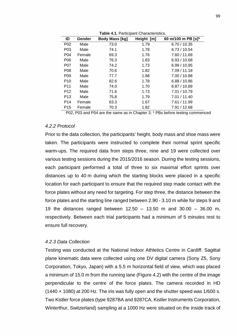
99

Table 4.1. Participant Characteristics. ID Gender Body Mass [kg] Height [m] 60 m/100 m PB [s]*

P02 Male 73.0 1.79 6.70 / 10.35 P03 Male 74.1 1.78 6.73 / 10.54 P04 Female 69.3 1.76 7.60 / 11.69 P06 Male 76.3 1.83 6.93 / 10.68 P07 Male 74.2 1.73 6.99 / 10.95 P08 Male 70.6 1.82 7.09 / 11.18 P09 Male 77.7 1.88 7.00 / 10.88 P10 Male 82.6 1.78 6.88 / 10.86 P11 Male 74.0 1.70 6.87 / 10.89 P12 Male 71.6 1.73 7.01 / 10.79 P13 Male 75.8 1.79 7.01 / 11.40 P14 Female 63.3 1.67 7.61 / 11.99 P15 Female 70.3 1.82 7.91 / 12.68 P02, P03 and P04 are the same as in Chapter 3; * PBs before testing commenced

4.2.2 Protocol

Prior to the data collection, the participants’ height, body mass and shoe mass were

taken. The participants were instructed to complete their normal sprint specific

warm-ups. The required data from steps three, nine and 19 were collected over

various testing sessions during the 2015/2016 season. During the testing sessions,

each participant performed a total of three to six maximal effort sprints over

distances up to 40 m during which the starting blocks were placed in a specific

location for each participant to ensure that the required step made contact with the

force plates without any need for targeting. For step three, the distance between the

force plates and the starting line ranged between 2.90 - 3.10 m while for steps 9 and

19 the distances ranged between 12.50 – 13.50 m and 30.00 – 36.00 m,

respectively. Between each trial participants had a minimum of 5 minutes rest to

ensure full recovery.

4.2.3 Data Collection

Testing was conducted at the National Indoor Athletics Centre in Cardiff. Sagittal

plane kinematic data were collected using one DV digital camera (Sony Z5, Sony

Corporation, Tokyo, Japan) with a 5.5 m horizontal field of view, which was placed

a minimum of 15.0 m from the running lane (Figure 4.2) with the centre of the image

perpendicular to the centre of the force plates. The camera recorded in HD

(1440 × 1080) at 200 Hz. The iris was fully open and the shutter speed was 1/600 s.

Two Kistler force plates (type 9287BA and 9287CA, Kistler Instruments Corporation,

Winterthur, Switzerland) sampling at a 1000 Hz were situated on the inside track of

100

the running straight and covered with the same Mondo surface as the surrounding

track. The GRF data was collected using CODAmotion analysis (version

6.68/MPx30, Charnwood Dynamics Ltd, Leicester, UK). GRF and kinematic data

were synchronised to within 0.001 s using a series of illuminating LEDs light (Wee

Beastie, UK).

Figure 4.2. Set-up.

To obtain the data required for camera calibration, a pole with six markers was

moved sequentially through five locations in the camera view. This allowed a

4.000 m × 1.900 m plane to be calibrated. As with Chapter 3, a pole with six points

of known locations was then placed at various known locations within the calibrated

plane. This would later be used to estimate the accuracy of coordinate

reconstruction.

4.2.4 Data Processing

The videos were extracted from the tapes using Dartfish Team Pro 6.0 (Dartfish)

and then converted to .avi format and de-interlaced in VLC 2.1.3 (VideoLan,

France). The videos were then digitised in Matlab (The MathWorks Inc., USA,

version R2014a) using an open source digitising package (Hedrick, 2008) at full

resolution and 2 × zoom. Digitising commenced at toe-off of the stance phase

preceding the stance phase being investigated and ended ten frames after the

touchdown of the contact after the one being investigated. Eighteen points on the

human body (Vertex, C7, hip, shoulder, elbow, wrist, knee, ankle, MTP joint centres

and distal end of the halluces) were digitised. A further point was used as a timing

mark to identify the touchdown (first frame of visible ground contact) and toe-off (first

1 2

101

frame after the foot left the ground) events of the contact of interest and the contact

after. The digitised trials were then reconstructed in Matlab using an open source 8

parameter 2D DLT camera calibration and point reconstruct function (Woltring and

Huiskes, 1985; Meershoek, 1997; http://isbweb.org/software/) which was edited to

include a ninth parameter 2D DLT which accounted for lens distortion (Walton,

1981). Digitising reliability was assessed by re-digitised one trial twice (see appendix

A4).

The reconstructed kinematic data were then imported into a custom written Matlab

script and synchronised to the force plate data using the information from the synch

lights. Following that the kinematic data was filtered. In order to ensure the joint

moment data were free of artefacts caused when kinematic and kinetic data are

filtered with mismatched cut-off frequencies (Bezodis et al., 2013), it was decided to

filter both the kinematic and kinetic data with the same cut-off frequency. Since

stance leg joint moments will be calculated later in this chapter, it was decided that

the selected cut-off frequency should be chosen to minimise the signal-to-noise ratio

within the landmarks on the stance leg and trunk. The optimal cut-off frequency was

determined based on the autocorrelation method (Challis, 1999). To ensure that

differences between the steps were not due to differences in filtering, a mean cut-

off frequency was calculated from all individual cut-offs. This mean cut-off (26 Hz)

was therefore applied to filter all the kinematic and kinetic time-history data from all

steps using a fourth-order Butterworth digital filter (Winter, 2009).

Data from de Leva (1996) was used to calculate the inertia data for all the segments

except the foot. For the foot segments, each participants shoe mass was added to

the mass of the foot segments. Data identifying the centre of mass location and

mass distribution of the fore and rear foot segment from Bezodis et al. (2014) was

used define the inertial properties of the fore and rear foot. The mass of the sprint

shoe was also split into a fore and rear foot segment according to the mass ratio

data from Bezodis et al. (2014). Whole-body CM was subsequently calculated using

the summation of segmental moments approach (Winter, 2009). Segment

orientations were calculated with 0° representing a horizontal orientation and a

positive increase an anti-clockwise rotation. In addition, descriptions of segment

rotations as clockwise or anti-clockwise are always relative to the direction of motion

http://isbweb.org/software/

102

being left to right. Joint angles were calculated as the 2D angle between two vectors

with extension of the hip, knee, ankle and MTP joints defined as positive (Figure

4.3). All linear and angular time-displacement histories were differentiated using a

three-point central difference method (Miller & Nelson, 1976) via the gradient

function in Matlab. Angular and linear velocity data were differentiated again to yield

linear and angular acceleration data. Step velocity, step length and step frequency

were calculated according to the methods outlined in Chapter 3 (section 3.2.7).

Figure 4.3. Convention used to describe positive changes (extension) in joint kinematic and

kinetics.

Since the touchdown and toe-off events for each step were defined using the 1000

Hz force data, the kinematic data was resampled at 1000 Hz using an interpolating

cubic spline. This would allow a more precise determination of touchdown and

toe-off joint kinematic variables, as the first 200 Hz video frames could occur 0.004 s

after touchdown or toe-off. Horizontal external power was selected as a

performance measure for steps three and nine. The incoming CM velocity was

calculated using CM displacement data as outlined in Bezodis et al. (2010). The first

derivative of a first order polynomial fitted through 10 frames prior to touchdown was

used to calculate the incoming CM velocity. This CM velocity together with the

measured GRF data was used to calculate the average external power produced

during the stance phase. The process of calculating average external power will be

described in more detail below. Step velocity was used as the performance measure

for step 19. The step characteristics were calculated according to the methods

outlined in Theme 1 (Chapter 3: section 3.2.7).

103

Before filtering the GRF data, data from the individual force channels were exported

using the CODAmotion software. Initially the appropriate force channels were

summed to calculate the vertical, anterior-posterior and medio-lateral forces. The

vertical forces were used to identify the touchdown and toe-off events. Touchdown

was defined as the first frame when the vertical ground reaction force rose above

10 N. Toe-off was defined as the first frame after vertical ground reaction force fell

below 10 N. For all the variables reported directly from the GRF data, the raw forces

were filtered with a higher cut-off frequency (~170 Hz) which was determined for

each force trace using the autocorrelation function described above.

Resultant forces were calculated from the vertical and anterior-posterior GRF. Peak

resultant, vertical and anterior-posterior (braking and propulsive) forces were

identified from the filtered forced data. Braking, propulsive, net anterior-posterior

and vertical (body weight removed) impulses were calculated via numerical

integration (trapezium rule) and expressed relative to the participant’s body mass to

reflect the change in velocity of the centre of mass. Using the relative

anterior-posterior impulse, the change in velocity across each frame of ground

contact was calculated and combined with the incoming CM velocity in order to

obtain the absolute instantaneous velocity throughout stance. External power was

then determined as the product of the instantaneous horizontal velocity and

horizontal force. Horizontal external power across the entire stance phase was

subsequently averaged and normalised for use as a measure of performance


The centre of pressure (COP) was calculated from the individual force channels

using the equations provided by the manufacturer of the force plates (Kistler

Instruments Corporation, Winterthur, Switzerland) and accounting for the thickness

of the track surface. When the ground contact occurred across both plates, the

global COP was calculated as the sum of the products between each plate’s COP

and a weighting factor (Exell et al., 2012). The centre of plate two (Figure 4.2) was

set as the origin of the two force plates. This coincided with the origin of the global

coordinate system. The centre of pressure coordinates from force plate 1 were

therefore offset by 0.906 m in the y direction. Finally, to match the GRF and centre

of pressure data with kinematic data for joint kinetics calculations these data were

104

down sampled to 200 Hz and filtered using a bi-directional Butterworth filter with the

previously determined cut-off frequency of 26 Hz.

4.2.4.1 Inverse dynamics analysis The synchronised kinematic data and force data (both sampled at 200 Hz and

filtered at 26 Hz) were used to calculate the internal joint forces and moments. This

was done using a 2D inverse dynamics analysis according to Winter (2009) starting

with the measured external GRF and moving up the body to calculate the joint

kinetics at the MTP, ankle, knee and hip. Since the MTP has previously been shown

to play an important role in sprinting (Stefanyshyn & Nigg, 1997; Bezodis et al.,

2012) it was decided to include this joint in the analysis. The fore foot segment and

MTP joint were only included in the calculation when the COP acted in front of the

MTP joint (Stefanyshyn & Nigg, 1997). Furthermore, the inertial properties of the

fore foot were assumed to be negligible and therefore the MTP joint moment was

influenced only by the GRF and moment arms relative to the MTP joint (Stefanyshyn

& Nigg, 1997, Smith et al., 2014).

Nomenclature for the inverse dynamics analysis

F Force

𝑎𝑎 Acceleration

g Gravity

m Mass

i Segment

CM Centre of mass

𝐹𝐹𝑦𝑦𝑖𝑖 Horizontal joint reaction force at proximal endpoint of the ith segment

𝐹𝐹𝑧𝑧𝑖𝑖 Vertical joint reaction force at the proximal endpoint of the ith segment

𝑎𝑎𝑦𝑦𝑖𝑖 Horizontal acceleration of the ith segment

𝑎𝑎𝑧𝑧𝑖𝑖 Vertical acceleration of the ith segment

𝐹𝐹𝑦𝑦𝑖𝑖−1 Horizontal joint reaction force at the distal endpoint of the ith segment

𝐹𝐹𝑧𝑧𝑖𝑖−1 Vertical joint reaction force at distal endpoint of the ith segment

𝑀𝑀 Moment

𝐼𝐼𝑖𝑖 R Moment of inertia of the ith segment

𝛼𝛼𝑖𝑖 Angular acceleration of the ith segment

𝑀𝑀𝑝𝑝𝑖𝑖 Moment acting on the proximal endpoint of the ith segment

𝑀𝑀𝑑𝑑𝑖𝑖 Moment acting on the distal endpoint of the ith segment

𝑟𝑟𝑖𝑖𝑝𝑝 Moment arm between the proximal end of the segment and the CM

𝑟𝑟𝑖𝑖𝑎𝑎 Moment arm between the distal end of the segment and the CM

105

𝑗𝑗 Joint

𝐽𝐽𝑃𝑃𝑗𝑗 Joint power of the jth joint

𝜔𝜔𝑗𝑗 Angular velocity of the jth joint

𝑊𝑊𝑛𝑛𝑗𝑗 Joint work of the nth power phase of joint j

𝐽𝐽𝑃𝑃𝑗𝑗 Joint power of the ith joint

∑ Sum of

Net joint forces were calculated according to Newton’s 2nd law of linear motion

(Equation 4.1).

∑𝑭𝑭𝒊𝒊 = 𝒎𝒎𝒊𝒊 × 𝒂𝒂𝒊𝒊 [Equation 4.1]

The free body diagram (Figure 4.4) below shows the forces acting on the ith segment

in both the vertical (z) and anterior-posterior direction (y). Using the known linear

acceleration and forces acting on the distal end of the segment, the unknown forces

acting on the proximal end of the segment could thus be calculated.

Figure 4.4. Free body diagram illustrating the forces acting on the ith segment.

The vertical and anterior-posterior internal joint forces were thus calculated using

the following equations:

𝑭𝑭𝒚𝒚𝒊𝒊 = 𝒎𝒎𝒊𝒊 × 𝒂𝒂𝒚𝒚𝒊𝒊 − 𝑭𝑭𝒚𝒚𝒊𝒊−𝟏𝟏 [Equation 4.2] 𝑭𝑭𝒛𝒛𝒊𝒊 = 𝒎𝒎𝒊𝒊 × 𝒂𝒂𝒛𝒛𝒊𝒊 − 𝒎𝒎𝒊𝒊 × 𝒈𝒈 − 𝑭𝑭𝒛𝒛𝒊𝒊−𝟏𝟏 [Equation 4.3]

The resultant joint moments were calculated using Newton-Euler equation

(Equation 4.4) which describes the combined translational and rotational dynamics

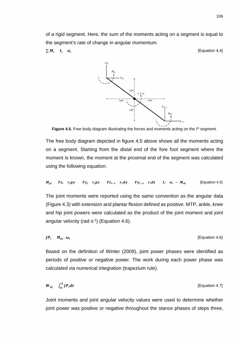
106

of a rigid segment. Here, the sum of the moments acting on a segment is equal to

the segment’s rate of change in angular momentum. ∑ 𝑴𝑴𝒊𝒊 = 𝑰𝑰𝒊𝒊 × 𝜶𝜶𝒊𝒊 [Equation 4.4]

Figure 4.5. Free body diagram illustrating the forces and moments acting on the ith segment.

The free body diagram depicted in figure 4.5 above shows all the moments acting

on a segment. Starting from the distal end of the fore foot segment where the

moment is known, the moment at the proximal end of the segment was calculated

using the following equation.

𝑴𝑴𝒑𝒑𝒊𝒊 = (𝑭𝑭𝒛𝒛𝒊𝒊 × 𝒓𝒓𝒊𝒊𝒑𝒑𝒚𝒚) + (𝑭𝑭𝒚𝒚𝒊𝒊 × 𝒓𝒓𝒊𝒊𝒑𝒑𝒛𝒛) + (𝑭𝑭𝒛𝒛𝒊𝒊−𝟏𝟏 × 𝒓𝒓𝒊𝒊𝒅𝒅𝒚𝒚) + (𝑭𝑭𝒚𝒚𝒊𝒊−𝟏𝟏 × 𝒓𝒓𝒊𝒊𝒅𝒅𝒛𝒛) + (𝑰𝑰𝒊𝒊 × 𝜶𝜶𝒊𝒊) − 𝑴𝑴𝒅𝒅𝒊𝒊 [Equation 4.5]

The joint moments were reported using the same convention as the angular data

(Figure 4.3) with extension and plantar flexion defined as positive. MTP, ankle, knee

and hip joint powers were calculated as the product of the joint moment and joint

angular velocity (rad·s-1) (Equation 4.6).

𝑱𝑱𝑷𝑷𝒊𝒊 = 𝑴𝑴𝒑𝒑𝒊𝒊 .𝝎𝝎𝒊𝒊 [Equation 4.6]

Based on the definition of Winter (2009), joint power phases were identified as

periods of positive or negative power. The work during each power phase was

calculated via numerical integration (trapezium rule).

𝑾𝑾𝒏𝒏𝒏𝒏 = ∫ 𝑱𝑱𝑷𝑷𝒊𝒊𝒅𝒅𝒕𝒕𝒕𝒕𝟏𝟏𝒕𝒕𝟏𝟏 [Equation 4.7]

Joint moments and joint angular velocity values were used to determine whether

joint power was positive or negative throughout the stance phases of steps three,

107

nine and 19. For example, when both the net joint moment was extensor dominant

and the joint angular velocity was positive (joint extending), the resulting positive

power phase was described as a positive extensor power phase and positive

extensor work.

At the MTP, ankle and hip joints two main power phases were identified (Figure 4.6).

At the MTP and ankle joints a plantar flexor moment power abortion phase (MTP-;

A-) was followed by a plantar flexor power generation phase (MTP+; A+). At the hip

joint a hip extensor moment power generation phase (H+) was followed by a hip

flexor power absorption phase (H-).

MTP joint power Ankle joint power Hip joint power

Nor

mal

ised

join

t

Figure 4.6. Definition of the power phases for the MTP, ankle and hip joints.

Up to four power phases were identified at the knee joint (Figure 4.7). The knee

flexors generated energy (Kf+) while a knee flexor moment and a knee flexor

angular velocity were present. The knee extensors absorbed energy (Ke-) when a

knee flexor angular velocity and a knee extensor moment were present. The knee

extensors generated energy (Ke+) when a knee extensor moment and knee

extensor angular velocity were present and the knee flexor absorbed energy (Kf-)

when a knee flexor moment and knee extensor angular velocity were present.

Step 3 Step 9 Step 19

Nor

mal

ised

join

t

Figure 4.7. Definition of the power phases for the knee during steps three, nine and 19.

-1.0-0.8-0.6-0.4-0.20.00.20.40.6

0.00 0.04 0.08 0.12

Contact Time [s]-4.0

-2.0

0.0

2.0

4.0

0.00 0.04 0.08 0.12

Contact Time [s]-3.0

-2.0

-1.0

0.0

1.0

2.0

0.00 0.04 0.08 0.12

Contact Time [s]

-0.4

-0.2

0.0

0.2

0.4

0.6

0.00 0.04 0.08 0.12 0.16

Contact time [s]

-0.6

-0.4

-0.2

0.0

0.2

0.4

0.6

0.00 0.05 0.10 0.15

Contact time [s]

-1.0-0.8-0.6-0.4-0.20.00.20.40.6

0.00 0.04 0.08 0.12

Contact time [s]

Kf+

Kf -

Kf+

Ke-

Ke+ Kf+

Ke-

Ke+

Ke- Kf -

MTP+

A+

A-

H+

H- MTP-

108

4.2.5 Data normalisation

The calculated joint angular velocities (deg·s-1), moments (Nm), powers (W) and

work (J) for each participant were normalised according to the recommendations of

Hof (1996) with height used for linear scaling. Angular velocities were normalised

using gravity (g; 9.81 m·s-2) and height (�𝑔𝑔

𝐻𝐻𝐻𝐻𝑖𝑖𝑔𝑔ℎ𝑐𝑐 ), joint moments and work were

normalised using body weight and height (𝐵𝐵𝑊𝑊 ∗ 𝐻𝐻𝐻𝐻𝐻𝐻𝐻𝐻ℎ𝑡𝑡). Joint powers were

normalised to body mass (BM), gravity and height (𝐵𝐵𝑀𝑀 ∗ 𝐻𝐻32 ∗ 𝐻𝐻𝐻𝐻𝐻𝐻𝐻𝐻ℎ𝑡𝑡

12) according to

Bezodis et al. (2010).

4.2.6 Data presentation

The best step three, nine and 19 trials from each participant was selected for further

analysis. The best step three and nine trial was based on identifying the trial during

which the participant produced the largest normalised average external horizontal

power. This was based on the fact that power production is of critical importance

during sprint acceleration and ultimately determines acceleration of the participants

(Bezodis, et al., 2010). The best step 19 trial was selected based on identifying the

trial where the participants achieved the largest maximal step velocity as this reflect

a higher level of performance during the maximal velocity phase. Minimum and

maximal joint kinematic and kinetic values and associated timings (absolute (s) and

percentages of stance (%)) were extracted from the time-histories. The

time-histories for each ground contact were then time-normalised to 101 data points

using a cubic spline. The time-normalised GRF, joint kinematics, joint kinetic data

as well as the segment angles and angular velocities were averaged across

participants to create an ensemble average for each step. The mean

time-normalised data for each step was presented relative to the mean contact time

for the relevant step.

4.2.7 Data analysis

Descriptive statistics (mean ± SD) were calculated for all the discrete variables. In

order to clarify the meaningfulness of the differences, magnitude-based inferences

were computed (Batterham & Hopkins, 2006). The mechanistic inference was used

to quantify the difference being either positive, trivial or negative. The differences

between means (step: 9-3; 19-3; 19-9) were calculated using post-only crossover

109

analysis (Hopkins, 2006). The confidence interval with which the inferences were

made (after adjusting for the number of comparisons, three) was 97%. To evaluate

the meaningfulness of the difference, a Cohen’s effect size of 0.2 was used as the

threshold for the smallest worthwhile change (Winter et al., 2014). The probability

(percentage and qualitative description) that the true effect size was bigger than 0.2

was defined as: very unlikely: <5%; unlikely: 5% - 24.9%; possibly 25 – 74.9%; likely:

75% - 94.9%; very likely: 95% - 99.4% and most likely >99.5% (Hopkins, Marshall,

Batterham & Hanin, 2009). When the outcome of the effect had a >5% chance of

being both positive and negative, the mechanistic outcome was described as

unclear. Otherwise, the mechanistic outcome was clear with differences being either

positive or negative. To evaluate the magnitude of the observed differences

between the steps, the scale based on Hopkins et al. (2009) was used to quantify

the effect sizes: 0.0 (trivial), 0.2 – 0.59 (small), 0.6 – 1.19 (moderate), 1.2 – 1.99

(large), 2.0 – 3.99 (very large) and >4.0 (extremely large).

4.3 Results 4.3.1 Kinematic variables

Starting with the step characteristics, the increases in step velocity (Table 4.2) from

step three to step nine were most likely extremely large and between steps nine and

19 were most likely very large. Increases in vertical CM velocity prior to touchdown

were most likely large between step three and nine and most likely moderate

between steps nine and 19. Step length increases were most likely very large

between steps three and nine and most likely large between steps nine and 19.

Table 4.2. Mean ± SD values for selected step characteristics, performance and temporal variables

for steps three, nine and 19 across all participants. Step 3 Step 9 Step 19

Mean SD Mean SD Mean SD Step velocity [m·s-1] 5.81 0.24 8.36 0.46 9.67 0.58 Vertical CM velocity [m·s-1] -0.24 0.13 -0.52 0.17 -0.69 0.11 Step length [m] 1.37 0.09 1.92 0.19 2.25 0.21 Step frequency [Hz] 4.27 0.34 4.39 0.45 4.33 0.43 NAHP 0.69 0.12 0.49 0.16 0.20 0.11 Contact time [s] 0.155 0.014 0.123 0.013 0.105 0.010 Flight time [s] 0.080 0.015 0.107 0.020 0.128 0.022 Step time [s] 0.236 0.019 0.230 0.028 0.233 0.026

- NAHP: normalised average horizontal power

Differences in step frequency were unclear between steps three and nine and

between steps three and 19 and possibly trivial between steps nine and 19.

110

Decreases in contact times were most likely very large from steps three to nine to

19. Flight time increases were most likely large between steps three and nine and

most likely moderate between steps nine and 19.

The differences in CM-h, trunk and shank angles at touchdown (Table 4.3) were

most likely large to extremely large in all three comparisons.

The increases in horizontal foot velocities at touchdown (Table 4.4) between steps

three and nine were most likely large and very likely moderate between steps nine

and 19. Increases in downward foot velocities were most likely large between steps

three and nine and very likely moderate between steps nine and 19. The differences

in touchdown and toe-off distances between steps three, nine and 19 were most

likely large to extremely large.

Table 4.4. Mean ± SD horizontal and vertical foot velocity and touchdown and toe-off distances

during steps three, nine and 19. Measure Step 3 Step 9 Step 19

Unit Mean SD Mean SD Mean SD Horizontal foot velocity [m·s-1] 0.45 0.86 1.96 0.90 2.53 0.65 Horizontal foot velocity relative to step velocity [m·s-1] -5.36 0.80 -6.41 1.00 -7.14 1.00

Vertical foot velocity [m·s-1] -1.75 0.45 -2.44 0.43 -2.96 0.37 Vertical foot velocity relative to vertical CM velocity prior to TD

[m·s-1] -1.51 0.39 -1.93 0.43 -2.27 0.38

Touchdown distance [m] 0.055 0.057 0.275 0.060 0.359 0.046 Toe-off distance [m] -0.731 0.037 -0.641 0.041 -0.546 0.028

4.3.2 GRF variables

Mean and peak vertical GRF (Table 4.5) increased from steps three to nine to 19.

These differences in were most likely very to extremely large. The absolute (and

relative) timings of the peak vertical forces occurred at 0.073 ± 0.017 s (47 ± 9%)

during step three, 0.039 ± 0.014 s (32 ± 12%) during step nine and 0.030 ± 0.008 s

(29 ± 8%) during step 19. Differences between in the absolute time at which peak

Table 4.3. Mean ± SD of touchdown CM-h, trunk and shank angles for steps three, nine and 19 Step 3 Step 9 Step 19

Mean SD Mean SD Mean SD CM-h [%] 51 2 54 1 57 1 θ trunk [°] 46 9 64 7 81 3 θshank [°] 63 5 87 4 97 3

111

vertical forces occurred were most likely large between steps three and nine and

between steps three and 19.

Table 4.5. Mean ± SD of stance mean and maximum resultant GRF from steps three, nine and 19.

Step 3 Step 9 Step 19 Mean SD Mean SD Mean SD Mean resultant force [BW] 1.6 0.2 1.9 0.2 2.2 0.2 Maximum resultant force [BW] 2.3 0.2 3.0 0.4 3.8 0.3 RF % 31 3 12 3 4 2

Decrease in mean horizontal forces between step three, nine and 19 (Figure 4.8a)

were most likely very large to extremely large. Differences in peak horizontal braking

forces were most likely large to very large between steps three to nine to 19 (Figure

4.8a). Differences in the durations of the braking phase were most likely very large

between steps three (0.012 ± 0.005 s; 8 ± 3% of stance) and nine (0.034 ± 0.011 s;

27 ± 6% of stance) and most likely moderate between steps nine and 19 (0.043 ±

0.008 s; 41 ± 5% of stance). Decreases in peak propulsive forces were most likely

moderate between steps three and nine and between steps three and 19 (Figure

4.8a).

Figure 4.8. Mean ± SD time-histories of horizontal (a) and vertical (b) ground reaction force data for step three (black), step nine (blue) and step 19 (red). The tables below the respective figures show the descriptive results of the MBI analysis of the differences between the three steps. For each comparison, there is a qualitative description of the probability of the standardised differences being larger than 0.02, followed by the size (standardised effect) and direction of the differences.

a) Anterior-posterior GRF b) Vertical GRF

Step: 9 – 3 Step: 19 – 3 Step: 19 – 9 Step: 9 – 3 Step: 19 – 3 Step: 19 – 9

Mean force

Most likely very large negative

differences

Most likely extremely

large negative

differences

Most likely very large negative

differences

Mean force

Most likely very large positive

differences


large positive differences


differences

Peak braking force

Most likely large

positive differences


differences

Most likely large

positive differences

Peak force


differences


large positive differences


differences

Peak propulsive force

Most likely moderate negative

differences

Very likely moderate negative

differences

unclear

-2.0-1.5-1.0-0.50.00.51.01.5

0.00 0.04 0.08 0.12 0.16

Forc

e [B

W]

Contact time [s]

0.0

1.0

2.0

3.0

4.0

5.0

0.00 0.04 0.08 0.12 0.16

Forc

e [B

W]

Contact time [s]

112

The absolute (% of stance) occurrence for the peak propulsive forces for steps

three, nine and 19 were 0.109 ± 0.012 s (70 ± 2%), 0.088 ± 0.010 s (71 ± 2%) and

0.075 ± 0.008 s (72 ± 2%) respectively. Durations of the propulsive phase showed

most likely extremely large decreases from step three (0.143 ± 0.015 s; 92 ± 3% of

stance) to step nine (0.089 ± 0.004 s; 73 ± 6% of stance) and most likely very large

decreases between steps nine and 19 (0.062 ± 0.004 s; 59 ± 5% of stance).

Increases in relative vertical impulse (Table 4.6) were most likely very large between

steps three and nine and most likely moderate between steps nine and 19. The

decrease in relative anterior-posterior impulses between steps three and nine was

most likely extremely large and between steps nine and 19 were most likely very

large. The increase in relative braking impulse (Table 4.6) was most likely large

between steps three and nine and most likely very large between steps nine and 19.

The decrease in relative propulsive impulse (Table 4.6) between steps three and

nine were most likely extreme large and between steps nine and 19 were most likely

very large.

Table 4.6. Mean ± SD changes in vertical, net horizontal velocity as well as the mean ± SD

horizontal velocity decrease and increase during steps three, nine and 19 across all participants. Step 3 Step 9 Step 19

Mean SD Mean SD Mean SD Change in vertical velocity [m·s-1] 0.66 0.14 1.00 0.18 1.18 0.15 Net change in horizontal velocity [m·s-1] 0.74 0.05 0.28 0.06 0.08 0.04 Horizontal velocity decrease [m·s-1] -0.03 0.02 -0.10 0.05 -0.19 0.04 Horizontal velocity increase [m·s-1] 0.77 0.04 0.38 0.03 0.27 0.03

Across participants, there was a trend for the relative braking impulse to increase

with increases in the horizontal velocity of the foot immediately prior to touchdown

of steps three, nine and 19 as well as touchdown distance during steps nine and 19

(Figure 4.9).

113

Figure 4.9. Scatter-plots and trend lines for steps three (black), nine (blue) and 19 (red) for a) foot touchdown velocity and b) touchdown distance against relative the relative braking impulse.

4.3.3 Joint kinematics and kinetics

4.3.3.1 MTP Joint

At the MTP joint, similar kinematic patterns were visible between steps three, nine

and 19. During ground contact, the MTP joint angle initially plantar flexed before

dorsiflexing from 0.027 ± 0.013 to 0.136 ± 0.014 s (18 ± 9 to 87 ± 2% of stance),

from 0.029 ± 0.006 to 0.104 ± 0.012 s (24 ± 5 to 85 ± 3% of stance) and from 0.027

± 0.004 to 0.089 ± 0.009 s (26 ± 3 to 85 ± 2% of stance) during steps three, nine

and 19 respectively (Figure 4.10a). After the MTP joint reached the minimum

dorsiflexion angles, the MTP joint plantar flexed until toe-off. The differences in peak

dorsiflexion angular velocity were likely moderate between steps three (-317 ± 65

(dimensionless units)) and nine (-390 ± 91) and most likely large between steps nine

and 19 (-507 ± 81).

The MTP moment (Figure 4.10c) was plantar flexor dominant throughout stance,

reaching peaks of 0.03 ± 0.01 (step 3), 0.03 ± 0.01 (step 9) and 0.04 ± 0.02 (step

19). The peak normalised negative power was -0.43 ± 0.13 (step three), -0.66 ± 0.22

(step nine) and -0.90 ± 0.44 (step 19). The increase in peak negative power was

very likely moderate between steps three and nine and likely moderate between

steps nine and 19. Differences in peak positive power were possibly small between

steps three (0.28 ± 0.09) and nine (0.32 ± 0.09), likely moderate between steps nine

and 19 (0.43 ± 0.19).

-0.35

-0.30

-0.25

-0.20

-0.15

-0.10

-0.05

0.00-1 0 1 2 3 4 5

Rel

ativ

e br

akin

g im

puls

e [m

·s-1

]

a) Foot velocity [m·s-1]

-0.35

-0.30

-0.25

-0.20

-0.15

-0.10

-0.05

0.00-0.10 0.00 0.10 0.20 0.30 0.40

Rel

ativ

e br

akin

g im

puls

e [m

·s-1

]

b) Touchdown distance [m]

114

Figure 4.10. Mean ± SD MTP angle (a), normalised MTP angular velocity (b), normalised MTP moment (c) and normalised power between steps three (black), nine (blue) and 19 (red). The tables below the respective figures show the descriptive results of the results of the MBI analysis of the differences between the three steps. For each comparison, there is a qualitative description of the probability of the standardised differences being larger than 0.02, followed by the size (standardised effect) and direction of the differences.

a) MTP angle b) MTP angular velocity

A

ngle

[°]

N

orm

alis

ed a

ngul

ar v

eloc

ity


TD angle Likely moderate positive differences

Likely moderate positive differences Unclear Peak doriflexion AV Likely moderate positive

differences Most likely very large positive

differences Most likely large positive

differences

Dorsiflexion ROM Likely moderate positive differences

Most likely large positive differences

Likely moderate positive differences Peak plantarflexion AV Likely small positive difference Most likely moderate positive

differences Likely small positive difference

Plantarflexion ROM Unclear Unclear Unclear

TO angle Likely moderate positive differences Unclear Unclear

c) MTP joint moment d) MTP joint power

Nor

mal

ised

mom

ent

N

orm

alis

ed p

ower


Peak plantar flexor moment Likely small positive differences Unclear Unclear Peak negative power Very likely moderate positive


differences Likely moderate positive

differences

Peak positive power Possibly small positive differences

Very likely moderate positive differences

Likely moderate positive differences

90100110120130140150160

0.00 0.02 0.04 0.06 0.08 0.10 0.12 0.14 0.16Contact Time [s]

-600

-300

0

300

600

900

1200

0 0.02 0.04 0.06 0.08 0.1 0.12 0.14 0.16Contact Time [s]

-0.02

0.00

0.02

0.04

0.06

0.00 0.02 0.04 0.06 0.08 0.10 0.12 0.14 0.16

Contact Time [s]

-1.5

-1.0

-0.5

0.0

0.5

1.0

0.00 0.02 0.04 0.06 0.08 0.10 0.12 0.14 0.16Contact Time [s]

Plantar flexion

Dorsiflexion

Generation

Absorption

Plantar flexion

Dorsiflexion

115

The energy absorbed by the MTP joint increased from steps three (-0.013 ± 0.005),

nine (-0.018 ± 0.006) and 19 (-0.018 ± 0.009; Figure 4.11). On each step, the energy

generated at the MTP joint (Step three: 0.003 ± 0.001; Step nine: 0.002 ± 0.001;

Step 19: 0.003 ± 0.001) was relatively small compared to the energy absorbed on

the step.

Figure 4.11. Mean ± SD normalised negative (MTP-) and positive (MTP+) MTP work for steps three (black), nine (blue) and 19 (red). The table shows the results of the MBI analysis of the differences between the three steps. For each comparison, there is a qualitative description of the probability of the standardised differences being larger than 0.02, followed by the size (standardised effect) and direction of the differences.

4.3.3.2 Ankle Joint

Similar angular kinematic and kinetic patterns at the ankle were exhibited during

steps three, nine and 19 (Figure 4.12a). Increases in touchdown ankle angles were

most likely moderate between steps three (111 ± 8°) and nine (120 ± 6°) and most

likely large between steps nine and 19 (130 ± 7°). The differences in dorsiflexion

ROM were most likely moderate (Figure 4.12a) between steps three (18 ± 4°) and

nine (24 ± 4°) and most likely large between steps nine and 19 (32 ± 7°). The

resulting dorsiflexion angular velocity peaked at 0.016 ± 0.003 s (step 3), 0.016 ±

0.004 s (step 9) and 0.015 ± 0.003 s (step 19). Differences in peak dorsiflexion

angular velocity (Figure 4.12b) between steps three (-261 ± 62) and step nine (-337

± 48) were very likely moderate to large. The differences in peak dorsiflexion angular

velocity were most likely large between steps nine and 19 (-448 ± 86).

Step: 9 – 3 Step: 19 – 3 Step: 19 – 9

Negative joint work Very likely moderate positive differences

Likely moderate positive differences Unclear

Positive joint work Unclear Unclear Unclear

-0.030

-0.020

-0.010

0.000

0.010

3 9 19

norm

alis

ed J

oint

wor

k

Steps

MTP- MTP- MTP-

MTP+ MTP+ MTP+

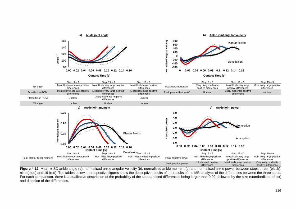
116

Figure 4.12. Mean ± SD ankle angle (a), normalised ankle angular velocity (b), normalised ankle moment (c) and normalised ankle power between steps three (black), nine (blue) and 19 (red). The tables below the respective figures show the descriptive results of the results of the MBI analysis of the differences between the three steps. For each comparison, there is a qualitative description of the probability of the standardised differences being larger than 0.02, followed by the size (standardised effect) and direction of the differences.

a) Ankle joint angle b) Ankle joint angular velocity

Ang

le [°

]

Nor

mal

ised

ang

ular

vel

ocity


TD angle Most likely moderate positive differences

Most likely very large positive differences

Most likely large positive differences Peak dorsi-flexion AV Very likely moderate

positive differences Most likely very large positive differences


Dorsiflexion ROM Most likely moderate positive differences


Most likely large positive differences Peak plantar-flexion AV Unclear Likely moderate positive

differences unclear

Plantarfleion ROM Unclear Likely moderate negative differences Unclear

TO angle Unclear Unclear Unclear

c) Ankle joint moment d) Ankle joint power

Nor

mal

ised

mom

ent

Nor

mal

ised

pow

er


Peak plantar flexor moment Most likley moderate positive differences

Most likley large positive differences

Most likley moderate positive differences Peak negative power Most likely large positive

differences Most likely very large positive differences


Peak positive power Likely small positive differences



80

100

120

140

160

0.00 0.02 0.04 0.06 0.08 0.10 0.12 0.14 0.16

Contact Time [s]

-600-400-200

0200400600800

0 0.02 0.04 0.06 0.08 0.1 0.12 0.14 0.16

Contact Time [s]

0.00

0.10

0.20

0.30

0.00 0.02 0.04 0.06 0.08 0.10 0.12 0.14 0.16Contact Time [s]

-6.0

-4.0

-2.0

0.0

2.0

4.0

6.0

0.00 0.02 0.04 0.06 0.08 0.10 0.12 0.14 0.16Contact Time [s]

Plantar flexion

Dorsiflexion

Plantar flexion

Dorsiflexion

Generation

Absorption

117

During the second half of stance, no clear differences in plantar flexion ROM (Figure

4.12a) were observed between steps three (48 ± 5°), nine (47 ± 5°) and 19 (44 ±

5°). The ankle plantar flexion angular velocities (step 3: 482 ± 62; step 9: 510 ± 66;

step 19: 543 ± 86) peaked 0.140 ± 0.015 s (step 3), 0.110 ± 0.015 s (step 9) and

0.089 ± 0.012 s (step 19) after touchdown.

Differences in peak ankle moments (Figure 4.12c) were most likely moderate

between steps three (0.18 ± 0.02) and nine (0.21 ± 0.03) and most likely moderate

between steps nine and 19 (0.24 ± 0.04). The peaks occurred at 0.087 ± 0.017 s

(56 ± 8% of stance), 0.060 ± 0.009 s (49 ± 5% of stance) and 0.048 ± 0.008 s (46 ±

6% of stance) during step three, nine and 19, respectively. The differences in the

absolute timings of the peaks of the plantar flexor ankle moment were most likely

very large between steps three and nine most likely moderate between steps nine

and 19. The peak negative ankle joint power (step 3: -1.18 ± 0.42; step 9: -2.20 ±

0.61; step 19: -3.66 ± 1.02) occurred at 0.023 ± 0.003 s (15 ± 3% of stance), 0.024

± 0.006 s (20 ± 5% of stance) and 0.023 ± 0.003 s (22 ± 3% of stance) after

touchdown of steps three, nine and 19 respectively. Peak joint power generation

(step 3: 2.32 ± 0.48; step 9: 2.73 ± 0.90; step 19: 3.61 ± 1.06) occurred at 0.122 ±

0.013 s (79 ± 2% of stance), 0.091 ± 0.011 s (74 ± 4% of stance) and 0.076 ± 0.008 s

(73 ± 2% of stance) respectively. The differences in peak power generation were

likely small between steps three and nine and very likely moderate between steps

nine and 19.

Step: 9 – 3 Step: 19 – 3 Step: 19 – 9 Negative joint work Most likely large positive



Positive joint work Unclear Unclear Likely small positive differences

Figure 4.13. Mean ± SD normalised negative (A-) and positive (A+) ankle work for steps three (black), nine (blue) and 19 (red). The table shows the results of the MBI analysis of the differences between the three steps. For each comparison, there is a qualitative description of the probability of the standardised differences being larger than 0.02, followed by the size (standardised effect) and direction of the differences.

-0.10

-0.05

0.00

0.05

0.10

3 9 19

Nor

mal

ised

ank

le

wor

k

Step

A- A- A-

A+ A+ A+

118

The differences in energy absorbed at the ankle (Figure 4.13) during the negative

power phases of steps three (-0.027 ± 0.007), nine (-0.050 ± 0.010) and 19 (-0.078

± 0.020) were most likely large to very large. The energy generated during the

positive power phases was 0.074 ± 0.013, 0.075 ± 0.013 and 0.081 ± 0.017 during

steps three, nine and 19, respectively. No clear differences were observed between

steps three and nine, while the differences between steps nine and 19 were likely

small. Throughout steps three, nine and 19, the ankle remained a net energy

generator. The energy absorbed (A-) to energy generated (A+) ratio was 2.9 ± 0.7

during step three, 1.5 ± 0.2 during step nine and 1.1 ± 0.2 during step 19.

4.3.3.3 Knee Joint

Different angular patterns were observed at the knee between step three and steps

nine and 19 (Figure 4.14a). In step three, the knee joint extended throughout the

majority of stance, while during steps nine and 19, the knee joint flexed during the

first half of stance before extending. Differences in touchdown knee joint angles

between steps three (117 ± 6°), nine (142 ± 6°) and 19 (156 ± 6°) were most likely

very large. Knee flexion ROM was 0°, 10 ± 5° and 16 ± 5° during steps three, nine

and 19, respectively. Differences between steps nine and 19 were most likely large.

During the second half of stance, the differences in knee extension ROM (Figure

4.14a) were most likely very large between steps three (42 ± 8°) and nine (25 ± 9°)

and most likely moderate between steps nine and 19 (17 ± 6°). Differences in toe-off

knee angle were likely small between steps three (159 ± 6°) and nine (156 ± 4°) and

likely moderate between steps three and 19 (156 ± 4°).

During step nine and 19, a knee flexor angular velocity was present which reached

a peak 0.035 ± 0.015 s (28 ± 12%) and 0.021 ± 0.005 s (20 ± 5%) after touchdown,

respectively. There was a most likely large increase in the knee flexor angular

velocity between steps nine (-124 ± 43) and 19 (-202 ± 60). The peak knee extension

angular velocity peaked at 0.119 ± 0.019 s, 0.100 ± 0.019 s and 0.084 ± 0.011 s

during steps three, nine and 19, respectively. There were no clear differences

between the peak extensor angular velocities during steps three and nine.

119

Figure 4.14. Mean ± SD knee angle (a), normalised Knee angular velocity (b), normalised Knee moment (c) and normalised knee power between steps three (black), nine (blue) and 19 (red). The tables below the respective figures show the descriptive results of the results of the MBI analysis of the differences between the three steps. For each comparison, there is a qualitative description of the probability of the standardised differences being larger than 0.02, followed by the size (standardised effect) and direction of the differences.

a) Knee joint angle b) Knee joint angular velocity

A

ngle

[°]

Nor

mal

ised

ang

ular

vel

ocity


TD angle Most likely very large positive differences

Most likely extremely large positive differences

Most likely very large positive differences Peak knee flexor AV - - Most likely large positive

differences

Flexion ROM Most likely very large positive differences


Most likely large positive differences Peak knee extensor AV Unclear Unclear Unclear

Extension ROM Most likely very large negative differences

Most likely very large negative differences

Most likely moderate negative differences

TO angle Likely small negative differences

Likely small negative differences Unclear

c) Knee joint moment d) Knee joint power

Nor

mal

ised

mom

ent

N

orm

alis

ed P

ower


Flexor moment (TD) Very likely moderate positive differences

Most likely modearte positive differences Unclear Peak knee extensor power

absorption Most likely large positive



Peak extensor moment Very likley moderate positive differences

Very likley moderate positive differences Unclear Peak knee extensor power

generation Unclear Likely moderate negative differences

Likely small negative differences

90

110

130

150

170

0.00 0.02 0.04 0.06 0.08 0.10 0.12 0.14 0.16Contact Time [s]

-250-150-5050

150250350

0 0.02 0.04 0.06 0.08 0.1 0.12 0.14 0.16Contact Time [s]

-0.20

-0.10

0.00

0.10

0.20

0.00 0.02 0.04 0.06 0.08 0.10 0.12 0.14 0.16Contact Time [s]

-1.5

-1.0

-0.5

0.0

0.5

1.0

0.00 0.02 0.04 0.06 0.08 0.10 0.12 0.14 0.16Contact Time [s]

Generation

Absorption

Extensor

Flexor

Extensor

Flexor

120

Similar resultant knee moment patterns were observed between steps three, nine

and 19 (Figure 4.14c). The joint moment was flexor dominant immediately after

touchdown. The net knee moment then become extensor dominant throughout most

of stance before becoming flexor dominant again before toe-off. At touchdown, the

knee flexor moments were -0.04 ± 0.03 (step 3), -0.07 ± 0.04 (step 9) and -0.08 ±

0.03 (step 19). The differences in knee flexor moment immediately following

touchdown were very likely moderate between steps three and nine and most likely

moderate between steps three and 19. The knee extensor moment peaked at 0.077

± 0.020 s (step three: 50 ± 16%), 0.050 ± 0.008 s (step nine: 41 ± 6%) and 0.045 ±

0.005 s (step 19: 43 ± 8%). The peak knee extensor moment very likely moderately

increased between steps three (0.09 ± 0.02), nine (0.12 ± 0.03) and between steps

three and 19 (0.12 ± 0.05).

During step three, immediately following touchdown and prior to toe-off the knee

flexor moment absorbed energy (-0.004 ± 0.004; Figure 4.15). During step nine and

19, the knee flexor moment generated energy immediately following touchdown

(step 9: 0.001 ± 0.001; step 19: 0.002 ± 0.003) and absorbed energy before toe-off

(step 9: -0.005 ± 0.004; step 19 -0.002 ± 0.002). Differences in total work done by

the knee flexor moment (i.e. combined energy absorbed and generated by the

resultant knee flexor joint moment) were unclear between steps three (0.004 ±

0.004) and nine (0.005 ± 0.004) and unclear between steps nine and 19 (0.005 ±

0.004).

During step three, the mid-stance phase was dominated by a knee extensor power

generation phase (0.023 ± 0.011; Figure 4.15). During steps nine and 19 two knee

power phases were observed during mid-stance. Firstly, the resultant knee extensor

moment led to absorption of energy (step 9: -0.011 ± 0.008; step 19: -0.016 ± 0.011)

while the knee flexed. Differences in negative work done by the knee extensor

moment (Figure 4.15) was very likely moderate between steps nine and 19.

Following this, the resultant knee extensor moment generated energy (step nine:

0.011 ± 0.008; step 19: 0.006 ± 0.004). The decrease in the energy generated by

the knee extensors between steps three and nine was most likely large and likely

small between steps nine to 19 (Figure 4.15). No clear differences in total work done

by the resultant knee extensor moment (i.e. combined energy absorbed and

121

generated by the resultant knee extensor joint moment) between steps three (0.023

± 0.011) and nine (0.022 ± 0.013) and between steps nine and 19 (0.022 ± 0.014).

Figure 4.15. Mean ± SD positive and negative knee work for steps three (black), nine (blue) and 19 (red). From left to right, the each cluster of bars represent knee flexor power generation (Kf+), knee extensor power absorption (Ke-), knee extensor power generation (Ke+) and knee flexor power absorption (Kf-). The table shows the results of the MBI analysis of the differences between the three steps. For each comparison, there is a qualitative description of the probability of the standardised differences being larger than 0.02, followed by the size (standardised effect) and direction of the differences.

4.3.3.4 Hip Joint

The hip joint extended throughout the stance phases of all three steps (Figure

4.16a). Differences in touchdown hip angles between steps three (100 ± 9°), nine

(119 ± 6°), and 19 (140 ± 5°) were most likely very large to extremely large. Hip

extension ROM decreases between steps three (73 ± 6°) and nine (68 ± 8°) were

likely moderate and most likely moderate between steps nine and 19 (60 ± 6°).

Differences in toe-off hip angles were most likely large between steps three (173 ±

10°) and step nine (187 ± 7°) and most likely large between steps nine and step 19

(200 ± 4°).

Step: 9 – 3 Step: 19 – 3 Step: 19 – 9 Positive knee flexor net work (Kf+)

Likely small positive difference

Very likely large positive difference

Very likely moderate positive difference

Negative knee extensor net work (Ke-)

Most likely large positive difference



Positive knee extensor net work (Ke+)

Most likely large negative difference

Most likely large negative difference Likely small negative difference

Negative knee flexor net work (Kf-) Unclear Likely small negative

difference Likely moderate negative

difference

-0.04

-0.03

-0.02

-0.01

0.00

0.01

0.02

0.03

0.04

3 9 19

Nor

mal

ised

kne

e w

ork

Steps

Kf+ Ke+ Ke+ Kf+ Ke+

Ke- Kf- Ke- Kf- Ke+ Kf-

122

Figure 4.16. Mean ± SD hip angle (a), normalised Hip angular velocity (b), normalised hip moment (c) and normalised hip power between steps three (black), nine (blue) and 19 (red). The tables below the respective figures show the descriptive results of the results of the MBI analysis of the differences between the three steps. For each comparison, there is a qualitative description of the probability of the standardised differences being larger than 0.02, followed by the size (standardised effect) and direction of the differences.

a) Hip joint angle b) Hip joint angular velocity

Ang

le [°

]

Nor

mal

ised

ang

ular

vel

ocity


TD angle Most likely very large positive differences

Most likely extremely large positive differences

Most likely very large positive differences TD hip extension AV Very likely moderate negative

differences Very likely moderate negative

differences Unclear

Extension ROM Likely moderate negative differences

Most likely large negative differences

Most likely moderate negative differences Peak hip extension AV Most likely moderate positive


differences Unclear

TO angle Most likely large positive differences



c) Hip joint moment d) Hip joint power

Nor

mal

ised

mom

ent

N

orm

alis

ed P

ower


TD Extensor moment Most likely large positive differences

Most likely large positive differences unclear Peak positive power Likely moderate positive

differences Unclear Very likely moderate negative differences

Peak extensor moment Very likely moderate positive differencess Unclear Unclear Peak negative power Most likely moderate

negative differences Most likely moderate negative

differences Unclear

Peak flexor moment Unclear Unclear Unclear

7090

110130150170190210

0.00 0.02 0.04 0.06 0.08 0.10 0.12 0.14 0.16Contact Time [s]

0

100

200

300

400

500

0 0.02 0.04 0.06 0.08 0.1 0.12 0.14 0.16Contact Time [s]

-0.40-0.30-0.20-0.100.000.100.200.30

0.00 0.02 0.04 0.06 0.08 0.10 0.12 0.14 0.16Contact Time [s]

-5.0-4.0-3.0-2.0-1.00.01.02.03.0

0.00 0.02 0.04 0.06 0.08 0.10 0.12 0.14 0.16Contact Time [s]

Generation

Absorption

Extensor

Flexor

Extensor

Flexor

123

A hip extensor angular velocity was observed through the stance phases of steps

three, nine and 19 (Figure 4.16b). The hip extension angular velocity at touchdown

was very likely moderately higher on step three (235 ± 41) compared to steps nine

(193 ± 56) and very likely moderately higher on step three compared to step 19 (180

± 42). The differences in peak hip extension angular velocity between step three

(317 ± 31) and nine (368 ± 38) were most likely moderate and were most likely large

between steps three and 19 (389 ± 51). Peak hip extensor angular velocity occurred

at 0.113 ± 0.020 s (72 ± 8%), 0.093 ± 0.013 s (75 ± 7%) and 0.077 ± 0.014 s (73 ±

10%) during steps three, nine and 19, respectively.

The increase in hip extensor moment at touchdown (Figure 4.16c) between steps

three (0.11 ± 0.04) and nine (0.21 ± 0.07) was most likely large and between steps

three and 19 (0.19 ± 0.06) was most likely moderate. A hip extensor moment was

dominant at the beginning of stance and became flexor dominant at 0.115 ± 0.016 s

(74 ± 7%) during step three, 0.091 ± 0.017 s (74 ± 9%) during step nine and 0.072

± 0.016 s (68 ± 11%) during step 19. The peak hip extensor moment was 0.20 ±

0.03 (step 3), 0.24 ± 0.04 (step 9) and 0.22 ± 0.05 (step 19) while the peak resultant

hip flexor moments were -0.24 ± 0.07 (step 3), -0.24 ± 0.08 (step 9) and -0.24 ± 0.09

(step 19).

Figure 4.17. Mean ± SD normalised positive (H+) and negative (H-) hip work for steps three (black), nine (blue) and 19 (red). The table shows the results of the MBI analysis. The table shows the results of the MBI analysis of the differences between the three steps. For each comparison, there is a qualitative description of the probability of the standardised differences being larger than 0.02, followed by the size (standardised effect) and direction of the differences.

Largely owing to the angular velocity being extensor throughout, the hip power

time-histories (Figure 4.16d) mostly mimicked the hip moment pattern. A positive

Step: 9 – 3 Step: 19 – 3 Step: 19 – 9

Positive work Unclear Most likely large negative differences

Most likely large negative differences

Negative work Unclear Unclear Unclear

-0.10

-0.05

0.00

0.05

0.10

0.15

3 9 19

Nor

mal

ised

hip

wor

k

Steps

H+ H+ H+

H- H- H-

124

power phase was observed during the first two thirds of stance and the differences

in the energy generated during this positive power phase were most likely large

between steps three (0.10 ± 0.03) and 19 (0.06 ± 0.02) and between steps nine

(0.09 ± 0.02) and 19. During the last third of stance, a negative power phase was

observed at the hip joint. No clear differences in energy absorbed were observed

during the negative power phases of steps three (-0.04 ± 0.02), nine (-0.04 ± 0.02)

and 19 (-0.04 ± 0.02).

4.3.4 Segment angles and angular velocities

The differences in touchdown rear foot angles (Figure 4.18g) were most likely large

between steps three (132 ± 9°) and nine (147 ± 6°) and between steps three and 19

(147 ± 5°) compared to step. Following touchdown, the rear foot segment rotated in

an anti-clockwise direction (direction of running left to right) as the segment angles

increased up to 137 ± 9° on step three, 149 ± 6° on step nine and 150 ± 4° on step

19. At toe-off, no clear differences in rear foot angles were observed between steps

three (74 ± 6°) and nine (75 ± 6°) and likely small differences were observed

between steps nine and 19 (79 ± 6°). Rear foot clockwise angular velocities peaked

(Figure 4.18h) at 0.146 ± 0.015 s (94 ± 5%) in steps three, at 0.112 ± 0.013 s (91 ±

6%) in step nine and at 0.088 ± 0.013 s (84 ± 7%) in step 19. The differences in

peak clockwise rear foot angular velocities were likely small between steps three

(-502 ± 83°) and nine (-555 ± 76°) and very likely moderate between steps nine and

19 (-630 ± 96°).

Touchdown shank angles (Figure 4.18e) differences were most likely extremely

large between steps three (63 ± 5°) and nine (87 ± 4°) and most likely very large

between steps nine and 19 (97 ± 3°). The peak clockwise angular velocity (Figure

4.18f) increases were most likely large between step three (-146 ± 19) to step nine

(-269 ± 75) and most likely moderate between step nine to 19 (-346 ± 86). At toe-off

shank angles increases were very likely moderate between steps three (36 ± 4°) to

nine (38 ± 3°) to 19 (41 ± 3°). Increases in shank ROM during stance were most

likely very large between steps three (27 ± 6°) and nine (49 ± 5°) and most likely

large between steps nine and 19 (56 ± 5°).

125

Figure 4.18. Mean segment angles across stance phases of steps three, nine and 19 (left) and mean segments angular velocities across steps three (black), nine (blue) and 19 (red).

Thigh angular velocity (Figure 4.18d) was clockwise (running direction left to right)

throughout stance. At touchdown, differences in clockwise angular velocity were

most likely moderate between steps three (-225 ± 34) and nine (-188 ± 36) and most

likely large between steps three and 19 (-178 ± 34). The clockwise angular velocity

Segment Angle Normalised segment angular velocity

T

runk

Thig

h

S

hank

Rea

r foo

t

F

ore

foot

30

50

70

90

0.00 0.04 0.08 0.12 0.16

Angl

e [°

]

Contact Time [s]

-60

-30

0

30

60

90

0.00 0.04 0.08 0.12 0.16

Nor

mal

ised

ang

ular

ve

loci

ty

Contact Time [s]

50

70

90

110

130

150

0.00 0.04 0.08 0.12 0.16

Angl

e [°

]

Contact Time [s]

-400

-300

-200

-100

0

0.00 0.04 0.08 0.12 0.16

Nor

mal

ised

ang

ular

ve

loci

ty

Contact Time [s]

30

50

70

90

110

0.00 0.04 0.08 0.12 0.16

Angl

e [°

]

Contact Time [s]

-400

-300

-200

-100

0

100

0.00 0.04 0.08 0.12 0.16

Nor

mal

ised

ang

ular

ve

loci

ty

Contact Time [s]

6080

100120140160

0.00 0.04 0.08 0.12 0.16

Angl

e [°

]

Contact Time [s]-800

-600

-400

-200

0

200

0.00 0.04 0.08 0.12 0.16

Nor

mal

ised

ang

ular

ve

loci

ty

Contact Time [s]

90110130150170190210

0.00 0.04 0.08 0.12 0.16

Angl

e [°

]

Contact Time [s]-2000-1700-1400-1100-800-500-200100

0.00 0.04 0.08 0.12 0.16

Nor

mal

ised

ang

ular

ve

loci

ty

Contact Time [s]

a)

c)

e)

g)

b)

d)

f)

h)

j) i)

126

peaked at 0.113 ± 0.020 s (73 ± 8% of stance) during step three, 0.091 ± 0.011 s

(74 ± 5% of stance) during step nine and 0.079 ± 0.015 s (74 ± 9% of stance) during

step 19. Differences in peak clockwise angular velocities of the thigh were very likely

small between steps three (-264 ± 57) and nine (-307 ± 86) and between step three

and 19 (-315 ± 92). In contrast to the segments of the stance leg, the trunk

orientation remained relatively consistent throughout the stance phases within the

steps, but were clearly different (most likely very to extremely large differences)

between steps three, nine and 19 (Figure 4.18a).

4.4 Discussion There is still a lack of understanding of the technical changes associated with a

maximal sprint. Therefore, the aim of Theme 2 (Technique analysis) was to

investigate the changes in joint kinetics between the initial acceleration, transition

and maximal velocity phases. This will provide a new understanding of the changes

in musculoskeletal characteristics as a sprint progresses, which will add valuable

novel information to the body of knowledge of maximal sprinting. In order to address

the aim of this chapter an IDA was undertaken to provide a full joint kinematic and

kinetic analysis of the stance phases of steps three, nine and 19 within a group of

sprinters. The discussion will focus on results that showed moderate to very large

differences and range from likely to most likely meaningful. Where appropriate,

mean ± SD values will be presented to illustrate the average size of these

differences.

The step characteristics presented for steps three, nine and 19 are similar to data

previously presented in Chapter 3 and previous literature during the initial

acceleration (Čoh et. al., 2006; Nagahara, Naito, Morin & Zushi, 2014; Nagahara,

Matsubayashi et al., 2014; Debaere et al., 2013), transition (Hunter et al., 2004c; Yu

et al., 2016; Chapter 3: Figure 3.7a) and maximal velocity phases Bezodis et al.,

2008; Yu et al., 2016). Furthermore, the touchdown CM-h, trunk and shank angles

(Table 4.3) as well as touchdown and toe-off distance (Table 4.4) in steps three,

nine and 19 were similar to results previously reported for the initial acceleration,

transition and maximal velocity phases in Chapter 3 of this thesis. The similarities

of this data compared to previous research and Chapter 3 confirms the choice of

steps three, nine and 19 as representative of steps in the initial acceleration,

127

transition and maximal velocity phases, respectively. The detailed kinetic analysis

presented in this study will therefore increase understanding of the changing

musculoskeletal demands as a maximal sprint progresses.

4.4.1 Ground reaction force and impulse

The current investigation revealed that average and peak vertical forces (Figure 4.8)

increased as step velocities (Table 4.2) increased between steps three, nine and

19. This supports previous research that have reported increasing stance average

vertical force production as running velocities increase during increasing steady

state running velocities (Weyand et al., 2000) and accelerated running (Nagahara

et al., 2017a). Although average vertical force was not previously associated with

acceleration performance (Rabita et al., 2015), higher average vertical forces have

previously been associated with increased performance when running velocities are

above 95% of maximal velocity (Nagahara et al., 2017a). Previously it has been

shown that the maximal velocity phase is associated with a more inclined posture

compared to previous phases (Clark & Weyand, 2014; Nagahara, Matsubayashi et

al., 2014; Chapter 3). Here the more vertically orientated trunk, thigh and shank

(Figure 4.18), and more extended knee and hip joints during steps nine and 19 could

have contributed to the more vertically orientated GRF vector while the more

horizontal foot segment will have resulted in more vertically orientated acceleration

vector at the proximal and distal end points of the rear foot segment.

An asymmetrical vertical GRF curve is visible during step 19 compared to steps

three and nine. This asymmetric vertical GRF curve, which is characterised by large

magnitudes of force immediately following touchdown (Clark & Weyand, 2014), has

previously been described as an important feature exhibited by sprinters when

maximising maximal running velocity (Clark & Weyand, 2014). The large application

of vertical GRF immediately following touchdown has previously been attributed to

the large downward foot velocities immediately prior to touchdown, which result in

large decelerations of the foot at touchdown (Clark & Weyand, 2014; Clark, Ryan &

Weyand, 2017). Furthermore, the upright posture adopted by sprinters during

maximal velocity sprinting contributes to the stiffness requirements needed to

decelerate the body quickly following touchdown and therefore contributes to

vertical force production (Clark & Weyand, 2014). In the current study, the more

128

inclined shank and trunk (Table 4.3), more extended knee (Figure 4.14a) and hip

(Figure 4.16a) angles at touchdown and larger absolute and relative downward foot

velocities prior to touchdown (Table 4.4) could have contributed to the large increase

in vertical GRF observed from step three to nine to 19. While differences in the joint

moments between steps three, nine and 19 will have played a key role in generating

the resulting GRF curves, the more upright posture and increasing downward foot

velocities may have contributed to the differences in the early increase in vertical

GRF following touchdown and also the earlier occurring vertical GRF peak identified

during step 19.

Although the vertical impulse generated by sprinters is necessary to overcome

gravity and prepare for the next flight phase, the relative horizontal impulse

ultimately determines the acceleration of the sprinters. In the current study, the

result that relative anterior-posterior impulse decreases as a sprint progresses

(Table 4.6) is in line with previous research (Morin et al., 2015; Nagahara et al.,

2016). The decrease in relative anterior-posterior impulse between steps three, nine

and 19 resulted from an increase in relative braking impulses and decrease in

relative propulsive impulses (Table 4.6). The increases in relative braking impulses

were influenced by moderate to very large increases in the braking phase duration

(step 3: 0.012 ± 0.005 s; step 9: 0.034 ± 0.011 s; step 19: 0.043 ± 0.008 s) and large

to very large increases in the peak braking forces (step 3: -0.4 ± 0.3 BW; step

9: -0.9 ± 0.3 BW; step 19: -1.2 ± 0.3 BW). On the other hand, decreases in relative

propulsive impulses were due to moderate differences in peak propulsive forces

between steps three and nine and very large to extremely large decreases in the

duration of the propulsive phase (step 3: 0.143 ± 0.015 s; step 9: 0.089 ± 0.004 s;

step 19: 0.062 ± 0.004 s). Furthermore, no clear differences were identified between

the peak propulsive forces measured on step nine and 19, which has also previously

been reported by Yu et al. (2016). While the decrease in propulsive forces during a

sprint may be inevitable due to the orientation of the sprinter becoming more

inclined, the increasing relative braking impulses due to increases in both braking

phase duration and braking force magnitude limit the anterior-posterior impulses

generated by sprinters during the transition and maximal velocity phase. The

braking phase therefore, may represent a potential area which sprinters can

manipulate for performance gains (Figure 4.8b).

129

Previous literature has suggested that increases in sprinting performance could be

achieved by minimising the braking forces generated during ground contact (Mann

& Sprague, 1983; Mero, Komi & Gregor, 1992; Hay, 1994; Hunter et al., 2005).

Specifically, it has been suggested that sprinters could minimise the braking forces

by minimising the horizontal velocity of the foot immediately prior to touchdown

(Mann & Sprague, 1983; Hay, 1994) as well as minimising touchdown distances

(Hunter et al., 2005). Hunter et al. (2005) showed that during sprint acceleration, a

smaller forwards horizontal foot velocity and small touchdown distances were

associated with lower braking forces during a single step near the 16 m mark. In the

current study, a similar trend was observed between horizontal foot velocity and

relative braking impulses (Figure 4.9a) and between touchdown distances and

relative braking impulses (Figure 4.9b). However, the relationships appear to be

stronger in steps nine (which aligns with the step investigated by Hunter et al., 2015)

and 19 compared to step three. Therefore, attempting to reduce braking impulses

by minimising horizontal foot velocities or touchdown distances may be more

beneficial during the transition and maximal velocity phases, which is when braking

impulses start to play an important role in determining acceleration performance

(Nagahara et al., 2017a). The link between horizontal foot velocities and braking

impulses and between touchdown distances and braking impulses supports the

hypothesis that minimising braking forces in sprinting could be achieved by

minimising the touchdown distance and the horizontal velocity of the foot prior to

touchdown (e.g. Mann & Sprague, 1983; Mero, Komi & Gregor, 1992; Hay, 1994;

Hunter et al., 2005; Crick, 2013b). However, there is still a lack of empirical evidence

quantifying the contributions to both the magnitudes and duration of braking forces

during ground contact phases in sprinting.

The GRFs sprinters generate are governed by a constraint to balance the moments

acting about the whole-body CM (Kugler & Janshen, 2010). Therefore, it could be

speculated that a change in a single GRF component (e.g. braking forces) will result

in a change in other GRF components to maintain postural stability. Interestingly,

figure 4.9 shows that sprinters that had a negative horizontal foot velocity or

touchdown distance on step three still produced a braking impulse, which suggests

that these variables alone do not explain all braking impulse generated during

130

stance. Therefore, further investigation is required to understand how braking forces

are generated.

4.4.2 Joint kinematics and kinetics

This section will consider the joint moments recorded in the current study in the

context of those reported in previous sprinting research. However, since not all

previous research has normalised their values in the same way, the values from

previous studies were adjusted according to methods outlined in section 4.2.5 using

the mean participant height and mass data presented in each individual study.

Furthermore, when comparing data to previous research it is important also to

consider differences in the running velocity, the phase of the sprint when data is

being collected, whether the data was collected during a steady state, acceleration

or deceleration sprint, the participants ability level and methodology used to process

the data as these will also influence differences between studies. Bearing this in

mind, the results from each joint will be discussed separately starting with the MTP

joint.

4.4.2.1 MTP Joint

The MTP joint has previously not received much attention in the sprinting literature.

However, Stefanyshyn and Nigg (1997) and Bezodis et al. (2012) have highlighted

the that this joint is worthy of consideration as the joint moments about the MTP joint

are similar in magnitude to those about the knee joint during the first step of a sprint.

Furthermore, it has been suggested that performance during sprinting could be

improved by minimising the energy absorbed at the MTP (e.g. Stefanyshyn & Nigg,

1997; Willwacher, König, Braunstein. Goldmann & Brüggemann, 2013). A plantar

flexor moment about the MTP was observed throughout the stance phases of steps

three, nine and 19 (Figure 4.10c). This was consistent with previous studies from

step one (Bezodis et al., 2014), ~15 m into a sprint (Stefanyshyn & Nigg, 1997) and

~20 m into a sprint (Smith et al., 2014). Furthermore, the results of the current study

were consistent with previous research (e.g. Stefanyshyn & Nigg, 1997; Smith et

al., 2014; Bezodis et al., 2014) showing that the MTP joint is a large net energy

absorber (Figure 4.11).

131

While the current study showed no clear differences in peak MTP moments between

steps three, nine and 19, small to moderate increases in energy absorbed from

steps three (normalised work: -0.013 ± 0.005) to nine (normalised work: -0.018 ±

0.006) and step 19 (normalised work: -0.018 ± 0.009) were found. This was partly

due to moderate to very large increases in the peak dorsiflexion angular velocity at

the MTP joint between steps three, nine and 19 (Figure 4.10b). Previously Smith et

al. (2014) showed MTP joint dorsiflexion and dorsiflexion angular velocities were

significantly reduced while plantar flexor moments were increased when athletes

wore sprint spikes versus barefoot conditions. This may be due to the increased

bending stiffness associated with the sprint spikes compared to barefoot sprinting

(Smith et al., 2014). In light of the results of Smith et al. (2014) it could be speculated

that increasing longitudinal bending stiffness (LBS) may reduce the larger

dorsiflexion ranges and larger dorsiflexion angular velocities reported for steps nine

and 19 of the current study. It is however unclear how this will influence performance

on an individual level, since Willwacher et al. (2013) identified two strategies when

increasing LBS of running shoes. These include; increased ankle moments while

maintaining ground contact times and decreased ankle moments with increased

ground contact times. The latter of these may be detrimental to performance

especially during maximal velocity sprinting when low ground contacts are important

to maximise running velocities (Weyand et al., 2000). Among the four joints

analysed in this study, it is clear that the MTP represents a unique joint in that

multiple factors (e.g. biological structures of the foot and the stiffness of the shoe)

potentially influence the resulting joint kinetics at that joint (Smith et al., 2014;

Bezodis et al., 2012). Investigating the influence of these factors are beyond the

scope of this thesis.

4.4.2.2 Ankle Joint

The kinematic and kinetic patterns at the ankle joint (Figure 4.12) were consistent

between steps three, nine and 19 and with those previously reported in sprinting

(e.g. Jacobs & van Ingen Schenau, 1992; Johnson & Buckley, 2001; Bezodis et al.,

2008; Charalambous et al., 2012; Bezodis et al., 2014; Yu et al., 2016). In the current

study, the resultant ankle moments, which were plantar flexor throughout stance,

reached peaks of 0.18 ± 0.02 (step 3), 0.21 ± 0.03 (step 9) and 0.24 ± 0.04 (step

19). These are quantitatively consistent with the corresponding values reported for

132

the first stance (Charalambous et al., 2012: 0.24 ± 0.01; Bezodis et al., 2014: 0.20

to 0.24), second stance (Jacobs & van Ingen Schenau, 1992: 0.17), transition phase

(Johnson & Buckley, 2001: 0.27; Yu et al., 2016: 0.17) and maximal velocity phase

(Bezodis et al., 2008: 0.25; Yu et al., 2016: 0.19).

Previous studies that have reported changes in joint kinetics over a range of steady

state running velocities, either reported no increase in ankle moments as steady

state running velocities increased (Belli et al., 2001; Kuitunen et al., 2002), or

reported a 1.36 times increase in ankle moment at the lower running velocities (3.50

to 5.02 m·s-1) followed by no further prominent increases up to 8.95 m·s-1 (Schache

et al., 2011). These results are different to the results in this study, which highlighted

that during accelerated sprinting moderate to large increases in peak ankle plantar

flexor moments were observed between step three, nine and 19. The results of the

current study show that an increasing ankle plantar flexor moment may be an

important requirement of accelerated sprinting and therefore should be addressed

in conditioning of the sprinter.

At the ankle joint, an energy absorption phase was immediately followed by an

energy generation phase in all steps. When these changes in joint moment were

combined with the increases in peak dorsiflexion angular velocities from steps three

to nine to 19, a large increase in the energy absorbed at the ankle joint (Figure 4.13)

was observed between steps three (-0.027 ± 0.007) and nine (-0.050 ± 0.010) and

between steps nine and 19 (-0.078 ± 0.020). These data suggest there is an

increased requirement by the ankle plantar flexors to absorb the larger impact forces

associated with sprinting during the transition and maximal velocity phases (Figure

4.8). The increase in energy absorbed at the ankle was achieved through a

moderate increase in the dorsiflexion ROM between steps three and nine and a

large increase in dorsiflexion ROM between steps nine and 19. This is consistent

with data previously presented by Braunstein et al. (2013) comparing the first three

steps from the initial acceleration phase to a step from the maximal velocity phase.

Interestingly, when investigating the individual motion of the rear foot and shank

segments, it becomes clear that the increased ROM was due to an increasing

clockwise rotation of the shank (Figure 4.18). This may play an important role in

absorbing larger vertical and larger braking forces associated with steps nine and

133

19. The increasing clockwise rotation observed at the shank between steps three to

nine to 19 was probably due to an increasingly larger clockwise moment acting on

the shank, which resulted from the GRF vector (Hunter et al., 2004c). This will have

required a larger plantar flexor ankle moment to generate an anti-clockwise moment

on the shank (Figure 4.12d), therefore preventing the collapse of the shank during

initial ground contact (Hunter et al., 2004c).

During the second half of stance, increases in peak ankle power were small between

steps three and nine, moderate between steps nine and 19 and large between steps

three and 19. This was due to increases in both the ankle plantar flexion velocity

(step 3: 482 ± 62; step 9: 510 ± 66; step 19: 543 ± 86) and plantar flexor moment

(step 3: 0.13 ± 0.01; step 9: 0.15 ± 0.03; step 19: 0.16 ± 0.03). The larger ankle

planter flexor moment on step nine and 19 compared to step three is probably

representative of a release of energy stored in the elastic components surrounding

the ankle during the negative power phase of the ankle (Cavagna, Komarek &

Mazzoleni, 1971). Positive power generated by muscles is enhanced when

preceded by a negative power phase during which the muscle tendon unit stretches

(Cavagna et al., 1971). This may be an important mechanism to ensure the ankle

remains a net energy generator as negative work at the ankle increases with

increasing running velocities and could be achieved through an increased

dorsiflexion ROM during the first half of stance (Figure 4.12a).

Although the energy absorbed at the ankle increased from steps three to nine to 19,

the ankle joint remained a net energy generator. The ratio between energy absorbed

(A-) to energy generated (A+) ratio was 2.9 ± 0.7 in step three, 1.5 ± 0.2 in step nine

and 1.1 ± 0.2 in step 19. The ratio in step three was similar to the 2.7 - 3.0 ratio

presented by Bezodis et al. (2014) during the first step in sprinting. During maximal

sprinting, data from Schache et al. (2011) also shows that the ankle remained a net

energy generator with a ratio of 1.7 (A-: -0.020; A+: 0.035) during their fastest

condition (8.95 ± 0.7 m·s-1) however, Bezodis et al. (2008) previously reported that

the ankle was a net energy absorber during the maximal velocity sprinting. The

differences in results regarding the ankle work during the maximal velocity phase in

this study compared to Bezodis et al. (2008) is probably due to the location were the

measurements were taken. In the current study, step 19 occurred between 30.00 –

134

36.00 m into the sprint while in the study by Bezodis et al. (2008) data was collected

at the 45 m mark of a sprint. Therefore, the participants in the current study may

have been further from their steady state Vmax compared to the participants

investigated by Bezodis et al. (2008).

4.4.2.3 Knee Joint

The knee joint shows the most notable differences between the steps compared to

the other three joints. Over the first few steps of a sprint, the knee joint has

previously been shown to extend throughout stance (Jacobs & van Ingen Schenau,

1992; Charalambous et al., 2012; Nagahara, Matsubayashi et al., 2014; Bezodis et

al., 2014). This was also evident from the step three data of the current study (Figure

4.14a). During step nine, knee flexion ROM (10 ± 5°) was observed at the start of

stance, which increased up to step 19 (16 ± 5°). Knee flexion following touchdown

has previously been reported to start from the fourth step onwards (Nagahara,

Matsubayashi et al., 2014) and has previously been reported during the transition

(Hunter et al., 2004; Johnson & Buckley, 2001) and maximal velocity phases


The knee patterns in this study revealed a resultant knee flexor moment during the

initial and late stance phase and a knee extensor moment during mid-stance. Due

to the matched filtering of kinematic and kinetic data (Bisseling & Hof, 2006; Bezodis

et. al., 2013), no high frequency fluctuations in knee moments were observed during

early stance for any step. A moderate increase in touchdown knee flexor moment

from step three (-0.04 ± 0.03) to nine (-0.07 ± 0.04) and 19 (-0.08 ± 0.03) was

observed, which probably carried over from the terminal swing phase. Previously,

Schache et al. (2011) reported that an increase in steady state running velocity was

associated with an increase in knee flexor moment during the terminal swing phase.

Also, increases in the negative work done by the knee flexors during the terminal

swing phase were previously associated with increases in running velocity during

steady state running (Schache et al., 2011) and accelerated sprinting (Nagahara et

al., 2017). With the horizontal velocity of the foot prior to touchdown suggested to

be an important determinant of braking forces (Hay, 1994), the knee flexor moment

during the terminal swing phase could be an important contributor to minimising the

135

horizontal velocity of the foot relative to the CM immediately prior to touchdown

(Table 4.4).

At touchdown, the moderate increase in knee flexor moment between steps three

and nine was likely influenced by the very large increases in both CM-h and TD

distances. This will have required a larger knee flexor moment to counter the

extensor moment generated by the GRF vector passing anterior to the knee joint

(Sun, Wei, Zhong, Fu, Li & Liu, 2015). A knee flexor moment that is present following

touchdown could reflect an attempt to minimise braking forces by quickly moving

their CM over the contact point (Mann & Sprague, 1980). The exact mechanism by

which a knee flexor moment accelerated the CM over the contact point is still

unclear, however, it could be speculated that a knee flexor moment accelerates the

shank in a clockwise direction. Therefore, the knee flexor moments on steps three,

nine and 19 could have contributed to the increase in the clockwise angular velocity

of the shank between the steps (Figure 4.18f) which would have accelerated the

knee forward over the contact point.

Within the same participants, the resultant knee extensor moment increased from

step three (0.09 ± 0.02) to step nine (0.12 ± 0.03) and 19 (0.12 ± 0.05) (moderate

positive differences). Disregarding initial high frequency fluctuations in knee

moments observed in previous studies that processed their data for IDA using

mismatched kinematic and kinetic cut-off frequencies, previously reported

magnitudes of peak knee extension moments were 0.05 to 0.12 (Bezodis et al.,

2014) and 0.06 ± 0.01 (Charalambous et al., 2011) from step one, 0.10 from step


(Yu et al., 2016) form the transition phase and 0.09 (Bezodis et al., 2008) and 0.12

(Yu et al., 2016) from the maximal velocity phase. Although the magnitudes of the

peak knee extensor moments were comparable to some previous studies in

sprinting (e.g. Jacobs & van Ingen Schenau, 1992; Bezodis et al., 2008; Bezodis et

al., 2014; Yu et al., 2016) other studies have reported higher knee extensor

moments ranging between 0.14 to 0.22 (e.g. Mann & Sprague, 1981; Belli et al.,

2001; Johnson & Buckley, 2001; Kuitunen et al., 2002). Due to a number of reasons

expressed earlier (e.g. participant ability, data processing methods), it is difficult to

compare changes in knee kinetics across a sprint between different studies. A key

136

strength of this research was that the same participants and methods were used to

collect data from steps three, nine and 19 providing confidence that differences

between steps represent true changes.

Previously, Belli et al. (2001) reported an increase in peak knee extensor moment

from 0.14 to 0.22 as steady state running velocities increased between 4.00 m·s-1

to 8.90 m·s-1. This is similar to the current findings showing an increase in peak knee

extensor moments between steps three (5.81 ± 0.24 m·s-1) and nine (8.36 ± 0.46

m·s-1). However, no clear differences were identified between steps nine and 19

where running velocities increased between 8.36 ± 0.46 m·s-1 and 9.67 ± 0.58 m·s-1.

Previously Kuitunen et al. (2002) reported that knee extensor moments decreased

from 0.22 to 0.17 as steady state running velocities increased between 70% to 100%

of maximal velocity (~7.00 to 9.73 m·s-1). The different results of the current study

compared to the results reported by Kuitunen et al. (2002) may be explained by the

differences in the task. While Kuitunen et al. (2002) collected data during steady

state running trials, the participants in the current study were asked to accelerate

maximally over the whole sprint. Therefore, findings from increasing steady state

velocity studies cannot be directly transferred to increasing speeds during maximal

effort accelerations. The current study therefore provides a new insight into maximal

acceleration, where resultant knee extension moments initially increases between

the initial acceleration and transition phases before plateauing up to the maximal

velocity phase.

The moderate increase in peak knee extensor moment from step three to nine may

have been a response to the large increase in downward velocity of the CM prior to

touchdown (Table 4.2) combined with the orientation of the sprinters becoming more

inclined (Table 4.3). A knee extensor moment generates an anti-clockwise rotation

on the shank (Hunter et al., 2004c). The increase in knee extensor moment between

steps three and nine may therefore be important to assist the ankle moment in

preventing the collapse of the shank during stance and minimise the loss in CM-h

during stance by minimising knee flexion (Johnson & Buckley, 2001). During step

three, the negative vertical velocity of the CM (-0.24 ± 0.13 m·s-1) was relatively

small (due to short flight times) compared to steps nine (-0.52 ± 0.17 m·s-1) and 19

(-0.69 ± 0.11 m·s-1). The downward velocities of the CM and impact forces

137

associated with steps three were therefore small enough to ensure that the

participants could extend their knee joint through stance. The knee extensor

moment was therefore able to generate energy throughout most of the stance phase

of step three (0.023 ± 0.011) therefore contributing to increasing horizontal velocity

and CM-h throughout the majority of step three (Jacobs & van Ingen Schenau, 1992,

Charalambous et al., 2012, Bezodis et al., 2014; Debaere et al., 2014).

During steps nine and 19, the downward CM velocity preceding touchdown and

resulting impact forces at touchdown were large enough to result in knee flexion. In

the current study, the increase in ankle moment, knee joint angle (Figure 4.14a) and

only moderate increase in downward CM velocity prior to touchdown (Table 4.2)

between steps nine and 19 may explain why further increases in knee extensor

moments were not reported between steps nine and 19. Although the peak knee

extensor moment showed no clear change between steps nine and 19, the energy

absorbed in the presence of a resultant knee extensor moment increased

moderately between steps nine (-0.011 ± 0.008) and 19 (-0.016 ± 0.011). A knee

extensor moment may be important in maintaining CM-h (Johnson & Buckley,

2001). However, the knee extensor moment did not increase between steps nine

and 19. Rather, the participants absorbed more energy at the knee through an

increased knee flexion ROM. This may have important training implications to

ensure that the knee extensors are properly conditioned to deal with the increasing

requirements to perform negative work as velocities increase. This could be

achieved using specific plyometric exercises or different version of the Olympic lifts,

which emphasise absorption of energy at the knee.

Following the power absorption phase, the knee extensor moment possibly assisted

with the increasing vertical and horizontal velocity of the CM (Mann, 1981) as energy

was generated at the knee joint. Interestingly, when comparing the total work done

at the knee while a resultant knee extensor moment was active no clear differences

were identified between steps three (0.023 ± 0.011), nine (0.022 ± 0.013) and 19

(0.022 ± 0.014). This novel finding highlights that although the functional role of the

knee extensor moment changes as the sprint progresses (i.e. from energy

generation during step three to energy absorption followed by energy generation

138

during steps nine and 19), the capacity of the knee extensors to do work appears to

remain unchanged.

4.4.2.4 Hip Joint

The hip joint extended throughout the stance phases of steps three, nine and 19.

Although Nagahara, Matsubayashi et al. (2014) showed that the total hip ROM

(minimum flexion to maximum extension angle) increases up to step 14 before

decreasing slightly up to step 25, the results of the current study revealed that during

stance, moderate to large decreases in hip extension ROM were observed.

Therefore, if total hip extension ROM increases as Nagahara, Matsubayashi et al.

(2014) showed, then this probably results from an increase in hip extension ROM

during the terminal swing phase. Interestingly, the stance ROM of the hip joint was

shifted dorsally on later steps. This was due to a more extended touchdown and

toe-off hip angles, due to the trunk angle being more ‘upright’ throughout during

stance (Figure 4.18a). So although toe-off distance decreased (Table 4.4; Chapter

3: Figure 3.9) the hip angle at toe-off increased up to step 19. This may have

important implications when it comes to selecting appropriate training exercises and

will be addressed in section 4.4.4.

Although the hip angle was ultimately determined by the orientation of the trunk and

thigh segments, the extension of the hip was due to the clockwise motion of the

thigh that resulted in the hip extending throughout stance (Figure 4.18). A hip

extensor moment directly influences the thigh and trunk segments by generating an

anti-clockwise and clockwise motion at the trunk and thigh respectively. Although

relatively large hip extensor moments were active early during the stance phases of

steps three, nine and 19, the trunk angle remained relatively consistent throughout

stance (Figure 4.18a). An anti-clockwise (running viewed from left to right) rotation

of the trunk would have been prevented by the gravitational moment acting on the

trunk as demonstrated by Bezodis (2009).

The relatively large hip extension velocities at touchdown suggests that the hip was

extending prior to touchdown. The lower hip extension velocities at touchdown of

steps nine 19 compared to step three suggests that the participants were not able

to take advantage of the higher knee lift and longer flight times associated with

139

sprinting at higher velocities to accelerate the leg down and back relative to the CM,

and achieve a high hip extension velocity at touchdown. This was possibly due to

an increased whole leg moment of inertia associated with more extended knee joint

prior to ground contact of steps nine and 19. Despite the lower hip extension

velocities of step nine and 19, the more extended leg prior to touchdown meant that

the participants were able to achieve a larger tangential velocity of the foot (i.e.

relative to the CM velocity) during steps nine and 19 compared to step three (Table

4.4).

The large increase in touchdown hip extension moments between steps three (0.11

± 0.04) and nine (0.21 ± 0.07) and between steps three and 19 (0.19 ± 0.06; Figure

4.16c) could be linked to the very large to extremely large increases in TD distance

and CM-h between steps three and nine and between steps three and 19. As with

the knee joint, an increasingly larger GRF vector will have passed anteriorly to the

hip, which was counteracted by a hip extensor moment (Sun et al., 2015). The hip

extension moment immediately following touchdown may be important to pull the

CM over the contact point (Mann & Sprague, 1980), therefore minimising the braking

impulse. Large knee flexor and hip extensor moments immediately following

touchdown have previously been suggested to place sprinters at an increased risk

of hamstring strain injuries (Mann & Sprague, 1980; Sun et al., 2015). From these

results it could be speculated that during the transition and maximal velocity phase,

sprinters are at an increasing risk of hamstring strain injuries due to the increasing

demands placed on the hamstring muscle group to generate a sufficiently large knee

flexor and hip extensor moments. This may play an important role during the

transition phase where the smaller trunk inclination could result in an increased

stretch of the biceps femoris long head and semimembranosus muscles and

therefore an increase “elongation load” on the hamstring muscle group during

ground contact (Higashihara, Nagano, Takahashi & Fukubayashi, 2015, p. 7).

The resultant hip moments were extensor dominant over the first 0.115 ± 0.016 s

(step 3), 0.091 ± 0.017 s (step 9) and 0.072 ± 0.016 s (step 19) of stance. The peak

resultant hip extension moment magnitudes in this study were 0.20 ± 0.03 (step 3),

0.24 ± 0.04 (step 9) and 0.22 ± 0.05 (step 19). The magnitudes of the hip extensor

moment were similar to the corresponding adjusted values reported in previous

140

sprint research for the first step (Charalambous et al., 2012: 0.20 ± 0.01; Bezodis et

al., 2014: 0.13 - 0.17), steps of the transition phase (Yu et al., 2016: 0.24; Johnson

& Buckley, 2001: 0.31) and the maximal velocity phase (Belli et al., 0.19 ± 0.05;

Kuitunen et al., 2002; 0.17; Bezodis et al., 2008: 0.19; Schache et al., 2011: 0.24;

Yu et al., 2016: 0.26). The peak hip extensor moment moderately increased

between steps three and nine. An increase in peak hip extensor moment has also

been shown during steady state running research by Belli et al. (2001), Kuitunen et

al. (2002) and Schache et al. (2011). However, the small decrease in peak hip

extensor moments between steps nine and 19 may represent a trade-off between

generating a maximal hip extension moment ensuring that the clockwise rotation of

the thigh is sufficiently large without inducing a detrimental anti-clockwise rotation

on the trunk segment (Bezodis, 2009) as the gravitational moment acting on the

trunk decreases with increasing trunk angles.

The energy generated by the hip extensor moment decreased from steps three to

nine to 19. This was due to the decreasing time over which a hip extensor moment

was active between steps three, nine and 19 (large difference). This is different to

results published from the terminal swing phase (e.g. Schache et al., 2011;

Nagahara et al., 2017) which shows that there is an increase in the energy

generated at the hip during the terminal swing phase. The time when the resultant

hip moment became hip flexor dominant occurred at a similar instant to when the

hip extensor angular velocity peaked. The peak extension angular velocity at the hip

occurred at 0.113 ± 0.020 s (step three; second peak), 0.093 ± 0.013 s (step 9) and

0.077 ± 0.014 s (step 19). The peak in hip extension angular velocity which aligns

with the peak clockwise angular velocity of the thigh (Figure 4.18d), occurred at a

time when the hip moment was relatively small. Since, all forces and moments

acting on a segment influence its motion, further increases in hip extension velocity

as the hip extensor moment decreased may have been due the knee extensor

moment, which generates a clockwise rotation of the thigh segment (Hunter et al.,

2004c).

After about two thirds of stance, the resultant hip joint moment became flexor

dominant. This would have helped to decrease the hip extension angular velocity

and control further hip extension as the hip approached its maximal range (Jacobs

141

& van Ingen Schenau, 1992). A key performance indicator in elite sprinters is a

reduction in the forward rotation of the thigh in an attempt to terminate hip extension

as the hip approaches extension (Mann & Hermann, 1985). Bearing this in mind,

the hip flexor moment plays an important role in decreasing the energy of the thigh

in preparation for the next swing phase (Charalambous et al., 2012). However, this

hip flexor joint moment may also play a further role preparing the sprinter for toe-off

by rotating the upper body in a clockwise direction (Mann & Sprague, 1980). This

would have helped to reduce the counter clockwise rotation of the trunk identified

during the second half of stance (Figure 4.18b). Although the energy absorbed at

the hip joint showed no clear differences between steps three, nine and 19 (Figure

4.17), studies investigating changes in joint kinetics during swing reported an

increase in negative hip work during the initial swing phase (Schache et al., 2011;

Nagahara et al., 2017). The decreasing hip work during stance reported in the

current study and the increasing hip work during swing reported by Nagahara et al.

(2017) suggests the main working range for the hip extensors change from stance

to terminal swing as the sprint progresses. This change in hip joint function from

stance to terminal flight phase may be an important characteristic of maximal sprint

acceleration.

4.4.3 Segment angles and angular velocities

During steps three, nine and 19 a proximal to distal timing of peak joint extension

angular velocities and peak power was observed. The pattern where the peak

angular extension and power at the hip (Figure 4.16 b & d) was followed by the knee

(Figure 4.14 b & d) then the ankle (Figure 4.12 b & d) and finally the MTP joint

(Figure 4.10 b & d) was consistent across all steps. This proximal-to-distal

sequencing of joint extension patterns is associated with the action of bi-articular

muscles and is thought to be related to a transfer of power to the more distal

segments (Bobbert & van Ingen Schenau, 1988). Ultimately, the angular velocities

of adjacent segments influence the joint angular velocity. Interestingly, the peak

clockwise angular velocity of the thigh, rear foot and fore foot followed a

proximal-to-distal sequencing in the timing of peak clockwise angular velocity

(Figure 4.18). This was however not the case for the shank which reached a

minimum value in clockwise angular velocity (Figure 4.18f) as the shank reached a

relatively poor position to contribute to forward translation of the CM. A stable shank

142

segment may be important to maximise knee angular velocity and facilitate a

transfer power from the thigh to the foot segment. The extension angular velocity of

the hip, knee and ankle joint and the clockwise angular velocity of the thigh and rear

foot segments peaked when the orientation of the thigh and foot segments were

close to vertical (~90°; Figure 4.18) in all steps. This ensured that the linear velocity

at the proximal endpoints of the segments had a relatively large horizontal

component (Jacobs & van Ingen Schenau, 1992) ensuring maximal contribution to

the horizontal velocity of the participants.

4.4.4 Practical Implications

So far, the discussion has touched on a few practical implications that emerged from

the findings of Theme 2. Previous research has shown that although the net

anterior-posterior forces that sprinters generate decreases as a sprint progresses,

an important characteristic of elite sprinters when compared to sub-elite sprinters is

their ability to continue to generate large net anterior-posterior forces as a sprint

progresses (Rabita et al., 2015). From the results of Theme 2 it could be inferred

that while the moderate decreases propulsive forces are inevitable due to changes

in the sprinters posture (Table 4.3), the large increases in braking forces and the

duration of the braking phase represents a potential area which sprinters can

manipulate for performance gains (Figure 4.8b). This was previously shown by

Nagahara et al. (2017a), who reported that lower braking impulses are important to

acceleration between 75% and 95% of maximal velocity. This corresponds to a

distance on the track of about 7.5 m to 21.1 m (Nagahara et al., 2017a). By

managing the step-to-step increases in the braking forces, sprinters could ensure

that the step-to-step decreases in the net anterior-posterior forces are minimised as

a sprint progresses. This aligns with the hypothesis that minimising braking forces

in sprinting could be beneficial to performance (Mann & Sprague, 1983; Mero, Komi

& Gregor, 1992; Hay, 1994; Hunter et al., 2005). Indeed, the results showed a

positive trend between horizontal foot velocity prior to touchdown and braking

impulse as well as the positive trend between touchdown distances and braking

impulse, which were especially relevant during steps nine and 19. This supports

previous suggestions that sprinters should attempt to minimise foot velocities prior

to touchdown and decrease TD distances (Hay, 1994; Hunter et al., 2005). This

could be achieved by emphasising an effective evolution of leg mechanics during

143

the terminal swing and early contact phase. Specifically, it is suggested that during

the terminal swing phase, sprinters should attempt to generate a high backward

angular thigh velocity, which reduces foot velocity and TD distance and therefore

results in smaller braking forces at touchdown (Seagrave, Mouchbahani &

O’Donnell, 2009). Based on the results of the current study, sprinters are

encouraged to manage between-step increases in touchdown distances and

horizontal foot velocities through development of their ‘front side mechanics’ (Mann,

2007, p. 86). However, it must be noted that some amount of positive TD distance

is probably needed to allow sprinters to generate a sufficient amount of vertical

impulse (Young, 2006; Mann, 2007) during transition and maximal velocity phase

sprinting.

Regarding changes in joint kinetics, the moderate increases in knee flexor moments

between steps three, nine and 19 could have important implications to sprinters. A

knee flexor moment immediately following touchdown is a characteristic that has

also been reported in previous studies (e.g. Mann & Sprague, 1980; Johnson &

Buckley, 2001; Bezodis et al., 2008; Bezodis et al., 2014) and is suggested to help

reduce braking forces by accelerating the CM over the contact point (Mann &

Sprague, 1980). However, an excessively large knee flexor moment combined with

a relatively large hip extensor moment could be considered a risk factor for

hamstring muscle strain (Sun et al., 2015). While it is beyond the scope of these

results to suggest what can be considered excessive, coaches should be aware of

these increasing knee flexor moments and should ensure that sprinters are

physically prepared for this increased musculoskeletal demand. Furthermore, knee

flexor moments are likely influenced by increases in TD distances (Sun et al., 2015)

where large TD distances are expected to result in larger knee flexor moments. This

may therefore be a further reason to ensure between-step increases in TD distances

are managed.

The results of Theme 2 also highlighted the increasing demand by the ankle plantar

flexors and knee extensor to absorb energy during stance as a sprint progresses.

This is probably to maintain the height of CM (Johnson & Buckley, 2001) and

stabilise the shank (Hunter et al., 2004c) during stance as running velocities

increase. Subsequently, this could allow the power generated at the hip to be

144

transferred to the ankle (Johnson & Buckley, 2001). Interestingly, the results showed

that the increasing ankle plantar flexor and knee extensor work was accompanied

by an increased ROM over which energy was absorbed which resulted from an

increased forward rotation of the shank relative to the motion of the thigh and foot

segments. This may be important to consider when selecting exercises to train the

plantar flexors and knee extensors to absorb energy. This could involve modified

weight training exercises, specific plyometric drills that have a horizontal emphasis

(Bosch & Klomp, 2005; Schiffer, 2009) or sprinting with added external load

(Seagrave, 1996).

Finally, while previous research has shown that hip ROM (peak hip flexion to peak

hip extension) increased (Nagahara, Matsubayashi et al., 2014) and the energy

generated by the hip extensor during the terminal swing phase increased (Nagahara

et al., 2017) as a sprint progresses, the results of Theme 2 showed during ground

contact, hip extension ROM and the energy generated by the hip extensors

decreased between steps three, nine and 19. Furthermore, the results of Theme 2

showed that during step 19, the hip joint was in a more extended position throughout

ground contact when compared to steps three and nine. These findings may have

important implications for training exercise selection. Specifically, when focusing on

the ground contact phase of a sprint, coaches should consider selecting closed-

chain exercises that mimic the orientation of the thigh relative to the trunk while

strengthening the hip extensors across the ranges observed during ground contact,

while minimising the motion of the trunk. Furthermore, from findings of Theme 2 and

the work of Nagahara et al. (2017), it could be inferred that the main function of the

hip extensors shifts to the terminal swing phase as a sprint progresses. This

capacity of the hip extensors to generate energy during the terminal swing phase

should be addressed through the use of specific open chain activities. By ensuring

that training is specific to the task, the carryover to the skill being developed could

be maximised (Contreras, Cronin, Schoenfeld, Nates & Sonmez, 2013).

4.5 Conclusion The research question posed in the introduction of this chapter asked how joint

kinematics and kinetics change between steps in the initial acceleration, transition

and maximal velocity phases. To answer this question, an IDA was undertaken. The

145

results showed some important between-step differences in ankle, knee and hip

joints. Meaningful increases in ankle dorsiflexion and knee flexion ROM following

touchdown as well as ankle plantar flexor and knee extensor moments were

identified between steps three, nine and 19. This was probably a necessary

response to allow the ankle and knee to absorb larger amounts of energy as the

impact forces at higher running velocities increased. Furthermore, the increasing

knee flexor and hip extensor moments at touchdown may have resulted from the

increases in TD distances and CM-h. While the large hip extensor and knee flexor

moments may have helped to reduce the braking forces experienced at higher

velocities, larger hip extensor and knee flexor moments may predispose the

hamstring muscles to a larger risk of injuries especially during the transition and

maximal velocity phases. During the second half of stance and approaching toe-off,

the joint kinematic and kinetic differences between the joints were less clear. This

suggests that joint kinetics may not represent a limiting factor to generating net

propulsive forces between steps three, nine and 19. Rather the increased demand

to absorb the energy during the first half of stance and therefore manage the larger

impact forces associated with high running velocities may play an important role in

explaining the differences in external GRF observed over the first half of stance in

the current and previous studies.

4.6 Chapter summary The aim of Theme 2 (Technique analysis) was to investigate the changes in joint

kinetics between the initial acceleration, transition and maximal velocity phases. The

purpose provide a new understanding of the changes in musculoskeletal

characteristics as a sprint progresses, which will add valuable novel information to

the body of knowledge of maximal sprinting. Based on the results of Theme 1

(Chapter 3), steps three, nine and 19 were selected to investigate the differences

between these phases in more detail. An IDA was used to provide a joint kinetic

analysis on the stance phases of steps three, nine and 19 within a group of sprinters.

To the author’s knowledge, this is the first time that steps from across these phases

have been directly compared in this manner within a population of experienced

sprinters.

146

The results of this analysis revealed that the largest between-step differences

occurred during the first half of stance while differences during the second half of

stance were generally less clear. Specifically, during the first half of stance, the

results revealed some important differences in joint moments and work at ankle and

knee joints. This was possibly in response to larger impact forces (i.e. large vertical

and braking GRF immediately following touchdown) and the need to decelerate the

CM vertically at higher running velocities (Mann, 1981). Furthermore, the results

from the current study and those previously publish by Nagahara et al. (2017)

suggest that the decrease in energy generated at hip and knee during the terminal

swing phase (Nagahara et al., 2017) and the increase and decrease in energy

generated at the knee and hip respectively may be an important characteristic of

maximal sprint acceleration.

While these results provide an important insight into the changing joint kinematic

and kinetic aspects of technique in sprinting, the translation of the CM is ultimately

dependent on the segment rotations generated by moment at the joints.

Furthermore, due to dynamic coupling of the multi-articulated body, forces or joint

moments acting on one segment can affect the acceleration all body segments

(Zajac, 2002). The next step of this thesis will therefore investigate how the changing

joint moments and segment orientations identified in this chapter influence the

vertical and horizontal acceleration of the CM during steps three, nine and 19.

147

Chapter 5 – Induced acceleration analysis: Changes in contributions to

performance

5.1 Introduction Themes 1 and 2 highlighted some important differences between the initial

acceleration, transition and maximal velocity phases of a sprint. Changes in posture

(Theme 1) were associated with both an increase in CM-h and touchdown distance

and a decrease in toe-off distance, as the sprinters’ posture became more inclined.

These changes in posture resulted from changes in segment orientations relative to

the ground where shank angles at touchdown increased relatively quickly during the

initial acceleration phase compared to the transition phase. Trunk angles increased

throughout the initial acceleration and transition phases and plateaued during the

maximal velocity phase. Chapter 4 demonstrated some meaningful differences in

the joint kinetics associated with steps from the initial acceleration, transition and

maximal velocity phase. These differences include increased peak ankle plantar

flexor and knee extensor joint moments between steps three, nine and 19. These

increased ankle plantar flexor and knee extensor moments were accompanied by

increased ankle dorsiflexion and knee flexion angular velocities, which resulted in

increased negative work done by the ankle plantar flexors and knee extensors

between steps three, nine and 19. Since relative segmental orientations ultimately

determine the direction of the CM acceleration while the magnitude of the joint

moments dictate the size of the induced accelerations (Hof & Otten, 2005), the

changes in posture and joint kinetics identified in Themes 3 and 4 both play and

important role in generating the external GRF. Although the changes in external

forces were characterised by increased peak braking forces and peak vertical forces

from step three to step nine to step 19, it is difficult to intuitively predict the

contributors to the changing ground reaction forces. Knowledge of these

contributors could ultimately explain why certain training drills or technical cues are

more appropriate than others are.

Contributions by joint moments and non-muscular forces (e.g. gravity and motion

dependent forces) to whole-body CM acceleration have previously been

investigated during walking (e.g. Hof & Otten, 2005; Kepple, Siegel & Stanhope,

1997; Pickle, Grabowski, Auyang & Silverman, 2016), running (e.g. Hamner, Seth

148

& Delp, 2010; Dorn, Schache & Pandy, 2012) and sprinting (e.g. Cabral et al., 2013;

Debaere et al., 2015; Koike & Nagai, 2015). Studies that have investigated the

contributions to CM acceleration during sprinting are generally in agreement that the

plantar flexor moment at the ankle induces the largest forward and upwards

acceleration on the CM (Cabral et al., 2013; Debaere et al., 2015; Koike & Nagai,

2015). However, given the changes in kinematics and joint kinetics throughout the

acceleration phase, it is not known how the contributions to vertical and horizontal

accelerations might change between different phases in sprinting. A comprehensive

understanding of how induced accelerations change across the initial acceleration,

transition and maximal velocity phases will provide understanding of the underlying

mechanical determinants of maximal sprinting which are fundamental for informing

training practice choices.

Considering the changes in segmental kinematics and joint kinetics associated with

different phases of maximal sprinting, the research question v - ‘What are the

primary contributors to the acceleration of the CM during the initial acceleration,

transition and maximal velocity phases?’ will be addressed to expand on the

knowledge gained from Themes 3 and 4. Furthermore, in order to better understand

how segment orientations and joint moments associate with specific ground reaction

forces, a further research question iv - ‘Why do the segmental accelerations induced

by the different joint moments change between the initial acceleration, transition and

maximal velocity phases?’ will be addressed in this chapter. Using empirical data

from Chapter 4, the aim of Theme 3 was to investigate the effects different forces

(joint moments and non-biological) acting on a sprinter have on the sagittal plane

acceleration of the sprinter during steps from different phases of a sprint. Using an

Induced acceleration analysis (Theme 3), the purpose was to build on the

knowledge gained from Themes 1 and 2 and develop a greater depth of knowledge

regarding the underlying mechanisms by which sprinters accelerate their CM during

steps during different phases of a sprint. This aim will be achieved by quantifying

the contributions to segmental and whole-body CM accelerations using an induced

acceleration analysis (IAA) (Zajac, 2002). The knowledge gained from this study will

ultimately provide a better understanding of the link between technique and the

performance of the sprinter and support coaches’ and sport scientists’ decision

149

making during technique analysis and training specificity within the initial

acceleration, transition and maximal velocity phases of sprinting.

5.2 Methods 5.2.1 Data Processing

The empirical GRFs and coordinate data from Theme 2 (Chapter 4; section 4.2.1)

was used in the current study. As previously outlined in Theme 2 (Chapter 4; section

4.2.2) the videos from steps three, nine and 19 were digitised in Matlab (The

MathWorks Inc., USA, version R2014a) using an 18 point model and reconstructed

using a nine parameter 2D-DLT with lens correction. Kinematic data were filtered

with a 4th order low pass Butterworth filter with a 26 Hz cut-off frequency. Data from

de Leva (1996) were used to calculate the inertia data for all the segments except

the foot. For the foot segments, data from Bezodis et al. (2014) was used with the

mass of the sprint shoe added. Linear and angular segment velocities and

accelerations were calculated using the three-point central differences method

(Miller & Nelson, 1976). Ground contact was identified using a 10 N threshold in

vertical GRF. The GRF data were down sampled to 200 Hz and filtered with a 4th

order low pass Butterworth filter with a 26 Hz cut-off frequency. Joint moments were

calculated according to Winter (2005), working from the ground up. The forefoot

segment and MTP were included in the calculation when the centre of pressure

(COP) was in front of the MTP joint (Stefanyshyn & Nigg, 1997).

5.2.1.1 Induced acceleration analysis Nomenclature for induced acceleration analysis

A Matrix of equations of motions (also see Appendix A5)

x Vector of unknowns (also see Appendix A5)

c Vector of known variables (also see Appendix A5)

𝐹𝐹𝑝𝑝𝑖𝑖 Force at joint (at proximal joint of segment i)

𝐹𝐹𝑑𝑑𝑖𝑖 Force at joint (at distal joint of segment i)

𝑚𝑚𝑖𝑖 Mass of ith segment

𝐻𝐻 Acceleration due to gravity

𝑎𝑎𝑐𝑐𝑐𝑐𝑖𝑖 Acceleration of centre of mass of ith segment

𝑎𝑎𝑐𝑐𝑐𝑐 Acceleration at the foot-floor contact point

𝐽𝐽𝑀𝑀𝑝𝑝𝑖𝑖 Joint moment (at proximal joint of segment i)

𝐽𝐽𝑀𝑀𝑑𝑑𝑖𝑖 Joint moment (at distal joint of segment i)

150

�̈�𝜃𝑖𝑖 Angular acceleration of ith segment

�̇�𝜃𝑖𝑖 Angular velocity of ith segment

𝑟𝑟𝑖𝑖𝑝𝑝 (y or z) Position vector of centre of mass of segment i relative to proximal joint

𝑟𝑟𝑖𝑖𝑑𝑑 (y or z) Position vector of centre of mass of segment i relative to distal joint

A two-dimensional IAA was performed in Matlab (The MathWorks Inc., USA, version

R2014a) using an open source induced acceleration code (Hof & Otten, 2005,

https://isbweb.org/software/movanal.html) which was adapted for the current study.

These adaptations included: increasing the number of segments used to model the

body to four, adjusting the definition of the contact constraints to include the

multi-point foot-floor model described in section 5.2.1.2. For the current study, the

model used in the IAA was based on a planar model of a sprinter and consisted of

five segments: a fore foot, rear foot, shank, thigh, and a combined head, arms and

trunk (HAT) segment. Kinematics and joint moments (JM) acting at the MTP, ankle,

knee and hip joints which were calculated in Chapter 4 were used as inputs to the

analysis. For this method, the Newton-Euler and constraint equations were written

in matrix form (Hoff & Otten, 2005).

𝐀𝐀 × 𝐱𝐱 = 𝐜𝐜 [Equation 5.1]

Where A is a matrix represents the coefficients of the Newton-Euler equations of

linear (Equation 5.2) and angular (Equation 5.4) motion as well as the constraint

equations (equation 5.10 and 5.12). Also see appendix A5 for a complete illustration

of matrix A. In matrix A rows 1 to 10 represent the equations for linear acceleration

(Equation 5.2).

𝑭𝑭𝒊𝒊 − 𝑭𝑭𝒊𝒊+𝟏𝟏 + 𝒎𝒎𝒊𝒊𝒈𝒈 = 𝒎𝒎𝒊𝒊𝒂𝒂𝒊𝒊 [Equation 5.2]

Rows 11 to 18 represent the constraint equations (Equation 5.3) which ensure equal

accelerations at the joints between segments.

𝒂𝒂��⃗ 𝒄𝒄𝒎𝒎𝒊𝒊 + ��̈�𝜽𝒊𝒊 × 𝒓𝒓�⃗ 𝒊𝒊𝒑𝒑� − (�̇�𝜽𝒊𝒊𝟏𝟏 × 𝒓𝒓�⃗ 𝒊𝒊𝒑𝒑) = 𝒂𝒂��⃗ 𝒄𝒄𝒎𝒎(𝒊𝒊+𝟏𝟏) + ��̈�𝜽(𝒊𝒊+𝟏𝟏) × 𝒓𝒓�⃗ (𝒊𝒊+𝟏𝟏)𝒅𝒅� − (�̇�𝜽(𝒊𝒊+𝟏𝟏)𝟏𝟏 × 𝒓𝒓�⃗ (𝒊𝒊+𝟏𝟏)𝒅𝒅) [Equation 5.3]

Rows 19 to 24 represent the equations of angular acceleration (Equation 5.4).

(𝑭𝑭𝒅𝒅𝒊𝒊 × 𝒓𝒓𝒊𝒊𝒅𝒅) − �𝑭𝑭𝒑𝒑𝒊𝒊 × 𝒓𝒓𝒊𝒊𝒑𝒑�+ 𝑱𝑱𝑴𝑴𝒅𝒅𝒏𝒏 − 𝑱𝑱𝑴𝑴𝒑𝒑𝒏𝒏 = 𝑰𝑰𝒊𝒊 × �̈�𝜽𝒊𝒊 [Equation 5.4]

https://isbweb.org/software/movanal.html

151

Rows 25 to 27 represent the contact equations with the ground (Equation 5.5) which

describe the accelerations at the contact point of the system.

𝒂𝒂𝒄𝒄 = 𝒂𝒂𝒄𝒄𝒎𝒎𝟏𝟏 + �̈�𝜽𝟏𝟏(𝒓𝒓𝟏𝟏𝒅𝒅) − �̇�𝜽𝟏𝟏𝟏𝟏(𝒓𝒓𝟏𝟏𝒅𝒅) [Equation 5.5]

Vector c is a 27 × 1 column vector containing the known variables from equations

5.9 - 5.12 (see also appendix A5). Rows 1 – 10 include known external forces acting

on segments 1 to 5. For this study, these external forces included the effect of gravity

and the force exerted by the swing leg on the HAT segment. The forces at the hip

joint of the swing leg were determined by performing an IDA by working from the

most distal segment (i.e. foot) and working up to the proximal segment (i.e. thigh).

Rows 11 to 18 include the variables of the centripetal accelerations (CA) of the MTP,

ankle, knee and hip joints. These use the known angular velocities of the segments

as inputs to equation 5.3 above. Rows 19 to 23 of vector c contain the known joint

moments (JM) of the MTP, ankle, knee and hip. Each joint moment acts on the

proximal end (+JM) the distal segment and on the distal end (-JM) of the proximal

segment. For example, the ankle moment acts on the proximal end of the rear foot

and on the distal end of the shank. Finally, rows 24 to 27 include the known

accelerations (acx, acy) at the contact point with the ground (Otten, 2003). These

accelerations at the contact point were calculated according to equation 5.5.

Vector x is a 1 × 27 column vector of unknowns. From top to bottom, this vector

consists of: the unknown y and z components of the intersegmental forces at the

MTP, ankle, knee and hip (rows 1 -8); the unknown y and z components of the linear

accelerations of the fore foot, rear foot, shank, thigh and HAT segments (rows 9 –

18); the unknown angular accelerations of the fore foot, rear foot, shank, thigh and

HAT segments (rows 19 – 23) and the unknown y and z components of the ground

reaction forces (rows 24 – 27) induced by individual inputs from vector c. By inverting

matrix A the equation can be solved for the unknown vector x (Equation 5.6).

𝐱𝐱 = 𝐀𝐀−𝟏𝟏 × 𝐜𝐜 [Equation 5.6]

5.2.1.2 Contact model

At the start and end of ground contact, when either the MTP or distal hallux (toe)

was above a vertical position threshold (see next paragraph) the foot-floor

152

interaction was modelled at a single contact point. The foot-floor interaction was

defined as a 1 degree of freedom revolute joint between the instantaneous COP

and the CM either of the rear foot or between the COP and MTP joint. As was the

case for calculating joint moments of the MTP joint (Chapter 4; see section 4.2.4),

when the COP was behind the MTP joint, the CM rear foot segment was connected

to the COP. On the other hand, while the COP was in front of the MTP joint, the CM

of the forefoot segment was connected COP. While the single point contact model

was used, the coefficients of the contact joint were entered in rows and columns 24

to 25 of matrix A while the acceleration at the contact point (Equation 5.5) were

entered into rows 24 and 25 of vector c. The calculated GRF was therefore simply

the vertical and horizontal forces calculated at the single contact point (rows 24 and

25 of vector x).

During ‘mid-stance’, two different multi-point contact models were used depending

on whether the MTP and toe were grounded. Two vertical displacement thresholds,

which were 0.01 m above the lowest vertical positions reached by the MTP and toe

coordinates, were used to identify when the MTP and toe were grounded. This

would account for any surface and soft tissue deformation that would occur during

ground contact. The first multi-point model was applied when 1) the COP was in

front of the MTP joint, 2) the MTP joint was below its vertical threshold and 3) the

toe was above its vertical threshold. When these conditions were met, the

multi-point contact model was defined at the horizontal location of the MTP and at

the instantaneous COP. In this case, the centre of mass of the forefoot was

connected to the MTP contact point and to the instantaneous COP. The second

multi-point model was used when 1) the COP was in front of the MTP joint, 2) the

MTP was below the vertical threshold and 3) the toe was below the vertical

threshold. With the second multi-point model, contact was defined at the horizontal

locations of the MTP and toe. In this case, the centre of mass of the forefoot was

connected to the MTP contact point and to the toe contact point. When the two-point

contact models were used, the coefficients of the contact points at the MTP contact

point were entered in rows and columns 24 to 25 of matrix A and the accelerations

at the MTP contact point were inserted in the rows 24 to 25 of vector c. The

coefficients relating to the COP or toe contact point were entered into rows and

columns 26 to 27 of matrix A while the accelerations at the COP or toe contact point

153

were inserted into rows 24 to 25 of vector c. Finally, the total vertical and horizontal

GRFs were calculated as the sum of the horizontal and vertical forces calculated

from the MTP and toe contact points (rows 24 to 27 of vector x).

5.2.1.3 Performing the IAA

To identify the individual contributions, the induced accelerations resulting from the

joint moments, gravity and centripetal accelerations were solved separately. The

intersegmental forces, induced accelerations and induced ground reaction forces

were solved using the following procedure:

1. Kinematic data (positons of segment end-points and entre of masses)

and inertial data (segment masses and moments of inertia) were used

as inputs to set-up matrix A for all instances of ground contact.

After filling matrix A with the necessary coefficients (see

appendix A5) the remap function was used to create a 27×27×k

matrix (k= number of ground contact frames)

2. Vector c was created by inserting the inputs separately. In other words,

a 27×k matrix for each of the inputs (i.e. gravity, centripetal

accelerations at the joints, individual joint moments, accelerations at

the contact point and the forces exerted by the swing leg on the trunk)

was created.

3. Matrix A was then inverted using the pseudo inverse function in

Matlab.

4. Matrix A-1 was then multiplied by the vector c.

5. Finally, all individual contributions were summed to calculate the total

induced acceleration.

The accuracy of the model was assessed according to the superposition principle

(Anderson & Pandy, 2003; Latash, 2008). Superposition implies that the total output

of a system is equal to the sum of the outputs produced by each individual input

separately (Latash, 2008). This means for the results of the IAA to be perfectly

accurate, the total induced CM accelerations calculated in step 5 above should be

equal to the empirically measured CM accelerations (using the GRF data). The

agreement between the calculated and measured CM acceleration was determined

by computing the RMSD (across stance) between the measured and total induced

154

horizontal and vertical ground reaction forces calculated by the IAA. These vertical

and horizontal RMSD’s were also expressed as a percentage of the total vertical

and horizontal force excursion, respectively, as is common when evaluating the

accuracy of ground contact models (e.g. Yeadon & King, 2002; Wilson, King, &

Yeadon, 2006; Bezodis et al., 2015).

To investigate the contribution of each input to changes in CM velocity, the induced

CM accelerations calculated for each input were integrated (trapezium rule) with

respect to time. While the induced vertical GRF were integrated across the entire

stance phase, the induced horizontal forces were split into those occurring during

the braking phase of ground contact and those occurring during the propulsive

phase of ground contact. The braking and propulsive phases of each ground contact

were determined from the total induced horizontal GRF data. All impulses are

presented relative to body mass.

5.2.1.4 Induced power analysis

To identify whether the segmental accelerations induced by the joint moments are

either increasing or decreasing the energy of a segment, the previously calculated

induced accelerations by the different joint moments were used as inputs to perform

an induced power analysis (IPA). The energy delivered to each of the HAT and LEG

(fore foot, rear foot, shank and thigh combined) were quantified to understand how

different joint moments influenced the current state of the system. This means if the

accelerations induced on a segment acted in the same direction as the velocity

vector, the energy was increased (i.e. the HAT or LEG was accelerated) by the joint

moment. On the other hand, if the acceleration induced acted in the opposite

direction to the velocity, the energy was decreased (i.e. the HAT or LEG was

decelerated) by the joint moment. For the purpose of this study the horizontal and

vertical induced powers were calculated.

5.2.2 Data presentation

To present discrete induced acceleration data for each step, the data for each

participant was averaged across the stance phase for each of their three steps. The

data for each step was then averaged across participants to create an ensemble

mean for each step. When presenting group means of continuous data for each

155

step, the time-history data for each participant was first time nominalised to 101 data

points. The data was then averaged across the participants to create an ensemble

mean for each step. The mean continuous data for each step was presented relative

to the mean contact time for each step. To address the research question v which

aimed to understand contributions to CM accelerations during steps three, nine and

19, all contributions will initially be included in the analysis. These will initially include

all contribution (i.e. contributions by all joint moments, by the foot-floor accelerations

(Equation 5.5), the contributions by the centripetal accelerations of the joints of the

stance leg (Equation 5.3) and the forces exerted on the HAT segment by the swing

leg). Then the analysis will focus on the contribution by each joint moment

individually (i.e. MTP, ankle, knee and hip moments).

5.2.2.1 Force events

To address research question iv which aims to understand how individual joint

moments generated the GRFs, three peak force events present in all three steps

were selected to analyse how different joint moments induced accelerations on the

different segments within the IAA model. These events, which were expressed in

percentage of stance, include the instants when peak braking, peak vertical and

peak propulsive forces occurred. The kinematic, induced acceleration and induced

power data associated with those instantaneous events were then identified. After

the relevant data at each force event were identified for each participant’s three

steps, the data were averaged across participants to create an ensemble mean for

each force event of steps three, nine and 19. This was used to create a

representative stick figure diagram for each of those force events. An example is

shown in figure 5.1.

In the results section, one complete figure for each force event will be presented for

each step. These figures will be accompanied by the corresponding joint moment

and induced CM acceleration data to assist interpretation of the figure while taking

into account the joint moment and segment orientation data. In addition, when

describing segment rotations as either clockwise or anti-clockwise, this will always

be relative to the direction of motion being from left to right. As an example, the hip

moment data in figure 5.1 could be interpreted in the following way: At the time of

the peak braking force event of step 19 (~9% of stance) the hip moment exhibited

156

an extensor joint moment of 0.14 (dimension less). The linear and angular

accelerations induced on the segments of the model were as follows: a backward

and downward linear acceleration and an anti-clockwise angular acceleration was

induced on the rear foot and shank. A backward and downward linear acceleration

and a clockwise angular acceleration was induced on the thigh segment. The linear

acceleration induced on the rear foot, shank and thigh decreased the horizontal

energy and increased the vertical energy of the LEG. This means that the horizontal

accelerations induced on the segments of the LEG were opposite to the direction of

the velocity vector of the LEG while the vertical accelerations induced on the LEG

were in the same direction as the velocity vector of the LEG. The hip extensor

moment induced a relatively small upward and forward acceleration on the HAT

segment. The linear accelerations induced on the HAT increased the horizontal

energy and decreased the vertical energy of the HAT. This means that the hip

extensor moment also accelerated the HAT forwards and the HAT downwards.

Figure 5.1. Orienation of the fore foot, rear foot, shank, thigh and HAT at the instants of peak braking force during step 19. The arrows indicate the contribution of the MTP and ankle (purple), knee (blue), hip (red) and total (black) joint moments on segment accelerations during steps three, nine and 19. The induced CM acceleration is represented by the light grey arrow. Below the figures, the joint moments, induced CM accelerations and segment orientations corresponding to the peak braking force event percentage of stance shown top left corner of each figure). The segments, coloured arrows and ground reaction force vectors are to scale. See text boxes for a description of the figure/table.

157

5.2.3 Data analysis

Descriptive statistics (ensemble mean ± SD) were calculated from the stance

averaged and time normalised induced GRF and acceleration data for each

participant. The meaningfulness of the differences between the discrete induced

acceleration data from steps three, nine and 19, were quantified using MBI

(Batterham & Hopkins, 2006; also see Chapter 4: section 4.2.7). Differences

between means (step: 9-3; 19-3; 19-9) were calculated using the post-only

crossover (Hopkins, 2006) with a confidence interval (after adjusting for the number

of comparisons, three) of 97%. The smallest worthwhile change was set at an effect

size of 0.2 (Hopkins, 2004; Winter et al., 2014). The mechanistic inference was used

to quantify whether the differences were either positive, trivial or negative and the

probability (% and qualitative description) that the differences were bigger than 0.2

was defined by: very unlikely: <5%; unlikely: 5% - 25%; possibly 25 - 75%; likely:

75% - 95%; very likely: 95% - 99.5% and most likely >99.5% (Hopkins et al., 2009).

When the outcome of the effect had a >5% chance of being positive and negative,

the mechanistic outcome was described as unclear. The magnitude of the observed

differences (effect sizes), were quantified using the following scale: 0.0 (trivial), 0.2

– 0.59 (small), 0.6 – 1.19 (moderate), 1.2 – 1.99 (large), 2.0 – 3.99 (very large) and

>4.0 (extremely large; Hopkins et al., 2009).

5.3 Results 5.3.1 Accuracy

The accuracy of the IAA shown in table 5.1 and figure 5.2. Relative errors of 1 ± 0

to 3 ± 1% of the horizontal and vertical force excursion were determined.

Table 5.1. Absolute and relative RMSD between the measured vertical and horizontal forces and the sum vertical and horizontal induced ground reaction forces calculated from all inputs.

Step 3 Step 9 Step 19 RMSD Absolute

[N] Relative

[%] Absolute

[N] Relative

[%] Absolute

[N] Relative

[%] Horizontal 11 ± 2 2 ± 0 17 ± 4 2 ± 1 33 ± 11 3 ± 1 Vertical 17 ± 6 1 ± 0 23 ± 9 1 ± 0 34 ± 11 1 ± 1

5.3.2 Induced CM accelerations

Initially all contributions were included in the analysis. These include the joint

moments, foot-floor accelerations, centripetal accelerations of the joints of the

stance leg and forces exerted on the HAT by the swing leg. The joint moments

158

induced the largest horizontal and vertical CM acceleration. Peak vertical

accelerations (Table 5.2) induced by the joint moments increases were most likely

very to extremely large between steps three, nine and 19. No clear differences were

found for the vertical impulse induced by the joint moments (Table 5.2). The

differences in relative impulses (Table 5.2) induced by the joint moments during the

braking phase of ground contact were very likely moderate between steps three and

nine and most likely very large between steps nine and 19. Differences in impulses

(Table 5.2) induced by the joint moments during the propulsive phase of ground

contact were most likely extremely large between steps three and nine and most

likely very large between steps nine and 19.

Table 5.2. Mean ± SD peak accelerations and relative impulses induced by the joint moments. Step 3 Step 9 Step 19

Peak induced accelerations: Backward [m·s-2] -0.04 ± 0.35 -1.60 ± 1.15 -4.19 ± 0.90Vertical [m·s-2] 22.40 ± 1.95 28.68 ± 2.98 35.22 ± 2.95Forward [m·s-2] 8.97 ± 0.95 7.66 ± 0.90 6.91 ± 0.78

JM relative impulse contribution to: Braking phase [m·s-1] 0.01 ± 0.01 -0.03 ± 0.04 -0.11 ± 0.03Vertical impulse [m·s-1] 0.60 ± 0.14 0.94 ± 0.17 1.14 ± 0.14Propulsive phase [m·s-1] 0.78 ± 0.04 0.37 ± 0.03 0.26 ± 0.03

There was a large contribution by the accelerations at the foot-floor joint to the

braking force and vertical force during initial ground contact (0.00 - 0.02 s) (Figure

5.2). The peak backward induced CM accelerations (and relative horizontal impulse)

due to the accelerations at the foot-floor interface were -1.41 ± 0.82 m·s-2 (-0.01 ±

0.01 m·s-1) on step three to -3.66 ± 1.13 m·s-2 (-0.05 ± 0.01 m·s-1) on step nine

to -5.72 ± 1.11 m·s-2 (-0.08 ± 0.02 m·s-1) on step 19. The differences in backward

induced CM accelerations were most likely large between steps nine and 19. The

backward accelerations induced by the accelerations at foot-floor joint contributed

145% (step 3), 68% (step 9) and 47% (step 19) of the total braking impulse with the

horizontal deceleration of the rear/fore foot segment at touchdown contributing

125%, 101% and 101% of the impulse induced by the total foot-floor accelerations

during steps three, nine and 19 respectively. The upward impulse generated by the

upward induced accelerations due to the accelerations at the foot-floor joint were

0.08 ± 0.02 m·s-1 (step 3) to 0.10 ± 0.03 m·s-1 (step 9) to 0.14 ± 0.04 m·s-1 (step 19)

which contributed 3% (step 3), 5% (step 9) and 6% (step 19) of the total vertical

159

impulse. The differences between steps three and nine and between nine and 19

were most likely moderate and most likely large, respectively.

Horizontal GRF Vertical GRF

Forc

e [B

W]

Acceleration [m·s

-2]

Forc

e [B

W]

Acceleration [m·s

-2]

Forc

e [B

W]

Acceleration [m·s

-2]

Contact Time [s] Contact Time [s] Measured GRF Joint moments Joint centrepital accelerations (CA) Forces due to contralateral leg

Calculated GRF Gravity Foot-floor accelerations

Figure 5.2. The horizontal and vertical induced GRF (and centre of mass accelerations) due to the joint moments (round dot line), gravity (square dot line), joint centripetal acceleration (CA; dashed line), foot-floor accelerations (dash dot line) and the contralateral leg (long dash line). The total calculated (sum of all inputs; solid line) and measured GRF (grey shaded area) are also presented. Data for step three (a & b), nine (c & d) and 19 (e & f) is presented.

The differences in relative anterior-posterior impulse induced by the centripetal

accelerations at the joints of the stance leg, which are calculated from the segmental

angular velocities, were most likely meaningful moderate between steps three (0.01

± 0.01 m·s-1) to nine (0.03 ± 0.01 m·s-1) and most likely large between steps nine

and 19 (0.05 ± 0.01 m·s-1). This input contributed 1% (step 3), 10% (step 9) and

57% (step 19) on the total horizontal impulse of the step. The relative vertical

-5

2

9

16

23

30

37

-0.50.00.51.01.52.02.53.03.54.0

0.00 0.05 0.10

d

-5

2

9

16

23

30

37

-0.50.00.51.01.52.02.53.03.54.0

0.00 0.05 0.10

f

-7

-4

-1

2

5

8

-0.7

-0.2

0.3

0.8

0.00 0.05 0.10

e

-7

-4

-1

2

5

8

-0.7

-0.2

0.3

0.8

0.00 0.05 0.10

c

-5

2

9

16

23

30

37

-0.50.00.51.01.52.02.53.03.54.0

0.00 0.05 0.10 0.15

b

-7

-4

-1

2

5

8

-0.7

-0.2

0.3

0.8

0.00 0.05 0.10 0.15

a

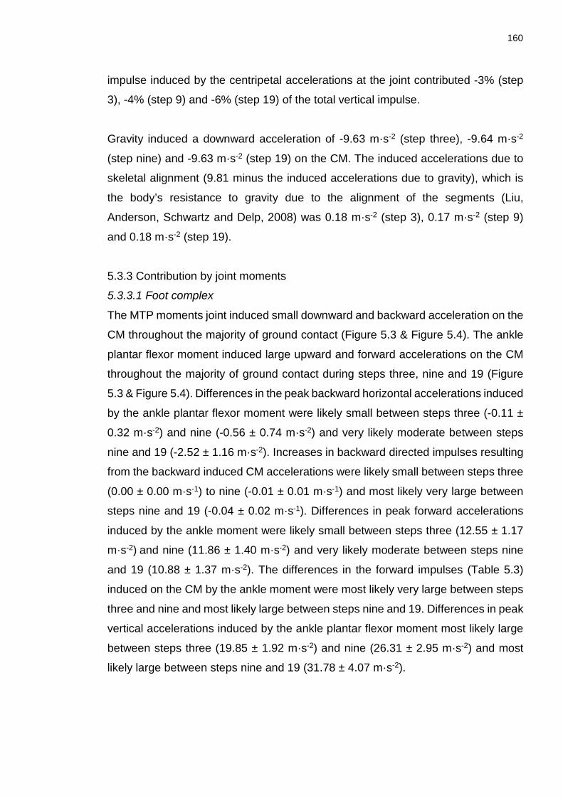
160

impulse induced by the centripetal accelerations at the joint contributed -3% (step

3), -4% (step 9) and -6% (step 19) of the total vertical impulse.

Gravity induced a downward acceleration of -9.63 m·s-2 (step three), -9.64 m·s-2

(step nine) and -9.63 m·s-2 (step 19) on the CM. The induced accelerations due to

skeletal alignment (9.81 minus the induced accelerations due to gravity), which is

the body’s resistance to gravity due to the alignment of the segments (Liu,

Anderson, Schwartz and Delp, 2008) was 0.18 m·s-2 (step 3), 0.17 m·s-2 (step 9)

and 0.18 m·s-2 (step 19).

5.3.3 Contribution by joint moments

5.3.3.1 Foot complex

The MTP moments joint induced small downward and backward acceleration on the

CM throughout the majority of ground contact (Figure 5.3 & Figure 5.4). The ankle

plantar flexor moment induced large upward and forward accelerations on the CM

throughout the majority of ground contact during steps three, nine and 19 (Figure

5.3 & Figure 5.4). Differences in the peak backward horizontal accelerations induced

by the ankle plantar flexor moment were likely small between steps three (-0.11 ±

0.32 m·s-2) and nine (-0.56 ± 0.74 m·s-2) and very likely moderate between steps

nine and 19 (-2.52 ± 1.16 m·s-2). Increases in backward directed impulses resulting

from the backward induced CM accelerations were likely small between steps three

(0.00 ± 0.00 m·s-1) to nine (-0.01 ± 0.01 m·s-1) and most likely very large between

steps nine and 19 (-0.04 ± 0.02 m·s-1). Differences in peak forward accelerations

induced by the ankle moment were likely small between steps three (12.55 ± 1.17

m·s-2) and nine (11.86 ± 1.40 m·s-2) and very likely moderate between steps nine

and 19 (10.88 ± 1.37 m·s-2). The differences in the forward impulses (Table 5.3)

induced on the CM by the ankle moment were most likely very large between steps

three and nine and most likely large between steps nine and 19. Differences in peak

vertical accelerations induced by the ankle plantar flexor moment most likely large

between steps three (19.85 ± 1.92 m·s-2) and nine (26.31 ± 2.95 m·s-2) and most

likely large between steps nine and 19 (31.78 ± 4.07 m·s-2).

161

Horizontal GRF Vertical GRF

Forc

e [B

W]

Acceleration [m·s

-2]

Forc

e [B

W]

Acceleration [m·s

-2]

Forc

e [B

W]

Acceleration [m·s

-2]

Contact Time [s] Contact Time [s]

Measured ground reaction force MTP moment Knee moment

Total joint moements Ankle moment Hip moment

Figure 5.3. Total and individual induced horizontal and vertical ground reaction forces (and centre of mass accelerations) due the joint moments. The measured ground reaction forces (shaded area) is also presented as a reference. Data for step three (a & b), nine (c & d) and 19 (e & f) is presented.

5.3.3.3 Knee

The knee flexor moment induced forward and downward acceleration on the CM

during the first 0.02 s of stance (Figure 5.3). The differences in peak forward CM

acceleration induced by the knee flexor moment at touchdown was most likely large

between steps three (0.93 ± 0.47 m·s-2) and nine (2.50 ± 0.90 m·s-2) and most likely

-5

2

9

16

23

30

37

-0.50.00.51.01.52.02.53.03.54.0

0.00 0.05 0.10

d

-7

-4

-1

2

5

8

11

14

-0.7

-0.4

-0.1

0.2

0.5

0.8

1.1

1.4

0.00 0.05 0.10 0.15

a

-7

-4

-1

2

5

8

11

14

-0.7

-0.4

-0.1

0.2

0.5

0.8

1.1

1.4

0.00 0.05 0.10

c

-5

2

9

16

23

30

37

-0.50.00.51.01.52.02.53.03.54.0

0.00 0.05 0.10 0.15

b

-7

-4

-1

2

5

8

11

14

-0.7

-0.4

-0.1

0.2

0.5

0.8

1.1

1.4

0.00 0.05 0.10

e

-5

2

9

16

23

30

37

-0.50.00.51.01.52.02.53.03.54.0

0.00 0.05 0.10

f

162

very large between steps three and 19 (3.10 ± 0.85 m·s-2). The knee flexor moment

induced a forward impulse on the CM during the braking phase of stance (Table

5.3). Differences in forward impulse induced on the CM by the knee flexor moment

were most likely moderate between steps three (0.00 ± 0.01 m·s-1) and nine (0.02 ±

0.02 m·s-1), and most likely large between steps three and 19 (0.03 ± 0.02 m·s-1).

The knee extensor moment induced backward and upward accelerations.

Differences in peak backward induced CM acceleration were most likely large

between steps three (-2.63 ± 0.68 m·s-2) and nine (-4.41 ± 1.01 m·s-2) and between

steps three and 19 (-4.93 ± 1.91 m·s-2). Differences in the peak vertical CM

accelerations induced by the knee extensor moment were likely small between

steps three (3.18 ± 0.92 m·s-2) and nine (3.86 ± 1.26 m·s-2) and unclear between

steps nine and 19 (3.94 ± 1.66 m·s-2).

5.3.3.4 Hip

The hip moment induced relatively small accelerations on the CM. A hip extensor

moment induced a backward and downward acceleration on the CM while a hip

flexor moment induced a forward and downward acceleration on the CM (Figure 5.3

& Figure 5.4).

Table 5.3. Group mean ± SD relative impulses induced by each of the joint moments.

Step 3 Step 9 Step 19 MTP: Backward [m·s-1] -0.20 ± 0.09 -0.16 ± 0.07 -0.12 ± 0.06 Vertical [m·s-1] -0.06 ± 0.08 -0.01 ± 0.06 -0.03 ± 0.07 Forward [m·s-1] 0.00 ± 0.00 0.00 ± 0.00 0.00 ± 0.00

Ankle: Backward [m·s-1] 0.00 ± 0.00 -0.01 ± 0.01 -0.04 ± 0.02 Vertical [m·s-1] 1.98 ± 0.18 1.96 ± 0.21 2.01 ± 0.16 Forward [m·s-1] 1.16 ± 0.13 0.73 ± 0.12 0.51 ± 0.09

Knee: Backward [m·s-1] -0.17 ± 0.06 -0.21 ± 0.08 -0.20 ± 0.09 Vertical [m·s-1] 0.19 ± 0.11 0.18 ± 0.11 0.15 ± 0.11 Forward [m·s-1] 0.01 ± 0.01 0.03 ± 0.02 0.04 ± 0.03

Hip: Backward [m·s-1] -0.03 ± 0.01 -0.05 ± 0.01 -0.05 ± 0.02 Vertical [m·s-1] 0.01 ± 0.03 0.03 ± 0.03 0.03 ± 0.02 Forward [m·s-1] 0.01 ± 0.00 0.01 ± 0.00 0.01 ± 0.01

163

Step: 9 – 3 Step: 19 – 3 Step: 19 – 9 Step: 9 – 3 Step: 19 – 3 Step: 19 – 9 Step: 9 – 3 Step: 19 – 3 Step: 19 – 9

Total Most likely very large positive difference

Most likely extremely large positive difference


Most likely very large negative difference

Most likely extremely large negative difference


Most likely very large positive difference

Most likely extremely large positive difference


MTP Unclear difference Unclear difference Unclear difference Unclear difference Unclear difference Unclear difference Unclear difference Unclear difference Unclear difference

Ankle Most likely moderate positive difference









Knee Likely small positive difference


Possibly small positive difference

Very likely small positive difference

Likely moderate positive difference Unclear difference Possibly small

positive difference Unclear difference Unclear difference

Hip Most likely moderate positive difference

Most likely large positive difference Unclear difference Most likely large

positive difference Most likely large positive difference Unclear difference

Most likely moderate positive difference


Unclear difference

Figure 5.4. Stance average induced a) resultant, b) horizontal and c) vertical CM accelerations due to the total joint moments (Total_JM) and the individual joint moments of the MTP, ankle, knee and hip. Step three is represented by the black bars, step nine is presented by the blue bars and step 19 is represented by the red bars. The tables below the respective figures show the descriptive results of the results of the MBI analysis of the differences between the three steps. For each comparison, there is a qualitative description of the probability of the standardised differences being larger than 0.02, followed by the size (standardised effect) and direction of the differences.

0

3

6

9

12

15

18

21

24

Acce

lera

tion

[m·s

-2]

a) Resultant contributions


-3 0 3 6 9

Hip

Knee

Ankle

MTP

Total_JM

Acceleration [m·s-2]

b) Horizontal contributions

Step3 Step 9 Step 19

-2

3

8

13

18

23

Acce

lera

tion

[m·s

-2]

c) Vertical contributions


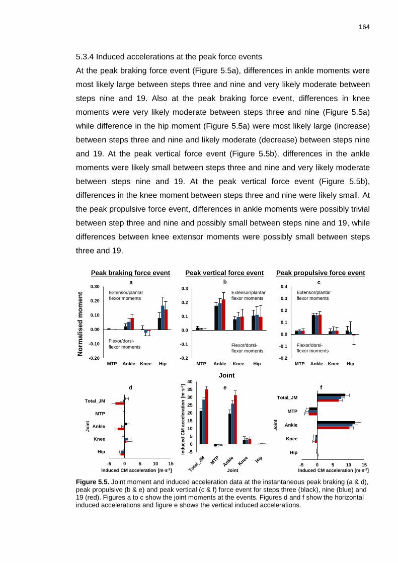
164

5.3.4 Induced accelerations at the peak force events

At the peak braking force event (Figure 5.5a), differences in ankle moments were

most likely large between steps three and nine and very likely moderate between

steps nine and 19. Also at the peak braking force event, differences in knee

moments were very likely moderate between steps three and nine (Figure 5.5a)

while difference in the hip moment (Figure 5.5a) were most likely large (increase)

between steps three and nine and likely moderate (decrease) between steps nine

and 19. At the peak vertical force event (Figure 5.5b), differences in the ankle

moments were likely small between steps three and nine and very likely moderate

between steps nine and 19. At the peak vertical force event (Figure 5.5b),

differences in the knee moment between steps three and nine were likely small. At

the peak propulsive force event, differences in ankle moments were possibly trivial

between step three and nine and possibly small between steps nine and 19, while

differences between knee extensor moments were possibly small between steps

three and 19.

Peak braking force event Peak vertical force event Peak propulsive force event

Nor

mal

ised

mom

ent

Joint

Figure 5.5. Joint moment and induced acceleration data at the instantaneous peak braking (a & d), peak propulsive (b & e) and peak vertical (c & f) force event for steps three (black), nine (blue) and 19 (red). Figures a to c show the joint moments at the events. Figures d and f show the horizontal induced accelerations and figure e shows the vertical induced accelerations.

-0.20

-0.10

0.00

0.10

0.20

0.30

MTP Ankle Knee Hip

a

Flexor/dorsi-flexor moments

-0.2

-0.1

0.0

0.1

0.2

0.3

MTP Ankle Knee Hip

b

-0.2

-0.1

0.0

0.1

0.2

0.3

0.4

MTP Ankle Knee Hip

c

-5 0 5 10 15

Hip

Knee

Ankle

MTP

Total_JM

Induced CM acceleration [m·s-2]

Join

t

d

-505

10152025303540

Indu

ced

CM

acc

eler

atio

n [m

·s-2

]

Joint

e

-5 0 5 10 15

Hip

Knee

Ankle

MTP

Total_JM

Induced CM acceleration [m·s-2]

Join

t

f

Extensor/plantar flexor moments



Flexor/dorsi- flexor moments

Flexor/dorsi- flexor moments

165

4.3.4.1 Peak braking force event

The horizontal induced accelerations were relatively small (Figure 5.5d) with the

ankle plantar flexor moment inducing the largest forward acceleration on the CM at

the step three peak braking force event, while the knee flexor moment induced the

largest forward acceleration on the CM during steps nine and 19 (Figure 5.6). Apart

from the linear acceleration induced by the joint moments (Figure 5.6), angular

acceleration were also induced by the joint moments acting on the segments. The

FC moment also induced a clockwise angular acceleration on the rear foot and an

anti-clockwise angular acceleration on the shank. The FC moment induced an

anti-clockwise acceleration on the thigh segment and a clockwise angular

acceleration on the HAT. The horizontal induced accelerations increased the

horizontal energy of the LEG and decreased the horizontal energy of the HAT on all

three steps. The vertical accelerations induced by the FC moment decreased the

vertical energy of the LEG and HAT.

Although the knee moments at the peak braking force events were relatively small,

an extensor moment was dominant on step three and flexor dominant on steps nine

and 19 (Figure 5.6). The knee flexor moment at the instant of braking during steps

nine and 19 induced a clockwise at the rear foot and shank, an anti-clockwise at the

thigh and an anti-clockwise acceleration at the HAT. The horizontal induced

accelerations increased the horizontal energy of the LEG and decreased the

horizontal energy of the HAT on all three steps. The vertical accelerations induced

by the FC moment decreased the vertical energy of the LEG and HAT.

The hip extensor moment induced an anti-clockwise angular acceleration at the rear

foot. The hip extensor moment induced a clockwise acceleration at the shank at the

peak braking force event of step three and anti-clockwise angular acceleration

during step nine and 19. The hip extensor moment also induced clockwise angular

accelerations at the thigh and an anti-clockwise acceleration at the HAT during all

three steps. At all three steps, the hip extensor moment decreased the horizontal

and increased the vertical energy of the LEG, and also increased the horizontal and

decreased the vertical energy of the HAT. Also, see Chapter 6Appendix A7 for a

more complete report of the results.

166

Peak braking force event Step 3 Step 9 Step 19

Normalized Joint Moments: Induced GRF: Vertical: 0.3 BW Horizontal: 0.0 BW

Segment Angles: HAT: 44° Thigh: 123° Shank: 62° Rear Foot: 132°



Normalized Joint Moments: Induced GRF: Vertical: 1.5 BW Horizontal: -0.3 BW


MTP: Ankle: Knee: Hip:

0.00 0.02 ↻ 0.00 ↺ 0.08 ↻


-0.00 -0.05 ↻ -0.02 ↻ -0.17 ↻


-0.00 -0.08 ↻ -0.01 ↻ -0.14 ↻

IP: Horizontal Vertical IP: Horizontal Vertical IP: Horizontal Vertical Net: + - - + - - - - Net: - + - - - + - - Net: - + - - - + - - Leg: + - - - - + + + Leg: + + - + - - + + Leg: + + - - - - + - HAT: - + + + - - - - HAT: - - + - - + - - HAT: - - + - - + - - → Induced accelerations due to the FC (MTP + ankle)→ Induced accelerations due to knee joint moment→ Induced accelerations due to hip joint moment

→ Total induced segment accelerations (sum of all joint moment contributions)→ Total induced CM acceleration (sum of all joint moment contributions)

Figure 5.6. Fore foot, rear foot, shank, thigh and HAT positions and orientation at the instants of peak braking force. The arrows indicate the contribution of the FC (MTP and ankle (purple)), knee (blue), hip (red) and total (black) joint moments on segment accelerations during steps three, nine and 19. The induced CM acceleration is represented by the grey arrow. Below the figures, the joint moments, induced CM accelerations and segment orientations corresponding to the peak braking force event are shown. The segments, coloured arrows and ground reaction force vectors are to scale. The results of the induced power (IP) analysis shows whether a joint moments increased (+) or decreased (-) the energy of either the LEG or HAT. The segments, coloured arrows and grand reaction force vectors are to scale.

3 ± 2%(0.005 ± 0.003 s)-0.1 ± 0.1 BW-0.01 ± 0.01 m·s-1

7 ± 3%(0.007 ± 0.004 s)-0.4 ± 0.1 BW-0.08 ± 0.05 m·s-1

9 ± 2% (0.013 ± 0.003 s)-0.6 ± 0.1 BW-0.17 ± 0.04 m·s-1

167

4.3.4.2 Peak vertical force event

The vertical induced CM accelerations at the peak vertical force event were

dominated by the ankle joint moment (Figure 5.5e). The linear induced acceleration

induced by the joint moments are presented in Figure 5.7. The FC moments

clockwise angular acceleration at the rear foot and shank while inducing an

anti-clockwise angular acceleration at the thigh during all three steps. From step

three to nine to 19 the FC moments induced a clockwise angular acceleration at the

HAT segment which increased from steps three to nine to 19 due to the increase in

the magnitude of the FC moments. On all three steps the FC moments increased

the LEG and decreased the HAT horizontal energy, and decreased the vertical

energy of both the LEG and HAT.

The knee extensor moment induced the second largest upward acceleration on the

CM (Figure 5.5e) during steps three, nine and 19. The knee moment induced an

anti-clockwise angular acceleration on the rear foot and shank segments and a

clockwise angular acceleration at the thigh segment. An anti-clockwise angular

acceleration was induced on the HAT segment during all three steps. The

accelerations induced by the knee extensor moment increased the horizontal and

decreased the vertical energy of the HAT on all three steps. The horizontal energy

at the LEG was decreased on all three steps while vertical energy at the LEG was

increased at step three and decreased on step nine and 19.

The hip extensor moments induced an anti-clockwise angular acceleration at the

rear foot and shank and a clockwise angular acceleration at the thigh segment on

all three steps. An anti-clockwise angular acceleration was induced on the HAT

segment on all three steps. The hip extensor moment decreased the horizontal and

increased the vertical energy at the LEG, and also increased the horizontal and

decreased the vertical energy at the HAT. Also, see Chapter 6Appendix A7 for a

more complete report of the results.

168

Peak vertical force event Step 3 Step 9 Step 19





Normalized Joint Moments: Induced GRF: Vertical: 3.6 BW Horizontal: -0.2 BW



0.02 ↻ 0.18 ↻ 0.08 ↺ 0.10 ↻


0.01 ↻ 0.20 ↻ 0.10 ↺ 0.11 ↻


0.00 ↻ 0.22 ↻ 0.10 ↺ 0.10 ↻

IP: Horizontal Vertical IP: Horizontal Vertical IP: Horizontal Vertical Net: + - - + - - - - Net: + - - + - - - - Net: + - - - - - - -Leg: + - - + - - + - Leg: + - - - - + + - Leg: + - - - - + + -HAT: - + + + - + - - HAT: - + + + - - - - HAT: - + + - - - - -→ Induced accelerations due to the FC (MTP + ankle)→ Induced accelerations due to knee joint moment→ Induced accelerations due to hip joint moment


Figure 5.7. Fore foot, rear foot, shank, thigh and HAT positions and orienation at the instants of peak braking force. The arrows indicate the contribution of the FC (MTP and ankle (purple)), knee (blue), hip (red) and total (black) joint moments on segment accelerations during steps three, nine and 19. The induced CM acceleration is represented by the grey arrow. Below the figures, the joint moments, induced CM accelerations and segment orientations corresponding to the peak vertical force event are shown. The segments, coloured arrows and ground reaction force vectors are to scale. The results of the induced power (IP) analysis shows whether a joint moments increased (+) or decreased (-) the energy of either the LEG or HAT. The segments, coloured arrows and grand reaction force vectors are to scale.

48 ± 5%(0.079 ± 0.008 s)2.2 ± 0.2 BW0.69 ± 0.13 m·s-1

34± 9%(0.038 ± 0.010 s)2.9 ± 0.3 BW1.03 ± 0.17 m·s-1

32 ± 7%(0.044 ± 0.010 s)3.6 ± 0.3 BW1.22 ± 0.14 m·s-1

169

4.3.4.3 Peak propulsive force event

The horizontal induced accelerations (Figure 5.5f) at the peak propulsive force event

were dominated by the ankle plantar flexor moment. The linear accelerations

induced by the joint moments are presented in Figure 5.8. The FC moment induced

a clockwise angular acceleration at the rear foot and shank and an anti-clockwise

angular acceleration at the thigh segment during all three steps. Upward and

forward linear and clockwise angular accelerations were also induced at the HAT

during all steps. The linear accelerations induced by the FC plantar flexor moments

increased the vertical and horizontal energy of all segments (Figure 5.8).

The knee extensor moment induced an anti-clockwise angular acceleration at the

rear foot, an anti-clockwise angular acceleration on the shank and a clockwise

angular acceleration at the thigh segment during all steps. The knee extensor

moments induced an anti-clockwise angular acceleration at the HAT segment. The

induced accelerations from the knee moment decreased the horizontal and vertical

energy at the LEG during all three steps. The horizontal and vertical energy of the

HAT was increased by the knee extensor moment on all three steps.

Although relatively small, the group mean hip moment was extensor dominant on

step three and nine and flexor dominant on step 19. The hip extensor moment

induced an anti-clockwise acceleration at the rear foot and shank, a clockwise

acceleration on the thigh and an anti-clockwise acceleration at the HAT. At the peak

propulsive force event of steps 19, the hip flexor moment induced a clockwise

angular acceleration at the rear foot, a clockwise angular acceleration at the shank,

an anti-clockwise angular acceleration at the thigh and a clockwise angular

acceleration at the HAT. Also, see Chapter 6Appendix A7 for a more complete

report of the results.

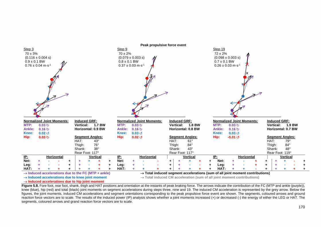
170

Peak propulsive force event Step 3 Step 9 Step 19








0.03 ↻ 0.16 ↻ 0.02 ↺ 0.03 ↻


0.03 ↻ 0.16 ↻ 0.03 ↺ 0.02 ↺


-0.03 ↻ -0.16 ↻ -0.03 ↺ -0.01 ↺

IP: Horizontal Vertical IP: Horizontal Vertical IP: Horizontal Vertical Net: + - - + + + + + Net: + - - + + + + + Net: + - + + + + - +Leg: + - - + + - + + Leg: + - - + + - - + Leg: + - + + + - - +HAT: + + + + + + + + HAT: + + + + + + + + HAT: + + - + + + + +→ Induced accelerations due to the FC (MTP + ankle)→ Induced accelerations due to knee joint moment→ Induced accelerations due to hip joint moment


Figure 5.8. Fore foot, rear foot, shank, thigh and HAT positions and orientation at the instants of peak braking force. The arrows indicate the contribution of the FC (MTP and ankle (purple)), knee (blue), hip (red) and total (black) joint moments on segment accelerations during steps three, nine and 19. The induced CM acceleration is represented by the grey arrow. Below the figures, the joint moments, induced CM accelerations and segment orientations corresponding to the peak propulsive force event are shown. The segments, coloured arrows and ground reaction force vectors are to scale. The results of the induced power (IP) analysis shows whether a joint moments increased (+) or decreased (-) the energy of either the LEG or HAT. The segments, coloured arrows and grand reaction force vectors are to scale.

70 ± 3%(0.116 ± 0.004 s)0.9 ± 0.1 BW0.76 ± 0.04 m·s-1

70 ± 2%(0.079 ± 0.003 s)0.8 ± 0.1 BW0.37 ± 0.03 m·s-1

72 ± 2%(0.098 ± 0.003 s)0.7 ± 0.1 BW0.26 ± 0.03 m·s-1

171

5.4 Discussion The changes in external forces that were identified in Chapter 4 were characterised

by increased peak braking forces and peak vertical forces from step three to step

nine to step 19. However, it is difficult to intuitively predict the contributors to the

GRF acting on the CM of the sprinters. The aim of this study was to investigate the

effects different forces (joint moments and non-biological) acting on a sprinter have

on the sagittal plane acceleration of the sprinter during steps from different phases

of a sprint. This aim was achieved by performing an IAA and IPA (Zajac, 2002) to

quantify the horizontal and vertical CM accelerations induced on the sprinter using

the empirical data from Chapter 4. The knowledge gained from this study can

ultimately build on the knowledge gained from Themes 1 and 2 and develop a

greater depth of knowledge regarding the underlying mechanisms by which

sprinters accelerate their CM during steps during different phases of a sprint.

5.4.1 Induced centre of mass acceleration

The model used for the IAA demonstrated a close match to the measured external

ground reaction forces. Absolute RMSD ranged between 11 ± 2 N and 34 ± 11 N.

whilst relative errors were 1 – 3% of the peak force excursion which aligns well with

previous studies that have shown errors less than 5% when using IAA to investigate

running (Dorn et al., 2012). Comparing the total induced ground reaction force

time-history to the measured GRF (Figure 5.2) shows that differences were largest

at the start and end of ground contact during step 19. This can be attributed to the

difficulties in modelling the rapid transition from flight to contact phases at higher

running velocities (Hamner et al., 2011). This could be influenced by the relatively

large fluctuations in COP at touchdown (Koike et al., 2017). While the comparison

between total induced acceleration and measured accelerations shows a good

match across the stance phases of all steps, a rigid foot-floor interface at the COP

was assumed at the beginning and end of ground contact. A more robust modelling

of the foot-floor interaction that includes the deformation of the soft tissues of the

foot and the surface at impact, as well as a more precise approximation of the

ground contact points (Koike et al., 2017) may provide greater accuracy at the start

and end of the stance phases. Nevertheless, the relative errors in the current study

shows good accuracy and provides confidence in the interpretation of the results.

Of the different inputs that made up the total induced GRF, the largest accelerations

172

induced on the CM were due to the action of the joint moments and accelerations

at the foot-floor contact. These results will be discussed in sections 5.4.1.1 and

5.4.1.2 below.

Gravity induced a mean downward acceleration on the body of -9.63 to -9.64 m·s-2

in all three steps. Although there were considerable changes in segment orientation

between steps three, nine and 19, the accelerations transmitted to the ground by

the skeletal alignment remained relatively small (0.17 - 0.18 m·s-2). These were

considerably lower than the contribution to vertical acceleration induced by

alignment of the segments during walking (~3 - 4 m·s-2; Anderson & Pandy, 2002;

Liu, Anderson, Schwartz & Delp, 2008). It is important to note that these induced

accelerations due to gravity are a function of the foot-floor interaction and segmental

alignment (Anderson & Pandy, 2002). The largest differences were probably caused

by the different foot-floor interactions during walking and sprinting. The relatively

large vertical accelerations due to skeletal alignment during walking tended to occur

during mid-stance when the foot was flat on the ground (Anderson & Pandy, 2002),

while at the start and end of stance when foot was not flat on the ground, the vertical

induced centre of mass accelerations were around 80% smaller (Anderson & Pandy,

2002). Furthermore, the increased knee extension during walking can partly explain

the larger contributions by skeletal alignment identified by Liu et al. (2008).

Increased leg extension (i.e. more extended knee joint) would resist gravity by

allowing compressive forces to be transferred to the ground more effectively

(Anderson & Pandy, 2002). Knee extension angles associated with walking (e.g. ~

>157°; Liu et al., 2008) are generally larger compared to maximal sprinting (Chapter

4: Figure 4.14a) where knee angles ranged between 110° to 171° (step 3), 134° to

163° (step 9) and 147° to 162° (step 19) from touchdown to toe-off.

The results of the current theme suggest that as segment angles (i.e. trunk, thigh,

and shank) and the knee extension angles during stance increased between steps

three, nine and 19, their ability to resist the downward force of gravity would also

increase. However, because of the predominantly fore foot contact during sprinting,

the increasing segment inclination and knee and hip angles between steps three,

nine and 19 could not be translated into an increased vertical centre of mass

acceleration contributed by the skeletal alignment. This suggests that there is a

173

large requirement on the ankle plantar flexors to resist the downward force of gravity

during sprinting.

When using the centripetal accelerations of the joints (which are based on

segmental angular velocities) of the stance leg as the input to the IAA model, forward

accelerations were induced on the centre of mass at the beginning and end of the

stance phases (Figure 5.2). The centripetal accelerations appear to have a lesser

influence on performance during the stance phases of sprinting when compared to

the swing phase (Koike & Sudo, 2015). Nonetheless, the forward accelerations

induced by the centripetal accelerations at the joints of the stance leg, which depend

on the angular velocities of the HAT, thigh, shank and foot, increased between steps

three, nine and 19 with the larger angular velocities of the segments at step 19

contributing 57% of the total horizontal impulse during step 19. Increasing

contributions by velocity dependent forces across a range of velocities has also

been reported by Hamner and Delp (2013). Furthermore, Hunter et al. (2005)

previously identified that a greater mean hip extension velocity was associated with

larger propulsive forces while Ae et al. (1992) reported that elite sprinters show an

increased during stance. These results show that the increasingly larger clockwise

segmental angular velocities identified in Theme 2 (Chapter 4; Figure 4.18) provide

an important contribution to the forward acceleration of the CM at high running

velocities.

This aligns with coaching theory (e.g. Seagrave, Mouchbahani & O’Donnell, 2009)

relating to maximal velocity sprinting mechanics. The coaching theory suggests that

during the terminal swing phase, sprinters should aim to generate a large hip

extension angular velocity. The idea is that this will effectively reduce horizontal foot

velocity and touchdown distances and therefore the braking forces that sprinters

generate. Regarding the influence of foot velocity on inducing ground reaction

forces, the results of the current study provide quantitative evidence showing the

influence of horizontal foot velocity on braking forces (see next section: 5.4.1.

Induced accelerations due to accelerations at the foot-floor interface). The results

of this study provide further evidence showing the importance of maximising the

angular velocity of the segments and the resulting contribution to the forward

acceleration of the centre of mass during maximal velocity sprinting. Since the

174

centripetal velocity of the segments represent the cumulative effect (Hirashima et

al., 2008) of all previous forces acting on the system, these results highlight the

importance of generating sufficiently large segmental angular velocities during

terminal swing through to toe-off.

5.4.1. Induced accelerations due to accelerations at the foot-floor interface

The accelerations at the foot-floor interface induced a backward and upward

acceleration on the CM during the braking phase of ground contact. These

accelerations, which are induced on the CM as the foot is decelerated following

touchdown may be representative of a passive force that is generated when the foot

decelerates rapidly following touchdown. Although the relative contributions to the

vertical and horizontal GRFs suggest that the horizontal contributions are more

influential on the horizontal GRFs, the absolute vertical contributions were larger

than the horizontal contributions. Increases in both vertical (moderate positive

differences) and horizontal (large positive differences) contributions increased from

steps three to nine to 19 which corresponds to the results from Theme 2 (Chapter

4; Table 4.4) where forward and downward foot velocities prior to touchdown

increased from step three to nine to 19. The relative contribution to horizontal

impulses during the braking phase of ground contact were 145% (step 3), 68% (step

9) and 47% (step 19) while the relative contributions to vertical impulse were 3%

(step 3), 5% (step 9) and 6% (step 19). These results provide within-athlete

empirical evidence to reinforce the relationship between foot velocity and braking

forces (Hunter et al., 2005) and supports the proposal by previous authors that

sprinters should minimise the forward velocity of the foot prior to touchdown if they

wish to reduce braking forces during stance (Mann & Sprague, 1980; Hunter et al.,

2005). However, there may be a point of diminishing returns where continued effort

to decrease the horizontal foot velocities prior to touchdown will not result in further

decreases in braking impulses and therefore will not be beneficial to performance.

A similar limit to performance enhancement was previously shown by Bezodis et al.

(2015) who investigated the influence of reducing touchdown distances on sprinting

performance. Performing a simulation of the first step in sprinting, Bezodis et al.

(2015) reported that decreasing TD distances initially resulted in a performance

increase. However, the authors identified a limit to performance enhancement and

noted that any further decreases in touchdown distances resulted in a decrease in

175

performance. Therefore, it could be speculated that while sprinters may initially

benefit from reducing horizontal foot velocities, excessively small or negative

horizontal foot velocities may have no further benefit or be worth the effort needed

to achieve those low horizontal foot velocities.

The accelerations at the contact point are calculated from the linear acceleration,

angular accelerations and centripetal accelerations of the segment in contact with

the ground (Equation 5.5). Across the three steps, there was no clear trend between

participants regarding whether ground contact occurred at the fore or rear foot.

However, the linear deceleration of the foot at touchdown contributed 125%, 101%

and 101% to overall impulse generated by the foot-floor accelerations during the

braking phases of steps three, nine and 19 respectively. By experimentally altering

the horizontal and vertical deceleration component and increasing the vertical

deceleration components of equation 5.5, the influence of this on the braking and

vertical impulse could be investigated further. Theoretically, the vertical and

horizontal velocity of the foot prior to touchdown can be altered independently

through a sensitivity analysis. However, it is unclear to what extent this is practical

as it is unlikely that sprinters can influence one variable without changing another.

Furthermore, it is unclear what effect these changes in either horizontal or vertical

foot velocities have on other components of ground contact (e.g. total vertical

impulse and propulsive impulse) which may negatively influence performance.

Researchers and coaches are encouraged to explore the influence of altering foot

velocities prior to touchdown to identify possible influences on their performance.

5.4.3 Joint moment induced accelerations

Joint moments were the dominant source of CM acceleration during the stance

phases of steps three, nine and 19. This is different from activities like overarm

throwing (Hirashima et al., 2008) and the swing phase in sprinting (Koike & Sudo,

2015) where the motion dependent term (e.g. centripetal accelerations) was the

dominant contributor to induced accelerations. This may be related to the nature of

the task where during the swing phase or overarm throwing the aim is to maximise

the end-point velocity, while during ground contact in sprinting the aim is to

maximise the velocity of the CM, which is much heavier and proximal to the joints

where the moments are generated.

176

The accelerations induced by the joint moments increased vertically and decreased

horizontally from steps three to nine to 19 (Figure 5.3). This was influenced by the

increasingly more vertically oriented segments (i.e. more upright posture) during

ground contact (Figure 5.6, Figure 5.7 & Figure 5.8), which caused in an increasingly

more inclined induced acceleration vector. Rabita et al., (2015) suggested the

possible importance of the hip and ankle moments in orientating the resultant GRF

vector. However, the results of the current investigation suggest that the orientation

of the segment of the sprinter is important when orientating the GRFs more

horizontally.

The increased touchdown distance and decreased toe-off distances associated with

steps nine and 19 resulted in increasing braking and decreasing propulsive forces,

respectively. Although lower touchdown distances have previously been associated

with a lower braking impulse (Hunter et al., 2005), the results of the current study

provide some important insight showing how touchdown and toe-off distances may

influence braking and propulsive forces generated by sprinters. Chapter 3 showed

that changes in touchdown and toe-off distances were due to shank and trunk

becoming more inclined as the sprint progressed. The current results suggest that

the decreasing anterior accelerations induced on centre of mass between steps

three, nine and 19 (Figure 5.4) were probably dictated by the increasingly more

inclined acceleration vectors induced on the HAT segment at the peak braking force

(Figure 5.6) and peak propulsive events (Figure 5.8). Since the type of joint

moments (i.e. flexor or extensor) did not necessarily change between the steps, the

differences in the anterior-posterior accelerations induced on the centre of mass

would have been influenced by the differences in segmental orientation between

steps three, nine and 19. This is especially clear when comparing the differences in

the anterior-posterior accelerations induced by the ankle plantar flexor moment

during the braking phases of steps three, nine and 19 (Figure 5.2, Figure 5.6). These

results highlight the influence the sprinters’ posture at touchdown and throughout

stance has on their performance. When combined with the results of the foot-floor

acceleration as discussed earlier, this further highlights the importance of the

sprinter’s ‘front side mechanics’ (Mann, 2007, p. 86) and its influence on the braking

forces generated during stance. Coaches and sprinters are therefore encouraged

177

to develop the mechanics during the terminal swing and braking phases at varying

running velocities and across a range of body orientations with the aim of decreasing

touchdown distances. However, there may exist an optimum (Bezodis et al., 2015)

and it is unclear how changes to touchdown distance will affect other variables

important to performance including vertical force production (e.g. Weyand et al.,

2000) and postural stability (e.g. Kugler & Janshen, 2010). Since larger vertical

forces are important to achieving high running velocities (Weyand et al., 2000),

finding the optimal touchdown distance may be a trade-off between generating

braking forces and maximising vertical force production. The mechanism by which

sprinters can minimise braking forces while ensuring performance is enhanced

requires further exploration.

5.4.3.1 Foot complex (FC)

The MTP joint has generally been described as a large absorber of energy

(Stefanyshyn & Nigg, 1997; Smith et al., 2014; Bezodis et al., 2014; Chapter 4:

Figure 4.11). When acting in isolation, the MTP moment induces a backward

acceleration on the CM (Figure 5.3 a-f) which decreases the horizontal energy of

the CM. These results associated with the two-point contact model agreed with

Koike, Ishikawa and Ae (2010) who used a similar foot contact model to the one in

this study. The differences in induced accelerations by the MTP joint between steps

three, nine and 19 were generally small and not meaningful. It has been suggested

that a larger MTP moment may allow athletes to increase their forward lean and as

such achieve a more horizontally orientated take-off trajectory (Goldmann, Sanno,

Willwacher, Heinrich & Brüggemann, 2013). This would place the sprinter into a

more appropriate posture for the more powerful plantar flexors of the ankle to propel

the sprinter forwards. Although the results suggest that an MTP plantar flexor

moment has a detrimental effect on the forward progression of the CM (i.e. by

inducing small backward CM accelerations), increasing the moment about the MTP

joint, however, has an important performance enhancing function by generating an

upward acceleration on the CM towards the end of stance (Figure 5.3 b, d, f).

The ankle plantar flexor moment induced the largest horizontal and vertical

accelerations on the CM. These results are in line with previous studies investigating

the induced CM accelerations during a single sprinting ground contact (Cabral et

178

al., 2013) or phase (Debaere et al., 2015; Koike & Nagai, 2015) and sub-maximal

running (Dorn et al., 2010; Hamner & Delp, 2013). The increasingly larger ankle

plantar flexor moment resulted in increased vertical and decreased horizontal

induced CM accelerations (Figure 5.4). This may be linked to the more inclined

shank, trunk and rear foot segments leading to larger vertical accelerations being

induced on the CM. Although there were no clear differences in vertical impulse

generated by the ankle plantar flexor moment between steps three, nine and 19, the

increasing vertical CM accelerations induced by the ankle plantar flexor moment

reflects the increased requirement to generate large vertical forces at higher running

velocities (Weyand et al., 2000).

Between steps three, nine and 19 the combined foot complex (FC) plantar flexor

moments induced increasingly larger forward and upward accelerations on the rear

foot and shank. This opposed the increasingly larger downward and backward

accelerations induced on the shank and rear foot segments by the more proximal

joint moments (Figure 5.6, Figure 5.7 & Figure 5.8) and gravity, particularly during

steps nine and 19. As this occurred at the time when the ankle joint was either

dorsiflexing (at the peak braking force event) or fixed (around the peak vertical force

event), the FC plantar flexor moments played an important role in providing a stable

ankle joint so that accelerations induced by more proximal joint moments are

transferred to the ground. A previous study has shown that during sprinting, the

ankle plantar flexors operate at a larger relative effort when compared to the knee

extensors (96% vs. 76%; Kulmala et al., 2016). This is may be due to the increasing

need to resist the dorsiflexion that would result from the accelerations induced at

the shank and rear foot by the proximal hip and knee extensor moments. Indeed, a

stiffer ankle (i.e. more resistant to dorsiflexion) may be linked to increased

performance during the first stance phase in sprinting (Charalambous et al., 2012;

Bezodis et al., 2015) and maximal velocity (Nagahara & Zushi, 2016) while a stiff

foot-floor joint (i.e. a fixed angle between the foot and the ground) has been

experimentally shown to transfer larger accelerations generated by the hip extensor

moment to the ground (Cabral et al., 2013). The ability of the FC to transfer

acceleration from proximal segments to the ground during the peak braking (Figure

5.6) and peak vertical (Figure 5.7) force events is important in all three steps

analysed and may represent a key factor limiting maximal sprinting performance.

179

This may relate to the ability of the ankle to remain stiff, and so limit dorsiflexion

following touchdown. In practical situations, this could be assessed during sprinting

tasks by measuring the dorsiflexion range of motion following touchdown, where a

smaller or decreasing dorsiflexion range of motion possibly represents a stiffer

ankle. Furthermore, reactive exercises including depth jumps or continuous rebound

ankle hops, which have previously been associated with performance during the

maximal velocity phases of sprinting (e.g. Bret, Rahmani, Dufour, Messonnier &

Lacour, 2002; Bissas & Havenetidis, 2008; Nagahara, Naito, Miyashiro, Morin &

Zushi, 2014) could be used to monitor changes in ankle joint stiffness. However,

touchdown position of the foot and shank needs to be taken into consideration as

this may determine the dorsiflexion range of motion following touchdown. For

example, a more plantar flexed ankle at touchdown may undergo larger dorsiflexion

following touchdown. The practical implications of this will be discussed in section

5.4.4.

During the propulsive phase, large horizontal and vertical accelerations are induced

by the ankle moment on the CM. This is similar to previous research showing that

the soleus and gastrocnemius are the largest contributors to forward acceleration of

the CM during the propulsive phase of sub-maximal running (Hamner et al., 2010)

with the soleus being the main contributor across a range of sub-maximal running

velocities (Hamner & Delp, 2013). At the peak propulsive force event the FC plantar

flexor moment (of which the ankle moment plays a large part) induced upward and

forward accelerations at the stance leg segments and HAT. This is unlike the peak

braking and peak vertical force events where the FC induced a forward and upward

accelerations at the stance leg segments but a backward and upward accelerations

at the HAT. A substantial period of power generation has previously been shown to

occur at the ankle joint prior to toe-off during all phases in sprinting (e.g. Johnson &

Buckley, 2001; Bezodis et al., 2008; Charalambous et al., 2011; Bezodis et al.,

2014; Chapter 4: Figure 4.12d). The power generating capability of the ankle plantar

flexors, which is likely aided by the release of elastic energy stored during the earlier

phases of stance (Cavagna et al., 1971; Hunter et al., 2005), has previously been

related to sprint performance at higher running velocities (Nagahara, Matsubayashi

et al., 2014). A powerful plantar flexion of the ankle and MTP joint during the

propulsive phase of ground contact therefore appears to be an important

180

mechanism to propel the sprinter forward and upward into the next flight phase. The

practical implications of this will also be discussed in section 5.4.2.

5.4.3.2 Knee

The knee moment was characterised by a flexor moment directly after touchdown,

an extensor moment during mid-stance and a flexor moment before toe-off (see

Chapter 4; Figure 4.14c). Although the knee flexor moment at the peak braking force

event of steps nine and 19 decelerated the HAT (i.e. decreased the energy of the

HAT) the increasingly larger forward acceleration of the LEG meant that the knee

flexor moment contributed an increasingly larger forward impulse on the CM

between steps three (0.00 ± 0.01 m·s-1), nine (0.02 ± 0.02 m·s-1) and 19

(0.03 ± 0.02 m·s-1) (Table 5.3). Although, a knee flexor moment was dominant

immediately following touchdown on all three steps (Figure 4.14c) it could be

speculated that the more inclined shank associated with steps nine and 19

increased the effectiveness of the knee flexor moment to contribute to forward CM

acceleration. This will ensure that the linear acceleration vector at the proximal and

distal ends of the shank is more horizontally orientated, increasing the forward and

backward acceleration of the knee and ankle joints respectively. This links to the

geometric constraints theory (van Ingen Schenau et al., 1987) which suggests that

at certain orientations (i.e. close to the vertical), segment rotational motions are

better able to contribute to the horizontal translation of the CM.

Previous research has suggested that the knee moment plays an important role in

transferring energy from proximal to distal segments (Bezodis et al., 2008). The

results of the current study suggest that a knee flexor moment may play an important

role in ensuring that the clockwise accelerations induced at the thigh by the hip

extensor moments are transferred to the shank. Following touchdown, the knee

flexor moment, which generates knee flexion, opposes the backward and

anticlockwise acceleration induced on the shank by the hip extensor moment

(Figure 5.6). The knee flexor moment therefore provides stability at the shank

allowing the clockwise rotating thigh to translate the upper body (HAT) forward and

upward via the knee joint (Figure 5.6). One first glance it might therefore seem

beneficial to have a large knee flexor moment, which could be achieved through and

increased TD distance (Sun et al., 2015). However, increasing TD distances is not

181

recommended as this could increase braking force by placing the sprinter in a less

efficient position to generate horizontal forces. Furthermore, increased TD distances

could increase the strain experienced by the hamstrings (via increased hip extensor

and knee flexor moments) and therefore increase the risk of injury (Sun et al., 2015).

Rather coaches and sprinters should attempt to effectively reduce TD distance

therefore possibly negating the need for a large knee flexor moment to accelerate

the sprinter over the contact point.

A second function suggested for the knee moment is to support the rise of the CM

during the initial acceleration phase (Charalambous et al., 2011; Debaere et al.,

2015) and maintain the height of the CM during the transition and maximal velocity

phases (Johnson & Buckley, 2001; Bezodis et al., 2008). After about 0.02 s of

stance, the knee extensor moments induced a backward and upward acceleration

on the CM (Figure 5.3). The knee extensor moment induced the second largest

upward acceleration on the CM. This therefore supports the theory that the knee

plays an important role in providing upward acceleration on the CM. However, the

larger knee extensor moments identified in Theme 2 (Chapter 4; Figure 4.14c) and

more upright postures associated with steps nine and 19 did not translate into larger

upward CM accelerations (Figure 5.4). Although the knee extensor joint moment

induced small forward and upward accelerations on the HAT, this appears to be

limited since a backward and downward acceleration was also induced on the rear

foot and shank. Unless a sufficiently large FC plantar flexor moment is present to

ensure the ankle is suitably stiff to oppose the downward and backward

accelerations induced on the rear foot and shank, the effectiveness of the knee

extensor moment in accelerating the HAT upward is limited. This is analogous to

stepping up onto a hard surface that resists the downward forces generated by the

leg or stepping up onto a soft surface that deforms under the forces applied. A knee

extensor moment is therefore reliant on a stable rear foot and shank segment in

order to accelerate the sprinter forward and upwards. If the rear foot and shank are

sufficiently supported by the plantar flexor FC moments, a knee extensor moment

has the potential to induce a larger upward and forward acceleration at HAT.

182

5.4.3.3 Hip moment

From touchdown until 0.080 to 0.120 s, the hip extensor moment induced a relatively

small backward and upward accelerations on the CM compared to the distal joint

moments. This was consistent across all three steps and was predominantly

influenced by the backward accelerations induced on the segments of the stance

leg (Figure 5.6 & Figure 5.7). These results are in agreement with Cabral et al.

(2013), Koike and Nagai (2015) and Debaere et al. (2015), but seem counter

intuitive given the relatively large hip extensor moments and powers generated at

the hip joint compared to the ankle and knee (Cabral et al., 2013; Debaere,

Delecluse et al., 2013; Chapter 4; Figure 4.16 c & d). Furthermore, “the hip extension

theory” (Hunter et al., 2004c, p. 1445) states that the clockwise rotation of the thigh,

caused primarily by the hip extensors, is an important contributor to the propulsive

GRF and suggests that a powerful hip extension is important for sprinting success.

According to the results of the current study, the hip extensor moment induced a

forward acceleration on the HAT (i.e. increase in the horizontal energy of the HAT)

and a clockwise acceleration on the thigh and anti-clockwise acceleration of the

shank and rear foot segments. These induced angular accelerations resulted in a

backward and downward linear acceleration induced on the segments of the stance

leg which could not be translated into a forward acceleration at the whole-body

centre of mass. Therefore, unless the clockwise angular accelerations induced on

the thigh are translated to the shank through the action of the knee flexor moments

and then to the ground by the action of the FC plantar flexor moment, the

acceleration induced by the hip extensors cannot be translated into large propulsive

GRF.

Interestingly, the results also showed that at the peak braking force event of step

three (Figure 5.6), the hip extensor joint moment induced a clockwise angular

acceleration on the shank while a hip extensor moment induced an anti-clockwise

acceleration on the shank during steps nine and 19. This negated the need for a

knee flexor moment at peak braking force events of step three to transfer the

accelerations from the thigh to the shank. Although it is not possible to identify which

muscles played a role in generating the different joint moments, a recent

experimental study has shown that hamstring activation and eccentric peak torque

capability play an important role in horizontal force production (Morin et al., 2015).

183

The bi-articular hamstrings and potentially the gastrocnemius may therefore play an

important role in generating both hip extension and knee flexion.

A hip extensor moment may also play an important role in providing support to the

upper body by assisting the knee extensors in resisting knee flexion during the

stance phases of steps nine and 19. The results show that a hip extensor moment

has the potential to generate knee extension (Figure 5.7) by inducing clockwise and

anti-clockwise angular accelerations at the thigh and shank respectively. This may

provide further explanation why knee extension moments and powers can remain

relatively small during the stance phases of sprinting (Bezodis et al., 2008) and

therefore work at a lower relative effort than the ankle joint (Kulmala et al., 2016).

However, the effectiveness of the hip extensor moments in inducing upward CM

accelerations is also dependent on a stable rear foot and shank to transfer

accelerations to the ground.

5.4.4 Practical Implications The new understanding gained from these results and their interpretation in the

context of existing relevant literature can be used to inform future technical or

physical preparation aspects of sprinting. Firstly, the results of the current study

provide empirical evidence showing the link between horizontal foot velocities prior

to touchdown and braking forces. In the current study 145% (-0.01 ± 0.01 m·s-1),

68% (-0.05 ± 0.01 m·s-1) and 47% (-0.08 ± 0.01 m·s-1) of the braking impulse was

generated by the accelerations at the foot-floor interface during steps three, nine

and 19 respectively. This study provided direct evidence to support the hypothesis

put forward by various authors (Mann & Sprague, 1983; Hay, 1994) that sprinters

should aim to reduce braking forces by minimising the forward velocity of the foot

prior to touchdown. Furthermore, the results of this study showed that 125% (step

3), 101% (step 9) and 101% (step 19) of the braking impulse generated by the

foot-floor acceleration was due to the foot being decelerated at touchdown. The

increasing contribution of the foot-floor accelerations to braking and vertical

impulses between steps three, nine and 19 and could be attributed to the increases

in forward and downward velocities of the foot identified in Theme 2 (Chapter 4;

Table 4.4). This supports the technical focus, which suggests that sprinters should

aim to develop a larger backward angular acceleration of the thigh (Seagrave et al.,

184

2009). This technical focus will not only reduce the forward velocity of the foot

immediately prior to touchdown, but also contribute to large centripetal accelerations

(via larger clockwise rotations (sprinting left to right) of the thigh and shank) at the

segments of the stance leg which contributed an important forward acceleration on

the CM at higher running velocities.

Secondly, the results of this study support the importance of posture (i.e.

orientations of segments) for performance as previously reported by scientific (e.g.

di Prampero et al., 2005; Kugler & Janshen, 2010) and coaching literature (e.g.

Seagrave et al., 2009; Crick, 2013e). As the orientations of the shank and HAT

became upright, the accelerations induced on the segments by the ankle joint

moments became more vertically orientated. These more vertically orientated linear

induced acceleration vectors combined with the increasing magnitudes of the ankle

plantar flexor moments as the sprint progresses contributed to the increasing

vertical GRF (Figure 5.5). This plays an important role during the acceleration phase

where a sprinter’s segmental orientations show step-to-step changes (Chapter 3;

Figure 3.10). Cueing a more efficient posture would provide the coach with a

powerful tool to influence the vertical and horizontal forces athletes can generate.

For example, coaches could emphasis a forward orientated trunk during the initial

acceleration phase to ensure increased horizontal forces are generated. Also,

specialised equipment (e.g. heavy sleds) could be used to place sprinters into more

appropriate positions to emphasise horizontal force production (Morin, Petrakos,

Jimenez-Reyes, Brown, Samozino & Cross, 2016). Furthermore, an interesting

finding of Theme 3 was that different magnitudes of acceleration were induced by

the joint moments at the different segments. Larger accelerations were induced on

lighter segments (e.g. shank, foot), however, lighter segments play a relatively small

role in influencing the overall acceleration and position of the CM compared to a

relatively massive segment like the thigh and trunk. From this, it could be speculated

that ensuring a more appropriate orientation of more massive segments (e.g. trunk)

could be more influential to performance than cueing the position of lighter segments

like the shank and foot. Future studies are encouraged to identify to what degree

individual segment kinematics can be altered and how these changes influence the

force generating capability of athletes.

185

Finally, the results of the current study also emphasised the importance of the ankle

plantar flexor moment. Firstly, a plantar flexor moment resists ankle dorsiflexion and

stabilises the position of the foot relative to the ground (Figure 5.6) and secondly it

induces large forward accelerations on the CM through a powerful plantar flexion of

the ankle joint during the propulsive phase of ground contact (Figure 5.8). While

pre-activation of the muscles surrounding the ankle joint (e.g. via ankle dorsiflexion)

can help sprinters generate a stiffer ankle (Mero & Komi, 1987, Seagrave et al.,

2009), sprinters should also develop the neuromuscular ability to quickly generate

large ankle plantar flexor moments. The ankle plantar flexors’ ability to both maintain

a stiff ankle and generate energy via plantar flexion can be develop through isolated

ankle plyometric and dynamic multi-joint exercises. Specific plyometric exercises

that isolate the ankle (e.g. ankle hops) and therefore condition the plantar flexors to

quickly generate force (Kubo, Morimoto, Komuro, Yata, Tsunoda & Kanehisa,

2007), thereby providing a stiff ankle after touchdown and enhancing the power

generating capacity of the plantar flexors during the propulsive phase, could be

included in an athletes training. Furthermore, the use of dynamic multi-joint

conditioning exercises like heavy sled sprinting (Petrakos, Morin & Egan, 2015;

Morin et al., 2016) which promotes force production via the fore foot is encouraged.

Although the exact mechanism of how heavy sled sprinting elicits improvements in

sprinting performance is still unclear, heavy sled sprinting has previously been

shown to increase the horizontal force production capability and improve 5 m and

10 m performance during sprinting (Morin et al., 2016).

The ankle plantar flexor moment during its negative power phase is largely

generated by the instantaneous hip and knee extensor moments (Koike & Nagai,

2015). This is because at any one instant, the hip and knee extensor moments

contribute to the vertical and horizontal force at the ankle joint, while also

contributing to the cumulative motion of the segments; which also contribute

additional forces at the ankle joint. Heavy sled sprinting not only has the potential to

overload the hip and knee extensors while the athlete is in a more specific position,

but also dynamically overload the ankle plantar flexors by generating large

downward and backward orientated forces at the ankle joint. This will develop the

ankle plantar flexors’ ability to generate a stiff ankle joint to transmit the

accelerations generated by the hip and knee extensors more effectively.

186

5.5 Conclusions The first research questions posed in the introduction of this chapter asked what the

primary contributors to CM acceleration are and how these contributions change

between the initial acceleration, transition and maximal velocity phases. The study

performed in this chapter identified the contributors to CM acceleration using an IAA.

The largest contributors to CM acceleration were the joint moments and the

accelerations at the foot-floor contact point. The backward and upward induced

acceleration resulting from the accelerations at the contact point increased from

steps three to nine to 19. This coincided with an increasing forward and downward

velocity of the foot prior to touchdown, which was reported in Theme 2 (Chapter 4;

Table 4.4). Out of the four joint moments investigated in this study, the plantar flexor

moment at the ankle induced the largest forward and upward acceleration on the

CM. The decreasing forward and increasing upward induced accelerations between

steps three, nine and 19 were associated with the increasingly more vertical

orientation of the segments. The joint moments of the knee and hip induced

relatively small accelerations on the CM. This suggests that their role is more related

to generating large acceleration at the thigh, and appropriately transferring

accelerations (e.g. knee flexor moment) from the thigh to the shank.

Because joint moments and segmental orientations play a large role in determining

the CM accelerations, the research question - ‘Why do the segmental accelerations

induced by the different joint moments change between the initial acceleration,

transition and maximal velocity phases?’ - was posed in the chapter. To address

this research question, three peak force events present in all three steps were

selected to analyse how different joint moments induced accelerations on the

different segments within the IAA model. These included the events when peak

braking, peak vertical and peak propulsive forces occurred. This analysis revealed

that at the peak braking force event the FC plantar flexor moment and to a lesser

extent the knee flexor moment on steps nine and 19 opposed the backward and

downward acceleration induced by the knee and hip extensor moments. This

ensured a fixed knee joint to allow the thigh and HAT to translate forward and

upward via a fixed knee joint. At the peak vertical force event, both the hip extensor

and knee extensor moments contributed to the upward acceleration on the CM.

However, these were dependent on the ability of the FC plantar flexor moments to

187

induce large forward and upward accelerations to stabilise the shank and rear foot

segments against the accelerations induced by the more proximal segments and

therefore ensure accelerations induced by proximal moments are transferred to the

ground. At the peak propulsive force events, the plantar flexors of the ankle

increased the horizontal and vertical energy of the whole body, emphasising the

importance of a powerful plantar flexion during the propulsive phase of ground

contact. This suggests that the work done by the plantar flexors is important to not

just transfer accelerations to the ground but also to accelerate the whole body

forward and upward through a powerful plantar flexion of the ankle.

5.6 Chapter Summary The aim of Theme 3 (Induced acceleration analysis) was to investigate the effects

different forces (joint moments and non-biological) acting on a sprinter have on the

sagittal plane acceleration of the sprinter during steps from different phases of a

sprint. The results of the current study were able to build on the knowledge gained

from Themes 1 (Chapter 3) and Theme 2 (Chapter 4) and develop a greater depth

of knowledge regarding the underlying mechanisms by which sprinters accelerate

their CM during steps during different phases of a sprint. Evaluation of the model

revealed that it realistically replicated the external kinetics of steps three, nine and

19. By running the IAA using individual inputs generated from the empirical data

gathered for Theme 2 (Chapter 4), individual contributions to CM and segment

accelerations were identified. A major contributor to the backward and upward

acceleration of the CM during the braking phase of ground contact were the

accelerations at the foot-floor interface which resulted from the deceleration of the

foot at touchdown. Coaches should therefore strive to encourage sprinters to

minimise the forward and maximise the downward velocity of the foot prior to

touchdown. Especially as a sprint progresses, this will help to minimise braking and

increase vertical GRF over the first 0.03 s of stance.

While the initial analysis revealed that the joint moments induced the largest forward

and upward accelerations on the CM, a more in-depth analysis showed that the

ankle plantar flexor moments had the largest relative contribution to the upward and

forward progression on the CM. The current study showed that the ankle moment

contribution decreased horizontally and increased vertically from steps three to nine

188

to 19. This was due to the orientation of the sprinter becoming more inclined

between steps three, nine and 19. To further investigate the effect the different joint

moments had on the different segments of the model (i.e. rear foot, shank, thigh and

HAT), three force events present in all three steps were identified and investigated

in more detail. This analysis revealed that the knee flexor and ankle plantar flexor

moments induced forward orientated accelerations on the segments of the stance

leg which increase the horizontal energy of the stance leg. The hip and knee

extensor moments induced backward accelerations at the segments of the stance

leg and forward accelerations at the upper body. This decreased the horizontal

energy of the stance leg and transferred it to the upper body. During the peak vertical

force event, both the hip and knee extensors were able to induce upward

accelerations on the CM. The magnitude of these accelerations are limited by the

ability of the ankle and MTP plantar flexor to maintain a stable rear foot segment

and resist the downward accelerations induced on the rear foot by the hip and knee

moments. Towards toe-off, the FC plantar flexor moment accelerated the segments

of the stance leg and upper body forward and upward. These results suggest an

important dual role of the plantar flexors of the ankle and MTP where they transfer

accelerations to the ground during the first half of stance and accelerate the

whole-body forwards and upwards via a powerful plantar flexion prior to toe-off.

189

Chapter 6 - General Discussion 6.1 Introduction There is currently limited research on the kinematic and kinetic changes that occur

as a sprint progresses. The aim of this thesis was to investigate biomechanical

differences in technique between the initial acceleration, transition and maximal

velocity phases of a sprint. The overall purpose of this thesis was to increase the

conceptual understanding of the biomechanical changes in technique as a sprint

progresses, and help develop coaching knowledge of biomechanical differences

between the initial acceleration, transition and maximal velocity phases. Following

a review of the current literature (Chapter 2) a thematic approach was used to

address the aim of this thesis. The thematic approach was based on three key

research themes that emerged from the literature. These included:

1) Theme 1: Phase analysis 2) Theme 2: Technique analysis 3) Theme 3: Induced acceleration analysis

The key findings from the three themes and their corresponding research questions,

which were addressed by the investigations outlined in Chapters 3 – 5, are

discussed in this chapter. Additionally, the appropriateness of the methods used

throughout this thesis, and the novel contributions to knowledge including practical

implications, will be discussed. Finally, potential future investigations will be

suggested.

6.2 Addressing the Research Themes The three themes and their respective research questions emerged from the review

of literature (Chapter 2). A sprinter accelerating from the starting blocks up to

maximal velocity undergoes large changes in kinematics and kinetics that influences

both the magnitude and direction of force production. To maximise performance as

a sprinting progresses, it is important to understand the kinematic and kinetic

changes that occur during maximal sprinting. Although some research has

previously reported step characteristics and kinematics across various steps in

sprinting, there is still a lack of scientific evidence of the kinematic changes

190

associated with a sprinter’s posture. A better understanding of the characteristics of

the phases within maximal sprinting was therefore required. This lead to the first

theme of this research:

Theme 1: Phase analysis: The aim of Theme 1 was to investigate differences in

step-to-step changes in step characteristics and kinematic variables between the

initial acceleration, transition and maximal velocity phases. Theme 1 increased

understanding of the initial acceleration, transition and maximal velocity phases and

which can ultimately help to develop the technical model of different phases in

sprinting. Specifically, between-step changes of step characteristics and kinematic

variables at touchdown and toe-off associated with the initial acceleration, transition

and maximal velocity phases were investigated. These phases were previously

identified using velocity profiles of multiple athletes (e.g. Delecluse et al., 1995), by

identifying breakpoints in the step-to-step progression of different measures (e.g.

Nagahara, Matsubayashi et al., 2014) or identifying specific events (e.g. Čoh et al.,

2006). However, it is unclear how the phases which were identified using different

measures compared. This formed the basis of the first research question of Theme

1:

Research question (i) - How comparable are the breakpoints separating the initial acceleration, transition and maximal velocity phases when identified using different measures?

Different measures proposed by research and coaching literature to identify the

breakpoint steps (Tstart) which separate the initial acceleration from the transition

phase, and the breakpoint steps (MVstart) which separate the transition phase from

the maximal velocity phase were compared. The measures used to identify Tstart

included: centre of mass height (CM-h; Nagahara, Matsubayashi et al., 2014),

touchdown shank angles (Crick, 2013e) and the event when flight times equalled or

exceeded contact times (CT≤FT, Čoh et al., 2006). Measures used to identify MVstart

included CM-h (Nagahara, Matsubayashi et al., 2014) and touchdown trunk angles

(Crick, 2013e). Sagittal plane kinematic data was collected while participants

performed 3 – 5 maximal 50 m sprints on two separate days. In order to compare

phase occurrences (i.e. differences in Tstart, MVstart) identified using the different

191

measures, an RMSD between the Tstart steps (based on CM-h, shank angles and

CT≤FT) as well as between the MVstart steps (based on CM-h and trunk angles) was

therefore calculated.

The results revealed that, while ranges of Tstart and MVstart steps detected using

either CM-h or segment angles at touchdown were comparable, the within-trial

RMSD calculated between CM-h and segment angles showed differences up to 2.3

steps. These differences were due to the CM being a more global variable

influenced by multiple segments while measuring changes in shank and trunk

angles only provide information about what is happening locally at the segments.

When comparing the step CT≤FT to the other Tstart steps, it was concluded that

CT≤FT was not representative of changes in the postural measures used in the

current study. CT≤FT is possibly more influenced by the sprinter’s velocity and

ability to generate sufficiently large vertical impulses during decreasing ground

contact times.

This study also revealed the consistency of the Tstart and MVstart step ranges

identified between two days. This further verifies the location of these breakpoint

steps and reinforces the idea proposed previously to sub-divide the acceleration

phase in sprinting based on abrupt changes in kinematics (Nagahara, Matsubayashi

et al., 2014). It was concluded that although segment angles provide an appropriate

measure in more applied settings as a way to provide quantitative feedback to

coaches and athletes; the CM-h represents a more holistic measure to quantify total

body changes. CM-h was therefore adopted for the remainder of this study to sub-

divide the 50 m trials and address the second research question of Theme 1:

Research question (ii) - How do step-to-step changes of step characteristics and kinematics differ between the initial acceleration phase, transition phase and maximal velocity phase?

The range of Tstart and MVstart steps identified from the fastest trials of each

participant from each data collection day were used to sub-divide the 50 m trials into

the initial acceleration, transition and maximal velocity phase. Step 1 - 3 were

identified as occurring in the initial acceleration phase, steps 6 - 13 were identified

192

as occurring in the transition phase and steps 17 onwards were identified as

occurring in the maximal velocity phase (Chapter 3, Figure 3.6). The step

characteristics and step-to-step changes in kinematic variables at touchdown and

toe-off exhibited clear differences in the step-to-step patterns of change during the

initial acceleration, transition and maximal velocity phases of the 50 m sprints. The

study also highlighted that the participants adjusted their step characteristics by

independently adjusting the components of step length (i.e. contact and flight

distance) and step frequency (i.e. contact and flight time).

The initial acceleration phase was characterised by a relatively steep rise in step

velocity, step length and step frequency. At the start of the transition phase (Tstart),

the participants had reached 65% to 77% of maximal velocity (6.06 m·s-1 to 7.83

m·s-1). These were slightly lower than the 75 to 80% of maximal velocity proposed

by the British Athletics model (Crick, 2013g). This may be due to an earlier occurring

Tstart (i.e. steps 4 – 6) than is suggested by the British Athletics coaching literature

which was based on a qualitative analysis of elite sprint races (i.e. between steps 5-

7; Crick, 2013e). Compared to the initial acceleration phase, further step-to-step

increases in step velocity during the transition phase were smaller. At the start of

the maximal velocity phase (MVstart), participants had reached 92% to 98% of

maximal velocity (8.19 m·s-1 to 10.07 m·s-1). The British Athletics performance

model for sprinting (Crick, 2013g) suggests that sprinters will have reached 95% of

their maximal velocity at the end of the transition phases. Although step-to-step

increases in step velocity still occurred these were relatively small in comparison to

the previous phases (Chapter 3; Figure 3.7).

Since step velocity is the product of step frequency and step length (Hay, 1994),

understanding the changes in these variables will increase understanding of how

step velocity is developed. During the initial acceleration phase, large step-to-step

increases in step frequency were likely due to larger step-to-step decreases in

contact times relative to the increases in flight times (Figure 3.9 a & b). The relatively

large step-to-step increases in step frequency have previously been correlated with

acceleration over the first three steps of a sprint (Nagahara, Naito, Morin & Zushi,

2014). This represents an important characteristic of the initial acceleration phase.

Throughout the transition phase, although contact and flight times continued to

193

decrease, step frequency plateaued as increases in flight times were approximately

matched by decreases in contact times. During the initial acceleration phase, step

lengths increased through increases in both contact distances and flight distances

(Figure 3.9 c & d). This is different to the transition phase where further step-to-step

increases in step lengths were largely due to increases in its flight component (flight

length) while changes in contact distance plateaued. This meant that during the

initial acceleration phase, the work done by the participants could increase by

increasing both GRF and distance (i.e. contact distance) while during the transition

phase any further increases in work done during ground contact were dependent on

increases in GRF. By the maximal velocity phase, increases in step length were

relatively small, which have been shown to continue to increase throughout a 100

m sprint (Ae et al., 1992).

The relatively large step-to-step increases in contact distances during the initial

acceleration phase has also previously been reported by Nagahara, Matsubayashi

et al. (2014) and will have resulted from larger increases in TD distances compared

to the decrease in toe-off distance (Figure 3.9 c & d). This increased the range of

motion over which the participants could produce force (Mann, 2007) while contact

times decreased from one-step to the next. The increasing TD distances during the

initial acceleration phase resulted from increasing touchdown shank (6 to 12° per

step) and trunk angles (2 to 9° per step) (Figure 3.10 a & g). These results aligned

with British Athletics coaching literature, which suggested that touchdown shank

angles should increase between 6 to 8° per step during the initial acceleration phase

(Crick, 2013e). The increasing shank angle and resulting touchdown distance may

have an important functional role allowing sprinters to generate larger vertical GRFs

early during ground contact and facilitating the step-to-step increases in flight times

(Crick, 2013e; Chapter 3: Figure 3.8). While step-to-step increases in touchdown

shank angles and therefore touchdown distances are an characteristic of the initial

acceleration and transition phases, excessive increases in shank angles may be

detrimental to generating large propulsive forces as they limit the toe-off distances

and therefore absolute magnitudes of propulsive forces sprinters can generate

during shorter contact times. Furthermore, ensuring step-to-step increases in shank

angles are sufficiently small may be important to ensure touchdown distances,

which have previously been associated with braking forces (Hunter et al., 2005),

194

remain relatively small compared to the transition and maximal velocity phases. This

was explored in Theme 2 (Technique analysis) and Theme 3 (Induced acceleration

analysis) and will be discussed later.

During the transition phase, step-to-step changes in contact distance plateaued.

This will have resulted as TD distances and toe-off distances changed at a similar

rate between successive steps (Figure 3.9 e & f). The continued decreases in toe-off

distances were probably due to the shorter contact times, increased TD distances

and increasing CM-h, which would have influenced the distance the centre of mass

could move over the contact point. Furthermore, the more inclined trunk will have

limited the clockwise rotation of the thigh and therefore the horizontal distance

between the CM and the contact point. This decrease in toe-off distance represents

an important factor limiting TD distances and therefore the propulsive forces of

similar magnitudes compared to the initial acceleration phase. As sprinters

commence their maximal velocity phase, further step-to-step changes in TD and

toe-off distances, CM-h and segment orientation plateau. This shows parity with the

suggestion by coaching literature (Crick, 2013f) where the maximal velocity phase

is characterised by a consistent trunk orientation.

The changing kinematics through the different phases may have important

implications for the performance of the sprinters. These were addressed further in

Theme 2 (Technique analysis) and Theme 3 (Induced acceleration analysis). Since

the step characteristic and kinematic changes identified in Theme 1 are largely

driven by the work done at the joints, Theme 2 used an inverse dynamics analysis

to investigate the changes in joint kinematics and kinetics between steps in the initial

acceleration, transition and maximal velocity phases. This added to the conceptual

understanding of the changing musculoskeletal characteristics as a sprint

progresses.

Theme 2: Technique analysis: The aim of Theme 2 was to investigate the changes

in joint kinetics between the initial acceleration, transition and maximal velocity

phases. Theme 2 provided novel insights to improve the understanding of the

changes in musculoskeletal demands as a sprint progresses and added valuable

information to the growing body of knowledge of maximal sprinting. Based on

195

Chapter 3, steps three, nine and 19 were selected to investigate the differences

between these phases in more detail. An IDA was used to provide a joint kinetic

analysis on the stance phases of steps three, nine and 19 within a group of sprinters.

This provided the necessary data to address the research question of Theme 2:

Research question (iii) - How do the joint kinematics and kinetics change between the initial acceleration, transition and maximal velocity phases?

The results of the between-step joint kinetic differences revealed some important

differences between step three, nine and 19. At the MTP joint, the energy absorbed

increased between steps three and nine and between steps three and 19 (moderate

differences). This was due to an increased dorsiflexion angular velocity as the MTP

dorsi-flexed over a larger ROM. Previous authors have suggested that performance

during sprinting could be improved by minimising the negative work done by the

MTP joint (e.g. Stefanyshyn & Nigg, 1997; Willwacher, König, Braunstein.

Goldmann & Brüggemann, 2013). Smith et al. (2014) showed that dorsiflexion and

dorsiflexion angular velocities at the MTP joint were significantly reduced while

plantar flexor joint moments were increased when athletes wore sprint spikes versus

barefoot conditions. From the results by Smith et al. (2014) it could be speculated

that increasing longitudinal bending stiffness (LBS) may reduce the dorsiflexion

ranges and dorsiflexion angular velocities which increased between steps three and

nine and between step three and 19. However, this may be detrimental to the

performance of sprinters especially at higher running velocities, as a stiffer MTP joint

may restrict the sprinters’ movement over the foot during the stance phases at

higher velocities. In addition, Willwacher et al. (2013) identified a strategy where

participants increased ground contact times as LBS increased. This may be

detrimental to maximise velocity as low contact times are a feature of good

performance during the maximum velocity phase (Weyand et al., 2000). While the

differences between steps three, nine and 19 may be due to the increase in running

velocity, further research is required to understand the influence of the reduction in

negative work done at the MTP joint to performance across various running

velocities.

196

The energy absorbed by the ankle plantar flexors increased from step three to step

nine to step 19. The increase in energy absorbed at the ankle was achieved through

a large increase in the dorsiflexion ROM at the ankle joint, which is consistent with

data previously presented by Braunstein et al. (2013). However, the increasing ROM

was associated with an increasing clockwise rotation of the shank. Previous results

from Hunter et al. (2004c) showed that a plantar flexor ankle joint moment causes

an anti-clockwise rotation at the shank. The increasing plantar flexor ankle moment

and resulting energy absorbed at the ankle decelerated the clockwise rotation of the

shank following touchdown (Chapter 4, Figure 4.18f). Previous studies have

highlighted the importance of ankle stiffness (as determined by dorsiflexion ROM

and ankle moment) when it comes to enhancing sprint performance during the first

step (Bezodis et al., 2015) and maximal velocity phase (Nagahara & Zushi, 2016)

in sprinting. The results suggest that controlling the relative rotation of the shank

may be key to allow the rear foot to rotate over the contact point.

Chapter 4 revealed large increases in knee flexor and hip extensor moments at

touchdown between step three and steps nine and between steps three and 19

(Figure 4.14 c & Figure 4.16 c). Combined with the increased touchdown knee flexor

angular velocities between steps three, nine and 19, these joint moment changes

may be representative of a more active touchdown as the participants attempted to

minimise the horizontal foot velocity relative to the CM before touchdown. The

relative horizontal velocity of the foot decreased from steps three (-5.36 ± 0.80 m·s-1)

to nine (-6.41 ± 1.00 m·s-1) to 19 (-7.14 ± 1.00 m·s-1). However, the larger knee

flexor and hip extensor moments on steps nine and 19 may have also resulted in

response to increased knee extensor and hip flexor moments generated by the

increased GRFs and influenced by larger TD distances (Sun et al., 2015). Previous

research (Mann & Sprague, 1980) has proposed that the presence of a hip extensor

and knee flexor moment after touchdown would allow sprinters to minimise braking

impulse by accelerating their body over the support foot. Indeed, the knee flexor

moment at the start of ground contact during steps nine and 19 generated work,

which represents a flow of energy from the muscle to the leg (Schache et al., 2011).

This was explored further in Theme 3 (Chapter 5). While this may help reduce the

braking forces experienced at higher velocities, these larger touchdown hip extensor

and knee flexor moments may predispose the hamstring muscles to a larger risk of

197

injuries (Mann & Sprague, 1980; Sun et al., 2015) during the transition and maximal

velocity phases.

The moderate increases in knee extensor moment from step three to nine and 19

were probably due to an increasing need to assist the ankle plantar flexors in

preventing the collapse of the shank following touchdown (Hunter et al., 2004) and

limiting the loss in CM-h by minimising knee flexion (Johnson & Buckley, 2001).

Especially during steps nine and 19, the knee extensor moment played an important

role in maintaining CM-h by resisting knee flexion. This was emphasised by the

appearance of a negative power phase while a knee extensor moment was active

during steps nine and 19. Interestingly, when comparing the total work done at the

knee while a knee extensor moment was active, no clear between-step differences

were identified. This suggests that while the functional role of the knee extensor

during first half of contact differs between the initial acceleration, transition and

maximal velocity phases, that the capacity of the knee extensors to do work does

not change. Although the knee moments were smaller compared to the ankle and

hip joint moments, the knee extensors should be conditioned to generate and

absorb energy as this allows them to fulfil the different functional roles during a

sprint.

Theme 2 revealed that during the second half of stance, differences in GRF, joint

kinematic and joint kinetic variables were generally small between steps three, nine

and 19. Instead, the results of Theme 2 suggest that increasing braking impulses

(via increasing braking forces and braking phase durations) and moderate to large

changes in joint kinetics during the braking phase of ground contact were the main

reasons for the differences in external GRF and CM acceleration observed between

steps three, nine and 19. This highlights the increasing importance of the sprinters’

“front side mechanics” (Mann, 2007, p. 86) as velocity increases and the sprinters

posture becomes more inclined. While the results of Theme 2 provided an important

insight of the joint kinematic and kinetic changes as a sprint progresses, based on

this analysis alone, it is difficult to intuitively predict how the results identified in

Theme 2 influence changes in CM translation, which is ultimately dependent on the

segment rotations generated by moments at the joints. Furthermore, due to dynamic

coupling of the multi-articulated systems, forces acting on one segment affect the

198

acceleration of all segments within the system (Zajac, 2002). Therefore, Theme 3

(Induced acceleration analysis) investigated how the changes in joint moments and

segment orientations contributed to the changes in CM accelerations that were

identified in Theme 1: Phases analysis (Chapter 3) and Theme 2: Technique

analysis (Chapter 4). Theme 3 investigated the influence on the changes in CM

acceleration (both magnitude and direction) during steps three, nine and 19.

Theme 3: Induced acceleration analysis: The final theme of this thesis aim to

investigate the effects different forces (joint moments and non-biological) acting on

a sprinter have on the sagittal plane acceleration of the sprinter during steps from

different phases of a sprint. By building on the knowledge gained from Themes 1

and 2 of this thesis, Theme 3 developed a greater depth of knowledge regarding the

underlying mechanisms by which sprinters accelerate their CM during steps from

different phases of a sprint. This was achieved by quantifying the contributions to

whole-body and segmental CM accelerations through an IAA (Zajac, 2001). The

knowledge gained from Theme 3 helped developed a better conceptual

understanding of the link between technique and performance of the sprinter within

the initial acceleration, transition and maximal velocity phases. Considering the

differences in joint kinetics and segment orientations between steps three, nine and

19 as identified in Theme 2, the following research question was addressed.

Research question (iv) – What are the primary contributors to the acceleration of the CM during the initial acceleration, transition and maximal velocity phases?

The largest contributors to CM acceleration were the joint moments and the

accelerations at the foot-floor interface. The absolute backward and upward induced

acceleration resulting from the accelerations at the foot-floor interface increased

between the three steps analysed and contributed to -0.01 ± 0.01 m·s-1

(145%), -0.05 ± 0.01 m·s-1 (68%) and -0.08 ± 0.02 m·s-1 (47%) of the braking

impulse on steps three, nine and 19 respectively. This coincided with an increasing

forward and downward velocity of the foot prior to touchdown, which was reported

in Chapter 4 (Table 4.4). Indeed, results from Theme 3 showed that the linear

deceleration of the foot following touchdown contributed to 125%, 101% and 101%

199

of the braking impulse induced by the accelerations at the foot-floor interface. In

Theme 2 (Chapter 4), the increasing braking impulse due to the increased braking

forces and the increased duration of the braking phase was suggested to be the

main reason for the decreasing net horizontal impulse between steps three, nine

and 19. These results support previous suggestions (e.g. Hay, 1994; Mann, 2007;

Seagrave et al., 2009) that sprinters should reduce the horizontal velocity of the foot

prior to touchdown. Coaches should therefore strive to encourage sprinters to

minimise the forward and maximise the downward velocity of the foot prior to

touchdown. This can be achieved by emphasising a large backward angular

acceleration of the thigh relative to the trunk (Seagrave et al., 2009). Especially at

higher running velocities, this will help to minimise braking and increase vertical

ground reaction forces over the first 0.03 s of stance.

Of the joint moments investigated in Theme 2 (Chapter 4), the ankle plantar flexor

moment induced the largest forward and upward acceleration on the CM.

Interestingly, the ankle plantar flexor moment induced a negative horizontal impulse

on the CM during the braking phases of steps nine (-0.01 ± 0.01 m·s-1) and 19 (-0.04

± 0.02 m·s-1), which was not the case during step three (Figure 5.3; Table 5.3). The

more inclined shank and trunk (Figure 5.6) and increases in TD distances between

steps three, nine and 19 will have caused the backward orientated GRF vector

induced by the ankle plantar flexor moment following touchdown. These results

highlight the importance of posture in dictating the direction of the GRF vector and

support the suggestion by the British Athletics coaching literature (Crick, 2013e) that

smaller touchdown shank angles and smaller CM angles are favourable to

generating larger propulsive forces. While the instantaneous orientation of the

sprinter ultimately determines the orientation of force generation during stance,

excessively large between-step increases in touchdown distance (via large

increases in shank and trunk angles) will result in large increases in braking

impulses during subsequent steps.

The knee flexor moment following touchdown induced a forward acceleration on the

CM. The magnitude of this forward induced acceleration increased from step three

to nine and 19 as the knee flexor moment increased between steps three and nine

and three and 19 (Chapter 4). The larger knee flexor moments presumably started

200

during late swing as the knee flexors performed negative work to reverse the motion

of the shank and foot prior to touchdown (Nagahara et al., 2017) increasing the

backward and downward velocity of the foot prior to touchdown (Table 4.4).

However, the increased TD distance will have also contributed to the increased knee

flexor moments (Sun et al., 2015) and this larger knee flexor moment during steps

nine and 19 resulted in a larger forward acceleration induced on the CM following

touchdown, which suggests that a knee flexor moment has potential benefits to

performance. However, caution is advised as an increased amount of negative work

done at the knee during terminal swing (Chumanov, Heiderscheit, & Thelen, 2007)

and a large hip extensor and knee flexor moment around touchdown may

predispose the sprinter to an increase risk of hamstring injuries (Mann & Sprague,

1980; Sun et al., 2015). Sprinters therefore need to be adequately conditioned to

cope with the increased demand placed on the hamstring muscles while also

ensuring their TD distances are effectively minimised to reduce their influence on

knee flexor moments and braking forces.

During mid-stance, the knee extensor moment induced the second largest upward

accelerations on the CM, which supports the suggestion by Johnson and Buckley

(2001) that the knee extensor moment plays an important role in maintaining CM-h.

However, the larger knee extensor moments and more upright postures associated

with steps nine and 19 did not translate into larger upward CM accelerations

compared to step three (Figure 5.4c & Figure 5.5e). A knee extensor moment is

therefore reliant on the plantar flexors of the ankle and MTP joints to stabilise the

shank and rear foot segments in order to accelerate the sprinter forward and

upwards. The joint moments of the hip induced relatively small accelerations on the

CM. This suggests that while the hip extensors induced large backward

accelerations at the thigh and forward accelerations at the HAT, the overall

contribution to centre of mass acceleration is limited by the capacity of the joint

moments at the knee and ankle to transfer these accelerations to the ground and

therefore contribute to the acceleration of the centre of mass. A holistic

strength-training program that places equal emphasis on the development of

muscles crossing the hip, knee and ankle is important to success in sprinting.

201

To investigate the effect that different joint moments had on the different segments

of the model (i.e. rear foot, shank, thigh and HAT), three force events present in all

three steps were identified and investigated in more detail. The resulting segmental

induced accelerations by the different joint moments were determined at those

events. This provided the necessary data to address the second research question

of Theme 3: Induced acceleration analysis.

Research question (v) - Why do the segmental accelerations induced by the different joint moments change between the initial acceleration, transition and maximal velocity phases?

The investigations of Chapter 5 revealed important couplings between proximal and

distal joint moments. At the peak braking force event (Figure 5.6) presented in

Chapter 5, the FC plantar flexor moments at all steps and to a lesser extent the knee

flexor moment on steps nine and 19 opposed the backward and downward

acceleration induced by the hip extensor moments. Although the accelerations

induced by the FC plantar flexor and knee flexor moments were consistently

opposite to those of the hip moments, the direction and magnitudes of the resulting

induced acceleration vectors became more inclined (i.e. more vertically orientated)

between steps three, nine and 19. The results of figure 5.6 highlight how the

orientation of the sprinter influenced the direction of the induced accelerations while

the magnitude of the moments determined the size of the induced accelerations.

The data from figure 5.6 also revealed that the backward acceleration induced on

the CM by the FC plantar flexor moments during steps nine and 19 was due to an

increasing backward orientated acceleration induced on the upper body and more

vertical acceleration induced on the stance leg segments. This resulted from the

increasing shank and trunk angles, which increased the TD distances between

steps three, nine and 19. Minimising TD distances and slowing the step-to-step

increases in shank and trunk angles may therefore represent an important

mechanism to decrease the braking forces generated by the FC plantar flexor

moments at the beginning of ground contact.

202

At the peak vertical force event, both the hip extensor and knee extensor moments

contributed to the upward acceleration on the CM. However, these were dependent

on the ability of the FC plantar flexor moment to induce large upward accelerations

on the rear foot to ensure a fixed rear foot to allow the hip and knee extensors to

provide support to the upper body. When acting in isolation, the hip and knee

extensor moments were therefore not able to increase the upward acceleration of

the CM (Figure 5.5e) despite the more vertical orientation of the segments (Figure

5.7) and larger knee extensor moments in steps nine and 19.

Through addressing research question v, an important dual role of the plantar

flexors of the FC was revealed. Firstly, during the first half of stance, the plantar

flexor played an important role in generating a fixed foot and shank segment by

opposing the accelerations induced by the more proximal joint moments (Figure 5.6

& Figure 5.7). This links to the importance of ankle stiffness identified by Bezodis et

al. (2015) during the first step of a sprint and Nagahara and Zushi (2016) during the

maximal velocity phase. A stiff ankle joint, which could be achieved through an

increased plantar flexor ankle moment and increased pre-activation of the muscles

surrounding the ankle joint (Mero & Komi, 1987) at touchdown, would provide a

stable foot and shank to allow accelerations generated by the proximal joint

moments to translate the upper body forwards and upwards. Secondly, as the

participants approached toe-off, the FC plantar flexor moments induced a forward

and upward acceleration on the upper body and stance leg (Figure 5.8) during steps

three, nine and 19. This shows parity to the results previously reported that the ankle

plantar flexors are the primary contributors to the propulsion of the CM during fast

walking (Liu et al., 2008) and running over a range of velocities between 2.00 -

5.00 m·s-1 (Hamner et al., 2013). Coaching literature suggests that this plantar

flexion of the ankle towards toe-off represents a recycling of the stored elastic

energy, which generates vertical centre of mass velocity and re-accelerates the foot

following the braking phase (Crick, 2013d). The results of the current study provide

evidence that the plantar flexor moment at the ankle and MTP is the primary source

that increases the forward and upward energy of the whole body during the

propulsive phase of stance (Figure 5.2; Figure 5.8). This supports the suggestions

by coaching literature (e.g. Crick, 2013d) and emphasises the importance of a

203

powerful plantar flexion about the ankle and MTP joints as sprinters approach

toe-off.

The thematic framework, which utilised a mixed methods approach consisting of

empirical and theoretical research, provided a meaningful contribution to knowledge

and understanding of the underlying mechanics of sprinting. Theme 1 (Phase

analysis) provided a better understanding of the different characteristics of the initial

acceleration, transition and maximal velocity phases. Theme 2 (Technique analysis)

identified specific differences in joint kinematics and kinetics between the three

phases. Finally, through a more in depth interpretation of the results from Theme 2,

Theme 3 (Induced acceleration analysis) contributed original knowledge concerning

the changes in technical variables and their link to the changes in GRFs as the sprint

progresses.

6.3 Discussion of Methodology In this section, some key aspects of the methodologies used throughout the thesis

will be discussed. This includes an assessment of the data collection methods to

obtain the empirical data, aspects of the study design, determination of phases in

maximal sprinting and the use of the IAA.

6.3.1 Assessment of data collection methods

When choosing the most appropriate data collection method for this thesis, it was

important to choose a system that provided accurate data without interfering with

the athlete and their execution of the movement. Furthermore, as data would be

collected in a training environment it was essential that the data collection provided

minimal interference with athletes training in the facility. As the sagittal plane motion

of sprinting provides the most relevant information and medial-lateral forces are

negligible (Rabita et al., 2015), it was decided that a 2D video-based approach was

an appropriate means of collecting accurate and externally valid data from sprinting.

To investigate Theme 1, a protocol involving high-resolution 50 Hz video

(1440 × 1080 pixels) and wide fields of view were used to maximise the number of

steps that could be captured per camera. The accuracy was found to be sufficiently

good (horizontal: 0.005 m; vertical: 0.004 m) to provide confidence in the

identification of changes between successive steps.

204

Due to the limitations of collecting data relating to specific events (e.g. touchdown

and toe-off, step frequency) using 50 Hz video (Salo et al., 1997), a 200 Hz panning

camera was used to collect the relevant temporal data. Data from the panning

camera was retrospectively synchronised to that of the 50 Hz cameras, using linear

interpolation between the two frames digitised at touchdown and toe-off. The

relevant variables at touchdown and toe-off were therefore identified to within

0.002 s of the event. Linear interpolation was deemed appropriate to approximate

touchdown and toe-off variables as a pilot study revealed sufficiently small

differences in segment angle between data calculated using a cubic spline

interpolation or linear interpolation.

To collect the empirical data for Themes 2 and 3 of this thesis, high-resolution video

(1440 × 1080 pixels) was collected at 200 Hz. Since data from only a single step at

a time was required, narrower fields of view ensured that the resolution of

measurement was sufficiently high when collecting data for the IDA and IAA

analysis. A 4.000 × 1.900 m plane was calibrated in the centre of the field of view.

This was wide enough to provide the necessary data for one step (touchdown to

touchdown) plus additional frames before and after the step, while ensuring that the

accuracy was increased (horizontal: 0.002 m; vertical: 0.002 m). Measures were

taken to reduce the number of rejected trials. These include using two force plates

in series, including trials where contact occurred across the two force plates and

ensuring the distance between the starting blocks and force plates were

pre-determined for each participant. Overall, only 24% of all collected trials were

unable to be used for further analysis. This also allowed the number of trials per

step to be kept to a minimum (~ 3) thus minimising the influence of fatigue on

performance.

6.3.2 Study design

A combination of multiple single-subject (Bates, 1996) and group design was used

throughout this thesis. Theme 1 used a multiple single-subject design to identify

step-to-step differences between the initial acceleration, transition and maximal

velocity phases. This allowed the identification of a range of Tstart (steps 4 to 6) and

MVstart (steps 14 to 16) steps based on each participant’s best trials. The

205

participants’ best performances on each data collection day were used as they were

regarded to represent higher performance throughout the phases compared to

slower trials and were therefore selected as a more appropriate indication of the

location of these breakpoint steps. The approach of using the best trial was adopted

in Chapters 4 and 5 to fulfil the aim of understanding changes in kinematics and

kinetics during a maximal sprint throughout all sprint phases.

For Themes 2 and 3, a cross-sectional repeated measure group-based study design

was selected to investigate the changes between the initial acceleration, transition

and maximal velocity phases within a group of 13 well trained sprinters. The

magnitude of the differences in key variables between single steps within each

phase were quantified via effect size statistics, and the meaningfulness of these

differences was determined using magnitude-based inferences (Batterham &

Hopkins, 2006). This provided an indication of the meaningfulness of the observed

differences in the context of the smallest worthwhile difference, and therefore

provided an objective and applied means through which to understand changes in

technique between the initial acceleration, transition and maximal velocity phases.

There were, however, large standard deviations within some variables reported in

Chapters 4 and 5. Although the meaningfulness of the between step differences

across the participants were quantified using effect size statistics and

magnitude-based inferences, the large standard deviation reported in Chapters 4

and 5 suggest individual strategies which may have been masked by grouping the

data. However, while investigating individual differences was beyond the scope of

this thesis, a future area of study could investigate individual differences between

steps as a sprint progresses.

Due to availability of only two force plates, an obvious delimitation of Themes 2 and

3 is that the data for steps three, nine and 19 was collected from separate trials.

However, the similarities of the step characteristic and kinematic touchdown and

toe-off data from Chapter 4 compared to the relevant data from Chapter 3 and

previous studies (e.g. Nagahara, Matsubayashi et al., 2014) provided sufficient

confidence that steps three, nine and 19 were representative of steps that occurred

in the initial acceleration, transition and maximal velocity phases of sprinting.

Furthermore, the identification of the best trials ensured that the steps that more

206

closely represented individual maximal performance were selected. The detailed

IDA and IAA analysis presented in Chapter 4 and 5 was therefore relevant to

increase understanding of the changes in musculoskeletal demands associated with

the initial acceleration, transition and maximal velocity phases and therefore

address Themes 2 and 3.

6.3.3 Determination of phases in maximal sprinting

This identification of the delimiting steps of the initial acceleration, transition and

maximal velocity phases was an important aspect of this thesis. Therefore, the

identification of these phases formed part of Theme 1. Because the start of the

transition phase (Tstart) and maximal velocity phase (MVstart) occurred at different

steps between sprinters and between different trials of the same sprinter, it was

decided to identify a range of Tstart and MVstart steps based on the participants’ best

trials. These ranges were then used to identify the steps occurring in the initial

acceleration, transition and maximal velocity phases. The analysis used in Theme

1 (Chapter 3) and the identification of a range of Tstart and MVstart steps provided

confidence that steps three, nine and 19 analysed in Theme 2 (Chapter 4) and

Theme 3 (Chapter 5) would occur in the initial acceleration, transition and maximal

velocity phases. This was later confirmed by retrospectively comparing the data

from steps three, nine and 19 to data from Theme 1 (Chapter 3).

6.3.3 Induced acceleration analysis

The use of IAA and IPA in Chapter 5 proved a valuable tool that enabled a more

in-depth interpretation of the underlying relationship between the joint moments

calculated in Theme 2 with the changes in CM acceleration between steps three,

nine and 19. Whilst it must be emphasised that certain assumptions were made

regarding the planar spatial model and foot-floor contact model used in Chapter 5,

the comparison between the measured and calculated GRF revealed a close match

(RMSD: 11 ± 2 to 34 ± 11 N or 1 ± 0 to 3 ± 1% of the force excursion). This provides

evidence of the appropriateness of the model and is a necessary condition for

accurate induced acceleration results (Hamner et al., 2010). However, while the

results of Chapter 5 revealed acceptably low errors in the calculated GRF, these do

not necessarily reflect the validity of the IAA results (Dorn et al., 2011).

207

When considering the influence of the foot model (i.e. one vs. two-segment foot)

and foot-floor contact model (single vs. multi-contact points) a pilot study revealed

(Appendix A6) that the errors between the measured and calculated GRFs were

generally low across the different models used while the resulting contributions by

the ankle and MTP moments differed considerably. While this further highlighted the

sensitivity of the IAA to the model in the analysis (Chen, 2006), it did show that the

overall level of detail within a model is ultimately dependent on the question. For

example, if the question was to understand the contribution by the FC as a whole,

then a simple one-segment foot model connected to the ground via a single contact

joint may be sufficient to address the aim. However, in Chapters 4 and 5, the aim

was to include the MTP joint in the investigation. Therefore, a two-segment foot and

multi-point contact model was required to provide the extra level of model detail to

address the aim of the chapter.

Previous research has shown that the errors associated with modelling the foot-floor

interaction can have an important influence on the results of an IAA (Koike et al.,

2017). In Theme 3, the use of the COP in the foot-floor model at the start and end

of ground contact could explain the larger errors in approximating the ground

reaction forces at touchdown and toe-off. This could be linked to the relatively large

fluctuations in COP positons when GRFs are low (Koike et al., 2017). Future studies

could investigate ways to better model the foot-floor contact points by optimally

treating the COP data or identifying virtual point along the foot were contact can be

defined (Koike et al., 2017). Nonetheless, the foot-floor model used in Chapter 5

provided sufficient accuracy allowing the GRFs to be approximated to within 3% of

the measured GRFs.

Compared to the spatial model used in previous IAA studies (e.g. Patel et al., 2007;

Dorn et al., 2012; Hamner et al., 2010; Koike & Nagai, 2015), the planar five

segment model could be considered relatively simple. Since the stance leg can be

considered the major contributor to performance during the ground contact, the

model in Chapter 5 was selected to closely represent the sagittal plane motion of

the stance leg (via the inclusion of an MTP joint) and ground contact (via the use of

a multi-point foot-floor contact model). The pelvis, trunk, head and arms were

modelled as a single segment (i.e. HAT) and therefore assumed to rotate as one.

208

While simpler models may express the results of an IAA differently to more complex

models (Chen, 2006), models should represent a valid simplification of reality

(Hatze, 2002) and should be as simple as possible while appropriately addressing

the purpose of the research (Yeadon & King, 2008). The results derived from the

IAA using the spatial and foot-floor models therefore are considered sufficiently

accurate (relative RMSD between 1 ± 0 to 3 ± 1% of the force excursion) to

represent the motion under investigation and address the research questions of

Theme 3 of this thesis. Furthermore, the repeated measures design of Themes 2

and 3 means that the differences observed would have represented actual

differences between the steps as other confounding factors (e.g. data collection and

processing methods) were controlled throughout.

The results of the IAA and IPA provided an important starting point to assess the

contributors to CM acceleration during steps three, nine and 19. While these results

should be interpreted in the context of the IAA performed in Chapter 5 and the aim

of this thesis, the results provided some important insights into the changes in

contributions to CM acceleration between steps three, nine and 19. Furthermore,

the IAA results in Chapter 5 were within a reasonable level of agreement with those

that have previously investigated the contributions of joint moments in sprinting (e.g.

Koike & Nagai, 2015) despite different spatial and foot-floor contact models being

used in the analysis.

6.4 Novel contributions to knowledge and practical implications To increase the knowledge and understanding of the changes associated with

acceleration up to the maximal velocity phase, a thematic approach based on three

main themes was used (Phase analysis, Technique analysis, Induced acceleration

analysis). These themes identified phases within maximal sprinting and investigated

the differences between those phases. Compared to the number of studies that

have investigated the biomechanics of sprinting, relatively few studies have

previously reported step-to-step kinematic changes across multiple steps (e.g. Čoh

et al., 2006; Nagahara, Naito, Morin & Zushi, 2014; Nagahara, Matsubayashi et al.,

2014). Research question 1 of Theme 1 compared different measures that were

previously used to identify the start of the transition and maximal velocity phases.

The results showed that breakpoints in sprinting that were identified using segment

209

angles (i.e. shank and trunk angles) as suggested in British Athletics coaching

literature (Crick, 2013a) provided similar ranges of steps when compared to using

CM-h to identify breakpoints. However, the within-trial comparison showed step

differences of up to 2.3 steps between segment angles and CM-h. While this

suggests that using shank and trunk orientations may be appropriate to provide

simple feedback in applied settings, measures based on segment angles only

provide information about what is happening locally at the segments. Therefore, for

research purposes, a measure of whole body changes (i.e. CM-h) may be more

beneficial. Overall, the results from Theme 1 (Chapter 3) show that maximal sprints

up to 5 to 10 m should be used to develop the initial acceleration phase and maximal

sprints between 20 to 35 m could be used to develop the transition phase combined

with the initial acceleration phase.

As highlighted in the conclusion of Theme 1 (Chapter 3), specific kinematic changes

were identified in the different phases. These included large step-to-step changes

in kinematic variables (especially shank angles and touchdown distances) during

the initial acceleration phase compared to the transition phase while trunk angles

increased throughout the initial acceleration and transition phases and plateaued

during the maximal velocity phase. The results of Theme 1 (Phase analysis)

increased knowledge of step-to-step changes in the variables more accessible to

coaches and sport scientists that are associated with the initial acceleration,

transition and maximal velocity phases in sprinting. Better knowledge of the

characteristics of these phases could ultimately allow coaches and sport scientists

to evaluate specific training drills to ensure they reflect the requirements of the steps

being developed while also facilitating the evolution of posture that occurs or is

desired in sprinting.

By combining an IDA and IAA, Themes 2 (Technique analysis) and 3 (Induced

acceleration analysis) provided meaningful insights into the changing

musculoskeletal characteristics and their contributions to performance between the

initial acceleration, transition and maximal velocity phases. This had not previously

been demonstrated across steps from different phases in sprinting. As

demonstrated in Chapter 4, the increasing relative braking impulse (due to a longer

braking phase and larger braking forces) between steps three, nine and 19

210

represents an important limiting factor influencing the large decreases in net

horizontal impulse between the three steps. The increasing braking phase durations

from steps three to nine to 19 was accompanied by an increased energy absorption

at the knee and ankle joints. Furthermore, the increased ROM over which energy

was absorbed resulted from an increased clockwise rotation of the shank relative to

the motion of the thigh and foot segments. This may be important to consider when

selecting training drills to best condition the plantar flexors and knee extensors to

absorb energy. Coaches may need to consider the increased forward rotation of the

shank relative to the foot that was identified during the transition and maximal

velocity phases when selecting specific exercises to develop the ankle plantar flexor

and knee extensor abilities to absorb energy during ground contact. This could be

achieved by using modified strength exercises, repeated jumps with a horizontal

emphasis (Bosch & Klomp, 2005; Schiffer, 2009) or sprinting with added external

load (Seagrave, 1996). Furthermore, horizontally orientated plyometric drills

involving a deliberate pause on landing could be used to focus on developing the

ankle plantar flexors and knee extensor ability to absorb impact forces (Gambetta,

2007).

During the second half of stance and approaching toe-off, the joint kinematic and

kinetic differences between the steps were smaller. This suggests that joint kinetics

may not necessarily represent a limiting factor to generating comparable propulsive

forces between steps three, nine and 19. Rather, the sprinters’ posture (segment

orientations) and shorter toe-off distances influenced the decreasing propulsive

forces between steps three, nine and 19. These decreasing propulsive forces

between the initial acceleration, transition and maximal velocity phases may

therefore be inevitable, and trying to generate larger forces during the latter half of

stance may have a detrimental effect on performance at higher velocities. These

results add new evidence to support the importance of a sprinters ‘front side

mechanics’ (Mann, 2007’ p. 86) which emphasises the mechanics occurring in front

of the CM during terminal swing and early stance as the most important factor

determining performance during maximum velocity sprinting.

A novel result presented in Chapters 4 and 5 is that the increasing braking impulses

identified in Chapter 4 resulted from increasing forward velocities of the foot relative

211

to the ground prior to touchdown and the increasing touchdown distance and

changing posture between steps three, nine and 19. Although these factors have

been previously linked to braking impulses in sprinting (Hay, 1994; Hunter et al.,

2005), the results of Chapter 5 quantified the amount of braking impulse that could

be directly attributed to these factors. Firstly, a major contributor to braking impulse

following touchdown was the acceleration at the foot-floor contact point, which

largely resulted from the deceleration of the foot at touchdown. Secondly, the

increasingly larger braking impulses identified between steps three, nine and 19

(Chapter 4; Table 4.6) were influenced by the larger touchdown distances, which

resulted from larger shank and trunk angles relative to forward horizontal. This can

be visualised in figure 5.3, figure 5.6 and figure 5.7. These figures show that as the

posture of the sprinters became more inclined between steps three, nine and 19

(due to larger shank and trunk angles), the joint moment induced centre of mass

accelerations (e.g. ankle plantar flexor moment; Figure 5.3, Figure 5.5d) also

became more inclined. This builds on the work by Bezodis et al. (2015) who

theoretically demonstrated that decreasing touchdown distances during the first

step of a sprint could increase performance. Although the magnitude of the joint

moments influence the magnitude of the resulting accelerations, the posture of the

system will influence the direction of the resulting accelerations (Hof & Otten, 2005).

Therefore, while the forces and joint moments acting on the system ultimately

determine the magnitude of the induced accelerations identified in Chapter 5, the

orientations of the segments and positioning of the segments relative to the contact

point determine the direction of those induced accelerations. Furthermore, these

findings build on the work by di Prampero et al. (2005), Kugler and Janshen (2010)

and Rabita et al. (2015) providing further evidence of the importance that the

sprinter’s posture plays in influencing the orientation of the GRF vector. Although

the step-to-step changes in posture during maximal acceleration are inevitable,

future studies could investigate coaching interventions and specific training drills

that could be used to encourage sprinters to alter their posture within specific

phases, with a view to investigating how to enhance performance and decrease

injury risk. This supports the practice of year round technical training to ensure

sprinters are able to achieve the correct positions necessary for optimal

performance.

212

A new finding from Theme 3 (Chapter 5) was the increased contribution to the

overall horizontal impulse by the centripetal accelerations at the joints of the stance

leg. This was also previously reported at lower steady state running velocities

(Hamner et al., 2013). While the contributions in steps three and nine were relatively

low (i.e. ≤10%), in step 19 the angular accelerations contributed 57% to the total

horizontal impulse. These results suggest that during the maximal velocity phase,

clockwise velocities (when performance is viewed from left to right) of the thigh,

shank and foot play an important role in contributing to overall performance during

stance. Sprinters should attempt to generate these angular velocities during the

terminal swing phase and ground contact phase. This could be achieved by

increasing the positive hip extensor work and negative knee flexor work during the

terminal swing phase by accelerating the leg backward and downward relative to

the upper body. However, it is worth noting that increasing the negative work done

by the knee flexors during the terminal swing phase has previously been reported

as a risk factor to hamstring injury (Chumanov et al., 2007). Sprinters therefore need

to be physically conditioned to cope with the increased demand placed on the

hamstring muscles when implementing this technical focus.

Increasing the angular velocity of the thigh and shank prior to touchdown may have

the added benefit of minimising the horizontal velocity of the foot prior to touchdown,

minimise touchdown distances and ensuring hip extensor and knee flexor moments

are sufficiently large at touchdown to accelerate the sprinter over their contact point

following touchdown (Mann & Sprague, 1980). An original finding from Chapter 5

was the forward induced acceleration on the CM due to the knee flexor moment at

touchdown, which increased from steps three to nine, and 19 (Chapter 4; Figure

4.14c). Although, these results provide evidence to support the suggestion by Mann

and Sprague (1980) that a knee flexor moment following touchdown accelerates the

CM forwards over the contact point, a more important finding was the knee flexor

moments role in transferring thigh accelerations which were induced by the relatively

larger hip extensor moment to the shank. This would oppose a backward motion of

the knee and therefore contribute to accelerating the hip and upper body over the

contact point (Figure 5.6: steps nine and 19).

213

Increased horizontal force application has previously been linked to an appropriate

coordination between hip and ankle moments during stance (Rabita et al., 2015).

The results of Chapter 5 highlighted how different joint moments work together to

induce different accelerations on the segments, which allows the sprinter to

accelerate the whole body in a way that could not be achieved by one joint moment

alone. Together these different contributions combined to allow the sprinters to

perform the skill. The analysis of Chapter 5 revealed that the hip and knee extensor

moments have the ability to induce relatively large accelerations on the segments.

These however rely on the ability of the FC plantar flexor moments to provide a

stable foot and shank to transfer these accelerations to the ground. These results

provide some mechanistic explanation supporting the use of dynamic conditioning

exercises like heavy sled sprinting (e.g. Morin et al., 2016) that encourage the

generation of large extensor joint moments at the proximal joints and dynamically

overload the FC plantar flexors. This will develop the FC joint plantar flexors’ ability

to transmit the accelerations generated by the hip extensors more effectively.

6.5 Directions of future research The work throughout this thesis has highlighted some potential avenues of future

work. These can be divided into four categories namely: methodology, future

research of sprint mechanics, training studies and additional applied research

questions.

Methodology

A delimitation highlighted in section 6.3.2 was that the empirical data collected for

Chapter 4 to compare between steps three, nine and 19 was collected from separate

trials. The recent emergence of multi force plate systems (e.g. Nagahara et al.,

2017a) means that kinematic and kinetic data can be collected across multiple steps

from the same trial. This could provide some unique insights into the mechanics of

sprinting. However, these systems are not readily available worldwide, and there is

precedent for combining data from separate trials (Rabita et al., 2015). To the

author’s knowledge, the approach adopted in this thesis was the first of its kind to

compare joint kinetics and contributions to CM motion across steps from the initial

acceleration, transition and maximal velocity phases of sprinting.

214

Future research of sprint mechanics

While the thesis has focused on understanding the differences between the initial

acceleration, transition and maximal velocity phases, future work could also

consider investigating the characteristics of the Tstart and MVstart breakpoints steps.

While the results of Chapter 3 and the recent work by Nagahara, Matsubayashi et

al. (2014) and Ettema et al. (2016) have added to the understanding of the

acceleration phase, there is still some uncertainty regarding these breakpoint steps.

Specifically, it remains unclear whether they are a characteristic of maximal sprinting

or reflect an imperfection in performance (Ettema et al. 2016). Nevertheless, three

separate studies have identified a Tstart step (Nagahara, Matsubayashi et al., 2014;

Ettema et al., 2016; Chapter 3) in a similar location in at least some sprint trials. This

event therefore warrants further investigation to understand why it occurs and what

the implications of it are for sprint performance.

The use of IAA provided a powerful tool to develop the knowledge gained from the

IDA alone. The findings that emerged from Theme 3 highlighted the importance that

accelerations at the contact point and posture have on the generation of horizontal

and vertical GRF. While beyond the scope of the current thesis, one potential area

of future research is to implement a sensitivity analysis to identify how systematic

changes in different variables (e.g. joint moments, segment orientations,

acceleration at the contact point) influence the results of the IAA. These results

could then be used as a precursor to inform future technical interventions or to

developing more complete forward dynamic simulations of sprinting. The results of

such a forward dynamics analysis could provide a more in-depth understanding of

the influence that certain technical changes may have on sprint performance.

The addition of EMG to the analysis of differences in technique between phases of

sprinting can provide additional understanding of differences in muscular activation

strategies during a sprint. These data can be used to supplement a joint kinetic

analysis in sprinting or combined with kinematic and kinetic data to develop a

musculoskeletal model that allows the estimation of muscle contributions to motion.

Furthermore, the data of the current thesis is based on a cross-sectional study

design. While this increased the understanding of the biomechanical differences

between different phases of sprinting, a longitudinal approach would further our

215

understanding of the key mechanical variables that are associated with changes in

performance over time. This would provide further evidence of which factors should

be addressed in athlete development.

Training studies

The results of the current thesis have highlighted some important practical

implications, which could have direct impact on a sprinters performance. Firstly, the

importance of horizontal foot velocities and touchdown distances on the generation

of braking impulses during stance have suggested an important avenue to enhance

performance during the transition and maximal velocity phases of sprinting.

Secondly, the importance of the sprinter’s body orientation plays in the forces they

ultimately generate has been highlighted by the results of this thesis. Future training

studies investigating how these mechanics can be tailored to minimise braking

forces and increase performance during different phases of sprinting will have

important real world applications. These interventions could range from identifying

effective cueing strategies (i.e. internal vs. external focus of attention; e.g. Bezodis,

North & Razavet, 2017) to investigating the inclusions of specific drills (e.g. wicket

runs; Altis World, 2015) which develop a sprinter’s ‘front side mechanics’ (Mann,

2007, p. 86).

Additional applied research questions

Apart from the questions that were addressed in this thesis, additional questions

can be addressed with the extensive data set collected over the course of this PhD.

Firstly, although only the fastest trials were analysed in the current thesis, interesting

questions could be addressed relating to the differences between faster and slower

trials within and between participants. For example, the questions ‘are faster trials

associated with less inclined body orientations?’ and ‘how do between-step changes

associated with the initial acceleration, transition and maximal velocity phases

compare between slower and faster trials?’ would contribute to our understanding

of the results discussed in the current thesis. Secondly, the ideas presented in this

thesis are based on the theoretical principle that the body orientation determines the

orientation of the external ground reaction forces vector (e.g. di Prampero et al.,

2005; Hof & Otten, 2005; Ettema et al., 2016). However, it is still unclear how specific

segment orientations relate to the orientation of the ground reaction force. For

216

example, addressing the question ‘do sprinters with larger horizontal force exhibit

smaller trunk and/or shank angles?’ may increase understanding of specific

segment orientation and kinematics related to better force application. Finally,

changes in joint or segment coordinative patterns between steps three, nine and 19

may provide additional insights into the movement strategies used by sprinters

during different phases of sprinting.

6.7 Thesis Conclusion The aim of this thesis was to investigate biomechanical differences in technique

between the initial acceleration, transition and maximal velocity phases of a sprint.

This aim was addressed by constructing three research themes (Phase analysis,

Technique analysis and Induced acceleration analysis) and their associated

research questions. By dividing the acceleration phase in sprinting into initial

acceleration, transition and maximal velocity phases, important inter-step

differences were identified in the step-to-step changes in postural variables between

the phases (Theme 1). Theme 2 investigated the differences between a step from

the initial acceleration, transition and maximal velocity phases, which allowed the

identification of important joint kinetic differences during the braking phase of ground

contacts. Finally, Theme 3 built on the knowledge gained from IDA analysis of

Theme 2 by investigating the changes in contributions to CM accelerations between

steps three, nine and 19.

Overall, through a combination of inverse dynamic and induced acceleration

analysis, a more in-depth understanding of the changing musculoskeletal

characteristics and their influence on performance during the initial acceleration,

transition and maximal velocity phases was gained. The research presented in this

thesis increased the conceptual understanding of the kinematic and

musculoskeletal changes between steps across different phases in sprinting.

Coaches can use this information to inform specific aspects of their training and

evaluate specific exercises and drills to assist with the preparation of the athletes

they coach for the challenges associated with the different phases of a sprint.

Specifically, the Phase analysis (Theme 1) provided insights into the characteristics

of the phases based on variables that are more visually accessible to coaches. The

knowledge gained could help assess specific drills used to develop specific

217

movement patterns associated with the different phases in sprinting and to facilitate

the step-to-step development of the sprinters posture throughout the phases. The

Technique analysis (Theme 2), using an IDA, identified trends between braking

impulses and foot velocities and between braking impulses and touchdown

distances across three phases in sprinting. Furthermore, specific differences

pertaining to the negative and positive work done at the joints of the stance leg, and

provided some unique insights into the changing musculoskeletal demands of

maximal sprinting. Building on the results of Theme 2, the Induced acceleration

analysis (Theme 3) contributed original knowledge by revealing how changes in

posture influences the orientation of ground reaction forces. Furthermore, Theme 3

showed that a major component of the braking forces at touchdown were induced

by the deceleration of the foot at touchdown.

The work of this Thesis developed the conceptual understanding of the technical

differences between steps from different phases. This increased understanding

could facilitate the development and evaluation of specific exercises or drills that

address the challenges associated with the biomechanical changes between the

phases of maximal sprinting. Specifically, the results of this Thesis highlighted

important changes during the braking phase of ground contact as a sprint

progresses. Therefore, throughout the durations of a sprint, sprinters should

emphasis the development of the leg mechanics during the terminal swing and early

stance phases to ensure step-to-step changes in braking impulses are managed.

218

References Ae, M., Ito, A. & Suzuki, M. (1992). The men’s 100 metres. New Studies in Athletics,

7, 47-52.

Altis World. (2015, December 31). Explanation of Wicket Runs [Video File].

Retrieved October 30, 2017 from https://www.youtube.com/watch?v=Tl-Q-

WUUBzQ&list=PLF3O24KJE3AAWSescK9G0vxYoBfqG7vm_&index=4

Anderson, F. C., & Pandy, M. G. (2003). Individual muscle contributions to support

in normal walking. Gait & posture, 17(2), 159-169.

Atwater, A. E. (1982). Kinematic analyses of sprinting. Track and Field Quarterly

Review, 82(2), 12-16.

Ballreich, R. (1969). Weg-und zeit-merkmale von sprintbewegungen: ein beitrag zur

bewegungslehre der leibesübungen. Bartels und Wernitz.

Bartlett, R. (2004). Is Movement Variability Important for Sports Biomechanists? In

M. Lamontagne, D. G. E. Robertson & H. Sveistrup (Eds), pp 521-524. Proceedings

of the 22nd International Conference on Biomechanics in Sports. Ottawa. Faculty of

Health Sciences, University of Ottawa, pp. 521-524.

Bartonietz, K. & Güllich, A. (1992) Die Bedeutung der Pick-up-Beschleunigung bei

Höchstleistungen im 100-m sprint. Leichtathletik (Die Lehre der Leichtatletik),

43(12), 17-18.

Bates, B. T. (1996). Single-subject methodology: an alternative approach. Medicine

and Science in Sports and Exercise, 28(5), 631-638.

Batterham, A. M., & Hopkins, W.G. (2006). Making meaningful inferences about

magnitudes. International journal of sports physiology and performance, 1(1), 50-

57.

https://www.youtube.com/watch?v=Tl-Q-WUUBzQ&list=PLF3O24KJE3AAWSescK9G0vxYoBfqG7vm_&index=4

https://www.youtube.com/watch?v=Tl-Q-WUUBzQ&list=PLF3O24KJE3AAWSescK9G0vxYoBfqG7vm_&index=4

219

Belli, A., Kyröläinen, H., & Komi, P. V. (2002). Moment and power of lower limb joints

in running. International Journal of Sports Medicine, 23(02), 136-141.

Bezodis, I.N. (2006). Biomechanical performance variation in maximum velocity

sprinting. Unpublished Doctoral; Thesis. University of Bath.

Bezodis, I. N., Irwin, G., Kuntze, G., & Kerwin, D. G. (2011). Changes in Step

Characteristics between the Maximum Velocity and Deceleration Phases of the 100

Metre Sprint Run. In: J.P. Vilas-Boas, L. Machado, W. Kim, A.P. Veloso, F. Alves,

R.J. Fernandes & F. Conceicao. (eds.), Proceedings of the 29th International

Conference on Biomechanics in Sports. Porto, Portugal, 455-458.

Bezodis, I. N., Kerwin, D. G., & Salo, A. I. (2008). Lower-limb mechanics during the

support phase of maximum-velocity sprint running. Medicine and Science in Sports

and Exercise, 40(4), 707-715.

Bezodis, N. E. (2009). Biomechanical investigations of sprint start technique and

performance. Unpublished Doctoral; Thesis. University of Bath.

Bezodis, N. E., Salo, A. I. T. & Trewartha, G., (2010). Choice of sprint start

Performance measure affects the performance-based ranking within a group of

sprinters: which is the most appropriate measure? Sports Biomechanics, 9(4), 258-

269.

Bezodis, N. E., Salo, A. I. T., & Trewartha, G. (2014). Lower limb joint kinetics during

the first stance phase in athletics sprinting: three elite athlete case studies. Journal

of sports sciences, 32(8), 738-746.

Bezodis, N. E., Salo, A. I., & Trewartha, G. (2012). Modelling the stance leg in two-

dimensional analyses of sprinting: inclusion of the MTP joint affects joint kinetics.

Journal of Applied Biomechanics, 28(2), 222-227.

http://www.bath.ac.uk/view/person_id/721.html

http://www.bath.ac.uk/view/person_id/1172.html

http://opus.bath.ac.uk/22332/



220

Bezodis, N. E., Salo, A. I., & Trewartha, G. (2013). Excessive fluctuations in knee

joint moments during early stance in sprinting are caused by digital filtering

procedures. Gait & Posture, 38(4), 653-657.

Bezodis, N. E., Trewartha, G., & Salo, A. I. T. (2015). Understanding the effect of

touchdown distance and ankle joint kinematics on sprint acceleration performance

through computer simulation. Sports Biomechanics, 14(2), 232-245.

Bezodis, N.E., North, J.S., & Razavet, J.L. (2017) Alterations to the orientation of

the ground reaction force vector affect sprint acceleration performance in team

sports athletes, Journal of Sports Sciences, 35(18), 1817-1824.

Bishop, D. (2008). An applied research model for the sport sciences. Sports

Medicine, 38(3), 253-263.

Bissas, A. I., & Havenetidis, K. (2008). The use of various strength-power tests as

predictors of sprint running performance. Journal of sports medicine and physical

fitness, 48(1), 49.

Bisseling, R. W., & Hof, A. L. (2006). Handling of impact forces in inverse dynamics.

Journal of Biomechanics, 39(13), 2438-2444.

Bobbert, M. F., & Schamhardt, H. C. (1990). Accuracy of determining the point of

force application with piezoelectric force plates. Journal of Biomechanics, 23(7),

705-710.

Bobbert, M. F., & van Ingen Schenau, G. J. (1988). Coordination in vertical jumping.

Journal of biomechanics, 21(3), 249-262.

Bosch, F., & Klomp, R. (2005). Running: Biomechanics and exercise physiology in

practice. Elsevier Churchill Livingstone.

221

Braunstein, B., Goldmann, J. P., Albracht, K., Sanno, M., Willwacher, S., Heinrich,

K., & Brüggemann, G. P. (2013). Joint specific contribution of mechanical power and

work during acceleration and top speed in elite sprinters. In: T.-Y. Shiang, W.-H.

Ho, P. C. Huang & C.-L. Tsai. (eds.), Proceedings of the 31st International

Conference on Biomechanics in Sports. Taipei, Taiwan.

Brazil, A., Exell, T., Wilson, C., Willwacher, S., Bezodis, I., & Irwin, G. (2016). Lower

limb joint kinetics in the starting blocks and first stance in athletic sprinting. Journal

of sports sciences, 35(16), 1629-1635.

Bret, C., Rahmani, A., Dufour, A. B., Messonnier, L., & Lacour, J. R. (2002). Leg

strength and stiffness as ability factors in 100 m sprint running. Journal of sports

medicine and physical fitness, 42(3), 274-281.

Brewin, M. A., & Kerwin, D. G. (2003). Accuracy of scaling and DLT reconstruction

techniques for planar motion analyses. Journal of Applied Biomechanics, 19(1), 79-

88.

Brüggemann, G.P. & Glad, B. (1990). Time analysis of the sprint events. Scientific

research project at the Games of the XXIVth Olympiad Seoul 1988: final report. New

Studies in Athletics, 1, 11-89.

Buchheit, M. (2016). The numbers will love you back in return—I promise.

International journal of sports physiology and performance, 11(4), 551-554.

Cabral, S., Kepple, T.M., Moniz-Pereira, V., João, F. & Veloso, A.P. (2013). Hip and

ankle joint moment synergies during a sprint block start. In 24th congress of the

international society of Biomechanics proceedings archive, Brazil, Natal.

Cavagna, G. A., Komarek, L. & Mazzoleni, S. (1971). The mechanics of sprint

running. Journal of Physiology, 217, 709-721.

222

Challis, J. H. (1999). A procedure for the automatic determination of filter cutoff

frequency for the processing of biomechanical data. Journal of Applied

Biomechanics, 15(3), 303-317.

Challis, J. H. (2001). The variability in running gait caused by force plate targeting.

Journal of Applied Biomechanics, 17(1), 77-83.

Challis, J. H., & Kerwin, D. G. (1996). Quantification of the uncertainties in resultant

joint moments computed in a dynamic activity. Journal of Sports Sciences, 14(3),

219-231.

Chandler, R.F., Clauser, C.E., McConville, J.T., Reynolds, H.M. & Young, J.W.

(1975). Investigation of inertia parameters of the human body. AMRL-TR-74-137.

Wright-Patterson Air Force Base, Ohio.

Charalambous, L. (2012). Biomechanical Feedback for enhancing Sprint

Performance and Technique. Unpublished Doctoral Thesis. The Cardiff

Metropolitan University.

Charalambous, L., Irwin, G., Bezodis, I.N. & Kerwin, D.G. (2012). Lower limb joint

kinetics and ankle stiffness in the sprint start push-off. Journal of Sport Sciences,

30(1), 1-9.

Charalambous, L., Kerwin, D.G., Irwin, G., Bezodis, I.N. & Hailes, S. (2011)

Changes in step characteristics during sprint performance development.

Portuguese Journal of Sport Sciences, 11(2), 467-470.

Chen, G. (2006). Induced acceleration contributions to locomotion dynamics are not

physically well defined. Gait & posture, 23(1), 37-44.

Chen, L., Armstrong, C. W., & Raftopoulos, D. D. (1994). An investigation on the

accuracy of three-dimensional space reconstruction using the direct linear

transformation technique. Journal of biomechanics, 27(4), 493-500.

223

Chumanov, E. S., Heiderscheit, B. C., & Thelen, D. G. (2007). The effect of speed

and influence of individual muscles on hamstring mechanics during the swing phase

of sprinting. Journal of biomechanics, 40(16), 3555-3562.

Churchill, S. M., Salo, A. I., & Trewartha, G. (2015). The effect of the bend on

technique and performance during maximal effort sprinting. Sports Biomechanics,

14(1), 106-121.

Clark, K.P., Ryan, L.J., & Weyand, P.G. (2014). Foot speed, foot-strike and

footwear: linking gait mechanics and running ground reaction forces. The Journal of

Experimental Biology, 217, 2037-2040. doi:10.1242/jeb.099523

Clark, K. P., Ryan, L. J., & Weyand, P. G. (2017). A general relationship links gait

mechanics and running ground reaction forces. Journal of Experimental Biology,

220(2), 247-258.

Clark, K. P., & Weyand, P. G. (2014). Are running speeds maximized with simple-

spring stance mechanics?. Journal of Applied Physiology, 117(6), 604-615.

Clauser, C.E., McConville, J.T. & Young, J.W. (1969). Weight, volume and centre

of mass of segments of the human body. AMRL-TR-69-70. Wright-Patterson Air

Force Base, Ohio.

Čoh, M. & Tomazin, K. (2006) Kinematic analysis of the sprint start and acceleration

from the blocks. New Studies in Athletics 21(3), 23-33.

Čoh, M., Tomažin, K., & Štuhec, S. (2006). The Biomechanical Model of the Sprint

Start and Block Acceleration. Physical Education and Sport, 4, 103-114.

Cohen, J. (1990). Things I have learned (so far). American psychologist, 45(12),

1304.

224

Contreras, B. M., Cronin, J. B., Schoenfeld, B. J., Nates, R. J., & Sonmez, G. T.

(2013). Are All Hip Extension Exercises Created Equal?. Strength & Conditioning

Journal, 35(2), 17-22.

Crick, T. (2013a, January 16). Understanding the performance profiles of sprint

events [PDF]. Retrieved November 9, 2014 from https://www.ulearnathletics.com/

Crick, T. (2013b, September 25). Sprints technical model part 2: High speed running

[PDF]. Retrieved November 9, 2014 from https://www.ulearnathletics.com/

Crick, T. (2013c, September 25). Sprints technical model part 3: The swing phase


Crick, T. (2013d, September 25). Sprints technical model part 4: The stance phase.


Crick, T. (2013e, September 25). Sprints technical model part 8: The Drive Phase.


Crick, T. (2013f, September 25). Sprints technical model part 9: The Transition, Max

Velocity and Speed Maintenance Phases. [PDF]. Retrieved November 9, 2014 from

https://www.ulearnathletics.com/

Crick, T. (2013g, September 27). Sprints technical model part 6: Fundamental

concepts of the start and Acceleration. [PDF]. Retrieved November 9, 2014 from


Cronin, J. & Hansen, K. T. (2006) Resisted Sprint Training for the Acceleration

phase of Sprinting. Strength and Conditioning Journal, 28(4), 42 – 51.

De Leva, P. (1996). Adjustments to Zatsiorsky-Seluyanov's segment inertia

parameters. Journal of biomechanics, 29(9), 1223-1230.








225

Debaere, S., Delecluse, C., Aerenhouts, D., Hagman, F. & Jonkers, I. (2013). From

block clearance to sprint running: characteristics underlying an effective Transition.

Journal of Sport Science, 31(2), 137-149.

Debaere, S., Delecluse, C., Aerenhouts, D., Hagman, F., & Jonkers, I. (2015).

Control of propulsion and body lift during the first two stances of sprint running: a

simulation study. Journal of sports sciences, 33(19), 2016-2024.

Debaere, S., Jonkers, I., & Delecluse, C. (2013). The contribution of step

characteristics to sprint running performance in high-level male and female athlete.

Journal of Strength and Conditioning Research, 27(1), 116-124.

Delecluse, C. (1997) Influence of strength training on sprint running performance.

Sports Medicine, 24, 147 – 156.

Delecluse, C.H., Van Coppenolle, H., Willems, R., Diels, M., Goris, M., Van

Leemputte, M., & Vuylsteke, M. (1995). Analysis of the 100 meter Sprint

Performance as a Multi-dimensional Skill. Journal of Human Movement Studies,

28(2), 87-101.

Dempster, W.T. (1955). Space requirements of the seated operator. WADC TR 55-

159, AD-087-892. Wright-Patterson Air Force Base, Ohio.

Derrick, T.E. (2004). Signal Processing. In D.G.E. Robertson, G. E. Caldwell, J.

Hamill, G. Kamen & S.N. Whittlesey (Eds.), Research methods in biomechanics

(second edition). Leeds, UK: Human Kinetics.

Di Prampero, P. E., Fusi, S., Sepulcri, L., Morin, J. B., Belli, A., & Antonutto, G.

(2005). Sprint running: a new energetic approach. Journal of experimental

Biology, 208(14), 2809-2816.

Dick, F. W. (1989). Development of maximum sprinting speed. Track Coach, 109,

3475-3480.

226

Dorn, T. W., Lin, Y. C., & Pandy, M. G. (2012). Estimates of muscle function in

human gait depend on how foot-ground contact is modelled. Computer methods in

biomechanics and biomedical engineering, 15(6), 657-668.

Dorn, T. W., Schache, A. G., & Pandy, M. G. (2012). Muscular strategy shift in

human running: dependence of running speed on hip and ankle muscle

performance. Journal of Experimental Biology, 215(11), 1944-1956.

Dufek, J.S., Bates, B.T., Stergiou, N. & James, C.R. (1995). Interactive effects

between group and single-subject response patterns. Human Movement Science,

14(3), 301-323.

Dyson, G. (1962). The mechanics of athletics. University of London Press Ltd.

Elftman, H. (1940). The work done by muscles in running. American Journal of

Physiology--Legacy Content, 129(3), 672-684.

Ettema, G., McGhie, D., Danielsen, J., Sandbakk, Ø., & Haugen, T. (2016). On the

Existence of Step-To-Step Breakpoint Transitions in Accelerated Sprinting. PloS

one, 11(7), e0159701.

Exell, T. A., Irwin, G., Gittoes, M. J., & Kerwin, D. G. (2012). Implications of intra-

limb variability on asymmetry analyses. Journal of Sports Sciences, 30(4), 403-409.

Fregly, B. J., & Zajac, F. E. (1996). A state-space analysis of mechanical energy

generation, absorption, and transfer during pedalling. Journal of Biomechanics,

29(1), 81-90.

Fuchs, P. & Lames, M. (1990) Mathematichse modellierung des

wettkampfverhaltens im sprint. Leistungssport, 19(5), 35-41.

Fukunaga, T., Matsuo, A. & Ichikawa, M. (1981). Mechanical energy output and joint

movements in sprint running. Ergonomics, 24(10), 765-772.

227

Gajer, B., Thépaut-Mathieu, C., & Lehénaff, D. (1999). Evolution of stride and

amplitude during course of the 100m event in athletics. New Studies in Athletics,

14(1), 43-50.

Gambetta, V. (2007). Athletic Development: The Art & Science of Functional Sports

Conditioning. Champaign, IL: Human Kinetics.

Goldmann, J. P., Sanno, M., Willwacher, S., Heinrich, K., & Brüggemann, G. P.

(2013). The potential of toe flexor muscles to enhance performance. Journal of

Sports Sciences, 31(4), 424-433.

Grimshaw, P., Fowler, N., Lees, A., & Burden, A. (2004). BIOS instant notes in sport

and exercise biomechanics. Garland Science.

Hamner, S. R., & Delp, S. L. (2013). Muscle contributions to fore-aft and vertical

body mass centre accelerations over a range of running speeds. Journal of

Biomechanics, 46(4), 780-787.

Hamner, S. R., Seth, A., & Delp, S. L. (2010). Muscle contributions to propulsion

and support during running. Journal of biomechanics, 43(14), 2709-2716.

Hanavan, E.P. (1964). A mathematical model of the human body. AMRL-TR-64-

102, AD-608-463. Aerospace Medical Research Laboratories, Wright-Patterson Air

Force Base, Ohio.

Hatze, H. (1980). A mathematical model for the computational determination of

parameter values of anthropomorphic segments. Journal of Biomechanics, 13(10),

833-843.

Hatze, H. (2000). The inverse dynamics problem of neuromuscular control.

Biological Cybernetics, 82(2), 133-141.

Hatze, H. (2002). The fundamental problem of myoskeletal inverse dynamics and

its implications. Journal of Biomechanics, 35(1), 109-115.

228

Hay, J.G. (1994). The Biomechanics of Sports Techniques. Englewood Cliffs, N.J.:

Prentice-Hall, Inc.

Hedrick, T. L. (2008). Software techniques for two-and three-dimensional kinematic

measurements of biological and biomimetic systems. Bioinspiration &

Biomimetics, 3(3), 034001.

Heitmann, S., Breakspear, M., & Ferns, N. (2012). Muscle co-contraction modulates

damping and joint stability in a three-link biomechanical limb. Frontiers in

Neurorobotics, 5(5). doi: 10.3389/fnbot.2011.00005

Higashihara, A., Nagano, Y., Takahashi, K., & Fukubayashi, T. (2015). Effects of

forward trunk lean on hamstring muscle kinematics during sprinting. Journal of


Hirashima, M. (2011). Induced acceleration analysis of three-dimensional multi-joint

movements and its application to sports movements (pp. 303-318). INTECH Open

Access Publisher.

Hirashima, M., Yamane, K., Nakamura, Y., & Ohtsuki, T. (2008). Kinetic chain of

overarm throwing in terms of joint rotations revealed by induced acceleration

analysis. Journal of Biomechanics, 41(13), 2874-2883.

Hof, A. L. (1996). Scaling gait data to body size. Gait & posture, 3(4), 222-223.

Hof, A. L. (2004). Induced acceleration software [m-file]. Retrieved October 2, 2015,

from https://isbweb.org/software/movanal.html

Hof, A. L., & Otten, E. (2005). Assessment of two-dimensional induced accelerations

from measured kinematic and kinetic data. Gait & posture, 22(3), 182-188.

Holden, J. P., & Stanhope, S. J. (1998). The effect of variation in knee center

location estimates on net knee joint moments. Gait & posture, 7(1), 1-6.

229

Hopkins, W., Marshall, S., Batterham, A., & Hanin, J. (2009). Progressive statistics

for studies in sports medicine and exercise science. Medicine & Science in Sports

& Exercise, 41(1), 1203-1209.

Hopkins, W.G. (2004). How to interpret changes in an athletic performance test.

Sportscience, 8, 1–7. Retrieved June 6, 2016 from

sportsci.org/jour/04/wghtests.htm

Hopkins, W.G. (2006). Spreadsheets for analysis of controlled trials with adjustment

for a predictor. Sportscience, 10, 46-50. Retrieved June 6, 2016 from

sportsci.org/2006/wghcontrial.htm

Hunter, J. P., Marshall, R.N., & McNair, P. J. (2004a). Interaction of Step Length

and Step Rate during Sprint Running. Medicine & Science in Sports & Exercise,

36(2), 261–271.

Hunter, J. P., Marshall, R. N., & McNair, P. (2004b). Reliability of Biomechanical

Variables of Sprint Running. Medicine & Science in Sports & Exercise, 36(5),

850-861.

Hunter, J. P., Marshall, R. N., & McNair, P. J. (2004c). Segment-interaction analysis

of the stance limb in sprint running. Journal of Biomechanics, 37(9), 1439-1446.

Hunter, J. P., Marshall, R. N., & McNair, P. J. (2005). Relationships between ground

reaction force impulse and kinematics of sprint-running acceleration. Journal of

applied biomechanics, 21(1), 31-43.

IAAF (n.d.). 100 metres [webpage]. Retrieved August 10, 2015, from

http://www.iaaf.org/disciplines/sprints/100-metres

Irwin, G. & Kerwin, D.G. (2006). Musculoskeletal work in the longswing on high bar.

In: E.F. Moritz and S. Haake (eds.), The Engineering of Sport 6 Volume 1:

Developments for Sports, 195-200. New York: Springer LLC.

http://www.iaaf.org/disciplines/sprints/100-metres

230

Ito, A., Fukuda, K., & Kijima, K. (2008). Mid-phase movements of Tyson Gay and

Asafa Powell in the 100 metres at the 2007 World Championships in Athletics. New

Studies in Athletics, 23(2), 39-43.

Ito, A., Ishikawa, M., Isolehto, J., & Komi, P. V. (2006). Changes in the step width,

step length, and step frequency of the world's top sprinters during the 100 metres.

New Studies in Athletics, 21(3), 35.

Ito, A., Saito, M., Fuchimoto, T., & Kaneko, M. (1992). Progressive changes of joint

power in sprint start. Journal of Biomechanics, 25(7), 708.

Jacobs, R. & van Ingen Schenau, G.J. (1992). Intermuscular Coordination in a

Sprint Push-Off. Journal of Biomechanics, 25(9), 953-965.

Johnson, M.D. & Buckley, J.G. (2001). Muscle power patterns in the mid-

acceleration phase of sprinting. Journal of Sports Sciences, 19(4), 263-272.

Jones, R., Bezodis, I., & Thompson, A. (2009). Coaching sprinting: expert coaches'

perception of race phases and technical constructs. International Journal of Sports

Science & Coaching, 4(3), 385-396.

Kawamori, N., Nosaka, K., & Newton, R. U. (2013). Relationships between ground

reaction impulse and sprint acceleration performance in team sport athletes. The

Journal of Strength & Conditioning Research, 27(3), 568-573.

Kepple, T. M., Siegel, K. L., & Stanhope, S. J. (1997). Relative contributions of the

lower extremity joint moments to forward progression and support during gait. Gait

& Posture, 6(1), 1-8.

Koike, S. & Nagai, Y. (2015). Dynamic contribution analysis of the propulsion

mechanism of sprinter during initial acceleration phase. In: F. Colloud, M. Domalain

and T. Monnet (Eds.), Proceedings of the 33rd International Conference on

Biomechanics in Sports. Poitiers, France, pp. 958 – 961.

231

Koike, S., & Harada, Y. (2014). Dynamic contribution analysis of tennis-serve-

motion in consideration of torque generating mode. Procedia Engineering, 72, 97-

102.

Koike, S., & Sudo, S. (2016, July). Main contributors to hip joint motion in swing leg

during maximal velocity phase in sprint. In: F. Colloud, M. Domalain and T. Monnet

(Eds.), Proceedings of the 33rd International Conference on Biomechanics in

Sports. Poitiers, France, pp. 1034 – 1037.

Koike, S., Ishikawa, T., & Ae, M. (2010). Quantification of Joint Function in Running

Motion: Functional Role of Support Leg Joints Including MP Joint. In: The Japan

Society of Mechanical Engineers (Eds.), Proceedings of the Sports and Human

Dynamics Conference, Japan, pp. 200-205.

Koike, S., Nakaya, S., Mori, H., Ishikawa, T., & Willmott, A.P. (2017). Modelling

error distribution in the ground reaction force during an induced acceleration

analysis of running in rear-foot strikers. Journal of Sports Sciences. Advance

online publication. doi: 10.1080/02640414.2017.1340658.

Kristianslund, E., Krosshaug, T., & Van den Bogert, A. J. (2012). Effect of low pass

filtering on joint moments from inverse dynamics: implications for injury prevention.

Journal of Biomechanics, 45(4), 666-671.

Kubo, K., Morimoto, M., Komuro, T., Yata, H., Tsunoda, N., Kanehisa, H., &

Fukunaga, T. (2007). Effects of plyometric and weight training on muscle-tendon

complex and jump performance. Medicine and Science in Sports and Exercise,

39(10), 1801-1810.

Kugler, F., & Janshen, L. (2010). Body position determines propulsive forces in

accelerated running. Journal of biomechanics, 43(2), 343-348.

Kuitunen, S., Komi, P.V. & Kyröläinen, H. (2002). Knee and ankle joint stiffness in

sprint running. Medicine and Science in Sports and Exercise, 34(1), 166-173.

232

Kulmala, J. P., Korhonen, M. T., Ruggiero, L., Kuitunen, S., Suominen, H.,

Heinonen, A., … & Avela, J. (2016). Walking and Running Require Greater Effort

from Ankle than Knee Extensor Muscles. Medicine & Science in Sports & Exercise,

48(11), 2181-2189.

Kuo, A. D. (2001). The action of two-joint muscles: the legacy of WP Lombard. In

M. Latash & V. Zatsiorsky (Eds), Classics in Movement Science. Leeds, UK: Human

Kinetics.

Kyröläinen, H., A. Belli & P. V. Komi (2001). Biomechanical factors affecting running

economy. Medicine and Science in Sports and Exercise, 33(8), 1330–1337.

Latash, M. L. (2008). Synergy. Oxford University Press.

Lees, A., & Lake, M. (2008). Force and pressure measurement. In C.J. Payton and

R.M. Bartlett (Eds.), Biomechanical evaluation of movement in sport and exercise:

the British Association of Sport and Exercise Sciences guidelines. Abingdon, Oxon:

Routledge.

Li, L., & Hamill, J. (2002). Characteristics of the vertical ground reaction force

component prior to gait transition. Research quarterly for exercise and sport, 73(3),

229-237.

Lin, Y. C., Kim, H. J., & Pandy, M. G. (2011). A computationally efficient method for

assessing muscle function during human locomotion. International Journal for

Numerical Methods in Biomedical Engineering, 27(3), 436-449.

Liu, M. Q., Anderson, F. C., Schwartz, M. H., & Delp, S. L. (2008). Muscle

contributions to support and progression over a range of walking speeds. Journal of

Biomechanics, 41(15), 3243-3252.

Maćkala, K. (2007) Optimisation of performance through kinematic analysis of the

different phases of the 100 metres. New Studies in Athletics, 22(2), 7-16.

233

Mann, R. (2007). The Mechanics of Sprinting and Hurdling. Las vegas, NV: Author.

Mann, R. V. (1981). A kinetic analysis of sprinting. Medicine and Science in Sports

and Exercise, 13(5), 325-328.

Mann, R., & Herman, J. (1985). Kinematic analysis of Olympic sprint performance:

men's 200 meters. International Journal of Sport Biomechanics, 1(2), 151-162.

Mann, R., & Sprague, P. (1980). A kinetic analysis of the ground leg during sprint

running. Research Quarterly for exercise and sport, 51(2), 334-348.

Manning, M. (2014). Biomechanics of Technique Selection in Woman’s Artistic

Gymnastics. Unpublished Doctoral Thesis. The Cardiff Metropolitan University.

McLean, S. P., Vint, P. F., Hinrichs, R. N., DeWitt, J. K., Morrison, B., & Mitchell, J.

(2004). Factors affecting the accuracy of 2D-DLT calibration. In 28th Annual Meeting

of the American Society of Biomechanics.

Meershoek, L. (1997). Matlab routines for 2-D camera calibration and point

reconstruction using DLT [m-file]. Retrieved February 10, 2014, from

http://isbweb.org/software/movanal.html

Mero, A. (1988). Force-time characteristics and running velocity of male sprinters

during the acceleration phase of sprinting. Research Quarterly for Exercise and

Sport, 59(2), 94-98.

Mero, A. N. T. T. I., & Komi, P. V. (1987). Electromyographic activity in sprinting at

speeds ranging from sub-maximal to supra-maximal. Medicine and science in sports

and exercise, 19(3), 266-274.

Mero, A., Komi, P.V. & Gregor, R.J. (1992). Biomechanics of Sprint Running – a

Review. Sports Medicine, 13(6), 376-392.

http://isbweb.org/software/movanal.html

234

Mero, A., Kuitunen, S., Harland, M., Kyröläinen, H., & Komi, P. V. (2006). Effects of

muscle–tendon length on joint moment and power during sprint starts. Journal of


Miller, D. and Nelson, R. (1973). Biomechanics of Sport: A Research Approach.

Philadelphia, PA, Lea and Febiger.

Moravec, P., Ruzicka, J., Susanka, P., Dostal, E., Kodejs, M., & Nosek, M. (1988).

The 1987 International Athletic Foundation/IAAF scientific project report: time

analysis of the 100 metres events at the II world championships in athletics. New

studies in Athletics, 3(3), 61-96.

Morin, J. B., Bourdin, M., Edouard, P., Peyrot, N., Samozino, P., & Lacour, J. R.

(2012). Mechanical determinants of 100-m sprint running performance. European

journal of applied physiology, 112(11), 3921-3930.

Morin, J. B., Gimenez, P., Edouard, P., Arnal, P., Jiménez-Reyes, P., Samozino, P.,

Brughelli, M., & Mendiguchia, J. (2015). Sprint Acceleration Mechanics: The Major

Role of Hamstrings in Horizontal Force Production. Frontiers in physiology, 6(404),

1-14. doi: 10.3389/fphys.2015.00404

Morin, J. B., Slawinski, J., Dorel, S., Couturier, A., Samozino, P., Brughelli, M., &

Rabita, G. (2015). Acceleration capability in elite sprinters and ground impulse: Push

more, brake less?. Journal of biomechanics, 48(12), 3149-3154.

Morin, J., Edouard, P., & Samozino, P. (2013). New insights into sprint

biomechanics and determinants of elite 100m performance. New Studies in

Athletics, 28(3), 87-103.

Mullineaux, D.R. (2008). Research methods: Sample size and variability effects on

statistical power. In C.J. Payton and R.M. Bartlett (Eds.), Biomechanical evaluation

of movement in sport and exercise: the British Association of Sport and Exercise

Sciences guidelines. Abingdon, Oxon: Routledge.

235

Nagahara, R., & Zushi, K. (2016). Development of maximal speed sprinting

performance with changes in vertical, leg and joint stiffness. The Journal of Sports

Medicine and Physical Fitness. Advance online publication.

Nagahara, R., Matsubayashi, T., Matsuo, A., & Zushi, K. (2014). Kinematics of

transition during human accelerated sprinting. Biology Open, 3(8), 689–699.

Nagahara, R., Matsubayashi, T., Matsuo, A., & Zushi, K. (2017). Alteration of swing

leg work and power during human accelerated sprinting. Biology Open, 6(5), 633-

641.

Nagahara, R., Mizutani, M., & Matsuo, A. (2016, July). Ground reaction force of the

first transition during accelerated sprinting: a pilot study. In: M. Ae, Y. Enomoto, N.

Fujii & H. Takagi (eds.). Proceedings of the 34rd International Conference on

Biomechanics in Sports. Tsukuba, Japan, pp. 859-862.

Nagahara, R., Mizutani, M., Matsuo, A., Kanehisa, H., & Fukunaga, T. (2017a).

Association of Sprint Performance With Ground Reaction Forces During

Acceleration and Maximal Speed Phases in a Single Sprint. Journal of Applied

Biomechanics. Advance online publication. doi: 10.1123/jab.2016-0356.

Nagahara, R., Mizutani, M., Matsuo, A., Kanehisa, H., & Fukunaga, T. (2017b).

Step-to-step spatiotemporal variables and ground reaction forces of intra-individual

fastest sprinting in a single session. Journal of Sports Sciences. Advance online

publication. doi: 10.1080/02640414.2017.1389101

Nagahara, R., Naito, H., Miyashiro, K., Morin, J. B., & Zushi, K. (2014). Traditional

and ankle-specific vertical jumps as strength-power indicators for maximal sprint

acceleration. Journal of sports medicine and physical fitness, 54(6), 691-699.

Nagahara, R., Naito, H., Morin, J-B. & Zushi, K. (2014). Association of Acceleration

with Spatiotemporal Variables in Maximal Sprinting. International Journal of Sports

Medicine, 35(9), 755-761.

236

Naito, H., Kariyama, Y., Miyashiro, K., Yamamoto, K., & Tanigawa, S. (2013, July).

Type-specific step characteristics of sprinters during acceleration phase of 100-m

race. In: T.-Y. Shiang, W.-H. Ho, P. C. Huang & C.-L. Tsai. (eds.), Proceedings of

the 31st International Conference on Biomechanics in Sports. Taipei, Taiwan.

Naito, H., Kariyama, Y., Yamamoto, K., & Tanigawa, S. (2015, June). Sprint step-

type specific characteristics of anthropometric and kinematic variables in sprinting

acceleration In: F. Colloud, M. Domolain and T. Monnet (Eds.), Proceedings of the

33rd International Conference on Biomechanics in Sports. Poitiers, France, pp.

1118 - 1121.

Neder, J. A., & Stein, R. (2006). A simplified strategy for the estimation of the

exercise ventilatory thresholds. Medicine and science in sports and exercise, 38(5),

1007.

Otten, E. (2003). Inverse and forward dynamics: models of multi–body systems.

Philosophical Transactions of the Royal Society of London B: Biological Sciences,

358(1437), 1493-1500.

Patel, M., Talaty, M., & Õunpuu, S. (2007). The impact of adding trunk motion to the

interpretation of the role of joint moments during normal walking. Journal of

Biomechanics, 40(16), 3563-3569.

Payton, C. J. (2008). Motion analysis using video. In C.J. Payton and R.M. Bartlett

(Eds.), Biomechanical evaluation of movement in sport and exercise: the British

Association of Sport and Exercise Sciences guidelines. Abingdon, Oxon: Routledge.

Petrakos, G., Morin, J. B., & Egan, B. (2016). Resisted sled sprint training to improve

sprint performance: A systematic review. Sports medicine, 46(3), 381.

Pickle, N. T., Grabowski, A. M., Auyang, A. G., & Silverman, A. K. (2016). The

functional roles of muscles during sloped walking. Journal of Biomechanics, 49(14),

3244-3251.

237

Qing, L. und Krüger, A. (1995) Die Beschleunigungphase im Sprint ist nicht ein-,

sondern zweiteilig. Leistungssport, 3, 39-45.

Rabita, G., Dorel, S., Slawinski, J., Sàez‐de‐Villarreal, E., Couturier, A., Samozino,

P., & Morin, J. B. (2015). Sprint mechanics in world‐class athletes: a new insight

into the limits of human locomotion. Scandinavian journal of medicine & science in

sports, 25(5), 583-594.

Riemer, R., Hsiao-Wecksler, E. T., & Zhang, X. (2008). Uncertainties in inverse

dynamics solutions: a comprehensive analysis and an application to gait. Gait &

posture, 27(4), 578-588.

Robertson, D. G. E. (2004). Body Segment Parameters. In D.G.E. Robertson, G. E.

Caldwell, J. Hamill, G. Kamen & S.N. Whittlesey (Eds.), Research methods in

biomechanics (second edition). Leeds, UK: Human Kinetics.

Robertson, D. G. E., & Caldwell, G. E. (2004). Planar kinematics. In D.G.E.

Robertson, G. E. Caldwell, J. Hamill, G. Kamen & S.N. Whittlesey (Eds.), Research

methods in biomechanics (second edition). Leeds, UK: Human Kinetics.

Salo, A. I. T., I. N. Bezodis, A. M. Batterham & D. G. Kerwin (2011) Elite Sprinting:

Are Athletes Individually Step-Frequency or Step-Length Reliant? Medicine and

Science in Sports and Exercise, 43(6), 1055–1062.

Salo, A. I. T., Keränen, T., & Viitasalo, J.T. (2005). Force production in the first four

steps of sprint running. In: Q. Wang (eds.), Proceedings of the 31st International

Conference on Biomechanics in Sports. Beijing, China, pp. 313-319.

Salo, A., Grimshaw, P. N., & Marar, L. (1997). 3-D biomechanical analysis of sprint

hurdles at different competitive levels. Medicine and Science in Sports and Exercise,

29(2), 231-237.

238

Salo, A., Grimshaw, P. N., & Viitasalo, J. T. (1997). Reliability of variables in the

kinematic analysis of spring hurdles. Medicine and Science in Sports and

Exercise, 29(3), 383-389.

Schache, A. G., Blanch, P. D., Dorn, T. W., Brown, N. A., Rosemond, D., & Pandy,

M. G. (2011). Effect of running speed on lower limb joint kinetics. Medicine &

Science in Sports & Exercise, 43(7), 1260-1271.

Schiffer, J. (2009). The sprints. New studies in athletics, 24(1), 7-17.

Schneider, D. A., Phillips, S. E., & Stoffolano, S. H. A. N. (1993). The simplified

V-slope method of detecting the gas exchange threshold. Medicine and science in

sports and exercise, 25(10), 1180-1184.

Seagrave, L. (1996). Introduction to sprinting. New Studies in Athletics, 11(2),

93-113.

Seagrave, L., Mouchbahani, R., O’Donnell, K. (2009). Neuro-Biomechanics of

Maximum Velocity Sprinting. New Studies in Athletics, 24(1), 19-27.

Selbie, W.S., Hamill, J., & Kepple, T.M. (2004). Three-Dimensional Kietics. In

D.G.E. Robertson, G. E. Caldwell, J. Hamill, G. Kamen & S.N. Whittlesey (Eds.),

Research methods in biomechanics (second edition). Leeds, UK: Human Kinetics.

Slawinski, J., Bonnefoy, A., Levêque, J. M., Ontanon, G., Riquet, A., Dumas, R., &

Chèze, L. (2010). Kinematic and kinetic comparisons of elite and well-trained

sprinters during sprint start. The Journal of Strength & Conditioning Research, 24(4),

896-905.

Slawinski, J., Bonnefoy, A., Ontanon, G., Leveque, J. M., Miller, C., Riquet, A., ... &

Dumas, R. (2010). Segment-interaction in sprint start: Analysis of 3D angular

velocity and kinetic energy in elite sprinters. Journal of biomechanics, 43(8), 1494-

1502.

239

Smith, G., Lake, M., & Lees, A. (2014). Metatarsophalangeal joint function during

sprinting: A comparison of barefoot and sprint spike shod foot conditions. Journal of

Applied Biomechanics, 30(2), 206-212.

Sprague, P., & Mann, R. V. (1983). The effects of muscular fatigue on the kinetics

of sprint running. Research quarterly for exercise and sport, 54(1), 60-66.

Stefanyshyn, D. J., & Nigg, B. M. (1997). Mechanical energy contribution of the

metatarsophalangeal joint to running and sprinting. Journal of biomechanics,

30(11), 1081-1085.

Sun, Y., Wei, S., Zhong, Y., Fu, W., Li, L., & Liu, Y. (2015). How joint torques affect

hamstring injury risk in sprinting swing–stance transition. Medicine and Science in

Sports and Exercise, 47(2), 373.

van Ingen Schenau, G. V., Bobbert, M. F., & Rozendal, R. H. (1987). The unique

action of bi-articular muscles in complex movements. Journal of Anatomy, 155, 1-5.

Vincent, W.J., & Weir, J.P. (2012). Statistics in kinesiology (4th Edition). Leeds, UK:

Human Kinetics.

Volkov, N. I., & Lapin, V. I. (1979). Analysis of the velocity curve in sprint running.

Medicine and Science in Sports and Exercise, 11(4), 332-337.

Walton, J. (1981). Close-range cine-photogrammetry: A generalised technique for

quantifying gross human motion. Unpublished Doctoral Thesis. The Pennsylvania

State University.

Wang, R. (2012). Biomechanical consequences of gait impairment at the ankle and

foot: Injury, malalignment, and co-contraction. Unpublished Doctoral Thesis. KTH

Royal Institute of Technology.

Weyand P., & Bundle M. (2010) Point: Artificial limbs do make artificially fast running

speeds possible. Journal of Applied Physiology, 108(4), 1011-1012.

240

Weyand, P.G., Sternlight, D.B., Bellizzi, M.J., & Wright, S. (2000). Faster top running

speeds are achieved with greater ground forces not more rapid leg movements.

Journal of Applied Physiology, 89(5), 1991-1999.

Whittlesey, S.N., & Robertson, D.G.E. (2004). Two-Dimensional Inverse Dynamics.

In D.G.E. Robertson, G. E. Caldwell, J. Hamill, G. Kamen & S.N. Whittlesey (Eds.),

Research methods in biomechanics (second edition). Leeds, UK: Human Kinetics.

Wiemann, K., & Tidow, G. (1995). Relative activity of hip and knee extensors in

sprinting-implications for training. New Studies in Athletics, 10(1), 29-49.

Williams III, D. B., Cole, J. H., & Powell, D. W. (2016). Lower Extremity Joint Work

during Acceleration, Deceleration and Steady State Running. Journal of applied

biomechanics, 33(1), 56-63.

Willwacher, S., Herrmann, V., Heinrich, K., & Brüggemann, G. P. (2013). Start block

kinetics: what the best do different than the rest. In: T.-Y. Shiang, W.-H. Ho, P. C.

Huang & C.-L. Tsai. (eds.), Proceedings of the 31st International Conference on

Biomechanics in Sports. Taipei, Taiwan.

Wilson, C., Yeadon, M. R., & King, M. A. (2007). Considerations that affect

optimised simulation in a running jump for height. Journal of Biomechanics, 40(14),

3155-3161.

Winter, D.A. (2009). Biomechanics and Motor Control of Human Movement (4th

Edition). Hoboken: John Wiley and Sons, Inc.

Winter, E. M., Abt, G. A., & Nevill, A. M. (2014). Metrics of meaningfulness as

opposed to sleights of significance. Journal of Sports Sciences, 32(10), 901–902.

Woltring, H. J., & Huiskes, R. (1990). Stereophotogrammetry. In N. Berme, & A.

Cappozzo (Eds.), Biomechanics of human movement: applications in rehabilitation,

sports and ergonomics (pp. 108-127). Worthington, Ohio: Bertec.

241

Wood, G. A. (1982). Data smoothing and differentiation procedures in

biomechanics. Exercise and sport sciences reviews, 10(1), 308-362.

Yeadon, M. R. (1990). The simulation of aerial movement—II. A mathematical

inertia model of the human body. Journal of biomechanics, 23(1), 67-74.

Yeadon, M. R., & King, M. A. (2002). Evaluation of a torque-driven simulation model

of tumbling. Journal of Applied Biomechanics, 18(3), 195-206.

Yeadon, M. R., & King, M. A. (2008). Biomechanical simulation models of sports

activities. In C.J. Payton and R.M. Bartlett (Eds.), Biomechanical evaluation of

movement in sport and exercise: the British Association of Sport and Exercise

Sciences guidelines. Abingdon, Oxon: Routledge.

Yu, J., Sun, Y., Yang, C., Wang, D., Yin, K., Herzog, W., & Liu, Y. (2016).

Biomechanical Insights into Differences between the Mid-Acceleration and

Maximum Velocity Phases of Sprinting. The Journal of Strength & Conditioning

Research, 30(7), 1906-1916.

Young, M. (2006, December 12). Maximal velocity sprint mechanics [PDF].

Retrieved May 17, 2016, from http://www.scarboroughtrack.com/

sprintingmechanics.pdf

Zajac, F. E., & Gordon, M. E. (1989). Determining muscle's force and action in multi-

articular movement. Exercise and sport sciences reviews, 17(1), 187-230.

Zajac, F. E., Neptune, R. R., & Kautz, S. A. (2002). Biomechanics and muscle

coordination of human walking: Part I: Introduction to concepts, power transfer,

dynamics and simulations. Gait & posture, 16(3), 215-232.

Zajac, F. E., Neptune, R. R., & Kautz, S. A. (2003). Biomechanics and muscle

coordination of human walking: part II: lessons from dynamical simulations and

clinical implications. Gait & Posture, 17(1), 1-17.

http://www.scarboroughtrack.com/%20sprintingmechanics.pdf

http://www.scarboroughtrack.com/%20sprintingmechanics.pdf

242

Zatsiorsky, V. M. (2002). Kinetics of human motion. Leeds, UK: Human Kinetics.

Zatsiorsky, V., & Seluyanov, V. (1983). The mass and inertia characteristics of the

main segments of the human body (pp 1152-1159). In H. Matsui and K. Kobayashi

(Eds), Biomechanics VIII-B. Leeds, UK: Human Kinetics.

Zeigler, B. P., Praehofer, H., & Kim, T. G. (2000). Theory of modelling and

simulation: integrating discrete event and continuous complex dynamic systems.

Academic press.

243

Appendix A - Overview

Appendix A provides additional data relating to Chapters 3 to 5. Chapter 3: Appendix A1 - Reliability and objectivity of digitising………………………………..244

Appendix A2 - Individual Tstart, MVstart and Vmax variables.……………………..….248

Appendix A3 - CM angle……………………………………………………………….251

Chapter 4: Appendix A4 - Accuracy and reliability of joint kinematics and kinetics………….252

Chapter 5: Appendix A5 - Components of IAA…………………………………………………..255

Appendix A6 - Foot-floor models in maximal sprinting……...………………………261

Appendix A7 - Induced segment accelerations at the peak braking, vertical and

propulsive force events………………………………………………………………..266

General: Appendix A8 - Example Participant information sheets and written informed consent

form…………………………………………...………………………………………...269

244

- Reliability and objectivity of digitising Introduction To assign value to the associated uncertainties within the digitising process,

reliability and objectivity of the digitising was determined. One way to make sense

of the level of reliability necessary to provide meaningful data is to compare the level

of uncertainty associated with digitising to the between trial standard deviation or to

the range over which a variable changes throughout a trial.

Method One trial from the data collected in Chapter 3 was digitised three times by two

experienced digitisers. Each re-digitisation included identifying the touchdown and

toe-off events in the panning camera as well as digitising two frames around

touchdown and toe off in the static cameras, to replicate the methods of Chapter 3.

Data from this was then used to calculate the within-digitiser (reliability) and

between-digitiser (objectivity) differences in step velocity, step length, step

frequency, trunk angles, thigh angles, shank angles, CM-h, contact distance and the

frames identified as touchdown and toe-off. In digitising, reliability refers to the ability

of an individual digitiser to consistently identify the same landmarks, while objectivity

referrers to the consistency between digitisers in identifying the same landmarks

(Payton, 2007). The reliability and objectivity of digitising was assessed by

calculating the within-digitiser (reliability) and between-digitiser (objectivity) absolute

and relative RMSD between the variables calculated from the re-digitised

coordinates. In order to calculate the relative RMSD, the range over which each

variable changed when using the original digitisation was used as the dividing

denominator. The identification of Tstart and MVstart was an important aspect of

Theme 1 (Chapter 3). Therefore, reliability and objectivity was assessed by

calculating the within and between digitiser RMS differences of the Tstart and

MVstart steps calculated from the re-digitised coordinates.

Results and Discussion

Regarding CM-h, an important variable for the detection of sprint phases in Chapter

3, the reliability analysis revealed that CM-h was consistent to within 0.3 ± 0.0% of

the participant’s stature or 3.0 ± 0.0% of the change in CM-h (Table A1). These

differences were sufficiently low to allow the identification of step-to-step changes

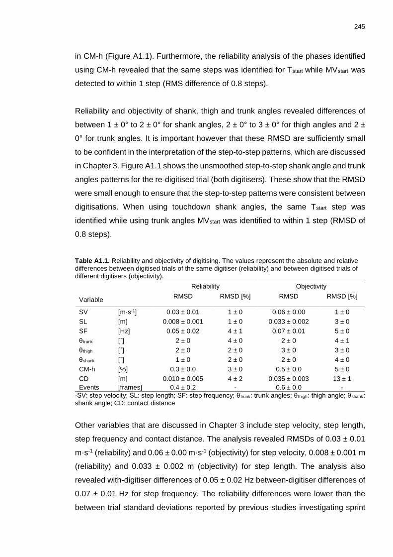
245

in CM-h (Figure A1.1). Furthermore, the reliability analysis of the phases identified

using CM-h revealed that the same steps was identified for Tstart while MVstart was

detected to within 1 step (RMS difference of 0.8 steps).

Reliability and objectivity of shank, thigh and trunk angles revealed differences of

between 1 ± 0° to 2 ± 0° for shank angles, 2 ± 0° to 3 ± 0° for thigh angles and 2 ±

0° for trunk angles. It is important however that these RMSD are sufficiently small

to be confident in the interpretation of the step-to-step patterns, which are discussed

in Chapter 3. Figure A1.1 shows the unsmoothed step-to-step shank angle and trunk

angles patterns for the re-digitised trial (both digitisers). These show that the RMSD

were small enough to ensure that the step-to-step patterns were consistent between

digitisations. When using touchdown shank angles, the same Tstart step was

identified while using trunk angles MVstart was identified to within 1 step (RMSD of

0.8 steps).

Table A1.1. Reliability and objectivity of digitising. The values represent the absolute and relative differences between digitised trials of the same digitiser (reliability) and between digitised trials of different digitisers (objectivity).

Reliability Objectivity

Variable RMSD RMSD [%] RMSD RMSD [%]

SV [m·s-1] 0.03 ± 0.01 1 ± 0 0.06 ± 0.00 1 ± 0 SL [m] 0.008 ± 0.001 1 ± 0 0.033 ± 0.002 3 ± 0 SF [Hz] 0.05 ± 0.02 4 ± 1 0.07 ± 0.01 5 ± 0 θ trunk [˚] 2 ± 0 4 ± 0 2 ± 0 4 ± 1 θ thigh [˚] 2 ± 0 2 ± 0 3 ± 0 3 ± 0 θshank [˚] 1 ± 0 2 ± 0 2 ± 0 4 ± 0 CM-h [%] 0.3 ± 0.0 3 ± 0 0.5 ± 0.0 5 ± 0 CD [m] 0.010 ± 0.005 4 ± 2 0.035 ± 0.003 13 ± 1 Events [frames] 0.4 ± 0.2 - 0.6 ± 0.0 -

-SV: step velocity; SL: step length; SF: step frequency; θ trunk: trunk angles; θ thigh: thigh angle; θshank: shank angle; CD: contact distance

Other variables that are discussed in Chapter 3 include step velocity, step length,

step frequency and contact distance. The analysis revealed RMSDs of 0.03 ± 0.01

m·s-1 (reliability) and 0.06 ± 0.00 m·s-1 (objectivity) for step velocity, 0.008 ± 0.001 m

(reliability) and 0.033 ± 0.002 m (objectivity) for step length. The analysis also

revealed with-digitiser differences of 0.05 ± 0.02 Hz between-digitiser differences of

0.07 ± 0.01 Hz for step frequency. The reliability differences were lower than the

between trial standard deviations reported by previous studies investigating sprint

246

acceleration and maximal velocity phase. During initial acceleration standard

deviation of 0.07 m·s-1 were reported for velocity, 0.016 m for step length and 0.09

Hz for step frequency (Coh et al., 2006). During the maximal velocity phase, within

participant SD ranged between 0.16 m·s-1 to 0.54 m·s-1 for step velocity,

0.04 to 0.06 m for step length and 0.08 to 0.27 Hz for step frequency (Bezodis,

2006). These reliability data show that uncertainties are small enough to allow the

identification of between step and between trial differences.

The reliability and objectivity RMSD for contact distances were 0.010 ± 0.005 m and

0.035 ± 0.003 m. The reliability (within-digitiser) differences were similar to the

reliability of 0.02 m reported by Churchill (2012) for touchdown distances. The larger

objectivity differences for contact distances are likely due to the uncertainties

associated with identifying the landmarks (i.e. centre of mass, MTP and toe), which

are used to calculate the variables for touchdown and toe-off distance. The larger

between-digitiser RMSDs for step length, step frequency and contact distances

could be a result of the differences between the touchdown and toe-off events

identified by the two digitisers. Due to the method used in Chapter 3 where

touchdown and toe-off variables were approximated using the events from the

panning camera, differences between the events will therefore have contributed to

between-digitiser differences. The between-digitiser RMSD were 0.6 ± 0.0 frames.

The between-digitiser differences in the identification of touchdown and toe-off

events revealed that the same event was identified 67% (34 events) of the time, that

with 31% (16 events) of the events there was one frame difference (0.005 s) and

with 2% (1 event) of the events there were two frames difference (0.010 s). The

differences in events would have influenced the step time and the position of the

CM at touchdown and therefore would have contributed to the between-digitiser

differences in step length, step frequency and contact distance.

Overall, the reliability and objectivity analysis revealed that the uncertainties due to

digitising were small enough to identify step-to-step changes between the initial

acceleration and transition phases. Furthermore, the reliability and objectivity of the

Tstart and MVstart measures were within one step therefore providing confidence that

these events are reliable enough to sub-divide the acceleration phase using either

CM-h or shank and trunk angles.

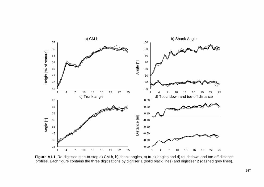
247

Figure A1.1. Re-digitised step-to-step a) CM-h, b) shank angles, c) trunk angles and d) touchdown and toe-off distance profiles. Each figure contains the three digitisations by digitiser 1 (solid black lines) and digistiser 2 (dashed grey lines).

a) CM-h b) Shank Angle

Hei

ght [

% o

f sta

ture

]

Ang

le [°

]

c) Trunk angle d) Touchdown and toe-off distance

Ang

le [°

]

Dis

tanc

e [m

]

43

45

47

49

51

53

55

57

1 4 7 10 13 16 19 22 2530

40

50

60

70

80

90

100

1 4 7 10 13 16 19 22 25

25

35

45

55

65

75

85

95

1 4 7 10 13 16 19 22 25-0.90

-0.70

-0.50

-0.30

-0.10

0.10

0.30

0.50

1 4 7 10 13 16 19 22 25

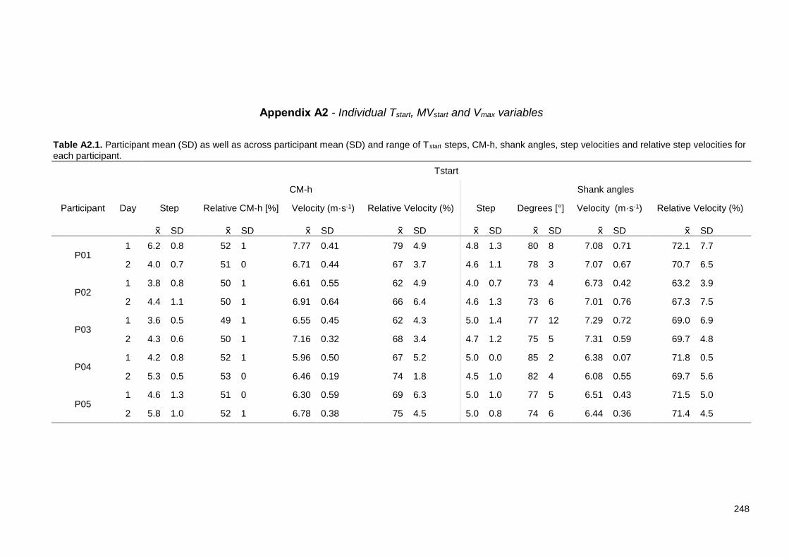
248

- Individual Tstart, MVstart and Vmax variables Table A2.1. Participant mean (SD) as well as across participant mean (SD) and range of Tstart steps, CM-h, shank angles, step velocities and relative step velocities for each participant.

Tstart CM-h Shank angles

Participant Day Step Relative CM-h [%] Velocity (m·s-1) Relative Velocity (%) Step Degrees [°] Velocity (m·s-1) Relative Velocity (%)

SD SD SD SD SD SD SD SD

P01 1 6.2 0.8 52 1 7.77 0.41 79 4.9 4.8 1.3 80 8 7.08 0.71 72.1 7.7

2 4.0 0.7 51 0 6.71 0.44 67 3.7 4.6 1.1 78 3 7.07 0.67 70.7 6.5

P02 1 3.8 0.8 50 1 6.61 0.55 62 4.9 4.0 0.7 73 4 6.73 0.42 63.2 3.9

2 4.4 1.1 50 1 6.91 0.64 66 6.4 4.6 1.3 73 6 7.01 0.76 67.3 7.5

P03 1 3.6 0.5 49 1 6.55 0.45 62 4.3 5.0 1.4 77 12 7.29 0.72 69.0 6.9

2 4.3 0.6 50 1 7.16 0.32 68 3.4 4.7 1.2 75 5 7.31 0.59 69.7 4.8

P04 1 4.2 0.8 52 1 5.96 0.50 67 5.2 5.0 0.0 85 2 6.38 0.07 71.8 0.5

2 5.3 0.5 53 0 6.46 0.19 74 1.8 4.5 1.0 82 4 6.08 0.55 69.7 5.6

P05 1 4.6 1.3 51 0 6.30 0.59 69 6.3 5.0 1.0 77 5 6.51 0.43 71.5 5.0

2 5.8 1.0 52 1 6.78 0.38 75 4.5 5.0 0.8 74 6 6.44 0.36 71.4 4.5

249

Table A2.2. Participant mean (SD) as well as across participant mean (SD) and range of MVstart steps, CM-h, shank angles, step velocities and relative step velocities for each participant.

MVstart CM-h Trunk angles

Participant Day Step Relative CM-h [%] Velocity (m·s-1) Relative Velocity (%) Step Degrees [°] Velocity (m·s-1) Relative Velocity (%)

SD SD SD SD SD SD SD SD

P01 1 15.4 1.1 56 0 9.56 0.18 97.3 0.9 16.6 1.1 82 3 9.63 0.16 98 1

2 15.2 1.8 56 1 9.67 0.18 96.7 1.7 15.6 0.9 83 3 9.72 0.14 97 1

P02 1 14.2 0.4 56 0 9.83 0.10 92.3 0.5 15.6 0.9 83 2 10.00 0.08 94 1

2 13.4 0.9 55 1 9.70 0.14 93.1 1.9 14.8 1.8 80 2 9.80 0.26 94 3

P03 1 15.4 0.9 56 0 9.96 0.09 94.3 0.8 17.6 0.5 77 1 10.17 0.13 96 1

2 15.3 1.5 55 0 9.97 0.09 95.0 0.5 15.7 1.5 81 3 10.04 0.12 96 1

P04 1 14.4 1.9 54 0 8.48 0.19 95.4 2.1 14.6 0.5 82 1 8.51 0.07 96 1

2 14.5 1.3 55 0 8.23 0.05 94.4 2.1 15.8 2.2 81 3 8.32 0.11 95 3

P05 1 15.6 0.9 56 0 8.71 0.10 95.6 0.7 15.8 1.8 86 2 8.76 0.20 96 2

2 15.8 1.3 56 0 8.67 0.13 96.1 1.6 14.3 1.0 83 1 8.60 0.08 95 1

250

Table A2.3. Participant mean (SD) as well as across participant mean (SD) and range of CT≤FT and Vmax steps, absolute and relative step velocity at those steps and trunk angle at Vmax.

CT≤FT Vmax

Participant Day Step Velocity (m·s-1) Relative Velocity (%) Step Velocity (m·s-1) Trunk angle (°) Relative CM-h (%)

SD SD SD SD SD SD SD

P01 1 14.0 1.4 9.44 0.19 96.1 1.2 21.2 1.8 9.83 0.14 84 2 57 1

2 11.8 1.1 9.26 0.22 92.6 2.7 22.2 1.8 10.00 0.16 86 3 57 0

P02 1 9.6 0.9 9.10 0.19 85.5 2.0 25.0 0.0 10.65 0.10 84 3 56 1

2 10.6 1.1 9.21 0.16 88.4 1.6 22.8 1.5 10.42 0.08 82 1 56 1

P03 1 15.6 0.9 10.07 0.18 95.3 1.5 23.6 0.9 10.57 0.04 82 2 56 0

2 12.0 0.0 9.62 0.05 91.7 0.9 23.3 1.2 10.49 0.12 84 2 55 0

P04 1 14.2 1.8 8.51 0.21 95.6 1.8 22.8 2.9 8.89 0.08 85 3 54 1

2 12.3 3.0 7.98 0.43 91.5 5.5 23.3 1.0 8.72 0.15 84 1 55 0

P05 1 12.8 1.1 8.52 0.17 93.5 1.9 23.8 1.8 9.11 0.07 87 1 56 0

2 11.3 1.7 8.17 0.28 90.5 3.5 23.0 1.4 9.03 0.07 85 2 56 0

251

- CM angle

During the ground contact phase the CM angle has previously been linked to the

anterior-posterior acceleration of the CM (di Prampero et al., 2005). In Chapter 3,

the step-to-step progression of the components of CM angles, namely TD distance

and toe-off distance and CM-h was investigated as these ultimately determine the

orientation of the CM relative to the contact point. Similar to the finding of Theme 3

(Phase analysis), TD angles (Figure A3.1) showed a relatively steep between step

increase during the initial acceleration phase when compared to the transition phase

and maximal velocity phase. The toe-off angles increased at a similar rate during

the initial acceleration and transition phases. When comparing the between-step

CM angle patterns to those of TD distances, toe-off distances and CM-h it is clear

that TD distances and toe-off distances have the largest influence on changes in

CM angle. This is due to the largest absolute changes in the horizontal variables

compared to step-to-step changes in CM-h.

Figure A3.1. a) Touchdown CM angle and b) toe-off CM angle.

70

80

90

100

110

120

1 3 5 7 9 11 13 15 17 19 21 23 25

Angl

e [°

]

Steps

303540455055606570

1 3 5 7 9 11 13 15 17 19 21 23 25Steps

a b

252

- Accuracy and reliability of joint kinematics and kinetics

Accuracies of reconstruction were determined as in Chapter 3. Six known points

located along a pole were digitised. These digitised locations were then

reconstructed and RMSD was calculated between the known and reconstructed

position. The RMSD were mean across each separate data collection data and

presented in figure A4.1.

Figure A4.1. Mean (-) and individual () horizontal and vertical reconstruction errors.

Reconstruction accuracies ranged from 0.001 m to 0.002 m horizontally and were

0.002 m vertically. These results show that data were reconstructed to comparable

levels of accuracies between the different days on which data were collected. Challis

and Kerwin (1996) showed that there is a degree of uncertainty associated with the

calculation of joint kinetics. A main source of this uncertainty is related to

inaccuracies associated with joint centre locations (Hunter et al., 2004c). Therefore,

a reliability analysis was conducted to quantify the level of uncertainty associated

with the digitising process. This was done by re-digitising one step three, nine and

19 trial three times on separate occasions. An RMSD and rel. RMSD was calculated

between the original and re-digitised trials to quantify the inter-digitiser uncertainties

associated with digitising.

0.000

0.001

0.002

0.003

0 1 2

RM

S di

ffere

nces

[m]

Reconstruction errors

Horizontal Vertical

253

Table A4.1. Absolute and relative RMSD between re-digitised trials for step 3.

*normalised to dimensionless values.





The results of this reliability analysis reveals a level of uncertainty associated with

the digitisation process that is largest for the joint variables. At the hip, uncertainties

in the calculated joint moments ranges between 0.025 – 0.039 (5 - 8% of the range)

while uncertainties in hip joint powers ranged between 0.631 – 1.110 (5 - 10% of the

range). This can in part be influenced by the propagation of errors as joint kinetics

higher up the chain are calculated, as well as the difficulty in identifying the hip joint

centre when digitising. The purpose of Chapter 4 is to identify changes between

steps three, nine and 19. Although some of these uncertainties are quite large

(especially the hip powers), figure A4.2 shows that these uncertainties are still low

enough to confidently identify differences between steps three, nine and 19.

Angular velocity* Joint moment* Joint Power* MTP Ankle Knee Hip MTP Ankle Knee Hip MTP Ankle Knee Hip

𝑅𝑅𝑀𝑀𝑅𝑅𝐷𝐷𝑟𝑟1 56.3 30.6 23.5 19.5 0.000 0.001 0.007 0.029 0.046 0.183 0.159 0.631

𝑟𝑟𝐻𝐻𝑟𝑟 𝑅𝑅𝑀𝑀𝑅𝑅𝐷𝐷1 4 5 10 11 1 1 8 5 4 5 12 5

𝑅𝑅𝑀𝑀𝑅𝑅𝐷𝐷𝑟𝑟2 54.1 28.7 30.7 36.9 0.000 0.001 0.009 0.029 0.035 0.231 0.176 0.692

𝑟𝑟𝐻𝐻𝑟𝑟 𝑅𝑅𝑀𝑀𝑅𝑅𝐷𝐷2 4 5 13 21 1 1 10 5 3 7 14 6

Angular velocity* Joint moment* Joint Power* MTP Ankle Knee Hip MTP Ankle Knee Hip MTP Ankle Knee Hip

𝑅𝑅𝑀𝑀𝑅𝑅𝐷𝐷𝑟𝑟1 82.7 42.4 27.0 30.7 0.001 0.002 0.007 0.039 0.054 0.410 0.231 1.053

𝑟𝑟𝐻𝐻𝑟𝑟 𝑅𝑅𝑀𝑀𝑅𝑅𝐷𝐷1 6 5 6 8 6 1 4 8 3 5 10 10

𝑅𝑅𝑀𝑀𝑅𝑅𝐷𝐷𝑟𝑟2 42.6 29.3 27.0 27.6 0.000 0.002 0.005 0.025 0.034 0.316 0.193 0.842

𝑟𝑟𝐻𝐻𝑟𝑟 𝑅𝑅𝑀𝑀𝑅𝑅𝐷𝐷2 3 4 6 7 2 1 3 5 2 4 8 8

Angular velocity* Joint moment* Joint Power* MTP Ankle Knee Hip MTP Ankle Knee Hip MTP Ankle Knee Hip 𝑅𝑅𝑀𝑀𝑅𝑅𝐷𝐷𝑟𝑟1 134.7 45.1 19.5 18.2 0.000 0.008 0.009 0.033 0.149 0.843 0.130 1.110

𝑟𝑟𝐻𝐻𝑟𝑟 𝑅𝑅𝑀𝑀𝑅𝑅𝐷𝐷1 8 4 6 8 2 4 4 6 8 5 7 8

𝑅𝑅𝑀𝑀𝑅𝑅𝐷𝐷𝑟𝑟2 103.8 32.2 20.8 20.1 0.001 0.003 0.006 0.032 0.136 0.547 0.117 1.045

𝑟𝑟𝐻𝐻𝑟𝑟 𝑅𝑅𝑀𝑀𝑅𝑅𝐷𝐷2 6 3 6 9 3 1 3 6 7 4 6 7

254

Figure A4.2. Continuous time-history joint angle, joint angular velocity, joint moment and joint power data obtained from the re-digitised step three (black), nine (blue) and 19 (red) trials.

90100110120130140150160

0 0.05 0.1 0.15 0.2

90100110120130140150160

0 0.05 0.1 0.15 0.2

90100110120130140150160170

0 0.05 0.1 0.15 0.2

7090

110130150170190210

0 0.05 0.1 0.15 0.2

-1000

-500

0

500

1000

1500

2000

0 0.05 0.1 0.15 0.2

-600

-400

-200

0

200

400

600

800

0 0.1 0.2

-200

-100

0

100

200

300

400

0 0.1 0.2

0

100

200

300

400

500

0 0.1 0.2

-0.01

0.00

0.01

0.01

0.02

0.02

0.03

0 0.05 0.1 0.15 0.2

-0.05

0.00

0.05

0.10

0.15

0.20

0.25

0 0.05 0.1 0.15 0.2

-0.15

-0.10

-0.05

0.00

0.05

0.10

0.15

0.20

0 0.05 0.1 0.15 0.2

-0.40-0.30-0.20-0.100.000.100.200.300.40

0 0.05 0.1 0.15 0.2

-1.50

-1.00

-0.50

0.00

0.50

1.00

1.50

0 0.1 0.2

-10.00

-5.00

0.00

5.00

10.00

0 0.05 0.1 0.15 0.2

-1.50

-1.00

-0.50

0.00

0.50

1.00

1.50

2.00

0 0.1 0.2

-15.00

-10.00

-5.00

0.00

5.00

10.00

0 0.1 0.2

Joint angle [°] Angular velocity [deg.s-1] Joint moment [N] Joint power [W]

MTP

Ankle

Knee

Hip

Contact time [s] Contact time [s] Contact time [s] Contact time [s]

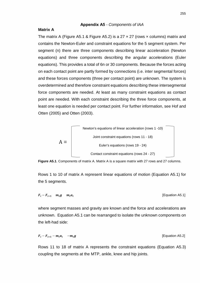
255

- Components of IAA Matrix A The matrix A (Figure A5.1 & Figure A5.2) is a 27 × 27 (rows × columns) matrix and

contains the Newton-Euler and constraint equations for the 5 segment system. Per

segment (n) there are three components describing linear acceleration (Newton

equations) and three components describing the angular accelerations (Euler

equations). This provides a total of 6n or 30 components. Because the forces acting

on each contact point are partly formed by connections (i.e. inter segmental forces)

and these forces components (three per contact point) are unknown. The system is

overdetermined and therefore constraint equations describing these intersegmental

force components are needed. At least as many constraint equations as contact

point are needed. With each constraint describing the three force components, at

least one equation is needed per contact point. For further information, see Hof and

Otten (2005) and Otten (2003).

Figure A5.1. Components of matrix A. Matrix A is a square matrix with 27 rows and 27 columns.

Rows 1 to 10 of matrix A represent linear equations of motion (Equation A5.1) for

the 5 segments.

𝑭𝑭𝒊𝒊 − 𝑭𝑭𝒊𝒊+𝟏𝟏 + 𝒎𝒎𝒊𝒊𝒈𝒈 = 𝒎𝒎𝒊𝒊𝒂𝒂𝒊𝒊 [Equation A5.1]

where segment masses and gravity are known and the force and accelerations are

unknown. Equation A5.1 can be rearranged to isolate the unknown components on

the left-had side:

𝑭𝑭𝒊𝒊 − 𝑭𝑭𝒊𝒊+𝟏𝟏 − 𝒎𝒎𝒊𝒊𝒂𝒂𝒊𝒊 = −𝒎𝒎𝒊𝒊𝒈𝒈 [Equation A5.2]

Rows 11 to 18 of matrix A represents the constraint equations (Equation A5.3)

coupling the segments at the MTP, ankle, knee and hip joints.

Newton’s equations of linear acceleration (rows 1 -10)

Joint constraint equations (rows 11 - 18)

Euler’s equations (rows 19 - 24)

Contact constraint equations (rows 24 - 27)

A =

256

𝒂𝒂��⃗ 𝒏𝒏𝒊𝒊 = 𝒂𝒂��⃗ 𝒊𝒊 + ��̈�𝜽𝒊𝒊 × 𝒓𝒓�⃗ 𝒏𝒏𝒊𝒊� − (�̇�𝜽𝒊𝒊𝟏𝟏 × 𝒓𝒓�⃗ 𝒏𝒏𝒊𝒊) [Equation A5.3]

Equation A5.3 represents the accelerations at the jth joint (�⃗�𝑎𝑗𝑗𝑖𝑖) of the ith segment. �⃗�𝑎𝑖𝑖

is the unknown acceleration of the centre off masses on the ith segments; �̈�𝜃𝑖𝑖 is the

unknown angular acceleration of the ith segments; �̇�𝜃𝑖𝑖2 is the known angular velocities

of the ith segment. The distances between the centre of mass of the segment and

the proximal (p) or distal (d) joint is represented by the known radial arm 𝑟𝑟𝑗𝑗𝑖𝑖. Equation

A5.4 and Equation A5.5 describe the coupling of the joints ensuring matched

accelerations of the joints between two adjoining segments (Hof & Otten, 2005;

Heitmann, Ferns & Breakspear, 2012).

𝒂𝒂��⃗ 𝒑𝒑𝒊𝒊 = 𝒂𝒂��⃗ 𝒅𝒅(𝒊𝒊+𝟏𝟏) [Equation A5.4] 𝒂𝒂��⃗ 𝒑𝒑𝒊𝒊 + ��̈�𝜽𝒊𝒊 × 𝒓𝒓�⃗ 𝒑𝒑𝒊𝒊� − (�̇�𝜽𝒊𝒊𝟏𝟏 × 𝒓𝒓�⃗ 𝒑𝒑𝒊𝒊) = 𝒂𝒂��⃗ 𝒅𝒅(𝒊𝒊+𝟏𝟏) + ��̈�𝜽𝒅𝒅(𝒊𝒊+𝟏𝟏) × 𝒓𝒓�⃗ 𝒅𝒅(𝒊𝒊+𝟏𝟏)� − (�̇�𝜽𝒅𝒅(𝒊𝒊+𝟏𝟏)

𝟏𝟏 × 𝒓𝒓�⃗ 𝒅𝒅(𝒊𝒊+𝟏𝟏)) [Equation A5.5]

Equation A5.5 can be rearranged to isolate the unknown linear and angular

acceleration terms:

𝒂𝒂��⃗ 𝟏𝟏𝒊𝒊 − 𝒂𝒂��⃗ (𝒊𝒊+𝟏𝟏) + ��̈�𝜽𝒊𝒊 × 𝒓𝒓�⃗ 𝒑𝒑𝒊𝒊� − ��̈�𝜽(𝒊𝒊+𝟏𝟏) × 𝒓𝒓�⃗ 𝒅𝒅(𝒊𝒊+𝟏𝟏)� = −(�̇�𝜽(𝒊𝒊+𝟏𝟏)

𝟏𝟏 × 𝒓𝒓�⃗ 𝒅𝒅(𝒊𝒊+𝟏𝟏)) + (�̇�𝜽𝒊𝒊𝟏𝟏 × 𝒓𝒓�⃗ 𝒑𝒑𝒊𝒊) [Equation A5.6]

Rows 19 to 23 of matrix A represent the equations of angular motion (Equation

A5.7).

(𝑭𝑭𝒅𝒅𝒊𝒊 × 𝒓𝒓𝒅𝒅𝒊𝒊) − �𝑭𝑭𝒑𝒑𝒊𝒊 × 𝒓𝒓𝒑𝒑𝒊𝒊�+ 𝑴𝑴𝒅𝒅𝒊𝒊 − 𝑴𝑴𝒑𝒑𝒊𝒊 = 𝑰𝑰𝒊𝒊 × �̈�𝜽𝒊𝒊 [Equation A5.7]

where 𝐹𝐹𝑑𝑑𝑖𝑖 and 𝐹𝐹𝑝𝑝𝑖𝑖 are the unknown distal and proximal forces; 𝑀𝑀𝑑𝑑𝑖𝑖 and 𝑀𝑀𝑝𝑝𝑖𝑖are the

known distal and proximal joint moments and �̈�𝜃𝑖𝑖 is the unknown angular acceleration

of the segment. Equation A5.7 can be re-arranged to isolate the unknown

components:

−(𝑭𝑭𝒅𝒅𝒊𝒊 × 𝒓𝒓𝒅𝒅𝒊𝒊) + �𝑭𝑭𝒑𝒑𝒊𝒊 × 𝒓𝒓𝒑𝒑𝒊𝒊� − 𝑰𝑰𝒊𝒊 × �̈�𝜽𝒊𝒊 = −𝑴𝑴𝒅𝒅𝒊𝒊 + 𝑴𝑴𝒑𝒑𝒊𝒊 [Equation A5.8]

Finally, Rows 24 to 27 of matrix A represents the contact constraint equations and

describe the force components at contact point between the foot and the ground

(Equation A5.9). The required components to describe these forces and

accelerations are put into rows and columns 24 to 27 of Matrix A. The contact

257

constraint equations ensure that the contact points with the ground have zero

acceleration meaning.

𝒂𝒂��⃗ 𝒑𝒑𝟏𝟏 = 𝒂𝒂��⃗ 𝒅𝒅𝟎𝟎 = 𝟎𝟎 [Equation A5.9]

where 𝑎𝑎��⃗ 𝑝𝑝1 and �⃗�𝑎𝑑𝑑0 are the accelerations at the contact point. Again, Equation A5.9

can be re-arranged to isolate the unknown components. In this case the

components relating to the acceleration of the ground are zero.

𝒂𝒂��⃗ 𝟏𝟏 + ��̈�𝜽𝟏𝟏 × 𝒓𝒓�⃗ 𝟏𝟏� − (�̇�𝜽𝟏𝟏𝟏𝟏 × 𝒓𝒓�⃗ 𝟏𝟏) = 𝟎𝟎 [Equation A5.10]

where �⃗�𝑎1 + ��̈�𝜃1 × 𝑟𝑟1� represent the known accelerations (acy &acz) at the contact point between the segment and the ground (Figure A5.3).

258

MTP Ankle Knee Hip fFoot rFoot Shank Thigh HAT fFoot rFoot Shank Thigh HAT Fe Fe Fe Fe Fx Fy Fx Fy Fx Fy Fx Fy ax ay ax ay ax ay ax ay ax ay �̈�𝜃 �̈�𝜃 �̈�𝜃 �̈�𝜃 �̈�𝜃 x y x y 1 2 3 4 5 6 7 8 9 10 11 12 13 14 15 16 17 18 19 20 21 22 23 24 25 26 27

fFoot x 1 -1 0 0 0 0 0 0 0 0 0 0 0 0 0 0 0 0 0 0 0 0 0 0 1 0 0 1 y 2 0 -1 0 0 0 0 0 0 0 0 0 0 0 0 0 0 0 0 0 0 0 0 0 0 1 1 0

rFoot x 3 1 0 -1 0 0 0 0 0 0 0 -m2 0 0 0 0 0 0 0 0 0 0 0 0 1 0 0 0 y 4 0 1 0 -1 0 0 0 0 0 0 0 -m2 0 0 0 0 0 0 0 0 0 0 0 0 1 0 0

Shank x 5 0 0 1 0 -1 0 0 0 0 0 0 0 -m3 0 0 0 0 0 0 0 0 0 0 0 0 0 0 y 6 0 0 0 1 0 -1 0 0 0 0 0 0 0 -m3 0 0 0 0 0 0 0 0 0 0 0 0 0

Thigh x 7 0 0 0 0 1 0 -1 0 0 0 0 0 0 0 -m4 0 0 0 0 0 0 0 0 0 0 0 0 y 8 0 0 0 0 0 1 0 -1 0 0 0 0 0 0 0 -m4 0 0 0 0 0 0 0 0 0 0 0

HAT x 9 0 0 0 0 0 0 1 0 0 0 0 0 0 0 0 0 -m5 0 0 0 0 0 0 0 0 0 0 y 10 0 0 0 0 0 0 0 1 0 0 0 0 0 0 0 0 0 -m5 0 0 0 0 0 0 0 0 0

MTP x 11 0 0 0 0 0 0 0 0 1 0 -1 0 0 0 0 0 0 0 -r12y r21y 0 0 0 0 0 0 0 y 12 0 0 0 0 0 0 0 0 0 1 0 -1 0 0 0 0 0 0 r12x - r21x 0 0 0 0 0 0 0

Ankle x 13 0 0 0 0 0 0 0 0 0 0 1 0 -1 0 0 0 0 0 0 -r22y r31y 0 0 0 0 0 0 y 14 0 0 0 0 0 0 0 0 0 0 0 1 0 -1 0 0 0 0 0 r22x - r31x 0 0 0 0 0 0

Knee x 15 0 0 0 0 0 0 0 0 0 0 0 0 1 0 -1 0 0 0 0 0 -r32y r41y 0 0 0 0 0 y 16 0 0 0 0 0 0 0 0 0 0 0 0 0 1 0 -1 0 0 0 0 r32x - r41x 0 0 0 0 0

Hip x 17 0 0 0 0 0 0 0 0 0 0 0 0 0 0 1 0 -1 0 0 0 0 -r42y r51y 0 0 0 0 y 18 0 0 0 0 0 0 0 0 0 0 0 0 0 0 0 1 0 -1 0 0 0 r42x - r51x 0 0 0 0

fFoot 19 r1py -r1px 0 0 0 0 0 0 0 0 0 0 0 0 0 0 0 0 0 0 0 0 0 -re1y re1x re2y -re2x

rFoot 20 -r2dy r2dx r2py - r2px 0 0 0 0 0 0 0 0 0 0 0 0 0 0 0 -I2 0 0 0 -re1y re1x 0 0 Shank 21 0 0 -r3dy r3dx r3py - r3px 0 0 0 0 0 0 0 0 0 0 0 0 0 0 -I3 0 0 0 0 0 0 Thigh 22 0 0 0 0 -r4dy r4dx r4py -r4px 0 0 0 0 0 0 0 0 0 0 0 0 0 -I4 0 0 0 0 0 HAT 23 0 0 0 0 0 0 -r5dy r5dx 0 0 0 0 0 0 0 0 0 0 0 0 0 0 -I5 0 0 0 0 CoP 24 0 0 0 0 0 0 0 0 1 0 1 0 0 0 0 0 0 0 -re1y -re1y 0 0 0 0 0 0 0 CoP 25 0 0 0 0 0 0 0 0 0 1 0 1 0 0 0 0 0 0 re1x re1x 0 0 0 0 0 0 0 CoP 26 0 0 0 0 0 0 0 0 0 1 0 0 0 0 0 0 0 0 -re2y 0 0 0 0 0 0 0 0 CoP 27 0 0 0 0 0 0 0 0 1 0 0 0 0 0 0 0 0 0 re2x 0 0 0 0 0 0 0 0

Figure A5.2. Full matrix A used for the IAA adapted from (Hof & Otten, 2005). Rows 1 to 10 contain the coefficients for the equations of linear acceleration (equations 5.10). Rows 11 to 18 contain the coefficients for the constraint equations (equations 5.13). Rows 19 to 20 are the coefficients for the equations of angular acceleration (equation 5.17). Rows 24 to 27 contain the coefficients for the constraint equations with the ground. It is important to remind the reader at this point that two contact models were used. At the beginning and end of ground contact when the one-point contact model applied, contact was modelled either between the fore foot (yellow shaded) or rear foot (red shading). This was dependent on the location of the COP relative to the MTP joint. For example, when the COP was behind the MTP joint, all the inputs in red text were removed from the matrix and replaced by zeros. During the stationary fore foot phase of ground contact, the two-point contact model was used (see 5.2.1.2 Contact model). Rows 24 to 27 and columns 24 to 27 were filled cording to the red text. In this case contact coefficients describing contact at the projected MTP location are added to rows and columns 24 to 25, while the coefficients describing contact at the projected TOE location are added to rows and columns 26 to 27.

259

Vector c Vector c is a 27 × 1 column vector containing known variables isolated on the right

side of equations A5.2, A5.6, A5.8, A5.10 (Figure A5.3). Rows 1 – 10 include the

external forces acting on segments 1 to 5. This was either gravity (mig) or the force

exerted by the contralateral leg on the trunk segment (F5x, F5y). Rows 11 to 18

include the variables of the centripetal accelerations of the MTP, ankle, knee and

hip joints. These use the angu7lar velocity of the segments (�̇�𝜃𝑖𝑖2) as inputs. Likewise,

rows 24 to 27 include the centripetal accelerations of the most distal segment. The

variables acx and acy (Equation A5.10) are the known accelerations at the contact

point between the foot and the ground (Otten, 2003). For further information see Hof

and Otten (2005) and Otten (2003).

0 – m1g

0 – m2g

0 – m3g

0 – m4g

F5x F5y – m5g

−(�̇�𝜃22 × 𝑟𝑟𝑑𝑑2𝑥𝑥) + (�̇�𝜃12 × 𝑟𝑟𝑝𝑝1𝑥𝑥) −(�̇�𝜃22 × 𝑟𝑟𝑑𝑑2𝑦𝑦) + (�̇�𝜃22 × 𝑟𝑟𝑝𝑝1𝑦𝑦) −(�̇�𝜃32 × 𝑟𝑟𝑑𝑑3𝑥𝑥) + (�̇�𝜃22 × 𝑟𝑟𝑝𝑝2𝑥𝑥) −(�̇�𝜃32 × 𝑟𝑟𝑑𝑑3𝑦𝑦) + (�̇�𝜃22 × 𝑟𝑟𝑝𝑝2𝑦𝑦) −(�̇�𝜃42 × 𝑟𝑟𝑑𝑑4𝑥𝑥) + (�̇�𝜃32 × 𝑟𝑟𝑝𝑝3𝑥𝑥) −(�̇�𝜃42 × 𝑟𝑟𝑑𝑑4𝑦𝑦) + (�̇�𝜃32 × 𝑟𝑟𝑝𝑝3𝑦𝑦) −(�̇�𝜃52 × 𝑟𝑟𝑑𝑑5𝑥𝑥) + (�̇�𝜃42 × 𝑟𝑟𝑝𝑝4𝑥𝑥) −(�̇�𝜃52 × 𝑟𝑟𝑑𝑑5𝑦𝑦) + (�̇�𝜃42 × 𝑟𝑟𝑝𝑝4𝑦𝑦)

-JMMTP

JMMTP ,-JMankle JMankle ,-JMknee JMknee ,-JMhip

JMhip (�̇�𝜃𝑖𝑖.12 × 𝑟𝑟𝑑𝑑𝑖𝑖.1𝑥𝑥) + acy (�̇�𝜃𝑖𝑖.12 × 𝑟𝑟𝑑𝑑𝑖𝑖.1𝑦𝑦) + acz (�̇�𝜃1.2

2 × 𝑟𝑟𝑑𝑑1.2𝑥𝑥) + acz (�̇�𝜃1.2

2 × 𝑟𝑟𝑑𝑑1.2𝑦𝑦) + acy Figure A5.3. Variables contained within the column vector c adapted from (Hof & Otten, 2003). When the COP was behind the MTP joint, all the inputs in red were removed from the matrix and replaced by zeros. Variables in red are replaced by zeros when the COP was behind the MTP joint.

Variables describing the effect of gravity acting on the segments.

The force (F5x, F5y) of the contralateral leg onthe trunk segment was added here

Variables accounting for the effect of centripetal accelerations around the MTP, ankle, knee and hip joints on the acceleration of the segments.

Variables accounting for the effect of the joint moments on the acceleration of the segments centripetal accelerations around the MTP, ankle,

Variables accounting for the accelerations at the foot-floor interface.

260

Vector x This is a 1 × 27 column vector of unknowns. From top to bottom, this vector consists

of: the y and z components of the intersegmental forces at the MTP, ankle, knee

and hip (rows 1 -10); the y and z components of the linear accelerations of the fore

foot, rear foot, shank, thigh and HAT segments (rows 11 - 18); the angular

accelerations of the fore foot, rear foot, shank, thigh and HAT segments (rows

19 - 24) and the y and z components of the ground reaction forces (rows 25 - 27).

For further information see Hof and Otten (2005) and Otten (2003).

261

- Foot-floor models in maximal sprinting

INTRODUCTION: The results of an IAA not only depends on the characteristics of

the model (Chen, 2005) but also model used to describe ground contact (Dorn et

al., 2012). In the literature the foot-floor interaction has previously been modelled at

a single point (i.e. the instantaneous COP; Kepple et al., 1997; Hof & Otten, 2005;

Cabral et al., 2013; Koike & Nagai, 2016; Koike et al., 2017) or across multiple-points

(e.g. Lin et al., 2011; Dorn et al., 2012; Koike, Ishikawa & Ae, 2010). Furthermore,

IAA studies in sprinting have generally modelled the foot as a single segment

(Cabral et al., 2013; Koike & Nagai, 2016). However, the foot is a complex

multi-segment structure (Hamner, Seth, Steele & Delp, 2013) with the MTP joint

showing a relatively large range of motion during the stance phases in sprinting

(Bezodis et al., 2012). The aim of this study was therefore to compare the results of

an IAA when using a single-segment or two-segment foot model. Furthermore, a

second aim was to compare IAA results when using a single point versus multi-point

model to define the foot-floor contact model when using a two-segment foot. The

purpose of this will be to inform future work using IAA in Chapter 5. For a contact

model to be identified as suitable, two conditions need to be met. Firstly, the model

needs to provide accurate results when compared to the measured CM

accelerations. Secondly, the contributions by the individual inputs (e.g. joint

moments) need to be realistic. This means that the contributions to CM acceleration

by the individual inputs need to provide a realistic and meaningful interpretation of

the results.

METHODS: Sagittal plane kinematics (200 Hz video) and three dimensional ground

reaction forces (1000 Hz) were collected from 13 participants performing

acceleration from blocks. Data was collected from steps three, nine and 19 and the

best trial from each step was selected for further analysis. After extracting the videos

using Dartfish Team Pro 6.0 (Dartfish), converting them to .avi format and de-

interlaced in VLC 2.1.3 (VideoLan, France), they were digitised in Matlab (The

MathWorks Inc., USA, version R2014a) using an 18 point model. The digitised

coordinates were then reconstructed using a nine-parameter 2D-DLT with lens

correction (Walton, 1981). Kinematic data were filtered with a 4th order low pass

Butterworth filter with a 26 Hz cut-off frequency. The body was modelled using five

segments; fore foot, rear foot, shank, thigh and head, arms and trunk (HAT). Data

262

from de Leva (1996) were used to calculate the inertia data for all the segments

except the foot. For the foot segments, data used by Bezodis et al. (2014) was used

with the mass of the sprint shoe added. Linear and angular segment velocities and

accelerations were calculated using a three point central differences method (Miller

& Nelson, 1976). Ground contact was identified using a 10 N threshold before down

sampling to 200 Hz and filtered with a 4th order low pass Butterworth filter with a

26 Hz cut-off frequency. Joint moments were calculated according to Winter (2009)

where the fore foot segment and MTP were included in the calculation when the

COP was in front of the MTP joint (Stefanyshyn & Nigg, 1997). An IAA was

performed according to the methods proposed by Hof & Otten (2005). Ground

contact was modelled using three methods (Figure A6.1). The first method involved

a single segment foot where ground contact was modelled as a joint between the

foot and the COP (Figure A6.1a). The second involved a two segment foot with a

joint being defined between the COP and CM of the rear foot when the COP was

located behind the MTP joint and the between the COP and the MTP joint when the

COP was located in front of the MTP (Figure A6.1b). The third foot model involved

a mix approach. At the start and end when the MTP and Toe were above a vertical

threshold the foot model two was used. When either the MTP, toe or both where

below the vertical threshold, then a two point contact model was used. In this case,

contact was defined at the locations of the MTP joint and the toe (Figure A6.1c; also

see 5.2.1.2 Contact model).

Figure A6.1. Three ground contact models used in the current study. The contact model in a) involves a 1 segment foot where contact is modelled between the foot and the ground via the COP (1SegFoot_ COP). The contact model in b) involves a two-segment foot where contact with the ground is modelled between the COP and the distal segment (2SegFoot_ COP). The contact model in c) involves a two-segment foot and used the COP at the beginning and end of ground contact and the MTP joint and toe when the forefoot was stationary on the ground (2SegFoot_TwoPoint).

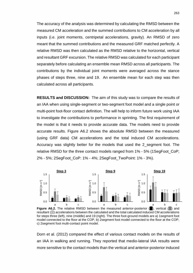
263

The accuracy of the analysis was determined by calculating the RMSD between the

measured CM acceleration and the summed contributions to CM acceleration by all

inputs (i.e. joint moments, centripetal accelerations, gravity). An RMSD of zero

meant that the summed contributions and the measured GRF matched perfectly. A

relative RMSD was then calculated as the RMSD relative to the horizontal, vertical

and resultant GRF excursion. The relative RMSD was calculated for each participant

separately before calculating an ensemble mean RMSD across all participants. The

contributions by the individual joint moments were averaged across the stance

phases of steps three, nine and 19. An ensemble mean for each step was then

calculated across all participants.

RESULTS and DISCUSSION: The aim of this study was to compare the results of

an IAA when using single-segment or two-segment foot model and a single point or

multi-point foot-floor contact definition. The will help to inform future work using IAA

to investigate the contributions to performance in sprinting. The first requirement of

the model is that it needs to provide accurate data. The models need to provide

accurate results. Figure A6.2 shows the absolute RMSD between the measured

(using GRF data) CM accelerations and the total induced CM accelerations.

Accuracy was slightly better for the models that used the 2_segment foot. The

relative RMSD for the three contact models ranged from 1% - 5% (1SegFoot_CoP;

2% - 5%; 2SegFoot_CoP: 1% - 4%; 2SegFoot_TwoPoint: 1% - 3%).


Figure A6.2. The relative RMSD between the measured anterior-posterior ( ), vertical ( ) and resultant ( ) accelerations between the calculated and the total calculated induced CM accelerations for steps three (left), nine (middle) and 19 (right). The three foot-ground models are a) 1segment foot model connected to the floor at the COP, b) 2segment foot model connected to the floor at the COP, c) 2segment foot multi-contact point model.

Dorn et al. (2012) compared the effect of various contact models on the results of

an IAA in walking and running. They reported that medio-lateral IAA results were

more sensitive to the contact models than the vertical and anterior-posterior induced

0.0

0.5

1.0

1.5

a b c

RM

SD

[m·s

-2]

0.0

0.5

1.0

1.5

a b c

RM

SD

[m·s

-2]

0.0

0.5

1.0

1.5

a b c

RM

SD

[m·s

-2]

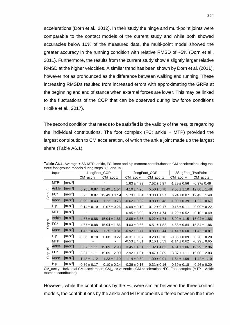
264

accelerations (Dorn et al., 2012). In their study the hinge and multi-point joints were

comparable to the contact models of the current study and while both showed

accuracies below 10% of the measured data, the multi-point model showed the

greater accuracy in the running condition with relative RMSD of ~5% (Dorn et al.,

2011). Furthermore, the results from the current study show a slightly larger relative

RMSD at the higher velocities. A similar trend has been shown by Dorn et al. (2011),

however not as pronounced as the difference between walking and running. These

increasing RMSDs resulted from increased errors with approximating the GRFs at

the beginning and end of stance when external forces are lower. This may be linked

to the fluctuations of the COP that can be observed during low force conditions

(Koike et al., 2017).

The second condition that needs to be satisfied is the validity of the results regarding

the individual contributions. The foot complex (FC; ankle + MTP) provided the

largest contribution to CM acceleration, of which the ankle joint made up the largest

share (Table A6.1).

Table A6.1. Average ± SD MTP, ankle, FC, knee and hip moment contributions to CM acceleration using the three foot-ground models during steps 3, 9 and 19. Input 1segFoot_COP 2segFoot_COP 2SegFoot_TwoPoint CM_acc y CM_acc z CM_acc y CM_acc z CM_acc y CM_acc z

Ste

p 3

MTP [m·s-2] - - 1.63 ± 4.22 7.52 ± 5.87 -1.29 ± 0.56 -0.37 ± 0.49 Ankle [m·s-2] 6.25 ± 0.87 12.49 ± 1.54 4.10 ± 4.26 5.50 ± 5.78 7.53 ± 1.10 12.80 ± 1.48 FC* [m·s-2] 6.25 ± 0.87 12.49 ± 1.54 5.73 ± 0.84 13.03 ± 1.37 6.24 ± 0.87 12.43 ± 1.49 Knee [m·s-2] -0.99 ± 0.43 1.22 ± 0.73 -0.62 ± 0.32 0.83 ± 0.48 -1.00 ± 0.39 1.22 ± 0.67 Hip [m·s-2] -0.14 ± 0.10 -0.07 ± 0.26 -0.09 ± 0.10 0.12 ± 0.17 -0.15 ± 0.11 0.09 ± 0.22

Ste

p 9

MTP [m·s-2] - - 0.95 ± 3.99 8.29 ± 4.74 -1.29 ± 0.52 -0.10 ± 0.49 Ankle [m·s-2] 4.67 ± 0.88 15.94 ± 1.86 3.08 ± 3.85 8.22 ± 4.74 5.92 ± 1.15 15.94 ± 1.88 FC* [m·s-2] 4.67 ± 0.88 15.94 ± 1.86 4.03 ± 0.66 16.51 ± 1.82 4.63 ± 0.84 15.84 ± 1.86 Knee [m·s-2] -1.42 ± 0.65 1.25 ± 0.81 -0.92 ± 0.47 0.88 ± 0.44 -1.44 ± 0.60 1.42 ± 0.81 Hip [m·s-2] -0.36 ± 0.10 0.08 ± 0.22 -0.31 ± 0.07 0.28 ± 0.16 -0.36 ± 0.09 0.26 ± 0.20

Ste

p 19

MTP [m·s-2] - - -0.53 ± 4.61 8.16 ± 5.59 -1.14 ± 0.62 -0.29 ± 0.65 Ankle [m·s-2] 3.37 ± 1.11 19.09 ± 2.90 3.45 ± 4.54 11.32 ± 4.62 4.51 ± 1.06 19.29 ± 2.96 FC* [m·s-2] 3.37 ± 1.11 19.09 ± 2.90 2.92 ± 1.01 19.47 ± 2.89 3.37 ± 1.11 19.00 ± 2.83 Knee [m·s-2] -1.48 ± 1.12 1.23 ± 1.10 -1.14 ± 0.89 1.00 ± 0.91 -1.54 ± 1.09 1.42 ± 1.10 Hip [m·s-2] -0.39 ± 0.17 0.10 ± 0.24 -0.36 ± 0.15 0.31 ± 0.16 -0.39 ± 0.18 0.26 ± 0.20

CM_acc y: Horizontal CM acceleration; CM_acc z: Vertical CM acceleration; *FC: Foot complex (MTP + Ankle moment contribution)

However, while the contributions by the FC were similar between the three contact

models, the contributions by the ankle and MTP moments differed between the three

265

contact models (Table A6.1). Since the fore foot motion is largely restricted by the

ground during the majority of stance, the two-point contact model might be a more

realistic representation. Furthermore, foot pressure mapping data from sprinting

shows that contact occurs across the metatarsals and toes (Smith, 2012). This

further suggests that modelling contact using constraints at the toe and MTP is more

realistic than just using a single point. This definition of modelling contact at the

horizontal locations of the MTP and toe has previously been successfully used by

Bezodis et al. (2015) in a simulation study of the first stance in sprinting. Using the

COP in the definition of ground contact could lead to errors in the calculation of an

IAA. This is due to the relatively large fluctuations in the anterior-posterior location

of the COP during ground contact, while the position of the foot remains relatively

unchanged (Koike et al., 2017). This will have the effect of creating large fluctuations

in the length of the moment arm between the COP and CM of either the fore or rear

foot, leading to an overestimation of the accelerations (Koike et al., 2017). Koike et

al. (2017) therefore suggested using contact points that are fixed to the base of the

foot.

While the 2SegFoot_CoP contact model might suggest that the MTP shows large

horizontal and vertical contributions to CM accelerations (Table A6.1), the two-point

model suggests that the MTP moment induces small negative accelerations on the

CM while the ankle moment contributed large upward and forward CM

accelerations. This is in line with the results by Koike, Ishikawa and Ae (2010). In

the study by Koike et al. (2010), relatively small backward and downward

accelerations induced by the MTP moment were reported, while the ankle moment

was the largest contributor to forward and upward CM acceleration. These results

can be understood in terms of the mechanics of linked segments. With the fore foot

constrained, an MTP plantar flexor moment would induce an anti-clockwise

(direction of movement viewed from left to right) motion on the rear foot segment.

This would result in a backward and downward motion of the rear foot, shank, thigh

and upper body segments. Overall, the multi-point contact model is therefore more

suitable, especially if a two-segment foot is used.

266

- Induced segment accelerations at the peak braking, vertical and propulsive force events

Table A7.1. Mean ±SD linear and angular induced segment accelerations at the peak braking force event of the third step. Joint Moment Linear induced accelerations [m·s-2] Angular induced accelerations [rad·s-2] [normalised] Rear Foot Shank Thigh HAT Rear Foot Shank Thigh HAT

Horizontal Vertical Horizontal Vertical Horizontal Vertical Horizontal Vertical Mean ± SD Mean ±SD Mean ±SD Mean ±SD Mean ±SD Mean ±SD Mean ±SD Mean ±SD Mean ±SD Mean ±SD Mean ±SD Mean ±SD Mean ±SD

MTP 0.00 0.01 -1.46 2.92 -0.98 1.63 -2.62 5.03 -1.76 3.01 -0.93 1.78 -0.81 1.44 0.12 0.21 -0.04 0.07 20.09 36.01 0.05 1.47 -7.43 13.93 0.67 1.21Ankle 0.02 0.02 10.68 8.22 9.41 7.37 18.51 13.93 16.94 13.06 5.06 3.78 8.77 6.61 -1.40 1.06 1.17 1.02 -158.50 118.01 0.79 9.44 56.36 42.81 -10.89 8.33Knee 0.00 0.02 -0.51 4.14 -0.48 3.65 -0.94 9.63 -0.68 5.35 -0.44 4.84 -0.22 0.70 0.10 0.72 0.22 1.89 8.22 64.37 -0.08 12.21 -2.61 28.65 0.35 5.51Hip 0.08 0.04 -17.67 8.66 -12.40 6.78 -27.03 11.81 -24.24 11.34 -4.01 2.86 -11.62 5.46 2.88 1.41 5.43 2.41 240.12 105.35 -12.10 22.32 -91.70 39.75 37.23 15.14

Table A7.2. Mean ±SD linear and angular induced segment accelerations at the peak braking force event of the ninth step. Joint Moment Linear induced accelerations [m·s-2] Angular induced accelerations [rad·s-2] [normalised] Rear Foot Shank Thigh HAT Rear Foot Shank Thigh HAT


MTP 0.00 0.00 -0.21 0.74 0.02 0.08 -0.06 0.21 0.04 0.15 0.01 0.05 0.01 0.04 0.00 0.00 0.00 0.00 -0.67 2.41 -0.52 1.89 0.10 0.38 -0.01 0.02 Ankle 0.05 0.03 20.99 6.50 18.76 8.16 31.32 11.31 38.42 16.03 2.88 2.54 22.21 9.25 -4.11 1.72 5.70 2.88 -340.00 124.77 9.09 18.70 114.73 49.20 -40.45 16.97Knee -0.02 0.02 3.77 3.35 3.66 4.19 12.00 12.09 7.20 8.71 6.81 7.16 0.93 2.12 -0.72 0.85 -2.43 2.19 -69.01 74.09 -25.54 30.23 41.92 44.14 3.77 3.13Hip 0.17 0.06 -32.42 11.98 -28.60 10.68 -56.58 18.82 -56.80 20.12 -6.78 5.14 -22.94 9.05 4.53 1.95 12.14 4.10 508.92 164.44 22.98 43.03 -231.46 79.30 93.46 31.57

Table A7.3. Mean ±SD linear and angular induced segment accelerations at the peak braking force event of the 19th step. Joint Moment Linear induced accelerations [m·s-2] Angular induced accelerations [rad·s-2] [normalised] Rear Foot Shank Thigh HAT Rear Foot Shank Thigh HAT


MTP 0.00 0.00 -0.10 0.31 -0.14 0.49 -0.24 0.86 -0.24 0.88 -0.05 0.18 -0.16 0.60 0.03 0.10 -0.08 0.28 1.77 6.44 0.33 1.32 -1.00 3.63 0.34 1.22Ankle 0.08 0.03 24.18 8.83 22.69 7.39 34.94 16.79 45.68 15.73 -2.10 4.91 28.15 8.44 -6.49 2.19 13.44 4.91 -412.85 170.37 19.47 20.61 135.02 57.17 -58.78 16.32Knee -0.01 0.03 1.01 5.17 1.28 5.19 6.57 21.18 2.96 10.46 3.93 11.46 0.73 2.10 -0.46 1.29 -1.10 4.10 -22.09 88.19 -21.27 58.29 26.56 80.66 -0.63 4.08Hip 0.14 0.05 -24.72 11.19 -23.11 9.26 -53.49 18.43 -46.25 17.19 -5.50 4.13 -16.11 6.43 3.60 1.51 9.71 3.65 410.74 162.70 60.37 43.83 -240.74 85.46 102.28 41.85 - Negative value represents a backward or downward linear and clockwise angular induced acceleration.

267

Table A7.4. Mean ±SD linear and angular induced segment accelerations at the peak vertical force event of the third step. Joint Moment [normalised]

Linear induced accelerations [m·s-2] Angular induced accelerations [rad·s-2] Rear Foot Shank Thigh HAT Rear Foot Shank Thigh HAT

Horizontal Vertical Horizontal Vertical Horizontal Vertical Horizontal Vertical Mean ±SD Mean ±SD Mean ±SD Mean ±SD Mean ±SD Mean ±SD Mean ±SD Mean ±SD Mean ±SD Mean ±SD Mean ±SD Mean ±SD Mean ±SD

MTP 0.02 0.01 -7.89 5.05 -6.15 3.61 -17.79 10.96 -7.07 4.01 -7.22 4.47 -3.09 1.61 0.47 0.30 -0.91 0.53 122.03 74.26 22.48 13.04 -50.36 29.60 6.81 3.89 Ankle 0.18 0.02 59.93 9.39 49.51 9.95 126.58 17.21 67.67 13.37 43.18 8.81 44.12 7.17 -2.93 1.22 16.14 2.42 -940.23 119.28 -121.31 30.35 371.21 44.43 -96.95 17.73Knee 0.08 0.02 -20.94 5.72 -17.40 5.73 -53.92 12.53 -13.70 6.56 -23.06 4.78 3.40 1.28 6.00 1.35 5.40 1.59 328.15 84.39 102.42 24.11 -165.23 38.62 0.49 5.46Hip 0.10 0.04 -21.08 7.25 -17.58 7.33 -46.54 16.08 -22.16 9.62 -10.33 4.88 -12.14 4.94 6.00 2.26 5.27 2.01 334.49 120.01 54.53 21.02 -163.34 53.46 63.40 20.74

Table A7.5. Mean ±SD linear and angular induced segment accelerations at the peak vertical force event of the ninth step. Joint Moment [normalised]

Linear induced accelerations [m·s-2] Angular induced accelerations [rad·s-2]

Rear Foot Shank Thigh HAT Rear Foot Shank Thigh HAT Horizontal Vertical Horizontal Vertical Horizontal Vertical Horizontal Vertical

Mean ±SD Mean ±SD Mean ±SD Mean ±SD Mean ±SD Mean ±SD Mean ±SD Mean ±SD Mean ±SD Mean ±SD Mean ±SD Mean ±SD Mean ±SD MTP 0.01 0.01 -2.14 2.03 -2.75 2.44 -5.65 5.23 -3.77 3.31 -2.31 2.14 -1.58 1.37 0.24 0.21 -0.37 0.36 42.56 38.27 9.36 8.51 -19.06 17.33 2.57 2.37 Ankle 0.20 0.03 52.01 8.73 61.44 10.75 115.05 16.50 100.29 15.00 31.44 10.32 57.58 6.76 -7.81 1.93 20.81 4.25 -1030.94 147.77 -123.89 47.88 406.48 57.82 -111.38 18.05Knee 0.10 0.03 -20.01 7.17 -24.55 10.15 -61.17 21.51 -30.07 11.32 -28.72 10.29 -2.77 1.96 5.49 2.37 8.35 2.68 398.68 145.32 129.44 45.84 -210.90 76.48 6.13 7.67Hip 0.11 0.06 -18.53 10.46 -21.11 9.85 -43.70 20.94 -33.41 18.30 -6.33 5.58 -13.41 7.04 4.43 2.19 6.75 3.65 359.68 185.86 58.95 33.01 -183.88 88.70 76.11 38.35

Table A7.6. Mean ±SD linear and angular induced segment accelerations at the peak vertical force event of the 19th step. Joint Moment [normalised]



Mean ±SD Mean ±SD Mean ±SD Mean ±SD Mean ±SD Mean ±SD Mean ±SD Mean ±SD Mean ±SD Mean ±SD Mean ±SD Mean ±SD Mean ±SD MTP 0.00 0.01 -0.65 2.34 -0.84 3.05 -1.82 6.60 -1.26 4.56 -0.73 2.64 -0.60 2.16 0.10 0.38 -0.21 0.76 14.41 52.23 3.04 11.02 -6.29 22.82 1.10 3.98 Ankle 0.22 0.05 53.13 9.93 54.09 13.84 108.09 24.37 97.23 13.63 24.43 13.85 58.41 5.20 -9.93 2.32 30.48 6.17 -954.02 169.19 -102.81 67.10 388.12 79.35 -109.31 14.32Knee 0.10 0.05 -21.33 12.09 -22.76 14.06 -63.85 35.96 -31.74 16.27 -28.28 15.80 -3.78 2.27 4.89 3.15 9.54 4.57 380.97 192.70 137.78 84.32 -225.39 131.11 19.56 15.14Hip 0.10 0.08 -16.41 14.50 -15.95 14.35 -40.25 32.92 -27.72 22.86 -4.43 5.40 -9.28 8.06 3.47 3.08 5.52 4.44 296.22 234.33 63.78 57.53 -179.10 144.75 76.25 61.08 - Negative value represents a backward or downward a linear and clockwise angular (shaded cells) induced acceleration.

268

Table A7.7. Mean ±SD linear and angular induced segment accelerations at the peak propulsive force event of the third step. Joint Moment [normalised]



Mean ± SD Mean ±SD Mean ±SD Mean ±SD Mean ±SD Mean ±SD Mean ±SD Mean ±SD Mean ±SD Mean ±SD Mean ±SD Mean ±SD Mean ±SD MTP 0.03 0.01 -10.10 4.57 -5.12 2.40 -22.88 9.45 -2.87 2.11 -9.34 3.84 -1.94 0.90 -0.10 0.33 -2.05 0.67 132.94 61.10 33.04 11.74 -65.88 23.17 10.43 3.86 Ankle 0.16 0.02 45.08 11.49 23.07 7.02 92.61 21.75 25.39 8.74 32.74 8.09 28.83 7.14 4.50 2.24 19.15 2.07 -590.68 143.33 -82.95 25.00 265.11 54.35 -80.12 20.97Knee 0.02 0.02 -7.17 7.17 -3.53 3.37 -17.53 16.84 0.09 1.32 -6.55 6.25 2.26 2.14 2.14 2.07 1.30 1.33 92.56 94.11 32.76 29.37 -55.41 51.14 4.39 5.10 Hip 0.03 0.08 -7.21 17.51 -3.85 10.09 -15.41 39.32 -3.63 8.05 -2.50 8.39 -3.14 6.94 1.86 4.87 1.33 2.82 91.21 232.48 16.66 58.09 -53.70 143.66 22.04 57.31

Table A7.8. Mean ±SD linear and angular induced segment accelerations at the peak propulsive force event of the ninth step. Joint Moment [normalised]



Mean ± SD Mean ±SD Mean ±SD Mean ±SD Mean ±SD Mean ±SD Mean ±SD Mean ±SD Mean ±SD Mean ±SD Mean ±SD Mean ±SD Mean ±SD MTP 0.03 0.01 -12.73 4.36 -6.32 1.74 -28.27 8.10 -5.37 2.30 -11.19 3.00 -2.84 1.17 0.20 0.34 -2.61 0.72 166.24 49.18 34.02 9.71 -82.76 21.21 10.19 3.45 Ankle 0.16 0.01 50.02 14.33 25.13 5.49 102.66 24.72 30.71 8.52 35.41 7.94 26.80 5.24 1.55 2.26 20.95 2.78 -657.78 166.70 -81.62 17.78 300.09 69.15 -63.61 21.00Knee 0.03 0.03 -8.56 9.60 -3.86 3.96 -20.09 21.17 -1.43 2.42 -6.73 7.11 1.71 1.62 2.25 2.40 2.05 2.33 108.63 119.24 30.51 27.98 -66.44 68.35 7.87 8.50Hip 0.03 0.03 -4.88 20.09 -2.57 10.11 -8.77 44.91 -4.70 8.54 -1.88 5.54 -3.20 6.05 1.06 4.57 1.23 2.81 63.37 255.26 -1.37 65.43 -23.61 182.36 11.88 74.34

Table A7.9. Mean ±SD linear and angular induced segment accelerations at the peak propulsive force event of the 19th step. Joint Moment [normalised]



Mean ± SD Mean ±SD Mean ±SD Mean ±SD Mean ±SD Mean ±SD Mean ±SD Mean ±SD Mean ±SD Mean ±SD Mean ±SD Mean ±SD Mean ±SD MTP 0.03 0.02 -10.65 5.72 -5.68 3.09 -25.12 12.53 -4.62 3.20 -10.83 5.26 -2.24 1.30 0.15 0.41 -3.23 1.71 139.70 71.47 34.16 17.19 -72.97 35.02 5.29 3.84 Ankle 0.16 0.02 41.89 11.58 22.41 7.13 88.33 23.36 27.55 8.18 35.60 6.98 23.03 3.21 1.29 2.40 24.87 2.95 -547.21 144.55 -76.76 31.11 242.37 71.18 -25.20 19.48Knee 0.03 0.03 -8.26 6.85 -4.34 3.69 -21.35 17.82 -1.47 1.95 -7.01 6.06 2.20 2.06 2.20 1.84 2.02 1.67 106.19 87.56 37.50 33.20 -74.32 64.34 12.50 11.26 Hip -0.01 0.07 -0.01 12.98 0.38 8.57 3.83 37.34 -2.44 4.33 1.04 4.69 -1.82 2.32 -0.41 3.55 0.51 1.01 -1.16 175.60 -19.60 79.80 25.36 169.99 -8.82 69.48- Negative value represents a backward or downward a linear and clockwise angular (shaded cells) induced acceleration.

269

- Example Participant information sheets and written informedconsent form

Ethical approved was gained from the University Research Ethics Committee.

Appendix A7 contains example participant information sheets and written informed

consent form. These forms were provided to all athletes that participated in the

studies within this thesis. The consent form was used to obtain written informed

consent from each athlete prior to testing.

270

Participant Information Sheet

Project Title: Quantification of the underlying kinetic and kinematic characteristics during a maximal 40 metre sprint from starting blocks. Principle Investigator: Hans von Lieres und Wilkau ([email protected]; 079 995 551 7 Supervisors: Dr Ian Bezodis & Prof Gareth Irwin Contact Details: [email protected] & [email protected] Purpose of this information sheet: This document has been given to you to disclose information about this research project; its aim is to help you to reach a decision about whether or not you would like to participate. Before an explanation of the research is given, it is important for you to realise that participation in the study is entirely voluntary and should you decide to participate, you will have the right to withdraw at any time without the need to provide a reason. What type of participants are we hoping to use in the study? This study requires experienced male and female junior (16-18 years) and senior (18+ years) sprinters (male = sub 11 s for 100 m or sub 7 s for 60 m; female = sub 12 s for 100m or sub 8 s for 60 m). You must be free of injury at the time of testing. Research background: The ability to acceleration out of the blocks to maximal velocity has been shown to be of high importance in achieving high performances during the event. My previous study identified three key phases during the acceleration phase of a sprint. These are the initial, transition, and late acceleration phases. Previous research suggested that a number key technical changes occur during the acceleration phase but little is known about the characteristics of these changes. These technical changes include, changes in magnitude and direction of force application, changes in musculoskeletal demands at the ankle, knee and hip joint as well as changes in centre of mass height, increasing step length, step frequency, decreasing contact times and increasing flight times. Aims of the research: The main aim of this research is to quantify biomechanical changes during acceleration by assessing the characteristics of the steps in the initial acceleration, transition and late acceleration phases. This will be based on a thorough analysis of technique and forces during ground contact. What will happen once you agree to participate in the study? Data collection will take place in NIAC and consist of repeat sessions in order to collect data from steps in the initial acceleration, transition and late acceleration phases. The testing session will last one hour during which time during which time you will be asked to complete up to ten maximal sprint runs of up to 40 m from starting blocks with full recovery between trials. These will be filmed by a number of cameras and this data will be analysed later. Furthermore, ground reaction forces during the steps of interest will be collected using Kistler force platforms imbedded in the ground. The data collection will be non-intrusive and you will not be asked to complete any task that does not constitute part of your normal training session. What are the risks of participating in the study? The tasks which you will be required to perform will be no more strenuous than those that are executed in a normal training session. While there are risks associated with maximal sprinting, the participants who fall within the selection criteria of this study should have achieved a good level of technical competence as well as physical conditioning. Further to this a qualified sprints coach will be present at all data collections. Your rights: You are in no way obliged to participate in this study and there will be no implications should you chose not to participate. Agreeing to participate in this study does not mean you give up any legal rights. In the very unlikely event of something going wrong, Cardiff Metropolitan University fully indemnifies its staff, and participants are covered by insurance. Benefits to you, the participant: There will be no direct benefit from participating in this study.

mailto:[email protected]



271

Benefits to us, the research team: The main benefit of completing this research is providing information regarding the biomechanics of the acceleration phase of sprinting. The research will give valuable information for biomechanists and sprints coaches. What will happen to the data and information collected during the study? The data will be analysed and stored using a coded format; therefore, all participants will be anonymous within the data. Following analysis, copies of your individualised results will be made available to you. Participant performance data will only be accessible by the research team, and so total confidentiality will be kept. The coded copies of all data will be stored in a secure holding location for 5 years, during which time, only the research team will be able to access it. What next? If you have any questions or concerns, please contact me on the e-mail address or phone number provided. If you are happy to participate in the study please complete the attached informed consent form. I will then contact you to confirm your availability for specific test dates. On behalf of all researchers involved Many thanks, Hans von Lieres und Wilkau BSc, MSc

272

Participant Informed Consent Form

Title of Project: Quantification of the underlying kinetic and kinematic characteristics during a maximal 40 metre sprint from starting blocks. Name of Researchers: Hans von Lieres, Dr Ian Bezodis, Prof Gareth Irwin

Participant to complete this section: Please initial each box. 1. I confirm that I have read and understand all of the information included

in the sheet titled ‘Participant Information Sheet’. I have had the opportunity to consider the information, ask questions and have had these answered satisfactorily.

2. I understand that the participation is voluntary and that it is possible to

stop taking part at any time without giving a reason.

3. I understand that if this happens, my relationship with Cardiff Metropolitan University and my legal rights will not be affected.

4. I understand that information from the study may be used for reporting

purposes, but that I will not be identified.

5. I have chosen and agree to take part in this research.

6. I am happy with pictures and video footage being taken and that these pictures can be used for presentation purposes in an anonymous way.

_________________________________ Name _______________________________ _______________ Signature Date _______________________________ _______________ Parent/Guardian Signature (if under 18) Date

_________________________________ _______________ Name of person taking consent Date

_______________________________________________ Signature of person taking consent

* When completed, one copy for participant and one copy for researcher’s files.

UNDERSTANDING BIOMECHANICAL DIFFERENCES IN …

Documents

Transcript of UNDERSTANDING BIOMECHANICAL DIFFERENCES IN …