UNDERSTANDING AND IMPROVING INFORMATION TRANSFER …

Published as a conference paper at ICLR 2020

UNDERSTANDING AND IMPROVING INFORMATIONTRANSFER IN MULTI-TASK LEARNING

Sen Wu∗Stanford University

Hongyang R. Zhang∗University of Pennsylvania

Christopher ReStanford University

ABSTRACT

We investigate multi-task learning approaches that use a shared feature represen-tation for all tasks. To better understand the transfer of task information, we studyan architecture with a shared module for all tasks and a separate output modulefor each task. We study the theory of this setting on linear and ReLU-activatedmodels. Our key observation is that whether or not tasks’ data are well-alignedcan significantly affect the performance of multi-task learning. We show that mis-alignment between task data can cause negative transfer (or hurt performance)and provide sufficient conditions for positive transfer. Inspired by the theoreti-cal insights, we show that aligning tasks’ embedding layers leads to performancegains for multi-task training and transfer learning on the GLUE benchmark andsentiment analysis tasks; for example, we obtain a 2.35% GLUE score averageimprovement on 5 GLUE tasks over BERTLARGE using our alignment method.We also design an SVD-based task reweighting scheme and show that it improvesthe robustness of multi-task training on a multi-label image dataset.

1 INTRODUCTION

Multi-task learning has recently emerged as a powerful paradigm in deep learning to obtain lan-guage (Devlin et al. (2018); Liu et al. (2019a;b)) and visual representations (Kokkinos (2017)) fromlarge-scale data. By leveraging supervised data from related tasks, multi-task learning approachesreduce the expensive cost of curating the massive per-task training data sets needed by deep learningmethods and provide a shared representation which is also more efficient for learning over multipletasks. While in some cases, great improvements have been reported compared to single-task learning(McCann et al. (2018)), practitioners have also observed problematic outcomes, where the perfor-mances of certain tasks have decreased due to task interference (Alonso and Plank (2016); Bingeland Søgaard (2017)). Predicting when and for which tasks this occurs is a challenge exacerbated bythe lack of analytic tools. In this work, we investigate key components to determine whether tasksinterfere constructively or destructively from theoretical and empirical perspectives. Based on theseinsights, we develop methods to improve the effectiveness and robustness of multi-task training.

There has been a large body of algorithmic and theoretical studies for kernel-based multi-task learn-ing, but less is known for neural networks. The conceptual message from the earlier work (Bax-ter (2000); Evgeniou and Pontil (2004); Micchelli and Pontil (2005); Xue et al. (2007)) show thatmulti-task learning is effective over “similar” tasks, where the notion of similarity is based on thesingle-task models (e.g. decision boundaries are close). The work on structural correspondencelearning (Ando and Zhang (2005); Blitzer et al. (2006)) uses alternating minimization to learn ashared parameter and separate task parameters. Zhang and Yeung (2014) use a parameter vector foreach task and learn task relationships via l2 regularization, which implicitly controls the capacity ofthe model. These results are difficult to apply to neural networks: it is unclear how to reason aboutneural networks whose feature space is given by layer-wise embeddings.

To determine whether two tasks interfere constructively or destructively, we investigate an architec-ture with a shared module for all tasks and a separate output module for each task (Ruder (2017)).See Figure 1 for an illustration. Our motivating observation is that in addition to model similaritywhich affects the type of interference, task data similarity plays a second-order effect after control-ling model similarity. To illustrate the idea, we consider three tasks with the same number of data∗Equal contribution. Correspondence to {senwu,hongyang,chrismre}@cs.stanford.edu

1


𝐴* 𝐴+ 𝐴, … 𝐴-$+ 𝐴-$* 𝐴-

Task-Specific Modules (A)

Shared Modules (B)

… …

𝑋* 𝑋+ 𝑋, … 𝑋-$+ 𝑋-$* 𝑋-

Multiple Tasks (X)

Figure 1: An illustration ofthe multi-task learning architecturewith a shared lower module B andk task-specific modules {Ai}ki=1.

More Points Fewer points

Figure 2: Positive vs. Negative transfer is affected by the data– not just the model. See lower right-vs-mid. Task 2 and 3have the same model (dotted lines) but different data distribu-tions. Notice the difference of data in circled areas.

samples where task 2 and 3 have the same decision boundary but different data distributions (seeFigure 2 for an illustration). We observe that training task 1 with task 2 or task 3 can either im-prove or hurt task 1’s performance, depending on the amount of contributing data along the decisionboundary! This observation shows that by measuring the similarities of the task data and the modelsseparately, we can analyze the interference of tasks and attribute the cause more precisely.

Motivated by the above observation, we study the theory of multi-task learning through the sharedmodule in linear and ReLU-activated settings. Our theoretical contribution involves three compo-nents: the capacity of the shared module, task covariance, and the per-task weight of the trainingprocedure. The capacity plays a fundamental role because, if the shared module’s capacity is toolarge, there is no interference between tasks; if it is too small, there can be destructive interference.Then, we show how to determine interference by proposing a more fine-grained notion called taskcovariance which can be used to measure the alignment of task data. By varying task covariances,we observe both positive and negative transfers from one task to another! We then provide sufficientconditions which guarantee that one task can transfer positively to another task, provided with suffi-ciently many data points from the contributor task. Finally, we study how to assign per-task weightsfor settings where different tasks share the same data but have different labels.

Experimental results. Our theory leads to the design of two algorithms with practical interest.First, we propose to align the covariances of the task embedding layers and present empirical evalu-ations on well-known benchmarks and tasks. On 5 tasks from the General Language UnderstandingEvaluation (GLUE) benchmark (Wang et al. (2018b)) trained with the BERTLARGE model by De-vlin et al. (2018), our method improves the result of BERTLARGE by a 2.35% average GLUE score,which is the standard metric for the benchmark. Further, we show that our method is applicableto transfer learning settings; we observe up to 2.5% higher accuracy by transferring between sixsentiment analysis tasks using the LSTM model of Lei et al. (2018).

Second, we propose an SVD-based task reweighting scheme to improve multi-task training for set-tings where different tasks have the same features but different labels. On the ChestX-ray14 dataset,we compare our method to the unweighted scheme and observe an improvement of 0.4% AUC scoreon average for all tasks . In conclusion, these evaluations confirm that our theoretical insights areapplicable to a broad range of settings and applications.

2 THREE COMPONENTS OF MULTI-TASK LEARNING

We study multi-task learning (MTL) models with a shared module for all tasks and a separate outputmodule for each task. We ask: What are the key components to determine whether or not MTL isbetter than single-task learning (STL)? In response, we identify three components: model capacity,task covariance, and optimization scheme. After setting up the model, we briefly describe the roleof model capacity. We then introduce the notion of task covariance, which comprises the bulk of thesection. We finish by showing the implications of our results for choosing optimization schemes.

2


2.1 MODELING SETUP

We are given k tasks. Letmi denote the number of data samples of task i. For task i, letXi ∈ Rmi×d

denote its covariates and let yi ∈ Rmi denote its labels, where d is the dimension of the data. Wehave assumed that all the tasks have the same input dimension d. This is not a restrictive assumptionand is typically satisfied, e.g. for word embeddings on BERT, or by padding zeros to the inputotherwise. Our model assumes the output label is 1-dimensional. We can also model a multi-labelproblem with k types of labels by having k tasks with the same covariates but different labels. Weconsider an MTL model with a shared module B ∈ Rd×r and a separate output module Ai ∈ Rrfor task i, where r denotes the output dimension of B. See Figure 1 for the illustration. We definethe objective of finding an MTL model as minimizing the following equation over B and the Ai’s:

f(A1, A2, . . . , Ak;B) =

k∑i=1

L (g(XiB)Ai, yi) , (1)

where L is a loss function such as the squared loss. The activation function g : R→ R is applied onevery entry of XiB. In equation 1, all data samples contribute equally. Because of the differencesbetween tasks such as data size, it is natural to re-weight tasks during training:

f(A1, A2, . . . , Ak;B) =

k∑i=1

αi · L(g(XiB)Ai, yi), (2)

This setup is an abstraction of the hard parameter sharing architecture (Ruder (2017)). The sharedmodule B provides a universal representation (e.g., an LSTM for encoding sentences) for all tasks.Each task-specific module Ai is optimized for its output. We focus on two models as follows.

The single-task linear model. The labels y of each task follow a linear model with parameter θ ∈ Rd:y = Xθ + ε. Every entry of ε follows the normal distribution N (0, σ2) with variance σ2. Thefunction g(XB) = XB. This is a well-studied setting for linear regression (Hastie et al. (2005)).

The single-task ReLU model. Denote by ReLU(x) = max(x, 0) for any x ∈ R. We will alsoconsider a non-linear model where Xθ goes through the ReLU activation function with a ∈ R andθ ∈ Rd: y = a ·ReLU(Xθ)+ε, which applies the ReLU activation on Xθ entrywise. The encodingfunction g(XB) then maps to ReLU(XB).

Positive vs. negative transfer. For a source task and a target task, we say the source task transferspositively to the target task, if training both through equation 1 improves over just training the targettask (measured on its validation set). Negative transfer is the converse of positive transfer.

Problem statement. Our goal is to analyze the three components to determine positive vs. negativetransfer between tasks: model capacity (r), task covariances ({X>i Xi}ki=1) and the per-task weights({αi}ki=1). We focus on regression tasks under the squared loss but we also provide synthetic exper-iments on classification tasks to validate our theory.

Notations. For a matrixX , its column span is the set of all linear combinations of the column vectorsof X . Let X† denote its pseudoinverse. Given u, v ∈ Rd, cos(u, v) is equal to u>v/(‖u‖ · ‖v‖).

2.2 MODEL CAPACITY

We begin by revisiting the role of model capacity, i.e. the output dimension ofB (denoted by r). Weshow that as a rule of thumb, r should be smaller than the sum of capacities of the STL modules.

Example. Suppose we have k linear regression tasks using the squared loss, equation 1 becomes:

f(A1, A2, . . . , Ak;B) =

k∑i=1

‖XiBAi − yi‖2F . (3)

The optimal solution of equation 3 for task i is θi = (X>i Xi)†X>i yi ∈ Rd. Hence a capacity of 1

suffices for each task. We show that if r ≥ k, then there is no transfer between any two tasks.

3


Positive Transfer

Negative Transfer−0.2

−0.1

0

0.1

0.2

# Data samples of source task2000 4000 6000 8000

Positive Transfer


−0.1

0

0.1

0.2


Positive Transfer


−0.1

0

0.1

0.2


Same covariance (Source: Task 2) Diff. covariance (Source: Task 3)

(a) Linear regression tasks (b) Logistic classification tasks (c) ReLU regression tasks

Targ

et ta

sk's

Perf.

: MTL

- ST

L Source vs. target (Task 1):

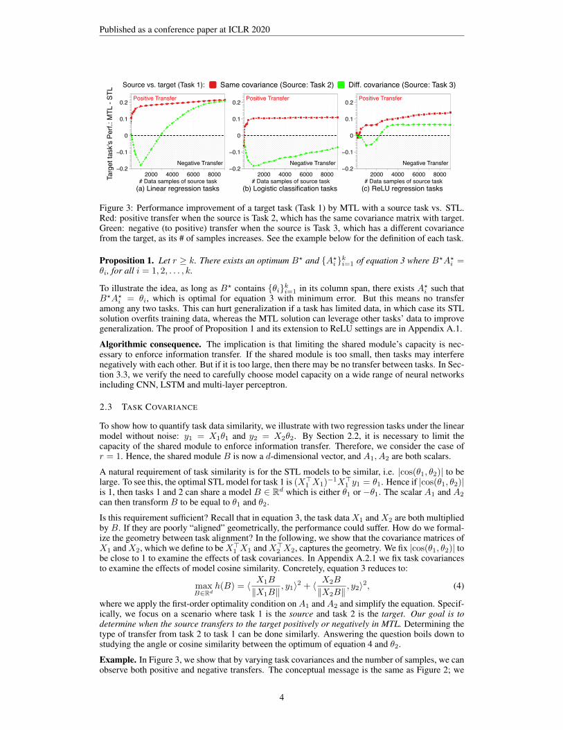
Figure 3: Performance improvement of a target task (Task 1) by MTL with a source task vs. STL.Red: positive transfer when the source is Task 2, which has the same covariance matrix with target.Green: negative (to positive) transfer when the source is Task 3, which has a different covariancefrom the target, as its # of samples increases. See the example below for the definition of each task.

Proposition 1. Let r ≥ k. There exists an optimum B? and {A?i }ki=1 of equation 3 where B?A?i =θi, for all i = 1, 2, . . . , k.

To illustrate the idea, as long as B? contains {θi}ki=1 in its column span, there exists A?i such thatB?A?i = θi, which is optimal for equation 3 with minimum error. But this means no transferamong any two tasks. This can hurt generalization if a task has limited data, in which case its STLsolution overfits training data, whereas the MTL solution can leverage other tasks’ data to improvegeneralization. The proof of Proposition 1 and its extension to ReLU settings are in Appendix A.1.

Algorithmic consequence. The implication is that limiting the shared module’s capacity is nec-essary to enforce information transfer. If the shared module is too small, then tasks may interferenegatively with each other. But if it is too large, then there may be no transfer between tasks. In Sec-tion 3.3, we verify the need to carefully choose model capacity on a wide range of neural networksincluding CNN, LSTM and multi-layer perceptron.

2.3 TASK COVARIANCE

To show how to quantify task data similarity, we illustrate with two regression tasks under the linearmodel without noise: y1 = X1θ1 and y2 = X2θ2. By Section 2.2, it is necessary to limit thecapacity of the shared module to enforce information transfer. Therefore, we consider the case ofr = 1. Hence, the shared module B is now a d-dimensional vector, and A1, A2 are both scalars.

A natural requirement of task similarity is for the STL models to be similar, i.e. |cos(θ1, θ2)| to belarge. To see this, the optimal STL model for task 1 is (X>1 X1)−1X>1 y1 = θ1. Hence if |cos(θ1, θ2)|is 1, then tasks 1 and 2 can share a model B ∈ Rd which is either θ1 or −θ1. The scalar A1 and A2

can then transform B to be equal to θ1 and θ2.

Is this requirement sufficient? Recall that in equation 3, the task data X1 and X2 are both multipliedby B. If they are poorly “aligned” geometrically, the performance could suffer. How do we formal-ize the geometry between task alignment? In the following, we show that the covariance matrices ofX1 andX2, which we define to beX>1 X1 andX>2 X2, captures the geometry. We fix |cos(θ1, θ2)| tobe close to 1 to examine the effects of task covariances. In Appendix A.2.1 we fix task covariancesto examine the effects of model cosine similarity. Concretely, equation 3 reduces to:

maxB∈Rd

h(B) = 〈 X1B

‖X1B‖, y1〉2 + 〈 X2B

‖X2B‖, y2〉2, (4)

where we apply the first-order optimality condition onA1 andA2 and simplify the equation. Specif-ically, we focus on a scenario where task 1 is the source and task 2 is the target. Our goal is todetermine when the source transfers to the target positively or negatively in MTL. Determining thetype of transfer from task 2 to task 1 can be done similarly. Answering the question boils down tostudying the angle or cosine similarity between the optimum of equation 4 and θ2.

Example. In Figure 3, we show that by varying task covariances and the number of samples, we canobserve both positive and negative transfers. The conceptual message is the same as Figure 2; we

4


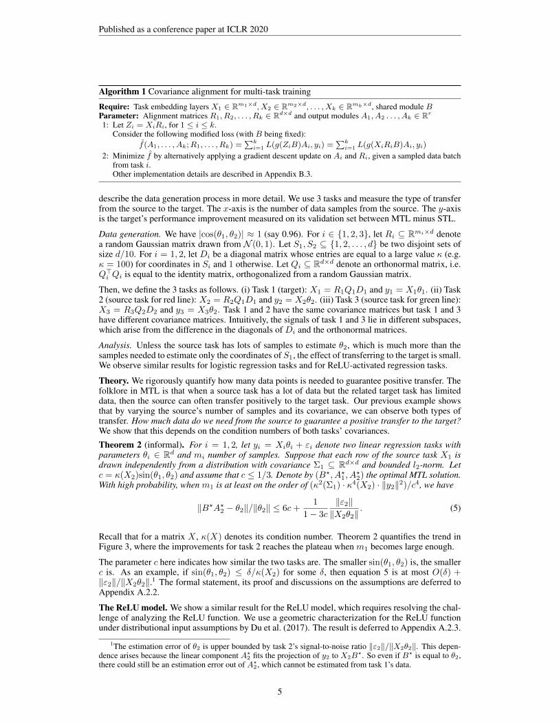
Algorithm 1 Covariance alignment for multi-task training

Require: Task embedding layers X1 ∈ Rm1×d, X2 ∈ Rm2×d, . . . , Xk ∈ Rmk×d, shared module BParameter: Alignment matrices R1, R2, . . . , Rk ∈ Rd×d and output modules A1, A2 . . . , Ak ∈ Rr

1: Let Zi = XiRi, for 1 ≤ i ≤ k.Consider the following modified loss (with B being fixed):

f(A1, . . . , Ak;R1, . . . , Rk) =∑k

i=1 L(g(ZiB)Ai, yi) =∑k

i=1 L(g(XiRiB)Ai, yi)

2: Minimize f by alternatively applying a gradient descent update on Ai and Ri, given a sampled data batchfrom task i.Other implementation details are described in Appendix B.3.

describe the data generation process in more detail. We use 3 tasks and measure the type of transferfrom the source to the target. The x-axis is the number of data samples from the source. The y-axisis the target’s performance improvement measured on its validation set between MTL minus STL.

Data generation. We have |cos(θ1, θ2)| ≈ 1 (say 0.96). For i ∈ {1, 2, 3}, let Ri ⊆ Rmi×d denotea random Gaussian matrix drawn from N (0, 1). Let S1, S2 ⊆ {1, 2, . . . , d} be two disjoint sets ofsize d/10. For i = 1, 2, let Di be a diagonal matrix whose entries are equal to a large value κ (e.g.κ = 100) for coordinates in Si and 1 otherwise. Let Qi ⊆ Rd×d denote an orthonormal matrix, i.e.Q>i Qi is equal to the identity matrix, orthogonalized from a random Gaussian matrix.

Then, we define the 3 tasks as follows. (i) Task 1 (target): X1 = R1Q1D1 and y1 = X1θ1. (ii) Task2 (source task for red line): X2 = R2Q1D1 and y2 = X2θ2. (iii) Task 3 (source task for green line):X3 = R3Q2D2 and y3 = X3θ2. Task 1 and 2 have the same covariance matrices but task 1 and 3have different covariance matrices. Intuitively, the signals of task 1 and 3 lie in different subspaces,which arise from the difference in the diagonals of Di and the orthonormal matrices.

Analysis. Unless the source task has lots of samples to estimate θ2, which is much more than thesamples needed to estimate only the coordinates of S1, the effect of transferring to the target is small.We observe similar results for logistic regression tasks and for ReLU-activated regression tasks.

Theory. We rigorously quantify how many data points is needed to guarantee positive transfer. Thefolklore in MTL is that when a source task has a lot of data but the related target task has limiteddata, then the source can often transfer positively to the target task. Our previous example showsthat by varying the source’s number of samples and its covariance, we can observe both types oftransfer. How much data do we need from the source to guarantee a positive transfer to the target?We show that this depends on the condition numbers of both tasks’ covariances.

Theorem 2 (informal). For i = 1, 2, let yi = Xiθi + εi denote two linear regression tasks withparameters θi ∈ Rd and mi number of samples. Suppose that each row of the source task X1 isdrawn independently from a distribution with covariance Σ1 ⊆ Rd×d and bounded l2-norm. Letc = κ(X2)sin(θ1, θ2) and assume that c ≤ 1/3. Denote by (B?, A?1, A

?2) the optimal MTL solution.

With high probability, when m1 is at least on the order of (κ2(Σ1) · κ4(X2) · ‖y2‖2)/c4, we have

‖B?A?2 − θ2‖/‖θ2‖ ≤ 6c+1

1− 3c

‖ε2‖‖X2θ2‖

. (5)

Recall that for a matrix X , κ(X) denotes its condition number. Theorem 2 quantifies the trend inFigure 3, where the improvements for task 2 reaches the plateau when m1 becomes large enough.

The parameter c here indicates how similar the two tasks are. The smaller sin(θ1, θ2) is, the smallerc is. As an example, if sin(θ1, θ2) ≤ δ/κ(X2) for some δ, then equation 5 is at most O(δ) +‖ε2‖/‖X2θ2‖.1 The formal statement, its proof and discussions on the assumptions are deferred toAppendix A.2.2.

The ReLU model. We show a similar result for the ReLU model, which requires resolving the chal-lenge of analyzing the ReLU function. We use a geometric characterization for the ReLU functionunder distributional input assumptions by Du et al. (2017). The result is deferred to Appendix A.2.3.

1The estimation error of θ2 is upper bounded by task 2’s signal-to-noise ratio ‖ε2‖/‖X2θ2‖. This depen-dence arises because the linear component A?

2 fits the projection of y2 to X2B?. So even if B? is equal to θ2,

there could still be an estimation error out of A?2, which cannot be estimated from task 1’s data.

5


Algorithm 2 An SVD-based task re-weighting scheme

Input: k tasks: (X, yi) ∈ (Rm×d,Rm); a rank parameter r ∈ {1, 2, . . . , k}Output: A weight vector: {α1, α2, . . . , αk}1: Let θi = X>yi.2: Ur, Dr, Vr = SVDr(θ1, θ2, . . . , θk), i.e. the best rank-r approximation to the θi’s.3: Let αi = ‖θ>i Ur‖, for i = 1, 2, . . . , k.

Algorithmic consequence. An implication of our theory is a covariance alignment method to im-prove multi-task training. For the i-th task, we add an alignment matrixRi before its inputXi passesthrough the shared module B. Algorithm 1 shows the procedure.

We also propose a metric called covariance similarity score to measure the similarity between twotasks. Given X1 ∈ Rm1×d and X2 ∈ Rm2×d, we measure their similarity in three steps: (a) Thecovariance matrix is X>1 X1. (b) Find the best rank-r1 approximation to be U1,r1D1,r1U

>1,r1 , where

r1 is chosen to contain 99% of the singular values. (c) Apply step (a),(b) to X2, compute the score:

Covariance similarity score :=‖(U1,r1D

1/21,r1

)>U2,r2D1/22,r2‖F

‖U1,r1D1/21,r1‖F· ‖U2,r2D

1/22,r2‖F

. (6)

The nice property of the score is that it is invariant to rotations of the columns of X1 and X2.

2.4 OPTIMIZATION SCHEME

Lastly, we consider the effect of re-weighting the tasks (or their losses in equation 2). When does re-weighting the tasks help? In this part, we show a use case for improving the robustness of multi-tasktraining in the presence of label noise. The settings involving label noise can arise when some tasksonly have weakly-supervised labels, which have been studied before in the literature (e.g. Mintzet al. (2009); Pentina and Lampert (2017)). We start by describing a motivating example.

Consider two tasks where task 1 is y1 = Xθ and task 2 is y2 = Xθ + ε2. If we train the twotasks together, the error ε2 will add noise to the trained model. However, by up weighting task 1,we reduce the noise from task 2 and get better performance. To rigorously study the effect of taskweights, we consider a setting where all the tasks have the same data but different labels. This settingarises for example in multi-label image tasks. We derive the optimal solution in the linear model.

Proposition 3. Let the shared module have capacity r ≤ k. Given k tasks with the same covariatesX ⊆ Rm×d but different labels {yi}ki=1. Let X be full rank and UDV > be its SVD. Let QrQ>r bethe best rank-r approximation to

∑ki=1 αiU

>yiy>i U . Let B? ⊆ Rd×r be an optimal solution for

the re-weighted loss. Then the column span of B? is equal to the column span of (X>X)−1V DQr.

We can also extend Proposition 3 to show that all local minima of equation 3 are global minima inthe linear setting. We leave the proof to Appendix A.3. We remark that this result does not extendto the non-linear ReLU setting and leave this for future work.

Based on Proposition 3, we provide a rigorous proof of the previous example. Suppose that X isfull rank, (X>X)†X[α1y1, α1y2]) = [α1θ, α2θ + α2(X>X)−1Xε2]. Hence, when we increaseα1, cos(B?, θ) increases closer to 1.

Algorithmic consequence. Inspired by our theory, we describe a re-weighting scheme in the pres-ence of label noise. We compute the per-task weights by computing the SVD over X>yi, for1 ≤ i ≤ k. The intuition is that if the label vector of a task yi is noisy, then the entropy of yi issmall. Therefore, we would like to design a procedure that removes the noise. The SVD proceduredoes this, where the weight of a task is calculated by its projection into the principal r directions.See Algorithm 2 for the description.

6


𝐴# 𝐴$ 𝐴% … 𝐴&'$ 𝐴&'# 𝐴&

Task Embeddings

Shared Modules (LSTM/BERT)

𝑅&𝐼# 𝑅$ 𝑅% … 𝑅&'$ 𝑅&'#

𝑋# 𝑋$ 𝑋% … 𝑋&'$ 𝑋&'# 𝑋&

𝐸,

𝑍,

Figure 4: Illustration of the covariance alignment module on task embeddings.

3 EXPERIMENTS

We describe connections between our theoretical results and practical problems of interest. We showthree claims on real world datasets. (i) The shared MTL module is best performing when its capacityis smaller than the total capacities of the single-task models. (ii) Our proposed covariance alignmentmethod improves multi-task training on a variety of settings including the GLUE benchmarks andsix sentiment analysis tasks. Our method can be naturally extended to transfer learning settings andwe validate this as well. (iii) Our SVD-based reweighed scheme is more robust than the standardunweighted scheme on multi-label image classification tasks in the presence of label noise.

3.1 EXPERIMENTAL SETUP

Datasets and models. We describe the datasets and models we use in the experiments.

GLUE: GLUE is a natural language understanding dataset including question answering, sentimentanalysis, text similarity and textual entailment problems. We choose BERTLARGE as our model,which is a 24 layer transformer network from Devlin et al. (2018). We use this dataset to evaluatehow Algorithm 1 works on the state-of-the-art BERT model.

Sentiment Analysis: This dataset includes six tasks: movie review sentiment (MR), sentence sub-jectivity (SUBJ), customer reviews polarity (CR), question type (TREC), opinion polarity (MPQA),and the Stanford sentiment treebank (SST) tasks.

For each task, the goal is to categorize sentiment opinions expressed in the text. We use an embed-ding layer (with GloVe embeddings2) followed by an LSTM layer proposed by Lei et al. (2018)3.

ChestX-ray14: This dataset contains 112,120 frontal-view X-ray images and each image has up to14 diseases. This is a 14-task multi-label image classification problem. We use the CheXNet modelfrom Rajpurkar et al. (2017), which is a 121-layer convolutional neural network on all tasks.

For all models, we share the main module across all tasks (BERTLARGE for GLUE, LSTM forsentiment analysis, CheXNet for ChestX-ray14) and assign a separate regression or classificationlayer on top of the shared module for each tasks.

Comparison methods. For the experiment on multi-task training, we compare Algorithm 1 bytraining with our method and training without it. Specifically, we apply the alignment procedure onthe task embedding layers. See Figure 4 for an illustration, where Ei denotes the embedding of taski, Ri denotes its alignment module and Zi = EiRi is the rotated embedding.

For transfer learning, we first train an STL model on the source task by tuning its model capacity(e.g. the output dimension of the LSTM layer). Then, we fine-tune the STL model on the targettask for 5-10 epochs. To apply Algorithm 1, we add an alignment module for the target task duringfine-tuning.

For the experiment on reweighted schemes, we compute the per-task weights as described in Algo-rithm 2. Then, we reweight the loss function as in equation 2. We compare with the reweightingtechniques of Kendall et al. (2018). Informally, the latter uses Gaussian likelihood to model classi-

2http://nlp.stanford.edu/data/wordvecs/glove.6B.zip3We also tested with multi-layer perceptron and CNN. The results are similar (cf. Appendix B.5).

7


−0.6

4.3

−2.4

1

−0.6

5.8

−1.9

2.7

4.3

5.8

0.1

0.7

−2.4

−1.9

0.1

1.1

1

2.7

0.7

1.1

SST

RTE

QNLI

MRPC

COLA

COLA MRPC QNLI RTE SST

(a) MTL on GLUE over 10 task pairs

BaselineCovariance Alignment

LSTM

Accu

racy

0.75

0.80

0.85

0.90

0.95

CR MPQA MR SUBJTREC

(b) Transfer learning on six sentiment analysis tasks

Figure 5: Performance improvements of Algorithm 1 by aligning task embeddings.

fication outputs. The weights, defined as inversely proportional to the variances of the Gaussian, areoptimized during training. We also compare with the unweighted loss (cf. equation 1) as a baseline.

Metric. We measure performance on the GLUE benchmark using a standard metric called theGLUE score, which contains accuracy and correlation scores for each task.

For the sentiment analysis tasks, we measure the accuracy of predicting the sentiment opinion.

For the image classification task, we measure the area under the curve (AUC) score. We run fivedifferent random seeds to report the average results. The result of an MTL experiment is averagedover the results of all the tasks, unless specified otherwise.

For the training procedures and other details on the setup, we refer the reader to Appendix B.

3.2 EXPERIMENTAL RESULTS

We present use cases of our methods on open-source datasets. We expected to see improvements viaour methods in multi-task and other settings, and indeed we saw such gains across a variety of tasks.

Improving multi-task training. We apply Algorithm 1 on five tasks (CoLA, MRPC, QNLI, RTE,SST-2) from the GLUE benchmark using a state-of-the-art language model BERTLARGE. 4 Wetrain the output layers {Ai} and the alignment layers {Ri} using our algorithm. We compare theaverage performance over all five tasks and find that our method outperforms BERTLARGE by 2.35%average GLUE score for the five tasks. For the particular setting of training two tasks, our methodoutperforms BERTLARGE on 7 of the 10 task pairs. See Figure 5a for the results.

Improving transfer learning. While our study has focused on multi-task learning, transfer learningis a naturally related goal – and we find that our method is also useful in this case. We validate thisby training an LSTM on sentiment analysis. Figure 5b shows the result with SST being the sourcetask and the rest being the target task. Algorithm 1 improves accuracy on four tasks by up to 2.5%.

Reweighting training for the same task covariates. We evaluate Algorithm 2 on the ChestX-ray14dataset. This setting satisfies the assumption of Algorithm 2, which requires different tasks to havethe same input data. Across all 14 tasks, we find that our reweighting method improves the techniqueof Kendall et al. (2018) by 0.1% AUC score. Compared to training with the unweighted loss, ourmethod improves performance by 0.4% AUC score over all tasks.

3.3 ABLATION STUDIES

Model capacity. We verify our hypothesis that the capacity of the MTL model should not exceed thetotal capacities of the STL model. We show this on an LSTM model with sentiment analysis tasks.Recall that the capacity of an LSTM model is its output dimension (before the last classificationlayer). We train an MTL model with all tasks and vary the shared module’s capacity to find theoptimum from 5 to 500. Similarly we train an STL model for each task and find the optimum.

In Figure 1, we find that the performance of MTL peaks when the shared module has capacity100. This is much smaller than the total capacities of all the STL models. The result confirms that

4https://github.com/google-research/bert

8


Table 1: Comparing the model capacity betweenMTL and STL.

Task STL MTL

Cap. Acc. Cap. Acc.

SST 200 82.3

100

90.8MR 200 76.4 96.0CR 5 73.2 78.7

SUBJ 200 91.5 89.5MPQA 500 86.7 87.0TREC 100 85.7 78.7

Overall 1205 82.6 100 85.1

Figure 6: Covariance similarity score vs.performance improvements from alignment.

TREC,SUBJCR,MRMPQA,SUBJCR, SUBJTREC,SST

LSTM Covariance Alignment

Baseline

Perfo

rman

ce Im

prov

emen

ts

0

0.02

0.04

Covariance similarity score0.1 0.2 0.3 0.4 0.5

constraining the shared module’s capacity is crucial to achieve the ideal performance. Extendedresults on CNN/MLP to support our hypothesis are shown in Appendix B.5.

Task covariance. We apply our metric of task covariance similarity score from Section 2.3 toprovide an in-depth study of the covariance alignment method. The hypothesis is that: (a) aligningthe covariances helps, which we have shown in Figure 5a; (b) the similarity score between two tasksincreases after applying the alignment. We verify the hypothesis on the sentiment analysis tasks. Weuse the single-task model’s embedding before the LSTM layer to compute the covariance.

First, we measure the similarity score using equation 6 between all six single-task models. Then,for each task pair, we train an MTL model using Algorithm 1. We measure the similarity score onthe trained MTL model. Our results confirm the hypothesis (Figure 6): (a) we observe increasedaccuracy on 13 of 15 task pairs by up to 4.1%; (b) the similarity score increases for all 15 task pairs.

Optimization scheme. We verify the robustness of Algorithm 2. After selecting two tasks from theChestX-ray14 dataset, we test our method by assigning random labels to 20% of the data on onetask. The labels for the other task remain unchanged.

On 10 randomly selected pairs, our method improves over the unweighted scheme by an average1.0% AUC score and the techniques of Kendall et al. (2018) by an average 0.4% AUC score. Weinclude more details of this experiment in Appendix B.5.

4 RELATED WORK

There has been a large body of recent work on using the multi-task learning approach to train deepneural networks. Liu et al. (2019a); McCann et al. (2018) and subsequent follow-up work showstate-of-the-art results on the GLUE benchmark, which inspired our study of an abstraction of theMTL model. Recent work of Zamir et al. (2018); Standley et al. (2019) answer which visual tasksto train together via a heuristic which involves intensive computation. We discuss several lines ofstudies related to this work. For complete references, we refer the interested readers to the survey ofRuder (2017); Zhang and Yang (2017) and the surveys on domain adaptation and transfer learningby Pan and Yang (2009); Kouw (2018) for references.

Theoretical studies of multi-task learning. Of particular relevance to this work are those thatstudy the theory of multi-task learning. The earlier works of Baxter (2000); Ben-David and Schuller(2003) are among the first to formally study the importance of task relatedness for learning multipletasks. See also the follow-up work of Maurer (2006) which studies generalization bounds of MTL.

A closely related line of work to structural learning is subspace selection, i.e. how to select acommon subspace for multiple tasks. Examples from this line work include Obozinski et al. (2010);Wang et al. (2015); Fernando et al. (2013); Elhamifar et al. (2015). Evgeniou and Pontil (2004);Micchelli and Pontil (2005) study a formulation that extends support vector machine to the multi-task setting. See also Argyriou et al. (2008); Pentina et al. (2015); Pentina and Ben-David (2015);Pentina and Lampert (2017) that provide more refined optimization methods and further study. Thework of Ben-David et al. (2010) provides theories to measure the differences between source andtarget tasks for transfer learning in a different model setup. Khodak et al. (2019); Kong et al. (2020);

9


Du et al. (2020) consider the related meta learning setting, which is in spirit an online setting ofmulti-task learning.

Our result on restricting the model capacities for multi-task learning is in contrast with recent the-oretical studies on over-parametrized models (e.g. Li et al. (2018); Zhang et al. (2019a); Bartlettet al. (2020)), where the model capacities are usually much larger than the regime we consider here.It would be interesting to better understand multi-task learning in the context of over-parametrizedmodels with respect to other phenomenon such as double descent that has been observed in othercontexts (Belkin et al. (2019)).

Finally, Zhang et al. (2019b); Shui et al. (2019) consider multi-task learning from the perspective ofadversarial robustness. Mahmud and Ray (2008) consider using Kolmogorov complexity measurethe effectiveness of transfer learning for decision tree methods.

Hard parameter sharing vs soft parameter sharing. The architecture that we study in this workis also known as the hard parameter sharing architecture. There is another kind of architecturecalled soft parameter sharing. The idea is that each task has its own parameters and modules. Therelationships between these parameters are regularized in order to encourage the parameters to besimilar. Other architectures that have been studied before include the work of Misra et al. (2016),where the authors explore trainable architectures for convolutional neural networks.

Domain adaptation. Another closely related line of work is on domain adaptation. The acutereader may notice the similarity between our study in Section 2.3 and domain adaptation. The cru-cial difference here is that we are minimizing the multi-task learning objective, whereas in domainadaptation the objective is typically to minimize the objective on the target task. See Ben-Davidet al. (2010); Zhang et al. (2019b) and the references therein for other related work.

Optimization techniques. Guo et al. (2019) use ideas from the multi-armed bandit literature to de-velop a method for weighting each task. Compared to their method, our SVD-based method is con-ceptually simpler and requires much less computation. Kendall et al. (2018) derive a weighted lossschme by maximizing a Gaussian likelihood function. Roughly speaking, each task is reweightedby 1/σ2 where σ is the standard deviation of the Gaussian and a penalty of log σ is added to theloss. The values of {σi}i are also optimized during training. The exact details can be found in thepaper. The very recent work of Li and Vasconcelos (2019) show empirical results using a similaridea of covariance normalization on imaging tasks for cross-domain transfer.

5 CONCLUSIONS AND FUTURE WORK

We studied the theory of multi-task learning in linear and ReLU-activated settings. We verified ourtheory and its practical implications through extensive synthetic and real world experiments.

Our work opens up many interesting future questions. First, could we extend the guarantees forchoosing optimization schemes to non-linear settings? Second, a limitation of our SVD-based op-timization scheduler is that it only applies to settings with the same data. Could we extend themethod for heterogeneous task data? More broadly, we hope our work inspires further studies tobetter understand multi-task learning in neural networks and to guide its practice.

Acknowledgements. Thanks to Sharon Y. Li and Avner May for stimulating discussions dur-ing early stages of this work. We are grateful to the Stanford StatsML group and the anony-mous referees for providing helpful comments that improve the quality of this work. We grate-fully acknowledge the support of DARPA under Nos. FA87501720095 (D3M), FA86501827865(SDH), and FA86501827882 (ASED); NIH under No. U54EB020405 (Mobilize), NSF under Nos.CCF1763315 (Beyond Sparsity), CCF1563078 (Volume to Velocity), and 1937301 (RTML); ONRunder No. N000141712266 (Unifying Weak Supervision); the Moore Foundation, NXP, Xilinx,LETI-CEA, Intel, IBM, Microsoft, NEC, Toshiba, TSMC, ARM, Hitachi, BASF, Accenture, Er-icsson, Qualcomm, Analog Devices, the Okawa Foundation, American Family Insurance, GoogleCloud, Swiss Re, and members of the Stanford DAWN project: Teradata, Facebook, Google, Ant Fi-nancial, NEC, VMWare, and Infosys. H. Zhang is supported in part by Gregory Valiant’s ONR YIPaward (#1704417). The experiments are partly run on Stanford’s SOAL cluster. 5 The U.S. Govern-ment is authorized to reproduce and distribute reprints for Governmental purposes notwithstanding

5https://5harad.com/soal-cluster/

10


any copyright notation thereon. Any opinions, findings, and conclusions or recommendations ex-pressed in this material are those of the authors and do not necessarily reflect the views, policies, orendorsements, either expressed or implied, of DARPA, NIH, ONR, or the U.S. Government.

REFERENCES

Hector Martınez Alonso and Barbara Plank. When is multitask learning effective? semantic se-quence prediction under varying data conditions. arXiv preprint arXiv:1612.02251, 2016.

Rie Kubota Ando and Tong Zhang. A framework for learning predictive structures from multipletasks and unlabeled data. Journal of Machine Learning Research, 6(Nov):1817–1853, 2005.

Andreas Argyriou, Andreas Maurer, and Massimiliano Pontil. An algorithm for transfer learning in aheterogeneous environment. In Joint European Conference on Machine Learning and KnowledgeDiscovery in Databases, pages 71–85. Springer, 2008.

Maria-Florina Balcan, Yingyu Liang, David P Woodruff, and Hongyang Zhang. Matrix completionand related problems via strong duality. In 9th Innovations in Theoretical Computer ScienceConference (ITCS 2018), 2018.

Peter L Bartlett, Philip M Long, Gabor Lugosi, and Alexander Tsigler. Benign overfitting in linearregression. Proceedings of the National Academy of Sciences, 2020.

Jonathan Baxter. A model of inductive bias learning. Journal of artificial intelligence research, 12:149–198, 2000.

Mikhail Belkin, Daniel Hsu, Siyuan Ma, and Soumik Mandal. Reconciling modern machine-learning practice and the classical bias–variance trade-off. Proceedings of the National Academyof Sciences, 116(32):15849–15854, 2019.

Shai Ben-David and Reba Schuller. Exploiting task relatedness for multiple task learning. In Learn-ing Theory and Kernel Machines, pages 567–580. Springer, 2003.

Shai Ben-David, John Blitzer, Koby Crammer, Alex Kulesza, Fernando Pereira, and Jennifer Wort-man Vaughan. A theory of learning from different domains. Machine learning, 79(1-2):151–175,2010.

Joachim Bingel and Anders Søgaard. Identifying beneficial task relations for multi-task learning indeep neural networks. arXiv preprint arXiv:1702.08303, 2017.

John Blitzer, Ryan McDonald, and Fernando Pereira. Domain adaptation with structural correspon-dence learning. In Proceedings of the 2006 conference on empirical methods in natural languageprocessing, pages 120–128. Association for Computational Linguistics, 2006.

Jacob Devlin, Ming-Wei Chang, Kenton Lee, and Kristina Toutanova. Bert: Pre-training of deepbidirectional transformers for language understanding. arXiv preprint arXiv:1810.04805, 2018.

Simon S Du, Jason D Lee, Yuandong Tian, Barnabas Poczos, and Aarti Singh. Gradient de-scent learns one-hidden-layer cnn: Don’t be afraid of spurious local minima. arXiv preprintarXiv:1712.00779, 2017.

Simon S Du, Wei Hu, Sham M Kakade, Jason D Lee, and Qi Lei. Few-shot learning via learningthe representation, provably. arXiv preprint arXiv:2002.09434, 2020.

Ehsan Elhamifar, Guillermo Sapiro, and S Shankar Sastry. Dissimilarity-based sparse subset selec-tion. IEEE transactions on pattern analysis and machine intelligence, 38(11):2182–2197, 2015.

Theodoros Evgeniou and Massimiliano Pontil. Regularized multi-task learning. In Proceedingsof the tenth ACM SIGKDD international conference on Knowledge discovery and data mining,pages 109–117. ACM, 2004.

Basura Fernando, Amaury Habrard, Marc Sebban, and Tinne Tuytelaars. Unsupervised visual do-main adaptation using subspace alignment. In Proceedings of the IEEE international conferenceon computer vision, pages 2960–2967, 2013.

11


Han Guo, Ramakanth Pasunuru, and Mohit Bansal. Autosem: Automatic task selection and mixingin multi-task learning. arXiv preprint arXiv:1904.04153, 2019.

Trevor Hastie, Robert Tibshirani, Jerome Friedman, and James Franklin. The elements of statisticallearning: data mining, inference and prediction. The Mathematical Intelligencer, 27(2):83–85,2005.

Minqing Hu and Bing Liu. Mining and summarizing customer reviews. In Proceedings of thetenth ACM SIGKDD international conference on Knowledge discovery and data mining, pages168–177. ACM, 2004.

Alex Kendall, Yarin Gal, and Roberto Cipolla. Multi-task learning using uncertainty to weigh lossesfor scene geometry and semantics. In Proceedings of the IEEE Conference on Computer Visionand Pattern Recognition, pages 7482–7491, 2018.

Mikhail Khodak, Maria-Florina Balcan, and Ameet Talwalkar. Provable guarantees for gradient-based meta-learning. arXiv preprint arXiv:1902.10644, 2019.

Yoon Kim. Convolutional neural networks for sentence classification. arXiv preprintarXiv:1408.5882, 2014.

Iasonas Kokkinos. Ubernet: Training a universal convolutional neural network for low-, mid-, andhigh-level vision using diverse datasets and limited memory. In Proceedings of the IEEE Confer-ence on Computer Vision and Pattern Recognition, pages 6129–6138, 2017.

Weihao Kong, Raghav Somani, Zhao Song, Sham Kakade, and Sewoong Oh. Meta-learning formixed linear regression. arXiv preprint arXiv:2002.08936, 2020.

Wouter M Kouw. An introduction to domain adaptation and transfer learning. arXiv preprintarXiv:1812.11806, 2018.

Tao Lei, Yu Zhang, Sida I Wang, Hui Dai, and Yoav Artzi. Simple recurrent units for highly par-allelizable recurrence. In Proceedings of the 2018 Conference on Empirical Methods in NaturalLanguage Processing, pages 4470–4481, 2018.

Xin Li and Dan Roth. Learning question classifiers. In Proceedings of the 19th internationalconference on Computational linguistics-Volume 1, pages 1–7. Association for ComputationalLinguistics, 2002.

Yuanzhi Li, Tengyu Ma, and Hongyang Zhang. Algorithmic regularization in over-parameterizedmatrix sensing and neural networks with quadratic activations. In Conference On Learning The-ory, pages 2–47, 2018.

Yunsheng Li and Nuno Vasconcelos. Efficient multi-domain learning by covariance normaliza-tion. In Proceedings of the IEEE Conference on Computer Vision and Pattern Recognition, pages5424–5433, 2019.

Xiaodong Liu, Pengcheng He, Weizhu Chen, and Jianfeng Gao. Multi-task deep neural networksfor natural language understanding. arXiv preprint arXiv:1901.11504, 2019a.

Yinhan Liu, Myle Ott, Naman Goyal, Jingfei Du, Mandar Joshi, Danqi Chen, Omer Levy, MikeLewis, Luke Zettlemoyer, and Veselin Stoyanov. Roberta: A robustly optimized bert pretrainingapproach. arXiv preprint arXiv:1907.11692, 2019b.

MM Mahmud and Sylvian Ray. Transfer learning using kolmogorov complexity: Basic theory andempirical evaluations. In Advances in neural information processing systems, pages 985–992,2008.

Pasin Manurangsi and Daniel Reichman. The computational complexity of training relu (s). arXivpreprint arXiv:1810.04207, 2018.

Andreas Maurer. Bounds for linear multi-task learning. Journal of Machine Learning Research, 7(Jan):117–139, 2006.

12


Bryan McCann, Nitish Shirish Keskar, Caiming Xiong, and Richard Socher. The natural languagedecathlon: Multitask learning as question answering. arXiv preprint arXiv:1806.08730, 2018.

Charles A Micchelli and Massimiliano Pontil. Kernels for multi–task learning. In Advances inneural information processing systems, pages 921–928, 2005.

Mike Mintz, Steven Bills, Rion Snow, and Dan Jurafsky. Distant supervision for relation extractionwithout labeled data. In Proceedings of the Joint Conference of the 47th Annual Meeting of theACL and the 4th International Joint Conference on Natural Language Processing of the AFNLP:Volume 2-Volume 2, pages 1003–1011. Association for Computational Linguistics, 2009.

Ishan Misra, Abhinav Shrivastava, Abhinav Gupta, and Martial Hebert. Cross-stitch networks formulti-task learning. In Proceedings of the IEEE Conference on Computer Vision and PatternRecognition, pages 3994–4003, 2016.

Guillaume Obozinski, Ben Taskar, and Michael I Jordan. Joint covariate selection and joint subspaceselection for multiple classification problems. Statistics and Computing, 20(2):231–252, 2010.

Sinno Jialin Pan and Qiang Yang. A survey on transfer learning. IEEE Transactions on knowledgeand data engineering, 22(10):1345–1359, 2009.

Bo Pang and Lillian Lee. A sentimental education: Sentiment analysis using subjectivity summa-rization based on minimum cuts. In Proceedings of the 42nd annual meeting on Association forComputational Linguistics, page 271. Association for Computational Linguistics, 2004.

Bo Pang and Lillian Lee. Seeing stars: Exploiting class relationships for sentiment categorizationwith respect to rating scales. In Proceedings of the 43rd annual meeting on association for com-putational linguistics, pages 115–124. Association for Computational Linguistics, 2005.

Anastasia Pentina and Shai Ben-David. Multi-task and lifelong learning of kernels. In InternationalConference on Algorithmic Learning Theory, pages 194–208. Springer, 2015.

Anastasia Pentina and Christoph H Lampert. Multi-task learning with labeled and unlabeled tasks.In Proceedings of the 34th International Conference on Machine Learning-Volume 70, pages2807–2816. JMLR. org, 2017.

Anastasia Pentina, Viktoriia Sharmanska, and Christoph H Lampert. Curriculum learning of multi-ple tasks. In Proceedings of the IEEE Conference on Computer Vision and Pattern Recognition,pages 5492–5500, 2015.

Pranav Rajpurkar, Jeremy Irvin, Kaylie Zhu, Brandon Yang, Hershel Mehta, Tony Duan, DaisyDing, Aarti Bagul, Curtis Langlotz, Katie Shpanskaya, et al. Chexnet: Radiologist-level pneumo-nia detection on chest x-rays with deep learning. arXiv preprint arXiv:1711.05225, 2017.

Sebastian Ruder. An overview of multi-task learning in deep neural networks. arXiv preprintarXiv:1706.05098, 2017.

Changjian Shui, Mahdieh Abbasi, Louis-Emile Robitaille, Boyu Wang, and Christian Gagne.A principled approach for learning task similarity in multitask learning. arXiv preprintarXiv:1903.09109, 2019.

Richard Socher, Alex Perelygin, Jean Wu, Jason Chuang, Christopher D Manning, Andrew Ng,and Christopher Potts. Recursive deep models for semantic compositionality over a sentimenttreebank. In Proceedings of the 2013 conference on empirical methods in natural language pro-cessing, pages 1631–1642, 2013.

Trevor Standley, Amir R Zamir, Dawn Chen, Leonidas Guibas, Jitendra Malik, and Silvio Savarese.Which tasks should be learned together in multi-task learning? arXiv preprint arXiv:1905.07553,2019.

Joel A Tropp et al. An introduction to matrix concentration inequalities. Foundations and Trends R©in Machine Learning, 8(1-2):1–230, 2015.

13


Alex Wang, Amanpreet Singh, Julian Michael, Felix Hill, Omer Levy, and Samuel Bowman. Glue:A multi-task benchmark and analysis platform for natural language understanding. In Proceedingsof the 2018 EMNLP Workshop BlackboxNLP: Analyzing and Interpreting Neural Networks forNLP, pages 353–355, 2018a.

Alex Wang, Amanpreet Singh, Julian Michael, Felix Hill, Omer Levy, and Samuel R Bowman.Glue: A multi-task benchmark and analysis platform for natural language understanding. arXivpreprint arXiv:1804.07461, 2018b.

Xiaosong Wang, Yifan Peng, Le Lu, Zhiyong Lu, Mohammadhadi Bagheri, and Ronald M Sum-mers. Chestx-ray8: Hospital-scale chest x-ray database and benchmarks on weakly-supervisedclassification and localization of common thorax diseases. In Proceedings of the IEEE conferenceon computer vision and pattern recognition, pages 2097–2106, 2017.

Yu Wang, David Wipf, Qing Ling, Wei Chen, and Ian James Wassell. Multi-task learning forsubspace segmentation. 2015.

Janyce Wiebe, Theresa Wilson, and Claire Cardie. Annotating expressions of opinions and emotionsin language. Language resources and evaluation, 39(2-3):165–210, 2005.

Ya Xue, Xuejun Liao, Lawrence Carin, and Balaji Krishnapuram. Multi-task learning for classifica-tion with dirichlet process priors. Journal of Machine Learning Research, 8(Jan):35–63, 2007.

Amir R Zamir, Alexander Sax, William Shen, Leonidas J Guibas, Jitendra Malik, and SilvioSavarese. Taskonomy: Disentangling task transfer learning. In Proceedings of the IEEE Con-ference on Computer Vision and Pattern Recognition, pages 3712–3722, 2018.

Hongyang Zhang, Vatsal Sharan, Moses Charikar, and Yingyu Liang. Recovery guarantees forquadratic tensors with limited observations. In International Conference on Artificial Intelligenceand Statistics (AISTATS), 2019a.

Yu Zhang and Qiang Yang. A survey on multi-task learning. arXiv preprint arXiv:1707.08114,2017.

Yu Zhang and Dit-Yan Yeung. A regularization approach to learning task relationships in multitasklearning. ACM Transactions on Knowledge Discovery from Data (TKDD), 8(3):12, 2014.

Yuchen Zhang, Tianle Liu, Mingsheng Long, and Michael I Jordan. Bridging theory and algorithmfor domain adaptation. arXiv preprint arXiv:1904.05801, 2019b.

14


A MISSING DETAILS OF SECTION 2

We fill in the missing details left from Section 2. In Section A.1, we provide rigorous argumentsregarding the capacity of the shared module. In Section A.2, we fill in the details left from Section2.3, including the proof of Theorem 2 and its extension to the ReLU model. In Section A.3, weprovide the proof of Proposition 3 on the task reweighting schemes. We first describe the notations.

Notations. We define the notations to be used later on. We denote f(x) . g(x) if there exists anabsolute constant C such that f(x) ≤ Cg(x). The big-O notation f(x) = O(g(x)) means thatf(x) . g(x).

Suppose A ∈ Rm×n, then λmax(A) denotes its largest singular value and λmin(A) denotes itsmin{m,n}-th largest singular value. Alternatively, we have λmin(A) = minx:‖x‖=1 ‖Ax‖. Letκ(A) = λmax(A)/λmin(A) denote the condition number of A. Let Id denotes the identity matrix.Let U† denote the Moore-Penrose pseudo-inverse of the matrix U . Let ‖ · ‖ denote the Euclideannorm for vectors and spectral norm for matrices. Let ‖ · ‖F denote the Frobenius norm of a matrix.Let 〈A,B,=〉Tr(A>B) denote the inner product of two matrices.

The sine function is define as sin(u, v) =√

1− cos(u, v)2, where we assume that sin(u, v) ≥ 0which is without loss of generality for our study.

A.1 MISSING DETAILS OF SECTION 2.2

We describe the full detail to show that our model setup captures the phenomenon that the sharedmodule should be smaller than the sum of capacities of the single-task models. We state the fol-lowing proposition which shows that the quality of the subspace B in equation 1 determines theperformance of multi-task learning. This supplements the result of Proposition 1.Proposition 4. In the optimum of f(·) (equation 1), each Ai selects the vector v within the columnspan of gB(Xi) to minimize L(v, yi). As a corollary, in the linear setting, the optimal B can beachieved at a rotation matrix B? ⊆ Rd×r by maximizing

k∑i=1

〈B(B>X>i XiB)†B>, X>i yiy>i Xi〉. (7)

Furthermore, any B? which contains {θi}ki=1 in its column subspace is optimal. In particular, forsuch a B?, there exists {A?i } so that B?A?i = θi for all 1 ≤ i ≤ k.

Proof. Recall the MTL objective in the linear setting from equation 3 as follows:

min f(A1, A2, . . . , Ak;B) =

k∑i=1

(XiBAi − yi)2 ,

Note that the linear layer Ai can pick any combination within the subspace of B. Therefore, wecould assume without loss of generality that B is a rotation matrix. i.e. B>B = Id. After fixing B,since objective f(·) is linear in Ai for all i, by the local optimality condition, we obtain that

Ai = (B>X>i XiB)†B>X>i yi

Replacing the solution of Ai to f(·), we obtain an objective over B.

h(B) =

k∑i=1

‖XiB(B>X>i XiB)†B>X>i yi − yi‖2F .

Next, note that

‖XiB(B>X>i XiB)†B>X>i yi‖2F = Tr(y>i XiB(B>X>i XiB)†B>X>i yi)

= 〈B(B>X>i XiB)B>, X>i yiy>i Xi〉,

where we used the fact thatA†AA† = A† forA = B>X>i XiB in the first equation. Hence we haveshown equation 7.

15


For the final claim, as long as B? contains {θi}ki=1 in its column subspace, then there exists A?i suchthat B?A?i = θi. The B? and {A?i }ki=1 are optimal solutions because each θi is an optimal solutionfor the single-task problem.

The above result on linear regression suggests the intuition that optimizing an MTL model reducesto optimizing over the span of B. The intuition can be easily extended to linear classification tasksas well as mixtures of regression and classification tasks.

Extension to the ReLU setting. If the shared module’s capacity is larger than the total capacitiesof the STL models, then we can put all the STL model parameters into the shared module. As inthe linear setting, the final output layer Ai can pick out the optimal parameter for the i-th task. Thisremains an optimal solution to the MTL problem in the ReLU setting. Furthermore, there is notransfer between any two tasks through the shared module.

A.2 MISSING DETAILS OF SECTION 2.3

A.2.1 THE EFFECT OF COSINE SIMILARITY

We consider the effect of varying the cosine similarity between single task models in multi-tasklearning. We first describe the following proposition to solve the multi-task learning objective whenthe covariances of the task data are the same. The idea is similar to the work of Ando and Zhang(2005) and we adapt it here for our study.Proposition 5. Consider the reweighted loss of equation 2 with the encoding function being linear,where the weights are {αi}ki=1. Suppose the task features of every task have the same covariance:X>i Xi = Σ for all 1 ≤ i ≤ k. Let Σ = V DV > be the singular vector decomposition (SVD) of Σ.Then the optimum of f(·) in equation 3 is achieved at:

B? = V D−1/2C?,

where C?C?> is the best rank-r approximation subspace of∑ki=1 αiU

>i yiy

>i Ui andXi = UiDV

>

is the SVD of Xi, for each 1 ≤ i ≤ k.

As a corollary, denote by λ1, λ2, . . . , λk as the singular values of D−1V >∑ki=1 αiX

>i yiy

>i Xi in

decreasing order. Then the difference between an MTL model with hidden dimension r and the allthe single task models is bounded by

∑ki=r+1 λ

2i .

Proof. Note that B? is obtained by maximizing

k∑i=1

〈B(B>X>i XiB)−1B>, αiX>i yiy

>i Xi〉

Let C = DV >B. Clearly, there is a one to one mapping between B and C. And we have B =V D−1C. Hence the above is equivalent to maximizing over C ⊆ Rd×r with

k∑i=1

〈C(C>C)−1C>, D−1V >

(k∑i=1

αiX>i yiy

>i Xi

)V D−1〉

=〈C(C>C)−1C>,

k∑i=1

αiU>i yiy

>i Ui〉.

Note that C(C>C)−1C> is a projection matrix onto a subspace of dimension r. Hencethe maximum (denote by C?) is attained at the best rank-r approximation subspace of∑ki=1 αiU

>i yiy

>i Ui.

To illustrate the above proposition, consider a simple setting where Xi is identity for every 1 ≤i ≤ k, and yi = ei, i.e. the i-th basis vector. Note that the optimal solution for the i-th task is(X>i Xi)

−1X>i yi = yi. Hence the optimal solutions are orthogonal to each other for all the tasks,with λi = 1 for all 1 ≤ i ≤ k. And the minimum STL error is zero for all tasks.

16


Consider the MTL model with hidden dimension r. By Proposition 5, the minimum MTL error isachieved by the best rank-r approximation subspace to

∑ki=1X

>i yiy

>i Xi =

∑ki=1 yiy

>i . Denote

the optimum as B?r . The MTL error is:

k∑i=1

‖yi‖2 − 〈k∑i=1

yiy>i , B

?rB

?r>〉 = k − r.

Different data covariance. We provide upper bounds on the quality of MTL solutions for differentdata covariance, which depend on the relatedness of all the tasks. The following procedure gives theprecise statement. Consider k regression tasks with data {(Xi, yi)}ki=1. Let θi = (X>i Xi)

†X>i yidenote the optimal solution of each regression task. Let W ⊆ Rd×k denote the matrix where thei-th column is equal to θi. Consider the following procedure for orthogonalizing W for 1 ≤ i ≤ k.

a) Let W ?i ∈ Rd denote the vector which maximizes

∑ki=1〈

XiB‖XiB‖ , yi〉

2 over B ∈ Rd;

b) Denote by λj =∑kj=1〈

XjW?j

‖XjW?j ‖, yj〉2;

c) For each 1 ≤ i ≤ k, project XiW?i off from every column of Xi. Go to Step a).

Proposition 6. Suppose that r ≤ d. Let B? denote the optimal MTL solution of capacity r inthe shared module. Denote by OPT =

∑ki=1(‖yi‖2 − ‖Xi(X

>i Xi)

†X>i yi‖2). Then h(B?) ≤OPT −

∑di=r+1 λi.

Proof. It suffices to show that OPT is equal to∑ki=1 λi. The result then follows since h(B?) is

less than the error given by W ?1 , . . . ,W

?k , which is equal to OPT −

∑di=r+1 λi.

A.2.2 PROOF OF THEOREM 2

We fill in the proof of Theorem 2. First, we restate the result rigorously as follows.

Theorem 2. For i = 1, 2, let (Xi, yi) ∈ (Rmi×d,Rmi) denote two linear regression tasks withparameters θi ∈ Rd. Suppose that each row of X1 is drawn independently from a distribution withcovariance Σ1 ⊆ Rd×d and bounded l2-norm

√L. Assume that θ>1 Σ1θ1 = 1 w.l.o.g.

Let c ∈ [κ(X2) sin(θ1, θ2), 1/3] denote the desired error margin. Denote by (B?, A?1, A?2) the

optimal MTL solution. With probability 1− δ over the randomness of (X1, y1), when

m1 & max

(L‖Σ1‖ log d

δ

λ2min(Σ1),κ(Σ1)κ2(X2)

c2‖y2‖2,

κ2(Σ1)κ4(X2)

c4σ21 log

1

δ

),

we have that ‖B?A?2 − θ2‖/‖θ2‖ ≤ 6c+ 11−3c‖ε2‖/‖X2θ2‖.

We make several remarks to provide more insight on Theorem 2.

• Theorem 2 guarantees positive transfers in MTL, when the source and target models areclose and the number of source samples is large. While the intuition is folklore in MTL, weprovide a formal justification in the linear and ReLU models to quantify the phenomenon.

• The error bound decreases with c, hence the smaller c is the better. On the other hand, therequired number of data points m1 increases. Hence there is a trade-off between accuracyand the amount of data.

• c is assumed to be at most 1/3. This assumption arises when we deal with the label noiseof task 2. If there is no noise for task 2, then this assumption is not needed. If there isnoise for task 2, this assumption is satisfied when sin(θ1, θ2) is less than 1/(3κ(X2)). Insynthetic experiments, we observe that the dependence on κ(X2) and sin(θ1, θ2) both arisein the performance of task 2, cf. Figure 3 and Figure 7, respectively.

The proof of Theorem 2 consists of two steps.

17


a) We show that the angle between B? and θ1 will be small. Once this is established, we geta bound on the angle between B? and θ2 via the triangle inequality.

b) We bound the distance between B?A2 and θ2. The distance consists of two parts. One partcomes from B?, i.e. the angle between B? and θ2. The second part comes from A2, i.e.the estimation error of the norm of θ2, which involves the signal to noise ratio of task two.

We first show the following geometric fact, which will be used later in the proof.

Fact 7. Let a, b ∈ Rd denote two unit vectors. Suppose that X ∈ Rm×d has full column rank withcondition number denoted by κ = κ(X). Then we have

|sin(Xa,Xb)| ≥ 1

κ2|sin(a, b)| .

Proof. Let X = UDV > be the SVD of X . Since X has full column rank by assumption, we haveX>X = XX> = Id. Clearly, we have sin(Xa,Xb) = sin(DV >a,DV >b). Denote by a′ = V >aand b′ = V >b. We also have that a′ and b′ are both unit vectors, and sin(a′, b′) = sin(a, b). Letλ1, . . . , λd denote the singular values of X . Then,

sin2(Da′, Db′) = 1−

(∑di=1 λ

2i a′ib′i

)2(∑di=1 λ

2i a′i2)(∑d

i=1 λ2i b′i2)

=

∑1≤i,j≤d λ

2iλ

2j (a′ib′j − a′jb′i)2(∑d

i=1 λ2i a′i2)(∑d

i=1 λ2jb′i2)

≥ λ4min

λ4max

·∑

1≤i,j≤d

(a′ib′j − a′jb′i)2

=1

κ4((

d∑i=1

a′i2)(

d∑i=1

b′i2)− (

d∑i=1

a′ib′i)

2) =1

κ4sin2(a′, b′).

This concludes the proof.

We first show the following Lemma, which bounds the angle between B? and θ2.

Lemma 8. In the setting of Theorem 2, with probability 1− δ over the randomness of task one, wehave that

|sin(B?, θ2)| ≤ sin(θ1, θ2) + c/κ(X2).

Proof. We note that h(B?) ≥ ‖y1‖2 by the optimality of B?. Furthermore, 〈 X2B?

‖X2B?‖ , y2〉 ≤ ‖y2‖2.

Hence we obtain that

〈 X1B?

‖X1B?‖, y1〉2 ≥ ‖y1‖2 − ‖y2‖2.

For the left hand side,

〈 X1B?

‖X1B?‖, y1〉2 = 〈 X1B

?

‖X1B?‖, X1θ1 + ε1〉2

= 〈 X1B?

‖X1B?‖, X1θ1〉2 + 〈 X1B

?

‖X1B?‖, ε1〉2 + 2〈 X1B

?

‖X1B?‖, X1θ1〉〈

X1B?

‖X1B?‖, ε1〉

Note that the second term is a chi-squared random variable with expectation σ21 . Hence it is

bounded by σ21

√log 1

δ with probability at least 1 − δ. Similarly, the third term is bounded by

2‖X1θ1‖σ1√

log 1δ with probability 1− δ. Therefore, we obtain the following:

‖X1θ1‖2 cos2(X1B?, X1θ1) ≥ ‖y1‖2 − ‖y2‖2 − (σ2

1 + 2σ1‖X1θ1‖)√

log1

δ

18


Note that

‖y1‖2 ≥ ‖X1θ1‖2 + 2〈X1θ1, ε1〉

≥ ‖X1θ1‖2 − 2‖X1θ1‖σ1

√log

1

δ.

Therefore,

‖X1θ1‖2 cos2(X1B?, X1θ1) ≥ ‖X1θ1‖2 − ‖y2‖2 − (σ2

1 + 3σ1‖X1θ1‖)√log

1

δ

⇒ sin2(X1B?, X1θ1) ≤ ‖y2‖2

‖X1θ1‖2+

4σ1

√log 1

δ

‖X1θ1‖

⇒ sin2(B?, θ1) ≤ κ2(X1)

‖y2‖2

‖X1θ1‖2+

4σ1

√log 1

δ

‖X1θ1‖

(by Lemma 7)

By matrix Bernstein inequality (see e.g. Tropp et al. (2015)), when m1 ≥ 10‖Σ1‖ log dδ /λ

2min(Σ1),

we have that: ∥∥∥∥ 1

m1X>1 X1 − Σ1

∥∥∥∥ ≤ 1

2λmin(Σ1).

Hence we obtain that κ2(X1) ≤ 3κ(Σ1) and ‖X1θ1‖2 ≥ m1 · θ>1 Σ1θ1/2 ≥ m1/2 (where weassumed that θ>1 Σ1θ1 = 1). Therefore,

sin2(B?, θ1) ≤ 3κ(Σ1)

‖y2‖2m2

1/4+

4σ1

√log 1

δ√m1/2

,

which is at most c2/κ2(X2) by our setting of m1. Therefore, the conclusion follows by triangleinequality (noting that both c and sin(θ1, θ2) are less than 1/2).

Based on the above Lemma, we are now to ready to prove Theorem 2.

Proof of Theorem 2. Note that in the MTL model, after obtaining B?, we then solve the linear layerfor each task. For task 2, this gives weight value A?2 := 〈X2θ, y2〉/‖X2θ‖2. Thus the regressioncoefficients for task 2 isB?A?2. For the rest of the proof, we focus on bounding the distance betweenB?A?2 and θ2. By triangle inequality,

‖B?A?2 − θ2‖ ≤|〈X2B

?, ε2〉|‖X2B?‖2

+

∣∣∣∣ 〈X2B?, X2θ2〉

‖X2B?‖2− ‖θ2‖

∣∣∣∣+ ‖B?‖θ2‖ − θ2‖ . (8)

Note that the second term of equation 8 is equal to

|〈X2B?, X2(θ2 − ‖θ2‖B?)〉|‖X2B?‖2

≤ κ(X2) · ‖θ2 − ‖θ2‖B?‖.

The first term of equation 8 is bounded by

‖ε2‖‖X2B?‖

≤ ‖ε2‖‖θ2‖‖X2θ2‖ − ‖X2(θ2 − ‖θ2‖B?)‖

. (9)

Lastly, we have that

‖θ2 − ‖θ2‖B?‖2 = ‖θ2‖22(1− cos(B?, θ2)) ≤ 2‖θ2‖2 sin2(B?, θ2)

By Lemma 8, we have

|sin(B?, θ2)| ≤ sin(θ1, θ2) + c/κ(X2)

19


Therefore, we conclude that equation 9 is at most

‖ε2‖ · ‖θ2‖‖X2θ2‖ −

√2λmax(X2)‖θ2‖ sin(θ1, θ2)−

√2cλmin(X2)‖θ2‖

≤ ‖ε2‖ · ‖θ2‖‖X2θ2‖ − 3cλmin(X2)‖θ2‖

≤ 1

1− 3c

‖ε2‖ · ‖θ2‖‖X2θ2‖

Thus equation 8 is at most the following.

‖θ2‖ ·(

1

1− 3c

‖ε2‖‖X2θ2‖

+√

2(κ(X2) + 1) · sin(B?, θ2)

)≤‖θ2‖ ·

(1

1− 3c

‖ε2‖‖X2θ2‖

+ 6c

).

Hence we obtain the desired estimation error of BA?2.

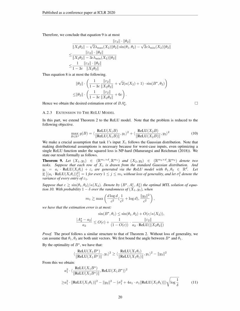
A.2.3 EXTENSION TO THE RELU MODEL

In this part, we extend Theorem 2 to the ReLU model. Note that the problem is reduced to thefollowing objective.

maxB∈Rd

g(B) = 〈 ReLU(X1B)

‖ReLU(X1B)‖, y1〉2 + 〈 ReLU(X2B)

‖ReLU(X2B)‖, y2〉2 (10)

We make a crucial assumption that task 1’s input X1 follows the Gaussian distribution. Note thatmaking distributional assumptions is necessary because for worst-case inputs, even optimizing asingle ReLU function under the squared loss is NP-hard (Manurangsi and Reichman (2018)). Westate our result formally as follows.Theorem 9. Let (X1, y1) ∈ (Rm1×d,Rm1) and (X2, y2) ∈ (Rm2×d,Rm2) denote twotasks. Suppose that each row of X1 is drawn from the standard Gaussian distribution. Andyi = ai · ReLU(Xiθi) + εi are generated via the ReLU model with θ1, θ2 ∈ Rd. LetE[(ai · ReLU(Xiθi))

2j

]= 1 for every 1 ≤ j ≤ m1 without loss of generality, and let σ2

1 denote thevariance of every entry of ε1.

Suppose that c ≥ sin(θ1, θ2)/κ(X2). Denote by (B?, A?1, A?2) the optimal MTL solution of equa-

tion 10. With probability 1− δ over the randomness of (X1, y1), when

m1 & max

(d log d

c2(

1

c2+ log d),

‖y2‖2

c2

),

we have that the estimation error is at most:

sin(B?, θ1) ≤ sin(θ1, θ2) +O(c/κ(X2)),

|A?2 − a2|a2

≤ O(c) +1

(1−O(c))· ‖ε2‖a2 · ReLU(‖X2θ2‖)

Proof. The proof follows a similar structure to that of Theorem 2. Without loss of generality, wecan assume that θ1, θ2 are both unit vectors. We first bound the angle between B? and θ1.

By the optimality of B?, we have that:

〈 ReLU(X1B?)

‖ReLU(X1B?)‖, y1〉2 ≥ 〈

ReLU(X1θ1)

‖ReLU(X1θ1)‖, y1〉2 − ‖y2‖2

From this we obtain:

a21 · 〈ReLU(X1B

?)

‖ReLU(X1B?)‖,ReLU(X1B

?)〉2

≥a21 · ‖ReLU(X1θ1)‖2 − ‖y2‖2 − (σ21 + 4a1 · σ1‖ReLU(X1θ1)‖)

√log

1

δ(11)

20


Note that each entry of ReLU(X1θ1) is a truncated Gaussian random variable. By the Hoeffdingbound, with probability 1− δ we have∣∣∣‖ReLU(X1θ1)‖2 − m1

2

∣∣∣ ≤√m1

2log

1

δ.

As for 〈ReLU(X1B?),ReLU(X1θ1)〉, we will use an epsilon-net argument over B? to show the

concentration. For a fixed B?, we note that this is a sum of independent random variables that areall bounded within O(log m1

δ ) with probability 1 − δ. Denote by φ the angle between B? and θ1,a standard geometric fact states that (see e.g. Lemma 1 of Du et al. (2017)) for a random Gaussianvector x ∈ Rd,

Ex

[ReLU(x>B?) · ReLU(x>θ1)

]=

cosφ

2+

cosφ(tanφ− φ)

2π:=

g(φ)

2.

Therefore, by applying Bernstein’s inequality and union bound, with probability 1− η we have:

|〈ReLU(X1B?),ReLU(X1θ1)〉 −m1g(φ)/2| ≤ 2

√m1g(φ) log

1

η+

2

3log

1

ηlog

m1

δ

By standard arguments, there exists a set of dO(d) unit vectors S such that for any other unit vectoru there exists u ∈ S such that ‖u − u‖ ≤ min(1/d3, c2/κ2(X2)). By setting η = d−O(d) andtake union bound over all unit vectors in S, we have that there exists u ∈ S satisfying ‖B? − u‖ ≤min(1/d3, c2/κ2(X2)) and the following:

|〈ReLU(X1u),ReLU(X1θ1)〉 −m1g(φ′)/2| .√m1d log d+ d log2 d

≤ 2m1c2/κ2(X2) (by our setting of m1)

where φ′ is the angle between u and θ1. Note that∣∣∣〈ReLU(X1θ)− ReLU(X1B?),ReLU(X1θ1)〉

∣∣∣ ≤ ‖X1(u−B?)‖ · ‖ReLU(X1θ1)‖

≤ c2/κ2(X2) ·O(m1)

Together we have shown that|〈ReLU(X1B

?),ReLU(X1θ1)〉 −m1g(φ′)/2| ≤ c2/κ2(X2) ·O(m1).

Combined with equation 11, by our setting of m1, it is not hard to show thatg(φ′) ≥ 1−O(c2/κ2(X2)).

Note that1− g(φ′) = 1− cosφ′ − cosφ′(tanφ′ − φ′)

≤ 1− cosφ′ = 2 sin2 φ′

2. c2/κ2(X2),

which implies that sin2 φ′ . c2/κ2(X2) (since cosφ′

2 ≥ 0.9). Finally note that ‖u − B?‖ ≤c2/κ2(X2), hence

‖u−B?‖2 = 2(1− cos(u, B?)) ≥ 2 sin2(u, B?).

Overall, we conclude that sin(B?, θ1) ≤ O(c/κ(X2)). Hencesin(B?, θ2) ≤ sin(θ1, θ2) +O(c/κ(X2)).

For the estimation of a2, we have∣∣∣∣ 〈ReLU(X2B?), y2〉

‖ReLU(X2B?)‖2− a2

∣∣∣∣ ≤|〈ReLU(X2B?), ε2〉|

‖ReLU(X2B?)‖2

+a2

∣∣∣∣ 〈ReLU(X2B?),ReLU(X2B

?)− ReLU(X2θ2)〉‖ReLU(X2B?)‖2

∣∣∣∣The first part is at most

‖ε2‖‖ReLU(X2B?)‖

≤ ‖ε2‖‖ReLU(X2θ2)‖ − ‖ReLU(X2θ2)− ReLU(X2B?)‖

≤ 1

1−O(c)

‖ε2‖‖ReLU(X2θ2)‖

Similarly, we can show that the second part is at most O(c). Therefore, the proof is complete.

21


A.3 PROOF OF PROPOSITION 3

In this part, we present the proof of Proposition 3. In fact, we present a more refined result, byshowing that all local minima are global minima for the reweighted loss in the linear case.

f(A1, A2, . . . , Ak;B) =

k∑i=1

αi‖XiBAi − yi)‖2F . (12)

The key is to reduce the MTL objective f(·) to low rank matrix approximation, and apply recentresults by Balcan et al. (2018) which show that there is no spurious local minima for the latterproblem .Lemma 10. Assume that X>i Xi = αiΣ with αi > 0 for all 1 ≤ i ≤ k. Then all the local minimaof f(A1, . . . , Ak;B) are global minima of equation 3.

Proof. We first transform the problem from the space of B to the space of C. Note that this iswithout loss of generality, since there is a one to one mapping between B and C with C = DV >B.In this case, the corresponding objective becomes the following.

g(A1, . . . , Ak;B) =

k∑i=1

αi · ‖UiCAi − yi‖2

=

k∑i=1

‖C(√αiAi)−

√αiU

>i yi‖2 +

k∑i=1

αi · (‖yi‖2 − ‖U>i yi‖2)

The latter expression is a constant. Hence it does not affect the optimization solution. For theformer, denote by A ∈ Rr×k as stacking the

√αiAi’s together column-wise. Similarly, denote by

Z ∈ Rd×k as stacking√αiU

>i yi together column-wise. Then minimizing g(·) reduces solving low

rank matrix approximation: ‖CA− Z‖2F

.

By Lemma 3.1 of Balcan et al. (2018), the only local minima of ‖CA − Z‖2F

are the ones whereCA is equal to the best rank-r approximation of Z. Hence the proof is complete.

Now we are ready to prove Proposition 3.

Proof of Proposition 3. By Proposition 5, the optimal solution of B? for equation 12 is V D−1times the best rank-r approximation to αiU>yiy>i U , where we denote the SVD of X as UDV >.Denote by QrQ

>r as the best rank-r approximation to U>ZZ>U , where we denote by Z =

[√α1y1,

√α2y2, . . . ,

√αkyk] as stacking the k vectors to a d by k matrix. Hence the result of

Proposition 5 shows that the optimal solution B? is V D−1Qr, which is equal to (X>X)−1XQr.By Proposition 4, the optimality ofB? is the same up to transformations on the column space. Hencethe proof is complete.

To show that all local minima are also equal to (X>X)−1XQr, we can simply apply Lemma 10and Proposition 3.

Remark. This result only applies to the linear model and does not work on ReLU models. The ques-tion of characterizing the optimization landscape in non-linear ReLU models is not well-understoodbased on the current theoretical understanding of neural networks. We leave this for future work.

22


B SUPPLEMENTARY EXPERIMENTAL RESULTS

We fill in the details left from our experimental section. In Appendix B.1, we review the datasetsused in our experiments. In Appendix B.2, we describe the models we use on each dataset. InAppendix B.3, we describe the training procedures for all experiments. In Appendix B.4 and Ap-pendix B.5, we show extended synthetic and real world experiments to support our claims.

B.1 DATASETS

We describe the synthetic settings and the datasets Sentiment Analysis, General Language Under-standing Evaluation (GLUE) benchmark, and ChestX-ray14 used in the experiments.

Synthetic settings. For the synthetic experiments, we draw 10,000 random data samples with di-mension d = 100 from the standard Gaussian N (0, 1) and calculate the corresponding labels basedon the model described in experiment. We split the data samples into training and validation setswith 9,000 and 1,000 samples in each. For classification tasks, we generate the labels by applyinga sigmoid function and then thresholding the value to binary labels at 0.5. For ReLU regressiontasks, we apply the ReLU activation function on the real-valued labels. The number of data samplesused in the experiments varies depending on the specification. Specifically, for the task covarianceexperiment of Figure 3, we fix task 1’s data with m1 = 9, 000 training data and vary task 2’s dataunder three settings: (i) same rotation Q1 = Q2 but different singular values D1 6= D2; (ii) samesingular values D1 = D2 but random rotations Q1 6= Q2.

Sentiment analysis. For the sentiment analysis task, the goal is to understand the sentiment opinionsexpressed in the text based on the context provided. This is a popular text classification task whichis usually formulated as a multi-label classification task over different ratings such as positive (+1),negative (-1), or neutral (0). We use six sentiment analysis benchmarks in our experiments:

• Movie review sentiment (MR): In the MR dataset (Pang and Lee (2005)), each movie re-view consists of a single sentence. The goal is to detect positive vs. negative reviews.

• Sentence subjectivity (SUBJ): The SUBJ dataset is proposed in Pang and Lee (2004) andthe goal is to classify whether a given sentence is subjective or objective.

• Customer reviews polarity (CR): The CR dataset (Hu and Liu (2004)) provides customerreviews of various products. The goal is to categorize positive and negative reviews.

• Question type (TREC): The TREC dataset is collected by Li and Roth (2002). The aim isto classify a question into 6 question types.

• Opinion polarity (MPQA): The MPQA dataset detects whether an opinion is polarized ornot (Wiebe et al. (2005)).

• Stanford sentiment treebank (SST): The SST dataset, created by Socher et al. (2013), is anextension of the MR dataset.

The General Language Understanding Evaluation (GLUE) benchmark. GLUE is a collectionof NLP tasks including question answering, sentiment analysis, text similarity and textual entail-ment problems. The GLUE benchmark is a state-of-the-art MTL benchmark for both academia andindustry. We select five representative tasks including CoLA, MRPC, QNLI, RTE, and SST-2 tovalidate our proposed method. We emphasize that the goal of this work is not to come up with astate-of-the-art result but rather to provide insights into the working of multi-task learning. It isconceivable that our results can be extended to the entire dataset as well. This is left for future work.More details about the GLUE benchmark can be found in the original paper (Wang et al. (2018a)).

ChestX-ray14. The ChestX-ray14 dataset (Wang et al. (2017)) is the largest publicly availablechest X-ray dataset. It contains 112,120 frontal-view X-ray images of 30,805 unique patients. Eachimage contains up to 14 different thoracic pathology labels using automatic extraction methods onradiology reports. This can be formulated as a 14-task multi-label image classification problem.The ChestX-ray14 dataset is a representative dataset in the medical imaging domain as well as incomputer vision. We use this dataset to examine our proposed task reweighting scheme since itsatisfies the assumption that all tasks have the same input data but different labels.

23


B.2 MODELS

Synthetic settings. For the synthetic experiments, we use the linear regression model, the logisticregression model and a one-layer neural network with the ReLU activation function.

Sentiment analysis. For the sentiment analysis experiments, we consider three different modelsincluding multi-layer perceptron (MLP), LSTM, CNN:

• For the MLP model, we average the word embeddings of a sentence and feed the result intoa two layer perceptron, followed by a classification layer.

• For the LSTM model, we use the standard one-layer single direction LSTM as proposedby Lei et al. (2018), followed by a classification layer.

• For the CNN model, we use the model proposed by Kim (2014) which uses one convolu-tional layer with multiple filters, followed by a ReLU layer, max-pooling layer, and classi-fication layer. We follow the protocol of Kim (2014) and set the filter size as {3, 4, 5}.

We use the pre-trained GLoVe embeddings trained on Wikipedia 2014 and Gigaword 5 corpora 6.We fine-tune the entire model in our experiments. In the multi-task learning setting, the sharedmodules include the embedding layer and the feature extraction layer (i.e. the MLP, LSTM, or CNNmodel). Each task has its separate output module.

GLUE. For the experiments on the GLUE benchmark, we use a state-of-the-art language modelcalled BERT (Devlin et al. (2018)). For each task, we add a classification/regression layer on top itas our model. For all the experiments, we use the BERTLARGE uncased model, which is a 24 layernetwork as described in Devlin et al. (2018). For the multi-task learning setting, we follow the workof Liu et al. (2019a) and use BERTLARGE as the shared module.

ChestX-ray14. For the experiments on the ChestX-ray14 dataset, we use the DenseNet modelproposed by Rajpurkar et al. (2017) as the shared module, which is a 121 layer network. For eachtask, we use a separate classification output layer. We use the pre-trained model7 in our experiments.

B.3 TRAINING PROCEDURES

In this subsection, we describe the training procedures for our experiments.

Mini-batch SGD. We describe the details of task data sampling in our SGD implementation.

• For tasks with different features such as GLUE, we first divide each task data into smallbatches. Then, we mix all the batches from all tasks and shuffle randomly. During everyepoch, a SGD step is applied on every batch over the corresponding task. If the currentbatch is for task i, then the SGD is applied on Ai, and possibly Ri or B depending on thesetup. The other parameters for other tasks are fixed.

• For tasks with the same features such as ChestX-ray14, the SGD is applied on all the tasksjointly to update all the Ai’s and B together.

Synthetic settings. For the synthetic experiments, we do a grid search over the learning rate from{1e − 4, 1e − 3, 1e − 2, 1e − 1} and the number of epochs from {10, 20, 30, 40, 50}. We pick thebest results for all the experiments. We choose the learning rate to be 1e− 3, the number of epochsto be 30, and the batch size to be 50. For regression task, we report the Spearman’s correlation scoreFor classification task, we report the classification accuracy.

Sentiment analysis. For the sentiment analysis experiments, we randomly split the data into train-ing, dev and test sets with percentages 80%, 10%, and 10% respectively. We follow the protocolof Lei et al. (2018) to set up our model for the sentiment analysis experiments.

The default hidden dimension of the model (e.g. LSTM) is set to be 200, but we vary this parameterfor the model capacity experiments. We report the accuracy score on the test set as the performancemetric.

6http://nlp.stanford.edu/data/wordvecs/glove.6B.zip7https://github.com/pytorch/vision

24


MTL

per

form

ance

ove

r STL

(S

pear

man

cor

rela

tion)

−0.4

−0.2

0

Cosine distance between tasks0 0.5 1.0

(a) Linear regression tasks

MTL

per

form

ance

ove

r STL

(A

ccur

acy)

−0.2

−0.1

0


(b) Logistic classification tasks

MTL

per

form

ance

ove

r STL

(S

pear

man

cor

rela

tion)

−0.04

−0.02

0

0.02


(c) Regression tasks with ReLU non-linearity

MTL

per

form

ance

ove

r STL

(A

ccur

acy)

−0.05

0

0.05


(d) Classification tasks with ReLU non-linearity

Figure 7: Comparing MTL model performance over different task similarity. For (a) and (c), MTLtrains two regression tasks; For (b) and (d), MTL trains two classification tasks. For regressiontasks, we use spearman correlation as model performance indicator. For classification tasks, weuse accuracy as the metric. We report the average model performance over two tasks. The x-axisdenotes the cosine distance, i.e. 1− cos(θ1, θ2).

GLUE. For the GLUE experiments, the training procedure is used on the alignment modules andthe output modules. Due to the complexity of the BERTLARGE module, which involves 24 layers ofnon-linear transformations.

We fix the BERTLARGE module during the training process to examine the effect of adding thealignment modules to the training process. In general, even after fine-tuning the BERTLARGE moduleon a set of tasks, it is always possible to add our alignment modules and apply Algorithm 1.

For the training parameters, we apply grid search to tune the learning rate from {2e−5, 3e−5, 1e−5}and the number of epochs from {2, 3, 5, 10}. We choose the learning rate to be 2e−5, the numberof epochs to be 5, and with batch size 16 for all the experiments.

We use the GLUE evaluation metric (cf. Wang et al. (2018b)) and report the scores on the develop-ment set as the performance metric.

ChestX-ray14. For the ChestX-ray14 experiments, we use the configuration suggested by Rajpurkaret al. (2017) and report the AUC score on the test set after fine-tuning the model for 20 epochs.

B.4 EXTENDED SYNTHETIC EXPERIMENTS

Varying cosine similarity on linear and ReLU models. We demonstrate the effect of cosine simi-larity in synthetic settings for both regression and classification tasks.

Synthetic tasks. We start with linear settings. We generate 20 synthetic task datasets (either forregression tasks, or classification tasks) based on data generation procedure and vary the task simi-larity between task 1 and task i. We run the experiment with a different dataset pairs (dataset 1 anddataset i).

25


Sim. 0.9Sim. 0.7

Sim. 0.5Sim. 0.3

Sim. 0.1

Perfo

rman

ce Im

prov

emen

ts

−0.2

0

0.2

# Data size2000 4000 6000 8000

(a) Regression tasks with non-linearity

Sim. 0.9Sim. 0.7

Sim. 0.5Sim. 0.3

Sim. 0.1

Perfo

rman

ce Im

prov

emen

ts

−0.2

−0.1

0

0.1

# Data size2000 4000 6000 8000

(b) Classification tasks with non-linearity

Figure 8: The performance improvement on the target task (MTL minus STL) by varying the cosinesimilarity of the two tasks’ STL models. We observe that higher similarity between the STL modelsleads to better improvement on the target task.

BaselineAlgorithm 1

Positive Transfer

Negative Transfer

Targ

et ta

sk's

Perf.

: MTL

- ST

L

−0.2

−0.1

0

0.1

0.2


(a) Linear regression tasks

Positive Transfer

Negative Transfer

BaselineAlgorithm 1

Targ

et ta

sk's

Perf.

: MTL

- ST

L

−0.2

−0.1

0

0.1

0.2


(b) Regression tasks with ReLU activation

Figure 9: Comparing Algorithm 1 to the baseline MTL training on the synthetic example in Section2.3. Algorithm 1 corrects the negative transfer phenomenon observed in Figure 3.

After generating the tasks, we compare the performance gap between MTL and STL model.

Results. From Figure 7a and Figure 7a, we find that for both regression and classification settings,with the larger task similarity the MTL outperforms more than STL model and the negative transfercould occur if the task similarity is too small.

ReLU settings. We also consider a ReLU-activated model. We use the same setup as the linearsetting, but apply a ReLU activation to generate the data. Similar results are shown in Figure 7c, 7d.

Higher rank regimes for ReLU settings. We provide further validation of our results on ReLU-activated models.

Synthetic tasks. In this synthetic experiment, there are two sets of model parameters Θ1 ⊆ Rd×r andΘ2 ⊆ Rd×r (d = 100 and r = 10). Θ1 is a fixed random rotation matrix and there are m1 = 100data points for task 1. Task 2’s model parameter is Θ2 = αΘ1 + (1−α)Θ′, where Θ′ is also a fixedrotation matrix that is orthogonal to Θ1. Note that α is the cosine value/similarity of the principalangle between Θ1 and Θ2.

We then generate X1 ⊆ Rm1×d and X2 ⊆ Rm2×d from Gaussian. For each task, the labels areyi = ReLU(XiΘi)e+ εi, where e ∈ Rr is the all ones vector and εi is a random Gaussian noise.

Given the two tasks, we use MTL with ReLU activations and capacity H = 10 to co-train the twotasks. The goal is to see how different levels of α or similarity affects the transfer from task two totask one. Note that this setting parallels the ReLU setting of Theorem 9 but applies to rank r = 5.

26


MTL-Avg.STL-SSTSTL-MRSTL-CRSTL-SUBJSTL-MPQASTL-TREC

MTL-Avg. peak

LSTM

Accu

racy

0.6

0.7

0.8

0.9

Model capacity0 100 200 300 400 500

Figure 10: Cross validation to choose the best performing model capacity for each model.

MTL-Avg.STL-SSTSTL-MR

STL-MR peak

MTL-Avg. peak

STL-SST peak

MLP

Accu

racy

0.76

0.78

0.80

Model capacity0 100 200 300 400 500


STL-MR peak

MTL-Avg. peak

STL-SST peak

CNN

Accu

racy

0.80

0.85

0.90

Model capacity0 500 1000


STL-MR peak

MTL-Avg. peakSTL-SST peak

LSTM

Accu

racy

0.75

0.80

0.85

0.90

Model capacity0 100 200 300 400 500

Figure 11: Validation on MLP, CNN and LSTM models for sentiment analysis tasks.

Results. In Figure 8 we show that the data size, the cosine similarity between the STL solutions andthe alignment of covariances continue to affect the rate of transfer in the new settings. The studyshows that our conceptual results are applicable to a wide range of settings.

Evaluating Algorithm 1 on linear and ReLU-activated models. We consider the synthetic ex-ample in Section 2.3 to compare Algorithm 1 and the baseline MTL training. Recall that in theexample, when the source and target tasks have different covariance matrices, MTL causes negativetransfer on the target task. Our hypothesis in this experiment is to show that Algorithm 1 can correctthe misalignment and the negative transfer.

Synthetic tasks. We evaluate on both linear and ReLU regression tasks. The linear case follows theexample in Section 2.3. For the ReLU case, the data is generated according to the previous example.

Results. Figure 9 confirms the hypothesis. We observe that Algorithm 1 corrects the negative transferin the regime where the source task only has limited amount of data. Furthermore, Algorithm 1matches the baseline MTL training when the source task has sufficiently many data points.

B.5 EXTENDED ABLATION STUDIES

Cross validation for choosing model capacities. We provide a cross validation experiment toindicate how we choose the best performing model capacities in Figure 1. This is done on the sixsentiment analysis tasks trained with an LSTM layer.

In Figure 10, we vary the model capacities to plot the validation accuracies of the MTL model trainedwith all six tasks and the STL model for each task. The result complements Table 1 in Section 3.3.

Choosing model capacities for CNN and MLP. Next we verify our result on model capacities forCNN and MLP models. We select the SST and MR datasets from the sentiment analysis tasks forthis experiment. We train all three models CNN, MLP and LSTM by varying the capacities.

Results. From Figure 11 we observe that the best performing MTL model capacity is less than totalbest performing model capacities of STL model on all models.

27


The effect of label noise on Algorithm 2. To evaluate the robustness of Algorithm 2 in the presenceof label noise, we conduct the following experiment. First, we subsample 10% of the ChestX-ray14dataset and select two tasks from it. Then, we randomly pick one task to add 20% of noise to itslabels by randomly flipping them with probability 0.5. We compare the performance of training bothtasks using our reweighting scheme (Algorithm 2) vs. the reweighting techniques of Kendall et al.(2018) and the unweighted loss scheme.

Results. On 10 randomly chosen task pairs, our method improves over the unweighted trainingscheme by 1.0% AUC score and 0.4% AUC score over Kendall et al. (2018) averaged over the 10task pairs. Figure 12 shows 5 example task pairs from our evaluation.

Unweighted loss Kendall et al. Algorithm 2

MTL

per

form

ance

0.4

0.5

0.6

0.7

0.8

ConsolidationCardiomegaly

ConsolidationEdema

ConsolidationInfiltration

EdemaAtelectasis

FibrosisConsolidation

Figure 12: Comparing Algorithm 2 to the unweighted scheme and Kendall et al. (2018).

28

UNDERSTANDING AND IMPROVING INFORMATION TRANSFER …

Documents

Transcript of UNDERSTANDING AND IMPROVING INFORMATION TRANSFER …