Journal of Artificial Intelligence Research X (X) X Submitted X; published X

Understanding Algorithm Performance on an

Oversubscribed Scheduling Application

Laura Barbulescu laurabar@cs.cmu.edu

The Robotics Institute

Carnegie Mellon University

Pittsburgh, PA 15213 USA

Adele E. Howe howe@cs.colostate.edu

L. Darrell Whitley whitley@cs.colostate.edu

Mark Roberts mroberts@cs.colostate.edu

Computer Science Department

Colorado State University

Fort Collins, CO 80523 USA

Abstract

The best performing algorithms for a particular oversubscribed scheduling application,Air Force Satellite Control Network (AFSCN) scheduling, appear to have little in com-mon. Yet, through careful experimentation and modeling of performance in real probleminstances, we can relate characteristics of the best algorithms to characteristics of theapplication. In particular, we find that plateaus dominate the search spaces (thus favor-ing algorithms that make larger changes to solutions) and that some randomization inexploration is critical to good performance (due to the lack of gradient information onthe plateaus). Based on our explanations of algorithm performance, we develop a newalgorithm that combines characteristics of the best performers; the new algorithm’s perfor-mance is better than the previous best. We show how hypothesis driven experimentationand search modeling can both explain algorithm performance and motivate the design ofa new algorithm.

1. Introduction

Effective solution of the Air Force Satellite Control Network (AFSCN) scheduling problemruns counter to conventional wisdom in AI. Other scheduling problems, e.g., United StatesAir Force (USAF) Air Mobility Command (AMC) airlift (Kramer & Smith, 2003) andscheduling telescope observations (Bresina, 1996), are well solved by heuristically guidedconstructive or repair based search. The best performing solutions to AFSCN are a geneticalgorithm (Genitor), Squeaky Wheel Optimization (SWO) and randomized next-descentlocal search. We have not yet found a constructive or repair based solution that is compet-itive.

The three best performing solutions to AFSCN appear to have little in common, makingit difficult to explain their superior performance. Genitor combines two candidate solutionspreserving elements of each. SWO creates an initial greedy solution and then attempts toimprove the scheduling of all tasks known to contribute detrimentally to the current eval-uation. Randomized local search makes incremental changes based on observed immediategradients in schedule evaluation. In this paper, we examine the performance of these differ-

c©X AI Access Foundation. All rights reserved.

ent algorithms, identify factors that do or do not help explain the performance and leveragethe explanations to design a new search algorithm that is well suited to the characteristicsof this application.

Our target application is an oversubscribed scheduling application with alternative re-sources. AFSCN (Air Force Satellite Control Network) access scheduling requires assigningaccess requests (communication relays to U.S.A. government satellites) to specific time slotson an antenna at a ground station. It is oversubscribed in that not all tasks can be ac-commodated given the available resources. To be considered to be oversubscribed, not allproblem instances need overtax the available resources, but for our application, that ap-pears to be the case. The application is challenging and shares characteristics with otherapplications such as Earth Observing Satellites (EOS). It is important in that a team ofhuman schedulers have laboriously performed the task every day for at least 15 years withminimal automated assistance.

All of the algorithms are designed to traverse essentially the same search space: solutionsare represented as permutations of tasks, which a greedy schedule builder converts into aschedule by assigning start time and resources to the tasks in the order in which they appearin the permutation. We find that this search space is dominated by plateaus. Additionally,the size of the plateau increases dramatically as the best solution is approached.

Given the dominance of plateaus, we have explored a number of different hypotheses toexplain the performance of each algorithm. Some of these hypotheses include the following:

Genitor, a genetic algorithm, identifies patterns of relative task orderings, similar to back-bones from SAT (Singer, Gent, & Smaill, 2000), which are preserved in the members ofthe population. This is in effect a type of classic building block hypothesis (Goldberg,1989).

SWO starts extremely close to the best solution and so need not enact much change. Thishypothesis also implies that it is relatively easy to modify good greedy solutions tofind the best known solutions.

Randomized Local Search performs essentially a random walk on the plateaus to findexits leading to better solutions; given the distribution of solutions and lack of gradientinformation, this may be as good a strategy as any.

We tested each of these hypotheses. There is limited evidence for the existence of buildingblocks or backbone structure. And while Squeaky Wheel Optimization does quickly findgood solutions, it cannot reliably find best known solutions. Therefore, while the firsttwo hypotheses were somewhat supported by the data, the hypotheses were not enough toexplain the observed performance.

The third hypothesis appears to be the best explanation of why the particular localsearch strategy we have used works so well. In light of this, we formulated another hypoth-esis:

SWO and Genitor make long leaps in the search space, which allow them to relativelyquickly traverse the plateaus.

This last hypothesis appears to well explain the performance of the two methods. Forthe genetic algorithm the leaps are naturally longer during the early phases of search whenparent solutions are less similar.

2

Based on these studies, we constructed a new search algorithm that exploits what wehave learned about the search space and the behavior of successful algorithms. AttenuatedLeap Local Search makes multiple changes to the solution before evaluating a candidatesolution. In addition, the number of changes decreases commensurate with expected prox-imity to the solution. The number of multiple changes, or the length of the leap, is largerearly in the search, and reduces (shortens) as better solutions are found. We find that thisalgorithm performs quite well: it quickly finds best known solutions to all of the AFSCNproblems.

2. AFSCN Scheduling

The U.S.A. Air Force Satellite Control Network is currently responsible for coordinatingcommunications between civilian and military organizations and more than 100 USAF man-aged satellites. Space-ground communications are performed using 16 antennas located atnine tracking stations around the globe1. Figure 1 shows a map of the current configurationof AFSCN; this map shows one fewer tracking station and antennae than are in our data,due to those resources apparently having been taken off-line recently. Customer organiza-tions submit task requests to reserve an antenna at a tracking station for a specified timeperiod based on the visibility windows between target satellites and tracking stations. Twotypes of task requests can be distinguished: low altitude and high altitude orbits. The lowaltitude tasks specify requests for access to low altitude satellites; such requests tend tobe short (e.g., 15 minutes) and have a tight visibility window. High altitude tasks specifyrequests for high altitude satellites; the durations for these requests are more varied andusually longer, with large visibility windows.

Approximately 500 requests are typically received for a single day. Separate schedulesare produced by a staff of human schedulers at Schriever Air Force Base for each day. Of the500 requests, often about 120 conflicts remain after the first pass of scheduling. “Conflicts”are defined as requests that cannot be scheduled, since they conflict with other scheduledrequests (this means that 120 requests remain unscheduled after an initial schedule isproduced).

From real problem data, we extract a description of the problem specification in terms oftask requests to be scheduled with their corresponding type (low or high altitude), duration,time windows and alternative resources. The AFSCN data also include information aboutsatellite revolution numbers, optional site equipment, tracking station maintenance times(downtimes), possible loss of data due to antenna problems, various comments, etc.; we donot incorporate such information in our problem specification. The information about thetype of the task (low or high altitude) as well as the identifier for the satellite involved areincluded in the task specification. However, we do not know how the satellite identifiercorresponds to an actual satellite and so rely on precomputed visibility information whichis present in the requests.

1. The U.S.A. government is planning to make the AFSCN the core of an Integrated Satellite ControlNetwork for managing satellite assets for other U.S.A. government agencies as well, e.g., NASA, NOAA,other DoD affiliates. By 2011, when the system first becomes operational, the Remote Tracking Stationswill be increased and enhanced to accommodate the additional load.

3

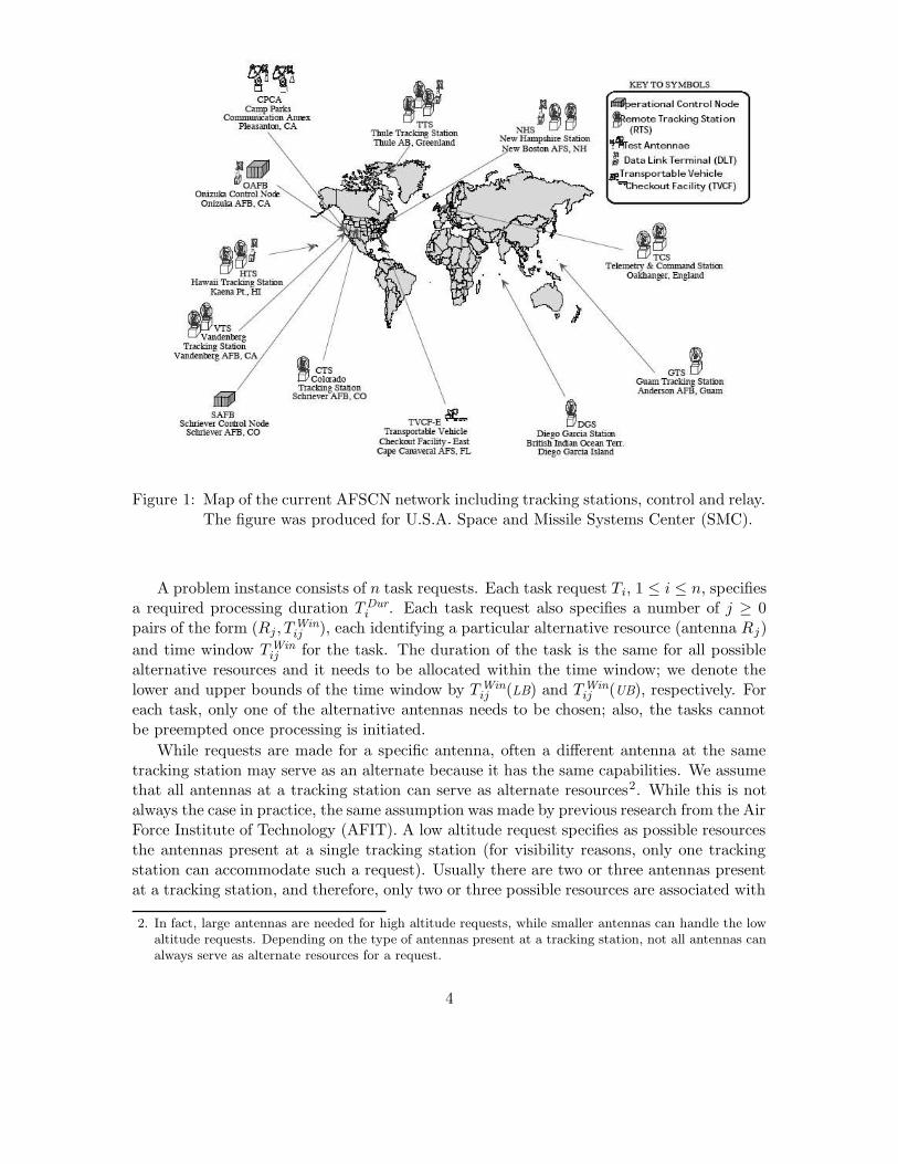
Figure 1: Map of the current AFSCN network including tracking stations, control and relay.The figure was produced for U.S.A. Space and Missile Systems Center (SMC).

A problem instance consists of n task requests. Each task request Ti, 1 ≤ i ≤ n, specifiesa required processing duration T Dur

i . Each task request also specifies a number of j ≥ 0pairs of the form (Rj , T

Winij ), each identifying a particular alternative resource (antenna Rj)

and time window T Winij for the task. The duration of the task is the same for all possible

alternative resources and it needs to be allocated within the time window; we denote thelower and upper bounds of the time window by T Win

ij (LB) and TWinij (UB), respectively. For

each task, only one of the alternative antennas needs to be chosen; also, the tasks cannotbe preempted once processing is initiated.

While requests are made for a specific antenna, often a different antenna at the sametracking station may serve as an alternate because it has the same capabilities. We assumethat all antennas at a tracking station can serve as alternate resources2. While this is notalways the case in practice, the same assumption was made by previous research from the AirForce Institute of Technology (AFIT). A low altitude request specifies as possible resourcesthe antennas present at a single tracking station (for visibility reasons, only one trackingstation can accommodate such a request). Usually there are two or three antennas presentat a tracking station, and therefore, only two or three possible resources are associated with

2. In fact, large antennas are needed for high altitude requests, while smaller antennas can handle the lowaltitude requests. Depending on the type of antennas present at a tracking station, not all antennas canalways serve as alternate resources for a request.

4

each of these requests. High altitude requests specify all the antennas present at all thetracking stations that satisfy the visibility constraints; as many as 14 possible alternativesare specified in our data.

Previous research and development on AFSCN scheduling focused on minimizing thenumber of request conflicts for AFSCN scheduling, or alternatively, maximizing the numberof requests that can be scheduled without conflict. Those requests that cannot be scheduledwithout conflict are bumped out of the schedule. This is not what happens when humanscarry out AFSCN scheduling3. Satellites are valuable resources, and the AFSCN operatorswork to fit in every request. What this means in practice is that after negotiation with thecustomers, some requests are given less time than requested, or shifted to less desirable,but still usable time slots. In effect, the requests are altered until all requests are at leastpartially satisfied or deferred to another day. By using an evaluation function that minimizesthe number of request conflicts, an assumption is being made that we should fit in as manyrequests as possible before requiring human schedulers to figure out how to place thoserequests that have been bumped.

However, given that all requests need to be eventually scheduled, we designed a newevaluation criterion that schedules all the requests by allowing them to overlap and minimiz-ing the sum of overlaps between conflicting tasks. This appears to yield schedules that aremuch closer to those that human schedulers construct. When conflicting tasks are bumpedout of the schedule, large and difficult to schedule tasks are most likely to be bumped;placing these requests back into a negotiated schedule means deconstructing the minimalconflict schedule and rebuilding a new schedule. Thus, a schedule that minimizes conflictsmay not help all that much when constructing the negotiated schedule, whereas a schedulethat minimizes overlaps can suggest ways of fitting tasks into the schedule, for exampleby reducing a task’s duration by two or three minutes, or shifting a start outside of therequested window by a short amount of time.

We obtained 12 days of data for the AFSCN application4. The first seven days are froma week in 1992 and were given to us by Colonel James Moore at the Air Force Institute ofTechnology. These data were used in the first research projects on AFSCN. We obtained anadditional five days of data from schedulers at Schriever Air Force Base. Table 2 summarizesthe characteristics of the data. We will refer to the problems from 1992 as the A problems,and to the more recent problems, as the R problems.

3. Related Scheduling Research

The AFSCN application is a multiple resource, oversubscribed problem. Examples of othersuch applications are USAF Air Mobility Command (AMC) airlift scheduling (Kramer &Smith, 2003), NASA’s shuttle ground processing (Deale, Yvanovich, Schnitzuius, Kautz,Carpenter, Zweben, Davis, & Daun, 1994), scheduling telescope observations (Bresina,

3. We met with the several of the schedulers at Schriever to discuss their procedure and have them cross-check our solution. We appreciate the assistance of Brian Bayless and William Szary in setting up themeeting and giving us data.

4. We have approval to make public some, but not all of the data. Seehttp://www.cs.colostate.edu/sched/data.html for details on obtaining the problems.

5

ID Date # Requests # High # Low Best Conflicts Best Overlaps

A1 10/12/92 322 169 153 8 104A2 10/13/92 302 165 137 4 13A3 10/14/92 311 165 146 3 28A4 10/15/92 318 176 142 2 9A5 10/16/92 305 163 142 4 30A6 10/17/92 299 155 144 6 45A7 10/18/92 297 155 142 6 46

R1 03/07/02 483 258 225 42 773R2 03/20/02 457 263 194 29 486R3 03/26/03 426 243 183 17 250R4 04/02/03 431 246 185 28 725R5 05/02/03 419 241 178 12 146

Table 1: Problem characteristics for the 12 days of AFSCN data used in our experiments.ID is used in other tables. Best conflicts and best overlaps are the best knownvalues for each problem for these two objective functions.

1996) and satellite observation scheduling (Frank, Jonsson, Morris, & Smith, 2001; Globus,Crawford, Lohn, & Pryor, 2003).

AMC scheduling assigns delivery missions to air wings (Kramer & Smith, 2003). Theirsystem adopts an iterative repair approach by greedily creating an initial schedule orderingthe tasks by priority and then attempting to insert unscheduled tasks by retracting andre-arranging conflicting tasks.

The Gerry scheduler was designed to manage the large set of tasks needed to preparea space shuttle for its next mission (Zweben, Daun, & Deale, 1994). Tasks are describedin terms of resource requirements, temporal constraints and required time windows. Theoriginal version used constructive search with dependency-directed backtracking, which wasnot adequate to the task; a subsequent version employed constraint-directed iterative repair.

In satellite scheduling, customer requests for data collection need to be matched withsatellite and tracking station resources. The requests specify the instruments required,the window of time when the request needs to be executed, and the location of the sens-ing/communication event. These task constraints need to be coordinated with resourceconstraints; these include the windows of visibility for the satellites, maintenance periodsand downtimes for the tracking stations, etc. Typically, more requests need to be scheduledthan can be accommodated by the available resources. A general description of the satellitescheduling domain is provided by Jeremy Frank et al.(2001).

Pemberton(2000) solves a simple one-resource satellite scheduling problem in whichthe requests have priorities, fixed start times and fixed durations. The objective functionmaximizes the sum of the priorities of the scheduled requests. A priority segmentation algo-rithm is proposed, which is a hybrid algorithm combining a greedy approach with branch-and-bound. Wolfe and Sorensen (2000) define a more complex one-resource problem, thewindow-constrained packing problem (WCP), which specifies for each request the earlieststart time, latest final time and the minimum and maximum duration. The objective func-

6

tion is complex, combining request priority with the position of the scheduled request in itsrequired window and the number of requests scheduled. Two greedy heuristic approachesand a genetic algorithm are implemented; the genetic algorithm is found to perform best.

Globus et al.(2003) compare a genetic algorithm, simulated annealing, Squeaky WheelOptimization (Joslin & Clements, 1999) and hill climbing on a simplified, synthetic formof the satellite scheduling problem (two satellites with a single instrument) and find thatsimulated annealing excels and that the genetic algorithm performs relatively poorly. Fora general version of satellite scheduling (EOS observation scheduling), Frank et al.(2001)propose a constraint-based planner with a stochastic greedy search algorithm based onBresina’s Heuristic-Biased Stochastic Sampling (HBSS) algorithm (Bresina, 1996). HBSS(Bresina, 1996) was originally applied to scheduling astronomy observations for telescopes.

Lemaıtre et al.(2000) research the problem of scheduling the set of photographs for AgileEOS (ROADEF Challenge, 2003). Task constraints include the minimal time between twosuccessive acquisitions, pairings of requests such that images are acquired twice in differenttime windows, and hard requirement that certain images must always be acquired. Theyfind that a local search approach performs better than a hybrid algorithm combining branch-and-bound with various domain-specific heuristics.

The AFSCN application was previously studied by researchers from the Air Force Insti-tute of Technology (AFIT). Gooley (Gooley, 1993) and Schalck (Schalck, 1993) describedalgorithms based on mixed-integer programming (MIP) and insertion heuristics, whichachieved good overall performance: 91% – 95% of all requests scheduled. Parish (Parish,1994) used the Genitor (Whitley, 1989) genetic algorithm, which scheduled roughly 96%of all task requests, out-performing the MIP approaches. All three of these researchersused the AFIT benchmark suite consisting of seven problem instances, representing actualAFSCN task request data and visibilities for seven consecutive days from October 12 to18, 1992. Later, Jang (Jang, 1996) introduced a problem generator employing a bootstrapmechanism to produce additional test problems that are qualitatively similar to the AFITbenchmark problems. Jang then used this generator to analyze the maximum capacity ofthe AFSCN, as measured by the aggregate number of task requests that can be satisfied ina single-day.

While the general decision problem of AFSCN Scheduling with minimal conflicts is NP-complete, special subclasses of AFSCN Scheduling are polynomial. Burrowbridge (Burrow-bridge, 1999) considers a simplified version of AFSCN scheduling, where each task specifiesonly one resource (antenna) and only low-altitude satellites are present. The objective isto maximize the number of scheduled tasks. Due to the orbital dynamics of low-altitudesatellites, the task requests in this problem have negligible slack ; i.e., the window size isequal to the request duration. Assuming that only one task can be scheduled per timewindow, the well-known greedy activity-selector algorithm (Cormen, Leiserson, & Rivest,1990) is used to schedule the requests since it yields a solution with the maximal num-ber of scheduled tasks. To schedule low altitude requests on one of the multiple antennaspresent at a particular ground station, we extended the greedy activity-selector algorithmfor multiple resource problems. We proved that this extension of the greedy activity-selectoroptimally schedules the low altitude requests for the general problem of AFSCN Scheduling(Barbulescu, Watson, Whitley, & Howe, 2004b).

7

4. Algorithms

We implemented a variety of algorithms for AFSCN scheduling: iterative repair, heuristicconstructive search, local search, a genetic algorithm (GA), and Squeaky Wheel Optimiza-tion (SWO). As will be shown in Section 5, we found that randomized next descent localsearch, the GA and SWO work best for AFSCN scheduling.

We also considered constructive search algorithms based on texture (Beck, Davenport,Sitarski, & Fox, 1997) and slack (Smith & Cheng, 1993) constraint-based scheduling heuris-tics. We implemented straightforward extensions of such algorithms for our application.The results were poor; the number of request tasks combined with the presence of multiplealternative resources for each task make the application of such methods impractical. We donot report the performance values for the constructive search methods because these meth-ods depend critically on the heuristics; we are uncomfortable concluding that the methodsare poor because we may not have found good enough heuristics for them. We also triedusing a commercial off-the-shelf satellite scheduling package and had similarly poor results.We do not report performance values for the commercial system because it had not been de-signed specifically for this application and we did not have access to the source to determinethe reason for the poor performance.

Solution Representation Permutation based representations are frequently used whensolving scheduling problems, e.g., (Whitley, Starkweather, & Fuquay, 1989), (Syswerda,1991) (Wolfe & Sorensen, 2000) (Aickelin & Dowsland, 2003) (Globus et al., 2003). All ofour algorithms, except iterative-repair, encode solutions using a permutation π of the n taskrequest IDs (i.e., [1..n]). A schedule builder is used to generate solutions from a permutationof request IDs. The schedule builder considers task requests in the order that they appearin π. Each task request is assigned to the first available resource (as sequenced by the listof resource and window pairs provided in the task description) and at the earliest possiblestarting time. When minimizing the number of conflicts, if the request cannot be scheduledon any of the alternative resources, it is dropped from the schedule (i.e., bumped). Whenminimizing the sum of overlaps, if a request cannot be scheduled without conflict on any ofthe alternative resources, we assign it to the resource on which the overlap with requestsscheduled so far is minimized. Note that our schedule builder does favor the order in whichthe alternative resources are specified in the request, even though no preference is specifiedfor any of the alternatives.

4.1 Iterative Repair

Iterative repair methods have been successfully used to solve various oversubscribed schedul-ing problems, e.g., Hubble Space Telescope observations (Johnston & Miller, 1994) and spaceshuttle payloads (Zweben et al., 1994; Rabideau, Chien, Willis, & Mann, 1999). NASA’sASPEN (A Scheduling and Planning Environment) framework (Chien, Rabideau, Knight,Sherwood, Engelhardt, Mutz, Estlin, Smith, Fisher, Barrett, Stebbins, & Tran, 2000), em-ploys both constructive and repair-based methods and has been used to model and solvereal-world space applications such as scheduling EOS. More recently, Kramer et al. (Kramer& Smith, 2003) used repair-based methods to solve the airlift scheduling problem for theUSAF Air Mobility Command.

8

In each case, a key component to the implementation was a domain appropriate orderingheuristic to guide the repairs. For AFSCN scheduling, Gooley’s algorithm (Gooley, 1993)uses domain-specific knowledge to implement a repair-based approach. We implement animprovement to Gooley’s algorithm that is guaranteed to yield results at least as good asthose produced by the original version.

Gooley’s algorithm has two phases. In the first phase, the low altitude requests arescheduled, mainly using Mixed Integer Programming (MIP). Because there is a large numberof low altitude requests, the requests are divided into two blocks. MIP procedures are firstused to schedule the requests in the first block. Then MIP is used to schedule the requestsin the second block, which are inserted in the schedule around the requests from the firstblock. Finally, an interchange procedure attempts to optimize the total number of lowaltitude requests scheduled. This is needed because the low altitude requests are scheduledin disjoint blocks. Once the low altitude requests are scheduled, their start time and assignedresources remain fixed. In our implementation, we replaced this first phase with a greedyalgorithm (Barbulescu et al., 2004b) proven to schedule the optimal number of low altituderequests5. Our version accomplishes the same function as Gooley’s first phase, but does sowith a guarantee that the optimal number of low-altitude requests are scheduled. Thus, theresult is guaranteed to be equal to or better than Gooley’s original algorithm.

In the second phase, the high altitude requests are inserted in the schedule (withoutrescheduling any of the low altitude requests). An order of insertion for the high altituderequests is computed. The requests are sorted in decreasing order of the ratio of the dura-tion of the request to the average length of its time windows (this is similar to the flexibilitymeasure defined by Kramer and Smith for AMC (Kramer & Smith, 2003)); ties are brokenbased on the number of alternative resources specified (fewer alternatives scheduled first).After all the high altitude requests have been considered for insertion, an interchange pro-cedure attempts to accommodate the unscheduled requests, by rescheduling some of thehigh altitude requests. For each unscheduled high altitude request, a list of candidate re-quests for rescheduling is computed (such that after a successful rescheduling operation,the unscheduled request can be placed in the spot initially occupied by such a candidate).A heuristic measure is used to determine which requests from the candidate list shouldbe rescheduled. For the chosen candidates, if no scheduling alternatives are available, thesame procedure is applied to identify requests that can be rescheduled. This interchangeprocedure is defined with two levels of recursion and is called “three satellite interchange”.

4.2 Randomized Local Search (RLS)

We implemented a hill-climber we call “randomized local search”. Because it has beensuccessfully applied to a number of well-known scheduling problems, we selected a domain-independent move operator, the shift operator. From a current solution π, a neighborhoodis defined by considering all (N −1)2 pairs (x, y) of positions in π, subject to the restrictionthat y 6= x − 1. The neighbor π

′

corresponding to the position pair (x, y) is produced byshifting the job at position x into the position y, while leaving all other relative job orders

5. Our algorithm optimally solves the problem of scheduling only the low altitude requests, in polynomialtime.

9

unchanged. If x < y, then π′ = (π(1), ..., π(x− 1), π(x+1), ..., π(y), π(x), π(y +1), ..., π(n)).If x > y, then π′ = (π(1), ..., π(y − 1), π(x), π(y), ..., π(x − 1), π(x + 1), ..., π(n)).

Given the large neighborhood size, we use the shift operator in conjunction with next-descent hill-climbing. Our implementation completely randomizes which neighbor to exam-ine next, and does so with replacement: at each step, both x and y are chosen randomly.This general approach has been termed “stochastic hill-climbing” by Ackley (Ackley, 1987).If the value of the randomly chosen neighbor is equal or better than the value of the currentsolution, it becomes the new current solution.

It should be emphasized that Randomized Local Search, or stochastic hill-climbing, cansometimes be much more effective than steepest-descent local search or next-descent localsearch where the neighbors are checked in a predefined order (as opposed to random order).Forrest and Mitchell (Forrest & Mitchell, 1993) showed that a random mutation hill climber(much like our RLS or Ackley’s stochastic hill climber) found solutions much faster thansteepest-descent local search on a problem they called “The Royal Road” function. Therandom mutation hill climber also found solutions much faster than a hill climber thatgenerated and examined the neighbors systematically (in a predefined order). Randommutation hill climber was also much more effective than a genetic algorithm for this problem– despite the existence of what would appear to be natural “building blocks” in the function.It is notable that “The Royal Road” function is a staircase like function, where each stepin the staircase is a plateau.

4.3 Genetic Algorithm

Genetic algorithms were found to perform well on the AFSCN scheduling problem in someearly studies (Parish, 1994). Genetic algorithms have also been found to be effective in otheroversubscribed scheduling applications, such as scheduling F-14 flight simulators (Syswerda,1991) or an abstraction of NASA’s EOS problem (Wolfe & Sorensen, 2000). For our studies,we used the version of Genitor originally developed for a warehouse scheduling application(Starkweather, McDaniel, Mathias, Whitley, & Whitley, 1991); this is also the versionused by Parish for AFSCN scheduling. Like all genetic algorithms, Genitor maintains apopulation of solutions; in our implementation, we fixed the population size to be 200. Ineach step of the algorithm, a pair of parent solutions is selected, and a crossover operatoris used to generate a single child solution, which then replaces the worst solution in thepopulation. Selection of parent solutions is based on the rank of their fitness, relative toother solutions in the population. Following Parish (1994) and (Starkweather et al., 1991),we used Syswerda’s (1991) position-based crossover operator.

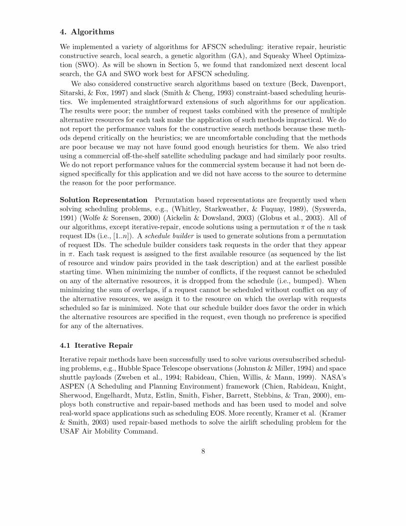
Syswerda’s position-based crossover operator starts by selecting a number of randompositions in the second parent. The corresponding selected elements will appear in exactlythe same positions in the offspring. The remaining positions in the offspring are filled withelements from the first parent in the order in which they appear in this parent:

Parent 1: A B C D E F G H I JParent 2: C F A J H D I G B E

Selected Elements: * * * *Offspring: C F A E G D H I B J

10

For our implementation, we randomly choose the number of positions to be selected,such that it is larger than one third of the total number of positions and smaller than twothirds of the total number of positions.

4.4 Squeaky Wheel Optimization

Squeaky Wheel Optimization (SWO) (Joslin & Clements, 1999) repeatedly iterates througha cycle composed of three phases. First, a greedy solution is built, based on priorities asso-ciated with the elements in the problem. Then, the solution is analyzed, and the elementscausing “trouble” are identified based on their contribution to the objective function. Third,the priorities of such “trouble makers” are modified, such that they will be considered ear-lier during the next iteration. The cycle is then repeated, until a termination condition ismet.

We constructed the initial greedy permutation for SWO by sorting the requests in in-creasing order of their flexibility. Our flexibility measure is similar to that defined for theAMC application (Kramer & Smith, 2003): the duration of the request divided by theaverage time window on the possible alternative resources. We break ties based on thenumber of alternative resources available. For requests with equal flexibilities and numbersof alternative resources, the earlier request is scheduled first. For multiple runs of SWO,we restarted it from a modified permutation created by performing 20 random swaps in theinitial greedy permutation.

When minimizing the sum of overlaps, we identified the overlapping requests as the“trouble spots” in the schedule. Note that for any overlap, we considered one request tobe scheduled; the other request (or requests, if more than two requests are involved) is”the overlapping request”. We sorted the overlapping requests in increasing order of theircontribution to the sum of overlaps. We associated with each such request a distance tomove forward, based on its rank in the sorted order. We fixed the minimum distance ofmoving forward to one and the maximum distance to five (this seems to work better thanother possible values we tried). The distance values are equally distributed among the ranks.We moved the requests forward in the permutation in increasing order of their contributionto the sum of overlaps: requests with smaller overlaps are moved first. We tried versionsof SWO where the distance to move forward is proportional with the contribution to thesum of overlaps or is fixed. However, these versions performed worse than the rank baseddistance implementation described above. When minimizing conflicts in the schedule allconflicts have an equal contribution to the objective function; therefore we decided to movethem forward for a fixed distance of five (we tried values between two and seven but fivewas best).

4.5 Heuristic Biased Stochastic Sampling (HBSS)

HBSS (Bresina, 1996) is an incremental construction algorithm in which multiple root-to-leaf paths are stochastically generated. At each step, the HBSS algorithm needs toheuristically choose the next request to schedule from the unscheduled requests. We used theflexibility measure as described for SWO to rank the unscheduled requests. We compute theflexibility for each request and order them in decreasing order of the flexibility; each requestis then given a rank according to this ordering (first request has rank 1, second request rank

11

2, etc.). A bias function is applied to the ranks; as noted by Bresina (1996:271), the choiceof bias function “reflects the confidence one has in the heuristic’s accuracy - the higher theconfidence, the stronger the bias.” The flexibility heuristic is an effective greedy heuristicfor constructing solutions in AFSCN scheduling. Therefore we used a relatively strong biasfunction, an exponential bias. For each rank r, the bias is computed: bias(r) = e−r. Theprobability to select the unscheduled request with rank r is then computed as:

P (r) =bias(r)

∑i∈Unscheduled bias(rank(i))

where Unscheduled represents the set of unscheduled requests.

5. What Works Well?

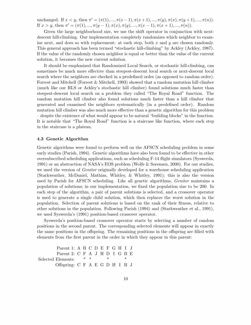
A first step to understanding how best to solve a problem is to assess what methods performbest. The results of running each of the algorithms are summarized in Tables 2 and 3respectively. For Genitor, randomized local search (RLS) and Squeaky Wheel Optimization(SWO), we report the best and mean value and the standard deviation observed over 30runs, with 8000 evaluations per run. For HBSS, the statistics are taken over 240,000 samples.Both Genitor and RLS were initialized from random permutations.

The best known values for the sum of overlaps (see Table 2) were obtained by runningGenitor with the population size increased to 400 and up to 50,000 evaluations; over hun-dreds of experiments using numerous algorithms, we have not found better solutions thanthese. When we report that an algorithm is better than Genitor it means that it was betterthan Genitor when both algorithms were limited to 8000 evaluations.

With the exception of Gooley’s algorithm, the CPU times are dominated by the numberof evaluations and therefore are similar. On a Dell Precision 650 with 3.06 GHz Xeonrunning Linux, 30 runs with 8000 evaluations per run take between 80 and 190 seconds (formore precise values, see (Barbulescu, Howe, Whitley, & Roberts, 2004a)). For HBSS, wedo not re-compute the flexibility of the unscheduled tasks every time we choose the nextrequest to be scheduled; therefore, the CPU times for HBSS are similar to the CPU timesfor the other algorithms.

The increase in the number of requests received for a day in the more recent R problemscauses an increase in the number and percentage of unscheduled requests. For the A prob-lems, at most eight task requests (or 2.5% of the tasks) are not scheduled; between 97.5%and 99% of the task requests are scheduled. For the R problems, at most 42 (or 8.7% ofthe tasks) are not scheduled; between 91.3% and 97.2% of the tasks requests are scheduled.

To compare algorithm performance, our statistical analyses include Genitor, SWO, andRLS. But to ensure fairness across the different algorithms we discuss in the paper, wealso include in our analyses the algorithms SWO1Move (a variant of SWO we explore inSection 6.5.2), and ALLS (a variant of Local Search we present in Section 7). We judgesignificant differences of the final evaluations using an ANOVA for the five algorithms oneach of the recent days of data. All ANOVAs came back significant, so we are justified inperforming pair-wise tests. We examined a single-tailed, two sample t-test as well as thenon-parametric Wilcoxon Rank Sum test. The Wilcoxon test significance results were the

12

same as the t-test except in two pairs, so we only present p-values from the t-test that areclose to our rejection threshold of p ≤ .005 per pair-wise test 6.

When minimizing conflicts, many of the algorithms find solutions with the best knownvalues. Pair-wise t-tests show that Genitor and RLS are not significantly different for R1,R3, and R4. Genitor significantly outperforms RLS on R2 (p = .0023) and R5 (p = .0017).SWO does not perform significantly different from RLS for all five days and significantlyoutperforms Genitor on R5. Genitor significantly outperforms SWO on R2 and R4; however,some adjusting of the parameters used to run SWO may fix this problem. It is in factsurprising how well SWO performs when minimizing the conflicts, given that we chose avery simple implementation, where all the tasks in conflict are moved forward with a fixeddistance. HBSS performs well for the A problems; however, it fails to find the best knownvalues for R1, R2 and R3. The original solution to the problem, Gooley’s, only computes asingle solution; its results can be improved by a sampling variant (see Section 6.2.1).

When minimizing overlaps, RLS finds the best known solutions for all but two of theproblems. It significantly outperforms Genitor on R1 and R2, significantly under-performson R3, and does not significantly differ in performance on R4 and R5. RLS and SWO do notperform significantly different except for R3 where RLS under-performs. SWO significantlyoutperforms Genitor on all five days. However, if run beyond 8000 evaluations, Genitorcontinues to improve the solution quality but SWO fails to find better solutions. HBSSfinds best known solutions to only a few problems. For comparison, we computed theoverlaps corresponding to the schedules built using Gooley’s algorithm and present themin the last column of Table 3; however, Gooley’s algorithm was not designed to minimizeoverlaps.

5.1 Progress Toward the Solution

SWO and Genitor apply different criteria to determine solution modifications. RLS ran-domly chooses the first shift resulting in an equally good or improving solution. To assessthe effect of the differences, we tracked the best value obtained so far when running thealgorithms. For each problem, we collected the best value found by SWO, Genitor and RLSin increments of 100 evaluations, for 8000 evaluations. We averaged these values over 30runs of SWO, RLS, and Genitor, respectively.

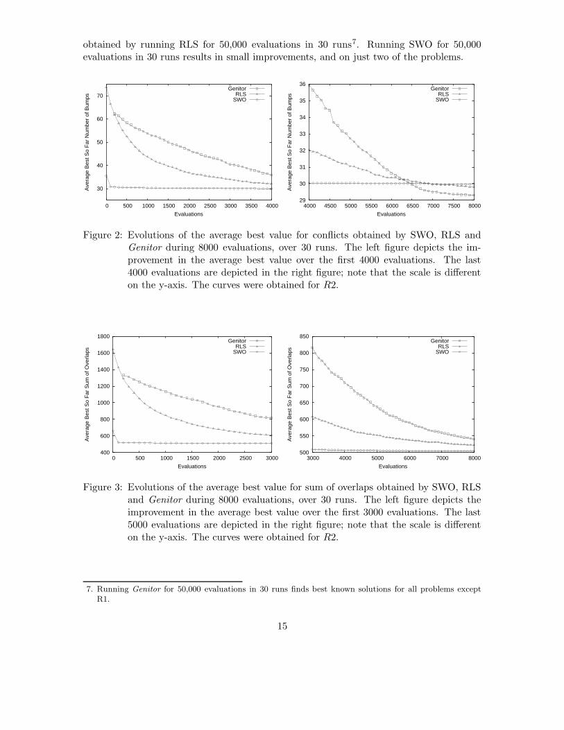
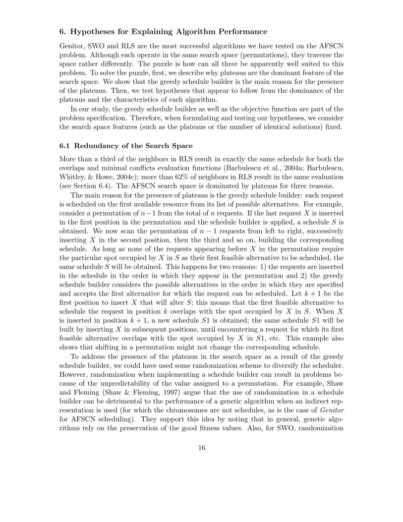
A typical example for each objective function is presented in Figures 2 and 3. For bothobjective functions, the curves are similar, as is relative performance. SWO quickly findsa good solution, then its performance levels off. RLS progresses quickly during the firsthalf of the search, while Genitor exacts smaller improvements. In the second half of thesearch though, RLS takes longer to find better solutions, while Genitor continues to steadilyprogress toward the best solution.

We observe two differences in the objective functions. First, when minimizing the num-ber of conflicts, both Genitor and RLS eventually equal or outperform SWO. For minimizingoverlaps, Genitor and RLS take longer to find good solutions; after 8000 evaluations, SWOfound the best solutions. Second, when minimizing the number of conflicts, toward the

6. Five algorithms imply, at worst, 10 pair-wise comparisons per day of data. To control the experiment-wise error, we use a (very conservative, but simple) Bonferroni adjustment; this adjustment is known toincrease the probability of a Type II error (favoring false acceptance that the distributions are similar).At α = .05, we judge two algorithms as significantly different if p ≤ .005.

13

Genitor RLS SWO HBSS GooleyDay Min Mean SD Min Mean SD Min Mean SD Min Mean SD

A1 8 8.6 0.49 8 8.7 0.46 8 8 0.0 8 9.76 0.46 11

A2 4 4 0 4 4.0 0 4 4 0.0 4 4.64 0.66 7

A3 3 3.03 0.18 3 3.1 0.3 3 3 0.0 3 3.37 0.54 5

A4 2 2.06 0.25 2 2.2 0.48 2 2.06 0.25 2 3.09 0.43 4

A5 4 4.1 0.3 4 4.7 0.46 4 4 0.0 4 4.27 0.45 5

A6 6 6.03 0.18 6 6.16 0.37 6 6 0.0 6 6.39 0.49 7

A7 6 6 0 6 6.06 0.25 6 6 0.0 6 7.35 0.54 6

R1 42 43.7 0.98 42 44.0 1.25 43 43.3 0.46 45 48.44 1.15 45

R2 29 29.3 0.46 29 29.8 0.71 29 29.96 0.18 32 35.16 1.27 36

R3 17 17.63 0.49 17 18.0 0.69 18 18 0.0 19 21.08 0.89 20

R4 28 28.03 0.18 28 28.36 0.66 28 28.3 0.46 28 31.22 1.10 29

R5 12 12.03 0.18 12 12.4 0.56 12 12 0 12 12.36 0.55 13

Table 2: Performance of Genitor, RLS, SWO, HBSS and Gooley’s algorithm in terms ofthe best and mean number of conflicts. Statistics for Genitor, local search andSWO are collected over 30 independent runs, with 8000 evaluations per run. ForHBSS, 240,000 samples are considered. Min numbers in boldface indicate bestknown values.

Genitor RLS SWO HBSS GooleyDay Min Mean SD Min Mean SD Min Mean SD Min Mean SD

A1 104 106.9 0.6 104 106.76 1.81 104 104 0.0 128 158.7 28.7 687

A2 13 13 0.0 13 13.66 2.59 13 13.4 2.0 43 70.1 31.1 535

A3 28 28.4 1.2 28 30.7 4.31 28 28.1 0.6 28 52.5 16.9 217

A4 9 9.2 0.7 9 10.16 2.39 9 13.3 7.8 9 45.7 13.0 216

A5 30 30.4 0.5 30 30.83 1.36 30 30 0.0 50 82.6 13.2 231

A6 45 45.1 0.4 45 45.13 0.5 45 45.1 0.3 45 65.5 16.8 152

A7 46 46.1 0.6 46 49.96 5.95 46 46 0.0 83 126.4 12.5 260

R1 913 987.8 40.8 798 848.66 38.42 798 841.4 14.0 1105 1242.6 42.1 1713

R2 519 540.7 13.3 494 521.9 20.28 491 503.8 6.5 598 681.8 27.0 1047

R3 275 292.3 10.9 250 327.53 55.34 265 270.1 2.8 416 571.0 46.0 899

R4 738 755.4 10.3 725 755.46 25.42 731 736.2 3.0 827 978.4 28.7 1288

R5 146 146.5 1.9 146 147.1 2.85 146 146.0 0.0 146 164.4 10.8 198

Table 3: Performance of Genitor, local search, SWO, HBSS and Gooley’s algorithm interms of the best and mean sum of overlaps. All statistics are collected over 30independent runs, with 8000 evaluations per run. For HBSS, 240,000 samples areconsidered. Min numbers in boldface indicate best known values.

end of the run, Genitor outperforms RLS. When minimizing overlaps, RLS performs betterthan Genitor. Best known solutions for the R problems when minimizing overlaps can be

14

obtained by running RLS for 50,000 evaluations in 30 runs7. Running SWO for 50,000evaluations in 30 runs results in small improvements, and on just two of the problems.

30

40

50

60

70

0 500 1000 1500 2000 2500 3000 3500 4000

Ave

rage

Bes

t So

Far

Num

ber

of B

umps

Evaluations

GenitorRLS

SWO

29

30

31

32

33

34

35

36

4000 4500 5000 5500 6000 6500 7000 7500 8000

Ave

rage

Bes

t So

Far

Num

ber

of B

umps

Evaluations

GenitorRLS

SWO

Figure 2: Evolutions of the average best value for conflicts obtained by SWO, RLS andGenitor during 8000 evaluations, over 30 runs. The left figure depicts the im-provement in the average best value over the first 4000 evaluations. The last4000 evaluations are depicted in the right figure; note that the scale is differenton the y-axis. The curves were obtained for R2.

400

600

800

1000

1200

1400

1600

1800

0 500 1000 1500 2000 2500 3000

Ave

rage

Bes

t So

Far

Sum

of O

verla

ps

Evaluations

GenitorRLS

SWO

500

550

600

650

700

750

800

850

3000 4000 5000 6000 7000 8000

Ave

rage

Bes

t So

Far

Sum

of O

verla

ps

Evaluations

GenitorRLS

SWO

Figure 3: Evolutions of the average best value for sum of overlaps obtained by SWO, RLSand Genitor during 8000 evaluations, over 30 runs. The left figure depicts theimprovement in the average best value over the first 3000 evaluations. The last5000 evaluations are depicted in the right figure; note that the scale is differenton the y-axis. The curves were obtained for R2.

7. Running Genitor for 50,000 evaluations in 30 runs finds best known solutions for all problems exceptR1.

15

6. Hypotheses for Explaining Algorithm Performance

Genitor, SWO and RLS are the most successful algorithms we have tested on the AFSCNproblem. Although each operate in the same search space (permutations), they traverse thespace rather differently. The puzzle is how can all three be apparently well suited to thisproblem. To solve the puzzle, first, we describe why plateaus are the dominant feature of thesearch space. We show that the greedy schedule builder is the main reason for the presenceof the plateaus. Then, we test hypotheses that appear to follow from the dominance of theplateaus and the characteristics of each algorithm.

In our study, the greedy schedule builder as well as the objective function are part of theproblem specification. Therefore, when formulating and testing our hypotheses, we considerthe search space features (such as the plateaus or the number of identical solutions) fixed.

6.1 Redundancy of the Search Space

More than a third of the neighbors in RLS result in exactly the same schedule for both theoverlaps and minimal conflicts evaluation functions (Barbulescu et al., 2004a; Barbulescu,Whitley, & Howe, 2004c); more than 62% of neighbors in RLS result in the same evaluation(see Section 6.4). The AFSCN search space is dominated by plateaus for three reasons.

The main reason for the presence of plateaus is the greedy schedule builder: each requestis scheduled on the first available resource from its list of possible alternatives. For example,consider a permutation of n−1 from the total of n requests. If the last request X is insertedin the first position in the permutation and the schedule builder is applied, a schedule S isobtained. We now scan the permutation of n − 1 requests from left to right, successivelyinserting X in the second position, then the third and so on, building the correspondingschedule. As long as none of the requests appearing before X in the permutation requirethe particular spot occupied by X in S as their first feasible alternative to be scheduled, thesame schedule S will be obtained. This happens for two reasons: 1) the requests are insertedin the schedule in the order in which they appear in the permutation and 2) the greedyschedule builder considers the possible alternatives in the order in which they are specifiedand accepts the first alternative for which the request can be scheduled. Let k + 1 be thefirst position to insert X that will alter S; this means that the first feasible alternative toschedule the request in position k overlaps with the spot occupied by X in S. When Xis inserted in position k + 1, a new schedule S1 is obtained; the same schedule S1 will bebuilt by inserting X in subsequent positions, until encountering a request for which its firstfeasible alternative overlaps with the spot occupied by X in S1, etc. This example alsoshows that shifting in a permutation might not change the corresponding schedule.

To address the presence of the plateaus in the search space as a result of the greedyschedule builder, we could have used some randomization scheme to diversify the scheduler.However, randomization when implementing a schedule builder can result in problems be-cause of the unpredictability of the value assigned to a permutation. For example, Shawand Fleming (Shaw & Fleming, 1997) argue that the use of randomization in a schedulebuilder can be detrimental to the performance of a genetic algorithm when an indirect rep-resentation is used (for which the chromosomes are not schedules, as is the case of Genitorfor AFSCN scheduling). They support this idea by noting that in general, genetic algo-rithms rely on the preservation of the good fitness values. Also, for SWO, randomization

16

in the schedule builder changes the significance of reprioritization from one iteration tothe next one. If the scheduler is randomized, the new order of requests is very likely toresult in a schedule that is not the “repaired version” of the previous one. If the samepermutation of requests can be transformed into multiple different schedules because of thenondeterministic nature of the scheduler, the SWO mechanism will not operate as intended.

A second reason for the plateaus in the search space is the presence of time windows.If a request X needs to be scheduled sometime at the end of the day, even if it appearsin the beginning of the permutation, it will still occupy a spot in the schedule towards theend (assuming it can be scheduled) and therefore, after most of the other requests (whichappeared after X in the permutation).

A third reason is the discretization of the objective function. Clearly, the range ofconflicts is a small number of discrete values (with a weak upper bound of the numberof tasks). The range for overlaps is still discrete but is larger than for conflicts. Usingoverlaps as the evaluation function, approximately 20 times more unique objective functionvalues are observed during search compared to searches where the objective is to minimizeconflicts. The effect of the discretization can be seen in the differing results using the twoobjective functions. Thus, one reason for including both in our studies is to show some ofthe effects of the discretization.

6.2 Does Genitor Learn Patterns of Request Ordering?

We hypothesize that Genitor performs well because it discovers which interactions betweenthe requests matter. We examine sets of permutations that correspond to schedules with thebest known values and identify chains of common request orderings in these permutations(similar in spirit to the notion of backbone in SAT (Singer et al., 2000)). The presence ofsuch chains would support the hypothesis that Genitor is discovering patterns of requestorderings. This is a classic building block hypothesis: some pattern that is present inparent solutions contributes to their evaluation in some critical way; these patterns arethen recombined and inherited during genetic recombination (Goldberg, 1989).

6.2.1 Common Request Orderings

One of the particular characteristics of the AFSCN scheduling problem is the presence oftwo categories of requests. The low altitude requests have fixed start times and specify onlyone to three alternative resources. The high altitude requests implicitly specify multiplepossible start times (because their corresponding time windows are usually longer than theduration that needs to be scheduled) and up to 14 possible alternative resources. Clearlythe low altitude requests are more constrained. This suggests a possible solution pattern,where low altitude requests would be scheduled first.

To explore the viability of such a pattern, we implemented a heuristic that schedulesthe low altitude requests before the high altitude ones; we call this heuristic the “splitheuristic”. We incorporated the split heuristic in the schedule builder: given a permutationof requests, the new schedule builder first schedules only the low altitude requests, in theorder in which they appear in the permutation. Without modifying the position of the lowaltitude requests in the schedule, the high altitude requests are then inserted in the schedule,again in the order in which they appear in the permutation. The idea of scheduling low

17

Best Random Sampling-SDay Known Min Mean Stdev

A1 8 8 8.2 0.41A2 4 4 4 0A3 3 3 3.3 0.46A4 2 2 2.43 0.51A5 4 4 4.66 0.48A6 6 6 6.5 0.51A7 6 6 6 0

Table 4: Results of running random sampling with the split heuristic (Random Sampling-S) in 30 experiments, by generating 100 random permutations per experiment forminimizing conflicts.

altitude requests before high altitude requests was the basis of Gooley’s heuristic (Gooley,1993). Also, the split heuristic is similar to the contention measures defined in (Frank et al.,2001).

Some of the results we obtained using the split heuristic are surprising: when minimizingconflicts, best known valued schedules can be obtained quickly for the A problems by simplysampling a small number of random permutations. The results obtained by sampling 100random permutations are shown in Table 4.

While such performance of the split heuristic does not transfer to the R problems or whenminimizing the number of overlaps, the results in Table 4 offer some indication of a possiblerequest ordering pattern in good solutions. Is Genitor in fact performing well because itdiscovers that scheduling low before high altitude requests produces good solutions?

As a more general explanation for Genitor’s performance, we hypothesize that Genitoris discovering patterns of request ordering: certain requests that must come before otherrequests. To test this, we identify common request orderings present in solutions obtainedfrom multiple runs of Genitor. We ran 1000 trials of Genitor and selected the solutionscorresponding to best known values. First, we checked for request orderings of the form“requestA before requestB” which appear in all the permutations corresponding to bestknown solutions for the A problems and corresponding to good solutions for the R problems.The results are summarized in Table 5. The Sol. Value columns show the value of thesolutions chosen for the analysis (out of 1000 solutions). The number of solutions (out of1000) corresponding to the chosen value is shown in the # of Solutions columns. Whenanalyzing the common pairs of request orderings for minimizing the number of conflicts, weobserved that most pairs specified a low altitude request appearing before a high altitudeone. Therefore, we separate the pairs into two categories: pairs specifying a low altituderequest before a high altitude requests (column: (Low,High) Pair Count) and the rest(column: Other Pairs). For the A problems, the results clearly show that most commonpairs of ordering requests specify a low altitude request before a high altitude request. Forthe R problems, more “Other pairs” can be observed. In part, this might be due to thesmall number of solutions corresponding to the same value (only 25 out of 1000 for R1 when

18

minimizing conflicts). The small number of solutions corresponding to the same value is alsothe reason for the big pair counts reported when minimizing overlaps for the R problems.

We know that for the A problems the split heuristic results in best-known solutions whenminimizing conflicts; therefore, the results in Table 5 are somewhat surprising. We expectedto see more low-before-high common pairs of requests for the A problems when minimizingthe number of conflicts; instead, the pair counts are similar for the two objective functions.Genitor seems to discover patterns of request interaction, and most of them specify a lowaltitude request before a high altitude request.

The results in Table 5 are heavily biased by the number of solutions considered8. Indeed,let s denote the number of solutions of identical value (the number in column # of Solutions).Also, let n denote the total number of requests. Suppose there are no preferences of orderingsbetween the tasks in good solutions. For a request ordering A before B there is a probabilityof 1/2 that it will be present in one of the solutions, and therefore, a probability of 1/2s thatit will be present in all s solutions. Given that there exist n ∗ (n− 1) possible precedences,the expected number of common orderings if no preferences of orderings between tasksexist is n(n − 1)/2s. For the A problems and for R5, s >= 420. The expected numberof common orderings assuming no preferences of orderings between tasks exist is smallerthan n(n−1)/2420, which is negligible. Therefore, the number of actually detected commonprecedences (approximately 30 to 125 for low before high pairs and anywhere from 1 to17 for the others) seem to be actual request patterns. This is also the case for the otherR problems. Indeed, for example, for R1, when s = 15, the expected number of commonorderings if no preferences of orderings between tasks exist is 7.1, while the number ofactually detected precedences is 2815 for low before high and 1222 for the other pairs.

The experiment above found evidence to support the hypothesis that Genitor solutionsexhibit patterns of low before high altitude requests. Given this result, we next investigateif the “split” heuristic (always scheduling low before high altitude requests) can enhance theperformance of Genitor. To answer this question, we run a second experiment using Genitor,where the split heuristic schedule builder is used to evaluate every schedule generated duringthe search.

Table 6 shows the results of using the split heuristic with Genitor on the R problems.Genitor with the split heuristic fails to find the best-known solution for R2 and R3. Thisis not surprising: in fact, we can show that scheduling all the low altitude requests beforehigh altitude requests may prevent finding the optimal solutions.

The results for minimizing sum of overlaps are shown in Table 7. With the exceptionof A3, A4 and A6, Genitor using the split heuristic fails to find best known solutions forthe A problems. For the R problems, using the split heuristic actually improves the resultsobtained by Genitor for R1 and R2; it should be noted that the R1 and R2 solutions arenot as good as those found by RLS using 8000 evaluation however. Thus a search thathybridizes the genetic algorithm with a schedule builder using the split heuristic sometimeshelps and sometimes hurts in terms of finding good solutions.

We attempted to identify longer chains of common request ordering. We were not suc-cessful: while Genitor does seem to discover patterns of request ordering, multiple differentpatterns of request orderings can result in the same conflicts (or even the same schedule).

8. We wish to thank the anonymous reviewer of an earlier version of this work for this insightful observation;the rest of the paragraph is based on his/her comments.

19

Minimizing Conflicts Minimizing OverlapsSol. # of (Low,High) Other Sol. # of (Low,High) Other

Day Value Solutions Pair Count Pairs Value Solutions Pair Count PairsA1 8 420 77 1 107 922 78 7A2 4 1000 29 1 13 959 50 3A3 3 936 86 1 28 833 72 10A4 2 937 132 3 9 912 117 5A5 4 862 45 9 30 646 48 17A6 6 967 101 10 45 817 124 10A7 6 1000 43 3 46 891 57 11

R1 43 25 2166 149 947 15 2815 1222R2 29 573 64 5 530 30 1597 308R3 17 470 78 21 285 37 1185 400R4 28 974 54 16 744 31 1240 347R5 12 892 57 10 146 722 109 11

Table 5: Common pairs of request orderings found in permutations corresponding to bestknown/good Genitor solutions for both objective functions.

Genitor with NewBest Schedule Builder

Day Known Min Mean Stdev

R1 42 42 42 0

R2 29 30 30 0

R3 17 18 18 0

R4 28 28 28 0

R5 12 12 12 0

Table 6: Minimizing conflicts: results of running Genitor with the split heuristic in 30 trials,with 8000 evaluations per trial.

We could think of these patterns as building blocks. Genitor identifies good building blocks(orderings of requests resulting in good partial solutions) and propagates them into the finalpopulation (and the final solution). Such patterns are essential in building a good solution.However, the patterns are not ubiquitous (not all of them are necessary) and, therefore,attempts to identify them across different solutions produced by Genitor have failed.

6.3 Is SWO’s Performance Due to Initialization?

The graphs of search progress for SWO (Figures 2 and 3) show that it starts with muchbetter solutions than do the other algorithms. The initial greedy solution for SWO trans-lated into best known values for five problems (A2, A3, A5, A6 and R5) when minimizingthe number of conflicts and for two problems (A6 and R5) when minimizing overlaps.

20

Genitor with NewBest Schedule Builder

Day Known Min Mean Stdev

A1 104 119 119 0.0

A2 13 43 43 0.0

A3 28 28 28 0.0

A4 9 9 9 0.0

A5 30 50 50 0.0

A6 45 45 45 0.0

A7 46 69 69 0.0

R1 774 907 924.33 6.01

R2 486 513 516.63 5.03

R3 250 276 276.03 0.18

R4 725 752 752.03 0.0

R5 146 146 146 0.0

Table 7: Minimizing sum of overlaps: results of running Genitor with the split heuristicusing the split heuristic schedule builder to evaluate each schedule. The resultsare based on 30 experiments, with 8000 evaluations per experiment.

How important is the initial greedy permutation for SWO? To answer this question, wereplaced the initial greedy permutation (and its variations in subsequent iterations of SWO)with random permutations and then used the SWO mechanism to iteratively move forwardthe requests in conflict. We call this version of SWO RandomStartSWO. We compared theresults produced by RandomStartSWO with results from SWO to assess the effects of theinitial greedy solution. The results produced by RandomStartSWO are presented in Table 8.With the exception of R2, when minimizing the number of conflicts, best known values areobtained by RandomStartSWO for all the problems. In fact, for R1 and R3, the best resultsobtained are slightly better than the best found by SWO. When minimizing the sum ofoverlaps, best known values are obtained for the A problems; only for the R problems, theperformance of SWO worsens when it is initialized with a random permutation. However,RandomStartSWO still performs better or as well as Genitor (with the exception of R2when minimizing the number of conflicts and R5 for overlaps) for both objective functions.These results suggest that the initial greedy permutation is not the main performance factorfor SWO: the performance of RandomStartSWO is competitive with that of Genitor.

6.4 Is RLS Performing a Random Walk?

RLS spends most of the time traversing plateaus in the search space (by accepting non-improving moves). In this section, we study the average length of random walks on theplateaus encountered by local search. We show that as search progresses the random walksbecome longer before finding an improvement, mirroring the progress of RLS. We note thata similar phenomenon has been observed for SAT (Frank, Cheeseman, & Stutz, 1997).

21

Day Minimizing Conflicts Minimizing OverlapsBest Known Min Mean Stdev Best Known Min Mean Stdev

A1 8 8 8.0 0.0 104 104 104.46 0.68A2 4 4 4.0 0.0 13 13 13.83 1.89A3 3 3 3.16 0.46 28 28 30.13 1.96A4 2 2 2.13 0.34 9 9 11.66 1.39A5 4 4 4.03 0.18 30 30 30.33 0.54A6 6 6 6.23 0.63 45 45 48.3 6.63A7 6 6 6.0 0.0 46 46 46.26 0.45

R1 42 42 43.43 0.56 774 851 889.96 31.34R2 29 30 30.1 0.3 486 503 522.2 9.8R3 17 17 17.73 0.44 250 268 276.4 4.19R4 28 28 28.53 0.57 725 738 758.26 12.27R5 12 12 13.1 0.4 146 147 151.03 2.19

Table 8: Statistics for the results obtained in 30 runs of SWO initialized with randompermutations (i.e., RandomStartSWO), with 8000 evaluations per run. The meanand best value from 30 runs as well as the standard deviations are shown. Foreach problem, the best known solution for each objective function is also included.

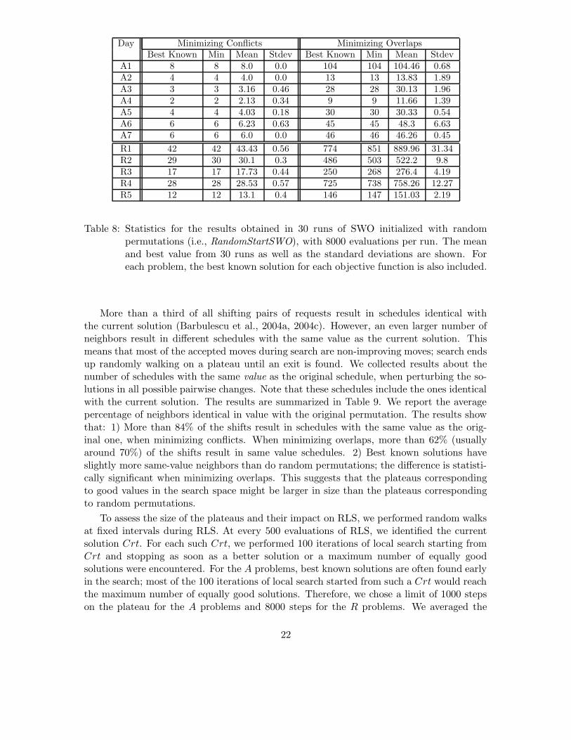
More than a third of all shifting pairs of requests result in schedules identical withthe current solution (Barbulescu et al., 2004a, 2004c). However, an even larger number ofneighbors result in different schedules with the same value as the current solution. Thismeans that most of the accepted moves during search are non-improving moves; search endsup randomly walking on a plateau until an exit is found. We collected results about thenumber of schedules with the same value as the original schedule, when perturbing the so-lutions in all possible pairwise changes. Note that these schedules include the ones identicalwith the current solution. The results are summarized in Table 9. We report the averagepercentage of neighbors identical in value with the original permutation. The results showthat: 1) More than 84% of the shifts result in schedules with the same value as the orig-inal one, when minimizing conflicts. When minimizing overlaps, more than 62% (usuallyaround 70%) of the shifts result in same value schedules. 2) Best known solutions haveslightly more same-value neighbors than do random permutations; the difference is statisti-cally significant when minimizing overlaps. This suggests that the plateaus correspondingto good values in the search space might be larger in size than the plateaus correspondingto random permutations.

To assess the size of the plateaus and their impact on RLS, we performed random walksat fixed intervals during RLS. At every 500 evaluations of RLS, we identified the currentsolution Crt. For each such Crt, we performed 100 iterations of local search starting fromCrt and stopping as soon as a better solution or a maximum number of equally goodsolutions were encountered. For the A problems, best known solutions are often found earlyin the search; most of the 100 iterations of local search started from such a Crt would reachthe maximum number of equally good solutions. Therefore, we chose a limit of 1000 stepson the plateau for the A problems and 8000 steps for the R problems. We averaged the

22

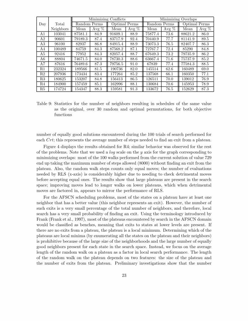
Minimizing Conflicts Minimizing OverlapsDay Total Random Perms Optimal Perms Random Perms Optimal Perms

Neighbors Mean Avg % Mean Avg % Mean Avg % Mean Avg %A1 103041 87581.1 84.9 91609.1 88.9 75877.4 73.6 88621.2 86.0A2 90601 79189.3 87.4 83717.9 92.4 70440.9 77.7 81141.9 89.5A3 96100 82937 86.8 84915.4 88.9 73073.3 76.5 82407.7 86.3A4 100489 84759 84.3 87568.2 87.1 72767.7 72.4 85290 84.8A5 92416 77952 84.3 82057.4 88.7 67649.3 73.2 79735.9 86.2A6 88804 74671.5 84.0 78730.3 88.6 63667.4 71.6 75737.9 85.2A7 87616 76489.6 87.3 79756.5 91.0 67839 77.4 77584.3 88.5R1 232324 189566 81.5 190736 82.0 145514 62.6 160489 69.0R2 207936 173434 83.4 177264 85.2 137568 66.1 160350 77.1R3 180625 153207 84.8 156413 86.5 126511 70.0 139012 76.9R4 184900 157459 85.1 162996 88.1 130684 70.6 145953 78.9R5 174724 154347 88.3 159581 91.3 133672 76.5 152629 87.3

Table 9: Statistics for the number of neighbors resulting in schedules of the same valueas the original, over 30 random and optimal permutations, for both objectivefunctions

number of equally good solutions encountered during the 100 trials of search performed foreach Crt; this represents the average number of steps needed to find an exit from a plateau.

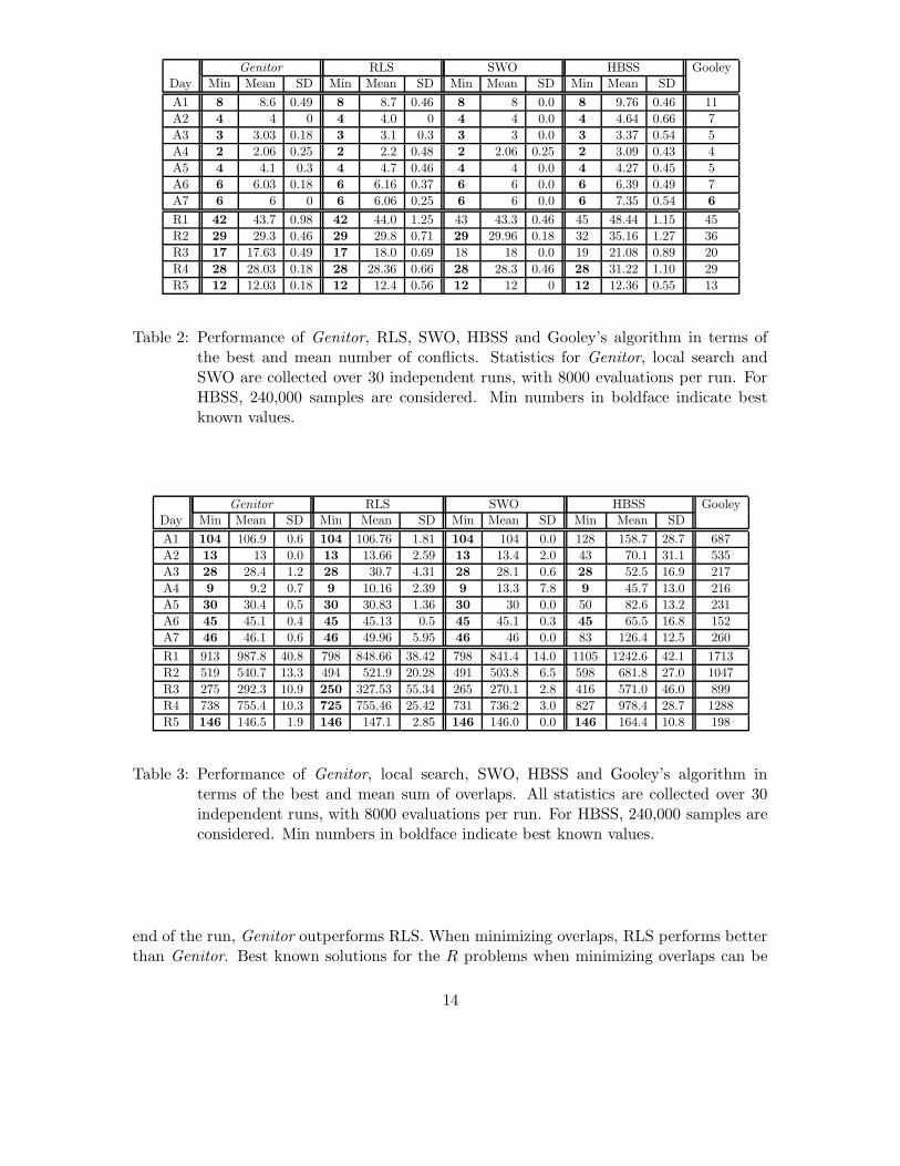
Figure 4 displays the results obtained for R4; similar behavior was observed for the restof the problems. Note that we used a log scale on the y axis for the graph corresponding tominimizing overlaps: most of the 100 walks performed from the current solution of value 729end up taking the maximum number of steps allowed (8000) without finding an exit from theplateau. Also, the random walk steps counts only equal moves; the number of evaluationsneeded by RLS (x-axis) is considerably higher due to needing to check detrimental movesbefore accepting equal ones. The results show that large plateaus are present in the searchspace; improving moves lead to longer walks on lower plateaus, which when detrimentalmoves are factored in, appears to mirror the performance of RLS.

For the AFSCN scheduling problems, most of the states on a plateau have at least oneneighbor that has a better value (this neighbor represents an exit). However, the number ofsuch exits is a very small percentage of the total number of neighbors, and therefore, localsearch has a very small probability of finding an exit. Using the terminology introduced byFrank (Frank et al., 1997), most of the plateaus encountered by search in the AFSCN domainwould be classified as benches, meaning that exits to states at lower levels are present. Ifthere are no exits from a plateau, the plateau is a local minimum. Determining which of theplateaus are local minima (by enumerating all the states on the plateau and their neighbors)is prohibitive because of the large size of the neighborhoods and the large number of equallygood neighbors present for each state in the search space. Instead, we focus on the averagelength of the random walk on a plateau as a factor in local search performance. The lengthof the random walk on the plateau depends on two features: the size of the plateau andthe number of exits from the plateau. Preliminary investigations show that the number

23

0

200

400

600

800

1000

1200

1400

1600

1800

0 1000 2000 3000 4000 5000 6000 7000 8000

Ave

rage

num

ber

step

s pl

atea

u

Evals

6345

33

3231

30

30

30

30

30

30

29

2929 29

29

LS

1

10

100

1000

10000

0 1000 2000 3000 4000 5000 6000 7000 8000

Ave

rage

num

ber

step

s pl

atea

u

Evals

1450

1068 944

864

814 794

786 786

782

777751

740

729 729 729 729LS

Figure 4: Average length of the random walk on plateaus when minimizing conflicts (left)or overlaps (right) for a single local search run on R4. The labels on the graphsrepresent the value of the current solution. Note the log scale on the y axis forthe graph corresponding to minimizing overlaps. The best known value for thisproblem is 28 when minimizing conflicts and 725 when minimizing overlaps.

of improving neighbors for a solution decreases as the solution becomes better - thereforewe conjecture that there are more exits from higher level plateaus than from the lowerlevel ones. This would account for the trend of needing more steps to find an exit whenmoving to lower plateaus (corresponding to better solutions). It is also possible that theplateaus corresponding to better solutions are larger in size; however, enumerating all thestates on a plateau for the AFSCN domain is impractical (following a technique developedby Frank (Frank et al., 1997), just the first iteration of breadth first search would result inapproximately 0.8 ∗ (n − 1)2 states on the same plateau).

6.5 Are Long Leaps Instrumental?

As in other problems with many plateaus (e.g., SAT), we hypothesize that long leaps inthe search space are instrumental for an algorithm to perform well on AFSCN scheduling.SWO is moving forward multiple requests that are known to be problematic. The positioncrossover mechanism in Genitor can be viewed as applying multiple consecutive shifts to thefirst parent, such that the requests in the selected positions of the second parent are movedinto those selected positions of the first. In a sense, each time the crossover operator isapplied, a multiple move is proposed for the first parent. We hypothesize that this multiplemove mechanism present in both SWO and Genitor allows them to make long leaps in thespace and thus reach solutions fast.

Note that if we knew exactly which requests to move, moving forward only a smallnumber of requests (or even only one) might be all that is needed to reach the solutionsquickly. Finding which requests to move is difficult; in fact we studied the performance ofa more informed move operator that only moves requests into positions which guaranteeschedule changes (see (Roberts, Whitley, Howe, & Barbulescu, 2005)). We found surprisingresults: the more informed move operator performs worse than the random unrestricted

24

Genitor-10 Genitor-50 Genitor-100 Genitor-150Day Min Mean Stdev Min Mean Stdev Min Mean Stdev Min Mean Stdev

A1 11 14.93 1.94 8 9.26 0.63 8 8.66 0.47 8 8.53 0.5

A2 5 7.13 1.77 4 4.03 0.18 4 4.0 0.0 4 4.0 0.0

A3 6 10.4 2.12 3 3.36 0.55 3 3.0 0.0 3 3.0 0.0

A4 5 10.66 2.7 2 3.13 0.81 2 2.23 0.50 2 2.06 0.25

A5 5 9.6 2.29 4 4.73 0.69 4 4.26 0.44 4 4.2 0.4

A6 9 12.63 1.8 6 6.83 0.94 6 6.03 0.18 6 6.06 0.25

A7 8 10.6 1.75 6 6.1 0.30 6 6.0 0.0 6 6.0 0.0

R1 57 66.5 4.38 47 52.0 2.82 42 45.83 1.68 42 44.36 1.24

R2 42 47.16 3.59 32 34.53 1.47 29 30.0 0.78 29 29.6 0.56

R3 27 31.1 2.41 19 21.6 1.67 17 18.03 0.61 17 17.63 0.61

R4 36 41.9 2.74 28 30.96 2.04 28 28.33 0.47 28 28.1 0.4

R5 13 20.73 2.53 12 13.23 0.81 12 12.46 0.62 12 12.2 0.4

Table 10: Performance of Genitor-k, where k represents the fixed number of selected posi-tions for Syswerda’s position crossover, in terms of the best and mean numberof conflicts. Statistics are taken over 30 independent runs, with 8000 evaluationsper run. Min numbers in boldface indicate best known values.

shift employed by RLS. We argue that the multiple moves are a desired algorithm featureas they make it more likely that one of the moves will be the right one.

To investigate our hypothesis about the role of multiple moves when traversing thesearch space, we perform experiments with a variable number of moves at each step forboth Genitor and SWO. For Genitor, we vary the number of crossover positions allowed.For SWO, we vary the number of requests in conflict moved forward.

6.5.1 The Effect of Multiple Moves on Genitor

To test the effect of multiple moves on Genitor, we change Syswerda’s position crossoverby imposing a fixed number of selected positions in the second parent (see Section 4.3 for adescription of Syswerda’s position crossover). We call this implementation Genitor-k wherek is the number of selected positions. Recall that our implementation of Syswerda’s positioncrossover randomly selects a number of positions that is larger than one third and smallerthan two thirds of the total number of positions. If multiple moves are indeed a factor inperformance then increasing the number of selected positions up to a point should result infinding improvements faster. If only a few positions are selected, the offspring will be verysimilar to the first parent. If the number of selected positions is large, close to the numberof total requests, the offspring will be very similar to the second parent. If the offspring isvery similar to one of its two parents, we expect a slower rate in finding improvements to thecurrent best solution. Therefore, both for small and for large k values, we expect Genitor-kto find improvements at a much slower rate than Genitor or Genitor-k with average k values(values closer to half of the number of requests).

For our study, we run Genitor-k with k=10, 50, 100, 150, 200, 250, 300 and 350. Weallowed 8000 evaluations per run and performed 30 runs for each problem. The results aresummarized in Tables 10 and 11 for minimizing the number of conflicts and in Tables 12

25

Genitor-200 Genitor-250 Genitor-300 Genitor-350Day Min Mean Stdev Min Mean Stdev Min Mean Stdev Min Mean Stdev

A1 8 8.56 0.56 8 8.9 0.3 9 11.8 1.66 - - -

A2 4 4.0 0.0 4 4.03 0.18 9 13.66 1.76 - - -

A3 3 3.0 0.0 3 3.06 0.25 4 9.2 2.1 - - -

A4 2 2.0 0.0 2 3.13 0.81 4 8.56 1.94 - - -

A5 4 4.3 0.46 4 4.73 0.58 10 13.86 2.14 - - -

A6 6 6.06 0.25 6 6.5 0.57 - - - - - -

A7 6 6.0 0.0 6 6.06 0.25 - - - - - -

R1 42 44.03 1.15 42 44.03 0.85 43 44.26 1.01 43 45.46 1.22

R2 29 29.36 0.49 29 29.4 0.49 29 29.7 0.59 29 30.13 0.86

R3 17 17.33 0.4 17 17.7 0.65 17 17.73 0.58 17 18.63 0.8

R4 28 28.03 0.18 28 28 0.0 28 28.03 0.18 28 28.63 0.71

R5 12 12.1 0.3 12 12.06 0.25 12 12.16 0.37 12 12.6 0.81

Table 11: Performance of Genitor-k, where k represents the fixed number of selected posi-tions for Syswerda’s position crossover, in terms of the best and mean numberof conflicts. Statistics are collected over 30 independent runs, with 8000 eval-uations per run. Min numbers in boldface indicate best known values. Thedashes indicate that the permutation solutions for A6 and A7 are shorter than300 (299 and 297, respectively), and therefore cannot select 300 positions in thesepermutations.

Genitor-10 Genitor-50 Genitor-100 Genitor-150Day Min Mean Stdev Min Mean Stdev Min Mean Stdev Min Mean Stdev

A1 149 221.53 38.85 107 115.76 11.53 107 107.2 0.76 107 107.1 0.54

A2 30 69.66 29.22 13 15.73 3.86 13 13.43 1.54 13 13.03 0.18

A3 51 122.86 36.12 28 36.26 8.19 28 28.9 1.72 28 28.16 0.64

A4 59 124.5 42.25 9 19.36 9.3 9 9.23 0.72 9 9.06 0.36

A5 43 90.7 32.01 30 33.06 3.62 30 30.36 0.96 30 30.43 0.5

A6 94 145.06 33.12 45 49.6 5.54 45 45.36 0.8 45 45.16 0.46

A7 67 115.66 27.96 46 51.7 7.89 46 46.5 2.23 46 47.63 3.9

R1 1321 1531.13 107.35 987 1139.5 76.57 914 991.13 38.19 915 963.96 26.89

R2 743 961.13 81.62 557 643.86 50.0 515 549.1 18.8 516 540.86 15.82

R3 480 652.5 90.37 319 391.56 47.31 268 305.3 20.63 269 291.3 13.36

R4 866 1069.23 74.65 768 840.23 38.79 735 757.43 15.95 731 752.7 14.07

R5 208 309.03 46.3 146 172.13 18.18 146 151.53 7.63 146 148.23 5.26

Table 12: Performance of Genitor-k, where k represents the fixed number of selected posi-tions for Syswerda’s position crossover, in terms of the best and mean number ofconflicts. Statistics are collected over 30 independent runs, with 8000 evaluationsper run. Min numbers in boldface indicate best known values.

and 13 for minimizing the sum of overlaps. Note that for A6 and A7 there are 299 and 297requests to schedule respectively. Therefore Genitor-k with k = 300 and k = 350 cannot berun for these two problems. Also note that for example, k = 200 does not mean that there

26

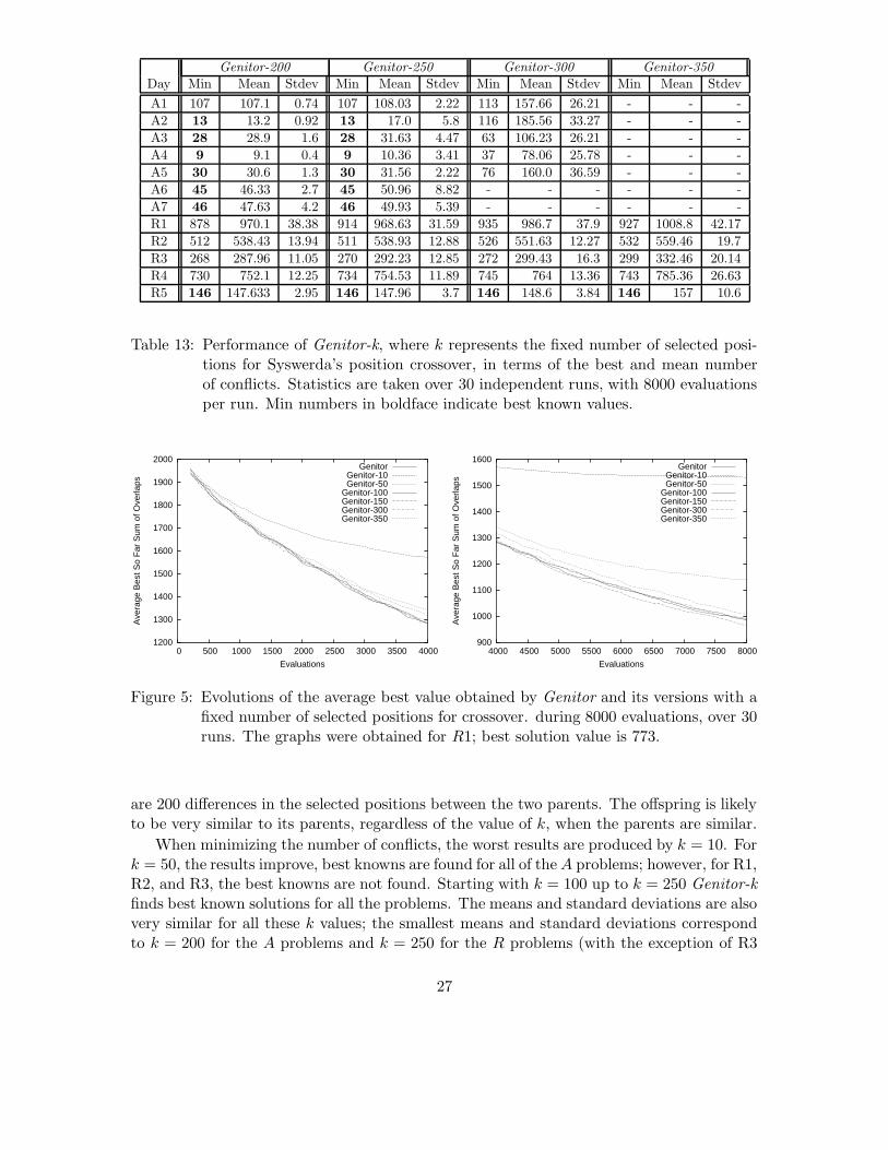
Genitor-200 Genitor-250 Genitor-300 Genitor-350Day Min Mean Stdev Min Mean Stdev Min Mean Stdev Min Mean Stdev

A1 107 107.1 0.74 107 108.03 2.22 113 157.66 26.21 - - -

A2 13 13.2 0.92 13 17.0 5.8 116 185.56 33.27 - - -

A3 28 28.9 1.6 28 31.63 4.47 63 106.23 26.21 - - -

A4 9 9.1 0.4 9 10.36 3.41 37 78.06 25.78 - - -

A5 30 30.6 1.3 30 31.56 2.22 76 160.0 36.59 - - -

A6 45 46.33 2.7 45 50.96 8.82 - - - - - -

A7 46 47.63 4.2 46 49.93 5.39 - - - - - -

R1 878 970.1 38.38 914 968.63 31.59 935 986.7 37.9 927 1008.8 42.17

R2 512 538.43 13.94 511 538.93 12.88 526 551.63 12.27 532 559.46 19.7

R3 268 287.96 11.05 270 292.23 12.85 272 299.43 16.3 299 332.46 20.14

R4 730 752.1 12.25 734 754.53 11.89 745 764 13.36 743 785.36 26.63

R5 146 147.633 2.95 146 147.96 3.7 146 148.6 3.84 146 157 10.6

Table 13: Performance of Genitor-k, where k represents the fixed number of selected posi-tions for Syswerda’s position crossover, in terms of the best and mean numberof conflicts. Statistics are taken over 30 independent runs, with 8000 evaluationsper run. Min numbers in boldface indicate best known values.

1200

1300

1400

1500

1600

1700

1800

1900

2000

0 500 1000 1500 2000 2500 3000 3500 4000

Ave

rage

Bes

t So

Far

Sum

of O

verla

ps

Evaluations

GenitorGenitor-10Genitor-50

Genitor-100Genitor-150Genitor-300Genitor-350

900

1000

1100

1200

1300

1400

1500

1600

4000 4500 5000 5500 6000 6500 7000 7500 8000

Ave

rage

Bes

t So

Far

Sum

of O

verla

ps

Evaluations

GenitorGenitor-10Genitor-50

Genitor-100Genitor-150Genitor-300Genitor-350

Figure 5: Evolutions of the average best value obtained by Genitor and its versions with afixed number of selected positions for crossover. during 8000 evaluations, over 30runs. The graphs were obtained for R1; best solution value is 773.

are 200 differences in the selected positions between the two parents. The offspring is likelyto be very similar to its parents, regardless of the value of k, when the parents are similar.

When minimizing the number of conflicts, the worst results are produced by k = 10. Fork = 50, the results improve, best knowns are found for all of the A problems; however, for R1,R2, and R3, the best knowns are not found. Starting with k = 100 up to k = 250 Genitor-kfinds best known solutions for all the problems. The means and standard deviations are alsovery similar for all these k values; the smallest means and standard deviations correspondto k = 200 for the A problems and k = 250 for the R problems (with the exception of R3

27

for which k = 200 produces better results). For k = 300, the best knowns are not foundanymore for the A problems; 300 is very close to the size of the five A problems for whichit is feasible to run Genitor-300. The decay in performance is not as significant for the Rproblems: there is an increase in the means and standard deviations for k = 300 and k = 350;however, best knowns are still found for four out of the five problems. Note that k = 400would have been a lot closer to the total number of requests for the R problems; we believethe performance would have degraded more for the R problems for larger k values. Whenminimizing overlaps, we observe trends that are very similar to the ones for minimizing thenumber of conflicts. k = 10 produces poor results, followed by k = 50. Similar results areproduced by k = 100, 150, 200, 250. k = 150 results in the smallest means and standarddeviations for the A problems, while k = 200 and k = 250 produce best results for the Rproblems. For k = 300 and k = 350, similarly to minimizing the number of conflicts, themeans and standard deviations increase and so do the best solutions found; best knownsare only found for R5.

In terms of the evolution to the solution, we observe very similar trends for the twoobjective functions. A typical examples is presented in Figure 5 (minimizing overlaps forR1). Genitor-k with k = 10 is slower in finding improvements than k = 50 which is slowerthan k = 100. k = 150 up to k = 250 are performing similarly and also similar to theoriginal Genitor implementation. k = 300 is still moving through the space at a rate that’ssimilar to Genitor’s. Only for k = 350 does the performance start to decay.

The original implementation of the crossover operator (with a variable number of se-lected position) was shown to work well not only for our domain but also for other schedulingapplications, such as (Syswerda, 1991; Watson, Rana, Whitley, & Howe, 1999; Syswerda &Palmucci, 1991). For our test problems, the results in this subsection show that the numberof crossover positions influences the performance of Genitor, both in terms of best solutionsfound and in terms of the rate of finding improvements. For a small number of crossoverpositions (10 or 50), the solutions found are not competitive, and the improvements arefound at a slower rate than in the original Genitor implementation. Similarity to Genitor’soriginal performance is obtained for k values between 100 and 250. Higher k values resultin a decay in performance. These results also offer an empirical motivation for the choiceof the number of crossover positions in the original Genitor implementation. Indeed, inthe original implementation, the crossover uses a number of positions randomly selectedbetween one third and two thirds of the total number of requests. This translates for thesizes of problems in our sets to a number of positions that is approximately between 100and 300.

6.5.2 The Effect of Multiple Moves on SWO

We hypothesize that the multiple moves present in SWO are necessary for its performance.To test this hypothesis, we start by investigating the effect of moving forward only onerequest. This is somewhat similar to the shifting operator present in RLS: a request is shiftedforward in the permutation. However, to implement the SWO reprioritization mechanism,we restrict both the chosen request to be moved and the position where it gets moved. Forminimizing the conflicts, one of the bumped requests is randomly chosen; for minimizingoverlaps, one of the requests contributing to the sum of overlaps is randomly chosen. For

28

Minimizing Conflicts Minimizing OverlapsDay Min Mean Stdev Min Mean Stdev

A1 8 8 0 104 104 0

A2 4 4 0 13 13 0

A3 3 3 0 28 28 0

A4 2 2 0 9 9 0

A5 4 4 0 30 30 0

A6 6 6 0 45 45 0

A7 6 6 0 46 46 0

R1 42 43.4 0.7 872 926.7 22.1

R2 29 29.9 0.3 506 522.9 8.9

R3 18 18 0 271 283.0 6.1

R4 28 28.1 0.3 745 765.2 10.7

R5 12 12 0 146 146 0

Table 14: Performance of a modified version of SWO where only one request is moved for-ward for a constant distance 5. For both minimizing conflicts and minimizing thesum of overlaps, the request is randomly chosen. All statistics are collected over30 independent runs, with 8000 evaluations per run. Min numbers in boldfaceindicate best known values.

both minimizing the conflicts and minimizing the sum of overlaps the chosen request ismoved forward for a constant distance of five9. We call this new algorithm SWO1Move.The results obtained by running SWO1Move for 30 runs with 8000 evaluations per run arepresented in Table 14. The initial solutions are identical to the solutions produced usingthe flexibility heuristic for initializing SWO.

When minimizing conflicts, SWO1Move performs as well as SWO (in fact, it finds thebest known solution for R1 as well). When minimizing the sum of overlaps, the performanceof SWO for the R problems worsens significantly when only one task is moved forward. Pre-viously, we implemented SWO1Move for minimizing overlaps by moving forward the requestthat contributes most to the total overlap (Barbulescu et al., 2004c). Randomly choosingthe request to be moved forward improved the performance of SWO1Move. Randomizationis useful because SWO can become trapped in cycles (Joslin & Clements, 1999); however,the improvement is not enough to equal the performance of SWO when minimizing overlapsfor the new days of data. In fact, longer runs of SWO1Move with a random choice of therequest to be moved (30 runs with 50,000 evaluations) produce solutions that are still worsethan those obtained by SWO. These results support the conjecture that the performanceof SWO is due to the simultaneous moves of requests.

We attribute the discrepancy in the SWO1Move performance for the two objectivefunctions to the difference in the discretization of the two search spaces. When minimizingconflicts, SWO1Move only needs to identify the requests that cannot be scheduled. More

9. We tried other values; on average, a value of five seems to work best.

29

k=10 k=20 k=30 k=40Day Min Mean Stdev Min Mean Stdev Min Mean Stdev Min Mean Stdev

R1 840 862.5 11.28 815 829.77 8.45 798 820.63 8.12 825 841.13 8.02

R2 512 530.2 9.18 498 506.53 5.25 493 508.97 5.26 508 526.26 6.25

R3 284 291.36 4.65 266 268.9 2.21 266 271.07 3.52 266 273.2 3.54

R4 764 778.57 8.45 749 757.3 6.16 740 744.47 2.6 737 747.2 5.06

Table 15: Performance of a modified version of SWO where k of the requests contributingto the sum of overlaps are moved forward for a constant distance 5. All statisticsare collected over 30 independent runs, with 8000 evaluations per run.

fine tuning is needed when minimizing the sum of overlaps; besides identifying the requeststhat cannot be scheduled, SWO1Move also needs to find the positions for these requests inthe permutation such that the sum of overlaps is minimized. We conjecture that this finetuning is achieved by simultaneously moving forward multiple requests.

Next, we investigate the changes in performance when an increasing number of requests(from the requests contributing to the objective function) are moved forward. We designan experiment where a constant number of the requests involved in conflicts are movedforward. To do this, we need to decide how many requests to move and which ones. Movingtwo or three requests forward results in small improvements over the results in Table 14.Therefore, we run multiple versions of SWO moving k requests forward, with k = 10, 20,30, 40. We determined empirically that when moving multiple requests (more than five)forward, choosing them at random as opposed to based on their contribution to the sumof overlaps hurts algorithm performance. To determine which requests are moved forward,at each step we sort the requests contributing to the sum of overlaps in decreasing order oftheir contribution and only move forward the first k (or all of them, if k is greater than thenumber of requests contributing to the sum of overlaps).

The results obtained for R1, R2, R3 and R4 are summarized in Table 15. For the Aproblems, all these new SWO versions find best known solutions. We did not include R5in this study because the SWO greedy initial permutation computed for R5 correspondsto a best known value schedule. The results show a general performance improvement ask grows from 10 to 20 and then 30. k = 40 results in worsening performance for R1 andR2. Note that the algorithm performance for R3 does not change when k >= 20. This isnot surprising; since good solutions (in terms of overlaps) for this problem correspond toschedules with a small number of overlapping tasks, moving forward 20 requests or moremeans moving most of the requests in conflict once good solutions are found. The resultsindicate that for the problems in our set, when minimizing overlaps, if SWO is allowed toonly move forward a constant number k of requests, k = 30 seems to be a good choice.

The results in this section support the hypothesis that moving multiple requests forwardis necessary to obtain good SWO performance. First, we showed that moving only onerequest forward (or a small number of requests, smaller than 30 for the R problems) resultsin inferior SWO performance. Second, as the number of requests moved forward is increased(from 10 up), the performance of SWO improves.

30

25

30

35

40

45

50

55

60

65

70

0 500 1000 1500 2000 2500 3000 3500 4000

Ave

rage

Bes

t So

Far

Num

ber

of B

umps

Evaluations

GenitorRLS

SWOALLS

28

28.5

29

29.5

30

30.5

31

31.5

32

4000 4500 5000 5500 6000 6500 7000 7500 8000

Ave

rage

Bes

t So

Far

Num

ber

of B

umps

Evaluations

GenitorRLS

SWOALLS

Figure 6: Evolutions of the average best value obtained by Genitor, RLS, SWO and ALLSduring 8000 evaluations, over 30 runs. The improvement over the first 4000evaluations is shown in the top figure. The last 4000 evaluations are depicted inthe bottom figure; note that the scale is different on the y-axis. The graphs wereobtained for R4; best solution value is 28.

7. New Algorithm: Attenuated Leap Local Search

The empirical data and analyses suggest that the key to competitive performance on thisapplication is moving as quickly as possible across the plateaus. Two of the competitivealgorithms, Genitor and SWO, perform multiple moves. A simpler algorithm, RLS, actuallyfinds more best known solutions in 8000 evaluations, even though it does not perform mul-tiple moves. RLS does however, perform a significant number of “neutral moves” between

31

700

800

900

1000

1100

1200

1300

1400

1500

1600

1700

0 500 1000 1500 2000 2500 3000 3500 4000

Ave

rage

Bes

t So

Far

Num

ber

of O

verla

ps

Evaluations

GenitorRLS

SWOALLS

720

740

760

780

800

820

840

860

880

900

4000 4500 5000 5500 6000 6500 7000 7500 8000

Ave

rage

Bes

t So

Far

Num

ber

of O

verla

ps

Evaluations

GenitorRLS

SWOALLS

Figure 7: Evolutions of the average best value obtained by Genitor, RLS, SWO and ALLSduring 8000 evaluations, over 30 runs. The improvement over the first 4000evaluations is shown in the top figure. The last 4000 evaluations are depicted inthe bottom figure; note that the scale is different on the y-axis.The graphs wereobtained for R4; best solution value is 725.

solutions with the same evaluation. Given this, we conjecture that a version of local searchthat performs multiple moves before evaluating the result may be even better suited to thisapplication. The intuition behind this conjecture is that the search should sample at greaterdistances (i.e., longer than a single move) to more quickly find exits from plateaus.

We modified the RLS move operator as follows: choose a number of pairs of positionsand apply shifting to these pairs, one after another, without building the schedule aftereach shift; build the schedule only after shifting has been applied for the designated number

32

of pairs. In our first version, we tried a static number of shifts (10 turned out to be thebest value); however, it performed no better and sometimes worse than the original moveoperator. We next conjectured that as search progresses to better solutions, the numberof shifts should also decrease because the probability of finding detrimental moves (ratherthan improving) increases significantly as well. The better the solution, the fewer exits areexpected and the harder they are to find.

We implemented a multiple move hill-climber with a variable move count operator: givena decay rate, we start by shifting ten requests, then nine, eight etc. We chose to decrementthe number of shifts for every 800 evaluations; we call this version of hill-climbing AttenuatedLeap Local Search (ALLS).

ALLS performs remarkably well. As shown in Table 16, it finds best known valuesfor all problems using conflicts and all but two of the problems using overlaps (as doesRLS). Additionally, it finds better best values than all the algorithms in our set for thetwo problems with non-best solutions. In fact, a single tailed, two sample t-test comparingALLS to RLS shows that ALLS finds statistically significantly better solutions (p < 0.023)on both conflicts and overlaps for the five more recent days.

In Section 5, we discussed a comparison across all algorithms (again at p < 0.005).Under this much more restrictive performance comparison, ALLS still outperforms RLS,SWO and Genitor for most of the pair-wise tests. Both when minimizing conflicts and whenminimizing overlaps, ALLS significantly outperforms all other algorithms on R1. Whenminimizing conflicts, ALLS outperforms for all but five of the twelve pair-wise tests on theother four days (for which the difference was not significant). The exceptions are: R2, R3,R4, and R5 for Genitor and R4 for RLS. When minimizing overlaps, ALLS significantlyoutperforms Genitor for R2, RLS for R3, Genitor for R4 and SWO for R5; the rest of thepair-wise comparisons were not statistically significant at p < 0.005. It is clear that ALLSis at least as good as the best algorithms and outperforms them on most days of data.

ALLS also finds improving solutions faster than both Genitor and RLS (see Figures 6and 7 for R4 on both conflicts and overlaps). ALLS achieves such good performance bycombining the power of finding good solutions fast using multiple moves in the beginningof the search with the accuracy of locating the best solutions using one-move shifting at theend of the search.

8. Conclusion

A key algorithm characteristic for AFSCN appears to be multiple moves. In fact, thisobservation might hold for other oversubscribed scheduling problems as well. Globus etal. (Globus, Crawford, Lohn, & Pryor, 2004) found that when solving the oversubscribedproblem of scheduling fleets of EOS using hill-climbing, moving only one request at a timewas inefficient. They developed a “temperature dependent” hill-climbing move operator,for which the number of requests to move is chosen by random (from between 1 and 15) butbiased such that a large number of requests are moved early in the search while later onlya few requests are moved. The temperature dependent hill-climbing operator proved towork better than simply choosing a random number of requests to move. As in our domain,a permutation representation and a greedy deterministic schedule builder are used. Weconjecture that their schedule builder also results in multiple permutations being mapped

33

Minimizing Conflicts Minimizing OverlapsDay Min Mean Stdev Min Mean Stdev

A1 8 8.2 0.4 104 107.1 1.24

A2 4 4.0 0.0 13 13.0 0.0

A3 3 3.0 0.0 28 28.33 1.3

A4 2 2.03 0.18 9 9.13 0.73

A5 4 4.1 0.3 30 30.23 0.43

A6 6 6.0 0.0 45 45.0 0.0

A7 6 6.0 0.0 46 46.0 0.0

R1 42 42.63 0.72 785 817.83 27.07

R2 29 29.1 0.3 490 510.37 19.14

R3 17 17.5 0.57 250 273.33 43.68

R4 28 28.07 0.25 725 740.07 19.56

R5 12 12.0 0.0 146 146.03 0.19

Table 16: Statistics for the results obtained in 30 runs of ALLS, with 8,000 evaluations perrun. The best and mean values as well as the standard deviations are shown.Bold indicates best known values.

to the same schedule, and therefore that plateaus are present in the EOS search space aswell. The fact that moving more than one request improved the results suggests that ourconjecture could also hold for EOS scheduling: multiple moves might speed up plateautraversal for this domain as well.

We developed and tested four hypotheses explaining the performance of three competi-tive algorithms for a real scheduling application. We found that all of the hypotheses heldto varying degrees. Based on the evidence, we designed a new algorithm that combinedwhat appeared to be critical elements of the best performing algorithms and produced analgorithm that performed better than the original ones. Our results suggest that multi-ple moves are a useful algorithm feature to obtain good performance results for AFSCNscheduling. Alternatively, it is possible that in fact only one move during each iterationwould be enough to obtain good performance, but it is difficult to identify which request tomove. Future research in this direction will examine heuristics such as combining HBSS andSWO to decide which request to move forward, as well as heuristics to find where to movethe request to guarantee a change in the schedule. Also as future research, we will be testingother oversubscribed scheduling applications to determine to what extent our analyses andresults generalize: do they exhibit the same characteristics and are they amenable to thesame kind of solution?

Acknowledgments

This research was supported in part by a grant from the Air Force Office of Scientific Re-search, Air Force Materiel Command, USAF under grant number F49620-03-1-0233. Adele

34

Howe was also supported by the National Science Foundation under Grant No. IIS-0138690.Any opinions, findings, and conclusions or recommendations expressed in this material arethose of the author(s) and do not necessarily reflect the views of the National ScienceFoundation. The U.S. Government is authorized to reproduce and distribute reprints forGovernmental purposes notwhithstanding any copyright notation thereon.

References

Ackley, D. (1987). A Connectionist Machine for Genetic Hillclimbing. Kluwer AcademicPublishers.

Aickelin, U., & Dowsland, K. (2003). An indirect genetic algorithm for a nurse schedulingproblem. Computers & Operations Research, 31 (5), 761–778.

Barbulescu, L., Howe, A., Whitley, L., & Roberts, M. (2004a). Trading places: How toschedule more in a multi-resource oversubscribed scheduling problem. In Proceedingsof the International Conference on Planning and Scheduling, Whistler, CA.

Barbulescu, L., Watson, J., Whitley, D., & Howe, A. (2004b). Scheduling Space-GroundCommunications for the Air Force Satellite Control Network. Journal of Scheduling,7, 7–34.

Barbulescu, L., Whitley, L., & Howe, A. (2004c). Leap before you look: An effective strategyin an oversubscribed problem. In Proceedings of the Nineteenth National ArtificialIntelligence Conference, San Jose, CA.

Beck, J. C., Davenport, A. J., Sitarski, E. M., & Fox, M. S. (1997). Texture-based Heuristicfor Scheduling Revisited. In Proceedings of the Fourteenth National Conference onArtificial Intelligence (AAAI-97), pp. 241–248, Providence, RI. AAAI Press / MITPress.

Bresina, J. (1996). Heuristic-Biased Stochastic Sampling. In Proceedings of the ThirteenthNational Conference on Artificial Intelligence, pp. 271–278, Portland, OR.

Burrowbridge, S. E. (1999). Optimal Allocation of Satellite Network Resources. In MastersThesis. Virginia Polytechnic Institute and State University.

Chien, S., Rabideau, G., Knight, R., Sherwood, R., Engelhardt, B., Mutz, D., Estlin, T.,Smith, B., Fisher, F., Barrett, T., Stebbins, G., & Tran, D. (2000). ASPEN - Au-tomating space mission operations using automated planning and scheduling. In 6thInternational SpaceOps Symposium (Space Operations), Toulouse (France).

Cormen, T., Leiserson, C., & Rivest, R. (1990). Introduction to Algorithms. MIT press,Cambridge, MA.

Deale, M., Yvanovich, M., Schnitzuius, D., Kautz, D., Carpenter, M., Zweben, M., Davis,G., & Daun, B. (1994). The Space Shuttle ground processing scheduling system. InZweben, M., & Fox, M. (Eds.), Intelligent Scheduling, pp. 423–449. Morgan Kaufmann.

Forrest, S., & Mitchell, M. (1993). Relative Building-Block Fitness and the Building BlockHypothesis. In Whitley, L. D. (Ed.), Foundations of Genetic Algorithms 2, pp. 109–126. Morgan Kaufmann.

35

Frank, J., Cheeseman, P., & Stutz, J. (1997). When gravity fails: Local search topology.Journal of Artificial Intelligence Research, 7, 249–281.

Frank, J., Jonsson, A., Morris, R., & Smith, D. (2001). Planning and scheduling for fleetsof earth observing satellites. In Proceedings of the Sixth International Symposium onArtificial Intelligence, Robotics, Automation and Space.

Globus, A., Crawford, J., Lohn, J., & Pryor, A. (2003). Scheduling earth observing satelliteswith evolutionary agorithms. In International Conference on Space Mission Chal-lenges for Information Technology, Pasadena, CA.

Globus, A., Crawford, J., Lohn, J., & Pryor, A. (2004). A comparison of techniques forscheduling earth observing satellites. In Proceedings of the Sixteenth Innovative Ap-plications of Artificial Intelligence Conference, San Jose, CA.

Goldberg, D. (1989). Genetic Algorithms in Search, Optimization and Machine Learning.Addison-Wesley, Reading, MA.

Gooley, T. (1993). Automating the Satellite Range Scheduling Process. In Masters Thesis.Air Force Institute of Technology.

Jang, K. (1996). The Capacity of the Air Force Satellite Control Network. In MastersThesis. Air Force Institute of Technology.

Johnston, M., & Miller, G. (1994). Spike: Intelligent scheduling of Hubble space telescopeobservations. In Morgan, M. B. (Ed.), Intelligent Scheduling, pp. 391–422. MorganKaufmann Publishers.

Joslin, D. E., & Clements, D. P. (1999). “Squeaky Wheel” Optimization. In Journal ofArtificial Intelligence Research, Vol. 10, pp. 353–373.

Kramer, L., & Smith, S. (2003). Maximizing flexibility: A retraction heuristic for oversub-scribed scheduling problems. In Proceedings of 18th International Joint Conferenceon Artificial Intelligence, Acapulco, Mexico.

Lemaıtre, M., Verfaillie, G., & Jouhaud, F. (2000). How to manage the new generation ofAgile Earth Observation Satellites. In 6th International SpaceOps Symposium (SpaceOperations), Toulouse, France.

Parish, D. (1994). A Genetic Algorithm Approach to Automating Satellite Range Schedul-ing. In Masters Thesis. Air Force Institute of Technology.

Pemberton, J. (2000). Toward Scheduling Over-Constrained Remote-Sensing Satellites. InProceedings of the Second NASA International Workshop on Planning and Schedulingfor Space, San Francisco, CA.

Rabideau, G., Chien, S., Willis, J., & Mann, T. (1999). Using iterative repair to automateplanning and scheduling of shuttle payload operations. In Innovative Applications ofArtificial Intelligence (IAAI 99), Orlando,FL.

ROADEF Challenge (2003). French Society of Operations Research and De-cision Analisys ROADEF Challenge 2003. http://www.prism.uvsq.fr/˜vdc/ROADEF/CHALLENGES/2003/.

36

Roberts, M., Whitley, L., Howe, A., & Barbulescu, L. (2005). Random walks and neighbor-hood bias in oversubscribed scheduling. In Multidisciplinary International Conferenceon Scheduling (MISTA-05), New York, NY.

Schalck, S. (1993). Automating Satellite Range Scheduling. In Masters Thesis. Air ForceInstitute of Technology.

Shaw, K., & Fleming, P. (1997). Use of rules and preferences for schedule builders ingenetic algorithms for production scheduling. Proceedings of the AISB’97 Workshopon Evolutionary Computation. Lecture Notes in Computer Science, 1305, 237–250.

Singer, J., Gent, I., & Smaill, A. (2000). Backbone Fragility and the Local Search CostPeak. In Journal of Artificial Intelligence Research, Vol. 12, pp. 235–270.

Smith, S., & Cheng, C. (1993). Slack-based Heuristics for Constraint Satisfaction Problems.In Proceedings of the Eleventh National Conference on Artificial Intelligence (AAAI-93), pp. 139–144, Washington, DC. AAAI Press.

Starkweather, T., McDaniel, S., Mathias, K., Whitley, D., & Whitley, C. (1991). A Com-parison of Genetic Sequencing Operators. In Booker, L., & Belew, R. (Eds.), Proc. ofthe 4th Int’l. Conf. on GAs, pp. 69–76. Morgan Kaufmann.

Syswerda, G. (1991). Schedule Optimization Using Genetic Algorithms. In Davis, L. (Ed.),Handbook of Genetic Algorithms, chap. 21. Van Nostrand Reinhold, NY.

Syswerda, G., & Palmucci, J. (1991). The Application of Genetic Algorithms to ResourceScheduling. In Booker, L., & Belew, R. (Eds.), Proc. of the 4th Int’l. Conf. on GAs.Morgan Kaufmann.

Watson, J. P., Rana, S., Whitley, D., & Howe, A. (1999). The Impact of Approximate Eval-uation on the Performance of Search Algorithms for Warehouse Scheduling. Journalof Scheduling, 2(2), 79–98.

Whitley, D., Starkweather, T., & Fuquay, D. (1989). Scheduling Problems and TravelingSalesmen: The Genetic Edge Recombination Operator. In Schaffer, J. D. (Ed.), Proc.of the 3rd Int’l. Conf. on GAs. Morgan Kaufmann.

Whitley, L. D. (1989). The GENITOR Algorithm and Selective Pressure: Why Rank BasedAllocation of Reproductive Trials is Best. In Schaffer, J. D. (Ed.), Proc. of the 3rdInt’l. Conf. on GAs, pp. 116–121. Morgan Kaufmann.

Wolfe, W. J., & Sorensen, S. E. (2000). Three Scheduling Algorithms Applied to the EarthObserving Systems Domain. In Management Science, Vol. 46(1), pp. 148–168.

Zweben, M., Daun, B., & Deale, M. (1994). Scheduling and rescheduling with iterativerepair. In Zweben, M., & Fox, M. (Eds.), Intelligent Scheduling. Morgan Kaufmann.

37