
Underground pipeline corrosion - University of...
44
Woodhead Publishing Series in Metals and Surface Engineering: Number 63 Underground pipeline corrosion Detection, analysis and prevention Edited by Mark E. Orazem amsterdam • boston • cambridge • heidelberg • london new york • oxford • paris • san diego san francisco • singapore • sydney • tokyo Woodhead Publishing is an imprint of Elsevier
Transcript of Underground pipeline corrosion - University of...

Woodhead Publishing Series in Metals and Surface Engineering: Number 63
Underground pipeline corrosion Detection, analysis and prevention
Edited by
Mark E. Orazem
amsterdam • boston • cambridge • heidelberg • london new york • oxford • paris • san diego
san francisco • singapore • sydney • tokyoWoodhead Publishing is an imprint of Elsevier

Woodhead Publishing is an imprint of Elsevier 80 High Street, Sawston, Cambridge, CB22 3HJ, UK 225 Wyman Street, Waltham, MA 02451, USA Langford Lane, Kidlington, OX5 1GB, UK
Copyright © 2014 Woodhead Publishing Limited. All rights reserved
No part of this publication may be reproduced, stored in a retrieval system or transmitted in any form or by any means electronic, mechanical, photocopying, recording or otherwise without the prior written permission of the publisher. Permissions may be sought directly from Elsevier’s Science & Technology Rights Department in Oxford, UK: phone (+44) (0) 1865 843830; fax (+44) (0) 1865 853333; email: [email protected]. Alternatively you can submit your request online by visiting the Elsevier website at http://elsevier.com/locate/permissions, and selecting Obtaining permission to use Elsevier material.
NoticeNo responsibility is assumed by the publisher for any injury and/or damage to persons or property as a matter of products liability, negligence or otherwise, or from any use oroperation of any methods, products, instructions or ideas contained in the material herein. Because of rapid advances in the medical sciences, in particular, independent verifi cation of diagnoses and drug dosages should be made.
British Library Cataloguing-in-Publication DataA catalogue record for this book is available from the British Library Library of Congress Control Number: 2013955405
ISBN 978-0-85709-509-1 (print) ISBN 978-0-85709-926-6 (online)
Typeset by Newgen Knowledge Works Pvt Ltd, India
Printed and bound in the United Kingdom
For information on all Woodhead Publishing publicationsvisit our website at http://store.elsevier.com/
© 2014 Woodhead Publishing Limited
85
4 Numerical simulations for cathodic
protection of pipelines
C. LIU , A. SHANKAR and M. E. ORAZEM ,
University of Florida, USA and D. P. RIEMER ,
Hutchinson Technology, Inc., USA
DOI : 10.1533/9780857099266.1.85
Abstract : Mathematical models may be used for design or evaluation of cathodic protection (CP) systems. This chapter provides a historical perspective and a mathematical framework for the development of such models. The mathematical description accounts for calculation of both on- and off-potentials at arbitrarily located surfaces, thus making this approach attractive for simulation of external corrosion direct assessment (ECDA) methods. The approach also allows simulation of independent CP systems. Application of the model is presented for three cases: (a) enhancing interpretation of ECDA results in terms of the condition of the buried pipe; (b) simulating the detrimental infl uences of competing rectifi er settings for crossing pipes protected by independent CP systems (e.g., rectifi er wars); and (c) simulating the infl uence of coatings and coating holidays on the CP of above-ground tank bottoms.
Key words: cathodic protection, boundary element method (BEM), modeling, tank bottoms, external corrosion direct assessment (ECDA), close interval survey.
4.1 Introduction
While simple design equations may be used to predict the performance of
corrosion mitigation strategies for simple geometries, more sophisticated
numerical models are needed to account for the complexity of industrial
structures. For example, the limited availability of right-of-way corridors
requires that new pipelines be located next to existing pipelines. Placement
of pipelines in close proximity introduces the potential for interference
between systems providing CP to the respective pipelines. In addition, the
modern use of coatings, introduced to lower the current requirement for CP
of pipelines, introduces as well the potential for localized failure of pipes at
discrete coating defects. The prediction of the performance of CP systems
under these conditions requires a mathematical model that can account for
Cop
yrig
hted
Mat
eria
l dow
nloa
ded
from
Woo
dhea
d Pu
blis
hing
Onl
ine
D
eliv
ered
by
http
://w
ww
.woo
dhea
dpub
lishi
ngon
line.
com
M
ark
Ora
zem
(28
7-40
-121
)
Mon
day,
Feb
ruar
y 24
, 201
4 8:
43:0
4 A
M
IP A
ddre
ss: 1
28.2
27.2
14.1
63

86 Underground pipeline corrosion
current and potential distributions in both angular and axial directions. The
objective of this chapter is to provide a mathematical description of a model
that accounts for CP of structures and to illustrate its application to some
complex structures.
4.2 Historical perspective
The design of CP systems for pipelines is typically based on the use of anode
resistance formulas (e.g., Dwight’s and Sunde’s equations), which were devel-
oped for bare copper grounding rods. 1,2 Under these conditions, the current
density at the anode is much larger than that on the pipe, and resistance
formulas, which ignore the current and potential distribution around the
pipe, can be used. Newman presented semi-analytic design calculations that
account for the potential distribution around the pipe under the assumption
that damage to the coating could be considered as having reduced the uni-
form coating effi ciency. 3
Such analytic and semi-analytic approaches are not suffi ciently general to
allow all the possible confi gurations of pipes within a domain, the detailed
treatment of potential variation within the pipes, and the polarization
behavior of the metal surfaces. 4 Thus, numerical techniques are required.
Of the available techniques, the boundary element method (BEM) is par-
ticularly attractive because it can provide accurate calculations for arbitrary
geometries. The method solves only the governing equation on the bound-
aries, which is ideal for corrosion problems where all the activity takes place
at the boundaries. Brebbia fi rst applied the BEM for potential problems
governed by Laplace’s equation. 5 Aoki et al . 6 and Telles et al . 7 reported the
fi rst practical utilization of the BEM with simple nonlinear boundary condi-
tions. Zamani and Chuang demonstrated optimization of cathodic current
through adjustment of anode location. 8
Brichau et al . fi rst demonstrated the technique of coupling a fi nite ele-
ment solution for pipe steel to a boundary element solution for the soil. 9
They also demonstrated stray current effects from electric railroad interfer-
ence utilizing the same solution formulation. 10 However, their method was
limited, in that it assumed that the potential and current distributions on the
pipes and anodes were axisymmetric, allowing only axial variations. Aoki
presented a similar technique that included optimization of anode locations
and several soil conductivity changes for the case of a single pipe without
angular variations in potential and current distributions. 11,12
Kennelley et al . 13,14 used a 2-dimensional fi nite element model to address
the infl uence of discrete coating holidays that exposed bare steel on other-
wise well-coated pipes. This work allowed calculations for the angular poten-
tial and current distributions. A subsequent analysis employed boundary
Cop
yrig
hted
Mat
eria
l dow
nloa
ded
from
Woo
dhea
d Pu
blis
hing
Onl
ine
D
eliv
ered
by
http
://w
ww
.woo
dhea
dpub
lishi
ngon
line.
com
M
ark
Ora
zem
(28
7-40
-121
)
Mon
day,
Feb
ruar
y 24
, 201
4 8:
43:0
4 A
M
IP A
ddre
ss: 1
28.2
27.2
14.1
63
Numerical simulations for cathodic protection of pipelines 87
elements to assess CP of a single pipe with discrete coating defects. 15,16 This
work provided axial and angular potential and current distributions, but was
limited to a short length of pipe.
Riemer and Orazem developed a solution for longer pipelines that
accounted for the current and potential distributions both around the cir-
cumference and along the length of the pipe. 17 Their approach was used
to evaluate the effectiveness of coupons used for assessing the level of CP
applied to buried pipelines. 18 They also used the program to assess CP of
tank bottoms. 19 Their development provides a foundation for modeling CP
of long stretches of multiple pipelines, including interaction among CP net-
works, while retaining the fl exibility to account for the role of discrete coat-
ing holidays. Adaptive integration techniques were used to generate values
of suffi cient accuracy for the terms appearing in the coeffi cient matrices.
An effi cient non-uniform meshing algorithm was used to avoid numerical
errors associated with abrupt changes in mesh size while minimizing the
computational cost of the program.
4.3 Model development
The model described below was originally designed to predict the perfor-
mance of one or more CP systems for an arbitrary number of long pipelines
with coating holidays (defects). 17 It has been applied as well for modeling
the bottoms of storage tanks. 19 The external domain, e.g., soil or water, was
assumed to have a uniform resistivity. Thus, concentrations of ionic species
were assumed uniform. Heterogeneous reactions were assumed to occur
only at boundaries to the domain of interest, and mass-transport or diffu-
sion effects were included in the expressions for heterogeneous reactions.
4.3.1 Governing equations
The electrolyte conductivity was assumed to be uniform except perhaps at
the boundaries. Thus, Laplace’s equation governs potential in the electrolyte
up to a thin boundary region surrounding the electrodes, i.e.,
∇ =2sol 0 [4.1]
where Φsol is the potential in the electrolyte referenced to some arbitrary
reference electrode. In laminar fl ow, the boundary (Nernst diffusion layer)
may be from 50 to 100 μ m and the domain would be large compared to this
dimension. For very long electrodes such as pipelines, or for high current
densities such as plating, the resistance of the electrode materials and cur-
Cop
yrig
hted
Mat
eria
l dow
nloa
ded
from
Woo
dhea
d Pu
blis
hing
Onl
ine
D
eliv
ered
by
http
://w
ww
.woo
dhea
dpub
lishi
ngon
line.
com
M
ark
Ora
zem
(28
7-40
-121
)
Mon
day,
Feb
ruar
y 24
, 201
4 8:
43:0
4 A
M
IP A
ddre
ss: 1
28.2
27.2
14.1
63
88 Underground pipeline corrosion
rent path cannot be neglected, and the potential distribution Φmet within the
electrode material can be found from
∇⋅ =( )∇∇ 0 [4.2]
where κ met is the electrical conductivity of the electrode material and its con-
necting circuitry. Then the thermodynamic driving force for electrochemical
reactions at the metal–soil interface can be written as
V = Φ Φ−met sΦ ol [4.3]
The two domains, electrode materials and electrolytes, are linked through
the electrode kinetics by the conversation of charge, which is expressed as
κ meκκ t met sol solmet sol∇ ∇ΦΦ κ nκ sol ⋅nκ l ∇ [4.4]
where κ sol is the conductivity of the electrolyte,
κ sol i
i
i iF= ∑2 2z ui2 c [4.5]
F is the Faraday’s constant, 96,485 C/eq, zi is the charge of species i , ui is the
mobility of species i , and ci is the concentration of species i .
4.3.2 Boundary conditions
To solve Equations [4.1] and [4.2], boundary conditions of the essential
kind, (Φ = C1 ), or natural (n C⋅∇ 2 ) are needed for all the boundaries
in the system (C1 and C2 may be constants or functions). For electrodes, the
model accounts for polarization kinetics at bare metal and coated surfaces,
and at anodes. Insulators may be treated as having a zero normal gradient,
i.e., n ⋅∇ =Φ 0 , and the insulating nature of the electrolyte–air interface are
accounted for through a method of refl ections, which is shown later to be
exact under the assumption that the interface is planar.
Bare electrode
Following Yan et al ., 20 the fl ux condition on bare metal was represented by a
polarization curve that included electrode oxidation, oxygen reduction, and
hydrogen evolution reactions, i.e.,
Cop
yrig
hted
Mat
eria
l dow
nloa
ded
from
Woo
dhea
d Pu
blis
hing
Onl
ine
D
eliv
ered
by
http
://w
ww
.woo
dhea
dpub
lishi
ngon
line.
com
M
ark
Ora
zem
(28
7-40
-121
)
Mon
day,
Feb
ruar
y 24
, 201
4 8:
43:0
4 A
M
IP A
ddre
ss: 1
28.2
27.2
14.1
63

Numerical simulations for cathodic protection of pipelines 89
i i
E E
= − +⎛
⎝⎜⎛⎛
⎝⎝
⎞
⎠⎟⎞⎞
⎠⎠−
− − −
101
10 1
1Φ Φ− Φ Φ−
met sΦ− ol Fe
F
2
met sΦ− ol O2
O2
lim,O
βFF βOO 00
−( )−−− 2
H2βHH [4.6]
where Φsol is the potential in the electrolyte just above the metal,Φmet is the
potential of the metal at its surface, ilim,O2 is the mass-transfer-limited cur-
rent density for oxygen reduction. The parameters βkββ and Ek represent the
Tafel slope and effective equilibrium potential, respectively, for reaction k .
The term Ek accounts for the concentration polarization, the equilibrium
potential for the reversible reaction VkVV , and the exchange-current-density io k, .
If there is supporting electrolyte, then the error due to changes in concen-
tration polarization will be small over a broad range of current densities.
When compared to a Butler-Volmer equation, the functionality of Ek takes
the form
E i Vk +βa oiβ oVVl g [4.7]
where Vo mVV et sol= Φ Φmet −t is the potential difference such that the anodic and
cathodic terms of the full Butler-Volmer equation for reaction k are equal
and βaβ is the anodic Tafel slope which takes the form
βαaβ
nF=
2 303. R303 T
a
[4.8]
Expressions similar to Equations [4.7] and [4.8] can be written for the
cathodic terms in Equation [4.6]. Depending on the chemistry of the electro-
lyte, additional anodic and cathodic terms may be added to Equation [4.6].
Coated electrode
In order to model the current demands of coated materials, such as may
be seen for a long coated pipeline, a model for the polarization of a coated
electrode was used. The coating was assumed to act both as a highly resis-
tive electronic conductor and as a barrier to mass-transport. Corrosion,
oxygen reduction, and hydrogen evolution reactions were assumed to take
place under the coating. The potential drop through the fi lm or coating was
expressed as 15
i =Φ Φ−sol iΦ n
ρδ [4.9]
Cop
yrig
hted
Mat
eria
l dow
nloa
ded
from
Woo
dhea
d Pu
blis
hing
Onl
ine
D
eliv
ered
by
http
://w
ww
.woo
dhea
dpub
lishi
ngon
line.
com
M
ark
Ora
zem
(28
7-40
-121
)
Mon
day,
Feb
ruar
y 24
, 201
4 8:
43:0
4 A
M
IP A
ddre
ss: 1
28.2
27.2
14.1
63

90 Underground pipeline corrosion
where Φsol is the potential in the electrolyte next to the coating, Φ in is the
potential at the underside of the coating just above the steel, ρ is the resis-
tivity of the coating and δ is the thickness of the coating. Thus,
iA
A i O
= − +− −
pore
Block lim,
101
(1 )10
met in F− e
F
2
met in 0−Φ Φmet − Φ Φ Φmet − Φ
βFF
α
22
2
2
H2
1( )met in H2
10β β002 HH10⎛
⎝⎜⎛⎛⎜⎜⎜
⎞
⎠
⎞⎞⎟⎠⎠⎟⎟ −
⎡
⎣
⎢⎡⎡
⎢
⎤
⎦
⎥⎤⎤
⎥⎦⎦
⎥⎥−
⎞⎞ −( met
[4.10]
where A Apore is the effective surface area available for reactions, and αBlαα ock
accounts for reduced transport of oxygen through the barrier. The coating was
assumed to have absorbed suffi cient water to ensure that the hydrogen reaction
was not mass-transfer limited within the effective surface area. Equation (4.9)
and (4.10) were solved simultaneously to eliminate Φ in and relate Φ sol to i .
Anodes
To account for potential draw-down at the anode, the fl ux condition at the
anode employed a simple polarization model accounting for corrosion and
oxygen reduction as
i i
E
−i⎛
⎝⎜⎛⎛
⎝⎝
⎞
⎠⎟⎞⎞
⎠⎠
−
O2
met sol coE rr
d10 1Φ Φ−met −
β
[4.11]
where iO2 is the mass-transfer-limited current density for oxygen reduction,
ECorr is the free corrosion potential of the anode and β is the Tafel slope for
the anode corrosion reaction. Typical parameter values are given in the lit-
erature. 19,21 In order to have the necessary essential boundary conditions,
Equation [4.11] was solved for Φsol , whereas Equations [4.6]–[4.10] were
used as natural boundary conditions on the cathodes.
4.3.3 Numerical solution
Equation [4.1] was solved using the boundary integral method (BIM), 22
which takes the form
Φ ΦΓ Γi
∂∂
⎛⎝
⎞⎠
∇∫ ∫Φ ΓΓ Γ
d∂
∂⎛⎝⎜⎛⎛⎝⎝
⎞⎠⎟
⎞⎞⎠⎠
G x
nGG∫ x n x
( )( ,( )( ) (Γd )
ξ ξ [4.12]
valid for any point i within a domain Ω , where Γ represents surfaces of elec-
trodes and insulators and G x( , )ξ,, is the Green’s function for Laplace’s equa-
tion. G relates to a source point ξ = ( , , )y, oy, and fi eld point x y( ,x , )z by
Cop
yrig
hted
Mat
eria
l dow
nloa
ded
from
Woo
dhea
d Pu
blis
hing
Onl
ine
D
eliv
ered
by
http
://w
ww
.woo
dhea
dpub
lishi
ngon
line.
com
M
ark
Ora
zem
(28
7-40
-121
)
Mon
day,
Feb
ruar
y 24
, 201
4 8:
43:0
4 A
M
IP A
ddre
ss: 1
28.2
27.2
14.1
63

Numerical simulations for cathodic protection of pipelines 91
G xx
( , )( , )
ξ,,π ξrr( ,,
=1
4 [4.13]
where r is defi ned as
r x x x y y z z( , ) ( ) ( ) ( )ξ,, x( y( −z(o oy y) (y( oy( )y( 2 [4.14]
Equation [4.12] is exact for any domain Ω with surface ∂ = Γ . Error will
come from discretizing Equation [4.12] into a boundary element method
(BEM).
When the source point i is moved to a boundary, both integrals will have
a singularity at i and the quantity Φ i appears in two places
cG x
nG x n xiiΦ i ΦG x n
Γ Γn
∂∂
⎛⎝
⎞⎠
nxG ∇∫dΓG x
n∫Φ ∂∂
⎛⎝⎜⎛⎛⎝⎝
⎞⎠⎟
⎞⎞⎠⎠
( )xx ( ,( )()( ) (dΓ )
ξ ξ [4.15]
where ci now represents the solid angle of the surface Γ at the source point,
and a second order singularity appears in the fi rst integral. It has a fi nite
value that can be quickly shown by transforming the integral to spherical
coordinates with origin i .
Half-space
In the present work, it is assumed that the domain of the electrolyte can
be accounted for as a half-space with a planar boundary described by the
equation zo = 0 . A specialization of the Green’s function is used to account
exactly for there being only a half-space. It is derived using the method of
images 23 and takes the form
Gr x r x
xi jx i jx
ξ,( ,xi ) ( ,xi )
= − −1 1
′ [4.16]
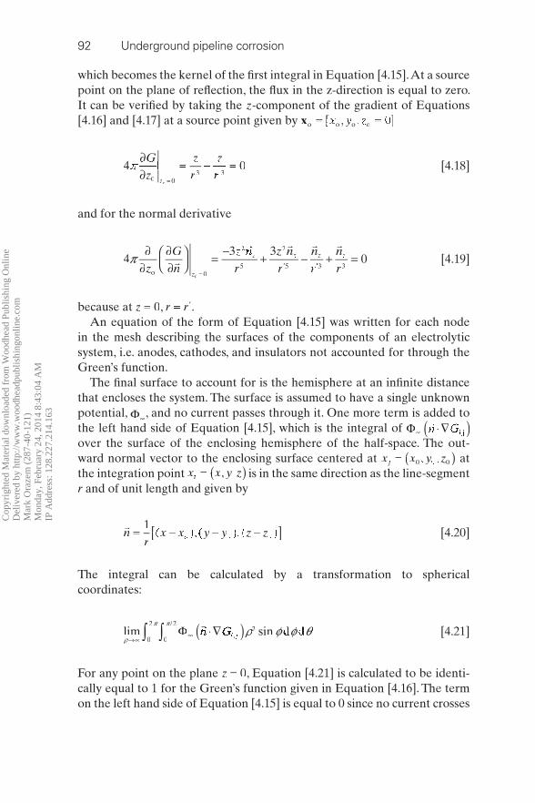
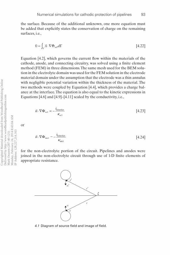
where, as is shown in Fig. 4.1, xj′ is the refl ected fi eld point about the plane
that defi nes the half-space, zo = 0 . The derivative of G with respect to the
unit normal vector at the fi eld point is
41 1π
∂∂
= − ⋅∇ − ⋅∇′ ′
G
nn
rn
ri,j
j j
1∇x x [4.17]
Cop
yrig
hted
Mat
eria
l dow
nloa
ded
from
Woo
dhea
d Pu
blis
hing
Onl
ine
D
eliv
ered
by
http
://w
ww
.woo
dhea
dpub
lishi
ngon
line.
com
M
ark
Ora
zem
(28
7-40
-121
)
Mon
day,
Feb
ruar
y 24
, 201
4 8:
43:0
4 A
M
IP A
ddre
ss: 1
28.2
27.2
14.1
63
92 Underground pipeline corrosion
which becomes the kernel of the fi rst integral in Equation [4.15]. At a source
point on the plane of refl ection, the fl ux in the z-direction is equal to zero.
It can be verifi ed by taking the z -component of the gradient of Equations
[4.16] and [4.17] at a source point given by xo o= [ ,[ , ]o =y,o
4 00 0
3 3π ∂
∂ =′
Gz
zr
zr
zo
[4.18]
and for the normal derivative
43 3
00
2
5
2
5 3 3π ∂
∂∂∂
⎛⎝⎛⎛⎛⎛⎝⎝⎛⎛⎛⎛ ⎞
⎠⎞⎞⎞⎞⎠⎠⎞⎞⎞⎞ =
−+ − + =
=′ ′5z
Gn
zr
z n2
rnr
nr
z
z z z z+n n
oo
[4.19]
because at z = 0 , r r ′ .
An equation of the form of Equation [4.15] was written for each node
in the mesh describing the surfaces of the components of an electrolytic
system, i.e. anodes, cathodes, and insulators not accounted for through the
Green’s function.
The fi nal surface to account for is the hemisphere at an infi nite distance
that encloses the system. The surface is assumed to have a single unknown
potential, Φ∞ , and no current passes through it. One more term is added to
the left hand side of Equation [4.15], which is the integral of Φ∞ ( )⋅∇⋅∇
over the surface of the enclosing hemisphere of the half-space. The out-
ward normal vector to the enclosing surface centered at x x y zj ( )0 y 0y at
the integration point x x y zi ( ), y is in the same direction as the line-segment
r and of unit length and given by
nr
= [ ]y yy1
x xx z zzy y [4.20]
The integral can be calculated by a transformation to spherical
coordinates:
lim sin/
ρ
π //πρ φ φ θ
→∞ρ ∞∫∫ ( )⋅∇Φ0∫∫
2
0∫∫2
2ρρ⋅∇ , d dφφ [4.21]
For any point on the plane z = 0 , Equation [4.21] is calculated to be identi-
cally equal to 1 for the Green’s function given in Equation [4.16]. The term
on the left hand side of Equation [4.15] is equal to 0 since no current crosses
Cop
yrig
hted
Mat
eria
l dow
nloa
ded
from
Woo
dhea
d Pu
blis
hing
Onl
ine
D
eliv
ered
by
http
://w
ww
.woo
dhea
dpub
lishi
ngon
line.
com
M
ark
Ora
zem
(28
7-40
-121
)
Mon
day,
Feb
ruar
y 24
, 201
4 8:
43:0
4 A
M
IP A
ddre
ss: 1
28.2
27.2
14.1
63
Numerical simulations for cathodic protection of pipelines 93
the surface. Because of the additional unknown, one more equation must
be added that explicitly states the conservation of charge on the remaining
surfaces, i.e.,
0 = ∇∫ n d⋅∇Γ∫∫ Γdsol [4.22]
Equation [4.2], which governs the current fl ow within the materials of the
cathode, anode, and connecting circuitry, was solved using a fi nite element
method (FEM) in three dimensions. The same mesh used for the BEM solu-
tion in the electrolyte domain was used for the FEM solution in the electrode
material domain under the assumption that the electrode was a thin annulus
with negligible potential variation within the thickness of the material. The
two methods were coupled by Equation [4.4], which provides a charge bal-
ance at the interface. The equation is also equal to the kinetic expressions in
Equations [4.6] and [4.9]–[4.11] scaled by the conductivity, i.e.,
ni⋅∇ = −Φsolkinetics
solκs
[4.23]
or
ni⋅∇ = −Φmetkinetics
metκm
[4.24]
for the non-electrolyte portion of the circuit. Pipelines and anodes were
joined in the non-electrolyte circuit through use of 1-D fi nite elements of
appropriate resistance.
n’
x’
r’
rn
x
ξ
4.1 Diagram of source fi eld and image of fi eld.
Cop
yrig
hted
Mat
eria
l dow
nloa
ded
from
Woo
dhea
d Pu
blis
hing
Onl
ine
D
eliv
ered
by
http
://w
ww
.woo
dhea
dpub
lishi
ngon
line.
com
M
ark
Ora
zem
(28
7-40
-121
)
Mon
day,
Feb
ruar
y 24
, 201
4 8:
43:0
4 A
M
IP A
ddre
ss: 1
28.2
27.2
14.1
63

94 Underground pipeline corrosion
Solving the nonlinear system
A variable transformation, Ψ Φ Φ−Φmet sΦ ol was needed to provide stable
convergence behavior for the combined BEM and FEM system of equa-
tions. Here, Ψ represents the driving force for the electrochemical kinetics.
The variable Φmet was eliminated from the system of equations and, upon
adding the necessary terms for the potential at infi nity and charge conversa-
tion, the system of equations could be written as
0 40 4
0 0 0
0 0 00 0 0 0
⎡ GGG H
K 0
K0A
a cG c c a c
a aG c a a a
c c00
a a
a
, ,c c ,
, ,a c ,
ππ
⎣⎣
⎢⎡⎡
⎢⎢⎢
⎢⎢⎢
⎢⎣⎣⎣⎣⎢⎢
⎤
⎦
⎥⎤⎤
⎥⎥⎥
⎥⎥⎥
⎥⎦⎦⎥⎥
⋅∇⎡
⎣
⎢⎡⎡
⎢⎢⎢
⎢⎢⎢
⎢⎣⎣⎢⎢
⎤
⎦
⎥⎤⎤
⎥⎥⎥
⎥⎥⎥
⎥⎦⎦⎥⎥
=−
∞
ΨΦ
ΦΦΦ
c
a
c
a
c c
c a
c
a
nGc
Gc
FK
A
,
,
00
00
cc
c
a
n
0
⎡
⎣
⎢⎡⎡
⎢⎢⎢
⎢⎢⎢
⎢⎣⎣⎢⎢
⎤
⎦
⎥⎤⎤
⎥⎥⎥
⎥⎥⎥
⎥⎦⎦⎥⎥
⋅∇⎡⎣⎢⎡⎡⎣⎣
⎤⎦⎥⎤⎤⎦⎦
ΦΨ
[4.25]
where all of the unknowns have been moved to the left hand side and all
the Φ terms refer to the potential in the electrolyte next to an electrode. The
terms H and G are sub-matrices resulting from evaluation of the integrals in
Equation [4.15]. Following the matrix notation of Brebbia et al ., 22 the fi rst
subscript to appear is the fi eld point and the second is the source point. The
sub-matrix K is the stiffness matrix from the FEM solution for the electrode
materials and F is the charge balance between the electrode and electro-
lyte domains. The sub-matrix A, given by
A J−∫ ξ η( )ξξ ( ) d Γ1
1
[4.26]
is the surface area as represented by the shape functions for the elements
used. The term J is the Jacobian of the coordinate transformations from
Cartesian to curvilinear . It provides the correct weighting of the nodal val-
ues of the current density such that electroneutrality is enforced.
4.3.4 Calculation of potentials within the electrolyte
The model allows calculation of both on- and off-potentials at arbitrarily
chosen locations within the electrolyte or on the electrolyte surface defi ned
by the Green’s function through the method of the images. The on-poten-
tial is defi ned as the potential that would be measured between a refer-
ence electrode at some point in the electrolyte and a cathode if the anodes
were connected to the cathodes and current were fl owing between them.
The off-potential is defi ned as the potential difference measured between a
Cop
yrig
hted
Mat
eria
l dow
nloa
ded
from
Woo
dhea
d Pu
blis
hing
Onl
ine
D
eliv
ered
by
http
://w
ww
.woo
dhea
dpub
lishi
ngon
line.
com
M
ark
Ora
zem
(28
7-40
-121
)
Mon
day,
Feb
ruar
y 24
, 201
4 8:
43:0
4 A
M
IP A
ddre
ss: 1
28.2
27.2
14.1
63
Numerical simulations for cathodic protection of pipelines 95
reference electrode at some point within the electrolyte and the cathode at a
moment just after the anodes have been disconnected but the cathodes are
still polarized. The method employed is summarized below.
On-potentials
The on-potential was obtained under the conditions where anodes are con-
nected to the cathodes and, in the case of impressed current systems, are
energized. The condition is straightforward to model. Using the solution for
the entire electrolytic systems, points in the domains were calculated using
equations described by Brebbia et al : 22
Φ Φ ΓΓ Γi ,j d∫ ∫Γ ΓiΓ ,j −Γ di j ∇Φ ( )i,j⋅∇n G⋅∇∫ [4.27]
where Φ i is the unknown potential at a point not on the boundary Γ , and Φ
and n ⋅∇Φ are the solutions on Γ found by solving Equation [4.17].
Current density vectors can be found by differentiating Equation [4.27]
at the source points.
∂∂
=∂ ∂
∂∫ ∫∂∂
ΦΓ
Γ∫ ∫∫ ∫∂i
∂∫ ∫− Φ∫ Φ dx
G
x∫Γ ∂∫ ∂⋅∇∇
( )⋅∇ i⋅∇ ji jG⋅∇⋅∇ [4.28]
where three equations of the form of Equation [4.28] are written for the
three components of the current vector, = 1, 2, 3. The resulting gradient of
Φ i is combined with the electrolyte conductivity to get the current.
Off-potentials
Off-potentials were calculated after a solution was obtained using the model
described above. The anodes were removed from the problem, and the cal-
culated potentials on the cathode were used as boundary conditions for a
new calculation. As the metal under the coating is polarized and, therefore,
the source of the potential, the potential used for coated electrodes was the
value underneath the coating, Φ in (see Equations [4.9] and [4.10]).
Equation [4.25] was rewritten dropping the anodes and using the previ-
ous solution for the potential on the cathodes as the known boundary con-
dition, i.e.,
H GA np,p in,p p,GG p
pin,p
−⎡⎣⎢⎡⎡⎣⎣
⎤⎦⎥⎦⎦
⎡⎣⎢⎣⎣
⎤⎦⎥⎤⎤⎦⎦
= ⎡⎣⎢⎡⎡⎣⎣
⎤⎦⎥⎤⎤⎦⎦
⋅∇⎡⎣⎡⎡ ⎤⎦⎤⎤∞
40 0
π ⎤⎤ ΦΦ Φ
[4.29]
Cop
yrig
hted
Mat
eria
l dow
nloa
ded
from
Woo
dhea
d Pu
blis
hing
Onl
ine
D
eliv
ered
by
http
://w
ww
.woo
dhea
dpub
lishi
ngon
line.
com
M
ark
Ora
zem
(28
7-40
-121
)
Mon
day,
Feb
ruar
y 24
, 201
4 8:
43:0
4 A
M
IP A
ddre
ss: 1
28.2
27.2
14.1
63
96 Underground pipeline corrosion
where a new potential at infi nity, Φ∞ , is found. All the values on the left
hand side of Equation [4.29] are known, and the current densities, driven by
the potential distribution along the cathodes, can be easily found. The new
solution is then used to fi nd the potentials within the electrolyte through
Equation [4.12] using only the previous cathodes as sources.
4.4 Model validation
A computer code was written that implements the above model. The model
can be compared to analytical solutions to Laplace’s equation to validate
the code.
4.4.1 Comparison to analytic solutions
The fi rst comparison was made to the variation of potential around a disk
electrode placed at the surface of a semi-infi nite electrolyte with a hemi-
spherical counter electrode infi nitely far away. An analytic solution by
Newman is available. 24 A limitation of the numerical model as implemented
was that all anodes/cathodes had to be either disks or cylinders. A simple
remedy would be to make the potential at infi nity ( )Φ∞ a known, and move
it to the other side of Equation [4.17]. Then the new unknown is the total
current entering or leaving the system through the hemisphere at infi nity
that encloses the system. In the case presented here, a counter electrode that
was a factor of 4 0 1011× times larger than the disk was used to approxi-
mate the counter electrode in Newman’s example. It was moved as far from
the disk as numerically practicable.
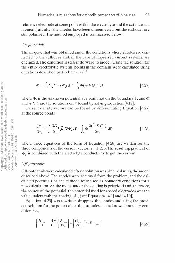
A number of points were selected on the electrolyte surface for calcula-
tion of the potential. To illustrate the procedure, a grid of points extending
away from the disk is presented in Fig. 4.2 where a calculation would be
performed at each line intersection. The center section of points oriented in
the r direction is used for comparison.
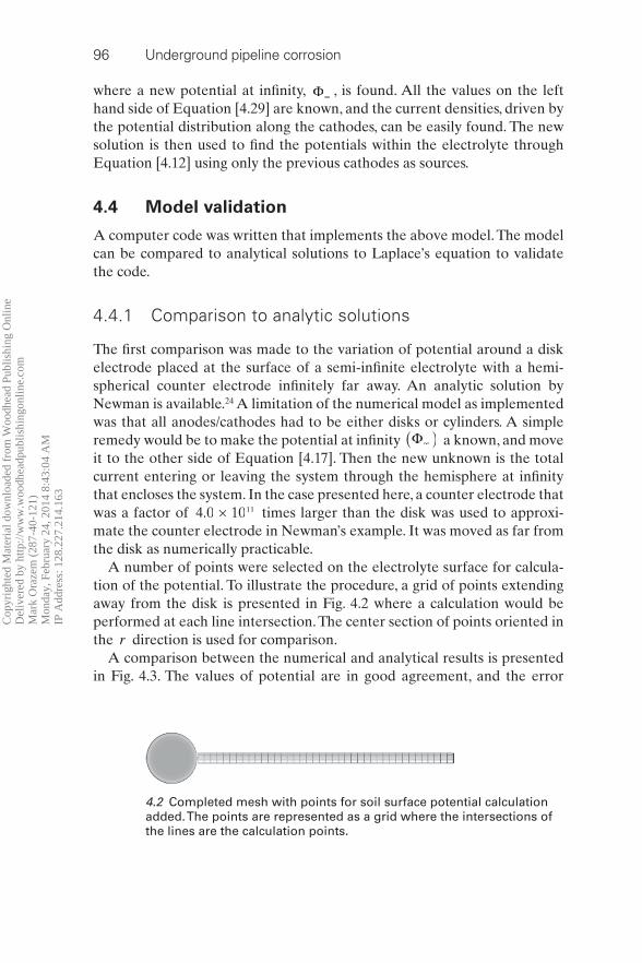
A comparison between the numerical and analytical results is presented
in Fig. 4.3. The values of potential are in good agreement, and the error
4.2 Completed mesh with points for soil surface potential calculation
added. The points are represented as a grid where the intersections of
the lines are the calculation points.
Cop
yrig
hted
Mat
eria
l dow
nloa
ded
from
Woo
dhea
d Pu
blis
hing
Onl
ine
D
eliv
ered
by
http
://w
ww
.woo
dhea
dpub
lishi
ngon
line.
com
M
ark
Ora
zem
(28
7-40
-121
)
Mon
day,
Feb
ruar
y 24
, 201
4 8:
43:0
4 A
M
IP A
ddre
ss: 1
28.2
27.2
14.1
63
Numerical simulations for cathodic protection of pipelines 97
between the analytical and numerical solutions is less than 1.8%. The
increase in error close to the disk is the due to the fact that the numerical
method cannot adequately represent the infi nite current density at the edge
of the disk. The constant error of 0.7% far from the disk is due to the fi nite
size of the counter electrode and decreases as the counter-electrode area is
increased.
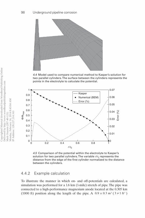
A second validation was done against Kasper’s solution for parallel cyl-
inders of unequal size. 25 In this case, two cylinders were placed far from the
electrolyte surface. One was 0.5 m diameter, the second was 0.1 m diameter,
and they were placed such that their centers were 1 m apart as presented in
Fig. 4.4. The boundary conditions for both surfaces were equipotential with
the fi rst set to 0 V and the second set to 1 V.
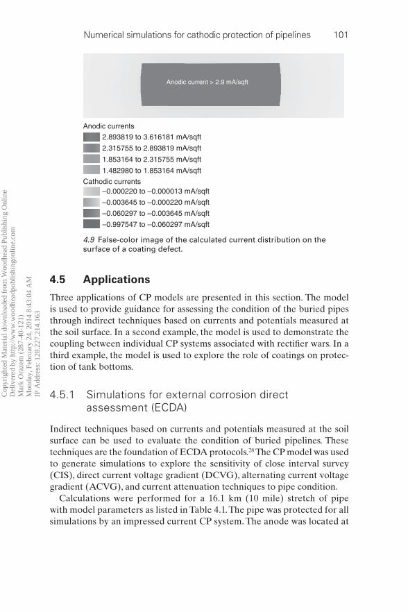
The potential in the electrolyte was calculated for a line running from the
large cylinder to the small. The result is compared to the analytic solution in
Fig. 4.5. The error in the numerical method does not exceed 0.1%. Therefore,
given any arbitrary current and potential distribution on a set of electrodes
that satisfi es Laplace’s equation, the resulting potential distribution within
the electrolyte can be calculated with reasonable accuracy.
If the potential calculated at some point in the electrolyte is subtracted
from another point at an electrode surface, one would have a reasonable
approximation of a physical measurement made with a reference electrode.
Therefore, the numerical method may be used to evaluate ways of using ref-
erence electrodes to determine the condition of an electrolytic system, such
as a CP system or solid phase electrolytes.
00
0.1
0
0.2
0.4
0.6
0.8 Err
or (
%)
1
1.2
1.4
1.6
1.8
2
Numerical (BEM)AnalyticalError (%)
0.2
0.3
0.4
0.5
Θ/Θ
o
0.6
0.7
0.8
0.9
1
2 4 6
(r – ro)/ro
8 10
4.3 Comparison of the analytical and numerical solutions for the
potential at the electrolyte surface. The term represents the distance
from the edge of the disk.
Cop
yrig
hted
Mat
eria
l dow
nloa
ded
from
Woo
dhea
d Pu
blis
hing
Onl
ine
D
eliv
ered
by
http
://w
ww
.woo
dhea
dpub
lishi
ngon
line.
com
M
ark
Ora
zem
(28
7-40
-121
)
Mon
day,
Feb
ruar
y 24
, 201
4 8:
43:0
4 A
M
IP A
ddre
ss: 1
28.2
27.2
14.1
63
98 Underground pipeline corrosion
4.4.2 Example calculation
To illustrate the manner in which on- and off-potentials are calculated, a
simulation was performed for a 1.6 km (1-mile) stretch of pipe. The pipe was
connected to a high-performance magnesium anode located at the 0.305 km
(1000 ft) position along the length of the pipe. A 0 9 0 39 0× m2 ( 3 1 ftff 2 )
4.4 Model used to compare numerical method to Kasper’s solution for
two parallel cylinders. The surface between the cylinders represents the
points in the electrolyte to calculate the potential.
00
0.1
0.2
0.3
0.4
0.5
Φ/Φ
max
0.6
0.7
0.8
0.9
1
0.2 0.4
r /r0
0.6 0.8 10
0.01
0.02
0.03 Err
or (
%)
0.04
0.05
0.06
0.07Kasper
Error (%)
Numerical (BEM)
4.5 Comparison of the potential within the electrolyte to Kasper’s
solution for two parallel cylinders. The variable r / r 0 represents the
distance from the edge of the fi rst cylinder normalized to the distance
between the cylinders.
Cop
yrig
hted
Mat
eria
l dow
nloa
ded
from
Woo
dhea
d Pu
blis
hing
Onl
ine
D
eliv
ered
by
http
://w
ww
.woo
dhea
dpub
lishi
ngon
line.
com
M
ark
Ora
zem
(28
7-40
-121
)
Mon
day,
Feb
ruar
y 24
, 201
4 8:
43:0
4 A
M
IP A
ddre
ss: 1
28.2
27.2
14.1
63

Numerical simulations for cathodic protection of pipelines 99
coating defect, exposing bare steel, was assumed to be located at the 0.762 km
(2500 ft) position. The pipeline was located 0.61 m (2 ft) below grade. Surface
on-potentials, shown in Fig. 4.6a, reveal the location of the anode. The grid
spacing used in these calculations was 6 1 6 11 6m m × (20 ft ff ft 20 ). For ref-
erence, the corresponding confi guration of pipe and anode is presented in
Fig. 4.7. As shown in Fig. 4.6b, surface off-potentials, calculated by removing
the infl uence of the anode, obscure the anode location.
The location of a massive ( 0 9 0 39 0× m2 ) coating defect is seen in the
surface on-potentials, shown in Fig. 4.8a, in which the color scale has been
changed to facilitate viewing of the potential variation. The signifi cant change
in potential at the soil surface level is seen for these calculations because the
defect is large, is located at the top of the pipe, is severely under-protected,
and is located very close to the soil surface. The values of the off-potential
readings shown in Fig. 4.8b suggest that the pipe is under-protected. The size
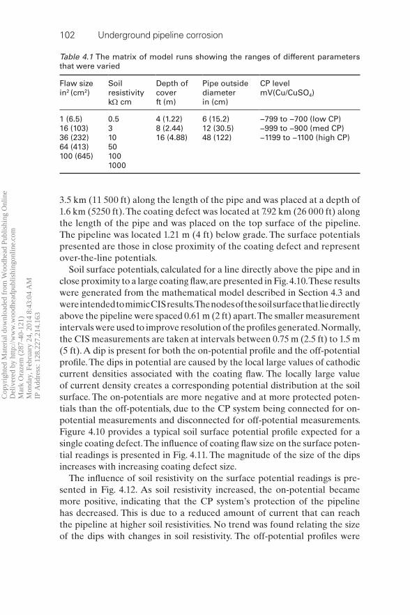
of the coating defect can be seen in Fig. 4.9, where a false-color image of the
cathodic current is presented. The majority of CP current is delivered to the
exposed steel at the coating defect.
The on- and off-potential distributions shown in Figs 4.8a and 4.8b may
be measured in the fi eld, whereas the information presented in Fig. 4.9 could
be inferred only after excavation. The BEM model could be used to calcu-
late other measurable quantities, such as the local values for current passed
through the pipe. Thus, the BEM model can be used to provide informa-
tion that can be correlated to the results of ECDA simulations. Such an
approach has been suggested for inverse models for interpretation of fi eld
ECDA data. 26,27
4.6 Calculated potential distribution on the soil surface above the
anode (see Fig. 4.7): (a) on-potentials; (b) off-potentials.
Cop
yrig
hted
Mat
eria
l dow
nloa
ded
from
Woo
dhea
d Pu
blis
hing
Onl
ine
D
eliv
ered
by
http
://w
ww
.woo
dhea
dpub
lishi
ngon
line.
com
M
ark
Ora
zem
(28
7-40
-121
)
Mon
day,
Feb
ruar
y 24
, 201
4 8:
43:0
4 A
M
IP A
ddre
ss: 1
28.2
27.2
14.1
63

100 Underground pipeline corrosion
4.7 Image revealing the location of the anode and pipeline
corresponding to Fig. 4.6.
4.8 Calculated potential distribution on the soil surface above
a 0 39 0× m2 (3 1 ftf 2) coating defect exposing bare steel:
(a) on-potentials and (b) off-potentials.
Cop
yrig
hted
Mat
eria
l dow
nloa
ded
from
Woo
dhea
d Pu
blis
hing
Onl
ine
D
eliv
ered
by
http
://w
ww
.woo
dhea
dpub
lishi
ngon
line.
com
M
ark
Ora
zem
(28
7-40
-121
)
Mon
day,
Feb
ruar
y 24
, 201
4 8:
43:0
4 A
M
IP A
ddre
ss: 1
28.2
27.2
14.1
63
Numerical simulations for cathodic protection of pipelines 101
4.5 Applications
Three applications of CP models are presented in this section. The model
is used to provide guidance for assessing the condition of the buried pipes
through indirect techniques based on currents and potentials measured at
the soil surface. In a second example, the model is used to demonstrate the
coupling between individual CP systems associated with rectifi er wars. In a
third example, the model is used to explore the role of coatings on protec-
tion of tank bottoms.
4.5.1 Simulations for external corrosion direct assessment (ECDA)
Indirect techniques based on currents and potentials measured at the soil
surface can be used to evaluate the condition of buried pipelines. These
techniques are the foundation of ECDA protocols. 28 The CP model was used
to generate simulations to explore the sensitivity of close interval survey
(CIS), direct current voltage gradient (DCVG), alternating current voltage
gradient (ACVG), and current attenuation techniques to pipe condition.
Calculations were performed for a 16.1 km (10 mile) stretch of pipe
with model parameters as listed in Table 4.1. The pipe was protected for all
simulations by an impressed current CP system. The anode was located at
Anodic currents
Anodic current > 2.9 mA/sqft
2.893819 to 3.616181 mA/sqft
2.315755 to 2.893819 mA/sqft
1.853164 to 2.315755 mA/sqft
1.482980 to 1.853164 mA/sqft
–0.000220 to –0.000013 mA/sqft
–0.003645 to –0.000220 mA/sqft
–0.060297 to –0.003645 mA/sqft
–0.997547 to –0.060297 mA/sqft
Cathodic currents
4.9 False-color image of the calculated current distribution on the
surface of a coating defect.
Cop
yrig
hted
Mat
eria
l dow
nloa
ded
from
Woo
dhea
d Pu
blis
hing
Onl
ine
D
eliv
ered
by
http
://w
ww
.woo
dhea
dpub
lishi
ngon
line.
com
M
ark
Ora
zem
(28
7-40
-121
)
Mon
day,
Feb
ruar
y 24
, 201
4 8:
43:0
4 A
M
IP A
ddre
ss: 1
28.2
27.2
14.1
63
102 Underground pipeline corrosion
3.5 km (11 500 ft) along the length of the pipe and was placed at a depth of
1.6 km (5250 ft). The coating defect was located at 7.92 km (26 000 ft) along
the length of the pipe and was placed on the top surface of the pipeline.
The pipeline was located 1.21 m (4 ft) below grade. The surface potentials
presented are those in close proximity of the coating defect and represent
over-the-line potentials.
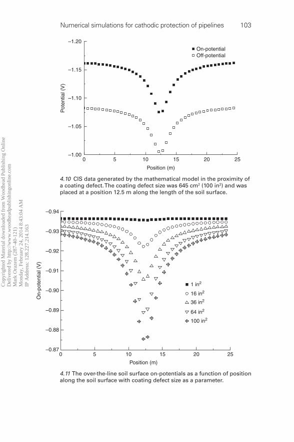
Soil surface potentials, calculated for a line directly above the pipe and in
close proximity to a large coating fl aw, are presented in Fig. 4.10. These results
were generated from the mathematical model described in Section 4.3 and
were intended to mimic CIS results. The nodes of the soil surface that lie directly
above the pipeline were spaced 0.61 m (2 ft) apart. The smaller measurement
intervals were used to improve resolution of the profi les generated. Normally,
the CIS measurements are taken at intervals between 0.75 m (2.5 ft) to 1.5 m
(5 ft). A dip is present for both the on-potential profi le and the off-potential
profi le. The dips in potential are caused by the local large values of cathodic
current densities associated with the coating fl aw. The locally large value
of current density creates a corresponding potential distribution at the soil
surface. The on-potentials are more negative and at more protected poten-
tials than the off-potentials, due to the CP system being connected for on-
potential measurements and disconnected for off-potential measurements.
Figure 4.10 provides a typical soil surface potential profi le expected for a
single coating defect. The infl uence of coating fl aw size on the surface poten-
tial readings is presented in Fig. 4.11. The magnitude of the size of the dips
increases with increasing coating defect size.
The infl uence of soil resistivity on the surface potential readings is pre-
sented in Fig. 4.12. As soil resistivity increased, the on-potential became
more positive, indicating that the CP system’s protection of the pipeline
has decreased. This is due to a reduced amount of current that can reach
the pipeline at higher soil resistivities. No trend was found relating the size
of the dips with changes in soil resistivity. The off-potential profi les were
Table 4.1 The matrix of model runs showing the ranges of different parameters
that were varied
Flaw size
in2 (cm2)
Soil
resistivity
k Ω cm
Depth of
cover
ft (m)
Pipe outside
diameter
in (cm)
CP level
mV(Cu/CuSO 4 )
1 (6.5) 0.5 4 (1.22) 6 (15.2) − 799 to − 700 (low CP)
16 (103) 3 8 (2.44) 12 (30.5) − 999 to − 900 (med CP)
36 (232) 10 16 (4.88) 48 (122) − 1199 to − 1100 (high CP)
64 (413) 50
100 (645) 100
1000
Cop
yrig
hted
Mat
eria
l dow
nloa
ded
from
Woo
dhea
d Pu
blis
hing
Onl
ine
D
eliv
ered
by
http
://w
ww
.woo
dhea
dpub
lishi
ngon
line.
com
M
ark
Ora
zem
(28
7-40
-121
)
Mon
day,
Feb
ruar
y 24
, 201
4 8:
43:0
4 A
M
IP A
ddre
ss: 1
28.2
27.2
14.1
63
Numerical simulations for cathodic protection of pipelines 103
0–1.00
–1.05
–1.10
–1.15P
oten
tial (
V)
–1.20
5 10 15
Position (m)
20 25
On-potentialOff-potential
4.10 CIS data generated by the mathematical model in the proximity of
a coating defect. The coating defect size was 645 cm 2 (100 in 2 ) and was
placed at a position 12.5 m along the length of the soil surface.
0–0.87
–0.88
–0.89
–0.90
On-
pote
ntia
l (V
)
–0.91
–0.92
–0.93
–0.94
5 10
Position (m)
1 in2
16 in2
36 in2
64 in2
100 in2
15 20 25
4.11 The over-the-line soil surface on-potentials as a function of position
along the soil surface with coating defect size as a parameter.
Cop
yrig
hted
Mat
eria
l dow
nloa
ded
from
Woo
dhea
d Pu
blis
hing
Onl
ine
D
eliv
ered
by
http
://w
ww
.woo
dhea
dpub
lishi
ngon
line.
com
M
ark
Ora
zem
(28
7-40
-121
)
Mon
day,
Feb
ruar
y 24
, 201
4 8:
43:0
4 A
M
IP A
ddre
ss: 1
28.2
27.2
14.1
63

104 Underground pipeline corrosion
then subtracted from the on-potential profi les and are presented in Fig. 4.13.
Figure 4.13 demonstrates that the difference in the on- and off-potentials
also yields a dip centered at the location of the coating defect. The simula-
tion results show that dips become smaller as soil resistivity increases. For
soil resistivity values of 100 kΩ and above, no dips in potential were pre-
sent, suggesting that high soil resistivities may hide the presence of a coating
fl aw.
The effect of soil resistivity and coating fl aw (holiday) size on the value
of calculated indications was fi rst explored using software utilizing Section
4.3. Figure 4.14 was developed to show the correlation between DCVG
indications in mV versus fl aw size based on changing soil resistivities. Two
main trends are found in Fig. 4.14. One trend is that DCVG indications in
mV will increase with increasing fl aw size, which is consistent with con-
ventional knowledge. The other trend is that as soil resistivity increases
the DCVG indication decreases. This trend is a result that was not initially
expected. Since these are competing trends, it is of interest to determine
which trend has a dominating effect on indications. By taking a closer look
at Fig. 4.14, it appears that soil resistivity plays a larger role than fl aw size
in determining DCVG indication in mV. This is supported by the behavior
252015
Position (m)
1050–0.65
–0.70
–0.75
–0.80On-
pote
ntia
l (V
)
–0.85
–0.90
–0.95
–1.00
–1.05
0.5 kΩ-cm
10 kΩ-cm100 kΩ-cm
1000 kΩ-cm
4.12 The over-the-line soil surface on-potentials as a function of
position along the soil surface with soil resistivity as a parameter.
Cop
yrig
hted
Mat
eria
l dow
nloa
ded
from
Woo
dhea
d Pu
blis
hing
Onl
ine
D
eliv
ered
by
http
://w
ww
.woo
dhea
dpub
lishi
ngon
line.
com
M
ark
Ora
zem
(28
7-40
-121
)
Mon
day,
Feb
ruar
y 24
, 201
4 8:
43:0
4 A
M
IP A
ddre
ss: 1
28.2
27.2
14.1
63

Numerical simulations for cathodic protection of pipelines 105
0.5 kΩ-cm
10 kΩ-cm100 kΩ-cm
1000 kΩ-cm
252015
Position (m)
1050
0.000
–0.004
–0.008
On
pote
ntia
l – o
ff po
tent
ial (
V)
–0.012
–0.016
–0.020
4.13 The difference in on- and off-potentials as a function of position
along the soil surface with soil resistivity as a parameter.
00
20
40
Flaw
siz
e (in
2 )
60
80
100
10 20 30
Voltage gradient (mV)
40
0.5 K
3 K
10 K
50 K
100 K
50
4.14 Coating fl aw size as a function of the DCVG indication in mV with
soil resistivity as a parameter. The pipe diameter was 12 in, the depth of
cover was 4 ft, and the anode potential was 5 V.
Cop
yrig
hted
Mat
eria
l dow
nloa
ded
from
Woo
dhea
d Pu
blis
hing
Onl
ine
D
eliv
ered
by
http
://w
ww
.woo
dhea
dpub
lishi
ngon
line.
com
M
ark
Ora
zem
(28
7-40
-121
)
Mon
day,
Feb
ruar
y 24
, 201
4 8:
43:0
4 A
M
IP A
ddre
ss: 1
28.2
27.2
14.1
63
106 Underground pipeline corrosion
at high soil resistivities, where the DCVG indications show almost no
dependence on fl aw size. Conversely, there is a wide distribution of DCVG
indications at low soil resistivities. This result shows that prioritization of
DCVG indications in mV can be much improved by taking soil resistivity
into account.
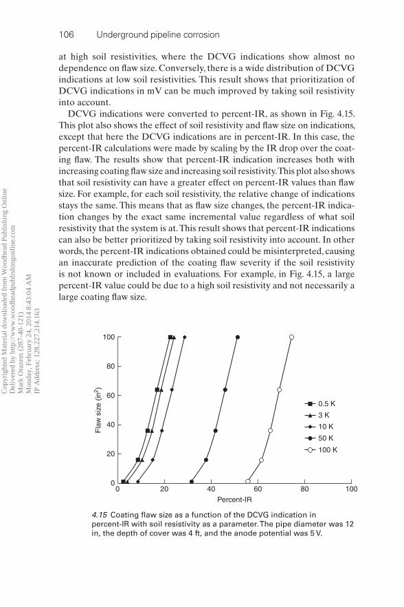
DCVG indications were converted to percent-IR, as shown in Fig. 4.15.
This plot also shows the effect of soil resistivity and fl aw size on indications,
except that here the DCVG indications are in percent-IR. In this case, the
percent-IR calculations were made by scaling by the IR drop over the coat-
ing fl aw. The results show that percent-IR indication increases both with
increasing coating fl aw size and increasing soil resistivity. This plot also shows
that soil resistivity can have a greater effect on percent-IR values than fl aw
size. For example, for each soil resistivity, the relative change of indications
stays the same. This means that as fl aw size changes, the percent-IR indica-
tion changes by the exact same incremental value regardless of what soil
resistivity that the system is at. This result shows that percent-IR indications
can also be better prioritized by taking soil resistivity into account. In other
words, the percent-IR indications obtained could be misinterpreted, causing
an inaccurate prediction of the coating fl aw severity if the soil resistivity
is not known or included in evaluations. For example, in Fig. 4.15, a large
percent-IR value could be due to a high soil resistivity and not necessarily a
large coating fl aw size.
00
20
40
Fla
w s
ize
(in2 )
60
80
100
20 40 60
Percent-IR
80 100
0.5 K
3 K
10 K
50 K
100 K
4.15 Coating fl aw size as a function of the DCVG indication in
percent-IR with soil resistivity as a parameter. The pipe diameter was 12
in, the depth of cover was 4 ft, and the anode potential was 5 V.
Cop
yrig
hted
Mat
eria
l dow
nloa
ded
from
Woo
dhea
d Pu
blis
hing
Onl
ine
D
eliv
ered
by
http
://w
ww
.woo
dhea
dpub
lishi
ngon
line.
com
M
ark
Ora
zem
(28
7-40
-121
)
Mon
day,
Feb
ruar
y 24
, 201
4 8:
43:0
4 A
M
IP A
ddre
ss: 1
28.2
27.2
14.1
63

Numerical simulations for cathodic protection of pipelines 107
In Fig. 4.16, the effect of changing CP levels is explored on DCVG indica-
tions in mV. The CP level was adjusted by increasing the anode voltage, and
CP levels were categorized by ensuring that off-potentials on the soil sur-
face far away from the coating fl aw were within certain ranges. The CP levels
and their corresponding potential ranges are shown in Table 4.1. Figure 4.16
also shows that DCVG indications increase with increasing coating fl aw size
as previously found. However, this graph is primarily included to show that
increased CP has a large effect on DCVG signal in mV. Notice that the
distribution in voltage gradients in Fig. 4.16 is more apparent at larger CP
levels. These larger voltage gradients at higher CP levels can be explained
by a larger amount of current entering the pipeline at the fl aw location. This
shows that at lower CP levels, the presence of a fl aw size could be unde-
tected. Therefore, the severity of a fl aw could be misinterpreted if CP levels
were not taken into account. A suffi cient amount of CP current is needed in
order to yield a measurable voltage gradient. DCVG in percent-IR was also
plotted exactly as in Fig. 4.16. This is shown in Fig. 4.17. The obvious result
shown here is that the percent-IR values do not change with increased CP
level. This result could be helpful in predicting fl aw size based on DCVG
indications in percent-IR.
Sensitivity of indications of DCVG in mV is also evaluated based
on changing depth of cover as shown in Fig. 4.18. The results show that
DCVG indications are more sensitive to a pipeline buried at 4 ft than at 8
ft. Although not shown here, previous simulations have further supported
Med CP
Low CP
604020
Voltage gradient (mV)
00
20
40
Fla
w s
ize
(sq
in)
60
80
100
High CP
4.16 Coating fl aw size as a function of the DCVG indication in mV with
CP level as a parameter. The pipe diameter was 12 in, the depth of cover
was 4 ft, and the soil resistivity was 500 Ω cm.
Cop
yrig
hted
Mat
eria
l dow
nloa
ded
from
Woo
dhea
d Pu
blis
hing
Onl
ine
D
eliv
ered
by
http
://w
ww
.woo
dhea
dpub
lishi
ngon
line.
com
M
ark
Ora
zem
(28
7-40
-121
)
Mon
day,
Feb
ruar
y 24
, 201
4 8:
43:0
4 A
M
IP A
ddre
ss: 1
28.2
27.2
14.1
63

108 Underground pipeline corrosion
this trend where indications at larger depths of cover are practically negli-
gible. This trend indicates that depth of cover should be used in prioritizing
indications. For similar conditions in Fig. 4.18, a plot of DCVG indication
in mV is given versus changing pipe diameter. There is no clear trend found
00
20
40
60
Fla
w s
ize
(sq
in)
80
100
5 10
Percent-IR
15 20
High CP
Med CP
Low CP
25
4.17 Coating fl aw size as a function of the DCVG indication in
percent-IR with CP level as a parameter. The pipe diameter was 12 in,
the depth of cover was 4 ft, and the anode potential was 5 V. The pipe
diameter was 12 in, the depth of cover was 4 ft, and the soil resistivity
was 500 Ω cm.
4ft DOC
8ft DOC
00
20
40
60
Fla
w s
ize
(sq
in)
80
100
20 40
Voltage gradient (mV)
60
4.18 Coating fl aw size as a function of the DCVG indication in mV with
depth of cover (DOC) as a parameter. The pipe diameter was 12 in, the
soil resistivity was 500 Ω cm, and the CP level was high.
Cop
yrig
hted
Mat
eria
l dow
nloa
ded
from
Woo
dhea
d Pu
blis
hing
Onl
ine
D
eliv
ered
by
http
://w
ww
.woo
dhea
dpub
lishi
ngon
line.
com
M
ark
Ora
zem
(28
7-40
-121
)
Mon
day,
Feb
ruar
y 24
, 201
4 8:
43:0
4 A
M
IP A
ddre
ss: 1
28.2
27.2
14.1
63

Numerical simulations for cathodic protection of pipelines 109
from this result, as shown in Fig. 4.19. However, this result is not considered
as proof that pipe diameter does not have an effect on DCVG indication
in mV.
CIS on-potential dip (on-dip) indications are plotted against fl aw size
based on changing soil resistivity in Fig. 4.20. One basic trend shows that
48in OD
12in OD
6in OD
00 20
Voltage gradient (mV)
40 60
20
40
60
Fla
w s
ize
(sq
in)
80
100
4.19 Coating fl aw size as a function of the DCVG indication in mV with
pipe diameter (OD) as a parameter. The soil resistivity was 500 Ω cm,
the DOC was 4 ft, and the CP level was high.
3K
10K
50K
100K
00 50 100
Potential (mV)
150 200 250
20
40
60
Fla
w s
ize
(sq
in)
80
100
4.20 Coating fl aw size as a function of the CIS on-potential dip
indication in mV with soil resistivity in Ω cm as a parameter. The pipe
diameter was 12 in, the DOC was 4 ft, and the CP level was high.
Cop
yrig
hted
Mat
eria
l dow
nloa
ded
from
Woo
dhea
d Pu
blis
hing
Onl
ine
D
eliv
ered
by
http
://w
ww
.woo
dhea
dpub
lishi
ngon
line.
com
M
ark
Ora
zem
(28
7-40
-121
)
Mon
day,
Feb
ruar
y 24
, 201
4 8:
43:0
4 A
M
IP A
ddre
ss: 1
28.2
27.2
14.1
63

110 Underground pipeline corrosion
CIS on-dip indication increases with increasing fl aw (holiday) size. Another
trend is that the CIS on-dips increase as soil resistivity increases. However,
this result is due to increasing the anode voltage for higher soil resistivi-
ties. The anode voltage was adjusted for each simulation to maintain a high
CP level (refer to Table 4.1). If the anode voltage had been held constant
throughout all runs, the indications would have decreased with increasing
soil resistivity. DCVG indications were also calculated for high CP levels, as
shown in Fig. 4.21. Note that the DCVG trend in mV for Fig. 4.21 is oppo-
site with respect to soil resistivity than it was in Fig. 4.14. This is because in
Fig. 4.14, the anode voltage was held constant for all runs. This indicates that
raising the anode voltage increases the DCVG indication found, even if soil
resistivity is simultaneously increased.
Figure 4.22 is based on data from the same simulations run in Fig. 4.20.
However, it shows a different result for some soil resistivities. The negative
CIS off-dips initially represented an area of concern. The on- and off-poten-
tial profi les are given for a simulation that gives a negative CIS off-dip in
Fig. 4.23. A general potential profi le represents current direction by moving
from positive to negative potentials. In Fig. 4.23, the on-potential profi le
shows that current enters the pipeline at the coating fl aw and then travels
away from the fl aw based on the profi le of on-potential moving from pos-
itive to negative. This behavior is normally expected for the off-potential
profi le as well. However, the negative CIS off-dip indicates that when the
CP current is turned off, the potential fl ows back toward the fl aw. This can
3K
10K
50K
100K
00 20 40
Voltage gradient (mV)
60 80
20
40
60
Fla
w s
ize
(sq
in)
80
100
4.21 Coating fl aw size as a function of the DCVG indication in mV with
soil resistivity in Ω cm as a parameter. The pipe diameter was 12 in, the
DOC was 4 ft, and the CP level was high.
Cop
yrig
hted
Mat
eria
l dow
nloa
ded
from
Woo
dhea
d Pu
blis
hing
Onl
ine
D
eliv
ered
by
http
://w
ww
.woo
dhea
dpub
lishi
ngon
line.
com
M
ark
Ora
zem
(28
7-40
-121
)
Mon
day,
Feb
ruar
y 24
, 201
4 8:
43:0
4 A
M
IP A
ddre
ss: 1
28.2
27.2
14.1
63

Numerical simulations for cathodic protection of pipelines 111
3K
10K
50K
100K
0–20 0 20 40
Potential (mV)
60 80 100
20
40
60
Fla
w s
ize
(sq
in)
80
100
4.22 Coating fl aw size as a function of the CIS off-potential dip
indication in mV with soil resistivity in Ω cm as a parameter. The pipe
diameter was 12 in, the DOC was 4 ft, and the CP level was high.
On-potential
Off-potential
7910–2
–1.8
–1.6
–1.4
Pot
entia
l (V
)
–1.2
–1
7920
Position along soil surface (m)
7930 7940
4.23 A profi le of soil surface on- and off-potentials from a simulated
CIS survey. The fl aw size was 36 in 2 , the soil resistivity was 500 Ω cm,
the pipe diameter was 12 in, the DOC was 4 ft, and the CP level was
high.
Cop
yrig
hted
Mat
eria
l dow
nloa
ded
from
Woo
dhea
d Pu
blis
hing
Onl
ine
D
eliv
ered
by
http
://w
ww
.woo
dhea
dpub
lishi
ngon
line.
com
M
ark
Ora
zem
(28
7-40
-121
)
Mon
day,
Feb
ruar
y 24
, 201
4 8:
43:0
4 A
M
IP A
ddre
ss: 1
28.2
27.2
14.1
63
112 Underground pipeline corrosion
be attributed to the pipeline being substantially over-protected underneath
the coating than it is at the fl aw. This is explained to occur at low soil resis-
tivities because the coating resistance is so much higher than the resistance
of the soil when the soil resistivities are low.
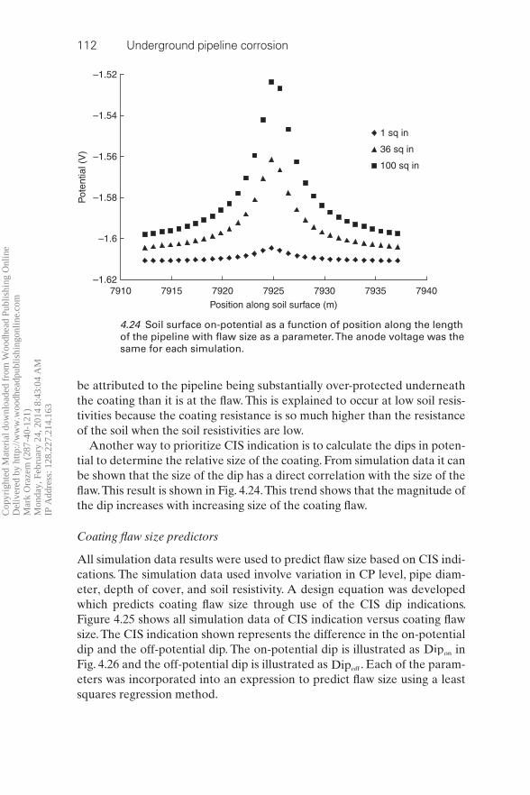
Another way to prioritize CIS indication is to calculate the dips in poten-
tial to determine the relative size of the coating. From simulation data it can
be shown that the size of the dip has a direct correlation with the size of the
fl aw. This result is shown in Fig. 4.24. This trend shows that the magnitude of
the dip increases with increasing size of the coating fl aw.
Coating fl aw size predictors
All simulation data results were used to predict fl aw size based on CIS indi-
cations. The simulation data used involve variation in CP level, pipe diam-
eter, depth of cover, and soil resistivity. A design equation was developed
which predicts coating fl aw size through use of the CIS dip indications.
Figure 4.25 shows all simulation data of CIS indication versus coating fl aw
size. The CIS indication shown represents the difference in the on-potential
dip and the off-potential dip. The on-potential dip is illustrated as Dipon in
Fig. 4.26 and the off-potential dip is illustrated as Dipoffff . Each of the param-
eters was incorporated into an expression to predict fl aw size using a least
squares regression method.
1 sq in
36 sq in
100 sq in
7910–1.62
–1.6
–1.58Pot
entia
l (V
) –1.56
–1.54
–1.52
7915 7920 7925
Position along soil surface (m)
7930 7935 7940
4.24 Soil surface on-potential as a function of position along the length
of the pipeline with fl aw size as a parameter. The anode voltage was the
same for each simulation.
Cop
yrig
hted
Mat
eria
l dow
nloa
ded
from
Woo
dhea
d Pu
blis
hing
Onl
ine
D
eliv
ered
by
http
://w
ww
.woo
dhea
dpub
lishi
ngon
line.
com
M
ark
Ora
zem
(28
7-40
-121
)
Mon
day,
Feb
ruar
y 24
, 201
4 8:
43:0
4 A
M
IP A
ddre
ss: 1
28.2
27.2
14.1
63

Numerical simulations for cathodic protection of pipelines 113
Once the expressions for the different parameters are lumped together,
a value for fl aw size can be predicted within a calculated confi dence inter-
val for a given simulation. This is used to show that the CIS predictor is not
predicting an exact coating fl aw size, but instead a range within which the
true coating fl aw size should be. For each simulation run, the corresponding
fl aw size was predicted. A plot of actual fl aw size versus predicted fl aw size
0 200
20
40
60
80
100
CIS
Indi
catio
n (m
V)
120
140
40 60
Flaw size (sq in)
80 100 120
4.25 CIS indications as a function of fl aw size obtained from a large
set of simulations. The CIS indication is the difference between the
on-potential dip and the off-potential dip, as is shown in Fig. 4.26.
Location along centerline
Pos (+)
IRtotal
Dipon
On-potential profile
Off-potential profileDipoff
IRlocalPot
entia
l
Neg (–)
4.26 A profi le of on- and off-potentials along the centerline at the soil
surface.
Cop
yrig
hted
Mat
eria
l dow
nloa
ded
from
Woo
dhea
d Pu
blis
hing
Onl
ine
D
eliv
ered
by
http
://w
ww
.woo
dhea
dpub
lishi
ngon
line.
com
M
ark
Ora
zem
(28
7-40
-121
)
Mon
day,
Feb
ruar
y 24
, 201
4 8:
43:0
4 A
M
IP A
ddre
ss: 1
28.2
27.2
14.1
63
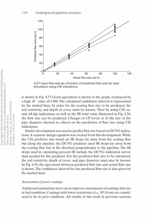
114 Underground pipeline corrosion
is shown in Fig. 4.27. Good agreement is shown in the graph, evidenced by
a high R2 value of 0.986. The calculated confi dence interval is represented
by the dashed lines. In order for the coating fl aw size to be predicted, the
soil resistivity and depth of cover must be known. Then by using CIS on-
and off-dip indications, as well as the IR total value illustrated in Fig. 4.26,
the fl aw size can be predicted. Changes in CP levels or in the size of the
pipe diameter showed no effects on the prediction of fl aw size using CIS
indications.
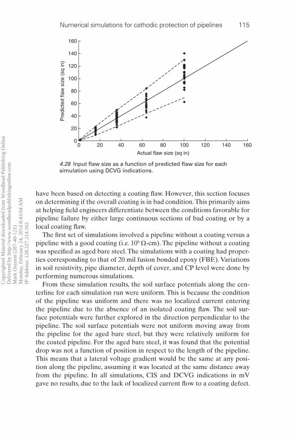
Similar development was used to predict fl aw size based on DCVG indica-
tions. A separate design equation was created from this development. While
the CIS predictor was based on IR drops far away from the coating fl aw
but along the pipeline, the DCVG predictor used IR drops far away from
the coating fl aw but in the direction perpendicular to the pipeline. The IR
drops used in calculating percent-IR include the DCVG indication survey
data needed for the predictor. For the predicted fl aw size to be calculated,
the soil resistivity, depth of cover, and pipe diameter must also be known.
In Fig. 4.28, the agreement between predicted fl aw size and actual fl aw size
is shown. The confi dence interval for the predicted fl aw size is also given by
the dashed lines.
Assessment of poor coatings
Additional simulations were run to improve assessments of coatings that are
in bad condition. Coatings with lower resistivities (i.e. 10 6 Ω -cm) are consid-
ered to be in poor condition. All results of this work in previous sections
00
20
40
60
Pre
dict
ed fl
aw s
ize
(sq
in)
80
100
120
20 40 60
Actual flaw size (sq in)
80 100 120
4.27 Input fl aw size as a function of predicted fl aw size for each
simulation using CIS indications.
Cop
yrig
hted
Mat
eria
l dow
nloa
ded
from
Woo
dhea
d Pu
blis
hing
Onl
ine
D
eliv
ered
by
http
://w
ww
.woo
dhea
dpub
lishi
ngon
line.
com
M
ark
Ora
zem
(28
7-40
-121
)
Mon
day,
Feb
ruar
y 24
, 201
4 8:
43:0
4 A
M
IP A
ddre
ss: 1
28.2
27.2
14.1
63
Numerical simulations for cathodic protection of pipelines 115
have been based on detecting a coating fl aw. However, this section focuses
on determining if the overall coating is in bad condition. This primarily aims
at helping fi eld engineers differentiate between the conditions favorable for
pipeline failure by either large continuous sections of bad coating or by a
local coating fl aw.
The fi rst set of simulations involved a pipeline without a coating versus a
pipeline with a good coating (i.e. 10 9 Ω -cm). The pipeline without a coating
was specifi ed as aged bare steel. The simulations with a coating had proper-
ties corresponding to that of 20 mil fusion bonded epoxy (FBE). Variations
in soil resistivity, pipe diameter, depth of cover, and CP level were done by
performing numerous simulations.
From these simulation results, the soil surface potentials along the cen-
terline for each simulation run were uniform. This is because the condition
of the pipeline was uniform and there was no localized current entering
the pipeline due to the absence of an isolated coating fl aw. The soil sur-
face potentials were further explored in the direction perpendicular to the
pipeline. The soil surface potentials were not uniform moving away from
the pipeline for the aged bare steel, but they were relatively uniform for
the coated pipeline. For the aged bare steel, it was found that the potential
drop was not a function of position in respect to the length of the pipeline.
This means that a lateral voltage gradient would be the same at any posi-
tion along the pipeline, assuming it was located at the same distance away
from the pipeline. In all simulations, CIS and DCVG indications in mV
gave no results, due to the lack of localized current fl ow to a coating defect.
00
20
40
60
80
100
Pre
dict
ed fl
aw s
ize
(sq
in)
120
140
160
20 40 60 80
Actual flaw size (sq in)
100 120 140 160
4.28 Input fl aw size as a function of predicted fl aw size for each
simulation using DCVG indications.
Cop
yrig
hted
Mat
eria
l dow
nloa
ded
from
Woo
dhea
d Pu
blis
hing
Onl
ine
D
eliv
ered
by
http
://w
ww
.woo
dhea
dpub
lishi
ngon
line.
com
M
ark
Ora
zem
(28
7-40
-121
)
Mon
day,
Feb
ruar
y 24
, 201
4 8:
43:0
4 A
M
IP A
ddre
ss: 1
28.2
27.2
14.1
63

116 Underground pipeline corrosion
However, due to the potential drop moving away from the pipeline in the
bare steel simulations, percent-IR calculations could be done. The length-
wise position of the percent-IR calculation was done near the center of the
pipeline to be consistent with calculations of percent-IR in previous sec-
tions. However, this location is arbitrary, since potential drops were found
to not change with position along the length of the pipeline. The percent-
IR results showed no substantial changes with respect to variations in soil
resistivity, depth of cover, pipe diameter, and oxygen blocking. It was found
that ranges in percent-IR for the aged bare steel were between 65% and
85%, while the percent-IR values were all near zero for that of the 20 mil
FBE coating. These results can be attributed to a large amount of current
entering the pipeline for the aged bare steel due to a larger current demand
to maintain the pipeline’s integrity. Since a minimal amount of current was
needed to protect the coated pipeline, the overall soil surface potential dis-
tribution was uniform.
Another set of simulations was performed for a pipeline with a poor coat-
ing. The coating resistivity was lowered to be equal to that of the soil resis-
tivity. Other properties of the coating were studied, such as oxygen blocking
and pore size. Percent-IR calculations found that variations in both of these
parameters had no infl uence, since the percent-IR values were the same for
each simulation run. Variations in soil resistivity and CP level all yielded the
same percent-IR values. This result showed that percent-IR is insensitive to
the amount of oxygen penetrating the coating.
For the fi nal set of simulations, the oxygen blocking level and the pore
size were held constant. Coating resistivity was the main parameter being
varied from 10 6 Ω -cm to 10 9 Ω -cm. Soil resistivity and CP level were also
varied. The percent-IR was calculated for each simulation. A relationship
was found by plotting the logarithm of the ratio of coating resistivity to soil
resistivity versus percent-IR. This result is shown in Fig. 4.29. The shape of
data in Fig. 4.29 resembles the curve of a rotated sigmoid function. The sig-
moid function with some slight modifi cation is given as
PA
=1
exp( )Bx CBx
[4.30]
where P represents percent-IR and x represents the logarithm of the ratio
of the coating resistivity to the soil resistivity. Parameters A , B and C were
adjusted to fi t the function to the simulation data. The equation is rear-
ranged for a rotated sigmoid function as
x = −
−ln( )P +.2 325
12
[4.31]
Cop
yrig
hted
Mat
eria
l dow
nloa
ded
from
Woo
dhea
d Pu
blis
hing
Onl
ine
D
eliv
ered
by
http
://w
ww
.woo
dhea
dpub
lishi
ngon
line.
com
M
ark
Ora
zem
(28
7-40
-121
)
Mon
day,
Feb
ruar
y 24
, 201
4 8:
43:0
4 A
M
IP A
ddre
ss: 1
28.2
27.2
14.1
63
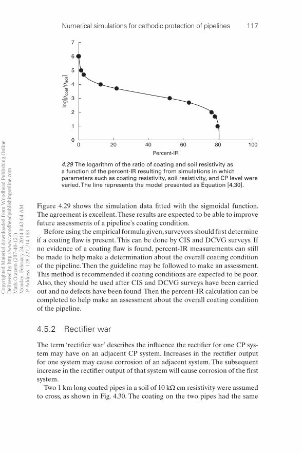
Numerical simulations for cathodic protection of pipelines 117
Figure 4.29 shows the simulation data fi tted with the sigmoidal function.
The agreement is excellent. These results are expected to be able to improve
future assessments of a pipeline’s coating condition.
Before using the empirical formula given, surveyors should fi rst determine
if a coating fl aw is present. This can be done by CIS and DCVG surveys. If
no evidence of a coating fl aw is found, percent-IR measurements can still
be made to help make a determination about the overall coating condition
of the pipeline. Then the guideline may be followed to make an assessment.
This method is recommended if coating conditions are expected to be poor.
Also, they should be used after CIS and DCVG surveys have been carried
out and no defects have been found. Then the percent-IR calculation can be
completed to help make an assessment about the overall coating condition
of the pipeline.
4.5.2 Rectifi er war
The term ‘ rectifi er war’ describes the infl uence the rectifi er for one CP sys-
tem may have on an adjacent CP system. Increases in the rectifi er output
for one system may cause corrosion of an adjacent system. The subsequent
increase in the rectifi er output of that system will cause corrosion of the fi rst
system.
Two 1 km long coated pipes in a soil of 10 k Ω cm resistivity were assumed
to cross, as shown in Fig. 4.30. The coating on the two pipes had the same
00
1
2
log[
ρ coa
t/ρ s
oil]
3
4
5
6
7
20 40 60
Percent-IR
80 100
4.29 The logarithm of the ratio of coating and soil resistivity as
a function of the percent-IR resulting from simulations in which
parameters such as coating resistivity, soil resistivity, and CP level were
varied. The line represents the model presented as Equation [4.30].
Cop
yrig
hted
Mat
eria
l dow
nloa
ded
from
Woo
dhea
d Pu
blis
hing
Onl
ine
D
eliv
ered
by
http
://w
ww
.woo
dhea
dpub
lishi
ngon
line.
com
M
ark
Ora
zem
(28
7-40
-121
)
Mon
day,
Feb
ruar
y 24
, 201
4 8:
43:0
4 A
M
IP A
ddre
ss: 1
28.2
27.2
14.1
63
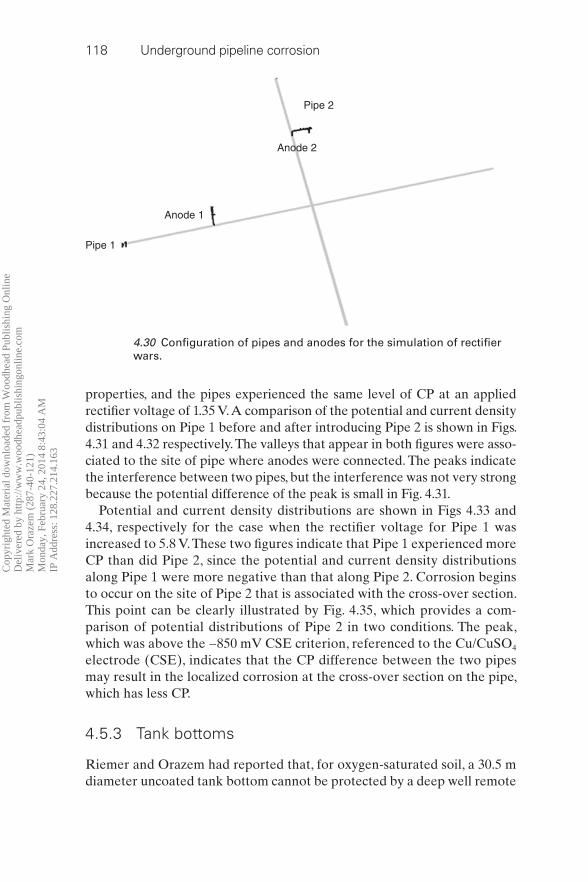
118 Underground pipeline corrosion
properties, and the pipes experienced the same level of CP at an applied
rectifi er voltage of 1.35 V. A comparison of the potential and current density
distributions on Pipe 1 before and after introducing Pipe 2 is shown in Figs.
4.31 and 4.32 respectively. The valleys that appear in both fi gures were asso-
ciated to the site of pipe where anodes were connected. The peaks indicate
the interference between two pipes, but the interference was not very strong
because the potential difference of the peak is small in Fig. 4.31.
Potential and current density distributions are shown in Figs 4.33 and
4.34, respectively for the case when the rectifi er voltage for Pipe 1 was
increased to 5.8 V. These two fi gures indicate that Pipe 1 experienced more
CP than did Pipe 2, since the potential and current density distributions
along Pipe 1 were more negative than that along Pipe 2. Corrosion begins
to occur on the site of Pipe 2 that is associated with the cross-over section.
This point can be clearly illustrated by Fig. 4.35, which provides a com-
parison of potential distributions of Pipe 2 in two conditions. The peak,
which was above the − 850 mV CSE criterion, referenced to the Cu/CuSO 4
electrode (CSE), indicates that the CP difference between the two pipes
may result in the localized corrosion at the cross-over section on the pipe,
which has less CP.
4.5.3 Tank bottoms
Riemer and Orazem had reported that, for oxygen-saturated soil, a 30.5 m
diameter uncoated tank bottom cannot be protected by a deep well remote
Pipe 1
Pipe 2
Anode 1
Anode 2
4.30 Confi guration of pipes and anodes for the simulation of rectifi er
wars.
Cop
yrig
hted
Mat
eria
l dow
nloa
ded
from
Woo
dhea
d Pu
blis
hing
Onl
ine
D
eliv
ered
by
http
://w
ww
.woo
dhea
dpub
lishi
ngon
line.
com
M
ark
Ora
zem
(28
7-40
-121
)
Mon
day,
Feb
ruar
y 24
, 201
4 8:
43:0
4 A
M
IP A
ddre
ss: 1
28.2
27.2
14.1
63
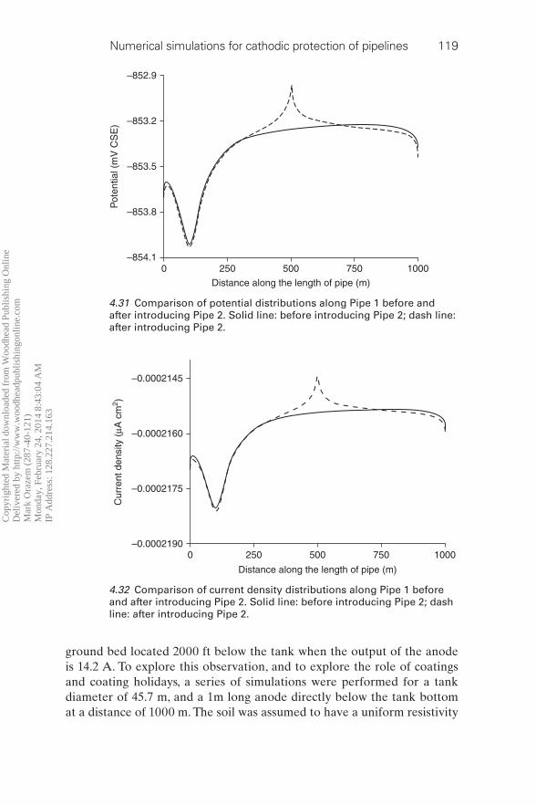
Numerical simulations for cathodic protection of pipelines 119
ground bed located 2000 ft below the tank when the output of the anode
is 14.2 A. To explore this observation, and to explore the role of coatings
and coating holidays, a series of simulations were performed for a tank
diameter of 45.7 m, and a 1m long anode directly below the tank bottom
at a distance of 1000 m. The soil was assumed to have a uniform resistivity
0–854.1
–853.8
Pot
entia
l (m
V C
SE
)
–853.5
–853.2
–852.9
250 500
Distance along the length of pipe (m)
750 1000
4.31 Comparison of potential distributions along Pipe 1 before and
after introducing Pipe 2. Solid line: before introducing Pipe 2; dash line:
after introducing Pipe 2.
0–0.0002190
–0.0002175
Cur
rent
den
sity
(μA
cm
2 )
–0.0002160
–0.0002145
250 500
Distance along the length of pipe (m)
750 1000
4.32 Comparison of current density distributions along Pipe 1 before
and after introducing Pipe 2. Solid line: before introducing Pipe 2; dash
line: after introducing Pipe 2.
Cop
yrig
hted
Mat
eria
l dow
nloa
ded
from
Woo
dhea
d Pu
blis
hing
Onl
ine
D
eliv
ered
by
http
://w
ww
.woo
dhea
dpub
lishi
ngon
line.
com
M
ark
Ora
zem
(28
7-40
-121
)
Mon
day,
Feb
ruar
y 24
, 201
4 8:
43:0
4 A
M
IP A
ddre
ss: 1
28.2
27.2
14.1
63

120 Underground pipeline corrosion
of 10 k Ω cm. The polarization parameters used are given in Table 4.2. The
difference between Steels A and B is that the mass-transfer-limited current
density for oxygen reduction was larger for Steel B than for Steel A, and
Coating B had greater permeability to oxygen than did Coating A.
0
–1200
–1100
Pot
entia
l (m
V C
SE
)
–1000
–900
–800
250 500 750
Distance along the length of pipe (m)
1000
4.33 Comparison of potential distributions along Pipe 1 and Pipe 2
respectively in Condition 2. Solid line: Pipe 1; dash line: Pipe 2.
0
–0.012
–0.008
–0.004
0.000
Cur
rent
den
sity
(μA
cm
2 )
250 500 750
Distance along the pipe (m)
1000
4.34 Comparison of current density distributions along Pipe 1 and Pipe
2 respectively in Condition 1. Solid line: Pipe 1; dash line: Pipe 2.
Cop
yrig
hted
Mat
eria
l dow
nloa
ded
from
Woo
dhea
d Pu
blis
hing
Onl
ine
D
eliv
ered
by
http
://w
ww
.woo
dhea
dpub
lishi
ngon
line.
com
M
ark
Ora
zem
(28
7-40
-121
)
Mon
day,
Feb
ruar
y 24
, 201
4 8:
43:0
4 A
M
IP A
ddre
ss: 1
28.2
27.2
14.1
63

Numerical simulations for cathodic protection of pipelines 121
The current distributions corresponding to the four cases are shown in
Fig. 4.36, and the corresponding parameter values are presented in Table 4.3.
In the case of Steel A and Steel B, where no coatings are present, the pro-
tection current distribution is observed to be non-uniform, with the periph-
ery having higher current density than the middle of the tank bottom. By
0
–855
–850
–845
Pot
entia
l (m
V C
SE
)–840
–835
250 500 750
Distance along the length of pipe (m)
1000
4.35 Potential distributions of Pipe 2 in Conditions 1 and 2, respectively.
Solid line: Pipe 2 in Condition 1; dash line: Pipe 2 in Condition 2.
0.00.4
0.6
0.8
1.0
i/iav
g
1.2
1.4
1.6
1.8
2.0
0.2
Coating A
Steel A/Steel B
Coating B
0.4 0.6
r/R
0.8 1.0 1.2
4.36 Calculated normalized current density as a function of
dimensionless radius on tank bottoms with different surface properties.
Cop
yrig
hted
Mat
eria
l dow
nloa
ded
from
Woo
dhea
d Pu
blis
hing
Onl
ine
D
eliv
ered
by
http
://w
ww
.woo
dhea
dpub
lishi
ngon
line.
com
M
ark
Ora
zem
(28
7-40
-121
)
Mon
day,
Feb
ruar
y 24
, 201
4 8:
43:0
4 A
M
IP A
ddre
ss: 1
28.2
27.2
14.1
63

122 Underground pipeline corrosion
increasing the current output, it was possible to drive potentials to values
below − 850 mV CSE, as shown in Fig. 4.37. The coated tank bottoms were
easily protected by the sacrifi cial Mg anodes. The current distributions were
uniform, and the potentials were well within the protected regime.
Additional simulations were performed for coated tank bottoms with
coating fl aws that exposed bare steel. The coating defect was located at the
center of the tank bottom and, as was done for the previous calculation,
the anode was placed at a large distance from the tank. Two confi gurations
were studied: Coating A with Steel B exposed in the center of the tank and
Coating B with Steel B exposed, respectively. The coating holiday covered
a relatively large 5.5 m 2 which represented 0.35% of the tank area. The soil
resistivity was assumed to be uniform, with a value of 10 k Ω cm. The corre-
sponding current and potential distributions are given in Figs 4.38 and 4.39,
respectively.
Table 4.3 Tank bottom simulation results
Tank steel/coating Steel A Steel B Coating A Coating B
Type of anode ICCP –
4750
ICCP –
15500
Standard
potential
magnesium
Standard
potential
magnesium
Potential applied,
V CSE
4750 15500 – –
Output current of
anode, A
111.62 364.34 0.0092 0.0118
Cross section area of
tank bottom, m 2
1641.7 1641.7 1641.7 1641.7
Table 4.2 Parameters corresponding to tank bottom simulations (see Equations
[4.6], [4.9], and [4.10])
Type of coating Coating A Coating B Steel A Steel B
Coating resistivity , M Ω cm 5000 200 – –
Coating Thickness δ , mm 0.508 0.508 – –
Oxygen blocking αblocαα k, % 99.9 99 – –
A Apore / , % 0.1 0.1 – –
EFe, mV − 522 − 522 − 522 − 522
βFeββ , mV/decade 62.6 62.6 62.6 62.6
ilim,Oii2, μ A/cm 2 1.05 1.05 3.1 10.8
EO2, mV CSE − 172 − 172 − 172 − 172
βOββ2, mV/decade 66.5 66.5 66.5 66.5
EH2,mV CSE − 942 − 942 − 942 − 942
βHβ2, mV/decade 132.1 132.1 132.1 132.1
Cop
yrig
hted
Mat
eria
l dow
nloa
ded
from
Woo
dhea
d Pu
blis
hing
Onl
ine
D
eliv
ered
by
http
://w
ww
.woo
dhea
dpub
lishi
ngon
line.
com
M
ark
Ora
zem
(28
7-40
-121
)
Mon
day,
Feb
ruar
y 24
, 201
4 8:
43:0
4 A
M
IP A
ddre
ss: 1
28.2
27.2
14.1
63
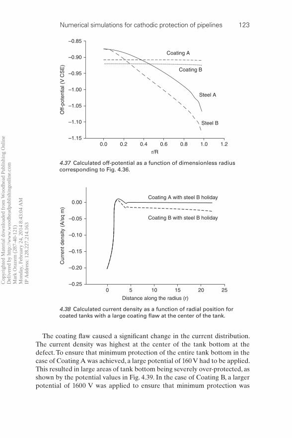
Numerical simulations for cathodic protection of pipelines 123
The coating fl aw caused a signifi cant change in the current distribution.
The current density was highest at the center of the tank bottom at the
defect. To ensure that minimum protection of the entire tank bottom in the
case of Coating A was achieved, a large potential of 160 V had to be applied.
This resulted in large areas of tank bottom being severely over-protected, as
shown by the potential values in Fig. 4.39. In the case of Coating B, a larger
potential of 1600 V was applied to ensure that minimum protection was
0.0–1.15
–1.10
–1.05
–1.00
Off-
pote
ntia
l (V
CS
E)
–0.95
–0.90
–0.85
0.2 0.4 0.6
r/R
0.8
Coating A
Coating B
Steel A
Steel B
1.0 1.2
4.37 Calculated off-potential as a function of dimensionless radius
corresponding to Fig. 4.36.
0–0.25
–0.20
–0.15
–0.10
Cur
rent
den
sity
(A
/sq
m)
–0.05
0.00
5 10
Distance along the radius (r)
15 20
Coating A with steel B holiday
Coating B with steel B holiday
25
4.38 Calculated current density as a function of radial position for
coated tanks with a large coating fl aw at the center of the tank.
Cop
yrig
hted
Mat
eria
l dow
nloa
ded
from
Woo
dhea
d Pu
blis
hing
Onl
ine
D
eliv
ered
by
http
://w
ww
.woo
dhea
dpub
lishi
ngon
line.
com
M
ark
Ora
zem
(28
7-40
-121
)
Mon
day,
Feb
ruar
y 24
, 201
4 8:
43:0
4 A
M
IP A
ddre
ss: 1
28.2
27.2
14.1
63
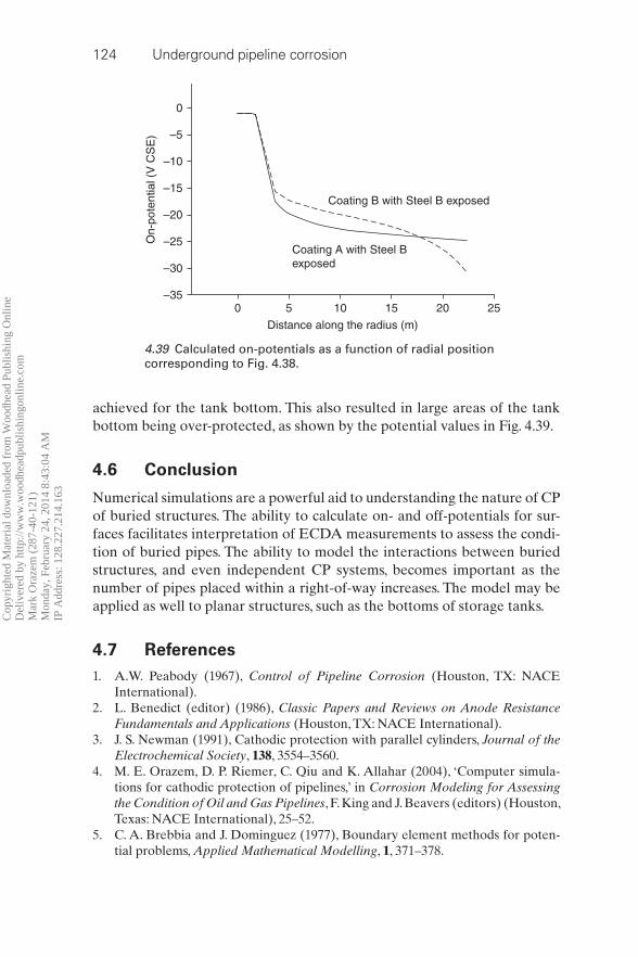
124 Underground pipeline corrosion
achieved for the tank bottom. This also resulted in large areas of the tank
bottom being over-protected, as shown by the potential values in Fig. 4.39.
4.6 Conclusion
Numerical simulations are a powerful aid to understanding the nature of CP
of buried structures. The ability to calculate on- and off-potentials for sur-
faces facilitates interpretation of ECDA measurements to assess the condi-
tion of buried pipes. The ability to model the interactions between buried
structures, and even independent CP systems, becomes important as the
number of pipes placed within a right-of-way increases. The model may be
applied as well to planar structures, such as the bottoms of storage tanks.
4.7 References 1. A.W. Peabody (1967), Control of Pipeline Corrosion (Houston, TX: NACE
International).
2. L. Benedict (editor) (1986), Classic Papers and Reviews on Anode Resistance Fundamentals and Applications (Houston, TX: NACE International).
3. J. S. Newman (1991), Cathodic protection with parallel cylinders, Journal of the Electrochemical Society , 138 , 3554–3560.
4. M. E. Orazem, D. P. Riemer, C. Qiu and K. Allahar (2004), ‘ Computer simula-
tions for cathodic protection of pipelines,’ in Corrosion Modeling for Assessing the Condition of Oil and Gas Pipelines , F. King and J. Beavers (editors) (Houston,
Texas: NACE International), 25–52.
5. C. A. Brebbia and J. Dominguez (1977), Boundary element methods for poten-
tial problems, Applied Mathematical Modelling , 1 , 371–378.
0–35
–30
–25
–20
On-
pote
ntia
l (V
CS
E)
–15
–10
–5
0
5 10
Distance along the radius (m)
Coating B with Steel B exposed
Coating A with Steel Bexposed
15 20 25
4.39 Calculated on-potentials as a function of radial position
corresponding to Fig. 4.38.
Cop
yrig
hted
Mat
eria
l dow
nloa
ded
from
Woo
dhea
d Pu
blis
hing
Onl
ine
D
eliv
ered
by
http
://w
ww
.woo
dhea
dpub
lishi
ngon
line.
com
M
ark
Ora
zem
(28
7-40
-121
)
Mon
day,
Feb
ruar
y 24
, 201
4 8:
43:0
4 A
M
IP A
ddre
ss: 1
28.2
27.2
14.1
63

Numerical simulations for cathodic protection of pipelines 125
6. S. Aoki, K. Kishimoto and M. Sakata (1985), Boundary element analysis of gal-
vanic corrosion, in Boundary Elements VII , C. A. Brebbia and G. Maier (edi-
tors) (Heidelberg: Springer-Verlag), 73–83.
7. J. C. F. Telles, L. C. Wrobel, W. J. Mansur and J. P. S. Azevedo (1985), Boundary
elements for cathodic protection problems, in Boundary Elements VII , C. A.
Brebbia and G. Maier (editors) (Heidelberg: Springer-Verlag), 63–71.
8. N.G. Zamani and J.M Chuang (1987), Optimal-control of current in a cathodic
protection system – a numerical investigation, Optimal Control Applications & Methods , 8 , 339–350.
9. F. Brichau and J. Deconinck (1994), A numerical-model for cathodic protection
of buried pipes, Corrosion , 50 , 39–49.
10. F. Brichau, J. Deconinck and T. Driesens (1996), Modeling of underground
cathodic protection stray currents, Corrosion , 52 , 480–488.
11. S. Aoki and K. Amaya (1997), Optimization of Cathodic Protection System by
BEM, Engineering Analysis with Boundary Elements , 19 , 147–156.
12. S. Aoki, K. Amaya and M. Miyasaka (1999), Boundary element analysis of
cathodic protection for complicated structures, in Proceedings of the NACE99
Topical Research Symposium: Cathodic Protection: Modeling and Experiment,
M. E. Orazem (editor),(Houston, TX: NACE International), 45–65.
13. K. J. Kennelley, L. Bone and M. E. Orazem (1993), Current and potential distri-
bution on a coated pipeline with holidays:1. model and experimental verifi ca-
tion, Corrosion , 49 , 199–210.
14. M. E. Orazem, K. J. Kennelley and L. Bone (1993), Current and potential dis-
tribution on a coated pipeline with holidays:2. a comparison of the effects of
discrete and distributed holidays, Corrosion , 49 , 211–219.
15. M. E. Orazem, J. M. Esteban, K. J. Kennelley and R. M. Degerstedt (1997),
Mathematical models for cathodic protection of an underground pipeline with
coating holidays: 1. theoretical development, Corrosion , 53 , 264–272.
16. M. E. Orazem, J. M. Esteban, K. J. Kennelley and R. M. Degerstedt (1997),
Mathematical models for cathodic protection of an underground pipeline with
coating holidays: 2. case studies of parallel anode CP systems, Corrosion , 53 ,
427–436.
17. D. P. Riemer and M. E. Orazem (2005), Modeling coating fl aws with non-
linear polarization curves for long pipelines, in Corrosion and Boundary Element Methods , R. A. Adey (editor) (Southampton, UK: WIT Press),
225–259.
18. D. P. Riemer and M. E. Orazem (2000), Application of boundary element mod-
els to predict effectiveness of coupons for assessing cathodic protection of bur-
ied structures, Corrosion , 56 , 794–800.
19. D. P. Riemer and M. E. Orazem (2005), A mathematical model for the cathodic
protection of tank bottoms, Corrosion Science , 47 , 849–868.
20. J. F. Yan, S. N. R. Pakalapati, T. V. Nguyen, R. E. White and R. B. Griffi n (1992),
Mathematical modeling of cathodic protection using the boundary element
method with a nonlinear polarization curve, Journal of the Electrochemical Society , 139 , 1932–1936.
21. D. P. Riemer (2000), Modeling Cathodic Protection for Pipeline Networks , PhD
dissertation, University of Florida, Gainesville, Florida.
22. C. A. Brebbia, J. C. F. Telles and L. C.Wrobel (1984), Boundary Element Techniques , (Heidelberg: Springer-Verlag).
Cop
yrig
hted
Mat
eria
l dow
nloa
ded
from
Woo
dhea
d Pu
blis
hing
Onl
ine
D
eliv
ered
by
http
://w
ww
.woo
dhea
dpub
lishi
ngon
line.
com
M
ark
Ora
zem
(28
7-40
-121
)
Mon
day,
Feb
ruar
y 24
, 201
4 8:
43:0
4 A
M
IP A
ddre
ss: 1
28.2
27.2
14.1
63
126 Underground pipeline corrosion
23. I. Stakgold (1979), Greens Functions and Boundary Value Problems (New York:
John Wiley & Sons).
24. J. Newman (1966), ‘Resistance for fl ow of current to a disk’, Journal of the Electrochemical Society , 113 501.
25. C. Kasper (1940), The theory of the potential and the technical practice of elec-
trodeposition: IV. The fl ow between and to circular cylinders’, Transactions of the Electrochemical Society , 78 147–161.
26. J. P. McKinney, M. E. Orazem, O. Moghissi and D. D’Zurko (2006), Development
of ECDA criteria for prioritization of indications, Proceedings of Corrosion/2006
(Houston, Texas: NACE International), Paper 06–188.
27. J. P. McKinney, M. E. Orazem, O. Moghissi and D. D’Zurko (2009), Predicting
coating holiday size using ECDA survey data, Proceedings of Corrosion/2009
(Houston, Texas: NACE International), Paper 09–146.
28. O. C. Moghissi, W. Harper, M. Celinski, V. Sottile and D. DiMeo (2004),
‘ External corrosion direct assessment validation through correlation between
indications and control excavations’, Proceedings of Corrosion /2004 (Houston,
Texas: NACE International), Paper 04–187.
Cop
yrig
hted
Mat
eria
l dow
nloa
ded
from
Woo
dhea
d Pu
blis
hing
Onl
ine
D
eliv
ered
by
http
://w
ww
.woo
dhea
dpub
lishi
ngon
line.
com
M
ark
Ora
zem
(28
7-40
-121
)
Mon
day,
Feb
ruar
y 24
, 201
4 8:
43:0
4 A
M
IP A
ddre
ss: 1
28.2
27.2
14.1
63


