UNDERGROUND ACOUSTIC S - Rupert Taylor

Proceedings of the Institute of Acoustics

Vol. 38. Pt. 1. 2016

UNDERGROUND ACOUSTICS R M Thornely-Taylor Rupert Taylor Ltd

1 INTRODUCTION

The characteristics of wave generation and propagation in a medium other than air, i.e. underground and in structures, differ from those of airborne sound waves. In some respects the differences are substantial. Elastic waves occurring underground and in structures are of course better known as vibration. While vibration may itself directly affect machines or structures, or be perceived by human recipients, it also can cause structures to radiate sound. A common example of structure-radiated sound is the rumble heard in buildings above railway tunnels with stiff track support. Characterising sources of vibration, whether railways, machines or construction activities is much more difficult than establishing the sound power of an airborne sound source, not least because readily measurable source characteristics are strongly influenced by the medium supporting the source. The system on which the source is founded and the medium providing the path from source to receiver have complex properties, and the response of the receiving structure is dependent on the path. The receptor, such as a human being, also has dynamic properties which may be coupled to the structure supporting it. When vibration is received as structure-radiated sound, understanding the interface between the structure and the airspace involves wave acoustics rather than more widely used diffuse-field room acoustics. The measurement, prediction and mitigation of vibration all require careful account to be taken of these peculiarities.

2 OVERVIEW OF GROUNDBORNE VIBRATION GENERATION, PROPAGATION AND RECEPTION

2.1 Vibration generation

Vibration is caused by time-varying force. It can be explosive in origin, as in blasting or a diesel piling hammer, gravitational due to the fall of (or rolling of) a mass on to the ground or a structure, due to the release of strain as in seismic events, non-smooth mechanical movement or out-of-balance rotation, turbulent or pulsating fluid flow, involving cyclical or random force at the foundations of the source. Whatever the nature of the source, the quantity of importance is power, although the direct measurement of power is non-trivial. Power is the product of force and velocity, or the square of velocity and mechanical impedance (force/velocity). The power that is radiated depends on the impedance. Standard procedures exist [1][2] for the measurement of vibration power flow from machines, but their application is challenging. What is important to take into account is that measurement of vibration acceleration or velocity in the ground does not alone tell you how much vibration power is being radiated. Large velocity amplitude in soft ground or a lightweight/mobile structure may carry less power than small amplitude velocity in rock, hard ground or a low mobility structure.

2.2 Vibration propagation

Once into the propagation medium, vibration can be propagated in many ways. The simplest case is an underground explosion which, if in an unbounded medium, would cause vibration propagated solely as a compression (dilatational) wave, analogous to a sound wave in air. Unbounded media do not exist, and when an underground compression wave reaches a boundary such as the surface

1


Vol. 38. Pt. 1. 2016

of the ground, other wave types are formed including shear waves and Rayleigh waves. To illustrate the waves that occur in a semi-infinite half space, approximated by a very deep layer of homogeneous, isotropic soil or rock, Figure 1 shows the waves that propagate from an impulse source applied to the surface of the ground. The outer semi-circle is the dilatational wave with the fastest phase velocity. The inner semi-circle is a shear wave which has a slower velocity than the dilatational wave, and is transformed into a Rayleigh wave at the surface. The phase speed of a Rayleigh wave is slightly less than that of a shear wave, hence the slight “waisting” of the curve at the surface. Between the dilatational wave and the shear wave is a head wave. This is caused by the fact that when the dilatational wave reaches the surface it causes locally generated shear waves to appear which propagate downwards. The head wave has two velocities – along the surface at the dilatational wave speed and down into the half space at the shear wave speed. It results from Huygens’ principle of wave construction – namely that every point on a wave front may be regarded as a new source of wavelets that expand in every direction. Figure 2 shows the formation of the effect.

Figure 1 Waves generated and propagated by an impulse at the surface of a homogeneous isotropic half-space

Figure 2 Formation of a head wave Figure 3 shows that when there is air above an elastic half space a head wave also occurs in air due to radiation upwards from the travelling Rayleigh wave front, as long as the Rayleigh wave speed is faster than the speed of sound in air. Thus the sound of an impulse on the ground surface

2


Vol. 38. Pt. 1. 2016

is heard twice, firstly as the re-radiated airborne wave from the Rayleigh wave passes the receiver and secondly as the airborne pressure wave originating at the source arrives.

Figure 3 Airborne head wave above an impulse on the surface of an elastic half space These are not the only forms of wave propagation in an elastic medium. The full list is Dilatational waves Shear waves (which may be polarized in more than one plane) Head Waves Rayleigh waves Lamb waves Love waves Stoneley (and Scholte) waves Biot slow waves In structures there are also torsional waves as well as bending and longitudinal waves. Lamb waves are surface waves which include Rayleigh waves; Love waves are surface shear waves with displacements normal to the direction of propagation. Stoneley and Sholte waves are waves in a layer bounded on both sides by media with different impedances. Biot slow waves or, as he described them, “dilatational waves of the second kind” occur in liquid-saturated porous elastic media. They are evanescent and only propagate a short distance as shown in Figure 4.

3


Vol. 38. Pt. 1. 2016

Figure 4 Biot slow waves These wave types have their own phase speeds, and in most cases for waves in an unbounded medium of a homogeneous half-space they are not dispersive. They have different rates of decay due to geometric spreading. For a point source, the amplitude of shear waves on the surface is inversely proportional to the square of the distance; Rayleigh wave amplitudes are inversely proportional to the square root of the distance and the amplitude of dilatational waves propagating into the half space are inversely proportional to distance (their intensity in watts/m

2 being therefore inversely proportional to the square of the distance – analogous to the inverse square law in airborne acoustics). Of interest is the fact that for a line source on the surface of a homogeneous half space, there is no decay with distance due to geometrical spreading of Rayleigh waves. The ground is seldom a homogeneous half-space, and due to confining pressure and layering the wave speed tends to increase with depth. A feature of Rayleigh waves is that their depth below the surface is frequency dependent, with low frequency/long wavelength waves extending deeper below the surface than high frequency waves. This causes dispersion, with long wavelength waves travelling faster. This effect is put to use as a way of measuring soil properties below the surface using a method called Spectral Analysis of Surface Waves (SASW) and Multi-channel Analysis of Surface Waves (MASW). By measuring a seismic impulse (e.g. a hammer blow) at an array of surface transducers and processing the signals to separate out the phase of the frequency components, it is possible to derive a soil/depth profile to match the characteristics of the received signals. An example of a MASW survey result is given in figure 5. The primary output shows shear wave speed with depth. This is accompanied by knowledge of the relevant lithology – in this case limestone with layers of clay and made ground. What is measured is the shear wave speed which is converted to small strain shear modulus Gmax. It can also be converted to compression modulus through Poisson’s ratio, but in water saturated ground where Poisson’s ratio is close to its maximum of 0.5, the value of the modulus is highly sensitive to small changes in Poisson’s ratio. Further guidance on the determination of soil properties is to be found in reference [10].

4


Vol. 38. Pt. 1. 2016

Figure 4 Example of MASW output Geometric spreading is of course only one mechanism that causes attenuation of waves in an elastic medium. Damping also occurs, due to energy loss caused by viscous, hysteretic or friction effects. Additionally other effects reduce wave amplitudes including reflections and scattering, as well as wave conversion at interfaces between layers. Although dilatational and shear waves

5


Vol. 38. Pt. 1. 2016

propagate independently in a homogeneous medium, once they meet an interface with a medium of different impedance there will be partial conversion to the other wave type in each case. This becomes important when damping is considered, because the rate of decay due to damping is inversely proportional to wave speed, and therefore the part of an incident dilatational wave that is converted into a shear wave at an interface becomes more rapidly attenuated than it would have been had it continued unreflected. Refraction also occurs, because of the increase in soil impedance with depth below ground, and associated wave speed increases cause bending of the propagation path in the direction of the surface. Attenuation due to damping is represented by the use of complex value for compression and shear moduli. This leads to a distance function of the form

e-iωδx/c

(1)

where ω is angular frequency, x is distance, c is the phase speed of the wave type and i is √−1. For loss factors less than about 0.2 δ can be approximated as η/2 where η is the imaginary part of a complex modulus. Converting from Nepers to dB gives the relationship 4.34 ωη/c in dB per metre, or approximatey 27η dB per wavelength. Since wavelength is dependent on phase velocity, which is dependent on wave type, shear wave having much lower phase speeds and therefore much shorter wavelengths, in order to estimate the attenuation due to material damping it is essential to know the relative proportion of the vibration power that is propagated by each different wave type. It is also important to note that the value of η is not necessarily the same for different wave types. If a value for η is derived from theory or from the literature its value will seldom be found to be more than about 0.05. The largest amount of data in the literature relates to the acoustics of the sea bed. Stoll [3] found the loss factor of shear waves in a water-saturated silt to be independent of frequency between 43 and 391 Hz. Tullos and Reid [4] found that in clay-sand the loss factor is independent of frequency between 20 and 400 Hz. In sands, Stoll found that loss factor was proportional to frequency (and therefore attenuation proportional to the square of the frequency) in the range 30-240 Hz. This suggests the existence of viscous damping. Hamilton [5][6] gives data on attenuation in dB per metre as a function of porosity in saturated surface (of the ocean floor) sediments. There is a peak attenuation at 52% porosity, of 0.78f dB per metre, where f is frequency in kilohertz, falling to 0.12f at 65%, 0.52f at 46%; 0.46f at 36% and 0.05f at 90%. Similarly he gives attenuation as a function of mean grain size peaking at 0.76f at 40μ. Hamilton quotes attenuation in hard, dense limestone of 0.02f and chalk 0.08f, dB per metre. For Basalts under the sea floor the attenuation is given as 0.02f to 0.05f. Hamilton summarises various references as follows:

Material Attenuation in dB per metre (f=kHz)

Diluvial sand 13.2f

Diluvial sand and clay 4.8f

Alluvial silt 13.4f

Mud (silt-clay) 17.3f

Water-saturated clay 15.2f

Tertiary mudstone 10.1f

Pierre shale 3.4f

Solenhofen limestone 0.02f to 0.05f

Chalk 0.1f

Basalt 0.07f

Table 1 Attenuation due to damping in soil and rock

6


Vol. 38. Pt. 1. 2016

Handbooks such as the Transportation Noise Reference Book [7] and the UMTA Handbook [8] quote values of attenuation some of which are higher than the authorities cited above indicate. However, it appears that the causes of attenuation over and above that due to geometric spreading are not solely due to damping of the viscous, hysteretic or frictional kind, but due to soil inhomogeneity. Figure 5 compares the surface vibration velocities due to an underground source in the form of a railway tunnel for two cases modelled using the finite-difference method. The first assumes homogeneous chalk and the second assumes layered chalk of varying density and wave velocity, this particular case being an example of lithology from Copenhagen. In both cases the loss factor is the same.

Figure 5 Effect of layering on vibration propagation in soil

2.3 Vibration reception

Vibration in the surface of the ground is seldom of direct interest. In most cases the matter of interest is vibration in a building or structure, or in a receptor located in a building, and while that receptor may be a sensitive instrument such as an electron microscope it is frequently a human being. Furthermore, human beings may receive the vibration not by way of the tactile sense but as airborne sound, having been radiated by vibrating building surfaces. It is therefore necessary to consider dynamic soil-structure interaction to translate vibration in the ground into building vibration, to consider the response of the building or structure, and the response of a human body if necessary.

2.3.1 Coupling soil-structure

Soil-structure interaction has been studied in seismology, and although the frequency range of interest is much lower than the range within which groundborne noise can occur, some of the basics are relevant. A mass of finite size resting on an elastic halfspace behaves as if a large region of the mass of the halfspace is attached to the building, and the elastic halfspace also behaves as a spring, Solution of the applicable equations is largely intractable. A closed-form solution is only

7


Vol. 38. Pt. 1. 2016

available for simplified cases such as a disc on an elastic half space. This was solved in the middle of the last century by Bycroft [9] building on the works of Rayleigh, Lamb and Reissner cited in reference [9]. As an example of the application of the Bycroft intergral, Figure 6 shows the coupling loss factor for a rigid body 150MN in weight on a circular base with an average radius of 18m resting on a semi-infinite halfspace of clay soil.

Figure 6 Coupling loss factor on transmission of vibration from an elastic halfspace of clay to a load of 150MN resting on a circular base of average radius 18m It is of interest that the coupling loss factor ranges from an average of around -5dB at low frequencies to the order of -15 dB in the range where groundborne noise commonly occurs above railways with unmitigated track support. These are consistent with some of the data reported in reference [8] and cited in reference [7]. Above about 80 Hz the coupling loss factor in Figure 6 continues to increase to -20 dB or below, but it should be borne in mind that no real building is actually a rigid body at these frequencies, and modes within the building structure will significantly modify the curve. A matter of importance is the precise definition of coupling loss factor, as the function required may be in one case the difference between vibration at the surface of the ground, as measured, and vibration in the foundations of a building, and in another case a calculated value for vibration within an unbounded soil above a source such as an underground railway. It is necessary to take into account the fact that for normal incidence of p-waves originating at a buried source the velocity at the surface of a half space is double that at the same location in an unbounded medium. The coupling loss factor plotted in Figure 6 is base vibration relative to ground surface vibration in its absence. For cases other than those solved in reference [9], numerical solutions are necessary. These can take account of the impedance of the building structure, coupled if necessary to the receiving structure be it a machine or a human.

8


Vol. 38. Pt. 1. 2016

2.3.2 Dynamic building response

In contrast to the simple case of a rigid body resting on a half-space is a tall building with many floors supported on columns. Such a case has interesting dynamic properties. For example, if the load on the ground floor columns is summed and considered as a single degree-of-freedom system with the ground floor columns treated as springs based on the compressive stiffness of the columns, it can be the case that the natural frequency of system is in single figures. Should it be necessary to consider base-isolation of such a building, the effect of inserting polymer or steel springs below the columns would seem intuitively to be somewhat nugatory. However, the actual situation is much more complex than that of a single-degree-of-freedom system, as illustrated in figure 7 plotted using transmission line theory. The curve at the top of the figure is a plot of the transmissibility, up the building, at the base of the columns on the 9

th floor of a nine-storey building,

showing the peak caused by the SDOF resonance of the columns under the mass of the slab above them. The next curve down shows what happens when you move down a floor. The single peak of the ninth floor gives way to a pair of coupled natural frequencies, one above and one below the ninth floor peak. Move down again to the seventh floor and other floors below and an additional

coupled frequency is introduced, and the others are shifted down. Down at the ground floor (bottom

curve) there is a peak for each floor, and the lowest peak is in the region that would be obtained by considering the whole structure above the ground floor as a lumped mass. The lowest peak is at 7Hz. In a case where groundborne noise is being transmitted into such a building, it might be necessary to consider whether inserting springs under the ground floor columns with a natural frequency of that order would have any useful effect. Figure 8 shows the bottom curve of Figure 7 expanded in scale together with the same curve after the insertion of bearings under the ground floor columns chosen to have a notional natural frequency of 7Hz under a load equivalent to the lumped mass of the entire building. It can be seen that the insertion loss, while much less than that of a SDOF system, is still exceeding 10 dB above 40Hz.

Figure 7 Coupled natural frequencies in a nine-storey building.

9


Vol. 38. Pt. 1. 2016

Figure 8 Coupled natural frequencies in a nine-storey building with and without 7Hz base-isolation bearings inserted.

2.3.3 Coupling structure-human body

The dynamic response of the human body is complex. Reference [10] provides a mechanical analogy of a three-degrees-of-freedom system as a biodynamic model of the seated human body. Unfortunately a corresponding model of the recumbent or standing body is not provided, but the data in reference [10] give an indication of the issues involved.

2.3.4 Coupling structure-air

In cases where the concern is sound in the airspace of a room resulting from vibration of room surfaces, it is necessary to use wave acoustics to calculate the sound field in the room which is coupled to the radiating plate which is the floor or other surfaces in the room. The basic equations governing this effect are set out in reference [14]. In the simplified case of a simply supported rectangular plate forming the floor of a rectangular room the shape function of the plate vibration [16] differs significantly from the shape function for the airspace in the room [17][18] as shown in figures 9 and 10. As a consequence of the mis-match between mode shapes, coupling between plate vibration and air sound pressure is restricted to mode combinations where the sum of the plate and room modes is odd and the plate and room mode numbers are not equal.

10


Vol. 38. Pt. 1. 2016

Figure 9 Mode shapes for a simply supported plate.

Figure 10 Mode shapes for a rectangular room.

11


Vol. 38. Pt. 1. 2016

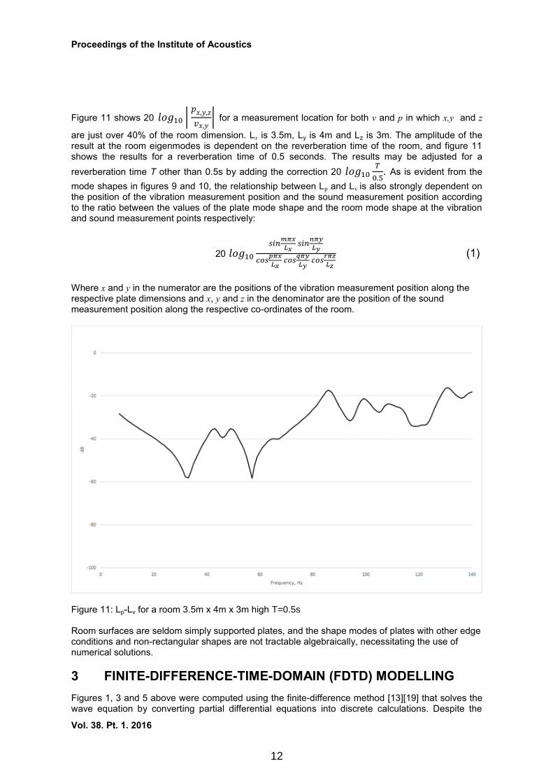
Figure 11 shows 20 𝑙𝑜𝑔10 | 𝑝𝑥,𝑦,𝑧

𝑣𝑥,𝑦| for a measurement location for both v and p in which x,y and z

are just over 40% of the room dimension. Lx is 3.5m, Ly is 4m and Lz is 3m. The amplitude of the result at the room eigenmodes is dependent on the reverberation time of the room, and figure 11 shows the results for a reverberation time of 0.5 seconds. The results may be adjusted for a

reverberation time T other than 0.5s by adding the correction 20 𝑙𝑜𝑔10𝑇

0.5. As is evident from the

mode shapes in figures 9 and 10, the relationship between Lp and Lv is also strongly dependent on the position of the vibration measurement position and the sound measurement position according to the ratio between the values of the plate mode shape and the room mode shape at the vibration and sound measurement points respectively:

20 𝑙𝑜𝑔10

𝑠𝑖𝑛𝑚𝜋𝑥

𝐿𝑥 𝑠𝑖𝑛

𝑛𝜋𝑦

𝐿𝑦

𝑐𝑜𝑠𝑝𝜋𝑥

𝐿𝑥 𝑐𝑜𝑠

𝑞𝜋𝑦

𝐿𝑦 𝑐𝑜𝑠

𝑟𝜋𝑧

𝐿𝑧

(1)

Where x and y in the numerator are the positions of the vibration measurement position along the respective plate dimensions and x, y and z in the denominator are the position of the sound measurement position along the respective co-ordinates of the room.

Figure 11: Lp-Lv for a room 3.5m x 4m x 3m high T=0.5s Room surfaces are seldom simply supported plates, and the shape modes of plates with other edge conditions and non-rectangular shapes are not tractable algebraically, necessitating the use of numerical solutions.

3 FINITE-DIFFERENCE-TIME-DOMAIN (FDTD) MODELLING

Figures 1, 3 and 5 above were computed using the finite-difference method [13][19] that solves the wave equation by converting partial differential equations into discrete calculations. Despite the

12


Vol. 38. Pt. 1. 2016

many types of wave propagation found in the transmission of vibration, there is only one wave equation for vibration in elastic media. It requires modification to include damping, but otherwise is universal. The wave equation for lossless propagation is

t

2

2

divgrad21

1

sssΔ

(2)

in which

s = i + j + k (3)

where , and are displacements in three orthogonal axes; is the Lamé constant identical to

the shear modulus; is the density and is Poisson’s ratio. Figure 12 shows the finite difference representation of equation (2). The region within the model is divided up into a 3-dimensional grid of “shoe-box” shaped cells at each corner of which is a point shown as a black dot. Each cell, defined as one of the hexahedrons with four black dots as corners, is assigned a value for its shear modulus, compression modulus, density and loss factor, and for its displacement and velocity in each of the i, j and k directions. The vibration input to the model involves displacing, or adding velocity to, one of the “black dot” points.

Figure 12 The basic finite-difference grid

At each time step, based on the displacement of the black dot points, the displacement of the white dot points which lie on a staggered grid halfway between the black dot points, is interpolated. These “white dot” displacements are then used to compute the strain on the grey cell in the centre. The strain is computed in terms of (i) the compression of the three pairs of opposite sides and (ii) the shear of each face.

13


Vol. 38. Pt. 1. 2016

The force acting in each i, j and k direction is determined from the product of the strains and the relevant dynamic moduli. The centre of the grey cell is then accelerated in the resultant direction by the force divided by the mass of the cell, i.e. its velocity increased by the product of the acceleration and the length of the time step. The displacement is then increased (or decreased) by the product of the velocity and the time step. This process is repeated for as many time steps as are required to achieve the necessary run time, e.g. one second. The outstanding feature of this approach is that all wave types, whether shear waves, compression waves, bending waves, Rayleigh waves, Lamb waves, Love waves or Stoneley waves will automatically occur simply as a consequence of the shape of the structure represented by the cells. A beam represented by a line of cells surrounded by air or a vacuum will exhibit bending waves, as will a plate represented by a two-dimensional slayer of cells. A body of cells with a surface bounded by air or a vacuum will exhibit Rayleigh waves. In principle, shear waves occur independently of compression waves, but where there is a reflection caused by an obliquely incident wave on the boundary between two regions with different properties, wave conversion takes place. This occurs automatically in the finite difference grid. The relationship between the general three-dimensional wave equation and equations for plates and shells when free surfaces are taken into account is explained in Reference 13. Damping may be included in a finite difference model by means of Boltzmann’s expression using relaxation functions.

01

)()()()()( tdttttt D (3)

where (t) =

/2 teD

The term (t) is an after-effect function, D1 is the compressive modulus, D2 is a constant and is a

relaxation time. D1 is a modulus, (t) is stress and (t) is strain. By combining several after-effect

functions with different values of D2 and , any relationship between loss factor and frequency may be represented.

3.1 Examples of FDTD modelling results

Many of the problems of vibration generation, propagation and reception discussed in the preceding section that are not capable of solution algebraically can be solved by numerical modelling, and a convenient method involves the use of the FDTD method. As an example a case involving an underground railway beneath layered soil above which is a building on piled foundations has been modelled using the FINDWAVE

® package. A section though the model is shown in figure 13. The

soil is clay, with a 2.4m thick layer of gravel just below the pile caps. The ground floor slab is concrete, but the upper floors are cross-laminated timber (CLT) on a steel frame. The coupling loss factor between the surface and the open site as modelled is shown in figure 13. An instantaneous view of the sound pressure in the rooms of the building is shown in figure 14. Figure 15 shows plots of floor slab vibration expressed as Lv-27 dB as suggested in reference [15] together with room sound pressure level, both for rooms at ground floor level and rooms at first floor, where the floor is CLT. Figures 16 and 17 compare Lv-27 and Lp for the two cases. It can be seen that there is reasonable agreement at ground floor, but a significant divergence at first floor.

14


Vol. 38. Pt. 1. 2016

Figure 13 Section through the FDTD model.

Figure 14 Coupling loss factor for the model in figure 13

15


Vol. 38. Pt. 1. 2016

Figure 14 Instantaneous view of sound pressure in the model

16


Vol. 38. Pt. 1. 2016

Figure 15 A-weighted vertical floor velocity -27 dB (left) and airborne sound level (right) for ground floor(top) and first floor(bottom)

Figure 16 Comparison between Lv-27 and SPL for the ground floor

17


Vol. 38. Pt. 1. 2016

Figure 17 Comparison between Lv-27 and SPL for the first floor

4 CONCLUSIONS

Underground acoustics has affinities with airborne acoustics, but introduces many additional considerations. In particular the interpretation of measured data, and the application of it to modelling and prediction of vibration is a complex topic involving a large degree of uncertainty. Provided that uncertainty can be reasonably quantified, simplified prediction methods that are widely used may yield useful results, but to address many of the causes of uncertainty more detailed methods involving 3-dimensional numerical modelling are required. Such models may be used to find ranges of uncertainty through variation in input assumptions.

5 REFERENCES

1. BS ISO 18312-1:2012 Mechanical vibration and shock-Measurement of vibration power flow from machines into connected support structures Part 1: Direct Method , BSI London 2012

2. BS ISO 18312-2:2012 Mechanical vibration and shock-Measurement of vibration power flow from machines into connected support structures Part 2: Indirect Method , BSI London 2012

3. Stoll, R.D. “Experimental Studies of Attenuation in Sediments”, J. Acoust. Soc. Am. 64, 5143(A) 1978

4. Tullos, F.N. and Reid, C., “Seismic Attenuation of Gulf Coast Sediments”, Geophysics 34, 516528, 1969

5. Hamilton, E.L. Geoacoustic modelling of the sea floor, J. Acoust.Soc.Am. 68(5), Nov 1980

6. Hamilton, E.L. Vp/Vs and Poisson’s ratios in marine sediments and rocks, J. Acoust. Soc. Am. 66(4), Oct 1969

7. Nelson, P.M. (ed), Transportation Noise Reference Book, Butterworths, 1987

18


Vol. 38. Pt. 1. 2016

8. Saurenman, H.J., Nelson, J.T. and Wildon, G.P. Handbook of Urban Rail Noise and Vibration Control, U.S. Department of Transportation Urban Mass Transportation Administration, Washington DC, 1982

9. Bycroft, G.N., Forced vibration of a rigid circular plate on a semi-infinite elastic space and on an elastic system. Philosophical Transactions of the Royal Society, 248, A.984, 1956.

10. ISO/TS 14837-32:2015 Mechanical vibration and shock- Ground-borne noise and vibration arising from rail systems - Part 32: Measurement of dynamic properties of the ground, ISO Geneva, 2015.

11. ISO 5982:2001(E) Mechanical vibration and shock-Range of idealized values to characterize seated-body biodynamic response under vertical vibration, ISO Geneva, 2015.

12. Thornely-Taylor, R.M. Numerical modelling of groundborne noise and vibration from

underground railways: Geotechnical considerations, Proceedings of the 12th International Congress on Sound and Vibration, Lisbon, Italy, 11–14 July, (2005).

13. Thornely-Taylor, R.M. The prediction of vibration, ground-borne and structure-radiated noise from railways using finite difference method-Part1- theory. Proceeding of the Institute of Acoustics. Vol.26. Pt.2 2004. pp 69-79.

14. Thornely-Taylor, R.M. The relationship between floor vibration from an underground source and airborne sound pressure level in the room Proceedings of the 23rd International Congress on Sound and Vibration, Athens, Greece, 12–16 July, (2016).

15. Kurzweil, L. G. Ground-borne noise and vibration from underground rail systems, Journal of Sound and Vibration 66(3), 363-370, (1979).

16. Leissa, A. Vibration of Plates, NASA-SP-160 (1969), reprinted by Acoustical Society of America, (1993).

17. Morse, P.M., and Bolt, R. H. Sound waves in rooms, Reviews of Modern Physics,16, 2, (April 1944).

18. Morse, P.M. Vibration and Sound, Published by the American Institute of Physics on behalf of the Acoustical Society of America, (1981).

19. Thornely-Taylor, R M. The use of numerical methods in the prediction of vibration, Proceedings of the Institute of Acoustics, Vol 29, Pt.1,(2007).

19

UNDERGROUND ACOUSTIC S - Rupert Taylor

Documents

Transcript of UNDERGROUND ACOUSTIC S - Rupert Taylor