UNCLASSIFIED

AD NUMBERAD 394475

CLASSIFICATION CHANGES

TO: unclassified

FROM: confidential

LIMITATION CHANGES

TO:Approved for public release, distribution

unlimited

FROM:

Controlling DoD Office.

AUTHORITYOffice of Naval Research ltr dtd 19 April2000; Same.

THIS PAGE IS UNCLASSIFIED

MA 9 '00 03:32PM APPLIED PHYSICS LABORATORY U.W. ' .

va3

Deep Ocean Amb,*enit No!is-e (U)

Arthur A. BrrtIes

r

)DcL&'LLL~ amr

@1,1. divormst enJ must b. -o inCh frollmilloI ovi.

we~. Th6 ftpow~m of "felm v Lmfurg ad prir u

aqmp 3. offlierudwd of i1.-ye Ims v l6rat aulso..mauy dgcisfAU&ed

Cc um inQi'ýrct

Hudson Laboratoriesof

Columbia UniversityDobbs Ferry. New York 10522

ARTEMIS Report No. 64

DEEP OCEAN AMBIENT NOISE (U)

by

Ar'thur A. Barrios

CONFIDENTIAL

December 1967

This report consists Copy No.of 156 pages. of 100 copies.

This work was supported by the Office of Naval Research un,.jr ContractNonr-266(66). In addition to security requirements which apply to this doc-ument and must be met, each transmittal outside the Department of Defensemust have prior approval of the Office of Naval Research, Code 480.

This document contains information affecting the national d, nse of theUnited States within the meaning of the Espionage Laws, Title 18, U.S.C.,Sections 793 and 794. The transmission or the revelation of its contents inany manner to an unauthorized person is prohibited by law.

UNCLASSIFIED

ABSTRACT

The objective of this report is to provide information on deep ocean

ambient noise which can be used in sonar system design and analysis.

'.auidelines are given for estimating wind-generated noise, oceanic ship

traffic noise, biological noise levels, and the composite ambient noise

background. The report also discusses recent measurements and studies

on the directional properties of noise, and on the space-time correlations.

Early and recent reports on ambient ocean noice are reviewed and

evaluated. Some conclusions are drawn on the variability of reported noise

levels in the northwest Atlantic area and on the correlation of wind speed

with respect to noise.

~1- UNCLASSIFIED

UNCLASSIFIED

TABLE OF CONTENTS

pageSummary and Conciusions ..................... xi-Xiv

Introduction .... .... .... .... .... .... .... .... .... ... 1

Sources of Ambiant Ocean Noise ....................... 4

Ambient Noise Spectrum Components .... .... .... .... ... 18

Survey of Ambient Noise Research . ...................

Prediction of Wind-Generated Noise ............... 35

Prediction of Oceanic Traffic Noise ............... ....... 61

Prediction of Biological Noise Levels .................... 71

Estimating the Composite Background of Ambient Noise ....... 76

Directional F .,perties and Space Time of Ambient Noise ....... 79

Bibliography .... .... .... .... .... .... .... .... .... ... 107

Appendices

A. Wind-Speed Distributions from Oceanographic Atlas1 8

February through December at 33* N, 671 W ........... A-I

B. Comparison of Artemis Noise Data with Data from

Ot.ler Areas .................................... B-I

C. Excerpts and Data from D. F. Morrison's Report53 on

Noise Data Obtained from the Portland and Bexington

Underwater Test Ranges (England) ................... C-I

D. Wind-Wave Generation ........ ................... D-1

-iii-

UNC LASSIFIED

UNCLASSIFIED

LIST OF ILLUSTRATIONS AND TABLES IN TEXT

Number Caption Page

Fig. I Ambient noise spectrum level as estimated for rate of 12

rainfall and frequency.

Fig. 2 Turbulent pressure level spectra. 19 * 12

Fig, 3 Percent of time whale-noise limiting occurred in four 16logit bands. Measurements during a 12-hour period,April 15-April 16, 1964.22

Fig, 4 Ambient noise spectra at the Artemis omnidirectioral 22hydrophone. 6

Fig. 5 Ambient noise spectra at the Artemis array up-beam 22module. 6

Fig. 6 Ambient noise spectra at the Artemis array down- 23beam module. 6

Fig. 7 Veitical patterns at 224 H2ý and 446 Hz frequency of 25Artemis up-beam module.°

Fig. 8 Vertical patterns of 891 Hz frequency of Artemis 25down-beam module. 6

Fig. 9 BTL median ambient noise spectrum levels in 27

Northwestern Atlantic. 6

Fig. 10 A. D. Little idealized average spectra of ambient noise. 6 27

Fig..1I Idealized composite spectra of traffic and sea noise 29compared with Artemis spectra. 6

Fig. 12 Standard deviation vs. wind speed interval.6

29

Fig. 13 Signal-to-noise ratio as a function of the number of 32elements. 11

Fig. 14 Sets I and 11. 1 1

32

Fig. 15 Sets III and IV. II 33

Fig. 16 Dependent sets X, Y, and Z. 11 33

* Number identifies the reference to the paper from which this figureis reproduced.

-iv-

UNCLASSIFIED

UNCLASSIFIED

Number Caption Page

Fig. 17 Surface wiud roses, January (from Oceanographic 36Atlasl

8).

Fig. 18 Cumulative distribution of wind speeds for January. 37

Fig. 19 Cumulative probability distribution data from 40Refs. 22 and 18.

Fig. 20 Combined wind speed distributions (weighted). 4418 4

Fig. 21 Wave spectrum curves. 47

Fig. 22 Wind speed distribution (weighted) for wind rose at 5133* N, 67* W. For curve (a) mean = 11 knots, std.deviation = 10 knots. For curve (b) mean = 10 knots,std. deviation = 8 knots.

Fig. 23 Correlation of ambient noise level with wind speed, 53

wave height. 22

Fig. 24 Ambient noise spectrum levels at 225, 45u, 900, and 56

1400 Hz.8

Fig. 25 Ambient noise spectrum levels vs. wind speed, sea 57state, and wind force Beaufort numbers.

Fig. 26 Composite of ambient noise spectra (from Wenz1 9

). 58

Fig. 27 Traffic-noise spectra deduced by Wenz1 9

from chip- 62noise source characteristics and attenuation effects.

Fig. 28 Distant traffic noise spectra.6 66

Fig. 29 Idealized average spectrum of ambient noise (1962) 68from Ref. 28.* See following Table XII for correspondence of shipping

curves with ocean areas.

Fig. 30 Ambient-noise levels produced by croakers and snapping 7Zshrimp. 42

Fig. 31 Time delay correlograms in the octave 200-400Hz for 34 80

various wind speeds and vertical hydrophone separations.

Fig. 32 Time delay correlograms in the octave 1-Z kHz for 80

various wind speeds and vertical hydrophone separations.34

UNCLASSIFIED

____________________________________

UNCLASSIFIED

Number Caption Page

Fig. 33 Correlogram types as dependent on wind speed and 82frequency. 34

Fig. 34 Simple visualization of two kinds of ambient noise. 34 8Z

Fig. 35 Theoretical and observed contour maps of ambient- 83noise correlation coefficient on normalized coordinates 34of time delay (horizontally) and separation (vertically). 3

Fig. 36 Clipped correlation coefficient as read from correlograr's 86plotted against separation in feet for two wind speedsand two steering arrays. The upper figure illustratesthe simple array considered in an example. 34

Fig. 37 Volume and surface noise models. 4 9

88

Fig. 38 Geometry for volume-noise model. 88

Fig. 39 Geometry for surface-noise model with one receiver.4 9

89

Fig. 40 Geometry for surface-noise model with two receivers. 49 89

Fig. 41 Experimental values of the spatial correlation compared 92with the theoretical curves for radiation pattern cosnaat 22 1Hz and horizontal. .ieparation.

Fig. 4Z Experimental values of the spatial correlation compared 9Zwith the theoretical curves for radiation pattern cosnoat 3Z Hz and horizontal separation.

Fig. 43 Experimental values of the spatial correlation compared 93with the theoretical curves for radiation pattern cosna*at 45 Hz and horizontal separation.

Fig. 44 Experimental values of the spatial correlation compared 93with the theoretical curves for radiation pattern cosn,at 63 Hz and horizontal separation.

Fig. 45 Experimencl and theoretical values of the space-time 95correlation at 45 Hz and horizontal separation distanced/, = 0. 0 .

Fig. 46 Experimental values of the spatial correlation compared 95with the theoretical curves for radiation pattern coon-at Z20 Hz and vertical separation. 14

UNC LASSIFIED

UNC LASSIFIED

Number Caption Page

Fig. 47 Experimental values of the spatial correlation compared 96with the theoretical curves for radiation pattern cosneat 400 Hz and vertical separation.

Fig. 48 Experimental values of the spatial correlation compared 96with the theoretical curves for radiation pattern cosnaat 500 Hz and vertical separation. 14

Fig. 49 Experimental values of the spatial correlation compared 97with the theoretical curves for radiation pattern cosnaat 800 Hz and vertical separation. 14

Fig. 50 Experimental values of the spatial correlation compared 97with the theoretical curves for radiation pattern cosnaat 1131 Hz and vertical separation. 14

Fig. 51 Best fit to experimental spatial correlation curves at 99SS5 and vertical spacing at 500 1131 Hz.

1 4

Fig. 5Z Experimental and theoretical values of the space- 99time correlation at 400 Hz and vertical separationdistance dA = 0.4 .14

Fig. 53 Time delay corresponding to principal maximum 101as a function of separation distance and comparedwith theoretical curv'q at 125, 250, and 500 Hz. 14

Fig. 54 Time delay as a function of separation distance at 102180, 400, 800 Hz.

Fig. 55 Time delay corresponding to principal maximum as 102a function of separation distance at SS3 and 5 for1131 Hz.

1 4

Fig. 56 Experimental map of the space-time correlation of 105ambient sea noise for vertical elements at 800 Hz, seastate 6. \\\\: Negative correlation. 0: Zero. *: Largest peak.

5

Fig. 57 Map of the experimental and theoretical (Ref. 46) 105space-time correlation for vertical elemeVts at800 Hz. -: Experimental. --- : Liggett.

Fig. 58 Map of the experimental and theoretical (dipole 105surface sources) space-time correlation forvertical elements ag 800 Hz. --- : Dipole model.-: Experimental.

-vii-

UNCLASSIFIED

UNCLASSIFIED

Number Captio Page

Table I Sources of Underwater Ambient Noise 5-6

Table II Principal Components of Prevailing Ambient 19Noise in Deep Ocean

1

Table III Index of Reports and Papers by Subject - Authored 31by T. Arase, E. Arase, et al.

Table IV Wind Speed Cumulative Frequency Distribution Data 39

Table V Tabulation of Cumulative Wind Speed Observations 42at the Four Wind Roses and Weighted Averages

Table VI Combined Weighted Cumulative Percentages for 43Four Wind Roses

Table VII Approximate Relation Between Wenz19 Sea Criteria 48of Wind Speed, Wave Height and Sea State, and theOceanographic Atlas

1 Sea Criteria of Wave Height

and "State- of-the-Sea"

Table VIII Cumulative Distribution Data For Approximate 50Corresponding Deaufcrt Wind Force Scale, SeaState Scale, and Wind Speed Range as Relatedto Oceanographic Atlas 18 Data on State-of-the-Sea Wave Height at 33' N, 6.7' W

Table IX Maximum Dimensions of the Recurrent Waves of the 54Ocean in Relation to Speed of Wind

34

Table X Some Comparisons of Wind Speeds and Respective 59

Noise Levels

Table XI Comparison of the Studies on Ship Traffic Density6

64

Table XII Underwater Ship Traffic Noise Types in Certain Areas2 8

69

Table XIII Some Biological Sources of Sustained Ambient Sea 74Noise

Table XIV Ambient Noise Data Sheet 77

Table XV Summary of Measured Horizontal and Vertical 103Correlations for the Arase Mode.l

-viii-

UNCLASSIFIED

__________________________________________

'UNCLASSIFIED

LIST OF ILLUSTRATIONS AND TABLES IN APPENDICES

Number Caption Page

Fig. A-I Wind speed distribution from Atlas1 8

for December, A-ZJanuary, and February.

Fig. A-2 Wind speed distribution from Atlas1 8

for March, A-ZApril, and May.

Fig. A-3 Wind speed distribution from Atlas18

for June, A-3July, and August.

Fig. A-4 Wind speed distribution from Atlas1 8

for September, A-3October, and November.

Fig. A-5 Wind speed distribution curve constructed from A-4average mean and standard deviation. Januarythrough December, 33- N, 67- W. 18

Fig. A-6 Wind speed distribution plotted as square rqt A-4speed (July). 33' N, 67* W, Z544 samples.

5 5

Fig. A-7 Wind ipeed distribution plotted as square root A-4of wind speed (January), 33* N, 670 W, Z660samples.

Fig. B-I Monthly variations of ambient noise near Bermuda B-4and other areas.

Fig. B-Z Noise levels vs. frequency in Bermuda, Atlantic B-5areas. 9, 19

Fig. B-3 Comparison curves of Artemis and Morrison noise B-6data. 9, 53

Fig. B-4 Comparison of noise data for various world areas.9

, 19, 53 B-7

Fig. B-5 Noise spectrum level vs. frequency, wind speed, B--8and sea state.

Fig. B-6 Monthly ambient spectrum noise level for 446.4 Hz.ZZ B-9

Fig. B-7 Monthly ambient spectrum noise level at 891. 1 Hz.ZZ B-9

Fig. B-8 Monthly ambient spectrum noise level at 274.7 Hz. 22 B-9

-ix-

UNC LASSIFIED

UNC LASSIFIED

Number Caption Page

Fig. 13-9 400 Hz spectrum level measured during the year B-10normalized to 20 knot noise level; wind speed isthe parameter. 9

Fig. B-10 400 Hz spectrum level v:;. wind speed during B-10winter and summer. 9

Fig. C-I Background sea noise 1962-1964.53 C-3

Fig. C-2 Background sea noise in one day SSO to SSI. 53 C-4

Fig. D-I A one-dimen.3ional wind wave spectrum. 3 3

D-3

Fig. D-2 Wind wave amplitude as a cumulative function of D-3wave length.

3 a

Table B-I Comparison of Arase and Wenz Data9

'19 B-Z

Table B-II Measured Ambient Noise Levels and Corresponding B-3Wind Speed, Sea-State and Beaufort Force Numbers

UNC LASSIFIED

UNCLASSIFIED

SUMMARY AND CONCLUSIONS

Summar

This report is a compilation of deep ocean ambient noise information.

Its purpose is to serve as a reference source of ambient noise that can be

used in sonar system design analysis and experimental planning. It also

provides a set of guidelines for making rough estimates of ambient noise

levels in deep ocean areas whoes experimental data is incomplete.

A set of guidelines* f( r :stimating noise is constructed for prediction

of wind generated noise, oceanic traffic noise, biological noise levels and

th, composite ambient noise background. The composite noise level due

to various sources is obtained by adding the noise levels before conversion

to decibels.

The respective noise levels may be estimatcd in the following steps:

1. Estimate wind-generated noise by using the ocean.'graphic atlas

charts. 18 This method was developed by the writer in the course of this

noise study. The manner in which the wind speed data are obtained and

analyzed is described using wind speed charts, wind speed data t:ibulations,

and probability distributions of wind speeds.

2. Estimate oceanic traffic noise; some typical reports which pro-

vide one set of data cn the density of ships in data on ships are by C. R.

Rumpel, 40 Wenz, '9 and Weigle and Perrone. 6

3. Estimate peak biological noise levels with respect to day,

month, season, etc. from literature on density and distribution of marine

life. 23,24 Determine when the biological noise peak effectively overrides

other noise and blanks out the receiver.

Guidelines for estimating noise have also been developed by others.Reference 28 refers to guidelines used in estimating noise levels; however,the basic guidelines do not appear in the referenced reports.

UNC LASSIFIED

UNC LASSIFIED

In the past decade, increasing attention hab been directed to other

characteristics of underwater noise. Measurements and studies have been

performed on the directional properties of noise, and on the space-time

correlations. Two current studies of interest are by R. J. Urick, 34 and

E. M. Arase and T. Arase. 14 In his paper Urick hypothesizes two different

noise types in a "mix" that depends on sea state and frequency. E. M. and

T. Arase interpret ambient-noise correlograms in terms of sea-surface

noise radiated. with an intensity proportional to cosn a . Some val.es of

n = 0 , 1/2 , 1 , 2 were examined for different ranges of sea stite and

frequency. It was found at 250 Hz and sea state 5 that the data fit the

cos la model; at 400 Hz and above, for sea state 5, they found that a

uniform distribtuion of cos a radiators gives a good fit for spatial and

principal peak of space-time correlations. At 400 to 1130 Hz, for sea

qtate 3, they could riot get any satisfactory fits to the theoretical model;

a possible explanation, advanced here, is that at the receiver, for this

sea state and frequency range, the magnitudes are the same order for the

oceanic traffic noise and the sea-state noise.

The statistics of ambient noise are discussed in an internal Hudson

Laboratories report by E. M. and T. Arase. I In their study they discuss

the amble nt noise statistical properties measured with an array of 30 to 60

elements. Although the noise distributions appear to be grossly normal,

they show by means of the Kolmogorov-Smirnov tests that in general the

distributions were nonstationary.

Conclusions

1. Yearly noise median.

-xii-

UNC LASSIF1ED

CONFIDENTIAL

There is no significant difference in the Artemis-Bermuda area

among the yearly median noise levels reported by BTL (19 62 )Z8 for the

northwest Atlantic area, E. M. Arase and T. Arase (1966),14 Weigle and

6 ZPerrone (1966), and Hasse (1966).22 The difference in median noise

levels between any two researchers rarely exceeded 4 dB.

2. Seasonal medians.

Winter season noise level medians in the Artemis area are not in

c)ose agreement. From Hasse22 the winter season average noise level is-28 dE, while. Arase8 gives -34 dE. No explanation is available for the

difference; it remains to be resolved. (C)

Summer noise levels in the same area (Artemis) agree closely; the

differences among Hasse, Arase, etc. are not more than 2 dB.

3. Correlation of wind speed and noise.

In the Artemis area it was shown 6' 8 that the wind speeds and wind-

generated waves correlate very well (80 to 95 percent) with measured noise

levels. Where similar close correlation between wind speed, waves and

noise levels holds in other ocean areas, it is possible to use wind speed

data (Oceanographic Atlas) to estimate monthly, seasonal, and yearly noise

levels for the frequencies at which wind-generated noise is dominant. But, one

must be careful in using the wind estimation technique. Wind speed by itself

is a rough measure of noise; needed also are data on the "fetch" and duration

*9of the wind. An example of this is the Arases' report9

in which a 5-dB

difference is shown for the same wind speed in winter and in summer; the

probable reason is that wind speeds in the winter season had a greater

For a tutorial paper on "Wave Forecasting" see C. L. Bretschneider33paper.

Cxiii-

CONFIDENTIAL

UNCLASSIFIED

"fetch" and duration than in the summer season. Therefore, when estimating

noise levels from wind speeds a weighting factor corresponding to the

season should be used. This weighting factor is related to the "fetch" and

duration of the wind, and the generation of waves.

4. Oceanic traffic noise.

.ppears from the literature that it is difficult to take the observed

data and separate oceanic traffic noise from wind-generated noise. Some

reports28,6 attempt to do this, but it is not at all clear how it is done.

The oceanic traffic noise estimates are based or. studies of oceanic shipping

patterns; in one case Wenz1 9

admits an uncertainty factor spread of 10 dB

in estimating the noise generated by a single ship.

This uncertainty factor is additive when summing up the total noise

source contributions from a number of ship noise so,.rces.

5. Directivity and space-time correlation.

The Artemis measurements indicate that the ambient noise field

is anisotropic. The noise field directivity has a time variability; it is

also a function of frequency, wind speed and ocean shipping distributions.

An effective directivity index is usually used in analyzing system performance.

This effective directivity is defined to be the signal-to-noise gain of the

module relative to that of the reference omnidirectional hydrophone.

-xiv-

UNCLASSIFIED

UNCLASSIFIED

INTRODUCTION

Ambient noise is but a part of the overall background nt.ae in a

sonar surveillance system. The overall background noise comprises the

following:

I. Ambienit noise that is a property of the medium itse1'.

2. Self noise caused by the equipment and/or platform and

noise* due to wi ter currents about the hydrophones and

movements of the hydrophones.

3. Reverberation noise that refers to unwanted returns due to

active sonar backsrattering from myriad scatterers in the ocean.

This report discusses only deep ocean ambient noise. The subjects

of self noise and rcverbeation will be treated separately in sul.3equent

reports.

The first comprehensive survey of ambient noise data vas made

during World War II by Knudsen et al. I in which ambient noise was corre-

lated above 20C Hz with sea state and/or wind force. These average curves

became standard for all UxWderwater sound calculations until 1952. About

that time researchers at Hudson Laboratories, 2.3 NEL,4

and Bell Telephone

Laboratories5 noted that ambient noise levelo below 300 Hz, 200 Hz, and

100 Hz often fall belov, the Knudsen curves and do not correlate well with

the sea state. It was suggested that distant oceanic shipping i Id account

for the low-frequency ambient noise. Re-examination of exii data

shows that ambient noise spectra in the deep ocean could be de tibed in

terms of two overlapping spectra:

This noise is sometimes considered as part of tht 'ambie, " noise ofthe medium; it is not so in the true sense of the word. However, it is verydifficult (if not impossible) to separate this type of self noise from the ambient.

-1-UNCLASSIFIED

UNCLASSIFIED

I. a mediuni frequency spectrum (10 to 500 Hz) attributable

tc distant shipping,

2. P high frequency spectrum (20 H% to ? kHz) dependent on

state of the sea.

Since 1954, the resultu of a large numbor of ambient noise measurem-.ents

have added substance to the concept of the ambient noise spectra in the

deep ocean. Also, studies of directivity, fluctuations, and correlations

have added other dimensions to the ambient noise picture.

Since March 1963 a rcntinuing ambient noise mneasurement program

has been carried out by resident personnel at the USL, Bermuda Research

Detachment. F. G. Weigle and A. J. Perrone in their latest report6 give

the results of a 23-month study of the noise spectra observed with three

types of Artemis receivers, the three receiver types being an omnidirectional

hydrophone, a down beam array, and an up beam array. A common feature

noted from three sets of corresponding curves was that the observed levels

were more subject to changes in wind speed at the higher frequencies than

at the lower frequencies (i.e., below 178 Hz). E. M. Arase and T. Arase,

of Hudson Laboratories, from 1963 on, have carried out a'rontiruis xg pro-

gram of Artemis amnbient noise research studies. Their work has covered

ambient noise spe,,tra, sea state and wind dependence, and correlation of

wind and noise, 7-10 and has been mainly concerned with noise statisticsII

and the directional properties and space time correlations of ambient

noise. 8-10, 12-17 The results are important in predicting the performance

of Artemis type scnar arrays in nonisotropic noise fields.

-2-

UNCLASSIFIED

UNC LASSIFIED

A method for estimating wind-generated noise by use of the Oceano-

graphic Atlas Chart1 8

is developed and discussed. The ambient noise levels

derived from the estimated wind level agree reasonably well with the actual

noise measurement median levels in the Artemis Bermuda area. Thi4

holds fairly well for frequencies (130 Hz to 1000 kHz) at which wind-generated

noise is dominant. Since wind speed by itself provides only the basis for a

rough estimate of noise, data on "fetch" a.7d duration of the wind are also

needed.

This report describes and collates much of the significant ambient

noise research carricd out to date. Attention is focused on ,eep ocean

ambient noise sources, spectral characteristicr, wind noise, oceanic traffic

noise, biological noise, statistical characteristics and directional properties.

It provides a set of guidelines for estimating ambient noise levels in a

deep ocean area.

-3-

!tNCLASSIFIED

UNCLASSIFIED

SOURkCES OF AMBIENT OCEAN NOISE

Table I lints the sources of ambient noise along with the frequencr

band, spectrum slope, dependence, cause, and maximum level. The

principal sources of interest to this study are oceanic ship traffic, hydro-

dynamic, * and biological.

1. Oceanic Traffic Noise

Traffic noise characteristics are determined by the mutual effect

of three factors: transmission loss, number of ships, and the distribution

of ships. The noise characteristics also depend on the nature of the

source; however, the base is usually broad so that individual source

differencus blend into an average source characteristic. Wenz1 9

in his

zaview of surface ship noises indicates that the average sound-pressure-

level spectra have a slope of about -6 dB per octave The spectrum is

highly variable at frequencies below 1000 Hz; under certain circumstances

the slope tends to flatten in the neighborhood of 100 Ha. This source-

spectrum shape is altered in transmission by the frequency dependent

attenuation part of the transmission loss. 'Variations in the spectra of

the composite set of curves are said to be caused by differences in source

depth, differences in the shape of the source-noise spectrum, and differences

in the attenuation at different ranges.

It is known from long-range transmission experiments in deep water

that propagation losses do not fit the free field spherical divergence law

too well; better agreemc it with experiment does result if boundaries and

sound velocity structure are taken into account.

Includes wii.,d-wave, rain, and various weather effects.

-4-

UNC LASSIFIEID

UNC LASSIFlIED

g a 3. h.z0z ~ w

Z 85

z ~ 4

NIN

4,4, o

f N z N

UNLSSFE

UNC LASSInED a

0 A.-�

� � *a�

*�; 4.4eu k)..

0t�

A

U

�

* S 4 4..� .7U

� 4JO

A � � 4.�

4 � x ,

I- � � I;B E�

U - Sg*

�

U 0C bO44 4 0 4

4 00' 0 C.C. 43I.. .3 *� .4

2

3o � 713 �. �p �

CO A 3

-6-UNCLASSIFIED

UNCLASSIFIED

Wenz19 estimates 105 dB as the average transmission loss at

100 Hz for a range of 500 miles. At a range of 1000 miles the propagation

loss would be 3 to 6 dB more. The source pressure levels for an average

surface ship in a I Hz band at 100 Hz at one yard distances are assumed to

be between 51 dB and 71 dB (relative to I pbar) in most instances. There-

fore,, the spectrum level (relative to 1 jxbar) at 100 Hz from one average

ship source is -54 dB to -34 dB; assuming power addition, the spectrum

level at a distance of 500 miles, from 10 ships, would be -44 dB to -24 dB.

From 100 ships the spectrum level would be -34 d-B to - 14 dB. Note that

the effective distance for traffic-noise sources in the deep ocean can be as

much as 1000 miles or more. The conclusion dr*wn by Wenz is that the

nonwind- dependent component of the ambient noise at frequencies between

10 Hz and 1000 Hz is traff,.c noise. While many places are isolated from

traffic noi-e, in a large part of the ocean traffic noise -is a significant ele-

ment of the observed ambient noise and often dominates the spectra betw- •n

20 Hz and 200 Hz.

In the Bermuda area Weigle and Perrone6

have considered traffic

noise as the most likely source of background noise seL.j by the Artemis

receivers at frequencies below 178 Hz. They point out that the observed

noise below that frequency is practically nonwind dependent and is relatively

stable over long periods of time. The results of two studies of ship traffic

density that were pertinent to the Artemis sector of interest are shown

again in Table XI in the section on "Prediction of Ocean Traffic Noise."

-7-

UNCLASSIFIED

UNCLASSIFIED

2. Hydrodynamic Sources of Ambient Noise

Ambient noise is often produced by a wide variety of hydrodynamic

processes. These processes are continuall) taking place, even at zero sea

state. The main processes are due to water motion including the effects of

surf, rain, hail, and tides. The various hydrodynamic processes are

discussed furtber:

a. Bubbles and Cavitation

It is believed (Wenzl9), that air bubbles and cavitation produced at

or near the surface of the oceans, as a result of the action of the wind, are

the main sources of wind-dependent ambient noise at frequencies between

50 Hz and 10 kHz. Both the level and shape of the observed wind-dependent

Sambient noise can be explained by the characteristics of bubble and cavitation

noise.

Although the wind is the most important generating mechanism,

bubbles are present in the ocean even when the wind speed is below that

at which white caps are produced. The breaking of waves is not the only

process which creates bubbles; they are also created by decaying matter,

fish belchings, and gas seepage from the sea floor. There is also evidence

of the existence of invisible microbubbles in the sea and of the occurrence

of gas supersaturation of varying degree near the surface. These micro-

Sbubble nuclei grow into visible bubbles as a result of temperature increases,

pressure decreases, and turbulence associated with surface waves. As

the bubles rise to the surface, they grow in size and are subjected to

transient pressures; this induces the oscillations that generate the noise.

On relatively quiet days, when there is no wind, bubbles have been seen to

-8-

UNCLASSIFIED

UNCLASSIFIED

emerge from below the water surface, sometimes persisting for a time as

foam, and then to burst at the surface. At sea state zero, therefore, it is

possible that nonwind dependent bubbles are significant contributors to

underwater ambient noise. However, the surface agitation resulting from

wind effects is the important process which produces an effective, highly

efficient noise sound source in the form of oscillating bubbles.

Exact predictions of bubble noise in the ocean cannot be made because

of insufficient observational data. However, some rough appraisals 1 9 '2

have been made on the radiation of suond by air bubbles in the water. The

natural frequency of oscillation for the zero mode is

fo = (3y•s p') I/2 (Zy -Ro) (I)

where y is the ratio of specific heats for the gas in the bubble, P. is

the static pressure, p is the density of the liquid (ocean water), and R°

is the mean radius of the bubble. The amplitude of the radiated sound

pressure at a distance d from the center of the bubble is

po = 3yps rod'1 (2)

where ro is the amplitude of the zero mode of oscillation. The zero mode

refers to single volume pulsatioi s. Only the zero oscillation mode is con-

sidered here because energy in the higher orders of free oscillation of the

bubbles is negligible. Furthermore, in the case of forced oscillations, the

sound energy tends to be concentrated at the natural frequency of oscillations

of the zero mode; in some instances, however, the frequencies associated

with the environmental fluctuations may be below the natural frequency of

bubble oscillation.

-9-

UNCLASSIFIED

UNCLASSIFIED

The natural frequency is inversely proportional to the bubble size,

and the radiated sound pressure amplitude is directly proportional to the

bubble- oscillation amplitude. In general, it is expected that the spectrum has

a maximum associated with either a predominant bubble size or a maximum

bubble size; the exact shape of the spectrum will depend on the distribution

of bubble sizes and of amplitudes of oscillation.

Using Eqs. (1) and (2), it was found that a spherical air bubble of

mean radius 0. 33 cm in water at atmospheric pressure, oscillating with

an amplitude of 1/10 the mean radius (r° = 0. 1 Re) , has a simple source

pressure level at 1 m of about 59 dB above 1 ibar at a frequency of about

1000 Hz 19 For a frequency of 500 Hz, the mean bubble radius is about

0.66 cm, and, for the same amplitude-to-size ratio, the source level is

6 dB higher.

The maxima in the observed wind-dependent ambient spectra occur

at freqencies between 300 Hz and 1000 Hz; this corresponds to bubble

sizes of 1.1 to 1.33 cm in mean radius. Tnls is a reasonable order of

magnitude. The characteristic broadness of the maxima in the wind-dependent

ambient noise spectra can be explained if one assumes that in the surface

agitation the bubble size and energy distributions are not sharply concentrated

around the averages. The ambient noise high-frequency slope (-6 dB per

octave) above the maximum value agrees with that of the bubble noise.

The shape of the spectrum* of wind-produced cavitation noisezl is

similar to that of air bubble noise. The anmplitude of oscillation due to

See Fig. 26 for curves of wind-generated noise spectrum.

-I0-

UNCLASSIFIED

UNCLASSIFIED

cavitation is usually greater. This results in higher noise levels for vapc,-

cavities than from the simple volume pulsations of gas bubbles. Cavitation

is produced at or near the surface as .a result of the action by he wind; it

increases in intensity with the increase in wind-wave agitation

It may be concluded on the basis of the current evidence that air

bubbles and cavitation produced at or near the surface are the main source

of the wind- dependent ambient noise at frequencies between 50 Hz and 10

kHz.

b. Water Droplets and Precipitation

A spray of water at the surface of-the sea will cause radiation of

underwater noise. The noise is generated by the impact and passage of the

droplet through the free surface. Moreover, air bubbles are usually trapped

so 11,at the total noise includes contribution from the bubble oscillations as

well. The noise spectrum has a broad maximum near a frequency equal

to twice the ratio of the impact velocity to the radius of the droplets.

Toward low frequencies the spectrum decreases at a rate of I or 2 dB per

octave. At frequencies above the maximum, the slope approaches -5 or

1 6 dB per octave. The impact part of the radiated sound energy increases

with increase in droplet size and impact velocity. However, the relation

is modified somewhat by the bubble noise, particularly at intermediate

velocities.

Estimates 20of noise spectrum levels due to rain (see Fig. 1) indicate

that rain exceeding a rate of 0. 1 in. /hour will raise the noise levels and

flatten the spectrum at frequencies above 1000 Hz under sea- state 1 conditions.

In many instances higher wind speeds occur simultaneously with the rain.

The resultant noise level in these m'atances is predominantly due to

-Il-

UNC LASS7YEED

UNC LASSIFIZ2D

U, 0.01"

1200 12000 20000FREQUENCY (hi)

Fig. 1 Ambient noise spectrum level 2s estimated, for rate ofrainfall and frequency,

!sU L ,I-

I It

Fig. 2 Turbulent pressure level spectra.19

.1S-UNCLASSIFIED

UNCLASSIFIED

wind-dependent surface agitatiun rather than rain impact on the surface.

At 400 Hz the increase in noise level due to rain has been observed to be

about 2 dB over the same wind speed condition without rain.

c. Surface Waves (Subsurface Pressure Fluctuations)

A surface wave is a fluctuation in the elevation of the surface of a

body of water; this causes subsurface pressure fluctuations. Wenz1 9

indicates that the maximum of the energy spectrum occurs at frequencies

below 0.5 Hz at wind speeds of Beaufort Force 3. As the wind speeds

increase, the maximum noise energy level moves to lower frequencies.

The effective frequency range of this noise source is well below 10 Hz.

d. Turbulence

Turbulence refers to the condition of unsteady flow with respect to

both time and space coordinates.

Turbulonce in the ocean occurs (1) at the ocean floor, particularly

in coastal areas, straits, and harbors; (2) at the sea surface because of

the movements and agitation of the surface; and (3) within the medium as

a result of horizontal and vertical movements, such as advection, convection,

and density currents. In his review, Wenz1 9

concludes that noise radiated by

turbulence does not greatly influence the ambient noise; but he indicates

that tarbulent pressure fluctuations are an important component of the noise

below 10 Hz, and sometimes in the range from 10 to 100 Hz. Turbulent-

pressure spectra derived by Wenz are shown in Fig. 2. The curve at the

top shows the effect of extreme tidal currents.

e. Seismic Sources

A brief survey indicates that noise from earthquakes may be noticeable

at frequencies between I Hz and 100 Hz; in general the spectrum has a

-13-

UNC LASSIFIED

CONFIDENTIAL

maximum between 2 and 20 Hz. However, such effects are transient and

highly dependent on time and location. This suggests the possibility that

some of the variability in ambient noise spectra in this frequency may be a

consequence of seismic background activity.

It ia conceivable that significant noise from lesser, but more or

less continuous, seismic disturbances may be possible when ocean current

velocities, turbulence, and oceanic traffic noise are at a minimum.

f. Biological Sources

Noise of biological origin covers a wide range of frequencies:

10 Hz to 100 kHz. Most of the noise energy from marine life is concen-

trated in the region between 100 Hz and 800 HzI. The contribution of biological

noise to the ambient noise in the ocean varies with frequency, with time,

and with location. Noise having the distinctive nature of biological sounds

is often readily detected in the ambient noise; the biological source, however,

is not always certain,

in some cases diurnal, seasonal, and geographical patterns may be

predicted from experimental data, or from the habits and habitats of known

noisemakers.

(C) Ha9sse 22 in a recent report indicates that in the Bermuda area

biological noise has not, in general, been a problem to the Artemis system;

however, at certain times and/or at certain receiver module locations,

the effects of biological noise have been severe. Noise from whales is a

seasonal problem, with the worst conditions persisting generally over the

latter three to four weeks in April. The greatest whale noise occurs from

dusk to dawn during the period of whale activity. Observations made in

-14-

CONFIDENTIAL

CONFIDENTIAL

a 12- hour period (15-16 April 1964) during a period of whale activity

indicated that the receiver was whale-noise limited at 446 Hz for 77% of

the time. Whale-noise to sea-noise ratios ranged to a maximum of 27 dB

with ratios of 8 dB being the most frequent. This is showni in Fig. 3 along

with three other frequency bands. The band centered at 224 Hz is the most

affected of the four frequency bands; it is whale-noise limited 80% of the time. (C)

From publications showing the distributions of sharks and whales

throughout the North Atlantic Ocean, it appears that the Bermuda area is

the sparsest (marine life) populated in the North Atlantic. 232 From these

references it would seem that biological noise sources could be significant

and serious to the ambient noise background in the frequency region below

I1kHz.

In conclusion, when determining the ambient noise background for

a particular area of ocean, it is important to estimatc, the magnitude, loca-

tion, and other characteristics of the biological noise sources.

g, Sonic Boom Sources

The introduction of the Super Sonic Transport (SSt) into commercial

air service in the 1975 era may result in a nay' source of underwater ambient

noise in some ocean areas. Shock waves are a normal consequence of

supersonic flight in the atmosphere; they pass over the ground and ucean

,iurface and result in excess pressures of 1 to 3 pounds per square foot

(psf). As the shock wave travels over the ocean surface, a certain amount

of the energy will be transformed into underwater noise,

It is not possible at this time to assess the magnitude and other

characteristics of the underwater noise generated by the sonic boom. The

-15-

CONFIDENTIAL

CONFIDENTL4L

90

w

U.0

zw

0.I

224 446 891 1414FREQUENCY (HO)

Fig. 3 Percent of time whale-noise limiting occurred in fourlogit bands. Measurements during a l2-hour period,April 15-April 16, 1964.22

-16-

CONFIDENTIAL

UNCLASSIFIED

ranner in which the sonic boom energy may be transformed into underwater

noise is not clearly understood at this time. * One possible mode of energy

transformatiln may involve the refraction of the incident sonic boom ray,

at the ocean surface, into the water. Another possible mode of energy

transformaticn may involve the cavitation (and subsequent noise) induced

by the negative pressure points in the sonic boun, 'IN" wave; this cavitation

process might be enhanced by the usual presence of bubbles just below the

ocean surface.

A more detailed description and discussion on the sonic boom noisesource is contained in Hudson Laboratories Technical MemorandumNo. 85, On the Sonic Boom Generation of Ocean Noise, by A. Barrios.

-17-

UNCLASSIFIED

UNCLASSIFIED

AMBIENT NIOISE SPECTRUM COMPONENTS

A simplified model of the ambient noise spectrurm, -by Wenz1 9

resolves the spectrum between I Hz and 10 kHz into several overlapping

subspectra (see Table II). Although the effects of marine life, nearby

ships, explosions, industrial activity, etc. are not included, the Wenz

model provides a good starting point for understanding the complexities

of underwater ambient noise. Later one may add to the baeic model the

effects 6f marine life and of any other additional sources that may be

significant contributors in a particular location and time.

The basic ambient noise spectrum model is resolved into three

overlapping subspectra:

1. Ambient Turbulence Spectrum

This is a low-frequency spectrum with a -8 dB to - 10 dB per octave

spectrumlevel slope in the range of 1 Hz to 100 Hz. A comparison of low-

frequency noise measurements made in five different areas by Wenz1 9

indicates that the noise level may differ by 20 to 25 dB from one place to

another and from one time to another. The -P dB to -10 dB spectrum slope

may not always be true. Between 10 Hz and 100 Hz the spectrum may

sometimes flatten and may even show a broad maximum; however, in other

instances the spectrum slope shows little or no change from the slope below

10 Hz,

2. Nonwind-Dependent Spectrum

The nonwind- dependent spectrum is in the range of 10 Hz to 1000 Hz.

The maximum level is between 20 to 100 Hz. Above 100 Hz it ordinarily,

-18-

UNCLASSIFIED

UNC LASSIFIED 00o:E4)0 0 4)

4 ) ,5N 0 ý

lu - 4) " . 4 l0 E4 o .N v&> 0 0 00 4 Q.N

wzov 4)Io 0 Z0.r4

0)N

a u 'N

0 0

4)

4)l

UNCLASIFIE

UNCLASSIFIED

but not always, falls off rapidly. The most probable source is oceanic

traffic.

3. Wind-Dependent Spectrum

The wind-dependent spectrum is in the range of 50 Hz to 10 kHz

with a broad maximum between 100 Hz and 1000 Hz; above 1000 Hz, the

spectrum slope is -5 dB or -6 dB per octave. Above 500 Hz the effects

of wind-generated ambient noise always prevail. The most probable source

is bubbles and spray due to surface agitation by the wind.

-20-

UNCLASSIFIED

CONFIDENTIAL

SURVEY OF AMBIENT NOISE RESEARCH

A continuing program of ambient noise measurements has been

carried out as a part of the Artemis research studies. The Artemis investi-

gations of ambient noise have used two approaches. One has been the

long-term measurements consisting of automatic broad-band recording

of the outputs of many sensors, providing two-minute noise samples on

magnetic.tape every two hours; the other approach has involved short-term

measurements consisting of continuous recordings of the filtered outputs

of one or more selected sensors for periods of hours or days made at

irregular intervals in pursuit of specific points of interest. Correlative

environmental data in the form of wind speed and direction and wave height

have been recordedfor both long- and short-term measurements. The long-

term measurements have to date extended over a two-year period and cover

ten contiguous logit frequency bands in the interval of 100 to 1000 Hz. (C)

1. USNUSL Artemis Noise Measurements

The latest available report is (dated Dec. 1966) "Ambient Noise

Sp~ctra in the Artemis Receiver Area," by F. G. Weigle and A. J. Perone. 6

Results are presented of a Z3-month study of the noise spectra observed

with three types of Artemis receivers of Bermuda. The dafa were grouped

in 10 wind speed intervals between zero and 50 knots and examined at 10

logit frequencies between lZ Hz and 891 Hz. Curves of spectrum levels

versus frequency are shown for an omnidirectional hydrophone (Fig. 4),

an up beam array (Fig. 5), and a down beam hydrophone array (Fig. 6). A

common feature noted from the three sets of curves is that the observed levels

are more subject to changes in wind speed at the higher frequencies than at

the lower frequencies. (C)

-21-

CONFIDENTIAL

CONFIDENTIAL

'00 200 300 400 300 600 700 11go #x 000FXIWNCY IN CPS

F~ig. '0 Ambient noise spectra at tJne Artemis omninoorectlonalhydrophone. 6

I11200 3 00 400 500 600 700 110 "0 MWORIOUINCY IN UYS

Fig. 5 Ambient noise spectra at the Artemis array up-beammodule.6

CONFIDENTIAL

CONFIDENTIAL

*41

£0200 300 400 s0o d0o P0o .OOO0aO0FIftIUINCY IN CPS

Fig. 6 Ambient noise spectra at the Artemis array down-beam module. 6

.23-

CONFIDENTIAL

CONFIDENTIAL

A comparison of the spectra in Figs.4, 5, and 6 indicates that the

shapes are quite similar in all cases. Corresponding levels differ by 4 dB

at the most and generally fall within a 2-dB spread among the three receivers.

Greatest deviation occurs between the omnidirectional hydrophone

and the up beam module at the lower frequencies (near 178 Hz) and at low

wind speeds. * In this region the module outputs are relatively high, as

might be expected from a consideration of, the vertical pattern (Fig. 7)

of this module. It has been concluded that the observed noise at those fre-

quencies originated as traffic noise at long ranges. Such signals would

arrive at the Artemis receiving array as low angle arrivals c,.ntered around

13, from the horizontal. The up beam module is, of course, designed to

favor reception at an angle 13* above the horizontal and will tend to reject

local surface noise more effectively than will the omnidirectional hydro-

phone; hence the up beam module will demonstrate a greater response

to traffic-originated noise than will the reference hydrophone. (C)

The same argument can be applied to the down beam module. How-

ever, in this case the argument is modified to include the fact observed in

past Artemis propagation measurements that some portions of the signal

energy arriving along low-angle paths (below -131 from the horizontal)

will actually reflect upward from the "knee" of the slope of Plantagenet

Bank and be scattered away from the receiver. This nay account for the

fact that the received signal levels at the low frequencies are lower in the

case of the down beaxn module than they are in the case the up beam module.

Received signals at the low frequencies are much lower when the downbeam module is used.

-24-

CONFIDENTIAL

CONFIDENTIAL

Fig. 7 Vertical patterns at 224 Hz and 446 Hz frequency ofArtemis up-bearn mo~dule. 6

\Q.-ea module.

downbeammodue. 6CONFIDENTIAL

CONFIDENTIAL

Finally, the exaggeration of the peak at 562 Hz observed in the

spectra for the down beam module (Fig. 6) is very likely associated with

the strong upward-directed side lobes seen in the vertical pattern of the

hydrophone receiver (Fig. 8) at the highest frequencies. (C)

The down beam module does not discriminate as effectively against

local s1irface noise as does the up beam module, but neither does it show

as high a. response to low-frequency distant traffic noise.

A comparison of Artemis6 data can be made with that reported by

Walkinshaw27 of BTL. In Fig. 9 the r.median Artemis ambient noise spectrum

for the case of the omnidirectional receiver is superimposed on the BTL

curves of median ambient noise spectrum levels in the Northwestern

Atlantic. The BTL median curve is a composite spectrum obtained from

observations at many locations. The upper and lower curves observed at

different locations are the respective limits of the individual median levels

observed at the different locations. The shape correspondence between the

Artemis curve and the BTL curve is generally good except at 891 Hz where

the difference is 5 dB. (C)

Another ambient noise summary was reported by A. D. Little, Inc. 28

The portion of these idealized average ambient noise spectra comparable to

the Artemis data reported here are reproduced in Fig. 10. The dashed curves

respresent estimated noise due to shipping for a receiver in the Bermuda

area. The solid-line .urves represent sea-generated noise at the wind

speeds indicated.

A compositeofthe idealized curves can be constructed by adding

the power of the curve due to average shipping noise in the Bermuda area (Fig. 10)

See Appendix B for comparison of Artemis data with data from other areas.

-26-

CONFIDENTIAL

CONFIDENTIAL

NFNINU1N11 IN CTS.T

Fig. 9 BTL median ambient noise spectrum levels inNorthwestern Atlantilc. 6

.10 .~j4:~,

%L LA0 SEA.OINIftATIC) 0015!k25 KNT IND SPEED

* . Ito

-4-

too 250 Soo t05 355 000 100, 800 900 1000PIIOUINCY IN CPS

Fig. 10 A. D, Little idealized average spectra of ambient noise. 6

*- 27-

CONFIDENTIAL

CONFIENTIAL

with each one of the sea-generated wind-wave noise curves in turn. To

accomplish this, a straight line extrapolation of the shipping noise curve

between 500 Hiz and 1000 Hz is assumed. In Fig. 11 the resulting composite

spectra are shown and compared with the Artemis data from Fig. 4 at

the four wind- speed intervals in closest correspondence. The Artemis

data tend to predict a high ambient noise level with a maximum differencc

of about 5 dB at the highest frequencies. The two sets of data agree

reasonably well in overall shape, supporting the prediction of ADL con-

cerning the contribution of traffic noise at the low frequencies. The curve

shape is also in reasonable accord with Wenz, 19who attributes the spec-

trum from 50 Hz to 10, 000 Hz to a wind mechanism with a broad maximum

occurring between 100 Hz and 1000 Hz. (C)

A pattern common to all three wave types is apparent in the values

of standard deviation plotted by Weigle and Perrone 6in Fig. 12. This

pattern does not appear to relate the standard deviation to sample size in

general, but to other factors. In Fig. 12 the resultant standard deviations

are plotted at each of ten wind- speed groups for four frequencies. The

standard deviation at 446 Hz and 224 Hz increases as the wind speeds fall

below 35 knots; the number of sample points increase as the winds drop

from 35 to 6 knots. Above 35 knots the sample sizes are small and the

deviations larger, as expected in such circumstances. At lower frequencies,

the standard deviation becomes less dependent on wind speed, and at the

lowest frequency (112 liz) it is practically independent of wind speed.

Finally, while the values of standard deviation demonstrate a dependence

on frequency at low wind speeds (below Z0 knots), no such frequency depend-

ence is observed at higher wind speeds. It appears that the ambient noise

-28-

CONFIDENTIAL

CONFIDENTIAL

-2510-10 MNT

4~~2 IIITSO....

B3

-- -- -- -- -- --

0-0 10 Il 2450"0 300*d0 Soo 4 4.0 loto1

Fig. 12 Standealizd dev.iaton~ vs.ectnd spee iterv~al.6

snos

No. OCONFIDENTIAL

CONFEMENTIAL

levels at 112 Hz are much less dependent upon wind speed; the reason is

that these low-frequency noise levels probably are largely the result of

distant traffic noise at all wind speeds. (C)

2. Hudson Laboratories Artemis Noise Research

The Artemis ambient noise i esearch at Hudson Laboratories has been

conducted primarily by T. Arase and E. M. Arase. Table III indexes

their work. Some of it has already been referred to in the present report.

The reports and papers on ambient noise directional properties is referenced

and discussed subsequently in another section.

The most recent work by AraselI deals with the statistics of

ambient noise. Up to this time this subject had not been studied in connection

with arrays, although ambient noise statistics were investigated previously

29for single receivers. In the Arase report data are presented for ambient

noise measured with arrays* of 30 to 60 receiver elements in the frequency

range 300 Hz to i00 Hz. Amplitude samples of noise (2000 to 3000 samples)

were taken at 30-msec intervals; this period was long enough to ensure that

successive samples were independent. Samples were also taken at I to 3

msec intervals to obtain dependent sets of samples. Noise statistics were

also taken with random addition of the elements.

Figure 13 shows the signal-to-noise ratio as a function of the

number of elements. Figures 14 and 15 show the ambient noise (Independent

samples) cumulative distribution for random delays and for a steered array;

ordinate values are the deflection in centimeters and deflection in volts.

Figure 16 shows the noise cumulative distribution for three sets of dependent

SThe arrays were steered for RSR arrivals.

-30-

CONFIDENTIAL

UNCLASSIFIED

Table III

Index of Reports and Papers by Subject -

Authored by T. Arase, E. Arase, et al.

Subject References

Review of ambient noise 30, 31

Ambient noise records 7, 8

Spictra 7, 8, 9, 10

Sea state and wind dependence 7, 8, 9, 10

Correlation coefficient, wind and noise 7, 8

Precipitation 7

Ar.•bient noise statistics 11

Directional Properties

Space-Time correlations 12, 13, f0, 14, 5

Noise gain 15, 8, 9

Effective directivity index 8, 9

Signal/noise calculations 8

Noise models 15, 10

Arrays in noise fields 16, 17, 15, 32

-31-

UNCLASSIFIED

UNCLASSIFIED

SII.

Fig. 13 Signal-to-noise ratio as a function of the number ofelements. I I

AMOIENT NOISE STATISTICS446 ELEMENTS 1

IN KNOTS

Fig. 14 Sets Iand II.

U3S-

UNCLI.ASSIFIED

.UNC LASSIFIED

AMBIENT NOISE STATISTICS

I. KNOTS -

0** I K 0 40 00 l~ 00 RT

Rd M 1 1 hi Mo k io 11 Ae 14

Fig. 15 Sets III and IV,.

MOMENT NOISESTATISTICS44 E 0EM0ENT$

Fig. 16 Dependent sets X, Y, and Z.1 1

-33-

UNCLASSIFIED

UNCLASSIFIED

noise samples; these sets vary as much from each other as the steered

and random delays do in the previous figures. Although the distributions

appear to be broadly normal, Arase shows by mneans of the moment and

Kolmogorov-Smirnov tests that sets III, IV, and X, Y, and Z exceed the

99%'confidenxce interval for a Gaussian distribution; stationarity tests

(usilng the Kolmogorov-Smirnov test) indicated that in general the distributions

were nonstationary.

-34-

UNCLASSIFIED

UNCLASSIFIED

PREDICTION OF WIND-GENERATED NOISE

1. Prediction of Surface Winds

A. D. Little 4 0

indicates that Oceanographic Atlas charts have been

used to estimate the mean ambient noise level generated by surface winds.

However, the specific atlas and the method used is not explained in the

referenced publication. In this report we have determined surface wind

predictions fro~m the Oceanographic Atlas charts 1 8 (for the North Atlantic).

These charts provide information on the frequency distribution of surface

winds in particular areas of the Atlantic Ocean. The frequency distributions

are derived from data collected over a period of years at various observation

areas. An example of one of the charts is shown in Fig. 17 "Surface Wind

Roses, January. 11 Charts for the other months of the year are also pro-

vided in the Atlas.

The coordinates-for the Bermuda area are approximately 32' N, 63* W.

The center of the nearest wind rose to the Bermuda area is 33* N, 67' W.

At this wind rose location the cumulative probability distribution in percent

is given in the form of a bar graph; this has been transformed in Fig. 18

to a cumulative frequency distribution of the wind speed for the month of

January, From this plot the mean wind speed appears to be 14 knots and

the estimated standard deviation is 12 knots. The wind speeds used in

the curve of Fig. 18 represent the top wind speed for the particular Beaufort

number indicated in the bar graph of Fig. 17. For example: 16 knots is

the top wind speed in Beaufort Fnrce number 4; 16 knots then corresponds

to the cumulative frequency of 59%.

See Appendix A for wind speed dintributions - February through December.

-35-

UNCLASSIFIED

UNC LASSIFIED

CAM MANSON? 4AI

I,! ROSE SCAMlE PS.RCE IIUlNCYI

.w D $NED SUM -ANu lAlL 11¢1QONS,

.. . .. . . .

15. W 1 5

Fig. 17 Surface wind roses, January (from OceanographicAtlasl 8

).-36-

UNCLASSIFIED

UNC LASSIFIED

-- 1 ' I i

o) 0

vi

0.

'0

, I I , ,I i II /

'4

*0

00 0 0 0

(SION)4) G33dS ONIM =x

-37-

UNCLASSIFIED

UNC LASSIFIED

Bar graph data on January and the other months of the year were

obtained from the Oceanographic Atlas and tabulated in Table IV along with

estimated yearly wind speed averages; the cumulative frequency distribution

curve for the yearly median is shown in Fig. 19 with a mean wind speed

of 11 knots and an estimated standard deviation of 1Z knots. Also shown in

Fig.ig re treedistibuion zzFig 19arethre dstrbutoncurves for Argus Island, Bermuda based

on measured wind data for the years 1962, 1963, and 1964; Ul.3 average

mean wind speed for these three curves is 15 knots and the standard deviation

is 9 knots. The reason for the difference between the Argus Island mean

wind speed value (15 knots) and that of the estimated mean (11 knots) from

the Oceanographic Atlas data is not immediately obvious and subject to

some speculation. Some possible reasons are:

(1) The Argus Ialand wind speeds were constantly measured and

recorded by the same instrumentation. On the other hand, the Oceanographic

Atlas wind data were obtained by a variety of instruments and observers in

the ocean area (Fig. 17) bounded by the coordinates 301 N to 35' N and

65*W to 70' W; the number of wind speed observations totals 30, 000 samples.

One wouild expect that instrumentation and observation errors would tend

to average out in such a large and diverisified sampling of data. It would

appear reasonable to place greater credence on Oceanographic Atlas data

than the data obtained by one instrument at one location. However, the fact

that the Argus Island data are based on three years of measurements makes

these data difficult to discredit,

(2) Another possible reason for the differenc~e in the mean wind speed

may lie in the use of the Beaufort wind force numbers. A Beaufort wind

force number of, say 4, includes wind speeds of 11 to 16 knots; a Beaufort

-38-

UNCLASSIFIED

UNC LASSIFIED

0V ý N in ý

ZN w0 .. 0nn NiN N'

in 0 -, N '0 moo

4.11

41. N in1NO N in.0n0 ' Nin tO i '0.*i3

z Z-'inn in NZn n . i 0 N On

N in - Nt

inN Aý 0

-'onin - n

41 '0-in NCI-S'0 EV

CONF'IDENTIAQ, S83SkAIN 30OCINM .L~ojfV38

- P - r-i r-i mmi - ri r-t a)

C~j 00N~ zz

LL.

-0 0)

C-i m

(D Coco

a..aco. C %

totor) U)-

00 ',

: xx x0 0 0 00

(S.LON)) (G3dS 0ONIPh%-40-

CONFIENTIAL

UNCLASSIFIED

number 3 includes wind speeds of 7 to 10 knots. It is possible that a large

number of measured wind speeds tended to fall between 10 and 11 knots;

these measurements might have been lumped in with the Beaufort number 3

(7 to 10 knots) and would skew the frequency distribution toward the lower

Beaufort wind numbers; this in turn lowers the estimate of the near wind

speed.

(3) A third possible reason is that the quadrangle bounded by coordinates

30* N to 35' N and 65* W to 70' W was not truly representative of wind speed

conditions it the Bermuda coordinates of 32' N, 63' W. This hypothesis has

been investigated by averaging in the wind rose dat.i in the nearest three

other quadrangles bounded by coordinates: 35' N to 40* N and 60* W to 65* W;

30* N to 35* N and 551 W to 60 W; 25° N to 30* N and 60° W to 65* W. The

data derived from the respective wind rose bar graphs for all months of the

year are tabulated in Tables V and VI along with the data of the quadrangle

at 30' N to 35' N and 65* W to 70' W. Figure 20 is a distribution of the

yearly median for the combined four sets of data. The total number of

observations for distribution is over 120, 000 sample points. Note that the

mean wind speed value is now 11. 5 knots and that the standard deviation is

16 knots (as compared with 12 knots previously). This result implies that

the mean wind speed in the greater ocean area around Bermuda is still

approximately 11 knots. However, one is again faced with the fact that

the Argus Island wind data measurements indicate a yearly mean speed of

15 knots. The nearness of the Argus Island wind measuring instruments

to the Bermuda land mass may be the cause: the effect of such a land mass

is to increase the wind speeds in the area.

-41-

UNCLASSIFIED

UNCLAkSSIFIED

2.t -1o.4oý'-

*~ NN

u 000 0 0 0 . 0 0 0 0 0

4 N.01.l .0110.0 0000.. 000. Vt

.42.0000I41.000UNC000 SSIFIED.

UNCLASSIFIED.0 0'0000000P 0 00 0�.4 0.000

1-.000N

*0000

C 0*0- -000 0000.

t �-v- - .000.00Z .00'0.

0.00� 00fr0

00000

0.00� 0.00'0'

* 0000.0* 000.0 .00000* 0. -. �000o 0 000.0

0 �.0frO0fr 0'0�

- .00P 0.0000

Ipo 00000fr�*- 0000 fr..0.000� .,.. Nfrfl00

0 0000OOO .000'0'

.0

0000 NONOt-

p0 0 .. 00 4; --

.4; � 0'.0.0 0000.0

p. 00.00 oNNOC�. 4 � os-c...

P �N0fr04 .00000

� u;4o;o; �Sd4

U 0000...00.00000000Io 4d...o oooo

000000 �

�iS0l�

I 0.000 0.000

¶1111

�00-000 NI N N

UNC LASaIFIED

UNCLASSIFIED

oi

0)

.i

-44-

U SF

OD

0.

0

0 0 0 -g(D~~ Icl

.44- 4

UNLSSFE

UNC LASSI1'IED

(4) Finally we should note that the standard deviations are rather

large with respect to the means. Therefore, the differences may be insignifi-

cant between the mean observed Argus wind speeds and the estimated Atlas

wind speeds.

2. State of the Sea and Swell

Waves on the ocean surface are dependent primarily on the wind speeds.

in the Oceanographic Atlas 18the terms "sea" and 'swell" describe the

surface of the ocean, "Sea" refers to waves generated by local winds blowing

over the water. These waves are short in period, closely approximate the

direction of the generating wind when considered as a group, appear in com-

binations of various short crested heights, and give the semblance of a

rapidly changing irregular surface.

"Swell" refers to waves that have progressed beyond the influence

of the generating winds. Swell waves are comparatively long in period, their

crests are rounded and usually lower than sea waves, and they are more

uniform in height and direction. The direction of swell is independent of w~e

local wind direction but is essentially the direction of the parent waves when

they departed from the generating area, Generally, sea and swell are pre-

sent in an area at the same time, though on occasion one may obscure the

other.

The sea surface actually consists of a range of differing wave heights.

However, by visupl observation one usually is capable of estimating only a

single wave height to describe sea, swell, or waves. The estimate of wave

height is based on the average height of the highest one-third of all waves

present at a given time and place; this is the concept of "significant" height.

-45-

UNC LASSIFIED

UNCLASSIFIED

It is believed that an observer's judgment is biased toward the higher

waves, which tend to have about the same height as significant waves.

Similarly, visual observation is capable of estimating only a predominant

wave period and direction.

3. Sea Surface Energy Spectrum

In modern practice the sea surface is described by its energy Spec-

trum, that is, the distribution of energy in the various frequency components

making up the sea surface. Figure 21 shows theoretical spectra of wave

heights, which are proportional to energy, and wave periods for fully arisen

seas with wind speeds of 20, 30, and 40 knots. Wave spectra for various

wind speeds, wind durations, and fetch distances have not been fully estab-

lished. Research is still underway to define these spectra more precisely

and to develop a better understanding of how the energy of waves is distri-

buted in regard to the direction of propagation. Instrumental observations

are required to provide the information from which wave spectra can be

determined.

4. Correlation of Wind Speeds and Sea State

The Oceanographic Atlas" also presents state- of-the- sea charts

for the various months of the year. Since waves are dependent primarily

upon wind force it is of interest to see if there is a close relationship

.,etween the observed sea- state and wind- speed distributions. To facilitate

comparison it is necessary to transform the sea-state distributions to

equivalent wind-force distributions. Table VII shows the Wenz sea criteria

of wind speed, wave height, and sea state and the Oceanographic Atlas

-46-

UNCLASSIFIED

UNCLASSIFIED

43 40 KNOTS

3 2 -3 KNOTS-

zIA - -- 25 KNOTS

PERIOD (SECONDS)

18

Fig. 21 Wave spectrum curves.

.47U

UNC LASSIFIED

UNCLASSIFED

0.0 0

g 3 3

* a a a a a-' � 0 0

* '0 - - 0 0' -.

V IA '- N 0

3d

A'. turnl 'at0 I� '0 08

- N 0 - - N 0

o;�I * * * * I I *0-

- N '0 0 I- U

- - 4 o'.1 IA U

0' 0

'ol0.�IK - N 0 0 - -

* V N IA 0 Nfill

*fi� �I�'.N N - A 0 21ONI

p .�II 10.

0' � 4� I N 100 0 0' * U

flU I

0 '0 - N 0 �

0 - - N N �a a a �2< � - - N N

0400

0 �

Co N N - 0 '0 0. � 00.1

A

0 A.r *�

*.o 2. 04

A � � *� �* Afit.

A � '� � DI.

____ � 0�

___ � �a

�. o4 IJA

4 0 1 � 141"o

U P � �. -

-48-

UNC L4SSIFIED

UNCLASSIFIED

sea criteria for wave height. A comparison of the Wenz wave height with the

Atlas reveals some differences for the case of the 'fully arisen sea." How-

ever, the Wenz and Atlas wave heights are approximately equivalent for

the 12-hour wind criterion. It appears that the Atlas sea criteria on wave

height deal only with waves generated by winds of 12-hour duration.

The Atlas sea criteria can then be transformed into the corresponding

Wens parameters of wind-force Beaufort numbers, wind-speed ranges, and

wind durations of 12 hours. This transformation has been done in Table VIII,

which shows the approximate Beaufort scale and approximate wind-speed

range (in knots), approximate sea-state number, and corresponding wave

heights and cumulative frequency data (Oceanographic Atlas) for all the

months of the year. The yearly median (unweighted) is also shown for the

wave-height range and corresponding wind-speed range. Weighting does

not appear necess-try here since the number of observations for each month

are approximately equal.

Figure 22 shows the cumulative frequency distribtuion for the sea-

state data (wave heights, transformed into equivalent wind-speed values

of Table VIIIp also shown is the wind-speed distribution curve derived

previously from the wind-speed data of Table VI at the same geo-

graphical coordinates. Comparison of the two curves shows a good degree

of correlation between the Atlas18 data derived from observations of wind

speeds and from observations of wave heights. However, it is not safe to

draw the general .onclusion that this will be so for all situations and

locations. Wind speed alone is a crude and incomplete measurement of the

surface agitation (see Table VIII). Surface agitation depends also on such

-49-

UNCLASSIFIED.i

UNCLASSIFIER 4

* N C .0

Ott a' '0� N .4 N N

C A C 0' 0' -

- � a' aZ .4 '0 a a' *

-� 0' -

N �

C a' a'

0. a'

C... * a'0'- a' -,

C a' a.1 at-c a a' �'

Ott a' N

�NC .4 C 0

a'

0 a N N 0 0 .4 0 '03 a A C a' a'

tOO 0' 0a.aa - .0 a' C - , a

it a C N 0' a' -a a j

f��d 4',; -

� 0� N

00 A 4*o�:�Ia" �

a ao d fl�aj � t a .a � a

Z a � a

S �V�OS�

a' " UNCLASSIFIEDa V a 0 C Al

UNCLASSIFID

co o .0

.~0 $4

_ C)

*0

0 0

(SJ.0ON A) 033dS QINIM=x

UNCLASSI. IED

UNCLASSIFIED

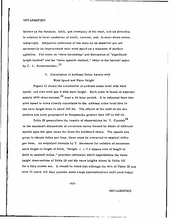
factors as the duration, fetch, and constancy of the wind, arid its direction

in relation to local conditions of swell, current, and, in near-shore areas,

topography. Subjective estimates of sea state by an observer are not

necessarily an improvement over wind speed as a measure of surface

agitation. For more on "wave forcasting" and discussion of "significant

height method" and the "wave spectra method, " refer to the tutorial paper

by C. L. Bretschneider. 3 3

5. Correlation of Ambient Noise Levels with

Wind Speed and Wave Height

Figure Z3 shows the correlation of ambient noise level with wind

speed, and also wind spe' d with wave height. Each point is based on approxi-

mately 4500 observations, Z' over a 24-hour period. It is indicated here that

wind speed is more closely correlated to the ambient noise level than is

the wave height down to about 200 Hz. The effects of the wind on the sea

surface are most pronounced at frequencies greater than 300 to 400 Hz.

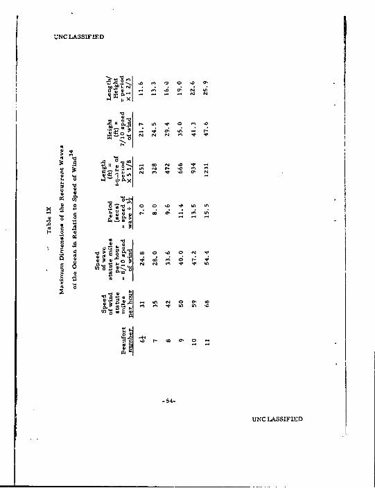
Table IX generalizes the results of observations by V. Cornish34

on the maximum dimensions of recurrent waves formed by winds of different

speeds upon the open ocean far from the windward shore. The speeds are

given in statute miles per hour; these must be converted to nautical miles

per hour. An empirical formula by T. Stevenson for relation of maximum

wave height to length of fetch, "Height = 1. 5 X square root of length of

fetch in nautical miles, provides estimates which approximate the wave-

height observations of Table IX and the wave heights shown in Table VII

for a fully'arisen sea. It should be noted that although the data of Table IX are

over 35 years old they provide some rough approximations (still used today)

UNCLASSIFIED

CONFID•2NT1A L

.8

E .6

0

2.4- ~ WAVE HEIGHT

010/ I I

0 200 400 600 800 1000FREQUENCY (Hi)

Fig. 23 Correlation of ambient noise level with wind speed.wave height. 22

-53-

CONFIDENTIAL

UNC LASSIFIED

N ' N m~

> A,

a Ný N

m a-

~~~~~~I 0 ~ ' 0 I e 0 0 .

X, . In N 0 a, 1

N Ný m v %n In '

to " ,,0

~~04

-54-

UNC LASSIFIED

UNCLASSIFIED

of the relationship between wind speed, speed of wave, wave period, and

wavelength and height. For a more comprehensive treatment we go to the

referenced paper by C. L. Bretschneider.

6. Estimating Wind-Generated Noise

-Figure 24 shows Artemis noise spectrum levels by Arase et al.

for frequencies of ZZ, 450, 900, and 1400 Hz as measured with an omni-

directional hydrophone. The scatter of the mean levels about the smooth

lines are relatively small; this indicates a good correlation between the wind

speed and ambient noise levels. The standard deviations of the mean

noise level are small at the high noise levels and larger at the low noise

levels. This is attributed, by Arase et al. , to the presence of system

noise (only in the 900 and 1400 Hz bands) and to the possible presence of

undetected noise sources.

Figure 25 shows a set of curves (by Arase 35) of ambient noise spec-

trum levels versus wind speed and sea state as observed during 1963-1965;

the corresponding values of Beaufort wind force have also been added. The

curves shown are in reasonably good agreement with those of Figure 24

and Figure 4 and Wenz's1 9

wind speed - noise curves: Figure Z6 and

A. D. Little'sl0 curves.* (See Table X for another comparison of

wind speeds and noise levels.)

Referring back to Figure 19 note that the mean estimate of wind

speed derived from the Atlas18 data is I I knots; this falls within the

Beaufort wind-force number 4 which is the same wind-force number esti-

mated for the measured Artemis data. Using the wind-force Beaufort

No. 4 the ainbirnt noise level is estimated as -36 dB/lIgbar for a (requency

See Figure 27.

-55-

UNCLASSIFIED

CONFID1ENTIA L

00

0

o0

NNN

0~ w

0-

an 0CU 0

CUj - N4

N (

-56-

CONFIDENTIAL

UNCLASSIFIED

I I --4t'

00 0 0

I WI

w/ 0- 4 0)

L0 0

0 0

,..

iON - Ifj OD

00 0 0 0 0- 10... Nto

-57-

UNCLASSIFIED

UNC LASSIFIED

INTERMITTENT ANO LOCAL EFFECTS- S HSTRAUAEES BO ~A 50 C EPIOAlO OT

$AIPE, INA)USTRIAL ACTIOYT¥100 SEA ICE..•" KEY

. • •~~~IMDOEITS OfN*AAVAI..I NO RA SE Ry•OS

5,3 AIAACPC At SWNDLt 8E AN SPRAY NOISE

So HEAV PAAClpTAIIOC

o USUAL TSAr. IC NOIE- ShALLW WATeR00 USUAL TP-CADTOSISE -'DEEP WATER

o - - TOESAL NOISE

S....... AHS.A -AL 0 ATT I i O FS 01 Fi

060 -- -- '--- .

PREVAILING NOISE

ALI- CAUPAR7

-- C SlIIIOOUI -- •1

a2 0- I1 -

Ct. PRVALINGposieS Lf amiet no -pcr (fo- ez1)

to

-58-

A CEASS TSATPIC

SEISMIC ACAAAOUSI-..---6 AAITATIA

.2.0 .1 I I I10' 100o, t, o

FRHESUENCY- HZ

F'ig. 26 Composite of ambient noise spectra (from Wenz1 9

).

-58-

UNC LASSIF'IED

CONFIDENTIAL

Table X

Some Comparisons of Wind Speeds

and Respective Noise Levels

Reference 22 Reference 28

Wind Noise at Wind Noise at

Speed 446 Hz Speed 400 Hz

Month Knots AAb Knot_ dB bar

Jan 18.5 -28 15.- -36

Feb 19 -26.5 17.4 -32.6

Mar 18.5 -30.5 -

April 16.5 -30.5 15.- -30.5

May 13 -34.5 17.5 -34.7

June 12.5 -35 -

July 12.5 -36 - -

Aug 10 -37 7.5 -39.5

Sep 10.5 -32. 5 - -

Oct 16 -30

Nov 18.2 -30.5 - -

Dec .8 -28 17.4 -37.8

Total 170.7 379 89.8 210.78

Average 14.2 -31.6 14.97 -35.13

-59-

CONFIDENTIAL

CONFIDENTIAL

of 400 HzI. If we use the peak value as the wind speed of I11 knots, we

find the ambient noise level to be -37 dB/I ýibar. This is about 3 to 4 dB

lower than the value shown by Weigle and Perrone 6(see Fig. 7). It may

be concluded that wind-generated noise estimates for the Artemis area are

within 3 to 4 d5 of measured noise levels. This is reasonably close enough

for estimating wind-generated noise levels. (C)

-60-

CONFIDENTIAL

UNCLASSIFIED

PREDICTION OF OCEANIC TRAFFIC NOISE

The magnitude of oceanic traffic noise that may be expected at a

particular hydrophone receiver array will be determined bj the average

transmission loss over the underwater path, the number of ships, and

the distribution of these ships. Although the noise source characteristics

depend on the nature of the ship source, the base is so broad for a larger

number of ships (ten or more) that the individual source differences blend

into an average source characteristic. This oceanic traffic noise is a

significant element of the observed ambient noise at frequencies below

178 Hz; below this frequ.incy the observed ambient noise is not strongly wind

dependent. At higher frequencies such as 200-500 Hz the oceanic traffic

noise may also be significant at low wind speeds, say below 5 knots.

For most surface ships, the effective source of the radiated noise is

between 10 and 30 ft below the ocean surface. Up to frequencies of 50 Hz,

the source and its image from surface reflection operate as an acoustic

doublet; noise is radiated with a spectrum slope of +6 dB per octave relative

to the spectrum of the simple source.

Wenz19

obtains some notion of the probable shape of traffic noise

spectra by deriving the curves shown in Fig. 27. The variations in the

spectra caused by differences in source depth and differences in the attenuation

at different ranges are indicated by the composite set of curves. The effect

of source depth at low frequencies is shown by the curves numbered (1) for

a depth of 20 ft, and (2) for 10 ft. The choices of source-noise spectrum

shape, based on the data recorded by Dow, 36 are described in terms of the

slopes of the sound-pressure-level spectra. The resulting curves are

-61-

UNCLASSIFIED

UNCLASSIFIED

"" 4

oq

Fig. 27 Traffic-noise spectra deducetd by Wenz1 from ship-

noise source characteristics and attenuation effects.

-62-

.

UNCLI.ASSIFI ED , 1

CONFIDENTIAL

* ~defined as follows: (A) -6 dBi per octave, (13) 0 dB per octave up to 100 Hz,

and (C) 0 dBi per octave up to 300 Hz and -6 dBi per octave abuve 300 Hiz.

The change in the spectrum shape as the range varies, due to attenuation,

is shown by curve (3) representing a range of 500 miles, curve (4) a range

of 100 miles, and curve (5) a range of 10 miles. The spectrum corres-

ponding to a particular set of conditions may be found by following the curves

identified by the relevant numbers and letter. For example, the curve 1 B4

is the spectrum form which would be observed at 100 miles~ from a source

located at a depth of Z0 ft, and whose spectrum is flat up to 100 Hz and

decreases at 6 dBi per octave above 100 Hz.

Note that the source spectrumn shape is altered in transmission by

the frequency- dependent attenuation* part of the transmission loss. Wenz 19

in his derivation of the curves of Fig. V? uses Sheely and Halley's attenua-

tion factor of 0. 066 f 3/2 dBi per nautical mile, where f is the frequency in

Hz. At lung ranges the attenuation increases rapidly with frequency above

500 Hz.

It has been shown by Hale 38

that experimental results from long-range

transmission in deep water do not fit the free field, spherical divergence

law very well; better agreement with experiment is shown to result if the

boundaries and sound velocity structure are taken into account.

Table XI is from Weigle's and Perrone' s report 6

on ambient noise

in the Artermis area; the table shows the results of two studies 39 0of ship

traffic density that are pertinent to the Artemis area. (C)

This does not include spreading loss, which is independent of frequency.

-63-

CONFIDENTIAL

CONFIDENTIAL

Table XI

Comparison of the Studies on Ship Traffic Den3ity

Range No. of Ships Per Degree No. of Ships Per 60 Degree Sector(nauticalmiles) Reference 39 Reference 40 Reference 39 Reference 40

0-150 .017 .055 1.20 3.31

150-250 .017 .120 1.02 7.Z5

250-350 .130 224 7.80 13.44

350-450 .300 .320 18.00 19.21

450-550 .350 .460 21.00 27.61

550"650 .500 .541 30.00 32.47

-64-

CONFIDENTIAL

CONFDENTIAL

From the data of Table XI when they are equally weighted, there is

obtained an expectation of 1. 51 ships/degree in the Artemis sector and a

mean ship range of 475 miles. (C)

In the 60-degree sector of major interest there are then a total of

103 ships at a mean range* of 475 miles. Each of these ships is consiiered

as a noice source36 with an output level at I yd of approxirmately

63 dB//l •bar/Hz ± 10 dB at 100 Hz and with a spectrum slope of -6 dB/

octave. A power addition of the outputs of 100 ships results in effective

source levels of approximately 83 dB//l gbar/Hz at 100 Hz and 77 dB//l Lbar/

Hz at 200 Hz. (C)

Long-range acoustic loss measurements at 400 Hz of the Artemis

receivers indicate a total expected loss of approximately 122 dB from a

range of 475 miles. The attenuation portion of the total loss for 400 Hz amounts

to 13.7 dB4 1

which leaves 108 dB for propagation losses exclusive of

attenuation. According to Thorp, 41 the expected attenuation values over

the 475-mile range for 100 and 200 Hz are 1.7 and 4.8 respectively. There-

fore, the expected received traffic noise level at the Artemis receiver

field is approximately -26.7 dB//l 4bar/Hz at 100 Hz and -35.8 dB//l labar/Hz

at 200 Hz, and -51 dB// I 4±bar/Hz at 400 Hz. (C)

(C) Figure 28 compares these values up to 200 Hz with the mean noise

levels measured at the Artemis receivers under the lowest wind speed

condition (0-5 knots). It is noted that Fig. 28 shows level differences up

to 4.5 dB and some slope differences. Hovever, Weigle and Perrone6

contend that the agreement is well within the uncertainity of the ship's source

In general, we cannot take average range as typical, since propagationloss (in dB) is not linear with range; e.g., for 500 miles at 400 Hz theconvergent zone transmission loss is 117 dB.

-65-

CONFIDENTIAL

CONFIDENTIAL

" 20

Q2 MEASURrO

S0 CALCULA4:TED• .

51 SPECTRUM • -

100 mo0 200

FREQUENCY IN CPS

6'

Fig. 28 Distant traffic noise spectra.

-66.

CONFIDENTIAL

CONFIDENTL'.L

level estimates and that this tends to support the thesis that ambient noise

observed ai low wind speeds in this frequency range has its origin in distant

ocean traffic. (C)

Figure 29 presents A. D. Lit le Co.'s 8 idealized average ambient

noise spectra based on the dominance of shipping noise below 2)0 to 300 Hz

and cf sea noise above this frequency region. Using the curves of Fig. 29

,me may roughly approximate the ambient noise, at any location and at

any season, by selecting the appropriate shipping and sea noise curves and

blending them together in the middle frequencies. (C)

Table XI1 indicates the shipping noise curvcls corresponding to some

oceaia areas and seasons of the year. The list is limited in the number of

areas indicated; al-io the seasons are not indicated for some of the areas

p. obably because of lack of data for all seasons.

Note from Table Xli and Fig. 29 that the shipping noise curve, for

the remc e parts of the Atlantic, varies from as low as "C" in the summer,

to as high as "E" in the winter; the ID" curve may be considered to be close

to the average for the year. Around Bermuda, the levels run about a half

letter higher. -. , the coastal areas (where shipping lanes are important)

the average level is between "El" and "F. " Curve G is the highest level

o! shipping noise th't could occur; however, this may be representative of

"near ship noise" in which the individual ships are close to the receiver

arrays. (C)

In very quiet areas, emote from shipping, the levels are as low as

curve "B" or curve "A."

SThe uncertainty of ship noise level is about 10 dB.

-67-

CONFIDENTIAL

CONFIDENTIAL

SPECTRUM LEVEL IN 08 RE I DYNE /CM 2

V V

* 00

4 4 4

-~~? - o

co- LL 0

~v3/ S 3N) XO ZOO0 38N 80 NI -12A31 VNA181DICIS

-68-

CONFIDENTIAL

CONFIDENTIAL

Table XII

Underwater Ship Traffic Noise Types in Certain AreasZ8

Area Season Curve Type

Eleuthera Average D

Eleuthera Summer C to D

Eleuthera Winter E

Bermuda Average D to E

Bermuda Summer D

Bermuda Winter E to F

Very deep SE Bermuda Fall C

Very deep W Bermuda Fall F

Puerto Rico Winter D

Grand Turk Island Summer C to D

San'Salvador Spring C

Lesser Antilles Summer C

Lesser Antilles Fall C

Capes May and Hatteras - E to F

Nantucket Area -E to F

North of Seattle - C to D

Cape Mendocino - D

Capo Blanco - E to F

Tongue-of-the-Ocean - B

New Zealand - A

Bearing Straits - B to C

-69-

CONFIDENTIAL

UNC LASSIFfMD

The curves in Fig. 29 are useful in roughly estimating average

oceanic traffic noise, sea noise, and the composite noise levels. However,

such estimates are only a rough approximation. For more accurate estimates

of averages it is necessary to incorporate any available experimfntal data,

and ship traffic data for a particular area of interest.

-70-

UNCLASSIFIED

UNCLASSIFIED

PREDICTION OF BIOLOGICAL NOISE LEVELS

It is difficult if not impossible to predict an average level of bio-

logical noise for any area, Noise from marine animals is very variable

in spectral and temporal characteristics; the statistics of such noise

involve a nonstationary process. The magnitude and other characteristics

of such noise will vary by area, year, season, and time of day. Also,

while many types of marine organisms ara known to produce sound, it

has not been possible to relate all the sounds heard to the particular marine

animals that make them.

1. Marine Animal Nz-. Coastal Areas

In coastal waters two types c s -.L- a',',-"' snapping shrimp

and croakers, appear to be the most likeiy sour., s ( biological noise.

Shrimp are common in shallow, hard-bottomed t ... water, whereas

croakers occur in such areas as Chesapeake ai cer ea.t coast bays;

croakers occur to a lesser extent on the Pacific coast. Figure 30 shows

some typical ambient-noise levels produced by croakers and snapping

shrimp; these levels will vary according to time of day and season cf

the year. In general one might assume that marine biological noise pro-

duced in coastal areas is not of concern to deep water surveillance systems.

However, some deep water hydrophone receiver arrays may be located near

a coastal area where propagation conditions might favor the reception of shrimp

and coastalnoise. This means that location of receiver arrays for deep water

surveillance systems should not discount entirely the effects of marine

animal noise from relatively close (i.e., propagation-wise) coastal areas.

-71-

UNC LASSIFIED

UNCLASSIFIED

* .. . v

•I I • TI

. -.... .....

Fig. 30 Ambient-noise levels produced by croakers and snapping

shrimp. 42

-72-

UNCLASSIFIED

CONFIDENTIAL

Other sources of marine animal noise in coastal waters have been

attributed to mussels, barnacles, sea uzrchins, toadfishes, and catfishes.

Cetaceans (whales and porpoises) sometimes occur in coastal areas; however,

since cetacean noise is more prevalent in some deep water areas it will

be discussed separately in the next paragraph. For a summary of the char-

acteristics of various marine animal noise sources in coastal areas ee

Tsble XIII.

2, Marine Animal Noise in the Deep Ocean

In the deep ocean the chief noisemakers are the cetaceans, (i. e.,

whales and porpoises). In general, the cetaceannoise signals produce

temporary changes in noise levels; that is the sound making is not a con-

tinuous noise. However, in many instances the cetacean signals are of

sufficient amplitude and duration to raise the ambient noise level past

tolerable limits.

In the Artemis area it was found2 2

that noise limiting occurred

about 70% of the time during a la-hour period of intense activity. This

may be expected on breeding or feeding grounds where cetaceans may tarry

and congregate; in such instances, it may be said that sound making may

be continuous over a continuous period of time. Noise from whales appears

to be a seasonal prc olem with the worst conditions, in the Artemis area,

persisting over the last three or four weeks in April. Greatest whale

noise occurs from dusk to dawn during the period of whale activity. Whale

noise of large magnitude has been found to occur in the 224, 446, 891, and

1414 Hz frequency bands (refer back to Fig. 3), the noisest of the four fre-

quency bands being 224 Hz. Whale-noise to sea-noise ratios ranged to a

maximum of 27 dB; ratios of 8 dB were the most frequent. (C)

-73-

CONFIDENTIAL

UNCLASSIFIED

5 *Uh�to-, E

5 >050 .j .0

�0�00 . 0.

� .5 35 0 0ae� *� 8 .5

- 0 41

do'2 5�o% 000oS*o So Vi

- 0

000 4.5 21.2 A 04:2 P

�- 2.5 00 - 0�0 < .5

z z � Vi

H Io I,Vi � 08�141 A 005 �

4 0 "s." 04..t0.0 0 A

04 sO... 0. >0 05� Vi 1. � kt

5Vi� �,

.5 V

� ? z WOO o-� o- I-

5 0.. 0 0 � 0

o � - -U 0 � 0 o ViC

.5 U 0 0'H � I . -, I

a�: g g

:2 5 5 -

O lti'� 'Vi. Vi. -

312 - -

0 0 0 A 5Vi Vi

U Vi.5 5. �A� 5. � q. Vi ood

aSA 15 .5 '5 �N 00 ,��oo AA 35 5O% J 0 5 .o

2 �

005.0 AOl' 5 U' �o flOk 0�Vi

.2 500 ?� 825

I. -* ... * og .5 osU..

�5 *v5 o53 5U o� 5 0

U.S �U � 0 0 0� 40 0 � � 0..� * A Viel a

04 014 oŽ2 o�5

a" F.o� 0.0 LoS 0. �a 0.0 <40 <

0 U 05�Zs * Vi

0 ViA .

a.74-

UNCLASSIFIED

UNC LASS IFIED

Publications giving estimates of whale (and shark distributions) are

listed as references Z3-26 and 43. From such reference sources one may

estimate the areas, expected magnitudes, and frequency of occurrence of

whale-noise sources.

The riagnitudes of whale noise should not be added in with the ambient

noise level due to sea state and oceanic traffic to provide an average median

yearly level. *However, the limiting effects of whale noise should be noted

for certain times of the year and for certain ocean areas; this may be

imp~ortant in the selection of underwater receiver array sites.

The whale noises are not continuous in nature and 'they are veryseasonal in occurrence.

-75-

UNCLASSIFIED

UNCLASSIFIED

ESTIMATING THE COMPOSITE BACKGROUND

OF AMBIENT NOISE

To determine the magnitudes of the ambient noise background levels

in a particular ocean area it is necessary to estimate and combine the

noise levels of the various contributory noise sources. In some instances

one may only be interested in estimating the yearly median noise levels;

however, in the evaluation of surveillance systems we also need to esti-

mate the seasonal and mionthly median levels; we may even need to consider,

*in the final analysis, diurnal noise level variations and such short term

variations as hourly and sporadic variations. The difference between the

yearly and monthly medians may be as much as 30 dB. There may also be

certain days during the year, or hours during the day, where a surveillance

"blackout" may occur due to a sudden onset of high noise levels; for such

cases it is important to indicate the percentage of time in which a "blackout"

could occur.

Suppose we are required to compare the effectiveness of some sur-

veillance receiver arrays that are to be emplaced in a particular ocean

area. The first step is to estimate the ambient noise background levels.

Assuming that the ambient noise background is the significant factor,

we need to specify as much of the noise characteristics as possible. As

an illustration a set of typical data sheets (Table XIV) has been prepared

as an example. The particular ocean area in this case is he Artemis

area off Bermuda; here we draw on the results of experimental measure-

ments over a period of several years. However, in other ocean areas

where few (or no) measurements have been made, we have no choice but

-76-

UNCLASSIFIED

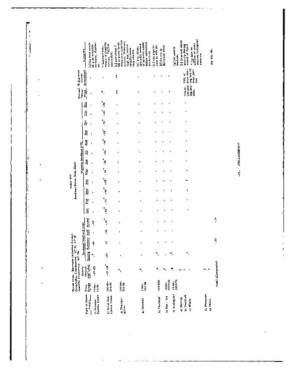
j ''2 at .

?o. 2 2o�.at.0. Za zt� 2.2?22 -- 44 ka

4 04 A-

-o a .4 - --

6-a

211 * �

-' , ,

- ,

34, �0

21 - , , , , C

I " ,

4 , , , , U

a , �- . ,

�*

a* - , , ,

C , a

a , ,

4 a ,

�2 � a .0 �

2 , -.

i* ** �� � -- 4444

'2 -2 .1

!¶ h I

UNCLASSIFIED

to rely on indirect methods of estimating noise levels. For example we

1hrs8could use the Oceanographic Atlas chrs to estimate the wind forces

and then deduce the noise levels; or we could use ship traffic data to esti-

mate the average oceanic traffic noise. When using indirect means of

estinmating noise levels, we identify them by an asterisk ()

-78-

UNCLASSIFIED

UNCLASSIFIED

DIRECTIONAL PROPERTIES AND SPACE TIME

OF AMBIENT NOISE

Space-Time Correlations

Some recent papers of interest on the subject of space-time corre-

lations of ambient noise are by R. J. Urick,34 E. M. Arase, T. Arase, 5,14

W. Liggett, M, Jacobsor,46

and D. Lytle, P. Moose.47

Urick hypothesizes an admixture of two different noise types in a "mix"

that depends on sea state and frequency. In the Urick study time-delay

correlograms were obtained in two frequency bands (Z00-400 Hz and

1-2 kHz), over a range of wind speeds and hydrophone separation; a 40-

element vertical array was used at Bermuda. The hydrophones were at a

depth of 14, 500 ft.

Figure 31 shows ambient-noise correlograms in the octave 200-400

Hz for a number of different separations and wind speeds. The autocorrelo-

gram from a single hydrophone, with paralleled inputs to the correlator, is

shown at the bottom of the figure; in the sequence above, it corresponds to

a separation of 0 ft. Figure 32 is a similar set of correlograms for the

octave 1-2 kHz.

The correlograms fall into two broad classes. Referring to Fig. 31

(200-400Hz), the correlograms at a wind speed of 4 knots show a high

peak value that remains nearly centered at 0 delay, even for the highest

separation of Z3.1 ft; these are called Type L At wind speeds of 25-30

knots, the correlogram peak diminishes in amplitude and moves outward

in time delay as the separation increases. These correlograms are called

Type II. At intermediate wind speeds, the correlograms suggest mixtures

-79-

UNCLASSIFIED

UNC LASSI"IZD

20o-4UO HI

LI7 0 II I, £7117 = 4-Z

i r • 2 4.lY,

........ [711....] [ .] L4 KTS. 9 KTS. 14 KTS. 25-30 KtS.

AUTOCORMlOGRAP6

Fig. 31 Time delay correlograms in the octave ZOO-400Iz 34various wind speeds and vertical hydrophone separations.

1-2 I1Ni

E-0

~ L~UNC~ iA-Si'I

.6 ~ .5 123.1'4 K(TS. 9 KTS 4 KTS. 25-30 IKTS,

MTOCOXRtLOOQAA

Fig. 32 Tilme delay correlograi'fl in the oc tave, - Z MIix forVarious wind Speeds and vertical hydrophone separations. 3

-80.

UNC LASSIFIED)

UNC LASSIFIED

of the two babic types. In Fig. 32 (1-2 kHz), the correlograms are all

Type II, except possibly at the 4-knot wind speed. Figure 33 shows the

distribution of the two correlogram types on a plot having wind speed and

frequency as coordinates.

In terms of the ambient noise that generates them, Urick interprets

the correlograms as indicating two different kinds of noise. The noise

generating the Type I correlograms is interpreted as arriving horizontally

at the array; it maintains a high coherence at 0 time delay over relatively

large separations in the vertical. One source of this noise is ship traffic

many miles away. This noise is lominant at low frequencies and low wind

speeds (Fig. 33). Type If noise* is postulated to originate at the sea surface,

and to become the dominant source of noise at high freqvencies and high

wind speeds. Figure 34 is a diagrammatic visualization of these two kinds

of noise.

The evidence that the Type II noise originates at the sea surface is

sought in a comparison of the theoretical correlation of sea-surface noise

with th6 observed correlograms. The correlative properties of sea-surfaceEde

4 4 igetadacbn 4

5'46

noise have been investigated by Edie, Liggett and Jacobson 6 and by

Lytle ai'd Moose. 47 Figure 35 shows a comparison between contour maps

of correlation coefficient plotted against normalized time delay r/(d/c)

where T is the time delay, d the distance between two vertically

separated receivers, and c the velocity of sound; and against normalized

separation d/'l , where T is the geometric mean wavelength of the

frequency band considered. The contour map on the left is computed

This type of noise (Type II) has a much lower correlation coefficient becausethe noise source is distributed over an area that is orthogonal to the verticalaxis of the hydrophone module.

-81-

UNCLASSIFIED

UNCLASSIFIED

30 -

WINDSPEMD 20 ,I IKNOTS •z l

10

• 1 AI+l[

1W 200 5W0 1000 2000

FREQUENCY, Itz

Fig. 33 Corralogram types as dependent on wind speed andfrequency. 34

0

II

l34

Fig. 34 Simple visualization of two kinds of ambient noise.

-82-

UNCLASSIFIED

UNCLASSIFIED

C4 fn i r. ~ ~

C C4ci 4ci

CC

d - -

C4, -83kU0LASIIE

UNCLASSIFIED

theoretically by Edie for a 1-octave band of white noise, with cos2 9

intensity- radiation pattern, from each elemental radiating area of sea

surface, corresponding to a surface distribution of dipoles. The right-

hand contour map is drawn from the values of the clipped correlation

coefficient read from the I- to Z-kHz correlograms of Fig. 32 for a wind

speed of 25-30 knots. The similarity of the two patterns indicates that

the interpretation of Type II noise as having a sea-surface origin may be

valid.

Urick shows how such correlograms may be used in array design to

discriminate against ambient noise by working out the following example.

(I) Example: To compute the improvements in S/N ratio to be

expected from a 4-element, linear additive vertical array of equally spaced

elements 5 ft apart, the ambient noise environment is said to be identical

to that at Bermuda. It is assumed that the signal is perfectly coherent,

with unit correlation coefficient between all elements of the array for all

steering directions.

The array gain (AG), in decibel notation, is defined by:

A A = 10 log [(S/N)o/(S/N)I] (1)

where (S/N)o denotes the ratio of signal power to noise power at the output

of the array, and where (S/IN) 1 is the same ratio at the output of a single

element. Then for a linear additive array of n identical elements,

the array gain is shown to be

AG = 10 log [j P. l j l (P.) i] (2)

-84-

UNCLASSIFIED

1UNC LASSIFIED

where (ps)ij is the cross-correlation coefficient, or normalized time-

averaged product, of the signal between the ith and the jth element

of the array, and (pn)ii is the cross-correlation coefficient of the noise.

In taking the p's , the tirne delays needed to fteer the array in the direc-

tion of the signal - and so maximize the numerjtor - must be included.

By the assumption of perfect signal coherence in the example chosen,

(Ps)ij = 1 for all i,j the numerator in the above expr.'zsion reduced to2

n . In the denominator, the various (pn )'s are determined by the spatial

coherence of the noise background.

Figure 3b shows the clipped correli tion coefficient of the ambient

noise at Bermuda plotted against separation distance d in feet, as read

from the correlograms for the 200- to 40.O-Hz band. Carrying through the

double summation in the denominator of the array gain expression, using

valucs of p from the same figure for values of d equal to 5, 10, and

15 ft, one finds for horizontal steering an array gain of 1.5 dB at a 4-knot

wind speed and 6.2 dB at a 25- to 30-knot wind speed; for a steering angle

of 60* to the horizontal, the array gain is computed to be 5.6 dB at 4 knots

and 2.9 dB at 25-30 knots.

Urick states that if unclipped, rather than clipped, correlation

coefficients were used in the computation, only slightly different values

of array gain would be found. * With horizontal steering at the low wind

speed, the array gain is low because of the high noise correlation at time

delays near 0 corresponding to the horizontal steering direction. At the

However, C. N. Pryor48 in a recent paper also shows that an errorin apparent signal-arrival time may occur when a clipped array is used innonuniform noise field; and that this error may become large enough undersome conditions to limit the usefulness of clipped array processing in anonuniform noise field.

-85-

UNCLASSIFIED

.. . ...

UNC LASSIFIED

7M CD

+ +

C3 r-JJ

k CC

LLi.S+iL&LI

- C + .C+

NZ+ + *A 0+ C,* 0 '

+ C+ C-C

L-8'oUNCLASIFIE

UNCLASSIFIED

60' steering angle at the high wind speed, the array gain is also low

because of the coherence of noise at time delays corresponding to this angle.

The above values may be compared with the array gain of 10 log4 = 6 dB

that would be found with uncorrelated noire. This exaniple illustrates the

precept that the gain of a linear additive array depends upon the correlative

characteristics of the signal (here assumed perfectly coherint) and of the

noise environment in which the array must operate.

The ambient noise correlations for the same 40-element vertical

array at Bermuda is interpreted by the Arases14 in terms of sea surface

noise radiated with an intensity proportional to cosn0 ; where n = 0, -, 1, 2

for different ranges of sea state and frequency. The Arases used a simple

model proposed by Cron and Sherman4 9' which is similar in concept to

Talham'sl description of measured noise directivit'y. Figure 37 illustrates

the concept of surface and volume noise models; Fig. 38 shows the geometry

for the volume noise model; Figs. 39 and 40 show the geometry for the surface-

noise model with one receiver and two receivers, respectively.

In the surface-noise model a uniform distribution of noise sources

is assumed on the surface of the ocean with an intensity radiation pattern:

g2(a) = cos ne

where a is the angle from the vertical. An equation for the cross-correlation

4 49,50coefficient was derived by Cron and Sherman. The distance d between

receivers was assumed to be small compared to the distance from the

receiver to the ocean surface. The effect of bottom reflections on the

correlation function was neglected for distances larger than 5 wavelengths

-87-

UNCLASSIFIED

UNCLASSIFIED

Fig. 37 Volume and surface noise models. 4 9

.4%

N,. NAOISE SOURCEft,. PIC EIVEA NO.RpRECEIVER NO.2

Fig. 38 Geometry for volume-noise model.4 9

-88-

UNCLASSIFIED

UNCLASSIFIED

N,. NOISE SOURCE IN 2y PLANE

R,'. RECEIVER

Fig. 39 Geom.otry for surface-noise model with one receiver. 49

N,.NOIESE SOURCE IV I, PLANE

R,,Rg.RECEIVERS IN y. PANE

Fig.. 40 Geometry for surface-noise model with two receivers.'4 9

-89-

UNCLASSIFIED

UNCLASSIFIED

from the bottom; also, a constant sound velocity ocean was assumed. Radia-

tion from the same noise source is assumed to correlate, while only the

intensity adds for noise from different sources. For time delay -r

angle -y between the line joining the receivers and the surface, at a single

circular frequency w , the space-time correlation coefficient was found

to be:

f g (a) tanacos (kd sin'ycos a - wr)da

p (d,ry) 0 (3)

J g (a) tan ad a0

Since noise is distributed in frequency axid is filtered to obtain samples in

frequency space, it is necessary to integrate over the frequency range.

A summary of the equations used for horizontal and vertical receivers by

14the Arases is given below for a flat spectrum between frequencies f1

and f2 * This is in a slightly differe.it form from that of Refs. 52 and 50

to make it more convenient for machine computation. The notation used was:

d 72

where c is the velocity of sound and X the wavelength. The case

= 0 corresponds to zero time delay.

For vertical receivers, with flat bandwidth Eq. 3 becomes:

'i" 2 in [2 byb. y s bJJ (4)

for n- 1 and y > 0

-90-

UNCLASSIFIED

UNCLASSIFIED

For horizontal receivers, with flat bandwidth Eq. 3 is therefore:

p, (y p, 0. b) 2'nn1 2yb Jn(x)

"0b= •y cosx~dx (5)b

for n =0, -, 1 ... and (m + (it) rl/Z 3

2m+1

y>o

Note that the case for n = 0 corresponds to omnidirectional surface

sources which violates a boundary condition that at a free surface the sound

pressure is equal to zero. However, Talham51 suggests another function

which approximates the case for n = 0 ; the results are not said to be

significantly different.

a. Correlations for Horizontal Elements14

In the Artemis experiments by the Arases, the spatial correlation

was measured with horizontally separated hydrophones at 22, 32, 45, and

63 Hz for various sea states. The experimental values corrected for clipping

are given in Figs. 41 through 44. Here the frequencies corresponding to the

-3 dB points of the filter response had a ratio of 1.7 (except for the 400-Hz

filter, where this ratio was 1.3); the actual response was therefore

approximated by white noise within this frequency range and the theoretical

curves were computed using Eq. (5) for n = 0,, 1, and 2 . These

curves are compared with the experimental points. With one exception, all

the data taken, namely at sea state 2 (SSZ) and 3, for 22 Hz and 45 Hz; at

sea state 1/2, 3, and 5 for 32 Hz; and at sea state Z, 3, and 5 for 63 Hz,

fit the theoretical curve computed on the basis of omnidirectional surface

-91-

UNC LASSIFIED

UNCLASSIFIED

922 ' S52n\V .. , .- ss-2

o. 0 IO .2 .G 4.0 2.4

Fig. 41 Experimental values of the spatial correlation comparedwith the theoretical curves for radiation pattern cosnc.at 22 Hz and horizontal separation.

at3 zn•orzna separaion

0,u

0.4 0, d I.2. 1.6 2-0 2,4

F'ig. 41 Experimental values of the spatial correlation comparedwith the theoretical curves for radiation pattern cosnc.at 2Z Hz and horizontal separation.

-92-

UNC LASSIFIED

UNCLASSIFIED

45 Hi+0.0-• SS 2' • SS 2

n -2n-i

-0.4 - '/2n-O

M 0

0.4-

-0 0 I I I I ' I I -I -- - -0 0.4 0.0 1.2 1.6 2.0 P..4

Fig. 43 Experimental values of the spatial correlation comparedwith the theoretical curves for radiation patte, n coln(at 45 Hz and horizontal separation.

0. 63 HzioU SSS2

n-12 L6.3

+0.4 - n 0

-0.4 - •

0 0.4 0.0 1.2 1.0 2.0 2.4

Fig. 44 Experimental values of the spatial correlation comparedwith the theoretical curves for radiation pattern cosncLat 63 Hz and horizontal separation.

-93-

UNCLASSIFIED

UNCLASSIFIED

sources. However, there is an exception at sea state 8 and 45 Hz; this

differs from all of the computed curves. The spatial correlation remained

positive and slowly decreased with spacing.

It is pointed out by the Arases 14that the space-time correlation

coefficient for horizontal spacing does not give any significant information

of the type of surface sources, From Eq. (3), it is seen that the coefficient

is symmetrical with respect to -r 0 for fixed d , and the principal

maximum or minimum is in general located at the origin. The time

dependence itself is influenced greatly by the filter characteristics, which

are only rough approximations. Figure 45 shows the delay time dependence

of the correlation coefficient at 45 Hz spacing of dA =0. 2 for the various

models as compared with the experimental data. Note that the experimental

data lies approximately between the omnidirectional curve and the (cos c 1/

curve.

b. Correlations for Vertically Separated Elements

Spatial snd s pace-time correlations were measured by the Arases

with pairs of vertically separated hydrophones at 250, 400, 500, 800, and

1131 Hz. The spatial correlations at these frequencies are shown in

Figs. 46 through 50 for sea state 5 at all the above frequencies and at

sea state 3 at 400, 800 and 1131 H-z. The sea state 3 data show a greater

scatter in the experimental points and are not as reproducible as the sea

state 5 data. If the measured results are compared with the theoretical

curves computed from Eq. (4) for zero time delay (at 250 Hz and sea

state 5), a model of surface radiatc with g(a) =(cos a)1/2 appears to

fit the data. Here the reproducibility of the correlation coefficients is

-94-

UNCLASSIFIED

UNCLASSIFIED

-- -. �20.6 . . I I

-A 00S -E EXP

0.4 .

S0

-0.04

o 0e

T(M SEC)20 3

Fig. 45 Experimental and theoretical values of the space-timecorrelation at 45 Hz and horizontal separation distance

-0.4

-0,• 0, 1.0 1 5 0 H ,Oe

FIg. 46 Experimental values of the spatial correlation comparedwith the theoretical curves for radiation pattern cosnoat Z50 Hz and vertical separation. 14

-95-

UNC LASSIFIED

S, ,

UNCLASSIFIED

0.4

400H

".0 0.4 0.8 1.2 I.6 2.0 5.,4

d/It

Fig. 47 Experimental values of the spatial correlation comparedwith the theoretical curves for radiation pattern cosne

at 400 Hr and vertical separation.

+040 HH

I~ ~ ~ s 3q. 2.s

+0.,4

oS a

-0.4

./ , ,n

Fig. 48 Experimental values of the spatial correlatio- comparedwith the theoretical curves for radiation pattern cosgnat 400 Hz and vertical separation. 14

-96-

UNCLASSIFIED

UNCLASSIFIED

-0.4 - \ ,, Gooo

0.-0..8IO

,Fig. 49 Experimental values of the spatial correlation comparedwith the theoretical curves for radiation pattern cos".eat 800 Hz and vertical separation. 14

s131 1 3

51/

"40.4

nZ

.. 0

-08 0.5 1.0 1.5 2.0 2.5

-0.6 "Fig. 40 Experimental

values of the -patial correlation compared

with the theoretical curves for radiation

pattern cosne

at 1131 Iz and vertical se

1 .aration. 14

-97-

UNCLASSIFIED0

;

UNCLASSIFIED

shown by the consistency of the data at the same sea state taken several

months apart. At sea state 5 and higher frequencies, a uniform distribution

of cos a radiators was found to agree best with the experimental points.

It is noted, however, that the measured results show a definite shift with

respect to the theoretical curve as the frequency increases. This is

illustrated in Fig. 51 on which the best fit curves to the experimental

data are given at sea state 5. This shift is explained in part by considering

the ambint noise spectrum itself. Typical ambient noise sprectrurn curves

decrease with frequency in this frequency range. The product of filter

response and ambient noise spectrum shilts the center of the response

curve to lower frequencies and effectively larger wavelengths; the equivalent

d/X therefore would be smaller.

The 400 Hz and 800 Hz measurements at SS3 seem to indicate a

good fit to the (cos o)1/2 computed values. This is questioned by the

Arases because the time dependence of the correlation does not confirm

the fit.

A typical time correlation at 400 Hz, sea state 3, and separation '1d/% = 0.4 is shown in Fig. 52. Here the agreement with the theoretical

curves is qualitative at best. The principal peak of the space-time corre-

lation is in general lower than the theoretically predicted one, and dis-

agreement increases with increasing time delay. The height of the prin-

cipal maximum is dependent on the filter characteristics; these character-

istics were only crudely approximated by the assumption of flat bandwidth.

However, the measured autocorrelation of a sample shown by the Arases

in Ref. 12 is said to agree well with that computed for a rectangular noise

spectrum.

-98-

UNC LASSIFIED

"UNC LASSIFIED

0.0500.

0o4'800 H.

~~ ~ 4006 H, //

-.04--H "" I I i," i

0.4 0.8 1. 116d X

Fig. 51 Best fit to experimental spatial correlation curves atS5S and vertical spacing at 500-1131 -lz. 14

ri2 4006.

+0.8 SS3Y2, n" • d/k. 0.4 -

-- - XP

+0.4

0

-0.4

-0.0

0 2 4 6r CM SEC)

Fig. 52 Experimental and theoretical values of the space-time correlation at 400 Hz and vertical separationdistance dA = 0.4 .14

-99-

UNCLASSIFIED

UNCLASSIFIED

The delay at which the principal peak of the space-time correlation

appears as a function of distance gives some information about possible types

1/zof sources. For a radiation pattern of g(a) (cos a) , the principal

maximum occurs at

'max (d/Zc) for d < X

At and above one wavelength for the cosl/2 del, two principal maxima

occur; this was not observed axperimentally. Since at 250 Hz a wavelength

is about 20 ft, the data given in Fig. 53 at this frequency may possibly be

explained by the (cos a)'/2 model. The data at 500 Hz, shown in the

sam3 figure, fit the cos a theoretical curve well. The same is said to

hold true for the results at 400 and 800 Hz, shown in Fig. 54, which was

given in a previous paper. At lower sea states the peak of the corre-

lation function does not seem to shiut with respect to delay time although

its height changes. This may be seen from Fig. 55 which gives the time

delay for the principal maximum as a function of separation at sea state 3

and 5 at 1131 Hz.

A summary of the results, by E. M. Arase and T. Arase, for

horizontal and vertical correlation measurements is tabulated in Table XV.

One of the most recent papers by E. M. Arase and T. Arase5 deals

with the mapping of the space-time correlation of ambient sea noise. The

space-time correlation of ambient noise in the ocean was measured with

vertical elements at a depth of 14,500 ft at 800 Hz and sea state 6. The

data are presented in the form of a map which shows the principal maximum

and zero axis crossings for comparison with recent theoretical work. 46.47

-100-

UNCLASSIFIED

UNCLASSIFIED

0

0z d

/ N -

on40"0

0 0 I

.0 In '

C!

oIný

N --

V4

(03S O xV I

Fig. 53 Time delay corresponding to principal maximumas a function of separation distance and comparedwith theoretical curves at 125, 250, and 500 H,. 14

-1lol

UNCLASSIFIED

UNC LASSIFIED

- 800 CPS- 400 CPSA 100 CPS 90* ,,'60-

6-

2

4 0

,-

w

020 O2

OISTANCE (FEETI

Fig. 54 Time delay as a function of separation distance at180, 400, 800 Hz.

Fig. 55 Time delay corresponding to principal maximum as

a function of separation distance at SS3 and 5 for

1131 H.. 14

UNCLASSIFIED

UNCLASSIFIED

Table XV

Summary of Measured Horizontal and Vertical Correlationsfor the Arase Model

Hydrophones FeEuenc Sea State Possible Model

Horizontal Pairs 22-63 Hz range 1i4 to 5 Uniform distributionof omnidirectionalsurface radiators

Horizontal Pairs 45 Hz 8 One of models fitsexperimental data

Vertical Pairs 250 Hz 5 (cos 1)4/ model

Vertical Pairs 400 Hz and above 5 Uniform distributionsof cos a radiatorsgive good fit for spatialcorrelations as well asdelay times, at whichthe principal peaks ofthe correlation occur

Vertical Pairs 400-1131 Hz 3 No satisfactory fits totheoretical model

-103-

UNCLASSIFIED

UNCLASSIFIED

Referring to a paper by Liggett and JAcobson 46the experimental data

obtained from directivity measurements with a vertical array are fitted

with a directional noise field at the receiver, of the form:

N(0)=Ae A Ccos e/(Zl eA_ 1)

where 0 is the angle from the vertical P-nd A is a parameter that varies

according to sea state and frequency. The correlation of ambient noise

is then computed from this noise field. In another paper (Lytle and

Moose 4 7 ), a uniform distribution of surface dipole noise sources is

assumed. This model has been shown to give reasonable agreement with

experimental results at 400 Hz and at higher frequencies. However, until

the publication of Ref. 5 there were no experimental maps of the space-

time correlation. Figures 56, 57, and 58 are experimental maps of the

space-time correlation as given in Ref. 5. Figure 56 illustratesa a map

of the space-time correlation at sea state 6 for vertical elements and

800 Hz, with time delay T~ in milliseconds and the element separation

d in feet or fraction of the wavelength X. as variables. Experimental

points for the zero axis crossings are connected by straight lines. Greater

detail from those measurements was not possible because the experimental

accuracy decreases with increasing spatial separation and time separation

from the principal peak. The time separation is shown explicitly, and is

reproducible to *0. 1 msec at all separations. The shaded areas corre-

spond to the negative correlations, the light areas to positive correlations.

All of the axis crossings lines show the general tendency and slope of the

line connecting the largest correlation peak. At sea state 6 and 800 Hz a

-104-

UNCLASSIFIED

UNCLASSIFIED

r4

A 4 6

Fig. 56 Experimrntal map of the space-time correlation ofambient sea noise for vertical elements at 800 Hz, seastate 6. '\\\: Negative correlation. 0: Zero. o: Largest peak.

5

- \. \ ,I• \.. ', 23 '

0 4 30 N I°' ... o I •\..

0 L- 0

04 01 0-U'Jt

Fig. 57 Map of the experimental and Fig. 58 Map of the experimental andtheoretical (Ref. 46) space-time theoretical (dipole surface sources)correlation for vertical elements at space-time correlation for vertical800 Hz. -: Experimental. elements at 800 Hz. --- : Dipole

Liggett. 5 model. -: Experimental. $

-105-

UNCLASSIFIED

rUNCLASSIFIED

value of A = 3 in the equation for N(O) seems to fit the directivity

data best. Only single frequency maps or those for a bandwidth of approxi-

mately 1.6 are given in Ref. 46. However, since the positions of the maxima

and zeros for small time delays are not greatly affected by the bandwidth,

the experimental results were compared with a bandwidth of 1. 25 with

those of Ref. 46 with a bandwidth of 1.6 in Fig. 57. The units are

dimensionless; whcre c = 500 ft/sec is the velocity of sound. In Fig. 58,

the experimental results are compared with the computed results for a

dipole model with white noise with a banuwidth of 1. Z5. From Figs. 57

and 58 it is suggested that the results for both theoretical models are

almost identical at small r c/d . Both of these fit the experimental data

qualitatively except at small spacings for the principal maximum and at

the location of the first 0 curve.

ACKNOWLEDGMENT

The author gratefully acknowledges permission granted by the authors

whose figures have been reproduced in this report.

-106-

UNCLASSIFIED

UJNC LASSIFlED

BIBLIOGRAPHY

1. V. 0. Knudsen, R. S. Alford, and J. W. Ewing, "Survey of under-

water sound, Report No. 3; Ambient Noise," NDRC SEC., No. 6.1 -

NDRC-1848, 1944 (Conf.); "Underwater an ient noise," 1J. Marine Res.

7, 410 (1948).

2. A. Berman and A. J. Saur, "Ambient noise power spectrum from 1 to

100 tps, " 8th Navy Symp. on Underwater Acoustics, New London, (1953).

3. W. C. Beckman, "Low-frequency ambient sea noise, " J. Underwater

Acoustics (USN) 5, 161 (1955).

4. R. Halley et al., Measurements of Underwater Ambient Noise at

Point Sur and Point Arena. California, NEL Report 623 (1955). (Conf.)

5. E. M. Arase and T. Araso, "Mapping of the space time correlation of

ambient sea noise, " J. Acoust. Soc. Am. 40, 499-500 (1966).

6. F. G. Weigle and A. J. Perrone, Ambient Noise Spectra in the ARTEMIS

Receiver Area, U.S. L. Report No. 737 (27 Dec. 1966). (Conf.)

7. T. Arase et al. , "Time variability of ambient noise directionality,"

J. Acoust. Soc. Am. 36, 1015 (1964).

8. T. Arase, E. Arase, F. Weigle, and A. Perrone, Effective Directivit?

Index of the 1963 Artemis Modules During Winter Conditions (U), Artemis

Report No. 33 (June 25, 1964). (Conf.

9. T. Arase and E. Arase, "Ambient noipe measurements with the Artemiv

modules, " Paper J6, Proc. of the ZZnd U.S. Navy Symposium on

Underwater Acoustics, Oct. 26-Z8, 1964, pp. 543-547. (Conf.

10. T. Arase and E. M. Arase, "Spectra and correlations of ambient

sea noise at Bermuda," Paper 2CZ, Proc. of 23rd Underwater

Sound Symposium, Nov. 30-Dec. 2, 1965, pp. 259-267. (Conf.)

-107-

UNCLASSIFIED

UNCLASSIFIED

11. E. M. Arase and T. Arase, "On the statistics of ambient noise,"

J. Acoust. Soc. Am. 41, 1597 (A) (1967).

12. T. Arase and ?:'. Arase, "Correlation of ambient noise in the ocean,"

J. Acoust. Soc. Am. 38, 146-148 (1965).

13. E. M. Arase and T. Arase, "Ambiknt sea-noise correlation,"

J. Acoust. Soc. Am. 38, 920 (1965).

14. E. Arase and T. Arase, "Correlation of ambient sea noise,

J. Acoust. Soc. Am. 40, Z05-210 (1966).

15. T. Arase, Directivity of Deep Water Ambient Noise in the Artemis

Frequency Range (U), Tech. Memo. A-107 (Dec. 19, 1963). (Conf.

16. T. Arase and E. M. Arase, "Directivity index of a three-dimensional

array of directional sources," J. Acoust. Soc. Am. 35, 735 (1963).

17. E. M. Arase and T. Arase, "Arrays for the measurement of the angular

distribution of ambient noise in the ocean, " J. Acoust. Soc. Am. 35,

1884 (1963).

18. Pub. No. 700, "Oceanographic Atlas of the North Atlantic Ocean,"

Section IV, Sea and Swell, U.S. Naval Oceanographic Office, Washington,

D.C. (1963).

19. G. M. Wenz, "Acoustic ambient noise in the ocean: Spectra and sources,"

J. Acoust. Soc. Am. 34, 1936-1956 (1962).

20. G. H. Franz, "Splashes as sources of sound in liquids," J. Acoust.

Soc. Am. 31, 1080 (1959).

21. H. M. Fitzpatrick and M. Strasberg, David Taylor Model Basin Report

1269 (January 1959).

-108-

UNCLASSIFIED

UNCLASSIFIED

22. R. W. Hasse, Draft. 6/1/65, "Artemis Ambient Noise Review,"

(for Artemis Handbook).

23. Whales and Sha.rks. Supplement Nc. I, Convoy Atlas for the North

Atlantic Ocean, HO Publication No. 764 (1954).

24. Charles H. Townsend, The Distribution of Certain Whales as Shown

by Logbook Records of American Whaleships, New York Zoological

Society, Zoologica, Volume XIX, No. 1 (1960).

25. M. D. Fish, Marine Mammals of the Pacif.'c with Particular Reference

to the Production of Underwater Sounds, Woods Hole Oceanographic

Institution, Report 49-30 (1944).

26. M. D. Fish, An Outline of Sounds Produced by Fishes in Atlantic

Coastal Waters - Sound Measurement and Ecological Notes, Narragansett

Marine Laboratory, Special Report No. 1, 53-1 (January 1953).

27. H. M. Walkinshaw, (B. T. L.), Ambient Noise Obtained on 460-Fathoms

Site at Bermuda, unpublished B.T. L. Memo (1961). (Conf.)

28. A. D. Little, Report No. 1250862, Survey on Ambient Sea Noise,

(August 1962). "Originated by Bolt, Beranek & Newman, Inc. under

subcontract to A. D. Little. " (Conf.)

29. A. H. Green, Bell Telephone Lab. Tech. Report No. 10 (1962).

30. T. Arase and E. M. Arase, "A review of recent developments in under-

water ambient noise, " J. Underwater Acoustics (USN) 15, 589-601

(July 1965). (Conf.)

31. E. Arase and T, Arase, "Ambient sea noise in the deep and shallow

ocean," J. Acoust. Soc. Am. 42, 73-77 (1967).

32. E. Arase, "On the discrimination factor for a continuous distribution

of noise sources," J. Acoust. Soc. Am. 36, 785-786 (1964).

-109-

UNCLASSIFIED

UNCLASSIFIED

33. C. L. Bretschneider, "Wave forecasting,' Ocean Industry (October 1967).

34. R. J. Urick, "Correlative Properties of ambient noise at Bermuda,"

J. Acoust. Soc. Am. 40, (1966).

35. T. Arase and E. Arase, "Curves of Ambient Noise Spectrum Levels

vs. Wind Speed. " These sets of curves are not part of any referenced

formal or informal document.

36. M. T. Dow, S. W. Emling, and V. 0. Knudson, "Survey of underwater

sound, " Report No. 4, Sounds from Surface Ships; Tech. Report

of Division 6, NDRC, No. 2124 (15 June 1945). (Conf.)

37. M. J. Sheely and R. Halley, "Measurement of the attenuation of low

frequency underwater sound," J. Acoust. Soc. Am. 29, 464 (1957).

38. F. E. Hale, "Long range propagation in the deep ocean, " J. Acoust.

Soc. Am. 33, 456 (1961).

39. P. G. Cable, Interference in an ARTEMIS System Due to Radiated

Shipping Noise, U.S. L. Tech. Memo. No. 905-053-61 (26 May 1961).

(Conf.)

40. C. R. Rumpel, "Density of ships in the North Atlantic. " (26 October

1964) (U), in Advance Defense System, Second Interim Report

B. T. L. Report No. OBJ-7829 X-2 (4 December 1964). (Secret)

41. W. H. Thorp, "De3p-sea ocean sound attenuation in the sub and low

kilocycle-per-second region," J. Acoust. Soc. Am. 4, 648-654 (i965).

42. V. M. Albers, Underwater Acoustics Handbook - II, Penn. State '-:iv.

Press (1965).

43. M. P. Fish, Biological Sources of Sustained Ambient Sea Noise,

Narragansett Marine Laboratory Tech. Report No. 19 (March 0964).

-110-

UNCLASSIFIED

UNCLASSIFIED

44. J. Edie, Space Time Correlation Functio. Surface Generated Noise,

Litton Systems, Inc., Waltham, Mass., Rept. TR63-9-BF, Contract

Nonr 3320(00) (1963).

45. W. S. Liggett and M. j. Jacobson, "Covariance of noise in attenuating

media," J. Acoust. Soc. Am. 36, 1183-1194 (1964).

46. W. S. Liggett and M. J. Jacobson, "Noise covariance and vertical

directivity in deep ocoan," S. Acoust. Soc. Am. 39, 280-288 (1966).

47. D. W. Lytle and P. H. Moose, "Space-time correlation functions for

surface-noise model, " J. Acoust. Soc. Am. 39, 487-590 (1966).

48. C. Nicholas Pryor, Some Effects of Inter-Element Correlation and

Clippinp on the Performance of Receiving Arrays (September 1966),

NOLTR 06-53, U.S. Naval Ordnance Laboratory, White Oak, Maryland.

49. B. F. Cron and C. H. Sherman, "Spatial-correlation functions for

various noise fields," JACSA, 1732 (Nov. 1962).

50. B. F. Cron and C. H. Sherman, "Spatial correlation functions for

various noise models," J. Acoust. Soc. Am. 38, 885.(1965).

51. R. J. Talham, "Ambient-sea noise model, " J. Acoiust. Soc. Am. 36,

1541-1544 (1964).

52. B. F. Cron, B. C. Hasse, and F. J. Keltonic, "Comparison of

theoretical and experimental values of epatial correlation, " J. Acoust.

Soc. Am. 37, 523-529 (1965).

53. D. F. Morrison, Some Statistic Information on Natural Background,

Sea Noise on the Portland and Bexington Noise Ranges Admiralty

Underwater Weapons Establishment, Portland, England, (Nov. 1964). (Conf.)

54. A. W. Ellinthorpe, Notes on Undersea Acoustic Comrnmunications, U.S.L.

Report No. 826, (May 1967). (Conf.)

-111-

UNC LAiSIFIED

UNCLASSIFIED

Additional Bibliography not Referenced

in Text and Appendix

55. S. M. Levin, "The SST - How Good?," Space/Aeronautics, p. 87

(July 1967).

56. D. Maglieri, "Source effects of airplane operations and the atmosphere

on sonic-boom signatures, " J. Acoust. Soc. Amn. 39, part 2, S36-S42

(May 1966).

57. H. Hubbard, "Nature of the sonic boom problerm, " J. Acoust. Soc. Am.

39, part 2, S3 (May 1966).

58. D. G. Tucker and B. K. Garey, Applied Underwat'.r Acoustics,

Pergammon Press, Ltd., London (1966).

59. R. W. Young, "Underwater ambient noise, a review, " U.S. NEL,

California, Paper No. 2CI, 23rd Symposium on Underwater Acoustics,

1965. (Conf.)

60. Axelrod et al., (A. D. Little and USNSL), "Vertical directionality of

ambient noise in the deep ocean at a site near Bermuda," 3J. Acoust.

Soc. Am. 37, 77-83 (19.65).

61. "Project AUTEC systems analysis study," Vol. 4, Environmental Factors,

Lockheed Aircraft Co. (August 1961). (Conf. ) (See Ref. 28.)

62. W. B. McAdams and R. I. Tait, "Ambient sea noise off the New Zealand

Coast," J. Underwater Acoustics (USN) 11, 653 (1961). (See Ref. 28.)

63. G. M. Wenz and C. Castien, Underwater• Ambient Noise Measurements

In the Bering Straits off Wales, Alaska, NEL Report 889 (1959). (Conf.)

(See Ref. 28.)

-112-

'TrCLASSIFIED

I.

UNCLASSIFIED

64. Project Jezebel Progress Reports, ONR Contract Nonr-210(00) B. T. L.

(1951-1954). (Secret)

65. D. Ross, Data for the Underwater Data Systems Dept., B.T.L.

(1958). (Conf.) (See Ref. 28.)

66. J. D. Richard, Jr., Underwater Ambient Noise in the Straits of

Flarida and Approaches, Miami U. Marine Lab., Report 56-IZ

01956). (Conf.) (See Ref. 28.)

67, T. E. Heindsmann, et al., "Effect of rain on underwater noise levels,'

J. Acoust. Soc. Am. 27, 378 (1955).

68. G. M. Wenz, H. M. Linnette, and C. N. Miller, Underwater Ambient

Noise Measurements in the North Central Pacific, Chinook Expedition,

NEL Report 855 (July 18, 1958).

69. E. Rhian, Acoustic Ambient Noie, in the Tongue of the Ocean, Univ.

of Miami Report (July 1959). (Conf.

70. B. C. Hassel and F. J. Keltonic. The Effect of Wind Speed on Spatial

Correlation of Ambient Noise, U.S. Navy Underwater Sound Lab.

Report No. 596 (9 May 1966).

71. Julian Stone, "Problems associated with measurement of ambient-

noise directivity by means of linear additive arrays. ' J. Acoust. Soc.

Am. 34, 328-333 (1962).

72. W. S. Liggett and M. J. Jacobson, "Covariance of surface-generated

noise in a deep ocean, " J. Acoust. Soc. Am. 38, 303 (1965).

73. D. Middleton, "Detection of random acoustic signals by receivers

with distributed elements, " J. Acoust Soc. Am. 38, 727 (1965),

74. D. W. Little, "Space time correlation functions for surface-noise mudel,"

J. Acoust. Soc. Am. 39, 587 (1966).

-113-

UN'C LASSIFIED

UNCLASSIFIED

75. H. M. Linnette and R. J. Thompson, "Directivity study of the noise

field in the ocean, employing a correlative dipole, " J. Acoust. Soc.

Am. 36, 1788 (1964).

76. E. H. Axelrod, B. H. Schooner, and W. A. Von Winkle, "Vertical

directionality of ambient noise in the deep ocean at a site near Bermuda,

J. Acoust. Soc. Am. 37, 77 (1965).

77. G. R. Fox, "Ambient-noise directivity measurements," J. Acoust.

Soc. Am. 36, 1537 (1964).

78. A. Berman, "Spatial correlation of ambient noise," J. Acoust. Soc.

Am. 32, 920 (A) (1960).

79. F. Weigle, Acoustic Propagation Measurements with the USS MALOY

in February 1962, U.S. L. Tech. Memo. No. 906-02-62, (17 Dec. 1962).

(Conf.)

80. M. Strasberg, "Gas bubbles as sources of sound in liquids," J. Acoust.

Soc. Am. 28. 20 (1956).

81. M. A. Calderson, Probability Density Analysis of Ocean Ambient

and Ship Noise, USNEL Report No. 1248 (5 Nov. 1964).

82. W. N. Tavolga, Ed., "Marine Bio-Acoustics. " Proceedings of a

Symposium held at Lerner Marine Laboratory, Bimini, Bahamas,

April 1963, Pergammon Press (1964).

83. C. Nixon and P. Borsky, "Effects of sonic boom on people: St. Louis,

Mo., 1961-1962," J. Acoust. Soc. Am. 35, part 2, S51 (1966).

84. H. Carlson, R. Mack, 0. Morris, "Sonic-boom pressure-field

estimation techniques," J. Acoust. Soc. Am. 39, part 2, S1O-SI8

(1966).

-114-

UNCLASSIFLED

UNC LASSIFIED

85. H. Von Gierke, "Effects of sonic-boom on people: Review and outlook,'

J. Acoust. Soc. Am. 39, part 2, S43-S50 (1960).

86. I. Tolstoy and C. S. Clay, Ocean Acoustics, McGraw-Hill Book Co.,

New York (1.966).

87. Blair Kirsenan, Wind Waves, Prentice-Hall, New York (1965).

88. W. J. Pierson and L. Moskowitz, "A proposed spectral form for fully

developed wind seas based on the similarity theory of S. A. Kitarlgorodski,"

J. Geophys. Res. 69, 5181-5190 (1964).

89. V. Cornish, Ocean Waves, University Press, Cambridge, Mass. (1934).

90, W. J. Piersor. et al., Observing and Forecastlng Ocean Waves by Means

of Wave Spectra and Statistics, Hydrographic Office Publication No. 603,

U.S. Dept. of the Navy (1955).

-115-

UNC LASSIFIED

I.

UNCLASSIFIED

APPENDIX A

Wind-Speed Distributions From Oceanographic Atlas1 8

February Through December at 33" N, 67, W

A-i

UNC LASSIFIED

UNCLASSIFIED

60 ..... DEC

-FEB

400

50 so S5 9S.99PROD (XR)

Fvi.. P. I Winid speed distribution from Atlas1 8 ot December,

Sanuary, and February.

60

;40

Ct

APRIL

Q MARCH

0 0 9 99,99OZ; LO PROS C4 ,0% "

Fig, A. Z Wind speed dim';ribution from Atlaslt for March,

April, and May.

A-Z

UNCLASSIFIED

UNCLASSIFIED

60

I-z

LaL0 ~JUNE---

z

go ~AUG -

2 1 50so 80 98 9999PROB (X'sx)

Fig. A-3 Wind speed distribution from Atlas1 8

for June,July, and August,

60

0C,,W40I. NOV

5 ~ OCT3:20 SEPT

01 tO 50 80 95 99.99

PROS (X s x)

Fig. A-4 Wind speed distribution from Atlas1 8 for September,

October, and November.

A-3

UNC LASSIFIED

UNC LASSIFIED

Io-

140o-

.2[

•POB (Y.SI

Fig. A-5 Wind speed distribution curve constructed fromaverage mean and standard deviation. Januarythrough December, 33" N, 67 W. 18

6o0

1> I0 O 0 , 1 0 9S.995

PRO@ Y~

Fig. A-6 Wind epeed distribution plotted as square rjtspeed (July). 33" N, 67" W, 2544 samples.

L

rI'

e ,s o Io 55 ,,j

Fig. A-7 Wind speed distribution plotted as square rootof wind spoed (January). 33" N. 670 W. 2660samples.

A-4

UNCLASSI: D

UNCLASSIFIED

APPENDIX. B

Comparison of Artemis Noise Data with

Data From Other Areas

B-I

CONMEDNT!AL

14 CO N

> I MNI I 1 0 -0.0

o 0)

vm N N N

0,q I~ I I I II

.44-0) N I

NI P N 0lI-0l I c0 m 14v OD a,

v .5.0 0 '1N

*00

- 0' Z

.0 NENIA

CONFIDENTIAL

Table B-U

Measured Ambient Noise Levels and Corresponding

WindSpeed, Sea-State and Beaufort Force Numbers

Arase WenzBeaufort Sea Wind Speed Mean dB/iA jbar dB//1 vbar

Force No. State (knots) Knots for 400 Hz for 400 Hz

8 7 34-40 37 -28 -30

7 6 28-33 30 1/2 -29 -

6 5 22-27 24 1/2 -31.5

5 4 17-21 19 -34 -33

4 3 11-16 13 1/2 -36 -35

3 2 7-10 8 1/2 -39 -37

2 1 4-6 5 -41 -40

I /Z 1-3 2 -44 -44

B-3

CONFIDENTIAL

CONFIDENTIAL

JAN MAR MAY JULY SEPT NOV

•//100 Hz, 460 FM (BERMUDA)

REFERENCE 27, 28 -1

ZL

S-40i- o z 6 M/[

400 Hz,.660 FM (BERMUDA)REFERENCE 27

w DepthJ Item Area Year FM Refs.

1 Pac. CoastCape Mendocino 1956 795 282 Pac. Coast,Cape Blanco 1956 748 283 Pac. Coast, N. of Seattle 1958 284 Pac. Coast, N. of Seattle 1957 28

I- 5 Grand Turk Island 1953 350 286 Puerto Rico 1955 28

I. -60- 7 San Salvador 1955 28CD 8 Barbados 19551430 28

9 Antigua 1955 850 2810 N.E. of Eleuthera 1955 780 2811 Cape May 1954 925 2812 Cape May 1954 1300 2813 Cape Hatteras 1957 Z814 Bermuda Abyssal Plain 1959 Very 28

Deep15 Bermuda Abyssal Hills 1959 i 2816 Bermuda - Artemis 1963 9

-so'

Fig. B-I .Monthly variations of ambient noise near Bermudaand other areas.

B-4

CONFIDENTIAL

CONFIDENTIAL

00

o

( a

t0

eI ,s / ,I /,.

llH ,mqdl "U G

OF 0

a.0Aq

B-0

0O0 ENXA

;ONFIDENTIAL

00'sly 0

0

0

A 0 0 z

0 4

/ ~10(8H -oq 0i l u

B-64'

C *0MNTA

CONFIDENTIAL

00

00M , CDo

- I p.0

a, oz

_ 0!!" .... ' , , ' I ,,

= -C O C NT u.

0 4)

I u

0 C

I z

~~_ 02

N[ . j * 17i '5 apCJ

P. P. U ~ . P. . P. B-/7

CONFMENT.k

o 4 ) .4 4 ) ----------P

r

UNCLASSIFIED

SI _ _ _ _ _ _ _-20 -

J. WI NDSPEED(KNOTS)

7 34-40

1 5 22-27

4 17-21

-4- .3 -- II-16-1 2 7-10

I 4- 6

20 50 100 200 400 000 1200FREQUENCY He

Fig. B-5 Noise spectruim level vs. frequency. wind speed,and sea state.

B-8

UNCLj.ASSIFIED

UNCL-ASSIF•IED

i

-S

I -"

Fig. B-6 Monthly ambient spectrum noisa level for 446.4 I{Iz.Z

Ii

Fig. B-I Monthly ambient spectrum noise level at 891.1 Hz.22

I

,n J.. , .. ,, *Af w

Fig. B-8 Monthly ambient spectrum noise level at 274. 7 Hs. 22

B-9

UNCLASSIFIED

CONFIDENTIAL

40: 30M5

45. 10-e5dS

log

DEC JAN FCI APR MAY JUL.Y AUG

Fig. B-9 400 Hz spectrum level measured during the yearnormalized to 20 knot noise level; wind speed isthe parameter. 9

0j

-20

"WINTER

f-40 :-' SUMMER-40

-60I2 4 6 610 20 40

WIND 3PEED (KNOTS)

Fig. 13-10 400 Fz spectrum level vs. wind speed duringwinter and summer. 9

B-10

CONFIDENTIAL

CONFIDENTIAL

APPENDIX C

Excerpts and Data from D. F. Morrison's Report5 3

on Noise Data Obtained from the Portland and

Bexington Underwater Test Ranges (England)

Systematic record compiled for last four years (1960-1964). Noise

spectrum levels measured regularly in each of 16 octaves from I Hz to

'16 kHz.

Low-Frequency Hydrophone Unit: covered I Hz to 00 Hz in

10 octaves.

High-Frequency Hydrophone Unit: covered 75 Hz to kHz in

10 octaves.

Deep Range. Noise levels approached symmetrical distribution in

higher low-frequency octaves and most of high-frequency octaves, except

for tendency to "tail" into the low noise levels. No explanation for skewness.

Octaves most affected by shipping interference are the lowest low-frequency

octaves (I to 8 H7); also lowest low-frequency octaves most susceptible to

long-range interference. (C)

Standard Deviation of Noise: 6 to 8 dB in 1 to 8 Hz band; 4 dB

over rest of bands. (C)

Coastal Range: On the average about 3 dB quieter than deep range

in the lowest octaves. Coastal range ,nore susceptible to noise due to

waves breaking on shore. (C)

Shipping Noise Screened Out: Background noise measurements

not taken when shipping was known to be interfuring: Variation in noise

levels in one day during "quiet" weather is much less than the long-term

varilation. (C)

C-1

CONFIDENTIAL

CONFIDENTIAL

Results from the three noise ranges referred to Knudsen curves:

for sea state 3 falls -13 dB//l 1bar at 50 Hz to -56 dB//l jibar at 15 kHz. (C)

Portland Deep Range: (Fig. C-i) Taking noise level in an octave

to be that at the center frequency - the mean noise curves for all sea

states, referred to Knudwen sea state 3 curve, are within 2 dB over the

above frequency -nge and coincide for large portions of it. (C)

Coastal Range: (Fig. C-2) Gives simiar characteristic or average

of 3 dB quieter, corresponding to Knudsen sea state 2-1/2. This is in

keeping with the partially sheltered position. (C)

Bexington Range: Mean spectrum level for observed sea state 3

is, however, more nearly correspondent with the Knudsen sea state 4

curve. Higher mean level probably due to noise of surf on the Chesil Beach. (C)

C-2

CONFIDENTIAL

CONFIDENTA.L

o,0

0 STD DEV (a) DEEP RANGE

Y -40-

o -6C -

_(b) COASTAL RANGE

-20-!'E

S~~~-40 -- '

; , ~- 6 0 - '

-- ,. • LF" HYDROPHONES __,

- HFFig. C-I Blackground sea noise 1962-1964.53

C-3

CONFIDENTIAL

SCONFIDENTIAL

20 1

0K MEAN (c) DEEP RANGE0 STD DIV

-20

-40 ,N4

£ ' I I t I I I I I - ,-60 --

wUz 0 0 0 0 •, tU)-- m Ft- i 0 o l ,

020

- 0 £ 0

" o (d) COASTAL RANGE-0

J20

•'• -40-

i, -6o0 _ _-.• ,,FHF

Fig. C-2 Background sea noise in one day SSO to SSI. 5 3

C-4CONFIDENTIAL

UNCLASSIFIED

APPENDIX D

Wind-Wave Generation

A. W. Ellinthorpe54 indicates that there does not exist a complete

theory of wind waves for a number of .,ery good reasons. The process of

wind-wave generation is non-linear and even in the steady state, non-linear

effects are present (such as white caps). The waves interact in complex

fashion with the wind, which is in itself a complicated function of space and

time. These waves propagate with little loss over great distances and

undergo lossy reflections from shores. Statistical descriptions must be

used but the process is non-stationary in time and variable in space. Results

obtained in water shallower than several wavelengths are affected by a drag

force imposed by the bottom; the wavelengths of interest are in tne range

of several hundreds of feet; so the expression "shallo.-i" in this context

is about 1, 000 ft. Results obtained from a ship are affected by the motion

of the ship.

Figure D-I is a plot of a widely accepted theoretical power spectrum

for wind waves. The normalized form of this curve is due to Bretschneider;3 3

the wind-speed relationship is due to Pierson. go This is a scalar or one-

dimensional spectrum which would be obtained by the rise and fall of water

along a pole thrust through the surface. The corresponding vector or

two-dimensional spectrum would be a thi ee-dimensional plot which included

arrival angles; there does not exist any precise vector spectra. There

is a fairly good agreement between the spectrum of Figure D-I and empirical

results. There are also empirical data which indicate that at least the

first order statistics, that is the distribution function, are Gaussian.

D-1

UNCLASSIFIED

~~$~ ----------------

UNC LASSIFIED

To round out this picture of the ocean surface and for subsequent

reference.Figure D-2 is shown as a plot of the rms amplitude (a') , of

the surface v' es. The curves of Figure D-2 are a calculation of what

would be four.d if the wavws were observed through a rectangular high-pass

filter whose cutoff point in wavelengths is plotted as the abscissa. The

wine' speed is also included as a parameter, and the wavelength corresponding

to the frequency at which the spectrum peaks (see Figure D I) is included

as a matter of interest. Note that at a 2-knot wind there is no surface

wave energy at wAvelengths longer than about 5 ft and the total rms

amplitude is about 0. 028 ft: at 10 knots the cutoff wavelength is about

* 120 ft and ar is 0.7 ft. Since the acoustic wavelengths of interest here

range upward from I ft the inference of surface wave interactions at

moderate wind speeds should be obvious.

D-2

UNC LASSIFIED

UNCLASSIFIED 0

SU 1 ACTUAL FRED. f, IS GIVEN BY

S I WHERE V IS T1HE WiND SPEED

I IN KNOTS

n 20-

w

N.j

-4020

0 2 4 10 12NORMALIZED FREQUENCY (a)

Fig. D- I A one-dimensional wind wave spectrum. 33

I0 V 40 KTS

30S. /iV 4 0 KTS

•0.0

20 r

ro

V ,0 KTS

020

a.

CUIT - OFF WAVELLNOI¶N r (FT)

F!11. D-2 oind wave amýplitude as & cumla'ive function ofwavs len.ath. J

D-3

UNCLASSIFIED

DOCUUENT CONTr LAA•

Hudson Labcratories of Columbia University CONFIDENTIAL145 Palisade StreetDobbs Ferry,, New York 1052 4

DEEP OCEAN AMBIENT NOISE

Technical Report

Arthur A. Barrios

O~cember 1967 16

Nonr- 266(66)• PCoJcV 00. ARTEMIS Report No. 64

In addition to security requirements which apply to this document and must bemet, each transmittal outside the Department of Defense must have priorapproval of the Office of Naval Research, Code 480.

Office of Naval Lesearch, Code 480.

The objective of this report is to provide information on deep oceanambient noise which can be used in sonar system design and analytis.Guidelines are given for estimating wind-generated noise, oceanic shiptraffic noise, biological noise levels, and the composite ambient noisebackground. The report also discusses recent measurements and studieson the directional properties of noise, and on the sppcce-timne correlations.

Early and recent reports on ambient ocean noise are reviewed andevaluated. Some conclusions are drawn on the variability of reported noiselevels in the northwest Atlantic area and on the correlation of wind speedwith respect to noise.

W13 AGE 1) UNCLASSIFIEDS/N 0101 -407-611..

UNC LASeSIFIED

Compilation of ambient noice ,

Reference for Ponar system design -

. .14J7 ( (BACK) UNCLASSIFIE/,DV.I .tl .. ..• .. cw l C I... IMc ".

________________________________________________________________

rM MI.

• i O Ni 1:1iii0- "111 i J-0 -;I I11r[ .

o -- : ---.:,

"My~ ~~~A aA s11

, 1E. • .0• . . "

I,,

;21 "WI 41

' ,_L x"___ __-0.• '.i:

MIN~~~e~a '1H Il1MM11

Z4'

C1O mu ~ ,0

Ii Zoy u 110 M

1g 1 dA MMW

-4 U

2 ~ U ; ZEA0

IX4' 1E. o

DEPARTMENT OF THE NAVY

OFFICE OF NAVAL RESEARCH

800 NORTH QUINCY STREETARLINGTON. VA 22217-5660 IN REPLY REFER TO

5510/1Ser 43/32619 Apr 00

From: Chief of Naval ResearchTo: Defense Technical Information Center

(DTIC-OCQ)8725 John J Kingman Road Suite 0944Ft. Belvoir VA 22060-6218

Subj: CLASSIFICATION CHANGE

Ref: (a) AD # 394 475 (ARTEMIS Report No. 64, Deep Ocean Ambient Noise)

1. Reference (a) has been downgraded to UNCLASSIFIED by authority of the Chief of NavalResearch, 19 April 2000. Distribution Statement A should be assigned to the document.

2. Questions may be directed to the undersigned on (703) 696-4619.

PEGGY LAMBERTBy direction