Uncertainty in eddy covariance flux estimates resulting ... · UNCERTAINTY IN EDDY COVARIANCE FLUX...

Chapter 4

UNCERTAINTY IN EDDY COVARIANCEFLUX ESTIMATES RESULTING FROMSPECTRAL ATTENUATION

W. J. [email protected]

R. Clement

AbstractSurface exchange fluxes measured by eddy covariance tend to be un-

derestimated as a result of limitations in sensor design, signal processingmethods, and finite flux-averaging periods. But, careful system design,modern instrumentation, and appropriate data processing algorithmscan minimize these losses, which, if not too large, can be estimatedand corrected using any of several different approaches. However, noflux-correction method is perfect so methodological uncertainties areinevitable. This study addresses the uncertainties in surface flux mea-surements that have been corrected for spectral attenuation with thetransfer function approach. The sources of the errors in the estimatesof flux attenuation examined here include the (flux-averaging) period-to-period variablity of cospectra, the departure of real cospectra frompresumed smooth curves, the inherent variability in maximum frequency(fx) of the frequency weighted cospectra, and possible imprecision ininstrument related time constants. A method is proposed to estimatethe uncertainty resulting from combining these effects. Also included inthis study are a general mathematical relationship to describe spectra orcospectra, comparisons of observed cospectra for cospectral similarity,and discussions about including high-pass filters (associated with theflux-averaging procedures) when accounting for low frequency losses.

39

40 HANDBOOK OF MICROMETEOROLOGY

1. General issues regarding flux attenuationEven the most carefully designed and deployed eddy covariance sys-

tem will not be able to completely sample all flux-carrying turbulentatmospheric eddies. As a result, all eddy covariance systems tend to un-derestimate the true atmospheric fluxes. This bias results from the phys-ical limitations in the size, separation distances, and response times ofthe sensors, the electronic filters used to reduce noise associated with aninstrument’s output signal, and the data processing algorithms intendedto separate the turbulent fluctuations and their means. In general terms,the physical limitations of the instruments and any electronic filters tendto limit a system’s ability to resolve the smallest eddies. Whereas, themean-removing and flux-averaging methods resrict a system’s ability tosample the largest eddies, a consequence of finite flux-averaging periods.Consequently, all eddy covariance systems are bandwidth limited andall measured fluxes are attenuated at both high and low frequencies (seeFigure 4.1). No eddy covariance instrument or system is free of theseshortcomings. But, by careful design and the use of modern instrumen-tation and electronics many of these effects can be reduced and, withinreason, quantified and corrected. To date there have been several ap-proaches developed to deal with sensor related attenuation effects. But,in most cases these approaches are variants of two broad methods: thetransfer function approach and in-situ methods.

Early attempts to deal with instrument-related attenuation largely fo-cused on developing transfer functions to describe how sonic and scalarsensor designs (sensor separation lengths and geometrical shapes) mightaffect the high frequency portion of spectra and cospectra measured withthese instruments (e. g., Gurvich 1962; Kaimal et al. 1968; Silverman1968; Wyngaard 1971; Hicks 1972; Horst 1973). In general, transferfunctions, such as those just cited, have been developed from knowledgeof atmospheric turbulence and the technology and physical principlesunderlying the operation of the instrumentation. However, sometimesthey are also empirically determined, as Laubach and Teichmann (1996)did for water vapor tube sorption effects. By comprehensively applyingspectral transfer functions to a collection of fast response instrumentsMoore (1986) initiated the transfer function method for estimating spec-tral loss associated with eddy covariance systems. More recently Horst(1997, 2000) and Massman (2000, 2001) have extended Moore’s (1986)approach by expanding it to include transfer functions appropriate tonewer instrumentation (e. g., Massman 1991) and by including low fre-quency attenuation associated with flux sampling and averaging proce-dures (e. g., Kaimal et al. 1989; Rannik and Vesala 1999; Rannik 2001).

Flux loss from spectral attenuation 41

10-2-.1

.0

.1

.2

.3

10-1 100 101 102

fCo(

f)To

tal C

o var

ianc

eTrue cospectraMeasured cospectra

for

ηηxfx

Figure 4.1. A comparison of a hypothetical frequency-weighted atmospheric cospec-trum (solid line) with one measured by an eddy covariance system (dash-dot). Thecospectral attenuation at high frequencies is a result of sensor line averaging, sep-aration, and response times. The low frequency loss is a consequence of the blockaveraging associated with calculating time averaged fluxes. The total flux loss isrelated to the difference in the areas under each of the cospectral curves. Here f isfrequency, fx is the frequency at which fCo(f) reaches its maximum value, and η andηx are their respective nondimensionalized forms. Further discussions can be foundin sections 2.1 and 3.2.

The transfer function method, useful as a aid in minimizing and recov-ering flux loss related to the design of eddy covariance systems and theirdata handling and flux-processing algorithms, can be summarized by thefollowing equation:

(w′β′)mw′β′ =

∫ ∞0

[1 − sin2(πfTb)

(πfTb)2

]H(f)Cowβ(f)df

∫ ∞0 Cowβ(f)df

(4.1)

where w′ and β′ are the fluctuations of vertical velocity and eitherthe horizontal wind speed or scalar concentration; (w′β′)m is the mea-sured covariance and (w′β′) is the true or unattenuated flux; f is fre-quency; H(f) =

∏Ni=1 Hi(f) is the product of all the appropriate trans-

fer functions associated with high frequency attenuation; Cowβ(f) isthe one-sided cospectrum; Tb is the block averaging period; and [1 −sin2(πfTb)/(πfTb)2] is the transfer function associated with block-averaging.This last transfer function or filter accounts for the low frequency spec-tral attenuation (Figure 4.1) and, as mentioned previously, is a conse-


quence of the need to use a finite flux averaging period and the specificmethod used to separate the turbulent fluctuations from their mean.

The advantages of the transfer function method are that it is fairlycomprehensive, it is independent of any measured fluxes, and it canbe reasonably accurate (Laubach and McNaughton 1999). All that isrequired to use this method are the flux averaging period, the transferfunctions, and a model of the cospectra. Unfortunately, the need fora cospectral model is also a weakness of the transfer function method.Usually the cospectra are modeled as relatively smooth (continuous)functions. For example, Moore (1986) used Kaimal’s et al. (1972) smoothflat terrain spectra and cospectra and Horst (2000) used a much simplerformulation for the cospectra that provided a very good approximationto the flat terrain cospectra. But, smooth spectra and cospectra are nottypical of the atmospheric surface layer. In fact, virtually all observedhalf hourly cospectra display significant variablity and virtually none ofthem resemble a smooth shape (e. g., Laubach and McNaughton 1999).

Another shortcoming with the transfer function method is that it ismathematically complicated and therefore numerically intensive. Al-though modern PCs have alleviated this problem somewhat, still someof the transfer functions are difficult to evaluate in their original formula-tions and the numerical techniques required to do the integration are notnecessarily obvious. Moore (1986) suggested approximating the transferfunctions by simpler functions, but retained the computational aspectsof Equation 4.1. Horst (1997) and Massman (2000), on the other hand,have suggested a much simpler analytical approach as an alternative tothe direct use of Equation 4.1. For relatively small (high frequency) at-tenuation effects the analytical model is an extremely good substitute forEquation 4.1 (Massman 2000, 2001). But for relatively larger amountsof (high frequency) attenuation, Massman (2000, 2001) indicates thatthe analytical method can significantly underestimate Equation 4.1.

A final concern with the transfer function method is that the associ-ated correction factors can become quite large (e. g., Villalobos 1996).This is particularly true at night or during low wind speeds (Massman2001). Although it is less clear how significant a large correction fac-tor, one greater than about 1.5 for example, may have on the long-termcarbon budget because they are typically associated with small fluxes(Massman and Lee 2002).

Unlike the transfer function approach, in situ methods do not re-quire smooth models of atmospheric cospectra. Fundamental to thesemethods is the assumption of cospectral similarity between scalar fluxes.Application of this method, in the most general terms, requires takingthe ratio of a reference flux (usually assumed to have no attenuation)


to an attenuated reference flux. This ratio is then used as a correctionfactor for a measured and cospectrally similar scalar flux. This basicapproach has several variants. The pass band covariance approach, firstproposed by Hicks and McMillen (1988), basically assumes cospectralsimilarity in the central portion of any measured scalar cospectra andthat this central cospectral band is not significantly influenced by eitherlow or high frequency attenuation effects. This approach has been usedin several different ways to reconstruct or correct measured fluxes (e. g.,Mestayer et al. 1990; Verma et al. 1992; Horst et al. 1997; Aubinet etal. 2001). A second variant is based on using the heat flux as both thereference flux and the degraded reference flux. This approach has beenused by, among others, by Koprov et al. (1973), Lee and Black (1994),Kristensen et al. (1997), Laubach and McNaughton (1999), and Villalo-bos (2001) to study and correct for attenuation resulting from lateralsensor separation effects. However, Goulden et al. (1997), using a recur-sive low pass digital filter, applied the degraded heat flux approach forreal time correction of CO2 fluxes measured with a closed-path sensor.

While these in situ methods do not suffer from issues regarding mod-eled cospectra like the transfer function approach does, they, neverthe-less, have drawbacks that introduce uncertainty into the fluxes whenthey are used to estimate flux corrections. First, cospectral similarityis not guaranteed (e. g., Katul and Hsieh 1999). Differing distributionsfor the sources and sinks of CO2, H2O, and heat will produce cospec-tral dissimilarity between these scalars. Second this method does notinclude any high frequency corrections to the reference flux, which isusually taken to be the heat flux as measured by sonic anemometry, orfor line averaging effects on the vertical velocity signal. These will resultin the underestimation of the corrected fluxes. However, this should bea relatively small amount (e. g., 2-6%, Massman 2001) that will likelyvary with wind speed and atmospheric stability. Third, the referenceflux must be large enough to be adequately resolved by the eddy co-variance system; otherwise it cannot be used to define the correctionfactor. This often makes nighttime flux corrections problematic. (Ofcourse flux measurement at night is difficult for other reasons as well.)Fourth, calibrating the in situ method (appropriate to closed path eddycovariance systems) is, by its nature, somewhat imprecise. For example,in order to digitally degrade the temperature flux so that it will emulatethe attenuation associated with a closed-path CO2 system, it is neces-sary to provide an appropriate time constant. How this time constantis determined is critical to this method. If the time constant is foundby comparing spectra of temperature and CO2 or some other trace gas,then attenuation effects resulting from any spatial separation between


the CO2 intake tube and the sonic anemometer will have to be treatedseparately. Furthermore, digitally degrading the temperature flux usingthis time constant will also introduce a phase between the sonic sig-nal and the degraded temperature signal, which may be different thanthe phase between the sonic signal and the CO2 signal. Depending onthe nature of these two different phase shifts, this could result in eitheroverestimating or underestimating the high frequency spectral correc-tion factor for CO2 flux. On the other hand, if this time constant isdetermined by comparing the observed scalar cospectra, then in princi-ple the time constant can be influenced by any effects associated withthe lateral and longitudinal separations between the CO2 intake tube,the temperature sensor, and the sonic anemometer. Therefore, empiri-cally determined time constants, often used to characterize closed patheddy covariance systems, can be a source of uncertainty for spectral cor-rections. This is much less of an issue with open path systems for whichthe time constants are much better defined. Fifth, low frequency cor-rections are not included with in situ methods, which may or may notbe a serious problem because the low frequency corrections are likely toneed special treatment, as discussed again in a later section.

In summary any method used for quantifying and correcting eddy co-variance fluxes for spectral loss will also carry some inherent uncertainty.Such methods must employ simplifying assumptions, which will be vio-lated to varying degrees from one eddy covariance system or instrumentto another and from one flux sampling period to another. Neverthe-less without such assumptions quantifying and compensating for spec-tral loss in eddy covariance flux data becomes prohibitive or impossible.It is, therefore, beneficial to examine the uncertainties associated withthese assumptions and, if possible, to quantify them.

Specifically, this study develops a simple expression (or method) forestimating the uncertainty in the spectral correction factors derived fromthe transfer function method. This expression, based on Massman’s(2000, 2001) analytical model for spectral corrections, includes the ma-jor aspects of cospectral variability. We focus on the transfer functionmethod because it lends itself to error estimation more easily than doesthe in situ method. Nevertheless, the uncertainty analysis is also appliedto a hypothetical closed path system with an empirically determinedtime constant. We also examine some aspects of cospectral similar-ity by introducing and using a general mathematical form for (ideal)spectra and cospectra and comparing heat and momentum cospectraat an AmeriFlux and a Euroflux site. Ultimately, we hope this studywill provide an extended example of how to develop and assess spectralcorrection factors that can be used at any site and with any eddy co-


variance system. The next section uses a formal error analysis to definethe sources of uncertainties associated with the transfer function methodfor estimating spectral corrections. The third section describes how theuncertainty analysis is applied to observed data.

2. Sources of uncertainties for the transferfunction method

For the sake of consistency and to emphasize the relationship withMassman’s (2000, 2001) approach for spectral corrections we will, asappropriate, employ his notation throughout this study. We will alsohenceforth reference his papers as M21.

For spectral correction methods based on transfer functions the ma-jor source of uncertainty is the variability in the cospectra from oneflux averaging period to another. This cospectral variation has threeaspects: (i) variability in the frequency, fx, at which the frequency-weighted cospectra, fCo(f), reaches a maximum value, (ii) variationsin how relatively broad or peaked fCo(f) might be (Horst 1997; M21),and (iii) departures of any observed cospectra during an averaging pe-riod from the assumed smooth shape. A fourth, but less significant,source of uncertainty results from (iv) uncertainties in an eddy covari-ance system’s time constants. Issues (i), (ii), and (iv) are treated withinthe analytic framework developed by M21. The third concern is treatednumerically. The next subsection defines the concepts related to (i) and(ii) in terms of a universal mathematical expression for cospectra andspectra. After that section 2.2 develops an uncertainty analysis usingM21’s analytical model. Later sections discuss closed path systems andthe associated uncertainties in system time constants and also describehow the analytical results are generalized to include the issues relatedto (iii).

2.1 A general mathematical expression forspectra and cospectra

A fairly general (smooth) mathematical expression or model of cospec-tra that will be used with transfer function based methods to estimatespectral correction factors is

fCo(f) = A0f/fx

[1 + m(f/fx)2µ]12µ

(m+1m

)(4.2)

where f is frequency (Hz), A0 is a normalization parameter (discussed inmore detail below), m is the (inertial subrange) slope parameter, and µis the broadness parameter. To describe cospectra, which are normally


10-2 10-1 100 101 102.0

.1

.2

.3

.4

µ = 7

µ = 1

µ = 12

4

6

fCo(

f)To

tal C

o var

ianc

e

for

ηηxfx

Figure 4.2. Influence of the broadness parameter µ on the shape of the cospectramodeled by Equation 4.1. For µ = 7/6 Equation 4.1 approximates the flat terrainstable-atmosphere cospectra of Kaimal et al. (1972). For µ = 1/2 it approximatestheir cospectra for an unstable atmosphere. All cospectra obey a -7/3 power law inthe inertial subrange.

characterized by a -7/3 power law in the inertial subrange, m must be3/4. To describe spectra m = 3/2 results in a -5/3 power law.

Equation 4.2 is a generalization of the models of spectra and cospec-tra discussed by Busch (1973) and Kristensen et al. (1997). It can beused to describe either normalized or unnormalized spectra or cospec-tra. A normalized spectra or cospectra would have unit area, i. e.,∫ ∞0 Co(f)df/(totalcovariance) = 1. Otherwise the area under Co(f)

would be the total covariance. Clearly, it is possible to employ the nor-malization condition to eliminate A0 from Equation 4.2. For example,the condition of unit area for a normalized spectra or cospectra yields

A0

B( 12µ , 1

2µm )

2µ(m1/2µ)= 1

where B(x, y) is the complete beta function (e. g., Spanier and Oldham1987). However, for the present study A0 will be taken as a free para-meter. This is done largely for ease of computation, otherwise obtainingthe parameters fx, µ, and m by nonlinear regression on observed cospec-tra would be considerably more complicated both mathematically andnumerically.


An example of the broadness parameter is shown in Figure 4.2. Form = 3/4 and µ = 7/6 Equation 4.2 closely approximates the flat ter-rain stable-atmosphere frequency-weighted cospectra of Kaimal et al.(1972); whereas, for µ = 1/2 it approximates their cospectral model ofan unstable atmosphere. In general, Figure 4.2 shows that relativelynarrow or peaked cospectra are associated with larger values of µ andthat relatively broad cospectra are associated with smaller values of µ.

2.2 Analytical expression for estimatinguncertainty

One of the benefits of any analytical model is that it can be usedin a formal error analysis to estimate model uncertainty resulting fromerrors or uncertainties associated with the model’s parameters. M21shares this advantage. In it’s simplest form his model yields the followingexpression for the ratio of the measured covariance, (w′β′)m, to the trueor spectrally unattenuated covariance, (w′β′):

(w′β′)mw′β′ = [

bα

(bα + 1)][

bα

(bα + pα)][

1pα + 1

] (4.3)

where b = 2πfxτb and τb = the equivalent time constant associated withblock averaging (Massman 2000); p = 2πfxτe and τe = the equivalenttime constant associated with all high frequency attenuation (Massman2000); and α is the broadness parameter for M21’s analytical model.[Note that α is really an adjustment factor to M21’s analytical modelthat improves the quality of the correction factor for relatively broadercospectra. It is not the same as µ, but it is related to µ and is associ-ated with cospectra for which µ ≤ 0.5.] This expression assumes thatrecursive filtering is not used when separating the mean and fluctuat-ing quantities so that the ‘a’ term of Massman (2000) is not necessary(Massman 2001).

It is useful for the present study to simplify Equation 4.3, which can bedone by noting that for most applications the flux averaging period farexceeds the time constants associated with high frequency attenuationeffects, i. e., τb >> τe. This allows the middle term on the right hand sideof Equation 4.3 to be approximated by unity, i. e., [ bα

(bα+pα) ] ≈ 1. Theresulting correction factor, F , is the inverse of the simplified Equation 4.3and is given next.

F =w′β′

(w′β′)m= [1 +

1(2πfxτb)α

][1 + (2πfxτe)α] (4.4)


This expression can be used to evaluate the expected error, ∆F , in thecorrection factor, F , resulting from period to period cospectral variationsin fx and α and from uncertainties in τe. Following Scarborough (1966)or Coleman and Steele (1999) the expected error is defined as

∆F =

√[∂F

∂fx∆fx

]2

+[∂F

∂α∆α

]2

+[∂F

∂τe∆τe

]2

(4.5)

where ∆fx and ∆α are the uncertainties associated with fx and α and∆τe is the uncertainty associated with τe. Usually τb is known withsufficient precision that there is no need to include any associated un-certainty. The uncertainties associated with fx and α can be evaluatedfrom data, as outlined in the next section. ∆τe is considered only forthe closed path system, which is also discussed later. For an open pathsystem ∆τe is considered negligible. [Note that the use of τe in M21’smodel for spectral corrections does introduce some uncertainties into thespectral estimates; however they result more from mathematical approx-imations than from random variations. Consequently, these uncertain-ties are likely to produce biases (underestimations) of the true spectralcorrection.] Using Equation 4.4 to evaluate the partial derivatives andthen setting the parameter α = 1 in the resulting expression yields thefollowing expression for the relative uncertainty in the correction factor,∆F/F :

∆F

F= {[(1 +

1b)p − 1 + p

b]2[

∆fx

fx]2

+[(1 +1b)p ln(p) − 1 + p

bln(b)]2[∆α]2

+[(1 +1b)p]2[

∆τe

τe]2}0.5/[(1 + p)(1 +

1b)] (4.6)

The broadness parameter, α, was set to 1 in this expression because itsobserved range variation, as discussed later, is not very great so thatexplicitly including it in Equation 4.6 is not necessary and because wewish to keep this expression as simple as possible.

Equation 4.6 can be interpreted in two ways. First, as previously em-phasized, this expression defines the relative uncertainty in the spectralcorrection factor, F , used with some eddy covariance systems. However,and maybe more importantly, its second interpretation is that it alsorepresents the uncertainty in flux estimates that use transfer functionbased methods to spectrally correct the measured covariances. This sec-ond interpretation follows from the fact that the correction factors areapplied by multiplying the measured covariance by F . Nevertheless, this


second interpretation is broader and more inclusive than what might beinferred from the assumptions underpinning its derivation. As discussedbelow Equation 4.6 is fairly robust and can be generalized to includeother sources of uncertainty associated with spectral correction factors.The next section discusses how the model parameters fx, ∆fx, α, ∆α,τe, and ∆τe are evaluated from observed data and how Equation 4.6 isgeneralized and applied to the measured covariances.

3. Application of uncertainty analysis toobserved data

3.1 Site description and data handlingpreliminaries: An AmeriFlux site

Data used in this study were obtained between January 2 and January5, 2001 at a subalpine site within the larger Glacier Lakes EcosystemExperiments Site (GLEES), located in the Rocky Mountains of southernWyoming about 70 km west of Laramie, Wyoming, USA. This Amer-iFlux eddy covariance site has an elevation of 3158 m and its locationis (41◦21′56.3′′N, 106◦14′22.6′′W). The mean topographical slope fromabout 2 km upwind from the eddy covariance tower is about +3 to+5◦. Beyond that the slope becomes quite steep as the land rises to amountain peak of about 3430 m. For the purpose of measuring fluxes,the general region should be considered micrometeorologically complex.During the time of this experiment the area was snow covered. The snowdepth in the clearing surrounding the eddy covariance tower was about1.1 m and within the nearby wooded area it was about 0.7 m.

At GLEES the sonic anemometer is zref = 27.1 m above the groundsurface and, being aligned with the dominant wind direction, is pointednearly due west (268◦). Year round the winds almost exclusively fallwithin the sector between 230◦ and 310◦. This sector is forested andcovered by Engelmann spruce (Picea engelmannii (Parry) Englem.) andsubalpine fir (Abies lasiocarpa [Hook.] Nutt.), which range in height (h)between 15 and 20 m and in age between 250 and 450 years old. However,the region generally is patchy and also includes seasonally wet meadows,open areas within the forest, and several lakes of various sizes. Duringthe winter months the half-hourly mean winds can vary between about 2m s−1 and 25 m s−1, with an mean ensemble average of about 10 m s−1.The zero-plane displacement height, d, for this site is assumed to be 13m (or d ≈ 0.75h). The mean temperature is about -10 C and the meanpressure is about 69 kPa. As a result of solar heating of the trees andneedles the sensible heat fluxes during the daylight can be large (∼300Wm−2), as can the latent heat fluxes (∼200 Wm−2), which is driven by


sublimation of the snow. CO2 fluxes during the winter are low (∼0.02mgm−2s−1) and are a combination of efflux from the snow surface andfrom the tree boles. Clearly the source distributions for heat, CO2, andwater vapor fluxes are quite different at GLEES. In spite of the relativelyhigh heat and vapor fluxes atmospheric stability at GLEES during thewinter is assumed to be neutral during the January 2001 study period.This is because GLEES is very windy and extremely turbulent almostcontinuously during the winter months so that zref/L = 0 virtually 24hours a day. Here L denotes the Monin-Obukhov length.

The turbulence data were obtained with an ATI sonic anemometer(thermometer), model no. SATI/3VX and an open-path NOAA ATDDinfrared CO2/H2O sensor (Auble and Meyers 1992). Also included aspart of this study is a fast response pressure sensor for measuring staticturbulent pressure fluctuations (Cook and Bedard 1971; Nishiyama andBedard 1991; Wyngaard et al. 1994), which is treated in this study asanother atmospheric scalar. The sonic has a path length of 0.15 m.The open-path CO2/H2O sensor has a path length of 0.20 m and ismounted 0.25 m below the center of the sonic. Relative to the sonic theopen-path sensor was displaced laterally by 0.051 m and longitudinally(behind the sonic) by 0.22 m. The pressure probe is connected to adifferential pressure sensor by a 6.1 m long garden hose with a diameterof 0.025 m. The probe is positioned 0.33 m above the center of the sonicand has a path length of 0.045 m. It is displaced laterally by 0.051 mrelative to the sonic and located 0.356 m behind the sonic.

For the purposes of the present work, we do not include any possibleattenuation associated with vertical displacements (e. g., Kristensen etal. 1997) or possible tube effects on the pressure fluctuations (e. g., Ay-din 1998; Iberall 1950). For the open path CO2/H2O instrument, whichis mounted 0.25 m below the sonic, Kristensen’s et al. (1997) results sug-gest that correction term is about +0.2%, which is negligible. However,at GLEES the pressure probe is mounted 0.33 m above the sonic. Todate there are no models of covariance loss to the pressure covariance,p′w′, resulting from vertical displacement. It is, therefore, possible thatmeasured values of p′w′ are underestimated because we neglect this as-pect of system design. We do not include any possible influences thehose may have on the pressure fluctuations measured with the differen-tial pressure sensor because again we expect this to be negligible (e. g.,Holman 2001, Chapter 7). With these few exceptions, we use all thesystem design distances and the other instrument and block averagingfiltering effects and Massman’s (2000) analytical approach to estimatethe system’s equivalent time constant for high frequency, τe, and lowfrequency, τb, attenuation.


All GLEES turbulence data are sampled at 20 Hz and the flux averag-ing period is half an hour. Before any fluxes are calculated the 20 Hz dataare screened for spikes using Højstrup’s (1993) despiking and interpolat-ing routine. The data are also tested for physically unrealistic values ofskewness and kurtosis (Vickers and Mahrt 1997). Nevertheless, this spe-cific period of time, consisting of 180 contiguous half hour periods, waschosen for this analysis because the data capture rate was extremely highand the data system and the data itself showed no significant problems.After despiking, the data were then used to form half-hourly mean windspeeds which are used with the planar fit method (Wilczak et al. 2001)to define the coordinate system. Next, all 20 Hz data are rotated intothis coordinate system and it is this rotated high frequency turbulencedata that are used for calculating cospectra. For this study the GLEEScospectral data include the momentum covariance, u′w′, the pressure co-variance, p′w′, the sonic virtual temperature covariance, w′T ′

v, and thewater vapor (w′ρ′v) and CO2 (w′c′) covariances. In the case of the lasttwo covariances we do not include the WPL terms (Webb et al. 1980)because we are correcting only the covariance between the sonic and theopen-path CO2/H2O sensor.

3.2 Observed values of the cospectralparameters fx, ∆fx, α, and ∆α

After rotation there are six steps that are performed to derive esti-mates of fx and ∆fx.

Each time series is padded with about 860 zeroes to make a total of36,864 (NFFT = 21232) data points. We note here that these win-ter time series showed no significant temporal half-hourly trendsso that padding with zeroes should cause only a minimum of dis-tortion in the cospectra (see Chapter 7 of Kaimal and Finnigan1994). The FFT we employed here is very general and because itcan accept any number of data points it is not restricted to a powerof 2. However, this FFT performs best and as fast as a standardFFT if the number of input data points is rich in powers of smallprimes. For a half-hour time series, sampled at 20 Hz, this valueof NFFT is the optimal value for FFT performance.

After transforming the time series and forming the cospectra, thediscrete cospectral estimates are corrected for the reduction asso-ciated with the padding by zeroes (Kaimal and Finnigan 1994).

The raw cospectra are then smoothed with a frequency windowthat expands with frequency (Kaimal and Finnigan 1994). How-


ever, no other windowing or tapering was used on the time seriesor the cospectra (e. g., Kaimal and Finnigan 1994).

The FFT frequencies, f , are nondimensionalized (multiplied) bythe ratio zref/u to yield the nondimensional frequency, η = fzref/u.

The smoothed cospectral estimates are then multiplied by fre-quency to form the frequency-weighted cospectra, which is fitted tothe universal cospectra given by Equation 4.2 using the Levenberg-Marquardt nonlinear least squares algorithm (Press et al. 1992).We fit the frequency weighted cospectrum rather than the cospec-trum itself because the frequency weighted cospectrum has morestructure (i. e., it is not monotonic, which the cospectrum tendsto be) so it provides a more reliable and precise estimate of theparameters. We also only fit the central portion of the observedcospectra to avoid influencing the fit by any high or low frequencyattenuation. Note here that the transformation to nondimensionalfrequencies has no impact on Equation 4.2 or the results of the fit-ting procedure because f/fx = η/ηx. Nor does it have any impacton the relative uncertainty in the correction factor, ∆F/F givenby Equation 4.6, because ∆fx/fx = ∆ηx/ηx. Nevertheless, whenpresenting the fx results we also include another nondimensionalform for fx, i. e., η′x = fx(zref − d)/u. This second formulation,which is more conventional, allows us to compare our results withthose of previous studies and is used specifically in Equations 4.6and 4.3 when parameterizing fx. But because the displacementheight, d, is somewhat uncertain, it also follows that η′x is less cer-tain that ηx. However, we do not include this source of uncertaintyin our results.

It is necessary to explore the parameter space in order to determinethe optimal values of the parameters fx, µ, and m, the slope para-meter. Although the slope parameter is not the primary objectiveof the study it is useful to be able to examine the slope of the in-ertial subrange for its own interest as well as to assess its possibleinfluence on the uncertainties in fx and µ. Exploring the parame-ter space consists of fitting each of the cospectra several differenttimes using different choices for the initial values of the parame-ters and different combinations of fixed and free parameters. Thegoal is to find a set of initial values for the parameters that pro-duce the highest ensemble R2 values (best fit to the ensemble ofcospectra). This results in a set of optimized parameter values foreach cospectrum. The ensemble mean and the root mean square


Table 4.1. Optimal parameter values for instrument covariances measured at GLEESin Rocky Mountains of southern Wyoming during January 2001. At this site duringwintertime the atmosphere is neutrally stable. The uncertainty associated with thevalue of each parameter is enclosed by parentheses. Here ηx = fxzref/u and η′

x =fx(zref − d)/u.

Parameter p′w′ u′w′ w′T ′v w′ρ′

v w′c′

µ 0.25 (0.06) 1.0 (0.35) 0.6 (0.28) 0.6 (0.28) 0.6 (0.38)ηx 0.22 (0.09) 0.14 (0.04) 0.21 (0.06) 0.19 (0.06) 0.22 (0.09)η′

x 0.11 (0.05) 0.07 (0.02) 0.11 (0.03) 0.10 (0.03) 0.11 (0.05)α 0.8 (0.2) 1.0 (0.2) 1.0 (0.2) 1.0 (0.2) 1.0 (0.2)

variance of these optimized parameter values are then taken to bethe final (best) values for a parameter and its inherent uncertaintyor variability. For these fitting runs m = 3/4 is fixed. After deter-mining the best estimates of ηx and µ, m is then varied between0.7 and 0.8 to test the influence different m values may have on thequality of the fits. A final run is then performed where ηx, µ, andm are fit simultaneously to confirm that all parameter values arenear optimal. This last run is performed primarily to confirm thatm ≡ 3/4 (-7/3 cospectral decay) is reasonable for these cospectra.

The results of the tests concerning the slope parameter, m, confirmedthat the inertial subrange decays according to -7/3 law and that nosignificant improvement in the quality of the fits could be achieved byanother value of the -7/3 slope (m = 3/4). This was true for all fiveinstrument covariances measured at GLEES.

The final values for µ, ηx, and η′x and their associated uncertaintiesare listed in Table 4.1. M21’s broadness parameter value is also listed inTable 4.1, but before discussing it is worthwhile comparing the presentresults with the results of Kaimal et al. (1972). For flat terrain and aneutral stability Kaimal et al. (1972) suggest that η′x = 0.085 for themomentum flux, u′w′, and 0.079 for the heat flux, w′T ′. This studyindicates that the peak in the frequency weighted cospectrum is shiftedto slightly lower values at GLEES for momentum flux and slightly highervalues for the heat flux. But, the uncertainties are relatively large forthe GLEES site, so an precise comparison is difficult.

From the formulations given by Kaimal and Finnigan (1994) for nearneutral momentum cospectra, it is straightforward to obtain that the flatterrain cospectral broadness is µ = 1/2. At the more topographicallycomplex GLEES site, however, µ = 1 indicating that the frequency-weighted cospectrum is more narrowly peaked than for flat terrain. For


heat flux the comparison is complicated by the fact that the modelcospectra presented by Kaimal and Finnigan (1994) is comprised of twoequations (i. e., it is piecewise continuous). But the same general conclu-sion seems to hold for the broadness of heat flux cospectra as for momen-tum cospectra, except that the difference between the flat terrain andthe GLEES heat flux cospectral broadness parameters, µ, is somewhatsmaller and less significant than for the momentum broadness parame-ter. We conclude that, except for some subtle nuances, the momentumand heat cospectra over the forested complex terrain at GLEES are sim-ilar to the flat terrain momentum and heat cospectra. Furthermore, itis not clear how significant, if at all, these subtle differences are. Thisis because (i) Kaimal et al. (1972) did not use Equation 4.2 to describetheir cospectra, (ii) they did not use the same coordinate system as thepresent study, and (iii) the variability we found in the GLEES cospec-tral parameter values suggests that Kaimal’s et al. (1972) sample sizemay not have been adequate to determine the natural variability thatwas present at the time their data were obtained. Nevertheless, whenusing M21’s analytical method to estimate the spectral correction fac-tors appropriate to GLEES we will use the data from Table 4.1, ratherthan the cospectral model from Kaimal et al. (1972).

Table 4.1 also indicates that the measured water vapor and CO2 co-variance cospectra largely follow the heat covariance cospectra becausewithout the WPL terms these covariances are dominated by the heatflux term. In fact the CO2 covariance is probably more strongly influ-enced by the heat flux term than is the water vapor covariance becausethe true CO2 flux is quite small, whereas the true water vapor flux canbe quite high even during the winter. Therefore, the heat flux term hasa relatively smaller contribution to the w′ρ′v covariance than to the CO2

covariance. This and the possibility of heat and vapor dissimilarity mayexplain why the cospectral parameter value of ηx or η′x for water vapordiffer more from the heat covariance values than do the CO2 covariances.We also note that the uncertainties in the parameter values for the CO2

covariance are greater than for either w′T ′v or w′ρ′v. This may be due

to the fact that the CO2 covariance combines the variability in all theother fluxes, CO2, water vapor, and heat.

Finally, because Kaimal et al. (1972) did not measure the pressurecovariance, p′w′, it is not possible to compare the present results withtheirs. However, Table 4.1 does indicate that the p′w′ cospectra areconsiderably broader than u′w′ cospectra. This may be a general char-acteristic of p′w′ cospectra as Wilczak (personal communication) hasfound the same characteristic also occurs over the ocean.


The parameter α and its associated uncertainty, ∆α, are determinedempirically by matching the correction factors generated by M21 ana-lytical approach to those generated by direct integration using Equa-tions 4.1 and 4.2. The results, shown in Table 4.1, indicate, as M21claimed, that the analytical method is not particularly sensitive to thebroadness parameter. The only possible exception to this in this studyare the p′w′ cospectra (α = 0.8), which are extraordinarily broad (µ =0.25) when compared to the other cospectra (µ > 0.50). M21 also foundthat Kaimal’s et al. (1972) flat terrain cospectra for neutral or unstableatmospheric stability also showed sufficient broadness that α = 0.925was required for a good match. These two non-unity values of α suggestthat ∆α can be estimated from the observed range of variability in thedifferent computed values for α. We, therefore, take ∆α = 0.2 since theobserved values of α range from 0.8 to 1.0. For the purposes of estimat-ing ∆F/F from Equation 4.6 we will take the nominal value of α as 1,as was discussed previously.

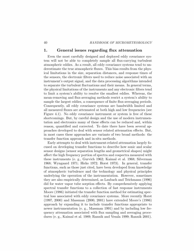
As an example of the different steps involved in this analysis, Figure4.3 compares the three following cospectra: the smoothed FFT cospec-trum for w′T ′

v obtained at 6:30 am MST January 2, 2001 (dashed line),the optimal fit of the FFT cospectrum by Equation 4.2 (solid line), andthe modeled cospectrum derived from Equation 4.2 using the ensemblebest fit parameters given in Table 4.1 (dotted line). This figure clearlyindicates the nature of the three types of cospectral variability mentionedpreviously.

3.3 Cospectral (dis)similarity between sites: AEuroflux site

The last section includes a brief comparison between the flat ter-rain (momentum and heat) cospectra of Kaimal et al. (1972) and thecospectra obtained at a topographically complex site during neutral at-mospheric conditions. The results indicated that there were cospectraldifferences between these sites, but it was less clear how significant thedifferences might be for discussions of cospectral similarity. However, forspectral attenuation issues the differences are quite significant becauseη′x for momentum flux was about 18% lower at GLEES than at the flatterrain site. Whereas η′x for heat flux was almost 40% higher at GLEES.It is, therefore, worthwhile to include another site in this comparison inan effort to determine how generalizable the previous results might befrom one site to another.

This section presents values of η′x were obtained at Griffin Forest,a Euroflux site located at (56◦ 36’ 30” N, 3◦ 47’ 15” W) near Aber-


feldy, Perthshire, Scotland. The forest at this site covers about 75% ofthe surface and is 97.3% Sitka spruce (Picea sitchensis), 2.1% Douglasfir (Pseudotsuga menziesii) and 0.6% birch (Betula pendula). The re-maining 25% of the surface is open space: roads, streams, and ridgesdominated by heather and grasses. The forest Leaf Area Index (LAI) isabout 8, and where the canopy is closed, the understory is quite sparseand dominated by mosses. The canopy height is about 7.5 m and daveraged about 6.5 m.

The site has an elevation of 350 m ASL, and is also a micrometeo-rologically complex site, being located in a region of ridge and valleyranging in height between 50 and 600 m. It is situated in a broad north-west facing valley with a mean slope of 9%. The fetch to the southwestis about 500 m before it is disturbed by a hill. To the northwest thefetch is about 2000 m and to the northeast and southeast it is about1000 m. The eddy covariance instruments are mounted at 15.5 m andconsist of a Solent R2 three dimensional sonic, a closed-path Licor (6262)CO2/H2O Infra Red gas analyzer (IRGA), and an open-path Licor 7500IRGA. The inlet to the closed-path IRGA is located 0.20 m below and0.05 m to the north of the sonic. The intake tube length is 18 m andit has an inside diameter of 0.00623 m. The flow rate is 6 L min−1 andthe flow Reynolds number is about 1400. The open-path sensor is po-sitioned 0.30 m from the center of the sonic. Data from this Eurofluxsite were obtained between July and September 2000. They were col-lected at 20.833 Hz (N1/2 = 37500 data points per half-hour) and wereprocessed by the Edisol/EdiRe software package. The eddy correlationsystem and the data processing package are described in more detail byMoncrieff et al. (1997). All covariances are calculated in the planar fitcoordinate system (Wilczak et al. 2001).

All Griffin forest cospectra are calculated for each 2-hour period usingsmoothed and spliced FFT (Kaimal and Finnigan 1994). To obtainthe high frequency portion of the cospectra the 20.833 Hz time seriesare divided into M sequential segments of contiguous 512-point timeseries. [Note that for this method of cospectral analysis NFFT = 29 andM = 4N1/2/NFFT if NFFT divides 4N1/2 exactly, otherwise M = 1+the integer part of {4N1/2/NFFT }.] If necessary, the final segment iszero-buffered to insure that NFFT is the same for all M data segments.Each segment is detrended using a linear least squares fit and taperedusing a Hamming window (Kaimal and Kristensen 1991). The FFTis applied to each segment and the transformed results are averagedprior to logarithmic bin-averaging of the spectral estimates. The lowfrequency cospectrum for the same data period is obtained by averagingM sequential data points to obtain a single set of NFFT averaged data


Table 4.2. Optimal values of η′x for instrument covariances measured at Griffin forest,

Scotland, during July through September 2000. The uncertainty associated with thevalue of each parameter is enclosed by parentheses. Here η′

x = fx(zref − d)/u.

Covariance η′x η′

x η′x

very unstable: z/L ≤ −2 neutral stability: stable: z/L > 0

u′w′ 0.009 (0.063) 0.027 (0.063) 0.029 (0.015)

w′T ′a 0.010 (0.032) 0.073 (0.032) 0.043 (0.025)

w′ρ′v (closed-path) 0.003 (0.008) 0.015 (0.008) 0.014 (0.011)

w′c′ (closed-path) 0.011 (0.015) 0.043 (0.015) 0.041 (0.023)

w′ρ′v (open-path) 0.014 (0.019) 0.041 (0.019) 0.036 (0.024)

w′c′ (open-path) 0.009 (0.011) 0.047 (0.011) 0.040 (0.021)

points. Again this data series is detrended, tapered, transformed, andlogarithmically bin-averaged using the same methods as with the highfrequency portion. The resulting high and low frequency portions aremerged and sorted by frequency to obtain a single cospectral curve, towhich Equation 4.2 is then fitted. About 200 cospectra for both stableand neutral/unstable atmospheric conditions were available for analysis.

Table 4.2 presents the cospectral parameter values for η′x obtained forGriffin forest. The other cospectral parameter values are not includedbecause they are of less significance. There are several key observa-tions concerning the Griffin forest results that need to be emphasized.First, comparing the neutral stability η′x values with those of GLEES(Table 4.1) indicates that for neutral conditions η′x at Griffin forest areassociated with much lower frequencies than at GLEES. Second, η′x atGriffin forest tends to decrease with increasing atmospheric instabilityand that η′x for stable conditions tend to be relatively constant andhighly variable. This stability dependency is opposite of the flat terrainsite of Kaimal et al. (1972), where constant η′x is associated with un-stable conditions and η′x tends to increase with increasing atmosphericstability. Third, the open-path water vapor and CO2 covariances andthe closed-path CO2 covariance can probably be considered cospectrallysimilar for any atmospheric stability, especially given the uncertaintyof their respective η′x values. But, some divergence between open- andclosed-path results should not be unexpected because the influence ofthe WPL temperature covariance (heat flux) term will be considerablygreater on the open-path covariance than on the closed-path covariance.However, the closed-path water vapor cospectra are so different fromthese other three scalar cospectra that they are probably untrustworthy.We hypothesize that the water vapor fluctuations have been so strongly


attenuated by the tube flow and interactions with the flow path wallsthat their associated η′x values should not be used for spectral atten-uation issues. Fourth, the w′T ′

a cospectra is for the atmospheric heatflux not for the sonic temperature covariance; but, any differences in-troduced by using w′T ′

a rather than w′T ′v should be small. Fifth, and

final, no continuity requirement between stable and neutral values of η′xwas imposed. Except for w′T ′

a, the results suggest that the η′x valuesare probably continuous across these two stability classes. Although thevariability of η′x for w′T ′

a is high in both stability classes, the data sug-gest that the value of 0.073 for the neutral case is likely to be biasedhigh.

In summary, the results from this Euroflux site, when combined withthose from GLEES and Kaimal et al. (1972), suggest that cospectra,which use the η′x normalization to parameterize fx, possess considerablesite-to-site variablity. Therefore, any investigation of issues involvingspectral attenuation of eddy covariance data needs to be examined ona site specific basis and that the arbitrary use of Kaimal’s et al. (1972)model for η′x has the potential to introduce significant errors into spectralcorrection factors for eddy covariance fluxes.

Besides any possible site-to-site variability in cospectra there is alsothe inherent variability of cospectra from one flux-averaging period tothe next.

3.4 Departures from smooth cospectral shapesAs Figure 4.3 clearly indicates observed cospectra are not particu-

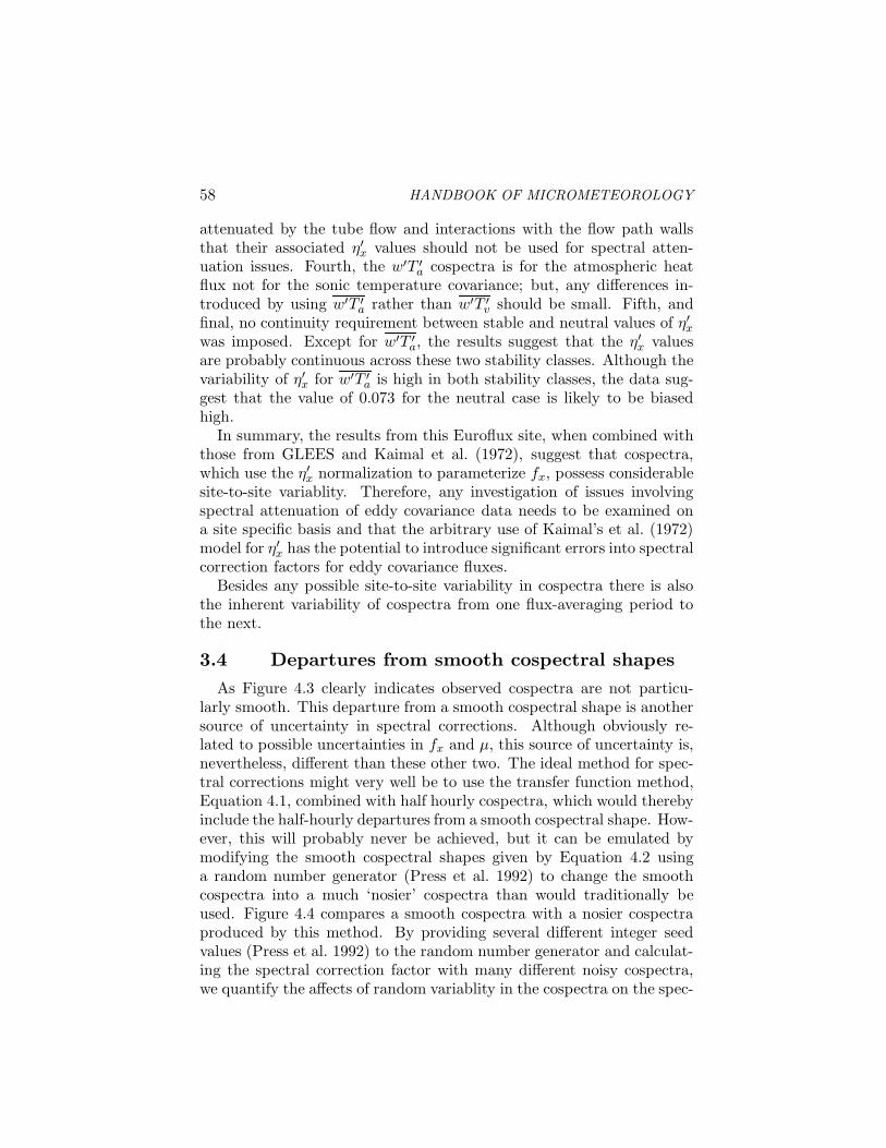
larly smooth. This departure from a smooth cospectral shape is anothersource of uncertainty in spectral corrections. Although obviously re-lated to possible uncertainties in fx and µ, this source of uncertainty is,nevertheless, different than these other two. The ideal method for spec-tral corrections might very well be to use the transfer function method,Equation 4.1, combined with half hourly cospectra, which would therebyinclude the half-hourly departures from a smooth cospectral shape. How-ever, this will probably never be achieved, but it can be emulated bymodifying the smooth cospectral shapes given by Equation 4.2 usinga random number generator (Press et al. 1992) to change the smoothcospectra into a much ‘nosier’ cospectra than would traditionally beused. Figure 4.4 compares a smooth cospectra with a nosier cospectraproduced by this method. By providing several different integer seedvalues (Press et al. 1992) to the random number generator and calculat-ing the spectral correction factor with many different noisy cospectra,we quantify the affects of random variablity in the cospectra on the spec-


10-3 10-2 10-1 100 101 102

f zrefu

-.1

.0

.1

.2

.3fC

o(f

)

wTw

T

’’

Measured cospectrum (smoothed)

Ensemble cospectrum

1 hour best fit cospectrum2

Figure 4.3. Comparison of the smoothed FFT cospectrum for w′T ′v obtained at 6:30

am MST January 2, 2001 at the GLEES (dashed line) with the optimal fit to thiscospectrum with Equation 4.2 (solid line) and the modeled cospectrum derived fromEquation 4.2 using the ensemble best fit parameters given in Table 4.1 (dotted line).

tral correction factor. Each of the spectral correction factors developedwith a non-smooth cospectra using the integral method is compared tothe correction factors determined by M21’s analytical method, whichuses the smooth cospectra. This produces a range of variation in Fthat could be conveniently incorporated into Equation 4.6 for ∆F/F bysimply multiplying Equation 4.6 by a constant, C = 1.2. Note that thevalue of 1.2 was synthesized from all five of the GLEES covariance mea-surements. A separate determination of C for a closed path CO2 systemwas also performed and is discussed in section 3.5. The final expressionfor the relative uncertainty, ∆F/F , is

∆F

F= C{[(1 +

1b)p − 1 + p

b]2[

∆fx

fx]2

+[(1 +1b)p ln(p) − 1 + p

bln(b)]2[∆α]2

+[(1 +1b)p]2[

∆τe

τe]2}0.5/[(1 + p)(1 +

1b)] (4.7)


10-2 10-1 100 101 102-.1

.1

.2

.3

.0

Smooth cospectrum‘ ’Noisy cospectrum

fCo(

f)To

tal C

o var

ianc

e

for

ηηxfx

Figure 4.4. A comparison of the hypothetical frequency-weighted atmosphericcospectrum shown in Figure 4.1 (solid line) with a version of it after modificationby a random number generator (dash-dot). This method of modifying the smoothcospectral shape is used to estimate the uncertainty in the spectral correction factorthat is associated with departures of true cospectra from smoothed versions of thecospectra.

3.5 Results for an open-path systemFigure 4.5 shows relative uncertainty in the spectral correction fac-

tor, ∆F/F , as a function of wind speed for the GLEES CO2 covariancemeasurement. This figure suggests that applying a spectral correctionfactor based on the transfer function approach to GLEES wintertimeCO2 covariances would lead to a 5 to 10% uncertainty in the resultingCO2 covariance at low wind speeds and a 2 to 4% uncertainty at higherwind speeds. Figure 4.6 shows the correction factor, F , as a function ofwind speed for the GLEES CO2 covariance measurement as estimatedby the analytical method of M21 along its inherent range of uncertaintyas predicted by Equation 4.7. The filters and equivalent time constantsemployed for this and the previous figure are taken from Table 1 ofMassman (2000) and include sonic line averaging for scalar fluxes, lat-eral separation, longitudinal separation without a first order instrument,and high pass block averaging. The results shown in this figure indicatethat the uncertainty associated with a relatively larger value of F is it-self relatively large and that the inherent uncertainty in F decreases asF decreases. This supports the conclusion that if an eddy covariance


10-1 100 101 1020

10

15

20

5

Wind speed (m s )-1

z= 0ref

L

∆ F(%

)F

Figure 4.5. The relative uncertainty in the spectral correction factor, ∆F/F , asa function of wind speed for the GLEES CO2 covariance measurement. Neutralatmospheric stability is assumed.

system is designed so that spectral attenuation is minimal (and there-fore relatively small), then the transfer method of estimating spectralcorrection factors is not particularly sensitive to the shape, the lack ofsmoothness in the cospectra, or the natural variablity of the cospectra.To rephrase, if the spectral correction factors are small, then the trans-fer function method should provide trustworthy and relatively accuratevalues for the spectral correction factors.

3.6 Extension to a closed-path system and ∆τe

The GLEES data provide an example of an eddy covariance systemwith an open path CO2 sensor. Now we wish to examine the same sys-tem with a closed path sensor. We construct this scenario primarily totest our present methods on a system that has a much longer equivalenttime constant for high frequency attenuation, τe, than the open pathsystem. All the methods and calculations remain the same, except weassume that the closed path system has an intake tube attached to afirst order instrument, which is housed in a separate shelter at the baseof the tower. We further assume that the time constant for the first or-der instrument (τ1) was determined in situ to be 0.1 s and we will take∆τe = 25 % of τ1. These values for τ1 and ∆τe are to be understood aspurely hypothetical. For any real application they could depart signifi-


10-1 100 101 102

1.5

1.4

1.3

1.2

1.1

1.0

.9

F (

anal

ytic

al m

etho

d)

z= 0ref

L

Wind speed (m s )-1

Figure 4.6. The correction factor, F , as a function of wind speed for the GLEES CO2

covariance measurement as estimated by the analytical method of M21 (dark solidline) and its inherent range of uncertainty as predicted by Equation 4.7 (shaded area).The factor C used with Equation 4.7 to account for variable (random) departures froma smooth cospectral shape is 1.2.

cantly from these present values and from one eddy covariance systemto another.

In this simulation we allow for the attenuation associated with tubeflow (M21; Massman 1991), a small amount of lateral separation, somesmall amount of longitudinal separation with first order effects (Mass-man 2000), and a first order time constant for the CO2 sensor equal to0.1 s. Because this closed path scenario falls into M21’s category for sys-tems characterized by equivalent time constants between 0.1 and 0.3 sand a neutrally stable atmosphere, his analytical approach would suggestthat Equation 4.3 above be augmented by the term [1 + 0.9pα]/[1 + pα].Here we do not employ the additional term. Rather we use Equation 4.3directly. Figure 4.7 shows the difference between the integral method,Equation 4.1, and Equation 4.3. For all wind speeds the difference issmall and the agreement is quite good.

Figure 4.8 shows the correction factor, F , as a function of wind speedfor the simulated closed path CO2 covariance measurement as estimatedwith analytical method of M21 along its inherent range of uncertaintyas predicted by Equation 4.7. For this example, the factor of C inEquation 4.7 was again found to be 1.2 using the same method as theopen path sensor. This figure is the closed path analog to Figure 4.6


10-1 100 101 102

.15

.10

.05

.00

-.05

-.10

-.15Cor

rect

ion

f act

or d

iffer

ence

wC

O’

’ 2

z= 0ref

L

Wind speed (m s )-1

Figure 4.7. Difference between the spectral correction factors estimated from thenumerical integration of Equation 4.1 and Equation 4.3 from M21. These calculationsare for a closed-path eddy covariance system and a neutral atmosphere and are shownas a function of the horizontal wind speed. The zero line is highlighted.

and clearly demonstrates the same conclusions. That is if the correc-tion factors are relatively large, which they are here by design, thenthe inherent uncertainties associated with the transfer function methodcan also be relatively large. For example the calculations shown in Fig-ure 4.8 suggest that for wind speeds between about 2 and 10 m s−1 thecorrection factor is about 1.1 ± 10%. For this same range of wind speedsFigure 4.6 suggests that the open path system has a correction factorand an inherent uncertainty about half of that. In these two examplesthe fundamental difference between the open and closed path systems istheir respective time constants, reinforcing the notion that longer timeconstants result in more spectral attenuation, greater uncertainty in thespectral corrections, and, therefore, greater inherent uncertainty in thefluxes or covariances that are spectrally corrected with the transfer func-tion method.

Most of the uncertainty shown in Figure 4.8 results from variabilityin the cospectra and from the uncertainty in the cospectral parameters,not from ∆τe. This is because the present example is fairly conservativein its estimate of τ1 and ∆τe. As either of these parameters increase invalue so also do the estimates for F and ∆F . At some eddy covariancesites τ1 can exceed 1 s, which is considerably longer than the presenthypothetical value of 0.1 s. At present there has been no information


10-1 100 101 102

1.5

1.4

1.3

1.2

1.1

1.0

.9

F (

anal

ytic

al m

etho

d)

z= 0ref

L

Wind speed (m s )-1

Figure 4.8. The correction factor, F , as a function of wind speed for the GLEES CO2

covariance measurement as estimated by the analytical method of M21 (dark solidline) and its inherent range of variablity as predicted by Equation 4.2 (shaded area).The factor C used with Equation 4.2 to account for the variable (random) departuresfrom smooth cospectral shape is 1.2, which is the same as with the GLEES open pathsensor.

published (of which we are aware) that discusses ∆τ1, which we wouldsuggest be used to estimate ∆τe. However, we can easily imagine that∆τ1 can exceed the value of 0.025 s we use in this study.

3.7 Discussion and caveats concerning lowfrequencies

One of the advantages of the analytical method is the ability to es-timate the high and low frequency portions of the correction factorsseparately. Rewriting Equation 4.4 using the b and p notation yieldsF = [1 + 1/b][1 + p]; where α = 1 is assumed for simplicity. The highfrequency correction factor is expressed by the p term, [1 + p], while thelow frequency portion is [1 + 1/b]. Table 4.3 (using η′x from Table 4.1)lists these two terms for the GLEES covariance data and the simulatedclosed path CO2 data. For the open path covariances both correctionsare small; however, the low frequency portion tends to be slightly largerthan the high frequency portion. In the case of the closed path CO2

system the high frequency portion is by far the dominant term, whichindicates the influence of the relatively longer high frequency time con-stant, τe, for closed path system than for the open path.


Table 4.3. Simplified (and approximate) high and flow frequency correction factorsfor the GLEES eddy covariance system estimated with M21’s analytical method. The(1+p) factor is for high frequency effects and the (1+1/b) factor is for low frequencyeffects. Wind speeds are assumed to be greater than 1 m s−1.

Covariance (1 + p) (1 + 1b)

p′w′ 1.04 1.01-1.06

u′w′ 1.00-1.01 1.00-1.05

w′T ′v 1.00-1.01 1.00-1.03

w′ρ′v 1.01 1.00-1.04

w′c′ (open) 1.01 1.00-1.03w′c′ (closed) 1.02-1.13 1.00-1.03

Nevertheless, in essence, both high and low frequency correction fac-tors are based on extrapolations into regions of the cospectra wherethere are no direct observations. In the case of the high frequency cor-rections, this extrapolation is probably quite trustworthy because the-7/3 decay law is theoretically sound and has been observationally ver-ified in many studies. But, considerably less is known about the verylow frequency portion of the cospectra. For any sampling period, Tb,there is no observationally based information on low frequencies withinthe spectral band [0, 1

Tb]. Therefore, by including the high pass filters

(block averaging filters, etc.) in Equation 4.1 and integrating over thewhole spectral waveband [0,∞] we implicitly assume that the observedturbulence cospectra extends smoothly and continuously into the unob-served portion of the cospectra. This assumption will not be true for allatmospheric conditions, like those that might occur during convectiveconditions or when other large scale planetary boundary layer processesare active at the time of the measurements. Under these conditions, thelow frequency correction factor, [1 + 1/b], will likely misrepresent thetrue correction factor.

At GLEES during the wintertime such large scale planetary boundarylayer effects do not seem to be significant. For example, Figure 4.9 isa ogive computed from one of the 180 half hourly periods for the tem-perature covariance w′T ′

v. This particular ogive indicates that virtuallyall the half hourly cospectral power is contained in motions with peri-ods shorter than about 5.5 minutes because the because the cumulativecospectral power has reached a relatively stable maximum at 3(10−3)Hz. We should note here that this particular example is an extremecase. Other ogives (not shown) indicate that motions somewhat longerthan 30 minutes can contribute to half hourly at GLEES during the win-


10-4 10-3 10-2 10-1 100 101-.5

.0

.5

1.5

1.0

f (Hz)

Frac

tion

of c

umul

ativ

e flu

x (o

giv e

)

Figure 4.9. An ogive calculated from the unsmoothed FFT cospectrum for the tem-perature covariance w′T ′

v. These data were obtained at 6:30 am MST January 2, 2001at the GLEES. Neutral atmospheric stability is assumed. This example indicates thatvirtually all cospectral power is located in atmospheric motions with periods less thanabout 5.5 minutes. Other examples (not shown) show contributions from longer pe-riod motions. The 1.0 line is highlighted.

tertime. However, we also performed other tests on the data by concate-nating two half hourly time series to form a single hour time series andby subsampling and concatenating four half hourly time series to form atwo hour time series. We could find no evidence of any long period, lowfrequency, flux contributions. Of course, this result should not be unex-pected because high elevation, wintertime, high-wind, high-turbulenceconditions are not particularly good candidates for low frequency plan-etary boundary layer motions. But when conditions are more conducivethese slow large scale motions will contribute to the fluxes (Sakai et al.2001; Finnigan et al. 2003). At present there is no single agreed-uponwell defined method for correcting fluxes for these low frequency contri-butions. Consequently, the spectral transfer method as it is posed byEquations 4.1 and 4.2 should not be understood as compensating for allflux loss due to undersampling the low frequency planetary boundarylayer motions. Issues concerning the influence of these types of motionson measured fluxes is discussed in Chapter 5 of this volume.


3.8 SummaryThis study has developed a method of estimating the uncertainty

in any measured covariance that is spectrally corrected by the transferfunction method. It includes the effects of the (flux-averaging) period-to-period variability in (i) the frequency-weighted cospectral peak, fx or η′x,(ii) the random departure of measured cospectra from a smooth shape(encapsuled by the parameter C of Equation 4.7), (iii) the broadness ofthe frequency-weighted cospectra (µ or α), and (iv) some of the possibleuncertainties in the effective time constant of an eddy covariance system,τe. This model, summarized by Equation 4.7, was calibrated mostlyusing cospectral data from one particular AmeriFlux site (GLEES), butalso included comparisons with similar data from Kaimal et al. (1972)and an Euroflux site (Griffin forest). Conclusions reached in this studyare

The uncertainty associated with variability in the cospectral broad-ness is constant, i. e., ∆α = 0.2.

It is reasonable to simplify Equation 4.7 by approximating relativeuncertainty in fx, i. e., ∆fx/fx, by 0.4 or 0.5; where ∆fx is ameasure of the inherent variability in fx. The value of 0.4 is theupper bound of values found at GLEES (Table 4.1) and 0.5 is avalue more representative of the Griffin forest site (Table 4.2). Thissimplification eliminates the need to evaluate ∆fx directly.

Spectral corrections and their associated uncertainties are likelyto be site specific because the nondimensional frequency, η′x =fx(zref − d)/u, was shown to be site specific in this study. In fact,this study has shown that η′x varies significantly between the flatterrain site of Kaimal et al. (1972) and the micrometeorologicallycomplex forested sites of GLEES and Griffin forest. Therefore,there is no a priori reason to assume that the values for nondi-mensional frequency, η′x, developed in this study or by Kaimal etal. (1972) apply universally. In turn this suggests that to find anytruly universal cospectral shape will require a different turbulenttime scale than (zref − d)/u.

Equation 4.7 uses a value of 1.2 for the parameter C, which seemsto be reasonable for both open and closed path CO2 systems. How-ever, we did not emulate all possible or observed eddy covariancesystems, so it is conceivable that C could be somewhat differentfor other eddy covariance systems. Thus there may remain a needto calibrate Equation 4.7 at more eddy covariance sites.


The uncertainty in spectral correction, F , estimated with the trans-fer function method, ∆F , increases as F increases and decreaseswith decreasing F . Careful attention to minimizing separation dis-tances and instrument time constants should help keep high fre-quency losses small so that F and ∆F are small. In this case thehigh frequency correction factors should be relatively independentof cospectral shape, lack of cospectral smoothness, and inherentvariability.

The spectral losses at low frequencies on the other hand are not somuch instrument related as they are related to the length of thesampling period and the nature of the low frequency atmosphericmotions present during a sampling period. Because so little isknown about the nature of these low frequency atmospheric mo-tions (1-4 hours) it is difficult to make specific recommendationsfor reducing this undersampling error. However, in general, as themeasurement height decreases the low frequency content of anymeasured flux should also decrease, which will reduce the prob-lem somewhat. Unfortunately, this improvement will be offset byincreasing high frequency content in the fluxes.

Present results indicate that further research is needed into the lowfrequency (1-4 hour) components of eddy covariance fluxes and inthe nature of the differences in the frequency-weighted cospectralpeaks, η′x and fx, between different sites.


ReferencesAubinet, M., Chermanne, B., Vandenhaute, M., Longdoz, B., Yernaux, M., Laitat,

E.: 2001, ‘Long term carbon dioxide exchange above a mixed forest in theBelgian Ardennes’, Agric. For. Meteorol. 108, 293-315.

Auble, D. L., Meyers, T. P.: 1992, ‘An open path, fast response infrared absorptiongas analyzer for H2O and CO2’, Bound.-Layer Meteorol. 59, 243-256.

Aydin, I.: 1998, ‘Evaluation of fluctuating pressure measured with connection tubes’,J. Hydraulic Engineering, 124, 413-418.

Busch, N. E.: 1973, ‘Turbulent transfer in the atmospheric surface layer’, In: (Ed.)Haugen, DA, Workshop on Micrometeorology, American Meteorological Soci-ety, Boston, 1-28.

Coleman, H. W., Steele, W. G.: 1999, Experimentation and Uncertainty Analysisfor Engineers. John Wiley, New York, 275 pp.

Cook, R. K., Bedard, A. J.: 1971, ‘On the measurement of infrasound’, GeophysicalJournal Royal Astronomical Society 26, 5-11.

Finnigan, J. J., Clement, R., Mahli, Y., Leuning, R., Cleugh, H.: A. 2003, ‘A re-evaluation of long-term flux measurement techniques: Part 1. Averaging andcoordinate rotation’, Bound.-Layer Meteorol. 107, 1-48.

Goulden, M. L., Daube, B. C., Fan, S.-M., Sutton, D. J., Bazzaz, A., Munger, J. W.,Wofsy, S. C.: 1997, ‘Physiological response of a black spruce forest to weather’,J. Geophys. Res. 102, 28,987-28,996.

Gurvich, A. S.: 1962, ‘The pulsation spectra of the vertical component of the windvelocity and their relations to micrometeorological conditions’, Izvestiya At-mospheric Oceanic Physics 4, 101-136.

Hicks, B. B.: 1972, ‘Propellor anemometers as sensors of atmospheric turbulence’,Bound.-Layer Meteorol. 3, 214-228.

Hicks, B. B., McMillen, R. T.: 1988, ‘On the measurement of dry deposition usingimperfect sensors and in non-ideal terrain’, Bound.-Layer Meteorol., 42, 79-84.

Højstrup, J.: 1993, ‘A statistical data screening procedure’, Measurement ScienceTechnology 4, 153-157.

Holman, J. P.: 2001, Experimental Methods for Engineers. 7th Edition. McGraw-Hill, Boston, MA, 698 pp.

Horst, T. W.: 1973, ‘Spectral transfer functions for a three-component sonic anemome-ter’, J. Appl. Meteorol. 12, 1072-1075.

Horst, T. W.: 1997, ‘A simple formula for attenuation of eddy fluxes measured withfirst-order-response scalar sensors’, Bound.-Layer Meteorol. 82, 219-233.

Horst, T. W.: 2000, ‘On frequency response corrections for eddy covariance fluxmeasurements’, Bound.-Layer Meteorol. 94, 517-520.

Horst, T. W., Oncley, S. P., Semmer, S. R.: 1997, ‘Measurement of water vapor fluxesusing capacitance RH sensors and cospectral similarity’, In: 12th Symposiumon Boundary Layers and Turbulence, American Meteorological Society, Boston,360-361.

Iberall, A. S.: 1950, ‘Attenuation of oscillatory pressures in instrument lines’, Jour-nal Research National Bureau Standards 45, 85-108.


Kaimal, J. C., Clifford, S. F., Lataitis, R. J.: 1989, ‘Effect of finite sampling onatmospheric spectra’, Bound.-Layer Meteorol. 47, 337-347.

Kaimal, J. C., Finnigan, J. J.: 1994, Atmospheric Boundary Layer Flows - TheirStructure and Measurement. Oxford University Press, New York, NY, 289 pp.

Kaimal, J. C., Kristensen, L.: 1991, ‘Time series tapering for short data samples’,Bound.-Layer Meteorol. 57, 187-194.

Kaimal, J. C., Wyngaard, J. C., Haugen, D. A.: 1968, ‘Spectral characteristics ofsurface-layer turbulence’, Quart. J. R. Meteorol. Soc. 98, 563-589.

Kaimal, J. C., Wyngaard, J. C., Izumi, Y., Cote, O. R.: 1972, ‘Spectral character-istics of surface-layer turbulence’, Quart. J. R. Meteorol. Soc. 98, 563-589.

Katul, G. G., Hsieh, C. I.: 1999,‘A note on the flux-variance similarity relationshipfor heat and water vapor in the unstable atmospheric surface layer’, Bound.-Layer Meteorol. 90, 327-338.

Koprov, B. M., Sokolov, D. Y.: 1973, ‘Spatial correlation functions of velocity andtemperature components in the surface layer of the atmosphere’, Izvestiya At-mospheric Oceanic Physics 4, 178-182.

Kristensen, L., Mann, J., Oncley, S. P., Wyngaard, J. C.: 1997, ‘How close isclose enough when measuring scalar fluxes with displaced sensors’, J. Atmos.Oceanic Technol. 14, 814-821.

Laubach, J., McNaughton, K. G.: 1999, ‘A spectrum-independent procedure for cor-recting eddy fluxes measured with separated sensors’, Bound.-Layer Meteorol.89, 445-467.

Laubach, J., Teichmann, U.: 1996, ‘Measuring energy budget components by eddycorrelation: Data corrections and application over low vegetation’, BeitragePhysik Atmosphare, 69, 307-320.

Lee, X., Black, T. A.: 1994, ‘Relating eddy correlation sensible heat flux to horizontalsensor separation in the unstable atmospheric surface layer’, J. Geophys. Res.99, 18,545-18,553.

Massman, W. J.: 1991, ‘The attenuation of concentration fluctuations in turbulentflow through a tube’, J. Geophys. Res. 96, 15,269-15,273.

Massman, W. J.,: 2000, ‘A simple method for estimating frequency response correc-tions for eddy covariance systems’, Agric. For. Meteorol. 104, 185-198.

Massman, W. J.: 2001, ‘Reply to comment by Rannik on “A simple method forestimating frequency response corrections for eddy covariance systems”’, Agric.For. Meteorol. 107, 247-251.

Massman, W. J., Lee, X.: 2002, ‘Eddy covariance flux corrections and uncertaintiesin long-term studies of carbon and energy exchanges’, Agric. For. Meteorol.113, 121-144.

Mestayer, P. G., Larsen, S. E., Fairall, C. W., Edson, J. B.: 1990, ‘Turbulence sensordynamic calibration using real-time spectral computations’, J. Atmos. OceanicTechnol. 7, 841-851.

Moncrieff, J., Massheder, J., Verhoef, A., Elbers, J., Heusinkveld, B., Scott, S. L.,DeBruin, H. A. R., Kabat, P. , Soegaard, H., Jarvis, P.: 1997, ‘A system tomeasure Surface fluxes of momentum, sensible heat, water vapour and carbondioxide’, J. Hydrol. 188, 589-611.


Moore, C. J.: 1986, ‘Frequency response corrections for eddy correlation systems’,Bound.-Layer Meteorol. 37, 17-35.

Nishiyama, R. T., Bedard, A. J.: 1991, ‘A “Quad-Disc” static pressure probe formeasurement in adverse atmospheres: With a comparative review of staticpressure probe designs’, Review Scientific Instruments 62, 2193-2204.

Press, W. H., Teutkolsky, S. A., Vetterling, W. T., Flannery, B. P.: 1992, NumericalRecipes, Second Edition, Cambridge University Press.

Rannik, U.: 2001, ‘A comment on the paper by W.J. Massman “A simple methodfor estimating frequency response corrections for eddy covariance systems”’Agric. For. Meteorol. 107, 241-245.

Rannik, U., Vesala, T.: 1999, ‘Autoregressive filtering versus linear detrending inestimation of fluxes by the eddy covariance method’, Bound.-Layer Meteorol.91, 259-280.

Sakai, R. K., Fitzjarrald, D. R., Moore, K. E.: 2001, ‘Importance of low-frequencycontributions to eddy fluxes observed over rough surfaces’, J. Appl. Meteorol.40, 2178-2192.

Scarborough, J. B.: 1966, Numerical Mathematical Analysis, 6th Edition, The JohnsHopkins Press, Baltimore.

Silverman, B. A.: 1968, ‘The effect of spatial averaging on spectrum estimation’ J.Appl. Meteorol. 7, 168-172.

Spanier, J., Oldham, K. B.: 1987, An Atlas of Functions, Springer-Verlag, Berlin,700 pp.

Verma, S. B., Ullman, F. G., Billesbach, D., Clement, R. J., Kim, J.: 1992, ‘Eddycorrelation measurements on methane flux in a northern peatland ecosystem’Bound.-Layer Meteorol. 58, 289-304.

Vickers, D., Mahrt, L.: 1997, ‘Quality control and flux sampling problems for towerand aircraft data’, J. Atmos. Oceanic Technol. 14, 512-526.

Villalobos, F. J.: 1996, ‘Correction to eddy covariance water vapor flux using addi-tional measurements of temperature’, Agric. For. Meteorol. 88, 77-83.

Webb, E. K., Pearman, G. I., Leuning, R.: 1980, ‘Correction of flux measurementsfor density effects due to heat and water vapor transfer’, Quart. J. R. Meteorol.Soc. 106, 85-106.

Wilczak, J. M., Oncley, S. P., Stage, S. A.: 2001, ‘Sonic anemometer tilt correctionalgorithms’, Bound.-Layer Meteorol. 99, 127-150.

Wyngaard, J. C.: 1971, ‘Spatial resolution of a resistance wire temperature sensor’,Physics of Fluids 14, 2052-2054.

Wyngaard, J. C., Siegel, A., Wilczak, J. M.: 1994, ‘On the response of a turbulent-pressure probe and the measurement of pressure transport’, Bound.-Layer Me-teorol. 69, 379-396.

Uncertainty in eddy covariance flux estimates resulting ... · UNCERTAINTY IN EDDY COVARIANCE FLUX...

Documents

Transcript of Uncertainty in eddy covariance flux estimates resulting ... · UNCERTAINTY IN EDDY COVARIANCE FLUX...