Uncertainty Analysis of Instrument Calibration and …mln/ltrs-pdfs/NASA-99-tp209545.pdfNational...
77
NASA/TP-1999-209545 Uncertainty Analysis of Instrument Calibration and Application John S. Tripp and Ping Tcheng Langley Research Center, Hampton, Virginia October 1999
Transcript of Uncertainty Analysis of Instrument Calibration and …mln/ltrs-pdfs/NASA-99-tp209545.pdfNational...
NASA/TP-1999-209545
Uncertainty Analysis of InstrumentCalibration and Application
John S. Tripp and Ping TchengLangley Research Center, Hampton, Virginia
October 1999

The NASA STI Program Office . . . in Profile
Since its founding, NASA has been dedicated
to the advancement of aeronautics and space
science. The NASA Scientific and Technical
Information (STI) Program Office plays a key
part in helping NASA maintain this
important role.
The NASA STI Program Office is operated by
Langley Research Center, the lead center for
NASA’s scientific and technical information.
The NASA STI Program Office provides
access to the NASA STI Database, the
largest collection of aeronautical and space
science STI in the world. The Program Office
is also NASA’s institutional mechanism for
disseminating the results of its research and
development activities. These results are
published by NASA in the NASA STI Report
Series, which includes the following report
types:
• TECHNICAL PUBLICATION. Reports of
completed research or a major significant
phase of research that present the results
of NASA programs and include extensive
data or theoretical analysis. Includes
compilations of significant scientific and
technical data and information deemed
to be of continuing reference value. NASA
counterpart or peer-reviewed formal
professional papers, but having less
stringent limitations on manuscript
length and extent of graphic
presentations.
• TECHNICAL MEMORANDUM.
Scientific and technical findings that are
preliminary or of specialized interest,
e.g., quick release reports, working
papers, and bibliographies that contain
minimal annotation. Does not contain
extensive analysis.
• CONTRACTOR REPORT. Scientific and
technical findings by NASA-sponsored
contractors and grantees.
• CONFERENCE PUBLICATION.
Collected papers from scientific and
technical conferences, symposia,
seminars, or other meetings sponsored or
co-sponsored by NASA.
• SPECIAL PUBLICATION. Scientific,
technical, or historical information from
NASA programs, projects, and missions,
often concerned with subjects having
substantial public interest.
• TECHNICAL TRANSLATION. English-
language translations of foreign scientific
and technical material pertinent to
NASA’s mission.
Specialized services that complement the
STI Program Office’s diverse offerings include
creating custom thesauri, building customized
databases, organizing and publishing
research results . . . even providing videos.
For more information about the NASA STI
Program Office, see the following:
• Access the NASA STI Program Home
Page at http://www.sti.nasa.gov
• Email your question via the Internet to
• Fax your question to the NASA STI
Help Desk at (301) 621-0134
• Telephone the NASA STI Help Desk at
(301) 621-0390
• Write to:
NASA STI Help Desk
NASA Center for AeroSpace Information
7121 Standard Drive
Hanover, MD 21076-1320

National Aeronautics and
Space Administration
Langley Research Center
Hampton, Virginia 23681-2199
NASA/TP-1999-209545
Uncertainty Analysis of InstrumentCalibration and Application
John S. Tripp and Ping TchengLangley Research Center, Hampton, Virginia
October 1999

Available from:
NASA Center for AeroSpace Information (CASI) National Technical Information Service (NTIS)
7121 Standard Drive 5285 Port Royal Road
Hanover, MD 21076-1320 Springfield, VA 22161-2171
(301) 621-0390 (703) 605-6000

Contents
Symbols . . . . . . . . . . . . . . . . . . . . . . . . . . . . . . . . . . . . . v
1. Summary . . . . . . . . . . . . . . . . . . . . . . . . . . . . . . . . . . . 1
2. Introduction . . . . . . . . . . . . . . . . . . . . . . . . . . . . . . . . . . 1
3. Instrument Modeling and Calibration Experimental Design . . . . . . . . . . . . . 2
3.1. General Multivariate Process . . . . . . . . . . . . . . . . . . . . . . . . . 2
3.2. Single-Input{Single-Output Process . . . . . . . . . . . . . . . . . . . . . . 3
3.3. Linear, Polynomial, and Nonlinear Multivariate Processes . . . . . . . . . . . . 3
3.4. Calibration Experimental Design . . . . . . . . . . . . . . . . . . . . . . . 4
4. Generalized Linear Multivariate Regression Analysis . . . . . . . . . . . . . . . . 5
4.1. Decorrelation of Covariance Matrix . . . . . . . . . . . . . . . . . . . . . . 6
4.2. Least-Squares Estimation of Process Parameters . . . . . . . . . . . . . . . . 6
5. Con�dence and Prediction Intervals . . . . . . . . . . . . . . . . . . . . . . . . 7
5.1. Con�dence Intervals of Estimated Parameters . . . . . . . . . . . . . . . . . . 7
5.2. Calibration Con�dence Intervals of Predicted Process Output . . . . . . . . . . . 8
5.3. Prediction Interval of New Measurement . . . . . . . . . . . . . . . . . . . . 8
6. Computation of Inferred Input With Con�dence and Prediction Intervals . . . . . . . 9
7. Calibration Uncertainty Caused by Combined Input Errors and Measurement Errors . . 9
8. E�ects of Process Modeling Error . . . . . . . . . . . . . . . . . . . . . . . . 11
8.1. Uncertainty Analysis of Modeling Error . . . . . . . . . . . . . . . . . . . 11
8.2. Design Figure of Merit . . . . . . . . . . . . . . . . . . . . . . . . . . . 12
8.3. E�ects of Experimental Design on Figure of Merit . . . . . . . . . . . . . . . 13
9. Uncertainty Analysis of Nonlinear Instrument Calibration . . . . . . . . . . . . . 13
9.1. Combined Input and Measurement Uncertainties . . . . . . . . . . . . . . . 13
9.2. Least-Squares Estimation of Process Parameters . . . . . . . . . . . . . . . 15
9.3. Uncertainty of Estimated Process Parameters . . . . . . . . . . . . . . . . . 15
9.4. Residual Sum of Squares and Standard Error of Regression . . . . . . . . . . . 16
9.5. Con�dence and Prediction Intervals of Predicted Output . . . . . . . . . . . . 17
10. Multivariate Multiple-Output Analysis . . . . . . . . . . . . . . . . . . . . . 19
11. Uncertainties of Inferred Inputs From Inverse Process Function . . . . . . . . . . 21
12. Replicated Calibration . . . . . . . . . . . . . . . . . . . . . . . . . . . . 21
12.1. Computation of Replicated Design Matrix . . . . . . . . . . . . . . . . . . 22
12.2. Replicated Moment Matrix for Linear Single-Output Process . . . . . . . . . 22
12.3. Replicated Moment Matrix for General Single-Output Process . . . . . . . . . 24
12.4. Analysis of Variance for Estimation of Bias and Precision Uncertainties . . . . . 25
12.5. Stationarity Test of Estimated Parameters . . . . . . . . . . . . . . . . . 27
13. Examples . . . . . . . . . . . . . . . . . . . . . . . . . . . . . . . . . . 28
13.1. Calibration of Single-Input{Single-Output Nonlinear Sensor . . . . . . . . . . 28
13.2. Two-Input{Two-Output Linear Instrument . . . . . . . . . . . . . . . . . 30
14. Concluding Remarks . . . . . . . . . . . . . . . . . . . . . . . . . . . . . 33
iii

Appendix|Mathematical Derivations . . . . . . . . . . . . . . . . . . . . . . . 35
A1. Preliminaries . . . . . . . . . . . . . . . . . . . . . . . . . . . . . . . 35
A1.1. Extended Least-Squares Analysis . . . . . . . . . . . . . . . . . . . 35
A1.2. Lemmas and Theorems . . . . . . . . . . . . . . . . . . . . . . . 35
A1.3. Linear Least-Squares Estimation . . . . . . . . . . . . . . . . . . . 40
A2. E�ects of Process Modeling Error . . . . . . . . . . . . . . . . . . . . . . 44
A3. Nonlinear Least-Squares Estimation With Input Uncertainty . . . . . . . . . . 46
A3.1. Residual Sum of Squares . . . . . . . . . . . . . . . . . . . . . . . 49
A3.2. Con�dence Intervals . . . . . . . . . . . . . . . . . . . . . . . . . 51
A4. Analysis of Replicated Calibrations . . . . . . . . . . . . . . . . . . . . . 52
A4.1. Single-Input{Single-Output Process With Uncorrelated Uncertainties . . . 53
A4.2. General Multi-Input{Single-Output Process . . . . . . . . . . . . . . 55
A4.3. Analysis of Variance of Replicated Calibrations . . . . . . . . . . . . . 58
A4.4. Stationarity Test of Estimated Parameters . . . . . . . . . . . . . . . 61
References . . . . . . . . . . . . . . . . . . . . . . . . . . . . . . . . . . . 64
iv

Symbols
A;B K �K matrix
amn; bmn mnth elements of matrices A and B
B bias error
b o�set voltage of angle of attack sensor
C Mc � L coe�cient matrix
c, cm Mc � 1 parameter vector with elements cm
bc;bcm Mc � 1 estimated parameter vector with elements bcm
bcG globally estimated parameter vector
bcRnMc � 1 estimated parameter vector of nth replication
cos � K � 1 vector formed by element-by-element cosine evaluation of K � 1 vector �
D experimental design, a subset of =
DNK NK �NK block-diagonal matrix
di distance
e(c,Z) K � 1 vector function of c and Z
eM ; eX error vectors
be; bev K � 1 residual vectors
ben K � 1 residual vector at nth replication
�ek averaged residual vector
�ek element of �ek
F ratio of variances
Fc K �Mc derivative matrix of f(c,Z) with respect to c
Fcc Mc �Mc �K array
FcK K �Mc derivative matrix of f(c,ZK) with respect to c
Fi; j(�) � percentile value of F-distribution with i; j degrees of freedom
f(c,Z) K � 1 vector function of c and Z
f(c; z) real-value multivariate function of c and z
fcm mth column of Fc
fc(c ,z) Mc � 1 gradient vector of f(c; z) with respect to c
fccij ijth column vector of length K contained in array Fcc
fccij k kth element of vector fccij
fz(c ; zk) 1 �K gradient vector of f with respect to z
�fz error vector
v

�fzk element of error vector �fz
G K � L matrix of gj(c.j , z) functions
GH NK �NK matrix
g(C, z) 1 � L row vector of scalar-value functions of C and z
gj(c.j , z) jth element of g(C, z)
H K �NK replication matrix containing N copies of K �K identity matrix IK
HE Mc �Mc matrix
h(c , Z) 1 �Mc vector gradient of SSQ with respect to c
hEijijth element of HE
I identity matrix
IK K �K identity matrix
IW diagonal matrix of ones and zeros
= subset of input space <M z
i; j; k;m; n integer indices
J normalized average predicted output variance over set =
K number of calibration observations
L dimension of multivariate function
M order of multivariate polynomial or integer
Mc length of parameter vector c
Mz length of extended input vector z
N number of replications or integer
NI number of input variables
P nonsingular matrix
Pm orthonormal matrix
Prm;Psm submatrices ofPm
pm mth row of R�1
Q Mz �Mz weighted moment matrix
Qc Mc �Mc nonlinear moment matrix
Qm N �N matrix
qm quadratic form
R Mc �Mc Jacobian matrix of SSQ with respect to c
Rr
N �N matrix
Rrm
submatrix of Rr of rank rm
vi

< set of real numbers
<M M-dimensional space over set of real numbers
r rank
rA rank of matrix A
rm rank of matrix Qm
S sensitivity of AOA sensor
SE , SY standard errors of regression
SM standard error due to measurement uncertainty after replication
SSE total residual sum of squares
SSGm total residual sum of squares of N replications with parameter substitution
SSGm;n residual sum of squares of nth replication with parameter substitution
SSM sum of squares due to measurement uncertainty after replication
SSQ inner product to be minimized by least-squares estimation of parameter vector
SSR total residual sum of squares of N replications
SSRn residual sum of squares of nth replication
SSW quadratic form
SSX sum of squares due to bias uncertainty after replication
SX standard error due to bias uncertainty after replication
sin � K � 1 vector formed by element-by-element sine evaluation of K � 1 vector �
TCM, TXM variance ratio
t ratio
tk(�) t-distribution with k degrees of freedom at con�dence level �
U symmetric positive de�nite matrix
V variance error
v transformed output or observation vector
W;WK matrix, subscript K denotes dimension
WF;WFK matrix, subscript K denotes dimension
x 1 �N input vector
x applied scalar input
bx estimated applied scalar input
xk kth applied 1 �N input vector of experimental design
Y K � L matrix of observed output vectors yk.
y K � 1 calibration observation vector
vii

y observed scalar output
yk kth observed scalar output
yk. kth observed output vector
y0 new observation for input z0 after calibration
yx(bx0) partial derivative of output y with respect to input x
by(z) predicted scalar output for input vector z
by0 predicted value of new observation y0
Z K �Mz general design matrix
ZK K �Mz submatrix of NK � Mz replicated design matrix ZNK
ZNK NK �Mz replicated design matrix
z, z(x) Mz � 1 extended input vector obtained from input x
z element of extended input vector z
zk 1 �Mz extended input vector from kth row of design matrix Z
z0 new extended input vector after calibration
� angle of attack or con�dence level; ratio
� variable
� matrix
transformed coe�cient vector
(Z) K � 1 vector of modeling errors
(z) modeling error
EV ;EE K � L matrix of measurement uncertainty vectors �vk. and �Ek.
�E K � 1 measurement error vector
�E scalar measurement uncertainty
�En K � 1 measurement error vector at nth replication
�v transformed K � 1 measurement error vector
�xk uncertainty vector of kth applied input xk
�0 uncertainty of new measurement
�w transformed vector
� K � 1 vector of angle of attack sensor outputs
� angle of attack sensor output
� diagonal matrix of eigenvalues
� element of �
�v expected value of vector v
viii
� N � 1 vector
�m rm � 1 subvector of �
�ij ijth element of inverse moment matrix Q�1
�y(z) quadratic form
�e , �y ,: : : covariance matrix of vector denoted by subscript
�zijcovariance matrix of input vectors zi and zj
�E standard deviation of measurement error
�ij covariance of ith and jth output measurements
�vij ijth element of measurement uncertainty covariance matrix �E
�Y variance coe�cient of �Y
�2y(z) variance function of variable y
�0 standard deviation of new measurement
� misalignment angle of angle of attack sensor
�� � percentile value of chi-square distribution
volume integral of input subspace =
F,FK ,K K �K matrix
0K K �K matrix of zeros
General notation:
cm. mth row of matrix C
c.n nth column of matrix C
E expected value operator
P�T = [P�1 ]T
T matrix transpose
tr(A) trace of matrix A
� uncertainty operator
� average value
b predicted value or least-squares estimate of associated variable
� element-by-element multiplication of equally dimensioned matrices
inner product of vector with columns of three-dimensional array
Bold capital letters represent matrices
Bold integer subscript denotes dimension of matrix
Bold lower case letters represent vectors
ix

Bold 0 or 1 denotes a vector of zeros or ones, respectively
Italic upper and lower case letters represent scalars
Lower case subscripts represent indices: ak denotes vector element; amn denotes matrix element;
zk denotes kth vector of sequence of vectors
Subscript 0 represents new measurement
x

1. Summary
In 1993, a detailed uncertainty analysis of the six-component strain-gauge balance wasundertaken for the �rst time in wind tunnel tests at the Langley Research Center to providecon�dence and prediction intervals of the outputs as functions of the measurands instead of usinga general root-mean-square error quantity per component as a percentage of full-scale output.The success of this e�ort, published in l994 as AIAA-94-2589, has demonstrated the need forsimilar analyses of the other wind tunnel instrumentation in use at Langley.
The present publication develops and documents a generalized set of mathematical toolsneeded for thorough statistical analyses of instrument calibration and application. A compre-hensive uni�ed treatment directed toward wind tunnel instrument calibration was not found inthe literature.
2. Introduction
Aerospace research requires measurement of basic physical properties such as aerodynamicforces and moments; strain; skin friction force; model attitude, including pitch, roll, and yawangles; translational position; temperature; pressure; mass- ow rate; and other properties.The aerospace industry now requires that experimental aerodynamic data be furnished withuncertainties speci�ed at a statistical con�dence level, typically 95 percent. This requirement,in turn, imposes the need to quantify the uncertainty of each basic physical measurement at thetransducer and instrument level in the test facil ity as a function of the corresponding propertyvalue at the speci�ed con�dence level.
A standard method for treatment of measurement uncertainty in gas turbine engine perfor-mance testing was developed by Abernethy et al. (ref. 1). Based on National Bureau of Stan-dards handbooks, Abernethy separated elementary measurement errors into two components:precision error, which is a zero-mean random error due to measurement scatter, and bias error,which is systematic and repeatable although unpredictable. The uncertainty of a �nal computedparameter is determined by propagation of individual measurement uncertainties through thefunctional expressions which de�ne the parameter, usually by means of multivariable Taylor'sseries expansions. The �nal total uncertainty equals the root-sum-square of the propagated biasand precision uncertainties.
Abernethy's techniques were extended and formalized into an American National Standard(ref. 2). Colemanand Steele (ref. 3) provide a detailed academic development of the standardizeduncertainty analysis speci�ed in reference 2 that includes statistical concepts, experimentaldesign, the e�ects of replication, and con�dence intervals. Reference 3 also provides practicaldetails for application of the standard to engineering practice. It introduces the concepts ofgeneralized uncertainty analysis for the conceptual validation of a proposed experiment anddetailed uncertainty analysis for processing experimental results of a completed experiment.The useful concept of \fossilized bias uncertainty" resulting from the acceptance of calibrationdata is introduced.
An international standard for wind tunnel data uncertainty analysis has been developed by anAGARD working group (ref. 4), which provides a standardized approach for estimating precisionand bias limits, for error propagation computation, and for determining con�dence intervals ofthe computed results in the wind tunnel testing context. Batill (ref. 5) has applied AGARDtechniques to the data reduction problem at the National Transonic Facil ity.
The present publication extends the analysis of instrument calibration uncertainty presentlyaddressed in the uncertainty analysis literature. Speci�cally, correlated measurement precisionerror, calibration standard uncertainties, and correlated calibration standard bias uncertaintiesare considered. The e�ects of mathematical modeling error on calibration bias uncertainty

are quanti�ed. Statistical tests for detection of modeling error and calibration standard errorthrough the use of replication are developed. The e�ects of experimental design on precisionand bias uncertainties are also investigated.
Measurement uncertainties of individual measurements during calibration and experimentaltesting have usually been considered to be statistically independent to facilitate computations.The extensive use of multichannel multiplexed data acquisition systems with common ampli�ersand analog-to-digital converters introduces correlated measurement uncertainties which may besigni�cant. This publication allows rigorous treatment of correlated measurement uncertaintieswhose covariance matrix is known.
During calibration, the uncertainties of the calibration standard are generally neglected byassuming that their level is at least 1 order of magnitude less than that of the instrument beingcalibrated. Often calibration standards must be used which do not satisfy this assumption. Inaddition for calibration, the common use of stacked deadweight loadings for load cell , strain-gauge balance, and skin friction balance introduces signi�cant correlated uncertainties thatcan magnify the resultant instrument calibration uncertainty several fold. Similar e�ects canoccur during calibration of any instrument with a similar \standard instrument" such as a loadcell or skin friction balance. This publication develops the rigorous statistical techniques forcomputation of calibration standard covariances and their inclusion in calculation of overallinstrument con�dence intervals. These techniques have been applied to calibration uncertaintyanalysis of the six-component strain-gauge balance as described in reference 6.
Precision errors are traditionally viewed as zero-mean random variables whose uncertaintiescan be reduced without limit by replication as shown by the central limit theorem (ref. 7).However, the presence of systematic bias errors during calibration can lead to unrealistically lowcomputed standard errors when very large calibration experimental designs are used. The largenumber of degrees of freedom can inadvertently reduce the portion of the standard error due tobias uncertainty if correlation e�ects are neglected.
Other speci�c work is in progress that applies this analysis to important wind tunnelinstruments, including invariable transducers such as load cells and skin friction balances, andmultivariable transducers, including the strain-gauge balance and inertial model attitude sensors.Other systems should be analyzed in the future.
3. Instrument Modeling and Calibration Experimental Design
Instruments are routinely calibrated by means of analytical models through the use ofmultivariate regression analysis to estimate calibration parameter. To quantify statisticalcon�dence levels of measurements obtained by a calibrated instrument, the uncertainty ofpredicted outputs must be estimated as a function of the input value through the use of theanalytic model.
3.1. General Multivariate Process
A formal mathematical representation of a multivariate (multiple-input){single-output staticprocess, including stochastic components, is presented to describe the steady-state input{outputrelationship for an instrument. The analysis does not include transient e�ects.
Let <Mc and <Mz denote Mc and Mz dimensional Euclidean spaces, respectively, where < isthe set of real numbers. Consider a real-valued multivariate function f of Mz � 1 input vectorz 2 <Mz , and Mc � 1 parameter vector c 2 <Mc . Function f maps the Cartesian product ofspaces <Mc and <Mz into the set of real numbers <; thus,
f : <Mc � <Mz )< (1)
2

The notation f(c; z) denotes the output value of the function, an analytic model of a physicalprocess dependent upon stochastic input vector z and deterministic parameter vector c.
The observed output y of the process is generally a measured voltage whose uncertainty �y
depends upon both the uncertainty of the applied input �z and the uncertainty of the stochasticprocess measurement �E , a zero-mean random variable which is independent of �z. Thus theobserved output is
y = f(c; z+�z) + �E (2)
where stochastic input vector z has been replaced by the sum of deterministic vector z plusstochastic input uncertainty vector �z. The purpose of calibration is to estimate parametervector c based upon multiple observations of output y corresponding to a set of selected inputsspeci�ed by an experimental design.
3.2. Single-Input{Single-Output Process
An example of a single-input{single-output process model in terms of a nonlinear polynomialusing inner-product notation is presented. Let x denote a known applied input to an instrument;let y denote the corresponding observed output, in electrical units, for example; and let �E denotethe measurement error, which is assumed to be a zero-mean random variable with standarddeviation � . Often the measurement process can be accurately modeled by an Mth degreepolynomial of the form
y = c0 + c1x + c2x2 + : : : + cMxM + �E (3)
which is seen to be a special case of equation (2). Arranging the polynomial coe�cients into(M + 1)� 1 vector c gives
c = [c0 c1 : : : cM ]T (4)
De�ne an (M + 1)� 1 input vector z, denoted the extended input vector, containing the �rst Mpowers of x as
z(x) = [1 x x2 : : : xM ]T (5)
The functional notation z(x) is used in the subsequent development only when needed for clarity.Equation (3) can then be expressed in inner-product form as
y = zTc + �E (6)
Note that although the actual process input is scalar variable x, the process model function f
is constructed as a multivariate linear function of the (M + 1)th element input vector z whichis, in turn, a nonlinear function of x.
3.3. Linear, Polynomial, and Nonlinear Multivariate Processes
More general notation suitable for representation of linear, polynomial, and general nonlinearmultivariate processes is presented. Consider a multivariate process with vector x denoting a1 �NI vector of input variables,
3
x = [x1 x2 : : : xNI] (7)
The multivariate process is represented by equation (6) where y is a linear function of anMZ � 1extended input vector z represented by
z = [1 z2 z3 : : : zMz]T (8)
where z1 � 1. For a univariate linear process, the elements of z , generated from input variablex, consist only of [1 x]T . For a univariate polynomial process, vector z consists of the powers ofx from degree 0 through M as shown in equation (5). For a multivariate linear process, vector
z consists of the independent variables z(x) = [1 x]T. For a multivariate polynomial process,
vector z contains the powers and cross products of the elements of x from degree 0 throughM .For example, if NI = 3, then x = [x1 x2 x3] ; if M = 2, thenMz = 10; and z(x) is given by
z(x) =h1 x1 x2 x3 x2
1 x1x2 x1x3 x22 x2x3 x2
3
iT(9)
For a multivariate polynomial process of power M; the length of z is equal to
Mz =(NI +M )!
NI !M !(10)
For example, for a six-component strain-gauge balance modeled by a second-degree multivariatepolynomial where NI = 6 and M = 2, the length Mz of vector z equals 28; that is, z contains28 terms. Finally, for a general nonlinear multivariate process, z is identical to input vector x.
3.4. Calibration Experimental Design
The experimental design for instrument calibration consists of a set of input values appliedby using calibrated input standards for which the instrument outputs are observed. Thecalibration data set is used to estimate the parameters of the mathematical model. Notation forrepresentation of the experimental design and a �gure of merit are introduced.
To estimate parameter vector c during calibration, output y is observed for K values ofapplied input vector z contained in a representative subset = of input space <Mz . Subset = isselected to cover the anticipated operating envelope of the instrument. The experimental design,D � =, is ideally chosen to minimize the variance of estimated process output by averaged over=, with parameter vector bc obtained by least-squares estimation. Box and Draper (ref. 8) de�nea design �gure of merit J as the average predicted output variance over set =, normalized bythe number of calibration points K and measurement variance �2 to remove the e�ects due tothe number of points in design D, and measurement noise. Thus,
J =K
R=�2y(z) dx
�2E
R=dx
(11)
where �2y(z) is the predicted output variance function de�ned later.
4

After determination of subset D � =, construct K �Mz design matrix Z from the elementsxk 2 D, where the kth row of Z equals the kth extended input vector z(xk) for k = 1 : : : K asfollows:
Z =
2666664
z(x1)T
z(x2)T
...z(xK )T
3777775 (12)
Arrange the corresponding observed output values and measurement errors into observationvector y and measurement error vector �E, respectively, each having dimension of K � 1 as
y = [y1 y2 : : : yK]T (13)
and
�E = [�E1 �E2 : : : �EK]T (14)
where measurement error vector �E has zero mean andK �K covariance matrix �E. For linearand polynomial models, equation (6) is extended to a matrix form for K observations with thehelp of equations (4) and (12) through (14) as
y = Zc + �E (15)
4. Generalized Linear Multivariate Regression Analysis
Multivariate linear regression techniques are developed (ref. 9) for least-squares estimation ofcoe�cient vector c in equation (15), denoted by bc, where the measurement errors are correlated.Techniques are also provided for determination of con�dence intervals for bc and for con�denceand prediction intervals for new measurements based on the calibrated value of bc. Measurementerror covariance matrix �E is assumed to be symmetric, positive de�nite, and expressible in theform
�E = �2EU (16)
where K � K matrix U is a known symmetric positive de�nite matrix and �2 is a scalarto be estimated. If the K calibration observations are uncorrelated, then covariance matrix�E is diagonal. Otherwise a linear transformation must be applied to output vector y
to diagonalize �E, which decorrelates the observations. If measurement error vector �E isnormally distributed, the decorrelated observations are independent, a necessary condition forcomputation of con�dence intervals using chi-square and t-distributions (ref. 7). Detailed proofsof the following results are given in the appendix.
5

4.1. Decorrelation of Covariance Matrix
A coordinate transformation is applied to observation y which diagonalizes measurementcovariance matrix �E . Because matrix U is symmetric and positive de�nite, a nonsingularmatrix P exists such that U can be decomposed into the matrix product as follows:
U = PPT (17)
De�ne transformed observation vector v as
v =P�1y (18)
Equation (15) can now be transformed through a change of coordinates into the following:
v = P�1Zc + �v (19)
where �v = P�1�E. The covariance matrix of v is given by
�v = P�1�EP�T = �2
EI (20)
where P�T� (P�1)T; thereby, the elements of v are con�rmed as uncorrelated (ref. 9).
4.2. Least-Squares Estimation of Process Parameters
The least-squares estimate of coe�cient vector c, denoted by bc, is obtained by minimizingthe following inner product with respect to c :
SSQ = (v�P�1Zc)T(v � P�1Zc)
= (y �Zc)TU�1(y �Zc) (21)
Note that S SQ equals the residual sum of squares of the multivariate regression on vector v andthat the regression is equivalent to least-squares estimation of c on vector y, weighted by theinverse of measurement uncertainty covariance matrix �E . De�ne Mz �Mz weighted momentmatrix Q as
Q � ZTU�1Z (22)
The least-squares estimated coe�cient vector bc is obtained as
bc = Q�1ZTU�1y (23)
The expected value of bc equals c and its covariance matrix is given by
�c = �2EQ
�1 (24)
6

De�ne K � 1 predicted output vector bv = P�1Zbc, and de�ne K � 1 residual vector bev by
bev � v � bv = WKev (25)
where K �K matrix WK is de�ned as
WK � IK � K (26)
IK is the K �K identity matrix, and K is de�ned as
K � (P�1Z)Q�1(P�1Z)T (27)
Note that K is symmetric. Residual vector bev has zero expected value and covariance matrix
�ev= �2
EWK (28)
The residual sum of squares SSE , obtained by minimization of equation (21), is de�ned as
S SE � beTv bev = �TvWK�v (29)
The standard error of the regression, de�ned as
SE �
SSE
K �Mz
!1=2
(30)
has expected value E [SE] = �E and is thus an unbiased estimate of �E .
5. Con�dence and Prediction Intervals
The con�dence interval for a statistical variate, such as the estimated parameter vector orthe predicted process output, is a closed interval within which the variate is computed to lie ata speci�ed probability or con�dence level. See references 7 and 10 for detailed de�nitions.
5.1. Con�dence Intervals of Estimated Parameters
If error vector �v is normally distributed, then SSE=�2E is chi-square distributed with K �Mz
degrees of freedom. It follows that a con�dence ellipsoid for estimated coe�cient vector bc atcon�dence level 1 � � is given by the following inequality:
(c �bc)TQ(c� bc) � MzS2EFMz ;K�Mz (�) (31)
where Fi;j(�) is the � level of the F -distribution with i; j degrees of freedom (ref. 7). Thelength and direction of the semiaxes of the ellipsoid are determined from the eigenvalues andeigenvectors, respectively, of matrix Q.
7

5.2. Calibration Con�dence Intervals of Predicted Process Output
The calibration con�dence interval is the closed interval within which a predicted processoutput is computed to lie based on the calibration uncertainty. Let by(z) denote the predictedscalar output for arbitrary input vector z based on estimated parameter vector bc; that is
by(z) = zTbc (32)
The expected value of by(z) equals zTc and its variance is given by the following quadratic form:
�2y(z) = �2
E zTQ�1z (33)
Equation (33) equals the variance of the calibration based on estimated parameter vector bc.Matrix Q, dependent only upon the experimental design Z and covariance matrix �v, is �xedafter calibration. Hence, the calibration uncertainty becomes a �xed deterministic function ofapplied input vector z. If �v is normally distributed, a con�dence interval at level � for predictedvalue by(z) is speci�ed by the following inequality:
jy � by j � (zTQ�1z)1=2SE tK�Mz
��2
�(34)
where tk(�) is the �-percentile value of the two-tailed t-distribution with k degrees of freedom(ref. 9).
5.3. Prediction Interval of New Measurement
The prediction interval is the closed interval within which the predicted process outputis computed to lie due to both calibration uncertainty and the uncertainty of a single newmeasurement. After calibration, let y0 denote a new observation of the response of the instrumentto input z0 , with uncertainty �0 and standard deviation �0 that is independent of calibrationmeasurement error vector �v. The observed value y0 is given by
y0 = zT0 c + �0 (35)
The predicted value of the new observed y0 obtained from equation (32), that is, the calibrationcurve, is given by
by0 = zT0 bc (36)
The prediction error �by0, de�ned as the di�erence between the observed and the predictedobservations, is given by
�by0 � y0 � by0 = zT0 (c � bc) + �0 (37)
and has zero mean and variance
�2y0(z0) = �2
0 + �2E z
T0Q
�1z0 (38)
8
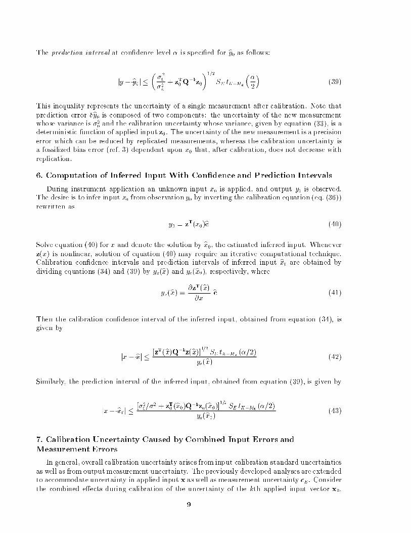
The prediction interval at con�dence level � is speci�ed for by0 as follows:
jy � by0 j ���20
�2E
+ zT0 Q�1z0
�1=2
SE tK�Mz
��
2
�(39)
This inequality represents the uncertainty of a single measurement after calibration. Note thatprediction error �by0 is composed of two components: the uncertainty of the new measurementwhose variance is �2
0 and the calibration uncertainty whose variance, given by equation (33), is adeterministic function of applied input z0. The uncertainty of the newmeasurement is a precisionerror which can be reduced by replicated measurements, whereas the calibration uncertainty isa fossilized bias error (ref. 3) dependent upon x0 that, after calibration, does not decrease withreplication.
6. Computation of Inferred Input With Con�dence and Prediction Intervals
During instrument application an unknown input x0 is applied, and output y0 is observed.The desire is to infer input x0 from observationy0 by inverting the calibration equation (eq. (36))rewritten as
y0 = zT(x0)bc (40)
Solve equation (40) for x and denote the solution by bx0, the estimated inferred input. Wheneverz(x) is nonlinear, solution of equation (40) may require an iterative computational technique.Calibration con�dence intervals and prediction intervals of inferred input bx0 are obtained bydividing equations (34) and (39) by yx(bx) and yx(bx0), respectively, where
yx(bx) = @zT(bx)@x
bc (41)
Then the calibration con�dence interval of the inferred input, obtained from equation (34), isgiven by
jx � bxj � [zT(bx)Q�1z(bx)]1=2 SE tK�Mz(�=2)
yx(bx) (42)
Similarly, the prediction interval of the inferred input, obtained from equation (39), is given by
jx� bx0j �[�2
0=�2 + zT0 (bx0)Q�1z0(bx0)]
1=2SE tK�Mz
(�=2)
yx(bx0)(43)
7. Calibration Uncertainty Caused by Combined Input Errors and
Measurement Errors
In general, overall calibration uncertainty arises from input calibration standard uncertaintiesas well as from outputmeasurement uncertainty. The previously developed analyses are extendedto accommodate uncertainty in applied input x aswell as measurement uncertainty �E . Considerthe combined e�ects during calibration of the uncertainty of the kth applied input vector xk,
9

denoted by �xk, and the corresponding measurement uncertainty �Ek . The uncertainty of thekth extended input vector zk, denoted by Mz � 1 vector �zk , is obtained as
�zk = z(xk + �xk)� z(x k) (44)
Vector �zk has zero expected value and Mz �Mz covariance matrix �zkk; the uncertainties of
the elements of zk may be correlated. In addition, every pair of input vectors zi and zj maybe correlated with covariance matrix �zij
. Design matrix Z, de�ned in equation (12), then hasK �Mz uncertainty matrix �Z constructed as follows:
�Z �
266666666664
�zT1
�zT2
...
�zTK
377777777775
(45)
which has expected value 0, where 0 is a K � Mz matrix of zeros. Each element of inputuncertainty matrix �Z is assumed to be independent of measurement error vector �E de�ned inequation (14).
The observed output vector y corresponding to the actual input matrix Z+ �Z is given by
y = (Z+ �Z)c + �E (46)
and the combined output error vector, denoted by �y , is given by
�y � y � Zc = �Zc + �E (47)
which has expected value 0. The K �K covariance matrix of combined output error vector �y,denoted by �y , is computed element-by-element with the following equation (eq. (48)) for i = 1to K and j = i to K . Because �Z and �E are independent, the covariance between elements�yi and �yj of �y is obtained as
cov (�yi ; �yj) = E�cT�zi�zjc
�+ E [�i�j ]
= cT�zijc + �ij (48)
where �ij is the ijth element of measurement uncertainty covariance matrix �E .
Rewrite equation (47) to express observed output vector y in the form of equation (15) as
y = Zc + �y (49)
10

where y has expected value Zc. Least-squares estimation of coe�cient vector c proceeds asbefore, after replacing vector �v by �y and matrix �v by �Y, respectively, in equations (16)through (39). An analysis of variance for replicated calibrations of a multi-input{single-outputsensor presented in the subsequent development provides a test of signi�cance for the presenceof calibration bias error due to loading uncertainty.
8. E�ects of Process Modeling Error
Models of instrument steady-state input{output relationships are typically approximateempirical relationships such as multivariate polynomials. The e�ects of modeling error andexperimental design on calibration uncertainty are quanti�ed, based on generalized multivariatelinear regression analysis. Calibration standard uncertainty is neglected.
8.1. Uncertainty Analysis of Modeling Error
Let process f(c; z) be modeled as a linear function of an extended input vector z accordingto f(c; z) = zc, whereas the actual functional relationship is given by
y(z) = f (c; z) = zc + (z) (50)
where (z) represents the modeling error. However, the system is calibrated by using experi-mental design matrix Z based on the linear model of equation (6). During calibration the kthobservation is given by
yk = zkc + (zk)+ �Ek(51)
which is extended overK observations into matrix form as
y = Zc + (Z)+ �E (52)
where (Z) is the K � 1 vector of modeling errors. Coe�cient vector bc is estimated by meansof equation (23); the expected value of bc, biased by the modeling error, is given by
E(bc) = c +Q�1ZTU�1 (Z) (53)
Predicted calibration output vector by is obtained by using equation (32). Then the expectedvalue of by is given by
E(by) = Zc + ZQ�1ZTU�1
(Z) (54)
where the second term represents the predicted output bias error due to modeling error. Residualvector bev, de�ned in equation (25), is found to be
bev =WK[P�1 (Z) + �v] (55)
11

and from this the expected value of bev is
E [bev] = WKP�1 (Z) (56)
The covariance matrix of bev is given by
�ev= �2
EWK (57)
The expected value of weighted error sum of squares SSE given in equation (29) equals thefollowing:
E [SSE ] = (K �MZ)�2E +
T(Z)P�TWKP
�1 (Z) (58)
It is seen that SE, given in equation (30), becomes a biased estimate of � whenever modelingerror (Z) is nonzero.
The variance function (ref. 8) of predicted output by is computed by using the above resultsas is now shown. For arbitrary vector z, the predicted output is given by equation (32).The corresponding actual output function value y without measurement uncertainty, shownin equation (50), is given by
y(z) = zc + (z) (59)
The corresponding predicted output error �by is then
�by(z) = y(z)� by(z)
= (z) � zQ�1ZTU�1[ (Z) + �E] (60)
To �nd the variance function of by, take the expected value of the square of equation (60) andafter some algebraic manipulation, the following result is obtained:
�2y(z) = �2
EzTQ�1z+ [ (z)� zQ�1
ZTU�1 (Z)]2 (61)
The �rst right-hand term of equation (61), identical to the predicted output variance functionof the model previously given in equation (33), represents the portion of the bias uncertainty ofthe predicted output due to calibration measurement uncertainty. The second right-hand termof equation (61) represents the portion of the bias uncertainty of the predicted output due tomodeling error.
8.2. Design Figure of Merit
Design �gure of merit J de�ned in equation (11) is obtained by integrating equation (61) overinput subspace =. It allows examination of the e�ects of the experimental design on predictedoutput error due to precision uncertainty and bias uncertainty. As in reference 8, �gure of meritJ is separated into variance error term V and bias error term B:
12

J = V + B (62)
The precision uncertainty portion of J obtained from the �rst right-hand term of equation (61)equals
V =K
Z=
zTQ�1z dx (63)
Similarly, the bias uncertainty portion of J obtained from the second right-hand term ofequation (61) equals
B =K
�2E
Z=
[ (z) � zQ�1ZT (Z)]2 dx (64)
where is the volume integral of subspace = given by
=
Z=
dx (65)
8.3. E�ects of Experimental Design on Figure of Merit
The e�ects of the experimental design on calibration uncertainty due to measurementuncertainty and on calibration error due to modeling error are quanti�ed by means of �gure ofmerit J . Simultaneous minimization of V and B imposes con icting requirements on selectionof experimental design D. Equation (63) indicates that precision uncertainty V tends to decreaseas the vector length magni�cation of matrix Q increases. The vector length magni�cation ofQ tends to increase as the distance of the design points from the origin increases, generally tothe boundary of volume =. On the other hand, reference 8 demonstrates that bias uncertaintyB tends to be minimized by uniform placement of test points throughout space =. Hence, theaccepted practice of uniformly spacing test points from zero input, to full scale input, and backto zero can reduce calibration uncertainty caused by improperly modeled phenomena such asnonlinearity and hysteresis.
A number of well-known methods exist for detection of modeling errors. Examination ofresidual error plots often discloses the presence of systematic errors in addition to randommeasurement errors (refs. 7 and 10). Residual normal probability plots (ref. 10) indicate thepresence of nonnormally distributed errors which are likely to be systematic. The process ofdetecting modeling error may indicate the functional extension required for model improvement.On the other hand, polynomial models should be limited to the minimum order needed to avoid�tting data to random noise (ref. 10).
9. Uncertainty Analysis of Nonlinear Instrument Calibration
The previously developed generalized linear regression analysis of instrument calibration,with calibration standard uncertainty, is extended to include general multivariable-input{single-output nonlinear processes.
9.1. Combined Input and Measurement Uncertainties
Consider a process modeled by nonlinear function y = f(c ; z) de�ned in equation (2). Outputuncertainty �y can be approximated as the sum of the di�erential of f(c; z) with respect to z
and measurement uncertainty �E as follows:
13

�y = f(c; z + �z)� f (c; z)+ �E =
�@f(c; z)
@z
��z + �E (66)
During calibration, K observations are acquired in accordance with K � Mz design matrix Zde�ned in equation (12). The uncertainty �yk of the kth observation yk is given by
�yk =
�@f(c; zk)
@z
��zk + �Ek = fz(c; zk)�zk + �Ek
(67)
where 1 �K gradient vector fz(c ; zk) � [@f(c; zk)=@z]. Note that �yk is normally distributed ifboth �zk and �Ek
are normally distributed. The actual value of the kth observation is given by
yk = f (c ; zk)+ �yk (68)
Let f (c;Z) denote the K � 1 vector function which is obtained by evaluating function f(c; z) foreach of the K rows of Z. Also, let y and �y denote the corresponding K � 1 vectors of observedoutputs and output uncertainties obtained by evaluating equations (67) and (68) for k = 1 toK ,respectively. Then y is given by
y = f(c;Z)+ �y (69)
The K � K covariance matrix of �y , denoted by �Y , is obtained element by element withequation (67) as follows:
�Yi j= fz(c; zi )�zi j
fTz (c; zj)+ �ij (70)
where �zijis the covariance matrix of the ith and jth input vectors zi and zj, �ij is the covariance
of the ith and jth voltage measurements, and i and j range from 1 to K . If �Y is symmetricand positive de�nite, then it can be expressed in the form of equation (16) as
�Y = �2Y U (71)
where K �K matrixU is known and can be decomposed into the productU = PPT as shown inequation (17). Output vector y is transformed into vector v by equation (18), that is, v = P�1y.Equation (69) then becomes
v = P�1f(c;Z)+ �v (72)
where �v = P�1�y . The expected value of v is
E [v] = P�1f(c; Z) (73)
The covariance matrix of �v is given by
14

�v = �2Y I (74)
Therefore the elements of �v are uncorrelated and �v is normally distributed whenever �y isnormally distributed.
9.2. Least-Squares Estimation of Process Parameters
The least-squares estimate of parameter vector c, denoted by bc, is obtained by minimizingthe error sum of squares SSQ, given by the following quadratic form, with respect to c :
SSQ = [v� P�1f (c ;Z)]T [v� P�1f (c; Z)] = [y � f (c;Z)]TU�1[y � f (c;Z)] (75)
To minimize SSQ , compute the gradient of equation (75) with respect to c and set the resultingset of Mc equations equal to zero and expressed in vector form as
h �1
2
@SSQ
@c= [v� P�1f (c;Z)]TP�1Fc = 0 (76)
where h is a function of independent arguments v, c, and Z; the dimension of h is 1 �Mc andof vector [v� P
�1f(c; Z)] is K � 1; and K � Mc matrix Fc is de�ned as
Fc(c ;Z) �@f(c; Z)
@c(77)
Equation (76) can be solved for bc by means of a Newton-Raphson iteration or a similar method,provided that the symmetric Mc �Mc Jacobian matrix of SSQ with respect to c, denoted by R,is nonsingular in some region about bc and Z; that is
R �
@ 2SSQ
@c2=@h
@c(78)
9.3. Uncertainty of Estimated Process Parameters
The uncertainty �bc of stochastic vector bc is obtained in terms of combined output uncertainty�v from the di�erential of equation (76) as follows:
�@h
@v
�T�v+R�bc = 0 (79)
where K �Mc matrix [@h=@v] equals
�@h
@v
�= P�TFc (80)
Matrix R is shown in the appendix to be
R =
�@h
@c
�= FT
cU�1Fc +HE (81)
15

where the ijth element of Mc �Mc matrix HE is given by
hEij= [v �P
�1f (c; Z)]TP�1fcci j (82)
where K � 1 vector fccij is the ijth column of Mc �Mc �K array Fcc de�ned by
Fcc =@FT
c (c;Z)
@c=
@2f(c; Z)
@c2(83)
and 1 � i; j � Mc. It is seen that the K � 1 vector expression [v �P�1f(bc;Z)] contained inequation (82) equals the vector of residuals denoted by bev . Then if the norm of bev is su�cientlysmall , matrix HE can be neglected in equation (81) to yield the following approximation:
R � FTc U
�1Fc (84)
From equations (77) to (80), the uncertainty of estimated parameter vector bc equals
�bc = �
�@h
@c
��1 �@h
@v
�T�v = �R�1FT
c P�T�v (85)
From equation (85), calibration parameter uncertainty �bc has zero mean, it is normallydistributed whenever �y is normally distributed, and its covariance matrix is given by
�c = �2Y Q
�1c (86)
where
Qc ��R�1FT
cU�1FcR
�1��1
(87)
If approximation (84) holds and if the rank of K �Mc matrix Fc equals Mc , then matrix R isnonsingular and matrix Qc is approximated by
Qc � R (88)
9.4. Residual Sum of Squares and Standard Error of Regression
Let bv denote the predicted calibration output vector corresponding to design matrix Z andestimated parameter vector bc, where
bv � P�1f(bc; Z) (89)
The vector of residuals bev is de�ned as follows:
bev � v � bv =P�1[f(c; Z) � f(bc; Z)] + �v (90)
16

which is represented in di�erential form as
bev �P�1Fc(bc ;Z)�bc + �v = (IK �F)�v (91)
where K �K matrix F is
F � (P�1Fc)R�1(P�1Fc)
T (92)
The expected value of bev equals zero, and the covariance matrix is given by
�ev= �2
Y (IK �F) (93)
An unbiased estimate of �2Y is now obtained. The residual sum of squares is de�ned as
SSE � beTvbev = �vT(IK �F)�v (94)
As shown in the appendix, SSE=�2Y is chi-square distributed with K � Mc degrees of freedom,
and the expected value of S SE is
E (SSE) = (K � Mc)�2Y (95)
Therefore an unbiased estimate of �Y is given by standard error S Y , which is de�ned as
SY �
�SSE
K �Mc
�1=2
(96)
A con�dence interval for �Y at con�dence level � is given by
(K �Mc)1=2SY
�(1+�)=2
� �Y �(K �Mc)1=2SY
�(1��)=2
(97)
where �� is the �-percentile value of the chi-square distribution with K�Mc degrees of freedom.
9.5. Con�dence and Prediction Intervals of Predicted Output
The con�dence ellipsoid for estimated calibration parameter vector bc is de�ned by thefollowing inequality:
(c � bc)TQC(c � bc) � McS2Y FMc ;K�Mc(�) (98)
where FMc ;K�Mc(�) is the �-percentile value of the F-distribution with Mc ; K � Mc degrees offreedom.
After calibration, consider z0 as an arbitrary deterministic input. The correspondingpredicted value by0 = f(bc; z0) is computed by using calibration parameter vector bc. The
17
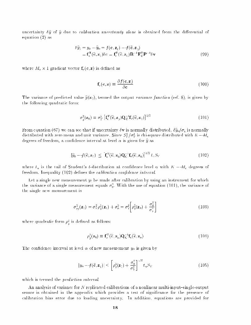
uncertainty �by of by due to calibration uncertainty alone is obtained from the di�erential ofequation (2) as
�by0 = y0 �by0 = f(c; z0) � f(bc; z0)
= f Tc (bc; z0)�c = fTc (bc; z0)R�1FTCP�1�v (99)
where Mc � 1 gradient vector fc(c; z) is de�ned as
fc(c; z) �@f(c;z)
@c(100)
The variance of predicted value by(z0), termed the output variance function (ref. 8), is given bythe following quadratic form:
�2y(z0) = �2
Y
�fTc (bc; z0)Q�1
C fc(bc; z0)�1=2
(101)
From equation (67) we can see that if uncertainty �v is normally distributed, �by0=�y is normallydistributed with zero mean andunit variance. Since S2
Y =�2Y is chi-square distributed with K�Mc
degrees of freedom, a con�dence interval at level � is given for by as
jby0 � f(bc; z0)j � �f Tc (bc; z0)Q� 1
C fc(bc ; z0)�1=2 t�SY (102)
where t� is the tail of Student's t-distribution at con�dence level � with K � Mc degrees offreedom. Inequality (102) de�nes the calibration con�dence interval.
Let a single new measurement y0 be made after calibration by using an instrument for whichthe variance of a single measurement equals �2
0. With the use of equation (101), the variance ofthe single new measurement is
�2y0(z0) = �2
Y �2y(z0) + �2
0 = �2Y
��2y(z0) +
�20
�2Y
�(103)
where quadratic form �2yis de�ned as follows:
�2y(z0) � f Tc (bc ; z0)Q�1
C fc(bc; z0) (104)
The con�dence interval at level � of new measurement y0 is given by
jy0 � f(bc; z0)j �
��2y(z0) +
�20
�2Y
�1=2t�SY (105)
which is termed the prediction interval.
An analysis of variance forN replicated calibrations of a nonlinear multi-input{single-outputsensor is obtained in the appendix which provides a test of signi�cance for the presence ofcalibration bias error due to loading uncertainty. In addition, equations are provided for
18

computation of matrix R, given by equation (81), in terms of the K �K covariance matrices ofa single replication.
10. Multivariate Multiple-Output Analysis
The preceding analysis is now extended to a multi-input{multi-output instrument such as asix-component strain-gauge balance. Although the notation becomes cumbersome, the extendedcomputational procedure simply iterates the previous multi-input{single-output technique foreach process output element.
Consider an L-valued process g represented by a 1 � L row vector of scalar functions of anMc�1 parameter vector c: j and z, each of the form ofmapping equation (1). Let gj (c.j ; z) denotethe jth function, where j ranges from 1 to L , where gj is dependent upon the correspondingMc � 1 parameter vector c.j and 1 �Mz input vector z which is common over all values of j.Arrange the coe�cient vectors L into Mc � L coe�cient matrix C as
C =hc.1 c.2 . .. c.L
i(106)
As usual, K observations are made during calibration in accordance with design matrix Z. Forthe kth observation let g, yk., and �vk. denote 1 � L vectors of functions gj , observed outputs,and measurement errors, respectively, where
g(C; zk) = [g1(c.1; zk) g2(c.2 ; zk) : : : gL(c.L; zk)] (107)
yk. = [yk;1 yk;2 : : : yk ;L ] (108)
�vk. = [�vk; 1 �vk;2 : : : �vk ;L ] (109)
respectively, where �vk. has zero mean and zTk denotes the corresponding 1 � Mz input vectorde�ned in equation (12) as the kth row of design matrix Z. Then the functional relationship forthe kth observation is obtained by extension of equation (2) to L space as follows:
yk. = g(C; zk+�zk) + �vk.
= g(C; zk)+ �yk. (110)
where uncertainty �yk. is given by
�yk. = g(C; zk+�z)� g(C; z
k)+ �vk.
= �zTk
�@g(C; z
k)
@z
�+ �vk. (111)
19

Note that matrix [@g(C; zz)=@z] has dimensionMz �L . Vector equation (110) is then extendedto a K � L matrix equation as shown by the following equations:
Y =G(C; Z+�Z) + EV
=G(C; Z) + �Y (112)
G(C;Z) =
266666666664
g(C; z1)
g(C; z2)
...
g(C; zK )
377777777775
(113)
Y =
266666664
y1.
y2.
...
yK.
377777775
(114)
Ev =
266666664
�v1.
�v2.
...
�vK.
377777775= [�v.1; �v.2 ; �v.L ] (115)
Note thatK � 1 vectors �v.1 , .. ., �v.L denote columns 1, . .., L of matrix Ev. Also K � L matrix�Y is obtained by extension of equation (111) as
�Y =
266666664
�y1.
�y2.
...
�yK .
377777775+ Ev (116)
Let �Vm;m denote the K�K covariance matrix of error vector �V.m, and�Ym;m denote the K�Kcovariance matrix of column m of matrix �Y, which is computed element by element by usingequation (48) withm ranging from 1 to L and f replaced by gm. Furthermore, de�ne SSQm as inequation (75) with f replaced by gm for each of the L elements of g. The least-squares estimated
coe�cient matrix, denoted by bC, is computed column by column by solving equation (76) to
20

minimize SSQm for m = 1, ... , L, with bc.m the mth column of bC. The covariance matrix andcon�dence ell ipsoid for bc.m are computed as before with equations (86) and (98), respectively.
After calibration, the predicted output matrix by for arbitrary input z using estimatedcoe�cient matrix bC is given by by = g(bC; z). The uncertainty �by due to calibration uncertaintyalone equals
�by = g(C; z)� bg(C ; z) (117)
The calibration con�dence interval for �by is obtained element by element by equation (102).Similarly, the prediction interval of a new measurement is obtained element by element byequation (105). This analysis is illustrated by an example of a two-input{two-output linearprocess given in the subsequent development.
11. Uncertainties of Inferred Inputs From Inverse Process Function
An instrument is normally employed to infer the value of an input x based on the corre-sponding observed output y by means of the process model f(c; z) for the single output case, org(C; z) for the L-dimensional case, following calibration. Calibration con�dence intervals andprediction intervals of the estimated process input are obtained.
Let g denote both cases in the following discussion. Input z can be computed if inversefunction g�1 exists. A necessary and su�cient condition for the existence of g�1 is that functiong be bijective, that is, a one-to-one onto mapping from <Mz to <L . If Mz = L, g is continuousand di�erentiable and if for observed output vector y0, an input vector z0 exists such thaty0 = g(C; z
0), then a necessary condition (ref. 11) for the existence of the inverse function g�1
is that L � L matrix @g=@z be nonsingular in a region about z0. Indeed, the inverse functionmay be obtained by solving the following system of ordinary di�erential equations obtained fromequation (111):
dzT = dy
�@g(C; z)
@z
��1
(118)
Whenever a closed-form inverse function is unavailable, given observed output y0, the corre-sponding predicted input value bz0 is computed iteratively from the relation y0 = g(C; bz0) bymeans of Newton-Raphson iteration or a similar method.
If input z0 were known, the uncertainty �by of the corresponding predicted output would begiven by equation (117). However, since predicted input z0 is inferred from known output y0,the uncertainty �by0 is obtained from equation (118) as
�bzT0 = �by0
�@g(C;bz0)
@z
��1
(119)
where @g=@z must be nonsingular and �by0 is estimated by equation (117) with z0 replaced bybz0. Con�dence and prediction intervals for bz0 are then obtained from those computed for by0
with equations (102) and (105) followed by transformation (eq. (119)).
12. Replicated Calibration
A statistical technique for detection and estimation of bias errors due to either modelingerror or calibration standard error is now developed, which requires multiple replications of
21

the calibration experiment. The use of replicated calibrations over an extended time period isimportant for the following reasons:
1. To obtain adequate statistical sampling over time
2. To test for nonstationarity and drift
3. To test for bias uncertainty
4. To estimate bias and precision uncertainties
The variance of averaged random errors is known to decrease as 1=N over N replications,whereas that of bias errors, which are repeatable, does not decrease with replication. Tests forthe existence of signi�cant bias uncertainty by analysis of variance are based on this fact. Thebias test, derived for a general multivariate nonlinear process in the appendix, computes thesum of squares SSX of the set of K residuals averaged over N replications. The mean value ofSSX is an estimate of the variance due to bias uncertainty. The mean value, denoted by SM, ofthe di�erence SSM between the sum of squares SSE of the global set of NK residuals and SSX isan estimate of the variance due to measurement error. The variance ratio NSX=SM provides atest of signi�cance for the presence of bias errors. A similar analysis allows detection of drift ofany estimated parameter during replication. Details are given in the appendix.
12.1. Computation of Replicated Design Matrix
A replication matrix is de�ned which provides convenient computational notation for repli -cated calibration experimental designs. Consider a single-output sensor modeled by an (Mz�1)thdegree polynomial. The sensor is typically calibrated by using K standard loadings applied ina prede�ned order, say zero to full scale and back in (K � 1) equal increments, represented byK � Mz experimental design matrix ZK . The calibration is replicated N times, described byNK �Mz design matrix ZNK, where
ZNK =
266666664
ZK
ZK
...
ZK
377777775=HTZK (120)
and where K � NK replication matrix H equals
H � [ IK IK : : : IK ] (121)
12.2. Replicated Moment Matrix for Linear Single-Output Process
Moment matrix Q is computed for a replicated experimental design for calibration of alinear single-output instrument with uncorrelated measurement uncertainties. Use of replicationmatrix H permits computation of Q in terms of the single-replication K � Mz experimentaldesign matrix ZK. Assume that the calibration standard uncertainties are �xed unknown biaserrors modeled as a zero-mean normally distributed random variable and that design matrix ZKhas K �K covariance matrix �2IK . Because complete design ZNK contains N replications ofdesign ZK , the N subsets of K loadings are correlated with the NK � NK covariance matrix�z of design ZNK given by
22

�z = �2xH
TH = �2
x
266666664
IK IK : : : IK
IK IK : : : IK
...... : : :
...
IK IK : : : IK
377777775
(122)
Assume also that sensor output measurements are uncorrelated with covariance matrix
�E = �2E
266666664
IK 0K : : : 0K
0K IK : : : 0K
...... : : :
...
0K 0K : : : IK
377777775= �2
EINK (123)
Then combined input covariance
�Y = �2xUNK
where
UNK = INK + �HTH =
266666664
(�+ 1)IK IK : : : IK
IK (�+ 1)IK : : : IK
...... : : :
...
IK IK : : : (� + 1)IK
377777775
(124)
and
� =�2x
�2E
(125)
It is readily shown that
U�1NK
= INK � �HTH = �
266666664
(1� �)=�IK �IK : : : �IK
�IK (1 � �)=�IK : : : �IK
...... : : :
...
�IK �IK : : : (1� �)=�IK
377777775
(126)
23

where
� =�
N� + 1(127)
As shown in the appendix, the Mz � Mz generalized moment matrix QNK = ZTNKU
�1NKZNK is
given by
QNK =�2E
(�2E=N)+ �2
x
ZTKZK (128)
The portion of the calibration uncertainty due to calibration standard uncertainty, repre-sented by �2
x in the denominator of equation (128), does not decrease with replication. On theother hand, the portion of the calibration uncertainty due to measurement uncertainty, repre-sented by �2
E in the denominator of equation (128), decreases asN�1=2 with replication. Note thatequation (128) permits more e�cient computation of uncertainties for an NK �Mz replicatedexperimental design in terms of nonreplicated K �Mz design matrix ZK because computationalstorage requirements are reduced by a factor of N .
12.3. Replicated Moment Matrix for General Single-Output Process
The technique developed in the previous section for computation of moment matrix Q for areplicated experimental design is extended to a general nonlinear single-output instrument withcorrelated measurement uncertainties. Consider a general multi-input{single-output processcalibrated by using experimental design ZK replicated N times. The K � 1 output uncertaintyvector of a single replication, denoted by �yK , is given by expanding equation (67) fork = 1; : : : ; K . Then for N replications, NK � 1 output uncertainty vector �yNK is given by
�yNK = HT�fz + �E (129)
where K � 1 gradient vector �fz, de�ned in the appendix, has K � K covariance matrix�fZK
= �2xUfZK
and NK � 1 measurement uncertainty vector �E has NK � NK covariancematrix �E = �2
EUENK , all de�ned in the appendix. The measurement uncertainty is assumeduncorrelated between replications and the K � K measurement covariance matrix of eachreplication is assumed to be �EK
= �2EUEK
. From equation (129),
�YNK = �E +�fZNK = �2EUENK + �2
xUfZNK = �2EUYNK (130)
where NK �NK covariance matrix �fZNKis given by
�fZNK= �2
xUfZNK= �2
xHTUfZK
H (131)
From equation (131), UYNKcan be written as
UYNK= UENK
+ �UfZNK(132)
where � is de�ned in equation (125).
24

As shown in the appendix, the inverse ofNK �NK matrix UYNKcan be expressed in terms
of K �K matrices UfZKandUEK
. De�ne K �K matrix B as
B ��UEK + (N � 1)�UfZK
��1UfZK (133)
and K � K matrix A as
A =�UEK
+ �UfZK[IK � (N � 1)B]
��1
(134)
If the inverse matrices contained in equations (133) and (134) exist, then Mz � Mz momentmatrix QNK = ZTNKU
�1YNK
ZNK, de�ned in terms of NK � Mz matrix ZNK , and NK � NK
matrix UYNK , can be computed in terms of K �Mz matrix ZK and K �K matrices IK , B, andA as
QNK = NZTK[IK � (N � 1)B]AZK (135)
12.4. Analysis of Variance for Estimation of Bias and Precision Uncertainties
A test of signi�cance for bias uncertainty due to calibration standard error or modelingerror and an estimate of the corresponding standard error are obtained by analysis of variancetechniques, as shown in detail in the appendix. Assume as null hypothesis that the calibrationbias error is zero; then matrix UNK equals INK in equation (124). By using equation (27),NK �NK matrix NK becomes
NK = ZNKQ�1NKZ
TNK =
1
NHTKH (136)
where the K �K matrix K is de�ned as
K � ZK(ZTKZK)
�1ZTK (137)
The NK� 1 residual vector be has zero expected value andNK�NK covariance matrix �2WNK,given in equation (26) as
WNK = INK �NK (138)
As shown in the appendix, the residual vector be can be expressed as
be = WNK�E (139)
where NK � 1 error vector �E is normally distributed with covariance matrix �2INK. Let b�ndenote the K � 1 residual vector at the nth replication, which has zero expected value andcovariance matrix �2WK , given in equation (26) as
WK = IK �K (140)
25

Thus, be is partitioned into N; (K � 1) subvectors
beT =�beT1 beT2 : : : beTN �T (141)
Let �eK denote the mean value of residual vector ben averaged overN replications; that is,
�eK =1
N
NXn=1
ben =1
NHbe =
1
NHWNK�E (142)
The total residual sum of squares can be partitioned as follows:
SSE � beTbe =
NXn=1
beTnben =N �eTK�eK +
NXn=1
(ben � �eK)T(ben � �eK) (143)
As shown previously, SSE=�2 is chi-square distributed with NK �Mz degrees of freedom, and
the standard error of the regression given by
SE =
�SSE
NK �Mz
�1=2
(144)
is an unbiased estimate of �. De�ne the �rst right-hand term of equation (143) as the sum ofsquares due to bias uncertainty, which can be expressed as
SSX � N
KXk=1
�e2k =N�eTK�eK =
1
N�T
EWNKGHWNK�E (145)
where GH � (1=N)HTH is de�ned in the appendix and �ek is the kth element of �eK. It canbe shown that S SX=�
2 is chi-square distributed with K �Mz degrees of freedom. Variable SX ,de�ned as
SX �
�SSX
K �Mz
�1=2
(146)
is interpreted as the standard error due to bias uncertainty. De�ne the second right-hand termof equation (143) as the sum of squares due to measurement uncertainty as follows:
S SM �
NXn=1
(ben � �eK)T(ben � �eK) = �T
EWNK(INK �GH)WNK�E (147)
It can be shown that SSM=�2 is chi-square distributed with NK �K degrees of freedom; the
mean value
26

SM =
�SSM
NK �K
�1=2
(148)
is interpreted as the standard error due to measurement uncertainty. Chi-square variates S2X =�
2E
and S2M=�
2E can be shown to be independent. Hence, the ratio S 2
X =S2M is F -distributed with
K �Mz, NK �K degrees of freedom; the test of signi�cance for bias error is as follows:
F �S2X
S2M
> FK�Mz ;NK�K(�) (149)
If inequality (149) is satis�ed, then the null hypothesis is rejected; this indicates the existenceof bias error at con�dence level �. The analysis of variance is summarized in table 1.
Table 1. Analysis of Variance of Residual Sum of Squares
Source of variation Degrees of freedom Sum of squares Root-mean-square
Bias uncertainty K �Mz SSX SX
Measurement uncertainty NK �K SSM SM
Residual sum of squares NK �Mz SSE = SSX + SSM SE
12.5. Stationarity Test of Estimated Parameters
A test for stationarity of an element bcm contained in estimated parameter vector bc over Nreplicated calibrations is developed in the appendix. For example, signi�cant variation of theintercept or slope during replicated calibrations may be detected.
Let bc denote the parameter vector estimated globally overN sets ofK-point calibrations. LetbcRn denote the parameter vector estimated over the K -point data set obtained during the nthreplication and SSRn equal the corresponding residual sum of squares for n = 1; : : : ; N . De�ne
SSR =NXn=1
SSRn (150)
It is shown that SSR/�2E is chi-square distributed with N(K �Mz) degrees of freedom.
To test for stationarity of parameter cm, replace the mth element of bcRn by bcm 2 bc, andcompute the resulting error sum of squares, denoted by SSGm;n , for n = 1; : : : ; N . Compute thesum
SSGm =NXn=1
SSGm;n (151)
It is shown that (SSGm � SSR)=�2 is chi-square distributed with N � 1 degrees of freedom.Therefore, the ratio [(SSGm � SSR)=(N � 1)]=fSSR=[N(K �Mz)]g is F-distributed with N � 1,
27

N(K �Mz) degrees of freedom. The test of signi�cance for nonstationarity of parameter bcm isthen as follows:
Tcm =(SSGm � SSR)=(N � 1)
SSR=[N(K �Mz)]> FN�1;N (K�Mz)(�) (152)
13. Examples
13.1. Calibration of Single-Input{Single-Output Nonlinear Sensor
Consider an inertial angle-of-attack sensor which senses the projection of the gravitationalforce onto the aircraft model axis. At zero roll , the angle of attack sensor is accurately modeledby the following equation:
� = f (c; �) = S sin (� � �) + b (153)
where the scalar �, the angle of attack in radians, is the independent variable z; the 3 � 1parameter vector is given by c = [b S �]T, where b = O�set in V , S = Sensitivity in V=g,� = Misalignment angle in radians, and � is the sensor output in V . For this example inputvector z equals applied angle � and �z denotes the uncertainty of � during calibration.
Calibrationdesignmatrix Z has dimensionK�1. Equation (153) is extended toK dimensionsas follows:
� = f (c ;Z) = S sin (z � �1)+ b1 (154)
where � denotes the K � 1 angle of attack sensor output vector, z denotes the single columnof design matrix Z, sin denotes the K � 1 vector obtained following element-by-element sinefunction evaluation of the elements of (z � �1), and 1 denotes a K � 1 vector of ones.
Let �z denote the calibration angle uncertainty, and let �E denote the uncertainty of thesensor voltage measurement with variance �2
E . Then the observed output y is given by
y = f(c; �+ �z) + �E = S sin (� + �z � �)+ b+ �E (155)
Output uncertainty �y is obtained with equations (66) and (153)
�y = S cos (z � �)�z + �E (156)
Equation (156) is extended to K dimensions as follows:
�y = S cos (z � �1) � �z + �E (157)
where cos denotes the K � 1 vector obtained following element-by-element cosine function eval-uation of the vector z� �1, � denotes element-by-element multiplication of equally dimensionedmatrices, and �y, �z, and �E denote K � 1 vectors of uncertainties �� , ��, and �E , respectively.
28

The observed calibration output vector, including measurement uncertainty and calibration in-put uncertainty, is thus extended toK dimensions with the use of equation (153) to the followingequation:
y = � + �y = S sin (z� �1)+ b1+ �y (158)
It can be shown that the K �K covariance matrix of y is given by
�Y = cov (�y) = S2[cos (z � �1) cos (z� �1)T ] � �Z +�E (159)
where �Z and �E are the covariance matrices of �z and �E, respectively. It is seen that �Y andU given by equation (71) are symmetric and positive de�nite.
The least-squares estimate of parameter vector c is obtained by minimization of the followingquadratic form given in equation (75):
SSQ = [y � b1 � S sin (z � �1)]TU�1Y [y � b1 � S sin (z � �1)] (160)
The K � 3 Jacobian matrix of f(c; Z) is found to be the following:
Fc(c; z) = [1 sin (z � �1) � S cos (z � �1)] (161)
The least-squares estimated coe�cient vector bc is obtained by solving the following 1� 3 systemof nonlinear equations:
h(c ;Z) = [y � b1 � S sin (z � �1)]TU�1[Fc(c; Z)]
= e(c ;Z)TU�1[Fc(c;Z)] = 0 (162)
where e(c; Z) = [y � b1 � S sin (z � �1)]. The standard error of the regression is given by
SY =
([y �bb1 � bS sin (z � b�1)]TU�1[y �bb1 � bS sin (z � b�1)]
K � 3
)1=2
(163)
which provides an unbiased estimate of �E .
From equation (161), equation (162) may be partitioned as follows:
h(c; Z) = [eT(c; Z)U�11 eT(c;Z)U�1
sin (z� �1) �SeT(c;Z)U�1cos (z � �1)] (164)
Then matrix R = [@h(c;Z)=@c], given in equation (81), is found to be
R = FTc (c ;Z)U
�1Fc(c ;Z) +HE (165)
29
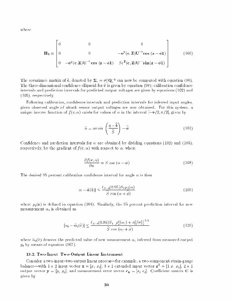
where
HE =
26666640 0 0
0 0 �eT(c;Z)U�1cos (z � �1)
0 �eT(c;Z)U�1cos (z � �1) SeT(c ;Z)U�1
sin(z � �1)
3777775 (166)
The covariance matrix of bc, denoted by �c = �2YQ
�1c can now be computed with equation (86).
The three-dimensional con�dence ell ipsoid for bc is given by equation (98); calibration con�denceintervals and prediction intervals for predicted output voltages are given by equations (102) and(105), respectively.
Following calibration, con�dence intervals and prediction intervals for inferred input angles,given observed angle of attack sensor output voltages are now obtained. For this system, aunique inverse function of f(c; �) exists for values of � in the interval [��=2; �=2], given by
b� = arcsin
� �bbbS
!� b� (167)
Con�dence and prediction intervals for � are obtained by dividing equations (102) and (105),respectively, by the gradient of f (c ; �) with respect to �, where
@f(c; �)
@�= S cos (�� �) (168)
The desired 95 percent calibration con�dence interval for angle � is then
j� � b�(bc)j � tK�3(0:95)SY�y(�)bS cos (� + b�) (169)
where �y(z) is de�ned in equation (104). Similarly, the 95 percent prediction interval for newmeasurement �0 is obtained as
j�0 � b�0(bc)j � tK�3(0:95)SY
��2y(�0) + �2
0=�2Y
�1=2bS cos (�0 + b�) (170)
where b�0(bc) denotes the predicted value of new measurement �0 inferred from measured outputy0 by means of equation (167).
13.2. Two-Input{Two-Output Linear Instrument
Consider a two-input{two-output linear process|for example, a two-component strain-gaugebalance|with 1� 2 input vector x = [x1 x2] , 3 � 1 extended input vector zT = [1 x1 x2], 2� 1output vector y = [y1 y2], and measurement error vector �E = [�1 �2] . Coe�cient matrix C isgiven by
30

C = [c.1 c.2] =
2664c01 c02
c11 c12
c21 c22
3775 (171)
where c.n = [c0n c1n c2n]T for n = 1; 2.
For a single observation, the output is given by y = zTC + �E. During calibration, K
calibration input vectors are applied, represented by the following K � 3 design matrix Z:
Z =
26666664
1 x11 x12
1 x21 x22
......
...
1 xK1 xK2
37777775
(172)
Measurement uncertainty is represented by K � 2 measurement error matrix EE, where
EE = [�E.1�E.2] =
26666664
�11 �12
�21 �22
......
�K 1 �K2
37777775
(173)
The K�K covariance matrix for error vectors �E.m and �E.n, form and n= 1 and 2, respectively,is denoted by �Emn
.
For K calibration measurements, the K �N output matrix Y is given by
Y = (Z+ �Z)C + EE (174)
where K �Mz input error matrix �Z is given by
�Z = [0 �x.1�x.2] =
2666664
0 �x11 �x12
0 �x21 �x22
......
...
0 �xK1 �xK2
3777775
(175)
The 2 � 2 covariance matrix of input error vectors �x.i and �x.j is denoted by �xij.
�x ij=
24 �Xij;11 �Xij;12
�Xij;12 �Xij;22
35 (176)
31

Let input vector x be random with zero-mean uncertainty �x = [�x1 �x2 ] . Then extended inputvector zT has uncertainty �
Tz = [0 �x1
�x2]; K � 3 design matrix Z has uncertainty matrix EZ,
whose rows �Zi and �Zj have 3 � 3 covariance matrix �Zij , where
�Zij= E
h�Zi
�TZj
i26640 0 00 �Xij;11
�Xij;12
0 �Xij;12�Xij;22
3775 (177)
Consider process outputs y1 and y2 separately; subscripts are omitted in the following computa-tions. The total error vector �Y , expressed as �Y = EZc + �E , expands into
�Y =
266666664
�x11c1 + �x12c2 + �1
�x21c1 + �x22c2 + �2
...
�xK1c1 + �xK2
c2 + �K
377777775(178)
The covariance between elements �yi and �yj of total error vector �y is given by
cov (�yi ; �yj) = cT�Zij c + �ij = c21�Xij;11+ c1c2�Xij;12
+ c22�Xij;22+ �ij (179)
The con�dence interval at level 1� � for estimated coe�cient vector bc is expressed as a three-dimensional ell ipsoid as
(c � bc)TQ(c � bc) � 3S2F3;K�3(�) (180)
The ellipsoid can be characterized as follows: Since Q is symmetric, it is unitarily similar to areal diagonal matrix �; in particular Q = PT�P, where � consists of the eigenvalues of Q andP is unitary; that is, PPT = I . Matrix P consists of the set of orthonormal eigenvectors of Q.Apply the transformation =Pc to coe�cient vector c. The con�dence ellipsoid then simpli�esto the form
T� = �1( 1 � b 1)
2 + �2( 2 � b 2)2 + �3( 3 � b 3)2 � 3S2F3;K�3(�) (181)
Let � denote the ith eigenvalue of Q . It is readily seen that the ith vertex of the ellipsoid islocated at distance
di =
s3S2F3;K�3(�)
�i
(182)
from point bc in the direction of the corresponding eigenvector, that is, the ith column of P.
32

The uncertainty of the regression function, which is dependent upon extended input vectorz, is expressed by the calibration con�dence interval at level of inequality (34):
jy � by j � (zTQ�1z)1=2StK�3(�)
� (�11 + 2�12x1 + 2�13x2 + �22x21 + 2�23x1x2 + �33x
22)
1=2StK�3(�) (183)
where �ij is the ijth element of Q�1.
After calibration, apply input z0 andmake a single new measurement, where the measurementuncertainty is �0. The prediction interval for output by0 is obtained as follows with equation (39):
jy � by0 j � ��20
�2+ zT0Q
�1z0
�1=2
StK�3(�)
=
��20
�2+ �11 + 2�12x1 + 2�13x2 + �22x
21 + 2�23x1x2 + �33x
22
�1=2
S tK�3(�) (184)
Con�dence and prediction intervals for inferred inputs are obtained as follows: let 1 � 2vector �y = [�y1 �y2] denote the simultaneous two-dimensional calibration con�dence intervalor prediction interval de�ned in equations (183) and (184) that corresponds to observed outputvector y0. Let �x denote the uncertainty (calibration con�dence interval or prediction interval)of inferred input vector x0 corresponding to observed output y0. Then �x is given by
�x0 = �y0bC�1
12 (185)
where
bC12 =
"bc11 bc12bc21 bc22#
(186)
14. Concluding Remarks
A generalized statistical treatment of uncertainty analysis for instrument calibration andapplication has been developed. Techniques for propagation of measurement uncertaintiesthrough experimental data reduction equations and for presentation of �nal engineering testdata results, which are well-established in the literature, have not been presented. Instead, theemphasis has been on rigorous development of the correct statistical treatment of correlatedmeasurement uncertainties, correlated calibration standard uncertainties, nonlinear mathemati-cal instrument models, and replicated calibrations, for which only heuristic approaches had beenavailable. Correlated bias errors may produce signi�cant magni�cation of the uncertainties ofthe calibration standard.
The e�ects of mathematical modeling error upon bias uncertainties have been quanti�ed. Adesign �gure of merit has been established to assess the e�ects of experimental design on bothprecision and bias uncertainties during calibration. Generally, predicted output variance due toprecision errors is minimized by calibrating only at zero and full-scale loads, whereas predictedoutput variance due to modeling error is minimized by uniformly spacing test points throughoutthe operating envelope of the instrument.
33

Calibration con�dence intervals and prediction intervals of a new measurement, for both the
predicted output and the inferred input, are obtained as functions of the applied load. Previously,
instrument uncertainties were typically speci�ed as constant error bands or as a �xed percentage
of the full-scale input.
Replicated calibration is necessary to obtain adequate statistical sampling, to test for
nonstationarity, and to test for signi�cant bias uncertainty. Analyses of variance of the regression
residual sum of squares have been applied to obtain individual estimated values of the standard
error due to bias uncertainty and the standard error due to precision uncertainty.
Additional associated uncertainty analyses are in progress which apply the results of this
document to the force sensor modeled by a linear function, the strain-gauge balance modeled
by a second-degree multivariate polynomial, and the inertial model attitude sensor in pitch and
roll modeled by a nonlinear coordinate transformation. The techniques have also been applied
to calibration of a skin friction balance modeled by a quadratic polynomial.
34

Appendix
Mathematical Derivations
A1. Preliminaries
A1.1. Extended Least-Squares Analysis. Let the instrument calibrationdata input-outputrelationship be expressed in matrix form as follows:
y = Zc + �E (187)
where Z is the K � Mz calibration design matrix, c is the Mz � 1 parameter vector, y is theK � 1 output observation vector, and �E is the K � 1 random measurement error vector withzero mean and K �K covariance matrix �E. It is assumed that �E can be expressed as
�E = �2EU (188)
where K �K matrix U is symmetric and positive de�nite and measurement variance �2Eis to
be determined. Then U can be decomposed into the matrix product
U = PPT (189)
where K � K matrix P is a nonsingular lower triangular matrix (ref. 12). For notational
convenience let P�T � [P�1 ]T.
A1.2. Lemmas and Theorems.
The following simple propositions, used frequently in the development, are proven for lateruse. A matrix is said to be diagonalizable if it is similar to a diagonal matrix.
Lemma 1. U�1 = P�TP�1
Proof:
U(P�TP�1) = PPTP�TP�1
= P(P�1P)TP�1 = PP�1 = IK (190)
where IK is the K �K identity matrix.
QED
Lemma 2. Matrix A is idempotent if and only if it is diagonalizable and its eigenvalues areeither 0 or 1.
Proof of Su�ciency: By hypothesis A2=A. It is well-known from linear algebra (ref. 12) thatthe eigenvalues of A must satisfy the scalar equation �2 = �, from which it follows that � = 0or � = 1. In reference 11, A is shown to be diagonalizable.
QED Su�ciency
35
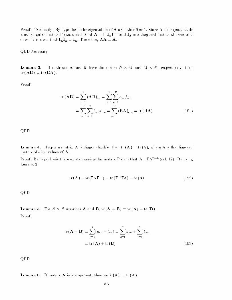
Proof of Necessity: By hypothesis the eigenvalues ofA are either 0 or 1. Since A is diagonalizablea nonsingular matrix � exists such that A = � IA��1 and IA is a diagonal matrix of zeros andones. It is clear that IAIA = IA: Therefore, AA = A:
QED Necessity
Lemma 3. If matrices A and B have dimension N � M and M � N , respectively, thentr(AB) = tr (BA).
Proof:
tr (AB) =NX
n=1
(AB)nn
=NX
n=1
MX
m=1
anmbmn
=MX
m=1
NX
n=1
bmnanm =MX
m=1
(BA)mm
= tr (BA) (191)
QED
Lemma 4. If square matrix A is diagonalizable, then tr (A) = tr (�), where � is the diagonalmatrix of eigenvalues of A.
Proof: By hypothesis there exists nonsingular matrix � such that A= ����1 (ref. 12). By usingLemma 3,
tr(A) = tr (����1) = tr (��1��) = tr (�) (192)
QED
Lemma 5. For N �N matrices A and B, tr (A + B) = tr (A) + tr (B) .
Proof:
tr(A+ B) =NX
n=1
(ann + bnn) =NX
n=1
ann +NX
n=1
bnn
= tr (A)+ tr (B) (193)
QED
Lemma 6. If matrix A is idempotent, then rank (A) = tr (A).
36
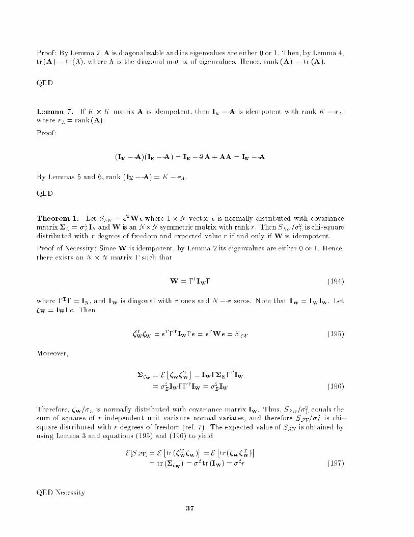
Proof: By Lemma 2,A is diagonalizable and its eigenvalues are either 0 or 1. Then, by Lemma 4,tr(A) = tr (�), where � is the diagonal matrix of eigenvalues. Hence, rank (A) = tr (A).
QED
Lemma 7. If K �K matrix A is idempotent, then IK �A is idempotent with rank K � rA,where rA = rank (A):
Proof:
(IK �A)(IK �A) = IK � 2A+AA = IK �A
By Lemmas 5 and 6, rank (IK � A) = K � rA .
QED
Theorem 1. Let SSW = �TW� where 1 �N vector � is normally distributed with covariancematrix �E = �2
EIN andW is anN�N symmetric matrix with rank r . ThenS SW=�2E is chi-square
distributed with r degrees of freedom and expected value r if and only if W is idempotent.
Proof of Necessity: Since W is idempotent, by Lemma 2 its eigenvalues are either 0 or 1. Hence,there exists anN �N matrix � such that
W = �TIW� (194)
where �T� = IN , and IW is diagonal with r ones and N � r zeros. Note that IW = IWIW . Let�W = IW��. Then
�TW�W = �T�TIW�� = �TW� = S SW (195)
Moreover,
��W= E
��W�TW
�= IW��E�
TIW
= �2EIW��TIW = �2
EIW (196)
Therefore, �W=�E is normally distributed with covariance matrix IW . Thus, SSW=�2E equals the
sum of squares of r independent unit variance normal variates, and therefore SSW=�2E is chi-
square distributed with r degrees of freedom (ref. 7). The expected value of SSW is obtained byusing Lemma 3 and equations (195) and (196) to yield
E [S SW ] = E�tr (�TW�W)
�= E
�tr(�W�TW)
�
= tr (��W) = �2 tr (IW) = �2r (197)
QED Necessity
37

Proof of Su�ciency: By hypothesis SSW =�2E is chi-square distributed with r degrees of freedom
and, hence, equals the sum of squares of r independent zero-mean, unit-variance normal variates.Symmetric matrix W can be written as
W = �T�W� (198)
where N � N diagonal matrix �W contains r nonzero elements since W has rank r . De�ne�W � �1=2
W��, where the elements of diagonal matrix �1=2
Wequal the square roots of the
corresponding elements of �W . Note that �W contains r nonzero elements. Then
�TW�W = �T�T�W�� = �TW� = S SW (199)
But��W
= E [�W�TW ] = �1=2W ��E�
T�1=2W = �2
E�1=2W ��T�1=2
W = �2E�W (200)
If any nonzero element of �W does not equal 1, the hypothesis that S SW=�2E equals the sum of
squares of r independent unit-variance normal variates is contradicted. Hence, diagonal matrix�W contains only ones and zeros, and by Lemma 2, W is idempotent.
QED Su�ciency
Theorem 2 (ref. 10). Let �T� = � qm , for 1 �m � M , where 1�N random vector � is normallydistributed with covariance matrix IN , qm = �TQm�, and nonnegative inde�nite N �N matrixQm is symmetric with rank rm. Then the variables qm are independent chi-square distributedrandom variables if and only if
Prm = N , for 1 � m � M .
Proof of Necessity: By Theorem 1, �T� is chi-square distributed. Also, by hypothesis
�T� =MX
m=1
�TQm� =MX
m=1
qm (201)
where Qm has rank rm and
MX
m=1
rm = N (202)
Since Qm is symmetric and nonnegative inde�nite with rank rm , it can be expressed in the form
Qm = PTm�mPm (203)
where Pm is orthonormal and �m is diagonal, containing rm positive elements and (N � rm)zero elements on the diagonal. After rearranging its elements, matrix Qm can be written inpartitioned form as
38

Qm =hPTrm
PTsm
i24�rm 0
0 0
3524Prm
Psm
35 =PT
rm�rmPrm (204)
where N�N matrixPTm = [PT
rmPTsm]; Prm has dimension rm�N; Psm has dimension (N�rm)�N ,
and �rm has dimension rm � rm. De�ne rm �N matrix Rrm as
Rrm � �1=2rmPrm (205)
It is seen that Rrm has rank rm and thatRTrmPrm = Qm. Also de�ne rm � 1 vector �m as
�m � Rrmx (206)
where x is an arbitrary N � 1 normally distributed random vector with covariance matrix IN.Then, inner product qm = �Tm�m = xTQmx forms N �N matrix Rr from the set of M matricesRrm as
Rr =
264R r1...
RrM
375 (207)
It follows from equation (202) thatRr has rank N and is therefore nonsingular. Construct N� 1vector � from subvectors �1 ; : ::; �M de�ned in equation (206) as
� =
24
�1...
�M
35 = R rx (208)
It follows that
xTx =MXm=1
xTQmx =MXm=1
�Tm�m = �T� = xTRTr R rx (209)
Since equation (209) holds for arbitrary vector x , it follows that RTr Rr = IN = RrR
Tr and,
hence, Rr is orthonormal. The covariance matrix of � is found to be
�� = E���T
�=R r E
�xxT
�RT
r = RrRTr = IN (210)
Therefore, the covariance matrix of �m equals Im . It then follows from Theorem 1 that randomvariable qm = �Tm�m is chi-square distributed with rm degrees of freedom. Moreover, since Rr isorthonormal, the set of random variables qm is mutually independent.
QED Necessity
39

Proof of Su�ciency: Construct matrixR r and vector � as before. By hypothesis, the elements �mare mutually independent with chi-square distributed inner products; thus, covariance matrix ��
contains r =�rm ones on the diagonal and zeros elsewhere. Since xTx is chi-square distributedwith N degrees of freedom, it follows from equation (209) that �T� is l ikewise distributed. Hence,rank �� equals N and N = r .
QED Su�ciency
A1.3. Linear Least-Squares Estimation.
From equation (187), note that the expected value of y is given by
E [y] = Zc (211)
De�ne K � 1 transformed observation vector v as
v �P�1y (212)
Equation (187) now becomes
v = P�1Zc +P�1�E = P�1Zc + �v (213)
where K � 1 vector �v � P�1�E . Immediately the expected value of v is
�v � E [v] = P�1Zc (214)
Then the K � K covariance matrix of v (which equals the covariance matrix of �v as well),denoted by �v, is obtained with the help of equations (188) and (189) as
�v � E [(v � �v)(v � �v )T ] = P�1
E [�E�TE ]P
�T
= P�1�EP�T = �2EP
�1PPTP�T = �2EIK (215)
Thus the elements of v and of �v are uncorrelated.
Based on transformed output observation vector v, the desire is to estimate the value ofparameter vector c, denoted by bc , which minimizes the sum of squaresSSQ given by the followinginner product:
SSQ = (v � �v)T(v � �V) = (v �P�1Zc)T(v �P�1Zc) (216)
Note that equation (216) may be rewritten as
S SQ = (y � Zc)TP�TP�1(y �Zc) = (y �Zc)TU�1(y �Zc) (217)
40

It is well-known (ref. 7) that the least-squares value bc which minimizes equation (216) is obtainedas follows:
bc = [(P�1Z)T(P�1Z)]�1(P�1Z)Tv = (ZTP�TP�1Z)�1ZTP�Tv
= (ZTU�1Z)�1ZTP�Tv = Q�1ZTP�Tv (218)
where Mz �Mz generalized moment matrix Q of the experimental design is de�ned as
Q � ZTU�1Z (219)
It is to be noted thatQT = Q. With the help of equations (213), (214), and (218) the expectedvalue of bc is found to be an unbiased estimate of c as follows:
E [bc] =Q�1ZTP�TE [v] = Q�1ZTU�1Zc
=Q�1Qc = c (220)
The covariance matrix of bc is found by �rst combining equations (213) and (218) to obtain
bc � c = Q�1ZTP�T(P�1Zc + �v) � c = Q�1ZTU�1Zc +Q�1ZTP�T�v � c
= Q�1Qc +Q�1ZTP�T�v � c = Q�1ZTP�T
�v (221)
It is seen that bc�c is normally distributed since �v is normally distributed. From equations (219)and (221) it follows thatMz �Mz covariance matrix �bc is given by
�bc = E�(bc � c)(bc � c)T� = Q�1ZTP�T
E [�v�Tv ] = P�1ZQ�1
= �2EQ�1ZTU�1ZQ�1 = �2
EQ�1QQ
�1 = �2EQ�1 (222)
De�ne K � 1 predicted output vector bv by
bv � P�1Zbc (223)
and de�ne K � 1 residual vector bev � v � bv. Using equations (213), (218), and (223) yields
bev = v � bv = v �P�1ZQ�1ZTP�Tv
=�IK �P
�1ZQ�1ZTP�T�(P�1Zc + �v)
=�IK �P
�1ZQ�1ZTP�T��v =WK�v (224)
where K �K matrix WK is de�ned as
WK � IK �K (225)
and K � K matrix K is de�ned as
41

K � (P�1Z)Q�1(P�1Z)T (226)
An integer subscript will be appended as needed to distinguish the dimension of matrices U,W, , Z, Q , and I for nonreplicated and replicated experimental designs.
It is seen that K is both symmetric and idempotent as follows:
KK =�P�1ZQ�1ZTP�T
� �P�1ZQ�1ZTP�T
�=P�1ZQ�1ZTU�1ZQ�1ZTP�T
=P�1ZQ�1QQ�1ZTP�T = P�1ZQ�1ZTP�T = K (227)
Also, using Lemmas 3, 4, and 6,
rank (K) = tr (P�1ZQ�1ZTP�T) = tr�Q�1ZTP�TP�1Z
�= tr (Q�1Q) = MZ (228)
Then by Lemma 7, WK is idempotent with rank K �Mz.
It is seen that bev is normally distributed. From equation (224), the expected value of bev iszero. The covariance matrix of bev then is found by using equations (215) and (224) as follows:
�b�v = E�bevbeTv
�= WK E
��v�
Tv
�WT
K
= �2EWKW
TK = �2
EWK (229)
The Mz � K covariance matrix of bc and bev is shown to be zero (ref. 7), and with the help ofequation (215),
cov (bc;bev) = E�(bc � c)beTv
�=Q�1ZTP�T
E��v�
Tv
� �IK �P
�1ZQ�1ZTP�T�
= �2E
�Q�1ZTP�T
�Q�1ZTP�T�= 0 (230)
Thus bc and bev are uncorrelated and independent.
The residual sum of squares SSE, de�ned as the sum of squares of the elements of residualvector bev, is obtained with the help of equation (224) as
SSE � beTvbev = �TvW
TKWK�v = �
TvWK�v (231)
E [SSE] = �2E(K �Mz) (232)
From equation (228) and Theorem 1, S SE=�2E is chi-square distributed with K �Mz degrees of
freedom and expected value K � Mz :
42

Therefore SE , denoted the standard error, is de�ned as
SE �
�SSE
K �Mz
�1=2
(233)
Note that SE is an unbiased estimate of �E .
A con�dence ellipsoid for bc is now obtained. Evaluate the quadratic form
SSC = (c � bc)TQ(c � bc)with equation (221) to yield
SSC = (c � bc)TQ(c � bc) = �TvP
�1ZQ�1ZTP�T�v = �
TvK�v (234)
Recall that K � K matrix K was shown by equation (228) to be idempotent with rank Mz.Then by Theorem 1, it follows that SSC=�2
E is chi-square distributed with Mz degrees of freedomand expected value Mz. Since bc � c and bev are independent, SSC and SSQ are independent.Hence, the ratio F = [SSC=(�2
EMz)]=fSSE= [�2E(K � Mz)]g is F-distributed with Mz; K � Mz
degrees of freedom (ref. 6). Therefore, a con�dence interval for bc at level � is given by thefollowing inequality:
(c �bc)TQ(c� bc) � MzS2EFMz ;K �Mz
(�) (235)
where Fi;j(�) is the 1�� tail of the F-distribution with i; j degrees of freedom and SE is de�nedin equation (233). The quadratic form of equation (235) de�nes an ellipsoid in Mz dimensionalhyperspace termed the con�dence ellipsoid.
Given Mz � 1 input vector z, the corresponding predicted scalar output by is given by
by(z) = zTbc (236)
From equation (220), the expected value of by(z) equals zTc. With equations (222) and (236),the variance of by(z) is obtained as follows:
�2y(z) � E(fby(z) � E [by(z)]g2) = E f[zT(c � bc)]2g
= E [zT(c � bc)(c � bc)Tz] = zTE [(c � bc)(c � bc)T ]z= zT�cz = �2
EzTQ�1z (237)
Then the normally distributed variate �by(z)= ��E(zTQ�1z)1=2�has zero mean and unit variance,
where �by = y�by. Recall that S 2SE=�
2E is chi-square distributed with K �Mz degrees of freedom.
Then the ratio t de�ned as follows has Student's t-distribution with K �Mz degrees of freedom(ref. 7):
t =�by(z)= ��E(zTQ�1z)1=2
�SSE= [�E(K �Mz)1=2]
(238)
43

Combine equations (233), (237), and (238) to obtain the calibration output con�dence intervalde�ned by the following inequality:
jy � by j � (zTQ�1z)1=2SE tK�Mz (�=2) (239)
where tn(�) is the �-percentile of the two-tailed t-distribution with n degrees of freedom.
A2. E�ects of Process Modeling Error
Consider a process f(c; z) modeled as a linear function of extended input vector z
f(c; z) = zc (240)
whereas the actual functional relationship is
f(c; z) = zc + (z) (241)
where (z) is the modeling error. Let the system be calibrated with calibration design Z inaccordance with equation (187) based on the linear model in equation (240). The observedcalibration output is then
y = Zc + (Z)+ �E (242)
where (Z) denotes the K � 1 vector of modeling errors
(z) =
2664 (z1)
...
(zK)
3775 (243)
Estimated coe�cient vector bc is obtained from equations (218) and (242) as follows:
bc = Q�1ZTU�1y = Q�1ZTU�1 [Zc + (Z) + �E ]
= c +Q� 1ZTU�1[ (Z) + �E] (244)
The expected value of bc is seen to be
E [bc] = c +Q�1ZTU�1 (Z) (245)
Predicted output vector by becomes
by = Zbc = Zc + ZQ�1ZTU�1[ (Z) + �E ] (246)
44

It follows from equation (246) that the expected value of predicted output vector by is given by
E [by] = Zc + ZQ�1ZTU�1 (Z) (247)
Combine equations (242) and (246) with (225) to obtain residual vector bev as
bev � v � bv =P�1(y � by) = P�1�IK �ZQ
�1ZTP�TP�1�[ (Z) + �E]
=�IK � P�1ZQ�1ZTP�T
�[P�1
(Z) + �v ] =WK[P�1 (Z) + �v] (248)
The expected value of bev is seen to be
E [bev] = WKP�1 (Z) (249)
After combining equations (215), (248), and (249), the covariance matrix of bev is found to be
�bev � Ef[bev � E(bev)][bev � E(bev)]Tg = �2EWK (250)
Since WK is idempotent, the residual sum of squares is obtained from equation (248) as follows:
SSE � beTvbev = [P�1 (Z) + �v]
TWK[P�1 (Z) + �v] (251)
Because WK has rank K �Mz, the expected value of S SE is
E [S SE ] = (K �Mz)�2E + (Z)TP�TWKP
�1 (Z) (252)
Note that SE = [S SE=(K � Mz)]1=2 is no longer an unbiased estimate of � when modeling error
(z) is nonzero.
Consider arbitrary input vector z. The corresponding output y , obtained with equation (241),is
y = f (c ; z) = zc + (z) (253)
The predicted output is by = zbc. Prediction error �y is then
�y � y � by = (z) �ZQ�1ZTU�1[ (Z) + �E] (254)
The expected mean-square prediction error is obtained from equation (254) as
�2by(z) = E [�by2] = [ (z)� zQ�1ZTU�1 (Z)]2 + �2
EzTQ�1z (255)
45

A3. Nonlinear Least-Squares Estimation With Input Uncertainty
Let c denote the Mc� 1 parameter vector; (z+ �z), the 1�Mz stochastic input vector, wherez is the 1 �Mz nominal input vector and �z is the 1 �Mz stochastic input uncertainty vector;�E , the measurement uncertainty, a zero-mean random variable. Then the process output is ofthe form
y = f(c; z + �z) + �E = f(c; z)+ �y (256)
The uncertainty �yk of the kth observation is then
�yk = �fzk + �Ek (257)
where
�fzk = fz(c ; zk)�zk (258)
and the 1 �Mz vector fz(c; zk) is de�ned as
fz(c ; zk) �
�@f(c;zk)
@z
�(259)
De�ne K � 1 error vector �fz as
�fz � [�fz1 : : : �fzK]T (260)
It is seen that �fz is given by
�fz =
2664fz(c ; z1)�zT1
...fz(c; zK )�z
TK
3775 (261)
Note that subscript z is appended to indicate that �f depends on the entire design matrix Z.The K �K covariance matrix of �fz is given by
�fz � E [�fz�fTz ] (262)
The K � 1 output vector y is obtained by extending scalar equation (256) to the following K � 1vector equation
y = f(c;Z)+ �y (263)
where Z is the K�Mz designmatrix, and �y is the K�1 zero-mean combined output uncertaintyvector given by
46

�y = �fz + �E (264)
and �y has K � K combined output covariance matrix �Y which can be expressed as
�Y = �fz +�E (265)
The assumption is that �Y can be expressed in the form of equation (188), namely �Y = �2Y U,
where U satis�es the conditions of equation (189), with transformed K � 1 output vector vde�ned in equation (213), and equation (263) becomes
v = P�1f (c;Z)+ �v (266)
where K � 1 uncertainty vector �v = P�1�y andK �K matrix P is de�ned as in equation (189).The expected value of �v is zero, and the expected value of v is
�v � E [v] = P�1f (c;Z) (267)
The K �K covariance matrix of �v, denoted by �v , then becomes
�v = E [�v�vT ] =P�1E [�y�yT ]P�T = �2
YP�1UP
�T = �2Y IK (268)
It is seen that �v is uncorrelated and normally distributed whenever �y is normallydistributed. As in equation (216) de�ne the sum of squares as
SSQ � (v � �v)T(v � �v ) = [v �P�1f (c ;Z)]T[v �P�1f (c ;Z)] (269)
To minimize S SQ (ref. 13) compute its gradient with respect to c and equate the resultant 1�Mc
set of equations to zero as follows:
h �1
2
�@SSQ
@c
�= [v �P�1f (c;Z)]TP�1
�@f
@c(c;Z)
�
= [v � P�1f (c;Z)]TP�1Fc = 0 (270)
where h is a function of independent arguments v, c , and Z and has dimension 1 � Mc,[v �P�1f (c;Z)] is K � 1, P is K � K , and K �Mc matrix Fc is de�ned as
Fc �
�@f
@c(c; Z)
�=
2666666666664
@f1(c;z1 )
@c1
: : :@f1(c;z1)
@cMc
... : : :...
@fK (c;zK )
@c1: : :
@fK (c;zK )
@cMc
3777777777775
(271)
47
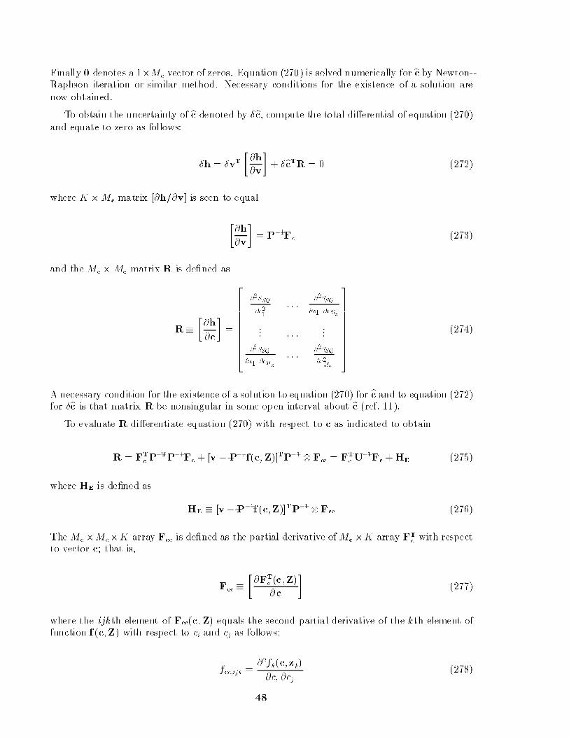
Finally 0 denotes a 1�Mc vector of zeros. Equation (270) is solved numerically forbc by Newton-Raphson iteration or similar method. Necessary conditions for the existence of a solution arenow obtained.
To obtain the uncertainty of bc denoted by �bc, compute the total di�erential of equation (270)and equate to zero as follows:
�h = �vT�@h
@v
�+ �bcTR = 0 (272)
where K �Mc matrix [@h=@v] is seen to equal
�@h
@v
�= P
�1Fc (273)
and the Mc � Mc matrix R is de�ned as
R �
�@h
@c
�=
2666666664
@2SSQ
@c21
: : :@2SSQ
@c1 @cMz
... : : :...
@2SSQ
@c1 @cMz
: : :@2SSQ
@c2Mz
3777777775
(274)
A necessary condition for the existence of a solution to equation (270) for bc and to equation (272)for �bc is that matrix R be nonsingular in some open interval about bc (ref. 11).
To evaluate R di�erentiate equation (270) with respect to c as indicated to obtain
R = FT
cP�TP�1Fc + [v �P�1 f(c; Z)]TP�1
Fcc = FT
cU�1Fc +HE (275)
where HE is de�ned as
HE � [v �P�1f (c;Z)]TP�1 Fcc (276)
The Mc �Mc�K array Fcc is de�ned as the partial derivative ofMc �K array FT
cwith respect
to vector c; that is,
Fcc �
�@FT
c(c ;Z)
@ c
�(277)
where the ijkth element of Fcc(c; Z) equals the second partial derivative of the kth element offunction f (c;Z) with respect to ci and cj as follows:
fcc;ijk =@2fk(c; zk)
@ci @cj(278)
48

for 1 � i; j � Mc , and 1 � k � K . The operator denotes formation of the inner product of1 � K row vector [v �P�1f (c;Z)]TP�1 with each K � 1 column of array Fcc . Thus the ijthelement of Mc �Mc matrix HE is given by
hE;ij =�v �P�1f(c; Z)
�TP�1Fcc; ij = eTv P
�1Fcc; ij (279)
for 1 � i; j � Mc, where Fcc;ij denotes the ijth (K � 1) column of array Fcc, andev = v �P�1f (c;Z). After least-squares estimation of vectorbc, vector ev becomes residual vectorbev de�ned subsequently. If norm k bev k is small, matrix HE can be neglected in equation (275).Then R is closely approximated by
R � FTc U�1Fc (280)
Note that matrix R has rank Mc, i .e., is nonsingular, only if rank (Fc) = Mc. Combineequations (272) and (273) and solve for Mc � 1 uncertainty vector �bc to yield
�bc = �R�1FTc P
�T�v (281)
From equation (281), �bc has zero mean and covariance matrix as follows:
�c = R�1FTc P�T�vP
�1FcR�1
= �2YR
�1FTc U
�1FcR�1 = �2
Y Q�1c (282)
where Mc �Mc matrix Qc equals
Qc =�R�1FT
cU�1FcR
�1��1
(283)
Note that satisfaction of the approximation in equation (280) is a su�cient condition, but notnecessary, for the existence of matrix Qc. Equation (280) implies that
Qc � R (284)
A3.1. Residual Sum of Squares.
As for calibration design matrix Z and estimated parameter vector bc, de�ne K � 1 predictedoutput vector bv as
bv = P�1f(bc; Z) = P�1 [f (c;Z)+ Fc�bc ]= P�1
�f(bc; Z) � FcR�1FT
cP�T�v
�= P�1f (c;Z)�F�v (285)
where
F ��P�1Fc
�R�1
�P�1Fc
�T(286)
As before, K � 1 residual vector bev is de�ned as
49

bev � v � bv =P�1[f(c; Z) � f(bc; Z)] + �v (287)
Let �fc � f (c;Z) � f(bc; Z), which is closely approximated by �fc = Fc(c; Z)�bc. Thenequation (287) can be expressed in di�erential form as
bev = P�1Fc(c;Z)�bc + �v (288)
Combine equations (281), (286), and (288) to obtain
bev =�IK �P
�1FcR
�1FT
cP�T
��v = WFK
�v (289)
where
WFK� IK �F (290)
SubscriptK, appended to denote the matrix dimension, is treated as an index. If approximationin equation (280) holds, then F is idempotent as is shown in the following equation:
FF = P�1FcR
�1FT
cP�TP�1FcR
�1FT
cP�T
= P�1FcR
�1�FT
cU
�1Fc
�R�1FT
cP�T
= P�1FcR
�1FT
cP�T = F (291)
By using Lemmas 2, 3, and 6,
rank (F) = tr�P�1FcR
�1FT
cP�T
�= tr
�R
�1FT
cP�TP�1Fc
�
= tr�R�1FT
cU
�1Fc
�= tr (R�1
R) = Mc (292)
Therefore, by Lemma 7, WFKis idempotent with rank K �Mc.
The covariance matrix of bev is given by
�ev= �2YWFK
(293)
and the residual sum of squares SSE is given by
SSE = beTvbev = �vTWFK
�v (294)
Then by Theorem 1, SSE is chi-square distributed with K � Mc degrees of freedom and withexpected value
E (SSE) = (K� Mc)�2Y (295)
An unbiased estimate of �Y is provided by standard error S Y , where
50

SY =
�SSE
K �Mc
�1=2
(296)
A con�dence interval for �Y at con�dence level � is given by
(K �Mc)1=2SY�(1+�)=2
� �Y �(K �Mc)1=2SY
�(1��)=2
(297)
where �� is the � percentile value of the chi-square distribution with K �Mc degrees of freedom.
A3.2. Con�dence Intervals.
A con�dence ellipsoid is now obtained for bc . LetSSC � (c � bc)TQC(c � bc) = �vTP�1FcR
�1QcR�1FT
c P�T�v
= �vTP�1FcR�1FT
cP�T�v = �vTF�v (298)
Because F is idempotent, SSC=�2Y is chi-square distributed with Mc degrees of freedom by
Theorem 1. Hence, the ratio F = [SSC=�2EMc]=fSSE=[�2
E(K � Mc)]g is F-distributed withMc; K �Mc degrees of freedom (ref. 7). Then the con�dence ellipsoid at level � for bc is de�nedby
(c � bc)TQc(c �bc) � McS2Y FMc ;K�Mc
(�) (299)
For arbitrary input vector z, the corresponding predicted scalar output denoted by by(z) isby(z) � f(bc; z) (300)
The uncertainty of by(z) due to calibration uncertainty alone is obtained with equation (281) as
�by = y � by = f (c; z)� f(bc; z)=
�@f (bc ; z)@ c
��bc = �f Tc (c; z)R�1FTc P
�1�v (301)
where Mc � 1 gradient vector fc(c; z) is de�ned as
fc(c; z) =
�@f(c;z)
@c
�(302)
It follows that �by is normally distributed with zero expected value. Then the expected value ofby(z) isE [by(z)] = f (c ; z) (303)
51

The variance of predicted output by(z), denoted the variance function, is obtained from equa-tion (301) as follows:
�2y(z) � E [�by �by] = f Tc (c; z)R
�1FTcP
�1E [�v �vT ]P�TFcR
�1fc(c; z)
= �2bY f Tc (c ; z)R�1FTcU
�1FcR
�1fc(c; z)
= �2bY f Tc (c ; z)Q�1
Cfc(c; z) (304)
If the approximation in equation (280) holds, then equation (304) simpli�es to
�2y(z) = �2
Y fTc (c; z)R
�1fc(c; z) (305)
The normally distributed variate �by(z)=��Y hfTc (c; z)Q�1
cfc(c ; z)
i1=2�has zero-mean and unit
variance. It was shown previously that SSE=�2Y is chi-square distributed with K �Mc degrees
of freedom when the approximation in equation (280) holds. Then the ratio t de�ned below hasStudent's t-distribution with K �Mc degrees of freedom.
t =�by(z)=n�Y �fTc (c; z)Q�1
C fc(c ; z)�1=2o
SSE= [�Y (K �Mc)1=2](306)
Then the output prediction con�dence interval at � con�dence level is given by
jy � by j � [f Tc (bc; z)Q�1C fc(bc; z)]1=2SY tK�Mc (�=2) (307)
where tn(�) is the � percentile value of the two-tailed t-distribution with n degrees of freedom.
A4. Analysis of Replicated Calibrations
In the following development, subscripts K and NK are appended to matrices I, Z, Q , U,and to distinguish between single calibrations (K observations) and replicated calibrations(NK observations). Consider an arbitrary K�Mz experimental design matrix ZK for calibrationof a single- output sensor, which is replicated N times. The sets of input loading uncertaintiesare seen to be intercorrelated among replications. The NK �Mz replicated experimental designZNK is
ZNK =
26664ZK
ZK
...ZK
37775 =HTZK (308)
where K �NK replication matrix H is de�ned as
H � [ IK IK : : : IK ] (309)
52

The following properties of H are used in the subsequent development. The K � K matrixproductHHT equals
HHT = NIK (310)
and NK � NK matrix product HTH equals
HTH =
26664
IK IK : : : IK
IK IK : : : IK...
... : : :...
IK IK : : : IK
37775 (311)
For any K �K matrix A, the NK �NK matrix productHTAH equals
HTAH =
26664
A A : : : A
A A : : : A...
... : : :...
A A : : : A
37775 (312)
Let DNK be anNK �NK block diagonal matrix constructed from K � K matrix A as
DNK =
26664
A 0K : : : 0K
0K A : : : 0K...
... : : :...
0K 0K : : : A
37775 (313)
where 0K is a K �K matrix of zeros. Then it follows that
HDNKHT = NA (314)
A4.1. Single-Input{Single-Output Process With Uncorrelated Uncertainties.
OverN replicated calibrations, let the elements ofNK�1 measurement uncertainty vector �Ebe uncorrelatedwith NK�NK covariance matrix �2
EINK, and let the unknownbias uncertaintiesof a single replication due to the calibration standard be uncorrelated with covariance matrix�2xIK . Since the loading sequence is replicated, then
cov (zkm; zlm) = �2x (jk � lj = nK ; n=1; : : : ; N�1;m=1; : : : ;Mz)
= 0 (Otherwise) (315)
where zkm is the mth element of vector zk and k = 1; : : : ; NK . Thus, from equation (311), theNK �NK covariance matrix of design matrix Z is given by
�Z = �2xH
TH (316)
53

Similarly, the NK �NK measurement uncertainty covariance matrix is given by
�E = �2EINK = �2
E
26664
IK 0K : : : 0K0K IK : : : 0K...
... : : :...
0K 0K : : : IK
37775 (317)
Noting that �2E > 0 and �2
x � 0, de�ne combined output covariance matrix �Y as
�Y � �E +�Z = �2EINK + �2
xHTH = �2
EUNK (318)
where
UNK = INK + �HTH =
266666664
(�+ 1)IK �IK : : : �IK
�IK (�+ 1)IK : : : �IK
...... : : :
...
�IK �IK : : : (� + 1)IK
377777775
(319)
and
� =�2x
�2E
(320)
It is readily shown that
U�1NK = INK � �H
TH =
266666664
(1 � �)IK ��IK : : : ��IK
��IK (1 � �)IK : : : ��IK
...... : : :
...
��IK ��IK : : : (1 � �)IK
377777775
(321)
where
� =�
N� + 1(322)
Then Mz �Mz generalized moment matrix QNK is obtained with the help of equation (310) asfollows:
QNK = ZTNKU�1NKZNK = ZTKH(INK � �HTH)HTZK
= N(1�N�)ZTKZK (323)
54

Combine equations (320), (322), and (323) to yield
QNK =�2E
(�2E=N) + �2
x
ZTKZK (324)
Note from equation (324) that the portion of calibration uncertainty due to calibration standardbias errors is not reduced by replication, whereas that due to measurement errors decreasesroughly as N�1=2.
For the analysis of variance tests presented subsequently in the null hypothesis the inputuncertainty is assumed to be zero. Then �x = 0 and matrix UNK equals INK ; consequently, Pequals INK in equation (189). For this special case, equations (308), (310), and (323) imply that
QNK = ZTNKZNK = ZTKHHTZK = NZTKZK = NQK (325)
From equations (226) and (325), NK �NK matrix NK is given by
NK = ZNKQ�1NKZ
TNK =
1
NHTKH (326)
where K �K matrix K is
K = ZKQ�1K Z
TK (327)
As shown in equations (226) and (228), K and NK are symmetric and idempotent withrank MZ .
A4.2. General Multi-Input|Single-Output Process.
Consider a general multi-input{single-output nonlinear process calibrated by using experi-mental design ZK replicated N times as before. The K � 1 output uncertainty vector of a singlereplication, denoted by �yK, is given by equation (264). Then for N replications NK� 1 outputuncertainty vector �yNK is given by
�yNK = HT�fZ+ �E (328)
where K � 1 vector �fZ is given by equation (261) with K�K covariance matrix �fZK= �2
xUfZK,
given in equation (262), and where NK � 1 measurement uncertainty vector �E has NK �NKcovariance matrix �E = �2
EUENK. The measurement uncertainty is assumed uncorrelated
between replications and the K � K measurement covariance matrix of each replication isassumed to be �EK = �2
EUEK . Then
UENK=
2666664
UEK0K : : : 0K
0K UEK: : : 0K
...... : : :
...
0K 0K : : : UEK
3777775
(329)
and from equation (328),
55
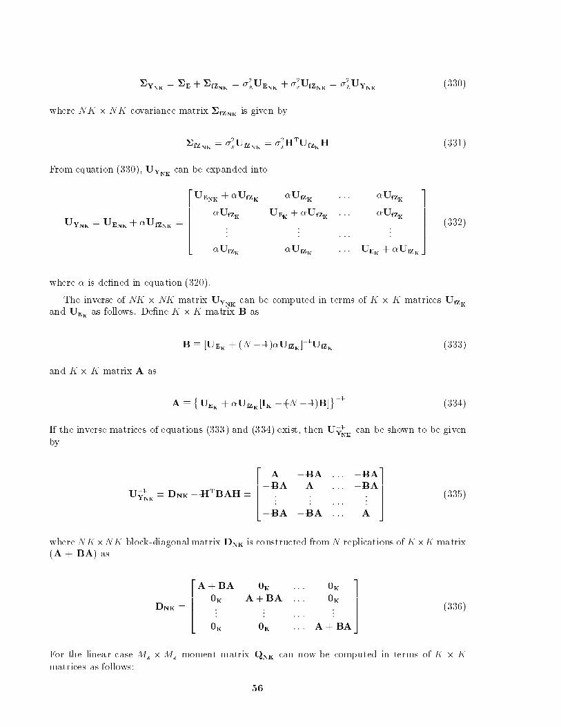
�YNK= �E +�fZNK
= �2EUENK
+ �2xUfZNK
= �2EUYNK
(330)
where NK �NK covariance matrix �fZNK is given by
�fZNK= �
2xUfZNK
= �2xHTUfZK
H (331)
From equation (330), UYNKcan be expanded into
UYNK = UENK + �UfZNK =
2666664
UENK+ �UfZK
�UfZK: : : �UfZK
�UfZKUEK
+ �UfZK: : : �UfZK
...... : : :
...
�UfZK�UfZK
: : : UEK+ �UfZK
3777775
(332)
where � is de�ned in equation (320).
The inverse of NK � NK matrix UYNKcan be computed in terms of K � K matrices UfZK
and UEKas follows. De�ne K �K matrix B as
B � [UEK + (N � 1)�UfZK ]�1UfZK (333)
and K � K matrix A as
A �
�UEK
+ �UfZK[IK � (N � 1)B]
�1
(334)
If the inverse matrices of equations (333) and (334) exist, then U�1YNK
can be shown to be givenby
U�1YNK
= DNK �HTBAH =
26664
A �BA : : : �BA
�BA A : : : �BA...
... : : :...
�BA �BA : : : A
37775 (335)
where NK�NK block-diagonal matrix DNK is constructed fromN replications ofK�K matrix(A + BA) as
DNK =
26664
A+BA 0K : : : 0K0K A+BA : : : 0K...
... : : :...
0K 0K : : : A+ BA
37775 (336)
For the linear case Mz �Mz moment matrix QNK can now be computed in terms of K � K
matrices as follows:
56

QNK = ZTNKU�1YNK
ZNK = (ZTKH)U�1YNK
(ZTKH)T (337)
It can readily be seen from equations (314), (335), and (336) that
HU�1YNK
HT = H(DNK �HTBAH)HT = N [IK � (N � 1)B]A (338)
Hence for the linear case,
QNK = NZTK[IK � (N � 1)B]AZK (339)
For the nonlinear case, a single replication of experimental design ZK , evaluation of equa-tion (271) yields K � Mc matrix FcK . Then over N replications of ZK , with design matrixZNK given by equation (308), equation (271) yields NK �Mc matrix FcNK = HTFcK . If equa-tion (275) holds, it follows from equation (338) that
R � FTcNKU�1YNK
FcNK = FTcKHU�1YNK
HTFcK
= NFTcK [IK � (N � 1)B]AFcK (340)
Equation (340) permits computation of con�dence and prediction intervals for replicated cali-bration data in terms ofK�K matrices; thereby, required computer storage and computationalresources are reduced when N is large.
With reference to equations (188) and (189), the analysis of variance null hypothesis assumesthat if matrix UYNK
= INK ; then matrix P = INK. If equation (280) holds, then for the nullhypothesis Mc �Mc matrix R becomes
R � FTcNKFcNK = FTcKHHTFcK
= NFTcKFcK (341)
It follows that NK �NK matrix FNK, given in equation (286), is given by
FNK= FcNKR
�1FTcNK =1
NHTFcK(F
TcKFcK)
�1FTcKH
=1
NHTFKH (342)
where K �K matrix FK is obtained from equation (286) as
FK = FcK(FTcKFcK)
�1FTcK (343)
As shown in equation (291), matrices FKand FNK
are symmetric and idempotent withrank Mc.
57

A4.3. Analysis of Variance of Replicated Calibrations.
Analysis of variance of replicated calibrations provides tests of signi�cance for the presenceof bias uncertainty due to input loading errors or mathematical modeling errors, as well as fornonstationarity of estimated parameters. The analysis of variance is developed in this sectionwith single-input{single-output process notation. Note that similar results are obtained for thegeneral multi-input{single output case by replacing NK, K, WNK , WK, and Mz by FNK
,FK
, WFNK, WFK, andMc , respectively.
Let the null hypothesis (ref. 7) assume that input loading uncertainties and modeling errorsare zero and thatNK � 1 measurement uncertainty vector �E has NK �NK covariance matrix�E = �2EINK. Then NK � NK matrices U and P are both equal to INK and do not appearin the following equations. Transformed output vector v is equal to and replaced by observedoutput vector y.
The K �K matrix WK is de�ned in equation (225) as
WK = IK �K (344)
Matrix WFKis de�ned similarly in equation (290). After N replications K �K matrix WK
expands to NK �NK matrix WNK given as
WNK = INK �NK (345)
where matrices NK and FNK are in equations (326) and (342) and has rank Mz. Since NK
is idempotent, then by Lemma 7 matrix WNK is idempotent with rank NK �Mz .
For use in the development, de�ne NK �NK matrix GH as
GH �1
NHTH =
1
N
2664IK IK : : : IK...
... : : :...
IK IK : : : IK
3775 (346)
It is readily seen that GH is idempotent with rank K . By Lemma 7, matrix INK � GH isidempotent with rank NK � K .
Next GH is shown to be a two-sided identity of any matrix of the form 1=NHTAH, inparticular NK . Indeed, from equations (326) and (342),
GHNK =1
N2HTHHT
KH =
1
NHT
KH = NK
=1
N2HTKHH
TH = NKGH (347)
From equations (345) and (347),
GHWNK =WNKGH (348)
58

Therefore, NK �NK matrix productWNKGHWNK , to be used later, is idempotent. Also, it isseen that
WNKGHWNK = (INK �NK)GH(INK �NK) = (GH �NK)(INK �NK)
= GH �NK (349)
Since GH has rank K andNK has rank Mz , it follows from Lemmas 5 and 6 and equation (349)that product WNKGHWNK has rank K �Mz . Note thatK �Mz > 0.
Estimated Mz � 1 parameter vector bc, NK � 1 predicted output vector by, and NK � 1residual vector be are obtained with equations (218), (223), and (224), respectively, for a linearprocess, and equations (270), (285), and (289), respectively, for a nonlinear process. Recall fromequation (224) that be can be expressed as
be = WNK�E (350)
with zero expected value and NK �NK covariance matrix �2WNK .
Let ben denote the K � 1 residual vector at the nth replication, which has zero expectedvalue and covariance matrix �2WK . Then residual vector be can be partitioned into N , K � 1subvectors as shown below:
beT =hbeT1 beT2 : : : beTN iT (351)
Let �eK denote the mean value of the set of residual vectors ben averaged overN replications; thatis,
�eK =1
N
NXn=1
ben = 1
NHbe =
1
NHWNK�E (352)
The residual sum of squares, denoted by SSE , is de�ned in equation (231) as
S SE � beTbe = �TEWNK�E (353)
By Theorem 1, S SE is chi-square distributed with NK �Mz degrees of freedom; the standarderror of the regression given by
SE =
�SSE
NK �Mz
�1=2
(354)
is an unbiased estimate of �.
59

Residual sum of squares SSE can be partitioned into the following sum of quadratic forms:
S SE = beTbe = beTWNKGHWNKbe + beT (INK �WNKGHWNK)be (355)
By using equations (348) and (350) and the fact thatWNK is idempotent, SSE can be expressedas
S SE = �T
EWNKGHWNK�E + �
T
EWNK (INK �GH)WNK�E (356)
Denote the �rst right-hand term in equation (355) by S SX as follows:
SSX � beTWNKGHWNKbe = �T
EWNKGHWNK�E (357)
which follows from equation (350) and the fact that WNK is idempotent. Then S SX can beexpressed as
S SX = �T
EWNKGHWNK�E = N�eT
K�eK (358)
which follows from equations (350), (352), and (357). It has been shown that WNKGHWNK
is idempotent with K � Mz degrees of freedom. Therefore, it follows from equation (358) andTheorem 1 that SSX=�2E is chi-square distributed with K �Mz degrees of freedom. De�ne theroot-mean-square value of SSX as
SX �
�SSX
K �Mz
�1=2
(359)
Variable SX is interpreted as the standard error due to bias uncertainty.
Consider next the second right-hand term of SSE in equation (355). De�ne SSM as
SSM �
KXk=1
NXn=1
(benk � �ek)2 =
NXn=1
(ben � �ek)T(ben � �eK) (360)
where benk is the kth element of K � 1 residual vector ben, and �ek is the kth element of K � 1vector �ek . Variable S SM is seen to equal the sum of squares about the means of the set of Nresidual vectors ben each of dimension K � 1. It follows from the de�nition of H that
SSM =
NXn=1
(ben � �eK)T(ben � �eK) = (be �HT�eK)T(be �HT
�eK) (361)
De�ne NK � 1 vector eM as follows and use equations (350) and (352) to obtain the result
eM � be �HT�eK = be � 1
NHTHbe = (INK � GH)be
= (INK � GH)WNK�E (362)
60

By using equations (360) to (362),
SSM = eTMeM = �
T
EWNK(INK �GH)WNK�E (363)
Comparison of equations (356) and (363) shows that SSM equals the second right-hand term ofSSE. Moreover, it is clear that matrix product
WNK(INK �GH)WNK = WNK �WNKGHWNK
is idempotent and, by Lemmas 5 and 6, has rank NK �K , since WNK has rank NK �Mz , andWNKGHWNK has rank K �Mz. By Theorem 1, S SM=�
2E is chi-square distributed with NK �K
degrees of freedom. Variable SSM can be interpreted as the portion of residual sum of squaresSSE due to measurement uncertainty. The root-mean-square value
SM =
�SSM
NK �K
�1=2
(364)
is interpreted as an estimate of the standard deviation �E of the measurement uncertainty.
It follows from Theorem 2 that SSX and SSM are independent. Therefore, the ratioTXM
= [S SX=(K � Mz)]=[S SM=(NK � K)] is F -distributed with K �Mz , NK �K degrees offreedom. The test of signi�cance for the existence of distinct input loading biases is as follows.Assume as the null hypothesis that input loading bias error and modeling error are zero. Formthe expression
TXM =SSX=(K � Mz)
SSM=(NK �K )> FK�Mz ; NK�K (�) (365)
If inequality (365) is satis�ed, then the null hypothesis that both input loading bias error andmodeling error equal zero is rejected at con�dence level �.
A4.4. Stationarity Test of Estimated Parameters.
A test is developed for nonstationarity of estimated individual parameter bcm 2 bc over Nreplicated calibrations. Let bcRn denote the parameter vector estimated at the nth replication bya K-point regression, with residual sum-of-squares SSRn, for n = 1; : : : ; N. De�ne
SSR =NXn=1
SSRn (366)
Let bc denote the parameter vector estimated by anNK-point global regression over the completeset of N replicated calibrations. To test for stationarity of parameter cm replace the mthelement of bcRn by bcm 2 bc and compute resulting the error sum-of-squares, denoted by SSGm;n forn = 1; : : : ;N . Compute SSGm =
PSSGm;n for n = 1, ... , N . The ratio (SSGm � SSR)=SSR
is subsequently shown to be F-distributed and thereby provides a test of signi�cance fornonstationarity of the estimated value of cm over the N replicated calibrations.
61

The null hypothesis assumes that calibration standard errors and modeling errors are zeroand that estimated parameter vector bcRn is stationary over the N replications. Let NK � 1measurement error vector �E be partitioned among the N replications as [�TE1 : ::�
TEN
]T , where �En
denotes the K � 1 measurement error vector at the nth replication. Also, let �bcRndenote the
uncertainty of the nth estimated parameter vector, which is obtained from equation (281) as
�bcRn= �R�1FTc �En (367)
The uncertainty of element bcRm;n 2 bcRn is seen to be
�bcRm;n= �pTmF
Tc �En (368)
where pTm is the mth row of R�1. Similarly, the uncertainty of globally estimated parametervector bcG is given by
�bcG = �1
NR�1FT
c H�E (369)
and the uncertainty of element bcGm 2 bcG is
�bcGm = �1
NpTmF
Tc H�E (370)
The residual vector of the nth replication, denoted by beRn, is found by using equation (288) as
beRn= Fc�bcRn + �En (371)
Replace bcRm;nby bcGm
in equation (371) to obtain the error vector of the nth replicationcomputed with the globally estimated value of parameter cm, which is denoted by beGm;n
. Fromequations (368) to (371), the di�erence between error vectors beGm;n
and beRn is given by
beGRm;n= fcmp
TmF
Tc
��En �
1
NH�E
�(372)
where fcm is the mth column of Fc .
Let NK � 1 error vector beGRm=hbeTGR
m;1: :: beTGRm;N
iT, which can then be expressed in terms
of NK � 1 measurement error vector �E as
beGRm=
�IA �
1
NHTAH
��E (373)
where K �K matrix A = fcmpTmF
Tc and NK �NK block diagonal matrix IA is de�ned as
62

IA =
2664A 0 : : : 0
0 A : : : 0...
... : : :...
0 0 : : : A
3775 (374)
It is seen that the inner product beTGRmbeGRm equals (SSGm�S SR). Clearly A has rank 1. It followsfrom equation (280) that pTmF
Tc fcm = 1. Hence,
AA = fcmpTmF
Tc fcmp
TmF
Tc = fcmp
TmF
Tc = A
and A is idempotent. It can then be seen that IA is idempotent with rank N , since A isidempotent with rank 1. Thus IA � 1=NHTAH is idempotent with rank (N � 1), and thereforethe inner product beTGRmbeGRm can be expressed as
S SGm � SSR = beTGRmbeGRm = �
TE
�IA �
1
NHTAH
��E (375)
It follows from Theorem 1 that SSGm � S SR is chi-square distributed with N � 1 degrees offreedom.
The residual sum of squares of the nth replicated regression, SSRn = �TEnWK�En , has been
shown as chi-square distributed with K �Mz degrees of freedom. Because the error vectors �Enare mutually independent, it follows from equation (366) and Theorem 2 that the total replicatedsum of squares SSR is chi-square distributed with N(K �Mz) degrees of freedom. Therefore, ifthe following inequality is satis�ed
Tcm =(SSGm � SSR)=(N� 1)
SSR=[N(K �Mz)]> F(N�1); N(K�Mz)(�) (376)
then the null hypothesis that parameter cm is stationary is rejected at con�dence level �.
63
References
1. Abernethy, R. B., et al.: Tutorial, Test Measurement Accuracy. Fundamentals of Aerospace Instrumentation,
Volume 7|Fundamentals of Test Measurement, Volume 2, B. W. Washburn, ed., ISA, 1975, pp. 47{57.
2. Measurement Uncertainty|Part 1: Instruments and Apparatus. ANSI/ASME PTC 19.1-1985, ASME, 1986.
3. Coleman, Hugh W.; and Steele, W. Glenn, Jr.: Experimentation and Uncertainty Analysis for Engineers. JohnWiley & Sons, 1989.
4. Quality Assessment for Wind Tunnel Testing. AGARD-AR-304, 1994.
5. Batill,StephenM.: Experimental Uncertainty and DragMeasurements in the National Transonic Facility. NASACR-4600, 1994.
6. Tripp, John S.; and Tcheng, Ping: Determination of Measurement Uncertainties of Multi-Component WindTunnel Balances. AIAA-94-2589, June 1994.
7. Johnson, Richard A.; and Wichern, Dean W.: Applied Multivariate Statist ical Analysis. Prentice-Hall, 1982.
8. Box, G. E. P.; and Draper, Norman R.: A Basis for the Selection of a Response Surface Design. J. American
Stat. Assoc., vol. 54, 1959, pp. 622{654.
9. Plackett, R. L.: Principles of Regression Analysis . Oxford Univ. Press, 1960.
10. Montgomery, Douglas C.; and Peck, Elizabeth A.: Introduction to Linear Regression Analysis. John Wiley &Sons, 1982.
11. Brand, Louis: Advanced Calculus. John Wiley & Sons, 1955.
12. Lancaster, Peter: Theory of Matrices. Academic Press, Inc., 1969.
13. Fletcher, Roger: Practical Methods of Optimization. John Wiley & Sons, 1987.
64

Form ApprovedOMB No. 07704-0188
Public reporting burden for this collection of information is estimated to average 1 hour per response, including the time for reviewing instructions, searching existing data sources,gathering and maintaining the data needed, and completing and reviewing the collection of information. Send comments regarding this burden estimate or any other aspect of thiscollection of information, including suggestions for reducing this burden, to Washington Headquarters Services, Directorate for Information Operations and Reports, 1215 JeffersonDavis Highway, Suite 1204, Arlington, VA 22202-4302, and to the Office of Management and Budget, Paperwork Reduction Project (0704-0188), Washington, DC 20503.
1. AGENCY USE ONLY (Leave blank) 2. REPORT DATE 3. REPORT TYPE AND DATES COVERED
4. TITLE AND SUBTITLE 5. FUNDING NUMBERS
6. AUTHOR(S)
7. PERFORMING ORGANIZATION NAME(S) AND ADDRESS(ES)
9. SPONSORING/MONITORING AGENCY NAME(S) AND ADDRESS(ES)
11. SUPPLEMENTARY NOTES
8. PERFORMING ORGANIZATIONREPORT NUMBER
10. SPONSORING/MONITORINGAGENCY REPORT NUMBER
12a. DISTRIBUTION/AVAILABILITY STATEMENT 12b. DISTRIBUTION CODE
13. ABSTRACT (Maximum 200 words)
14. SUBJECT TERMS
17. SECURITY CLASSIFICATIONOF REPORT
18. SECURITY CLASSIFICATIONOF THIS PAGE
19. SECURITY CLASSIFICATIONOF ABSTRACT
20. LIMITATIONOF ABSTRACT
15. NUMBER OF PAGES
16. PRICE CODE
NSN 7540-01-280-5500 Standard Form 298 (Rev. 2-89)Prescribed by ANSI Std. Z39-18298-102
REPORT DOCUMENTATION PAGE
October 1999 Technical Publication
Uncertainty Analysis of Instrument Calibration and ApplicationWU 519-20-21-01
John S. Tripp and Ping Tcheng
L-17652
NASA/TP-1999-209545
Experimental aerodynamic researchers require estimated precision and bias uncertainties of measured physicalquantities, typically at 95 percent confidence levels. Uncertainties of final computed aerodynamic parameters areobtained by propagation of individual measurement uncertainties through the defining functional expressions. Inthis paper, rigorous mathematical techniques are extended to determine precision and bias uncertainties of anyinstrument-sensor system. Through this analysis, instrument uncertainties determined through calibration are nowexpressed as functions of the corresponding measurement for linear and nonlinear univariate and multivariate pro-cesses. Treatment of correlated measurement precision error is developed. During laboratory calibration, calibra-tion standard uncertainties are assumed to be an order of magnitude less than those of the instrument beingcalibrated. Often calibration standards do not satisfy this assumption. This paper applies rigorous statistical meth-ods for inclusion of calibration standard uncertainty and covariance due to the order of their application. The effectsof mathematical modeling error on calibration bias uncertainty are quantified. The effects of experimental designon uncertainty are analyzed. The importance of replication is emphasized; techniques for estimation of both biasand precision uncertainties using replication are developed. Statistical tests for stationarity of calibration parame-ters over time are obtained.
Uncertainty analysis; Bias and precision errors; Instrument calibration; Multivariateprocesses; Experimental design; Aerodynamic measurements
77
A05
UL
NASA Langley Research CenterHampton, VA 23681-2199
National Aeronautics and Space AdministrationWashington, DC 20546-0001
Unclassified–UnlimitedSubject Category 35 Distribution: StandardAvailability: NASA CASI (301) 621-0390
Unclassified Unclassified Unclassified