Faculty of Civil Engineering

University of Belgrade

Uncer ta in ty ana lys i s a s a complement to f l ood r i sk a s se s sment

- Theoretical background -

Dr. Dejan Komatina Nemanja Branisavljević

Belgrade, September 2005

Uncertainty analysis as a complement to flood risk assessment 1. Introduction

The flood protection projects are designed to reduce the risk of undesirable economic, environmental and social consequences of flooding. But floods occur randomly and the effectiveness of the protective system varies from year to year. A system that eliminates all damage one year may not be resistant enough to eliminate all damage the next year. In order to solve this problem, the long-term average damage is used as an index of damage potential. This value is computed with estimates of the probability of flooding. This way, the projects are developed considering the consequences of a wide range of floods and the benefits of reducing the adverse impacts.

However, there is often considerable difficulty in determining the probability and the consequences. Failures of protective systems often arise from a complex combination of events and thus statistical information on their probability and consequence may be scarce or unavailable. Therefore, the engineer has to resort to models and expert judgment. Models are a simplified representation of reality and hence generate probability of failure which is inherently uncertain. Similarly, expert judgments are subjective and inherently uncertain. Thus practically every measure of risk has uncertainty associated with it. 2. Types of uncertainties associated with a risk

There is a wide range of factors that can give rise to uncertainties, from environmental loading to the structural performance of defences.

All the uncertainties can be divided into two main classes (Tung and Yen, 1993): - Natural variability (aleatory uncertainty, objective uncertainty, stochastic uncertainty,

stochastic variability, inherent variability, randomness, type-A uncertainty) – refers to uncertainties associated with the inherent randomness of natural processes, that is: - annual maximum discharge, - changes in river channel over time, - hysteresis during a flood wave.

- Knowledge uncertainty (epistemic uncertainty, subjective uncertainty, lack-of-knowledge or limited-knowledge uncertainty, ignorance, specification error, type-B uncertainty) – results from incomplete knowledge of the system under consideration and is related to the ability to understand, measure and describe the system. This class can be further divided into: - model uncertainty, reflecting the inability of the simulation model to represent

precisely the true physical behaviour of the system; - model parameter uncertainty, that relates to the accuracy and precision with which

parameters can be derived from field data, judgment, and the technical literature; - data uncertainties, which are the principal contributors to parameter uncertainty,

including measurement errors, inconsistency or heterogeneity of data sets, data handling errors, and nonrepresentative sampling caused by limitations in time, space, or financial means.

Sources of knowledge uncertainty are listed in Table 1. Knowledge uncertainty can be reduced by an increase of knowledge, while the natural

variability is inherent to the system and can not be reduced by more detailed information (Apel et al., 2004).

1

Table 1. Sources of knowledge uncertainty and their corresponding types (USACE, 1996a, 1996c; Faber and Nachtnebel, 2002; Apel et al., 2004). Variable Source of uncertainty Type of uncertainty

Rainfall-runoff modelling Model uncertainty Selection of distribution function Model uncertainty Parameters of the statistical distribution Parameter uncertainty Short or unavailable records Data uncertainty

Annual maximum discharge

Measurement errors Data uncertainty Model selection (1D or 2D model) Model uncertainty Steady or unsteady calculation Model uncertainty Frictional resistance equation Model uncertainty Channel roughness Parameter uncertainty Channel geometry Parameter uncertainty Sediment transport and bed forms Data uncertainty

Water stage

Debris accumulation and ice effects Data uncertainty Dependence on water stage Model uncertainty Dependence on water stage Parameter uncertainty Land/building use, value and location Data uncertainty Content value Data uncertainty Structure first-floor elevation Data uncertainty Flood warning time Data uncertainty Public response to a flood (flood evacuation effectiveness) Data uncertainty

Flood damage

Performance of the flood protection system (possibility of failure below the design standard) Data uncertainty

An additional source of uncertainties is a temporal variability of both the hazard and

vulnerability of a system (Table 2). In this respect, a major cause of uncertainty is the assessment of future land development, for example the effect of increasing urbanization. Also, protection against hazards influences development and thus changes the risk, as happens after completion of a flood proofing scheme. The higher protection of an area attracts people and industry to settle in it, and when an extreme event occurs that overtops the levees, then the disaster might be larger than if the unprotected but less utilized area had been flooded. In comparison to these uncertainties of human actions, the possible effect of natural variability, such as anticipated climate changes, are minor in most regions (Plate, 1998). Table 2. Some factors of the risk change in time.

Factor Risk element affected Climate (natural variability, climate change) Probability, Intensity Change in land use Intensity, Vulnerability Defences (deterioration, maintenance, new works) Exposure, Vulnerability Flood damage (new development) Vulnerability Changing value of assets at risk Vulnerability Improved flood warning / response Vulnerability

2

3. Uncertainty analysis

The traditional risk assessment is based on the well-known relationship:

SPR ×= , (1)

where: R – the risk, P – the probability of hazard occurrence, or the probability of a flood event, S – the expected consequence, corresponding to the flood event.

If the consequence is expressed in monetary terms, i.e. flood damage (€), then the damage is determined as:

maxSS ⋅α= , (2)

where: α – damage factor (or vulnerability, degree of loss, damage ratio), which takes values

from 0 (no damage) to 1 (total damage), and Smax – damage potential (the total potential damage).

The risk is usually measured by the expected annual damage, S (€/year):

∑∫=

+ ∆⋅+

≈⋅==m

ii

ii PSS

PPSSR1

11

0 2d)( , (3)

which is calculated on the basis of a number of flood events considered and pairs ( , ) defined, where:

iS iP

i = 1,..., m – index of a specific flood event considered, and

iii PPP −=∆ +1 . (4)

The expected annual damage, S (€/year), is the average value of such damages taken over floods of all different annual exceedance probabilities and over a long period of years. This actually means that the uncertainty due to natural variability (sometimes called the hydrologic risk) is accounted for in such a procedure. Therefore, uncertainty analysis is a consideration of the knowledge uncertainty, thus being a complement to the traditional procedure of flood risk assessment. 3.1. Performance of a flood defence system

The task of uncertainty analysis is to determine the uncertainty features of the model

output as a function of uncertainties in the model itself and in the input parameters involved (Tung and Yen, 1993).

To illustrate the methodology, it is useful to recall the basic terms from reliability theory. The main variables, used in reliability analysis, are resistance of the system and load, while often used synonyms to these terms are:

resistance (r) = capacity (c) = benefit (B)

load, or stress (l) = demand (d) = cost (C)

3

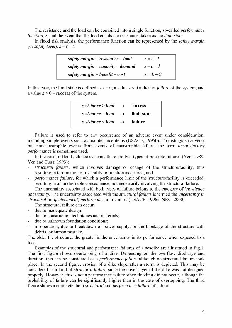
The resistance and the load can be combined into a single function, so-called performance function, z, and the event that the load equals the resistance, taken as the limit state.

In flood risk analysis, the performance function can be represented by the safety margin (or safety level), z = r – l.

safety margin = resistance – load lrz −=

safety margin = capacity – demand z c d= −

safety margin = benefit – cost z B C= −

In this case, the limit state is defined as z = 0, a value z < 0 indicates failure of the system, and a value z > 0 – success of the system.

resistance > load → success

resistance = load → limit state

resistance < load → failure

Failure is used to refer to any occurrence of an adverse event under consideration,

including simple events such as maintenance items (USACE, 1995b). To distinguish adverse but noncatastrophic events from events of catastrophic failure, the term unsatisfactory performance is sometimes used.

In the case of flood defence systems, there are two types of possible failures (Yen, 1989; Yen and Tung, 1993): - structural failure, which involves damage or change of the structure/facility, thus

resulting in termination of its ability to function as desired, and - performance failure, for which a performance limit of the structure/facility is exceeded,

resulting in an undesirable consequence, not necessarily involving the structural failure. The uncertainty associated with both types of failure belong to the category of knowledge

uncertainty. The uncertainty associated with the structural failure is termed the uncertainty in structural (or geotechnical) performance in literature (USACE, 1996c; NRC, 2000).

The structural failure can occur: - due to inadequate design; - due to construction techniques and materials; - due to unknown foundation conditions; - in operation, due to breakdown of power supply, or the blockage of the structure with

debris, or human mistake. The older the structure, the greater is the uncertainty in its performance when exposed to a load.

Examples of the structural and performance failures of a seadike are illustrated in Fig.1. The first figure shows overtopping of a dike. Depending on the overflow discharge and duration, this can be considered as a performance failure although no structural failure took place. In the second figure, erosion of a dike slope after a storm is depicted. This may be considered as a kind of structural failure since the cover layer of the dike was not designed properly. However, this is not a performance failure since flooding did not occur, although the probability of failure can be significantly higher than in the case of overtopping. The third figure shows a complete, both structural and performance failure of a dike.

4

Fig.1. Example failures of a seadike (Kortenhaus et al., 2002).

In relation to flood hazard, different failure types can be recognized (Table 3), all of them

being described by the relationship: z = r – l < 0. However, the most common failure mechanism of new or well-maintained flood defence systems is overtopping of the structures, that is the performance failure. Table 3. Flood defence system failure types (Kortenhaus et al., 2002). Failure type Load, l Resistance, r Unit

The flood water level, Z The structure crest level, Zd [m] The maximum flood discharge, Q The system design discharge, Qd [m3/s] The actual overflow The critical overflow [m3/s] Overtopping*

The actual overflow velocity The critical overflow velocity [m/s] Breaching The actual flood duration The critical flood duration [h] Sliding The actual force The critical force [kN] Scouring The actual shear stress The critical shear stress [kPa] Tipping The actual moment The critical moment [kNm] Instability of revetment The actual force The critical force [kN]

Infiltration The actual flood duration The critical flood duration [h] Seepage The actual hydraulic gradient The critical hydraulic gradient [/] * the performance failure

5

3.2. Probability of failure of a flood defence system

The failure of flood defence systems due to overtopping of flood defence structures is commonly expressed in terms of water and crest levels (Table 3), so that the performance function takes the form: z = Zd – Z. This simply means that, provided the performance failure only is considered, flooding will take place if Z > Zd.

However, flooding is possible to occur even if Z ≤ Zd, when a structural failure occurs in an element of the flood defence system. Considering multiple possible types of the structural failure (Table 3), a relationship can be defined (Fig.2) between the probability of failure of the flood defence system (e.g. levee), , and the flood water level, Z, along with the two characteristic water levels (NRC, 2000):

fP

- the probable failure point (the level associated with a high probability of failure), Zo, and - the probable non-failure point (the level associated with a negligible probability of

failure), Zo.

Figure 2. Relationship between the probability of failure

of the flood defence system (e.g. levee) and the flood water level.

Accordingly, the following possibilities exist:

- = 0, if Z ≤ ZfP o; - 0 < < 1, if ZfP o < Z ≤ Zo; (5) - = 1, if Z > ZfP o.

By definition, Zo represents the damage threshold, or resistance of the system. It is often assumed, for simplicity, that Zo ≈ Zd. Obviously, is a conditional probability, or a probability of exceedance of the damage

threshold, given a flood event with the maximum discharge Q and the corresponding water level Z. As a system is considered reliable unless it fails, the reliability and probability of failure sum to unity. So, the conditional reliability, or the conditional non-exceedance probability, is: = 1 – .

fP

fR fPThe conditional probabilities can be defined for each type of failure, at any location along

the river, or at the whole river section.

6

For the event i, the conditional probability of a specified failure type j (e.g. overflowing) at any location x along the river, is:

∫Ω

Φ⋅Θ=Θ d)()( ,,,, xjzxjf fPi

, (6)

where: Θ – the input parameter space; Ω – the “failure region”, where the safety margin z is negative; Φ – the vector containing all the random variables considered.

For a river section of the length X, the conditional probability of failure of the type j at the whole river section is:

XfPX

xjzjfidd)()( ,,, ∫ ∫ ⋅Φ⋅Θ=Θ

Ω

. (7)

For the whole system (river section having the length X and all the failure types considered, I), treated as a series system which fails when at least one section fails, the conditional probability of failure of the system (given a flood i of certain probability of occurrence) is:

∫ ∫ ∫ ⋅⋅Φ⋅Θ=ΘΩI X

xjzf IXfPi

ddd)()( ,, . (8)

For a complex system involving many components and contributing random parameters, it

is impracticable and often impossible to directly combine the uncertainties of the components and parameters to yield the system reliability. Instead, the system is subdivided according to the failure types (or orher criteria), for which the component probabilities are first determined and then combined to give the system reliability (Yen and Tung, 1993). Fault tree analysis is a useful tool for this purpose. Fault tree analysis is a backward analysis which begins with a system failure (e.g. flood disaster) and traces backward, searching for possible causes of the failure.

A fault tree approach can be efficiently applied in analysis of multiple failure types (see the example in Kortenhaus et al., 2002). However, the independence of failure modes from each other should be carefully checked.

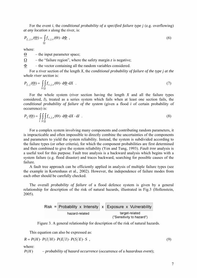
The overall probability of failure of a flood defence system is given by a general

relationship for description of the risk of natural hazards, illustrated in Fig.3 (Hollenstein, 2005).

Figure 3. A general relationship for description of the risk of natural hazards.

This equation can also be expressed as:

SESPIEPHIPHPR ⋅⋅⋅⋅= )()()()( , (9)

where: )(HP – probability of hazard occurrence (occurrence of a hazardous event);

7

)( HIP – probability of the hazard intensity (load), given the event; )( IEP – probability of exposure to the hazard (or failure, or a consequence occurrence),

given the intensity of the hazard (note that )( IEP = ); fP)( ESP – probability of a specific value of damage factor (or vulnerability, degree of loss,

damage ratio), given the failure of defence system; S – the consequence.

It should be noted that:

- The probability of exposure to a hazard, )( IEP , is a conditional probability! It is the probability that damage occurs (i.e. an object or a system is exposed to a hazard), given the occurrence of a hazard of a certain probability and intensity. Thus, the exposure to hazard relates to the probability of consequence occurrence.

- Human vulnerability to disaster contributes to the extent of the consequence itself. The probability of disaster occurrence, or the probability of consequence occurrence, PS,

can be defined as the product of the probabilities (Fig.4):

fS PHIPHPIEPHIPHPP ⋅⋅=⋅⋅= )()()()()( . (10)

Figure 4. Difference in definition of probabilities of

hazard occurrence and disaster occurrence. The following variables are used in the case of flood hazard:

H – the maximum discharge of a particular flood event, having a probability of *Qoccurrence ; *P

I – any variable representing load, say the water level *Z , corresponding to the flow discharge (Table 3); *Q

E – failure of the system (z < 0) due to the water level *Z (described by the condition: z = Zo – *Z < 0), or exceedance of the damage threshold,

so that:

*])0*(*[]*)0*[()**()**(*)**(*)(

SZZSPZZZPQZPPQPPRZSP

ooQP

⋅≤−⋅≤−⋅⋅⋅=4444444444444444 2144 344 21 3

, (11)

or:

8

*])0*(*[)**()**(*)**(

*

*)(

SZZSPPQZPPQPPRZSP

ofQP

⋅≤−⋅⋅⋅⋅=4444 34444 2144 344 21

, (12)

and: *

*)(

* )**()**(* fQP

S PQZPPQPPP ⋅⋅⋅=44 344 21

. (13)

The probabilities describe the following uncertainties:

*P - natural variability; )**( PQP - uncertainty in the discharge-probability relationship; )**( QZP - uncertainty in the stage-discharge relationship;

]*)0*[( ZZZP o ≤− - uncertainty in structural performance of defence system (uncertainty of damage threshold value);

])0*(*[ ≤− ZZSP o - uncertainty in the stage-damage relationship.

If no uncertainties are taken into account, then:

**** SPSPR S ⋅=⋅= . (14)

Therefore, the deterministic case can be defined as:

** PPS = , (15)

provided a flooding took place ( , or Z > Z1* =fP d). If it is assumed, for a moment, that there exist unique functions Q(P) and Z(Q), then:

1)**( =PQP ,

1)**( =QZP , and:

** * fS PPP ⋅= . (16)

Possibilities of performance of a flood defence system are shown in Table 4.

Table 4. A possible performance of a flood defence system.

Case Performance P* *fP *

SP S

Z* ≤ Zo no failure P* ≥ Po*fP = 0 *

SP = 0 S = 0

Zo < Z* ≤ Zd structural failure P* < Po 0 < < 1 *fP 0 < < P* *

SP S ≠ 0

Z* > Zd performance failure P* < Po*fP = 1 *

SP = P* S ≠ 0

Po – the probability of occurrence of the water level Zo

If the performance failure only is considered, then it means that the system is assumed to perform perfectly well until the overtopping occurs, that is Zo = Zd, so that the two states only are possible (Table 5).

9

Table 5. A possible performance of a flood defence system (the performance failure only is considered).

Case Performance P* *fP *

SP S

Z ≤ Zd no failure P* ≥ Po*fP = 0 *

SP = 0 S = 0

Z > Zd failure P* < Po*fP = 1 *

SP = P* S ≠ 0

Provided the expected damage Sj is defined for each type of failure j (having the probability of occurrence determined by Eq.7, then the expected damage Sjfi

P , i having a probability Pi can be estimated:

∑=

⋅=n

jjfji i

PSS1

, , . (17) ∑=

⋅≈⋅==n

jjfifiiSi ii

PPPPPP1

,****

,

By weighing values of Sj (the expected damage due to a specific failure type) by the corresponding probabilities ( ), a more accurate estimate of Sjfi

P , i can be provided (which is then to be used in Eq.3). 3.3. The procedure of flood damage assessment

A (socio-economic) system, exposed to a flood, is considered. Occurrence of a hazard results in an impact to the system, called load, which is proportional to the hazard intensity (i.e. the hazard magnitude and/or hazard duration). On the other hand, the exposure of the system to the hazard is an inverse function of the system resistance.

The standard procedure of flood damage assessment is illustrated in Fig.5. It should be noted that: - The hydrologic input is generally represented by the function Q(t), describing the whole

wave of a flood having the probability of occurrence P(Q) = P*. For simplicity, the maximum flow discharge, hereinafter noted as Q*, is used for representation of the flood wave.

- The load l is a measure of intensity of the flood hazard, and is a function of the maximum flow discharge Q*. For an event under consideration, the load l can be represented by one or more hydraulic parameters (Table 3), obtained on the basis of the flow simulation (flow depth or water stage, flow velocity, flood duration, flood water load such as sediment, salts, sewage, chemicals, etc.).

- The set of all possible cases of failure (for all the events causing the failure), defined by z < 0, is called failure region and accounts for failures due to different causes and at different places (i.e. river cross-sections) of the system. Obviously, the safety margin z is a measure of exposure to the hazard.

- The expected annual damage, S , is calculated using Eq.3. - By this procedure, the uncertainty due to natural variability of flow is taken into account. 3.4. Flood damage assessment under no uncertainty (damage due to performance failure only)

The procedure is illustrated in Fig.6. In this figure, load (or hazard intensity) is represented by the water stage, which is a typical case in damage assessment. In principle, any relevant parameter (Table 3) can be used in such an analysis, as well.

10

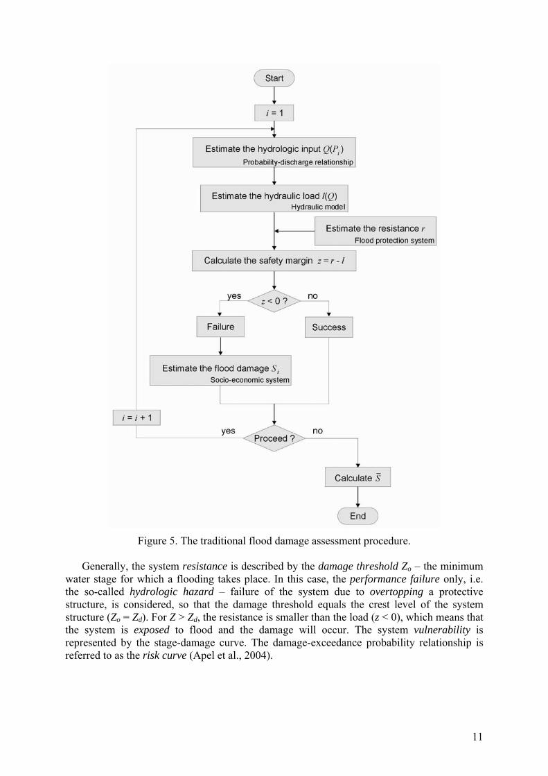
Figure 5. The traditional flood damage assessment procedure.

Generally, the system resistance is described by the damage threshold Zo – the minimum

water stage for which a flooding takes place. In this case, the performance failure only, i.e. the so-called hydrologic hazard – failure of the system due to overtopping a protective structure, is considered, so that the damage threshold equals the crest level of the system structure (Zo = Zd). For Z > Zd, the resistance is smaller than the load (z < 0), which means that the system is exposed to flood and the damage will occur. The system vulnerability is represented by the stage-damage curve. The damage-exceedance probability relationship is referred to as the risk curve (Apel et al., 2004).

11

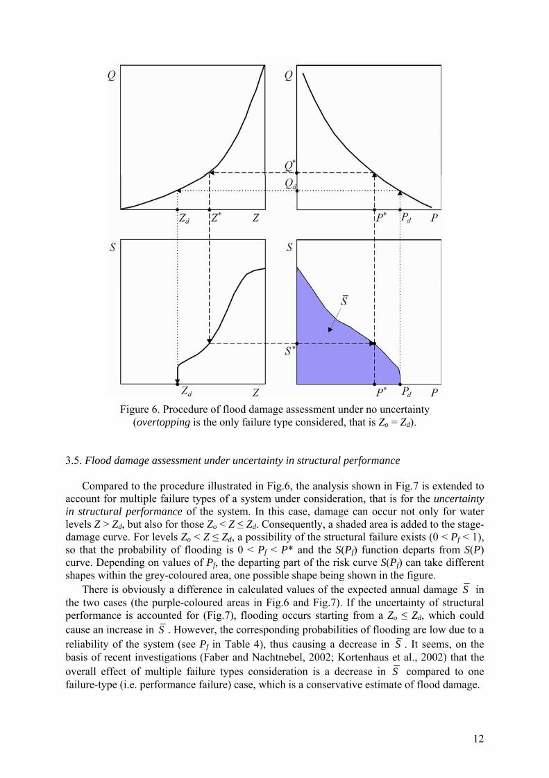
Figure 6. Procedure of flood damage assessment under no uncertainty

(overtopping is the only failure type considered, that is Zo = Zd). 3.5. Flood damage assessment under uncertainty in structural performance

Compared to the procedure illustrated in Fig.6, the analysis shown in Fig.7 is extended to account for multiple failure types of a system under consideration, that is for the uncertainty in structural performance of the system. In this case, damage can occur not only for water levels Z > Zd, but also for those Zo < Z ≤ Zd. Consequently, a shaded area is added to the stage-damage curve. For levels Zo < Z ≤ Zd, a possibility of the structural failure exists (0 < Pf < 1), so that the probability of flooding is 0 < Pf < P* and the S(Pf) function departs from S(P) curve. Depending on values of Pf, the departing part of the risk curve S(Pf) can take different shapes within the grey-coloured area, one possible shape being shown in the figure.

There is obviously a difference in calculated values of the expected annual damage S in the two cases (the purple-coloured areas in Fig.6 and Fig.7). If the uncertainty of structural performance is accounted for (Fig.7), flooding occurs starting from a Zo ≤ Zd, which could cause an increase in S . However, the corresponding probabilities of flooding are low due to a reliability of the system (see Pf in Table 4), thus causing a decrease in S . It seems, on the basis of recent investigations (Faber and Nachtnebel, 2002; Kortenhaus et al., 2002) that the overall effect of multiple failure types consideration is a decrease in S compared to one failure-type (i.e. performance failure) case, which is a conservative estimate of flood damage.

12

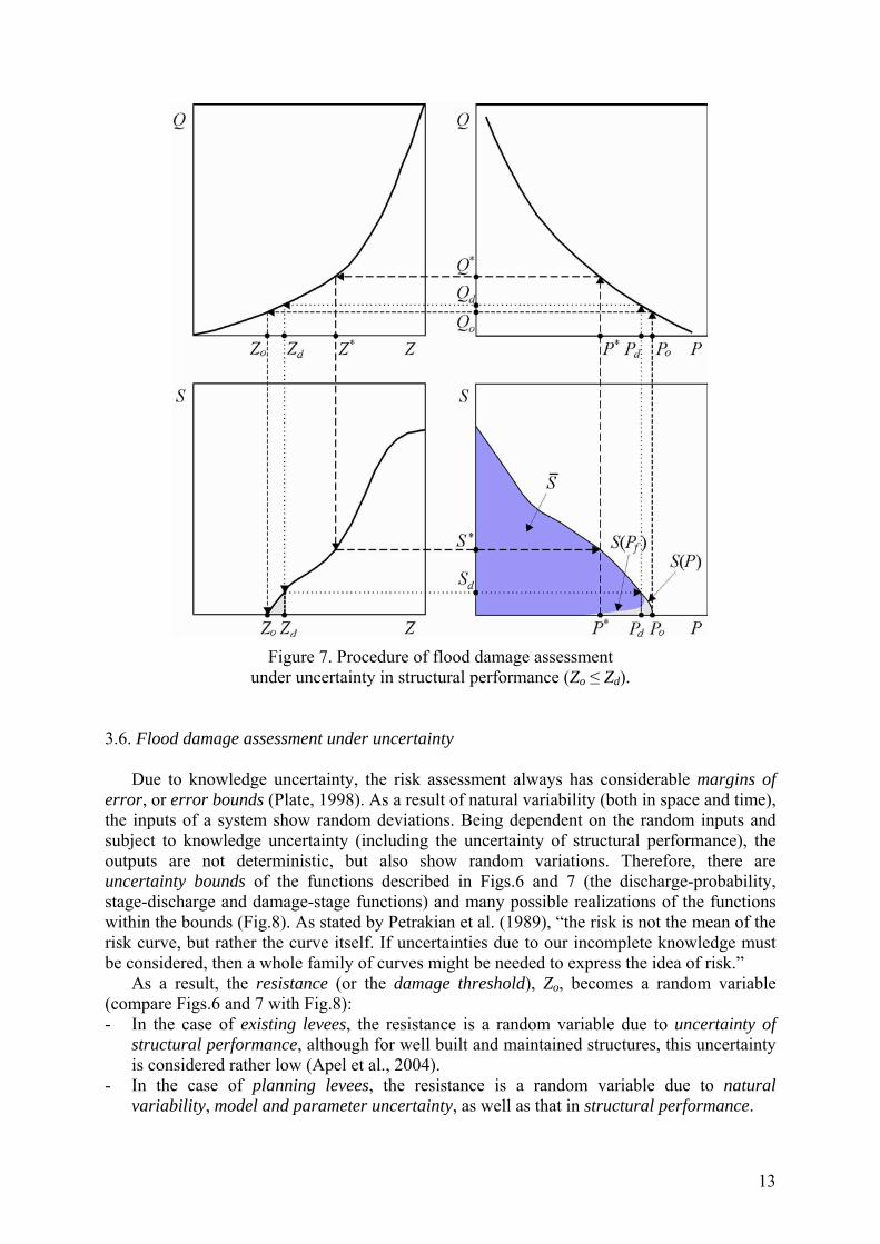
Figure 7. Procedure of flood damage assessment

under uncertainty in structural performance (Zo ≤ Zd). 3.6. Flood damage assessment under uncertainty

Due to knowledge uncertainty, the risk assessment always has considerable margins of error, or error bounds (Plate, 1998). As a result of natural variability (both in space and time), the inputs of a system show random deviations. Being dependent on the random inputs and subject to knowledge uncertainty (including the uncertainty of structural performance), the outputs are not deterministic, but also show random variations. Therefore, there are uncertainty bounds of the functions described in Figs.6 and 7 (the discharge-probability, stage-discharge and damage-stage functions) and many possible realizations of the functions within the bounds (Fig.8). As stated by Petrakian et al. (1989), “the risk is not the mean of the risk curve, but rather the curve itself. If uncertainties due to our incomplete knowledge must be considered, then a whole family of curves might be needed to express the idea of risk.”

As a result, the resistance (or the damage threshold), Zo, becomes a random variable (compare Figs.6 and 7 with Fig.8): - In the case of existing levees, the resistance is a random variable due to uncertainty of

structural performance, although for well built and maintained structures, this uncertainty is considered rather low (Apel et al., 2004).

- In the case of planning levees, the resistance is a random variable due to natural variability, model and parameter uncertainty, as well as that in structural performance.

13

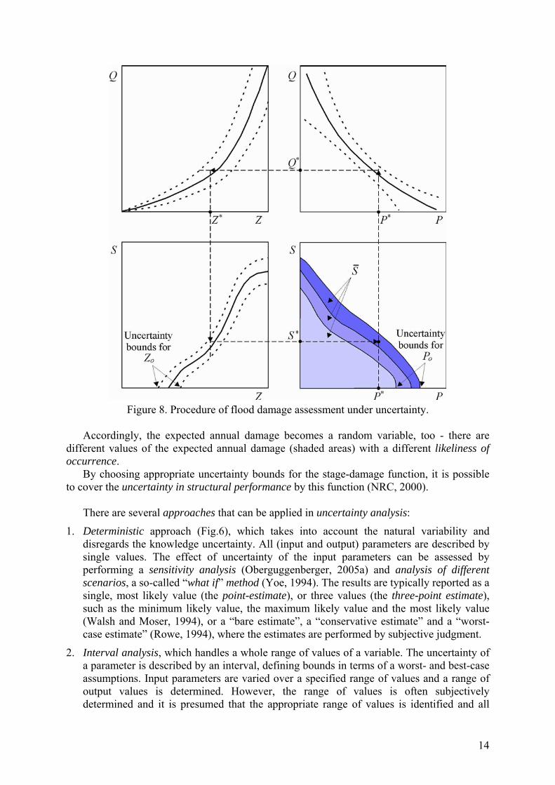
Figure 8. Procedure of flood damage assessment under uncertainty.

Accordingly, the expected annual damage becomes a random variable, too - there are

different values of the expected annual damage (shaded areas) with a different likeliness of occurrence.

By choosing appropriate uncertainty bounds for the stage-damage function, it is possible to cover the uncertainty in structural performance by this function (NRC, 2000).

There are several approaches that can be applied in uncertainty analysis:

1. Deterministic approach (Fig.6), which takes into account the natural variability and disregards the knowledge uncertainty. All (input and output) parameters are described by single values. The effect of uncertainty of the input parameters can be assessed by performing a sensitivity analysis (Oberguggenberger, 2005a) and analysis of different scenarios, a so-called “what if” method (Yoe, 1994). The results are typically reported as a single, most likely value (the point-estimate), or three values (the three-point estimate), such as the minimum likely value, the maximum likely value and the most likely value (Walsh and Moser, 1994), or a “bare estimate”, a “conservative estimate” and a “worst-case estimate” (Rowe, 1994), where the estimates are performed by subjective judgment.

2. Interval analysis, which handles a whole range of values of a variable. The uncertainty of a parameter is described by an interval, defining bounds in terms of a worst- and best-case assumptions. Input parameters are varied over a specified range of values and a range of output values is determined. However, the range of values is often subjectively determined and it is presumed that the appropriate range of values is identified and all

14

values in that range are equally likely. Although the total variability of the parameters can be captured, no detailed information on the uncertainty is provided.

3. Probabilistic approach, in which the uncertainty is described in the most informative, but also the most strict way – by means of probability. Input parameters are treated as random variables with known probability distributions, and the result is a probability distribution of an output parameter. However, disadvantages of this approach have been identified in many engineering applications, such as: - it generally requires much input data, often more than can be provided, so that

choosing a distribution and estimating its parameters are the critical factors (Ossenbruggen, 1994);

- it requires that probabilities of events considered have to sum up to 1; therefore, when additional events are taken into consideration, the probabilities of events change;

- probabilities have to be set up in a consistent way and thus do not admit incorporating conflicting information (which could make confusion about the statistical independen-ce of events).

4. Alternative approaches, based on the “imprecise probability”, in which some axioms of probability theory are relaxed (Oberguggenberger, 2005a; Oberguggenberger and Fellin, 2005): 4.1. Fuzzy set approach, in which the uncertainty is described as a family of intervals

parametrized in terms of the degree of possibility that a parameter takes a specified value. This approach admits much more freedom in modelling (for example, it is possible to mix fuzzy numbers with relative frequencies or histograms), and may be used to model vagueness and ambiguity. It is useful when no sufficient input data is available.

4.2. Random set approach, in which the uncertainty is described by a number of intervals, focal sets, along with their corresponding probability weights. For example, the focal sets may be estimates given by different experts and the weights might correspond to relative credibility of each expert. The probability weight could be seen as the relative frequency (histogram), however the difference is that the focal sets may overlap. This is the most general approach – every interval, every histogram, and every fuzzy set can be viewed as a random set.

The probabilistic and fuzzy approaches to uncertainty analysis in flood risk assessment

will be described in the following text. 3.6.1. Probabilistic approach

The main objective of the probabilistic approach to risk assessment is to describe the uncertainties of input parameters in terms of probabilities (Fig.9), in order to define a probability distribution of the output, that is, of the expected annual damage (Fig.10).

Different measures exist to describe the degree of uncertainty of a parameter, function, a model, or a system (Tung and Yen, 1993): - The probability density function (PDF) of the quantity subject to uncertainty. It is the most

complete description of uncertainty. However, in most practical problems such a function can not be derived or found precisely.

- A reliability domain, such as the confidence interval. The related problems include that: 1. the parameter population may not be normally distributed as usually assumed; 2. there are no means to combine directly the confidence intervals of random input

15

variables to give the confidence interval of the output.

- Statistical moments of the random variable. For example, the second moment is a measure of dispersion of a random variable.

Figure 9. Probabilistic approach to uncertainty analysis.

Figure 10. Probability density function of the expected annual damage.

16

There are the following methods of probabilistic uncertainty analysis (Yen and Tung, 1993): - Analytical methods, deriving the PDF of model output analytically as a function of the

PDFs of input parameters. - Approximation methods (or parameter estimation methods):

1. methods of moments (e.g. first-order second-moment methods, second-order method); 2. simulation or sampling (e.g. Monte Carlo simulation); 3. integral transformation techniques (Fourier transform, Laplace transform).

Theoretically, the statistical moments can be obtained by integrating the performance function with the distribution range of the random input variables. In practice, the integration is usually approximated using point-estimate methods, Taylor series approximations or simulation methods (Leggett, 1994). In these methods, probability distributions of the random variables are replaced by means and standard deviations of the random variables. The approximate integration is achieved by performing repetitive, deterministic analyses using various possible combinations of values of the random variables.

Some of the methods, relevant for flood risk assessment, will be described in the following text.

It should be noted that:

- Indices of S refer to probability of exceedance (95%, 50%, and 5%), and the probability density function (Fig.10) is related to probability of non-exceedance (the corresponding values being 5%, 50%, and 95%, respectively).

- The expectation of S reflects only natural variability, the probability distribution of S (Fig.10) reflects only knowledge uncertainty (NRC, 2000).

- The uncertainty in structural performance can be included in the stage-damage curve or can be introduced in the simulation as an independent function connecting the conditional probability of failure, Pf, with the probability of hazard occurrence, P* (NRC, 2000). In the latter case, it is necessary to calculate the overall probability of failure, Pf, using Eq.8.

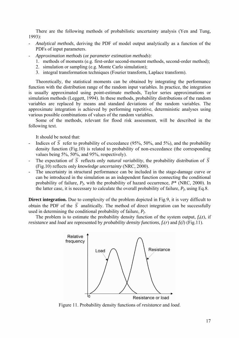
Direct integration. Due to complexity of the problem depicted in Fig.9, it is very difficult to obtain the PDF of the S analitically. The method of direct integration can be successfully used in determining the conditional probability of failure, Pf.

The problem is to estimate the probability density function of the system output, fz(z), if resistance and load are represented by probability density functions, fr(r) and fl(l) (Fig.11).

Figure 11. Probability density functions of resistance and load.

17

In a general case, the function fl(l) overlaps fr(r) to some extent, due to variances of both functions (as a result of uncertainties). This indicates a possibility that load may exceed resistance of the system (r – l < 0), even though the expected value of resistance is greater than the expected value of load, )()( lErE − > 0.

The probability density function of safety margin, fz(z), is a useful means for analyzing reliability of a system (Fig.12). In case the function fl(l) overlaps fr(r), as shown in Fig.11, a part of the function fz(z) extends to the region where z < 0 (Fig.12).

Figure 12. Probability density function of safety margin.

The probability density function of the safety margin provides an explicit characterization

of expected system performance. As mentioned before, failure of a system (which refers to any occurrence of an adverse event under consideration), takes place if z < 0. So, the probability of failure given the load l, Pf, , can be expressed as:

∫∞−

⋅=≤=0

d)(0 zzfzPP zf , (18)

and the probability of success (reliability) of the system (or the probability that the system will not be exposed to hazard), Rf, as:

fzf PzzfzPR −=⋅=>= ∫∞

1d)(00

. (19)

If r and l are assumed to follow the normal probability distribution, then z is also normally

distributed, and the functions fr(r), fl(l) and fz(z) can be described by a well-known formula, which, for the safety margin z, has the following form:

2

2

2)]([

21)( z

zEz

zz ezf σ⋅

−−

⋅π⋅σ

= , (20)

A parameter of the distribution, σz (standard deviation of z), can be defined as:

lrlrz σ⋅σ⋅⋅−σ+σ=σ r222 , (21)

18

where σr and σl – standard deviations of r and l, respectively; r – correlation coefficient, (if r and l are not correlated, r = 0). 1 r 1− ≤ ≤ +

Another parameter of the distribution, (expected value of z), depends on the formulation of z (Yen and Tung, 1993):

)(zE

1. z = r – l (then ); )()()( lErEzE −=

2. z = f – 1 ;

3. z = ln f ,

where f is the factor of safety:

ll

rr

upper

lower

nlEnrE

lr

fσ⋅+σ⋅−

==)()( , (22)

where rlower – conservative estimate of the resistance, lupper – liberal estimate of the load, nc and nd – sigma units for resistance and load, respectively, or:

)()( lErEff c == , (23)

where fc is the central factor of safety.

The major limitation of using fc is that variance of the distributions is not considered. Therefore, the preferred procedure is to use the factor of safety according to Eq.22, which reduces the resistance as a function of the standard deviation in order to obtain a conservative estimate of the resistance, and a higher than average load is used to define a worst-case condition.

It is useful to address the following equivalencies, which exist between the terms used in

reliability engineering and cost-benefit analyses:

safety margin = benefit – cost = the net benefit

central factor of safety = benefit / cost = the cost-effectiveness

Method of moments (first-order second-moment methods). The first-order second-moment method estimates uncertainty in terms of the variance of system output using variances of contributing factors. The load and resistance functions are expanded in Taylor series at a reference point (about the expected values of input variables) and the second and higher-order terms in the series expansion are truncated, resulting in an approximation involving only the first two statistical moments of the variables (the expected value and the standard deviation).

This simplification greatly enhances the practicality of the method because it is often difficult to find the PDF of the variable and relatively simple to estimate the first two statistical moments – either by calculating them from data, or by estimating them from experience (USACE, 1995b).

Once the expected value and variance of z are estimated, an another useful indicator of system performance, the reliability index, can be defined as:

zzE σ=β )( . (24)

It is a measure of the distance between the expected value of z and the limit state z = 0 (the number of standard deviations by which the expected value of a normally distributed performance function exceeds zero). It is a measure of reliability of an engineering system

19

that reflects both mechanics of the problem and the uncertainty in the input variables. Formally, it is not necessary to assume or determine the shape of the probability function (which is necessary to calculate an exact value of the probability of achieving the limit state), to be able to define the reliability index. Values of the reliability index are not absolute measures of probability, but are used as a relative measure of reliability or confidence in the ability of a structure to perform its function in a satisfactory manner.

The probability of failure, associated with the reliability index, is a probability per structure – it has no time-frequency basis. Once a structure is constructed or loaded as modelled, it either performs satisfactorily or not (USACE, 1995b).

It is noted that, especially for low probability events, the probability of failure is a rather poor indicator of performance. In these cases, the risk is an important additional indicator (Plate, 1993).

Simulation (Monte Carlo simulation). The most commonly used procedure for risk assessment under uncertainty is Monte Carlo simulation. It has been succesfully applied in flood risk analyses (Moser, 1994; Faber and Nachtnebel, 2002; Kortenhaus et al., 2002; Apel et al., 2004).

Monte Carlo simulation is a method to estimate the statistical properties of a random variable that is related to a number of random variables which may or may not be correlated (Yen and Tung, 1993). The method is useful when the direct calculation of probability functions is complicated (Ossenbruggen, 1994). The values of stochastic input parameters (random numbers) are generated according to their distributional properties (i.e. to the specifed probability laws). Theoretically, each uncertain parameter can be introduced as a random number (Faber and Nachtnebel, 2002). The input probability distributions are repeatedly sampled in order to derive the PDF of the output. Expressing uncertainty in terms of probability distributions is an essential step (Yoe, 1994).

The input required for performing the simulation are the means and standard deviations for the input variables (flow discharge, water stage and flood damage, see Fig.9). As mentioned before, the means and standard deviations as a measure of uncertainty can be quantified through statistical analysis of existing data, or judgmentally assigned (USACE, 1995b). For example, for the purpose of uncertainty analysis in flood risk assessment, recommendations on standard deviations of flow-frequency, flow-stage and damage-stage functions can be found in literature (Davis and Burnham, 1994; Moser, 1994).

The Monte Carlo simulation routine randomly samples a discharge over a range of frequencies and within the confidence bands of the discharge-frequency curve. At that discharge, the routine then samples between the upper and lower confidence bands of the stage-discharge curve and randomly chooses a stage. At that stage, the routine samples between the upper and lower confidence bands of the stage-damage relationship and chooses a corresponding damage. This process is repeated until a statistically representative sample is developed.

The Monte Carlo simulation can be applied for estimating the conditional probability of failure of a flood defence system, as well. In this case, the generated input parameter values are used to compute the value of the performance function z. After a large number of simulated realizations of z are generated, the reliability of the structure can be estimated by computing the ratio of number of realizations with to the total number of simulated realizations. This procedure enables all possible failure modes to be considered (Kortenhaus et al., 2002).

0≥z

A detailed description of the procedure can be found in literature (USACE, 1996c; NRC, 2000). An example is given in Appendix, at the end of this document.

20

Conclusions. The main features of the probabilistic approach are the following:

- Knowledge uncertainty is quantified and explicitly included in evaluating project performance and benefit (USACE, 1995b);

- This approach allows for several types of failures of the system to be considered, provided the safety margin of each of them is represented by a specific probability density function;

- Each uncertain parameter can be introduced into analysis by means of their probability distributions.

- The actual probability of failure or reliability is used as a measure of performance of a system, rather than some empirical rule (Plate, 1993; Davis and Burnham, 1994).

- Engineering and economic performance of a project can be expressed in terms of probability distributions (USACE, 1996a),

- The following indicators of engineering performance can be determined (USACE, 1995c, 1996c): the expected annual exceedance probability, the expected lifetime exceedance probability (or long-term risk), the conditional annual probability of non-exceedance, given the occurrence of an event.

- A solid database is required in order to perform a probabilistic analysis. An example is illustrated in a paper by Mai and von Lieberman (2000), where two internet-based atlases, containing a collection of hydraulic loads and information on resistance of protection structures (including the information on land use of the protected area), were used as a source for analysis of different scenarios of failure of the system.

Deterministic approach. It can be concluded that the deterministic approach is a special case of the probabilistic one, for which:

- No (knowledge) uncertainty is taken of the discharge-probability curve ( 1)**( =PQP ). The expected value of discharge, E(Q), is used, given the probability of occurrence.

- No uncertainty is taken of the stage-discharge curve ( 1)**( =QZP ). Consequently, the expected value of the water stage, E(Z), is used, given the flow discharge.

- No uncertainty in structural performance is taken into account (Zo = Zo = Zd). The only failure mode considered is the hydrologic hazard. This is based on a simplified concept that the flood defence system will fail (Pf = 1) only in case of occurrence of the water levels Z > Zd, due to overtopping of the protective structure, whereas it will work perfectly well (Pf = 0) during more frequent flood events, Z < Zd. As a result, the expected value of resistance, E(Zd), is used, given the water level Z. The system resistance is a deterministic quantity.

- Finally, the expected value of the safety margin, E(z), is used, with no regard to its probability distribution. So, the user of numerical models does not know how large the safety margin of the deterministic results is. In other words, the probability of failure of the system, Pi, which is used in design, is based on the expected values of resistance and load, with no regard of their variances (distributions). However, even if the > 0, there is still a chance for r – l < 0 (for failure to occur), if the functions p

)()( lErE −z(r) and pz(l)

overlap to some extent (Figs.11 and 12). - No uncertainty is taken of the stage-damage curve ( 1)**( =ZSP ). Consequently, the

expected value of damage, E(S), is used, given the flood water level. - The probability (i.e. ) of occurrence of a consequence (of the damage SiP *

,iSP i), is taken equal to the probability of occurrence of a flood, P*, which will cause the overtopping (see Eqs.14 and 15). Hence, this approach is based on an implicit assumption that every hazard will create a consequence (i.e. hazard = disaster). In practice, it means that a probability of a flood event is adopted a priori, and the corresponding consequence

21

(damage) is assessed (NRC, 2000). However, the probability of consequence may be higher (or lower) due to the uncertainty. For example, if a levee is designed on the basis of the 100-year flood event, a probability exists that failure will take place on occurrence of the very same (or even lesser) flood event (e.g. due to inaccurate estimate of probability of occurrence of the design flood event, due to dike-breach, etc.).

- The output from the calculations is a composite of assumed reasonable and worst-case values, which does not provide any illustration of the probabilistic density function of the output, pz(z). Estimates of variables, factors and parameters are considered the “most likely” values (USACE, 1996a). However, there is no indication on the probability that the calculated expected annual damages will not be exceeded (NRC, 2000). Traditionally, the uncertainty is considered (Davis and Burnham, 1994):

- by application of professional judgment - conducting sensitivity analysis - by the addition of freeboard (in the case of levees/flood walls).

This problem is conventionally overcome by developing conservative designs, using a

safety factor (USACE, 1995b). For instance, when constructing a levee, a freeboard is added to the design water level, which accounts for all influences and uncertainties neglected by the model. An alternative is to define the actual safety level, and use it, instead of the design safety level, to determine Pi. The actual safety level is obtained by multiplying the design safety with reduction factors, which account for the following factors (van der Vat et al., 2001): the quality of the design and construction of the dike, its maintenance, chance of failure of operation of essential structures, reduced capacity of the river section due to sedimentation, etc.

The safety concept has short-comings as a measure of the relative reliability of a system for different performance modes. A primary defficiency is that parameters must be assigned single values, although the appropriate values may be uncertain. The safety factor thus reflects (USACE, 1995b): - the condition of the feature; - the engineer´s judgment; - the degree of conservatism incorporated into the parameter values.

From the standpoint of the engineering performance, the freeboard approach provides

(NRC, 2000): - inconsistent degrees of flood protection to different communities, and - different levels of protection in different regions.

Nevertheless, there are still several advantages of the deterministic approach:

- simplicity (avoiding the issue of dealing with probabilistic evaluations), - level of risk acceptability is implied within engineering standards, - legal liability is clear, - cost-effectiveness in terms of project study costs. For these reasons, it is still commonly used in practice.

22

3.6.2. Fuzzy set approach

Several shortcomings have been identified in the probabilistic approach to risk assessment and the formulation of the expected annual damage (Bogardi and Duckstein, 2003): - the analysis of low-failure-probability/high-consequence events may be misrepresented by

the expected value; - the selection of the probability distribution, the two PDF’s, is often arbitrary, while results

may be sensitive to this choice; - statistical data on load and resistance are often lacking; - the consequence functions are often quite uncertain; - the covariances among the various types of loads and resistances and the parameters

involved in their estimation are commonly unknown; the results are, again, highly sensitive in this respect. Obviously, the probabilistic formulation may have difficulties when no sufficient

statistical data are available (Bogardi and Duckstein, 2003). However, the size of the sample of data is commonly small and the data are often augmented by prior expert knowledge (Oberguggenberger and Russo, 2005). This necessitates the development of more flexible tools for assessing and processing subjective knowledge and expert estimates (Fetz, 2005; Fetz et al., 2005; Oberguggenberger, 2005b).

In such a case, the fuzzy set formulation appears to be a practical alternative having a number of advantages: - fuzzy sets and fuzzy numbers may be used to characterize input uncertainty whenever

variables (and/or relationships) are not defined precisely; - fuzzy arithmetic is considerably simpler and more manageable than the algebra of random

numbers (Ganoulis et al., 1991); - fuzzy set analysis can be used with very few and weak prerequisite assumptions (if

hypotheses are considerably weaker than those of the probability theory); - in probability theory, functions of random variables are again random variables; in fuzzy

set theory, computability is guaranteed. A detailed description of the procedure can be found in Appendix, at the end of this

document. The procedure of flood damage assessment under uncertainty, based on the fuzzy set

approach, is schematically illustrated in Figs.13 and 14. Several illustrative examples of application of the fuzzy set approach to risk assessment

and reliability analysis can be recommended: - groundwater contamination (Bogardi et al., 1989); - water resources and environmental engineering (Ganoulis et al., 1991); - flood management (Bogardi and Duckstein, 2003).

23

Figure 13. Fuzzy set approach to uncertainty analysis.

Figure 14. Membership function of the expected annual damage.

24

4. References Apel, H., Thieken, A.H., Merz, B., Blöschl, G., 2004, Flood risk assessment and associated

uncertainty, Natural Hazards and Earth System Sciences, European Geosciences Union, Vol.4, 295-308.

Bogardi, I., Duckstein, L., 1989, Uncertainty in environmental risk analysis, in: Risk analysis and management of natural and man-made hazards, Haimes, Y.Y. and Stakhiv, E.Z. (Ed.), ASCE, 154-174.

Bogardi, I., Duckstein, L., 2003, The fuzzy logic paradigm of risk analysis, in: Risk-based decision making in water resources X, Haimes, Y.Y., Moser. D.A., Stakhiv, E.Z., (Eds.), ASCE, 12-22.

Davis, D., Burnham, M.W., 1994, Risk-based analysis for flood damage reduction, in: Risk-based decision making in water resources VI, Haimes, Y.Y., Moser. D.A., Stakhiv, E.Z., (Eds.), ASCE, 194-200.

Faber, R., Nachtnebel, H.-P., 2002, Flood risk assessment in urban areas: development and application of a stochastic hydraulic analysis method considering multiple failure types, in: Proceedings of the Second Annual IIASA-DPRI Meeting, Integrated Disaster Risk Management, Linnerooth-Bayer, J. (Ed.), Laxenburg, Austria, 8 pp.

Fetz, T., 2005, Multi-parameter models: rules and computational methods for combining uncertainties, in: Analyzing Uncertainty in Civil Engineering, Fellin, W., Lessmann, H., Oberguggenberger, M., Vieider, R. (Eds.), Springer, Berlin, Germany, 73-99.

Fetz, T., Jäger, J., Köll, D., Krenn, G., Lessmann, H., Oberguggenberger, M., Stark, R.F., 2005, Fuzzy models in geotechnical engineering and construction management, in: Analyzing Uncertainty in Civil Engineering, Fellin, W., Lessmann, H., Oberguggenberger, M., Vieider, R. (Eds.), Springer, Berlin, Germany, 211-239.

Ganoulis, J., Duckstein, L., Bogardi, I., 1991, Risk analysis of water quantity and quality problems: the engineering approach, in: Water resources engineering risk assessment, Ganoulis, J., (Ed.), NATO ASI Series, Vol.629, Springer, 3-17.

Hollenstein, K., 2005, Reconsidering the risk assessment concept: Standardizing the impact description as a building block for vulnerability assessment, Natural Hazards and Earth System Sciences, European Geosciences Union, Vol.5, 301-307.

Kortenhaus, A., Oumeraci, H., Weissmann, R. Richwien, W., 2002, Failure mode and fault tree analysis for sea and estuary dikes, Proc. International Conference on Coastal Engineering (ICCE), No.28, Cardiff, Wales, UK, 13 pp.

Leggett, M.A., 1994, Reliability-based Assessment of Corps Structures, in: Risk-based decision making in water resources VI, Haimes, Y.Y., Moser. D.A., Stakhiv, E.Z., (Eds.), ASCE, 73-81.

Mai, S., von Lieberman, N., 2000, Internet-based tools for risk assessment for coastal areas, Proc. of the 4th Int. Conf. On Hydroinformatics, Iowa, USA.

Moser, D.A., 1994, Quantifying flood damage uncertainty, in: Risk-based decision making in water resources VI, Haimes, Y.Y., Moser. D.A., Stakhiv, E.Z., (Eds.), ASCE, 194-200.

NRC (National Research Council), 2000, Risk Analysis and Uncertainty in Flood Damage Reduction Studies, National Academy Press, Washington, D.C., 202 pp.

Oberguggenberger, M., 2005a, The mathematics of uncertainty: models, methods and interpretations, in: Analyzing Uncertainty in Civil Engineering, Fellin, W., Lessmann, H., Oberguggenberger, M., Vieider, R. (Eds.), Springer, Berlin, Germany, 51-72.

Oberguggenberger, M., 2005b, Queueing models with fuzzy data in construction management, in: Analyzing Uncertainty in Civil Engineering, Fellin, W., Lessmann, H., Oberguggenberger, M., Vieider, R. (Eds.), Springer, Berlin, Germany, 197-210.

25

Oberguggenberger, M., Fellin, W., 2005, The fuzziness and sensitivity of failure probabilities, in: Analyzing Uncertainty in Civil Engineering, Fellin, W., Lessmann, H., Oberguggen-berger, M., Vieider, R. (Eds.), Springer, Berlin, Germany, 33-49.

Oberguggenberger, M., Russo, F., 2005, Fuzzy, probabilistic and stochastic modelling of an elastically bedded beam, in: Analyzing Uncertainty in Civil Engineering, Fellin, W., Lessmann, H., Oberguggenberger, M., Vieider, R. (Eds.), Springer, Berlin, Germany, 183-196.

Ossenbruggen, P.J., 1994, Fundamental principles of systems analysis and decision-making, John Wiley & Sons, Inc., New York, 412 pp.

Petrakian, R., Haimes, Y.Y., Stakhiv, E., Moser, D.A., 1989, Risk analysis of dam failure and extreme floods, in: Risk analysis and management of natural and man-made hazards, Haymes, Y.Y. and Stakhiv, E.Z. (Eds.), ASCE, 81-122.

Plate, E., 1993, Some remarks on the use of reliability analysis in hydraulic engineering applications, in: Reliability and uncertainty analysis in hydraulic design, Yen, B.C., Tung, Y.-K., (Eds.), ASCE, 5-15.

Plate, E., 1998, Flood risk management: a strategy to cope with floods, in: The Odra/Oder flood in summer 1997: Proceedings of the European expert meeting in Potsdam, 18 May 1998, Bronstert, A., Ghazi, A., Hladny, J., Kundzewicz, Z., Menzel, L. (Eds.), Potsdam institute for climate impact research, Report No.48, 115-128.

Rowe, W.D., 1994, Uncertainty versus computer response time, in: Risk-based decision making in water resources VI, Haimes, Y.Y., Moser. D.A., Stakhiv, E.Z., (Eds.), ASCE, 263-273.

Tung, Y.-K., Yen, B.C., 1993, Some recent progress in uncertainty analysis for hydraulic design, in: Reliability and uncertainty analysis in hydraulic design, Yen, B.C., Tung, Y.-K., (Eds.), ASCE, 17-34.

USACE, 1995b, Introduction to Probability and Reliability Methods for Use in Geotechnical Engineering, Technical Letter, ETL 1110-2-547, Washington, D.C.

USACE, 1995c, Hydrologic Engineering Requirements for Flood Damage Reduction Studies, Manual, EM 1110-2-1419, Washington, D.C.

USACE, 1996a, Risk-based Analysis for Evaluation of Hydrology/Hydraulics, Geotechnical Stability, and Economics in Flood Damage Reduction Studies, Engineer Regulation, ER 1105-2-101, Washington, D.C.

USACE, 1996c, Risk-based Analysis for Flood Damage Reduction Studies, Manual, EM 1110-2-1619, Washington, D.C.

van der Vat, M., Hooijer, A., Kerssens, P., Li, Y., Zhang, J., 2001, Risk assessment as a basis for sustainable flood management, Proceedings of the XXIX IAHR Congress, Beijing, China, 7 pp.

Walsh, M.R., Moser, D.A., 1994, Risk-based budgeting for maintenance dredging, in: Risk-based decision making in water resources VI, Haimes, Y.Y., Moser. D.A., Stakhiv, E.Z., (Eds.), ASCE, 234-242.

Yen, B.C., Tung, Y.-K., 1993, Some recent progress in reliability analysis for hydraulic design, in: Reliability and uncertainty analysis in hydraulic design, Yen, B.C., Tung, Y.-K., (Eds.), ASCE, 35-79.

Yoe, C., 1994, Development in risk analysis commercial software, in: Risk-based decision making in water resources VI, Haimes, Y.Y., Moser. D.A., Stakhiv, E.Z., (Eds.), ASCE, 243-262.

26

Appendix

Application of stochastic models to uncertainty analysis in risk assessment

1. Introduction There are many different ways to make a mathematical model. A common one is to make a, so called, deterministic model (Fig.1). That means that the model consists of a system of equations, and has a number of input parameters which, on application of the equations, provide output values. Deterministic model gives the same result no mater how many times the model is simulated, as long as the input parameter values are the same. Only change of input parameters may change the result.

Figure 1: Schematisation of a model with a three-component input vector

X = [x1, x2, x3], and a two-component output vector Y = [y1, y2]. The other type of mathematical model is a stochastic model. The main difference between the deterministic and stochastic models is that the input parameters of a model are not exact, precise values, but random, uncertain values, usually presented as statistical distributions, fuzzy sets, or intervals. As opposed to deterministic models, stochastic models have different result every time the model output is evaluated (Fig.2). That is the consequence of random input variables.

Figure 2: Uncertain input and output parameters.

27

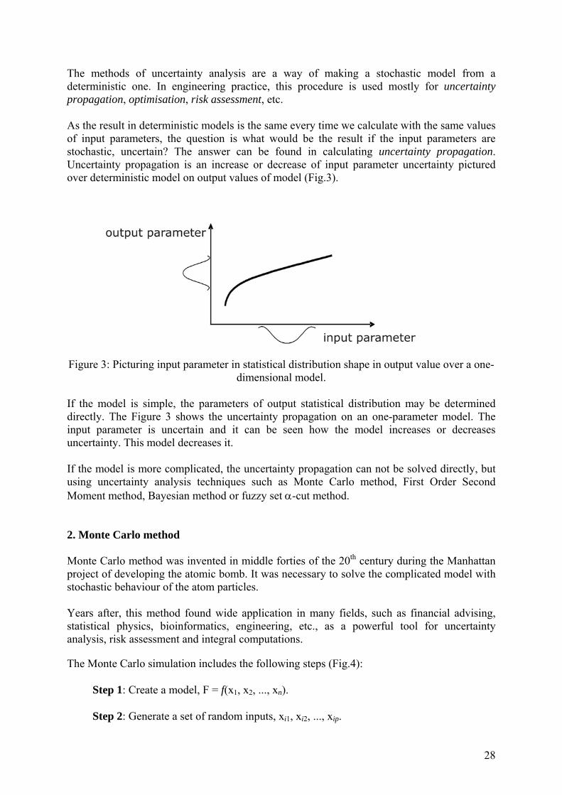
The methods of uncertainty analysis are a way of making a stochastic model from a deterministic one. In engineering practice, this procedure is used mostly for uncertainty propagation, optimisation, risk assessment, etc. As the result in deterministic models is the same every time we calculate with the same values of input parameters, the question is what would be the result if the input parameters are stochastic, uncertain? The answer can be found in calculating uncertainty propagation. Uncertainty propagation is an increase or decrease of input parameter uncertainty pictured over deterministic model on output values of model (Fig.3).

Figure 3: Picturing input parameter in statistical distribution shape in output value over a one-

dimensional model. If the model is simple, the parameters of output statistical distribution may be determined directly. The Figure 3 shows the uncertainty propagation on an one-parameter model. The input parameter is uncertain and it can be seen how the model increases or decreases uncertainty. This model decreases it. If the model is more complicated, the uncertainty propagation can not be solved directly, but using uncertainty analysis techniques such as Monte Carlo method, First Order Second Moment method, Bayesian method or fuzzy set α-cut method. 2. Monte Carlo method Monte Carlo method was invented in middle forties of the 20th century during the Manhattan project of developing the atomic bomb. It was necessary to solve the complicated model with stochastic behaviour of the atom particles. Years after, this method found wide application in many fields, such as financial advising, statistical physics, bioinformatics, engineering, etc., as a powerful tool for uncertainty analysis, risk assessment and integral computations. The Monte Carlo simulation includes the following steps (Fig.4):

Step 1: Create a model, F = f(x1, x2, ..., xn).

Step 2: Generate a set of random inputs, xi1, xi2, ..., xip.

28

Step 3: Simulate the model and store the results as yi.

Step 4: Repeat steps 2 and 3 for i = 1 to n.

Step 5: Analyze the results (array F = [y1, y2, …, yp]).

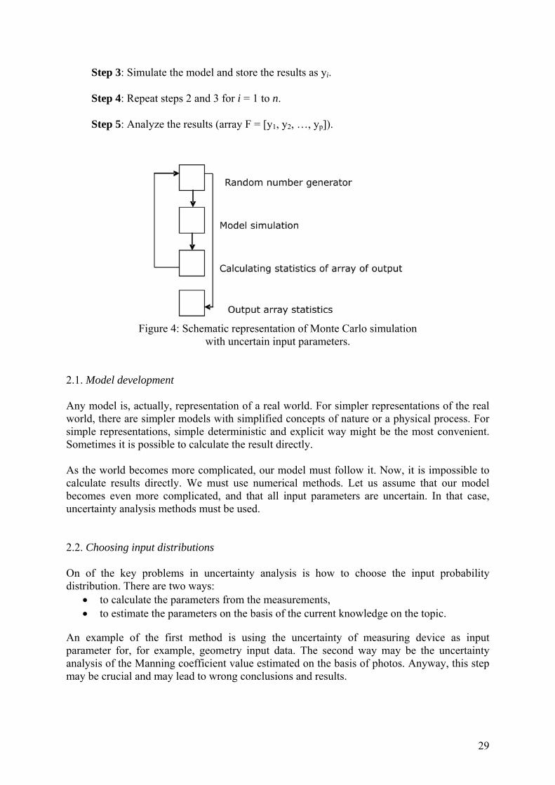
Figure 4: Schematic representation of Monte Carlo simulation with uncertain input parameters.

2.1. Model development Any model is, actually, representation of a real world. For simpler representations of the real world, there are simpler models with simplified concepts of nature or a physical process. For simple representations, simple deterministic and explicit way might be the most convenient. Sometimes it is possible to calculate the result directly. As the world becomes more complicated, our model must follow it. Now, it is impossible to calculate results directly. We must use numerical methods. Let us assume that our model becomes even more complicated, and that all input parameters are uncertain. In that case, uncertainty analysis methods must be used. 2.2. Choosing input distributions On of the key problems in uncertainty analysis is how to choose the input probability distribution. There are two ways:

• to calculate the parameters from the measurements, • to estimate the parameters on the basis of the current knowledge on the topic.

An example of the first method is using the uncertainty of measuring device as input parameter for, for example, geometry input data. The second way may be the uncertainty analysis of the Manning coefficient value estimated on the basis of photos. Anyway, this step may be crucial and may lead to wrong conclusions and results.

29

2.3. Way of sampling and statistics of output Sampling may be the crucial thing in choosing Monte Carlo as an uncertainty analysis method. An unintentional sampling is often quite demanding in CPU time, which is the most important when time-consuming models are simulated. Although plain sampling is the most accurate, for an economical use of Monte Carlo method several sampling methods were developed to achieve faster convergence. 2.4. Statistics of the Monte Carlo output Output statistics are the post-processing of the method. In statistical parameters estimation, crucial ones are the main statistical moments of a statistical distribution – the mean value and the variance/standard deviation.

2.5. Example of risk assessment – the case of the river Jadar (Serbia) River Jadar is a small watercourse flowing through the western part of Serbia. Due to urbanization and diferent agricultural activities, the land-use of riparian land is highly variable during one year and not the same over years. Within the flood risk assessment study, it was attempted to analyse risk of flooding under uncertainty of the Manning coefficient values in the main channel and floodplains. The uncertain parameter was chosen to be represented by means of statistical distribution. The analyzed section of the river Jadar was of 1650 m in length. For the purpose of one-dimensional flow modelling, 15 cross-sections were defined (Figs.5 and 6). As the flow is subcritical, the critical depth in the most downstream cross-section was assumed as boundary condition. The flow discharge was Q=147 m3/s. The water level in a chosen cross-section was analyzed under uncertainty of the input Manning roughness coefficient values of the main channel and inundation areas. The main channel river bed consists of gravel. The uncertainty of the Manning value was described by the normal distribution with parameters N(0.04,0.0052). Floodplains at the section considered are covered mainly with crops and there are locally bushes and trees. Accordingly, the normal distribution with parameters N(0.08,0.0052) was chosen (Fig.7). A set of 100 simulations were necessary until the statistical parameters of the output value (the water level) stabilized. The results are shown in Figs.8 and 9. The parameters of a statistical distribution of water depth in the cross-section of interest were µ = 3.49 m and σ = 0.053 m.

30

Figure 5: Perspective view of flooded floodplains at a section of the river Jadar.

Figure 6: The section of the river Jadar under consideration.

Figure 7: Schematic representation of main channel and inundation areas.

31

Figure 8: Monte Carlo simulation on a diagram.

Figure 9: Statistical distribution of the water level in the control cross-section. 3. Fuzzy set method Sometimes there is a need for making a subjective decision or estimation on some occurrence or a process. In rare occasions it is possible to give strict and direct acts and to be sure about them. Usually there is a want for soft boundaries of acts. Not to be so strict and precise. Usually it is not good to say YES or NO, but words MAYBE, ALMOST or POSSIBLY would give the best representation of a situation, and the best explanation about the decision. Although it is a common way in real life, there should be a way to mathematically express that kind of situation. Fuzzy sets and fuzzy logic is one way. History of fuzzy sets begins in 1965, in the system theory (Zadeh). Defining a new way of managing the industry, he developed the way of decision making more familiar to humans. The first application of fuzzy sets was in the system theory, and after that it found its place in the variety of fields like decision-making, conflict resolving, and uncertainty analysis.

32

Nowadays, even trains and wash machines have fuzzy set controllers for better braking or a better exploitation of the resources. Fuzzy set is a set of values without defined strict boundaries. Despite regular sets, fuzzy set does not have just 1 and 0 as representative marks for an element belonging and not belonging to the set, but have the interval for evaluating the belonging to a set. That means that the belonging or belonging may be represented with a number like 0.2, 0.3, 0.9 or any else. So, fuzzy sets are a further development of the mathematical concept of a set. If the largest value that represents belonging is 1, then the fuzzy set is standardized (Fig.10). The set may be standardized by dividing each belonging value with the largest belonging in the set. Standardized sets are compatible with each other so they can be compared.

Figure 10: Example of fuzzy set.

The following example is a well defined list of collections of objects, therefore it is convenient to be called sets:

(a) The set of positive integers between 0 and 5. This finite set has 4 members and it is finite.

(b) The set of reptiles with the ability to fly still living. This set has 0 members and there is no need to define its finiteness.

(c) The set of measurements of water heads over 5 meters. Even though this set is infinite, it is possible to determine whether a given measurement is a member or not.

3.1. Fuzzy set example In weather forecasting, beside the temperature there is always a subjective judgment about if outside is hot or cold. So, we can ask ourselves: where is the boundary that divides those two sets – set of cold temperatures and set of hot temperatures? The traditional set theory requires a strict boundary to exist. For example, a boundary can be T=15o, and all temperatures above this boundary are considered as hot and below 15o, as cold weather. But, in real life, during the winter the temperature of T=12o is considered as hot, and in the summer 16o is really cold. What to do? To soften the boundaries, say:

o the temperature of 5o can never be considered as hot, o the temperature of 10o might be hot sometimes during the winter, o the temperature of 15o might be considered as cold, but most of the time it is hot, and o the temperature above 20o is always considered as hot, during the winters or summers.

The corresponding interpretation in fuzzy terms is as follows (Fig.11):

33

o the temperature of 5o is not a member for sure, so its belonging is 0, o belonging of the temperature of 10o is about 0.3, o belonging of the temperature of 15o is about 0.7, o belonging of the temperature of 20o is 1.

Figure 11: The fuzzy set of hot weather. In addition to the shape shown in Fig.11, the fuzzy sets may have a number of other shapes. This function, that represent the fuzzy set is called membership function. 3.2. Membership function of a fuzzy set The key feature of a fuzzy set is its membership function. Membership function represents the belonging of a value, from fuzzy set universe of values, to a set. There are many ways to represent the membership function. Some of them are triangular shape, trapezoidal shape or Gaussian shape (Fig.12).

Figure 12: Membership functions. Membership function is usualy called µ(x). In standardized membersihip functions, the maximum of a function is 1 and minimum is 0 and there are one or more values that belong to a set with µ = 1. These values are called the 'most likely values' or the 'most likely intervals'. Despite the values/intervals where µ = 1, there is always an interval where µ > 0. The biggest interval with such a property is called 'base' or 'support' to fuzzy set.

34

There is no formal basis for how to determine the level of membership. For example, the membership of the temperature of 15o in the set of cold weather depends on a person's view. The level of membership is precise, but subjective measure is the one that depends on the context and that gives the most for determing it. The interval for a single value of µ is called α-cut of a fuzzy set where α = µ(x), Fig.13. So, the fuzzy set can be presented as an array of α-cut intervals. The complexity of representation of a set depends on a number of α-cuts in the array.

Figure 13: α-cut, where α = 0.5.

3.3. Fuzzy sets and uncertainty Although fuzzy sets do not have statistical meaning, the impresion of uncertainty is obvious (Fig.14). Since deterministic models do not have ability to take uncertain data as an input value, a methodology of incorporating fuzzy sets in a deterministic model had to be developed. The most convinient method was α-cut method using interval mathematics and optimisation methods.

Figure 14: Fuzzy method of estimating uncertainties. In this method, the fuzzy set is divided into a certain number of α-cut intervals, and the model is simulated with those intervals as input values. 3.4. α-cut method It is a challenge to solve complicated mathematical problems (mathematical models) that incorporate numerical analysis, with fuzzy input values. One of the approaches is schematically described in Figure 15.

35

Figure 15: α-cut methodology.

The Figure 15 presents basic steps in calculating fuzzy output parameters by the α-cut methodology. There are four steps in the α-cut methodology (Fig.16):

Step 1: Estimation of fuzzy input parameters. Step 2: Dividing fuzzy input parameters in α-cut intervals. Step 3: Applying interval mathematics and/or optimisation methods on deterministic

model with intervals as input parameters. Step 4: Forming output fuzzy set from output intervals.

Figure 16: α-cut method procedure.

Calculating extremes of output intervals (when the model is designed for crisp input values and actual input values are intervals, deterministic model) requires interval mathematics and/or optimization methods:

• if the model output value is monotonic on the universe of input parameter values, then extremes are calculated only with extreme values of input parameter intervals as input data (Fig.17),

• if not, optimization method should be used for finding output extremes.

36

Figure 17: Monotonic and non-monotonic function. This procedure should be repeated for every α-cut that input fuzzy numbers are divided in. The greater the number of α-cut intervals, the more precise will be the output fuzzy set. 3.5. Example of application of the fuzzy α-cut method – the case of the river Jadar (Serbia) River Jadar is a small watercourse flowing through the western part of Serbia. Due to urbanization and diferent agricultural activities, the land-use of riparian land is highly variable during one year and not the same over years. Within the flood risk assessment study, it was attempted to analyse risk of flooding under uncertainty of the Manning coefficient values in the main channel and floodplains. The representation of the uncertain parameter was chosen to be fuzzy. The analyzed section of the river Jadar was of 1650 m in length. For the purpose of one-dimensional flow modelling, 15 cross-sections were defined (Figs.5 and 6). As the flow is subcritical, the critical depth in the most downstream cross-section was assumed as boundary condition. The flow discharge was Q=147 m3/s. Estimation of fuzzy input parameters may be acomplished in two ways:

• to calculate the parameters from the set of measurements, • to estimate the parameters on the basis of the current knowledge on the topic.

To get the fuzzy number from statistical analysis of array of measured values, let us assume that there is a statistical distribution of possible values of the Manning coefficient defined by normal, Gaussian distribution. Parameters of that distribution are N(µ,σ). To achieve to have all (or almost all) possible values from the distribution in our fuzzy set universe, it is convenient to take 4σ or 6σ as the base interval of a fuzzy set (Fig.18). In that case we will have 68% or 95% of population of values in the fuzzy set universe. So, the parameters of fuzzy set should be:

• The most likely value = the mean value of statistical distribution, • The base interval = [µ-2σ, µ+2σ].

Example of calculating fuzzy input parameters on current knowledge depends on our subjective judgment about the boundaries and the shape of fuzzy number. The assumption may be supported with any kind of experience about the subject. For example, photos can be used for estimation of the Manning coefficient value of a kind of complex coverage.

37

Figure 18: Fuzzy input parameter derived on statistics. After calculating input parameters, an appropriate number of α-cuts should be determined. There is a dependence of the number of α-cuts and whether the model is monotonic on input parameters (in other words – there are no extreme values in the input parameter universe) or not. If the function is monotonic and if the input fuzzy sets are in triangular or trapezoidal shape and if we need no information about sensitivity of the output on the input values universe, it is enough to take only one α-cut interval – the base one. If the model is not monotonic on the input intervals universe, the optimisation methods have to be used to determine the output interval boundaries, and the shape of the output fuzzy value will not be well defined if only one input interval is used. Since the water level is monotonic on Manning value in linear model of compound channel, there is no need for more than one fuzzy α-cut to be defined. And that would be the base of fuzzy set. But in this simulation we divided input fuzzy sets in 4 α-cuts (Fig.19), and got its boundary intervals using analytical geometry.

Figure 19: Schematic representation of the main channel and inundation areas. As the model is monotonic on input data, then there is no need for optimisation methods but the output interval can be obtained by simulation with input values as extremes of input fuzzy numbers. Since the flow is subcritical, the influences are propagated upstream, so, the result, water level in the most upstream cross section, is shown in Figure 20.

38

Most upstream cross section fuzzy water levelQ=147 m3/s

00.20.40.60.8

1

207.200 207.250 207.300 207.350 207.400 207.450 207.500

water level [m]

Figure 20: Fuzzy output – water level.

4. Conclusion The results of Monte Carlo simulation and the fuzzy α-cut method, presented in the previous sections, are highly comparable. It can be seen that the methods give almost the same results. But using some more complicated input uncertain data with a lack of information, vagueness or imprecision would cause much more problems. The Monte Carlo method is the most accurate method for uncertainty estimation. However, it is a rather time- and CPU-consuming technique. For some complicated models, the Monte Carlo simulation can last for hours, even on modern computers. On the other hand, the Monte Carlo simulation gives a statistical distribution as output, which is an advantage with respect to fuzzy sets. A disadvantage of Monte Carlo is that it is hard to show the third moment of statistical distribution – skewness. That is a big advantage of fuzzy sets – the skewness can be easily sown. Sо, a choice of one of these two methods depends on the problem and on the situation, and usually the simplest one method should be applied.

39