Unbound Docking of Rigid Molecules. Problem Definition Given two molecules find their correct...
44
Unbound Docking of Rigid Molecules
-
date post
22-Dec-2015 -
Category
Documents
-
view
221 -
download
4
Transcript of Unbound Docking of Rigid Molecules. Problem Definition Given two molecules find their correct...

Unbound Docking of Rigid Molecules

Problem Definition
• Given two molecules find their correct association:
+ =

Problem Importance
• Computer aided drug design – a new drug should fit the active site of a specific receptor.
• Understanding of the biochemical pathways - many reactions in the cell occur through interactions between the molecules.
• Crystallizing large complexes and finding their structure is difficult.

Bound Docking
• In the bound docking we are given a complex of 2 molecules.
• The goal is to separate and reconstruct them.• No conformational changes are involved.

Unbound Docking
• In the unbound docking we are given 2 molecules in their native conformation
• The goal is to find the correct association.
• Problems: conformational changes (side-chain and backbone movements), experimental errors in the structures.
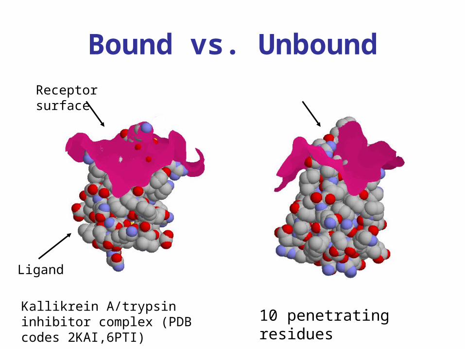
Bound vs. Unbound
10 penetrating residuesKallikrein A/trypsin inhibitor complex (PDB codes 2KAI,6PTI)
Receptor surface
Ligand
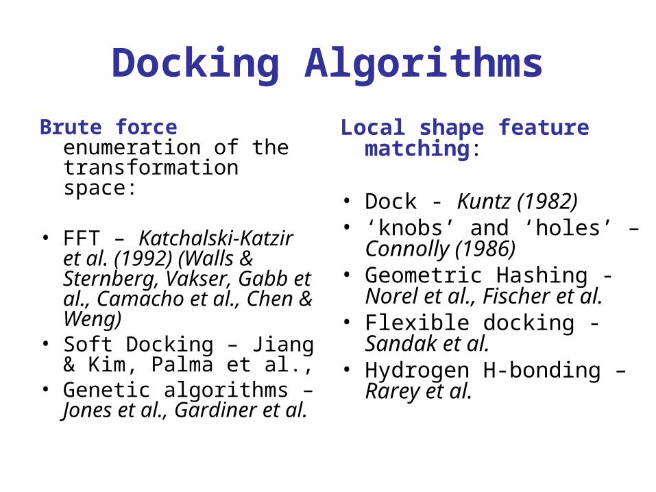
Docking AlgorithmsBrute force enumeration of
the transformation space:
• FFT – Katchalski-Katzir et al. (1992) (Walls & Sternberg, Vakser, Gabb et al., Camacho et al., Chen & Weng)
• Soft Docking – Jiang & Kim, Palma et al.,
• Genetic algorithms – Jones et al., Gardiner et al.
Local shape feature matching:
• Dock - Kuntz (1982)• ‘knobs’ and ‘holes’ –
Connolly (1986)• Geometric Hashing - Norel et
al., Fischer et al. • Flexible docking - Sandak et
al. • Hydrogen H-bonding – Rarey
et al.

Docking Algorithm (Name???)
• We develop local shape feature matching docking algorithm.
• We try to focus on local shape patches that are likely to be in the binding site.
• The algorithm also improves the geometric scoring.
• Although it may be used for any type of molecules (protein-protein, protein-drug), it has features specific to each type.

Docking Algorithm Scheme
• Molecular shape representation
• Matching of critical features
• Filtering and scoring of candidate transformations
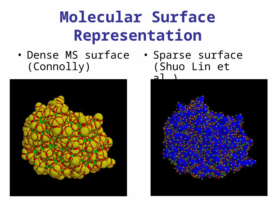
Molecular Surface Representation
• Dense MS surface (Connolly)
• Sparse surface (Shuo Lin et al.)

Distance Transform Grid
• Dense MS surface (Connolly)
0
+1
-1

Sparse Surface (Shuo Lin)
• Caps, pits, belts:
• Gtop – Surface topology graph:
V=surface points
E={(u,v)| u,v belong to the same atom}

Shape function
• Shape function is a measure of local curvature.
• ‘knobs’ and ‘holes’ are local minima and maxima (<1/3 or >2/3).
• Problem: more than 70% of surface points are ignored.
• Solution: divide the values of the shape function to 3 equal sized sets: ‘knobs’, ‘flats’ and ‘holes’.

Patch Detection• Goal: divide the surface into connected,
non-intersecting, equal sized patches of critical points.
• connected – the points of the patch correspond to a connected sub-graph of Gtop.
• equal sized – to assure better matching we want shape features of the same size.

• Construct a graph for each type of points (knobs,holes,flats). For example Gknob will include all surface points that are nodes and an edge between two ‘knobs’ if they belong to the same atom.
• Compute connected components of every graph.
• Output: connected components, but the sizes can vary.
• Solution: apply ‘split’ and ‘merge’ routines.
Patch Detection
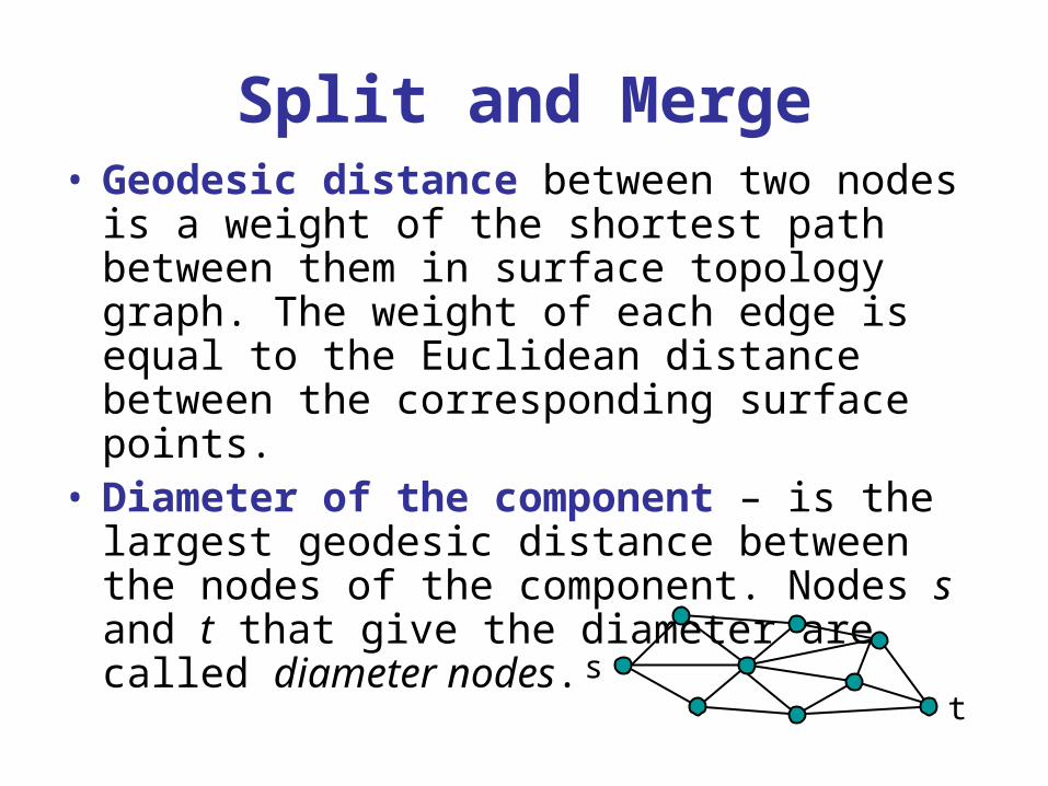
Split and Merge• Geodesic distance between two nodes is a
weight of the shortest path between them in surface topology graph. The weight of each edge is equal to the Euclidean distance between the corresponding surface points.
• Diameter of the component – is the largest geodesic distance between the nodes of the component. Nodes s and t that give the diameter are called diameter nodes.
st
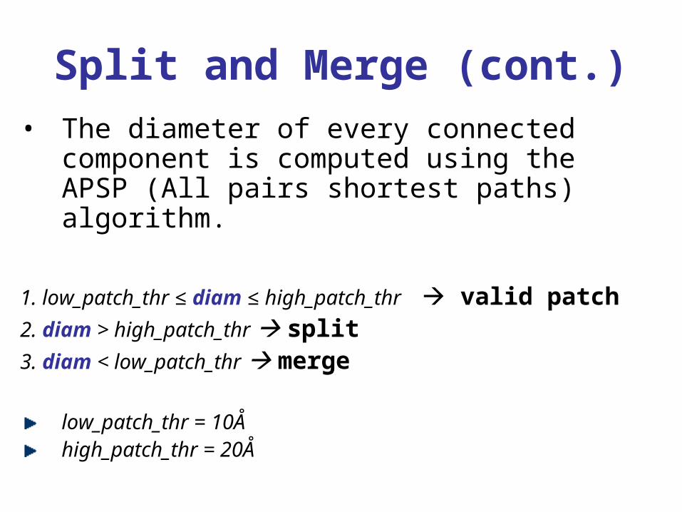
Split and Merge (cont.)• The diameter of every connected
component is computed using the APSP (All pairs shortest paths) algorithm.
1. low_patch_thr ≤ diam ≤ high_patch_thr valid patch2. diam > high_patch_thr split3. diam < low_patch_thr merge
low_patch_thr = 10Åhigh_patch_thr = 20Å

Split and Merge (cont.)• Split routine: compute Voronoi cells of the
diameter nodes s,t. Points closer to s belong to new component S, points closer to t belong to new component T. The split is applied until the new component has a valid diameter.
• Merge routine: compute the geodesic distance of every component point to all the patches. Merge with the patch with closest distance.
st

Examples of Patches:
Yellow – knob patches, cyan – hole patches, green – flat patches, the proteins are in blue

Active Site FocusingThere are major differences in the interactions of different types of molecules (protease-inhibitor, antibody-antigen, protein drug). Studies have shown the presence of energetic hot spots in the active sites of the molecules.
Protease/inhibitor – select patches with high enrichment of hot spot residues (Ser,Gly,Asp and His for protease; and Arg,Lys,Leu,Cys and Pro for protease inhibitor).
Antibody/antigen – 1.detect CDRs of the antibody. 2. select hot spot patches (Tyr,Asp,Asn,Glu,Ser and Trp for antibody; and Arg,Lys,Asn and Asp for antigen)
Protein/drug – select largest protein cavity (highest value of average shape function for the patch)

Active Site Focusing
surfacesurfaceresidue
patchpatchresiduei areaarea
areaareapatchresiduepropensity
i
i
/
/),(
,
,
• The enrichment of hot spot residue in patch is measured by propensity. Propensity is a ratio of residue frequency in patch and residue frequency in surface.
• The CDRs are detected by aligning the sequence of the given antibody to the consensus sequence of the library of the antibodies.

Docking Algorithm Scheme
• Molecular shape representation
• Matching of critical features
• Filtering and scoring of candidate transformations

Matching of patchesThe aim is to match knob patches with hole patches, and flat patches with any patch. We use two types of matching:
• Single Patch Matching – one patch from the receptor is matched with one patch from the ligand. Used in protein-drug cases.
• Patch-Pair Matching – two patches from the receptor are matched with two patches from the ligand. Used in protein-protein cases.

Matching of patchesThe transformations are computed by matching 2 points and their normals.
The signature of the base is defined as follows:
1. Euclidean and geodesic distances between 2 points
2. The angles α,β between a,b segment and the normals
3. The torsion angle w between the planes
Two bases are compatible if their signatures match.

Single Patch Matching
• Preprocessing: the bases are built for each ligand base and stored in hash table. There are 3 hash tables for each type.
• Recognition: for each patch of the receptor build the bases and access the hash-table with base signature. The transformations set is computed for all compatible bases.
• At the end of this step each patch has a list of ligand transformations.

Patch-Pair Matching
• Two patches are neighbors if there is an edge connecting them in surface topology graph.
• Preprocessing: the bases are built for each pair of the ligand patches. We use one point and normal from each patch. The bases are stored in hash table. There are 32 hash tables for each pair of types.
• Recognition: for each pair of the receptor patches we build the bases and access the hash-table with the base signature. The transformations set is computed for all compatible bases.

Clustering
• Since local features are matched, we may have multiple instances of “almost” the same transformation.
• We apply 2 clustering techniques:
1.Clustering transformation parameters – coarse but very fast.
2.RMSD clustering – accurate but slow. (according to FLEXX, Rarey et al., 1996)

Clustering Transformation
Parameters• Use 6 transformation parameters: 3 rotational and 3 translational.
• The transformations are stored in the hash-table with bucket size 0.1 for rotation and 2.0 for translation.
• It is assumed that the correct solution is obtained by matching a large enough number of local features. Thus, we compute a histogram of cluster sizes and traverse only high scoring buckets (10% of the total number of buckets).
• The transformation of each cluster is computed by applying the best least-squares fitting method on the points of matched bases.
• Note, that it is possible to improve the clustering by using 4 quaternion rotation parameters instead of 3.
Complexity: proportional to the number of transformations

Docking Algorithm Scheme
• Molecular shape representation
• Matching of critical features
• Filtering and scoring of candidate transformations

Filtering and Scoring• Since the transformations were computed by local shape features matching they may include unacceptable steric clashes.
• The scoring is necessary to rank the remaining solutions.
• Steric clash test: For each candidate ligand transformation transform ligand surface points For each transformed point access Distance Transform Grid and check distance value If it is more than max_penetration Disqualify transformation
• Geometric score: the surface of the receptor is divided into five ranges: [-5.0,-3.6), [-3.6,-2.2), [-2.2, -1.0), [-1.0,1.0), [1.0) and each range is given a weight: -10, -6, -2, 1, 0. The geometric score is a weighted average on a number of points inside every range.

Filtering and ScoringPerformance Problem: the number of surface points for high resolution MS surface may reach 100,000. For each candidate transformation, for each surface point we apply the transformation and access distance transform grid.
We develop multi-resolution surface data structure that supports fast queries for penetrations and geometric score.
119,000 points 16,000 points 4,100 points 1,000 points

Multi-resolution surface
Level 0: Connolly Surface points
Level 1:
Level 2:
point radius number of leaves low-level pointers
Node:

Queries in Multi-resolution surface data structure
• The queries are: isPenetrating(trans, threshold), maxPenetration(trans), score(trans), interface(trans).
• All the searches are performed by DFS.• We check every node from highest level and go
down if it is in interface.• For each node we check distance transform value
and radius. If they are within the threshold we don’t check the children.
• Worst case complexity of each query: O(interface size + highest level size)

Antibody-Antigen Scoring
• Although only the patches including CDRs are used in the matching stage, the results may still include transformations where most of the interface doesn’t belong to CDRs.
• In addition to regular score, we compute the percentage of the interface included in the CDRs. All the transformations with less than 70% of CDRs are disqualified.

Results
Datasets:Protein-Protein docking:• Enzyme-inhibitor – 22 cases• Antibody-antigen – 13 cases
Protein-DNA docking: 2 unbound-bound cases
Protein-drug docking: tens of bound cases (Estrogen receptor, HIV protease, CYP450cam, COX)
Performance:Several minutes for large protein molecules and
seconds for small drug molecules

Enzyme-inhibitor cases

Enzyme-inhibitor results

Antibody-antigen cases

Antibody-antigen results

PicturesAntibody-antigen
(unbound)Enzyme-inhibitor
(unbound)
Antibody Fab 5G9 (1FGN) with tissue factor (1BOY). RMSD 2.27Å, rank 8
Α-chymotrypsin (5CHA) with Eglin C (1CSE(I)). RMSD 1.46Å, rank 10

PicturesProtein-DNA
(unbound-bound)Protein-drug
(bound)
Estrogen receptor with estradiol (1A52). RMSD 0.9Å, rank 1
Endonuclease I-PpoI (1EVX) with DNA (1A73). RMSD 0.87Å, rank 2

Factors that influence the rank of the correct solution
• Shape complementarity• Interface shape – in the
concave/convex interfaces (enzyme-inhibitor, receptor-drug), shape complementarity is easier to detect comparing to flat interfaces (antibody-antigen).
• Sizes of molecules – the larger the molecules the higher the number of the results.

Conclusions and Future Work
The division to shape-based patches improves the performance of the unbound cases.Multi-resolution data structure and distance transform grid improve the efficiency and quality of the geometric score.Hot-spots allow to focus on relevant surface parts.
Additional biological scores will improve the ranking of the correct association.Introducing side-chain flexibility into algorithms will improve the results for difficult unbound cases.

“Small” Points
• Local curvature computation
• Matching of patches by critical points
• Transformation clustering – memory allocations
• Geometric score by ranges
• Weights on ranges