UMIST - University of Southern California

ISSN 1360-1725

UMIST

The Test Matrix Toolbox for Matlab (Version 3.0)

N. J. Higham

Numerical Analysis Report No. 276

September 1995

Manchester Centre for Computational Mathematics

Numerical Analysis Reports

DEPARTMENTS OF MATHEMATICS

Reports available from:

Department of Mathematics

University of Manchester

Manchester M13 9PL

England

And over the World-Wide Web from URLs

http://www.ma.man.ac.uk/MCCM/MCCM.html

ftp://ftp.ma.man.ac.uk/pub/narep

The Test Matrix Toolbox for Matlab (Version 3.0)

Nicholas J. Higham�

September 22, 1995

Abstract

We describe version 3.0 of the Test Matrix Toolbox for Matlab 4.2. The toolbox con-tains a collection of test matrices, routines for visualizing matrices, routines for direct searchoptimization, and miscellaneous routines that provide useful additions to Matlab's exist-ing set of functions. There are 58 parametrized test matrices, which are mostly square,dense, nonrandom, and of arbitrary dimension. The test matrices include ones with knowninverses or known eigenvalues; ill-conditioned or rank de�cient matrices; and symmetric,positive de�nite, orthogonal, defective, involutary, and totally positive matrices. The vi-sualization routines display surface plots of a matrix and its (pseudo-) inverse, the �eldof values, Gershgorin disks, and two- and three-dimensional views of pseudospectra. Thedirect search optimization routines implement the alternating directions method, the multi-directional search method and the Nelder{Mead simplex method. We explain the need forcollections of test matrices and summarize the features of the collection in the toolbox. Wegive examples of the use of the toolbox and explain some of the interesting properties of theFrank matrix and magic square matrices. The leading comment lines from all the toolboxroutines are listed.

Key words. test matrix, Matlab, pseudospectrum, visualization, Frank matrix,magic square matrix, random matrix, direct search optimization.

AMS subject classi�cations. primary 65F05

Contents

1 Distribution 2

2 Installation 2

3 Release History 2

4 Quick Reference Tables 3

5 Test Matrices 7

6 Visualization 12

7 Direct Search Optimization 15

8 Miscellaneous Routines 21

�Department of Mathematics, University of Manchester, Manchester, M13 9PL, England([email protected]). This work was supported by Science and Engineering Research Councilgrant GR/H52139.

1

9 Examples 23

9.1 Magic Squares . . . . . . . . . . . . . . . . . . . . . . . . . . . . . . . . . . . . . 23

9.2 The Frank Matrix . . . . . . . . . . . . . . . . . . . . . . . . . . . . . . . . . . . 259.3 Numerical Linear Algebra . . . . . . . . . . . . . . . . . . . . . . . . . . . . . . . 28

10 M-File Leading Comment Lines 33

1 Distribution

If you wish to distribute the toolbox please give exact copies of it, not selected routines.

2 Installation

The Test Matrix Toolbox is available by anonymous ftp from The MathWorks with URL

ftp://ftp.mathworks.com/pub/contrib/linalg/testmatrix

This document is testmatrix.ps in the same location. The MathWorks ftp server providesinformation on how to download a complete directory as one �le.

The toolbox is also available from the URL

ftp://ftp.ma.man.ac.uk/pub/higham/testmatrix.tar.Z

This document is narep276.ps.Z in the same location. To install the toolbox from this location,download the tar �le (in binary mode) into a testmatrix directory (matlab/testmatrix isrecommended). Then uncompress the tar �le and untar it:

uncompress testmatrix.tar.Z

tar xvf testmatrix

To try the toolbox from within Matlab, change to the testmatrix directory and run thedemonstration script by typing tmtdemo. For serious use it is best to put the testmatrix

directory on the Matlab path before the matlab/toolbox entries|this is because severaltoolbox routines have the same name as Matlab routines and are intended to replace them(namely, compan, cond, hadamard, hilb, and pascal).

This document describes version 3.0 of the toolbox, dated September 19, 1995.

3 Release History

The �rst release of this toolbox (version 1.0, July 4 1989) was described in a technical report [19].The collection was subsequently published as ACM Algorithm 694 [21]. Prior to the currentversion, version 3.0, the most recent release was version 2.0 (November 14 1993) [24]. Version2.0 incorporated many additions and improvements over version 1.3 and took full advantage ofthe features of Matlab 4.

The major changes in version 3.0 are as follows.

� New routines: cgs (classical Gram{Schmidt), mgs (modi�ed Gram{Schmidt), gj (Gauss{Jordan elimination), diagpiv (diagonal pivoting factorization with partial pivoting for asymmetric matrix); adsmax, mdsmax and nmsmax for direct search optimization.

� Bug in eigsens corrected. Minor bugs in other routines corrected.

2

Version 3.0 of the toolbox was developed in conjunction with the book Accuracy and Stabilityof Numerical Algorithms [26]. The book contains a chapter A Gallery of Test Matrices whichhas sections

� The Hilbert and Cauchy Matrices

� Random Matrices

� \Randsvd" Matrices

� The Pascal Matrix

� Tridiagonal Toeplitz Matrices

� Companion Matrices

� Notes and References

� LAPACK

� Problems

Users of the toolbox should consult [26] for further information not contained in this document.

4 Quick Reference Tables

This section contains quick reference tables for the Test Matrix Toolbox. All the M-�les in thetoolbox are listed by category, with a short description. More detailed documentation is givenin Section 10, or can be obtained on-line by typing help M-file_name.

3

Demonstration

tmtdemo Demonstration of Test Matrix Toolbox.

Test Matrices, A{K

augment Augmented system matrix.cauchy Cauchy matrix.chebspecChebyshev spectral di�erentiation matrix.chebvandVandermonde-like matrix for the Chebyshev polynomials.chow Chow matrix|a singular Toeplitz lower Hessenberg matrix.circul Circulant matrix.clement Clement matrix|tridiagonal with zero diagonal entries.compan Companion matrix.condex \Counterexamples" to matrix condition number estimators.cycol Matrix whose columns repeat cyclically.dingdongDingdong matrix|a symmetric Hankel matrix.dorr Dorr matrix|diagonally dominant, ill conditioned,

tridiagonal.dramadahA (0; 1) matrix whose inverse has large integer entries.fiedler Fiedler matrix|symmetric.forsytheForsythe matrix|a perturbed Jordan block.frank Frank matrix|ill conditioned eigenvalues.gallery Famous, and not so famous, test matrices.gearm Gear matrix.gfpp Matrix giving maximal growth factor for Gaussian elimination

with partial pivoting.grcar Grcar matrix|a Toeplitz matrix with sensitive eigenvalues.hadamardHadamard matrix.hanowa A matrix whose eigenvalues lie on a vertical line in the complex

plane.hilb Hilbert matrix.invhess Inverse of an upper Hessenberg matrix.invol An involutory matrix.ipjfact A Hankel matrix with factorial elements.jordblocJordan block.kahan Kahan matrix|upper trapezoidal.kms Kac{Murdock{Szeg�o Toeplitz matrix.krylov Krylov matrix.

4

Test Matrices, L{Z

lauchli Lauchli matrix|rectangular.lehmer Lehmer matrix|symmetric positive de�nite.lesp A tridiagonal matrix with real, sensitive eigenvalues.lotkin Lotkin matrix.makejcf A matrix with given Jordan canonical form.minij Symmetric positive de�nite matrix min(i; j).moler Moler matrix|symmetric positive de�nite.neumann Singular matrix from the discrete Neumann problem (sparse).ohess Random, orthogonal upper Hessenberg matrix.orthog Orthogonal and nearly orthogonal matrices.parter Parter matrix|a Toeplitz matrix with singular values near �.pascal Pascal matrix.pdtoep Symmetric positive de�nite Toeplitz matrix.pei Pei matrix.pentoep Pentadiagonal Toeplitz matrix (sparse).poisson Block tridiagonal matrix from Poisson's equation (sparse).prolate Prolate matrix|symmetric, ill-conditioned Toeplitz matrix.rando Random matrix with elements �1, 0 or 1.randsvd Random matrix with pre-assigned singular values.redheff A (0,1) matrix of Redhe�er associated with the Riemann

hypothesis.riemann A matrix associated with the Riemann hypothesis.rschur An upper quasi-triangular matrix.smoke Smoke matrix|complex, with a \smoke ring"

pseudospectrum.tridiag Tridiagonal matrix (sparse).triw Upper triangular matrix discussed by Wilkinson and others.vand Vandermonde matrix.wathen Wathen matrix|a �nite element matrix (sparse, random entries).wilk Various speci�c matrices devised/discussed by Wilkinson.

Visualization

fv Field of values (or numerical range).gersh Gershgorin disks.ps Dot plot of a pseudospectrum.pscont Contours and colour pictures of pseudospectra.see Pictures of a matrix and its (pseudo-) inverse.

Decompositions and Factorizations

cgs Classical Gram{Schmidt QR factorization.cholp Cholesky factorization with pivoting of a positive semide�nite

matrix.cod Complete orthogonal decomposition.diagpiv Diagonal pivoting factorization with partial pivoting.ge Gaussian elimination without pivoting.gecp Gaussian elimination with complete pivoting.gj Gauss{Jordan elimination to solve Ax = b.mgs Modi�ed Gram{Schmidt QR factorization.poldec Polar decomposition.signm Matrix sign decomposition.

5

Direct Search Optimization

adsmax Alternating directions direct search method.mdsmax Multidirectional search method for direct search optimization.mmsmax Nelder{Mead simplex method for direct search optimization.

Miscellaneous

bandred Band reduction by two-sided unitary transformations.chop Round matrix elements.comp Comparison matrices.cond Matrix condition number in 1, 2, Frobenius, or 1-norm.cpltaxesDetermine suitable axis for plot of complex vector.dual Dual vector with respect to H�older p-norm.eigsens Eigenvalue condition numbers.house Householder matrix.matrix Test Matrix Toolbox information and matrix access by number.matsigntMatrix sign function of a triangular matrix.pnorm Estimate of matrix p-norm (1 � p � 1).qmult Pre-multiply by random orthogonal matrix.rq Rayleigh quotient.seqa Additive sequence.seqcheb Sequence of points related to Chebyshev polynomials.seqm Multiplicative sequence.show Display signs of matrix elements.skewpartSkew-symmetric (skew-Hermitian) part.sparsifyRandomly sets matrix elements to zero.sub Principal submatrix.symmpartSymmetric (Hermitian) part.trap2triUnitary reduction of trapezoidal matrix to triangular form.

6

5 Test Matrices

Numerical experiments are an indispensable part of research in numerical analysis. We do themfor several reasons:

� To gain insight and understanding into an algorithm that is only partially understoodtheoretically.

� To verify the correctness of a theoretical analysis and to see if the analysis completelyexplains the practical behaviour.

� To compare rival methods with regard to accuracy, speed, reliability, and so on.

� To tune parameters in algorithms and codes, and to test heuristics.

One of the di�culties in designing experiments is �nding good test problems|ones thatreveal extremes of behaviour, cover a wide range of di�culty, are representative of practicalproblems, and (ideally) have known solutions. In many areas of numerical analysis good testproblems have been identi�ed, and several collections of such problems have been published. Forexample, collections are available in the areas of nonlinear optimization [33], linear programming[13], [31], ordinary di�erential equations [10], and partial di�erential equations [34].

Probably the most proli�c devisers of test problems have been workers in matrix compu-tations. Indeed, in the 1950s and 1960s it was common for a whole paper to be devoted to aparticular test matrix: typically its inverse or eigenvalues would be obtained in closed form. Anearly survey of test matrices was given by Rutishauser [36]; most of the matrices he discussescome from continued fractions or moment problems. Two well-known books present collectionsof test matrices. Gregory and Karney [15] deal exclusively with the topic, while Westlake [43]gives an appendix of test matrices. In the 24 years since these books appeared several interest-ing matrices have been discovered (and in fact both books omit some worthy test matrices thatwere known at the time).

The Test Matrix Toolbox contains an up-to-date, well documented and readily accessiblecollection of test matrices. The matrices are given in the form of self-documenting Matlab

M-�les. For some of the matrices we give mathematical formulas for the matrix elements incomment lines; in other cases the formulas can be reconstructed from the Matlab code. Wedo not give exhaustive descriptions of matrix properties, or proofs of these properties; instead,in the comment lines we list a few key properties and give references where further details canbe found.

With a few exceptions each of the 58 matrices satis�es the following requirements:

� It is a square matrix with one or more variable parameters, one of which is the dimension.Thus it is actually a parametrized family of matrices of arbitrary dimension.

� It is dense.

� It has some property that makes it of interest as a test matrix.

The �rst criterion is enforced because it is often desirable to explore the behaviour of anumerical method as parameters such as the matrix dimension vary. The third criterion issomewhat subjective, and the matrices presented here represent the author's personal choice.Note that we have omitted plausible matrices that we thought not \su�ciently di�erent" fromothers in the collection. Although all but two of our test matrices are usually real, those withan arbitrary parameter can be made complex by choosing a non-real value for the parameter.

7

As well as their obvious application to research in matrix computations we hope that thematrices presented here will be useful for constructing test problems in other areas, such asoptimization (see, for example, [3]) and ordinary di�erential equations.

We mention some other collections of test matrices that complement ours. The Harwell-Boeing collection of sparse matrices, largely drawn from practical problems, is presented by Du�,Grimes and Lewis [8], [9]. Bai [2] is building a collection of test matrices for the large-scalenonsymmetric eigenvalue problem. Zielke [46] gives various parametrized rectangular matricesof �xed dimension with known generalized inverses. Demmel and McKenney [7] present a suiteof Fortran 77 codes for generating random square and rectangular matrices with prescribedsingular values, eigenvalues, band structure, and other properties. This suite is part of thetesting code for LAPACK [1]. Our focus is primarily on non-random matrices but we include aclass of random matrices randsvd that has some of the features of the Demmel and McKenneytest set.

Where possible, we have chosen the names of the test matrices eponymously, since it is easierto remember, for example, \the Kahan matrix", than \Example 3.8". For portability reasonswe restrict all M-�le names in the toolbox to eight characters (since this is the limit in theMSDOS operating system, under which the Microsoft Windows version of Matlab runs). Wehave written a routine matrix that accesses the matrices by number rather than by name; thismakes it easy to run experiments on the whole collection of matrices (with parameters otherthan the matrix dimension set to their default values.)

The matrices described here can be modi�ed in various ways while still retaining some or allof their interesting properties. Among the many ways of constructing new test matrices fromold are:

� Similarity transformations A X�1AX .

� Unitary transformations A UAV , where U�U = V �V = I .

� Kronecker products A A B or B A (for which Matlab has a routine kron).

� Powers A Ak .

For a discussion of these techniques, and others, see [15, Chapter 2]. Techniques for obtaininga triangular, orthogonal, or symmetric positive de�nite matrix that is related to a given matrixinclude

� Bandwidth reduction using unitary transformations (see toolbox routine bandred).

� LU, Cholesky, QR and polar decompositions (see lu, chol, qr and, from the toolbox,cholp, ge, gecp and poldec.)

See [14] for details of these techniques.Another way to generate a new matrix is to perturb an existing one. One approach is to

add a random perturbation. Another is to round the matrix elements to a certain number ofbinary places; this can be done using the toolbox routine chop.

Our programming style is as follows. Each M-�le foo begins with comment lines that aredisplayed when the user types help foo. The �rst comment line, the H1 line, is a self-containedstatement of the purpose of the routine; the H1 lines are searched and displayed by Matlab'slookfor command (e.g., lookfor toeplitz). Any further comments and references follow ablank line and so are not displayed by help. As far as possible, every routine sets default valuesfor any arguments that are not speci�ed. In particular, for most test matrix routines testmat,A = testmat(n) is a valid way to generate an n � n matrix. In general we have strived for

8

conciseness, modularity, speed, and minimal use of temporary storage in our Matlab codes.Hence, where possible, we used matrix or vector constructs instead of for loops and have usedcalls to existing M-�les.

Some of those matrices that are banded with a small bandwidth are given the sparse storageformat, to allow large matrices to be generated. The full function can be used to convert tonon-sparse storage (e.g., A = full(tridiag(32))). We check for errors in parameters in some,but not all, cases. A few of the test matrix routines do not properly handle the dimension n = 1(for example, they halt with an error, or return an empty matrix). We decided not to add extracode for this case, since the routines are unlikely to be called with n = 1.

Tables 5.1 and 5.2 provide a summary of the properties of the test matrices. The columnheadings have the following meanings:

Inverse: the inverse of the matrix is known explicitly.

Ill-cond: the matrix is ill-conditioned for some values of the parameters.

Rank: the matrix is rank-de�cient for some values of the parameters (we exclude \trivial"examples such as vand, which is singular if its vector argument contains repeated points).Note that there are some matrices that are mathematically rank-de�cient but behave asill-conditioned full rank matrices in the presence of rounding errors; these are listed onlyas rank-de�cient (for example, chebspec).

Symm: the matrix is symmetric for some values of the parameters.

Pos Def: the matrix is symmetric positive de�nite for some values of the parameters.

Orth: the matrix is orthogonal, or a diagonal scaling of an orthogonal matrix, for some valuesof the parameters.

Eig: something is known about the eigensystem (or the singular values), ranging from boundsor qualitative knowledge of the eigenvalues to explicit formulas for some or all eigenvaluesand eigenvectors.

We summarise further interesting properties possessed by some of the matrices. Recall thatA is a Hankel matrix if the anti-diagonals are constant (aij = ri+j), idempotent if A2 = A,normal if A�A = AA� (or, equivalently, A is unitarily diagonalizable), nilpotent if Ak = 0 forsome k, involutary if A2 = I , totally positive (nonnegative) if the determinant of every submatrixis positive (nonnegative), and a Toeplitz matrix if the diagonals are constant (aij = rj�i).A totally positive matrix has distinct, real and positive eigenvalues and its ith eigenvector(corresponding to the ith largest eigenvalue) has exactly i � 1 sign changes [12, Theorem 13,p. 105]; this property is important in testing regularization algorithms [16], [17]. See [28] forfurther details of these matrix properties.

defective: chebspec, gallery, gear, jordbloc, triw

Hankel: dingdong, hilb, ipjfact

Hessenberg: chow, frank, grcar, ohess, randsvd

idempotent: invol

involutary: invol, orthog, pascal

normal (but not symmetric or orthogonal): circul

9

Matrix Inverse Ill-cond Rank Symm Pos Def Orth Eig

augmentp p

cauchyp p p p

chebspecp p

chebvandp p

chowp p

circulp p p

clementp p p p

companp p p

condexp

cycolp

dingdongp p

dorrp

dramadahp

�edlerp p p

forsythep p p

frankp p

galleryp p p p p p

gearmp p

gfppp p

grcarp

hadamardp p p

hanowap

hilbp p p p

invhessp p p p p

involp p p

ipjfactp p

jordblocp p p p

kahanp p p

kmsp p p p

krylovp

Table 5.1: Properties of the test matrices, A{K.

10

Matrix Inverse Ill-cond Rank Symm Pos Def Orth Eig

lauchlip

lehmerp p p

lespp

lotkinp p p

minijp p p p

molerp p p p

neumannp p

ohessp p p

orthogp p p

parterp

pascalp p p p p

pdtoepp p p p p

peip p p p p

pentoepp p p p

poissonp p p p

prolatep p p p

randorandsvd

p p p p predhe�

priemann

prschur

p psmoke

p ptridiag

p p p p p ptriw

p pvand

p pwathen

p p pwilk

p p p p

Table 5.2: Properties of the test matrices, L{Z.

11

nilpotent: chebspec, gallery

rectangular: chebvand, cycol, kahan, krylov, lauchli, rando, randsvd, triw,vand

Toeplitz: chow, dramadah, grcar, kms, parter, pentoep, prolate

totally positive or totally nonnegative: cauchy1, hilb, lehmer, pascal, vand2

tridiagonal: clement, dorr, gallery, lesp, randsvd, tridiag, wilk

inverse of a tridiagonal matrix: kms, lehmer, minij

triangular: dramadah, jordbloc, kahan, pascal, triw

Finally, we note that several of the test matrices are related to those supplied with Mat-

lab. The functions hadamard and pascal were in the �rst release of the toolbox and weresubsequently included by The MathWorks in the Matlab distribution. The toolbox version ofhadamard is the same as the one in Matlab 4.2 except for the addition of an H1 line, whereasthe toolbox version of pascal contains more informative comment lines than the Matlab 4.2version and produces a di�erent pascal(n,2) matrix3 (but one that is still a cube root of theidentity). The toolbox routine compan is more versatile than theMatlab 4.2 version. Similarly,the toolbox routine vand is more versatile than Matlab 4.2's vander. The toolbox version ofhilb is coded di�erently and contains more informative comments than the one inMatlab 4.2.The toolbox routine augment is similar toMatlab 4.2's spaugment, but produces a non-sparsematrix instead of a sparse one. The toolbox function cond supports the 1, 2, 1 and Frobeniusnorms, whereas Matlab 4.2's cond supports only the 2-norm.

6 Visualization

The toolbox contains �ve routines for visualizing matrices. The routines can give insight intothe properties of a matrix that is not easy to obtain by looking at the numerical entries. Theyalso provide an easy way to generate pretty pictures!

The routine see displays a �gure with four subplots (strictly speaking four \axes", in Mat-

lab terminology) in the format

mesh(A) mesh(pinv(A))

semilogy(svd(A)) fv(A)

An example for the chebvand matrix is given in Figure 6.1. Matlab's mesh command plots athree-dimensional, coloured, wire-frame surface, by regarding the entries of a matrix as spec-ifying heights above a plane. We use axis('ij'), so that the coordinate system for the plotmatches the (i; j) matrix element numbering. pinv(A) is the Moore{Penrose pseudo-inverse A+

of A, which is the usual inverse when A is square and nonsingular. semilogy(svd(A)) plots thesingular values of A (ordered in decreasing size) on a logarithmic scale; the singular values aredenoted by circles, which are joined by a solid line to emphasise the shape of the distribution.From Figure 6.1 we can see that chebvand(8) has a 2-norm condition number of about 105 andthat the largest elements of its inverse are in the lower triangle. For a sparse Matlab matrix,see simply displays a spy plot, which shows the sparsity pattern of the matrix. The user could,

1cauchy(x,y) is totally positive if 0 < x1 < � � � < xn and 0 < y1 < � � � < yn [39, p. 295].2vand(p) is totally positive if the pi satisfy 0 < p1 < � � � < pn [12, p. 99].3The new pascal(n,2) is generated by a call to rot90 and is \reverse upper triangular" instead of \reverse

lower triangular" as in the Matlab 4.2 version.

12

05

100

510

-1

0

1

05

100

510

-5

0

5

x 104

0 2 4 6 810

-6

10-4

10-2

100

102

-2 0 2

-2

0

2

Figure 6.1: see(chebvand(8)).

of course, try see(full(A)) for a sparse matrix, but for large dimensions the storage and timerequired would be prohibitive. Figure 6.2 displays the result of applying see to the Wathenmatrix|a symmetric positive de�nite sparse matrix that comes from a �nite element problem.

The routine fv plots the �eld of values of a square matrix A 2 Cn�n (also called thenumerical range), which is the set of all Rayleigh quotients,

�x�Ax

x�x: 0 6= x 2 Cn

�;

the eigenvalues of A are plotted as crosses. The �eld of values is a convex set that containsthe eigenvalues. It is the convex hull of the eigenvalues when A is a normal matrix. If A isHermitian, the �eld of values is just a segment of the real line. For non-Hermitian A the �eldof values is usually two-dimensional and its shape and size gives some feel for the behaviour ofthe matrix. Trefethen [41] notes that the �eld of values is the largest reasonable answer to thequestion \Where in C does a matrix A `live' ?" and the spectrum is the smallest reasonableanswer.

Some examples of �eld of values plots are given in Figure 6.3. The circul matrix is normal,hence its �eld of values is the convex hull of the eigenvalues. For an example of how the �eld ofvalues gives insight into the problem of �nding a nearest normal matrix see [35]. An excellentreference for the theory of the �eld of values is [29, Chapter 1].

The routine gersh plots the Gershgorin disks for an A 2 Cn�n, which are the n disks

Di = f z 2 C : jz � aiij �nX

j=1j 6=i

jaij j g

in the complex plane. Gershgorin's theorem tells us that the eigenvalues of A lie in the union ofthe disks, and an extension of the theorem states that if k disks form a connected region thatis isolated from the other disks, then there are precisely k eigenvalues in this region. Thus thesize of the disks gives a feel for how nearly diagonal A is, and their locations give information

13

0 20 40 60 80 100 120 140 160

0

20

40

60

80

100

120

140

160

nz = 2416

Figure 6.2: see(wathen(7,7)).

on where the eigenvalues lie in the complex plane. Four examples of Gershgorin disk plots aregiven in Figure 6.4; Gershgorin's theorem provides nontrivial information only for the thirdmatrix, ipjfact(8,1).

The last two routines, ps and pscont, are concerned with pseudospectra. The �-pseudospectrumof a matrix A 2 Cn�n is de�ned, for a given � > 0, to be the set

��(A) = f z : z is an eigenvalue of A +E for some E with kEk2 � � g:

In other words, it is the set of all complex numbers that are eigenvalues of A + E for someperturbation E of 2-norm at most �. For a normal matrix A the �-pseudospectrum is theunion of the balls of radius � around the eigenvalues of A. For nonnormal matrices the �-pseudospectrum can take a wide variety of shapes and sizes, depending on the matrix and hownonnormal it is. Pseudospectra play an important role in many numerical problems. For fulldetails see the work of Trefethen|in particular, [40] and [41].

The routine ps plots an approximation to the �-pseudospectrum ��(A), which it obtains bycomputing the eigenvalues of a given number of random perturbations of A. The eigenvaluesare plotted as crosses and the pseudo-eigenvalues as dots. Arguments to ps control the numberand type of perturbations. Figure 6.5 gives four examples of 10�3-pseudospectra, all of whichinvolve the pentadiagonal Toeplitz matrix pentoep.

Another characterization of ��(A), in terms of the resolvent (zI � A)�1, is

��(A) = f z : k(zI � A)�1k2 � ��1 g:

An alternative way of viewing the pseudospectrum is to plot the function

f(z) = k(zI �A)�1k�12 = �min(zI � A)

over the complex plane, where �min denotes the smallest singular value [41]. The routine pscontplots log10 f(z)

�1 and o�ers several ways to view the surface: by its contour lines alone, or as

14

-2 0 2 4

-2

0

2

grcar(20)

-10 -5 0 5-10

-5

0

5

10compan(8)

0 20 40

-20

-10

0

10

20

circul(8)

-20 -15 -10 -5-10

-5

0

5

10

lesp(8)

Figure 6.3: Fields of values (fv).

a coloured surface plot in two or three dimensions, with or without contour lines. (The two-dimensional plot is the view from directly above the surface.) Two di�erent pscont views ofthe pseudospectra of the triangular matrix triw(11) are given in Figures 6.6 and 6.7. Sinceall the eigenvalues of this matrix are equal to 1, there is a single point where the resolventis unbounded in norm|this is the \bottomless pit" in the pictures. The spike in Figure 6.7should be in�nitely deep; since pscont evaluates f(z) on a �nite grid, the spike has a �nitedepth dependent on the grid spacing. Also because of the grid spacing chosen, the contours area little jagged. Various aspects of the plots can be changed from the Matlab command lineupon return from pscont; for example, the colour map (colormap), the shading (shading), andthe viewing angle (view). For Figure 6.6 we set shading interp and colormap copper.

Both pseudospectrum routines are computationally intensive, so the defaults for the argu-ments are chosen to produce a result in a reasonable time (under 20 seconds on a SPARC-2processor or equivalent); for plots that reveal reasonable detail it is usually necessary to overridethe defaults.

7 Direct Search Optimization

The toolbox contains three multivariate direct search maximization routines mdsmax, adsmaxand nmsmax, together with a demonstration function fdemo on which to try them. The routinesare competitors to fmins, which is supplied with Matlab (but fmins minimizes rather thanmaximizes). nmsmax is actually a modi�ed version of fmins with the same interface as mdsmaxand adsmax.

mdsmax, adsmax and nmsmax are direct search methods (as is fmins), that is, they attempt tomaximize a real function f of a vector argument x using function values only. mdsmax uses themultidirectional search method, adsmax uses the method of alternating directions, and nmsmax

uses the Nelder{Mead simplex method. In general, mdsmax and nmsmax can be expected toperform better than adsmax since they use a more sophisticated method.

These routines were developed during the work described in [23].

15

-40 -20 0-20

-10

0

10

20lesp(12)

-5 0 5

-5

0

5

hanowa(10)

-0.2 0 0.2 0.4 0.6 0.8-0.5

0

0.5ipjfact(8,1)

-2 0 2

-2

-1

0

1

2

smoke(16,1)

Figure 6.4: Gershgorin disks (gersh).

Note: These routines, like fmins, are not competitive with more sophisticated methodssuch as (quasi-)Newton methods when applied to smooth problems. They are at their bestwhen applied to non-smooth problems such as the one in the example below.

The routines are fully documented in their leading comment lines, but it is appropriate toadd here a few comments about the format of the output and the use of the savit argument.

mdsmax produces output to the screen (this can be suppressed by setting the input argumentstopit(5) = 0). The output is illustrated by

Iter. 10, inner = 2, size = -4, nf = 401, f = 4.7183e+001 (51.0%)

The means that on the tenth iteration, two inner iterations were required, and at the end of theiteration the simplex edges were 2�4 times the length of those of the initial simplex. Further,nf is the total number of function evaluations so far, f is the current highest function value,and the percentage increase in function value over the tenth iteration is 51%.

The output produced by adsmax is similar to that of mdsmax and is illustrated by thefollowing extract from the start of the second outer iteration:

Iter 2 (nf = 146)

Comp. = 1, steps = 12, f = 1.5607e+000 (0.4%)

Comp denotes the component of x being varied on the current stage and steps is the number ofsteps in the crude line search for this stage.

The output from nmsmax is also similar to that from mdsmax, but only iterations on whichan increase in the function value is achieved are reported.

In all three routines, if a non-empty fourth input argument string savit is present then atthe end of each iteration the following \snapshot" is written to the �le speci�ed by savit: thelargest function value found so far, fmax, the point at which it is achieved, x, and the totalnumber of function evaluations, nf. This option enables the user to abort an optimization, loadand examine x, fmax and nf using Matlab's load command, and then possibly restart theoptimization at x.

16

-1 0 1

-1

-0.5

0

0.5

1

pentoep(32,0,1/2,0,0,1)

0 1 2-1

-0.5

0

0.5

1

inv(pentoep(32,0,1,1,0,.25))

0 1 2 3

-1

0

1

pentoep(32,0,1/2,1,1,1)

-0.5 0 0.5 1 1.5

-1

-0.5

0

0.5

1

pentoep(32,0,1,0,0,1/4)

Figure 6.5: Pseudospectra (ps).

One further point worth mentioning is that mdsmax, adsmax and nmsmax always call thefunction f to be maximized with an argument of the same dimensions (or shape) as the startingvalue x0. Similarly, the output argument x and the variable x in savit saves have the sameshape as x0. This feature is very convenient when f is a function of a matrix, as in the examplebelow.

To facilitate a quick test of the routines the toolbox includes a function fdemo, which takesa square matrix argument A and evaluates the ratio of rcond(A) to the exact 1-norm conditionnumber of the matrix A. (rcond isMatlab's built-in condition estimator.) Making fdemo largecorresponds to �nding a matrix where rcond returns a poor condition number estimate.

Here is an extract from output produced by Matlab 4.2b on a 486DX PC; similar outputshould be obtained on other machines (a machine that uses IEEE arithmetic will probablyproduce identical results). In this example MDSMAX rapidly achieves a function value of over100, but ADSMAX and NMSMAX make only slow progress and terminate when the defaultconvergence tests are satis�ed.

>> A = hilb(5); % Starting matrix.

>> B = mdsmax('fdemo', A);

f(x0) = 1.3596e+000

Iter. 1, inner = 0, size = 0, nf = 26, f = 1.3648e+000 (0.4%)









17

-0.5 0 0.5 1 1.5-1

-0.8

-0.6

-0.4

-0.2

0

0.2

0.4

0.6

0.8

1

Figure 6.6: pscont(triw(11), 0, 30, [-0.5 1.5 -1 1]).

-2-1

01

2

-2

-1

0

1

2-10

-8

-6

-4

-2

0

Figure 6.7: pscont(triw(11), 2, 15, [-2 2 -2 2]).

18

























Simplex size 5.7156e-004 <= 1.0000e-003...quitting

>> format short e, format compact

>> B

B =

3.4019e+000 2.0181e+000 7.5303e+000 1.7681e+000 -3.5852e+000

-6.8208e+000 1.8514e+000 1.7681e+000 1.7181e+000 1.6847e+000

-6.2348e-001 1.7681e+000 1.6960e+000 1.6847e+000 -1.1421e+001

3.2707e+000 1.7181e+000 1.6847e+000 1.6609e+000 1.6431e+000

3.2477e+001 1.6847e+000 1.8156e+000 1.6431e+000 1.6292e+000

>> % Confirm that the returned B defines a matrix where RCOND does badly.

>> [1/rcond(B) cond(B,1) rcond(B)*cond(B,1)]

ans =

1.4329e+001 1.9849e+003 1.3852e+002

>> B = adsmax('fdemo', A);

f(x0) = 1.3596e+000

Iter 1 (nf = 1)

Comp. = 1, steps = 10, f = 1.3609e+000 (0.1%)

Comp. = 2, steps = 2, f = 1.3609e+000 (0.0%)

Comp. = 3, steps = 0, f = 1.3609e+000 (0.0%)

Comp. = 4, steps = 0, f = 1.3609e+000 (0.0%)

19

Comp. = 5, steps = 0, f = 1.3609e+000 (0.0%)

Comp. = 6, steps = 8, f = 1.3617e+000 (0.1%)

Comp. = 7, steps = 1, f = 1.3617e+000 (0.0%)

Comp. = 8, steps = 0, f = 1.3617e+000 (0.0%)

Comp. = 9, steps = 0, f = 1.3617e+000 (0.0%)

Comp. = 10, steps = 0, f = 1.3617e+000 (0.0%)

Comp. = 11, steps = 7, f = 1.3618e+000 (0.0%)

Comp. = 12, steps = 2, f = 1.3618e+000 (0.0%)

Comp. = 13, steps = 0, f = 1.3618e+000 (0.0%)

Comp. = 14, steps = 0, f = 1.3618e+000 (0.0%)

Comp. = 15, steps = 0, f = 1.3618e+000 (0.0%)

Comp. = 16, steps = 10, f = 1.3944e+000 (2.4%)

Comp. = 17, steps = 5, f = 1.4223e+000 (2.0%)

Comp. = 18, steps = 2, f = 1.4395e+000 (1.2%)

Comp. = 19, steps = 7, f = 2.2811e+000 (58.5%)

Comp. = 20, steps = 2, f = 2.3077e+000 (1.2%)

Comp. = 21, steps = 4, f = 2.3166e+000 (0.4%)

Comp. = 22, steps = 0, f = 2.3166e+000 (0.0%)

Comp. = 23, steps = 0, f = 2.3166e+000 (0.0%)

Comp. = 24, steps = 5, f = 2.5066e+000 (8.2%)

Comp. = 25, steps = 0, f = 2.5066e+000 (0.0%)

Iter 2 (nf = 108)

...

Iter 7 (nf = 394)

Comp. = 1, steps = 0, f = 4.5918e+000 (0.0%)

Comp. = 2, steps = 0, f = 4.5918e+000 (0.0%)

Comp. = 3, steps = 0, f = 4.5918e+000 (0.0%)

Comp. = 4, steps = 1, f = 4.5936e+000 (0.0%)

Comp. = 5, steps = 0, f = 4.5936e+000 (0.0%)

Comp. = 6, steps = 0, f = 4.5936e+000 (0.0%)

Comp. = 7, steps = 0, f = 4.5936e+000 (0.0%)

Comp. = 8, steps = 0, f = 4.5936e+000 (0.0%)

Comp. = 9, steps = 0, f = 4.5936e+000 (0.0%)

Comp. = 10, steps = 0, f = 4.5936e+000 (0.0%)

Comp. = 11, steps = 0, f = 4.5936e+000 (0.0%)

Comp. = 12, steps = 0, f = 4.5936e+000 (0.0%)

Comp. = 13, steps = 0, f = 4.5936e+000 (0.0%)

Comp. = 14, steps = 0, f = 4.5936e+000 (0.0%)

Comp. = 15, steps = 0, f = 4.5936e+000 (0.0%)

Comp. = 16, steps = 0, f = 4.5936e+000 (0.0%)

Comp. = 17, steps = 0, f = 4.5936e+000 (0.0%)

Comp. = 18, steps = 0, f = 4.5936e+000 (0.0%)

Comp. = 19, steps = 0, f = 4.5936e+000 (0.0%)

Comp. = 20, steps = 0, f = 4.5936e+000 (0.0%)

Comp. = 21, steps = 0, f = 4.5936e+000 (0.0%)

Comp. = 22, steps = 0, f = 4.5936e+000 (0.0%)

Comp. = 23, steps = 0, f = 4.5936e+000 (0.0%)

Comp. = 24, steps = 0, f = 4.5936e+000 (0.0%)

Comp. = 25, steps = 0, f = 4.5936e+000 (0.0%)

Function values 'converged'...quitting

20

>> B = nmsmax('fdemo', A);

f(x0) = 1.3596e+000

Iter. 1, how = initial nf = 26, f = 1.3648e+000 (0.4%)

Iter. 2, how = shrink, nf = 53, f = 1.4331e+000 (5.0%)




Iter. 16, how = contract, nf = 200, f = 1.7651e+000 (5.1%)

Iter. 20, how = contract, nf = 205, f = 1.8961e+000 (7.4%)


Iter. 36, how = reflect, nf = 279, f = 2.0306e+000 (1.9%)

Iter. 37, how = reflect, nf = 281, f = 2.0734e+000 (2.1%)


Simplex size 6.5338e-004 <= 1.0000e-003...quitting

For more on the use of direct search in \automatic error analyis" see [23] or [26, Ch. 24].

8 Miscellaneous Routines

In addition to the test matrices and visualization routines, the Test Matrix Toolbox providesseveral routines that can be used to manipulate matrices or compute matrix functions or de-compositions.

The decomposition functions o�ered are as follows.� cgs and mgs apply the classical and modi�ed Gram{Schmidt methods, respectively, to a

matrix A 2 Cm�n of full rank n, to produce the factorization A = QR, where Q 2 Cm�n hasorthonormal columns and R 2 Cn�n is upper triangular. The methods are identical in exactarithmetic but produce di�erent results in the presence of rounding errors [26].� cholp computes the Cholesky factorization with pivoting �TA� = R�R of a Hermitian

positive semi-de�nite matrix A 2 Cn�n. Here, R is upper triangular with nonnegative diagonalelements and � is a permutation matrix chosen to permute the largest diagonal element to thepivot position at each stage of the reduction (see [14, Section 4.2.9]). For the usual Choleskyfactorization, as computed by chol, � is the identity. Whereas chol can break down whenpresented with a Hermitian positive semi-de�nite matrix that is singular, cholp will alwayssucceed.� cod computes the complete orthogonal decomposition of a rank r matrix A 2 Cm�n,

A = U

�R 00 0

�V;

where R 2 Cr�r is upper triangular and U 2 Cm�m and V 2 Cn�n are unitary. The criterionused to de�ne the numerical rank is a simple one based on the diagonal elements of the uppertriangular matrix from the QR factorization with column pivoting. The complete orthogonaldecomposition is an important tool in rank-de�cient least squares problems [14, Sec. 5.5.2], [37].� diagpiv implements the diagonal pivoting factorization with partial pivoting of a sym-

metric matrix A. It produces the factorization PAPT = LDLT , where P is a permutation, Lis unit lower triangular, and D is block diagonal with 1 � 1 and 2 � 2 diagonal blocks. TheBunch{Kaufman partial pivoting strategy is used [4].� ge implements Gaussian elimination without pivoting. This routine is similar to lu, except

that no row interchanges are done. Thus the routine computes, if possible, the LU factorization

21

A = LU of A 2 Cn�n. The routine is of pedagogical interest, but also of practical interestbecause there are certain classes of Ax = b problem where a more accurate solution is obtainedfrom LU factorization when there are no row or column interchanges [20], [26].

� gecp implements Gaussian elimination with complete pivoting. Thus it computes thefactorization PAQ = LU of A 2 Cn�n, where P and Q are permutation matrices and L and Uare lower and upper triangular, respectively. At the kth stage of the reduction of A to triangularform, row and column interchanges are used to bring the element of largest absolute value inthe active submatrix to the pivot position (k; k) [14, Sec. 3.4.8].

� gj implements Gauss{Jordan elimination for solving a nonsingular linear system Ax = b.

� poldec computes the polar decomposition A = UH 2 Cm�n, where H 2 Cn�n is Her-mitian positive semi-de�nite and U 2 Cm�n has orthonormal columns or rows, according asm � n or m � n. The polar decomposition is a generalization of the polar representationz = rei� for complex numbers. The factor U has the property that when m � n it is the nearestmatrix with orthonormal columns to A for both the 2-norm and the Frobenius norm:

kA� Uk = minf kA�Qk : Q�Q = I; Q 2 Cm�n g:

For more details see [18] or [28].

� signm computes the matrix sign decomposition A = SN 2 Cn�n, where S = sign(A) isthe matrix sign function [25]. If A has the Jordan canonical form

A = XJX�1 = X

�J1 00 J2

�X�1;

where the eigenvalues of J1 lie in the open left half-plane and those of J2 lie in the open righthalf-plane, then

sign(A) = X

��I 00 I

�X�1:

(The sign function is not de�ned if A has any pure imaginary eigenvalues). The matrix signfunction has several applications and is the subject of much recent research; see [25] for detailsand further references. Since sign(A)2 = I , signm provides one way to generate involutarymatrices.

The toolbox contains further miscellaneous routines, including the following ones.

bandred: bandwidth reduction by unitary transformation (called by randsvd).

comp: forms comparison matrices.

cond: generalizes the cond function supplied with Matlab 4.0 to work with the 1, 1 andFrobenius norms (for square matrices) as well as the 2-norm.

qmult: Premultiplies a matrix by a random real orthogonal matrix from the Haar distribution(called by randsvd).

seqa, seqm: form additive or multiplicative sequences.

sparsify: randomly sets elements of a matrix to zero.

pnorm: estimates the p-norm of a matrix for 1 � p � 1 (Matlab's norm works only forp = 1; 2;1;'fro').

eigsens: evaluates the Wilkinson condition numbers for the eigenvalues of a matrix.

22

-300 -200 -100 0 100 200 300-300

-200

-100

0

100

200

300

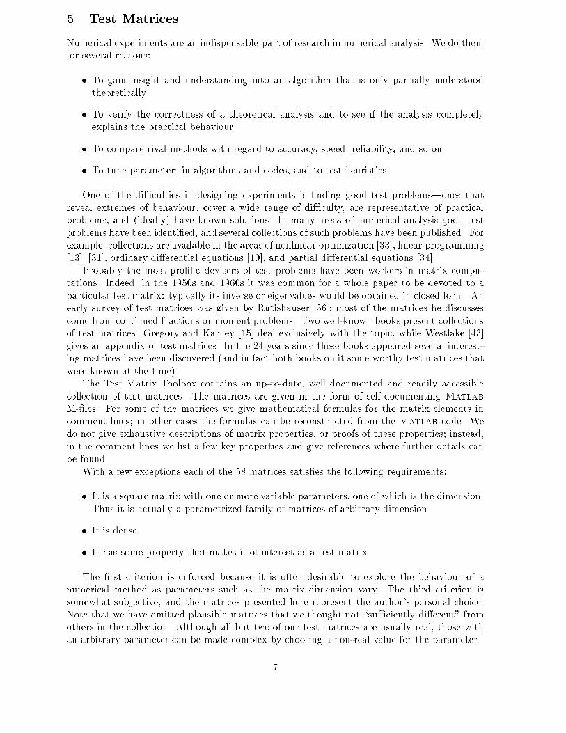
Figure 9.1: Gershgorin disks for magic(8).

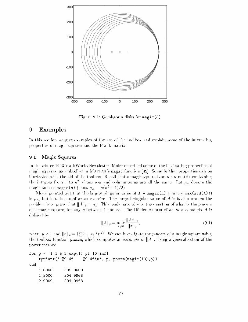
9 Examples

In this section we give examples of the use of the toolbox and explain some of the interestingproperties of magic squares and the Frank matrix.

9.1 Magic Squares

In the winter 1993 MathWorks Newsletter, Moler described some of the fascinating properties ofmagic squares, as embodied in Matlab's magic function [32]. Some further properties can beillustrated with the aid of the toolbox. Recall that a magic square is an n�n matrix containingthe integers from 1 to n2 whose row and column sums are all the same. Let �n denote themagic sum of magic(n) (thus, �n = n(n2 + 1)=2).

Moler pointed out that the largest singular value of A = magic(n) (namely max(svd(A)))is �n, but left the proof as an exercise. The largest singular value of A is its 2-norm, so theproblem is to prove that kAk2 = �n. This leads naturally to the question of what is the p-normof a magic square, for any p between 1 and 1. The H�older p-norm of an m � n matrix A isde�ned by

kAkp = maxx6=0

kAxkpkxkp ; (9.1)

where p � 1 and kxkp = (Pn

i=1 jxijp)1=p. We can investigate the p-norm of a magic square usingthe toolbox function pnorm, which computes an estimate of kAkp using a generalization of thepower method.

for p = [1 1.5 2 exp(1) pi 10 inf]

fprintf(' %9.4f %9.4f\n', p, pnorm(magic(10),p))

end

1.0000 505.0000

1.5000 504.9968

2.0000 504.9968

23

0 200 400

-200

-100

0

100

200

n = 9

-200 0 200 400

-200

0

200

n = 10

-200 0 200 400 600-500

0

500

n = 11

-200 0 200400600800

-500

0

500

n = 12

Figure 9.2: Field of values for magic(n).

2.7183 504.9971

3.1416 504.9997

10.0000 504.9988

Inf 505.0000

All the p-norms in this example are very close to �10 = 505. Since the default convergencetolerance for pnorm is 10�4, the exact p-norms could all be 505, as far as we can tell from theestimates. In fact, kAkp � �n for all 1 � p � 1. The proof relies on the convexity of thep-norm, which yields the inequality (see, [22], for example)

kAkp � kAk1=p1 kAk1�1=p1 :

(This inequality is well-known for p = 2.) For a magic square, kAk1 = kAk1 = �n, so theinequality gives kAkp � �n. But by taking x in (9.1) to be the vector of all ones, we seethat kAkp � �n, and so it follows that kAkp = �n. This result is actually a special case ofan apparently little-known 1962 result of Stoer and Witzgall, which says that the norm of adoubly stochastic matrix is 1 for any norm subordinate to a permutation-invariant absolutevector norm [38].

To estimate the eigenvalues of magic(n) we can apply Gershgorin's theorem. Unfortunately,the results are not very informative because the Gershgorin disks are all approximately the same,as is clear from the structure of the matrix; see Figure 9.1.

In his article, Moler pointed out that the function magic uses di�erent algorithms for oddn, even n divisible by 4, and even n not divisible by 4. He gave four mesh plots to illustratethe di�erence. Another approach is to look at the �elds of values|see Figure 9.2. The plotfor n = 10 re ects the fact that magic(n) has rank n=2 + 2 when n is even and not divisibleby 4|there are only 6 eigenvalues away from the origin (magic(10) is diagonalizable). For ndivisible by 4 the rank is only 3.

24

9.2 The Frank Matrix

A famous test matrix for eigensolvers is the n � n upper Hessenberg matrix Fn introduced byFrank in 1958 [11], illustrated for n = 8 by

F = frank(8)

F =

8 7 6 5 4 3 2 1

7 7 6 5 4 3 2 1

0 6 6 5 4 3 2 1

0 0 5 5 4 3 2 1

0 0 0 4 4 3 2 1

0 0 0 0 3 3 2 1

0 0 0 0 0 2 2 1

0 0 0 0 0 0 1 1

In evaluating three eigenvalue algorithms Frank found that this matrix \gives our selectedprocedures di�culties", and that \accuracy was lost in the smaller roots". The di�cultiesencountered by Frank's codes were shown by Wilkinson [44, Section 8], [45, pp. 92{93] to becaused by the inherent sensitivity of the eigenvalues to perturbations in the matrix.

The Frank matrix is interesting to analyze using Matlab. The toolbox function eigsens

evaluates the Wilkinson eigenvalue condition numbers, which are the reciprocals of the cosinesof the angles between the left and right eigenvectors:

F = frank(10);

[V, D, s] = eigsens(F); d = diag(D); [x, k] = sort(d);

[d(k) s(k)] % Eigenvalue followed by its condition number.

ans =

3.9100e-002 1.4082e+005

6.7743e-002 2.5897e+005

1.2426e-001 1.4103e+005

2.5692e-001 2.4028e+004

6.1859e-001 1.1837e+003

1.6166e+000 3.1920e+001

3.8922e+000 2.2871e+000

8.0476e+000 1.8287e+000

1.4762e+001 3.0303e+000

2.5575e+001 2.3393e+000

The output shows that the condition numbers grow, almost monotonically, as the eigenvaluesdecrease in size|in other words, the smallest eigenvalues are the most sensitive to perturbationsin the matrix. The varying eigenvalue sensitivities can also be seen from pseudospectral plots.Figure 9.3 shows the 0:1-pseudospectrum, which shows that perturbations to F10 of 2-normat most 0:1 have the greatest e�ect on the smallest eigenvalues. Another view is provided byFigure 9.4, for which we set colormap hot.

Further insight into the eigenvalues of Fn can be obtained by looking at its characteristicpolynomial:

poly(F)

25

0 5 10 15 20 25

-15

-10

-5

0

5

10

15

Figure 9.3: ps(frank(10), 50, 1e-1, 0, 1).

ans =

1.0e+004 *

Columns 1 through 7

0.0001 -0.0055 0.1035 -0.8310 2.9505 -4.5297 2.9505

Columns 8 through 11

-0.8310 0.1035 -0.0055 0.0001

The coe�cients seem to be palindromic! As a check we use the function charpoly fromMatlab

4's Maple Symbolic Toolbox [5] to compute the characteristic polynomial exactly:

charpoly(F)

ans =

1-55*x+1035*x^2-8310*x^3+29505*x^4-45297*x^5+29505*x^6-8310*x^7+1035*x^8-55*x^9+x^10

Any matrix whose characteristic polynomial �n has a palindromic coe�cient vector has eigen-values occurring in reciprocal pairs, since �n(�) = �n�n(1=�). In particular, it has determinant1, and 1 is an eigenvalue when n is odd. We can check the determinant property numerically:

F = frank(20); [det(F) det(F')]

ans =

26

-20

0

20

40

-20

-10

0

10

20-4

-3

-2

-1

0

1

2

Figure 9.4: pscont(frank(10), 2, 25, [-7 33 -20 20]).

1 -14

F = frank(25); [det(F) det(F')]

ans =

1 -48886168

Since det(A) = det(AT ) for any matrix A, the output is mathematically incorrect. The reason isthat rounding errors in uenceMatlab's evaluation of det(FT

n ) much more than its evaluation ofdet(Fn); an illuminating discussion of this phenomenon is given by Frank [11] and Wilkinson [44,Section 8], [45, pp. 92{93]. The extreme sensitivity of det(Fn) to perturbations in Fn is easyto see: if we change the (1; n) element from 1 to 1 + �, then det(Fn) changes from 1 to 1 +(�1)n(n� 1)!�.

The inverse of Fn is lower Hessenberg. This can be seen using the following representationof Fn noted by Rutishauser [36, Sec. 9]:

Fn = PCnP;

where P is the identity with the order of its columns reversed (I = eye(n); P = I(:, n:-1:1)

in Matlab notation) and

Cn =

2666664

1�1 1

�1 1. ..

. . .

�1 1

3777775

�1 2666664

1 11 2

1. . .. . . n � 1

1

3777775:

(By manipulating the identity det(Fn � �I) = det(Cn� �I) the reciprocal pair property of theeigenvalues can be proved; cf. [42].) As an illustration, here is the exact inverse as returned

27

by the Maple Symbolic Toolbox (the Matlab function inv produces nonzero, but tiny, uppertriangular elements because of rounding errors):

inverse(frank(8))

ans =

[ 1, -1, 0, 0, 0, 0, 0, 0]

[ -7, 8, -1, 0, 0, 0, 0, 0]

[ 42, -48, 7, -1, 0, 0, 0, 0]

[ -210, 240, -35, 6, -1, 0, 0, 0]

[ 840, -960, 140, -24, 5, -1, 0, 0]

[-2520, 2880, -420, 72, -15, 4, -1, 0]

[ 5040, -5760, 840, -144, 30, -8, 3, -1]

[-5040, 5760, -840, 144, -30, 8, -3, 2]

In his 1958 paper, Frank commented

\At the moment, the largest matrices resolved on the [Univac] 1103A are two 20-order matrices, one real symmetric and one complex. In both cases computing timewas approximately one hour, and 6{8 places of accuracy were obtained."

The complete eigensystem of a complex 20 � 20 matrix A is found in under a second by theMatlab command eig(A) on the workstation used for the examples reported here! Thisimprovement over Frank's timing is attributable not only to hardware advances but also to analgorithmic breakthrough: eig uses the QR algorithm, which was not available to Frank.

9.3 Numerical Linear Algebra

The Test Matrix Toolbox M-�les embody some well-known and other not so well-known resultsfrom numerical linear algebra.

The function gfpp generates n � n matrices that produce the maximum growth of 2n�1

for Gaussian elimination with partial pivoting; these include Wilkinson's classic example [45,p. 212]

gfpp(7)

ans =

1 0 0 0 0 0 1

-1 1 0 0 0 0 1

-1 -1 1 0 0 0 1

-1 -1 -1 1 0 0 1

-1 -1 -1 -1 1 0 1

-1 -1 -1 -1 -1 1 1

-1 -1 -1 -1 -1 -1 1

as well as all members of the \2n�1 class" described by Higham and Higham [27]. The followingextract uses the toolbox routine gecp to evaluate the growth factor for complete pivoting onthe Wilkinson matrix.

28

n = 20; A = gfpp(n);

[L, U] = lu(A); % Partial pivoting.

[max(max(abs(U))) / max(max(abs(A))) 2^(n-1)] % Approximation to growth factor.

ans =

524288 524288

% Complete pivoting using toolbox routine GECP.

[L, U, P, Q, rho] = gecp(A); rho

rho =

2

As the output shows, complete pivoting is perfectly stable for these matrices. However, severalof the matrices produced by orthog yield relatively large growth for complete pivoting: growthof order n=2 for real data, or n for a particular complex matrix [27].

n = 50;

for k = [-2 -1 1 2 3]

A = orthog(n, k);

[L, U, P, Q, rho] = gecp(A);

fprintf(' %g\n', rho)

end

25.3116

24.7028

25.6214

25.3296

50

A = hadamard(64);

[L, U, P, Q, rho] = gecp(A); rho

rho =

64

It is easy to show that complete pivoting su�ers growth of at least n for an n � n Hadamardmatrix. However, Hadamard matrices do not exist for all n.

The Matlab function rcond computes an upper bound for �1(A)�1 = (kAk1kA�1k1)�1

using the LINPACK condition estimation algorithm. Although this algorithm is very reliable ingeneral, parametrized matrices are known for which it can perform arbitrarily badly [6]. Hereare two examples, from the toolbox routine condex. The underestimation ratio is approximatelythe same in both examples, but the second is probably the more serious because rcond doesnot detect any ill-conditioning whatsoever.

A = condex(4, 1, 1e8); format short e

% True estimate true/estimate

[cond(A,1) 1/rcond(A) cond(A,1)*rcond(A)]

ans =

29

8.0000e+016 5.6000e+008 1.4286e+008

A = condex(3, 2, 1e8);

[cond(A,1) 1/rcond(A) cond(A,1)*rcond(A)]

ans =

6.0000e+008 7.5000e+000 8.0000e+007

The QR decomposition with column pivoting of A 2 Cm�n (m � n) is a decomposition

A� = QhR0

iwhere � is a permutation matrix chosen according to a certain pivoting strategy,

Q is orthogonal, and R is upper triangular [14, Section 5.4.1]. This decomposition is often usedto estimate the rank of A; in particular, jrnnj provides an upper bound for the smallest singularvalue �min(A) of A that is usually at most a factor of 10 too big. Kahan [30] designed a matrixfor which jrnnj can be approximately 2n�1 times bigger than �min(A), and which thus showsthe fallibility of the QR decomposition with column pivoting for revealing rank. The toolboxfunction kahan generates Kahan's matrix:

n = 25;

A = kahan(n, 0.6);

[Q, R, Pi] = qr(A);

norm(Pi-eye(n),1), R(n,n)/min(svd(A))

ans =

0

ans =

1.0638e+006

Kahan's matrix A(�) is upper triangular and is designed so that � is the identity in the QRdecomposition with column pivoting. In practice, rounding errors can cause � to di�er fromthe identity for the Kahan matrix, thus nullifying the example (the test on � � I in theabove example con�rms that � is indeed the identity here). The toolbox routine adds a smallperturbation to the diagonal elements of A(�) so that � = I for a range of choices of n and �.If we set the perturbation in the above example to zero, this is what happens:

A = kahan(n, 0.6, 0); % Third parameter is the diagonal perturbation.

[Q, R, Pi] = qr(A);

norm(Pi-eye(n),1), R(n,n)/min(svd(A))

ans =

2

ans =

1.1953

30

The toolbox contains two matrices, one a Toeplitz matrix and the other a Hankel matrix,whose eigenvalues or singular values are related to �:

A = parter(10); format long

e = svd(A); [e e-pi]

ans =

3.14159265358968 -0.00000000000011

3.14159265356666 -0.00000000002313

3.14159265139317 -0.00000000219663

3.14159252749873 -0.00000012609106

3.14158778157056 -0.00000487201924

3.14145930586226 -0.00013334772753

3.13895248060091 -0.00264017298888

3.10410768313639 -0.03748497045341

2.78691548240413 -0.35467717118566

1.30096907002970 -1.84062358356009

A = dingdong(10);

e = eig(A); [e abs(e)-pi/2]

ans =

-1.57079632679484 -0.00000000000006

-1.57079632569658 -0.00000000109831

-1.57079389078528 -0.00000243600962

1.57079632678333 -0.00000000001157

1.57079626374937 -0.00000006304553

1.57072965293113 -0.00006667386377

-1.56947624030045 -0.00132008649444

1.55205384156819 -0.01874248522670

-1.39345774120206 -0.17733858559283

0.65048453501485 -0.92031179178005

Finally, here is an example of the use of the function matrix to access the test matricessequentially, by number. The following piece of code steps through all the square matricesof arbitrary dimension, setting A to each 10 � 10 matrix in turn (any matrix parameters areat their default values). It evaluates the 2-norm condition number and the ratio �(A) =maxi j�i(A)j=mini j�i(A)j of the largest to smallest eigenvalue in absolute value.

c = []; e = [];

j = 1;

for i=1:matrix(0)

A = full(matrix(i, 10));

if norm(skewpart(A),1) % If not Hermitian...

c1 = cond(A);

eg = eig(A);

e1 = max(abs(eg)) / min(abs(eg));

% Filter out extremely ill-conditioned matrices.

31

0 5 10 15 20 25 3010

0

102

104

106

108

cond: x, eig_ratio: o

0 5 10 15 20 25 3010

0

102

104

106

108

cond/eig_ratio

Figure 9.5: Comparison of condition number with extremal eigenvalue ratio.

if c1 <= 1e10, c(j) = c1; e(j) = e1; j = j + 1; end

end

end

As is well known, �2(A) can be arbitrarily larger than �(A). The plots in Figure 9.5, producedfrom the vectors c and e from the above code, con�rm that �2(A)=�(A) can be large.

32

10 M-File Leading Comment Lines

The demonstration �le tmtdemo is not listed here.

function [x, fmax, nf] = adsmax(f, x, stopit, savit, P)

%ADSMAX Alternating directions direct search method.

% [x, fmax, nf] = ADSMAX(f, x0, STOPIT, SAVIT, P) attempts to

% maximize the function specified by the string f, using the starting

% vector x0. The alternating directions direct search method is used.

% Output arguments:

% x = vector yielding largest function value found,

% fmax = function value at x,

% nf = number of function evaluations.

% The iteration is terminated when either

% - the relative increase in function value between successive

% iterations is <= STOPIT(1) (default 1e-3),

% - STOPIT(2) function evaluations have been performed

% (default inf, i.e., no limit), or

% - a function value equals or exceeds STOPIT(3)

% (default inf, i.e., no test on function values).

% Progress of the iteration is not shown if STOPIT(5) = 0 (default 1).

% If a non-empty fourth parameter string SAVIT is present, then

% `SAVE SAVIT x fmax nf' is executed after each inner iteration.

% By default, the search directions are the co-ordinate directions.

% The columns of a fifth parameter matrix P specify alternative search

% directions (P = EYE is the default).

% NB: x0 can be a matrix. In the output argument, in SAVIT saves,

% and in function calls, x has the same shape as x0.

% Reference:

% N.J. Higham, Optimization by direct search in matrix computations,

% SIAM J. Matrix Anal. Appl, 14(2): 317-333, April 1993.

function C = augment(A, alpha)

%AUGMENT Augmented system matrix.

% AUGMENT(A, ALPHA) is the square matrix

% [ALPHA*EYE(m) A; A' ZEROS(n)] of dimension m+n, where A is m-by-n.

% It is the symmetric and indefinite coefficient matrix of the

% augmented system associated with a least squares problem

% minimize NORM(A*x-b). ALPHA defaults to 1.

% Special case: if A is a scalar, n say, then AUGMENT(A) is the

% same as AUGMENT(RANDN(p,q)) where n = p+q and

% p = ROUND(n/2), that is, a random augmented matrix

% of dimension n is produced.

% The eigenvalues of AUGMENT(A) are given in terms of the singular

% values s(i) of A (where m>n) by

% 1/2 +/- SQRT( s(i)^2 + 1/4 ), i=1:n (2n eigenvalues),

% 1, (m-n eigenvalues).

% If m < n then the first expression provides 2m eigenvalues and the

33

% remaining n-m eigenvalues are zero.

%

% See also SPAUGMENT.

% Reference:

% G.H. Golub and C.F. Van Loan, Matrix Computations, Second

% Edition, Johns Hopkins University Press, Baltimore, Maryland,

% 1989, sec. 5.6.4.

function A = bandred(A, kl, ku)

%BANDRED Band reduction by two-sided unitary transformations.

% B = BANDRED(A, KL, KU) is a matrix unitarily equivalent to A

% with lower bandwidth KL and upper bandwidth KU

% (i.e. B(i,j) = 0 if i > j+KL or j > i+KU).

% The reduction is performed using Householder transformations.

% If KU is omitted it defaults to KL.

% Called by RANDSVD.

% This is a `standard' reduction. Cf. reduction to bidiagonal form

% prior to computing the SVD. This code is a little wasteful in that

% it computes certain elements which are immediately set to zero!

%

% Reference:

% G.H. Golub and C.F. Van Loan, Matrix Computations, second edition,

% Johns Hopkins University Press, Baltimore, Maryland, 1989.

% Section 5.4.3.

function C = cauchy(x, y)

%CAUCHY Cauchy matrix.

% C = CAUCHY(X, Y), where X, Y are N-vectors, is the N-by-N matrix

% with C(i,j) = 1/(X(i)+Y(j)). By default, Y = X.

% Special case: if X is a scalar CAUCHY(X) is the same as CAUCHY(1:X).

% Explicit formulas are known for DET(C) (which is nonzero if X and Y

% both have distinct elements) and the elements of INV(C).

% C is totally positive if 0 < X(1) < ... < X(N) and

% 0 < Y(1) < ... < Y(N).

% References:

% N.J. Higham, Accuracy and Stability of Numerical Algorithms,

% Society for Industrial and Applied Mathematics, Philadelphia, PA,

% USA, 1996; sec. 26.1.

% D.E. Knuth, The Art of Computer Programming, Volume 1,

% Fundamental Algorithms, second edition, Addison-Wesley, Reading,

% Massachusetts, 1973, p. 36.

% E.E. Tyrtyshnikov, Cauchy-Toeplitz matrices and some applications,

% Linear Algebra and Appl., 149 (1991), pp. 1-18.

% O. Taussky and M. Marcus, Eigenvalues of finite matrices, in

% Survey of Numerical Analysis, J. Todd, ed., McGraw-Hill, New York,

% pp. 279-313, 1962. (States the totally positive property on p. 295.)

34

function [Q, R] = cgs(A)

%CGS Classical Gram-Schmidt QR factorization.

% [Q, R] = cgs(A) uses the classical Gram-Schmidt method to compute the

% factorization A = Q*R for m-by-n A of full rank,

% where Q is m-by-n with orthonormal columns and R is n-by-n.

function C = chebspec(n, k)

%CHEBSPEC Chebyshev spectral differentiation matrix.

% C = CHEBSPEC(N, K) is a Chebyshev spectral differentiation

% matrix of order N. K = 0 (the default) or 1.

% For K = 0 (`no boundary conditions'), C is nilpotent, with

% C^N = 0 and it has the null vector ONES(N,1).

% C is similar to a Jordan block of size N with eigenvalue zero.

% For K = 1, C is nonsingular and well-conditioned, and its eigenvalues

% have negative real parts.

% For both K, the computed eigenvector matrix X from EIG is

% ill-conditioned (MESH(REAL(X)) is interesting).

% References:

% C. Canuto, M.Y. Hussaini, A. Quarteroni and T.A. Zang, Spectral

% Methods in Fluid Dynamics, Springer-Verlag, Berlin, 1988; p. 69.

% L.N. Trefethen and M.R. Trummer, An instability phenomenon in

% spectral methods, SIAM J. Numer. Anal., 24 (1987), pp. 1008-1023.

% D. Funaro, Computing the inverse of the Chebyshev collocation

% derivative, SIAM J. Sci. Stat. Comput., 9 (1988), pp. 1050-1057.

function C = chebvand(m,p)

%CHEBVAND Vandermonde-like matrix for the Chebyshev polynomials.

% C = CHEBVAND(P), where P is a vector, produces the (primal)

% Chebyshev Vandermonde matrix based on the points P,

% i.e., C(i,j) = T_{i-1}(P(j)), where T_{i-1} is the Chebyshev

% polynomial of degree i-1.

% CHEBVAND(M,P) is a rectangular version of CHEBVAND(P) with M rows.

% Special case: If P is a scalar then P equally spaced points on

% [0,1] are used.

% Reference:

% N.J. Higham, Stability analysis of algorithms for solving confluent

% Vandermonde-like systems, SIAM J. Matrix Anal. Appl., 11 (1990),

% pp. 23-41.

function [R, P, I] = cholp(A, pivot)

%CHOLP Cholesky factorization with pivoting of a pos. semidefinite matrix.

% [R, P] = CHOLP(A) returns R and a permutation matrix P such that

% R'*R = P'*A*P. Only the upper triangular part of A is used.

% [R, P, I] = CHOLP(A) returns in addition the index I of the last

% positive diagonal element of R. The first I rows of R contain

% the Cholesky factor of A.

35

% [R, I] = CHOLP(A, 0) forces P = EYE(SIZE(A)), and therefore produces

% the same output as R = CHOL(A) when A is positive definite (to

% within roundoff).

% This routine is based on the LINPACK routine CCHDC. It works

% for both real and complex matrices.

%

% Reference:



% 1989, sec. 4.2.9.

function c = chop(x, t)

%CHOP Round matrix elements.

% CHOP(X, t) is the matrix obtained by rounding the elements of X

% to t significant binary places.

% Default is t = 24, corresponding to IEEE single precision.

function A = chow(n, alpha, delta)

%CHOW Chow matrix - a singular Toeplitz lower Hessenberg matrix.

% A = CHOW(N, ALPHA, DELTA) is a Toeplitz lower Hessenberg matrix

% A = H(ALPHA) + DELTA*EYE, where H(i,j) = ALPHA^(i-j+1).

% H(ALPHA) has p = FLOOR(N/2) zero eigenvalues, the rest being

% 4*ALPHA*COS( k*PI/(N+2) )^2, k=1:N-p.

% Defaults: ALPHA = 1, DELTA = 0.

% References:

% T.S. Chow, A class of Hessenberg matrices with known

% eigenvalues and inverses, SIAM Review, 11 (1969), pp. 391-395.

% G. Fairweather, On the eigenvalues and eigenvectors of a class of

% Hessenberg matrices, SIAM Review, 13 (1971), pp. 220-221.

function C = circul(v)

%CIRCUL Circulant matrix.

% C = CIRCUL(V) is the circulant matrix whose first row is V.

% (A circulant matrix has the property that each row is obtained

% from the previous one by cyclically permuting the entries one step

% forward; it is a special Toeplitz matrix in which the diagonals

% `wrap round'.)

% Special case: if V is a scalar then C = CIRCUL(1:V).

% The eigensystem of C (N-by-N) is known explicitly. If t is an Nth

% root of unity, then the inner product of V with W = [1 t t^2 ... t^N]

% is an eigenvalue of C, and W(N:-1:1) is an eigenvector of C.

% Reference:

% P.J. Davis, Circulant Matrices, John Wiley, 1977.

36

function A = clement(n, k)

%CLEMENT Clement matrix - tridiagonal with zero diagonal entries.

% CLEMENT(N, K) is a tridiagonal matrix with zero diagonal entries

% and known eigenvalues. It is singular if N is odd. About 64

% percent of the entries of the inverse are zero. The eigenvalues

% are plus and minus the numbers N-1, N-3, N-5, ..., (1 or 0).

% For K = 0 (the default) the matrix is unsymmetric, while for

% K = 1 it is symmetric.

% CLEMENT(N, 1) is diagonally similar to CLEMENT(N).

% Similar properties hold for TRIDIAG(X,Y,Z) where Y = ZEROS(N,1).

% The eigenvalues still come in plus/minus pairs but they are not

% known explicitly.

%

% References:

% P.A. Clement, A class of triple-diagonal matrices for test

% purposes, SIAM Review, 1 (1959), pp. 50-52.

% A. Edelman and E. Kostlan, The road from Kac's matrix to Kac's

% random polynomials. In John~G. Lewis, editor, Proceedings of

% the Fifth SIAM Conference on Applied Linear Algebra Society

% for Industrial and Applied Mathematics, Philadelphia, 1994,

% pp. 503-507.

% O. Taussky and J. Todd, Another look at a matrix of Mark Kac,


function [U, R, V] = cod(A, tol)

%COD Complete orthogonal decomposition.

% [U, R, V] = COD(A, TOL) computes a decomposition A = U*T*V,

% where U and V are unitary, T = [R 0; 0 0] has the same dimensions as

% A, and R is upper triangular and nonsingular of dimension rank(A).

% Rank decisions are made using TOL, which defaults to approximately

% MAX(SIZE(A))*NORM(A)*EPS.

% By itself, COD(A, TOL) returns R.

% Reference:



% 1989, sec. 5.4.2.

function C = comp(A, k)

%COMP Comparison matrices.

% COMP(A) is DIAG(B) - TRIL(B,-1) - TRIU(B,1), where B = ABS(A).

% COMP(A, 1) is A with each diagonal element replaced by its

% absolute value, and each off-diagonal element replaced by minus

% the absolute value of the largest element in absolute value in

% its row. However, if A is triangular COMP(A, 1) is too.

% COMP(A, 0) is the same as COMP(A).

% COMP(A) is often denoted by M(A) in the literature.

37

% Reference (e.g.):

% N.J. Higham, A survey of condition number estimation for

% triangular matrices, SIAM Review, 29 (1987), pp. 575-596.

function A = compan(p)

%COMPAN Companion matrix.

% COMPAN(P) is a companion matrix. There are three cases.

% If P is a scalar then COMPAN(P) is the P-by-P matrix COMPAN(1:P+1).

% If P is an (n+1)-vector, COMPAN(P) is the n-by-n companion matrix

% whose first row is -P(2:n+1)/P(1).

% If P is a square matrix, COMPAN(P) is the companion matrix

% of the characteristic polynomial of P, computed as

% COMPAN(POLY(P)).

% References:

% J.H. Wilkinson, The Algebraic Eigenvalue Problem,

% Oxford University Press, 1965, p. 12.


% Johns Hopkins University Press, Baltimore, Maryland, 1989,

% sec 7.4.6.

% C. Kenney and A.J. Laub, Controllability and stability radii for

% companion form systems, Math. Control Signals Systems, 1 (1988),

% pp. 239-256. (Gives explicit formulas for the singular values of

% COMPAN(P).)

function y = cond(A, p)

%COND Matrix condition number in 1, 2, Frobenius, or infinity norm.

% For p = 1, 2, 'fro', inf, COND(A,p) = NORM(A,p) * NORM(INV(A),p).

% If p is omitted then p = 2 is used.

% A may be a rectangular matrix if p = 2; in this case COND(A)

% is the ratio of the largest singular value of A to the smallest

% (and hence is infinite if A is rank deficient).

function A = condex(n, k, theta)

%CONDEX `Counterexamples' to matrix condition number estimators.

% CONDEX(N, K, THETA) is a `counterexample' matrix to a condition

% estimator. It has order N and scalar parameter THETA (default 100).

% If N is not equal to the `natural' size of the matrix then

% the matrix is padded out with an identity matrix to order N.

% The matrix, its natural size, and the estimator to which it applies

% are specified by K (default K = 4) as follows:

% K = 1: 4-by-4, LINPACK (RCOND)

% K = 2: 3-by-3, LINPACK (RCOND)

% K = 3: arbitrary, LINPACK (RCOND) (independent of THETA)

% K = 4: N >= 4, SONEST (Higham 1988)

% (Note that in practice the K = 4 matrix is not usually a

% counterexample because of the rounding errors in forming it.)

38

% References:

% A.K. Cline and R.K. Rew, A set of counter-examples to three

% condition number estimators, SIAM J. Sci. Stat. Comput.,

% 4 (1983), pp. 602-611.

% N.J. Higham, FORTRAN codes for estimating the one-norm of a real or

% complex matrix, with applications to condition estimation

% (Algorithm 674), ACM Trans. Math. Soft., 14 (1988), pp. 381-396.

function x = cpltaxes(z)

%CPLTAXES Determine suitable AXIS for plot of complex vector.

% X = CPLTAXES(Z), where Z is a complex vector,

% determines a 4-vector X such that AXIS(X) sets axes for a plot

% of Z that has axes of equal length and leaves a reasonable amount

% of space around the edge of the plot.

% Called by FV, GERSH, PS and PSCONT.

function A = cycol(n, k)

%CYCOL Matrix whose columns repeat cyclically.

% A = CYCOL([M N], K) is an M-by-N matrix of the form A = B(1:M,1:N)

% where B = [C C C...] and C = RANDN(M, K). Thus A's columns repeat

% cyclically, and A has rank at most K. K need not divide N.

% K defaults to ROUND(N/4).

% CYCOL(N, K), where N is a scalar, is the same as CYCOL([N N], K).

%

% This type of matrix can lead to underflow problems for Gaussian

% elimination: see NA Digest Volume 89, Issue 3 (January 22, 1989).

function [L, D, P, rho] = diagpiv(A)

%DIAGPIV Diagonal pivoting factorization with partial pivoting.

% Given a symmetric matrix A,

% [L, D, P, rho] = diagpiv(A) computes a permutation P,

% a unit lower triangular L, and a block diagonal D

% with 1x1 and 2x2 diagonal blocks, such that

% P*A*P' = L*D*L'.

% The Bunch-Kaufman partial pivoting strategy is used.

% Rho is the growth factor.

% Reference:

% J.R. Bunch and L. Kaufman, Some stable methods for calculating

% inertia and solving symmetric linear systems, Math. Comp.,

% 31(137):163-179, 1977.

function A = dingdong(n)

%DINGDONG Dingdong matrix - a symmetric Hankel matrix.

% A = DINGDONG(N) is the symmetric N-by-N Hankel matrix with

% A(i,j) = 0.5/(N-i-j+1.5).

39

% The eigenvalues of A cluster around PI/2 and -PI/2.

% Invented by F.N. Ris.

%

% Reference:

% J.C. Nash, Compact Numerical Methods for Computers: Linear

% Algebra and Function Minimisation, second edition, Adam Hilger,

% Bristol, 1990 (Appendix 1).

function [c, d, e] = dorr(n, theta)

%DORR Dorr matrix - diagonally dominant, ill conditioned, tridiagonal.

% [C, D, E] = DORR(N, THETA) returns the vectors defining a row diagonally

% dominant, tridiagonal M-matrix that is ill conditioned for small

% values of the parameter THETA >= 0.

% If only one output parameter is supplied then

% C = FULL(TRIDIAG(C,D,E)), i.e., the matrix iself is returned.

% The columns of INV(C) vary greatly in norm. THETA defaults to 0.01.

% The amount of diagonal dominance is given by (ignoring rounding errors):

% COMP(C)*ONES(N,1) = THETA*(N+1)^2 * [1 0 0 ... 0 1]'.

% Reference:

% F.W. Dorr, An example of ill-conditioning in the numerical

% solution of singular perturbation problems, Math. Comp., 25 (1971),

% pp. 271-283.

function A = dramadah(n, k)

%DRAMADAH A (0,1) matrix whose inverse has large integer entries.

% An anti-Hadamard matrix A is a matrix with elements 0 or 1 for

% which MU(A) := NORM(INV(A),'FRO') is maximal.

% A = DRAMADAH(N, K) is an N-by-N (0,1) matrix for which MU(A) is

% relatively large, although not necessarily maximal.

% Available types (the default is K = 1):

% K = 1: A is Toeplitz, with ABS(DET(A)) = 1, and MU(A) > c(1.75)^N,

% where c is a constant.

% K = 2: A is upper triangular and Toeplitz.

% The inverses of both types have integer entries.

%

% Another interesting (0,1) matrix:

% K = 3: A has maximal determinant among (0,1) lower Hessenberg

% matrices: det(A) = the n'th Fibonacci number. A is Toeplitz.

% The eigenvalues have an interesting distribution in the complex

% plane.

% References:

% R.L. Graham and N.J.A. Sloane, Anti-Hadamard matrices,


% L. Ching, The maximum determinant of an nxn lower Hessenberg

% (0,1) matrix, Linear Algebra and Appl., 183 (1993), pp. 147-153.

40

function y = dual(x, p)

%DUAL Dual vector with respect to Holder p-norm.

% Y = DUAL(X, p), where 1 <= p <= inf, is a vector of unit q-norm

% that is dual to X with respect to the p-norm, that is,

% norm(Y, q) = 1 where 1/p + 1/q = 1 and there is

% equality in the Holder inequality: X'*Y = norm(X, p)*norm(Y, q).

% Special case: DUAL(X), where X >= 1 is a scalar, returns Y such

% that 1/X + 1/Y = 1.

% Called by PNORM.

function [X, D, s] = eigsens(A)

%EIGSENS Eigenvalue condition numbers.

% EIGSENS(A) is a vector of condition numbers for the eigenvalues

% of A (reciprocals of the Wilkinson s(lambda) numbers).

% These condition numbers are the reciprocals of the cosines of the

% angles between the left and right eigenvectors.

% [V, D, s] = EIGSENS(A) is equivalent to

% [V, D] = EIG(A); s = EIGSENS(A);

% Reference:



% 1989, sec. 7.2.2.

function f = fdemo(A)

%FDEMO Demonstration function for direct search maximizers.

% FDEMO(A) is the reciprocal of the underestimation ratio for RCOND

% applied to the square matrix A.

% Demonstration function for ADSMAX, MDSMAX and NMSMAX.

function A = fiedler(c)

%FIEDLER Fiedler matrix - symmetric.

% A = FIEDLER(C), where C is an n-vector, is the n-by-n symmetric

% matrix with elements ABS(C(i)-C(j)).

% Special case: if C is a scalar, then A = FIEDLER(1:C)

% (i.e. A(i,j) = ABS(i-j)).

% Properties:

% FIEDLER(N) has a dominant positive eigenvalue and all the other

% eigenvalues are negative (Szego, 1936).

% Explicit formulas for INV(A) and DET(A) are given by Todd (1977)

% and attributed to Fiedler. These indicate that INV(A) is

% tridiagonal except for nonzero (1,n) and (n,1) elements.

% [I think these formulas are valid only if the elements of

% C are in increasing or decreasing order---NJH.]

% References:

% G. Szego, Solution to problem 3705, Amer. Math. Monthly,

41

% 43 (1936), pp. 246-259.

% J. Todd, Basic Numerical Mathematics, Vol. 2: Numerical Algebra,

% Birkhauser, Basel, and Academic Press, New York, 1977, p. 159.

function A = forsythe(n, alpha, lambda)

%FORSYTHE Forsythe matrix - a perturbed Jordan block.

% FORSYTHE(N, ALPHA, LAMBDA) is the N-by-N matrix equal to

% JORDBLOC(N, LAMBDA) except it has an ALPHA in the (N,1) position.

% It has the characteristic polynomial

% DET(A-t*EYE) = (LAMBDA-t)^N - (-1)^N ALPHA.

% ALPHA defaults to SQRT(EPS) and LAMBDA to 0.

function F = frank(n, k)

%FRANK Frank matrix---ill conditioned eigenvalues.

% F = FRANK(N, K) is the Frank matrix of order N. It is upper

% Hessenberg with determinant 1. K = 0 is the default; if K = 1 the

% elements are reflected about the anti-diagonal (1,N)--(N,1).

% F has all positive eigenvalues and they occur in reciprocal pairs

% (so that 1 is an eigenvalue if N is odd).

% The eigenvalues of F may be obtained in terms of the zeros of the

% Hermite polynomials.

% The FLOOR(N/2) smallest eigenvalues of F are ill conditioned,

% the more so for bigger N.

% DET(FRANK(N)') comes out far from 1 for large N---see Frank (1958)

% and Wilkinson (1960) for discussions.

%

% This version incorporates improvements suggested by W. Kahan.

%

% References:

% W.L. Frank, Computing eigenvalues of complex matrices by determinant

% evaluation and by methods of Danilewski and Wielandt, J. Soc.

% Indust. Appl. Math., 6 (1958), pp. 378-392 (see pp. 385, 388).

% G.H. Golub and J.H. Wilkinson, Ill-conditioned eigensystems and the

% computation of the Jordan canonical form, SIAM Review, 18 (1976),

% pp. 578-619 (Section 13).

% H. Rutishauser, On test matrices, Programmation en Mathematiques

% Numeriques, Editions Centre Nat. Recherche Sci., Paris, 165,

% 1966, pp. 349-365. Section 9.

% J.H. Wilkinson, Error analysis of floating-point computation,

% Numer. Math., 2 (1960), pp. 319-340 (Section 8).

% J.H. Wilkinson, The Algebraic Eigenvalue Problem, Oxford University

% Press, 1965 (pp. 92-93).

% The next two references give details of the eigensystem, as does

% Rutishauser (see above).

% P.J. Eberlein, A note on the matrices denoted by B_n, SIAM J. Appl.

% Math., 20 (1971), pp. 87-92.

% J.M. Varah, A generalization of the Frank matrix, SIAM J. Sci. Stat.

% Comput., 7 (1986), pp. 835-839.

42

function [f, e] = fv(B, nk, thmax, noplot)

%FV Field of values (or numerical range).

% FV(A, NK, THMAX) evaluates and plots the field of values of the

% NK largest leading principal submatrices of A, using THMAX

% equally spaced angles in the complex plane.

% The defaults are NK = 1 and THMAX = 16.

% (For a `publication quality' picture, set THMAX higher, say 32.)

% The eigenvalues of A are displayed as `x'.

% Alternative usage: [F, E] = FV(A, NK, THMAX, 1) suppresses the

% plot and returns the field of values plot data in F, with A's

% eigenvalues in E. Note that NORM(F,INF) approximates the

% numerical radius,

% max {abs(z): z is in the field of values of A}.

% Theory:

% Field of values FV(A) = set of all Rayleigh quotients. FV(A) is a

% convex set containing the eigenvalues of A. When A is normal FV(A) is

% the convex hull of the eigenvalues of A (but not vice versa).

% z = x'Ax/(x'x), z' = x'A'x/(x'x)

% => REAL(z) = x'Hx/(x'x), H = (A+A')/2

% so MIN(EIG(H)) <= REAL(z) <= MAX(EIG(H))

% with equality for x = corresponding eigenvectors of H. For these x,

% RQ(A,x) is on the boundary of FV(A).

%

% Based on an original routine by A. Ruhe.

%

% References:

% R.A. Horn and C.R. Johnson, Topics in Matrix Analysis, Cambridge

% University Press, 1991, Section 1.5.

% A.S. Householder, The Theory of Matrices in Numerical Analysis,

% Blaisdell, New York, 1964, Section 3.3.

% C.R. Johnson, Numerical determination of the field of values of a

% general complex matrix, SIAM J. Numer. Anal., 15 (1978),

% pp. 595-602.

function [A, e] = gallery(n)

%GALLERY Famous, and not so famous, test matrices.

% A = GALLERY(N) is an N-by-N matrix with some special property.

% The following values of N are currently available:

% N = 3 is badly conditioned.

% N = 4 is the Wilson matrix. Symmetric pos def, integer inverse.

% N = 5 is an interesting eigenvalue problem: defective, nilpotent.

% N = 8 is the Rosser matrix, a classic symmetric eigenvalue problem.

% [A, e] = GALLERY(8) returns the exact eigenvalues in e.

% N = 21 is Wilkinson's tridiagonal W21+, another eigenvalue problem.

% Original version supplied with MATLAB. Modified by N.J. Higham.

%

% References:

43

% J.R. Westlake, A Handbook of Numerical Matrix Inversion and Solution

% of Linear Equations, John Wiley, New York, 1968.


% Press, 1965.

function [L, U, rho] = ge(A)

%GE Gaussian elimination without pivoting.

% [L, U, RHO] = GE(A) computes the factorization A = L*U,

% where L is unit lower triangular and U is upper triangular.

% RHO is the growth factor.

% By itself, GE(A) returns the final reduced matrix from the

% elimination containing both L and U.

function A = gearm(n, i, j)

%GEARM Gear matrix.

% A = GEARM(N,I,J) is the N-by-N matrix with ones on the sub- and

% super-diagonals, SIGN(I) in the (1,ABS(I)) position, SIGN(J)

% in the (N,N+1-ABS(J)) position, and zeros everywhere else.

% Defaults: I = N, j = -N.

% All eigenvalues are of the form 2*COS(a) and the eigenvectors

% are of the form [SIN(w+a), SIN(w+2a), ..., SIN(w+Na)].

% The values of a and w are given in the reference below.

% A can have double and triple eigenvalues and can be defective.

% GEARM(N) is singular.

% (GEAR is a Simulink function, hence GEARM for Gear matrix.)

% Reference:

% C.W. Gear, A simple set of test matrices for eigenvalue programs,

% Math. Comp., 23 (1969), pp. 119-125.

function [L, U, P, Q, rho] = gecp(A)

%GECP Gaussian elimination with complete pivoting.

% [L, U, P, Q, RHO] = GECP(A) computes the factorization P*A*Q = L*U,

% where L is unit lower triangular, U is upper triangular,

% and P and Q are permutation matrices. RHO is the growth factor.

% By itself, GECP(A) returns the final reduced matrix from the

% elimination containing both L and U.

function [G, e] = gersh(A, noplot)

%GERSH Gershgorin disks.

% GERSH(A) draws the Gershgorin disks for the matrix A.

% The eigenvalues are plotted as crosses `x'.

% Alternative usage: [G, E] = GERSH(A, 1) suppresses the plot

% and returns the data in G, with A's eigenvalues in E.

%

% Try GERSH(LESP(N)) and GERSH(SMOKE(N,1)).

44

function A = gfpp(T, c)

%GFPP Matrix giving maximal growth factor for Gaussian elim. with pivoting.

% GFPP(T) is a matrix of order N for which Gaussian elimination

% with partial pivoting yields a growth factor 2^(N-1).

% T is an arbitrary nonsingular upper triangular matrix of order N-1.

% GFPP(T, C) sets all the multipliers to C (0 <= C <= 1)

% and gives growth factor (1+C)^(N-1).

% GFPP(N, C) (a special case) is the same as GFPP(EYE(N-1), C) and

% generates the well-known example of Wilkinson.

% Reference:

% N.J. Higham and D.J. Higham, Large growth factors in

% Gaussian elimination with pivoting, SIAM J. Matrix Analysis and

% Appl., 10 (1989), pp. 155-164.

function x = gj(A, b, piv)

%GJ Gauss-Jordan elimination to solve Ax = b.

% x = GJ(A, b, PIV) solves Ax = b by Gauss-Jordan elimination,

% where A is a square, nonsingular matrix.

% PIV determines the form of pivoting:

% PIV = 0: no pivoting,

% PIV = 1 (default): partial pivoting.

function G = grcar(n, k)

%GRCAR Grcar matrix - a Toeplitz matrix with sensitive eigenvalues.

% GRCAR(N, K) is an N-by-N matrix with -1s on the

% subdiagonal, 1s on the diagonal, and K superdiagonals of 1s.

% The default is K = 3. The eigenvalues of this matrix form an

% interesting pattern in the complex plane (try PS(GRCAR(32))).

% References:

% J.F. Grcar, Operator coefficient methods for linear equations,

% Report SAND89-8691, Sandia National Laboratories, Albuquerque,

% New Mexico, 1989 (Appendix 2).

% N.M. Nachtigal, L. Reichel and L.N. Trefethen, A hybrid GMRES

% algorithm for nonsymmetric linear systems, SIAM J. Matrix Anal.

% Appl., 13 (1992), pp. 796-825.

function H = hadamard(n)

%HADAMARD Hadamard matrix.

% HADAMARD(N) is a Hadamard matrix of order N, that is,

% a matrix H with elements 1 or -1 such that H*H' = N*EYE(N).

% An N-by-N Hadamard matrix with N>2 exists only if REM(N,4) = 0.

% This function handles only the cases where N, N/12 or N/20

% is a power of 2.

% Reference:

% S.W. Golomb and L.D. Baumert, The search for Hadamard matrices,

% Amer. Math. Monthly, 70 (1963) pp. 12-17.

45

function A = hanowa(n, d)

%HANOWA A matrix whose eigenvalues lie on a vertical line in the complex plane.

% HANOWA(N, d) is the N-by-N block 2x2 matrix (thus N = 2M must be even)

% [d*EYE(M) -DIAG(1:M)

% DIAG(1:M) d*EYE(M)]

% It has complex eigenvalues lambda(k) = d +/- k*i (1 <= k <= M).

% Parameter d defaults to -1.

% Reference:

% E. Hairer, S.P. Norsett and G. Wanner, Solving Ordinary

% Differential Equations I: Nonstiff Problems, Springer-Verlag,

% Berlin, 1987. (pp. 86-87)

function H = hilb(n)

%HILB Hilbert matrix.

% HILB(N) is the N-by-N matrix with elements 1/(i+j-1).

% It is a famous example of a badly conditioned matrix.

% COND(HILB(N)) grows like EXP(3.5*N).

% See INVHILB (standard MATLAB routine) for the exact inverse, which

% has integer entries.

% HILB(N) is symmetric positive definite, totally positive, and a

% Hankel matrix.

% References:

% M.-D. Choi, Tricks or treats with the Hilbert matrix, Amer. Math.

% Monthly, 90 (1983), pp. 301-312.



% USA, 1996; sec. 26.1.

% M. Newman and J. Todd, The evaluation of matrix inversion

% programs, J. Soc. Indust. Appl. Math., 6 (1958), pp. 466-476.

% D.E. Knuth, The Art of Computer Programming,

% Volume 1, Fundamental Algorithms, second edition, Addison-Wesley,

% Reading, Massachusetts, 1973, p. 37.

function [v, beta] = house(x)

%HOUSE Householder matrix.

% If [v, beta] = HOUSE(x) then H = EYE - beta*v*v' is a Householder

% matrix such that Hx = -sign(x(1))*norm(x)*e_1.

% NB: If x = 0 then v = 0, beta = 1 is returned.

% x can be real or complex.

% sign(x) := exp(i*arg(x)) ( = x./abs(x) when x ~= 0).

% Theory: (textbook references Golub & Van Loan 1989, 38-43;

% Stewart 1973, 231-234, 262; Wilkinson 1965, 48-50).

% Hx = y: (I - beta*v*v')x = -s*e_1.

% Must have |s| = norm(x), v = x+s*e_1, and

% x'y = x'Hx =(x'Hx)' real => arg(s) = arg(x(1)).

% So take s = sign(x(1))*norm(x) (which avoids cancellation).

46

% v'v = (x(1)+s)^2 + x(2)^2 + ... + x(n)^2

% = 2*norm(x)*(norm(x) + |x(1)|).

%

% References:



% G.W. Stewart, Introduction to Matrix Computations, Academic Press,

% New York, 1973,


% Press, 1965.

function A = invhess(x, y)

%INVHESS Inverse of an upper Hessenberg matrix.

% INVHESS(X, Y), where X is an N-vector and Y an N-1 vector,

% is the matrix whose lower triangle agrees with that of

% ONES(N,1)*X' and whose strict upper triangle agrees with

% that of [1 Y]*ONES(1,N).

% The matrix is nonsingular if X(1) ~= 0 and X(i+1) ~= Y(i)

% for all i, and its inverse is an upper Hessenberg matrix.

% If Y is omitted it defaults to -X(1:N-1).

% Special case: if X is a scalar INVHESS(X) is the same as

% INVHESS(1:X).

% References:

% F.N. Valvi and V.S. Geroyannis, Analytic inverses and

% determinants for a class of matrices, IMA Journal of Numerical

% Analysis, 7 (1987), pp. 123-128.

% W.-L. Cao and W.J. Stewart, A note on inverses of Hessenberg-like

% matrices, Linear Algebra and Appl., 76 (1986), pp. 233-240.

% Y. Ikebe, On inverses of Hessenberg matrices, Linear Algebra and

% Appl., 24 (1979), pp. 93-97.

% P. Rozsa, On the inverse of band matrices, Integral Equations and

% Operator Theory, 10 (1987), pp. 82-95.

function A = invol(n)

%INVOL An involutory matrix.

% A = INVOL(N) is an N-by-N involutory (A*A = EYE(N)) and

% ill-conditioned matrix.

% It is a diagonally scaled version of HILB(N).

% NB: B = (EYE(N)-A)/2 and B = (EYE(N)+A)/2 are idempotent (B*B = B).

% Reference:

% A.S. Householder and J.A. Carpenter, The singular values

% of involutory and of idempotent matrices, Numer. Math. 5 (1963),

% pp. 234-237.

function [A, detA] = ipjfact(n, k)

%IPJFACT A Hankel matrix with factorial elements.

47

% A = IPJFACT(N, K) is the matrix with

% A(i,j) = (i+j)! (K = 0, default)

% A(i,j) = 1/(i+j)! (K = 1)

% Both are Hankel matrices.

% The determinant and inverse are known explicitly.

% If a second output argument is present, d = DET(A) is returned:

% [A, d] = IPJFACT(N, K);

% Suggested by P. R. Graves-Morris.

%

% Reference:

% M.J.C. Gover, The explicit inverse of factorial Hankel matrices,

% Dept. of Mathematics, University of Bradford, 1993.

function J = jordbloc(n, lambda)

%JORDBLOC Jordan block.

% JORDBLOC(N, LAMBDA) is the N-by-N Jordan block with eigenvalue

% LAMBDA. LAMBDA = 1 is the default.

function U = kahan(n, theta, pert)

%KAHAN Kahan matrix - upper trapezoidal.

% KAHAN(N, THETA) is an upper trapezoidal matrix

% that has some interesting properties regarding estimation of

% condition and rank.

% The matrix is N-by-N unless N is a 2-vector, in which case it

% is N(1)-by-N(2).

% The parameter THETA defaults to 1.2.

% The useful range of THETA is 0 < THETA < PI.

%

% To ensure that the QR factorization with column pivoting does not

% interchange columns in the presence of rounding errors, the diagonal

% is perturbed by PERT*EPS*diag( [N:-1:1] ).

% The default is PERT = 25, which ensures no interchanges for KAHAN(N)

% up to at least N = 90 in IEEE arithmetic.

% KAHAN(N, THETA, PERT) uses the given value of PERT.

% The inverse of KAHAN(N, THETA) is known explicitly: see

% Higham (1987, p. 588), for example.

% The diagonal perturbation was suggested by Christian Bischof.

%

% References:

% W. Kahan, Numerical linear algebra, Canadian Math. Bulletin,

% 9 (1966), pp. 757-801.

% N.J. Higham, A survey of condition number estimation for

% triangular matrices, SIAM Review, 29 (1987), pp. 575-596.

function A = kms(n, rho)

%KMS Kac-Murdock-Szego Toeplitz matrix.

48

% A = KMS(N, RHO) is the N-by-N Kac-Murdock-Szego Toeplitz matrix with

% A(i,j) = RHO^(ABS((i-j))) (for real RHO).

% If RHO is complex, then the same formula holds except that elements

% below the diagonal are conjugated.

% RHO defaults to 0.5.

% Properties:

% A has an LDL' factorization with

% L = INV(TRIW(N,-RHO,1)'),

% D(i,i) = (1-ABS(RHO)^2)*EYE(N) except D(1,1) = 1.

% A is positive definite if and only if 0 < ABS(RHO) < 1.

% INV(A) is tridiagonal.

% Reference:

% W.F. Trench, Numerical solution of the eigenvalue problem

% for Hermitian Toeplitz matrices, SIAM J. Matrix Analysis and Appl.,

% 10 (1989), pp. 135-146 (and see the references therein).

function B = krylov(A, x, j)

%KRYLOV Krylov matrix.

% KRYLOV(A, x, j) is the Krylov matrix

% [x, Ax, A^2x, ..., A^(j-1)x],

% where A is an n-by-n matrix and x is an n-vector.

% Defaults: x = ONES(n,1), j = n.

% KRYLOV(n) is the same as KRYLOV(RANDN(n)).

% Reference:


% Johns Hopkins University Press, Baltimore, Maryland, 1989, p. 369.

function A = lauchli(n, mu)

%LAUCHLI Lauchli matrix - rectangular.

% LAUCHLI(N, MU) is the (N+1)-by-N matrix [ONES(1,N); MU*EYE(N))].

% It is a well-known example in least squares and other problems

% that indicates the dangers of forming A'*A.

% MU defaults to SQRT(EPS).

% Reference:

% P. Lauchli, Jordan-Elimination und Ausgleichung nach

% kleinsten Quadraten, Numer. Math, 3 (1961), pp. 226-240.

function A = lehmer(n)

%LEHMER Lehmer matrix - symmetric positive definite.

% A = LEHMER(N) is the symmetric positive definite N-by-N matrix with

% A(i,j) = i/j for j >= i.

% A is totally nonnegative. INV(A) is tridiagonal, and explicit

% formulas are known for its entries.

% N <= COND(A) <= 4*N*N.

49

% References:

% M. Newman and J. Todd, The evaluation of matrix inversion

% programs, J. Soc. Indust. Appl. Math., 6 (1958), pp. 466-476.

% Solutions to problem E710 (proposed by D.H. Lehmer): The inverse

% of a matrix, Amer. Math. Monthly, 53 (1946), pp. 534-535.



function T = lesp(n)

%LESP A tridiagonal matrix with real, sensitive eigenvalues.

% LESP(N) is an N-by-N matrix whose eigenvalues are real and smoothly

% distributed in the interval approximately [-2*N-3.5, -4.5].

% The sensitivities of the eigenvalues increase exponentially as

% the eigenvalues grow more negative.

% The matrix is similar to the symmetric tridiagonal matrix with

% the same diagonal entries and with off-diagonal entries 1,

% via a similarity transformation with D = diag(1!,2!,...,N!).

% References:

% H.W.J. Lenferink and M.N. Spijker, On the use of stability regions in

% the numerical analysis of initial value problems,

% Math. Comp., 57 (1991), pp. 221-237.

% L.N. Trefethen, Pseudospectra of matrices, in Numerical Analysis 1991,

% Proceedings of the 14th Dundee Conference,

% D.F. Griffiths and G.A. Watson, eds, Pitman Research Notes in

% Mathematics, volume 260, Longman Scientific and Technical, Essex,

% UK, 1992, pp. 234-266.

function A = lotkin(n)

%LOTKIN Lotkin matrix.

% A = LOTKIN(N) is the Hilbert matrix with its first row altered to

% all ones. A is unsymmetric, ill-conditioned, and has many negative

% eigenvalues of small magnitude.

% The inverse has integer entries and is known explicitly.

% Reference:

% M. Lotkin, A set of test matrices, MTAC, 9 (1955), pp. 153-161.

function A = makejcf(n, e, m, X)

%MAKEJCF A matrix with given Jordan canonical form.

% MAKEJCF(N, E, M) is a matrix having the Jordan canonical form

% whose i'th Jordan block is of dimension M(i) with eigenvalue E(i),

% and where N = SUM(M).

% Defaults: E = 1:N, M = ONES(SIZE(E)) with M(1) so that SUM(M) = N.

% The matrix is constructed by applying a random similarity

% transformation to the Jordan form.

% Alternatively, the matrix used in the similarity transformation

% can be specified as a fifth parameter.

50

% In particular, MAKEJCF(N, E, M, EYE(N)) returns the Jordan form

% itself.

% NB: The JCF is very sensitive to rounding errors.

function A = matrix(k, n)

%MATRIX Test Matrix Toolbox information and matrix access by number.

% MATRIX(K, N) is the N-by-N instance of the matrix number K in

% the Test Matrix Toolbox (including some of the matrices provided

% with MATLAB), with all other parameters set to their default.

% N.B. Only those matrices which take an arbitrary dimension N

% are included (thus GALLERY is omitted, for example).

% MATRIX(K) is a string containing the name of the K'th matrix.

% MATRIX(0) is the number of matrices, i.e. the upper limit for K.

% Thus to set A to each N-by-N test matrix in turn use a loop like

% for k=1:matrix(0)

% A = matrix(k, N);

% Aname = matrix(k); % The name of the matrix

% end

% MATRIX(-1) returns the version number and date of the toolbox.

% MATRIX with no arguments lists the names of the M-files in the

% collection.

% References:

% N.J. Higham. The Test Matrix Toolbox for Matlab (version 3.0),

% Numerical Analysis Report No. 276, Manchester Centre for

% Computational Mathematics, Manchester, England, September 1995.

% N.J. Higham, Algorithm 694: A collection of test matrices in

% MATLAB, ACM Trans. Math. Soft., 17 (1991), pp. 289-305.

%

% Matrices omitted are: gallery, hadamard, hanowa, lauchli,

% neumann, wathen, wilk.

% Matrices provided with MATLAB that are included here: invhilb,

% magic.

function S = matsignt(T)

%MATSIGNT Matrix sign function of a triangular matrix.

% S = MATSIGN(T) computes the matrix sign function S of the

% upper triangular matrix T using a recurrence.

% Adapted from FUNM. Called by SIGNM.

function [x, fmax, nf] = mdsmax(fun, x, stopit, savit)

%MDSMAX Multidirectional search method for direct search optimization.

% [x, fmax, nf] = MDSMAX(fun, x0, STOPIT, SAVIT) attempts to

% maximize the function specified by the string fun, using the

% starting vector x0. The method of multidirectional search is used.

% Output arguments:


51




% - the relative size of the simplex is <= STOPIT(1)

% (default 1e-3),





% The form of the initial simplex is determined by STOPIT(4):

% STOPIT(4) = 0: regular simplex (sides of equal length, the default)

% STOPIT(4) = 1: right-angled simplex.






% References:

% [1] V.J. Torczon, Multi-directional search: A direct search algorithm for

% parallel machines, Ph.D. Thesis, Rice University, Houston, Texas, 1989.

% [2] V.J. Torczon, On the convergence of the multidirectional search

% algorithm, SIAM J. Optimization, 1 (1991), pp. 123-145.

% [3] N.J. Higham, Optimization by direct search in matrix computations,


function [Q, R] = mgs(A)

%MGS Modified Gram-Schmidt QR factorization.

% [Q, R] = mgs(A) uses the modified Gram-Schmidt method to compute the

% factorization A = Q*R for m-by-n A of full rank,

% where Q is m-by-n with orthonormal columns and R is n-by-n.

function A = minij(n)

%MINIJ Symmetric positive definite matrix MIN(i,j).

% A = MINIJ(N) is the N-by-N symmetric positive definite matrix with

% A(i,j) = MIN(i,j).

% Properties, variations:

% INV(A) is tridiagonal: it is minus the second difference matrix

% except its (N,N) element is 1.

% 2*A-ONES(N) (Givens' matrix) has tridiagonal inverse and

% eigenvalues .5*sec^2([2r-1)PI/4N], r=1:N.

% (N+1)*ONES(N)-A also has a tridiagonal inverse.

% References:



% D.E. Rutherford, Some continuant determinants arising in physics and

% chemistry---II, Proc. Royal Soc. Edin., 63, A (1952), pp. 232-241.

% (For the eigenvalues of Givens' matrix.)

52

function A = moler(n, alpha)

%MOLER Moler matrix - symmetric positive definite.

% A = MOLER(N, ALPHA) is the symmetric positive definite N-by-N matrix

% U'*U where U = TRIW(N, ALPHA).

% For ALPHA = -1 (the default) A(i,j) = MIN(i,j)-2, A(i,i) = i.

% A has one small eigenvalue.

% Nash (1990) attributes the ALPHA = -1 matrix to Moler.

%

% Reference:

% J.C. Nash, Compact Numerical Methods for Computers: Linear

% Algebra and Function Minimisation, second edition, Adam Hilger,

% Bristol, 1990 (Appendix 1).

function [A, T] = neumann(n)

%NEUMANN Singular matrix from the discrete Neumann problem (sparse).

% NEUMANN(N) is the singular, row diagonally dominant matrix resulting

% from discretizing the Neumann problem with the usual five point

% operator on a regular mesh.

% It has a one-dimensional null space with null vector ONES(N,1).

% The dimension N should be a perfect square, or else a 2-vector,

% in which case the dimension of the matrix is N(1)*N(2).

% Reference:

% R.J. Plemmons, Regular splittings and the discrete Neumann

% problem, Numer. Math., 25 (1976), pp. 153-161.

function [x, fmax, nf] = nmsmax(fun, x, stopit, savit)

%NMSMAX Nelder-Mead simplex method for direct search optimization.

% [x, fmax, nf] = NMSMAX(fun, x0, STOPIT, SAVIT) attempts to

% maximize the function specified by the string fun, using the

% starting vector x0. The Nelder-Mead direct search method is used.

% Output arguments:





% - the relative size of the simplex is <= STOPIT(1)

% (default 1e-3),





% The form of the initial simplex is determined by STOPIT(4):

% STOPIT(4) = 0: regular simplex (sides of equal length, the default)

% STOPIT(4) = 1: right-angled simplex.




53



% References:

% J.E. Dennis, Jr., and D.J. Woods, Optimization on microcomputers:

% The Nelder-Mead simplex algorithm, in New Computing Environments:

% Microcomputers in Large-Scale Computing, A. Wouk, ed., Society for

% Industrial and Applied Mathematics, Philadelphia, 1987, pp. 116-122.

% N.J. Higham, Optimization by direct search in matrix computations,


function H = ohess(x)

%OHESS Random, orthogonal upper Hessenberg matrix.

% H = OHESS(N) is an N-by-N real, random, orthogonal

% upper Hessenberg matrix.

% Alternatively, H = OHESS(X), where X is an arbitrary real

% N-vector (N > 1) constructs H non-randomly using the elements

% of X as parameters.

% In both cases H is constructed via a product of N-1 Givens rotations.

% Note: See Gragg (1986) for how to represent an N-by-N (complex)

% unitary Hessenberg matrix with positive subdiagonal elements in terms

% of 2N-1 real parameters (the Schur parametrization).

% This M-file handles the real case only and is intended simply as a

% convenient way to generate random or non-random orthogonal Hessenberg

% matrices.

%

% Reference:

% W.B. Gragg, The QR algorithm for unitary Hessenberg matrices,

% J. Comp. Appl. Math., 16 (1986), pp. 1-8.

function Q = orthog(n, k)

%ORTHOG Orthogonal and nearly orthogonal matrices.

% Q = ORTHOG(N, K) selects the K'th type of matrix of order N.

% K > 0 for exactly orthogonal matrices, K < 0 for diagonal scalings of

% orthogonal matrices.

% Available types: (K = 1 is the default)

% K = 1: Q(i,j) = SQRT(2/(n+1)) * SIN( i*j*PI/(n+1) )

% Symmetric eigenvector matrix for second difference matrix.

% K = 2: Q(i,j) = 2/SQRT(2*n+1)) * SIN( 2*i*j*PI/(2*n+1) )

% Symmetric.

% K = 3: Q(r,s) = EXP(2*PI*i*(r-1)*(s-1)/n) / SQRT(n) (i=SQRT(-1))

% Unitary, the Fourier matrix. Q^4 is the identity.

% This is essentially the same matrix as FFT(EYE(N))/SQRT(N)!

% K = 4: Helmert matrix: a permutation of a lower Hessenberg matrix,

% whose first row is ONES(1:N)/SQRT(N).

% K = 5: Q(i,j) = SIN( 2*PI*(i-1)*(j-1)/n ) + COS( 2*PI*(i-1)*(j-1)/n ).

% Symmetric matrix arising in the Hartley transform.

% K = -1: Q(i,j) = COS( (i-1)*(j-1)*PI/(n-1) )

54

% Chebyshev Vandermonde-like matrix, based on extrema of T(n-1).

% K = -2: Q(i,j) = COS( (i-1)*(j-1/2)*PI/n) )

% Chebyshev Vandermonde-like matrix, based on zeros of T(n).

% References:

% N.J. Higham and D.J. Higham, Large growth factors in Gaussian

% elimination with pivoting, SIAM J. Matrix Analysis and Appl.,

% 10 (1989), pp. 155-164.

% P. Morton, On the eigenvectors of Schur's matrix, J. Number Theory,

% 12 (1980), pp. 122-127. (Re. ORTHOG(N, 3))

% H.O. Lancaster, The Helmert Matrices, Amer. Math. Monthly, 72 (1965),

% pp. 4-12.

% D. Bini and P. Favati, On a matrix algebra related to the discrete

% Hartley transform, SIAM J. Matrix Anal. Appl., 14 (1993),

% pp. 500-507.

function A = parter(n)

%PARTER Parter matrix - a Toeplitz matrix with singular values near PI.

% PARTER(N) is the matrix with (i,j) element 1/(i-j+0.5).

% It is a Cauchy matrix and a Toeplitz matrix.

% At the Second SIAM Conference on Linear Algebra, Raleigh, N.C.,

% 1985, Cleve Moler noted that most of the singular values of

% PARTER(N) are very close to PI. An explanation of the phenomenon

% was given by Parter; see also the paper by Tyrtyshnikov.

%

% References:

% The MathWorks Newsletter, Volume 1, Issue 1, March 1986, page 2.

% S.V. Parter, On the distribution of the singular values of Toeplitz

% matrices, Linear Algebra and Appl., 80 (1986), pp. 115-130.

% E.E. Tyrtyshnikov, Cauchy-Toeplitz matrices and some applications,


function P = pascal(n, k)

%PASCAL Pascal matrix.

% P = PASCAL(N) is the Pascal matrix of order N: a symmetric positive

% definite matrix with integer entries taken from Pascal's

% triangle.

% The Pascal matrix is totally positive and its inverse has

% integer entries. Its eigenvalues occur in reciprocal pairs.

% COND(P) is approximately 16^N/(N*PI) for large N.

% PASCAL(N,1) is the lower triangular Cholesky factor (up to signs

% of columns) of the Pascal matrix. It is involutary (is its own

% inverse).

% PASCAL(N,2) is a transposed and permuted version of PASCAL(N,1)

% which is a cube root of the identity.

% References:

% R. Brawer and M. Pirovino, The linear algebra of the Pascal matrix,

55

% Linear Algebra and Appl., 174 (1992), pp. 13-23 (this paper

% gives a factorization of L = PASCAL(N,1) and a formula for the

% elements of L^k).



% USA, 1996; sec. 26.4.

% S. Karlin, Total Positivity, Volume 1, Stanford University Press,

% 1968. (Page 137: shows i+j-1 choose j is TP (i,j=0,1,...).

% PASCAL(N) is a submatrix of this matrix.)

% M. Newman and J. Todd, The evaluation of matrix inversion programs,

% J. Soc. Indust. Appl. Math., 6(4):466--476, 1958.



% 1966, pp. 349-365. (Gives an integral formula for the

% elements of PASCAL(N).)



% H.W. Turnbull, The Theory of Determinants, Matrices, and Invariants,

% Blackie, London and Glasgow, 1929. (PASCAL(N,2) on page 332.)

function T = pdtoep(n, m, w, theta)

%PDTOEP Symmetric positive definite Toeplitz matrix.

% PDTOEP(N, M, W, THETA) is an N-by-N symmetric positive (semi-)

% definite (SPD) Toeplitz matrix, comprised of the sum of M rank 2

% (or, for certain THETA, rank 1) SPD Toeplitz matrices.

% Specifically,

% T = W(1)*T(THETA(1)) + ... + W(M)*T(THETA(M)),

% where T(THETA(k)) has (i,j) element COS(2*PI*THETA(k)*(i-j)).

% Defaults: M = N, W = RAND(M,1), THETA = RAND(M,1).

% Reference:

% G. Cybenko and C.F. Van Loan, Computing the minimum eigenvalue of

% a symmetric positive definite Toeplitz matrix, SIAM J. Sci. Stat.

% Comput., 7 (1986), pp. 123-131.

function P = pei(n, alpha)

%PEI Pei matrix.

% PEI(N, ALPHA), where ALPHA is a scalar, is the symmetric matrix

% ALPHA*EYE(N) + ONES(N).

% If ALPHA is omitted then ALPHA = 1 is used.

% The matrix is singular for ALPHA = 0, -N.

% Reference:

% M.L. Pei, A test matrix for inversion procedures,

% Comm. ACM, 5 (1962), p. 508.

function P = pentoep(n, a, b, c, d, e)

%PENTOEP Pentadiagonal Toeplitz matrix (sparse).

56

% P = PENTOEP(N, A, B, C, D, E) is the N-by-N pentadiagonal

% Toeplitz matrix with diagonals composed of the numbers

% A =: P(3,1), B =: P(2,1), C =: P(1,1), D =: P(1,2), E =: P(1,3).

% Default: (A,B,C,D,E) = (1,-10,0,10,1) (a matrix of Rutishauser).

% This matrix has eigenvalues lying approximately on

% the line segment 2*cos(2*t) + 20*i*sin(t).

%

% Interesting plots are

% PS(FULL(PENTOEP(32,0,1,0,0,1/4))) - `triangle'

% PS(FULL(PENTOEP(32,0,1/2,0,0,1))) - `propeller'

% PS(FULL(PENTOEP(32,0,1/2,1,1,1))) - `fish'

% References:

% R.M. Beam and R.F. Warming, The asymptotic spectra of

% banded Toeplitz and quasi-Toeplitz matrices, SIAM J. Sci.

% Comput. 14 (4), 1993, pp. 971-1006.



% 1966, pp. 349-365.

function [est, x, k] = pnorm(A, p, tol, noprint)

%PNORM Estimate of matrix p-norm (1 <= p <= inf).

% [EST, x, k] = PNORM(A, p, TOL) estimates the Holder p-norm of a

% matrix A, using the p-norm power method with a specially

% chosen starting vector.

% TOL is a relative convergence tolerance (default 1E-4).

% Returned are the norm estimate EST (which is a lower bound for the

% exact p-norm), the corresponding approximate maximizing vector x,

% and the number of power method iterations k.

% A nonzero fourth argument causes trace output to the screen.

% If A is a vector, this routine simply returns NORM(A, p).

%

% See also NORM, NORMEST.

% Note: The estimate is exact for p = 1, but is not always exact for

% p = 2 or p = inf. Code could be added to treat p = 2 and p = inf

% separately.

%

% Calls DUAL and SEQA.

%

% Reference:

% N.J. Higham, Estimating the matrix p-norm,

% Numer. Math., 62 (1992), pp. 539-555.

function A = poisson(n)

%POISSON Block tridiagonal matrix from Poisson's equation (sparse).

% POISSON(N) is the block tridiagonal matrix of order N^2

% resulting from discretizing Poisson's equation with the

% 5-point operator on an N-by-N mesh.

57

% Reference:


% Johns Hopkins University Press, Baltimore, Maryland, 1989

% (Section 4.5.4).

function [U, H] = poldec(A)

%POLDEC Polar decomposition.

% [U, H] = POLDEC(A) computes a matrix U of the same dimension

% as A, and a Hermitian positive semi-definite matrix H,

% such that A = U*H.

% U has orthonormal columns if m>=n, and orthonormal rows if m<=n.

% U and H are computed via an SVD of A.

% U is a nearest unitary matrix to A in both the 2-norm and the

% Frobenius norm.

% Reference:

% N.J. Higham, Computing the polar decomposition---with applications,

% SIAM J. Sci. Stat. Comput., 7(4):1160--1174, 1986.

%

% (The name `polar' is reserved for a graphics routine.)

function A = prolate(n, w)

%PROLATE Prolate matrix - symmetric, ill-conditioned Toeplitz matrix.

% A = PROLATE(N, W) is the N-by-N prolate matrix with parameter W.

% It is a symmetric Toeplitz matrix.

% If 0 < W < 0.5 then

% - A is positive definite

% - the eigenvalues of A are distinct, lie in (0, 1), and

% tend to cluster around 0 and 1.

% W defaults to 0.25.

% Reference:

% J.M. Varah. The Prolate matrix. Linear Algebra and Appl.,

% 187:269--278, 1993.

function y = ps(A, m, tol, rl, marksize)

%PS Dot plot of a pseudospectrum.

% PS(A, M, TOL, RL) plots an approximation to a pseudospectrum

% of the square matrix A, using M random perturbations of size TOL.

% M defaults to a SIZE(A)-dependent value and TOL to 1E-3.

% RL defines the type of perturbation:

% RL = 0 (default): absolute complex perturbations of 2-norm TOL.

% RL = 1: absolute real perturbations of 2-norm TOL.

% RL = -1: componentwise real perturbations of size TOL.

% The eigenvalues of A are plotted as crosses `x'.

% PS(A, M, TOL, RL, MARKSIZE) uses the specified marker size instead

% of a size that depends on the figure size, the matrix order, and M.

58

% If MARKSIZE < 0, the plot is suppressed and the plot data is returned

% as an output argument.

% PS(A, 0) plots just the eigenvalues of A.

% For a given TOL, the pseudospectrum of A is the set of

% pseudo-eigenvalues of A, that is, the set

% { e : e is an eigenvalue of A+E, for some E with NORM(E) <= TOL }.

%

% Reference:

% L.N. Trefethen, Pseudospectra of matrices, in D.F. Griffiths and

% G.A. Watson, eds, Numerical Analysis 1991, Proceedings of the 14th

% Dundee Conference, vol. 260, Pitman Research Notes in Mathematics,

% Longman Scientific and Technical, Essex, UK, 1992, pp. 234-266.

function [x, y, z, m] = pscont(A, k, npts, ax, levels)

%PSCONT Contours and colour pictures of pseudospectra.

% PSCONT(A, K, NPTS, AX, LEVELS) plots LOG10(1/NORM(R(z))),

% where R(z) = INV(z*I-A) is the resolvent of the square matrix A,

% over an NPTS-by-NPTS grid.

% NPTS defaults to a SIZE(A)-dependent value.

% The limits are AX(1) and AX(2) on the x-axis and

% AX(3) and AX(4) on the y-axis.

% If AX is omitted, suitable limits are guessed based on the

% eigenvalues of A.

% The eigenvalues of A are plotted as crosses `x'.

% K determines the type of plot:

% K = 0 (default) PCOLOR and CONTOUR

% K = 1 PCOLOR only

% K = 2 SURFC (SURF and CONTOUR)

% K = 3 SURF only

% K = 4 CONTOUR only

% The contours levels are specified by the vector LEVELS, which

% defaults to -10:-1 (recall we are plotting log10 of the data).

% Thus, by default, the contour lines trace out the boundaries of

% the epsilon pseudospectra for epsilon = 1e-10, ..., 1e-1.

% [X, Y, Z, NPTS] = PSCONT(A, ...) returns the plot data X, Y, Z

% and the value of NPTS used.

%

% After calling this function you may want to change the

% color map (e.g., type COLORMAP HOT - see HELP COLOR) and the

% shading (e.g., type SHADING INTERP - see HELP INTERP).

% For an explanation of the term `pseudospectra' see PS.M.

% When A is real and the grid is symmetric about the x-axis, this

% routine exploits symmetry to halve the computational work.

% Colour pseduospectral pictures of this type are referred to as

% `spectral portraits' by Godunov, Kostin, and colleagues.

% References:

% V. I. Kostin, Linear algebra algorithms with guaranteed accuracy,

59

% Technical Report TR/PA/93/05, CERFACS, Toulouse, France, 1993.

% L.N. Trefethen, Pseudospectra of matrices, in D.F. Griffiths and

% G.A. Watson, eds, Numerical Analysis 1991, Proceedings of the 14th

% Dundee Conference, vol. 260, Pitman Research Notes in Mathematics,

% Longman Scientific and Technical, Essex, UK, 1992, pp. 234-266.

function B = qmult(A)

%QMULT Pre-multiply by random orthogonal matrix.

% QMULT(A) is Q*A where Q is a random real orthogonal matrix from

% the Haar distribution, of dimension the number of rows in A.

% Special case: if A is a scalar then QMULT(A) is the same as

% QMULT(EYE(A)).


%

% Reference:

% G.W. Stewart, The efficient generation of random

% orthogonal matrices with an application to condition estimators,

% SIAM J. Numer. Anal., 17 (1980), 403-409.

function A = rando(n, k)

%RANDO Random matrix with elements -1, 0 or 1.

% A = RANDO(N, K) is a random N-by-N matrix with elements from

% one of the following discrete distributions (default K = 1):

% K = 1: A(i,j) = 0 or 1 with equal probability,

% K = 2: A(i,j) = -1 or 1 with equal probability,

% K = 3: A(i,j) = -1, 0 or 1 with equal probability.

% N may be a 2-vector, in which case the matrix is N(1)-by-N(2).

function A = randsvd(n, kappa, mode, kl, ku)

%RANDSVD Random matrix with pre-assigned singular values.

% RANDSVD(N, KAPPA, MODE, KL, KU) is a (banded) random matrix of order N

% with COND(A) = KAPPA and singular values from the distribution MODE.

% N may be a 2-vector, in which case the matrix is N(1)-by-N(2).

% Available types:

% MODE = 1: one large singular value,

% MODE = 2: one small singular value,

% MODE = 3: geometrically distributed singular values,

% MODE = 4: arithmetically distributed singular values,

% MODE = 5: random singular values with unif. dist. logarithm.

% If omitted, MODE defaults to 3, and KAPPA defaults to SQRT(1/EPS).

% If MODE < 0 then the effect is as for ABS(MODE) except that in the

% original matrix of singular values the order of the diagonal entries

% is reversed: small to large instead of large to small.

% KL and KU are the lower and upper bandwidths respectively; if they

% are omitted a full matrix is produced.

% If only KL is present, KU defaults to KL.

% Special case: if KAPPA < 0 then a random full symmetric positive

60

% definite matrix is produced with COND(A) = -KAPPA and

% eigenvalues distributed according to MODE.

% KL and KU, if present, are ignored.

% Reference:



% USA, 1996; sec. 26.3.

function A = redheff(n)

%REDHEFF A (0,1) matrix of Redheffer associated with the Riemann hypothesis.

% A = REDHEFF(N) is an N-by-N matrix of 0s and 1s defined by

% A(i,j) = 1 if j = 1 or if i divides j,

% A(i,j) = 0 otherwise.

% It has N - FLOOR(LOG2(N)) - 1 eigenvalues equal to 1,

% a real eigenvalue (the spectral radius) approximately SQRT(N),

% a negative eigenvalue approximately -SQRT(N),

% and the remaining eigenvalues are provably ``small''.

% Barrett and Jarvis (1992) conjecture that

% ``the small eigenvalues all lie inside the unit circle

% ABS(Z) = 1'',

% and a proof of this conjecture, together with a proof that some

% eigenvalue tends to zero as N tends to infinity, would yield

% a new proof of the prime number theorem.

% The Riemann hypothesis is true if and only if

% DET(A) = O( N^(1/2+epsilon) ) for every epsilon > 0

% (`!' denotes factorial).

% See also RIEMANN.

% Reference:

% W.W. Barrett and T.J. Jarvis,

% Spectral Properties of a Matrix of Redheffer,


function A = riemann(n)

%RIEMANN A matrix associated with the Riemann hypothesis.

% A = RIEMANN(N) is an N-by-N matrix for which the

% Riemann hypothesis is true if and only if

% DET(A) = O( N! N^(-1/2+epsilon) ) for every epsilon > 0

% (`!' denotes factorial).

% A = B(2:N+1, 2:N+1), where

% B(i,j) = i-1 if i divides j and -1 otherwise.

% Properties include, with M = N+1:

% Each eigenvalue E(i) satisfies ABS(E(i)) <= M - 1/M.

% i <= E(i) <= i+1 with at most M-SQRT(M) exceptions.

% All integers in the interval (M/3, M/2] are eigenvalues.

%

% See also REDHEFF.

61

% Reference:

% F. Roesler, Riemann's hypothesis as an eigenvalue problem,


function z = rq(A,x)

%RQ Rayleigh quotient.

% RQ(A,x) is the Rayleigh quotient of A and x, x'*A*x/(x'*x).

% Called by FV.

function A = rschur(n, mu, x, y)

%RSCHUR An upper quasi-triangular matrix.

% A = RSCHUR(N, MU, X, Y) is an N-by-N matrix in real Schur form.

% All the diagonal blocks are 2-by-2 (except for the last one, if N

% is odd) and the k'th has the form [x(k) y(k); -y(k) x(k)].

% Thus the eigenvalues of A are x(k) +/- i*y(k).

% MU (default 1) controls the departure from normality.

% Defaults: X(k) = -k^2/10, Y(k) = -k, i.e., the eigenvalues

% lie on the parabola x = -y^2/10.

% References:

% F. Chatelin, Eigenvalues of Matrices, John Wiley, Chichester, 1993;

% Section 4.2.7.

% F. Chatelin and V. Fraysse, Qualitative computing: Elements

% of a theory for finite precision computation, Lecture notes,

% CERFACS, Toulouse, France and THOMSON-CSF, Orsay, France,

% June 1993.

function see(A, k)

%SEE Pictures of a matrix and its (pseudo-) inverse.

% SEE(A) displays MESH(A), MESH(PINV(A)), SEMILOGY(SVD(A),'o'),

% and (if A is square) FV(A) in four subplot windows.

% SEE(A, 1) plots an approximation to the pseudospectrum in the

% third window instead of the singular values.

% SEE(A, -1) plots only the eigenvalues in the fourth window,

% which is much quicker than plotting the field of values.

% If A is complex, only real parts are used for the mesh plots.

% If A is sparse, just SPY(A) is shown.

function y = seqa(a, b, n)

%SEQA Additive sequence.

% Y = SEQA(A, B, N) produces a row vector comprising N equally

% spaced numbers starting at A and finishing at B.

% If N is omitted then 10 points are generated.

62

function x = seqcheb(n, k)

%SEQCHEB Sequence of points related to Chebyshev polynomials.

% X = SEQCHEB(N, K) produces a row vector of length N.

% There are two choices:

% K = 1: zeros of T_N, (the default)

% K = 2: extrema of T_{N-1},

% where T_k is the Chebsyhev polynomial of degree k.

function y = seqm(a, b, n)

%SEQM Multiplicative sequence.

% Y = SEQM(A, B, N) produces a row vector comprising N

% logarithmically equally spaced numbers, starting at A ~= 0

% and finishing at B ~= 0.

% If A*B < 0 and N > 2 then complex results are produced.

% If N is omitted then 10 points are generated.

function show(x)

%SHOW Display signs of matrix elements.

% SHOW(X) displays X in `FORMAT +' form, that is,

% with `+', `-' and blank representing positive, negative

% and zero elements respectively.

function [S, N] = signm(A)

%SIGNM Matrix sign decomposition.

% [S, N] = SIGNM(A) is the matrix sign decomposition A = S*N,

% computed via the Schur decomposition.

% S is the matrix sign function, sign(A).

% Reference:

% N.J. Higham, The matrix sign decomposition and its relation to the

% polar decomposition, Linear Algebra and Appl., 212/213:3-20, 1994.

function S = skewpart(A)

%SKEWPART Skew-symmetric (skew-Hermitian) part.

% SKEWPART(A) is the skew-symmetric (skew-Hermitian) part of A,

% (A - A')/2.

% It is the nearest skew-symmetric (skew-Hermitian) matrix to A in

% both the 2- and the Frobenius norms.

function A = smoke(n, k)

%SMOKE Smoke matrix - complex, with a `smoke ring' pseudospectrum.

% SMOKE(N) is an N-by-N matrix with 1s on the

% superdiagonal, 1 in the (N,1) position, and powers of

% roots of unity along the diagonal.

% SMOKE(N, 1) is the same except for a zero (N,1) element.

% The eigenvalues of SMOKE(N, 1) are the N'th roots of unity;

63

% those of SMOKE(N) are the N'th roots of unity times 2^(1/N).

%

% Try PS(SMOKE(32)). For SMOKE(N, 1) the pseudospectrum looks

% like a sausage folded back on itself.

% GERSH(SMOKE(N, 1)) is interesting.

% Reference:

% L. Reichel and L.N. Trefethen, Eigenvalues and pseudo-eigenvalues of

% Toeplitz matrices, Linear Algebra and Appl., 162-164:153-185, 1992.

function A = sparsify(A, p)

%SPARSIFY Randomly sets matrix elements to zero.

% S = SPARSIFY(A, P) is A with elements randomly set to zero

% (S = S' if A is square and A = A', i.e. symmetry is preserved).

% Each element has probability P of being zeroed.

% Thus on average 100*P percent of the elements of A will be zeroed.

% Default: P = 0.25.

function S = sub(A, i, j)

%SUB Principal submatrix.

% SUB(A,i,j) is A(i:j,i:j).

% SUB(A,i) is the leading principal submatrix of order i,

% A(1:i,1:i), if i>0, and the trailing principal submatrix

% of order ABS(i) if i<0.

function S = symmpart(A)

%SYMMPART Symmetric (Hermitian) part.

% SYMMPART(A) is the symmetric (Hermitian) part of A, (A + A')/2.

% It is the nearest symmetric (Hermitian) matrix to A in both the

% 2- and the Frobenius norms.

function [Q, T] = trap2tri(L)

%TRAP2TRI Unitary reduction of trapezoidal matrix to triangular form.

% [Q, T] = TRAP2TRI(L), where L is an m-by-n lower trapezoidal

% matrix with m >= n, produces a unitary Q such that QL = [T; 0],

% where T is n-by-n and lower triangular.

% Q is a product of Householder transformations.


%

% Reference:



% P5.2.5, p. 220.

64

function T = tridiag(n, x, y, z)

%TRIDIAG Tridiagonal matrix (sparse).

% TRIDIAG(X, Y, Z) is the tridiagonal matrix with subdiagonal X,

% diagonal Y, and superdiagonal Z.

% X and Z must be vectors of dimension one less than Y.

% Alternatively TRIDIAG(N, C, D, E), where C, D, and E are all

% scalars, yields the Toeplitz tridiagonal matrix of order N

% with subdiagonal elements C, diagonal elements D, and superdiagonal

% elements E. This matrix has eigenvalues (Todd 1977)

% D + 2*SQRT(C*E)*COS(k*PI/(N+1)), k=1:N.

% TRIDIAG(N) is the same as TRIDIAG(N,-1,2,-1), which is

% a symmetric positive definite M-matrix (the negative of the

% second difference matrix).

% References:



% D.E. Rutherford, Some continuant determinants arising in physics and

% chemistry---II, Proc. Royal Soc. Edin., 63, A (1952), pp. 232-241.

function t = triw(n, alpha, k)

%TRIW Upper triangular matrix discussed by Wilkinson and others.

% TRIW(N, ALPHA, K) is the upper triangular matrix with ones on

% the diagonal and ALPHAs on the first K >= 0 superdiagonals.

% N may be a 2-vector, in which case the matrix is N(1)-by-N(2) and

% upper trapezoidal.

% Defaults: ALPHA = -1,

% K = N - 1 (full upper triangle).

% TRIW(N) is a matrix discussed by Kahan, Golub and Wilkinson.

%

% Ostrowski (1954) shows that

% COND(TRIW(N,2)) = COT(PI/(4*N))^2,

% and for large ABS(ALPHA),

% COND(TRIW(N,ALPHA)) is approximately ABS(ALPHA)^N*SIN(PI/(4*N-2)).

%

% Adding -2^(2-N) to the (N,1) element makes TRIW(N) singular,

% as does adding -2^(1-N) to all elements in the first column.

% References:

% G.H. Golub and J.H. Wilkinson, Ill-conditioned eigensystems and the

% computation of the Jordan canonical form, SIAM Review,

% 18(4), 1976, pp. 578-619.

% W. Kahan, Numerical linear algebra, Canadian Math. Bulletin,

% 9 (1966), pp. 757-801.

% A.M. Ostrowski, On the spectrum of a one-parametric family of

% matrices, J. Reine Angew. Math., 193 (3/4), 1954, pp. 143-160.

% J.H. Wilkinson, Singular-value decomposition---basic aspects,

% in D.A.H. Jacobs, ed., Numerical Software---Needs and Availability,

% Academic Press, London, 1978, pp. 109-135.

65

function V = vand(m, p)

%VAND Vandermonde matrix.

% V = VAND(P), where P is a vector, produces the (primal)

% Vandermonde matrix based on the points P, i.e. V(i,j) = P(j)^(i-1).

% VAND(M,P) is a rectangular version of VAND(P) with M rows.

% Special case: If P is a scalar then P equally spaced points on [0,1]

% are used.

% Reference:

% N.J. Higham, Stability analysis of algorithms for solving

% confluent Vandermonde-like systems, SIAM J. Matrix Anal. Appl.,

% 11 (1990), pp. 23-41.

function A = wathen(nx, ny, k)

%WATHEN Wathen matrix - a finite element matrix (sparse, random entries).

% A = WATHEN(NX,NY) is a sparse random N-by-N finite element matrix

% where N = 3*NX*NY + 2*NX + 2*NY + 1.

% A is precisely the `consistent mass matrix' for a regular NX-by-NY

% grid of 8-node (serendipity) elements in 2 space dimensions.

% A is symmetric positive definite for any (positive) values of

% the `density', RHO(NX,NY), which is chosen randomly in this routine.

% In particular, if D = DIAG(DIAG(A)), then

% 0.25 <= EIG(INV(D)*A) <= 4.5

% for any positive integers NX and NY and any densities RHO(NX,NY).

% This diagonally scaled matrix is returned by WATHEN(NX,NY,1).

% Reference:

% A.J. Wathen, Realistic eigenvalue bounds for the Galerkin

% mass matrix, IMA J. Numer. Anal., 7 (1987), pp. 449-457.

function [A, b] = wilk(n)

%WILK Various specific matrices devised/discussed by Wilkinson.

% [A, b] = WILK(N) is the matrix or system of order N.

% N = 3: upper triangular system Ux=b illustrating inaccurate solution.

% N = 4: lower triangular system Lx=b, ill-conditioned.

% N = 5: HILB(6)(1:5,2:6)*1.8144. Symmetric positive definite.

% N = 21: W21+, tridiagonal. Eigenvalue problem.

% References:

% J.H. Wilkinson, Error analysis of direct methods of matrix inversion,

% J. Assoc. Comput. Mach., 8 (1961), pp. 281-330.

% J.H. Wilkinson, Rounding Errors in Algebraic Processes, Notes on Applied

% Science No. 32, Her Majesty's Stationery Office, London, 1963.


% Press, 1965.

66

Acknowledgements

In preparing the earlier test matrix collections I bene�ted from the helpful suggestions of peopletoo numerous to mention. While working on version 2.0 of the toolbox I received valuable advicefrom Cleve Moler and Nick Trefethen, and Per Christian Hansen o�ered helpful comments ona draft version of the manual accompanying version 2.0.

67

References

[1] E. Anderson, Z. Bai, C. H. Bischof, J. W. Demmel, J. J. Dongarra, J. J. Du Croz, A. Green-baum, S. J. Hammarling, A. McKenney, S. Ostrouchov, and D. C. Sorensen. LAPACKUsers' Guide. Society for Industrial and Applied Mathematics, Philadelphia, PA, USA,1992. ISBN 0-89871-294-7. xv+118+listings pp.

[2] Zhaojun Bai. A collection of test matrices for large scale nonsymmetric eigenvalue problems(version 1.0). Manuscript, July 1994.

[3] Richard Bartels and Barry Joe. On generating discrete linear l1 test problems. SIAM J.Sci. Stat. Comput., 10(3):550{561, 1989.

[4] James R. Bunch and Linda Kaufman. Some stable methods for calculating inertia andsolving symmetric linear systems. Math. Comp., 31(137):163{179, 1977.

[5] Denise Chen and Cleve Moler. Symbolic Math Toolbox: User's Guide. The MathWorks,Inc., Natick, MA, USA, 1993.

[6] A. K. Cline and R. K. Rew. A set of counter-examples to three condition number estimators.SIAM J. Sci. Stat. Comput., 4(4):602{611, 1983.

[7] James W. Demmel and A. McKenney. A test matrix generation suite. Preprint MCS-P69-0389, Mathematics and Computer Science Division, Argonne National Laboratory,IL, USA, March 1989. 16 pp. LAPACK Working Note 9.

[8] Iain S. Du�, Roger G. Grimes, and John G. Lewis. Sparse matrix test problems. ACMTrans. Math. Software, 15(1):1{14, 1989.

[9] Iain S. Du�, Roger G. Grimes, and John G. Lewis. Users' guide for the Harwell{Boeingsparse matrix collection (release 1). Report RAL-92-086, Atlas Centre, Rutherford Apple-ton Laboratory, Didcot, Oxon, UK, December 1992. 84 pp.

[10] W. H. Enright and J. D. Pryce. Two FORTRAN packages for assessing initial valuemethods. ACM Trans. Math. Soft., 13(1):1{27, 1987.

[11] Werner L. Frank. Computing eigenvalues of complex matrices by determinant evaluationand by methods of Danilewski and Wielandt. J. Soc. Indust. Appl. Math., 6:378{392, 1958.

[12] F. R. Gantmacher. The Theory of Matrices, volume two. Chelsea, New York, 1959. ISBN0-8284-0133-0. ix+276 pp.

[13] David M. Gay. Electronic mail distribution of linear programming test problems. Mathe-matical Programming Society COAL Newsletter, December:10{12, 1985.

[14] Gene H. Golub and Charles F. Van Loan. Matrix Computations. Johns Hopkins UniversityPress, Baltimore, MD, USA, second edition, 1989. ISBN 0-8018-3772-3 (hardback), 0-8018-3739-1 (paperback). xix+642 pp.

[15] Robert T. Gregory and David L. Karney. A Collection of Matrices for Testing Computa-tional Algorithms. Wiley, New York, 1969. ISBN 0-88275-649-4. ix+154 pp. Reprintedwith corrections by Robert E. Krieger, Huntington, New York, 1978.

[16] Per Christian Hansen. Regularization tools. A Matlab package for analysis and solution ofdiscrete ill-posed problems. Report UNIC-92-03, UNI�C, Technical University of Denmark,DK-2800 Lyngby, Denmark, June 1992.

68

[17] Per Christian Hansen. Test matrices for regularization methods. SIAM J. Sci. Comput.,16(2):506{512, 1995.

[18] Nicholas J. Higham. Computing the polar decomposition|with applications. SIAM J.Sci. Stat. Comput., 7(4):1160{1174, October 1986.

[19] Nicholas J. Higham. A collection of test matrices in MATLAB. Numerical Analysis ReportNo. 172, University of Manchester, Manchester, England, July 1989.

[20] Nicholas J. Higham. How accurate is Gaussian elimination? In D. F. Gri�ths and G. A.Watson, editors, Numerical Analysis 1989, Proceedings of the 13th Dundee Conference,volume 228 of Pitman Research Notes in Mathematics, pages 137{154. Longman Scienti�cand Technical, Essex, UK, 1990.

[21] Nicholas J. Higham. Algorithm 694: A collection of test matrices in MATLAB. ACMTrans. Math. Software, 17(3):289{305, September 1991.

[22] Nicholas J. Higham. Estimating the matrix p-norm. Numer. Math., 62:539{555, 1992.

[23] Nicholas J. Higham. Optimization by direct search in matrix computations. SIAM J.Matrix Anal. Appl., 14(2):317{333, April 1993.

[24] Nicholas J. Higham. The Test Matrix Toolbox for Matlab. Numerical Analysis Report No.237, Manchester Centre for Computational Mathematics, Manchester, England, December1993. 76 pp.

[25] Nicholas J. Higham. The matrix sign decomposition and its relation to the polar decom-position. Linear Algebra and Appl., 212/213:3{20, 1994.

[26] Nicholas J. Higham. Accuracy and Stability of Numerical Algorithms. Society for Industrialand Applied Mathematics, Philadelphia, PA, USA, 1996. ISBN 0-89871-355-2. Approxxxiv+690 pp. In press.

[27] Nicholas J. Higham and Desmond J. Higham. Large growth factors in Gaussian eliminationwith pivoting. SIAM J. Matrix Anal. Appl., 10(2):155{164, April 1989.

[28] Roger A. Horn and Charles R. Johnson. Matrix Analysis. Cambridge University Press,1985. ISBN 0-521-30586-1. xiii+561 pp.

[29] Roger A. Horn and Charles R. Johnson. Topics in Matrix Analysis. Cambridge UniversityPress, 1991. ISBN 0-521-30587-X. viii+607 pp.

[30] W. Kahan. Numerical linear algebra. Canadian Math. Bulletin, 9:757{801, 1966.

[31] I. J. Lustig. An analysis of an available set of linear programming test problems. Computersand Operations Research, 16:173{184, 1989.

[32] Cleve B. Moler. MATLAB's magical mystery tour. The MathWorks Newsletter, 7(1):8{9,1993.

[33] J. J. Mor�e, B. S. Garbow, and K. E. Hillstrom. Testing unconstrained optimization soft-ware. ACM Trans. Math. Software, 7:17{41, 1981.

[34] John R. Rice and R. E. Boisvert. Solving Elliptic Problems using ELLPACK. Springer-Verlag, New York, 1985.

[35] A. Ruhe. Closest normal matrix �nally found! BIT, 27:585{598, 1987.

69

[36] H. Rutishauser. On test matrices. In Programmation en Math�ematiques Num�eriques,Besan�con, 1966, volume 7 (no. 165) of �Editions Centre Nat. Recherche Sci., Paris, pages349{365, 1968.

[37] G. W. Stewart. Updating a rank-revealing ULV decomposition. SIAM J. Matrix Anal.Appl., 14(2):494{499, 1993.

[38] J. Stoer and C. Witzgall. Transformations by diagonal matrices in a normed space. Numer.Math., 4:158{171, 1962.

[39] Olga Taussky and Marvin Marcus. Eigenvalues of �nite matrices. In John Todd, editor,Survey of Numerical Analysis, pages 279{313. McGraw-Hill, New York, 1962.

[40] Lloyd N. Trefethen. Pseudospectra of matrices. In D. F. Gri�ths and G. A. Watson,editors, Numerical Analysis 1991, Proceedings of the 14th Dundee Conference, volume260 of Pitman Research Notes in Mathematics, pages 234{266. Longman Scienti�c andTechnical, Essex, UK, 1992.

[41] Lloyd N. Trefethen. Spectra and Pseudospectra: The Behavior of Non-Normal Matricesand Operators. Book in preparation.

[42] J. M. Varah. A generalization of the Frank matrix. SIAM J. Sci. Stat. Comput., 7(3):835{839, 1986.

[43] Joan R. Westlake. A Handbook of Numerical Matrix Inversion and Solution of LinearEquations. Wiley, New York, 1968.

[44] J. H. Wilkinson. Error analysis of oating-point computation. Numer. Math., 2:319{340,1960.

[45] J. H. Wilkinson. The Algebraic Eigenvalue Problem. Oxford University Press, 1965. ISBN0-19-853403-5 (hardback), 0-19-853418-3 (paperback). xviii+662 pp.

[46] G. Zielke. Report on test matrices for generalized inverses. Computing, 36:105{162, 1986.

70

UMIST - University of Southern California

Documents

Transcript of UMIST - University of Southern California