Umbral Moonshine and K3 CFTs

Miranda Cheng!University of Amsterdam*

2015, LMS EPSRC Symposium

*: on leave from CNRS, France.

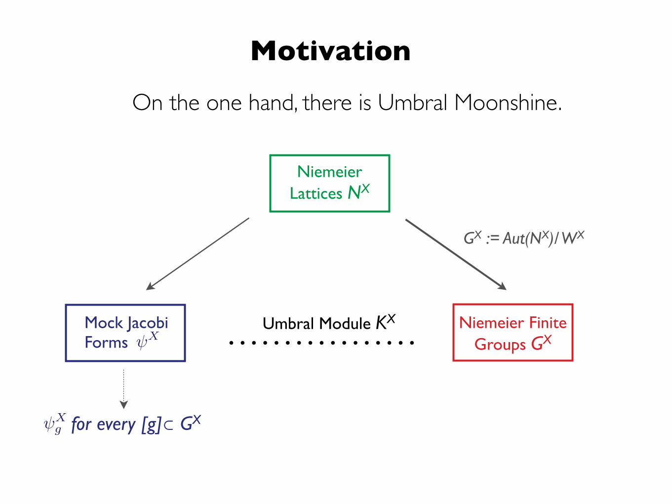
MotivationOn the one hand, there is Umbral Moonshine.

Niemeier Finite Groups GX

Niemeier Lattices NX

GX := Aut(NX)/ WX

Umbral Module KX

M CHENG for every [g]⊂ GX Xg

Mock Jacobi!Forms X

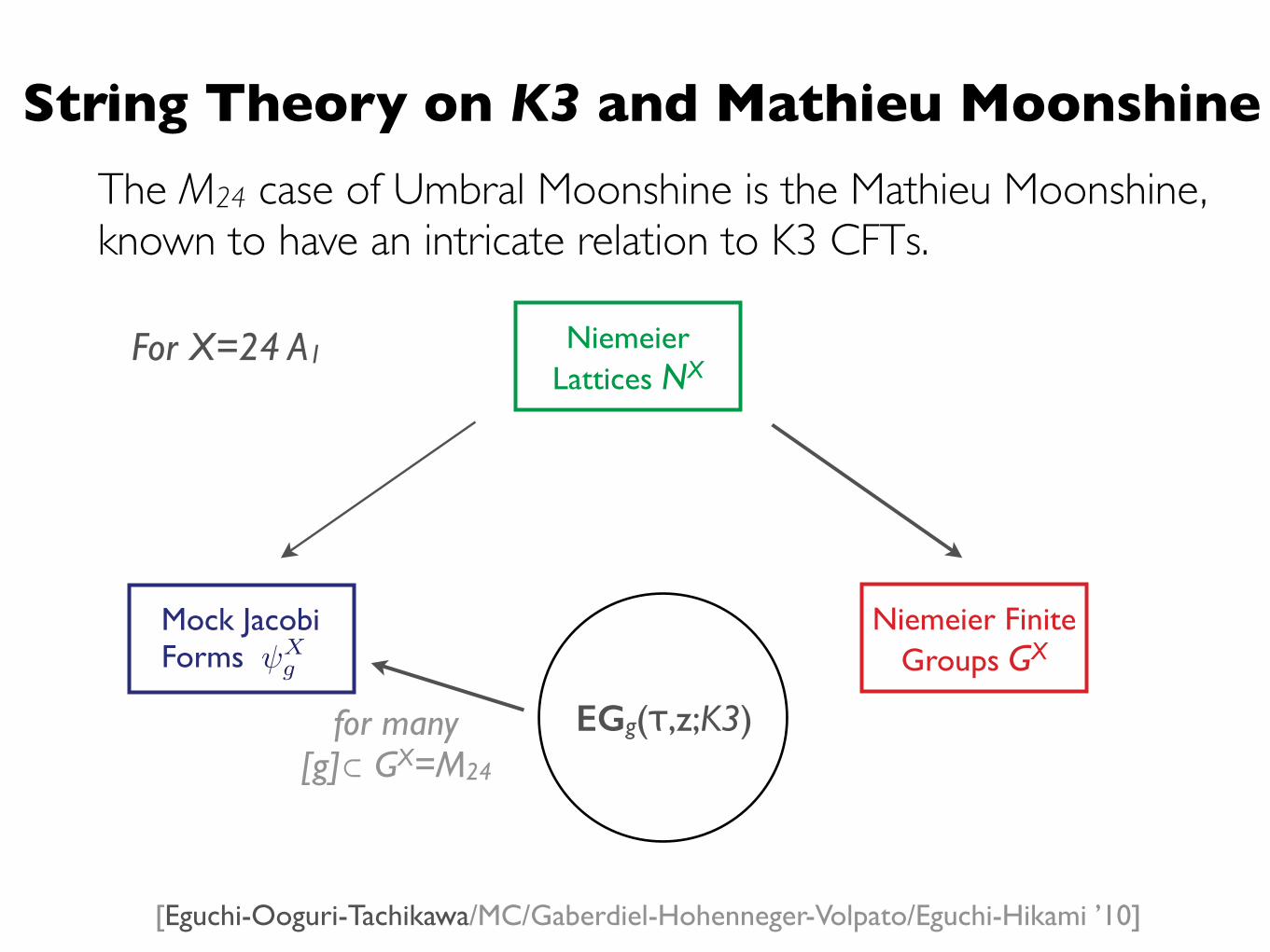
String Theory on K3 and Mathieu MoonshineThe M24 case of Umbral Moonshine is the Mathieu Moonshine,!known to have an intricate relation to K3 CFTs.

[Eguchi-Ooguri-Tachikawa/MC/Gaberdiel-Hohenneger-Volpato/Eguchi-Hikami ’10]

Niemeier Lattices NX

Niemeier Finite Groups GX

For X=24 A1

EGg(τ,z;K3) for many ![g]⊂ GX=M24

Mock Jacobi!Forms X

g

String Theory on K3 and Umbral Moonshine?Q: What about the other 22 cases (X≠24 A1) of umbral moonshine? !What is the physical and geometric context of umbral moonshine?

Niemeier Lattices NX

Niemeier Finite Groups GX

For X=24 A1

EGg(τ,z;K3) for many ![g]⊂ GX=M24

Mock Jacobi!Forms X

g

Outline

I. The Idea: !Umbral Moonshine and K3 CFT!

!II. Further exploration: !

Landau-Ginzburg Models and Umbral Moonshine!!

Mostly based on work (in progress) with

and many other fantastic collaborators!

Sarah Harrison!(Harvard)

Part I!The Idea: !Umbral Moonshine and K3 CFT!Mostly based on 1406.0619 w. S. Harrison

UM(24A1), EG(K3) !and Representations of N=4 SCA

UM associates a unique optimal mock Jacobi form to the 23 NX.

[Dabholkar–Murthy–Zagier’12 /MC–Duncan–Harvey ‘13/MC–Duncan to appear]

vector-valued mock theta functions of wt 1/2

h = Cox(X)

X(⌧, z) =

X

r2Z/2hHX

r (⌧)✓h,r(⌧, z)

✓h,r(⌧, z) =X

k2Z, k=r (2m)

qk2/4hyk

= the index h theta function

UM(24A1), EG(K3) !and Representations of N=4 SCA

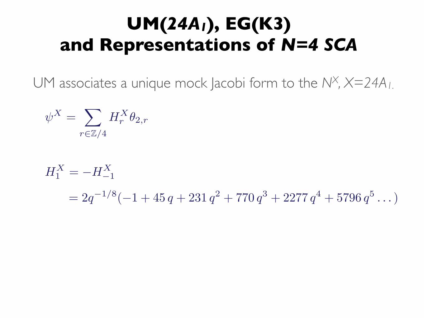
UM associates a unique mock Jacobi form to the NX, X=24A1.

X =X

r2Z/4HX

r ✓2,r

HX1 = �HX

�1

UM(24A1), EG(K3) !and Representations of N=4 SCA

UM(24A1) mock Jacobi formpolar part cor. into!a mero. Jac form

EG(⌧, z;K3)

=i✓21(⌧, z)

⌘3(⌧)✓1(⌧, 2z)( X

polar

+ X)

Recall: 2d sigma model on K3 is a N=(4,4) SCFT.

[Eguchi–Ooguri–Taormina–Yang ’88]

⇒ The spectrum fall into irred. representations of the N=4 SCA.

number of long N=4 multiplets

It seems difficult to generalise such an algebraic relation between EG(K3) and UM(24A1) to the other cases.

Appell-Lerch function

=

✓21(⌧, z)

⌘3(⌧)

⇣24µ(⌧, z) + 2 q�1/8

(�1 + 45 q + 231 q2 + 770 q3 + . . . )⌘

= 24⇥ short multiplet ch + long multiplet ch’s

[Zwegers, DMZ]

Roots and UM Mock Mod. Forms

Niemeier Lattices NX

The lattice roots X (ADE) determines the modular properties in a way reminiscent to the ADE classification of N=2 minimal models of [Cappelli–Itzykson–Zuber ’87].

Q: What is the physical and geometric meaning !of this construction?

Mock Jacobi!Forms X

g

Q: What is CIZ classification doing here ??

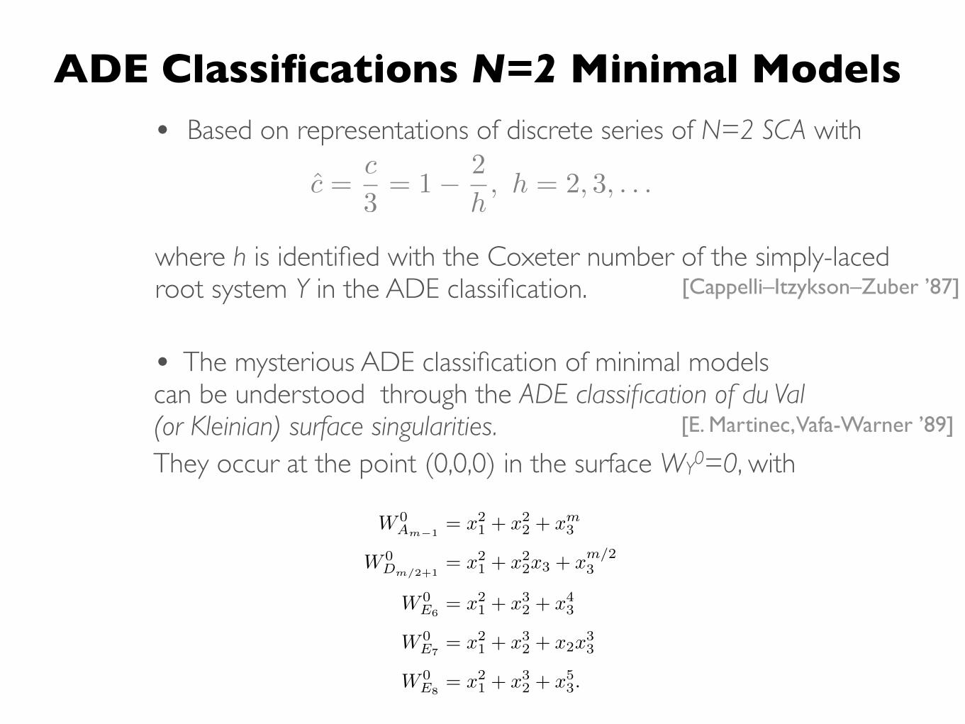
ADE Classifications N=2 Minimal Models• Based on representations of discrete series of N=2 SCA with

where h is identified with the Coxeter number of the simply-laced !root system Y in the ADE classification. [Cappelli–Itzykson–Zuber ’87]

• The mysterious ADE classification of minimal models can be understood through the ADE classification of du Val (or Kleinian) surface singularities.

Umbral Moonshine and K3 Surfaces 8

The organisation of the paper is as follows. In §2 we compute the elliptic genus of the ADE

du Val singularities that K3 surfaces can develop. In §3 we review the umbral moonshine con-

struction from 23 Niemeier lattices and introduce the necessary ingredients for later calculations.

Utilising the results of §2, in §4 we establish the relation between the (twined) elliptic genus and

the mock modular forms of umbral moonshine. In §5 we provide a geometric interpretation of

this result. In §6 we close this paper by discussing some open questions and point to some pos-

sible future directions. In Appendix A we collect useful definitions. In Appendix B we present

the calculations and proofs, and present our conjectures for the twined (or equivariant) elliptic

genus for the du Val singularities. The explicit results for the twining functions are recorded in

the Appendix C.

2 The Elliptic Genus of Du Val Singularities

The rational singularities in two (complex) dimensions famously admit an ADE classification.

See, for instance, [50]. They are also called the du Val or Kleinian singularities and are iso-

morphic to the quotient singularity C2/G, with G being the finite subgroup of SU2

(C) with

the corresponding ADE classification [47]. Any such singularity has a unique minimal reso-

lution. The so-called resolution graph, the graph of the intersections of the smooth rational

(genus 0) curves of the minimal resolution, gives precisely the corresponding ADE Dynkin dia-

gram. We will denote by � the corresponding simply-laced irreducible root system. In terms of

hypersurfaces, it is given by W 0

�

= 0 with

W 0

Am�1= x2

1

+ x2

2

+ xm3

(2.1)

W 0

Dm/2+1= x2

1

+ x2

2

x3

+ xm/23

(2.2)

W 0

E6= x2

1

+ x3

2

+ x4

3

(2.3)

W 0

E7= x2

1

+ x3

2

+ x2

x3

3

(2.4)

W 0

E8= x2

1

+ x3

2

+ x5

3

. (2.5)

These singularities show up naturally as singularities of K3 surfaces and play an important role

in various physical setups, such as in heterotic–type II dualities and in geometric engineering,

in string theory compactifications. See, for instance, [51, 52] and [53].

The 2d conformal field theory description of these (isolated) singularities was proposed in [54]

to be the product of a non-compact super-coset model SL(2,R)U(1)

(the Kazama–Suzuki model [55])

and an N = 2 minimal model, followed by an orbifoldisation by the discrete group Z/mZ, where

They occur at the point (0,0,0) in the surface WY0=0, with [E. Martinec, Vafa-Warner ’89]

c =c

3= 1� 2

h, h = 2, 3, . . .

Landau–Ginzburg Models

•It is an N=2, d=2 supersymmetric quantum field theory. !!•It does not have conformal symmetry, but “flow to the IR” to a 2d CFT.!!•From the LG point of view, the EG computes the graded index of Q, one of

the susy generators. The Q-cohomology forms representations of an N=2 superconformal algebra. The EG is invariant under the RG flow. !

!•Deformations of W are Q-exact and hence one can send W→0 and

compute the EG using a free field theory. !!•For our purpose, it can be thought of as a gadget to compute EG(CFT) and

study the symmetries easily.

: chiral superfields �i

L =

Zd2z d4✓K(�i,�i) +

Zd2z d2✓W (�i) + c.c.

superpotential

[Witten 1994]

(z, z; ✓+, ✓�, ✓+, ✓�) : local coordinates on the super Riemann surface

ADE Classification in terms of ADE Sing.

LG model with W=WY0

The Y type N=2 minimal model “min(Y)” of CIZ

eg. LG model with W (�) = �m the Am-1 type minimal model

WZW model at level m-2SU(2)

U(1)

[E. Martinec, Vafa-Warner, Schellekens–Waarner, Witten, Qiu, Di Francesco–Yankielowicz …..late 80’]

Its elliptic genus, , can be computed either from the LG description via its chiral ring, or from the min(Y) description in terms of the Ramond N=2 characters at c=3(1-2/h).

EGYmin

Roots, Singularities, and Curves

•ADE classification of minimal models ⟷ ADE singularities

ADE root system X � ADE singularities X ?

• Their resolution gives rise to genus 0 curves with the corresponding ADE intersection matrix.

• They are singularities a K3 can develop. Locally they look like C2/Γ.

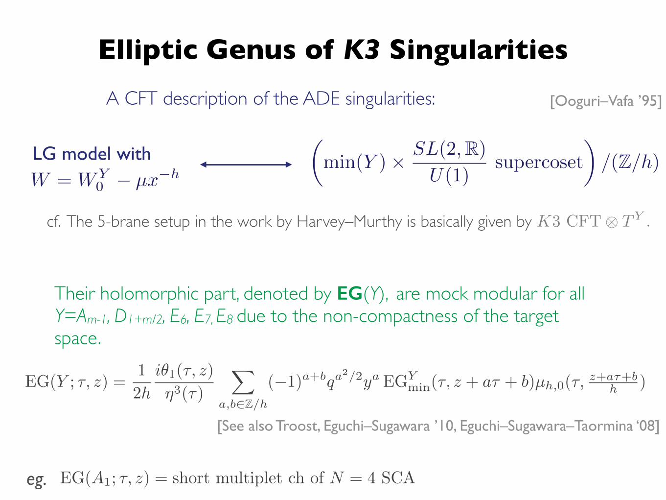
A CFT description of the ADE singularities: [Ooguri–Vafa ’95]

cf. The 5-brane setup in the work by Harvey–Murthy is basically given by !K3 CFT⌦ TY .

W = W

Y0 � µx

�hLG model with !

✓min(Y )⇥ SL(2,R)

U(1)

supercoset

◆/(Z/h)

Elliptic Genus of K3 Singularities

Their holomorphic part, denoted by EG(Y), are mock modular for all Y=Am-1, D1+m/2, E6, E7, E8 due to the non-compactness of the target space.

EG(Y ; ⌧, z) =1

2h

i✓1(⌧, z)

⌘3(⌧)

X

a,b2Z/h(�1)a+bqa

2/2ya EGYmin(⌧, z + a⌧ + b)µh,0(⌧,

z+a⌧+bh )

[See also Troost, Eguchi–Sugawara ’10, Eguchi–Sugawara–Taormina ‘08]

eg. EG(A1; ⌧, z) = short multiplet ch of N = 4 SCA

Elliptic Genus of K3 Singularities

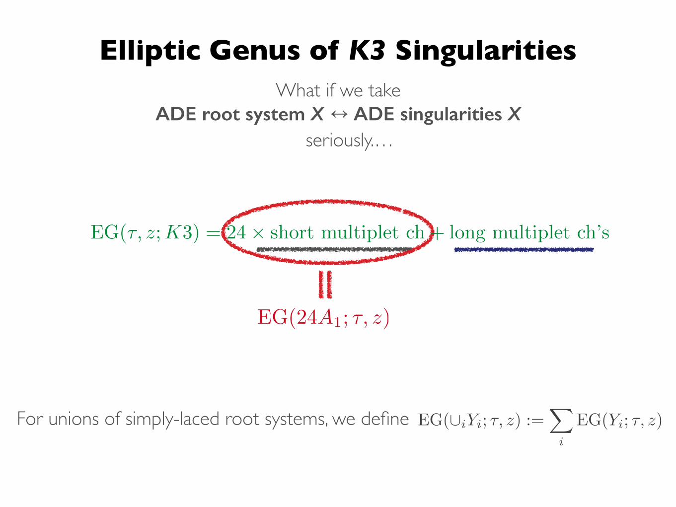
ADE root system X � ADE singularities X What if we take

seriously.…

EG(⌧, z;K3) = 24⇥ short multiplet ch + long multiplet ch’s

EG(24A1; ⌧, z)

EG([iYi; ⌧, z) :=X

i

EG(Yi; ⌧, z)For unions of simply-laced root systems, we define

A Geometric Interpretation of the N=4 Decomposition

(algebraic)

in the case X=24A1

(geometric)

Q: Can we generalise this geometric relation between EG(K3) and UM(24A1) to the other cases?

(modular)

EG(⌧, z;K3)

=

i✓21(⌧, z)

⌘3(⌧)✓1(⌧, 2z)( X

polar

+ X

)

= 24⇥ short multiplet ch + long multiplet ch’s

= EG(⌧, z;X) + contribution from the umbral function X

A Geometric Decomposition for all UM(X)

for all 23 Niemeier lattices with X=24A1, 12A2, ... , A11D7E6, ...., 3E8, D24.

It turns out that the following is true

where

EG(⌧, z;K3) = EG(⌧, z;X) +✓21(⌧, z)

⌘6(⌧)@ X(⌧, 0)

contribution from the !root system

contribution from the !umbral function

@f(⌧, z) =1

2⇡i

@

@zf(⌧, z).

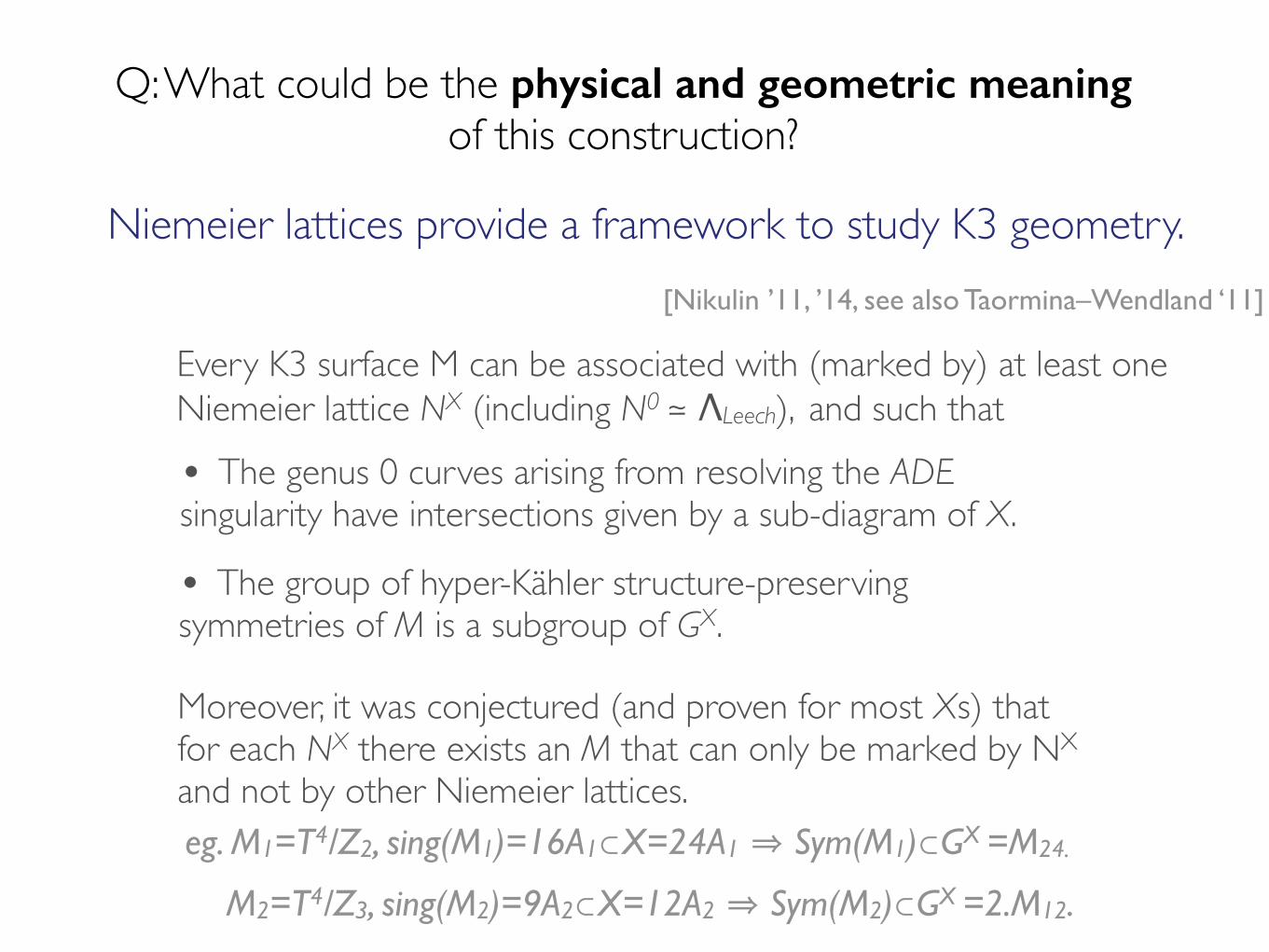
Q: What could be the physical and geometric meaning !of this construction?

Niemeier lattices provide a framework to study K3 geometry. [Nikulin ’11, ’14, see also Taormina–Wendland ‘11]

Every K3 surface M can be associated with (marked by) at least one Niemeier lattice NX (including N0 ≃ ΛLeech), and such that

• The genus 0 curves arising from resolving the ADE singularity have intersections given by a sub-diagram of X.

• The group of hyper-Kähler structure-preserving symmetries of M is a subgroup of GX.

Moreover, it was conjectured (and proven for most Xs) that for each NX there exists an M that can only be marked by NX and not by other Niemeier lattices. eg. M1=T4/Z2, sing(M1)=16A1⊂X=24A1 ⇒ Sym(M1)⊂GX =M24. !

M2=T4/Z3, sing(M2)=9A2⊂X=12A2 ⇒ Sym(M2)⊂GX =2.M12.

Checks: How do we twine?

??given by!

UM(X) for all g∈GX

Q: How to twine the root system contribution to EG(K3) for all g∈GX?

Recall that GX acts on the root system X=⋃i Yi as permutation of the identical components Yi (eg. 24A1, 3E8 or 2A9 in 2A9⊕D8 ) and as diagram automorphisms of Yi (Z/2 for An>1, E6 and D>1 except for D4 which have Dih3 automorphism).

Z/2

g g gEGX(⌧, z;K3) = EG (⌧, z;X) +✓21(⌧, z)

⌘6(⌧)@ X (⌧, 0)

Checks: How do we twine?

As a result, we just need to compute the the EG of a simply-laced root system twined by its automorphisms.

If X=⋃i=1,…,n Yi ,

g : (Y1, . . . , Yn) ! (h1(Y⇡(1)), . . . , hn(Y⇡(n))) , hi 2 Aut(Y⇡(i))

) EGg(⌧, z;X) =X

i

�i,⇡(i) EGhi(⌧, z;Yi)

This can be done using the Landau–Ginzburg description of the ADE minimal model and the identification between the chiral ring & the corresponding ADE weight space.

EG(Y ; ⌧, z) =1

2h

i✓1(⌧, z)

⌘3(⌧)

X

a,b2Z/h(�1)a+bqa

2/2ya EGYmin (⌧, z + a⌧ + b)µh,0(⌧,

z+a⌧+bh )h

twine this part

Recall: we have an explicit GX action on the CFT on singularity X.

Twining: the Results In the way we obtain, for each of the 23 X, the twinings

•For the case X=24A1, by construction it agrees with the result of Mathieu Moonshine.

[EOT, MC, Gaberdiel–Hohenegger–Volpato, Eguchi-Hikami ’10-11]

•Sanity Checks: All <g> corresponding to geometric K3 sym. have the same result independent of from which UM(X) it arises, as required by the global Torelli theorem.

• For non-geometric type symmetries, no such theorem applies; twinings from different X can differ.

EGXg (K3; ⌧, z) 8 g 2 GX

EG

Xg (K3; ⌧, z) = EG

X0

g0 (K3; ⌧, z) if ⇡g = ⇡g0has at least 1 fixed point and 5 orbits.

24 Ways to Twine EG(K3)

ΛLeech=N0

NX UM(X)

V s\

all g∈ GX

all g∈ G0≅Co0 which preserves a 4-dim sublattice[Duncan–Mack-Crane ’15]

Q: Which one(s) of the twinings is relevant for a given K3 CFT?

• Twinings for non-geometric type depends on X.

eg.

EG24A1g 6= EG12A2

g0 = EG0g00 , ⇡g = ⇡g0 = ⇡g00 = 38

EG24A1g = EG6A4

g0 6= EG0g00 , ⇡g = ⇡g0 = ⇡g00 = 64

EG24A1g = EG0

g1 6= EG12A2g0 = EG0

g2 , ⇡g = ⇡g0 = ⇡g1 = ⇡g2 = 12112

• Twinings for geometric type symmetries all agree.

EGXg (K3)

EG0g(K3)

The CFT counterpart of the result by Nikulin, generalising the classification of [Gaberdiel–Hohenegger–Volpato ’11] to include singular CFTs, is expected to hold.

[in discussion w. M. Gaberdiel, S. Harrison, R. Volpato]

In a theory whose can only be embedded in NX, it’s natural to conjecture that the corresponding twinings coincide with those arising from UM(X).

⇤⇧

More on the Physical Interpretation

G ⇢ GX .

⇧ �4,20.Let be the orthogonal complement of in !Then we can show that , whether or not it contains a root vector, can always be embedded into one of the 24 even, self-dual negative definite lattices NX.

⇤⇧

⇤⇧

[Aspinwall–Morrison ’94, Nahm–Wendland ‘99]Recall that a K3 CFT is specified by a 4-dimensional positive definite subspace

From this one concludes that the N=(4,4) preserving symmetries of the corresponding theory has symmetries

⇧ ⇢ �4,20 ⌦Z R.

Part II!Further Exploration: !Symmetries of the Landau–Ginzburg Models!Based on work in progress w. F. Ferrari, S. Harrison, N. Paquette

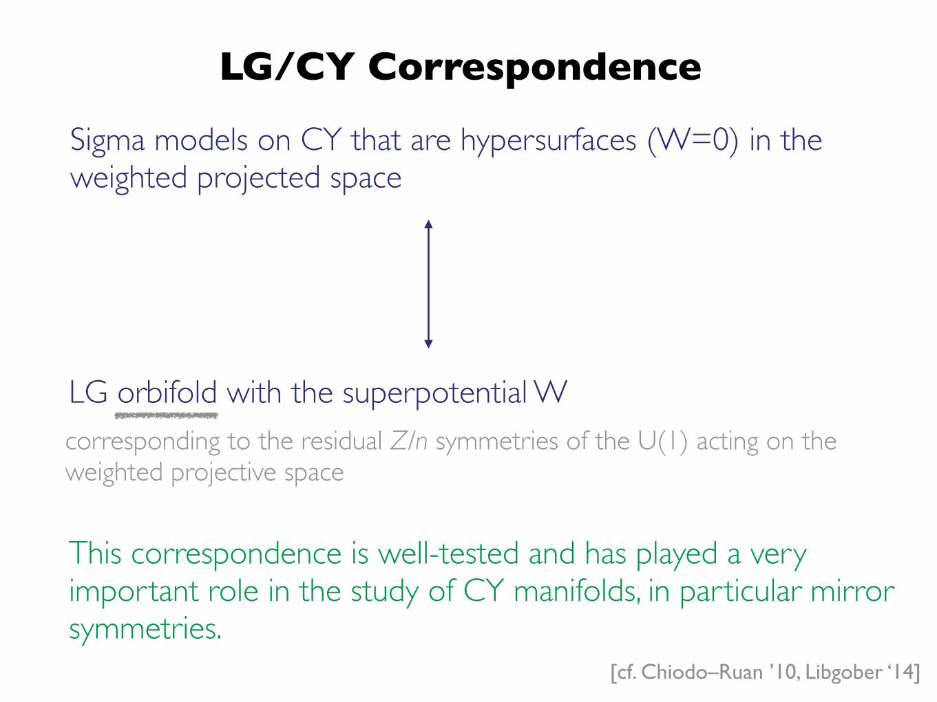
LG/CY Correspondence

Sigma models on CY that are hypersurfaces (W=0) in the weighted projected space

LG orbifold with the superpotential W corresponding to the residual Z/n symmetries of the U(1) acting on the weighted projective space

This correspondence is well-tested and has played a very important role in the study of CY manifolds, in particular mirror symmetries.

[cf. Chiodo–Ruan ’10, Libgober ‘14]

LG/CY Correspondenceeg1. Quintic 3-folds

the 3-fold: W (z1, . . . , z5) =5X

i=1

z5i = 0

the orbifold group: invariant under Z/5 generated byW zi 7! e2⇡i/5zi

⇒ the LG theory: the theory with chiral superfields !and superpotential!orbifolded by Z/5

W = W (�1, . . . ,�5) =5X

i=1

�5i

�1, . . . ,�5

the CFT:

LG —!minimal model

(3)5 := (A4)⌦5/(Z/5) [Gepner ’87, ‘88]

eg2. the non-compact CY: the E8 ALE space

the orbifold group Z/30:

WE8 = �µ��300 + �2

1 + �32 + �5

3

� 7! e2⇡iqi/30, (q0, . . . , q3) = (�1, 15, 10, 6)

the CFT: ✓min(E8)⇥

SL(2,R)U(1)

supercoset

◆/(Z/30)

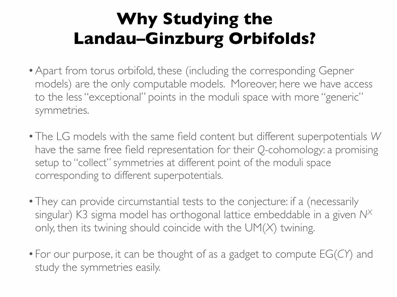
Why Studying the !Landau–Ginzburg Orbifolds?

•Apart from torus orbifold, these (including the corresponding Gepner models) are the only computable models. Moreover, here we have access to the less “exceptional” points in the moduli space with more “generic” symmetries. !

!•The LG models with the same field content but different superpotentials W

have the same free field representation for their Q-cohomology: a promising setup to “collect” symmetries at different point of the moduli space corresponding to different superpotentials. !

!•They can provide circumstantial tests to the conjecture: if a (necessarily

singular) K3 sigma model has orthogonal lattice embeddable in a given NX only, then its twining should coincide with the UM(X) twining. !

!•For our purpose, it can be thought of as a gadget to compute EG(CY) and

study the symmetries easily.

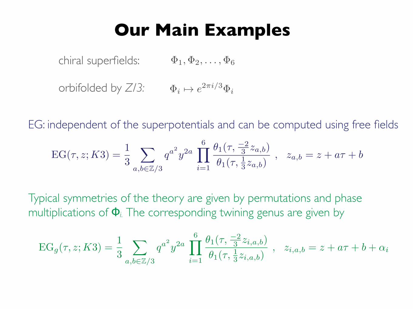
Our Main Examples�1,�2, . . . ,�6chiral superfields:!

!orbifolded by Z/3: �i 7! e2⇡i/3�i

EG(⌧, z;K3) =1

3

X

a,b2Z/3qa

2

y2a6Y

i=1

✓1(⌧,�23 za,b)

✓1(⌧,13za,b)

, za,b = z + a⌧ + b

EG: independent of the superpotentials and can be computed using free fields

Typical symmetries of the theory are given by permutations and phase !multiplications of Φi. The corresponding twining genus are given by

EGg(⌧, z;K3) =1

3

X

a,b2Z/3qa

2

y2a6Y

i=1

✓1(⌧,�23 zi,a,b)

✓1(⌧,13zi,a,b)

, zi,a,b = z + a⌧ + b+ ↵i

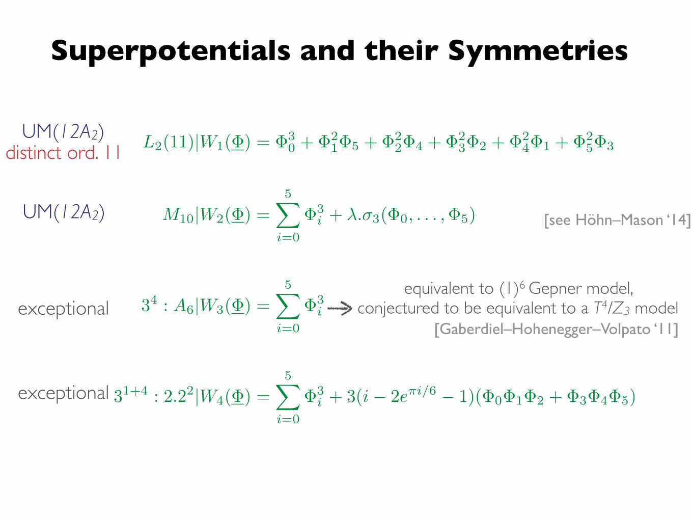
Superpotentials and their Symmetries

equivalent to (1)6 Gepner model, !conjectured to be equivalent to a T4/Z3 model

[Gaberdiel–Hohenegger–Volpato ‘11]

[see Höhn–Mason ‘14]

UM(12A2)

UM(12A2)

exceptional

exceptional

distinct ord. 11 L2(11)|W1(�) = �30 + �2

1�5 + �22�4 + �2

3�2 + �24�1 + �2

5�3

M10|W2(�) =5X

i=0

�3i + �.�3(�0, . . . ,�5)

34 : A6|W3(�) =5X

i=0

�3i

31+4 : 2.22|W4(�) =5X

i=0

�3i + 3(i� 2e⇡i/6 � 1)(�0�1�2 + �3�4�5)

Summary of the Cubic LG Symmetries•From these symmetries one obtains all the M11⊂2.M12≃G(12A2) twinings of

UM(12A2), including the one (ord. 11) distinct from M24-twinings.!!•If we just twine the free field theory without requiring them to be

symmetries of a concrete superpotential, we obtain more 2.M12≃G(12A2) twinings. !

!•This shows that LG theories is a promising setup to study the symmetries

of K3 sigma models. !

pG

ps

pW 0

•Moreover, the close connection to UM(12A2) provides circumstantial evidence for the relation between ADE theories and K3 sigma models: twinings other than M24 twinings (even with the same action on 24-dim rep) do appear where expected.

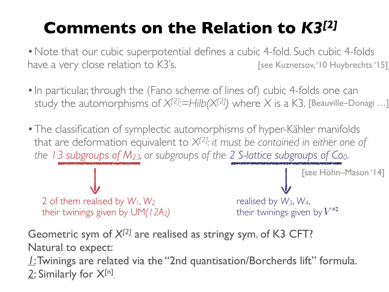
Comments on the Relation to K3[2]

•Note that our cubic superpotential defines a cubic 4-fold. Such cubic 4-folds !have a very close relation to K3’s. !!•In particular, through the (Fano scheme of lines of) cubic 4-folds one can

study the automorphisms of X[2]:=Hilb(X[2]) where X is a K3. !!•The classification of symplectic automorphisms of hyper-Kähler manifolds

that are deformation equivalent to X[2]: it must be contained in either one of the 13 subgroups of M23, or subgroups of the 2 S-lattice subgroups of Co0. !

[see Kuznetsov, ‘10 Huybrechts ‘15]

[Beauville–Donagi …]

[see Höhn–Mason ‘14]

2 of them realised by W1, W2 !

their twinings given by UM(12A2)realised by W3, W4, !their twinings given byV s\

Geometric sym of X[2] are realised as stringy sym. of K3 CFT? !Natural to expect:!1: Twinings are related via the “2nd quantisation/Borcherds lift” formula. !2: Similarly for X[n].

Thank you!