HAL Id: hal-01007405https://hal.archives-ouvertes.fr/hal-01007405v2

Submitted on 9 Apr 2021

HAL is a multi-disciplinary open accessarchive for the deposit and dissemination of sci-entific research documents, whether they are pub-lished or not. The documents may come fromteaching and research institutions in France orabroad, or from public or private research centers.

L’archive ouverte pluridisciplinaire HAL, estdestinée au dépôt et à la diffusion de documentsscientifiques de niveau recherche, publiés ou non,émanant des établissements d’enseignement et derecherche français ou étrangers, des laboratoirespublics ou privés.

Distributed under a Creative Commons Attribution| 4.0 International License

Ultrasonic Welding of Thermoplastic Composites,Modeling of the Process Using Time Homogenization.

Arthur Levy, Steven Le Corre, Arnaud Poitou, Eric Soccard

To cite this version:Arthur Levy, Steven Le Corre, Arnaud Poitou, Eric Soccard. Ultrasonic Welding of Thermoplas-tic Composites, Modeling of the Process Using Time Homogenization.. International Journal forMultiscale Computational Engineering, Begell House, 2011, 9 (6), pp.53-72. 10.1615/IntJMultCom-pEng.v9.i1.50. hal-01007405v2

Ultrasonic Welding of ThermoplasticComposites, Modeling of the Process Using

Time Homogenization.

Arthur LEVY1, Steven LE CORRE1, Arnaud POITOU1, Eric SOCCARD2.

March 4, 2009

1: GeM - Ecole Centrale Nantes, Université de Nantes - 1 rue de la Noë 44321 Nantes,France.e-mail: [arthur.levy; steven.le-corre; arnaud.poitou]@ec-nantes.fr.

2: EADS IW - Technocampus, 1 rue de la Noé 44321 Nantes, France.e-mail: eric.soccard@eads.net.

Abstract

The process of ultrasonic welding allows to assemble thermoplastic compos-ite parts. A high frequency vibration imposed to the processing zone induces selfheating and melting of the polymer. The main feature of this process is the ex-istence of phenomena that occur on two very different time scales: the vibration(about 10−5 s) and the flow of molten polymer (about 1s). In order to simulateaccurately these phenomena without the use of a very fine time discretizationover the whole process, we apply a time homogenization technique. First, thethermo-mechanical problem is formulated using a Maxwell viscoelastic consti-tutive law and then, it is homogenized using asymptotic expansion. This leadsto three coupled problems: a micro-chronological mechanical problem, a macro-chronological mechanical problem and a macro-chronological thermal problem.This coupled formulation is actually simpler because the macro-chronologicalproblems do not depend on the micro time scale and its associated fast variations.Lastly, a uniform simple test case is proposed to compare the homogenized solu-tion to a direct calculation. It shows that the method gives good results providedthat the vibration is fast enough compared to the duration of the process. More-over, the time saving appears to be highly reduced down to one thousand timesless.

Keywords : Polymer, Welding, Time-homogenization, Asymptotic Expan-sion, Viscoelasticity.

1

IntroductionIn the wide field of thermoplastic composite material, the ability of the matrix to

melt allowed new processes to appear. Beside the forming processes, this paper focuseson assembling processes, among which welding appears as a revolution in the domainof composites materials. Nevertheless, whereas metal welding implies conductive me-dia, thermoplastic matrix reveals a very insulating behaviour. This property led to de-velop new techniques that produce heat very locally, at the welding interface. We canmention resistance welding or induction welding [Ageorges et al., 2000]. This studydeals with the ultrasonic welding, where a tool, the sonotrode, applies an ultrasonicvibration to the processing zone at the interface, where little triangles called “energydirectors” are molded to create a kind of controlled rugosity. This induces self-heatingand melting of the energy directors which enable welding.

Although this process has been used for few decades (for polymer sealing for in-stance), the innovation here consists in the “dynamic” welding. Instead of having a socalled “static” welding where the sonotrode doesn’t move on the plate, in our case, thesonotrode slides along the directors direction and performs a weld line. The inducedthree dimensional flow of the polymer then results in high quality welds.

Many studies [Wang et al., 2006, Benatar and Gutowski, 1989, Tolunay, 1983,Suresh et al., 2007] have been carried out on the modeling of the classical “static pro-cess” where a plane strain assumption can be stated for the flow, the simulation ofthe fully three dimensional dynamic process is much heavier. The main problem thatarises when trying to perform this simulation comes from the existence of two timescales. The first one which will be denoted by “micro-chronological” is linked to theshort ultrasonic period. The second one, called the“macro-chronological” time scale,is the characteristic duration of the polymer flow at the interface which is the processduration. Simulating each ultrasonic cycle would need very small time steps (about 20per cycle), over a quite long process time (about 3 s). This would induce a lot of timesteps (about a hundred thousand for a 20kHz load) which would lead to huge calcula-tion times especially in a three dimensional context. A time homogenization method istherefore needed to allow calculation time reductions.

To overcome the existence of two time scales in a given process, many authors [Wang-et al., 2006, Benatar and Gutowski, 1989, Tolunay, 1983, Suresh et al., 2007] consid-ered the two mechanical phenomena to be dissociated. Given no flow of polymer, theultrasonic vibration of the sonotrode only induces small strains at a high frequency inthe processing zone. Therefore the polymer is assumed to have a linear elastic be-haviour. This allowed them to calculate a self-heating source independently of themacro-chronological flow. Nevertheless our process exhibit simultaneously both me-chanical phenomena.

The same difficulty appears when dealing with structures subjected to fatigue. Inthe continuum damage domain, in order to simulate numerically such a multi timescale process, authors like Van-Paepegem et al. [Van Paepegem et al., 2001] or Cojo-caru and Karlsson [Cojocaru and Karlsson, 2006] propose the “cycle jump” method.

2

It consists in solving a micro-chronological problem over a full cycle once for eachmacro-chronological time step. The main difficulty lies in determining the macro-chronological time-step reasonably. One has to determines how many micro-chronologicalcycles can be jumped without affecting the global accuracy. In the present paper, con-sidering the two time scales as well separated, we rather propose a time homogenizationtechnique which may avoid the use of cycle jump.

The homogenization techniques first appeared in the field of heterogeneous mediawith a multi spatial scale problem. In early eighties Benssoussan Lions and Papanico-laou [Benssousan et al., 1978] followed by Sanchez-Palancia [Sanchez-Palencia, 1980]considered a material presenting a periodic structure at the representative volume ele-ment scale. The solution is therefore supposed to be periodic in the small scale variable.One can then define a scale factor and seek the solution as a spatial asymptotic expan-sion in the power of this factor. The initial multiscale problem can then be split into sev-eral eventually coupled quite standard sub-problems. Francfort and Suquet [Francfortand Suquet, 1986] confirmed and extended the convergence results for a thermo-visco-elastic material. More recently, we can mention Geindreau and Auriault [Geindreauand Auriault, 1999] for the metallic alloys, Boutin and Auriault [Boutin and Auriault,1990] for the bituminous concrete or Le Corre et al. [Le Corre et al., 2005] who con-sidered a fibre suspension behaviour in composite forming.

In contrast to spatial homogenization, a time homogenization method can be ap-plied when there exist two separated time scales in a problem. Back to the fatigueproblem, for instance, from an initial elastoviscoplastic problem, Guennouni [Guen-nouni, 1988] obtained two sub problems: an elastic behaviour that describes the micro-chronological effects, and a elastoviscoplastic behaviour for the homogenized macro-chronological behaviour. Since macro-chronological domain evolution and dependencyof material parameters are not taken into account, the micro-chronological problemdoes not depend on the macro chronological time scale. Therefore, it can be solved in-dependently once only. This enables those rather standard problems to be solved verysimply. With the same mathematical tool, Oskay and Fish [Oskay and Fish, 2004] de-scribed the fatigue phenomena using the continuum damage evolution approach. Theyobtain two coupled micro and macro-chronological mechanics and a damage evolu-tion law. This was validated on a test case by a numerical FEM implementation. Tosummarize, the micro-chronological resolution allows to determine the field of interestwhich is the damage field. Similarly, in our approach, the resolution of the micro-chronological ultrasonic loading allows to determine the heat source and therefore thetemperature field.

Closer to our application, we can mention Boutin and Wong [Boutin and Wong,1998], who treated a coupled visco-elastic and transient thermal problem in two steps.First they applied a space homogenization technique to the mechanical problem andobtained a macroscopic spatial problem. Then, after having discussed the cases whereboth spatial and temporal scale can be homogenized, they propose an homogenizedthermal problem where the source is simply averaged over a micro-chronological pe-riod. Note that, they did not use any asymptotic expansion in time. For a fully simulta-

3

neous time and space homogenization, we can refer to Yu and Fish [Yu and Fish, 2002]who considered the spatial and temporal scale factors to be equal and therefore proposea “double scale asymptotic expansion”.

In the first part of this paper, after a short description of the initial thermo-mechanicalproblem, a dimensional analysis is carried out in relation with the industrial process or-ders of magnitude. We then propose a time homogenization technique using asymptoticexpansion and obtain three coupled sub-problems (a micro and a macro chronologicalmechanical problems, and a macro chronological thermal problem). Even if in thescope of the ultrasonic welding process, the methodology proposed in this work aimsto be rather general, so that it may be applied to any high frequency processing. In thesecond part, with the use of an analytical test case, we validate the proposed method bycomparing results with a direct resolution.

1 Formulation of the Thermo - Mechanical ProblemLet us consider an energy director represented by a domain Ω as described in fig-

ure 1. It is subjected to an evolving small oscillatory displacement on the boundaryΓu (see figure 1). We aim to describe its thermo-mechanical evolution equations. Notethat even though the presented figure is two dimensional, the analysis proposed is moregeneral and can be led for a three dimensional problem.

1.1 Mechanical problem.Because of the small dimensions of our domain, we can assume a quasi static de-

scription for the mechanics. Neglecting the body force as well, we get:

∇∇∇ ·ΣΣΣ = 000, (1)

where ΣΣΣ is the Cauchy stress tensor.

Figure 1: Geometry of the problem.

4

Considering the polymer to be incompressible we also assume:

∇ ·uuu = 0, (2)

where uuu is the displacement field. Therefore, the total stress ΣΣΣ may be expressed as ΣΣΣ =−pIII +σσσ where p is the hydrostatic pressure that can be seen as the Lagrange multiplierassociated to incompressibility condition (2) and σσσ is the extra stress tensor whichis determined by given constitutive equations for the polymer. In order to simplifythe analysis, a Maxwell law is adopted as a first approach. In this first part, study isrestricted to a small displacement framework where the constitutive equations can bewritten as:

λσσσ +σσσ = 2ηεεε, (3)

where λ is the relaxation time, η the viscosity, εεε the strain tensor and the dot expressesthe time derivation.

The domain Ω is subjected to evolving oscillatory displacement boundary condi-tions on Γu (see figure 1) which is the sum of a macro-chronological displacementboundary condition uuus linked to the squeezing of the energy director, and a micro-chronological harmonic boundary condition of amplitude aaa, linked to the ultrasonicvibration:

uuu = uuus(t)+aaasin(ωt) (onΓu) (4)

The boundary Γσ is assumed to be free:

ΣΣΣ ·nnn = 000 (onΓσ ). (5)

Initial conditions. At the initial time, we consider the displacement to be zero and arelaxed configuration:

uuu(x, t = 0) = 000; σσσ(x, t = 0) = 000; p(x, t = 0) = 0. (6)

1.2 Thermal problem.Ω is supposed to be thermally insulated. Considering the elasticity to be fully en-

tropic, which is a classical assumption when dealing with polymer at the rubbery stateabove the glassy temperature, the internal energy e depends on temperature only andthe energy balance can be written as:

ρdedθ

θ = ρcθ = ∇ · (k∇∇∇θ)+σσσ : εεε

k∇∇∇θ ·nnn = 0 on(Γu∪Γσ ), (7)

where θ is the temperature, k the thermal conductivity, c the specific heat capacity andρ the density.

5

2 Dimensional Analysis

2.1 Dimensionless variablesIn order to deal with comparable quantities, we have to turn the initial problem

defined by equations (1) to (7) into a dimensionless problem. We proceed by usingcharacteristic magnitudes of the process. Note that these values are specific to theultrasonic welding.

• The characteristic length used in this work is e = 1mm which corresponds to theinitial height of the processing zone in our industrial application.

• The time λ0 = 1s which is approximately the duration of the process is used ascharacteristic time.

• We choose a characteristic stress σc = η0/λ0, where η0 = 107 Pa.s that is anupper bound of the Newtonian viscosity of the studied polymer (PEEK) close tothe glassy temperature θ = θg = 143°C: σc = 107 Pa

• Calling θm the melting temperature of the polymer and θr the room temperature,the temperature variation ∆θc = θm − θr is chosen as the process characteristictemperature variation. In the case of the studied PEEK polymer, θm ∼ 330°C sothat ∆θc ∼ 300°C.

We then introduce new dimensionless coordinates:

x = e.x∗

t = λ0.t∗

and finally dimensionless variables σσσ∗, uuu∗, εεε∗ and θ ∗:

σσσ (x=ex∗, t=λ0t∗) = σc.σσσ∗(x∗, t∗)

uuu(x=ex∗, t=λ0t∗) = e.uuu∗(x∗, t∗)εεε(x=ex∗, t=λ0t∗) = εεε∗(x∗, t∗)θ (x=ex∗, t=λ0t∗) = ∆θc.θ

∗(x∗, t∗)+θamb

. (8)

Note that the form taken for the dimensionless temperature allows to have it varyingbetween 0 and 1 when it rises from room temperature to melting temperature.

In the same way, dimensionless space derivation operators are introduced:

∇∗ () ≡ e.∇()

∇∗ · () ≡ e.∇ · () (9)∆∗ () ≡ ∇

∗ · (∇∗ ()) = e2∆()

6

2.2 Dimensionless resulting problemsDimensionless equations corresponding to the general thermo-mechanical problem

(equations (1) to (7)) can be deduced1:Λ

∂σσσ∗

∂ t∗+σσσ

∗ = 2N∂εεε∗

∂ t∗∇∇∇∗ · (σσσ∗− p∗III) = 000

∇∗ ·uuu∗ = 0

(in Ω)

uuu∗ = UUU s(t∗)+RRRsin(ωλ0t∗) (on Γu)(σσσ∗− p∗III) ·nnn = 000 (on Γσ )

(10)

∂θ ∗

∂ t∗= A∆

∗θ∗+Bσσσ

∗ :(

∂εεε∗

∂ t∗

)(in Ω)

∇∇∇∗θ ∗ ·nnn = 0 (onΓσ ∪Γu)

. (11)

The obtained problem is defined with 6 dimensionless numbers that depend on theboundary conditions and the material parameters:

RRR = aaa/eUUU s = uuus/e

A = (kλ0)/(ρce2)

B = σc/(ρc∆θc)Λ = λ/λ0N = η/η0

. (12)

2.3 Scale factorLet us introduce the dimensionless scale factor which defines how well the two time

scales are separated. It is the ratio of a characteristic micro-chronological time and acharacteristic macro-chronological one. As already mentioned, the macro-chronologicaltime is λ0, the characteristic duration of the squeezing of the energy director. Now,we introduce the micro-chronological time, characteristic of the vibrating loading asτ = 1/ω , ω = 2π f being the loading pulsation of the sonotrode. The scale factor isfinally:

ξ =1

ωλ0. (13)

Considering the wide range of multi time scales phenomena, we can identify severalcases. In the domain of high cycle fatigue, for instance, the number of cycles can reachfew millions. Therefore, the scale factor may be around ξ ∼ 10−9. If we focus onageing phenomena in civil engineering life-time calculation, the number of cycle maybe of few tens of thousands. In this case, ξ ∼ 10−4. In the case of an ultrasonic

1the constitutive law has been divided by σc and the thermal equation by ρc∆θc/λ0

7

process as the considered welding technique, the typical ultrasonic frequency is aroundf ∼ 20kHz, so that the scale factor is about:

ξ ∼ 10−5. (14)

Scales appear to be well separated in such processes and justifies a homogenizationapproach.

2.4 Evaluation of the dimensionless parametersAs it will be detailed in the following section, the dimensionless parameters (12)

have to be evaluated with respect to powers of ξ . Different powers of ξ (i.e. differentorders of magnitude with respect to the scale separation) can lead to different models.

Boundary conditions. The amplitude of the vibrations in ultrasonic welding is offew percents of the energy director’s dimension, so that:

RRR ∼ ξ0111, (15)

where 111 is a unit displacement vector giving the direction of the loading. It remainstrue even in the case of very high power ultrasonic processing where the amplitude ofthe vibration might exceed 50% of the energy director’s height. On the contrary, to getan RRR of order of ξ , we would need a vibration amplitude of about 10−5 times the heightof the processing zone. Obviously, such a small vibration would not have any effect onthe material and is therefore never used in ultrasonic processing.

The macro-chronological displacement UUU s is clearly of the order of magnitude ofthe energy director’s height. Therefore, the macro-chronological displacement stays inthe vicinity of ξ 0 over the whole process:

UUU s ∼ ξ0111. (16)

Thermal parameters. The diffusivity of a polymer being around 10−7 m2s−1, we getA ∼ 1 which allows to fix:

A ∼ ξ0. (17)

If we generalize to other materials, the diffusivity ranges between 410−8 for a rubbermaterial and 10−4 for a copper alloy, so that 0.5 < A < 103. Only for metals with a highthermal diffusivity, A grows to the order of ξ−1. The present analysis will be restrictedto the case where A ∼ ξ 0 as in the polymers case.

The specific thermal capacity ρc of all engineering material are of the order of106W.m−3K−1, so that B ∼ 0.03 with the characteristic stress chosen, and:

B ∼ ξ0. (18)

8

Constitutive law. During the process the temperature of the domain rises from theroom temperature to the melting temperature. The material properties (λ and η) beinghighly temperature dependant, they also vary a lot. Indeed, we can not assume, asBoutin and Wong [Boutin and Wong, 1998], that the temperature does not vary mucharound the reference temperature, and can not apply a Taylor expansion of the thermo-dependant parameters around this reference temperature. Nevertheless, having limitedthe study to very well separated time scales (ξ ∼ 10−5), even if λ and η vary over fewdecades, it is quite likely that they will not vary over more than 1 order of ξ . We mayphysically consider 2 case: (i) Λ ∼ ξ 0 and N ∼ ξ 0 and (ii) Λ ∼ ξ−1 and N ∼ ξ−1.

Case (i) is strictly valid above the glassy temperature, when the polymer is fullyviscoelastic, because the characteristic relaxation time is between 10ms and 100s, andthe viscosity is between 107 Pa.s and 104 Pa.s, so that:

λ ∼ 1s Λ ∼ ξ 0

η ∼ 5.105 Pa.s N ∼ ξ 0 . (19)

Case (ii) represents the evolution towards ambient temperature. It is discussed inthe appendix where we show that it leads to a similar equation set.

3 Homogenization

3.1 Time scalesThe very noticeable time scale separation justifies the use of a time homogenization

approach to model the process [Guennouni, 1988]. To proceed, we first define twoindependent dimensionless time variables:

• The micro-chronological time scale τ∗ = ωt = ωλ0t∗, related to the oscillation,is the expression of the fast variations.

• The macro-chronological time scale T ∗ = tλ0

= t∗, associated with the observa-tion time, is the expression of the process evolution, and in this case, is similar tothe dimensionless time already defined.

Since the two times scales are independent, the time derivation of a function φ thatdepends on both variables is expanded as follow:

φ (T ∗,τ∗) =1λ0

∂φ

∂T ∗ +1ξ

1λ0

∂φ

∂τ∗. (20)

3.2 Asymptotic expansionIn order to separate the different orders of the physical phenomena in the problem,

a variable φ of the problem is sought as an expansion in power of ξ :

φ (t∗) = φ0(T ∗,τ∗)+φ1(T ∗,τ∗)ξ +φ2(T ∗,τ∗)ξ 2 + ..., (21)

9

where φ stands for σσσ∗, p∗, uuu∗, εεε∗ or θ ∗. The two time scales being independent,a classical assumption then consists in seeking the solution φi as periodic in τ∗, asin [Guennouni, 1988] or [Boutin and Wong, 1998]. Therefore the global evolution isdescribed by the T ∗ dependency whereas the periodic vibration is contained in the τ∗

dependency. Doing so, one expects to obtain simpler problems at different powers ofξ .

Velocity formulation We define the dimensionless velocity:

vvv∗ = λ0uuu∗. (22)

Starting from the assumption that the expansion of the displacement fields begins atorder 0, in our time derivation framework, the velocity expansion starts at order −1with:

vvv∗−1 =∂uuu∗0∂τ∗

vvv∗i =∂uuu∗i∂T ∗ +

∂uuu∗i+1

∂τ∗∀i ≥ 0

. (23)

In a similar way, the strain rate tensor is expanded as:DDD∗−1 = ∇∇∇

∗s vvv∗−1 = ∂εεε∗0

∂τ∗

DDD∗i = ∇∇∇

∗s vvv∗−1 = ∂εεε∗i

∂T ∗ + ∂εεε∗i+1∂τ∗ ∀i ≥ 0

. (24)

Notice that in the following, for the sake of legibility, the stared notation will bedropped, keeping in mind that all variables are dimensionless

3.3 Identification of the mechanical problems at first orders.Once injected in the previous problem, identification of different orders of ξ leads

to sets of equations. The equilibrium equations and incompressibility constraint can beidentified trivially at every order i of ξ . We get:

∀i > 0

∇∇∇ · (σσσ i− piIII) = 000∇ ·uuui = 0(σσσ i− piIII) ·nnn = 000 onΓσ

(25)

which can be written in terms of velocity as:

∀i >−1

∇∇∇ · (σσσ i− piIII) = 000∇ · vvvi = 0(σσσ i− piIII) ·nnn = 000 on Γσ

. (26)

10

On the contrary, the boundary condition on Γu, given in the system (10), appears atorder 0:

uuui = 0 ∀i > 0uuu0 = uuu = UUU s(T )+RRRsin(τ) (on Γu) , (27)

which can be written in terms of velocity as:vvv−1 =

∂uuu0

∂τ= RRRcos(τ)

vvv0 =∂uuu1

∂τ+

∂uuu0

∂T=

dUUU s

dT= vvvs

vvvi = 000 ∀i > 0

(on Γu) . (28)

The expansion of the constitutive law (10) leads to the following set of constitutiveequations:

• at order -1 of ξ :

Λ∂σσσ0

∂τ= 2N

∂εεε0

∂τ= 2NDDD−1. (29)

• at order 0 of ξ :

Λ∂σσσ0

∂T+Λ

∂σσσ1

∂τ+σσσ0 = 2N

∂εεε0

∂T+2N

∂εεε1

∂τ= 2NDDD0. (30)

We now introduce the time average operator 〈·〉 defined as 〈·〉= 1|κ|

∫κ(·)dτ , κ being

the ultrasonic period. The periodicity of functions φi in asymptotic expansion of type(21) enables to write the following general property:⟨

∂φi

∂τ

⟩= 0 (31)

where φ stands for σσσ or εεε . Applying the averaging process to equation (30) leads to:

Λ∂ 〈σσσ0〉

∂T+ 〈σσσ0〉= 2N

∂ 〈εεε0〉∂T

= 2N 〈DDD0〉 . (32)

Then, combining constitutive laws (29) and (32) , equilibrium, incompressibilityand boundary conditions (26) and (28), we can write two mechanical problems detailedhereunder.

The first one only deals with short time τ . It is the micro-chronological mechanicalproblem:

Λ∂σσσ0∂τ

= 2NDDD−1∇∇∇ · (σσσ0− p0III) = 000∇ · vvv−1 = 0

(inΩ)

vvv−1 = RRRcos(τ) (onΓu)(σσσ0− p0III) ·nnn = 000 (onΓσ )

. (33)

11

It is an hypo-elastic problem which is equivalent to an elastic problem in the smalldisplacement framework. Indeed, for short time loading (i.e. fast displacement), theMaxwell model is mainly elastic. This problem describes a small amplitude oscillatorystress of order ξ 0 that is linked to a velocity of order ξ−1. Integrating this micro-chronological problem in τ we get the system:

σσσ0 = 2NΛ

εεε +σσσ0 (T,τ = 0)∇∇∇ · (σσσ0− p0III) = 000∇ ·uuu = 0

(inΩ)

uuu = RRRsin(τ) (onΓu)(σσσ0− p0III) ·nnn = 000 (onΓσ )

, (34)

in which the constitutive equation shows that σσσ0 can be decomposed into two terms: amicro-chronological evolution 2Λ

N εεε and the integration constant σσσ0 (T,τ = 0) that de-scribes the macro-chronological evolution. Since the boundary condition on Γu reducesto a micro-chronological harmonic boundary condition and problem is linear, the mi-cro chronological displacement uuu can be sight as harmonic: uuu = uuu.sin(τ) and solvedin terms of uuu, which does not depend on τ any more. Then, εεε being a sinus, aver-aging the first equation of the system gives 〈σσσ0〉 = σσσ0 (T,τ = 0) which confirms thatσσσ0 (T,τ = 0) is the macro-chronological evolution of σσσ0.

〈σσσ0〉 is determined using the second problem, which deals with long time T . It is themacro-chronological mechanical homogenized problem obtained from equations (32),(26) and (28):

Λ∂ 〈σσσ0〉

∂T + 〈σσσ0〉= 2N 〈DDD0〉∇∇∇ · (〈σσσ0〉−〈p0〉 III) = 000∇ · 〈vvv0〉= 0

(inΩ)

〈vvv0〉= vvvs(T ) (onΓu)(〈σσσ0〉−〈p0〉 III) ·nnn = 000 (onΓσ )

(35)

with the initial condition:

〈σσσ0〉(xxx,T = 0) = 000 (36)

It describes the slow mechanical variations as a viscoelastic Maxwell flow. The stressaverage 〈σσσ0〉= σσσ0 (T,τ = 0) that allows to complete the problem (34) is also of orderξ 0 but is linked to a velocity of order ξ 0. The boundary condition on Γu is the macro-chronological velocity condition only.

3.4 Identification of the thermal problem at first orders.In the thermal problem, the boundary condition of insulation of the system (11) is

trivially identified at every order of ξ as:

∀i ∇∇∇θi ·nnn = 0 (Γu∪Γσ ). (37)

12

The constitutive equation (11) can be identified at order ξ−1 as:

∂θ0

∂τ= Bσσσ0 : DDD−1. (38)

Using the first equation of the system (33) we can write:

〈σσσ0 : DDD−1〉=⟨

σσσ0 :∂σσσ0

∂τ

⟩=

12

⟨∂σσσ2

0∂τ

⟩= 0 (39)

because σσσ20 is τ-periodic. Therefore the micro-chronological thermal equation (38) will

not induce global temperature evolution, but will only describe a periodic fast variation.In order to describe a macro-chronological evolution, we need to identify higher orders.

At order ξ 0 we get:

∂θ0

∂T+

∂θ1

∂τ= A∆θ0 +Bσσσ0 : DDD0 +Bσσσ1 : DDD−1, (40)

which can be averaged as:

∂ 〈θ0〉∂T

= A∆〈θ0〉+B〈σσσ0 : DDD0〉+B〈σσσ1 : DDD−1〉 . (41)

Back to the identification of DDD0 and DDD−1 given in equations (29) and (30), we candevelop:

〈σσσ0 : DDD0〉+〈σσσ1 : DDD−1〉=⟨

σσσ0 :(

Λ

2N∂σσσ0

∂T+

Λ

2N∂σσσ1

∂τ+

12N

σσσ0

)⟩+

⟨σσσ1 :

Λ

2N∂σσσ0

∂τ

⟩.

(42)Periodicity of σσσ i given by the assumption (21) then gives:⟨

σσσ0 :∂σσσ1

∂τ

⟩+

⟨σσσ1 :

∂σσσ0

∂τ

⟩=

⟨∂ (σσσ0 : σσσ1)

∂τ

⟩= 0 (43)

so that:

〈σσσ0 : DDD0〉+ 〈σσσ1 : DDD−1〉=1

2N

⟨σσσ0 :

(Λ

∂σσσ0

∂T+σσσ0

)⟩. (44)

The stress σσσ0 can then be decomposed according to the first equation of the system (34)in its macro and micro chronological parts:

〈σσσ0 : DDD0〉+ 〈σσσ1 : DDD−1〉=2NΛ2

⟨εεε :

(Λ

∂εεε

∂T+ εεε

)⟩+

12N

〈σσσ0〉 :(

Λ∂ 〈σσσ0〉

∂T+ 〈σσσ0〉

).

(45)

13

Finally we obtain the following macro-chronological thermal problem:

∂ 〈θ0〉

∂T= A∆〈θ0〉+

2BNΛ2

⟨εεε :

(Λ

∂εεε

∂T+ εεε

)⟩+

B2N

〈σσσ0〉 :(

Λ∂ 〈σσσ0〉

∂T+ 〈σσσ0〉

)∇∇∇θ0 ·nnn = 0 (Γu∪Γσ )〈θ0〉(xxx,T = 0) = 0

(46)

3.5 SummaryThe three problems obtained thanks to the homogenization technique are coupled,

which brings up the following comments:

• In spite of being defined on the small time scale τ , the micro-chronological me-chanical problem depends on the large time scale T through:

– the term σσσ0(T,τ = 0) of equation (34),

– the geometry that evolves as the director is squeezed,

– and the evolution of the mechanical parameters with the temperature.

Therefore, in the context of a time integration scheme, it needs to be solved overone cycle at each macro-chronological time step.

• The source term of the macro-chronological thermal problem does not dependon the small time τ . Indeed, even if the micro chronological mechanical strainεεε appears in the source term of the equation (46), we only need the average⟨

εεε :(

Λ∂εεε

∂T + εεε

)⟩that can be post processed once εεε is known over a whole

micro-period.

• The macro-chronological mechanical problem does not depend directly on thesmall time scale τ . Nevertheless it is weakly coupled to the thermal problemthrough the dependency of material parameters with the temperature.

Finally we are able to propose an integration scheme where each resolution may beperformed over a realistic time discretization. It is illustrated in the flow diagram givenin figure 2.

As a conclusion, it is worth underlining the advantage of the method proposed overmore pragmatic ones like those proposed by [Wang et al., 2006, Benatar and Gutowski,1989, Tolunay, 1983, Suresh et al., 2007]. It is systematic and rigorous and requires noother assumption than the scale separation to get the resulting formulation. In particu-lar, the original source term of the thermal problem (46) would not have been obtainedwithout the use of the asymptotic homogenization technique. Indeed, the identificationat each order of ξ allows to discriminate the needed macro chronological term from the

14

Figure 2: Integration scheme proposed to solve the three coupled problems.

15

fluctuations. Moreover, the method clearly gives the order of magnitude of the fieldsinvolved in the problems. Namely, the stress is of order 0 in both mechanical problems,but is induced by velocity fields of order −1 in the micro chronological mechanicalproblem (33) and of order 0 in the macro chronological mechanical problem (35).

4 Validation testIn order to illustrate the presented method, we apply it to an uniform test case. In-

dependently from the material consideration, we analyze the convergence of the math-ematical forms obtained as ξ becomes very small. Ignoring the spatial dimension, wefocus on a homogeneous test which enables a direct and simple numerical solving ofthe full thermo-mechanical problem given by equations (10) and (11) by using verysmall time steps. This will allow a comparison between the direct and the proposedhomogenized resolution.

Let us consider a rectangular domain Ω of height h(t) and width b(t) as shown infigure 3. The material is supposed to follow a Maxwell law (3) and we assume a planestrain kinematics. We impose a fluctuating squeezing boundary condition on the upperface Γsup as described on figure 4 , such as:

h(t) = h0.exp(− tts

)+a.sin(ωt), (47)

where ts is a characteristic time of the squeezing.The velocity boundary condition on Γsup becomes:

vvvd = h = (vs(t)+aω.cos(ωt)) · eeey, (48)

with:

vs(t) =−h0

tsexp(− t

ts). (49)

Considering the domain Ω to be thermally insulated, we fulfill the conditions of theprevious part and therefore can apply our homogenization technique.

4.1 Direct resolution.Given such boundary conditions, kinematics is homogeneous and:

DDD =vd

h(−eeex⊗ eeex + eeey⊗ eeey) . (50)

Considering the Maxwell law (3), we get 6 scalar differential equations amongwhich four obviously leads to ;

σi j = σ33 = 0 ∀i 6= j, ∀t. (51)

16

Figure 3: Geometry of the test case and boundary conditions.

Figure 4: Fluctuating boundary condition on the upper face.

17

Moreover, σ11 and σ22 follow two opposite differential equations:

λσ11 +σ11 = 2ηvd

hλσ22 +σ22 = −2η

vd

h

with the same initial condition σ11(t = 0) = σ22(t = 0) = 0 so that σ11 =−σ22.Defining the scalar σ = σ11, the extra-stress σσσ can be written as:

σσσ = σ(t)(−eeex⊗ eeex + eeey⊗ eeey) , (52)

with:

λσ +σ = 2ηvd(t)h(t)

; σ(t = 0) = 0. (53)

We restrict the study to an idealized test case where material parameters are sup-posed to be thermally independent. This allows to solve the mechanics and the thermalproblems independently. The temperature field follows the partial differential equa-tion (7). But the stress and strain fields being homogeneous in Ω, the thermal dissipa-tion σσσ : DDD is also homogeneous, and because of the adiabatic boundary conditions, thetemperature field itself is homogeneous in the domain. The temperature finally followsthe ordinary differential equation:

ρcθ = σσσ : DDD = 2σvd

h. (54)

4.2 Use of the homogenization technique.Micro chronological problem: Rewriting the micro-chronological problem (34) interms of this test notation, we get:

σσσ0 = 2NΛ

εεε +σσσ0(T,τ=0)

∇∇∇ · (σσσ0− p0III) = 000∇ ·uuu = 0

(onΩ)

uuu = a.sin(τ)eeey (on Γsup)(σσσ0− p0III) ·nnn = 000 (on Γlat)

(55)

Considering the kinematics of the problem, εεε can be written as:

εεε =ah

(−eeex⊗ eeex + eeey⊗ eeey) (56)

where a = a.sin(τ). The extra-stress σσσ0 is therefore determined as soon as σσσ0(T,τ = 0)is known.

18

Macro chronological problem: As for the direct resolution, considering the kine-matic of the macro-chronological squeezing, we can write:

〈DDD0〉=vs

h(−eeex⊗ eeex + eeey⊗ eeey) . (57)

The constitutive law of the macro-chronological problem (35) becomes:

Λ∂ 〈σσσ0〉

∂T+ 〈σσσ0〉= 2N

vs

h(−eeex⊗ eeex + eeey⊗ eeey) , (58)

and the extra-stress 〈σσσ0〉 can be searched in the direction of 〈DDD0〉, as in the directresolution:

〈σσσ0〉= σM (−eeex⊗ eeex + eeey⊗ eeey) , (59)

where σM follows the ordinary differential equation:

Λ∂σM

∂T+σM = 2N

vs

hσM(T=0) = 0. (60)

Thermal resolution: Let us now consider the thermal problem (46). Using equa-tion (55), we remind that σσσ0 is the sum of a micro-chronological fluctuating stress anda macro-chronological stress:

σσσ0 =2NΛ

εεε +σσσ0(T,τ=0), (61)

which implies that 〈σσσ0〉 = σσσ0(T,τ=0) because the micro-chronological strain depen-dence in τ is periodic. Therefore,

σσσ0 = (σm(T,τ)+σM(T ))(−eeex⊗ eeex + eeey⊗ eeey)

where

σm =2NΛ

a(τ)h(T )

. (62)

This helps us to develop the average term needed to calculate the heat generation:⟨σσσ0 :

(Λ

∂σσσ0

∂T+σσσ0

)⟩= 2

⟨σ

2m

(−Λ

hh

+1)⟩

+2σM

(Λ

∂σM

∂T+σM

)(63)

As in the direct resolution, the temperature field is homogeneous, ∆θ = 0 and thepartial differential equation (46) becomes an ordinary differential equation:

∂θ0

∂T=

BN

⟨σ

2m

(1−Λ

hh

)⟩+

BN

σM

(Λ

∂σM

∂T+σM

)(64)

19

Table 1: Parameters used in the test case.η = 3104 Pa.s

λ = 0.1sρc = 2.6106WK−1m−3

h0 = 300 µmts = 4s

a = 40 µmCase A Case B Case Cf = 1Hz f = 100Hz f = 10000Hz

ω = 6.3rad.s−1 ω = 630rad.s−1 ω = 6.3104 rad.s−1

ξ ∼ 0.16 ξ ∼ 1.610−3 ξ ∼ 1.610−5

(a) f = 1Hz, ξ = 0.16: low scale separation (b) f = 100Hz, ξ = 0.0016: good scale separation

Figure 5: Comparison of stresses calculated by the direct and homogeneous method.

4.3 ResultsSince this case is homogeneous, solving directly the initial fluctuating problem

is possible even for quite high values of the pulsation ω . This was done using Matlab’s Runge-Kutta (4,5) algorithm. Considering our industrial material (PEEK thermo-plastic) around 200°C, we adapted DMA modulus values found in the literature [Li,1999, Goyal et al., 2006, Benatar and Gutowski, 1989] and got order of magnitudesof λ and η . The calculation of the direct and homogeneous cases were performed onthree different test cases. Case A and B were done over 3 seconds using two differentpulsations ω , and case C using frequency of our process, which is very high. There-fore the resolution of this case was only performed over 0.5s. The parameters used aresummarized in table 1.

High value of ξ : The functions σ of equation (53), representing the stresses com-puted directly, and the function σm +σM, representing the stresses calculated using the

20

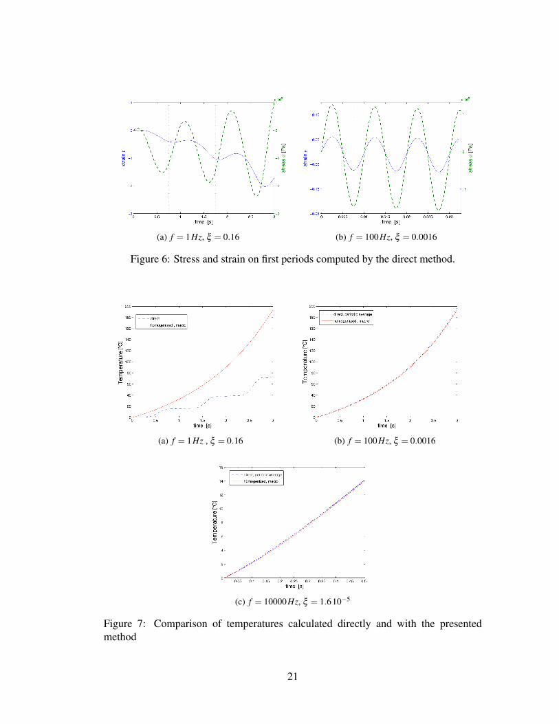
(a) f = 1Hz, ξ = 0.16 (b) f = 100Hz, ξ = 0.0016

Figure 6: Stress and strain on first periods computed by the direct method.

(a) f = 1Hz , ξ = 0.16 (b) f = 100Hz, ξ = 0.0016

(c) f = 10000Hz, ξ = 1.610−5

Figure 7: Comparison of temperatures calculated directly and with the presentedmethod

21

homogenization method, are compared on figure 5.Analyzing figure 5(a) we notice that for a high value of ξ (here, 0.16) , when the

two time scales are not well separated, the homogenized stress does not fit the onecalculated directly. This can partly be explained by the fact that the micro-chronologicalproblem is calculated as elastic, whereas the direct problem involves quite long timefluctuation (ω is around 10rad.s−1 compared to the characteristic Maxwell time of0.1s). Therefore, the impact of the fluctuation on the Maxwell material are not elasticonly. Indeed, as shown on figure 6(a), the fluctuating stress is not in phase with thestrain.

Concerning the temperature, the directly calculated one was compared to the ho-mogenized macro chronological temperature calculated from equation (64). Figure 7(a)illustrates their differences. With a final temperature relative error around 150%, ourhomogenization method is clearly not relevant when the scale factor is to big.

Low values of ξ : Increasing the pulsation allows to better separate scales. This isillustrated on case B, where the fluctuation frequency is increased by a factor of 100(see table 2).

The time scale factor then drops to about 10−3 and the homogenization techniqueexhibits good results. The two stresses are represented on Figure 5(b). Because ofthe high frequency, only their envelopes, and their macro-chronological part (periodicaverage, for the direct stress σ ) were represented. The two curves match almost per-fectly. The relevance of the homogenized solution can be explained by the nearly elas-tic response of the material to the fluctuation. This is visible on the stress and strainrepresentation over the first periods, on figure 6(b), which are totally in phase.

Furthermore, figure 7(b) shows the perfect matching of directly calculated tempera-ture averaged over each micro-chronological period, and macro-chronological homog-enized temperature. The relative difference between the final homogenized and directlycalculated temperature drops to about 2%. When ξ is much lower, the homogenizationmethod therefore works very well.

Very high frequency: Because of the sharp conditions imposed by the very high fre-quency (10 kHz), the direct problem was solved on [0,0.5s] only. Figure 7(c) showsa good matching between direct and homogenized temperature evolutions. The finaltemperature relative error is now less than 1%. In such case, which is close to morecomplex industrial situations, the time integration on longer times is already difficultand an accurate solution is very difficult to obtain by the direct calculation. The ho-mogenized solution even seems more relevant and eventually more precise if appliedto more complex geometry.

Time saving: Concerning the calculation times, in case B, the present method is morethan ten times faster than the direct method. This is of course explained by the con-ditions imposed to the Runge Kutta solver, which are much smoother than the one

22

Table 2: Comparison of the efficiency of the direct and presented method.CPU time (s) Case A Case B Case C

time scale factor ξ 0.16 1.610−3 1.610−5

CPU time (s) direct 0.39 10.51 219homogenized 0.17 0.16 0.12

Speed up 2.3 65 1820Final temperature relative error 160% 1.8% 0.8%

imposed initially in the direct problem. The convergence is therefore obtained rapidly,since the time discretization is coarser. In case C, the time saving increases to a factorof 1800 (see table 2). Indeed, the homogenized solution calculation does not dependon the frequency whereas the direct resolution is calculated using a time discretizationthat is directly linked to the frequency.

Self heating: In addition to validating the efficiency of the presented method withregard to the calculation time saving, this uniform test case allows to put forward aconclusion concerning the process. Observing figure 7(c), one can evaluate the temper-ature increase around 30°C per seconds. Nevertheless, even in the static case, wherethe process lasts no more than few seconds,in the real process, the temperature increaseis much higher (around 300°C/s). Thus it allows the fusion of the director and theflow of molten polymer. This illustrates the importance of the energy director shape.Indeed the heating, initiated at the tip of the director, would not be possible in the caseof rectangular directors and bulk heating. In other words, energy directors have have animportant role of heat concentrator and the heating and melting are local phenomena,at least in the initial stage.

5 ConclusionUnlike most studies where vibration and flow are considered as independent, we

here consider a thermo-mechanical problem including micro and macro chronologicalphenomena. After having analyzed characteristic dimensions of the ultrasonic problemtrying to stay rather general, we applied an asymptotic expansion method based on theintroduction of two independent time scales. The method leads to three coupled prob-lems depending on both time scales. It is worth noticing that those two time scales canbe treated as independent and be discretized separately. Instead of imposing very smalltime steps on the large time scale in order to capture the fluctuations, these theoreticalresults show that we can solve the micro-chronological problem on one vibration pe-riod only, once for each macro-chronological time step. In a global simulation of theprocess, the total number of time iterations can therefore be reasonable.

In order to validate the present method and illustrate its efficiency, it was comparedto the solution of the direct problem on a uniform test case. It was shown to give

23

good results even for quite high values of ξ . Furthermore, even in this homogeneoustest, the resolution of the direct problem at 10kHz was very long because of the sharpconditions induced by such a high frequency. The present method is therefore naturallymore suited in this case. Concerning the time saving, the efficiency is convincing: at10kHz, the calculation time was shown to be divided by one thousand. One has tohighlight the interest of such a time saving if applied to a 3 dimensional nonlinearproblem.

Furthermore, the test case brings a first conclusion about the process: the shape ofthe energy director is essential to the process. It induces highly heterogeneous fieldsat the tip of the energy director which allow the process to initiate. With a simplerectangular cross section, the bulk heating would not be important enough. To furtherinvestigate this last point, a finite element simulation tool handling geometrical evolu-tions is currently under development.

Finally, thanks to a rigorous mathematical framework, this paper reinforces theapproaches of the literature consisting in modelling straightaway the process with threecoupled problems. Nevertheless, the small displacement theory may be considered asrather unrealistic in the case of our process, and the present work should be extendedto finite transformations. In this case new assumptions will undoubtably be required.

A Homogenization with low temperature conditionsIn this case, the order of magnitude of the Maxwell relaxation time and Maxwell

viscosity of the initial problem (10) are changed. Let us consider that the orders ofmagnitude (19) become:

λ ∼ 105s Λ ∼ ξ−1

η ∼ 1011Pa.s N ∼ ξ−1 , (65)

which would be the case when the temperature drops to ambient temperature.Defining Λ0 = Λξ ∼ ξ 0 and N0 = Nξ ∼ ξ 0, the dimensionless constitutive mechan-

ical equation (10) then becomes:

Λ0ξ−1 ∂σσσ

∂T+Λ0ξ

−2 ∂σσσ

∂τ+σσσ = 2N0ξ

−1 ∂εεε

∂T+2N0ξ

−2 ∂εεε

∂τ, (66)

which identification leads to the two following mechanical problems.

Micro-chronological problem Identification of order −2 in ξ gives

Λ0∂σσσ0

∂τ= 2N0

∂εεε0

∂τ(67)

which is exactly the same as the previous case given by equations (33)

24

Macro-chronological problem Identification of order -1 in ξ gives

Λ0∂σσσ0

∂T+Λ0

∂σσσ1

∂τ= 2N0

∂εεε0

∂T+2N0

∂εεε1

∂τ= 2N0DDD0 (68)

which after averaging gives the macro-chronological constitutive equation:

Λ0∂ 〈σσσ0〉

∂T= 2N0

∂ 〈εεε0〉∂T

. (69)

At low temperature, the macro-chronological viscoelastic problem (35) turns intoan hypo-elastic problem:

Λ0∂ 〈σσσ0〉

∂T = 2N0 〈DDD0〉∇∇∇ · (〈σσσ0〉−〈p0〉 III) = 000∇ · 〈vvv0〉= 0

(onΩ)

〈vvv0〉= vvvd(T ) (on Γu)(〈σσσ0〉−〈p0〉 III) ·nnn = 000 (on Γσ )

(70)

Thermal problem: The thermal analysis remains the same, the temperature is oforder 0 in ξ , and the macro-chronological evolution is still given by averaging equa-tion (40):

∂ 〈θ0〉∂T

= A∆〈θ0〉+B〈σσσ0 : DDD0〉+B〈σσσ1 : DDD−1〉 . (71)

Nevertheless, in this case, DDD0 is given by equation (68). Applying the same methodas in section 3.4, we finally get a macro chronological thermal problem of the form:

∂ 〈θ0〉∂ t

= A∆〈θ0〉+B

2N

⟨σσσ0 :

(Λ0

∂σσσ0

∂ tT

)⟩∇∇∇θi ·nnn = 0 (Γu∪Γσ )

. (72)

The three obtained problems are therefore very similar to those of the first casediscussed in main text. The viscoelastic contributions simply disappears. A generaltreatment over the whole temperature range with temperature dependent parameterscan be envisaged with the first case formulation, which appears to be the richest one.

References[Ageorges et al., 2000] Ageorges, C. , Ye, L. et Hou, M. , 2000. Avdances in fusion

bonding techniques for joining thermoplastic matrix composites: a review. TheUniversity of Sydney, The University of Sydney.

[Benatar and Gutowski, 1989] Benatar, Avraham et Gutowski, Timothy G. , 1989. Ul-trasonic welding of peek graphite apc-2 composites. Polymer Engineering and Sci-ence, 29(23):1705.

25

[Benssousan et al., 1978] Benssousan, Alain , Lions, Jacques Louis et Papanicoulau,George. . Asymptotic analysis for periodic structures., volume 5. North Holland,1978.

[Boutin and Auriault, 1990] Boutin, C. et Auriault, JL , 1990. Dynamic behaviour ofporous media saturated by a viscoelastic fluid. application to bituminous concretes.International journal of engineering science, 28(11):1157–1181.

[Boutin and Wong, 1998] Boutin, Claude et Wong, Henri , 1998. Study of thermosen-sitive heterogeneous media via space-time homogenisation. European Journal ofMechanics - A/Solids, 17(6):939–968.

[Cojocaru and Karlsson, 2006] Cojocaru, D. et Karlsson, A. M. , 2006. A simple nu-merical method of cycle jumps for cyclically loaded structures. International Jour-nal of Fatigue, 28(12):1677–1689.

[Francfort and Suquet, 1986] Francfort, G.A. et Suquet, P.M. , 1986. Homogenizationand mechanical dissipation in thermoviscoelasticity. Archive for Rational Mechanicsand Analysis, 96(3):265–293.

[Geindreau and Auriault, 1999] Geindreau, C. et Auriault, J.L. , 1999. Investigationof the viscoplastic behaviour of alloys in the semi-solid state by homogenization.Mechanics of Materials, 31(8):535–551.

[Goyal et al., 2006] Goyal, R.K. , Tiwari, A. N. , Mulik, U. P. et Negi, Y. S. , 2006. Dy-namic mechanical properties of al2o3/poly(ether ether ketone) composites. Journalof Applied Polymer Science, 104(1):568–575.

[Guennouni, 1988] Guennouni, Tajeddine , 1988. Sur une méthode de calcul de struc-tures soumises à des chargements cycliques: l’homogénéisation en temps. Modéli-sation mathématique et analyse numérique, 22(3):417–455.

[Le Corre et al., 2005] Le Corre, S. , Dumont, P. , Orgeas, L. et Favier, D. , 2005. Uneapproche multi-échelle de la rhéologie des suspensions concentrées de fibres. Revuedes Composites et des Matériaux Avancés, 15(3):355.

[Li, 1999] Li, Rongzhi , 1999. Time-temperature superposition method for glass tran-sition temperature of plastic materials. Materials Science and Engineering A, 278(1-2):36–45.

[Oskay and Fish, 2004] Oskay, Caglar et Fish, Jacob , 2004. Fatigue life predictionusing 2-scale temporal asymptotic homogenization. International Journal for Nu-merical Methods in Engineering, (61):329–359.

[Sanchez-Palencia, 1980] Sanchez-Palencia, E. , 1980. Non-homogeneous media andvibration theory. Lecture Notes in Physics, 127.

26

[Suresh et al., 2007] Suresh, KS , Rani, M.R. , Prakasan, K. et Rudramoorthy, R. ,-2007. Modeling of temperature distribution in ultrasonic welding of thermoplasticsfor various joint designs. Journal of Materials Processing Tech., 186(1-3):138–146.

[Tolunay, 1983] Tolunay, MN , 1983. Heating and bonding mechanisms in ultrasonicwelding of thermoplastics. Polymer Engineering and Science, 23(13):726–733.

[Van Paepegem et al., 2001] Van Paepegem, W. , Degrieck, J. et De Baets, P. , 2001.Finite element approach for modelling fatigue damage in fibre-reinforced compositematerials. Composites Part B, 32(7):575–588.

[Wang et al., 2006] Wang, X. , Yan, J. , Li, R. et Yang, S. , 2006. Fem investigation ofthe temperature field of energy director during ultrasonic welding of peek compos-ites. Journal of Thermoplastic Composite Materials, 19(5):593.

[Yu and Fish, 2002] Yu, Qing et Fish, Jacob , 2002. Multiscale asymptotic homog-enization for multiphysics problems with multiple spatial and temporal scales: acoupled thermo-viscoelastic example problem. International Journal of Solids andStructures, 39(26):6429–6452.

27