ULTRASONIC TESTING AND FLAW CHARACTERIZATION

Alex KARPELSON Kinectrics Inc., Toronto, Canada

1. Introduction Ultrasonic Testing (UT) is a commonly used inspection method. Various techniques are employed e.g. for tube examination in order to detect, characterize and size different flaws. However, sometimes the results of the inspection are not satisfactory due to insufficient sensitivity and/or inability to characterize the flaw (i.e. determine flaw shape). Typically the pulse-echo (PE) and pitch-catch (PC) techniques are used for tube testing to detect, characterize and size flaws located within the tube wall, on the inside diameter (ID) or outside diameter (OD). (Sometimes terms ID and OD are used in context of inside and outside surfaces, respectively). Normal beam (NB) longitudinal waves and angle shear waves are commonly employed [1-2]. However, only tomographic method, as the most accurate and reliable one, allows fully characterize the flaw. Such a method assumes insonification of each area of the tested object from different points and at various angles; in other words, it allows “seeing” each area of the object from different points of view. But unfortunately, tomography is a very complicated and expensive technique, it is still on the development stage only, and the commercial UT tomographs are not available. Therefore it is worth to develop something like “quasi-tomographic” approach for UT testing, which could significantly improve the inspection capability by employing only a few rather simple tomographic techniques. 2. General approach UT computed tomography has significant potential advantages. For example, UT tomographic method can generate cross-sectional images (tomograms) of internal structure of the test object depicting distributions of four different material properties (acoustic impedance, ultrasound speed, density, and attenuation coefficient), thus providing high resolution 2D and 3D images. We assume that tube is filled with water, and transducers are positioned inside the tube. All experiments described below were performed on metal tubes with ID=4” and wall thickness 4mm. Calibrated UT system and computerized scanning rig with rotary and three axial motions were employed for experiments. The UT system includes Winspect™ data acquisition software, a SONIX STR-8100 digitizer card, and a UTEX UT-340 pulser-receiver. Transducers with different center frequencies (10, 15 and 20MHz), various diameters (from 0.375” to 1.375”) and focal lengths (from 25 to 100mm, including probes with logarithmic lenses [3] forming stretched focal zones) were used for testing. To improve performance of the system, different techniques and probes will be used in parallel to allow “seeing” the flaw from various directions simultaneously. Obtained different images should be interposed (combined). As a result, one will get something like a rather simple “quasi-tomographic”

1

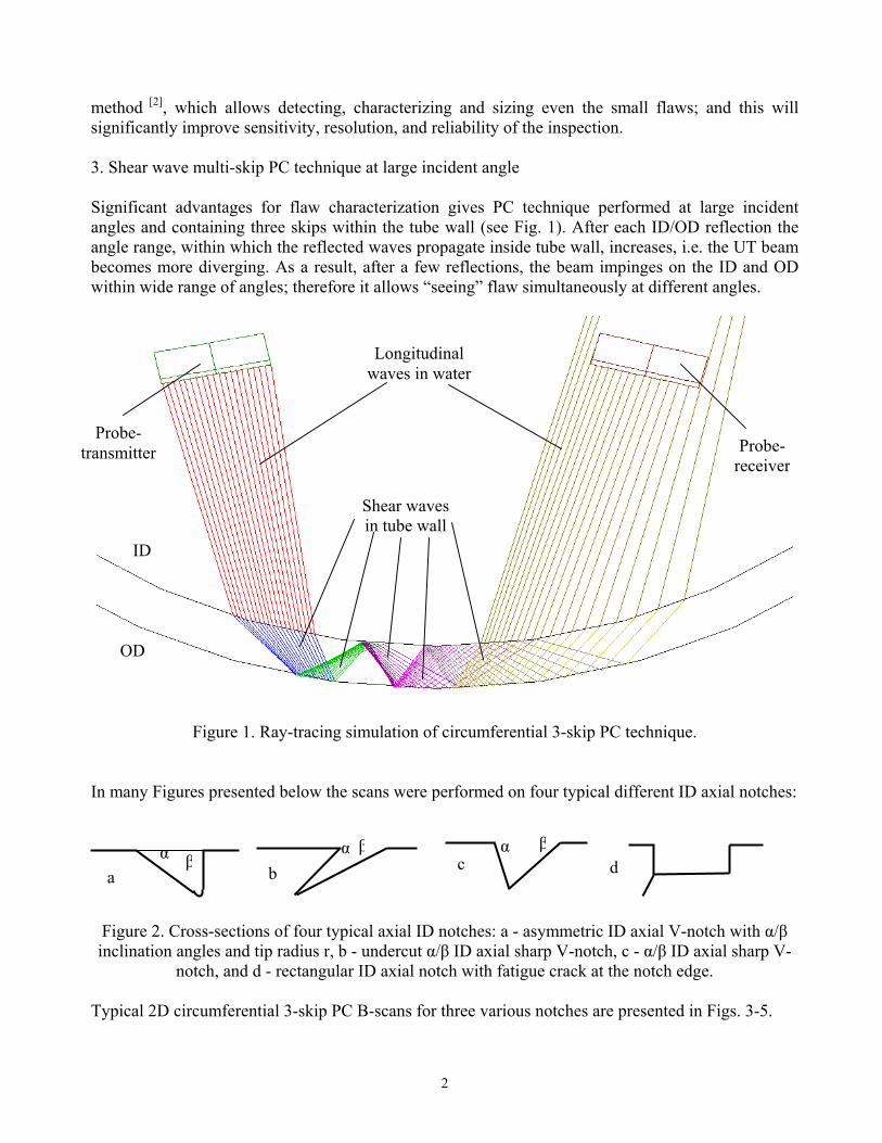
method [2], which allows detecting, characterizing and sizing even the small flaws; and this will significantly improve sensitivity, resolution, and reliability of the inspection. 3. Shear wave multi-skip PC technique at large incident angle Significant advantages for flaw characterization gives PC technique performed at large incident angles and containing three skips within the tube wall (see Fig. 1). After each ID/OD reflection the angle range, within which the reflected waves propagate inside tube wall, increases, i.e. the UT beam becomes more diverging. As a result, after a few reflections, the beam impinges on the ID and OD within wide range of angles; therefore it allows “seeing” flaw simultaneously at different angles.

Probe- transmitter

OD

Longitudinal waves in water

Probe-receiver

ID

Shear waves in tube wall

Figure 1. Ray-tracing simulation of circumferential 3-skip PC technique.

In many Figures presented below the scans were performed on four typical different ID axial notches:

α β

a b cβα α βd

Figure 2. Cross-sections of four typical axial ID notches: a - asymmetric ID axial V-notch with α/β inclination angles and tip radius r, b - undercut α/β ID axial sharp V-notch, c - α/β ID axial sharp V-

notch, and d - rectangular ID axial notch with fatigue crack at the notch edge. Typical 2D circumferential 3-skip PC B-scans for three various notches are presented in Figs. 3-5.

2

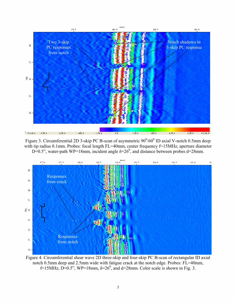
Notch shadows in 3-skip PC response

Two 3-skip PC responses from notch

Figure 3. Circumferential 2D 3-skip PC B-scan of asymmetric 900/600 ID axial V-notch 0.5mm deep with tip radius 0.1mm. Probes: focal length FL=40mm, center frequency f=15MHz, aperture diameter

D=0.5”, water-path WP=18mm, incident angle δ=260, and distance between probes d=28mm.

Responses from crack

Responses from notch

Figure 4. Circumferential shear wave 2D three-skip and four-skip PC B-scan of rectangular ID axial notch 0.5mm deep and 2.5mm wide with fatigue crack at the notch edge. Probes: FL=40mm,

f=15MHz, D=0.5”, WP=18mm, δ=260, and d=28mm. Color scale is shown in Fig. 3.

3

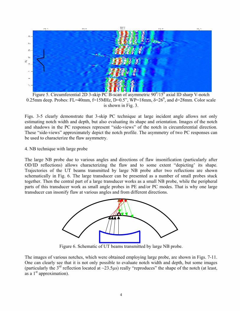
Figure 5. Circumferential 2D 3-skip PC B-scan of asymmetric 900/150 axial ID sharp V-notch

0.25mm deep. Probes: FL=40mm, f=15MHz, D=0.5”, WP=18mm, δ=260, and d=28mm. Color scale is shown in Fig. 3.

Figs. 3-5 clearly demonstrate that 3-skip PC technique at large incident angle allows not only estimating notch width and depth, but also evaluating its shape and orientation. Images of the notch and shadows in the PC responses represent “side-views” of the notch in circumferential direction. These “side-views” approximately depict the notch profile. The asymmetry of two PC responses can be used to characterize the flaw asymmetry. 4. NB technique with large probe The large NB probe due to various angles and directions of flaw insonification (particularly after OD/ID reflections) allows characterizing the flaw and to some extent “depicting’ its shape. Trajectories of the UT beams transmitted by large NB probe after two reflections are shown schematically in Fig. 6. The large transducer can be presented as a number of small probes stuck together. Then the central part of a large transducer works as a small NB probe, while the peripheral parts of this transducer work as small angle probes in PE and/or PC modes. That is why one large transducer can insonify flaw at various angles and from different directions.

Figure 6. Schematic of UT beams transmitted by large NB probe. The images of various notches, which were obtained employing large probe, are shown in Figs. 7-11. One can clearly see that it is not only possible to evaluate notch width and depth, but some images (particularly the 3rd reflection located at ~23.5µs) really “reproduces” the shape of the notch (at least, as a 1st approximation).

4

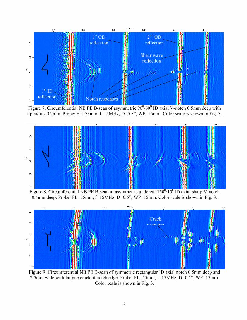
Figure 7. Circumferential NB PE B-scan of asymmetric 900/600 ID axial V-notch 0.5mm deep with tip radius 0.2mm. Probe: FL=55mm, f=15MHz, D=0.5”, WP=15mm. Color scale is shown in Fig. 3.

Figure 8. Circumferential NB PE B-scan of asymmetric undercut 1500/150 ID axial sharp V-notch 0.4mm deep. Probe: FL=55mm, f=15MHz, D=0.5”, WP=15mm. Color scale is shown in Fig. 3.

Notch responses 1st ID

reflection

1st OD reflection

2nd OD reflection

Shear wave reflection

Crack response

Figure 9. Circumferential NB PE B-scan of symmetric rectangular ID axial notch 0.5mm deep and 2.5mm wide with fatigue crack at notch edge. Probe: FL=55mm, f=15MHz, D=0.5”, WP=15mm.

Color scale is shown in Fig. 3.

5

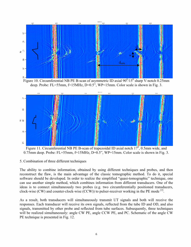
Figure 10. Circumferential NB PE B-scan of asymmetric ID axial 900/150 sharp V-notch 0.25mm

deep. Probe: FL=55mm, f=15MHz, D=0.5”, WP=15mm. Color scale is shown in Fig. 3.

d

w

dtube

Figure 11. Circumferential NB PE B-scan of trapezoidal ID axial notch 170, 0.5mm wide, and 0.75mm deep. Probe: FL=55mm, f=15MHz, D=0.5”, WP=15mm. Color scale is shown in Fig. 3.

5. Combination of three different techniques The ability to combine information, obtained by using different techniques and probes, and then reconstruct the flaw, is the main advantage of the classic tomographic method. To do it, special software should be developed. In order to realize the simplified “quasi-tomographic” technique, one can use another simple method, which combines information from different transducers. One of the ideas is to connect simultaneously two probes (e.g. two circumferentially positioned transducers, clock-wise (CW) and counter-clock-wise (CCW)) to pulser-receiver working in the PE mode [2]. As a result, both transducers will simultaneously transmit UT signals and both will receive the responses. Each transducer will receive its own signals, reflected from the tube ID and OD, and also signals, transmitted by other probe and reflected from tube surfaces. Subsequently, three techniques will be realized simultaneously: angle CW PE, angle CCW PE, and PC. Schematic of the angle CW PE technique is presented in Fig. 12.

6

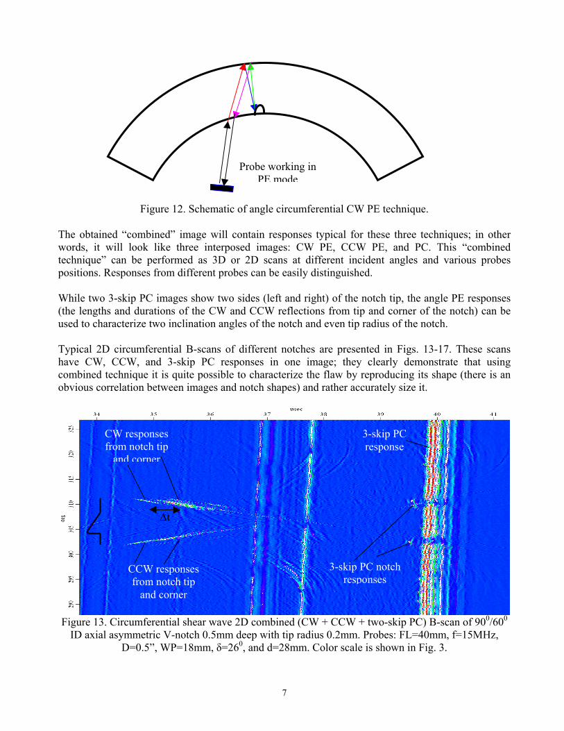
Probe working in PE mode

Figure 12. Schematic of angle circumferential CW PE technique. The obtained “combined” image will contain responses typical for these three techniques; in other words, it will look like three interposed images: CW PE, CCW PE, and PC. This “combined technique” can be performed as 3D or 2D scans at different incident angles and various probes positions. Responses from different probes can be easily distinguished. While two 3-skip PC images show two sides (left and right) of the notch tip, the angle PE responses (the lengths and durations of the CW and CCW reflections from tip and corner of the notch) can be used to characterize two inclination angles of the notch and even tip radius of the notch. Typical 2D circumferential B-scans of different notches are presented in Figs. 13-17. These scans have CW, CCW, and 3-skip PC responses in one image; they clearly demonstrate that using combined technique it is quite possible to characterize the flaw by reproducing its shape (there is an obvious correlation between images and notch shapes) and rather accurately size it.

3-skip PC notch responses

CCW responses from notch tip

and corner

CW responses from notch tip

and corner

3-skip PC response

∆t

Figure 13. Circumferential shear wave 2D combined (CW + CCW + two-skip PC) B-scan of 900/600 ID axial asymmetric V-notch 0.5mm deep with tip radius 0.2mm. Probes: FL=40mm, f=15MHz,

D=0.5”, WP=18mm, δ=260, and d=28mm. Color scale is shown in Fig. 3.

7

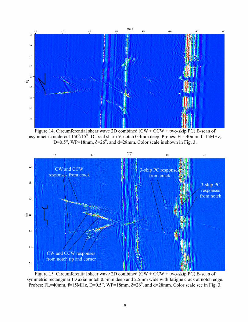
Figure 14. Circumferential shear wave 2D combined (CW + CCW + two-skip PC) B-scan of

asymmetric undercut 1500/150 ID axial sharp V-notch 0.4mm deep. Probes: FL=40mm, f=15MHz, D=0.5”, WP=18mm, δ=260, and d=28mm. Color scale is shown in Fig. 3.

CW and CCW ponses from cracres k

CW and CCW responses from notch tip and corner

3-skip PC responses

from notch

3-skip PC responses from crack

Figure 15. Circumferential shear wave 2D combined (CW + CCW + two-skip PC) B-scan of symmetric rectangular ID axial notch 0.5mm deep and 2.5mm wide with fatigue crack at notch edge. Probes: FL=40mm, f=15MHz, D=0.5”, WP=18mm, δ=260, and d=28mm. Color scale see in Fig. 3.

8

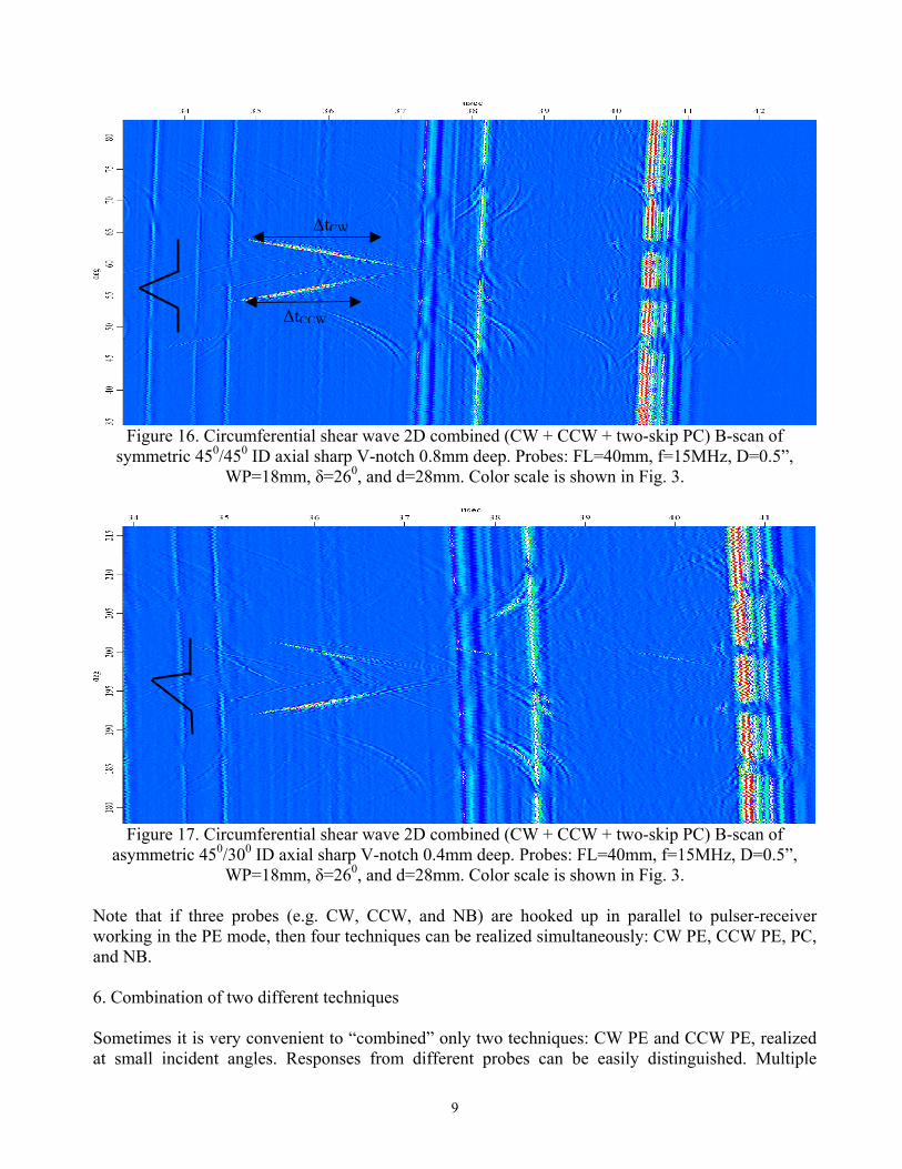
∆tCCW

∆tCW

Figure 16. Circumferential shear wave 2D combined (CW + CCW + two-skip PC) B-scan of symmetric 450/450 ID axial sharp V-notch 0.8mm deep. Probes: FL=40mm, f=15MHz, D=0.5”,

WP=18mm, δ=260, and d=28mm. Color scale is shown in Fig. 3.

Figure 17. Circumferential shear wave 2D combined (CW + CCW + two-skip PC) B-scan of

asymmetric 450/300 ID axial sharp V-notch 0.4mm deep. Probes: FL=40mm, f=15MHz, D=0.5”, WP=18mm, δ=260, and d=28mm. Color scale is shown in Fig. 3.

Note that if three probes (e.g. CW, CCW, and NB) are hooked up in parallel to pulser-receiver working in the PE mode, then four techniques can be realized simultaneously: CW PE, CCW PE, PC, and NB. 6. Combination of two different techniques Sometimes it is very convenient to “combined” only two techniques: CW PE and CCW PE, realized at small incident angles. Responses from different probes can be easily distinguished. Multiple

9

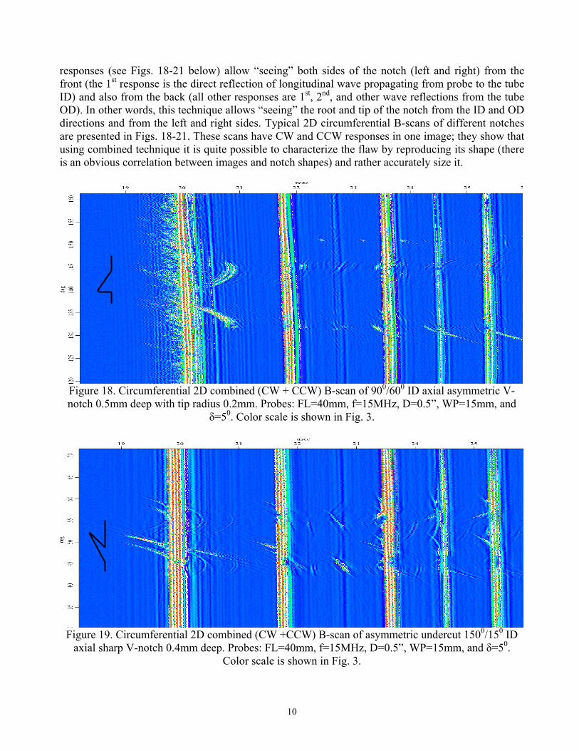
responses (see Figs. 18-21 below) allow “seeing” both sides of the notch (left and right) from the front (the 1st response is the direct reflection of longitudinal wave propagating from probe to the tube ID) and also from the back (all other responses are 1st, 2nd, and other wave reflections from the tube OD). In other words, this technique allows “seeing” the root and tip of the notch from the ID and OD directions and from the left and right sides. Typical 2D circumferential B-scans of different notches are presented in Figs. 18-21. These scans have CW and CCW responses in one image; they show that using combined technique it is quite possible to characterize the flaw by reproducing its shape (there is an obvious correlation between images and notch shapes) and rather accurately size it.

Figure 18. Circumferential 2D combined (CW + CCW) B-scan of 900/600 ID axial asymmetric V-notch 0.5mm deep with tip radius 0.2mm. Probes: FL=40mm, f=15MHz, D=0.5”, WP=15mm, and

δ=50. Color scale is shown in Fig. 3.

Figure 19. Circumferential 2D combined (CW +CCW) B-scan of asymmetric undercut 1500/150 ID

axial sharp V-notch 0.4mm deep. Probes: FL=40mm, f=15MHz, D=0.5”, WP=15mm, and δ=50. Color scale is shown in Fig. 3.

10

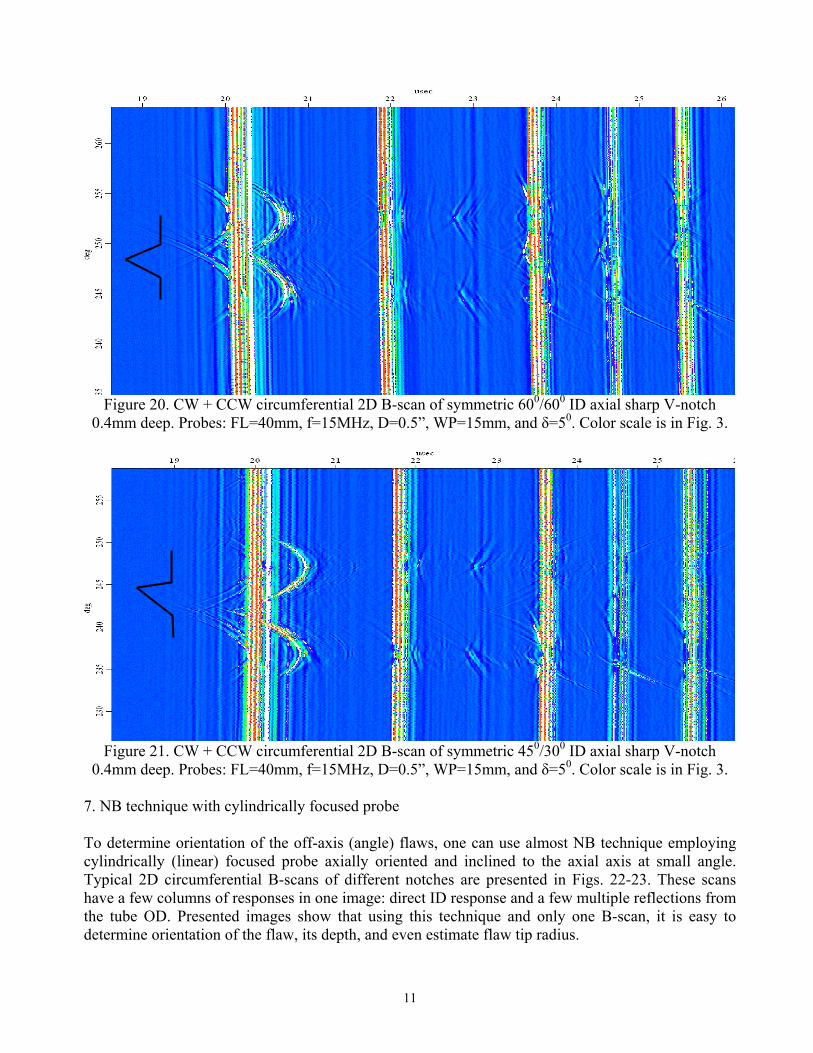
Figure 20. CW + CCW circumferential 2D B-scan of symmetric 600/600 ID axial sharp V-notch

0.4mm deep. Probes: FL=40mm, f=15MHz, D=0.5”, WP=15mm, and δ=50. Color scale is in Fig. 3.

Figure 21. CW + CCW circumferential 2D B-scan of symmetric 450/300 ID axial sharp V-notch

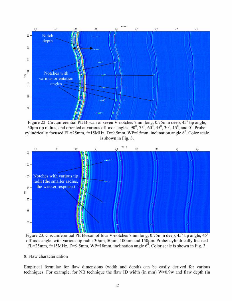
0.4mm deep. Probes: FL=40mm, f=15MHz, D=0.5”, WP=15mm, and δ=50. Color scale is in Fig. 3. 7. NB technique with cylindrically focused probe To determine orientation of the off-axis (angle) flaws, one can use almost NB technique employing cylindrically (linear) focused probe axially oriented and inclined to the axial axis at small angle. Typical 2D circumferential B-scans of different notches are presented in Figs. 22-23. These scans have a few columns of responses in one image: direct ID response and a few multiple reflections from the tube OD. Presented images show that using this technique and only one B-scan, it is easy to determine orientation of the flaw, its depth, and even estimate flaw tip radius.

11

Notches with various orientation

angles

Notch depth

Figure 22. Circumferential PE B-scan of seven V-notches 7mm long, 0.75mm deep, 450 tip angle, 50µm tip radius, and oriented at various off-axis angles: 900, 750, 600, 450, 300, 150, and 00. Probe:

cylindrically focused FL=25mm, f=15MHz, D=9.5mm, WP=15mm, inclination angle 60. Color scale is shown in Fig. 3.

Notches with various tip radii (the smaller radius,

the weaker response)

Figure 23. Circumferential PE B-scan of four V-notches 7mm long, 0.75mm deep, 450 tip angle, 450 off-axis angle, with various tip radii: 30µm, 50µm, 100µm and 150µm. Probe: cylindrically focused FL=25mm, f=15MHz, D=9.5mm, WP=18mm, inclination angle 60. Color scale is shown in Fig. 3.

8. Flaw characterization Empirical formulae for flaw dimensions (width and depth) can be easily derived for various techniques. For example, for NB technique the flaw ID width (in mm) W≈0.9w and flaw depth (in

12

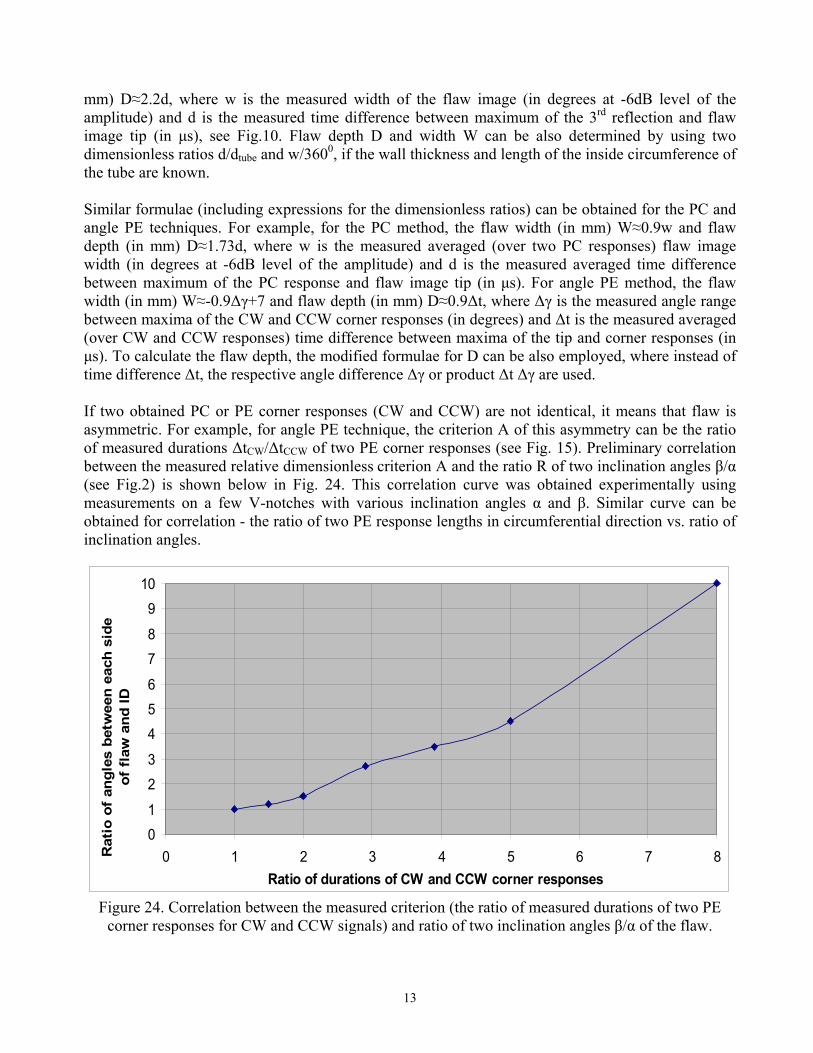
mm) D≈2.2d, where w is the measured width of the flaw image (in degrees at -6dB level of the amplitude) and d is the measured time difference between maximum of the 3rd reflection and flaw image tip (in µs), see Fig.10. Flaw depth D and width W can be also determined by using two dimensionless ratios d/dtube and w/3600, if the wall thickness and length of the inside circumference of the tube are known. Similar formulae (including expressions for the dimensionless ratios) can be obtained for the PC and angle PE techniques. For example, for the PC method, the flaw width (in mm) W≈0.9w and flaw depth (in mm) D≈1.73d, where w is the measured averaged (over two PC responses) flaw image width (in degrees at -6dB level of the amplitude) and d is the measured averaged time difference between maximum of the PC response and flaw image tip (in µs). For angle PE method, the flaw width (in mm) W≈-0.9∆γ+7 and flaw depth (in mm) D≈0.9∆t, where ∆γ is the measured angle range between maxima of the CW and CCW corner responses (in degrees) and ∆t is the measured averaged (over CW and CCW responses) time difference between maxima of the tip and corner responses (in µs). To calculate the flaw depth, the modified formulae for D can be also employed, where instead of time difference ∆t, the respective angle difference ∆γ or product ∆t ∆γ are used. If two obtained PC or PE corner responses (CW and CCW) are not identical, it means that flaw is asymmetric. For example, for angle PE technique, the criterion A of this asymmetry can be the ratio of measured durations ∆tCW/∆tCCW of two PE corner responses (see Fig. 15). Preliminary correlation between the measured relative dimensionless criterion A and the ratio R of two inclination angles β/α (see Fig.2) is shown below in Fig. 24. This correlation curve was obtained experimentally using measurements on a few V-notches with various inclination angles α and β. Similar curve can be obtained for correlation - the ratio of two PE response lengths in circumferential direction vs. ratio of inclination angles.

01

23

456

78

910

0 1 2 3 4 5 6 7Ratio of durations of CW and CCW corner responses

Rat

io o

f an

gles

bet

wee

n ea

ch s

id

8

eof

fla

w a

nd ID

Figure 24. Correlation between the measured criterion (the ratio of measured durations of two PE

corner responses for CW and CCW signals) and ratio of two inclination angles β/α of the flaw.

13

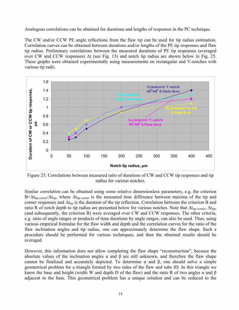
Analogous correlations can be obtained for durations and lengths of responses in the PC technique. The CW and/or CCW PE angle reflections from the flaw tip can be used for tip radius estimation. Correlation curves can be obtained between durations and/or lengths of the PE tip responses and flaw tip radius. Preliminary correlations between the measured durations of PE tip responses (averaged over CW and CCW responses) ∆t (see Fig. 13) and notch tip radius are shown below in Fig. 25. These graphs were obtained experimentally using measurements on rectangular and V-notches with various tip radii.

0

0.2

0.4

0.6

0.8

1

1.2

1.4

1.6

0 50 100 150 200 250 300 350 400 450

Notch tip radius, µm

Dur

atio

n of

CW

or C

CW

tip

resp

onse

, µs

Symmetric V-notch 600/600 0.3mm deep

Asymmetric V-notch 900/600 0.5mm deep

Rectangular notch 0.5mm deep

Rectangular notch 1mm deep

Figure 25. Correlations between measured ratio of durations of CW and CCW tip responses and tip radius for various notches.

Similar correlation can be obtained using some relative dimensionless parameters, e.g. the criterion B=∆ttip-corner/∆ttip, where ∆ttip-corner is the measured time difference between maxima of the tip and corner responses and ∆ttip is the duration of the tip reflection. Correlation between the criterion B and ratio R of notch depth to tip radius are presented below for various notches. Note that ∆ttip-corner, ∆ttip, (and subsequently, the criterion B) were averaged over CW and CCW responses. The other criteria, e.g. ratio of angle ranges or products of time durations by angle ranges, can also be used. Thus, using various empirical formulae for the flaw width and depth and the correlation curves for the ratio of the flaw inclination angles and tip radius, one can approximately determine the flaw shape. Such a procedure should be performed for various techniques, and then the obtained results should be averaged. However, this information does not allow completing the flaw shape “reconstruction”, because the absolute values of the inclination angles α and β are still unknown, and therefore the flaw shape cannot be finalized and accurately depicted. To determine α and β, one should solve a simple geometrical problem for a triangle formed by two sides of the flaw and tube ID. In this triangle we know the base and height (width W and depth D of the flaw) and the ratio R of two angles α and β adjacent to the base. This geometrical problem has a unique solution and can be reduced to the

14

transcendental equation: Dsinα(1+R)=Wsinαsin(Rα). This equation can be easily solved numerically, e.g. using Matlab; and subsequently, the angle α will be determined. Then angle β=Rα. As a result, all parameters of the flaw are now determined; and therefore the flaw shape can be rather accurately reproduced. 9. Conclusions

• Sometimes results of the UT inspection are not satisfactory due to inability to characterize a flaw, i.e. determine its shape. To characterize a flaw, it is necessary to apply different methods and probes, which allow “seeing” a flaw at various angles. In addition, information obtained by using various transducers and methods, should be combined.

• Different techniques and probes give the possibility, after processing the obtained responses, to “reproduce” the flaw profile and rather accurately size the flaw.

• “Combined” images, containing various responses, allow determining pretty accurately flaw shape and orientation and “reconstruct” the flaw.

• Empirical formulae for flaw dimensions (width and depth) can be easily derived for various techniques by sizing the responses.

• Correlations between durations and/or lengths of the PC and/or PE responses vs. ratio of the inclination angles of the flaw can be obtained.

• Absolute values of the inclination angles of the flaw can be derived. Subsequently, orientation of the flaw can be determined.

• Correlations between durations and/or lengths of the tip PE responses vs. flaw tip radius can be obtained. As a result, the tip radius of the flaw can be estimated.

References [1] M. Trelinski, “Inspection of CANDU Reactor Pressure Tubes Using Ultrasonics”, Proceedings of 17th World Conference on Nondestructive Testing, Oct 2008, Shanghai, China. [2] A. Karpelson, “Quasi-Tomographic Ultrasonic Technique for Tube Inspection”, The e-journal of NDT, vol. 10, No. 6, June 2005. [3] A. Karpelson and B. Hatcher, “Collimating and Wideband Ultrasonic Piezotransducers”, The e- journal of NDT, vol. 9, No. 1, January 2004.

15