ULTRASHORT LASER PULSE SHAPING FOR NOVELLIGHT FIELDS AND EXPERIMENTAL BIOPHYSICS

Andrew Peter Rudhall

A Thesis Submitted for the Degree of PhDat the

University of St Andrews

2013

Full metadata for this item is available inResearch@StAndrews:FullText

at:http://research-repository.st-andrews.ac.uk/

Please use this identifier to cite or link to this item:http://hdl.handle.net/10023/3682

This item is protected by original copyright

This item is licensed under aCreative Commons License

Abstract

Broadband spectral content is required to support ultrashort pulses. However thisbroadband content is subject to dispersion and hence the pulse duration of correspondingultrashort pulses may be stretched accordingly. I used a commercially-available adaptiveultrashort pulse shaper featuring multiphoton intrapulse interference phase scan technol-ogy to characterise and compensate for the dispersion of the optical system in situ andconducted experimental and theoretical studies in various inter-linked topics relating tothe light-matter interaction.

Firstly, I examined the role of broadband ultrashort pulses in novel light-matter in-teracting systems involving optically co-trapped particle systems in which inter-particlelight scattering occurs between optically-bound particles. Secondly, I delivered dispersion-compensated broadband ultrashort pulses in a dispersive microscope system to investigatethe role of pulse duration in a biological light-matter interaction involving laser-inducedcell membrane permeabilisation through linear and nonlinear optical absorption. Finally, Iexamined some of the propagation characteristics of broadband ultrashort pulse propaga-tion using a computer-controlled spatial light modulator. The propagation characteristicsof ultrashort pulses is of paramount importance for defining the light-matter interactionin systems. The ability to control ultrashort pulse propagation by using adaptive disper-sion compensation enables chirp-free ultrashort pulses to be used in experiments requiringthe shortest possible pulses for a specified spectral bandwidth. Ultrashort pulsed beamsmay be configured to provide high peak intensities over long propagation lengths, forexample, using novel beam shapes such as Bessel-type beams, which has applications inbiological light-matter interactions including phototransfection based on laser-induced cellmembrane permeabilisation. The need for precise positioning of the beam focus on thecell membrane becomes less strenuous by virtue of the spatial properties of the Besselbeam. Dispersion compensation can be used to control the temporal properties of ultra-short pulses thus permitting, for example, a high peak intensity to be maintained alongthe length of a Bessel beam, thereby reducing the pulse energy required to permeabilisethe cell membrane and potentially reduce damage therein.

Contents

1 Introduction 6

1.1 Introduction to ultrashort pulses . . . . . . . . . . . . . . . . . . . . . . . . 81.1.1 Peak power of ultrashort pulsed lasers . . . . . . . . . . . . . . . . . 8

1.2 The relationship between spectral intensity and pulse duration . . . . . . . 101.2.1 Interference of multiple waves . . . . . . . . . . . . . . . . . . . . . . 101.2.2 Fourier transform approach . . . . . . . . . . . . . . . . . . . . . . . 121.2.3 Dispersion . . . . . . . . . . . . . . . . . . . . . . . . . . . . . . . . . 17

1.3 Nonlinear optics . . . . . . . . . . . . . . . . . . . . . . . . . . . . . . . . . 241.3.1 Second harmonic generation . . . . . . . . . . . . . . . . . . . . . . . 251.3.2 Phase-matching . . . . . . . . . . . . . . . . . . . . . . . . . . . . . . 261.3.3 Further considerations for ultrashort pulse SHG . . . . . . . . . . . 28

1.4 Generation of ultrashort pulses . . . . . . . . . . . . . . . . . . . . . . . . . 301.4.1 Dispersion management in femtosecond laser oscillators . . . . . . . 31

1.5 Applications of broadband ultrashort pulses . . . . . . . . . . . . . . . . . . 321.6 Conclusions . . . . . . . . . . . . . . . . . . . . . . . . . . . . . . . . . . . . 331.7 Chapter acknowledgements . . . . . . . . . . . . . . . . . . . . . . . . . . . 34

2 Control of broadband ultrashort pulses 35

2.1 Introduction . . . . . . . . . . . . . . . . . . . . . . . . . . . . . . . . . . . . 352.2 Management of dispersion in optical setups . . . . . . . . . . . . . . . . . . 352.3 Established methods of dispersion compensation . . . . . . . . . . . . . . . 36

2.3.1 Prisms . . . . . . . . . . . . . . . . . . . . . . . . . . . . . . . . . . . 362.3.2 Diffraction gratings . . . . . . . . . . . . . . . . . . . . . . . . . . . . 372.3.3 Chirped mirrors . . . . . . . . . . . . . . . . . . . . . . . . . . . . . 382.3.4 Spatial light modulators . . . . . . . . . . . . . . . . . . . . . . . . . 39

2.4 Measurement of pulse duration and dispersion: established methods . . . . 432.5 Multiphoton intrapulse interference phase scan (MIIPS) . . . . . . . . . . . 44

1

2.6 Operation of MIIPS system . . . . . . . . . . . . . . . . . . . . . . . . . . . 482.6.1 MIIPS experimental procedure . . . . . . . . . . . . . . . . . . . . . 492.6.2 Pulse stretching . . . . . . . . . . . . . . . . . . . . . . . . . . . . . 52

2.7 MIIPS results . . . . . . . . . . . . . . . . . . . . . . . . . . . . . . . . . . . 522.7.1 SHG as function of pulse energy and duration . . . . . . . . . . . . . 52

2.8 Conclusions . . . . . . . . . . . . . . . . . . . . . . . . . . . . . . . . . . . . 572.9 Chapter acknowledgements . . . . . . . . . . . . . . . . . . . . . . . . . . . 58

3 Transverse optical binding 59

3.1 Introduction . . . . . . . . . . . . . . . . . . . . . . . . . . . . . . . . . . . . 593.2 Transversal Optical Binding . . . . . . . . . . . . . . . . . . . . . . . . . . . 61

3.2.1 Rayleigh Regime . . . . . . . . . . . . . . . . . . . . . . . . . . . . . 623.2.2 Mie Regime . . . . . . . . . . . . . . . . . . . . . . . . . . . . . . . . 62

3.3 Longitudinal Optical Binding . . . . . . . . . . . . . . . . . . . . . . . . . . 633.4 Experimental procedure . . . . . . . . . . . . . . . . . . . . . . . . . . . . . 633.5 Experimental results . . . . . . . . . . . . . . . . . . . . . . . . . . . . . . . 66

3.5.1 Experimental images . . . . . . . . . . . . . . . . . . . . . . . . . . . 673.5.2 Optical binding potentials . . . . . . . . . . . . . . . . . . . . . . . . 67

3.6 Computational study: finite element method . . . . . . . . . . . . . . . . . 693.6.1 Maxwell Stress Tensor and Surface Force . . . . . . . . . . . . . . . 693.6.2 Computational results: finite element method . . . . . . . . . . . . . 70

3.7 Computational study: interacting dipole method . . . . . . . . . . . . . . . 713.7.1 Optical binding: Rayleigh regime . . . . . . . . . . . . . . . . . . . . 723.7.2 Theory . . . . . . . . . . . . . . . . . . . . . . . . . . . . . . . . . . 723.7.3 Broadband ultrashort pulsed optical binding . . . . . . . . . . . . . 753.7.4 Broadband SHG ultrashort pulsed optical binding . . . . . . . . . . 77

3.8 Conclusions . . . . . . . . . . . . . . . . . . . . . . . . . . . . . . . . . . . . 793.9 Chapter acknowledgements . . . . . . . . . . . . . . . . . . . . . . . . . . . 82

4 The role of femtosecond pulse duration in the membrane permeabilisa-

tion of mammalian cells 83

4.1 Introduction . . . . . . . . . . . . . . . . . . . . . . . . . . . . . . . . . . . . 834.2 Methods . . . . . . . . . . . . . . . . . . . . . . . . . . . . . . . . . . . . . . 86

4.2.1 Experimental arrangement using MIIPS system . . . . . . . . . . . . 864.2.2 Optoinjection: cell culture and experimental procedure . . . . . . . . 87

4.3 Results: optoinjection . . . . . . . . . . . . . . . . . . . . . . . . . . . . . . 90

2

4.3.1 The role of pulse duration . . . . . . . . . . . . . . . . . . . . . . . . 904.3.2 The role of pulse energy . . . . . . . . . . . . . . . . . . . . . . . . . 934.3.3 The role of number of pulses . . . . . . . . . . . . . . . . . . . . . . 95

4.4 Discussion . . . . . . . . . . . . . . . . . . . . . . . . . . . . . . . . . . . . . 964.5 Phototransfection experiments . . . . . . . . . . . . . . . . . . . . . . . . . 994.6 Conclusions . . . . . . . . . . . . . . . . . . . . . . . . . . . . . . . . . . . . 1004.7 Chapter acknowledgements . . . . . . . . . . . . . . . . . . . . . . . . . . . 101

5 Advanced beam shaping with broadband ultrashort pulses 102

5.1 Introduction . . . . . . . . . . . . . . . . . . . . . . . . . . . . . . . . . . . . 1025.1.1 Bessel beams . . . . . . . . . . . . . . . . . . . . . . . . . . . . . . . 103

5.2 Ultrashort pulse novel beams: studies . . . . . . . . . . . . . . . . . . . . . 1055.2.1 Experimental setup . . . . . . . . . . . . . . . . . . . . . . . . . . . . 1055.2.2 Choice of lens for the focusing of ultrashort pulses . . . . . . . . . . 1065.2.3 Spatial chirp . . . . . . . . . . . . . . . . . . . . . . . . . . . . . . . 1085.2.4 Gaussian and Bessel beam propagation introduction . . . . . . . . . 1115.2.5 Concentric annular rings, their phase, and interference in the focal

plane . . . . . . . . . . . . . . . . . . . . . . . . . . . . . . . . . . . 1185.3 Conclusions . . . . . . . . . . . . . . . . . . . . . . . . . . . . . . . . . . . . 1275.4 Chapter acknowledgements . . . . . . . . . . . . . . . . . . . . . . . . . . . 128

6 Conclusions and prospects for future work 129

7 Appendix 149

7.1 Calculation of pulse shape profiles . . . . . . . . . . . . . . . . . . . . . . . 1497.1.1 Gaussian pulses . . . . . . . . . . . . . . . . . . . . . . . . . . . . . . 1497.1.2 Sech-squared pulses . . . . . . . . . . . . . . . . . . . . . . . . . . . 150

7.2 Well-known pulse measurement techniques . . . . . . . . . . . . . . . . . . 1517.2.1 Autocorrelation (AC) and interferometric autocorrelation (IAC) . . 1517.2.2 Frequency resolved optical gating (FROG) . . . . . . . . . . . . . . 1567.2.3 Spectral interferometry for direct electric field reconstruction (SPI-

DER) . . . . . . . . . . . . . . . . . . . . . . . . . . . . . . . . . . . 1577.3 Finite element modeling using COMSOL . . . . . . . . . . . . . . . . . . . 159

7.3.1 Derivation of Maxwell stress tensor force for use in COMSOL . . . . 1597.3.2 Surface force for use in COMSOL . . . . . . . . . . . . . . . . . . . . 160

7.4 Phototransfection methods . . . . . . . . . . . . . . . . . . . . . . . . . . . 1617.4.1 Chinese Hamster Ovary cells . . . . . . . . . . . . . . . . . . . . . . 161

3

7.4.2 Human Embryonic Kidney cells . . . . . . . . . . . . . . . . . . . . . 1627.5 Use of MATLAB and other programs for producing theoretical/computational

images . . . . . . . . . . . . . . . . . . . . . . . . . . . . . . . . . . . . . . . 163

4

List of publications

Here, the publications obtained throughout the course of the PhD work are listed:

Peer-reviewed publications

(i) ’Exploring the ultrashort pulse laser parameter space for membrane permeabilisationin mammalian cells’, Andrew P. Rudhall, Maciej Antkowiak, Xanthi Tsampoula, MichaelMazilu, Nikolaus K. Metzger, Frank Gunn-Moore and Kishan Dholakia, Nat. Sci. Rep.,2, 858, 2012.(ii) ’An interacting dipole model to explore broadband transverse optical binding’, M.Mazilu, A. Rudhall, E. M. Wright, and K. Dholakia, J. Phys.: Condens. Matter, 24,464117, 2012.

Conference publications

(iii) ’Revisiting transverse optical binding,’ Jorg Baumgartl, Andrew P. Rudhall, MichaelMazilu, Ewan Wright and Kishan Dholakia, Proc. SPIE, 7400, 2009.(iv) ’The role of spectral bandwidth in transverse optical binding’, Michael Mazilu, An-drew P. Rudhall, Ewan Wright and Kishan Dholakia, Proc. SPIE, 8458, 2012.

Posters

(v) ’Measuring the transversal optical binding interaction between dielectric Particles’,A.P. Rudhall, J. Baumgartl, M. Mazilu, E.M. Wright and K. Dholakia, COST meeting,Aberfoyle, 2009.(vi) ’Ultrashort pulse dispersion compensation for transfection by photoporation usingmultiphoton intrapulse interference phase scan’, A.P. Rudhall, X. Tsampoula and K. Dho-lakia, Biophotonics Summer School, Ven, Sweden, 2009.(vii) ’The role of pulse duration in the laser-induced membrane permeabilization of mam-malian cells’, Andrew P. Rudhall, Maciej Antkowiak, Xanthi Tsampoula, Michael Mazilu,Nikolaus K. Metzger, Frank Gunn-Moore and Kishan Dholakia, SUPA/SU2P meeting,University of St Andrews, 2011.

5

Chapter 1

Introduction

In this thesis dispersion measurement and compensation of broadband ultrashort pulsesis investigated. Ultrashort pulses have found a vast array of applications in the naturalsciences. From a historical perspective, the term ultrashort pulse generally referred topulse durations in the range from picosecond to around a hundred femtoseconds. Tech-nological progress yielded shorter duration pulses which were more greatly affected bychromatic dispersion than typical 100 fs ultrashort pulses and were hence termed broad-band ultrashort pulses. These broadband ultrashort pulses are subject to more severedispersion and change their duration after passing through dispersive optical elementssuch as lenses, chirped mirrors, Gires-Tournois interferometers [1] and the like. However,provided the bandwidth is sufficiently narrow the pulse duration will not significantly in-crease. Broadband ultrashort pulses are generally associated with ultrashort pulses whichbecome significantly stretched in dispersive optical systems. Depending upon the opticalsystem, a broadband ultrashort pulse may experience significant dispersion which has thepotential to increase its overall pulse duration, potentially by many orders of magnitude.For this reason broadband ultrashort pulses have not been routinely used in practicalsettings, for example, in biophotonics. However, this situation is rapidly changing withcommercially viable systems. With the advent of flexible commercial compensation sys-tems such as those utilising multiphoton intrapulse interference phase scan (MIIPS), whichfully compensate for dispersion and associated pulse broadening, there has been increas-ing interest in using broadband ultrashort pulses across a wider research base, and inparticular, biophotonics.

Along with some theoretical work, this thesis reports our experimental results con-ducted using the MIIPS commercial pulse shaper by Biophotonic Solutions, Inc. Thethesis is organised as follows.

6

(i) The introduction begins with a discussion of ultrashort pulses, their propertiesand generation. This chapter is designed to point out the advantages and disadvantagesof broadband ultrashort pulses along with concepts essential for introducing the pulseshaping chapter.

(ii) The pulse shaping chapter examines the role of dispersion and discusses in detailthe experimental arrangement and method used to compensate for dispersion, which isrelevant for subsequent chapters.

(iii) This chapter contains new experimental work and concerns the optically bindinginteraction between trapped colloids. Experiments were performed with a continous wavebeam to establish the monochromatic binding interaction between two co-trapped parti-cles. Furthermore, the chapter theoretically investigates the prospect of using broadbandultrashort pulses for optical binding and the resulting inter-particle interaction.

(iv) Next, this chapter consider the light-biological-matter interaction using broadbandultrashort pulses. In the first of these chapters I present a study of the parameter spacerequired for laser-induced membrane permeabilsation using the technique known as optoin-jection to characterise the probability of mammalian cell dye uptake caused by membranepermeabilisation. In the second part of this chapter the technique of phototransfection isdiscussed under the context of broadband ultrashort pulses.

(v) Finally, the propagation of broadband ultrashort pulses is investigated using aspatial light modulator to create novel beam shapes and to impart additional phase ontospatial components of the beam. This is potentially useful for optics having a spatially-dependent dispersion profile which cannot ordinarily be compensated for using a time-domain pulse shaper. In this chapter I demonstrate that a radial-dispersion dependenceexists in lenses which cannot be compensated for using the MIIPS system alone. There-fore, use of a spatial light modulator operating in the spatial domain can be useful formeasurement of spatial dispersion, and in future work, compensation of said dispersioncould be achieved using the same spatial light modulator. This would have implicationsfor practical applications such as in biophotonics involving ultrashort pulses a dispersioncompensation scheme such as this could help ensure the shortest possible pulse was ob-tained and that the pulse was spatially adapted to the application, for example, by use ofa Bessel beam.

7

Parameter CWNarrowband

ultrashort pulseBroadband

ultrashort pulse

Average power (W) 1.0 1.0 1.0

FWHM pulse duration (fs) ∞ 100 10

Pulse shape N/A Gaussian Gaussian

Repetition rate (MHz) N/A 80 80

Peak power (W) 1.0 1.2× 105 1.2× 106

Table 1.1: Peak powers calculated for a CW laser, Gaussian 100 fs pulsed laser andGaussian 10 fs pulsed laser.

1.1 Introduction to ultrashort pulses

1.1.1 Peak power of ultrashort pulsed lasers

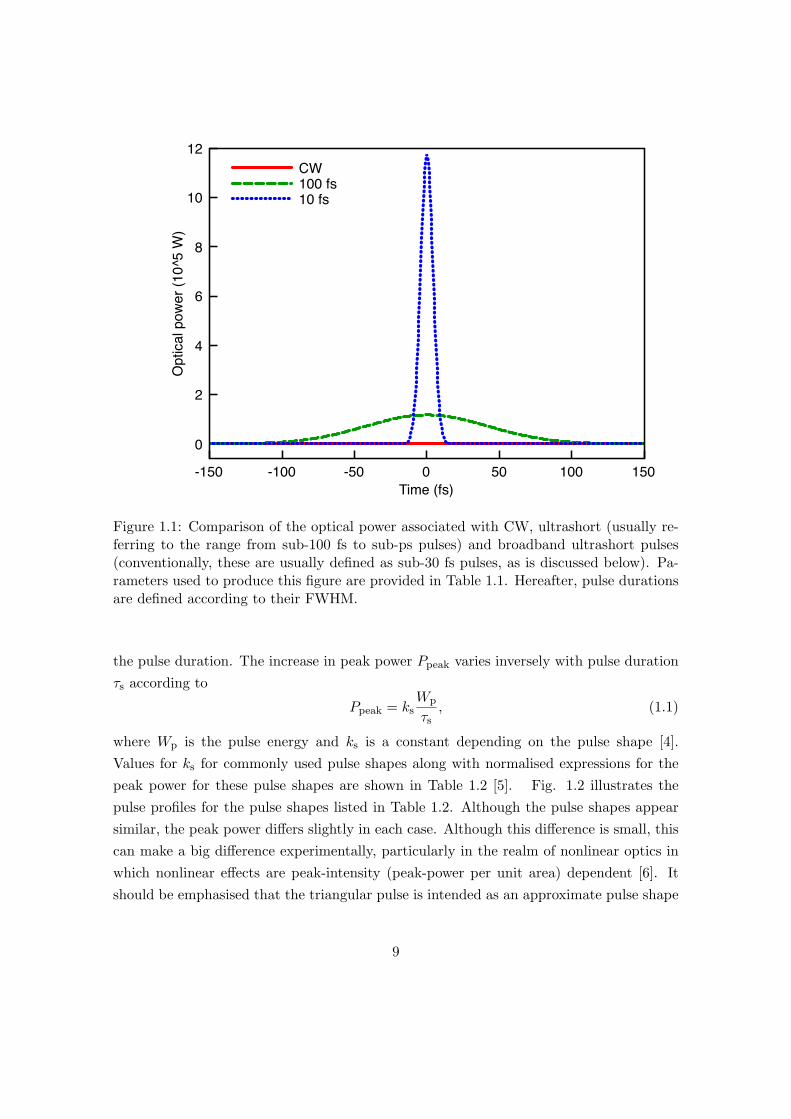
The laser has had a profound impact on scientific research in all aspects of the naturalsciences. Consequently, advancement in laser technology has been driven by the desireto facilitate new scientific discovery and understanding. Many different laser types havebeen invented with advancements made in output power, wavelength, beam quality andlaser pulse duration. Of these parameters, this chapter considers the pulse duration,which is inherently connected with the spectral content. Monochromatic lightmust bemathematically defined from minus to plus infinity in space or time [2]. Lasers whichproduce monochromatic light are generally associated with being continuous wave (CW)light sources due to their constant production of laser light. CW lasers are constrainedby having a constant output power over time, which is a very useful property for manyapplications. Up to many tens of kilo-Watts of optical output power can be generated bycertain types of CW laser, such as the increasingly important fibre laser [3]. An alternativeway to increase the optical power is by pulsing the output, such that the laser continuallygenerates optical pulses that exist for short periods of time, thus enabling the opticalpower to be concentrated in time with the laser output being essentially switched offotherwise. Pulsed lasers thus have a higher-than-CW peak power for the same amount ofoptical energy per unit time. Fig. 1.1 depicts the difference in peak power between a CWlaser, narrowband ultrashort pulse laser of 100 fs full-width half-maximum (FWHM) pulseduration and a broadband ultrashort pulse laser of 10 fs FWHM pulse duration, with theparameters used listed in Table 1.1.

Fig. 1.1 shows that a dramatic increase in peak power can be obtained by decreasing

8

-150 -100 -50 0 50 100 150Time (fs)

0

2

4

6

8

10

12

Opt

ical p

ower

(10^

5 W

)CW100 fs10 fs

Figure 1.1: Comparison of the optical power associated with CW, ultrashort (usually re-ferring to the range from sub-100 fs to sub-ps pulses) and broadband ultrashort pulses(conventionally, these are usually defined as sub-30 fs pulses, as is discussed below). Pa-rameters used to produce this figure are provided in Table 1.1. Hereafter, pulse durationsare defined according to their FWHM.

the pulse duration. The increase in peak power Ppeak varies inversely with pulse durationτs according to

Ppeak = ksWp

τs, (1.1)

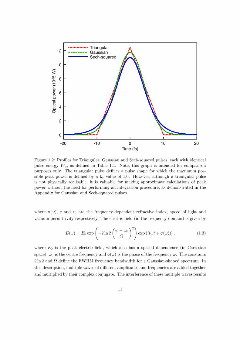
where Wp is the pulse energy and ks is a constant depending on the pulse shape [4].Values for ks for commonly used pulse shapes along with normalised expressions for thepeak power for these pulse shapes are shown in Table 1.2 [5]. Fig. 1.2 illustrates thepulse profiles for the pulse shapes listed in Table 1.2. Although the pulse shapes appearsimilar, the peak power differs slightly in each case. Although this difference is small, thiscan make a big difference experimentally, particularly in the realm of nonlinear optics inwhich nonlinear effects are peak-intensity (peak-power per unit area) dependent [6]. Itshould be emphasised that the triangular pulse is intended as an approximate pulse shape

9

Pulse shape Expression for Ppeak(t) ks(t = 0)

TriangularWp/τs ((τs + t)/τs) for −τs < t ≤ 0,Wp/τs ((τs − t)/τs) for 0 < t < τs,

0 otherwise1.0

Gaussian Wp/τs

√4 ln(2)/π exp(−4 ln(2)t2/τ2

s ) 0.94

Sech squared Wp/τs cosh−1(√

2) sech2(2 cosh−1(√

2)t/τs) 0.88

Table 1.2: Peak power expressions as function of time (t) for various pulse shapes withks values representing the relative difference in peak power for the listed pulse shapes.Appendix 7.1 discusses the calculations required to obtain the expressions and values forGaussian and Sech-squared pulses.

and does not correspond to a physically realisable ultrashort pulse shape.

1.2 The relationship between spectral intensity and pulse

duration

1.2.1 Interference of multiple waves

The laser pulse shape (and hence pulse duration) depends upon the generated spectrumassociated with the laser pulses and as such, the laser spectrum defines the minimumpossible pulse duration obtainable [4]. The minimum possible pulse duration is constrainedby the spectral frequency width of the laser for a given spectral shape. The productof spectral bandwidth and minimum pulse duration is commonly known as the time-bandwidth product and has a value which depends upon the assumed pulse shape [4]. Theresulting product obtained from measurement of the pulse duration and spectral widthdefines whether the pulse is transform-limited (minimum pulse duration) or not transform-limited (chirped pulse). By considering the coherent interference of multiple waves ofdifferent frequencies and examining the time domain the temporal shape of the pulse isobtained. The time-averaged intensity for multiple waves, Ej of different frequencies isgiven by [7]

I =12n(ω)cε0

⟨N∑j=1

Ej

N∑j=1

E∗j

⟩. (1.2)

10

-20 -10 0 10 20Time (fs)

0

2

4

6

8

10

12O

ptica

l pow

er (1

0^5

W)

TriangularGaussianSech-squared

Figure 1.2: Profiles for Triangular, Gaussian and Sech-squared pulses, each with identicalpulse energy Wp, as defined in Table 1.1. Note, this graph is intended for comparisonpurposes only. The triangular pulse defines a pulse shape for which the maximum pos-sible peak power is defined by a ks value of 1.0. However, although a triangular pulseis not physically realisable, it is valuable for making approximate calculations of peakpower without the need for performing an integration procedure, as demonstrated in theAppendix for Gaussian and Sech-squared pulses.

where n(ω), c and ε0 are the frequency-dependent refractive index, speed of light andvacuum permittivity respectively. The electric field (in the frequency domain) is given by

E(ω) = E0 exp

(−2 ln 2

(ω − ω0

Ω

)2)

exp (i(ωt+ φ(ω))) , (1.3)

where E0 is the peak electric field, which also has a spatial dependence (in Cartesianspace), ω0 is the centre frequency and φ(ω) is the phase of the frequency ω. The constants2 ln 2 and Ω define the FWHM frequency bandwidth for a Gaussian-shaped spectrum. Inthis description, multiple waves of different amplitudes and frequencies are added togetherand multiplied by their complex conjugate. The interference of these multiple waves results

11

in a time-dependent intensity profile. Providing the phase φ(ω) is zero, the interference ofmultiple waves defines the minimum possible duration of the resulting pulse. The intensityof the interference pattern is maximised when the waves are exactly in phase.

The more frequencies present within the spectrum (wider bandwidth) then the result-ing interference pattern will be constrained to a narrower frame of time. Figs. 1.3 and1.4 show the intensity-time profiles and the electric field amplitudes for two bandwidthstypically available in Titanium-Sapphire ultrashort pulsed lasers (10 nm and 100 nm re-spectively, both centred at 800 nm). Comparing Figs. 1.3 and 1.4, shorter pulses areobtained in the broadband case due to the broader spectral content providing a range offrequencies which can only constructively interfere over a narrower time range by virtueof the substantially different frequencies within the pulse itself. In Fig. 1.4 this is illus-trated by frequencies which go out of phase rapidly outside of t = 0 due to the differencein time period of each oscillation, for example, the red coloured frequency has a timeperiod of approximately 3 fs and the violet-coloured frequency has a time period of 2.4fs. Hence after several cycles the frequencies will become substantially out of phase.In both figures a time width of 40 fs has been selected to illustrate the overlapping ofdifferent spectral frequencies over that time width. For the narrowband case the differentspectral frequencies remain mostly overlapped, and hence interfere (mostly) constructivelywithin the 40 fs range. Whereas for the broadband case the different spectral frequenciesrapidly go out of phase relative to each other by virtue of their substantially differentcycle periods and hence destructive interference contributes to the shorter pulse durationshown. Both figures were generated using MATLAB code provided in the supplementaryCD accompanying this thesis (see Appendix 7.5 for acknowledgements).

1.2.2 Fourier transform approach

This conceptual model vividly illustrates the relationship between electric field amplitude,frequency and phase in order to support ultrashort pulses. However, a more convenientmethod for calculating pulse shapes involves a mathematical approach for simultaneouslydealing with multiple frequencies. In this approach the Fourier transform can be usedto switch between time and frequency domain descriptions of a signal in terms of a time-varying function, f(t) and a corresponding frequency function f(ω) [8]. The inverse Fouriertransform converts a frequency signal, f(ω) to a time signal f(t) and isgiven by

f(t) =1√2π

∫ ∞−∞

f(ω) exp(iωt)dω = F −1 f(ω) . (1.4)

12

−20 −15 −10 −5 0 5 10 15 20−1

−0.5

0

0.5

1(a)

Time (fs)

Elec

tric

field

(arb

. uni

ts)

−200 −150 −100 −50 0 50 100 150 2000

200

400

600(b)

Time (fs)

Inte

nsity

(arb

. uni

ts)

FWHM

Figure 1.3: Interference of frequencies within a Gaussian narrowband (10 nm) spectrum,centred at 800 nm. Fig. (a) shows the electric field of several different frequencies containedwithin the spectrum. Different electric field amplitude contributions have been plotted;the colours refer to whether the wave is lower (red) or higher (violet) frequency. Fig. (b)shows the resulting pulse from the interference of all waves contained within the spectrum,with a FWHM duration of 94 fs. In order to retain clarity, the violet box indicates thetime width correspondence between (a) and (b) as both are on different scales.

To convert from a time-domain signal to a frequency-domain function is provided by thecomplementary Fourier transform,

f(ω) =1√2π

∫ ∞−∞

f(t) exp(−iωt)dt = F f(t) . (1.5)

This provides a suitable way for describing electric fields and for switching between theirassociated time and frequency domain descriptions. In equation 1.2 the interference of

13

−20 −15 −10 −5 0 5 10 15 20−1

−0.5

0

0.5

1(a)

Time (fs)

Elec

tric

field

(arb

. uni

ts)

−20 −15 −10 −5 0 5 10 15 200

2000

4000

6000(b)

Time (fs)

Inte

nsity

(arb

. uni

ts)

FWHM

Figure 1.4: Interference of frequencies within a Gaussian broadband (100 nm) spectrum,centred at 800 nm. Fig. (a) shows the electric field of several different frequencies containedwithin the spectrum. Different electric field amplitude contributions have been plotted;the colours refer to whether the wave is lower (red) or higher (violet) frequency. Fig. (b)shows the resulting pulse from the interference of all waves contained within the spectrum,with a FWHM duration of 9.4 fs, a factor of ten shorter than in Fig. 1.3.

waves are described in terms of a sum of discretely-separated waves

Etotal =N∑i=1

Ei(ω, t) =N∑i=1

Ei(ω − ω0) exp(iωt+ iφ(ω)), (1.6)

where Ei(ω − ω0) describes the amplitude of the ith electric field, Ei(ω, t) and the term,exp(iωt + iφ(ω)) describes the oscillatory nature of the wave at a frequency ω, time t

and spectral phase φ(ω). Mapping the frequency domain from −∞ to 0 is clearly notpossible since there is no physical meaning to negative frequencies, however the choice of

14

function (such as a Gaussian centred at ω0), which is zero in the region −∞ to 0 solvesthis issue. In the limit of ωi+1 − ωi → 0 the electric field function Ei may be representedby an integral across the frequency domain, with the possibility of the amplitude beingrepresented by a continuous function, therefore with an existent integral within definedlimits. Representing the electric field by

E(t) = limδω→0

N∑i=1

Ei(ω − ω0) exp(iωt+ iφ(ω)) (1.7)

=∫ ∞−∞

E(ω − ω0) exp(−iωt− iφ(ω))dω, (1.8)

which has the same form as the inverse Fourier transform of equation 1.4 (the factor of1/√

2π is an arbitrary part of the Fourier transform definition, but needs to be included inany calculation, where the product of the constants in equations 1.4 and 1.5 should equal1/2π). Therefore the Fourier transform integral can be used to represent the coherentsum of multiple electric field waves of different frequencies, and be converted to a time-domain description of the electric field, and vice versa, through calculation of the Fouriertransform integrals. Hence, equation 1.2 can be re-written in terms of Fourier transformintegrals as

I(t) =n(ω)cε0

4π

∫ ∞−∞

E(ω − ω0) exp(iωt+ iφ(ω))dω∫ ∞−∞

E∗(ω − ω0) exp(iωt+ iφ(ω))dω

(1.9)

I(t) =12n(ω)cε0F −1 EF −1 E∗ (1.10)

The Fourier transform approach is an alternative (and more common) method for calcu-lating the pulse shape that results from a user-defined spectrum. In the following example,an experimental spectrum is used, rather than a theoretical spectrum, however the ap-proach detailed previously is also applicable. There are two ways to calculate the Fouriertransform integrals in equation 1.9; analytical or computational. Experimental narrow-band spectra can usually be fitted with either a Gaussian or Sech-squared profile, andtherefore their associated Fourier transforms can be obtained analytically. For broadbandspectra, this becomes more tricky due to the increasing complexity of spectral shapeswith increasing spectral width, therefore a computational approach is required. The fastFourier transform algorithm [9] allows for efficient computation of pulse duration fromuser-defined spectra and phase. Laser spectra are usually experimentally measured inthe wavelength domain, therefore it is necessary to convert any experimentally measured

15

spectrum to the frequency domain,

ω =2πcλ, (1.11)

where λ is the wavelength. The width of spectrum in the frequency domain, δω is con-nected to the wavelength domain through differentiation of equation 1.11

∆ω =∣∣∣∣−2πc∆λ

λ2

∣∣∣∣ (1.12)

Given the need to calculate the Fourier transform of the electric field amplitude from thespectral intensity, the wavelength-to-frequency converted spectrum is obtained and thesquare root of the measured spectrum is taken, I(ω) to obtain the electric field amplitude

E(ω) = kft

√I(ω), (1.13)

where kft is a constant which relates the intensity (frequency) to the electric field amplitude(frequency). The relationship between intensity (time domain) and electric field (timedomain) is well established from Poynting’s theorem [10]

I(t) =12n(ω)cε0E(t)E∗(t), (1.14)

where n(ω) is the frequency-dependent refractive index. The factor kft can be calculatedby considering the experimental measurable quantities, pulse energy Wp, detector areaand efficiency according to

Wp =∫ ∞−∞

∫ ∞−∞

∫ ∞−∞

I(t)dxdydt, (1.15)

with I(t) and I(ω) related by the Fourier transform. Starting from equation 1.13 we notethat the phase requires the form exp(iφ) and should be incorporated as follows

E(ω) = kft exp(

ln(I(ω)) + 2iφ(ω)2

). (1.16)

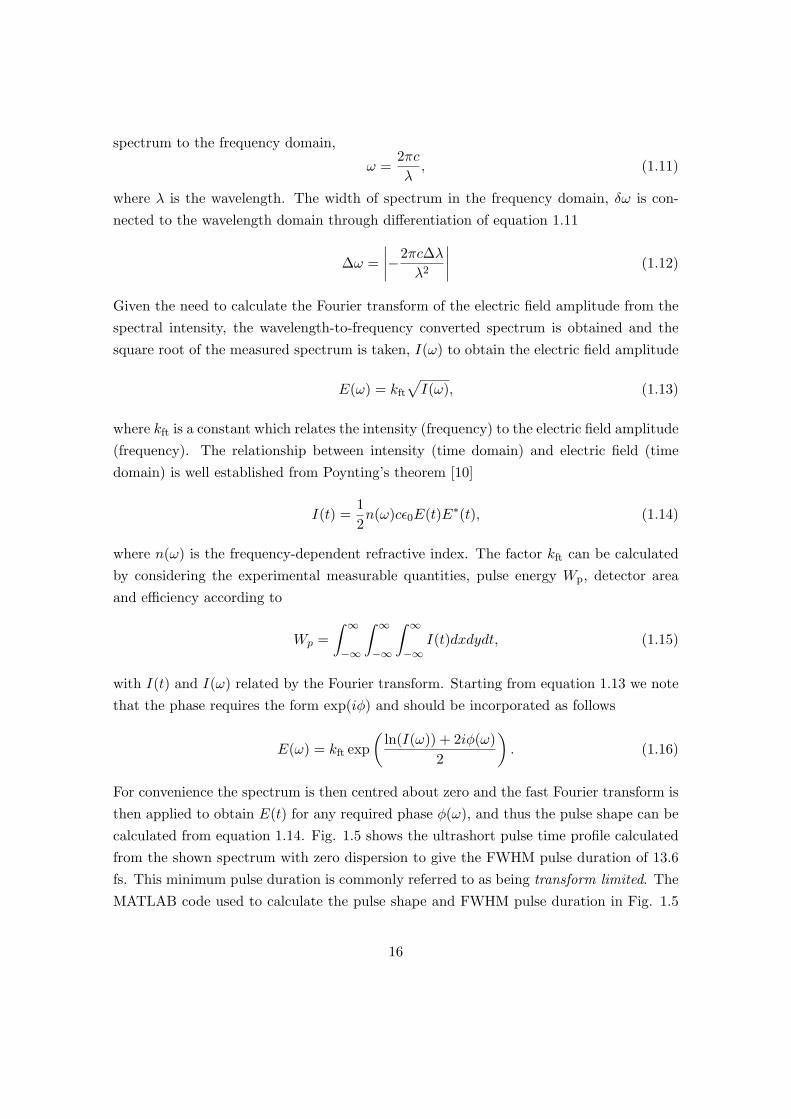
For convenience the spectrum is then centred about zero and the fast Fourier transform isthen applied to obtain E(t) for any required phase φ(ω), and thus the pulse shape can becalculated from equation 1.14. Fig. 1.5 shows the ultrashort pulse time profile calculatedfrom the shown spectrum with zero dispersion to give the FWHM pulse duration of 13.6fs. This minimum pulse duration is commonly referred to as being transform limited. TheMATLAB code used to calculate the pulse shape and FWHM pulse duration in Fig. 1.5

16

is given in the supplementary CD accompanying this thesis (acknowledgements discussedin Appendix 7.5).

720 760 800 840 8800

0.5

1

1.5

2 x 104

Spec

tral i

nten

sity

(arb

. uni

ts)

Wavelength (nm)

(a)

720 760 800 840 880−1

−0.5

0

0.5

1

Spec

tral p

hase

(rad

ians

)

−100 −50 0 50 1000

1

2

3

4

5(b)

Time (fs)

Inte

nsity

(arb

. uni

ts)

Figure 1.5: (a) An example of the experimentally measured spectrum from the KM LabsSwift 10 laser with zero spectral phase, and (b) the ultrashort pulse time profile, as cal-culated by the fast Fourier transform algorithm. This yields the minimum achievable(transform-limited) FWHM pulse duration of 13.6 fs.

1.2.3 Dispersion

When considering the propagation of ultrashort pulses in optical media dispersion be-comes important. The velocity of propagation of an electromagnetic wave is frequencydependent, except in vacuo, where all electromagnetic waves travel at the same phasevelocity (the vacuum speed of light), as can be demonstrated through solving Maxwell’sequations [10]. This frequency dependent velocity is best observed in the natural worldthrough the observation of the rainbow, in which white light from the Sun is refractedthrough water droplets at different angles, resulting in the well-known arc of spatiallydistinct colours in the rainbow.

Propagating electromagnetic waves have an electric field whose oscillatory space and

17

time dependence can be given by [7]

E = E0 exp (i(k · r− ωt+ φ(ω))) , (1.17)

where r is a vector describing the position in space, and k is the wave vector, which definesthe frequency dependence of the refractive index in any propagation direction in space. Inany particular direction k provides the wave number,

k = n(ω)ω

c. (1.18)

where n(ω) is the (frequency dependent) refractive index. The velocity of a set of prop-agating waves is given by the rate of change of frequency with respect to wave number,and is known as the group velocity,

νg =δω

δk. (1.19)

The quantity νg describes the propagation of a wave packet, and is dependent upon theoptical properties of the propagation medium. For a particular wave, the phase velocitydescribes the velocity of propagation of an individual wave according to

νp =ω

k. (1.20)

The quantities νg and νs are identical in a non-dispersive medium, where the refractiveindex is not a function of frequency. In this case

νg = νp =c

n(ω), (1.21)

which is equal to c in vacuo, where n(ω) = 1. In general, this is not the case. Even in air,where the refractive index is very close to unity, there exists a frequency dependent refrac-tive index that is important, in particular for ultrashort pulses [11]. The physical originof dispersion can be accounted for by considering the propagation of an electromagneticwave through an atomic or molecular medium. This propagation occurs due to the atomsbecoming polarised by the passing oscillatory electromagnetic field, and providing thereis no absorption, the wave propagates through the medium unattenuated by virtue of thequasi-elastic restoring force acting on the electrons that have been polarised within theatomic or molecular medium [7]. However at frequencies where there is absorption, energyis transferred from the wave into the medium, with the energy dissipated either in theform of subsequent atomic emissions or heat [12]. The polarisability of a medium there-

18

fore defines the propagation of electromagnetic waves which pass through the medium, andfeatures complex features such as resonances around given frequencies. This polarisabilityis therefore a complex function which depends upon the exact response of the atoms ormolecules to a propagating electromagnetic wave. The linear polarisation induced by anelectric field is proportional to the electric field amplitude and is given by

P = ε0χ(1)(ω)E, (1.22)

where, E is the electric field and χ(1)(ω) is the susceptibility of the medium [6]. Thesusceptibility indicates the strength of the induced polarisation and can be describedby [13]

χ(1)(ω) =Ne2

m· 1

(ω20 − ω2) + iωΛ

, (1.23)

where N is the density of polarisable atoms, e is the electron charge, m is the mass of theelectron, ω0 is the resonance frequency and Λ is a damping constant resulting from resonantenergy transfer from the optical field to the medium, e.g. in the form of phonons. In thevisible optical region, there are usually no resonances for typical optical materials such asglass [7]. By considering the typical resonances in the ultraviolet region the frequency-dependent refractive index is expressed in terms of a set of coefficients for increasing ordersof frequencies, which is known as the Sellmeier equation [7]

n(ω)2 − 1 = A+Bν2 + Cν4 + · · · − B′

ν2− C ′

ν4− · · ·, (1.24)

where ν is the optical frequency, as given by 2πν = ω. The Sellmeier equation can also bein terms of wavelength λ as

n(ω)2 − 1 = A+Bc2

λ2+Cc4

λ4+ · · · − B′λ2

c2− C ′λ4

c4− · · ·, (1.25)

where the coefficients A, B, B′, C and C ′ are the Sellmeier coefficients, and are determinedexperimentally. With these coefficients established, the frequency dependent refractiveindex can be calculated for any given material for the visible region. Outside this region,resonances may have a significant effect.

Dispersion has serious consequences for ultrashort pulses resulting in pulses stretchingin time when passing through optical media [13]. The frequency-dependent refractiveindex results in the phase of spectral components of an ultrashort pulse being shiftedrelative to each other. The most common way to express this mathematically is a Taylor

19

expansion about the centre frequency [14]

φ(ω) = φ(ω0) + φ(1)(ω0)(ω − ω0) +12φ(2)(ω0)(ω − ω0)2 +

16φ(3)(ω0)(ω − ω0)3

+124φ(4)(ω0)(ω − ω0)4 + · · ·+ 1

n!φ(n)(ω0)(ω − ω0)n, (1.26)

where φ(n)(ω0) is the nth derivative of the phase function with respect to frequency aboutω0. The derivatives of the phase, φ(1), φ(2), φ(3) and φ(4) are known as the group delay(GD), second order (group velocity) dispersion (GVD), third order dispersion (TOD) andfourth order dispersion (FOD) [14]. Each of these types of dispersion have a distinctiveeffect upon the initial pulse shape. GD results in a time delay of the group, shiftingthe pulse in time. GVD causes a smooth symmetrical stretching in time with no otherdistortion. This type of dispersion is very helpful for maintaining a well-defined and easily-calculated relationship between pulse duration and peak power. TOD results in a set ofsub pulses which accompany the main pulse. The sign of the TOD defines whether thesub pulses precede or succeed the main pulse. FOD results in a symmetrical stretching intime with a more complex shape than for GVD and TOD. A combination of GD, GVD,TOD and FOD (and higher orders) results in very complex pulse shapes. Generally, opticalsystems have multiple contributions of different dispersion orders, hence pulse shapes tendto be complex. The MATLAB code included in the supplementary CD (acknowledgementsin Appendix 7.5) explores how these types of dispersion influence the relative phase ofdifferent spectral components of the electric field and hence influencing the pulse shape.

Fig. 1.6 illustrates the effect of TOD in (b), FOD in (c) and GD, GVD, TOD andFOD combined in (d) upon the pulse in (a) with 100 nm bandwidth centred at 800 nm.Note the substantial decrease in intensity when additional dispersion is added.

In Fig. 1.6 an ideal Gaussian spectra was considered, however the true spectral shapeof a typical ultrashort pulse is not well approximated by an analytic function. By usingthe Fourier transform method, the resulting pulse after GVD is shown to be inherentlyconnected to the shape of the spectrum and therefore this method is very useful for calcu-lating the pulse duration for a user-defined spectrum. Fig. 1.7 shows the same spectrumas in Fig. 1.5 but with 400 fs2 of GVD applied (as might be obtained experimentally fortypical optical systems with no higher order dispersion compensations) to give a FWHMpulse duration of 76.5 fs. Note how the shape of the spectrum affects the shape of theultrashort pulse time profile.

A given amount of dispersion results in the increase in pulse duration. Therefore incertain situations it may be preferable to start off with a longer pulse duration so that

20

!!"" !#$" !#"" !$" " $" #"" #$" !"""

$"""

%&'

()*+,%-.'

/01+0.)12,%&345,60)1.'

!!"" !#$" !#"" !$" " $" #"" #$" !"""

#"""

!"""

7"""%4'

()*+,%-.'

/01+0.)12,%&345,60)1.'

!!"" !#$" !#"" !$" " $" #"" #$" !"""

$""

%8'

()*+,%-.'

/01+0.)12,%&345,60)1.'

!!"" !#$" !#"" !$" " $" #"" #$" !"""

$""

%9'

()*+,%-.'

/01+0.)12,%&345,60)1.'

Figure 1.6: (a) A transform-limited pulse generated by 100 nm bandwidth centred at 800nm; (b) the same pulse as (a) with 2000 fs3 of TOD added resulting in decaying pulseshape oscillations; (c) the same pulse as (a) with 670000 fs4 of FOD added resulting in asymmetrical complex pulse shape; (d) the same pulse as (a) but with -50 fs of GD, 300 fs2

of GVD, 35000 fs3 of TOD and -550000 fs4 of FOD added resulting in an asymmetricalcomplex pulse shape.

the pulses are not necessarily increased in duration, thereby decreasing peak power. Anestimate of the final pulse duration (τfinal) for a given initial pulse duration (τinitial) for a

21

720 760 800 840 8800

1

2 x 104

Spec

tral i

nten

sity

(arb

. uni

ts)

Wavelength (nm)

(a)

720 760 800 840 8800

20

40

Spec

tral p

hase

(rad

ians

)

−100 −50 0 50 1000

0.5

1(b)

Time (fs)

Inte

nsity

(arb

. uni

ts)

Figure 1.7: (a) An example of the experimentally measured spectrum from the KM LabsSwift 10 laser with theoretical phase function of the second order applied (400 fs2), and(b) the ultrashort pulse time profile, as calculated by the fast Fourier transform algorithm.This yields the (non transform-limited) FWHM pulse duration of 76.5 fs.

Gaussian pulse is provided by [15]

τfinal = τinitial

√1 +

16 ln2(2)φ22

τ2initial

, (1.27)

where φ2 is the GVD. Equation 1.27 is found by obtaining the inverse Fourier transformof the square root of the spectral intensity and including the second order dispersionterm in the calculations. Squaring the result provides the temporal pulse shape and theFWHM time can be obtained from this and the ratio of final to initial durations calculatedaccordingly. Fig. 1.8 illustrates the increase in pulse duration for femtosecond systemscovering the range from 5 fs up to 100 fs with 10000 fs2 of GVD dispersion. A startingpulse duration of 10 fs results in a final pulse duration of 2.8 ps, whereas starting at 100fs results in a pulse duration of 280 fs.

Optimum delivery of transform-limited ultrashort pulses can only be achieved through

22

10 20 30 40 50 60 70 80 90 1000

1000

2000

3000

4000

5000

6000

Initial pulse duration (fs)

Fin

al puls

e d

ura

tion (

fs)

Figure 1.8: Graph illustrating stretching of pulse from initial to final durations using10000 fs2 of GVD dispersion, i.e. starting from transform limited pulse durations wherethe shortest initial pulse durations have the widest bandwidth, and conversely the longestinitial pulse durations have the narrowest bandwidths.

dispersion compensation means. In an experimental setting the dispersion of an opticalsystem should be at least calculated theoretically based on the choice of optics and thethickness of glass through which the ultrashort pulses pass. However, this is non-idealas other environmental factors may influence results including temperature, pressure andhumidity, which is especially true for broadband ultrashort pulses. Therefore, it wouldbe preferable to measure the dispersion at a preferred point in the optical system and ifpossible, corrected or taken into account in any experiments performed. However in anyapplication which may benefit from use of transform-limited pulses it would be necessaryto perform at least some kind of dispersion compensation, for example, using prisms [16].Prisms are relatively inflexible, however they do offer a relatively low-cost solution to the

23

problem. Many fields may stand to benefit from use of transform-limited ultrashort pulses,not least in biophotonics, where ultrashort pulses are regularly used for nonlinear imag-ing [17] and manipulation [18]. Biophotonics applications invariably involve a microscopeobjective for imaging purposes and delivery of laser. Microscope objectives suffer from sig-nificant dispersion owing to the contained glass [19] and have the potential to significantlytemporally distort the ultrashort pulses. In this thesis, dispersion-compensated ultrashortpulses are applied through a microscope objective, in which the objective would other-wise stretch the pulses by many orders of magnitude. It is possible that through use of areflective setup as well as a reflective microscope objective the optical system dispersioncould be minimised. However, system dispersion may not be completely removed throughuse of this method and in the case of highly broadband sources, the pulse duration couldstill be stretched.

1.3 Nonlinear optics

A key aspect of this thesis is in the implementation of nonlinear generation of light andspectral measurements for dispersion measurement. A short review of the most relevantfeatures of nonlinear optics is provided for reference purposes. In particular, the role ofdispersion of ultrashort pulses in nonlinear crystals is discussed.

In linear optics the polarisation induced by a propagating electromagnetic wave isproportional to the strength of the electric field according to equation 1.22. However,in nonlinear optics the induced polarisation cannot be described by equation 1.22 as thepolarisation no longer follows this simple relationship. This behaviour is most pronouncedwhen using high intensity lasers, particularly when operating in pulsed mode. As such,it becomes necessary to employ a series expansion of powers to describe the polarisation(per unit volume) by

P (t) = ε0

[χ(1)E(t) + χ(2)E2(t) + χ(3)E3(t) + · · ·

], (1.28)

where χ(n) is the n-th order nonlinear optical susceptibility, which is dependent upon thefrequency, material type and propagation direction [6]. In equation 1.28 the higher orderterms become relevant when the electric field amplitude is sufficiently large to initiate anonlinear optical effect. The discovery of second harmonic generation (SHG) by Frankenet al. in 1961 [20] is regarded as the beginning of the field of nonlinear optics [6]. SHGis one of many types of nonlinear optical interactions, and is of particular importance tothe measurement and characterisation of ultrashort pulses. In this section, the nonlinear

24

optical interactions of greatest relevance to this thesis are described.

1.3.1 Second harmonic generation

A number of nonlinear optical processes can be described using a harmonic wave andinserted into the individual terms equation 1.28. In particular, by taking two differentfrequencies ω1 and ω2 with corresponding time-varying electric fields

E(t) = E1 exp(−iω1t) + E2 exp(−iω2t) + c.c. (1.29)

and substituting into the second order nonlinear optical polarisation

P (2)(t) = ε0χ(2)E2(t), (1.30)

thus obtaining

P (2)(t) = ε0χ(2)[E2

1 exp(−2iω1t) + E22 exp(−2iω2t) + 2E1E2 exp(−i(ω1 + ω2)t)

+2E1E∗2 exp(−i(ω1 − ω2)t+ c.c.] + 2ε0χ(2) [E1E

∗1 + E2E

∗2 ] , (1.31)

where c.c. and ∗ denote the complex conjugate of the previous sequence and of the fieldcomponent, respectively. The efficiency of nonlinear optical processes depends on the ma-terial type, propagation direction and incident field strength. Second harmonic generated(SHG) light can be generated through a special case of sum-frequency generation and canbe used to tunably generate higher frequencies. In summary, the ability to generate newfrequencies using nonlinear optics is extremely useful when a desired frequency cannot begenerated directly.

The characteristics of a material define the efficiency of SHG. SHG generally requiresa material which has a non-centrosymmetric structure, that is, a material whose electronssit within a potential energy function that is not symmetric about the centre [6]. Manymaterials have been produced which possess a non-centrosymmetric structure, and aretypically in the form of a crystal [21]. A centrosymmetric material, which has a molecularstructure leading to a symmetric potential energy functions will not allow SHG in itsbulk [22]. SHG is allowable for a centrosymmetric material under specific situations, suchas at the surface of the material [23], or when the centrosymmetric molecules collect innon-centrosymmetric aggregates [24].

In the context of this thesis, SHG refers to sum-frequency generation as broadbandpulses permit intrapulse interference in SHG nonlinear crystals in which different frequency

25

components interfere. The nonlinear field intensity for sum-frequency generated waveshaving two different frequencies is given by

I3 ∝ I1I2 sinc2

(∆kL

2

), (1.32)

where I1 and I2 are the incident field intensities and ∆k is the phase-matching term, asdiscussed below. When the incident fields have identical frequencies (ω) the nonlinear field(2ω) produced has an intensity dependence according to

I2ω ∝ I2ω, (1.33)

where the subscript numbers have been replaced by the relevant frequency. ThereforeSHG, and indeed any two-photon process has an intensity dependence which is quadraticwith the incident intensity, and therefore SHG efficiency can be increased significantly byincreasing the incident intensity, either through increasing the pulse energy, decreasingthe pulse duration or through beam focussing [25].

1.3.2 Phase-matching

Phase-matching is essential in nonlinear optics as it describes the condition for conservationof photon momentum (k-vector) within a nonlinear crystal. Equation 1.32 is maximisedwhen the phase-matching term ∆k is zero

∆k = k1 + k2 − k3 = 0, (1.34)

where ki is the i-th wavenumber. In general the phase-matching term is not equal tozero because the refractive index experienced by the field differs between the involvedfrequencies. In order to ensure phase-matching is optimised, the following is required

n1ω1

c+n2ω2

c=n3ω3

c. (1.35)

For SHG where ω1 = ω2 = ω3/2, equation 1.35 simplifies to

n1(ω) = n3(2ω). (1.36)

This condition is difficult to satisfy due to dispersion and therefore SHG is normally phase-mismatched with the incident field. The standard strategy to deal with phase-mismatch isby employing a nonlinear material of polarisation-dependent refractive index. An example

26

of such a material is a anisotropic, or birefringent crystal [26]. The phase matchingcondition can then be satisfied by arranging the crystal such that over the interactionlength of the crystal the effective path length of the different frequencies is the same. Thiscan be achieved primarily by altering incident direction of the field (through angle tuning).In experiments involving SHG it was crucial to ensure correct crystal orientation to obtainmaximum SHG spectral signal.

Ultrashort pulse SHG

Ultrashort pulses are associated with a range of frequencies and therefore any second-ordernonlinear interaction will involve the combined effect of these frequencies, sum-frequencygeneration being the most relevant interaction. For convenience in this section, sum-frequency generation is referred to as SHG, in line with how ultrashort pulse SHG isnormally referred to in the literature on the topic. Ultrashort pulse duration measure-ment techniques often require the use of SHG. Therefore the SHG produced by ultrashortpulses is of significant importance to pulse measurement, however ultrashort pulse SHGis significantly more complicated than CW SHG [27,28].

In SHG involving ultrashort pulses the phase-matching conditions become more dif-ficult to adhere to due to the large bandwidths involved. However phase-matching canbe aided through the use of high numerical aperture objectives, in which the light isfocussed into a tight cone, with the beam propagating at high angles into the nonlin-ear material, simultaneously satisfying the phase-matching conditions to some degree forall the contained frequencies [29]. In competition with phase-matching, spatial walk-offbetween the incident and generated beams due to material birefringence reduces the non-linear conversion efficiency [30]. Phase-matching is of critical importance to the SHGprocess for any pulse duration, but the shorter the pulses are, then higher-order phasedistortions come into effect. Second order dispersion brings about two effects. Firstly, agroup-velocity mismatch (GVM) arises between the ultrashort (fundamental) pulse andthe resulting SHG pulse [27]. GVM increases the duration of SHG pulses such that theybecome longer than that of the fundamental pulse and the nonlinear conversion efficiencyis decreased [31]. However the effect is most pronounced for broadband ultrashort pulses,and type II SHG is more strongly affected than type I SHG, which has significant impli-cations for autocorrelation experiments [32]. GVM can be minimised by decreasing theinteraction length between fundamental and SHG pulses by decreasing the thickness ofthe nonlinear material [33]. The GVM manifests itself in terms of a temporal walk-offbetween the fundamental and SHG pulses [30]. The SHG efficiency can be affected by

27

the interplay between focussing strength and GVM [34], and SHG efficiency can be dulymaximised by adjusting the GVM via a pre-dispersive method such as prisms [35]. Inaddition to GVM, intrapulse group-velocity dispersion (IGVD) introduces distortions toultrashort pulses that are non-negligible for durations of less than 50 fs, and indeed be-come significant below the 10 fs regime [27]. IGVD is the group-velocity dispersion withinthe bandwidth of the fundamental and SHG pulses [27]. GVM and IGVD act together toaffect the pulse characteristics of the fundamental and SHG pulses, and this phenomenonis further complicated by chirped fundamental pulses [28]. Higher order effects such asTOD and FOD will also complicate ultrashort pulse SHG [28]. It should be noted that inaddition to SHG, third harmonic generation (THG) can be used for pulse measurementpurposes, and as such, the phase-matching and spatial walk-off issues can be bypassedby using isotropic materials such as glass [36]. The disadvantage of THG is the gener-ally lower nonlinear conversion efficiency compared with SHG and the higher generatedfrequencies are subject to greater scattering and absorption in optical materials.

1.3.3 Further considerations for ultrashort pulse SHG

In addition to the aforementioned there are further considerations in relation to ultrashortpulse SHG. Equation 1.32 shows the intensity of the phase-matching process, but this isdefined for a set of three wavelengths (the pump, signal and idler). In broadband ultrashortpulse SHG the so-called signal and idler wavelengths (contained within the fundamentalspectrum) combine to provide the so-called pump wavelength (SHG). Therefore the ef-ficiency of the SHG process will vary according to the phase-matching relation betweenthe range of wavelengths within the spectrum [6]. This results in a spectral acceptancebandwidth (also called phase-matching bandwidth) associated with a nonlinear crystalwhich defines a range over which SHG (or in relation to any other nonlinear process) canoccur [37]. However, GVM between the fundamental pulse and SHG pulse limits the crys-tal interaction length, thereby decreasing the phase-matching bandwidth [37]. This meansthat shorter length crystals are required for broadband ultrashort pulse SHG in order tomake use of broad spectral bandwidth. The spectral acceptance bandwidth (SAB) fortype I phase-matching is provided by [37]

∆λSAB =0.886λ2

f

(nSHG − nf)Lcryst, (1.37)

where λf is the fundamental (centre) wavelength, nSHG and nf are the refractive indices ofthe fundamental and SHG (centre) wavelengths, respectively. The crystal length, Lcryst

28

can be varied to change the spectral acceptance bandwidth. Using equation 1.37 and 800nm as the centre fundamental wavelength in Beta Barium Borate (BBO) for example, thespectral acceptance bandwidth of a crystal of length 1 cm is 1.1 nm, while for a 100 µmcrystal it is 110 nm [21,38]. For the aforementioned ultrashort pulses, associated spectralbandwidths in excess of 1 nm will only be frequency doubled across the full fundamentalspectral range, crystals thinner than 1 cm are required. Broadband ultrashort pulses suchas those supporting 10 fs pulses or less require crystals of order 100 µm or less in orderfor efficient conversion of the full fundamental bandwidth for frequency doubling. Whilebroad bandwidth acceptance is desirable for ultrashort pulsed SHG, the disadvantage ofusing thin crystals is that the overall conversion efficiency is decreased by virtue of thecrystal thickness.

The phase-matching condition leading to a spectral acceptance bandwidth is closelyassociated with a so-called angular acceptance bandwidth. An expression can be foundaccordingly for the angular acceptance bandwidth [37]. Again, the angular acceptancebandwidth is similarly increased for shorter crystal lengths. For the aforementioned ex-ample of a BBO crystal, the angular acceptance bandwidth is 0.04 degrees for 1 cm crystal,whereas for a 100 µm crystal it is 4 degrees. Clearly these are much less than the an-gles obtained with high numerical aperture lenses but nevertheless, the increased intensityobtained by such lenses provides more efficient SHG by virtue of the intensity conditionof equation 1.32 [21, 38]. As a phase-matching condition is defined for a single incidentangle only, multiple phase-matching conditions are made possible by changing the angleof incidence. Therefore focussing on a nonlinear crystal invokes multiple phase-matchingconditions simultaneously. This is useful for broadband ultrashort pulsed SHG as phase-matching is simultaneously achieved for a broader spectral range. However, the totalconversion efficiency will be decreased as waves of given frequencies propagating at angleswill not always follow the phase-matching condition appropriate for that frequency/anglecombination. Although, schemes have been proposed in which different frequencies prop-agate at different angles, each of which are phase-matched appropriately [39,40].

Further to the aforementioned effects, the temperature acceptance bandwidth definesa range of temperatures over which the phase-matching condition remains appropriate.However, in later experiments the temperature is held constant and therefore temperaturefluctuations are not relevant. However a typical temperature acceptance bandwidth of 20degrees Kelvin is obtainable with a BBO crystal.

All of the considerations above are important in decided how to select a nonlinearcrystal for ultrashort pulsed SHG. In this regard, nonlinear crystals should ideally be asthin enough to overcome GVM and IGVD and permit sufficiently broad acceptance band-

29

widths. However, too thin and the overall conversion efficiency will mean the SHG signalwill be decreased. Therefore, the crystal parameters should be appropriately calculated.

1.4 Generation of ultrashort pulses

Due to the significant relevance of ultrashort pulses for this thesis, it is appropriate tobriefly discuss some of the theoretical and practical aspects of ultrashort pulse generation.However in the interest of brevity, the scope of this discussion is restricted to the keypoints of ultrashort pulse generation.

Nonlinear optical methods have led to significant developments in ultrashort pulselasers, and in turn these ultrashort pulse lasers allow precise control over nonlinear opticalprocesses [41]. A number of phenomena in a laser are required to act cooperatively in orderto generate ultrashort pulses. The shortest pulses require the broadest bandwidth, andas such a gain medium is required that has a broad gain bandwidth. The most relevantexample of a broadband gain medium is Titanium-doped Sapphire (Ti-Sapphire), whichexhibits broad gain (fluorescence spectrum) [42] and can generate wavelengths rangingfrom 600 nm to 1200 nm, for example, supporting a 5 fs pulse [43]. Ti-Sapphire lasersprimarily exhibit homogenous broadening, that is, the atomic dipole oscillators collectivelyexperience the same energy-decay and de-phasing characteristics [44]. In particular, the(vibronic) broadening mechanism arises from heat energy (temperature) transfers actingupon the Titanium centres from the Sapphire lattice, thus creating the continuously vary-ing fluorescence spectrum essential for broadband pulsed laser action [45]. The length ofthe laser cavity defines the frequency-mode structure of the fields which circulate in thecavity according to [44]

νm =mc

2navL, (1.38)

where νm is the frequency of the m-th mode of a laser cavity of length L having an averagerefractive index nav. For any mode to oscillate within a laser cavity equation 1.38 musthold and as such the modes are equally separated according to

∆ν = νm+1 − νm =c

2navL. (1.39)

The modes which experience gain greater than loss will oscillate within the laser cavityand contribute to the laser output; as such the broadening mechanism defines the numberof modes which may oscillate [44]. Laser oscillators prefer to oscillate over a small numberof modes, hence the gain tends to saturate over a limited spectral bandwidth [46], thus lim-iting the bandwidth potential of the laser oscillator. Since a broad bandwidth is required

30

to sustain ultrashort pulses, a gain modulation mechanism is required to de-saturate thegain and repopulate the gain bandwidth with more oscillating modes which retain a fixedphase relationship relative to each other. However the mode spacing is not in generalequal, given the refractive index term nav is frequency dependent. These modes thereforeinitially have a random phase relationship relative to each other and must be locked to-gether (modelocking) in equal spacing in order to produce the wider bandwidth [13]. Ifthe phase relationship between these modes becomes unlocked, the gain will re-saturateat limited preferential frequencies for the cavity configuration and the laser will no longeroperate in pulsed mode, instead switching to CW mode.

The discovery of Kerr-lens modelocking (KLM) in 1991 heralded a new dawn of ul-trashort pulse laser research [47]. The KLM scheme offered a convenient way to generateultrashort pulses (initially as short as 60 fs [47]). Later, systems involving KLM incorpo-rated significant developments in terms of dispersion compensation to provide substantiallyshorter pulses [48–50].

1.4.1 Dispersion management in femtosecond laser oscillators

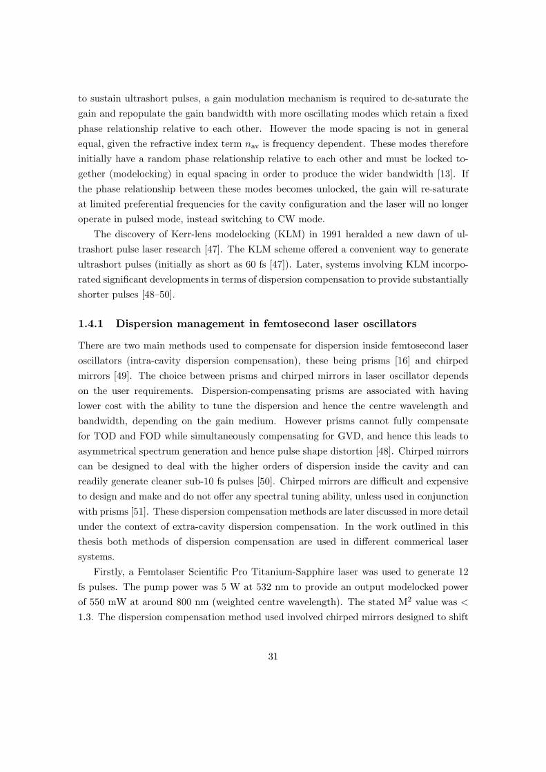
There are two main methods used to compensate for dispersion inside femtosecond laseroscillators (intra-cavity dispersion compensation), these being prisms [16] and chirpedmirrors [49]. The choice between prisms and chirped mirrors in laser oscillator dependson the user requirements. Dispersion-compensating prisms are associated with havinglower cost with the ability to tune the dispersion and hence the centre wavelength andbandwidth, depending on the gain medium. However prisms cannot fully compensatefor TOD and FOD while simultaneously compensating for GVD, and hence this leads toasymmetrical spectrum generation and hence pulse shape distortion [48]. Chirped mirrorscan be designed to deal with the higher orders of dispersion inside the cavity and canreadily generate cleaner sub-10 fs pulses [50]. Chirped mirrors are difficult and expensiveto design and make and do not offer any spectral tuning ability, unless used in conjunctionwith prisms [51]. These dispersion compensation methods are later discussed in more detailunder the context of extra-cavity dispersion compensation. In the work outlined in thisthesis both methods of dispersion compensation are used in different commerical lasersystems.

Firstly, a Femtolaser Scientific Pro Titanium-Sapphire laser was used to generate 12fs pulses. The pump power was 5 W at 532 nm to provide an output modelocked powerof 550 mW at around 800 nm (weighted centre wavelength). The stated M2 value was <1.3. The dispersion compensation method used involved chirped mirrors designed to shift

31

the relative spectral phase of generated bandwidth so as to support the shortest possiblepulses. This laser was used in the preliminary optoinjection and transfection experimentsin chapter 4.

Secondly, a KM Labs Swift 10 was used to generate sub-12 fs pulses with the abilityto change the spectral bandwidth to support longer pulse durations of around 35 fs. Theaverage pump power was varied between 6-8 W depending on whether shorter pulses werepreferred (lower average power) or longer pulses were preferred (higher average power).The pump wavelength was 532 nm. It was possible to tune the central wavelength ofthe optical pulses and associated spectral bandwidth. The tuning ability was provided bymotorised prisms mounted to movably traverse the beam path to vary cavity dispersion,hence changing the resulting pulse duration. The stated M2 value was < 1.1. The KMLabs Swift laser was used for all experiments outlined in this thesis other than thosementioned for the Femtolaser system outlined previously.

1.5 Applications of broadband ultrashort pulses

In this thesis several aspects of broadband ultrashort pulses were investigated. The termbroadband is generally used to refer to pulses which have sufficient bandwidth that af-ter travelling through dispersive optics, dispersion causes pulses to be shaped temporally;substantially so and enough to appreciably stretch (or compress) the pulses accordingly.Naturally this depends upon what kind of optics are used but typically for Ti-Sapphirewavelengths (around 800 nm) the threshold transform-limited pulse duration below whichdispersion becomes significant is 30 fs [52]. Measurement and control of chromatic dis-persion is key to applying broadband ultrashort pulses in a variety of situations. In thisthesis several distinctly different situations involving broadband ultrashort pulses are con-sidered. Firstly, chapter 2 introduces dispersion compensation methods and experiments,in particular focussing on the apparatus used in experiments to measure and deal withdispersion, referred to as multiphoton intrapulse interference phase scan (MIIPS). The MI-IPS method was essential for many of our experiments as without it the dispersion causedsignificant pulse stretching. Chapter 3 further examines the light-matter interaction, butinstead in dielectric colloidal systems in which focussed laser light can trap colloids in sucha manner that the colloids and light self-consistently interact in what is known as opticalbinding. In this chapter experimental studies demonstrate the optical binding effect inthe CW regime and theoretical studies investigate the optical binding phenomenon whensubjected to broadband ultrashort pulses. Chapter 4 concerns the interaction betweenbroadband ultrashort pulses and biological matter. These chapters discuss laser-induced

32

membrane permeabilisation for introduction of dye and genetic material. In particular,experiments are introduced which, to-date, cover the widest parameter space relevant formembrane permeabilisation. Finally, chapter 5 begins to examine the nature of broadbandultrashort pulse beam propagation. This chapter builds upon the pulse shaping chapterby introducing the concept of spatial pulse shaping, in which spatial modulations revealtemporal changes in the beam. Through use of a spatial light modulator I performedexperimental studies concerned the propagation of broadband ultrashort pulse Gaussianand Bessel beams.

1.6 Conclusions

This chapter is intended as an introduction to ultrashort pulses and highlights some ofthe key issues in the present context. In particular, the pulse shape is considered to becritical for defining the peak intensity, and hence the strength of any nonlinear interaction.An increase in peak power can be achieved by increasing pulse energy or decreasing pulseduration. Decreasing the pulse duration is a way of increasing the peak power withoutincreasing the total energy delivered by any sequence of pulses. However, a decrease ofpulse duration can only be sustained through an increase in spectral bandwidth. This is aparticular issue for the shortest of ultrashort pulses, whereby dispersive effects cause therelative spectral phase to be distorted, hence increasing the pulse duration and decreas-ing the peak intensity. Dispersion compensation is therefore required to deal with thesedispersive effects for optimum delivery of transform-limited ultrashort pulses. Ultrashortpulses are becoming increasingly important in many fields, particularly in biophotonics,wherein ultrashort pulses are used for imaging and manipulation purposes. It is particu-larly crucial that dispersion is dealt with in systems requiring the shortest available pulseduration in order to take maximum advantage of the peak intensity available. A key topicof the following chapter on pulse shaping addresses some of these issues and investigatesa commercially-available solution to the dispersion problem for the experimentalist. Inparticular, I demonstrate a commercial pulse shaper referred to as multiphoton intrapulseinterference phase scan, which is used in combination with SHG spectral measurementsfor dispersion measurement and compensation. The pulse shaping chapter builds uponthe foundations provided by this chapter and leads on to subsequent chapters in whichdispersion-compensated ultrashort pulses are delivered for several applications concerningthe light-matter interaction in terms of (i) optical trapping and binding; (ii) manipula-tion of biological matter through nonlinear-initiated processes and (iii) propagation ofnovel beam shapes which are affected by spatio-temporal distortions, whereby spectral

33

and spatial phase can affect the outputted beam profile and hence peak intensity, therebylinking back to optical trapping and binding, and biological manipulation in that the peakintensity is extremely important for defining nonlinear processes therein.

1.7 Chapter acknowledgements

The author designed all models used in this chapter to generate figures.

34

Chapter 2

Control of broadband ultrashort

pulses

2.1 Introduction

The previous chapter introduced ultrashort pulses along with their respective advantagesand disadavantages. Principally, ultrashort pulses have the advantage that they may offerenhanced peak intensity for any given pulse energy. However, this advantage can be nul-lified, and in fact made worse by dispersion. The purpose of this chapter is to follow onfrom the discussion of the previous chapter and introduce pulse shaping and measurementtechniques for (i) measuring and (ii) dealing with dispersion. The ability to accuratelymeasure and control the spectral phase, or dispersion allows complete control over the tem-poral features of an ultrashort pulse. Established methods of controlling dispersion arediscussed and a detailed description of the dispersion control method used in our experi-ments, known as MIIPS is presented. Finally, we discuss experiments performed using ourlaser and dispersion control system and relate the results to future chapters in this thesis.The purpose of this chapter is therefore to explain in detail the control of ultrashort pulsesin our experiments so that future chapters can focus on the experiment concerned whilereferring back to this chapter if necessary. This chapter also critically discusses featuresof the MIIPS system along with known issues and strategies for optimising performance.

2.2 Management of dispersion in optical setups

One of the main barriers to the use of broadband ultrashort pulses is that the dispersionintroduced by optical elements is significant and can result in pulse distortions (temporally

35

and spatially) which increase the pulse duration and decrease the peak optical power. Fig.1.8 illustrated how an ultrashort pulse can become significantly increased in duration ifthe initial duration is too short. In reality this means that it is better to start off with anultrashort pulse that is initially longer and hence not-broadband so that dispersion is nolonger such a significant issue, rather than waste effort on intra-cavity and extra-cavitydispersion compensation. However if broadband ultrashort pulses are required, then somemeans of dispersion management is required in most setups. There are two aspects todispersion management: measurement and compensation. Accurate measurement of dis-persion is critical, particularly for the shortest pulse durations, however in-situ dispersionmeasurement is non-trivial and the following sections discuss dispersion measurement indetail. Once the dispersion has been measured dispersion compensation methods can bedesigned and controllably utilised to deal with the dispersion in the setup.

2.3 Established methods of dispersion compensation

In this subsection the current technologies used for dispersion compensation for bothintra-cavity and extra-cavity purposes are discussed.

2.3.1 Prisms

Prisms are dispersive optical elements that introduce a form of geometrical dispersion re-sulting in an angular spread of spectral components (angular dispersion) within a beam [13].Fig. 2.1 illustrates a two-prism arrangement in which prism (a) introduces an angularspread that results in the lower optical frequencies exiting the prism at a different angleto the higher optical frequencies. This angularly spread beam is introduced into prism(b), at which point the beam frequency components have become spatially distinct, prop-agating at different angles. After propagation through prism (b) the beam contains thespatially distinct frequency components propagating parallel to each other. Prisms (c)and (d) mirror prisms formation (a) and (b) and return the beam to its original shape,with spatially recombined spectral components that have been dispersed according to theprism configurations and materials. The angular spread introduced by prisms is due tothe frequency-dependent refractive index experienced by the input beam resulting in anangular deviation according to Snell’s law [2]. For positive dispersion the lower frequen-cies experience a lower refractive index than higher frequencies, so the higher frequenciesbecome phase-delayed with respect to the lower frequencies. The spatially distinct fre-quency spread is referred to as angular dispersion and is a special case of spatial chirp [13].

36

Adjusting the separation between (a) and (b) (and (c) and (d)) in Fig. 2.1 results in acourse GVD tuning, while lateral insertion of prisms (b) and (c) provides fine-tuning ofthe GVD [15]. This prism arrangement provides negative GVD tuning by delaying shorterfrequencies by effectively passing them through more prism material, thus compensatingfor positive GVD [16]. However prisms do not readily compensate for higher order disper-sive effects and as a result they cannot generally create sub-10 fs pulses [48]. In general

Figure 2.1: The four-prism sequence which allows GVD compensation whilst simultane-ously dealing with the spatial chirp introduced by prism (a) and (b). One or two prismarrangements can be used, however these introduce unwanted spatial chirp that mustotherwise be corrected for.

prisms offer good negative GVD compensation and have low insertion losses at Brewster’sangle [2]. However their lack of higher order dispersion compensating ability limits theirapplication in the formation and control of the shortest of ultrashort pulses. They alsorequire careful alignment and can take up significant space in an optical setup unless novelarrangements are considered such as the single prism 4-pass compressor [53].

2.3.2 Diffraction gratings

Diffraction gratings also introduce angular dispersion to a beam [54]. Like prisms, diffrac-tion grating pairs can be utilised to shift the phase of spectral components of a pulse andprovide another route for pulse compression [55]. Fig. 2.2 shows a diffraction gratingconfiguration involving a reflecting mirror which can be used to control the dispersion andremove spatial chirp [14]. By varying the distance between the second grating (G2) and theimage of grating (G1), the dispersion is altered. A large variety of grating configurationshave been demonstrated and implemented in ultrashort pulse dispersion compensationschemes. In particular, rather than using lenses (which introduce dispersion and chro-matic aberrations) as in Fig. 2.2, it is possible to implement an all-reflective scheme that

37

Figure 2.2: A telescope arrangement between a grating pair in the so-called 4-f arrange-ment [56] provides a means for dispersion compensation. The 4-f arrangement is discussedin more detail in the spatial light modulator section. Note, the angular displacement isexaggerated in this example, wherein the image plane defines the image of grating G1through the telescope arrangement.

eliminates these issues [57]. Furthermore, sets of 4-prism and 4-grating arrangements havebeen used to compress chirped pulses to six femtoseconds [58]. A more compact arrange-ment has been achieved through novel arrangements of prisms and gratings to achieveGVD and TOD compensation [59].

Unlike prisms, gratings are not (in general) used inside laser cavities for dispersioncompensation due to the higher losses introduced by the grating, especially into thehigher diffraction orders. Gratings are however successfully implemented in high energyultrashort pulse systems such as in chirped pulse amplification (CPA) whereby gratingpairs disperse a pre-generated ultrashort pulse to lower its peak power to prevent damageto the enclosed gain medium, with the second grating subsequently re-compressing thepulse [14,57].

2.3.3 Chirped mirrors

Chirped mirrors, consisting of multiple layers of high and low refractive index dielec-tric coatings have been successfully implemented to compensate for dispersion in opticalsetups with pre-calculated or pre-measured dispersion [50]. Chirped mirrors are oftenused in Ti-Sapphire oscillators to generate ultra-broaband bandwidth which, when com-pressed, yields sub-5 fs pulses [60, 61]. However they can also be used for extra-cavity

38

dispersion compensation [62]. The design of chirped mirrors differs from that of standardBragg mirrors in that the layer-to-layer thickness varies. Accordingly, as the periodicityof the grating increases, so does the reflected wavelength. Therefore, by depositing thelonger wavelength layers deeper than shorter wavelength layers, the longer wavelengthsare delayed with respect to the shorter wavelengths, thereby contributing to a negativeGVD [63]. In this way, the dispersion can be pre-tuned according to the required dis-persion configuration by layering different index layers of different thicknesses. Generallythis results in an extended reflectivity range and allows the incorporation of a frequency-dependent group delay dispersion and if no glass or prisms are used in the setup the higherorder dispersive effects are minimised [63]. An extension of the chirped mirror design isthe double-chirped mirror, which utilises an impedance matching section, which aims tominimise the interference between small reflections from the front portion of the mirror,and the more-substantial reflections from the rear part of the mirror [63]. This typeof interference results in oscillations in the frequency-dependent group delay, as seen inGire-Tournois interferometers, in which higher-order dispersion control is limited [63–65].Chirped mirrors need to incorporate a highly reflective (low loss) broadband design withwell engineered multi-layer coatings for accurate dispersion control [66]. They are used inmultiple beam reflection configurations for maximising the introduced dispersion [50].

2.3.4 Spatial light modulators

A spatial light modulator (SLM) is a device which modulates amplitude or phase of lightwhich pass through spatial positions within the modulator. They are best utilised in theFourier plane in a 4-f configuration as per Fig. 2.3, which is a small modification of theapparatus in Fig. 2.2. Spatial light modulators (SLMs) offer a convenient way to controldispersion and they come in a number of formats. SLMs can be operated in many differ-ent configurations and have the potential for near-unlimited control over ultrashort pulses.This level of control differs to prisms, where the control is limited, and chirped mirrors,which offer no adjustability. SLMs have the disadvantage that they require careful cali-bration and computer control if they are to be adapted actively. Originally, SLMs werenot actively adaptable and employed a pre-designed phase mask to control dispersion [56].In these pre-designed masks, phase and amplitude features were imprinted upon a trans-parent substrate to effect changes in the properties of the pulses. In its simplest example,amplitude-only modulation can be implemented by physically blocking some of the spa-tially separated frequencies, thus lengthening the pulse duration. Phase-only modulationcan be used to synthesize any required dispersive characteristics and does not imply any

39

Figure 2.3: An example pulse shaper featuring 4-f arrangement with a spatial light modula-tor located in the Fourier plane, which can be utilised in either amplitude-only, phase-only,and dual amplitude and phase operation.

spectral loss.The manner of actively modifying an SLM can take several forms. Acousto-optic

modulation (AOM), in which a crystal is driven with a radio-frequency voltage signal anda traveling wave is formed which modifies the refractive index according to its position inthe crystal [67,68]. Therefore AOM requires constant updating from the signal generator orcomputer and is unsuitable for use with MHz repetition rate lasers [69]. Deformable mirror(DM) technology includes an array of electrically-addressed actuators under a mirroredmembrane which effectively create an position dependent phase modulation line, whichcan be utilised either in extra-cavity pulse shaping [70] or intra-cavity pulse control [71].Liquid crystal spatial light modulators (LC SLMs) are very commonly used for pulseshaping purposes [69]. The most common type of LC SLM make use of the electro-opticeffect to effect a refractive index and/or birefringence change upon light passing throughthe cell [69]. Less commonly used are optically addressed LC SLMs which make use ofthe photo-conductive effect to continuously vary the conductivity between electrodes toeliminate pixelation effects [72].

The most relevant type of SLM for this thesis is the electrically-addressed LC SLMand is discussed in more detail here. LC SLMs consist of an array of windows, or pixelscontaining a liquid crystal (LC) whose properties are adjusted according to the voltageapplied by an individual electrode. The LC consists of a set of molecules (usually nematic,wherein the long axis of the crystals are arranged in parallel lines) that are elongated

40

and align according to the applied electric field [73]. The alignment of these moleculeswithin the electric field effects either a refractive index or polarisation change. Dependingon the application the array of pixels may be enclosed within half-waveplates and/orpolarisers. In the case of half-waveplates, the LC cells require the correct input polarisationso waveplates are used to appropriately adjust the input polarisation. Twin polarisers areused (either in crossed or uncrossed configuration depending on LC configuration) to allowpixel-amplitude control by rotating the polarisation by 0-90 degrees to continuously varythe transmission from 0 to 1. To obtain dual phase and amplitude control, two separateelectrically-addressed pixel arrays are required; these arrays can be positioned together atthe Fourier plane within the shaper [74]. In this dual arrangement type the phase andamplitude LC arrays are accurately bonded together, one array with molecules alignedat -45 degrees, the other array with molecules aligned at +45 degrees, that is, withinthe plane perpendicular to the beam propagation direction with respect to the definedpolarisation axis. The LC arrays are sandwiched between polarisers in the uncrossedformation. The pixels are operated such that they cooperatively modulate the amplitudeand phase. With no voltage applied to the LC cell the molecules are aligned with theirlong axis parallel to the plane previously defined, and upon application of the voltage themolecules orient themselves towards the propagation direction. This alters the refractiveindex of the pixel concerned. Since each pixel in the first array is co-aligned with itscorresponding pixel in the second array and the refractive index is modified independentlyin orthogonal directions (-45 and +45 degrees) it is possible to change the phase accordingto the average refractive index imparted upon the beam [75]

φphase = Lωn1(V1) + n2(V1)

2c, (2.1)

where L is the pixel length (along the propagation axis), n1, n2 are the refractive indicesof the pixel concerned in the two pixel arrays at the specified voltages V1 and V2, respec-tively. For the amplitude change the difference in orthogonal refractive indices defines thebirefringence, and hence changes the phase difference and is given by

φamplitude = Lωn1(V1)− n2(V1)

c. (2.2)

The second polariser then allows or rejects portions of light through given pixel pairs.Through careful calibration this allows complete, independent control of phase and am-plitude of spectral components of the pulse.Figure 2.4 shows a simplified diagrammaticillustration of elements of the previously described spatial light modulator. In the illus-

41

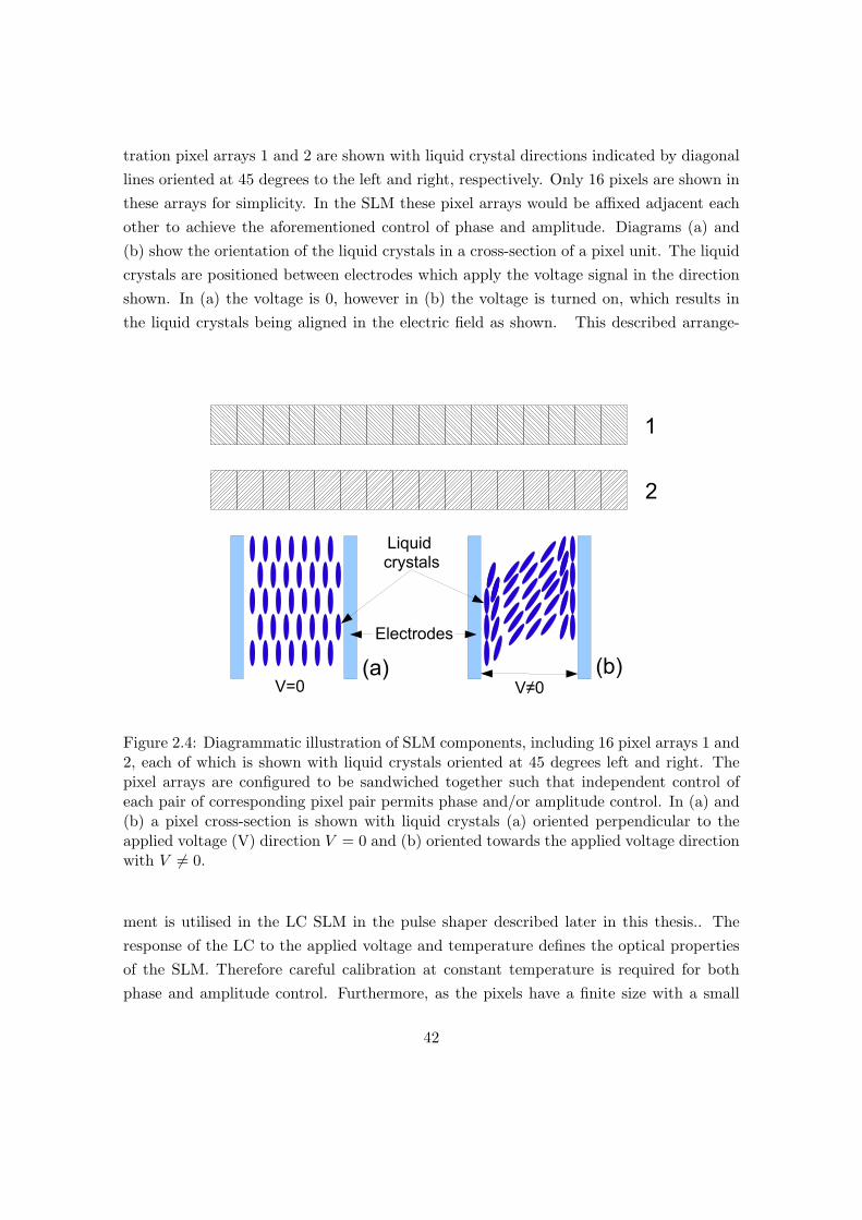
tration pixel arrays 1 and 2 are shown with liquid crystal directions indicated by diagonallines oriented at 45 degrees to the left and right, respectively. Only 16 pixels are shown inthese arrays for simplicity. In the SLM these pixel arrays would be affixed adjacent eachother to achieve the aforementioned control of phase and amplitude. Diagrams (a) and(b) show the orientation of the liquid crystals in a cross-section of a pixel unit. The liquidcrystals are positioned between electrodes which apply the voltage signal in the directionshown. In (a) the voltage is 0, however in (b) the voltage is turned on, which results inthe liquid crystals being aligned in the electric field as shown. This described arrange-

Figure 2.4: Diagrammatic illustration of SLM components, including 16 pixel arrays 1 and2, each of which is shown with liquid crystals oriented at 45 degrees left and right. Thepixel arrays are configured to be sandwiched together such that independent control ofeach pair of corresponding pixel pair permits phase and/or amplitude control. In (a) and(b) a pixel cross-section is shown with liquid crystals (a) oriented perpendicular to theapplied voltage (V) direction V = 0 and (b) oriented towards the applied voltage directionwith V 6= 0.

ment is utilised in the LC SLM in the pulse shaper described later in this thesis.. Theresponse of the LC to the applied voltage and temperature defines the optical propertiesof the SLM. Therefore careful calibration at constant temperature is required for bothphase and amplitude control. Furthermore, as the pixels have a finite size with a small

42

gap between each pixel, the SLM does not offer truly continuous phase and amplitudecontrol over the entire spectral content of the pulse. Therefore diffractive effects from sud-den phase-jumps in the pixel-pixel transitions within the arrays result in dips in spectralpower at the spectral pixel locations. As such, these features cannot be removed withoutinfinite pixel resolution and they are inherent to pulse shaping systems [75]. This is not asignificant problem unless there is a significant amount of dispersion,for GVD alone thisis typically around 45000 fs2 [11].

LC SLMs are very convenient as they allow full electrical control over spectral phaseand amplitude content. The SLM is stable and can be held in a constant state and doesnot require continual signal updates, apart from being driven at a constant-amplitudealternating current voltage signal (the molecular orientation is voltage sign invariant) toprevent migration effects within the LC [69]. The SLMs described in this section areone-dimensional arrays and are frequently used for pulse shaping purposes. LC SLMs arealso available as two-dimensional arrays and can also be used for pulse shaping purposes,however this is discussed in more detail in chapter 5.

2.4 Measurement of pulse duration and dispersion: estab-

lished methods

Since any pulse duration measurement requires use of optics, a method for completelycharacterising an optical pulse is required wherein those optics are taken into accountduring that measurement. The dispersion introduced by optical elements is well estab-lished theoretically [13]. However experimentally it is necessary to measure the dispersionin an optical setup as it is usually impractical to theoretically calculate dispersion in agiven setup. This is especially important as some optical elements such as microscopeobjectives do not have manufacturer data included and so a theoretical calculation is un-available. Complete pulse characterisation is a non-trivial problem owing to the fact thatoptical events are among the shortest known processes. Therefore to characterise an eventin time, one requires a shorter event in time, however there are no known controllableevents which are shorter than the typical times for ultrashort pulses (sub-picosecond).Electronics cannot be used to characterise sub-picosecond pulses, therefore we have toresort to using the pulses themselves to characterise themselves [46]. For brevity, more de-tailed discussions of the techniques of autocorrelation, FROG and SPIDER are presentedin the appendix of this thesis.

43

2.5 Multiphoton intrapulse interference phase scan (MIIPS)

So far the mainstream methods of dispersion measurement have been considered. Thissection concerns the measurement and compensation system which was used in experi-ments requiring dispersion compensation. This system is a commercial product producedby Biophotonic Solutions Inc. and used multiphoton intrapulse interference phase scantechnology, otherwise known as MIIPS

TM. There are two aspects to the MIIPS technol-

ogy. Firstly, the dispersion of an optical system is measured using multiphoton intrapulseinterference (MII) in SHG spectral measurements (i.e. with a spectrometer), while thephase scan operates in conjunction with a liquid crystal based SLM, which modulatesamplitude and/or phase of the spectral components of the beam to effect a change inthe MII. Once the dispersion has been measured, the SLM appropriately modulates thespectral components according to the iterative solution provided by the software, therebyremoving the spectral phase introduced by the optics [76]. MIIPS is a single-beam methodwhich makes it ideally suited to applications where the phase may need to be found fordifferent experiments such as in microscopy [76]. The phase is inferred from the scannedphase modulation applied on the pulse which directly affects the probability of SHG atspecific frequencies [77].

MIIPS Procedure

MIIPS takes some known reference function f(ω) and uses this function to cancel theunknown spectral phase of the pulse, ϕ(ω) [78]. The total phase for the pulse is thengiven by ϕ(ω) = f(ω) + φ(ω). The second harmonic spectrum is then used to calculatethe form of the unknown phase function, ϕ(ω). The generated second harmonic intensitycan be written as a function of phase and spectral electric field amplitude [78]

S(2)(2ω) ∝∣∣∣∣∫ |E(ω + Ω)||E(ω − Ω)|exp (i[ϕ(ω + Ω) + ϕ(ω − Ω)]) dΩ

∣∣∣∣2 , (2.3)

where ϕ(ω ± Ω) and E(ω ± Ω) describes the spectral phase and electric field at anyfrequency, respectively, and where Ω is any frequency used as a dummy variable duringthe integration procedure (Ω is hereafter referred to as the detuning frequency). Transformlimited pulses have ϕ = 0 and thus generate the maximum second harmonic intensity. Ifthe phase modulation produced by any physical process is continuous in nature, then wecan expand the phase with a Taylor expansion about ω with the sum of the positive and

44

negative detuning frequencies being

ϕ(ω + Ω) + ϕ(ω − Ω) = 2ϕ(ω) + ϕ′′(ω)Ω2 + · · ·+ 2(2n)!

ϕ2n′(ω)Ω2n (2.4)

where ϕn′ω = dnϕ(ω)/dωn. To the first order the SHG is maximised when ϕ = 0 and

ϕ′′(ω) is zero so that ϕ(ω) = f(ω) + φ(ω) → 0. So as long as the second harmonic ismaximised with the reference frequency f ′′(ω), then φ′′(ω) can be retrieved [78]. TheMIIPS procedure is now discussed in more detail [78].

The MIIPS software performs a phase-sweep δ running from 0 to 4π and iteratively cal-culating the spectral phase accordingly. By measuring the SHG spectral signal as functionof δ we obtain a function f(δ, 2ω), with which a two-dimensional map of the spectral phaseis obtained. Noting the sensitivity of SHG according to the spectral phase, the spectralsignal provides information regarding the unknown spectral phase. The maximum inten-sity of the SHG spectrum is achieved when the second-order spectral phase term is givenby

φ′′(ω) = −f(δ, ω), (2.5)

where f(δ, ω) describes the two-dimensional map of the spectral SHG signal. The phase,φ(ω) is obtained through direct double-integration of φ′′(ω). A starting point in MIIPS isobtained by using a known reference function, f(δ, ω), with a double integration procedure.Typically a sine function is used,

f(δ, ω) = α sin(γωω − δ), (2.6)

where α and γω are constants defining the amplitude and periodicity of the applied MIIPSfunction. During the MIIPS procedure the SHG plot, f(δ, 2ω) is used to find δ(ω) for eachfrequency. For each frequency, δ0(ω) is found through use of the analytic equation,

φ′′(ω) = αγ2 sin[γωω − δ0(ω)

], (2.7)

where γω is a constant, generally being the inverse of the pulse duration. Once obtainedafter double-integration, the first phase term in the compensation is −φ1(ω), which isadded to the phase in-use in the pulse shaper. Subsequent phase terms can be obtainedthus, φtotal = φ1 + φ2 + φ3 + · · ·. These additional phase terms decrease in magnitudewith repeated iterations until a solution is converged towards. The obtained spectralphase is then implemented in the pulse shaper to obtain net zero spectral phase in thedetection plane. Generally, six iterations are required for optimum phase minimisation.

45

Practical details about the MIIPS procedure for obtaining near transform-limited pulsesare included in the experimental procedure section below.

Implementation of the MIIPS system

MIIPS has been implemented in several compensation schemes in addition to laser pulsecompression with a high success rate. MIIPS lends itself for compensation schemes involv-ing high dispersion optics, such as microscope objectives. So in principle any experimentwhich requires the passage of a single ultrashort pulse laser beam through an objectivecan benefit from the highest peak power transform limited pulses. Furthermore the pulseshaper can be made to fashion pulses which excite multiple chemical processes by se-lective excitation [79, 80]. Control of photo-sensitive chemical reactions [81, 82] can beachieved using femtosecond pulses using binary phase pulse shaping methods [83]. Binaryphase modulation works on the principle that to maximise or minimise certain pathwayswe need only to adjust the phase between two values: 0 and π between each frequencycomponent [84].

Much work has been done to identify chemicals accurately. Mass spectrometry is a wellknown technique for identifying chemicals but lacks the ability to differentiate betweenisomers, such as o-xylene and p-xylene [85]. Ultrashort laser pulses shaped using MIIPShave been used to control molecular fragmentation in combination with mass spectrometryto achieve high sensitive molecular identification [85,86]. The ultimate goal is to suppressa certain molecular fragmentation path while increasing the probability that the desiredfragmentation type will occur; as yet this goal has not been achieved because coherenceappears to play a limited role in defining fragmentation pathways [87]. Atomic emissionsmeasured in laser induced breakdown spectroscopy were found to be more efficient usingfemtosecond pulses that have a very large bandwidth and with pulses exhibiting positivelinear chirp, as can be achieved using MIIPS [88].

The MIIPS system has also been used for measuring the spectral phase of ultra-broadband ultrashort pulses, indeed such as that of a 2.12 GHz repetition rate Ti-Sapphirelaser compressed using dispersion compensating mirrors and compensated for using MI-IPS [89]. This same laser system was used to transmit encrypted information, but waslimited by the slow response speed of the SLM [90]. An octave-spanning laser with ultra-broad bandwidth pulses (400nm) has been demonstrated with a grating based shaper inconjunction with MIIPS to generate a second harmonic spectrum spanning 200 nm [91].Dispersion measurements of various media using a MIIPS-compensated laser is possibleand relatively simple due to only needing a single-beam to take the measurements. Ex-

46

amples include group velocity dispersion measurements of water, seawater and ocularcomponents [92]. Remote dispersion measurement has also proven possible at a distanceof 28.9 m with amplified pulses [93] where the GVD of air at 800 nm was measured to be20.1± 1.5 fs2/m.

Applications of MIIPS also extend to Raman and coherent anti-Stokes Raman scat-tering (CARS) spectroscopy using the high peak power to enhance the signal strength.The amount of Raman scattered light is very low when using CW lasers, so signal-to-noise ratio is relatively poor, although methods using frequency modulation complementthis method [94]. Higher intensity lasers will cause more Raman transitions to occur andhence more signal will be produced; providing the background signal can be suppressedthen the Raman scattered light may be detected. Stand-off detection of several chemi-cals using CARS at a distance of 12 m has been demonstrated using MIIPS compensatedpulses [95, 96]. A similar level of detection has been achieved using a pulse compressorbut instead of suppressing the background as in the MIIPS system, the background iscoherently interfered with the weak resonant signals [97]. Obvious applications includehazardous material detection such as biological and chemical agents and explosive detec-tion. The ability to arbitrarily compensate for dispersion in optics using MIIPS allowsmicroscope objectives to be incorporated into experiments involving ultrashort pulses. Thebiggest barrier to doing so is due to the dispersive optics that microscope objectives typi-cally contain, particularly so for high numerical aperture objectives comprising substantiallengths of glass or other refractive materials. The development of dispersion compensationtechniques maximises the benefits of using ultrashort pulses, in which the signal intensitycan be order of magnitudes higher [98]. In systems using dispersion pre-compensation in-stead of active compensation is possible but require knowledge of the dispersion propertiesof the objective concerned [99]. The second order dispersion characteristics of various high-NA objectives were measured in [99] and were found to be in the range of 580 to 1100 fs2.Other literature has pointed towards a second order dispersion range of 4600 to 5400 fs2 forsimilar objective types [100]. Technical difficulties are presented in pre-compensation sys-tems such as prism-based systems due to significant higher order dispersion, which meansthat the numerical aperture must be kept low for sub 10 fs pulses [78]. With the problemof dispersion all but eliminated, we can take advantage of the high peak powers affordedby ultrashort laser pulses and initiate nonlinear processes at the focus of the objective.Since the time-averaged efficiency of second harmonic generation is proportional to thepeak intensity of the light, it makes sense to take advantage of such properties. Henceimaging using the second harmonic signal has been demonstrated along with selective flu-orescent excitation using the MIIPS system [81, 98]. The advantages of using the second

47

harmonic signal are clear such as increased depth penetration, reduced photobleaching aslower average power is needed. Selective imaging is demonstrated using the same laserin which the excitation wavelength can be chosen by shaping the laser pulse such thatthe two-photon absorption at two different wavelengths can be achieved using the samepulse and thus observing the fluorescence signal from specifically marked structures insidecells [81]. Coherent control of the laser pulse can be used for functional imaging, in whichselective two-photon excitation is achieved in a pH-sensitive chromophore, which is placedbehind a highly scattering biological tissue [101]. This suggests that pulse shaping meth-ods may have benefits for imaging and photo-dynamic therapy while minimising damageto healthy biological tissue.

It should be noted that while the MIIPS system can accurately measure and correctfor dispersion in microscope-based systems, the choice of optics can have a profound effecton the operation of the MIIPS system. In particular, optical fibres introduce significantproblems and may not be easily compensated using the MIIPS system. The MIIPS systempermits pixel wrapping on the SLM to provide an appropriate phase relationship betweenneighbouring pixels. At the phase equals 2π boundary, the phase may be equivalentlyrepresent by 0 instead, and hence permits phase wrapping. Generally, a sequence of leastfour adjacent pixels is required to permit one phase wrap of 2π in order to prevent signif-icant error in the applied spectral phase [78]. However, depending on the pixel resolutionof the SLM, this condition may become further constrained and require additional pixelsto maintain accurate phase wrapping.

2.6 Operation of MIIPS system

The MIIPS system requires careful alignment an operation to achieve the best results.The purpose of this section is to detail the manner in which to achieve the best resultsusing the MIIPS system. In an inverted microscope arrangement a specially adapted(commercially-supplied) SHG detection module referred to as MIIPS detection unit (MDU,described below) was used. An alternative MDU is obtainable for an upright microscope.For each type the MDU is configured to be easily rotatable (for angular phase-matching)and optimised for overall stability in the desired microscope type. The MDU compriseda 100 µm thick Potassium Dihydrogen Phosphate (KDP) Type I crystal configured tobe situated at the focus of a lens and optics for directing SHG signal down a fibre into aspectrometer (described below). The MIIPS system was also adapted for use in an uprightmicroscope setup and also in free-space optics arrangement, but the MDU was not wellsuited to these applications. The MDU allowed for the most efficient collection of SHG

48

signal compared with other free-space optics detection configurations. It should be notedthat a Beta Barium Borate (BBO) Type I crystal of similar thickness was used in thefree-space optics experiments.

2.6.1 MIIPS experimental procedure

Here, the procedure for setting up the MIIPS system is detailed. It is perfectly rea-sonable to use either achromat or singlet lenses however achromats were found to offeroptimal performance. Furthermore, dispersion-free focussing mirrors can be used in placeof lenses, however this option is more expensive and the MIIPS system adequately dealswith dispersion in the entire optical system.

(i) The femtosecond laser system was running stably and modelocked before beingdirected into the MIIPS pulse shaper. Spectral components were angularly dispersedwithin the pulse shaper and were focussed into the spatial light modulator (SLM) withthe laser power distributed over a wide spatial region. If the laser was running in CWmode, the power would be focussed into a narrow spatial location on the SLM, potentiallyresulting in damage. If the laser switched to CW mode the beam was immediately blockedfrom entering the pulse shaper.

(ii) The beam was well collimated and expanded to around 3-5 mm in diameter usinga telescope and directed into the pulse shaper in the horizontal polarisation for maximumpulse shaper transmission efficiency. The beam was aligned through two alignment aper-tures (the second aperture to be removed after alignment). If the beam is too small thegrating will not be efficiently utilised and individual spectral components will disperseover a wider angular range resulting in spectral phase error, whereas if the beam is toolarge it will be blocked by pulse shaper components.

(iii) The beam was then aligned through the pulse shaper. In general if the pulseshaper is pre-aligned then not much work is required apart from adjusting the focussingmirror and the second mirror so that the two beams on grating are vertically displaced withrespect to one another by approximately 5-6 mm, but with no horizontal displacement.The beam should then exit the final aperture with no evidence of any diffractive effects(generally) caused by the beam passing too near the first mirror. Figure 2.5 shows asimplified illustration of the MIIPS pulse shaper arrangement for reference purposes. Thepulse shaper design can be adapted in a number of ways including changing the gratingto accommodate different spectral bandwidths.

(iv) The beam which exits the pulse shaper was appropriately directed into the ex-perimental setup (e.g. microscope). Spectral SHG measurements should be taken at the

49

Figure 2.5: Simplified illustration of MIIPS pulse shaper setup depicting a typical ar-rangement. The arrangement may be adapted to accommodate laser parameter changes.CM is a concave mirror configured one focal length away from the grating and one focallength away from the mirror behind the SLM (hereafter referred to as the back mirror).The SLM admits the beam as shown through the SLM pixels (not shown directly, butindicated by the decreased line width of the SLM box). The concave mirror images thegrating onto the back mirror and back again, thereby passing the beam through the SLMtwice. The grating angularly spreads spectral components of the beam on the first beampass and then recombines them on the second beam pass. The components of pulse shaperare angled such that the beam is displaced in terms of height so that the beam is directedtowards an output upon return from the pulse shaper.

point at which transform-limited pulses are required. As SHG generally requires a certainamount of beam focussing to obtain high intensities, the MIIPS procedure cannot be per-formed directly on collimated beams. Instead, focussing mirrors can be used, although inpractice this method is not ideal due to the aberrations introduced.

(v) The MDU (or other SHG collection optics) was placed appropriately at the beamfocus and the SHG signal obtained. The MDU should then be rotated to obtain maximumSHG signal through optimal phase matching. In this part of the setup it was necessary

50

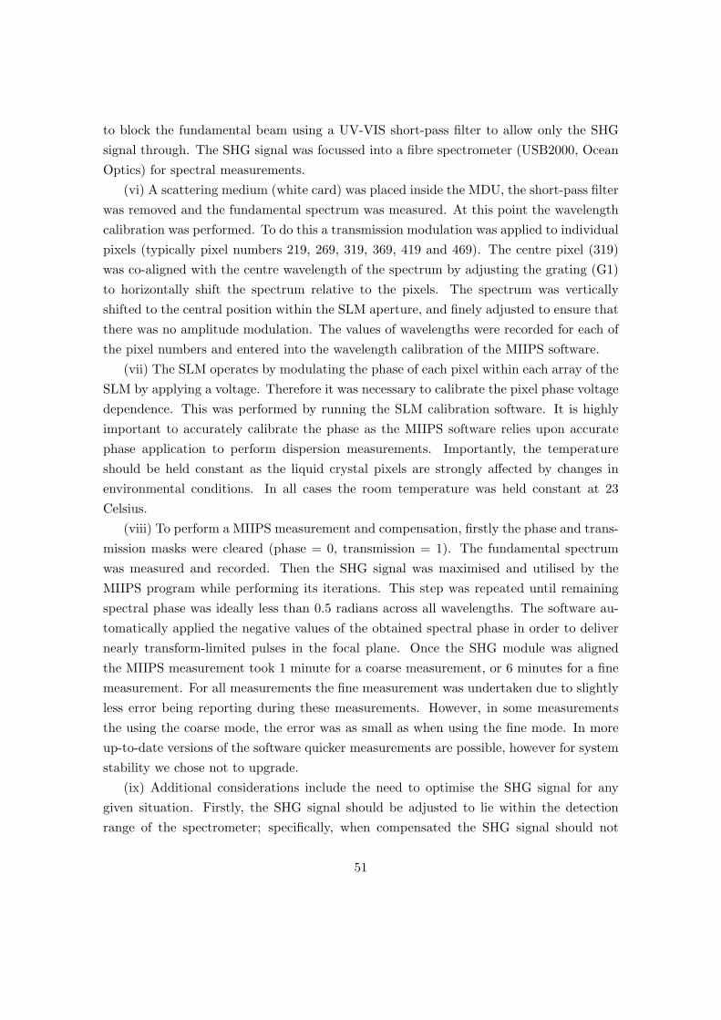
to block the fundamental beam using a UV-VIS short-pass filter to allow only the SHGsignal through. The SHG signal was focussed into a fibre spectrometer (USB2000, OceanOptics) for spectral measurements.

(vi) A scattering medium (white card) was placed inside the MDU, the short-pass filterwas removed and the fundamental spectrum was measured. At this point the wavelengthcalibration was performed. To do this a transmission modulation was applied to individualpixels (typically pixel numbers 219, 269, 319, 369, 419 and 469). The centre pixel (319)was co-aligned with the centre wavelength of the spectrum by adjusting the grating (G1)to horizontally shift the spectrum relative to the pixels. The spectrum was verticallyshifted to the central position within the SLM aperture, and finely adjusted to ensure thatthere was no amplitude modulation. The values of wavelengths were recorded for each ofthe pixel numbers and entered into the wavelength calibration of the MIIPS software.

(vii) The SLM operates by modulating the phase of each pixel within each array of theSLM by applying a voltage. Therefore it was necessary to calibrate the pixel phase voltagedependence. This was performed by running the SLM calibration software. It is highlyimportant to accurately calibrate the phase as the MIIPS software relies upon accuratephase application to perform dispersion measurements. Importantly, the temperatureshould be held constant as the liquid crystal pixels are strongly affected by changes inenvironmental conditions. In all cases the room temperature was held constant at 23Celsius.

(viii) To perform a MIIPS measurement and compensation, firstly the phase and trans-mission masks were cleared (phase = 0, transmission = 1). The fundamental spectrumwas measured and recorded. Then the SHG signal was maximised and utilised by theMIIPS program while performing its iterations. This step was repeated until remainingspectral phase was ideally less than 0.5 radians across all wavelengths. The software au-tomatically applied the negative values of the obtained spectral phase in order to delivernearly transform-limited pulses in the focal plane. Once the SHG module was alignedthe MIIPS measurement took 1 minute for a coarse measurement, or 6 minutes for a finemeasurement. For all measurements the fine measurement was undertaken due to slightlyless error being reporting during these measurements. However, in some measurementsthe using the coarse mode, the error was as small as when using the fine mode. In moreup-to-date versions of the software quicker measurements are possible, however for systemstability we chose not to upgrade.

(ix) Additional considerations include the need to optimise the SHG signal for anygiven situation. Firstly, the SHG signal should be adjusted to lie within the detectionrange of the spectrometer; specifically, when compensated the SHG signal should not

51

saturate the detector of the spectrometer. Secondly, the dispersion-compensated SHGspectrum should ideally be a smooth shape (Gaussian SHG spectrum if using a Gaussianfundamental spectrum). However, if the fundamental spectrum is asymmetric or has anyuneven features, then these affect the SHG spectrum if residual chirp remains or is addedto the optical system. For example, if compensating and subsequently stretching the pulseby adding dispersion then the SHG spectrum may no longer have smooth features.

2.6.2 Pulse stretching

Two methods were used to stretch the pulses. Firstly, the MIIPS software provided aplatform to apply arbitrary phase and/or transmission functions on top of the obtaineddispersion profile. Most relevantly the pulses were stretched by applying a second orderpolynomial function, with the resultant pulse duration calculated using the MATLABprogram in the supplementary CD and acknowledged in Appendix 7.5. It should benoted that the fundamental spectrum is modified by the phase compensation function,especially when the applied function requires multiple phase wrapping. However, whenadding additional (second order) phase functions this did not yield a substantial changein the fundamental spectrum. Secondly, anti-reflection coated optical flats made of BK7glass were inserted into the setup. These were found to contribute mainly second orderdispersion, with negligible third order dispersion and no measured loss in transmission,even when multiple flats were inserted. Fig. 2.6 shows the SHG spectra for severalpulse durations obtained with the two methods. The overall shape of the spectra werecomparable however the total signal differed slightly. This was due to the change infundamental spectral intensity which occurs when an additional phase function was appliedon top of the compensation function, in particular where the compensation function wasnegative in sign and the addition of positive GVD decreased phase wrapping and increasedthe fundamental intensity. For this reason optical flats were chosen for all experiments asthey did not alter fundamental spectral intensity.

2.7 MIIPS results

2.7.1 SHG as function of pulse energy and duration

It is expected that the SHG intensity follows an exact relationship for any pulse energyand duration. In the case of the instantaneous SHG intensity this is given by

ISHG ∝ I2fund ∝

(Wp

τp

)2

, (2.8)

52

380 390 400 410 420 430Wavelength (nm)

0

5000

10000

15000

20000

25000In

tens

ity (a

rb. u

nits

)53 fs - GLASS104 fs - GLASS155 fs - GLASS53 fs - SLM104 fs - SLM155 fs - SLM

Figure 2.6: Comparison of SHG spectra from the two pulse stretching methods for severalpulse durations. Note the trend of the SHG spectrum shifted towards longer wavelengthsfor greater chirp occurs due to the asymmetric fundamental pulse spectrum shape; itwould not shift in this way for a symmetrical spectrum. The expected SHG shift can becalculated from equation 2.3

where Ifund is the fundamental intensity and Wp is the pulse energy. However, an instan-taneous measurement of SHG intensity is not possible and therefore the signal is averagedout over a sequence of pulses of duration τp, with the following relationship

〈ISHG〉 ∝

(W 2

p

τp

), (2.9)

where 〈ISHG〉 denotes the time-averaged SHG intensity. Fig. 2.7 shows the total SHGsignal for given pulse energies on a log-log scale. The obtained gradient was 1.89 ± 0.05indicating ISHG ∝W 1.89

p . This is reasonably close to the expected gradient of 2. Note thatthe error bars are provided but are insignificant in size. The spectral SHG intensity followsan inverse reciprocal relationship with pulse duration. Fig. 2.8 shows a log-log graph of theSHG data for a set of pulse durations with the fundamental spectrum from the Femtolaseroscillator. The gradient of the fit indicates that above 33 fs the 1/τp relationship followsalmost exactly with a small deviation of 1/τ0.97

p . Clearly, below 33 fs the relationship

53

1Log(Pulse energy) (nJ)

1x105

1x106

Log(

SHG

inte

nsity

) (ar

b. u

nits

)

0.5 2

Figure 2.7: The integrated spectral SHG data for a set of pulse energies on a log-log scale.

breaks down with a linear fit over the entire pulse duration range corresponding to 1/τ0.74p .

This deviation from theory was observed every time, and the behaviour was repeated whentwo different fs lasers were used. The KM Labs laser had a slightly narrower bandwidthwith a minimum pulse duration of 16-17 fs. In an identical similar experiment with theKM Labs laser we found the relationship to follow 1/τ0.91

p indicating that at or near 12fs there is a significant deviation from theory. Following on from this the spectral dataaccompanying this data is presented in the top panel in Fig. 2.9. The spectral SHG signalis strongly dependent upon the spectral phase relationship according to equation 2.3. Thebottom panel of FIg. 2.9 shows the theoretical SHG spectral signal, as calculated throughequation 2.3. The MATLAB code used to generate the data in the plot is provided inthe supplementary CD and acknowledged in Appendix 7.5. The theoretical data sets havebeen normalised with respect to the 33 fs experimental data set so an easy comparisoncan be made. Fig. 2.8 demonstrated that above 33 fs the spectral signal closely followedtheoretical predictions, hence the choice for normalising with respect to this data set.Clearly the 12 fs data set does not produce as much SHG signal as expected. However,above 33 fs the SHG signal more closely matches the theoretical values, and the spectraloscillations for longer pulse durations are also predicted by the model. Importantly, theSHG spectra are narrower than expected. There are a number of possible explanations,

54

10 100Log(Pulse duration) (fs)

1x105

1x106

Log(

Inte

grat

ed S

HG

inte

nsity

) (ar

b. u

nits

)

20 40 60 80

Figure 2.8: The integrated spectral SHG data for various pulse durations plotted on log-log scale. The linear fit shown was calculated for the data down to 33 fs. The deviationof the 12 fs data point from this fit indicates a discrepancy in the SHG model.

not limited to:(i) The SHG crystal does not offer a uniform conversion efficiency across the spectral

bandwidth. For example, this could be due to imperfect phase-matching. Despite our bestefforts we could not obtain a broader SHG signal through changing crystal angles.

(ii) The focussing behaviour of the beam is strongly influenced by the spatial andspectral/temporal characteristics of the beam. There are a number of possibilities in thiscategory. For example, chromatic aberrations lead to a non-uniform spatial spectral spreadat the beam focus. Also, spectral phase can influence the spatial beam characteristicsthrough spatio-temporal couplings [102]. Hence, the focal spot size (and peak intensity)could be influenced by the spectral phase.

(iii) The MIIPS method does not offer perfect spectral phase correction. In particu-lar, the MIIPS system cannot deal with (transverse) spatially-dependent spectral phase.The MIIPS measurements provide a spectral phase correction error value. This aspect isdiscussed further in chapter 5. Furthermore, it was not possible to make an exact com-parison between MIIPS-obtained spectral phase and other pulse measurement techniques,although MIIPS has been found to be comparable with other techniques such as FROG

55

360 380 400 420 440Wavelength (nm)

0

20000

40000

60000

80000

100000

120000In

tens

ity (a

rb. u

nits

)12.3 fs (0 mm)33.2 fs (3 mm)53.0 fs (5 mm)83.5 fs (8 mm)104 fs (10 mm)135 fs (13 mm)155 fs (15 mm)186 fs (18 mm)

360 380 400 420 440Wavelength (nm)

0

20000

40000

60000

80000

100000

120000

Inte

nsity

(arb

. uni

ts)

12.3 fs33.2 fs53.0 fs83.5 fs104 fs135 fs155 fs186 fs

Figure 2.9: Top: Experimental spectral SHG data for different pulse durations obtainedby inserting anti-reflection coated optical flats into the beam path. Bottom: TheoreticalSHG spectra obtained for the same fundamental spectrum used in the experiments. Thetheoretical data was calculated using equation 2.3.

56

and SPIDER [78]. In particular, the spectral phase measurement of all three techniqueswere comparable in measuring the pulse duration, thereby establishing MIIPS within thefield as a comparable dispersion compensation technique.

2.8 Conclusions

This chapter built upon some of the principles of ultrashort pulses outlined in chapter1. In particular, dispersion is known to be of paramount importance in ultrashort pulsepropagation through dispersive optical systems. This chapter discusses dispersion com-pensation in more detail and considers the well known dispersion compensation methodssuch as prisms and gratings. A further development in dispersion compensation came inthe form of pulse shaping in so-called 4-f pulse shapers. Programmable pulse shapers pro-vide the ability to controllably modulate spectral phase and amplitude, hence changingthe time-domain characteristics of an ultrashort pulse. Pulse shaping provides suitablemeans for obtaining unlimited ultrashort pulse shapes. This ability to control pulse shapeallows the user to adjust the pulse duration according to the experimental requirements.However, broadband ultrashort pulses suffer from significant dispersion and hence pulseshapers provide the opportunity for dispersion compensation to achieve pulse durationminimisation in situ. We used a commercially-available pulse shaping system known asMIIPS, in which spectral SHG measurements are taken in sequence according to the modu-lating phase function within the pulse shaper. The MIIPS algorithm retrieves the spectralphase and uses this function to compensate for the dispersion in the optical setup fromlaser output coupler to the SHG crystal. We characterised the performance of the MI-IPS system, particularly concentrating on obtaining optimum performance through carefuland repeated calibration procedures. We further investigated the performance of the pulseshaper and found that for the shortest pulse durations the SHG signal obtained did notcorrelate with theoretical expectations. This issue is investigated in the beam shapingchapter 5. The ability to provide dispersion-compensated ultrashort pulses in situ is par-ticularly desirable since dispersion at the shortest pulse durations is known to significantlystretch the pulse duration. This chapter therefore serves as a pre-requisite for subsequentchapters concerning studies involving ultrashort pulses. In the optical binding chapter weconsider the effect of ultrashort pulses on the light-matter interaction between co-trappeddielectric spheres within an ultrashort pulse light field. We further investigated opticalbinding within SHG ultrashort pulse light fields, wherein the SHG spectral signal is par-ticularly sensitive to spectral phase. In the optoinjection chapter we examined the linearand nonlinear absorption processes initiated by ultrashort pulses in cell membrane perme-

57

abilisation. In particular we investigated the role of pulse duration in this light-biomatterinteraction process which is relevant for all biophotonics applications involving ultrashortpulse lasers. Finally, in chapter 5 we further advanced this study of pulse shaping inthe time-domain to pulse shaping in the space-domain, wherein spatio-temporal couplingsplay a key role in defining ultrashort pulse beam propagation. This is relevant for any ap-plication of ultrashort pulses as it is possible to tailor pulses effectively in four dimensionsto provide multiple possibilities in biophotonics, spectroscopy, pulse compression and thelike.

2.9 Chapter acknowledgements

The author designed the MATLAB models in this chapter and performed related experi-ments.

58

Chapter 3

Transverse optical binding

3.1 Introduction

An important aspect of the light-matter interaction concerns the ability for light to ma-nipulate objects, for example dielectric particles using optical tweezers. In this chapterI further expand on the relevance of ultrashort pulses in the domain of so-called opticalbinding in which scattered light between particles is found to bring about sufficient forceto effect movement or restriction of said particles within some trapping medium such aswater. In particular, we consider the role of broadband ultrashort pulses in terms ofthe force dependence between particles as function of separation and spectral bandwidth.The relevance of pulse shaping is considered in the section concerning SHG optical bindingwhereby, the phase-dependent SHG spectral bandwidth is affected by dispersion and re-sults in decreased optical binding strength where dispersion is not sufficiently compensatedfor.

Optical tweezers are extremely powerful tools in the colloidal and biological sciences [103–105]. The term optical tweezer was coined to describe the ability to hold microscopic parti-cles in space in a laser-created potential well deep enough to prevent Brownian fluctuationsfrom knocking the particle out of the trap. The optically induced forces that result fromthe light-matter interaction are sufficient enough to control and manipulate microscopic,and even nano-sized particles. This is due to the change in momentum as photons are scat-tered and refracted through a particle (or instead owing to the electromagnetic field fluxdensity as modified by the particle involved). The invention of the laser has allowed con-siderable progress in creating high intensity, highly directional beams which are associatedwith high a flux of photons, each carrying momentum of hk.

Optical tweezers are widely used tools in, for example, microfluidics [106], measurement

59

of Raman signatures in trapped particles [107] and measurement of torque forces in flagellaroptical motors [108], to name but a few applications. The term optical tweezers describesan optical tool configured to hold microscopic particles in 2D, or 3D space in a laser-created potential well deep enough to prevent Brownian fluctuations from knocking theparticle out of the trap. The optically induced forces that result from the light-matterinteraction are sufficient enough to control and manipulate microscopic, and even nano-sized particles. The origin of optical trapping forces for dielectric micro-particles caninitially be decomposed into two classes. In the first class the radiation pressure exertedby scattered fields on particles is sufficient to move the particle by a measurable amount.In the second class the laser spatial profile is typically Gaussian and the particle is forcedtowards the highest intensity part of the beam provided the refractive index is higher inthe particle than in the host medium. The trapping strength is enhanced by focussing thebeam, in particular with a microscope objective the gradient force becomes much largerand enables particle trapping in all three dimensions against the effect of gravity and lightscattering forces.

Twenty years ago, Burns et al. demonstrated that systems of free-floating microscopicdielectric particles may become optically bound under intense laser light [109]. An opticalline trap was created using two crossed cylindrical lenses. The high intensity gradientachieved perpendicular to the long trap axis strongly confines any trapped particles in thisdirection, however parallel to the long trap axis the particles are less strongly confined.Hence the trapped particles may float freely along this axis and hence the system iseffectively one-dimensional. Fig. 3.1 illustrates the relative differences between opticaltrapping and optical binding. Firstly, independent traps refer to optically trapped particlesheld in position by an optical tweezers indicated by the green circles. In independent trap 2the particle is non-central indicating how particles actually fluctuate positionally aroundthe centre of an optical trap. In optical binding there exists two or more co-trappedparticles which are subject to the same optical (elliptical) trap, but scattered light actingbetween the co-trapped particles results in binding forces acting therebetween. The generaldirection of force within the elliptical beam focus is indicated by the appropriate arrowsalong with the relative polarisation directions. The symmetry of this situation means thateach particle is equally illuminated. The interesting point demonstrated in the paper wasthe oscillatory nature of the optical binding forces, which were periodic in the wavelength ofilluminating light in the host medium, water. In a later paper, Burns et al. demonstratedthat arrays of extended crystalline and non-crystalline structures could be fashioned withcorrectly applied interfering laser beams [110].

To summarise, optical trapping refers to the phenomenon of using focussed laser beams

60

Figure 3.1: Illustration depicting the difference between independent trapping of twospheres using independent optical tweezers wherein independent trap 1 contains a particlethat is centred with the highest intensity region of the trap; independent trap 2 contains atrapped particle that is oscillating about its centre position (due to Brownian motion). Inthe co-trapped particles example a line (elliptical) trap is formed such that two particlesare confined within the same trap simultaneously while scattered light therebetween pro-duces an additional binding force; the direction of said binding force within the focal planedefined by the (green) oval. LA represents the longitudinal axis of the beam focus. Im-portantly, the particles which are held in optical tweezers are subject to an equally-actingradial force due to symmetry considerations. The particles held in the elliptical trap arestrongly confined in the vertical direction, but less strongly confined in the horizontaldirection, along the longitudinal axis (LA).

to effect trapping of a particle through gradient and scatterring forces such that the particlewill not readily escape. Optical binding refers to an inter-particle interaction between co-trapped particles.

3.2 Transversal Optical Binding

In transverse binding the scattered light from each co-trapped particle is mostly responsiblefor the inter-particle binding. External influences may further result in changes of theoptical binding potential. For example, the substrate adjacent to the particles causesadditional scattering and may result in modification of the optical trapping potential [111].

61

3.2.1 Rayleigh Regime

Optical binding between Rayleigh (particle diameter, d λ) particles has been theoret-ically investigated [112] but experimentally this is difficult to execute because standardparticle tracking methods are not possible for true Rayleigh particles due to low scatteredsignal intensity and most fundamentally, the limit imposed by optics principles that it isnot possible to resolve the images of two objects separated by less than 0.61λ/NA [113].The point-dipole model neatly explains the oscillatory nature of the force acting betweenthe two particles. This approach is described in [109] whereby the interaction potential isgiven by

W = −12α2E2k2 cos(kr)

r(3.1)

where α is the polarisability, E is the electric field amplitude and k is the wavevector ofthe light. An expression for the binding force can then found by differentiation of thepotential energy with respect to r. This approach is inappropriate for Mie-sized particles,but does at least explain how the oscillations observed occur at integral values equal theilluminating wavelength in water. This model is discussed later in this chapter under thecontext of broadband ultrashort pulses.

3.2.2 Mie Regime

In the ray-optics regime (particle diameter, d λ) we cannot accurately model particlesin a tightly focussed beam but this approach has been attempted for single particle op-tical trapping [114]. Generally modelling the region between the ray-optics and Rayleighregimes is difficult. The Mie regime is more difficult as approximations are usually unsuit-able for the situation concerned. Many studies have been made into the Mie regime forsingle particles because analytical solutions exist and exact solutions can be found [113].The situation with two Mie particles and a substrate is particularly difficult to analyseanalytically because the substrate breaks any symmetry that one might consider. Therehas been some success for multiple Mie scatters, for example in calculating the Mie scat-tering for an arbitrary number of infinite length cylindrical particles of any diameter froman in-plane electromagnetic field [115] in which the force contributed by optical bindingin a multiple particle system was found to depend on the number of particles involved.Owing to the lack of analytical solutions for multiple spherical particles adjacent to a flatsubstrate, a numerical computational method is required in order to converge towards agood solution and is discussed later in this report.

62

3.3 Longitudinal Optical Binding

In the transversal optical binding interaction the force acts between particles which areperpendicular to the propagation direction of the laser beam. This differs from longitudinalbinding in which two counter-propagating laser beams bring about optical binding betweenthe particles. Longitudinal binding has been demonstrated between two counter-opposinglaser beams [116]. A first particle scatters the light, modifying the light field experiencedby a second particle, and vice versa. A stable particle arrangement is obtained wherebythe forces due to the incident laser light and the forces arising from the scattered lightfield balance equally. Any change in particle separation alters the force balance from thescattered light, which in turn changes the stable position of the particles.

Longitudinal binding appears similar to transverse binding but both are different innature. In longitudinal binding the gradient force holds the particles in place along thebeam axis, while the radiation pressure due to scattering determines the longitudinalposition; the particles then refocus the light and along with the forward scattered lightthis allows stable longitudinal positions to be set up. Metzger et al. demonstrated ahysteresis effect when changing the separation of the fibres whereby the stable positions ofthe particles depending upon whether the fibres were approaching or retreating [116,117].This observation was due to the particles self-consistently modifying the scattered lightfields, which in turn affected their position which they preferred to occupy. A femtosecondsystem has been developed for observing the binding process and scattered light intensityvia two-photon fluorescence [118]. The longitudinal binding effect can be made to collapseunder secondary illumination from two more counter-propagating laser beams [119].

3.4 Experimental procedure

Pilot experiments were carried out to establish the ideal protocol for performing the op-tical binding studies. Ideally, an optimum particle concentration in the host mediumensured sufficient particles were available for binding studies without potentially causingmechanical interference with particles of interest. The experiments were performed on anair-floated optical bench to minimise external vibrations. Sample preparation was con-ducted while underneath a protective hood with airflow designed to protect the samplefrom contaminants, for example, bacteria or dust. A solution of 1.8 micron diameterpolystyrene particles were prepared with sterile water and sonicated to further clean theparticles and to charge the particles up to prevent them sticking to the surface. The effectof charge on optical binding is negligible, see analysis below for more information. 20 µm

63

of the solution was extracted using a pipette and pipette tip sterilised by autoclaving andthe solution placed inside a vinyl spacer placed on 22 by 50 mm BK7 glass substrate (0.15± 0.02 mm thick) and sealed with a cover slip of the same thickness and material butof dimensions 20 by 20 mm. The sample was then sealed using clear nail varnish. Theglass substrates were previously cleaned by firstly applying a few drops of ethanol onto thesurface and then dabbing clean using a lens tissue. Once dried the substrates were treatedwith a plasma cleaning gun to eliminate any remaining bacteria. Fresnel reflections withinthe optical setup were reduced using index-matching oil between the lower substrate sur-face and the objective. Anti-reflection coated slides were for the water-glass interface at514 nm in order to reduce inner-sample reflections to prevent interference with the bindinginteraction. The slides were custom made by CVI-Melles Griot and had a reflectance of<0.25% on the water-glass side and <0.5% on the air-glass side of the slides.

The sample was placed into the experimental arrangement shown in Fig. 3.2 andirradiated with an Argon-ion laser (Spectra Physics) operating on the 514 nm spectralline as this provided the most power for a single wavelength. The microscope objectiveused was a Comar 60x/0.85NA achromat objective with a tube length of 150 mm and coverglass correction of 0.17 mm, which was appropriate for the cover glass thickness. Further,index-matching oil of refractive index 1.52 at 514 nm was used as this corresponded to therefractive index of the BK7 glass at this wavelength. .Two particles were located, irradiatedand trapped by the elliptical laser beam and their positions directly tracked at 30 Hz scanrate using a program written in LABVIEW with an algorithm based on detection of thebrightest spot across the particle cross-section [120]. In principle the particles could bescanned at a higher data rate but this is not necessary since the statistical variations donot largely manifest themselves for time intervals of less than 1/30 seconds. The statisticalprobability of the positions of the particles were used to calculate the binding potentialbased on the Boltzmann probability distribution P (Vtot)

P (Vtot) ∝ exp(− VtotkBT

)(3.2)

The electrostatic interaction is zero in our experiments except for when the particles arenearly touching. The particles are confined in a one-dimensional system. If they arelocated at x1 and x2 then the system has a total potential energy given by

Vtot = Vline-trap(x1) + Vline-trap(x2) + Vel(|x1 − x2|) + Vopt-bind(|x1 − x2|) (3.3)

where Vel is the electrostatic potential acting between the particles, line− trap represents

64

the potential created by the line trap as seen by each particle located at x1 and x2, andopt-bind represents the optical binding interaction. Vline-trap is correct near the centre ofthe line trap potential so is approximated by a parabola

Vline-trap(x) = bx2, b > 0 (3.4)

then the total potential energy separates in the centre-of-mass coordinates

Vtotal = V (R) + V (r) (3.5)

using the expressions

R =12

(x1 + x2), r = x1 − x2 (3.6)

yields the following potentials in the separated coordinates

V (R) = 2bR2 (3.7)

andV (r) = Vel(r) + Vopt-bind(r) +

b

2r2 (3.8)

The data analysis is performed in ORIGIN. By calculating the value of 2b from evaluationof the centre-of-mass trajectory data using the above analysis, and using the fit parameterb in a plot of −kBT lnP (Vtot) − (kBTbr2)/4 versus r to find the form of the opticalbinding potential, Vopt-bind. Computation of the force requires a function to be fitted tothe experimental data and differentiated with respect to r. In addition to the experimentswith monochromatic laser beams we attempted to use a supercontinuum source Fianium:4 ps pulse duration, 10 MHz repetition rate, 464-1750 nm spectral coverage, up to 6Waverage power, which has a broad bandwidth. Due to spatial overlap of spectral bindingpotentials we anticipated a lack of binding force oscillations. The powers required foroscillations to be observed were of the order of hundreds of mW for the monochromaticsource. The supercontinuum source had a 6W output power, but only 1.3 W of this lightwas in the visible spectral region. After the required polarising beam splitters and optics,the power at the sample was not high enough for oscillations to be observed. Furthermore,particle tracking experiments were impossible to perform due to the requirement to imagein transmission and simultaneously prevent laser power from saturating the camera. Thesolution of using a narrow bandwidth filter and corresponding illumination wavelengthdid not work. Furthermore, the sample was imaged in reflection, however the image wascompromised by the presence of the cylindrical lens.

65

Figure 3.2: The experimental arrangement used for the optical binding setup, whereinparticles trapped in the beam focus potentially undergo optical binding due to the inter-scattering fields subjecting mutual forces upon each trapped particle. The beam from anArgon-ion CW laser source operating on the 514 nm line was expanded and the power con-trolled using a rotatable half-waveplate (WP1) in conjunction with a polarising beam split-ter (PBS) with remaining power dumped into a beam dump (BD). A second half-waveplate(WP2) was used to control the polarisation of the laser beam. A 50 cm cylindrical lens(CL1) focussed weakly in one direction and a 3 cm cylindrical lens (CL2) oriented perpen-dicular to the first lens focussed strongly in the perpendicular direction. The sample washeld securely on an xyz stage (XYZ) and imaged using a Comar 60x/0.85NA objectiveand tube lens with index-matching oil (not shown) between the sample substrate and theobjective. The beam power was attenuated by means of a dichroic mirror (DC), selectivefilter (not shown) and neutral density filters (not shown). Imaging was performed usinga Basler Pilot PIA640-210GM camera and a 10 cm achromat lens for imaging thereon.The illumination was provided by a fibre linked to a halogen light bulb (Thorlabs highintensity fibre-coupled source).

3.5 Experimental results

Experiments were performed to examine the transverse optical binding interaction betweentwo spherical particles having a diameter of 1.8 microns. A long-ranged interaction wasobserved for the perpendicular polarisation, with a comparatively short-ranged interactionfor the parallel polarisation. The results from the optical binding experiments are shownbelow [121].

66

3.5.1 Experimental images

Figures 3.3 and 3.4 show intensity cross sections for the displayed particle separationswith no external illumination (under laser illumination only). These images are providedto demonstrate the proximity of the particles and the relative separation under the micro-scope.

Figure 3.3: The panels show the field of view with the field intensity show for 5 λ (leftpanels) and 6 λ (right panels) separation.

Figure 3.4: Top panels show the field of view with the field intensity show for 17 λ (leftpanels) and 18 λ (right panels) separation.

3.5.2 Optical binding potentials

The results of the optical binding potential are shown in figures 3.5 to 3.6 which showthe potential well for the two particle system along with the centre-of-mass potential longaxis of the beam trap. Note the distinct difference between the situation for the parallelpolarisation and perpendicular polarisation. The optical binding interaction acts over amuch longer range with light polarised perpendicular to the long trap axis. The periodicoscillations in wavelength are clearly visible in both cases and these oscillations continuefor up to at least 15 wavelengths in the perpendicular case.

67

!"# !$# # $# "#

%&'()(&*+,*()'-&.-/01232*4)5

!6

!7

!8

!9

!:

%&)2*)(03+,*()'-&.-;<

=2*)>2!&.!?0''-?&)(&*-@0)0=2*)>2!&.!?0''-?&)(&*-!)

Figure 3.5: Example centre-of-mass potential for the perpendicular polarisation. Note theshape of the potential is quadratic bar some statistical fluctuations, which is ideal for theexperiments as this suggests the particles are illuminated evenly. A similar potential wasfound for the parallel polarisation. It is expected that the centre-of-mass potentials wouldbe identical as these relate to the incident field.

The binding potential differed for irradiation from perpendicular and parallel polarisa-tions. For the case of the perpendicular polarisation the oscillations were extremely longranged, and in fact increased in amplitude over increasing separation until about 10 λ,after which the oscillations decreased slightly. This demonstrates the long range nature ofthe forces arising from the scattered fields. The range of the optical binding for the parallelpolarisation was smaller, and decreased in amplitude at greater rate. The binding forcefrom the different polarisation had the oscillation peaks and troughs located at slightlydifferent locations.

We have demonstrated the transversal optical binding when two polystyrene 1.8 microndiameter particles are irradiated by monochromatic light at 514 nm. Experimental resultsshow that for the polarisation set perpendicular to the long axis of the trap the bindingoscillations are extremely long ranged, indeed up to about 15 wavelengths, or about 5.8microns. For the parallel polarisation the oscillations last for about 8 wavelengths, orabout 3.1 microns.

68

6 8 10 12 14Separation/units of wavelength

-8

-6

-4

-2

0

Pote

ntia

l/uni

ts o

f kT

Binding potential - perpendicularBinding potential - parallel

Figure 3.6: Optical binding potential as function of particle separation for the perpen-dicular and parallel polarisations. Note the long range of the binding potential for theperpendicular polarisation relative to the parallel polarisation. Data ended at 8.5 wave-lengths for parallel example due to no further data collected

3.6 Computational study: finite element method

For the computational studies two different approaches were considered. Firstly, the finiteelement method was utilised to characterise the force acting between two co-particlesof the same geometry of the aforementioned experiment. It was not possible to resolveaspects relating to the resolution of the individual elements in the model however indicativeresults of these computations are included. The situation is simplified by using Rayleigh-sized particles and utilising an interacting dipole method. The forces acting on Rayleigh-sized particles was calculated using the aforementioned method under monochromatic andbroadband illumination. The methods of the Maxwell Stress Tensor and Surface force arediscussed in Appendix 7.3.

3.6.1 Maxwell Stress Tensor and Surface Force

A number of methods can be used to calculate the force acting on and between opticallybound particles. Our calculations of the binding force required two equivalent approaches,

69

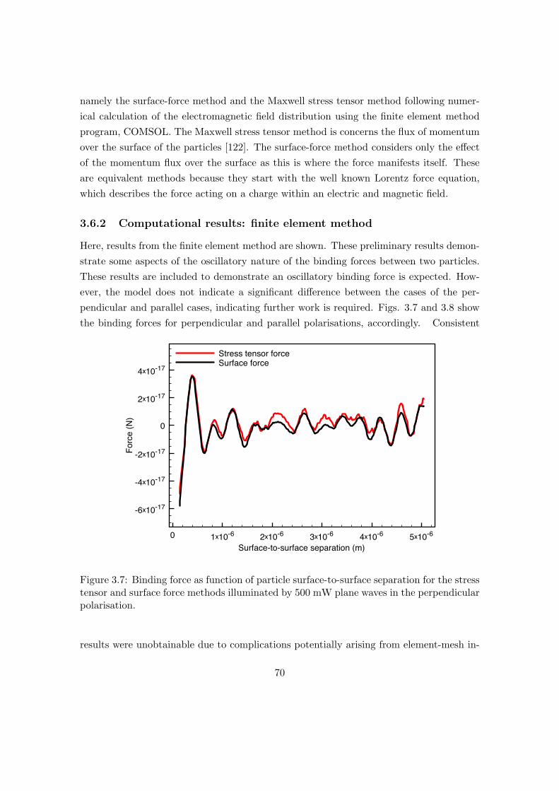
namely the surface-force method and the Maxwell stress tensor method following numer-ical calculation of the electromagnetic field distribution using the finite element methodprogram, COMSOL. The Maxwell stress tensor method is concerns the flux of momentumover the surface of the particles [122]. The surface-force method considers only the effectof the momentum flux over the surface as this is where the force manifests itself. Theseare equivalent methods because they start with the well known Lorentz force equation,which describes the force acting on a charge within an electric and magnetic field.

3.6.2 Computational results: finite element method

Here, results from the finite element method are shown. These preliminary results demon-strate some aspects of the oscillatory nature of the binding forces between two particles.These results are included to demonstrate an oscillatory binding force is expected. How-ever, the model does not indicate a significant difference between the cases of the per-pendicular and parallel cases, indicating further work is required. Figs. 3.7 and 3.8 showthe binding forces for perpendicular and parallel polarisations, accordingly. Consistent

0 1x10-6 2x10-6 3x10-6 4x10-6 5x10-6

Surface-to-surface separation (m)

-6x10-17

-4x10-17

-2x10-17

0

2x10-17

4x10-17

Forc

e (N

)

Stress tensor forceSurface force

Figure 3.7: Binding force as function of particle surface-to-surface separation for the stresstensor and surface force methods illuminated by 500 mW plane waves in the perpendicularpolarisation.

results were unobtainable due to complications potentially arising from element-mesh in-

70

0 1x10-6 2x10-6 3x10-6 4x10-6 5x10-6

Surface-to-surface separation (m)

-8x10-17

-6x10-17

-4x10-17

-2x10-17

0

2x10-17Fo

rce

(N)

Stress tensor forceSurface force

Figure 3.8: Binding force as function of particle surface-to-surface separation for the stresstensor and surface force methods illuminated by 500 mW plane waves in the parallelpolarisation.

consistencies, particularly when particles were in close proximity. However in principle,infinitesimally small elements may improve results, however this is not to say that thisalone would necessarily solve the problems with this model.

3.7 Computational study: interacting dipole method

In light of the results of the finite element models it is prudent to consider the case ofa simple pair of interacting dipoles instead. In this situation the problem is simplifiedsignificantly, such that an analytical study is feasible due to the relative small size ofthe interacting dipoles relative to the illuminating wavelength. A model was developedinvolving an interacting dipole method to calculate the binding forces acting on at leasta pair of Rayleigh-sized particles. Further, the model was implemented for broadbandspectral content.

71

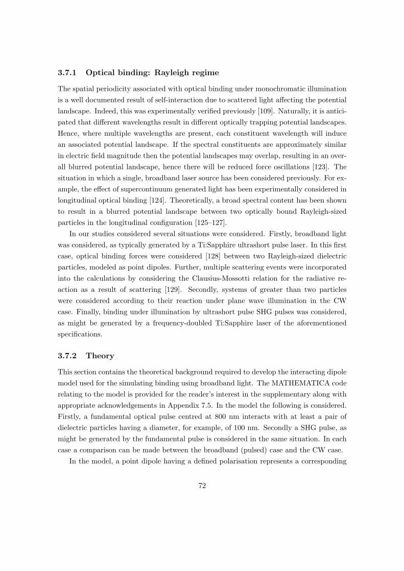
3.7.1 Optical binding: Rayleigh regime

The spatial periodicity associated with optical binding under monochromatic illuminationis a well documented result of self-interaction due to scattered light affecting the potentiallandscape. Indeed, this was experimentally verified previously [109]. Naturally, it is antici-pated that different wavelengths result in different optically trapping potential landscapes.Hence, where multiple wavelengths are present, each constituent wavelength will inducean associated potential landscape. If the spectral constituents are approximately similarin electric field magnitude then the potential landscapes may overlap, resulting in an over-all blurred potential landscape, hence there will be reduced force oscillations [123]. Thesituation in which a single, broadband laser source has been considered previously. For ex-ample, the effect of supercontinuum generated light has been experimentally considered inlongitudinal optical binding [124]. Theoretically, a broad spectral content has been shownto result in a blurred potential landscape between two optically bound Rayleigh-sizedparticles in the longitudinal configuration [125–127].

In our studies considered several situations were considered. Firstly, broadband lightwas considered, as typically generated by a Ti:Sapphire ultrashort pulse laser. In this firstcase, optical binding forces were considered [128] between two Rayleigh-sized dielectricparticles, modeled as point dipoles. Further, multiple scattering events were incorporatedinto the calculations by considering the Clausius-Mossotti relation for the radiative re-action as a result of scattering [129]. Secondly, systems of greater than two particleswere considered according to their reaction under plane wave illumination in the CWcase. Finally, binding under illumination by ultrashort pulse SHG pulses was considered,as might be generated by a frequency-doubled Ti:Sapphire laser of the aforementionedspecifications.

3.7.2 Theory

This section contains the theoretical background required to develop the interacting dipolemodel used for the simulating binding using broadband light. The MATHEMATICA coderelating to the model is provided for the reader’s interest in the supplementary along withappropriate acknowledgements in Appendix 7.5. In the model the following is considered.Firstly, a fundamental optical pulse centred at 800 nm interacts with at least a pair ofdielectric particles having a diameter, for example, of 100 nm. Secondly a SHG pulse, asmight be generated by the fundamental pulse is considered in the same situation. In eachcase a comparison can be made between the broadband (pulsed) case and the CW case.

In the model, a point dipole having a defined polarisation represents a corresponding

72

dielectric particle and is given by [130]

pj = ε0αE, (3.9)

where pj and E represent the jth microscopic polarisation and electric field, respectively.While, ε0 is the permittivity of free space. The macroscopic polarisability, α is providedby [130]

α = 4πa3n2 − 1n2 + 2

, (3.10)

where n is the index of refraction (relative to unity) and a is the assumed particle radius(note the polarisability of particles is calculated from the volume; however the modelassumes these particles are point dipoles). The illuminating laser field observed by thepoint dipole is assumed to be constant due to the particle being sized in the Rayleighregime. The field E′, which is scattered by any jth dipole can be described by [130]

E′ =eiω|r|/c

4πε0

(ω2(r× pj)× r

c2|r|3+

(c− iω|r|)(3(r · pj)r− |r|2pj

)c|r|5

), (3.11)

wherein the constants c, ε0 represent the speed of light and free space permittivity, respec-tively. The angular frequency is represented by its normal symbol, ω. A position vector,r is used to define a displaced position with respect to the corresponding position of thejth dipole given by rj.

Equation (3.11) is unified byE′ = M(r)E (3.12)

wherein M is a second order tensor. The matrix, Mij

describes the scattered electric fieldat the ith position ri. This field comprises two parts. In the first part, E = E0

j + Ej,where E0

j is the incident field. The second part, Ej corresponds to the scattered fieldthat originates from all other dipoles, rj. Multiple scattering events can be considered bydefining a self-consistent relationship, whereby all the fields are linked together through

Ei =∑j 6=i

Mij

(E0j + Ej). (3.13)

Equation 3.13 comprises 3N equations with N unknown vector fields. The solution ofthis system of equations provides the the total scattered optical fields, whereby N dipolesmay be subjected to an arbitrary incident field. Larger particles can be instead consideredthrough the coupled dipole method [131], whereby the larger particles are treated as a

73

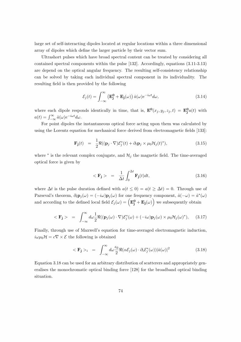
large set of self-interacting dipoles located at regular locations within a three dimensionalarray of dipoles which define the larger particle by their vector sum.

Ultrashort pulses which have broad spectral content can be treated by considering allcontained spectral components within the pulse [132]. Accordingly, equations (3.11-3.13)are depend on the optical angular frequency. The resulting self-consistency relationshipcan be solved by taking each individual spectral component in its individuality. Theresulting field is then provided by the following

Ej(t) =∫ ∞−∞

(E0

j + Ej(ω))a(ω)e−iωtdω, (3.14)

where each dipole responds identically in time, that is, E0(xj , yj , zj , t) = E0j a(t) with

a(t) =∫∞−∞ a(ω)e−iωtdω.

For point dipoles the instantaneous optical force acting upon them was calculated byusing the Lorentz equation for mechanical force derived from electromagnetic fields [133]:

Fj(t) =12<((pj · ∇)E∗j (t) + ∂tpj × µ0Hj(t)∗), (3.15)

where ∗ is the relevant complex conjugate, and Hj the magnetic field. The time-averagedoptical force is given by

< Fj > =1

∆t

∫ ∆t

0Fj(t)dt, (3.16)

where ∆t is the pulse duration defined with a(t ≤ 0) = a(t ≥ ∆t) = 0. Through use ofParseval’s theorem, ∂tpj(ω) = (−iω)pj(ω) for one frequency component, a(−ω) = a∗(ω)and according to the defined local field Ej(ω) =

(E0

j + Ej(ω))

we subsequently obtain

< Fj > =∫ ∞−∞

dω12<((pj(ω) · ∇)E∗j (ω) + (−iω)pj(ω)× µ0Hj(ω)∗), (3.17)

Finally, through use of Maxwell’s equation for time-averaged electromagnetic induction,iωµ0H = c∇× E the following is obtained

< Fj >i =∫ ∞−∞

dωε02<(αEj(ω) · ∂iE∗j (ω))|a(ω)|2 (3.18)

Equation 3.18 can be used for an arbitrary distribution of scatterers and appropriately gen-eralises the monochromatic optical binding force [128] for the broadband optical bindingsituation.

74

Figure 3.9: Optical binding force between two particles under illumination from light at 800nm having a perpendicular polarisation (blue, large oscillations) or a parallel polarisation(magenta line). An illustration in this figure indicates the general orientation used inobtaining the graph.

3.7.3 Broadband ultrashort pulsed optical binding

It is known that the optical binding spatial periodicity for CW illumination depends uponthe wavelength within the host medium [109, 121]. As such, where multiple wavelengthsare present, each constituent has its own associated binding potential, which overlap withone another. When using broadband light therefore, the binding potentials are certainlyexpected to overlap. The analysis in the previous section presents this exact argumentthrough equation 3.18. In this section broadband illumination is considered having a band-width of 100 nm centred at 800 nm, thus corresponding to a 9.4 fs pulse. For calculationof polarisability the particles have a diameter of 100 nm. The peak electric field amplitudeused was 1.1 × 107 V/m, which corresponds to an average power of 1.0 W with a beamwaist of 2 µm. In each case the perpendicular and parallel polarisations relative to thelong axis of the focussed beam were considered. The broadband situation was also directlycompared with the CW case to demonstrate how much distortion might be expected. Fig.3.9 refers to a comparison between the binding forces when the particles are illuminated

75

by perpendicular or parallel polarisations, wherein the amplitude of oscillations decreasesmore rapidly with distance for the parallel case.

Figure 3.10: Comparison of binding forces for perpendicular polarisation optical bindingunder 800 nm-centred broadband illumination. In this case the larger oscillations (ma-genta) refer to the CW case; the smaller oscillations (blue) refer to the broadband case.Note the significant decrease in oscillation amplitude with increasing separation.

Fig. 3.10 features broadband binding, wherein a 100 nm bandwidth pulse is directlycompared with the CW equivalent for the perpendicular polarisation. Further, Fig. 3.11includes the same parameters but with parallel polarisation instead.

As expected for the broadband case the binding forces are decreased in magnituderelative to the CW case. Further, there is a significant difference between the two illumi-nation polarisations. In the case of the perpendicular polarisation the difference betweenbroadband and CW illumination is obvious. Whereas for the parallel polarisation casethere is not much observable difference. This would likely manifest itself in an experimen-tal regime, thus a difference as described would be most likely observed with the correctpolarisation direction. It should be re-stated that these results refer to Rayleigh-sizedparticles. However, equivalent results have been demonstrated in the Mie-size regime.The main point to consider is the minimum centre-to-centre distance between the parti-cles described in the experiments is 1.8 microns. Therefore this would be equivalent to

76

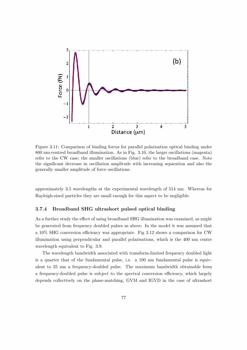
Figure 3.11: Comparison of binding forces for parallel polarisation optical binding under800 nm-centred broadband illumination. As in Fig. 3.10, the larger oscillations (magenta)refer to the CW case; the smaller oscillations (blue) refer to the broadband case. Notethe significant decrease in oscillation amplitude with increasing separation and also thegenerally smaller amplitude of force oscillations.

approximately 3.5 wavelengths at the experimental wavelength of 514 nm. Whereas forRayleigh-sized particles they are small enough for this aspect to be negligible.

3.7.4 Broadband SHG ultrashort pulsed optical binding

As a further study the effect of using broadband SHG illumination was examined, as mightbe generated from frequency doubled pulses as above. In the model it was assumed thata 10% SHG conversion efficiency was appropriate. Fig 3.12 shows a comparison for CWillumination using perpendicular and parallel polarisations, which is the 400 nm centrewavelength equivalent to Fig. 3.9.

The wavelength bandwidth associated with transform-limited frequency doubled lightis a quarter that of the fundamental pulse, i.e. a 100 nm fundamental pulse is equiv-alent to 25 nm a frequency-doubled pulse. The maximum bandwidth obtainable forma frequency-doubled pulse is subject to the spectral conversion efficiency, which largelydepends collectively on the phase-matching, GVM and IGVD in the case of ultrashort

77

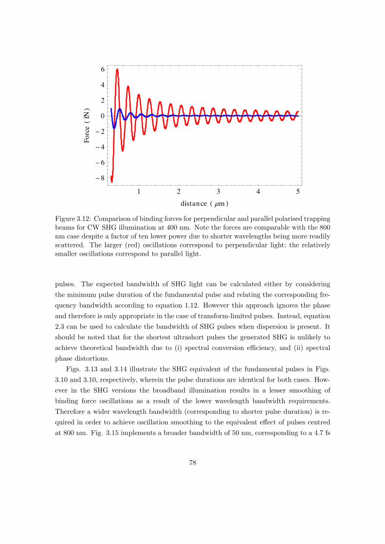
1 2 3 4 5

!8

!6

!4

!2

0

2

4

6

distance ! "m "

Force!fN"

Figure 3.12: Comparison of binding forces for perpendicular and parallel polarised trappingbeams for CW SHG illumination at 400 nm. Note the forces are comparable with the 800nm case despite a factor of ten lower power due to shorter wavelengths being more readilyscattered. The larger (red) oscillations correspond to perpendicular light; the relativelysmaller oscillations correspond to parallel light.

pulses. The expected bandwidth of SHG light can be calculated either by consideringthe minimum pulse duration of the fundamental pulse and relating the corresponding fre-quency bandwidth according to equation 1.12. However this approach ignores the phaseand therefore is only appropriate in the case of transform-limited pulses. Instead, equation2.3 can be used to calculate the bandwidth of SHG pulses when dispersion is present. Itshould be noted that for the shortest ultrashort pulses the generated SHG is unlikely toachieve theoretical bandwidth due to (i) spectral conversion efficiency, and (ii) spectralphase distortions.

Figs. 3.13 and 3.14 illustrate the SHG equivalent of the fundamental pulses in Figs.3.10 and 3.10, respectively, wherein the pulse durations are identical for both cases. How-ever in the SHG versions the broadband illumination results in a lesser smoothing ofbinding force oscillations as a result of the lower wavelength bandwidth requirements.Therefore a wider wavelength bandwidth (corresponding to shorter pulse duration) is re-quired in order to achieve oscillation smoothing to the equivalent effect of pulses centredat 800 nm. Fig. 3.15 implements a broader bandwidth of 50 nm, corresponding to a 4.7 fs

78

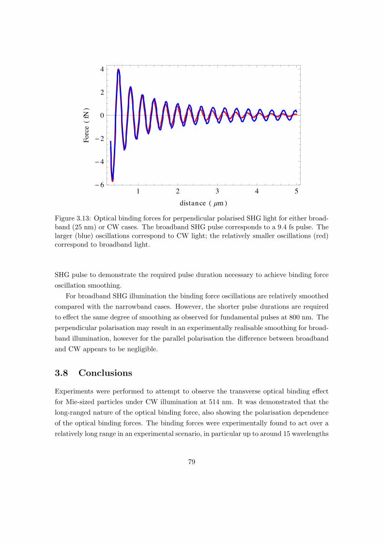
1 2 3 4 5!6

!4

!2

0

2

4

distance ! "m "

Force!fN"

Figure 3.13: Optical binding forces for perpendicular polarised SHG light for either broad-band (25 nm) or CW cases. The broadband SHG pulse corresponds to a 9.4 fs pulse. Thelarger (blue) oscillations correspond to CW light; the relatively smaller oscillations (red)correspond to broadband light.

SHG pulse to demonstrate the required pulse duration necessary to achieve binding forceoscillation smoothing.

For broadband SHG illumination the binding force oscillations are relatively smoothedcompared with the narrowband cases. However, the shorter pulse durations are requiredto effect the same degree of smoothing as observed for fundamental pulses at 800 nm. Theperpendicular polarisation may result in an experimentally realisable smoothing for broad-band illumination, however for the parallel polarisation the difference between broadbandand CW appears to be negligible.

3.8 Conclusions

Experiments were performed to attempt to observe the transverse optical binding effectfor Mie-sized particles under CW illumination at 514 nm. It was demonstrated that thelong-ranged nature of the optical binding force, also showing the polarisation dependenceof the optical binding forces. The binding forces were experimentally found to act over arelatively long range in an experimental scenario, in particular up to around 15 wavelengths

79

1 2 3 4 5

!1.0

!0.5

0.0

0.5

1.0

1.5

distance ! "m "

Force!fN"

Figure 3.14: Optical binding forces for parallel polarised SHG light for either broadband(25 nm) or CW cases. The larger (blue) oscillations correspond to CW light; the slightlysmaller oscillations (red) correspond to broadband light.

for the perpendicular polarisation at 514 nm. The force arising from parallel polarised lightdecays far more quickly with increasing distance than the perpendicular polarisation.

In relation to the broadband optical binding work it should be noted that broadbandsources could include: a) a broadband 10fs source, b) an ultrabroadband 5fs source or c)a supercontinuum-ultrabroadband source. CW experiments were necessary as a prelimi-nary study as little experimental work on this topic had been previously considered. Theamplitude and direction of the incident and scattered electric field in the region of thefocus defines the strength of any binding force. Importantly, if the electric field amplitudewas too small, statistical fluctuations (Brownian motion) would wash out binding oscilla-tions. In this case, the results would provide a flat potential with no oscillations, which isidentical to the expected result from a sufficiently broadband source. Therefore, the sameoptical power would be required for broadband sources (providing focussing conditionsare identical). However, after transmission through a typical optical binding experimentalsetup, average powers from typical Ti:Sapphire systems may not be enough to permitobservation of optical binding. Therefore, a supercontinuum source was attempted due toits high average power (6W). In this case only 50 mW of average power remained aftertransmission through the setup. Alternative configurations may provide sufficient bindingforce amplitudes, for example, by enhancing the focussing conditions to provide a higher

80

1 2 3 4 5!6

!4

!2

0

2

4

distance ! "m "

Force!fN"

Figure 3.15: Optical binding forces for perpendicular polarisation under either broadband(50 nm) or CW SHG illumination. The broadband pulse corresponds to a 4.7 fs pulse. Thisshorter pulse duration is necessary in order to introduce sufficient smoothing of oscillationsas seen for fundamental pulses. The larger (blue) oscillations correspond to CW light; therelatively smaller oscillations (red) correspond to broadband light.

peak intensity at the beam focus. However, the purpose of the theoretical studies was tobuild a framework for future experiments. In order to understand how much bandwidthis required to observe binding then modelling is required. This way future experimentscould be designed with those modelling results in mind.

We further attempted to model the experimental studies using the finite elementmethod to investigate the optical binding forces from a computational perspective. Wedid not obtain reliable results in this endeavor, however some indicative data demonstrat-ing the oscillatory nature of optical binding was observed. We also used an interactingdipole method to model point oscillators with the polarisability calculated from 100 nmdiameter particles for CW and broadband illumination. The wavelength of the illuminat-ing light provides a well defined oscillatory optical binding force relationship for varyinginter-particle distance or broadband illumination. However in broadband illumination thiswell-defined relationship breaks down because the optical binding potential is spatially de-pendent upon wavelength and so regions which attract the particles do so with less forcethan if using CW illumination. We further investigated SHG-illuminated optical binding

81

and found that the pulse duration required for binding wavelength-dependent oscillationsis substantially shorter for SHG than for fundamental pulses due to the lower wavelengthcontent within the pulse. The computational results are potentially indicative of the bind-ing interaction in an experimental setting in that a very wide bandwidth is required forsmoothing of the binding oscillations. It should be noted that in any future work involv-ing ultrashort pulses, the MIIPS system would be arbitrarily capable of delivering neartransform-limited ultrashort pulses at the sample plane for the envisaged experiments..

The experimental work in this chapter has been published in (i) Proc. SPIE, 7400,2009 [121], (ii) J. Phys. Condens. Matter, 2012 (accepted) [134] and (iii) Proc. SPIE,2012 (accepted).

3.9 Chapter acknowledgements

In this chapter Michael Mazilu designed and implemented the computational studies in-cluding finite element models and the interacting dipole models. Further, Joerg Baumgartldesigned the experimental aspects and related particle tracking software in LABVIEW.The author built experimental setups and performed computational studies by adaptingand editing the computational models as appropriate.

82

Chapter 4

The role of femtosecond pulse

duration in the membrane

permeabilisation of mammalian

cells

4.1 Introduction

This chapter covers experimental work to characterise the ultrashort laser pulse-inducedmembrane permeabilisation of mammalian cells. Most importantly, the studies in thischapter would not be permitted were it not for the pulse shaping and measurement appa-ratus referred to previously. This is because dispersion is difficult to measure accurately.The MIIPS procedure provides means for measuring phase in situ to enable delivery of op-timised transform-limited ultrashort pulses. The membrane permeability is quantified byperforming dye injection experiments known as optoinjection. In this study I performedexperiments across a wide parameter space including pulse duration, pulse energy andnumber of pulses. The results show that two distinct membrane permeabilisation regimesexist. The first of these regimes show an initial nonlinear dependence of order 3.5-9.6, withthe second regime exhibiting a typically linear dependence. The transition between thesetwo regimes is marked by a threshold peak power of between 6-20 kW. These results indi-cate that multiphoton absorption produces a quasi-free electron plasma within the focusof the beam, with the membrane permeabilisation mechanism requiring this multiphotoninitiation for the subsequent regime change, whereby linear absorption dominates. Fur-

83

thermore I show that the number of pulses define the probability with which membranepermeabilisation occurs over time, with the peak power defining the mean and standarddeviation number of pulses in order to achieve 50 % efficiency.

Ultrashort laser pulses have proven to be important in the field of biophotonics [135].The high peak power associated with the ultrashort pulses is crucial for initiating a non-linear response from matter, and this nonlinear property is very useful in the case ofbiological matter. However, manipulating biological matter using ultrashort pulses re-quires extraordinary care due to the possibility of damage resulting from over-exposureto the high intensities associated with focussed laser beams. Therefore it is important tounderstand what effect different laser parameters have on biological material. The relevantparameters are laser wavelength (and bandwidth), pulse energy, spatial beam profile, laserrepetition rate, number of pulses and pulse duration (and pulse shape).

Ultrashort pulses have been used in a wide variety circumstances concerning biologicalmatter. These can be defined in terms of regimes relating to extent of damage which occursupon laser irradiation. The first of these regimes is the low damage regime, with low celldeath rates associated with irradiation with laser beams whose parameters are such thatno short term damage occurs. Naturally, any exposure to light can cause damage and somecell death ensues. The main application of ultrashort pulses in the low damage regimeis imaging. For example, two-photon excited fluorescence (TPEF) and second harmonicgeneration (SHG) are important methods for the high resolution imaging of thick biologicalmatter [136]. The application of longer wavelengths, typically in the near infrared also addsthe prospect of deeper penetration using such modalities. Both TPEF and SHG exhibita quadratic dependence upon the peak intensity of the incident laser field [17], thereforethe signal to noise ratio is greatly improved owing to the nonlinear response associatedwith the ultrashort pulses. The high damage regime can be defined in terms of therapid onset of irreversible damage and cell death. This regime has applications in single-cell nanosurgery and tissue surgery, wherein nanosurgery is defined in terms of spatiallyconstrained surgery down to the nano-scale [137, 138]. In this regime a wide parameterspace covering pulse energy [139] and repetition rate [140, 141] have been investigated.The pulse duration dependence of nanosurgery has also been investigated in which anapproximate τ−1/2 relationship was found [142]. Typically the laser parameters used inoptoinjection and phototransfection experiments are similar, for example being of theorder of nJ for MHz repetition rate pulses [141]. Phototransfection using sub-20 fs pulseshas been demonstrated using pulse energies of less than 93 pJ [18].

For this chapter, the region between the low damage and high damage regimes is par-ticularly relevant. The correct choice of laser parameter is essential for maintaining the

84

desired effect and therefore it is crucial to understand the processes leading up cell damagein order to either prevent this damage, or to utilise this damage. One of the applicationsin this region between low and high damage is phototransfection [143]. Phototransfec-tion involves the permeabilisation of a single-cell membrane using focussed a laser beamin order to permit the introduction of membrane-impermeable genetic material into thecell itself. Understanding the mechanisms which permit the phototransfection of cells isessential for future development of the field. Due to the multiple biological fluctuationsassociated with cell transfection, it is impractical to gather sufficient statistics to helpunderstand the processes leading to cell membrane permeabilisation. Instead, we utiliseanother light-induced membrane permeabilisation technique known as optoinjection [144].Optoinjection involves the introduction of membrane-impermeable fluorescent dyes intosingle cells. This technique is completely equivalent to the phototransfection technique,however, the technique offers superior statistical information due to the consistent repro-ducibility of the technique.

The processes leading up to membrane permeabilisation are complicated and not yetfully understood [137]. Currently, the model by Vogel et al. offers the greatest insightinto membrane permeabilisation mechanisms [137]. In this model, biological material isconsidered as an amorphous semiconductor based on pure water, due to the high watercontent of cells. The justification of using water is due to the high water content ofcells. However, it is noted in this model that in reality the situation is considerably morecomplicated, for example, by proteins, lipids, dyes and the like. Upon irradiation withultrashort laser pulses, multiphoton absorption promotes electrons from the valence bandup to the conduction band. Inverse Bremsstrahlung absorption events in which conductionelectrons are scattered by incident photons increases the kinetic energy of these electronsup to a critical energy sufficient for impact ionisation to occur. An avalanche increase inthe population density of conduction electrons means that a quasi-free electron plasmais formed in the region of high intensity laser pulses. This plasma is associated with thedisruption and modification of chemical bonds in the region and subsequently membranepermeabilisation can occur. The multiphoton initiation of membrane permeabilisation istherefore a critical feature for ultrashort pulse optoinjection and phototransfection. Theparameters associated with defining the multiphoton response are the pulse duration andpulse energy due to their connection with the peak power through the formula

Ppeak = ksEpτp

(4.1)

where ks is a constant which depends on the temporal profile of the pulse, Wp is the pulse

85

energy and τp is the pulse duration. Several studies have investigated the parameter spacefor cell membrane permeabilisation. In particular, the optoinjection efficiency as functionof pulse energy and number of pulses has been investigated [139, 144]. The phototrans-fection efficiency has been investigated for various parameter including laser fluence [143]and spatial beam profile through the generation of novel beam shapes [145]. In terms ofpulse duration, there has been one study concerning optoinjection and phototransfectionof cells using sub-20 fs pulses, in which significant decreases in pulse duration permittedphototransfection at decreased pulse energies [18].

We have experimentally determined the absorption characteristics of mammalian cellmembranes to ultrashort pulses within the temporary modifcation regime. This studycomprehensively covers the laser parameters pulse duration, pulse energy and number ofpulses. Crucially, this study is made possible through the implementation of the MIIPStechnique in order to measure and characterise the pulse duration in situ at the focus of themicroscope objective. Without the MIIPS technique this would not have been possible dueto the complicated dispersion profile of the experimental setup. The implications of theresults and have found that the nonlinear (multiphoton) absorption is critical for initiatingefficient linear absorption. The nonlinear absorption generates a quasi-free electron plasmawithin the focal region of the laser pulse which collectively alters the nonlinear and linearabsorption characteristics over a series of pulses. In particular it was found that a peakpower threshold defines the region between the (intially) nonlinear and (finally) linearabsorption. Furthermore, the number of pulses required to initiate optoinjection stronglydepends upon the peak power associated with pulse duration and energy, with a sufficientlyhigh peak power necessary for efficient optoinjection.

4.2 Methods

4.2.1 Experimental arrangement using MIIPS system

The experimental arrangement is shown in Fig. 4.1. A KM Labs Swift 10 TitaniumSapphire oscillator (bandwidth = 60 nm, center wavelength = 800 nm, transform-limitedpulse duration of 17 fs) was used for all the optoinjection experiments. A Nikon EclipseTi inverted microscope was used with two objectives employed. A Nikon 0.8NA/60x airobjective was used when acquiring and measuring the shortest possible pulse durationand for completing the optoinjection experiments. A Nikon 40x/0.75NA phase contrastobjective and an Andor Clara CCD camera cooled to -55C were used for phase contrastand fluorescent images. An electronic shutter (home-built electronic controller; Newport

86

shutter) was used to controllably permit a specified number of pulses.Fig. 4.2 shows the fundamental laser spectrum and typical phase distortion obtained

and corrected by the MIIPS procedure, as discussed in described in chapter 2. Crucially,the shape of the dispersion profile indicates significant higher order phase contributionsthat would not be easily measured and compensated for without the MIIPS procedure. Wecontrollably stretched the pulses using anti-reflection coated BK7 optical flats. The flatscontribute GVD to the beam, stretching the pulse without introducing higher order effects.This was confirmed by measuring the dispersion caused by the flats using the MIIPSsystem. Only second-order dispersion was introduced by the optical flats with negligiblehigher-order contributions. Furthermore, the anti-reflection coated flats maintained thesame optical transmission even when several flats were inserted into the beam path. Usinga combination of 3mm and 5mm thickness flats the following pulse durations were obtained:17, 28, 44, 68, 80, 105, 120 and 143 fs. GVD does not change the temporal profile otherthan affecting the peak power inversely for increasing pulse duration [132]. The opticalflats did not in away change the spatial profile or direction of the beam and were carefullyinserted into the beam path so as to avoid any adverse effects.

4.2.2 Optoinjection: cell culture and experimental procedure

Chinese Hamster ovary (CHO) cells were cultured in medium consisting of MinimumEssential Medium (Sigma), 10% Fetal Calf Serum (Sera Laboratories International) andL-Glutamine, Penicillin and Streptomycin (Sigma). The cells were plated on 23 mm glass-bottom Petri dishes (Fluorodish, World Precision Instruments) and incubated for at least24 hours until cells populated the bottom of the Petri dish.

Optoinjection experiments were performed to assess the cell membrane permeability asfunction of laser parameter [146]. The membrane-impermeable dye, Propidium Iodide (PI,Sigma-Aldrich) was used to indicate whether the cell was permeabilised by the absorptionof laser pulses. The medium was subsequently removed from the Petri dish containingthe adherent cells. The Petri dish was washed twice with Opti-MEM (Invitrogen). A 3µM solution of PI in Opti-MEM was added to the sample dish, wherein Opti-MEM wasthe solvent. PI molecules bind to DNA and RNA in the cell and glow red under greenexcitation when suitably bound to those molecules [147]. The phase-contrast objectivewas used to image cells as it provided better contrast for the cells, which are relativelytransparent. The laser parameter choice was selected and the 60x/0.8NA objective usedto irradiate the cell of interest at 3 axial locations, separated by 1-2 microns. The cellsof interest were chosen by drawing a small square (on the underside of the sample dish)

87

Figure 4.1: Experimental setup with CAM representing the electronically cooled camera,DCM: dichroic mirror, ESH: electronically controlled shutter, MDU: MIIPS microscopedetection unit, OBJ: objective lens and OF: optical flats. The lens f1 through f4 refer tothe following sequence of focal lengths: 10 cm, 20 cm, 10 cm and 25 cm. The illuminationscheme, mercury lamp and filter cubes are not shown for clarity.

so as to identify the relevant cells within that square when viewed under the microscope.Preferably the square was small enough so that approximately less than 50-60 cells werein the square at one time. This was to assist in decreasing the number of cells requiringidentification during each stage of the process. Targeting at three sufficiently separateaxial locations does not compromise cell viability providing the axial separation is largeenough [146]. The pulse energy at the sample was calculated using the dual-objectivetransmission method [148] with a power meter to measure average power and using theknown repetition rate of 76 MHz. The Nikon 60x/0.8NA objective was found to have atransmission ratio of 66%. Thirty cells were targeted and irradiated by the laser in each

88

700 750 800 850 900Wavelength (nm)

0

10000

20000

30000

40000

50000

60000Fu

ndam

enta

l spe

ctru

m in

tens

ity (a

rb. u

nits

)

-50

0

50

100

150

200

250

300

Ret

rieve

d sp

ectra

l pha

se (r

adia

ns)

Fundamental spectrumRetrieved spectral phase

Figure 4.2: Fundamental laser spectrum with the retrieved spectral phase dispersion profileobtained by the MIIPS procedure.

Petri dish. After 5 minutes a fluorescence image was taken to check which of the targetedcells contained PI. This was compared with a control fluorescence image to check for falsepositives. The efficiency of optoinjection was calculated as the ratio between successfullyoptoinjected (fluorescent) cells and the number of targeted cells. The PI solution wasthen removed and the cells were washed twice with culture medium and fresh mediumwas added and the cells incubated for at least 90 minutes. A live assay with CalceinAM (CAM, Invitrogen) was implemented to check the viability of cells after 90 minutes,wherein CAM interacts with esterases in the cell, which are only present if the cell isalive [146]. Viability was consistently 100% for the low-medium optoinjection efficiency(<60%) samples. After which, viability was only checked where optoinjection efficiencywas significantly higher than 60%, or if a visible microbubble was observed during thetargeting procedure.

To obtain adequate statistics, each experiment involving a different set of parame-ters was repeated 8 times per set, each referring to 8x30 cells. The phase contrast andfluorescent images obtained from a representative optoinjection experiment are shown infalse colour in Fig. 4.3 and show cells that were successfully optically injected and the

89

corresponding viable cells.

Figure 4.3: Example image of cells optically injected with PI and tested for viability withCAM. Left: Before irradiating (phase contrast), Center: PI uptake (false colour), Right:CAM viability test (false colour).

4.3 Results: optoinjection

A wide parameter space covering multiple combinations of pulse duration, pulse energy andnumber of pulses was explored. For reference purposes, Table 4.1 displays the relationshipbetween these three parameters and the associated expressions which relate the parametersto the independent variables: peak power and total energy. Table 4.2 summarises theparameter space explored.

4.3.1 The role of pulse duration

By varying the pulse duration it was possible to controllably change the peak powerwithout affecting the total energy, thereby defining the efficiency with which nonlinearprocessed occurred without being concerned with separate linear absorption issues. Thetime-averaged intensity-response (Sn) for number of photons (n) follows

Sn ∝Wnp τ

1−np , (4.2)

where Wp is the pulse energy and τp is the pulse duration [149]. The optoinjection pro-cess requires optical absorption in the locality of the cellular membrane, with the efficiencydepending upon linear and nonlinear absorption. However, the nonlinear absorption mech-anisms do not necessarily depend upon any one order of n-photon processes. Therefore weintroduce a new concept which we refer to as an effective photon number, nef. This is dueto the multiple possibilities for multiphoton absorption owing to the complex nature of thebiological matter. The molecules contained within the biological matter each have their

90

Pulse duration(τ)

Pulse energy(Wp)

Number ofpulses (Np)

Expression

Peak power(Ppeak)

∝ τ−1 ∝Wp no effectPpeak =kWpτ

−1p

Total energy(Etotal)

no effect ∝Wp ∝ Np Etotal = WpNp

Associatedabsorption

mechanismsNonlinear only

Nonlinear andlinear

Linear only〈Sn〉 ∝Wn

p τ1−n

Fig. reference: 4.4 4.5 4.6

Table 4.1: The three varied parameters: pulse duration, pulse energy and number of pulsesinfluence peak power and total energy in the manner shown on the table. The expressionsassociated with peak power (Ppeak) and total energy (Etotal) are also shown with k being aconstant depending on the temporal profile of the pulse. The table also shows whether theparameter is generally associated with influencing either the nonlinear or linear absorptionmechanisms and the associated expression.

own nonlinear cross section, defining the probability of nonlinear processes occurring. Wetherefore can represent Sn in terms of a sum of several different nonlinear orders

〈Sn〉 =n∑i=1

k(i)W ipτ

1−ip , (4.3)

where k(i) represents the probability that the i number of photons are responsible forthe given interaction. If the sum is normalized it will yield a probability that a n-photonprocess is responsible for the interaction. However it is not possible to establish the proba-bility of each the n-photon components. Therefore we must average the number of photonsresponsible and instead calculate the effective photon number, nef. The interpretation ofthe effective photon number therefore indicates the number of photons with the highestprobability of being responsible for an interaction, or the dominating photon number.However it must be stressed that a different photon number could simultaneously be re-sponsible for the interaction and therefore the effective photon number is weighted overseveral photon numbers. Consequently the effective photon number will not necessarilyhave an integer value but instead it indicates the approximate photon number responsiblefor the interaction.

By considering the parameter 〈Sn〉 to be equivalent to the probability that the cell

91

Experimentalset: (Fig.reference)

Pulsedurationrange (fs)

Pulseenergyrange(nJ)

Numberof pulses(×106)

Photonorder(nef)

Thresholdpeakpower(kW)

Meanpulse

number(×106)

1: (4.4) 17-68 0.5 3.0 1.5 ± 0.2 8 ± 2 N/A1: (4.4) 68-143 0.5 3.0 3.5 ± 2.0 as above N/A2: (4.4) 17-80 1.1 1.5 1.5 ± 0.2 11 ± 2 N/A2: (4.4) 80-143 1.1 1.5 6.6 ± 2.5 as above N/A3: (4.4) 17-80 1.8 0.4 3.6 ± 0.5 N/A N/A

4: (4.5) 17 0.33-0.6 3.0 0.9 ± 0.2 18 ± 2 N/A4: (4.5) 17 0.26-0.33 3.0 7.6 ± 2.0 as above N/A5: (4.5) 68 0.53-0.8 3.0 1.3 ± 0.5 7 ± 1 N/A5: (4.5) 68 0.40-0.53 3.0 5.7 ± 2.3 as above N/A6: (4.5) 17 0.53-0.8 0.4 3.3 ± 1.0 N/A N/A

7: (4.6) 17 0.5 0.4-3.0 N/A N/A 1.1 ± 0.58: (4.6) 44 0.5 0.8-6.0 N/A N/A 3.4 ± 1.59: (4.6) 80 0.5 1.5-7.5 N/A N/A 10 ± 6

Table 4.2: Summary of experimental parameter space explored. Sets 1-3 refer to experi-ments involving varying the pulse duration, sets 4-6 refer to experiments involving varyingthe pulse energy and sets 7-9 refer to experiments involving varying the number of pulses.Also note the threshold peak powers are calculated at the inflection points on the data fits;the inflection points are unavailable for sets 3 and 6 and are listed as N/A in the table.Finally, the mean pulse numbers were calculated by considering a Gaussian error functionfitted to the data in Fig. 4.6 and performing a linear regression fit to find the mean pulsenumber. The ERF was numerically differentiated to find the probability density function(PDF) and corresponding standard deviation. Where not applicable these are also listedas N/A. The parameters were chosen initially to reflect typical values used in the field (40ms irradiation times). Subsequently, parameters were chosen to see what happened if oneparameter was dramatically changes, for example, doubling the pulse energy.

92

will be permeabilized we can associate the effective photon number with the optoinjectionefficiency. We do this by taking the logarithm of

〈Sn〉 = Wnefp τ1−nef (4.4)

and varying τp and holding Wp constant, or vice versa. We perform a linear regression fiton the gradient obtained on a log-log scale of optoinjection efficiency. We associate theobtained gradient with the effective photon number. Therefore in varying τp the effectivephoton number is given by nef = 1 −m for a gradient m When varying Wp the effectivephoton number is given by nef = m. We use this effective photon number nef to indicatethe dominating order of the photon absorption process.

Fig. 4.4 shows the results from the optoinjection experiments for varying pulse dura-tion. The optoinjection efficiency decreased rapidly with increasing pulse duration. In sets1 and 2 there is a clear transition between low and high gradients. Next, by relating thegradients of optoinjection efficiency in the shorter pulse duration and longer pulse dura-tion regions to the effective photon number, nef we obtained the effective photon numberslisted in Table 4.2. For sets 1 and 2 the effective photon number was between 1.3 and1.7 below the 80 fs region for set 1 and 68 fs for set 2. Above these pulse durations theeffective photon number was between 3.5 and 9.1. It should be noted that this defines themaximum range of effective photon numbers for these parameter sets. The larger errorfor longer pulse durations results from the requirement of log-log data for the analysis,where the lower efficiencies and error values record a log-value that is much greater inmagnitude than for log-values from near unity. The point of inflection between high andlow gradients defines the threshold pulse duration between the two separate regression fits.Where possible the threshold peak power was calculated at this threshold pulse durationThe threshold peak powers were in the range 6-13 kW. For set 3 the behaviour is distinctlydifferent from sets 1 and 2, with a higher effective photon number. This is probably dueto the greater pulse energy and fewer number of pulses associated with this experimentalset.

4.3.2 The role of pulse energy

To complement the pulse duration results we also performed optoinjection experimentsfor varying pulse energies, as indicated in Fig. 4.5. By increasing the pulse energy, boththe peak power and total energy are simultaneously increased. This allows an interestingcomparison with the pulse duration data as both methods imply an change in peak power,the only difference being whether the total energy accumulation is constant or varies

93

100Pulse duration (fs)

1

10

100

Efc

ienc

y (%

)Set 1Set 2Set 3Set 1 FITSet 2 FITSet 3 FIT

20 40 60 80

Figure 4.4: Optoinjection efficiency as function of pulse duration (τp), with each datapoint referring to the mean ± standard error of mean (s.e.m). The calculated fits shownfor each data set represent continuous functions, which incorporate two separate linearregressions in the shorter pulse duration and longer pulse duration regimes. The point ofinflection between each fit defines a transition value between the two regimes.

proportionally.For each set of data we observed a substantial change in the optoinjection efficiency,

which increased with pulse energy. As with the pulse duration data, a transitionary pointwas also observed between lower pulse energies and higher pulse energies The effectivephoton numbers were obtained by performing linear regression fits in the appropriateregions and these are summarised in Table 4.2. Below the threshold peak power theeffective photon number was located in the maximum range of 3.4 and 9.6 for sets 4 and 5.It should be noted that this is the maximum range of effective photon number. Above thethreshold, the effective photon order was approximately unity for each experimental set,implying a linear-type relationship. The threshold peak powers were found to lie withinthe range of 6-20 kW (sets 4 and 5). Set 6 behaved similarly to set 3. This similarity canbe attributed to the greater peak power associated with these data sets.

94

Pulse energy (nJ)

10

100

Efc

ienc

y (%

)

Set 4Set 5Set 6Set 4 FITSet 5 FITSet 6 FIT

0.3 0.5 0.70.4 0.6 0.8

Figure 4.5: Optoinjection efficiency for varying pulse energy (Wp). Each data point isrepresented by the mean ± s.e.m. The fits shown represent continuous functions withgradients appropriately reflecting the effective photon number in both low and high pulseenergy regimes. In each fit the value which defines the transition from low to high gradientis the peak power.

4.3.3 The role of number of pulses

Finally, we explored the efficiency as a function of the number of pulses applied. Theseexperiments probe the time-dependent optical absorption properties of the cell membrane.By varying the number of pulses, as shown in Fig. 4.6 we observed a rapid change inmembrane permeabilisation efficiency when shorter pulses (17 fs) are used compared tothe case for longer pulses (80 fs). The typical number of pulses required for efficientmembrane permeabilisation strongly depends on pulse duration.

In our experimental approach the efficiency of membrane permeabilisation was mea-sured by the presence of fluorescent signal in the cytoplasm rather than its relative inten-sity. This stems from the observation that there is a clearly distinguishable difference influorescence intensity between the cells successfully optoinjected and the control popula-tion. This binary type of response to laser irradiation suggests that there is a thresholdamount of accumulative damage required for permeabilisation with a step transition from

95

the impermeable to permeabilised state. A function f(t) was utilised that describes theprobability distribution of this transition as a function of time. The integral of f(t) from0 to Np is equal to the experimentally measured membrane permeabilisation efficiency(shown in Fig. 4.6).

To find this probability distribution, one would ideally differentiate the data in Fig.4.6 but this would result in significant numerical error. Instead, note that the obtainedmembrane permeabilisation efficiency curves for each parameter set can be approximatedby a Gaussian error function (ERF), given by the solid lines in Fig. 4.6. Consequently,the membrane permeabilisation probability distribution has a form of normal distributionwith the mean and standard deviation characteristic to the given set of laser parameters(dashed lines in Fig. 4.6). Considering a normal distribution of probabilities that agiven parameter set will initiate membrane permeabilisation. By performing a linearregression fit on the data displaying a linear trend the mean number of pulses is found.The standard deviation is then found by visually fitting the ERF to the optoinjection data.The membrane permeabilisation probability density function is then found by numericallydifferentiating the ERF fit. Table 4.2 lists the mean number of pulses required to achieve50 % efficiency and the corresponding standard deviation number of pulses. Clearly, therequired number of pulses and standard deviation decrease significantly with the pulseduration providing robust and reliable membrane permeabilisation at short irradiationtimes. The similarity between the initiation behaviour when varying pulse duration orpulse energy mean that regardless of method of increasing the peak power one would alsoexpect to see a decrease in the mean number of pulses if one were to increase the pulseenergy.

4.4 Discussion

I have shown that the pulse duration is a crucial component in establishing high membranepermeabilisation efficiency. Yet, crucially, a short pulse duration alone will not necessarilyyield efficient membrane permeabilisation unless it is accompanied by sufficient pulse en-ergy and number of pulses. The observed threshold-like behaviour when pulse duration isvaried is particularly interesting as it demonstrates a clear change in behaviour, suggestingthat two different mechanisms with significantly different dependencies on effective photonnumber are relevant for membrane permeabilisation.

The model proposed by Vogel et al. [137] and others [138] show that when operating inthe high laser repetition rate regime (tens of MHz) and using tightly focussed femtosecondpulses, a low density free electron plasma is created which causes chemical decomposition of

96

Number of pulses (millions)

0

20

40

60

80

100Efc

ienc

y an

d ER

F (%

)

0

0.01

0.02

0.03

0.04

0.05

0.06

PDF/

rela

tive

scal

e

Set 7Set 8Set 9Set 7 ERFSet 8 ERFSet 9 ERFSet 7 PDFSet 8 PDFSet 9 PDF

0 1.5 3.0 4.5 6.0 7.5

Figure 4.6: Optoinjection efficiency as function of number of pulses, again each data pointrepresents the mean ± s.e.m. The solid line represents a cumulative density function inthe form of a Gaussian error function (ERF) fitted to the data. The mean was obtainedby regression fit of the linear part of the ERF, and the standard deviation was obtainedfrom the probability density function (PDF) obtained by differentiating the ERF.

the molecules in the region of the focus. Alongside multiphoton-induced chemical changes,chemical bonds in the cell membrane are broken, hence leading to membrane permeabili-sation without heating or thermo-elastic stress. The formation of the (quasi) free-electronlow density plasma is initiated by multiphoton-ionisation and/or tunneling-ionisation. Insolid dielectric media the threshold electric field required to change the ionisation mecha-nism from multiphoton to tunneling occurs at approximately 100 MV/cm [150]. Howeverthe relative roles of ionisation mechanisms requires further investigation [151].

Our findings support the fact that nonlinear absorption mechanisms are initially dom-inant at creating free electrons, with linear absorption mechanisms dominating once suf-ficient electron density is reached, leading to efficient membrane permeabilisation. Thethreshold-like behaviour indicates that efficient nonlinear absorption is required for effi-cient membrane permeabilisation. However, once the threshold is reached, typically atpeak powers with magnitudes between 6-20 kW, the nonlinear processes saturate and the

97

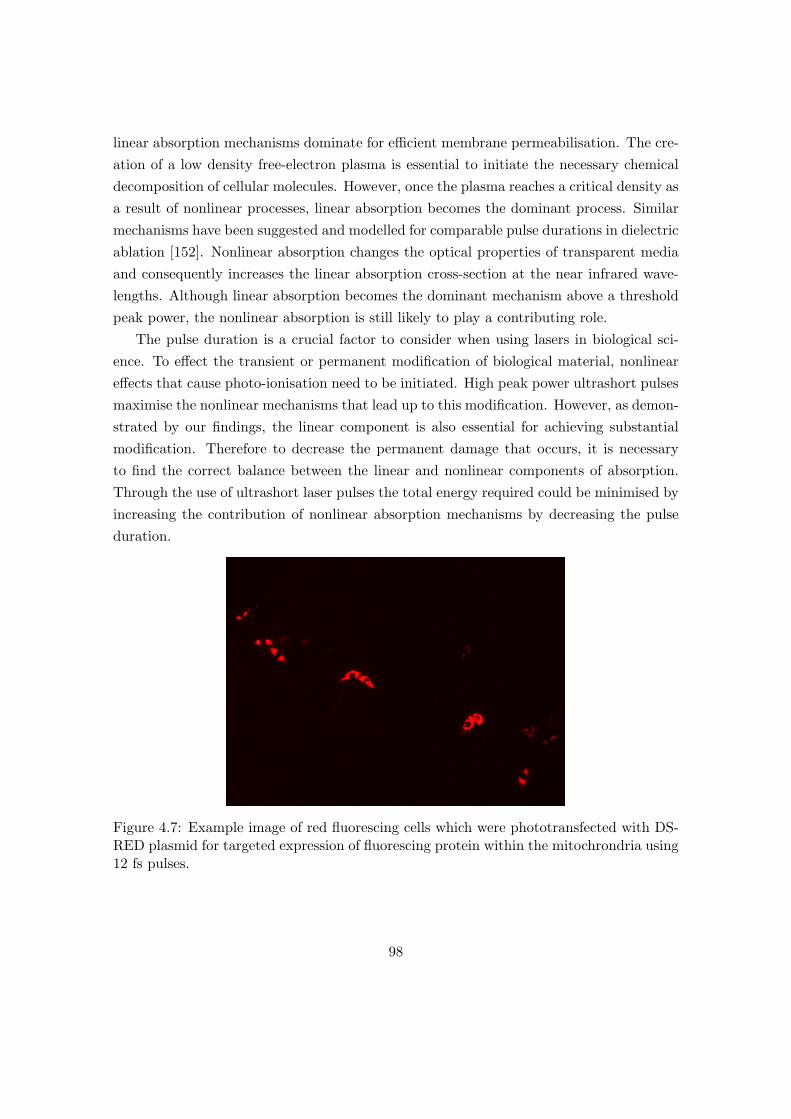
linear absorption mechanisms dominate for efficient membrane permeabilisation. The cre-ation of a low density free-electron plasma is essential to initiate the necessary chemicaldecomposition of cellular molecules. However, once the plasma reaches a critical density asa result of nonlinear processes, linear absorption becomes the dominant process. Similarmechanisms have been suggested and modelled for comparable pulse durations in dielectricablation [152]. Nonlinear absorption changes the optical properties of transparent mediaand consequently increases the linear absorption cross-section at the near infrared wave-lengths. Although linear absorption becomes the dominant mechanism above a thresholdpeak power, the nonlinear absorption is still likely to play a contributing role.

The pulse duration is a crucial factor to consider when using lasers in biological sci-ence. To effect the transient or permanent modification of biological material, nonlineareffects that cause photo-ionisation need to be initiated. High peak power ultrashort pulsesmaximise the nonlinear mechanisms that lead up to this modification. However, as demon-strated by our findings, the linear component is also essential for achieving substantialmodification. Therefore to decrease the permanent damage that occurs, it is necessaryto find the correct balance between the linear and nonlinear components of absorption.Through the use of ultrashort laser pulses the total energy required could be minimised byincreasing the contribution of nonlinear absorption mechanisms by decreasing the pulseduration.

Figure 4.7: Example image of red fluorescing cells which were phototransfected with DS-RED plasmid for targeted expression of fluorescing protein within the mitochrondria using12 fs pulses.

98

0 50 100 150 200 250Pulse duration (fs)

0

5

10

15

20

Efc

ienc

y (%

)

Transfection efciency

Figure 4.8: Uncorrected transfection efficiency as function of pulse duration (12, 35, 60,120 and 250 fs).

4.5 Phototransfection experiments

Transfection experiments were carried out in a similar manner to the optoinjection stud-ies using equivalent home-built optical microscope setups with the same objectives andutilising the ultrashort pulse Femtolaser system. The methods used are discussed in Ap-pendix 7.4. Generally the process of phototransfection is poorly understood due to therelative unpredictability of the transfection process. One major question concerns thespecific physical interactions and how the DNA is permitted through the membrane uponpermeabilisation. Despite a significant devotion of time we did not obtain the level ofstatistical evidence (dish number, n=4; 50 cells per dish) necessary to make any strongstatement about phototransfection as function of pulse duration. Fig. 4.7 shows an exam-ple population of cells transfected with DS-RED DNA plasmid, which encodes for targetedexpression of red-fluorescing proteins inside the mitochondria. Fig. 4.8 shows the trans-fection efficiencies obtained as function of pulse duration. We repeated experiments ata multitude of laser parameters. In particular, we began with the standard parameterapproach, which is to use a few tens of mWs and irradiate cells three times axially for40 ms each. However we only obtained transfection in these experiments when using 20mW average power for a duration of 2 ms was used to irradiate individual cells covering

99

5-7 axial irradiation events. Note, this graph could not be replicated and the procedurewas unusual in comparison with the standard 40 ms duration and 3 axial shots used inprevious literature [143,145].

Clearly, no distinct relationship between transfection efficiency and pulse duration wasfound. It should be noted that with future work it should be possible to obtain morestatistically significant results. It should further be noted that optoinjection experimentsprovide more consistent data because they are mostly dependent upon a physical responseto the laser, whereas for transfection, the biological response is critical. It was not possibleto obtain sufficiently consistent data such that a clear picture emerges in terms of laserpulse duration in optoinjection.

4.6 Conclusions

The nature of the coupling between pulse duration, pulse energy and number of pulsesdefines absorption characteristics of the cell membrane. We identify some key features ofour findings which help to explain the processes leading to membrane permeabilisationand hence optoinjection.

(i) The absorption behaviour is initially dominated by multiple-effective photon num-bers in the range 3.5-9.6. The equivalence of decreasing the pulse duration and increasingthe pulse energy is apparent, as both parameter types initiate efficient optoinjection.

(ii) For peak powers in the range of 6-20 kW there is a behaviour transition, abovewhich the multiphoton absorption transforms into near linear absorption.

(iii) Above the peak power threshold the multiphoton absorption saturates revealingthe linear absorption as the dominant mechanism. Figs. 4.4 and 4.5 display this beahviourin the linear regimes of shorter pulse durations and higher pulse energies, respectively.

(iv) The number of pulses required to support efficient optoinjection for fixed pulse du-ration and energy must exceed a specified value, which was defined as 50 %. Only throughappropriate selection of a high peak power parameter choice does the mean number ofpulses decrease. This observation also supports the idea that the optoinjection processrequires a high peak power initiation.

These findings complement the Vogel model of femtosecond optical absorption in bio-logical material [137]. Importantly, the initial multiphoton absorption events lead to theavalanche creation of a quasi-free electron plasma at the focus, which may be supported bytunneling ionisation, inverse Bremsstrahlung and impact ionisation events. The thresholdpeak power defines a critical plasma density, which, once exceeded the linear absorptiondominates leading to accumulation of energy, bringing about thermo-elastic stress along

100

with the simultaneous multiphoton-induced chemical breakdown near to the membrane,hence leading to permeabilisation.

To the best of our knowledge this work is the first experimental demonstration of thepeak power threshold. Our findings demonstrate that careful selection of laser parameterswill achieve efficient membrane permeabilisation and this has significant importance inlaser-mediated drug and gene delivery. These findings also have implications for imagingand cell surgery using ultrashort pulses lasers as they describe the processes leading up todamage formation, which is not desirable for imaging, but is potentially desirable for cellsurgery.

The optoinjection work in this chapter has been published in Nature Scientific Reports:’Exploring the ultrashort pulse laser parameter space for membrane permeabilisation inmammalian cells’, Andrew P. Rudhall, Maciej Antkowiak, Xanthi Tsampoula, MichaelMazilu, Nikolaus K. Metzger, Frank Gunn-Moore and Kishan Dholakia, Nat. Sci. Rep.,2, 858, 2012.

4.7 Chapter acknowledgements

The author designed the experiments with advice from Maciej Antkowiak and Lani Torres.The author performed all experiments in this chapter. The author performed the dataanalysis with assistance from Maciej Antkowiak. Michael Mazilu assisted in providing fitsfor the experimental data.

101

Chapter 5

Advanced beam shaping with

broadband ultrashort pulses

5.1 Introduction

The following chapter builds upon chapter 2 by examining some of the propagation char-acteristics of ultrashort pulses. Most specifically ultrashort pulse propagation is examinedfrom a spatial light modulator computationally configured to display a grating pattern,which in the corresponding focal plane yields an interference pattern (beam spot) whichcontains spatio-temporal couplings. These spatio-temporal couplings can cause problemsin terms of ultrashort pulse duration and spatial profile. In the present example, the SLMcauses angular dispersion due to its grating display and broad spectral content of theultrashort pulses. This chapter address how spatial modulation using a SLM can lead tonovel beam propagation types. The ability to tailor ultrashort light pulses both spatiallyand temporally provides the possibility for application-specific light fields, for example, inbiophotonics experiments, where an ultrashort pulse is required with different propagationcharacteristics such as a Bessel beam.

Since the introduction of pulsed lasers there has been remarkable progress concerningthe pulse duration. In particular, the ability to generate sub-picosecond pulses heralded anew domain, often referred to as ultrashort pulses. Chapters 1 and 2 introduced the con-cept of moulding the pulses into any desired temporal shape by arbitrarily adjusting thespectral phase. The controllable formation of arbitrary pulse shapes provides new oppor-tunities for the use of ultrashort pulses lasers. However a further degree of freedom exists,which determines the spatial characteristics of a beam. In the context of monochromaticlight, it is possible to phase and/or amplitude modulate spatial zones of the beam to ac-

102

quire a desired pattern within a corresponding focal plane [7]. The most obvious examplesof this type of spatial modulation is in novel beam shape generation, such as Bessel beamformation. In this case, a pattern such as an annulus yields the typical concentric ringpattern associated with Bessel beams.

In the context of ultrashort pulses, this phase and/or amplitude modulation of spatialaspects of the beam can, in addition to focal plane pattern formation, result in spectralphase modulations. The converse is also true, wherein the spectral phase and ampli-tude modulation may affect the spatial pattern formed at the focal plane. This type ofinteraction between spatial and spectral components is referred to as spatio-temporal cou-pling [102, 153]. The spatio-temporal couplings associated with ultrashort pulse result inbeam shape distortions including spatial chirp (observed as a spread in phase across thewavefront), angular dispersion (resulting in spatial chirp, such as would be generated froma grating) and pulse front tilt (as would be generated from a prism), to name but a few. Amore complete listing of first-order spatio-temporal couplings is found in [102,153]. Note,the term temporal is correspondingly equivalent to the term spectral, wherein the phaseand amplitude spectral information directly infers the temporal information through theassociated Fourier transform, as discussed previously.

In this chapter I examine the ultrashort pulse beam profiles generated by differentfunctions applied to a spatial light modulator placed the back aperture of a lens. Inparticular I generate Gaussian and Bessel beams and study the transverse beam profile,propagation and spectral phase of ultrashort pulses occurring in the focal plane. The useof the SLM opens up the opportunity of using spatial phase modulations to effect temporalmodulation due to the associated spatio-temporal couplings.

5.1.1 Bessel beams

The main part of this study considers the use of Bessel beams. This type of beam hasbeen studied extensively in the CW regime as well as a number of studies of polychromaticand/or ultrashort pulse Bessel beams [154, 155]. However, some studies have been con-cerned with applications of ultrashort pulsed Bessel beams, for example ultrashort pulseBessel beam photoporation [145]. Nonetheless, novel beam shapes continue to fascinatedue to their unique propagation characteristics and surprising properties.

The introduction of so-called diffraction-free beams, in particular those having a Bessel-like solution in 1987 provided an intriguing possibility of needle-like beams which maypropagate over long distances compared with Gaussian equivalents [156,157]. Bessel beamsof the zeroth order are characterised in the transverse plane by having a high intensity

103

circular core with a multitude of radially progressing concentric annuluses having pro-gressively less intensity extending radially outwards from the central core; although anequal amount of energy can be contained within each ring [156]. It should be noted thatideally the Bessel beam could propagate in a diffraction-free manner, however in practicethis is unachievable, as the ideal Bessel beam would require infinite energy to do so [156].Therefore experimental implementations of the Bessel beam are usually referred to asquasi-Bessel beams. Throughout this chapter the term quasi is not used, but in all casesit is implied.

The equation used to describe the monochromatic Bessel beam electric field in thez-direction is one of the solutions of the wave equation,

(∇2 − µ0ε0

∂2

∂t2

)E(r, t) = 0 and is

given by [158]

E(r, z) = AJ0(αr) exp(−i2πf

λ

)exp

(−iπρ

2a

fλ

)exp(−iβz), (5.1)

where

A = i2πλfEincident(ρa)ρa∆ρ, (5.2)

α =2πρaλf

, (5.3)

β =2πλ− πρ2

a

λf2, (5.4)

for a monochromatic beam of wavelength λ, annular aperture radius ρa, annular aperturethickness ∆ρ with a lens of focal length f .

Bessel beams are usually generated in two ways. In the first case the Bessel beamcan be generated by illuminating an annular aperture.. This type of configuration wasused in the experiments presented in this chapter. The other solution is to use a conicallens, better known as an axicon. The axicon method is more light-efficient as no light isblocked, however axial intensity modulations appear as a result of the finite tip size of theaxicon [159]. These are discussed in the context of ultrashort pulses below.

Bessel beams generated using broadband ultrashort pulses

The transverse spatial distribution associated with Bessel beams is wavelength depen-dent. Therefore in broadband Bessel beams each spectral component provides concen-trically displaced rings, resulting in decreased concentric fringe visibility, as was showntheoretically [158]. In this study 10 fs beams were found to have slightly decreased fringe

104

visibility, while a 3 fs beam was found to have substantially decreased fringe visibility. Anexperimental demonstration of this decrease in fringe visibility was obtained using a micro-axicon array to generate a multitude of Bessel beams with various pulse durations [154].Further, a programmable array of ultrashort pulsed needle-like beams was achieved usinga SLM [160]. A marked change in fringe visibility was observed in [154] which was alsoobserved in our experiments, for example, in Fig. 5.6, in which the beam was subject toangular dispersion in one direction. The generation of ultrashort pulse Bessel beams isoften referred to as the so-called X-pulse formation in which the axial propagation has anapparent X-shaped transverse profile extending axially [161, 162]. However, in [162] theexperimental realisations of the Bessel-X pulses were emphasised with the use of super-broadband emission from a Xe-arc lamp with a 3 fs correlation time. The possibility ofgenerating so-called light bullets in which the propagation of a beam is transversally in-variant and localised in time may be potentially realised in linear optics through the useAiry-Bessel beams [163].

5.2 Ultrashort pulse novel beams: studies

Various experiments were conducted involving a spatial light modulator in conjunctionwith the MIIPS pulse shaper. For the purposes of clarity this section introduces eachseparate experiment in more detail in subsections containing the related methods, resultsand discussion. A conclusion is presented after the experiments.

5.2.1 Experimental setup

In this section the experimental arrangements used are outlined for reference to the latersections in which different experiments are discussed. In the first instance, a single passon the SLM was used and subsequently a double pass on the SLM was used (in order tocompensate for spatial chirp). The single pass SLM version either used lenses or focusingmirrors. Fig. 5.1 illustrates the single-pass arrangement; Fig. 5.2 illustrates the double-pass arrangement. The single-pass arrangement was set up by expanding a beam to overfillthe SLM display, which was oriented to match the input polarisation of the laser beam,and the reflected orders were imaged at a closed aperture. The SLM was modulated toshow a grating, of which the first order was selected and passed through the aperture andsubsequently imaged onto the camera. The arrangement for the double-pass arrangementwas a little more involved. Firstly, the SLM display was split in two halves; and thebeam was configured to slightly overfill one half of the SLM display. The first order was

105

imaged onto a mirror placed behind the aperture and the reflection directed towards theother half of the SLM display. The reflection from this half was collected by a mirror andsubsequently imaged onto the camera. It should be first noted that in order to displacethe second pass of the beam sufficiently it was necessary to transversely displace the beamas shown at f5 in Figure 5.2, wherein the beam passed through either side of the lenssymmetrically so as to not introduce unwanted aberrations. it should be secondly notedthat it was beneficial to use small optics (e.g. mirrors) in order to prevent blocking thebeam inappropriately. The single-pass arrangement resulting in an extended transversal

Figure 5.1: The initial experimental arrangement in which a single-pass arrangement isutilised; an equivalent setup is later used whereby focusing mirrors are used appropriately.SLM refers to spatial light modulator, Ap is an aperture, CAM is a camera (Basler Pi-A640-210GM) and MDU is the MIIPS detection unit outlined in chapter 4. Lenses f1through f7 refer to 10 cm, 25 cm, 7.5 cm, 40 cm, 30 cm, 20 cm and 20 cm (interchangedwith 5 cm) (image not to scale).

beam profile for Gaussian and Bessel beams due to the diffraction grating displayed by theSLM. It was found that the double-pass arrangement assisted in decreasing spatial chirp.This is discussed below.

106

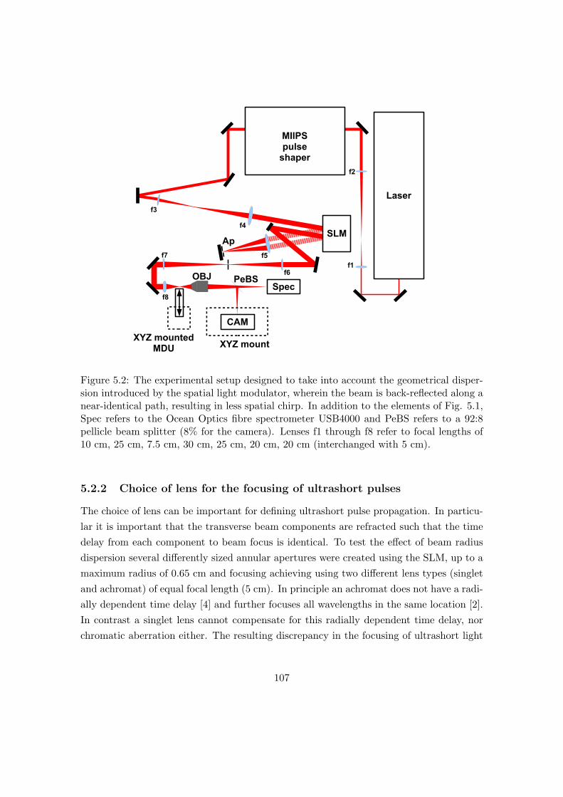
Figure 5.2: The experimental setup designed to take into account the geometrical disper-sion introduced by the spatial light modulator, wherein the beam is back-reflected along anear-identical path, resulting in less spatial chirp. In addition to the elements of Fig. 5.1,Spec refers to the Ocean Optics fibre spectrometer USB4000 and PeBS refers to a 92:8pellicle beam splitter (8% for the camera). Lenses f1 through f8 refer to focal lengths of10 cm, 25 cm, 7.5 cm, 30 cm, 25 cm, 20 cm, 20 cm (interchanged with 5 cm).

5.2.2 Choice of lens for the focusing of ultrashort pulses

The choice of lens can be important for defining ultrashort pulse propagation. In particu-lar it is important that the transverse beam components are refracted such that the timedelay from each component to beam focus is identical. To test the effect of beam radiusdispersion several differently sized annular apertures were created using the SLM, up to amaximum radius of 0.65 cm and focusing achieving using two different lens types (singletand achromat) of equal focal length (5 cm). In principle an achromat does not have a radi-ally dependent time delay [4] and further focuses all wavelengths in the same location [2].In contrast a singlet lens cannot compensate for this radially dependent time delay, norchromatic aberration either. The resulting discrepancy in the focusing of ultrashort light

107

pulses has been shown theoretically to provide pulse broadening in the focus [164]. Theannular aperture radii used were: 0-1.6 mm (for Gaussian profiles), 1.6-3.2 mm (for Besselprofiles), 3.2-4.8 mm (for Bessel profiles), 4.8-6.4 mm (for Bessel profiles) and 0-6.4 mm (forGaussian profiles). Note that the SLM was arranged in the aforementioned double-passmanner to control the angularly dispersive spectral components.

Lens choice: method and results

For each case the maximum SHG signal at the focus of the lens in question and performedthe standard MIIPS analysis to retrieve the system dispersion. Each step was repeated atleast ten times to minimise error in determining the system dispersion. In each case thedifference in dispersion between each annular radius and the averaged radial dispersion(that is, Gaussian 0-6.4mm) was calculated. This way a direct comparison was made whichdemonstrated the small differences in dispersion that would not otherwise be shown if onewere to examine the pulse shape from the total dispersion in each case. In Fig. 5.3 thesinglet lens dispersion is shown. Importantly note the equivalent (frequency equivalent ofwavelength) frequency width over which the difference is exactly zero (where the lines donot deviate from zero) is equivalent to 0.02 × 1015/s, corresponding to a minimum sech-squared pulse duration of τmin = 99 fs. This is the minimum pulse duration obtainable thatMIIPS can completely compensate using a singlet lens of 5 cm. In Fig. 5.4 the situationis improved when using the achromat. The angular frequency width is now equivalent to0.07 × 1015/s, corresponding to a minimum sech-squared pulse duration of τmin = 28 fs.The implication is that the achromat is ideal down to 28 fs whereas the singlet is idealdown to 99 fs for this focal length and annular radius.

The lens choice is critical for achieving a good quality MIIPS (or otherwise) compen-sation of spectral phase dispersion. The achromatic lens type was found to be preferablein that the radial dispersion profile was relatively flatter compared with the singlet lenstype. Therefore in experiments involving the shortest pulses the best lenses should bechosen to suit the purpose, in particular paying attention to the radial time delay.

5.2.3 Spatial chirp

Spatial chirp arises when a spatially-dependent phase modulation is imparted upon spec-tral components of the beam [102]. Spatial chirp becomes particularly important for ultra-short pulses as it can mean that spectral content is converted into spatial content and viceversa. While spatial chirp can be useful, for example, in ultrashort pulse measurement orcompensating for dispersion it must be compensated for so as to prevent unwanted beam

108

740 760 780 800 820 840 860−4

−3

−2

−1

0

1

2

3

4

Wavelength (nm)

Phas

e di

stor

tion

(radi

ans)

GaussianBessel 1Bessel2Bessel 3Spectrum

Figure 5.3: Spectral phase distortion differences for a 5 cm singlet lens. Graph showingrelative phase distortions for (i) Gaussian beam of pre-lens radius 6.4 mm, (ii) Bessel 1 ofpre-lens radius of 4.8-6.4 mm, (iii) Bessel 2 of pre-lens radius of 3.2-4.8 mm, Bessel 3 ofpre-lens radius of 1.6-3.2 mm and the related spectrum.

distortion [165]. A feature of using a spatial light modulator for defining the desired beamshape is that a grating is displayed. A consequence of using the grating is the resultingwavelength-dependent angular dispersion according to the grating equation, hence result-ing in spatial chirp. In the single-pass arrangement this manifests itself in terms of a spatialwavelength dependence in the focal plane which can not be eliminated. In this patternthe beam spot becomes elongated with wavelength, with a different spectrum as functionof position. For this reason the pulse is no longer well defined in tight spot, instead byconsidering each spatial location the local spectral content defines the pulse duration. Forthis reason very little SHG was found due to the exceptionally long pulse duration andthe associated spectral dispersion, which could not be compensated using MIIPS due tolack of SHG signal. Fig. 5.5 shows the fundamental spectrum as function of position for aGaussian pulse with 80 nm bandwidth. The detector could not discriminate between tinyspatial locations, therefore the graph indicates a general tendency for the centre wave-length to shift with position. As a further demonstration of this effect an image of thespatial beam profile (Bessel) was recorded as function of spectral width. The Gaussianbeam become elongated in the same fashion as the core of the Bessel beam. In this study,beams corresponding to CW, 25 nm and 80 nm were examined, as shown in Fig. 5.6.In the case of CW the beam the Bessel beam had the usual spatial profile, as expected.

109

740 760 780 800 820 840 860−3

−2

−1

0

1

2

3

4

Wavelength (nm)

Phas

e di

stor

tion

(radi

ans)

GaussianBessel 1Bessel 2Bessel 3Spectrum

Figure 5.4: Spectral phase distortion differences for a 5 cm achromat lens. Graph showingrelative phase distortions for (i) Gaussian beam of pre-lens radius 6.4 mm, (ii) Bessel 1 ofpre-lens radius of 4.8-6.4 mm, (iii) Bessel 2 of pre-lens radius of 3.2-4.8 mm, Bessel 3 ofpre-lens radius of 1.6-3.2 mm and the related spectrum.

However for 80 nm the Bessel beam is very distorted. Note the angle of 45 degrees isintroduced by the grating being oriented at 45 degrees. The most important consequenceswere that no SHG could be generated in this arrangement, either for narrower or broaderbandwidths due the lowered peak intensity. This is compounded by the fact that SHG is a2-photon process, and further still, the spectral phase at these pulse durations plays a sig-nificant role. We did, however manage to correct for the angular dispersion by employingthe double-pass arrangement shown previously in Fig. 5.2. In this setup the half of SLMarea was imaged back to the opposite half and the transverse displacement achieved al-lowed the double-passed beam to be directed towards the detection setup. The transversedisplacement was achieved by passing the beam initially through the left-hand side of alens (introducing aberrations) and reflected through the corresponding right-hand side ofthe lens, thus compensating for the introduced aberrations. In this setup, the beam wassufficiently localised such that a sufficiently short fundamental pulse was defined and SHGcould be generated, thus permitting MIIPS compensation. Fig. 5.7 shows the Bessel beamgenerated using this method (with a few minor aberrations). Importantly however, SHGsignal could be collected this way. It would have been desirable to examine the fundamen-tal and SHG beams as function of propagation distance however due to time constraints

110

700 720 740 760 780 800 820 840 860 880 900−1000

0

1000

2000

3000

4000

5000

6000

7000

Wavelength (nm)

Inte

nsity

(arb

. uni

ts)

Figure 5.5: Spatial chirp demonstration with a spectrometer partially translated acrossthe width of the beam in the SLM focal plane resulting in a position-dependent spectrum.Note the centre wavelength shifting to the left (going from red to violet in the usualsequence).

it was not possible to deal with some significant problems. For example, to collect theSHG the alignment needed to be perfect while translating along the beam propagationaxis. While this concept is trivial, the implementation of such an arrangement was not.However, it should be noted that it should be possible to design a system as such. In alatter experimental arrangement the beam was imaged instead. This provide means forpost-processing of the SHG data. However in this configuration the single-pass methodwas used and the spatial chirp prevented sufficient generation of SHG. A further problemis the need to completely eliminate the fundamental pulse from transmitting through theSHG filter. However these are all engineering problems that could be overcome in a futurestudy.

5.2.4 Gaussian and Bessel beam propagation introduction

In the following set of experiments the axial propagation characteristics of Gaussian andBessel beams of different bandwidths was examined. For a Gaussian beam the beam waistradius for a given wavelength at an input beam radius r0 can be approximated as [44]

w0 ≈fλ

2r0, (5.5)

111

(a)

100 200 300

50

100

150

20050

100150200

(c)

100 200 300

50

100

150

20050

100150

(e)

100 200 300

50

100

150

20020406080

100120140

700 750 800 850 9000

2000

4000(b)

Wavelength (nm)

Inte

nsity

(arb

. uni

ts)

700 750 800 850 9000

1000

2000(d)

Wavelength (nm)

Inte

nsity

(arb

. uni

ts)

700 750 800 850 9000

200

400

(f)

Wavelength (nm)

Inte

nsity

(arb

. uni

ts)

Figure 5.6: Angular frequency spread within Bessel beams; (a) corresponds to a Besselbeam generated by the CW spectrum indicated by (b); (c) corresponds to the equivalentBessel beam but with 25 nm bandwidth indicated by spectrum (d); (e) corresponds to theequivalent Bessel beam as (a) and (c), but with 80 nm bandwidth, as seen in spectrum(f). The intensity scale clearly shows that the CW case exhibits the highest fundamentalintensity (at constant average power) due to the spatial spread of the beam.

where the beam width convention used was 1/e. The beam propagation equation in theparaxial approximation is given by [44]

∇2u(x, y, z)− 2ik∂u(x, y, z)

∂z= 0, (5.6)

112

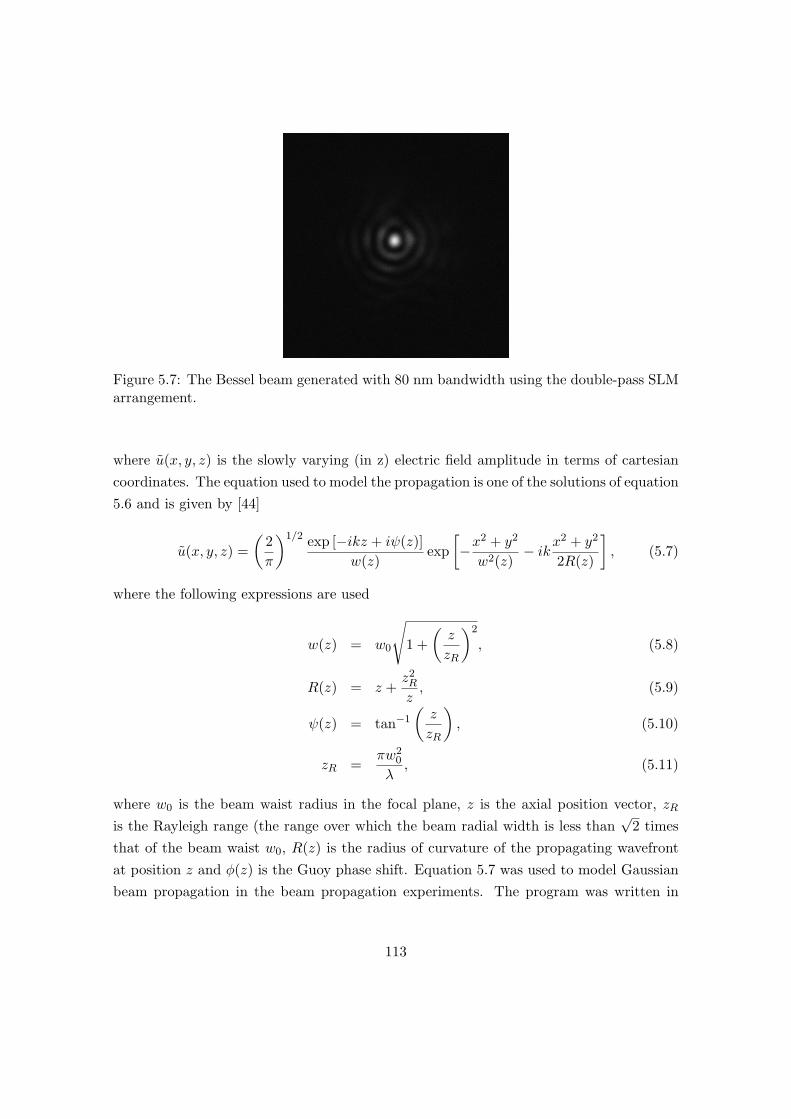
Figure 5.7: The Bessel beam generated with 80 nm bandwidth using the double-pass SLMarrangement.

where u(x, y, z) is the slowly varying (in z) electric field amplitude in terms of cartesiancoordinates. The equation used to model the propagation is one of the solutions of equation5.6 and is given by [44]

u(x, y, z) =(

2π

)1/2 exp [−ikz + iψ(z)]w(z)

exp[−x

2 + y2

w2(z)− ikx

2 + y2

2R(z)

], (5.7)

where the following expressions are used

w(z) = w0

√1 +

(z

zR

)2

, (5.8)

R(z) = z +z2R

z, (5.9)

ψ(z) = tan−1

(z

zR

), (5.10)

zR =πw2

0

λ, (5.11)

where w0 is the beam waist radius in the focal plane, z is the axial position vector, zRis the Rayleigh range (the range over which the beam radial width is less than

√2 times

that of the beam waist w0, R(z) is the radius of curvature of the propagating wavefrontat position z and φ(z) is the Guoy phase shift. Equation 5.7 was used to model Gaussianbeam propagation in the beam propagation experiments. The program was written in

113

MATLAB and is provided in the supplementary CD (acknowledged in Appendix 7.5).The following parameters were used to model propagation. The focal length was 20 cm,the small beam radius was 2.4 mm and the large beam radius was 5.0 mm. The beam widthradius w0 was calculated theoretically. Further, the multiple wavelength components wereconsidered, each of which having a wavelength-dependent amplitude. Once taken intoaccount these multiple wavelengths did not change the propagation length due; insteadthe central wavelength of 800 nm defined the propagation length.

Gaussian beam propagation

We measured the Gaussian beam propagation using the values outlined in Table 5.1 usingthe lens values outlined in Fig. 5.1 and analysed the axial intensity data. Fig. 5.8refer to the measured propagation characteristics of an apertured Gaussian beams with80 nm of bandwidth. Table 5.1 shows the calculated and measured propagation lengths

z position (units of 0.5 mm)

pixe

l num

ber

(a)

2 4 6 8 10 12 14 16 18 20 22 24

20

40

60

80

100

120

2 4 6 8 10 12x 10−3

0

50

100

150(b)

z position (m)

axia

l int

ensi

ty (a

rb. u

nits

)

Figure 5.8: Top panel: colour-scaled propagation of a broadband Gaussian beam in thedirection of beam propagation. Bottom panel: intensity cross section corresponding toabove Gaussian beam.

for various-sized broadband (80 nm) and narrowband (25 nm) apertured Gaussian beams.

114

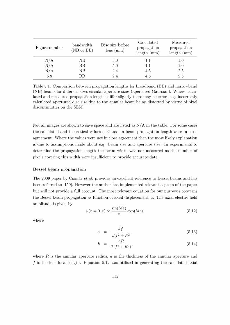
Figure numberbandwidth(NB or BB)

Disc size beforelens (mm)

Calculatedpropagationlength (mm)

Measuredpropagationlength (mm)

N/A NB 5.0 1.1 1.0N/A BB 5.0 1.1 1.0N/A NB 2.4 4.5 2.55.8 BB 2.4 4.5 2.5

Table 5.1: Comparison between propagation lengths for broadband (BB) and narrowband(NB) beams for different sizes circular aperture sizes (apertured Gaussian). Where calcu-lated and measured propagation lengths differ slightly there may be errors e.g. incorrectlycalculated apertured disc size due to the annular beam being distorted by virtue of pixeldiscontinuities on the SLM.

Not all images are shown to save space and are listed as N/A in the table. For some casesthe calculated and theoretical values of Gaussian beam propagation length were in closeagreement. Where the values were not in close agreement then the most likely explanationis due to assumptions made about e.g. beam size and aperture size. In experiments todetermine the propagation length the beam width was not measured as the number ofpixels covering this width were insufficient to provide accurate data.

Bessel beam propagation

The 2009 paper by Cizmar et al. provides an excellent reference to Bessel beams and hasbeen referred to [159]. However the author has implemented relevant aspects of the paperbut will not provide a full account. The most relevant equation for our purposes concernsthe Bessel beam propagation as function of axial displacement, z. The axial electric fieldamplitude is given by

u(r = 0, z) ∝ sin(bdz)z

exp(iaz), (5.12)

where

a =kf√

f2 +R2, (5.13)

b =aR

2(f2 +R2), (5.14)

where R is the annular aperture radius, d is the thickness of the annular aperture andf is the lens focal length. Equation 5.12 was utilised in generating the calculated axial

115

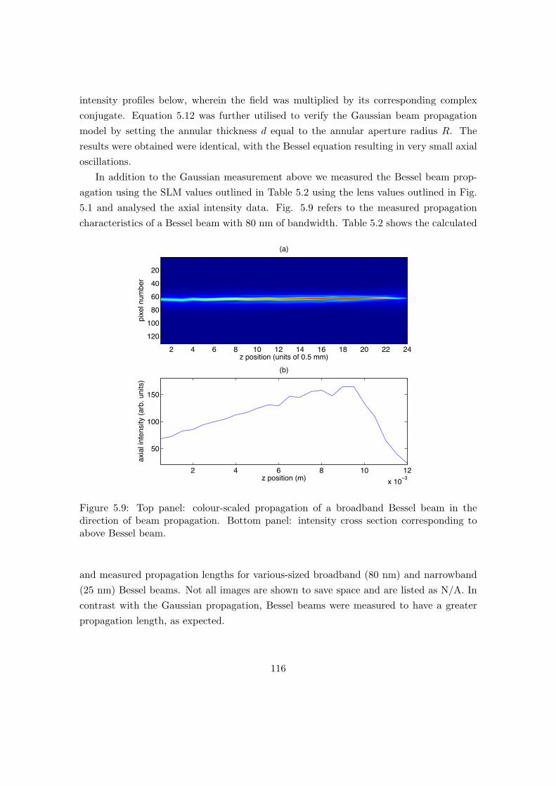
intensity profiles below, wherein the field was multiplied by its corresponding complexconjugate. Equation 5.12 was further utilised to verify the Gaussian beam propagationmodel by setting the annular thickness d equal to the annular aperture radius R. Theresults were obtained were identical, with the Bessel equation resulting in very small axialoscillations.

In addition to the Gaussian measurement above we measured the Bessel beam prop-agation using the SLM values outlined in Table 5.2 using the lens values outlined in Fig.5.1 and analysed the axial intensity data. Fig. 5.9 refers to the measured propagationcharacteristics of a Bessel beam with 80 nm of bandwidth. Table 5.2 shows the calculated

z position (units of 0.5 mm)

pixe

l num

ber

(a)

2 4 6 8 10 12 14 16 18 20 22 24

20

40

60

80

100

120

2 4 6 8 10 12x 10−3

50

100

150

(b)

z position (m)

axia

l int

ensi

ty (a

rb. u

nits

)

Figure 5.9: Top panel: colour-scaled propagation of a broadband Bessel beam in thedirection of beam propagation. Bottom panel: intensity cross section corresponding toabove Bessel beam.

and measured propagation lengths for various-sized broadband (80 nm) and narrowband(25 nm) Bessel beams. Not all images are shown to save space and are listed as N/A. Incontrast with the Gaussian propagation, Bessel beams were measured to have a greaterpropagation length, as expected.

116

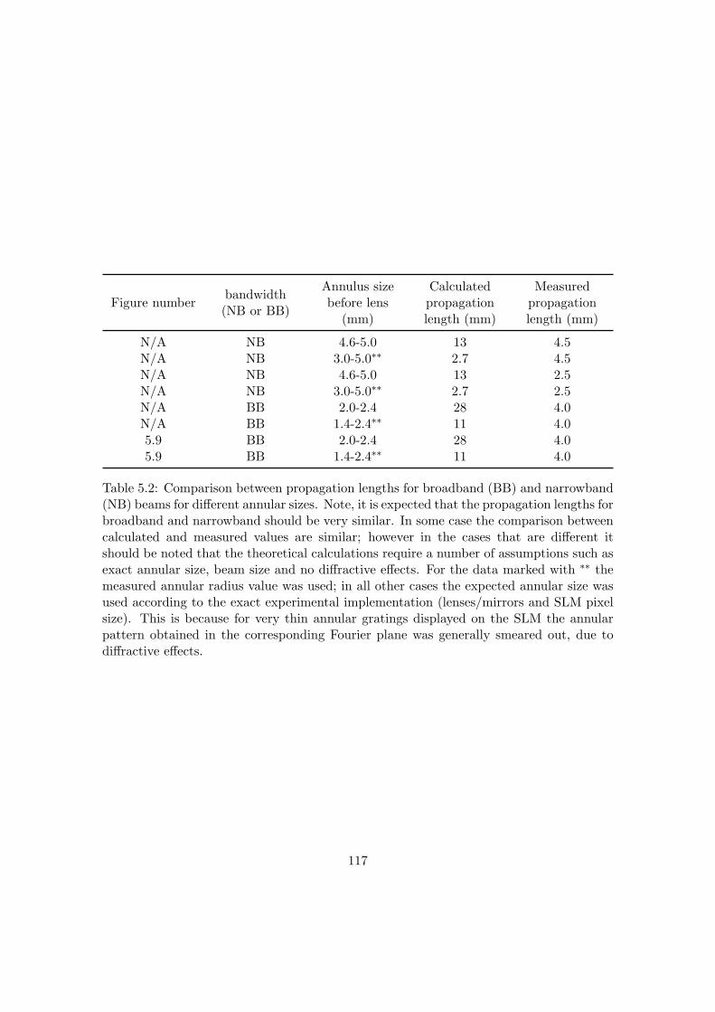
Figure numberbandwidth(NB or BB)

Annulus sizebefore lens

(mm)

Calculatedpropagationlength (mm)

Measuredpropagationlength (mm)

N/A NB 4.6-5.0 13 4.5N/A NB 3.0-5.0∗∗ 2.7 4.5N/A NB 4.6-5.0 13 2.5N/A NB 3.0-5.0∗∗ 2.7 2.5N/A BB 2.0-2.4 28 4.0N/A BB 1.4-2.4∗∗ 11 4.05.9 BB 2.0-2.4 28 4.05.9 BB 1.4-2.4∗∗ 11 4.0

Table 5.2: Comparison between propagation lengths for broadband (BB) and narrowband(NB) beams for different annular sizes. Note, it is expected that the propagation lengths forbroadband and narrowband should be very similar. In some case the comparison betweencalculated and measured values are similar; however in the cases that are different itshould be noted that the theoretical calculations require a number of assumptions such asexact annular size, beam size and no diffractive effects. For the data marked with ∗∗ themeasured annular radius value was used; in all other cases the expected annular size wasused according to the exact experimental implementation (lenses/mirrors and SLM pixelsize). This is because for very thin annular gratings displayed on the SLM the annularpattern obtained in the corresponding Fourier plane was generally smeared out, due todiffractive effects.

117

5.2.5 Concentric annular rings, their phase, and interference in the focal

plane

One aspect of interest concerns the interference from individual spatial portions withinthe beam profile, as imaged from the SLM. In particular, portions of the SLM can bemodulated to effect a change of phase of one spatial portion with respect to any otherchosen spatial portion. As a result the interference pattern (beam focus) can be modulatedsuch that the transverse intensity distribution within the beam focus may be significantlyaltered. In this way the effective chirp in one portion of the beam may potentially bechanged.

Concentric annular ring interference: theory

A basic theory of the interference pattern in the focal plane, as provided by a circlesurrounded by an annulus of varying phase is presented. It is firstly assumed that thepeak electric field amplitude of the inner circle is equal to the outer circle. The innerelectric field Einner can be described by

Einner = E exp(−f(ω) + iφ(ω))f(x, y, z), (5.15)

where f(ω) is a general function describing the spectral electric field amplitude as functionof frequency (e.g. a non-Gaussian distribution such as some asymmetric non-analyticfunction could be approximated by some unknown function exp(−(f(ω)))), φ(ω) is thespectral phase and f(x, y, z) is a general function describing the spatial beam profile (e.g.a Gaussian) in terms of cartesian coordinates x,y and z. The outer electric field is givenby

Eouter = E exp(−f(ω) + iφ(ω) + iΦ)f(x, y, z), (5.16)

where Φ is the spectral phase imparted by the SLM. For simplicity it is initially assumedthat Φ is constant, however this unduly complicates the point of this description. Inpractice the SLM imparts a different phase as function of wavelength and this may havecontributed to deviations from theory, as reported later. The total field is provided by

Esum = Einner + Eouter = E(exp(−f(ω) + iφ(ω)) [1 + exp(iΦ)] . (5.17)

From equation 1.2 in Chapter 1 we can write the intensity as

I(ω,Φ, x, y, z) ∝∫ ∞

0EsumE

∗sumdω, (5.18)

118

where ∗ denotes the complex conjugate and where the spatial aspects of the integer havebeen incorporated into the ∝ sign. We obtain

I(ω,Φ, x, y, z) ∝ EE∗(1 + exp(iΦ))(1 + exp(−iΦ)), (5.19)

where the integer relating to the frequency terms have been further incorporated into theproportionality term. Thus,

I(ω,Φ, x, y, z) ∝ 4 cos2(Φ/2). (5.20)

Hence, at any frequency and position, there is a cosine-squared relationship between in-tensity and SLM outer pattern phase. This results in an intensity modulation as functionof phase. Therefore it should be possible to obtain near zero field at certain phases. Overa 2π range, the maxima intensities are obtained at 2mπ for integer values of m. Theminima intensities are obtained at (2m + 1)π/2 for integer values of m. To verify this a2D Fourier transform model is provided for establishing the intensity for this particularcase of interfering concentric annular components. The model does not take into accountthe wavelengths involved due to lack of knowledge of the mapping between frequency andposition and so the broadband case is not described. However, this model is instructive forexamining what happens when the spatial phase is changed. It should be emphasised thatthis model refers to monochromatic waves (as this is only allowed in the Fourier transformmodel). Therefore this model is indicative but not definitive. The MATLAB code for thismodel is provided in the supplementary CD and acknowledgements given in Appendix 7.5.

Figs. 5.10(a-d) show some of the computationally calculated beam spot resulting frominterfering outer pattern with the inner pattern, whereby the phase difference of the outerpattern is varied continually from 0 to 2π, wherein four cases are selected including outerannulus phase of 0, π/2, π and 3π/2. Note how the beam spot changes in shape signifi-cantly for varying phase. To accompany the fundamental beam spots the correspondingSHG beam spots were also calculated and are presented in Figs. 5.11(a-d). In the model33 units of π/16 were used to cover phase values of 0 to 2π inclusively. Equation 5.20shows that the fundamental intensity signal is oscillatory and positive. From the compu-tational model the centre pixel values were recorded across the 33 units and the resultsare shown in Fig. 5.12. These calculations serve as an introduction to the experimentsinvolving interference between concentric rings. Importantly, these experiments are in-dicative and do not consider broadband light, nor the spectral phase response of the SLM.Further, they are not scaled according to wavelength and actual beam profile. However

119

(a)

100 200 300 400

50

100

150

200

250

300

350

400

1000 2000 3000 4000 5000

(b)

100 200 300 400

50

100

150

200

250

300

350

400

200 400 600 800 100012001400

(c)

100 200 300 400

50

100

150

200

250

300

350

400

500 1000 1500

(d)

100 200 300 400

50

100

150

200

250

300

350

400

200 400 600 800 100012001400

Figure 5.10: Calculated fundamental beam profiles for the following outer annular phasevalues: (a) 0, (b) π/2, (c) π and (d) 3π/2. Note the significant change in beam shape.The full range of shapes can be calculated through use of the code in the supplementaryCD. In each case the signal is not scaled absolutely, instead the scaling colours are evenlyspread out using the obtained range of signal values. Actual values can be obtained fromthe aforementioned code.

they do indicate that a spectral intensity response can be expected for given relative phasedifference between different spatial beam components.

Concentric annular ring interference: experiments

The phase was adjusted by displaying on the SLM an an outer annular pattern and aconcentrically aligned inner Gaussian pattern. The resulting beam interference patternat the focus of an achromat lens was imaged onto a CCD. The power of the outer andinner patterns was adjusted relatively so that when measured, the two-photon intensityresponse was similar whether using either the inner or outer pattern. The radius of theinner pattern before the focusing lens was 2.3 mm. The radius of the outer (annular)

120

SHG (a)

100 200 300 400

50

100

150

200

250

300

350

400

1000 2000 3000

SHG (b)

100 200 300 400

50

100

150

200

250

300

350

400

50 100 150 200

SHG (c)

100 200 300 400

50

100

150

200

250

300

350

400

50 100 150 200 250

SHG (d)

100 200 300 400

50

100

150

200

250

300

350

400

50 100 150 200

Figure 5.11: Calculated SHG beam profiles corresponding with Fig. 5.10 for the followingouter annular phase values: (a) 0, (b) π/2, (c) π and (d) 3π/2. Again, in each case thesignal is not scaled absolutely.

pattern was 2.5-4 mm. The bandwidth of the laser used was 50 nm FWHM bandwidth,and was corrected by MIIPS to have a corresponding minimum pulse duration of 16 fs.

Fig. 5.13 demonstrates that the spectral content within the spatial distribution of thebeam is constant, with the inner and outer patterns separately contributing to give the sumof the spectral content, as given when the inner and outer patterns were simultaneouslydisplayed. Note that in Fig. 5.13 the spectrum is different to that of a compensatedbeam, where the spectrum is modulated by the MIIPS compensation function. Fig. 5.14shows the uncompensated SHG obtained with the fundamental spectrum obtained in Fig.5.13. By ensuring the SHG of the inner or outer pattern was constant, thus indicatedthat the peak intensity of the inner and outer pattern was similar, the beam spot sizeand corresponding axial intensity would be approximately the same. However at thispoint it should be noted that alternatively it may have been appropriate to calculate an

121

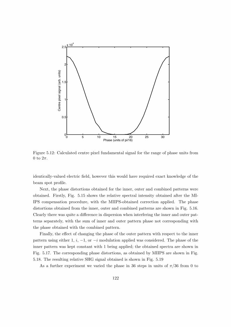
0 5 10 15 20 25 300

0.5

1

1.5

2

2.5x 10

4

Phase (units of pi/16)

Centr

e p

ixel sig

nal (a

rb. units)

Figure 5.12: Calculated centre pixel fundamental signal for the range of phase units from0 to 2π.

identically-valued electric field, however this would have required exact knowledge of thebeam spot profile.

Next, the phase distortions obtained for the inner, outer and combined patterns wereobtained. Firstly, Fig. 5.15 shows the relative spectral intensity obtained after the MI-IPS compensation procedure, with the MIIPS-obtained correction applied. The phasedistortions obtained from the inner, outer and combined patterns are shown in Fig. 5.16.Clearly there was quite a difference in dispersion when interfering the inner and outer pat-terns separately, with the sum of inner and outer pattern phase not corresponding withthe phase obtained with the combined pattern.

Finally, the effect of changing the phase of the outer pattern with respect to the innerpattern using either 1, i, −1, or −i modulation applied was considered. The phase of theinner pattern was kept constant with 1 being applied; the obtained spectra are shown inFig. 5.17. The corresponding phase distortions, as obtained by MIIPS are shown in Fig.5.18. The resulting relative SHG signal obtained is shown in Fig. 5.19

As a further experiment we varied the phase in 36 steps in units of π/36 from 0 to

122

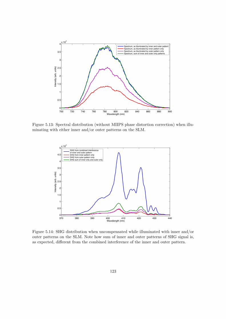
700 720 740 760 780 800 820 840 860 880 9000

0.5

1

1.5

2

2.5

3

3.5

4x 104

Wavelength (nm)

Inte

nsity

(arb

. uni

ts)

Spectrum, as illuminated by inner and outer patternSpectrum, as illuminated by inner pattern onlySpectrum, as illuminated by outer pattern onlySpectrum, sum of inner and outer only patterns

Figure 5.13: Spectral distribution (without MIIPS phase distortion correction) when illu-minating with either inner and/or outer patterns on the SLM.

370 380 390 400 410 420 430 4400

0.5

1

1.5

2

2.5

3

3.5

4

4.5

5x 104

Wavelength (nm)

Inte

nsity

(arb

. uni

ts)

SHG from combined interferenceof inner and outer patternSHG from inner pattern onlySHG from outer pattern onlySHG sum of inner only and outer only

Figure 5.14: SHG distribution when uncompensated while illuminated with inner and/orouter patterns on the SLM. Note how sum of inner and outer patterns of SHG signal is,as expected, different from the combined interference of the inner and outer pattern.

123

720 740 760 780 800 820 840 8600

0.1

0.2

0.3

0.4

0.5

0.6

0.7

0.8

0.9

1

Wavelength (nm)

Inte

nsity

(rel

ative

)

Spectrum obtained from combinedpattern with MIIPS correctionSpectrum obtained from innerpattern only with MIIPS correctionSpectrum obtained from outerpattern only with MIIPS correctionSpectrum obtained from combinedpattern without MIIPS correction

Figure 5.15: Measured spectra after MIIPS compensation function applied. Note theslight spectral difference between inner, outer, and combined patterns on SLM. Also notethe spectral modification from uncompensated to compensated spectra.

720 740 760 780 800 820 840 860 880−2

−1.5

−1

−0.5

0

0.5

1

1.5

2

Wavelength (nm)

Phas

e di

stor

tion

(radi

ans)

MIIPS−extracted phase for combined pattern on SLMMIIPS−extracted phase for inner pattern only on SLMMIIPS−extracted phase for outer pattern only on SLMSum of inner and outer pattern phase

Figure 5.16: MIIPS-obtained phase distortion for the inner, outer, and combined patterns.Also shown is the sum of the inner and outer phase. In this case the outer pattern phasewas kept at ’1’, or exp(0i), with the inner pattern phase being also kept at ’1’.

124

720 740 760 780 800 820 840 860 8800

0.1

0.2

0.3

0.4

0.5

0.6

0.7

0.8

0.9

1

Wavelength (nm)

Inte

nsity

(rel

ative

)

Outer pattern: +1Outer pattern: +iOuter pattern: −1Outer pattern: −i

Figure 5.17: Relative spectra obtained with outer ring phase modulated by 1, i, −1, or−i.

720 740 760 780 800 820 840 860 880−2

−1.5

−1

−0.5

0

0.5

1

1.5

2

Wavelength (nm)

Phas

e di

stor

tion

(radi

ans)

MIIPS−obtained phase; outer ring: +1MIIPS−obtained phase; outer ring: +iMIIPS−obtained phase; outer ring: −1MIIPS−obtained phase; outer ring: −i

Figure 5.18: Phase distortions measured by MIIPS obtained with outer ring phase mod-ulated by 1, i, −1, or −i.

2π to establish whether the results from theory could be replicated such as in Fig. 5.12.In the experiment we took the fundamental spectrum from the inner circle, concentric

125

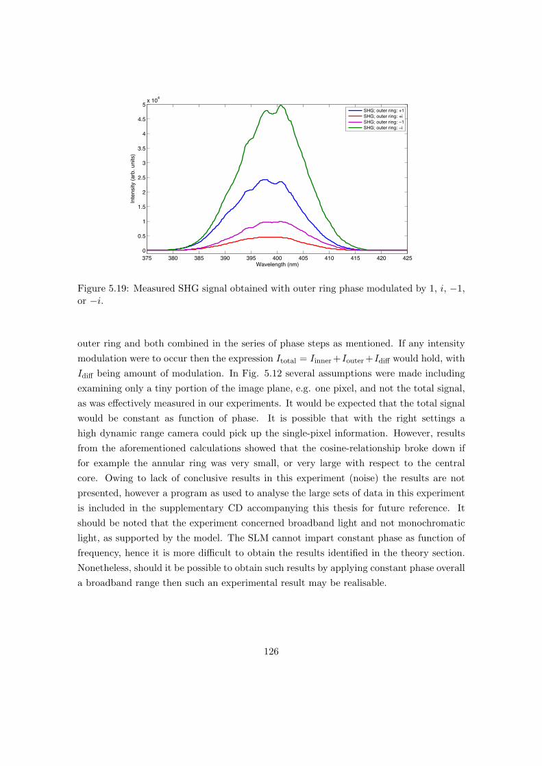
375 380 385 390 395 400 405 410 415 420 4250

0.5

1

1.5

2

2.5

3

3.5

4

4.5

5x 104

Wavelength (nm)

Inte

nsity

(arb

. uni

ts)

SHG; outer ring: +1SHG; outer ring: +iSHG; outer ring: −1SHG; outer ring: −i

Figure 5.19: Measured SHG signal obtained with outer ring phase modulated by 1, i, −1,or −i.

outer ring and both combined in the series of phase steps as mentioned. If any intensitymodulation were to occur then the expression Itotal = Iinner +Iouter +Idiff would hold, withIdiff being amount of modulation. In Fig. 5.12 several assumptions were made includingexamining only a tiny portion of the image plane, e.g. one pixel, and not the total signal,as was effectively measured in our experiments. It would be expected that the total signalwould be constant as function of phase. It is possible that with the right settings ahigh dynamic range camera could pick up the single-pixel information. However, resultsfrom the aforementioned calculations showed that the cosine-relationship broke down iffor example the annular ring was very small, or very large with respect to the centralcore. Owing to lack of conclusive results in this experiment (noise) the results are notpresented, however a program as used to analyse the large sets of data in this experimentis included in the supplementary CD accompanying this thesis for future reference. Itshould be noted that the experiment concerned broadband light and not monochromaticlight, as supported by the model. The SLM cannot impart constant phase as function offrequency, hence it is more difficult to obtain the results identified in the theory section.Nonetheless, should it be possible to obtain such results by applying constant phase overalla broadband range then such an experimental result may be realisable.

126

5.3 Conclusions

In this chapter the propagation characteristics of ultrashort pulse Gaussian and Besselbeams were examined, as generated by a SLM configured to provide these beam types.The SLM performs amplitude and phase modulation by displaying a grating, which has awavelength dependent diffraction angle. As a result the broadband spectral componentswere angularly dispersed such that when imaged, the spatial beam profile was elongated,with transversally displaced spectral components. As a result the pulse duration was sig-nificantly lengthened due to lack of spectral content within one spatial location. ThereforeSHG signal was minimal and as a result MIIPS compensation could not be conducted. Wefurther examined the radial dispersion dependence of two lens types and found that radialdispersion within the system can have a significant impact of the pulse duration. We alsoexamined the fringe visibility of ultrashort pulse Bessel beams. The wide spectral band-width associated with ultrashort pulses for Bessel beams means that the outer fringesare washed out due to overlapping spectral components in the spatial domain. In ourexperiments the angular dispersion distorted the results so it was not immediately clearwhether the annular ring intensity was reduced. However on close inspect it is possible tomake out 6 rings on the CW example and 4 concentric rings for the broadband example.We further found a way of correcting for the angular dispersion by spatially-displacinga the beam through a lens with a mirror for reflecting the beam and directing towardsthe opposite side of the lens for subsequent reflection from the SLM, thus compensatingfor some angular dispersion. We also examined concentric spatial annular zones, whereinconcentric zones were interferes to provide an interference pattern in the focal plane whichdepended on the phase difference between spatial annular zones within the beam. Theflexibility of the SLM-based beam shaping provides a multitude of opportunities for ul-trashort pulse spatio-temporal manipulation with applications in all the natural sciences.Most importantly, it is possible to apply ultrashort beam propagation techniques for anyof the aforementioned techniques listed. In particular a broadband Bessel beam could beused for effecting membrane permeabilisation without strict focusing requirements, whilemaintaining low overall dose in terms of pulse energy. This beam type may also be usedfor other light-matter experiments in which a broadband spectral width is required, forexample in optical binding using ultrashort pulses, in which novel beams shapes may beuseful.

127

5.4 Chapter acknowledgements

The author performed experiments and data analysis in this chapter with assistance fromSvetlana Zolotovskaya. Further, Michael Mazilu and Tom Vettenburg provided differentSLM programs.

128

Chapter 6

Conclusions and prospects for

future work

The invention of ultrashort pulsed lasers has provided us with an important tool for prob-ing light-matter interactions. Ultrashort pulses have a very high peak power for a givenaverage power, which is particularly useful in situations requiring a nonlinear response.The time gap between the arrival of each ultrashort pulse may permit the dissipation ofsome of the energy accumulated in a given region irradiated by the laser, which helps tominimise damage caused by localised heating. This advantage is maximised with broad-band ultrashort pulses, wherein the peak power may be substantially higher than for stan-dard ultrashort pulses whereby the light-matter interaction may require less accumulationof energy, which may otherwise be translated into heat. However, broadband ultrashortpulses are susceptible to dispersion, which can significantly increase their pulse duration.Therefore, the use of broadband ultrashort pulses can be relatively restricted unless ap-propriate compensation means are employed. Many dispersion management techniquesexist such as using prism pairs. However these dispersion management techniques arerelatively inflexible and cannot compensate for arbitrary dispersion. I employed a disper-sion measurement and compensation device for the purposes of dispersion compensation.The measurement technique is known as multiphoton intrapulse interference phase scan(MIIPS) and involves using a spatial light modulator (SLM) operating in the frequencydomain in combination with performing SHG spectral measurements to obtain the dis-persion profile of the optical system from output coupler to the plane of interest wherethe SHG measurements are performed in order to apply a compensation function onto theSLM to appropriately compensate for the optical system dispersion, thereby deliveringtransform-limited ultrashort pulses to the plane of interest.

129

In this thesis several inter-linked themes were considered. Dispersion-compensatedbroadband ultrashort pulses were generated and compensated using the MIIPS systemand pulse shaper and were considered both experimentally and theoretically throughoutthis thesis. Firstly, transverse optical binding was considered. Under laser illumination,optically co-trapped particles may undergo additional forces due to the inter-particle lightscattering. When under CW illumination the co-trapped particles may be subjected tooscillatory binding forces which are proportional to the wavelength in the host mediumat different inter-particle separations. I initially observed the CW optical binding in anexperimental setting and found that as expected, the perpendicular polarisation yieldedgreater binding forces than for the longitudinal polarisation. Further, the binding forcesacted over a long separation range of up to around 15 wavelengths in the host medium,water. Further to this, a theoretical model for optically bound particle systems for broad-band illumination was considered. In principle each of the spectral constituents providesa different binding force characteristic to that spectral component, resulting in the loss ofthe oscillatory nature of the binding forces. Instead, a smooth binding potential wouldbe observed for a given inter-particle separation. It was found that for broadband pulsesthere was some decrease in binding force oscillations. For the case of SHG, optical bindingrequired transform-limited pulses (for maximum SHG generation) in order to have similardecreases in binding oscillations.

I attempted to investigate the expected decrease in binding oscillation amplitude usinga super-broadband supercontinuum laser source for the experimental studies. However theneed to simultaneously image the particles and block a spectral covering the entire visiblerange prevented us from realising any experimental results. In the future this experimentmay be achieved using a broadband source not covering the entire visible and near-infraredspectrum. Instead, a broadband laser covering several hundred nanometres of bandwidthmay be sufficient to investigate the broadband binding effect providing a sufficient widespectral window for imaging is provided. One possible solution, which at the time was notinvestigated, is imaging the experiment in reflection rather than in transmission. At thetime this was not possible as a short focus (f = 3 cm) cylindrical lens was used howeveran objective in place of this lens with a weakly focussed cylindrical lens for illuminatedthe back aperture of said objective may provide means to permit imaging in reflection.

A further aspect to be considered in any future experiments is to perform a centre-of-mass intensity correction for particles imaged when in close proximity. When performingvideo-based tracking the particles are tracked by considering the peak intensity of lightcorresponding to the centre of the particle. When two particles are in close proximitythey appear closer together than they really are due to spatial overlap of these central

130

intensities. A correction method has been implemented previously in which a movingparticle is tracked relative to a single fixed particle and the data used to correct for twomoving particles [166].

I performed optoinjection experiments upon cells using broadband ultrashort pulseswith the appropriate laser parameters such that the cell membrane became permeabilised.In this study the laser parameters pulse duration, pulse energy and number of pulses werevaried to examine the interplay between linear and nonlinear absorption processes lead-ing up to cell membrane permeabilisation. I found that nonlinear absorption was crucialfor initiating efficient cell membrane permeabilisation, with subsequent linear absorptionprocesses also playing a crucial role in this. Importantly, both nonlinear and linear pro-cesses appear to be important in that one without the other was not effective. It wouldappear that a nonlinear initiation is required for bringing about free electron generationand avalanche creation, thereby increasing the initially low linear absorption cross sectionsuch that linear absorption is permitted. This process is necessary for permeabilisationof cell membranes and is likely to be of significance to other applications such as in cellnano-surgery.

The laser parameter space that could be explored is vast and is limited only by thesignificant time required to perform sufficient experiments for adequate statistical mean-ing. Furthermore, the parameter type could be widened to include wavelength, whichwould be particularly relevant for probing the multiphoton response of dyes and othermolecules. From an application point of view, the lower number of pulses required forthe shortest pulses may prove useful in high-throughput applications such as in microflu-idics [167], wherein short irradiation times and low total cumulative dose are required.Furthermore, it would be highly desirable to examine the phototransfection pulse param-eter space dependence however this is particularly challenging owing the unpredictabilityof the phototransfection process.

Finally, I examined the propagation characteristics of broadband ultrashort pulsesusing a SLM to create novel beam shapes, in particular a Bessel beam. I found that bothGaussian and Bessel beams were subject to angular dispersion resulting from interactionof the beam with the grating of the SLM. Consequently, the beams became elongatedin the image planes due to the spatial spread of spectral components. Importantly, thismeant that the pulse duration was also increased for any given spatial location withinthe beam focus and insufficient SHG was generated to provide MIIPS capabilities. SHGis key to the operation of the MIIPS system and MIIPS will not function without it.In one experiment I configured the setup into a double-pass SLM arrangement, therebynegating the issues with angular dispersion as this configuration compensated for such

131

dispersion. In this configuration SHG was obtained and used for MIIPS experiments. Idemonstrated that the radial dependence of dispersion from a lens has a significant effectupon laser pulse duration. Most notably an achromatic lens provides a more consistentradial dispersion profile compared with a singlet lens. Furthermore, concentric annularzones were interfered together to examine the interference pattern in the focal plane of thelens for different relative phase relationships between the respective annular zones. I didnot find the expected relationship, however with further work this should be achievable inthe future.

Due to time constraints it was not possible to continue these experiments further.Nonetheless I have demonstrated the use of dispersion-compensated ultrashort pulses in avariety of topics. In particular I note that the SHG propagation characteristics could beobtained in a well designed system. For example, the SHG signal could be better detectedusing a camera to perform localised detection in the beam focal plane as the camera istranslated along the beam.

Novel ultrashort pulsed beams have a multitude of potential applications, not leastin the other topics in this thesis. For example, a broadband ultrashort pulsed Besselbeam could be used for cell membrane permeabilisation to obviate the stringent focussingrequirements. The higher peak power afforded by broadband ultrashort pulses would com-pensate for the lower power density in the central core of the Bessel beam. Furthermore,the Bessel beam could be used in a longitudinal optical binding arrangement, or even thebeam could spatially chirped with the potential for varying spatial binding periodicityalong the full extent of the beam. Looking ahead it may be possible to create novel ultra-short beam shapes which can be shaped in four dimensions to provide tailored pulse andbeam profiles, as provided by the spatio-temporal coupling of ultrashort pulses.

132

Bibliography

[1] F. Gires and P. Tournois. Interferometre utilisable pour la compression d’impulsionslumineuses modulees en frequence. CR Acad. Sci. Paris, 258:6112–6115, 1964.

[2] E. Hecht. Optics. Pearson Education Inc., 4th edition, 2006.

[3] D.J. Richardson, J. Nilsson, and W.A. Clarkson. High power fiber lasers: Currentstatus and future perspectives. J. Opt. Soc. Am B, 27:110B63(1–30), 2010.

[4] J.-C. Diels and W. Rudolph. Ultrashort Laser Pulse Phenomena. Academic Press,1st edition, 1996.

[5] K.L. Sala, G.A. Kenney-Wallace, and G.E. Hall. CW autocorrelation measurementsof picosecond laser pulses. IEEE J. Quantum Electron., 16:990–996, 1980.

[6] R.W. Boyd. Nonlinear optics. Academic Press, 3rd edition, 2008.

[7] M. Born and E. Wolf. Principles of Optics. Cambridge University Press, 7th edition,1999.

[8] K. Riley, M. Hobson, and S. Bence. Mathematical methods for physics and engineer-ing. Cambridge University Press, 2nd edition, 2002.

[9] J.W. Cooley and J.W. Tukey. An algorithm for the machine computation of thecomplex Fourier series. Math. Comput., 19:297–301, 1965.

[10] J.D. Jackson. Classical electrodynamics. John Wiley & Sons, Inc., 3rd edition, 1999.

[11] I. Pastirk, X. Zhu, R.M. Martin, and M. Dantus. Remote characterization anddispersion compensation of amplified shaped femtosecond pulses using miips. Opt.Express, 14:8885–8889, 2006.

[12] G.K. Woodgate. Elementary atomic structure. Oxford University Press, 2nd edition,1980.

133

[13] I. Walmsley, L. Waxer, and C. Dorrer. The role of dispersion in ultrafast optics.Rev. Sci. Instrum., 72:1–29, 2001.

[14] S. Backus, C.G. Durfee III, M.M. Murnane, and H.C. Kapteyn. High power ultrafastlasers. Rev. Sci. Instrum., 69:1207–1223, 1998.

[15] F. Salin. Dispersion compensation for femtosecond pulses using high-index prisms.J. Appl. Phys., 61:4736–4739, 1987.

[16] R.L. Fork, O.E. Martinez, and J.P Gordon. Negative dispersion using pairs of prisms.Opt. Lett., 9:150–152, 1984.

[17] P. Xi, Y. Andegeko, D. Pestov, V.V. Lozovoy, and M. Dantus. Two-photon imag-ing using adaptive phase compensated ultrashort laser pulses. J. Biomed. Opt.,14:014002, 2009.

[18] A. Uchugonova, K. Konig, R. Bueckle, A. Isemann, and G. Tempea. Targeted trans-fection of stem cells with sub-20 femtosecond laser pulses. Opt. Express, 16:9357–9364, 2008.

[19] M. Muller, J. Squier, R. Wolleschensky, U. Simon, and G.J. Brakenhoff. Disper-sion pre-compensation of 15 femtosecond optical pulses for high-numerical-apertureobjectives. J. Microscopy, 191:141–150, 1998.

[20] P.A. Franken, A.E. Hill, C.W. Peters, and G. Weinreich. Generation of opticalharmonics. Phys. Rev. Lett., 7:118–120, 1961.

[21] D.N. Nikogosyan. Nonlinear optical crystals: A complete survey. Springer, 1stedition, 2005.

[22] J.E. Sipe, D.J. Moss, and H.M. van Driel. Phenomenological theory of optical second-and third-harmonic generation from cubic centrosymmetric crystals. Phys. Rev. B,35:1129–1141, 1987.

[23] T. Stehlin, M. Feller, P. Guyot-Sionnest, and Y.R. Shen. Optical second-harmonicgeneration as a surface probe for noncentrosymmetric media. Opt. Lett., 13:389–39,1988.

[24] G.J. Ashwell, G. Jefferies, D.G. Hamilton, D.E. Lynch, M.P.S. Roberts, G.S. Bahra,and C.R. Brown. Strong second-harmonic generation from centrosymmetric dyes.Nature, 375:385–387, 1995.

134

[25] G.D. Boyd and D.A. Kleinman. Parametric interaction of focused Gaussian lightbeams. J. Appl. Phys., 39:3597–3639, 1968.

[26] D.A. Kleinman. Theory of second harmonic generation of light. Phys. Rev.,128:1761–1775, 1962.

[27] E. Sidick, A. Knoesen, and A. Dienes. Ultrashort-pulse second-harmonic generation.I. Transform-limited fundamental pulses. J. Opt. Soc. Am. B, 12:1704–1712, 1995.

[28] E. Sidick, A. Dienes, and A. Knoesen. Ultrashort-pulse second-harmonic generation.II. Non-transform-limited fundamental pulses. J. Opt. Soc. Am. B, 12:1713–1722,1995.

[29] D.N. Fittinghoff, J.A. Squier, C.P.J. Barty, J.N. Sweetser, R. Trebino, andM. Muller. Collinear type II second-harmonic-generation frequency-resolved opticalgating for use with high-numerical-aperture objectives. Opt. Lett., 23:1046–1048,1998.

[30] H. Wang and A.M. Weiner. Efficiency of short-pulse type-I second harmonic gen-eration with simultaneous spatial walk-off, temporal walk-off, and pump depletion.IEEE J. Quantum Electron., 39:1600–1618, 2003.

[31] W.H. Glenn. Second-harmonic generation by picosecond optical pulses. IEEE J.Quantum Electron., 5:284–290, 1969.

[32] A.M. Weiner. Effect of group velocity mismatch on the measurement of ultrashort op-tical pulses via second harmonic generation. IEEE J. Quantum Electron., 19:1276–1283, 1983.

[33] J. Comly and E. Garmire. Second harmonic generation from short pulses. Appl.Phys. Lett., 12:7–9, 1968.

[34] S.M. Saltiel, K. Koynov, B. Agate, and W. Sibbett. Second-harmonic generationwith focused beams under conditions of large group-velocity mismatch. J. Opt. Soc.Am. B, 21:591–598, 2004.

[35] T.R. Zhang, H.R. Choo, and M.C. Downer. Phase and group velocity matching forsecond harmonic generation of femtosecond pulses. Appl. Opt., 29:3927–3933, 1990.

[36] D. Meshulach, Y. Barad, and Y. Silberberg. Measurement of ultrashort opticalpulses by third-harmonic generation. J. Opt. Soc. Am. B, 14:2122–2125, 1997.

135

[37] P.E. Powers. Fundamentals of nonlinear optics. CRC Press, 1st edition, 2011.

[38] A.V. Smith. SNLO, 2013. SNLO nonlinear optics code available from A.V. Smith,AS-Photonics, Albuquerque. NM.

[39] O.E. Martinez. Achromatic phase matching for second harmonic generation of fem-tosecond pulses. IEEE J. Quant. Electron., 25:2464–2468, 1989.

[40] A.M. Schober, M. Charbonneau-Lefort, and M.M. Fejer. Broadband quasi-phase-matched second-harmonic generation of ultrashort optical pulses with spectral an-gular dispersion. J. Opt. Soc. Am. B, 22:1699–1713, 2005.

[41] G. Steinmeyer, D.H. Sutter, L. Gallmann, N. Matuschek, and U. Keller. Frontiersin ultrashort pulse generation: Pushing the limits in linear and nonlinear optics.Science, 286:1507–1512, 1999.

[42] P.F. Moulton. Spectroscopic and laser characteristics of Ti:Al2O3. J. Opt. Soc. Am.B, 3:125–133, 1986.

[43] R. Ell, U. Morgner, F. X. K AArtner, J. G. Fujimoto, E. P. Ippen, V. Scheuer,G. Angelow, T. Tschudi, M. J. Lederer, A. Boiko, and B. Luther-Davies. Generationof 5-fs pulses and octave-spanning spectra directly from a ti:sapphire laser. Opt.Lett., 26(6):373–375, 2001.

[44] A.E. Siegman. Lasers. University Science Books, 1st edition, 1986.

[45] C.E. Byvik and A.M. Buoncristiani. Analysis of vibronic transitions in Titaniumdoped Sapphire using the temperature of the fluorescence spectra. IEEE J. QuantumElectron., 21:1619–1624, 1985.

[46] G. Steinmeyer. A review of ultrafast optics and optoelectronics. J. Opt. A: PureAppl. Opt., 5:1–15, 2003.

[47] D.E. Spence, P.N. Kean, and W. Sibbett. 60-fsec pulse generation from a self-mode-locked Ti:sapphire laser. Opt. Lett., 16:42–44, 1991.

[48] C. Spielmann, P.F. Curley, T. Brabec, and F. Krausz. Ultrabroadband femtosecondlasers. IEEE J. Quantum Electron., 30:1100 –1114, apr 1994.

[49] R. Szipocs, K. Ferencz, C. Spielmann, and F. Krausz. Chirped multilayer coatingsfor broadband dispersion control in femtosecond lasers. Opt. Lett., 19:201–203, 1994.

136

[50] A. Stingl, M. Lenzner, Ch. Spielmann, and F. Krausz. Sub-10-fs mirror-dispersion-controlled Ti:sapphire laser. Opt. Lett., 20:602–604, 1995.

[51] D.H. Sutter, L. Gallmann, N. Matuschek, F. Morier-Genoud, V. Scheuer, G. An-gelow, T. Tschudi, G. Steinmeyer, and U. Keller. Sub-6-fs pulses from a SESAM-assisted Kerr-lens modelocked Ti:sapphire laser: at the frontiers of ultrashort pulsegeneration. Appl. Phys. B, 70:S(5–12), 2000.

[52] V.V. Lozovoy, I. Pastirk, and M. Dantus. Multiphoton intrapulse interference. IV.Ultrashort laser pulse spectral phase characterization and compensation. Opt. Lett.,29:775–777, 2004.

[53] S. Akturk, X. Gu, M. Kimmel, and R. Trebino. Extremely simple single-prismultrashort-pulse compressor. Opt. Express, 14:10101–10108, 2006.

[54] O.E. Martinez. Grating and prism compressors in the case of finite beam size. J.Opt. Soc. Am. B, 7:929–934, 1986.

[55] E.B. Treacy. Optical pulse compression with diffraction gratings. IEEE J. QuantumElectron., 5:454–458, 1969.

[56] A.M. Weiner, J.P Heritage, and E.M. Kirschner. High-resolution femtosecond pulseshaping. J. Opt. Soc. AM. B, 5:1563–1572, 1988.

[57] J. Zhou, C.-P. Huang, C. SHi, M.M. Murnane, and H.C. Kapteyn. Generation of21-fs millijoule-energy pulses by use of Ti:sapphire. Opt. Lett., 19:126–128, 1994.

[58] R.L. Fork, C.H. Brito Cruz, P.C. Becker, and C.V. Shank. Compression of opticalpulses to six femtoseconds by using cubic phase compensation. Opt. Lett., 12:483–485, 1987.

[59] V.K. Chauhan, J. Cohen, P.M. Vaughan, P. Bowlan, and R. Trebino. Distortion-freesingle-prism/grating ultrashort laser pulse compressor. IEEE J. Quantum Electron.,46:1726–1730, 2010.

[60] U. Morgner, F.X. Kartner, S.H. Cho, Y. Chen, H.A. Haus, J.G. Fujimoto, andE.P.Ippen. Sub-two-cycle pulses from a Kerr-lens mode-locked Ti:sapphire laser.Opt. Lett., 24:411–413, 1999.

[61] F.X. Kartner, U. Morgner, R. Ell, T. Schibli, J.G. Fujimoto, E.P. Ippen, V. Scheuer,G. Angelow, and T. Tschudi. Ultrabroadband double-chirped mirror pairs for gen-eration of octave spectra. J. Opt. Soc. Am. B, 18:882–885, 2001.

137

[62] M. Nisoli, S. De Silvestri, O. Svelto, R. Szipocs, K. Ferencz, Ch. Spielmann, S. Sar-tania, and F. Krausz. Compression of high-energy laser pulses below 5 fs. Opt. Lett.,22:522–524, 1997.

[63] N. Matuschek, F.X. Kartner, and U. Keller. Theory of double-chirped mirrors. IEEEJ. Sel Top. Quant., 4:197–208, 1998.

[64] B. Golubovic, R.R. Austin, M.K. Steiner-Shepard, M.K. Reed, S.A. Diddams,D.J. Jones, and A.G. Van Engen. Double Gires-Tournois interferometer negative-dispersion mirrors for use in tunable mode-locked lasers. Opt. Lett., 25:275–277,2000.

[65] R. Szipocs, A. Kohazi-Kis, S. Lako, P. Apai, A.P. Kovacs, G. DeBell, L. Mott,A.W. Louderback, A.V. Tikhonravov, and M.K. Trubetskov. Negative dispersionmirrors for dispersion control in femtosecond lasers: chirped dielectric mirrors andmulti-cavity Gires-Tournois interferometers. Appl. Phys. B, 70:S(51–57), 2000.

[66] F.X. Kartner, N. Matuschek, T. Schibili, U. Keller, H.A. Haus, C. Heine, R. Morf,V. Scheuer, M. Tilsch, and T. Tschudi. Design and fabrication of double-chirpedmirrors. Opt. Lett., 22:831–833, 1997.

[67] C.W. Hillegas, J.X. Tull, D. Goswami, D. Strickland, and W.S. Warren. Femtosecondlaser pulse shaping by use of microsecond radio-frequency pulses. Opt. Lett., 19:737–739, 1994.

[68] M.A. Dugan, J.X. Tull, and W.S. Warren. High-resolution acousto-optic shaping ofunamplified and amplified femtosecond laser pulses. J. Opt. Soc. Am. B, 14:2348–2358, 1997.

[69] A.M. Weiner. Femtosecond pulse shaping using spatial light modulators. Rev. Sci.Instrum., 71:1929–1960, 2000.

[70] E. Zeek, K. Maginnis, S. Backus, U. Russek, M. Murnane, G. Mourou, H. Kapteyn,and G. Vdovin. Pulse compression by use of deformable mirrors. Opt. Lett., 24:493–495, 1999.

[71] N.K. Metzger, W. Lubeigt, D. Burns, M. Griffith, L. Laycock, A.A. Lagatsky, C.T.A.Brown, and W. Sibbett. Ultrashort-pulse laser with an intracavity phase shapingelement. Opt. Express, 18:8123–8134, 2010.

138

[72] C. Dorrer, F. Salin, F. Verluise, and J.P. Huignard. Programmable phase controlof femtosecond pulses by use of a nonpixelated spatial light modulator. Opt. Lett.,23:709–711, 1998.

[73] J. Wilson and J.F.B. Hawkes. Optoelectronics: An introduction. Prentice HallInternational (UK) Ltd., 2nd edition, 1989.

[74] M.M. Wefers and K.A. Nelson. Generation of high-fidelity programmable ultrafastoptical waveforms. Opt. Lett., 20:1047–1049, 1995.

[75] A.M. Weiner. Ultrafast optical pulse shaping: A tutorial review. Opt. Commun.,284:3669–3692, 2011.

[76] M Dantus, VV Lozovoy, and I Pastirk. Miips characterizes and corrects femtosecondpulses. Laser Focus World, 43:101–104, 2007.

[77] VV Lozovoy, I Pastirk, and M Dantus. Multiphoton intrapulse interference. iv.ultrashort laser pulse spectral phase characterization and compensation. Opticsletters, 29(7):775–777, 2004.

[78] B. Xu, J.M. Gunn, J.M. Dela Cruz, V.V. Lozovoy, and M. Dantus. Quantitativeinvestigation of the multiphoton intrapulse interference phase scan method for si-multaneous phase measurement and compensation of femtosecond laser pulses. J.Opt. Soc. Am. B, 23:750–759, 2006.

[79] VV Lozovoy, I Pastirk, KA Walowicz, and M Dantus. Multiphoton intrapulse inter-ference. ii. control of two- and three-photon laser induced fluorescence with shapedpulses. J. Chem. Phys., 118(7):3187–3196, 2003.

[80] Vadim V Lozovoy and Marcos Dantus. Systematic control of nonlinear optical pro-cesses using optimally shaped femtosecond pulses. ChemPhysChem, 6(10):1970–2000, Oct 2005.

[81] VV Lozovoy, Y Andegeko, X Zhu, and M Dantus. Applications of ultrashort shapedpulses in microscopy and for controlling chemical reactions. Chem. Phys., 350:118–124, 2008.

[82] VV Lozovoy, TC Gunaratne, JC Shane, and M Dantus. Control of molecular frag-mentation using binary phase-shaped femtosecond laser pulses. Chem. Phys. Chem.,7:2471–2473, 2006.

139

[83] I Pastirk, M Kangas, and M Dantus. Multidimensional analytical method based onbinary phase shaping of femtosecond pulses. J. Phys. Chem. A, 109(11):2413–2416,2005.

[84] M Comstock, VV Lozovoy, I Pastirk, and M Dantus. Multiphoton intrapulse inter-ference 6; binary phase shaping. Optics Express, 12(6):1061–1066, 2004.

[85] JM Dela Cruz, VV Lozovoy, and M Dantus. Quantitative mass spectrometric iden-tification of isomers applying coherent control. J. Phys. Chem. A, 109:8447–8450,2005.

[86] JM Dela Cruz, M Kangas, I Pastirk, VV Lozovoy, and M Dantus. Systematicchemical recognition using shaped laser pulses. J. Mod. Opt., 53(16):2533–2541,2006.

[87] VV Lozovoy, X Zhu, TC Gunaratne, D Ahmasi Hassis, JC Shane, and M Dantus.Control of molecular fragmentation using shaped femtosecond pulses. J. Phys. Chem.A, 112(17):3789–3812, 2008.

[88] T Gunaratne, M Kangas, S Singh, A Gross, and M Dantus. Influence of bandwidthand phase shaping on laser induced breakdown spectroscopy with ultrashort laserpulses. Chem. Phys. Lett., 423:197–201, 2006.

[89] GT Nogueira, B Xu, Y Coello, M Dantus, and FC Cruz. Broadband 2.12 ghzti: sapphire laser compressed to 5.9 femtoseconds using miips. Optics Express,16(14):10033–10038, 2008.

[90] B Xu, Y Coello, GT Nogueira, FC Cruz, and M Dantus. Asynchronous encryptedinformation transmission with sub-6 fs laser system at 2.12 GHz repetition rate.Optics Express, 16(19):15109–15114, 2008.

[91] B Xu, Y Coello, VV Lozovoy, DA Harris, and M Dantus. Pulse shaping of octavespanning femtosecond laser pulses. Optics Express, 14(22):10939–10944, 2006.

[92] Y Coello, B Xu, T.L Miller, VV Lozovoy, and M Dantus. Group-velocity disper-sion measurements of water, seawater, and ocular components using multiphotonintrapulse interference phase scan. Applied Optics, 46(35):8394–8401, Nov 2007.

[93] I Pastirk, X Zhy, RM Martin, and M Dantus. Remote characterization and dispersioncompensation of amplified shaped femtosecond pulses using miips. Optics Express,14(19):8885–8889, 2006.

140

[94] M. Mazilu, A. C. De Luca, A. Riches, and and K. Dholakia C. S. Herrington. Opti-mal algorithm for fluorescence suppression of modulated Raman spectroscopy. Opt.Express, 18:11382–11395, 2010.

[95] H Li, DA Harris, B Xu, PJ Wrzesinski, VV Lozovoy, and M Dantus. Coherent mode-selective raman excitation towards standoff detection. Optics Express, 16(8):5499–5504, 2008.

[96] H Li, D Ahmasi Harris, B Xu, PJ Wrzesinski, VV Lozovoy, and M Dantus. Standoffand arms-length detection of chemicals with single-beam coherent anti-stokes ramanscattering. Appl. Opt., 48(4):17–22, 2009.

[97] O Katz, A Natan, Y Silberberg, and S Rosenwaks. Standoff detection of traceamounts of solids by nonlinear raman spectroscopy using shaped femtosecond pulses.Appl. Phys. Lett., 92(171116):1–3, 2008.

[98] P Xi, Y Andegeko, LR Weisel, VV Lozovoy, and M Dantus. Greater signal, increaseddepth, and less photobleaching in two-photon microscopy with 10fs pulses. OpticsCommunications, 281(7):1841–1849, 2008.

[99] M Muller, J Squier, R Wolleschensky, U Simon, and GJ Brakenhoff. Dispersionpre-compensation of 15 femtosecond optical pulses for high-numerical-aperture ob-jectives. Journal of Microscopy, 191(2):141, 1998.

[100] R. Wolleschensky, T. Feurer, R. Sauerbrey, and U. Simon. Characterization andoptimization of a laser-scanning microscope in the femtosecond regime. Appl. Phys.B, 67:87–94, 1998.

[101] JM Dela Cruz, I Pastirk, M Comstock, VV Lozovoy, and M Dantus. Use of coherentcontrol methods through scattering biological tissue to achieve functional imaging.Proceedings of the National Academy of Sciences, 101(49):16996–17001, 2004.

[102] S. Akturk, X. Gu, P. Gabolde, and R. Trebino. The general theory of first-orderspatio-temporal distortions of Gaussian pulses and beams. Opt. Express, 13:8642–8661, 2005.

[103] A. Ashkin. Acceleration and trapping of particles by radiation pressure. Phys. Rev.Lett., 24(4):156–159, Jan 1970.

[104] A. Ashkin. Applications of laser radiation pressure. Science, 210(4474):1081–1088,1980.

141

[105] A Ashkin. Optical trapping and manipulation of neutral particles using lasers. Proc.Natl. Acad. Sci. USA, 64:4853–4860, 1997.

[106] MP MacDonald, , GC Spalding, and K Dholakia. Microfluidic sorting in an opticallattice. Nature, 426:421–424, 2003.

[107] PRT Jess, V Garces-Chavez, AC Riches, CD Herrington, and K Dholakia. Simul-taneous raman micro-spectroscopy of optically trapped and stacked cells. J. RamanSpectrosc., 38(9):1082–1088, 2007.

[108] RM Berry and HC Berg. Absence of a barrier to backwards rotation of the bacterialflagellar motor demonstrated with optical tweezers. Proc. Natl. Acad. Sci. USA,94:14433–14437, 1997.

[109] MM Burns, J-M Fournier, and JA Golovchenko. Optical binding. Phys. Rev. Lett.,63:1233–1236, 1989.

[110] MM Burns, J-M Fournier, and JA Golovchenko. Optical matter: Crystallizationand binding in intense fields. Science, 249:749–754, 1990.

[111] S Mohanty, J Andrews, and P Gupta. Optical binding between dielectric particles.Optics Express, 12(12):2746–2753, 2004.

[112] Maria Dienerowitz, Michael Mazilu, and Kishan Dholakia. Optical manipulation ofnanoparticles: a review. J. Nanophoton., 2(1):021875, Jan 2008.

[113] M Born and E Wolf. Principles of Optics. Cambridge University Press, 7th edition,1999.

[114] E Aspnes, T Milster, and K Visscher. Optical force model based on sequential raytracing. Applied Optics, Jan 2009.

[115] T.M Grzegorczyk, B.A Kemp, and J.A Kong. Trapping and binding of an arbitrarynumber of cylindrical particles in an in-plane electromagnetic field. J. Opt. Soc. Am.A, 23(9):2324–2330, Jul 2006.

[116] N. K Metzger, K Dholakia, and E. M Wright. Observation of bistability and hys-teresis in optical binding of two dielectric spheres. Phys. Rev. Lett., 96(6):1–4, Feb2006.

142

[117] N K Metzger, E M Wright, and K Dholakia. Theory and simulation of the bistablebehaviour of optically bound particles in the mie size regime. New J. Phys., 8(8):139–139, Aug 2006.

[118] NK Metzger, EM Wright, W Sibbett, and K Dholakia. Visualization of opticalbinding of microparticles using a femtosecond fiber optical trap. Optics Express,14(8):3677–3687, 2006.

[119] DLAJ Rodrıguez. Collapse of optical binding under secondary irradiation. Opt. Lett,33:1830–1832, 2008.

[120] JC Crocker and DG Grier. Methods of digital video microscopy for colloidal studies.Journal of colloid and interface science, 179(1):298–310, 1996.

[121] J Baumgartl, AP Rudhall, M Mazilu, E Wright, and K Dholakia. Revisiting trans-verse optical binding. Proc. SPIE, 7400:74001, 2009.

[122] BA Kemp, TM Grzegorczyk, and JA Kong. Lorentz force on dielectric and magneticparticles. Journal of Electromagnetic Waves and Applications, 20(6):827–839, 2006.

[123] DL Andrews and J Rodrıguez. Collapse of optical binding under secondary irradia-tion. Opt. Lett., 33:1830–1832, 2008.

[124] D.M. Gherardi, A.E. Carruthers, T Cizmar, E.M. Wright, and K Dholakia. Adual beam photonic crystal fiber trap for microscopic particles. Appl. Phys. Lett.,93:041110, 2008.

[125] J Rodrıguez and DL Andrews. Influence of the state of light on the optically inducedinterparticle interaction. Phys. Rev. A, 79:022106, 2009.

[126] J Rodrıguez and DL Andrews. Inter-particle interaction induced by broadbandradiation. Opt. Comm., 282:2267–2269, 2009.

[127] DS Bradshaw and DL Andrews. Optically induced forces and torques: Interactionsbetween nanoparticles in a laser beam. Phys. Rev. A, 72:033816, 2005.

[128] PC Chaumet and M Nieto-Vesperinas. Time-averaged total force on a dipolar spherein an electromagnetic field. Opt. Lett., 25:1065–1067, 2000.

[129] BT Draine. The discrete-dipole approximation and its application to interstellargraphite grains. Astrophys. J., 333:848–872, 1988.

143

[130] J.D. Jackson. Classical Electrodynamics. Wiley, 3rd edition, 1998.

[131] V Karasek, O. Brzobohaty, and P Zemanek. Longitudinal optical binding of severalspherical particles studied by the coupled dipole method. J. Opt. A, 11(3):034009,2009.

[132] J.C. Shane, M. Mazilu, W.M. Lee, and K. Dholakia. Effect of pulse temporal shapeon optical trapping and impulse transfer using ultrashort pulsed lasers. Opt. Express,18:7554–7568, 2010.

[133] J Gordon. Radiation Forces and Momenta in Dielectric Media. Phys Rev A, 8(1):14–21, 1973.

[134] M. Mazilu, A. Rudhall, E. Wright, and K. Dholakia. An interacting dipole modelto explore broadband transverse optical binding. J. Phys. Condens. Matter ”toappear”, 2012.

[135] W.R. Zipfel, R.M. Williams, and W.W. Webb. Nonlinear magic: multiphoton mi-croscopy in the biosciences. Nat. Biotechnol., 21:1369–1377, 2003.

[136] R. Carriles, D.N. Schafer, K.E. Sheetz, J.J. Field, R. Cisek, V. Barzda, A.W.Sylvester, and J.A. Squier. Imaging techniques for harmonic and multiphoton ab-sorption fluorescence microscopy. Rev. Sci. Instrum., 80:081101(1–23), 2009.

[137] A. Vogel, J. Noack, G. Huttman, and G. Paltauf. Mechanisms of femtosecond lasernanosurgery of cells and tissues. Appl. Phys. B, 81:1015–1047, 2005.

[138] P.A. Quinto-Su and V. Venugopalan. Mechanisms of laser cellular microsurgery.Methods Cell Biol., 82:113–151, 2007.

[139] A. Heisterkamp, I.Z. Maxwell, E. Mazur, J.M. Underwood, J.A. Nickerson, S. Ku-mar, and D.E. Ingber. Pulse energy dependence of subcellular dissection by fem-tosecond by femtosecond laser pulses. Opt. Express, 13:3690–3696, 2005.

[140] K. Kuetemeyer, J. Baumgart, H. Lubatschowski, and A. Heisterkamp. Repeti-tion rate dependency of low-density plasma effects during femtosecond-laser-basedsurgery of biological tissue. Appl. Phys. B, 97:695–699, 2009.

[141] J. Baumgart. Repetition rate dependency of reactive oxygen species formation dur-ing femtosecond laser-based cell surgery. J. Biomed. Opt., 14:054040(1–9), 2009.

144

[142] A. Uchugonova, M. Lessel, S. Nietzsche, C. Zeitz, K. Jacobs, C. Lemke, andK. Konig. Nanosurgery of cells and chromosomes using near-infrared twelve-femtosecond laser pulses. J. Biomed. Opt., 17:101502(1–6), 2012.

[143] D. Stevenson. Femtosecond optical transfection of cells: viability and efficiency. Opt.Express, 14:7125–7133, 2006.

[144] J. Baumgart, W. Bintig, A. Ngezahayo, S. Willenbrock, H. M. Escobar, W. Ertmer,H. Lubatschowski, and A. Heisterkamp. Quantified femtosecond laser based opto-perforation of living GFSHR-17 and MTH53a cells. Opt. Express, 16:3021–3031,2008.

[145] X. Tsampoula, V. Garces-Chavez, M. Comrie, D.J. Stevenson, B. Agate, C.T.A.Brown, F. Gunn-Moore, and K. Dholakia. Femtosecond cellular transfection usinga nondiffracting light beam. Appl. Phys. Lett., 91:053902(1–3), 2007.

[146] M. Antkowiak, M.L. Torres-Mapa, F. Gunn-Moore, and K. Dholakia. Applicationof dynamic diffractive optics for enhanced femtosecond laser based cell transfection.J. Biophotonics, 3:696–705, 2010.

[147] J. Tas and G. Westerneng. Fundamental aspects of the interaction of PropidiumDiiodide with nucleic acids studied in a model system of polyacrylamide films. J.Histochem Cytochem, 29:929–936, 1981.

[148] H. Misawa, M. Koshioka, K. Sasaki, and N. Kitamura. Three-dimensional opticaltrapping and laser ablation of a single polymer latex particle in water. J. Appl.Phys., 70:3829–3836, 1991.

[149] D. Pestov, Y. Andegeko, V.V. Lozovoy, and M. Dantus. Photobleaching and pho-toenhancement of endogenous fluorescence observed in two-photon microscopy withbroadband laser sources. J. Opt., 12:084006, 2010.

[150] A.C. Tien, S. Backus, H. Kapteyn, M. Murnane, and G. Mourou. Short-pulse laserdamage in transparent materials as a function of pulse duration. Phys. Rev. Lett.,82:3883–3886, 1999.

[151] M. Lenzner, J. Kruger, S. Sartania, Z. Cheng, Ch. Spielmann, G. Mourou,W. Kautek, and F. Krausz. Femtosecond optical breakdown in dielectrics. Phys.Rev. Lett., 80:4076–4079, 1998.

145

[152] B.C. Stuart, M.D. Feit, A.M. Rubenchik, B.W. Shore, and M.D. Perry. Laser-induced damage in dielectrics with nanosecond to subpicosecond pulses. Phys. Rev.Lett., 74:2248–2252, 1995.

[153] S. Akturk, X. Gu, P. Bowlan, and R. Trebino. Spatio-temporal couplings in ultra-short laser pulses. J. Opt., 12(093001):1–20, 2010.

[154] R. Grunwald, U. Griebner, F. Tschirschwitz, E. T. J. Nibbering, T. Elsaesser,V. Kebbel, H.-J. Hartmann, and W. Juptner. Generation of femtosecond besselbeams with microaxicon arrays. Opt. Lett., 25(13):981–983, Jul 2000.

[155] JE Morris, AE Carruthers, M Mazilu, PJ Reece, T Cizmar, P Fischer, and K Dho-lakia. Optical micromanipulation using supercontinuum laguerre-gaussian and gaus-sian beams. Optics Express, 16(14):10117–10129, 2008.

[156] J. Durnin, J.J. Miceli, and J. Eberly. Diffraction-free beams. Phys. Rev. Lett.,58:1499–1501, 1987.

[157] J. Durnin. Exact solutions for nondiffracting beams. I The scalar theory. J. Opt.Soc. Am. A, 4:641–651, 1987.

[158] M. Piche, G. Rousseau, C. Varin, and N. McCarthy. Concical wave packets:their propagation speed and their longitudinal fields. SPIE Laser Resonators II,3611:332–343, 1999.

[159] T. Cizmar and K. Dholakia. Tunable Bessel light modes: engineering the axialpropagation. Opt. Express, 17:15558–15570, 2009.

[160] M. Bock, S.K. Dad, and R. Grunwald. Programmable ultrashort-pulsed flying im-ages. Opt. Express, 17:7465–7478, 2009.

[161] Heiki S onajalg, Margus Ratsep, and Peeter Saari. Demonstration of the bessel-xpulse propagating with strong lateral and longitudinal localization in a dispersivemedium. Opt. Lett., 22(5):310–312, Mar 1997.

[162] P. Saari and K. Reivelt. Evidence of X-shaped propagation-invariant localized lightwaves. Phys. Rev. Lett., 79:4135–4138, 1997.

[163] A. Chong, W.H. Renninger, D.N. Christodoulides, and F.W. Wise. Airy-Bessel wavepackets as versatile linear light bullets. Nat. Photon., 4:103–106, 2010.

146

[164] Z. Bor. Distortion of femtosecond laser pulses in lenses and lens systems. J. Mod.Opt., 35:1907–1918, 1988.

[165] D Li, S Zeng, Q Luo, P Bowlan, V Chauahan, and R Trebino. Propagation de-pendence of chirp in gaussian pulses and beams due to angular dispersion. Opticsletters, 34(7):962–964, 2009.

[166] J. Baumgartl and C. Bechinger. On the limits of digital video microscopy. Europhys.Lett., 71:487–493, 2005.

[167] R.F. Marchington, Y. Arita, X. Tsampoula, F.J. Gunn-Moore, and K. Dholakia.Optical injection of mammalian cells using a microfluidic platform. Biomed. Opt.Express, 1:527–536, 2010.

[168] D.J. Bradley and G.H.C. New. Ultrashort pulse measurements. Proc. IEEE, 62:313–345, 1974.

[169] W. Rudolph, M. Sheik-Bahae, A. Bernstein, and L.F. Lester. Femtosecond autocor-relation measurements based on two-photon photoconductivity in ZnSe. Opt. Lett.,22:313–315, 1997.

[170] J.-C.M. Diels, J.J Fontaine, I.C. McMichael, and F. Simoni. Control and measure-ment of ultrashort pulse shapes (in amplitude and phase) with femtosecond accuracy.Appl. Opt., 24:1270–1282, 1985.

[171] D.J. Kane and R. Trebino. Characterization of arbitrary femtosecond pulses usingfrequency-resolved optical gating. IEEE J. Quantum Electron., 29:571–579, 1993.

[172] R. Trebino and D.J. Kane. Using phase retrieval to measure the intensity andphase of ultrashort pulses: frequency-resolved optical gating. J. Opt. Soc. Am. A,10:1101–1111, 1993.

[173] A. Baltuska, M.S. Pschenichnikov, and D.A. Wiersma. Amplitude and phase charac-terization of 4.5-fs pulses by frequency-resolved optical gating. Opt. Lett., 23:1474–1476, 1998.

[174] K.W. DeLong, R. Trebino, J. Hunter, and W.E. White. Frequency-resolved opticalgating with the use of second-harmonic generation. J. Opt. Soc. Am. B, 11:2206–2215, 1994.

[175] C. Iaconis and I.A. Walmsley. Spectral phase interferometry for direct electric-fieldreconstruction of ultrashort pulses. Opt. Lett., 23:792–794, 1998.

147

[176] K.C. Chu, J.P Heritage, R.S. Grant, K.X. Liu, A. Dienes, W.E. White, and A. Sul-livan. Direct measurement of the spectral phase of femtosecond pulses. Opt. Lett.,20:904–906, 1995.

[177] JD Jackson. Classical Electrodynamics. John Wiley and Sons, Inc, 3rd edition, 1999.

[178] R Gussard, T Lindmo, and I Brevik. Calculation of the trapping force in a stronglyfocused laser beam. J. Opt. Soc. Am. B, 9(10):1922–1930, 1992.

[179] B.B. Praveen, D.J. Stevenson, M. Antkowiak, K. Dholakia, and F.J. Gunn-Moore.Enhancement and optimization of plasmid expression in femtosecond optical trans-fection. J. Biophotonics, 4:229–235, 2011.

148

Chapter 7

Appendix

7.1 Calculation of pulse shape profiles

In chapter 1 expressions for different pulse profiles are presented. This section of theappendix explains how the values obtained in Table 1.2 are calculated as well as theprofiles in Fig. 1.1.

7.1.1 Gaussian pulses

The following method was used to calculate the power of the pulse profile for Gaussian-shaped pulses. The Gaussian profile is written as

P = P0 exp(kpt2

τ2p

), (7.1)

where P0 is the peak power, kp is a constant depending upon the pulse profile and τp isthe FWHM pulse duration. To find the constant kp we find the half-maximum power bysetting the ratio of power to peak power to one half.

P

P0=

12

= exp(kpt2

τ2p

). (7.2)

The FWHM pulse duration occurs at

t =τp2. (7.3)

149

Rearranging equation 7.2 using equation 7.2 results in

kp = 4 ln 2. (7.4)

To find the peak power P0 we integrate a single pulse (in terms of power) with respect totime from minus to plus infinity, which gives the pulse energy, Ep.

Ep =∫ ∞−∞

Pdt, (7.5)

Ep = P0

∫ ∞−∞

exp(kpt2

τ2p

)dt = P0

√πτ2

p

kp. (7.6)

Rearranging equation 7.6 gives

P0 =Epτp

√kpπ

=Epτp

√4 ln 2π

= ksEpτp, (7.7)

where ks is the constant which relates the pulse shape with the peak power, as demon-strated in Table 1.2. Therefore the Gaussian power pulse profile for any given FWHMpulse duration τp is given by

PGaussian(t) =Epτp

√4 ln(2)π

exp(−4 ln(2)t2

τ2p

). (7.8)

7.1.2 Sech-squared pulses

The same method is used to calculate the Sech-squared pulse profile. In short, kp is foundto be

kp = 2 cosh−1(√

2). (7.9)

The integration of the power pulse profile gives the pulse energy,

Ep = P0

∫ ∞−∞

sech2

(kp

t

τp

)dt =

P0τpkp

[tanh

(kp

t

τp

)]∞−∞

=2P0τpkp

, (7.10)

which gives the Sech-squared power pulse profile for any given FWHM pulse duration as

PSech−squared(t) =Epτp

cosh−1(√

2) sech2

(2 cosh−1(

√2)t

τp

). (7.11)

150

7.2 Well-known pulse measurement techniques

In this section other measurement techniques are discussed as they are considered relevantto the subject matter, However as these techniques were not performed experimentally(with the exception of interferometric autocorrelation), this discussion has been reservedfor the Appendix.

7.2.1 Autocorrelation (AC) and interferometric autocorrelation (IAC)

The intensity autocorrelation (AC) is a relatively simple way to measure the pulse du-ration. This technique involves splitting the pulse into two identical pulses and thendelaying one pulse with respect to the other and measuring the resulting intensity as func-tion of pulse overlap [4]. This is generally performed using a nonlinear medium, such asa nonlinear crystal optimised for SHG [4]. Fig 7.1 illustrates a typical arrangement foran autocorrelator aligned for interferometric detection. Intensity autocorrelation (AC)and interferometric autocorrelation can both be performed in the interferometric setupby adjusting the scanning rate (fast for AC, low for IAC). The scan rate allows pulses offemtoseconds duration to slowly sweep over the reference pulse by spatially displacing thepulse (which is equivalent to a time-displaced pulse). The reason for choosing a nonlinearmethod over a linear method can be attributed to the better signal to background ratio ob-tained. By using E1(t−δ) exp(iφ1) for the time-dependent electric field in δ time-sweepingarm 1 and E2(t) exp(iφ2) for arm 2 where E is the amplitude and φ is the phase, we canobtain the intensity obtained at the detector by considering equation 1.2 [4]. For lineardetection as in Fig. the intensity is given by

Ilinear(t, δ) =12ncε0

∫ ∞−∞

(E1(t− δ)E∗1(t− δ) + E1(t− δ)E∗2(t) exp(iΦ)

+ E∗1(t− δ)E2(t) exp(−iΦ) + E2(t)E∗2(t)) dt, (7.12)

where Φ = φ1 − φ2. Depending on whether AC or IAC is used the peak-to-backgroundratio varies. For IAC the peak signal occurs at δ = 0 and results in

Ilinear(max) ∝ 4∫ ∞−∞

E2dt, (7.13)

151

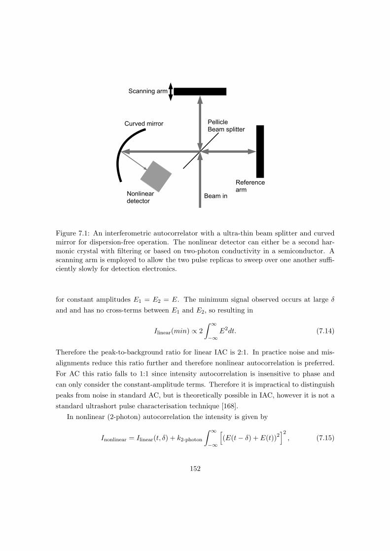
PellicleBeam splitter

Scanning arm

Referencearm

Beam inNonlineardetector

Curved mirror

Figure 7.1: An interferometric autocorrelator with a ultra-thin beam splitter and curvedmirror for dispersion-free operation. The nonlinear detector can either be a second har-monic crystal with filtering or based on two-photon conductivity in a semiconductor. Ascanning arm is employed to allow the two pulse replicas to sweep over one another suffi-ciently slowly for detection electronics.

for constant amplitudes E1 = E2 = E. The minimum signal observed occurs at large δand and has no cross-terms between E1 and E2, so resulting in

Ilinear(min) ∝ 2∫ ∞−∞

E2dt. (7.14)

Therefore the peak-to-background ratio for linear IAC is 2:1. In practice noise and mis-alignments reduce this ratio further and therefore nonlinear autocorrelation is preferred.For AC this ratio falls to 1:1 since intensity autocorrelation is insensitive to phase andcan only consider the constant-amplitude terms. Therefore it is impractical to distinguishpeaks from noise in standard AC, but is theoretically possible in IAC, however it is not astandard ultrashort pulse characterisation technique [168].

In nonlinear (2-photon) autocorrelation the intensity is given by

Inonlinear = Ilinear(t, δ) + k2-photon

∫ ∞−∞

[(E(t− δ) + E(t))2

]2, (7.15)

152

where knonlinear is a factor defining the efficiency of the 2-photon process. Since the linearsignal dominates, this must be removed in order obtain the peak 2-photon signal fromthe background. This is usually achieved by use of a filter or by arranging the setup forbackground-free SHG (AC only) [5]. The need for a filter can be obviated by utilising 2-photon conductivity in a semiconductor such that the 2-photon process is integrated intothe detection unit [169]. By the same reasoning as previously, the peak-to-backgroundratio in 2-photon AC is 3:1, and in 2-photon IAC the ratio 8:1. Therefore using 2-photonprocesses for the autocorrelation improves the peak-to-background ratio. Further improve-ments to this ratio can be achieved by utilising 3-photon processes to achieve a 3-photonAC ratio of 10:1 and 3-photon IAC ratio of 32:1 [36].

The expression usually used to describe the autocorrelation of an ultrashort pulse withGVD [4]. Starting with the electric field for a chirped pulse

E(t) = exp(−(1 + ia)t2

τ2G

), (7.16)

where a is the chirp parameter and τG is related to the Gaussian FWHM pulse duration,τp by τG = 1.177τp. Equation 7.16 is inserted into equation 7.15 to obtain

I2nd-AC(δ) = 1 + 2 exp

[(δ

τG

)2]

+ 4 exp

[(a2 + 3

4

)(δ

τG

)2]

cos

(a

2

(δ

τG

)2)

cos(ωcδ)

+ 2 exp

[−(1 + a2)

(δ

τG

)2]

cos(2ωcδ), (7.17)

where ωc is the centre frequency.Figs. 7.2 and 7.3 show the theoretical IAC traces of a 100 nm bandwidth pulse centred

at 800 nm when unchirped and chirped, respectively. Note the 1:8 ratio in intensity of thebackground to maximum fringe intensity. The chirped IAC trace shows a narrower setof fringes which are overlapped with the AC intensity corresponding to the chirped pulseduration.

We obtained an example set of interferometric autocorrelation results for reference.However we did not utilise the technique during experiments. The results of the ex-periment using a Femtochrome FR-103PD autocorrelator with additional phase added(explained below in the MIIPS section) are illustrated in Fig. 7.4. The interferometric au-tocorrelations contained higher-order spectral phase contributions due to dispersion thatcould not be corrected in this arrangement. The autocorrelation traces extended beyondthe shown times but is not fully shown for clarity. A MATLAB program is provided in the

153

!! !" !# !$ !% & % $ # " !

'(%&!%"

&

%

$

#

"

!

)

*

+

,-./(012

345/41-56(0789:(;4-512

Figure 7.2: The IAC trace of an unchirped pulse of 100 nm bandwidth centred at 800 nm.

!! !" !# !$ !% & % $ # " !

'(%&!%"

&

%

$

#

"

!

)

*

+

,-./(012

345/41-56(0789:(;4-512

Figure 7.3: The IAC trace of a chirped pulse for the same parameters as the unchirpedexample in Fig. 7.2. The chirp parameter used was 5.

supplementary CD to demonstrate the calibration procedure (appropriate for the afore-mentioned autocorrelator family) and simple re-scaling of the data. The autocorrelation

154

!!"# !!## !"# # "# !## !"#

#

#$%

#$&'()

*+,(-.'/0)

123+2043-.'(56$.72430)

!!"# !!## !"# # "# !## !"#

#

#$%

#$&'6)

*+,(-.'/0)

123+2043-.'(56$.72430)

!!"# !!## !"# # "# !## !"#

#

#$%

#$&'8)

*+,(-.'/0)

123+2043-.'(56$.72430)

Figure 7.4: Example interferometric autocorrelation traces obtained for (a) zero-phaseadded, (b) 500 fs2 phase added and (c) 1000 fs2 phase added. Note the optical systemdispersion dominates and results in complex autocorrelation traces.

offers a relatively simple way to estimate the pulse duration however this method has somedisadvantages. Most importantly, the the pulse shape needs to be known or retrieved. Ingeneral it is difficult to know exactly what the pulse shape looks like and direct pulseshape retrieval is impossible because the same autocorrelation can be produced by manydifferent pulse shapes. The problem is even worse in the sub-10 fs regime where pulses be-come increasingly complex and autocorrelator design must be totally dispersion-free [46].Therefore additional knowledge is required in order to describe the pulse. A partial so-

155

lution involves measuring the spectrum and using an iterative computer program [170],however this does not remove ambiguities [46]. Further methods have been developed toimprove upon the results obtained by autocorrelation methods and are discussed below.

7.2.2 Frequency resolved optical gating (FROG)

Following autocorrelation techniques, a major step forward in ultrashort pulse characteri-sation was achieved in what is known as frequency resolved optical gating (FROG) [171].FROG offered a more complete picture of ultrashort pulse intensity and phase by split-ting the pulse into two identical parts and varying the overlap of the pulse replicas ina nonlinear medium such as glass and then imaging the resultant pulse in terms of itsspectral components [172]. In Fig. 7.5 (a) the setup used in [171] is summarised. In thisarrangement the Kerr-induced diffracted light is spectrally resolved and imaged onto acamera and a two dimensional image is created of delay time vs frequency. The resultantimage width shows the pulse duration in one direction, while any chirp will be seen as afrequency-dependent evolution in time whose angle shows whether the pulse is positivelyor negatively chirped. Part (b) of Fig. 7.5 illustrates this effect of chirp. The equationwhich describes the FROG trace is given by [172]

SFROG(ω, δ) =∣∣∣∣∫ ∞−∞

E(t)g(t− δ) exp(−iωt)dt∣∣∣∣2 , (7.18)

where the g(t − δ) = |E(t − δ)|2 is the delay gate defining the strength of the nonlinearprocess as function of delay time δ. Equation 7.18 defines the example traces in Fig. 7.5and allows full characterisation of the pulse since the problem has been converted from oneto two dimensions, allowing simultaneous display of frequency and gate delay time [172].FROG has been successfully used for the characterisation of ultrashort pulses down to 4.5fs, however the design of the setup requires particular care to avoid dispersive effects [173].

The use of the third-order Kerr process for FROG eliminates the direction of timeambiguity that exists in second-order autocorrelation that means that it is impossible todistinguish the difference between a pulse that is reversed in time. A version of FROGinvolving SHG retains this ambiguity in time but allows the use of lower peak power pulsesdue to the higher effective nonlinearity afforded by second-order processes [174].

156

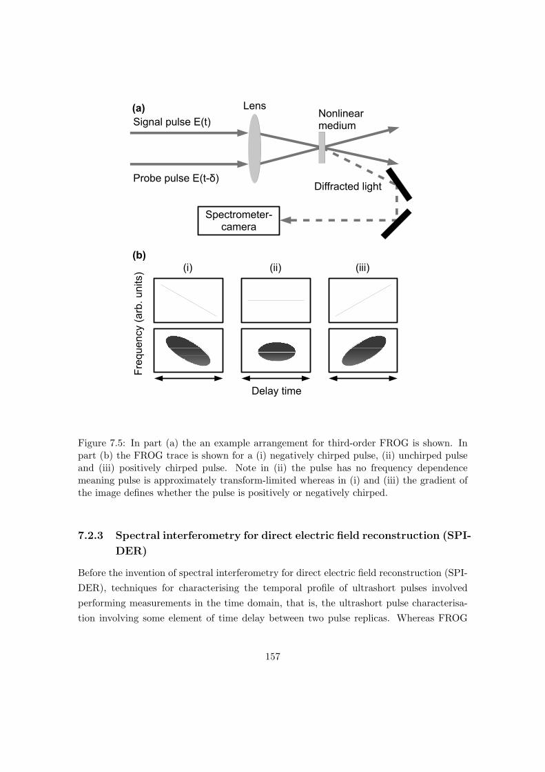
Figure 7.5: In part (a) the an example arrangement for third-order FROG is shown. Inpart (b) the FROG trace is shown for a (i) negatively chirped pulse, (ii) unchirped pulseand (iii) positively chirped pulse. Note in (ii) the pulse has no frequency dependencemeaning pulse is approximately transform-limited whereas in (i) and (iii) the gradient ofthe image defines whether the pulse is positively or negatively chirped.

7.2.3 Spectral interferometry for direct electric field reconstruction (SPI-

DER)

Before the invention of spectral interferometry for direct electric field reconstruction (SPI-DER), techniques for characterising the temporal profile of ultrashort pulses involvedperforming measurements in the time domain, that is, the ultrashort pulse characterisa-tion involving some element of time delay between two pulse replicas. Whereas FROG

157

offered a spectral measurement in combination with a temporal measurement, SPIDERoffered a frequency-domain only technique for characterising ultrashort pulses [175]. It isunimportant whether one characterises in the time or spectral domains as a measurementin one domain can simply be transferred to the other domain via the appropriate Fouriertransform, which requires a small amount of computational power. Although conceptuallya time-domain measurement is the preferred method, a frequency-domain measurementis a perfectly adequate method for ultrashort pulse characterisation if the method canreliably obtain the full spectral phase. The SPIDER method [175] is an interferometrictechnique that built upon a pre-existing technique involving spectral interference [176].In SPIDER an interferometric arrangement is employed in which two pulse replicas arecreated with a constant time delay, both of which are mixed with a strongly chirped pulsewithin a nonlinear crystal. The resulting frequency-converted spectrum is then collectedin a spectrometer. Fig. 7.6 summarises the SPIDER process. The spectral inteference

Figure 7.6: SPIDER is an interferometric technique that utilises nonlinear mixing betweentwo pulse replicas with constant delay and a further chirped pulse. The two pulse replicaseffectively create a spectral amplitude modulation of constant reference frequency (throughthe Fourier transform of a double-pulse), which when frequency mixed with the chirpedpulse results in an up-converted sample whose intensity depends upon the relative phasebetween the replica pulse spectrum and chirped pulse spectrum.

pattern has an intensity given by [175]

SSPIDER = |E(ωc)|2+|E(ωc−Ω)|2+2|E(ωc)E(ωc+Ω)|cos[φ(ωc+Ω)−φ(ωc)+ωcτ ], (7.19)

where E(ω) is the rapidly-varying spectral electric field, ωc is the centre frequency of theportion of spectrum under investigation, Ω defines the amount of spectral phase introducedby the chirping element. The spectral phase is obtained by calculating or measuring thefixed delay time, fundamental spectral intensity and dispersion introduced by the setup

158

and subsequently removing these terms from equation 7.19 through appropriate filteringafter Fourier transforming the up-converted spectrum.

7.3 Finite element modeling using COMSOL

In this Appendix the derivations of the expressions used to describe the Maxwell Stresstensor and surface force are described.

7.3.1 Derivation of Maxwell stress tensor force for use in COMSOL

To compute the force acting on two dielectric particles in close location, the equations ofmotion for the system in an electromagnetic field are derived [122]. Starting with the time-averaged Lorentz force density expression we derive the generalised force on a dielectricparticle by following the approach in [177]

f =12(ρE∗ + J × B∗

)(7.20)

with the ∗ representing the complex conjugate. Maxwell’s equations for monochromaticwaves are given by:

ρ = ∇. D (7.21)

J = ∇× H + iωD (7.22)

∇. B = 0 (7.23)

iωB = ∇× E (7.24)

Using equation 7.20 and the Maxwell equations and inserting equation 7.23 for complete-ness the force density is given by:

f =12<((∇. D)E∗ + (∇× E∗)× D + (∇. B∗)H + (∇× H)× B∗

)(7.25)

Equation 7.25 can be reduced to:

f = −12<(∇. ¯T (r)

)(7.26)

where¯T (r) =

12(D. E∗ + B∗. H

) ¯I − D ⊗ E∗ − B∗ ⊗ H (7.27)

159

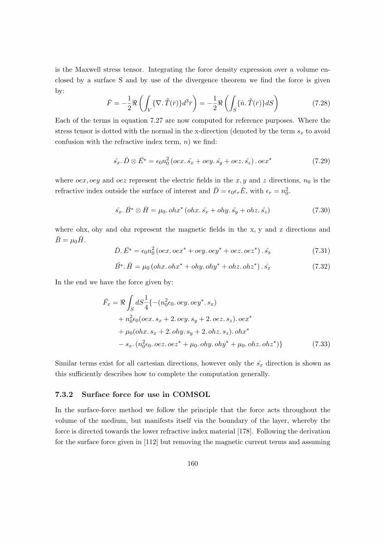
is the Maxwell stress tensor. Integrating the force density expression over a volume en-closed by a surface S and by use of the divergence theorem we find the force is givenby:

F = −12<(∫

V∇. ¯T (r)d3r

)= −1

2<(∫

Sn. ¯T (r)dS

)(7.28)

Each of the terms in equation 7.27 are now computed for reference purposes. Where thestress tensor is dotted with the normal in the x-direction (denoted by the term sx to avoidconfusion with the refractive index term, n) we find:

sx. D ⊗ E∗ = ε0n20 (oex. sx + oey. sy + oez. sz) . oex∗ (7.29)

where oex, oey and oez represent the electric fields in the x, y and z directions, n0 is therefractive index outside the surface of interest and D = ε0εrE, with εr = n2

0.

sx. B∗ ⊗ H = µ0. ohx∗ (ohx. sx + ohy. sy + ohz. sz) (7.30)

where ohx, ohy and ohz represent the magnetic fields in the x, y and z directions andB = µ0H.

D. E∗ = ε0n20 (oex. oex∗ + oey. oey∗ + oez. oez∗) . sx (7.31)

B∗. H = µ0 (ohx. ohx∗ + ohy. ohy∗ + ohz. ohz∗) . sx (7.32)

In the end we have the force given by:

Fx = <∫SdS

14−(n2

0ε0. oey. oey∗. sx)

+ n20ε0(oex. sx + 2. oey. sy + 2. oez. sz). oex∗

+ µ0(ohx. sx + 2. ohy. sy + 2. ohz. sz). ohx∗

− sx. (n20ε0. oez. oez

∗ + µ0. ohy. ohy∗ + µ0. ohz. ohz

∗) (7.33)

Similar terms exist for all cartesian directions, however only the sx direction is shown asthis sufficiently describes how to complete the computation generally.

7.3.2 Surface force for use in COMSOL

In the surface-force method we follow the principle that the force acts throughout thevolume of the medium, but manifests itself via the boundary of the layer, whereby theforce is directed towards the lower refractive index material [178]. Following the derivationfor the surface force given in [112] but removing the magnetic current terms and assuming

160

the medium is non-absorbing; from equation 7.25 we get the surface force density term

fsurf = −ε04

(E · E∗)∇(ε′r) (7.34)

where ε′r is the real component of the local relative permittivity. This yields the form ofthe surface force in the x-direction, appropriate only for the system of two non-absorbingdielectrics

fx = −14<(ε0(n2

0 − n21)[iex · oex∗ + iey · oey∗ + iez · oez∗]) · sx (7.35)

where n0 and n1 are the real refractive indices of the dielectric medium outside andinside the particle respectively. iex represents the inside electric field amplitude and oexrepresents the outside electric field amplitude, and so on for the y and z components. Thisequation is then used to compute the force by integration of the surface boundaries withrespect to area. Note, in the case of both derivations for surface and stress tensor forces,the newer versions of COMSOL do not require any equation input.

7.4 Phototransfection methods

Detailed here are the phototransfection methods used in Chapter 4.

7.4.1 Chinese Hamster Ovary cells

Chinese Hamster Ovary (CHO) cells were cultured in a medium consisting of MinimumEssential Medium (Sigma), 10 % Fetal Calf Serum (Sera Laboratories International) andL-Glutamine, Penicillin and Streptomycin (Sigma). Cells were cultured in plastic flasksand incubated 37 degrees centigrade and with 5 % atmospheric Carbon Dioxide. In orderto remove cells from the plastic flask the medium was removed and washed with Trypsin-EDTA (Sigma). 1 ml of Typsin was added and the cells were incubated for 4 minutes.During this time the Trypsin removed adherent cells from the bottom of the flask to allowthe cells to float freely in the Trypsin mixture. Any remaining adherent cells were removedby tapping the flask several times. The vibration causes the cells to detach from the flaskand float in the Trypsin solution. After 5 minutes 4 ml of medium is added and mixedwith the Trypsin. An amount of the resulting mixture was used to create the next passageof cells. Typically 1 ml was used and placed in a clean flask. A further 4 ml was added tothe new flask and the solution mixed such that an even coating of cells was ensured.

Glass bottomed petri dishes (World Precision Instruments) were populated with 2 ml of

161

the cell mixture. The required concentration of cell solution depends upon the confluencyand growth rate of the cells in question. Typical amounts used were 50 to 100 /mul ofcell solution per 2 ml of medium. 2 ml of diluted cell solution is added to each petri dish.The dishes were then incubated over a period of 24-48 hours.

A (DS-Red) DNA solution was prepared using 300 /mul of OPTIMEM and DNA plas-mid solution was added to attain a DNA concentration of 10 /mug per ml. A preparedcell sample was taken and the medium removed. Each sample dish was washed with OP-TIMEM twice before the DNA solution described above was gently added. The dish wascovered and sealed with UNESCO film to limit loss due to evaporation; the dish was thenincubated for 15 mins at 37 degrees centigrade with an atmospheric CO2 concentrationof 5.0 %. The cells were then transferred to the photoporation setup. Following the pho-toporation procedure the cells were washed twice with the cell culture medium describedabove and 2 ml of cell culture medium was added to the petri dish. The cells were thenincubated as described above for 48 hours. In some experiments 15 µl of Nupherin (EnzoLife Sciences) was added to the DNA plasmid solution to potentially enhance transfectionefficiency [179].

The cells which were transfected with DS-Red were identified using a fluorescencemicroscope (Nikon Eclipse Ti) utilising a Nikon TRITC filter cube, with a Nikon PlanFluor 20x/0.50NA phase contrast objective for imaging. Fluorescent cells within themarked region of interest were counted. The number of fluorescent cells divided by thenumber of cells photoporated gives the uncorrected transfection efficiency.

7.4.2 Human Embryonic Kidney cells

Human Embryonic Kidney (HEK) cells were cultured and photoporated in the same man-ner as CHO cells apart from requiring a different procedure to maintain cell attachment tothe surface substrate of the petri dishes. Glass bottomed petri dishes (World Precision In-struments) were prepared with a Laminin-OPTIMEM (Sigma) mixture with surface areaconcentration 5 µg/cm2 and incubated at 37 degrees centigrade with an atmospheric CO2

concentration of 5.0 % for 24 hours. The Laminin-OPTIMEM solution was removed andthe dish washed with medium two times. Following this procedure cells were introducedin a manner identical to above. Further, transfection experiments were carried out in thesame manner also.

162

7.5 Use of MATLAB and other programs for producing the-

oretical/computational images

The author independently wrote the MATLAB programs used to generate the theoreticalimages in all chapters except for in the optical binding chapter. Also provided is theMATHEMATICA program written by Michael Mazilu for calculating the optical bindingforces between Rayleigh-sized particles, as used in the optical binding chapter. Theseare provided with the supplementary CD accompanying this thesis or can be emailed onrequest. Please contact Kishan Dholakia for the author’s most up-to-date email address,if required.

163

Acknowledgements

I am exceptionally grateful to my supervisor, Prof. Kishan Dholakia for his guidance,understanding, and hard work throughout the course of my PhD. I am particularly appre-ciative to him for providing me with the opportunity to work in the Optical ManipulationGroup with cutting-edge laser technology. I am very grateful to Prof. Frank Gunn-Moorefor his guidance and encouragement in aspects relating to all aspects of science. I wouldalso like to thank my mentors, Dr. Tom Brown and Prof. Wilson Sibbett for their un-abated encouragement and enthusiasm for my work.

I am completely indebted to Dr. Michael Mazilu for the many hours he has spenttalking to me about science, correcting my scientific understanding and the many modelsprovided by him throughout my PhD, often at particularly short notice. I am also indebtedto Dr. Maciej Antkowiak for the multitude of discussions about the light-biomatter inter-action which took up so much of our time. I am further indebted to Dr. Joerg Baumgartlfor all of his support in the lab, and most importantly, introducing me to coffee breaks,without which, my world would have been further darkened by the windowless depths ofthe optics laboratories!

To Christine Crombie, Darran Milne, Claire Mitchell, Niall Quinn, Christian Reimer,Helen Rendall, Sebastian Schulz and Richard Tatham, I thank you all for your friendshipthroughout the PhD and for making coffee break, lunchtimes, and sometimes evening-timesall the more memorable and entertaining(!)

To Lani Torres-Mapa I thank you for the many wonderful conversations about literallyanything. To Martin Ploschner, for the multitude of self-deprecating conversations regard-ing philosophy of science and life in addition to many discussions about theoretical andexperimental aspects of science. I am certainly better informed as a result of these discus-sions! To, in no particular order, Tom Cizmar, Tom Vettenburg, David Stevenson, HeatherDalgarno, Yoshi Arita, Svetlana Zolotovskaya, Sebastian Kosmeier, Praveen Ashok, Bav-ishna Balagopal, Areti Mourka, Maria Dienerowitz, Dave Walsh, Klaus Metzger, FionaBaumgartl, Alexander Lagatsky, Matthieu Robert de Saint Vincent, Jill Morris, XanthiTsampoula, Rob Marchington, Andrew McKinley and Craig McDougall, to name but afew. I thank you all for the scientific support and most excellent discussions we have hadover the years.

To Dr. David Stothard I thank you for many hours of discussion about life and scienceand for taking the time to create stunning photographs of my wedding to Mrs. RachelRudhall.

I am also very grateful to all of my family down South for their kind understanding,

164

support in everything that I do and for teaching me to read, write, do maths and makemusic at the earliest stages of my life, all of which provided me with the foundationnecessary for me to pursue my academic journey and enjoy life.

I reserve the most personal gratitude to my wonderful wife, Rachel Rudhall, withoutwhom, I could not sustain myself in life. You have had to put up with evenings, weekendsand holidays without me and I cannot thank you enough for your unending support. I alsocannot thank you enough for bringing our wonderful daughter, Alice Eveleigh Rudhall intothe world. She never ceases to brighten up my day with her brilliant smiles and giggles.

Finally, on a less emotional note, I finish with my favourite proverb: If you drink, youdie. If you don’t drink, you die. So you may as well drink.

165