UK Greenhouse Gas Inventory, 1990 to 2013
534
UK Greenhouse Gas Inventory, 1990 to 2016 Annual Report for Submission under the Framework Convention on Climate Change Main authors Brown P, Broomfield M, Cardenas L, Choudrie S, Kilroy E, Jones L, MacCarthy J, Passant N, Thistlethwaite G, Thomson A, Wakeling D With contributions from Buys G, Gilhespy S, Glendining M, Gluckman R, Hampshire K, Henshall P, Hobson M, Malcolm H, Manning A, Matthews R, Milne A, Misselbrook T, Moxley J, Murrells T, Salisbury E, Walker C, Watterson J April 2018 This work forms part of the Science Research Programme of the Department for Business, Energy & Industrial Strategy. 978-0-9933975-4-7
Transcript of UK Greenhouse Gas Inventory, 1990 to 2013
UK Greenhouse Gas Inventory, 1990 to 2016
Annual Report for Submission under the Framework Convention on Climate Change
Main authors Brown P, Broomfield M, Cardenas L, Choudrie S, Kilroy E, Jones L, MacCarthy J, Passant N, Thistlethwaite G, Thomson A, Wakeling D
With contributions from
Buys G, Gilhespy S, Glendining M, Gluckman R, Hampshire K, Henshall P, Hobson M, Malcolm H, Manning A, Matthews R, Milne A, Misselbrook T, Moxley J, Murrells T, Salisbury E, Walker C, Watterson J
April 2018
This work forms part of the Science Research Programme of the Department for Business, Energy & Industrial Strategy.
978-0-9933975-4-7

UK NIR 2018 (Issue 1.1) Ricardo Energy & Environment Page 3
Title
UK Greenhouse Gas Inventory 1990 to 2016: Annual Report for submission under the Framework Convention on Climate Change
Customer Department for Business, Energy & Industrial Strategy
Confidentiality, copyright and reproduction
Crown Copyright
File reference N:\naei16\8_ghgi\1_nir\ukghgi-90-16_Main_Issue1.1.docx
NAEI contacts database reference
ED62689/0/CD8977/PB
Reference number Ricardo Energy & Environment/R/3468
ISBN 978-0-9933975-4-7
Issue number Issue 1.1
Peter Brown Ricardo Energy & Environment The Gemini Building, Fermi Avenue Harwell Didcot Oxfordshire, OX11 0QR, UK. Telephone: +44 1235 75 3273 Facsimile: +44 1235 75 3001 Ricardo Energy & Environment is the trading name of Ricardo-AEA Ltd. Ricardo-AEA Ltd. is certified to ISO 9001 and to ISO 14001
Lead Author Name Peter Brown
Approved by Name Joanna MacCarthy
Signature
Date 12/04/2018
Preface
UK NIR 2018 (Issue 1.1) Ricardo Energy & Environment Page 4
Preface
This is the United Kingdom’s National Inventory Report (NIR) submitted in 2018 to the United Nations Framework Convention on Climate Change (UNFCCC). It contains national greenhouse gas emission estimates for the period 1990-2016, and descriptions of the methods used to produce the estimates. The report is prepared in accordance with decision 24/CP.191 and includes elements required for reporting under the Kyoto Protocol, as outlined in the Annotated outline of the National Inventory Report including reporting elements under the Kyoto Protocol2. This submission constitutes the UK’s submission under the Kyoto Protocol.
The greenhouse gas inventory (GHGI) is based on the same datasets used by the UK in the National Atmospheric Emissions Inventory (NAEI) for reporting atmospheric emissions under other international agreements. The GHGI is therefore consistent with these other air emissions inventories where they overlap.
The greenhouse gas inventory is compiled on behalf of the UK Department for Business, Energy and Industrial Strategy (BEIS) Science and Innovation for Climate and Energy (SICE) Directorate, by Ricardo Energy & Environment. We acknowledge the positive support and advice from BEIS throughout the work, and we are grateful for the help of all those who have contributed to this NIR. A list of the contributors can be found in Chapter 18.
The GHGI is compiled according to IPCC 2006 Guidelines (IPCC, 2006). Each year the inventory is updated to include the latest data available. Improvements to the methodology are backdated as necessary to ensure a consistent time series. Methodological changes are made to take account of new data sources, or new guidance from IPCC, and new research, sponsored by BEIS or otherwise.
1 FCCC Decision 24/CP.19. Revision of the UNFCCC reporting guidelines on annual inventories for Parties included in Annex I to the Convention http://unfccc.int/resource/docs/2013/cop19/eng/10a03.pdf
2 http://unfccc.int/files/national_reports/annex_i_ghg_inventories/reporting_requirements/application/pdf/annotated_nir_outline.pdf
Units and Conversions
UK NIR 2018 (Issue 1.1) Ricardo Energy & Environment Page 5
Units and Conversions
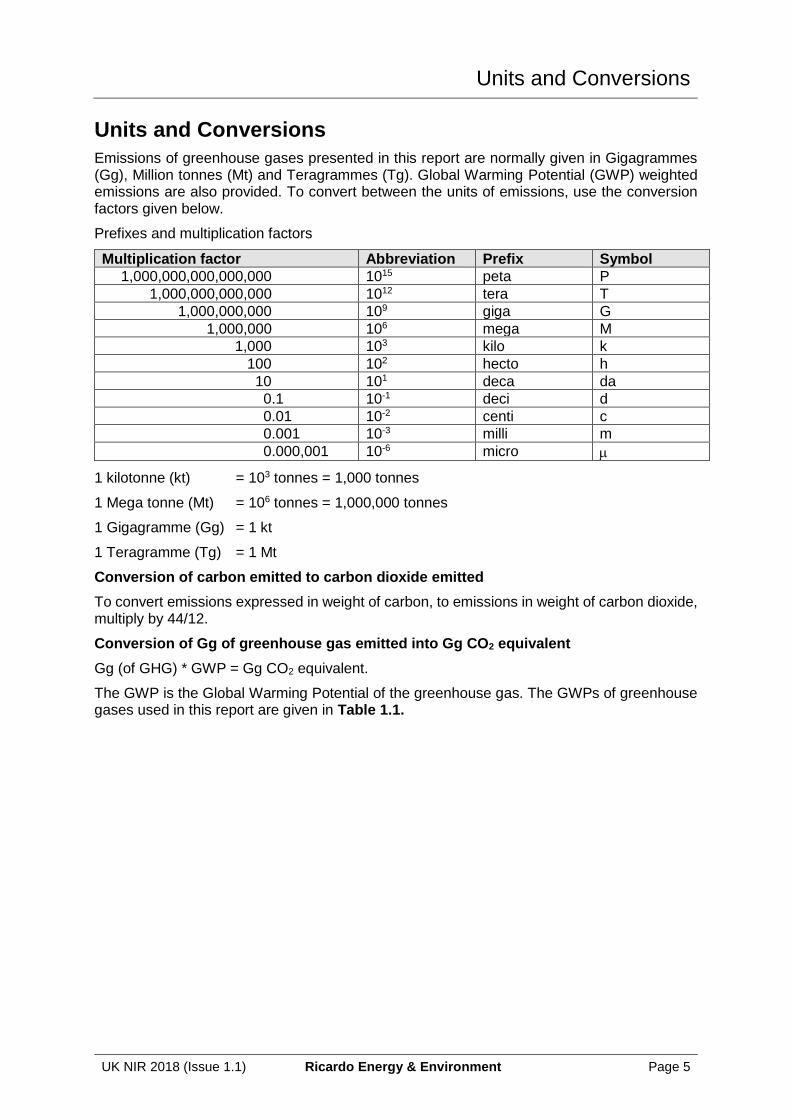
Emissions of greenhouse gases presented in this report are normally given in Gigagrammes (Gg), Million tonnes (Mt) and Teragrammes (Tg). Global Warming Potential (GWP) weighted emissions are also provided. To convert between the units of emissions, use the conversion factors given below.
Prefixes and multiplication factors
Multiplication factor Abbreviation Prefix Symbol
1,000,000,000,000,000 1015 peta P
1,000,000,000,000 1012 tera T
1,000,000,000 109 giga G
1,000,000 106 mega M
1,000 103 kilo k
100 102 hecto h
10 101 deca da
0.1 10-1 deci d
0.01 10-2 centi c
0.001 10-3 milli m
0.000,001 10-6 micro
1 kilotonne (kt) = 103 tonnes = 1,000 tonnes
1 Mega tonne (Mt) = 106 tonnes = 1,000,000 tonnes
1 Gigagramme (Gg) = 1 kt
1 Teragramme (Tg) = 1 Mt
Conversion of carbon emitted to carbon dioxide emitted
To convert emissions expressed in weight of carbon, to emissions in weight of carbon dioxide, multiply by 44/12.
Conversion of Gg of greenhouse gas emitted into Gg CO2 equivalent
Gg (of GHG) * GWP = Gg CO2 equivalent.
The GWP is the Global Warming Potential of the greenhouse gas. The GWPs of greenhouse gases used in this report are given in Table 1.1.
Common Abbreviations
UK NIR 2018 (Issue 1.1) Ricardo Energy & Environment Page 6
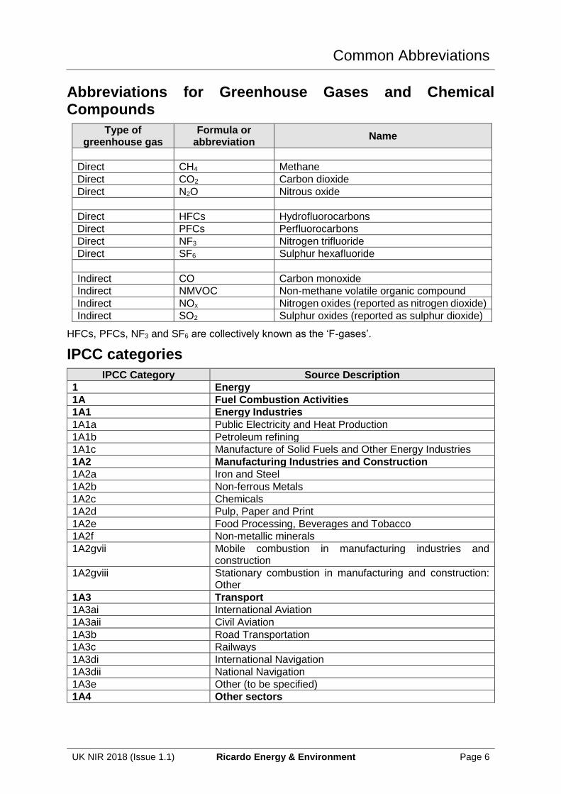
Abbreviations for Greenhouse Gases and Chemical Compounds
Type of greenhouse gas
Formula or abbreviation
Name
Direct CH4 Methane
Direct CO2 Carbon dioxide
Direct N2O Nitrous oxide
Direct HFCs Hydrofluorocarbons
Direct PFCs Perfluorocarbons
Direct NF3 Nitrogen trifluoride
Direct SF6 Sulphur hexafluoride
Indirect CO Carbon monoxide
Indirect NMVOC Non-methane volatile organic compound
Indirect NOx Nitrogen oxides (reported as nitrogen dioxide)
Indirect SO2 Sulphur oxides (reported as sulphur dioxide)
HFCs, PFCs, NF3 and SF6 are collectively known as the ‘F-gases’.
IPCC categories
IPCC Category Source Description
1 Energy
1A Fuel Combustion Activities
1A1 Energy Industries
1A1a Public Electricity and Heat Production
1A1b Petroleum refining
1A1c Manufacture of Solid Fuels and Other Energy Industries
1A2 Manufacturing Industries and Construction
1A2a Iron and Steel
1A2b Non-ferrous Metals
1A2c Chemicals
1A2d Pulp, Paper and Print
1A2e Food Processing, Beverages and Tobacco
1A2f Non-metallic minerals
1A2gvii Mobile combustion in manufacturing industries and construction
1A2gviii Stationary combustion in manufacturing and construction: Other
1A3 Transport
1A3ai International Aviation
1A3aii Civil Aviation
1A3b Road Transportation
1A3c Railways
1A3di International Navigation
1A3dii National Navigation
1A3e Other (to be specified)
1A4 Other sectors
Common Abbreviations
UK NIR 2018 (Issue 1.1) Ricardo Energy & Environment Page 7
IPCC Category Source Description
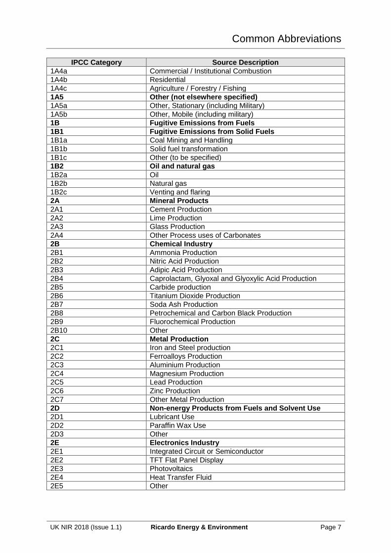
1A4a Commercial / Institutional Combustion
1A4b Residential
1A4c Agriculture / Forestry / Fishing
1A5 Other (not elsewhere specified)
1A5a Other, Stationary (including Military)
1A5b Other, Mobile (including military)
1B Fugitive Emissions from Fuels
1B1 Fugitive Emissions from Solid Fuels
1B1a Coal Mining and Handling
1B1b Solid fuel transformation
1B1c Other (to be specified)
1B2 Oil and natural gas
1B2a Oil
1B2b Natural gas
1B2c Venting and flaring
2A Mineral Products
2A1 Cement Production
2A2 Lime Production
2A3 Glass Production
2A4 Other Process uses of Carbonates
2B Chemical Industry
2B1 Ammonia Production
2B2 Nitric Acid Production
2B3 Adipic Acid Production
2B4 Caprolactam, Glyoxal and Glyoxylic Acid Production
2B5 Carbide production
2B6 Titanium Dioxide Production
2B7 Soda Ash Production
2B8 Petrochemical and Carbon Black Production
2B9 Fluorochemical Production
2B10 Other
2C Metal Production
2C1 Iron and Steel production
2C2 Ferroalloys Production
2C3 Aluminium Production
2C4 Magnesium Production
2C5 Lead Production
2C6 Zinc Production
2C7 Other Metal Production
2D Non-energy Products from Fuels and Solvent Use
2D1 Lubricant Use
2D2 Paraffin Wax Use
2D3 Other
2E Electronics Industry
2E1 Integrated Circuit or Semiconductor
2E2 TFT Flat Panel Display
2E3 Photovoltaics
2E4 Heat Transfer Fluid
2E5 Other
Common Abbreviations
UK NIR 2018 (Issue 1.1) Ricardo Energy & Environment Page 8
IPCC Category Source Description
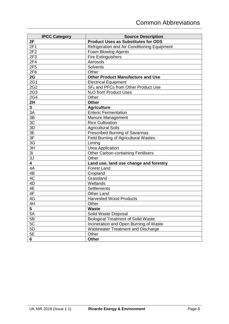
2F Product Uses as Substitutes for ODS
2F1 Refrigeration and Air Conditioning Equipment
2F2 Foam Blowing Agents
2F3 Fire Extinguishers
2F4 Aerosols
2F5 Solvents
2F6 Other
2G Other Product Manufacture and Use
2G1 Electrical Equipment
2G2 SF6 and PFCs from Other Product Use
2G3 N2O from Product Uses
2G4 Other
2H Other
3 Agriculture
3A Enteric Fermentation
3B Manure Management
3C Rice Cultivation
3D Agricultural Soils
3E Prescribed Burning of Savannas
3F Field Burning of Agricultural Wastes
3G Liming
3H Urea Application
3I Other Carbon-containing Fertilisers
3J Other
4 Land use, land use change and forestry
4A Forest Land
4B Cropland
4C Grassland
4D Wetlands
4E Settlements
4F Other Land
4G Harvested Wood Products
4H Other
5 Waste
5A Solid Waste Disposal
5B Biological Treatment of Solid Waste
5C Incineration and Open Burning of Waste
5D Wastewater Treatment and Discharge
5E Other
6 Other
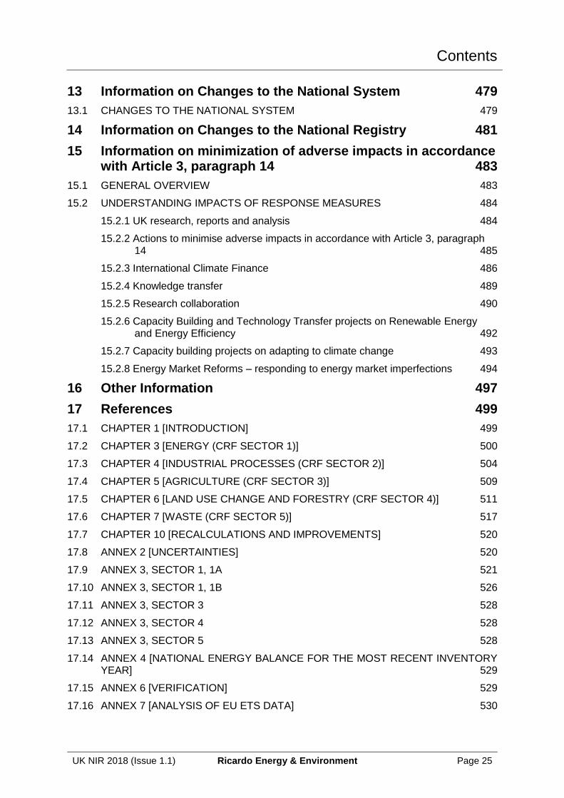
Contents
UK NIR 2018 (Issue 1.1) Ricardo Energy & Environment Page 9
Contents Preface 4
Units and Conversions 5
Abbreviations for Greenhouse Gases and Chemical Compounds 6
IPCC categories 6
Contents 9
Executive Summaries 31
ES.1 BACKGROUND INFORMATION 31
ES.1.1 Climate Change 31
ES.1.2 Greenhouse Gas Inventories 31
ES.1.3 Supplementary Information Required under Article 7, paragraph 1, of the Kyoto Protocol. 33
ES.2 SUMMARY OF NATIONAL EMISSION AND REMOVAL RELATED TRENDS, AND EMISSIONS AND REMOVALS FROM KP-LULUCF ACTIVITIES 34
ES.2.1 GHG Inventory 34
ES.2.2 KP-LULUCF Activities 35
ES.3 OVERVIEW OF SOURCE AND SINK CATEGORY EMISSION ESTIMATES AND TRENDS, INCLUDING KP-LULUCF ACTIVITIES 37
ES.3.1 GHG Inventory 37
ES.3.2 KP Basket and KP-LULUCF Activities 37
ES.4 OTHER INFORMATION 41
Contacts 42
1 Introduction 43
1.1 BACKGROUND INFORMATION ON GREENHOUSE GAS INVENTORIES, AND CLIMATE CHANGE 43
1.1.1 Background Information on Climate Change 43
1.1.2 Background Information on Greenhouse Gas Inventories 44
1.1.3 Background Information on Supplementary Information Required under Article 7, paragraph 1, of the Kyoto Protocol 47
1.2 INSTITUTIONAL ARRANGEMENTS FOR INVENTORY PREPARATION 48
1.2.1 Institutional, Legal and Procedural Arrangements for Compiling the UK inventory 48
1.2.2 Overview of Inventory Planning 51
1.2.3 Overview of Inventory Preparation and Management, Including for Supplementary Information Required under Article 7, Paragraph 1 of the Kyoto Protocol 63
1.3 INVENTORY PREPARATION 64
Contents
UK NIR 2018 (Issue 1.1) Ricardo Energy & Environment Page 10
1.3.1 GHG Inventory 64
1.3.2 Data collection, processing and storage 64
1.3.3 Quality assurance/quality control (QA/QC) procedures and extensive review of GHG inventory 65
1.4 METHODOLOGIES AND DATA SOURCES 65
1.4.1 GHG Inventory 65
1.5 DESCRIPTION OF KEY SOURCE CATEGORIES 69
1.5.1 GHG Inventory 69
1.5.2 KP-LULUCF analysis 74
1.6 QUALITY ASSURANCE AND QUALITY CONTROL (QA/QC) 74
1.6.1 Description of the current QA/QC system 75
1.6.2 Improvements to the QA/QC System 78
1.6.3 Verification 91
1.6.4 Treatment of Confidentiality 91
1.7 GENERAL UNCERTAINTY EVALUATION 92
1.7.1 GHG Inventory 92
1.8 GENERAL ASSESSMENT OF COMPLETENESS 92
1.8.1 GHG Inventory 92
2 Trends in Greenhouse Gas Emissions 93
2.1 DESCRIPTION AND INTERPRETATION OF EMISSION TRENDS FOR AGGREGATED GREENHOUSE GAS EMISSIONS 93
2.2 DESCRIPTION AND INTERPRETATION OF EMISSION TRENDS BY GAS 94
2.2.1 Carbon Dioxide 94
2.2.2 Methane 95
2.2.3 Nitrous Oxide 96
2.2.4 Fluorinated-Gases 97
2.3 DESCRIPTION AND INTERPRETATION OF EMISSION TRENDS BY CATEGORY 99
2.3.1 Energy 100
2.3.2 Industrial Processes and Other Product Use 102
2.3.3 Agriculture 102
2.3.4 Land Use, Land Use Change and Forestry 103
2.3.5 Waste 103
2.4 EMISSION TRENDS FOR INDIRECT GREENHOUSE GASES AND SO2 103
2.4.1 Carbon Monoxide 104
2.4.2 Nitrogen Oxides 104
2.4.3 Sulphur Dioxide 105
Contents
UK NIR 2018 (Issue 1.1) Ricardo Energy & Environment Page 11
2.4.4 Non Methane Volatile Organic Compounds 105
2.5 EMISSION TRENDS FROM KP LULUCF ACTIVITIES 105
3 Energy (CRF Sector 1) 109
3.1 OVERVIEW OF SECTOR 109
3.2 FUEL COMBUSTION (CRF 1.A) 111
3.2.1 Comparison of Sectoral and Reference Approaches 111
3.2.2 International Bunker Fuels (memo item) 115
3.2.3 Feedstock and Non-Energy Use of Fuels 115
3.2.4 Use of UK Energy Statistics in the GHG inventory 116
3.2.5 Biomass 117
3.2.6 Unoxidized Carbon 117
3.3 CO2 TRANSPORT AND STORAGE 118
3.4 METHOD STATEMENTS 118
MS 1 Power stations, refineries and other energy industries 120
MS 2 Upstream oil and gas production – fuel combustion 125
MS 3 Manufacturing industries and construction (excluding iron and steel use of derived fuels, and off road machinery) 129
MS 4 Iron and steel, and coke manufacture 133
MS 5 Other stationary combustion 138
MS 6 Off road machinery 140
MS 7 Aviation 145
MS 8 Road Transport 149
MS 9 Railways 159
MS 10 National navigation and fishing 161
MS 11 Shipping between UK and OTs 168
MS 12 Inland Waterways 170
MS 13 Fishing outside of UK territorial waters 173
MS 14 International shipping 174
MS 15 Naval shipping 177
MS 16 Military aircraft 178
MS 17 Coal mining and handling 179
MS 18 Closed coal mines 184
MS 19 1B2 excluding: Oil refining, storage and distribution (1B2aiv to v) and natural gas distribution (1B2biii to v) 187
MS 20 Gas leakage 193
4 Industrial Processes and Product Use (IPPU; CRF Sector 2) 201
4.1 OVERVIEW OF SECTOR 201
Contents
UK NIR 2018 (Issue 1.1) Ricardo Energy & Environment Page 12
4.2 SOURCE CATEGORY 2A1 – CEMENT PRODUCTION 205
4.2.1 Source Category Description 205
4.2.2 Methodological Issues 206
4.2.3 Uncertainties and Time Series Consistency 206
4.2.4 Source Specific QA/QC and Verification 208
4.2.5 Source Specific Recalculations 208
4.2.6 Source Specific Planned Improvements 208
4.3 SOURCE CATEGORY 2A2 – LIME PRODUCTION 208
4.3.1 Source Category Description 208
4.3.2 Methodological Issues 208
4.3.3 Uncertainties and Time Series Consistency 210
4.3.4 Source-specific QA/QC and Verification 210
4.3.5 Source Specific Recalculations 211
4.3.6 Source Specific Planned Improvements 211
4.4 SOURCE CATEGORY 2A3 – GLASS PRODUCTION 211
4.4.1 Source Category Description 211
4.4.2 Methodological Issues 211
4.4.3 Uncertainties and Time Series Consistency 213
4.4.4 Source Specific QA/QC and Verification 214
4.4.5 Source Specific Recalculations 214
4.4.6 Source Specific Planned Improvements 214
4.5 SOURCE CATEGORY 2A4 – OTHER PROCESS USES OF CARBONATES 214
4.5.1 Source Category Description 214
4.5.2 Methodological Issues 215
4.5.3 Uncertainties and Time Series Consistency 219
4.5.4 Source Specific QA/QC and Verification 219
4.5.5 Source Specific Recalculations 219
4.5.6 Source Specific Planned Improvements 219
4.6 SOURCE CATEGORY 2B1 – AMMONIA PRODUCTION 219
4.6.1 Source Category Description 219
4.6.2 Methodological Issues 220
4.6.3 Uncertainties and Time Series Consistency 222
4.6.4 Source Specific QA/QC and Verification 222
4.6.5 Source Specific Recalculations 222
4.6.6 Source Specific Planned Improvements 222
4.7 SOURCE CATEGORY 2B2 – NITRIC ACID PRODUCTION 222

Contents
UK NIR 2018 (Issue 1.1) Ricardo Energy & Environment Page 13
4.7.1 Source Category Description 222
4.7.2 Methodological Issues 223
4.7.3 Uncertainties and Time Series Consistency 226
4.7.4 Source Specific QA/QC and Verification 226
4.7.5 Source Specific Recalculations 227
4.7.6 Source Specific Planned Improvements 227
4.8 SOURCE CATEGORY 2B3 – ADIPIC ACID PRODUCTION 227
4.8.1 Source Category Description 227
4.8.2 Methodological issues 227
4.8.3 Uncertainties and Time Series Consistency 227
4.8.4 Source Specific QA/QC and Verification 228
4.8.5 Source Specific Recalculations 228
4.8.6 Source Specific Planned Improvements 228
4.9 SOURCE CATEGORY 2B4 – CAPROLACTAM, GLYOXAL AND GLYOXYLIC ACID PRODUCTION 228
4.10 SOURCE CATEGORY 2B5 – CARBIDE PRODUCTION 228
4.11 SOURCE CATEGORY 2B6 – TITANIUM DIOXIDE PRODUCTION 228
4.11.1 Source Category Description 228
4.11.2 Methodological Issues 229
4.11.3 Uncertainties and Time Series Consistency 229
4.11.4 Source Specific QA/QC and Verification 230
4.11.5 Source Specific Recalculations 230
4.11.6 Source Specific Planned Improvements 230
4.12 SOURCE CATEGORY 2B7 – SODA ASH PRODUCTION & USE 230
4.12.1 Source Category Description 230
4.12.2 Methodological Issues 230
4.12.3 Uncertainties and Time Series Consistency 231
4.12.4 Source Specific QA/QC and Verification 231
4.12.5 Source Specific Recalculations 231
4.12.6 Source Specific Planned Improvements 231
4.13 SOURCE CATEGORY 2B8 – PETROCHEMICAL AND CARBON BLACK PRODUCTION 231
4.13.1 Source Category Description 231
4.13.2 Methodological Issues 232
4.13.3 Uncertainties and Time Series Consistency 234
4.13.4 Source Specific QA/QC and Verification 235
4.13.5 Source Specific Recalculations 235
Contents
UK NIR 2018 (Issue 1.1) Ricardo Energy & Environment Page 14
4.13.6 Source Specific Planned Improvements 235
4.14 SOURCE CATEGORY 2B9 – FLUOROCHEMICAL PRODUCTION 235
4.14.1 Source Category Description 235
4.14.2 Methodological Issues 235
4.14.3 Uncertainties and Time-Series Consistency 236
4.14.4 Source Specific QA/QC and Verification 236
4.14.5 Source Specific Recalculations 236
4.14.6 Source Specific Planned Improvements 236
4.15 SOURCE CATEGORY 2B10 – OTHER 237
4.15.1 Source Category Description 237
4.15.2 Methodological Issues 237
4.15.3 Uncertainties and Time Series Consistency 238
4.15.4 Source Specific QA/QC and Verification 239
4.15.5 Source Specific Recalculations 239
4.15.6 Source Specific Planned Improvements 239
4.16 SOURCE CATEGORY 2C1 – IRON AND STEEL PRODUCTION 239
4.16.1 Source Category Description 239
4.16.2 Methodological Issues 241
4.16.3 Uncertainties and Time Series Consistency 242
4.16.4 Source Specific QA/QC and Verification 242
4.16.5 Source Specific Recalculations 242
4.16.6 Source Specific planned Improvements 242
4.17 SOURCE CATEGORY 2C2 – FERROALLOYS PRODUCTION 242
4.18 SOURCE CATEGORY 2C3 – ALUMINIUM PRODUCTION 243
4.18.1 Source Category Description 243
4.18.2 Methodological Issues 244
4.18.3 Uncertainties and Time Series Consistency 246
4.18.4 Source Specific QA/QC and Verification 247
4.18.5 Source Specific Recalculations 247
4.18.6 Source Specific Planned Improvements 247
4.19 SOURCE CATEGORY 2C4 – MAGNESIUM PRODUCTION 247
4.19.1 Source Category Description 247
4.19.2 Methodological Issues 247
4.19.3 Uncertainties and Time Series Consistency 248
4.19.4 Source Specific QA/QC and Verification 249
4.19.5 Source Specific Recalculations 249
Contents
UK NIR 2018 (Issue 1.1) Ricardo Energy & Environment Page 15
4.19.6 Source Specific Planned Improvements 249
4.20 SOURCE CATEGORY 2C5 – LEAD PRODUCTION 249
4.21 SOURCE CATEGORY 2C6 – ZINC PRODUCTION 249
4.21.1 Source Category Description 249
4.21.2 Methodological Issues 249
4.21.3 Uncertainties and Time Series Consistency 250
4.21.4 Source Specific QA/QC and Verification 251
4.21.5 Source Specific Recalculations 251
4.21.6 Source Specific Planned Improvements 251
4.22 SOURCE CATEGORY 2D1 – LUBRICANT USE 251
4.22.1 Source Category Description 251
4.22.2 Methodological Issues 251
4.22.3 Uncertainties and Time Series Consistency 252
4.22.4 Source Specific QA/QC and Verification 252
4.22.5 Source Specific Recalculations 252
4.22.6 Source Specific Planned Improvements 252
4.23 SOURCE CATEGORY 2D2 – PARAFFIN WAX USE 252
4.23.1 Source Category Description 252
4.23.2 Methodological Issues 252
4.23.3 Uncertainties and Time Series Consistency 252
4.23.4 Source Specific QA/QC and Verification 253
4.23.5 Source Specific Recalculations 253
4.23.6 Source Specific Planned Improvements 253
4.24 SOURCE CATEGORY 2D3 – OTHER NON-ENERGY PRODUCTS FROM FUELS AND SOLVENT USE 253
4.24.1 Source Category Description 253
4.24.2 Methodological Issues 253
4.24.3 Uncertainties and Time Series Consistency 256
4.24.4 Source Specific QA/QC and Verification 257
4.24.5 Source Specific Recalculations 257
4.24.6 Source Specific Planned Improvements 257
4.25 SOURCE CATEGORY 2E1 – INTEGRATED CIRCUIT OR SEMICONDUCTOR 257
4.26 SOURCE CATEGORY 2E2 – TFT FLAT PANEL DISPLAY 257
4.26.1 Source Category Description 257
4.26.2 Methodological Issues 257
4.26.3 Source Specific Planned Improvements 258
4.27 SOURCE CATEGORY 2E3 – PHOTOVOLTAICS 258
Contents
UK NIR 2018 (Issue 1.1) Ricardo Energy & Environment Page 16
4.27.1 Source Category Description 258
4.27.2 Methodological Issues 258
4.27.3 Source Specific Planned Improvements 259
4.28 SOURCE CATEGORY 2E4 – ELECTRONICS INDUSTRY – HEAT TRANSFER FLUID 259
4.28.1 Source Category Description 259
4.28.2 Methodological Issues 259
4.28.3 Source Specific Planned Improvements 259
4.29 SOURCE CATEGORY 2F1 – REFRIGERATION AND AIR CONDITIONING EQUIPMENT 259
4.29.1 Source Category Description 259
4.29.2 Methodological Issues 261
4.29.3 Uncertainties and Time-Series Consistency 264
4.29.4 Source Specific QA/QC and Verification 264
4.29.5 Source Specific Recalculations 264
4.29.6 Source Specific Planned Improvements 264
4.30 SOURCE CATEGORY 2F2A – CLOSED CELLS (FOAM BLOWING AGENTS) 264
4.30.1 Source Category Description 264
4.30.2 Methodological Issues 265
4.30.3 Uncertainties and Time-Series Consistency 268
4.30.4 Source Specific QA/QC and Verification 269
4.30.5 Source Specific Recalculations 269
4.30.6 Source Specific Planned improvements 269
4.31 SOURCE CATEGORY 2F2B – OPEN CELLS (ONE COMPONENT FOAMS) 269
4.31.1 Source Category Description 269
4.31.2 Methodological Issues 269
4.31.3 Uncertainties and Time-Series Consistency 270
4.31.4 Source Specific QA/QC and Verification 270
4.31.5 Source Specific Recalculations 270
4.31.6 Source Specific Planned improvements 270
4.32 SOURCE CATEGORY 2F3 – FIRE EXTINGUISHERS 270
4.32.1 Source Category Description 270
4.32.2 Methodological Issues 271
4.32.3 Uncertainties and Time Series Consistency 272
4.32.4 Source Specific QA/QC and Verification 272
4.32.5 Source Specific Recalculations 272
4.32.6 Source Specific Planned Improvements 272
Contents
UK NIR 2018 (Issue 1.1) Ricardo Energy & Environment Page 17
4.33 SOURCE CATEGORY 2F4 – AEROSOLS 273
4.33.1 Source Category Description 273
4.33.2 Methodological Issues 273
4.33.3 Uncertainties and Time Series Consistency 274
4.33.4 Source Specific QA/QC and Verification 274
4.33.5 Source Specific Recalculations 274
4.33.6 Source Specific Planned Improvements 274
4.34 SOURCE CATEGORY 2F5 – SOLVENTS 275
4.34.1 Source Category Description 275
4.34.2 Methodological Issues 275
4.34.3 Uncertainties and Time Series Consistency 276
4.34.4 Source Specific QA/QC and Verification 276
4.34.5 Source Specific Recalculations 276
4.34.6 Source Specific Planned Improvements 276
4.35 SOURCE CATEGORY 2F6 – OTHER (INCLUDING TRANSPORT OF REFRIGERANTS) 277
4.35.1 Source Category Description 277
4.35.2 Methodological Issues 277
4.35.3 Uncertainties and Time Series Consistency 280
4.35.4 QA/QC and Verification 281
4.35.5 Source Specific Recalculations 281
4.35.6 Source Specific Planned Improvements 281
4.36 SOURCE CATEGORY 2G1 – ELECTRICAL EQUIPMENT 281
4.36.1 Source Category Description 281
4.36.2 Methodological Issues 281
4.36.3 Uncertainties and Time Series Consistency 282
4.36.4 Source Specific QA/QC and Verification 282
4.36.5 Source Specific Recalculations 282
4.36.6 Source Specific Planned Improvements 282
4.37 SOURCE CATEGORY 2G2A – MILITARY APPLICATIONS – AWACS 282
4.37.1 Source Category Description 282
4.37.2 Methodological Issues 282
4.37.3 Uncertainties and Time Series Consistency 282
4.37.4 Source Specific QA/QC and Verification 283
4.37.5 Source Specific Recalculations 283
4.37.6 Source Specific Planned Improvements 283
4.38 SOURCE CATEGORY 2G2B – PARTICLE ACCELERATORS 283
Contents
UK NIR 2018 (Issue 1.1) Ricardo Energy & Environment Page 18
4.38.1 Source Category Description 283
4.38.2 Methodological Issues 283
4.38.3 Uncertainties and Time Series Consistency 284
4.38.4 Source Specific QA/QC and Verification 285
4.38.5 Source Specific Recalculations 285
4.38.6 Source Specific Planned Improvements 285
4.39 SOURCE CATEGORY 2G2E – SF6 AND PFCS FROM OTHER PRODUCT USE 285
4.39.1 Source Category Description 285
4.39.2 Methodological Issues 286
4.39.3 Uncertainties and Time-Series Consistency 290
4.39.4 Source Specific QA/QC and Verification 290
4.39.5 Source Specific Recalculations 290
4.39.6 Source Specific Planned Improvements 290
4.40 SOURCE CATEGORY 2G3A – MEDICAL APPLICATIONS 291
4.40.1 Source Category Description 291
4.40.2 Methodological Issues 291
4.40.3 Uncertainties and Time Series Consistency 291
4.40.4 Source Specific QA/QC and Verification 291
4.40.5 Source Specific Recalculations 292
4.40.6 Source Specific Planned Improvements 292
4.41 SOURCE CATEGORY 2G3B – OTHER FOOD – CREAM CONSUMPTION 292
4.41.1 Source Category Description 292
4.41.2 Uncertainties and Time Series Consistency 292
4.41.3 Source Specific QA/QC and Verification 292
4.41.4 Source Specific Recalculations 292
4.41.5 Source Specific Planned Improvements 292
4.42 SOURCE CATEGORY 2G4 – CHEMICAL INDUSTRY – OTHER PROCESS SOURCES 293
4.42.1 Source Category Description 293
4.42.2 Methodological Issues 293
4.42.3 Uncertainties and Time Series Consistency 293
4.42.4 Source Specific QA/QC and Verification 294
4.42.5 Source Specific Recalculations 294
4.42.6 Source Specific Planned Improvements 294
4.43 SOURCE CATEGORY 2H1 – PULP AND PAPER INDUSTRY 294
4.43.1 Source Category Description 294
4.43.2 Methodological Issues 294
Contents
UK NIR 2018 (Issue 1.1) Ricardo Energy & Environment Page 19
4.44 SOURCE CATEGORY 2H2 – FOOD AND BEVERAGES INDUSTRY 294
4.44.1 Source Category Description 294
4.44.2 Methodological Issues 295
5 Agriculture (CRF sector 3) 297
5.1 OVERVIEW OF SECTOR 297
5.2 SOURCE CATEGORY 3A – ENTERIC FERMENTATION 299
5.2.1 Source category description 299
5.2.2 Methodological issues 299
5.2.3 Uncertainties and time-series consistency 301
5.2.4 Source-specific QA/QC and verification 301
5.2.5 Source-specific recalculations 301
5.2.6 Source-specific planned improvements 304
5.3 SOURCE CATEGORY 3B – MANURE MANAGEMENT 304
5.3.1 Source category description 304
5.3.2 Methodological issues 305
5.3.3 Uncertainties and time-series consistency 307
5.3.4 Source-specific QA/QC and verification 307
5.3.5 Source-specific recalculations 307
5.3.6 Source-specific planned improvements 313
5.4 SOURCE CATEGORY 3D – AGRICULTURAL SOILS 313
5.4.1 Source category description 313
5.4.2 Methodological issues 314
5.4.3 Uncertainties and time-series consistency 317
5.4.4 Source-specific QA/QC and verification 317
5.4.5 Source-specific recalculations 317
5.4.6 Source-specific planned improvements 320
5.5 SOURCE CATEGORY 3E – PRESCRIBED BURNING OF SAVANNAS 320
5.6 SOURCE CATEGORY 3F – FIELD BURNING OF AGRICULTURAL RESIDUES 320
5.6.1 Source category description 320
5.6.2 Methodological issues 320
5.6.3 Uncertainties and time-series consistency 321
5.6.4 Source-specific QA/QC and verification 321
5.6.5 Source-specific recalculations 321
5.6.6 Source-specific planned improvements 323
5.7 SOURCE CATEGORY 3G - LIMING 323
5.7.1 Source category description 323
Contents
UK NIR 2018 (Issue 1.1) Ricardo Energy & Environment Page 20
5.7.2 Methodological issues 323
5.7.3 Uncertainties and time-series consistency 324
5.7.4 Source-specific QA/QC and verification 324
5.7.5 Source-specific recalculations 324
5.8 SOURCE CATEGORY 3H - UREA APPLICATION 325
5.8.1 Source category description 325
5.8.2 Methodological issues 325
5.8.3 Uncertainties and time-series consistency 325
5.8.4 Source-specific QA/QC and verification 325
5.8.5 Source-specific recalculations 326
5.9 GENERAL COMMENTS ON QA/QC 326
6 Land-Use, Land Use Change and Forestry (CRF Sector 4) 327
6.1.1 The land use transition matrix 328
6.2 CATEGORY 4A – FOREST LAND 330
6.2.1 Description 330
6.2.2 Information on approaches used for representing land areas and on land use databases used for the inventory preparation 331
6.2.3 Land-use definitions and the classification system used and their correspondence to the LULUCF categories 331
6.2.4 Methodological Issues 332
6.2.5 Uncertainties and Time-Series Consistency 332
6.2.6 Category-Specific QA/QC and Verification 333
6.2.7 Category-Specific Recalculations 333
6.2.8 Category-Specific Planned Improvements 338
6.3 CATEGORY 4B – CROPLAND 338
6.3.1 Description 338
6.3.2 Information on approaches used for representing land areas and on land use databases used for the inventory preparation 339
6.3.3 Land-use definitions and the classification system used and their correspondence to the LULUCF categories 339
6.3.4 Methodological Issues 340
6.3.5 Uncertainties and Time-Series Consistency 340
6.3.6 Category-Specific QA/QC and Verification 341
6.3.7 Category-Specific Recalculations 341
6.3.8 Category-Specific Planned Improvements 344
6.4 CATEGORY 4C – GRASSLAND 344
6.4.1 Description 344
Contents
UK NIR 2018 (Issue 1.1) Ricardo Energy & Environment Page 21
6.4.2 Information on approaches used for representing land areas and on land use databases used for the inventory preparation 345
6.4.3 Land-use definitions and the classification system used and their correspondence to the LULUCF categories 345
6.4.4 Methodological Issues 346
6.4.5 Uncertainties and Time-Series Consistency 346
6.4.6 Category-Specific QA/QC and Verification 347
6.4.7 Category-Specific Recalculations 347
6.4.8 Category-Specific Planned Improvements 350
6.5 CATEGORY 4D – WETLANDS 350
6.5.1 Description 350
6.5.2 Information on approaches used for representing land areas and on land use databases used for the inventory preparation 351
6.5.3 Land-use definitions and the classification system used and their correspondence to the LULUCF categories 351
6.5.4 Methodological Issues 351
6.5.5 Uncertainties and Time-Series Consistency 352
6.5.6 Category-Specific QA/QC and Verification 352
6.5.7 Category-Specific Recalculations 352
6.5.8 Category-specific planned improvements 354
6.6 CATEGORY 4E – SETTLEMENTS 354
6.6.1 Description 354
6.6.2 Information on approaches used for representing land areas and on land use databases used for the inventory preparation 354
6.6.3 Land-use definitions and the classification system used and their correspondence to the LULUCF categories 355
6.6.4 Methodological Issues 355
6.6.5 Uncertainties and Time-Series Consistency 356
6.6.6 Category-Specific QA/QC and Verification 356
6.6.7 Category-Specific Recalculations 356
6.6.8 Category-Specific Planned Improvements 358
6.7 CATEGORY 4F – OTHER LAND 358
6.7.1 Description 358
6.7.2 Information on approaches used for representing land areas and on land use databases used for the inventory preparation 358
6.7.3 Land-use definitions and the classification system used and their correspondence to the LULUCF categories 358
6.7.4 Category-specific recalculations 358
6.7.5 Category-specific planned improvements 359
Contents
UK NIR 2018 (Issue 1.1) Ricardo Energy & Environment Page 22
6.8 CATEGORY 4G – HARVESTED WOOD PRODUCTS 359
6.8.1 Description 359
6.8.2 Methodological Issues 359
6.8.3 Uncertainties and Time-Series Consistency 359
6.8.4 Category-Specific QA/QC and Verification 360
6.8.5 Category-Specific Recalculations 360
6.8.6 Category-Specific Planned Improvements 362
6.9 LULUCF EMISSIONS AND REMOVALS IN THE OVERSEAS TERRITORIES AND CROWN DEPENDENCIES 362
6.9.1 Description 362
6.9.2 Land use areas 363
6.9.3 Methodological Issues 366
6.9.4 Recalculations 366
6.9.5 Planned improvements 366
6.10 GENERAL COMMENTS ON QA/QC 366
7 Waste (CRF Sector 5) 369
7.1 OVERVIEW OF SECTOR 369
7.2 SOURCE CATEGORY 5A – SOLID WASTE DISPOSAL ON LAND 371
7.2.1 Source category description 371
7.2.2 Methodological issues 372
7.2.3 Activity data 375
7.2.4 Uncertainties and time-series consistency 377
7.2.5 Source-specific QA/QC and verification 378
7.2.6 Source-specific recalculations 380
7.2.7 Source-specific planned improvements 380
7.3 SOURCE CATEGORY 5B – BIOLOGICAL TREATMENT OF SOLID WASTE 381
7.3.1 Source Category Description 381
7.3.2 Methodological Issues 381
7.3.3 Uncertainties and Time Series Consistency 382
7.3.4 Source Specific QA/QC and Verification 382
7.3.5 Source Specific Recalculations 382
7.3.6 Source Specific Planned Improvements 383
7.4 SOURCE CATEGORY 5C – WASTE INCINERATION 383
7.4.1 Source Category Description 383
7.4.2 Methodological Issues 384
7.4.3 Uncertainties and Time-Series Consistency 386
7.4.4 Source Specific QA/QC and Verification 386
Contents
UK NIR 2018 (Issue 1.1) Ricardo Energy & Environment Page 23
7.4.5 Source Specific Recalculations 386
7.4.6 Source Specific Planned improvements 386
7.5 SOURCE CATEGORY 5D – WASTEWATER HANDLING 387
7.5.1 Source Category Description 387
7.5.2 Methodological Issues 387
7.5.3 Uncertainties and Time-Series Consistency 400
7.5.4 Source Specific QA/QC and Verification 400
7.5.5 Source Specific Recalculations 402
7.5.6 Source Specific Planned improvements 402
8 Other (CRF Sector 6) 403
8.1 OVERVIEW OF SECTOR 403
9 Indirect CO2 and Nitrous Oxide Emissions 405
9.1 DESCRIPTION OF SOURCES OF INDIRECT EMISSIONS IN GHG INVENTORY 405
9.2 METHODOLOGICAL ISSUES 405
9.3 UNCERTAINTIES AND TIME-SERIES CONSISTENCY 405
9.4 CATEGORY-SPECIFIC QA/QC AND VERIFICATION 405
9.5 CATEGORY-SPECIFIC RECALCULATIONS 405
9.6 CATEGORY-SPECIFIC PLANNED IMPROVEMENTS 405
10 Recalculations and Improvements 407
10.1 EXPLANATIONS AND JUSTIFICATIONS FOR RE-CALCULATIONS, INCLUDING IN RESPONSE TO THE REVIEW PROCESS 407
10.1.1 KP-LULUCF Activities 428
10.2 IMPLICATIONS FOR EMISSION LEVELS 429
10.2.1 GHG Inventory 429
10.2.2 KP-LULUCF Activities 430
10.3 IMPLICATIONS FOR EMISSION TRENDS, INCLUDING TIME SERIES CONSISTENCY 431
10.3.1 GHG Inventory 431
10.3.2 KP-LULUCF Activities 431
10.4 RECALCULATIONS, INCLUDING IN RESPONSE TO THE REVIEW PROCESS, AND PLANNED IMPROVEMENTS TO THE INVENTORY 432
10.4.1 GHG Inventory 433
11 KP-LULUCF 447
11.1 GENERAL INFORMATION 447
11.1.1 Definition of Forest 447
11.1.2 Elected activities under Article 3, paragraph 4 of the Kyoto Protocol 448
Contents
UK NIR 2018 (Issue 1.1) Ricardo Energy & Environment Page 24
11.1.3 Description of how the definitions of each activity under Article 3.3 and each mandatory and elected activity under Article 3.4 have been implemented and applied consistently over time 448
11.1.4 Precedence conditions and hierarchy among Art. 3.4 activities 450
11.2 LAND-RELATED INFORMATION 450
11.2.1 Spatial assessment unit used for determining the area of the units of land under Article 3.3 450
11.2.2 Methodology used to develop the land transition matrix 451
11.2.3 Maps and database to identify the geographical locations, and the system of identification codes for the geographical locations 455
11.3 ACTIVITY-SPECIFIC INFORMATION 456
11.3.1 Methods for carbon stock change and GHG emission and removal estimates 456
11.4 ARTICLE 3.3 465
11.4.1 Information that demonstrates that activities began on or after 1 January 2013 and before 31 December 2020 and are directly human-induced 465
11.4.2 Information on how harvesting or forest disturbance that is followed by the re-establishment of forest is distinguished from deforestation 465
11.4.3 Information on the size and geographical location of forest areas that have lost forest cover but which are not yet classified as deforested 466
11.4.4 Information related to the natural disturbances provision under Article 3.3 466
11.4.5 Information on Harvested Wood Products under Article 3.3 467
11.5 ARTICLE 3.4 468
11.5.1 Information that demonstrates that activities under Article 3.4 have occurred since 1 January 1990 and are human-induced 468
11.5.2 Information relating to Forest Management 468
11.5.3 Information relating to Cropland Management, Grazing Land Management and Revegetation, Wetland Drainage and Rewetting, if elected, for the base year 471
11.6 OTHER INFORMATION 471
11.6.1 Key category analysis for Article 3.3 activities and any elected activities under Article 3.4 471
11.6.2 Information relating to Article 6 471
12 Information on Accounting of Kyoto Units 473
12.1 BACKGROUND INFORMATION 473
12.2 SUMMARY OF INFORMATION REPORTED IN THE SEF TABLES 473
12.3 DISCREPANCIES AND NOTIFICATIONS 474
12.4 PUBLICLY ACCESSIBLE INFORMATION 475
12.5 CALCULATION OF THE COMMITMENT PERIOD RESERVE (CPR) 477
Contents
UK NIR 2018 (Issue 1.1) Ricardo Energy & Environment Page 25
13 Information on Changes to the National System 479
13.1 CHANGES TO THE NATIONAL SYSTEM 479
14 Information on Changes to the National Registry 481
15 Information on minimization of adverse impacts in accordance with Article 3, paragraph 14 483
15.1 GENERAL OVERVIEW 483
15.2 UNDERSTANDING IMPACTS OF RESPONSE MEASURES 484
15.2.1 UK research, reports and analysis 484
15.2.2 Actions to minimise adverse impacts in accordance with Article 3, paragraph 14 485
15.2.3 International Climate Finance 486
15.2.4 Knowledge transfer 489
15.2.5 Research collaboration 490
15.2.6 Capacity Building and Technology Transfer projects on Renewable Energy and Energy Efficiency 492
15.2.7 Capacity building projects on adapting to climate change 493
15.2.8 Energy Market Reforms – responding to energy market imperfections 494
16 Other Information 497
17 References 499
17.1 CHAPTER 1 [INTRODUCTION] 499
17.2 CHAPTER 3 [ENERGY (CRF SECTOR 1)] 500
17.3 CHAPTER 4 [INDUSTRIAL PROCESSES (CRF SECTOR 2)] 504
17.4 CHAPTER 5 [AGRICULTURE (CRF SECTOR 3)] 509
17.5 CHAPTER 6 [LAND USE CHANGE AND FORESTRY (CRF SECTOR 4)] 511
17.6 CHAPTER 7 [WASTE (CRF SECTOR 5)] 517
17.7 CHAPTER 10 [RECALCULATIONS AND IMPROVEMENTS] 520
17.8 ANNEX 2 [UNCERTAINTIES] 520
17.9 ANNEX 3, SECTOR 1, 1A 521
17.10 ANNEX 3, SECTOR 1, 1B 526
17.11 ANNEX 3, SECTOR 3 528
17.12 ANNEX 3, SECTOR 4 528
17.13 ANNEX 3, SECTOR 5 528
17.14 ANNEX 4 [NATIONAL ENERGY BALANCE FOR THE MOST RECENT INVENTORY YEAR] 529
17.15 ANNEX 6 [VERIFICATION] 529
17.16 ANNEX 7 [ANALYSIS OF EU ETS DATA] 530
Contents
UK NIR 2018 (Issue 1.1) Ricardo Energy & Environment Page 26
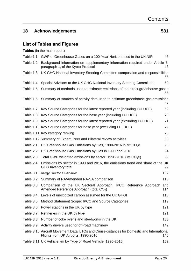
18 Acknowledgements 531
List of Tables and Figures
Tables (in the main report)
Table 1.1 GWP of Greenhouse Gases on a 100-Year Horizon used in the UK NIR 46
Table 1.2 Background information on supplementary information required under Article 7, paragraph 1, of the Kyoto Protocol 48
Table 1.3 UK GHG National Inventory Steering Committee composition and responsibilities 56
Table 1.4 Special Advisors to the UK GHG National Inventory Steering Committee 60
Table 1.5 Summary of methods used to estimate emissions of the direct greenhouse gases 65
Table 1.6 Summary of sources of activity data used to estimate greenhouse gas emissions 67
Table 1.7 Key Source Categories for the latest reported year (including LULUCF) 69
Table 1.8 Key Source Categories for the base year (including LULUCF) 70
Table 1.9 Key Source Categories for the latest reported year (excluding LULUCF) 71
Table 1.10 Key Source Categories for base year (excluding LULUCF) 72
Table 1.11 Key category ranking 73
Table 1.12 Summary of Expert, Peer and Bilateral review activities 88
Table 2.1 UK Greenhouse Gas Emissions by Gas, 1990-2016 in Mt CO2e 93
Table 2.2 UK Greenhouse Gas Emissions by Gas in 1990 and 2016 94
Table 2.3 Total GWP weighted emissions by sector, 1990-2016 (Mt CO2e) 99
Table 2.4 Emissions by sector in 1990 and 2016, the emissions trend and share of the UK GHG Inventory total 99
Table 3.1 Energy Sector Overview 109
Table 3.2 Summary of RA/Amended RA-SA comparison 113
Table 3.3 Comparison of the UK Sectoral Approach, IPCC Reference Approach and Amended Reference Approach (total CO2) 114
Table 3.4 Levels of unoxidized carbon assumed for the UK GHGI 118
Table 3.5 Method Statement Scope: IPCC and Source Categories 119
Table 3.6 Power stations in the UK by type 121
Table 3.7 Refineries in the UK by type 121
Table 3.8 Number of coke ovens and steelworks in the UK 133
Table 3.9 Activity drivers used for off-road machinery 142
Table 3.10 Aircraft Movement Data: LTOs and Cruise distances for Domestic and International Flights from UK Airports, 1990-2016 146
Table 3.11 UK Vehicle km by Type of Road Vehicle, 1990-2016 152
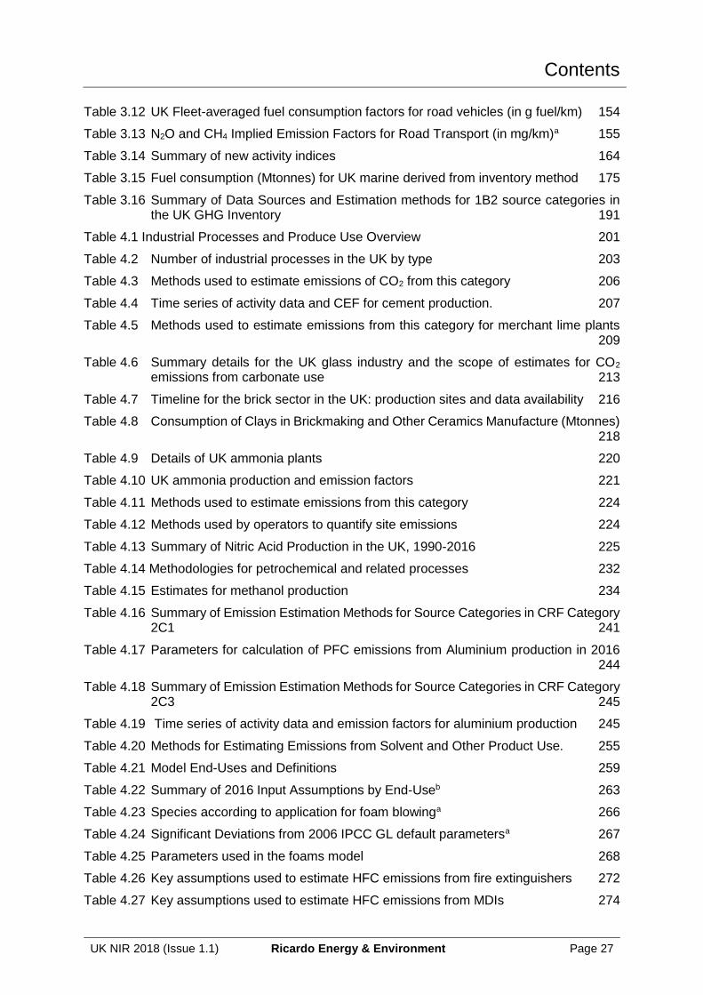
Contents
UK NIR 2018 (Issue 1.1) Ricardo Energy & Environment Page 27
Table 3.12 UK Fleet-averaged fuel consumption factors for road vehicles (in g fuel/km) 154
Table 3.13 N2O and CH4 Implied Emission Factors for Road Transport (in mg/km)a 155
Table 3.14 Summary of new activity indices 164
Table 3.15 Fuel consumption (Mtonnes) for UK marine derived from inventory method 175
Table 3.16 Summary of Data Sources and Estimation methods for 1B2 source categories in the UK GHG Inventory 191
Table 4.1 Industrial Processes and Produce Use Overview 201
Table 4.2 Number of industrial processes in the UK by type 203
Table 4.3 Methods used to estimate emissions of CO2 from this category 206
Table 4.4 Time series of activity data and CEF for cement production. 207
Table 4.5 Methods used to estimate emissions from this category for merchant lime plants 209
Table 4.6 Summary details for the UK glass industry and the scope of estimates for CO2 emissions from carbonate use 213
Table 4.7 Timeline for the brick sector in the UK: production sites and data availability 216
Table 4.8 Consumption of Clays in Brickmaking and Other Ceramics Manufacture (Mtonnes) 218
Table 4.9 Details of UK ammonia plants 220
Table 4.10 UK ammonia production and emission factors 221
Table 4.11 Methods used to estimate emissions from this category 224
Table 4.12 Methods used by operators to quantify site emissions 224
Table 4.13 Summary of Nitric Acid Production in the UK, 1990-2016 225
Table 4.14 Methodologies for petrochemical and related processes 232
Table 4.15 Estimates for methanol production 234
Table 4.16 Summary of Emission Estimation Methods for Source Categories in CRF Category 2C1 241
Table 4.17 Parameters for calculation of PFC emissions from Aluminium production in 2016 244
Table 4.18 Summary of Emission Estimation Methods for Source Categories in CRF Category 2C3 245
Table 4.19 Time series of activity data and emission factors for aluminium production 245
Table 4.20 Methods for Estimating Emissions from Solvent and Other Product Use. 255
Table 4.21 Model End-Uses and Definitions 259
Table 4.22 Summary of 2016 Input Assumptions by End-Useb 263
Table 4.23 Species according to application for foam blowinga 266
Table 4.24 Significant Deviations from 2006 IPCC GL default parametersa 267
Table 4.25 Parameters used in the foams model 268
Table 4.26 Key assumptions used to estimate HFC emissions from fire extinguishers 272
Table 4.27 Key assumptions used to estimate HFC emissions from MDIs 274
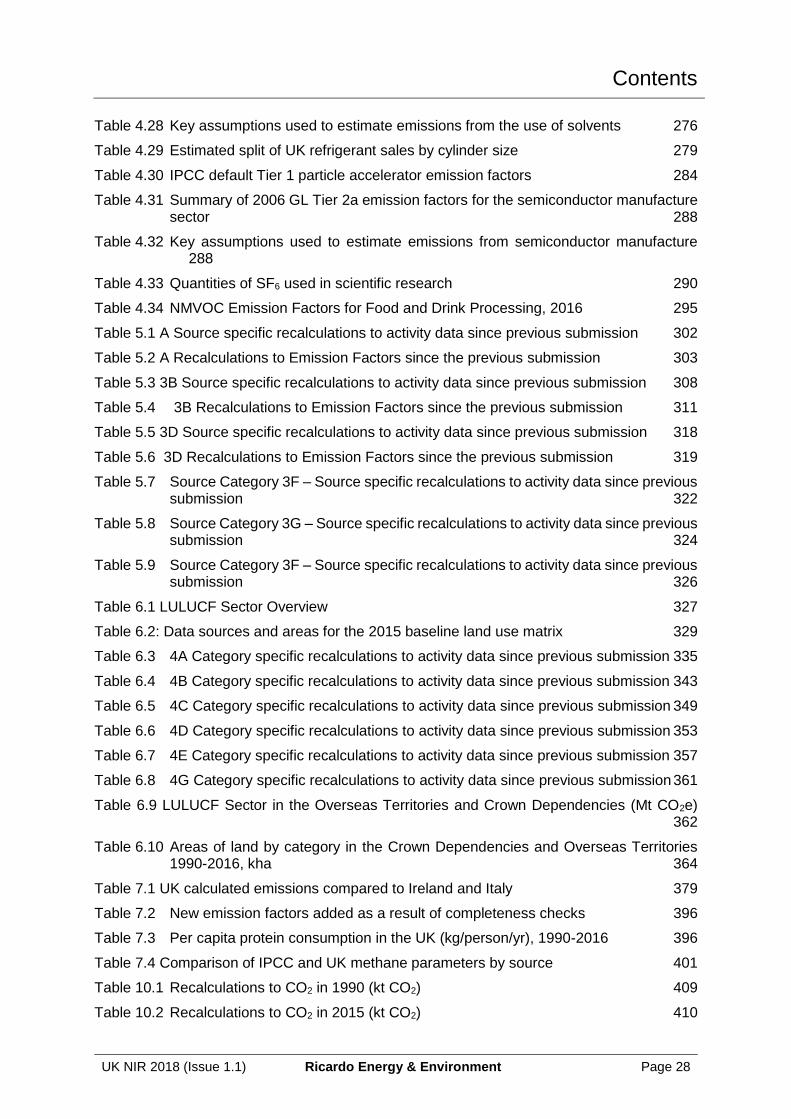
Contents
UK NIR 2018 (Issue 1.1) Ricardo Energy & Environment Page 28
Table 4.28 Key assumptions used to estimate emissions from the use of solvents 276
Table 4.29 Estimated split of UK refrigerant sales by cylinder size 279
Table 4.30 IPCC default Tier 1 particle accelerator emission factors 284
Table 4.31 Summary of 2006 GL Tier 2a emission factors for the semiconductor manufacture sector 288
Table 4.32 Key assumptions used to estimate emissions from semiconductor manufacture 288
Table 4.33 Quantities of SF6 used in scientific research 290
Table 4.34 NMVOC Emission Factors for Food and Drink Processing, 2016 295
Table 5.1 A Source specific recalculations to activity data since previous submission 302
Table 5.2 A Recalculations to Emission Factors since the previous submission 303
Table 5.3 3B Source specific recalculations to activity data since previous submission 308
Table 5.4 3B Recalculations to Emission Factors since the previous submission 311
Table 5.5 3D Source specific recalculations to activity data since previous submission 318
Table 5.6 3D Recalculations to Emission Factors since the previous submission 319
Table 5.7 Source Category 3F – Source specific recalculations to activity data since previous submission 322
Table 5.8 Source Category 3G – Source specific recalculations to activity data since previous submission 324
Table 5.9 Source Category 3F – Source specific recalculations to activity data since previous submission 326
Table 6.1 LULUCF Sector Overview 327
Table 6.2: Data sources and areas for the 2015 baseline land use matrix 329
Table 6.3 4A Category specific recalculations to activity data since previous submission 335
Table 6.4 4B Category specific recalculations to activity data since previous submission 343
Table 6.5 4C Category specific recalculations to activity data since previous submission 349
Table 6.6 4D Category specific recalculations to activity data since previous submission 353
Table 6.7 4E Category specific recalculations to activity data since previous submission 357
Table 6.8 4G Category specific recalculations to activity data since previous submission 361
Table 6.9 LULUCF Sector in the Overseas Territories and Crown Dependencies (Mt CO2e) 362
Table 6.10 Areas of land by category in the Crown Dependencies and Overseas Territories 1990-2016, kha 364
Table 7.1 UK calculated emissions compared to Ireland and Italy 379
Table 7.2 New emission factors added as a result of completeness checks 396
Table 7.3 Per capita protein consumption in the UK (kg/person/yr), 1990-2016 396
Table 7.4 Comparison of IPCC and UK methane parameters by source 401
Table 10.1 Recalculations to CO2 in 1990 (kt CO2) 409
Table 10.2 Recalculations to CO2 in 2015 (kt CO2) 410
Contents
UK NIR 2018 (Issue 1.1) Ricardo Energy & Environment Page 29
Table 10.3 Recalculations to CH4 in 1990 (kt CH4) 413
Table 10.4 Recalculations to CH4 in 2015 (kt CH4) 415
Table 10.5 Recalculations to N2O in 1990 (kt N2O) 416
Table 10.6 Recalculations to N2O in 2015 418
Table 10.7 Recalculations to SF6 in base year (CO2 eq., kt) 421
Table 10.8 Recalculations to SF6 in 2015 (CO2 eq., kt) 421
Table 10.9 Recalculations to HFC in base year (CO2 eq., kt) 421
Table 10.10 Recalculations to HFC in 2015 (CO2 eq., kt) 422
Table 10.11 Recalculations to PFC in base year (CO2 eq., kt) 422
Table 10.12 Recalculations to PFC in 2015 (CO2 eq., kt) 422
Table 10.13 Recalculations to NF3 in base year (CO2 eq., kt) 422
Table 10.14 Recalculations to NF3 in 2015 (CO2 eq., kt) 423
Table 10.15 Changes in Methodological Descriptions 423
Table 10.16 Brief Details of Improvements to the NIR and the Inventory in response to UNFCCC Reviews in response to the 2016 reviews 433
Table 11.1 Land area and changes in land areas in 2015 (UK only) 452
Table 11.2 Data Sources on Afforestation, Reforestation and Deforestation (ARD), Forest Management (FM), Cropland Management (CM), and Grazing Land Management (GM) Activities 453
Table 11.3 The background emissions estimated for disturbance events over the calibration period for Forest Management and Afforestation and Reforestation 457
Table 11.4 Recalculations of previous emissions/removals in the latest KP-LULUCF submission 462
Table 11.5: Areas converted to KP activities after 2013 (UK and OTs & CDs) 465
Table 11.6 Area under forest management and emissions/removals from forest management 1990-2020 (UK only, based on the latest inventory submission)* 469
Table 11.7: Forest Management Reference Levels and Technical Correction for the period 2013-2020. 470
Table 18.1 Contributors to this National Inventory Report and the CRF 531
Table 18.2 Key Data Providers to the Greenhouse Gas Inventory 532
Figures (in the main report)
Figure 1.1 Key organisational structure of the UK National Inventory System 49
Figure 1.2 Main elements for the preparation of the UK greenhouse gas inventory 50
Figure 1.3 QA/QC system used within UK greenhouse gas inventory 77
Figure 2.1 Trend in Greenhouse Gas Emissions by Gas, 1990 to 2016, relative to 1990 Emission Levels. 94
Figure 2.2 UK CO2 Emissions Trend by Sector for 1990 to 2016 95
Figure 2.3 UK CH4 Emissions (Mt CO2e) Trend by Sector for 1990 to 2016 96
Contents
UK NIR 2018 (Issue 1.1) Ricardo Energy & Environment Page 30
Figure 2.4 UK N2O Emissions (Mt CO2e) Trend by Sector for 1990 to 2016 97
Figure 2.5 UK F- Gas Emissions (Mt CO2e) Trend by Sector for 1990 to 2016 98
Figure 2.6 Trend in GHG emissions by sector for 1990 to 2016, Relative to 1990 Emission Levels 100
Figure 2.7 UK Emissions of Indirect Greenhouse Gases for 1990 to 2016 104
Figure 2.8 Article 3.3 Emissions and Removals, by gas and by activity 107
Figure 2.9 Article 3.4 Emissions and removals, by gas and activity 107
Figure 3.1 Carbon balance model for 2016a 136
Figure 3.2 Ratio of calculated consumption of petrol and diesel fuel 156
Figure 4.1 Breakdown of total GHG emissions in Industrial Processes sector 205
Figure 4.2 Trend in total GHG emissions in Industrial Processes sector 205
Figure 4.3 Comparison of original and revised RAC models 262
Figure 4.4 Trends in refrigerant container emissions 280
Figure 5.1 Breakdown of total GHG emissions in the Agriculture sector in 2015 298
Figure 5.2 Trend in total GHG emissions in the Agriculture sector 298
Figure 5.3 Simplified nitrogen cycle highlighting the steps involved in the production of N2O from agriculture. 314
Figure 6.1 LULUCF emissions and removals from the UK 1990-2016 by category 328
Figure 7.1 Breakdown of total GHG emissions from the Waste sector in 2016 370
Figure 7.2 Trend in total GHG emissions in the Waste sector 370
Figure 7.3 Waste water flow diagram 390
Figure 10.1 Time series of changes in GWP emissions between the inventory presented in the current and the previous NIR, according to IPCC source sector. 429
Figure 10.2 Time series of changes in total net GWP emissions, and percentage changes in total net GWP emissions, between the inventory presented in the current and the previous NIR. 430
Figure 10.3 Reported trends from the current and previous inventory submissions 431
Figure 11.1 Geographical areas used for reporting Kyoto Protocol LULUCF activities 456
Executive Summaries
UK NIR 2018 (Issue 1.1) Ricardo Energy & Environment Page 31
Executive Summaries
ES.1 BACKGROUND INFORMATION
ES.1.1 Climate Change
Countries that have signed and ratified the Kyoto Protocol are legally bound to reduce their greenhouse gas emissions by an agreed amount. A single European Union Kyoto Protocol reduction target for greenhouse gas emissions of -8% compared to base-year levels was negotiated for the first commitment period, and a Burden Sharing Agreement allocated the target between Member States of the European Union. Under this agreement, the UK reduction target was -12.5% on base-year levels. The first commitment period of the Kyoto Protocol was from 2008 to 2012.
The second commitment period of the Kyoto Protocol applies from 2013 to 2020 inclusive. For this second commitment period, the EU and the Member States communicated an independent quantified economy-wide emission reduction target of a 20 percent emission reduction by 2020 compared with 1990 levels (base year) (“the EU2020 target”). The EU2020 target is based on the understanding that it will be fulfilled jointly by the European Union and the Member States. The EU2020 target is unconditional and supported by EU legislation in place since 2009 (The EU Climate and Energy Package). This Kyoto target will cover the UK, and the relevant Crown Dependencies and Overseas Territories for whom the ratification is extended.
The Climate Change Act3 became UK Law on the 26th November 2008. This legislation introduced a new, more ambitious and legally binding target for the UK to reduce GHG emissions to 80% below base year by 2050, with legally binding five year GHG budgets. The independent Committee on Climate Change (CCC) was set up to advise the UK Government on the setting and meeting of UK carbon budgets as well as monitoring progress against them scope and level of UK carbon budgets.
Further information on the UK’s action to tackle climate change can be found on the following Government Department websites:
https://www.gov.uk/government/organisations/department-for-business-energy-and-industrial-strategy
https://www.gov.uk/government/policies/adapting-to-climate-change
ES.1.2 Greenhouse Gas Inventories
The UK ratified the United Nations Framework Convention on Climate Change (UNFCCC) in December 1993, and the Convention came into force in March 1994. Parties to the Convention are committed to develop, publish and regularly update national emission inventories of greenhouse gases (GHGs).
This is the United Kingdom’s National Inventory Report (NIR) submitted in 2018 to the UNFCCC and covering both the UK’s submission under the Kyoto Protocol and the Convention. It contains national greenhouse gas emission estimates for the period 1990-2016, and the descriptions of the methods used to produce the estimates. The report is prepared in
3 Climate Change Act 2008.
http://www.legislation.gov.uk/ukpga/2008/27/contents
Executive Summaries
UK NIR 2018 (Issue 1.1) Ricardo Energy & Environment Page 32
accordance with decision 24/CP.194 and includes elements required for reporting under the Kyoto Protocol.
The UK Greenhouse Gas Inventory is compiled and maintained by a consortium led by Ricardo Energy & Environment – the Inventory Agency – under contract to the UK Department for Business, Energy and Industrial Strategy (BEIS). Ricardo Energy & Environment is directly responsible for producing the emissions estimates for CRF categories Energy (CRF sector 1), Industrial Processes and Product Use (CRF Sector 2), and Waste (CRF Sector 5). Ricardo Energy & Environment is also responsible for inventory planning, data collection, QA/QC and inventory management and archiving. Aether, a member within the consortium, is responsible for compiling emissions from railways and for the UK’s Overseas Territories (OTs) and Crown Dependencies (CDs).
Forestry emissions and removals in the Land Use, Land-Use Change and Forestry sector (CRF sector 4) are calculated by Forest Research and the remainder of the sector is calculated and compiled by the UK Centre for Ecology and Hydrology (CEH), both partners within the consortium. Agricultural sector emissions estimates (CRF sector 3) are produced by Rothamsted Research, under contract to the UK Department for Environment, Food and Rural Affairs (Defra).
BEIS, Defra and the Devolved Administrations also fund research contracts to provide improved emissions estimates for certain sources such as fluorinated gases, landfill methane, enteric fermentation and shipping; information from these programmes is fed into the inventory via the national inventory system.
The inventory covers the seven direct greenhouse gases under the Kyoto Protocol (NF3 was included under the Doha Amendment). These are as follows:
• Carbon dioxide (CO2);
• Methane (CH4);
• Nitrous oxide (N2O);
• Hydrofluorocarbons (HFCs);
• Perfluorocarbons (PFCs);
• Sulphur hexafluoride (SF6); and
• Nitrogen trifluoride (NF3).
These gases contribute directly to climate change owing to their positive radiative forcing effect. Also reported are four indirect greenhouse gases:
• Nitrogen oxides;
• Carbon monoxide;
• Non-Methane Volatile Organic Compounds (NMVOC); and
• Sulphur oxides (reported as SO2).
Emissions of indirect N2O from emissions of NOx and NH3 are also estimated as a memo item. These emissions are not included in the national total.
Unless otherwise indicated, percentage contributions and changes quoted refer to net emissions (i.e. emissions minus removals), based on the full coverage of UK emissions including all relevant Overseas Territories and Crown Dependencies, consistent with the UK’s submission to the UNFCCC.
The UK inventory provides data to assess progress of the UK’s commitments under the Kyoto Protocol, the UK’s contribution to the EU’s targets under the KP, progress towards the UK
4 FCCC Decision 24/CP.19. Revision of the UNFCCC reporting guidelines on annual inventories for Parties included in Annex I to the Convention http://unfccc.int/resource/docs/2013/cop19/eng/10a03.pdf
Executive Summaries
UK NIR 2018 (Issue 1.1) Ricardo Energy & Environment Page 33
Government’s own Carbon Budgets and to meet commitments as a Party to the UN Framework Convention on Climate Change. Geographical coverage for these four purposes differs to some extent, because of the following:
1) The UK Government Carbon Budgets apply to the UK only, and exclude all emissions from the UK’s Crown Dependencies and Overseas Territories.
2) Kyoto Protocol coverage (the ‘GBK’ submission). For the second commitment period, this submission includes the UK plus:
a. Crown Dependencies (Guernsey, Isle of Man and Jersey) b. Overseas Territories (Cayman Islands, Falkland Islands and Gibraltar)
3) The MMR coverage (the ‘GBE’ submission). The UK’s commitments under the EU Monitoring Mechanism Regulation, which has been set up to enable the EU to monitor progress against its Kyoto Protocol target, only includes the UK and Gibraltar, since the Crown Dependencies and other Overseas Territories are not part of the EU.
4) UNFCCC coverage (the ‘GBR’ submission). The UK’s ratification of the UNFCCC has been extended to Bermuda, the Cayman Islands, the Falkland Islands, Gibraltar, Guernsey, the Isle of Man and Jersey and the UK reports an inventory on this basis.
Emissions data for Coverage 1 are reported here for information and to facilitate comparison between different publications. Coverage 2 is used for the data in the CRF tables submitted to the UNFCCC under the Kyoto Protocol. Coverage 3 is used for the data in the CRF tables submitted under the MMR. Coverage 4 is used for the data in the CRF tables submitted to the UNFCCC under the Convention. Table ES 2.1 to Table ES 2.2 show CO2 and the direct greenhouse gases, disaggregated by gas and by sector for geographical Coverage 4. Table ES 3.2 and Table ES 3.3 show emissions for the Kyoto basket based on Coverage 2 and 3, respectively.
Table ES 4.1 has data on indirect greenhouse gas emissions, for geographical coverage 4.
ES.1.3 Supplementary Information Required under Article 7, paragraph 1, of the Kyoto Protocol.
Background information on supplementary information required under Article 7, Paragraph 1 of the KP is presented in Section 1.1.3.
Executive Summaries
UK NIR 2018 (Issue 1.1) Ricardo Energy & Environment Page 34
ES.2 SUMMARY OF NATIONAL EMISSION AND REMOVAL RELATED TRENDS, AND EMISSIONS AND REMOVALS FROM KP-LULUCF ACTIVITIES
ES.2.1 GHG Inventory
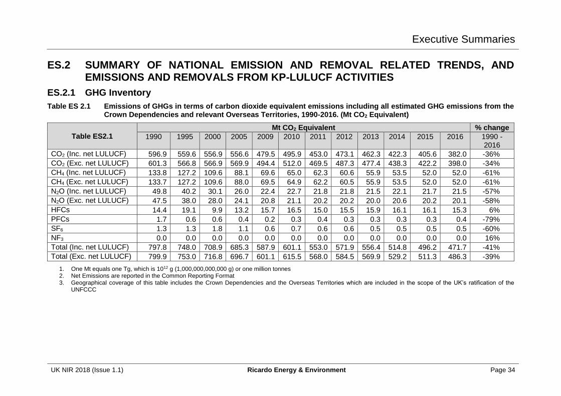
Table ES 2.1 Emissions of GHGs in terms of carbon dioxide equivalent emissions including all estimated GHG emissions from the Crown Dependencies and relevant Overseas Territories, 1990-2016. (Mt CO2 Equivalent)
Table ES2.1
Mt CO2 Equivalent % change
1990 1995 2000 2005 2009 2010 2011 2012 2013 2014 2015 2016 1990 - 2016
CO2 (Inc. net LULUCF) 596.9 559.6 556.9 556.6 479.5 495.9 453.0 473.1 462.3 422.3 405.6 382.0 -36%
CO2 (Exc. net LULUCF) 601.3 566.8 566.9 569.9 494.4 512.0 469.5 487.3 477.4 438.3 422.2 398.0 -34%
CH4 (Inc. net LULUCF) 133.8 127.2 109.6 88.1 69.6 65.0 62.3 60.6 55.9 53.5 52.0 52.0 -61%
CH4 (Exc. net LULUCF) 133.7 127.2 109.6 88.0 69.5 64.9 62.2 60.5 55.9 53.5 52.0 52.0 -61%
N2O (Inc. net LULUCF) 49.8 40.2 30.1 26.0 22.4 22.7 21.8 21.8 21.5 22.1 21.7 21.5 -57%
N2O (Exc. net LULUCF) 47.5 38.0 28.0 24.1 20.8 21.1 20.2 20.2 20.0 20.6 20.2 20.1 -58%
HFCs 14.4 19.1 9.9 13.2 15.7 16.5 15.0 15.5 15.9 16.1 16.1 15.3 6%
PFCs 1.7 0.6 0.6 0.4 0.2 0.3 0.4 0.3 0.3 0.3 0.3 0.4 -79%
SF6 1.3 1.3 1.8 1.1 0.6 0.7 0.6 0.6 0.5 0.5 0.5 0.5 -60%
NF3 0.0 0.0 0.0 0.0 0.0 0.0 0.0 0.0 0.0 0.0 0.0 0.0 16%
Total (Inc. net LULUCF) 797.8 748.0 708.9 685.3 587.9 601.1 553.0 571.9 556.4 514.8 496.2 471.7 -41%
Total (Exc. net LULUCF) 799.9 753.0 716.8 696.7 601.1 615.5 568.0 584.5 569.9 529.2 511.3 486.3 -39%
1. One Mt equals one Tg, which is 1012 g (1,000,000,000,000 g) or one million tonnes 2. Net Emissions are reported in the Common Reporting Format 3. Geographical coverage of this table includes the Crown Dependencies and the Overseas Territories which are included in the scope of the UK’s ratification of the
UNFCCC
Executive Summaries
UK NIR 2018 (Issue 1.1) Ricardo Energy & Environment Page 35
Table ES 2.1 presents the UK Greenhouse Gas Inventory totals by gas, including and excluding net emissions from LULUCF. The largest contribution to total emissions is CO2, which contributed 81% to total net emissions in 2016. Methane emissions account for the next largest share (11%), and N2O emissions make up a further 5%. Emissions of all of these gases have decreased since 1990, contributing to an overall decrease of 41%.
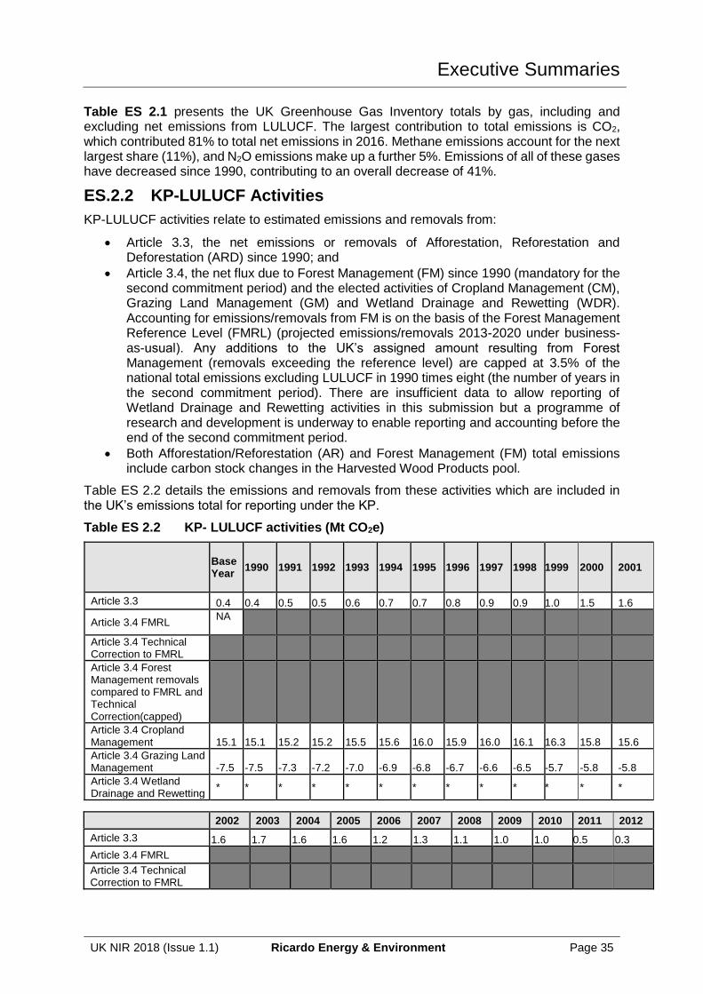
ES.2.2 KP-LULUCF Activities
KP-LULUCF activities relate to estimated emissions and removals from:
• Article 3.3, the net emissions or removals of Afforestation, Reforestation and Deforestation (ARD) since 1990; and
• Article 3.4, the net flux due to Forest Management (FM) since 1990 (mandatory for the second commitment period) and the elected activities of Cropland Management (CM), Grazing Land Management (GM) and Wetland Drainage and Rewetting (WDR). Accounting for emissions/removals from FM is on the basis of the Forest Management Reference Level (FMRL) (projected emissions/removals 2013-2020 under business-as-usual). Any additions to the UK’s assigned amount resulting from Forest Management (removals exceeding the reference level) are capped at 3.5% of the national total emissions excluding LULUCF in 1990 times eight (the number of years in the second commitment period). There are insufficient data to allow reporting of Wetland Drainage and Rewetting activities in this submission but a programme of research and development is underway to enable reporting and accounting before the end of the second commitment period.
• Both Afforestation/Reforestation (AR) and Forest Management (FM) total emissions include carbon stock changes in the Harvested Wood Products pool.
Table ES 2.2 details the emissions and removals from these activities which are included in the UK’s emissions total for reporting under the KP.
Table ES 2.2 KP- LULUCF activities (Mt CO2e)
Base Year
1990 1991 1992 1993 1994 1995 1996 1997 1998 1999 2000 2001
Article 3.3 0.4 0.4 0.5 0.5 0.6 0.7 0.7 0.8 0.9 0.9 1.0 1.5 1.6
Article 3.4 FMRL NA
Article 3.4 Technical Correction to FMRL
Article 3.4 Forest Management removals compared to FMRL and Technical Correction(capped)
Article 3.4 Cropland Management 15.1 15.1 15.2 15.2 15.5 15.6 16.0 15.9 16.0 16.1 16.3 15.8 15.6
Article 3.4 Grazing Land Management -7.5 -7.5 -7.3 -7.2 -7.0 -6.9 -6.8 -6.7 -6.6 -6.5 -5.7 -5.8 -5.8
Article 3.4 Wetland Drainage and Rewetting
* * * * * * * * * * * * *
2002 2003 2004 2005 2006 2007 2008 2009 2010 2011 2012
Article 3.3 1.6 1.7 1.6 1.6 1.2 1.3 1.1 1.0 1.0 0.5 0.3
Article 3.4 FMRL
Article 3.4 Technical Correction to FMRL
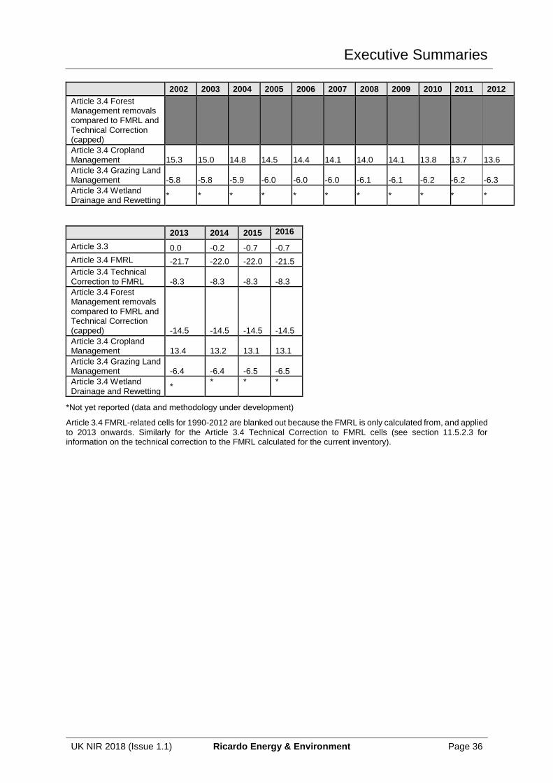
Executive Summaries
UK NIR 2018 (Issue 1.1) Ricardo Energy & Environment Page 36
2002 2003 2004 2005 2006 2007 2008 2009 2010 2011 2012
Article 3.4 Forest Management removals compared to FMRL and Technical Correction (capped)
Article 3.4 Cropland Management 15.3 15.0 14.8 14.5 14.4 14.1 14.0 14.1 13.8 13.7 13.6
Article 3.4 Grazing Land Management -5.8 -5.8 -5.9 -6.0 -6.0 -6.0 -6.1 -6.1 -6.2 -6.2 -6.3
Article 3.4 Wetland Drainage and Rewetting
* * * * * * * * * * *
2013 2014 2015 2016
Article 3.3 0.0 -0.2 -0.7 -0.7
Article 3.4 FMRL -21.7 -22.0 -22.0 -21.5
Article 3.4 Technical Correction to FMRL -8.3 -8.3 -8.3 -8.3
Article 3.4 Forest Management removals compared to FMRL and Technical Correction (capped) -14.5 -14.5 -14.5 -14.5
Article 3.4 Cropland Management 13.4 13.2 13.1 13.1
Article 3.4 Grazing Land Management -6.4 -6.4 -6.5 -6.5
Article 3.4 Wetland Drainage and Rewetting
* * * *
*Not yet reported (data and methodology under development)
Article 3.4 FMRL-related cells for 1990-2012 are blanked out because the FMRL is only calculated from, and applied to 2013 onwards. Similarly for the Article 3.4 Technical Correction to FMRL cells (see section 11.5.2.3 for information on the technical correction to the FMRL calculated for the current inventory).
Executive Summaries
UK NIR 2018 (Issue 1.1) Ricardo Energy & Environment Page 37
ES.3 OVERVIEW OF SOURCE AND SINK CATEGORY EMISSION ESTIMATES AND TRENDS, INCLUDING KP-LULUCF ACTIVITIES
ES.3.1 GHG Inventory
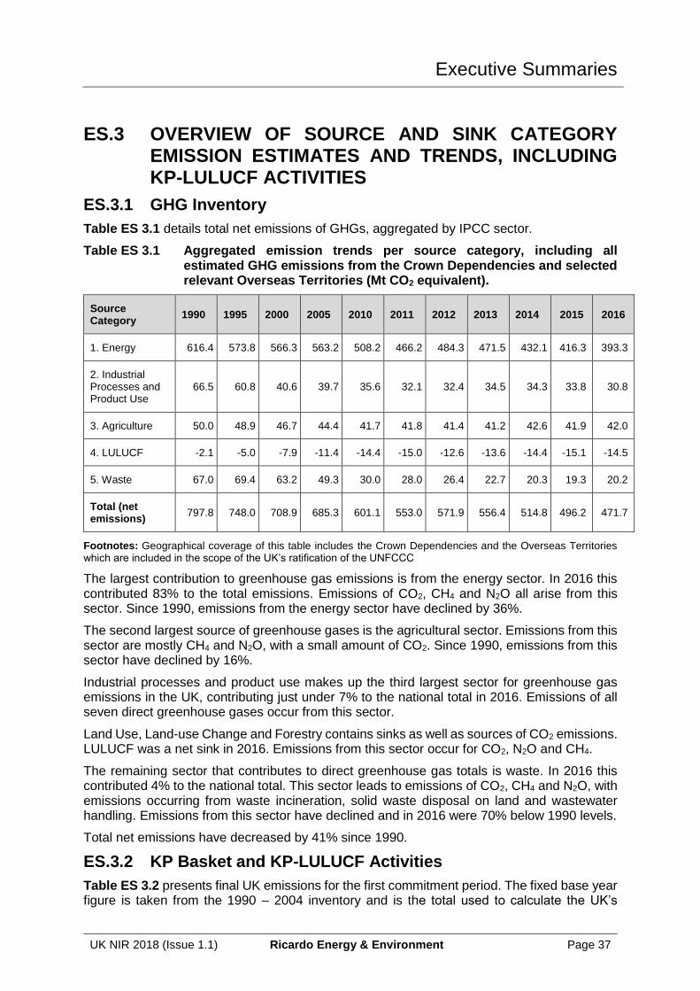
Table ES 3.1 details total net emissions of GHGs, aggregated by IPCC sector.
Table ES 3.1 Aggregated emission trends per source category, including all estimated GHG emissions from the Crown Dependencies and selected relevant Overseas Territories (Mt CO2 equivalent).
Source Category
1990 1995 2000 2005 2010 2011 2012 2013 2014 2015 2016
1. Energy 616.4 573.8 566.3 563.2 508.2 466.2 484.3 471.5 432.1 416.3 393.3
2. Industrial Processes and Product Use
66.5 60.8 40.6 39.7 35.6 32.1 32.4 34.5 34.3 33.8 30.8
3. Agriculture 50.0 48.9 46.7 44.4 41.7 41.8 41.4 41.2 42.6 41.9 42.0
4. LULUCF -2.1 -5.0 -7.9 -11.4 -14.4 -15.0 -12.6 -13.6 -14.4 -15.1 -14.5
5. Waste 67.0 69.4 63.2 49.3 30.0 28.0 26.4 22.7 20.3 19.3 20.2
Total (net emissions)
797.8 748.0 708.9 685.3 601.1 553.0 571.9 556.4 514.8 496.2 471.7
Footnotes: Geographical coverage of this table includes the Crown Dependencies and the Overseas Territories which are included in the scope of the UK’s ratification of the UNFCCC
The largest contribution to greenhouse gas emissions is from the energy sector. In 2016 this contributed 83% to the total emissions. Emissions of CO2, CH4 and N2O all arise from this sector. Since 1990, emissions from the energy sector have declined by 36%.
The second largest source of greenhouse gases is the agricultural sector. Emissions from this sector are mostly CH4 and N2O, with a small amount of CO2. Since 1990, emissions from this sector have declined by 16%.
Industrial processes and product use makes up the third largest sector for greenhouse gas emissions in the UK, contributing just under 7% to the national total in 2016. Emissions of all seven direct greenhouse gases occur from this sector.
Land Use, Land-use Change and Forestry contains sinks as well as sources of CO2 emissions. LULUCF was a net sink in 2016. Emissions from this sector occur for CO2, N2O and CH4.
The remaining sector that contributes to direct greenhouse gas totals is waste. In 2016 this contributed 4% to the national total. This sector leads to emissions of CO2, CH4 and N2O, with emissions occurring from waste incineration, solid waste disposal on land and wastewater handling. Emissions from this sector have declined and in 2016 were 70% below 1990 levels.
Total net emissions have decreased by 41% since 1990.
ES.3.2 KP Basket and KP-LULUCF Activities
Table ES 3.2 presents final UK emissions for the first commitment period. The fixed base year figure is taken from the 1990 – 2004 inventory and is the total used to calculate the UK’s
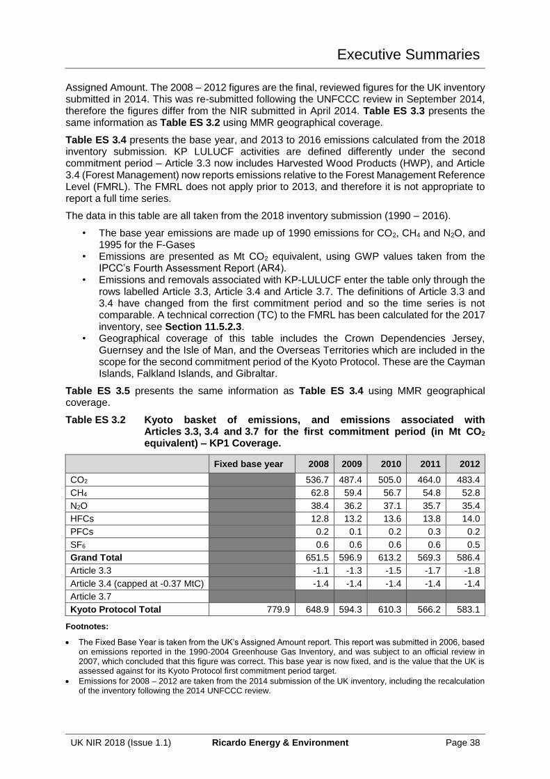
Executive Summaries
UK NIR 2018 (Issue 1.1) Ricardo Energy & Environment Page 38
Assigned Amount. The 2008 – 2012 figures are the final, reviewed figures for the UK inventory submitted in 2014. This was re-submitted following the UNFCCC review in September 2014, therefore the figures differ from the NIR submitted in April 2014. Table ES 3.3 presents the same information as Table ES 3.2 using MMR geographical coverage.
Table ES 3.4 presents the base year, and 2013 to 2016 emissions calculated from the 2018 inventory submission. KP LULUCF activities are defined differently under the second commitment period – Article 3.3 now includes Harvested Wood Products (HWP), and Article 3.4 (Forest Management) now reports emissions relative to the Forest Management Reference Level (FMRL). The FMRL does not apply prior to 2013, and therefore it is not appropriate to report a full time series.
The data in this table are all taken from the 2018 inventory submission (1990 – 2016).
• The base year emissions are made up of 1990 emissions for CO2, CH4 and N2O, and 1995 for the F-Gases
• Emissions are presented as Mt CO2 equivalent, using GWP values taken from the IPCC’s Fourth Assessment Report (AR4).
• Emissions and removals associated with KP-LULUCF enter the table only through the rows labelled Article 3.3, Article 3.4 and Article 3.7. The definitions of Article 3.3 and 3.4 have changed from the first commitment period and so the time series is not comparable. A technical correction (TC) to the FMRL has been calculated for the 2017 inventory, see Section 11.5.2.3.
• Geographical coverage of this table includes the Crown Dependencies Jersey, Guernsey and the Isle of Man, and the Overseas Territories which are included in the scope for the second commitment period of the Kyoto Protocol. These are the Cayman Islands, Falkland Islands, and Gibraltar.
Table ES 3.5 presents the same information as Table ES 3.4 using MMR geographical coverage.
Table ES 3.2 Kyoto basket of emissions, and emissions associated with Articles 3.3, 3.4 and 3.7 for the first commitment period (in Mt CO2 equivalent) – KP1 Coverage.
Fixed base year 2008 2009 2010 2011 2012
CO2 536.7 487.4 505.0 464.0 483.4
CH4 62.8 59.4 56.7 54.8 52.8
N2O 38.4 36.2 37.1 35.7 35.4
HFCs 12.8 13.2 13.6 13.8 14.0
PFCs 0.2 0.1 0.2 0.3 0.2
SF6 0.6 0.6 0.6 0.6 0.5
Grand Total 651.5 596.9 613.2 569.3 586.4
Article 3.3 -1.1 -1.3 -1.5 -1.7 -1.8
Article 3.4 (capped at -0.37 MtC) -1.4 -1.4 -1.4 -1.4 -1.4
Article 3.7
Kyoto Protocol Total 779.9 648.9 594.3 610.3 566.2 583.1
Footnotes:
• The Fixed Base Year is taken from the UK’s Assigned Amount report. This report was submitted in 2006, based on emissions reported in the 1990-2004 Greenhouse Gas Inventory, and was subject to an official review in 2007, which concluded that this figure was correct. This base year is now fixed, and is the value that the UK is assessed against for its Kyoto Protocol first commitment period target.
• Emissions for 2008 – 2012 are taken from the 2014 submission of the UK inventory, including the recalculation of the inventory following the 2014 UNFCCC review.
Executive Summaries
UK NIR 2018 (Issue 1.1) Ricardo Energy & Environment Page 39
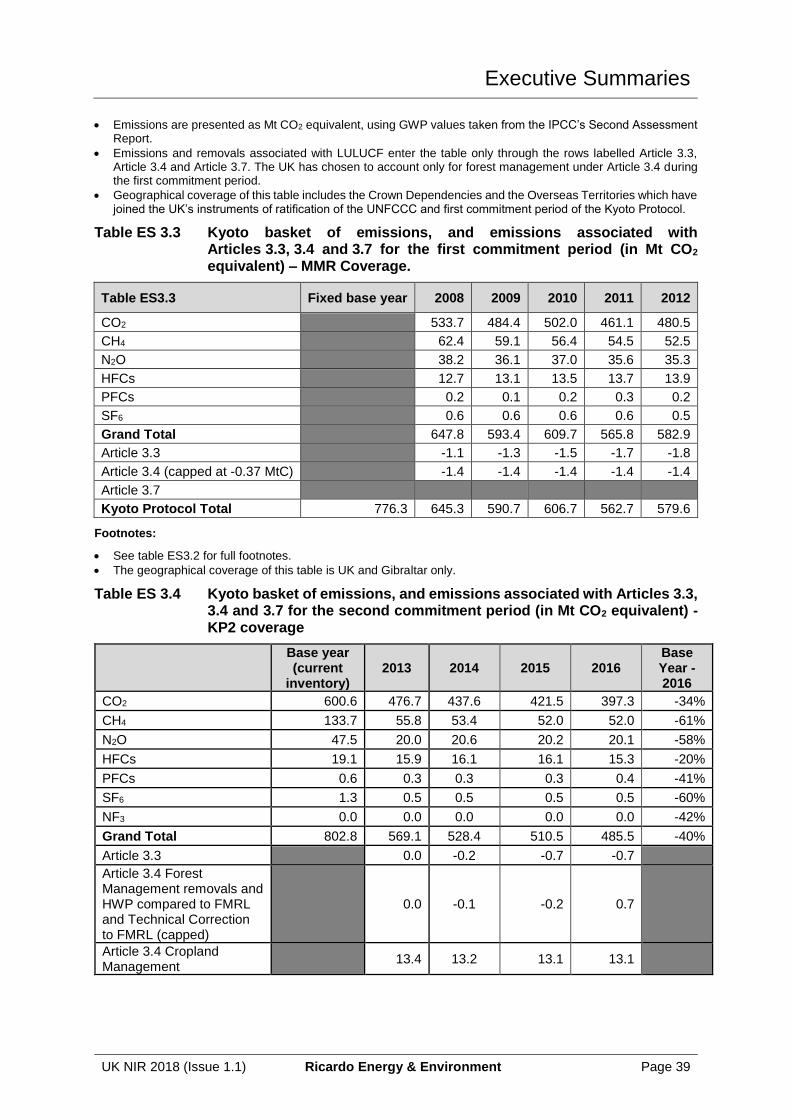
• Emissions are presented as Mt CO2 equivalent, using GWP values taken from the IPCC’s Second Assessment Report.
• Emissions and removals associated with LULUCF enter the table only through the rows labelled Article 3.3, Article 3.4 and Article 3.7. The UK has chosen to account only for forest management under Article 3.4 during the first commitment period.
• Geographical coverage of this table includes the Crown Dependencies and the Overseas Territories which have joined the UK’s instruments of ratification of the UNFCCC and first commitment period of the Kyoto Protocol.
Table ES 3.3 Kyoto basket of emissions, and emissions associated with Articles 3.3, 3.4 and 3.7 for the first commitment period (in Mt CO2 equivalent) – MMR Coverage.
Table ES3.3 Fixed base year 2008 2009 2010 2011 2012
CO2 533.7 484.4 502.0 461.1 480.5
CH4 62.4 59.1 56.4 54.5 52.5
N2O 38.2 36.1 37.0 35.6 35.3
HFCs 12.7 13.1 13.5 13.7 13.9
PFCs 0.2 0.1 0.2 0.3 0.2
SF6 0.6 0.6 0.6 0.6 0.5
Grand Total 647.8 593.4 609.7 565.8 582.9
Article 3.3 -1.1 -1.3 -1.5 -1.7 -1.8
Article 3.4 (capped at -0.37 MtC) -1.4 -1.4 -1.4 -1.4 -1.4
Article 3.7
Kyoto Protocol Total 776.3 645.3 590.7 606.7 562.7 579.6
Footnotes:
• See table ES3.2 for full footnotes.
• The geographical coverage of this table is UK and Gibraltar only.
Table ES 3.4 Kyoto basket of emissions, and emissions associated with Articles 3.3, 3.4 and 3.7 for the second commitment period (in Mt CO2 equivalent) - KP2 coverage
Base year (current
inventory) 2013 2014 2015 2016
Base Year - 2016
CO2 600.6 476.7 437.6 421.5 397.3 -34%
CH4 133.7 55.8 53.4 52.0 52.0 -61%
N2O 47.5 20.0 20.6 20.2 20.1 -58%
HFCs 19.1 15.9 16.1 16.1 15.3 -20%
PFCs 0.6 0.3 0.3 0.3 0.4 -41%
SF6 1.3 0.5 0.5 0.5 0.5 -60%
NF3 0.0 0.0 0.0 0.0 0.0 -42%
Grand Total 802.8 569.1 528.4 510.5 485.5 -40%
Article 3.3 0.0 -0.2 -0.7 -0.7
Article 3.4 Forest Management removals and HWP compared to FMRL and Technical Correction to FMRL (capped)
0.0 -0.1 -0.2 0.7
Article 3.4 Cropland Management
13.4 13.2 13.1 13.1
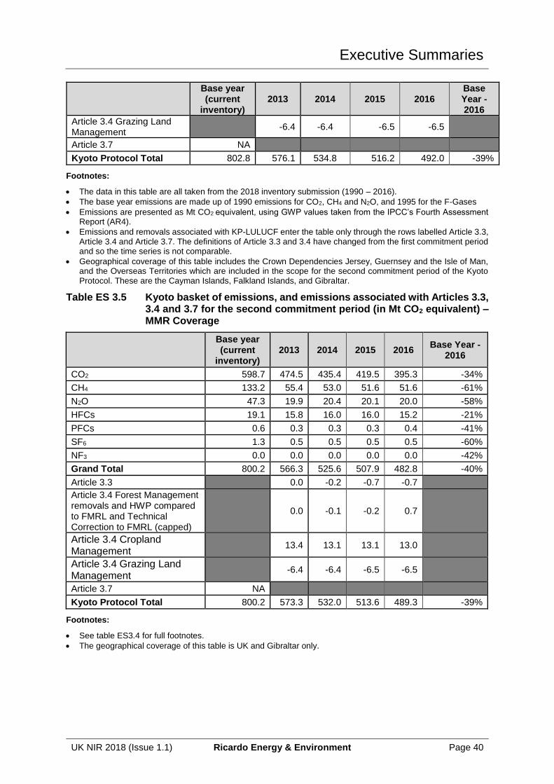
Executive Summaries
UK NIR 2018 (Issue 1.1) Ricardo Energy & Environment Page 40
Base year (current
inventory) 2013 2014 2015 2016
Base Year - 2016
Article 3.4 Grazing Land Management
-6.4 -6.4 -6.5 -6.5
Article 3.7 NA
Kyoto Protocol Total 802.8 576.1 534.8 516.2 492.0 -39%
Footnotes:
• The data in this table are all taken from the 2018 inventory submission (1990 – 2016).
• The base year emissions are made up of 1990 emissions for CO2, CH4 and N2O, and 1995 for the F-Gases
• Emissions are presented as Mt CO2 equivalent, using GWP values taken from the IPCC’s Fourth Assessment
Report (AR4).
• Emissions and removals associated with KP-LULUCF enter the table only through the rows labelled Article 3.3, Article 3.4 and Article 3.7. The definitions of Article 3.3 and 3.4 have changed from the first commitment period and so the time series is not comparable.
• Geographical coverage of this table includes the Crown Dependencies Jersey, Guernsey and the Isle of Man, and the Overseas Territories which are included in the scope for the second commitment period of the Kyoto Protocol. These are the Cayman Islands, Falkland Islands, and Gibraltar.
Table ES 3.5 Kyoto basket of emissions, and emissions associated with Articles 3.3, 3.4 and 3.7 for the second commitment period (in Mt CO2 equivalent) – MMR Coverage
Base year (current
inventory) 2013 2014 2015 2016
Base Year - 2016
CO2 598.7 474.5 435.4 419.5 395.3 -34%
CH4 133.2 55.4 53.0 51.6 51.6 -61%
N2O 47.3 19.9 20.4 20.1 20.0 -58%
HFCs 19.1 15.8 16.0 16.0 15.2 -21%
PFCs 0.6 0.3 0.3 0.3 0.4 -41%
SF6 1.3 0.5 0.5 0.5 0.5 -60%
NF3 0.0 0.0 0.0 0.0 0.0 -42%
Grand Total 800.2 566.3 525.6 507.9 482.8 -40%
Article 3.3 0.0 -0.2 -0.7 -0.7
Article 3.4 Forest Management removals and HWP compared to FMRL and Technical Correction to FMRL (capped)
0.0 -0.1 -0.2 0.7
Article 3.4 Cropland Management
13.4 13.1 13.1 13.0
Article 3.4 Grazing Land Management
-6.4 -6.4 -6.5 -6.5
Article 3.7 NA
Kyoto Protocol Total 800.2 573.3 532.0 513.6 489.3 -39%
Footnotes:
• See table ES3.4 for full footnotes.
• The geographical coverage of this table is UK and Gibraltar only.
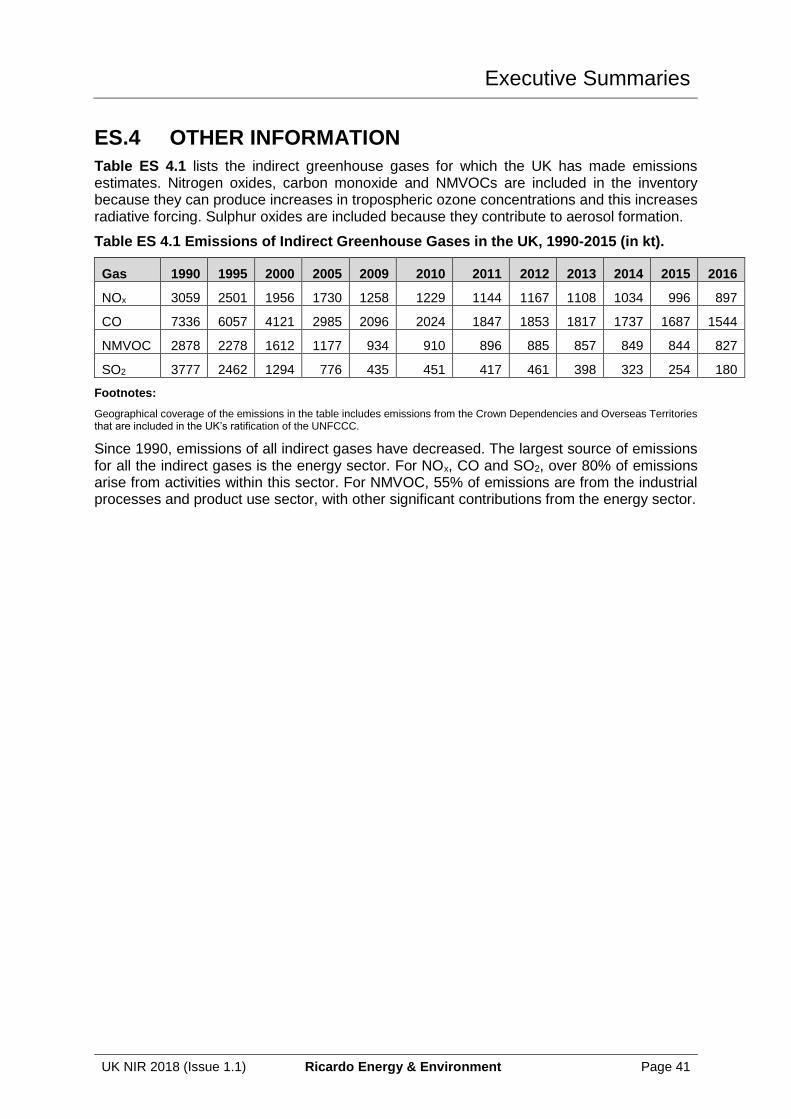
Executive Summaries
UK NIR 2018 (Issue 1.1) Ricardo Energy & Environment Page 41
ES.4 OTHER INFORMATION
Table ES 4.1 lists the indirect greenhouse gases for which the UK has made emissions estimates. Nitrogen oxides, carbon monoxide and NMVOCs are included in the inventory because they can produce increases in tropospheric ozone concentrations and this increases radiative forcing. Sulphur oxides are included because they contribute to aerosol formation.
Table ES 4.1 Emissions of Indirect Greenhouse Gases in the UK, 1990-2015 (in kt).
Gas 1990 1995 2000 2005 2009 2010 2011 2012 2013 2014 2015 2016
NOx 3059 2501 1956 1730 1258 1229 1144 1167 1108 1034 996 897
CO 7336 6057 4121 2985 2096 2024 1847 1853 1817 1737 1687 1544
NMVOC 2878 2278 1612 1177 934 910 896 885 857 849 844 827
SO2 3777 2462 1294 776 435 451 417 461 398 323 254 180
Footnotes:
Geographical coverage of the emissions in the table includes emissions from the Crown Dependencies and Overseas Territories that are included in the UK’s ratification of the UNFCCC.
Since 1990, emissions of all indirect gases have decreased. The largest source of emissions for all the indirect gases is the energy sector. For NOx, CO and SO2, over 80% of emissions arise from activities within this sector. For NMVOC, 55% of emissions are from the industrial processes and product use sector, with other significant contributions from the energy sector.

Contacts
UK NIR 2018 (Issue 1.1) Ricardo Energy & Environment Page 42
Contacts
This work is part of the Science Research Programme of the Department for Business, Energy and Industrial Strategy. The Land Use Change and Forestry estimates were provided by the Centre for Ecology and Hydrology (CEH) Edinburgh with the support of Forest Research. Rothamsted Research provide the estimates of agricultural emissions.
BEIS Contract Officer:
Roger Littlewood
Department for Business, Energy and Industrial Strategy
1 Victoria Street
London
SW1H 0ET
Tel: +44 (0) 20 7215 3609
E-mail: [email protected]
Technical enquiries should be directed to:
Peter Brown
Ricardo Energy & Environment
The Gemini Building, Fermi Avenue
Harwell
Didcot
Oxfordshire OX11 0QR
UK
Tel: +44 (0) 1235 753273
E-mail: [email protected]
A copy of this report and related data may be found on the website maintained by Ricardo Energy & Environment for Defra and BEIS: http://naei.beis.gov.uk/
Introduction 1
UK NIR 2018 (Issue 1.1) Ricardo Energy & Environment Page 43
1 Introduction
This is the UK’s 2018 National Inventory Report (NIR). From 2008 onwards, the NIR contains information required for reporting under the Kyoto Protocol as set out in decision 15/CMP.15.
The National Inventory Report (NIR) is one element of the annual greenhouse gas (GHG) inventory that is compulsory to submit to the UNFCCC by signatories to the Convention on 15th April of each year. The NIR is compiled in accordance with the revised UNFCCC reporting guidelines, see decision 24/CP.196.
The other elements of this submission include the reporting of GHG emissions by sources and removals by sinks in the Common Reporting Format (CRF) tables, and any other additional information in support of this submission.
The UK is a signatory to the Convention and is also a Party to the Kyoto Protocol. This means the UK must report supplementary information required under Article 7, paragraph 1, of the Kyoto Protocol7, with the inventory submission due under the Convention, in accordance with paragraph 3(a) of decision 15/CMP.1. This NIR contains this supplementary information in the appropriate sections.
1.1 BACKGROUND INFORMATION ON GREENHOUSE GAS INVENTORIES, AND CLIMATE CHANGE
1.1.1 Background Information on Climate Change
Countries that have signed and ratified the Kyoto Protocol are legally bound to reduce their greenhouse gas emissions by an agreed amount. A single European Union Kyoto Protocol reduction target for greenhouse gas emissions of -8% compared to base-year levels was negotiated for the first commitment period, and a Burden Sharing Agreement allocated the target between Member States of the European Union. Under this agreement, the UK reduction target was -12.5% on base-year levels. The first commitment period of the Kyoto Protocol was from 2008 to 2012.
The second commitment period of the Kyoto Protocol (the Doha Amendment) runs for eight years, from 2013 to 2020 inclusive. For this second commitment period, alongside the EU and its member States, the UK (including Gibraltar) communicated an independent quantified economy-wide emission reduction target of a 20 percent emission reduction by 2020 compared with 1990 levels (base year). The target for the European Union and its Member States is based on the understanding that it will be fulfilled jointly with the European Union and its Member States. The 20 percent emission reduction target by 2020 is unconditional and supported by legislation in place since 2009 (Climate and Energy Package). This Kyoto target covers the UK, and the relevant Crown Dependencies and Overseas Territories to whom
5 15/CMP.1 Guidelines for the preparation of the information required under Article 7 of the Kyoto Protocol.
http://unfccc.int/resource/docs/2005/cmp1/eng/08a02.pdf#page=54
6 24/CP.19 Revision of the UNFCCC reporting guidelines on annual inventories for Parties included in Annex I to the Convention http://unfccc.int/resource/docs/2013/cop19/eng/10a03.pdf#page=2
7 Kyoto Protocol to the United Nations Framework Convention on Climate Change.
http://unfccc.int/resource/docs/convkp/kpeng.pdf
Introduction 1
UK NIR 2018 (Issue 1.1) Ricardo Energy & Environment Page 44
ratification has been extended. The UK and the EU formally ratified the Doha Amendment on 17th November 2017, and 21st December 2017, respectively.
The Climate Change Act8 became UK Law on the 26th November 2008. This legislation introduced a new, more ambitious and legally binding target for the UK to reduce GHG emissions to 80% below base year by 2050, with legally binding five year GHG budgets. The independent Committee on Climate Change (CCC) was set up to advise the UK Government on the setting and meeting of UK carbon budgets as well as monitoring progress against them scope and level of UK carbon budgets.
Further information on the UK’s action to tackle climate change can be found on the following Government Department websites:
https://www.gov.uk/government/organisations/department-for-business-energy-and-industrial-strategy
https://www.gov.uk/government/policies/adapting-to-climate-change
1.1.2 Background Information on Greenhouse Gas Inventories
1.1.2.1 Reporting of the UK Greenhouse Gas Inventory
The UK ratified the UNFCCC in December 1993 and the Convention came into force in March 1994. Parties to the Convention are committed to develop, publish and regularly update national emission inventories of GHGs.
The UK’s NIR is prepared in accordance with Decision 24/CP.199 and includes elements required for reporting under the Kyoto Protocol, as outlined in the Annotated outline of the National Inventory Report including reporting elements under the Kyoto Protocol10. In addition, the UK also reports GHG emissions by sources and removals by sinks in the CRF tables. The estimates are consistent with the IPCC 2006 Guidelines.
The UK Greenhouse Gas Inventory is compiled and maintained by a consortium led by Ricardo Energy & Environment – the Inventory Agency - under contract to the Science and Innovation for Climate and Energy Directorate in BEIS. Full details of the institutional arrangements for the preparation of the GHG inventory are explained in Section 1.2.1.
This report and corresponding CRF tables provide annual emission estimates submitted by the UK to the UNFCCC for the period 1990 to 2016. To fulfil both European Union Monitoring Mechanism Regulation (MMR)11 and UNFCCC reporting requirements the UK prepares three sets of CRF tables and officially reports all sets. These three sets of tables present emission estimates for different geographical coverages:
1. MMR CRF (the ‘GBE’ submission): Includes UK, and Gibraltar
8 Climate Change Act 2008.
http://www.legislation.gov.uk/ukpga/2008/27/contents
9 FCCC Decision 24/CP.19. Revision of the UNFCCC reporting guidelines on annual inventories for Parties included in Annex
I to the Convention http://unfccc.int/resource/docs/2013/cop19/eng/10a03.pdf
10 Annotated NIR outline:
http://unfccc.int/files/national_reports/annex_i_ghg_inventories/reporting_requirements/application/pdf/annotated_nir_outline.pdf
11 REGULATION (EU) No 525/2013 OF THE EUROPEAN PARLIAMENT AND OF THE COUNCIL of 21 May 2013 on a
mechanism for monitoring and reporting greenhouse gas emissions and for reporting other information at national and Union level relevant to climate change and repealing Decision No 280/2004/EC http://eur-lex.europa.eu/legal-content/EN/TXT/PDF/?uri=CELEX:32013R0525&from=EN
Introduction 1
UK NIR 2018 (Issue 1.1) Ricardo Energy & Environment Page 45
2. Kyoto Protocol CRF (the ‘GBK’ submission): Includes UK, Crown Dependencies (Jersey, Guernsey, Isle of Man) and the Overseas Territories (Cayman Islands, Falkland Islands, Gibraltar). Reporting under the first commitment period also included Bermuda under this scope.
3. UNFCCC CRF (‘the ‘GBR’ submission): Includes UK, Crown Dependencies (Jersey, Guernsey, Isle of Man) and the Overseas Territories (Bermuda, Cayman Islands, Falkland Islands, Gibraltar). This scope is not included in the submission to the EU under the MMR.
The main part of this report presents GHG emissions for the years 1990-2016, and discusses the reasons for the trends and any changes in the estimates due to revisions made since the last inventory. The Annexes provide supplementary detail regarding the methodology of the estimates, and include sections on the estimation of uncertainties and atmospheric verification of the inventory. Full time series of emission factors and other background data are included on the NAEI website and are uploaded as part of the UK’s official submission.
The CRF consists of a series of detailed spreadsheets, with one set for each year. A copy of the CRF for each reported geographical coverage accompanies this report, available on the NAEI website.
1.1.2.2 Geographical coverage of UK emissions
The UK compiles and reports three different sets of CRF tables, each with a different geographical coverage of emissions to fulfil the reporting requirements of the MMR, the Kyoto Protocol, and the UNFCCC.
A major source of activity data for the UK inventory is provided by BEIS through the publication of the Digest of UK Energy Statistics (DUKES) (see Table 1.6). The geographical coverage of DUKES is the United Kingdom (BEIS, 2017). Shipments to the Channel Islands and the Isle of Man from the United Kingdom are not classed as exports, and supplies of solid fuel and petroleum to these islands are therefore included as part of the United Kingdom inland consumption or deliveries.
The definition of the UK used by BEIS accords with that of the "economic territory of the United Kingdom" used by the UK Office for National Statistics, which in turn accords with the definition required to be used under the European System of Accounts (ESA95).
Depending on the required reporting framework, the geographical coverage of the UK inventory presented in this NIR includes emissions from territories associated with the UK. These are:
• Crown Dependencies (CDs)
The Crown Dependencies are the Isle of Man and the Channel Islands (Jersey and Guernsey). They are not part of the United Kingdom, and are largely self-governing with their own legislative assemblies and systems of law. The British Government, however, is responsible for their defence and international relations. The Crown Dependencies are not members of the European Union.
• Overseas Territories (OTs), formerly called Dependent Territories The Overseas Territories are the Cayman Islands, Bermuda, Falkland Islands, and Gibraltar. They are constitutionally not part of the United Kingdom. They have separate constitutions, and most Overseas Territories have elected governments with varying degrees of responsibilities for domestic matters. The Governor, who is appointed by, and represents, Her Majesty the Queen, retains responsibility for external affairs, internal security, defence, and in most cases the public service. Gibraltar is additionally a member of the European Union.
Introduction 1
UK NIR 2018 (Issue 1.1) Ricardo Energy & Environment Page 46
Activity data estimates for individual OTs and CDs are provided by their respective government departments, through direct communications with the inventory agency or with BEIS. These data are used to supplement UK national statistics (such as DUKES) in order to compile and report a complete inventory for all territories.
1.1.2.3 Greenhouse Gases Reported in the UK Inventory
The greenhouse gases reported are:
Direct greenhouse gases
• Carbon dioxide (CO2);
• Methane (CH4);
• Nitrous oxide (N2O);
• Hydrofluorocarbons (HFCs);
• Perfluorocarbons (PFCs);
• Sulphur hexafluoride (SF6); and,
• Nitrogen trifluoride (NF3).
Indirect greenhouse gases
• Nitrogen oxides (NOx, as NO2);
• Carbon monoxide (CO);
• Non-Methane Volatile Organic Compounds (NMVOC); and,
• Sulphur dioxide (SO2).
These indirect gases have indirect effects on radiative forcing and estimates are requested by the UNFCCC guidelines.
In addition to the gases listed above, Parties may also report indirect emissions of N2O resulting from NOx and NH3 emissions, from sources other than agriculture. These are included in the UK’s inventory report and are reported as a memo item.
Emissions estimates are made using methodologies corresponding mostly to the detailed sectoral Tier 2 or Tier 3 methods in the IPCC Guidelines.
Most sources are reported in the detail required by the CRF. The main exceptions are the emissions from certain F-gas categories which are also considered commercially sensitive. Consequently, emissions data have been aggregated to protect this information. Appropriate steps to weight emission factors have been taken prior to aggregation, hence retaining the completeness of the UK inventory.
1.1.2.4 Global Warming Potentials of the Greenhouse Gases
The direct greenhouse gases have different effectiveness in radiative forcing. The GWP is a means of providing a simple measure of the relative radiative effects of the emissions of the various gases. The index is defined as the cumulative radiative forcing between the present and a future time horizon caused by a unit mass of gas emitted now, expressed relative to that of CO2. It is necessary to define a time horizon because the gases have different lifetimes in the atmosphere. Table 1.1 shows GWPs defined on a 100-year horizon (IPCC, 2007). These are the GWP values required by FCCC/CP/2013/10/Add.3.
Table 1.1 GWP of Greenhouse Gases on a 100-Year Horizon used in the UK NIR
Gas GWP
Carbon dioxide CO2 1
Methane CH4 25
Nitrous oxide N2O 298
Hydrofluorocarbons
HFC-23 CHF3 14,800
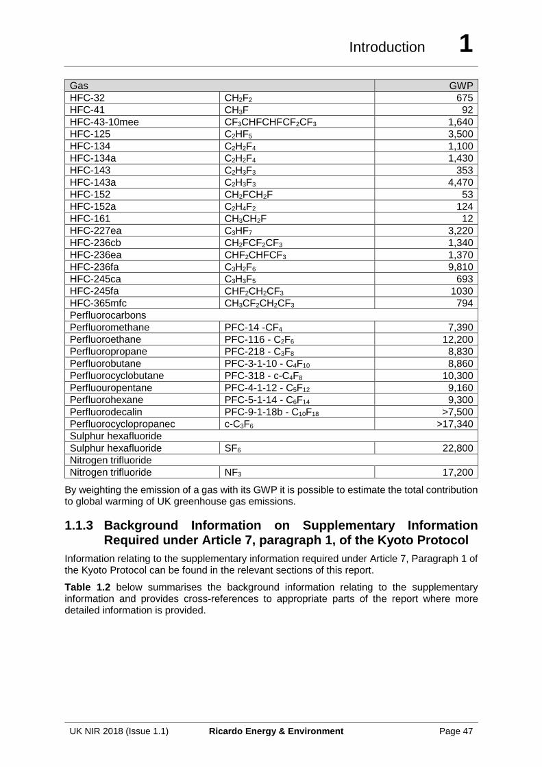
Introduction 1
UK NIR 2018 (Issue 1.1) Ricardo Energy & Environment Page 47
Gas GWP
HFC-32 CH2F2 675
HFC-41 CH3F 92
HFC-43-10mee CF3CHFCHFCF2CF3 1,640
HFC-125 C2HF5 3,500
HFC-134 C2H2F4 1,100
HFC-134a C2H2F4 1,430
HFC-143 C2H3F3 353
HFC-143a C2H3F3 4,470
HFC-152 CH2FCH2F 53
HFC-152a C2H4F2 124
HFC-161 CH3CH2F 12
HFC-227ea C3HF7 3,220
HFC-236cb CH2FCF2CF3 1,340
HFC-236ea CHF2CHFCF3 1,370
HFC-236fa C3H2F6 9,810
HFC-245ca C3H3F5 693
HFC-245fa CHF2CH2CF3 1030
HFC-365mfc CH3CF2CH2CF3 794
Perfluorocarbons
Perfluoromethane PFC-14 -CF4 7,390
Perfluoroethane PFC-116 - C2F6 12,200
Perfluoropropane PFC-218 - C3F8 8,830
Perfluorobutane PFC-3-1-10 - C4F10 8,860
Perfluorocyclobutane PFC-318 - c-C4F8 10,300
Perfluouropentane PFC-4-1-12 - C5F12 9,160
Perfluorohexane PFC-5-1-14 - C6F14 9,300
Perfluorodecalin PFC-9-1-18b - C10F18 >7,500
Perfluorocyclopropanec c-C3F6 >17,340
Sulphur hexafluoride
Sulphur hexafluoride SF6 22,800
Nitrogen trifluoride
Nitrogen trifluoride NF3 17,200
By weighting the emission of a gas with its GWP it is possible to estimate the total contribution to global warming of UK greenhouse gas emissions.
1.1.3 Background Information on Supplementary Information Required under Article 7, paragraph 1, of the Kyoto Protocol
Information relating to the supplementary information required under Article 7, Paragraph 1 of the Kyoto Protocol can be found in the relevant sections of this report.
Table 1.2 below summarises the background information relating to the supplementary information and provides cross-references to appropriate parts of the report where more detailed information is provided.
Introduction 1
UK NIR 2018 (Issue 1.1) Ricardo Energy & Environment Page 48
Table 1.2 Background information on supplementary information required under Article 7, paragraph 1, of the Kyoto Protocol
Reporting element Background information
Supplementary inventory information for activities under Article 3, Paragraphs 3 and 4
The reporting of KP-LULUCF is carried out by the Centre for Ecology and Hydrology (CEH) on behalf of BEIS. The UK has chosen to elect Forest Management, Cropland Management, Grazing Land Management and Wetland Drainage and Rewetting as activities under Article 3.4. The calculations follow the same method and use the same models as the UNFCCC estimates for LULUCF, which are also prepared by CEH. Further information can be found in Chapter 11.
Information on Kyoto Protocol units
The UK National Registry is operated and maintained by the Environment Agency on behalf of BEIS. Information on accounting of Kyoto Protocol units, including a summary of information reported in the standard electronic format (SEF) tables is provided in Chapter 11.1. SEF tables are reported alongside this report.
Changes in National Systems
The UK National System is managed and maintained by BEIS, who is the Single National Entity. Changes to the National System are reported in Chapter 13 of this report.
Changes in National Registry
The UK National Registry is operated and maintained by the Environment Agency on behalf of BEIS. The National Registry is represented on the National Inventory Steering Committee. All changes in the National Registry are reported in Chapter 14.
Minimisation of adverse impacts in accordance with Article 3, Paragraph 14
The UK has undertaken several assessments, reviews and analysis projects to better understand the impacts its policies could have on developing countries, and how they could be addressed. We have supported many initiatives to advance knowledge transfer, research collaboration and capacity building. Further details on the UK’s efforts to minimise adverse impacts is provided in Chapter 15.
1.2 INSTITUTIONAL ARRANGEMENTS FOR INVENTORY PREPARATION
1.2.1 Institutional, Legal and Procedural Arrangements for Compiling the UK inventory
The UK greenhouse gas inventory is compiled and maintained by a consortium led by Ricardo Energy & Environment – the Inventory Agency - under contract to the SICE Directorate in BEIS. Ricardo Energy & Environment is responsible for producing the emissions estimates for CRF categories Energy (CRF sector 1), Industrial Processes and Product Use (CRF sector 2), and Waste (CRF sector 5). Land Use, Land-Use Change and Forestry emissions (CRF sector 4) are calculated by the UK Natural Environment Research Council’s Centre for Ecology and Hydrology (CEH) with the support of Forest Research. The KP-LULUCF information is also produced by CEH with the support of Forest Research. The mechanism for generating
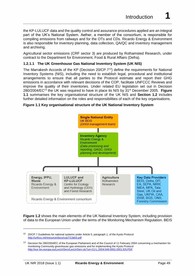
Introduction 1
UK NIR 2018 (Issue 1.1) Ricardo Energy & Environment Page 49
the KP-LULUCF data and the quality control and assurance procedures applied are an integral part of the UK’s National System. Aether, a member of the consortium, is responsible for compiling emissions from railways and for the OTs and CDs. Ricardo Energy & Environment is also responsible for inventory planning, data collection, QA/QC and inventory management and archiving.
Agricultural sector emissions (CRF sector 3) are produced by Rothamsted Research, under contract to the Department for Environment, Food & Rural Affairs (Defra).
1.2.1.1 The UK Greenhouse Gas National Inventory System (UK NIS)
The Marrakesh Accords of the KP (Decision 20/CP.712) define the requirements for National Inventory Systems (NIS), including the need to establish legal, procedural and institutional arrangements to ensure that all parties to the Protocol estimate and report their GHG emissions in accordance with relevant decisions of the COP, facilitate UNFCCC Reviews and improve the quality of their inventories. Under related EU legislation set out in Decision 280/2004/EC13 the UK was required to have in place its NIS by 31st December 2005. Figure 1.1 summarises the key organisational structure of the UK NIS and Section 1.2 includes further detailed information on the roles and responsibilities of each of the key organisations.
Figure 1.1 Key organisational structure of the UK National Inventory System
Figure 1.2 shows the main elements of the UK National Inventory System, including provision of data to the European Union under the terms of the Monitoring Mechanism Regulation. BEIS
12 20/CP.7 Guidelines for national systems under Article 5, paragraph 1, of the Kyoto Protocol
http://unfccc.int/resource/docs/cop7/13a03.pdf
13 Decision No 280/2004/EC of the European Parliament and of the Council of 11 February 2004 concerning a mechanism for
monitoring Community greenhouse gas emissions and for implementing the Kyoto Protocol http://eur-lex.europa.eu/LexUriServ/LexUriServ.do?uri=OJ:L:2004:049:0001:0001:EN:PDF
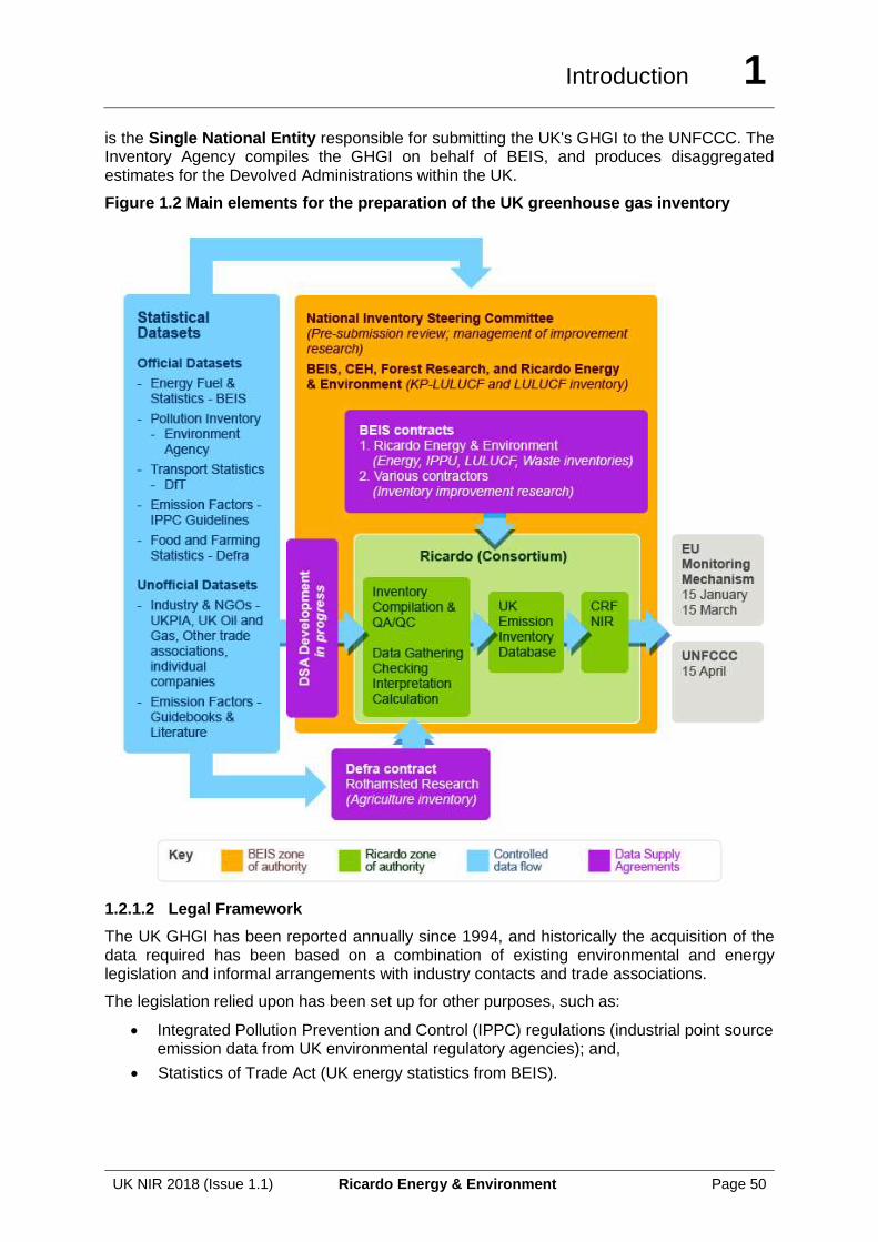
Introduction 1
UK NIR 2018 (Issue 1.1) Ricardo Energy & Environment Page 50
is the Single National Entity responsible for submitting the UK's GHGI to the UNFCCC. The Inventory Agency compiles the GHGI on behalf of BEIS, and produces disaggregated estimates for the Devolved Administrations within the UK.
Figure 1.2 Main elements for the preparation of the UK greenhouse gas inventory
1.2.1.2 Legal Framework
The UK GHGI has been reported annually since 1994, and historically the acquisition of the data required has been based on a combination of existing environmental and energy legislation and informal arrangements with industry contacts and trade associations.
The legislation relied upon has been set up for other purposes, such as:
• Integrated Pollution Prevention and Control (IPPC) regulations (industrial point source emission data from UK environmental regulatory agencies); and,
• Statistics of Trade Act (UK energy statistics from BEIS).
Introduction 1
UK NIR 2018 (Issue 1.1) Ricardo Energy & Environment Page 51
To meet the standards required under the KP, the UK introduced new legislation specifically for national inventory purposes which took effect from November 200514. This legislation makes provision for BEIS’s Secretary of State to issue a notice in the event that information required for the inventory that has been sought voluntarily is not provided. The UK values voluntary participation and this legislation is intended as a last resort once all other avenues to elicit the required data, in the format and to the timing specified, have failed. This legislation was updated in 2014 (The Greenhouse Gas Emissions Trading Scheme (Amendment) Regulations 201415).To ensure that the system works most effectively and to minimise the need for legislative action, BEIS is establishing data supply agreements (DSAs) with relevant organisations to build upon existing relationships with data supply organisations. These agreements formalise the acquisition of data and clarify the main requirements of quality, format, security and timely delivery of data for the national inventory. This process is on-going, through the National Inventory Steering Committee which is a forum of inventory stakeholders that BEIS chairs (see Section 1.2.2.4 below).
There are currently DSAs in place with the Scottish Government, SEPA, NIEA, NRW and DfT.
1.2.2 Overview of Inventory Planning
As summarised in Section 1.2.1, the UK has designated authorities with clear roles and responsibilities. The following sections summarise the roles and responsibilities of key stakeholders in the UK’s National Inventory System (NIS).
1.2.2.1 Single National Entity – BEIS
In 2016, BEIS was created from the Department of Energy and Climate Change (DECC) and the Department for Business, Innovation and Skills (BIS) and became the Single National Entity for the UK. This has been confirmed in writing to the UNFCCC Executive Secretary. BEIS has overall responsibility for the UK Greenhouse Gas Inventory and the UK National System and carries out this function on behalf of Her Majesty’s Government and the Devolved Administrations (Wales, Scotland and Northern Ireland). BEIS is responsible for the institutional, legal and procedural arrangements for the national system and for the strategic development of the national inventory.
Within BEIS, the SICE Directorate administers this responsibility. The SICE Directorate coordinates expertise from across Government and manages research contracts to ensure that the UK Greenhouse Gas Inventory meets international standards set out in the UNFCCC reporting guidelines, the Kyoto Protocol and the IPCC 2006 Guidelines.
As the designated Single National Entity for the UK GHG NIS, BEIS has the following roles and responsibilities:
National Inventory System management and planning
• Overall control of the NIS development and function;
• Management of contracts and delivery of the GHG inventory; and,
• Definition of performance criteria for NIS key organisations.
Development of legal and contractual infrastructure
• Review of legal and organisational structure; and,
14 Greenhouse Gas Emissions Trading Scheme (Amendment) and National Emissions Inventory Regulations 2005
http://www.opsi.gov.uk/si/si2005/20052903.htm
15 http://www.legislation.gov.uk/uksi/2014/3075/contents/made
Introduction 1
UK NIR 2018 (Issue 1.1) Ricardo Energy & Environment Page 52
• Implementation of legal instruments and contractual developments as required to meet guidelines.
The contact point for the Single National Entity is provided on the Contacts page of the NIR.
1.2.2.2 Inventory Agency – Ricardo Energy & Environment Consortium
A new 3.5-year contract was established for the Inventory Agency in late 2016 following a competitive tendering exercise. Ricardo Energy & Environment leads the consortium responsible for compiling the inventory, under contract to BEIS. Ricardo Energy & Environment is responsible for all aspects of national inventory preparation, reporting and quality management. The consortium consists of:
• Ricardo Energy & Environment – lead contractor;
• CEH – overall responsibility for the LULUCF and KP-LULUCF estimates.
• Forest Research – responsible for forestland estimates that feed into the LULUCF and KP-LULUCF estimates.
• Aether – responsible for estimates from railways and the Overseas Territories (OTs) and Crown Dependencies (CDs); and DA inventories.
• Ray Gluckman Consulting – contributions to the F-gas inventory.
Ricardo Energy & Environment together with the project partners prepares the National Atmospheric Emissions Inventory (NAEI) which is the core air emissions database from which the greenhouse gas inventory (GHGI) is extracted. This arrangement ensures consistency in reporting across all air emissions for different reporting purposes (UNFCCC, UNECE etc.). Activities include: collecting and processing data from a wide range of sources; selecting appropriate emission factors and estimation methods according to IPCC guidance; compiling the inventory; managing inventory QA/QC including QC of raw and processed data and data management tools, documentation and archiving, prioritisation of methodology and data improvements; carrying out uncertainty assessments; delivering the NIR (including CRF tables) by deadlines set to the EU Monitoring Mechanism Regulation (MMR) and the UNFCCC on behalf of BEIS; and assisting with Article 8 reviews under the KP.
As the designated Inventory Agency for the UK GHG National Inventory System, Ricardo Energy & Environment has the following roles and responsibilities:
Planning
• Co-ordination with BEIS to deliver the NIS;
• Review of current NIS performance and assessment of required development action; and,
• Scheduling of tasks and responsibilities to deliver GHG inventory and NIS.
Preparation
• Drafting of agreements with key data providers; and,
• Review of source data and identification of developments required to improve GHG inventory data quality.
Management
• Documentation and archiving;
• Dissemination of information regarding NIS to Key Data Providers; and,
• Management of inventory QA/QC plans, programmes and activities.
Inventory compilation
• Data acquisition, processing and reporting; and,
• Delivery of NIR (including associated CRF tables) to time and quality.
Introduction 1
UK NIR 2018 (Issue 1.1) Ricardo Energy & Environment Page 53
The Inventory Agency has formal systems in place to ensure that staff working on the inventory are well trained and able to carry out their duties effectively and efficiently. The technical competence of the staff is facilitated through a combination of the formal Ricardo Energy & Environment and inventory-specific staff management and training systems. Roles and responsibilities for all inventory team members are clearly defined, and a comprehensive system of QA/QC is in place. Section 1.6 sets out the QA/QC plan in detail. Ricardo Energy & Environment systems ensure subcontractors are managed actively and deliver inputs to the inventory on time and to the specified quality.
The contact point for the Inventory Agency is provided on the Contacts page of the NIR.
Rothamsted Research, under contract to Defra, is responsible for the preparation and development of the agriculture inventory. Rothamsted Research conducts specific research in the agriculture sector and provides finalised GHG emissions data to Ricardo Energy & Environment for inclusion within the UK GHG inventory.
Rothamsted Research are directly responsible for compiling the agriculture sections of the CRF, and for maintaining documentation and archiving of their models and processes. Ricardo Energy & Environment are responsible for checking consistency between outputs.
1.2.2.3 Key Data Providers and Reference Sources
The organisations that provide the raw data to the UK GHGI include a wide range of Government Departments, non-Departmental public bodies and Government Agencies, private companies and industrial trade associations.
Within the UK GHG National Inventory System, organisations that are Key Data Providers have the following roles and responsibilities:
Data quality, Format, Timeliness, Security
• delivery of source data in the appropriate format and in time for inventory compilation, allowing for completion of required QA/QC procedures;
• assessment of their data acquisition, processing and reporting systems, having regard for QA/QC requirements;
• identification of any required organisational or legal development and resources to meet more stringent NIS data requirements, notably the security of data provision in the future; and,
• communication with BEIS, Ricardo Energy & Environment and their peers or members to help to disseminate information regarding the GHG inventory and National System.
Energy statistics required for compilation of the GHGI are obtained from DUKES, which is compiled and published annually by a team of energy statisticians within BEIS.
Information on industrial processes is provided either directly to the inventory agency by the individual plant operators or from:
• The Environment Agency's (EA) Pollution Inventory for England;
• Natural Resources Wales’s (NRW) Pollution Inventory for Wales;
• The Scottish Environment Protection Agency’s (SEPA) Scottish Pollutant Release Inventory; and
• The Northern Ireland Environment Agency’s (NIEA) Northern Ireland Pollution Inventory.
Reporting to these UK inventories for the purposes of environmental regulation is a statutory requirement for industries under the Industrial Emissions Directive (IED) and Integrated Pollution Prevention and Control (IPPC). The data from these inventory sources is also used
Introduction 1
UK NIR 2018 (Issue 1.1) Ricardo Energy & Environment Page 54
to quality check data provided voluntarily by companies directly to Ricardo Energy & Environment.
In addition, the inventory agency receives energy, fuel compositional data and emission estimates from all UK installations that operate within the EU Emissions Trading System, from detailed annual operator returns to the UK regulators of EU ETS (EA, SEPA, NRW, NIEA, BEIS Offshore Inspectorate). These data are used by the inventory agency and the BEIS energy statistics team to improve the UK energy balance and emission estimates for high-emitting source categories in the Energy and IPPU sectors (see Annex 7 for further details).
The UK Natural Environment Research Council’s Centre for Ecology and Hydrology (CEH) compiles estimates of emissions and removals from LULUCF as part of the Ricardo Energy & Environment consortium using land-use data and information on forestry from the Forestry Commission Research Agency (an executive agency of the Forestry Commission, known as Forest Research), Government Departments, Devolved Administrations and from other sources.
Rothamsted Research compiles the inventory for agricultural emissions using agricultural statistics from Defra and the Northern Ireland Department of Agriculture, Environment and Rural Affairs (NI DAERA).
1.2.2.4 The National Inventory Steering Committee, pre-Submission Review and Approval of the UK GHGI
To meet the detailed requirements of a National System and to ensure the UK efficiently and effectively works towards implementing best practices, a formal cross-Government body, the National Inventory Steering Committee (NISC) was formed in 2006. The NISC is tasked with the official consideration and approval of the national inventory prior to submission to the UNFCCC. This pre-submission review is achieved at a NISC meeting prior to the finalisation of the inventory, and any recalculations to the inventory are presented and discussed at this meeting.
One of the main roles of the committee is to assist the BEIS GHG inventory management team to manage and to prioritise the over-arching inventory QA and facilitate review and improvement and better communication between inventory stakeholders across Government Departments and Agencies.
Members of the Steering Committee include the Inventory Agency team at Ricardo Energy & Environment, other contractors, plus appropriate sector, legal and economic experts. These experts are responsible for reviewing methodologies, activity data, emission factors and emission estimates at a sectoral level and report their findings and recommendations to the steering committee on a regular basis. The committee is responsible for ensuring that the inventory meets international standards of quality, accuracy and completeness, and is delivered on time each year to the EU Monitoring Mechanism Regulation and the UNFCCC. The NISC is responsible for agreeing the priorities for the UK GHGI improvement programme. Where inventory improvement research is commissioned by the NISC, the research reports are reviewed and approved for use within the UK GHGI compilation by members of the NISC, managed by BEIS, as part of the pre-submission review process.
Following the NISC meeting in the autumn, any changes to the inventory methodology are signed off by the Director of Science and Innovation for Climate and Energy (SICE), who is the Senior Responsible Officer in BEIS.
Final technical sign-off of inventory outputs rests with the Inventory Agency, as part of the governance procedures agreed with BEIS as Single National Entity:
Introduction 1
UK NIR 2018 (Issue 1.1) Ricardo Energy & Environment Page 55
• Any outputs relating to financial mechanisms are signed off by the Senior
Responsible Officer at the Inventory Agency, as evidence that all quality control has
been conducted on these outputs
• National inventory outputs and technical delivery sign-off (e.g. on improvement
projects) are signed off by either the inventory Senior Analyst or Technical Director at
the Inventory Agency
Table 1.3 and Table 1.4 below shows the main organisations engaged in the UK NISC, and their roles and responsibilities in relation to the preparation and development of the national inventory. These tables include organisations from the following categories, many of which are classed as key data providers:
• UK government departments – including BEIS, the Department for Environment, Food and Rural Affairs (Defra), and Department for Transport (DfT)
• Devolved administrations (DAs) in Scotland, Wales and Northern Ireland
• Inventory contractors (who compile data for the Inventory among other tasks)
• Government agencies (e.g. environmental regulators)
• Industry bodies or associations
• Consultants and invited experts
The development of the inventory is driven through the NISC, which meets twice a year to discuss the outcomes of recent peer, internal and expert reviews and to agree the prioritisation, funding, implementation and review of items on the UK inventory improvement programme. The Key Category Analysis and the uncertainty analysis, qualitative analysis from Inventory Agency experts as well as recommendations from reviews of the UK GHG inventory are used as guidance to help the members of the NISC make decisions on which improvements are the most important. Key categories with high uncertainty are given priority over non-key categories or categories with a low uncertainty. The annual inventory review feedback from the UNFCCC and outcomes from QA/QC checks and reviews carried out under the MMR and ESD, as well as sector-specific peer- or bilateral review findings are also considered to guide decisions on UK GHGI improvement priorities.
Following a UN Expert Review Team recommendation, a qualitative uncertainty analysis of the inventory is now implemented by the Inventory Agency. This qualitative uncertainty analysis supports the Key Category Analysis and helps determine the highest priority emission sources in the UK where methodological improvements could be applied to improve the accuracy of emission estimates, or more detailed reporting used to improve transparency. This qualitative assessment is conducted by experts of the inventory team within the inventory cycle, including through a post-submission review of data sources, methods and feedback from the MMR and UNFCCC ERTs.
In spring each year, BEIS and the Inventory Agency hold a review meeting, at which the findings of the EU and UN reviews, internal post-submission review and qualitative analysis of source categories are discussed in order to develop a comprehensive list of inventory improvement items for discussion, prioritisation and implementation via the NISC.
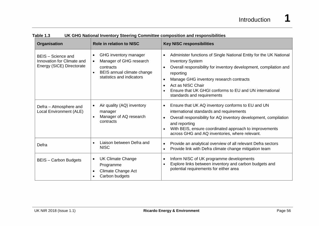
Introduction 1
UK NIR 2018 (Issue 1.1) Ricardo Energy & Environment Page 56
Table 1.3 UK GHG National Inventory Steering Committee composition and responsibilities
Organisation Role in relation to NISC Key NISC responsibilities
BEIS – Science and Innovation for Climate and Energy (SICE) Directorate
• GHG inventory manager
• Manager of GHG research
contracts
• BEIS annual climate change statistics and indicators
• Administer functions of Single National Entity for the UK National
Inventory System
• Overall responsibility for inventory development, compilation and
reporting
• Manage GHG inventory research contracts
• Act as NISC Chair
• Ensure that UK GHGI conforms to EU and UN international standards and requirements
Defra – Atmosphere and Local Environment (ALE)
• Air quality (AQ) inventory
manager
• Manager of AQ research contracts
• Ensure that UK AQ inventory conforms to EU and UN
international standards and requirements
• Overall responsibility for AQ inventory development, compilation
and reporting
• With BEIS, ensure coordinated approach to improvements across GHG and AQ inventories, where relevant.
Defra • Liaison between Defra and
NISC • Provide an analytical overview of all relevant Defra sectors
• Provide link with Defra climate change mitigation team
BEIS – Carbon Budgets • UK Climate Change
Programme
• Climate Change Act
• Carbon budgets
• Inform NISC of UK programme developments
• Explore links between inventory and carbon budgets and potential requirements for either area
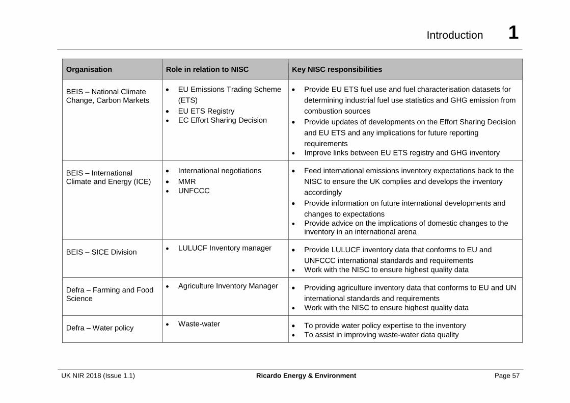
Introduction 1
UK NIR 2018 (Issue 1.1) Ricardo Energy & Environment Page 57
Organisation Role in relation to NISC Key NISC responsibilities
BEIS – National Climate Change, Carbon Markets
• EU Emissions Trading Scheme
(ETS)
• EU ETS Registry
• EC Effort Sharing Decision
• Provide EU ETS fuel use and fuel characterisation datasets for
determining industrial fuel use statistics and GHG emission from
combustion sources
• Provide updates of developments on the Effort Sharing Decision
and EU ETS and any implications for future reporting
requirements
• Improve links between EU ETS registry and GHG inventory
BEIS – International Climate and Energy (ICE)
• International negotiations
• MMR
• UNFCCC
• Feed international emissions inventory expectations back to the
NISC to ensure the UK complies and develops the inventory
accordingly
• Provide information on future international developments and
changes to expectations
• Provide advice on the implications of domestic changes to the inventory in an international arena
BEIS – SICE Division • LULUCF Inventory manager • Provide LULUCF inventory data that conforms to EU and
UNFCCC international standards and requirements
• Work with the NISC to ensure highest quality data
Defra – Farming and Food Science
• Agriculture Inventory Manager • Providing agriculture inventory data that conforms to EU and UN
international standards and requirements
• Work with the NISC to ensure highest quality data
Defra – Water policy • Waste-water • To provide water policy expertise to the inventory
• To assist in improving waste-water data quality
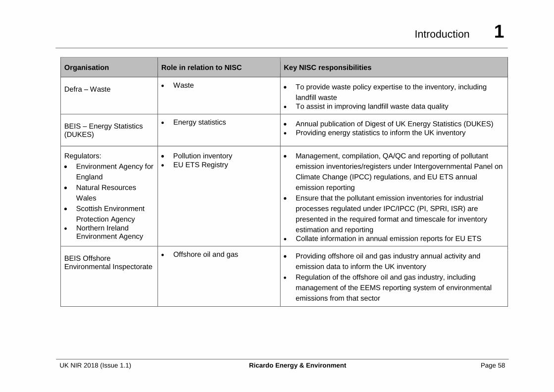
Introduction 1
UK NIR 2018 (Issue 1.1) Ricardo Energy & Environment Page 58
Organisation Role in relation to NISC Key NISC responsibilities
Defra – Waste • Waste • To provide waste policy expertise to the inventory, including
landfill waste
• To assist in improving landfill waste data quality
BEIS – Energy Statistics (DUKES)
• Energy statistics • Annual publication of Digest of UK Energy Statistics (DUKES)
• Providing energy statistics to inform the UK inventory
Regulators:
• Environment Agency for
England
• Natural Resources
Wales
• Scottish Environment
Protection Agency
• Northern Ireland Environment Agency
• Pollution inventory
• EU ETS Registry
• Management, compilation, QA/QC and reporting of pollutant
emission inventories/registers under Intergovernmental Panel on
Climate Change (IPCC) regulations, and EU ETS annual
emission reporting
• Ensure that the pollutant emission inventories for industrial
processes regulated under IPC/IPCC (PI, SPRI, ISR) are
presented in the required format and timescale for inventory
estimation and reporting
• Collate information in annual emission reports for EU ETS
BEIS Offshore Environmental Inspectorate
• Offshore oil and gas • Providing offshore oil and gas industry annual activity and
emission data to inform the UK inventory
• Regulation of the offshore oil and gas industry, including
management of the EEMS reporting system of environmental
emissions from that sector
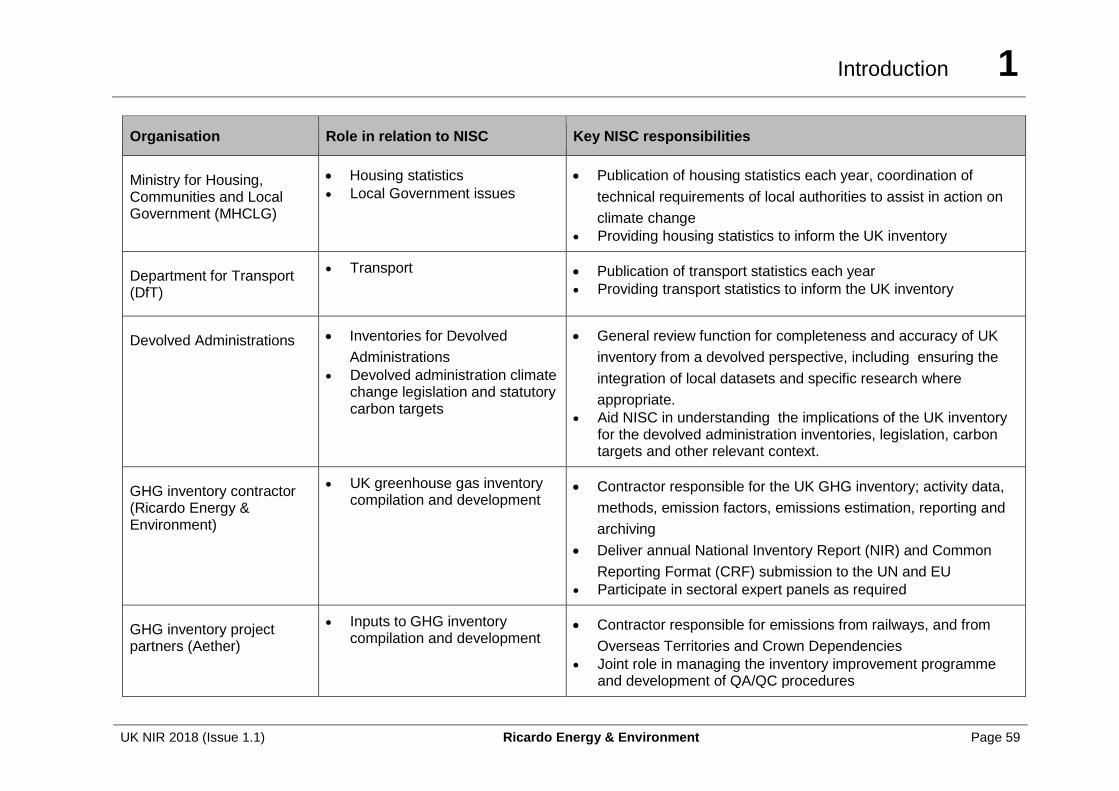
Introduction 1
UK NIR 2018 (Issue 1.1) Ricardo Energy & Environment Page 59
Organisation Role in relation to NISC Key NISC responsibilities
Ministry for Housing, Communities and Local Government (MHCLG)
• Housing statistics
• Local Government issues
• Publication of housing statistics each year, coordination of
technical requirements of local authorities to assist in action on
climate change
• Providing housing statistics to inform the UK inventory
Department for Transport (DfT)
• Transport • Publication of transport statistics each year
• Providing transport statistics to inform the UK inventory
Devolved Administrations • Inventories for Devolved
Administrations
• Devolved administration climate change legislation and statutory carbon targets
• General review function for completeness and accuracy of UK
inventory from a devolved perspective, including ensuring the
integration of local datasets and specific research where
appropriate.
• Aid NISC in understanding the implications of the UK inventory for the devolved administration inventories, legislation, carbon targets and other relevant context.
GHG inventory contractor (Ricardo Energy & Environment)
• UK greenhouse gas inventory compilation and development
• Contractor responsible for the UK GHG inventory; activity data,
methods, emission factors, emissions estimation, reporting and
archiving
• Deliver annual National Inventory Report (NIR) and Common
Reporting Format (CRF) submission to the UN and EU
• Participate in sectoral expert panels as required
GHG inventory project partners (Aether)
• Inputs to GHG inventory compilation and development
• Contractor responsible for emissions from railways, and from
Overseas Territories and Crown Dependencies
• Joint role in managing the inventory improvement programme and development of QA/QC procedures
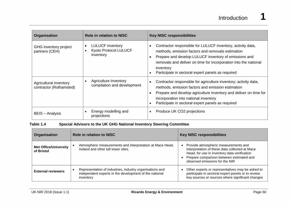
Introduction 1
UK NIR 2018 (Issue 1.1) Ricardo Energy & Environment Page 60
Organisation Role in relation to NISC Key NISC responsibilities
GHG inventory project partners (CEH)
• LULUCF inventory
• Kyoto Protocol LULUCF inventory
• Contractor responsible for LULUCF inventory, activity data,
methods, emission factors and removals estimation
• Prepare and develop LULUCF inventory of emissions and
removals and deliver on time for incorporation into the national
inventory
• Participate in sectoral expert panels as required
Agricultural inventory contractor (Rothamsted)
• Agriculture Inventory compilation and development
• Contractor responsible for agriculture inventory; activity data,
methods, emission factors and emission estimation
• Prepare and develop agriculture inventory and deliver on time for
incorporation into national inventory
• Participate in sectoral expert panels as required
BEIS – Analysis • Energy modelling and
projections
• Produce UK CO2 projections
Table 1.4 Special Advisors to the UK GHG National Inventory Steering Committee
Organisation Role in relation to NISC Key NISC responsibilities
Met Office/University of Bristol
• Atmospheric measurements and interpretation at Mace Head, Ireland and other tall tower sites.
• Provide atmospheric measurements and interpretation of these data collected at Mace Head, for use in inventory data verification
• Prepare comparison between estimated and observed emissions for the NIR
External reviewers • Representation of industries, industry organisations and
independent experts in the development of the national inventory
• Other experts or representatives may be asked to participate in sectoral expert panels or to review key sources or sources where significant changes
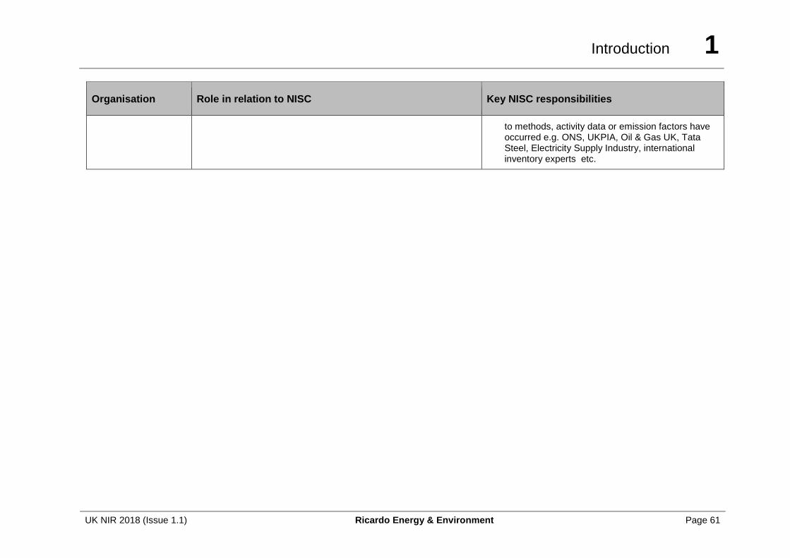
Introduction 1
UK NIR 2018 (Issue 1.1) Ricardo Energy & Environment Page 61
Organisation Role in relation to NISC Key NISC responsibilities
to methods, activity data or emission factors have occurred e.g. ONS, UKPIA, Oil & Gas UK, Tata Steel, Electricity Supply Industry, international inventory experts etc.
Introduction 1
UK NIR 2018 (Issue 1.1) Ricardo Energy & Environment Page 62
1.2.2.5 UK Inventory Improvement Programme
Each year the inventory is updated to include the latest data available. Improvements to the methodology are made and are backdated to ensure a consistent time series. Methodological changes are made to take account of new research and data sources, any new guidance from IPCC, relevant work or emission factors from sources such as EMEP-EEA and the US EPA, or from specific research programmes sponsored by BEIS and other UK Departments.
The UK NIS has a formal Inventory Improvement Programme, managed by the NISC. This achieves the dual aims of (i) progressing research to improve the UK GHGI data quality, and (ii) developing inter-Departmental/Agency working relationships to integrate inventory-related information from across Government.
The NISC helps prioritise improvements across the inventory. These improvements are designed to improve the transparency, accuracy, consistency, comparability, and completeness of the inventory. Incremental improvements are made routinely to ensure the inventory uses the most accurate activity data and emission factors. A detailed and prioritised list of larger inventory improvement tasks is maintained by the Inventory Agency. The list is kept under review continually, and is formally reviewed annually at a NISC meeting. This list is prioritised by taking into account the Key Category Analysis (see Section 1.5), the quantitative uncertainty analysis, sector and pollutant expert judgements, and the future obligations of the inventory. The timing of the improvements and resourcing of the work are important considerations for the NISC. The Single National Entity takes the final decision on timing and implementation of improvements to the inventory.
1.2.2.6 Integrated UK-DA GHGI improvement programme
The UK compiles a national level inventory, and in addition separate inventories for the Devolved Administrations (DAs). A single improvement programme is in place to manage improvements to these inventories.
During 2017-18, the integrated UK-DA GHGI improvement programme implemented a number of specific research projects to address inventory uncertainties and reporting requirements, including:
• Conversion of default emission factors – The UK inventory is calculated using fuel data on a mass basis (for liquid and solid fuels), for consistency with the UK energy statistics (DUKES). This means that in order to use default or literature based emission factors, conversions are made. A new approach has been implemented to make these conversions in a database, applying consistent assumptions across fuels, users, and pollutants, as well as allowing for interannual variations in fuel calorific values. This has led to minor recalculations for non CO2 pollutants.
• Development of DA Specific Landfill Models – separate models have been developed for each of the Devolved Administrations. It is anticipated that devolved policies on waste disposal will lead to notable differences in waste composition for the DA’s and as such the models were developed to enable the accurate reflection of these data at DA level. In producing the new models, new data for waste arisings from 2006 onwards have been identified and incorporated into the model, leading to some recalculations to the emissions estimates at UK level.
• Shipping – the UK shipping inventory model underwent a review and update during the 2016-17 cycle. This was a longer project and the results have been fed into the 2018 submission. This impacts on the activity data and emission factors for domestic and international shipping, and for fishing vessels. The revised emission factors have also been used for naval shipping.
• The CARBINE model for calculating forest carbon stock change has had four main changes:
Introduction 1
UK NIR 2018 (Issue 1.1) Ricardo Energy & Environment Page 63
o Inclusion of in-year turnover of standing tree carbon (for example fine roots).
o Improvement to the soil and litter model to include an assumption that there is a quantity of litter input to the soil from non-tree vegetation on transition to forest.
o The soil model has been adjusted to incorporate all the organic matter transfer to the soil to avoid over-estimates of soil carbon accumulation if decomposition losses to the atmosphere are omitted.
o The inclusion of roots in the litter/dead carbon pool. • An improvement has been made to Harvested Wood Products to change the mix of
semi-finished wood products to vary over time to match the information from Forest Statistics and FAO data.
Improvement priorities are discussed and agreed each April and incorporate the findings from the latest UNFCCC review of the inventory.
1.2.2.7 Agriculture inventory improvements
The UK GHG agricultural inventory has recently undergone a major improvement program resulting in the adoption of a new coded (C#) inventory model with finer spatial, temporal and sectoral resolution in underlying calculations, implementation of a number of country-specific emission factors and improvements to activity data. A full description of the changes made is included in chapter 5 of this report.
Further planned improvements are more modest, but include:
1. Review of activity data and emission factors for anaerobic digestion of livestock manure and subsequent management of digestate
2. Review of manure management practice activity data for the England and the Devolved Administrationsof the UK with a view to developing robust evidence for trends over the reporting time series
3. Review UK livestock feed data and revise inventory parameters according to outcomes of Defra project SCF0203.
4. Continue to review the scientific literature to revise and refine UK-specific emission factors as relevant data arise.
1.2.3 Overview of Inventory Preparation and Management, Including for Supplementary Information Required under Article 7, Paragraph 1 of the Kyoto Protocol
For details of inventory preparation, see Section 1.3.
The Environment Agency is appointed as the UK Registry Administrator for the EU ETS/Kyoto Registry by BEIS. The UK for this purpose comprises England, Wales, Scotland, Northern Ireland, Offshore oil and gas installations and Gibraltar. The Environment Agency is a Government Agency.
Responsibilities of the Environment Agency include to:
• Manage the contractors responsible for maintaining the computer systems (Siemens for software/hosting the Registry and Trustis for digital certificates);
• Conform to the Kyoto Protocol and the COP/MOP decisions as implemented by the UNFCCC;
• Conform to the EU Registries Regulations as amended from time to time;
Introduction 1
UK NIR 2018 (Issue 1.1) Ricardo Energy & Environment Page 64
• Allow access for authorised users16.
• Act on instructions from Competent Authorities to manage accounts; and,
• Assist registry users.
1.3 INVENTORY PREPARATION
1.3.1 GHG Inventory
The present UK GHG inventory for the period 1990-2016 was compiled in accordance with the 2006 IPCC Guidelines for National Greenhouse Gas Inventories (IPCC, 2006).
1.3.2 Data collection, processing and storage
The data acquisition task provides the fundamental activity data from which the GHG inventory is constructed. The process starts in June with the annual requests for data. A database which contains a list of contacts and datasets is used to track progress of the data acquired.
The following activities are carried out each year, in order, as the inventory is compiled:
Method improvement
Improvements to calculation methods are implemented before the inventory is compiled. These improvements are in part based on recommendations of UNFCCC reviews, EC reviews, peer reviews, bilateral reviews and relevant research sponsored by BEIS, Defra or other organisations.
Data request
Requests for activity data and background data are issued to a wide range of data suppliers. Each request is issued with a unique code, and a database is used to track the request and the data supplied from that request.
Data verification
Activity data received are examined. Anomalies are investigated, such as time series discrepancies, or large changes in values from the previous to the current inventory year.
Data processing
Data are prepared to allow emissions of direct and indirect GHG to be estimated.
Emission estimation
Provisional emissions are estimated using the most recent activity data available.
Emissions review
A series of internal reviews are carried out to detect anomalies in the estimates (time series variations and year to year changes). Errors and omissions are then rectified.
Emissions reporting (including background data)
Estimates of emissions are prepared for the various reporting formats (e.g. IPCC, UNECE etc. including differing geographical coverages).
16 Terms and Conditions at http://emissionsregistry.environment-agency.gov.uk/Default.aspx
Introduction 1
UK NIR 2018 (Issue 1.1) Ricardo Energy & Environment Page 65
Report generation
Draft reports are written to satisfy the reporting criteria of the various agencies, e.g. the UNFCCC.
Report review
The reports are reviewed internally, by external contributing agencies, and by BEIS. Errors and omissions are then rectified.
Report publication
Final reports and data sets are then submitted via approved reporting routes, published in print and made available on publicly accessible web sites.
Data archiving
At the end of each inventory cycle, all data, spreadsheets, databases and reports are archived, allowing all data to remain traceable, should it be needed in future years.
The system outlined above complies with the Tier 1 QA/QC procedures outlined in Volume 1, Chapter 6 of IPCC, 2006.
Rothamsted Research and CEH, who are the sector experts for agriculture and LULUCF (including KP LULUCF), respectively, have their own systems in place for data collection. As the Inventory Agency responsible for compiling the overall inventory estimates, Ricardo Energy & Environment receives completed emission estimates from these organisations as part of the annual data collection process.
Ricardo Energy & Environment has work programmes in place with CEH and Rothamsted to help harmonise the quality systems used with those Ricardo Energy & Environment use in the core GHG inventory.
1.3.3 Quality assurance/quality control (QA/QC) procedures and extensive review of GHG inventory
The QA/QC plan for the UK inventory is explained in Section 1.6. Additional details of QA/QC in the LULUCF and Agriculture sectors can be found in Chapter 6, Section 6.10 and Chapter 5, Section 5.9 respectively.
1.4 METHODOLOGIES AND DATA SOURCES
1.4.1 GHG Inventory
The methods used to estimate emissions are described in detail in the relevant sections of this report. The direct and indirect GHGs reported are estimated using methodologies which mostly correspond to the detailed sectoral Tier 2/3 methods in the IPCC Guidelines.
Table 1.5 provides a brief summary of the methods used to estimate UK GHG emissions, which are described in more detail in the subsequent Chapters and Appendices.
Table 1.5 Summary of methods used to estimate emissions of the direct greenhouse gases
CRF sector Comments on methods
1A • Basic combustion module (fuel use * emission factor);
• Transport models (see MS 6, to MS 16); and,
• Carbon balance approach (See MS 4).
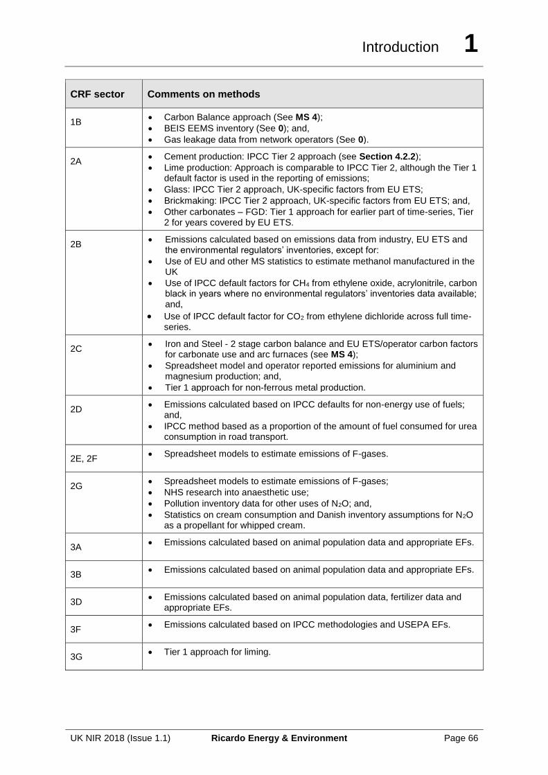
Introduction 1
UK NIR 2018 (Issue 1.1) Ricardo Energy & Environment Page 66
CRF sector Comments on methods
1B • Carbon Balance approach (See MS 4);
• BEIS EEMS inventory (See 0); and,
• Gas leakage data from network operators (See 0).
2A • Cement production: IPCC Tier 2 approach (see Section 4.2.2);
• Lime production: Approach is comparable to IPCC Tier 2, although the Tier 1 default factor is used in the reporting of emissions;
• Glass: IPCC Tier 2 approach, UK-specific factors from EU ETS;
• Brickmaking: IPCC Tier 2 approach, UK-specific factors from EU ETS; and,
• Other carbonates – FGD: Tier 1 approach for earlier part of time-series, Tier 2 for years covered by EU ETS.
2B • Emissions calculated based on emissions data from industry, EU ETS and
the environmental regulators’ inventories, except for:
• Use of EU and other MS statistics to estimate methanol manufactured in the UK
• Use of IPCC default factors for CH4 from ethylene oxide, acrylonitrile, carbon black in years where no environmental regulators’ inventories data available; and,
• Use of IPCC default factor for CO2 from ethylene dichloride across full time-series.
2C • Iron and Steel - 2 stage carbon balance and EU ETS/operator carbon factors
for carbonate use and arc furnaces (see MS 4);
• Spreadsheet model and operator reported emissions for aluminium and magnesium production; and,
• Tier 1 approach for non-ferrous metal production.
2D • Emissions calculated based on IPCC defaults for non-energy use of fuels;
and,
• IPCC method based as a proportion of the amount of fuel consumed for urea consumption in road transport.
2E, 2F • Spreadsheet models to estimate emissions of F-gases.
2G • Spreadsheet models to estimate emissions of F-gases;
• NHS research into anaesthetic use;
• Pollution inventory data for other uses of N2O; and,
• Statistics on cream consumption and Danish inventory assumptions for N2O as a propellant for whipped cream.
3A • Emissions calculated based on animal population data and appropriate EFs.
3B • Emissions calculated based on animal population data and appropriate EFs.
3D • Emissions calculated based on animal population data, fertilizer data and
appropriate EFs.
3F • Emissions calculated based on IPCC methodologies and USEPA EFs.
3G • Tier 1 approach for liming.
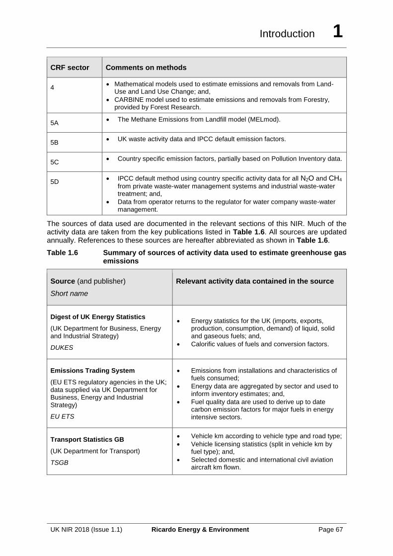
Introduction 1
UK NIR 2018 (Issue 1.1) Ricardo Energy & Environment Page 67
CRF sector Comments on methods
4 • Mathematical models used to estimate emissions and removals from Land-
Use and Land Use Change; and,
• CARBINE model used to estimate emissions and removals from Forestry, provided by Forest Research.
5A • The Methane Emissions from Landfill model (MELmod).
5B • UK waste activity data and IPCC default emission factors.
5C • Country specific emission factors, partially based on Pollution Inventory data.
5D • IPCC default method using country specific activity data for all N2O and CH4
from private waste-water management systems and industrial waste-water treatment; and,
• Data from operator returns to the regulator for water company waste-water management.
The sources of data used are documented in the relevant sections of this NIR. Much of the activity data are taken from the key publications listed in Table 1.6. All sources are updated annually. References to these sources are hereafter abbreviated as shown in Table 1.6.
Table 1.6 Summary of sources of activity data used to estimate greenhouse gas emissions
Source (and publisher)
Short name
Relevant activity data contained in the source
Digest of UK Energy Statistics
(UK Department for Business, Energy and Industrial Strategy)
DUKES
• Energy statistics for the UK (imports, exports, production, consumption, demand) of liquid, solid and gaseous fuels; and,
• Calorific values of fuels and conversion factors.
Emissions Trading System
(EU ETS regulatory agencies in the UK; data supplied via UK Department for Business, Energy and Industrial Strategy)
EU ETS
• Emissions from installations and characteristics of fuels consumed;
• Energy data are aggregated by sector and used to inform inventory estimates; and,
• Fuel quality data are used to derive up to date carbon emission factors for major fuels in energy intensive sectors.
Transport Statistics GB
(UK Department for Transport)
TSGB
• Vehicle km according to vehicle type and road type;
• Vehicle licensing statistics (split in vehicle km by fuel type); and,
• Selected domestic and international civil aviation aircraft km flown.
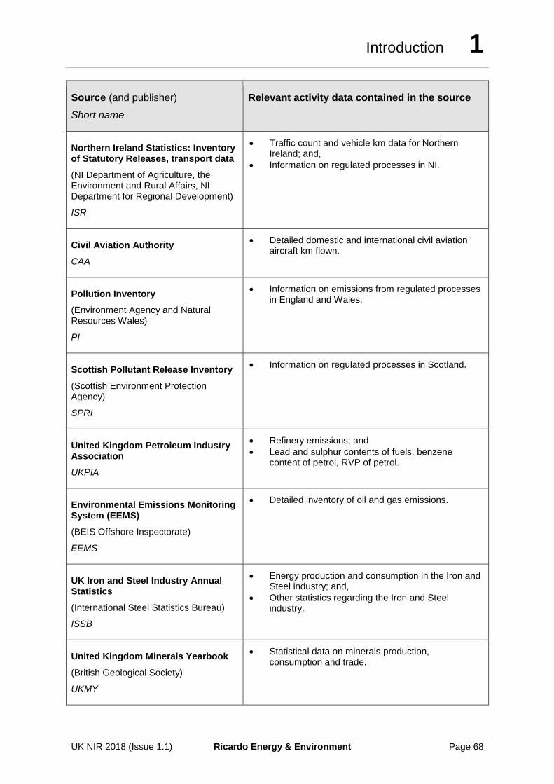
Introduction 1
UK NIR 2018 (Issue 1.1) Ricardo Energy & Environment Page 68
Source (and publisher)
Short name
Relevant activity data contained in the source
Northern Ireland Statistics: Inventory of Statutory Releases, transport data
(NI Department of Agriculture, the Environment and Rural Affairs, NI Department for Regional Development)
ISR
• Traffic count and vehicle km data for Northern Ireland; and,
• Information on regulated processes in NI.
Civil Aviation Authority
CAA
• Detailed domestic and international civil aviation aircraft km flown.
Pollution Inventory
(Environment Agency and Natural Resources Wales)
PI
• Information on emissions from regulated processes in England and Wales.
Scottish Pollutant Release Inventory
(Scottish Environment Protection Agency)
SPRI
• Information on regulated processes in Scotland.
United Kingdom Petroleum Industry Association
UKPIA
• Refinery emissions; and
• Lead and sulphur contents of fuels, benzene content of petrol, RVP of petrol.
Environmental Emissions Monitoring System (EEMS)
(BEIS Offshore Inspectorate)
EEMS
• Detailed inventory of oil and gas emissions.
UK Iron and Steel Industry Annual Statistics
(International Steel Statistics Bureau)
ISSB
• Energy production and consumption in the Iron and Steel industry; and,
• Other statistics regarding the Iron and Steel industry.
United Kingdom Minerals Yearbook
(British Geological Society)
UKMY
• Statistical data on minerals production, consumption and trade.
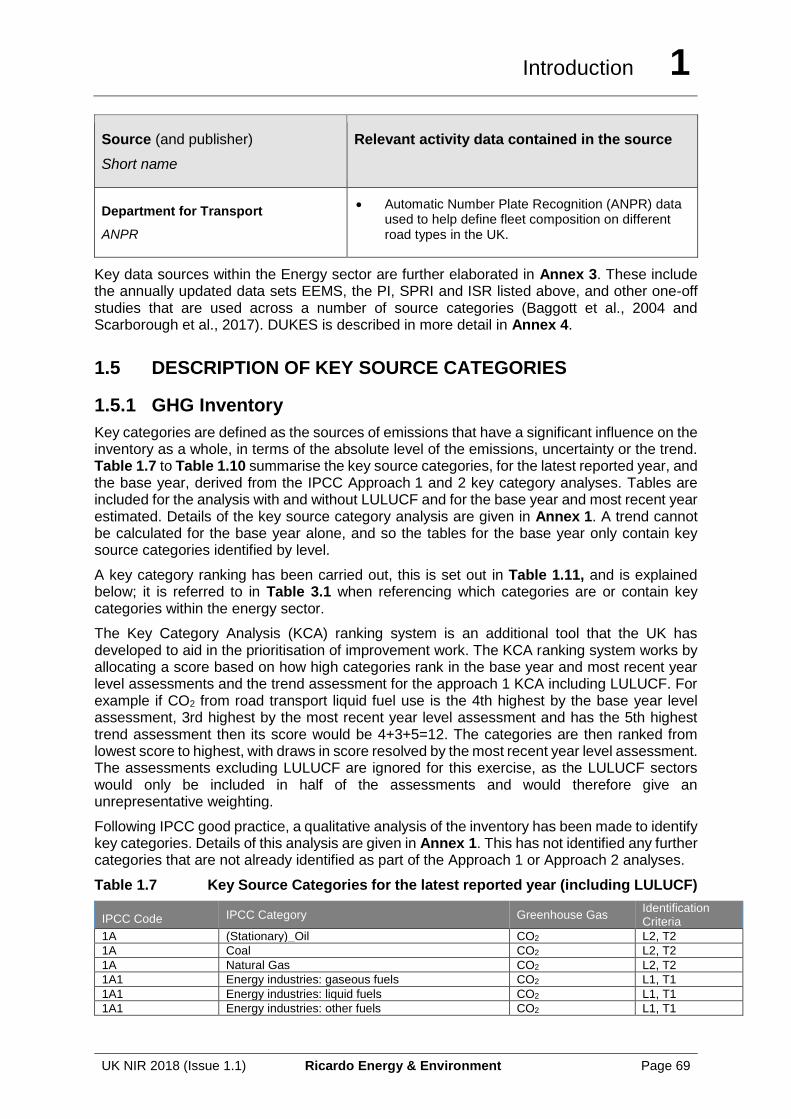
Introduction 1
UK NIR 2018 (Issue 1.1) Ricardo Energy & Environment Page 69
Source (and publisher)
Short name
Relevant activity data contained in the source
Department for Transport
ANPR
• Automatic Number Plate Recognition (ANPR) data used to help define fleet composition on different road types in the UK.
Key data sources within the Energy sector are further elaborated in Annex 3. These include the annually updated data sets EEMS, the PI, SPRI and ISR listed above, and other one-off studies that are used across a number of source categories (Baggott et al., 2004 and Scarborough et al., 2017). DUKES is described in more detail in Annex 4.
1.5 DESCRIPTION OF KEY SOURCE CATEGORIES
1.5.1 GHG Inventory
Key categories are defined as the sources of emissions that have a significant influence on the inventory as a whole, in terms of the absolute level of the emissions, uncertainty or the trend. Table 1.7 to Table 1.10 summarise the key source categories, for the latest reported year, and the base year, derived from the IPCC Approach 1 and 2 key category analyses. Tables are included for the analysis with and without LULUCF and for the base year and most recent year estimated. Details of the key source category analysis are given in Annex 1. A trend cannot be calculated for the base year alone, and so the tables for the base year only contain key source categories identified by level.
A key category ranking has been carried out, this is set out in Table 1.11, and is explained below; it is referred to in Table 3.1 when referencing which categories are or contain key categories within the energy sector.
The Key Category Analysis (KCA) ranking system is an additional tool that the UK has developed to aid in the prioritisation of improvement work. The KCA ranking system works by allocating a score based on how high categories rank in the base year and most recent year level assessments and the trend assessment for the approach 1 KCA including LULUCF. For example if CO2 from road transport liquid fuel use is the 4th highest by the base year level assessment, 3rd highest by the most recent year level assessment and has the 5th highest trend assessment then its score would be 4+3+5=12. The categories are then ranked from lowest score to highest, with draws in score resolved by the most recent year level assessment. The assessments excluding LULUCF are ignored for this exercise, as the LULUCF sectors would only be included in half of the assessments and would therefore give an unrepresentative weighting.
Following IPCC good practice, a qualitative analysis of the inventory has been made to identify key categories. Details of this analysis are given in Annex 1. This has not identified any further categories that are not already identified as part of the Approach 1 or Approach 2 analyses.
Table 1.7 Key Source Categories for the latest reported year (including LULUCF)
IPCC Code IPCC Category Greenhouse Gas Identification Criteria
1A (Stationary)_Oil CO2 L2, T2
1A Coal CO2 L2, T2
1A Natural Gas CO2 L2, T2
1A1 Energy industries: gaseous fuels CO2 L1, T1
1A1 Energy industries: liquid fuels CO2 L1, T1
1A1 Energy industries: other fuels CO2 L1, T1
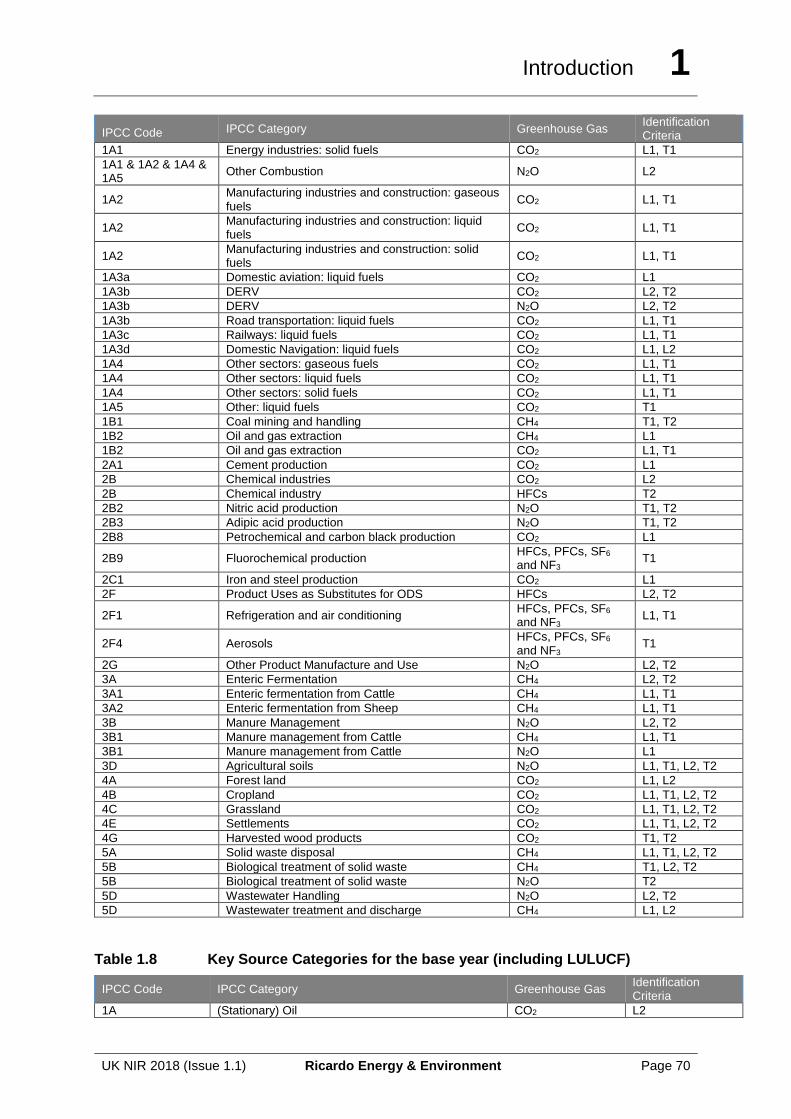
Introduction 1
UK NIR 2018 (Issue 1.1) Ricardo Energy & Environment Page 70
IPCC Code IPCC Category Greenhouse Gas Identification Criteria
1A1 Energy industries: solid fuels CO2 L1, T1
1A1 & 1A2 & 1A4 & 1A5
Other Combustion N2O L2
1A2 Manufacturing industries and construction: gaseous fuels
CO2 L1, T1
1A2 Manufacturing industries and construction: liquid fuels
CO2 L1, T1
1A2 Manufacturing industries and construction: solid fuels
CO2 L1, T1
1A3a Domestic aviation: liquid fuels CO2 L1
1A3b DERV CO2 L2, T2
1A3b DERV N2O L2, T2
1A3b Road transportation: liquid fuels CO2 L1, T1
1A3c Railways: liquid fuels CO2 L1, T1
1A3d Domestic Navigation: liquid fuels CO2 L1, L2
1A4 Other sectors: gaseous fuels CO2 L1, T1
1A4 Other sectors: liquid fuels CO2 L1, T1
1A4 Other sectors: solid fuels CO2 L1, T1
1A5 Other: liquid fuels CO2 T1
1B1 Coal mining and handling CH4 T1, T2
1B2 Oil and gas extraction CH4 L1
1B2 Oil and gas extraction CO2 L1, T1
2A1 Cement production CO2 L1
2B Chemical industries CO2 L2
2B Chemical industry HFCs T2
2B2 Nitric acid production N2O T1, T2
2B3 Adipic acid production N2O T1, T2
2B8 Petrochemical and carbon black production CO2 L1
2B9 Fluorochemical production HFCs, PFCs, SF6 and NF3
T1
2C1 Iron and steel production CO2 L1
2F Product Uses as Substitutes for ODS HFCs L2, T2
2F1 Refrigeration and air conditioning HFCs, PFCs, SF6 and NF3
L1, T1
2F4 Aerosols HFCs, PFCs, SF6 and NF3
T1
2G Other Product Manufacture and Use N2O L2, T2
3A Enteric Fermentation CH4 L2, T2
3A1 Enteric fermentation from Cattle CH4 L1, T1
3A2 Enteric fermentation from Sheep CH4 L1, T1
3B Manure Management N2O L2, T2
3B1 Manure management from Cattle CH4 L1, T1
3B1 Manure management from Cattle N2O L1
3D Agricultural soils N2O L1, T1, L2, T2
4A Forest land CO2 L1, L2
4B Cropland CO2 L1, T1, L2, T2
4C Grassland CO2 L1, T1, L2, T2
4E Settlements CO2 L1, T1, L2, T2
4G Harvested wood products CO2 T1, T2
5A Solid waste disposal CH4 L1, T1, L2, T2
5B Biological treatment of solid waste CH4 T1, L2, T2
5B Biological treatment of solid waste N2O T2
5D Wastewater Handling N2O L2, T2
5D Wastewater treatment and discharge CH4 L1, L2
Table 1.8 Key Source Categories for the base year (including LULUCF)
IPCC Code IPCC Category Greenhouse Gas Identification Criteria
1A (Stationary) Oil CO2 L2
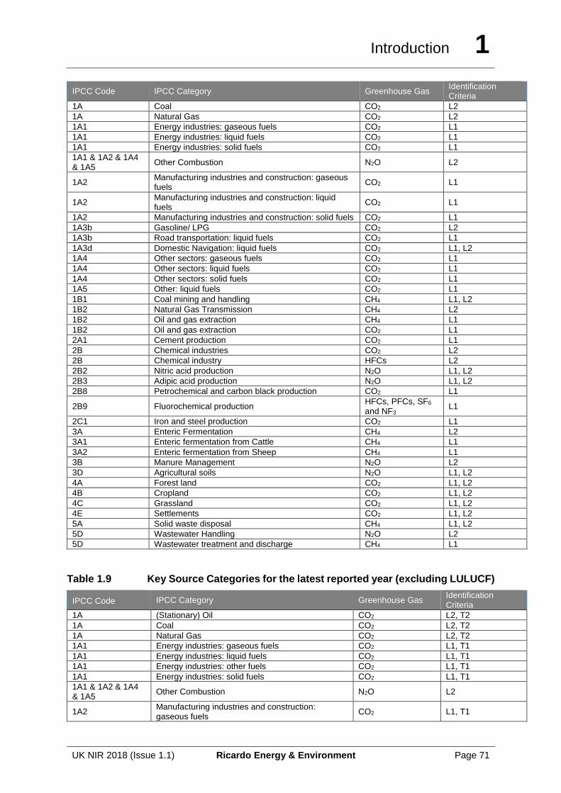
Introduction 1
UK NIR 2018 (Issue 1.1) Ricardo Energy & Environment Page 71
IPCC Code IPCC Category Greenhouse Gas Identification Criteria
1A Coal CO2 L2
1A Natural Gas CO2 L2
1A1 Energy industries: gaseous fuels CO2 L1
1A1 Energy industries: liquid fuels CO2 L1
1A1 Energy industries: solid fuels CO2 L1
1A1 & 1A2 & 1A4 & 1A5
Other Combustion N2O L2
1A2 Manufacturing industries and construction: gaseous fuels
CO2 L1
1A2 Manufacturing industries and construction: liquid fuels
CO2 L1
1A2 Manufacturing industries and construction: solid fuels CO2 L1
1A3b Gasoline/ LPG CO2 L2
1A3b Road transportation: liquid fuels CO2 L1
1A3d Domestic Navigation: liquid fuels CO2 L1, L2
1A4 Other sectors: gaseous fuels CO2 L1
1A4 Other sectors: liquid fuels CO2 L1
1A4 Other sectors: solid fuels CO2 L1
1A5 Other: liquid fuels CO2 L1
1B1 Coal mining and handling CH4 L1, L2
1B2 Natural Gas Transmission CH4 L2
1B2 Oil and gas extraction CH4 L1
1B2 Oil and gas extraction CO2 L1
2A1 Cement production CO2 L1
2B Chemical industries CO2 L2
2B Chemical industry HFCs L2
2B2 Nitric acid production N2O L1, L2
2B3 Adipic acid production N2O L1, L2
2B8 Petrochemical and carbon black production CO2 L1
2B9 Fluorochemical production HFCs, PFCs, SF6 and NF3
L1
2C1 Iron and steel production CO2 L1
3A Enteric Fermentation CH4 L2
3A1 Enteric fermentation from Cattle CH4 L1
3A2 Enteric fermentation from Sheep CH4 L1
3B Manure Management N2O L2
3D Agricultural soils N2O L1, L2
4A Forest land CO2 L1, L2
4B Cropland CO2 L1, L2
4C Grassland CO2 L1, L2
4E Settlements CO2 L1, L2
5A Solid waste disposal CH4 L1, L2
5D Wastewater Handling N2O L2
5D Wastewater treatment and discharge CH4 L1
Table 1.9 Key Source Categories for the latest reported year (excluding LULUCF)
IPCC Code IPCC Category Greenhouse Gas Identification Criteria
1A (Stationary) Oil CO2 L2, T2
1A Coal CO2 L2, T2
1A Natural Gas CO2 L2, T2
1A1 Energy industries: gaseous fuels CO2 L1, T1
1A1 Energy industries: liquid fuels CO2 L1, T1
1A1 Energy industries: other fuels CO2 L1, T1
1A1 Energy industries: solid fuels CO2 L1, T1
1A1 & 1A2 & 1A4 & 1A5
Other Combustion N2O L2
1A2 Manufacturing industries and construction: gaseous fuels
CO2 L1, T1
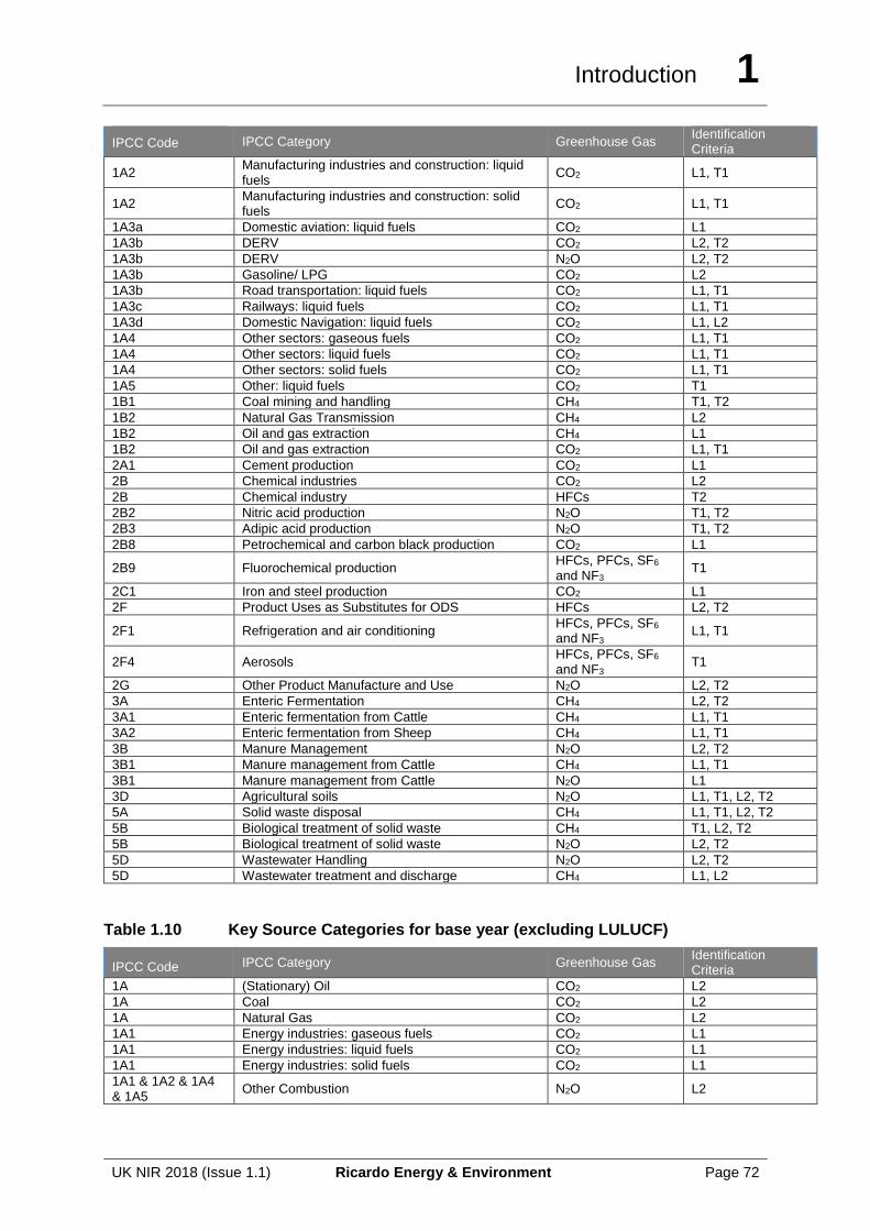
Introduction 1
UK NIR 2018 (Issue 1.1) Ricardo Energy & Environment Page 72
IPCC Code IPCC Category Greenhouse Gas Identification Criteria
1A2 Manufacturing industries and construction: liquid fuels
CO2 L1, T1
1A2 Manufacturing industries and construction: solid fuels
CO2 L1, T1
1A3a Domestic aviation: liquid fuels CO2 L1
1A3b DERV CO2 L2, T2
1A3b DERV N2O L2, T2
1A3b Gasoline/ LPG CO2 L2
1A3b Road transportation: liquid fuels CO2 L1, T1
1A3c Railways: liquid fuels CO2 L1, T1
1A3d Domestic Navigation: liquid fuels CO2 L1, L2
1A4 Other sectors: gaseous fuels CO2 L1, T1
1A4 Other sectors: liquid fuels CO2 L1, T1
1A4 Other sectors: solid fuels CO2 L1, T1
1A5 Other: liquid fuels CO2 T1
1B1 Coal mining and handling CH4 T1, T2
1B2 Natural Gas Transmission CH4 L2
1B2 Oil and gas extraction CH4 L1
1B2 Oil and gas extraction CO2 L1, T1
2A1 Cement production CO2 L1
2B Chemical industries CO2 L2
2B Chemical industry HFCs T2
2B2 Nitric acid production N2O T1, T2
2B3 Adipic acid production N2O T1, T2
2B8 Petrochemical and carbon black production CO2 L1
2B9 Fluorochemical production HFCs, PFCs, SF6 and NF3
T1
2C1 Iron and steel production CO2 L1
2F Product Uses as Substitutes for ODS HFCs L2, T2
2F1 Refrigeration and air conditioning HFCs, PFCs, SF6 and NF3
L1, T1
2F4 Aerosols HFCs, PFCs, SF6 and NF3
T1
2G Other Product Manufacture and Use N2O L2, T2
3A Enteric Fermentation CH4 L2, T2
3A1 Enteric fermentation from Cattle CH4 L1, T1
3A2 Enteric fermentation from Sheep CH4 L1, T1
3B Manure Management N2O L2, T2
3B1 Manure management from Cattle CH4 L1, T1
3B1 Manure management from Cattle N2O L1
3D Agricultural soils N2O L1, T1, L2, T2
5A Solid waste disposal CH4 L1, T1, L2, T2
5B Biological treatment of solid waste CH4 T1, L2, T2
5B Biological treatment of solid waste N2O L2, T2
5D Wastewater Handling N2O L2, T2
5D Wastewater treatment and discharge CH4 L1, L2
Table 1.10 Key Source Categories for base year (excluding LULUCF)
IPCC Code IPCC Category Greenhouse Gas Identification Criteria
1A (Stationary) Oil CO2 L2
1A Coal CO2 L2
1A Natural Gas CO2 L2
1A1 Energy industries: gaseous fuels CO2 L1
1A1 Energy industries: liquid fuels CO2 L1
1A1 Energy industries: solid fuels CO2 L1
1A1 & 1A2 & 1A4 & 1A5
Other Combustion N2O L2
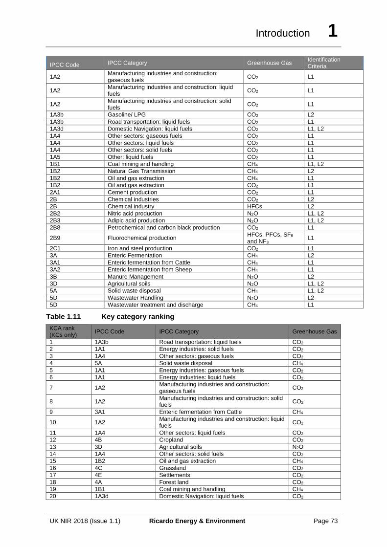
Introduction 1
UK NIR 2018 (Issue 1.1) Ricardo Energy & Environment Page 73
IPCC Code IPCC Category Greenhouse Gas Identification Criteria
1A2 Manufacturing industries and construction: gaseous fuels
CO2 L1
1A2 Manufacturing industries and construction: liquid fuels
CO2 L1
1A2 Manufacturing industries and construction: solid fuels
CO2 L1
1A3b Gasoline/ LPG CO2 L2
1A3b Road transportation: liquid fuels CO2 L1
1A3d Domestic Navigation: liquid fuels CO2 L1, L2
1A4 Other sectors: gaseous fuels CO2 L1
1A4 Other sectors: liquid fuels CO2 L1
1A4 Other sectors: solid fuels CO2 L1
1A5 Other: liquid fuels CO2 L1
1B1 Coal mining and handling CH4 L1, L2
1B2 Natural Gas Transmission CH4 L2
1B2 Oil and gas extraction CH4 L1
1B2 Oil and gas extraction CO2 L1
2A1 Cement production CO2 L1
2B Chemical industries CO2 L2
2B Chemical industry HFCs L2
2B2 Nitric acid production N2O L1, L2
2B3 Adipic acid production N2O L1, L2
2B8 Petrochemical and carbon black production CO2 L1
2B9 Fluorochemical production HFCs, PFCs, SF6 and NF3
L1
2C1 Iron and steel production CO2 L1
3A Enteric Fermentation CH4 L2
3A1 Enteric fermentation from Cattle CH4 L1
3A2 Enteric fermentation from Sheep CH4 L1
3B Manure Management N2O L2
3D Agricultural soils N2O L1, L2
5A Solid waste disposal CH4 L1, L2
5D Wastewater Handling N2O L2
5D Wastewater treatment and discharge CH4 L1
Table 1.11 Key category ranking
KCA rank (KCs only)
IPCC Code IPCC Category Greenhouse Gas
1 1A3b Road transportation: liquid fuels CO2
2 1A1 Energy industries: solid fuels CO2
3 1A4 Other sectors: gaseous fuels CO2
4 5A Solid waste disposal CH4
5 1A1 Energy industries: gaseous fuels CO2
6 1A1 Energy industries: liquid fuels CO2
7 1A2 Manufacturing industries and construction: gaseous fuels
CO2
8 1A2 Manufacturing industries and construction: solid fuels
CO2
9 3A1 Enteric fermentation from Cattle CH4
10 1A2 Manufacturing industries and construction: liquid fuels
CO2
11 1A4 Other sectors: liquid fuels CO2
12 4B Cropland CO2
13 3D Agricultural soils N2O
14 1A4 Other sectors: solid fuels CO2
15 1B2 Oil and gas extraction CH4
16 4C Grassland CO2
17 4E Settlements CO2
18 4A Forest land CO2
19 1B1 Coal mining and handling CH4
20 1A3d Domestic Navigation: liquid fuels CO2
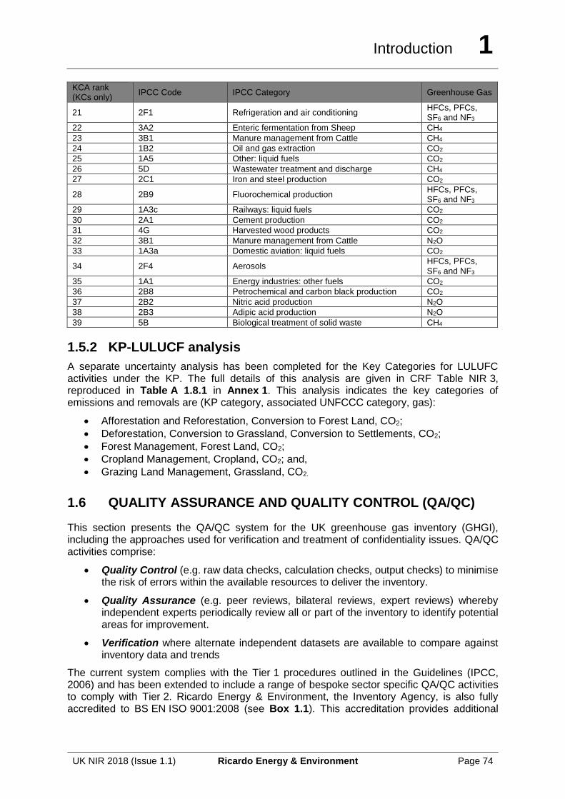
Introduction 1
UK NIR 2018 (Issue 1.1) Ricardo Energy & Environment Page 74
KCA rank (KCs only)
IPCC Code IPCC Category Greenhouse Gas
21 2F1 Refrigeration and air conditioning HFCs, PFCs, SF6 and NF3
22 3A2 Enteric fermentation from Sheep CH4
23 3B1 Manure management from Cattle CH4
24 1B2 Oil and gas extraction CO2
25 1A5 Other: liquid fuels CO2
26 5D Wastewater treatment and discharge CH4
27 2C1 Iron and steel production CO2
28 2B9 Fluorochemical production HFCs, PFCs, SF6 and NF3
29 1A3c Railways: liquid fuels CO2
30 2A1 Cement production CO2
31 4G Harvested wood products CO2
32 3B1 Manure management from Cattle N2O
33 1A3a Domestic aviation: liquid fuels CO2
34 2F4 Aerosols HFCs, PFCs, SF6 and NF3
35 1A1 Energy industries: other fuels CO2
36 2B8 Petrochemical and carbon black production CO2
37 2B2 Nitric acid production N2O
38 2B3 Adipic acid production N2O
39 5B Biological treatment of solid waste CH4
1.5.2 KP-LULUCF analysis
A separate uncertainty analysis has been completed for the Key Categories for LULUFC activities under the KP. The full details of this analysis are given in CRF Table NIR 3, reproduced in Table A 1.8.1 in Annex 1. This analysis indicates the key categories of emissions and removals are (KP category, associated UNFCCC category, gas):
• Afforestation and Reforestation, Conversion to Forest Land, CO2;
• Deforestation, Conversion to Grassland, Conversion to Settlements, CO2;
• Forest Management, Forest Land, CO2;
• Cropland Management, Cropland, CO2; and,
• Grazing Land Management, Grassland, CO2.
1.6 QUALITY ASSURANCE AND QUALITY CONTROL (QA/QC)
This section presents the QA/QC system for the UK greenhouse gas inventory (GHGI), including the approaches used for verification and treatment of confidentiality issues. QA/QC activities comprise:
• Quality Control (e.g. raw data checks, calculation checks, output checks) to minimise the risk of errors within the available resources to deliver the inventory.
• Quality Assurance (e.g. peer reviews, bilateral reviews, expert reviews) whereby independent experts periodically review all or part of the inventory to identify potential areas for improvement.
• Verification where alternate independent datasets are available to compare against inventory data and trends
The current system complies with the Tier 1 procedures outlined in the Guidelines (IPCC, 2006) and has been extended to include a range of bespoke sector specific QA/QC activities to comply with Tier 2. Ricardo Energy & Environment, the Inventory Agency, is also fully accredited to BS EN ISO 9001:2008 (see Box 1.1). This accreditation provides additional
Introduction 1
UK NIR 2018 (Issue 1.1) Ricardo Energy & Environment Page 75
institutional standards which the inventory agency has to apply to all projects and ensures that the wider company conforms to good practice in project management and quality assurance.
1.6.1 Description of the current QA/QC system
The National Atmospheric Emissions Inventory and the UK Greenhouse Gas Inventory are compiled and maintained together by Ricardo Energy & Environment (the Inventory Agency), on behalf of the UK Department for Business, Energy & Industrial Strategy (BEIS) and the Department for Environment, Food and Rural Affairs (Defra). Ricardo Energy & Environment prepares the GHG submissions to the EC under the MMR and to the UNFCCC. The data compilation for some source sectors of the UK inventory are performed by other contractors (i.e. Rothamsted Research compile the agriculture sector under contract to Defra, and CEH compile the land use, land-use change and forestry sector under sub-contract to Ricardo Energy & Environment).
Most of the data received by Ricardo Energy & Environment for the UK GHGI compilation come from other government departments, agencies, research establishments or consultants working on behalf of UK government or for trade associations. Several of the organisations (e.g. BEIS, the Office of National Statistics and British Geological Survey) qualify as the UK’s National Statistical Agencies referred to in the Guidance and abide by strict statistical QA/QC standards. Other organisations (e.g. CEH, providing the LULUCF estimates, and the UK environmental regulatory agencies that provide installation-level emissions data) supply important datasets for the Inventory and have their own comprehensive QA/QC systems. CEH is implementing a QA/QC system for LULUCF following the methodology of Ricardo Energy & Environment (detailed below). Whilst these organisations have their own QA/QC systems, Ricardo Energy & Environment is responsible for co-ordinating inventory-wide QA/QC activities relating to the submitted datasets. In addition, Ricardo Energy & Environment is working continuously with organisations supplying data to the GHG inventory to encourage them to demonstrate their own levels of QA/QC that comply with either 2006 IPCC Guidelines or the UK’s National Statistics standards.
The UK inventory QA/QC system encompasses a wide range of activities to cover:
• inventory planning tasks, including: review of historic data and methods, identification of improvement priorities, data and method selection, inventory team training and development;
• inventory compilation and reporting tasks, including: management and documentation of data flows from raw data through calculation of emission estimates to reporting, input data requests/acquisition, management of compilation processes and quality checking systems, documentation of data, methods and assumptions, assessment of key source categories and uncertainties, reporting of inventory outputs;
• inventory checking tasks, including: raw data checks, inventory model / calculation checks, source-specific and cross-cutting output checks, checking reasons for changes compared to previous inventory estimates, emission trend checks, emission factor checks; and,
• inventory QA review tasks, including: pre-submission reviews, post-submission reviews, peer reviews, bilateral reviews, expert reviews.
1.6.1.1 Overview of the UK QA/QC system
An overview of the UK’s GHGI QA/QC system is illustrated in Figure 1.3 below. The UK inventory QA/QC system includes three core components.
1. The QA/QC Plan is a document maintained by the GHGI’s QA/QC manager (at Ricardo Energy & Environment) and defines the specific Quality Objectives and QA/QC
Introduction 1
UK NIR 2018 (Issue 1.1) Ricardo Energy & Environment Page 76
activities required in undertaking the compilation and reporting of GHG estimates. The plan sets out source-specific and general (cross-cutting) activities to ensure that quality objectives are met within the required inventory reporting time-frame. The QA/QC plan also assigns roles and responsibilities for the inventory agency team, and records the key outcomes from inventory QA activities in order to underpin a programme of continuous improvement.
2. QA/QC implementation includes the physical undertaking of the QA/QC activities throughout the data gathering, compilation and reporting phases of the annual inventory cycle and in accordance with the QA/QC plan.
3. Documentation and Archiving. Documentation is embedded within the UK’s compilation tools. The NIR transparently describes the data sources, methods, assumptions and QA/QC implementation used in producing the GHG inventory including records of activities undertaken, findings/issue logs, recommendations and any necessary actions taken or planned. Archiving ensures a complete backup and storage of all material used for the compilation of the estimates.
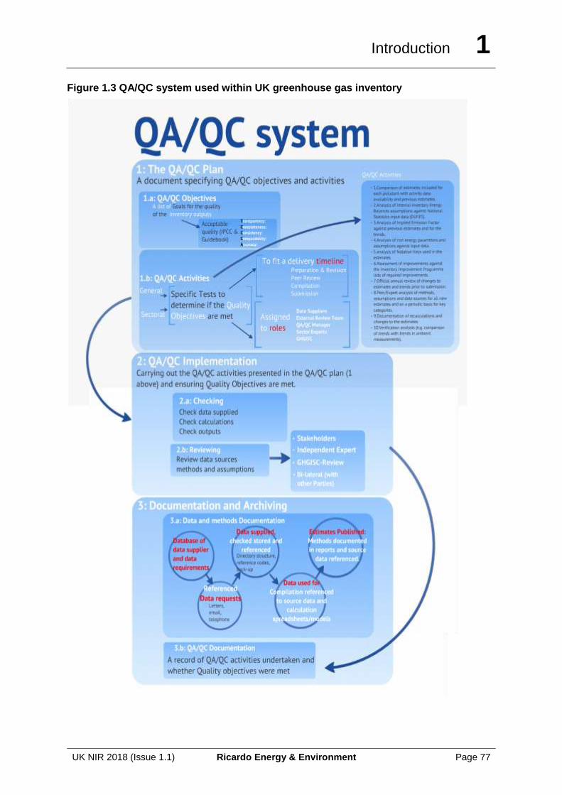
Introduction 1
UK NIR 2018 (Issue 1.1) Ricardo Energy & Environment Page 77
Figure 1.3 QA/QC system used within UK greenhouse gas inventory
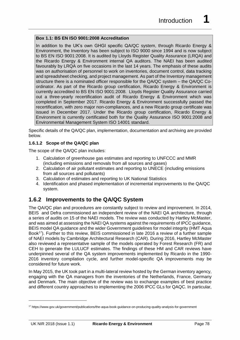
Introduction 1
UK NIR 2018 (Issue 1.1) Ricardo Energy & Environment Page 78
Box 1.1: BS EN ISO 9001:2008 Accreditation
In addition to the UK’s own GHGI specific QA/QC system, through Ricardo Energy & Environment, the Inventory has been subject to ISO 9000 since 1994 and is now subject to BS EN ISO 9001:2008. It is audited by Lloyds Register Quality Assurance (LRQA) and the Ricardo Energy & Environment internal QA auditors. The NAEI has been audited favourably by LRQA on five occasions in the last 14 years. The emphasis of these audits was on authorisation of personnel to work on inventories, document control, data tracking and spreadsheet checking, and project management. As part of the Inventory management structure there is a nominated officer responsible for the QA/QC system – the QA/QC Co-ordinator. As part of the Ricardo group certification, Ricardo Energy & Environment is currently accredited to BS EN ISO 9001:2008. Lloyds Register Quality Assurance carried out a three-yearly recertification audit of Ricardo Energy & Environment which was completed in September 2017. Ricardo Energy & Environment successfully passed the recertification, with zero major non-compliances, and a new Ricardo group certificate was issued in December 2017. Under the Ricardo group certification, Ricardo Energy & Environment is currently certificated both for the Quality Assurance ISO 9001:2008 and Environmental Management System ISO 14001 standard.
Specific details of the QA/QC plan, implementation, documentation and archiving are provided below.
1.6.1.2 Scope of the QA/QC plan
The scope of the QA/QC plan includes:
1. Calculation of greenhouse gas estimates and reporting to UNFCCC and MMR (including emissions and removals from all sources and gases)
2. Calculation of air pollutant estimates and reporting to UNECE (including emissions from all sources and pollutants)
3. Calculation of estimates and reporting to UK National Statistics 4. Identification and phased implementation of incremental improvements to the QA/QC
system.
1.6.2 Improvements to the QA/QC System
The QA/QC plan and procedures are constantly subject to review and improvement. In 2014, BEIS and Defra commissioned an independent review of the NAEI QA architecture, through a series of audits on 15 of the NAEI models. The review was conducted by Hartley McMaster, and was aimed at assessing the NAEI QA systems against the requirements of IPCC guidance, BEIS model QA guidance and the wider Government guidelines for model integrity (HMT Aqua Book17). Further to this review, BEIS commissioned in late 2016 a review of a further sample of NAEI models by Cambridge Architectural Research (CAR). During 2016, Hartley McMaster also reviewed a representative sample of the models operated by Forest Research (FR) and CEH to generate the LULUCF estimates. The findings of these HM and CAR reviews have underpinned several of the QA system improvements implemented by Ricardo in the 1990-2016 inventory compilation cycle, and further model-specific QA improvements may be considered for future work.
In May 2015, the UK took part in a multi-lateral review hosted by the German inventory agency, engaging with the QA managers from the inventories of the Netherlands, France, Germany and Denmark. The main objective of the review was to exchange examples of best practice and different country approaches to implementing the 2006 IPCC GLs for QAQC. In particular,
17 https://www.gov.uk/government/publications/the-aqua-book-guidance-on-producing-quality-analysis-for-government
Introduction 1
UK NIR 2018 (Issue 1.1) Ricardo Energy & Environment Page 79
several areas of ambiguity in the GLs were discussed and a common view sought on how to address and prioritise the new QA guidance.
The following is a list of the main improvements made to the inventory QA/QC system during the 2018 submission:
• Development of improved pollutant-specific checking templates that facilitate a more consistent checking procedure for the inventories for GHGs and air quality pollutants, and to collect information on recalculations and reported trends in a more systematic, prioritised way;
• Further improvements to inventory model design to ensure consistent and transparent documentation of model compilation, QC, version control, with supporting guidance to the inventory compilation team, including the development of an NAEI overview document and greater use of graphical visualisation of data time series to identify outliers;
• Model upgrades for a number of inventory models, to re-build and test inventory models against UK Government QA guidelines, primarily focusing on inventory models that generate the time series of activity data for key UK fuels;
• Consolidation of a range of models used to derive emission factors on a mass basis (as used in the UK inventory database) from various data sources (often presenting factors on an energy basis), in order to ensure a more consistent approach to the selection of default factors and their conversion from energy to mass units. Aggregating these models into one common database has reduced the risk of inconsistent assumptions being applied (e.g. selection of the most appropriate default factor from reference sources) or of errors in conversion calculations;
• Upgrade of seven LULUCF models, including verification of model calculations and further development of model quality checks;
• Review of all LULUCF models by Hartley McMaster using Excel screening software, resulting in improvements to model documentation, improved version control and minor revisions to data inputs and gap-filling assumptions.
1.6.2.1 Quality Objectives
The key objectives of the QA/QC plan are to ensure that the estimates in the GHG and air pollutant inventories are of a suitably high quality and will meet the methodological and reporting requirements for UK submissions to the UNECE and UNFCCC, as set out within national inventory reporting guidance from the Intergovernmental Panel on Climate Change (IPCC)18 and European Environment Agency (EEA)19. The inventory data quality objectives are to achieve the principles of Transparency, Completeness, Consistency, Comparability and Accuracy (TCCCA):
• Transparent in:
o The description of methods, assumptions, data sources used to compile estimates in internal (spreadsheets and other calculation tools) and published material (e.g. the NIR) and on the inclusion of national and EU wide assumptions (e.g. source category detail and the split between EU ETS and non EU ETS sources, implementation of policies and measures, carbon contents of fuels, site specific estimates, national statistics such as population, GDP, energy prices, carbon prices etc.).
18 2006 IPCC Guidelines for National Greenhouse Gas Inventories: http://www.ipcc-nggip.iges.or.jp/public/2006gl/
19 EMEP/EEA air pollutant emission inventory guidebook – 2013: http://www.eea.europa.eu/publications/emep-eea-guidebook-2013
Introduction 1
UK NIR 2018 (Issue 1.1) Ricardo Energy & Environment Page 80
o The documentation of QA/QC activities and their implementation using internal checklists and summarised in relevant public material (e.g. NIR).
• Complete: and include all relevant (anthropogenic) emission/removal activities, using representative data for the national territory for socio-economic assumptions and policies and measures for all required years, categories, gases and scenarios.
• Consistent: across trends in emissions/removals for all years (especially where applicable between the historic and projected estimates) and that there is internal consistency in aggregation of emissions/removals. Where possible, the same methodologies are used for the base year and all subsequent years and consistent data sets are used to estimate emissions or removals from sources or sinks.
• Comparable: with other reported emission/removal estimates through use of the latest reporting templates and nomenclature consistent with reporting requirements. Using the correct IPCC category level and consistent units for expressing mass of emissions/removals by gas, split between EU ETS and non EU ETS sources, scenarios, units for parameters and of input parameters with EU assumptions (e.g. energy prices, carbon price, population etc.).
• Accurate: ensuring the most accurate methods are used in the application of methods, minimising the uncertainty in assumptions and in use of data sources used for the estimates and inclusion of national and EU wide assumptions.
The overall aim of the inventory QA/QC system is to meet the above objectives, and to minimise the risk of errors in the UK inventory data such that emission estimates are not knowingly over- or under-estimated as far as can reasonably be judged.
The inventory QA/QC system also reflects that quality is one of three often competing attributes for a given project scope: quality, time, and resources. Noting that the complete set of UK GHGI and AQPI estimates contain a large number of large and small contributors to emissions/removals, key category analysis is used to prioritise the most important categories (i.e. the highest-emitting source categories in the UK and/or the most uncertain sources). More resources and time are typically directed towards method development, compilation, reporting and associated QA/QC activities for these key source categories, with simpler methods and less rigorous approaches typically applied to lower-emitting / more certain (non-key) source categories.
1.6.2.2 Roles and Responsibilities
The QA/QC plan sets out specific responsibilities for the different QA (review) and QC (data controls, checking) activities and to different roles within the inventory compilation and reporting team. These are embedded within compilation and processing spreadsheets and databases. Training and project management communication across the inventory agency ensures that these responsibilities are clear, with specific tasks and checks signed-off at appropriate stages throughout the inventory process. The following responsibilities are outlined in the QA/QC plan:
• QA/QC Manager (“Senior Analyst”): Coordinates all QA/QC activities and manages the contributions from data suppliers, sector experts and independent experts and undertakes cross cutting QA/QC activities. Maintains the QA/QC plan, co-ordinates action across the team to: set quality objectives, communicate and implement QA/QC activities, identify training and development needs (individual, systematic);
• Knowledge Leaders: Lead the technical development and implementation of the NAEI programme, supporting the QA manager and Project management team in delivering the project to meet technical requirements of international reporting as well as UK-specific and other output quality expectations. Manage periodic review and perform final checking activities on data and report submissions.
Introduction 1
UK NIR 2018 (Issue 1.1) Ricardo Energy & Environment Page 81
• Project Manager: Lead all key management activities including management of the project finances, commercial issues, liaison with BEIS and Defra, manage and attend project meetings, communicating project tasks and requirements to the team and oversee the day-to-day running of the project. Manage team resources and support QA Manager, Technical Director and Knowledge Leaders in identifying and resolving resource limitations (e.g. skills gaps, continuity planning);
• Task Managers /Sector Experts: Task managers (or sector experts) are responsible for the maintenance of task documentation (e.g. compiler manual, scope documents, quality checking records and correspondence) and task QA Plan to include: definition of checking requirements; timeline delivery of work; coordination of task sign-off; identification of team training requirements and risk management. They perform sector specific review and checking activities and report to the QA/QC Manager. Sector Experts also collaborate with data suppliers and other key stakeholders to review data quality (input data and outputs), perform quality checks on supplied information, assess and report on uncertainties associated with NAEI outputs. Identify improvement requirements for their tasks / sectors and promote / implement cross-cutting QAQC improvements by sharing best practice and engaging in team communication activities; and,
• External Review experts: Provide expert/peer review of projections for specific sectors, identify key findings and inventory improvement recommendations, and report to the QA/QC Manager.
1.6.2.3 Timeline
The QA/QC plan sets out a detailed timeline for QA/QC checks. The timeline is designed to fit in with compilation and reporting requirements for all UK GHG and Air Pollutant reporting commitments.
1.6.2.4 Quality Control and Documentation
The UK’s GHGI Quality Control (checking, documentation and archiving) occurs throughout the data gathering, compilation and reporting cycle. Figure 1.4 illustrates the process of data checks used within the UK greenhouse gas inventory. The horizontal bars symbolise ‘gates’ through which data does not pass until it meets the quality criteria and the appropriate checks have been performed. The key activities that are undertaken and documented to check the estimates include:
1. Checking of input data for scope, completeness, consistency with data for recent years and (where available) verification against other independent datasets. Compilers check the incoming data from data providers to assess whether the data are complete and consistent with data for recent years. In some cases, checks are performed to compare data between individual operators (e.g. gas composition data from multiple UK gas transporters) and between different reporting mechanisms (such as comparisons of operator-reported activity and emissions data between IED/PRTR and EUETS). For several sources, production-based emission estimates can be compared with other data (e.g. sales data, plant capacity data) to check that the trends and values are reasonable.
2. Analysis of internal inventory energy and mass balances and other statistics assumptions against National Statistics input data (e.g. DUKES and ONS). Mass or energy balances are performed for each major fuel in the UK economy and any deviations from UK energy statistics are checked and documented. Several sector methods for key categories also have Tier 2 checks to assess internal consistency, such as carbon balance checks for the carbon flows through integrated iron and steel works.
3. Completeness checks. The database is checked for completeness and consistency of entry across the different pollutants and gases. For example, combustion sources are
Introduction 1
UK NIR 2018 (Issue 1.1) Ricardo Energy & Environment Page 82
checked for inclusion of all relevant pollutants and the database checked for any missing estimates and appropriate use of notation keys.
4. Recalculation checks. The latest inventory dataset is compared against the previous inventory submission. Any recalculations are documented by inventory compilers and signed off by checkers. Reasons for the recalculations are documented, e.g. method improvements, revisions to input data or assumptions. These recalculation notes are referenced within the inventory database to facilitate reporting and transparency of recalculations.
5. Time series checks and benchmarking checks. The time series of emissions are checked for step changes, trends and any outlier data (e.g. outlier EFs or peaks/dips in activity data trends). Any unusual features are checked and explained, with reasons for significant trends and outliers documented in the method sections of the NIR. Implied Emission Factors (IEFs) are checked against previous estimates and for key categories against defaults (from IPCC guidance) to identify any notable UK-specific EF outliers.
6. Method implementation checks. A range of common checks are performed across inventory calculation models, such as: checking that units are correct for input parameters; checking that selection of NCVs or default EFs is consistent across years / pollutants; checking for either new emission estimates (e.g. due to new UK data or new methodological guidance or new EFs within the IPCC guidance) or for any missing emission sources compared to previous submissions.
7. Reporting checks. Inventory submissions are checked to ensure correct allocation into the CRF categories. Emission totals at national and sub-category level are checked against the “master” dataset derived from the UK inventory database outputs, to minimise risks of data transcription errors into reporting templates.
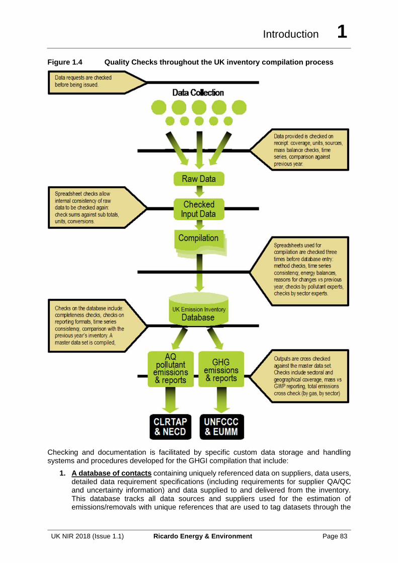
Introduction 1
UK NIR 2018 (Issue 1.1) Ricardo Energy & Environment Page 83
Figure 1.4 Quality Checks throughout the UK inventory compilation process
Checking and documentation is facilitated by specific custom data storage and handling systems and procedures developed for the GHGI compilation that include:
1. A database of contacts containing uniquely referenced data on suppliers, data users, detailed data requirement specifications (including requirements for supplier QA/QC and uncertainty information) and data supplied to and delivered from the inventory. This database tracks all data sources and suppliers used for the estimation of emissions/removals with unique references that are used to tag datasets through the
Introduction 1
UK NIR 2018 (Issue 1.1) Ricardo Energy & Environment Page 84
inventory compilation process. The contacts database also tracks all outputs from the GHGI including formal submissions and data supplied in response to informal and ad-hoc data requests.
2. Individual data processing tools are used to prepare the majority of source data into suitable AD and EFs for UK emissions estimates. These data processing tools (spreadsheets and database models) are uniquely identified and include QC procedures, summaries and source data referencing and documentation within them. QC procedures are embedded in the tools which provide sector specific checks (e.g. energy/mass balance) and implied emission factor checking for default and country specific emission factors. The QC procedures within each tool/spreadsheet include calculation input/output checking cells and flags to identify calculation errors. The QC summary sheets in each tool/spreadsheet include links to QC activities that need to be performed, flags for the QC activities, their status and sign off; details of source data; key assumptions, methods, data processing activities and progress; the scope of activities, gases and years included; relationships with other models (where inter-dependencies exist); records of authorship; version control and checking. All relevant cells in the data processing spreadsheets are colour coded for ease of reference indicating whether the cells are calculation cells, output cells, checking cells or data input cells. All input data are referenced to the unique data source and data supplier held in the contacts database so all source data can be traced back to its originator and date of supply. All spreadsheets are subject to second-person checking prior to data uploading to the NAEI database.
3. A core database (NAEI database) of AD and EFs with embedded tier 1 QC routines and data source and data processing referencing. The database provides the quality assured data source of emission/removal estimates used for reporting (including CRF population), responding to ad-hoc queries or deriving other downstream estimates (e.g. emissions by Devolved Government and emissions by Local Authority). The detailed Activity Data and Emission Factor components for each estimate are held within the central database and include all sources, activities, gases/pollutants (GHGI and AQPI) and years. The majority of data in the database are imported directly from the individual data processing models (described above). Data transparency: All data points in the database carry a reference to either the upstream data processing tools used to derive the data, the external data source and supplier or both. It also includes details of the date entered, the person uploading the data, its units (to ensure correct calculation), and a revision or recalculation code (which ensures that recalculations of historic data can be easily traced and summarised in reports). Automated data import routines used to populate the database minimise transcription errors and errors resulting from importing data that has not been properly checked. This process extracts output data from the upstream data processing models and can be controlled by the Inventory Agency via a data import dashboard. The automated system ensures that data is only uploaded to the database once it meets specified QA/QC criteria of data checking, completion and consistency. A number of detailed QC checking queries20 are embedded within the database that support the annual QA activities defined in the QA/QC Plan and include:
a. Checks with previous submissions for changes due to recalculations or errors at a detailed level (a designated auditor identifies sources where there have
20 A full list is included in the QA/QC plan.
Introduction 1
UK NIR 2018 (Issue 1.1) Ricardo Energy & Environment Page 85
been significant changes or new sources. Inventory compilers are then required to explain these changes to satisfy the auditor)21;
b. Assessment of trends and time series consistency for selected key sources; c. Mass balance checks to ensure that the total fuel consumptions in the GHG
inventory are in accordance with those published in energy National Statistics from BEIS;
d. Other activity data checks (e.g. production and consumption with National Statistics);
e. Implied Emission Factor checks (assessing trends in IEF and comparison with previous submissions);
f. A consistency check between IPCC output and CLRTAP formatted output.
4. Data extraction checking routines and procedures: Data exported from the NAEI
database and entered into reporting tools (e.g. the CRF Reporter tool) are finally checked against the direct database output totals to ensure that any inconsistencies are identified and rectified prior to submission. This includes interrogating the output xml from the CRF software and comparing this against a series of queries from the NAEI database to compare both emissions and activity data.
5. Official annual reports to UNFCCC and UNECE provide full documentation of inventory estimation methodologies, data sources and assumptions by source sector, key data sources and significant revisions to methods and historic data, where appropriate. In addition the annual report to the UNFCCC includes details of planned prioritising improvements identified by the Inventory Agency and agreed by the National Inventory Steering Committee, and from Expert and Peer Reviews. Any data presented in reports are checked against accompanying submission datasets and the NAEI database.
6. Archiving: At the end of each reporting cycle, all the database files, spreadsheets, online manuals, electronic source data, records of communications, paper source data, output files representing all calculations for the whole time series are frozen and archived on a central server. An annual report outlining the methodology of the inventory and data sources is produced. Electronic information is stored on secure and separately located servers (with one acting purely as back-up) that are regularly backed up. Paper information is archived in a Roller Racking system with a simple electronic database of all items referenced in the archive.
• The agriculture inventory (compiled by Rothamsted Research, North Wyke) is backed up on a daily basis on their network storage system. This system is mirrored with the Rothamsted Research Harpenden site, comprising an offsite backup.
• At CEH, all data and information relating to the LULUCF inventory is stored on a networked drive (accessible only by the project team) which is backed up daily by CEH computer support. There is a separate folder for each inventory year and at the end of an inventory cycle the final versions of all datasets remain unchanged for back reference if required. In addition to this the model code used within CEH for inventory compilation is stored in a subversion repository to ensure a clear record of all amendments and iterations.
21 This is somewhat more detailed than the recalculation explanations required by Table 8 in the CRF, as it is based on the more disaggregated source sectors used in the NAEI database.
Introduction 1
UK NIR 2018 (Issue 1.1) Ricardo Energy & Environment Page 86
1.6.2.5 Quality Assurance and Verification
Quality Assurance and verification activities provide an objective, independent review of inventory source data, methods and assumptions. These activities are primarily conducted to assess compliance with reporting requirements (e.g. comparing UK inventory methods against international guidelines) and also to identify areas for future inventory improvement. QA and verification activities include:
1. Assessment of improvements against recommendations and the Inventory Improvement Programme lists of required improvements.
2. Official annual review of changes to estimates and trends, prior to submission, by stakeholders supplying key datasets and by UK government departments responsible for the inventory reporting.
3. Peer/Expert review of methods, assumptions and data sources for new / revised estimates and on a periodic basis for key categories to determine whether methods should be improved due to the availability of new datasets and assumptions (focussing on key categories).
4. Documentation of recalculations and changes to the estimates.
5. Verification analysis (e.g. comparison of trends with trends in ambient measurements).
1.6.2.5.1 NISC annual review
Annually and prior to submission the National Inventory Steering Committee (NISC) review the emissions inventory datasets. The NISC is tasked with the official consideration and approval of the national inventory prior to submission to the UNFCCC. The NISC comprises key stakeholders, including the Single National Entity (BEIS) (see Institutional Arrangements section), who have an understanding of the GHG estimates and input data sources.
1.6.2.5.2 Stakeholder Consultation with Key Data Providers
The inventory agency consults with a wide range of stakeholders in order to ensure that the UK inventory uses the best available data and research, interprets information from data providers correctly and improves outputs to address user requirements. The inventory agency plans and participates in a series of one-to-one meetings and engagement activities each year. Stakeholder consultation activities completed during the compilation of the 1990-2016 inventory include:
Department for Business, Energy & Industrial Strategy
• The inventory agency met with the BEIS energy statistics team that produces the Digest of UK Energy Statistics to discuss changes (to both activity and methodology) in the 2017 publication of the statistics, and to clarify some outstanding queries. Subsequently, improvements to the inventory activity data were identified and implemented for the 2018 submission, including:
o Derivation of a consistent time series of activity data for wood use in the residential and industrial sectors. The BEIS team made minor revisions to the assumed calorific values for wood used as a fuel in different sectors of the UK economy, which led to minor modifications to the reported mass-based time series used in the inventory. This follows on from a major update to this data set made by BEIS in 2016 and reported in the NIR for the 2017 submission.
o Improved understanding of the scope of reported data in UK energy statistics on renewables, biomass/biofuels and fossil and bio-carbon sources in waste-derived fuels. This has led to several revisions in the assumptions applied to generate emission estimates, including improvements to the activity data used in the inventory for waste-derived fuels in the generation of heat.
Introduction 1
UK NIR 2018 (Issue 1.1) Ricardo Energy & Environment Page 87
o Improved understanding of the data sources and uncertainties associated with the DUKES data for shipping and bunker fuels, leading to the use of new bottom-up analysis to inform fuel use and emission estimates from national navigation, and retention of the DUKES data for international bunker fuels.
• Consultation with the BEIS Offshore Inspectorate (O-I) to request clarifications on the scope and completeness of Environmental and Emissions Monitoring System (EEMS) reported data for several individual installations, to ensure correct interpretation of the available data. The Inventory Agency met with BEIS O-I in 2017 to also revisit whether there may be scope to generate estimates of fugitive emissions from oil and gas well blow-outs that are not currently included in inventory estimates. However, there are still no data available to generate any such estimates.
Environmental Regulators
• Meetings, teleconferences and emails with sector experts and emission inventory analysts from the environmental regulatory agencies in the UK (Environment Agency - EA, National Resources Wales - NRW, Scottish Environment Protection Agency - SEPA and Northern Ireland Environment Agency - NIEA) and plant operators. These were undertaken to address source-specific emission factor uncertainties and obtain up-to-date information regarding site-specific activities, abatement and changes to plant design or scope of reporting. In some instances, this has led to corrections to previous estimates, notably for methane and NMVOCs from onshore installations where consultation has identified incorrect data reported by plant operators, leading to improvements in the inventory time series.
• As in previous years we have contacted environmental regulators to clarify discrepancies between data reported in the regulator inventories used for IED/PRTR reporting (PI, SPRI, WEI and NIPI), EU ETS, and other data sources. Through consultation with regulators, the Inventory Agency has been able to access supplementary data to provide more complete understanding of activity data and emissions where operators are allowed by UK regulators to apply the fall-back approach to EU ETS reporting.
• Consultation with environmental regulator waste statistics (Environment Agency, SEPA, NIEA, NRW) to obtain data on individual waste consignments sent to landfill. This was used to improve activity data for the waste sector inventory.
Other data providers
• Consultation with steelworks operators to check on data reporting discrepancies identified by the Inventory Agency on receipt of new annual data, and to access more detailed data (by sub-source) for integrated steelworks during 2013-2015, leading to improvements in allocation of emissions between sub-sources in integrated steelworks across 1A1c, 1B1b, 1A2a and 2C1.
• Consultation with the UK Petroleum Industry Association (UKPIA), the refinery operators’ trade association, to clarify the scope and basis of the refinery sector emissions and to seek better understanding of the refinery and fuel supply infrastructure and market as part of research to assess options for a potential UK sampling strategy to gather new data on carbon content of refined petroleum fuels.
• Consultation with the Coal Merchants Federation and three major UK fuel suppliers: CPL, Celtic Energy and Hargreaves Fuels, to seek any new data on fuel sales, fuel composition and type, and the main sectors into which they sell their products.
• Consultation via webinars and presentations with the Institute of Refrigeration (IoR), to maintain current information on Refrigeration and Air Conditioning sources in the UK.
Introduction 1
UK NIR 2018 (Issue 1.1) Ricardo Energy & Environment Page 88
• Consultation with the Animal and Plant Health Agency (APHA) to understand scope and upstream QC of the Cattle Tracing Service dataset, to clarify our understanding of the database information to ensure correct application in inventory compilation.
• Consultation with NNFCC to secure and use a database of anaerobic digestion installations and throughput in the UK. This was used to improve activity data for the waste sector inventory.
• Consultation with Scottish Government to improve understanding of waste data in Scotland, policy framework for reducing biowaste landfilled in Scotland, and allocation of composite EWC categories to waste material descriptors.
• Consultation with ESD Review Team (Hans Oonk) and EPA Ireland (Paul Duffy) to investigate potential new data on initial waste decomposition rates in landfill sites.
• The inventory agency attended the ERMES Meeting (European Research on Mobile Emission Sources) at EMPA to consult with peers on development in vehicle emission factor research and modelling, including planned developments in tools such as COPERT which is an inventory data source.
• The inventory agency attended a Maritime Air Quality Strategy Stakeholder Workshop in November 2017 organised by the UK Department for Transport, hosted by the London Chamber of Shipping and involving key stakeholders in national, regional and local government, the shipping industry and port operators. This meeting enabled an industry panel to review the new UK shipping inventory model and consider its usefulness for future assessment on the impact of shipping emissions and development of mitigation options.
1.6.2.5.3 Expert, Peer and Bilateral Reviews
The UK’s programme of bilateral and external peer reviews is managed by the NISC as part of the improvement programme. Bilateral reviews are initiated with other countries as a means to learn from good practice in other countries as well as to provide independent expertise to review estimates. The UK has participated in a number of bilateral exchanges and the current contract makes allowances for biennial bilateral reviews.
Since 2002, the UK has implemented a programme of peer reviews by experts outside of the organisation responsible for the estimates. The UKs programme of peer review is managed by the NISC as part of the improvement programme. External Peer review is applied in two cases:
1) When new methods have been developed for important source categories.
2) On a rolling programme to determine whether methods should be improved due to the availability of new datasets and assumptions (focussing on key categories).
In addition, the UK participates in the annual UNFCCC and EU review processes.
Review activities to date are summarised in the table below.
Table 1.12 Summary of Expert, Peer and Bilateral review activities
Review description
Summary
2006 - 2017: Annual UNFCCC review
Annual review by the UNFCCC expert review team. Reviews highlight reporting issues of transparency, completeness, consistency, comparability or accuracy that need to be resolved by the UK. A list of the current issues and their status are provided in Chapter 10. No annual review was carried out by the UNFCCC in 2015 due to delays in reporting.
Introduction 1
UK NIR 2018 (Issue 1.1) Ricardo Energy & Environment Page 89
Review description
Summary
2016: Review under the Effort Sharing Decision
A full review was conducted for all Member states. Reviews highlight reporting issues of transparency, completeness, consistency, comparability or accuracy that need to be resolved by the UK. A list of the current issues and their status are provided in Chapter 10.
2015: Review under the Effort Sharing Decision
Although a full review for all Member States was not conducted, the UK volunteered for the second stage of the review to consider any potentially significant issues. None were found with the UK submission.
2015: Bilateral review with Denmark, focussing on energy and IPPU sectors.
Bilateral review with Denmark, focusing on energy, and industrial processes and product use. Also considered the changes made to the UK NIR for the 2015 submission, in the absence of a formal UNFCCC review. The findings of the review fed into the compilation of the 2016 inventory submission.
2015: Multi-lateral review with Germany, France, Netherlands, Denmark, on QAQC.
The UK participated in a multi-lateral review workshop hosted by the German UBA inventory team, to consider the IPCC 2006 Guidelines on QAQC and review implementation across all participating countries to exchange best practice, identify any areas of ambiguity and/or difference in Member State approach to QA implementation. The findings fed into a paper submitted by UBA to the EU Working Group 1 for inventory agencies.
2014: Independent Review of the UK Kyoto Protocol LULUCF Inventory Estimates
Preparatory review to the UNFCCC assessment of UK KP reporting.
2014: Bilateral review with Germany, focussing on the energy and waste sectors
Bilateral review with Germany, focusing on the energy balance, iron and steel, refineries, the chemical industry and waste and biofuels. The recommendations from this review fed into the UK inventory improvement programme.
2012: Peer review of all except Sector 5. Conducted by EC Technical Expert Review Team
The review focussed on non LULUCF sectors and provided a report for each Member State (including the UK) highlighting recommendations for improvements as well as documentation of any revised estimates as a result of the review. The UK made 3 minor (in total ~ 0.1%) revisions as recommended by this review for lime production and burning of biomass for energy to address underestimates, and for Dairy Cattle to address an over estimate. The review also presented another 20 recommendations for the UK to consider.
2011: Bilateral review of F-gases (2E, 2F) between Austrian, German and UK inventory teams
The object of the review was to share methods, experiences and potential data sources across the three teams and to provide recommendations on how to improve each of the inventories for these sectors. The recommendations for the UK were added to the UK GHGI improvement programme for consideration by the NISC.
2010 and 2008: Peer review of Refrigeration and air conditioning (2F1) with Industry experts; SKM Enviros
Assumptions about leakage rates and the mix of HFC fluids in each sub-sector were peer reviewed, by a workshop of experts in 2008. Losses during manufacture/initial charging and at decommissioning in the original refrigeration sector model were generally based on factors recommended by the IPCC or the recommendations from this workshop. The model was again peer reviewed by SKM Enviros in 2010, and has since been replaced by new research in 2011.
2009: Peer review of LULUCF
BEIS funded an external peer review of the research programme that provides LULUCF emissions estimates to the Greenhouse Gas Inventory in 2009. In addition, in 2009 the LULUCF inventory project was audited by an independent CEH team to
Introduction 1
UK NIR 2018 (Issue 1.1) Ricardo Energy & Environment Page 90
Review description
Summary
(5). BEIS funded peer review, CRH independent team
confirm compliance with the Joint Code of Practice, where the project was praised for its high standards.
2008: Bilateral review of Agriculture (4) with the French inventory team
The objectives of the review were to develop emissions inventory capacity in collaboration with France, and to provide elements of expert peer review to meet quality assurance requirements under national inventory systems e.g. Article 5, paragraph 1, of the Kyoto Protocol and European Union Monitoring Mechanism (EUMM) e.g. 280/2004/EC. Specific activities undertaken included sharing good practice between the UK and France and the development of ideas for efficient future technical collaboration.
1.6.2.5.4 Capacity building and knowledge sharing
The UK actively participates in capacity building and knowledge sharing activities with other countries. These initiatives are usually led by the NISC but also include some projects led by Ricardo Energy & Environment (the inventory agency) and funded by the EU and EEA through the European Topic Centre on Air and Climate Mitigation. The list below highlights some recent examples of these activities.
1. Knowledge sharing on emissions inventory compilation methods with Moscow State Government officials.
2. Study tour by representatives of the Israeli Ministry of Environmental Protection and Central Bureau of Statistics, who compile the GHG inventory for Israel.
3. Knowledge sharing with Chinese energy statisticians on GHG emissions trading and statistics.
4. Capacity building activities in South Africa in the agricultural sector.
5. Knowledge sharing with the Romanian GHG inventory team during December 2011 to support the improvement of energy sector reporting.
6. Knowledge sharing with the Chinese Energy Research Institute regarding the UK experience of integrating facility-level data into the national inventory and outlining all of the QA procedures that govern energy and emissions data from facility to sector to national level within the UK, to support their efforts in developing a national system of data management to account for GHG emissions, working from provincial and facility-level data.
7. Capacity building in Spain – invited presentation of the UK agricultural inventory improvements and further conversations with Spanish government representatives.
8. Knowledge sharing with Russian and French inventory teams.
9. CEH participation in annual yearly knowledge sharing with European LULUCF inventory compilers at EU Joint Research Council LULUCF meetings.
10. Knowledge sharing with the Vietnam inventory team.
11. Capacity building workshop with Balkan EU accession countries on National System development.
12. Study visit by delegation from the Chinese National Center for Climate Change Strategy and International Cooperation (NCSC) as part of their week-long visit to the UK arranged by BEIS. Ricardo hosted representatives from NCSC, BEIS and Welsh Government, presenting on compilation and usage of national, devolved, local and city inventories.
Introduction 1
UK NIR 2018 (Issue 1.1) Ricardo Energy & Environment Page 91
13. Knowledge sharing between CEH LULUCF inventory compilers and Maltese LULUCF inventory compilers in 2016.
1.6.3 Verification
BEIS has a research programme that derives independent emission estimates for the UK using in-situ high-precision high-frequency atmospheric observations of the Kyoto gases and a range of other trace gases at the Mace Head Atmospheric Research Station on the west coast of the Republic of Ireland. The UK Met Office employs the Lagrangian dispersion model NAME (Numerical Atmospheric dispersion Modelling Environment) to sort the observations made at Mace Head into those that represent northern hemisphere baseline air masses and those that represent regionally-polluted air masses arriving from Europe. The Met Office inversion modelling system, InTEM (Inversion Technique for Emission Modelling), is then used to estimate the magnitude and spatial distribution of the UK and European emissions that best support the observations and provide a fully independent estimate of annual emission trends for the UK. The technique has been applied to 3 year rolling subsets of the data.
The work was extended to three new sites across the UK, at Angus (north of Dundee), Talcolneston (Norfolk), and Ridge Hill (Herefordshire), to create the UK DECC (Deriving Emissions linked to Climate Change) Network. The Angus site was replaced in 2015 by a site at Bilsdale in the north of England. The data from these additional sites have resulted in significant increases in the spatial and temporal resolution of the InTEM emission estimates, and hence, an improvement in the UK estimates. The uncertainties associated with the UK emission estimates have also decreased.
Most recently a comparison of inventory estimates of HFC-134a with those modelled through the InTEM system has suggested that the inventory may be over estimating its HFC-134a emissions. Further analysis of the mobile air conditioning sector of the inventory, the main UK source of HFC-134a, has suggested several parameters with high uncertainty that may be the source of the difference. Revisions to the refrigeration and air conditioning model (to review assumptions following the implementation of the EU f-gas regulations, , and to look consider computational errors in the model) have been made, and this comparison is now in better agreement.
The complete results of the verification using the atmospheric observations and a more detailed description of the modelling method used are given in Annex 6 of the UK NIR.
1.6.4 Treatment of Confidentiality
Many of the data necessary to compile the UK inventory are publicly available. The main exception relates to the reporting of emissions from SF6, PFCs and HFCs from some sources. For example, private companies that have provided data to estimate emissions of these gases from training shoes have provided data on condition that the data remains confidential, and it is therefore not possible to report emissions of PFC or HFC species from this source in isolation. Therefore, a number of sources are reported in combination, and estimates of the total emissions in the main IPCC categories are provided.
In addition, industrial production data are commercially sensitive in a handful of cases, such as cement production and adipic acid production. For adipic acid production, whilst emissions data are reported openly, the production data (required within the CRF to derive Implied Emission Factors to enable cross-party benchmarking) are reported as confidential using the notation key “C”. For cement, data for clinker production in Great Britain are reported since these are publically available. UK data are not used since this would allow the calculation of clinker production for Northern Ireland, which is supplied in confidence.
Detailed EU ETS data are also supplied by the regulators to the Inventory Agency, which allows further analysis of the data to develop new emission factors or to cross check fuel use
Introduction 1
UK NIR 2018 (Issue 1.1) Ricardo Energy & Environment Page 92
data with other sources. This detailed data set is not publically available, and therefore information obtained from the analysis of this data is suitably aggregated before it can be explicitly reported within the CRF tables or within the NIR.
The inventory agency manages confidential data on a password-protected secure server that has limited access rights, to limit access to the inventory compilers and checkers that are required to use the data, and the confidential data are not permitted for use on any research or reporting output for non-national-inventory work programme purposes. Access to the raw data, e.g. from regulators of EUETS data, is managed via BEIS and using encrypted files and separate email communication of passwords.
The UK National Inventory Reports from the 1999 NIR onwards, and estimates of emissions of GHGs, are all publicly available on the web22.
1.7 GENERAL UNCERTAINTY EVALUATION
1.7.1 GHG Inventory
The UK GHG inventory estimates uncertainties using both Approach 1 (error propagation) and Approach 2 (Monte Carlo simulation) described by the IPCC. Approach 1 provides estimates of uncertainty by GHG according to IPCC sector. Approach 2 considers the correlations between sources and provides estimates of uncertainty according to GHG in 1990 and the latest reporting year, and by IPCC sector.
Approach 2 (Monte Carlo simulation) suggests that the uncertainty in the combined GWP weighted emissions of all the greenhouse gases is 5% in 1990 and 3% in 2016. The trend in the total GWP weighted emissions expressed as the fall between 1990 and 2016 is -41%, with a 95% confidence interval of between -38% and -44%.
A full description of the uncertainty analysis is presented in Annex 2.
1.8 GENERAL ASSESSMENT OF COMPLETENESS
1.8.1 GHG Inventory
The UK GHG inventory aims to include all anthropogenic sources of GHGs. Table 9 of the CRF shows sources of GHGs that are not estimated in the UK GHG inventory, and the reasons for those sources being omitted.
Completeness of the KP-LULUCF inventory is reported in Chapter 11.
22 http://naei.beis.gov.uk/
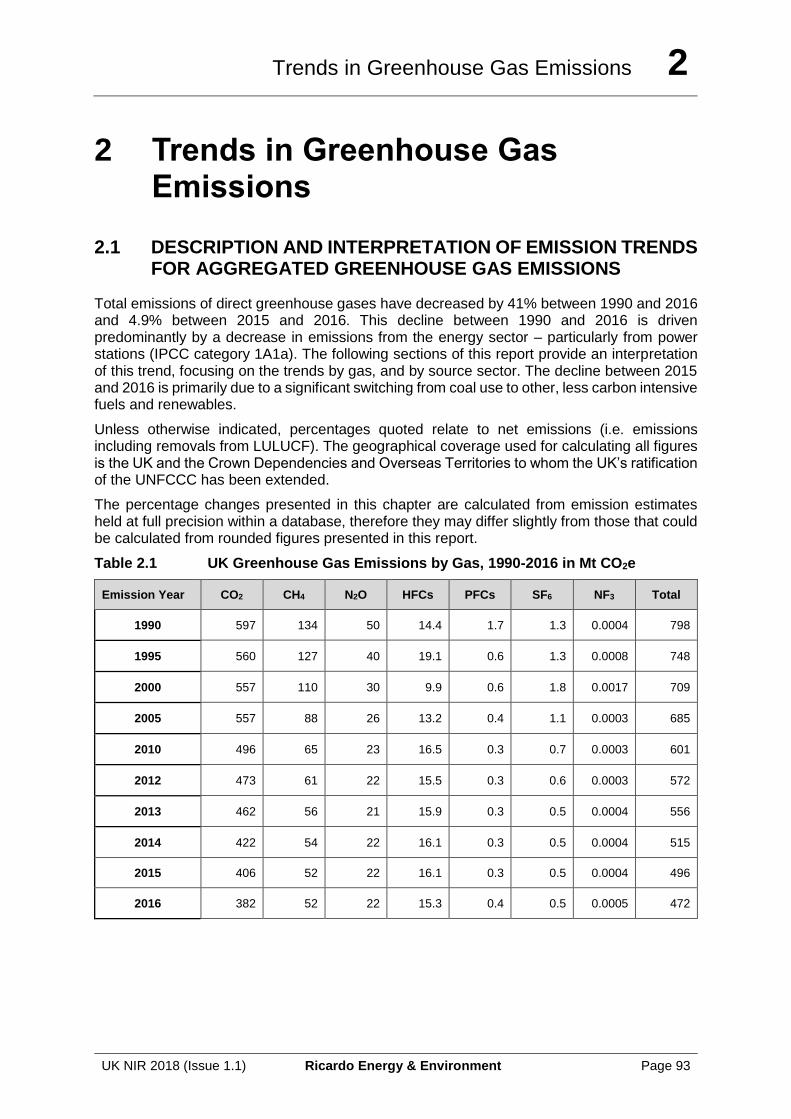
Trends in Greenhouse Gas Emissions 2
UK NIR 2018 (Issue 1.1) Ricardo Energy & Environment Page 93
2 Trends in Greenhouse Gas Emissions
2.1 DESCRIPTION AND INTERPRETATION OF EMISSION TRENDS FOR AGGREGATED GREENHOUSE GAS EMISSIONS
Total emissions of direct greenhouse gases have decreased by 41% between 1990 and 2016 and 4.9% between 2015 and 2016. This decline between 1990 and 2016 is driven predominantly by a decrease in emissions from the energy sector – particularly from power stations (IPCC category 1A1a). The following sections of this report provide an interpretation of this trend, focusing on the trends by gas, and by source sector. The decline between 2015 and 2016 is primarily due to a significant switching from coal use to other, less carbon intensive fuels and renewables.
Unless otherwise indicated, percentages quoted relate to net emissions (i.e. emissions including removals from LULUCF). The geographical coverage used for calculating all figures is the UK and the Crown Dependencies and Overseas Territories to whom the UK’s ratification of the UNFCCC has been extended.
The percentage changes presented in this chapter are calculated from emission estimates held at full precision within a database, therefore they may differ slightly from those that could be calculated from rounded figures presented in this report.
Table 2.1 UK Greenhouse Gas Emissions by Gas, 1990-2016 in Mt CO2e
Emission Year CO2 CH4 N2O HFCs PFCs SF6 NF3 Total
1990 597 134 50 14.4 1.7 1.3 0.0004 798
1995 560 127 40 19.1 0.6 1.3 0.0008 748
2000 557 110 30 9.9 0.6 1.8 0.0017 709
2005 557 88 26 13.2 0.4 1.1 0.0003 685
2010 496 65 23 16.5 0.3 0.7 0.0003 601
2012 473 61 22 15.5 0.3 0.6 0.0003 572
2013 462 56 21 15.9 0.3 0.5 0.0004 556
2014 422 54 22 16.1 0.3 0.5 0.0004 515
2015 406 52 22 16.1 0.3 0.5 0.0004 496
2016 382 52 22 15.3 0.4 0.5 0.0005 472
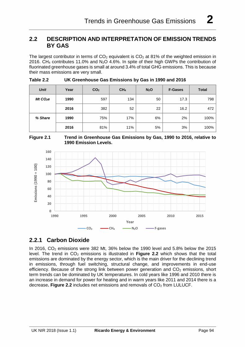
Trends in Greenhouse Gas Emissions 2
UK NIR 2018 (Issue 1.1) Ricardo Energy & Environment Page 94
2.2 DESCRIPTION AND INTERPRETATION OF EMISSION TRENDS BY GAS
The largest contributor in terms of CO2 equivalent is CO2 at 81% of the weighted emission in 2016. CH4 contributes 11.0% and N2O 4.6%. In spite of their high GWPs the contribution of fluorinated greenhouse gases is small at around 3.4% of total GHG emissions. This is because their mass emissions are very small.
Table 2.2 UK Greenhouse Gas Emissions by Gas in 1990 and 2016
Unit Year CO2 CH4 N2O F-Gases Total
Mt CO2e
1990 597 134 50 17.3 798
2016 382 52 22 16.2 472
% Share
1990 75% 17% 6% 2% 100%
2016 81% 11% 5% 3% 100%
Figure 2.1 Trend in Greenhouse Gas Emissions by Gas, 1990 to 2016, relative to 1990 Emission Levels.
2.2.1 Carbon Dioxide
In 2016, CO2 emissions were 382 Mt, 36% below the 1990 level and 5.8% below the 2015 level. The trend in CO2 emissions is illustrated in Figure 2.2 which shows that the total emissions are dominated by the energy sector, which is the main driver for the declining trend in emissions, through fuel switching, structural change, and improvements in end-use efficiency. Because of the strong link between power generation and CO2 emissions, short term trends can be dominated by UK temperatures. In cold years like 1996 and 2010 there is an increase in demand for power for heating and in warm years like 2011 and 2014 there is a decrease. Figure 2.2 includes net emissions and removals of CO2 from LULUCF.
0
20
40
60
80
100
120
140
160
1990 1995 2000 2005 2010 2015
Emis
sio
ns
(19
90
= 1
00
)
Year
CO₂ CH₄ N₂O F-gases
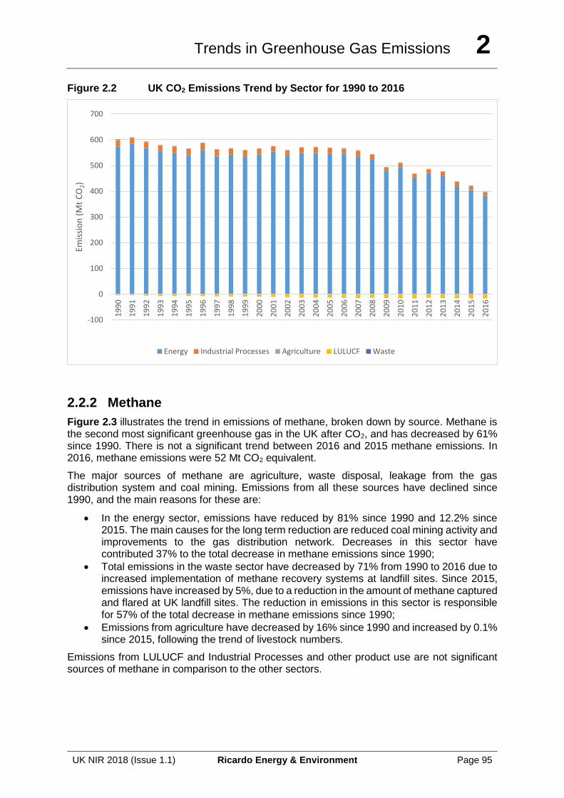
Trends in Greenhouse Gas Emissions 2
UK NIR 2018 (Issue 1.1) Ricardo Energy & Environment Page 95
Figure 2.2 UK CO2 Emissions Trend by Sector for 1990 to 2016
2.2.2 Methane
Figure 2.3 illustrates the trend in emissions of methane, broken down by source. Methane is the second most significant greenhouse gas in the UK after CO2, and has decreased by 61% since 1990. There is not a significant trend between 2016 and 2015 methane emissions. In 2016, methane emissions were 52 Mt CO2 equivalent.
The major sources of methane are agriculture, waste disposal, leakage from the gas distribution system and coal mining. Emissions from all these sources have declined since 1990, and the main reasons for these are:
• In the energy sector, emissions have reduced by 81% since 1990 and 12.2% since 2015. The main causes for the long term reduction are reduced coal mining activity and improvements to the gas distribution network. Decreases in this sector have contributed 37% to the total decrease in methane emissions since 1990;
• Total emissions in the waste sector have decreased by 71% from 1990 to 2016 due to increased implementation of methane recovery systems at landfill sites. Since 2015, emissions have increased by 5%, due to a reduction in the amount of methane captured and flared at UK landfill sites. The reduction in emissions in this sector is responsible for 57% of the total decrease in methane emissions since 1990;
• Emissions from agriculture have decreased by 16% since 1990 and increased by 0.1% since 2015, following the trend of livestock numbers.
Emissions from LULUCF and Industrial Processes and other product use are not significant sources of methane in comparison to the other sectors.
-100
0
100
200
300
400
500
600
7001
99
0
19
91
19
92
19
93
19
94
19
95
19
96
19
97
19
98
19
99
20
00
20
01
20
02
20
03
20
04
20
05
20
06
20
07
20
08
20
09
20
10
20
11
20
12
20
13
20
14
20
15
20
16
Emis
sio
n (
Mt
CO
2)
Energy Industrial Processes Agriculture LULUCF Waste
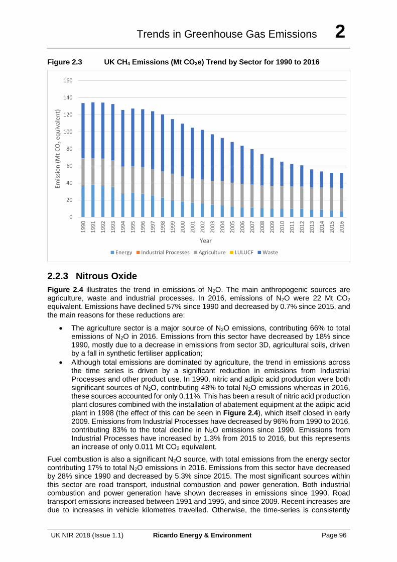
Trends in Greenhouse Gas Emissions 2
UK NIR 2018 (Issue 1.1) Ricardo Energy & Environment Page 96
Figure 2.3 UK CH4 Emissions (Mt CO2e) Trend by Sector for 1990 to 2016
2.2.3 Nitrous Oxide
Figure 2.4 illustrates the trend in emissions of N2O. The main anthropogenic sources are agriculture, waste and industrial processes. In 2016, emissions of N2O were 22 Mt CO2 equivalent. Emissions have declined 57% since 1990 and decreased by 0.7% since 2015, and the main reasons for these reductions are:
• The agriculture sector is a major source of N2O emissions, contributing 66% to total emissions of N2O in 2016. Emissions from this sector have decreased by 18% since 1990, mostly due to a decrease in emissions from sector 3D, agricultural soils, driven by a fall in synthetic fertiliser application;
• Although total emissions are dominated by agriculture, the trend in emissions across the time series is driven by a significant reduction in emissions from Industrial Processes and other product use. In 1990, nitric and adipic acid production were both significant sources of N2O, contributing 48% to total N2O emissions whereas in 2016, these sources accounted for only 0.11%. This has been a result of nitric acid production plant closures combined with the installation of abatement equipment at the adipic acid plant in 1998 (the effect of this can be seen in Figure 2.4), which itself closed in early 2009. Emissions from Industrial Processes have decreased by 96% from 1990 to 2016, contributing 83% to the total decline in N2O emissions since 1990. Emissions from Industrial Processes have increased by 1.3% from 2015 to 2016, but this represents an increase of only 0.011 Mt CO2 equivalent.
Fuel combustion is also a significant N2O source, with total emissions from the energy sector contributing 17% to total N2O emissions in 2016. Emissions from this sector have decreased by 28% since 1990 and decreased by 5.3% since 2015. The most significant sources within this sector are road transport, industrial combustion and power generation. Both industrial combustion and power generation have shown decreases in emissions since 1990. Road transport emissions increased between 1991 and 1995, and since 2009. Recent increases are due to increases in vehicle kilometres travelled. Otherwise, the time-series is consistently
0
20
40
60
80
100
120
140
1601
99
0
19
91
19
92
19
93
19
94
19
95
19
96
19
97
19
98
19
99
20
00
20
01
20
02
20
03
20
04
20
05
20
06
20
07
20
08
20
09
20
10
20
11
20
12
20
13
20
14
20
15
20
16
Emis
sio
n (
Mt
CO
2eq
uiv
alen
t)
Year
Energy Industrial Processes Agriculture LULUCF Waste
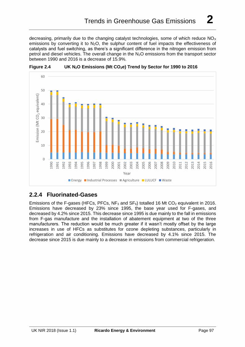
Trends in Greenhouse Gas Emissions 2
UK NIR 2018 (Issue 1.1) Ricardo Energy & Environment Page 97
decreasing, primarily due to the changing catalyst technologies, some of which reduce NOX emissions by converting it to N2O, the sulphur content of fuel impacts the effectiveness of catalysts and fuel switching, as there’s a significant difference in the nitrogen emission from petrol and diesel vehicles. The overall change in the N2O emissions from the transport sector between 1990 and 2016 is a decrease of 15.9%.
Figure 2.4 UK N2O Emissions (Mt CO2e) Trend by Sector for 1990 to 2016
2.2.4 Fluorinated-Gases
Emissions of the F-gases (HFCs, PFCs, NF3 and SF6) totalled 16 Mt CO2 equivalent in 2016. Emissions have decreased by 23% since 1995, the base year used for F-gases, and decreased by 4.2% since 2015. This decrease since 1995 is due mainly to the fall in emissions from F-gas manufacture and the installation of abatement equipment at two of the three manufacturers. The reduction would be much greater if it wasn’t mostly offset by the large increases in use of HFCs as substitutes for ozone depleting substances, particularly in refrigeration and air conditioning. Emissions have decreased by 4.1% since 2015. The decrease since 2015 is due mainly to a decrease in emissions from commercial refrigeration.
0
10
20
30
40
50
60
19
90
19
91
19
92
19
93
19
94
19
95
19
96
19
97
19
98
19
99
20
00
20
01
20
02
20
03
20
04
20
05
20
06
20
07
20
08
20
09
20
10
20
11
20
12
20
13
20
14
20
15
20
16
Emis
sio
n (
Mt
CO
2eq
uiv
alen
t)
Year
Energy Industrial Processes Agriculture LULUCF Waste
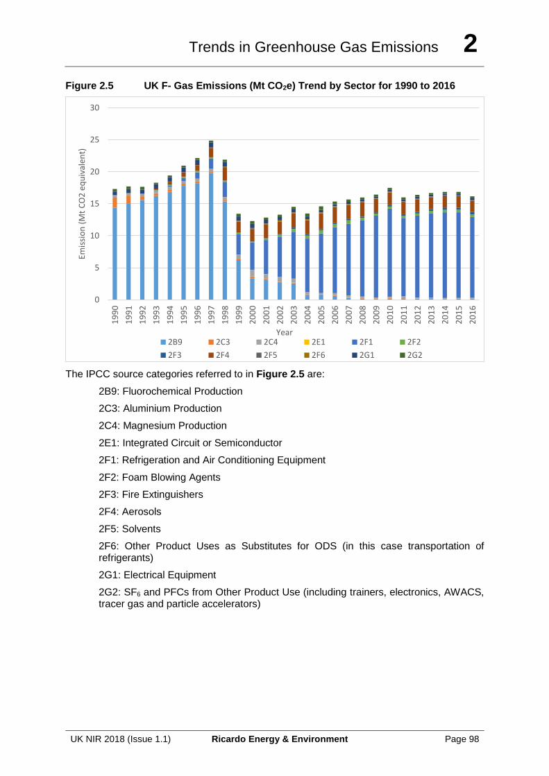
Trends in Greenhouse Gas Emissions 2
UK NIR 2018 (Issue 1.1) Ricardo Energy & Environment Page 98
Figure 2.5 UK F- Gas Emissions (Mt CO2e) Trend by Sector for 1990 to 2016
The IPCC source categories referred to in Figure 2.5 are:
2B9: Fluorochemical Production
2C3: Aluminium Production
2C4: Magnesium Production
2E1: Integrated Circuit or Semiconductor
2F1: Refrigeration and Air Conditioning Equipment
2F2: Foam Blowing Agents
2F3: Fire Extinguishers
2F4: Aerosols
2F5: Solvents
2F6: Other Product Uses as Substitutes for ODS (in this case transportation of refrigerants)
2G1: Electrical Equipment
2G2: SF6 and PFCs from Other Product Use (including trainers, electronics, AWACS, tracer gas and particle accelerators)
0
5
10
15
20
25
301
99
0
19
91
19
92
19
93
19
94
19
95
19
96
19
97
19
98
19
99
20
00
20
01
20
02
20
03
20
04
20
05
20
06
20
07
20
08
20
09
20
10
20
11
20
12
20
13
20
14
20
15
20
16
Emis
sio
n (
Mt
CO
2 e
qu
ival
ent)
Year2B9 2C3 2C4 2E1 2F1 2F2
2F3 2F4 2F5 2F6 2G1 2G2
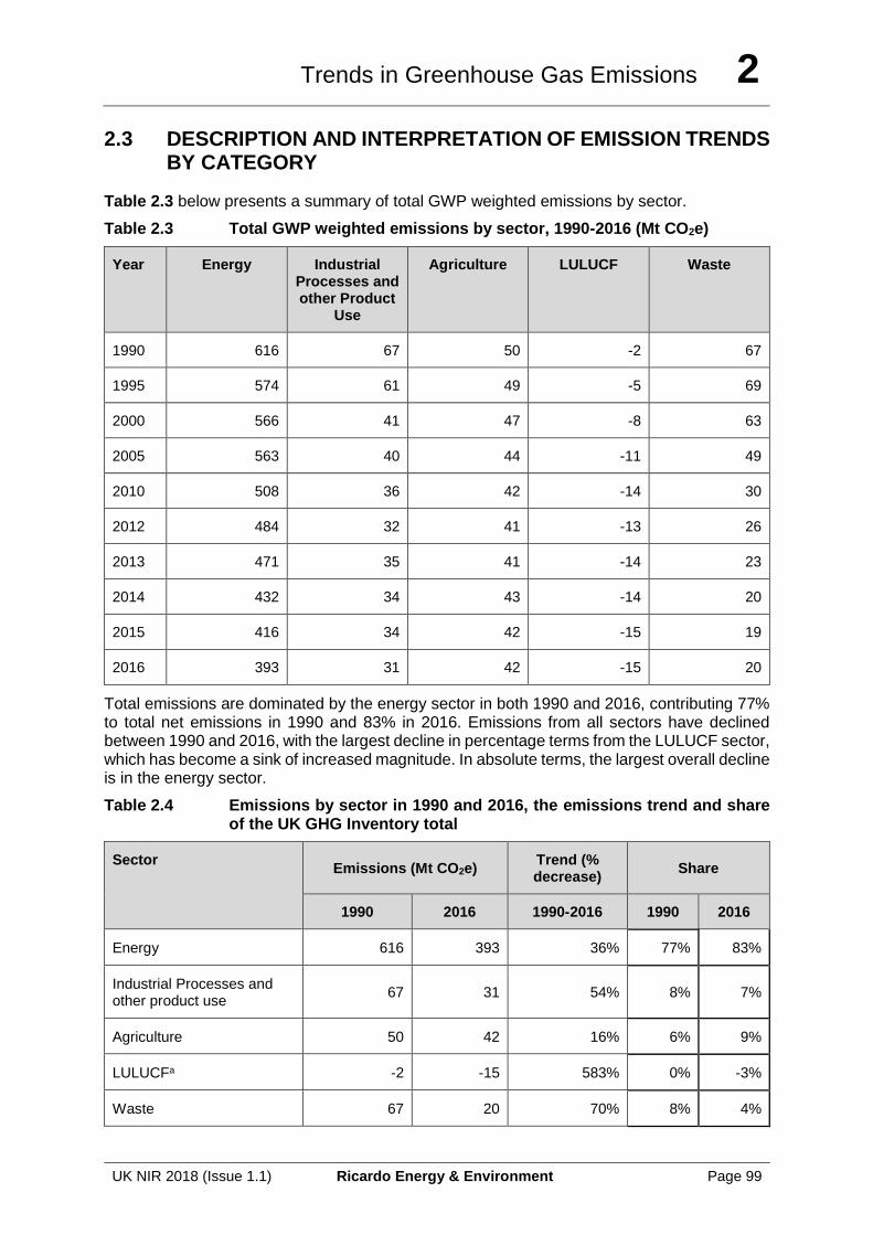
Trends in Greenhouse Gas Emissions 2
UK NIR 2018 (Issue 1.1) Ricardo Energy & Environment Page 99
2.3 DESCRIPTION AND INTERPRETATION OF EMISSION TRENDS BY CATEGORY
Table 2.3 below presents a summary of total GWP weighted emissions by sector.
Table 2.3 Total GWP weighted emissions by sector, 1990-2016 (Mt CO2e)
Year Energy Industrial Processes and other Product
Use
Agriculture LULUCF Waste
1990 616 67 50 -2 67
1995 574 61 49 -5 69
2000 566 41 47 -8 63
2005 563 40 44 -11 49
2010 508 36 42 -14 30
2012 484 32 41 -13 26
2013 471 35 41 -14 23
2014 432 34 43 -14 20
2015 416 34 42 -15 19
2016 393 31 42 -15 20
Total emissions are dominated by the energy sector in both 1990 and 2016, contributing 77% to total net emissions in 1990 and 83% in 2016. Emissions from all sectors have declined between 1990 and 2016, with the largest decline in percentage terms from the LULUCF sector, which has become a sink of increased magnitude. In absolute terms, the largest overall decline is in the energy sector.
Table 2.4 Emissions by sector in 1990 and 2016, the emissions trend and share of the UK GHG Inventory total
Sector Emissions (Mt CO2e)
Trend (% decrease)
Share
1990 2016 1990-2016 1990 2016
Energy 616 393 36% 77% 83%
Industrial Processes and other product use
67 31 54% 8% 7%
Agriculture 50 42 16% 6% 9%
LULUCFa -2 -15 583% 0% -3%
Waste 67 20 70% 8% 4%
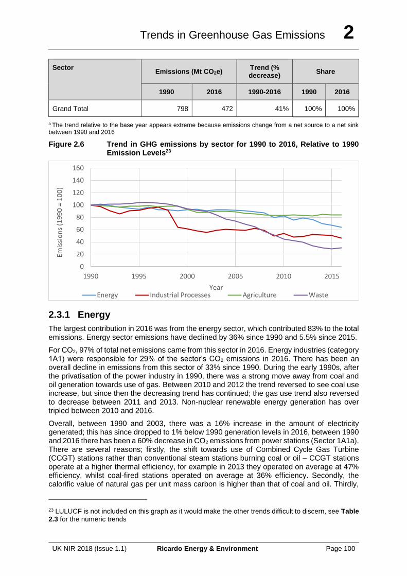
Trends in Greenhouse Gas Emissions 2
UK NIR 2018 (Issue 1.1) Ricardo Energy & Environment Page 100
Sector Emissions (Mt CO2e)
Trend (% decrease)
Share
1990 2016 1990-2016 1990 2016
Grand Total 798 472 41% 100% 100%
a The trend relative to the base year appears extreme because emissions change from a net source to a net sink between 1990 and 2016
Figure 2.6 Trend in GHG emissions by sector for 1990 to 2016, Relative to 1990 Emission Levels23
2.3.1 Energy
The largest contribution in 2016 was from the energy sector, which contributed 83% to the total emissions. Energy sector emissions have declined by 36% since 1990 and 5.5% since 2015.
For CO2, 97% of total net emissions came from this sector in 2016. Energy industries (category 1A1) were responsible for 29% of the sector’s CO2 emissions in 2016. There has been an overall decline in emissions from this sector of 33% since 1990. During the early 1990s, after the privatisation of the power industry in 1990, there was a strong move away from coal and oil generation towards use of gas. Between 2010 and 2012 the trend reversed to see coal use increase, but since then the decreasing trend has continued; the gas use trend also reversed to decrease between 2011 and 2013. Non-nuclear renewable energy generation has over tripled between 2010 and 2016.
Overall, between 1990 and 2003, there was a 16% increase in the amount of electricity generated; this has since dropped to 1% below 1990 generation levels in 2016, between 1990 and 2016 there has been a 60% decrease in CO2 emissions from power stations (Sector 1A1a). There are several reasons; firstly, the shift towards use of Combined Cycle Gas Turbine (CCGT) stations rather than conventional steam stations burning coal or oil – CCGT stations operate at a higher thermal efficiency, for example in 2013 they operated on average at 47% efficiency, whilst coal-fired stations operated on average at 36% efficiency. Secondly, the calorific value of natural gas per unit mass carbon is higher than that of coal and oil. Thirdly,
23 LULUCF is not included on this graph as it would make the other trends difficult to discern, see Table 2.3 for the numeric trends
0
20
40
60
80
100
120
140
160
1990 1995 2000 2005 2010 2015
Emis
sio
ns
(19
90
= 1
00
)
YearEnergy Industrial Processes Agriculture Waste
Trends in Greenhouse Gas Emissions 2
UK NIR 2018 (Issue 1.1) Ricardo Energy & Environment Page 101
there has been an increase in electricity generated from non-fossil fuel energy sources, due to increased use of wastes and renewable energy sources, and an increase in nuclear generation. In 2016, low carbon electricity accounted for 46.5% of UK electricity generation.
Emissions from category 1A2 – Manufacturing Industries and Construction contributed 13% to overall net CO2 emissions in the UK in 2016. Since 1990, these emissions have declined by 47%, mainly as a result of a decline in the emissions from the Iron and steel industry. This sector has seen a significant decrease in coke, coal and fuel oil usage, with an increase occurring in the emissions from combustion of burning oil and waste. Reductions in emissions from other industrial combustion (1A2gviii) also contribute a large part to the overall 1A2 trend. Emissions have declined by 33% since 1990, contributing to 23% of the 1A2 trend. This is largely a result of reduced gas oil and fuel oil activity, with respective increases in burning oil and biomass use within the sector.
Emissions of CO2 from 1A3 (Transport) are dominated by road transport (1A3b), which in 2016 were responsible for 92% of the total emissions from transport. Emissions from road transport peaked in 2007 at 11% above 1990 levels. Carbon dioxide emissions from road transport have declined since 2007 back almost exactly to 1990 levels mostly due to improvements in average fuel efficiency of vehicles, switching from petrol to diesel cars and a reduction in traffic volumes. The increased displacement of fossil fuels by biofuels since 2002 has also had a significant impact on total CO2 emissions as carbon emissions from the consumption of biofuels are not included in the UK totals. Emissions of CO2 from domestic aviation (1A3a) increased by 63% between 1990 and 2005, but have since shown a decrease of 40% since 2005 and are now slightly below 1990 levels. This is because of a move to use more fuel efficient aeroplanes in 2006 and a smaller number of air miles being flown.
Emissions of CO2 in the domestic sector (1A4b) account for 73% of CO2 emissions in 1A4. Emissions from this sector changed little between 1990 and 2009 but have declined more recently. The effect of annual temperatures can produce some large variations between any two years. Fuel consumption data since 1990 indicates a general trend in fuel switching in these sectors, away from more carbon-intensive fuels such as coal, coke, fuel oil and gas oil, towards natural gas. This shift has partly been driven by fuel prices but also through the growth of the UK gas supply network (most notably in Northern Ireland).
Methane emissions in the energy sector are mostly from fugitive emissions (1B). In 1990, 64% of these emissions came from the production of solid fuels (1B1); however these emissions have decreased by 98% and now make up just 9% of fugitive CH4 emissions. Fugitive emissions from oil and gas operations (1B2) have also decreased over this period, by 61%.
Nitrous oxide emissions from the energy sector have decreased by 28% since 1990 and accounted for 17% of total N2O emissions in the UK during 2016. Of this, 22% arose from energy industries (1A1). Within this category, emissions from public electricity production (1A1a) have shown a 67% decrease since 1990. Over this period the use of coal has decreased and the use of natural gas increased, as emissions of N2O per GWh is significantly lower for natural gas use than coal in power generation, this represents a significant reduction in N2O emissions.
The other major contribution towards N2O emissions within the energy sector is the transport sector (1A3) (35%). Road transport emissions increased between 1991 and 1995, and since 2009, consistently decreasing otherwise. The trend is driven by 3 key factors; the changing catalyst technologies (some of which reduce N2O, but others reduce NOx emissions by converting it to N2O, hence increasing N2O emissions), the sulphur content of fuel (which has decreased significantly due to regulation) impacts the effectiveness of catalysts and fuel switching, as there’s a significant difference in the nitrogen emission from petrol and diesel vehicles. The overall change in the N2O emissions from the transport sector between 1990 and 2016 is a decrease of 16%.
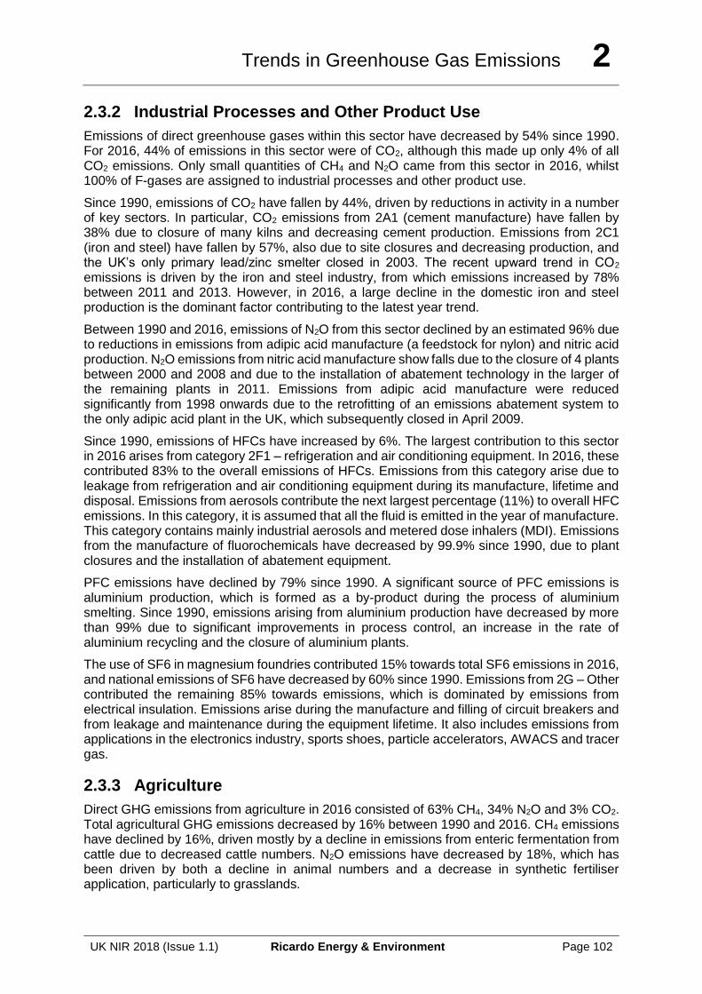
Trends in Greenhouse Gas Emissions 2
UK NIR 2018 (Issue 1.1) Ricardo Energy & Environment Page 102
2.3.2 Industrial Processes and Other Product Use
Emissions of direct greenhouse gases within this sector have decreased by 54% since 1990. For 2016, 44% of emissions in this sector were of CO2, although this made up only 4% of all CO2 emissions. Only small quantities of CH4 and N2O came from this sector in 2016, whilst 100% of F-gases are assigned to industrial processes and other product use.
Since 1990, emissions of CO2 have fallen by 44%, driven by reductions in activity in a number of key sectors. In particular, CO2 emissions from 2A1 (cement manufacture) have fallen by 38% due to closure of many kilns and decreasing cement production. Emissions from 2C1 (iron and steel) have fallen by 57%, also due to site closures and decreasing production, and the UK’s only primary lead/zinc smelter closed in 2003. The recent upward trend in CO2 emissions is driven by the iron and steel industry, from which emissions increased by 78% between 2011 and 2013. However, in 2016, a large decline in the domestic iron and steel production is the dominant factor contributing to the latest year trend.
Between 1990 and 2016, emissions of N2O from this sector declined by an estimated 96% due to reductions in emissions from adipic acid manufacture (a feedstock for nylon) and nitric acid production. N2O emissions from nitric acid manufacture show falls due to the closure of 4 plants between 2000 and 2008 and due to the installation of abatement technology in the larger of the remaining plants in 2011. Emissions from adipic acid manufacture were reduced significantly from 1998 onwards due to the retrofitting of an emissions abatement system to the only adipic acid plant in the UK, which subsequently closed in April 2009.
Since 1990, emissions of HFCs have increased by 6%. The largest contribution to this sector in 2016 arises from category 2F1 – refrigeration and air conditioning equipment. In 2016, these contributed 83% to the overall emissions of HFCs. Emissions from this category arise due to leakage from refrigeration and air conditioning equipment during its manufacture, lifetime and disposal. Emissions from aerosols contribute the next largest percentage (11%) to overall HFC emissions. In this category, it is assumed that all the fluid is emitted in the year of manufacture. This category contains mainly industrial aerosols and metered dose inhalers (MDI). Emissions from the manufacture of fluorochemicals have decreased by 99.9% since 1990, due to plant closures and the installation of abatement equipment.
PFC emissions have declined by 79% since 1990. A significant source of PFC emissions is aluminium production, which is formed as a by-product during the process of aluminium smelting. Since 1990, emissions arising from aluminium production have decreased by more than 99% due to significant improvements in process control, an increase in the rate of aluminium recycling and the closure of aluminium plants.
The use of SF6 in magnesium foundries contributed 15% towards total SF6 emissions in 2016, and national emissions of SF6 have decreased by 60% since 1990. Emissions from 2G – Other contributed the remaining 85% towards emissions, which is dominated by emissions from electrical insulation. Emissions arise during the manufacture and filling of circuit breakers and from leakage and maintenance during the equipment lifetime. It also includes emissions from applications in the electronics industry, sports shoes, particle accelerators, AWACS and tracer gas.
2.3.3 Agriculture
Direct GHG emissions from agriculture in 2016 consisted of 63% CH4, 34% N2O and 3% CO2. Total agricultural GHG emissions decreased by 16% between 1990 and 2016. CH4 emissions have declined by 16%, driven mostly by a decline in emissions from enteric fermentation from cattle due to decreased cattle numbers. N2O emissions have decreased by 18%, which has been driven by both a decline in animal numbers and a decrease in synthetic fertiliser application, particularly to grasslands.
Trends in Greenhouse Gas Emissions 2
UK NIR 2018 (Issue 1.1) Ricardo Energy & Environment Page 103
2.3.4 Land Use, Land Use Change and Forestry
The UK has been an increasing net sink of CO2 from LULUCF activities for all years since 1990. As the LULUCF sector comprises both emissions and removals of greenhouse gases, expressing the total change in the sector since 1990 on a percentage basis can be misleading. Total estimated net emissions of direct greenhouse gases from the LULUCF sector changed from a sink of 2 MtCO2e in 1990 to a sink of 15 MtCO2e in the latest inventory. The land use categories which have the greatest effect on the net LULUCF emissions/removals are forest land (a net sink) and cropland (a net source). The size of the Forest land sink increased by 40% between 1990 and 2010 but has levelled off in recent years due to a decrease in the contribution of land converted to forest caused by reduced afforestedand the earlier substantial afforested area reaching maturity. Emissions from cropland have decreased by 25% since 1990.
Methane emissions from LULUCF activities are insignificant (<0.05 MtCO2e). Emissions of nitrous oxide have decreased by 36% from 2.3 MtCO2e in 1990 to 1.4 MtCO2e in 2016. The main reason for the reduction in nitrous oxide emissions is a reduction in nitrogen mineralization arising from land conversion to cropland.
2.3.5 Waste
Overall emissions from the waste sector have decreased by 70% since 1990 but increased by 5% since 2015. Over 99% of this reduction is due to a decline in methane emissions from landfill. Emissions estimates from landfill are derived from the amount of biodegradable waste disposed of to landfill and are based on a model of the kinetics of anaerobic digestion involving four classifications of landfill site. The model also accounts for the effects of methane recovery, utilisation and flaring. Since 1990, methane emissions from landfill have declined by 77% due to the implementation of methane recovery systems. This trend is likely to continue as all new landfill sites are required to have these systems and many existing sites may have systems retrofitted.
2.4 EMISSION TRENDS FOR INDIRECT GREENHOUSE GASES AND SO2
The indirect greenhouse gases in the UK consist of Nitrogen Oxides (NOx), Carbon Monoxide (CO), Non-Methane Volatile Organic Compounds (NMVOC) and Sulphur dioxide (SO2). Of these, NOx, CO and NMVOC can increase tropospheric ozone concentration and hence radiative forcing. Sulphur dioxide contributes to aerosol formation in the atmosphere. This is believed to have a negative net radiative forcing effect, tending to cool the surface. Emission trends for the indirect greenhouse gases are shown in Figure 2.7.
Trends in Greenhouse Gas Emissions 2
UK NIR 2018 (Issue 1.1) Ricardo Energy & Environment Page 104
Figure 2.7 UK Emissions of Indirect Greenhouse Gases for 1990 to 2016
2.4.1 Carbon Monoxide
In 2016, the total emissions of CO were 1,544 kt, and since 1990, emissions have decreased by 79%.
Emissions of carbon monoxide from the energy sector contributed 84% to overall UK CO emissions in 2016, 26% of these emissions occur from transport (1A3). Since 1990, emissions from 1A3 have declined by 93%, which is mainly because of the increased use of three way catalysts, although a proportion is a consequence of fuel switching in moving from petrol to diesel cars.
Emissions from sector 1A2 contributed 21% to overall emissions of CO in 2016. Emissions from within this category mostly come biomass combustion and off-road vehicles used in manufacturing, industry and construction.
2.4.2 Nitrogen Oxides
In 2016, total emissions of NOx were 897 kt, and since 1990, emissions have decreased by 71%.
98% of NOx emissions in the UK came from the energy sector in 2016. Since 1990 emissions from this sector have decreased by 71%, mostly as a result of abatement measures on power stations, three-way catalysts fitted to cars and stricter emission regulations on trucks. The main source of NOx emissions from transport contributed 50% to the total emissions of NOx in the UK, 69% of which arising from road transport (1A3b). From 1970, emissions from transport increased (especially during the 1980s) and reached a peak around 1990. The reduction in emissions since 1990 is due to the requirement since the early 1990s for new petrol cars to be fitted with three way catalysts and the further tightening up of emission standards on these and all types of new diesel vehicles over the last decade.
Emissions from the energy industries (1A1) contributed 23% to total NOx emissions in the UK during 2016. Between 1990 and 2016, emissions from this sector decreased by 77%, the main
0
1000
2000
3000
4000
5000
6000
7000
8000
1990
1991
1992
1993
1994
1995
1996
1997
1998
1999
2000
2001
2002
2003
2004
2005
2006
2007
2008
2009
2010
2011
2012
2013
2014
2015
2016
Emis
sio
ns
(kt)
CO
NOx
SO2
VOC
Trends in Greenhouse Gas Emissions 2
UK NIR 2018 (Issue 1.1) Ricardo Energy & Environment Page 105
reason for this was a decrease in emissions from public electricity and heat production (1A1a) of 84%. Since 1998 the electricity generators adopted a programme of progressively fitting low NOx burners to their 500 MWe coal fired units. Since 1990, further changes in the electricity supply industry such as the increased use of nuclear generation and the introduction of CCGT plant have resulted in additional reduction in NOx emissions.
Emissions from Manufacturing, Industry and Construction (1A2) have fallen by 69% since 1990. In 2016, emissions from this sector contributed 15% to overall emissions of NOx. Over this period, the industrial sector has seen a move away from the use of coal, coke and fuel oil towards natural gas and gas oil usage.
2.4.3 Sulphur Dioxide
In 2016, total emissions of SO2 were 180 kt, and since 1990, emissions have decreased by 95%.
91% of emissions of sulphur dioxide came from the energy sector in 2016, 41% of these emissions arose from energy industries (1A1). Since 1990, emissions from power stations (1A1a) have declined by 99%. This decline has been due to the increase in the proportion of electricity generated CCGT stations, other gas fired plants, the increase in the proportion of electricity generated in nuclear plants, and the application of Flue Gas Desulphurisation abatement equipment on several of the largest coal-fired power stations in the UK. CCGTs run on natural gas and are more efficient than conventional coal and oil stations and have negligible SO2 emissions.
Emissions from Manufacturing, Industry and Construction (1A2) were responsible for 18% of UK emissions of SO2 in 2016. Since 1990, emissions from this category have declined by 92%. This decline is due to the reduction in the use of coal and oil in favour of natural gas, and also some improvement in energy efficiency.
2.4.4 Non Methane Volatile Organic Compounds
In 2016, total emissions of NMVOCs were 827 kt, and since 1990, overall emissions have decreased by 71%.
Emissions from the industrial processes and other product use sector contributed 55% to overall UK emissions of NMVOCs. 75% of these emissions in 2016 were from the Non-energy Products from Fuels and Solvent Use sector which contributed 41% to total NMVOC emissions in 2016 and since 1990 emissions have declined by 49%. Most of the remaining NMVOC emissions in the industrial processes and other product use sector are from the food and drink and chemicals industries.
30% of non-methane volatile organic compound emissions came from the energy sector in 2016. Of these, the largest contribution arises from the fugitive emissions of oil and natural gas (1B2), which contributed 15% towards the overall UK emissions of NMVOCs in 2016. This includes emissions from gas leakage, which comprise around 52% of the total for the energy sector, the remaining emissions arise from oil transportation, refining, storage and offshore. Emissions from transport (1A3) contribute 5.3% to overall emissions of NMVOC in the UK in 2016, but emissions from this sector have decreased by 95% since 1990.
2.5 EMISSION TRENDS FROM KP LULUCF ACTIVITIES
The main driver of the emission and removal trends for KP-LULUCF is the large area of forest planted between the 1950s and the 1980s, and the low level of forest planting since then. As the mid-20th Century forest stands have reached maturity and are now being harvested, the net removal of carbon dioxide from forests has started to fall (Article 3.4 Forest Management
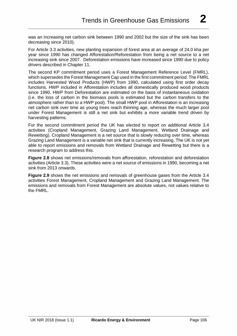
Trends in Greenhouse Gas Emissions 2
UK NIR 2018 (Issue 1.1) Ricardo Energy & Environment Page 106
was an increasing net carbon sink between 1990 and 2002 but the size of the sink has been decreasing since 2010).
For Article 3.3 activities, new planting expansion of forest area at an average of 24.0 kha per year since 1990 has changed Afforestation/Reforestation from being a net source to a net increasing sink since 2007. Deforestation emissions have increased since 1990 due to policy drivers described in Chapter 11.
The second KP commitment period uses a Forest Management Reference Level (FMRL), which supersedes the Forest Management Cap used in the first commitment period. The FMRL includes Harvested Wood Products (HWP) from 1990, calculated using first order decay functions. HWP included in Afforestation includes all domestically produced wood products since 1990. HWP from Deforestation are estimated on the basis of instantaneous oxidation (i.e. the loss of carbon in the biomass pools is estimated but the carbon transfers to the atmosphere rather than to a HWP pool). The small HWP pool in Afforestation is an increasing net carbon sink over time as young trees reach thinning age, whereas the much larger pool under Forest Management is still a net sink but exhibits a more variable trend driven by harvesting patterns.
For the second commitment period the UK has elected to report on additional Article 3.4 activities (Cropland Management, Grazing Land Management, Wetland Drainage and Rewetting). Cropland Management is a net source that is slowly reducing over time, whereas Grazing Land Management is a variable net sink that is currently increasing. The UK is not yet able to report emissions and removals from Wetland Drainage and Rewetting but there is a research program to address this.
Figure 2.8 shows net emissions/removals from afforestation, reforestation and deforestation activities (Article 3.3). These activities were a net source of emissions in 1990, becoming a net sink from 2013 onwards.
Figure 2.9 shows the net emissions and removals of greenhouse gases from the Article 3.4 activities Forest Management, Cropland Management and Grazing Land Management. The emissions and removals from Forest Management are absolute values, not values relative to the FMRL.
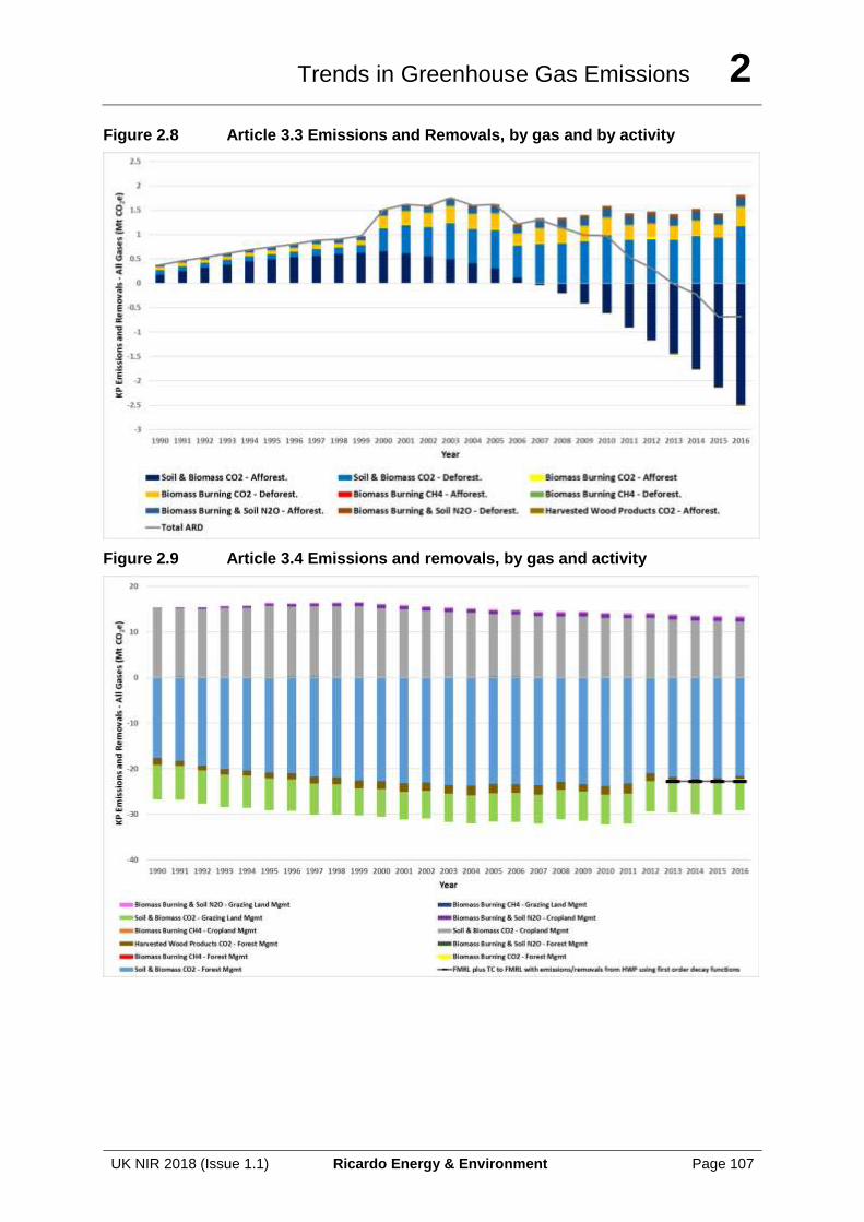
Trends in Greenhouse Gas Emissions 2
UK NIR 2018 (Issue 1.1) Ricardo Energy & Environment Page 107
Figure 2.8 Article 3.3 Emissions and Removals, by gas and by activity
Figure 2.9 Article 3.4 Emissions and removals, by gas and activity
Trends in Greenhouse Gas Emissions 2
UK NIR 2018 (Issue 1.1) Ricardo Energy & Environment Page 108
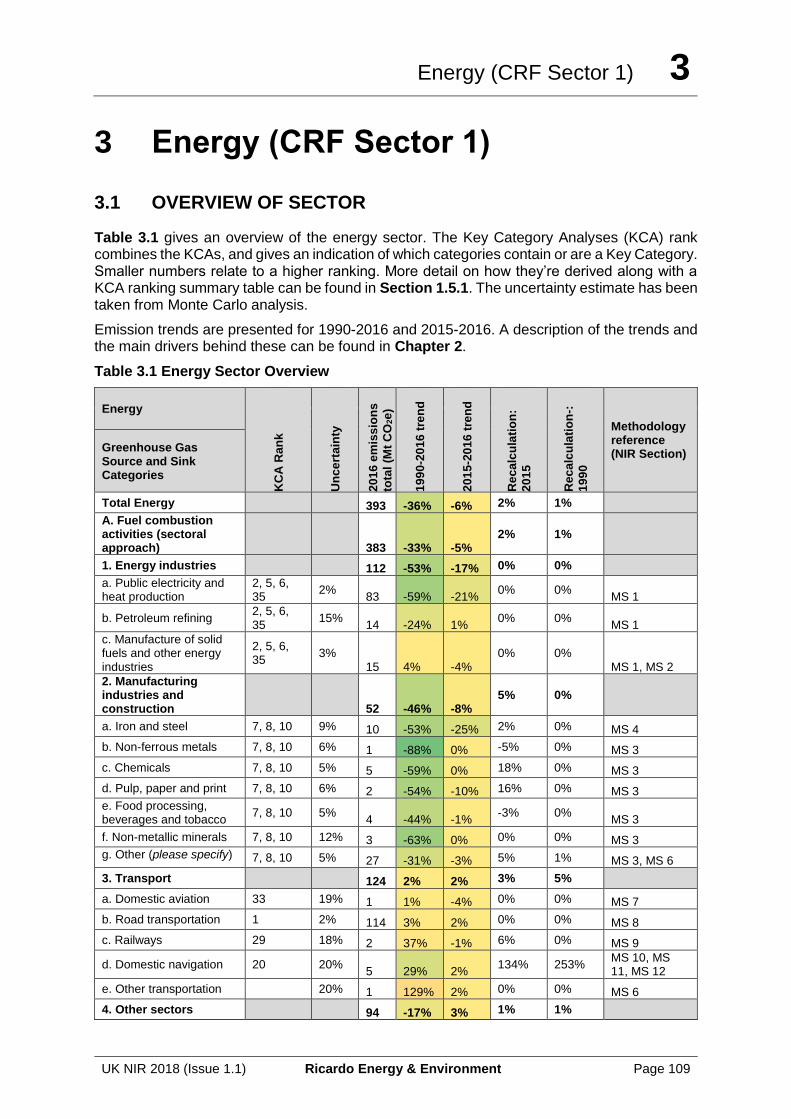
Energy (CRF Sector 1) 3
UK NIR 2018 (Issue 1.1) Ricardo Energy & Environment Page 109
3 Energy (CRF Sector 1)
3.1 OVERVIEW OF SECTOR
Table 3.1 gives an overview of the energy sector. The Key Category Analyses (KCA) rank combines the KCAs, and gives an indication of which categories contain or are a Key Category. Smaller numbers relate to a higher ranking. More detail on how they’re derived along with a KCA ranking summary table can be found in Section 1.5.1. The uncertainty estimate has been taken from Monte Carlo analysis.
Emission trends are presented for 1990-2016 and 2015-2016. A description of the trends and the main drivers behind these can be found in Chapter 2.
Table 3.1 Energy Sector Overview
Energy
KC
A R
an
k
Un
ce
rtain
ty
20
16
em
iss
ion
s
tota
l (M
t C
O2e
)
19
90
-20
16
tre
nd
20
15
-20
16
tre
nd
Rec
alc
ula
tio
n:
20
15
Rec
alc
ula
tio
n-:
19
90
Methodology reference (NIR Section)
Greenhouse Gas Source and Sink Categories
Total Energy 393 -36% -6% 2% 1%
A. Fuel combustion activities (sectoral approach)
383 -33% -5%
2% 1%
1. Energy industries 112 -53% -17% 0% 0%
a. Public electricity and heat production
2, 5, 6, 35
2% 83 -59% -21%
0% 0% MS 1
b. Petroleum refining 2, 5, 6, 35
15% 14 -24% 1%
0% 0% MS 1
c. Manufacture of solid fuels and other energy industries
2, 5, 6, 35
3% 15 4% -4%
0% 0% MS 1, MS 2
2. Manufacturing industries and construction
52 -46% -8%
5% 0%
a. Iron and steel 7, 8, 10 9% 10 -53% -25% 2% 0% MS 4
b. Non-ferrous metals 7, 8, 10 6% 1 -88% 0% -5% 0% MS 3
c. Chemicals 7, 8, 10 5% 5 -59% 0% 18% 0% MS 3
d. Pulp, paper and print 7, 8, 10 6% 2 -54% -10% 16% 0% MS 3
e. Food processing, beverages and tobacco
7, 8, 10 5% 4 -44% -1%
-3% 0% MS 3
f. Non-metallic minerals 7, 8, 10 12% 3 -63% 0% 0% 0% MS 3
g. Other (please specify) 7, 8, 10 5% 27 -31% -3% 5% 1% MS 3, MS 6
3. Transport 124 2% 2% 3% 5%
a. Domestic aviation 33 19% 1 1% -4% 0% 0% MS 7
b. Road transportation 1 2% 114 3% 2% 0% 0% MS 8
c. Railways 29 18% 2 37% -1% 6% 0% MS 9
d. Domestic navigation 20 20% 5 29% 2%
134% 253% MS 10, MS 11, MS 12
e. Other transportation 20% 1 129% 2% 0% 0% MS 6
4. Other sectors 94 -17% 3% 1% 1%
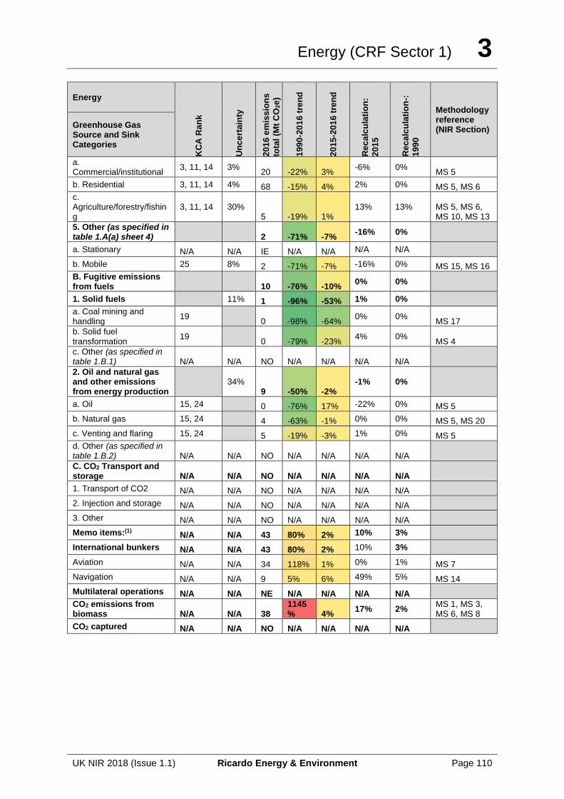
Energy (CRF Sector 1) 3
UK NIR 2018 (Issue 1.1) Ricardo Energy & Environment Page 110
Energy
KC
A R
an
k
Un
ce
rta
inty
20
16
em
iss
ion
s
tota
l (M
t C
O2e
)
19
90
-20
16
tre
nd
20
15
-20
16
tre
nd
Re
ca
lcu
lati
on
:
20
15
Re
ca
lcu
lati
on
-:
19
90
Methodology reference (NIR Section)
Greenhouse Gas Source and Sink Categories
a. Commercial/institutional
3, 11, 14 3% 20 -22% 3%
-6% 0% MS 5
b. Residential 3, 11, 14 4% 68 -15% 4% 2% 0% MS 5, MS 6
c. Agriculture/forestry/fishing
3, 11, 14 30% 5 -19% 1%
13% 13% MS 5, MS 6, MS 10, MS 13
5. Other (as specified in table 1.A(a) sheet 4)
2 -71% -7%
-16% 0%
a. Stationary N/A N/A IE N/A N/A N/A N/A
b. Mobile 25 8% 2 -71% -7% -16% 0% MS 15, MS 16
B. Fugitive emissions from fuels
10 -76% -10%
0% 0%
1. Solid fuels 11% 1 -96% -53% 1% 0%
a. Coal mining and handling
19 0 -98% -64%
0% 0% MS 17
b. Solid fuel transformation
19 0 -79% -23%
4% 0% MS 4
c. Other (as specified in table 1.B.1) N/A N/A NO N/A N/A N/A N/A
2. Oil and natural gas and other emissions from energy production
34% 9 -50% -2%
-1% 0%
a. Oil 15, 24 0 -76% 17% -22% 0% MS 5
b. Natural gas 15, 24 4 -63% -1% 0% 0% MS 5, MS 20
c. Venting and flaring 15, 24 5 -19% -3% 1% 0% MS 5
d. Other (as specified in table 1.B.2) N/A N/A NO N/A N/A N/A N/A
C. CO2 Transport and storage N/A N/A NO N/A N/A N/A N/A
1. Transport of CO2 N/A N/A NO N/A N/A N/A N/A
2. Injection and storage N/A N/A NO N/A N/A N/A N/A
3. Other N/A N/A NO N/A N/A N/A N/A
Memo items:(1) N/A N/A 43 80% 2% 10% 3%
International bunkers N/A N/A 43 80% 2% 10% 3%
Aviation N/A N/A 34 118% 1% 0% 1% MS 7
Navigation N/A N/A 9 5% 6% 49% 5% MS 14
Multilateral operations N/A N/A NE N/A N/A N/A N/A
CO2 emissions from biomass N/A N/A 38
1145% 4%
17% 2% MS 1, MS 3, MS 6, MS 8
CO2 captured N/A N/A NO N/A N/A N/A N/A
Energy (CRF Sector 1) 3
UK NIR 2018 (Issue 1.1) Ricardo Energy & Environment Page 111
3.2 FUEL COMBUSTION (CRF 1.A)
3.2.1 Comparison of Sectoral and Reference Approaches
The UK compares its Sectoral Approach (SA) and Reference Approach (RA) as one of the means of verification of its energy sector GHG estimates in accordance with the UNFCCC decision 24/CP.19 paragraph 40.
The Sectoral Approach is the detailed ‘bottom up’ sectoral methodology for estimating energy CO2 emissions described in Section 3.4, The Reference Approach is a ‘top down’ approach for estimating energy CO2 emissions using national fuel statistics that acts as a verification tool for the Sectoral Approach.
The RA-SA comparison shows very close consistency between the two datasets (once the major known differences are accounted for) for the UK, and provides verification of the reported SA emission estimates for 1A. The UK greenhouse gas inventory is compiled using a detailed Sectoral Approach methodology, to produce sector-specific inventories of the 10 pollutants in accordance with the IPCC reporting format. These UK GHGI emission estimates are based on bottom-up activity data, including:
• national energy statistics (DUKES) that present annual consumption of primary and secondary fuels within different economic sectors in the UK; and
• a wide range of other statistical datasets (e.g. raw material extraction and use, production statistics for minerals, metals, glass, cement, specific chemicals, waste statistics, livestock and crop data, land use survey information) to generate estimates of non-combustion emissions from other known sources.
As a verification of the detailed Sectoral Approach inventory estimates, the inventory agency also calculates alternative UK emission estimates for carbon dioxide from energy sources in the UK, using the IPCC Reference Approach. This is a top-down inventory compilation method, which calculates emission estimates from National Statistics on production, imports, exports, stock changes and non-energy uses of fossil fuels: crude oil, natural gas and solid fuels.
The Reference Approach inventory method utilises different sections of the UK national energy statistics, combining aggregated data on fuel inputs and outputs from the overall UK economy, using top-level data on oils, gas and solid fuels to assess the UK carbon balance for combustion sources. This more simplistic, non-source-specific methodology provides a very useful quality check against the more rigorous Sectoral Approach.
Differences between the RA and SA arise primarily due to statistical differences between production-side and demand-side fuel estimates within national energy statistics, the exclusion of carbon estimates from specific activities (e.g. some carbon within coke and coal deliveries to the iron and steel and non-ferrous metal industries) and the more aggregated approach to applying emission factors to activity data across fuel types.
Some minor adjustments to the reference approach has been made this year, mostly in response to review recommendations.
3.2.1.1 Discrepancies between the IPCC Reference and Sectoral Approach
The IPCC Reference Approach total can be compared with the IPCC Table 1A total for all fossil fuels, and under the new 2006 GLs approach the Reference Approach (RA) CO2 estimates for the UK typically range between 1.7% lower to 3.5% lower than the comparable bottom-up emission totals of the Sectoral Approach (SA).
There are a number of ‘known differences’ between the reference approach and sectoral approach which are discussed in the subsequent sections.
Energy (CRF Sector 1) 3
UK NIR 2018 (Issue 1.1) Ricardo Energy & Environment Page 112
3.2.1.1.1 Statistical Differences in Energy Balance Data
The SA is based on the demand side of the national energy statistics, which is some cases informs us to what quality of fuel may be used (e.g. petroleum coke used for anodes we expect to be calcined). The RA however, uses the supply side of the national energy statistics. The difference between the total of the supply and demand sides of energy statistics is the statistical difference, which is a cause of differences between the RA and SA. Because of evolving methodologies and improved data collection the statistical difference is generally quite small in later years, but as some data are not available for earlier years the gap is much more significant in the 90s.
The system of energy statistics operated by BEIS aims to keep UK statistical differences (without normalisation) at less than 0.5% of energy supply, for total supply and also for each fuel. Nevertheless, a proportion of the difference between the Reference Approach and the Sectoral Approach totals will be accounted for by statistical differences.
3.2.1.1.2 Application of Carbon Factors: Aggregated (RA) vs. Detailed (SA)
In the RA the carbon balance is calculated based on the apparent consumption of fuels, for primary fuels (e.g. crude oil). This mean that the estimated carbon content of fuel that’s transformed into other fuels (e.g. petroleum products) is assumed to be accounted for by the commodity balance for the primary fuel from which they’re derived, which differs from the SA which estimates emissions at end use. Because the estimates of primary and derived fuel carbon contents are made independently, the estimated carbon content of the primary fuel to be transformed and the estimated carbon content of the resulting transformed secondary fuel can differ, particularly as primary fuels have a generally more variable carbon content. In general, we have greater confidence in the SA Carbon Emission Factors (CEFs) because they are fuel/process/site specific and the carbon content of end use fuels are less variable than primary fuels.
3.2.1.1.3 Fuels Excluded from the UK RA
Emissions from use of waste oils, fossil-containing wastes, scrap tyres and waste solvents that are reported within the SA but are not included in the estimates for the RA in the UK. The RA doesn’t include complete emissions from these fuels because there isn’t complete reporting of these fuels in UK energy statistics; the data for the SA is based on EU ETS and operator data.
3.2.1.1.4 Treatment of Blast Furnace Gas
Some emissions from the blast furnace gas are reported under IPCC source categories 1A1ci and 1A2 in the UK GHGI SA. In the RA totals, the carbon in the blast furnace gas is excluded from the total, as it is associated with the carbon content of coal and coke deliveries to the iron and steel industry.
3.2.1.1.5 Deviations from National Statistics
The UK GHG SA method deviates from UK energy statistics for specific fuels (e.g. natural gas, OPG), in a handful of cases where industry data indicates higher usage than DUKES suggests. More details on deviations from DUKES can be found in Annex 4.2.1. As the reference approach is based on DUKES fuel balances, deviations from DUKES will lead to discrepancies between the SA and RA.
3.2.1.2 Comparisons of UK Emissions: Sectoral Approach vs. Reference Approach and Amended Reference Approach
Table 3.3 shows the percentage differences in CO2 emissions from fuel combustion sources between the IPCC Reference Approach and the UK GHGI (Sectoral Approach) IPCC sector 1A, for each year since 1990 and the resulting comparison when we have accounted for most of the known differences. Table 3.2 gives a summary of the RA/Amended RA-SA comparison for the 3 main fuel groups.
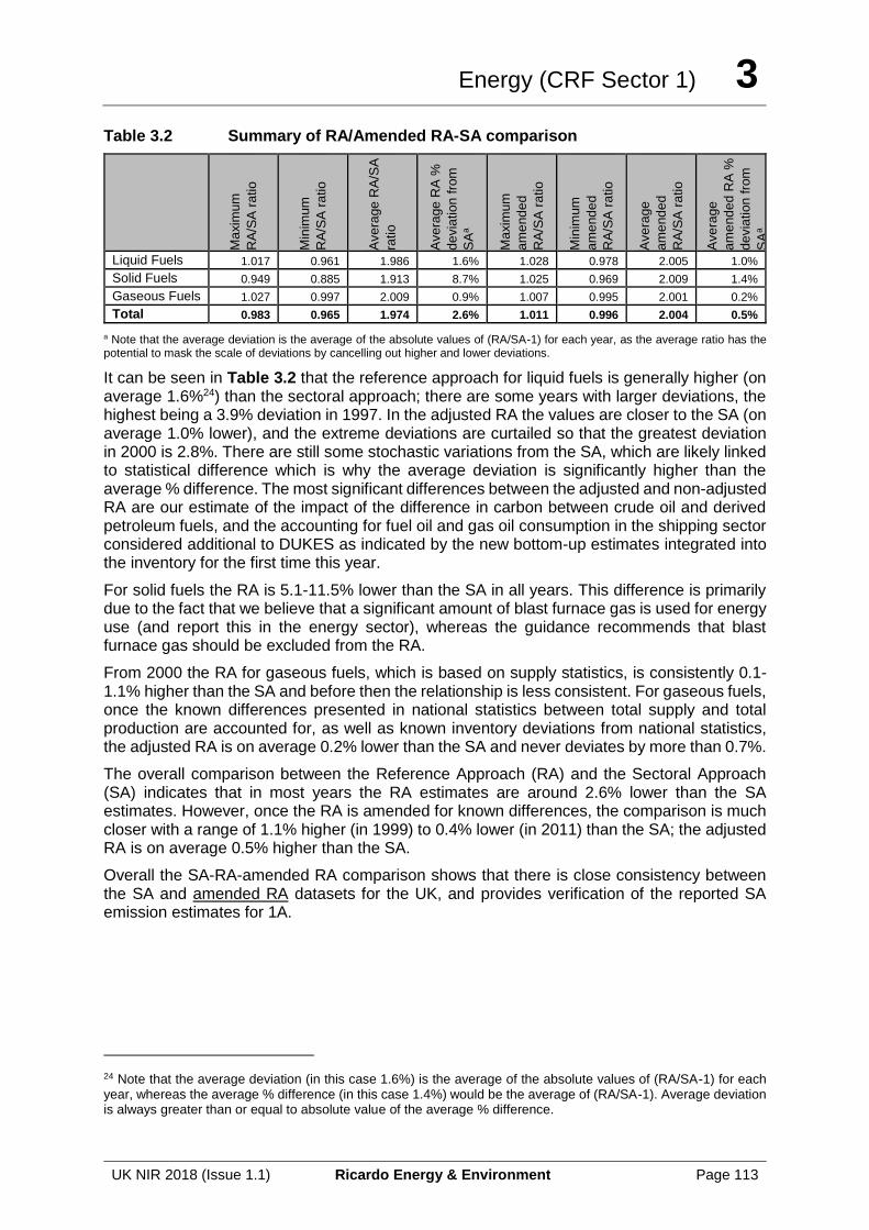
Energy (CRF Sector 1) 3
UK NIR 2018 (Issue 1.1) Ricardo Energy & Environment Page 113
Table 3.2 Summary of RA/Amended RA-SA comparison
Ma
xim
um
RA
/SA
ra
tio
Min
imum
RA
/SA
ra
tio
Ave
rage
RA
/SA
ratio
Ave
rage
RA
%
de
via
tion
fro
m
SA
a
Ma
xim
um
am
end
ed
RA
/SA
ra
tio
Min
imum
am
end
ed
RA
/SA
ra
tio
Ave
rage
am
end
ed
RA
/SA
ra
tio
Ave
rage
am
end
ed
RA
%
de
via
tion
fro
m
SA
a
Liquid Fuels 1.017 0.961 1.986 1.6% 1.028 0.978 2.005 1.0%
Solid Fuels 0.949 0.885 1.913 8.7% 1.025 0.969 2.009 1.4%
Gaseous Fuels 1.027 0.997 2.009 0.9% 1.007 0.995 2.001 0.2%
Total 0.983 0.965 1.974 2.6% 1.011 0.996 2.004 0.5%
a Note that the average deviation is the average of the absolute values of (RA/SA-1) for each year, as the average ratio has the potential to mask the scale of deviations by cancelling out higher and lower deviations.
It can be seen in Table 3.2 that the reference approach for liquid fuels is generally higher (on average 1.6%24) than the sectoral approach; there are some years with larger deviations, the highest being a 3.9% deviation in 1997. In the adjusted RA the values are closer to the SA (on average 1.0% lower), and the extreme deviations are curtailed so that the greatest deviation in 2000 is 2.8%. There are still some stochastic variations from the SA, which are likely linked to statistical difference which is why the average deviation is significantly higher than the average % difference. The most significant differences between the adjusted and non-adjusted RA are our estimate of the impact of the difference in carbon between crude oil and derived petroleum fuels, and the accounting for fuel oil and gas oil consumption in the shipping sector considered additional to DUKES as indicated by the new bottom-up estimates integrated into the inventory for the first time this year.
For solid fuels the RA is 5.1-11.5% lower than the SA in all years. This difference is primarily due to the fact that we believe that a significant amount of blast furnace gas is used for energy use (and report this in the energy sector), whereas the guidance recommends that blast furnace gas should be excluded from the RA.
From 2000 the RA for gaseous fuels, which is based on supply statistics, is consistently 0.1-1.1% higher than the SA and before then the relationship is less consistent. For gaseous fuels, once the known differences presented in national statistics between total supply and total production are accounted for, as well as known inventory deviations from national statistics, the adjusted RA is on average 0.2% lower than the SA and never deviates by more than 0.7%.
The overall comparison between the Reference Approach (RA) and the Sectoral Approach (SA) indicates that in most years the RA estimates are around 2.6% lower than the SA estimates. However, once the RA is amended for known differences, the comparison is much closer with a range of 1.1% higher (in 1999) to 0.4% lower (in 2011) than the SA; the adjusted RA is on average 0.5% higher than the SA.
Overall the SA-RA-amended RA comparison shows that there is close consistency between the SA and amended RA datasets for the UK, and provides verification of the reported SA emission estimates for 1A.
24 Note that the average deviation (in this case 1.6%) is the average of the absolute values of (RA/SA-1) for each year, whereas the average % difference (in this case 1.4%) would be the average of (RA/SA-1). Average deviation is always greater than or equal to absolute value of the average % difference.
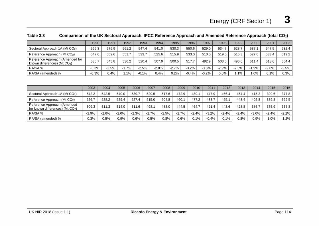
Energy (CRF Sector 1) 3
UK NIR 2018 (Issue 1.1) Ricardo Energy & Environment Page 114
Table 3.3 Comparison of the UK Sectoral Approach, IPCC Reference Approach and Amended Reference Approach (total CO2)
1990 1991 1992 1993 1994 1995 1996 1997 1998 1999 2000 2001 2002
Sectoral Approach 1A (Mt CO2) 566.3 576.9 561.2 547.4 541.0 530.3 550.6 529.0 534.7 528.7 537.1 547.5 532.4
Reference Approach (Mt CO2) 547.6 562.6 551.7 533.7 525.6 515.9 533.0 510.5 519.0 515.3 527.0 533.4 519.2
Reference Approach (Amended for known differences) (Mt CO2)
530.7 545.8 536.2 520.4 507.9 500.5 517.7 492.9 503.0 496.0 511.4 518.6 504.4
RA/SA % -3.3% -2.5% -1.7% -2.5% -2.8% -2.7% -3.2% -3.5% -2.9% -2.5% -1.9% -2.6% -2.5%
RA/SA (amended) % -0.3% 0.4% 1.1% -0.1% 0.4% 0.2% -0.4% -0.2% 0.0% 1.1% 1.0% 0.1% 0.3%
2003 2004 2005 2006 2007 2008 2009 2010 2011 2012 2013 2014 2015 2016
Sectoral Approach 1A (Mt CO2) 542.2 542.5 540.0 539.7 529.5 517.6 472.9 489.1 447.9 466.4 454.4 415.2 399.6 377.8
Reference Approach (Mt CO2) 526.7 528.2 529.4 527.4 515.0 504.8 460.1 477.2 433.7 455.1 443.4 402.8 389.8 369.5
Reference Approach (Amended for known differences) (Mt CO2)
509.3 511.3 514.0 511.6 498.1 488.0 444.5 464.7 421.4 443.6 428.8 386.7 375.9 356.8
RA/SA % -2.9% -2.6% -2.0% -2.3% -2.7% -2.5% -2.7% -2.4% -3.2% -2.4% -2.4% -3.0% -2.4% -2.2%
RA/SA (amended) % 0.3% 0.5% 0.9% 0.6% 0.5% 0.8% 0.6% 0.1% -0.4% 0.1% 0.8% 0.9% 1.0% 1.2%
Energy (CRF Sector 1) 3
UK NIR 2018 (Issue 1.1) Ricardo Energy & Environment Page 115
3.2.2 International Bunker Fuels (memo item)
International bunker emissions (international aviation and shipping) are not included in the national total but are reported separately.
These estimates are consistent with the Tier 3 method adopted for aviation and described in MS 7 and the revised Tier 3 method adopted for shipping as described in MS 14. The methods for the calculation of international bunker fuels are presented in the relevant method statements.
Each year the Inventory Agency confirms that the UK energy balance is consistent with data submitted to EUROSTAT and IEA and that the total fuel consumption used for the GHG estimates is consistent with the UK energy balance. For marine bunkers the UK GHG estimates are based on the bottom up analysis from the BEIS shipping inventory (Scarborough et al., 2017). This leads to a different total fuel use allocation for marine fuels from the allocations in the national energy statistics (DUKES) and submissions to IEA/EUROSTAT.
3.2.3 Feedstock and Non-Energy Use of Fuels
The methodology for estimating emissions from fuels used for non-energy purposes is set out in the relevant sections of this NIR. A summary of the method, including all non-energy uses is included in Annex 3.
The UK energy statistics (DUKES, 2017) contain an allocation for non-energy use for each fuel in the commodity balance tables. The UK inventory estimates emissions from fuels, including emissions arising from non-energy uses. In some cases, the inventory estimate for non-energy use does not agree with the DUKES allocation, and reallocations are made between energy and non-energy use for inventory reporting. In 2013, the Inventory Agency carried out research into non-energy uses of fuels; this was followed up by the DECC (now BEIS as of 2016) energy statistics team during 2014, and a series of revised allocations were introduced in the Digest of UK Energy Statistics 2014 (DECC, 2014), improving consistency between the inventory and the UK energy statistics. The activity data used for the national inventory and any deviations from the UK energy balance are presented and explained in Annex 4.
The evidence that the Inventory Agency uses to make estimates for NEU includes:
• annual reporting by plant operators (e.g. EU ETS returns include data on the use of process off-gases in the chemical and petrochemical production sector);
• periodic surveys or research by trade associations / research organisations / environmental regulators, such as to assess the fate of coal tars and benzoles, petroleum coke or waste oils, or the impact of regulations on solvents, waste, product design and use; and,
• information on the estimated split of stored: emitted carbon from feedstock chemicals in literature sources, including other country NIRs, where UK-specific information is not available.
In many cases the energy statistics allocate fuels to non-energy use that are used in chemical and petrochemical production processes where either:
• fossil carbon-containing off-gases are used for combustion in facility boilers; or
• products containing the “stored” carbon are subsequently used / partly combusted / disposed and degraded with some proportion of the “stored carbon” in products ultimately emitted to atmosphere.
In other instances, the allocation of fuels to “non-energy use” in the UK energy balance is contrary to other statistical evidence from industry or surveys that the Inventory Agency has
Energy (CRF Sector 1) 3
UK NIR 2018 (Issue 1.1) Ricardo Energy & Environment Page 116
access to in the compilation of the national inventory. For example, petroleum coke for residential use was not recorded in the national energy data, nor was industrial use prior to 2008, and so use has been made of other data for both industrial and domestic sector consumption. Evidence from environmental reporting and from research indicates that several industries use petroleum coke directly as a fuel or process input (e.g. cement kilns, chemical manufacturing processes, domestic fuel manufacturers), and that petroleum coke is supplied as a fuel for the residential market.
3.2.4 Use of UK Energy Statistics in the GHG inventory
The main source of official national statistics and energy balances data used in the UK inventory is the Digest of UK Energy Statistics (BEIS, 2017), hereafter referred to as DUKES. This annual publication gives detailed sectoral energy consumption broken down by fuel type, and covering the entire time period relevant to the inventory. In many cases, these data are used directly in the inventory without modification. However, the activity data used to derive emission estimates in the UK inventory may not exactly match the fuel consumption figures given in DUKES and other national statistics. This occurs for one of four reasons:
• Data in DUKES and other national statistics are not always available to the level of detail required for inventory reporting. For example, activity data within DUKES do not distinguish between fuel used in stationary and mobile combustion units. Emissions from these different types of appliances have to be separately reported in the inventory and furthermore they may exhibit very different combustion characteristics (for non-CO2 gases) and therefore require application of different emission factors in the UK inventory.
• Data in DUKES and other national statistics are subject to varying levels of uncertainty, especially at the sector-specific level, and in some cases alternative data suggesting higher fuel consumption are available from other sources, which we use in preference. For example, the EU Emissions Trading System indicates higher fuel use for several high-emitting industrial sectors which is used in preference to DUKES data.
• DUKES and other national statistics do not include any data for a given source. For example, DUKES does not provide any information on secondary fuels such as process off-gases that are derived from petroleum feedstocks and are commonly used as fuels in petrochemical and chemical industries.
• Where the BEIS DUKES team make improvements to national energy statistics, they typically do not revise the full time series of data; usually, DUKES data are typically retrospectively revised for up to the 5 most recent years. This can lead to step changes in the DUKES time-series that are due to methodological differences rather than reflecting real changes in fuel use. Therefore, to ensure time series consistency of reported emissions, the inventory agency works with the BEIS energy statistics team to derive a defensible historic time series back to at least 1990 for use in the UK inventory. For example, in DUKES 2015 the estimates for residential wood use were significantly revised due to new research into uptake of biomass combustion units. In this case, the data were only revised back to 2008 in the DUKES 2015 statistical publication, therefore new activity data for wood use in 1990-2007 were estimated by the inventory agency in consultation with the DUKES team, which are then used in the inventory in place of the published DUKES data.
The rationale for those modifications or deviations from DUKES data that are made, and the sources of alternate data are discussed in the sections detailing methodology for each CRF source category that follow Section 3. A summary of all modifications is given in Annex 4.
The modifications described above involve changes to the sector-level estimates of fuel use used in the UK inventory, when compared with the original source data from DUKES. As a
Energy (CRF Sector 1) 3
UK NIR 2018 (Issue 1.1) Ricardo Energy & Environment Page 117
general rule, the overall demand for each fuel in the UK inventory is kept consistent with the overall demand for that fuel in DUKES; the Inventory Agency approach is such that in almost all cases, any modifications to the sector allocation of DUKES data is matched by an equal and opposite allocation change in another sector, to ensure a zero net change in fuel demand relative to DUKES. Annex 4 includes a series of tables that demonstrate this consistency between the UK inventory and DUKES.
There are some exceptions to the general rule of consistency with DUKES, for petroleum coke and for OPG, where other statistical evidence indicates that the energy balance data for fuel combustion sources may be too low, and where re-allocations of fuel use from the “non-energy use” lines in DUKES are made by the Inventory Agency (see Annex 4).
Apart from DUKES, the main other data source used for fuel use estimates in the inventory is the installation-level data available for processes covered by the EU Emissions Trading System (BEIS, 2017), which has been analysed and compared with the data from DUKES. Further details of the analysis of EU ETS and use of the data within the UK GHG inventory are given in Annex 7. Further fuel consumption data are taken from the Environmental Emissions Monitoring System (EEMS) data set (BEIS Offshore Inspectorate, 2017) and from data supplied by the UK Mineral Products Association (MPA, 2017), and from the UK solid fuel supply sector (Roberts, 2015). These are used to modify fuel use and emission estimates for 1A1c, 1A2f, and 1A4b respectively, and are described more fully in the sections below that deal with those source categories.
Fuel use estimates for transport sources also rely upon data taken from DUKES, with some further detail provided from other sources.
3.2.5 Biomass
Combustion of biomass and other biofuels is included in the UK energy statistics and also in the UK inventory. The inventory considers the possible use of such fuels in all subsectors of CRF 1A. The UK energy statistics reports biomass activity data that are complete for all UK consumption, and these are presented in the inventory reported across a number of source sectors (including: 1A1a, 1A2g, 1A3b, 1A4b and 1A4c). The underlying energy data are not wholly consistent with the needs of inventory reporting, and it is likely that biofuels consumption for industry (reported in 1A2g) will include some consumption within 1A2d, 1A2e and 1A4a and, to a lesser extent, other sectors as well, but the inventory agency does not have sufficient data on which to base estimates at this greater level of sector resolution.
Greenhouse gas emissions including CO2 are estimated for these fuels and presented in the relevant sections of the CRF. The CO2 emissions from biomass are, however, not added to the total UK emissions from fuel combustion and are instead recorded as a memo item. Emissions of N2O and CH4 from biomass combustion are included within the UK inventory totals although in the case of emissions from use of biofuels in road transport, the emissions are not reported separately, and are instead included in the emissions reported for petrol and DERV. The impact of biomass use on carbon stocks in the UK is recorded in the LULUCF sector; biomass imported into the UK will affect the LULUCF sector in the country from which the biomass is imported.
3.2.6 Unoxidized Carbon
When fuels are combusted, a small proportion of the carbon in the fuel is not fully oxidized. For example, unburnt carbon can remain in the ash left after combustion of coal. Emission estimates for CO2 need to take account of any carbon in fuels that remains long-term in this unoxidized form.
In the UK Inventory, it is assumed that unoxidized carbon is only significant for solid fuels. For gaseous and liquid fuels, although some carbon might not be oxidized fully during combustion

Energy (CRF Sector 1) 3
UK NIR 2018 (Issue 1.1) Ricardo Energy & Environment Page 118
(for example emitted as VOC or particulate matter), based on discussions with fuel suppliers, it is assumed than any indefinite storage of unoxidized carbon will be sufficiently trivial to be ignored. For solid fuels, UK-specific assumptions are employed, either based on expert judgements provided by UK industry, or based on EU ETS returns. Table 3.4 summarises the assumptions used.
Table 3.4 Levels of unoxidized carbon assumed for the UK GHGI
Fuel Type
Fuel sub-type Source Sector Years
Assumed unoxidized carbon
UK GHGIc IPCC default
Gaseous All fuels All sectors All 0% 0%
Liquid All fuels (incl. petroleum coke)
All sectors All 0% 0%
Solid Coal 1A1a 1990-2004 2%a
0%
2005 1.8%b
2006 2.0%b
2007 1.7%b
2008 2.0%b
2009 1.9%b
2010 1.9%b
2011 1.8%b
2012 1.6%b
2013 1.8%b
2014 1.8%b
2015 1.8%b
2016 1.8%b
1A2f (cement) All 0%
1A4b All 0%
All others All 0%
Anthracite 1A4b All 0%
Coke, solid smokeless fuel
1A4b All 0%
All others All 0%
a Expert judgements provided by UK fuel producers and fuel users (see Baggott et al, 2004).
b Calculated from site-specific EU ETS returns for all UK coal-fired power stations except in 2005 and 2016 where no information is not available for one site.
c From the 2006 IPCC Guidelines for National Greenhouse Gas Inventories, unless otherwise stated.
3.3 CO2 TRANSPORT AND STORAGE
Currently in the UK, CO2 emitted from flue gases is not captured and stored. This source is not occurring for the UK.
3.4 METHOD STATEMENTS
The rest of the energy chapter is structured using a series of inventory compilation “method statements” in order to group together categories where the source data and methods are similar, thus avoiding unnecessary repetition of method descriptions and improving the clarity of the NIR. The method statements are numbered, and are cross referenced with the summary
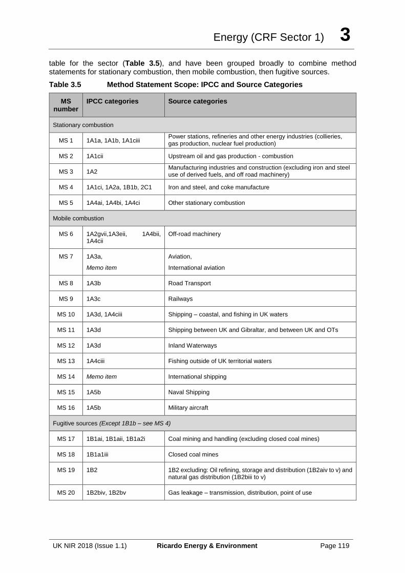
Energy (CRF Sector 1) 3
UK NIR 2018 (Issue 1.1) Ricardo Energy & Environment Page 119
table for the sector (Table 3.5), and have been grouped broadly to combine method statements for stationary combustion, then mobile combustion, then fugitive sources.
Table 3.5 Method Statement Scope: IPCC and Source Categories
MS number
IPCC categories Source categories
Stationary combustion
MS 1 1A1a, 1A1b, 1A1ciii Power stations, refineries and other energy industries (collieries, gas production, nuclear fuel production)
MS 2 1A1cii Upstream oil and gas production - combustion
MS 3 1A2 Manufacturing industries and construction (excluding iron and steel use of derived fuels, and off road machinery)
MS 4 1A1ci, 1A2a, 1B1b, 2C1 Iron and steel, and coke manufacture
MS 5 1A4ai, 1A4bi, 1A4ci Other stationary combustion
Mobile combustion
MS 6 1A2gvii,1A3eii, 1A4bii, 1A4cii
Off-road machinery
MS 7 1A3a,
Memo item
Aviation,
International aviation
MS 8 1A3b Road Transport
MS 9 1A3c Railways
MS 10 1A3d, 1A4ciii Shipping – coastal, and fishing in UK waters
MS 11 1A3d Shipping between UK and Gibraltar, and between UK and OTs
MS 12 1A3d Inland Waterways
MS 13 1A4ciii Fishing outside of UK territorial waters
MS 14 Memo item International shipping
MS 15 1A5b Naval Shipping
MS 16 1A5b Military aircraft
Fugitive sources (Except 1B1b – see MS 4)
MS 17 1B1ai, 1B1aii, 1B1a2i Coal mining and handling (excluding closed coal mines)
MS 18 1B1a1iii Closed coal mines
MS 19 1B2 1B2 excluding: Oil refining, storage and distribution (1B2aiv to v) and natural gas distribution (1B2biii to v)
MS 20 1B2biv, 1B2bv Gas leakage – transmission, distribution, point of use
Energy (CRF Sector 1) 3
UK NIR 2018 (Issue 1.1) Ricardo Energy & Environment Page 120
MS 1 Power stations, refineries and other energy industries
Relevant Categories, source names
1A1a: Power stations
1A1b: Refineries
1A1ciii: Collieries, gas production and nuclear fuel production
Relevant Gases
CO2, CH4, N2O
Relevant fuels, activities
Burning oil, Coal, Colliery methane, Fuel oil, Gas oil, Landfill gas, Liquid bio-fuels, LPG, MSW, Naphtha, Natural gas, OPG, Orimulsion, Petrol, Petroleum coke, Poultry litter, Refinery miscellaneous, Scrap tyres, Sewage gas, Sour gas, Straw, Waste oils and Wood
[Note that this MS excludes: coke production, smokeless solid fuel production (both MS 4) and upstream oil and gas production (MS 2).]
Background
This Method Statement (MS) includes information about UK power stations, refineries and other energy industries.
Table 3.6 shows the number of power stations in the UK, by the type of fuel burnt. The main fossil fuels used by the UK electricity supply industry are bituminous coal and natural gas. The number of coal stations has decreased markedly across the time series, and the number of gas fired stations peaked in 2012 but has decreased slightly since then. The share of total UK electricity generated in 2016 was 10% from coal and 45% from gas, compared with 26% from coal and 30% from natural gas in 2015. The big shift in generation from coal to gas followed policy that supported market preference for the use of gas, as opposed to coal, and also reflected the closure of some coal-fired plant in 2015 and 2016. Generation by other means contributed the same share in 2016 as in the previous year: nuclear stations generated a further 24%, and almost all of the remaining 20% was generated from renewables (6%) or non-thermal sources such as wind and hydro (14%).
Biomass is being burnt at an increasing number of power generation sites to help electricity generators meet Government targets for renewable energy production. These sites use poultry litter, straw, or wood as the main fuel, whilst many coal-fired power stations have increased the use of biofuels such as short-rotation coppice to supplement the use of fossil fuels. Electricity is also generated in a large number of engines running on biogas at landfill sites and sewage treatment works. CO2 emissions associated with biofuel combustion are estimated and reported as memo items, but not included here; these emissions will be reflected in the LULUCF carbon stocks of the country producing the fuel. Emissions of other greenhouse gases from biofuel use are estimated and included in the national inventory totals, in accordance with IPCC guidance on the treatment of biofuel-derived emissions.
Electricity is also generated at an increasing number of Energy from Waste (EfW) installations in the UK. Formerly classed as municipal solid waste (MSW) incinerators, all such installations have since the late 1990s been required to be fitted with boilers to raise power and heat, and their emissions are therefore reported under CRF source category 1A1 (electricity generation), rather than 5C (Waste Incineration). Prior to 1997 at least some MSW was burnt in older installations without energy recovery.
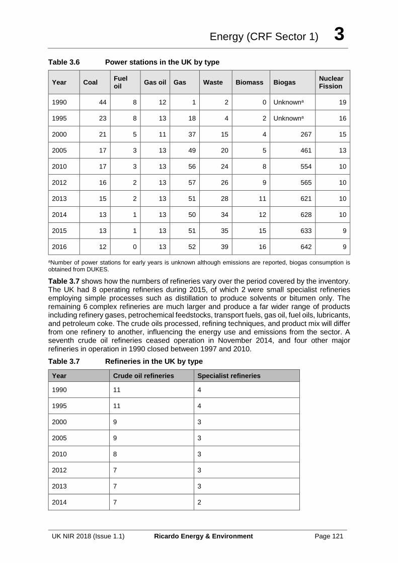
Energy (CRF Sector 1) 3
UK NIR 2018 (Issue 1.1) Ricardo Energy & Environment Page 121
Table 3.6 Power stations in the UK by type
Year Coal Fuel oil
Gas oil Gas Waste Biomass Biogas Nuclear Fission
1990 44 8 12 1 2 0 Unknowna 19
1995 23 8 13 18 4 2 Unknowna 16
2000 21 5 11 37 15 4 267 15
2005 17 3 13 49 20 5 461 13
2010 17 3 13 56 24 8 554 10
2012 16 2 13 57 26 9 565 10
2013 15 2 13 51 28 11 621 10
2014 13 1 13 50 34 12 628 10
2015 13 1 13 51 35 15 633 9
2016 12 0 13 52 39 16 642 9
aNumber of power stations for early years is unknown although emissions are reported, biogas consumption is obtained from DUKES.
Table 3.7 shows how the numbers of refineries vary over the period covered by the inventory. The UK had 8 operating refineries during 2015, of which 2 were small specialist refineries employing simple processes such as distillation to produce solvents or bitumen only. The remaining 6 complex refineries are much larger and produce a far wider range of products including refinery gases, petrochemical feedstocks, transport fuels, gas oil, fuel oils, lubricants, and petroleum coke. The crude oils processed, refining techniques, and product mix will differ from one refinery to another, influencing the energy use and emissions from the sector. A seventh crude oil refineries ceased operation in November 2014, and four other major refineries in operation in 1990 closed between 1997 and 2010.
Table 3.7 Refineries in the UK by type
Year Crude oil refineries Specialist refineries
1990 11 4
1995 11 4
2000 9 3
2005 9 3
2010 8 3
2012 7 3
2013 7 3
2014 7 2

Energy (CRF Sector 1) 3
UK NIR 2018 (Issue 1.1) Ricardo Energy & Environment Page 122
Year Crude oil refineries Specialist refineries
2015 6 2
2016 6 2
Much of the crude oil and natural gas input to the refineries comes from a large number of offshore installations in UK waters, together with a small number of onshore production facilities. Emissions estimates from these activities are described in MS 2, 0 and 0. Coal is extracted in the UK from deep mines and open-cast sites. The production of coal has been in rapid decline in the UK and levels of UK activity are far lower in recent years than in 1990. The last large deep mine closed in 2015 and so production of deep-mined coal was negligible in 2016. Emissions from combustion at UK collieries are covered in this MS. Fugitive emission estimates from these mining and extraction activities are included in MS 17 and 0.
Nuclear fuel production is a very minor user of fossil fuel in the UK, and is included in this MS.
Key Data sources
Activity data: DUKES, EU ETS, UK PIA
Emission Factors: Carbon factors are predominantly derived from EU ETS data (2005 onwards) and from the 2004 Carbon Factors Review (Baggott et al., 2004), with some solid fuel factors derived from UK research (Fynes and Sage, 1994); non-CO2 EFs are predominantly IPCC defaults (IPCC, 2006).
An accompanying spreadsheet “Energy_background_data_uk_2018.xlxs” lists all emission factors used in the energy sector, including a full list of references25. The justification for use of several references, such as EU ETS, the 2004 Carbon Factors Review and Fynes and Sage, are presented in Annex 3.1.2.
Table 1.6 gives additional information for common activity data sources.
Method approach
The calculation of direct greenhouse gases for the sources covered by this MS is:
UK Emissions = EF x AD
The sources of emission factors and activity data are summarised under “key data sources” above, with a full list of emission factors set out in “Energy_background_data_uk_2018.xlxs”. The activity data are taken from DUKES, noting the exceptions set out under Assumptions & observations, below. Annex 4 described the energy balance for the UK and how this is used for the inventory, and any deviations from these data.
Assumptions & observations
• Power stations - gas oil / fuel oil / burning oil activity data: DUKES reports less fuel oil burnt by power producers than is reported by operators either directly to the Inventory Agency or via the EU Emissions Trading System (EU ETS). For some years this is also true of gas oil, and in the case of burning oil, DUKES does not give any figures for any year. For each oil therefore, we take the larger of either the DUKES
25 This can be found as one of the additional documents in on http://naei.defra.gov.uk/reports/reports?report_id=929. Note that there can be a delay between the NIR being published on the NAEI website after official submission.
Energy (CRF Sector 1) 3
UK NIR 2018 (Issue 1.1) Ricardo Energy & Environment Page 123
figure or the operator data each year. Where we choose to use the operator data, fuel is reallocated from industry (1A2) to power stations to ensure consistency with the operator data, while maintaining consistency with the overall UK fuel consumption data in DUKES;
• Coal-fired power stations – oxidation factors (OF). All UK coal-fired power stations report to EU ETS and present installation-specific data on coal composition (carbon content), and almost all also report the fuel OF. The weighted-average figure is reported in Table 3.4 above. The range of OFs at UK coal-fired stations is typically 95-99%. There are some UK power stations that consistently report a low OF due to the grate design and nature of the coal fired; in 2016, the lowest OF reported is around 96.4%, whereas most stations report 98-99%. The factors presented in “Energy_background_data_uk_2018.xlxs” are the factors including consideration of the oxidation factor. The data for recent years are taken from installation-specific analysis through EU ETS, and from the underlying data we can derive the weighted average oxidation factor across UK coal-fired power stations. The data for earlier years are all taken from the Carbon Factors review in 2004. The data may be low compared to the IPCC default, but they are based on country-specific analysis and the CEF is consistently low across the time series. For 1990-2004, the assumed oxidation factor for power station coal is 0.98. For 2005 onwards, CS oxidation factors are derived from the EU ETS data. These EU ETS data indicate that 0.98 is a defensible estimate.
• Power stations – MSW: The activity data reported in the UK inventory is a combination of fossil and bio-wastes and there has been analysis conducted by Defra on waste composition to derive a fossil carbon only factor, which is as used here. Table 28 of Defra report “WR1003 Biodegradability of municipal solid waste” presents the percentage split of biogenic and fossil carbon according to waste type, and these percentages have been applied to UK specific waste compositions.
• Refineries - OPG activity data: As noted in the Recalculation justification & summary of change section below, for OPG, discrepancies in activity data are evident between EU ETS and DUKES. Based on data from EU ETS and the refinery trade association, UKPIA, potential under-reports were identified in the UK energy balance data for the refinery sector from 2004 onwards, although not in all years. The Inventory Agency takes the conservative approach of using the higher fuel consumption data for each year. The estimates for 2004 in the UK GHGI are therefore based on data supplied directly to the Inventory Agency by the UK Petroleum Industry Agency (UKPIA) data, whilst the data for 2006-2011 and 2013-2016 are based on EU ETS data. Data from DUKES are used for 2005 and 2012. Prior to 2004 the UK GHGI emission estimates based on DUKES energy data are closely consistent with UKPIA sector estimates, and are therefore retained; and,
•
• Refineries - Petroleum coke activity data: Similar to the issue noted above for OPG, comparison of the AD presented in DUKES versus the AD reported via the EU ETS indicates for several years that the DUKES AD are under-reported. The UK GHGI estimates from refinery petroleum coke use are therefore based on the higher value of DUKES or EU ETS and applying the EF for petroleum coke provided by UKPIA; EU ETS data are higher (and therefore used in the GHGI, deviating from DUKES) for all years 2005 to 2010 and again in 2013 and 2015-2016. In 2011, 2012 and 2014, the DUKES data are higher than EU ETS and are therefore retained; we note, however that this is a possible over-report and leads to UK GHGI emission estimates for the sector as a whole being higher than EU ETS totals in 2012. The Inventory Agency retains this approach in order to use EU ETS emission estimates as a de-minimis, and taking a conservative approach to deriving the time series of refinery emissions. Note that the UK GHGI estimates for the refinery sector are also higher than the EU ETS figures for 2005: this is because DUKES reports higher consumption of other fuels
Energy (CRF Sector 1) 3
UK NIR 2018 (Issue 1.1) Ricardo Energy & Environment Page 124
(including fuel oil and natural gas) than given in EU ETS, rather than due to differences for OPG and petroleum coke as in 2012.
Recalculations
Activity data revisions include:
• Revision to the time-series for MSW use. The data previously excluded DUKES data for non-biodegradable waste burnt for heat recovery. Historically, this was done because these data were expected to refer to waste burnt at clinical waste and other incinerators, however it is now known that some of the waste is burnt at waste-fired power stations. Energy statisticians are prevented from supplying us with a breakdown due to confidentiality and so we have therefore taken the conservative approach of including all of the waste in our activity data for 1A1a.
• Revisions to DUKES have been incorporated, but are mostly trivial in terms of their impact on emissions. Most significant is a revision to the 2015 figure for coal burnt in power stations, and changes to recent data for natural gas combustion at refineries;
For emission factors:
A change has been made to the method for processing many methane and nitrous oxide emission factors for the NAEI database. Emission factors are now imported in the original units as presented in the literature source for the factors, and converted to NAEI units (mass units for liquid and solid fuels, Mth for gaseous fuels) centrally in the database. This forces consistency in assumptions across pollutants, and allows for the time series to vary where the calorific values change from year to year. For many factors, there are very small changes due to using a time-series of year-specific Calorific Values (CVs) instead of a fixed year or average of years’ CV, but these changes have a trivial impact on overall UK emissions.
Quantitative information on recalculations is included in Chapter 10.
Improvements (completed and planned)
Completed: Recalculations and updates completed as described above.
Planned/Ongoing: Emission factors and activity data remain under annual review.
QA/QC
Specific QA/QC and validation exercises relevant to these source categories include:
• The Inventory Agency conducts extensive quality checks on the operator-reported EU ETS data covering: emissions, AD, EFs, NCVs. The QC assesses the fuel quality data, time-series consistency of reported data by installation, detailed source-specific EU ETS data against the installation-wide total emissions reported to the EU Transaction Log, and comparisons between DUKES and EU ETS AD to identify and resolve any potential mis-allocations or under-reports in the DUKES dataset. Findings are discussed with the BEIS energy statistics team and (where necessary) the EU ETS regulators and/or operators. This process has led to many significant improvements in UK GHGI accuracy;
• The comparison of the reference/sectoral approach;
• A bilateral exchange with Denmark in 2015, providing peer review and quality assurance in updating to 2006 Guidelines; and
• A bilateral exchange with Germany in 2014, providing peer review and quality assurance of the energy sector and refinery estimates. (Ricardo-AEA, 2014).
Energy (CRF Sector 1) 3
UK NIR 2018 (Issue 1.1) Ricardo Energy & Environment Page 125
The energy AD used in these estimates that come from DUKES are subject to the UK Statistics Authority’s Official Statistics Code of Practice26. The EU ETS data, is subject to its own QA process, defined and managed by the competent authority and compliant with EU rules.
Time series consistency
Activity data for petroleum coke and OPG consumption in refineries are based on DUKES data for certain years, and data directly from EU ETS or trade association (UKPIA) for other years in the time series. This is described in the method approach section above. The differing data sources have been used to ensure a consistent complete coverage of emissions from refineries, addressing under-reports in DUKES and ensuring the time series consistency is maintained.
For some sources and fuels, carbon emission factors are taken from Baggott et al., for the period 1990-2003, and from ETS for 2005 onwards (2004 is interpolated). This makes best use of available data and the time series trend of EFs shows a smooth transition between data sources. We note that the key data providers that informed the 2004 Carbon Factors Review are the same operators of high-emitting plants (i.e. power stations, refineries, cement kilns, iron and steel works) that subsequently provide data to the EU ETS. Therefore, whilst the EU ETS data provides a larger dataset of more detailed, installation-specific fuel composition and hence carbon emission factors for recent years, the underlying source data available prior to EU ETS comes from the same operators. This means that, despite use of a smaller dataset prior to the availability of EU ETS data, the time series consistency of this approach is good.
Uncertainties
Uncertainties for both activity and emission factors are based on expert judgement. The uncertainty analysis set out in Annex 2 provides details of these uncertainty values. Uncertainties in fuel use statistics are typically low. The carbon emission factors are based on UK specific data. Since there is a direct link between the carbon emitted and the carbon content of the fuel, it is possible to estimate CO2 emissions accurately. Non-CO2 emissions are dependent on a greater number of parameters, and are largely based on defaults. As such, the uncertainties are higher, but since the emissions are smaller, this does not have a significant impact on the overall uncertainty of total GHG emissions.
MS 2 Upstream oil and gas production – fuel combustion
Relevant Categories, source names
1A1cii: Upstream gas production – combustion;
Upstream oil production - combustion;
Upstream oil and gas production – combustion at gas separation plant
Relevant Gases
CO2, CH4, N2O
Relevant fuels, activities
Gas oil, Natural Gas, LPG, OPG
26 Available from http://randd.defra.gov.uk/Document.aspx?Document=12266_WR1003BiodegradabilityofMSWReportfinal.pdf
Energy (CRF Sector 1) 3
UK NIR 2018 (Issue 1.1) Ricardo Energy & Environment Page 126
Background
Crude oil and natural gas are produced mainly from a large number of offshore installations located in the North Sea, together with a small number of production facilities in the Irish Sea or on land. In addition, crude oil, gas and condensate are treated at onshore terminals in the UK. The emissions in 1A1cii comprise all of the fuel combustion emissions at these installations. LPG and OPG are used for fuel combustion at onshore terminals. Gas oil and natural gas (i.e. untreated natural gas, upstream of gas processing facilities) are widely used as fuels in combustion units across the upstream oil and gas industry.
Key Data sources
Activity Data: Primarily taken from DUKES (BEIS, 2017), with some supplementary data from the EU ETS and EEMS data sets (both from BEIS Offshore Inspectorate, 2017).
Emission Factors: Carbon factors for natural gas are derived from operator-reporting to EU ETS and EEMS (both from BEIS Offshore Inspectorate, 2017), supplemented by periodic analysis for the earlier years in the time series (UKOOA, 2005); the carbon factors for LPG and gas oil are derived from the 2004 Carbon Factors Review (Baggott et al, 2004); the carbon factor for OPG used at gas separation plant is taken from the IPCC 2006 Guidelines CEF for ethane. Methane and Nitrous Oxide EFs are based on operator reporting via EEMS from 1998 onwards with earlier data based on industry research (UKOOA, 2005).
An accompanying spreadsheet “Energy_background_data_uk_2018.xlxs” lists all emission factors used in the energy sector, including a full list of references25. Table 1.6 gives additional information for common activity data sources.
Method approach
Fuel consumption data for this source are largely taken from DUKES, with the exceptions noted below. An overview of the data sources and methods used to derive estimates for the categories included in this MS is below. Note that in the UK there are different regulatory mechanisms that govern the activities of: (i) offshore oil & gas exploration and production, and (ii) onshore conventional oil & gas exploration and production, including onshore terminals. These different regulatory systems define the data that is available for upstream oil and gas activities, which impacts on the best available method for each sector of the inventory; for example, the data available for offshore rigs is more detailed (source-specific) than for onshore terminals (where only some resolution of emissions by source is feasible).
It is important to note however that despite these different methods and data availability, the UK inventory agency does report in a time series consistent manner for each source, and that the UK inventory is complete for all emission sources in this Method Statement. For upstream oil & gas combustion, the inventory agency has access to complete reporting of emissions to at least one regulatory mechanism for all installations; for onshore terminals, data are available from EU ETS to provide resolution of activity and emissions data separately for combustion and flaring sources.
Amendments are made to DUKES activity data for LPG, OPG and natural gas, in consultation with the BEIS DUKES team as the combined EEMS and EU ETS activity data for these fuels are considered to be more complete. These deviations from DUKES are as follows:
• From 2003 onwards there are no data in DUKES for LPG/OPG use in oil & gas terminals and therefore EU ETS data are used to provide activity and emission estimates; and
Energy (CRF Sector 1) 3
UK NIR 2018 (Issue 1.1) Ricardo Energy & Environment Page 127
• Prior to 2001 (when BEIS energy data gathering systems were updated) the collection of data on natural gas use at oil and gas facilities was incomplete. Therefore, the more complete and consistent data available from EEMS has been used to generate new estimates of natural gas use for the upstream sector back to 1990.
Operator reporting via the EEMS and EU ETS mechanisms both provide activity and emissions data from the consumption of gas oil and natural gas in combustion units in the upstream oil and gas industry. EU ETS data are only available from 2005 onwards and have an incomplete scope (i.e. not all combustion activities are included within EU ETS), whilst EEMS data are available from 1998 onwards with more limited periodic industry research available to inform activity and emission estimates for 1990-1997 (UKOOA, 2005).
Activity data for natural gas use from DUKES is compared against data reported via EEMS and EU ETS; where any DUKES under-reports are observed then the DUKES data are modified (see above). Carbon emission factors for natural gas are derived from the EEMS data and applied to the DUKES (or modified DUKES) activity data. The calculated (implied) emission factor is cross checked with UK specific natural gas emission factors to ensure that the upstream gas composition is broadly consistent with downstream gas CEFs.
The method for gas oil is simpler; the activity data are taken from DUKES and a carbon emission factor is applied that is derived from the 2004 Carbon Factors Review. There are no modifications to DUKES activity data, as analysis of the EEMS dataset is used by the BEIS energy statistics team in deriving the commodity balance estimates for gas oil, i.e. the EEMS data are ultimately the source of the DUKES allocation for the sector, so there are no data discrepancies.
For LPG and OPG combustion, the DUKES activity data are used from 1990-2002. For 2003 onwards, there are no DUKES data so the operator-reported activity data within EEMS are used, with (from 2008) the EU ETS activity data also considered. Carbon emission factors are derived from the 2004 Carbon Factors Review (for LPG) and from the IPCC 2006 GLs (for OPG).
Assumptions & observations
Emissions from OTs and CDs are Not Occurring for this source.
Emission factors for N2O for 1A1cii are higher than the IPCC default range but these factors are based on detailed operator data covering offshore oil & gas facilities using natural gas, and so we consider them to be more accurate than defaults.
Recalculations
There have been no method changes but there have been minor recalculations due to some small changes in the interpretation of EEMS data, leading to some small changes in emission totals. The impact of changes is set out in Section 10.
Improvements (completed and planned)
Emission factors and activity data remain under review.
The data capture mechanism (the Petroleum Producers Reporting System) used to compile DUKES has not been changed to address the reporting gap for LPG and OPG use at terminals, for which EUETS data are used by the inventory agency (as noted above in the method description). Hence this issue of inconsistency with the national statistics cannot be resolved. We note however that this does not impact upon the completeness nor the accuracy of the UK inventory submission; it is merely an issue of relevance for the national energy balance, and not the national emissions inventory total.
Energy (CRF Sector 1) 3
UK NIR 2018 (Issue 1.1) Ricardo Energy & Environment Page 128
QA/QC
Specific QA/QC and validation exercises relevant to these source categories include:
• the comparison of the reference/sectoral approach;
• comparison of EEMS, EU ETS and DUKES activity data for natural gas combustion. The data underpinning DUKES estimates are gathered via the Petroleum Producers Reporting System (PPRS) which presents facility-level activity data that are compared against EEMS and EU ETS to identify and reconcile any data inconsistencies;
• comparisons between EEMS and EU ETS, to review installation-specific activity data and emissions data (and hence implied IEFs for each site and source) to identify any possible gaps in the EEMS dataset, using EU ETS as a de-minimis. The EU ETS data typically covers a smaller scope of activities on a given installation, but the data quality (AD, EFs) are third-party verified, whereas the EEMS dataset should be a comprehensive record of all combustion activities on upstream oil and gas installations but the data are subject to less rigorous QC.
• comparisons on total emissions data reported by each onshore oil and gas installation via the Pollution Inventory/Scottish Pollutant Release Inventory/Welsh Emissions Inventory to assess time-series consistency and completeness of reporting, comparing CO2 emissions data against those presented in EU ETS.
The energy AD used in these estimates that come from DUKES are subject to the UK Statistics Authority’s Official Statistics Code of Practice26. EU ETS data is subject to its own QA process.
Time series consistency
Extensive consultation over many years with the BEIS energy statistics team has enabled the Inventory Agency to clarify areas of the DUKES data that are incomplete for the upstream oil and gas sector, and to take steps to address these gaps. Wherever possible the Inventory Agency has filled activity data gaps with operator-reported estimates; this is possible as there are a defined number of installations that are active in this sector and their activities are generally well documented with gaps in data being relatively minor.
The quality checks between different reporting mechanisms (PPRS and DUKES, EEMS, EU ETS) and significant overlap of the data reported (DUKES across all years; EEMS all years since 1998 with limited data for 1996 and 1997; periodic industry reports by the trade association, UKOOA; EU ETS all years since 2005) enables the Inventory Agency to deploy gap-filling techniques that are consistent with IPCC GLs and Good Practice Guidance (GPG). For example, the extrapolation of natural gas activity data from 1990 to 2000 (to address a gap in DUKES) is based on analysis of the data reported during 1998 to 2000 (“overlap” years) in EEMS and DUKES, which indicates a systematic under-report in DUKES data of an estimated 14% per year (then used to uplift the reported DUKES data for 1990-1997). There is a higher uncertainty associated with the estimates for earlier years, but the inventory method has been developed to minimise that uncertainty despite the data limitations.
Uncertainties
Uncertainties for both activity and emission factors are based on expert judgement. The uncertainty analysis set out in Annex 2 provides details of these uncertainty values. Uncertainties in fuel use statistics are typically low. However, we note (as outlined in the section above) that there are known data gaps in national statistics for earlier years of the time series and hence uncertainties for the estimates in 1990 are higher than for recent years where much more extensive and complete operator-reporting of activity and emissions are evident. The carbon emission factors are based on UK specific data. Since there is a direct link between the carbon emitted and the carbon content of the fuel, it is possible to estimate CO2
emissions accurately. Non-CO2 emissions are dependent on a greater number of parameters,
Energy (CRF Sector 1) 3
UK NIR 2018 (Issue 1.1) Ricardo Energy & Environment Page 129
and are largely based on defaults. As such, the uncertainties are higher, but since the emissions are smaller, this does not have a significant impact on the overall uncertainty of total GHG emissions.
MS 3 Manufacturing industries and construction (excluding iron and steel use of derived fuels, and off road machinery)
Relevant Categories, source names
1A2a – Iron and Steel (combustion) – excluding blast furnace gas, coke oven gas and coke (see MS 4)
1A2b - Non-Ferrous Metal (combustion), Autogeneration - exported to grid (coal), Autogenerators (coal)
1A2c - Chemicals (combustion)
1A2d - Pulp, Paper and Print (combustion)
1A2e - Food & drink, tobacco (combustion)
1A2f - Cement production – combustion, Lime production - non decarbonising
1A2gvii - Other industrial combustion, Autogeneration - exported to grid (gas), Autogenerators (gas)
Relevant Gases
CO2, CH4, N2O
Relevant fuels, activities
Biogas, Biomass, Burning oil, Coal, Coke, Coke oven gas, Colliery methane, Fuel oil, Gas oil, LPG, Natural gas, OPG, Petroleum coke, Scrap tyres, Waste, Waste oils, Waste solvent, Wood, SSF
Background
This MS covers the use of fossil fuels for heat and power production in industry. Estimates cover a range of large and small installations. Larger installations are included in the EU ETS, but there are large numbers of small industrial plants which are not. Sectoral emissions for iron and steel, non-ferrous metal, chemical, paper, food and drink, and mineral industries are reported under 1A2a to 1A2f. Emissions for fuel use that cannot be allocated to these industries are reported under 1A2g.
According to the 2006 IPCC GLs, electricity generation by companies primarily for their own use is autogeneration, and the emissions produced should be reported under the industry concerned. However, most National Energy Statistics (including those of the UK) report fuels used by industry for electricity generation as a separate category. The UK statistics for autogeneration covers all industry sectors in a single figure for coal use, and another for natural gas. The UK inventory attempts to report this as far as possible according to the IPCC methodology by placing emission estimates in 1A2g, except for where further information is available to allow the allocation to another source category.
The sectoral estimates reported under 1A2a to 1A2g include fuels reported in the national energy statistics for ‘heat generation’. These are fuels that are used by sites that generate heat for other users e.g. many UK paper mills and chemical manufacturers are supplied with steam from a separate combustion plant run on a neighbouring site by a different operator.
Energy (CRF Sector 1) 3
UK NIR 2018 (Issue 1.1) Ricardo Energy & Environment Page 130
The re-allocation from the heat generation category to industry sectors is made on the basis of estimates provided by UK energy statisticians.
Key Data sources
Activity Data: DUKES (BEIS, 2017), cement sector fuel use estimates (MPA, 2017) and, installation-specific activity data from EU ETS e.g. for lime kilns (EA, SEPA, NRW, NIEA, all 2017).
Emission Factors: Where available, operator-reported EFs from EU ETS are used for high-emitting source sectors. Other UK CS CEFs are taken from the 2004 Carbon Factors Review (Baggott et al., 2004). Defaults for non-CO2 gases are derived from IPCC (IPCC 2006).
An accompanying document “Energy_background_data_uk_2018.xlxs” lists all emission factors used in the energy sector, including a full list of references. Table 1.6 gives additional information for common activity data sources.
Method approach
For most source estimates, the inventory method uses national energy statistics and applies country-specific factors for CO2 (Tier 2), and default factors (typically from IPCC) for other gases (Tier 1).
DUKES provides most of the energy activity statistics. The full breakdown is available for all categories under 1A2 for coal, natural gas, fuel oil and gas oil. Other fuels such as LPG, coke and burning oil cannot be split within 1A2 and are therefore allocated solely under 1A2g due to a lack of any data on sectoral use in DUKES. A number of approaches are used to fine tune the allocation of energy use under the different subcategories to maximise consistency with other datasets such as EU ETS, industrial data (e.g. from trade associations) and other estimates in the GHG inventory (e.g. the off-road machinery model). These approaches are listed below:
• Fuel use in cement kilns (1A2f) is collected from process operators, via the Mineral Products Association (MPA). These data are not complete for all of the earlier part of the time series, so some assumptions have to be made to fill these gaps (see assumptions). Reallocations are sometimes made between cement and other subcategories compared with DUKES, to account for known fuel uses;
• Fuel use in lime kilns (1A2f) is estimated based on EU ETS data. All lime kilns are included in the scope of EU ETS from 2008 onwards, so there is a full set of fuel data for 2008-2016, with incomplete data for the years 2005-2007. For the earlier part of the time-series, fuel use is estimated by extrapolation from the EU ETS data using lime production estimates;
• Balancing of energy consumption data between 1A2 and other source categories, to accommodate source-specific AD from other data sources (e.g. operator data, EU ETS) in preference to DUKES data. Key examples of fuel re-allocations in 1A2 are: AD for natural gas for gas network operators (i.e. gas use re-allocation between 1A2 and 1A1c); AD for oils for power stations (i.e. gas and fuel oil re-allocations between 1A2 and 1A1a);
• Analysis of EU ETS indicates that there are a number of installations which use petroleum coke as a fuel, where there is no such allocation of petroleum coke as a fuel for that source in DUKES. The inventory agency therefore re-allocates some petroleum coke from the non-energy use estimate in DUKES to address this reporting discrepancy and align emission estimates in 1A2f and 1A2g with EU ETS. This re-allocation increases the overall reporting of petroleum coke as an emissive energy use, deviating from DUKES;
Energy (CRF Sector 1) 3
UK NIR 2018 (Issue 1.1) Ricardo Energy & Environment Page 131
• Analysis of EU ETS data has identified several chemical and petrochemical manufacturers that utilise carbon-containing process off-gases and residues as fuel sources. Consultation with industry and with the BEIS energy statistics team has clarified that in DUKES the delivery of feedstock materials to chemical and petrochemical sites are reported as non-energy use, with no subsequent reporting in DUKES of the use of process off-gases as an energy source in these industries. The EU ETS data are therefore used to derive inventory estimates to account for this use of feedstock-derived process gases, which are reported as “other petroleum gas” use within the inventory, in addition to DUKES allocations to fuel use in these sectors. However, in accordance with the 2006 GLs, these emissions are reported under source category 2B8 (see IPPU chapter) rather than 1A2; and,
• Separation of gas oil used for stationary and mobile machinery is based on data on populations of mobile equipment, or train or ship movements etc. The approach developed for allocating gas oil between different source categories is described in Annex 4.
Emission factors for carbon are almost exclusively derived from country specific data. Site-specific data, (including both EU ETS data, and data provided by process operators directly or via industrial trade associations) is aggregated up to generate factors for a small number of sectors. Sector-wide factors are derived in other cases based usually on the methods described in Baggott et al, 2004. In the case of coal-fired autogeneration, EU ETS-based factors are available for 2005-2011. This sector is dominated by a single plant that supplied electricity to a large aluminium smelter until 2012. Originally, the UK inventory used a combination of EU ETS factors for 2005 onwards, and factors from Baggott et al, 2004 for earlier years but this resulted in a large step change in the emission factor between 2003 and 2005. In response to ERT recommendations during the UNFCCC review of the 2016 submission, the inventory agency reviewed the available data for the one installation (Lynemouth smelter) from the EUETS which shows a very stable CEF across all reported years (2005 to 2011). It was therefore concluded that it was very unlikely that this plant would have used significantly different quality coal in 2003 from that used in 2005, and therefore to improve the inventory time series consistency, the inventory agency revised the method to extrapolate CEFs from the EUETS back to 1990, and use the 2011 value for subsequent years. Emission factors for waste oils are based on the analysis of 8 samples of waste oils collected from UK sites in 2003. The factors for coke and other manufactured fuels are based on carbon balance approaches (see MS 4 for coke). Emission factors for methane and nitrous oxide are largely IPCC defaults. An accompanying spreadsheet “Energy_background_data_uk_2018.xlxs” lists all emission factors used in the energy sector, including a full list of references25
Assumptions & observations
• Breakdown of fuel use for cement from the MPA data are not available for 1991-1999, and so fuel usage for these years must be interpolated between the 1990 and 2000 data, taking into account changes in cement clinker production in each year; and,
• Combined Heat and Power (CHP) systems where all of the electricity is fed into the public supply are classified as power stations and excluded from estimates described here.
Allocation of industrial electricity generation:
• The UK’s statistical data for autogenerators relate to fuels used for electricity generation by companies primarily for their own consumption. This includes CHP systems where electricity is used by the generator. The UK methodology allocates gas-fired autogeneration to 1A2g (as no other sub-categorisation is available) while coal use by autogenerators is allocated to 1A2b since until 2013, almost all of the coal is
Energy (CRF Sector 1) 3
UK NIR 2018 (Issue 1.1) Ricardo Energy & Environment Page 132
known to have been used in a power station, operated by an aluminium producer, which supplied electricity to their smelter operation. The smelter closed in 2012 and since then the power station has supplied electricity to the national grid and coal used at that site is now allocated to 1A1a. The coal use by autogenerators since 2013 is relatively trivial compared with that previously, because of the re-allocation of this one site, but emissions are still reported in 1A2b, in the absence of any information on the nature of the remaining small users.
• The large change in the quantity of coal burnt by autogenerators between 2012 (when consumption was over 1,000,000 tonnes) to 2013 (33,000 tonnes) and then 2014 onwards (less than 20,000 tonnes) has a marked impact on the time-series for the CH4 IEF reported for 1A2b in the CRF. Since the factors applied for autogeneration and non-autogeneration use of coal are quite different, there are large step changes in the time-series over the 2012-2014 period as a result.
Recalculations
The following summarises the recalculations in 1A2:
• DUKES data revisions have affected data in later years, particularly for natural gas (2008 onwards), coal (2013-2015), and fuel oil (2012-2015);
• DUKES revisions for total gas oil, and minor changes to the off-road machinery model have led to changes to the allocation for off road, which has in turn led to revisions to the allocation of gas oil for stationary combustion sources in 1A2;
• A change has been made to the method for processing many methane and nitrous oxide emission factors for the NAEI database. Emission factors are now imported in the original units as presented in the literature source for the factors, and converted to NAEI units (mass units for liquid and solid fuels, Mth for gaseous fuels) centrally in the database. This forces consistency in assumptions across pollutants, and allows for the time series to vary where the calorific values change from year to year. For many factors, there are very small changes due to using a time-series of year-specific Calorific Values (CVs) instead of a fixed year or average of years’ CV, but these changes have a trivial impact on overall UK emissions.
Improvements (completed and planned)
Completed: Recalculations and updates completed as described above.
Planned/Ongoing: Emission factors and activity data remain under annual review.
QA/QC
Specific QA/QC and validation exercises relevant to these source categories include:
• the comparison of the reference/sectoral approach; and,
• comparison of EU ETS data with DUKES and data direct from industry
The energy AD used in these estimates that come from DUKES are subject to the UK Statistics Authority’s Official Statistics Code of Practice26.
The EU ETS data, is subject to its own QA process, defined and managed by the competent authority and compliant with EU rules.
Time series consistency
Differences in data sources across the time series are noted in the method approach section above. These do not lead to time series consistency issues, since they have been introduced in order to ensure the scope of emissions included remains consistent.
Energy (CRF Sector 1) 3
UK NIR 2018 (Issue 1.1) Ricardo Energy & Environment Page 133
Uncertainties
Uncertainties for both activity and emission factors are based on expert judgement. The uncertainty analysis set out in Annex 2 provides details of these uncertainty values. Uncertainties in fuel use statistics are typically low. The carbon emission factors are based on UK specific data. Since there is a direct link between the carbon emitted and the carbon content of the fuel, it is possible to estimate CO2 emissions accurately. Non-CO2 emissions are dependent on a greater number of parameters, and are largely based on defaults. As such, the uncertainties are higher, but since the emissions are smaller, this does not have a significant impact on the overall uncertainty of total GHG emissions.
MS 4 Iron and steel, and coke manufacture
Relevant Categories, source names
1A1ci: Coke production
1A2a: Blast furnaces, Iron and steel - combustion plant (coke oven gas, blast furnace gas & coke oven coke only)
1B1b: Coke production
Iron and steel - flaring
2C1a: Basic oxygen furnaces
2C1b: Iron and steel - flaring
2C1d: Sinter production
Relevant Gases
CO2, CH4, N2O
Relevant fuels, activities
Blast furnace gas, Coal, Coke, Coke oven gas, Coke produced, Colliery methane, Dolomite, Fuel oil, Gas oil, Limestone, LPG, Natural gas
Background
This MS covers the carbon balance approach used for integrated steelworks and independent coke manufacture. Integrated steelworks use the blast furnace/basic oxygen furnace route to produce steel from iron ore.
Most UK coke is produced at coke ovens associated with the UK's three integrated steelworks, although one independent coke manufacturer also existed until closure at the end of 2014. The Teesside steelworks was closed in September 2015 and one of the two coke ovens at Scunthorpe steelworks was closed in early 2016 so, at the end of 2016, there were two coke ovens left in the UK, both at steelworks. Four other coke ovens were in existence in 1990 but closed in the years up to 2005 due to closure of two integrated steelworks and other coke consumers, such as the UK's only lead/zinc smelter in 1999. Table 3.8 shows how the numbers of coke ovens and steelworks vary over the period covered by the inventory. Coke production emissions are reported under 1A1ci (combustion) and 1B1b (fugitive).
Table 3.8 Number of coke ovens and steelworks in the UK
Year Coke ovens Integrated steelworks Electric arc steelworks
1990 10 5 Unknown
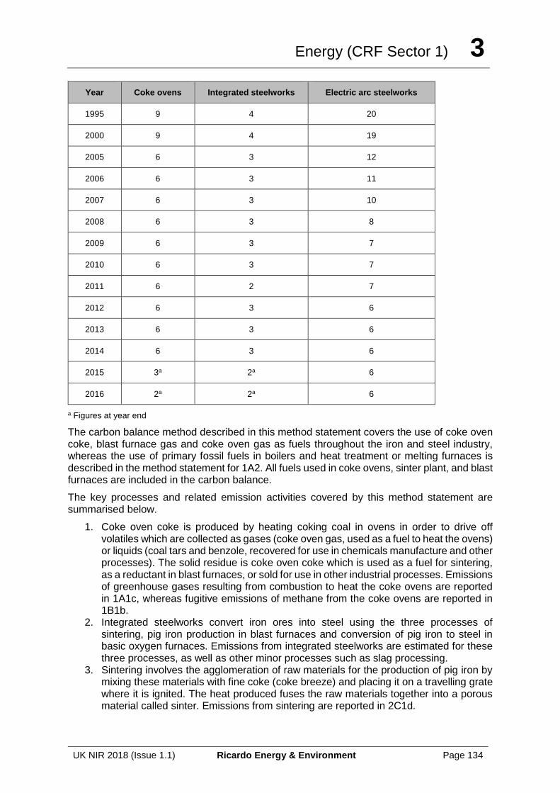
Energy (CRF Sector 1) 3
UK NIR 2018 (Issue 1.1) Ricardo Energy & Environment Page 134
Year Coke ovens Integrated steelworks Electric arc steelworks
1995 9 4 20
2000 9 4 19
2005 6 3 12
2006 6 3 11
2007 6 3 10
2008 6 3 8
2009 6 3 7
2010 6 3 7
2011 6 2 7
2012 6 3 6
2013 6 3 6
2014 6 3 6
2015 3a 2a 6
2016 2a 2a 6
a Figures at year end
The carbon balance method described in this method statement covers the use of coke oven coke, blast furnace gas and coke oven gas as fuels throughout the iron and steel industry, whereas the use of primary fossil fuels in boilers and heat treatment or melting furnaces is described in the method statement for 1A2. All fuels used in coke ovens, sinter plant, and blast furnaces are included in the carbon balance.
The key processes and related emission activities covered by this method statement are summarised below.
1. Coke oven coke is produced by heating coking coal in ovens in order to drive off volatiles which are collected as gases (coke oven gas, used as a fuel to heat the ovens) or liquids (coal tars and benzole, recovered for use in chemicals manufacture and other processes). The solid residue is coke oven coke which is used as a fuel for sintering, as a reductant in blast furnaces, or sold for use in other industrial processes. Emissions of greenhouse gases resulting from combustion to heat the coke ovens are reported in 1A1c, whereas fugitive emissions of methane from the coke ovens are reported in 1B1b.
2. Integrated steelworks convert iron ores into steel using the three processes of sintering, pig iron production in blast furnaces and conversion of pig iron to steel in basic oxygen furnaces. Emissions from integrated steelworks are estimated for these three processes, as well as other minor processes such as slag processing.
3. Sintering involves the agglomeration of raw materials for the production of pig iron by mixing these materials with fine coke (coke breeze) and placing it on a travelling grate where it is ignited. The heat produced fuses the raw materials together into a porous material called sinter. Emissions from sintering are reported in 2C1d.
Energy (CRF Sector 1) 3
UK NIR 2018 (Issue 1.1) Ricardo Energy & Environment Page 135
4. Blast furnaces are used to reduce the iron oxides in iron ore to iron. They are continuously charged with a mixture of sinter, fluxing agents such as limestone, and reducing agents such as coke, fuel oil and coal. Hot air is blown into the lower part of the furnace and reacts with the reducing agent, producing carbon monoxide, which reduces the iron ore to iron.
5. Gas leaving the top of the blast furnace has a high heat value because of the residual CO content, and is used as a fuel in the steelworks. Molten iron and liquid slag are withdrawn from the base of the furnace. The most significant greenhouse gas emissions to occur directly from the blast furnace process are the combustion gases from the 'hot stoves' used to heat the blast air.
6. These generally use blast furnace gas, together with coke oven gas and/or natural gas as fuels. These emissions are reported under CRF category 1A2. Gases emitted from the top of the blast furnace are collected and emissions should only occur when this gas is subsequently used as fuel. These emissions are allocated to the process using them. However, some blast furnace gas is lost and the carbon content of this gas is reported under CRF category 2C1.
7. Pig iron has a high carbon content derived from the coke used in the blast furnace. A substantial proportion of this must be removed to make steel and this is done in the basic oxygen furnace. Molten pig iron is charged to the furnace and oxygen is blown through the metal to oxidise carbon and other contaminants. As a result, carbon monoxide and carbon dioxide are emitted from the furnace and are collected for use as a fuel. As with blast furnace gases, some losses occur and these losses are reported with blast furnace gas losses under CRF category 2C1. In DUKES, basic oxygen furnace gas is combined with blast furnace gas and so separate figures for production and use of the two gases are not given.
8. The fuels derived in coke ovens and integrated steelworks are used in boilers and in heat treatment or melting furnaces and CO2 emissions from these energy uses are calculated using emission factors derived using the carbon balance.
Key Data sources
Activity Data: Main sources of activity data (fuel use, production data) are DUKES (BEIS, 2017), ISSB annual statistics (ISSB, 2017), installation-specific activity data from EU ETS (EA, NRW, both 2017), operator information for integrated steelworks (Tata Steel and SSI Steel, both 2015)
Emission Factors: Input parameters for the carbon balance method are derived from EU ETS data or operators of integrated steelworks (reference as for AD). Other UK CS CEFs are derived from the 2004 Carbon Factors Review (Baggott et al., 2004). EFs for non-CO2 gases are predominantly IPCC defaults (IPCC 2006), Baggott et al., 2004.
An accompanying spreadsheet “Energy_background_data_uk_2018.xlxs” lists all emission factors used in the energy sector, including a full list of references25. Table 1.6 gives additional information for common activity data sources.
Method approach
The carbon balance for the combined coke ovens and integrated steelmaking processes is based on tracking the carbon through four successive stages – coke making, sintering, pig iron production, and basic oxygen steel production. At each stage carbon is input as fuels and/or feedstocks; carbon leaves in products; is emitted to air or removed as waste products. The carbon flow description and Figure 3.1 below presents a simplified version of the model listing main inputs and outputs:
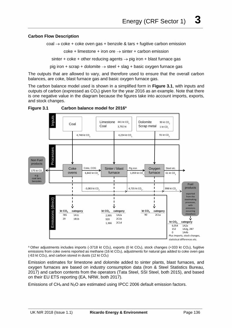
Energy (CRF Sector 1) 3
UK NIR 2018 (Issue 1.1) Ricardo Energy & Environment Page 136
Carbon Flow Description
coal coke + coke oven gas + benzole & tars + fugitive carbon emission
coke + limestone + iron ore sinter + carbon emission
sinter + coke + other reducing agents pig iron + blast furnace gas
pig iron + scrap + dolomite steel + slag + basic oxygen furnace gas
The outputs that are allowed to vary, and therefore used to ensure that the overall carbon balances, are coke, blast furnace gas and basic oxygen furnace gas.
The carbon balance model used is shown in a simplified form in Figure 3.1, with inputs and outputs of carbon (expressed as CO2) given for the year 2016 as an example. Note that there is one negative value in the diagram because the figures take into account imports, exports, and stock changes.
Figure 3.1 Carbon balance model for 2016a
a Other adjustments includes imports (-3718 kt CO2), exports (0 kt CO2), stock changes (+333 kt CO2), fugitive emissions from coke ovens reported as methane (16 kt CO2), adjustments for natural gas added to coke oven gas (-63 kt CO2), and carbon stored in dusts (12 kt CO2)
Emission estimates for limestone and dolomite added to sinter plants, blast furnaces, and oxygen furnaces are based on industry consumption data (Iron & Steel Statistics Bureau, 2017) and carbon contents from the operators (Tata Steel, SSI Steel, both 2015), and based on their EU ETS reporting (EA, NRW, both 2017).
Emissions of CH4 and N2O are estimated using IPCC 2006 default emission factors.
Coke
ovens
Sinter / blast
furnace
Oxygen
furnace
CoalLimestone 437 kt CO2
Coal 2,736 kt CO2
Dolomite 98 kt CO2
Scrap metal 7 kt CO2
3,173 kt CO2 105 kt CO2
Coke, COG Pig iron
1,142 kt CO2
Steel etc.
3,036 kt CO2 5,891 kt CO2 1,068 kt CO2
kt CO2 category
1,241 1A1c
111 1B1b
Inp
uts
Pro
ce
sse
s
14,396 kt CO2
9,491 kt CO281 kt CO2
Non Fuel
products
517 kt CO2
e.g.
coal tars,
benzoles
Fuel
products
exported from the
steelmaking processes,
with emissions occurring elsewhere
kt CO2 category
4,166 1A2a
437 2A3
1,028 2C1
kt CO2 category
98 2A3
kt CO2 category
6,984 1A2a
147 1A2f
27 1A4bPlus exports, stock changes,
statistical differences etc.
Em
issio
ns (
dire
ct)
4,234 kt CO2 4,748 kt CO
2
441 kt CO2
3,792 kt
CO 91 kt CO
2
6,842 kt CO2 1,059 kt CO
2 61 kt CO
2
175 kt CO2
90 kt CO2
1 kt CO2
785
29 1A1c
1B1b
2,995
920
1,366
1A2a
2C1b
2C1d
90
2C1a
6,054
152 0
1A2a
1A2g, 2B7 1A4b
-3,083 kt CO2 4,735 kt CO
2 998 kt CO
2
Plus imports, stock changes,
statistical differences etc.
Energy (CRF Sector 1) 3
UK NIR 2018 (Issue 1.1) Ricardo Energy & Environment Page 137
Assumptions & observations
A detailed description of the carbon balance methodology has been given in Ricardo-AEA, GHG Inventory Research: Use of EU ETS Data - Iron & Steel Sector, Chemical Industry Feedstock Use, April 2014 (available for download on the NAEI website27
) and so only a brief summary of assumptions is given here.
The carbon balance method requires the carbon content in input fuels and feedstocks to be estimated using consumption data and carbon contents for each fuel or feedstock. The balance is then used to distribute that carbon amongst the various derived fuels, products and wastes from the coke ovens and steelmaking processes. The total emission of CO2 is therefore dependent upon the assumptions made about the quantity of carbon in inputs, and in the main input – coking coal – in particular. The carbon content of coking coal and blast furnace coal has, in recent years, been measured by operators as a result of their need to collect data for EU ETS reporting purposes, and operators have also been able to supply high quality measurement-based data for the carbon contents of derived fuels, coal tars, benzole, limestone, dolomite, steel scrap, and steel product. The EU ETS data indicate that the carbon contents of fuels do not vary greatly from one year to another and therefore, for earlier years, where EU ETS data are not available, carbon factors are assumed to be the same as for those years where EU ETS data are available. For each fuel, the average carbon content is calculated for years with EU ETS reporting, and these values then used for the earlier years.
The operators also supply data on the consumption and production of fuels and these data should be consistent with UK energy statistics. This is largely so, but in a couple of instances where the UK statistics seem to underestimate consumption of a particular fuel in a particular year, we have used the operators' data instead. For example, operator data for the consumption of coking coal in coke ovens for the years 2003-2016 is mostly higher than the figures given in DUKES, and the operator data are used in preference. The coal consumption figures for other industrial use are also modified by an equal and opposite amount so that overall coal consumption in the GHGI is the same as in DUKES. DUKES also excludes a small quantity of coke oven gas generated at one steelworks which is then supplied as a fuel to a co-located process, and so we have used operator data on this fuel in the inventory. In this case, it would not be appropriate to maintain consistency with overall UK demand figures in DUKES (since this fuel is missing from DUKES, not classified to a different sector). Finally, some small deviations are made for 2009, where operator data on consumption of coal and coke oven coke in blast furnaces are somewhat higher. The changes to coal are treated as misallocations in DUKES (so UK totals for coal consumption are adhered to), whereas for coke oven coke, it is necessary to increase UK consumption to above the level given in DUKES, since coke consumption by known users exceeds the DUKES figure.
Recalculations
There have only been minor recalculations due to revisions to UK energy statistics and other input data.
Improvements (completed and planned)
There have been no changes to the methodology for this version of the inventory, and no improvement work is planned, though all input data and assumptions are kept under review.
27 https://uk-air.defra.gov.uk/assets/documents/reports/cat19/1405081135_GHG_Inventory_Research_Report_EUETS_final.pdf
Energy (CRF Sector 1) 3
UK NIR 2018 (Issue 1.1) Ricardo Energy & Environment Page 138
QA/QC
Specific QA/QC and validation exercises relevant to these source categories include:
• the comparison of the reference/sectoral approach;
• comparison of inventory estimates based on the carbon balance, with EU ETS data and detailed emission estimates provided by the operators;
• comparison of DUKES data with industry-reported activity data (e.g. from ISSB);
• comparison of carbon emission factors derived from the carbon balance, with IPCC default emission factors; and,
• checks on the time-series consistency of carbon emission factors generated by the carbon balance method.
The energy AD used in these estimates that come from DUKES are subject to the UK Statistics Authority’s Official Statistics Code of Practice26. EU ETS data is subject to its own QA process. A bilateral exchange was undertaken in May 2015 with the inventory agency from Germany, which included a review of the revisions to the iron and steel sector method in the 2014 submission.
Time series consistency
All activity data used are available for the full time series of the estimates. Carbon factors for key inputs such as coking coal and blast furnace coal are available from operators only for recent years (2005 onwards in the case of coking coal, 2007 onwards for other fuels) so the same values must be assumed to be appropriate in earlier years. Data were not available for 2015 and 2016, partly due to the Teesside works closing in September of that year, and the sale of the Scunthorpe works to a new operator in early 2016, so 2014 values have been assumed to be correct for 2015-2016 as well. While this does introduce some additional uncertainty for parts of the time-series, the assumed factors for coking coal and blast furnace coal, and the derived factors for coke oven coke, coke oven gas and blast furnace gas for these years are all within the ranges suggested in the IPCC 2006 Guidelines.
Uncertainties
Uncertainties for both activity and emission factors are based on expert judgement. The uncertainty analysis set out in Annex 2 provides details of these uncertainty values. Uncertainties in fuel use statistics are typically low. The carbon emission factors are based on UK specific data. Since there is a direct link between the carbon emitted and the carbon content of the fuel, it is possible to estimate CO2 emissions accurately.
MS 5 Other stationary combustion
Relevant Categories, source names
1A4ai: Miscellaneous industrial/commercial combustion
Public sector combustion
Railways - stationary combustion
1A4bi: Domestic combustion
1A4ci: Agriculture - stationary combustion
Miscellaneous industrial/commercial combustion
Relevant Gases
CO2, CH4, N2O
Energy (CRF Sector 1) 3
UK NIR 2018 (Issue 1.1) Ricardo Energy & Environment Page 139
Relevant fuels, activities
Anthracite, Burning oil, Charcoal, Coal, Coke, Fuel oil, Gas oil, LPG, Natural gas, Peat, Petroleum coke, Straw, Wood, SSF
Background
This method statement covers emissions from fuel combustion by non-industrial sectors including commercial, agricultural public sector and residential. Most stationary plants are small-scale, apart from a few large installations providing energy for large commercial or public sector buildings (e.g. banks, hospitals, schools, sport centres). Emissions from stationary railway sources are reported under 1A4a where the fuel is used in stationary combustion of burning oil and fuel oil to heat buildings, as well as natural gas combustion. This gas usage may include fuel used for electricity generation for own use by the railway sector. The ‘miscellaneous’ source includes energy use by a range of other users including the sewage and refuse disposal sector, and fuels used by television and radio broadcasters.
Key Data sources
Activity: DUKES (BEIS, 2017)
Emission factors: Baggott et al., 2004, IPCC, 2006
An accompanying spreadsheet “Energy_background_data_uk_2018.xlxs” lists all emission factors used in the energy sector, including a full list of references25. Table 1.6 gives additional information for common activity data sources.
Method approach
Emissions for this category are calculated based multiplying activity data by an emission factor. Activity data are taken directly from DUKES, with a few exceptions (see assumptions and observations). A full list of emission factors is included in Annex 3. Carbon emission factors are largely UK specific, whereas non-CO2 emissions use default emission factors.
Assumptions & observations
The NAEI source public service includes emissions from stationary combustion at military installations, which should ideally be reported under 1A5a Stationary. However, we do not have separate data for the military fuel component.
Bottom up estimates are made for a number of categories using gas oil (railways, off road machinery etc.). In order to reconcile the gas oil used in these categories with the total in DUKES, reallocations (subtractions) are made from other categories, including AD used for the estimates of 1A4. These deviations from DUKES are presented in Annex 4.
Activity data estimates for domestic sector use of fuels derived from petroleum coke are based on annual estimates provided by industry experts (CPL, 2015).
Recalculations
There have been no changes to methods. The following summarises the recalculations:
• Any revisions to DUKES and other input data have been incorporated into the inventory. This included some knock-on impacts from revisions to fuel use estimates for shipping – see MS10 for details. DUKES also made revisions to natural gas figures for 2008 onwards, resulting in re-allocation of some gas from 1A4a to 1A2, as well as revisions to the figures for domestic sector gas use for recent years;
• A change has been made to the method for processing many methane and nitrous oxide emission factors for the NAEI database, as well as carbon factors for domestic
Energy (CRF Sector 1) 3
UK NIR 2018 (Issue 1.1) Ricardo Energy & Environment Page 140
use of peat. Emission factors are now imported in the original units as presented in the literature source for the factors, and converted to NAEI units (mass units for liquid and solid fuels, Mth for gaseous fuels) centrally in the database. This forces consistency in assumptions across pollutants, and allows for the time series to vary where the calorific values change from year to year. For many factors, there are very small changes due to using a time-series of year-specific Calorific Values (CVs) instead of a fixed year or average of years’ CV, but these changes have a trivial impact on overall UK emissions.
The impact of changes is set out in Chapter 10.
Improvements (completed and planned)
No improvements to this method are currently planned. Emission factors and activity data are kept under review.
QA/QC
This source category is covered by the general QA/QC of the greenhouse gas inventory in Section 1.6. Fuel combustion estimates are verified through the comparison of the reference and sectoral approaches.
The energy AD used in these estimates that come from DUKES are subject to the UK Statistics Authority’s Official Statistics Code of Practice26.
For gas oil, bottom up estimates are made for various sources, which leads to changes in the sectoral allocations within DUKES. There are no official top down statistics to verify the bottom up statistics, however, the totals are reconciled with DUKES. Pet coke and peat data are outside of DUKES, but are small emission sources included for completeness.
Time series consistency
Emission factors and activity data are taken from consistent data sets, there are no time series consistency issues to note.
Uncertainties
Uncertainties for both activity and emission factors are based on expert judgement. The uncertainty analysis set out in Annex 2 provides details of these uncertainty values. There are no additional official statistics to compare the category specific fuel use for 1A4 with, as such it is difficult to verify the activity data allocations in DUKES. As such the uncertainty for the sources included in this MS will be higher than for power stations, for example. Uncertainties in total fuel use statistics are typically low. The carbon emission factors are based on UK specific data. Since there is a direct link between the carbon emitted and the carbon content of the fuel, it is possible to estimate CO2 emissions accurately. Non-CO2 emissions are dependent on a greater number of parameters, and are largely based on defaults. As such, the uncertainties are higher, but since the emissions are smaller, this does not have a significant impact on the overall uncertainty of total GHG emissions.
MS 6 Off road machinery
Relevant Categories, source names
1A2gvii: Industrial off-road mobile machinery
1A3eii: Aircraft - support vehicles
1A4bii: House and garden machinery
Energy (CRF Sector 1) 3
UK NIR 2018 (Issue 1.1) Ricardo Energy & Environment Page 141
1A4cii: Agriculture - mobile machinery
Relevant Gases
CO2, CH4, N2O
Relevant fuels, activities
DERV, Gas oil, Petrol
Background
This MS includes all emissions from off road machinery. These are compiled in a single model, and the outputs reported in the IPCC categories set out above.
Emissions are estimated for 77 different types of portable or mobile equipment powered by diesel or petrol driven engines. These range from machinery used in agriculture such as tractors and combine harvesters; industry such as portable generators, forklift trucks and air compressors; construction such as cranes, bulldozers and excavators; domestic lawn mowers; aircraft support equipment. In the inventory they are grouped into four main categories:
• Domestic house & garden – reported under 1A4b;
• Agricultural power units (includes forestry) – reported under 1A4c;
• Industrial off-road (includes construction and quarrying) – reported under 1A2gvii; and
• Aircraft support machinery – reported under 1A3e.
Key Data sources
Activity: Netcen, 2004, ONS, UKMY, BEIS Projections (pers. comm.), CAA
Emission factors: Baggott et al., 2004, EMEP-EEA Guidebook, EU Non-Road Mobile Machinery Directive.
An accompanying spreadsheet “Energy_background_data_uk_2018.xlsx” lists all emission factors used in the energy sector, including a full list of references25. Table 1.6 gives additional information for common activity data sources.
Method approach
A Tier 3 methodology is used for calculating emissions from individual types of mobile machinery. Default machinery or engine-specific fuel consumption and emission factors (g/kWh) are taken from EMEP-EEA Guidebook. For methane, emission factors for more modern machinery based on engine or machinery-specific emission limits for total hydrocarbons established in EU Non-Road Mobile Machinery Directive are also included where available. The measures introduced to reduce total hydrocarbon emissions are assumed to effect methane emissions. Activity data are based on bottom-up estimates of equipment numbers and hours of use in 2004 (Netcen, 2004). Various proxy statistics are used as activity drivers for different groups of machinery types to estimate fuel consumption across the full time series.
Emissions are calculated from a bottom-up approach using machinery- or engine-specific emission factors in g/kWh based on the power of the engine and estimates of the UK population and annual hours of use of each type of machinery. The emission estimates are calculated using a modification of the methodology given in EMEP/ EEA (2009).
The population, usage and lifetime of different types of off-road machinery were updated following a study carried out by the Inventory Agency on behalf of the Department for Transport (Netcen, 2004). This study researched the current UK population, annual usage
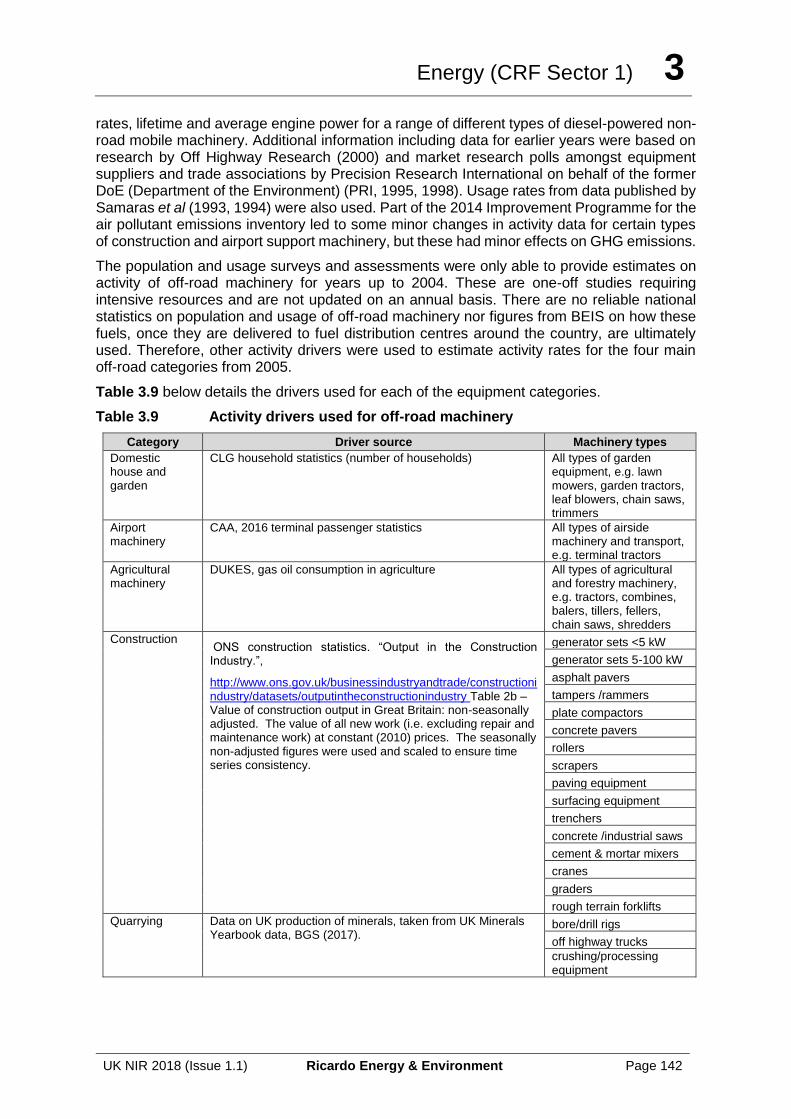
Energy (CRF Sector 1) 3
UK NIR 2018 (Issue 1.1) Ricardo Energy & Environment Page 142
rates, lifetime and average engine power for a range of different types of diesel-powered non-road mobile machinery. Additional information including data for earlier years were based on research by Off Highway Research (2000) and market research polls amongst equipment suppliers and trade associations by Precision Research International on behalf of the former DoE (Department of the Environment) (PRI, 1995, 1998). Usage rates from data published by Samaras et al (1993, 1994) were also used. Part of the 2014 Improvement Programme for the air pollutant emissions inventory led to some minor changes in activity data for certain types of construction and airport support machinery, but these had minor effects on GHG emissions.
The population and usage surveys and assessments were only able to provide estimates on activity of off-road machinery for years up to 2004. These are one-off studies requiring intensive resources and are not updated on an annual basis. There are no reliable national statistics on population and usage of off-road machinery nor figures from BEIS on how these fuels, once they are delivered to fuel distribution centres around the country, are ultimately used. Therefore, other activity drivers were used to estimate activity rates for the four main off-road categories from 2005.
Table 3.9 below details the drivers used for each of the equipment categories.
Table 3.9 Activity drivers used for off-road machinery
Category Driver source Machinery types
Domestic house and garden
CLG household statistics (number of households) All types of garden equipment, e.g. lawn mowers, garden tractors, leaf blowers, chain saws, trimmers
Airport machinery
CAA, 2016 terminal passenger statistics All types of airside machinery and transport, e.g. terminal tractors
Agricultural machinery
DUKES, gas oil consumption in agriculture All types of agricultural and forestry machinery, e.g. tractors, combines, balers, tillers, fellers, chain saws, shredders
Construction ONS construction statistics. “Output in the Construction Industry.”,
http://www.ons.gov.uk/businessindustryandtrade/constructionindustry/datasets/outputintheconstructionindustry Table 2b – Value of construction output in Great Britain: non-seasonally adjusted. The value of all new work (i.e. excluding repair and maintenance work) at constant (2010) prices. The seasonally non-adjusted figures were used and scaled to ensure time series consistency.
generator sets <5 kW
generator sets 5-100 kW
asphalt pavers
tampers /rammers
plate compactors
concrete pavers
rollers
scrapers
paving equipment
surfacing equipment
trenchers
concrete /industrial saws
cement & mortar mixers
cranes
graders
rough terrain forklifts
Quarrying Data on UK production of minerals, taken from UK Minerals Yearbook data, BGS (2017).
bore/drill rigs
off highway trucks
crushing/processing equipment
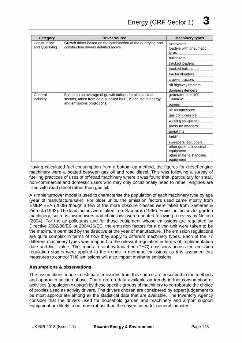
Energy (CRF Sector 1) 3
UK NIR 2018 (Issue 1.1) Ricardo Energy & Environment Page 143
Category Driver source Machinery types
Construction and Quarrying
Growth driver based on the combination of the quarrying and construction drivers detailed above.
excavators
loaders with pneumatic tyres
bulldozers
tracked loaders
tracked bulldozers
tractors/loaders
crawler tractors
off highway tractors
dumpers /tenders
General Industry
Based on an average of growth indices for all industrial sectors, taken from data supplied by BEIS for use in energy and emissions projections.
generator sets 100-1000KW
pumps
air compressors
gas compressors
welding equipment
pressure washers
aerial lifts
forklifts
sweepers/ scrubbers
other general industrial equipment
other material handling equipment
Having calculated fuel consumption from a bottom-up method, the figures for diesel engine machinery were allocated between gas oil and road diesel. This was following a survey of fuelling practices of uses of off-road machinery where it was found that, particularly for small, non-commercial and domestic users who may only occasionally need to refuel, engines are filled with road diesel rather than gas oil.
A simple turnover model is used to characterise the population of each machinery type by age (year of manufacture/sale). For older units, the emission factors used came mostly from EMEP-EEA (2009) though a few of the more obscure classes were taken from Samaras & Zierock (1993). The load factors were taken from Samaras (1996). Emission factors for garden machinery, such as lawnmowers and chainsaws were updated following a review by Netcen (2004). For the air pollutants and for those equipment whose emissions are regulated by Directive 2002/88/EC or 2004/26/EC, the emission factors for a given unit were taken to be the maximum permitted by the directive at the year of manufacture. The emission regulations are quite complex in terms of how they apply to different machinery types. Each of the 77 different machinery types was mapped to the relevant regulation in terms of implementation date and limit value. The trends in total hydrocarbon (THC) emissions across the emission regulation stages were applied to the trends in methane emissions as it is assumed that measures to control THC emissions will also impact methane emissions.
Assumptions & observations
The assumptions made to estimate emissions from this source are described in the methods and approach section above. There are no data available on trends in fuel consumption or activities (population x usage) by these specific groups of machinery to corroborate the choice of proxies used as activity drivers. The drivers chosen are considered by expert judgement to be most appropriate among all the statistical data that are available. The Inventory Agency consider that the drivers used for household garden and machinery and airport support equipment are likely to be more robust than the drivers used for general industry.
Energy (CRF Sector 1) 3
UK NIR 2018 (Issue 1.1) Ricardo Energy & Environment Page 144
A fuel reconciliation procedure is followed for gas oil which takes account of consumption from all sources, as described in Annex 4. For the industrial and construction machinery, the fuel reconciliation process essentially overrides any changes in estimates of fuel consumption calculated from the bottom-up procedure arising from the 2014 review of activity data for some selected machinery types. However, this review still affects the emissions of methane by leading to changes in implied emission factors for these machinery types, e.g. through revisions to the lifetime and turnover in the machinery fleet.
Recalculations
There have been no changes to the method.
The main re-calculation is due to changes in fuel consumption for industrial and construction mobile machinery affecting 1A2gvii arising from the re-allocation of changed gas oil activity data in DUKES. The changes to this sector are made to retain fuel mass balance with DUKES and are affected by changes made to other sectors using gas oil.
Minor re-calculations arise from:
• Revision to DUKES gas oil consumed in agriculture used as a driver for the agricultural machinery sector. The 2014 and 2015 values are 36% greater than the previous values used.
• Consideration of emissions from Stage IIIA forklifts and dumpers. This affects emission factors from 2006 and the impact increases roughly steadily each year from 2006 as more Stage IIIA machines enter the fleet. This change leads to an increase in emissions from industrial machinery 1A2gvii (around 0.5% in 2006-2008 up to around 2-5% for 2012-2015) but is variable by pollutant.
Improvements (completed and planned)
There have been no improvements completed for this submission. It is being considered to develop the model used for how sales and population data are handled for different machinery types.
QA/QC
This source category is covered by the general QA/QC of the greenhouse gas inventory in Section 1.6.
An expert judgement quality check has been done to verify that the amount of gas oil used by off-road machinery estimated from the bottom-up approach is neither excessively high or low as a proportion of total UK gas oil available for consumption as given in DUKES.
Time series consistency
Although the bottom up data for machinery population and usage is only available for one year, the proxy statistics used to generate the time series are consistent across the time series.
Uncertainties
Fuel consumption by these off-road machinery sources is not provided in DUKES so is estimated for each machinery type from a bottom-up Tier 3 approach to derive machinery population and usage rates. See Section 3.2.4 for information. There are no centralised statistics on machinery population and usage so the uncertainties are considered quite high. An overall fuel balance taking account of consumption by other uses of gas oil, diesel and petrol ensures consistency with total consumption figures in DUKES. Various proxy data are used to establish a consistent time-series in activity rates, as explained in this section.
Energy (CRF Sector 1) 3
UK NIR 2018 (Issue 1.1) Ricardo Energy & Environment Page 145
The highest uncertainties are considered to be in the estimates for general industrial machinery as these cover a wide range of machinery types of a fairly diffuse nature, e.g. portable generators. The estimates in the year-to-year trends for this particular off-road source are also influenced by the uncertainties in the other sources using gas oil via the fuel reconciliation step. Uncertainties in the trends for the other off-road sources (domestic house and garden, airport machinery and agricultural machinery) are considered to be smaller and less biased by the choice of proxy data.
MS 7 Aviation
Relevant Categories, source names
1A3a: Aviation
International bunkers - Aviation
Relevant Gases
CO2, CH4, N2O
Relevant fuels, activities
Aviation turbine fuel (jet kerosene), Aviation spirit (aviation gasoline)
Background
In accordance with the agreed guidelines, the UK inventory contains estimates for both domestic and international civil aviation. Emissions from international aviation are recorded as a memo item, and are not included in national totals. Emissions from both the Landing and Take-Off (LTO) phase and the Cruise phase (including climb and descent) are estimated. Emissions of a range of pollutants are estimated in addition to the reported greenhouse gases. The method reflects differences between airports and the aircraft that use them. In addition to aircraft main engines exhaust, emissions from aircraft auxiliary power units are also included. A full description is given in Watterson et al. (2004). The method used to estimate emissions from military aviation can be found in MS 160.
Key Data sources
Activity data: CAA (2017a), CAA (2017b), BEIS (2017), DfT (2017)
Emission Factors: Baggott et al., 2004, EMEP/EEA, 2016 IPCC, 1997
An accompanying spreadsheet “Energy_background_data_uk_2018.xlsx” lists all emission factors used in the energy sector, including a full list of references25. In addition, Annex 3 includes a table to map all aircraft types evident in UK activity data from the CAA to the EMEP-EEA Guidebook aircraft categories.
Table 1.6 gives additional information for common activity data sources.
Method approach
Estimates are based on IPCC Tier 3 and use the number of aircraft movements broken down by aircraft type at each UK airport.
Activity data
The methods used to estimate emissions from aviation require the following activity data:

Energy (CRF Sector 1) 3
UK NIR 2018 (Issue 1.1) Ricardo Energy & Environment Page 146
• Aircraft movements and distances travelled
Detailed activity data has been provided by the UK Civil Aviation Authority (CAA). These data include aircraft movements broken down by: airport; aircraft type; whether the flight is international or domestic; and, the next/last POC (port of call) from which sector lengths (great circle) have been calculated. The data covered all Air Transport Movements (ATMs) excluding air-taxi. The CAA also compiles summary statistics at reporting airports, which include air-taxi and non-ATMs.
• Inland Deliveries of Aviation Turbine Fuel and Aviation Spirit
Total inland deliveries of aviation spirit and aviation turbine fuel to air transport are given in DUKES (BEIS (2017)). This is the best approximation of aviation bunker fuel consumption available and is assumed to cover international, domestic and military use.
• Consumption of Aviation Turbine Fuel and Aviation Spirit by the Military
These data are supplied by the Ministry of Defence (MoD). Military aviation estimates are included in MS 16. The data for total fuel use for military aviation is used in the normalisation to the DUKES total.
Calendar year activity data are derived from the data sources described above.
Table 3.10 Aircraft Movement Data: LTOs and Cruise distances for Domestic and International Flights from UK Airports, 1990-2016
Year International LTOs
(000s) Domestic LTOs
(000s) International
Aircraft, Gm flown Domestic Aircraft,
Gm flown
1990 460.5 377.0 652.0 116.4
1995 530.9 365.3 849.0 118.3
2000 704.3 407.1 1190.7 145.2
2005 800.5 488.2 1447.6 178.7
2010 734.0 393.9 1395. 146.4
2015 821.7 356.0 1565.8 135.0
2016 874.6 349.5 1675.5 133.7
Gm Giga metres, or 109 metres
Estimated emissions from aviation are based on data provided by the CAA and, for overseas territories, the DfT.
Gm flown calculated from total flight distances for departures from UK and overseas territories airports.
Emission factors used
A combination of national airport specific LTO factors (derived from local airport studies) and EMEP/EEA Eurocontrol cruise factors for generic aircraft are used.
An accompanying spreadsheet “Energy_background_data_uk_2018.xlsx” lists all emission factors used in the energy sector, including aviation, and associated references. Carbon emission factors are country specific, whereas defaults are used for other gases.
Method
The basic approach to estimating emissions from the LTO cycle is as follows. The contribution to aircraft exhaust emissions (in kg) arising from a given mode of aircraft operation (see list below) is given by the product of the duration (seconds) of the operation, the engine fuel flow
Energy (CRF Sector 1) 3
UK NIR 2018 (Issue 1.1) Ricardo Energy & Environment Page 147
rate at the appropriate thrust setting (kg fuel per second) and the emission factor for the pollutant of interest (kg pollutant per kg fuel).
The annual emissions total for each mode (kg per year) is obtained by summing contributions over all engines for all aircraft movements in the year. The time in each mode of operation for each type of airport and aircraft has been taken from individual airport studies. The time in mode is multiplied by an emission rate (the product of fuel flow rate and emission factor) at the appropriate engine thrust setting in order to estimate emissions for phase of the aircraft flight. The sum of the emissions from all the modes provides the total emissions for a particular aircraft journey. The modes considered are:
• Taxi-out;
• Hold;
• Take-off Roll (start of roll to wheels-off);
• Initial-climb (wheels-off to 450 m altitude);
• Climb-out (450 m to 1000 m altitude);
• Approach (from 1000 m altitude);
• Landing-roll;
• Taxi-in;
• Auxiliary Power Unit (APU) use after arrival; and
• APU use prior to departure.
Departure movements comprise the following LTO modes: taxi-out, hold, take-off roll, initial-climb, climb-out and APU use prior to departure.
Arrivals comprise: approach, landing-roll, taxi-in and APU use after arrival.
Aircraft often take-off at reduced thrust (i.e. less than 100% thrust). Thrust setting for Take-off roll; Initial-climb; and Climb-out depend on airport and aircraft type and are derived from local airport studies. Thrust setting during Approach are 15% for the initial phase (above 600 ft) and 30% for the final phase (below 600 ft). Depending on airport and aircraft type, the Landing-roll often includes periods or reverse thrust at either at idle or 30%, the remainder of the time is at idle thrust setting. Other modes (Taxi and Hold) are at idle thrust. Idle thrust is nominally 7%, however an adjustment is made to the idle fuel flow to account for engine specific variations.
The approaches to estimating emissions in the cruise are summarised below. Cruise emissions are only calculated for aircraft departures from UK airports (emissions therefore associated with the departure airport), which gives a total fuel consumption compatible with recorded deliveries of aviation fuel to the UK. This procedure prevents double counting of emissions allocated to international aviation.
The EMEP-EEA Emission Inventory Guidebook (EMEP-EEA, 2016) provides fuel consumption and emission data for non-GHGs (NOx, HC and CO) for a number of aircraft cruise modes (climb cruise and descent). The data are given for a selection of generic aircraft type and for a number of standard flight distances.
The breakdown of the CAA movement by aircraft type contains a more detailed list of aircraft types than in the EMEP-EEA Emission Inventory Guidebook. Therefore, each specific aircraft type in the CAA data has been assigned to a generic type in the Guidebook. Details of this mapping are given in Table A 3.1.4 in Annex 3.1.4.
Piecewise linear regression has been applied to these data to give fuel consumption as a function of distance:
𝐹𝐶_𝐶𝑟𝑢𝑖𝑠𝑒𝑑,𝑔,𝑝 = 𝑚𝑔,𝑝 × 𝑑 + 𝑐𝑔,𝑝
Energy (CRF Sector 1) 3
UK NIR 2018 (Issue 1.1) Ricardo Energy & Environment Page 148
Where:
𝐹𝐶_𝐶𝑟𝑢𝑖𝑠𝑒𝑑,𝑔,𝑝 is the fuel consumption in cruise of pollutant 𝑝 for generic aircraft
type 𝑔 and flight distance 𝑑 (kg)
𝑔 is the generic aircraft type
𝑝 is the pollutant (or fuel consumption)
𝑚𝑔,𝑝 is the slope of regression for generic aircraft type 𝑔 and pollutant 𝑝
(kg / km)
𝑐𝑔,𝑝 is the intercept of regression for generic aircraft type 𝑔 and pollutant
𝑝 (kg)
Estimates of CO2 were derived from estimates of fuel consumed in the cruise (see equation above) and the carbon contents of the aviation fuels. Methane emissions are believed to be negligible at cruise altitudes (IPCC, 2006).
Estimates of N2O have been derived from an emission factor recommended by the IPCC (IPCC, 1997) and the estimates of fuel consumed in the cruise (see equation above).
The estimates of aviation fuels consumed in the commodity balance table in the BEIS publication DUKES are the national statistics on fuel consumption, and IPCC guidance states that national total emissions must be on the basis of fuel sales. Therefore, the estimates of emissions have been re-normalised based on the results of the comparison between the fuel consumption data in DUKES and the estimate of fuel consumed produced from the civil aviation emissions model, having first scaled up the emissions and fuel consumption to account for air-taxi and non-ATMs. The scaling is done separately for each airport to reflect the different fractions of air-taxi and non-ATMs at each airport and the different impacts on domestic and international emissions. Air-taxi and non-ATM fuel consumption estimates are not documented by Watterson et al. (2004), as this revision to methodology occurred after publication of the report. The aviation fuel consumptions presented in BEIS DUKES include the use of both civil and military fuel, and the military fuel use must be subtracted from the DUKES total to provide an estimate of the civil aviation consumption. This estimate of civil aviation fuel consumption has been used in the fuel reconciliation. Emissions from flights originating from the overseas territories have been excluded from the fuel reconciliation process as the fuel associated with these flights is not included in DUKES. Emissions will be re-normalised each time the aircraft movement data are modified or data for another year added.
For aviation turbine fuel reconciliation is quite close; pre-normalised fuel estimates generally agree with DUKES within 5%. However, the reconciliation for aviation spirit is poor due to limited coverage of smaller flights by the CAA dataset.
Assumptions & observations
The following modifications are made to the CAA data in order to ensure complete geographical coverage of the inventory and full compliance with the IPCC definitions of domestic and international:
• Flights between the UK and overseas territories are reclassified from international to domestic;
• International flights with an intermediate stop at a domestic airport are considered international in the CAA aircraft movement data. These are reclassified as having a domestic leg and an international leg in response to a recommendation from the UNFCCC centralised review in 2013; and
• The CAA data have been supplemented with data from overseas territories, supplied by DfT.
Energy (CRF Sector 1) 3
UK NIR 2018 (Issue 1.1) Ricardo Energy & Environment Page 149
Recalculations
For recalculations, see improvements listed below (for 2018). There have been no method changes.
Improvements (completed and planned)
A number of improvements have been made to the model over recent years, to include findings from UK specific research. The 2018 inventory submission incorporates revisions to the fuel consumptions assumed for a number of smaller aircraft, particularly for piston aircraft, which consume aviation spirit. Fleet assumptions have also been reviewed, which has led to minor modification of assumptions regarding the choice of some surrogate aircraft data.
A watching brief is kept on developments in emission factors and activity data for all modes of transport.
QA/QC
This source category is covered by the general QA/QC of the greenhouse gas inventory in Section 1.6.
Time series consistency
Consistent data sets and methods are used across the full time series to ensure time series consistency.
Uncertainties
Uncertainties for both activity and emission factors are based on expert judgement. The uncertainty analysis set out in Annex 2 provides details of these uncertainty values. Uncertainties in fuel use statistics are typically low. The carbon emission factors are based on UK specific data. Since there is a direct link between the carbon emitted and the carbon content of the fuel, it is possible to estimate CO2 emissions accurately. Non-CO2 emissions are dependent on a greater number of parameters, and are largely based on defaults. As such, the uncertainties are higher, but since the emissions are smaller, this does not have a significant impact on the overall uncertainty of total GHG emissions.
MS 8 Road Transport
Relevant Categories, source names
1A3bi: Road transport - cars - cold start
Road transport - cars - motorway driving
Road transport - cars - rural driving
Road transport - cars - urban driving
1A3bii: Road transport - LGVs - cold start
Road transport - LGVs - motorway driving
Road transport - LGVs - rural driving
Road transport - LGVs - urban driving
1A3biii: Road transport - buses and coaches - motorway driving
Road transport - buses and coaches - rural driving
Road transport - buses and coaches - urban driving
Energy (CRF Sector 1) 3
UK NIR 2018 (Issue 1.1) Ricardo Energy & Environment Page 150
Road transport - HGV articulated - motorway driving
Road transport - HGV articulated - rural driving
Road transport - HGV articulated - urban driving
Road transport - HGV rigid - motorway driving
Road transport - HGV rigid - rural driving
Road transport - HGV rigid - urban driving
1A3biv: Road transport - mopeds (<50cc 2st) - urban driving
Road transport - mopeds (<50cc 2st) – lubricants use
Road transport - motorcycle (>50cc 2st) - rural driving
Road transport - motorcycle (>50cc 2st) - urban driving
Road transport - motorcycle (>50cc 4st) - motorway driving
Road transport - motorcycle (>50cc 4st) - rural driving
Road transport - motorcycle (>50cc 4st) - urban driving
1A3bv: Road transport - all vehicles LPG use
Relevant Gases
CO2, CH4, N2O
Relevant fuels, activities
Petrol (gasoline), Diesel (DERV), LPG
Background
This MS includes all fuel related emissions from road transport. Emissions from Urea consumption are reported under IPPU, in Chapter 4.
Key Data sources
Activity data: DfT (traffic data, vehicle licensing statistics, ANPR data). Data on petrol and diesel fuels consumed by road transport in the UK are taken from the Digest of UK Energy Statistics (DUKES) published by BEIS and corrected for consumption by off-road vehicles and the very small amount of fuel consumed by the Crown Dependencies included in DUKES (emissions from the Crown Dependencies are calculated elsewhere).
Emission factors: COPERT 5, EMEP/EEA 2016 Emission Inventory Guidebook.
An accompanying spreadsheet “Energy_background_data_uk_2018.xlxs” lists all emission factors used in the energy sector, including a full list of references25. Table 1.6 gives additional information for common activity data sources.
Method approach
A Tier 3 methodology is used for calculating exhaust emissions from passenger cars (1A3bi), light goods vehicles (1A3bii), heavy goods vehicles, buses and coaches (1A3biii) and motorcycles (1A3biv).
Petrol and diesel vehicle fuel consumption (and emissions) are estimated for individual vehicle types from a bottom up approach using an array of traffic statistics and exhaust emission and fuel consumption factors representing real-world performance of vehicles. These estimates
Energy (CRF Sector 1) 3
UK NIR 2018 (Issue 1.1) Ricardo Energy & Environment Page 151
are reconciled to national energy consumption statistics from DUKES. This approach provides estimates that are consistent with the IPCC 2016 Guidelines and includes inherent QA/QC in the comparison of bottom-up traffic activity related estimates and top down fuel sales data.
Emissions from vehicles running on LPG are estimated on the basis of national figures (from DUKES) on the consumption of this fuel by road transport. The CO2 emissions from LPG consumption cannot be broken down by vehicle type because there are no reliable figures available on the total number of vehicles or types of vehicles running on this fuel. It is believed that many vehicles running on LPG are cars and vans converted by their owners and that these conversions are not necessarily reported to vehicle licensing agencies. Figures from DUKES suggest that the consumption of LPG is only a small percentage (<1%) of the total amount of petrol and diesel consumed by road transport and vehicle licensing data suggest a similar percentage of all light duty vehicles run on LPG.
The UK inventory does not currently estimate emissions from vehicles running on natural gas. The number of such vehicles in the UK is extremely small, with most believed to be running in captive fleets on a trial basis in a few areas. Estimates are not made as there are no separate figures from BEIS on the amount of natural gas used by road transport, nor are there useable data on the total numbers and types of vehicles equipped to run on natural gas from vehicle licensing sources. The small amount of gas that is used in the road transport sector would currently be allocated to other sources in DUKES, and therefore the omission of this source does not represent an underestimate in the UK inventory.
Traffic-based emission calculations: an overview
A Tier 3 method is used to calculate fuel consumption and emissions from different types of petrol and diesel vehicles using detailed traffic and fleet information before a final fuel reconciliation is done. Details of the methodology are given in a separate report “Methodology for the UK’s Road Transport Emissions Inventory” (Brown et al (2018)) which will be updated annually covering the current methodology for both greenhouse gases and air pollutants. This describes the very detailed information available on road transport activities in the UK and how these are used in estimating the road transport inventory. Only a brief overview of the approach used and the activity data and emission factors specific to the Greenhouse gases in the current inventory are provided in this report.
Fuel consumption and emissions of CH4 and N2O, as well as the indirect GHGs and air pollutants, NMVOCs, NOx, CO and SO2, from individual vehicle types are calculated from measured emission factors expressed in g/km and road traffic and fleet composition statistics from the Department for Transport. The emission factors are from the COPERT 5 (Emisia, 2016) and EMEP/EEA (2016) Emissions Inventory Guidebook source, expressed as equations relating emission factor to average vehicle speed or road type for different vehicle types compliant with different legislative emission standards (Euro standards).
The type of emissions include:
• Hot exhaust emissions: emissions from the vehicle exhaust when the engine has warmed up to its normal operating temperature.
• Cold start emissions: the excess emissions that occur when a vehicle is started with its engine below its normal operating temperature.
For NMVOCs, evaporative emissions of fuel vapour from petrol-fuelled vehicles are also included.
Emissions are calculated for vehicles of the following types:
• Petrol cars;
• Diesel cars;
• Petrol Light Goods Vehicles (Gross Vehicle Weight (GVW) ≤ 3.5 tonnes);
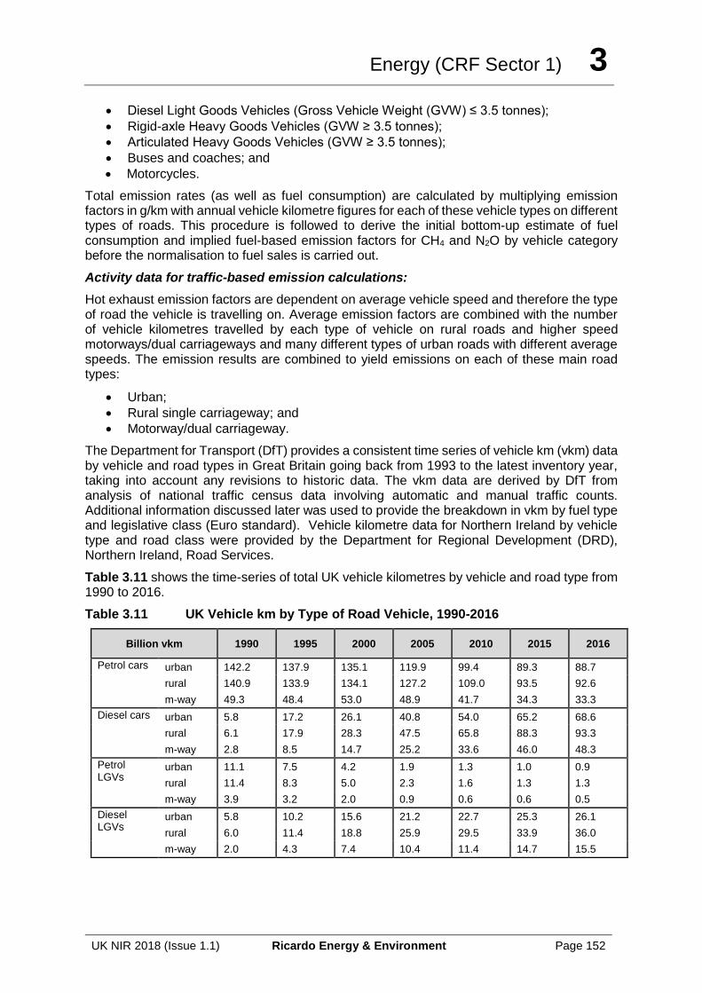
Energy (CRF Sector 1) 3
UK NIR 2018 (Issue 1.1) Ricardo Energy & Environment Page 152
• Diesel Light Goods Vehicles (Gross Vehicle Weight (GVW) ≤ 3.5 tonnes);
• Rigid-axle Heavy Goods Vehicles (GVW ≥ 3.5 tonnes);
• Articulated Heavy Goods Vehicles (GVW ≥ 3.5 tonnes);
• Buses and coaches; and
• Motorcycles.
Total emission rates (as well as fuel consumption) are calculated by multiplying emission factors in g/km with annual vehicle kilometre figures for each of these vehicle types on different types of roads. This procedure is followed to derive the initial bottom-up estimate of fuel consumption and implied fuel-based emission factors for CH4 and N2O by vehicle category before the normalisation to fuel sales is carried out.
Activity data for traffic-based emission calculations:
Hot exhaust emission factors are dependent on average vehicle speed and therefore the type of road the vehicle is travelling on. Average emission factors are combined with the number of vehicle kilometres travelled by each type of vehicle on rural roads and higher speed motorways/dual carriageways and many different types of urban roads with different average speeds. The emission results are combined to yield emissions on each of these main road types:
• Urban;
• Rural single carriageway; and
• Motorway/dual carriageway.
The Department for Transport (DfT) provides a consistent time series of vehicle km (vkm) data by vehicle and road types in Great Britain going back from 1993 to the latest inventory year, taking into account any revisions to historic data. The vkm data are derived by DfT from analysis of national traffic census data involving automatic and manual traffic counts. Additional information discussed later was used to provide the breakdown in vkm by fuel type and legislative class (Euro standard). Vehicle kilometre data for Northern Ireland by vehicle type and road class were provided by the Department for Regional Development (DRD), Northern Ireland, Road Services.
Table 3.11 shows the time-series of total UK vehicle kilometres by vehicle and road type from 1990 to 2016.
Table 3.11 UK Vehicle km by Type of Road Vehicle, 1990-2016
Billion vkm 1990 1995 2000 2005 2010 2015 2016
Petrol cars urban 142.2 137.9 135.1 119.9 99.4 89.3 88.7
rural 140.9 133.9 134.1 127.2 109.0 93.5 92.6
m-way 49.3 48.4 53.0 48.9 41.7 34.3 33.3
Diesel cars urban 5.8 17.2 26.1 40.8 54.0 65.2 68.6
rural 6.1 17.9 28.3 47.5 65.8 88.3 93.3
m-way 2.8 8.5 14.7 25.2 33.6 46.0 48.3
Petrol LGVs
urban 11.1 7.5 4.2 1.9 1.3 1.0 0.9
rural 11.4 8.3 5.0 2.3 1.6 1.3 1.3
m-way 3.9 3.2 2.0 0.9 0.6 0.6 0.5
Diesel LGVs
urban 5.8 10.2 15.6 21.2 22.7 25.3 26.1
rural 6.0 11.4 18.8 25.9 29.5 33.9 36.0
m-way 2.0 4.3 7.4 10.4 11.4 14.7 15.5
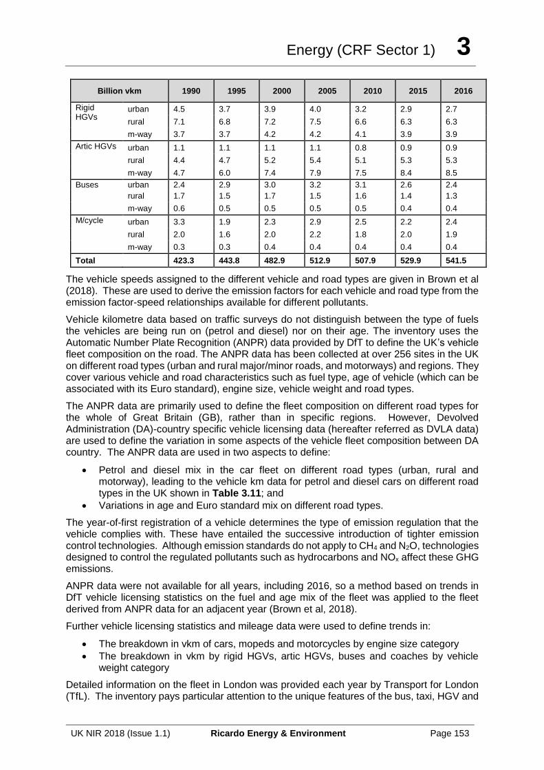
Energy (CRF Sector 1) 3
UK NIR 2018 (Issue 1.1) Ricardo Energy & Environment Page 153
Billion vkm 1990 1995 2000 2005 2010 2015 2016
Rigid HGVs
urban 4.5 3.7 3.9 4.0 3.2 2.9 2.7
rural 7.1 6.8 7.2 7.5 6.6 6.3 6.3
m-way 3.7 3.7 4.2 4.2 4.1 3.9 3.9
Artic HGVs urban 1.1 1.1 1.1 1.1 0.8 0.9 0.9
rural 4.4 4.7 5.2 5.4 5.1 5.3 5.3
m-way 4.7 6.0 7.4 7.9 7.5 8.4 8.5
Buses urban 2.4 2.9 3.0 3.2 3.1 2.6 2.4
rural 1.7 1.5 1.7 1.5 1.6 1.4 1.3
m-way 0.6 0.5 0.5 0.5 0.5 0.4 0.4
M/cycle urban 3.3 1.9 2.3 2.9 2.5 2.2 2.4
rural 2.0 1.6 2.0 2.2 1.8 2.0 1.9
m-way 0.3 0.3 0.4 0.4 0.4 0.4 0.4
Total 423.3 443.8 482.9 512.9 507.9 529.9 541.5
The vehicle speeds assigned to the different vehicle and road types are given in Brown et al (2018). These are used to derive the emission factors for each vehicle and road type from the emission factor-speed relationships available for different pollutants.
Vehicle kilometre data based on traffic surveys do not distinguish between the type of fuels the vehicles are being run on (petrol and diesel) nor on their age. The inventory uses the Automatic Number Plate Recognition (ANPR) data provided by DfT to define the UK’s vehicle fleet composition on the road. The ANPR data has been collected at over 256 sites in the UK on different road types (urban and rural major/minor roads, and motorways) and regions. They cover various vehicle and road characteristics such as fuel type, age of vehicle (which can be associated with its Euro standard), engine size, vehicle weight and road types.
The ANPR data are primarily used to define the fleet composition on different road types for the whole of Great Britain (GB), rather than in specific regions. However, Devolved Administration (DA)-country specific vehicle licensing data (hereafter referred as DVLA data) are used to define the variation in some aspects of the vehicle fleet composition between DA country. The ANPR data are used in two aspects to define:
• Petrol and diesel mix in the car fleet on different road types (urban, rural and motorway), leading to the vehicle km data for petrol and diesel cars on different road types in the UK shown in Table 3.11; and
• Variations in age and Euro standard mix on different road types.
The year-of-first registration of a vehicle determines the type of emission regulation that the vehicle complies with. These have entailed the successive introduction of tighter emission control technologies. Although emission standards do not apply to CH4 and N2O, technologies designed to control the regulated pollutants such as hydrocarbons and NOx affect these GHG emissions.
ANPR data were not available for all years, including 2016, so a method based on trends in DfT vehicle licensing statistics on the fuel and age mix of the fleet was applied to the fleet derived from ANPR data for an adjacent year (Brown et al, 2018).
Further vehicle licensing statistics and mileage data were used to define trends in:
• The breakdown in vkm of cars, mopeds and motorcycles by engine size category
• The breakdown in vkm by rigid HGVs, artic HGVs, buses and coaches by vehicle weight category
Detailed information on the fleet in London was provided each year by Transport for London (TfL). The inventory pays particular attention to the unique features of the bus, taxi, HGV and
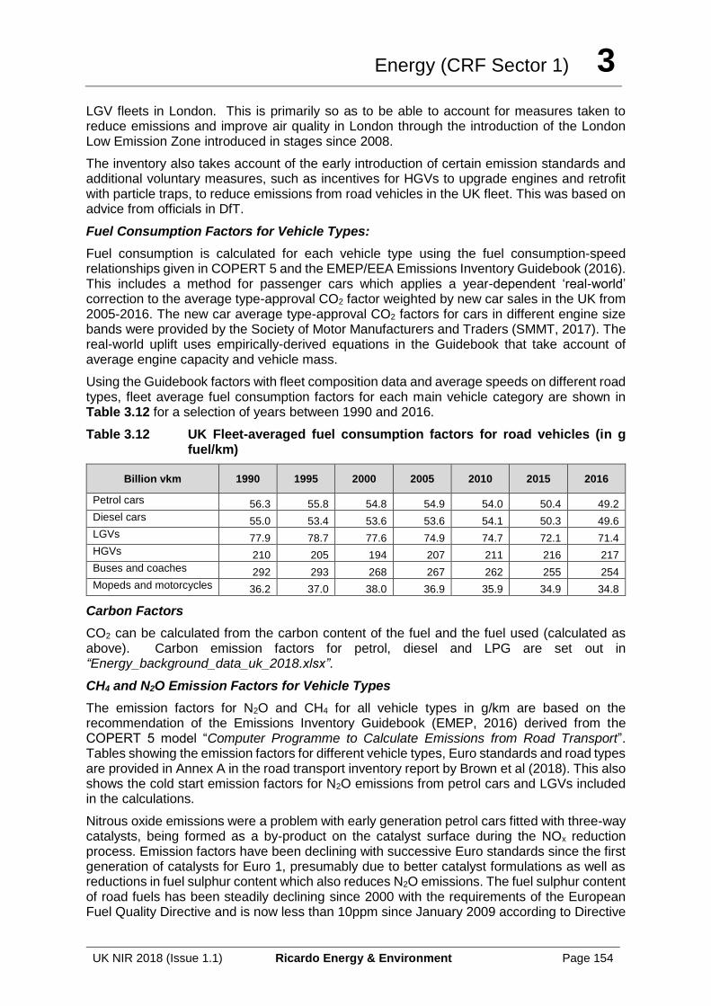
Energy (CRF Sector 1) 3
UK NIR 2018 (Issue 1.1) Ricardo Energy & Environment Page 154
LGV fleets in London. This is primarily so as to be able to account for measures taken to reduce emissions and improve air quality in London through the introduction of the London Low Emission Zone introduced in stages since 2008.
The inventory also takes account of the early introduction of certain emission standards and additional voluntary measures, such as incentives for HGVs to upgrade engines and retrofit with particle traps, to reduce emissions from road vehicles in the UK fleet. This was based on advice from officials in DfT.
Fuel Consumption Factors for Vehicle Types:
Fuel consumption is calculated for each vehicle type using the fuel consumption-speed relationships given in COPERT 5 and the EMEP/EEA Emissions Inventory Guidebook (2016). This includes a method for passenger cars which applies a year-dependent ‘real-world’ correction to the average type-approval CO2 factor weighted by new car sales in the UK from 2005-2016. The new car average type-approval CO2 factors for cars in different engine size bands were provided by the Society of Motor Manufacturers and Traders (SMMT, 2017). The real-world uplift uses empirically-derived equations in the Guidebook that take account of average engine capacity and vehicle mass.
Using the Guidebook factors with fleet composition data and average speeds on different road types, fleet average fuel consumption factors for each main vehicle category are shown in Table 3.12 for a selection of years between 1990 and 2016.
Table 3.12 UK Fleet-averaged fuel consumption factors for road vehicles (in g fuel/km)
Billion vkm 1990 1995 2000 2005 2010 2015 2016
Petrol cars 56.3 55.8 54.8 54.9 54.0 50.4 49.2
Diesel cars 55.0 53.4 53.6 53.6 54.1 50.3 49.6
LGVs 77.9 78.7 77.6 74.9 74.7 72.1 71.4
HGVs 210 205 194 207 211 216 217
Buses and coaches 292 293 268 267 262 255 254
Mopeds and motorcycles 36.2 37.0 38.0 36.9 35.9 34.9 34.8
Carbon Factors
CO2 can be calculated from the carbon content of the fuel and the fuel used (calculated as above). Carbon emission factors for petrol, diesel and LPG are set out in “Energy_background_data_uk_2018.xlsx”.
CH4 and N2O Emission Factors for Vehicle Types
The emission factors for N2O and CH4 for all vehicle types in g/km are based on the recommendation of the Emissions Inventory Guidebook (EMEP, 2016) derived from the COPERT 5 model “Computer Programme to Calculate Emissions from Road Transport”. Tables showing the emission factors for different vehicle types, Euro standards and road types are provided in Annex A in the road transport inventory report by Brown et al (2018). This also shows the cold start emission factors for N2O emissions from petrol cars and LGVs included in the calculations.
Nitrous oxide emissions were a problem with early generation petrol cars fitted with three-way catalysts, being formed as a by-product on the catalyst surface during the NOx reduction process. Emission factors have been declining with successive Euro standards since the first generation of catalysts for Euro 1, presumably due to better catalyst formulations as well as reductions in fuel sulphur content which also reduces N2O emissions. The fuel sulphur content of road fuels has been steadily declining since 2000 with the requirements of the European Fuel Quality Directive and is now less than 10ppm since January 2009 according to Directive
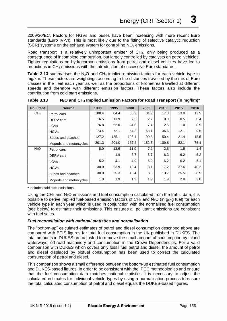
Energy (CRF Sector 1) 3
UK NIR 2018 (Issue 1.1) Ricardo Energy & Environment Page 155
2009/30/EC. Factors for HGVs and buses have been increasing with more recent Euro standards (Euro IV-VI). This is most likely due to the fitting of selective catalytic reduction (SCR) systems on the exhaust system for controlling NOx emissions.
Road transport is a relatively unimportant emitter of CH4, only being produced as a consequence of incomplete combustion, but largely controlled by catalysts on petrol vehicles. Tighter regulations on hydrocarbon emissions from petrol and diesel vehicles have led to reductions in CH4 emissions with the introduction of successive Euro standards.
Table 3.13 summarises the N2O and CH4 implied emission factors for each vehicle type in mg/km. These factors are weightings according to the distances travelled by the mix of Euro classes in the fleet each year as well as the proportions of kilometres travelled at different speeds and therefore with different emission factors. These factors also include the contribution from cold start emissions.
Table 3.13 N2O and CH4 Implied Emission Factors for Road Transport (in mg/km)a
Pollutant Source 1990 1995 2000 2005 2010 2015 2016
CH4 Petrol cars 108.4 84.4 53.2 31.9 17.8 13.0 12.5
DERV cars 16.5 11.9 7.5 2.7 0.9 0.5 0.4
LGVs 76.8 52.0 24.8 7.4 2.5 1.0 0.9
HGVs 73.4 72.1 64.2 63.1 36.6 12.1 9.5
Buses and coaches 127.2 135.1 108.4 90.3 50.4 21.4 15.5
Mopeds and motorcycles 201.3 201.0 187.2 152.5 109.8 82.1 76.4
N2O Petrol cars 8.0 13.6 11.0 7.2 2.8 1.5 1.4
DERV cars - 1.9 3.7 5.7 6.3 6.2 6.2
LGVs 5.2 4.1 4.9 5.9 6.2 6.2 6.1
HGVs 30.0 23.9 13.4 8.1 17.2 37.6 40.2
Buses and coaches 30.0 25.3 15.4 8.8 13.7 25.5 28.5
Mopeds and motorcycles 1.9 1.9 1.9 1.9 1.9 2.0 2.0
a Includes cold start emissions.
Using the CH4 and N2O emissions and fuel consumption calculated from the traffic data, it is possible to derive implied fuel-based emission factors of CH4 and N2O (in g/kg fuel) for each vehicle type in each year which is used in conjunction with the normalised fuel consumption (see below) to estimate their emissions. This ensures all pollutant emissions are consistent with fuel sales.
Fuel reconciliation with national statistics and normalisation
The “bottom-up” calculated estimates of petrol and diesel consumption described above are compared with BEIS figures for total fuel consumption in the UK published in DUKES. The total amounts in DUKES are adjusted to remove the small amount of consumption by inland waterways, off-road machinery and consumption in the Crown Dependencies. For a valid comparison with DUKES which covers only fossil fuel petrol and diesel, the amount of petrol and diesel displaced by biofuel consumption has been used to correct the calculated consumption of petrol and diesel.
This comparison shows a small difference between the bottom-up estimated fuel consumption and DUKES-based figures. In order to be consistent with the IPCC methodologies and ensure that the fuel consumption data matches national statistics it is necessary to adjust the calculated estimates for individual vehicle types by using a normalisation process to ensure the total calculated consumption of petrol and diesel equals the DUKES-based figures.
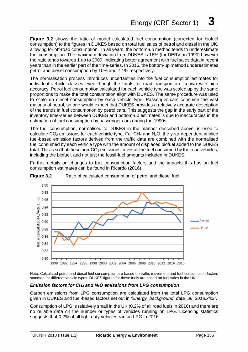
Energy (CRF Sector 1) 3
UK NIR 2018 (Issue 1.1) Ricardo Energy & Environment Page 156
Figure 3.2 shows the ratio of model calculated fuel consumption (corrected for biofuel consumption) to the figures in DUKES based on total fuel sales of petrol and diesel in the UK, allowing for off-road consumption. In all years, the bottom-up method tends to underestimate fuel consumption. The maximum deviation from DUKES is 16% (for DERV, in 1990) however the ratio tends towards 1 up to 2009, indicating better agreement with fuel sales data in recent years than in the earlier part of the time-series. In 2016, the bottom-up method underestimates petrol and diesel consumption by 10% and 7.1% respectively.
The normalisation process introduces uncertainties into the fuel consumption estimates for individual vehicle classes even though the totals for road transport are known with high accuracy. Petrol fuel consumption calculated for each vehicle type was scaled up by the same proportions to make the total consumption align with DUKES. The same procedure was used to scale up diesel consumption by each vehicle type. Passenger cars consume the vast majority of petrol, so one would expect that DUKES provides a relatively accurate description of the trends in fuel consumption by petrol cars. This suggests the gap in the early part of the inventory time-series between DUKES and bottom-up estimates is due to inaccuracies in the estimation of fuel consumption by passenger cars during the 1990s.
The fuel consumption, normalised to DUKES in the manner described above, is used to calculate CO2 emissions for each vehicle type. For CH4 and N2O, the year-dependent implied fuel-based emission factors derived from the traffic data are combined with the normalised fuel consumed by each vehicle type with the amount of displaced biofuel added to the DUKES total. This is so that these non-CO2 emissions cover all the fuel consumed by the road vehicles, including the biofuel, and not just the fossil-fuel amounts included in DUKES.
Further details on changes to fuel consumption factors and the impacts this has on fuel consumption estimates can be found in Ricardo (2016).
Figure 3.2 Ratio of calculated consumption of petrol and diesel fuel
Note: Calculated petrol and diesel fuel consumption are based on traffic movement and fuel consumption factors summed for different vehicle types. DUKES figures for these fuels are based on fuel sales in the UK.
Emission factors for CH4 and N2O emissions from LPG consumption
Carbon emissions from LPG consumption are calculated from the total LPG consumption given in DUKES and fuel-based factors set out in “Energy_background_data_uk_2018.xlsx”.
Consumption of LPG is relatively small in the UK (0.2% of all road fuels in 2016) and there are no reliable data on the number or types of vehicles running on LPG. Licencing statistics suggests that 0.2% of all light duty vehicles ran on LPG in 2016.
Energy (CRF Sector 1) 3
UK NIR 2018 (Issue 1.1) Ricardo Energy & Environment Page 157
Assuming all the LPG consumed in the UK is by Light Goods Vehicles, the amount of LPG consumed was used to estimate the number of vehicle km travelled by LGVs using LPG. Emissions of CH4 and N2O from consumption of LPG were then calculated from the vehicle km data and emission factors (expressed as g of pollutant per km) available from the EMEP/EEA Emissions Inventory Guidebook (2016) covering all types of light duty vehicles. Further details are given in Brown et al (2018)..
Emission from lubricants
Lubricant consumption by the unintended combustion in vehicle engines is estimated using the method from the EMEP/EEA Emissions Inventory Guidebook (2016). These consumption estimates were used to calculate CO2 emissions from lubricant combustion in road vehicle engines and are reported in IPCC sector 2D1 (Section 4.22) except for lubricants use by 2-stroke mopeds, which is deemed to be intentional fuel use and hence reported in IPCC sector 1A3biv.
Emissions of CH4 and N2O also arise from lubricant combustion in engines. However, the exhaust emission factors for these gases will include the contribution of lubricants as well as the main fuel to the pollutant emissions when the vehicles were tested. Hence, the emissions of CH4 and N2O (and other air pollutants) from lubricants are included implicitly in the hot exhaust emissions calculated for each vehicle and fuel type. Treating emissions of these pollutants separately would lead to a double count.
Overseas Territories and Crown Dependencies
Fuel consumption data for 1A3b were obtained from national statistics for all Overseas Territories and Crown Dependencies. Fleet composition data were available for all territories and used to disaggregated the fuel consumption data. More detailed fleet composition data for the UK were used to further disaggregate the fuel consumption data in order to apply UK-specific emission factors.
Assumptions & observations
There are many assumptions made, using expert judgement, in the Tier 3 approach and these are referred to in the detailed road transport inventory methodology report by Brown et al (2018).
Emissions of direct greenhouse gases are calculated on the basis of fuel sold (and not vkm travelled) and are consistent with UK energy statistics.
For CO2, the assumptions have little effect on total road transport emissions as this is based on fuel sales figures in DUKES, but the assumptions used during the normalisation process affect the distribution of emissions between vehicle types. In particular, the procedure used to normalise the diesel consumption calculated for each vehicle type with the total DUKES figure is important as all vehicle types have a similar share of diesel consumption.
For CH4 and N2O emissions, the diesel normalisation method assumed has a direct effect on emission estimates as emissions per unit of fuel consumed vary for each vehicle type.
A sensitive parameter in the emission calculations of CH4 and N2O for petrol cars is the assumption made about the proportion of the fleet with catalyst systems that have failed, for example due to mechanical damage or failure of the lambda sensor. Following discussions with DfT, it is assumed that the failure rate is 5% per annum for all Euro standards and that up to 2008 only 20% of failed catalysts were rectified properly, but those that were rectified were done so within a year of failing. From 2009, a change in the repair rate is taken into account for Euro 3 and above petrol LDVs assuming all failed vehicles are rectified properly due to the introduction of EU Regulations Controlling Sale and Installation of Replacement Catalytic Converters. Further details are given in Brown et al (2018).
Energy (CRF Sector 1) 3
UK NIR 2018 (Issue 1.1) Ricardo Energy & Environment Page 158
Other key assumptions that affect CH4 and N2O emissions include:
• Application of vehicle speeds measured on a sample of roads to cover the whole road network;
• Distances covered by petrol car engines not fully warmed up in calculation of cold start emissions; and
• All LPG is consumed by light goods vehicles.
Recalculations
There have been no major recalculations. Smaller re-calculations have occurred for the following reasons:
• A re-allocation of a very small amount of petrol and diesel fuel consumption from non-road sources to the road transport sector
• A minor re-allocation of fuel consumption between vehicle types due to changes in new car sales figures for 2015, including hybrids. Generally increasing the amount of diesel fuel assigned to LGVs, HGVs and buses, reducing the fuel assigned to cars. This has an overall effect on the non-CO2 GHG emissions because fuel-based factors are different for different vehicle types
• A very small reduction in fleet-averaged factors for CH4 and N2O in 2015 for passenger cars due to the increase in new car sales figures, making the fleet slightly younger than previously estimated.
Improvements (completed and planned)
No specific improvements are currently planned. A watching brief is kept on developments in emission factors and activity data for all modes of transport.
QA/QC
This source category is covered by the general QA/QC of the greenhouse gas inventory in Section 1.6.
An internationally established Tier 3 method is used consistent with IPCC Guidelines and EMEP/EEA Emissions Inventory Guidebook approaches. The Method Approach section has described a comparison between the bottom-up, traffic-based approach for calculating fuel consumption and the total fuel sales figures provided in DUKES; the agreement is within 16% across the time-series.
The traffic data (vkm) and fleet composition data are provided by DfT and have been assessed by the UK Statistics Authority and confirmed as National Statistics. A Statement on Quality Strategy Principles and Processes for DfT statistics is provided at https://www.gov.uk/government/uploads/system/uploads/attachment_data/file/10957/statement-on-quality.pdf.https://www.gov.uk/government/uploads/system/uploads/attachment_data/file/10957/statement-on-quality.pdf
Emission factors and fuel consumption factors are from standard IPCC and EMEP/EEA Inventory Guidebooks and COPERT. These are peer-reviewed sources.
Time series consistency
There are no time-series issues. Time-series consistency is ensured by the use of DUKES fuel consumption and use of continuous, consistent vkm traffic data from DfT. Chapter 2 describes trends in implied emission factors for CH4 and N2O. These are consistent with trends in fleet turnover made using trends in new vehicle sales and constant survival rates combined with ANPR observations showing usage patterns from 2007-present.
Energy (CRF Sector 1) 3
UK NIR 2018 (Issue 1.1) Ricardo Energy & Environment Page 159
Uncertainties
The uncertainty analysis is set out in Annex 2. The reconciliation between bottom up and top down approaches gives a high level of confidence in the calculated emissions for road transport. There is greater uncertainty in the division in CO2 emissions between vehicle types.
There are greater uncertainties in the emission factors for CH4 and N2O because of limited emission factor measurements, in particular for more recent vehicle technologies and emission standards entering service. The main sources of uncertainties in the activity data affecting the CH4 and N2O inventories are in the division of diesel fuel consumption between vehicle types and the uncertainty in the fuel consumption factors that determine how much CH4 and N2O emissions are scaled to be consistent with national fuel consumption. There are also uncertainties affecting the emission estimates for CH4 and N2O in the on-road fleet composition, catalyst failure rates, trip lengths (for estimating cold start emissions).
MS 9 Railways
Relevant Categories, source names
1A3c: Rail - coal
Railways: freight – gas oil
Railways: intercity – gas oil
Railways: regional – gas oil
Relevant Gases
CO2, CH4, N2O
Relevant fuels, activities
Gas oil, coal
Background
This MS includes emissions from gas oil used to power trains and from the consumption of coal used to power steam trains. The methodology for gas oil is based around three categories of railway locomotive: freight, intercity and regional. Stationary combustion in the rail sector is included in MS 5. Most of the electricity used by the railways for electric traction is supplied from the public distribution system, so the emissions arising from its generation are reported under 1A1a Public Electricity.
Key Data sources
Activity: DUKES, Office of Rail and Road (ORR) National Rail Trends Yearbook (NRTY), ORR data portal
Emission factors: EMEP/EEA 2013, DfT’s Rail Emissions Model (DfT 2012b), AP-42 (USEPA)
An accompanying spreadsheet “Energy_background_data_uk_2018.xlxs” lists all emission factors used in the energy sector, including a full list of references25. Table 1.6 gives additional information for common activity data sources.
Method approach
Emissions are calculated based on AD x EF.
Energy (CRF Sector 1) 3
UK NIR 2018 (Issue 1.1) Ricardo Energy & Environment Page 160
Coal consumption data has been obtained from DUKES. Estimates have been made for 2005-2016 and are believed to be due to consumption by heritage trains. No coal use is allocated to railways in DUKES for earlier years, it is assumed that this is included within other reporting categories. For the indirect GHG emissions, US EPA emission factors for hand-stoked coal-fired boilers are used to estimate emissions from coal-fired steam trains.
The UK GHGI reports emissions from trains that run on gas oil in three categories: freight, intercity and regional. Emissions from these are reported under the IPCC category 1A3c Railways. Emission estimates are based on:
• Vehicle kilometres travelled and emission factors in grams per vehicle kilometre for passenger trains; and
• Train kilometres travelled and emission factors in grams per train kilometre for freight trains.
For Great Britain, vehicle kilometre data for intercity and regional trains has been obtained from the UK’s Department for Transport’s Rail Emissions Model for 2009 to 2011 and then estimated for other years from ORR’s National Rail Trends Yearbook (NRTY) and data portal. Train kilometre data for freight trains has been estimated from ORR’s National Rail Trends Yearbook (NRTY) and data portal, which provides data on the tonne kilometres travelled. An assumption is then made that the ratio between the tonne kilometres and freight train kilometres is the same as it was in 2004 for all years.
Gas oil consumption by passenger and freight trains is obtained from the 2011 NRTY for the period 2005-2009 and from ORR’s data portal for the years 2011-2015. No data is available for the years 1970-2004 and 2010 and data for 2016 was not published at the time of compilation. Therefore, fuel consumption for these years was estimated based on the trend in train kilometres.
For Northern Ireland, train kilometre data and fuel consumption data are provided by Translink, the operator of rail services in the region.
Carbon, sulphur dioxide and nitrous oxide emissions are calculated using fuel-based emission factors and the total fuel consumed. The CEF for coal is derived from Fynes & Sage (1994) whilst the CEF for gas oil is taken from Baggott et al. (2004).
Emissions of other pollutants are based on the vehicle / train kilometre estimates, and emission factors for different train classes. The distribution of the train fleet by train class is determined based on:
• For passenger trains: Vehicle train kilometres data for different train classes for 2009, 2010 and 2011 are derived from the Department for Transport’s Rail Emissions Model. The fleet for other years is estimated based on the year of introduction of new engines.
• For freight trains: The breakdown by locomotive class was obtained from the Department for Transport’s Rail Emissions Model of 2009. The fleet for other years is estimated based on the year of introduction of new engines.
The emission factor for SO2 decreased from 0.76 kt/ Mt fuel in 2011 to 0.02 kt/ Mt fuel in 2012 in line with requirements introduced from the 1st January 2012 in the EU Fuel Quality Directive (2009/30/EC) that limited the sulphur content of gas oil to 10ppm.
For coal-fired steam trains, US EPA emission factors for hand-stoked coal-fired boilers are used to estimate emissions. These are considered most appropriate for the type of coal-fired boilers on heritage trains.
Energy (CRF Sector 1) 3
UK NIR 2018 (Issue 1.1) Ricardo Energy & Environment Page 161
Assumptions & observations
In recent years passenger train kilometres have steadily increased until a small decline in 2016. This trend is generally reflected in the passenger train fuel consumption data. The amount of freight moved has declined steadily since 2013 as a result of a substantial decline in the amount of coal hauled. The amount of freight moved in 2016 is around 78% of the amount estimated for 2013. However, fuel consumption has not reduced accordingly due to an increase in container traffic. Freight fuel consumption in 2016 is 95% of the 2013 fuel consumption.
It has been assumed that new passenger trains and freight locomotives introduced since 2012 are compliant with the European Non Road Mobile Machinery Stage IIIB regulations.
Recalculations
Actual intercity and regional train kilometres from 2012-2016 are now obtained from ORR rather than using timetable train kilometres, leading to a slight reduction in emissions. Fuel consumption for 2015 was updated to reflect finalised ORR data. The fuel consumption for freight trains in 2015 was higher than estimated in the previous submission leading to lower aggregated implied emission factors for freight trains for this year in the case of CH4 and other pollutants where emissions are derived from train km data.
Improvements (completed and planned)
A watching brief is kept on developments in emission factors and activity data for all modes of transport, especially those that may arise from stakeholder initiatives and which can be reasonably incorporated in the inventory.
QA/QC
This source category is covered by the general QA/QC of the greenhouse gas inventory in Section 1.61.6
Time series consistency
Coal use in heritage railways is not reported in DUKES for all years. For the years in which no activity data are reported, emissions are reported as “IE.” Consultation with the DUKES team has indicated a high level of confidence in total coal use for the UK. As such although no data are available to allocate emissions to rail for earlier years in the time series, this does not represent an under report in the UK inventory.
Gas oil consumed by the rail sector is estimated based on the change in train / vehicle kilometres prior to 2005, for 2010 and for 2016. However, the total amount of gas oil consumed in the UK is thought to be reliable and therefore this does not represent an under / over report in the UK inventory as a whole.
Uncertainties
The uncertainty analysis is set out in Annex 2. The main uncertainties for the rail sector relate to the poor emission factor data across all sources and the lack of detailed train kilometre data by train class.
MS 10 National navigation and fishing
Relevant Categories, source names
1A3d: Shipping – coastal
1A4ciii: Fishing vessels
Energy (CRF Sector 1) 3
UK NIR 2018 (Issue 1.1) Ricardo Energy & Environment Page 162
Relevant Gases
CO2, CH4, N2O
Relevant fuels, activities
Gas oil, fuel oil
Background
This MS includes emissions from UK domestic and crown dependency coastal shipping and fishing, including fishing outside UK territorial waters. Emissions from inland waterways are covered in MS 12, and shipping between the UK and OTs (classified as domestic) are described in MS 11.
Key Data sources
Activity: UK Maritime and Coastguard Agency, DfT Maritime Statistics (2017), MMO Fishing statistics (MMO, 2016), DUKES (BEIS 2017), Scarbrough et al. (2017).
Emission factors: IMO (2015).
An accompanying spreadsheet “Energy_background_data_uk_2018.xlxs” lists all emission factors used in the energy sector, including a full list of references25. Table 1.6 gives additional information for common activity data sources.
Method approach
A new shipping emissions model has been developed as part of the UK’s Greenhouse Gas Inventory Improvement Programme using 2014 high resolution terrestrial Automatic Identification System (AIS) vessel movement data supplied by the UK Maritime and Coastguard Agency. The new methodology meets and exceeds the requirements of a Tier 3 methodology set out in the EMEP EEA Emissions Inventory Guidebook 2016 and the requirements for reporting national greenhouse gas emissions to the UNFCCC under the 2006 IPCC Guidelines. The new methodology carries out an emission calculation specific to each vessel and for each point of the vessel’s voyage around the UK coast that is tracked with AIS receivers on the UK shore. This replaces the previous approach of determining emissions based on the total length of a voyage along assumed routes and vessel speeds rather than actual routes and speeds undertaken and also accounts for vessel draught.
The receivers capture a number of smaller vessels and voyages such as movements to and from off-shore oil and gas rigs, and journeys to/from crown dependencies, not captured in the previous approach.It also captures some vessels such as tugs that were previously captured in the methodology used for estimating emissions from inland waterway vessels. As the new approach is considered to capture these vessel movements more accurately than estimated in the inland waterways model, those vessel categories were removed from the inland waterways emission estimation model. The new approach also uses a more detailed set of port statistics for different vessel categories as proxies for estimating activities in years back to 1990 and forward to 2016 from the 2014 base year.
A significant step in the process is identifying whether a vessel movement is a UK domestic movement, and reported under 1A3dii, or part of an international voyage calling in the UK reported as a Memo item under 1A3di.
Details of the new methodology are given in the report by Scarbrough et al (2017) and only a summary is given here.
Energy (CRF Sector 1) 3
UK NIR 2018 (Issue 1.1) Ricardo Energy & Environment Page 163
a) Activity data for 2014
The model methodology estimates the Heavy Fuel Oil (HFO) and Marine Diesel Oil (MDO) fuel consumption for each AIS position message down-sampled to 5-minute temporal resolution. The calculation takes into account where available the individual vessel characteristics of main engine power, engine speed and load, and makes bottom-up assumptions for auxiliary engines. The fuel and emissions are estimated for each AIS message to cover the time period until the next AIS message, which is often 5 minutes, but in cases where the vessel travels at or outside the range of the terrestrial AIS receivers, may be longer or much longer. Many assumptions for the modelling have been drawn from the International Maritime Organization’s (IMO) Third Greenhouse Gas Study (IMO, 2015).
The emissions are calculated separately for each vessel and for each AIS data point assuming that the vessel continues to combust fuel and emit pollution at the same rate until the subsequent AIS message. The fuel consumption and emission factors are tailored to the specific vessel that is identified in the AIS dataset. The factors account for:
• The fuel type assumed to be used by the vessel, the known engine type and engine speed (rpm).
• The rated power of the engines, which are either known from a third party vessel characteristics database, or estimated based on other known or reported vessel characteristics (e.g. vessel length)
• The actual power demands on the main engines for each AIS message, expressed as a function of reported and designed vessel speed, and reported and designed vessel draught.
• The location and type of the vessel, i.e. whether the vessel is in a Sulphur Emission Control Area (SECA), whether the vessel is at berth, and whether the vessel is a passenger vessel.
In those cases where part of a voyage is not captured within the range of the terrestrial AIS dataset (defined as a gap in AIS coverage of 24 hours), allocation assumptions have been based on vessel type. Specifically, if cargo or passenger vessel journeys had a gap between AIS messages of greater than 24 hours, these vessels were assumed to have been on UK international voyages if they had started or finished at a UK port. For the remaining vessel types, which includes offshore industry vessels, fishing fleets and service vessels, voyages were assumed to be UK domestic if the AIS dataset showed the vessel had started and finished at a UK port, regardless of the length of time of any gaps in AIS coverage.
The detailed Tier 3 approach used in Scarbrough et al. (2017) is able to distinguish fuel consumption and emissions between domestic movements from one UK port to another and UK international movements between a UK port and a port overseas. This enables the correct activities and emissions to be allocated to the NFR14 category 1A3dii Domestic Water-borne Navigation.
The Scarbrough et al. (2017) inventory excluded emissions and fuel consumption from military vessel movements which are not captured in the AIS movements database. Naval shipping emissions are reported separately using fuel consumption data supplied by the Ministry of Defence (MoD). Emissions from these vessels are covered in MS 15.
The Scarbrough et al. (2017) study did not cover small tugs and service craft used in estuaries, private leisure craft and vessels used in UK rivers, lakes and canals as these were not captured in the AIS data. These were captured in the estimates for inland waterways described in MS 12.
Commercial fishing vessels were captured by AIS data, including those that eventually leave the UK to fish in overseas waters, before returning later so emissions could be calculated in the same way as for other domestic navigation and reported separately under 1A4ciii. This
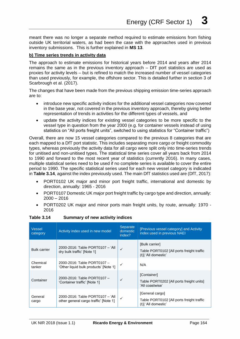
Energy (CRF Sector 1) 3
UK NIR 2018 (Issue 1.1) Ricardo Energy & Environment Page 164
meant there was no longer a separate method required to estimate emissions from fishing outside UK territorial waters, as had been the case with the approaches used in previous inventory submissions. This is further explained in MS 13.
b) Time series trends in activity data
The approach to estimate emissions for historical years before 2014 and years after 2014 remains the same as in the previous inventory approach – DfT port statistics are used as proxies for activity levels – but is refined to match the increased number of vessel categories than used previously, for example, the offshore sector. This is detailed further in section 3 of Scarbrough et al. (2017).
The changes that have been made from the previous shipping emission time-series approach are to:
• introduce new specific activity indices for the additional vessel categories now covered in the base year, not covered in the previous inventory approach, thereby giving better representation of trends in activities for the different types of vessels, and
• update the activity indices for existing vessel categories to be more specific to the vessel type in question from the year 2000 (e.g. for container vessels instead of using statistics on “All ports freight units”, switched to using statistics for “Container traffic”)
Overall, there are now 15 vessel categories compared to the previous 8 categories that are each mapped to a DfT port statistic. This includes separating more cargo or freight commodity types, whereas previously the activity data for all cargo were split only into time-series trends for unitised and non-unitised types. The statistical time series cover all years back from 2014 to 1990 and forward to the most recent year of statistics (currently 2016). In many cases, multiple statistical series need to be used if no complete series is available to cover the entire period to 1990. The specific statistical series used for each new vessel category is indicated in Table 3.14, against the index previously used. The main DfT statistics used are (DfT, 2017):
• PORT0102 UK major and minor port freight traffic, international and domestic by direction, annually: 1965 - 2016
• PORT0107 Domestic UK major port freight traffic by cargo type and direction, annually: 2000 – 2016
• PORT0202 UK major and minor ports main freight units, by route, annually: 1970 - 2016
Table 3.14 Summary of new activity indices
Vessel category
Activity index used in new model Separate domestic index?
[Previous vessel category] and Activity index used in previous NAEI
Bulk carrier 2000-2016: Table PORT0107 – ‘All dry bulk traffic’ [Note 1]
✓
[Bulk carrier]
Table PORT0102 [All ports freight traffic (t)] ‘All domestic’
Chemical tanker
2000-2016: Table PORT0107 – ‘Other liquid bulk products’ [Note 1]
✓ N/A
Container 2000-2016: Table PORT0107 – ‘Container traffic’ [Note 1]
✓
[Container]
Table PORT0202 [All ports freight units] ‘All coastwise’
General cargo
2000-2016: Table PORT0107 – ‘All other general cargo traffic’ [Note 1]
✓
[General cargo]
Table PORT0102 [All ports freight traffic (t)] ‘All domestic’
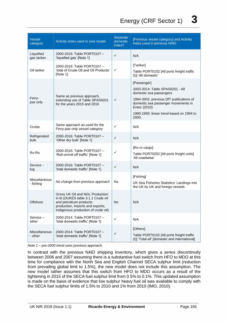
Energy (CRF Sector 1) 3
UK NIR 2018 (Issue 1.1) Ricardo Energy & Environment Page 165
Vessel category
Activity index used in new model Separate domestic index?
[Previous vessel category] and Activity index used in previous NAEI
Liquefied gas tanker
2000-2016: Table PORT0107 – ‘liquefied gas’ [Note 1]
✓ N/A
Oil tanker 2000-2016: Table PORT0107 – ‘total of Crude Oil and Oil Products’ [Note 1]
✓
[Tanker]
Table PORT0102 [All ports freight traffic (t)] ‘All domestic’
Ferry- pax only
Same as previous approach, extending use of Table SPAS0201 for the years 2015 and 2016
✓
[Passenger]
2003-2014: Table SPAS0201 - All domestic sea passengers
1994-2002: previous DfT publications of domestic sea passenger movements in Entec (2010)
1990-1993: linear trend based on 1994 to 2000.
Cruise Same approach as used for the Ferry-pax only vessel category
✓ N/A
Refrigerated bulk
2000-2016: Table PORT0107 – ‘Other dry bulk’ [Note 1]
✓ N/A
Ro-Ro 2000-2016: Table PORT0107 – ‘Roll-on/roll-off traffic’ [Note 1]
✓
[Ro-ro cargo]
Table PORT0202 [All ports freight units] ‘All coastwise’
Service - tug
2000-2016: Table PORT0107 – ‘total domestic traffic’ [Note 1]
✓ N/A
Miscellaneous - fishing
No change from previous approach No
[Fishing]
UK Sea Fisheries Statistics: Landings into the UK by UK and foreign vessels.
Offshore
Gross UK Oil and NGL Production in kt (DUKES table 3.1.1 Crude oil and petroleum products: production, imports and exports; Indigenous production of crude oil)
No N/A
Service – other
2000-2014: Table PORT0107 – ‘total domestic traffic’ [Note 1]
✓ N/A
Miscellaneous - other
2000-2014: Table PORT0107 – ‘total domestic traffic’ [Note 1]
✓
[Others]
Table PORT0102 [All ports freight traffic (t)] ‘Total all’ [domestic and international]
Note 1 – pre-2000 trend uses previous approach.
In contrast with the previous NAEI shipping inventory, which gives a series discontinuity between 2006 and 2007 assuming there is a substantive fuel switch from HFO to MDO at this time for compliance with the North Sea and English Channel SECA sulphur limit (reduction from prevailing global limit to 1.5%), the new model does not include this assumption. The new model rather assumes that this switch from HFO to MDO occurs as a result of the tightening in 2015 of the SECA fuel sulphur limit from 0.5% to 0.1%. This updated assumption is made on the basis of evidence that low sulphur heavy fuel oil was available to comply with the SECA fuel sulphur limits of 1.5% to 2010 and 1% from 2010 (IMO, 2010).
Energy (CRF Sector 1) 3
UK NIR 2018 (Issue 1.1) Ricardo Energy & Environment Page 166
The requirement that vessels at berth from 2010 use fuel which complies with a sulphur limit of 0.1% implies the need for MDO. Therefore, in the backcasted inventory prior to 2010, any vessels that would have used HFO, save for the at berth requirement of 0.1% S fuel, are assumed prior to 2010 to use HFO.
c) Emission factors
The source of the raw emission factors used for CO2, CH4 and N2O is given in section 2.2.8 of Scarbrough et al. (2017). Fuel-based emission factors in kg/tonne fuel are used and may differ by engine type and/or fuel type.
The fuel-based CO2 emissions factors for main and auxiliary engines are the same as assumed in IMO (2015) and are based on MEPC 63/23, Annex 8:
• HFO: 3,114 kg CO2/tonne fuel
• MDO: 3,206 kg CO2/ tonne fuel
The CO2 factors listed above differ from the factors previously used in the NAEI. They are 3.4% lower than previously used values for fuel oil and 0.5% higher for gas oil. The new figures are much closer to the defaults in the 2006 IPCC Guidelines than the values previously used in the NAEI.
Methane emission factors for diesel-fuelled engines, steam boilers and gas turbines are the same as used in IMO (2015). These are derived from IVL (2004) which states that CH4 emissions are approximately 2% the magnitude of NMVOCs. Therefore, the CH4 factors are derived by multiplying the NMVOC factors by 2%. Values of methane emission factors are 0,04-0.06 kg/tonne fuel depending on engine type.
The N2O emission factors are taken from IMO (2015). N2O emission factors are unaffected by fuel sulphur content but do differ slightly between HFO and MDO. Values for HFO are 0.16 kg/tonne fuel and are 6% less for MDO.
Emission factors for other pollutants are given in section 2.2.8 of Scarbrough et al. (2017). These emission factors also derive from IMO (2015).
Emission factors remain constant over the time-series. However, vessels using HFO in a SECA are assumed to switch to using MDO from 2015 onwards, with an SO2 emission factor reduction of 90% (from 1% S HFO to 0.1% MDO) accordingly.
Fuel consumption is calculated for each vessel based on the characteristics of the vessel, engine type, movement and draught for the 2014 activity dataset received.
It is expected that shipping transport efficiency increases over time in response to financial and regulatory drivers. For all vessels it is assumed that the efficiency of sea transport improves by 1% per year from 2014 onwards to account for lower fuel consumption per unit (tonne or container or passenger) transported and more fuel efficient new vessels compared to old vessels
i.e. 𝐸𝑓𝑓𝑖𝑐𝑖𝑒𝑛𝑐𝑦 𝑖𝑛𝑑𝑒𝑥𝑦 = 0.99(𝑦−2014)
Further details on how this value was derived are given in section 3.2.3. of Scarbrough et al. (2017). The current inventory therefore implies a small improvement in the fuel efficiency of the fleet from the 2014 base to 2016.
Assumptions & observations
The coverage of vessels captured by the AIS receivers is considered complete for this sector. Small vessels which do not have AIS transmitters, such as small recreational craft and service vessels, are captured in the inventory for inland waterways. The main assumption concerns the allocation of a vessel movement to UK domestic or international for a cargo or passenger
Energy (CRF Sector 1) 3
UK NIR 2018 (Issue 1.1) Ricardo Energy & Environment Page 167
vessel starting or finishing at a UK port when it goes out of AIS signal range, based on the gap between AIS messages being greater or less than 24 hours.
Recalculations
A major methodology change was undertaken for this submission based on detailed AIS vessel movement data, updated DfT port statistics and updated emission factors. This has led to an increase in the amount of fuel consumption, hence emissions, allocated to domestic coastal shipping and fishing. This is mainly due to more complete coverage of vessel activities, including movements by vessels to UK offshore oil and gas installations, and improved engine emission calculations.
Improvements (completed and planned)
The major change in methodology has taken two years to develop and introduce to the UK inventory. No further method changes are anticipated in the near future.
QA/QC
This source category is covered by the general QA/QC of the greenhouse gas inventory in Section 1.6. The new approach that has been adopted is described in detail in Scarbrough et al (2017) and has been peer-reviewed by BEIS, Defra, DfT as well as presented to experts in the maritime industry. Scarbrough et al (2016) also reports on validation with other estimates of shipping emissions given in the literature covering the same geographical area of the North Sea and English Channel.
Time series consistency
The time-series for national navigation and fishing is derived from trends in port activity statistics for different vessel types. Some of these show an increase in activities over time, others a decrease in activities over the time series for different vessel types..
The approach assumes that a switch from HFO to MDO occurs as a result of the tightening in 2015 of the North Sea and English Channel SECA fuel sulphur limit from 0.5% to 0.1%.
This break in the time series is not considered to be a time series consistency issue.
Uncertainties
The uncertainty analysis is set out in Annex 2. The uncertainty in the bottom up calculated estimates of fuel consumption in 2014 is considered to be less than the allocation of fuel to national navigation provided in DUKES and more representative of UK domestic shipping activities as defined in the IPCC 2006 Guidelines.
Further consideration of uncertainties in the approach is given in Scarbrough et al (2017), particularly with respect to the allocation of a vessel movement to domestic or international when the vessel goes out of AIS range. However, overall, the emission calculations are estimated to have relatively low uncertainty for most large vessels which are responsible for 85% of total emissions. Scarbrough et al (2017) also report that the model estimates compare well with those from other European shipping inventories when comparisons are made on a like-for-like basis.
Additional uncertainty is introduced through the use of proxy statistics to develop the time series. The uncertainty in the carbon emission factor is considered low, whereas the uncertainties for non-CO2 gases are higher.
Energy (CRF Sector 1) 3
UK NIR 2018 (Issue 1.1) Ricardo Energy & Environment Page 168
MS 11 Shipping between UK and OTs
Relevant Categories, source names
1A3d: Shipping between UK and Gibraltar
Shipping between UK and OTs (excl. Gibraltar)
Relevant Gases
CO2, CH4, N2O
Relevant fuels, activities
Fuel oil
Background
This MS includes estimates of emissions from shipping movements between the UK and the Overseas Territories. These were not included in the new methodology for domestic shipping developed by Scarbrough et al (2017) (described in MS 10) and are therefore calculated separately. These are included as domestic emissions for UNFCCC reporting, and reported under 1A3d.
Key Data sources
Activity: DfT (personal communication), OT port authorities (personal communications), EMEP/EEA 2016
Emission factors: Scarbrough et al. (2017) and based on IMO (2015)
An accompanying spreadsheet “Energy_background_data_uk_2018.xlxs” lists all emission factors used in the energy sector, including a full list of references25. Table 1.6 gives additional information for common activity data sources.
Method approach
a) Activity data
The total fuel consumed by vessels moving between the UK and each OT is calculated as the sum of all fuel consumed by freight and passenger vessels. This is calculated separately for movements from the UK to each OT and from each OT to the UK.
There are no published data on the number and types of voyages between the UK and overseas territories (OTs). However, officials at the UK Department for Transport (DfT, Personal communication, 2017) were able to interrogate their ports database which forms the basis of the less detailed information published in DfT’s Maritime Statistics. This included information on freight shipping movements and passenger vessel movements. Additional information on passenger vessel movements were gathered from individual OT port authorities.
For freight shipping, the DfT were able to provide the number of trips made between a UK port and an OT port by each unique vessel recorded. The information provided the type of vessel and the departure and arrival port. Figures were provided for all years between 2000 and the latest inventory year.
The information on the type of vessel combined with information from the EMEP Emissions Inventory Guidebook 2016 was used to define:
• the average cruise speed of the vessel;
• the average main engine power (in kW); and
Energy (CRF Sector 1) 3
UK NIR 2018 (Issue 1.1) Ricardo Energy & Environment Page 169
• the specific fuel consumption factor (g/kWh).
DfT were unable to provide the detailed port data for years before 2000. The individual OT port authorities also did not have this information. The trends in fuel consumption calculated for all UK international shipping from 1990 to 2000 (based on less detailed UK port statistics) were used to define the trend in fuel consumption for shipping between the UK and OTs over these years.
For passenger vessels, the information held by OT port authorities indicated the only movements were by cruise ships (i.e. not ferries). Data from DfT was used for the years 2013-2016 (DfT, 2017a). Detailed movement data were held by the port authority of Gibraltar listing all voyages departing to or arriving from the UK from 2003 to 201228. The DfT also held information on the number of UK port arrivals by cruise ships from the OTs, but only between 1999 and 2004. This is unpublished information and was provided via direct communication with DfT officials.
Information held by the other OTs indicated that none had any cruise ship sailings with the UK logged. The data held by DfT showed the majority of sailings were from Gibraltar and the data were consistent with the information provided by the Gibraltar port authority. However, the DfT data also showed a total of 3 arrivals from the Falkland Islands between 1999 and 2004.
No cruise ship information was available before 1999 from either DfT or the individual OT port authorities. Trends in the total number of passengers on cruises beginning or ending at UK ports between 1990 and 1999 published in DfT’s Maritime Statistics (from Table 3.1(a) UK international short sea passenger movements, by port and port area: 1950 – 2009) were used to define the trend in fuel consumption by cruise ships between the UK and OTs over these years.
Distance travelled: Distances for each voyage for freight and passenger were taken from http://www.portworld.com/map/. This has a tool to calculate route distance by specifying the departure and arrival ports. Using the distance, average speed, engine power and fuel consumption factor it was possible to calculate the amount of fuel consumed for every voyage made.
Emission factors
All fuel used for voyages between the UK and OTs is assumed to be fuel oil. The emission factors used are average factors implied by Scarbrough et al. (2017) for all vessels involved in international voyages from or to a UK port from/to a non-UK destination.
Assumptions & observations
All fuel used for voyages between the UK and OTs is assumed to be fuel oil. Emission factors are assumed to be the average of all vessels involved in UK international voyages.
Data provided by various data sources are assumed to be complete.
Recalculations
There have been no method changes but there have been recalculations using emission factors taken from Scarbrough et al (2017).
Improvements (completed and planned)
This emission source was introduced in response to the UNFCCC ERT in 2012. No improvements to this method are currently planned.
28 http://www.gibraltarport.com/cruise/schedules
Energy (CRF Sector 1) 3
UK NIR 2018 (Issue 1.1) Ricardo Energy & Environment Page 170
QA/QC
This source category is covered by the general QA/QC of the greenhouse gas inventory in Section 1.6. There are no official statistical data sets available to verify the information provided for the calculation of these estimates. They are considered to be the best available data.
Time series consistency
The method approach section above details which years data were available for. Gaps have been filled for the early part of the time series based on other statistics, to ensure that the inventory is complete for all years.
Uncertainties
The uncertainty analysis is set out in Annex 2. The uncertainty in this particular source is high although the contribution to the total inventory is low and as such, it does not warrant further research. Estimates are included for completeness, following a recommendation from the ERT.
MS 12 Inland Waterways
Relevant Categories, source names
1A3d Inland goods-carrying vessels
Motorboats / workboats (e.g. canal boats, dredgers, service boats, tourist boats, river boats)
Personal watercraft e.g. jet ski
Sailing boats with auxiliary engines
Relevant Gases
CO2, CH4, N2O
Relevant fuels, activities
DERV, Gas oil, Petrol
Background
The category 1A3dii Waterborne Navigation includes emissions from fuel used for small passenger vessels, ferries, recreational watercraft, other inland watercraft, and other gasoline-fuelled watercraft. Methods for estimating emissions for these small vessels are presented separately here as they are calculated using different approaches to other marine emissions in the UK inventory.
Key Data sources
Activity: Walker et al (2011), ONS Social Trends, Visit England, OECD Stat, DfT Maritime Statistics (elaborated under Method approach, below).
Emission factors: EMEP/EEA 2016
An accompanying spreadsheet “Energy_background_data_uk_2018.xlsx” lists all emission factors used in the energy sector, including a full list of references25. Table 1.6 gives additional information for common activity data sources.
Energy (CRF Sector 1) 3
UK NIR 2018 (Issue 1.1) Ricardo Energy & Environment Page 171
Method approach
The Guidelines recommend national energy statistics be used to calculate emissions, but if these are unavailable then emissions should be estimated from surveys of fuel suppliers, vessel movement data or equipment (engine) counts and passenger and cargo tonnage counts. The UK has no separate national fuel consumption statistics on the amount of fuel used by inland waterways in DUKES. However, they are included in the overall marine fuel statistics. A Tier 3 bottom-up approach based on estimates of population and usage of different types of inland waterway vessels is used to estimate their emissions. In the UK, all emissions from inland waterways are included in domestic shipping totals.
The methodology applied to derive emissions from the inland waterways sector uses an approach consistent with the 2016 EMEP/EEA Emissions Inventory Guidebooks (EMEP, 2016).
Emissions from individual vessel types are calculated using the following equation:
𝐸 = ∑ 𝑁 × 𝐻𝑅𝑆 × 𝐻𝑃 × 𝐿𝐹 × 𝐸𝐹𝑖
𝑖
where:
𝐸 = mass of emissions of pollutant i or fuel consumed during inventory period, 𝑁 = source population (units),
𝐻𝑅𝑆 = annual hours of use, 𝐻𝑃 = average rated horsepower,
𝐿𝐹 = typical load factor, 𝐸𝐹𝑖 = average emissions of pollutant i or fuel consumed per unit of use (e.g. g/kWh).
The method requires:
• a categorisation of the types of vessels and the fuel that they use (petrol, DERV or gas oil);
• numbers for each type of vessel, together with the number of hours that each type of vessel is used;
• data on the average rated engine power for each type of vessel, and the fraction of this (the load factor) that is used on average to propel the boat; and
• g/kWh fuel consumption factors and fuel-based emission factors.
The inland waterways class is divided into four categories and sub-categories (Walker et al, 2011):
• Sailing Boats with auxiliary engines;
• Motorboats / Workboats (e.g. dredgers, canal, service, tourist, river boats); o recreational craft operating on inland waterways; o recreational craft operating on coastal waterways; o workboats;
• Personal watercraft i.e. jet ski; and
• Inland goods carrying vessels.
Activity data for 2008
A bottom-up approach was used based on estimates of the population and usage of different types of craft and the amounts of different types of fuels consumed. Estimates of both population and usage were made for the baseline year of 2008 for each type of vessel used on canals, rivers and lakes and small commercial, service and recreational craft operating in estuaries / occasionally going to sea. For this, data were collected from stakeholders, including the British Waterways, DfT, Environment Agency, Maritime and Coastguard Agency (MCGA), and Waterways Ireland.
Energy (CRF Sector 1) 3
UK NIR 2018 (Issue 1.1) Ricardo Energy & Environment Page 172
As it was only possible to estimate population and activities for one year (2008), proxy statistics were used to estimate activities for different groups of vessels for other years in the time series:
• Private leisure craft – ONS Social Trends 41: Expenditure, Table 1, Volume of household expenditure on "Recreation and culture"; http://www.ons.gov.uk/ons/rel/social-trends-rd/social-trends/social-trends-41/social-trends-41---expenditure.pdf. No data were available for this dataset after 2009, therefore a second dataset was used to estimate the activity from 2010: OECD.Stat data: http://stats.oecd.org/Index.aspx?DataSetCode=SNA_TABLE5 - ‘Final consumption expenditure of household, UK, P31CP090: Recreation and culture);
• Commercial passenger/tourist craft – Visit England, Visitor Attraction Trends in England 2016, Full Report: https://www.visitbritain.org/annual-survey-visits-visitor-attractions-latest-results : "Total England Attractions"
• Freight – DfT Waterborne Freight in the United Kingdom, Table DWF0101: Waterborne transport within the United Kingdom (Goods lifted - UK inland waters traffic - Non-seagoing traffic – Internal) https://www.gov.uk/government/statistical-data-sets/dwf01-waterborne-transport
One of these three proxy data sets was assigned to each of the detailed vessel types covered in the inventory and used to define the trends in their fuel consumption from the 2008 base year estimate to all other years in the inventory.
Emission factors
The fuel-based emission factors used for all inland waterway vessels for CH4 and N2O were taken from the EMEP/EEA 2009. Emission factors for carbon are from Baggott et al, 2004.
Assumptions & observations
A key assumption made is that privately owned vessels with diesel engines used for recreational purposes use DERV while only commercial and service craft and canal boats use gas oil (Walker et al., 2011). Some smaller vessels also run on petrol engines.
Walker at al. (2011) and Murrells et al. (2011) had previously drawn attention to the potential overlap between the larger vessels using the inland waterways and the smaller vessels in the shipping sectors (namely tugboats and chartered and commercial fishing vessels), and the judgement and assumptions made to try to avoid such an overlap. This potential overlap was reconsidered in light of the new methodology for domestic shipping since certain types of vessels operating at sea close to shore that were previously included in the inland waterways sector of the inventory were now captured in the AIS data. Hence their emissions were now included under coastal shipping described above and by Scarbrough et al (2017). These vessels were considered to be passenger vessels with >12 passengers and 3 or more engines operating in estuaries, tugs, cranes, and chartered and commercial fishing vessels. To avoid a double count, the activities for these vessels were therefore removed from the inland waterways database.
Recalculations
The main method change has been to remove the estimates of emissions of vessel types using gas oil that are now estimated in the new shipping model used for reporting domestic coastal emissions under 1A3dii. This leads to downward revisions of fuel consumption by 55-70% across the time series for this sector compared with the previous inventory. Changes in the proxy time-series data used for some of the remaining vessels included under inland waterways are responsible for smaller changes in the activity data for specific years. This included:
Energy (CRF Sector 1) 3
UK NIR 2018 (Issue 1.1) Ricardo Energy & Environment Page 173
• A 27% decrease in the estimated activity in 2015 in the proxy statistics used to estimate the activity from freight vessels within the inland waterways sector.
• Recalculations in the proxy statistics used to estimate the activity from private leisure craft. This change varies from up to a -4.8% change in 2015 to a +0.6% change in 2010.
Improvements (completed and planned)
No improvements to this method are currently planned. Emission factors and activity data are kept under review.
QA/QC
This source category is covered by the general QA/QC of the greenhouse gas inventory in Section 1.6.
Time series consistency
The bottom up analysis for this source category was carried out for one year, and the time series is generated using proxy statistics, as set out in the method approach section, above. Consistent time series of proxy statistics, where available, have been used to estimate the inland waterways activities time series. For private water craft, two data sets have been combined. Where the two data sets overlap, there is a correlation in the trend. The combination of these data sets does not introduce any time consistency issues.
Uncertainties
The uncertainty analysis is set out in Annex 2. There are no official statistics for the population of vessels, the total fuel consumption or the annual usage of the vessels. There may also be some overlap in definitions between small coastal shipping and inland waterways.
MS 13 Fishing outside of UK territorial waters
Relevant Categories, source names
1A4ciii: Fishing vessels (outside UK waters)
Relevant Gases
CO2, CH4, N2O
Relevant fuels, activities
Gas oil, fuel oil
Background
Previously, a separate method was used to estimate emissions from UK fishing vessels operating in sea territories outside UK waters, as these had not been captured in the original Entec (2010) study which was the basis of the UK inventory, but are required to be included in the national totals of the UK’s inventory. The new shipping methodology based on AIS includes emissions from all commercial fishing vessels so a separate calculation approach is no longer required. Although these fishing vessels go out of range of UK shore-based terrestrial AIS data capture, the time period between successive AIS messages from these vessels is known corresponding to the times when the vessels first go out of range on route to their fishing destination to the point when they return. Fuel consumption and emissions are then estimated based on the assumption that the vessels are travelling at the same speed and using fuel at the same rate during the period they are out of range. The method for calculating emissions is therefore essentially the same as that used for coastal shipping (1A3dii).
Energy (CRF Sector 1) 3
UK NIR 2018 (Issue 1.1) Ricardo Energy & Environment Page 174
MS 14 International shipping
Relevant Categories, source names
Marine bunkers: Shipping - international IPCC definition
Relevant Gases
CO2, CH4, N2O
Relevant fuels, activities
Gas oil, fuel oil
Background
This method statement covers estimates of international marine bunkers which are reported as a Memo item and not included in the UK totals.
Key Data sources
Activity: DUKES (BEIS, 2017);
Emission factors: Scarbrough et al. (2017) and based on IMO (2015)
An accompanying spreadsheet “Energy_background_data_uk_2018.xlxs” lists all emission factors used in the energy sector, including a full list of references25. Table 1.6 gives additional information for common activity data sources.
Method approach
Activity data
Fuel consumption for international shipping is taken directly from DUKES figures for international marine fuel bunkers.
The previous approach taken in the NAEI for international navigation activity was by difference in the bottom-up estimates of fuel consumption for sources included in the national totals (national navigation, naval shipping, inland waterways, fishing, overseas territories) and the total fuel sales given in DUKES for international bunkers plus national navigation combined. This was on the basis that whilst the total amount of fuel made available for consumption in DUKES was reliable, the split between international bunkers and national navigation was more uncertain.
Further discussions with BEIS indicate that there is now higher confidence in the DUKES estimates of the international ‘marine bunkers’ fuel sales data than the portion allocated to national navigation such that marine bunkers fuel statistics in DUKES should now be used without further adjustment as the activity data for emissions from the international navigation Memo item under 1A3di. This procedure was adopted in this inventory..
The consequence of having emissions for national navigation and inland waterways (1A3dii), fishing (1A4ciii) and naval (1A5b) based on a bottom-up method derived from vessel activity and of having emissions for international navigation (1A3di) based on DUKES data for international bunkers is that the total marine fuel consumption exceeds that given in DUKES for national navigation plus marine bunkers. In some years, the fuel consumption for national navigation and inland waterways (1A3dii), fishing (1A4ciii) and naval (1A5b) alone exceeds the total given in DUKES for national navigation plus marine bunkers.
Notwithstanding uncertainties in the modelling approach which were discussed by Scarbrough et al (2017), one possible reason for this difference is that a significant proportion of domestic
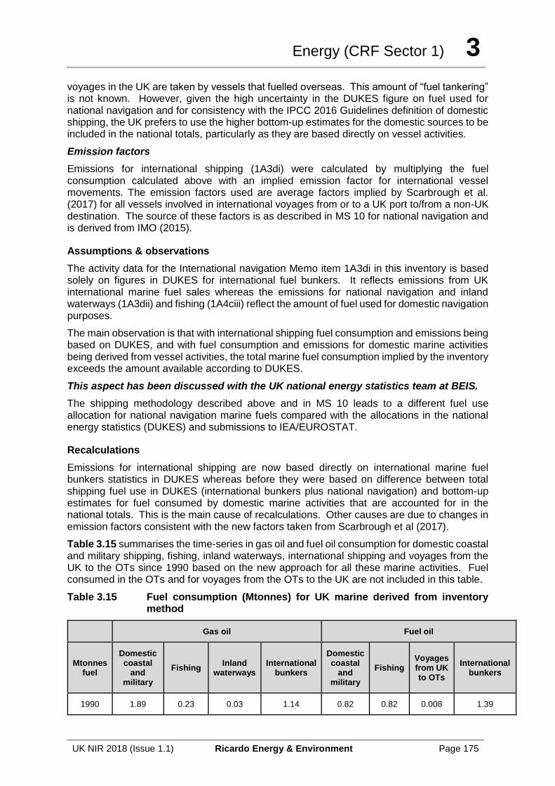
Energy (CRF Sector 1) 3
UK NIR 2018 (Issue 1.1) Ricardo Energy & Environment Page 175
voyages in the UK are taken by vessels that fuelled overseas. This amount of “fuel tankering” is not known. However, given the high uncertainty in the DUKES figure on fuel used for national navigation and for consistency with the IPCC 2016 Guidelines definition of domestic shipping, the UK prefers to use the higher bottom-up estimates for the domestic sources to be included in the national totals, particularly as they are based directly on vessel activities.
Emission factors
Emissions for international shipping (1A3di) were calculated by multiplying the fuel consumption calculated above with an implied emission factor for international vessel movements. The emission factors used are average factors implied by Scarbrough et al. (2017) for all vessels involved in international voyages from or to a UK port to/from a non-UK destination. The source of these factors is as described in MS 10 for national navigation and is derived from IMO (2015).
Assumptions & observations
The activity data for the International navigation Memo item 1A3di in this inventory is based solely on figures in DUKES for international fuel bunkers. It reflects emissions from UK international marine fuel sales whereas the emissions for national navigation and inland waterways (1A3dii) and fishing (1A4ciii) reflect the amount of fuel used for domestic navigation purposes.
The main observation is that with international shipping fuel consumption and emissions being based on DUKES, and with fuel consumption and emissions for domestic marine activities being derived from vessel activities, the total marine fuel consumption implied by the inventory exceeds the amount available according to DUKES.
This aspect has been discussed with the UK national energy statistics team at BEIS.
The shipping methodology described above and in MS 10 leads to a different fuel use allocation for national navigation marine fuels compared with the allocations in the national energy statistics (DUKES) and submissions to IEA/EUROSTAT.
Recalculations
Emissions for international shipping are now based directly on international marine fuel bunkers statistics in DUKES whereas before they were based on difference between total shipping fuel use in DUKES (international bunkers plus national navigation) and bottom-up estimates for fuel consumed by domestic marine activities that are accounted for in the national totals. This is the main cause of recalculations. Other causes are due to changes in emission factors consistent with the new factors taken from Scarbrough et al (2017).
Table 3.15 summarises the time-series in gas oil and fuel oil consumption for domestic coastal and military shipping, fishing, inland waterways, international shipping and voyages from the UK to the OTs since 1990 based on the new approach for all these marine activities. Fuel consumed in the OTs and for voyages from the OTs to the UK are not included in this table.
Table 3.15 Fuel consumption (Mtonnes) for UK marine derived from inventory method
Gas oil Fuel oil
Mtonnes fuel
Domestic coastal
and military
Fishing Inland
waterways International
bunkers
Domestic coastal
and military
Fishing Voyages from UK to OTs
International bunkers
1990 1.89 0.23 0.03 1.14 0.82 0.82 0.008 1.39
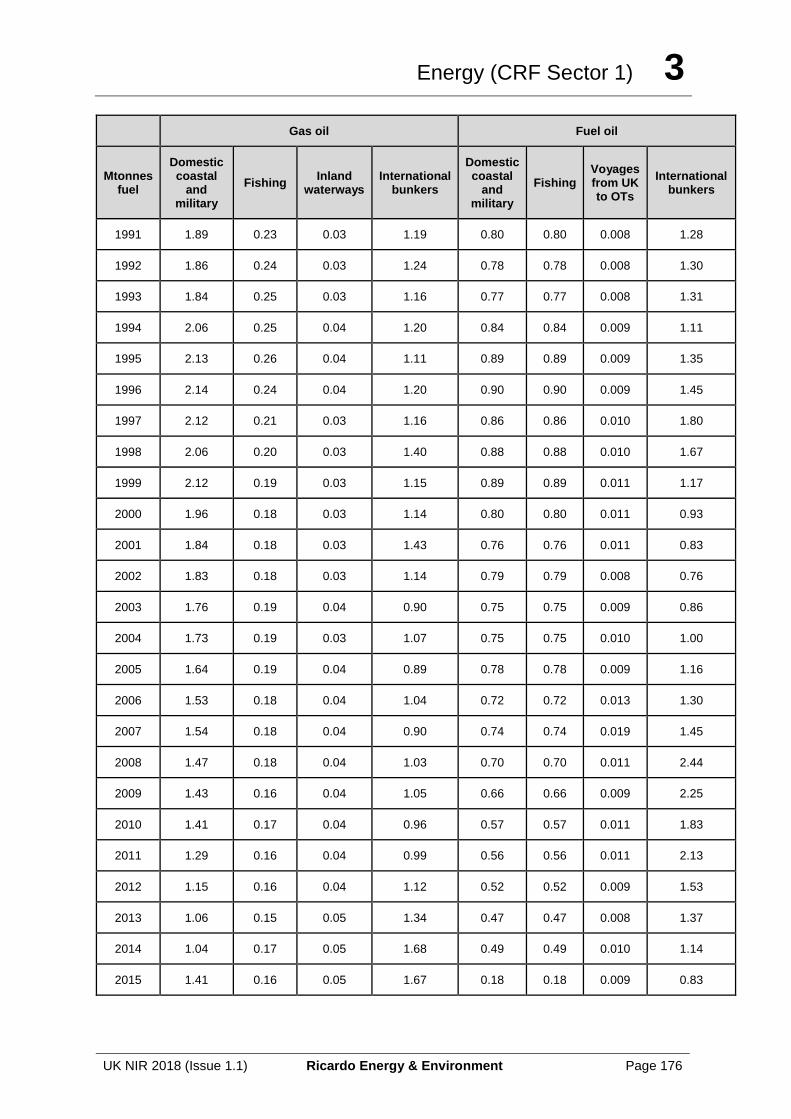
Energy (CRF Sector 1) 3
UK NIR 2018 (Issue 1.1) Ricardo Energy & Environment Page 176
Gas oil Fuel oil
Mtonnes fuel
Domestic coastal
and military
Fishing Inland
waterways International
bunkers
Domestic coastal
and military
Fishing Voyages from UK to OTs
International bunkers
1991 1.89 0.23 0.03 1.19 0.80 0.80 0.008 1.28
1992 1.86 0.24 0.03 1.24 0.78 0.78 0.008 1.30
1993 1.84 0.25 0.03 1.16 0.77 0.77 0.008 1.31
1994 2.06 0.25 0.04 1.20 0.84 0.84 0.009 1.11
1995 2.13 0.26 0.04 1.11 0.89 0.89 0.009 1.35
1996 2.14 0.24 0.04 1.20 0.90 0.90 0.009 1.45
1997 2.12 0.21 0.03 1.16 0.86 0.86 0.010 1.80
1998 2.06 0.20 0.03 1.40 0.88 0.88 0.010 1.67
1999 2.12 0.19 0.03 1.15 0.89 0.89 0.011 1.17
2000 1.96 0.18 0.03 1.14 0.80 0.80 0.011 0.93
2001 1.84 0.18 0.03 1.43 0.76 0.76 0.011 0.83
2002 1.83 0.18 0.03 1.14 0.79 0.79 0.008 0.76
2003 1.76 0.19 0.04 0.90 0.75 0.75 0.009 0.86
2004 1.73 0.19 0.03 1.07 0.75 0.75 0.010 1.00
2005 1.64 0.19 0.04 0.89 0.78 0.78 0.009 1.16
2006 1.53 0.18 0.04 1.04 0.72 0.72 0.013 1.30
2007 1.54 0.18 0.04 0.90 0.74 0.74 0.019 1.45
2008 1.47 0.18 0.04 1.03 0.70 0.70 0.011 2.44
2009 1.43 0.16 0.04 1.05 0.66 0.66 0.009 2.25
2010 1.41 0.17 0.04 0.96 0.57 0.57 0.011 1.83
2011 1.29 0.16 0.04 0.99 0.56 0.56 0.011 2.13
2012 1.15 0.16 0.04 1.12 0.52 0.52 0.009 1.53
2013 1.06 0.15 0.05 1.34 0.47 0.47 0.008 1.37
2014 1.04 0.17 0.05 1.68 0.49 0.49 0.010 1.14
2015 1.41 0.16 0.05 1.67 0.18 0.18 0.009 0.83
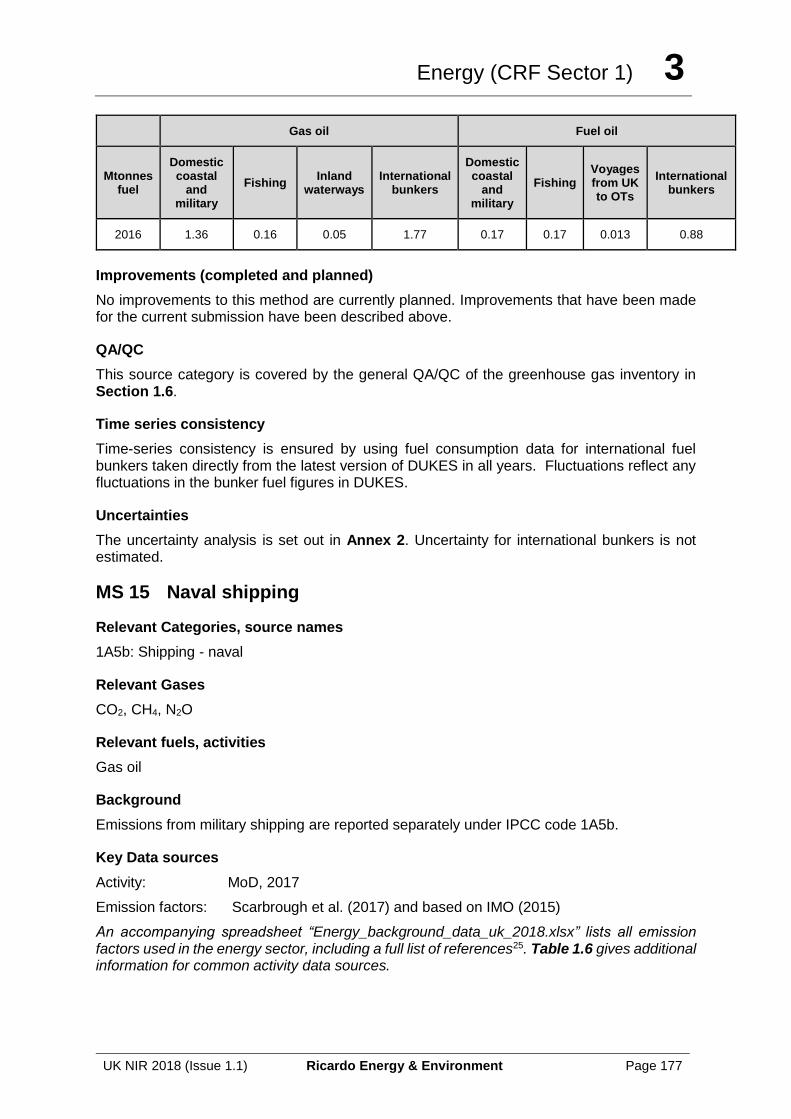
Energy (CRF Sector 1) 3
UK NIR 2018 (Issue 1.1) Ricardo Energy & Environment Page 177
Gas oil Fuel oil
Mtonnes fuel
Domestic coastal
and military
Fishing Inland
waterways International
bunkers
Domestic coastal
and military
Fishing Voyages from UK to OTs
International bunkers
2016 1.36 0.16 0.05 1.77 0.17 0.17 0.013 0.88
Improvements (completed and planned)
No improvements to this method are currently planned. Improvements that have been made for the current submission have been described above.
QA/QC
This source category is covered by the general QA/QC of the greenhouse gas inventory in Section 1.6.
Time series consistency
Time-series consistency is ensured by using fuel consumption data for international fuel bunkers taken directly from the latest version of DUKES in all years. Fluctuations reflect any fluctuations in the bunker fuel figures in DUKES.
Uncertainties
The uncertainty analysis is set out in Annex 2. Uncertainty for international bunkers is not estimated.
MS 15 Naval shipping
Relevant Categories, source names
1A5b: Shipping - naval
Relevant Gases
CO2, CH4, N2O
Relevant fuels, activities
Gas oil
Background
Emissions from military shipping are reported separately under IPCC code 1A5b.
Key Data sources
Activity: MoD, 2017
Emission factors: Scarbrough et al. (2017) and based on IMO (2015)
An accompanying spreadsheet “Energy_background_data_uk_2018.xlsx” lists all emission factors used in the energy sector, including a full list of references25. Table 1.6 gives additional information for common activity data sources.
Energy (CRF Sector 1) 3
UK NIR 2018 (Issue 1.1) Ricardo Energy & Environment Page 178
Method approach
Emissions are calculated using a time-series of naval fuel consumption data (naval diesel and marine gas oil) provided directly by the Sustainable Development team of the MoD (MoD, 2017). Data are provided on a financial year basis and are amended to derive figures on a calendar year basis.
Implied emission factors derived for international shipping vessels running on marine distillate oil (MDO) from Scarbrough et al. (2017) were assumed to apply for military shipping vessels.
Assumptions & observations
It is assumed that emission factors for international shipping vessels apply to military vessels.
Recalculations
Emission factors from the new shipping model have been applied to the fuel use estimates supplied by the MoD, leading to recalculations in emissions for all gases. Further, the total fuel use supplied by the MoD has been revised for 2015.
Improvements (completed and planned)
No improvements to this method are currently planned. Emission factors and activity data are kept under review.
QA/QC
This source category is covered by the general QA/QC of the greenhouse gas inventory in Section 1.6.
Time series consistency
The time series is generated from consistent data sets for all years, there are no known issues to raise.
Uncertainties
The uncertainty in the fuel use estimates is low since these are taken directly from the MoD. The carbon factors of fuel used by naval vessels would be known with low uncertainty, but default factors for CH4 and N2O taken from international shipping vessels and their relevance to naval vessel engines are much more uncertain.
MS 16 Military aircraft
Relevant Categories, source names
1A5b: Aircraft - military
Relevant Gases
CO2, CH4, N2O
Relevant fuels, activities
Aviation spirit, aviation turbine fuel
Background
Emissions from military aviation are reported separately under IPCC code 1A5b.
Key Data sources
Activity: MoD, 2015, 2017
Energy (CRF Sector 1) 3
UK NIR 2018 (Issue 1.1) Ricardo Energy & Environment Page 179
Emission factors: Baggott et al., 2004, EMEP/EEA 1999, IPCC, 1997.
An accompanying spreadsheet “Energy_background_data_uk_2018.xlxs” lists all emission factors used in the energy sector, including a full list of references24. Table 1.6 gives additional information for common activity data sources.
Method approach
LTO data are not available for military aircraft movements, so a simple, Tier 1 approach is used to estimate emissions from military aviation. The estimate of military emissions is made using military fuel consumption data (MoD, 2017) and IPCC (1997) and EMEP-EEA (1999) cruise defaults shown in Table 1 of EMEP-EEA (1999). The military fuel data include fuel consumption by all military services in the UK. An earlier data set (MoD, 2015) also includes fuel shipped to overseas garrisons and casual uplift at civilian airports; these data have been extrapolated assuming constant consumption at the level the latest data indicates to generate a complete time-series.
Assumptions & observations
Most fuel use for military aviation is included in the DUKES totals. Military aircraft consumption data provided directly by the Sustainable Development and Continuity Division of the Defence Fuels Group of the MoD (MoD, 2017) is subtracted from DUKES to ensure there is no double counting (see Annex 4). Fuel use for casual uplift is considered to be outside of DUKES.
The EMEP-EEA (1999) factors used are considered appropriate for military aircraft.
Recalculations
There have been no method changes and revised fuel use statistics from the MoD.
Improvements (completed and planned)
No improvements to this method are currently planned. Emission factors and activity data are kept under review.
QA/QC
This source category is covered by the general QA/QC of the greenhouse gas inventory in Section 1.6.
Time series consistency
The time series is generated from consistent data sets for all years, there are no known issues to raise.
Uncertainties
The uncertainty in the fuel use estimates is low since these are taken from a reliable source. Carbon emission factors are based on country specific data, whereas the non-CO2 gases are reliant on defaults, which can lead to higher uncertainties.
MS 17 Coal mining and handling
Relevant Categories, source names
1B1a1i: Deep-mined coal
1B1a1ii: Coal storage and transport
1B1a2i:Open-cast coal
Relevant Gases
CH4
Energy (CRF Sector 1) 3
UK NIR 2018 (Issue 1.1) Ricardo Energy & Environment Page 180
Relevant fuels, activities
Coal produced
Background
In 2016 there were only 5 small deep-mining collieries operational in the UK. The UK coal industry has been in decline for many years and during 2015 the last large deep coal mines closed, and this is reflected in the 99% reduction in UK coal production from 2015 to 2016, according to UK energy statistics (BEIS, 2017). None of the remaining 5 mines are large enough to warrant investment in methane drainage and recovery systems used to collect and burn mine gas to raise power; until 2015 there were still operational deep mines in the UK that did capture and utilise methane. . A further 17 open cast coal mines were also operating in the UK in 2016. This is compared with 188 deep mining collieries and 126 open cast mines operating in 199029.
Key Data sources
Activity Data: All activity data on coal production at open cast and deep mines is from DUKES (BEIS, 2017), except for production at licensed mines during 1990-1995 (only) which are from an industry reference (Barty, 1995).
Emission Factors: Operator reported data on methane emissions from deep mines are available for many years of the inventory time series (1998-2014), and are used to derive CS EFs (UK Coal, 2015; Coal Authority, 2015), in conjunction with UK energy statistics from DUKES (BEIS, 2017). However, due to the closure of all UK large deep mines there are no operator-reported emissions data for 2015 and 2016. Up to and including 2014, many UK deep mines were operating and, for a high proportion of those deep mines, data are available at the mine-specific level on coal production, methane drainage, methane used in gas engines and methane emitted to atmosphere. From these data, mine-specific methane emission factors are derived for (i) total methane released from the mining activity (i.e. including the methane that is available for use in gas engines), and (ii) the total methane emitted to atmosphere (i.e. after having subtracted the amount of methane used in gas engines). In deriving inventory estimates for 2015, the mine-specific emission factors from 2014 (UK Coal, 2015) were applied to 2015 data on mine-specific production (Coal Authority, 2016), taking account of where those deep mines were still utilising methane in engines. In 2016, UK coal production is only at 5 small mines with no methane capture and utilisation, and therefore inventory estimates are derived based on the UK weighted-average emission factor from 2014 (UK Coal, 2014) excluding any mitigation of methane in gas engines, applied to the 2016 UK activity data on coal production in deep mines (BEIS, 2017). Methane EFs from mining operations from UK research are used to estimate emissions from open cast mines and licensed mines (both from Williams, 1993), and emissions from coal storage and transport (Bennett et al, 1995).
29 http://webarchive.nationalarchives.gov.uk/20140721140515/http://coal.decc.gov.uk/assets/coal/DyGgJafg_pdf_part.pdf
Energy (CRF Sector 1) 3
UK NIR 2018 (Issue 1.1) Ricardo Energy & Environment Page 181
An accompanying spreadsheet “Energy_background_data_uk_2018.xlxs” lists all emission factors used in the energy sector, including a full list of references25. Table 1.6 gives additional information for common activity data sources.
Method approach
Emissions are calculated from saleable coal production statistics for open cast and deep mined coal, taken from DUKES (BEIS, 2017). For all sources, UK-specific emission factors are applied, which in the early part of the time series are derived from periodic industry publications, and for later years (1998 onwards) are primarily derived from company-specific or mine-specific reporting of methane emissions by mine operators. Industry-wide colliery methane utilisation data are taken from DUKES (BEIS, 2017).
From 1990-1995, a small number of privately-owned mines classified as “deep mines” operating in the UK were shallower and smaller than Government-owned deep mines. These mines were licensed by the UK Government and in all years produced less than 3% of total UK deep-mined coal, whilst the majority of deep mines were Government-owned and operated. The Watt Committee Report #28 (Williams, 1993) indicates that these smaller licensed mines emitted less methane than the nationalised deeper mines, and therefore the aggregate emission factor for the early part of the time series is slightly lower. Activity data for production at licensed mines is taken from Barty (1995), with the activity data for non-licensed mines calculated by difference from the UK deep-mine coal production total in UK energy statistics.
Emission factors for methane from deep-mined coal production are taken from:
1990-1992 Bennett et al (1995) was a study on deep mines which produced estimates of emissions for the period 1990-93. This was a period over which significant numbers of mines were being closed, hence the range in emission factors from 10 to 13.1 kg CH4 per tonne coal extracted.
1990-1995 The methane emission factor of 1.36 kg CH4/tonne coal produced at licensed, shallow mines is from Williams (1993).
1993-1997 No time series of emissions data or industry research for deep-mined mines are available for 1993-97, and therefore the 1998 factor from operator reporting at deep mines (see below) is used. The combination of this 1998 factor for deep-mined coal and the lower factor for licensed, shallow mines operating to 1995 leads to a variable aggregate factor during 1993-1995.
1998-2014 The emission factors for UK mines in 1998-2014 are based on operator measurements of the methane extracted by the mine ventilation systems for all collieries operated by UK Coal (UK Coal, 2015) and for collieries owned by other operators that report methane utilisation and venting data (Coal Authority, 2015). Not all UK collieries provide data on methane utilisation and venting. The emission factor derived from the sites that provide data is applied across all UK production at deep mined sites. The proportion of UK production that is covered by the reporting collieries ranges from 77% in 1998 to 96% in 2004 and 2007, and was around 90% from 2008 to 2012, but following closures fell back to 78% in 2014 and no mine-specific data from operators are available for either 2015 nor 2016.
In 2015, only data on the production of coal at the UK’s large deep mines was available (Coal Authority, 2016). In order to maintain time series consistency of the method, the inventory agency used the mine-specific production data from 2015 and applied the emission factors derived from the 2014 dataset for each of the large deep mines.
In 2016, all of the UK’s deep mines were already closed leaving just 5 small deep mines, and total UK coal production declined its lowest level across the time series. Again to maintain time series consistency, the inventory agency applied the 2014 emission factor derived for all
Energy (CRF Sector 1) 3
UK NIR 2018 (Issue 1.1) Ricardo Energy & Environment Page 182
UK coal deep-mined extraction but discounting any methane mitigation as none of the remaining small mines have any systems to capture and use the eluted methane in gas engines. This is reflected in the increase in the IEF for 2016 compared to recent years.
Methane extracted at deep mines is either emitted into the atmosphere or utilised for energy production; the gas is not flared for safety reasons. Data provided by colliery operators provides mine-specific annual data on the mass of methane:
• vented to atmosphere, fan drift (A);
• drainage to surface (B); and
• utilisation of methane in electricity generation (C).
The total methane vented to atmosphere from these sites that report the methane vented drained and utilised is therefore calculated as “A + B – C”.
For the non-reporting sites that are typically smaller sites with no methane utilisation, the EF derived from the reporting sites (from the vented and drained methane) is applied. Annual data (methane generation, methane utilisation, coal production) are obtained from mine operators. In 2005 there were 7 mines that reported methane emissions, then 6 in 2006, 5 in 2007 to 2010, 4 in 2011-12 and only three in 2013 and 2014. For these mines the aggregate emissions of methane (before any utilisation in gas engines) has been used together with the annual production data to derive an “unabated” methane IEF that is regarded as the most representative factor to apply to the production data from the smaller non-reporting (of emissions) UK deep coal mines.
Therefore, total methane emission estimates for deep-mined coal in the UK from 1998 onwards are calculated as follows:
UK Emissions = D + (E*F)
Where:
D = the sum of methane emissions reported (after any utilisation in gas engines) by the (typically larger) UK deep coal mines that can provide annual methane emission estimates;
E = UK total deep mined coal production from DUKES – Annual coal production at all sites included in D; and
F = IEF for unabated methane emissions, based on reported methane emissions data from sites included in D (i.e. methane elution before any utilisation) / production at the sites included in D.
The decline in methane emissions in recent years in the UK reflects both the decline in UK deep-mined coal production and the increase in uptake of technology to utilise coal mine methane to generate electricity.
The emission factor for methane from coal storage and transport factor of 1.16 kg CH4 per tonne of coal produced is only applied to deep mined coal production and is taken from industry research, Bennett et al (1995).
The emission factor for methane emissions from open cast coal production of 0.34 kg CH4 per tonne of coal production is taken from industry research, Williams (1993). The total production of saleable coal is derived from the DUKES statistics. Where coal is upgraded to saleable form, some coal is rejected in the form of coarse discards containing high mineral matter and also in the form of unrecoverable fines. Typically, around 20% of the weight of the raw coal feed is lost through these preparation processes, as per the 2006 IPCC guidelines. Raw coal production is therefore estimated by increasing the amount of ‘saleable coal’ by the fraction lost through washing. The total emissions from open-cast mining are based on measurements of the total methane content of freshly sampled coal cores from open-cast sites from the three main producing regions in the UK. These data are used to generate the total
Energy (CRF Sector 1) 3
UK NIR 2018 (Issue 1.1) Ricardo Energy & Environment Page 183
emission factor for all open-cast coal production, regardless of the stage at which this emission takes place.
Assumptions & observations
• Open cast coal emission factor: As noted in the method section, the CS EF for CH4 emissions from open cast coal production are based on analysis of the total methane content of freshly sampled coal cores and these EFs reflect the total methane emissions for all open-cast coal produced, regardless of the stage at which this emission takes place. i.e. it is assumed in the UK GHGI estimation method that all of the measured methane content of the coal is released prior to combustion, and these emissions are all allocated within 1B1a2i open-cast coal mining (Mining activities). This is consistent with the 1996 IPCC GLs method where country-specific data are used, in section 1.7.2.4, Equation 5 and the text on page 1.111: "In most cases, if the Tier 2 approach is used to estimate methane emissions from surface mines, post-mining emissions from surface-mined coals are assumed to be zero." Furthermore, the UK approach is consistent with the general equation for estimating fugitive emissions from surface coal mining presented in section 4.1.4 of the 2006 GLs, as the UK EF comprises all methane in the coal produced that could be released at any stage post-mining. As a result, the UK estimate for open-cast coal mining activities is likely to be an over-estimate, as some methane will be retained within the coal up to the point of combustion, especially for lump coal used in domestic grates, where desorption of the methane is much slower than for fine coal processed for use in other sources such as power stations. The basis for this open-cast coal production factor also explains why the EF on methane from coal storage and transport (see paragraph above) is only applied to the activity of deep-mined coal in the UK, rather than to the total UK coal production data; to apply it to open-cast production also would introduce a double-count;
• Other coal: In the UK energy balance, there is an additional line for coal production which is for “other” sources of coal into the UK economy, which are typically very small numbers (95 kt in 2013 and zero in 2015) and represent coal obtained from slurries, ponds and rivers. We therefore include the activity data for "other" sources of coal within the UK energy balance, as part of the overall supply of coal as reported in the CRF table 1. Ab, but we do not derive any estimates of fugitive emissions from this production source, as it is not coal that has been abstracted from open cast or deep mines.
• Decline in emissions from deep-mined coal. The 99% reduction in emissions reported in 1B1a1i, for 2015 to 2016, is fully consistent with the almost complete closure of UK deep-mined coal production. The UK energy statistics publication, DUKES 2017, states on p39 that:
• "Deep mined production fell to just 0.02 million tonnes in 2016, from 2.8 million tonnes in 2015. Kellingley, the last remaining large deep mine, closed in December 2015."
Recalculations
There have been no recalculations to any of the coal mining fugitive emission estimates.
Improvements (completed and planned)
No improvements to this method are currently planned. Emission factors and activity data are kept under review. As the UK deep mined coal market continues to undergo restructuring and closures due to economic constraints, we anticipate that the number of mines that will remain operating and reporting may continue to reduce and therefore the data availability and method options may be further impacted.
Energy (CRF Sector 1) 3
UK NIR 2018 (Issue 1.1) Ricardo Energy & Environment Page 184
QA/QC
Activity data for coal production in deep-mined and open-cast mines in the UK are quality-checked through comparison of data reported within DUKES and data reported directly by the UK Coal Authority, which provides regional and UK totals of coal production. The information provided directly by colliery operators regarding their methane recovery systems are also checked against the data published by BEIS on coal mine methane projects in the UK (which encompasses both operating and closed / abandoned mines with coal mine methane recovery systems).
Time series consistency
The factors for coal mining are all based on UK industry research. Emission factors from coal storage and transport, licensed mines and from open cast mines do not vary through the time series; in each case the same factor is applied to the UK activity in every year. For deep-mined coal emissions there is a variable emission factor across the time series, derived from operator reporting and reflecting the changing methane management practices within UK collieries, especially to increase methane capture and oxidation for power-raising in recent years, leading to a gradually declining methane emission factor per unit coal produced since the early 2000s. The variability in the factor also reflects the changes in production from different mines that have different methane management practices, as for some UK collieries the capture and use of methane has not proved cost-effective and therefore the technology is not uniformly implemented. The variability of the time series of emission factors represents changes in UK coal mining, and not time series consistency issues. As described in the methodology section above, for the last two years of reporting (2015, 2016) the inventory agency has extrapolated the latest EFs from 2014 in order to maintain time series consistency of the method, in light of the decline in the industry and the cessation of any operator-reported data on methane elution, utilisation (in gas engines) and emissions to atmosphere.
Uncertainties
The uncertainty in the coal production statistics is low, since these are based on national statistics. The emission factors applied are country specific, and in some cases based on mine specific data, and therefore the uncertainty is lower than using default literature values. Additional uncertainty is introduced through the application of emission factors based on a sub-set of mines to represent full UK coal production, but we note that the total UK deep mined production where a methane elution factor is applied based on data from other sites is typically smaller sites that together produce (for many years in the time series) only around 10% of UK coal. However, we also note that the proportion of UK production at non-reporting deep mines has grown due to recent closures to 28%, 22% and 15% in 2013, 2014, and 2015 respectively and now 100% in 2016. Therefore the overall uncertainty of deep-mined coal methane emissions is higher for these years, but it this is set against the context that deep mined coal emissions only account for 0.01% of total methane emissions in the UK in 2016, whilst open-cast coal mining only accounts for 0.09% of total UK methane emissions
MS 18 Closed coal mines
Relevant Categories, source names
1B1a1iii: Closed Coal Mines
Relevant Gases
CH4
Energy (CRF Sector 1) 3
UK NIR 2018 (Issue 1.1) Ricardo Energy & Environment Page 185
Relevant fuels, activities
Modelled emissions
Background
Methane emissions from closed coal mines are accounted for within category 1B1a1iii of the UK inventory. Emission estimates are based on a study funded by DECC (WSP, 2011) which updated research from 2005 (White Young Green, 2005) to:
• reflect the UK trend in mine closures and re-openings driven by fluctuations in energy prices since the 2005 research; and
• improve the representation of methane recovery and utilisation at closed collieries (Colliery methane combustion emissions are reported in the energy sector, 1A).
Methane emissions from closed mines reach the surface through many possible flow paths: vents, old mine entries, diffuse emission through fractured and permeable strata. Direct measurement of the total quantity of gas released from abandoned mines is not practical.
Data for 32 mines closed between 1990 and 2015, and 121 mines closed before 1990 are included in the model. The model also includes projections, which can be changed to account for mine closures occurring earlier or later than predicted. Note that all UK deep coal mines (other than 5 very small mines) were closed by the end of 2015 and the model was updated to reflect this for the 2017 submission, and therefore there has been no further update to the model in the 2018 submission. Methane utilisation has increased significantly across the time series, up to a maximum of 94% in 2004.
Key Data sources
WSP, 2011 and White Young Green, 2005
An accompanying spreadsheet “Energy_background_data_uk_2018.xlxs” lists all emission factors used in the energy sector, including a full list of references25. Table 1.6 gives additional information for common activity data sources.
Method approach
The UK model was developed in 2005 (White Young Green, 2005) and revised in 2011 (WSP, 2011). The 2011 study used the same method, updating data for mine closures during 2005-2010.
The model generates both historic and projected methane emission estimates from closed UK coal mines, combining two separate sets of calculations to estimate emissions from:
• coal mines that were closed before 2005 and included in the 2005 update; and
• mines that were not included in the 2005 update, including mines closing or predicted to close between 2004 and 2028.
The model uses a relationship between emissions and the quantity of the underlying methane gas within the abandoned mine workings, including site-specific considerations of the most appropriate decay model for the recently closed mines.
The model calculates methane reserves for all UK coalfields that are not totally flooded from 1990 with projections to 2050. The gas reserves are calculated by totalling all the gas quantities in individual coal seams likely to have been disturbed by mining activity. To enable calculation of the reserves over time, the rise in water levels in the abandoned mines due to water inflow has been calculated based on industry consultation, with a date estimated for each of the mines to be fully flooded; as mine workings become flooded they cease to release significant amounts of methane to the surface.
Energy (CRF Sector 1) 3
UK NIR 2018 (Issue 1.1) Ricardo Energy & Environment Page 186
The development of the model has drawn on industry monitoring to measure methane emission from vents and more diffuse sources, including measurement of the flow rate and methane concentrations of vented mine gases. The industry knowledge of these methane sources has increased greatly in the UK over the last 10 years as the technology to capture and utilise the methane for power generation has developed alongside new economic incentives to utilise the mine methane in this way. Monitoring of more diffuse sources involves the collection of long-term gas samples to measure any increases in background atmospheric methane level in the locality.
Methane flows measured by both methods showed a general increase with the size of the underlying gas reserve. The data indicate an emission of 0.74% of the reserve per year as a suitable factor to apply to the methane reserve data in order to derive methane emission estimates for abandoned UK coalfields for 1990 to 2050, and this factor is applied within the model to derive the UK emission estimates.
Estimates have been made for both deep mined and open cast coal.
Assumptions & observations
WSP (2011) derived estimates for historic methane emissions from closed coal mines and also generated projections to 2050, based on forecasts for UK coal mining activity and industry information on the quantity of underlying methane gas and expected rates of flooding of each mine following closure. The 2016 emission estimates in this 2018 UK GHGI submission are therefore taken from the projections of emissions within the 2011 WSP report, with the emission profiles through time for all major UK deep mines recently closed (i.e. since the study in 2011) brought forward to the actual date of closure, as all such mines were closed by the end of 2015. Each large deep mine within the model had a profile of projected flooding and emissions of methane upon closure; the closure dates in the model have now been fixed to the actual dates rather than projected dates, and the emissions of methane following closure are therefore now occurring for every deep mine, and will diminish over time. Following the rapid decline of the UK deep-mined coal industry, this source is now the most significant emission source in 1B1, and accounts for 0.1% of total UK GHGI emissions in 2016.
The inventory agency further notes that whilst the reduction in deep-mined coal production 2015 to 2016 may infer that a peak in emissions now ought to be evident in the 2016 value for closed mines, this is not the case with almost a flat trajectory reported for closed coal mines between 2015 and 2016. As all large deep mines were closed by the end of 2015, the inventory agency knew that all these deep mines were closed in time for the 2017 submission, and therefore the model used for abandoned mine emissions had already been updated to bring forward (from projected closure dates) the fugitive emissions from the closures of all of the remaining deep mines during 2015 (three closed that year, Kellingley being the last). The emissions from all abandoned mines are included within the 1B1a1iii source category. The emissions from the recently closed mines offset the declining trend from deep mines closed earlier in the time series, and this leads to an almost flat trajectory 2015-2016, and there will now be a continuing declining trend into the future.
Recalculations
There were no recalculations or method changes to the closed coal mines source category in this submission. The WSP model uses mine-specific projected dates of closure for all mines that were still operating in 2011. However, early closure of these mines compared to these projections therefore requires the model to be updated to reflect this. All remaining large deep coal mines closed by the end of 2015, and the model was modified to reflect the closures in deriving estimates for the 2017 submission. No further modifications to the model were required for the 2018 submission.
Energy (CRF Sector 1) 3
UK NIR 2018 (Issue 1.1) Ricardo Energy & Environment Page 187
All deep-mines in the UK have now closed, and therefore this source category will decline in significance in future years.
Improvements (completed and planned)
No improvements to this method are currently planned. The model is periodically reviewed and updated. However, as all large deep mines in the UK that contribute significantly to this emission source are now closed, the emissions trend is diminishing through time and in 2016 only accounts for 0.1% of the UK GHGI total, this source is considered a low priority for future improvement work.
QA/QC
This source category is covered by the general QA/QC of the greenhouse gas inventory in Section 1.6. WSP (2011) was subject to review by a steering committee, and final sign off by DECC. The research also includes benchmarking of UK specific estimates with other inventories to ensure that the method used remains appropriate for the UK.
Time series consistency
No time series consistency issues have been identified.
Uncertainties
The uncertainty in the emissions from this source was assessed as part of WSP (2011). The uncertainty assessment indicated a range of ±17% to ±41% over the period 1990-2050. This level of uncertainty is in line with IPCC guidance on Tier 2 and Tier 3 methodologies. This considered the uncertainty in the future mine closure dates, gas reserve estimates, the annual methane emissions rate as % of gas reserve, the open cast mine methane emissions factor and the methane utilisation factor.
MS 19 1B2 excluding: Oil refining, storage and distribution (1B2aiv to v) and natural gas distribution (1B2biii to v)
Relevant Categories, source names
1B2a1: Upstream Oil Production - Offshore Well Testing
1B2a2: Petroleum processes
Upstream Oil Production - process emissions
1B2a3: Upstream Oil Production - offshore oil loading
Upstream Oil Production - onshore oil loading
1B2a4: Upstream Oil Production - oil terminal storage
1B2b1: Upstream Gas Production - offshore well testing
1B2b3: Upstream Gas Production - process emissions
1B2b4: Upstream Gas Production - gas terminal storage
1B2c1i: Upstream Oil Production - venting
1B2c1ii:Upstream Gas Production - venting
1B2c2i: Upstream Oil Production - flaring
1B2c2ii:Upstream Gas Production - flaring
Energy (CRF Sector 1) 3
UK NIR 2018 (Issue 1.1) Ricardo Energy & Environment Page 188
Relevant Gases
CO2, CH4, N2O
Relevant fuels, activities
All fugitive releases from oil and gas production, excluding leakage from gas transmission and distribution. Distribution of oil products is not described since there are no direct GHG emissions.
Background
This source category covers emissions which occur during the production, transportation, or use of liquid and gaseous fuels. It excludes combustion of those fuels used by the industry during the production, transportation, or use of liquid and gaseous fuels. Fuel combustion emissions associated with upstream oil and gas exploration and production are reported within 1A1cii Oil and Gas Extraction, the method for which is presented in MS 2. Emissions from leakage during gas transmission and distribution, and the point of use are included in 0.
UK upstream oil and gas exploration and production is almost entirely offshore, with a very small number of onshore oil wells. No onshore gas production occurs in the UK. Shale gas reserves have been identified and some preliminary research into prospective shale gas extraction is on-going, but there is no active exploration or production currently in the UK.
Offshore oil and gas is transported to processing plants via pipelines and marine tankers; emissions of CH4 and VOC occur during loading of oil into the ship's tanks (including from the onshore terminal when oil is transferred to tankers for export or transfer to UK refineries), and then subsequently at the unloading stage to onshore storage vessels. Emissions of CH4 and VOC also occur from storage tanks at oil terminals.
Key Data sources
Activity data: EEMS (BEIS, 2017), DUKES (BEIS, 2017), IPPC/EPR-reported data (EA and SEPA, 2017) EU ETS data (BEIS, 2017), UKOOA (2005), UKPIA (2017)
Emission factors: EEMS (BEIS, 2017), EU ETS (BEIS, 2017), UKOOA (2005)
An accompanying spreadsheet “Energy_background_data_uk_2018.xlsx” lists all emission factors used in the energy sector, including a full list of references25. Table 1.6 gives additional information for common activity data sources.
Method approach
An overview of the data sources and methods used to derive estimates for the categories included in this MS is below. Note that in the UK there are different regulatory mechanisms that govern the activities of: (i) offshore oil & gas exploration and production, (ii) onshore conventional oil & gas exploration and production, and (iii) onshore unconventional shale gas exploration (there is no current production). These different regulatory systems define the data that is available for upstream oil and gas activities, which impacts on the best available method for each sector of the inventory; for example, the data available for offshore rigs is more detailed (source-specific) than for onshore terminals (where only some resolution of emissions by source is feasible).
It is important to note however that despite these different methods and data availability, the UK inventory agency does report in a time series consistent manner for each source, and that the UK inventory is complete for all emission sources, with two exceptions: (i) there are no data available currently to estimate emissions from oil & gas well blowouts, and (ii) there are no data available to enable the inventory agency to derive estimates for the ten onshore shale
Energy (CRF Sector 1) 3
UK NIR 2018 (Issue 1.1) Ricardo Energy & Environment Page 189
gas sites that have been spudded30 since 2010, with eight well completions. These issues are detailed below.
The key methodology for 1B2 source categories is based around a number of data sources/studies.
• Oil and gas operators submit annual source-specific emission estimates to the Environmental and Emissions Reporting System (EEMS), regulated by the BEIS Offshore Inspectorate and developed in conjunction with the trade association Oil & Gas UK. For further details see Annex 3. UK GHGI estimates are based on EEMS (activity data and emission factors derived from operator-reported emissions) from 1998 to the latest inventory year for all offshore installations. Industry studies from the trade association (UKOOA, 2005) are used to inform estimates prior to the EEMS system, 1990-1997;
• Annual reporting of emissions by pollutant aggregated across all emission sources under the IED/PRTR reporting system to the UK environmental regulatory agencies (i.e. EA, NRW, SEPA) are available for onshore sites only (i.e. including oil and gas terminals, but excluding all offshore oil and gas installations). These data are available from 1998 in England and Wales and for 2002 and 2004 onwards in Scotland and include emission estimates for a suite of GHG and air quality pollutants including CO2, CH4 and N2O;
• For 1995 to 2009, all terminals reported source-specific emission estimates to the EEMS system. For combustion and flaring sources, the EEMS dataset for this period includes mass-based activity data, and emission estimates for a suite of GHG and air quality pollutants including CO2, CH4 and N2O. However, in2010 it was agreed with the offshore regulator (DECC) that onshore terminals no longer had to report to EEMS, as it was a duplication of regulatory reporting, as onshore terminals are also regulated under the IED/PRTR regulatory system by the EA and SEPA. Since 2010 onshore terminals may report voluntarily to EEMS, but the reporting is incomplete across UK terminals. Therefore from 2010 onwards the EEMS dataset does not provide a comprehensive dataset from which to derive emission estimates for onshore terminals for the UK GHGI, and the IED/PRTR data are used in conjunction with EUETS data in preference; together these data provide a complete dataset for emission sources on terminals and they provide source-specific detail for combustion and flaring sources;
• From 2005 onwards, combustion CO2 emissions from upstream oil and gas facilities (both offshore installations and onshore terminals) have been reported under EU ETS, and from 2008 onwards combustion and flaring CO2 emissions from upstream oil and gas facilities has been reported under EU ETS. The scope of sources on each installation is not as comprehensive as EEMS or IPPC (e.g. EU ETS does not include emissions from fugitives or venting), but the data are useful to check carbon emission factors and to inform a de-minimis emission value for each site. The EU ETS data submissions by operators are also subject to third party verification as part of the requirements for the trading scheme, and therefore the EU ETS data are regarded as high quality data. For oil and gas terminals the EU ETS data provides useful additional detail, where facilities may not report to EEMS but do report facility-wide (i.e. aggregated across all sources) emission estimates under IED/PRTR. The EU ETS data provides emission estimates that can be broken down by fuel and between combustion and flaring sources, to augment the IED/PRTR emissions data, enabling more accurate source-specific emission reporting;
30 Spudding is the initial process of beginning to drill a new well. A large drill bit is used to create a surface hole, which is subsequently lined (cement casing) to protect groundwater, prior to the next phase of drilling and well completion.
Energy (CRF Sector 1) 3
UK NIR 2018 (Issue 1.1) Ricardo Energy & Environment Page 190
• The EEMS data are only comprehensive post 1998, as such further data sets are used to compile the time series: To do this the Petroleum Processing Reporting System (PPRS) is used to provide data on gas flaring volumes at offshore and onshore installations, as well as oil and gas production data to extrapolate the activity data back to 1990. PPRS is the mechanism by which upstream oil and gas operators are required to report energy and other activity data to the BEIS Energy Statistics team as part of the wider system of regulation of the oil & gas extraction and production sector, and to inform upstream energy market trends;
• The UK GHG inventory estimates for categories during 1990-1997 inclusive are based on industry estimates provided within periodic reports in the 1990s, with a comprehensive review and update by the trade association provided in 2005 (UKOOA, 2005). This 2005 update was based on a UKOOA report from 1998, updated to use latest emission factors and activity data from across the sector. The 1998 UKOOA report presents data from detailed industry studies in 1991 and 1995 to derive emission estimates for 1990 from available operator estimates. Emission estimates for 1991-1994 were then calculated using production-weighted interpolations. Only limited data were available from operators in 1990-1994, and emission totals were only presented in broadly aggregated sectors of: drilling (offshore), production (offshore), loading (offshore) and total emissions onshore. Emission estimates for the more detailed oil & gas processing sources (well testing, fuel combustion, flaring, venting, process and fugitive, oil loading / unloading and oil storage) were then based on applying the fraction of total emissions derived from the 1997 data from EEMS; and
• The inventory agency continues to investigate ways in which methane emissions from oil and gas well blow outs can be estimated, however no data are currently available with which to estimate emissions. The inventory agency continues to explore the possibility of accessing data from UK researchers, regulators and operators, and will continue to review published research and engage with oil & gas sector experts.
• All UK onshore oil and gas production to date is from conventional oil and gas wells. These installations are all regulated under the IED/PRTR by UK environmental regulators (EA, SEPA) and the operators report on annual methane emissions from their E&P activities and these estimates are aggregated and included within the UK GHGI under 1B2a2. However, the inventory agency continues to investigate ways in which methane emissions from onshore shale gas exploration activities can be estimated; there are currently no estimates of emissions from this activity in the UK GHGI. To date there has been no production of natural gas from unconventional shale gas resources in the UK, however the inventory agency notes that since 2010 there have been ten shale gas wells spudded in the UK, eight of which have been completed. None of these sites are actively producing gas as UK planning applications have yet to be passed on a site-by-site bases. Therefore none of the shale gas sites are yet under IED/PRTR regulation by the EA or SEPA, and there are no annual reported emission estimates by operators from their initial well spudding and completion activities. Also as there has been no production of natural gas at any of these sites, there is no activity data that the inventory agency can use to apply a Tier 1 factor as provided in Table 4.2.4 in section 4.2.2.3 of the Fugitives chapter of the IPCC 2006 Guidelines. Any fugitive emissions from these initial well spudding and completion activities are expected to be well below the threshold of significance for UK reporting for sources that are Not Estimated. We note that using the fugitive EF 0.0023 Gg CH4 per million m3 gas produced, from Table 4.2.4 of the IPCC 2006 Guidelines (the upper value in the table, for onshore gas production) that for the source to exceed the 0.05% value of annual reported UK GHGI emissions from 2010 to 2016 would require an annual production each year of over 4,000 million m3 gas. Annual production each year at these well sites to date is zero.
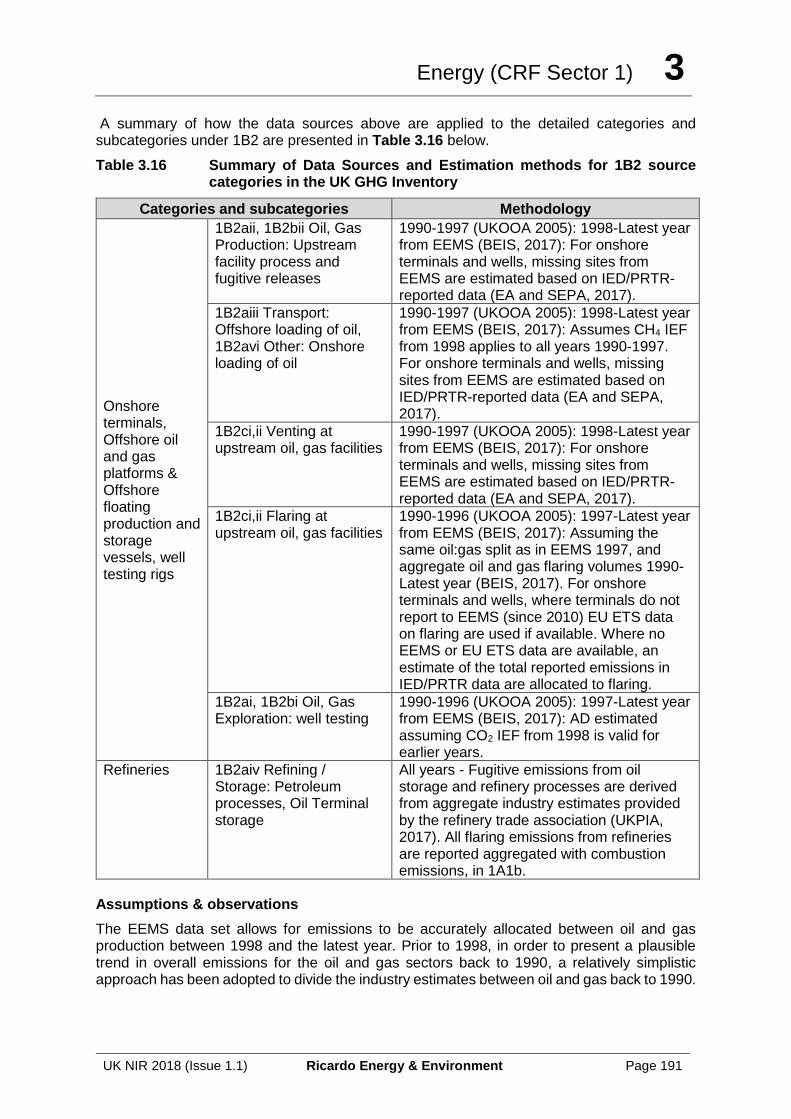
Energy (CRF Sector 1) 3
UK NIR 2018 (Issue 1.1) Ricardo Energy & Environment Page 191
A summary of how the data sources above are applied to the detailed categories and subcategories under 1B2 are presented in Table 3.16 below.
Table 3.16 Summary of Data Sources and Estimation methods for 1B2 source categories in the UK GHG Inventory
Categories and subcategories Methodology
Onshore terminals, Offshore oil and gas platforms & Offshore floating production and storage vessels, well testing rigs
1B2aii, 1B2bii Oil, Gas Production: Upstream facility process and fugitive releases
1990-1997 (UKOOA 2005): 1998-Latest year from EEMS (BEIS, 2017): For onshore terminals and wells, missing sites from EEMS are estimated based on IED/PRTR-reported data (EA and SEPA, 2017).
1B2aiii Transport: Offshore loading of oil, 1B2avi Other: Onshore loading of oil
1990-1997 (UKOOA 2005): 1998-Latest year from EEMS (BEIS, 2017): Assumes CH4 IEF from 1998 applies to all years 1990-1997. For onshore terminals and wells, missing sites from EEMS are estimated based on IED/PRTR-reported data (EA and SEPA, 2017).
1B2ci,ii Venting at upstream oil, gas facilities
1990-1997 (UKOOA 2005): 1998-Latest year from EEMS (BEIS, 2017): For onshore terminals and wells, missing sites from EEMS are estimated based on IED/PRTR-reported data (EA and SEPA, 2017).
1B2ci,ii Flaring at upstream oil, gas facilities
1990-1996 (UKOOA 2005): 1997-Latest year from EEMS (BEIS, 2017): Assuming the same oil:gas split as in EEMS 1997, and aggregate oil and gas flaring volumes 1990-Latest year (BEIS, 2017). For onshore terminals and wells, where terminals do not report to EEMS (since 2010) EU ETS data on flaring are used if available. Where no EEMS or EU ETS data are available, an estimate of the total reported emissions in IED/PRTR data are allocated to flaring.
1B2ai, 1B2bi Oil, Gas Exploration: well testing
1990-1996 (UKOOA 2005): 1997-Latest year from EEMS (BEIS, 2017): AD estimated assuming CO2 IEF from 1998 is valid for earlier years.
Refineries 1B2aiv Refining / Storage: Petroleum processes, Oil Terminal storage
All years - Fugitive emissions from oil storage and refinery processes are derived from aggregate industry estimates provided by the refinery trade association (UKPIA, 2017). All flaring emissions from refineries are reported aggregated with combustion emissions, in 1A1b.
Assumptions & observations
The EEMS data set allows for emissions to be accurately allocated between oil and gas production between 1998 and the latest year. Prior to 1998, in order to present a plausible trend in overall emissions for the oil and gas sectors back to 1990, a relatively simplistic approach has been adopted to divide the industry estimates between oil and gas back to 1990.
Energy (CRF Sector 1) 3
UK NIR 2018 (Issue 1.1) Ricardo Energy & Environment Page 192
For flaring, gas consumption and well testing emissions, the oil:gas ratio of activity data in 1998 has been used to extrapolate back the activities to 1990, retaining the previous emission factors for the “oil and gas” sources. For process and fugitive sources, oil storage and venting emissions, where the EEMS data are simply presented as emissions data without any underlying activity and emission factor information, the estimates for the early part of the time series are simply based on the oil:gas ratio (for each pollutant) from 1998.
Recalculations
There have been no method changes. There have been some minor revisions to UK estimates for sources from the upstream oil and gas sector and downstream petroleum processes, where QC and stakeholder consultation with regulators and operators has enabled the Inventory Agency to address any identified reporting gaps or inconsistencies. One notable revision in 2015 is to 1B2a2 – petroleum processes, where an estimate from the PI has been identified as incorrect and revised. Flaring data from one missing platform has also been incorporated, although this revision is relatively minor. Quantitative data are presented in Section 10.
Improvements (completed and planned)
Emission factors and activity data are kept under review. The inventory agency will maintain dialogue with regulators and industry experts in order to seek any new data on emissions from oil and gas well blowouts. The inventory agency will also maintain a watching brief on the development of the shale gas industry, in order to ensure that if the industry does start to produce gas in the UK, that the inventory agency will have access to information to allow emission estimates to be derived for future inventory submissions.
QA/QC
The EEMS dataset quality system is managed by the regulatory agency (BEIS) and developed in conjunction with the trade association (UK Oil & Gas). EEMS uses an online reporting system with controls over data entry, together with guidance notes provided to operators to provide estimation methodology options and emission factors for specific processes.
The Inventory Agency combines UK energy statistics, the EEMS data, EU ETS and IPPC data to derive the oil and gas sector estimates. The data reported from the EEMS system must be reconciled with the UK Energy Statistics and integrated into the NAEI without double-counting emissions. Where the EU ETS or IPPC data are inconsistent with the EEMS data, the Inventory Agency works with the BEIS Offshore Inspectorate and facility operators to determine the best available data for each source. The Inventory Agency also conducts time-series consistency checks to identify missing sites or sources, and for those sources where the EEMS data includes emissions and activity data the Inventory Agency reviews the time series of implied emission factors to identify outliers. Any sites or sources where the quality checks identify gaps, outliers or inconsistent reporting between different regulatory systems are resolved in consultation with the BEIS Offshore Inspectorate.
Time series consistency
The emission estimates for the offshore industry are based on the EEMS dataset for 1998-2016, whilst emission estimates for 1990-1997 are based on trade association data (UKOOA, 2005) to update earlier industry studies (UKOOA, 1998) that had used production data as a basis for generating sector-wide estimates from 1990. The EEMS dataset (BEIS, 2017) provides a consistent time-series of emission estimates for many facilities and sources, but since 2010 the reporting by onshore terminals is voluntary and the completeness of the dataset is variable for recent years. Furthermore, whilst the EEMS data quality appears to be improving over recent years, the completeness of EEMS data for specific facilities and sources
Energy (CRF Sector 1) 3
UK NIR 2018 (Issue 1.1) Ricardo Energy & Environment Page 193
is still subject to uncertainty; reporting gaps appear to be systematic for some facilities, such as frequent non-reporting of oil loading / unloading emissions at some terminals. The Inventory Agency continues to work with the regulatory agency, BEIS, in the continued development of emission estimates from this sector.
The time-series of the IEF of CO2 emissions in sector 1.B.2.a.2 (Oil Production) show a significant drop between 2011-2012 and a sharp rise between 2013 and 2015. Whilst oil production activity data is comparatively steady between 2011 and 2015, CO2 emissions from this source are highly variable. This is because CO2 emissions for this source are dominated by one installation which processes sour gas in the UK. This site was offline for most of 2012, 2013, and part of 2014, explaining the large variation in IEF over this period of the time-series.
Uncertainties
Uncertainties are presented in Annex 2. Emissions data taken from the EEMS reporting system 1998 onwards are considered to be high quality, emissions data for other years are subject to greater uncertainties.
MS 20 Gas leakage
Relevant Categories, source names
1B2b4: Natural Gas (transmission leakage)
1B2b5: Natural gas (distribution leakage)
Natural Gas (leakage at point of use)
Relevant Gases
CO2, CH4
Relevant fuels, activities
Leakage from gas transmission and distribution, leakage at the point of use
Background
The UK GHG inventory includes estimates of methane and carbon dioxide emissions from natural gas leakage from the downstream gas supply network, including releases from: high pressure transmission network; distribution network; gas leaks at point of use. Annual activity data and gas compositional analysis are provided by National Grid, four companies (formed in 2005) that operate the low-pressure gas distribution networks within Great Britain, and Airtricity in Northern Ireland.
Key Data sources
Activity data: Natural gas leakage data in energy and mass units, from the UK downstream natural gas network operators: National Grid, Scotia Gas, Northern Gas Networks, Wales & West, and Airtricity (NI).
AD for gas use in domestic and commercial sectors from DUKES (BEIS, 2017) are used to generate leakage at point of use estimates.
Emission factors: Natural gas compositional data (mass % data for: nitrogen, carbon dioxide, methane, ethane, propane, i-butane, n-butane, neo-pentane, i-pentane, n-pentane, hexanes+) supplied by the gas network operators as listed above. UK estimates of natural gas consumption within each Local Distribution Zone (LDZ) are used to generate a weighted-average UK
Energy (CRF Sector 1) 3
UK NIR 2018 (Issue 1.1) Ricardo Energy & Environment Page 194
compositional analysis of natural gas consumed annually. From 2007 these data are available from Long Term Development Plans published by each of the gas network operators; earlier data by LDZ are based on Local Authority-level consumption estimates aggregated into LDZs (CLARE database, 2012).
EFs for the gas leakage at point of use are derived from UK data on gas fitting performance and assumptions regarding unit operational cycles, ignition times.
An accompanying spreadsheet “Energy_background_data_uk_2018.xlxs” lists all emission factors used in the energy sector, including a full list of references25.
Method approach
The leakage estimates are calculated using separate methodologies to cover:
1. Natural gas leaks from the high-pressure transmission mains (National Grid Gas); (reported under 1B2b4 Transmission)
2. Natural gas leaks from the low pressure distribution network, medium pressure gas mains, Above Ground Installations (AGIs), AGI working losses and interference (National Grid Gas, Scotia Gas, Northern Gas Networks, Wales & West, Airtricity); (Reported under 1B2b5 Distribution)
3. Other losses of natural gas at the point of use (BEIS DUKES, UK research); (Reported under 1B2b5 Distribution)
For methods 1 and 2 above, from 2004 onwards the gas network operators provide annual gas leakage estimates on a mass basis, providing a breakdown of emissions across all 14 regional gas networks in the UK, which are called Local Distribution Zones (LDZs). National Grid Gas operates the high-pressure natural gas transmission network and 5 of the LDZs; Northern Gas Networks operates 2 LDZs; Scotia Gas operates 3 LDZs; Wales and West Utilities operates 3 LDZs; Airtricity operates 1 LDZ. In addition, each of the gas network operators provides annual natural gas compositional analysis for their networks. Prior to 2004, the data on gas leakage (activity data and compositional analysis) was all provided by British Gas, which operated all of the UK networks before the industry was privatised.
The information on methane losses from the high pressure transmission system (1B2b4) are estimated by National Grid based on (i) periodic fugitive emission surveys for the NTS, compressor stations and LNG terminals, and (ii) NG records of intentional venting actions on the network. These data have not been available for every year across the time series, with only two data points in the 1990s, annual data from 2000-2004, then data for 2011 and 2012. Data for other years are estimated using interpolation (2005-2010) and extrapolation (early time series and for 2013 and 2015-2016).
The UK GHG inventory estimates for 1B2b5 (distribution leakage) are based on the aggregate of mass of gas leaked across all networks (low pressure mains and other losses), with the methane content of the natural gas based on compositional analysis from all of the gas network operators.
The activity data reported in the CRF for these sources are the final UK annual gas demand data. These data are not used within the GHG inventory estimation method, but are presented to enable IEFs to be derived, to aid comparability of the UK estimates with those of other countries.
UK Gas Network Leakage Model
The UK gas network operators use a common industry leakage model to derive their annual estimates of gas leakage from the low and medium pressure distribution systems. The UK gas network leakage model was developed by British Gas and uses factors and assumptions on
Energy (CRF Sector 1) 3
UK NIR 2018 (Issue 1.1) Ricardo Energy & Environment Page 195
leakage rates for different types of gas mains and installations, based on measurements and surveys conducted in 1992 and 2002, with annual updates to maintain the representation of the UK gas network infrastructure (such as length and type of pipelines and other units) and reflect the rolling programme of network replacement. Historical data for the leakage from the low-pressure distribution network and other losses is based on studies from British Gas in the early 1990s (British Gas, 1993; Williams, 1993).
Natural Gas Compositional Data
Data on the methane and NMVOC content of natural gas have been provided by contacts within British Gas Research for 1990-1996 and by UK Transco from 1997 to 2005 (Personal Communication: Dave Lander, 2008), and from the gas network operators from 2006 onwards. NMVOC content for 2001-2003 has been estimated by interpolation due to a lack of data; CO2 compositional data from 2004 onwards are derived from annual compositional analysis by gas network operators, whilst the 1990-2003 data have been extrapolated back from the 2004 figure. No gas composition data have been provided by Airtricity and hence the UK average gas composition is assumed for Northern Ireland.
Each of the gas network operators obtain their compositional analysis from a central system of data logging from the automated sampling and analysis network that was operated previously under the Transco ownership, prior to the network being opened up to greater market competition. The Inventory Agency has direct contacts within the organisation (GL-Advantica) that manages the compositional data from across the UK gas network, and works directly with their gas analysis team to ensure that gas compositional data provided to the Inventory Agency by network operators is representative of the gas quality year-round, rather than a snap-shot from a limited number of analyses.
The calculation of the reported UK average gas composition is derived from the sum-product of the annual Local Distribution Zone (LDZ) compositional data and the estimated gas consumption through each of the LDZs, to provide an average gas composition for Great Britain which is then applied across the UK. The estimates of gas consumption within each LDZ are based, from 2007 onwards, on LDZ throughput data presented within Long Term Development Statements by each of the gas network operators; prior to 2007 these data are unavailable, and the best available data to inform the UK weighted average composition are sub-national gas use statistics at local authority level (then aggregated to LDZs) which are published by BEIS annually and processed for UK Local Authority CO2 emission estimates via the CLARE database.
Northern Ireland Gas Network
The gas infrastructure in Northern Ireland is much newer than in the rest of the UK, as the gas pipeline (from Scotland) was only commissioned in 1999. Since then, the gas network has continued to develop across Northern Ireland. Annual estimates of gas leakage from 2005 onwards have been provided by the main gas operator (Airtricity, 2017), and the data for 1999 to 2004 have been extrapolated back from the 2005 figure.
The third inventory estimation methodology is used to determine estimates of natural gas leakage at the point of use, and these estimates are also reported in 1B2b5. Leakages are estimated for a range of different appliances that use gas, combined with national statistics on natural gas consumption in the domestic and commercial sectors (BEIS, 2017).
Industrial Heating Boilers
Methane releases are assumed to be “Not Occurring” from these appliances, based on consultation with technical experts that advise the UK Government for the CHP QA scheme (Personal Communication: R Stewart, 2011). Larger boilers typically operate almost permanently once ignited (particularly if used for steam-raising) with little or no cycling from
Energy (CRF Sector 1) 3
UK NIR 2018 (Issue 1.1) Ricardo Energy & Environment Page 196
on to off states. Furthermore, releases of un-burnt natural gas are strictly controlled in industrial locations for safety reasons.
Domestic Heating, Water Heating Boilers and cooking
Methane emissions from pre-ignition losses of gas appliances domestic properties are based on activity data from Energy Consumption in the UK (BEIS, 2017) which provides a time-series of gas use for heating, water heating and cooking in the domestic sector, using a series of assumptions regarding the size of units, number of units, age of units, gas flow rates, air flow rates, delays to ignition, operation times from used to determine the percentage of gas that is not burned. The estimates of UK appliance stock, by capacity and design and estimated average gas consumption per appliance per day are all derived from Ecodesign studies (energy efficiency analysis) through the UK Government Market Transformation Programme (Ecodesign Lot 22 and Lot 23, 2011). The estimates of appliance cycle operation times and estimated delays to ignition for different appliances are based on expert judgement of UK combustion technology experts (Personal communication, Stewart, 2012).
Commercial Gas Appliances: Catering and other uses
Methane emissions from pre-ignition losses of gas appliances used in commercial catering and other uses are based on activity data from ECUK (BEIS, 2017) which provides a time series of gas use for catering and other uses in the commercial sector to 2016. The method then applies a series of assumptions regarding the operational cycles and delays to ignition, to derive a simple percentage non-combusted estimate for each gas appliance type using references and expert judgements as noted above for domestic appliances.
An overview of the time series of gas leak at point of use estimates in the UK, together with overall gas use by economic sector and appliance type is presented in Annex 3.
Assumptions & observations
Assumptions used to estimate the leakage at point of use for domestic heating and water heating boilers are as follows:
• average boiler size in the UK of 30kW;
• a burn chamber size, natural gas flow rate taken from a typical combination boiler;
• estimated delay to ignition: 0.25 seconds for automatic ignition, 2 seconds for manual ignition;
• an air flow rate based on 25% excess oxygen in the combustion chamber when compared to stoichiometric ratio;
• an equation for a mixed reactor (1-ex) that when integrated will provide an estimate of the concentration of un-burnt air/fuel mixture released; and
• assumptions relating to the boiler yearly operation and cycling frequency, between heating and water heating applications
o On average in the UK domestic properties have heating systems operating for half of the year and on average the heating is on for 5 hours per day. It is also assumed that during each hour that the boiler providing heating cycles on and off 4 times.
o All UK domestic properties that have hot water heating systems also have gas heated hot water.
o Average water heating is on for 4 hours per day every day of the year. o During each hour that a boiler is heating water, the boiler cycles on and off 5
times.
The number of boilers across the time series is thought to have increased (ca. 22 million in 2008) due to the increasing use of gas central heating for space heating, and the increase in the number of houses. However, it is assumed that pre-ignition gas loss in boilers installed in
Energy (CRF Sector 1) 3
UK NIR 2018 (Issue 1.1) Ricardo Energy & Environment Page 197
houses in 1990 were greater than in the current boilers installed, as technology has improved. Therefore, it is assumed that the proportion of gas leaked (i.e. % of the total gas use) from domestic heating and water heating appliances per annum is steady across the time series, with the rationale that the sum of greater pre-ignition losses from fewer older-technology boilers in the early part of the time series will be roughly equivalent to the sum of lower pre ignition losses per unit from the greater number of newer-technology boilers in recent years.
Assumptions used to estimate the leakage at point of use for domestic cooking appliances (manual and automatic ignition) and gas fires are as follows:
• gas fires use an estimated 2.5% of total gas used for space heating in the domestic sector, with the remainder used in (automatic ignition) boilers;
• gas use in cooking hobs is estimated to be 73.6% of the total domestic gas use in cooking, with the remainder in gas ovens. This is based on data of average annual gas oven fuel use in kWh/yr and average domestic gas hob fuel use in kWh/yr, combined with data on UK stock of gas ovens and hobs, taken from a series of 2011 European Commission Eco-design studies (Bio IS / ERA Technology, 2011);
• for manual ignition devices, a conservative estimate of the delay prior to ignition of 2 seconds has been assumed (expert judgement), whilst the average operational cycle times for different types of appliance have been estimated at 900 seconds for a domestic hob (expert judgement) and 5400 seconds for a gas fire (EC Eco-design Lot 20 Task 5, gas stove base case, 2011); and
• for automatic ignition appliances, a conservative estimate of the delay prior to ignition of 0.25 seconds has been assumed (expert judgement), whilst the average operational cycle times of domestic ovens has been estimated at 900 seconds (expert judgement).
Assumptions used to estimate the leakage at point of use for commercial gas appliances (catering and other uses) are as follows:
• for commercial catering gas use, a conservative estimate of the delay prior to ignition of 0.5 seconds has been assumed (expert judgement, to reflect a mixture of hobs and oven use), whilst the average operational cycle has been estimated at 900 seconds (expert judgement); and
• for other commercial gas appliances, assumed to be predominantly gas-fired boilers of automatic ignition design, a conservative estimate of the delay prior to ignition of 0.25 seconds has been assumed (expert judgement), whilst the average operational cycle time has been estimated at 1800 seconds (expert judgement).
Recalculations
A number of minor revisions to the model have been made to reduce rounding errors. Specific revisions have also been made to the following categories:
1B2b5 Natural gas (distribution leakage)
Up to date data for Northern Ireland has been incorporated, in place of rolled data
1B2b5 Natural Gas (leakage at point of use)
The 2017 submission used data from an older edition of ECUK, with extrapolations beyond 2013. This publication was updated for 2017 and therefore extrapolated data have been replaced with actual values. Gas composition data for this source was using a constant value from 1990, this has been replaced with a time series for consistency with other gas leakage sources.
Energy (CRF Sector 1) 3
UK NIR 2018 (Issue 1.1) Ricardo Energy & Environment Page 198
Improvements (completed and planned)
No improvements to this method are currently planned. Emission factors and activity data are kept under review.
QA/QC
The sector estimates are subject to the same Tier 1 QA/QC routines as all other source categories in the UK GHGI.
Checks on data reported by gas network operators are conducted to check consistency across the time series and also between operators; for example, in compiling the 2015 submission data, through quality checks between gas network operators it was noted that the gas compositional data for 2013 from Wales and West Utilities was an outlier. The Inventory Agency identified that estimated mass percentage calculations were incorrect, and the values were subsequently revised and then used in the UK GHGI compilation.
As recommended during the September 2014 centralised review of the UK inventory, the UK Inventory Agency has also conducted verification checks on the UK GHGI estimates, by deriving separate emission estimates for methane using the Tier 1 default methods outlined in both the 1996 GLs and the 2006 GLs. The method in the 1996 GLs uses max and min default factors based on the pipeline length of the transmission and distribution network, whilst the 2006 GLs Tier 1 method uses max and min default factors based on the total volume of delivered natural gas. The results are summarised below for 1990 and 2013 data:
1990 UK GHGI total (transmission plus distribution) = 378.8 kt CH4
Using IPCC 1996 GLs Tier 1 method, the range for emissions is derived as 155 to 215 kt CH4
Using IPCC 2006 GLs Tier 1 method, the range for emissions is derived as 67 to 105 kt CH4
Therefore, compared to both Tier 1 methods, the 1990 UK GHGI estimate is higher than the range of values.
2013 UK GHGI total (transmission plus distribution) = 168.5 kt CH4
Using IPCC 1996 GLs Tier 1 method, the range for emissions is derived as 155 to 215 kt CH4
Using IPCC 2006 GLs Tier 1 method, the range for emissions is derived as 95 to 148 kt CH4
Therefore, compared to the Tier 1 methods, the 2013 UK GHGI estimate is within the range of values for the 1996 GLs method and higher than the range of values for the 2006 GLs method.
The comparison against the IPCC Tier 1 methods indicates that the UK GHGI estimates are of a similar order of magnitude as the Tier 1 defaults. The 1990 UK GHGI value appears to be high, as it is above the range of values derived from the IPCC Tier 1 methods, whilst the 2013 UK GHGI value is also higher than the range for the 2006 GLs Tier 1 method. However, the UK estimates are derived from a country-specific method and we note that the uncertainty estimates provided in the 2006 GLs for the default EFs provided for gas network distribution (which is by far the greatest contributor to overall methane leakage) are cited as -20 % to +500% for factors for developed countries. Therefore, given the large uncertainty range, the UK data are consistent with the IPCC Tier 1 estimates.
Energy (CRF Sector 1) 3
UK NIR 2018 (Issue 1.1) Ricardo Energy & Environment Page 199
Time series consistency
As far as possible, consistent source data and methods are used across the time series. However, we note the following limitations of the current methods:
• The available data on methane leakage from the high pressure gas transmission system is limited. Data are not available for all years of the time series and therefore gap-filling techniques (extrapolation and interpolation) are used;
• The calibration of the UK gas leakage model used by all natural gas network operators in based on two in-depth studies of the leakage rates from different constituent elements of the UK gas network – one in 1992, another in 2002. These studies have been used to establish estimated leakage rates in the UK model that are then applied to activity data gathered annually through surveys and from gas network renewal projects; and
• The derivation of the UK average natural gas composition uses the best available data for every year of the time series, as the factors are critical for the UK GHGI estimates as a whole (not just for the leakage estimates, but also for natural gas combustion estimates). Since 2007 the weighted average has been calculated using actual data available on gas throughout for each LDZ; prior to 2007 these data are not available and the LDZ gas throughput estimates used in the calculation of the UK average gas composition use Local Authority level gas use estimates, aggregated up to LDZs. These earlier data at Local Authority level were regarded as “experimental statistics” by DECC until the 2005 dataset were published as national statistics, and as such are regarded as more uncertain than the more recent data.
Uncertainties
Uncertainties are presented in Annex 2. Uncertainties in the emission estimates from leakage from the gas transmission and distribution network stem predominantly from the assumptions within the industry model that derives mass leakage estimates based on input data such as network pipe replacement (plastic replacing old metal pipelines) and activities/incidents at Above Ground Installations; for these sources the methane content of the gas released is known to a high degree of accuracy, but the mass emitted is based on industry calculations.
As noted in the section above, the uncertainties for the estimates of gas leakage at point of use are high due to the lack of source data, an IPCC method and the need to use a series of assumptions and expert judgement to estimate the leakage from different gas appliance types. The Inventory Agency considers that the assumptions provide a conservative estimate of gas leakage at point of use across the time series.
Energy (CRF Sector 1) 3
UK NIR 2018 (Issue 1.1) Ricardo Energy & Environment Page 200
.
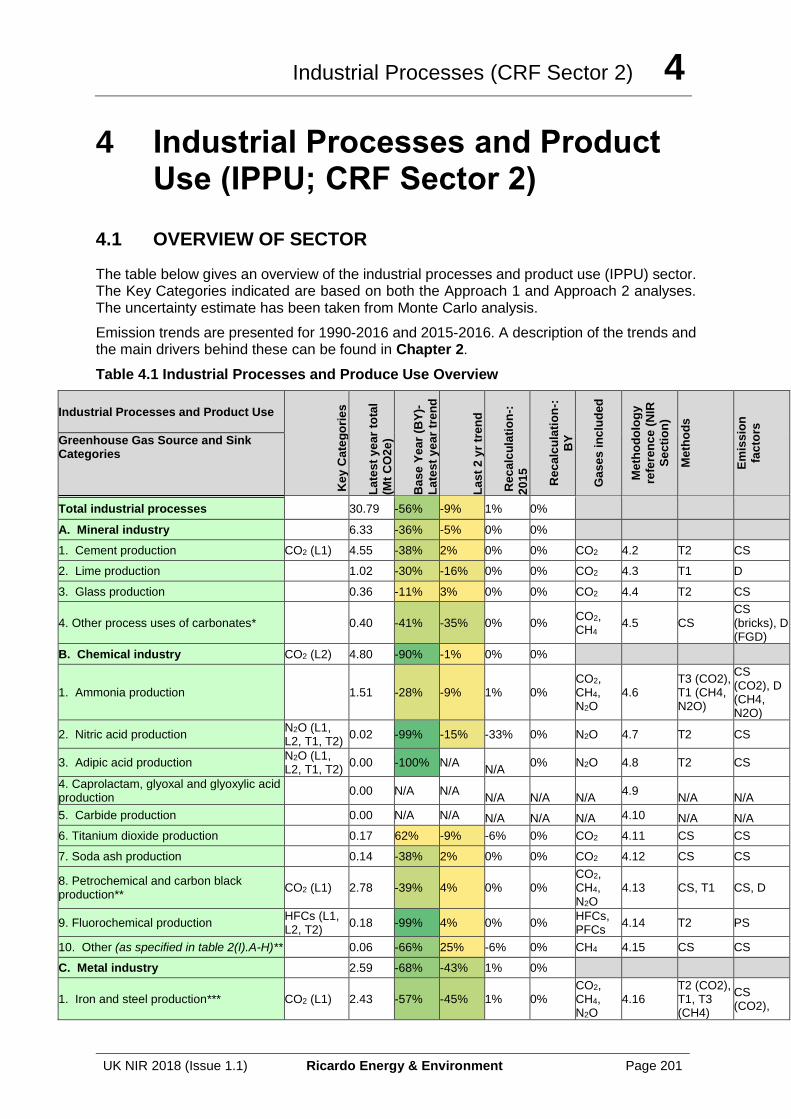
Industrial Processes (CRF Sector 2) 4
UK NIR 2018 (Issue 1.1) Ricardo Energy & Environment Page 201
4 Industrial Processes and Product Use (IPPU; CRF Sector 2)
4.1 OVERVIEW OF SECTOR
The table below gives an overview of the industrial processes and product use (IPPU) sector. The Key Categories indicated are based on both the Approach 1 and Approach 2 analyses. The uncertainty estimate has been taken from Monte Carlo analysis.
Emission trends are presented for 1990-2016 and 2015-2016. A description of the trends and the main drivers behind these can be found in Chapter 2.
Table 4.1 Industrial Processes and Produce Use Overview
Industrial Processes and Product Use
Key
Ca
teg
ori
es
La
tes
t y
ea
r to
tal
(Mt
CO
2e
)
Ba
se
Ye
ar
(BY
)-
La
tes
t y
ea
r tr
en
d
La
st
2 y
r tr
en
d
Rec
alc
ula
tio
n-:
20
15
Rec
alc
ula
tio
n-:
BY
Ga
se
s i
nc
lud
ed
Me
tho
do
log
y
refe
ren
ce
(N
IR
Se
cti
on
)
Me
tho
ds
Em
iss
ion
fac
tors
Greenhouse Gas Source and Sink Categories
Total industrial processes 30.79 -56% -9% 1% 0%
A. Mineral industry 6.33 -36% -5% 0% 0%
1. Cement production CO2 (L1) 4.55 -38% 2% 0% 0% CO2 4.2 T2 CS
2. Lime production 1.02 -30% -16% 0% 0% CO2 4.3 T1 D
3. Glass production 0.36 -11% 3% 0% 0% CO2 4.4 T2 CS
4. Other process uses of carbonates* 0.40 -41% -35% 0% 0% CO2, CH4
4.5 CS CS (bricks), D (FGD)
B. Chemical industry CO2 (L2) 4.80 -90% -1% 0% 0%
1. Ammonia production 1.51 -28% -9% 1% 0% CO2, CH4, N2O
4.6 T3 (CO2), T1 (CH4, N2O)
CS (CO2), D (CH4, N2O)
2. Nitric acid production N2O (L1, L2, T1, T2)
0.02 -99% -15% -33% 0% N2O 4.7 T2 CS
3. Adipic acid production N2O (L1, L2, T1, T2)
0.00 -100% N/A N/A
0% N2O 4.8 T2 CS
4. Caprolactam, glyoxal and glyoxylic acid production
0.00 N/A N/A N/A N/A N/A
4.9 N/A N/A
5. Carbide production 0.00 N/A N/A N/A N/A N/A 4.10 N/A N/A
6. Titanium dioxide production 0.17 62% -9% -6% 0% CO2 4.11 CS CS
7. Soda ash production 0.14 -38% 2% 0% 0% CO2 4.12 CS CS
8. Petrochemical and carbon black production**
CO2 (L1) 2.78 -39% 4% 0% 0% CO2, CH4, N2O
4.13 CS, T1 CS, D
9. Fluorochemical production HFCs (L1, L2, T2)
0.18 -99% 4% 0% 0% HFCs, PFCs
4.14 T2 PS
10. Other (as specified in table 2(I).A-H)** 0.06 -66% 25% -6% 0% CH4 4.15 CS CS
C. Metal industry 2.59 -68% -43% 1% 0%
1. Iron and steel production*** CO2 (L1) 2.43 -57% -45% 1% 0% CO2, CH4, N2O
4.16 T2 (CO2), T1, T3 (CH4)
CS (CO2),
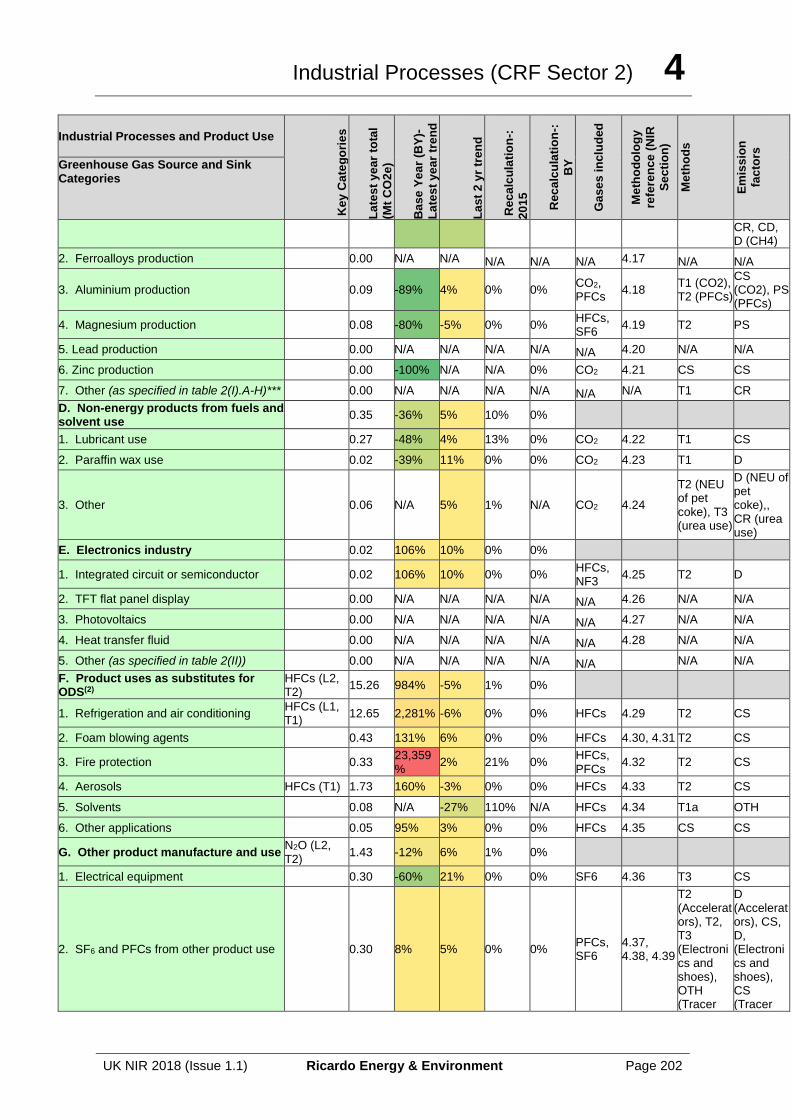
Industrial Processes (CRF Sector 2) 4
UK NIR 2018 (Issue 1.1) Ricardo Energy & Environment Page 202
Industrial Processes and Product Use
Ke
y C
ate
go
rie
s
La
tes
t y
ea
r to
tal
(Mt
CO
2e
)
Ba
se
Ye
ar
(BY
)-
La
tes
t y
ea
r tr
en
d
La
st
2 y
r tr
en
d
Re
ca
lcu
lati
on
-:
20
15
Re
ca
lcu
lati
on
-:
BY
Ga
se
s i
nc
lud
ed
Me
tho
do
log
y
refe
ren
ce
(N
IR
Se
cti
on
)
Me
tho
ds
Em
iss
ion
fac
tors
Greenhouse Gas Source and Sink Categories
CR, CD, D (CH4)
2. Ferroalloys production 0.00 N/A N/A N/A N/A N/A 4.17 N/A N/A
3. Aluminium production 0.09 -89% 4% 0% 0% CO2, PFCs
4.18 T1 (CO2), T2 (PFCs)
CS (CO2), PS (PFCs)
4. Magnesium production 0.08 -80% -5% 0% 0% HFCs, SF6
4.19 T2 PS
5. Lead production 0.00 N/A N/A N/A N/A N/A 4.20 N/A N/A
6. Zinc production 0.00 -100% N/A N/A 0% CO2 4.21 CS CS
7. Other (as specified in table 2(I).A-H)*** 0.00 N/A N/A N/A N/A N/A N/A T1 CR
D. Non-energy products from fuels and solvent use
0.35 -36% 5% 10% 0%
1. Lubricant use 0.27 -48% 4% 13% 0% CO2 4.22 T1 CS
2. Paraffin wax use 0.02 -39% 11% 0% 0% CO2 4.23 T1 D
3. Other 0.06 N/A 5% 1% N/A CO2 4.24
T2 (NEU of pet coke), T3 (urea use)
D (NEU of pet coke),, CR (urea use)
E. Electronics industry 0.02 106% 10% 0% 0%
1. Integrated circuit or semiconductor 0.02 106% 10% 0% 0% HFCs, NF3
4.25 T2 D
2. TFT flat panel display 0.00 N/A N/A N/A N/A N/A 4.26 N/A N/A
3. Photovoltaics 0.00 N/A N/A N/A N/A N/A 4.27 N/A N/A
4. Heat transfer fluid 0.00 N/A N/A N/A N/A N/A 4.28 N/A N/A
5. Other (as specified in table 2(II)) 0.00 N/A N/A N/A N/A N/A N/A N/A
F. Product uses as substitutes for ODS(2)
HFCs (L2, T2)
15.26 984% -5% 1% 0%
1. Refrigeration and air conditioning HFCs (L1, T1)
12.65 2,281% -6% 0% 0% HFCs 4.29 T2 CS
2. Foam blowing agents 0.43 131% 6% 0% 0% HFCs 4.30, 4.31 T2 CS
3. Fire protection 0.33 23,359%
2% 21% 0% HFCs, PFCs
4.32 T2 CS
4. Aerosols HFCs (T1) 1.73 160% -3% 0% 0% HFCs 4.33 T2 CS
5. Solvents 0.08 N/A -27% 110% N/A HFCs 4.34 T1a OTH
6. Other applications 0.05 95% 3% 0% 0% HFCs 4.35 CS CS
G. Other product manufacture and use N2O (L2, T2)
1.43 -12% 6% 1% 0%
1. Electrical equipment 0.30 -60% 21% 0% 0% SF6 4.36 T3 CS
2. SF6 and PFCs from other product use 0.30 8% 5% 0% 0% PFCs, SF6
4.37, 4.38, 4.39
T2 (Accelerators), T2, T3 (Electronics and shoes), OTH (Tracer
D (Accelerators), CS, D, (Electronics and shoes), CS (Tracer
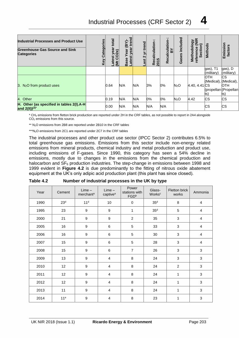
Industrial Processes (CRF Sector 2) 4
UK NIR 2018 (Issue 1.1) Ricardo Energy & Environment Page 203
Industrial Processes and Product Use
Ke
y C
ate
go
rie
s
La
tes
t y
ea
r to
tal
(Mt
CO
2e
)
Ba
se
Ye
ar
(BY
)-
La
tes
t y
ea
r tr
en
d
La
st
2 y
r tr
en
d
Re
ca
lcu
lati
on
-:
20
15
Re
ca
lcu
lati
on
-:
BY
Ga
se
s i
nc
lud
ed
Me
tho
do
log
y
refe
ren
ce
(N
IR
Se
cti
on
)
Me
tho
ds
Em
iss
ion
fac
tors
Greenhouse Gas Source and Sink Categories
gas), T1 (military)
gas), D (military)
3. N2O from product uses 0.64 N/A N/A 3% 0% N2O 4.40, 4.41
OTH (Medical), CS (propellants)
CS (Medical), OTH (Propellants)
4. Other 0.19 N/A N/A 0% 0% N2O 4.42 CS CS
H. Other (as specified in tables 2(I).A-H and 2(II))(3)*
0.00 N/A N/A N/A N/A CS CS
* CH4 emissions from fletton brick production are reported under 2H in the CRF tables, as not possible to report in 2A4 alongside CO2 emissions from this source.
** N2O emissions from 2B8 are reported under 2B10 in the CRF tables
***N2O emissions from 2C1 are reported under 2C7 in the CRF tables
The industrial processes and other product use sector (IPCC Sector 2) contributes 6.5% to total greenhouse gas emissions. Emissions from this sector include non-energy related emissions from mineral products, chemical industry and metal production and product use, including emissions of F-gases. Since 1990, this category has seen a 54% decline in emissions, mostly due to changes in the emissions from the chemical production and halocarbon and SF6 production industries. The step-change in emissions between 1998 and 1999 evident in Figure 4.2 is due predominantly to the fitting of nitrous oxide abatement equipment at the UK’s only adipic acid production plant (this plant has since closed).
Table 4.2 Number of industrial processes in the UK by type
Year Cement Lime –
merchanta
Lime – captivea
Power stations with
FGDb
Glass- Worksc
Fletton brick works
Ammonia
1990 23d 11d 10 0 35d 8 4
1995 23 9 9 1 35d 5 4
2000 21 9 9 2 35 3 4
2005 16 9 6 5 33 3 4
2006 16 9 6 5 30 3 4
2007 15 9 6 5 28 3 4
2008 15 9 6 7 26 3 3
2009 13 9 4 8 24 3 3
2010 12 9 4 8 24 2 3
2011 12 9 4 8 24 1 3
2012 12 9 4 8 24 1 3
2013 11 9 4 8 24 1 3
2014 11e 9 4 8 23 1 3
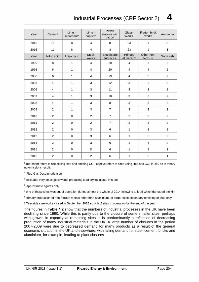
Industrial Processes (CRF Sector 2) 4
UK NIR 2018 (Issue 1.1) Ricardo Energy & Environment Page 204
Year Cement Lime –
merchanta
Lime – captivea
Power stations with
FGDb
Glass- Worksc
Fletton brick works
Ammonia
2015 11 8 4 8 23 1 3
2016 11 8 4 8 23 1 3
Year Nitric acid Adipic acid Steel- works
Electric arc furnaces
Primary aluminium
Other non-ferrousf
Soda ash
1990 8 1 4 20 4 5 2
1995 6 1 4 20 4 4 2
2000 6 1 4 19 4 3 2
2005 4 1 3 12 3 2 2
2006 4 1 3 11 3 3 2
2007 4 1 3 10 3 3 2
2008 4 1 3 8 3 3 2
2009 2 1 3 7 3 3 2
2010 2 0 2 7 2 3 2
2011 2 0 2 7 2 3 2
2012 2 0 3 6 1 3 2
2013 2 0 3 6 1 3 2
2014 2 0 3 6 1 3 2
2015 2 0 3g 6 1 3 1
2016 2 0 2 6 1 3 1
a merchant refers to site selling lime and emitting CO2, captive refers to sites using lime and CO2 in-situ so in theory
no emissions result.
b Flue Gas Desulphurisation
c excludes very small glassworks producing lead crystal glass, frits etc.
d approximate figures only
e one of these sites was out of operation during almost the whole of 2014 following a flood which damaged the kiln
f primary production of non-ferrous metals other than aluminium, or large-scale secondary smelting of lead only
g Teesside steelworks closed in September 2015 so only 2 sites in operation by the end of the year
The figures in Table 4.2 show that the numbers of industrial processes in the UK have been declining since 1990. While this is partly due to the closure of some smaller sites, perhaps with growth in capacity at remaining sites, it is predominantly a reflection of decreasing production of many industrial materials in the UK. A large number of closures in the period 2007-2009 were due to decreased demand for many products as a result of the general economic situation in the UK and elsewhere, with falling demand for steel, cement, bricks and aluminium, for example, leading to plant closures.
Industrial Processes (CRF Sector 2) 4
UK NIR 2018 (Issue 1.1) Ricardo Energy & Environment Page 205
Figure 4.1 Breakdown of total GHG emissions in Industrial Processes sector
Figure 4.2 Trend in total GHG emissions in Industrial Processes sector
4.2 SOURCE CATEGORY 2A1 – CEMENT PRODUCTION
4.2.1 Source Category Description
Emissions of CO2 from fuel combustion in cement kilns are reported under CRF source category 1A2f, whilst emissions from calcination of non-fuel feedstock to cement kilns are reported under category 2A1.
Fuel combustion also gives rise to emissions of NOx and N2O which are reported under 1A2f. Finally, emissions of methane, NMVOC, SO2 and CO also occur, both due to fuel combustion but also due to the evaporation of organic or sulphurous components present in the raw materials. The current GHGI methodology for estimating emissions of these pollutants does not allow emissions from fuels and emissions from raw materials to be quantified separately and so all emissions of these four pollutants are reported under 1A2f.
The UK had 11 sites producing cement clinker during 2016.
2A = 20.6%
2B = 15.6%
2C = 8.4%
2D = 1.1%
2E = 0.1%
2F = 49.6%
2G = 4.6%
0
2
4
6
8
10
12
14
16
18
20
19
90
19
91
19
92
19
93
19
94
19
95
19
96
19
97
19
98
19
99
20
00
20
01
20
02
20
03
20
04
20
05
20
06
20
07
20
08
20
09
20
10
20
11
20
12
20
13
20
14
20
15
20
16
Em
issio
ns (
Mt
CO
2e
q)
NF3
SF6
PFCs
HFCs
N2O
CH4
Carbon
Industrial Processes (CRF Sector 2) 4
UK NIR 2018 (Issue 1.1) Ricardo Energy & Environment Page 206
4.2.2 Methodological Issues
Emission estimates for 2005-2016 are available from the annual UK production of clinker and emission factors provided by the Mineral Products Association (MPA), formerly the British Cement Association (BCA). This in turn is based on data generated by UK cement clinker producers for the purposes of reporting to the EU Emission Trading Scheme. Data received from the MPA have been cross-checked against the EU ETS data set supplied directly by regulators for use in the inventory. Since 2011, the emissions reported in the EU ETS have mostly been slightly higher. As a conservative approach, we have therefore used the higher of the two figures each year i.e. MPA data for 2005-2010 & 2015-2016, and EU ETS for 2011-2014. The EU ETS and MPA/BCA data both include emissions associated with cement kiln dust.
EU ETS and MPA data are available for 2005 to 2016 only, and so the emission factor value for 2005 has been applied to earlier years as well.
The methodology used for estimating CO2 from calcination is summarised in Table 4.3.
Table 4.3 Methods used to estimate emissions of CO2 from this category
Period Activity data Emission factor, kt C / kt carbonate
Emission
1990-2000 British Geological Survey – UK Minerals Yearbook, figure for UK
Use of 2005 factor from BCA
AD x EF
2001 British Geological Survey – UK Minerals Yearbook, figure for Great Britain only
Use of 2005 factor from BCA
AD x EF
2002-2004 British Cement Association, clinker production data for UK
Use of 2005 factor from BCA
AD x EF
2005-2010, 2015-2016
Mineral Products Association, clinker production data for UK
Factor derived from annual, site-specific data compiled from EU ETS data by Mineral Products Association (since higher than EU ETS-based CEF for that year)
AD x EF
2011-2014
Mineral Products Association, clinker production data for UK
Factor derived from site-specific EU ETS returns for all UK sites (since higher than MPA-based CEF for that year).
AD x EF
4.2.3 Uncertainties and Time Series Consistency
The time-series consistency of the MPA (formerly called BCA) data is very good due to its continuity. Cross-checks with the EU ETS data received directly from UK regulators indicates only very small differences. Data originally supplied for 2013 was significantly different, but dialogue with MPA established that this was due to an error, since data for one site had been
Industrial Processes (CRF Sector 2) 4
UK NIR 2018 (Issue 1.1) Ricardo Energy & Environment Page 207
omitted. Subsequently, a corrected dataset was received which was closely consistent with EU ETS data for that year.
Table 4.4 summarises activity data and implied emission factors over the time series. The activity data for 2001 onwards are for Great Britain only due to confidentiality issues surrounding data for the few sites located in Northern Ireland. The CO2 emissions data in the table are for the whole of the UK. The CO2 emission factors are therefore a mixture of those based entirely on UK data (for 1990-2000) and those that mix UK emissions and GB activity data (2001 onwards), but are presented to give an indication of the trend in the factor over time.
Table 4.4 Time series of activity data and CEF for cement production.
Year Cement Clinker production (kt)a
CO2 emitted (kt) CO2 emission factor, (t / t clinker)
1990 13,199 7,295 0.553
1991 10,845 5,994 0.553
1992 9,872 5,456 0.553
1993 9,996 5,525 0.553
1994 11,521 6,368 0.553
1995 11,371 6,285 0.553
1996 11,609 6,416 0.553
1997 12,141 6,710 0.553
1998 12,372 6,838 0.553
1999 11,816 6,531 0.553
2000 11,456 6,332 0.553
2001 10,183 5,844 0.574
2002 10,327 5,988 0.580
2003 10,146 5,868 0.578
2004 10,402 5,977 0.575
2005 10,074 5.941 0.590
2006 10,069 5,893 0.585
2007 10,227 6,117 0.598
2008 8,700 5,203 0.598
2009 6,421 3,720 0.579
2010 6,598 3,792 0.575
2011 7,096 4,097 0.577
2012 6,555 3,724 0.568
2013 6,712 4,029 0.600
2014 7,197 4,215 0.586
2015 7,804 4,461 0.572
2016 8,056 4,553 0.565
a Figures in italics exclude production in Northern Ireland
An initial large drop in clinker production over the period 1990-1993 can be explained by a sharp drop in construction activity and hence a decline in the need for cement (confirmed by statistics available for the construction industry). This initial large drop and a less pronounced downward trend in production over the period 1994-2007 may, in part, also be due to increased use of slag cement, the production of which is likely to have risen sharply over the same period – we estimate that capacity for slag cement production increased from 0.75 Mtonnes at the start of 1990 to 1.5 Mtonnes by 2004, with a further increase to 2 Mtonnes by 2007. The drop in activity data between 2000 and 2001 is at least partially due to the change in the scope of the data, with data for 2001 onwards excluding Northern Ireland. A sharp decrease in clinker production between 2007 and 2009 is linked to the recession, which

Industrial Processes (CRF Sector 2) 4
UK NIR 2018 (Issue 1.1) Ricardo Energy & Environment Page 208
caused a decline in construction and therefore demand for cement. A number of cement kilns were closed or mothballed during 2008 and 2009, and none of these have subsequently been re-opened. However, there has been a slow increase in clinker production since 2009, and production in 2016 was at the highest level since 2008.
The country-specific emission factors for cement clinker production are constant for the period 1990-2000 because no data are available, and so a default UK factor is applied. Factors presented in Table 4.3 for the period 2001-2015 are all higher than the factor for 1990-2000, because of the change in the activity data from UK to GB in 2001. Since the later activity data exclude a small number of sites in Northern Ireland, the activity data are lower, and the CO2
emission factors are therefore higher. The factors in the period 2001-2016 do vary from year to year, from a minimum value of 0.565 t CO2 / t in 2016 and a maximum value of 0.600 t CO2 / t in 2013. The reason for the large increase in the IEF in 2013 compared with the previous year is not known, although the inconsistency between the activity data (excluding Northern Ireland) and emissions (including Northern Ireland) may be at least partially responsible.
4.2.4 Source Specific QA/QC and Verification
This source category is covered by the general QA/QC of the greenhouse gas inventory in Section 1.6. Emissions reported to the Inventory Agency by the Mineral Products Association are cross checked with plant specific data reported in the EU ETS to ensure complete coverage of all emissions.
4.2.5 Source Specific Recalculations
No recalculations have been made in this category.
4.2.6 Source Specific Planned Improvements
Emission factors and activity data will be kept under review.
4.3 SOURCE CATEGORY 2A2 – LIME PRODUCTION
4.3.1 Source Category Description
Lime (CaO) is manufactured by the calcination of limestone (CaCO3) and dolomite (CaCO3MgCO3) in kilns fired by coal, coke or gas. The calcination results in the evolution of carbon dioxide. However, for the inventory it is necessary to distinguish between merchant lime processes where the purpose is to produce lime for use off-site and where carbon dioxide is an unwanted by-product emitted to atmosphere, and those captive lime processes where lime is produced so that both the carbon dioxide and lime can be used on-site in the process. In these latter processes, which include sugar refining, none of the carbon dioxide is emitted to atmosphere, apart from the exception listed in the next section. Lime production related to the manufacture of sodium carbonate was previously included in emissions reported under 2A2, but these emissions, in line with IPCC Guidelines, are now reported in 2B7.
Lime was produced at 12 UK sites during 2016. Four of these produce lime for use on-site in sugar manufacturing.
4.3.2 Methodological Issues
The UK method uses EU ETS data to determine emissions from 2005 onwards, Pollution Inventory (PI) data from 1994 to 2004 and British Geological Survey (BGS) data from 1990 to 1993. The EU ETS data consist of CO2 emission estimates (including emissions associated
Industrial Processes (CRF Sector 2) 4
UK NIR 2018 (Issue 1.1) Ricardo Energy & Environment Page 209
with lime kiln dust) and activity data. The activity data takes various forms e.g. feedstock or product, depending upon site, and so the emissions data have been adopted, with the lime activity data then being back-calculated using a default emission factor of 121.5 t carbon/kt limestone or dolomite. This emission factor is derived by assuming that 85% of UK lime production is from limestone and the remaining 15% is from dolomite (based on a recommendation from the EU’s UNFCCC review). For limestone, an emission factor of 120 t carbon/kt limestone is then assumed, based on the stoichiometry of the chemical reaction, and for dolomite, the corresponding emission factor of 130 t carbon/kt dolomite is used.
Prior to 2005 there are no EU ETS data, and data are also missing for 2005-2006 for some lime kilns because of UK exemptions from the EU ETS for some sites in those years. Therefore, between 1994 and 2004, CO2 emission estimates for lime production are based on emissions data published for each site in the Pollution Inventory (PI). The PI data are mostly for total CO2 i.e. include emissions from both decarbonisation and fuel combustion on a site, but estimates of the CO2 from decarbonisation only are made using EU ETS data and PI data for 2006-2008, both of which give fuel combustion emissions separately from decarbonisation. For the period 1994-1997, there is less reporting of CO2 in the PI and so site-specific CO2 emissions are estimated based on other site-specific data such as emissions data for particulate matter from those sites in the relevant years. The PI data are assumed to cover the same scope as the later EU ETS data i.e. to include emissions from lime kiln dust as well as lime product. We have no PI data for the period 1990-1993 so BGS activity data are the only data available to calculate emissions. As emissions estimates based on BGS data are consistently lower than emissions from PI and EU ETS sources for the period from 1994 onwards, we have assumed that BGS data for 1990-1993 would also underestimate emissions and have therefore applied a ‘correction’ factor of 1.08 to the BGS data for those years. The methods used for each part of the time series are summarised below.
Table 4.5 Methods used to estimate emissions from this category for merchant lime plants
Period Activity data
Emission factor,
kt C / kt
carbonate
Emission
1990-1993 BGS x 1.08 121.5 AD x EF
1994-1997 (back-calculated) 121.5
PI CO2 + estimates extrapolated
from later PI data on basis of
other data such as emissions
data for other pollutants
1998-2004 (back-calculated) 121.5 PI CO2
2005-2006 (back-calculated) 121.5 EU ETS & PI CO2
2007-2016 (back-calculated) 121.5 EU ETS
The calculated emissions and activity data exclude carbonates calcined in the chemical industry since this is all used in the Solvay process, for which emissions are reported in 2B7.
The EU ETS data used for merchant lime production do not report any emissions from calcination at sugar plant, although these sites are covered by EU ETS. However, the
Industrial Processes (CRF Sector 2) 4
UK NIR 2018 (Issue 1.1) Ricardo Energy & Environment Page 210
UNFCCC centralised review of the 2013 submission of the UK GHG Inventory recommended that CO2 emission estimates were needed for lime production associated with sugar production. Based on consultation with the UK sugar industry, the UK inventory estimates have previously assumed that all of the lime used in the carbonatation process (whereby lime and carbon dioxide are used to remove impurities in sugar solutions) was converted to calcium carbonate, meaning no net emission in CO2. The ERT recommended instead that this conversion was assumed not to be complete and that instead some unreacted lime was present in waste sludges at the end of the carbonatation process. Emission estimates were therefore included for the 2014 submission onwards, using a default percentage of unreacted lime as advised by the ERT, this ERT default is based on data from other countries since UK-specific data are not available and EU ETS returns from UK sugar producers do not include any emissions associated with unreacted lime. Due to the confidentiality of the lime production data at the sugar production sites, further details of the methodology cannot be given here.
The calcium carbonate produced by the sugar industry is marketed as a soil liming agent and is assumed to be wholly used by UK agriculture. Emissions associated with this usage are included in the estimates for agriculture as described in Section 5.
Emission factors for indirect gases from the production of lime are calculated from emissions reported in the PI in the case of CO and NOx, and for VOC based on literature factors.
4.3.3 Uncertainties and Time Series Consistency
Uncertainty in the emission estimates for merchant lime plants is low for recent years but higher for earlier years in the time series. EU ETS data provides a comprehensive dataset for UK facilities from 2008 onwards, and the uncertainties associated with these verified data are low; the EU ETS data from 2005 provide partial coverage of the sector and are used in conjunction with other data sources to derive inventory estimates, and hence the data for 2005-2007 are also regarded to be associated with low uncertainty. Uncertainty is higher for the estimates before 2005, because of the need for assumptions to be made in deriving the estimates (for example, assumptions regarding the split between combustion and process emissions in the PI data used between 1994 and 2004). Estimates for the years 1990 to 1993 are the most uncertain, because no reported CO2 emissions data are available, and emissions have therefore to be based on the BGS data that are known to be inaccurate for later years. An adjustment is made to the BGS data to try to deal with the expected underestimating of activity by BGS, but a comparison of BGS and other data for later years indicates that the BGS underestimates are not consistent and so the scale of any underestimation in 1990-1993 is difficult to predict with any confidence.
The estimates for lime kilns at facilities producing sugar are regarded as highly uncertain since EU ETS data for those sites do not provide any evidence that any CO2 is emitted at those sites from this source. In addition, a study for the European Commission on EU ETS emission allowances for the lime sector (Ecofys, 2009b) states that it can be assumed that “there are no process-dependent CO2 emissions released from the limestone that is used”. The UK producer has also indicated that they consider the conversion of lime back to calcium carbonate as being complete (Personal Communication: British Sugar, 2013).
4.3.4 Source-specific QA/QC and Verification
This source category is covered by the general QA/QC of the greenhouse gas inventory in Section 1.6. Cross comparison of the BGS data with the EU ETS data as a means of verification has indicated a potential under report in the BGS data. This has led to a change in the methodology to ensure completeness of the inventory reporting.
Industrial Processes (CRF Sector 2) 4
UK NIR 2018 (Issue 1.1) Ricardo Energy & Environment Page 211
4.3.5 Source Specific Recalculations
There have been no significant changes to this category.
4.3.6 Source Specific Planned Improvements
Emission factors and activity data will be kept under review.
4.4 SOURCE CATEGORY 2A3 – GLASS PRODUCTION
4.4.1 Source Category Description
Emissions from glass manufacture include those emissions of carbon dioxide that result from the use of limestone, dolomite and soda ash as sources of CaO, MgO and Na2O respectively in soda-lime and other glasses. Emissions from fuels used in glass furnaces are reported in 1A2g.
The UK had 23 large sites making glass at the end of 2016, for the production of container glass (12 sites), flat glass (4 sites), continuous filament glass fibre (1 site), glass wool (4 sites), and stone wool (2 sites). A fifth site producing flat glass by the float process closed in November 2013. There is also a small site producing ceramic fibres. Ballotini are produced at three sites, but production is small - output was less than 1% of UK glass production in 2016. Special and non-lead domestic glasses are no longer manufactured in the UK, and production of lead glass is only on a very small scale. The last producer of frits closed in 2014. It is assumed that limestone and dolomite are used in the production of container, flat, and special glass, and in glass and stone wool. Any use of carbonates in frits and lead glass is assumed to be trivial because of the small-scale production of these in the UK (together, both sectors account for about 0.1% of UK glass production). EU ETS data for the sole UK site making ceramic fibres indicate that this process does not involve the use of the three carbonate minerals. The ballotini processes are not covered by EU ETS but are based almost exclusively on the use of recycled glass (cullet) and so carbonates are not used in significant quantities. Since the production of ballotini is a trivial fraction of UK glass production and the use of carbonates for ballotini is also trivial, emissions are not estimated.
Due to the very small number of sites involved, and the confidential nature of the EU ETS data used to generate the emissions data, reporting the emissions from stone wool separately would be problematic. The UK therefore combines the data with emissions for other glass industry sites.
As well as carbon dioxide emissions resulting from the decomposition of carbonate feedstocks, certain types of glass manufacture will give rise to emissions of other pollutants including VOC emissions from the use of coating materials for glass fibres. Both continuous filament glass fibre and glass/stone wool manufacture involve the attenuation of molten product into fine fibres, which are then cooled and coated with organic materials.
Process emissions of N2O are not estimated for production of glass because suitable methods or data have not been found. Operators of UK plant regulated under the Industrial Emissions Directive do not report any emissions data to the regulators and so any releases of N2O from each of these sites (including N2O from combustion of fuels) must be below the reporting threshold of 10 tonnes and therefore any process emissions will be very low for the UK as a whole.
4.4.2 Methodological Issues
Emissions from the use of carbonates in glass production are calculated using data from two sources:
Industrial Processes (CRF Sector 2) 4
UK NIR 2018 (Issue 1.1) Ricardo Energy & Environment Page 212
• A detailed, site by site survey of raw material usage in the glass industry, carried out in 2006 (GTS, 2008). This report covered the flat, container, and fibre sectors;
• Data reporting under the EU Emissions Trading System (EU ETS) from 2008 onwards.
In the case of the survey of raw material usage, data are available on the quantities of each type of carbonate used by each sub-sector of the industry during 2006. Emissions must be estimated, and this is done based on the stoichiometric relationship between carbon and the related carbonate i.e.
120 t carbon/kt limestone;
130 t carbon/kt dolomite;
113 t carbon/kt soda ash.
These factors assume that all of the carbon in the carbonates is released to atmosphere.
The data from the EU ETS are for emissions of CO2, but disaggregated by the source of the emission (e.g. use of natural gas, or use of limestone etc.). The data have first to be analysed so that the emissions can be separated into those that occur due to use of various fuels, and those that are due to use of the three carbonates. Data are available for all significant glassmaking sites for the period 2008-2016 i.e. all sites manufacturing flat, container, continuous filament glass fibre, glass wool and stone wool. Consumption of carbonates can be back-calculated, using the same stoichiometric relationships as given above. Since ETS data are available on a site by site basis, the emissions data and the derived activity data can be agglomerated to give estimates for each sub-sector of the glass industry. The EU ETS data set also includes details of extremely small CO2 emissions (less than 1 tonne) occurring due to the use of barium carbonate or potassium carbonate by the UK glass sector, but these have been ignored from the UK inventory due to their trivial nature.
The two data sources can be used to derive estimates of carbonate use / CO2 emissions for each sub-sector of the glass industry as follows:
2008-2016: flat, container, glass fibre, glass wool, stone wool;
2006: flat, container, glass fibre/glass wool (combined in the survey).
The two data sets indicate some changes over time in rates of carbonate use for flat, container and glass wool, and partial EU ETS data for 2005-2007 also support this. Therefore, the 2006 survey, rather than the later EU ETS data, is assumed to be more reliable as a guide to the rates of carbonate usage in the three sectors in the years 1990-2005. Carbonate usage for that period is therefore extrapolated from the 2006 figures on the basis of production in each sub-sector in each year. For stone wool, we only have data from the EU ETS for 2008-2016, and so the average consumption rate calculated for those years is then applied to the period 1990-2007 using stone wool production estimates for each year. The data indicate that some glass industry sub-sectors in the UK do not use all three carbonate minerals, or only use small quantities of some.
Neither of the two data sources described above contains information on special or domestic glasses because the only significant UK sites producing either type of glass closed before the end of 2006. Therefore, carbonate consumption rates for both types of glass have been assumed to be equal to the average rate for container, flat and glass wool in 2006, as given in the raw material usage study.
Glass production data are available on an annual basis for container glass only (British Glass, 2017), and a full time-series of production for other types of glass has therefore to be estimated based on the partial time series of production data covering a limited number of years (e.g. data for late 1990s from EIPPCB, 2000, flat glass data for 2003 onwards from British Glass). These are then extrapolated to other years on the basis of estimated plant capacity. In the case of flat and container glass, the glass production data used to estimate carbonate usage
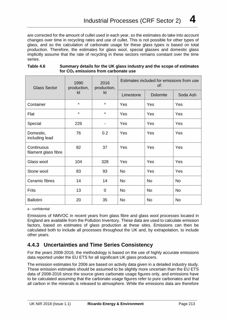
Industrial Processes (CRF Sector 2) 4
UK NIR 2018 (Issue 1.1) Ricardo Energy & Environment Page 213
are corrected for the amount of cullet used in each year, so the estimates do take into account changes over time in recycling rates and use of cullet. This is not possible for other types of glass, and so the calculation of carbonate usage for these glass types is based on total production. Therefore, the estimates for glass wool, special glasses and domestic glass implicitly assume that the rate of recycling in these sectors remains constant over the time series.
Table 4.6 Summary details for the UK glass industry and the scope of estimates for CO2 emissions from carbonate use
Glass Sector 1990
production, kt
2016 production,
kt
Estimates included for emissions from use of:
Limestone Dolomite Soda Ash
Container a a Yes Yes Yes
Flat a a Yes Yes Yes
Special 226 - Yes Yes Yes
Domestic, including lead
76 0.2 Yes Yes Yes
Continuous filament glass fibre
82 37 Yes Yes Yes
Glass wool 104 328 Yes Yes Yes
Stone wool 83 93 No Yes Yes
Ceramic fibres 14 14 No No No
Frits 13 0 No No No
Ballotini 20 35 No No No
a - confidential
Emissions of NMVOC in recent years from glass fibre and glass wool processes located in England are available from the Pollution Inventory. These data are used to calculate emission factors, based on estimates of glass production at these sites. Emissions can then be calculated both to include all processes throughout the UK and, by extrapolation, to include other years.
4.4.3 Uncertainties and Time Series Consistency
For the years 2008-2016, the methodology is based on the use of highly accurate emissions data reported under the EU ETS for all significant UK glass producers.
The emission estimates for 2006 are based on activity data given in a detailed industry study. These emission estimates should be assumed to be slightly more uncertain than the EU ETS data of 2008-2016 since the source gives carbonate usage figures only, and emissions have to be calculated assuming that the carbonate usage figures refer to pure carbonates and that all carbon in the minerals is released to atmosphere. While the emissions data are therefore
Industrial Processes (CRF Sector 2) 4
UK NIR 2018 (Issue 1.1) Ricardo Energy & Environment Page 214
conservative, we think that the uncertainty is still likely to be relatively low since fairly pure carbonate minerals are readily available.
For the remaining years in the time-series, the methodology relies upon the extrapolation of highly accurate activity/emissions data for one year to all other years based on glass production. The glass production data are, however, a mixture of actual production data from the glass industry, and Ricardo Energy & Environment estimates, which are far more uncertain. The emission estimates for 2A3 are therefore subject to far greater uncertainty for the earlier part of the time-series than for recent years, because of the greater reliance on extrapolation, and the lower quality of the glass production estimates for the earlier part of the time-series.
4.4.4 Source Specific QA/QC and Verification
This source category is covered by the general QA/QC of the greenhouse gas inventory in Section 1.6.
4.4.5 Source Specific Recalculations
Estimates for 2010 were revised upward, following identification of a gap in the detailed EU ETS data available for the UK inventory. There were no other significant revisions.
4.4.6 Source Specific Planned Improvements
Emission factors and activity data will be kept under review.
4.5 SOURCE CATEGORY 2A4 – OTHER PROCESS USES OF CARBONATES
4.5.1 Source Category Description
The UK has a large number of sites involved in the production of heavy clay goods – bricks and roofing tiles, and similar items. These sites range from the smallest operations where bricks are hand-made, to bigger sites where bricks are manufactured on a large scale, using automatic production methods. The brick industry can also be divided into fletton and non-fletton types. Fletton bricks are manufactured using the Lower Oxford Clay, found in South-East England only. This clay has an exceptionally high content of carbonaceous material which acts as an additional fuel when the bricks are fired, but also produces a characteristic appearance in the finished bricks. The Lower Oxford clay also contains sulphurous material, which results in SO2 emissions during firing. Non-fletton bricks are made from other clays and shales and these have much lower carbon contents. For all bricks, firing leads to emissions of CO2 from the carbonaceous material in the clay. Limestone, dolomite and barium carbonate can also be used in brickmaking and also release CO2 when fired. Finally, many brick manufacturers add crushed coke ("colourant") to some bricks to change the final appearance of the bricks. Coke oven coke is known to be used in this manner, and we have assumed that petroleum coke is as well. Colourant is added at rates of up to 15% of the raw material weight. A high proportion of the carbon in the colourant is known not to be oxidised during firing and remains in the brick: for EU ETS reporting purposes, all UK brick makers use a figure of 50% oxidation. Although 2A4 explicitly covers use of carbonates, we have included carbon emissions from the use of colourants in bricks here as well, in the absence of anywhere more appropriate to report them.
The 2006 GLs draws attention to other sources of CO2 emissions from use of soda ash and other carbonates. These other uses include flue gas desulphurisation (FGD), magnesia production, and use of soda ash in soaps & detergents, and other applications.
Industrial Processes (CRF Sector 2) 4
UK NIR 2018 (Issue 1.1) Ricardo Energy & Environment Page 215
Limestone is used in FGD systems for abatement of SO2 emissions at most remaining UK coal-fired power stations and emissions are reported under 2A4. The power stations at Drax and Ratcliffe were the first to get FGD (in 1997), followed by West Burton A in 2004, Eggborough and Cottam in 2005, then Ferrybridge C, Fiddlers Ferry and Rugeley B in 2008/2009. Various small, predominantly waste and/or biomass-fired stations also report CO2 emissions from limestone scrubbing in the EU ETS. In all of these processes, limestone reacts with the SO2 present in flue gases, being converted to gypsum, with CO2 being evolved. Uskmouth B has a dry lime-injection system, so there is no potential for CO2 emissions at this site. Seawater scrubbing systems are used at Aberthaw, Kilroot, and Longannet power stations but CO2 emission estimates are not included in the GHGI for this type of FGD system: there is no estimation method for this process. Some MSW incinerators are believed to use the dry lime injection process to remove SO2 emissions: as with Uskmouth B, there will be no CO2 emissions from this type of FGD technology.
Magnesia production in the UK is thought to be limited to a single plant that closed in 2005. This site produced magnesia from seawater, with magnesium salts in the seawater precipitated as magnesium hydroxide, followed by conversion to magnesia in kilns. No process emissions of CO2 occurred at this site. We have no information on any use of soda ash in the UK outside of the glass industry, and so no emission estimates are made.
4.5.2 Methodological Issues
CO2 emissions from production of bricks and tiles are based on data reported in the EU ETS. The EU ETS data set provides site by site emissions, broken down by the source of emission (e.g. from clays, fuels, colourants etc.) and begins in 2005, although the data are only representative of the sector from 2008 onwards, when all significant manufacturing sites were included in EU ETS. The data can easily be divided into emissions from fuels and emissions from non-fuels (i.e. process emissions). It is slightly more difficult to divide the non-fuel data into sub-types such as emissions from clays, colourants, or 'pure' carbonates like limestone, dolomite and barium carbonate, since some of the information within the ETS data set on the source of the CO2 is ambiguous. So although it is possible to make a crude split, we have instead reported the process emissions as a group. Note that this does mean that emissions from the colourant (coke oven or petroleum coke) are included here, but we think this is justified both because of the slight ambiguity in some of the ETS data, but also because there is no other category which would be more appropriate.
The ETS data are calculated by each brick and tile producer using site-specific activity data, and industry-wide emission factors, compiled by the industry trade association each year (British Ceramics Confederation, 2014). These factors include factors for simple carbonates based on the stoichiometric relationship of carbon to the carbonate, as well as measured emission factors for different types of clay e.g. Keuper Marl, Weald Clay, and Lower Oxford Clay. The industry factors also include an estimate for colourants which is based on the assumption that 50% of carbon in the colourant is oxidised during firing.
Consultation with the brick industry indicates that the ETS data for 2008-2010 represents 93% of sector production, and that has been taken into account in the UK GHGI approach. In 2013, a single further site reported in EU ETS, bringing coverage thereafter to 95%. The emissions data for 2008-2016 are therefore increased slightly to reflect non-reporting brickworks, assuming that emission rates at non-reporting sites will be the same as on average at reporting sites. With the exception of the large site that joined EU ETS in 2013, the non-reporting sites over the period 2008-2016 are all the smaller producers and it is not known how representative the industry factors will be for these atypical sites. In the absence of better data, however, we have assumed that emission rates are the same.
ETS data is very limited before 2008, and therefore is not used to derive a national total. Instead, we have used annual brick production data, available in Government Statistics
Industrial Processes (CRF Sector 2) 4
UK NIR 2018 (Issue 1.1) Ricardo Energy & Environment Page 216
(Monthly Statistics of Building Materials and Components, July 2017, available from www.gov.uk) to extrapolate back from the ETS data. These data are for total numbers of bricks produced, and it is necessary to consider what proportion of these bricks are of the fletton type, since this type of brick is associated with higher process emissions. Fletton bricks have had a declining share of the UK brick market for many years and fletton bricks are no longer used in the construction of new buildings. Information on the market share is, however limited: Ove Arup (1990) puts it at 25%, Blythe (1995) states it is 20%, and by 2011, following the announcement that the last but one fletton brickworks was being closed, local media reports all stated that fletton bricks now accounted for less than 10% of the UK market. We have therefore assumed a 25% share in 1990, falling to 20% in 1995, then falling to 10% by 2010. EU ETS data for the fletton works suggest production has fallen further since 2010 and so is used to estimate the trend for fletton bricks since 2010. Using these data and assumptions, it is possible to then generate estimates of the numbers of fletton bricks and non-fletton bricks produced each year.
For non-fletton bricks, a figure of 152 grams CO2 per brick can be calculated from the ETS-based emission estimates for 2008-2013, and then the estimates of non-fletton bricks produced can be used to generate emission estimates for the period 1990-2007 using this emission factor.
In the case of fletton bricks, the PI provides additional data to supplement the information in the EU ETS for 2008 onwards. Total emissions of CO2 are reported at the Stewartby site, and at the combined Saxon/Kings Dyke works for each year between 1998 and 2007. The later ETS data at these sites is used to separate the PI data for 1998-2007 into a fuel component and a process component. This gives a time series of process emission estimates back to 1998, and this is further extrapolated back to 1990 on the basis of the estimates of fletton brick production.
Table 4.7 gives a timeline for the brick sector, summarising what is known about the sites operating and the data available for emission estimates over the time series.
Table 4.7 Timeline for the brick sector in the UK: production sites and data availability
Years Number of sites and fuels Availability of data
1990-1997
8 fletton works in operation in 1990; only 5 still in operation by 1993. Those in 1993 burnt coal, or a mixture of coal and natural gas. Unknown number of non-fletton works.
No emissions data available, annual production (numbers) of all bricks available and fletton and non-fletton brick production estimated from this. Emission estimates require use of emission factors generated from later PI and ETS data.
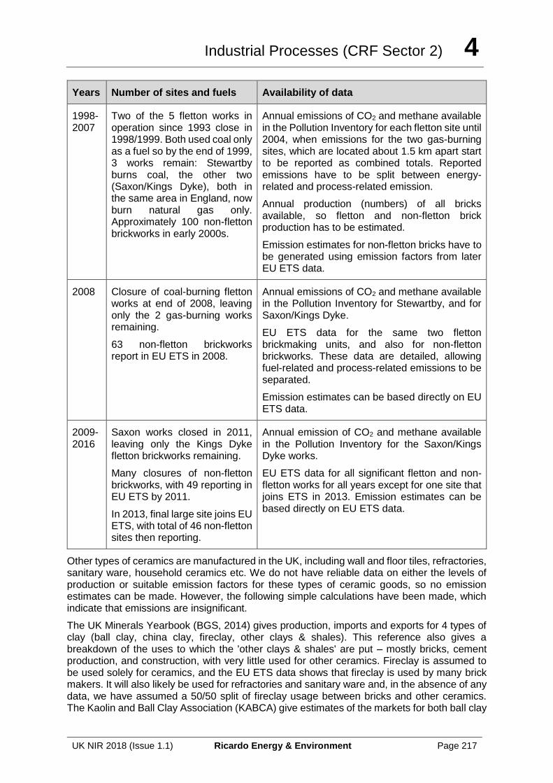
Industrial Processes (CRF Sector 2) 4
UK NIR 2018 (Issue 1.1) Ricardo Energy & Environment Page 217
Years Number of sites and fuels Availability of data
1998-2007
Two of the 5 fletton works in operation since 1993 close in 1998/1999. Both used coal only as a fuel so by the end of 1999, 3 works remain: Stewartby burns coal, the other two (Saxon/Kings Dyke), both in the same area in England, now burn natural gas only. Approximately 100 non-fletton brickworks in early 2000s.
Annual emissions of CO2 and methane available in the Pollution Inventory for each fletton site until 2004, when emissions for the two gas-burning sites, which are located about 1.5 km apart start to be reported as combined totals. Reported emissions have to be split between energy-related and process-related emission.
Annual production (numbers) of all bricks available, so fletton and non-fletton brick production has to be estimated.
Emission estimates for non-fletton bricks have to be generated using emission factors from later EU ETS data.
2008 Closure of coal-burning fletton works at end of 2008, leaving only the 2 gas-burning works remaining.
63 non-fletton brickworks report in EU ETS in 2008.
Annual emissions of CO2 and methane available in the Pollution Inventory for Stewartby, and for Saxon/Kings Dyke.
EU ETS data for the same two fletton brickmaking units, and also for non-fletton brickworks. These data are detailed, allowing fuel-related and process-related emissions to be separated.
Emission estimates can be based directly on EU ETS data.
2009-2016
Saxon works closed in 2011, leaving only the Kings Dyke fletton brickworks remaining.
Many closures of non-fletton brickworks, with 49 reporting in EU ETS by 2011.
In 2013, final large site joins EU ETS, with total of 46 non-fletton sites then reporting.
Annual emission of CO2 and methane available in the Pollution Inventory for the Saxon/Kings Dyke works.
EU ETS data for all significant fletton and non-fletton works for all years except for one site that joins ETS in 2013. Emission estimates can be based directly on EU ETS data.
Other types of ceramics are manufactured in the UK, including wall and floor tiles, refractories, sanitary ware, household ceramics etc. We do not have reliable data on either the levels of production or suitable emission factors for these types of ceramic goods, so no emission estimates can be made. However, the following simple calculations have been made, which indicate that emissions are insignificant.
The UK Minerals Yearbook (BGS, 2014) gives production, imports and exports for 4 types of clay (ball clay, china clay, fireclay, other clays & shales). This reference also gives a breakdown of the uses to which the 'other clays & shales' are put – mostly bricks, cement production, and construction, with very little used for other ceramics. Fireclay is assumed to be used solely for ceramics, and the EU ETS data shows that fireclay is used by many brick makers. It will also likely be used for refractories and sanitary ware and, in the absence of any data, we have assumed a 50/50 split of fireclay usage between bricks and other ceramics. The Kaolin and Ball Clay Association (KABCA) give estimates of the markets for both ball clay
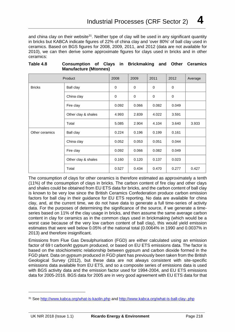
Industrial Processes (CRF Sector 2) 4
UK NIR 2018 (Issue 1.1) Ricardo Energy & Environment Page 218
and china clay on their website31. Neither type of clay will be used in any significant quantity in bricks but KABCA indicate figures of 22% of china clay and 'over 80%' of ball clay used in ceramics. Based on BGS figures for 2008, 2009, 2011, and 2012 (data are not available for 2010), we can then derive some approximate figures for clays used in bricks and in other ceramics:
Table 4.8 Consumption of Clays in Brickmaking and Other Ceramics Manufacture (Mtonnes)
Product 2008 2009 2011 2012 Average
Bricks Ball clay 0 0 0 0
China clay 0 0 0 0
Fire clay 0.092 0.066 0.082 0.049
Other clay & shales 4.993 2.839 4.022 3.591
Total 5.085 2.904 4.104 3.640 3.933
Other ceramics Ball clay 0.224 0.196 0.199 0.161
China clay 0.052 0.053 0.051 0.044
Fire clay 0.092 0.066 0.082 0.049
Other clay & shales 0.160 0.120 0.137 0.023
Total 0.527 0.434 0.470 0.277 0.427
The consumption of clays for other ceramics is therefore estimated as approximately a tenth (11%) of the consumption of clays in bricks. The carbon content of fire clay and other clays and shales could be obtained from EU ETS data for bricks, and the carbon content of ball clay is known to be very low since the British Ceramics Confederation produce carbon emission factors for ball clay in their guidance for EU ETS reporting. No data are available for china clay, and, at the current time, we do not have data to generate a full time-series of activity data. For the purposes of determining the significance of the source, if we generate a time-series based on 11% of the clay usage in bricks, and then assume the same average carbon content in clay for ceramics as in the common clays used in brickmaking (which would be a worst case because of the very low carbon content of ball clay), this would yield emission estimates that were well below 0.05% of the national total (0.0064% in 1990 and 0.0037% in 2013) and therefore insignificant.
Emissions from Flue Gas Desulphurisation (FGD) are either calculated using an emission factor of 69 t carbon/kt gypsum produced, or based on EU ETS emissions data. The factor is based on the stoichiometric relationship between gypsum and carbon dioxide formed in the FGD plant. Data on gypsum produced in FGD plant has previously been taken from the British Geological Survey (2012), but these data are not always consistent with site-specific emissions data available from EU ETS, and so a composite series of emissions data is used with BGS activity data and the emission factor used for 1994-2004, and EU ETS emissions data for 2005-2016. BGS data for 2005 are in very good agreement with EU ETS data for that
31 See http://www.kabca.org/what-is-kaolin.php and http://www.kabca.org/what-is-ball-clay-.php
Industrial Processes (CRF Sector 2) 4
UK NIR 2018 (Issue 1.1) Ricardo Energy & Environment Page 219
year, and so it has been assumed that BGS data for 1994-2004 are also comparable with the later EU ETS data.
4.5.3 Uncertainties and Time Series Consistency
The uncertainty analysis in Annex 2 provides estimates of uncertainty according to IPCC source category and fuel type.
In the case of FGD plant there is a change in methodology between 2004 and 2005. However, BGS and EU ETS-based emission estimates for 2005 are very close, and for 2006-2014 are within 6% of each other (with the EU ETS numbers usually higher). We have no data from BGS for 2015-2016 and so no comparison can be made with the EU ETS based figures.
Estimates for bricks are considered to be highly reliable for the period 2008-2016 where EU ETS data are available for almost all sites. For earlier years, the emission estimates rely upon extrapolation of the 2008 emissions data using brick production estimates and this will introduce uncertainty within the earlier part of the time series. Emission estimates for methane from fletton brickworks are, similarly, based on reported data in later years and extrapolation using brick production for the early part of the time-series, so the uncertainty will again be greatest in the earlier part of the time series.
4.5.4 Source Specific QA/QC and Verification
This source category is covered by the general QA/QC of the greenhouse gas inventory in Section 1.6.
4.5.5 Source Specific Recalculations
There have been no significant changes to this category.
4.5.6 Source Specific Planned Improvements
Emission factors and activity data will be kept under review.
4.6 SOURCE CATEGORY 2B1 – AMMONIA PRODUCTION
4.6.1 Source Category Description
Ammonia is typically produced using the Haber process, which starts with the steam reforming of natural gas to make hydrogen. The simplified reactions are:
CH4 + H2O CO + 3H2
CO + H2O CO2 + H2
The hydrogen is then reacted with nitrogen to form ammonia.
N2 + 3H2 2NH3
If the by-products CO and CO2 are not captured and used, then these are emitted to atmosphere. Ammonia plants can be integrated with methanol manufacture for greater efficiency, since the carbon oxides can be used to manufacture methanol:
CO + 2H2 CH3OH
CO2 + 3H2 CH3OH + H2O
Over the time period covered by the UK greenhouse gas inventory, ammonia has been manufactured at four locations in the UK. CO2 emissions are reported from three of those
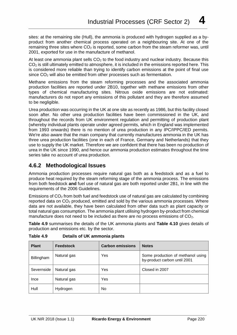
Industrial Processes (CRF Sector 2) 4
UK NIR 2018 (Issue 1.1) Ricardo Energy & Environment Page 220
sites: at the remaining site (Hull), the ammonia is produced with hydrogen supplied as a by-product from another chemical process operated on a neighbouring site. At one of the remaining three sites where CO2 is reported, some carbon from the steam reformer was, until 2001, exported for use in the manufacture of methanol.
At least one ammonia plant sells CO2 to the food industry and nuclear industry. Because this CO2 is still ultimately emitted to atmosphere, it is included in the emissions reported here. This is considered more reliable than trying to identify carbon emissions at the point of final use since CO2 will also be emitted from other processes such as fermentation.
Methane emissions from the steam reforming processes and the associated ammonia production facilities are reported under 2B10, together with methane emissions from other types of chemical manufacturing sites. Nitrous oxide emissions are not estimated: manufacturers do not report any emissions of this pollutant and they are therefore assumed to be negligible.
Urea production was occurring in the UK at one site as recently as 1986, but this facility closed soon after. No other urea production facilities have been commissioned in the UK, and throughout the records from UK environment regulation and permitting of production plant (whereby individual plants operate under agreed permits, which in England was implemented from 1993 onwards) there is no mention of urea production in any IPC/IPPC/IED permits. We're also aware that the main company that currently manufactures ammonia in the UK has three urea production facilities (one in each of France, Germany and Netherlands) that they use to supply the UK market. Therefore we are confident that there has been no production of urea in the UK since 1990, and hence our ammonia production estimates throughout the time series take no account of urea production.
4.6.2 Methodological Issues
Ammonia production processes require natural gas both as a feedstock and as a fuel to produce heat required by the steam reforming stage of the ammonia process. The emissions from both feedstock and fuel use of natural gas are both reported under 2B1, in line with the requirements of the 2006 Guidelines.
Emissions of CO2 from both fuel and feedstock use of natural gas are calculated by combining reported data on CO2 produced, emitted and sold by the various ammonia processes. Where data are not available, they have been calculated from other data such as plant capacity or total natural gas consumption. The ammonia plant utilising hydrogen by-product from chemical manufacture does not need to be included as there are no process emissions of CO2.
Table 4.9 summarises the details of the UK ammonia plants and Table 4.10 gives details of production and emissions etc. by the sector.
Table 4.9 Details of UK ammonia plants
Plant Feedstock Carbon emissions Notes
Billingham Natural gas Yes Some production of methanol using
by-product carbon until 2001
Severnside Natural gas Yes Closed in 2007
Ince Natural gas Yes
Hull Hydrogen No
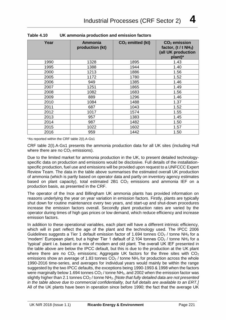
Industrial Processes (CRF Sector 2) 4
UK NIR 2018 (Issue 1.1) Ricardo Energy & Environment Page 221
Table 4.10 UK ammonia production and emission factors
Year Ammonia production (kt)
CO2 emitted (kt) CO2 emission factor, (t / t NH3)
(all UK production plant)*
1990 1328 1895 1.43
1995 1388 1944 1.40
2000 1213 1886 1.56
2005 1172 1780 1.52
2006 949 1385 1.46
2007 1251 1865 1.49
2008 1082 1683 1.56
2009 889 1296 1.46
2010 1084 1488 1.37
2011 687 1043 1.52
2012 1017 1574 1.55
2013 957 1383 1.45
2014 987 1482 1.50
2015 1022 1602 1.57
2016 959 1442 1.50
*As reported within the CRF table 2(I).A-Gs1
CRF table 2(I).A-Gs1 presents the ammonia production data for all UK sites (including Hull where there are no CO2 emissions).
Due to the limited market for ammonia production in the UK, to present detailed technology-specific data on production and emissions would be disclosive. Full details of the installation-specific production, fuel use and emissions will be provided upon request to a UNFCCC Expert Review Team. The data in the table above summarises the estimated overall UK production of ammonia (which is partly based on operator data and partly on inventory agency estimates based on plant capacity), total estimated 2B1 CO2 emissions and ammonia IEF on a production basis, as presented in the CRF.
The operator of the Ince and Billingham UK ammonia plants has provided information on reasons underlying the year on year variation in emission factors. Firstly, plants are typically shut down for routine maintenance every two years, and start-up and shut-down procedures increase the emission factors overall. Secondly plant production rates are varied by the operator during times of high gas prices or low demand, which reduce efficiency and increase emission factors.
In addition to these operational variables, each plant will have a different intrinsic efficiency, which will in part reflect the age of the plant and the technology used. The IPCC 2006 Guidelines suggests a Tier 1 default emission factor of 1.694 tonnes CO2 / tonne NH3 for a ‘modern’ European plant, but a higher Tier 1 default of 2.104 tonnes CO2 / tonne NH3 for a ‘typical’ plant i.e. based on a mix of modern and old plant. The overall UK IEF presented in the table above are below the IPCC default, but this is due to the production at the UK plant where there are no CO2 emissions; Aggregate UK factors for the three sites with CO2 emissions show an average of 1.83 tonnes CO2 / tonne NH3 for production across the whole 1990-2016 time-series, and averages for individual years would mainly be within the range suggested by the two IPCC defaults, the exceptions being 1990-1993 & 1998 when the factors were marginally below 1.694 tonnes CO2 / tonne NH3, and 2002 when the emission factor was slightly higher than 2.1 tonnes CO2 / tonne NH3. [Note that fully detailed data are not presented in the table above due to commercial confidentiality, but full details are available to an ERT.] All of the UK plants have been in operation since before 1990; the fact that the average UK
Industrial Processes (CRF Sector 2) 4
UK NIR 2018 (Issue 1.1) Ricardo Energy & Environment Page 222
factor lies between the 2006 IPCC Guideline defaults for modern plant and mixed modern/old plant indicates that the performance of the UK ammonia plants is broadly typical of a European plant.
4.6.3 Uncertainties and Time Series Consistency
The uncertainty analysis in Annex 2 provides estimates of uncertainty according to IPCC source category and fuel type. The uncertainty associated with this source is low, since the carbon content of natural gas is well known and plant specific data are received from the operators annually.
A consistent time series of activity data has been reported from the manufacturers of ammonia, and this results in good time series consistency of emissions.
4.6.4 Source Specific QA/QC and Verification
This source category is covered by the general QA/QC of the greenhouse gas inventory in Section 1.6 and the source emissions data from plant operators is subject to the QA/QC procedures of the Environment Agency’s Pollution Inventory.
4.6.5 Source Specific Recalculations
There have been no significant recalculations to this category.
4.6.6 Source Specific Planned Improvements
Emission factors and activity data will be kept under review.
4.7 SOURCE CATEGORY 2B2 – NITRIC ACID PRODUCTION
4.7.1 Source Category Description
Emissions sources Sources included Method Emission Factors
2B2: Nitric Acid Production T3, T2 CS
Gases Reported N2O, NOx
Key Categories 2B2: Nitric acid production - N2O (L1, L2, T1, T2)
Key Categories (Qualitative)
None identified
Overseas Territories and Crown Dependencies Reporting
Not occurring
Completeness No known omissions. A general assessment of completeness for the inventory is included in Section 1.8.
Major improvements since last submission
No major improvements
Nitric acid is produced by the catalytic oxidation of ammonia:
4NH3 + 5O2 4NO + 6H2O
2NO + O2 2NO2
3NO2 + H2O 2HNO3 + NO
Industrial Processes (CRF Sector 2) 4
UK NIR 2018 (Issue 1.1) Ricardo Energy & Environment Page 223
Nitrous oxide is also formed by oxidation of ammonia:
4NH3 + 3O2 2N2O + 6H2O
Nitrous oxide is emitted from the process, as well as a small percentage of the NOx that cannot be recovered for conversion into nitric acid. At the end of 2016, nitric acid was being manufactured at 2 UK sites with a total of 4 production plants. At one site, the nitric acid production plant has had NOx/N2O abatement fitted to all units since commissioning (pre-1990), whilst at the other UK production site, all three production lines have had nitrous oxide abatement retrospectively fitted during 2011 Quarter 1. This has led to a notable reduction in the UK IEF for nitrous oxide emissions from nitric acid production in the UK between 2010 and 2011 (see Table 4.13 below).
4.7.2 Methodological Issues
Across the 1990-2016 time-series the availability of emissions and production data for UK nitric acid plant is inconsistent, and hence a range of methodologies have had to be used to provide estimates and derive emission factors for this sector. Where possible, emission estimates are based on site-specific data provided by process operators.
Site-specific production estimates are largely based on production capacity reported directly by the plant operators. This approach may overestimate actual production. No data are available for three sites operating between 1990 and 1993, and production at these sites is calculated based on the difference between estimates of total production and the sum of production at the other sites.
Emission estimates for N2O are derived for each nitric acid site using one of the following:
a) Emissions data provided by the process operators directly or via the Pollution Inventory (1998 onwards for plant in England, 2001 onwards for plant in N Ireland);
b) Site-specific emission factors derived from reported emissions data for the same site for another year (1990-1997 for some plant in England, 1994-1997 for other plant in England, 1990-2000 for plant in N Ireland); and
c) A default emission factor of 7 kt N2O /Mt 100% acid produced in cases where no emissions data are available for the site (some sites in England, Scotland, 1990-1993). This default factor is the default factor provided in the 2006 IPCC Guidelines (IPCC, 2006) for medium pressure plant.
Table 4.11 gives a summary of the approaches used across the time series to estimate production and N2O emissions for the UK inventory and Table 4.12 summarises the methods used by operators to derive the emissions data they report to regulators and the inventory team. The emissions monitoring at the two sites still in operation was originally based on periodic (at least quarterly, if not more frequent) sampling, but from 2010 onwards has been continuous, using on-line infra-red monitoring systems. The monitors at both sites are certified to MCERTS, installed and maintained to EN14181, and subject to EU ETS Permit. The details of monitoring at the closed sites are not known, but it is assumed to have been the same as the sites that remain in operation i.e. periodic prior to 2010. The closed sites were shut before the fitting of continuous monitoring devices was required for EU ETS reporting purposes. Full details of the abatement systems (such as technology type and efficiency) are not known, but the N2O monitoring systems at these sites comply with the requirements of EU ETS reporting, and are subject to low uncertainty (5-10%). Therefore, we consider the emissions data reported by operators to be far more reliable than emission estimates based on IPCC defaults.
Inventory emission estimates for NOX are derived for each nitric acid site using emissions data provided by the process operators directly or via the Pollution Inventory. No emissions data are available before 1994. Emissions between 1990 and 1993 are estimated by interpolating between the 1994 emission based on plant-specific data, and an estimate for emissions in
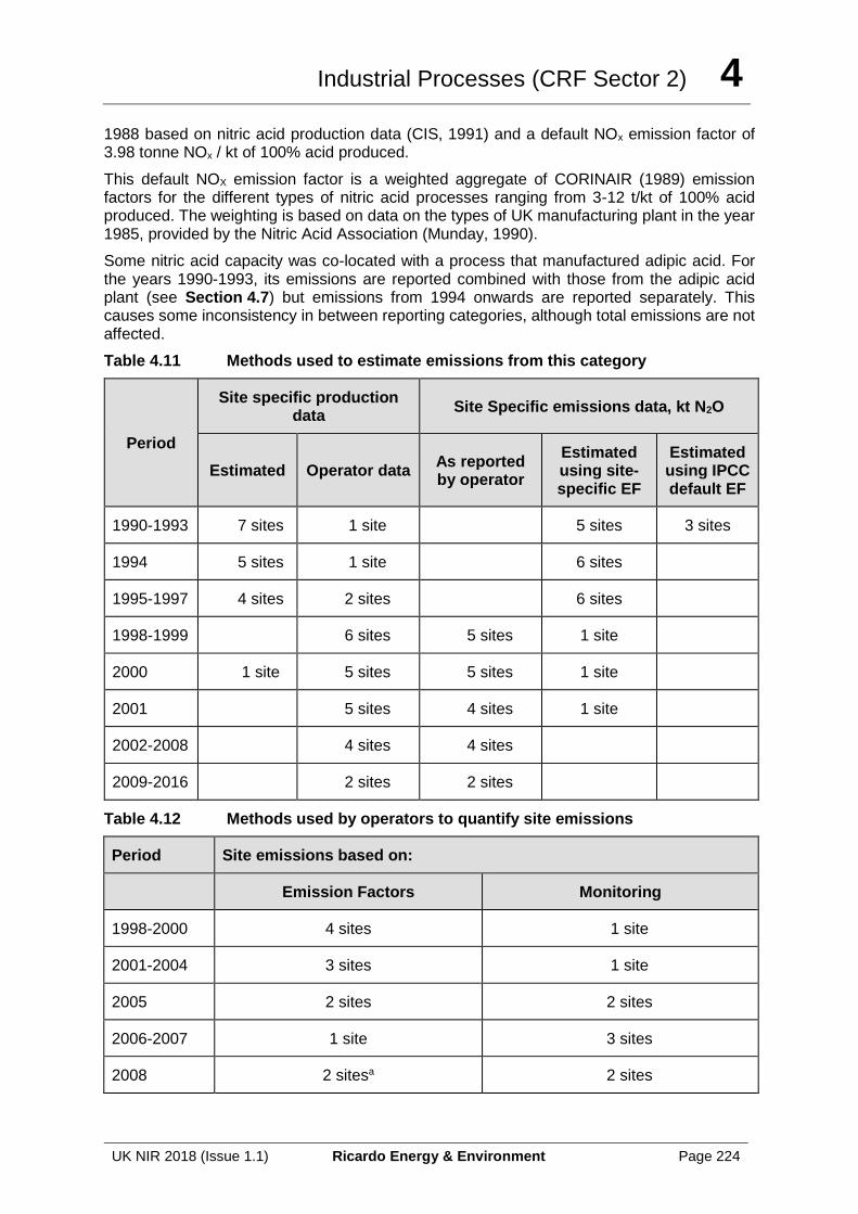
Industrial Processes (CRF Sector 2) 4
UK NIR 2018 (Issue 1.1) Ricardo Energy & Environment Page 224
1988 based on nitric acid production data (CIS, 1991) and a default NOx emission factor of 3.98 tonne NOx / kt of 100% acid produced.
This default NOX emission factor is a weighted aggregate of CORINAIR (1989) emission factors for the different types of nitric acid processes ranging from 3-12 t/kt of 100% acid produced. The weighting is based on data on the types of UK manufacturing plant in the year 1985, provided by the Nitric Acid Association (Munday, 1990).
Some nitric acid capacity was co-located with a process that manufactured adipic acid. For the years 1990-1993, its emissions are reported combined with those from the adipic acid plant (see Section 4.7) but emissions from 1994 onwards are reported separately. This causes some inconsistency in between reporting categories, although total emissions are not affected.
Table 4.11 Methods used to estimate emissions from this category
Period
Site specific production data
Site Specific emissions data, kt N2O
Estimated Operator data As reported by operator
Estimated using site-specific EF
Estimated using IPCC default EF
1990-1993 7 sites 1 site 5 sites 3 sites
1994 5 sites 1 site 6 sites
1995-1997 4 sites 2 sites 6 sites
1998-1999 6 sites 5 sites 1 site
2000 1 site 5 sites 5 sites 1 site
2001 5 sites 4 sites 1 site
2002-2008 4 sites 4 sites
2009-2016 2 sites 2 sites
Table 4.12 Methods used by operators to quantify site emissions
Period Site emissions based on:
Emission Factors Monitoring
1998-2000 4 sites 1 site
2001-2004 3 sites 1 site
2005 2 sites 2 sites
2006-2007 1 site 3 sites
2008 2 sitesa 2 sites
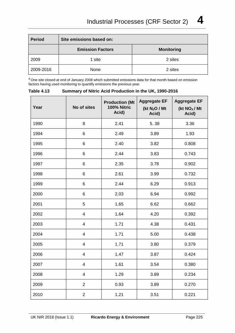
Industrial Processes (CRF Sector 2) 4
UK NIR 2018 (Issue 1.1) Ricardo Energy & Environment Page 225
Period Site emissions based on:
Emission Factors Monitoring
2009 1 site 2 sites
2009-2016 None 2 sites
a One site closed at end of January 2008 which submitted emissions data for that month based on emission
factors having used monitoring to quantify emissions the previous year.
Table 4.13 Summary of Nitric Acid Production in the UK, 1990-2016
Year No of sites Production (Mt
100% Nitric Acid)
Aggregate EF
(kt N2O / Mt Acid)
Aggregate EF
(kt NOX / Mt Acid)
1990 8 2.41 5. 38 3.36
1994 6 2.49 3.89 1.93
1995 6 2.40 3.82 0.808
1996 6 2.44 3.83 0.743
1997 6 2.35 3.78 0.902
1998 6 2.61 3.99 0.732
1999 6 2.44 6.29 0.913
2000 6 2.03 6.94 0.992
2001 5 1.65 6.62 0.662
2002 4 1.64 4.20 0.392
2003 4 1.71 4.38 0.431
2004 4 1.71 5.00 0.438
2005 4 1.71 3.80 0.379
2006 4 1.47 3.87 0.424
2007 4 1.61 3.54 0.380
2008 4 1.29 3.89 0.234
2009 2 0.93 3.89 0.270
2010 2 1.21 3.51 0.221
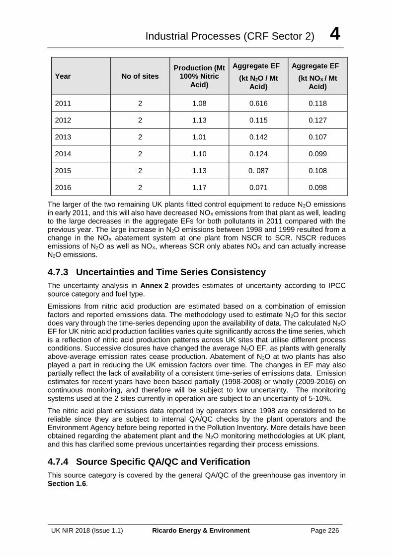
Industrial Processes (CRF Sector 2) 4
UK NIR 2018 (Issue 1.1) Ricardo Energy & Environment Page 226
Year No of sites Production (Mt
100% Nitric Acid)
Aggregate EF
(kt N2O / Mt Acid)
Aggregate EF
(kt NOX / Mt Acid)
2011 2 1.08 0.616 0.118
2012 2 1.13 0.115 0.127
2013 2 1.01 0.142 0.107
2014 2 1.10 0.124 0.099
2015 2 1.13 0. 087 0.108
2016 2 1.17 0.071 0.098
The larger of the two remaining UK plants fitted control equipment to reduce N2O emissions in early 2011, and this will also have decreased NOX emissions from that plant as well, leading to the large decreases in the aggregate EFs for both pollutants in 2011 compared with the previous year. The large increase in N2O emissions between 1998 and 1999 resulted from a change in the NOX abatement system at one plant from NSCR to SCR. NSCR reduces emissions of N2O as well as NOX, whereas SCR only abates NOX and can actually increase N2O emissions.
4.7.3 Uncertainties and Time Series Consistency
The uncertainty analysis in Annex 2 provides estimates of uncertainty according to IPCC source category and fuel type.
Emissions from nitric acid production are estimated based on a combination of emission factors and reported emissions data. The methodology used to estimate N2O for this sector does vary through the time-series depending upon the availability of data. The calculated N2O EF for UK nitric acid production facilities varies quite significantly across the time series, which is a reflection of nitric acid production patterns across UK sites that utilise different process conditions. Successive closures have changed the average N2O EF, as plants with generally above-average emission rates cease production. Abatement of N2O at two plants has also played a part in reducing the UK emission factors over time. The changes in EF may also partially reflect the lack of availability of a consistent time-series of emissions data. Emission estimates for recent years have been based partially (1998-2008) or wholly (2009-2016) on continuous monitoring, and therefore will be subject to low uncertainty. The monitoring systems used at the 2 sites currently in operation are subject to an uncertainty of 5-10%.
The nitric acid plant emissions data reported by operators since 1998 are considered to be reliable since they are subject to internal QA/QC checks by the plant operators and the Environment Agency before being reported in the Pollution Inventory. More details have been obtained regarding the abatement plant and the N2O monitoring methodologies at UK plant, and this has clarified some previous uncertainties regarding their process emissions.
4.7.4 Source Specific QA/QC and Verification
This source category is covered by the general QA/QC of the greenhouse gas inventory in Section 1.6.

Industrial Processes (CRF Sector 2) 4
UK NIR 2018 (Issue 1.1) Ricardo Energy & Environment Page 227
4.7.5 Source Specific Recalculations
The operator of one site provided a correction to the figure for N2O emissions in 2015 that they had provided the previous year, leading to a downward revision in the N2O emission estimate for the sector in that year. There were no other significant changes to this category.
4.7.6 Source Specific Planned Improvements
Emission factors and activity data will be kept under review.
4.8 SOURCE CATEGORY 2B3 – ADIPIC ACID PRODUCTION
4.8.1 Source Category Description
Adipic acid is manufactured in a multi-stage process from cyclohexane via oxidation with nitric acid. Nitrous oxide is produced as a breakdown product from the nitric acid.
4.8.2 Methodological issues
There was only one company manufacturing adipic acid in the UK, but this closed in early 2009. Production data are not provided in the NIR because of commercial confidentiality concerns.
Production data and emission estimates have been provided by the process operator (Invista, 2010). The emission estimates are based on the use of plant-specific emission factors for unabated flue gases, which were determined through a series of measurements on the plant, combined with plant production data and data on the proportion of flue gases that are unabated.
In 1998 an N2O abatement system was fitted to the plant. The abatement system was a thermal oxidation unit and was reported by the operators to be 99.99% efficient at N2O destruction. The abatement unit was not available 100% of the time, and typically achieved 90-95% availability during adipic acid production.
A small nitric acid plant was associated with the adipic acid plant, and this also emitted N2O. From 1994 until the plant’s closure in 2009, the emission from the nitric acid production is reported under 2B2, but prior to 1994 it is included under adipic acid production because separate emissions data for the different processes on that site were not available for those years. This discrepancy in reporting will cause a variation in the reported effective emission factor for these years for 2B2 and 2B3 but overall emission estimates are not affected.
4.8.3 Uncertainties and Time Series Consistency
The uncertainty analysis in Annex 2 provides estimates of uncertainty according to IPCC source category and fuel type.
Emissions data for N2O from adipic acid production are provided by the process operator, but can be cross-checked against emissions reported in the Pollution Inventory.
The level of uncertainty associated with reported emissions of N2O is not known, but the data are considered to be reliable as they are subject to QA/QC checks by the operator, and the related Pollution Inventory data are also checked by the Environment Agency. A higher uncertainty is assumed for 1990 than for later years. Emissions no longer occur from this source since the plant has now closed.
Fluctuations in the N2O EF from this plant are apparent since the installation of the abatement plant. Following direct consultation with the plant operators, it has been determined that the
Industrial Processes (CRF Sector 2) 4
UK NIR 2018 (Issue 1.1) Ricardo Energy & Environment Page 228
variability of emissions is due to the varying level of availability of the abatement plant. A small change in the availability of the abatement system can have a very significant impact upon overall plant emissions and hence upon the annual IEF calculated.
4.8.4 Source Specific QA/QC and Verification
This source category is covered by the general QA/QC of the greenhouse gas inventory in Section 1.6. During summer 2005, consultation between Defra, AEA, plant operators and the UK Meteorological Office was conducted to discuss factors affecting emissions from the adipic acid plant, including: plant design, abatement design, abatement efficiency and availability, emission measurement techniques, historic stack emission datasets and data to support periodic fluctuations in reported emissions. The meeting prompted exchange of detailed plant emissions data and recalculation of back-trajectory emission models.
4.8.5 Source Specific Recalculations
There have been no significant recalculations in this category.
4.8.6 Source Specific Planned Improvements
Emission factors and activity data will be kept under review.
4.9 SOURCE CATEGORY 2B4 – CAPROLACTAM, GLYOXAL AND GLYOXYLIC ACID PRODUCTION
Caprolactam was made at one site in the UK in the early 1970s. The site was destroyed in a serious explosion in 1974, and no other production sites have been built since. Glyoxal and glyoxylic acid have not been produced on an industrial scale in the UK at any time. A literature search of documents from the last 25 years on chemical production in Europe as well as consultation with the Chemical Industries Association has confirmed that these sources should be reported as not occurring.
4.10 SOURCE CATEGORY 2B5 – CARBIDE PRODUCTION
This source category includes silicon carbide and calcium carbide. Neither chemical is known to have been manufactured on an industrial scale in the UK since the 1960s, when calcium carbide plants at Kenfig and Runcorn closed. As above for 2B4, literature searches and consultations with UK chemical industry representatives have confirmed that this source should be reported as not occurring in the UK.
4.11 SOURCE CATEGORY 2B6 – TITANIUM DIOXIDE PRODUCTION
4.11.1 Source Category Description
Titanium dioxide has been produced in the UK by two methods: i) from ilmenite, using the sulphate process; and ii) from rutile, using the chloride process. Only the chloride process leads to process emissions of greenhouse gases. In 1990, there were two sites each using the chloride and the sulphate process, but the two sulphate processes closed in 1997 and 2009, so all titanium dioxide in the UK is now produced using the chloride process at the two sites at Stallingborough and Greatham. The chloride process involves the chlorination of rutile ore in a reducing atmosphere to produce titanium tetrachloride (TiCl4), followed by oxidation
Industrial Processes (CRF Sector 2) 4
UK NIR 2018 (Issue 1.1) Ricardo Energy & Environment Page 229
of the TiCl4 to titanium dioxide. The reducing atmosphere is produced by combustion of petroleum coke or coke oven coke.
4.11.2 Methodological Issues
The 2006 GLs recommend the use of either a Tier 1 method involving a default emission factor and national activity data, or a Tier 2 method using installation-specific data on reducing agent usage. For the UK, neither of these methods are feasible options due to limited data; there are no UK activity data (i.e. annual production statistics) for any individual chemical product, and the only site-specific data for the UK plant is in the form of CO2 emissions data. These emissions data are available from two regulatory reporting sources:
• From the PI, covering CO2 from reducing agents and fuel use in plant utilities; and
• From the EU ETS, covering fuel use for energy production only until 2012, and coke use in addition from 2013 onwards.
Operator reporting has been variable over the years, in line with the evolving scope and detail required for EU ETS and PI data returns.
• During Phase II of the EU ETS (2008-2012), the titanium dioxide plants only reported CO2 from fuels burnt in the site boilers in their EU ETS returns;
• For Phase III (2013 onwards), coverage of EU ETS reporting was extended to cover fuels burnt in furnaces, driers etc. as well as use of reducing agents; and
• For three years (2006-2008), the process operators were required to report thermal CO2 and chemical CO2 separately to the PI.
From these data it is possible to obtain the emissions from the chemical process for some years: 2006-2008 (using the PI data for chemical CO2 emissions), and 2013-2016 (by difference between the PI/EU ETS totals covering all CO2 emissions and the detailed EU ETS data covering all energy-related emissions. The fuel/process split in emissions for these 7 years can be calculated, and the PI provides total CO2 emissions at each site back to 1998. Prior to 1998, there is no data on either emissions or production, and therefore it is assumed that emissions in 1990-1997 are at the same level as in later years (the production capacity at all UK sites producing TiO2 by the chloride route is the same for all years).
In order to avoid a potential double-count in emissions in the UK GHGI, it is necessary to ensure that the reductant used in the processes is not included as a fuel and emissions reported in 1.A. The method adopted by the inventory team addresses this issue by back-calculating the coke oven coke/petroleum coke activity data (used as a reductant) from the emissions data using UK carbon emission factors for the feedstock, and discounting this amount from the Energy sector estimates.
4.11.3 Uncertainties and Time Series Consistency
The country-specific method used is regarded as the best available method for the UK GHGI estimates, given the lack of any production activity data. The use of site-specific EU ETS and PI data, even if not relating to input materials as required by the Tier 2 method in the GLs, ensures that emissions data are quite certain for the period from 1998 onwards. Estimates for 1990-1997 are more uncertain due to the need to extrapolate 1998 data backwards in the absence of any specific information on production, materials usage or emissions in those years.
Industrial Processes (CRF Sector 2) 4
UK NIR 2018 (Issue 1.1) Ricardo Energy & Environment Page 230
4.11.4 Source Specific QA/QC and Verification
This source category is covered by the general QA/QC of the greenhouse gas inventory in Section 1.6.
4.11.5 Source Specific Recalculations
There has been a correction to the methodology to ensure consistency between the carbon emission factor used to back-calculate activity data for petroleum coke from emissions data in the first place, and the carbon emission factor subsequently used to derive the emissions reported in the UK inventory. As a result, CO2 emissions decrease by between 6% and 12% for each year in the time-series from 1992 onwards, when petroleum coke is first used by the sector.
4.11.6 Source Specific Planned Improvements
Emission factors and activity data will be kept under review.
4.12 SOURCE CATEGORY 2B7 – SODA ASH PRODUCTION & USE
4.12.1 Source Category Description
Soda ash has been produced in the UK using the Solvay process at two sites both of which have been operating since the start of the time period covered by the inventory. The Solvay process involves the conversion of limestone (calcium carbonate) and brine (sodium chloride) to soda ash (sodium carbonate) and calcium chloride. The initial stage in the process is the calcination of limestone in a kiln to produce lime and CO2 gas, both of which are used in the process. Coke oven coke is used to fire the lime kilns and CO2 from the coke is included in the gases used in the soda ash plant. In theory, if limestone and brine are converted completely to soda ash and calcium chloride, then that part of the soda ash process is carbon-neutral and the CO2 emitted should be equal just to those emissions occurring from the coke. In practice, the process is not 100% efficient, so emissions of CO2 are actually somewhat higher than would just be due to the coke use. Soda ash production at one of the two UK sites (Winnington) ceased in February 2014, although the site is still being used to make sodium bicarbonate from sodium carbonate solution & CO2, which we assume is sourced from the neighbouring Lostock plant. EU ETS data suggest this sodium bicarbonate process does emit some CO2 – presumably unreacted CO2 that passes through the process and, since this CO2 probably originates with the soda ash process at Lostock, it is included in the emission estimates for 2B7.
Emissions from soda ash (sodium carbonate, Na2CO3) used in the manufacture of soda-lime glasses is reported under source category 2A4.
4.12.2 Methodological Issues
The 2006 GLs suggests that emissions should be based "on an overall balance of CO2 around the whole chemical process”. In the UK, soda ash is produced at two sites and both began to report under the EU ETS in 2013. The EU ETS emissions data for the two sites is calculated using a carbon balance approach with inputs in coke and limestone balanced against soda ash and waste products. The 2013-2016 EU ETS data therefore meets the requirements for the method suggested in the GLs.
Prior to 2013, no data for the UK plant were reported in EU ETS, but CO2 emissions were reported in the PI between 1998 and 2014. Comparison of the PI and EU ETS data for 2013-2016 shows that EU ETS data were 38% higher than emissions in the PI in 2013, 68% higher
Industrial Processes (CRF Sector 2) 4
UK NIR 2018 (Issue 1.1) Ricardo Energy & Environment Page 231
in 2014, 80% higher in 2015, and 69% higher in 2016. The reason for this is not known, but since the PI data for 1998-2013 are fairly consistent, it is assumed that there is a systematic underestimate in the PI data across the entire time-series (possibly they represent CO2 releases from just part of the process, rather than the whole-process balance used in the EU ETS), and that this underestimate is at the same level as in 2013. We have therefore used the PI data for 1998-2012 but multiplied by a factor of 1.38 to give estimates of emissions in those years. The difference in 2014-2016 was higher and so a more conservative approach would be to use a factor based on all four years (1.64). However, the Winnington plant was closed in 2014 and so the years from 2014 onwards are atypical compared with the 1990-2013 period of full operation of both processes. For 1990-1997, no data of any type are available, but since the same two sites have been in operation in the UK across the entire time-series, emissions in 1990-1997 are assumed to be at the same level as in later years.
4.12.3 Uncertainties and Time Series Consistency
The method used is regarded as the best available given the lack of any production activity data, or a time-series of coke consumption. The use of site-specific EU ETS data for 2013-2016 should ensure that the emission estimates for those years are quite certain. The poor agreement between the PI and EU ETS data in 2013-2016 means that the emission estimates for 1998-2012, based on PI data, are far more uncertain. The difference between EU ETS and PI data is even greater (in percentage terms) in 2014-2016 than in 2013, however both sites only operated fully throughout 2013, Winnington having closed in February 2014. We have therefore treated the 2013 EU ETS/PI ratio of 1.38 (based on both plant operating throughout the year) as a more reliable guide to the potential underestimation in the PI data in earlier years. Estimates for 1990-1997 are more uncertain still due to the need to extrapolate 1998 data backwards in the absence of any specific information on production, materials usage or emissions in those years.
4.12.4 Source Specific QA/QC and Verification
This source category is covered by the general QA/QC of the greenhouse gas inventory in Section 1.6.
4.12.5 Source Specific Recalculations
There have been no significant recalculations in this category.
4.12.6 Source Specific Planned Improvements
Emission factors and activity data will be kept under review.
4.13 SOURCE CATEGORY 2B8 – PETROCHEMICAL AND CARBON BLACK PRODUCTION
4.13.1 Source Category Description
This category includes emissions from the following sources: 2B8a Methanol, 2B8b Ethylene, 2B8c Ethylene Dichloride, 2B8d Ethylene Oxide, 2B8e Acrylonitrile, 2B8f Carbon Black and 2B8g Chemicals: OPG.
The UK has a large petrochemical industry, with manufacture of all of the chemicals explicitly mentioned in the 2006 IPCC Guidelines for at least part of the period 1990-2016, although a series of site closures in recent years has reduced the number of products manufactured in the UK.
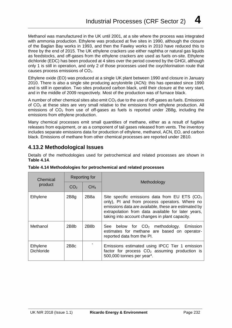
Industrial Processes (CRF Sector 2) 4
UK NIR 2018 (Issue 1.1) Ricardo Energy & Environment Page 232
Methanol was manufactured in the UK until 2001, at a site where the process was integrated with ammonia production. Ethylene was produced at five sites in 1990, although the closure of the Baglan Bay works in 1993, and then the Fawley works in 2010 have reduced this to three by the end of 2015. The UK ethylene crackers use either naphtha or natural gas liquids as feedstocks, and off-gases from the ethylene crackers are used as fuels on-site. Ethylene dichloride (EDC) has been produced at 4 sites over the period covered by the GHGI, although only 1 is still in operation, and only 2 of those processes used the oxychlorination route that causes process emissions of CO2.
Ethylene oxide (EO) was produced at a single UK plant between 1990 and closure in January 2010. There is also a single site producing acrylonitrile (ACN): this has operated since 1990 and is still in operation. Two sites produced carbon black, until their closure at the very start, and in the middle of 2009 respectively. Most of the production was of furnace black.
A number of other chemical sites also emit CO2 due to the use of off-gases as fuels. Emissions of CO2 at these sites are very small relative to the emissions from ethylene production. All emissions of CO2 from use of off-gases as fuels is reported under 2B8g, including the emissions from ethylene production.
Many chemical processes emit small quantities of methane, either as a result of fugitive releases from equipment, or as a component of tail gases released from vents. The inventory includes separate emissions data for production of ethylene, methanol, ACN, EO, and carbon black. Emissions of methane from other chemical processes are reported under 2B10.
4.13.2 Methodological Issues
Details of the methodologies used for petrochemical and related processes are shown in Table 4.14.
Table 4.14 Methodologies for petrochemical and related processes
Chemical product
Reporting for Methodology
CO2 CH4
Ethylene 2B8g 2B8a Site specific emissions data from EU ETS (CO2 only), PI and from process operators. Where no emissions data are available, these are estimated by extrapolation from data available for later years, taking into account changes in plant capacity.
Methanol 2B8b 2B8b See below for CO2 methodology. Emission estimates for methane are based on operator-reported data from the PI.
Ethylene Dichloride
2B8c -
Emissions estimated using IPCC Tier 1 emission factor for process CO2 assuming production is 500,000 tonnes per yeara.
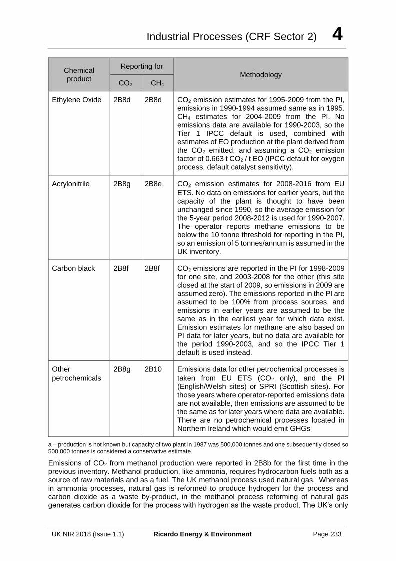
Industrial Processes (CRF Sector 2) 4
UK NIR 2018 (Issue 1.1) Ricardo Energy & Environment Page 233
Chemical product
Reporting for Methodology
CO2 CH4
Ethylene Oxide 2B8d 2B8d CO2 emission estimates for 1995-2009 from the PI, emissions in 1990-1994 assumed same as in 1995. CH4 estimates for 2004-2009 from the PI. No emissions data are available for 1990-2003, so the Tier 1 IPCC default is used, combined with estimates of EO production at the plant derived from the CO2 emitted, and assuming a CO2 emission factor of 0.663 t CO2 / t EO (IPCC default for oxygen process, default catalyst sensitivity).
Acrylonitrile 2B8g 2B8e CO2 emission estimates for 2008-2016 from EU ETS. No data on emissions for earlier years, but the capacity of the plant is thought to have been unchanged since 1990, so the average emission for the 5-year period 2008-2012 is used for 1990-2007. The operator reports methane emissions to be below the 10 tonne threshold for reporting in the PI, so an emission of 5 tonnes/annum is assumed in the UK inventory.
Carbon black 2B8f 2B8f CO2 emissions are reported in the PI for 1998-2009 for one site, and 2003-2008 for the other (this site closed at the start of 2009, so emissions in 2009 are assumed zero). The emissions reported in the PI are assumed to be 100% from process sources, and emissions in earlier years are assumed to be the same as in the earliest year for which data exist. Emission estimates for methane are also based on PI data for later years, but no data are available for the period 1990-2003, and so the IPCC Tier 1 default is used instead.
Other petrochemicals
2B8g 2B10 Emissions data for other petrochemical processes is taken from EU ETS (CO2 only), and the PI (English/Welsh sites) or SPRI (Scottish sites). For those years where operator-reported emissions data are not available, then emissions are assumed to be the same as for later years where data are available. There are no petrochemical processes located in Northern Ireland which would emit GHGs
a – production is not known but capacity of two plant in 1987 was 500,000 tonnes and one subsequently closed so 500,000 tonnes is considered a conservative estimate.
Emissions of CO2 from methanol production were reported in 2B8b for the first time in the previous inventory. Methanol production, like ammonia, requires hydrocarbon fuels both as a source of raw materials and as a fuel. The UK methanol process used natural gas. Whereas in ammonia processes, natural gas is reformed to produce hydrogen for the process and carbon dioxide as a waste by-product, in the methanol process reforming of natural gas generates carbon dioxide for the process with hydrogen as the waste product. The UK’s only
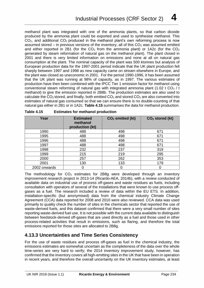
Industrial Processes (CRF Sector 2) 4
UK NIR 2018 (Issue 1.1) Ricardo Energy & Environment Page 234
methanol plant was integrated with one of the ammonia plants, so that carbon dioxide produced by the ammonia plant could be exported and used to synthesise methanol. This CO2, and additional CO2 produced in the methanol plant’s own reforming process is now assumed stored – in previous versions of the inventory, all of this CO2 was assumed emitted and either reported in 2B1 (for the CO2 from the ammonia plant) or 1A2c (for the CO2 generated by steam reformation of natural gas on the methanol plant). The plant closed in 2001 and there is very limited information on emissions and none at all on natural gas consumption at the plant. The nominal capacity of the plant was 500 ktonnes but analysis of European production data for the 1997-2001 period indicate that the UK plant production fell sharply between 1997 and 1998 as new capacity came on stream elsewhere in Europe, and the plant was closed as uneconomic in 2001. For the period 1990-1996, it has been assumed that the UK plant was running at 98% of capacity, as in 1997. The various estimates of production have then been combined with the IPCC Tier 1 emission factor for methanol using conventional steam reforming of natural gas with integrated ammonia plant (1.02 t CO2 / t methanol) to give the emission reported in 2B8b. The production estimates are also used to calculate the CO2 stored, and finally, both emitted CO2 and stored CO2 are also converted into estimates of natural gas consumed so that we can ensure there is no double-counting of that natural gas either in 2B1 or in 1A2c. Table 4.15 summarises the data for methanol production.
Table 4.15 Estimates for methanol production
Year Estimated methanol
production (kt)
CO2 emitted (kt) CO2 stored (kt)
1990 488 498 671
1995 488 498 671
1996 488 498 671
1997 488 498 671
1998 232 237 319
1999 215 219 295
2000 257 262 353
2001 130 133 179
2002 onwards 0 0 0
The methodology for CO2 estimates for 2B8g were developed through an inventory improvement research project in 2013-14 (Ricardo-AEA, 2014b), with a review conducted of available data on industrial use of process off-gases and waste residues as fuels, including consultation with operators of several of the installations that were known to use process off-gases as a fuel. The research included a review of data within the EU ETS. In addition, installation-specific (but anonymised) data from the chemical industry Climate Change Agreement (CCA) data reported for 2008 and 2010 were also reviewed. CCA data was used primarily to quality check the number of sites in the chemicals sector that reported the use of waste-derived fuels, and this dataset confirmed that there were a very small number of sites reporting waste-derived fuel use. It is not possible with the current data available to distinguish between feedstock-derived off-gases that are used directly as a fuel and those used in other process-related activities that result in emissions, such as flaring, and therefore the total emissions reported for those sites are allocated to 2B8g.
4.13.3 Uncertainties and Time Series Consistency
For the use of waste residues and process off-gases as fuel in the chemical industry, the emissions estimates are somewhat uncertain as the completeness of the data over the whole time-series are very hard to verify; the 2014 inventory improvement study, however, has confirmed that the inventory covers all high-emitting sites in the UK that have been in operation in recent years, and therefore the overall uncertainty on the UK inventory estimates, at least
Industrial Processes (CRF Sector 2) 4
UK NIR 2018 (Issue 1.1) Ricardo Energy & Environment Page 235
for the period covered by EU ETS data, is not regarded as significant. Energy and environmental experts within the UK trade association for the chemical sector, the Chemical Industries Association, also confirmed that they were not aware of any other sites in the UK that used process off-gases, over and above the sites identified included in the UK GHGI (Personal communication, Chemical Industries Association, 2014). These are dominated by the four ethylene production sites and a handful of other sites producing organic chemicals, typically co-located with refineries.
Emission estimates for other sources are mostly based on a mixture of PI and/or EU ETS data with estimates for earlier years then based on the assumption that emissions are as in later years. Tier 1 IPCC default emission factors are used for the minor sources 2B8c (for CO2), 2B8d and 2B8f (both CH4, part of time-series only). No UK-wide activity data (production data) are available with which to generate a better time series for any of the sub-sectors within 2B8, so the earlier part of the time-series for all of the chemical industry sectors is particularly uncertain. EU ETS-based emissions are considered the most reliable basis for estimates in the GHGI and the uncertainty is estimated to be +- 5%. PI data are more uncertain, because it is not clear what methods are used and the emission sources (combustion, process, other) are not transparent. Uncertainty for GHGI estimates based on the PI data is estimated to be +- 15%. Emissions data for methane are likely to be more uncertain than those for CO2 since the former are often fugitive in nature, or minor components in stack emissions (thus requiring stack monitoring to quantify).
4.13.4 Source Specific QA/QC and Verification
This source category is covered by the general QA/QC of the greenhouse gas inventory in Section 1.6.
4.13.5 Source Specific Recalculations
There have been no significant recalculations to this category.
4.13.6 Source Specific Planned Improvements
It is noted that this sector has been identified as a key category, and that not all of the estimates within this sector use a tier 2 or higher approach. The UK has recently reviewed this sector and included some additional sources using what is believed to be the best currently available data. The UK will review this position should further information come to light.
4.14 SOURCE CATEGORY 2B9 – FLUOROCHEMICAL PRODUCTION
4.14.1 Source Category Description
Emissions arise from the UK manufacture of HFCs, PFCs and HCFC-22. HFC-23 is a by-product of HCFC-22 manufacture. There are two single manufacturers of HFCs and PFCs respectively in the UK, and two companies were operating HCFC-22 plants. Both HCFC plants closed in 2008/9; one reopened in 2013 and was shut down again in 2016. HFC production ended in 2016.
There is no UK production of SF6.
4.14.2 Methodological Issues
A full description of the emission model and associated methodology used for this sector is contained in AEA (2008). Within the model, manufacturing emissions from UK production of
Industrial Processes (CRF Sector 2) 4
UK NIR 2018 (Issue 1.1) Ricardo Energy & Environment Page 236
HFCs, PFCs and HFC-23 (by-product of HCFC-22 manufacture) are estimated from reported data from the respective manufacturers. Manufacturers have reported both production and emissions data, but only for certain years, and for a different range of years for different manufacturers. Therefore, the emissions model is based on implied emission factors, and production estimates are used to calculate emissions in those years for which reported data are not available. Two of the three manufacturers were members of the UK greenhouse gas Emissions Trading Scheme. As a requirement of participation in the scheme, their reported emissions were verified annually via external and independent auditors. For PFC production, emissions are now reported to the Environment Agency’s Pollution Inventory, and these emissions are directly used within the GHG inventory. The operator of the HFC and (now closed) HCFC-22 plant provides speciated emissions data directly to the Inventory Agency, based on vent analysis and flowmeter readings, or on weighbridge differences. The other HCFC-22 plant, which closed in 2008, also reported to the Pollution Inventory and these emissions were used within the GHG inventory.
4.14.3 Uncertainties and Time-Series Consistency
The uncertainty analysis in Annex 2, provides estimates of uncertainty according to IPCC source category and fuel type. The uncertainty estimate for emissions from HFC manufacture has been revised for this submission, based on information from the plant operator. The uncertainty is now estimated at 10%.
There is a significant decrease in HFC emissions in 1998/1999. This step-change in emissions is due to the installation of thermal oxidiser pollution abatement equipment at one of the UK manufacturing sites. Fugitive HFC emissions from both an HCFC-22 plant and HFC manufacturing plant (run by the same operator) are treated using the same thermal oxidiser unit. Emissions also decrease in 2004, reflecting the installation of a thermal oxidiser at the second of the UK’s HCFC-22 manufacturing sites. This was installed in late 2003, and became fully operational in 2004. HFC-23 emissions decreased in 2009 and 2010 following the closure of both HCFC-22 manufacturing sites. A small emission of HFC-23 remains, which arises from the production of HFC-125, most likely due to impurities in the feedstock. HCFC-22 manufacture restarted in 2013 and was shut down in 2016.
A significant increase in PFC emissions from the production of halocarbons is observed from 1992 to 1996 (with the trend changing after 1996). The increase in emissions was due to increasing production levels at the single UK manufacturing plant during this period. Since 1996, the level of emissions has changed each year which broadly reflects the demand (and hence production levels) for PFCs. In 2004 and 2005, emissions reported by the company increased compared with the preceding 3 years of fairly stable emission levels 2001-2003. Emissions declined sharply in 2007-2009, before increasing again in 2010 and 2011 and then declining again.
4.14.4 Source Specific QA/QC and Verification
This source category is covered by the general QA/QC of the greenhouse gas inventory in Section 1.6, and details of verification of emissions are given in Annex 6. Data reported via the Pollution Inventory are also further checked by the Environment Agency.
4.14.5 Source Specific Recalculations
No recalculations have been made to emissions from this sector.
4.14.6 Source Specific Planned Improvements
There are currently no planned improvements for this sector, however data sources will be kept under review.
Industrial Processes (CRF Sector 2) 4
UK NIR 2018 (Issue 1.1) Ricardo Energy & Environment Page 237
4.15 SOURCE CATEGORY 2B10 – OTHER
4.15.1 Source Category Description
The UK has a large chemical manufacturing sector and emissions of methane, carbon monoxide, NOx, SO2, and NMVOC in the inventory are treated in some detail to reflect the many different types of process. Emissions from processes not covered elsewhere in 2B, are reported under 2B10.
Chemical manufacturing processes are a significant source of NMVOC emissions. Due to the complexity of the sector and the difficulty of separating emissions from different chemical processes, almost all emissions are reported using a single, general, category.
Emissions of the remaining pollutants are less significant compared with national totals but are reported in more detail.
Methane emissions are reported elsewhere in 2B for emissions from specific chemical processes, but also reported in 2B10 in the case of emissions from other, general petrochemical processes. Methane emissions from ammonia production sites have historically been included in the latter, and reported under 2B10, rather than being reported separately in 2B1.
Emissions of other pollutants are reported under the following source categories:
• Chemical industry - CO, SO2, NMVOC;
• Chemical industry (nitric acid use) - NOx;
• Chemical industry (pigment manufacture) - SO2;
• Chemical industry (reforming) – CO;
• Chemical industry (sulphuric acid use) - SO2;
• Coal, tar and bitumen processes – NMVOC; and
• Sulphuric acid production - SO2.
The first source listed is the general category used where emissions occur from processes which do not fit elsewhere. The remaining categories are specific and often relate to small numbers of sites. The categories 'chemical industry (nitric acid use) and 'chemical industry (sulphuric acid use) refer to processes using these acids and emitting NOX and SO2 respectively. Manufacture of nitric acid (see Section 4.7) and sulphuric acid are treated separately from use. Sulphuric acid was being produced at one site at the end of 2014. Pigment manufacture relates to a single plant where sulphur was burnt as part of the manufacturing process – this site closed in 2008. The sulphur oxides produced were largely consumed in the process, although some emissions did occur.
Reforming processes convert natural gas or other light hydrocarbons into hydrogen and carbon monoxide for use in further chemical processes, and can result in emissions of CO. The remaining source category is reserved for minor sources of NMVOC from processes involving coal-based and bitumen-based chemicals.
4.15.2 Methodological Issues
Site-specific emissions data for chemical processes located in England and Wales are available in the Pollution Inventory (Environment Agency, 2017) and Welsh Emission Inventory (NRW, 2017) respectively. Reporting generally started in 1994 or 1995, and few data exist for the years prior to 1994. Site specific emissions data for processes in Scotland have been obtained from the Scottish Pollutant Release Inventory (SEPA, 2017). The Scottish Environment Protection Agency has also, on previous occasions, supplied some data on emissions of NMVOC from individual Scottish chemical processes and additional NMVOC data for processes located in both Scotland and Northern Ireland have been obtained from
Industrial Processes (CRF Sector 2) 4
UK NIR 2018 (Issue 1.1) Ricardo Energy & Environment Page 238
process operators. Additional data on Northern Ireland’s only major chemical works is provided by NIEA (2017).
The National Sulphuric Acid Association (NSAA, 2003) has provided historical emissions data for sulphuric acid production processes. Emissions from ship purging are based on a single estimate given by Rudd et al (1996), which is applied to all years.
All of the data available are in the form of emission estimates, usually generated by the process operators and based on measurements or calculated based on process chemistry. Emission factors and activity data are not available, but emission factors are estimated using the best available ‘surrogate’ activity data that are available across the time series; this approach then enables estimates of emissions to be made for the years prior to operator-reported emission estimates (typically pre-1994). For most commodities, the extrapolation is linked to changes in the level of output from the chemicals manufacturing sector as measured by the 'index of output' figures published by the Office for National Statistics (2017). In the case of SO2 from sulphuric acid production, emissions data are available from operators across the whole time-series.
4.15.3 Uncertainties and Time Series Consistency
The uncertainty analysis in Annex 2 provides estimates of uncertainty according to IPCC source category and fuel type.
Estimates for 1994 onwards are mostly based on data reported by process operators through the regulatory agency data management and checking systems that govern UK industrial emissions data within the PI, WEI, SPRI and NIPI. The dataset is evidently incomplete in some years, due to the variations through time in the reporting thresholds for different pollutants. The Inventory Agency has used good practice techniques to address these reporting inconsistencies, and therefore the completeness of the data is good through the time series.
Unfortunately, UK production data are not readily available for chemicals and other products from the sites reported under 2B8. This inhibits the Inventory Agency’s ability to conduct data validation tests on the reported emissions data against a reliable time-series of production estimates.
Emission estimates for NMVOC in the early part of the time series are more uncertain than the estimates for other pollutants due to inconsistencies in operator reporting to the Pollution Inventory until the late 1990s. For the first few years of the Pollution Inventory, operators reported NMVOCs using a range of different approaches (e.g. “as toluene”, “as carbon”, reporting several individual compounds and then also a total NMVOC figure – but not sufficiently transparent to unambiguously identify double-counts). As a result, the data have to be interpreted using expert judgement in order to derive as consistent a time series as possible.
Emission estimates for the period prior to 1994 are also more uncertain, with the exception of sulphuric acid production. This is due to the need for extrapolation of emissions data for 1994 or some other year backwards, using general indicators of chemical industry output.
The uncertainty of some emission estimates from 2002 onwards is higher for some of the sources included in this sector. This is due to changes in the reporting requirements for the Pollution Inventory and other regulator’s inventories, with the de minimis limits for reporting of emissions of some pollutants being raised, and a greater need to extrapolate data to fill reporting gaps.
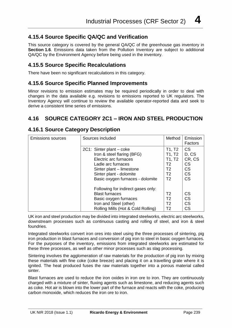
Industrial Processes (CRF Sector 2) 4
UK NIR 2018 (Issue 1.1) Ricardo Energy & Environment Page 239
4.15.4 Source Specific QA/QC and Verification
This source category is covered by the general QA/QC of the greenhouse gas inventory in Section 1.6. Emissions data taken from the Pollution Inventory are subject to additional QA/QC by the Environment Agency before being used in the inventory.
4.15.5 Source Specific Recalculations
There have been no significant recalculations in this category.
4.15.6 Source Specific Planned Improvements
Minor revisions to emission estimates may be required periodically in order to deal with changes in the data available e.g. revisions to emissions reported to UK regulators. The Inventory Agency will continue to review the available operator-reported data and seek to derive a consistent time series of emissions.
4.16 SOURCE CATEGORY 2C1 – IRON AND STEEL PRODUCTION
4.16.1 Source Category Description
Emissions sources Sources included Method Emission Factors
2C1: Sinter plant – coke Iron & steel flaring (BFG) Electric arc furnaces Ladle arc furnaces Sinter plant – limestone Sinter plant - dolomite Basic oxygen furnaces - dolomite Following for indirect gases only: Blast furnaces Basic oxygen furnaces Iron and Steel (other) Rolling Mills (Hot & Cold Rolling)
T1, T2 T1, T2 T1, T2 T2 T2 T2 T2 T2 T2 T2 T2
CS D, CS CR, CS CS CS CS CS CS CS CS CS
UK iron and steel production may be divided into integrated steelworks, electric arc steelworks, downstream processes such as continuous casting and rolling of steel, and iron & steel foundries.
Integrated steelworks convert iron ores into steel using the three processes of sintering, pig iron production in blast furnaces and conversion of pig iron to steel in basic oxygen furnaces. For the purposes of the inventory, emissions from integrated steelworks are estimated for these three processes, as well as other minor processes such as slag processing.
Sintering involves the agglomeration of raw materials for the production of pig iron by mixing these materials with fine coke (coke breeze) and placing it on a travelling grate where it is ignited. The heat produced fuses the raw materials together into a porous material called sinter.
Blast furnaces are used to reduce the iron oxides in iron ore to iron. They are continuously charged with a mixture of sinter, fluxing agents such as limestone, and reducing agents such as coke. Hot air is blown into the lower part of the furnace and reacts with the coke, producing carbon monoxide, which reduces the iron ore to iron.
Industrial Processes (CRF Sector 2) 4
UK NIR 2018 (Issue 1.1) Ricardo Energy & Environment Page 240
Gas leaving the top of the blast furnace has a high heat value because of the residual CO content, and is used as a fuel in the steelworks. Molten iron and liquid slag are withdrawn from the base of the furnace. Subsequent cooling of the slag with water can cause emissions of SO2. The most significant greenhouse gas emissions to occur directly from the blast furnace process are the combustion gases from the 'hot stoves' used to heat the blast air. These generally use blast furnace gas, together with coke oven gas and/or natural gas as fuels. Emissions are reported under CRF category 1A2a. Gases emitted from the top of the blast furnace are collected and emissions should only occur when this blast furnace gas (BFG) is subsequently used as fuel. These emissions from BFG combustion are reported in the UK inventory according to the process using them, rather than all being reported in 2C1. However, some blast furnace gas is lost and the carbon content of this gas is reported under CRF category 2C1.
Pig iron has a high carbon content derived from the coke used in the blast furnace. A substantial proportion of this must be removed to make steel and this is done in the basic oxygen furnace. Molten pig iron is charged to the furnace and oxygen is blown through the metal to oxidise carbon and other contaminants. As a result, carbon monoxide and carbon dioxide are emitted from the furnace and are collected for use as a fuel. As with blast furnace gases, some losses occur and these losses are reported with blast furnace gas losses under CRF category 2C1.
Limestone and dolomite are used in steelmaking, typically being added to sinter where they are calcined, releasing CO2 which is emitted to the atmosphere, while the other products subsequently act as slag formers in blast furnaces. In practice, some of the limestone or dolomite used may be added directly to blast furnaces without being sintered first, which would mean that the CO2 released would be emitted from the blast furnace stage of steelmaking rather than the sintering stage. However, this distinction is not important for GHG reporting and the practice is ignored for the GHGI with all additions and, therefore, emissions being reported as from sintering. Dolomite is also an important addition as a fluxing agent in basic oxygen furnaces and CO2 evolved from the dolomite is reported as a separate category under 2C1.
Electric arc furnaces produce steel from ferrous scrap, using electricity to provide the high temperatures necessary to melt the scrap. Emissions of carbon dioxide occur due to the breakdown of the graphite electrodes used in the furnace and NOx is formed due to oxidation of nitrogen in air at the high temperatures within the furnace. Emissions of NMVOC and CO occur due to the presence of organic contaminants in the scrap, which are evaporated and partially oxidised. Emissions from electric arc furnaces are reported under CRF category 2C1.
The inventory contains estimates of NMVOC emissions from rolling mills. Lubricants are needed and contain organic material, some of which evaporates. These emissions are reported under 2C1. A more significant emission from rolling mills and other downstream processing of steel are those emissions from use of fuels to heat the metal. These emissions are reported under 1A2a.
The UK had 2 integrated steelworks (at Port Talbot & Scunthorpe) in operation at the end of 2016, following the closure of the Teesside works in September 2015. In 1990, five sites had been in operation, with the steelworks at Ravenscraig in Scotland closing in 1992, followed by the closure of Llanwern in Wales in 2001. Teesside was mothballed between January 2010 and April 2012, due to the loss in demand for its steel products.
Electric steel is manufactured in 2 large steelworks, in Rotherham and Tremorfa, and a few smaller works. Other large steelworks once operated in Sheffield, Sheerness, and Newport but have closed.

Industrial Processes (CRF Sector 2) 4
UK NIR 2018 (Issue 1.1) Ricardo Energy & Environment Page 241
4.16.2 Methodological Issues
The methodology for the prediction of carbon dioxide emissions from fuel combustion, fuel transformation, and related processes at integrated steelworks is based on a detailed carbon balance (this methodology is described in more detail within the section on CRF sector 1A2a). Carbon emissions from integrated steelworks are reported under 1A1c, 1B1b, 1A2a, 2A3 and 2C1, depending upon the emission source. Emissions from sintering (from use of both coke breeze and limestone & dolomite), flaring of blast furnace gas and basic oxygen furnace gas, use of dolomite in oxygen furnaces, and emissions from electric arc and ladle arc furnaces are all reported under 2C1.
Flared losses of blast furnace gas (including basic oxygen furnace gas) are given in DUKES and carbon factors are derived using the carbon balance described previously.
Data on the usage of limestone and dolomite for steel production are available from the Iron & Steel Statistics Bureau (2017). The carbon content of limestone and dolomite used at steelworks is available from operators via the EU ETS data. Separate values are available for the years 2007-2016. These data show close consistency across the EU ETS reported time series and therefore the 2007 value has been extrapolated back across the time series as the best estimate for the limestone and dolomite quality back to 1990.
Carbon emissions from electrodes in electric arc furnaces and ladle arc furnaces are calculated using emission factors provided by Corus (2005). Emissions from the addition of petroleum coke to electric arc furnaces at one steelworks are based on EU ETS data for the period 2005-2016, with estimates for the period 1990-2004 being extrapolated from the 2005 data on the basis of our estimates of steel production at that site. Emissions from the use of coke oven coke in foundries and other iron & steel industry processes are included in category 1A2a but any other process emissions from foundries of direct GHGs are likely to be very small and are not estimated. Table 4.16summarises the methods used for direct gas emissions reported under 2C1.
Table 4.16 Summary of Emission Estimation Methods for Source Categories in CRF Category 2C1
Source Category Method Activity Data Emission Factors
Sintering – coke breeze
AD x EF BEIS energy statistics
Carbon: UK-specific factor from carbon balance
CH4: UK-specific based on reported emissions
N2O: Fynes & Sage (1994)
Sintering – carbonates
AD x EF ISSB Carbon: UK-specific from EU ETS
Iron & steel - flaring AD x EF BEIS energy statistics
Carbon: UK-specific factor from carbon balance
CH4, N2O: IPCC (2006)
Electric arc furnaces AD x EF ISSB Carbon: UK-specific factor
CH4, N2O:EMEP/EEA
Ladle arc furnaces AD x EF ISSB Carbon: UK-specific factors
Industrial Processes (CRF Sector 2) 4
UK NIR 2018 (Issue 1.1) Ricardo Energy & Environment Page 242
Emissions of indirect gases are generally based on emissions data reported by process operators either directly to the Inventory Agency, or via the Environment Agency Pollution Inventory. In a few instances where emissions data are not available, literature factors are used.
4.16.3 Uncertainties and Time Series Consistency
The uncertainty analysis in Annex 2 provides estimates of uncertainty according to IPCC source category and fuel type.
Much of the activity data used to estimate emissions from this source category come from the Iron and Steel Statistics Bureau (ISSB) and BEIS publication DUKES. Time-series consistency of these activity data are very good due to the continuity in data provided in these two publications.
4.16.4 Source Specific QA/QC and Verification
This source category is covered by the general QA/QC of the greenhouse gas inventory in Section 1.6.
The UK inventory carbon balance method uses the best available industry data across the time series, including EU ETS data from integrated steelworks from 2005 onwards. The comparison in recent years between the UK GHGI method and the EU ETS data for individual installations indicates that the GHGI method is somewhat conservative, as the GHGI data are generally slightly higher than installation data. The inventory agency will continue to keep the method and input data under review to ensure that the carbon balance model delivers estimates that are as accurate as possible for the UK.
4.16.5 Source Specific Recalculations
There have been a few small updates to the AD and EFs used in this category, due to revisions to UK energy statistics affecting the carbon balance calculations. The EU ETS data for petroleum coke use at a single electric arc steelworks has also been re-evaluated for 2015, and emission estimates revised downwards slightly to avoid double-counting petroleum coke used in the carbon electrodes.
For information on the magnitude of recalculations, see Section 10.
4.16.6 Source Specific planned Improvements
It is noted that this sector has been identified as a key category, and that not all of the estimates within this sector use a tier 2 or higher approach. The UK uses what is believed to be the best currently available data, and that tier 1 methods are only used for very limited parts of this sector. The UK will review this position should further information come to light. Emission factors and activity data will be kept under review. Where appropriate, fuel characterisation data from verified Emission Trading Scheme datasets will be considered in future GHGI cycles.
4.17 SOURCE CATEGORY 2C2 – FERROALLOYS PRODUCTION
The term ferroalloy covers a wide range of products, manufactured by various means, only some of which lead to industrial process emissions of greenhouse gases. Potential sources of CO2 emissions include:
• Use of reductants such as coke oven coke;
• Consumption of carbon electrodes in furnaces used for melting raw materials;

Industrial Processes (CRF Sector 2) 4
UK NIR 2018 (Issue 1.1) Ricardo Energy & Environment Page 243
• Decarbonisation of limestone or dolomite used as a fluxing agents;
• Decarbonisation of any carbonate ores used.
The UK has been a minor producer of ferroalloys. The previous version of the BREF note (Best Available Techniques Reference document) for the non-ferrous metals industry, produced by the European IPPC Bureau32 estimated UK production in 1993 as 55 ktonnes out of a European total production of 2,620 ktonnes while the updated version of that document, published in 2017, does not identify any production of ferroalloys at all in the UK in the period 2005-2012.
Other than the estimate for 1993 given in the BREF note, the inventory agency has not found any data on UK production of ferroalloys. The absence of the UK as a European producer in the recent update of the BREF note suggests that UK production is either zero or insignificant; through consultation with trade associations and industry statistics experts (ISSB) the inventory agency has only been able to identify a few small-scale manufacturers of specialist ferroalloys such as ferro-molybdenum and ferro-vanadium. The production data for 1993 lists 45,000 tonnes of ferromanganese production in a blast furnace (where emissions would arise from use of reductants), and 10,000 tonnes of other ferroalloys in electric furnaces. The ferroalloy producers identified as in operation in recent years either carry out exothermic processes only (for ferro-molybdenum alloys) or use electric induction furnaces for melting. None of the processes report any CO2 emissions in the Pollution Inventory, or are included in the EU ETS; the inventory agency has not identified any process currently in operation that would cause any industrial process emissions of direct GHGs. The estimated production of 45,000 tonnes of ferromanganese in 1993 would use coke oven coke or coal as a reductant, and therefore the emissions are already included in the inventory (Included Elsewhere), as all UK consumption of these fuels is assumed to lead to emissions of CO2. Any emissions associated with ferroalloy production would therefore already be included in 1A2a or 1A2b for coal, or 1A2g or 2C6 for coke oven coke. Given the lack of a time-series of production data, or information on the type or quantities of any reductant used in the ferromanganese production, the inventory agency has not made any re-allocation of emissions from 1A or 2C6 to 2C2.
There is no evidence of any current use of electric arc furnaces, or the use of limestone or dolomite fluxes or carbonate ores. Therefore, UK emissions from ferroalloys are i) Included Elsewhere in the case of any emissions from use of reductants; ii) Not Occurring in the case of emissions from other sources.
4.18 SOURCE CATEGORY 2C3 – ALUMINIUM PRODUCTION
4.18.1 Source Category Description
Aluminium was produced by the electrolytic reduction of alumina at two sites in the UK at the end of 2011, although the larger of these two sites subsequently closed in early 2012, leaving just one small smelter operating in the UK. A third site had closed during 2009, and a fourth process closed in mid-2000. The operational site and the recently-closed processes all use or used the pre-baked anode process, whereas the plant that closed in 2000 used the Soderberg Cell process. This distinction is important because of large differences in emission rates for some pollutants.
Both process types make use of carbon anodes and these anodes are consumed as the process proceeds, resulting in emissions of CO2, CO, NMVOC and SO2. The high temperatures necessary in the process mean that NOx is also emitted. Finally, the PFC
32 downloadable from http://eippcb.jrc.ec.europa.eu/reference/
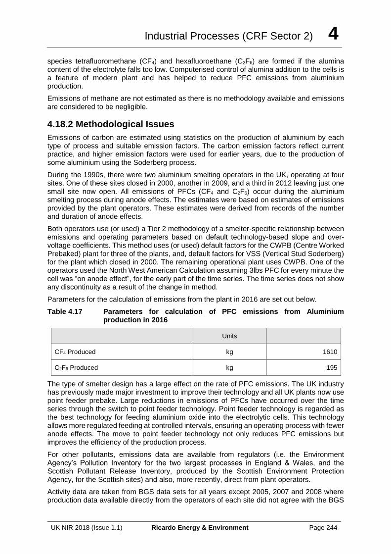
Industrial Processes (CRF Sector 2) 4
UK NIR 2018 (Issue 1.1) Ricardo Energy & Environment Page 244
species tetrafluoromethane (CF4) and hexafluoroethane (C2F6) are formed if the alumina content of the electrolyte falls too low. Computerised control of alumina addition to the cells is a feature of modern plant and has helped to reduce PFC emissions from aluminium production.
Emissions of methane are not estimated as there is no methodology available and emissions are considered to be negligible.
4.18.2 Methodological Issues
Emissions of carbon are estimated using statistics on the production of aluminium by each type of process and suitable emission factors. The carbon emission factors reflect current practice, and higher emission factors were used for earlier years, due to the production of some aluminium using the Soderberg process.
During the 1990s, there were two aluminium smelting operators in the UK, operating at four sites. One of these sites closed in 2000, another in 2009, and a third in 2012 leaving just one small site now open. All emissions of PFCs (CF4 and C2F6) occur during the aluminium smelting process during anode effects. The estimates were based on estimates of emissions provided by the plant operators. These estimates were derived from records of the number and duration of anode effects.
Both operators use (or used) a Tier 2 methodology of a smelter-specific relationship between emissions and operating parameters based on default technology-based slope and over-voltage coefficients. This method uses (or used) default factors for the CWPB (Centre Worked Prebaked) plant for three of the plants, and, default factors for VSS (Vertical Stud Soderberg) for the plant which closed in 2000. The remaining operational plant uses CWPB. One of the operators used the North West American Calculation assuming 3lbs PFC for every minute the cell was “on anode effect”, for the early part of the time series. The time series does not show any discontinuity as a result of the change in method.
Parameters for the calculation of emissions from the plant in 2016 are set out below.
Table 4.17 Parameters for calculation of PFC emissions from Aluminium production in 2016
Units
CF4 Produced kg 1610
C2F6 Produced kg 195
The type of smelter design has a large effect on the rate of PFC emissions. The UK industry has previously made major investment to improve their technology and all UK plants now use point feeder prebake. Large reductions in emissions of PFCs have occurred over the time series through the switch to point feeder technology. Point feeder technology is regarded as the best technology for feeding aluminium oxide into the electrolytic cells. This technology allows more regulated feeding at controlled intervals, ensuring an operating process with fewer anode effects. The move to point feeder technology not only reduces PFC emissions but improves the efficiency of the production process.
For other pollutants, emissions data are available from regulators (i.e. the Environment Agency’s Pollution Inventory for the two largest processes in England & Wales, and the Scottish Pollutant Release Inventory, produced by the Scottish Environment Protection Agency, for the Scottish sites) and also, more recently, direct from plant operators.
Activity data are taken from BGS data sets for all years except 2005, 2007 and 2008 where production data available directly from the operators of each site did not agree with the BGS
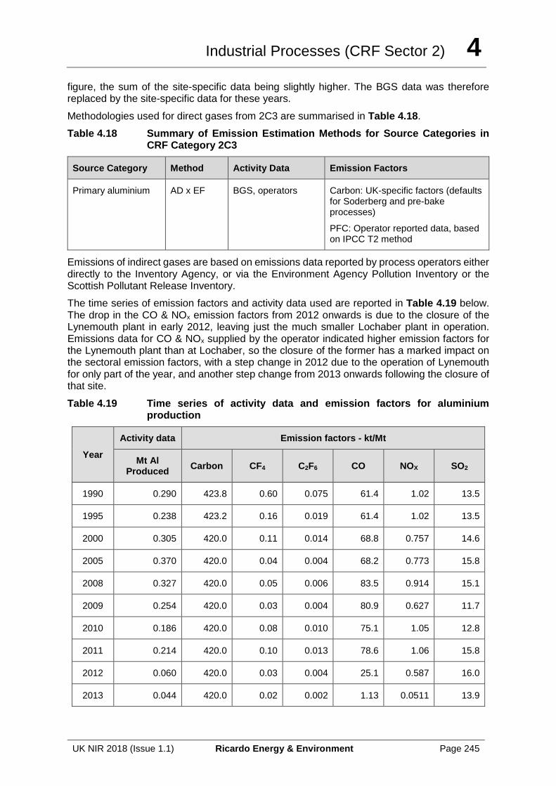
Industrial Processes (CRF Sector 2) 4
UK NIR 2018 (Issue 1.1) Ricardo Energy & Environment Page 245
figure, the sum of the site-specific data being slightly higher. The BGS data was therefore replaced by the site-specific data for these years.
Methodologies used for direct gases from 2C3 are summarised in Table 4.18.
Table 4.18 Summary of Emission Estimation Methods for Source Categories in CRF Category 2C3
Source Category Method Activity Data Emission Factors
Primary aluminium AD x EF BGS, operators Carbon: UK-specific factors (defaults for Soderberg and pre-bake processes)
PFC: Operator reported data, based on IPCC T2 method
Emissions of indirect gases are based on emissions data reported by process operators either directly to the Inventory Agency, or via the Environment Agency Pollution Inventory or the Scottish Pollutant Release Inventory.
The time series of emission factors and activity data used are reported in Table 4.19 below. The drop in the CO & NOx emission factors from 2012 onwards is due to the closure of the Lynemouth plant in early 2012, leaving just the much smaller Lochaber plant in operation. Emissions data for CO & NOx supplied by the operator indicated higher emission factors for the Lynemouth plant than at Lochaber, so the closure of the former has a marked impact on the sectoral emission factors, with a step change in 2012 due to the operation of Lynemouth for only part of the year, and another step change from 2013 onwards following the closure of that site.
Table 4.19 Time series of activity data and emission factors for aluminium production
Year
Activity data Emission factors - kt/Mt
Mt Al Produced
Carbon CF4 C2F6 CO NOX SO2
1990 0.290 423.8 0.60 0.075 61.4 1.02 13.5
1995 0.238 423.2 0.16 0.019 61.4 1.02 13.5
2000 0.305 420.0 0.11 0.014 68.8 0.757 14.6
2005 0.370 420.0 0.04 0.004 68.2 0.773 15.8
2008 0.327 420.0 0.05 0.006 83.5 0.914 15.1
2009 0.254 420.0 0.03 0.004 80.9 0.627 11.7
2010 0.186 420.0 0.08 0.010 75.1 1.05 12.8
2011 0.214 420.0 0.10 0.013 78.6 1.06 15.8
2012 0.060 420.0 0.03 0.004 25.1 0.587 16.0
2013 0.044 420.0 0.02 0.002 1.13 0.0511 13.9
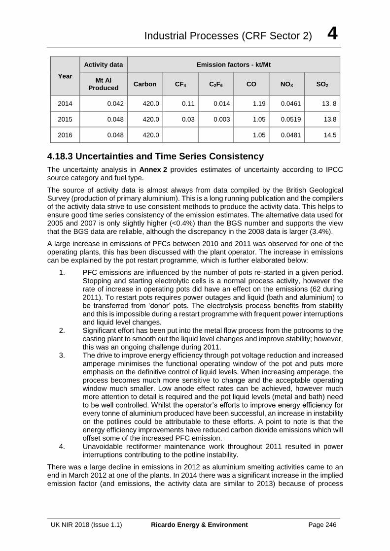
Industrial Processes (CRF Sector 2) 4
UK NIR 2018 (Issue 1.1) Ricardo Energy & Environment Page 246
Year
Activity data Emission factors - kt/Mt
Mt Al Produced
Carbon CF4 C2F6 CO NOX SO2
2014 0.042 420.0 0.11 0.014 1.19 0.0461 13. 8
2015 0.048 420.0 0.03 0.003 1.05 0.0519 13.8
2016 0.048 420.0 1.05 0.0481 14.5
4.18.3 Uncertainties and Time Series Consistency
The uncertainty analysis in Annex 2 provides estimates of uncertainty according to IPCC source category and fuel type.
The source of activity data is almost always from data compiled by the British Geological Survey (production of primary aluminium). This is a long running publication and the compilers of the activity data strive to use consistent methods to produce the activity data. This helps to ensure good time series consistency of the emission estimates. The alternative data used for 2005 and 2007 is only slightly higher (<0.4%) than the BGS number and supports the view that the BGS data are reliable, although the discrepancy in the 2008 data is larger (3.4%).
A large increase in emissions of PFCs between 2010 and 2011 was observed for one of the operating plants, this has been discussed with the plant operator. The increase in emissions can be explained by the pot restart programme, which is further elaborated below:
1. PFC emissions are influenced by the number of pots re-started in a given period. Stopping and starting electrolytic cells is a normal process activity, however the rate of increase in operating pots did have an effect on the emissions (62 during 2011). To restart pots requires power outages and liquid (bath and aluminium) to be transferred from ‘donor’ pots. The electrolysis process benefits from stability and this is impossible during a restart programme with frequent power interruptions and liquid level changes.
2. Significant effort has been put into the metal flow process from the potrooms to the casting plant to smooth out the liquid level changes and improve stability; however, this was an ongoing challenge during 2011.
3. The drive to improve energy efficiency through pot voltage reduction and increased amperage minimises the functional operating window of the pot and puts more emphasis on the definitive control of liquid levels. When increasing amperage, the process becomes much more sensitive to change and the acceptable operating window much smaller. Low anode effect rates can be achieved, however much more attention to detail is required and the pot liquid levels (metal and bath) need to be well controlled. Whilst the operator’s efforts to improve energy efficiency for every tonne of aluminium produced have been successful, an increase in instability on the potlines could be attributable to these efforts. A point to note is that the energy efficiency improvements have reduced carbon dioxide emissions which will offset some of the increased PFC emission.
4. Unavoidable rectiformer maintenance work throughout 2011 resulted in power interruptions contributing to the potline instability.
There was a large decline in emissions in 2012 as aluminium smelting activities came to an end in March 2012 at one of the plants. In 2014 there was a significant increase in the implied emission factor (and emissions, the activity data are similar to 2013) because of process
Industrial Processes (CRF Sector 2) 4
UK NIR 2018 (Issue 1.1) Ricardo Energy & Environment Page 247
issues during 2014, in particular an ‘anode crisis’. Aluminium manufacture has to be kept under specific conditions to maintain low PFC emissions.
Aluminium alloy production
No emissions of SF6 are reported by any of the aluminium foundries in the Pollution Inventory or SPRI. Emissions from the use of SF6 in the UK aluminium sector are therefore reported as Not Occurring.
4.18.4 Source Specific QA/QC and Verification
This source category is covered by the general QA/QC of the greenhouse gas inventory in Section 1.6. Emissions data taken from the Pollution Inventory are subject to additional QA/QC from the Inventory Agency.
4.18.5 Source Specific Recalculations
There have been no significant recalculations for this sector.
4.18.6 Source Specific Planned Improvements
Emission factors and activity data will be kept under review.
4.19 SOURCE CATEGORY 2C4 – MAGNESIUM PRODUCTION
4.19.1 Source Category Description
In the UK, SF6 and an HFC act as cover gases to prevent molten magnesium from burning during the production of magnesium.
4.19.2 Methodological Issues
magnesium oxidising when exposed to air. It is estimated that 95% of SF6 (Gluckman, 2013) used in this way is released to the atmosphere unless capture/recycle technologies are employed. SF6 is non-flammable and non-toxic, and is therefore a safe gas to use. In the UK, SF6 has been used as an alternative cover gas to SO2 in magnesium alloy production and sand and die-casting since the early 1990s. Since 2006, EU magnesium producers have looked for alternatives to SF6 in response to bans in the EU F-Gas regulation. Some die casters have gone back to using SO2. Others have used HFC-134a and a fluoro-ketone (FK 5-1-12) with the trade name Novec 612.
The UK magnesium casting industry is very small. There are three significant manufacturers (one alloy producer, one die-caster and one sand-caster) plus two very small operations (both sand-casters). Alloy production involves the use of primary magnesium ingots, recycled scrap material and second-generation magnesium materials (i.e. material already made into alloys) for the production of different alloys. Both die and sand casters use these magnesium alloys to produce specific components for a wide range of industries. For the casting industry, SF6 is used for casting specific magnesium alloys where other cover gases, such as HFC-134a, are currently considered not suitable.
The 2014 EU F-Gas Regulation prohibits the use of SF6 in magnesium die casting, from 1 Jan 2018, the ban is extended to installations using a quantity below 850kg per year. Note that, as mentioned below, most UK magnesium production uses processes other than die casting, so this ban only has a limited impact on this sector.
A review of the data sources and methodology used to estimate emissions from F-gases used as cover gases in magnesium foundries was carried out in 2013 (Gluckman, 2013). In all cases
Industrial Processes (CRF Sector 2) 4
UK NIR 2018 (Issue 1.1) Ricardo Energy & Environment Page 248
UK magnesium companies were able to report consumption, but had no actual measured data on emissions. The assumptions about the fraction of SF6 and HFCs that are emitted from the consumption of these F-gases were reviewed through discussion with industry experts and in some cases amended. It is estimated that 95% of SF6 consumption is emitted but that only 20% of HFC-134a consumption is emitted (as a much greater proportion reacts with the magnesium). These figures are based on expert estimates by Gluckman (2013). The estimates of emissions in the 2016 inventory are similar to those reported in the previous inventory until approximately 2005.
For magnesium alloy production, SF6 emissions from 1998 onwards are estimated based on the data reported to the Environment Agency Pollution Inventory (EA, 2015), whilst emissions prior to 1998 are estimated based on consultations with the plant operators.
From 2004, one of the main industry users of SF6 as a cover gas has implemented a cover gas system using HFC-134a for some of its production capacity. There has not been a complete switch to HFC-134a, although the operator is considering this on an ongoing basis depending on suitability for the different alloys produced. In addition to having a significantly lower GWP than SF6 (and thus reducing emissions on a CO2 equivalent basis), use of HFC-134a is further advantageous in that a significant fraction of it is destroyed by the high process temperatures (80%) thus reducing the fraction of gas emitted as a fugitive emission.
From 2008, emissions of HFCs have been reported in the Pollution Inventory, and therefore the reported data are used directly.
As part of a study to update the F-gas inventory (Gluckman, 2013), castings operators were re-contacted to provide activity data for recent years (the previous survey was conducted in 2004). The two largest users of SF6 and HFC-134a (that represent 99% of UK emissions from magnesium) are now contacted annually for their activity data (consumption of SF6 and HFC-134a).
Emissions of FK 5-1-12 cannot currently be reported via the CRF as there is no space to report this product, it would also be a low priority to include as it is a sparingly used product with a GWP comparable to CO2. It is estimated that the decomposition of 1 tonne of FK 5-1-12 during use as a cover gas generates ~400 tonnes CO2e of PFCs, but as this product is used only at 1 small magnesium site and trialled at one larger site, total emissions in the UK due to the decomposition of FK 5-1-12 have been estimated to be less than 0.001% of the UK national total since 2012 and 0 beforehand. According to the UNFCCC Guidance for reporting, emissions could be “… considered insignificant if the likely level of emissions is below 0.05 per cent of the national total GHG emissions, and does not exceed 500 kt CO2 eq.”. Therefore, the UK considers this a low priority to formally estimate and report emissions for.
As far as we know, HFC-134a does not decompose into other potent GHGs; any other products potentially emitted would be offset by our conservative estimate of the proportion of HFC-134a emitted.
4.19.3 Uncertainties and Time Series Consistency
The main area of uncertainty is regarding emissions of SF6 from casting based on discussions with the sector Trade Association for the period prior to 1998. Data from the main magnesium alloy producer is also uncertain for this period.
For the period 1998-2016, the uncertainty of the time-series emissions is estimated to be significantly lower. Data received from the main magnesium alloy producer and the other 4 casting operations are associated with low uncertainty and show good consistency across the time series.
SF6 emissions from UK magnesium producers peaked in 2000 at approximately 1,000 kt CO2 equivalent. The use has fallen steadily, particularly from 2006 onwards, being 75 kt CO2
Industrial Processes (CRF Sector 2) 4
UK NIR 2018 (Issue 1.1) Ricardo Energy & Environment Page 249
equivalent in 2016. HFC-134a emissions were zero until 2008 and are 2 kt CO2 equivalent in 2016.
4.19.4 Source Specific QA/QC and Verification
This source category is covered by the general QA/QC of the greenhouse gas inventory in Section 1.6. Emissions data taken from the Pollution Inventory are subject to additional QA/QC from the Inventory Agency.
4.19.5 Source Specific Recalculations
For information on the magnitude of recalculations to this Source Category, see Section 10.
4.19.6 Source Specific Planned Improvements
Emission factors and activity data will be kept under review.
4.20 SOURCE CATEGORY 2C5 – LEAD PRODUCTION
Primary lead production is limited in the UK to a single site, which produced zinc and lead from imported ore concentrates. Emissions are reported under 2C6 and so this process is described in the following section. Emissions of CO from a number of small secondary lead producers are estimated based on data reported by the process operators.
Emissions of CO2 can, in theory, occur from the use of reductants such as coal, coke oven coke, or natural gas during secondary lead processes, however none of the UK’s secondary lead processes are known to involve the use of reductants. If any use of reductant does occur, however, it would be included in UK fuel statistics as an energy use, and thus emissions of CO2 would already be included in the UK inventory, reported under 1A2.
4.21 SOURCE CATEGORY 2C6 – ZINC PRODUCTION
4.21.1 Source Category Description
Zinc was produced in the UK until early 2003, using the Imperial Smelting Process (ISP) at a smelter operated by Britannia Zinc at Avonmouth. The site processed imported ore concentrates, and had a capacity to produce approximately 150,000 tonnes of zinc, as well as 65,000 tonnes of lead and small quantities of other metals such as cadmium. The ISP involves the use of a blast furnace to reduce zinc and lead oxides to the metal using coke as a reductant. Limestone could also be added to act as a slag-forming agent.
The UK also had two other non-ferrous metal production facilities that would have emitted CO2 from processes. These were:
• the Capper Pass Tin Smelter at Melton, Humberside (closed in 1991)
• IMI Refiners' secondary copper smelter at Walsall (closed in 1997)
There is very little data specific to these installations available to the inventory agency as their closure pre-dates most of the routine annual emissions reporting regulations in the UK. Both processes used coke oven coke as a reductant that would lead to process emissions of CO2, and emission estimates from these two sites are also reported under 2C6.
4.21.2 Methodological Issues
Britannia Zinc reported CO2 emissions in the Pollution Inventory from 1998 until 2002, at which point the site ceased operation. Emissions of CO2 would have occurred from the use of coke
Industrial Processes (CRF Sector 2) 4
UK NIR 2018 (Issue 1.1) Ricardo Energy & Environment Page 250
in the ISP, but also from decarbonisation of any limestone used, and from the other fuels used on site e.g. gas/oil burners used on the sinter plant and oil-fired furnaces used in the zinc refinery. We have not been able to discover any data on the quantities of coke and other fuels used, or the quantities of limestone that might have been used. The operator-reported CO2 emissions in the Pollution Inventory are totals only, and no conclusions can be drawn regarding the split between coke, other fuels and limestone. The reported emissions are, however, much higher than would be implied by the Tier 1 factors given in the 2006 GLs for the ISP. There is insufficient data to determine whether this is due to a high level of fuel combustion emissions on site, or that the process-related emissions at this site were higher than is typical for this type of process.
The Digest of UK Energy Statistics (DUKES) does give a full time-series of data on the consumption of coke oven coke by the non-ferrous metal industry. The consumption shown in this source is zero after 2003, confirming that after the closure of Britannia Zinc, no other non-ferrous metal processes in the UK used coke oven coke. We also believe that very few, other than Britannia Zinc, Capper Pass and IMI Refiners have used coke oven coke at any point in the period covered by the UK inventory.
Because all three sites have been closed for many years, there is no information on the consumption of coke oven coke at each site. Of the three, it is likely that IMI Refiners used relatively small amounts of coke, whereas the Capper Pass smelter was the largest of its kind in the world, and its closure in 1991 coincides with a big reduction in the non-ferrous metal industry's consumption of coke as shown in DUKES. There is insufficient data to split the coke consumption data between the three sites, and instead all of the coke use in DUKES is reported in 2C6. This will ensure completeness and reduce the uncertainty in the reported emissions, since only the total coke use figure is known to a high level of certainty. Carbon factors for the coke oven coke are derived from the carbon balance approach previously described for 1A2a.
As previously described, limestone may have been used at Britannia Zinc (and probably in the blast furnaces at Capper Pass as well) but we do not have any evidence on which to base emission estimates. Since all of these plants closed more than 10 years ago, there is no scope to access new information to improve this situation, and therefore we recommend that no emission estimates for these source categories be reported. Further, we note that the UK GHGI already includes emissions from all reported limestone and dolomite activity based on data from the British Geological Survey on UK supply and demand of these materials, and hence there is no gap in the UK GHGI, but possibly a small mis-allocation with higher estimates in another sector to counter the possible under-report here.
Emissions of CO from the lead/zinc smelter and the copper refinery are reported in 2C6 and 2C7 respectively and estimates are based on emissions data reported by the process operators in the Pollution Inventory (EA, 2015). No CO emissions data exist for Capper Pass and so no estimate has been made.
4.21.3 Uncertainties and Time Series Consistency
The use of DUKES data for coke consumption by non-ferrous metal processes ensures time series consistency and completeness, which is important since it is impossible to now determine how much coke oven coke was used in each of the 3 three non-ferrous metal processes that once existed in the UK. Any limestone used in the blast furnaces at Britannia Zinc and Capper Pass cannot be estimated, but emissions data for 2C1 cover all use of limestone and dolomite for blast furnaces and so overall completeness is assured.
Industrial Processes (CRF Sector 2) 4
UK NIR 2018 (Issue 1.1) Ricardo Energy & Environment Page 251
4.21.4 Source Specific QA/QC and Verification
This source category is covered by the general QA/QC of the greenhouse gas inventory in Section 1.6.
4.21.5 Source Specific Recalculations
There have been no significant recalculations in this category.
4.21.6 Source Specific Planned Improvements
It is noted that this sector has been identified as a key category this year, and that a tier 1 method is used. The UK has recently reviewed this sector and included some additional sources using what is believed to be the best currently available data. Unfortunately as the only site for this sector has now been closed for a number of years it is highly unlikely that new data will mean a better estimate will be possible; incidentally the reason it is identified as a key category is due to the fact that this one large site closed since the base year.
4.22 SOURCE CATEGORY 2D1 – LUBRICANT USE
4.22.1 Source Category Description
Emissions sources Sources included Method Emission Factors
2D1:Industrial engines – lubricants Agricultural engines – lubricants Marine engines – lubricants Road vehicle engines – lubricants
T1 T1 T1 T1
D, CS D, CS D, CS D, CS
Lubricant consumption by the unintended combustion in vehicle engines is estimated using the method from the EMEP/EEA Emissions Inventory Guidebook (2016). These consumption estimates were used to calculate CO2 emissions from lubricant combustion in road vehicle engines and are reported in IPCC sector 2D1, except for lubricants use from mopeds, which are deemed to be intentional fuel use and hence is reported in IPCC sector 1A3biv.
Emissions of CH4 and N2O also arise from lubricant combustion in engines. However, the exhaust emission factors for these gases will include the contribution of lubricants as well as the main fuel to the pollutant emissions when the vehicles were tested. Hence, the emissions of CH4 and N2O (and other air pollutants estimated on a vkm-travelled basis) from lubricants are included implicitly in the hot exhaust emissions (IPCC Sector 1A3b) calculated for each vehicle and fuel type. Treating emissions of these pollutants separately would lead to a double count.
Lubricant use in the remaining sectors is calculated from the difference between the UK demand figure in DUKES & the COPERT-based road transport lubricant figures.
4.22.2 Methodological Issues
Detailed activity data on lubricants are not available in the UK; DUKES does include data on sector-specific lubricant use (e.g. use by industry, agricultural sector, shipping etc.) in addition to the total lubricant demand time-series, but this falls short of what is required for the Tier 2 method. Therefore we have used the 2006 GLs Tier 1 method, with UK lubricant activity data from DUKES and the IPCC default ODU factor of 0.2, together with the UK-specific carbon emission factor for lubricants which is based on analysis of UK waste oil samples.
Industrial Processes (CRF Sector 2) 4
UK NIR 2018 (Issue 1.1) Ricardo Energy & Environment Page 252
4.22.3 Uncertainties and Time Series Consistency
DUKES gives a full time series of lubricant consumption data so consistency of the emission estimates is good. The use of the Tier 1 methodology means that estimates are quite uncertain.
4.22.4 Source Specific QA/QC and Verification
This source category is covered by the general QA/QC of the greenhouse gas inventory in Section 1.6.
4.22.5 Source Specific Recalculations
Apart from a revision to UK energy statistics for 2015, there have been no significant recalculations in this category.
4.22.6 Source Specific Planned Improvements
Emission factors and activity data will be kept under review.
4.23 SOURCE CATEGORY 2D2 – PARAFFIN WAX USE
4.23.1 Source Category Description
This category includes CO2 emissions form paraffin wax use.
4.23.2 Methodological Issues
DUKES gives total consumption of petroleum waxes for the years 1990-2009 only. For 2010 onwards, petroleum wax consumption is only available as part of the much larger consumption of 'miscellaneous petroleum products'. In 2009, the consumption of petroleum waxes was equal to 5.9% of the total consumption of waxes plus other miscellaneous products, so this figure of 5.9% is then applied to the DUKES figures for miscellaneous product use in 2010-2016 to obtain an estimate of petroleum wax use in those years. During the review of the 2017 submission, alternative data were suggested by reviewers. These data, reported by Eurostat (at http://ec.europa.eu/eurostat) do not agree well with the DUKES data for 2007-2009, and for 5 out of 7 years in the period 2010-2016 are lower than the estimates derived using the method described above (the Eurostat data are higher in 2013-2014 only). As a result of the poor agreement between the two datasets in 2007-2009, we have not used the Eurostat figures for 2010 and for most years, the method we do use gives a more conservative estimate of petroleum wax consumption.
Emissions are estimated using the Tier 1 ODU factor of 0.2, and the IPCC default carbon content of 20 kg C/ GJ (net basis).
4.23.3 Uncertainties and Time Series Consistency
Emission estimates for this sector are highly uncertain because of the use of a Tier 1 methodology. In addition, the activity data for 2010-2016 are especially uncertain due to the loss of detail in DUKES meaning that the consumption of petroleum waxes has to be estimated by the Inventory Agency based on trends in consumption of a much wider group of petroleum products.
Industrial Processes (CRF Sector 2) 4
UK NIR 2018 (Issue 1.1) Ricardo Energy & Environment Page 253
4.23.4 Source Specific QA/QC and Verification
This source category is covered by the general QA/QC of the greenhouse gas inventory in Section 1.6.
4.23.5 Source Specific Recalculations
There have been no significant recalculations in this category.
4.23.6 Source Specific Planned Improvements
Emission factors and activity data will be kept under review.
4.24 SOURCE CATEGORY 2D3 – OTHER NON-ENERGY PRODUCTS FROM FUELS AND SOLVENT USE
4.24.1 Source Category Description
Emissions of CO2 are estimated from consumption of urea by road vehicles with relevant types of catalytic converters for control of pollutant emissions and are reported under 2D3. Urea has the chemical formula (NH2)2CO and is injected into the exhaust stream of certain types of diesel vehicles (currently Euro IV and V HGVs and buses) as a 32.5% (by weight) aqueous solution. The catalytic process of converting NOx to nitrogen in the exhaust leads to the release of CO2 from the urea in the tailpipe.
Petroleum coke is known to be used by various sectors either as a fuel (e.g. at power stations and in cement kilns), or in various processes (e.g. in brickmaking, titanium dioxide manufacture, aluminium smelting, or electric arc steelmaking). The consumption of petroleum coke for each sector is either available directly from DUKES or estimated, based on EU ETS and other data. For most years, there is more petroleum coke listed in the UK energy statistics than can be accounted for by these known users. In other years, the known users require more petroleum coke than is available in the energy statistics. But, since there is excess petroleum coke for most years (18 out of 27) between 1990 and 2016, it is assumed that there are additional, unknown uses of petroleum coke in those years. The excess petroleum coke in the energy statistics is reported as being for non-energy uses but this will include both fuel grade and anode grade coke, so it is possible that the coke could be used as a fuel, or in processes, or both. In the absence of any data, and because the coke appears in UK energy statistics as ‘non-energy use’, it has been assumed that it is used for an unknown non-energy use. Such uses could be emissive or the carbon could be stored, but we have taken the conservative approach and assumed that all of the carbon in this petroleum coke is emitted, and reported it in 2D3.
Emissions of NMVOC from numerous uses of solvents and other volatile petroleum products are reported under 2D3. These NMVOC sources include the manufacture and use of paints, printing inks, adhesives and other types of coatings (both in industry and in households), degreasing and dry cleaning, manufacture of tyres, vegetable oil, and agrochemicals, and the use of consumer products such as aerosols, fragrances and automotive products such as screenwash. Also included is the use of kerosene as a viscosity-reducer in 'cutback' asphalt grades.
4.24.2 Methodological Issues
The 2006 IPCC Guidelines specify two approaches for estimating CO2 emissions from urea consumption. This is either from statistics on total urea sales or by estimating urea consumption as a proportion of the amount of fuel consumed. There are no statistics on urea
Industrial Processes (CRF Sector 2) 4
UK NIR 2018 (Issue 1.1) Ricardo Energy & Environment Page 254
sales in the UK, so the approach based on fuel consumption is used. Not all diesel vehicles use urea so it is necessary to know the amount of fuel consumed specifically from those vehicles with the relevant exhaust after treatment technology that require urea injection.
Urea is used by HGVs and buses in the UK manufactured to Euro IV and V standards. These came into effect from 2006. The EMEP/EEA Emissions Inventory Guidebook (2013) provides the means for estimating urea consumption as a proportion of fuel consumed by these specific types of vehicles. Fuel consumption by Euro IV and V HGVs and buses was estimated using a bottom-up method described in Chapter 3. The estimations involve the use of vehicle km activity and fleet composition data from DfT and g/km fuel consumption factors, with total fuel consumption calculated for road transport by this method normalised to national fuel sales in DUKES.
Following figures given in the EMEP/EEA Guidebook for estimating other pollutant emissions, an assumption was made that 75% of Euro V HGVs and buses are equipped with SCR – the catalyst system that uses urea. The same assumption was also applied to Euro IV vehicles. Fuel consumption was calculated for these types of vehicles using SCR technology. Following the EMEP/EEA Guidebook, urea consumption is assumed to be 4% of fuel consumption for a Euro IV HGV and bus and 6% for a Euro V HGV and bus. Independent assessment in the UK from suppliers of urea and vehicle manufacturers supports these assumptions. These assumptions allowed the time-series for consumption of urea by UK road transport to be estimated. No urea was consumed before 2006.
A constant emission factor of 0.238 kgCO2/kg urea solution, as given in the EMEP/EEA Guidebook was used. This is consistent with the factor and emission equation given in the 2006 IPCC Guidelines, assuming urea is used as a 32.5% aqueous solution which is the norm in the UK.
The emissive non-energy use of petroleum coke is assumed to result in 100% of the carbon content of this fuel being emitted. The 2006 IPCC default factor for petroleum coke has been used in conjunction with calorific values for petroleum coke used in sectors other than electricity generation, taken from UK energy statistics. The relatively high calorific value given for this type of petroleum coke means that the IPCC default factor implies that this petroleum coke is over 90% carbon, which is higher than the carbon content of coke oven coke or anthracite.
Solvents are used by a wide range of industrial sectors as well as being used by the general public. Many applications for industrial solvent use require that the solvent is evaporated at some stage, for example solvent in the numerous types of paints, inks, adhesives and other industrial coatings must evaporate in order for the coating to cure. The solvent contained in many consumer products such as fragrances, polishes and aerosols is also expected to be released to atmosphere when the product is used.
Emissions of NMVOC from use of these solvents can therefore be assumed to be equal to solvent consumed in these products, less any solvent that is recovered or destroyed. In the case of consumer products and smaller industrial processes, such as vehicle refinishing processes, the use of arrestment devices such as thermal oxidisers would be prohibitively expensive and abatement strategies therefore concentrate on minimising the solvent consumption. Solvent recovery and destruction can be ignored for these processes.
In comparison, larger industrial solvent users such as flexible packaging print works, car manufacturing plants and specialist coating processes such as the manufacture of hot stamping foils are generally carried out using thermal oxidisers or other devices to capture and destroy solvent emissions. In these cases, NMVOC emissions will still occur, partly due to incomplete destruction of solvent by the arrestment device, but also because some ‘fugitive’ emissions will avoid being captured and treated by that device. The level of fugitive emissions will vary from process to process, and will depend upon the extent to which the process is
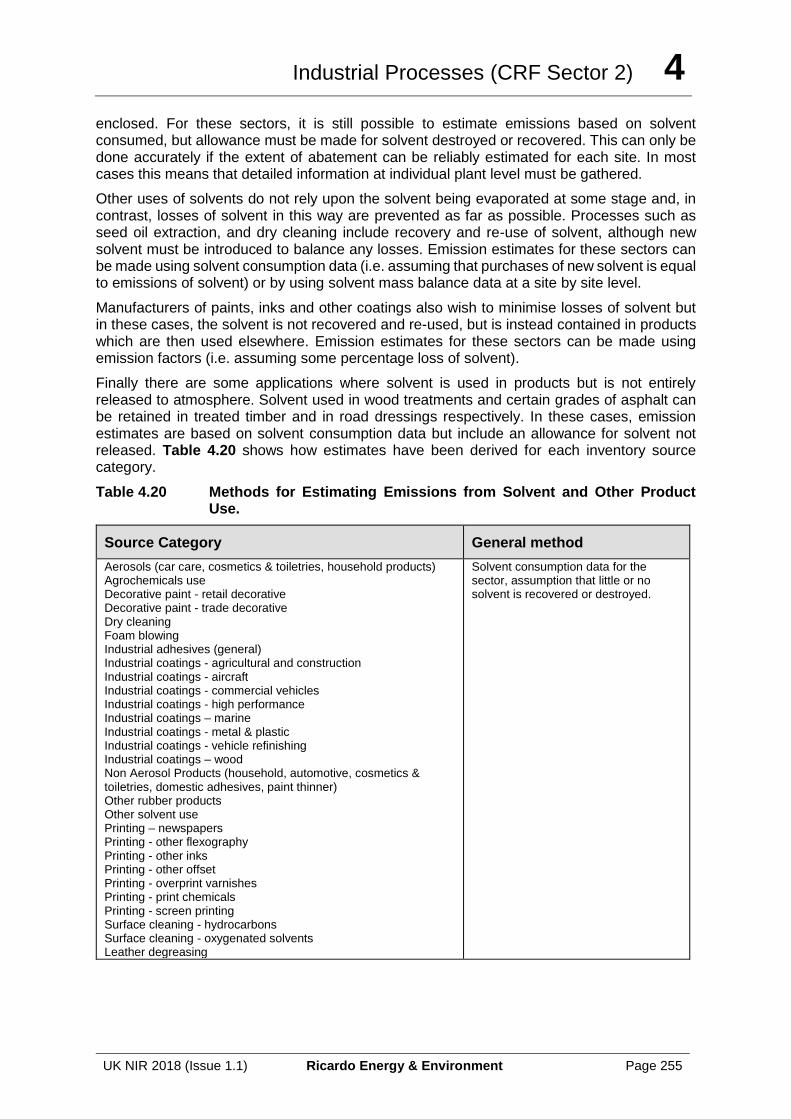
Industrial Processes (CRF Sector 2) 4
UK NIR 2018 (Issue 1.1) Ricardo Energy & Environment Page 255
enclosed. For these sectors, it is still possible to estimate emissions based on solvent consumed, but allowance must be made for solvent destroyed or recovered. This can only be done accurately if the extent of abatement can be reliably estimated for each site. In most cases this means that detailed information at individual plant level must be gathered.
Other uses of solvents do not rely upon the solvent being evaporated at some stage and, in contrast, losses of solvent in this way are prevented as far as possible. Processes such as seed oil extraction, and dry cleaning include recovery and re-use of solvent, although new solvent must be introduced to balance any losses. Emission estimates for these sectors can be made using solvent consumption data (i.e. assuming that purchases of new solvent is equal to emissions of solvent) or by using solvent mass balance data at a site by site level.
Manufacturers of paints, inks and other coatings also wish to minimise losses of solvent but in these cases, the solvent is not recovered and re-used, but is instead contained in products which are then used elsewhere. Emission estimates for these sectors can be made using emission factors (i.e. assuming some percentage loss of solvent).
Finally there are some applications where solvent is used in products but is not entirely released to atmosphere. Solvent used in wood treatments and certain grades of asphalt can be retained in treated timber and in road dressings respectively. In these cases, emission estimates are based on solvent consumption data but include an allowance for solvent not released. Table 4.20 shows how estimates have been derived for each inventory source category.
Table 4.20 Methods for Estimating Emissions from Solvent and Other Product Use.
Source Category General method
Aerosols (car care, cosmetics & toiletries, household products) Agrochemicals use Decorative paint - retail decorative Decorative paint - trade decorative Dry cleaning Foam blowing Industrial adhesives (general) Industrial coatings - agricultural and construction Industrial coatings - aircraft Industrial coatings - commercial vehicles Industrial coatings - high performance Industrial coatings – marine Industrial coatings - metal & plastic Industrial coatings - vehicle refinishing Industrial coatings – wood Non Aerosol Products (household, automotive, cosmetics & toiletries, domestic adhesives, paint thinner) Other rubber products Other solvent use Printing – newspapers Printing - other flexography Printing - other inks Printing - other offset Printing - overprint varnishes Printing - print chemicals Printing - screen printing Surface cleaning - hydrocarbons Surface cleaning - oxygenated solvents Leather degreasing
Solvent consumption data for the sector, assumption that little or no solvent is recovered or destroyed.
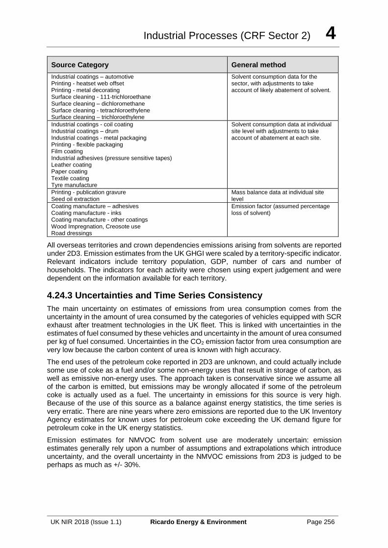
Industrial Processes (CRF Sector 2) 4
UK NIR 2018 (Issue 1.1) Ricardo Energy & Environment Page 256
Source Category General method
Industrial coatings – automotive Printing - heatset web offset Printing - metal decorating Surface cleaning - 111-trichloroethane Surface cleaning – dichloromethane Surface cleaning - tetrachloroethylene Surface cleaning – trichloroethylene
Solvent consumption data for the sector, with adjustments to take account of likely abatement of solvent.
Industrial coatings - coil coating Industrial coatings – drum Industrial coatings - metal packaging Printing - flexible packaging Film coating Industrial adhesives (pressure sensitive tapes) Leather coating Paper coating Textile coating Tyre manufacture
Solvent consumption data at individual site level with adjustments to take account of abatement at each site.
Printing - publication gravure Seed oil extraction
Mass balance data at individual site level
Coating manufacture – adhesives Coating manufacture - inks Coating manufacture - other coatings Wood Impregnation, Creosote use Road dressings
Emission factor (assumed percentage loss of solvent)
All overseas territories and crown dependencies emissions arising from solvents are reported under 2D3. Emission estimates from the UK GHGI were scaled by a territory-specific indicator. Relevant indicators include territory population, GDP, number of cars and number of households. The indicators for each activity were chosen using expert judgement and were dependent on the information available for each territory.
4.24.3 Uncertainties and Time Series Consistency
The main uncertainty on estimates of emissions from urea consumption comes from the uncertainty in the amount of urea consumed by the categories of vehicles equipped with SCR exhaust after treatment technologies in the UK fleet. This is linked with uncertainties in the estimates of fuel consumed by these vehicles and uncertainty in the amount of urea consumed per kg of fuel consumed. Uncertainties in the CO2 emission factor from urea consumption are very low because the carbon content of urea is known with high accuracy.
The end uses of the petroleum coke reported in 2D3 are unknown, and could actually include some use of coke as a fuel and/or some non-energy uses that result in storage of carbon, as well as emissive non-energy uses. The approach taken is conservative since we assume all of the carbon is emitted, but emissions may be wrongly allocated if some of the petroleum coke is actually used as a fuel. The uncertainty in emissions for this source is very high. Because of the use of this source as a balance against energy statistics, the time series is very erratic. There are nine years where zero emissions are reported due to the UK Inventory Agency estimates for known uses for petroleum coke exceeding the UK demand figure for petroleum coke in the UK energy statistics.
Emission estimates for NMVOC from solvent use are moderately uncertain: emission estimates generally rely upon a number of assumptions and extrapolations which introduce uncertainty, and the overall uncertainty in the NMVOC emissions from 2D3 is judged to be perhaps as much as +/- 30%.
Industrial Processes (CRF Sector 2) 4
UK NIR 2018 (Issue 1.1) Ricardo Energy & Environment Page 257
4.24.4 Source Specific QA/QC and Verification
This source category is covered by the general QA/QC of the greenhouse gas inventory in Section 1.6.
4.24.5 Source Specific Recalculations
Because the estimate of Urea emissions is dependent on the fraction of specific HDVs’ fuel use the revision to the fuel consumption factors and fuel normalisation methodologies in 1A3b means that there is a significant revision to Urea emissions.
For information on the magnitude of recalculations, see Section 10.
4.24.6 Source Specific Planned Improvements
Emission factors and activity data will be kept under review.
4.25 SOURCE CATEGORY 2E1 – INTEGRATED CIRCUIT OR SEMICONDUCTOR
Emissions of SF6 from semiconductor manufacturing are combined with emissions from training shoes and electrical insulation in source category 2G2e for reasons of commercial confidentiality. This source category is described in Section 4.39.
4.26 SOURCE CATEGORY 2E2 – TFT FLAT PANEL DISPLAY
4.26.1 Source Category Description
Emissions sources Sources included Method Emission Factors
None
Gases Reported None (gases possible are PFCs, NF3 or SF6)
Key Categories None identified
Key Categories (Qualitative)
None identified
Overseas Territories and Crown Dependencies Reporting
Not occurring
Completeness Potentially a small amount of emissions from small scale flat panel manufacturing in the 90s and early 2000s.
Major improvements since last submission
No major improvements since last submission.
4.26.2 Methodological Issues
ICF (2014) determined that the UK does not have volume Flat Panel manufacturing. ICF reached this conclusion after contacting the National Microelectronics Institute (NMI) who represent flat panel display manufacturers in the UK.
Further market analysis by Ricardo (2016) confirmed that there are no UK emissions from this sector. This included discussions with representatives of the flat panel supply sector and PFC supply sector – all those contacted confirmed that all flat panel displays used in the UK are
Industrial Processes (CRF Sector 2) 4
UK NIR 2018 (Issue 1.1) Ricardo Energy & Environment Page 258
imported. It was noted that in the 2006 IPCC guidelines that there was activity data given33 for the UK in 2003-5. When using this activity data and the default methodology the resulting emission was well below the threshold to be considered insignificant, so is reported by the UK as ‘NE’ for years before 2014.
4.26.3 Source Specific Planned Improvements
Any emergence of volume manufacturing capacity of TFT flat panel display is kept under review.
4.27 SOURCE CATEGORY 2E3 – PHOTOVOLTAICS
4.27.1 Source Category Description
Emissions sources Sources included Method Emission Factors
None
Gases Reported None (gases possible are PFCs)
Key Categories None identified
Key Categories (Qualitative)
None identified
Overseas Territories and Crown Dependencies Reporting
Not occurring
Completeness Potentially a small amount of emissions from small scale photovoltaics manufacturing in the 90s and early 2000s.
Major improvements since last submission
No major improvements since last submission.
4.27.2 Methodological Issues
ICF (2014) determined that the UK does not have volume photovoltaics (PV) manufacturing. ICF reached this conclusion after contacting the British Photovoltaic Association (BPA) to gather data from PV manufacturing in the UK. The BPA also confirmed that statistics on F-gas use in the PV manufacturing in the UK are not available.
Further market analysis by Ricardo (2016) confirmed that there are no UK emissions from this sector. This included discussions with representatives of the PV supply sector and PFC supply sector – all those contacted confirmed that all PV cells used in the UK are currently imported or manufactured in the UK using emerging technology that does not require F-gases in the process. It was noted that in the 2006 IPCC guidelines that there was activity data given34 for the UK in 2003. When using this activity data and the default methodology the resulting emission was well below the threshold to be considered insignificant, so is reported by the UK as ‘NE’ for years before 2014.
33 Table 6.7 of Volume 3 of the IPCC 2006 Guidelines
34 Table 6.8 of Volume 3 of the IPCC 2006 Guidelines
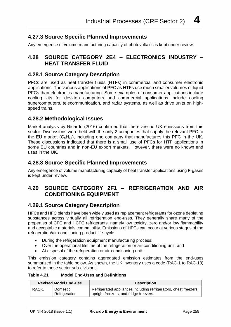
Industrial Processes (CRF Sector 2) 4
UK NIR 2018 (Issue 1.1) Ricardo Energy & Environment Page 259
4.27.3 Source Specific Planned Improvements
Any emergence of volume manufacturing capacity of photovoltaics is kept under review.
4.28 SOURCE CATEGORY 2E4 – ELECTRONICS INDUSTRY – HEAT TRANSFER FLUID
4.28.1 Source Category Description
PFCs are used as heat transfer fluids (HTFs) in commercial and consumer electronic applications. The various applications of PFC as HTFs use much smaller volumes of liquid PFCs than electronics manufacturing. Some examples of consumer applications include cooling kits for desktop computers and commercial applications include cooling supercomputers, telecommunication, and radar systems, as well as drive units on high-speed trains.
4.28.2 Methodological Issues
Market analysis by Ricardo (2016) confirmed that there are no UK emissions from this sector. Discussions were held with the only 2 companies that supply the relevant PFC to the EU market (C6H14), including one company that manufactures this PFC in the UK. These discussions indicated that there is a small use of PFCs for HTF applications in some EU countries and in non-EU export markets. However, there were no known end uses in the UK.
4.28.3 Source Specific Planned Improvements
Any emergence of volume manufacturing capacity of heat transfer applications using F-gases is kept under review.
4.29 SOURCE CATEGORY 2F1 – REFRIGERATION AND AIR CONDITIONING EQUIPMENT
4.29.1 Source Category Description
HFCs and HFC blends have been widely used as replacement refrigerants for ozone depleting substances across virtually all refrigeration end-uses. They generally share many of the properties of CFC and HCFC refrigerants, namely low toxicity, zero and/or low flammability and acceptable materials compatibility. Emissions of HFCs can occur at various stages of the refrigeration/air-conditioning product life-cycle:
• During the refrigeration equipment manufacturing process;
• Over the operational lifetime of the refrigeration or air-conditioning unit; and
• At disposal of the refrigeration or air-conditioning unit.
This emission category contains aggregated emission estimates from the end-uses summarized in the table below. As shown, the UK inventory uses a code (RAC-1 to RAC-13) to refer to these sector sub-divisions.
Table 4.21 Model End-Uses and Definitions
Revised Model End-Use Description
RAC-1 Domestic Refrigeration
Refrigerated appliances including refrigerators, chest freezers, upright freezers, and fridge freezers.
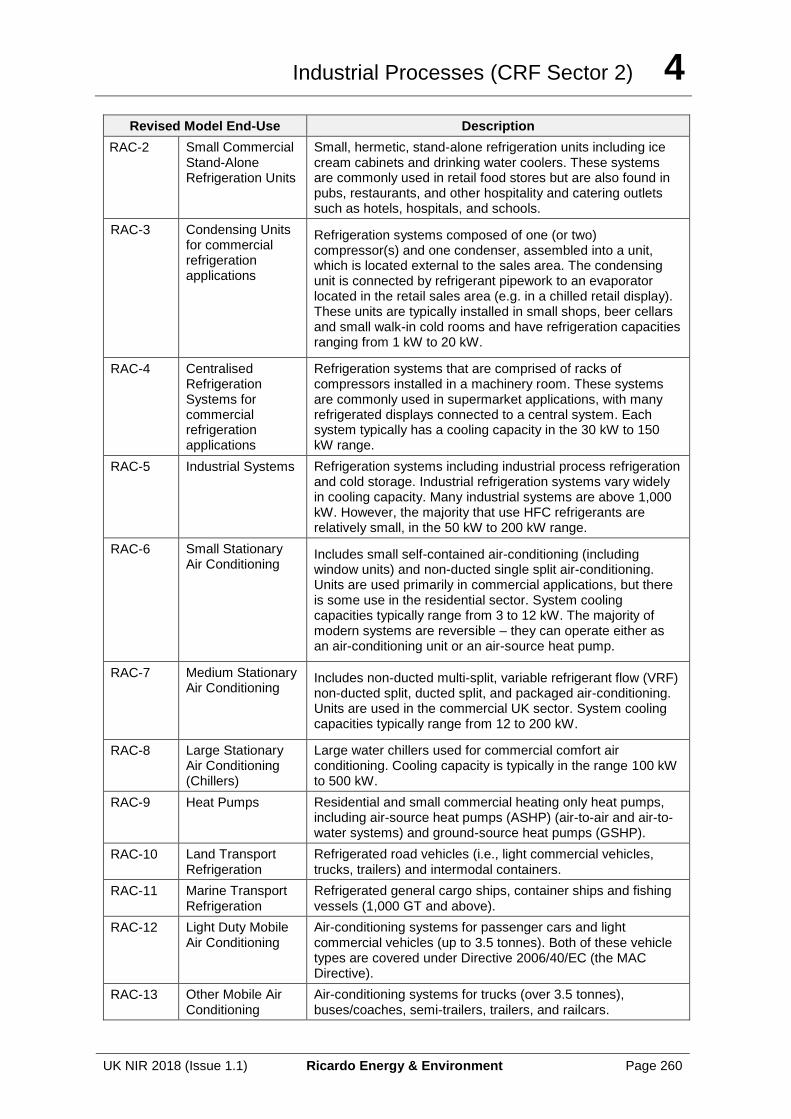
Industrial Processes (CRF Sector 2) 4
UK NIR 2018 (Issue 1.1) Ricardo Energy & Environment Page 260
Revised Model End-Use Description
RAC-2 Small Commercial Stand-Alone Refrigeration Units
Small, hermetic, stand-alone refrigeration units including ice cream cabinets and drinking water coolers. These systems are commonly used in retail food stores but are also found in pubs, restaurants, and other hospitality and catering outlets such as hotels, hospitals, and schools.
RAC-3 Condensing Units for commercial refrigeration applications
Refrigeration systems composed of one (or two) compressor(s) and one condenser, assembled into a unit, which is located external to the sales area. The condensing unit is connected by refrigerant pipework to an evaporator located in the retail sales area (e.g. in a chilled retail display). These units are typically installed in small shops, beer cellars and small walk-in cold rooms and have refrigeration capacities ranging from 1 kW to 20 kW.
RAC-4 Centralised Refrigeration Systems for commercial refrigeration applications
Refrigeration systems that are comprised of racks of compressors installed in a machinery room. These systems are commonly used in supermarket applications, with many refrigerated displays connected to a central system. Each system typically has a cooling capacity in the 30 kW to 150 kW range.
RAC-5 Industrial Systems Refrigeration systems including industrial process refrigeration and cold storage. Industrial refrigeration systems vary widely in cooling capacity. Many industrial systems are above 1,000 kW. However, the majority that use HFC refrigerants are relatively small, in the 50 kW to 200 kW range.
RAC-6 Small Stationary Air Conditioning
Includes small self-contained air-conditioning (including window units) and non-ducted single split air-conditioning. Units are used primarily in commercial applications, but there is some use in the residential sector. System cooling capacities typically range from 3 to 12 kW. The majority of modern systems are reversible – they can operate either as an air-conditioning unit or an air-source heat pump.
RAC-7 Medium Stationary Air Conditioning
Includes non-ducted multi-split, variable refrigerant flow (VRF) non-ducted split, ducted split, and packaged air-conditioning. Units are used in the commercial UK sector. System cooling capacities typically range from 12 to 200 kW.
RAC-8 Large Stationary Air Conditioning (Chillers)
Large water chillers used for commercial comfort air conditioning. Cooling capacity is typically in the range 100 kW to 500 kW.
RAC-9 Heat Pumps Residential and small commercial heating only heat pumps, including air-source heat pumps (ASHP) (air-to-air and air-to-water systems) and ground-source heat pumps (GSHP).
RAC-10 Land Transport Refrigeration
Refrigerated road vehicles (i.e., light commercial vehicles, trucks, trailers) and intermodal containers.
RAC-11 Marine Transport Refrigeration
Refrigerated general cargo ships, container ships and fishing vessels (1,000 GT and above).
RAC-12 Light Duty Mobile Air Conditioning
Air-conditioning systems for passenger cars and light commercial vehicles (up to 3.5 tonnes). Both of these vehicle types are covered under Directive 2006/40/EC (the MAC Directive).
RAC-13 Other Mobile Air Conditioning
Air-conditioning systems for trucks (over 3.5 tonnes), buses/coaches, semi-trailers, trailers, and railcars.
Industrial Processes (CRF Sector 2) 4
UK NIR 2018 (Issue 1.1) Ricardo Energy & Environment Page 261
4.29.2 Methodological Issues
The previous version of the refrigeration/air conditioning inventory model developed by AEA (2010) was updated by ICF International in the summer/autumn of 2011 based on revised industry input and a more transparent, robust Tier 2 modelling approach. Specifically, the model was reorganized from 9 to 13 end-use sub-sectors (as described in Table 4.21), for which detailed assumptions were developed to utilise a fully bottom-up approach. Both the new model and the previous version make use of a bottom up approach with assumptions made about emission factors and stock levels. The new model is more comprehensive and allows for updating of the assumptions made. Both bottom up models are verified by comparing the predicted HFC consumption for the whole RAC sector with top-down data for the sales of HFCs in the UK. In 2015 the ICF model was reviewed (Gluckman, 2015). A key aspect of the review was to revise input assumptions due to the impact of the revised EU F-Gas Regulation (517/2014), including bans of some higher HFCs for some applications and a general phased down of HFC consumption. The review process also identified some other input assumptions and stock calculations that required updating. See the end of this section for details of the 2015 RAC model updates. The model is reviewed on an annual basis.
For each of the 13 end-use sub-sectors, market data and other country-specific information were considered in the development of assumptions on equipment stocks, market growth, equipment lifetimes, refrigerant market penetrations, charge sizes, manufacturing loss rates, operational loss rates, and disposal loss rates across the 1990-2050 time-series. To revise and develop new input assumptions, an extensive literature review was conducted and key industry stakeholders were contacted. Priority industry stakeholders were selected across all end-uses and initially contacted to fill data gaps and corroborate information found in the literature. Following the development of preliminary assumptions for all end-uses, draft assumptions were then shared with a broader range of stakeholders to solicit additional industry input and vet assumptions.
In developing modelling input assumptions by end-use, expert judgment was applied to select appropriate values when more than one estimate was provided by literature and/or stakeholders. In general, more weight was given to estimates that are UK- or region specific and/or more recent. In cases of equal data quality where numerous data points were available, values were selected based on the mid-point of the data range. Where no UK- or EU-specific information was available, the 2006 Intergovernmental Panel on Climate Change (IPCC) Guidelines default assumptions were relied on to estimate emissions.
The various input assumptions used by the model can be varied on an annual basis. This allows changes in response to market growth or regulatory constraint to be reflected in the bottom-up estimates of HFC emissions made by the model. For example, the 2006 EU F-Gas Regulation has led to significant reductions in the levels of leakage from some RAC sub-sectors and improvements in the level of refrigerant recovery during servicing and at end-of-life. This is reflected in the model by changes to the annual operating emission factors and end-of-life recovery factors.
In the process of finalising the input assumptions, an analysis was conducted to compare estimated refrigerant consumption (calculated as the amount of refrigerant used to manufacture new equipment produced in the UK plus the amount used to service leaking equipment) with annual refrigerant sales data from the British Refrigeration Association (BRA). A summary table of the 2015 input assumptions is provided below. A full description of the methodology, sources, and input assumptions used to update emission estimates by end-use is contained in ICF (2011) and Gluckman (2015).
A key input assumption is the split of different refrigerants used in new and existing equipment in each of the 13 sub-sectors. The accuracy of the input assumptions is checked by comparisons with top-down BRA data for the whole RAC market. The model then generates
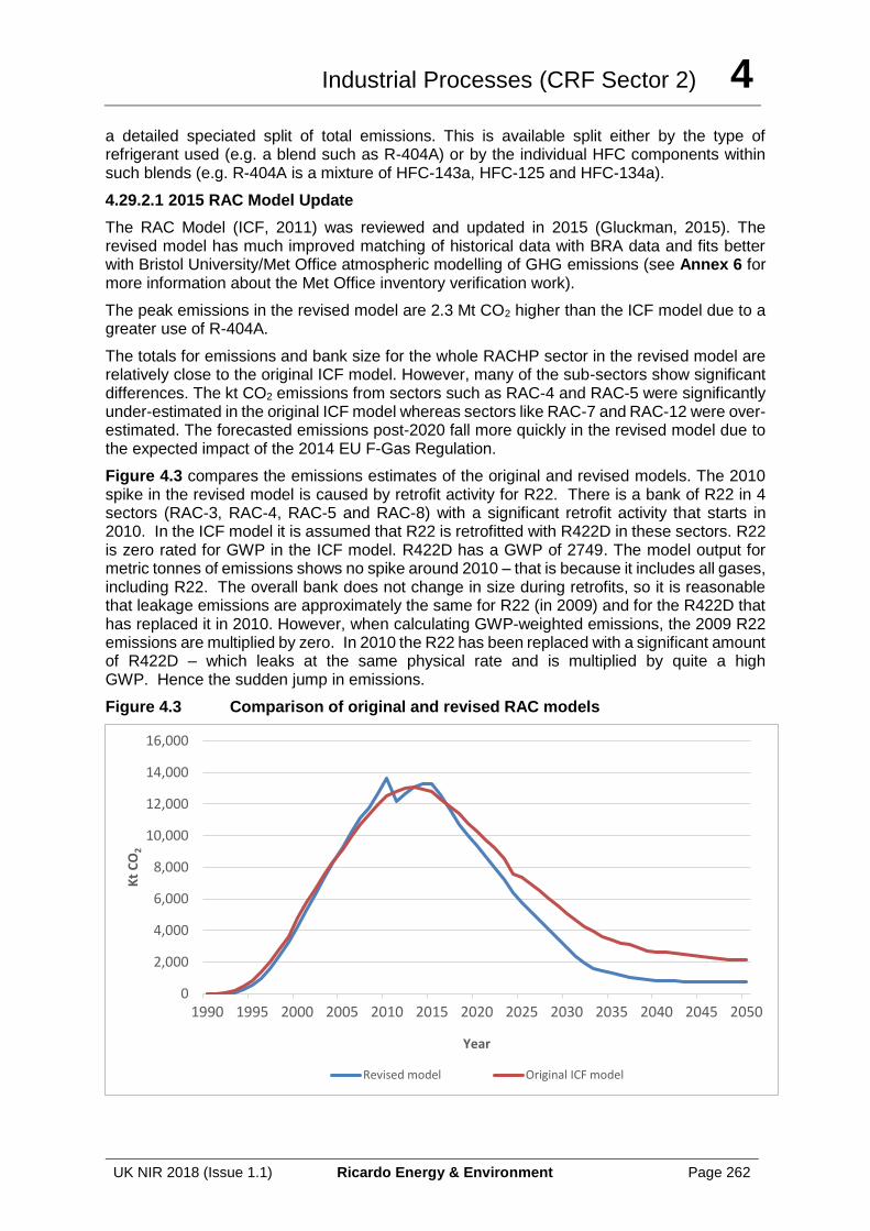
Industrial Processes (CRF Sector 2) 4
UK NIR 2018 (Issue 1.1) Ricardo Energy & Environment Page 262
a detailed speciated split of total emissions. This is available split either by the type of refrigerant used (e.g. a blend such as R-404A) or by the individual HFC components within such blends (e.g. R-404A is a mixture of HFC-143a, HFC-125 and HFC-134a).
4.29.2.1 2015 RAC Model Update
The RAC Model (ICF, 2011) was reviewed and updated in 2015 (Gluckman, 2015). The revised model has much improved matching of historical data with BRA data and fits better with Bristol University/Met Office atmospheric modelling of GHG emissions (see Annex 6 for more information about the Met Office inventory verification work).
The peak emissions in the revised model are 2.3 Mt CO2 higher than the ICF model due to a greater use of R-404A.
The totals for emissions and bank size for the whole RACHP sector in the revised model are relatively close to the original ICF model. However, many of the sub-sectors show significant differences. The kt CO2 emissions from sectors such as RAC-4 and RAC-5 were significantly under-estimated in the original ICF model whereas sectors like RAC-7 and RAC-12 were over-estimated. The forecasted emissions post-2020 fall more quickly in the revised model due to the expected impact of the 2014 EU F-Gas Regulation.
Figure 4.3 compares the emissions estimates of the original and revised models. The 2010 spike in the revised model is caused by retrofit activity for R22. There is a bank of R22 in 4 sectors (RAC-3, RAC-4, RAC-5 and RAC-8) with a significant retrofit activity that starts in 2010. In the ICF model it is assumed that R22 is retrofitted with R422D in these sectors. R22 is zero rated for GWP in the ICF model. R422D has a GWP of 2749. The model output for metric tonnes of emissions shows no spike around 2010 – that is because it includes all gases, including R22. The overall bank does not change in size during retrofits, so it is reasonable that leakage emissions are approximately the same for R22 (in 2009) and for the R422D that has replaced it in 2010. However, when calculating GWP-weighted emissions, the 2009 R22 emissions are multiplied by zero. In 2010 the R22 has been replaced with a significant amount of R422D – which leaks at the same physical rate and is multiplied by quite a high GWP. Hence the sudden jump in emissions.
Figure 4.3 Comparison of original and revised RAC models
0
2,000
4,000
6,000
8,000
10,000
12,000
14,000
16,000
1990 1995 2000 2005 2010 2015 2020 2025 2030 2035 2040 2045 2050
Kt
CO
2
Year
Revised model Original ICF model
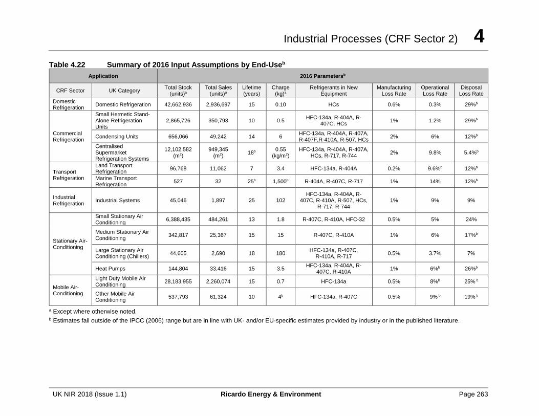
Industrial Processes (CRF Sector 2) 4
UK NIR 2018 (Issue 1.1) Ricardo Energy & Environment Page 263
Table 4.22 Summary of 2016 Input Assumptions by End-Useb
Application 2016 Parametersb
CRF Sector UK Category Total Stock
(units)a Total Sales
(units)a Lifetime (years)
Charge (kg)a
Refrigerants in New Equipment
Manufacturing Loss Rate
Operational Loss Rate
Disposal Loss Rate
Domestic Refrigeration
Domestic Refrigeration 42,662,936 2,936,697 15 0.10 HCs 0.6% 0.3% 29%b
Commercial Refrigeration
Small Hermetic Stand-Alone Refrigeration Units
2,865,726 350,793 10 0.5 HFC-134a, R-404A, R-
407C, HCs 1% 1.2% 29%b
Condensing Units 656,066 49,242 14 6 HFC-134a, R-404A, R-407A, R-407F,R-410A, R-507, HCs
2% 6% 12%b
Centralised Supermarket Refrigeration Systems
12,102,582 (m2)
949,345 (m2)
18b 0.55 (kg/m2)
HFC-134a, R-404A, R-407A, HCs, R-717, R-744
2% 9.8% 5.4%b
Transport Refrigeration
Land Transport Refrigeration
96,768 11,062 7 3.4 HFC-134a, R-404A 0.2% 9.6%b 12%b
Marine Transport Refrigeration
527 32 25b 1,500b R-404A, R-407C, R-717 1% 14% 12%b
Industrial Refrigeration
Industrial Systems 45,046 1,897 25 102 HFC-134a, R-404A, R-
407C, R-410A, R-507, HCs, R-717, R-744
1% 9% 9%
Stationary Air-Conditioning
Small Stationary Air Conditioning
6,388,435 484,261 13 1.8 R-407C, R-410A, HFC-32 0.5% 5% 24%
Medium Stationary Air Conditioning
342,817 25,367 15 15 R-407C, R-410A 1% 6% 17%b
Large Stationary Air Conditioning (Chillers)
44,605 2,690 18 180 HFC-134a, R-407C,
R-410A, R-717 0.5% 3.7% 7%
Heat Pumps 144,804 33,416 15 3.5 HFC-134a, R-404A, R-
407C, R-410A 1% 6%b 26%b
Mobile Air-Conditioning
Light Duty Mobile Air Conditioning
28,183,955 2,260,074 15 0.7 HFC-134a 0.5% 8%b 25% b
Other Mobile Air Conditioning
537,793 61,324 10 4b HFC-134a, R-407C 0.5% 9% b 19% b
a Except where otherwise noted. b Estimates fall outside of the IPCC (2006) range but are in line with UK- and/or EU-specific estimates provided by industry or in the published literature.
Industrial Processes (CRF Sector 2) 4
UK NIR 2018 (Issue 1.1) Ricardo Energy & Environment Page 264
Speciated emissions are reported for the OTs and CDs under 2F1. Emission estimates from the UK GHGI were scaled by a territory-specific indicator. Relevant indicators include territory population, GDP and number of cars. The indicators for each activity were chosen based on expert judgement and are as follows:
• GDP for refrigerated transport and commercial and industrial refrigeration
• Population for domestic refrigeration and stationary air conditioning
• Number of vehicles for mobile air conditioning
4.29.3 Uncertainties and Time-Series Consistency
The uncertainty analysis in Annex 2 provides estimates of uncertainty according to IPCC source category and fuel type.
4.29.4 Source Specific QA/QC and Verification
End-use input assumptions used to generate the refrigeration and air conditioning emissions were developed based on industry consultation and were peer-reviewed. Further, to verify the emissions estimates generated by the revised model, the results were compared with the sales data provided by BRA. The results of the comparison reveal that the data sets align closely, with the 2015 revised model output for UK refrigerant consumption being within 1% of the collective annual BRA data for HFCs from 2006-2010.
Historic emissions estimates generated by the revised model were also compared with concentration observations captured by the dispersion model NAME (Numerical Atmospheric dispersion Modelling Environment) for the years 1995 through to 2008. Results of this comparison show that the revised model output aligns significantly more closely to the NAME observations than historic inventory estimates. More information relating to atmospheric measurements and verification of UK emissions estimates is provided in Annex 6.
A list of industry stakeholders consulted on the input assumptions, as well as detailed results from the BRA and emission observation comparisons are discussed in more detail in ICF (2011).
4.29.5 Source Specific Recalculations
For information on the magnitude of recalculations, see Section 10.
4.29.6 Source Specific Planned Improvements
Emission factors, model parameters, and activity data will be kept under review. A number of potential updates have been identified to further improve upon the emission estimates from this source, including additional stakeholder consultation in the (non-food) industrial refrigeration and marine transport refrigeration sectors. These tasks will be added to the improvement programme; although they are currently not considered a high priority, they will be considered if resources are available.
4.30 SOURCE CATEGORY 2F2A – CLOSED CELLS (FOAM BLOWING AGENTS)
4.30.1 Source Category Description
Emissions of HFCs from foams can occur as follows:
• During the manufacturing process;

Industrial Processes (CRF Sector 2) 4
UK NIR 2018 (Issue 1.1) Ricardo Energy & Environment Page 265
• Over the lifetime of the foam; most rigid foams are closed cell foams and the blowing agent is designed to remain in the foam and contributes to its performance. Loss of HFCs is undesirable as it may affect the performance of the foam but is estimated to occur, albeit at a low rate through diffusion;
• At disposal of the foam; and
• In the waste stream, if the blowing agent is not destroyed following decommissioning
Emissions at each point vary significantly according to the type of foam and the type of application. For the bulk of product types, of the HFC used in the product, less than 10% is emitted during manufacture (although emissions may be as high as 40 to 45% for some types of foam), less than 1% per year over the useful lifetime of the product and the remainder on decommissioning and through the waste cycle35.
4.30.2 Methodological Issues
The methodology used to estimate emissions corresponds to the IPCC Tier 2b 'bottom-up' approach. The emission factors from the sector have been summarised below.
Emissions are considered separately from the following categories of foams:
PU Appliances (F1); PU, PIR Flexibly faced laminate (or boardstock) (F2); PU Discontinuous Panel (F3); PU Continuous Panel (F4); PU, PIR, Phenolic block (F5); Phenolic flexibly faced laminate (F6); PU Spray/injected/pipe-in-pipe (F7); Extruded polystyrene (XPS) (F8); Polyethylene Foam (F9); Integral Skin Foam (F10).
A full description of the emissions and associated methodology used for this sector is set out in Ricardo (2016), which built upon previous work (AEA, 2010). The emissions for the years 1990 to 2002 were based originally on data from March (1999). However, these and emissions data for more recent years (2003 onward) have been obtained from UK industry experts supported by market information from reputable market sources. The methodology is based on a bottom-up assessment of Activity Data which requires information on five elements to complete it:
• Overall dynamics of the thermal insulation market in the UK (including imports and exports);
• The market share changes on-going in the sector which determine the demand for closed cell insulation foams;
• The segregation of the insulation foam sector by manufacturing process and product type;
• The adoption of HFCs as one of the blowing agent options in any chosen process/product combination leading to market penetration assessments against other blowing agent types; and
• The formulation levels at which HFCs have been and will be used in the identified products and processes.
The application of the relevant emission factors to this Activity Data delivers information not only on annual emissions, but also on how banks of blowing agents can develop in products and latterly in waste streams. These banks too will emit steadily, and because of the long-lifetime of many foam applications, the emissions can take place over long periods of time, leading to a number of potential legacy issues. That said, the derived average annual emission
35 Any building insulation that goes into landfill degrades slowly and gives off the remaining gas over many years. This is not well documented and there is little data available on rate of degradation / emission, which is believed to vary depending on the conditions in the landfill.
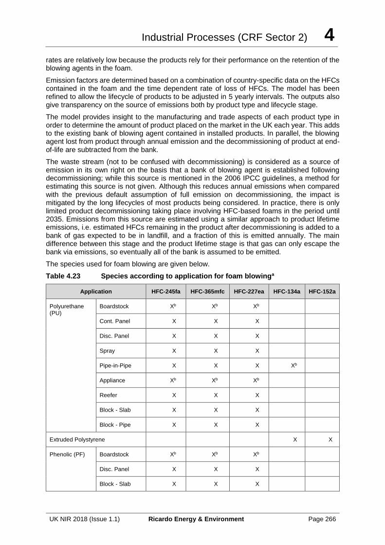
Industrial Processes (CRF Sector 2) 4
UK NIR 2018 (Issue 1.1) Ricardo Energy & Environment Page 266
rates are relatively low because the products rely for their performance on the retention of the blowing agents in the foam.
Emission factors are determined based on a combination of country-specific data on the HFCs contained in the foam and the time dependent rate of loss of HFCs. The model has been refined to allow the lifecycle of products to be adjusted in 5 yearly intervals. The outputs also give transparency on the source of emissions both by product type and lifecycle stage.
The model provides insight to the manufacturing and trade aspects of each product type in order to determine the amount of product placed on the market in the UK each year. This adds to the existing bank of blowing agent contained in installed products. In parallel, the blowing agent lost from product through annual emission and the decommissioning of product at end-of-life are subtracted from the bank.
The waste stream (not to be confused with decommissioning) is considered as a source of emission in its own right on the basis that a bank of blowing agent is established following decommissioning; while this source is mentioned in the 2006 IPCC guidelines, a method for estimating this source is not given. Although this reduces annual emissions when compared with the previous default assumption of full emission on decommissioning, the impact is mitigated by the long lifecycles of most products being considered. In practice, there is only limited product decommissioning taking place involving HFC-based foams in the period until 2035. Emissions from this source are estimated using a similar approach to product lifetime emissions, i.e. estimated HFCs remaining in the product after decommissioning is added to a bank of gas expected to be in landfill, and a fraction of this is emitted annually. The main difference between this stage and the product lifetime stage is that gas can only escape the bank via emissions, so eventually all of the bank is assumed to be emitted.
The species used for foam blowing are given below.
Table 4.23 Species according to application for foam blowinga
Application HFC-245fa HFC-365mfc HFC-227ea HFC-134a HFC-152a
Polyurethane (PU)
Boardstock Xb Xb Xb
Cont. Panel X X X
Disc. Panel X X X
Spray X X X
Pipe-in-Pipe X X X Xb
Appliance Xb Xb Xb
Reefer X X X
Block - Slab X X X
Block - Pipe X X X
Extruded Polystyrene X X
Phenolic (PF) Boardstock Xb Xb Xb
Disc. Panel X X X
Block - Slab X X X
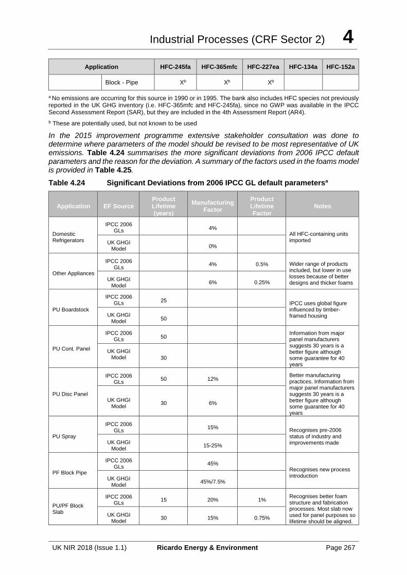
Industrial Processes (CRF Sector 2) 4
UK NIR 2018 (Issue 1.1) Ricardo Energy & Environment Page 267
Application HFC-245fa HFC-365mfc HFC-227ea HFC-134a HFC-152a
Block - Pipe Xb Xb Xb
a No emissions are occurring for this source in 1990 or in 1995. The bank also includes HFC species not previously reported in the UK GHG inventory (i.e. HFC-365mfc and HFC-245fa), since no GWP was available in the IPCC Second Assessment Report (SAR), but they are included in the 4th Assessment Report (AR4).
b These are potentially used, but not known to be used
In the 2015 improvement programme extensive stakeholder consultation was done to determine where parameters of the model should be revised to be most representative of UK emissions. Table 4.24 summarises the more significant deviations from 2006 IPCC default parameters and the reason for the deviation. A summary of the factors used in the foams model is provided in Table 4.25.
Table 4.24 Significant Deviations from 2006 IPCC GL default parametersa
Application EF Source Product Lifetime (years)
Manufacturing Factor
Product Lifetime Factor
Notes
Domestic Refrigerators
IPCC 2006 GLs 4%
All HFC-containing units imported UK GHGI
Model 0%
Other Appliances
IPCC 2006 GLs
4% 0.5% Wider range of products included, but lower in use losses because of better designs and thicker foams
UK GHGI Model
6% 0.25%
PU Boardstock
IPCC 2006 GLs
25 IPCC uses global figure influenced by timber-framed housing UK GHGI
Model 50
PU Cont. Panel
IPCC 2006 GLs 50
Information from major panel manufacturers suggests 30 years is a better figure although some guarantee for 40 years
UK GHGI Model 30
PU Disc Panel
IPCC 2006 GLs
50 12% Better manufacturing practices. Information from major panel manufacturers suggests 30 years is a better figure although some guarantee for 40 years
UK GHGI Model
30 6%
PU Spray
IPCC 2006 GLs
15% Recognises pre-2006 status of industry and improvements made UK GHGI
Model 15-25%
PF Block Pipe
IPCC 2006 GLs
45% Recognises new process introduction
UK GHGI Model
45%/7.5%
PU/PF Block Slab
IPCC 2006 GLs
15 20% 1% Recognises better foam structure and fabrication processes. Most slab now used for panel purposes so lifetime should be aligned.
UK GHGI Model
30 15% 0.75%
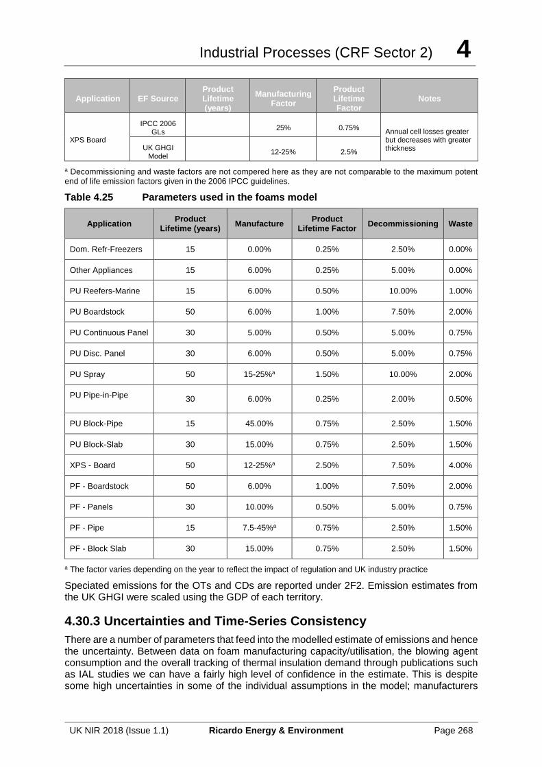
Industrial Processes (CRF Sector 2) 4
UK NIR 2018 (Issue 1.1) Ricardo Energy & Environment Page 268
Application EF Source Product Lifetime (years)
Manufacturing Factor
Product Lifetime Factor
Notes
XPS Board
IPCC 2006 GLs
25% 0.75% Annual cell losses greater but decreases with greater thickness UK GHGI
Model 12-25% 2.5%
a Decommissioning and waste factors are not compered here as they are not comparable to the maximum potent end of life emission factors given in the 2006 IPCC guidelines.
Table 4.25 Parameters used in the foams model
Application Product
Lifetime (years) Manufacture
Product Lifetime Factor
Decommissioning Waste
Dom. Refr-Freezers 15 0.00% 0.25% 2.50% 0.00%
Other Appliances 15 6.00% 0.25% 5.00% 0.00%
PU Reefers-Marine 15 6.00% 0.50% 10.00% 1.00%
PU Boardstock 50 6.00% 1.00% 7.50% 2.00%
PU Continuous Panel 30 5.00% 0.50% 5.00% 0.75%
PU Disc. Panel 30 6.00% 0.50% 5.00% 0.75%
PU Spray 50 15-25%a 1.50% 10.00% 2.00%
PU Pipe-in-Pipe 30 6.00% 0.25% 2.00% 0.50%
PU Block-Pipe 15 45.00% 0.75% 2.50% 1.50%
PU Block-Slab 30 15.00% 0.75% 2.50% 1.50%
XPS - Board 50 12-25%a 2.50% 7.50% 4.00%
PF - Boardstock 50 6.00% 1.00% 7.50% 2.00%
PF - Panels 30 10.00% 0.50% 5.00% 0.75%
PF - Pipe 15 7.5-45%a 0.75% 2.50% 1.50%
PF - Block Slab 30 15.00% 0.75% 2.50% 1.50%
a The factor varies depending on the year to reflect the impact of regulation and UK industry practice
Speciated emissions for the OTs and CDs are reported under 2F2. Emission estimates from the UK GHGI were scaled using the GDP of each territory.
4.30.3 Uncertainties and Time-Series Consistency
There are a number of parameters that feed into the modelled estimate of emissions and hence the uncertainty. Between data on foam manufacturing capacity/utilisation, the blowing agent consumption and the overall tracking of thermal insulation demand through publications such as IAL studies we can have a fairly high level of confidence in the estimate. This is despite some high uncertainties in some of the individual assumptions in the model; manufacturers
Industrial Processes (CRF Sector 2) 4
UK NIR 2018 (Issue 1.1) Ricardo Energy & Environment Page 269
were cautious in providing comment on the HFC market penetration which is the assumption that has greatest cause for uncertainty. Regulatory pressures to label products containing HFCs may help in future to hone the estimates and reduce uncertainties in Activity Data.
The uncertainty analysis in Annex 2 provides estimates of uncertainty according to IPCC source category and fuel type.
4.30.4 Source Specific QA/QC and Verification
This source category is covered by the general QA/QC of the greenhouse gas inventory in Section 1.6. Details of verification of emissions are given in Annex 6.
4.30.5 Source Specific Recalculations
As part of the GHGI improvement programme the model underlying the estimates of UK F-gas emissions from closed foams has been updated. Detailed information on the work done can be found in the improvement project report (Ricardo, 2016). The main changes made to the model are as follows:
• Consideration of ongoing emissions due to decommissioned product being disposed to landfill, previously all decommissioning emissions were assumed to occur in the year of decommissioning;
• Revision of underlying assumptions in light of stakeholder consultation, the impact of recent global economic events and the impact of evolving EU F-gas regulations; and
• Increased transparency; emissions can now be reported by lifecycle stage and underlying assumptions of the model can be published and scrutinised.
For information on the magnitude of recalculations, see Section 10.
4.30.6 Source Specific Planned improvements
This source has recently been updated so there are no immediate plans for improvement. However, we will be recommending that this sector is revisited when we have a few years’ data on the impact of recent F-gas regulations.
4.31 SOURCE CATEGORY 2F2B – OPEN CELLS (ONE COMPONENT FOAMS)
4.31.1 Source Category Description
One Component Foams (OCFs) are used by building tradesmen (and in the DIY home improvement sector, to a lesser extent) to mount doors and windows and to insulate different types of open joints and gaps. When used as an OCF propellant, HFC (134a, 152a) is blended with various flammable gases. HFC escapes from the foam on application, leaving small residues, which remain in the hardened foam for up to a year. These products are not manufactured in the UK, although they are imported. The use of HFCs of GWP 150 or greater in OCFs has been banned under the EC Regulation on fluorinated greenhouse gases (EC 842/2006) from July 4th 2008, except for where their use is safety critical. This was maintained in the 2014 F-gas regulations (EC 517/2014).
4.31.2 Methodological Issues
The method of calculation is an IPCC Tier 2 method.
Industrial Processes (CRF Sector 2) 4
UK NIR 2018 (Issue 1.1) Ricardo Energy & Environment Page 270
UK estimates of emissions from this source were based on a European evaluation of emissions from this sector (Harnisch and Schwarz, 2003), subsequently disaggregated by GDP to provide a top-down UK estimate.
It has been very difficult to establish the exact size of the UK import market and, therefore, hard to generate an accurate estimate of emissions from the use of this product.
Harnisch and Schwarz (2003) estimated EU emissions from OCFs as follows:
• 1996: 4,000 kt CO2 equivalent per annum (3100 tonnes of HFC-134a); and
• 2000: 1,700 kt CO2 equivalent per annum (1200 tonnes of HFC-134a; 1000 tonnes of HFC-152a)
Emissions in tonnes of CO2 equivalent have reduced between 1996 and 2000 due to the use of HFCs with lower GWP values, and the manufacture of cans containing less HFC. In 2000, 23 million OCF cans that contained HFCs were sold in Germany while 7 million where sold to the rest of the EU market. Research indicated that Germany accounted for 77% of the total EU emission, and that out of the remaining 23%, the UK accounts for 24%, based on a percentage of total EU GDP (excluding Germany). This is equivalent to 1.68 million cans (AEA, 2008).
The estimates of HFCs assume that the ban on F-gas use in one component foams (banned from July 2008 under the F-Gas regulations) has been successful, and this success has been confirmed with the UK Defra F-Gas Regulation team. Therefore, no emissions occur from 2009 onwards.
4.31.3 Uncertainties and Time-Series Consistency
Estimates of the uncertainties associated with time-series data for this sector were made in AEA (2004), based on an understanding of the uncertainties within the sector and from discussion with industry. Emissions from this sector are estimated to fall within an uncertainty range of 10-25%. Uncertainty data from this study have been used in the uncertainty analysis presented in Annex 2.
4.31.4 Source Specific QA/QC and Verification
This source category is covered by the general QA/QC of the greenhouse gas inventory in Section 1.6. Details of verification of emissions are given in Annex 6.
4.31.5 Source Specific Recalculations
There have been no recalculations to the mass based estimates from this source.
4.31.6 Source Specific Planned improvements
Emission factors and activity data will be kept under review.
4.32 SOURCE CATEGORY 2F3 – FIRE EXTINGUISHERS
4.32.1 Source Category Description
In the UK, manufacturers of fixed suppression systems for firefighting have been using HFCs as an alternative to Halons for many years. HFC-based systems are used for the protection of electronic and telecommunications equipment, and in military applications, records offices, bank vaults and oil production facilities.
The main HFC used in UK fixed systems is HFC-227ea.
Industrial Processes (CRF Sector 2) 4
UK NIR 2018 (Issue 1.1) Ricardo Energy & Environment Page 271
4.32.2 Methodological Issues
The IPCC 2006 GLs state that, because F-gases in fire extinguishers are emitted over a period longer than one year, countries must represent emissions from equipment charged during previous years. As such, the revised emission estimation equation (Equation 7.17) requires a modified approach to the one used in 2014 NIR (2012 inventory) to consider the time dependence of the emissions. Effectively, this requires disaggregating the annual bank estimates into ‘new’ versus ‘existing’ systems and then applying emission factors accordingly (i.e., applying a lifetime loss rate to banks from both new and existing systems, a servicing loss rate to the bank of existing systems, and a disposal loss rate to the bank of existing systems reaching disposal in any given year, based on an assumed average lifetime). Further, additional research was required to ensure that a manufacture loss rate should not be applied by confirming whether there is any production of F-gas fire protection agents in the UK. These updates apply the IPCC Tier 2 methodology.
ICF reviewed available literature to confirm/update key assumptions—notably, EEA (2014, 2016)—and then refined and finalized the estimates based on consultation with ASSURE (European Association for Responsible Use of HFCs in Fire Fighting) and the UK Fire Industry Association (FIA). The sections below outline the updates implemented by key area.
Note that the most recent report available for the 2018 (EEA, 2016) submission cycle presented data for solvents together with fire protection, so an older version (EEA, 2014), which presented the data in more detail was used to disaggregate these data.
4.32.2.1 Stock
Annual stock estimates from the years 1990 – 2005 (from the 2012 GHG inventory) were maintained, since they were based on historical data and input from industry experts. However, these annual stock figures were disaggregated into new versus existing systems by subtracting the current year’s bank from the previous year’s bank to estimate consumption in new systems, and then allocating the remainder of the bank to existing systems.
To determine the equipment stock in years beyond 2005, EEA (2014, 2016) estimates for net supply of F-gases in the fire protection sector from 2007-2012 (metric tonnes) in the EU, 85% of which is HFC-227ea, were scaled to the UK using a time-dependent GDP ratio. This annual net supply was assumed to equal annual UK consumption of fire protection agent in new and existing systems. The bank estimate for 2006 was interpolated based on the existing 2005 estimate and the new 2007 estimate. The methodology and resulting stock estimates were reviewed and approved by ASSURE (2013) and FIA (2013). ASSURE confirmed that the estimates looked reasonable; FIA noted that the estimates looked reasonable for recent years, but that the 2000 estimates are slightly high. Additional information to refine these historical estimates was not available but this is a conservative bias as it will slightly overestimate emissions.
4.32.2.2 Chemicals in use
According to FIA (2013) and ASSURE (2013), HFC-227ea accounts for virtually 100% of F-gas consumption in this sector in the UK; consumption of other HFCs (e.g., HFC-23, HFC-125, and HFC-236fa) in the UK are statistically insignificant. Therefore, is it assumed that HFC-227ea accounts for 100% of F-gas consumption in this sector (over the full product lifetime).
4.32.2.3 Equipment lifetime
According to FIA (2013) and ASSURE (2013), the average equipment lifetime of fire protection systems is 20 years.
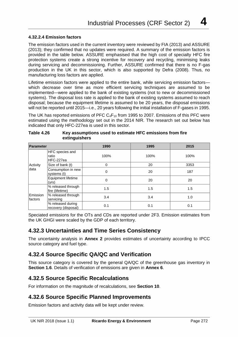
Industrial Processes (CRF Sector 2) 4
UK NIR 2018 (Issue 1.1) Ricardo Energy & Environment Page 272
4.32.2.4 Emission factors
The emission factors used in the current inventory were reviewed by FIA (2013) and ASSURE (2013); they confirmed that no updates were required. A summary of the emission factors is provided in the table below. ASSURE emphasised that the high cost of specialty HFC fire protection systems create a strong incentive for recovery and recycling, minimising leaks during servicing and decommissioning. Further, ASSURE confirmed that there is no F-gas production in the UK in this sector, which is also supported by Defra (2008). Thus, no manufacturing loss factors are applied.
Lifetime emission factors were applied to the entire bank, while servicing emission factors—which decrease over time as more efficient servicing techniques are assumed to be implemented—were applied to the bank of existing systems (not to new or decommissioned systems). The disposal loss rate is applied to the bank of existing systems assumed to reach disposal; because the equipment lifetime is assumed to be 20 years, the disposal emissions will not be reported until 2015—i.e., 20 years following the initial installation of F-gases in 1995.
The UK has reported emissions of PFC C4F10 from 1995 to 2007. Emissions of this PFC were estimated using the methodology set out in the 2014 NIR. The research set out below has indicated that only HFC-227ea is used in this sector.
Table 4.26 Key assumptions used to estimate HFC emissions from fire extinguishers
Parameter 1990 1995 2015
Activity data
HFC species and ratio HFC-227ea
100% 100% 100%
Size of bank (t) 0 20 3353
Consumption in new systems (t)
0 20 187
Equipment lifetime (yrs)
0 20 20
Emission factors
% released through fire (lifetime)
1.5 1.5 1.5
% released through servicing
3.4 3.4 1.0
% released during recovery (disposal)
0.1 0.1 0.1
Speciated emissions for the OTs and CDs are reported under 2F3. Emission estimates from the UK GHGI were scaled by the GDP of each territory.
4.32.3 Uncertainties and Time Series Consistency
The uncertainty analysis in Annex 2 provides estimates of uncertainty according to IPCC source category and fuel type.
4.32.4 Source Specific QA/QC and Verification
This source category is covered by the general QA/QC of the greenhouse gas inventory in Section 1.6. Details of verification of emissions are given in Annex 6.
4.32.5 Source Specific Recalculations
For information on the magnitude of recalculations, see Section 10.
4.32.6 Source Specific Planned Improvements
Emission factors and activity data will be kept under review.
Industrial Processes (CRF Sector 2) 4
UK NIR 2018 (Issue 1.1) Ricardo Energy & Environment Page 273
4.33 SOURCE CATEGORY 2F4 – AEROSOLS
4.33.1 Source Category Description
Most aerosols use hydrocarbon propellants, with a relatively small proportion of the market favouring other volatile liquids including dimethyl ether (DME) and HFCs. Compressed gases are used in very few aerosols since they suffer from a number of disadvantages compared with liquefied gas propellants such as DME and hydrocarbons. HFCs are used only in a few applications where the use of a more expensive propellant is required to provide a non-flammable material. The most important industrial applications in volume terms are air dusters and pipe freezing products; other applications include specialised lubricants and surface treatments, and specialised insecticides. The use of HFCs for novelty applications, such as ‘silly string’ was banned from July 2009, under the EC Regulation on fluorinated greenhouse gases (EC 842/2006).
Metered dose inhalers (MDIs) are used to deliver certain pharmaceutical products as an aerosol. For patients with respiratory illnesses, such as asthma and chronic obstructive pulmonary disease (COPD), medication needs to be delivered directly to the lungs. MDIs are one of the preferred means of delivering inhaled medication to patients with these illnesses. MDIs originally used CFC propellants but, as with industrial aerosols, concern over ozone destruction led to replacement of CFCs with HFCs. Note that HFC use in MDIs are excepted from the 2014 EU F-gas regulation phase down of HFC comsumption.
4.33.2 Methodological Issues
4.33.2.1 Aerosols
The methodology used to estimate emissions corresponds to an IPCC Tier 2 method. Aerosol HFC emission estimates have been derived on the basis of fluid consumption data provided by the British Aerosol Manufacturers’ Association (BAMA) up to 2012. BAMA discontinued collecting data for 2013 onwards, so for these years we have projected estimates of HFC consumption using knowledge of the regulatory landscape and industry insight of the market from a contact at BAMA. An average product lifetime of one year for all aerosols containing HFC has been assumed, based on discussions with BAMA, although this may be shorter or longer depending on the specific aerosol application. It is estimated that 1% of HFC emissions from aerosols occur during manufacture. The majority is released during the product lifetime (97%), with end of life emissions accounting for the other 2%. These emission factors are the same as those estimated in previous work by March (1999). The lifetime and end of life emissions are calculated after import and exports have been taken into account.
4.33.2.2 Metered Dose Inhalers (MDIs)
The methodology used to estimate emissions corresponds to an IPCC Tier 2 method. The current approach is essentially a “UK consumption model”. The number of MDIs used each year in the UK is derived from the UK National Health Service (NHS) prescription data. HFC emissions have been calculated with estimates of the species and volumes of HFCs used as MDI propellants. Detailed data from the UK NHS are used for estimates between 1998 and 2015. Estimates for 1990-1997 are based on extrapolated data from 1998. This method ensures time series consistency. The NHS data are available for England, Wales, Scotland and Northern Ireland, allowing an accurate split to be made of the UK totals.
The NHS data gives good estimates of the number of MDIs of each drug type that have been prescribed. However, the data gives no information about the amount of HFC propellant per MDI prescribed. The estimates assume an average figure of 12g/MDI (Gluckman, 2013).
The table below shows the way in which emissions are estimated from NHS data on total number of MDIs used in the UK each year. The majority of MDIs use HFC-134a. A small
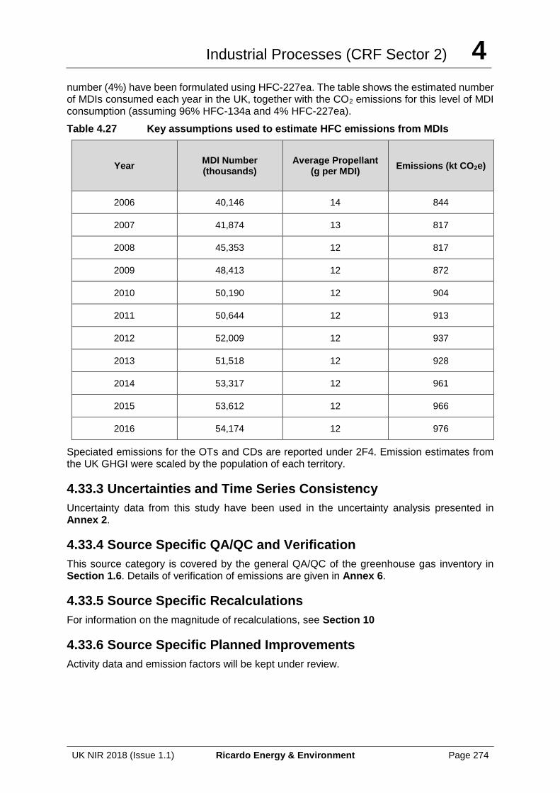
Industrial Processes (CRF Sector 2) 4
UK NIR 2018 (Issue 1.1) Ricardo Energy & Environment Page 274
number (4%) have been formulated using HFC-227ea. The table shows the estimated number of MDIs consumed each year in the UK, together with the CO2 emissions for this level of MDI consumption (assuming 96% HFC-134a and 4% HFC-227ea).
Table 4.27 Key assumptions used to estimate HFC emissions from MDIs
Year MDI Number (thousands)
Average Propellant (g per MDI)
Emissions (kt CO2e)
2006 40,146 14 844
2007 41,874 13 817
2008 45,353 12 817
2009 48,413 12 872
2010 50,190 12 904
2011 50,644 12 913
2012 52,009 12 937
2013 51,518 12 928
2014 53,317 12 961
2015 53,612 12 966
2016 54,174 12 976
Speciated emissions for the OTs and CDs are reported under 2F4. Emission estimates from the UK GHGI were scaled by the population of each territory.
4.33.3 Uncertainties and Time Series Consistency
Uncertainty data from this study have been used in the uncertainty analysis presented in Annex 2.
4.33.4 Source Specific QA/QC and Verification
This source category is covered by the general QA/QC of the greenhouse gas inventory in Section 1.6. Details of verification of emissions are given in Annex 6.
4.33.5 Source Specific Recalculations
For information on the magnitude of recalculations, see Section 10
4.33.6 Source Specific Planned Improvements
Activity data and emission factors will be kept under review.
Industrial Processes (CRF Sector 2) 4
UK NIR 2018 (Issue 1.1) Ricardo Energy & Environment Page 275
4.34 SOURCE CATEGORY 2F5 – SOLVENTS
4.34.1 Source Category Description
HFCs can be used as solvents in a range of applications such as precision cleaning to replace CFCs, HCFCs or 1,1,1-trichloroethane. HFCs have been developed that are used for precision cleaning in sectors such as aerospace and electronics.
4.34.2 Methodological Issues
Emissions from solvent applications are considered to be prompt emissions because 100% of the chemical is typically emitted within two years of initial use (IPCC 2006). To calculate HFC emissions from the solvent sector using a Tier 1a method, the 2006 IPCC Guidelines specify that activity data should be the quantity of solvent sold in a given year. Therefore, obtaining annual sales of solvents in the UK is required. Using sales data, emissions of HFCs from solvent use in year t are calculated using the following equation, as provided in the 2006 GLs:
Emissionst = St x EF + St-1 x (1-EF) - Dt-1
Where:
Emissionst = emissions in year t, tonnes
St = quantity of solvents sold in year t, tonnes
St–1 = quantity of solvents sold in year t-1, tonnes
EF = emission factor (= fraction of chemical emitted from solvents in the year of initial use), fraction
Dt–1 = quantity of solvents destroyed in year t-1, tonnes
Because of the diverse industrial and commercial applications in which solvents are used, there is no UK or EU trade association for the solvents industry from which to solicit activity data. Therefore, ICF reviewed available literature to confirm/update key assumptions -
notably, Harnish & Schwarz (2003), and EEA (2013). The sections below outline the updates implemented by key area.
4.34.2.1 Stock
Annual sales data of HFCs in the UK solvent sector were not available. Therefore, consumption of HFCs in this sector was estimated using the same estimates as in the previous inventory for 2001 and 2002 (i.e., based on Harnish & Schwarz 2003) in addition to historical F-gas supply data in the EU. Because the consumption estimates in Harnish & Schwarz (2003) in years beyond 2002 were projections, EEA (2014, 2016) data on intended F-gas supply data in the EU in the solvents sector was used to estimate HFC consumption from 2007-2012. Note that the most recent report available for the 2018 (EEA, 2016) submission cycle presented data for solvents together with fire protection, so an older version (EEA, 2014), which presented the data in more detail was used to disaggregate these data.
To estimate the amount of HFCs placed on the market in the UK, the EU estimates from EEA (2014, 2016) were scaled down using a time-dependent UK to EU GDP ratio from EuroStat (2017). Using GDP as a scaling factor to estimate the UK F-gas supply in the solvent sector was deemed appropriate, given the wide variety of industrial and commercial industries that use solvents.
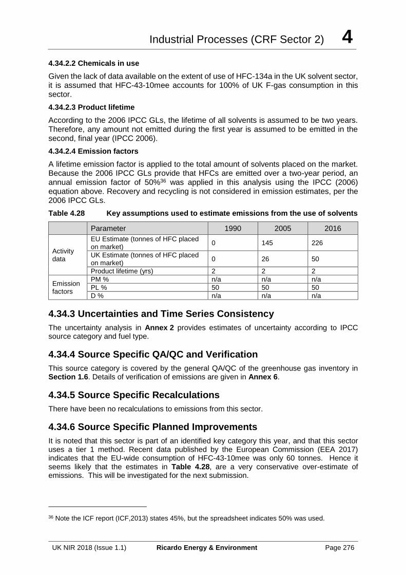
Industrial Processes (CRF Sector 2) 4
UK NIR 2018 (Issue 1.1) Ricardo Energy & Environment Page 276
4.34.2.2 Chemicals in use
Given the lack of data available on the extent of use of HFC-134a in the UK solvent sector, it is assumed that HFC-43-10mee accounts for 100% of UK F-gas consumption in this sector.
4.34.2.3 Product lifetime
According to the 2006 IPCC GLs, the lifetime of all solvents is assumed to be two years. Therefore, any amount not emitted during the first year is assumed to be emitted in the second, final year (IPCC 2006).
4.34.2.4 Emission factors
A lifetime emission factor is applied to the total amount of solvents placed on the market. Because the 2006 IPCC GLs provide that HFCs are emitted over a two-year period, an annual emission factor of 50%36 was applied in this analysis using the IPCC (2006) equation above. Recovery and recycling is not considered in emission estimates, per the 2006 IPCC GLs.
Table 4.28 Key assumptions used to estimate emissions from the use of solvents
Parameter 1990 2005 2016
Activity data
EU Estimate (tonnes of HFC placed on market)
0 145 226
UK Estimate (tonnes of HFC placed on market)
0 26 50
Product lifetime (yrs) 2 2 2
Emission factors
PM % n/a n/a n/a
PL % 50 50 50
D % n/a n/a n/a
4.34.3 Uncertainties and Time Series Consistency
The uncertainty analysis in Annex 2 provides estimates of uncertainty according to IPCC source category and fuel type.
4.34.4 Source Specific QA/QC and Verification
This source category is covered by the general QA/QC of the greenhouse gas inventory in Section 1.6. Details of verification of emissions are given in Annex 6.
4.34.5 Source Specific Recalculations
There have been no recalculations to emissions from this sector.
4.34.6 Source Specific Planned Improvements
It is noted that this sector is part of an identified key category this year, and that this sector uses a tier 1 method. Recent data published by the European Commission (EEA 2017) indicates that the EU-wide consumption of HFC-43-10mee was only 60 tonnes. Hence it seems likely that the estimates in Table 4.28, are a very conservative over-estimate of emissions. This will be investigated for the next submission.
36 Note the ICF report (ICF,2013) states 45%, but the spreadsheet indicates 50% was used.
Industrial Processes (CRF Sector 2) 4
UK NIR 2018 (Issue 1.1) Ricardo Energy & Environment Page 277
4.35 SOURCE CATEGORY 2F6 – OTHER (INCLUDING TRANSPORT OF REFRIGERANTS)
4.35.1 Source Category Description
Emissions sources Sources included Method Emission Factors
2F6b: Refrigerant Containers CS CS
Gases Reported HFCs
Key Categories 2F: Product Uses as Substitutes for ODS - HFCs (L2, T2)
Key Categories (Qualitative)
None identified
Overseas Territories and Crown Dependencies Reporting
All relevant emissions from OTs and CDs are included within the UK totals for this sector. Emissions are calculated by scaling emissions from the UK model using GDP as a scaling factor.
Completeness No known omissions. A general assessment of completeness for the inventory is included in Section 1.8.
Major improvements since last submission
No major improvements
4.35.2 Methodological Issues
Under the 2006 GLs, a new term in the IPCC Tier 2a method emissions equation for the Refrigeration and Air Conditioning sector is introduced to include emissions from the management of refrigerant containers used to service existing refrigeration/air-conditioning equipment, including refrigerant cylinders used by professional service technicians and small cans used by Do-It-Yourselfers (DIYers). No Tier 1 methodology is provided for this source.
Emissions from refrigerant containers occur when refrigerant is transferred from bulk containers (e.g. 20-tonne isotanks) to smaller capacity containers, typically ranging from approximately 300-500 grams (small cans) to 60 - 70 kg (cylinders). Emissions also occur at time of cylinder reprocessing (for reusable cylinders) or cylinder disposal (for non-returnable cylinders) if the refrigerant “heel” is not fully recovered. IPCC 2006 GLs require that emissions from each type of refrigerant container be calculated separately for refrigerant sold in small cans and in cylinders, including both disposables and reusables. The IPCC 2006 GLs default disposal emissions factors are 20% for small cans and 2% for disposable cylinders. Although the GLs do not specify a default emission rate for losses during the transfer of refrigerant into smaller containers, they do specify a default loss rate of 0.5% during the charging of refrigeration/air-conditioning equipment.
ICF (2014) provides a review of available literature to develop key assumptions on stock and emission factors—notably, Enviros (2008), Defra (2008), BRA (2010). ICF also contacted the five largest refrigerant Fillers & Packers in the UK that reported sales data to BRA in order to confirm/refine the estimates. Further work was carried out and is reported in Ricardo (2016) to refine a refrigerant containers model that is now used for the UK emissions estimate. The sections below outline the assumptions and methodology applied based on this process.
4.35.2.1 Package Sizes and Types
Refrigerants are used by four different types of end users who each use different sizes of refrigerant packaging:
Industrial Processes (CRF Sector 2) 4
UK NIR 2018 (Issue 1.1) Ricardo Energy & Environment Page 278
a) Original equipment manufacturers that manufacture pre-charged RACHP equipment. They purchase the majority of refrigerant in large volumes e.g. 20 tonne iso-containers or 1 tonne drums.
b) RACHP system installers that charge new systems after construction at an end user site. For larger sized systems (e.g. supermarket refrigeration systems or air-conditioning water chillers) the majority of refrigerant is supplied in large cylinders (e.g. 60 kg). For small systems (e.g. split air-conditioning) small cylinders (e.g. 15 kg) may also be used.
c) RACHP maintenance companies that carry out regular maintenance of equipment. The majority of refrigerant used for maintenance is supplied in small cylinders.
d) DIY activities for mobile air-conditioning – refrigerant is supplied in small cans (e.g. 0.3 to 0.5 kg) for use in the DIY market.
All large package sizes (e.g. 20 tonne iso-containers, 1 tonne drums, 60 kg cylinders) have been sold as re-usable containers since before 1990.
A small proportion of smaller cylinders (e.g. 15 kg) were sold as non-returnable containers from 1990 to 2008. From 2008 the supply of non-returnable cylinders was banned under the 2006 EU F-Gas Regulation.
The majority of small cans for mobile air-conditioning were sold as non-returnable containers from 1990 to 2008. From 2008 the supply of non-returnable small cans was banned under the 2006 EU F-Gas Regulation.
4.35.2.2 Sources of emission from refrigerant containers
The refrigerant containers emissions model takes into account 4 sources of HFC emission:
a) During package filling at a specialist company that transfers refrigerant from bulk storage into the package sizes described above.
b) During the re-processing of re-usable packages, at the specialist packer-filler companies
c) From non-returnable cylinders in the waste stream (only until 2008 when they were banned)
d) From the use of cylinders in the field by installers and maintenance companies.
All emissions are assumed to occur when cylinders are connected or disconnected to other equipment. There are small losses each time a cylinder is filled, used in the field or reprocessed. The emissions are on a “per event” basis. For example each time a cylinder is filled there is a small emission – the filling emission is the same for filling a large 60 kg cylinder as for filling a small 15 kg cylinder. There are no emissions from cylinders in storage.
4.35.2.3 Number of cylinders filled, used and reprocessed
Annual estimates of cylinder use were developed using data on the sales of refrigerant into the UK market from British Refrigeration Association (2015) for the years 2006 – 2014. The total quantity of refrigerant sold is available for each of the main refrigerant types (e.g. R-404A, HFC-134a etc.). The split of cylinder sizes for each refrigerant type was estimated through discussions with packer-fillers as summarised in the table below. Quantities sold prior to 2006 were extrapolated back to the dates when each refrigerant type was first introduced into the UK market (around 1992 for HFC-134a, 1995 for R-404A and 1998 for R-410A).
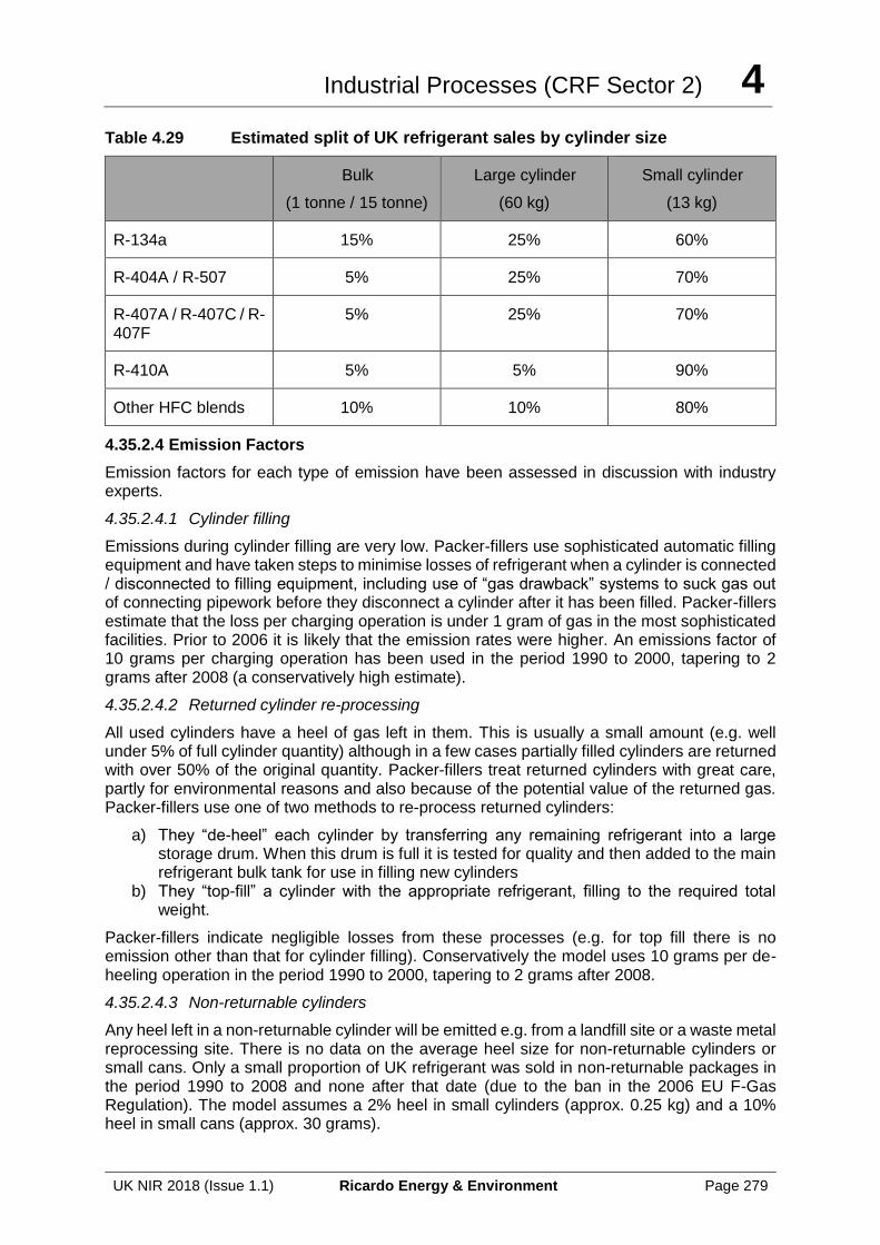
Industrial Processes (CRF Sector 2) 4
UK NIR 2018 (Issue 1.1) Ricardo Energy & Environment Page 279
Table 4.29 Estimated split of UK refrigerant sales by cylinder size
Bulk
(1 tonne / 15 tonne)
Large cylinder
(60 kg)
Small cylinder
(13 kg)
R-134a 15% 25% 60%
R-404A / R-507 5% 25% 70%
R-407A / R-407C / R-407F
5% 25% 70%
R-410A 5% 5% 90%
Other HFC blends 10% 10% 80%
4.35.2.4 Emission Factors
Emission factors for each type of emission have been assessed in discussion with industry experts.
4.35.2.4.1 Cylinder filling
Emissions during cylinder filling are very low. Packer-fillers use sophisticated automatic filling equipment and have taken steps to minimise losses of refrigerant when a cylinder is connected / disconnected to filling equipment, including use of “gas drawback” systems to suck gas out of connecting pipework before they disconnect a cylinder after it has been filled. Packer-fillers estimate that the loss per charging operation is under 1 gram of gas in the most sophisticated facilities. Prior to 2006 it is likely that the emission rates were higher. An emissions factor of 10 grams per charging operation has been used in the period 1990 to 2000, tapering to 2 grams after 2008 (a conservatively high estimate).
4.35.2.4.2 Returned cylinder re-processing
All used cylinders have a heel of gas left in them. This is usually a small amount (e.g. well under 5% of full cylinder quantity) although in a few cases partially filled cylinders are returned with over 50% of the original quantity. Packer-fillers treat returned cylinders with great care, partly for environmental reasons and also because of the potential value of the returned gas. Packer-fillers use one of two methods to re-process returned cylinders:
a) They “de-heel” each cylinder by transferring any remaining refrigerant into a large storage drum. When this drum is full it is tested for quality and then added to the main refrigerant bulk tank for use in filling new cylinders
b) They “top-fill” a cylinder with the appropriate refrigerant, filling to the required total weight.
Packer-fillers indicate negligible losses from these processes (e.g. for top fill there is no emission other than that for cylinder filling). Conservatively the model uses 10 grams per de-heeling operation in the period 1990 to 2000, tapering to 2 grams after 2008.
4.35.2.4.3 Non-returnable cylinders
Any heel left in a non-returnable cylinder will be emitted e.g. from a landfill site or a waste metal reprocessing site. There is no data on the average heel size for non-returnable cylinders or small cans. Only a small proportion of UK refrigerant was sold in non-returnable packages in the period 1990 to 2008 and none after that date (due to the ban in the 2006 EU F-Gas Regulation). The model assumes a 2% heel in small cylinders (approx. 0.25 kg) and a 10% heel in small cans (approx. 30 grams).
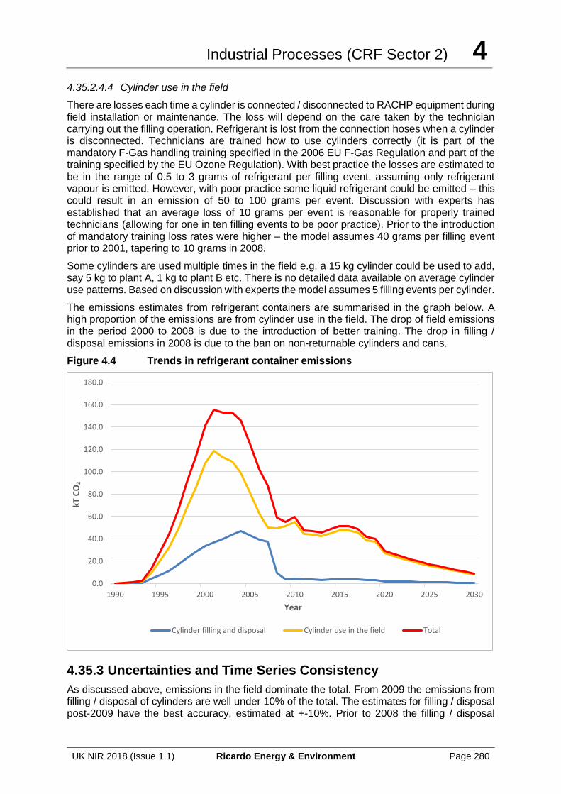
Industrial Processes (CRF Sector 2) 4
UK NIR 2018 (Issue 1.1) Ricardo Energy & Environment Page 280
4.35.2.4.4 Cylinder use in the field
There are losses each time a cylinder is connected / disconnected to RACHP equipment during field installation or maintenance. The loss will depend on the care taken by the technician carrying out the filling operation. Refrigerant is lost from the connection hoses when a cylinder is disconnected. Technicians are trained how to use cylinders correctly (it is part of the mandatory F-Gas handling training specified in the 2006 EU F-Gas Regulation and part of the training specified by the EU Ozone Regulation). With best practice the losses are estimated to be in the range of 0.5 to 3 grams of refrigerant per filling event, assuming only refrigerant vapour is emitted. However, with poor practice some liquid refrigerant could be emitted – this could result in an emission of 50 to 100 grams per event. Discussion with experts has established that an average loss of 10 grams per event is reasonable for properly trained technicians (allowing for one in ten filling events to be poor practice). Prior to the introduction of mandatory training loss rates were higher – the model assumes 40 grams per filling event prior to 2001, tapering to 10 grams in 2008.
Some cylinders are used multiple times in the field e.g. a 15 kg cylinder could be used to add, say 5 kg to plant A, 1 kg to plant B etc. There is no detailed data available on average cylinder use patterns. Based on discussion with experts the model assumes 5 filling events per cylinder.
The emissions estimates from refrigerant containers are summarised in the graph below. A high proportion of the emissions are from cylinder use in the field. The drop of field emissions in the period 2000 to 2008 is due to the introduction of better training. The drop in filling / disposal emissions in 2008 is due to the ban on non-returnable cylinders and cans.
Figure 4.4 Trends in refrigerant container emissions
4.35.3 Uncertainties and Time Series Consistency
As discussed above, emissions in the field dominate the total. From 2009 the emissions from filling / disposal of cylinders are well under 10% of the total. The estimates for filling / disposal post-2009 have the best accuracy, estimated at +-10%. Prior to 2008 the filling / disposal
0.0
20.0
40.0
60.0
80.0
100.0
120.0
140.0
160.0
180.0
1990 1995 2000 2005 2010 2015 2020 2025 2030
kT C
O₂
Year
Cylinder filling and disposal Cylinder use in the field Total
Industrial Processes (CRF Sector 2) 4
UK NIR 2018 (Issue 1.1) Ricardo Energy & Environment Page 281
estimates are less accurate because of uncertainties regarding the quantity of refrigerant left in non-returnable cylinders/cans on disposal – the overall accuracy is estimated as -10% to +25%. There are significant uncertainties regarding cylinder use in the field. In particular there is no data on the proportion of “poor practice” filling events or on the average number of filling events per cylinder. The accuracy of the use in field emissions is estimated to be -10% to +30%. We believe that a skewed confidence interval best represents the uncertainty of emissions from this source. This is because there is much more space for emissions to be higher due to less good practice than we anticipated than the amount that emissions could be lower if bad practice is less prevalent that we estimated.
As the emissions from use in the field are the dominant source and have the highest uncertainty we would conservatively say that the overall uncertainty for the sector is -10% to +30%.
The uncertainty analysis in Annex 2 provides estimates of uncertainty according to IPCC source category and fuel type.
4.35.4 QA/QC and Verification
The uncertainty analysis in Annex 2 provides estimates of uncertainty according to IPCC source category and fuel type.
4.35.5 Source Specific Recalculations
No recalculations have been made to this category.
4.35.6 Source Specific Planned Improvements
Activity data and emission factors will be kept under review.
4.36 SOURCE CATEGORY 2G1 – ELECTRICAL EQUIPMENT
4.36.1 Source Category Description
SF6 is released from activities in this source sector.
Sulphur hexafluoride has been used in high and medium voltage switch gear and transformers since the mid-1960s. The physical properties of the gas make it uniquely effective as an arc-quenching medium and as an insulator. Consequently, it has gradually replaced equipment using older technologies, namely oil filled and air blast equipment. Currently, there are no alternative fluids that have the same properties as SF6.
4.36.2 Methodological Issues
A review of the data sources and methodology used to estimate emissions from electrical switchgear was carried out in 2013. Data was collected from all the key UK users of Gas Insulated Switchgear (GIS), including National Grid and the UK electricity distribution companies. Data was also obtained from ENA (Electrical Networks Association) and from the electricity industry Regulator, Ofgem. Since the introduction of the EU F-Gas Regulation in 2006, the UK electricity industry has made significant efforts to monitor and reduce consumption of SF6. The Regulator collects annual data from each electricity company. These data were used to estimate the size of the SF6 bank in GIS and emissions for 2008-2012. Emissions from earlier years were estimated by extrapolating the data backwards, using the previously reported bank size in 1995 and 2000 and previously reported leakage rates. This approach ensured time series consistency, whilst making best use of good quality available
Industrial Processes (CRF Sector 2) 4
UK NIR 2018 (Issue 1.1) Ricardo Energy & Environment Page 282
data. Being based on reported consumption and emission data, this methodology is a considerable improvement on previous estimates.
4.36.3 Uncertainties and Time Series Consistency
The uncertainty analysis in Annex 2 provides estimates of uncertainty according to IPCC source category and fuel type.
4.36.4 Source Specific QA/QC and Verification
This source category is covered by the general QA/QC of the greenhouse gas inventory in Section 1.6. Details of verification of emissions are given in Annex 6.
4.36.5 Source Specific Recalculations
There have been no recalculations to emissions from this sector.
4.36.6 Source Specific Planned Improvements
Activity data and emission factors will be kept under review.
4.37 SOURCE CATEGORY 2G2A – MILITARY APPLICATIONS – AWACS
4.37.1 Source Category Description
Military applications include Airborne Warning and Control System (AWACS), which are military reconnaissance planes. In AWACS, the SF6 is used as an insulating gas in the radar system.
4.37.2 Methodological Issues
A Tier 1 method, country specific activity data, and an IPCC default emission factor of 740 kg SF6 per plane per year is used to estimate emissions.
The method uses the total number of planes carrying AWACs as the activity data. ICF’s research of the UK Royal Air Force (RAF) website confirmed that the RAF carries the same number of AWACS (seven) in 2012 as reported in the 2006 GLs (RAF, 2013). ICF further confirmed that RAF has had seven AWACS since 1990. Indeed, AWACS are a part of the Number 8 squadron of the RAF and they were acquired in 1985 (8 Squadron 2012). However, of the seven AWACS present in UK Fleet, not all are designated as forward available fleets. During times of low activity, some AWACS are placed as depth fleet, i.e., not operational, and therefore do not contribute to emissions. In 2012, only four AWACs were classified as forward available fields (MOD 2012), as we do not have data on how many are in the forward fleet at any one date (with the exception of 2012) all 7 are conservatively assumed to be active in all years.
4.37.3 Uncertainties and Time Series Consistency
The Tier 1 method relies on a constant emission factor, but actual emissions will vary based on the number of sorties (missions), with emissions higher during periods of high military operations and lower during times of low military operations.
The uncertainty analysis in Annex 2 provides estimates of uncertainty according to IPCC source category and fuel type.
Industrial Processes (CRF Sector 2) 4
UK NIR 2018 (Issue 1.1) Ricardo Energy & Environment Page 283
4.37.4 Source Specific QA/QC and Verification
This source category is covered by the general QA/QC of the greenhouse gas inventory in Section 1.6. Details of verification of emissions are given in Annex 6.
4.37.5 Source Specific Recalculations
There have been no recalculations to emissions from this sector.
4.37.6 Source Specific Planned Improvements
Activity data and emission factors will be kept under review.
4.38 SOURCE CATEGORY 2G2B – PARTICLE ACCELERATORS
4.38.1 Source Category Description
Particle accelerators are used for research purposes (at universities and research institutions), for industrial applications (in cross-linking polymers for cable insulation and for rubber parts and hoses), and in medical (radiotherapy) applications.
Estimates of emissions in the UK are confined to those from research and university accelerators particle accelerators.
4.38.2 Methodological Issues
The emissions from industrial particle accelerators are a result of leakage during operation and repair. Research and industrial high voltage systems usually need to be opened more frequently than industrial low voltage accelerators. Hence the emission factor of low voltage industrial accelerators is comparably lower. In the case of radiotherapy applications, industrially pre-set particle accelerators with hollow conductors filled with SF6 are used. The emissions of SF6 are planned releases. Radiotherapy accelerators are typically opened two times a year when being serviced and the SF6 contained is not captured but completely released. (Schwartz, 2005).
SF6 emissions from research and university accelerators are estimated using an IPCC Tier 2 method – an accelerator-level emission-factor approach. This required information on the individual charge of the various research and university accelerators operating in the UK. This information is used in the following equation along with default emission factors (IPCC 2006):
Total emissions = University and research particle accelerator Emission Factor x Σ Individual Accelerator Charges
Where:
SF6 university and research particle accelerator Emission Factor = 0.07 kg SF6 per kg SF6 charge, the average annual university and research particle accelerator emission rate as a fraction of the total charge.
Individual Accelerator Charges = SF6 contained within each university and research accelerator.
The SF6 emissions from medical and industrial accelerators are estimated using a Tier 1 method – country-level method. Given the scale of the number of medical and industrial particle accelerators, it was not feasible to collect individual charge information of each accelerator. The Tier 1 estimation method consists of the following equation, which relies on default emission factors (IPCC 2006):
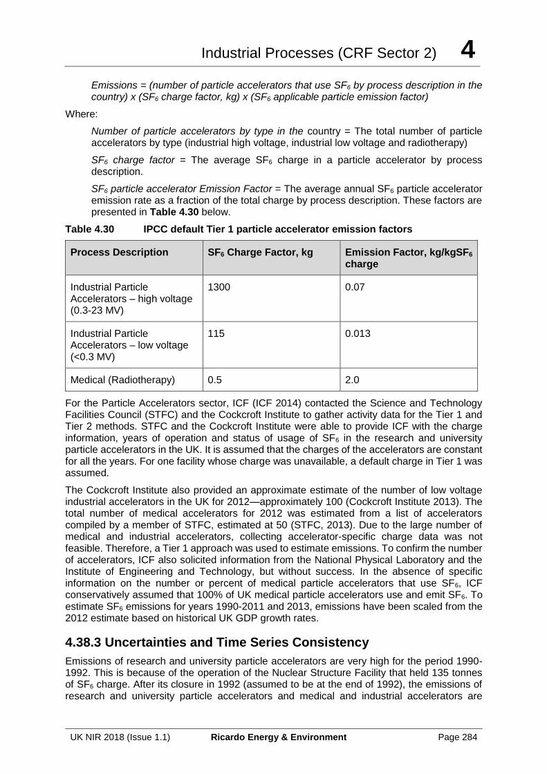
Industrial Processes (CRF Sector 2) 4
UK NIR 2018 (Issue 1.1) Ricardo Energy & Environment Page 284
Emissions = (number of particle accelerators that use SF6 by process description in the country) x (SF6 charge factor, kg) x (SF6 applicable particle emission factor)
Where:
Number of particle accelerators by type in the country = The total number of particle accelerators by type (industrial high voltage, industrial low voltage and radiotherapy)
SF6 charge factor = The average SF6 charge in a particle accelerator by process description.
SF6 particle accelerator Emission Factor = The average annual SF6 particle accelerator emission rate as a fraction of the total charge by process description. These factors are presented in Table 4.30 below.
Table 4.30 IPCC default Tier 1 particle accelerator emission factors
Process Description SF6 Charge Factor, kg Emission Factor, kg/kgSF6 charge
Industrial Particle Accelerators – high voltage (0.3-23 MV)
1300 0.07
Industrial Particle Accelerators – low voltage (<0.3 MV)
115 0.013
Medical (Radiotherapy) 0.5 2.0
For the Particle Accelerators sector, ICF (ICF 2014) contacted the Science and Technology Facilities Council (STFC) and the Cockcroft Institute to gather activity data for the Tier 1 and Tier 2 methods. STFC and the Cockcroft Institute were able to provide ICF with the charge information, years of operation and status of usage of SF6 in the research and university particle accelerators in the UK. It is assumed that the charges of the accelerators are constant for all the years. For one facility whose charge was unavailable, a default charge in Tier 1 was assumed.
The Cockcroft Institute also provided an approximate estimate of the number of low voltage industrial accelerators in the UK for 2012—approximately 100 (Cockcroft Institute 2013). The total number of medical accelerators for 2012 was estimated from a list of accelerators compiled by a member of STFC, estimated at 50 (STFC, 2013). Due to the large number of medical and industrial accelerators, collecting accelerator-specific charge data was not feasible. Therefore, a Tier 1 approach was used to estimate emissions. To confirm the number of accelerators, ICF also solicited information from the National Physical Laboratory and the Institute of Engineering and Technology, but without success. In the absence of specific information on the number or percent of medical particle accelerators that use SF6, ICF conservatively assumed that 100% of UK medical particle accelerators use and emit SF6. To estimate SF6 emissions for years 1990-2011 and 2013, emissions have been scaled from the 2012 estimate based on historical UK GDP growth rates.
4.38.3 Uncertainties and Time Series Consistency
Emissions of research and university particle accelerators are very high for the period 1990-1992. This is because of the operation of the Nuclear Structure Facility that held 135 tonnes of SF6 charge. After its closure in 1992 (assumed to be at the end of 1992), the emissions of research and university particle accelerators and medical and industrial accelerators are
Industrial Processes (CRF Sector 2) 4
UK NIR 2018 (Issue 1.1) Ricardo Energy & Environment Page 285
comparable. In 2004, the only operational particle accelerator ceased usage of SF6 and, hence, the emissions are considered to be zero. Three other particle accelerators began operation in 2010, 2011, and 2012, respectively, leading to non-zero but small SF6 emissions due to their small charges.
For the medical and industrial particle accelerators, the emissions rise as they were estimated based on GDP as proxy.
The uncertainty analysis in Annex 2 provides estimates of uncertainty according to IPCC source category and fuel type.
4.38.4 Source Specific QA/QC and Verification
This source category is covered by the general QA/QC of the greenhouse gas inventory in Section 1.6. Details of verification of emissions are given in Annex 6.
4.38.5 Source Specific Recalculations
There have been no recalculations to emissions from this sector.
4.38.6 Source Specific Planned Improvements
Activity data and emission factors will be kept under review.
4.39 SOURCE CATEGORY 2G2E – SF6 AND PFCS FROM OTHER PRODUCT USE
4.39.1 Source Category Description
Emissions of PFCs and SF6 from the production of semiconductors, the use of SF6 as a tracer gas, and PFCs and SF6 from sporting goods (training shoes) have been combined in order to preserve the confidentiality of estimates of emissions of SF6 and PFCs used in training shoes.
4.39.1.1 Integrated circuit or semiconductor manufacture:
PFCs, SF6 and NF3 are released from activities in this source sector.
The electronics industry is one of the largest sources of PFC emissions in the UK. The main uses of PFCs are as follows:
• Cleaning of chambers used for chemical vapour deposition (CVD) processes;
• Dry plasma etching;
• Vapour phase soldering and vapour phase blanketing;
• Leak testing of hermetically sealed components; and
• Cooling liquids, e.g. in supercomputers or radar systems.
In addition, SF6 is used in etching processes for polysilicon and nitrite surfaces, and there is some usage of CHF3 and NF3.
4.39.1.2 Use of SF6 as a tracer gas in scientific research:
The UK uses of SF6 as a tracer in scientific research.
4.39.1.3 Use and disposal of training shoes:
A sports goods manufacturer selling shoes in the UK used SF6 as a cushioning material in a range of training shoes from 1990 to 2003. Prior to 1990, the manufacturer used perfluoroethane (a PFC) for cushioning. SF6 is well suited to this application because it is chemically and biologically inert and its high molecular weight means it cannot easily diffuse
Industrial Processes (CRF Sector 2) 4
UK NIR 2018 (Issue 1.1) Ricardo Energy & Environment Page 286
across membranes. This means the gas is not released until the training shoe is destroyed at the end of its useful life.
The manufacturer committed itself to eliminating SF6 from its training shoes by 30 June 2003 – a goal which was achieved. It had originally planned to replace all SF6 applications with nitrogen-filled cushioning but technical difficulties mean it had to switch temporarily to perfluoropropane (a PFC) in some high-performance applications. The use of F gases in footwear was banned in 2006 by the F-gas Regulation and discussions with the manufacturer have confirmed that they are no longer using PFCs or SF6.
Cushioning units typically outlast the lifetime of the training shoe because the rate of diffusion of SF6 is so slow. In the UK, training shoes are generally sent to landfill at the end of their useful lives, where any SF6 or PFC will eventually leak to the atmosphere.
4.39.2 Methodological Issues
4.39.2.1 Semiconductor manufacture:
ICF (2014) updated estimates of emissions from this source.
The 2006 GLs provide an updated method for estimating semiconductor manufacture emissions as compared to the 2000 GPG. Specifically, the 2006 GLs include updated methodologies for each tier, updates to emission factors, as well as inclusion of other sectors in the electronics manufacturing source category – flat panels display manufacturing, and photovoltaic manufacturing. For the semiconductor manufacture sector, the 2006 GLs Tier 1 method estimates emissions based on the amount of substrate processed, in units of m2. The Tier 1 method in the 2000 GPG most closely resembles the Tier 2a method of the 2006 GLs, which estimates emissions based on gas-specific consumption data, as well as the amount left in shipping containers after use, use rate of gas, fraction of gas used in processes with emission control technologies, and the fraction of gas destroyed by the emission control technology.
The 2006 GL Tier 2a method is represented by the following equation:
Emissions for Ei = (1-h)*FCi*(1-Ui)*(1-ai*di)
Where:
i = F-gas species
Ei = emissions of gasi, kg
h = fraction of gas i remaining in container (heel)
FCi = consumption of gasi, kg
Ui = use rate of gasi
ai = abatement rate of gasi
di = fraction of gasi destroyed by the abatement
The Tier 2a method also introduces by-product emissions of CF4, C2F6, C3F8 and CHF3. In the 2000 GPG, by-product emissions were limited to only CF4. The Tier 2a equation used for by-product emissions is:
By-Product Emissions of gas j (BPEj,i)= (1-h)*Bj,i*FCi*(1-ai*dj)
Industrial Processes (CRF Sector 2) 4
UK NIR 2018 (Issue 1.1) Ricardo Energy & Environment Page 287
Where:
BPEj,i = by-product emissions of gas j from the gas i used, kg
Bj,i = emission factor, kg gas j created/kg gas i used
dj = fraction of gas j by-product destroyed by the abatement
j = CF4, C2F6, CHF3 and C3F8
The 2006 GLs also introduce updated emission factors, or use rates for gases. The destruction rates of abatement systems have been assumed to be the same in the 2006 GLs for all species except NF3. The destruction rate of NF3 has been updated to 0.95 from 0.90.
4.39.2.1.1 Approach to estimating emissions
ICF attempted to update consumption data based on actual consumption as opposed to the previous approach of estimating consumption based on growth rates. However, it was not feasible to collect individual gas collection data from each of the semiconductor manufacturers.
ICF identified several potential sources to use to update the activity data (i.e., consumption data) –notably, the National Microelectronics Institute (NMI) and European Semiconductor Industry Association (ESIA). ESIA collects industry F-gas emissions data at the European level and the data are not broken down by Member State; therefore UK-level emissions were not available via ESIA. ICF requested NMI to consult its members to ascertain availability of activity data, but no response was received in time for the analysis. Hence, the previous approach of estimating activity data based on assumed growth rates (which is compliant with the 2006 GLs) was kept.
The NF3 consumption has been further sub-divided into NF3 Remote Clean and all other NF3 consumption (i.e., for in-situ chamber clean and etch processes). NF3 remote clean refers to a cleaning method for chemical vapour deposition chambers in which the film cleaning-agents formed from NF3 (F-atoms) are produced in a plasma upstream (remote) from the chamber being cleaned (IPCC 2006). In situ chamber cleans are chemical vapour deposition chamber cleaning processes, which may use NF3 or other F-gases to generate F-atoms in the chambers whose walls are being cleaned. NF3 may also be used to etch patterns (i.e., circuits) on semiconductors. The use of NF3 remote clean is assumed to start in 2003 and growing increasingly over time. As no data on the UK’s use of NF3 remote clean processes was made available from NMI, the US semiconductor market was used as a proxy to estimate the use of NF3 in remote clean processes relative to all other processes.
Specifically, the share of NF3 remote clean versus other uses was estimated based on industry-reported NF3 usage data from US semiconductor manufacturers for the years 2009 and 2010 (US EPA, 2011). This US data was readily available and is believed to be a good proxy for the UK given that semiconductor processes do not typically vary by world region. The ratio of NF3 remote to other uses was interpolated for years between 2003 and 2009, assuming 0.0 (nil) in the year 2003. This was done as 2006 GLs provide emission factors for the NF3 use in remote clean and NF3 in-situ and etch use.
4.39.2.1.2 Emission factors and other default factors
The emission factors used in the updated inventory were taken from 2006 GLs. A summary of the emission factors for the 2006 GL Tier 2a method is provided in the table below.
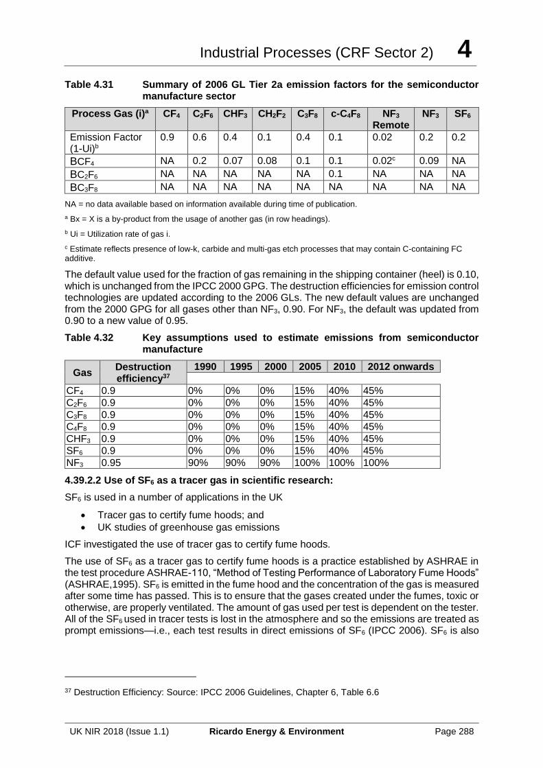
Industrial Processes (CRF Sector 2) 4
UK NIR 2018 (Issue 1.1) Ricardo Energy & Environment Page 288
Table 4.31 Summary of 2006 GL Tier 2a emission factors for the semiconductor manufacture sector
Process Gas (i)a CF4 C2F6 CHF3 CH2F2 C3F8 c-C4F8 NF3
Remote NF3 SF6
Emission Factor (1-Ui)b
0.9 0.6 0.4 0.1 0.4 0.1 0.02 0.2 0.2
BCF4 NA 0.2 0.07 0.08 0.1 0.1 0.02c 0.09 NA
BC2F6 NA NA NA NA NA 0.1 NA NA NA
BC3F8 NA NA NA NA NA NA NA NA NA
NA = no data available based on information available during time of publication.
a Bx = X is a by-product from the usage of another gas (in row headings).
b Ui = Utilization rate of gas i.
c Estimate reflects presence of low-k, carbide and multi-gas etch processes that may contain C-containing FC additive.
The default value used for the fraction of gas remaining in the shipping container (heel) is 0.10, which is unchanged from the IPCC 2000 GPG. The destruction efficiencies for emission control technologies are updated according to the 2006 GLs. The new default values are unchanged from the 2000 GPG for all gases other than NF3, 0.90. For NF3, the default was updated from 0.90 to a new value of 0.95.
Table 4.32 Key assumptions used to estimate emissions from semiconductor manufacture
Gas Destruction efficiency37
1990 1995 2000 2005 2010 2012 onwards
CF4 0.9 0% 0% 0% 15% 40% 45%
C2F6 0.9 0% 0% 0% 15% 40% 45%
C3F8 0.9 0% 0% 0% 15% 40% 45%
C4F8 0.9 0% 0% 0% 15% 40% 45%
CHF3 0.9 0% 0% 0% 15% 40% 45%
SF6 0.9 0% 0% 0% 15% 40% 45%
NF3 0.95 90% 90% 90% 100% 100% 100%
4.39.2.2 Use of SF6 as a tracer gas in scientific research:
SF6 is used in a number of applications in the UK
• Tracer gas to certify fume hoods; and
• UK studies of greenhouse gas emissions
ICF investigated the use of tracer gas to certify fume hoods.
The use of SF6 as a tracer gas to certify fume hoods is a practice established by ASHRAE in the test procedure ASHRAE-110, “Method of Testing Performance of Laboratory Fume Hoods” (ASHRAE,1995). SF6 is emitted in the fume hood and the concentration of the gas is measured after some time has passed. This is to ensure that the gases created under the fumes, toxic or otherwise, are properly ventilated. The amount of gas used per test is dependent on the tester. All of the SF6 used in tracer tests is lost in the atmosphere and so the emissions are treated as prompt emissions—i.e., each test results in direct emissions of SF6 (IPCC 2006). SF6 is also
37 Destruction Efficiency: Source: IPCC 2006 Guidelines, Chapter 6, Table 6.6
Industrial Processes (CRF Sector 2) 4
UK NIR 2018 (Issue 1.1) Ricardo Energy & Environment Page 289
used for tracer testing of nuclear power plant control room emergency ventilation systems (CARB, 2009).
Due to data limitations, SF6 emissions were estimated using a slightly modified Equation 8.23 of Volume 3 of the 2006 GLs. The SF6 emission is calculated on a per-use basis as opposed to the amount purchased/sold as provided in the equation. This modified method relies on the number of tracer tests conducted annually as the activity data, which when multiplied by the emissions per test as the emission factor, gives the total SF6 emissions from this sector. This method is represented in the following equation:
Total emissions = emissions per test x number of tests
Additional emissions may also occur from bottling, leakage, and piping; however, such emissions cannot be estimated without activity data and are believed to be de minimis.
In order to apply the method above, ICF had to gather information on the number of tracer tests conducted annually (activity data) and the emissions per test (emission factor). ICF first identified various companies that performed fume hood tracer testing. ICF contacted the three largest companies that perform tracer tests in the UK (Crowthorne, Dale Flow, and Invent-UK) and obtained the company-specific emissions per test and the total number of tests performed in 2012 (Crowthorne 2013, Dale Flow 2013, Invent-UK 2013). For the prior years, the total numbers of tests have been estimated by scaling the number of tests performed in 2012 to the UK’s historical GDP growth rate. The amount of emissions per test for prior years was held constant unless a company specified that the volume had increased after a certain period. The value of the emissions per test differed among companies and ranged from 0.033 to 0.046 kg SF6 per test.
ICF also verified when these companies came into existence. Other, smaller companies were identified but were not contacted as—according to qualitative information from Dale Flow (2013)—the bulk of the market is covered by the three major companies, and any additional research was not expected to result in significant changes to the emission estimates, which only account for a very small share of total F-gas emissions.
ICF also contacted Sellafield Ltd, a nuclear decommissioning company, which uses SF6 to conduct tracer tests, and included their company specific emission factor and total number of emissions (Sellafield, 2013).
Finally, ICF contacted the UK Nuclear Regulation Agency to confirm if there is any use of SF6 in the tracer testing of nuclear power plant control room emergency ventilation systems in the UK. ICF was unable to obtain information because the inquiry did not fall within the remit of the Office of Nuclear Regulation/Health and Safety Executive. However, ICF experts believe that such use was replaced many years ago.
SF6 is used as a tracer gas in UK studies of greenhouse gas emissions from ruminant livestock. It is currently the only viable way to measure emissions of methane from ruminant livestock individuals at pasture (Defra, per. comm.).
Emissions for this source, which are very small, are now included under 2F9 from 2011 onwards.
A small charge of SF6 is stored in a permeation tube, which is then introduced to the rumen of the animal. The gas emissions are vacuum sampled from eructation via a tube near the animal’s muzzle connected to an evacuated flask. The total CH4 emissions are inferred from the differential concentrations of SF6 and CH4 between the flask and atmosphere.
The total amounts of SF6 used are given in the table below:
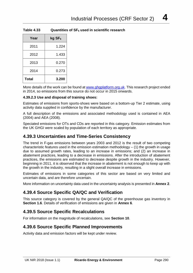
Industrial Processes (CRF Sector 2) 4
UK NIR 2018 (Issue 1.1) Ricardo Energy & Environment Page 290
Table 4.33 Quantities of SF6 used in scientific research
Year kg SF6
2011 1.224
2012 1.433
2013 0.270
2014 0.273
Total 3.200
More details of the work can be found at www.ghgplatform.org.uk. This research project ended in 2014, so emissions from this source do not occur in 2015 onwards.
4.39.2.3 Use and disposal of training shoes:
Estimates of emissions from sports-shoes were based on a bottom-up Tier 2 estimate, using activity data supplied in confidence by the manufacturer.
A full description of the emissions and associated methodology used is contained in AEA (2004) and AEA (2008).
Speciated emissions for OTs and CDs are reported in this category. Emission estimates from the UK GHGI were scaled by population of each territory as appropriate.
4.39.3 Uncertainties and Time-Series Consistency
The trend in F-gas emissions between years 2003 and 2012 is the result of two competing characteristic features used in the emission estimation methodology – (1) the growth in usage due to assumed growth rates, leading to an increase in emissions; and (2) an increase in abatement practices, leading to a decrease in emissions. After the introduction of abatement practices, the emissions are estimated to decrease despite growth in the industry. However, beginning in 2011, it is observed that the increase in abatement is not enough to keep up with the growth in the industry, resulting in a slight overall increase in emissions.
Estimates of emissions in some categories of this sector are based on very limited and uncertain data, and are therefore uncertain.
More information on uncertainty data used in the uncertainty analysis is presented in Annex 2.
4.39.4 Source Specific QA/QC and Verification
This source category is covered by the general QA/QC of the greenhouse gas inventory in Section 1.6. Details of verification of emissions are given in Annex 6.
4.39.5 Source Specific Recalculations
For information on the magnitude of recalculations, see Section 10.
4.39.6 Source Specific Planned Improvements
Activity data and emission factors will be kept under review.
Industrial Processes (CRF Sector 2) 4
UK NIR 2018 (Issue 1.1) Ricardo Energy & Environment Page 291
4.40 SOURCE CATEGORY 2G3A – MEDICAL APPLICATIONS
4.40.1 Source Category Description
This category includes emissions from N2O used as an anaesthetic. Emissions from medical applications in veterinary and dental practices and private hospitals are not accounted for; total emissions from these sources will be much smaller than the uncertainty in the conservative NHS estimate.
4.40.2 Methodological Issues
Emissions have been calculated using the outcomes of a study by NHS England (2013). This report calculates the total N2O emissions based on the number of bed-days in NHS England 2011 – 2012, multiplied by the EU GHG inventory derived emission factor of 10.3 kg N2O/bed/year38. This provides an estimated total N2O emission of 1,641,147 kg per annum, arising from the use of anaesthetic at NHS England facilities. This is not the recommended methodology given in the 2006 IPCC guidelines, but as we have been unable to obtain the data required to follow the default methodology (sales of N2O for anaesthetic use) this was considered the best approach to a country specific estimate for this source. Suppliers of N2O for anaesthesia were contacted, but they declined to provide data.
In order to expand this figure to incorporate all emissions within the United Kingdom a per-capita N₂O emission of 0.031 kg per annum has been derived from the total N₂O figure provided in the Carbon Footprint report. This has then been applied to the total population for the England, Wales, Scotland and Northern Ireland to provide a time-series of emissions.
4.40.3 Uncertainties and Time Series Consistency
As the duration of a patient’s hospital stay can vary considerably, the use of bed-days as an indicator of N2O should be considered to have a high degree of uncertainty. Additionally this methodology doesn’t take into account N2O used in non-NHS hospital environments (for example dental and veterinary practices or private hospitals), however total emissions from these sources are estimated to be much smaller than the uncertainty in the conservative NHS estimate.
The time series estimate does not consider trends in the uptake of alternative anaesthetics or alternative approaches to applying N2O as an anaesthetic, as some methods can reduce the consumption of N2O. Though using population as an indicator of trend should well reflect demand for anaesthetics, it would not take into account changing practices. We also make the assumption that the rest of the UK consumes anaesthetic in the same way as England.
4.40.4 Source Specific QA/QC and Verification
This source category is covered by the general QA/QC of the greenhouse gas inventory in Section 1.6.
In the case of Gibraltar, we have actual data on N2O imports for anaesthetic use for one year. When compared to the population of Gibraltar this yields an IEF of 0.015 kg per capita. In addition to providing robust data upon which to base Gibraltar emission estimates (using population data to generate a time-series), this improves our confidence that the UK estimate is of the correct order of magnitude.
38 http://www.eea.europa.eu/publications/european-union-greenhouse-gas-inventory-2013
Industrial Processes (CRF Sector 2) 4
UK NIR 2018 (Issue 1.1) Ricardo Energy & Environment Page 292
4.40.5 Source Specific Recalculations
There are no major recalculations to this source for this submission. For information on the magnitude of recalculations, see Section 10.
4.40.6 Source Specific Planned Improvements
The inventory team will continue to search for sources of data relating to the sales of N2O for anaesthetic use, and will make improvements to the current methodology when this information is available.
4.41 SOURCE CATEGORY 2G3B – OTHER FOOD – CREAM CONSUMPTION
4.41.1 Source Category Description
Very little UK data are available on the use of N2O in cream products, therefore the approach adopted has been based on the method used in the Danish GHG Inventory (Katja Hjelgaard, 2015). The method therefore assumes:
• 1% of cream consumption is in the form of whipped cream sprays;
• N2O consumption in those sprays is equal to 5% of the mass of the cream; and
• All N2O is emitted.
UK cream consumption data are available from Government (DEFRA) statistics (Defra, 2017).
4.41.2 Uncertainties and Time Series Consistency
The UK method relies upon the assumption that UK consumption of whipped cream sprays is similar to that in Denmark i.e. 1% of total cream consumption. Overall cream consumption in Denmark and the UK are similar on a per-capita basis, but the market share of whipped cream sprays in the UK is not known, and so the 1% assumption is the most significant source of uncertainty for the UK estimates. The assumption regarding the 5% usage of N2O relative to cream content is expected to be reasonable – there is no reason to think that the products sold in Denmark and the UK will differ significantly in design. UK cream consumption data are available for the full time-series from 1990 onwards.
4.41.3 Source Specific QA/QC and Verification
This source category is covered by the general QA/QC of the greenhouse gas inventory in Section 1.6.
4.41.4 Source Specific Recalculations
Revisions to milk utilisation data from DEFRA statistics (Defra, 2017) since 2012 causes a 37-59% increase in activity data from this source.
4.41.5 Source Specific Planned Improvements
No improvements are planned.
Industrial Processes (CRF Sector 2) 4
UK NIR 2018 (Issue 1.1) Ricardo Energy & Environment Page 293
4.42 SOURCE CATEGORY 2G4 – CHEMICAL INDUSTRY – OTHER PROCESS SOURCES
4.42.1 Source Category Description
This category reports N2O emissions from the chemical industry that are not captured elsewhere. All chemical manufacturing sites reporting significant quantities of N2O, and where that emission is believed to be from a chemical process, rather than combustion, are included. Other sites do report N2O emissions, but these emissions are small, and there is no evidence that they are from chemical processes. As such, these estimates are thought to be complete. Emissions from nitric and adipic acid are not included here, as these are reported in 2B2 and 2B3.
4.42.2 Methodological Issues
The UK has a large chemicals sector and all manufacturing sites are regulated and required to report emissions of N2O (as well as other pollutants). From 1998, when reporting was first required, until 2001 there was no threshold for reporting N2O, but since 2002, reporting is required only when emissions exceed 10 tonnes. Across the 18 years of reported data, N2O emissions have been reported in at least one year for 19 sites which can loosely be described as chemical sites. For most of those sites, N2O is reported for only one or two years out of the time-series and we think it is likely that the reported N2O is an error (operators do occasionally confuse N2O and NOX on their reporting submissions) and in a few other cases it is likely that the N2O occurs from the substantial combustion processes that constitute part of the reporting installation. In three cases however N2O is reported in multiple years, from processes which are either known to emit the gas, or thought to be the most likely source:
• A process to manufacture nitrous oxide, and to transfer it into gas cylinders for sale. This process was commissioned in 2004;
• A further process manufacturing industrial gases, which probably also supplied nitrous oxide in cylinders and which closed in 2008;
• A catalyst manufacturing process which involves dissolving metals in nitric acid, leading to emissions of oxides of nitrogen (including both NOX and N2O). This process has been in operation since the 1940s.
Emission estimates are based on the data reported by the process operators to the Environment Agency for inclusion in the Pollution Inventory. A gap in the reported data for the first site listed above (for 2004) is filled by assuming that operation started half-way through the year and that emissions were 50% of the level reported in 2005. The second plant only reports N2O back to 2002, but reports NOx in 2002 as well, and also in 1997-2001. Emissions of N2O in the years 1997-2001 are therefore assumed to follow the same trend as for NOx back to 1997 and to be at 1997 levels prior to that. Emissions for the third site for the years 1990-1997 i.e. before reporting of N2O was required, are assumed to follow the same trend as emissions of NOx, which is reported back to 1995, and to be the same as in 1995 before that. Using this approach suggests that emissions from this plant were about 2 times higher in 1990 than in 1998, when data are first reported.
4.42.3 Uncertainties and Time Series Consistency
No reported emissions are available for one of the sites in operation during 1990-1997 and for another there is no data between 1990 and 2001 so we have had to estimate emissions using NOx data where available, or to assume that emissions are the same as in later years. This is the most significant source of uncertainty in the estimates. It is possible but unlikely that other sites that report N2O, emit the gas from chemical manufacturing processes but if this were the case, these emissions would be much smaller than those from the two sites currently included.
Industrial Processes (CRF Sector 2) 4
UK NIR 2018 (Issue 1.1) Ricardo Energy & Environment Page 294
4.42.4 Source Specific QA/QC and Verification
This source category is covered by the general QA/QC of the greenhouse gas inventory in Section 1.6 and the source emissions data from plant operators is subject to the QA/QC procedures of the Environment Agency’s Pollution Inventory.
4.42.5 Source Specific Recalculations
No significant recalculations have been made for this category.
4.42.6 Source Specific Planned Improvements
The estimates will be kept under review, and additional sites added if appropriate.
4.43 SOURCE CATEGORY 2H1 – PULP AND PAPER INDUSTRY
4.43.1 Source Category Description
The UK paper industry is mainly confined to the production of pulp from recycled material and the production of papers using either imported virgin pulp, recycled pulp or a combination of the two. Production of virgin pulp is limited to a few processes producing mechanical or neutral sulphite semi-chemical pulp. Emissions from UK paper processes consist largely of emissions from the associated combustion processes, which supply steam and power to the papermaking processes. These emissions are reported under CRF category 1A2d. Other atmospheric emissions of greenhouse gases from UK paper and pulp processes will be minor and are currently not estimated.
Emissions of NMVOC from the manufacture of chipboard, fibreboard and Oriented Strand Board (OSB) are reported under 2H1. These products differ in the type of wood material that is made into board. Chipboard is made from assorted wood shavings, dust & chippings etc., while fibreboard is made from mechanically pulped wood fibres and OSB is made from long, thin wafers of wood with fairly uniform dimensions. All three processes involve steps for drying of the wood particles and hot pressing of the formed board and both steps give rise to some NMVOC emissions.
4.43.2 Methodological Issues
Emissions of NMVOC from wood product manufacture are estimated using emission factors derived from those available in the USEPA Compilation of Air Emission Factors (USEPA, 2014). Production of the wood products is estimated from data published by the Office for National Statistics (2017). These data are given as areas or volumes of product depending upon the type of product and must be converted to a mass basis by making assumptions about the thickness and/or density of the products.
4.44 SOURCE CATEGORY 2H2 – FOOD AND BEVERAGES INDUSTRY
4.44.1 Source Category Description
A number of food and drink manufacturing processes give rise to emissions of NMVOC. Most significant are emissions of ethanol from whisky maturation. Whisky is matured for a period of years in wooden barrels. This process develops the character of the whisky but an inevitable consequence is that spirit evaporates from the barrel. Other spirit manufacturing stages such as fermentation, distillation, casking (whisky only) and drying of spent grains also give rise to
Industrial Processes (CRF Sector 2) 4
UK NIR 2018 (Issue 1.1) Ricardo Energy & Environment Page 295
NMVOC emissions although these emissions are relatively small in comparison with those from maturation. Whisky manufacture is confined mainly to Scotland, which had 5 large grain distilleries and approximately 90 smaller malt distilleries at the end of 2015. There is a single small whisky distillery in Wales and a large whiskey distillery in Northern Ireland. Scotland and England also produce other distilled spirits such as gin and vodka, with production being concentrated in Scotland.
Malt production also creates emissions of NMVOC. Malting is occasionally carried out by distilleries but most malt, both for distillers and breweries, is produced by specialist maltsters. Brewing processes such as fermentation and wort boiling and fermentation for production of cider and wine are all very minor sources of NMVOC.
Bread manufacture involves fermentation reactions and ethanol is released as a result. Most bread in the UK is made in large mechanised bakeries, of which there are about 70. The remainder is made in small –‘craft bakeries’. Some other baked products include a fermentation stage and also emit ethanol. Heating of food products can cause reactions that produce organic emissions, and so processes such as drying of vegetable matter, preparation of compounded animal foods and cooking of meat and fish can cause NMVOC emissions. Finally, the processing of oils and fats is also a source of emissions, although emissions of hexane, a solvent used to extract vegetable oil from rape and other oilseeds is included in estimates of solvent use rather than as a food industry emission.
Emissions of CO2 from this category are not estimated since no appropriate data are available.
4.44.2 Methodological Issues
Emissions of NMVOC from food and drink manufacture are all calculated using emission factors and activity data obtained from either industry or Government sources. In the case of whisky maturation, data are available for volumes of whisky in storage at the end of each year from the Scotch Whisky Association (2017), and so emissions can be calculated by applying an annual emission rate factor with the average volume of whisky in storage for each year. This is more accurate than using an overall emission factor applied to whisky production since whiskies are stored for varying lengths of time and stock levels will rise or fall depending upon production, demand and changes in the length of maturation required.
NMVOC emission factors for food and drink are shown below.
Table 4.34 NMVOC Emission Factors for Food and Drink Processing, 2016
Food/Drink Process Emission
Factor Units
Beer Wort Boiling Fermentation
0.0048c
0.02c
g/L beer
Cider Fermentation 0.02c g/L cider
Wine Fermentation 0.2c kg/m3
Spirits Fermentation Distillation Casking Spent grain drying Maturation
1.58d
0.79g
0.40h
1.31i
15.78d
g/ L alcohol g/ L alcohol g/ L whiskey kg/ t grain g/ L alcohol
Malting Malting 4.8 Kg/tonne malt
Bread Baking 1a kg/tonne
Meat, Fish & Poultry 0.3f kg/tonne
Sugar 0.017b kg/tonne
Margarine and solid cooking fat 10f kg/tonne
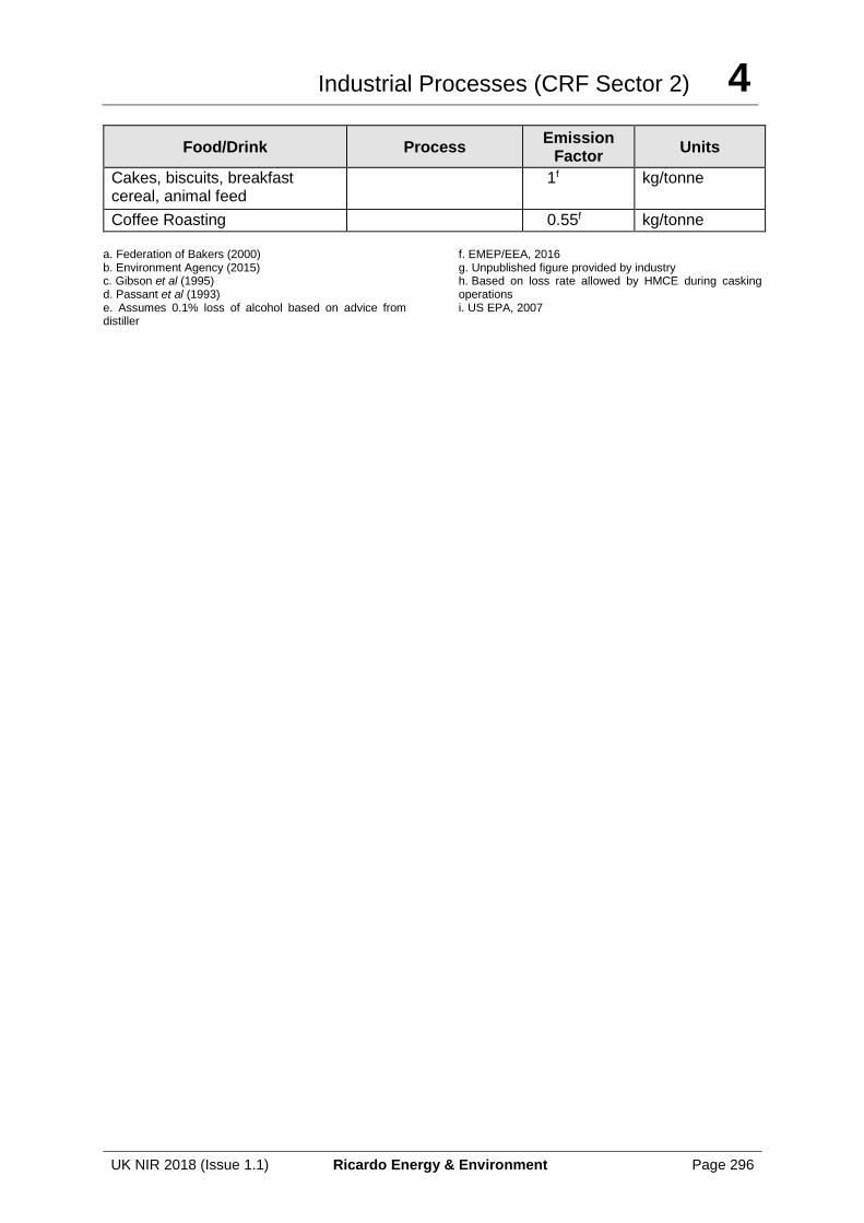
Industrial Processes (CRF Sector 2) 4
UK NIR 2018 (Issue 1.1) Ricardo Energy & Environment Page 296
Food/Drink Process Emission
Factor Units
Cakes, biscuits, breakfast cereal, animal feed
1f kg/tonne
Coffee Roasting 0.55f kg/tonne
a. Federation of Bakers (2000) b. Environment Agency (2015) c. Gibson et al (1995) d. Passant et al (1993) e. Assumes 0.1% loss of alcohol based on advice from distiller
f. EMEP/EEA, 2016 g. Unpublished figure provided by industry h. Based on loss rate allowed by HMCE during casking operations i. US EPA, 2007
Agriculture (CRF Sector 3) 5
UK NIR 2018 (Issue 1.1) Ricardo Energy & Environment Page 297
5 Agriculture (CRF sector 3)
5.1 OVERVIEW OF SECTOR
IPCC Categories Included
3A: Enteric Fermentation 3B: Manure Management 3D: Agricultural Soils 3F: Field Burning of Agricultural Residues 3G: Liming 3H: Urea application
Gases Reported CO2, CH4, N2O, NOx, CO, NMVOC, SO2
Key Categories (‘T’ or ‘L’ indicates whether it has been identified in the trend or level assessment respectively and the number indicates which KCA approach it was identified in)
3A: Enteric Fermentation - CH4 (L2, T2) 3A1: Enteric fermentation from Cattle - CH4 (L1, T1) 3A2: Enteric fermentation from Sheep - CH4 (L1, T1) 3B: Manure Management - N2O (L2) 3B1: Manure management from Cattle - CH4 (L1) 3D: Agricultural soils - N2O (L1, T1, L2, T2)
Key Categories (Qualitative)
None identified
Overseas Territories and Crown Dependencies Reporting
Emissions for OTs and CDs are included for enteric fermentation, animal wastes and agricultural soils.
Completeness A general assessment of completeness for the inventory is included in Section 1.8.
Major improvements since last submission
A new model has been integrated into the agriculture inventory for the 2018 submission meaning there are improvements to all agriculture subsectors and large recalculations to many of the subsectors.
The agriculture sector has the second largest contribution to total GHG emissions in the UK, after the energy sector. It contributed approximately 8.9% to total emissions in 2016. The emissions from this sector have shown an overall decrease of 16% since 1990, reflecting trends in livestock numbers and emissions from fertiliser application.
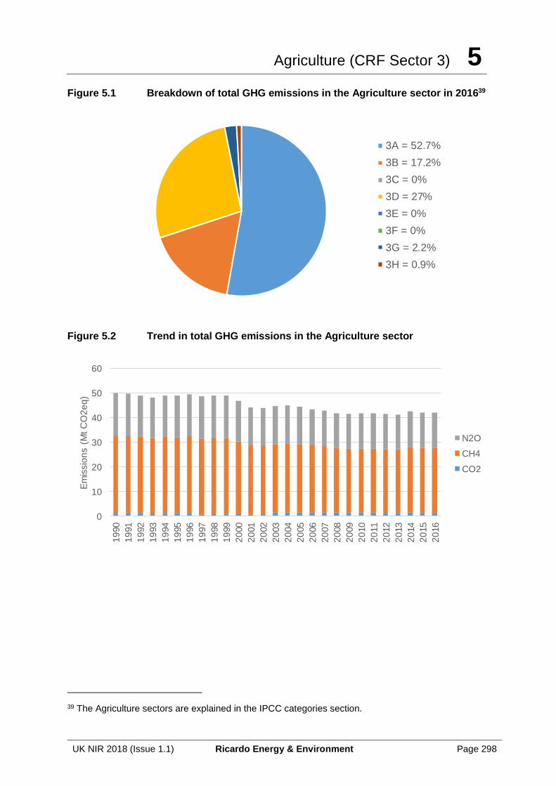
Agriculture (CRF Sector 3) 5
UK NIR 2018 (Issue 1.1) Ricardo Energy & Environment Page 298
Figure 5.1 Breakdown of total GHG emissions in the Agriculture sector in 201639
Figure 5.2 Trend in total GHG emissions in the Agriculture sector
39 The Agriculture sectors are explained in the IPCC categories section.
3A = 52.7%
3B = 17.2%
3C = 0%
3D = 27%
3E = 0%
3F = 0%
3G = 2.2%
3H = 0.9%
0
10
20
30
40
50
60
19
90
19
91
19
92
19
93
19
94
19
95
19
96
19
97
19
98
19
99
20
00
20
01
20
02
20
03
20
04
20
05
20
06
20
07
20
08
20
09
20
10
20
11
20
12
20
13
20
14
20
15
20
16
Em
issio
ns (
Mt
CO
2e
q)
N2O
CH4
CO2
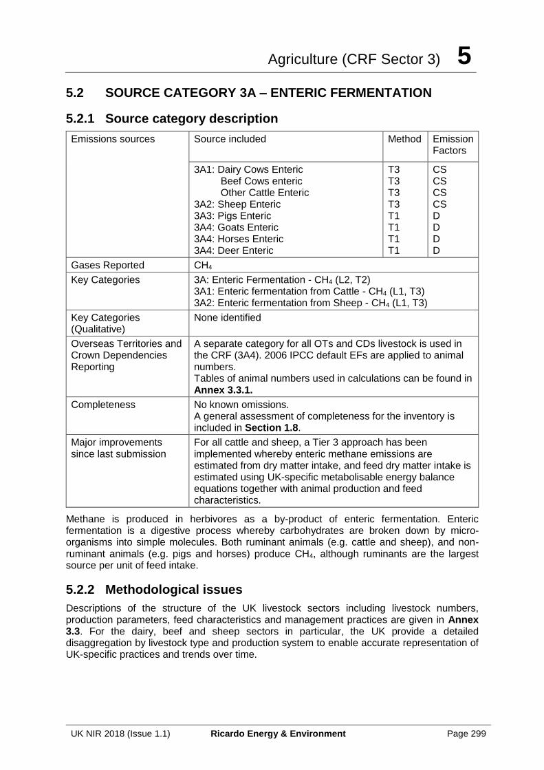
Agriculture (CRF Sector 3) 5
UK NIR 2018 (Issue 1.1) Ricardo Energy & Environment Page 299
5.2 SOURCE CATEGORY 3A – ENTERIC FERMENTATION
5.2.1 Source category description
Emissions sources Source included Method Emission Factors
3A1: Dairy Cows Enteric Beef Cows enteric Other Cattle Enteric
3A2: Sheep Enteric 3A3: Pigs Enteric 3A4: Goats Enteric 3A4: Horses Enteric 3A4: Deer Enteric
T3 T3 T3 T3 T1 T1 T1 T1
CS CS CS CS D D D D
Gases Reported CH4
Key Categories 3A: Enteric Fermentation - CH4 (L2, T2) 3A1: Enteric fermentation from Cattle - CH4 (L1, T3) 3A2: Enteric fermentation from Sheep - CH4 (L1, T3)
Key Categories (Qualitative)
None identified
Overseas Territories and Crown Dependencies Reporting
A separate category for all OTs and CDs livestock is used in the CRF (3A4). 2006 IPCC default EFs are applied to animal numbers. Tables of animal numbers used in calculations can be found in Annex 3.3.1.
Completeness No known omissions. A general assessment of completeness for the inventory is included in Section 1.8.
Major improvements since last submission
For all cattle and sheep, a Tier 3 approach has been implemented whereby enteric methane emissions are estimated from dry matter intake, and feed dry matter intake is estimated using UK-specific metabolisable energy balance equations together with animal production and feed characteristics.
Methane is produced in herbivores as a by-product of enteric fermentation. Enteric fermentation is a digestive process whereby carbohydrates are broken down by micro-organisms into simple molecules. Both ruminant animals (e.g. cattle and sheep), and non-ruminant animals (e.g. pigs and horses) produce CH4, although ruminants are the largest source per unit of feed intake.
5.2.2 Methodological issues
Descriptions of the structure of the UK livestock sectors including livestock numbers, production parameters, feed characteristics and management practices are given in Annex 3.3. For the dairy, beef and sheep sectors in particular, the UK provide a detailed disaggregation by livestock type and production system to enable accurate representation of UK-specific practices and trends over time.
Agriculture (CRF Sector 3) 5
UK NIR 2018 (Issue 1.1) Ricardo Energy & Environment Page 300
5.2.2.1 Dairy cows
Enteric methane emissions for dairy cows are estimated using a UK-specific relationship between daily enteric emission and feed dry matter intake, as developed under Defra-funded projects AC0115 and AC0114:
𝐶𝐻4_𝑒𝑛𝑡𝑒𝑟𝑖𝑐_𝑑𝑐 = (15.8185 × 𝐷𝑀𝐼) + 88.6002
Where:
CH4_enteric_dc is the enteric methane emission per dairy cow, g d-1
DMI is feed dry matter intake, kg d-1
and standard error values for the slope and intercept are 0.8338 and 14.5782, respectively.
Dry matter intake by dairy cows is determined using UK-specific energy balance equations as published in Feed into Milk (Thomas, 2004), based on metabolisable energy (ME). The daily ME intake by the animal is assumed to correspond with the requirement for live weight gain, activity, milk and gestation. Standard dietary components have been defined and associated with the outdoor grazing and indoor housing periods for each production system. These include grazed grass (with and without clover), grass silage, maize silage, whole crop silage and concentrates. Calculations are performed at a monthly resolution, with characterisation of production, management and feed by dairy cow category for each month. Further details are given in Annex 3.3.
5.2.2.2 Other cattle
Enteric methane emissions from other cattle, including dairy sector replacements and calves, and all beef sector cattle, are estimated using the same approach as for dairy cows but with different relationships between enteric emission and dry matter intake for lactating and non-lactating cattle. For lactating cattle (i.e. beef suckler cows) the same equation as for dairy cows (presented above in 5.2.2.1) is used. For all non-lactating cattle, the relationship as developed under Defra-funded projects AC0115 and AC0114 is:
𝐶𝐻4_𝑒𝑛𝑡𝑒𝑟𝑖𝑐_𝑜𝑐 = (17.5653 × 𝐷𝑀𝐼) + 45.8688
Where:
CH4_enteric_oc is the enteric methane emission per other cattle, g d-1
DMI is feed dry matter intake, kg d-1
and standard error values for the slope and intercept are 2.4112 and 16.1505, respectively.
As for dairy cows, dry matter intake for other cattle categories is determined using UK-specific energy balance equations, derived for non-lactating cattle from AFRC (1993) combined with cattle category- and system-specific production and diet characteristics at a monthly resolution as described for dairy cows (and further detail given in Annex 3.3).
5.2.2.3 Sheep
The same approach to estimating enteric emissions for cattle is taken with sheep, but using a UK-measurement derived relationship between enteric emission and dry matter intake specific to sheep:
𝐶𝐻4_𝑒𝑛𝑡𝑒𝑟𝑖𝑐_𝑠ℎ𝑒𝑒𝑝 = (12.3894 × 𝐷𝑀𝐼) + 5.1595
Where:
CH4_enteric_sheep is the enteric methane emission per sheep, g d-1
DMI is feed dry matter intake, kg d-1
Agriculture (CRF Sector 3) 5
UK NIR 2018 (Issue 1.1) Ricardo Energy & Environment Page 301
and standard error values for the slope and intercept are 1.483 and 0.8301, respectively.
As for cattle, dry matter intake for sheep categories is determined using UK-specific energy balance equations as described in AFRC (1993). The energy requirement is a function of the animal’s live-weight, stage of pregnancy, growth rate and production of milk. Application of the model is dependent on estimates of live-weight at slaughter, derived from national slaughter house statistics, and of age at slaughter, derived from a national survey of lamb slaughter age (Wheeler et al., 2009). The model is applied to a growth curve describing the daily live-weight gain and physiological state of the animal specific to sheep sub-category (ewe, ram, lamb) and production system (lowland, upland, hill). Further details are given in Annex 3.3.
5.2.2.4 Other livestock
Enteric emissions for pigs, goats, horses and deer are estimated using IPCC (2006) Tier 1 methodology by combining the Tier 1 default EF with the UK-specific activity data on animal numbers.
5.2.2.5 Overseas Territories and Crown Dependencies
Emission estimates were compiled by Aether-UK using animal numbers sourced from the territories directly and can be found in Annex 3.6. In the case of OTs, IPCC default emission factors were applied to animal numbers. For CDs, UK implied emission factors were applied.
5.2.3 Uncertainties and time-series consistency
The uncertainty analysis in Annex 2 provides estimates of uncertainty according to IPCC source category.
Note that, due to time constrains, the uncertainty analysis has not been updated to fully reflect the differences to uncertainty due to the adoption of new methods and data for estimating emissions from agriculture this year. These parameters will be reviewed for the next inventory cycle. It is likely uncertainties will be lower than the current assessment, as the new methodology makes use of data and methodologies which we have higher confidence in than previously. Uncertainties will likely be of a similar order of magnitude as previously used.
Emissions are calculated from animal population data and appropriate emission factors. The animal population data are collected in the June Agricultural Census, published annually by the devolved administrations (i.e. England, Wales, Scotland and Northern Ireland). These are long running publications and the compilers of the activity data strive to use consistent methods to produce the activity data. The time-series consistency of these activity data is very good due to the continuity in data provided.
Control measures introduced in response to the BSE outbreak in the UK introduced an inconsistency in the slaughter weight statistics and the derived dairy cow live weights for the years 1997 to 2005. To correct for the artefacts introduced by these control measures in the data time-series, data for this period were interpolated using the linear trend of increasing lives weight with time for the years immediately prior to and following this period.
5.2.4 Source-specific QA/QC and verification
This source category is covered by the general QA/QC procedures, which are discussed in Section 5.9.
5.2.5 Source-specific recalculations
Details of and justifications for recalculations to activity data and to emission factors are given in Table 5.1 and Table 5.2, respectively. For information on the magnitude of recalculations to Source Category 3A, see Section 10.
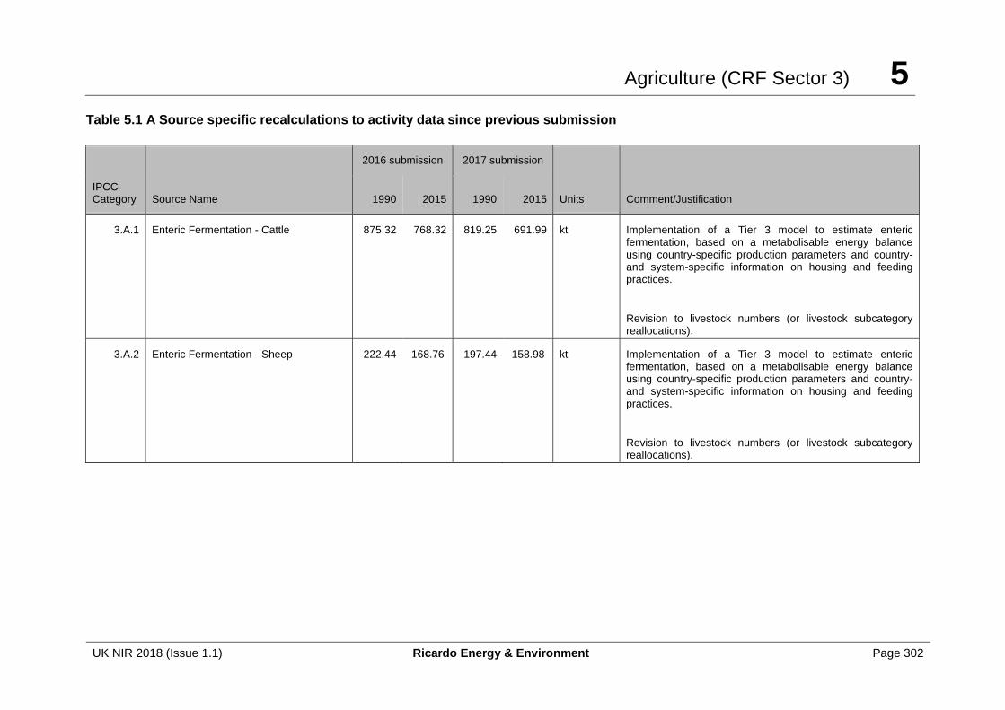
Agriculture (CRF Sector 3) 5
UK NIR 2018 (Issue 1.1) Ricardo Energy & Environment Page 302
Table 5.1 A Source specific recalculations to activity data since previous submission
IPCC Category Source Name
2016 submission 2017 submission
Units Comment/Justification 1990 2015 1990 2015
3.A.1 Enteric Fermentation - Cattle 875.32 768.32 819.25 691.99 kt Implementation of a Tier 3 model to estimate enteric fermentation, based on a metabolisable energy balance using country-specific production parameters and country- and system-specific information on housing and feeding practices.
Revision to livestock numbers (or livestock subcategory reallocations).
3.A.2 Enteric Fermentation - Sheep 222.44 168.76 197.44 158.98 kt Implementation of a Tier 3 model to estimate enteric fermentation, based on a metabolisable energy balance using country-specific production parameters and country- and system-specific information on housing and feeding practices.
Revision to livestock numbers (or livestock subcategory reallocations).
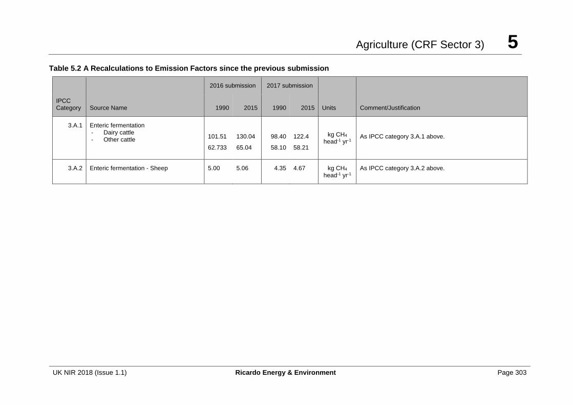
Agriculture (CRF Sector 3) 5
UK NIR 2018 (Issue 1.1) Ricardo Energy & Environment Page 303
Table 5.2 A Recalculations to Emission Factors since the previous submission
IPCC Category Source Name
2016 submission 2017 submission
Units Comment/Justification 1990 2015 1990 2015
3.A.1 Enteric fermentation - Dairy cattle - Other cattle
101.51
62.733
130.04
65.04
98.40
58.10
122.4
58.21
kg CH4 head-1 yr-1
As IPCC category 3.A.1 above.
3.A.2 Enteric fermentation - Sheep
5.00 5.06 4.35 4.67 kg CH4 head-1 yr-1
As IPCC category 3.A.2 above.
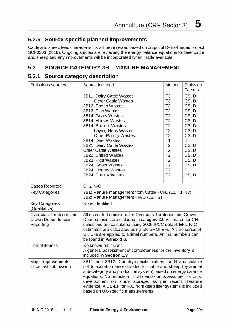
Agriculture (CRF Sector 3) 5
UK NIR 2018 (Issue 1.1) Ricardo Energy & Environment Page 304
5.2.6 Source-specific planned improvements
Cattle and sheep feed characteristics will be reviewed based on output of Defra-funded project SCF0203 (2018). Ongoing studies are reviewing the energy balance equations for beef cattle and sheep and any improvements will be incorporated when made available.
5.3 SOURCE CATEGORY 3B – MANURE MANAGEMENT
5.3.1 Source category description
Emissions sources
Source included Method Emission Factors
3B11: Dairy Cattle Wastes Other Cattle Wastes
3B12: Sheep Wastes 3B13: Pigs Wastes 3B14: Goats Wastes 3B14: Horses Wastes 3B14: Broilers Wastes
Laying Hens Wastes Other Poultry Wastes
3B14: Deer Wastes 3B21: Dairy Cattle Wastes Other Cattle Wastes 3B22: Sheep Wastes 3B23: Pigs Wastes 3B24: Goats Wastes 3B24: Horses Wastes 3B24: Poultry Wastes
T3 T3 T3 T2 T2 T2 T2 T2 T2 T1 T2 T2 T2 T2 T2 T2 T2
CS, D CS, D CS, D CS, D CS, D CS, D CS, D CS, D CS, D D CS, D CS, D CS, D CS, D CS, D D CS, D
Gases Reported CH4, N2O
Key Categories 3B1: Manure management from Cattle - CH4 (L1, T1, T3) 3B2: Manure Management - N2O (L2, T2)
Key Categories (Qualitative)
None identified
Overseas Territories and Crown Dependencies Reporting
All estimated emissions for Overseas Territories and Crown Dependencies are included in category 3J. Estimates for CH4 emissions are calculated using 2006 IPCC default EFs. N2O estimates are calculated using UK GHGI EFs. A time series of UK EFs are applied to animal numbers. Animal numbers can be found in Annex 3.6.
Completeness No known omissions. A general assessment of completeness for the inventory is included in Section 1.8.
Major improvements since last submission
3B11 and 3B12: Country-specific values for N and volatile solids excretion are estimated for cattle and sheep (by animal sub-category and production system) based on energy balance equations. No reduction in CH4 emission is assumed for crust development on slurry storage, as per recent literature evidence. A CS-EF for N2O from deep litter systems is included based on UK-specific measurements.
Agriculture (CRF Sector 3) 5
UK NIR 2018 (Issue 1.1) Ricardo Energy & Environment Page 305
Full implementation of the N-flow approach (Webb and Misselbrook, 2004) in the combined ammonia and GHG inventory model for UK agriculture, accounting for all N losses and transformations through the manure management chain.
This category reports emissions of CH4 from animal manures as well as N2O emissions from their manures arising during its storage.
5.3.2 Methodological issues
5.3.2.1 Methane emissions from animal manures
Methane is produced from the decomposition of manure under anaerobic conditions. When manure is stored or treated as a liquid in a lagoon, pond or tank it tends to decompose anaerobically and produce a significant quantity of methane. When manure is handled as a solid or when it is deposited on pastures, it tends to decompose aerobically and little or no methane is produced. Hence the system of manure management used affects emission rates.
The emission factors for manure management are calculated following IPCC Tier 2 methodology for cattle, sheep, pigs and poultry, according to IPCC (2006) Equation 10.23. For cattle and sheep, country-specific values for volatile solids (VS) excretion are derived by animal sub-category and production system using the UK-specific ME balance equations (as described in Section 5.2.2) and an estimate of GE intake (based on estimated dry matter intake and feed energy content) according to a variation of IPCC (2006) Equation 10.24:
𝑉𝑆𝑒𝑥 = (𝐺𝐸𝑖 × (1 − (𝑀𝑒𝑟𝑒𝑞 𝐺𝐸𝑖⁄ ))) × ((1 − 𝐴𝑆𝐻) (𝐺𝐸𝑖 𝐷𝑀𝐼⁄ )⁄ )
Where:
VSex is the volatile solids excretion, kg d-1
GEi is the gross energy intake, MJ d-1
ASH is the ash content of the manure as a fraction of the dry matter feed intake
DMI is the dry matter intake, kg d-1
UK-specific data on the methane producing potential (Bo) of cattle excreta were not significantly different from IPCC (2006) default values (Defra AC0115), so the default values are retained. For pigs and poultry, IPCC (2006) default values for VS and Bo are used.
Default IPCC (2006) MCF values (IPCC Table 10.17) are applied, with the exception of liquid/slurry systems with a natural crust cover, where no reduction in the MCF value is assumed in accordance with recent literature evidence (e.g. Petersen et al., 2013). These data are combined with country-specific data for the proportion of manure from each livestock type managed according to the different animal waste management systems (AWMS). The emission factors are listed in Table A 3.3.2 in Annex 3. Table A 3.3.3 in Annex 3 shows the methane conversion factors assumed for the different systems.
For goats, deer and horses, IPCC (2006) Tier 1 default emission factors were used (IPCC Tables 10.15).
5.3.2.2 Nitrous Oxide emissions from Animal Waste Management Systems
Animals are assumed not to give rise to nitrous oxide emissions directly, but emissions will arise from N excreted by livestock. Emissions from manures during storage are calculated for different animal waste management systems (AWMS) defined by IPCC. Emissions from the following AWMS are reported under the Manure Management IPCC category (it is assumed that uncovered anaerobic lagoons are not present in the UK:
Agriculture (CRF Sector 3) 5
UK NIR 2018 (Issue 1.1) Ricardo Energy & Environment Page 306
• Liquid/slurry;
• Solid storage/deep litter/poultry manure
According to IPCC (2006), the following AWMS are reported in the Agricultural Soils category:
• All animal manures and slurries applied to soils; and
• Pasture range and paddock
The UK has implemented a detailed N-flow model describing the flow of N from livestock excretion through the manure management chain (Webb and Misselbrook, 2004), accounting for all N losses (via NH3, N2O, NO, N2 and N leaching) and transformations (immobilisation, mineralisation) at each manure management stage. Nitrous oxide emissions from manure management are estimated following IPCC (2006) (equation 10.25) for each livestock category and subcategory, using country-specific data for N excretion by the different livestock types and for the proportion of manure managed according to the different AWMS, and a combination of default and country-specific emission factors for the different AWMS.
For cattle and sheep, N excretion is estimated based as the balance of N intake and N retained in live weight gain, milk, wool and developing foetus, specific to livestock sub-category, production system and diet. N intake is estimated from the calculation of dry matter intake, based on energy requirement and feed characteristics (Section 5.2.2), and the crude protein content of the feed. For cattle, N excreta are partitioned to urine N and dung N, based on literature equations relating N excreta to N intake (Reed et al., 2015). The urine N is assumed to rapidly convert to ammoniacal N whereas the dung N remains as organic N; these different N forms have important implications for subsequent N losses and transformations through the manure management chain (Webb and Misselbrook, 2004). For sheep, 60% of excreta N is assumed to be excreted as urine and 40% as dung. For other livestock types, country-specific values for N excretion were derived from the report of Defra project WT0715NVZ (Cottrill and Smith, 2007) with interpretation by Cottrill and Smith (ADAS) Table A 3.3.4 in Annex 3. For pigs and poultry, 70% of excreta is assumed to rapidly become ammoniacal N with 30% remaining as organic N. For goats, horses and deer, the respective excretal proportions are assumed to be 60 and 40%.
The conversion of excreted N into N2O emissions is determined by the type of manure management system used. The distribution of AWMS is given in Table A 3.3.5 in Annex 3. For manure types with bedding addition, the N content of the added bedding is included in the manure N content. Default emission factors (IPCC, 2006; Table 10.21) are assumed except for cattle, pig, sheep, goat, deer and horse deep litter systems where a UK-specific EF of 2.0 is used and for poultry manure where a UK-specific EF of 0.5 is used (Table A 3.3.6 in Annex 3).
For estimation of indirect N2O emissions from manure management, country-specific values for FracGASM and FracLEACH are used. FracGASM is derived directly as output from the UK N-flow model for each livestock x AWMS combination, as the sum of the NH3-N and NO-N emissions (further details can be found in the UK Informative Inventory Report). A country-specific value of 3% of manure N for FracLEACH is used, based on Nicholson et al. (2011) and applied only to solid manure heaps stored in fields. For manure heaps stored on concrete pads, the leachate is assumed to be collected and is subsequently included in the N content of liquid/slurry managed manure. Indirect emissions from manure management due to volatilisation and leaching are then calculated according to IPCC (2006) equations 10.27 and 10.29, respectively, applying IPCC (2006) default values for EF4 and EF5.
Agriculture (CRF Sector 3) 5
UK NIR 2018 (Issue 1.1) Ricardo Energy & Environment Page 307
5.3.2.3 Emissions in the Overseas Territories and Crown Dependencies
Animal numbers are sourced from the territories directly and can be found in Annex 3.6. In the case of OTs, IPCC default emissions factors were applied to the data. For CDs, UK implied emission factors were applied to the data, both for CH4 and N2O.
5.3.3 Uncertainties and time-series consistency
The uncertainty analysis in Annex 2 provides estimates of uncertainty according to IPCC source category.
Note that, due to time constrains, the uncertainty analysis has not been updated to fully reflect the differences to uncertainty due to the adoption of new methods and data for estimating emissions from agriculture this year. These parameters will be reviewed for the next inventory cycle. It is likely uncertainties will be lower than the current assessment, as the new methodology makes use of data and methodologies which we have higher confidence in than previously, but would be of a similar order of magnitude
Emissions are calculated from livestock population data and appropriate emission factors. The livestock population data are collected in the June Agricultural Census, published annually by the devolved administrations (i.e. England, Wales, Scotland and Northern Ireland). These are long running publications and the compilers of the activity data strive to use consistent methods to produce the activity data. The time-series consistency of these activity data is very good due to the continuity in data provided.
5.3.4 Source-specific QA/QC and verification
This source category is covered by the general QA/QC procedures, which are discussed in Section 5.9.
5.3.5 Source-specific recalculations
Details of and justifications for recalculations to activity data and to emission factors are given in Table 5.3 and Table 5.4, respectively. For information on the magnitude of recalculations to Source Category 3A, see and Section 10.
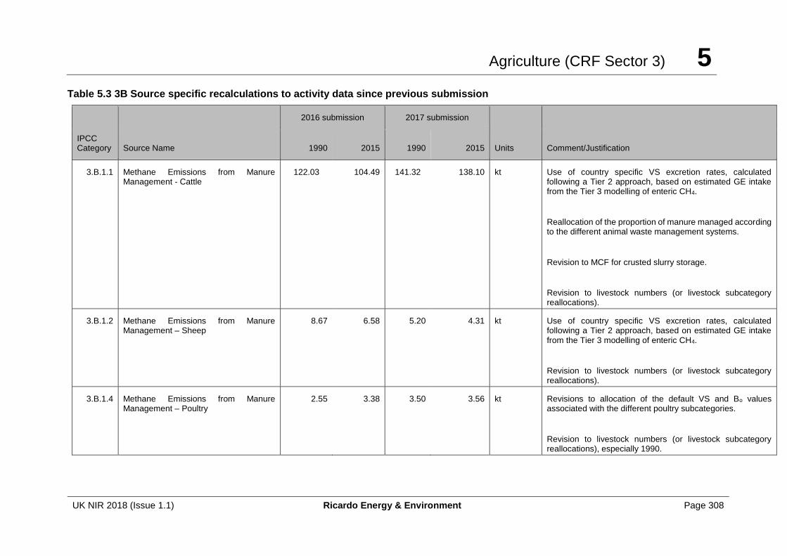
Agriculture (CRF Sector 3) 5
UK NIR 2018 (Issue 1.1) Ricardo Energy & Environment Page 308
Table 5.3 3B Source specific recalculations to activity data since previous submission
IPCC Category Source Name
2016 submission 2017 submission
Units Comment/Justification 1990 2015 1990 2015
3.B.1.1 Methane Emissions from Manure Management - Cattle
122.03 104.49 141.32 138.10 kt Use of country specific VS excretion rates, calculated following a Tier 2 approach, based on estimated GE intake from the Tier 3 modelling of enteric CH4.
Reallocation of the proportion of manure managed according to the different animal waste management systems.
Revision to MCF for crusted slurry storage.
Revision to livestock numbers (or livestock subcategory reallocations).
3.B.1.2 Methane Emissions from Manure Management – Sheep
8.67 6.58 5.20 4.31 kt Use of country specific VS excretion rates, calculated following a Tier 2 approach, based on estimated GE intake from the Tier 3 modelling of enteric CH4.
Revision to livestock numbers (or livestock subcategory reallocations).
3.B.1.4 Methane Emissions from Manure Management – Poultry
2.55 3.38 3.50 3.56 kt Revisions to allocation of the default VS and Bo values associated with the different poultry subcategories.
Revision to livestock numbers (or livestock subcategory reallocations), especially 1990.
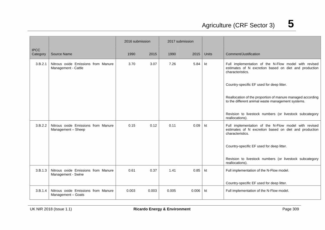
Agriculture (CRF Sector 3) 5
UK NIR 2018 (Issue 1.1) Ricardo Energy & Environment Page 309
IPCC Category Source Name
2016 submission 2017 submission
Units Comment/Justification 1990 2015 1990 2015
3.B.2.1 Nitrous oxide Emissions from Manure Management - Cattle
3.70 3.07 7.26 5.84 kt Full implementation of the N-Flow model with revised estimates of N excretion based on diet and production characteristics.
Country-specific EF used for deep litter.
Reallocation of the proportion of manure managed according to the different animal waste management systems.
Revision to livestock numbers (or livestock subcategory reallocations).
3.B.2.2 Nitrous oxide Emissions from Manure Management – Sheep
0.15 0.12 0.11 0.09 kt Full implementation of the N-Flow model with revised estimates of N excretion based on diet and production characteristics.
Country-specific EF used for deep litter.
Revision to livestock numbers (or livestock subcategory reallocations).
3.B.1.3 Nitrous oxide Emissions from Manure Management - Swine
0.61 0.37 1.41 0.85 kt Full implementation of the N-Flow model.
Country-specific EF used for deep litter.
3.B.1.4 Nitrous oxide Emissions from Manure Management – Goats
0.003 0.003 0.005 0.006 kt Full implementation of the N-Flow model.
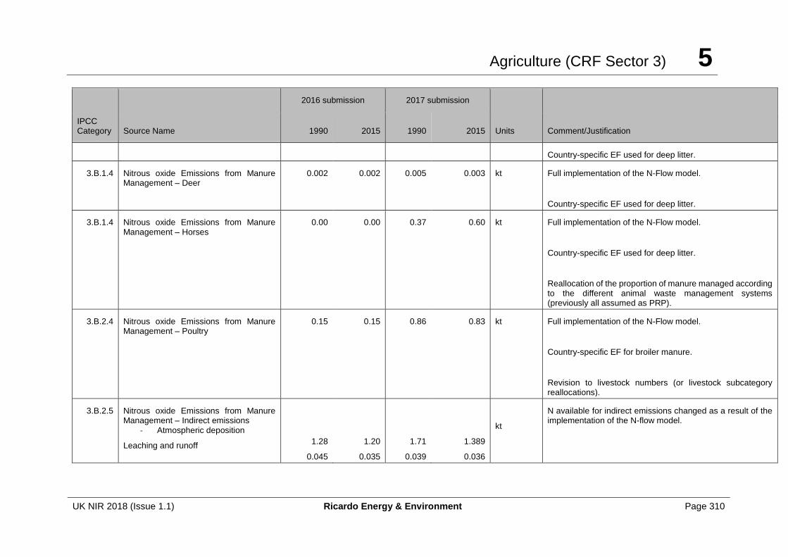
Agriculture (CRF Sector 3) 5
UK NIR 2018 (Issue 1.1) Ricardo Energy & Environment Page 310
IPCC Category Source Name
2016 submission 2017 submission
Units Comment/Justification 1990 2015 1990 2015
Country-specific EF used for deep litter.
3.B.1.4 Nitrous oxide Emissions from Manure Management – Deer
0.002 0.002 0.005 0.003 kt Full implementation of the N-Flow model.
Country-specific EF used for deep litter.
3.B.1.4 Nitrous oxide Emissions from Manure Management – Horses
0.00 0.00 0.37 0.60 kt Full implementation of the N-Flow model.
Country-specific EF used for deep litter.
Reallocation of the proportion of manure managed according to the different animal waste management systems (previously all assumed as PRP).
3.B.2.4 Nitrous oxide Emissions from Manure Management – Poultry
0.15 0.15 0.86 0.83 kt Full implementation of the N-Flow model.
Country-specific EF for broiler manure.
Revision to livestock numbers (or livestock subcategory reallocations).
3.B.2.5 Nitrous oxide Emissions from Manure Management – Indirect emissions
- Atmospheric deposition
Leaching and runoff
1.28
0.045
1.20
0.035
1.71
0.039
1.389
0.036
kt
N available for indirect emissions changed as a result of the implementation of the N-flow model.
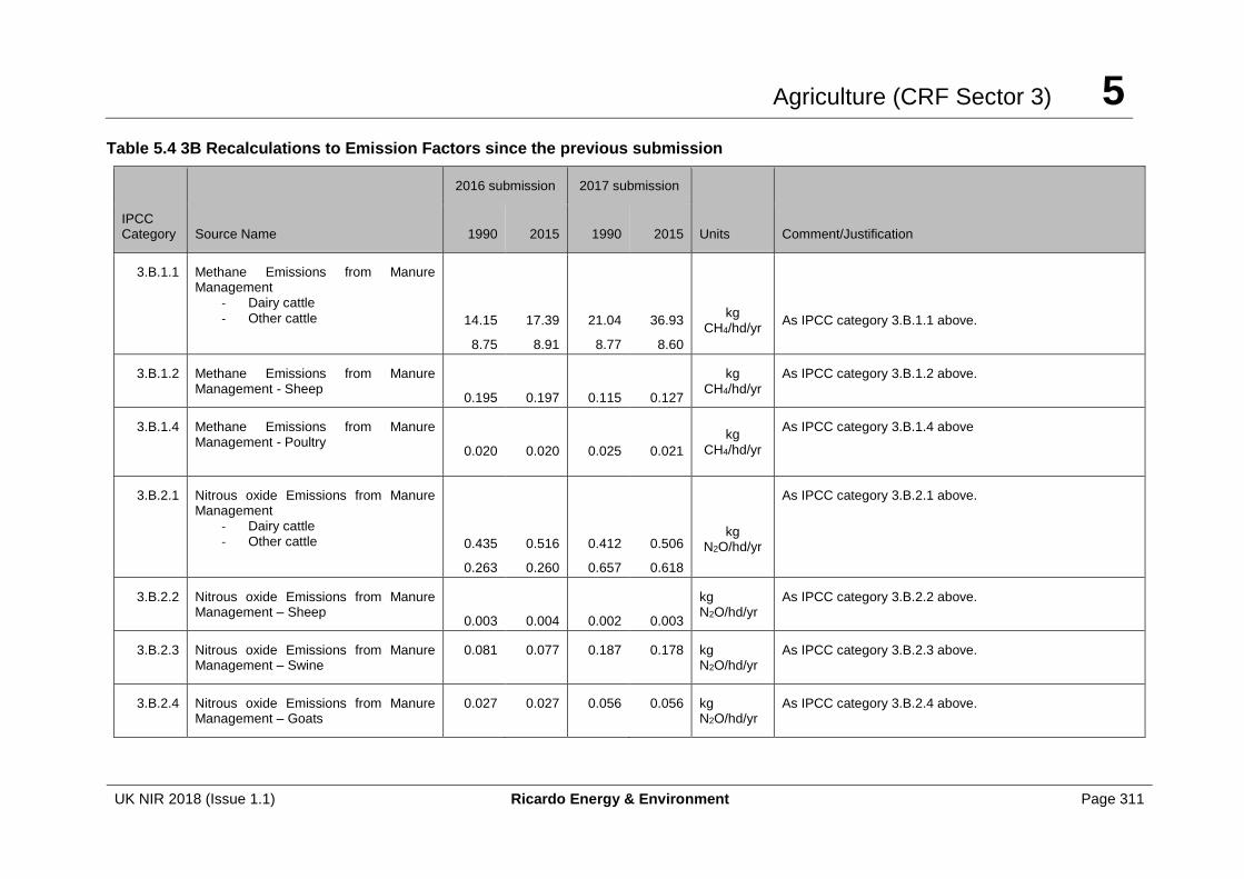
Agriculture (CRF Sector 3) 5
UK NIR 2018 (Issue 1.1) Ricardo Energy & Environment Page 311
Table 5.4 3B Recalculations to Emission Factors since the previous submission
IPCC Category Source Name
2016 submission 2017 submission
Units Comment/Justification 1990 2015 1990 2015
3.B.1.1 Methane Emissions from Manure Management
- Dairy cattle
- Other cattle
14.15
8.75
17.39
8.91
21.04
8.77
36.93
8.60
kg CH4/hd/yr
As IPCC category 3.B.1.1 above.
3.B.1.2 Methane Emissions from Manure Management - Sheep
0.195
0.197
0.115
0.127
kg CH4/hd/yr
As IPCC category 3.B.1.2 above.
3.B.1.4 Methane Emissions from Manure Management - Poultry
0.020
0.020
0.025
0.021
kg CH4/hd/yr
As IPCC category 3.B.1.4 above
3.B.2.1 Nitrous oxide Emissions from Manure Management
- Dairy cattle - Other cattle
0.435
0.263
0.516
0.260
0.412
0.657
0.506
0.618
kg N2O/hd/yr
As IPCC category 3.B.2.1 above.
3.B.2.2 Nitrous oxide Emissions from Manure Management – Sheep
0.003
0.004
0.002
0.003
kg N2O/hd/yr
As IPCC category 3.B.2.2 above.
3.B.2.3 Nitrous oxide Emissions from Manure Management – Swine
0.081 0.077 0.187 0.178 kg N2O/hd/yr
As IPCC category 3.B.2.3 above.
3.B.2.4 Nitrous oxide Emissions from Manure Management – Goats
0.027 0.027 0.056 0.056 kg N2O/hd/yr
As IPCC category 3.B.2.4 above.
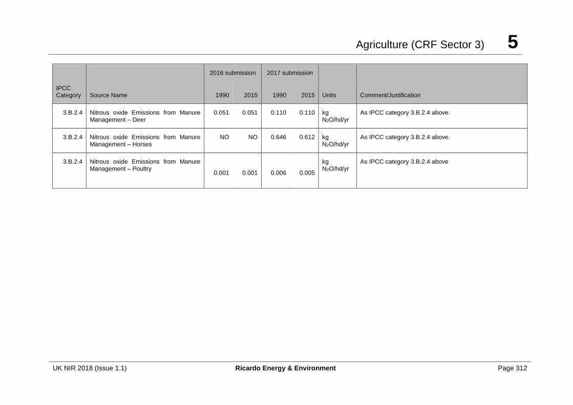
Agriculture (CRF Sector 3) 5
UK NIR 2018 (Issue 1.1) Ricardo Energy & Environment Page 312
IPCC Category Source Name
2016 submission 2017 submission
Units Comment/Justification 1990 2015 1990 2015
3.B.2.4 Nitrous oxide Emissions from Manure Management – Deer
0.051 0.051 0.110 0.110 kg N2O/hd/yr
As IPCC category 3.B.2.4 above.
3.B.2.4 Nitrous oxide Emissions from Manure Management – Horses
NO NO 0.646 0.612 kg N2O/hd/yr
As IPCC category 3.B.2.4 above.
3.B.2.4 Nitrous oxide Emissions from Manure Management – Poultry
0.001
0.001
0.006
0.005
kg N2O/hd/yr
As IPCC category 3.B.2.4 above
Agriculture (CRF Sector 3) 5
UK NIR 2018 (Issue 1.1) Ricardo Energy & Environment Page 313
5.3.6 Source-specific planned improvements
Emission factors and activity data will continue to be reviewed including the use of more detailed emission factors and activity data to improve emission estimates and allow estimation of the effect of future mitigation policies.
Anaerobic digestion of livestock manures (currently accounting for a very small percentage of manure, but projected to increase) will be fully implemented in the next submission.
5.4 SOURCE CATEGORY 3D – AGRICULTURAL SOILS
5.4.1 Source category description
Emissions sources Source included Method Emission Factors
3D1: Direct N2O Emissions From Managed Soils 3D2: Indirect N2O Emissions From Managed Soil
T2, T1 T2,T1,CS
D, CS D, CS
Gases Reported N2O
Key Categories 3D: Agricultural soils - N2O (L1, T1, L2, T2)
Key Categories (Qualitative)
None identified
Overseas Territories and Crown Dependencies Reporting
Emissions included under 3D1.7 ‘other’ within the CRF. In the case of OTs, IPCC default emission factors were applied to the data. For CDs, UK implied emission factors were applied.
Completeness A general assessment of completeness for the inventory is included in Section 1.8.
Major improvements since last submission
Spatial disaggregation of the country-specific value of EF1 for inorganic N fertiliser applications, with EF calculated on a 10 km grid basis according to fertiliser type, application rate and annual rainfall amount. Full implementation of the N-flow model (Webb and Misselbrook, 2004) in the combined ammonia and GHG inventory model for UK agriculture, accounting for all N losses and transformations through the manure management chain and thus influencing the N remaining for land application.
Direct emissions of nitrous oxide from agricultural soils are estimated using IPCC (2006) Tier 2 methodology (IPCC Equation 11.2), implementing UK-specific EF and parameters where available. The IPCC (2006) method involves estimating contributions from:
(i) The use of inorganic fertiliser (ii) Application of livestock manures to land (iii) Application of sewage sludge to land (iv) Urine and dung deposited by grazing animals in the field (v) Crop residues returned to soils (vi) Mineralisation (vii) Cultivation of histosols (organic soils)
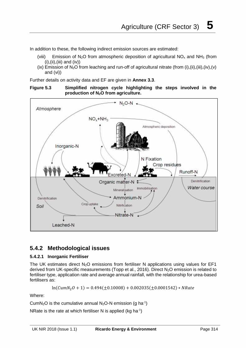
Agriculture (CRF Sector 3) 5
UK NIR 2018 (Issue 1.1) Ricardo Energy & Environment Page 314
In addition to these, the following indirect emission sources are estimated:
(viii) Emission of N2O from atmospheric deposition of agricultural NOx and NH3 (from (i),(ii),(iii) and (iv))
(ix) Emission of N2O from leaching and run-off of agricultural nitrate (from (i),(ii),(iii),(iv),(v) and (vi))
Further details on activity data and EF are given in Annex 3.3.
Figure 5.3 Simplified nitrogen cycle highlighting the steps involved in the production of N2O from agriculture.
5.4.2 Methodological issues
5.4.2.1 Inorganic Fertiliser
The UK estimates direct N2O emissions from fertiliser N applications using values for EF1 derived from UK-specific measurements (Topp et al., 2016). Direct N2O emission is related to fertiliser type, application rate and average annual rainfall, with the relationship for urea-based fertilisers as:
ln(𝐶𝑢𝑚𝑁2𝑂 + 1) = 0.494(±0.10008) + 0.002035(±0.0001542) ∗ 𝑁𝑅𝑎𝑡𝑒
Where:
CumN2O is the cumulative annual N2O-N emission (g ha-1)
NRate is the rate at which fertiliser N is applied (kg ha-1)
Agriculture (CRF Sector 3) 5
UK NIR 2018 (Issue 1.1) Ricardo Energy & Environment Page 315
For other all other fertiliser types the relationship used is:
Ln(𝐶𝑢𝑚𝑁2𝑂 + 1)= 0.1616(±0.13526) + 0.00006093(±0.000240365) ∗ 𝑁𝑅𝑎𝑡𝑒+ 0.0005187(±0.00016259) ∗ 𝑅𝑎𝑖𝑛𝑌𝑟 + 0.00000354(±0.0000002785)∗ 𝑁𝑅𝑎𝑡𝑒 ∗ 𝑅𝑎𝑖𝑛𝑌𝑟
Where:
CumN2O is the cumulative annual N2O-N emission (g ha-1)
NRate is the rate at which fertiliser N is applied (kg ha-1)
RainYr is the annual average rainfall (mm).
EF are derived as ((CumN2O at specified NRate – CumN2O at zero NRate) / NRate).
Calculations are made at a 10 km spatial resolution, using information on crop type within each spatial cell from the June Agricultural Survey for each Devolved Administration (England, Wales, Scotland, Northern Ireland), information on crop-specific N fertiliser application rates from the British Survey of Fertiliser Practice for England, Wales and Scotland and from the Farm Business Survey for Northern Ireland (further details given in Annex 3.3) and 30-year average rainfall for each 10 km cell from the UK Meteorological Office.
5.4.2.2 Application of livestock manures to land
The quantities of livestock manure being applied to land, by livestock subcategory and production system type, are estimated using the N-flow model for livestock manure management, accounting for all N losses and transformations through the manure management chain (Webb and Misselbrook, 2004). Country-specific values for EF1 for manure applications to land are used, based on UK-specific experimental data (Topp et al., 2006). Separate values have been derived for liquid slurries and solid manures (farm yard manure, poultry manure) but are not spatially or temporally disaggregated (Annex 3.3, Table A3.3.14).
5.4.2.3 Application of sewage sludge to land
Following IPCC (2006, equation 11.1), emissions from sewage sludge applied to land are reported under agricultural soils. The calculation involves estimating the amount of N contained per dry matter unit of sludge that is applied to land and applying the default IPCC EF1. Data sources for the annual production of sewage sludge (as dry matter) are described in the Waste sector (Section 7).
5.4.2.4 Urine and dung deposited by grazing animals in the field
Direct N2O emissions from livestock grazing returns to land are estimated following IPCC (2006, equation 11.1) using UK-specific values for excreta N deposited at grazing and UK-specific values for EF3 for cattle as derived from experiments conducted under Defra study AC0116 (Topp et al., 2016). N excretion for cattle is partitioned to urine and dung N as described in Section 5.3.2.2, and the separate UK-specific values for EF3 for urine and dung are applied accordingly (Annex 3.3, Table A3.3.7). The default IPCC (2006) EF3 for sheep is lower than that for cattle. The UK do not have any experimental data specifically for sheep grazing, but as the weighted average (across dung and urine) UK-specific EF3 for cattle is lower than the IPCC (2006) default EF3 for sheep, the UK assumes the same value for sheep as for cattle (and for goats, horses and deer), rather than create an anomaly by having a higher EF3 value for sheep than for cattle. For pigs and poultry, where behaviour of outdoor animals is quite different to that of cattle and sheep, the default IPCC (2006) EF3 is used.
5.4.2.5 Crop Residues returned to soils
Direct N2O emissions from crop residues are estimated following IPCC (2006, equation 11.2) using the default value for EF1. However, a country-specific approach is taken to deriving the
Agriculture (CRF Sector 3) 5
UK NIR 2018 (Issue 1.1) Ricardo Energy & Environment Page 316
quantity of N returned in crop residues, based on UK-specific data for the harvest index and, where available, UK-specific data for N content of crop residues (Annex 3.3, Tables A 3.3.10 and A 3.3.11).
5.4.2.6 Mineralisation
N2O emissions from mineralisation of soil organic matter on land converted to Cropland more than 20 years ago are included in the Agricultural inventory (emissions from more recent land use change are included in the LULUCF inventory). The emissions are estimated using the areas of Forest land and Grassland converted to Cropland from the land use change matrices. The land use change matrices are calculated from the Monitoring Landscape Change (MLC) data from 1947 & 1980 (MLC 1986) and the Countryside Surveys (CS) of 1984, 1990, 1998 (Haines-Young et al. 2000) and 2007 (Smart et al. 2009) for Great Britain. For Northern Ireland, the data comes from the Northern Ireland Countryside Surveys of 1990, 1998 (Cooper and McCann 2002) and 2007 (Cooper, McCann and Rogers 2009).
N2O emissions from mineralisation of soil organic matter as a result of Cropland Management activities are estimated from the change in soil carbon stocks due to Cropland Management using a Tier 1 approach. The methodology used to assess change in soil carbon stocks due to Cropland Management is described in Section 6.3.4 and Annex A3.4.7.
5.4.2.7 Cultivation of histosols (organic soils)
Direct N2O emissions from the cultivation of histosols are estimated following IPCC (2006, equation 11.2) using the default value for EF2 and UK-specific data for the area of cultivated histosols.
5.4.2.8 Atmospheric deposition of NOX and NH3
Indirect emissions of N2O from the atmospheric deposition of ammonia and NOx are estimated according to IPCC (2006, equation 11.9) using the default value for EF4 and country-specific values for the fraction of N that is volatilised as NH3 and NO from inorganic fertiliser and organic (livestock manure, sewage sludge, digestate, grazing returns) N applications to land (FracGASF and FracGASM, respectively) derived directly from the combined ammonia and greenhouse gas inventory model for UK agriculture, using an N-flow approach (Webb and Misselbrook, 2004). UK-specific NH3 EF are used for inorganic fertiliser and organic manure applications to land, as detailed in the UK Informative Inventory Report. Emissions of NO from fertiliser, organic manure applications and grazing returns are assumed to be a factor of 0.1 of the N2O emissions estimated for each source. The method used corrects for the N content of manures used as fuel (poultry litter incineration) and therefore not applied to land.
5.4.2.9 Leaching and runoff
Indirect emissions of N2O from leaching and runoff are estimated according IPCC (2006, equation 11.10) using the default value for EF5. The sources of nitrogen considered are synthetic fertiliser application, animal manures and sewage sludge applied to soils, excretal grazing returns (dung and urine), crop residues and mineralisation. A country-specific value for the proportion of N applied that is leached (FracLEACH) is used for both inorganic fertiliser and manure application to grassland and excretal returns from grazing livestock, based on a modelling study using the NITCAT model at a UK county level disaggregation (Cardenas et al., 2013). For fertiliser and manure application to arable land, crop residues and sewage sludge the default IPCC (2006) FracLEACH value is used as this was supported by Cardenas et al. (2013) for UK conditions. For mineralisation, the default IPCC (2006) value is also used. The method used corrects for the N content of manures used as fuel (poultry litter incineration) which are not applied to land.
Agriculture (CRF Sector 3) 5
UK NIR 2018 (Issue 1.1) Ricardo Energy & Environment Page 317
5.4.2.10 Overseas Territories and Crown Dependencies
The Tier 1 methodology from the IPCC Guidelines was applied to calculate emissions from agricultural soils for the OTs and CDs. Livestock data were provided from each of the OTs/ CDs or sourced from FAO. The quantity of synthetic fertiliser applied and crop production data were obtained from FAO and Defra; these data can be found in Annex 3.9. Emission factors taken from the 2006 IPCC guidelines and Western European emission factors were applied to all CDs (Isle of Man, Guernsey and Jersey) whilst Latin American emission factors were applied to all OTs (Cayman Islands, Falkland Islands, Montserrat and Bermuda). This decision was based on both geographical location, and the understanding of farming practices.
5.4.3 Uncertainties and time-series consistency
The uncertainty analysis in Annex 2 provides estimates of uncertainty according to IPCC source category.
Note that, due to time constrains, the uncertainty analysis has not been updated to fully reflect the differences to uncertainty due to the adoption of new methods and data for estimating emissions from agriculture this year. These parameters will be reviewed for the next inventory cycle. It is likely uncertainties will be lower than the current assessment, as the new methodology makes use of data and methodologies which we have higher confidence in than previously, but would be of a similar order of magnitude.
Emissions are calculated from a range of activity data and appropriate emission factors (see Annex 3). Emissions of N2O from the use of fertilisers are important in this source category. The annual consumption of synthetic fertiliser is estimated based on crop areas (crop area data reported annually by the Devolved Administrations) and fertiliser application rates (reported annually in the British Survey of Fertiliser Practice). These are both long running datasets and the compilers of the activity data strive to use consistent methods to produce the activity data. The time-series consistency of these activity data is very good due to the continuity in data provided.
5.4.4 Source-specific QA/QC and verification
This source category is covered by the general QA/QC procedures, which are discussed in Section 5.9.
5.4.5 Source-specific recalculations
Details of and justifications for recalculations to activity data are given in Table 5.5 and Table 5.6. For information on the magnitude of recalculations to Source Category 3D, see Section 10. Emissions from histosols cropland cultivation in Falkland Islands have been included, while histosols in Grassland are considered unmanaged. N2O emissions from soil mineralisation are not included any longer, since all soils in the Falklands are organic. Bermuda estimates have been included.
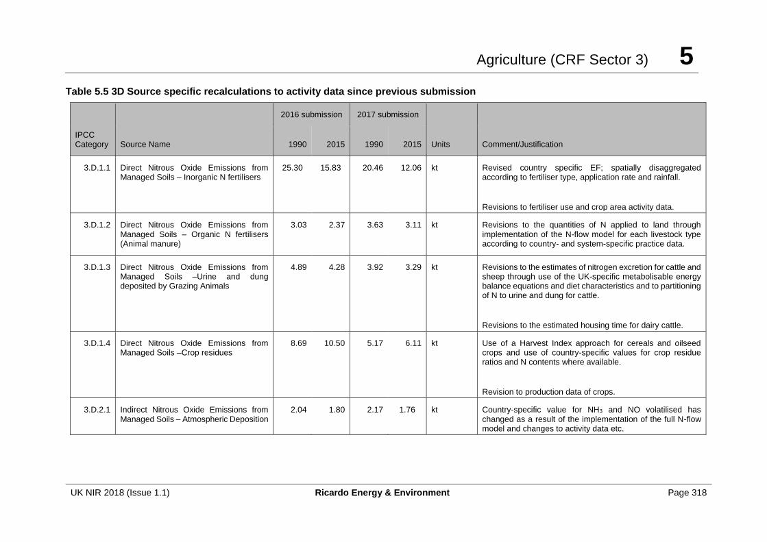
Agriculture (CRF Sector 3) 5
UK NIR 2018 (Issue 1.1) Ricardo Energy & Environment Page 318
Table 5.5 3D Source specific recalculations to activity data since previous submission
IPCC Category Source Name
2016 submission 2017 submission
Units Comment/Justification 1990 2015 1990 2015
3.D.1.1 Direct Nitrous Oxide Emissions from Managed Soils – Inorganic N fertilisers
25.30 15.83 20.46 12.06 kt Revised country specific EF; spatially disaggregated according to fertiliser type, application rate and rainfall.
Revisions to fertiliser use and crop area activity data.
3.D.1.2 Direct Nitrous Oxide Emissions from Managed Soils – Organic N fertilisers (Animal manure)
3.03 2.37 3.63 3.11 kt Revisions to the quantities of N applied to land through implementation of the N-flow model for each livestock type according to country- and system-specific practice data.
3.D.1.3 Direct Nitrous Oxide Emissions from Managed Soils –Urine and dung deposited by Grazing Animals
4.89 4.28 3.92 3.29 kt Revisions to the estimates of nitrogen excretion for cattle and sheep through use of the UK-specific metabolisable energy balance equations and diet characteristics and to partitioning of N to urine and dung for cattle.
Revisions to the estimated housing time for dairy cattle.
3.D.1.4 Direct Nitrous Oxide Emissions from Managed Soils –Crop residues
8.69 10.50 5.17 6.11 kt Use of a Harvest Index approach for cereals and oilseed crops and use of country-specific values for crop residue ratios and N contents where available.
Revision to production data of crops.
3.D.2.1 Indirect Nitrous Oxide Emissions from Managed Soils – Atmospheric Deposition
2.04 1.80 2.17 1.76 kt Country-specific value for NH3 and NO volatilised has changed as a result of the implementation of the full N-flow model and changes to activity data etc.
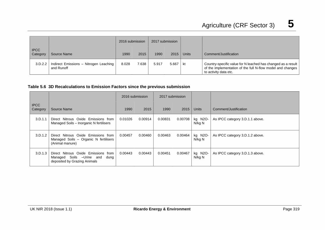
Agriculture (CRF Sector 3) 5
UK NIR 2018 (Issue 1.1) Ricardo Energy & Environment Page 319
IPCC Category Source Name
2016 submission 2017 submission
Units Comment/Justification 1990 2015 1990 2015
3.D.2.2 Indirect Emissions – Nitrogen Leaching and Runoff
8.028 7.638 5.917 5.667 kt Country-specific value for N leached has changed as a result of the implementation of the full N-flow model and changes to activity data etc.
Table 5.6 3D Recalculations to Emission Factors since the previous submission
IPCC Category Source Name
2016 submission 2017 submission
Units Comment/Justification 1990 2015 1990 2015
3.D.1.1 Direct Nitrous Oxide Emissions from Managed Soils – Inorganic N fertilisers
0.01026 0.00914 0.00831
0.00708 kg N2O-N/kg N
As IPCC category 3.D.1.1 above.
3.D.1.2 Direct Nitrous Oxide Emissions from Managed Soils – Organic N fertilisers (Animal manure)
0.00457 0.00460 0.00463 0.00464 kg N2O-N/kg N
As IPCC category 3.D.1.2 above.
3.D.1.3 Direct Nitrous Oxide Emissions from Managed Soils –Urine and dung deposited by Grazing Animals
0.00443 0.00443 0.00451 0.00467 kg N2O-N/kg N
As IPCC category 3.D.1.3 above.
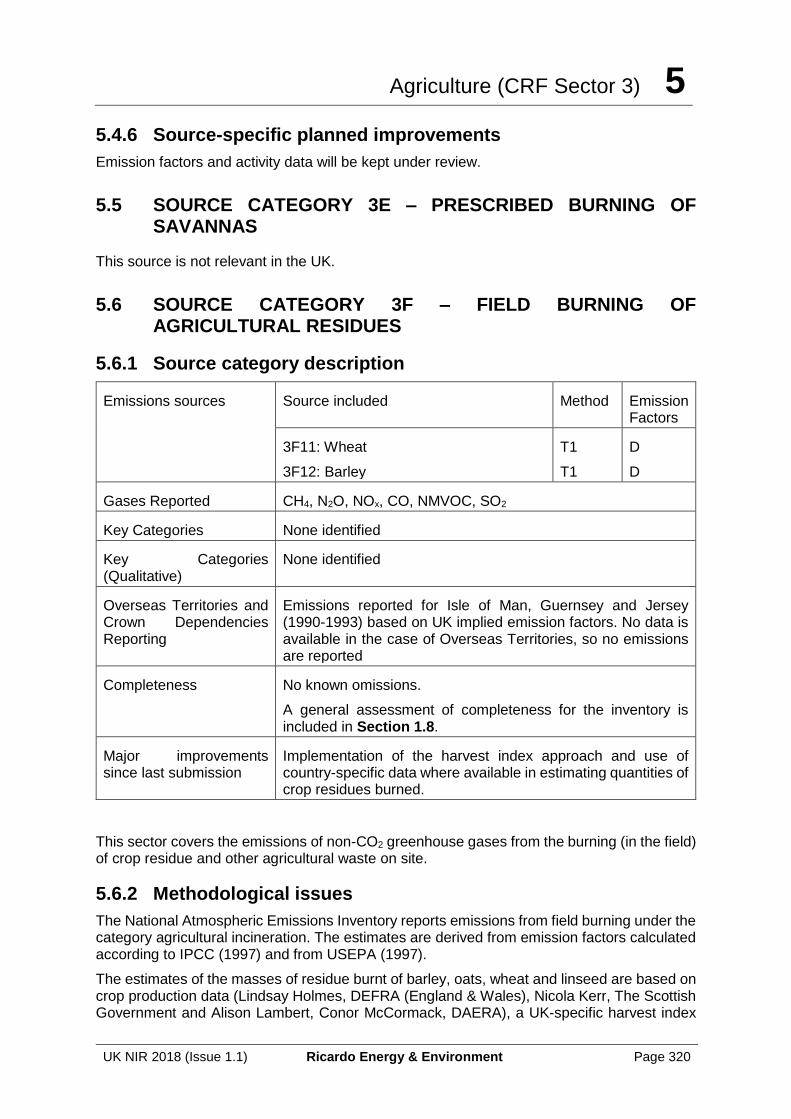
Agriculture (CRF Sector 3) 5
UK NIR 2018 (Issue 1.1) Ricardo Energy & Environment Page 320
5.4.6 Source-specific planned improvements
Emission factors and activity data will be kept under review.
5.5 SOURCE CATEGORY 3E – PRESCRIBED BURNING OF SAVANNAS
This source is not relevant in the UK.
5.6 SOURCE CATEGORY 3F – FIELD BURNING OF AGRICULTURAL RESIDUES
5.6.1 Source category description
Emissions sources Source included Method Emission Factors
3F11: Wheat
3F12: Barley
T1
T1
D
D
Gases Reported CH4, N2O, NOx, CO, NMVOC, SO2
Key Categories None identified
Key Categories (Qualitative)
None identified
Overseas Territories and Crown Dependencies Reporting
Emissions reported for Isle of Man, Guernsey and Jersey (1990-1993) based on UK implied emission factors. No data is available in the case of Overseas Territories, so no emissions are reported
Completeness No known omissions.
A general assessment of completeness for the inventory is included in Section 1.8.
Major improvements since last submission
Implementation of the harvest index approach and use of country-specific data where available in estimating quantities of crop residues burned.
This sector covers the emissions of non-CO2 greenhouse gases from the burning (in the field) of crop residue and other agricultural waste on site.
5.6.2 Methodological issues
The National Atmospheric Emissions Inventory reports emissions from field burning under the category agricultural incineration. The estimates are derived from emission factors calculated according to IPCC (1997) and from USEPA (1997).
The estimates of the masses of residue burnt of barley, oats, wheat and linseed are based on crop production data (Lindsay Holmes, DEFRA (England & Wales), Nicola Kerr, The Scottish Government and Alison Lambert, Conor McCormack, DAERA), a UK-specific harvest index
Agriculture (CRF Sector 3) 5
UK NIR 2018 (Issue 1.1) Ricardo Energy & Environment Page 321
approach to derive residue amounts (Williams and Goglio, 2017) and data on the fraction of crop residues burnt (MAFF, 1995; ADAS, 1995). Field burning ceased in 1993 in England and Wales. Burning in Scotland and Northern Ireland is considered negligible, so no estimates are reported from 1993 onwards. The carbon dioxide emissions are not estimated because these are part of the annual carbon cycle.
5.6.3 Uncertainties and time-series consistency
The uncertainty analysis in Annex 2 provides estimates of uncertainty according to IPCC source category.
Field burning ceased in 1993 and emissions are reported as NO after this date.
5.6.4 Source-specific QA/QC and verification
Emissions for the period 1990-1993 have been included for Isle of Man, Guernsey and Jersey, based on area of crops and UK implied emission factors.
This source category is covered by the general QA/QC procedures, which are discussed in Section 5.9.
5.6.5 Source-specific recalculations
Recalculations since the previous inventory submission are shown in Table 5.7.
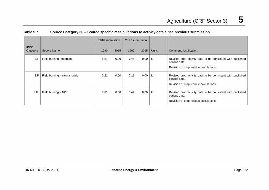
Agriculture (CRF Sector 3) 5
UK NIR 2018 (Issue .11) Ricardo Energy & Environment Page 322
Table 5.7 Source Category 3F – Source specific recalculations to activity data since previous submission
IPCC Category Source Name
2016 submission 2017 submission
Units Comment/Justification 1990 2015 1990 2015
3.F Field burning - methane 8.21 0.00 7.46 0.00 kt Revised crop activity data to be consistent with published census data.
Revision of crop residue calculations.
3.F Field burning – nitrous oxide 0.21 0.00 0.19 0.00 kt Revised crop activity data to be consistent with published census data.
Revision of crop residue calculations.
3.F. Field burning – NOx 7.61 0.00 6.44 0.00 kt Revised crop activity data to be consistent with published census data.
Revision of crop residue calculations.
Agriculture (CRF Sector 3) 5
UK NIR 2018 (Issue 1.1) Ricardo Energy & Environment Page 323
5.6.6 Source-specific planned improvements
No improvements are planned.
5.7 SOURCE CATEGORY 3G - LIMING
5.7.1 Source category description
Emissions sources Source included Method Emission Factors
3G1: Limestone CaCO3
3G2: Dolomite CaMg(CO3)2
T1
T1
D
D
Gases Reported CO2
Key Categories None identified
Key Categories (Qualitative)
None identified
Overseas Territories and Crown Dependencies Reporting
Emissions from 3G1 have been estimated for CDs. Emissions for OTs have not been estimated.
Completeness A general assessment of completeness for the inventory is included in Section 1.8.
Major improvements since last submission
Revision of the historical time series for activity data based on a new data provider.
5.7.2 Methodological issues
CO2 emissions due to the application of lime and related compounds are estimated using the Tier 1 IPCC (2006) methodology. For calcium carbonate (limestone, chalk and LimeX) an emission factor of 120 tC/kt applied is used, and for dolomite application, 130 tC/kt. These factors are based on the stoichiometry of the CO2 loss from the carbonates and assume pure limestone/chalk and dolomite.
Liming activity data (% area limed and application rate to three land use types: ‘all tillage’, ‘grass under 5 years old’ and ‘grass 5 years and over’) were obtained from the British Survey of Fertiliser Practice (BSFP; Table EW1.4 for England & Wales and Table SC1.4 for Scotland) from 1992 onwards; activity for 1990 and 1991 were assumed to be the same as for 1992. The % area limed and application rate of lime in Northern Ireland was assumed to be the same as that for Scotland by land use type. For each of the liming types in BSFP ( i) Ground limestone, ii) Ground chalk, iii) Magnesian limestone, iv) Sugar beet lime, iv) Other), the application rate and % area limed were multiplied by the area of ‘all tillage’, ‘grass under 5 years old’ and ‘grass 5 years and over’ to derive the total limestone and dolomite applied for each Devolved Administration.
The ‘Other’ category in BSFP is made up of Ag slag, Calcified pelleted limestone, Calicfert, Granules, Humistar, Lime slag, Screed lime (personal communication Alison Wray, Defra); the majority of these are CaCO3 based limes and thus were included in the activity data for limestone.
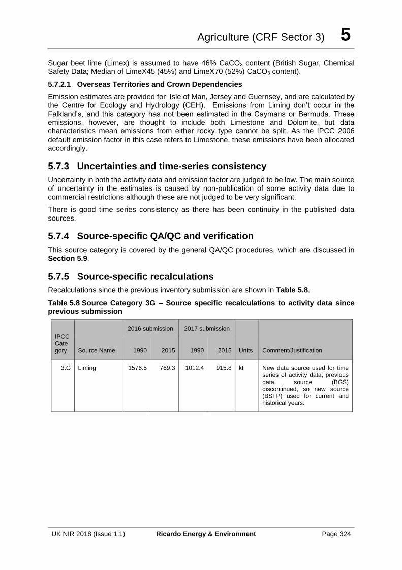
Agriculture (CRF Sector 3) 5
UK NIR 2018 (Issue 1.1) Ricardo Energy & Environment Page 324
Sugar beet lime (Limex) is assumed to have 46% CaCO3 content (British Sugar, Chemical Safety Data; Median of LimeX45 (45%) and LimeX70 (52%) CaCO3 content).
5.7.2.1 Overseas Territories and Crown Dependencies
Emission estimates are provided for Isle of Man, Jersey and Guernsey, and are calculated by the Centre for Ecology and Hydrology (CEH). Emissions from Liming don’t occur in the Falkland’s, and this category has not been estimated in the Caymans or Bermuda. These emissions, however, are thought to include both Limestone and Dolomite, but data characteristics mean emissions from either rocky type cannot be split. As the IPCC 2006 default emission factor in this case refers to Limestone, these emissions have been allocated accordingly.
5.7.3 Uncertainties and time-series consistency
Uncertainty in both the activity data and emission factor are judged to be low. The main source of uncertainty in the estimates is caused by non-publication of some activity data due to commercial restrictions although these are not judged to be very significant.
There is good time series consistency as there has been continuity in the published data sources.
5.7.4 Source-specific QA/QC and verification
This source category is covered by the general QA/QC procedures, which are discussed in Section 5.9.
5.7.5 Source-specific recalculations
Recalculations since the previous inventory submission are shown in Table 5.8.
Table 5.8 Source Category 3G – Source specific recalculations to activity data since previous submission
IPCC Category Source Name
2016 submission 2017 submission
Units Comment/Justification 1990 2015 1990 2015
3.G Liming
1576.5
769.3
1012.4
915.8 kt New data source used for time series of activity data; previous data source (BGS) discontinued, so new source (BSFP) used for current and historical years.
Agriculture (CRF Sector 3) 5
UK NIR 2018 (Issue 1.1) Ricardo Energy & Environment Page 325
5.8 SOURCE CATEGORY 3H - UREA APPLICATION
5.8.1 Source category description
Emissions sources Source included Method Emission Factors
3H: Urea Application T1 D
Gases Reported CO2
Key Categories None identified
Key Categories (Qualitative)
None identified
Overseas Territories and Crown Dependencies Reporting
Emissions from 3H have been estimated for all OTs and CDs, excluding the Falkland Islands and Bermuda.
Completeness A general assessment of completeness for the inventory is included in Section 1.8.
Major improvements since last submission
Revision to the historical time series of urea use
CO2 emissions due to the application of urea and related compounds are estimated using the Tier 1 methodology from the IPCC 2006 Guidelines.
5.8.2 Methodological issues
The annual amount of fertiliser as urea (alone or as part of urea ammonium nitrate, UAN) used in ktN was estimated from the British Survey of Fertiliser Practice (for England, Wales and Scotland) and the Northern Ireland Fertiliser Supply statistics. Both fertilisers are applied to grassland and cropland in the UK. It was assumed that 35% of UAN was urea. The EF used was the IPCC (2006) default value of 0.2 tonne of C tonnes of urea-1, and emission estimates were made using IPCC Tier 1 (2006, equation 11.13).
5.8.2.1 Overseas Territories and Crown Dependencies
For all Crown Dependencies, emissions have been estimated applying implied emission factors for urea application per hectare, sourced directly from Rothamsted Research Institute - an UK agricultural research body, to cropland and grassland land cover data. For the Cayman Islands, the amount of urea applied was provided by the focal point, and IPCC default value used for the estimates. Emissions for the Falklands Islands and Bermuda were not calculated due to lack of data availability.
5.8.3 Uncertainties and time-series consistency
The uncertainty analysis in Annex 2 provides estimates of uncertainty according to IPCC source category. The same data source is used for the entire time series to ensure consistency.
5.8.4 Source-specific QA/QC and verification
This source category is covered by the general QA/QC procedures, which are discussed in Section 5.9
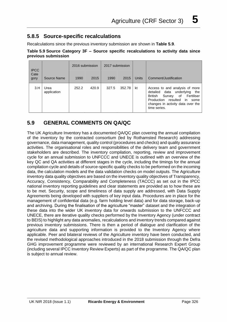
Agriculture (CRF Sector 3) 5
UK NIR 2018 (Issue 1.1) Ricardo Energy & Environment Page 326
5.8.5 Source-specific recalculations
Recalculations since the previous inventory submission are shown in Table 5.9.
Table 5.9 Source Category 3F – Source specific recalculations to activity data since previous submission
IPCC Category Source Name
2016 submission 2017 submission
Units Comment/Justification 1990 2015 1990 2015
3.H Urea application
252.2 420.9 327.5 352.78 kt Access to and analysis of more detailed data underlying the British Survey of Fertiliser Production resulted in some changes in activity data over the time series.
5.9 GENERAL COMMENTS ON QA/QC
The UK Agriculture Inventory has a documented QA/QC plan covering the annual compilation of the inventory by the contracted consortium (led by Rothamsted Research) addressing governance, data management, quality control (procedures and checks) and quality assurance activities. The organisational roles and responsibilities of the delivery team and government stakeholders are described. The inventory compilation, reporting, review and improvement cycle for an annual submission to UNFCCC and UNECE is outlined with an overview of the key QC and QA activities at different stages in the cycle, including the timings for the annual compilation cycle and details of source-specific quality checks to be performed on the incoming data, the calculation models and the data validation checks on model outputs. The Agriculture inventory data quality objectives are based on the inventory quality objectives of Transparency, Accuracy, Consistency, Comparability and Completeness (TACCC) as set out in the IPCC national inventory reporting guidelines and clear statements are provided as to how these are to be met. Security, scope and timeliness of data supply are addressed, with Data Supply Agreements being developed with suppliers of key input data. Procedures are in place for the management of confidential data (e.g. farm holding level data) and for data storage, back-up and archiving. During the finalisation of the agriculture “master” dataset and the integration of these data into the wider UK inventory data for onwards submission to the UNFCCC and UNECE, there are iterative quality checks performed by the Inventory Agency (under contract to BEIS) to highlight any data anomalies, recalculations and inventory trends compared against previous inventory submissions. There is then a period of dialogue and clarification of the agriculture data and supporting information is provided to the Inventory Agency where applicable. Peer and bilateral reviews of the Agriculture inventory have been conducted, and the revised methodological approaches introduced in the 2018 submission through the Defra GHG improvement programme were reviewed by an international Research Expert Group (including several IPCC Inventory Review Experts) as part of the programme. The QA/QC plan is subject to annual review.
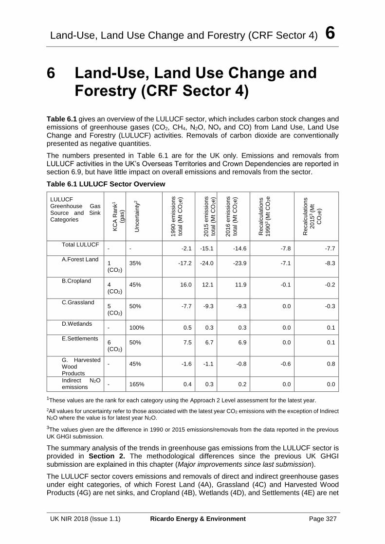
Land-Use, Land Use Change and Forestry (CRF Sector 4) 6
UK NIR 2018 (Issue 1.1) Ricardo Energy & Environment Page 327
6 Land-Use, Land Use Change and Forestry (CRF Sector 4)
Table 6.1 gives an overview of the LULUCF sector, which includes carbon stock changes and emissions of greenhouse gases (CO2, CH4, N2O, NOx and CO) from Land Use, Land Use Change and Forestry (LULUCF) activities. Removals of carbon dioxide are conventionally presented as negative quantities.
The numbers presented in Table 6.1 are for the UK only. Emissions and removals from LULUCF activities in the UK’s Overseas Territories and Crown Dependencies are reported in section 6.9, but have little impact on overall emissions and removals from the sector.
Table 6.1 LULUCF Sector Overview
LULUCF Greenhouse Gas Source and Sink Categories
KC
A R
an
k1
(ga
s)
Unce
rtain
ty2
19
90
em
issio
ns
tota
l (M
t C
O2e
)
20
15
em
issio
ns
tota
l (M
t C
O2e
)
20
16
em
issio
ns
tota
l (M
t C
O2e
)
Reca
lcu
lation
s
19
90
3 (M
t C
O2e
Reca
lcu
lation
s
20
15
3 (M
t
CO
2e
)
Total LULUCF - - -2.1 -15.1 -14.6 -7.8 -7.7
A.Forest Land 1
(CO2) 35% -17.2 -24.0 -23.9 -7.1 -8.3
B.Cropland 4 (CO2)
45% 16.0 12.1 11.9 -0.1 -0.2
C.Grassland 5 (CO2)
50% -7.7 -9.3 -9.3 0.0 -0.3
D.Wetlands - 100% 0.5 0.3 0.3 0.0 0.1
E.Settlements 6 (CO2)
50% 7.5 6.7 6.9 0.0 0.1
G. Harvested Wood Products
- 45% -1.6 -1.1 -0.8 -0.6 0.8
Indirect N2O emissions
- 165% 0.4 0.3 0.2 0.0 0.0
1These values are the rank for each category using the Approach 2 Level assessment for the latest year.
2All values for uncertainty refer to those associated with the latest year CO2 emissions with the exception of Indirect N2O where the value is for latest year N2O.
3The values given are the difference in 1990 or 2015 emissions/removals from the data reported in the previous
UK GHGI submission.
The summary analysis of the trends in greenhouse gas emissions from the LULUCF sector is provided in Section 2. The methodological differences since the previous UK GHGI submission are explained in this chapter (Major improvements since last submission).
The LULUCF sector covers emissions and removals of direct and indirect greenhouse gases under eight categories, of which Forest Land (4A), Grassland (4C) and Harvested Wood Products (4G) are net sinks, and Cropland (4B), Wetlands (4D), and Settlements (4E) are net
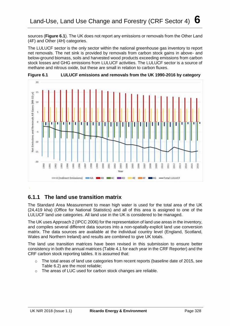
Land-Use, Land Use Change and Forestry (CRF Sector 4) 6
UK NIR 2018 (Issue 1.1) Ricardo Energy & Environment Page 328
sources (Figure 6.1). The UK does not report any emissions or removals from the Other Land (4F) and Other (4H) categories.
The LULUCF sector is the only sector within the national greenhouse gas inventory to report net removals. The net sink is provided by removals from carbon stock gains in above- and below-ground biomass, soils and harvested wood products exceeding emissions from carbon stock losses and GHG emissions from LULUCF activities. The LULUCF sector is a source of methane and nitrous oxide, but these are small in relation to carbon fluxes.
Figure 6.1 LULUCF emissions and removals from the UK 1990-2016 by category
.
6.1.1 The land use transition matrix
The Standard Area Measurement to mean high water is used for the total area of the UK (24,419 kha) (Office for National Statistics) and all of this area is assigned to one of the LULUCF land use categories. All land use in the UK is considered to be managed.
The UK uses Approach 2 (IPCC 2006) for the representation of land use areas in the inventory, and compiles several different data sources into a non-spatially-explicit land use conversion matrix. The data sources are available at the individual country level (England, Scotland, Wales and Northern Ireland) and results are combined to give UK totals.
The land use transition matrices have been revised in this submission to ensure better consistency in both the annual matrices (Table 4.1 for each year in the CRF Reporter) and the CRF carbon stock reporting tables. It is assumed that:
o The total areas of land use categories from recent reports (baseline date of 2015, see Table 6.2) are the most reliable;
o The areas of LUC used for carbon stock changes are reliable.
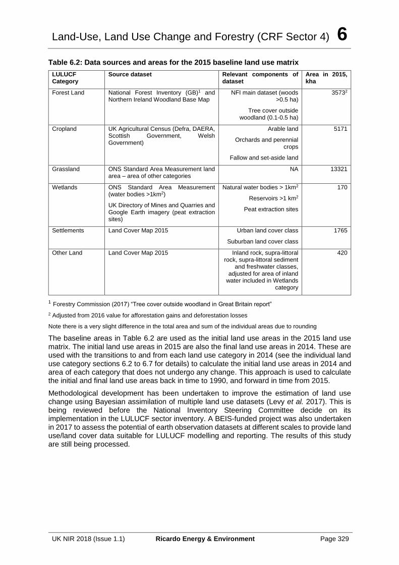
Land-Use, Land Use Change and Forestry (CRF Sector 4) 6
UK NIR 2018 (Issue 1.1) Ricardo Energy & Environment Page 329
Table 6.2: Data sources and areas for the 2015 baseline land use matrix
LULUCF Category
Source dataset Relevant components of dataset
Area in 2015, kha
Forest Land National Forest Inventory (GB)1 and Northern Ireland Woodland Base Map
NFI main dataset (woods >0.5 ha)
Tree cover outside woodland (0.1-0.5 ha)
35732
Cropland UK Agricultural Census (Defra, DAERA, Scottish Government, Welsh Government)
Arable land
Orchards and perennial crops
Fallow and set-aside land
5171
Grassland ONS Standard Area Measurement land area – area of other categories
NA 13321
Wetlands ONS Standard Area Measurement (water bodies >1km2)
UK Directory of Mines and Quarries and Google Earth imagery (peat extraction sites)
Natural water bodies > 1km2
Reservoirs >1 km2
Peat extraction sites
170
Settlements Land Cover Map 2015 Urban land cover class
Suburban land cover class
1765
Other Land Land Cover Map 2015 Inland rock, supra-littoral rock, supra-littoral sediment
and freshwater classes, adjusted for area of inland
water included in Wetlands category
420
1 Forestry Commission (2017) “Tree cover outside woodland in Great Britain report”
2 Adjusted from 2016 value for afforestation gains and deforestation losses
Note there is a very slight difference in the total area and sum of the individual areas due to rounding
The baseline areas in Table 6.2 are used as the initial land use areas in the 2015 land use matrix. The initial land use areas in 2015 are also the final land use areas in 2014. These are used with the transitions to and from each land use category in 2014 (see the individual land use category sections 6.2 to 6.7 for details) to calculate the initial land use areas in 2014 and area of each category that does not undergo any change. This approach is used to calculate the initial and final land use areas back in time to 1990, and forward in time from 2015.
Methodological development has been undertaken to improve the estimation of land use change using Bayesian assimilation of multiple land use datasets (Levy et al. 2017). This is being reviewed before the National Inventory Steering Committee decide on its implementation in the LULUCF sector inventory. A BEIS-funded project was also undertaken in 2017 to assess the potential of earth observation datasets at different scales to provide land use/land cover data suitable for LULUCF modelling and reporting. The results of this study are still being processed.
Land-Use, Land Use Change and Forestry (CRF Sector 4) 6
UK NIR 2018 (Issue 1.1) Ricardo Energy & Environment Page 330
6.2 CATEGORY 4A – FOREST LAND
6.2.1 Description
Emissions sources 4A Forest Land: carbon stock change 4(I) Direct nitrous oxide (N2O) emissions from nitrogen (N) inputs to managed soils 4(II) Emissions and removals from drainage and rewetting and other management of organic and mineral soils 4(III) Direct nitrous oxide (N2O) emissions from nitrogen (N) mineralization/immobilization associated with loss/gain of soil organic matter resulting from change of land use or management of mineral soils 4(V) Biomass burning
Gases Reported CO2, CH4, N2O
Methods T3 for carbon stock changes, T1 for other emissions
Emission Factors Country-specific for T3 methods
Key Categories 4A: Forest land - CO2 (L1, L2)
Key Categories (Qualitative)
None identified
Completeness Methane emissions from drained forest soils are not estimated due to insufficient information. GHG emissions from rewetted forest soils are not estimated due to insufficient information.
Major improvements since last submission
Assumptions of forest age and location have been adjusted for Forest land in the 0.1-0.5 ha size range, increasing the area of Forest remaining Forest and changing the proportion of forest on mineral soil. Changes to the CARBINE model to include litter input from non-forest vegetation, fine root turnover, soil carbon decomposition and inclusion of roots in the litter pool.
Forest Land includes carbon stock gains and losses and GHG emissions from forest management and overall is the biggest net sink in the UK. All UK forests are temperate and about 72% of these have been planted since 1921 on land that had not been forested for many decades.
The UK reports carbon stock changes in all forests. Forest surveys have been intermittent in the UK and to date there has been no network of permanent sample plots suitable for constructing a GHG inventory. Consequently, estimates of carbon stock gains and losses for biomass and soils are modelled based on planting history,productivity (yield class) data and assumptions over approaches to forest management. Forest carbon stock changes and fluxes are modelled by CARBINE, the Forest Research forest carbon stock model (described in Annex 3.4.1). CARBINE takes account of the effects of forest management on carbon stocks, and also calculates the carbon stocks in the Harvested Wood Products pool.
Carbon stock changes resulting from afforestation on Cropland, Grassland and Settlement areas are calculated. Conversion of Wetlands and Other Land to Forest Land does not occur in the UK. The reported forest area and carbon stock changes take account of losses of forest land converted to other land use categories (deforestation) and the associated carbon stock changes and emissions and removals are then estimated and reported under the category concerned.
Land-Use, Land Use Change and Forestry (CRF Sector 4) 6
UK NIR 2018 (Issue 1.1) Ricardo Energy & Environment Page 331
In the UK inorganic nitrogen fertilisers are only applied to forest when absolutely necessary. This occurs during the first rotation on ‘poor’ soils, such as reclaimed slag heaps, impoverished brown field sites and upland organic soils, hence N fertilisation is assumed for all areas of Settlements converted to Forest Land and Grassland converted to Forest Land on organic soils. N2O emissions from this fertilisation are reported under 4.A.2 in CRF Table 4(I). Nitrogen fertilisers are not generally applied to native woodlands, mature forests or re-planted forests in the UK, so emissions of N2O from N fertilisation of forests (CRF Table 4(I)) for 4.A.1 are reported as Not Occurring.
Drainage of forest land occurs in UK forests planted since 1920 on certain soil types. It is assumed that all forests planted on organic soils are drained prior to planting. Forests planted on mineral or organo-mineral soils which have slow natural drainage and are prone to waterlogging are also assumed to be artificially drained. CO2 emissions from drainage are included with carbon stock changes in Table 4.A and N2O emissions from drainage in Table 4(II). There is insufficient information to enable reporting of methane and rewetting emissions.
Controlled burning of forest land (for example for habitat management) does not take place in the UK. Wildfires do occur but the activity data are not sufficient to split reporting between 4.A.1 and 4.A.2. Therefore emissions of greenhouse gases from wildfires are all reported under 4.A.1 in Table 4(V). It is assumed that land use change does not occur following wildfire.
6.2.2 Information on approaches used for representing land areas and on land use databases used for the inventory preparation
The agencies responsible for forests in the UK are the Forestry Commission (England and Scotland), Natural Resources Wales (Wales) and the Forest Service (Northern Ireland). Areas of forest planted annually are published in Forest Statistics40 and a detailed breakdown (by forest type and management) is used as input to the CARBINE model, supplemented by information from the National Forest Inventory (NFI) field survey. The allocation of land use change from other land use categories is based on the proportional changes in the land use change matrices from the Countryside Survey (see section 6.3 and Annex 3.4).
6.2.3 Land-use definitions and the classification system used and their correspondence to the LULUCF categories
The UK uses the following definition of forest for reporting UK forestry statistics as it relates to the UK’s greenhouse gas inventory submitted under the UNFCCC:
• Minimum area of 0.1 hectares;
• Minimum width of 20 metres;
• Tree crown cover of at least 20 per cent, or the potential to achieve it;
• Minimum height of 2 metres, or the potential to achieve it.
This definition includes felled areas awaiting restocking and integral open spaces up to 0.5 hectares.
All forest areas in the UK can be regarded as managed from the point of view of regulation against deforestation and protection against fire, storms and disease. In general, forest areas are actively managed for landscape, soil protection, habitat conservation, amenity and recreation, which may or may not include active management for wood production.
40 http://www.forestry.gov.uk/statistics
Land-Use, Land Use Change and Forestry (CRF Sector 4) 6
UK NIR 2018 (Issue 1.1) Ricardo Energy & Environment Page 332
6.2.4 Methodological Issues
In this inventory submission the carbon uptake by UK forests is calculated using a Tier 3 carbon accounting model, CARBINE. Overall carbon uptake is calculated as the net change in the pools of carbon in standing trees, litter, soil and products from harvested material, for conifer and broadleaf forests. The model is able to represent all of the introduced and native plantation and naturally-occurring species relevant to UK forestry, the different growth rates of forests and four broad classes of forest management (clear-fell with thinnings, clear-fell without thinnings, thinned but not clear-felled and no timber production). The forest carbon sub-model is further compartmentalised to represent fractions associated with tree stems, branches, foliage, and roots.
The CARBINE model produces separate gains and losses for carbon stock change in living biomass, rather than net change. Carbon stock changes in dead wood are included with carbon stock changes in litter. Further detail on the CARBINE model is given in Annex 3.4.1 and Matthews et al. (2014). There have been methodological improvements to the CARBINE model for this submission: these improvements and their impact are described in the recalculations (section 6.2.7).
Other greenhouse gas emissions, including those arising from forest fertilisation and wildfires together with estimates of N2O emissions from forest drainage, are estimated using Tier 1 or Tier 2 approaches, and are described in Annex 3.4.
6.2.5 Uncertainties and Time-Series Consistency
4A Forest Land is estimated to have a combined uncertainty of 35% for CO2, 55% for CH4 and 100-105% for N2O.
An uncertainty analysis was undertaken in 2011 to reassess sources of uncertainty (input data, model parameters and structural/model choice) in the LULUCF sector and identify priority areas for improvement (Annex 3.4.12). Monte Carlo simulations were run to propagate input and parameter uncertainty for different source categories, and the uncertainty arising from model choice was quantified by using alternative sub-models for key processes. The main sources of uncertainty (ranked by standard deviation in output distributions) are afforestation model parameters, afforestation input data, forest soil carbon model choice and afforestation model choice. Although this analysis was done for the C-Flow model, the functionality of CARBINE is broadly similar and we assume that the uncertainty of the inputs and parameters are also similar. These assumptions are currently under review and will be updated. The main difference due to the switch to the CARBINE model is that there is a greater range of species, growth rates and possible management regimes giving a more realistic representation of forestry in the UK (Matthews et al. 2014). Future uncertainty analyses will include the processes represented in CARBINE and the revised forestry datasets.
The planting statistics used as activity data mostly come from operational systems, for grants and for planting on the National Forest Estates of the four countries comprising the UK (supplemented by information from the NFI field survey), and have no measures of statistical uncertainty attached to them as complete coverage is assumed. Grants are paid once planting has occurred. The grant-aided planting is allocated by year of payment, so all the recorded planting should have taken place. There is ongoing work within the Forestry Commission to assess the level of error attached to the data, e.g. for failed planting. The area of forest in GB is based on the new NFI woodland map, together with small woods of between 0.1 and 0.5 ha. A field survey used to estimate the stocked area and composition (including age distribution) of the non-FC/NRW forest estate is based on a sub-sampling of the population and scaling to the mapped level.
Land-Use, Land Use Change and Forestry (CRF Sector 4) 6
UK NIR 2018 (Issue 1.1) Ricardo Energy & Environment Page 333
With regard to series consistency:
• For forest carbon stock changes, N fertilization of forests and emissions from drainage, time series consistency is expected to be good as activity data are obtained consistently from the same national forestry sources; and,
• For emissions from wildfires, data have been collated from several published sources. From 1990 – 2004 all data originate from the state forestry agencies so there is good time series consistency during this period. Data have been extrapolated for 2005-2009. A newer and more complete data source for England, Scotland and Wales is used from 2010 onwards, and gives wildfire burnt areas which are the same magnitude as the previous dataset.
6.2.6 Category-Specific QA/QC and Verification
This source category is covered by the general QA/QC procedures, which are discussed in Section 6.10. Information on forest planting and the area affected by wildfires is consistent with that reported to the FAO (2005, 2010, 2015).
As part of a separate research project, a comparison has been made of the predictions made by the CEH C-Flow model and Forest Research CARBINE model. The results demonstrated that the models produce consistent predictions when given the same input data and assumptions (e.g. about woodland management practices). Further work has been undertaken comparing the inventory as predicted by CARBINE to the inventory as predicted by C-Flow and detailing the changes in assumptions that drive the changes in the inventory (Matthews et al., 2014). Verification of carbon stock changes will be undertaken once the second cycle of the NFI is completed (in 2020).
A review of inventory data and models has been undertaken (Levy and Rowland, 2011), during which data were collated and critically assessed on soil carbon stocks following afforestation. Generally, soil carbon stocks are assumed to increase after afforestation in the UK, following on as a result of the increased above-ground biomass and litter inputs, based on a small number of long term studies. In fact, in the UK studies which attempt to measure this, soil carbon stocks in forested plots were 15 to 60 % lower than in adjacent unplanted, grassland or moorland (Reay et al., 2001; Chapman et al. 2003; Zerva and Mencuccini 2005; Mitchell et al. 2007; Bellamy and Rivas-Casado 2009; Levy and Clark 2009). These results are in agreement with global meta-analyses, which have reported mean changes in soil carbon stocks of around -10 %, -7 %, +3 % and -4 % associated with conversion of pasture to forest plantation (Guo and Gifford 2002; Laganiere, Angers et al. 2010; Poeplau, Don et al. 2011 respectively). The treatment of the litter layer in these studies is a significant uncertainty, as it is possible that some of the reported decreases in soil carbon following afforestation were compensated by increases in carbon stocks of the above-ground litter layer which is not included in the soil samples.
A new soil and litter model has been implemented in CARBINE to better model the carbon emissions from forest soils. The full specification and information on the validation of this model will be published in a separate technical report.
6.2.7 Category-Specific Recalculations
The reported overall net GHG sink in category 4A has increased by between 7 and 8 Mt CO2e (50-70%) across the time series compared to the 2015 inventory.
The changes were mainly seen in the carbon stock changes in the litter pool under Forest Remaining Forest, and in the soil pool of Land converted to Forest. The main causes of this change were modifications of the litter model in CARBINE and the inclusion of non-forest ground vegetation, but other improvements also contributed.
Land-Use, Land Use Change and Forestry (CRF Sector 4) 6
UK NIR 2018 (Issue 1.1) Ricardo Energy & Environment Page 334
The changes and their justification are:
• Forest area changes: The area of recent afforestation was brought into line with new planting statistics by altering the age assumptions for small woodlands (0.1-0.5 ha) and increasing the ages of some larger woodlands. The reported area of Forest remaining Forest has increased and the proportion of forest on mineral and organic soils changed. This also affected the volume of fertiliser and the area of drainage.
• Improvements to CARBINE
o Added non-tree vegetation: It is now assumed that there is litter input to the soils from non-tree vegetation when the forest canopy is not fully closed. If this litter input is not included there is an excessive loss of soil carbon following afforestation, particularly on low productivity stands with longer times before canopy closure.
o Added in-year turnover: In-year turnover of fine-roots is now included in live biomass. This is modelled as an in-year gain and loss of carbon so that carbon entering the litter and deadwood pools can be traced back to source.
o Added roots to litter: Roots are now included in the litter/dead biomass pool.
o Constrained soil carbon accumulation: The soil model has been adjusted to incorporate all the organic matter transfer to the soil to avoid over-estimates of soil carbon accumulation.
• Change of FL sub-category: The small area of Other Land converted to Forest Land has been re-allocated to Grassland converted to Forest Land, following a UN review recommendation, as Grassland now functions as the “buffer” land use category in the UK GHGI.
• Updated average area value: The latest data on wildfires has been used to update the time series average used for back-calculating to 1990.
The magnitude of the changes and the abbreviated justification are given in Table 6.3.
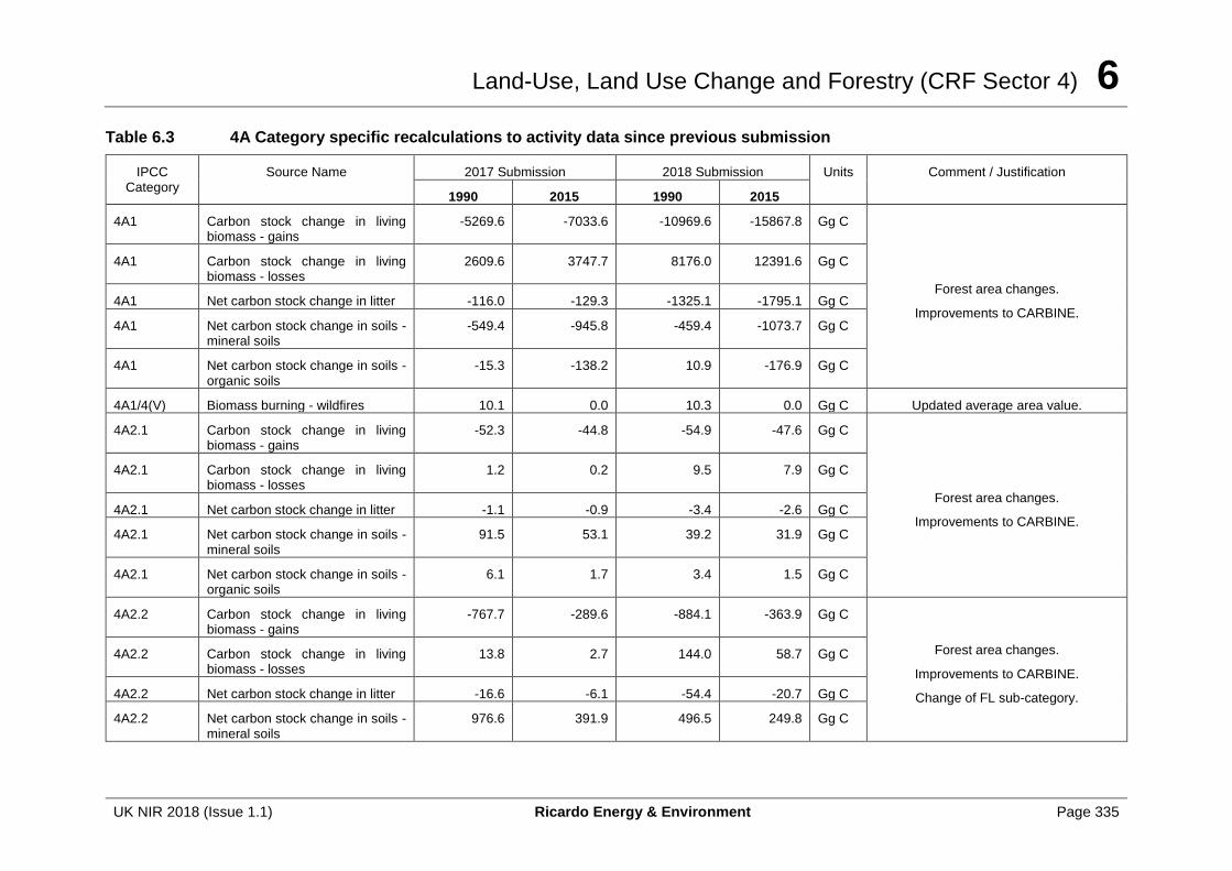
Land-Use, Land Use Change and Forestry (CRF Sector 4) 6
UK NIR 2018 (Issue 1.1) Ricardo Energy & Environment Page 335
Table 6.3 4A Category specific recalculations to activity data since previous submission
IPCC Category
Source Name 2017 Submission 2018 Submission Units Comment / Justification
1990 2015 1990 2015
4A1 Carbon stock change in living biomass - gains
-5269.6 -7033.6 -10969.6 -15867.8 Gg C
Forest area changes.
Improvements to CARBINE.
4A1 Carbon stock change in living biomass - losses
2609.6 3747.7 8176.0 12391.6 Gg C
4A1 Net carbon stock change in litter -116.0 -129.3 -1325.1 -1795.1 Gg C
4A1 Net carbon stock change in soils - mineral soils
-549.4 -945.8 -459.4 -1073.7 Gg C
4A1 Net carbon stock change in soils - organic soils
-15.3 -138.2 10.9 -176.9 Gg C
4A1/4(V) Biomass burning - wildfires 10.1 0.0 10.3 0.0 Gg C Updated average area value.
4A2.1 Carbon stock change in living biomass - gains
-52.3 -44.8 -54.9 -47.6 Gg C
Forest area changes.
Improvements to CARBINE.
4A2.1 Carbon stock change in living biomass - losses
1.2 0.2 9.5 7.9 Gg C
4A2.1 Net carbon stock change in litter -1.1 -0.9 -3.4 -2.6 Gg C
4A2.1 Net carbon stock change in soils - mineral soils
91.5 53.1 39.2 31.9 Gg C
4A2.1 Net carbon stock change in soils - organic soils
6.1 1.7 3.4 1.5 Gg C
4A2.2 Carbon stock change in living biomass - gains
-767.7 -289.6 -884.1 -363.9 Gg C
Forest area changes.
Improvements to CARBINE.
Change of FL sub-category.
4A2.2 Carbon stock change in living biomass - losses
13.8 2.7 144.0 58.7 Gg C
4A2.2 Net carbon stock change in litter -16.6 -6.1 -54.4 -20.7 Gg C
4A2.2 Net carbon stock change in soils - mineral soils
976.6 391.9 496.5 249.8 Gg C
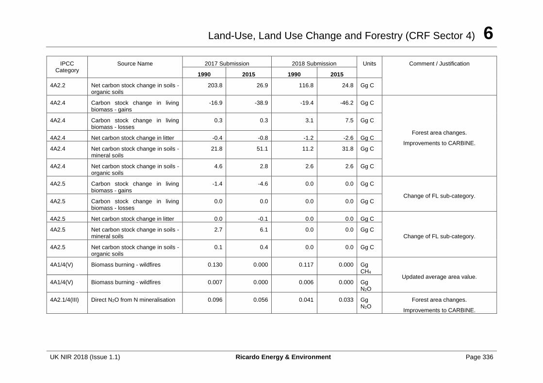
Land-Use, Land Use Change and Forestry (CRF Sector 4) 6
UK NIR 2018 (Issue 1.1) Ricardo Energy & Environment Page 336
IPCC Category
Source Name 2017 Submission 2018 Submission Units Comment / Justification
1990 2015 1990 2015
4A2.2 Net carbon stock change in soils - organic soils
203.8 26.9 116.8 24.8 Gg C
4A2.4 Carbon stock change in living biomass - gains
-16.9 -38.9 -19.4 -46.2 Gg C
Forest area changes.
Improvements to CARBINE.
4A2.4 Carbon stock change in living biomass - losses
0.3 0.3 3.1 7.5 Gg C
4A2.4 Net carbon stock change in litter -0.4 -0.8 -1.2 -2.6 Gg C
4A2.4 Net carbon stock change in soils - mineral soils
21.8 51.1 11.2 31.8 Gg C
4A2.4 Net carbon stock change in soils - organic soils
4.6 2.8 2.6 2.6 Gg C
4A2.5 Carbon stock change in living biomass - gains
-1.4 -4.6 0.0 0.0 Gg C
Change of FL sub-category. 4A2.5 Carbon stock change in living
biomass - losses 0.0 0.0 0.0 0.0 Gg C
4A2.5 Net carbon stock change in litter 0.0 -0.1 0.0 0.0 Gg C
Change of FL sub-category. 4A2.5 Net carbon stock change in soils -
mineral soils 2.7 6.1 0.0 0.0 Gg C
4A2.5 Net carbon stock change in soils - organic soils
0.1 0.4 0.0 0.0 Gg C
4A1/4(V) Biomass burning - wildfires 0.130 0.000 0.117 0.000 Gg CH4
Updated average area value. 4A1/4(V) Biomass burning - wildfires 0.007 0.000 0.006 0.000 Gg
N2O
4A2.1/4(III) Direct N2O from N mineralisation 0.096 0.056 0.041 0.033 Gg N2O
Forest area changes.
Improvements to CARBINE.
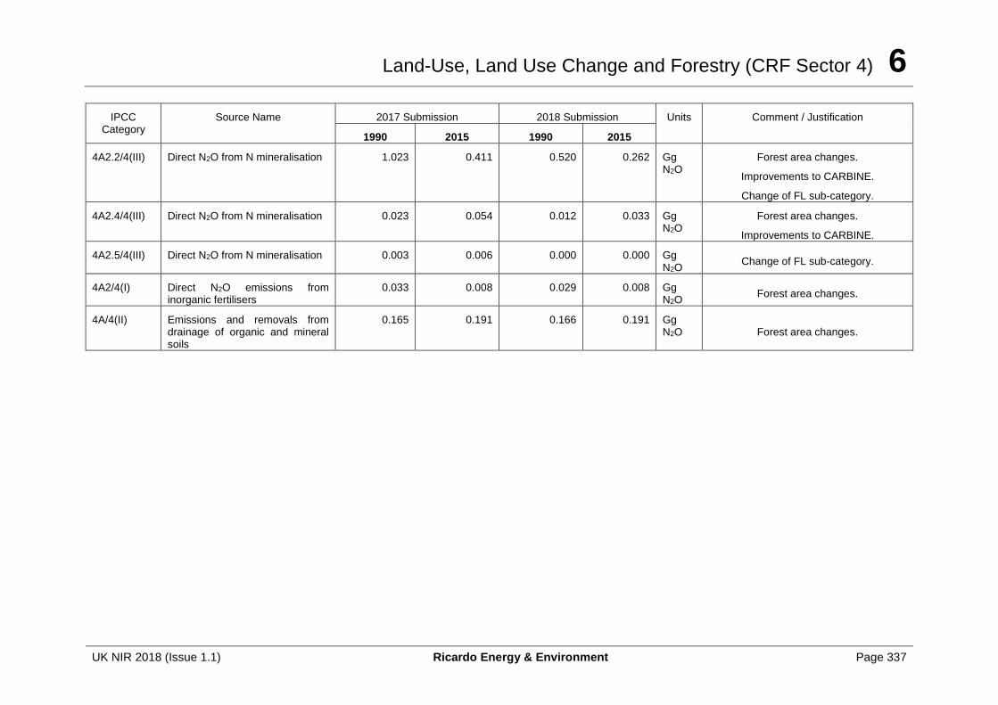
Land-Use, Land Use Change and Forestry (CRF Sector 4) 6
UK NIR 2018 (Issue 1.1) Ricardo Energy & Environment Page 337
IPCC Category
Source Name 2017 Submission 2018 Submission Units Comment / Justification
1990 2015 1990 2015
4A2.2/4(III) Direct N2O from N mineralisation 1.023 0.411 0.520 0.262 Gg N2O
Forest area changes.
Improvements to CARBINE.
Change of FL sub-category.
4A2.4/4(III) Direct N2O from N mineralisation 0.023 0.054 0.012 0.033 Gg N2O
Forest area changes.
Improvements to CARBINE.
4A2.5/4(III) Direct N2O from N mineralisation 0.003 0.006 0.000 0.000 Gg N2O
Change of FL sub-category.
4A2/4(I) Direct N2O emissions from inorganic fertilisers
0.033 0.008 0.029 0.008 Gg N2O
Forest area changes.
4A/4(II) Emissions and removals from drainage of organic and mineral soils
0.165 0.191 0.166 0.191 Gg N2O Forest area changes.
Land-Use, Land Use Change and Forestry (CRF Sector 4) 6
UK NIR 2018 (Issue 1.1) Ricardo Energy & Environment Page 338
6.2.8 Category-Specific Planned Improvements
In order to better ensure time series consistency between the estimates of timber production before and after the forest inventory year an automated algorithm will be introduced to adjust the assumed forest management to harmonise the level of timber production.
6.3 CATEGORY 4B – CROPLAND
6.3.1 Description
Emissions sources 4B Cropland: carbon stock change 4B Cropland:4(III) N2O emissions from disturbance associated with LUC to Cropland 4B Cropland:4(V) Biomass burning
Gases Reported CO2, CH4, N2O
Methods T3 for carbon stock changes, T1 for other emissions
Emission Factors Country-specific for T3 methods, T1/2 for other emissions
Key Categories 4B: Cropland - CO2 (L1, T1, L2, T2)
Key Categories (Qualitative)
None identified
Completeness No known omissions.
Major improvements since last submission
A change in reporting table for cropland on drained organic soils, in response to a review team recommendation (see section 6.3.7 for more details)
Net emissions from the Cropland category include carbon stock gains and losses due to land use change (LUC) and GHG emissions from cropland management and overall is the largest net source in the LULUCF sector.
Ongoing carbon stock changes in soils arising from LUC to Cropland are reported under both 4.B.2. (for LUC in the past 20 years) and 4.B.1 (for historic LUC >20 years before the inventory reporting year). These soil net carbon stock changes are the largest component of the category total emissions, and are calculated using a Tier 3 dynamic soil carbon model.
Other contributors to the Cropland net total emissions are:
• carbon emissions resulting from drainage of organic soils;
• carbon stock changes in biomass and soils resulting from changes in cropland management;
• biomass carbon stock changes due to LUC;
• N2O emissions from soil disturbance associated with LUC;
• biomass burning emissions of GHGs from controlled burning following forest land conversion to cropland; and
• biomass burning emissions of GHGs due to wildfires.
All forms of land use change, including deforestation, are considered and both mineral and organic soils are included. In some categories, e.g. Forest Land converted to Cropland, the area of land undergoing transition falls to zero and is subsequently reported as Not Occurring.
Ongoing N2O emissions from soil as a result of land use change > 20 years ago are reported in the Agricultural sector inventory as N2O emissions from managed agricultural soils (CEH provide the appropriate areas and carbon stock changes to Rothamsted Research). Nitrous oxide emissions from loss of soil organic matter as a result of Cropland Management are also reported in the Agricultural sector inventory as N2O emissions from managed agricultural soils.
Land-Use, Land Use Change and Forestry (CRF Sector 4) 6
UK NIR 2018 (Issue 1.1) Ricardo Energy & Environment Page 339
Emissions of CO2, CH4 and N2O from controlled biomass burning arising from Forest Land conversion to Cropland are reported in Table 4(V). Burning of agricultural residues (cereal straw or stubble) are reported under category 3F Field Burning of Agricultural Residues. Full details of the method and activity data are given in Annex 3.4.
6.3.2 Information on approaches used for representing land areas and on land use databases used for the inventory preparation
The UK uses Approach 2 (IPCC 2006) for the representation of land use areas in the inventory, and compiles several different data sources into a non-spatially-explicit land use conversion matrix (see section 6.1.1 for details).
Data sources that contain area information for reporting carbon stock changes and/or emissions from Cropland are:
• Habitat/landscape surveys o Countryside Survey (1984, 1990, 2000, 2007) is used to compile land use
transition matrices.
• An assessment of Cropland drainage o Areas of Cropland that are losing carbon due to historical drainage (reported
under Cropland remaining Cropland) have been assessed by Anthony et al. (personal communication - unpublished report from Defra project AC0114, 2013) Their analysis overlaid areas of Cropland from the Land Cover Map and the Integrated Administration and Control System (IACS) with mapping of organic soils from soil surveys. All Cropland on organic soils was assumed to be drained. The vast majority of Cropland on drained organic soils is in England, but small areas in the other UK administrations are also identified.
• Agricultural survey data o Areas of the main crop types are obtained from the June Agricultural Censuses
for each UK administration. o The areas of Cropland receiving inputs of manure, fertiliser and crop residues
are obtained from the British Survey of Fertiliser Practice.
• Data on wildfires on agricultural land from Fire and Rescue service and satellite data. o Areas of wildfire on Cropland for 2010-present come from Fire and Rescue
service data. o Between 2001 and 2009 the area of wildfire on Cropland is calculated by using
satellite data on the total area of wildfires in the UK which are apportioned to land use using the same ratios as found in the Fire and Rescue service data.
o Cropland wildfire areas prior to 2001 are extrapolated (see Annex 3.4.5 for details)
6.3.3 Land-use definitions and the classification system used and their correspondence to the LULUCF categories
Cropland is defined in accordance with the Agriculture, Forestry and Other Land Use Guidance (IPCC 2006). For pre-1980 land use matrices cropland is the sum of the Crops, Orchards and Market Garden land cover types in the Monitoring Landscape Change project (MLC 1986). Post-1980, Cropland is the area of cropland reported in the June Agricultural censuses. Crop types definitions are those used in the June Agricultural censuses.
Land-Use, Land Use Change and Forestry (CRF Sector 4) 6
UK NIR 2018 (Issue 1.1) Ricardo Energy & Environment Page 340
6.3.4 Methodological Issues
6.3.4.1 Land Use change
Activity data for land use change are estimated using a land use change (LUC) matrix approach. Detailed descriptions of the methods, emission factors and data flows used for Cropland activities are given in Annex 3.4.2.
A dynamic model of carbon stock change is used with the LUC matrices to estimate soil carbon stock changes due to all LUC. Soil carbon stock changes are modelled as changing exponentially between initial and final land uses with the most rapid change in the early years following the transition. It is assumed that LUC does not occur on cropland on organic soils because of the high productivity (and high monetary value) of these areas.
The carbon stocks for each land use category are calculated as averages for Scotland, England, Northern Ireland and Wales using a database of soil carbon density for the UK (Milne and Brown 1997; Cruickshank et al. 1998; Bradley et al. 2005) which has been constructed based on information on soil type, land cover and carbon content of soil cores to a depth of 1 m or to bedrock, whichever was the shallower, for mineral and organo-mineral soils. The rate of loss or gain of soil carbon is dependent on the type of land use transition. A Monte Carlo approach is used to vary the rate of change, the area activity data and the values for soil carbon equilibrium (under initial and final land use). The mean soil carbon flux for each region is summed to give the UK total for the Inventory.
Biomass carbon stock change is calculated using the LUC matrix and country-specific biomass carbon stocks, with all stock gains or losses assumed to occur in a single year.
N2O emissions associated with soil disturbance from LUC are reported using the areas of Forest land and Grassland converted to Cropland from the LUC matrices and the IPCC Tier 1 emission factors.
6.3.4.2 Cropland management
Carbon stock change (CSC) in mineral soils as a result of cropland management is estimated using agricultural survey activity data and Tier 1 CSC factors for most activities except for tillage reduction (Tier 2).
Carbon stock changes in biomass due to cropland management activities are estimated using literature-derived Tier 2 stock change factors and activity data from agricultural surveys.
6.3.4.3 Drained organic soils
Emissions from Cropland on drained organic soils are reported using Tier 1 emission factors which assume constant rates of soil organic carbon loss and activity data from Anthony (personal communication, 2013).
6.3.4.4 Biomass burning emissions
Emissions from controlled burning on cropland are only reported for Forest Land conversion to Cropland and are estimated using Tier 1 emission factors and country-specific fuel densities.
Emissions from wildfires on Cropland are reporting using Tier 1 emission factors and activity from a range of sources (see 6.3.2).
6.3.5 Uncertainties and Time-Series Consistency
4B Cropland is estimated to have a combined uncertainty of 45% for CO2, 55% for CH4 and 35% for N2O.
The areas undergoing land use change are the biggest source of uncertainty in the LULUCF inventory (see Annex 3.4.12), but model choice and soil carbon parameters are also
Land-Use, Land Use Change and Forestry (CRF Sector 4) 6
UK NIR 2018 (Issue 1.1) Ricardo Energy & Environment Page 341
significant. Emissions from Cropland on drained organic soils has the largest uncertainties of the minor emissions sources (i.e. not land use change) as the effects of drainage are highly uncertain.
With regard to time series consistency:
• Drainage of organic soils: it is assumed that all drainage of organic soils on Cropland occurred before 1990 as recent policy has favoured protection of organic soils. There have been no policy incentives to encourage new land drainage for agricultural use since 1990, and major drainage of large areas of Cropland on organic soils in areas such as the East Anglian fens is known to have occurred well before this. No Cropland on drained organic soils has been rewetted since 1990 as there have been no incentives to promote this, therefore a single area is used throughout the time series.
• Changes in biomass and soil carbon due to LUC: the data sources for Great Britain have maintained consistent methodology across the time series. Consistency between these and Northern Ireland data sources has improved with better methodological integration between land use surveys.
• Controlled biomass burning after conversion of Forest Land to Cropland: the time series consistency is high as country-specific data sets are used.
• Wildfires: a consistent dataset is used from 2010 onwards. Burnt areas are extrapolated back to 2001 based on remote sensing data, but between 1990 and 2001 there are no observed data on the extent of wildfires on Cropland, and the time series is filled by extrapolating the 2001 – 2011 average wildfire area.
• Cropland management: The June Agricultural censuses are very long standing datasets with good time series consistency. The British Survey of Fertiliser Practice has contained information on the proportion of Cropland receiving manure since 2008. For years prior to 2008, the 2008 – 2015 average value has been used. The British Survey of Fertiliser Practice has contained information on the proportion of Cropland receiving fertiliser since 1992. For years prior to 1992, the 1992 - 2001 average value has been used.
6.3.6 Category-Specific QA/QC and Verification
This source category is covered by the general QA/QC procedures, which are discussed in Section 6.10.
A resampling of the 1980-based National Soil Inventory (NSI) in England and Wales in 1995-2003 found large losses of soil carbon across all land use types (Bellamy et al. 2005). It was hypothesized that this loss was due to climate change because all land uses showed losses and the size of the loss was realted to initial carbon concentration, suggesting that the UK’s LUC modelling approach was incorrect. In contrast, a more recent study using Countryside Survey (CS) data (Reynolds et al. 2013) found no significant change in soil carbon stocks under most Grassland habitat types between 1978 and 2007. The reason for the different results obtained by NSI and CS is not clear (Kirk et al. 2011), although there are methodological differences between the two surveys. Subsequent modelling studies (e.g. Smith et al. 2007, Barraclough et al. 2015) have shown that climate changes could only account for a small part of the decrease in soil carbon reported in Bellamy et al. (2005). The importance of prior land use history in priming soil carbon dynamic models has also been highlighted.
6.3.7 Category-Specific Recalculations
The reported overall net GHG source in category 4B has reduced by between 0.1 and 0.2 Mt CO2e (0.6-1.5 %) across the time series compared to the 2015 inventory.
Land-Use, Land Use Change and Forestry (CRF Sector 4) 6
UK NIR 2018 (Issue 1.1) Ricardo Energy & Environment Page 342
The changes were mainly seen in soil carbon stock change in Cropland remaining Cropland. The emissions associated with drainage of cropland organic soils were moved from CRF table 4(II) to CRF Table 4B in the latest submission but this did not affect overall emissions from the category. The changes and their justification are:
• Change in reporting: The CO2 emissions from drainage of Cropland on organic soils are now reported as carbon stock changes in organic soils. The value is the same for all years (1.7 Mt CO2e) and the total emissions for Cropland are unaffected, however the value is now reported in the CRF table 4B (Cropland remaining Cropland carbon stock change) instead of table 4(II) (Emissions and removals from drainage and rewetting). This was in response to a UK review team recommendation.
• Revision of cropland management model: The original models were implemented in spreadsheets. Minor inconsistencies in the modelling of cropland management were identified during the development of a coded version of the model. These were corrected and QA checked in the spreadsheet models first and then applied to the new coded models which were validated against the spreadsheet output.
• Rounding of deforestation factors: An inconsistency in the value precision was corrected between the Countryside Survey deforestation ‘reduction factors (see table A3.4.24) used in the LUC matrices (pre-2000) and the deforestation model.
• Improvements to CARBINE: See section 6.2.7 for justification. These modifications affected the average biomass density used to calculate biomass burning emissions and biomass losses.
• Updated average area value: The latest data on wildfires has been used to update the time series average used for back-calculating to 1990.
• Deforestation area updated: The post-2000 deforestation areas have been amended to use the most up-to-date NFI data which has led to some differences in areas and in the assignment between resulting land uses following deforestation. An error in the processing of the Northern Ireland deforestation output from CARBINE has also been resolved.
Changes in emissions are described in Table 6.4.
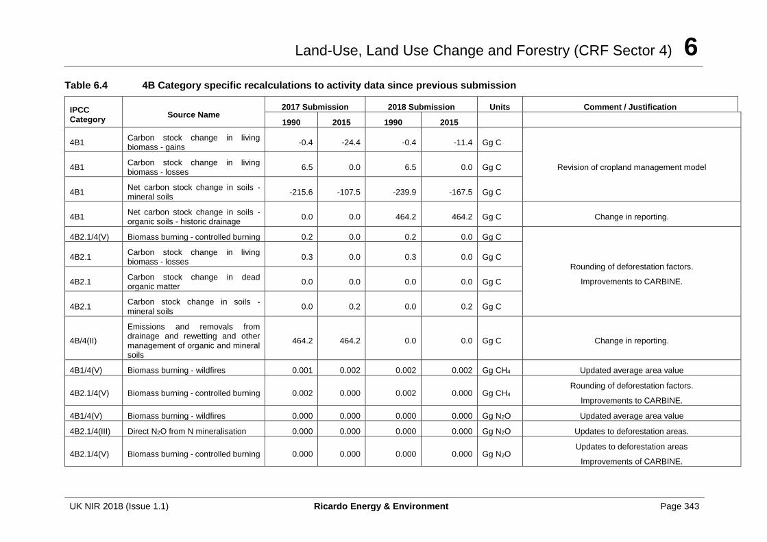
Land-Use, Land Use Change and Forestry (CRF Sector 4) 6
UK NIR 2018 (Issue 1.1) Ricardo Energy & Environment Page 343
Table 6.4 4B Category specific recalculations to activity data since previous submission
IPCC Category
Source Name 2017 Submission 2018 Submission Units Comment / Justification
1990 2015 1990 2015
4B1 Carbon stock change in living biomass - gains
-0.4 -24.4 -0.4 -11.4 Gg C
Revision of cropland management model 4B1 Carbon stock change in living biomass - losses
6.5 0.0 6.5 0.0 Gg C
4B1 Net carbon stock change in soils - mineral soils
-215.6 -107.5 -239.9 -167.5 Gg C
4B1 Net carbon stock change in soils - organic soils - historic drainage
0.0 0.0 464.2 464.2 Gg C Change in reporting.
4B2.1/4(V) Biomass burning - controlled burning 0.2 0.0 0.2 0.0 Gg C
Rounding of deforestation factors.
Improvements to CARBINE.
4B2.1 Carbon stock change in living biomass - losses
0.3 0.0 0.3 0.0 Gg C
4B2.1 Carbon stock change in dead organic matter
0.0 0.0 0.0 0.0 Gg C
4B2.1 Carbon stock change in soils - mineral soils
0.0 0.2 0.0 0.2 Gg C
4B/4(II)
Emissions and removals from drainage and rewetting and other management of organic and mineral soils
464.2 464.2 0.0 0.0 Gg C Change in reporting.
4B1/4(V) Biomass burning - wildfires 0.001 0.002 0.002 0.002 Gg CH4 Updated average area value
4B2.1/4(V) Biomass burning - controlled burning 0.002 0.000 0.002 0.000 Gg CH4 Rounding of deforestation factors.
Improvements to CARBINE.
4B1/4(V) Biomass burning - wildfires 0.000 0.000 0.000 0.000 Gg N2O Updated average area value
4B2.1/4(III) Direct N2O from N mineralisation 0.000 0.000 0.000 0.000 Gg N2O Updates to deforestation areas.
4B2.1/4(V) Biomass burning - controlled burning 0.000 0.000 0.000 0.000 Gg N2O Updates to deforestation areas
Improvements of CARBINE.
Land-Use, Land Use Change and Forestry (CRF Sector 4) 6
UK NIR 2018 (Issue 1.1) Ricardo Energy & Environment Page 344
6.3.8 Category-Specific Planned Improvements
A vector based approach to tracking land use change has been piloted that assimilates data from the European Commission Integrated Administration and Control System (IACS) data to provide a more accurate assessment of Grassland/Cropland rotation lengths for each UK administration (Levy et al. 2017). A decision on the further implementation of this approach is awaiting the outcome of related projects on the potential of earth observation to track LUC in the UK and clarity on the long-term availability of relevant datasets.
6.4 CATEGORY 4C – GRASSLAND
6.4.1 Description
Emissions sources 4C Grassland: carbon stock change 4C Grassland: 4(II) Emissions from drainage of organic soils. 4C Grassland: 4(III) Direct N2O emissions from N mineralisation. 4C Grassland: 4(V) Biomass burning
Gases Reported CO2, CH4, N2O
Methods T3 for carbon stock changes, T1 for other emissions
Emission Factors Country-specific for T3 methods, T1/2 for other emissions
Key Categories 4C: Grassland - CO2 (L1, T1, L2, T2)
Key Categories (Qualitative)
None identified
Completeness No known omissions- areas are reported for land uses with no associated emissions.
Major improvements since last submission
None.
Net emissions from the Grassland category include carbon stock gains and losses due to land use change (LUC) and GHG emissions from grassland management. It is the second largest net sink in the LULUCF sector.
Ongoing carbon stock changes in soils arising from LUC to Grassland are reported under both 4.C.2 Land Converted to Grassland (for LUC in the past 20 years) and 4.C.1 Grassland Remaining Grassland (for historic LUC >20 years before the inventory reporting year). These soil net carbon stock changes are the largest component of the category total emissions and removals, and are calculated using a Tier 3 dynamic soil carbon model.
The area of undisturbed grassland which has not been converted from other land uses in the past is reported in 4.C.1. “Undisturbed” grassland is used as a buffer category (on the recommendation of UNFCCC reviewers, as Grassland is the most extensive land type in the UK) and is calculated as the difference between the total land area (from the official national statistic of UK land area, Office for National Statistics) and the sum of all other land use areas (calculated from land use matrices, afforestation areas, peat extraction areas etc.) for each year. No anthropogenic emissions or removals are associated with this undisturbed area.
Other contributors to the Grassland net total emissions are:
• carbon emissions resulting from drainage of organic soils (reported in 4(II));
• carbon stock changes in biomass resulting from changes in grassland management;
• biomass carbon stock changes due to LUC;
• N2O emissions from soil disturbance associated with LUC;
Land-Use, Land Use Change and Forestry (CRF Sector 4) 6
UK NIR 2018 (Issue 1.1) Ricardo Energy & Environment Page 345
• biomass burning emissions of GHGs from controlled burning following forest land conversion to grassland; and
• biomass burning emissions of GHGs due to wildfires.
Carbon stock changes from drainage of improved Grassland on organic soils arise from areas which were drained many decades ago for agriculture. Soil carbon in these areas continues to oxidise and be released as CO2, resulting in an ongoing change in soil carbon stock. These emissions are reported in Table 4(II). There are large areas of organic and organo-mineral soils under unimproved Grassland throughout the UK and it is known that there has been some drainage of these areas although the full extent is unclear. Consequently, reporting just the area of, and emissions from, drained and improved grassland under Table 4C would be misleading. Work has been undertaken to address this in the BEIS-funded project on the implementation of the Wetlands Supplement guidance, but is awaiting the completion of further work before sign-off for implementation in the GHGI.
Full details of the methods and activity data are given in Annex 3.4.4 and Annex 3.4.5.
6.4.2 Information on approaches used for representing land areas and on land use databases used for the inventory preparation
The UK uses Approach 2 (IPCC 2006) for the representation of land use areas in the inventory, and compiles several different data sources into a non-spatially-explicit land use conversion matrix (see section 6.1.1 for details).
Data sources that contain area information for reporting carbon stock changes and/or emissions from Grassland:
• Habitat/landscape surveys; o Countryside Survey (1984, 1990, 2000, 2007) is used to compile land use
transition matrices. Changes in grassland types and in hedge length/condition are used to calculate biomass carbon stock changes under grassland management.
• Data on deforestation areas from various sources; o Post-2000 deforestation areas are assessed from the NFI o Pre-2000 deforestation areas are estimated from unconditional felling licence
data (felling licences granted without a requirement to restock), national forest estate administrative information and land conversion ratios from Countryside Survey. Details are given in Annex 3.4.4.
• An assessment of the area of improved Grassland on drained organic soils (see 6.2 for further details).
• Data on wildfires on agricultural land and moorland from Fire and Rescue service and satellite data.
6.4.3 Land-use definitions and the classification system used and their correspondence to the LULUCF categories
Grassland that has undergone land use change and direct management is defined in accordance with the Agriculture, Forestry and Other Land Uses guidance (IPCC 2006).There are also large areas of extensively grazed semi-natural grassland, which are assigned to the 4.C.1 “undisturbed grassland” sub-category (calculated as the area remaining after all other land use areas are subtracted from the total UK land area). This is the buffer land use category for the UK, so may contain small areas of other land uses that are not directly managed.
Grazing is the main land use on wetlands, so areas of wetland habitat not used for peat extraction, such as bogs, are also included in the Grassland category.

Land-Use, Land Use Change and Forestry (CRF Sector 4) 6
UK NIR 2018 (Issue 1.1) Ricardo Energy & Environment Page 346
For pre-1980 LUC the grassland area is the sum of the following land cover types in the Monitoring Landscape Change project (MLC 1986): upland heath, upland smooth grass, upland coarse grass, blanket bog, bracken, lowland rough grass, lowland heather, gorse, neglected grassland, marsh, improved grassland, rough pasture, peat bog, fresh marsh and salt marsh. For post-1980 LUC, grassland is the sum of the following Broad Habitat types in the Countryside Survey: improved grassland, neutral grassland, calcareous grassland, acid grassland, bracken, dwarf shrub heath, fen/marsh/swamp, bogs, montane, supra littoral sediment and littoral sediment (Jackson, 2000).
6.4.4 Methodological Issues
6.4.4.1 Land Use Change
Activity data for land use change are estimated using a land use matrix approach. Detailed descriptions of the methods, emission factors and data flows used for the Grassland are given in Annex 3.4.2.
The dynamic model of soil carbon stock change is described in Section 6.3.4. Biomass carbon stock change is calculated using the LUC matrix and country-specific biomass carbon stocks, with all stock gains or losses assumed to occur in a single year.
N2O emissions associated with the soil disturbance from LUC are reported using the areas of Forest land converted to Grassland from the LUC matrices and the IPCC Tier 1 emission factors.
6.4.4.2 Grassland management
Carbon stock changes in biomass due to grassland management activities are estimated using literature-derived Tier 2 stock change factors and activity data from agricultural surveys. These include changes in the length and condition of hedgerows.
6.4.4.3 Drained organic soils
Emissions from Grassland on drained organic soils are reported using Tier 1 emission factors which assume constant rates of soil organic carbon loss and activity data from Anthony (personal communication, 2013).
6.4.4.4 Biomass burning emissions
Emissions from controlled burning on grassland are only reported for Forest Land conversion to Grassland and are estimated using Tier 1 emission factors and country-specific fuel densities.
Emissions from wildfires on Grassland (agricultural grassland and semi-natural grassland) are reporting using Tier 1 emission factors and activity from a range of sources (see Section 6.3.2).
6.4.5 Uncertainties and Time-Series Consistency
4C Grassland is estimated to have a combined uncertainty of 40-50% for CO2, 55% for CH4 and 55-105% for N2O.
The areas undergoing land use change are the biggest source of uncertainty in the LULUCF inventory (see Annex 3.4.12), but model choice and soil carbon parameters are also significant. Emissions from Grassland on drained organic soils has the largest uncertainties of the minor emissions sources (i.e. not land use change) as the effects of drainage are highly uncertain.
With regard to series consistency:
• Drainage of organic soils: it is assumed that all drainage of organic soils under improved Grassland occurred before 1990, as policy has favoured protection of organic soils.
Land-Use, Land Use Change and Forestry (CRF Sector 4) 6
UK NIR 2018 (Issue 1.1) Ricardo Energy & Environment Page 347
There have been no policy incentives to encourage new land drainage for agricultural use since before 1990, and major drainage of large areas of improved Grassland on organic soils in areas such as the Somerset Levels fens is known to have occurred well before this. No improved Grassland on drained organic soils has been rewetted since 1990 as there have been no policy incentives for this, therefore a single area is used throughout the time series.
• Changes in biomass and soil carbon due to LUC: the data sources for Great Britain have maintained consistent methodology across the time series. Consistency between these and Northern Ireland data sources has improved with better methodological integration between land use surveys.
• Controlled biomass burning after conversion of Forest Land to Grassland: the time series consistency is as country-specific data sets are used.
• Grassland management: activity data come from Countryside Survey, which is also used to estimate change in carbon stocks due to land use change and has good internal consistency.
• Wildfires: a consistent dataset is used for 2010 onwards. Burnt areas are extrapolated back to 2001 based on remote sensing data, but between 1990 and 2001 there are no observed data on the extent of wildfires on Grassland, and the time series is filled by extrapolating the 2001 -2011 average wildfire area.
6.4.6 Category-Specific QA/QC and Verification
This source category is covered by the general QA/QC procedures, which are discussed in Section 6.10.
As discussed in Section 6.3.6 resampling of the 1980-based National Soil Inventory (NSI) in England and Wales in 1995-2003 found large losses of soil carbon across all land use types (Bellamy et al. 2005) but, a more recent study using Countryside Survey (CS) data (Reynolds et al. 2013) found no significant change in soil carbon stocks under most Grassland habitat types between 1978 and 2007. The possible reasons for these differences are unclear, as discussed in Section 6.3.6.
6.4.7 Category-Specific Recalculations
The reported overall net GHG sink in category 4C has reduced slightly by up to 0.3 Mt CO2e (0.1-2.7 %) compared to the 2015 inventory.
The changes were mainly in deforestation, both historic (affecting Grassland remaining Grassland) and recent (affecting Forest Land converted to Grassland).
The changes and their justification are:
• Revision of grassland management model: The original models were implemented in spreadsheets. Minor inconsistencies in the modelling of grassland management were identified during the development of a coded version of the model. These were corrected and QA checked in the spreadsheet models first and then applied to the new coded models which were validated against the spreadsheet output.
• Reallocation of orchards from Forest to Cropland: In response to a UN review team recommendation, the pre-1980 orchard area previously reported under Forest Land is now reported under Cropland. There has been a net loss of orchards over time, and this area previously reported under Forest Land converted to Grassland is now reported under Cropland converted to Grassland.
Land-Use, Land Use Change and Forestry (CRF Sector 4) 6
UK NIR 2018 (Issue 1.1) Ricardo Energy & Environment Page 348
• Improved rounding of deforestation factors: An inconsistency in the value precision was corrected between the Countryside Survey deforestation ‘reduction factors (see table A3.4.24) used in the LUC matrices (pre-2000) and the deforestation model.
• Improvements to CARBINE: see section 6.2.7 for justification. These modifications affected the average biomass density used to calculate biomass burning emissions and biomass losses.
• Updated average area value: The latest data on wildfires has been used to update the time series average used for back-calculating to 1990.
• Deforestation area updated: The post-2000 deforestation areas have been amended to use the most up-to-date NFI data which has led to some differences in areas and in the assignment between resulting land uses following deforestation. An error in the processing of the Northern Ireland deforestation output from CARBINE has also been resolved.
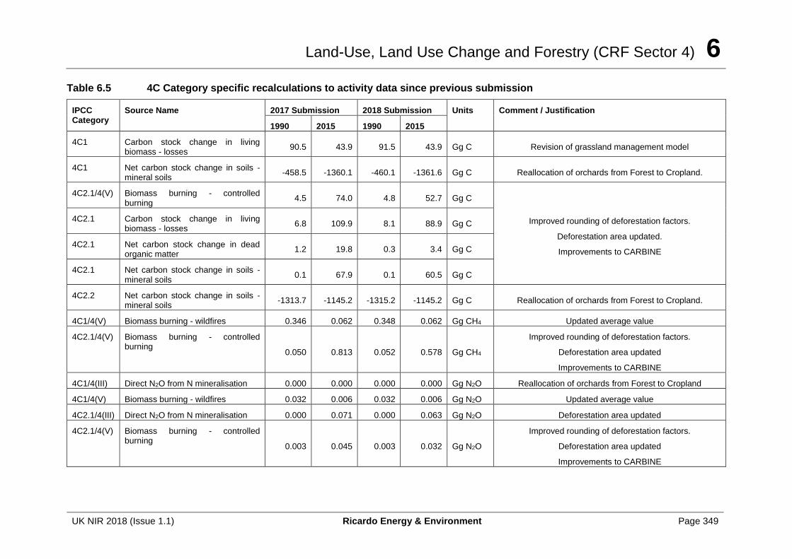
Land-Use, Land Use Change and Forestry (CRF Sector 4) 6
UK NIR 2018 (Issue 1.1) Ricardo Energy & Environment Page 349
Table 6.5 4C Category specific recalculations to activity data since previous submission
IPCC Category
Source Name 2017 Submission 2018 Submission Units Comment / Justification
1990 2015 1990 2015
4C1 Carbon stock change in living biomass - losses
90.5 43.9 91.5 43.9 Gg C Revision of grassland management model
4C1 Net carbon stock change in soils - mineral soils
-458.5 -1360.1 -460.1 -1361.6 Gg C Reallocation of orchards from Forest to Cropland.
4C2.1/4(V) Biomass burning - controlled burning
4.5 74.0 4.8 52.7 Gg C
Improved rounding of deforestation factors.
Deforestation area updated.
Improvements to CARBINE
4C2.1 Carbon stock change in living biomass - losses
6.8 109.9 8.1 88.9 Gg C
4C2.1 Net carbon stock change in dead organic matter
1.2 19.8 0.3 3.4 Gg C
4C2.1 Net carbon stock change in soils - mineral soils
0.1 67.9 0.1 60.5 Gg C
4C2.2 Net carbon stock change in soils - mineral soils
-1313.7 -1145.2 -1315.2 -1145.2 Gg C Reallocation of orchards from Forest to Cropland.
4C1/4(V) Biomass burning - wildfires 0.346 0.062 0.348 0.062 Gg CH4 Updated average value
4C2.1/4(V) Biomass burning - controlled burning
0.050 0.813 0.052 0.578 Gg CH4
Improved rounding of deforestation factors.
Deforestation area updated
Improvements to CARBINE
4C1/4(III) Direct N2O from N mineralisation 0.000 0.000 0.000 0.000 Gg N2O Reallocation of orchards from Forest to Cropland
4C1/4(V) Biomass burning - wildfires 0.032 0.006 0.032 0.006 Gg N2O Updated average value
4C2.1/4(III) Direct N2O from N mineralisation 0.000 0.071 0.000 0.063 Gg N2O Deforestation area updated
4C2.1/4(V) Biomass burning - controlled burning
0.003 0.045 0.003 0.032 Gg N2O
Improved rounding of deforestation factors.
Deforestation area updated
Improvements to CARBINE
Land-Use, Land Use Change and Forestry (CRF Sector 4) 6
UK NIR 2018 (Issue 1.1) Ricardo Energy & Environment Page 350
6.4.8 Category-Specific Planned Improvements
A BEIS-funded research project is underway to improve understanding of the effect of grassland management practices on carbon stock changes in organic and organo-mineral soils. This will fill a knowledge gap and enable carbon stock changes resulting from Grassland management to be included in the inventory.
A vector based approach to tracking land use change has been piloted that assimilates data from the European Commission Integrated Administration and Control System (IACS) data to provide a more accurate assessment of Grassland/Cropland rotation lengths for each UK administration (Levy et al. 2017). A decision on the further implementation of this approach is awaiting the outcome of related projects on the potential of earth observation to track LUC in the UK and clarity on the long-term availability of relevant datasets.
6.5 CATEGORY 4D – WETLANDS
6.5.1 Description
Emissions sources 4D Wetlands: Carbon stock change 4D Wetlands: 4(II) Non-CO2 emissions from drainage of soils
Gases Reported CO2, N2O
Methods Tier 1
Emission Factors Country specific and default EFs
Key Categories None identified
Key Categories (Qualitative)
None identified
Completeness No known omissions- areas are reported for land uses with no associated emissions.
Major improvements since last submission
None.
Net emissions from the Wetlands category includes emissions from peatlands that are cleared and drained for peat production (for energy or horticultural purposes) and for areas converted to permanently flooded land (reservoirs). As most UK wetland habitats (e.g. marsh, bog, swamp and fen) are grazed their emissions and removals are estimated within the Grassland category. A research project been completed to identify UK-specific activity data and emission factors to use with the 2013 Wetlands Supplement methodology but is awaiting the completion of further work before sign-off for implementation in the GHGI..
Emissions from on-site peat production and off-site emissions from horticultural peat are reported under 4.D.1 Wetlands remaining Wetlands. Small areas of grassland converted to Wetland for peat extraction (4.D.2.1) and to flooded land (4.D.2.2) are reported under 4.D.2. The associated soil emissions and living biomass carbon stock changes estimated using the appropriate Tier 1 methodologies. N2O emissions from wetland drainage (as part of peat production) are reported under 4.D and 4(II).
The area of UK natural inland water is reported in the category Other Wetlands remaining Other Wetlands and the area of reservoirs created before 1990 is reported in Flooded Land remaining Flooded Land. A small number of reservoirs have been created since 1990, and emissions from these due to change in biomass carbon stocks on conversion are included in the inventory (under 4.D.2.2.3 Grassland converted to Flooded Land).
Land-Use, Land Use Change and Forestry (CRF Sector 4) 6
UK NIR 2018 (Issue 1.1) Ricardo Energy & Environment Page 351
6.5.2 Information on approaches used for representing land areas and on land use databases used for the inventory preparation
The approach used for representing Wetlands differs from that used for other land use categories because peat extraction sites and reservoirs are not explicitly identified in the habitat and landscape surveys used for the land use matrix.
Data from the Directory of Mines and Quarries, Google Earth, the Minerals Extraction in Great Britain report (and its predecessor the Minerals Raised Inquiry, Office for National Statistics), and papers on peat extraction in Northern Ireland were used in combination to produce an activity dataset for active peat extraction areas in the UK (see Annex 3.4.8 for further details).
Activity data for post-1990 constructed reservoirs were compiled from the Public Register of Large Raised Reservoirs (supplied by the Environment Agency for England and Wales) and the SEPA Water Body Classification database (see Annex 3.4.9 for further details).
The remaining area of inland water (natural water bodies and reservoirs established before 1990) is known from the area of inland water reported as part of the Standard Area Measurement. There are no emissions or removals associated with this area.
6.5.3 Land-use definitions and the classification system used and their correspondence to the LULUCF categories
Areas of peat extraction are defined as areas that are currently undergoing, or have recently undergone, peat extraction activities (locations are known from administrative records: see Section 6.5.2). It is assumed that extraction areas continue to produce emissions while there is visible evidence of exposed peat soil from Google Earth satellite imagery. An extraction site is considered to have ceased emissions when there is visible evidence of the re-establishment of vegetation cover on the satellite imagery.
The area of inland water is taken from the “UK Standard Area Measurements” (Office for National Statistics). It defines inland water as ‘bounded’ permanent water bodies, e.g. lakes, lochs and reservoirs, exceeding 1 km2 (100 hectares) in area. ‘Open’ tracts of water, e.g. rivers, canals and streams are excluded from this definition. Reservoirs (flooded land) were identified either by their inclusion in the Public Register of Large Raised Reservoirs or by their classification as “Heavily modified” in the SEPA Water Body Classification database. Areas of water below the size threshold are included in the 4F Other Land category.
6.5.4 Methodological Issues
6.5.4.1 Peat extraction
Emissions from peat extraction are estimated using a Tier 1 methodology, which does not distinguish between peat extraction production phases,(i.e. it includes conversion and vegetation clearing. On-site emissions associated with peat extraction are reported under 4.D.1.1. All carbon in horticultural peat is assumed to be emitted during the extraction year. Methane emissions are assumed to be insignificant. N2O emissions from drainage are reported, although emissions are considered insignificant on nutrient-poor peatlands. The administrative records categorise sites as producing horticultural or energy source (fuel) peat. This information is used to extract the area of nutrient-rich peats that will produce N2O emissions, following the IPCC Tier 1 methodology. Further information is given in Annex 3.4.8.
Google Earth imagery is used to track the change in the area of individual extraction sites over time. Google Earth is imagery is checked annually and extraction site areas are updated as new imagery becomes available.
The site records show that the area under active peat extraction diminished between 1990 and 2002 for Great Britain and 1991 and 2007 for Northern Ireland. Some sites show no change in
Land-Use, Land Use Change and Forestry (CRF Sector 4) 6
UK NIR 2018 (Issue 1.1) Ricardo Energy & Environment Page 352
area on the Google Earth imagery, and are assumed to be abandoned extraction sites that are still producing emissions (reported under 4D1). Sites where extraction is no longer visible on the Google Earth imagery are assumed to have been converted to Grassland. Changes in biomass carbon and organic soil carbon from this land use change are reported using the Tier 1 approach from the IPCC 2006 Guidelines.
A small area of land conversion to Wetlands occurs between 2003 and 2005, which is assumed to be all from Grassland based on the examination of Google Earth imagery. This area and the associated on-site emissions are reported under 4D.2 Land converted to Wetlands, using the 5-year transition period recommended by the IPCC 2006 Guidelines.
6.5.4.2 Land converted to Flooded Land
A Tier 1 methodology was applied for emissions from Flooded Lands. This estimated carbon stock changes in living biomass stock in the year of flooding (for reservoirs established since 1990) but not carbon stock changes in soils. The locations of the reservoirs was established on maps, and due to their location in upland areas, all were assumed to be Grassland prior to flooding. A living biomass density of 2 t dry matter/ha was used to estimate carbon stock losses.
6.5.5 Uncertainties and Time-Series Consistency
4D Wetland is estimated to have a combined uncertainty of 100% for CO2 and 100% for N2O.
Uncertainties in the emission factors for peat extracted for horticultural and fuel use and for emissions from Flooded Land are the default IPCC values given in the 2006 Guidelines. Uncertainty in the Flooded Land activity data was very low as there were a limited number of reservoirs established since 1990, five in total.
Time- series consistency for activity data for peat extraction sites is affected by uncertainty in survey dates. Time- series consistency for flooded lands was good due to the complete nature of the data set.
6.5.6 Category-Specific QA/QC and Verification
The peat extraction site activity dataset has been partially verified by comparing the measured areas with reported areas of planning permission, which were available for some extraction sites in England and Scotland. The measured areas either matched or were smaller than the planning permission areas, which is to be expected as it is known that not all areas with planning permission are undergoing active extraction.
The locations and previous land-use of new reservoirs were verified using the www.magic.gov.uk geographic information portal.
6.5.7 Category-Specific Recalculations
The reported overall net GHG source in category 4D has increased slightly by 0.1 Mt CO2e (19 %) in 2015 in the latest submission compared to the 2015 inventory.
The change was due to a revision of the peat extraction activity data: the publication source for the volume of off-site horticultural peat has been discontinued, so the 2015 and 2016 values are now an average of the previous ten years rather than a roll-over of the 2014 value. Options for replacing the publication source are being investigated.
The changes in emissions are shown in Table 6.6.
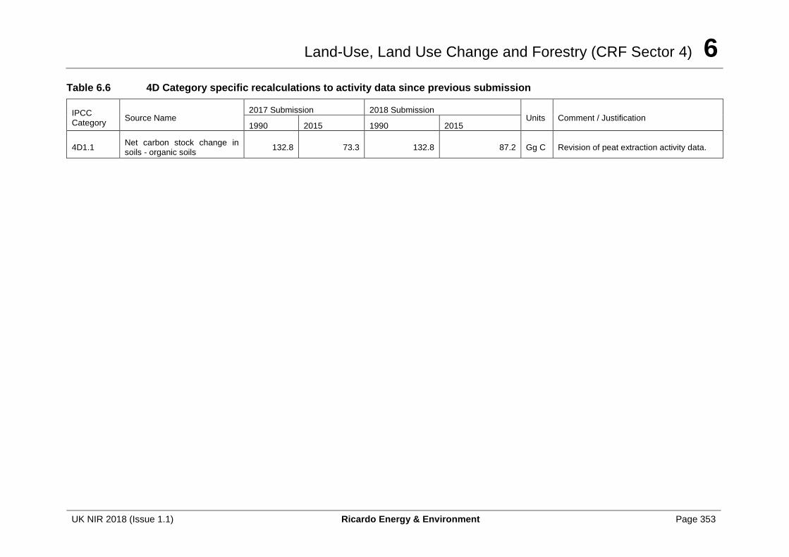
Land-Use, Land Use Change and Forestry (CRF Sector 4) 6
UK NIR 2018 (Issue 1.1) Ricardo Energy & Environment Page 353
Table 6.6 4D Category specific recalculations to activity data since previous submission
IPCC Category
Source Name 2017 Submission 2018 Submission
Units Comment / Justification 1990 2015 1990 2015
4D1.1 Net carbon stock change in soils - organic soils
132.8 73.3 132.8 87.2 Gg C Revision of peat extraction activity data.
Land-Use, Land Use Change and Forestry (CRF Sector 4) 6
UK NIR 2018 (Issue 1.1) Ricardo Energy & Environment Page 354
6.5.8 Category-specific planned improvements
A BEIS-funded project to implement the Wetlands Supplement (IPCC, 2013a) guidance was completed in 2017. The results of the project are still under careful review and preliminary results show significant uncertainty in the areas assigned to different management actions around drainage and rewetting. Further work is being considered to improve our understanding of the areas of peatland in different conditions of implied drainage and rewetting and it is hoped that this work may enable the research to be implemented within the inventory.
6.6 CATEGORY 4E – SETTLEMENTS
6.6.1 Description
Emissions sources 4E Settlements: Carbon stock change 4E Settlements: 4(III) Direct N2O emissions from N mineralization 4E Settlements: 4(V) Biomass burning
Gases Reported CO2, CH4, N2O
Methods T3 for carbon stock changes, T1 for other emissions
Emission Factors Country-specific for T3 methods, T1/2 for other emissions
Key Categories 4E: Settlements – CO2 (L1, T1, L2, T2)
Key Categories (Qualitative)
None identified
Completeness No known omissions- areas are reported for land uses with no associated emissions.
Major improvements since last submission
None.
Net emissions from the Settlements category include carbon stock gains and losses due to land use change (LUC) and associated GHG emissions.
Ongoing carbon stock changes in soils and direct N2O emissions from N mineralization arising from LUC to Settlements are reported under both 4.E.1 Settlements remaining Settlements (for historic LUC >20 years before the inventory reporting year) and 4.E.2 Land converted to Settlements (for LUC in the past 20 years). These soil net carbon stock changes are the largest component of the category total emissions, and are calculated using a Tier 3 dynamic soil carbon model.
Other contributors to the Settlements net total emissions are:
• biomass carbon stock changes due to LUC;
• N2O emissions from soil disturbance associated with LUC; and
• biomass burning emissions of GHGs from controlled burning following forest land conversion to Settlements.
Full details of the methods and activity data are given in Annex 3.4.4 and Annex 3.4.5.
6.6.2 Information on approaches used for representing land areas and on land use databases used for the inventory preparation
The UK uses Approach 2 (IPCC 2006) for the representation of land use areas in the inventory, and compiles several different data sources into a non-spatially-explicit land use conversion matrix (see section 6.1.1 for details).
Land-Use, Land Use Change and Forestry (CRF Sector 4) 6
UK NIR 2018 (Issue 1.1) Ricardo Energy & Environment Page 355
Data sources that contain area information for reporting carbon stock changes and/or emissions from Settlements are:
• Habitat/landscape surveys o Countryside Survey (1984, 1990, 2000, 2007) is used to compile land use
transition matrices.
• Data on deforestation areas from various sources; o Post-2000 deforestation areas are assessed from the NFI o Pre-2000 deforestation areas are estimated from unconditional felling licence
data (felling licences granted without a requirement to restock), national forest estate administrative information and land conversion ratios from Countryside Survey. Details are given in Annex 3.4.4.
6.6.3 Land-use definitions and the classification system used and their correspondence to the LULUCF categories
Settlement is defined in accordance with the Agriculture, Forestry and Other Land Use Guidance (IPCC 2006).
For pre-1980 LUC Settlement land is the sum of the Built-up, Urban open, Transport, Mineral workings and Derelict land cover types in the Monitoring Landscape Change project (MLC 1986). For post-1980 LUC, Settlement land corresponds to the “Built-up and Gardens” and “Boundary and linear features” Broad Habitat types in the Countryside Survey (Haines-Young et al. 2000, Appendix A), defined as:
• Built-up and Gardens: “Covers urban and rural settlements, farm buildings, caravan parks and other man-made built structures such as industrial estates, retail parks, waste and derelict ground, urban parkland and urban transport infrastructure. It also includes domestic gardens and allotments.”; and
• Boundary and linear features: “a diverse range of linearly arranged landscape features such as hedgerows, walls, stone and earth banks, grass strips and dry ditches. This habitat type also includes some of the built components of the rural landscape including roads, tracks and railways and their associated narrow verges of semi-natural habitat.”
Although hedgerows are included in the definition of the “Boundary and linear features” Broad Habitat type, any carbon stock changes associated with hedgerow change are calculated separately under grassland management. The “Boundary and linear features” Broad Habitat type is a very small component of the UK land area (<2% in the 2007 Countryside Survey) so the overlap in definitions will not materially affect net LULUCF emissions.
6.6.4 Methodological Issues
6.6.4.1 Land Use Change
A summary of the land use matrix approach and the dynamic model of soil carbon stock change used to estimate changes in biomass and soil carbon due to LUC is given in Section 6.3.4. Detailed descriptions of the methods, emission factors and data flows used for the Grassland are given in Annex 3.4.7.
N2O emissions associated with the soil disturbance from LUC are reported using the areas from the LUC matrices and the IPCC Tier 1 emission factors.
6.6.4.2 Biomass burning emissions
Emissions from controlled burning on settlement land are only reported for Forest Land conversion to Settlements and are estimated using Tier 1 emission factors and country-specific fuel densities.
Land-Use, Land Use Change and Forestry (CRF Sector 4) 6
UK NIR 2018 (Issue 1.1) Ricardo Energy & Environment Page 356
6.6.5 Uncertainties and Time-Series Consistency
4E Settlement is estimated to have a combined uncertainty of 50% for CO2, 55% for CH4 and 15-135% for N2O.
The areas undergoing land use change are the biggest source of uncertainty in the LULUCF inventory (see Annex 3.4.13), but model choice and soil carbon parameters are also significant.
With regard to series consistency:
• Changes in biomass and soil carbon due to LUC: the data sources for Great Britain have maintained consistent methodology across the time series. Consistency between these and Northern Ireland data sources has improved with better methodological integration between land use surveys.
• Controlled biomass burning after conversion of Forest Land to Settlement: there is good time series consistency as there has been continuity in the activity data source.
6.6.6 Category-Specific QA/QC and Verification
This source category is covered by the general QA/QC procedures, which are discussed in Section 6.10. Research described in Section 6.1.1. is also relevant to this section.
6.6.7 Category-Specific Recalculations
The reported overall net GHG source in category 4E has increased slightly by up to 0.1 Mt CO2e (0.2-2.2 %) compared to the 2015 inventory across the time series.
The changes resulted from changes in the deforestation time series and factors.
The changes and their justification are:
• Improved rounding of deforestation factors: An inconsistency in the precision of data was corrected between the Countryside Survey deforestation ‘reduction factors (see table A3.4.24) used in the LUC matrices (pre-2000) and the deforestation model.
• Improvements to CARBINE: see section 6.2.7 for justification. These modifications affected the average biomass density used to calculate biomass burning emissions and biomass losses.
• Deforestation area updated: The post-2000 deforestation areas have been amended to use the most up-to-date NFI data which has led to some differences in areas and in the assignment between resulting land uses following deforestation. An error in the processing of the Northern Ireland deforestation output from CARBINE has also been resolved.
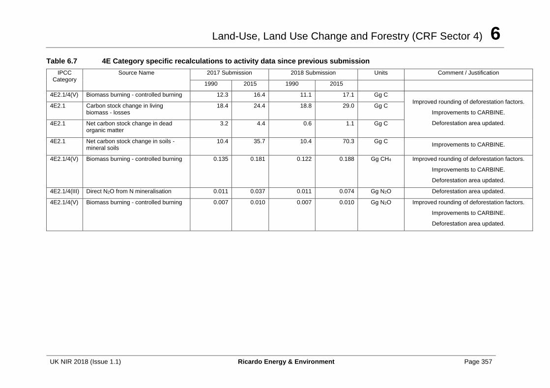
Land-Use, Land Use Change and Forestry (CRF Sector 4) 6
UK NIR 2018 (Issue 1.1) Ricardo Energy & Environment Page 357
Table 6.7 4E Category specific recalculations to activity data since previous submission
IPCC Category
Source Name 2017 Submission 2018 Submission Units Comment / Justification
1990 2015 1990 2015
4E2.1/4(V) Biomass burning - controlled burning 12.3 16.4 11.1 17.1 Gg C
Improved rounding of deforestation factors.
Improvements to CARBINE.
Deforestation area updated.
4E2.1 Carbon stock change in living biomass - losses
18.4 24.4 18.8 29.0 Gg C
4E2.1 Net carbon stock change in dead organic matter
3.2 4.4 0.6 1.1 Gg C
4E2.1 Net carbon stock change in soils - mineral soils
10.4 35.7 10.4 70.3 Gg C Improvements to CARBINE.
4E2.1/4(V) Biomass burning - controlled burning 0.135 0.181 0.122 0.188 Gg CH4 Improved rounding of deforestation factors.
Improvements to CARBINE.
Deforestation area updated.
4E2.1/4(III) Direct N2O from N mineralisation 0.011 0.037 0.011 0.074 Gg N2O Deforestation area updated.
4E2.1/4(V) Biomass burning - controlled burning 0.007 0.010 0.007 0.010 Gg N2O Improved rounding of deforestation factors.
Improvements to CARBINE.
Deforestation area updated.
Land-Use, Land Use Change and Forestry (CRF Sector 4) 6
UK NIR 2018 (Issue 1.1) Ricardo Energy & Environment Page 358
6.6.8 Category-Specific Planned Improvements
A vector based approach to tracking land use change has been piloted that assimilates data from the European Commission Integrated Administration and Control System (IACS) data. A decision on the further implementation of this approach is awaiting the outcome of related projects on the potential of earth observation to track LUC in the UK and clarity on the long-term availability of relevant datasets.
6.7 CATEGORY 4F – OTHER LAND
6.7.1 Description
Emissions sources None
Gases Reported None
Methods NA
Emission Factors NA
Key Categories None identified
Key Categories (Qualitative)
None identified
Completeness No known omissions- areas are reported for land uses with no associated emissions.
Major improvements since last submission
None
No emissions or removals are reported in this category in the UK. It is assumed that there are very few areas of land of other types that become bare rock or water bodies, which make up the majority of this type. Therefore the UK rows in Table 4.F. (Other Land) are completed with ‘NO’ (Not Occurring).
6.7.2 Information on approaches used for representing land areas and on land use databases used for the inventory preparation
The approaches used for representing land use areas in the inventory are described in Section 6.1.1
6.7.3 Land-use definitions and the classification system used and their correspondence to the LULUCF categories
Other Land is defined as areas that do not fall into the other land use categories. For pre-1980 land use matrices Other Land is the sum of the bare rock, sand/shingle, inland water and coastal water land cover types in the Monitoring Landscape Change project (MLC 1986). Post-1980, Other Land contains the inland rock, standing water and canals and rivers and streams broad habitat types in the Countryside Survey (Jackson, 2000). As described in Section 6.5, areas of inland water exceeding 1km2 are included in 4D Wetlands, but water bodies below this threshold would still be included under Other Land.
6.7.4 Category-specific recalculations
There are no emissions associated with Other Land and no recalculations.
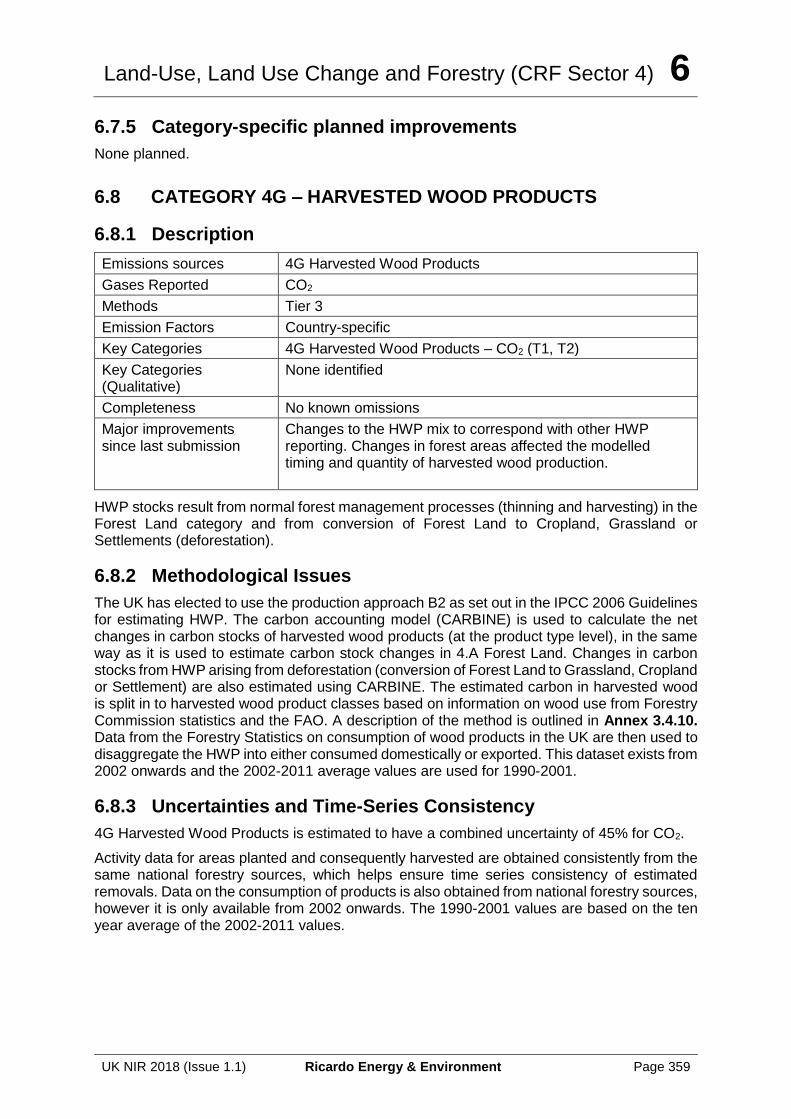
Land-Use, Land Use Change and Forestry (CRF Sector 4) 6
UK NIR 2018 (Issue 1.1) Ricardo Energy & Environment Page 359
6.7.5 Category-specific planned improvements
None planned.
6.8 CATEGORY 4G – HARVESTED WOOD PRODUCTS
6.8.1 Description
Emissions sources 4G Harvested Wood Products
Gases Reported CO2
Methods Tier 3
Emission Factors Country-specific
Key Categories 4G Harvested Wood Products – CO2 (T1, T2)
Key Categories (Qualitative)
None identified
Completeness No known omissions
Major improvements since last submission
Changes to the HWP mix to correspond with other HWP reporting. Changes in forest areas affected the modelled timing and quantity of harvested wood production.
HWP stocks result from normal forest management processes (thinning and harvesting) in the Forest Land category and from conversion of Forest Land to Cropland, Grassland or Settlements (deforestation).
6.8.2 Methodological Issues
The UK has elected to use the production approach B2 as set out in the IPCC 2006 Guidelines for estimating HWP. The carbon accounting model (CARBINE) is used to calculate the net changes in carbon stocks of harvested wood products (at the product type level), in the same way as it is used to estimate carbon stock changes in 4.A Forest Land. Changes in carbon stocks from HWP arising from deforestation (conversion of Forest Land to Grassland, Cropland or Settlement) are also estimated using CARBINE. The estimated carbon in harvested wood is split in to harvested wood product classes based on information on wood use from Forestry Commission statistics and the FAO. A description of the method is outlined in Annex 3.4.10. Data from the Forestry Statistics on consumption of wood products in the UK are then used to disaggregate the HWP into either consumed domestically or exported. This dataset exists from 2002 onwards and the 2002-2011 average values are used for 1990-2001.
6.8.3 Uncertainties and Time-Series Consistency
4G Harvested Wood Products is estimated to have a combined uncertainty of 45% for CO2.
Activity data for areas planted and consequently harvested are obtained consistently from the same national forestry sources, which helps ensure time series consistency of estimated removals. Data on the consumption of products is also obtained from national forestry sources, however it is only available from 2002 onwards. The 1990-2001 values are based on the ten year average of the 2002-2011 values.
Land-Use, Land Use Change and Forestry (CRF Sector 4) 6
UK NIR 2018 (Issue 1.1) Ricardo Energy & Environment Page 360
6.8.4 Category-Specific QA/QC and Verification
This source category is covered by the general QA/QC procedures, which are discussed in Section 6.10. The timber production predicted has been compared to the national timber production statistics produced by the Forestry Commission based on data from sawmills.
6.8.5 Category-Specific Recalculations
The reported overall net GHG sink in category 4G reduced in 1990 and increased in 2015 by -0.6 to 0.8 Mt CO2e (-60 to +41 %) across the time series compared to the 2015 inventory.
The changes resulted from improvements to the category to change the mix of semi-finished wood products (Changes to HWP mix) to vary over time to match the information from Forest Statistics and FAO data, prompted by a UN review team recommendation. Changes in the forest planting areas (Forest area changes) also had an impact on HWP stocks, as described in 6.2.7.
The changes are described in Table 6.8.
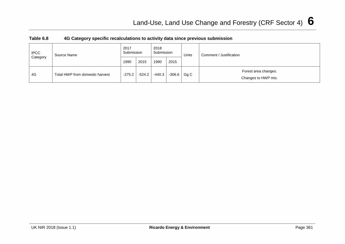
Land-Use, Land Use Change and Forestry (CRF Sector 4) 6
UK NIR 2018 (Issue 1.1) Ricardo Energy & Environment Page 361
Table 6.8 4G Category specific recalculations to activity data since previous submission
IPCC Category
Source Name
2017 Submission
2018 Submission
Units Comment / Justification
1990 2015 1990 2015
4G Total HWP from domestic harvest -275.2 -524.2 -440.3 -306.6 Gg C Forest area changes.
Changes to HWP mix.
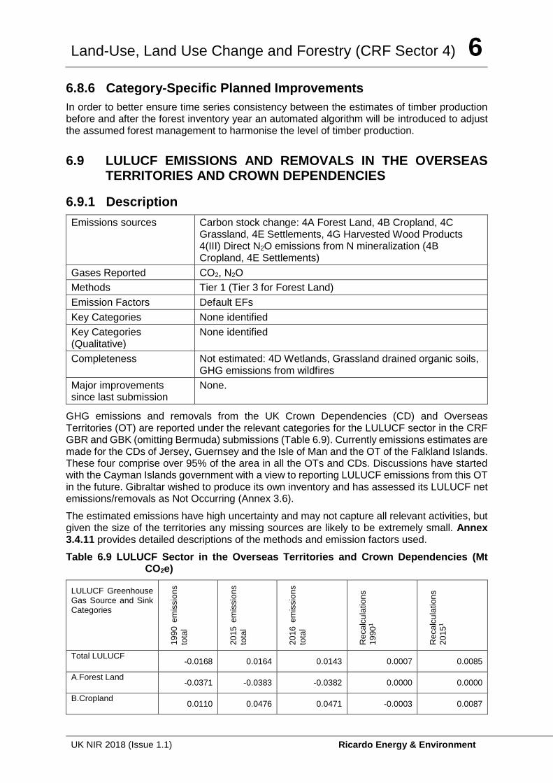
Land-Use, Land Use Change and Forestry (CRF Sector 4) 6
UK NIR 2018 (Issue 1.1) Ricardo Energy & Environment Page 362
6.8.6 Category-Specific Planned Improvements
In order to better ensure time series consistency between the estimates of timber production before and after the forest inventory year an automated algorithm will be introduced to adjust the assumed forest management to harmonise the level of timber production.
6.9 LULUCF EMISSIONS AND REMOVALS IN THE OVERSEAS TERRITORIES AND CROWN DEPENDENCIES
6.9.1 Description
Emissions sources Carbon stock change: 4A Forest Land, 4B Cropland, 4C Grassland, 4E Settlements, 4G Harvested Wood Products 4(III) Direct N2O emissions from N mineralization (4B Cropland, 4E Settlements)
Gases Reported CO2, N2O
Methods Tier 1 (Tier 3 for Forest Land)
Emission Factors Default EFs
Key Categories None identified
Key Categories (Qualitative)
None identified
Completeness Not estimated: 4D Wetlands, Grassland drained organic soils, GHG emissions from wildfires
Major improvements since last submission
None.
GHG emissions and removals from the UK Crown Dependencies (CD) and Overseas Territories (OT) are reported under the relevant categories for the LULUCF sector in the CRF GBR and GBK (omitting Bermuda) submissions (Table 6.9). Currently emissions estimates are made for the CDs of Jersey, Guernsey and the Isle of Man and the OT of the Falkland Islands. These four comprise over 95% of the area in all the OTs and CDs. Discussions have started with the Cayman Islands government with a view to reporting LULUCF emissions from this OT in the future. Gibraltar wished to produce its own inventory and has assessed its LULUCF net emissions/removals as Not Occurring (Annex 3.6).
The estimated emissions have high uncertainty and may not capture all relevant activities, but given the size of the territories any missing sources are likely to be extremely small. Annex 3.4.11 provides detailed descriptions of the methods and emission factors used.
Table 6.9 LULUCF Sector in the Overseas Territories and Crown Dependencies (Mt CO2e)
LULUCF Greenhouse Gas Source and Sink Categories
19
90
em
issio
ns
tota
l
20
15
em
issio
ns
tota
l
20
16
em
issio
ns
tota
l
Reca
lcu
lation
s
19
90
1
Reca
lcu
lation
s
20
15
1
Total LULUCF -0.0168 0.0164 0.0143 0.0007 0.0085
A.Forest Land -0.0371 -0.0383 -0.0382 0.0000 0.0000
B.Cropland 0.0110 0.0476 0.0471 -0.0003 0.0087
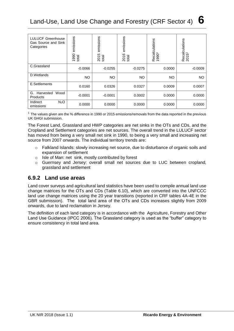
Land-Use, Land Use Change and Forestry (CRF Sector 4) 6
UK NIR 2018 (Issue 1.1) Ricardo Energy & Environment Page 363
LULUCF Greenhouse Gas Source and Sink Categories
19
90
em
issio
ns
tota
l
20
15
em
issio
ns
tota
l
20
16
em
issio
ns
tota
l
Re
ca
lcu
lation
s
19
90
1
Re
ca
lcu
lation
s
20
15
1
C.Grassland -0.0066 -0.0255 -0.0275 0.0000 -0.0009
D.Wetlands NO NO NO NO NO
E.Settlements 0.0160 0.0326 0.0327 0.0009 0.0007
G. Harvested Wood Products
-0.0001 -0.0001 0.0002 0.0000 0.0000
Indirect N2O emissions
0.0000 0.0000 0.0000 0.0000 0.0000
1 The values given are the % difference in 1990 or 2015 emissions/removals from the data reported in the previous
UK GHGI submission.
The Forest Land, Grassland and HWP categories are net sinks in the OTs and CDs, and the Cropland and Settlement categories are net sources. The overall trend in the LULUCF sector has moved from being a very small net sink in 1990, to being a very small and increasing net source from 2007 onwards. The individual territory trends are:
o Falkland Islands: slowly increasing net source, due to disturbance of organic soils and expansion of settlement
o Isle of Man: net sink, mostly contributed by forest o Guernsey and Jersey: overall small net sources due to LUC between cropland,
grassland and settlement
6.9.2 Land use areas
Land cover surveys and agricultural land statistics have been used to compile annual land use change matrices for the OTs and CDs (Table 6.10), which are converted into the UNFCCC land use change matrices using the 20 year transitions (reported in CRF tables 4A-4E in the GBR submission). The total land area of the OTs and CDs increases slightly from 2009 onwards, due to land reclamation in Jersey.
The definition of each land category is in accordance with the Agriculture, Forestry and Other Land Use Guidance (IPCC 2006). The Grassland category is used as the “buffer” category to ensure consistency in total land area.
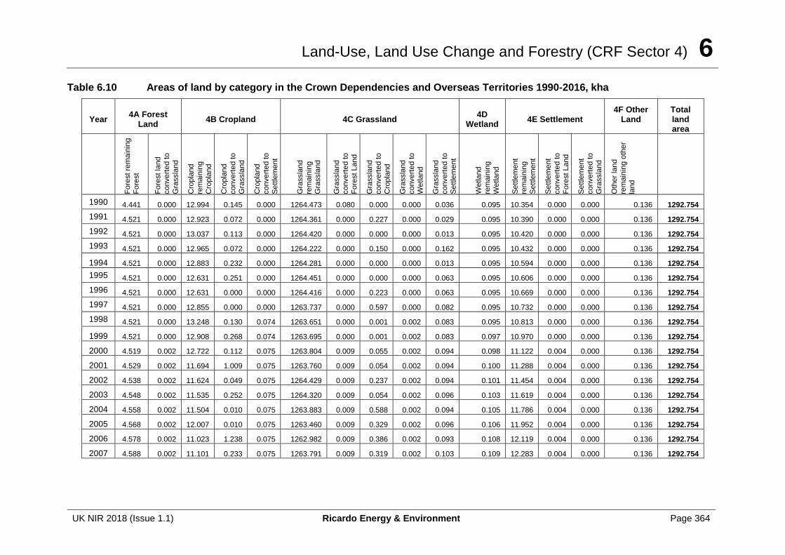
Land-Use, Land Use Change and Forestry (CRF Sector 4) 6
UK NIR 2018 (Issue 1.1) Ricardo Energy & Environment Page 364
Table 6.10 Areas of land by category in the Crown Dependencies and Overseas Territories 1990-2016, kha
Year 4A Forest
Land 4B Cropland 4C Grassland
4D Wetland
4E Settlement 4F Other
Land Total land area
Fo
rest re
ma
inin
g
Fo
rest
Fo
rest la
nd
convert
ed t
o
Gra
ssla
nd
Cro
pla
nd
rem
ain
ing
Cro
pla
nd
Cro
pla
nd
convert
ed t
o
Gra
ssla
nd
Cro
pla
nd
convert
ed t
o
Settle
me
nt
Gra
ssla
nd
rem
ain
ing
Gra
ssla
nd
Gra
ssla
nd
convert
ed t
o
Fo
rest Land
Gra
ssla
nd
convert
ed t
o
Cro
pla
nd
Gra
ssla
nd
convert
ed t
o
Wetla
nd
Gra
ssla
nd
convert
ed t
o
Settle
me
nt
Wetla
nd
rem
ain
ing
Wetla
nd
Settle
me
nt
rem
ain
ing
Settle
me
nt
Settle
me
nt
convert
ed t
o
Fo
rest Land
Settle
me
nt
convert
ed t
o
Gra
ssla
nd
Oth
er
land
rem
ain
ing o
ther
land
1990 4.441 0.000 12.994 0.145 0.000 1264.473 0.080 0.000 0.000 0.036 0.095 10.354 0.000 0.000 0.136 1292.754
1991 4.521 0.000 12.923 0.072 0.000 1264.361 0.000 0.227 0.000 0.029 0.095 10.390 0.000 0.000 0.136 1292.754
1992 4.521 0.000 13.037 0.113 0.000 1264.420 0.000 0.000 0.000 0.013 0.095 10.420 0.000 0.000 0.136 1292.754
1993 4.521 0.000 12.965 0.072 0.000 1264.222 0.000 0.150 0.000 0.162 0.095 10.432 0.000 0.000 0.136 1292.754
1994 4.521 0.000 12.883 0.232 0.000 1264.281 0.000 0.000 0.000 0.013 0.095 10.594 0.000 0.000 0.136 1292.754
1995 4.521 0.000 12.631 0.251 0.000 1264.451 0.000 0.000 0.000 0.063 0.095 10.606 0.000 0.000 0.136 1292.754
1996 4.521 0.000 12.631 0.000 0.000 1264.416 0.000 0.223 0.000 0.063 0.095 10.669 0.000 0.000 0.136 1292.754
1997 4.521 0.000 12.855 0.000 0.000 1263.737 0.000 0.597 0.000 0.082 0.095 10.732 0.000 0.000 0.136 1292.754
1998 4.521 0.000 13.248 0.130 0.074 1263.651 0.000 0.001 0.002 0.083 0.095 10.813 0.000 0.000 0.136 1292.754
1999 4.521 0.000 12.908 0.268 0.074 1263.695 0.000 0.001 0.002 0.083 0.097 10.970 0.000 0.000 0.136 1292.754
2000 4.519 0.002 12.722 0.112 0.075 1263.804 0.009 0.055 0.002 0.094 0.098 11.122 0.004 0.000 0.136 1292.754
2001 4.529 0.002 11.694 1.009 0.075 1263.760 0.009 0.054 0.002 0.094 0.100 11.288 0.004 0.000 0.136 1292.754
2002 4.538 0.002 11.624 0.049 0.075 1264.429 0.009 0.237 0.002 0.094 0.101 11.454 0.004 0.000 0.136 1292.754
2003 4.548 0.002 11.535 0.252 0.075 1264.320 0.009 0.054 0.002 0.096 0.103 11.619 0.004 0.000 0.136 1292.754
2004 4.558 0.002 11.504 0.010 0.075 1263.883 0.009 0.588 0.002 0.094 0.105 11.786 0.004 0.000 0.136 1292.754
2005 4.568 0.002 12.007 0.010 0.075 1263.460 0.009 0.329 0.002 0.096 0.106 11.952 0.004 0.000 0.136 1292.754
2006 4.578 0.002 11.023 1.238 0.075 1262.982 0.009 0.386 0.002 0.093 0.108 12.119 0.004 0.000 0.136 1292.754
2007 4.588 0.002 11.101 0.233 0.075 1263.791 0.009 0.319 0.002 0.103 0.109 12.283 0.004 0.000 0.136 1292.754
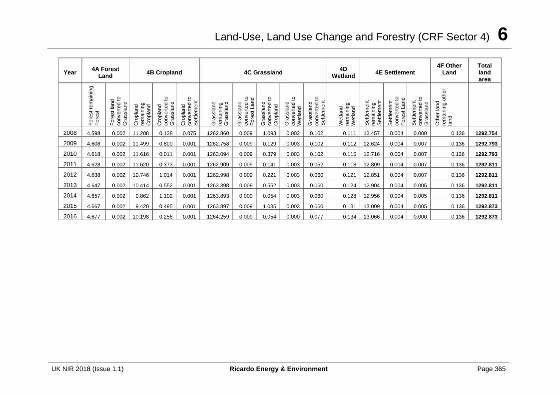
Land-Use, Land Use Change and Forestry (CRF Sector 4) 6
UK NIR 2018 (Issue 1.1) Ricardo Energy & Environment Page 365
Year 4A Forest
Land 4B Cropland 4C Grassland
4D Wetland
4E Settlement 4F Other
Land Total land area
Fo
rest re
ma
inin
g
Fo
rest
Fo
rest la
nd
convert
ed t
o
Gra
ssla
nd
Cro
pla
nd
rem
ain
ing
Cro
pla
nd
Cro
pla
nd
convert
ed t
o
Gra
ssla
nd
Cro
pla
nd
convert
ed t
o
Settle
me
nt
Gra
ssla
nd
rem
ain
ing
Gra
ssla
nd
Gra
ssla
nd
convert
ed t
o
Fo
rest L
and
Gra
ssla
nd
convert
ed t
o
Cro
pla
nd
Gra
ssla
nd
convert
ed t
o
Wetla
nd
Gra
ssla
nd
convert
ed t
o
Settle
me
nt
Wetla
nd
rem
ain
ing
Wetla
nd
Settle
me
nt
rem
ain
ing
Settle
me
nt
Settle
me
nt
convert
ed t
o
Fo
rest Land
Settle
me
nt
convert
ed t
o
Gra
ssla
nd
Oth
er
land
rem
ain
ing o
ther
land
2008 4.598 0.002 11.208 0.138 0.075 1262.860 0.009 1.093 0.002 0.102 0.111 12.457 0.004 0.000 0.136 1292.754
2009 4.608 0.002 11.499 0.800 0.001 1262.758 0.009 0.129 0.003 0.102 0.112 12.624 0.004 0.007 0.136 1292.793
2010 4.618 0.002 11.616 0.011 0.001 1263.094 0.009 0.379 0.003 0.102 0.115 12.716 0.004 0.007 0.136 1292.793
2011 4.628 0.002 11.620 0.373 0.001 1262.909 0.009 0.141 0.003 0.052 0.118 12.809 0.004 0.007 0.136 1292.811
2012 4.638 0.002 10.746 1.014 0.001 1262.998 0.009 0.221 0.003 0.060 0.121 12.851 0.004 0.007 0.136 1292.811
2013 4.647 0.002 10.414 0.552 0.001 1263.398 0.009 0.552 0.003 0.060 0.124 12.904 0.004 0.005 0.136 1292.811
2014 4.657 0.002 9.862 1.102 0.001 1263.893 0.009 0.054 0.003 0.060 0.128 12.956 0.004 0.005 0.136 1292.811
2015 4.667 0.002 9.420 0.495 0.001 1263.897 0.009 1.035 0.003 0.060 0.131 13.009 0.004 0.005 0.136 1292.873
2016 4.677 0.002 10.198 0.256 0.001 1264.259 0.009 0.054 0.000 0.077 0.134 13.066 0.004 0.000 0.136 1292.873
Land-Use, Land Use Change and Forestry (CRF Sector 4) 6
UK NIR 2018 (Issue 1.1) Ricardo Energy & Environment Page 366
6.9.3 Methodological Issues
Similar climate and land management parameters are assumed as for the UK. Land areas have been interpolated between land area surveys in some cases. More detailed activity data allowed a Tier 3 method to be applied for forestry in the Isle of Man and Guernsey. The IPCC Tier 1 default factors and GWPs from the 2006 AFOLU Guidelines have been used to estimate all other emissions and removals.
6.9.4 Recalculations
The net LULUCF emissions from the OTs and CDs changed slightly compared to the previous inventory, with a 0.08 Gg CO2e reduction in the net sink in 1990 and a 1.94 Gg CO2e increase in the net source in 2015.
The changes were due to updated agricultural census data and the correction of two minor errors in (i) applying the 20-year transition period to Cropland, and (ii) the calculation of direct N2O emissions from land conversion to Settlement.
6.9.5 Planned improvements
CEH are in discussion with the Cayman Islands government regarding the reporting of LULUCF net emissions from the Cayman Islands in the future. The initial work has been focussed on gathering appropriate land use and activity data and ascertaining its compatibility with IPCC land use definitions.
6.10 GENERAL COMMENTS ON QA/QC
CEH has adopted the quality assurance principles set out in the Joint Code of Practice for Research issued by the Biotechnology and Biological Sciences Research Council, the Department for Environment, Food and Rural Affairs, the Food Standards Agency and the Natural Environment Research Council. CEH is accredited to ISO9001, the internationally recognised standard for the quality management of businesses.
Forest Research also carries out its work in accordance with the Joint Code of Practice for Research described above.
In 2015 a review of the QA framework and procedures for the full UK inventory was carried out (Hartley McMaster Ltd, 2015). In 2016 all the LULUCF models based in Excel spread spreadsheets were reviewed by Hartley McMaster using a bespoke quality auditing tool developed in Excel. The outputs from this auditing tool resulted in improvements to model documentation and the correction of a few minor errors.
In addition to internal quality assurance procedures the submitted inventory data is also checked by Ricardo Energy & Environment (the national inventory compilers) and the European Environment Agency.
A programme of upgrade to the LULUCF models began in 2016. This includes verification of model calculations, improvement of documentation, addition of built in QA checks and storage in a version control repository. So far seven LULUCF models have been upgraded. A Microsoft Access database is used to compile all the LULUCF inventory numbers and associated data. This database is used to produce consistent outputs for the CRF and other national and international reporting requirements, and for archiving purposes.
Issue management software is used for project management and tracking issues such as recording requests for data from stakeholders and external parties.
Land-Use, Land Use Change and Forestry (CRF Sector 4) 6
UK NIR 2018 (Issue 1.1) Ricardo Energy & Environment Page 367
In collaboration with Ricardo Energy & Environment, CEH has been developing a QA/QC plan to standardise and structure the way checks are carried out within the LULUCF inventory. The plan is now being implemented and will be reviewed and updated as required. The QA/QC Plan is embedded into all planning, preparation and management activities of the Inventory. The plan sets out five key Data Quality Objectives (DQOs), covering Transparency, Consistency, Completeness, Comparability and Accuracy, which ensure consistency to the IPCC core QA/QC criteria during inventory preparation and checking.
Land-Use, Land Use Change and Forestry (CRF Sector 4) 6
UK NIR 2018 (Issue 1.1) Ricardo Energy & Environment Page 368
Waste (CRF Sector 5) 7
UK NIR 2018 (Issue 1.1) Ricardo Energy & Environment Page 369
7 Waste (CRF Sector 5)
7.1 OVERVIEW OF SECTOR
IPCC Categories Included
5A: Solid Waste Disposal on Land 5B: Biological Treatment of Solid Waste 5C: Waste Incineration 5D: Wastewater Handling
Gases Reported CO2, CH4, N2O, NOx, CO, NMVOC, SO2
Key Categories (‘T’ or ‘L’ indicates whether it’s been identified in the trend or level assessment respectively and the number indicates which KCA approach it was identified in)
5A: Solid waste disposal – CH4 (L1, L2) 5D: Wastewater handling – N2O (L2) 5D: Wastewater treatment and discharge – CH4 (L1)
Key Categories (Qualitative)
None identified
Overseas Territories and Crown Dependencies Reporting
Emissions from all sectors are included within UK CRF tables.
Completeness No known omissions. A general assessment of completeness for the inventory is included in Section 1.8.
Major improvements since last submission
5A1: The UK’s model for estimating emissions from landfill has been replaced with four models, to handle data for each of the UK’s Devolved Administrations. This allows model assumptions and parameters to be tailored to the specific circumstances for each Devolved Administration
Emissions from the waste sector contributed 4.3% to greenhouse gas emissions in 2016. Emissions consist of CO2, N2O and CH4 from waste incineration, CH4 from solid waste disposal on land, and both CH4 and N2O from wastewater handling and biological treatment of solid waste. Overall emissions from the waste sector have decreased by 70% since 1990. This is mostly due to the implementation of methane recovery systems at UK landfill sites and reductions in the amount of waste disposed of at landfill sites.
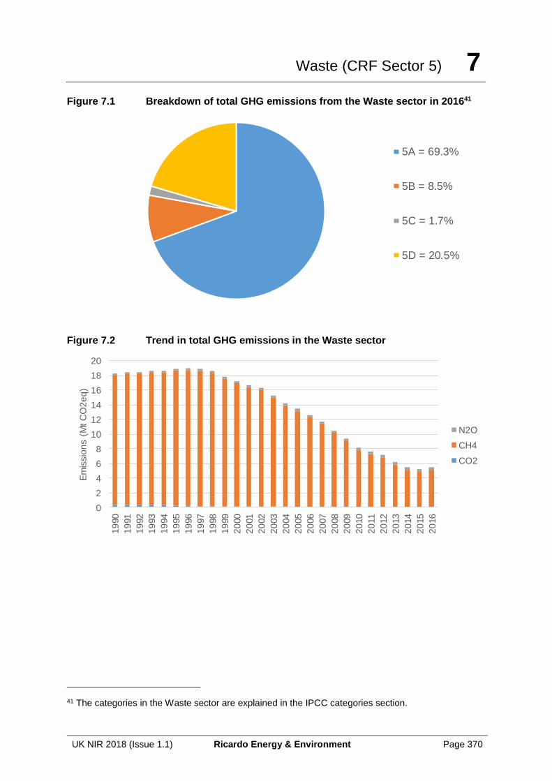
Waste (CRF Sector 5) 7
UK NIR 2018 (Issue 1.1) Ricardo Energy & Environment Page 370
Figure 7.1 Breakdown of total GHG emissions from the Waste sector in 201641
Figure 7.2 Trend in total GHG emissions in the Waste sector
41 The categories in the Waste sector are explained in the IPCC categories section.
5A = 69.3%
5B = 8.5%
5C = 1.7%
5D = 20.5%
0
2
4
6
8
10
12
14
16
18
20
19
90
19
91
19
92
19
93
19
94
19
95
19
96
19
97
19
98
19
99
20
00
20
01
20
02
20
03
20
04
20
05
20
06
20
07
20
08
20
09
20
10
20
11
20
12
20
13
20
14
20
15
20
16
Em
issio
ns (
Mt
CO
2e
q)
N2O
CH4
CO2
Waste (CRF Sector 5) 7
UK NIR 2018 (Issue 1.1) Ricardo Energy & Environment Page 371
7.2 SOURCE CATEGORY 5A – SOLID WASTE DISPOSAL ON LAND
7.2.1 Source category description
Emissions sources Sources included Method Emission Factors
5A: Landfill OTH, T2
CS
Gases Reported CH4, NMVOC
Key Categories 5A: Solid waste disposal - CH4 (L1, T1, L2, T2)
Key Categories (Qualitative)
None identified
Overseas Territories and Crown Dependencies Reporting
OT & CD emissions for 5A are included as a separate category within 5A.
Completeness No known omissions. A general assessment of completeness for the inventory is included in Section 1.8.
Major improvements since last submission
The input data and parameters for the MELMod model were updated based on new data on the quantity of waste landfilled. Data on methane collection and combustion in landfill gas engines and flares have been updated.
The NAEI category “Landfill” maps directly on to IPCC category 5A Solid Waste Disposal for methane emissions. Emissions are reported from Solid Waste Disposal Sites (SWDS – also known as landfills) that started receiving waste in 1980, when legislative changes took effect to improve management of landfill sites, and old unmanaged waste disposal sites that closed prior to 1980.
Estimated emissions from this sector in 2016 were 13.8 Mt CO2e. Emissions have been on a downward trend since 1996.
In addition to CH4, anaerobic decomposition also produces an approximately equivalent amount of carbon dioxide and further CO2 is also produced by aerobic decomposition processes. However, as the decaying organic matter originates from biomass sources derived from contemporary crops and forests, we do not need to consider the greenhouse impacts of this carbon dioxide. Waste also contains fossil-derived organic matter, predominantly in the form of plastics, but these are essentially non-biodegradable under landfill conditions, and so emissions of fossil-derived CO2 from SWDS are not considered further. Emissions of CO2 from landfills are not estimated as they are considered to be entirely biogenic in origin and therefore not counted towards the national total as this would introduce a double count with net carbon losses reported in the LULUCF sector.
Non-methane volatile organic compounds (NMVOCs) are also released by SWDS. These are estimated using an emission factor relating the NMVOC to the amount of CH4 emitted. An emission factor of 0.0036 kg NMVOC/tonne landfill gas was used (Broomfield et al., 2010).
The 2006 guidelines confirm that nitrous oxide emissions from SWDS are not significant.
The amount of methane emitted from landfills depends primarily on the amount of carbon in biodegradable waste landfilled and how the sites are operated to reduce the escape of the methane produced from such wastes. Policy measures to reduce methane emissions from
Waste (CRF Sector 5) 7
UK NIR 2018 (Issue 1.1) Ricardo Energy & Environment Page 372
landfills have focused on both these aspects. Diverting biodegradable waste away from landfill avoids the future formation of methane, but landfills continue to produce CH4 for many years from waste that has already been deposited. Improving the efficiency of gas capture from landfills results in an immediate reduction in emissions, but is by nature an “end of pipe” solution, which does not itself prevent the formation of methane. In practice, a combination of measures based on both reducing the amount of biodegradable waste landfilled and improving the management of sites have, in the UK, provided the foundations for reducing emissions from this source. These two broad approaches are outlined below.
The most important legislative and regulatory measures which have reduced the emissions of methane from UK landfills derive from the 1999 Landfill Directive (1999/31/EC). The requirements of the Directive were transposed into national legislation through the Landfill (England and Wales) Regulations 2002, subsequently amended in 2004 and 2005 to transpose the requirements of Council Decision 2003/33/EC on Waste Acceptance Criteria. The provisions were re-transposed most recently as part of the Environmental Permitting (England and Wales) Regulations 216. In Scotland, the Landfill Directive is implemented through the Landfill (Scotland) Regulations 2003, as amended, and in Northern Ireland, through the Landfill Regulations (Northern Ireland) 2003. The provisions of the Landfill Directive require reduction of the amount of biodegradable waste landfilled to specific targets and improved landfill design, operation and management in order to reduce release of methane.
The EU Waste Framework Directive 2008/98/EC and Landfill Directive 1999/31/EC provides the legislative framework for collection, transport, recovery and disposal of waste. The Waste Framework Directive mandates management of waste according to the waste hierarchy – with the first and preferred method being prevention, followed by reuse, recycling, recovery, and lastly disposal. This mandates the movement away from landfilling of waste.
7.2.2 Methodological issues
The UK approach to calculating emissions of methane from landfills uses a “Tier 2” methodology based on national data on waste quantities, composition, properties and disposal practices over several decades. The equations for calculating methane generation use a first-order decay (FOD) methodology (IPCC (2006) p3.6 – 3.12). The IPCC FOD methodology is based on the premise that Dissimilable Degradable Organic Carbon compounds (DDOC; those that can be converted to methane and carbon dioxide)42 decay under the airless conditions in landfills to form methane, carbon dioxide and a variety of stable decomposition products that remain in the landfill, and represent a sink for carbon. First order means that the rate of reaction is proportional to the amount of reactant (i.e. DDOC) present at any given time. This means that as the reactant is used up, the rate of reaction slows down.
In the UK model, the various waste types are allocated to three pools (p) of DDOC that decompose according to their characteristic first order rate constant, kp. This parameter defines the proportion of material decomposing per year in each year following disposal. The three pools are described as Rapidly, Moderately, and Slowly Decomposing Organics (RDO, MDO and SDO, respectively). Allocation of DDOC in waste materials to these pools was described in a report produced by Eunomia Consulting and Research (2011) and updated for the 2013 and 2014 inventories. Fats, sugars and proteins are assigned to the rapidly
42 DDOC is the amount of degradable organic carbon (DOC) that is converted (i.e. dissimilated) to methane and carbon dioxide under landfill conditions. DDOC = DOC x DOCF where DOCF is the fraction of DOC that dissimilates.
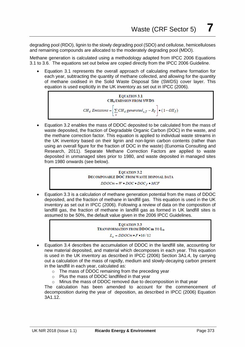
Waste (CRF Sector 5) 7
UK NIR 2018 (Issue 1.1) Ricardo Energy & Environment Page 373
degrading pool (RDO), lignin to the slowly degrading pool (SDO) and cellulose, hemicelluloses and remaining compounds are allocated to the moderately degrading pool (MDO).
Methane generation is calculated using a methodology adapted from IPCC 2006 Equations 3.1 to 3.6. The equations set out below are copied directly from the IPCC 2006 Guideline.
• Equation 3.1 represents the overall approach of calculating methane formation for each year, subtracting the quantity of methane collected, and allowing for the quantity of methane oxidised in the Solid Waste Disposal Site (SWDS) cover layer. This equation is used explicitly in the UK inventory as set out in IPCC (2006).
• Equation 3.2 enables the mass of DDOC deposited to be calculated from the mass of
waste deposited, the fraction of Degradable Organic Carbon (DOC) in the waste, and the methane correction factor. This equation is applied to individual waste streams in the UK inventory based on their lignin and non-lignin carbon contents (rather than using an overall figure for the fraction of DOC in the waste) (Eunomia Consulting and Research, 2011). Separate Methane Correction Factors are applied to waste deposited in unmanaged sites prior to 1980, and waste deposited in managed sites from 1980 onwards (see below).
• Equation 3.3 is a calculation of methane generation potential from the mass of DDOC
deposited, and the fraction of methane in landfill gas. This equation is used in the UK inventory as set out in IPCC (2006). Following a review of data on the composition of landfill gas, the fraction of methane in landfill gas as formed in UK landfill sites is assumed to be 50%, the default value given in the 2006 IPCC Guidelines.
• Equation 3.4 describes the accumulation of DDOC in the landfill site, accounting for
new material deposited, and material which decomposes in each year. This equation is used in the UK inventory as described in IPCC (2006) Section 3A1.4, by carrying out a calculation of the mass of rapidly, medium and slowly-decaying carbon present in the landfill in each year, calculated as:
o The mass of DDOC remaining from the preceding year o Plus the mass of DDOC landfilled in that year o Minus the mass of DDOC removed due to decomposition in that year
The calculation has been amended to account for the commencement of decomposition during the year of deposition, as described in IPCC (2006) Equation 3A1.12.
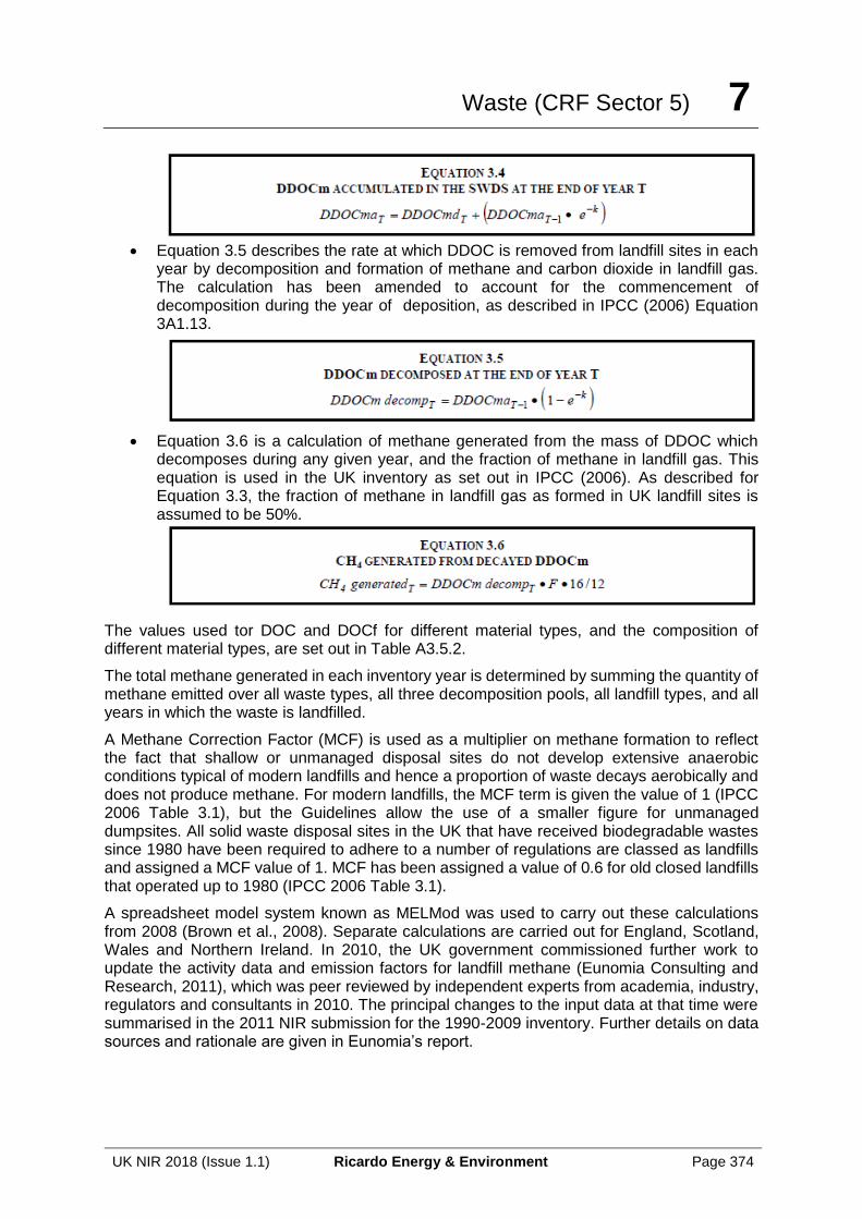
Waste (CRF Sector 5) 7
UK NIR 2018 (Issue 1.1) Ricardo Energy & Environment Page 374
• Equation 3.5 describes the rate at which DDOC is removed from landfill sites in each
year by decomposition and formation of methane and carbon dioxide in landfill gas. The calculation has been amended to account for the commencement of decomposition during the year of deposition, as described in IPCC (2006) Equation 3A1.13.
• Equation 3.6 is a calculation of methane generated from the mass of DDOC which
decomposes during any given year, and the fraction of methane in landfill gas. This equation is used in the UK inventory as set out in IPCC (2006). As described for Equation 3.3, the fraction of methane in landfill gas as formed in UK landfill sites is assumed to be 50%.
The values used tor DOC and DOCf for different material types, and the composition of different material types, are set out in Table A3.5.2.
The total methane generated in each inventory year is determined by summing the quantity of methane emitted over all waste types, all three decomposition pools, all landfill types, and all years in which the waste is landfilled.
A Methane Correction Factor (MCF) is used as a multiplier on methane formation to reflect the fact that shallow or unmanaged disposal sites do not develop extensive anaerobic conditions typical of modern landfills and hence a proportion of waste decays aerobically and does not produce methane. For modern landfills, the MCF term is given the value of 1 (IPCC 2006 Table 3.1), but the Guidelines allow the use of a smaller figure for unmanaged dumpsites. All solid waste disposal sites in the UK that have received biodegradable wastes since 1980 have been required to adhere to a number of regulations are classed as landfills and assigned a MCF value of 1. MCF has been assigned a value of 0.6 for old closed landfills that operated up to 1980 (IPCC 2006 Table 3.1).
A spreadsheet model system known as MELMod was used to carry out these calculations from 2008 (Brown et al., 2008). Separate calculations are carried out for England, Scotland, Wales and Northern Ireland. In 2010, the UK government commissioned further work to update the activity data and emission factors for landfill methane (Eunomia Consulting and Research, 2011), which was peer reviewed by independent experts from academia, industry, regulators and consultants in 2010. The principal changes to the input data at that time were summarised in the 2011 NIR submission for the 1990-2009 inventory. Further details on data sources and rationale are given in Eunomia’s report.
Waste (CRF Sector 5) 7
UK NIR 2018 (Issue 1.1) Ricardo Energy & Environment Page 375
7.2.3 Activity data
Records of individual waste consignments treated and disposed, together with European Waste Category (EWC) codes are compiled by the regulatory authorities in the Devolved Administrations:
• Data on waste consignments landfilled in England for the period 2006 to 2016 are published by the Environment Agency.
• Data on waste consignments landfilled in Scotland for the period 2005 to 2016 are published by the Scottish Environmental Protection Agency.
• Data on waste consignments landfilled in Wales for the period 2006 to 2016 are published by Natural Resources Wales.
• Data on waste consignments landfilled in Northern Ireland for the period 2008 to 2016 were provided by the Northern Ireland Environment Agency.
This information is considered to be of good quality. The composition of waste landfilled was evaluated by allocating EWC codes to the categories used in the UK model, as set out in Section A3.5.1.1.
For years prior to 2005-2008, the quantities of waste landfilled and its composition were taken from a report compiled and peer-reviewed on behalf of the UK Government (Eunomia, 2011). The quantities of waste landfilled are set out in Table A3.5.3.
7.2.3.1 Methane recovery from modern landfills
Landfill operators are required under their permit conditions to control the release of landfill gas. For large landfills containing biodegradable wastes, this requires the use of impermeable liners and cover material, and gas extraction systems. These typically consist of a system of gas wells (perforated pipes sunk into the waste) connected to a network of gas collection pipes. Suction is applied to the gas wells, resulting in a slight negative pressure sufficient to draw out the landfill gas but not enough to draw excessive air into the waste. Air ingress is avoided, as it can result in aerobic decomposition of the waste, which produces considerable heat, and may lead to the waste catching fire, as well as shutting off methane formation. The landfill gas collected is normally used to generate electricity on a commercial basis. Where this is not practicable, gas collected can be burnt in flares. In either case, the net effect of the combustion process is to convert the methane to carbon dioxide. The carbon dioxide so produced is not taken into further consideration for inventory purposes as it is considered to be entirely biogenic in origin.
The key factors in determining methane emissions are estimates of the quantity of methane generated, and information on the amount of methane collected, either for utilisation or flaring. Data on utilisation is available and of good quality (see section 7.2.3.2), but recent analysis indicates that data on flaring prior to 2009 is either unavailable or only accessible at disproportionate cost. The current inventory uses operator-provided data on the quantities of gas collected and burnt in landfill gas flares (see section 7.2.3.3). No gas collection is assumed to be carried out at old pre-1980 closed sites. At sites and inventory years for which robust data on landfill gas flaring are not available, it is conservatively assumed that no landfill gas was flared.
Current estimates for methane recovered are given in Table A 3.5.4.
A high standard of gas collection and combustion efficiency is achieved by compliance with the Landfill Directive requirements for gas collection, and by implementing national guidance on landfill gas collection. This is enforced via the landfill permitting and regulatory processes. Large-scale passive venting of landfill gas is no longer accepted under permitting conditions
Waste (CRF Sector 5) 7
UK NIR 2018 (Issue 1.1) Ricardo Energy & Environment Page 376
and impermeable barriers are required as best practice to prevent the migration of landfill gas off-site.
7.2.3.2 Gas Utilisation
Power generation is currently the dominant use for landfill gas in the UK and good data are available on this from official sources. The method for calculating methane combusted in landfill gas engines is as reported in the 2013 UK NIR. The assumed efficiency of landfill gas engines in these calculations was calculated in accordance with research carried out for the UK Government (Golder Associates, 2014).
Current data on the amount of methane used for power generation in England, Scotland, Wales and Northern Ireland, calculated from the electricity generated from landfill gas as reported in the Digest of UK Energy Statistics (BEIS, 2017), is given in Table A 3.5.4. In 2016, 4703 GWh renewable electricity was generated from combustion of landfill gas. Carbon dioxide emitted from the combustion of landfill gas is biogenic in origin and is therefore not reported.
7.2.3.3 Flaring
Since 2009, operators of landfills in England and Wales permitted under the Integrated Pollution Prevention and Control (IPPC) Directive have been required to report the annual quantity of methane flared at the regulated sites under the terms of their operating permits. As it has been obtained under the terms of IPPC operating permits, this data has documentation and quality control built in via the permitting procedures and operator obligations at an individual site level. The use of this dataset is therefore a robust and appropriate basis on which to evaluate the quantities of methane flared by operators. Based on guidance from the Expert Review of the 2013 GHG Inventory (para 98 of the 2013 Annual Review Report), this dataset was used to estimate the quantity of methane flared at landfill sites in England and Wales in 2008.
Similarly, landfill site operators in Scotland have been required to compile a similar annual report on the quantity of landfill gas flared since 2013. This dataset was used to evaluate the quantity of methane flared by operators at landfill sites in Scotland in 2013.
Further work was commissioned by BEIS (then DECC) to identify all reasonably available data on the quantities of methane flared at landfill sites in England, Scotland and Wales for other years (DECC, 2015). This project identified some additional site-specific data which was also taken into account in compiling the inventory. Additionally, landfill operators voluntarily provided further site-specific data on the quantities of methane flared at older sites without a reporting requirement set in permit conditions for 2010 to 2015.
The landfill methane flaring data provided represents information for approximately 300 individual sites in 2015. Data checking/validation therefore relies on the regulatory authorities and processes, rather than comprising additional checks on individual operators. The information on landfill gas flaring is provided via under the Environmental Permitting (England/Wales) and Pollution Prevention and Control (Scotland/Northern Ireland) regulatory processes. This information is consequently subject to quality obligations under these regulations, as with any other information reported to the regulatory authorities by regulated process operators under the terms of their operating permits. The data is then forwarded to the compilation agency by each regulatory authority.
At all other sites and inventory years, robust data on landfill gas flaring was not available, and it was conservatively assumed that no landfill gas was flared.
The estimates shown in Table A 3.5.4 are based on the estimate of methane used for power generation added to the estimated quantity of methane flared. The minor proportion of landfill
Waste (CRF Sector 5) 7
UK NIR 2018 (Issue 1.1) Ricardo Energy & Environment Page 377
gas used for non-electricity generation purposes such as direct use and as a vehicle fuel is neglected in these calculations due to a lack of data, and assumed to be emitted to the atmosphere as a conservative assumption.
7.2.3.4 Overseas Territories and Crown Dependencies
The IPCC landfill model is used for all landfill estimates. Where available, country-specific waste generation and composition data have been applied and appropriate defaults have been chosen e.g. taking into account climatic variation. There are no landfill emissions for Gibraltar as waste is exported. Parameters used in these calculations are shown in Annex 3.5.
7.2.4 Uncertainties and time-series consistency
The uncertainty analysis in Annex 2 provides estimates of uncertainty according to IPCC source category and fuel type. There are many uncertainties in estimating methane emissions from landfill sites. The model is sensitive to the values assumed for the degradable organic carbon (DOC) present in different fractions of waste, and the amount of this that is dissimilable (i.e. is converted to methane and carbon dioxide), as well as to the quantity of methane combusted in engines and flares, and the oxidation factor. A recent programme of work has assisted in reducing these uncertainties. The uncertainty estimates in Annex 2 are intended to reflect the current uncertainties in data and model parameters.
The estimates for all years have been calculated from the MELMod model and thus the methodology is consistent throughout the time series. Estimates of waste composition and quantities have been taken from different sources as described in Section 7.2.3. The new sources of data on waste receipts from 2005 – 2008 onwards are considered to be more robust and consistent than the previous combination of data sources. The approach to calculating DDOC, the main driver behind methane formation, was reviewed and updated in 2011, and was endorsed by peer reviewers.
Uncertainty in the quantity of methane collected is also an important contributory factor to uncertainty in the calculation of overall landfill methane emissions. Uncertainties in the key components of this calculation are as follows.
• Current and historical combustion of methane in landfill gas engines: Reliable data on methane collected for power generation are available, based on national statistics for energy generated from landfill gas engines (BEIS 2017). The methane to carbon dioxide ratio of gas burnt in landfill gas engines is assumed to be 50:50, following the IPCC default approach. Gas engine efficiency is assumed to be 30% up to 1996, increasing linearly to 36% in 2012 and thereafter, following peer review (Golder Associates, 2014). This is considered to be a reasonably reliable calculation of the quantity of methane combusted in landfill gas engines; and
• Combustion of methane in flares. These data are based on site-specific records where available and are considered to be accurate for the sites where data exist. However, records of the quantity of landfill gas are incomplete, particularly for the years prior to 2008. In cases where records of landfill gas flaring are not available, the quantity of methane flared was assumed to be zero. This means that the landfill methane inventory is subject to greater uncertainty for the years prior to 2008, although because of the conservative approach adopted in respect of landfill gas flaring, it is considered that the inventory represents an over-estimate of methane emissions from landfill sites in the UK, particularly for the years prior to 2008.
Landfill permit conditions are designed to deliver a high standard of gas collection and combustion efficiency. Requirements to design and operate landfills in order to minimise gas
Waste (CRF Sector 5) 7
UK NIR 2018 (Issue 1.1) Ricardo Energy & Environment Page 378
escape have strengthened considerably since the 1990s. In this context, the calculated collection efficiency of 64% in 2015 derived in this analysis appears reasonable. Lower collection efficiencies in the years between 1990 and 2013 are likely to be more conservative.
Oxidation of methane in the surface layers of landfills is a further source of uncertainty in overall emissions. In the absence of better data, the IPCC oxidation default factor of 10% is applied to the estimated quantity of gas released as a fugitive emission. A recent pilot survey carried out on behalf of the UK Government and Environment Agency included measurements of surface methane oxidation. This study did not support a move away from the IPCC default position. A particular challenge in deciding oxidation rates for use in a national landfill model is the high level of variability in field measurements, reflecting a wide range of factors such as nature and porosity of the surface layers, moisture content and temperature, along with methane production rates in the underlying waste.
7.2.5 Source-specific QA/QC and verification
This chapter provides the information described in IPCC (2006) Section 3.8 “QA/QC, Reporting and Documentation.”
Methodological data are described in Section 7.2.2 above, with quantitative data in Annex 3.5.1. Activity data are described in Section 7.2.3 above, with quantitative data on annual waste amounts and the quantities of landfill gas collected in Annex 3.5.1. A breakdown of waste composition for each year is available but as noted in IPCC (2006) Section 3.8, it is not practical to provide all documentation in the National Inventory Report.
In relation to specific recommendations of IPCC (2006) Section 3.8:
• “Countries using other methods or models should provide similar data (description of
the method, key assumptions and parameters)” – this is provided in Section 7.2.2.
• “If country-specific data are used for any part of the time series, it should be
documented.” – country-specific data on DOC, DOCf and MCF are used, as
documented in Section 7.2.2 and Table A 3.5.2.
• “The distribution of waste to managed and unmanaged sites for the purpose of MCF
estimation should also be documented with supporting information.” This is
documented in Section 7.2.2.
• “If CH4 recovery is reported, an inventory of known recovery facilities is desirable.
Flaring and energy recovery should be documented separately from each other.” Data
on methane recovery for electricity generation is based on national statistics on
electricity generation from landfill methane combustion, rather than reports of recovery
at individual facilities. Data on methane recovery and flaring in 2016 is based on
records from a total of 278 individual facilities in England, 40 in Scotland, 17 in Wales,
and 6 in Northern Ireland: however, it is not practical to provide documentation for all
these facilities in the National Inventory Report. Methane recovery for flaring and
energy recovery are separately documented in Section 7.2.3 and Annex 3.5.1.
• “Changes in parameters from year to year should be clearly explained and referenced.”
The change in source of waste data from 2015 to 2016 is described in Section 7.2.3.
The landfill methane model has been subject to peer review in 2011 and 2014 (see Eunomia
Consulting and Research, 2011; Golder Associates 2014). The landfill methane model is
subject to normal quality assurance procedures, as described in Section 1.6.
The Inventory Agency intends to provide a comparison of country-specific values for waste
generated and waste composition against default IPCC values, together with an evaluation of
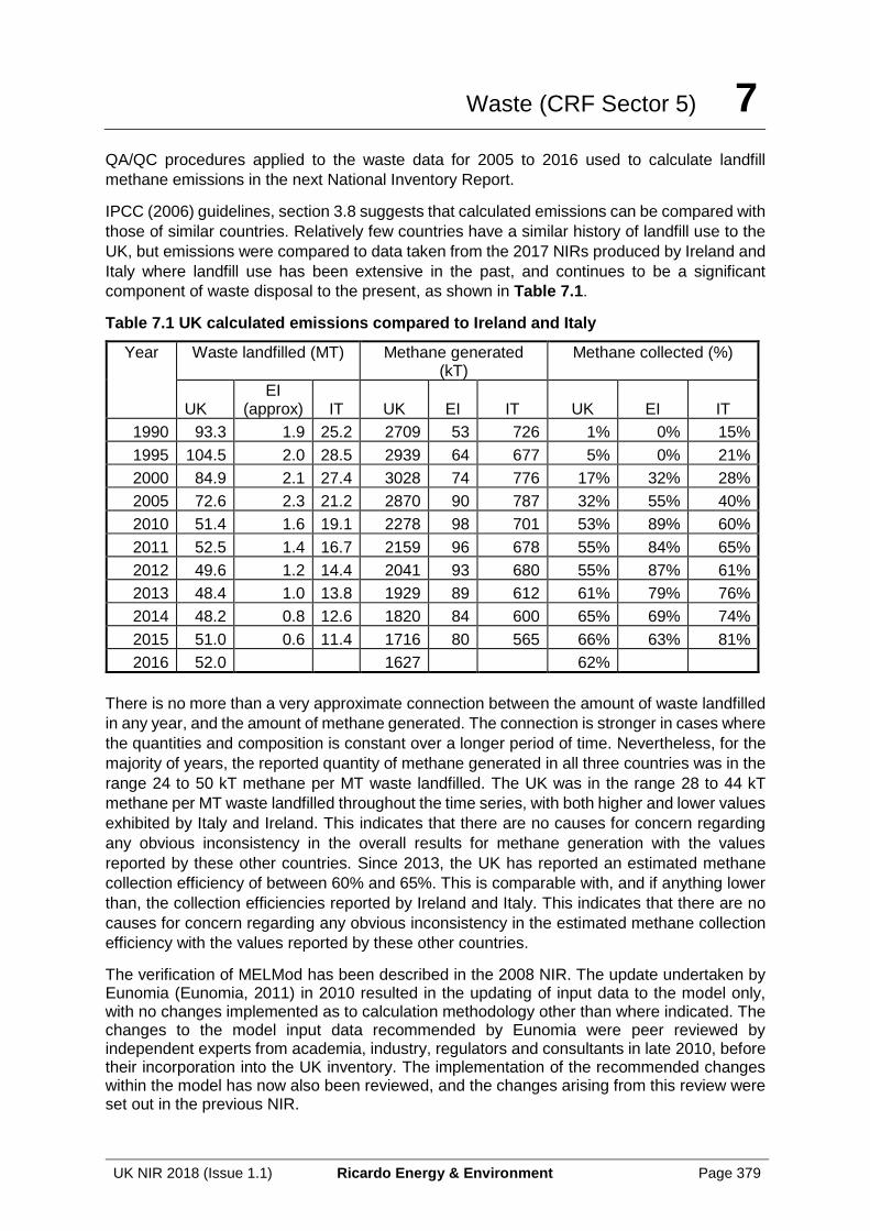
Waste (CRF Sector 5) 7
UK NIR 2018 (Issue 1.1) Ricardo Energy & Environment Page 379
QA/QC procedures applied to the waste data for 2005 to 2016 used to calculate landfill
methane emissions in the next National Inventory Report.
IPCC (2006) guidelines, section 3.8 suggests that calculated emissions can be compared with
those of similar countries. Relatively few countries have a similar history of landfill use to the
UK, but emissions were compared to data taken from the 2017 NIRs produced by Ireland and
Italy where landfill use has been extensive in the past, and continues to be a significant
component of waste disposal to the present, as shown in Table 7.1.
Table 7.1 UK calculated emissions compared to Ireland and Italy
Year Waste landfilled (MT) Methane generated (kT)
Methane collected (%)
UK EI
(approx) IT UK EI IT UK EI IT
1990 93.3 1.9 25.2 2709 53 726 1% 0% 15%
1995 104.5 2.0 28.5 2939 64 677 5% 0% 21%
2000 84.9 2.1 27.4 3028 74 776 17% 32% 28%
2005 72.6 2.3 21.2 2870 90 787 32% 55% 40%
2010 51.4 1.6 19.1 2278 98 701 53% 89% 60%
2011 52.5 1.4 16.7 2159 96 678 55% 84% 65%
2012 49.6 1.2 14.4 2041 93 680 55% 87% 61%
2013 48.4 1.0 13.8 1929 89 612 61% 79% 76%
2014 48.2 0.8 12.6 1820 84 600 65% 69% 74%
2015 51.0 0.6 11.4 1716 80 565 66% 63% 81%
2016 52.0 1627 62%
There is no more than a very approximate connection between the amount of waste landfilled
in any year, and the amount of methane generated. The connection is stronger in cases where
the quantities and composition is constant over a longer period of time. Nevertheless, for the
majority of years, the reported quantity of methane generated in all three countries was in the
range 24 to 50 kT methane per MT waste landfilled. The UK was in the range 28 to 44 kT
methane per MT waste landfilled throughout the time series, with both higher and lower values
exhibited by Italy and Ireland. This indicates that there are no causes for concern regarding
any obvious inconsistency in the overall results for methane generation with the values
reported by these other countries. Since 2013, the UK has reported an estimated methane
collection efficiency of between 60% and 65%. This is comparable with, and if anything lower
than, the collection efficiencies reported by Ireland and Italy. This indicates that there are no
causes for concern regarding any obvious inconsistency in the estimated methane collection
efficiency with the values reported by these other countries.
The verification of MELMod has been described in the 2008 NIR. The update undertaken by Eunomia (Eunomia, 2011) in 2010 resulted in the updating of input data to the model only, with no changes implemented as to calculation methodology other than where indicated. The changes to the model input data recommended by Eunomia were peer reviewed by independent experts from academia, industry, regulators and consultants in late 2010, before their incorporation into the UK inventory. The implementation of the recommended changes within the model has now also been reviewed, and the changes arising from this review were set out in the previous NIR.
Waste (CRF Sector 5) 7
UK NIR 2018 (Issue 1.1) Ricardo Energy & Environment Page 380
MELMod was subject to a further peer review process in 2014 (Golder Associates, 2014). In the light of this peer review, changes were made to the assumed efficiency of landfill gas engines.
7.2.6 Source-specific recalculations
There has been one significant change to the UK landfill methane inventory for 2016, as follows:
• Change in the source of data used to quantify the amount of waste landfilled from 2005-2008 to 2016.
The UK inventory of methane emissions from this sector is set out in Table A 3.5.2. This table shows the quantity of methane generated, combusted in engines and flares, oxidised by the landfill surface and emitted to the atmosphere.
Emission estimates for the OTs and CDs are now calculated using the IPCC waste model taking into account country-specific data and parameters. Previously, the majority of estimates were made by scaling against historic UK data.
7.2.7 Source-specific planned improvements
The Inventory Agency intends to conduct further QA/QC checks and to further evaluate model parameters against the IPCC (2006) default values.
Emission factors, model parameters, and activity data will be kept under review. Defra and the environmental regulatory agencies in the UK have carried out a number of studies to measure methane emissions from a selection of landfills, and a programme of research on closed landfills is now complete (https://www.gov.uk/government/groups/acumen-assessing-capturing-and-utilising-methane-from-expired-and-non-operational-landfills). We are now in a position to use validated Tracer Gas Release techniques to gather data on a larger number of landfills than that covered by the initial Differential Absorption Lidar work. In the longer term, this may facilitate the production of additional site-specific data on landfill methane releases.
Waste (CRF Sector 5) 7
UK NIR 2018 (Issue 1.1) Ricardo Energy & Environment Page 381
7.3 SOURCE CATEGORY 5B – BIOLOGICAL TREATMENT OF SOLID WASTE
7.3.1 Source Category Description
Emissions sources Sources included Method Emission Factors
5B: Composting (non-household) Composting (household) Anaerobic digestion (non-agricultural) Mechanical biological treatment
T2 T2 T2 T2
D D D D
Gases Reported CH4, N2O
Key Categories 5B: Biological treatment of solid waste - CH4 (T1, T2, L2) 5B: Biological treatment of solid waste – N2O (T2)
Key Categories (Qualitative)
None identified
Overseas Territories and Crown Dependencies Reporting
Estimates have been made for OT and CD emissions from 5B1, composting of municipal solid waste, where data on the total amount of waste composted is available. In these cases 2006 IPCC default EFs are applied. These estimates are included within 5B for CRF reporting.
Completeness No known omissions. A general assessment of completeness for the inventory is included in Section 1.8.
Major improvements since last submission
A new source of activity data for anaerobic digestion has been identified and used.
7.3.2 Methodological Issues
Emissions of methane and nitrous oxide from composting of MSW (Category 5.B.1) and anaerobic digestion (AD) and Mechanical Biological Treatment (MBT) (Category 5.B.2) were introduced into the inventory for 2013 using a Tier 2 methodology. This was identified as an appropriate approach in view of the scale of emissions from this sector (DECC, 2015b).
Activity data for composting and anaerobic digestion relies on the approaches used in the GHG and ammonia inventories. Activity data for composting was derived from Devolved Administrations’ data on organic waste fractions. Inputs to household composting were calculated by using population statistics and district level analysis for home composting in the UK (Parfitt, 2009).
Activity data for anaerobic digestion was derived from the new site information database recorded in the National Non-Food Crops Centre (NNFCC 2017). The new AD data differs from the previous data collections, which were based on information on anaerobic digestion processing capacity and “feedstock demand” from two datasets compiled by WRAP and the Biogas Association respectively (Biogas, 2016; WRAP, 2016). The reported inputs to each site in NNFCC reflect the actual tonnes inputted by feedstock category, as opposed to previously available datasets which utilised the capacity of the site as the presumed input. The newly available NNFCC dataset provides a substantial improvement to the inventory, due to a large reduction in uncertainty on the quantities of different materials.
Waste (CRF Sector 5) 7
UK NIR 2018 (Issue 1.1) Ricardo Energy & Environment Page 382
Emissions from the anaerobic digestion of agricultural residues are not considered in the waste sector. These emissions are reported in the agriculture sector, as it is suggested by the IPCC 2006 Guidelines.
Emission factors for source category 5.B.1 and the anaerobic digestion component of 5.B.2 were taken from IPCC (2006) default emission factors. IPCC 2006 Guidelines published an update for the waste sector in July 2015. This update is related to the default CH4 and N2O emission factors proposed for composting and anaerobic digestion and it has been applied to the complete time series. CO2, in line with the IPCC methodology, is not included in the Inventory calculation as it comes from a renewable source of organic matter. The emission factors for the AD component of mechanical biological treatment were assumed to be the same as for anaerobic digestion.
7.3.2.1 Overseas Territories and Crown Dependencies
Emissions from 5.B.1 have been estimated, however due to data availability, only estimates for Guernsey can be derived. Within Guernsey, composting has only occurred on the Island since 2008, due to creation of a new national composting scheme. The total amount of waste composted within this scheme has been supplied by Guenrsey, and IPCC 2006 default emission factors for both CH4 and N2O have been applied.
7.3.3 Uncertainties and Time Series Consistency
The uncertainty analysis in Annex 2 provides estimates of uncertainty according to IPCC source category and fuel type.
Activity data for industrial activities over the time series were taken from relevant publications, and are considered to provide robust and accurate data. Activity data for home composting is less reliable, but now represents a small proportion (approximately 3%) of total composting activity carried out in the UK.
IPCC Tier 1 default emission factors were used for this analysis. These are considered to be less reliable, and hence subject to greater uncertainty. This is the key source of uncertainty in emissions from the 5.B sector.
Time series consistency is based on activity data and is considered to be reasonably representative of activity in this sector between 1990 and 2016.
7.3.4 Source Specific QA/QC and Verification
This source category is covered by the general QA/QC of the greenhouse gas inventory in Section 1.6.
7.3.5 Source Specific Recalculations
The use of new activity data for anaerobic digestion and composting, as a consequence of methodological improvements to the inventory this year, has resulted in changes in calculated emissions throughout the time series.
The main change for the AD data reflects the use of the NNFCC dataset (NNFCC 2017) as inputs data. Pre 2002 values are now less than half compared to last year due to a combination of real inputs and estimated inputs, and closed sites now being removed from the list. A significant step change between 2004 and 2005 is due to a very large AD plant being included in 2005 in the new dataset (but not until 2010 in the old data).
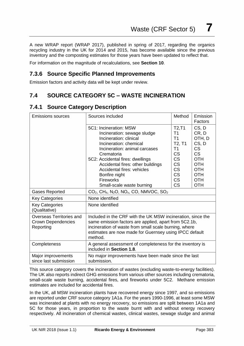
Waste (CRF Sector 5) 7
UK NIR 2018 (Issue 1.1) Ricardo Energy & Environment Page 383
A new WRAP report (WRAP 2017), published in spring of 2017, regarding the organics recycling industry in the UK for 2014 and 2015, has become available since the previous inventory and the composting estimates for those years have been updated to reflect that.
For information on the magnitude of recalculations, see Section 10.
7.3.6 Source Specific Planned Improvements
Emission factors and activity data will be kept under review.
7.4 SOURCE CATEGORY 5C – WASTE INCINERATION
7.4.1 Source Category Description
Emissions sources Sources included Method Emission Factors
5C1: Incineration: MSW Incineration: sewage sludge Incineration: clinical Incineration: chemical Incineration: animal carcases Crematoria
5C2: Accidental fires: dwellings Accidental fires: other buildings Accidental fires: vehicles Bonfire night Fireworks Small-scale waste burning
T2,T1 T1 T1 T2, T1 T1 CS CS CS CS CS CS CS
CS, D CR, D OTH, D CS, D CS CS OTH OTH OTH OTH OTH OTH
Gases Reported CO2, CH4, N2O, NOx, CO, NMVOC, SO2
Key Categories None identified
Key Categories (Qualitative)
None identified
Overseas Territories and Crown Dependencies Reporting
Included in the CRF with the UK MSW incineration, since the same emission factors are applied, apart from 5C2.1b, incineration of waste from small scale burning, where estimates are now made for Guernsey using IPCC default method.
Completeness A general assessment of completeness for the inventory is included in Section 1.8.
Major improvements since last submission
No major improvements have been made since the last submission.
This source category covers the incineration of wastes (excluding waste-to-energy facilities). The UK also reports indirect GHG emissions from various other sources including crematoria, small-scale waste burning, accidental fires, and fireworks under 5C2. Methane emission estimates are included for accidental fires.
In the UK, all MSW incineration plants have recovered energy since 1997, and so emissions are reported under CRF source category 1A1a. For the years 1990-1996, at least some MSW was incinerated at plants with no energy recovery, so emissions are split between 1A1a and 5C for those years, in proportion to the waste burnt with and without energy recovery respectively. All incineration of chemical wastes, clinical wastes, sewage sludge and animal
Waste (CRF Sector 5) 7
UK NIR 2018 (Issue 1.1) Ricardo Energy & Environment Page 384
carcasses is reported under 5C1, since we have no information on any recovery of energy from these processes. In-situ burning of agricultural waste e.g. crop residue burning is reported under category 3F.
The numbers of chemical waste, clinical waste and sewage sludge incinerators in the UK are not known with certainty, although that number has almost certainly decreased significantly between 1990 and 2015. A total of 31 incinerators regulated under the Industrial Emissions Directive (IED) have been identified as operating in 2016 - 4 burning sewage sludge, 15 burning clinical wastes, and 12 burning chemical wastes. It is possible that a few very small incinerators, outside the scope of IED, may also exist. Approximately 2600 animal carcass incinerators are believed to be in use (estimated in AEA Technology, 2002). These are typically much smaller than the incinerators used to burn other forms of waste. Numbers of crematoria are slowly increasing in the UK: there were 282 in 2016 compared with 239 in 1999 (based on statistics published by the Cremation Society of Great Britain, website at http://www.cremation.org.uk/).
This source category also includes emissions from the open burning of wood waste in Guernsey.
7.4.2 Methodological Issues
Emissions of CO2, CO, NOx, SO2, and VOC from chemical waste incinerators are estimated based on analysis of emissions data reported to the Pollution Inventory (Environment Agency, 2017), the Welsh Emissions Inventory (NRW, 2017) and the Northern Ireland Pollution Inventory (NIEA, 2017). These data sources cover England, Wales and Northern Ireland respectively. There are not thought to be any plants in Scotland. Emissions data are not available for all pollutants for all sites and so some extrapolation of data from reporting sites to non-reporting sites has been done, using estimates of waste burnt at each site as a basis. The gaps in reported data are usually for smaller plants but the need for extrapolation of data may contribute to significant variations in the quality of the estimates. Emissions of N2O from chemical waste incinerators are estimated using the 100 g N2O / t waste default factor for industrial waste incineration given in the IPCC guidelines (2006). Waste tonnages burnt at the largest individual chemical waste incinerators for the period 2006 – 2016 have been obtained from the Environment Agency, but the overall quantity of chemical waste burnt must then be estimated by the Inventory Agency, with estimates for the smaller plant based on their capacity. For the earlier part of the time series, we use the following estimates of total waste burnt:
1993 290,000 tonnes (HMIP, 1995)
2002 284,000 tonnes (Entec, 2003)
The HMIP figure is assumed to also be applicable for 1990-1992, and we interpolate between the HMIP and Entec figures for the years 1994-2001. For the period 2003-2005, we interpolate between the Entec figure of 284,000 tonnes and our estimate for 2006 of 177,000 tonnes. The use of reported emissions data for pollutants other than N2O avoids the need to rely upon the highly uncertain activity data.
Emissions of CH4, CO, N2O, SO2 and VOC from sewage sludge incineration are estimated using literature-based emission factors, while emissions of NOx are estimated using Pollution Inventory data. The factor for N2O is the average of the range of emission factors given in the 2000 IPCC good practice guidance for UK sewage sludge incineration. Emission factors for other pollutants are taken from the EMEP-EEA Emission Inventory Guidebook. The quantity of waste burnt annually is estimated using data from various sources:
Waste (CRF Sector 5) 7
UK NIR 2018 (Issue 1.1) Ricardo Energy & Environment Page 385
1990 RCEP, 1993
1991-1998 Digest of Environmental Statistics (Defra, 2004)
2006-2016 Environment Agency, waste disposal data for individual sites in England
2004-2016 Inventory Agency estimates for Northern Ireland, based on design capacity of incinerator plant at only site.
2013, 2015, 2016 Scottish Environment Protection Agency, estimates of total sewage sludge incinerated in Scotland
Interpolation between the various estimates is used to fill the gaps in the activity data time series.
Emissions of CO2, CH4, CO, N2O, NOx, SO2, and VOC from clinical waste incineration are estimated using literature-based emission factors. The factors for CO2 and N2O are IPCC default factors. Emission factors for other pollutants are largely taken from the EMEP-EEA Emission Inventory Guidebook. The quantity of waste burnt annually is also estimated, these estimates being based on information given in the following sources:
1991 RCEP, 1993
1997 Wenborn et al, 1998
2002 Entec, 2003
2006-2014 Environment Agency, waste disposal data for individual sites in England and Wales
2004-13, 2015-16 Scottish Environment Protection Agency, estimates of total clinical waste incinerated in Scotland
Interpolation between the various estimates is used to fill the gaps in the activity data time series.
Emission estimates for animal carcass incinerators are taken directly from a Defra-funded study (AEA Technology, 2002) and are based on emissions monitoring carried out at a cross section of incineration plants. No activity data are available and so the emission estimates given in this report are assumed to apply for all years.
Emissions of CO, NOX, SO2 and VOC from crematoria are based on literature-based emission factors, expressed as emissions per corpse, and taken from US EPA (2008). Data on the annual number of cremations is available from the Cremation Society of Great Britain (2017).
Emissions from MSW incineration for the period 1990-1996 are reported as a split between 1A1a and 5C, in proportion to the tonnages of waste burnt with and without waste recovery respectively. The same methodology is used to estimate emissions for both types.
Estimates for accidental fires are based on statistics from the Fire Service of Great Britain, available from the Department for Communities and Local Government (DCLG, 2014; now called the Ministry of Housing, Communities, and Local Government as of January 2018). These statistics give the number and severity of fires in dwellings and other buildings, and the number of fires in road vehicles by type. The statistics have then been converted into masses of material burnt by applying country-specific assumptions for each type of fire e.g. for the many fires in dwellings that are limited to just a single item, the mass of material combusted is assumed to be 1 kg. The total material burnt is then combined with emission factors to obtain emission estimates for methane, CO, NOX and NMVOC. The methane factors are taken from AP 42 (USEPA, 2014) and relate to open burning of municipal waste (for dwellings and other buildings) and automobile parts (for vehicle fires). Factors for other pollutants are taken from the same source, or from UK-specific literature. The UK is not aware of any source of
Waste (CRF Sector 5) 7
UK NIR 2018 (Issue 1.1) Ricardo Energy & Environment Page 386
appropriate emission factors for carbon or nitrous oxide emissions from this source, but emissions of these pollutants from this source are expected to be small.
The tonnage of MSW burnt in incinerators in the Cayman Islands and the Falklands is provided by their respective local governments. UK GHGI EFs were then applied to these activity data to estimate emissions from this sector. Emissions from waste incineration in Jersey and the Isle of Man are reported under 1A1a. Data are available for the amount of waste open-burned in Guernsey, so these are used to estimate emissions for 5C2 using IPCC 2006 default EFs. It is assumed that this source is not occurring in the remaining territories.
The inventory also includes estimates for emissions of:
• CO, NOX & VOC from small-scale burning of domestic and garden waste, for example on domestic grates and on garden bonfires;
• CO from open fires lit as part of 'bonfire night' celebrations; and
• CO from fireworks.
All of these estimates are very uncertain, because of the need for expert judgements and assumptions in order to derive any activity data from waste arising data, and the need, because of a lack of suitable emission factors, to instead use factors that were designed for other types of emission source such as domestic fires.
Activity and emissions data for this sector can be found in Annex 3, Table A 3.5.5 and Table A 3.5.6.
7.4.3 Uncertainties and Time-Series Consistency
The uncertainty analysis in Annex 2 provides estimates of uncertainty according to IPCC source category and gas.
7.4.4 Source Specific QA/QC and Verification
This source category is covered by the general QA/QC of the greenhouse gas inventory in Section 1.6.
7.4.5 Source Specific Recalculations
In response to a recommendation of the ESD review of the 2017 submission of the UK inventory, the CEF for clinical waste incineration has been corrected from 228 to 240 kg C / tonne dry weight, in line with the IPCC 2006 default.
Data on waste burnt during 2015 & 2016 has become available since the previous inventory and the estimates for that year have been updated to reflect that.
For information on the magnitude of recalculations to Source Category 5C, see Section 10.
7.4.6 Source Specific Planned improvements
Emission estimates for chemical waste incineration currently do not include the burning of chemical wastes in flares and it is unclear whether these emissions might be included in the estimates reported in 2B10. As recommended in the 2014 Expert Review and associated report, if data on flaring becomes available within the pollution inventory for chemical waste incineration this data will be included in the GHG inventory. No evidence has been found for any chemical waste incineration processes carried out in Scotland or Northern Ireland, and so emissions in these regions are assumed to be zero. The need to deal with significant gaps in the reported data means that estimates are quite uncertain. Emission estimates for clinical waste, animal carcass and sewage sludge incineration are also quite uncertain and ideally
Waste (CRF Sector 5) 7
UK NIR 2018 (Issue 1.1) Ricardo Energy & Environment Page 387
would be improved. However, all incineration processes are relatively minor sources of greenhouse gases and further development of the methodology is not a priority.
7.5 SOURCE CATEGORY 5D – WASTEWATER HANDLING
7.5.1 Source Category Description
Emissions sources Sources included Method Emission Factors
5D1: Domestic Waste-water treatment 5D2: Industrial Waste-water Treatment
T1, CS T1
CS, D D
Gases Reported CH4, N2O
Key Categories 5D: Wastewater Handling - N2O (L2, T2) 5D: Wastewater Handling – CH4 (L2) 5D: Wastewater treatment and discharge - CH4 (T1, L1, L2)
Key Categories (Qualitative)
None identified
Overseas Territories and Crown Dependencies Reporting
Emissions from wastewater handling within OTs and CDs are included in 5D1. Estimates are based on 2006 IPCC Guidelines and EFs with country-specific parameters applied, where available.
Completeness No known omissions. A general assessment of completeness for the inventory is included in Section 1.8.
Major improvements since last submission
None
Emissions reported in 5D2 arise from wastewater handling in a number of industry sectors in the UK where organic content of effluent is high. No data are currently available on sludge removal so all water treatment, sludge treatment and disposal emissions are reported as aggregated under 5D2.
Emissions reported in 5D1 arise from wastewater handling, sludge treatment and disposal in the UK’s municipal waste-water treatment system and private waste-water management systems. The UK’s municipal waste-water treatment system encompasses the treatment of effluent and sludge from residential and commercial sectors as well as trade waste from many industrial sites in the UK.
Methane is released from handling of wastewater and its residual solid by-products (i.e. sludge) under anaerobic conditions, due to the decomposition of organic matter by bacteria.
Nitrous oxide is released from human sewage during waste-water handling due to the release of nitrogenous material from proteins.
7.5.2 Methodological Issues
The emissions from 5D1 and 5D2 are estimated for the following sources in the UK:
• 5D1 Domestic and Commercial Waste-Water. Which consists of 4 main aspects: o UK CH4 emissions from municipal waste-water treatment. UK-specific
method, using activity data for the municipal waste-water treatment volumes, organic content and sludge treatment and disposal routes. Emission factors are
Waste (CRF Sector 5) 7
UK NIR 2018 (Issue 1.1) Ricardo Energy & Environment Page 388
derived from water company reported since 2013 and extrapolated back to 1990;
o UK CH4 emissions from private waste-water management. Default IPCC methodology using UK-specific per capita Biochemical Oxygen Demand (BOD) and estimated population using private waste-water management systems;
o UK N2O emissions. Default IPCC methodology applied to UK time series of population and protein intake estimates from food surveys;
o OT and CD Sewage Treatment. For the majority of overseas territories and crown dependencies, wastewater emissions are estimated using UK data and scaled by population. Data specific to Bermuda were provided by the territory and used within the time series, interpolating and extrapolating where necessary.
• 5D2 Industrial Waste-water Treatment (CH4). Default IPCC methodology applied to UK waste-water estimates of organic load from the food and drink and chemical industries.
7.5.2.1 5D1: UK CH4 emissions from municipal waste-water treatment
The UK estimates for methane from municipal domestic and commercial waste-water and sewage sludge treatment and disposal are derived from a time series of activity data for (i) total mass of sewage sludge disposed, and (ii) population equivalent of effluent treated in the municipal water treatment systems. These data cover most of the UK water company activity since 1990, which reflects shifts in UK water sector regulation and management.
7.5.2.1.1 UK Industry Overview
The UK waste water treatment industry is a highly-regulated sector that has undergone a high level of investment in infrastructure and improvement of management practices over several decades in order to deliver a service that achieves high environmental standards and meets key performance indicators (e.g. treatment parameters and volumes, economic and sustainability standards). Even prior to 1990 the UK network of waste water treatment plants were at the fore-front of engineering and technological development globally, and this has been strengthened by the impacts of successive and more stringent regulations in the intervening years, notably the Urban Waste Water Treatment Directive in the late 1990s / early 2000s which banned dumping of sewage to sea.
The UK water sector was previously publicly owned, and is now comprised of around 15 individual companies that operate regional networks and infrastructure. There is a long history of UK-wide research and co-operation across these companies, and in response to the challenge to monitor and report environmental performance, all major UK water companies engage via a central body, UK Water Industry Research, through which common reporting frameworks and systems are researched, developed and updated to reflect latest science and industry practices.
In the UK, a typical Waste Water Treatment Plant (WWTP) involves a number of interrelated processes each of which have different emissive behaviour. The different combinations of treatment options and the local waste water arising characteristics (especially where high volumes of industrial waste are combined and treated together with municipal waste water, altering the waste water input characteristics away from “typical” municipal waste water arisings) lead to a range of performance in the management of organic waste and the emission performance of the treatment works. The UK tools to monitor WWTP performance, estimate the input water characteristics (which in the UK is linked to regulatory and charging regimes for industrial customers, often based on periodic sampling of industrial effluents that pass into the predominantly municipal system), and to estimate the GHG emissions from these activities have been developed through research focussed on the UK waste water sector and the
Waste (CRF Sector 5) 7
UK NIR 2018 (Issue 1.1) Ricardo Energy & Environment Page 389
existing infrastructure. This research underpins the UK GHGI estimates of methane emissions, as the country-specific model uses company-reported data via the Carbon Accounting Workbook (CAW) which accounts for plant specific processes using CS emission factors that reflect UK circumstances.
Figure 7.3 provides an overview of the key processes in a typical UK WWTP.
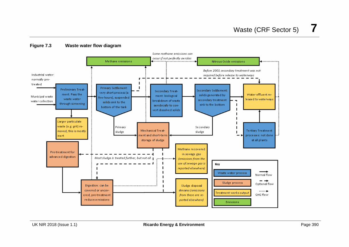
Waste (CRF Sector 5) 7
UK NIR 2018 (Issue 1.1) Ricardo Energy & Environment Page 390
Figure 7.3 Waste water flow diagram
Waste (CRF Sector 5) 7
UK NIR 2018 (Issue 1.1) Ricardo Energy & Environment Page 391
7.5.2.1.1.1 Preliminary Treatment
All waste water is initially filtered for large objects and particulate matter. The filtering process is not emissive and the screened material is largely inert. Any emissions associated with the disposal of non-inert content of the screened waste are included in estimates for other sectors (e.g. landfill in sector 5A).
7.5.2.1.1.2 Settlement (Primary, Secondary and Tertiary)
After preliminary treatment all waste water undergoes primary settlement. Primary settlement involves allowing suspended solids to settle at the bottom of the tank to form a sludge. The sludge can then be extracted for separate sludge treatment. The process is relatively short (a few hours), and hence there is no time for methane generating bacteria to proliferate. Methane emissions from process are therefore insignificant.
During Secondary and Tertiary treatment, the biological processes can lead to the conversion of dissolved solids to suspended solids. When this occurs, additional settlement stages are typically used to extract more solids from the water. The process of secondary and tertiary settlement is otherwise the same as primary settlement.
7.5.2.1.1.3 Secondary Treatment
The standard secondary treatment in the UK is an aerobic treatment which reduces the biological dissolved solids by allowing bacteria to proliferate and process the dissolved solids. The dissolved solids are converted to suspended solids which are separated from the water in the settlement stages.
This process was made compulsory for large WWTP in 2001 under the Urban Waste Water Treatment Directive. Before 2001 this treatment practice was widespread, but was not implemented at all UK WWTP. As a result, the effluent to UK waterways prior to 2001 would typically have had a higher biological load. For this reason, the UK GHGI method applies the IPCC default methodology for waste water disposed to waterways, to account for the increased biological load of this water. The additional biological load is estimated by finding the difference between the sludge generated per capita before and after 2001.
Secondary treatment is a source of nitrous oxide emissions, and a small amount of methane emissions (primarily due to potential disruptions in the process which may allow anaerobic conditions to occur). Emissions of nitrous oxides are included in the company reported data; the Inventory Agency does not use this as we do not have sufficient information to determine what impact this process has on downstream nitrous oxide emissions. Emissions of methane are reported with mechanical treatment and short term storage of sludge in the CAW, and the Inventory Agency uses these values as part of the emissions estimates.
7.5.2.1.1.4 Tertiary Treatment(s)
In many UK WWTPs, there is a requirement for tertiary waste water treatment, in order to meet the regulatory permit conditions and/or to meet water quality criteria for the water-ways receiving the WWTP effluent outflow. There are a number of tertiary processes that can occur depending on what products require removal from the water.
The most common tertiary treatments are nitrification and denitrification which aim to reduce the nitrogen load of effluents. These processes can be a significant source of nitrous oxide within the WWTP, but they also reduce the level of nitrous oxide emissions occurring downstream due to the removal of nitrogen from the effluent. Similar to secondary treatment, the UK cannot estimate nitrous oxide emissions from this source (using the directly-reported emissions from WWTP operators) without introducing a potential double count with downstream emissions, as the data are not available to establish the impact of these tertiary treatments on the residual nitrogen loads in WWTP effluent.
Waste (CRF Sector 5) 7
UK NIR 2018 (Issue 1.1) Ricardo Energy & Environment Page 392
Similar to secondary treatment processes, methane emissions from tertiary treatments do not occur through routine operation and are considered negligible by the UK industry.
7.5.2.1.1.5 Mechanical Treatment and Short Term Storage
All sludge extracted from waste water goes through an initial mechanical treatment and to short term storage. This process thickens, dewaters and homogenises the sludge to reduce the volume of the sludge and prepare it for further treatments. The gravity thickening process and storage of sludge under anaerobic conditions leads to methane emissions which are reported by waste water companies via the CAW, and these data are used to derive the UK inventory estimates.
7.5.2.1.1.6 Digestion
In the UK the vast majority of sludge undergoes anaerobic digestion after mechanical treatment, particularly in recent years. This process allows anaerobic bacteria to process the sludge, reducing the volume of sludge and generating methane. WWTPs collect the generated methane and burn it in engines to generate electricity; this generation of electricity by the industry using sewage gas is reported within the UK energy statistics. Emissions from the burning of sewage gas are reported in the UK inventory within sector 1A1a Power generation, whilst emissions from the disposal of sludge is reported according to the water company reporting of sludge fate, to landfills (5A), incinerators (5C) and agricultural soils (3D).
There is an increasing trend in the UK to pre-treat the sludge before digestion to improve the efficiency of digestion; this is known as advanced digestion. There are two main advanced digestion processes; Cambi’s patented Thermal Hydrolysis Process (CambiTHP™) which involves high pressure steam to improve anaerobic digestion conditions and Acid Phase Digestion (ADP) which involves creating two sets of conditions which suits two types of bacteria. These processes allow for a higher biogas yields and greater reductions in sludge volume than conventional digestion.
Digestion is the main source of methane emissions in UK WWTP as methane is intentionally generated but not all methane is collected. The data reported to the UK inventory team by waste water companies via the CAW accounts for the types of digestion occurring and whether or not the digestion is enclosed.
Nitrous oxide emissions from digestion are negligible, due to the lack of oxygen in the system.
7.5.2.1.1.7 Composting
In some cases, UK WWTPs may compost the sludge after mechanical treatment, instead of digestion. This is a source of methane and nitrous oxide emissions. These emissions are reported by waste water companies in the UK through the CAW, the method for which applies default methane and nitrous oxide emission factors for composting from the 2006 IPCC guidelines.
7.5.2.1.2 Waste-water Treatment and Sludge Disposal Activity Data
Activity data are available at an aggregated level (across countries: England and Wales, Scotland, Northern Ireland, and with no detail on treatment) for the early part of the time series within EPSIM data published by UK Government (Defra, 2006).
In recent years, each of the UK’s 12 water and sewerage companies report annual activity data on water treatment, sewage sludge arising and the ultimate fate of sewage sludge, to UK industry regulators. The activity data reported by each company includes data that are used to estimate company GHG emissions:
Waste (CRF Sector 5) 7
UK NIR 2018 (Issue 1.1) Ricardo Energy & Environment Page 393
• Total volume of sludge disposed (kt total dissolved solids (tds)); and
• Population Equivalent (PE) Served (‘000), this is the estimated resident and non-resident (e.g. tourist) population served which acts as an alternative indicator of sewage load.
In addition, each company provides a detailed split of sewage sludge disposal routes, including data (kt tds per year) for the following activities:
• Incineration;
• Composted;
• Landfill;
• Land reclamation;
• Farmland;
• Disposal at sea (up to the year 2000, when this activity was banned); and
• Other.
For the 2013 inventory cycle the Carbon Accounting Workbook (CAW), developed by UK Water Industry Research (UKWIR), was the tool used by the water industry for reporting emissions to Defra and OFWAT. It was adapted to provide detailed data for the inventory. The inventory team was provided with a methodology report that included a number of the underlying assumptions and emission factors and activity (in PE for secondary treatment, m3 for biogas use and kt tds otherwise); CH4 and N2O emissions were reported for the following:
• Mechanical treatment and short term storage of sludge (activity and CH4 emissions only);
• Secondary treatment (activity and N2O emissions only);
• Digestion (activity and CH4 emissions only);
• Advanced digestion (activity and CH4 emissions only);
• Composting (activity and CH4 emissions only);
• Digested sludge to land;
• Advanced digested sludge to land;
• Composted sludge to land;
• Raw and limed sludge to land;
• Raw and composted sludge to landfill (activity and CH4 emissions only);
• Digested sludge to landfill (activity and CH4 emissions only);
• Sludge to incineration (activity and N2O emissions only);
• Biogas used in CHP for energy generation (activity only); and
• Biogas used for combustion other than by CHP (activity only).
From 2000 to 2009, each of the 10 water companies in England and Wales reported sludge disposal activity to the industry regulator, OFWAT, broken down across 8 sludge disposal routes: incineration, composting, landfill, land reclamation, farmland untreated, farmland conventional, farmland advanced and other. After 2009 the requirements of data reported to OFWAT changed, and data was no longer publically available. For 2013 onwards, company reported data from the CAW has been available.
For 1991 to 2005, the EPSIM data present a breakdown of sewage sludge disposal data across five options: farmland, incineration, landfill, sea disposal and other, and for 1986-2005 this data set gives total estimates sewage sludge arising. No additional information is available, such as the BOD loading of the municipal sewerage system, treatment methods, or the population equivalents treated by UK water companies. The overlap in time-series between the EPSIM data and company reported data confirms that the total and split of disposal methods are largely consistent with each other.
In Scotland the same level of detailed activity data as outlined above for companies in England and Wales have been available since 2002 and continues to be published, from the Water
Waste (CRF Sector 5) 7
UK NIR 2018 (Issue 1.1) Ricardo Energy & Environment Page 394
Commissioner for Scotland; EPSIM data are used for 1990-2001. The totals reported in the EPSIM data fit the company reported data very well, but because the disposal split fits very poorly in the overlapping years the company reported split from 2002 is used with the EPSIM total for the earlier part of the time series.
In Northern Ireland, data are only available from the water regulator, UREGNI, for 2006-9 and 2012 onwards, with a disposal split only available for 2013. The Defra EPSIM statistics are used to provide activity data for the early part of the time series to 2005, whilst the year gap between the 2 data sets and the 2 year gap in company reported data is interpolated. The EPSIM time-series trend fits well with the company reported trend in later years, as the disposal split is similar in the 2013 reported data and at the end of EPSIM time-series it is reasonable to assume a similar split for the intervening years.
7.5.2.1.3 Emission Estimation: Use of UK-specific Factors
The UK GHG inventory mostly follows the UK water industry GHG emission estimation methodology developed by UKWIR for the submission of 2013 data in 2015, and used by all UK water companies to generate their annual emission estimates from all sources / activities. UKWIR have not provided an approach for estimating emissions associated with waste to sea in the 1990s, so to avoid an omission the 2006 IPCC default approach using the Methane Correction Factor (MCF) for sea, river and lake discharge has been used. Discharges would have only been to the cold seas with low organic loadings around the UK, so this is likely to be a very conservative approach for estimating emissions.
Methane emissions from sewage sludge disposed to landfill and incineration are accounted for in 5A and 5C, and hence no estimates are included in 5D1 to avoid a double-count. Waste disposed of via ‘other’ means has been given a weighted average emission factor based on the emissions from other disposal methods. Where the treatment before disposal isn’t specified, the treatment split is estimated based on the profile given in CAW reported data for since 2013; for example it was only after 2013 that the sludge disposed to landfill has been disaggregated based on treatment, this split has been used to estimate the treatment split for the earlier years where none is specified.
UK-specific emission factors are applied to the treatment and disposal methods reported in the CAW, outlined above. Most of these factors are derived from UK water industry emissions data reported to the Inventory Agency, through use of the UKWIR estimation spreadsheet tool that all UK water companies utilise. The UKWIR tool provides emission factors for sub-processes within the industry, enabling water companies to calculate their methane emissions based on their stock of water treatment equipment and effluent inputs to individual water treatment works. From the aggregated industry reported emissions and activity data, implied emission factors for each of the treatment and disposal approaches can be derived. The emission factor for composted sewage sludge treatment is derived from the 2006 IPCC guidelines.
Water company reporting of emissions to the Inventory Agency is not comprehensive; emissions data are only available from 2009 onwards, and only from up to 9 of the 12 UK water companies in any one year before 2013; for example in 2009, emission reporting by water companies was estimated to cover around 53% of total UK water treatment.
During 2013 the Inventory Agency met with all UK water company carbon managers and the authors of the UKWIR reporting tool that all companies use under a voluntary mechanism for GHG emissions reporting. Through this consultation, 9 out of 12 water companies provided 2012 emissions data, covering around 65% of UK water company activities. In addition, a reporting template has been drafted for inclusion within the UKWIR tool, which means that since 2013 we have received data from all 12 of the water companies, covering over 86% of water company activities (2 companies reported lower activity for disposal than treatment, we believed that this meant there was a reporting omission of about 10% of the disposal emissions. This gap was filled by assuming waste was disposed of in similar ways to other
Waste (CRF Sector 5) 7
UK NIR 2018 (Issue 1.1) Ricardo Energy & Environment Page 395
companies). In future we should continue to receive this much more comprehensive data from the industry, and therefore have much more confidence in emissions estimates.
Despite limitations to data collection in previous years, there is good consistency across the emission factors derived from the different water companies and the data are based on UK-specific water treatment facilities, effluent inputs and treatment / disposal activities, and therefore are regarded as the best available data upon which to derive inventory estimates.
The implied emission factors are given in Annex 3.5.2.
7.5.2.1.4 Reporting of Methane Recovery from Sewage Treatment
The methodology report provided by UKWIR for the 2013 version of the CAW provides the emission factor assumed for digestion without capture. Using this factor we calculated what emissions would have been reported had there been no methane capture, then necessarily the difference between reported emissions and this unabated emission estimate would be the amount of methane captured.
Data on the annual amount of sewage gas being produced are provided in DUKES (BEIS, 2017). Using this we can establish a link between the DUKES estimate based on energy use and the mass based estimate based on the difference between unabated and reported methane emissions. Assuming that the relationship between energy use and methane captured is consistent throughout the time series, the amount of methane removed can be calculated for all years and removed from the estimate for unabated emissions.
Using the data suggest that 6-19% of potential methane emitted during digestion is captured for flaring or energy use, with the highest value being observed in 2015 after a steady increase over a number of years.
7.5.2.2 5D1: UK CH4 emissions from private waste-water management
An estimate of the number of households that are likely to be using off-grid systems in the UK in 2013 has been made based on data provided by the Environment Agency (EA), the Scottish Environmental Protection Agency (SEPA), the Northern Ireland Department of the Environment (NIEA) and Natural Resources Wales (NRW).
A time series of emissions has been developed using population data. This time series of number of households has been combined with ONS data for average household occupancy and the calculated volume of waste produced per person per year based on water company statistics to produce an estimate of total waste-water being disposed of via off-grid systems.
The emissions are then calculated following the method set out in the 2006 guidelines Volume 5, Chapter 6: Wastewater treatment and discharge. Equation 6.2 in the GLs, reproduced below, calculates the emission factor.
EFj = B0 ∗ MCFj
Where
EFj= emission factor, kg CH4/kg BOD (Biochemical Oxygen Demand)
j = each treatment/discharge pathway or system
B0= maximum CH4 producing capacity, kg CH4/kg BOD
MCFj= methane correction factor (fraction), See Table 6.3 of the GLs.
Table 7.2 lists the parameters which were used and the calculated EF. The MCF of 0.5 was the default factor for septic tanks. The team did not have enough data to establish the activity by waste treatment process. As the vast majority of private waste management systems observed were septic tanks, and the septic tank factor is conservative when compared to other
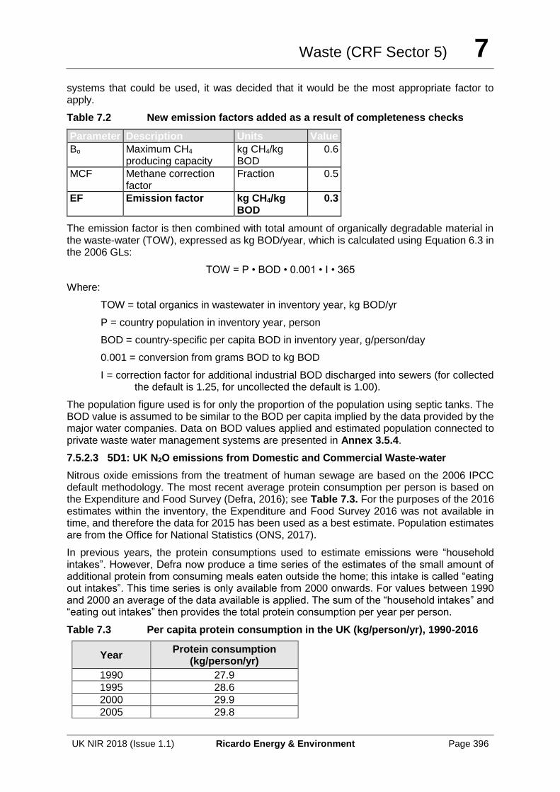
Waste (CRF Sector 5) 7
UK NIR 2018 (Issue 1.1) Ricardo Energy & Environment Page 396
systems that could be used, it was decided that it would be the most appropriate factor to apply.
Table 7.2 New emission factors added as a result of completeness checks
Parameter Description Units Value
Bo Maximum CH4 producing capacity
kg CH4/kg BOD
0.6
MCF Methane correction factor
Fraction 0.5
EF Emission factor kg CH4/kg BOD
0.3
The emission factor is then combined with total amount of organically degradable material in the waste-water (TOW), expressed as kg BOD/year, which is calculated using Equation 6.3 in the 2006 GLs:
TOW = P • BOD • 0.001 • I • 365
Where:
TOW = total organics in wastewater in inventory year, kg BOD/yr
P = country population in inventory year, person
BOD = country-specific per capita BOD in inventory year, g/person/day
0.001 = conversion from grams BOD to kg BOD
I = correction factor for additional industrial BOD discharged into sewers (for collected the default is 1.25, for uncollected the default is 1.00).
The population figure used is for only the proportion of the population using septic tanks. The BOD value is assumed to be similar to the BOD per capita implied by the data provided by the major water companies. Data on BOD values applied and estimated population connected to private waste water management systems are presented in Annex 3.5.4.
7.5.2.3 5D1: UK N2O emissions from Domestic and Commercial Waste-water
Nitrous oxide emissions from the treatment of human sewage are based on the 2006 IPCC default methodology. The most recent average protein consumption per person is based on the Expenditure and Food Survey (Defra, 2016); see Table 7.3. For the purposes of the 2016 estimates within the inventory, the Expenditure and Food Survey 2016 was not available in time, and therefore the data for 2015 has been used as a best estimate. Population estimates are from the Office for National Statistics (ONS, 2017).
In previous years, the protein consumptions used to estimate emissions were “household intakes”. However, Defra now produce a time series of the estimates of the small amount of additional protein from consuming meals eaten outside the home; this intake is called “eating out intakes”. This time series is only available from 2000 onwards. For values between 1990 and 2000 an average of the data available is applied. The sum of the “household intakes” and “eating out intakes” then provides the total protein consumption per year per person.
Table 7.3 Per capita protein consumption in the UK (kg/person/yr), 1990-2016
Year Protein consumption
(kg/person/yr)
1990 27.9
1995 28.6
2000 29.9
2005 29.8
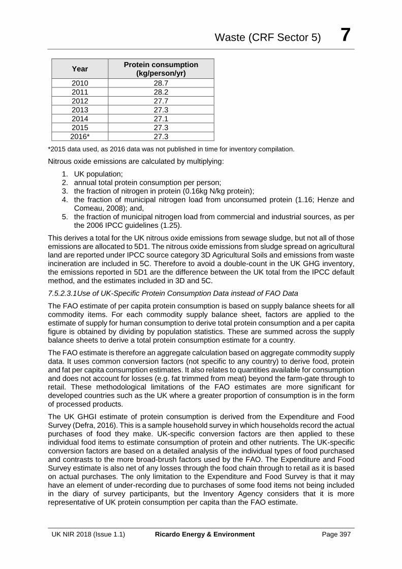
Waste (CRF Sector 5) 7
UK NIR 2018 (Issue 1.1) Ricardo Energy & Environment Page 397
Year Protein consumption
(kg/person/yr)
2010 28.7
2011 28.2
2012 27.7
2013 27.3
2014 27.1
2015 27.3
2016* 27.3
*2015 data used, as 2016 data was not published in time for inventory compilation.
Nitrous oxide emissions are calculated by multiplying:
1. UK population; 2. annual total protein consumption per person; 3. the fraction of nitrogen in protein (0.16kg N/kg protein); 4. the fraction of municipal nitrogen load from unconsumed protein (1.16; Henze and
Comeau, 2008); and, 5. the fraction of municipal nitrogen load from commercial and industrial sources, as per
the 2006 IPCC guidelines (1.25).
This derives a total for the UK nitrous oxide emissions from sewage sludge, but not all of those emissions are allocated to 5D1. The nitrous oxide emissions from sludge spread on agricultural land are reported under IPCC source category 3D Agricultural Soils and emissions from waste incineration are included in 5C. Therefore to avoid a double-count in the UK GHG inventory, the emissions reported in 5D1 are the difference between the UK total from the IPCC default method, and the estimates included in 3D and 5C.
7.5.2.3.1 Use of UK-Specific Protein Consumption Data instead of FAO Data
The FAO estimate of per capita protein consumption is based on supply balance sheets for all commodity items. For each commodity supply balance sheet, factors are applied to the estimate of supply for human consumption to derive total protein consumption and a per capita figure is obtained by dividing by population statistics. These are summed across the supply balance sheets to derive a total protein consumption estimate for a country.
The FAO estimate is therefore an aggregate calculation based on aggregate commodity supply data. It uses common conversion factors (not specific to any country) to derive food, protein and fat per capita consumption estimates. It also relates to quantities available for consumption and does not account for losses (e.g. fat trimmed from meat) beyond the farm-gate through to retail. These methodological limitations of the FAO estimates are more significant for developed countries such as the UK where a greater proportion of consumption is in the form of processed products.
The UK GHGI estimate of protein consumption is derived from the Expenditure and Food Survey (Defra, 2016). This is a sample household survey in which households record the actual purchases of food they make. UK-specific conversion factors are then applied to these individual food items to estimate consumption of protein and other nutrients. The UK-specific conversion factors are based on a detailed analysis of the individual types of food purchased and contrasts to the more broad-brush factors used by the FAO. The Expenditure and Food Survey estimate is also net of any losses through the food chain through to retail as it is based on actual purchases. The only limitation to the Expenditure and Food Survey is that it may have an element of under-recording due to purchases of some food items not being included in the diary of survey participants, but the Inventory Agency considers that it is more representative of UK protein consumption per capita than the FAO estimate.
Waste (CRF Sector 5) 7
UK NIR 2018 (Issue 1.1) Ricardo Energy & Environment Page 398
7.5.2.4 5D2: Industrial Waste-water Treatment
In the UK, a high proportion of industry trade waste-water is disposed to the municipal sewer system and treated by water companies together with the sewage and effluent from domestic and commercial sectors.
In the data reported by the water companies and used to generate methane emission estimates in 5D1 (see above), some of the annual reporting to water regulators includes explicit data on the BOD from “trade waste” and the total BOD treated (i.e. including domestic and commercial effluent) in the municipal systems. The share of total BOD that is attributable to the industry sector (i.e. “trade waste”, managed via contracts between water companies and industry operators) is variable across the UK and across years. In 2008 (before the economic down-turn) the trade waste share of total BOD treated in the municipal waste-water systems (i.e. emissions from which are reported in 5D2) has been estimated to be 13.2%, but from 2009-2012 the figure has been in the range 10.8-11.7%. We are attempting to collect information on the domestic-industrial split in wastewater treatment from water companies in order to have confidence in building a time series that removes this double count.
In addition to the above, where large industrial sites that have on-site waste-water treatment plant are regulated under IPPC/EPR, the annual IPPC/EPR reporting to regulator inventories (PI/SPRI/NIPI) includes the requirement to report any methane emissions from the waste-water effluent plant. The PI/SPRI/NIPI data on methane emissions are used within the UK GHGI, and included within many IPCC source categories, but the lack of source-specific detail in the PI/SPRI/NIPI reporting does not enable the waste-water treatment emission estimates from these industrial facilities to be split out and reported separately in the CRF.
In practice it is not straightforward to ascertain the extent to which emissions from waste-water treatment are consistently included in operator estimates across different industry sectors, as the IPPC/EPR data are not presented “by source”, but rather “by installation”. Within sector-specific guidance to plant operators on pollution inventory data preparation, emissions of methane from wastewater treatment are not highlighted as a common source to be considered, whilst in guidance for several industrial sectors, wastewater treatment is singled out as a potentially significant source of ammonia and nitrous oxide emissions.
Therefore, some industrial waste-water treatment methane emissions are already reported within a range of IPCC source categories, but cannot be quantified explicitly due to the lack of transparency of available source data from UK environmental regulatory reporting systems.
At the 2012 in-country review, the lack of transparency and level of emissions reported in 5D2 (at the time 6B2) led the expert review team to recommend that the UK introduces new separate estimates of emissions of methane from industrial waste-water treatment. Therefore in the 2013 submission the Inventory Agency added a new time series estimates using the IPCC default methodology and available UK activity data from high-BOD-emitting UK industry sources, primarily in the food and drink and chemical production sectors. The UK Inventory Agency considers that this introduces a double count to the inventory, but is a conservative estimate to ensure completeness. The method is retained to the present, as no further evidence has been obtained by the Inventory Agency.
7.5.2.4.1 Summary of Estimation method for UK 5D2 Estimates
In developing industrial waste-water methane emission estimates, the following UK industries have been considered, as they are high-BOD-emitting waste-water source sectors in the UK economy:
• Organic Chemicals; and
• Food and Drink, including: o milk-processing; o manufacture of fruit and vegetable products;
Waste (CRF Sector 5) 7
UK NIR 2018 (Issue 1.1) Ricardo Energy & Environment Page 399
o potato processing; o meat processing; o production of alcohol and alcoholic beverages; o breweries; o manufacture of animal feed from plant products; o manufacture of gelatine and of glue from hides, skin and bones o malt houses; and o fish processing.
The estimation methodology is based on the following data and assumptions:
• Default values for Chemical Oxygen Demand (COD) and amount of wastewater generated used for organic chemical production from the IPCC 2006 GLs;
• PRODCOM data (supplied by the Office for National Statistics) used for organic chemical production (2009) and scaled using Office for National Statistics Index of Production (IOP) for other years (1997 is earliest year for IOP so 1990-1996 estimates use the 1997 value); and
• Total organic load obtained for food and drink industry sub-sectors in a 2002 paper by Defra43, scaled across the time series using Office for National Statistics Index of Production data (as above, 1997 data are used for 1990-1996 also).
[The UK activity data are summarised for selected years across the time series in Annex 3.5.4]
The Inventory Agency considers that these new emission estimates are very conservative, and likely to be over-estimates, noting that:
• There is no information currently available on how much wastewater for the chemical and food and drinks industries are treated on site and how much is included in emissions of wastewater sent to sewers. We have therefore used IPCC default values for the amount of wastewater consumed per tonne of output and amount of COD in the wastewater, and assumed all wastewater is treated on site rather than any of it disposed to municipal sewers;
• There is no information currently available on how much sewage sludge is removed and sent to landfill or applied to agricultural land. Although it is likely that this activity does take place, due to the absence of information, the default value of zero has been used;
• There is no information on the amount of methane recovered, so the default value of zero has been used, although it is likely that this activity also takes place. There is some evidence from the EU ETS dataset that several UK food and industry facilities collect methane from anaerobic digestion systems and use the gas as a fuel source; and
• There is no UK specific information on the split of aerobic and anaerobic industrial wastewater treatment and therefore the IPCC default estimate has been used. It is likely that aerobic treatment systems will be used in many UK facilities.
7.5.2.5 Overseas Territories and Crown Dependencies
Estimates from the OTs and CDs are calculated using the Tier 1 approach from the 2006 IPCC Guidelines and default EFs. Country-specific parameters have been chosen based on information provided through a waste survey (distributed in 2014) and through expert judgement. Per capita protein consumption data were taken from FAOSTAT with data for Bermuda applied to all OTs other than Gibraltar, and data from the UK applied to all CDs and Gibraltar.
43 http://www.defra.gov.uk/publications/files/pb6655-uk-sewage-treatment-020424.pdf
Waste (CRF Sector 5) 7
UK NIR 2018 (Issue 1.1) Ricardo Energy & Environment Page 400
7.5.3 Uncertainties and Time-Series Consistency
As outlined in Section 7.5.2, the method for deriving methane emission estimates for 5D1 uses activity data from across the time series, and applies emission factors that are derived from reported emissions data from 2009 onwards. The method uses a published national set of activity statistics that reflect the changing fate of sewage sludge treatment and disposal; the UK water industry has undergone a marked shift in treatment and disposal practices since the Urban Waste-water Treatment Directive of 1999 banned the dumping of sewage to sea and in 2001 the same directive required all large WWTP to conduct secondary treatment; the sludge disposal trends are consistent with this regulatory change.
Not all UK water companies reported their emission estimates in all years since 2009, and the available dataset for deriving country-specific factors is limited in some cases to only around 50% coverage of UK water treatment and sludge treatment / disposal activity. The Inventory Agency has continued to develop working relationships with the 12 UK water companies and in from 2013 onwards obtained activity and emissions data from all of the 12 water companies. Therefore, we have a much more complete, consistent set of activity and emissions data reported from across the UK. This helps to further develop the UK-specific dataset from which estimates can be derived, improving accuracy through accessing more complete, representative data which reflects the range of waste-water quality and the design / stock of waste-water treatment facilities across the UK. The template for UK water company reporting used last year will be sent to the Inventory Agency on an annual basis, and we have negotiated for further detail to be provided to improve other estimates.
The reported emissions and activity by UK water companies since 2013 has been used to derive country-specific emission factors for water treatment, methane capture, sludge treatment and most disposal routes, and these factors are applied to the activity dataset back to 1990. We are therefore using the best available data to estimate the emissions back to 1990. The use of the IPCC default for methane emissions from waste disposal to sea introduces a significant uncertainty to the early part of the time series where the activity is known to have taken place. This is because the IPCC default factor is for a wide range of situations including stagnant lakes with high organic loads in temperate climates, which would have very different emissive behaviour to the cold, low organic load seas around the UK. Furthermore, the limited activity data time series for 5D1 due to changes in data reporting across the time series limits the accuracy and time series consistency of the estimates for the early part of the time series; however it is observed that the overlaps in trend between the data sets typically show strong agreement.
See Annex 3.5.4 for further details on the activity data, implied emissions factors and emissions estimates, and Section 7.5.6 below for an insight into the planned improvements for this source method.
7.5.4 Source Specific QA/QC and Verification
This source category is covered by the general QA/QC of the greenhouse gas inventory in Section 1.6.
The 2016 UK GHGI reviews under the EU Effort Sharing Decision (ESD) and the UNFCCC Expert Review Team (ERT) concluded that the UK should carry out a verification of the methodology by comparing it with a tier 1 default methodology set out in the 2006 IPCC guidelines. Below this comparison is detailed.
The UK currently uses a 2006 IPCC default methodology to estimate emissions from waste water disposed to waterways and private waste management systems. The verification calculations below compare the emission estimates using the IPCC 2006 GLs Tier 1 method
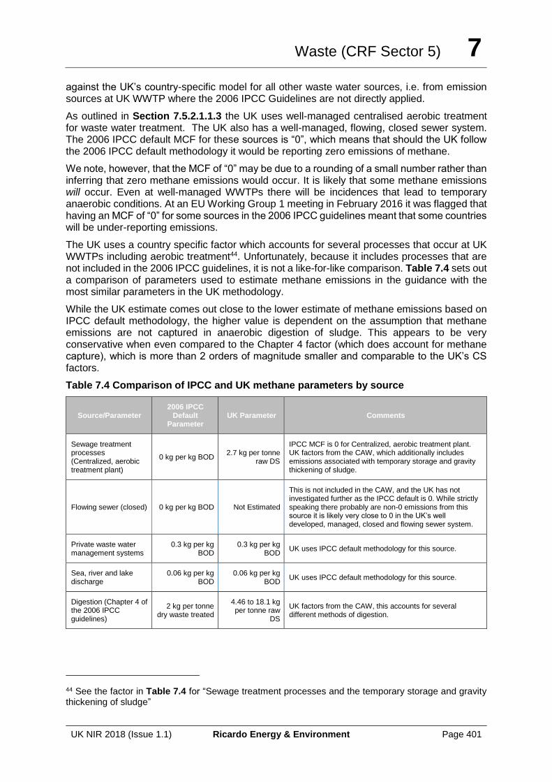
Waste (CRF Sector 5) 7
UK NIR 2018 (Issue 1.1) Ricardo Energy & Environment Page 401
against the UK’s country-specific model for all other waste water sources, i.e. from emission sources at UK WWTP where the 2006 IPCC Guidelines are not directly applied.
As outlined in Section 7.5.2.1.1.3 the UK uses well-managed centralised aerobic treatment for waste water treatment. The UK also has a well-managed, flowing, closed sewer system. The 2006 IPCC default MCF for these sources is “0”, which means that should the UK follow the 2006 IPCC default methodology it would be reporting zero emissions of methane.
We note, however, that the MCF of “0” may be due to a rounding of a small number rather than inferring that zero methane emissions would occur. It is likely that some methane emissions will occur. Even at well-managed WWTPs there will be incidences that lead to temporary anaerobic conditions. At an EU Working Group 1 meeting in February 2016 it was flagged that having an MCF of “0” for some sources in the 2006 IPCC guidelines meant that some countries will be under-reporting emissions.
The UK uses a country specific factor which accounts for several processes that occur at UK WWTPs including aerobic treatment44. Unfortunately, because it includes processes that are not included in the 2006 IPCC guidelines, it is not a like-for-like comparison. Table 7.4 sets out a comparison of parameters used to estimate methane emissions in the guidance with the most similar parameters in the UK methodology.
While the UK estimate comes out close to the lower estimate of methane emissions based on IPCC default methodology, the higher value is dependent on the assumption that methane emissions are not captured in anaerobic digestion of sludge. This appears to be very conservative when even compared to the Chapter 4 factor (which does account for methane capture), which is more than 2 orders of magnitude smaller and comparable to the UK’s CS factors.
Table 7.4 Comparison of IPCC and UK methane parameters by source
Source/Parameter 2006 IPCC
Default Parameter
UK Parameter Comments
Sewage treatment processes (Centralized, aerobic treatment plant)
0 kg per kg BOD 2.7 kg per tonne
raw DS
IPCC MCF is 0 for Centralized, aerobic treatment plant. UK factors from the CAW, which additionally includes emissions associated with temporary storage and gravity thickening of sludge.
Flowing sewer (closed) 0 kg per kg BOD Not Estimated
This is not included in the CAW, and the UK has not investigated further as the IPCC default is 0. While strictly speaking there probably are non-0 emissions from this source it is likely very close to 0 in the UK’s well developed, managed, closed and flowing sewer system.
Private waste water management systems
0.3 kg per kg BOD
0.3 kg per kg BOD
UK uses IPCC default methodology for this source.
Sea, river and lake discharge
0.06 kg per kg BOD
0.06 kg per kg BOD
UK uses IPCC default methodology for this source.
Digestion (Chapter 4 of the 2006 IPCC guidelines)
2 kg per tonne dry waste treated
4.46 to 18.1 kg per tonne raw
DS
UK factors from the CAW, this accounts for several different methods of digestion.
44 See the factor in Table 7.4 for “Sewage treatment processes and the temporary storage and gravity thickening of sludge”
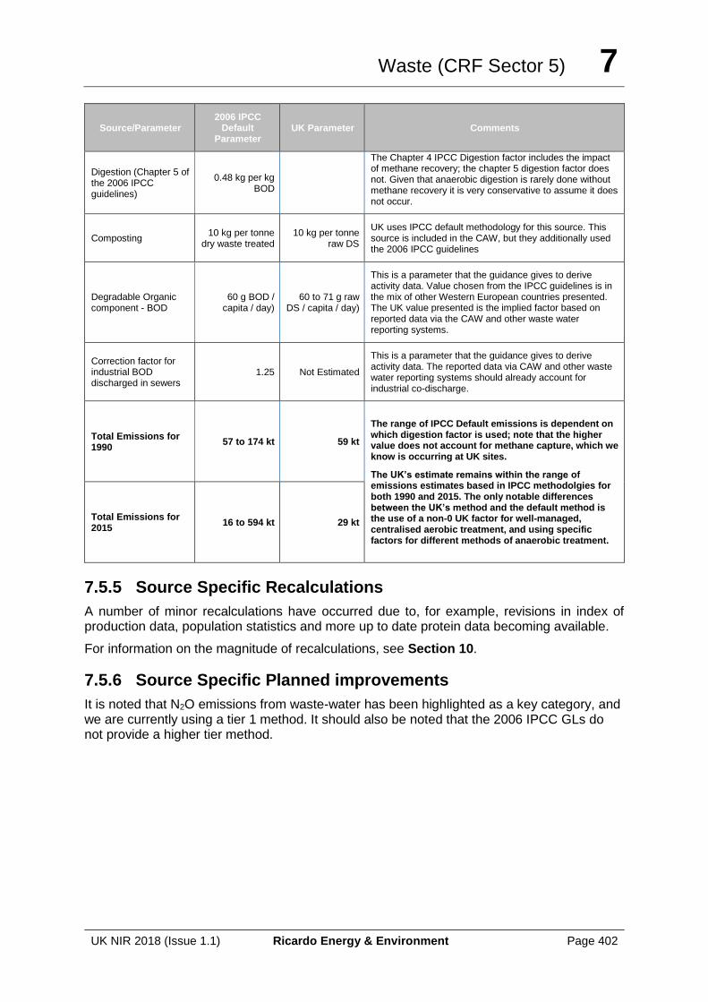
Waste (CRF Sector 5) 7
UK NIR 2018 (Issue 1.1) Ricardo Energy & Environment Page 402
Source/Parameter 2006 IPCC
Default Parameter
UK Parameter Comments
Digestion (Chapter 5 of the 2006 IPCC guidelines)
0.48 kg per kg BOD
The Chapter 4 IPCC Digestion factor includes the impact of methane recovery; the chapter 5 digestion factor does not. Given that anaerobic digestion is rarely done without methane recovery it is very conservative to assume it does not occur.
Composting 10 kg per tonne
dry waste treated 10 kg per tonne
raw DS
UK uses IPCC default methodology for this source. This source is included in the CAW, but they additionally used the 2006 IPCC guidelines
Degradable Organic component - BOD
60 g BOD / capita / day)
60 to 71 g raw DS / capita / day)
This is a parameter that the guidance gives to derive activity data. Value chosen from the IPCC guidelines is in the mix of other Western European countries presented. The UK value presented is the implied factor based on reported data via the CAW and other waste water reporting systems.
Correction factor for industrial BOD discharged in sewers
1.25 Not Estimated
This is a parameter that the guidance gives to derive activity data. The reported data via CAW and other waste water reporting systems should already account for industrial co-discharge.
Total Emissions for 1990
57 to 174 kt 59 kt
The range of IPCC Default emissions is dependent on which digestion factor is used; note that the higher value does not account for methane capture, which we know is occurring at UK sites.
The UK’s estimate remains within the range of emissions estimates based in IPCC methodolgies for both 1990 and 2015. The only notable differences between the UK’s method and the default method is the use of a non-0 UK factor for well-managed, centralised aerobic treatment, and using specific factors for different methods of anaerobic treatment.
Total Emissions for 2015
16 to 594 kt 29 kt
7.5.5 Source Specific Recalculations
A number of minor recalculations have occurred due to, for example, revisions in index of production data, population statistics and more up to date protein data becoming available.
For information on the magnitude of recalculations, see Section 10.
7.5.6 Source Specific Planned improvements
It is noted that N2O emissions from waste-water has been highlighted as a key category, and we are currently using a tier 1 method. It should also be noted that the 2006 IPCC GLs do not provide a higher tier method.
Other (CRF Sector 6) 8
UK NIR 2018 (Issue 1.1) Ricardo Energy & Environment Page 403
8 Other (CRF Sector 6)
8.1 OVERVIEW OF SECTOR
No emissions are reported in Sector 6.

Other (CRF Sector 6) 8
UK NIR 2018 (Issue 1.1) Ricardo Energy & Environment Page 404
Indirect CO2 and Nitrous Oxide Emissions 9
UK NIR 2018 (Issue 1.1) Ricardo Energy & Environment Page 405
9 Indirect CO2 and Nitrous Oxide Emissions
9.1 DESCRIPTION OF SOURCES OF INDIRECT EMISSIONS IN GHG INVENTORY
The calculation of indirect CO2 and N2O is not mandatory. The UK calculates indirect emissions of N2O from emissions of NOX and NH3 from non-AFOLU sources. These are reported as a memo item.
The methods and data sources for the calculation of NOX and NH3 emissions are described in the UK’s Informative Inventory Report (IIR), as submitted under the Convention on Long Range Transboundary Air Pollution.
9.2 METHODOLOGICAL ISSUES
Emissions of indirect N2O are calculated using Equation 7.1 of Volume 1 of IPCC, 2006. EF4 within the equation is the IPCC default of 0.01 kg N2O-N/kg NH3-N or NOX-N emitted.
9.3 UNCERTAINTIES AND TIME-SERIES CONSISTENCY
No formal uncertainty or trend analysis for indirect N2O emissions has been carried out. Uncertainties and trends for NOX and NH3 are described in the IIR.
9.4 CATEGORY-SPECIFIC QA/QC AND VERIFICATION
Emissions of NOX reported under the GHG inventory are cross checked with those reported under CLRTAP and are consistent. NH3 emissions are only reported under CLRTAP and not under the GHG inventory, however, calculated emissions from the UK inventory database have been carefully cross checked with the submitted totals to ensure completeness.
9.5 CATEGORY-SPECIFIC RECALCULATIONS
None.
9.6 CATEGORY-SPECIFIC PLANNED IMPROVEMENTS
Indirect nitrous oxide emissions will change in line with changes made to the NOX and NH3 inventories. Air quality pollutants are subject to a separate improvement programme to the GHG inventory, this is described in the IIR.

Indirect CO2 and Nitrous Oxide Emissions 9
UK NIR 2018 (Issue 1.1) Ricardo Energy & Environment Page 406
Recalculations and Improvements 10
UK NIR 2018 (Issue 1.1) Ricardo Energy & Environment Page 407
10 Recalculations and Improvements
This section of the report summarises the recalculations and improvements made to the UK GHG inventory since the 2017 NIR submission (1990-2015 inventory), including responses to reviews of the inventory. It summarises material that has already been presented and discussed in more detail in Chapter 3 to Chapter 7.
Each year the UK greenhouse gas inventory is updated, extended and may be expanded.
Updating often entails revision of emission estimates, most commonly because of revision to the core energy statistics presented in the Digest of UK Energy Statistics (DUKES). The inventory also makes use of other datasets (see Table 1.6 for a summary) and these too may be revised. Updating also covers adoption of revised methodologies. Updating, particularly involving revised methodologies may affect the whole time series, so estimates of emissions for a given year may differ from estimates of emissions for the same year reported previously. Therefore comparisons between submissions should take account of whether there have been changes to the following:
• the emission estimation methodology, including revisions to assumptions or conversion factors;
• the reporting guidelines under which the submissions are made (i.e. 1996 GLs or 2006 GLs);
• the emission factors applied; and/or
• the activity data.
The time series of the inventory is extended by included a new inventory year. For example, the previous report covered years up to and including 2015. This report gives emission estimates for 2015 and also includes estimates for the year 2016.
The time series of the inventory may also be expanded to include emissions from additional sources if a new source has been identified within the context of the IPCC Guidelines and Good Practice Guidance and there are sufficient activity data and suitable emission factors.
10.1 EXPLANATIONS AND JUSTIFICATIONS FOR RE-CALCULATIONS, INCLUDING IN RESPONSE TO THE REVIEW PROCESS
Table 10.1 to Table 10.12 summarise the recalculations that have occurred in estimates of CO2, CH4, N2O and F-gases since the 2017 NIR submission (1990-2015 inventory). The changes in emissions are net changes (the sum of any increases and decreases) in the source category, for each GHG in the Base Year (1990) (1995 for F-gases) and latest recalculated year (2015).
Table 10.15 summarises where changes to methodological descriptions have been made and where these descriptions can be found in the main text of this document.
All revisions to source data and methods, and all recalculations that are reported in the latest UK GHG inventory are conducted by the Inventory Agency in agreement with the BEIS GHG inventory management team; all major recalculations and systematic improvements to the UK GHG inventory are approved and managed via the NISC, with new outputs approved through the UK’s system for pre-submission review. The inventory improvement process that manages the prioritisation and implementation of revisions to inventory data and methods uses the guiding principles of the 2006 IPCC Guidelines to govern the decisions over whether to
Recalculations and Improvements 10
UK NIR 2018 (Issue 1.1) Ricardo Energy & Environment Page 408
implement changes to inventory estimates or not. The most common justifications for implementing changes that lead to recalculations are:
✓ Improved accuracy of the estimates, e.g. where underlying data from data providers has been revised (e.g. revisions to energy statistics), where less uncertain data are now available (e.g. use of EU ETS activity data to inform energy allocations, in preference to UK energy statistics data sources), or where the inventory agency has applied more representative (ideally UK-specific) EFs in estimation methods (e.g. use of carbon emission factors derived from EU ETS fuel compositional analysis);
✓ Improved transparency of the inventory estimates, e.g. the restructuring of inventory data reporting to improve the level of detail of the UK inventory (such as the reporting of F-gas estimates by species wherever this is achievable);
✓ Improved comparability of the inventory estimates, e.g. the restructuring of inventory data reporting to enable UK estimates to align more closely with IPCC GLs and GPGs, (e.g. re-allocations of limestone and dolomite data in the glass sector from 2A3 and 2A4 to 2A7, which was implemented in the 2012 submission to enable more harmonised data reporting across EU Member States).
✓ Improved completeness of the inventory estimates, e.g. the addition of emission estimates for new sources that come to light in the UK, or where new data for an existing source indicates that the activity data previously used in the method omitted some portion of the source emissions (e.g. use of EU ETS activity data to revise the estimates of emissions from refineries in the UK, where a gap in UK energy data reporting was identified through comparison against EU ETS data for the sector);
✓ Improved consistency of the inventory estimates, e.g. to implement new or revised methods that deliver estimates based on more consistent underlying data or assumptions across the time series.
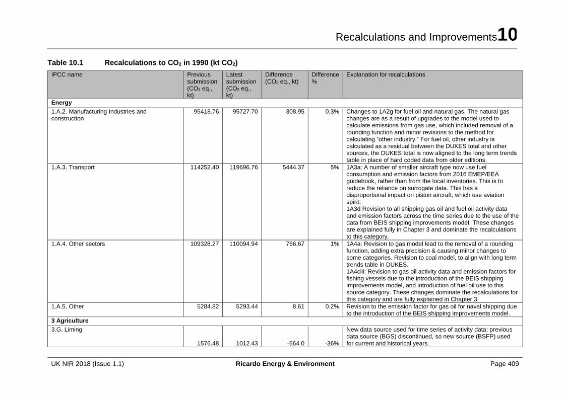
Recalculations and Improvements10
UK NIR 2018 (Issue 1.1) Ricardo Energy & Environment Page 409
Table 10.1 Recalculations to CO2 in 1990 (kt CO2)
IPCC name Previous submission (CO2 eq., kt)
Latest submission (CO2 eq., kt)
Difference (CO2 eq., kt)
Difference %
Explanation for recalculations
Energy
1.A.2. Manufacturing Industries and construction
95418.76 95727.70 308.95 0.3% Changes to 1A2g for fuel oil and natural gas. The natural gas changes are as a result of upgrades to the model used to calculate emissions from gas use, which included removal of a rounding function and minor revisions to the method for calculating “other industry.” For fuel oil, other industry is calculated as a residual between the DUKES total and other sources, the DUKES total is now aligned to the long term trends table in place of hard coded data from older editions.
1.A.3. Transport 114252.40 119696.76 5444.37 5% 1A3a: A number of smaller aircraft type now use fuel consumption and emission factors from 2016 EMEP/EEA guidebook, rather than from the local inventories. This is to reduce the reliance on surrogate data. This has a disproportional impact on piston aircraft, which use aviation spirit; 1A3d Revision to all shipping gas oil and fuel oil activity data and emission factors across the time series due to the use of the data from BEIS shipping improvements model. These changes are explained fully in Chapter 3 and dominate the recalculations to this category.
1.A.4. Other sectors 109328.27 110094.94 766.67 1% 1A4a: Revision to gas model lead to the removal of a rounding function, adding extra precision & causing minor changes to some categories. Revision to coal model, to align with long term trends table in DUKES. 1A4ciii: Revision to gas oil activity data and emission factors for fishing vessels due to the introduction of the BEIS shipping improvements model, and introduction of fuel oil use to this source category. These changes dominate the recalculations for this category and are fully explained in Chapter 3.
1.A.5. Other 5284.82 5293.44 8.61 0.2% Revision to the emission factor for gas oil for naval shipping due to the introduction of the BEIS shipping improvements model.
3 Agriculture
3.G. Liming
1576.48 1012.43 -564.0 -36%
New data source used for time series of activity data; previous data source (BGS) discontinued, so new source (BSFP) used for current and historical years.
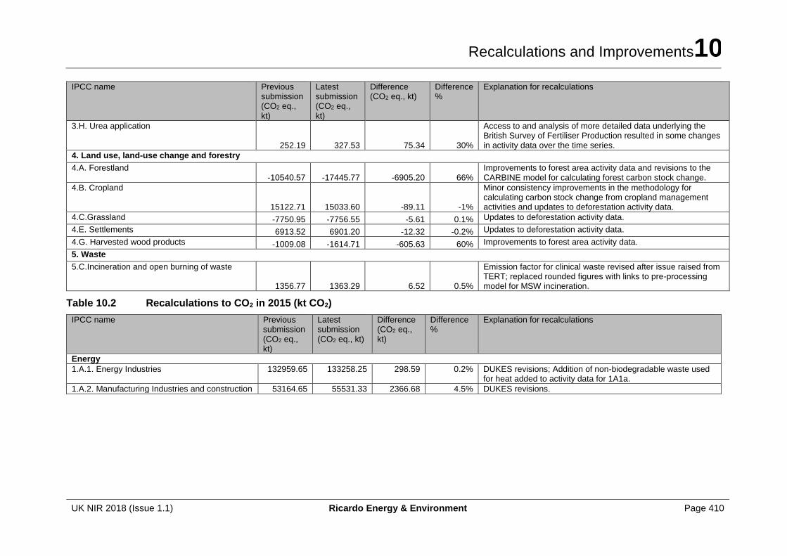
Recalculations and Improvements10
UK NIR 2018 (Issue 1.1) Ricardo Energy & Environment Page 410
IPCC name Previous submission (CO2 eq., kt)
Latest submission (CO2 eq., kt)
Difference (CO2 eq., kt)
Difference %
Explanation for recalculations
3.H. Urea application
252.19 327.53 75.34 30%
Access to and analysis of more detailed data underlying the British Survey of Fertiliser Production resulted in some changes in activity data over the time series.
4. Land use, land-use change and forestry
4.A. Forestland -10540.57 -17445.77 -6905.20 66%
Improvements to forest area activity data and revisions to the CARBINE model for calculating forest carbon stock change.
4.B. Cropland
15122.71 15033.60 -89.11 -1%
Minor consistency improvements in the methodology for calculating carbon stock change from cropland management activities and updates to deforestation activity data.
4.C.Grassland -7750.95 -7756.55 -5.61 0.1% Updates to deforestation activity data.
4.E. Settlements 6913.52 6901.20 -12.32 -0.2% Updates to deforestation activity data.
4.G. Harvested wood products -1009.08 -1614.71 -605.63 60% Improvements to forest area activity data.
5. Waste
5.C.Incineration and open burning of waste
1356.77 1363.29 6.52 0.5%
Emission factor for clinical waste revised after issue raised from TERT; replaced rounded figures with links to pre-processing model for MSW incineration.
Table 10.2 Recalculations to CO2 in 2015 (kt CO2)
IPCC name Previous submission (CO2 eq., kt)
Latest submission (CO2 eq., kt)
Difference (CO2 eq., kt)
Difference %
Explanation for recalculations
Energy
1.A.1. Energy Industries 132959.65 133258.25 298.59 0.2% DUKES revisions; Addition of non-biodegradable waste used for heat added to activity data for 1A1a.
1.A.2. Manufacturing Industries and construction 53164.65 55531.33 2366.68 4.5% DUKES revisions.
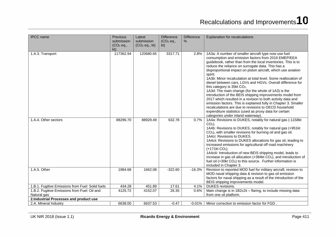
Recalculations and Improvements10
UK NIR 2018 (Issue 1.1) Ricardo Energy & Environment Page 411
IPCC name Previous submission (CO2 eq., kt)
Latest submission (CO2 eq., kt)
Difference (CO2 eq., kt)
Difference %
Explanation for recalculations
1.A.3. Transport 117362.94 120680.65 3317.71 2.8% 1A3a: A number of smaller aircraft type now use fuel consumption and emission factors from 2016 EMEP/EEA guidebook, rather than from the local inventories. This is to reduce the reliance on surrogate data. This has a disproportional impact on piston aircraft, which use aviation spirit; 1A3b: Minor recalculation at total level. Some reallocation of diesel between cars, LGVs and HGVs. Overall difference for this category is 35kt CO2. 1A3d: The main change (for the whole of 1A3) is the introduction of the BEIS shipping improvements model from 2017 which resulted in a revision to both activity data and emission factors. This is explained fully in Chapter 3. Smaller recalculations are due to revisions to OECD household expenditure statistics (used as proxy data for certain categories under inland waterway).
1.A.4. Other sectors 88296.70 88929.49 632.78 0.7% 1A4a: Revisions to DUKES, notably for natural gas (-1158kt CO2). 1A4b: Revisions to DUKES, notably for natural gas (+951kt CO2), with smaller revisions for burning oil and gas oil. 1A4ci: Revisions to DUKES. 1A4cii: Revisions to DUKES allocations for gas oil, leading to increased emissions for agricultural off road machinery (+171kt CO2). 1A4ciii: Introduction of new BEIS shipping model, leads to increase in gas oil allocation (+384kt CO2), and introduction of fuel oil (+30kt CO2) to this source. Further information is included in Chapter 3.
1.A.5. Other 1984.68 1662.08 -322.60 -16.3% Revision to reported MOD fuel for military aircraft; revision to MOD naval shipping data & revision to gas oil emission factors for naval shipping as a result of the introduction of the BEIS shipping improvements model.
1.B.1. Fugitive Emissions from Fuel: Solid fuels 434.28 451.89 17.61 4.1% DUKES revisions.
1.B.2. Fugitive Emissions from Fuel: Oil and Natural gas
4125.72 4152.07 26.35 0.6% Main change is in 1B2c2ii – flaring, to include missing data from one oil platform.
2.Industrial Processes and product use
2.A. Mineral Industry 6638.00 6637.53 -0.47 -0.01% Minor correction to emission factor for FGD .
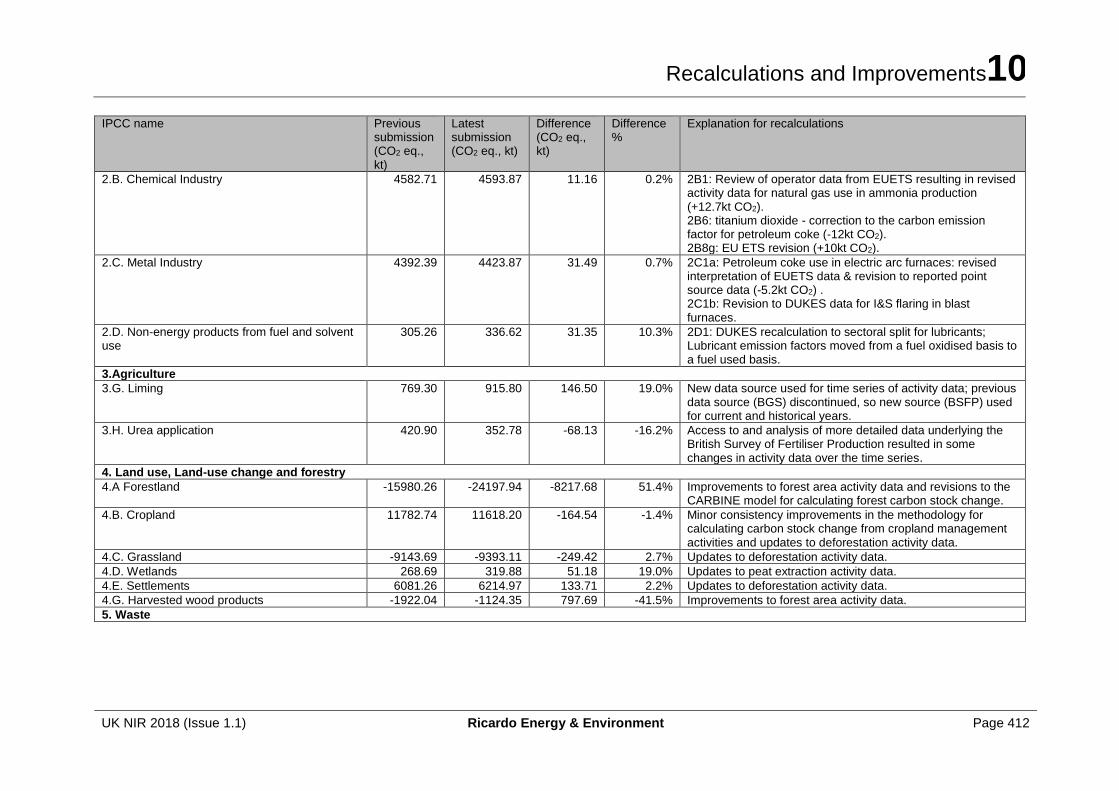
Recalculations and Improvements10
UK NIR 2018 (Issue 1.1) Ricardo Energy & Environment Page 412
IPCC name Previous submission (CO2 eq., kt)
Latest submission (CO2 eq., kt)
Difference (CO2 eq., kt)
Difference %
Explanation for recalculations
2.B. Chemical Industry 4582.71 4593.87 11.16 0.2% 2B1: Review of operator data from EUETS resulting in revised activity data for natural gas use in ammonia production (+12.7kt CO2). 2B6: titanium dioxide - correction to the carbon emission factor for petroleum coke (-12kt CO2). 2B8g: EU ETS revision (+10kt CO2).
2.C. Metal Industry 4392.39 4423.87 31.49 0.7% 2C1a: Petroleum coke use in electric arc furnaces: revised interpretation of EUETS data & revision to reported point source data (-5.2kt CO2) . 2C1b: Revision to DUKES data for I&S flaring in blast furnaces.
2.D. Non-energy products from fuel and solvent use
305.26 336.62 31.35 10.3% 2D1: DUKES recalculation to sectoral split for lubricants; Lubricant emission factors moved from a fuel oxidised basis to a fuel used basis.
3.Agriculture
3.G. Liming 769.30 915.80 146.50 19.0% New data source used for time series of activity data; previous data source (BGS) discontinued, so new source (BSFP) used for current and historical years.
3.H. Urea application 420.90 352.78 -68.13 -16.2% Access to and analysis of more detailed data underlying the British Survey of Fertiliser Production resulted in some changes in activity data over the time series.
4. Land use, Land-use change and forestry
4.A Forestland -15980.26 -24197.94 -8217.68 51.4% Improvements to forest area activity data and revisions to the CARBINE model for calculating forest carbon stock change.
4.B. Cropland 11782.74 11618.20 -164.54 -1.4% Minor consistency improvements in the methodology for calculating carbon stock change from cropland management activities and updates to deforestation activity data.
4.C. Grassland -9143.69 -9393.11 -249.42 2.7% Updates to deforestation activity data.
4.D. Wetlands 268.69 319.88 51.18 19.0% Updates to peat extraction activity data.
4.E. Settlements 6081.26 6214.97 133.71 2.2% Updates to deforestation activity data.
4.G. Harvested wood products -1922.04 -1124.35 797.69 -41.5% Improvements to forest area activity data. 5. Waste
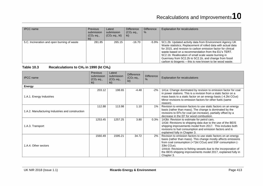
Recalculations and Improvements10
UK NIR 2018 (Issue 1.1) Ricardo Energy & Environment Page 413
IPCC name Previous submission (CO2 eq., kt)
Latest submission (CO2 eq., kt)
Difference (CO2 eq., kt)
Difference %
Explanation for recalculations
5.C. Incineration and open burning of waste 281.85 265.15 -16.70 -5.9% 5C1.2b: Updated activity data from Environment Agency UK Waste statistics; Replacement of rolled data with actual data for 2015, and revision to carbon emission factor for clinical waste based on a recommendation from the EU’s TERT. 5C2.1b: Reallocation of small scale waste burning in Guernsey from 5C2.2b to 5C2.1b, and change from fossil carbon to biogenic – this is now known to be wood waste.
Table 10.3 Recalculations to CH4 in 1990 (kt CH4)
IPCC name
Previous submission (CO2 eq., kt)
Latest submission (CO2 eq., kt)
Difference (CO2 eq., kt)
Difference %
Explanation for recalculations
Energy
1.A.1. Energy Industries
203.12 198.65 -4.48 -2% 1A1a: Change dominated by revision to emission factor for coal in power stations. This is a revision from a static factor on a mass basis to a static factor on an energy basis (-4.2kt CO2e) Minor revisions to emission factors for other fuels (same reason).
1.A.2. Manufacturing Industries and construction
112.88 113.98 1.10 1% Revision to emission factors to use static factors on an energy basis (rather than mass). The change is dominated by the revisions to EFs for coal (an increase), partially offset by a decrease in the EF for wood combustion.
1.A.3. Transport
1253.45 1257.25 3.80 0.3% 1A3bi: Revision to estimate for petrol cars. 1A3d: Revisions to shipping data due to the use of the BEIS shipping improvements model from 2017. This includes both revisions to fuel consumption and emission factors and is explained fully in Chapter 3.
1.A.4. Other sectors
1560.49 1595.21 34.72 2% Revision to emission factors to use static factors on an energy basis (rather than mass). This change mostly affects emissions from coal consumption (+71kt CO2e) and SSF consumption (-33kt CO2e). 1A4ciii: Revisions to fishing vessels due to the incorporation of the BEIS shipping improvements model 2017, explained fully in Chapter 3.
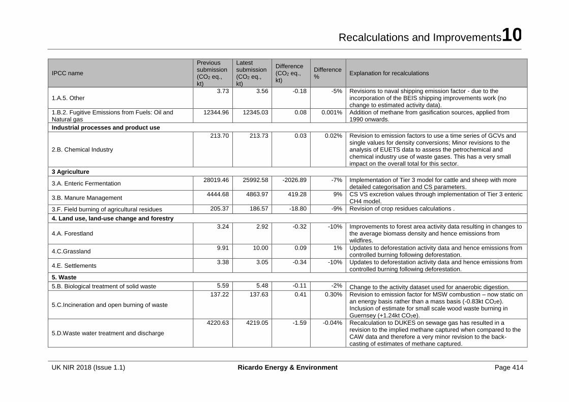
Recalculations and Improvements10
UK NIR 2018 (Issue 1.1) Ricardo Energy & Environment Page 414
IPCC name
Previous submission (CO2 eq., kt)
Latest submission (CO2 eq., kt)
Difference (CO2 eq., kt)
Difference %
Explanation for recalculations
1.A.5. Other 3.73 3.56 -0.18 -5% Revisions to naval shipping emission factor - due to the
incorporation of the BEIS shipping improvements work (no change to estimated activity data).
1.B.2. Fugitive Emissions from Fuels: Oil and Natural gas
12344.96 12345.03 0.08 0.001% Addition of methane from gasification sources, applied from 1990 onwards.
Industrial processes and product use
2.B. Chemical Industry
213.70 213.73 0.03 0.02% Revision to emission factors to use a time series of GCVs and single values for density conversions; Minor revisions to the analysis of EUETS data to assess the petrochemical and chemical industry use of waste gases. This has a very small impact on the overall total for this sector.
3 Agriculture
3.A. Enteric Fermentation 28019.46 25992.58 -2026.89 -7% Implementation of Tier 3 model for cattle and sheep with more
detailed categorisation and CS parameters.
3.B. Manure Management 4444.68 4863.97 419.28 9% CS VS excretion values through implementation of Tier 3 enteric
CH4 model.
3.F. Field burning of agricultural residues 205.37 186.57 -18.80 -9% Revision of crop residues calculations .
4. Land use, land-use change and forestry
4.A. Forestland 3.24 2.92 -0.32 -10% Improvements to forest area activity data resulting in changes to
the average biomass density and hence emissions from wildfires.
4.C.Grassland 9.91 10.00 0.09 1% Updates to deforestation activity data and hence emissions from
controlled burning following deforestation.
4.E. Settlements 3.38 3.05 -0.34 -10% Updates to deforestation activity data and hence emissions from
controlled burning following deforestation.
5. Waste
5.B. Biological treatment of solid waste 5.59 5.48 -0.11 -2% Change to the activity dataset used for anaerobic digestion.
5.C.Incineration and open burning of waste
137.22 137.63 0.41 0.30% Revision to emission factor for MSW combustion – now static on an energy basis rather than a mass basis (-0.83kt CO2e). Inclusion of estimate for small scale wood waste burning in Guernsey (+1.24kt CO2e).
5.D.Waste water treatment and discharge
4220.63 4219.05 -1.59 -0.04% Recalculation to DUKES on sewage gas has resulted in a revision to the implied methane captured when compared to the CAW data and therefore a very minor revision to the back-casting of estimates of methane captured.
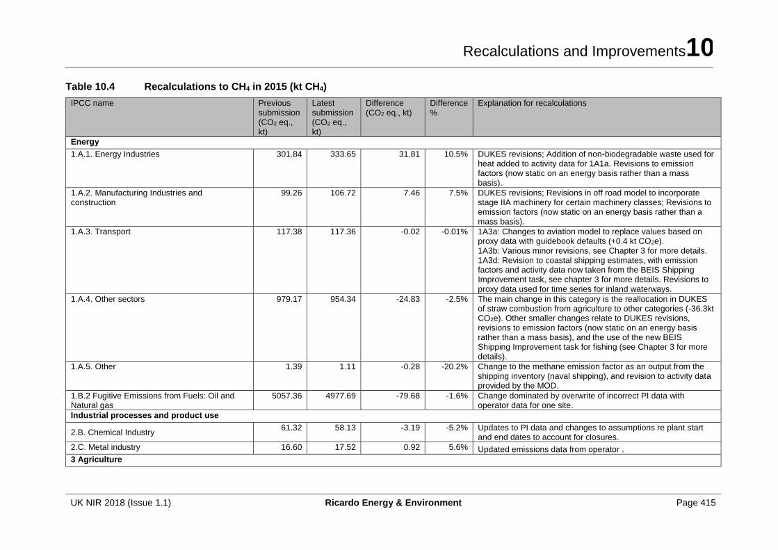
Recalculations and Improvements10
UK NIR 2018 (Issue 1.1) Ricardo Energy & Environment Page 415
Table 10.4 Recalculations to CH4 in 2015 (kt CH4)
IPCC name Previous submission (CO2 eq., kt)
Latest submission (CO2 eq., kt)
Difference (CO2 eq., kt)
Difference %
Explanation for recalculations
Energy
1.A.1. Energy Industries 301.84 333.65 31.81 10.5% DUKES revisions; Addition of non-biodegradable waste used for heat added to activity data for 1A1a. Revisions to emission factors (now static on an energy basis rather than a mass basis).
1.A.2. Manufacturing Industries and construction
99.26 106.72 7.46 7.5% DUKES revisions; Revisions in off road model to incorporate stage IIA machinery for certain machinery classes; Revisions to emission factors (now static on an energy basis rather than a mass basis).
1.A.3. Transport 117.38 117.36 -0.02 -0.01% 1A3a: Changes to aviation model to replace values based on proxy data with guidebook defaults (+0.4 kt CO2e). 1A3b: Various minor revisions, see Chapter 3 for more details. 1A3d: Revision to coastal shipping estimates, with emission factors and activity data now taken from the BEIS Shipping Improvement task, see chapter 3 for more details. Revisions to proxy data used for time series for inland waterways.
1.A.4. Other sectors 979.17 954.34 -24.83 -2.5% The main change in this category is the reallocation in DUKES of straw combustion from agriculture to other categories (-36.3kt CO2e). Other smaller changes relate to DUKES revisions, revisions to emission factors (now static on an energy basis rather than a mass basis), and the use of the new BEIS Shipping Improvement task for fishing (see Chapter 3 for more details).
1.A.5. Other 1.39 1.11 -0.28 -20.2% Change to the methane emission factor as an output from the shipping inventory (naval shipping), and revision to activity data provided by the MOD.
1.B.2 Fugitive Emissions from Fuels: Oil and Natural gas
5057.36 4977.69 -79.68 -1.6% Change dominated by overwrite of incorrect PI data with operator data for one site.
Industrial processes and product use
2.B. Chemical Industry 61.32 58.13 -3.19 -5.2% Updates to PI data and changes to assumptions re plant start
and end dates to account for closures.
2.C. Metal industry 16.60 17.52 0.92 5.6% Updated emissions data from operator .
3 Agriculture
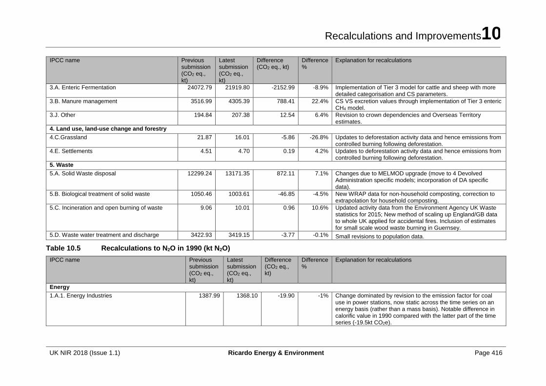
Recalculations and Improvements10
UK NIR 2018 (Issue 1.1) Ricardo Energy & Environment Page 416
IPCC name Previous submission (CO2 eq., kt)
Latest submission (CO2 eq., kt)
Difference (CO2 eq., kt)
Difference %
Explanation for recalculations
3.A. Enteric Fermentation 24072.79 21919.80 -2152.99 -8.9% Implementation of Tier 3 model for cattle and sheep with more detailed categorisation and CS parameters.
3.B. Manure management 3516.99 4305.39 788.41 22.4% CS VS excretion values through implementation of Tier 3 enteric CH4 model.
3.J. Other 194.84 207.38 12.54 6.4% Revision to crown dependencies and Overseas Territory estimates.
4. Land use, land-use change and forestry
4.C.Grassland 21.87 16.01 -5.86 -26.8% Updates to deforestation activity data and hence emissions from controlled burning following deforestation.
4.E. Settlements 4.51 4.70 0.19 4.2% Updates to deforestation activity data and hence emissions from controlled burning following deforestation.
5. Waste
5.A. Solid Waste disposal 12299.24 13171.35 872.11 7.1% Changes due to MELMOD upgrade (move to 4 Devolved Administration specific models; incorporation of DA specific data).
5.B. Biological treatment of solid waste 1050.46 1003.61 -46.85 -4.5% New WRAP data for non-household composting, correction to extrapolation for household composting.
5.C. Incineration and open burning of waste 9.06 10.01 0.96 10.6% Updated activity data from the Environment Agency UK Waste statistics for 2015; New method of scaling up England/GB data to whole UK applied for accidental fires. Inclusion of estimates for small scale wood waste burning in Guernsey.
5.D. Waste water treatment and discharge 3422.93 3419.15 -3.77 -0.1% Small revisions to population data.
Table 10.5 Recalculations to N2O in 1990 (kt N2O)
IPCC name Previous submission (CO2 eq., kt)
Latest submission (CO2 eq., kt)
Difference (CO2 eq., kt)
Difference %
Explanation for recalculations
Energy
1.A.1. Energy Industries 1387.99 1368.10 -19.90 -1% Change dominated by revision to the emission factor for coal use in power stations, now static across the time series on an energy basis (rather than a mass basis). Notable difference in calorific value in 1990 compared with the latter part of the time series (-19.5kt CO2e).
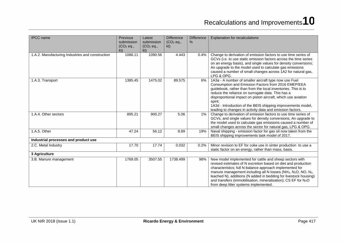
Recalculations and Improvements10
UK NIR 2018 (Issue 1.1) Ricardo Energy & Environment Page 417
IPCC name Previous submission (CO2 eq., kt)
Latest submission (CO2 eq., kt)
Difference (CO2 eq., kt)
Difference %
Explanation for recalculations
1.A.2. Manufacturing Industries and construction 1086.11 1090.56 4.443 0.4% Change to derivation of emission factors to use time series of GCVs (i.e. to use static emission factors across the time series on an energy basis), and single values for density conversions; An upgrade to the model used to calculate gas emissions caused a number of small changes across 1A2 for natural gas, LPG & OPG.
1.A.3. Transport 1385.45 1475.02 89.575 6% 1A3a - A number of smaller aircraft type now use Fuel Consumption and Emission Factors from 2016 EMEP/EEA guidebook, rather than from the local inventories. This is to reduce the reliance on surrogate data. This has a disproportional impact on piston aircraft, which use aviation spirit; 1A3d - Introduction of the BEIS shipping improvements model, leading to changes in activity data and emission factors.
1.A.4. Other sectors 895.21 900.27 5.06 1% Change to derivation of emission factors to use time series of GCVs, and single values for density conversions; An upgrade to the model used to calculate gas emissions caused a number of small changes across the sector for natural gas, LPG & OPG.
1.A.5. Other 47.24 56.12 8.89 19% Naval shipping - emission factor for gas oil now taken from the BEIS shipping improvements task model of 2017.
Industrial processes and product use
2.C. Metal Industry 17.70 17.74 0.032 0.2% Minor revision to EF for coke use in sinter production to use a static factor on an energy, rather than mass, basis.
3 Agriculture
3.B. Manure management 1769.05 3507.55 1738.499 98% New model implemented for cattle and sheep sectors with revised estimates of N excretion based on diet and production characteristics; full N-balance approach implemented for manure management including all N losses (NH3, N2O, NO, N2, leached N), additions (N added in bedding for livestock housing) and transfers (immobilisation, mineralisation); CS EF for N2O from deep litter systems implemented.
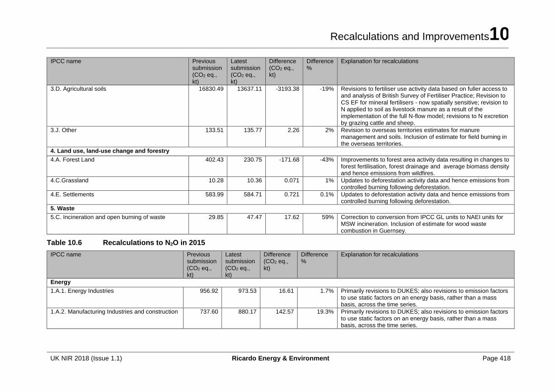
Recalculations and Improvements10
UK NIR 2018 (Issue 1.1) Ricardo Energy & Environment Page 418
IPCC name Previous submission (CO2 eq., kt)
Latest submission (CO2 eq., kt)
Difference (CO2 eq., kt)
Difference %
Explanation for recalculations
3.D. Agricultural soils 16830.49 13637.11 -3193.38 -19% Revisions to fertiliser use activity data based on fuller access to and analysis of British Survey of Fertiliser Practice; Revision to CS EF for mineral fertilisers - now spatially sensitive; revision to N applied to soil as livestock manure as a result of the implementation of the full N-flow model; revisions to N excretion by grazing cattle and sheep.
3.J. Other 133.51 135.77 2.26 2% Revision to overseas territories estimates for manure management and soils. Inclusion of estimate for field burning in the overseas territories.
4. Land use, land-use change and forestry
4.A. Forest Land 402.43 230.75 -171.68 -43% Improvements to forest area activity data resulting in changes to forest fertilisation, forest drainage and average biomass density and hence emissions from wildfires.
4.C.Grassland 10.28 10.36 0.071 1% Updates to deforestation activity data and hence emissions from controlled burning following deforestation.
4.E. Settlements 583.99 584.71 0.721 0.1% Updates to deforestation activity data and hence emissions from controlled burning following deforestation.
5. Waste
5.C. Incineration and open burning of waste 29.85 47.47 17.62 59% Correction to conversion from IPCC GL units to NAEI units for MSW incineration. Inclusion of estimate for wood waste combustion in Guernsey.
Table 10.6 Recalculations to N2O in 2015
IPCC name Previous submission (CO2 eq., kt)
Latest submission (CO2 eq., kt)
Difference (CO2 eq., kt)
Difference %
Explanation for recalculations
Energy
1.A.1. Energy Industries 956.92 973.53 16.61 1.7% Primarily revisions to DUKES; also revisions to emission factors to use static factors on an energy basis, rather than a mass basis, across the time series.
1.A.2. Manufacturing Industries and construction 737.60 880.17 142.57 19.3% Primarily revisions to DUKES; also revisions to emission factors to use static factors on an energy basis, rather than a mass basis, across the time series.
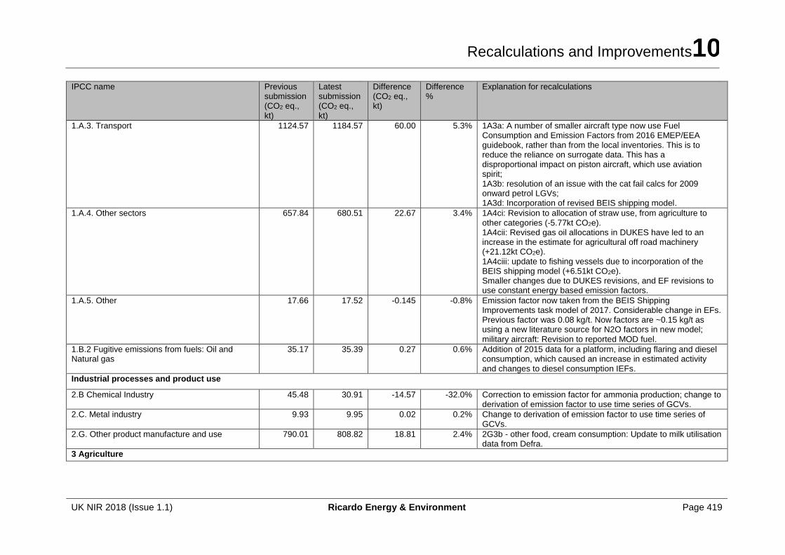
Recalculations and Improvements10
UK NIR 2018 (Issue 1.1) Ricardo Energy & Environment Page 419
IPCC name Previous submission (CO2 eq., kt)
Latest submission (CO2 eq., kt)
Difference (CO2 eq., kt)
Difference %
Explanation for recalculations
1.A.3. Transport 1124.57 1184.57 60.00 5.3% 1A3a: A number of smaller aircraft type now use Fuel Consumption and Emission Factors from 2016 EMEP/EEA guidebook, rather than from the local inventories. This is to reduce the reliance on surrogate data. This has a disproportional impact on piston aircraft, which use aviation spirit; 1A3b: resolution of an issue with the cat fail calcs for 2009 onward petrol LGVs; 1A3d: Incorporation of revised BEIS shipping model.
1.A.4. Other sectors 657.84 680.51 22.67 3.4% 1A4ci: Revision to allocation of straw use, from agriculture to other categories (-5.77kt CO2e). 1A4cii: Revised gas oil allocations in DUKES have led to an increase in the estimate for agricultural off road machinery (+21.12kt CO2e). 1A4ciii: update to fishing vessels due to incorporation of the BEIS shipping model (+6.51kt CO2e). Smaller changes due to DUKES revisions, and EF revisions to use constant energy based emission factors.
1.A.5. Other 17.66 17.52 -0.145 -0.8% Emission factor now taken from the BEIS Shipping Improvements task model of 2017. Considerable change in EFs. Previous factor was 0.08 kg/t. Now factors are ~0.15 kg/t as using a new literature source for N2O factors in new model; military aircraft: Revision to reported MOD fuel.
1.B.2 Fugitive emissions from fuels: Oil and Natural gas
35.17 35.39 0.27 0.6% Addition of 2015 data for a platform, including flaring and diesel consumption, which caused an increase in estimated activity and changes to diesel consumption IEFs.
Industrial processes and product use
2.B Chemical Industry 45.48 30.91 -14.57 -32.0% Correction to emission factor for ammonia production; change to derivation of emission factor to use time series of GCVs.
2.C. Metal industry 9.93 9.95 0.02 0.2% Change to derivation of emission factor to use time series of GCVs.
2.G. Other product manufacture and use 790.01 808.82 18.81 2.4% 2G3b - other food, cream consumption: Update to milk utilisation data from Defra.
3 Agriculture
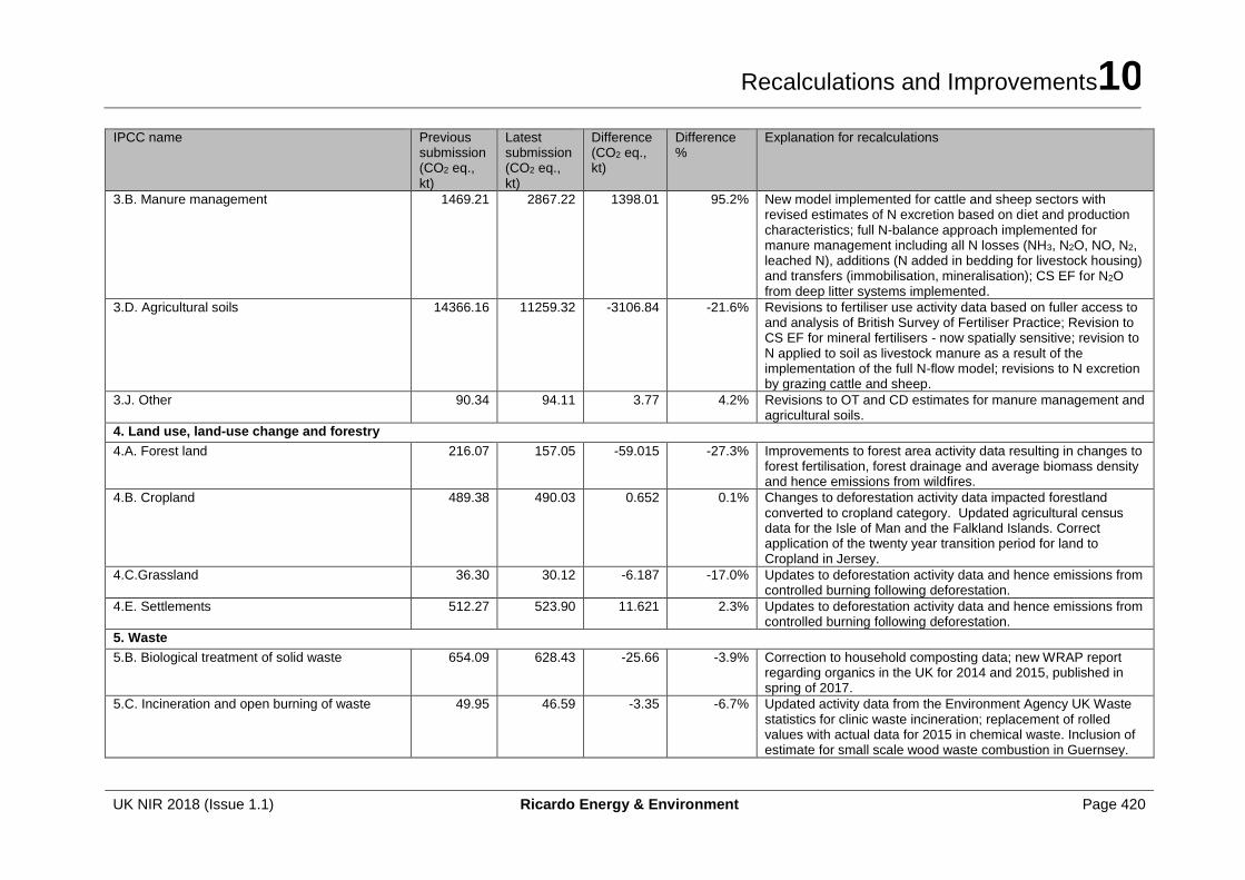
Recalculations and Improvements10
UK NIR 2018 (Issue 1.1) Ricardo Energy & Environment Page 420
IPCC name Previous submission (CO2 eq., kt)
Latest submission (CO2 eq., kt)
Difference (CO2 eq., kt)
Difference %
Explanation for recalculations
3.B. Manure management 1469.21 2867.22 1398.01 95.2% New model implemented for cattle and sheep sectors with revised estimates of N excretion based on diet and production characteristics; full N-balance approach implemented for manure management including all N losses (NH3, N2O, NO, N2, leached N), additions (N added in bedding for livestock housing) and transfers (immobilisation, mineralisation); CS EF for N2O from deep litter systems implemented.
3.D. Agricultural soils 14366.16 11259.32 -3106.84 -21.6% Revisions to fertiliser use activity data based on fuller access to and analysis of British Survey of Fertiliser Practice; Revision to CS EF for mineral fertilisers - now spatially sensitive; revision to N applied to soil as livestock manure as a result of the implementation of the full N-flow model; revisions to N excretion by grazing cattle and sheep.
3.J. Other 90.34 94.11 3.77 4.2% Revisions to OT and CD estimates for manure management and agricultural soils.
4. Land use, land-use change and forestry
4.A. Forest land 216.07 157.05 -59.015 -27.3% Improvements to forest area activity data resulting in changes to forest fertilisation, forest drainage and average biomass density and hence emissions from wildfires.
4.B. Cropland 489.38 490.03 0.652 0.1% Changes to deforestation activity data impacted forestland converted to cropland category. Updated agricultural census data for the Isle of Man and the Falkland Islands. Correct application of the twenty year transition period for land to Cropland in Jersey.
4.C.Grassland 36.30 30.12 -6.187 -17.0% Updates to deforestation activity data and hence emissions from controlled burning following deforestation.
4.E. Settlements 512.27 523.90 11.621 2.3% Updates to deforestation activity data and hence emissions from controlled burning following deforestation.
5. Waste
5.B. Biological treatment of solid waste 654.09 628.43 -25.66 -3.9% Correction to household composting data; new WRAP report regarding organics in the UK for 2014 and 2015, published in spring of 2017.
5.C. Incineration and open burning of waste 49.95 46.59 -3.35 -6.7% Updated activity data from the Environment Agency UK Waste statistics for clinic waste incineration; replacement of rolled values with actual data for 2015 in chemical waste. Inclusion of estimate for small scale wood waste combustion in Guernsey.
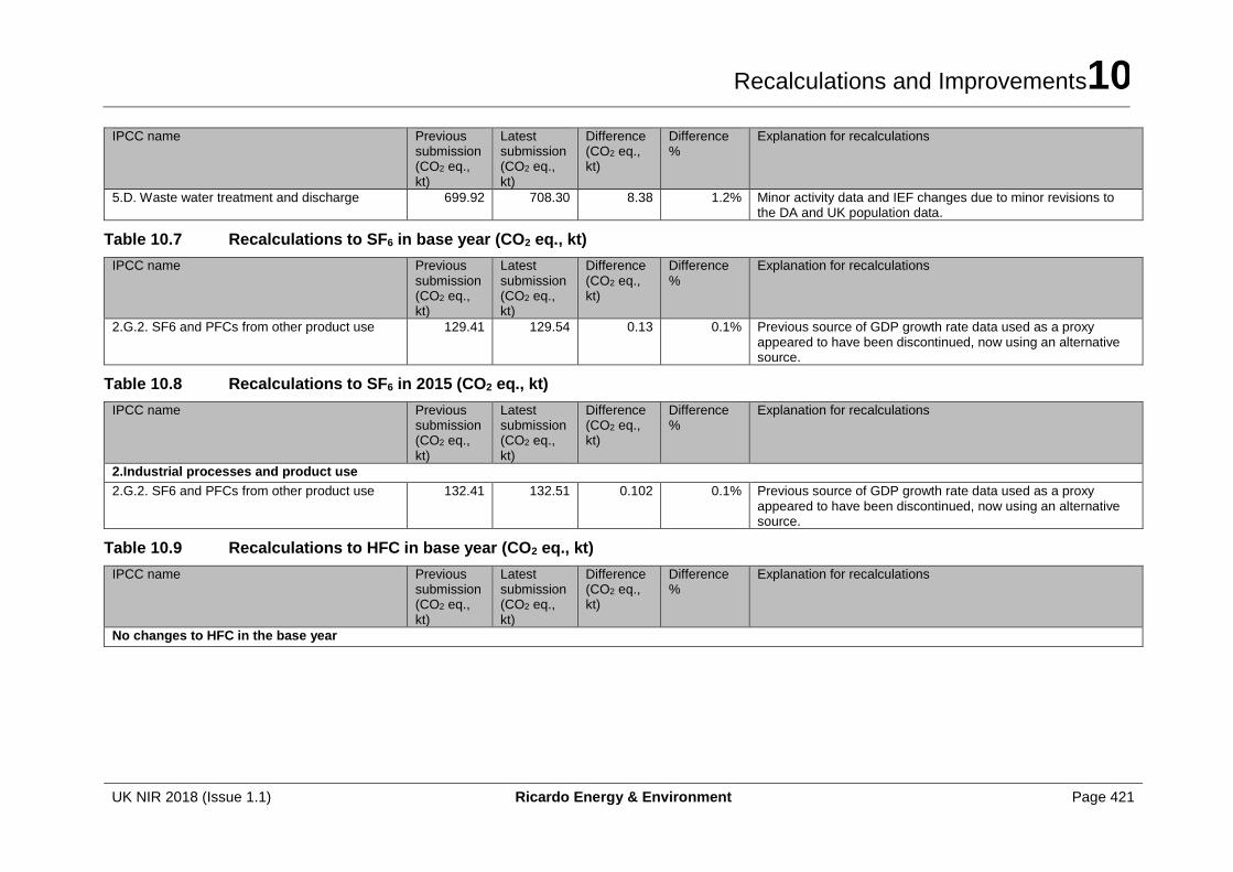
Recalculations and Improvements10
UK NIR 2018 (Issue 1.1) Ricardo Energy & Environment Page 421
IPCC name Previous submission (CO2 eq., kt)
Latest submission (CO2 eq., kt)
Difference (CO2 eq., kt)
Difference %
Explanation for recalculations
5.D. Waste water treatment and discharge 699.92 708.30 8.38 1.2% Minor activity data and IEF changes due to minor revisions to the DA and UK population data.
Table 10.7 Recalculations to SF6 in base year (CO2 eq., kt)
IPCC name Previous submission (CO2 eq., kt)
Latest submission (CO2 eq., kt)
Difference (CO2 eq., kt)
Difference %
Explanation for recalculations
2.G.2. SF6 and PFCs from other product use 129.41 129.54 0.13 0.1% Previous source of GDP growth rate data used as a proxy appeared to have been discontinued, now using an alternative source.
Table 10.8 Recalculations to SF6 in 2015 (CO2 eq., kt)
IPCC name Previous submission (CO2 eq., kt)
Latest submission (CO2 eq., kt)
Difference (CO2 eq., kt)
Difference %
Explanation for recalculations
2.Industrial processes and product use
2.G.2. SF6 and PFCs from other product use 132.41 132.51 0.102 0.1% Previous source of GDP growth rate data used as a proxy appeared to have been discontinued, now using an alternative source.
Table 10.9 Recalculations to HFC in base year (CO2 eq., kt)
IPCC name Previous submission (CO2 eq., kt)
Latest submission (CO2 eq., kt)
Difference (CO2 eq., kt)
Difference %
Explanation for recalculations
No changes to HFC in the base year
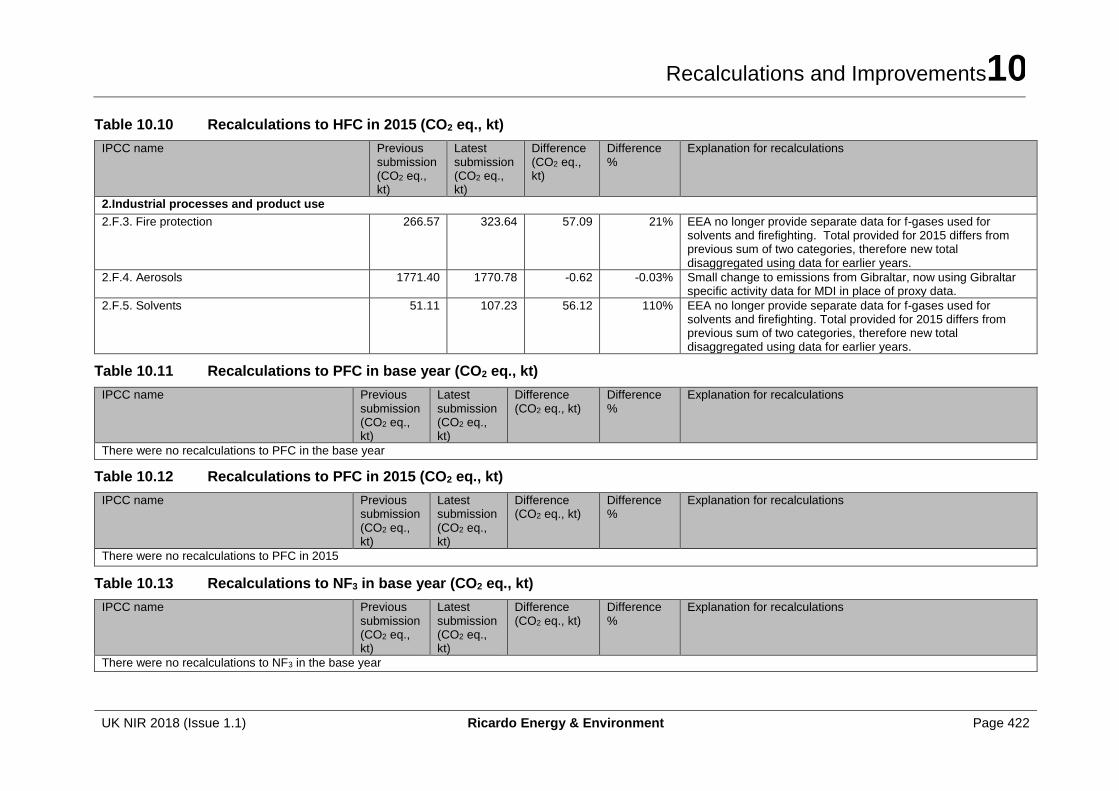
Recalculations and Improvements10
UK NIR 2018 (Issue 1.1) Ricardo Energy & Environment Page 422
Table 10.10 Recalculations to HFC in 2015 (CO2 eq., kt)
IPCC name Previous submission (CO2 eq., kt)
Latest submission (CO2 eq., kt)
Difference (CO2 eq., kt)
Difference %
Explanation for recalculations
2.Industrial processes and product use
2.F.3. Fire protection 266.57 323.64 57.09 21% EEA no longer provide separate data for f-gases used for solvents and firefighting. Total provided for 2015 differs from previous sum of two categories, therefore new total disaggregated using data for earlier years.
2.F.4. Aerosols 1771.40 1770.78 -0.62 -0.03% Small change to emissions from Gibraltar, now using Gibraltar specific activity data for MDI in place of proxy data.
2.F.5. Solvents
51.11 107.23 56.12 110% EEA no longer provide separate data for f-gases used for solvents and firefighting. Total provided for 2015 differs from previous sum of two categories, therefore new total disaggregated using data for earlier years.
Table 10.11 Recalculations to PFC in base year (CO2 eq., kt)
IPCC name Previous submission (CO2 eq., kt)
Latest submission (CO2 eq., kt)
Difference (CO2 eq., kt)
Difference %
Explanation for recalculations
There were no recalculations to PFC in the base year
Table 10.12 Recalculations to PFC in 2015 (CO2 eq., kt)
IPCC name Previous submission (CO2 eq., kt)
Latest submission (CO2 eq., kt)
Difference (CO2 eq., kt)
Difference %
Explanation for recalculations
There were no recalculations to PFC in 2015
Table 10.13 Recalculations to NF3 in base year (CO2 eq., kt)
IPCC name Previous submission (CO2 eq., kt)
Latest submission (CO2 eq., kt)
Difference (CO2 eq., kt)
Difference %
Explanation for recalculations
There were no recalculations to NF3 in the base year

Recalculations and Improvements10
UK NIR 2018 (Issue 1.1) Ricardo Energy & Environment Page 423
Table 10.14 Recalculations to NF3 in 2015 (CO2 eq., kt)
IPCC name Previous submission (CO2 eq., kt)
Latest submission (CO2 eq., kt)
Difference (CO2 eq., kt)
Difference %
Explanation for recalculations
There were no recalculations to NF3 in 2014
Table 10.15 Changes in Methodological Descriptions
GREENHOUSE GAS SOURCE AND SINK CATEGORIES
DESCRIPTION OF METHODS
RECALCULATIONS REFERENCE
Total (Net Emissions) Y Y
1. Energy Y Y Chapter 3
A. Fuel Combustion (sectoral approach) Y Y Chapter 3
1. Energy industries Y Y Chapter 3
2. Manufacturing industries and construction Y Y Chapter 3
3. Transport Y Y Chapter 3
4. Other sector Y Y Chapter 3
5. Other Y Y Chapter 3
B. Fugitive emissions from fuels Y Y Chapter 3
1. Solid fuels Y Y Chapter 3
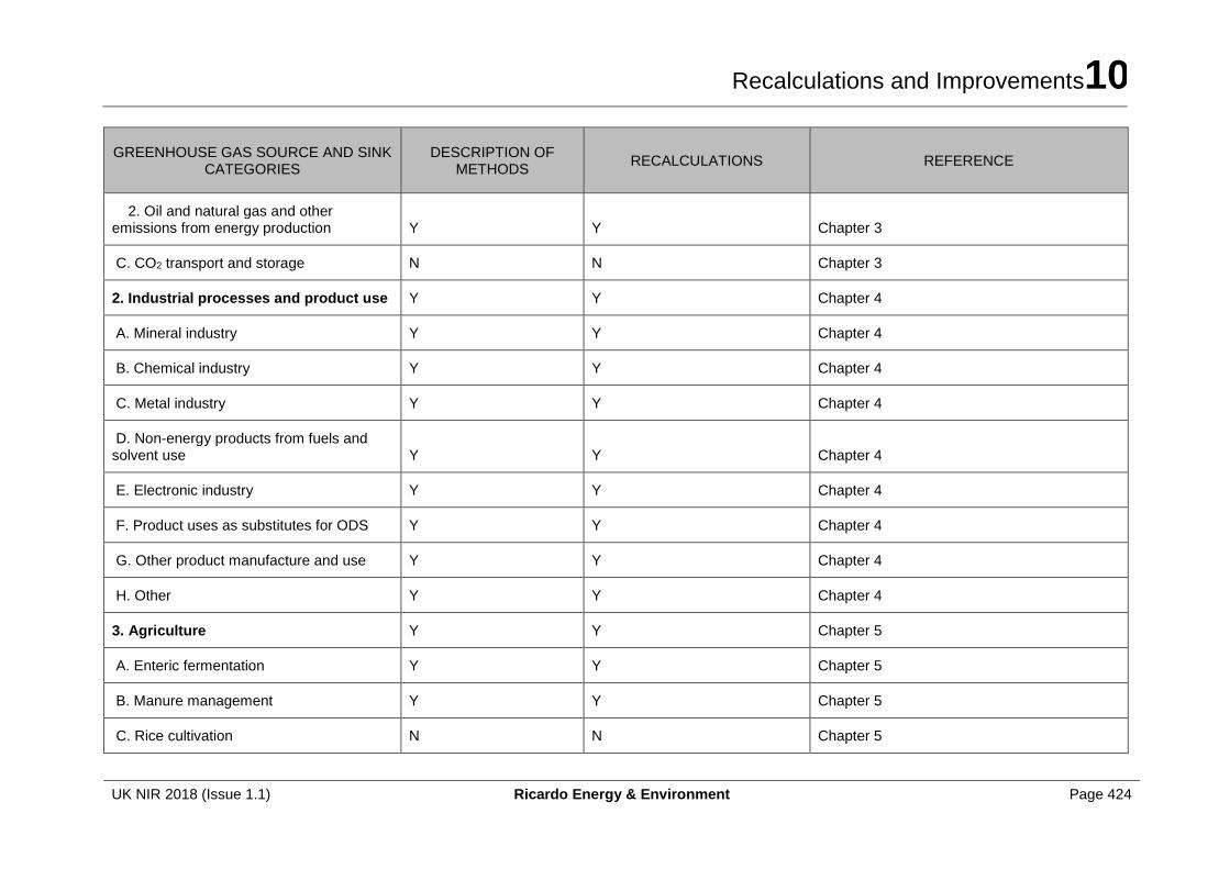
Recalculations and Improvements10
UK NIR 2018 (Issue 1.1) Ricardo Energy & Environment Page 424
GREENHOUSE GAS SOURCE AND SINK CATEGORIES
DESCRIPTION OF METHODS
RECALCULATIONS REFERENCE
2. Oil and natural gas and other emissions from energy production Y Y Chapter 3
C. CO2 transport and storage N N Chapter 3
2. Industrial processes and product use Y Y Chapter 4
A. Mineral industry Y Y Chapter 4
B. Chemical industry Y Y Chapter 4
C. Metal industry Y Y Chapter 4
D. Non-energy products from fuels and solvent use Y Y Chapter 4
E. Electronic industry Y Y Chapter 4
F. Product uses as substitutes for ODS Y Y Chapter 4
G. Other product manufacture and use Y Y Chapter 4
H. Other Y Y Chapter 4
3. Agriculture Y Y Chapter 5
A. Enteric fermentation Y Y Chapter 5
B. Manure management Y Y Chapter 5
C. Rice cultivation N N Chapter 5
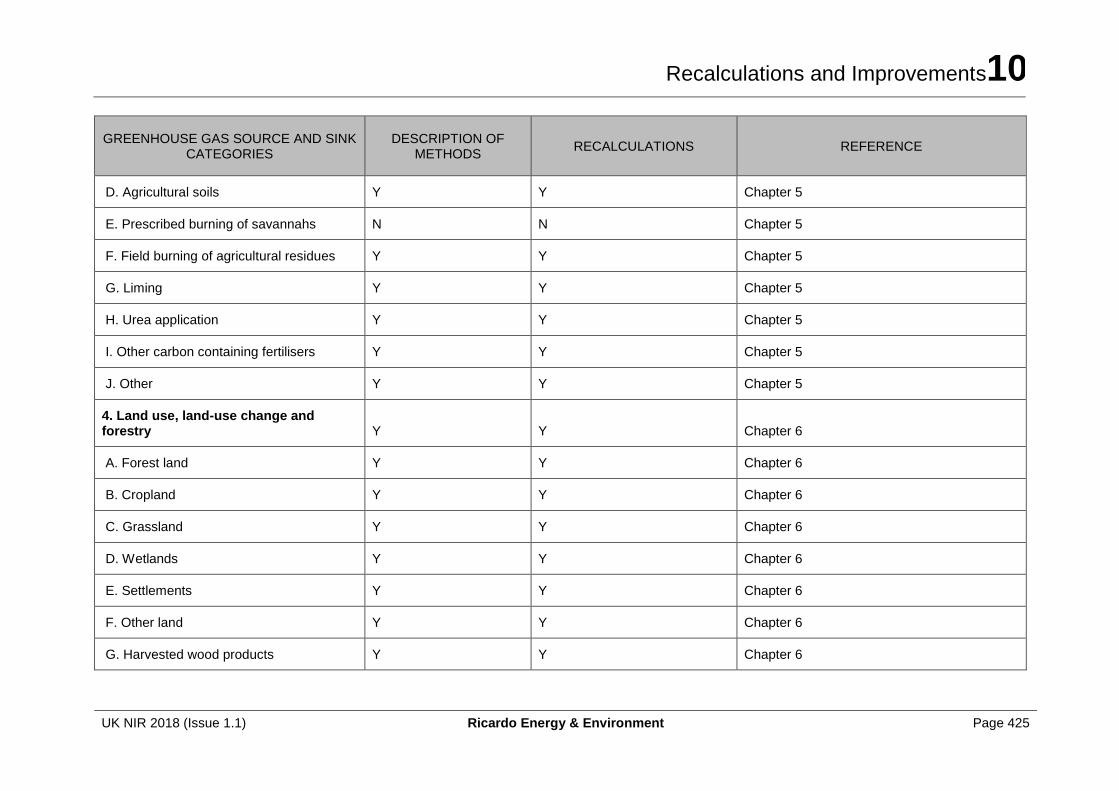
Recalculations and Improvements10
UK NIR 2018 (Issue 1.1) Ricardo Energy & Environment Page 425
GREENHOUSE GAS SOURCE AND SINK CATEGORIES
DESCRIPTION OF METHODS
RECALCULATIONS REFERENCE
D. Agricultural soils Y Y Chapter 5
E. Prescribed burning of savannahs N N Chapter 5
F. Field burning of agricultural residues Y Y Chapter 5
G. Liming Y Y Chapter 5
H. Urea application Y Y Chapter 5
I. Other carbon containing fertilisers Y Y Chapter 5
J. Other Y Y Chapter 5
4. Land use, land-use change and forestry Y Y Chapter 6
A. Forest land Y Y Chapter 6
B. Cropland Y Y Chapter 6
C. Grassland Y Y Chapter 6
D. Wetlands Y Y Chapter 6
E. Settlements Y Y Chapter 6
F. Other land Y Y Chapter 6
G. Harvested wood products Y Y Chapter 6
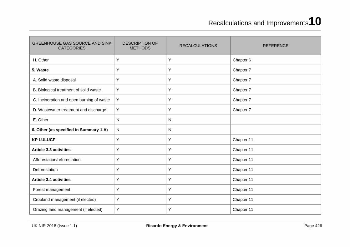
Recalculations and Improvements10
UK NIR 2018 (Issue 1.1) Ricardo Energy & Environment Page 426
GREENHOUSE GAS SOURCE AND SINK CATEGORIES
DESCRIPTION OF METHODS
RECALCULATIONS REFERENCE
H. Other Y Y Chapter 6
5. Waste Y Y Chapter 7
A. Solid waste disposal Y Y Chapter 7
B. Biological treatment of solid waste Y Y Chapter 7
C. Incineration and open burning of waste Y Y Chapter 7
D. Wastewater treatment and discharge Y Y Chapter 7
E. Other N N
6. Other (as specified in Summary 1.A) N N
KP LULUCF Y Y Chapter 11
Article 3.3 activities Y Y Chapter 11
Afforestation/reforestation Y Y Chapter 11
Deforestation Y Y Chapter 11
Article 3.4 activities Y Y Chapter 11
Forest management Y Y Chapter 11
Cropland management (if elected) Y Y Chapter 11
Grazing land management (if elected) Y Y Chapter 11
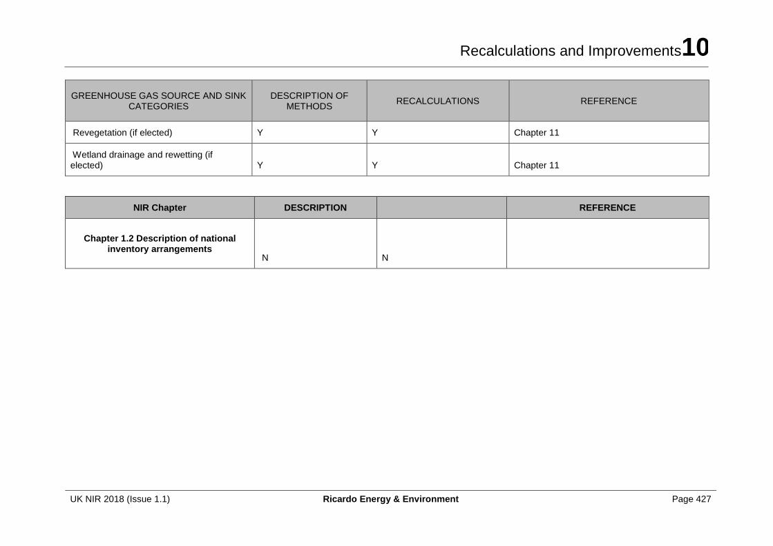
Recalculations and Improvements10
UK NIR 2018 (Issue 1.1) Ricardo Energy & Environment Page 427
GREENHOUSE GAS SOURCE AND SINK CATEGORIES
DESCRIPTION OF METHODS
RECALCULATIONS REFERENCE
Revegetation (if elected) Y Y Chapter 11
Wetland drainage and rewetting (if elected) Y Y Chapter 11
NIR Chapter DESCRIPTION REFERENCE
Chapter 1.2 Description of national inventory arrangements
N N
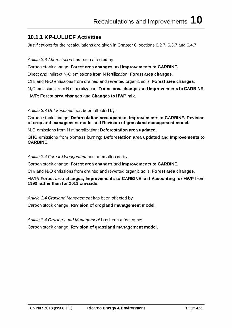
Recalculations and Improvements 10
UK NIR 2018 (Issue 1.1) Ricardo Energy & Environment Page 428
10.1.1 KP-LULUCF Activities
Justifications for the recalculations are given in Chapter 6, sections 6.2.7, 6.3.7 and 6.4.7.
Article 3.3 Afforestation has been affected by:
Carbon stock change: Forest area changes and Improvements to CARBINE.
Direct and indirect N2O emissions from N fertilization: Forest area changes.
CH4 and N2O emissions from drained and rewetted organic soils: Forest area changes.
N2O emissions from N mineralization: Forest area changes and Improvements to CARBINE.
HWP: Forest area changes and Changes to HWP mix.
Article 3.3 Deforestation has been affected by:
Carbon stock change: Deforestation area updated, Improvements to CARBINE, Revision of cropland management model and Revision of grassland management model.
N2O emissions from N mineralization: Deforestation area updated.
GHG emissions from biomass burning: Deforestation area updated and Improvements to CARBINE.
Article 3.4 Forest Management has been affected by:
Carbon stock change: Forest area changes and Improvements to CARBINE.
CH4 and N2O emissions from drained and rewetted organic soils: Forest area changes.
HWP: Forest area changes, Improvements to CARBINE and Accounting for HWP from 1990 rather than for 2013 onwards.
Article 3.4 Cropland Management has been affected by:
Carbon stock change: Revision of cropland management model.
Article 3.4 Grazing Land Management has been affected by:
Carbon stock change: Revision of grassland management model.
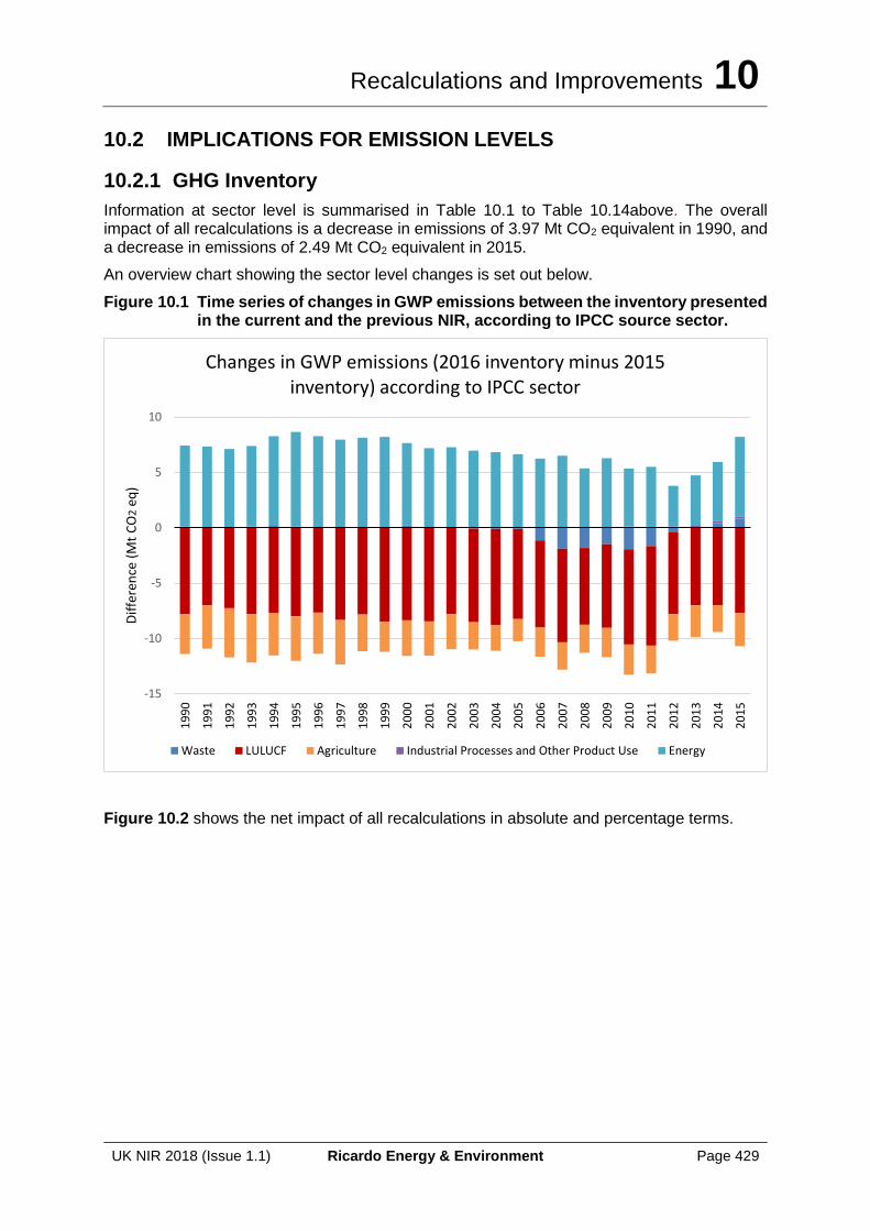
Recalculations and Improvements 10
UK NIR 2018 (Issue 1.1) Ricardo Energy & Environment Page 429
10.2 IMPLICATIONS FOR EMISSION LEVELS
10.2.1 GHG Inventory
Information at sector level is summarised in Table 10.1 to Table 10.14above. The overall impact of all recalculations is a decrease in emissions of 3.97 Mt CO2 equivalent in 1990, and a decrease in emissions of 2.49 Mt CO2 equivalent in 2015.
An overview chart showing the sector level changes is set out below.
Figure 10.1 Time series of changes in GWP emissions between the inventory presented in the current and the previous NIR, according to IPCC source sector.
Figure 10.2 shows the net impact of all recalculations in absolute and percentage terms.
-15
-10
-5
0
5
10
19
90
19
91
19
92
19
93
19
94
19
95
19
96
19
97
19
98
19
99
20
00
20
01
20
02
20
03
20
04
20
05
20
06
20
07
20
08
20
09
20
10
20
11
20
12
20
13
20
14
20
15
Dif
fere
nce
(M
t C
O2
eq)
Changes in GWP emissions (2016 inventory minus 2015 inventory) according to IPCC sector
Waste LULUCF Agriculture Industrial Processes and Other Product Use Energy
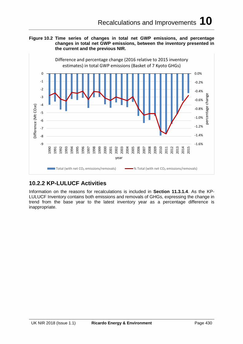
Recalculations and Improvements 10
UK NIR 2018 (Issue 1.1) Ricardo Energy & Environment Page 430
Figure 10.2 Time series of changes in total net GWP emissions, and percentage changes in total net GWP emissions, between the inventory presented in the current and the previous NIR.
10.2.2 KP-LULUCF Activities
Information on the reasons for recalculations is included in Section 11.3.1.4. As the KP-LULUCF Inventory contains both emissions and removals of GHGs, expressing the change in trend from the base year to the latest inventory year as a percentage difference is inappropriate.
-1.6%
-1.4%
-1.2%
-1.0%
-0.8%
-0.6%
-0.4%
-0.2%
0.0%
-9
-8
-7
-6
-5
-4
-3
-2
-1
0
19
90
19
91
19
92
19
93
19
94
19
95
19
96
19
97
19
98
19
99
20
00
20
01
20
02
20
03
20
04
20
05
20
06
20
07
20
08
20
09
20
10
20
11
20
12
20
13
20
14
20
15
per
cen
tage
ch
ange
Dif
fere
nce
(M
t C
O2e)
year
Difference and percentage change (2016 relative to 2015 inventory estimates) in total GWP emissions (Basket of 7 Kyoto GHGs)
Total (with net CO₂ emissions/removals) % Total (with net CO₂ emissions/removals)
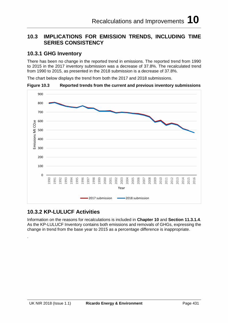
Recalculations and Improvements 10
UK NIR 2018 (Issue 1.1) Ricardo Energy & Environment Page 431
10.3 IMPLICATIONS FOR EMISSION TRENDS, INCLUDING TIME SERIES CONSISTENCY
10.3.1 GHG Inventory
There has been no change in the reported trend in emissions. The reported trend from 1990 to 2015 in the 2017 inventory submission was a decrease of 37.8%. The recalculated trend from 1990 to 2015, as presented in the 2018 submission is a decrease of 37.8%.
The chart below displays the trend from both the 2017 and 2018 submissions.
Figure 10.3 Reported trends from the current and previous inventory submissions
10.3.2 KP-LULUCF Activities
Information on the reasons for recalculations is included in Chapter 10 and Section 11.3.1.4. As the KP-LULUCF Inventory contains both emissions and removals of GHGs, expressing the change in trend from the base year to 2015 as a percentage difference is inappropriate.
.
0
100
200
300
400
500
600
700
800
900
19
90
19
91
19
92
19
93
19
94
19
95
19
96
19
97
19
98
19
99
20
00
20
01
20
02
20
03
20
04
20
05
20
06
20
07
20
08
20
09
20
10
20
11
20
12
20
13
20
14
20
15
20
16
Emis
sio
ns
Mt
CO
2e
Year
2017 submission 2018 submission
Recalculations and Improvements 10
UK NIR 2018 (Issue 1.1) Ricardo Energy & Environment Page 432
10.4 RECALCULATIONS, INCLUDING IN RESPONSE TO THE REVIEW PROCESS, AND PLANNED IMPROVEMENTS TO THE INVENTORY
All recalculations to the inventory, including those made in response to the review process and other recalculations e.g. due to data revisions are described in detail within chapters 3-8, and are summarised in Table 10.1 to Table 10.14. This section of the report summarises all recommendations from the review process, including where these have led to:
• Recalculations;
• changes in reporting in the NIR;
• changes in reporting in the CRF; and
• planned improvements for future submissions.
The UNFCCC conducted a Centralised Review of the 2016 greenhouse gas inventory submission (2016 NIR) in accordance with decision 22/CMP.1. In accordance with the conclusions of the Subsidiary Body for Implementation at its twenty-seventh session, the focus of the review was on the most recent (2016) submission. The review took place during September 2016 and the review report was published on December 4, 2017.
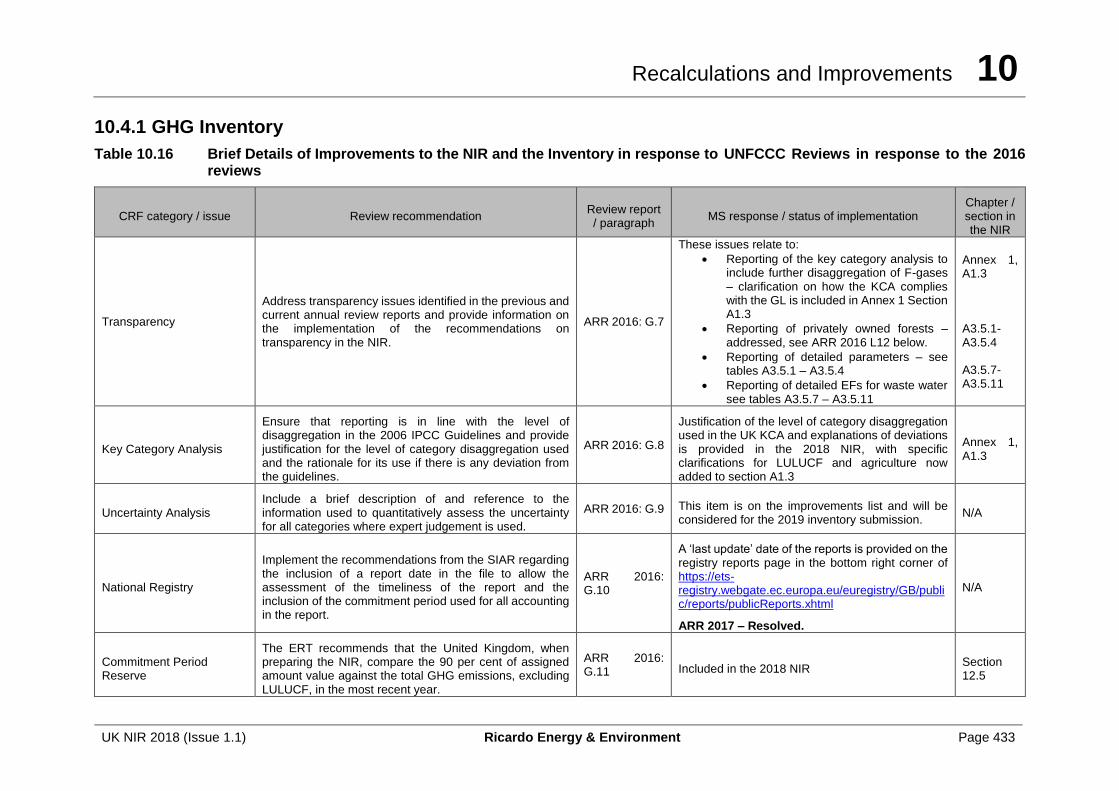
Recalculations and Improvements 10
UK NIR 2018 (Issue 1.1) Ricardo Energy & Environment Page 433
10.4.1 GHG Inventory
Table 10.16 Brief Details of Improvements to the NIR and the Inventory in response to UNFCCC Reviews in response to the 2016 reviews
CRF category / issue Review recommendation Review report / paragraph
MS response / status of implementation Chapter / section in the NIR
Transparency
Address transparency issues identified in the previous and current annual review reports and provide information on the implementation of the recommendations on transparency in the NIR.
ARR 2016: G.7
These issues relate to:
• Reporting of the key category analysis to include further disaggregation of F-gases – clarification on how the KCA complies with the GL is included in Annex 1 Section A1.3
• Reporting of privately owned forests – addressed, see ARR 2016 L12 below.
• Reporting of detailed parameters – see tables A3.5.1 – A3.5.4
• Reporting of detailed EFs for waste water see tables A3.5.7 – A3.5.11
Annex 1, A1.3 A3.5.1-A3.5.4 A3.5.7-A3.5.11
Key Category Analysis
Ensure that reporting is in line with the level of disaggregation in the 2006 IPCC Guidelines and provide justification for the level of category disaggregation used and the rationale for its use if there is any deviation from the guidelines.
ARR 2016: G.8
Justification of the level of category disaggregation used in the UK KCA and explanations of deviations is provided in the 2018 NIR, with specific clarifications for LULUCF and agriculture now added to section A1.3
Annex 1, A1.3
Uncertainty Analysis Include a brief description of and reference to the information used to quantitatively assess the uncertainty for all categories where expert judgement is used.
ARR 2016: G.9 This item is on the improvements list and will be considered for the 2019 inventory submission.
N/A
National Registry
Implement the recommendations from the SIAR regarding the inclusion of a report date in the file to allow the assessment of the timeliness of the report and the inclusion of the commitment period used for all accounting in the report.
ARR 2016: G.10
A ‘last update’ date of the reports is provided on the registry reports page in the bottom right corner of https://ets-registry.webgate.ec.europa.eu/euregistry/GB/public/reports/publicReports.xhtml
ARR 2017 – Resolved.
N/A
Commitment Period Reserve
The ERT recommends that the United Kingdom, when preparing the NIR, compare the 90 per cent of assigned amount value against the total GHG emissions, excluding LULUCF, in the most recent year.
ARR 2016: G.11 Included in the 2018 NIR
Section 12.5
Recalculations and Improvements 10
UK NIR 2018 (Issue 1.1) Ricardo Energy & Environment Page 434
CRF category / issue Review recommendation Review report / paragraph
MS response / status of implementation Chapter / section in the NIR
National System
The ERT recommends that the United Kingdom strengthen its national system in order to ensure that it can ensure the completeness of the coverage of the LULUCF and KP-LULUCF estimates of emissions and removals, and report on the improvements made in the next NIR.
ARR 2016: G.13 See item L.19 below.
1. General (energy sector) – all fuels – CO2, CH4 and N2O
The ERT recommends that the United Kingdom improve the transparency of its reporting by clearly indicating the geographical coverage of DUKES as well as by demonstrating how fuel consumption data at the subcategory level for each overseas territories and Crown dependencies are obtained and incorporated into the national totals for that subcategory.
ARR 2016: E.20
DUKES coverage and the provision of AD from OTs and CDs is clarified in the 2018 NIR.
Activity data for the OTs and CDs and their integration into the UK inventory national totals are explained in the Annex 4 National Energy Balance, including sub-sector allocations set out within the reconciliation tables for major fuels.
Section 1.1.2.2
Annex 4
1. General (energy sector) – liquid fuels and natural gas – CO2, CH4 and N2O
The ERT recommends that the United Kingdom rectify the stock data in its energy statistics and implement relevant recalculations in the CRF tables, as necessary, and explain all the recalculations in its NIR.
ARR 2016: E.21
The difference arises due to the treatment of international tickets. These are counted separately in DUKES national statistics in table 3.7 and are not included as part of the balances table (table 3.2). Table 3.2 only includes physical stocks to show how builds and draws affect supply. However as part of the UK stock, we do have tickets and these are counted as part of total stocks by the IEA. There are no plans to change how the international tickets are reported in national statistics.
Feedstocks, reductants and other NEU of fuels – other fuels – CO2
The ERT recommends that the United Kingdom rectify its reporting of NEU of coking coal (coke oven/gas coke and coking coal) in CRF table 1.A(d).
ARR 2016: E.22
This issue will be resolved subject to the CRF Reporter software functioning correctly in the 2018 submission, as it did for the 2017 submission
ARR 2017 – Resolved.
CRF
Feedstocks, reductants and other NEU of fuels – liquid fuels – CO2
The ERT recommends that the United Kingdom rectify its reporting on carbon excluded and CO2 emissions from NEU of gas/diesel oil, residual fuel oil, LPG, ethane, naphtha, bitumen, lubricants and other oil in CRF table 1.A(d) in order to make it consistent with CRF table 1.A(b).
ARR 2016: E.23
This issue will be resolved subject to the CRF Reporter software functioning correctly in the 2018 submission, as it did for the 2017 submission
ARR 2017 – Resolved.
CRF
Recalculations and Improvements 10
UK NIR 2018 (Issue 1.1) Ricardo Energy & Environment Page 435
CRF category / issue Review recommendation Review report / paragraph
MS response / status of implementation Chapter / section in the NIR
International navigation – liquid fuels – CO2, CH4 and N2O
The ERT recommends that the United Kingdom ensure the accuracy of the emission estimates for international navigation bunkers as well as the internal consistency between CRF table 1.D and CRF table 1.A(b) by using the correct calorific values to convert activity from a mass basis to an energy basis in its future submissions.
ARR 2016: E.24
This issue is resolved in the 2018 submission.
CRF
1.A.1.c Manufacture of solid fuels and other energy industries – liquid fuels – CO2, CH4 and N2O
The ERT recommends that the United Kingdom improve the transparency of its reporting by providing in its next submission a clear and concise explanation that the estimates for AD and for CO2, CH4 and N2O emissions from category 1.A.1.C.ii (oil and gas extraction) are complete, including relevant information such as that made available to the ERT during the review (as described above). The ERT also recommends that the United Kingdom provide in its next submission up-to-date information on its consideration of or progress in its efforts to improve the energy statistics collection system for LPG and OPG fuels abstracted from upstream oil and gas exploration and production sources.
ARR 2016: E.25
This additional information is included within the full NIR of the 2018 submission, within the method approach, QAQC and improvements sections of MS2.
No progress has been made with regard to the completeness of the DUKES data reporting for terminal use of OPG/LPG, but the previous approach to use other reporting mechanisms to address the gap in energy statistics is retained to ensure a complete and accurate inventory submission.
MS2
1.A.2 Manufacturing Industries and Construction – other fuels – CO2, CH4 and N2O
The ERT recommends that the United Kingdom improve the transparency of its reporting by providing a clear and concise explanation that the estimates for subcategory 1.A.2 (manufacturing industries and construction – other fuels) are complete, including relevant information such as that made available to the ERT during the review.
ARR 2016: E.26
Additional information to clarify the UK's approach to assuring completeness of the inventory for waste-derived fuels in 1A2 in included in the 2017 NIR and the 2018 NIR.
ARR 2017 – Resolved.
MS3
Recalculations and Improvements 10
UK NIR 2018 (Issue 1.1) Ricardo Energy & Environment Page 436
CRF category / issue Review recommendation Review report / paragraph
MS response / status of implementation Chapter / section in the NIR
1.A.2.b Non-ferrous metals – solid fuels – CO2
The ERT recommends that the United Kingdom investigate the underlying cause of the drop in the carbon EF for coal use at the Lynemouth Aluminium Smelter between 2003 and 2005 and report the findings of this investigation in its NIR.
ARR 2016: E.27
This issue has been reviewed by the inventory agency and a change in method was implemented in the 2017 submission to remove the step-change in CEF. On reviewing the available evidence the UK agreed with the ERT's inference that the time series of data from the Lynemouth plant from 2005 onwards (from EUETS reporting) provided the best available CEF information to extrapolate to the activity data for earlier years, rather than applying the weighted-average coal CEF from power station operator data from prior to 2005. No data specific to the Lynemouth plant was identified within the raw data underpinning the 2004 Carbon Factors Review dataset for power station coal. This is therefore already addressed and the recalculations were transparently reported in the 2017 submission NIR.
Further text of clarification has now been added to MS3 in response to the 2017 submission review.
2017 NIR, and also MS3 (Method Approach section) in the 2018 NIR
1.B.1.a Coal mining and handling – solid fuels - CO2
The ERT recommends that the United Kingdom use the more appropriate notation key “NE” for CO2 emissions from category 1.B.1.a in future submissions if data are still not available for an estimation.
ARR 2016: E.28
The UK has revised its reporting of this source to "NE" in the CRF for the 2017 and 2018 submissions.
ARR 2017 – Resolved.
CRF
2.A.1 Cement Production - CO2
The ERT recommends that the United Kingdom include the information provided during the review on the different sources for AD and CO2 EF and on all the assumptions used in the estimations in its next NIR to improve the transparency of time-series consistency.
ARR 2016: I.10 The text in the NIR has been reviewed and additional information included where necessary.
ARR 2017 – Resolved.
Section 4.2
2.A.2 Lime production – CO2
The ERT recommends that the United Kingdom include the information provided during the review on the different sources for AD and CO2 EF and on all the assumptions used in the estimations in its NIR to improve the transparency of time-series consistency.
ARR 2016: I.11 The text in the NIR has been reviewed and additional information included where necessary.
ARR 2017 – Resolved.
Section 4.3
Recalculations and Improvements 10
UK NIR 2018 (Issue 1.1) Ricardo Energy & Environment Page 437
CRF category / issue Review recommendation Review report / paragraph
MS response / status of implementation Chapter / section in the NIR
2.B.1 Ammonia production – CO2
The ERT recommends that the United Kingdom include the information provided during the review on urea production at ammonia plants in the NIR to improve the transparency of its reporting.
ARR 2016: I.12 This information is now included in the NIR.
ARR 2017 – Resolved.
Chapter 4
2.B.1 Ammonia production – CO2
The ERT recommends that the United Kingdom include information on the methodology used, including type of fuels used, origin of emission data, tier level and explanation of the trends of EF for the Severnside, Billingham, Ince and Hull plants.
ARR 2016: I.13 NIR method text updated in the 2017 and 2018 submissions.
ARR 2017 – Resolved.
4.6.2
2.B.2 Nitric acid production - N2O
The ERT recommends that the United Kingdom include the information provided during the review on AD and EFs used for the estimates for the entire time series in its NIR in order to improve the transparency of its reporting.
ARR 2016: I.14 NIR method text updated in the 2017 and 2018 submissions.
ARR 2017 – Resolved.
4.7.2
2.C.1 Iron and steel production – CO2
The ERT recommends that the United Kingdom include an appropriate explanation of how NEU of coke oven coke is considered across different subcategories and along the time series in its NIR.
ARR 2016: I.15 NIR method text updated in the 2017 and 2018 submissions.
ARR 2017 – Resolved
4.16
2.D.1 Lubricant use – CO2, CH4 and N2O
The ERT recommends that the United Kingdom assess the methodology used for the estimation of emissions for lubricant use (category 2.D.1) and apply the methodology from the 2006 IPCC Guidelines.
ARR 2016: I.16 The UK inventory uses the methodology from the 2006 IPCC guidelines for estimating emissions from lubricant use. The industrial combustion of waste lubricants for energy has been reallocated to 1A2. This reallocation means that the NIR methodology for this sector is consistent with the data presented in the CRF.
ARR 2017 – Resolved
Chapter 4
2.D.2 Paraffin wax use – CO2
The ERT recommends that the United Kingdom improve its QA/QC procedures and review its NIR to include information on the methodology to estimate CO2 emissions from paraffin wax, and to correct the text from lubricants to paraffin wax, as appropriate.
ARR 2016: I.17 NIR method text updated in the 2017 and 2018 submissions.
ARR 2017 – Resolved
Chapter 4
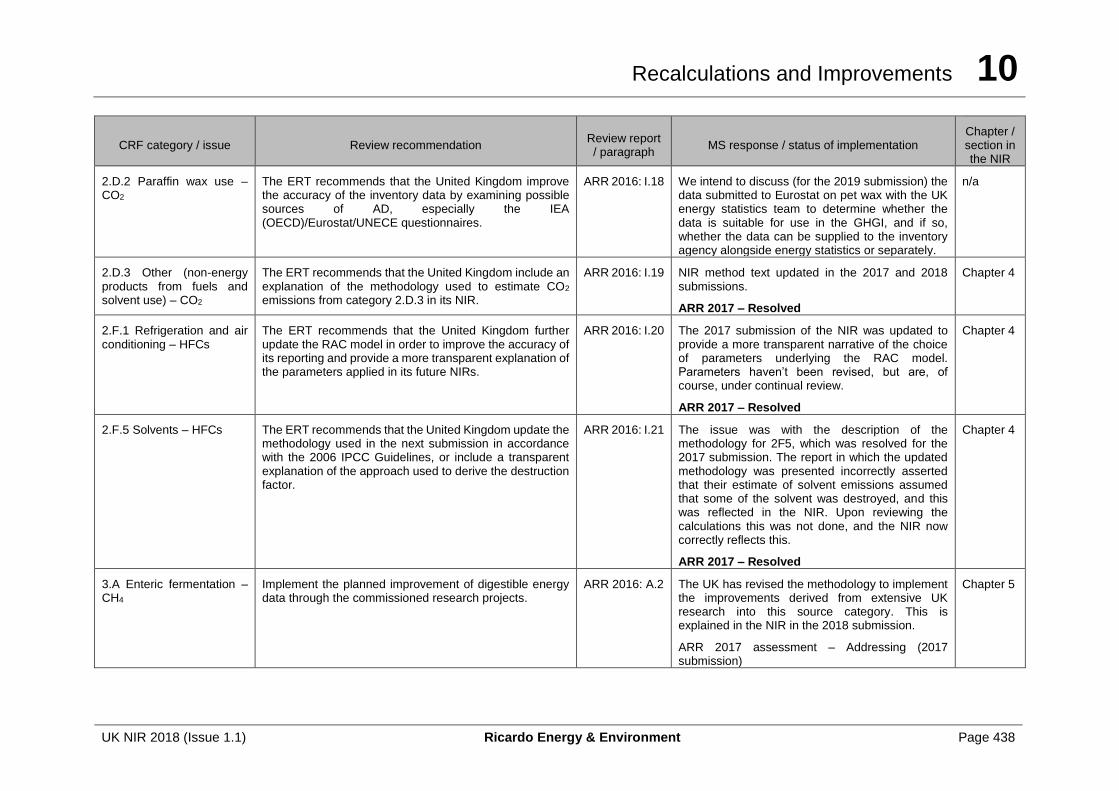
Recalculations and Improvements 10
UK NIR 2018 (Issue 1.1) Ricardo Energy & Environment Page 438
CRF category / issue Review recommendation Review report / paragraph
MS response / status of implementation Chapter / section in the NIR
2.D.2 Paraffin wax use – CO2
The ERT recommends that the United Kingdom improve the accuracy of the inventory data by examining possible sources of AD, especially the IEA (OECD)/Eurostat/UNECE questionnaires.
ARR 2016: I.18 We intend to discuss (for the 2019 submission) the data submitted to Eurostat on pet wax with the UK energy statistics team to determine whether the data is suitable for use in the GHGI, and if so, whether the data can be supplied to the inventory agency alongside energy statistics or separately.
n/a
2.D.3 Other (non-energy products from fuels and solvent use) – CO2
The ERT recommends that the United Kingdom include an explanation of the methodology used to estimate CO2 emissions from category 2.D.3 in its NIR.
ARR 2016: I.19 NIR method text updated in the 2017 and 2018 submissions.
ARR 2017 – Resolved
Chapter 4
2.F.1 Refrigeration and air conditioning – HFCs
The ERT recommends that the United Kingdom further update the RAC model in order to improve the accuracy of its reporting and provide a more transparent explanation of the parameters applied in its future NIRs.
ARR 2016: I.20 The 2017 submission of the NIR was updated to provide a more transparent narrative of the choice of parameters underlying the RAC model. Parameters haven’t been revised, but are, of course, under continual review.
ARR 2017 – Resolved
Chapter 4
2.F.5 Solvents – HFCs The ERT recommends that the United Kingdom update the methodology used in the next submission in accordance with the 2006 IPCC Guidelines, or include a transparent explanation of the approach used to derive the destruction factor.
ARR 2016: I.21 The issue was with the description of the methodology for 2F5, which was resolved for the 2017 submission. The report in which the updated methodology was presented incorrectly asserted that their estimate of solvent emissions assumed that some of the solvent was destroyed, and this was reflected in the NIR. Upon reviewing the calculations this was not done, and the NIR now correctly reflects this.
ARR 2017 – Resolved
Chapter 4
3.A Enteric fermentation – CH4
Implement the planned improvement of digestible energy data through the commissioned research projects.
ARR 2016: A.2 The UK has revised the methodology to implement the improvements derived from extensive UK research into this source category. This is explained in the NIR in the 2018 submission.
ARR 2017 assessment – Addressing (2017 submission)
Chapter 5
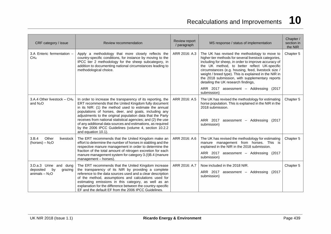
Recalculations and Improvements 10
UK NIR 2018 (Issue 1.1) Ricardo Energy & Environment Page 439
CRF category / issue Review recommendation Review report / paragraph
MS response / status of implementation Chapter / section in the NIR
3.A Enteric fermentation – CH4
Apply a methodology that more closely reflects the country-specific conditions, for instance by moving to the IPCC tier 2 methodology for the sheep subcategory, in addition to documenting national circumstances leading to methodological choice.
ARR 2016: A.3 The UK has revised the methodology to move to higher tier methods for several livestock categories, including for sheep, in order to improve accuracy of the UK method, to better reflect UK-specific circumstances (e.g. housing, feed, livestock size / weight / breed type). This is explained in the NIR in the 2018 submission, with supplementary reports detailing the UK research findings,
ARR 2017 assessment – Addressing (2017 submission)
Chapter 5
3.A.4 Other livestock – CH4 and N2O
In order to increase the transparency of its reporting, the ERT recommends that the United Kingdom fully document in its NIR: (1) the method used to estimate the annual populations of horses, deer, and goats, including any adjustments to the original population data that the Party receives from national statistical agencies; and (2) the use of any additional data sources and estimations, as required by the 2006 IPCC Guidelines (volume 4, section 10.2.2 and equation 10.1).
ARR 2016: A.5 The UK has revised the methodology for estimating horse population. This is explained in the NIR in the 2018 submission.
ARR 2017 assessment – Addressing (2017 submission)
Chapter 5
3.B.4 Other livestock (horses) – N2O
The ERT recommends that the United Kingdom make an effort to determine the number of horses in stabling and the respective manure management in order to determine the fraction of the total amount of nitrogen excretion for each manure management system for category 3.(I)B.4 (manure management – horses).
ARR 2016: A.6 The UK has revised the methodology for estimating manure management from horses. This is explained in the NIR in the 2018 submission.
ARR 2017 assessment – Addressing (2017 submission)
Chapter 5
3.D.a.3 Urine and dung deposited by grazing animals – N2O
The ERT recommends that the United Kingdom increase the transparency of its NIR by providing a complete reference to the data sources used and a clear description of the method, assumptions and calculations used for estimating emissions in this category, as well as an explanation for the difference between the country-specific EF and the default EF from the 2006 IPCC Guidelines.
ARR 2016: A.7 Now included in the 2018 NIR.
ARR 2017 assessment – Addressing (2017 submission)
Chapter 5
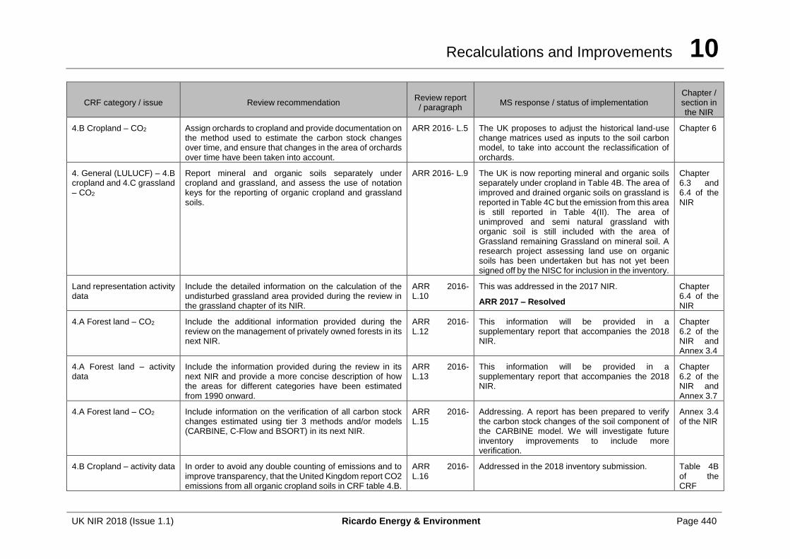
Recalculations and Improvements 10
UK NIR 2018 (Issue 1.1) Ricardo Energy & Environment Page 440
CRF category / issue Review recommendation Review report / paragraph
MS response / status of implementation Chapter / section in the NIR
4.B Cropland – CO2 Assign orchards to cropland and provide documentation on the method used to estimate the carbon stock changes over time, and ensure that changes in the area of orchards over time have been taken into account.
ARR 2016- L.5 The UK proposes to adjust the historical land-use change matrices used as inputs to the soil carbon model, to take into account the reclassification of orchards.
Chapter 6
4. General (LULUCF) – 4.B cropland and 4.C grassland – CO2
Report mineral and organic soils separately under cropland and grassland, and assess the use of notation keys for the reporting of organic cropland and grassland soils.
ARR 2016- L.9 The UK is now reporting mineral and organic soils separately under cropland in Table 4B. The area of improved and drained organic soils on grassland is reported in Table 4C but the emission from this area is still reported in Table 4(II). The area of unimproved and semi natural grassland with organic soil is still included with the area of Grassland remaining Grassland on mineral soil. A research project assessing land use on organic soils has been undertaken but has not yet been signed off by the NISC for inclusion in the inventory.
Chapter 6.3 and 6.4 of the NIR
Land representation activity data
Include the detailed information on the calculation of the undisturbed grassland area provided during the review in the grassland chapter of its NIR.
ARR 2016- L.10
This was addressed in the 2017 NIR.
ARR 2017 – Resolved
Chapter 6.4 of the NIR
4.A Forest land – CO2 Include the additional information provided during the review on the management of privately owned forests in its next NIR.
ARR 2016- L.12
This information will be provided in a supplementary report that accompanies the 2018 NIR.
Chapter 6.2 of the NIR and Annex 3.4
4.A Forest land – activity data
Include the information provided during the review in its next NIR and provide a more concise description of how the areas for different categories have been estimated from 1990 onward.
ARR 2016- L.13
This information will be provided in a supplementary report that accompanies the 2018 NIR.
Chapter 6.2 of the NIR and Annex 3.7
4.A Forest land – CO2 Include information on the verification of all carbon stock changes estimated using tier 3 methods and/or models (CARBINE, C-Flow and BSORT) in its next NIR.
ARR 2016- L.15
Addressing. A report has been prepared to verify the carbon stock changes of the soil component of the CARBINE model. We will investigate future inventory improvements to include more verification.
Annex 3.4 of the NIR
4.B Cropland – activity data In order to avoid any double counting of emissions and to improve transparency, that the United Kingdom report CO2 emissions from all organic cropland soils in CRF table 4.B.
ARR 2016- L.16
Addressed in the 2018 inventory submission. Table 4B of the CRF
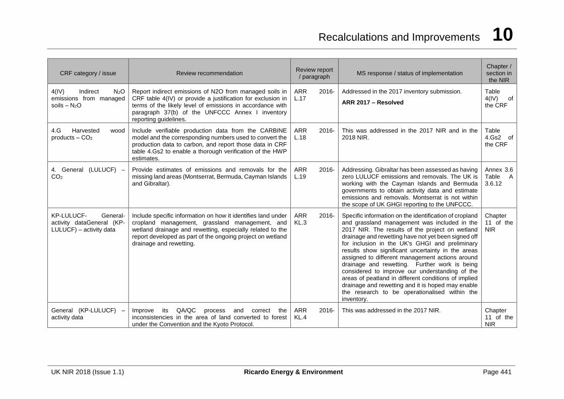
Recalculations and Improvements 10
UK NIR 2018 (Issue 1.1) Ricardo Energy & Environment Page 441
CRF category / issue Review recommendation Review report / paragraph
MS response / status of implementation Chapter / section in the NIR
4(IV) Indirect N2O emissions from managed soils – N2O
Report indirect emissions of N2O from managed soils in CRF table 4(IV) or provide a justification for exclusion in terms of the likely level of emissions in accordance with paragraph 37(b) of the UNFCCC Annex I inventory reporting guidelines.
ARR 2016- L.17
Addressed in the 2017 inventory submission.
ARR 2017 – Resolved
Table 4(IV) of the CRF
4.G Harvested wood products – CO2
Include verifiable production data from the CARBINE model and the corresponding numbers used to convert the production data to carbon, and report those data in CRF table 4.Gs2 to enable a thorough verification of the HWP estimates.
ARR 2016- L.18
This was addressed in the 2017 NIR and in the 2018 NIR.
Table 4.Gs2 of the CRF
4. General (LULUCF) – CO2
Provide estimates of emissions and removals for the missing land areas (Montserrat, Bermuda, Cayman Islands and Gibraltar).
ARR 2016- L.19
Addressing. Gibraltar has been assessed as having zero LULUCF emissions and removals. The UK is working with the Cayman Islands and Bermuda governments to obtain activity data and estimate emissions and removals. Montserrat is not within the scope of UK GHGI reporting to the UNFCCC.
Annex 3.6 Table A 3.6.12
KP-LULUCF- General- activity dataGeneral (KP-LULUCF) – activity data
Include specific information on how it identifies land under cropland management, grassland management, and wetland drainage and rewetting, especially related to the report developed as part of the ongoing project on wetland drainage and rewetting.
ARR 2016- KL.3
Specific information on the identification of cropland and grassland management was included in the 2017 NIR. The results of the project on wetland drainage and rewetting have not yet been signed off for inclusion in the UK's GHGI and preliminary results show significant uncertainty in the areas assigned to different management actions around drainage and rewetting. Further work is being considered to improve our understanding of the areas of peatland in different conditions of implied drainage and rewetting and it is hoped may enable the research to be operationalised within the inventory.
Chapter 11 of the NIR
General (KP-LULUCF) – activity data
Improve its QA/QC process and correct the inconsistencies in the area of land converted to forest under the Convention and the Kyoto Protocol.
ARR 2016- KL.4
This was addressed in the 2017 NIR. Chapter 11 of the NIR
Recalculations and Improvements 10
UK NIR 2018 (Issue 1.1) Ricardo Energy & Environment Page 442
CRF category / issue Review recommendation Review report / paragraph
MS response / status of implementation Chapter / section in the NIR
General (KP-LULUCF) – CO2
Ensure that emissions and removals from land-use change between cropland and grassland/grazing land and conversion of cropland and grassland/grazing land to settlements are included in Kyoto Protocol accounting.
ARR 2016- KL.5
This was addressed in the 2017 NIR. Chapter 11 of the NIR
General (KP-LULUCF) – activity data
Include in its next submission the information required in accordance with decision 2/CMP.8, annex II, paragraph 5(c) and (e).
ARR 2016- KL.6
This was addressed in the 2017 NIR. Chapter 11 of the NIR
Afforestation and reforestation – CO2
Implement the new model in its next annual submission. ARR 2016- KL.7
This was addressed in the 2017 NIR. Chapter 11 of the NIR and Annex 3.4
Deforestation – CO2 Provide further information on the drivers of deforestation and the associated carbon stock changes.
ARR 2016- KL.8
This was addressed in the 2017 NIR. Chapter 11 of the NIR
Deforestation – CO2 Find a method to verify that the carbon stocks prior to deforestation are not underestimated.
ARR 2016- KL.9
Addressing. The UK will continue to investigate what data might be available to demonstrate that underestimation is not occurring.
Article 3.4 activities activity data
Provide estimates of the carbon stock changes in litter and deadwood for cropland management, litter, deadwood and organic soils for grazing land management, and all carbon pools under wetland drainage and rewetting, and include a description of how these changes are estimated.
ARR 2016- KL.10
Addressing. The use of notation keys has been clarified for CM and GM reporting. The results of the project on wetland drainage and rewetting have not yet been signed off for inclusion in the UK's GHGI and preliminary results show significant uncertainty in the areas assigned to different management actions around drainage and rewetting. Further work is being considered to improve our understanding of the areas of peatland in different conditions of implied drainage and rewetting and it is hoped may enable the research to be operationalised within the inventory.
Chapter 11 of the NIR
Forest management – CO2 Include the information on the main changes in the inventory leading to the technical correction of the FMRL in its next submission.
ARR 2016- KL.11
This was addressed in the 2017 NIR. Chapter 6 and annex 3
Recalculations and Improvements 10
UK NIR 2018 (Issue 1.1) Ricardo Energy & Environment Page 443
CRF category / issue Review recommendation Review report / paragraph
MS response / status of implementation Chapter / section in the NIR
Forest management Article 3.4 activities – CO2, CH4 and N2O
Correct the value of the forest management cap in the CRF table “accounting”.
ARR 2016- KL.12
This was addressed in the 2017 NIR. Chapter 6 and Annex 3, In the 2017 CRF
Cropland management – CO2
Report emissions from drained organic soils under cropland management and ensure that the reporting of cropland management under the Kyoto Protocol is consistent with the reporting of LULUCF and agriculture under the Convention.
ARR 2016- KL.13
This was addressed in the 2017 NIR, with further improvements in the 2018 submission.
Chapter 6 and Annex 3, In the 2017 CRF
Harvested wood products – CO2
Increase the transparency of its reporting by including information in the NIR on the data used for the HWP calculations and by providing corresponding AD (harvest) for deforestation, afforestation and reforestation, and forest management separately.
ARR 2016- KL.14
This was addressed in the 2017 NIR. Chapter 6 and Annex 3, In the 2017 CRF
Direct and indirect N2O emissions from N fertilization- N2O
Include indirect emissions of N2O for relevant activities under the Kyoto Protocol.
ARR 2016- KL.15
This was addressed in the 2017 NIR. Chapter 6 and Annex 3, In the 2017 CRF
General (KP-LULUCF General)- activity data
Provide estimates of emissions and removals for the Cayman Islands and Gibraltar.
ARR 2016- KL.16
Addressing. Gibraltar has been assessed as having zero LULUCF emissions and removals. The UK is working with the Cayman Islands government to obtain activity data and estimate emissions and removals.
Annex 3.6 Table A 3.6.12
5.A Solid waste disposal on land – CH4
Implement the proposed improvements of the emission estimates for solid waste disposal sites in the OTs and CDs by providing further information on the methodologies used to estimate the emissions and by completing the CRF tables with specific parameters such as AD, MCF and DOC.
ARR 2016: W.2
Information on the landfill methodologies for OTs and CDs are presented in table A.3.5.4.
Annex 3
Recalculations and Improvements 10
UK NIR 2018 (Issue 1.1) Ricardo Energy & Environment Page 444
CRF category / issue Review recommendation Review report / paragraph
MS response / status of implementation Chapter / section in the NIR
5.A Solid waste disposal on land – CH4
The ERT recommends that the United Kingdom provide information on the parameters used in the MELMod model in its next NIR, including the exact figures and background information on their origin or method of derivation, and also that the Party include in its next NIR the web link to the report on the review of landfill methane emissions modelling.
ARR 2016: W.5
Included in the 2018 NIR.
2017 ARR assessment: Addressing
Section 7.2.2 and table A3.5.2
Web link provided in section 17.6
5.A Solid waste disposal on land – CH4
The ERT noted a discrepancy in the information on CH4 emissions from overseas territories and Crown dependencies. The NIR (section 7.2.3.4) states that the IPCC landfill model was not applied for the Isle of Man as sufficient information is not currently available. Table A 3.5.3 in annex 3 to the NIR, however, shows that the IPCC landfill model was also applied for the Isle of Man. In response to a question raised by the ERT during the review, the Party stated that the landfill model was used for the Isle of Man but with simplified parameters (population and regional defaults) The ERT recommends that the United Kingdom modify the text in the NIR (section 7.2.3.4) to avoid inconsistency of the information on the estimation of CH4 emissions from the Isle of Man.
ARR 2016: W.6
Included in the 2017 NIR and 2018 NIR.
ARR 2017 – Resolved
Chapter 7
5.B. Biological treatment of solid waste – CH4 and N2O
The ERT recommends that the United Kingdom report CH4 and N2O emissions from the composting stage of mechanical-biological treatment under composting (5.B.1) and not under anaerobic digestion at biogas facilities (5.B.2).
ARR 2016: W.7
This is now complete in the 2017 and 2018 submissions
ARR 2017 – Resolved
Chapter 7
Recalculations and Improvements 10
UK NIR 2018 (Issue 1.1) Ricardo Energy & Environment Page 445
CRF category / issue Review recommendation Review report / paragraph
MS response / status of implementation Chapter / section in the NIR
5.D.1 Domestic wastewater – CH4
The ERT recommends that the United Kingdom increase the transparency of its reporting by more clearly stating in the NIR which paths are covered under category 5.D.1 and by providing more information on the methodology applied by the water companies for their reporting according to the Carbon Accounting Workbook. Moreover, the ERT recommends that the Party implement verification activities in accordance with paragraph 41 of the UNFCCC Annex I inventory reporting guidelines, provide justification for the use of the country-specific model, and report thereon in the sectoral chapter on QA/QC activities.
ARR 2016: W.8
Complete and reported in the NIR 2017 and 2018.
ARR 2017 – Resolved
Chapter 7
5.D.1 Domestic wastewater – CH4
The method used for estimating CH4 emissions from domestic wastewater from private wastewater management is based on the 2006 IPCC Guidelines and is well described in the NIR. However, it remained unclear to the ERT what BOD value is applied to the wastewater of this origin. In response to a question raised by the ERT, the Party provided information on population numbers connected to a septic system, as well as the BOD values applied. The ERT recommends that the United Kingdom include the information provided during the review on population numbers and BOD values applied in the next NIR.
ARR 2016: W.9
This information has now been added to the 2018 NIR.
Chapter 7 & Annex 3
5.D.1 Domestic wastewater – N2O
The ERT recommends that the United Kingdom provide a detailed description and justification in the NIR for the use of this new approach adopted in response to the list of potential problems and further questions raised by the ERT during the review (i.e. the update of the fractions FNPR (to 1.16) and FIND-COM (to 1.25), and the information on the consideration of sludge incineration and sludge spreading on agricultural lands) and update the CRF tables accordingly.
ARR 2016: W.10
The fractions FNPR and FIND-COM were updated in the 2017 NIR.
2017 ARR assessment: Addressing
Chapter 7
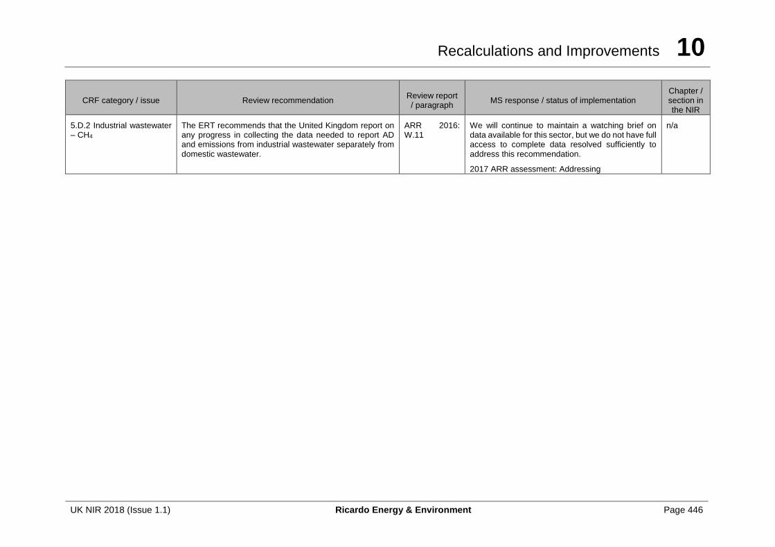
Recalculations and Improvements 10
UK NIR 2018 (Issue 1.1) Ricardo Energy & Environment Page 446
CRF category / issue Review recommendation Review report / paragraph
MS response / status of implementation Chapter / section in the NIR
5.D.2 Industrial wastewater – CH4
The ERT recommends that the United Kingdom report on any progress in collecting the data needed to report AD and emissions from industrial wastewater separately from domestic wastewater.
ARR 2016: W.11
We will continue to maintain a watching brief on data available for this sector, but we do not have full access to complete data resolved sufficiently to address this recommendation.
2017 ARR assessment: Addressing
n/a
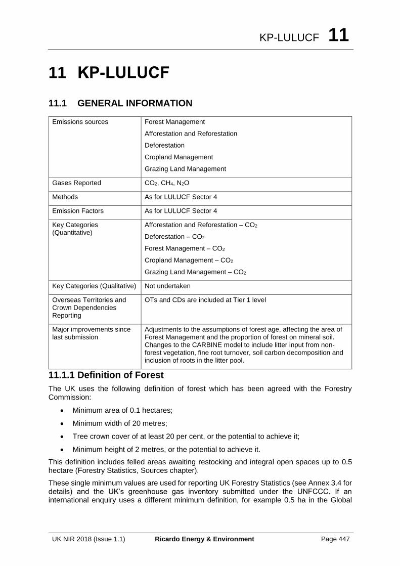
KP-LULUCF 11
UK NIR 2018 (Issue 1.1) Ricardo Energy & Environment Page 447
11 KP-LULUCF
11.1 GENERAL INFORMATION
Emissions sources Forest Management
Afforestation and Reforestation
Deforestation
Cropland Management
Grazing Land Management
Gases Reported CO2, CH4, N2O
Methods As for LULUCF Sector 4
Emission Factors As for LULUCF Sector 4
Key Categories (Quantitative)
Afforestation and Reforestation – CO2
Deforestation – CO2
Forest Management – CO2
Cropland Management – CO2
Grazing Land Management – CO2
Key Categories (Qualitative) Not undertaken
Overseas Territories and Crown Dependencies Reporting
OTs and CDs are included at Tier 1 level
Major improvements since last submission
Adjustments to the assumptions of forest age, affecting the area of Forest Management and the proportion of forest on mineral soil. Changes to the CARBINE model to include litter input from non-forest vegetation, fine root turnover, soil carbon decomposition and inclusion of roots in the litter pool.
11.1.1 Definition of Forest
The UK uses the following definition of forest which has been agreed with the Forestry Commission:
• Minimum area of 0.1 hectares;
• Minimum width of 20 metres;
• Tree crown cover of at least 20 per cent, or the potential to achieve it;
• Minimum height of 2 metres, or the potential to achieve it.
This definition includes felled areas awaiting restocking and integral open spaces up to 0.5 hectare (Forestry Statistics, Sources chapter).
These single minimum values are used for reporting UK Forestry Statistics (see Annex 3.4 for details) and the UK’s greenhouse gas inventory submitted under the UNFCCC. If an international enquiry uses a different minimum definition, for example 0.5 ha in the Global
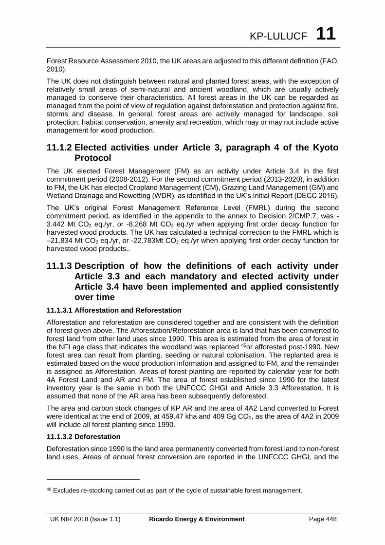
KP-LULUCF 11
UK NIR 2018 (Issue 1.1) Ricardo Energy & Environment Page 448
Forest Resource Assessment 2010, the UK areas are adjusted to this different definition (FAO, 2010).
The UK does not distinguish between natural and planted forest areas, with the exception of relatively small areas of semi-natural and ancient woodland, which are usually actively managed to conserve their characteristics. All forest areas in the UK can be regarded as managed from the point of view of regulation against deforestation and protection against fire, storms and disease. In general, forest areas are actively managed for landscape, soil protection, habitat conservation, amenity and recreation, which may or may not include active management for wood production.
11.1.2 Elected activities under Article 3, paragraph 4 of the Kyoto Protocol
The UK elected Forest Management (FM) as an activity under Article 3.4 in the first commitment period (2008-2012). For the second commitment period (2013-2020), in addition to FM, the UK has elected Cropland Management (CM), Grazing Land Management (GM) and Wetland Drainage and Rewetting (WDR), as identified in the UK’s Initial Report (DECC 2016).
The UK’s original Forest Management Reference Level (FMRL) during the second commitment period, as identified in the appendix to the annex to Decision 2/CMP.7, was -3.442 Mt CO2 eq./yr, or -8.268 Mt CO2 eq./yr when applying first order decay function for harvested wood products. The UK has calculated a technical correction to the FMRL which is –21.834 Mt CO2 eq./yr, or -22.783Mt CO2 eq./yr when applying first order decay function for harvested wood products..
11.1.3 Description of how the definitions of each activity under Article 3.3 and each mandatory and elected activity under Article 3.4 have been implemented and applied consistently over time
11.1.3.1 Afforestation and Reforestation
Afforestation and reforestation are considered together and are consistent with the definition of forest given above. The Afforestation/Reforestation area is land that has been converted to forest land from other land uses since 1990. This area is estimated from the area of forest in the NFI age class that indicates the woodland was replanted 45or afforested post-1990. New forest area can result from planting, seeding or natural colonisation. The replanted area is estimated based on the wood production information and assigned to FM, and the remainder is assigned as Afforestation. Areas of forest planting are reported by calendar year for both 4A Forest Land and AR and FM. The area of forest established since 1990 for the latest inventory year is the same in both the UNFCCC GHGI and Article 3.3 Afforestation. It is assumed that none of the AR area has been subsequently deforested.
The area and carbon stock changes of KP AR and the area of 4A2 Land converted to Forest were identical at the end of 2009, at 459.47 kha and 409 Gg CO2, as the area of 4A2 in 2009 will include all forest planting since 1990.
11.1.3.2 Deforestation
Deforestation since 1990 is the land area permanently converted from forest land to non-forest land uses. Areas of annual forest conversion are reported in the UNFCCC GHGI, and the
45 Excludes re-stocking carried out as part of the cycle of sustainable forest management.
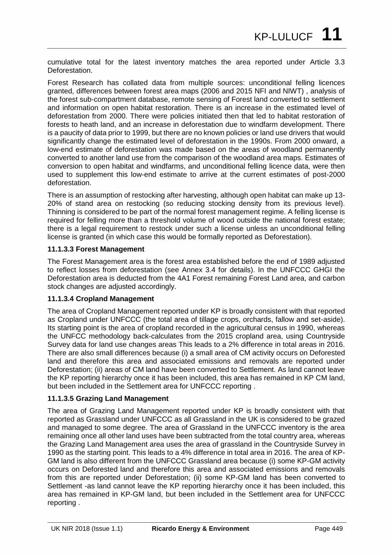
KP-LULUCF 11
UK NIR 2018 (Issue 1.1) Ricardo Energy & Environment Page 449
cumulative total for the latest inventory matches the area reported under Article 3.3 Deforestation.
Forest Research has collated data from multiple sources: unconditional felling licences granted, differences between forest area maps (2006 and 2015 NFI and NIWT) , analysis of the forest sub-compartment database, remote sensing of Forest land converted to settlement and information on open habitat restoration. There is an increase in the estimated level of deforestation from 2000. There were policies initiated then that led to habitat restoration of forests to heath land, and an increase in deforestation due to windfarm development. There is a paucity of data prior to 1999, but there are no known policies or land use drivers that would significantly change the estimated level of deforestation in the 1990s. From 2000 onward, a low-end estimate of deforestation was made based on the areas of woodland permanently converted to another land use from the comparison of the woodland area maps. Estimates of conversion to open habitat and windfarms, and unconditional felling licence data, were then used to supplement this low-end estimate to arrive at the current estimates of post-2000 deforestation.
There is an assumption of restocking after harvesting, although open habitat can make up 13-20% of stand area on restocking (so reducing stocking density from its previous level). Thinning is considered to be part of the normal forest management regime. A felling license is required for felling more than a threshold volume of wood outside the national forest estate; there is a legal requirement to restock under such a license unless an unconditional felling license is granted (in which case this would be formally reported as Deforestation).
11.1.3.3 Forest Management
The Forest Management area is the forest area established before the end of 1989 adjusted to reflect losses from deforestation (see Annex 3.4 for details). In the UNFCCC GHGI the Deforestation area is deducted from the 4A1 Forest remaining Forest Land area, and carbon stock changes are adjusted accordingly.
11.1.3.4 Cropland Management
The area of Cropland Management reported under KP is broadly consistent with that reported as Cropland under UNFCCC (the total area of tillage crops, orchards, fallow and set-aside). Its starting point is the area of cropland recorded in the agricultural census in 1990, whereas the UNFCC methodology back-calculates from the 2015 cropland area, using Countryside Survey data for land use changes areas This leads to a 2% difference in total areas in 2016. There are also small differences because (i) a small area of CM activity occurs on Deforested land and therefore this area and associated emissions and removals are reported under Deforestation; (ii) areas of CM land have been converted to Settlement. As land cannot leave the KP reporting hierarchy once it has been included, this area has remained in KP CM land, but been included in the Settlement area for UNFCCC reporting .
11.1.3.5 Grazing Land Management
The area of Grazing Land Management reported under KP is broadly consistent with that reported as Grassland under UNFCCC as all Grassland in the UK is considered to be grazed and managed to some degree. The area of Grassland in the UNFCCC inventory is the area remaining once all other land uses have been subtracted from the total country area, whereas the Grazing Land Management area uses the area of grassland in the Countryside Survey in 1990 as the starting point. This leads to a 4% difference in total area in 2016. The area of KP-GM land is also different from the UNFCCC Grassland area because (i) some KP-GM activity occurs on Deforested land and therefore this area and associated emissions and removals from this are reported under Deforestation; (ii) some KP-GM land has been converted to Settlement -as land cannot leave the KP reporting hierarchy once it has been included, this area has remained in KP-GM land, but been included in the Settlement area for UNFCCC reporting .
KP-LULUCF 11
UK NIR 2018 (Issue 1.1) Ricardo Energy & Environment Page 450
11.1.3.6 Wetland Drainage and Rewetting
BEIS commissioned a programme of research and methodological development to compile activity data and UK-specific emission factors for Wetland Drainage and Rewetting (WDR) activities (completed in 2017). The results of the project are currently under review for implementation in the UK's GHGI and preliminary results show significant uncertainty in the areas assigned to different management actions around drainage and rewetting. Further work is being considered to improve our understanding of the areas of peatland in different conditions of implied drainage and rewetting and it is hoped may enable the research to be implemented within the inventory and KP reporting.
11.1.4 Precedence conditions and hierarchy among Art. 3.4 activities
The UK has elected additional activities under Article 3.4 for the second commitment period. There is a programme of research and methodological development underway for the newly elected activities (CM, GM and WDR) and the UK is now able to report some of the emissions and removals for these activities and will be able to account for emissions/removals from these activities by the end of the commitment period.
The UK will follow the precedence conditions recommended by the 2013 Kyoto Supplementary Guidance (section 1.2), with Article 3.3 Deforestation highest in the hierarchy, and Article 3.4 WDR lowest. Article 3.4 CM and GM are considered equivalent in the hierarchy: however, in some regions of the UK, rotational management is dominated by crops, with the occasional grass ley, and vice versa in other regions, therefore cropland-grassland land use change is temporary. In the future land undergoing rotational crop/grass management will be specifically allocated to either CM or GM as a sub-category, rather than regularly moving between activities. Development work on land use vectors (see Annex 3.4) may allow the identification and pattern of areas under rotational land use.
There is no double-counting of emissions and removals from Article 3.4 activities under Article 3.3. The UK has consistent records for the land areas in all Article 3.3 and 3.4 activities since 1990, as illustrated by the NIR-2 tables in the CRF, and these are used as the activity data for estimating emissions and removals.
11.2 LAND-RELATED INFORMATION
11.2.1 Spatial assessment unit used for determining the area of the units of land under Article 3.3
The UK uses Reporting Method 1 for Article 3.3 and 3.4 activities. Data sources for tracking areas of afforestation and forest management are spatially explicit, whilst those for deforestation are mostly not. The data sources and methodology can detect a land use change at a resolution consistent with the forest definition in Section 11.1.1 (0.1ha). Data sources for Article 3.4 activities Cropland Management (CM) and Grazing Land Management (GM) are not spatially explicit at present although the inventory development programme’s plans to integrate new datasets for reporting land use change may enable more spatially explicit data to be used in future.
The geographic boundaries used for international reporting are the United Kingdom (for the GBE CRF submission) together with the combined area of the UK’s Overseas Territories and Crown Dependencies (for the GBK and GBR CRF submissions). Disaggregated emissions and removals are estimated at the level of the four countries of the UK (England, Scotland, Wales and Northern Ireland) using both KP and UNFCCC methodology and are reported in an Annexe to the annual report on Greenhouse Gas Inventories for England, Scotland, Wales and Northern Ireland.
KP-LULUCF 11
UK NIR 2018 (Issue 1.1) Ricardo Energy & Environment Page 451
11.2.2 Methodology used to develop the land transition matrix
The land transition matrix is shown in CRF Table NIR 2 (Table 11.1). The same data sources are used for the UNFCCC greenhouse gas inventory (as described in chapter 6.1.1 and Annex 3.4) and emissions/removals under Articles 3.3 and 3.4.
Forest Research has compiled a forest dataset of estimated forest age from 1500 to the present day. The Forestry Commission, Natural Resources Wales and Forest Service of Northern Ireland have provided national forest planting statistics from 1921 to the present. The age of establishment for pre-1921 forests is estimated using information on the distribution of forest area by age class from forest inventories and an algorithm to assign areas of forest to years based on assumed management and rotation length. Areas planted since 1990 in this dataset are used in Article 3.3 Afforestation/ Reforestation.
There is currently no detailed information on the age and type of forests subject to deforestation, so it is assumed that for areas that have been afforested since 1990 very little deforestation will have taken place. New planting in the UK is usually grant aided and it is a condition of these grants that the area of forest be maintained. Estimates of areas in Article 3.3 Deforestation are collated from multiple sources (see Annex 3.4.4 for details). Further information on these data sources is in Chapter 6 and a summary is given in Table 11.2.
The area of Article 3.4 Forest Management land is the area of forest planted before 1990, adjusted to take account of the area lost through deforestation.
The area of Art 3.4 Cropland Management 4 is estimated by combining annual agricultural census data and Countryside Survey data. The CM area at the start of 1990 is the area of cropland recorded in the agricultural census. The CM area at the end of each year is the sum of the initial cropland area and the area gained by land use change from non-forest land, minus the area of cropland converted to Afforestation land or GM land (calculated using the Countryside Survey LUC matrices, described in Annex 3.4.2). The area of cropland at the start of the subsequent year is equal to the cropland area at the end of the previous year.
The area of Art. 3.4 Grazing Land Management is estimated from Countryside Survey data using the assumption that all grassland in the UK is subject to grazing and management to some degree (this area is greater than that reported in the agricultural census). The GM area at the start of 1990 is the area of grassland recorded in the Countryside Survey. The GM area at the end of each year is the sum of the initial grazing land area and the area gained by land use change from non-forest land, minus the area of grazing land converted to Afforestation land or CM land (calculated using the Countryside Survey LUC matrices, described in Annex 3.4.2). The area of grazing land at the start of the subsequent year is equal to the grazing land area at the end of the previous year.
The area of Other Land in CRF table NIR 2 is adjusted so that the total area adds up to the land area reported for the UK and Overseas Territories and is constant for all years.
The UK is not yet in a position to report emissions from land in the Wetland Drainage and Rewetting (WDR) category, although emissions from some WDR practices on land classified under activities higher in the KP hierarchy have been reported in the latest inventory. A programme of research and methodological development is in progress which will enable the full reporting of WDR activities by the end of the commitment period.
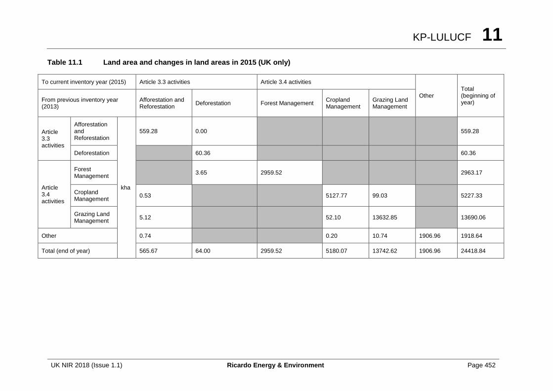
KP-LULUCF 11
UK NIR 2018 (Issue 1.1) Ricardo Energy & Environment Page 452
Table 11.1 Land area and changes in land areas in 2015 (UK only)
To current inventory year (2015) Article 3.3 activities Article 3.4 activities
Other Total (beginning of year) From previous inventory year
(2013) Afforestation and Reforestation
Deforestation Forest Management Cropland Management
Grazing Land Management
Article 3.3 activities
Afforestation and Reforestation
kha
559.28 0.00 559.28
Deforestation 60.36 60.36
Article 3.4 activities
Forest Management
3.65 2959.52 2963.17
Cropland Management
0.53 5127.77 99.03 5227.33
Grazing Land Management
5.12 52.10 13632.85 13690.06
Other 0.74 0.20 10.74 1906.96 1918.64
Total (end of year) 565.67 64.00 2959.52 5180.07 13742.62 1906.96 24418.84
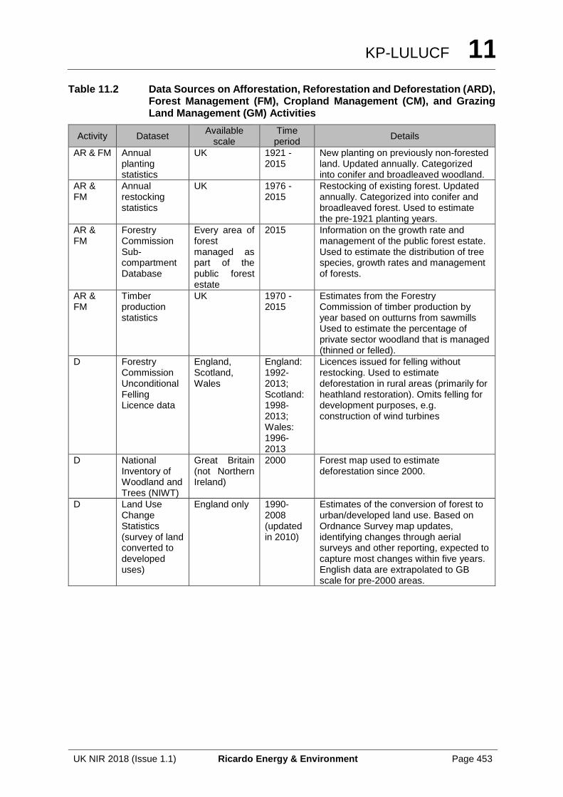
KP-LULUCF 11
UK NIR 2018 (Issue 1.1) Ricardo Energy & Environment Page 453
Table 11.2 Data Sources on Afforestation, Reforestation and Deforestation (ARD), Forest Management (FM), Cropland Management (CM), and Grazing Land Management (GM) Activities
Activity Dataset Available
scale Time period
Details
AR & FM Annual planting statistics
UK 1921 - 2015
New planting on previously non-forested land. Updated annually. Categorized into conifer and broadleaved woodland.
AR & FM
Annual restocking statistics
UK 1976 - 2015
Restocking of existing forest. Updated annually. Categorized into conifer and broadleaved forest. Used to estimate the pre-1921 planting years.
AR & FM
Forestry Commission Sub-compartment Database
Every area of forest managed as part of the public forest estate
2015 Information on the growth rate and management of the public forest estate. Used to estimate the distribution of tree species, growth rates and management of forests.
AR & FM
Timber production statistics
UK 1970 - 2015
Estimates from the Forestry Commission of timber production by year based on outturns from sawmills Used to estimate the percentage of private sector woodland that is managed (thinned or felled).
D Forestry Commission Unconditional Felling Licence data
England, Scotland, Wales
England: 1992-2013; Scotland: 1998-2013; Wales: 1996-2013
Licences issued for felling without restocking. Used to estimate deforestation in rural areas (primarily for heathland restoration). Omits felling for development purposes, e.g. construction of wind turbines
D National Inventory of Woodland and Trees (NIWT)
Great Britain (not Northern Ireland)
2000 Forest map used to estimate deforestation since 2000.
D Land Use Change Statistics (survey of land converted to developed uses)
England only 1990-2008 (updated in 2010)
Estimates of the conversion of forest to urban/developed land use. Based on Ordnance Survey map updates, identifying changes through aerial surveys and other reporting, expected to capture most changes within five years. English data are extrapolated to GB scale for pre-2000 areas.
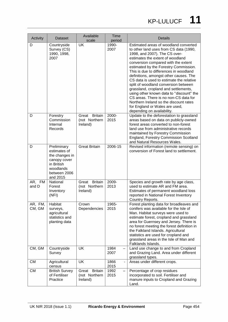
KP-LULUCF 11
UK NIR 2018 (Issue 1.1) Ricardo Energy & Environment Page 454
Activity Dataset Available
scale Time period
Details
D Countryside Survey (CS) 1990, 1998, 2007
UK 1990-2007
Estimated areas of woodland converted to other land uses from CS data (1990, 1998, and 2007). The CS over-estimates the extent of woodland conversion compared with the extent estimated by the Forestry Commission. This is due to differences in woodland definitions, amongst other causes. The CS data is used to estimate the relative split of woodland conversion between grassland, cropland and settlements, using other known data to '‘discount'’ the CS areas. There is no non-CS data for Northern Ireland so the discount rates for England or Wales are used, depending on availability.
D Forestry Commission Internal Records
Great Britain (not Northern Ireland)
2000-2015
Update to the deforestation to grassland areas based on data on publicly-owned forest areas converted to non-forest land use from administrative records maintained by Forestry Commission England, Forestry Commission Scotland and Natural Resources Wales.
D Preliminary estimates of the changes in canopy cover in British woodlands between 2006 and 2015
Great Britain 2006-15 Revised information (remote sensing) on conversion of Forest land to settlement.
AR, FM and D
National Forest Inventory (NFI)
Great Britain (not Northern Ireland)
2009-2013
Species and growth rate by age class, used to estimate AR and FM area. Estimates of permanent woodland loss reported in National Forest Inventory Country Reports.
AR, FM, CM, GM
Habitat surveys, agricultural statistics and planting data
Crown Dependencies
1965-2015
Forest planting data for broadleaves and conifers was available for the Isle of Man. Habitat surveys were used to estimate forest, cropland and grassland area for Guernsey and Jersey. There is no forest meeting the forest definition in the Falkland Islands. Agricultural statistics are used for cropland and grassland areas in the Isle of Man and Falklands Islands.
CM, GM Countryside Survey
UK 1984 – 2007
Land use change to and from Cropland and Grazing Land. Area under different grassland types.
CM Agricultural census
UK 1866 - 2015
Areas under different crops.
CM British Survey of Fertiliser Practice
Great Britain (not Northern Ireland)
1992 – 2015
Percentage of crop residues incorporated to soil. Fertiliser and manure inputs to Cropland and Grazing Land.
KP-LULUCF 11
UK NIR 2018 (Issue 1.1) Ricardo Energy & Environment Page 455
Activity Dataset Available
scale Time period
Details
CM Farm Practice Survey
England 2010 Percentage of Cropland under conventional, reduced and no tillage regimes.
CM Scottish Survey of Agricultural Production Methods
Scotland 2010 Percentage of Cropland under conventional, reduced and no tillage regimes.
CM Scottish Survey of Farm Structure and Methods
Scotland 2013 Percentage of Cropland under conventional, reduced and no tillage regimes.
CM, GM Spatial extent of cultivated organic (Histosol) soils
UK 2013 Area of drained organic soils under cropland and improved grassland in the UK.
AR, D, FM, CM, GM
Fire and Rescue Service Incidence Reporting System
Great Britain (not Northern Ireland)
2010-2015
Area of wildfires on forest, cropland and grassland.
11.2.3 Maps and database to identify the geographical locations, and the system of identification codes for the geographical locations
The whole area of the United Kingdom and the combined area of the Overseas Territories and Crown Dependencies have been used as the geographical units for reporting (Figure 11.1). Only the OTs/CDs of Isle of Man, Jersey, Guernsey and the Falkland Islands have sufficient information to allow us to estimate GHG emissions and removals from KP-LULUCF. CEH is in discussion with the Cayman Islands to develop KP-LULUCF reporting for future submissions.

KP-LULUCF 11
UK NIR 2018 (Issue 1.1) Ricardo Energy & Environment Page 456
Figure 11.1 Geographical areas used for reporting Kyoto Protocol LULUCF activities
11.3 ACTIVITY-SPECIFIC INFORMATION
11.3.1 Methods for carbon stock change and GHG emission and removal estimates
11.3.1.1 Description of the methodologies and the underlying assumptions used
11.3.1.1.1 ARD and FM carbon stock changes
The methods for estimating carbon stock changes in forests for Article 3.3 Afforestation/Reforestation and Article 3.4 Forest Management are the same as those used for the UNFCCC greenhouse gas inventory: details are given in Annex 3.4.1. A Tier 3 carbon accounting model, CARBINE, is used to estimate the net change in pools of carbon in living biomass, litter and soil in conifer and broadleaved forests. In the KP CRF tables changes in carbon stock are reported for: above-ground biomass (gains and losses), litter (net changes) and soils (net changes in mineral and organic soils). Carbon stock changes in below-ground biomass and dead wood are reported as Included Elsewhere, because below-ground biomass is calculated as part of the above-ground biomass and dead wood is calculated as part of the litter pool. Additional information on dead wood may be available from the NFI in future and CARBINE will be modified to report dead wood separately.
Estimates for carbon stock changes as a result of Article 3.3 Deforestation use the same methods as the UNFCCC greenhouse gas inventory (Annex 3.4.4). During deforestation, 40% of the above-ground biomass is assumed to be burnt and emissions of CO2, CH4 and N2O are reported in Table 5(KP-II)5. The remaining carbon stock in biomass is assumed to be immediately lost (instantaneous oxidation) (in UNFCCC reporting this biomass stock is transferred to the harvested wood products pool). This loss (in Gg C) is calculated as:
Isle of Man
Jersey and Guernsey
United Kingdom of Great Britain & Northern Ireland
© George Bosanko
©BBC
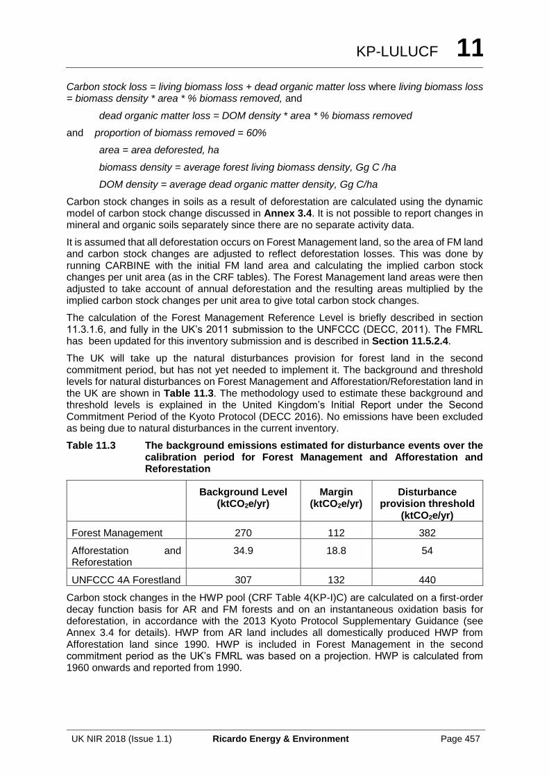
KP-LULUCF 11
UK NIR 2018 (Issue 1.1) Ricardo Energy & Environment Page 457
Carbon stock loss = living biomass loss + dead organic matter loss where living biomass loss = biomass density * area * % biomass removed, and
dead organic matter loss = DOM density * area * % biomass removed
and proportion of biomass removed = 60%
area = area deforested, ha
biomass density = average forest living biomass density, Gg C /ha
DOM density = average dead organic matter density, Gg C/ha
Carbon stock changes in soils as a result of deforestation are calculated using the dynamic model of carbon stock change discussed in Annex 3.4. It is not possible to report changes in mineral and organic soils separately since there are no separate activity data.
It is assumed that all deforestation occurs on Forest Management land, so the area of FM land and carbon stock changes are adjusted to reflect deforestation losses. This was done by running CARBINE with the initial FM land area and calculating the implied carbon stock changes per unit area (as in the CRF tables). The Forest Management land areas were then adjusted to take account of annual deforestation and the resulting areas multiplied by the implied carbon stock changes per unit area to give total carbon stock changes.
The calculation of the Forest Management Reference Level is briefly described in section 11.3.1.6, and fully in the UK’s 2011 submission to the UNFCCC (DECC, 2011). The FMRL has been updated for this inventory submission and is described in Section 11.5.2.4.
The UK will take up the natural disturbances provision for forest land in the second commitment period, but has not yet needed to implement it. The background and threshold levels for natural disturbances on Forest Management and Afforestation/Reforestation land in the UK are shown in Table 11.3. The methodology used to estimate these background and threshold levels is explained in the United Kingdom’s Initial Report under the Second Commitment Period of the Kyoto Protocol (DECC 2016). No emissions have been excluded as being due to natural disturbances in the current inventory.
Table 11.3 The background emissions estimated for disturbance events over the calibration period for Forest Management and Afforestation and Reforestation
Background Level (ktCO2e/yr)
Margin (ktCO2e/yr)
Disturbance provision threshold
(ktCO2e/yr)
Forest Management 270 112 382
Afforestation and Reforestation
34.9 18.8 54
UNFCCC 4A Forestland 307 132 440
Carbon stock changes in the HWP pool (CRF Table 4(KP-I)C) are calculated on a first-order decay function basis for AR and FM forests and on an instantaneous oxidation basis for deforestation, in accordance with the 2013 Kyoto Protocol Supplementary Guidance (see Annex 3.4 for details). HWP from AR land includes all domestically produced HWP from Afforestation land since 1990. HWP is included in Forest Management in the second commitment period as the UK’s FMRL was based on a projection. HWP is calculated from 1960 onwards and reported from 1990.
KP-LULUCF 11
UK NIR 2018 (Issue 1.1) Ricardo Energy & Environment Page 458
11.3.1.1.2 CM and GM carbon stock changes
Changes in soil and biomass carbon due to LUC under KP-Cropland Management and KP-Grazing Land Management are modelled using a Tier 3 model of dynamic stock change, driven by matrices of change calculated from the Countryside Survey and historical data sources. Further description of the model, country-specific soil and biomass carbon densities and rates of change can be found in Annex 3.4.2. Carbon stock changes resulting from deforestation to cropland or grazing land are reported under KP-Deforestation.
Carbon stock changes in biomass as a result of agricultural management activities on cropland are calculated for annual crops, orchards, shrubby perennial crops, perennial grasses grown as biomass fuel, short rotation coppice, and set aside and fallow. Soil carbon stock changes are estimated using data on crop areas supplemented with data on residue removals and fertiliser and manure inputs methodology full description of these Tier 1 and 2 methodologies is given in Annex 3.4.
Carbon stock changes in biomass as a result of agricultural management activities on grazing land are calculated using shrubby and non-shrubby grassland areas from Countryside Survey data and country-specific biomass carbon stocks (Tier 2). Details are given in Annex 3.4. The reporting of emissions from grazing land soils as a result of management activities is awaiting the outcome of further research in this area, as a literature review (Moxley et al, 2014a) suggested that Tier 1 emission factors were not appropriate for the high carbon organo-mineral soils underlying large areas of grazing land in the UK.
11.3.1.1.3 Other GHG emissions from KP-LULUCF
Greenhouse gas emissions (rather than carbon stock changes) from LULUCF activities under the Kyoto Protocol are reported in CRF Tables 4(KP-II)1-5.
Table 4(KP-II)1. Direct and indirect N2O emissions from N fertilization
The method used to estimate emissions is the same as that used in the UNFCCC greenhouse gas inventory and described in Annex 3.4.1. It is assumed that nitrogen fertilizer is only applied to newly planted forests on settlement land and on grassland on organic soils (i.e. AR land) in the UK (see section 6.2) for more information). Indirect emissions from leaching and deposition of N fertiliser are calculated using a Tier 1 methodology.
Table 4(KP-II)2. CH4 and N2O emissions from drained and rewetted organic soils
The method used to estimate N2O emissions from drained forest land is the same as that used in the UNFCCC greenhouse gas inventory and described in Annex 3.4.1. Drainage of forest land only occurs on certain soil types in the UK and is reported for AR and FM land. Carbon emissions from the drainage of forest soils are included with emissions from soils in the carbon stock change tables for AR and FM. There is insufficient information to estimate CH4 emissions from drainage and non-CO2 emissions from rewetted soils at this time.
Table 4(KP-II)3. N2O emissions from N mineralization/immobilization due to carbon loss/gain associated with land-use conversion and management change in mineral soils
Indirect emissions of N2O from leaching of mineral soils as a result of N mineralization following land use change are calculated at Tier 1 methodology. Direct N2O following deforestation to Cropland, Grassland and Settlement and with land use change between Forest Land, Cropland, Grazing Land and Settlement in the UK since 1990 are reported. N2O emissions resulting from the artificial drainage of mineral soils on AR and FM land are also reported in this table, as Table 4(KP-II)2 is for organic soils only.
Table 4(KP-II)4. GHG emissions from biomass burning
The method used to estimate emissions from controlled and wildfire biomass burning is the same as that used in the UNFCCC greenhouse gas inventory and described in Annex 3.4.
KP-LULUCF 11
UK NIR 2018 (Issue 1.1) Ricardo Energy & Environment Page 459
There is no controlled burning of AR or FM forest land in the UK or on managed Cropland. Controlled burning on managed Grazing Land is not included in the inventory at present.
There is insufficient information on the occurrence of wildfires on different forest types so wildfire emissions have been split between AR land and FM land on the basis of their proportion of the whole forest area. As described above, it is assumed that 40% of the standing biomass and DOM undergoes controlled burning during Deforestation and emissions from that burning are reported in this table. It is assumed that wildfires that cause deforestation do not occur in the UK, as there is a general commitment to maintaining forest area. However, it is possible for previously deforested land to undergo wildfire (for example on restored heathland). The wildfire activity data are spatially explicit, so it was possible to assess of the incidence of wildfires on deforested areas but they do not occur every year. Estimated emissions from these events are included in Table 4(KP-II)4.
Emissions from wildfires on grassland and cropland not on Deforested land are reported under Grazing Land Management and Cropland Management, also in Table 4(KP-II)4.
11.3.1.2 Justification for omitting any carbon pool or GHG emissions/removals from activities under Article 3.3 and elected activities under Article 3.4
The UK has elected three additional Article 3.4 activities: Cropland Management, Grazing Land Management and Wetland Drainage and Rewetting. The UK has put in place a research and methodological development programme for these activities to enable full reporting by the end of the commitment period and progress has been made towards this goal.
Table 4(KP-I)A.1.1 Article 3.3 activities: Afforestation and Reforestation. Additional information: emissions and removals from natural disturbance
(GBE, GBR and GBK submissions) The UK has signed up to the provision to exclude emissions from natural disturbances with respect to Article 3(3) (Afforestation and Reforestation), but has not yet needed to implement it. The background levels of emissions
from natural disturbances and the disturbance provision thresholds are shown in Table 11.3. No emissions from natural disturbance above the disturbance provision threshold level have occurred on Afforested and Reforested land in the period covered by the latest inventory. The tables have been filled with NA notation keys (Not Applicable) for the current submission.
Table 4(KP-I)A.2 Article 3.3 activities: Deforestation.
(GBR and GBK submissions) A small amount of deforestation in the Overseas Territories and Crown Dependencies on mineral soils is reported but limited data only allow Tier 1 estimation of carbon stock changes in biomass and litter. Other carbon stock changes are reported as Not Occurring.
Table 4(KP-I)A.2 Article 3.3 activities: Deforestation. Deforestation land previously reported under afforestation/reforestation and forest management and subject to natural disturbances
(GBE, GBR and GBK submissions) No emissions from natural disturbance above the disturbance provision threshold level have occurred in the period covered in the latest inventory. The tables have been filled with NA notation keys (Not Applicable) for the current submission.
Table 4(KP-I)A.2 Article 3.3 activities: Deforestation. Information items: Land areas under deforestation by land-use category in the current reporting year
(GBE, GBR and GBK submissions) The rows for Forest Land, Wetlands and Other land are filled with the Not Occurring (NO) notation key as only deforestation to Cropland, Grassland or Settlements occurs in the UK. Deforestation to Cropland and Settlement does not occur in the Overseas Territories and Crown Dependencies.
KP-LULUCF 11
UK NIR 2018 (Issue 1.1) Ricardo Energy & Environment Page 460
Table 4(KP-I)B.1 Article 3.4 activities: Forest management. Newly established forest (CEF-ne) and Harvested and converted forest plantations (CEF-hc)
(GBE, GBR and GBK submissions) The UK has not elected to report carbon-equivalent forests and therefore the relevant cells are filled with the notation key NA (Not Applicable).
Table 4(KP-I)B.1 Article 3.4 activities: Forest management. Land subject to natural disturbances
(GBE, GBR and GBK submissions) No emissions from natural disturbance above the disturbance provision threshold level have occurred on Forest Management land in the period covered in the latest inventory. The tables have been with filled NO notation keys (Not Occurring) for the current submission.
Table 4(KP-I)B.2. Elected Article 3.4 activities: Cropland Management
(GBR and GBK submissions) Carbon stock changes on cropland in the Overseas Territories and Crown Dependencies are calculated using Tier 1 methodologies, therefore carbon stock changes in below-ground biomass, litter and dead wood are reported as Not Estimated (no guidance).
Table 4(KP-I)B.3. Elected Article 3.4 activities: Grazing Land Management
(GBR and GBK submissions) Carbon stock changes on grazing land in the Overseas Territories and Crown Dependencies are calculated using Tier 1 methodologies, therefore carbon stock changes in below-ground biomass, litter and dead wood are reported as Not Estimated (no guidance).
Table 4(KP-I)B.5 Elected Article 3.4 activities: Wetland drainage and rewetting
(GBE, GBR and GBK submissions) UK-specific activity data and emission factors are still in development for this activity so all carbon stock changes are currently reported as Not Estimated.
Table 4(KP-I)C Carbon stock changes in the harvested wood products (HWP) pool
(GBE submission) HWP resulting from deforestation is assumed to be instantaneously oxidised and is reported as NA in this CRF table.
(GBK and GBR submission) There is a very small amount of HWP arising from timber harvesting in the UK’s Overseas Territories and Crown Dependencies, with none (NO) arising from AR or D land. The small amount from FM land is assumed to all go into paper products for domestic consumption only, and all other products are reported as NO.
Table 4(KP-II)1. Direct N2O emissions from N fertilization
(GBE, GBR and GBK submissions) It is assumed that nitrogen is only applied to newly planted forests on certain land use types in the UK, and therefore that no N fertilization occurs on Deforestation or Forest Management land (NO).
Table 4(KP-II)2. CH4 and N2O emissions from drained and rewetted organic soils
(GBE, GBR and GBK submissions) At present there is insufficient information to allow the estimation of CH4 fluxes and non-CO2 fluxes from drained and rewetted soils under CM, GM and WDR activities (Not Estimated). There are no known occurrences of rewetting on ARD and FM soils.
Table 4(KP-II) N2O emissions from N mineralization/immobilization due to carbon loss/gain associated with land-use conversions and management change in mineral soils
(GBE, GBR and GBK submissions)There are no continuing carbon stock losses, and hence no N2O emissions, associated with LUC from FM land in the UK or from ARD or FM land in the UK’S Overseas Territories and Crown Dependencies (Not Occurring).
KP-LULUCF 11
UK NIR 2018 (Issue 1.1) Ricardo Energy & Environment Page 461
Table 4(KP-II)4. GHG emissions from biomass burning
(GBE submission) There is no controlled burning for management in UK forests, so this is reported as Not Occurring for AR and FM. Controlled burning is prohibited on UK cropland (Not Occurring) but does occur on Grazing Land in the UK, particularly on heather moorland. However, these controlled burning events affect very small patches and occur intermittently and there is no activity data available on their occurrence and extent. At present, emissions for this activity have not been estimated (NE) but this is being kept under review.
Wildfires on Deforested land are infrequent and do not occur every year, so are reported using the notation key NO in most years.
(GBR and GBK submissions) There are no records of either controlled burning or wildfires in the UK’s Overseas Territories and Crown Dependencies. At present, these emissions are reported as Not Estimated, but it is likely (given the small area of land potentially affected) that any emissions are insignificant and could be reported as Not Occurring. An assessment of this will be made for the next submission.
11.3.1.3 Information on whether or not indirect and natural GHG emissions and removals have been factored out
The UK inventory approach to estimating forest carbon stock changes is based on modelled growth data rather than national-scale measurements of forest annual volume increments. The CARBINE model is based on yield class tables, and, in principle assumes constant weather and management conditions; therefore ‘factoring out’ of climate change effects is not required. Work has been undertaken to model the impact of climate, CO2 and land use change on the carbon balance of terrestrial ecosystems in Great Britain (Levy and Clark 2009) and interaction between these factors. This suggested that interactions are small and the effects of these environmental factors are additive. Nitrogen dynamics were not considered in this work: the extent to which enhanced nitrogen deposition affects forest carbon sequestration remains contentious (Magnani et al 2007; Sutton et al 2008).
11.3.1.4 Changes in data and methods since the previous submission (recalculations)
Details of recalculations are given in Table 11.4. Justifications for the recalculations are given in Chapter 6, sections 6.2.7, 6.3.7 and 6.4.7.
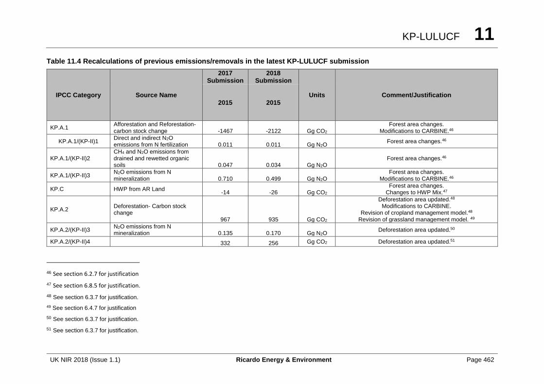
KP-LULUCF 11
UK NIR 2018 (Issue 1.1) Ricardo Energy & Environment Page 462
Table 11.4 Recalculations of previous emissions/removals in the latest KP-LULUCF submission
IPCC Category Source Name
2017 Submission
2018 Submission
Units Comment/Justification
2015 2015
KP.A.1 Afforestation and Reforestation- carbon stock change -1467 -2122 Gg CO2
Forest area changes. Modifications to CARBINE.46
KP.A.1/(KP-II)1 Direct and indirect N2O emissions from N fertilization 0.011 0.011 Gg N2O
Forest area changes.46
KP.A.1/(KP-II)2 CH4 and N2O emissions from drained and rewetted organic soils 0.047 0.034 Gg N2O
Forest area changes.46
KP.A.1/(KP-II)3 N2O emissions from N mineralization 0.710 0.499 Gg N2O
Forest area changes. Modifications to CARBINE.46
KP.C HWP from AR Land -14 -26 Gg CO2
Forest area changes. Changes to HWP Mix.47
KP.A.2 Deforestation- Carbon stock change
967 935 Gg CO2
Deforestation area updated.48 Modifications to CARBINE.
Revision of cropland management model.48 Revision of grassland management model. 49
KP.A.2/(KP-II)3 N2O emissions from N mineralization 0.135 0.170 Gg N2O
Deforestation area updated.50
KP.A.2/(KP-II)4 332 256 Gg CO2 Deforestation area updated.51
46 See section 6.2.7 for justification
47 See section 6.8.5 for justification.
48 See section 6.3.7 for justification.
49 See section 6.4.7 for justification
50 See section 6.3.7 for justification.
51 See section 6.3.7 for justification.
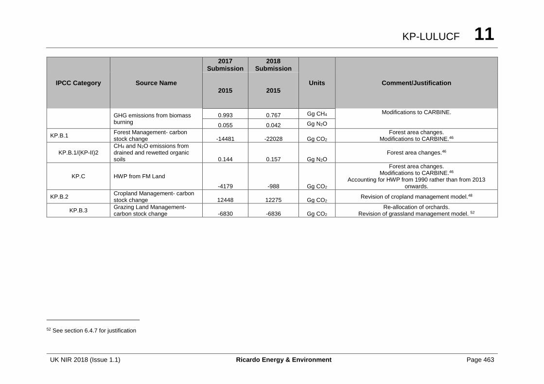
KP-LULUCF 11
UK NIR 2018 (Issue 1.1) Ricardo Energy & Environment Page 463
IPCC Category Source Name
2017 Submission
2018 Submission
Units Comment/Justification
2015 2015
GHG emissions from biomass burning
0.993 0.767 Gg CH4 Modifications to CARBINE.
0.055 0.042 Gg N2O
KP.B.1 Forest Management- carbon stock change -14481 -22028 Gg CO2
Forest area changes. Modifications to CARBINE.46
KP.B.1/(KP-II)2 CH4 and N2O emissions from drained and rewetted organic soils 0.144 0.157 Gg N2O
Forest area changes.46
KP.C HWP from FM Land
-4179 -988 Gg CO2
Forest area changes. Modifications to CARBINE.46
Accounting for HWP from 1990 rather than from 2013 onwards.
KP.B.2 Cropland Management- carbon stock change 12448 12275 Gg CO2
Revision of cropland management model.48
KP.B.3 Grazing Land Management- carbon stock change -6830 -6836 Gg CO2
Re-allocation of orchards. Revision of grassland management model. 52
52 See section 6.4.7 for justification
KP-LULUCF 11
UK NIR 2018 (Issue 1.1) Ricardo Energy & Environment Page 464
11.3.1.5 Uncertainty estimates
Uncertainty assessment and quantification of the inventory was undertaken during 2007-2009, with particular focus on the forest carbon modelling components (van Oijen and Thomson 2010). This analysis was based on the previously used carbon accounting model used to model carbon pools and fluxes in UK forests, CFlow (Dewar and Cannell 1992), but much of the analysis will also apply to the CARBINE model (described in Annex 3.4.1 of this report) as they are very similar models, although CARBINE allows wider range of representation of species, growth rates (yield class) and assumed management.
An uncertainty of 35% for Article 3.3 Afforestation/Reforestation and Article 3.4 Forest Management is used (as estimated for UNFCCC category 4A), an uncertainty of 50% for Article 3.3 Deforestation (based on expert judgement) and an uncertainty of 45% and 50%, respectively, for Article 3.4 Cropland Management and Grazing Land Management (as estimated for the UNFCCC categories 4B and 4C).
Uncertainty from model inputs.
CARBINE requires input data on the afforestation rate (ha yr-1), species, yield class (mean wood volume production at time of maximum mean annual increment, m3 ha-1 yr-1), whether the forest is thinned and felled, the age of harvesting, and whether the forest is clear-felled or not for different forest types and countries in the UK. The management and yield class of private sector woodlands is assumed to be the same as for the national forest estates. Information on the percentage of private sector woodland in production was estimated for each country by comparing the timber production estimated by CARBINE to the timber production statistics for each country.
No measures of statistical uncertainty are associated with the planting statistics because they come from administrative systems (assumed to have total coverage) rather than surveys (Forestry Commission, pers. comm.). This inventory involves the use of data from the National Forest Inventory, which does have estimates of the error associated with the information on the stocked area of woodland, based on the sampling intensity. This is estimated at 1.5% at the 95% confidence interval.
11.3.1.6 Information on other methodological issues
Natural disturbances.
The UK has indicated that it will use the provision to exclude emissions from natural disturbances with respect to Article 3(3) (Afforestation and Reforestation) and Article 3(4) Forest Management, but has not yet needed to do so. The background levels of emissions from natural disturbances and the disturbance provision thresholds are shown in Table 11.3. Areas and emissions from wildfires on forest land, cropland and grazing land are included in the KP-LULUCF inventory (see section 6.2 and Annex 3.4 for further details). Wildfires are not assumed to result in a permanent change in land use.
Inter-annual variability.
The method used to estimate emissions and removals from AR and FM is based on the CARBINE model. This model is not sensitive to inter-annual variation in environmental conditions so these will not affect the annual growth and decay rates. The area burnt in wildfires does show inter-annual variation and this is included in the emissions methodology.
Deforestation
The method used to estimate emissions and removals from D assumes deforestation is evenly applied to the FM area – which implies that the deforestation has the same age, growth rate and species distribution as the FM area. It is unknown whether this assumption leads to an under- or over-estimate of emissions due to deforestation. We intend to investigate whether
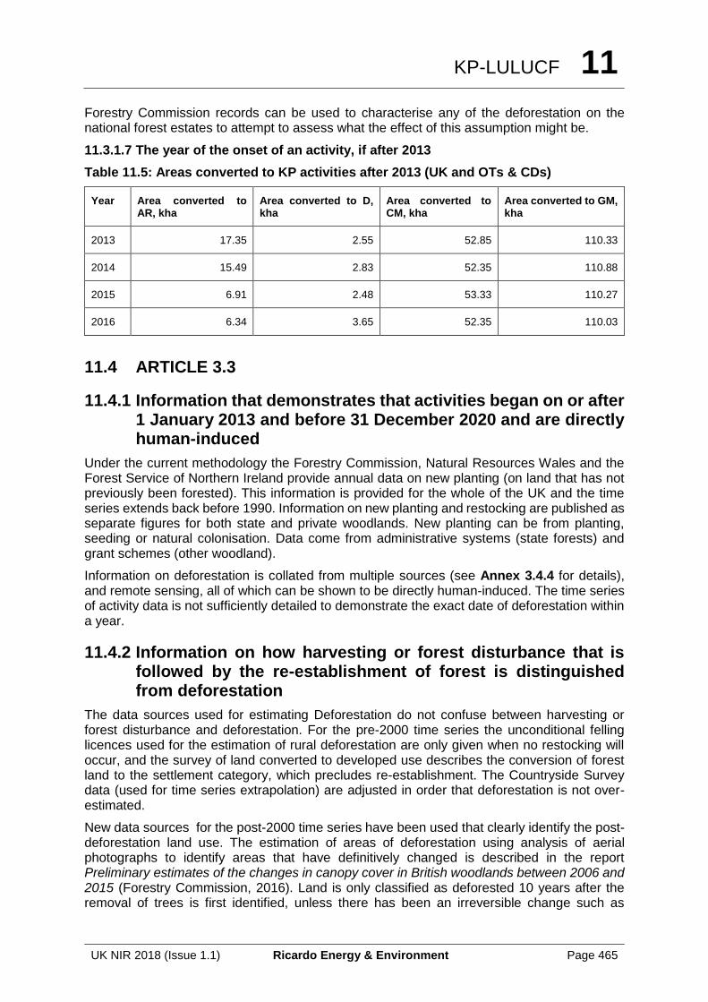
KP-LULUCF 11
UK NIR 2018 (Issue 1.1) Ricardo Energy & Environment Page 465
Forestry Commission records can be used to characterise any of the deforestation on the national forest estates to attempt to assess what the effect of this assumption might be.
11.3.1.7 The year of the onset of an activity, if after 2013
Table 11.5: Areas converted to KP activities after 2013 (UK and OTs & CDs)
Year Area converted to AR, kha
Area converted to D, kha
Area converted to CM, kha
Area converted to GM, kha
2013 17.35 2.55 52.85 110.33
2014 15.49 2.83 52.35 110.88
2015 6.91 2.48 53.33 110.27
2016 6.34 3.65 52.35 110.03
11.4 ARTICLE 3.3
11.4.1 Information that demonstrates that activities began on or after 1 January 2013 and before 31 December 2020 and are directly human-induced
Under the current methodology the Forestry Commission, Natural Resources Wales and the Forest Service of Northern Ireland provide annual data on new planting (on land that has not previously been forested). This information is provided for the whole of the UK and the time series extends back before 1990. Information on new planting and restocking are published as separate figures for both state and private woodlands. New planting can be from planting, seeding or natural colonisation. Data come from administrative systems (state forests) and grant schemes (other woodland).
Information on deforestation is collated from multiple sources (see Annex 3.4.4 for details), and remote sensing, all of which can be shown to be directly human-induced. The time series of activity data is not sufficiently detailed to demonstrate the exact date of deforestation within a year.
11.4.2 Information on how harvesting or forest disturbance that is followed by the re-establishment of forest is distinguished from deforestation
The data sources used for estimating Deforestation do not confuse between harvesting or forest disturbance and deforestation. For the pre-2000 time series the unconditional felling licences used for the estimation of rural deforestation are only given when no restocking will occur, and the survey of land converted to developed use describes the conversion of forest land to the settlement category, which precludes re-establishment. The Countryside Survey data (used for time series extrapolation) are adjusted in order that deforestation is not over-estimated.
New data sources for the post-2000 time series have been used that clearly identify the post-deforestation land use. The estimation of areas of deforestation using analysis of aerial photographs to identify areas that have definitively changed is described in the report Preliminary estimates of the changes in canopy cover in British woodlands between 2006 and 2015 (Forestry Commission, 2016). Land is only classified as deforested 10 years after the removal of trees is first identified, unless there has been an irreversible change such as
KP-LULUCF 11
UK NIR 2018 (Issue 1.1) Ricardo Energy & Environment Page 466
conversion to settlement or administrative records, for example the granting of an unconditional felling licence, indicates intent to convert to another non-forest land cover.
11.4.3 Information on the size and geographical location of forest areas that have lost forest cover but which are not yet classified as deforested
Restocking is assumed for forest areas that have lost forest cover through harvesting or forest disturbance, unless there is deforestation as described above. Information on the size and location of forest areas that have lost forest cover is not explicitly collected on an annual basis. The National Forest Inventory will track areas of clear-felled forest (through satellite imagery and field survey) where canopy cover has been re-established, with any areas remaining unstocked after ten years being classified as confirmed woodland loss (Forestry Commission 2016). A partial assessment of clearfell and restocking in 2012 identified 29 kha of clearfell between 2006 and 2009, of which 18 kha had been restocked by 2012. Further partial assessments are due in 2018 and 2020, which will give a more complete picture of the proportions of clear-felled land awaiting restocking and confirmed deforestation over the second commitment period.
11.4.4 Information related to the natural disturbances provision under Article 3.3
The UK will take up the natural disturbances provision for forest land in the second commitment period. The background, margin and threshold levels for natural disturbances on Forest Management and Afforestation/Reforestation land in the UK are shown in Table 11.3. No emissions have been excluded as being due to natural disturbances in the latest inventory.
Forest management in the UK has evolved to cope with disturbance events, notably windstorms, wildfires and extreme weather events with guidance and decision support systems in place. Historical records show that drought, floods and snow and ice are unlikely to cause substantial damage to UK forests as even events which are extreme for the UK have not caused stand mortality. The UK is not subject to geological disturbance likely to affect forests.
As disturbance events are generally considered to be part of the forest management cycle in the UK, monitoring mechanisms have not yet been established to provide comprehensive, geo-referenced, data on disturbance events. Background levels and margins for natural disturbances with potential to affect stand mortality have been estimated from historical data sets combined with expert judgement, following the methodology set out in Chapter 2 of the 2013 Kyoto Protocol Supplement of the 2006 IPCC Guidelines.
The timeframes covered by the individual data-sets do not overlap in all cases, with the longest continuous data-set being 2000 to 2013 (for windstorms), which is taken as the calibration period. Where data are not available for individual disturbance categories, data-filling has used the mean over their individual calibration periods. Assumptions concerning salvage logging (see details under individual disturbance categories, below) has allowed emissions associated with salvage-logging to be excluded from the background emissions.
The avoidance of net credits/debits during the accounting period has been achieved through establishing a margin of twice the standard deviation of the sum of emissions resulting from each of the disturbance categories over the calibration period, both for Forest Management and Afforestation and Reforestation, separately. Monitoring of disturbance events in the future will also be more robust than the data-sets over calibration period, ensuring that all disturbances are geo-referenced and excluded from Forest Management, Afforestation or Reforestation activities for the duration of the Commitment Period, if the disturbance provision is enacted. Emissions resulting from disturbance events (after the exclusion of emissions from
KP-LULUCF 11
UK NIR 2018 (Issue 1.1) Ricardo Energy & Environment Page 467
salvage-logging) have been estimated on the basis of instantaneous oxidation. In the event that the UK claims under the natural disturbance provisions, a technical correction will amend the FMRL to account for emissions associated with the natural ‘factor’ in question, to ensure the avoidance of net credits.
For Forest Management, carbon stocks and thus emissions (per hectare) are estimated on the basis of mean carbon stocks for conifers (295 tCO2e/ha) and broadleaves (298 tCO2e/ha), respectively, reported by the National Forest Inventory. With the exception of wildfire events (see below) carbon stocks associated with Afforested and Reforested land are assumed to be 20% of those of Forest Managed land, reflecting their younger growth phase.
The annual emissions from wildfire on Forest Management and Afforestation and Reforestation land reported in the UK’s LULUCF GHG inventory have been used for the calibration period. 45% of biomass is assumed to be burned, with no distinction made between total carbon stocks on Forest Management and Afforestation and Reforestation land. Wildfire is apportioned to Forest Management and Afforestation and Reforestation on the basis of the ratio between the two forest categories. Salvage-logging is not assumed to occur on land affected by wildfire. The more detailed data recorded by the UK Fire and Rescue Services will be used if the disturbance provision was implemented during the second commitment period.
Data on pest and disease infestations came from Statutory Plant Health Notices (SPHNs) which are issued when felling is required to combat the infestation (published in Forestry Statistics). Restocking is not required following issuance of an SPHN; however it is strongly encouraged, supported by grant-aid and experience to date indicates that more than 99% of the area has been restocked either by planting or natural regeneration. 80% of the SPHN area has been allocated to Forest Management and 20% to Afforestation and Reforestation (expert judgement), with 80% salvage-logging assumed for Forest Management land and 20% for Afforestation and Reforestation land. Further surveillance is provided through the field survey associated with the National Forest Inventory across approximately 1,500-2,000 one hectare sample squares per annum.
Data on wind damage came from detailed records which the Forestry Commission holds on the wind throw damage to the 250 kha of land it manages in England which was extrapolated to the UK. It is assumed that Afforestation and Reforestation land is not affected by windstorm due the young age of the forest, with all emissions from Forest Management land. 80% salvage-logging is assumed to have occurred in conifer woodland and 50% in broadleaf woodland, based on experience from a severe windstorm in 1987 (Forestry Commission 1996). Remote sensing is being deployed more extensively to monitor woodlands in the UK as part of the National Forest Inventory. If the disturbance provision was enacted to cover a major windstorm event, these data would be used to provide robust coverage, including geo-referencing across public and private woodlands.
Full details of the methodology used to assess background levels, margins and thresholds for emissions from natural disturbances is in the UK’s Initial Report under the Second Commitment Period of the Kyoto Protocol (DECC, 2016).
11.4.5 Information on Harvested Wood Products under Article 3.3
Carbon stock changes in the HWP pool (Table 4(KP-I)C) are calculated on a first-order decay function basis for AR and FM forests and on an instantaneous oxidation basis for Deforestation, in accordance with the 2013 Kyoto Protocol Supplementary Guidance (see Annex 3.4 for details). The HWP pool includes all domestically produced HWP since 1990.
KP-LULUCF 11
UK NIR 2018 (Issue 1.1) Ricardo Energy & Environment Page 468
11.5 ARTICLE 3.4
11.5.1 Information that demonstrates that activities under Article 3.4 have occurred since 1 January 1990 and are human-induced
All managed forests (planted on or before 31st December 1989) that have not been deforested since 1990 are included in Article 3.4 Forest Management. The CARBINE model is used to calculate emissions that have arisen from thinning, harvesting and restocking since 1990. The area under Forest Management is adjusted to reflect losses from deforestation, as recorded in Section 11.1.2.
Emissions from Article 3.4 Cropland Management since 1990 are calculated using agricultural census data and surveys of farming practices collected from 1990 onwards. Cropland is subject to intensive management interventions, and therefore any changes in carbon stock can be assumed to be human-induced.
Emissions from Article 3.4 Grazing Land Management are calculated using Countryside Survey data from 1990 onwards. Grazing land in the UK is all subject to management activity, and therefore it can be assumed that any changes in carbon stocks are human-induced.
11.5.2 Information relating to Forest Management
11.5.2.1 Conversion of natural forest to planted forest
It is assumed that no emissions arise from the conversion of natural forests to plantation forests. It has been a long-standing and on-going policy in the UK to restore areas of woodland historically converted to plantations back towards semi-natural woodland.
11.5.2.2 Forest Management Reference Level (FMRL)
The UK’s Forest Management Reference Level (FMRL) during the second commitment period, as identified in the appendix to the annex to Decision 2/CMP.7, is -3.442 Mt CO2 eq./yr, or -8.268 Mt CO2 eq./yr when applying first order decay function for harvested wood products.
The forest management reference level for the UK was estimated using the same methodology for forest carbon stock changes and GHG emissions as the UNFCCC LULUCF inventory, the KP-LULUCF inventory and national projections of LULUCF emissions and removals. The methodology is described in Chapter 6 and Annex 3. A technical correction to the FMRL was calculated for the latest inventory submission and is described below.
11.5.2.3 Technical Corrections of FMRL
The UK has calculated a technical correction (TC) to the FMRL for the current inventory. The FMRL submitted by the UK in 2011 was based on the 1990-2008 UK greenhouse gas inventory. A technical correction was submitted based on the last inventory, since when the following changes in data and assumptions necessitate a new technical correction for the current submission:
• The new soil and litter model has been updated to better model the litter incorporation into the soil under UK conditions.
• The assumptions about the distribution of afforestation by year have been refined to better match timber production and the new planting records.
• The area of small woods, between 0.1 and 0.5 ha, has been updated based on the final analysis of small woodland areas
• Small woodland area is now assumed to have been afforested evenly between 1900 and 1970
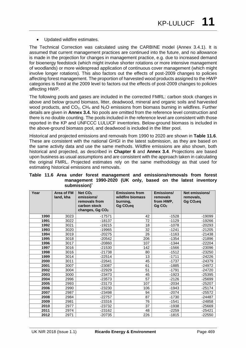
KP-LULUCF 11
UK NIR 2018 (Issue 1.1) Ricardo Energy & Environment Page 469
• Updated wildfire estimates.
The Technical Correction was calculated using the CARBINE model (Annex 3.4.1). It is assumed that current management practices are continued into the future, and no allowance is made in the projection for changes in management practice, e.g. due to increased demand for bioenergy feedstock (which might involve shorter rotations or more intensive management of woodlands) or more widespread application of continuous cover management (which might involve longer rotations). This also factors out the effects of post-2009 changes to policies affecting forest management. The proportion of harvested wood products assigned to the HWP categories is fixed at the 2009 level to factors out the effects of post-2009 changes to policies affecting HWP.
The following pools and gases are included in the corrected FMRL: carbon stock changes in above and below ground biomass, litter, deadwood, mineral and organic soils and harvested wood products, and CO2, CH4 and N2O emissions from biomass burning in wildfires. Further details are given in Annex 3.4. No pools are omitted from the reference level construction and there is no double counting. The pools included in the reference level are consistent with those reported in the KP and UNFCCC LULUCF inventories. Below-ground biomass is included in the above-ground biomass pool, and deadwood is included in the litter pool.
Historical and projected emissions and removals from 1990 to 2020 are shown in Table 11.6. These are consistent with the national GHGI in the latest submission, as they are based on the same activity data and use the same methods. Wildfire emissions are also shown, both historical and projected, as described in Chapter 6 and Annex 3.4. Projections are based upon business as usual assumptions and are consistent with the approach taken in calculating the original FMRL. Projected estimates rely on the same methodology as that used for estimating historical emissions and removals.
Table 11.6 Area under forest management and emissions/removals from forest management 1990-2020 (UK only, based on the latest inventory submission)*
Year Area of FM land, kha
Net CO2 emissions/ removals from carbon stock changes, Gg CO2
Emissions from wildfire biomass burning, Gg CO2eq
Emissions/ removals from HWP, Gg CO2
Net emissions/ removals, Gg CO2eq
1990 3023 -17571 42 -1528 -19099
1991 3022 -18137 72 -1129 -19266
1992 3021 -19215 18 -1078 -20293
1993 3020 -19965 32 -1241 -21205
1994 3019 -20275 26 -1163 -21438
1995 3018 -20542 206 -1354 -21896
1996 3017 -20860 107 -1344 -22204
1997 3016 -21530 142 -1566 -23096
1998 3016 -21738 80 -1512 -23250
1999 3014 -22514 13 -1711 -24226
2000 3011 -22641 45 -1737 -24379
2001 3007 -23087 61 -1885 -24972
2002 3004 -22929 51 -1791 -24720
2003 3000 -23473 45 -1923 -25395
2004 2996 -23573 57 -2126 -25699
2005 2993 -23173 107 -2034 -25207
2006 2990 -23230 106 -1943 -25174
2007 2987 -23498 94 -2074 -25572
2008 2984 -22757 87 -1730 -24487
2009 2981 -23316 76 -1541 -24858
2010 2977 -23732 37 -1938 -25669
2011 2974 -23162 48 -2259 -25421
2012 2971 -20735 226 -1815 -22550
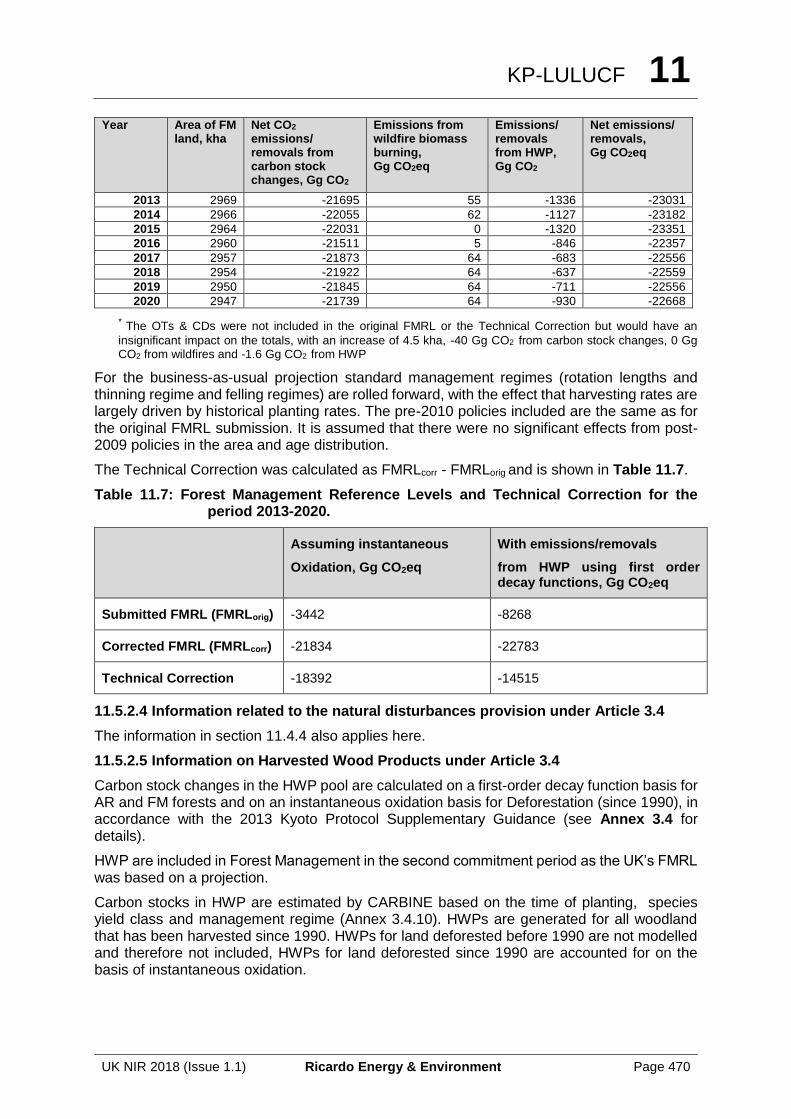
KP-LULUCF 11
UK NIR 2018 (Issue 1.1) Ricardo Energy & Environment Page 470
Year Area of FM land, kha
Net CO2 emissions/ removals from carbon stock changes, Gg CO2
Emissions from wildfire biomass burning, Gg CO2eq
Emissions/ removals from HWP, Gg CO2
Net emissions/ removals, Gg CO2eq
2013 2969 -21695 55 -1336 -23031
2014 2966 -22055 62 -1127 -23182
2015 2964 -22031 0 -1320 -23351
2016 2960 -21511 5 -846 -22357
2017 2957 -21873 64 -683 -22556
2018 2954 -21922 64 -637 -22559
2019 2950 -21845 64 -711 -22556
2020 2947 -21739 64 -930 -22668
* The OTs & CDs were not included in the original FMRL or the Technical Correction but would have an
insignificant impact on the totals, with an increase of 4.5 kha, -40 Gg CO2 from carbon stock changes, 0 Gg CO2 from wildfires and -1.6 Gg CO2 from HWP
For the business-as-usual projection standard management regimes (rotation lengths and thinning regime and felling regimes) are rolled forward, with the effect that harvesting rates are largely driven by historical planting rates. The pre-2010 policies included are the same as for the original FMRL submission. It is assumed that there were no significant effects from post-2009 policies in the area and age distribution.
The Technical Correction was calculated as FMRLcorr - FMRLorig and is shown in Table 11.7.
Table 11.7: Forest Management Reference Levels and Technical Correction for the period 2013-2020.
Assuming instantaneous
Oxidation, Gg CO2eq
With emissions/removals
from HWP using first order decay functions, Gg CO2eq
Submitted FMRL (FMRLorig) -3442 -8268
Corrected FMRL (FMRLcorr) -21834 -22783
Technical Correction -18392 -14515
11.5.2.4 Information related to the natural disturbances provision under Article 3.4
The information in section 11.4.4 also applies here.
11.5.2.5 Information on Harvested Wood Products under Article 3.4
Carbon stock changes in the HWP pool are calculated on a first-order decay function basis for AR and FM forests and on an instantaneous oxidation basis for Deforestation (since 1990), in accordance with the 2013 Kyoto Protocol Supplementary Guidance (see Annex 3.4 for details).
HWP are included in Forest Management in the second commitment period as the UK’s FMRL was based on a projection.
Carbon stocks in HWP are estimated by CARBINE based on the time of planting, species yield class and management regime (Annex 3.4.10). HWPs are generated for all woodland that has been harvested since 1990. HWPs for land deforested before 1990 are not modelled and therefore not included, HWPs for land deforested since 1990 are accounted for on the basis of instantaneous oxidation.
KP-LULUCF 11
UK NIR 2018 (Issue 1.1) Ricardo Energy & Environment Page 471
11.5.3 Information relating to Cropland Management, Grazing Land Management and Revegetation, Wetland Drainage and Rewetting, if elected, for the base year
The UK has elected three additional Article 3.4 activities: Cropland Management, Grazing Land Management and Wetland Drainage and Rewetting. Emissions and removals from Cropland soils and biomass as a result of land use change, management activities and wildfires are reported for both Cropland Management and Grazing Land Management.
The UK is not yet in a position to report emissions and removals from soils as a result of grassland management or from drainage of semi-natural Grazing Land on organic soils. Nor is it yet able to report on emissions and removals from other Wetland Drainage and Rewetting activities. The UK has put in place a research and methodological development programme for these activities to enable full reporting by the end of the commitment period.
11.6 OTHER INFORMATION
11.6.1 Key category analysis for Article 3.3 activities and any elected activities under Article 3.4
Five categories are considered to be key: Article 3.3 Afforestation and Reforestation (CO2), Article 3.3 Deforestation (CO2), Article 3.4 Forest Management (CO2), Article 3.4 Cropland Management (CO2), and Article 3.4 Grazing Land Management (CO2). These have been assessed according to the IPCC 2013 Kyoto Protocol Supplement Section 2.3.6. The numbers have been compared with key category analysis for the latest reported year based on level of emissions (including LULUCF).
Article 3.3 Afforestation and Reforestation (CO2): The associated UNFCCC category 4A (-24 050 Gg CO2e) is a key category but the AR component (i.e. its category contribution (-2 362 Gg CO2e) is smaller than the smallest UNFCCC key category (1B2 Natural Gas Transmission). Removals from this category are also predicted to increase over time as a result of tree planting schemes partially focussed on climate change mitigation.
Article 3.3 Deforestation (CO2): The associated UNFCCC categories (4B, 4C and 4E) are key categories (11 505, -9 372 and 6 422 Gg CO2e respectively), although the Deforestation category contribution (1 655 Gg CO2e) is not key on its own.
Article 3.4 Forest Management (CO2): The associated UNFCCC category 4A is a key category (-24 050 Gg CO2e). The Forest Management category contribution (-22 101 Gg CO2e) is also greater than other categories in the UNFCCC key category analysis.
Article 3.4 Cropland Management (CO2): The associated UNFCCC category 4B is a key category (11 505 Gg CO2e ). The Cropland Management category contribution (13 050 Gg CO2e) is also greater than the smallest UNFCCC key category.
Article 3.4 Grazing Land Management (CO2): The associated UNFCCC category 4C is a key category (-9 372 Gg CO2e). The Grazing Land Management category contribution (-6 534 Gg CO2e ) is also greater than the smallest UNFCCC key category.
11.6.2 Information relating to Article 6
Not applicable in the United Kingdom.
KP-LULUCF 11
UK NIR 2018 (Issue 1.1) Ricardo Energy & Environment Page 472
Information on Accounting of Kyoto Units 12
UK NIR 2018 (Issue 1.1) Ricardo Energy & Environment Page 473
12 Information on Accounting of Kyoto Units
12.1 BACKGROUND INFORMATION
The UK’s Standard Electronic Format report for 2017 containing the information required in paragraph 11 of the annex to decision 15/CMP.1 and adhering to the guidelines of the SEF has been submitted to the UNFCCC Secretariat electronically – RREG1_GB_2017_2_2.xls for commitment period 2 and RREG_GB_2017_1_1.xls for commitment period 1.
12.2 SUMMARY OF INFORMATION REPORTED IN THE SEF TABLES
At the end of 2017, the total CP2 holdings for the UK Registry was 3,543,661 CERs, of which 655,749 were in the voluntary cancellation account. There was also a total of 2 ERUs.
In total for 2017, the UK Registry received 6,359,998 CERs and 2 ERUs. Conversely, 5,641,754 CERs were externally transferred to other national registries. No other CP2 units were transferred or acquired.
293,561 CERs were cancelled.
Full details are available in the SEF tables; the full tables are shown in Annex 6.
Information on legal entities authorised to participate in mechanisms under Articles 6, 12 and 17 of the Kyoto Protocol can be found on the UK Emissions Registry website in the Kyoto Protocol Public Reports area at
https://ets-registry.webgate.ec.europa.eu/euregistry/GB/public/reports/publicReports.xhtml
Annual Submission Item Reporting Guidance
15/CMP.1 annex I.E paragraph 11:
Standard electronic format (SEF)
UK’s Standard Electronic Format report for 2017 containing the information required in paragraph 11 of the annex to decision 15/CMP.1 and adhering to the guidelines of the SEF has been submitted to the UNFCCC Secretariat electronically.
SEF_RREG1_GB_2017_2_2.xlsx (Commitment Period 2 only).
SEF_RREG1_GB_2017_1_1.xlsx (Commitment Period 1 only).
Information on Accounting of Kyoto Units 12
UK NIR 2018 (Issue 1.1) Ricardo Energy & Environment Page 474
Annual Submission Item Reporting Guidance
The contents of the SEF report (R1) can also be found in Annex 6 of this document.
12.3 DISCREPANCIES AND NOTIFICATIONS
Annual Submission Item Reporting Guidance
15/CMP.1 annex I.E paragraph 12:
List of discrepant transactions
No discrepant transactions occurred in 2017.
This is confirmed in the table named “R2” in the Excel file included,
SIAR Reports 2017-GB v1.0.xls
The contents of the Report R2 can also be found in Annex 6 of this document.
15/CMP.1 annex I.E paragraph 13 & 14:
List of CDM notifications
No CDM notifications occurred in 2017.
Refer to Separate Electronic Attachment “SIAR Reports 2017-GB v1.0.xls” Worksheet R3.
The contents of the Report R3 can also be found in Annex 6 of this document.
15/CMP.1 annex I.E paragraph 15:
List of non-replacements
No non-replacements occurred in 2017.
Refer to Separate Electronic Attachment “SIAR Reports 2017-GB v1.0.xls” Worksheet R4.
The contents of the Report R4 can also be found in Annex 6 of this document.
Information on Accounting of Kyoto Units 12
UK NIR 2018 (Issue 1.1) Ricardo Energy & Environment Page 475
Annual Submission Item Reporting Guidance
15/CMP.1 annex I.E paragraph 16:
List of invalid units
No invalid units exist as at 31 December 2017.
Refer to Separate Electronic Attachment “SIAR Reports 2017-GB v1.0.xls” Worksheet R5.
The contents of the Report R5 can also be found in Annex 6 of this document.
15/CMP.1 annex I.E paragraph 17
Actions and changes to address discrepancies
Actions and changes are addressed in Chapter 14: Information on Changes to National Register under section Change of discrepancies procedures.
12.4 PUBLICLY ACCESSIBLE INFORMATION
Annual Submission Item Reporting Guidance
15/CMP.1 annex I.E
Publicly accessible information
The following information is deemed publicly accessible and as such is usually available via the homepage of the UK registry via the Kyoto Protocol Public Reports link at https://ets-registry.webgate.ec.europa.eu/euregistry/GB/public/reports/publicReports.xhtml
In accordance with the requirements of Annex E to Decision 13/CMP.1, all required information for a Party with an active Kyoto registry is provided with the exceptions as outlined below.
Information on Accounting of Kyoto Units 12
UK NIR 2018 (Issue 1.1) Ricardo Energy & Environment Page 476
Annual Submission Item Reporting Guidance
Account Information (Paragraph 45)
In line with the data protection requirements of Regulation (EC) No 45/2001 and Directive 95/46/EC and in accordance with Article 110 and Annex XIV of Commission Regulation (EU) no 389/2013, the information on account representatives, account holdings, account numbers, all transactions made and carbon unit identifiers, held in the EUTL, the Union Registry and any other KP registry (required by paragraph 45) is considered confidential.
JI projects in UK (Paragraph 46)
Note that no Article 6 (Joint Implementation) project is reported as conversion to an ERU under an Article 6 project, as this did not occur in the specified period. The United Kingdom has taken the decision not to host any domestic JI projects, clarification of which is on our registry public reports page https://ets-registry.webgate.ec.europa.eu/euregistry/GB/public/reports/publicReports.xhtml
Paragraph 47 a/d/f - Holding and transaction information of units
Holding and transaction information is provided on a holding type level, due to more detailed information being declared confidential by EU Regulation.
Article 110 of Commission Regulation (EU) 389/2013, provides that “Information, including the holdings of all accounts, all transactions made, the unique unit identification code of the allowances and the unique numeric value of the unit serial number of the Kyoto units held or affected by a transaction, held in the EUTL, the Union Registry and any other KP registry shall be considered confidential except as otherwise required by Union law, or by provisions of national law that pursue a legitimate objective compatible with this Regulation and are proportionate..”
Paragraph 47c
The United Kingdom is not hosting domestic JI projects as per paragraph 46 above.
Information on Accounting of Kyoto Units 12
UK NIR 2018 (Issue 1.1) Ricardo Energy & Environment Page 477
Annual Submission Item Reporting Guidance
Paragraph 47e
The United Kingdom is currently not participating in any LULUCF projects for 2017.
Paragraph 47g
No ERUs, CERs, AAUs and RMUs have been cancelled on the basis of activities under Article 3, paragraphs 3 and 4 to date.
Paragraph 47h
No ERUs, CERs, AAUs and RMUs have been cancelled following determination by the Compliance Committee that the Party is not in compliance with its commitment under Article 3, paragraph 1 to date.
Paragraph 47j
No ERUs and CERs have been retired in 2017 for CP2.
Paragraph 47k
Although we have now entered a new commitment period, no previous commitment period carry over transactions have yet taken place. This will be completed as part of the true up process.
Account holders authorised to hold Kyoto units in their account (Paragraph 48)
In line with the data protection requirements of Regulation (EC) No 45/2001 and Directive 95/46/EC and in accordance with Article 110 and Annex III of the Commission Regulation (EU) no 389/2013, the legal entity contact information (required by paragraph 48) is considered confidential.
12.5 CALCULATION OF THE COMMITMENT PERIOD RESERVE (CPR)
15/CMP.1 annex I.E paragraph 18
CPR Calculation
The Annex to Decision 11/CMP.1 (paragraph 6) specifies that: ‘each Party included in Annex I shall maintain, in its national registry, a commitment period reserve which should not drop below 90 per cent of the Party’s assigned amount calculated pursuant to Article 3, paragraphs 7
Information on Accounting of Kyoto Units 12
UK NIR 2018 (Issue 1.1) Ricardo Energy & Environment Page 478
and 8 of the Kyoto Protocol, or 100 per cent of eight times its most recently reviewed inventory, whichever is lowest’.
Therefore the UK’s commitment period reserve is calculated as:
Either
UK’s Adjusted Assigned Amount
x 90%
2,746,287,369 x 0.90
= 2,471,658,632 assigned amount units
Or
2015 Total Emissions* x Total years of the
second commitment period
506,044,110 x 8
= 4,048,352,880 assigned amount units
*Emissions total is taken from Table A1.3.4 – Approach 1 Key Category Analysis for the latest reported year based on level of emissions (excluding LULUCF) of the 2017 NIR and are shown in tonnes CO2 equivalent.
Our rationale for using this figure is that the Report on the individual review of the annual submission of the United Kingdom of Great Britain and Northern Ireland submitted in 2016, para G.11 on page 19 states:
“The ERT recommends that the United Kingdom, when preparing the NIR, compare the 90 per cent of assigned amount value against the total GHG emissions, excluding LULUCF, in the most recent year.”
The lower of the two numbers is that calculated as 90 per cent of the UK’s assigned amount.
The UK’s Commitment Period Reserve is therefore 2,471,658,632 tonnes of CO2 equivalent (or assigned amount units).

Information on Changes to the National System 13
UK NIR 2018 (Issue 1.1) Ricardo Energy & Environment Page 479
13 Information on Changes to the National System
13.1 CHANGES TO THE NATIONAL SYSTEM
There have been no changes to the National System since the previous inventory submission.

Information on Changes to the National System 13
UK NIR 2018 (Issue 1.1) Ricardo Energy & Environment Page 480
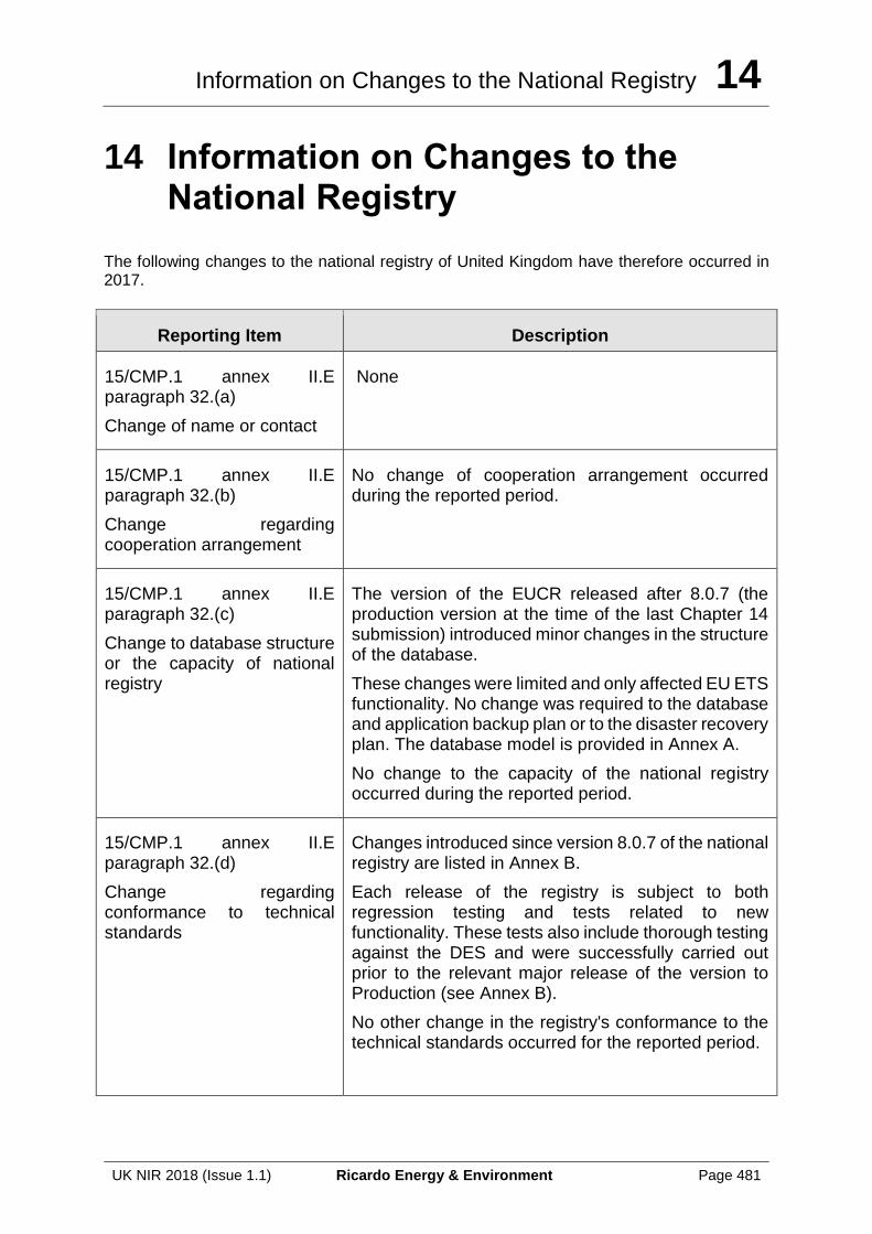
Information on Changes to the National Registry 14
UK NIR 2018 (Issue 1.1) Ricardo Energy & Environment Page 481
14 Information on Changes to the National Registry
The following changes to the national registry of United Kingdom have therefore occurred in 2017.
Reporting Item Description
15/CMP.1 annex II.E paragraph 32.(a)
Change of name or contact
None
15/CMP.1 annex II.E paragraph 32.(b)
Change regarding cooperation arrangement
No change of cooperation arrangement occurred during the reported period.
15/CMP.1 annex II.E paragraph 32.(c)
Change to database structure or the capacity of national registry
The version of the EUCR released after 8.0.7 (the production version at the time of the last Chapter 14 submission) introduced minor changes in the structure of the database.
These changes were limited and only affected EU ETS functionality. No change was required to the database and application backup plan or to the disaster recovery plan. The database model is provided in Annex A.
No change to the capacity of the national registry occurred during the reported period.
15/CMP.1 annex II.E paragraph 32.(d)
Change regarding conformance to technical standards
Changes introduced since version 8.0.7 of the national registry are listed in Annex B.
Each release of the registry is subject to both regression testing and tests related to new functionality. These tests also include thorough testing against the DES and were successfully carried out prior to the relevant major release of the version to Production (see Annex B).
No other change in the registry's conformance to the technical standards occurred for the reported period.
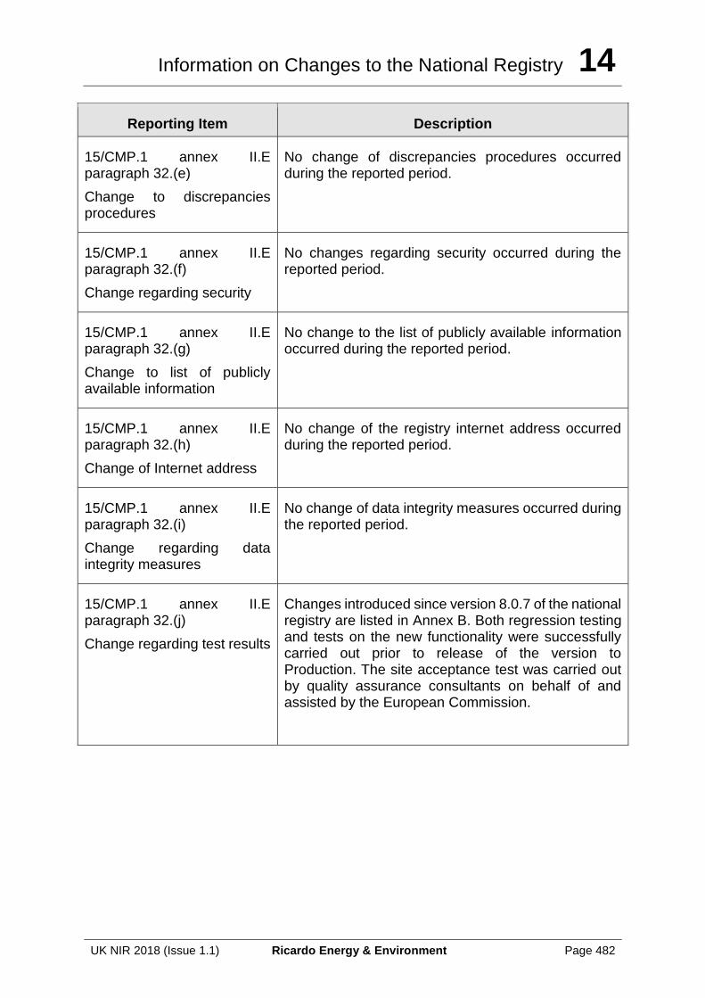
Information on Changes to the National Registry 14
UK NIR 2018 (Issue 1.1) Ricardo Energy & Environment Page 482
Reporting Item Description
15/CMP.1 annex II.E paragraph 32.(e)
Change to discrepancies procedures
No change of discrepancies procedures occurred during the reported period.
15/CMP.1 annex II.E paragraph 32.(f)
Change regarding security
No changes regarding security occurred during the reported period.
15/CMP.1 annex II.E paragraph 32.(g)
Change to list of publicly available information
No change to the list of publicly available information occurred during the reported period.
15/CMP.1 annex II.E paragraph 32.(h)
Change of Internet address
No change of the registry internet address occurred during the reported period.
15/CMP.1 annex II.E paragraph 32.(i)
Change regarding data integrity measures
No change of data integrity measures occurred during the reported period.
15/CMP.1 annex II.E paragraph 32.(j)
Change regarding test results
Changes introduced since version 8.0.7 of the national registry are listed in Annex B. Both regression testing and tests on the new functionality were successfully carried out prior to release of the version to Production. The site acceptance test was carried out by quality assurance consultants on behalf of and assisted by the European Commission.
Information on Minimization of Adverse Impacts 15
UK NIR 2018 (Issue 1.1) Ricardo Energy & Environment Page 483
15 Information on minimization of adverse impacts in accordance with Article 3, paragraph 14
15.1 GENERAL OVERVIEW
The UK is committed to action aimed at minimising the impacts from climate change, including any adverse impacts resulting from action taken to mitigate climate change as outlined in Article 3, paragraph 14 of the Kyoto Protocol.
The Paris Agreement, reached at the 21st United Nations Framework Convention on Climate Change (UNFCCC) Conference of Parties in December 2015, takes a significant step towards reducing the emissions that cause climate change on a global scale. The UK fully supports the Paris Agreement and played an integral role, alongside the EU and its Member States, in the negotiations. In addition to driving forward efforts to keep average global temperature rise to well below 2°C and to pursue efforts to 1.5°C, the Agreement also sets a long-term goal of net zero emissions in the second half of the century.
Integral to the Agreement is the recognition of the role of both developed and emerging economies in helping the poorest and most vulnerable to curb emissions whilst developing, and protecting themselves from the worst effects of climate change. The Agreement establishes a new long-term goal to strengthen adaptation and resilience and reduce vulnerability to climate change. The UK, through deployment of International Climate Finance (ICF), drives sustainable economic development and helps millions of poor and vulnerable people in developing countries build resilience and cope with the increased risk of floods and droughts.
The Paris Agreement sends a clear signal to businesses and investors that the shift to the low carbon economy is global and irreversible, underpinning confidence to drive the scale of investment needed. Low carbon opportunities can unlock markets in countries around the world and support poorer and more vulnerable countries to develop sustainably. However, we must also be alert to any negative impacts of this transition, and make efforts to prevent them and improve the exchange of evidence-based information to inform our understanding of the effects.
The UK continues to pursue climate initiatives, which we have mentioned in previous inventory reports and national communications. This chapter is not an exhaustive list, but instead outlines recent examples of what the UK is doing to support developing countries to adapt to climate change, build capacity to curb their emissions, and develop sustainably. It also includes efforts aimed at understanding the impacts of mitigation action on developing countries and how to minimise any adverse impacts.
This chapter has been updated for the 2018 NIR submission. Changes include:
• An update on new research programmes in 15.2.1;
• An update on Actions to minimize adverse impacts in accordance with Article 3, paragraph 14 in 15.2.2;
• An update on International Climate Finance in 15.2.3;
Information on Minimization of Adverse Impacts 15
UK NIR 2018 (Issue 1.1) Ricardo Energy & Environment Page 484
• An update on Knowledge Transfer in 15.2.4;
• An update on Research Collaboration in 15.2.5;
• An update on Capacity Building and Technology Transfer projects on Renewable Energy and Energy Efficiency in 15.2.6;
• An update on capacity building projects on adapting to climate change in 15.2.7;
• An update on Energy Market Reforms in 15.2.8; and
• The section “within the EU (15.2.2 in the previous NIR) has been removed to prevent duplication of information in the EU NIR.
15.2 UNDERSTANDING IMPACTS OF RESPONSE MEASURES
Understanding the impacts of response measures is a key step to minimising the adverse impacts. The UK continues to undertake assessments, reviews and analysis to better understand the impacts its policies could have on developing countries, and how they could be addressed. Consequently, the UK takes these findings and seeks to apply them in the UK and through our international engagement to minimise adverse impacts, in accordance with article 3, paragraph 14. Recent examples of areas where ongoing research and action is taking place are outlined below.
15.2.1 UK research, reports and analysis
The UK has undertaken research to determine the extent of impacts of response measures and uses this information to implement policies in a way that takes into account the impacts of response measures on all developing countries. Examples of ongoing work are listed below.
• A scoping study commissioned by the department of Business, Energy, and Industrial Strategy (BEIS) to review the available scientific literature on the co-benefits and possible adverse side effects of climate change mitigation. This research will identify knowledge gaps and make recommendations for areas of future research.
• BEIS recently funded two major programmes of research on 1.5 degree pathways and the limitations and possible impacts of 1.5 degree consistent mitigation options (for example widespread deployment of Bioenergy and Carbon Capture and Storage).
To support the UK 2050 Pathways Analysis the Department of Energy and Climate Change (DECC, now BEIS as of 2016) developed a 2050 Energy and Emissions Calculator model. The Calculator is a tool that helps strengthen the level of debate on energy issues in the UK. Over the last four years, BEIS has supported countries around the world to develop their own calculators to explore their options to reduce greenhouse gas emissions and help tackle energy challenges.
• An International Climate Finance programme has directly supported teams in India, Indonesia, Brazil, Mexico, Colombia, Nigeria, South Africa, Vietnam, Thailand and Bangladesh. These ten countries have now published finished calculators online. Many other countries have also adopted the model, for example China, Japan and Austria.
• There is evidence that they are starting to have a policy impact. For example, four countries (India, Colombia, Vietnam and Nigeria) used their calculators to help develop their Intended Nationally-Determined Contributions (INDCs) for the UNFCCC conference in Paris, and India has used it to develop their new National Energy Policy. Other countries have used their calculators to communicate with stakeholders and the general public. For example, the South African Government has developed a simplified version for use in schools, and has provided training to teachers on how to use it.
Information on Minimization of Adverse Impacts 15
UK NIR 2018 (Issue 1.1) Ricardo Energy & Environment Page 485
• BEIS, working in collaboration with a number of other organisations, has built a Global Calculator, which enables users to explore the options for reducing global emissions, and the impacts of climate change associated with them.53
The UK Department for Transport (DfT) has and continues to lead work into understanding Indirect Land Use Change (ILUC) impacts from biofuels. Examples include:
• A study in 2011 which considered the potential for regional (i.e. sub-national, national and supranational) approaches to avoid ILUC from biofuels production. This work highlighted potential actions that may reduce ILUC, and assessed the potential to measure and monitor any such regional level actions to avoid ILUC54.
• In 2013 DfT published a report on the sustainability of feedstock55.
The UK Department for the Environment, Food and Rural Affairs (Defra) has funded and continues to fund research looking at embedded emissions and sustainable production and consumption, in particular:
• The development of an embedded carbon emissions indicator. The aim of this project is to monitor greenhouse gas emissions associated with UK consumption, including those relating to trade flows. This work will provide a high level analysis of the UK national “carbon footprint”, and in particular will assess the emissions which are embedded in products which the UK imports and exports56.
This year’s output from the monitoring, in the Official Statistics Release, is published online57. The UK continues to take an active part in the EU’s Strategic Energy Technology Plan, the technology element of Energy Union and the EU’s Horizon 2020 research and development funding programme.
15.2.2 Actions to minimise adverse impacts in accordance with Article 3, paragraph 14
The UK Government supports the historic agreement reached in the 21st UNFCCC Conference of Parties in Paris in December 2015. The Paris Agreement is a significant step forward on our path to limiting global temperature rises to below 2°C, and agrees to pursue efforts towards 1.5°C. The Agreement also recognises the role of both developed and emerging economies in helping the poorest and most vulnerable to curb emissions whilst developing, and protect themselves from the worst effects of climate change. The transition to a low carbon world requires support to developing countries in their domestic efforts to mitigate and adapt to climate change and to develop their own low carbon economies.
The UK has taken action to minimise adverse impacts in accordance with article 3, paragraph 14 through its International Climate Finance (ICF) and other international action.
53 www.globalcalculator.org
54 http://www.dft.gov.uk/publications/regional-level-actions-to-avoid-iluc
55 https://www.gov.uk/government/publications/biofuel-research
56http://randd.defra.gov.uk/Default.aspx?Menu=Menu&Module=More&Location=None&ProjectID=17729&FromSearch=Y&Publisher=1&SearchText=emissions&GridPage=7&SortString=ProjectCode&SortOrder=Asc&Paging=10#Description
57 http://www.defra.gov.uk/statistics/environment/green-economy/scptb01-ems/
Information on Minimization of Adverse Impacts 15
UK NIR 2018 (Issue 1.1) Ricardo Energy & Environment Page 486
15.2.3 International Climate Finance
Recognising the growing importance and urgency of tackling climate change and its impact on growth and poverty reduction, the UK invested £3.87 billion in International Climate Finance (ICF) from 2011-2016 (financial years 2011/12 to 2014/15). The UK has committed to provide at least a further £5.8 billion from 2016-2020 (financial years 2015/16 to 2020/21), with a commitment to achieve a 50:50 balance between mitigation and adaptation over this period. This will lead to a doubling in UK climate finance in 2020, relative to 2014. This commitment reflects our view that climate change is the biggest threat to the long-term eradication of global poverty, and that the impacts of climate change will hit the poorest hardest. The UK’s ICF is supporting a portfolio of investments managed by the Department for International Development (DFID), BEIS, and Defra. It aims to support international poverty eradication now and in the future by helping developing countries to manage risk and build resilience to the impacts of climate change, take up low-carbon development at scale, and manage natural resources sustainably. The UK aims to spend half of its ICF on mitigation, and half on adaptation. To achieve this, the UK ICF delivers transformational change through well-targeted finance. For example, it helps to pay the incremental cost of making infrastructure investments climate smart and avoid lock-in of high carbon technologies. It also incentivises countries to reduce deforestation and promote sustainable land use. This demonstrates that low-carbon, climate resilient development paths are viable and compatible with economic growth and poverty alleviation. Cumulative data that we collect show that, between 2011/12 and 2016/17, UK ICF programmes have:
• Supported 34 million people to cope with the effects of climate change;
• Provided 12 million people with improved access to clean energy;
• Reduced or avoided 9.2 million tonnes of greenhouse gas (GHG) emissions (tCO2e);
• Installed more than 400 MW of clean energy capacity; and
• Mobilised £2.2 billion public and £500 million private finance for climate change purposes in developing countries.
Through its ICF, the UK is supporting a number of bilateral and multilateral programmes, including (but not limited to) the following examples: The Green Climate Fund – Since becoming operational in 2015, the Green Climate Fund (GCF) has become the key multilateral climate fund, with a mandate to make ‘an ambitious contribution to the global efforts towards attaining the goals set by the international community to combat climate change’. The UK is a strong supporter of the GCF, having committed £720 million for the initial resource mobilisation period, and is committed to ensuring that the GCF delivers maximum impacts in the developing countries it supports. The GCF funds transformational projects with a strong focus on leveraging private finance, with a commitment to provide 50% of its resources for mitigation and 50% for adaptation. At least 50% of its adaptation support will be provided to particularly vulnerable countries including Least Developed Countries (LDCs), Small Island Developing States (SIDS) and African States. In the past year, the GCF has made significant progress in terms of programming, tightening its policy framework, and building the Secretariat’s capacity. So far, the GCF has committed $2.65 billion of funding to 54 projects, representing a balanced
Information on Minimization of Adverse Impacts 15
UK NIR 2018 (Issue 1.1) Ricardo Energy & Environment Page 487
geographical and thematic split, with over 50% of funds going to private sector projects, and over $400 million to Small Island Developing States. The Nationally Appropriate Mitigation Action (NAMA) Facility is a bilateral programme supported by the UK, working in partnership with the German Federal Ministry for the Environment (BMUB), Denmark and the European Commission. NAMAs are country owned projects, policies, or programmes that shift a technology or sector in a country onto a low-carbon development trajectory. The Facility seeks to support and fund the implementation of the most transformational parts of the NAMAs, for which countries are unable to attract private sector funding. It has an open application process, welcoming projects across a diverse range of sectors and geographies. Since 2012, 20 climate mitigation projects across 16 countries have been supported, with each project chosen for its ability to catalyse change in the sector. To support this demand the UK has committed £140 million into the Facility, of which £40 million has been allocated to the 5th Call of the Facility, launched on 13 November 2017
Climate Investment Funds - The UK is the largest investor in the $8.3 billion Climate Investment Funds (CIFs), having invested £1,252.9 million between 2011/12 and 2016/17, to pilot low-emission and climate resilient development through projects implemented by the multilateral development banks. The CIFs now operate across 72 countries and have a total portfolio of 310 projects. CIFs finance is enabling the construction of the equivalent of over a quarter of the current globally installed geothermal and concentrated solar power. The projects are unlocking finance flows in the green markets of developing countries and are expected to generate $58 billion of co-financing.
The Clean Technology Fund (CTF) - Of the four funds that sit under the Climate Investment Fund, the UK has contributed £701 million, between 2011/12 and 2016/17, to the Clean Technology Fund (CTF). The CTF provides concessional finance and technical assistance in 21 countries, delivering significant development benefits, such as increased energy security, reduced local air pollution, and job opportunities. It has supported national governments to identify and implement ambitious low carbon investment plans, and helped demonstrate technologies and create markets. South Africa’s KaXu Solar One Concentrated Solar Power project, with funding from the Clean Technology Fund, has recently been awarded a Momentum for Change Award by the UNFCCC for its innovative and game-changing approach to climate change and wider economic, social and environmental challenges. The Scaling up Renewable Energy Programme (SREP) is another of the four Climate Investment Funds. The UK has provided £268m to SREP, which aims to stimulate energy access and economic activity by working with governments to build renewable energy markets and support productive uses of energy at the household level. As of June 2017, SREP had endorsed investment plans for 19 pilot countries. Expected results under these plans, and the Fund’s Private Sector Set Aside, include an estimated 6,686 gigawatt hours (GWh) of electricity to be generated annually from renewable energy sources (equivalent to the annual electricity production of Armenia) and new or improved access to clean, modern energy services for 17.3 million people (approximately the population of Malawi). The total estimated greenhouse gas (GHG) emissions to be avoided are approximately 5.4 million tons CO2e/yr. Pilot Programme for Climate Resilience (PPCR): the UK is the largest contributor to the $1.2 billion Pilot Programme for Climate Resilience (PPCR), one of the four Funds that sit under the CIFs. The PPCR assists governments with the integration of climate resilience into development planning, and pilots innovative public and private solutions to climate-related risks, primarily in Least Developed Countries or Small Island Developing States. For example, a $15.75 million project in Mozambique will develop climate resilient infrastructure to improve the ability of 8,200 farming families to withstand extreme weather events.
Information on Minimization of Adverse Impacts 15
UK NIR 2018 (Issue 1.1) Ricardo Energy & Environment Page 488
Least Developed Countries Fund (LDCF): the UK is also a long-standing contributor to the Least Developed Countries Fund (LDCF), which supports LDCs in developing their National Adaptation Programmes of Action (NAPAs) and funding the resultant programming. Through our most recent contribution of £30 million, the UK is aiming to help nearly a million people become more resilient to climate change, and to bring approximately 200,000 hectares of land under more sustainable management. This was the fourth contribution that the UK has made to the LDCF – total contributions amount to £122 million since 2006. The LDCF has provided $8 million towards a project strengthening the climate resilience of vulnerable communities in Somalia. Outcomes so far include the construction of a sand dam which has stored enough water for 40,000 people and their livestock to survive through the prolonged drought period in the Bari region. Reduce Emissions from Deforestation and forest Degradation (REDD+)+ is a framework agreed under the UNFCCC to Reduce Emissions from Deforestation and forest Degradation and enhance forest carbon stocks (+) in developing countries. It is aiming to demonstrate the potential of a new land-use paradigm that delivers large-scale forest protection alongside sustainable agricultural intensification. The UK will continue to support “jurisdictional” REDD+ results-based finance that unlocks key barriers in the enabling environment and mobilises private finance, including the examples below:
• The UK has committed £145 million to the Forest Carbon Partnership Facility to support more than 40 countries to develop and then deliver ambitious plans to reduce deforestation. It provides payments based on progress to reduce deforestation as an incentive for countries to take action.
• The UK is also supporting the BioCarbon Fund with £115 million. This is funding to fund policy reform and land-use projects across large areas, to roll out new landscape-wide approaches that produce verified emission reductions from agriculture, forests and other land use.
REDD for Early Movers (REM) - The UK has committed £73 million to the REDD for Early Movers (REM) programme which is an accelerator for the most ambitious and committed countries to reduce emissions from deforestation. REM rewards programmes that are already successful in driving down deforestation trends, with finance re-invested in agreed activities to deliver further results. UK support focusses on Colombia’s programme to achieve zero net deforestation in its Amazon region, as well as programmes to decouple increases in production from forest loss in two Brazilian States – Acre and Mato Grosso. The Sustainable Infrastructure Programme - In 2017 the UK established the Sustainable Infrastructure Program (SIP) in Latin America in partnership with the Inter-American Development Bank. The purpose of the programme is to enable and accelerate the implementation of the Nationally Determined Contributions in Latin America, initially Brazil, Colombia, Mexico and Peru, focusing on supporting and catalysing private sector investments in low carbon infrastructure. The UK will provide up to £177.5 million from its ICF budget over 5 years to provide technical and financial support. This can include technical assistance to governments to help them shape their regulatory frameworks in a way that is attractive to private investors, support the development of local capital markets, while also investing in a few demonstration projects to show commercial viability. UK Climate Investments - UK Climate Investments LLP has been mandated to invest in up to £200 million of UK ICF in low carbon projects in emerging markets its pilot phase (2015-2018). The Investment Mandate requires UKCI to make equity investments into renewable energy and energy efficiency projects in India and Sub-Saharan Africa. Through investing in a
Information on Minimization of Adverse Impacts 15
UK NIR 2018 (Issue 1.1) Ricardo Energy & Environment Page 489
minority equity stake, UKCI aims to leverage additional private equity and debt investment into the projects. The central objectives of the pilot are:
• Use a private sector actor to have a demonstration effect, build a successful track record and prove commerciality of low carbon investments to the broader market by making a strong return on investment; and
• Achieve better value for money by more effectively and nimbly interacting with the private sector.
UKCI’s first investment in India was alongside a UK solar developer in a partnership platform to fund the development, acquisition and ownership of large scale solar power generation assets in India. The Renewable Energy Performance Platform (REPP) - The REPP seeks to mobilise private sector development activity and investment in small and medium scale renewable energy projects (up to 25MW) in sub-Saharan Africa. REPP aims to increase the number of sound ‘bankable’ smaller renewable energy projects by assisting project proponents throughout the project development stage, by financing Technical Assistance, drawing on existing risk mitigation instruments such as political risk insurance and providing results-based finance where necessary. The UK has committed £48 million for 2015 to 2020. The Climate Public Private Partnership (CP3) a £130 million programme that aims to support clean energy and demonstrate the commercial viability of investments in climate-related businesses in emerging markets. By anchoring two private equity funds – i.e. providing committed investment into these funds to help attract additional investors – the programme mobilised private climate finance of $279 million and kick-started the largest private equity climate fund in Asia. The funds have so far invested in 68 businesses and renewable energy developers across developing countries in Asia, Africa and South and Central America. CP3 is expected to avoid 57.4m tonnes of CO2 equivalent over its lifetime (to 2026).
15.2.4 Knowledge transfer
Knowledge transfer can help accelerate the development and deployment of low-carbon and climate resilient technologies to help developing countries mitigate and adapt to climate change.
The UK supports the Technology Mechanism (TM), as agreed at COP16 in Cancun 2010, and is already involved with several knowledge transfer initiatives. In addition to the UK’s long standing involvement in initiatives such as the Climate Technology Initiative, recent actions in this area include:
• The UK-funded Global Network of Climate Innovation Centres programme provides funding to the World Bank’s Climate Technology Programme (CTP) to support the design, implementation, and international coordination of Climate Innovation Centres (CICs) in developing countries. The programme assists local entrepreneurs to develop innovative technology and business solutions to domestic energy, resource and environmental challenges.
The UK also supports CICs in Ethiopia and Vietnam through bi-lateral programmes, while there are additional non-DFID supported CICs in South Africa, the Caribbean, Ghana and Morocco. The programme helps gather evidence on climate technology innovation in developing countries, enabling national CICs to respond to technology trends.
Information on Minimization of Adverse Impacts 15
UK NIR 2018 (Issue 1.1) Ricardo Energy & Environment Page 490
• DFID has committed approximately £103m to the Climate and Development Knowledge Network (CDKN) which is generating and sharing knowledge and building the capacity of developing country decision-makers to design and deliver climate-compatible development policies and programmes. The CDKN does this by providing access to high quality, demand-led technical assistance, research, capacity building, knowledge management and climate negotiation support to support policy and implementation processes at the country and regional level. CDKN has four priority thematic areas which helps prioritise its work across its three focus regions (Africa, Asia and Latin America). These are:
o Climate compatible development (CCD) strategies and plans; o Improving developing countries’ access to climate finance; o Strengthening resilience through climate-related disaster risk management
(DRM); and o Supporting climate negotiators from the Least Developed Countries.
• The UK has a detailed monitoring system in place for capturing results delivered through the ICF portfolio. ICF has a Monitoring, Evaluation and Learning programme that aims to further enhance the monitoring system and generate evidence and knowledge from the portfolio.
15.2.5 Research collaboration
Enhancing global collaboration on research, development and demonstration (RD&D) will be essential to ensure innovation and take-up of climate technologies in developing countries. The UK is cooperating in the technological development of non-energy uses of fossil fuels, and doing so in partnership and supporting developing countries. We are exploring opportunities to support RD&D ‘gap-filling’ activity on climate technologies (both for mitigation/low carbon development and adaptation activities).
The UK will continue to play a leading role in international research efforts to reduce the costs of low carbon energy, working with other countries to strengthen collaboration and transparency in clean energy research, development, and demonstration. The UK continues to be an active participant in EU-based research and development initiatives through the EU’s Strategic Energy Technology Plan, the EU’s Horizon 2020 research and development funding programme and through the International Energy Agency’s Technology Collaboration Programmes. This UK commitment was further underlined at the COP21 climate change conference in Paris, where the UK joined Mission Innovation.
Mission Innovation is an international initiative which aims to accelerate clean energy investment and innovation in order to provide reliable and affordable energy for all. In line with the Mission Innovation pledge, the Government committed to double the UK’s energy innovation spend, such that by 2021 it will have doubled to over £400m per year.
The UK is participating in all seven of Mission Innovation “Innovation Challenges” and co-leads the affordable heating and cooling of Buildings Innovation Challenge alongside the European Commission and United Arab Emirates. These challenges are aimed at catalysing global research efforts in areas that could provide significant benefits in reducing greenhouse gas emissions, increasing energy security, and creating new opportunities for clean economic growth.
Further examples of the UK’s commitment to collaborative research are 2010-2011 projects on low carbon technology transfer to China and India that the DECC supported. The main focus of the studies was to provide new empirical evidence to low carbon innovation in developing countries to inform international policy development. Both studies featured a range
Information on Minimization of Adverse Impacts 15
UK NIR 2018 (Issue 1.1) Ricardo Energy & Environment Page 491
of low carbon technologies and examined the factors that influence innovation and technology transfer, including technological capacity, access to intellectual property rights and the role of policy frameworks.
BEIS, in collaboration with DFID and the Engineering and Physical Sciences Research Council (EPSRC) on behalf of the Research Councils UK (RCUK), are jointly funding a programme of research in the field of energy and international development. Understanding Sustainable Energy Solutions in Developing Countries (USES) is the first major joint call between DFID, BEIS and EPSRC. With a focus on research that will improve our understanding of the opportunities and challenges associated with scaling up sustainable access to modern energy services in developing countries, the programme has been established to help build the evidence base that supports how the UK will spend its International Climate Finance (ICF).
The programme is supporting 12 projects between UK and developing country institutions. It is hoped that this will deliver high quality research that addresses key development challenges in one or more of the following five areas: bioenergy, solar, decentralised generation, urban and transport, and energy efficiency.
International engagement is a significant part of the Avoiding Dangerous Climate Change Research Programme (AVOID). For example, the first phase of the programme investigated technology options for reducing CO2 emissions from the energy sector in India and China to meet national 2050 emissions targets consistent with limiting global temperature rise to below 2°C. It then shared these results with Indian and Chinese officials at international workshops. The second phase of AVOID involved extensive engagement with international researchers and officials on a range of issues, including regional climate impacts, feasibility of energy sector decarbonisation, and the potential role of land-use in both mitigating and contributing to climate change.
The UK is playing a key role in promoting knowledge sharing and capacity building in developing countries on Carbon Capture & Storage (CCUS). The UK has committed up to £60 million of finance from the International Climate Finance (ICF) to raise the level of understanding of CCUS within emerging economies – including China, South Africa, Indonesia and Mexico – leading to the establishment of necessary policy frameworks, technical know-how and incentive structures to support CCUS demonstration and ultimately accelerate the deployment of CCUS. The UK is extending this support by £10 million in 2017-18. The UK will support a range of capacity building projects, including: i) preparation and implementation of early-stage full scale integrated CCUS pilot demonstration projects by financing CCUS planning and pre-investment, capital costs for CCUS units and components, and CCUS related post-completion & operation activities; ii) development of geological site characterisation intended for integrated full scale CCUS projects, both at the pilot and commercial demonstration scales to maximise knowledge on both near-term and future storage capacities; and iii) pilot and demonstration activities aimed at reducing the cost of the technology application across the CCUS chain. It is expected that the UK’s funding will lead to full scale demonstration projects in developing countries, and ultimately accelerate the deployment of CCUS.
The UK continues to jointly lead with Australia the Carbon Capture Usage or Storage (CCUS) initiative under the Clean Energy Ministerial, involving governments of both developed and developing nations. The UK is active in a number of multilateral organisations such as the Carbon Sequestration Leadership Forum (CSLF) which aims to promote the deployment of CCS worldwide in both developed and developing countries. In addition, in April 2013 the UK co-hosted the third 4 Kingdoms Initiative workshop with the government of Norway, bringing together representatives of four oil-producing countries to drive efforts to reduce the economic losses of CCS through alternative uses for CO2.
The UK provided £35m in 2015/16 to the CGIAR consortium of 15 agriculture research centres. Research conducted by the CGIAR has underpinned global agriculture development
Information on Minimization of Adverse Impacts 15
UK NIR 2018 (Issue 1.1) Ricardo Energy & Environment Page 492
since the green revolution. Over 60% of modern plant varieties grown in developing countries have CGIAR ancestry and 30% of global yield growth between 1965 and 1998 can be attributed to plant genetic improvement by the CGIAR. A significant part of the UK support to the CGIAR will develop the next generation of agricultural technology which has the potential to lead to further increases in agricultural productivity, improve the resilience of small-holder agriculture and improve the nutrition and food security of poor people in developing countries.
15.2.6 Capacity Building and Technology Transfer projects on Renewable Energy and Energy Efficiency
The world needs increasing energy supplies to sustain economic growth and development. However, energy resources are under pressure and CO2 emissions from today’s energy use are already changing the climate. It is necessary to accelerate the deployment of low carbon energy technologies and increase energy efficiency to address the global challenges of energy security, climate change and economic development. The following are some examples of the technology transfer activities that the UK undertakes:
o Carbon Capture, Usage and Storage (CCUS): Since 2012, the UK has provided £60 million to support developing countries to build up the technical and institutional knowledge necessary to enable the deployment of CCUS technologies. The UK is extending this support by £10 million in 2017-2018. CCUS development and deployment is crucial for meeting the 2°C target set out under the Paris Agreement. The UK recently completed an evidence review of the global evidence base on CCUS, which highlights that globally, 12-14% of cost-effective decarbonisation needs to come from CCUS in order to meet the 2°C target. The programme aims to raise the level of technical understanding of CCUS in key developing countries, leading to the establishment of the necessary policy frameworks and incentive structures to support CCUS demonstration and ultimately accelerate the deployment of CCUS.
o The Clean Technology Fund (CTF), to which the UK is the largest contributor
(providing £701 million), has demonstrated and deployed low carbon technologies at scale across 21 countries. Examples include supporting the first generation of utility scale Concentrated Solar Power (CSP) plants to be built in developing countries, with the plant in South Africa now providing power to 80,000 people and winning a Momentum for Change award from the UNFCCC. CTF finance for the Noor CSP complex in Morocco has helped to bring down technology costs and overall CTF has supported around a fifth of global CSP deployment to date. The fund has dramatically scaled up geothermal development across multiple countries, as well as a wide range of other renewable and clean transport technologies.
o Capacity Building and Transparency: As agreed by COP21, the Capacity Building
Initiative for Transparency (CBIT) was established by the Global Environment Facility (GEF) in 2015 to support developing countries to meet new reporting requirements under the enhanced transparency framework of the Paris Agreement. The UK is the largest donor to CBIT to date, committing £10 million from the ICF and £1 million from the Scottish Government.
o The Asian Development Bank (ADB)’s Clean Energy Fund was set up to improve
energy access, energy security and the transition to low-carbon technologies through cost-effective investments. The UK’s contribution of £10 million is specifically used to fund the technical assistance elements of the fund.
o Climate Innovation Centres Programme: The UK-funded Global Network of Climate
Innovation Centres programme provides funding to the World Bank’s Climate
Information on Minimization of Adverse Impacts 15
UK NIR 2018 (Issue 1.1) Ricardo Energy & Environment Page 493
Technology Programme (CTP). This supports) to support the design, implementation, and international coordination of Climate Innovation Centres (CICs) in developing countries. The programme assists local entrepreneurs develop innovative technology and business solutions to domestic energy, resource and environmental challenges.
The UK has continued to leverage the collective commitment of the international community in other key fora and institutions to deliver policy interventions and high level actions that encourage the promotion of low carbon technologies, including: International Renewable Energy Agency (IRENA) - The UK supports IRENA’s mission to promote widespread and sustainable use of renewable energy through its role as a centre of excellence for energy transformation, a global voice for renewables, a network hub for international collaboration, and a source of support and advice. The UK has been an IRENA Council member for 2016-2017 and has helped to drive forward IRENA’s medium-term strategy which is consistent with UK government objectives regarding energy security and decarbonisation.
International Partnership for Energy Efficiency Co-operation (IPEEC) - The UK is working in the International Partnership for Energy Efficiency Co-operation (IPEEC),) with key developed and developing countries, to share experience and learn from each other’s policy successes and failures. This identifies, and identify opportunities for collaborative work to address issues of mutual interest or concern, where such international action can add value to domestic efforts/expertise. A work programme has been developed encompassing a range of activities including appliance standards and labels, sustainable buildings, financing, data collection and indicators, energy management, transport, and capacity building activities. Much of this work is also being taken forward within the G20’s Energy Efficiency Leading programme which IPEEC is co-ordinating The UK is also working with members of the G20, IPEEC and the International Energy Agency (IEA) to establish an “Energy Efficiency Hub”, to help coordinate international efforts to drive forward energy efficiency improvements.
15.2.7 Capacity building projects on adapting to climate change
UK ICF investments aim to support international poverty reduction now and in the future by helping developing countries manage risk and build resilience to the impacts of climate change, take up low-carbon development at scale, and manage natural resources sustainably. The poorest and most vulnerable people in the world will be hit first and hardest by the impacts of climate change. This is why the UK aims to spend half of its climate finance on adaptation. We support capacity-building to assist developing countries to better:
Adapt to long-term impacts well in advance, for example by changing or diversifying livelihoods and ensuring infrastructure is fit for purpose. Anticipate and reduce the impact of climate variability and extremes, for example through effective forecasting and preparedness measures. Absorb the effects of climate extremes and disasters - for example through effective and rapid response that enables people to cope with disaster and recover quickly.
Adapt
• The Building Resilience and Adaptation to Climate Extremes and Disasters (BRACED) programme is helping people become more resilient to climate extremes in South and Southeast Asia, as well as in the African Sahel and neighbouring countries. It does this through improved integration of disaster risk reduction and climate adaptation methods into development approaches, influencing local, national and international policies and practices.
Information on Minimization of Adverse Impacts 15
UK NIR 2018 (Issue 1.1) Ricardo Energy & Environment Page 494
• The Blue Forest programme is introducing models for the sustainable management of mangroves in Madagascar and scaling these models in Indonesia and South East Asia to help increase coastal adaptation and resilience. The £10.1 million project, involving fisheries management and mangrove livelihood diversification, is expected to protect 20,000 hectares of mangrove forests and benefit over 100,000 people. Key progress made on livelihood adaptation includes the creation and implementation of 11 sustainable community-owned mangrove forestry management plans, and the development and integration of multiple alternative livelihoods, including bee keeping and sea cucumber farming.
Anticipate
• UK Aid funds the Weather and Climate Information and Services for Africa (WISER) programme. Its mission is to deliver transformational change in the quality, accessibility and use of weather and climate information services at all levels of decision making for sustainable development in Africa. It is strengthening the capacity of the national and regional mandated organisations and channels in order to deliver weather and climate services which support poverty reduction, directed by user needs.
• UK Aid also funds the Future Climate for Africa (FCFA) research programme, which aims to enhance the scientific understanding and prediction of climate variability and change in Africa and, at the same time, is working with stakeholders to bring this information into use in adaptation planning. FCFA includes 11 pilot studies, building capacity across sub-Saharan Africa in using climate information to inform decisions, including infrastructure development, climate-smart agriculture, and urban and national planning.
Absorb
• The UK is a major contributor to African Risk Capacity (ARC) which strengthens African governments’ understanding of drought risk and enables them to buy insurance that will pay out after harvest failures due to droughts. Senegal, Mauritania and Niger received payments totalling $26.5 million after poor rains in 2014, providing food aid, animal fodder and other assistance to 1.3 million people. Malawi received a payment of $8.1 million in 2016, which they have used for emergency cash transfers to affected people and to replenish the national strategic grain reserve. Five countries are currently insured.
15.2.8 Energy Market Reforms – responding to energy market imperfections
Launched under the last Government, Electricity Market Reform (EMR) introduced two key mechanisms – Contracts for Difference (CfD) and the Capacity Market, designed to incentivise the investment required in the UK’s energy infrastructure and deliver low carbon energy and reliable supplies, while minimising costs to consumers.
CfDs are long term (15 year) contracts designed to give greater certainty and stability of revenues to electricity generators by reducing their exposure to volatile wholesale prices, whilst protecting consumers from paying for higher support costs when electricity prices are high. Following the award of investment contracts to eight projects in 2014 and a first competitive allocation round in 2015 currently supporting 24 projects, a second CfD Allocation Round took place in September 2017. This led to 16 contracts being signed for ten projects, representing over 3GW of new renewable generation capacity to commission from 2021/22 onwards.
In total, the CfD scheme is now supporting 42 renewable electricity projects across 56 contracts, and is expected to deliver around 10GW of new installed capacity by 2023. Six projects have so far been commissioned, providing a combined capacity of over 1.6 GW of
Information on Minimization of Adverse Impacts 15
UK NIR 2018 (Issue 1.1) Ricardo Energy & Environment Page 495
renewable electricity. The Government announced in its Clean Growth Strategy in October 2017 that it plans to hold a further allocation round in spring 2019.
Three main Capacity Market auctions have been completed so far, with the fourth due in February 2018. Along with a special, early auction, which brought forward the start of the Capacity Market by a year to 2017/18, the auctions held so far have secured supplies up to 2020/21.
The most recent main auction was held in December 2016, for delivery in 2020/21. This), saw around 3.4 GW of new projects clear, with 1.5GW of new gas including a new CCGT plant (Centrica: Kings Lynn), a new OCGT plant (Spalding), and a variety of smaller scale, flexible gas resources.
The UK is continuing to reduce its reliance on coal and is bringing innovative and low-carbon technologies into its energy mix, as part of a cleaner, more flexible energy system. The last two main auctions together have seen around 7.5GW of new capacity coming though,, with significant innovation (demand-side response, battery storage) alongside more traditional gas projects and new interconnectors. The Government has confirmed plans to close all unabated coal power stations by 2025.

Information on Minimization of Adverse Impacts 15
UK NIR 2018 (Issue 1.1) Ricardo Energy & Environment Page 496

Other Information 16
UK NIR 2018 (Issue 1.1) Ricardo Energy & Environment Page 497
16 Other Information
There is no additional information to include in this chapter.

Other Information 16
UK NIR 2018 (Issue 1.1) Ricardo Energy & Environment Page 498
References 17
UK NIR 2018 (Issue 1.1) Ricardo Energy & Environment Page 499
17 References
References for the main chapters and the annexes are listed here and are organised by chapter and annex. During 2008 the BERR energy team and the Defra climate teams formed the Department of Energy and Climate Change (DECC). In July 2016 DECC was replaced by the Department of Business, Energy & Industrial Strategy (BEIS), which has taken over all of DECC’s responsibilities with regards to the UK’s GHG Inventory. BEIS is now the Single National Entity for the UK’s National Inventory System. References in this document refer to correct name at the time of original publication.
17.1 CHAPTER 1 [INTRODUCTION]
Baggott SL, Lelland A, Passant NP, and Watterson J (2004) Review of Carbon Emission Factors in the UK Greenhouse Gas Inventory. AEA Energy and Environment, The Gemini Building, Fermi Avenue, Didcot, Oxfordshire, OX11 0QR, UK. November 2004. AEA report number AEAT/ENV/R/2347. Report prepared for UK Defra under contract RMP/2106.
DECC (2017), Digest of United Kingdom Energy Statistics 2017, London, The Stationery Office.
IPCC (1996) Climate Change 1995 – The science of climate change. Contribution of Working Group 1 to the Second Assessment Report of the Intergovernmental Panel on Climate Change, Ed. Houghton, JT., Cambridge University Press.
IPCC (1997a), IPCC Revised 1996 Guidelines for National Greenhouse Gas Inventories, Volume 1, Greenhouse Gas Inventory Reporting Instructions, IPCC WGI Technical Support Unit, Hadley Centre, Meteorological Office, Bracknell, UK.
IPCC (1997b), IPCC Revised 1996 Guidelines for National Greenhouse Gas Inventories, Volume 2, Greenhouse Gas Inventory Workbook, IPCC WGI Technical Support Unit, Hadley Centre, Meteorological Office, Bracknell, UK.
IPCC (1997c), IPCC Revised 1996 Guidelines for National Greenhouse Gas Inventories, Volume 3, Greenhouse Gas Inventory Reference Manual, IPCC WGI Technical Support Unit, Hadley Centre, Meteorological Office, Bracknell, UK.
IPCC (2000), Good Practice Guidance and Uncertainty Management in National Greenhouse Gas Inventories, ed. Penman, J, Kruger, D, Galbally, I, et al., IPCC National Greenhouse Gas Inventories Programme, Technical Support Programme Technical Support Unit, Institute for Global Environmental Strategies, Hayama, Kanagawa, Japan.
IPCC (2001), Climate change 2001 – The scientific basis. Contribution of Working Group 1 to the Third Assessment Report of the Intergovernmental Panel on Climate Change, Cambridge University Press.
IPCC (2003), Good Practice Guidance for Land Use, Land-Use Change and Forestry. Institute for Global Environmental strategies (IGES) for the Intergovernmental Panel on Climate Change, Kanagawa, Japan.
IPCC (2006), 2006 IPCC Guidelines for National Greenhouse Gas Inventories
http://www.ipcc-nggip.iges.or.jp/public/2006gl/
IPCC (2007), Climate change 2007 – The scientific basis. Contribution of Working Group 1 to the Fourth Assessment Report of the Intergovernmental Panel on Climate Change, Cambridge University Press.
References 17
UK NIR 2018 (Issue 1.1) Ricardo Energy & Environment Page 500
http://www.ipcc.ch/publications_and_data/publications_ipcc_fourth_assessment_report_synthesis_report.htm
Scarbrough, T., Tsagatakis, I., Smith, K., Wakeling, D. (Ricardo), Smith, T., O’Keeffe, E., Hauerhoff, E. (UCL Consultants, U-MAS). (2017). A Review of the NAEI Shipping Emissions Methodology. Ricardo Energy & Environment. https://uk-air.defra.gov.uk/assets/documents/reports/cat07/1712140936_ED61406_NAEI_shipping_report_12Dec2017.pdf
van Oijen, M. (2008). Quantification of uncertainties in the inventory. Thomson, A.M. (ed.) Inventory and projections of UK emissions by sources and removals by sinks due to land use, land use change and forestry. Annual report July 2008. Centre for Ecology and Hydrology. http://www.edinburgh.ceh.ac.uk/ukcarbon/reports.htm
van Oijen, M. (2009). Quantification of uncertainties in the inventory. K. E. Dyson (ed.), Inventory and projections of UK emissions by sources and removals by sinks due to land use, land use change and forestry. Annual report July 2009. Centre for Ecology and Hydrology. http://www.edinburgh.ceh.ac.uk/ukcarbon/reports.htm
van Oijen, M. and A. M. Thomson (submitted). "Towards Bayesian uncertainty quantification for forestry models used in the United Kingdom Greenhouse Gas Inventory for Land Use, Land Use Change and Forestry." Climatic Change.
van Oijen, M., J. Rougier, et al.. (2005). "Bayesian calibration of process-based forest models: bridging the gap between models and data." Tree Physiology 25: 915-927.
17.2 CHAPTER 3 [ENERGY (CRF SECTOR 1)]
Airtricity (2017). Gas demand, gas compositional analysis and leakage information for Northern Ireland gas provision by Airtricity in 2016, personal communication from Chris Conville, July 2017.
Baggott SL, Lelland A, Passant NP, and Watterson J (2004) Review of Carbon Emission Factors in the UK Greenhouse Gas Inventory. AEA Energy and Environment, The Gemini Building, Fermi Avenue, Didcot, Oxfordshire, OX11 0QR, UK. November 2004. AEA report number AEAT/ENV/R/2347. Report prepared for UK Defra under contract RMP/2106.
Barty, R (1995), Energy Policy and Analysis Unit, DTI, Personal Communication.
Bennet, S, Kershaw, S & Burrell, R, (1995), Control Measures for Methane Emissions from Coal Production, ETSU N/01/00006/REP.
BEIS (2017), Digest of United Kingdom Energy Statistics 2017, London, The Stationery Office.
BP Chemicals (2015), Personal Communication, David Ingram, BP Chemicals, May 2015.
BGS (2017) British Geological Survey (2017), UK Minerals Yearbook 2016
Brown, P, Wakeling, D, Pang, Y and Murrells TP (2018). “Methodology for the UK’s Road Transport Emissions Inventory”. Task 53/54 of the 2015 GHG Improvement Programme, Report by Ricardo Energy & Environment for the Department for Business, Energy & Industrial Strategy, Report ED59803130, 2018.
British Geological Survey (2016), UK Minerals Yearbook 2015
CAA (2017a), UK Airport data 2016 – Annual data from 2016. Table 3.1 Airport data 2016
http://www.caa.co.uk/uploadedFiles/CAA/Content/Standard_Content/Data_and_analysis/Datasets/Airport_stats/Airport_data_2016_annual/Table_03_1_Aircraft_Movements.csv
References 17
UK NIR 2018 (Issue 1.1) Ricardo Energy & Environment Page 501
[Accessed on 19/07/17]
CAA (2017b), personal communication with Jouse Grant, records of individual air transport movements operations between UK and worldwide destinations for all reporting airports.
CLG (Communities and Government) (2016), Table 401, Household projections, United Kingdom, 1961-2039
https://www.gov.uk/government/statistical-data-sets/live-tables-on-household-projections [Accessed on 22/08/2016].
Coal Authority (2015), Production and manpower returns for 12 month period January 2014 - December 2014. Personal communication from Simon Cooke, the Coal Authority, June 2015.
CPL (2015), Information about petroleum coke uses, Personal Communication from Trevor Roberts, Coal Products Limited (CPL), June 2015.
DECC (2015a), Digest of United Kingdom Energy Statistics 2015, London, The Stationery Office.
DECC (2015b). EU ETS data for all UK installations, as provided by the UK regulators to DECC (2016), Digest of United Kingdom Energy Statistics 2016, London, The Stationery Office.
DECC Offshore Inspectorate (2016). EEMS data from upstream oil and gas installations, personal communication from Cara Moir, DECC, 2016.
DfT (2017) Maritime and Shipping Statistics. Downloaded from https://www.gov.uk/government/collections/maritime-and-shipping-statistics
DfT (2017a), private communication, Barinder Hundle, DfT Maritime Statistics, September 2017
EMEP (2009b). EMEP/EEA air pollutant emission inventory guidebook — 2009. Part B, Section 1A4 Other Mobile. http://www.eea.europa.eu/publications/emep-eea-emission-inventory-guidebook-2009/part-b-sectoral-guidance-chapters/1-energy/1-a-combustion/1-a-4-other-mobile-tfeip-endorsed-draft.pdf
EMEP/EEA (2009). http://www.eea.europa.eu/themes/air/emep-eea-air-pollutant-emission-inventory-guidebook/emep
EMEP/EEA, (2016), EMEP/EEA air pollutant emission inventory guidebook 2016, https://www.eea.europa.eu/publications/emep-eea-guidebook-2016
Emisia (2016), COPERT 5 “Computer Programme to Calculate Emissions from Road Transport” http://emisia.com/products/copert/copert-5
Entec (2010). UK Ship Emissions Inventory. Final Report to Defra, November 2010. http://uk-air.defra.gov.uk/reports/cat15/1012131459_21897_Final_Report_291110.pdf
Environment Agency (2016), Pollution Inventory, Personal Communication from Ray Gallagher, the Environment Agency, July 2016.
EA (2016), EU ETS data for English installations, Personal Communication from Michael Hughes, 2016.
Fynes, G and Sage, PW, (1994), Emissions of Greenhouse Gases from Coal Fired Plant, British Coal, Coal Research Establishment, CERCHAR, DMT, Delft University of Technology, TPS Termiska Processor AB, CONTRACT NO JOUF 0047-C(SMA)
Hedmark (2015). Clarifications regarding the completeness and detail of reporting of several EU ETS installations in Scotland, for sites using the “fall-back” reporting approach. Personal communication from Asa Hedmark of SEPA, October 2015.
IMO (2010). MEPC 61/4, 16 February 2010, Sulphur monitoring for 2009
References 17
UK NIR 2018 (Issue 1.1) Ricardo Energy & Environment Page 502
IMO (2015) Third IMO Greenhouse Gas 2014 study. Smith, T. W. P.; Jalkanen, J. P.; Anderson, B. A.; Corbett, J. J.; Faber, J.; Hanayama, S.; O’Keeffe, E.; Parker, S.; Johansson, L.; Aldous, L.; Raucci, C.; Traut, M.; Ettinger, S.; Nelissen, D.; Lee, D. S.; Ng, S.; Agrawal, A.; Winebrake, J. J.; Hoen, M.; Chesworth, S.; Pandey, A.
IPCC (1997), IPCC Revised 1996 Guidelines for National Greenhouse Gas Inventories, Volume 3, Greenhouse Gas Inventory Reference Manual, IPCC WGI Technical Support Unit, Hadley Centre, Meteorological Office, Bracknell, UK.
IPCC (2006), 2006 IPCC Guidelines for National Greenhouse Gas Inventories
http://www.ipcc-nggip.iges.or.jp/public/2006gl/
ISSB (2016), Personal Communication from Phil Hunt, Iron & Steel Statistics Bureau, June 2016
IVL (2004) Cooper, D., Gustafsson, T., Methodology for calculating emissions from ships: 1. Update of emission factors, IVL (Swedish Environmental Research Institute).
Kershaw (2005), “Projected Methane Emissions from Abandoned Coal Mines in the UK”, White Young Green report to Defra, 2005.
Lakhani (2015). Updated estimates of natural gas use in gas compressors, and in upstream oil and gas sector were confirmed by Shyam Lakhani of DECC energy statistics, to clarify that the UK GHGI should deviate from DUKES 2015 data for these sources. Personal communication, October 2015.
Livingston (2011), Personal Communication, Fiona Livingston (DECC Offshore Inspectorate)
MPA (2016), UK cement clinker production, emissions, and fuel consumption data for all sites in 2015. Personal communication from Diana Casey, 2016.
MMO (2016) UK Sea Fisheries Statistics 2015, Marine Management Organisation. https://www.gov.uk/government/statistical-data-sets/uk-sea-fisheries-annual-statistics-report-2015
MoD (2017), personal communication with MoD, Whitehall, London, September 2017.
Murrells et al. (2011). Murrells T, John Norris, Glen Thistlethwaite, Neil Passant, Helen Walker, Nikki Webb (2011). Definitions of Gas Oil and DERV and Allocations to Sectors in the UK Greenhouse Gas Inventory. AEA Report for DECC under Task 5 of the 2011 UK GHG Inventory Improvement Programme. AEAT/ENV/R/3234, November 2011.
Netcen (2004), “Non-Road Mobile Machinery Usage, Life and Correction Factors”, Report to the Department for Transport, AEAT/ENV/R/1895, November 2004, www.airquality.co.uk/archive/reports/reports.php?report_id=304
NIEA (2016). Northern Ireland Pollution Inventory (NIPI), personal communication from Michael Moody, Northern Ireland Environment Agency, July 2016.
Northern Gas Networks (2015). Natural gas leakage estimates and gas compositional analysis for all gas distribution infrastructure operated by NGN, personal communication from John Morrison, July 2015.
NRW (2016a), Welsh Emissions Inventory, Personal Communication from Susan Freeman, Natural Resources Wales, August 2016.
NRW (2016b), EU ETS data for Welsh installations, Personal Communication from Iwan Hughes, 2016.
Off Highway Research Ltd (2000), International Database Service, March 2000
ORR (2017) Office of Rail & Road, National Rail Trends Data Portal, https://dataportal.orr.gov.uk/browsereports/9
References 17
UK NIR 2018 (Issue 1.1) Ricardo Energy & Environment Page 503
PRI (1995), Communication from Precision Research International.
PRI (1998), Communication from Precision Research International. Samaras, Z & Zierock
Resource Futures, Biodegradability of municipal solid waste (WR1003), 2012
Ricardo-AEA (2014a), GHG Inventory Research: Use of EU ETS Data - Iron and Steel Sector: Review of UK data on emissions of GHGs from the Iron and Steel sector to utilise EU ETS data in the national inventory
Ricardo-AEA (2014b), GHG Inventory Research: Non-Energy Use of Fuels: Review of UK data on emissions of GHGs from Process Feedstock and other non-energy uses of fossil fuels.
Ricardo (2016). “Updated Emission and Fuel Consumption Factors for Road Transport in the UK Greenhouse Gas Inventory. Report on the 2015 GHG Improvement Programme by Ricardo Energy & Environment to DECC, January 2016
Rypdal et al.. (2000), Kristin Rypdal and Ketil Flugsrud (Statistics Norway), and William Irving (USEPA). Good Practice – Methodological Choice, Good Practice – Methodological Choice – background paper
Salway, (1998), Comparison between the IPCC default and UK Detailed Inventories 1990-1996, National Environmental Technology Centre, AEA Technology, AEAT-4457
Samaras Z & Zierock KH (1993). Notes on the assessment of the emissions of off-road mobile machinery in the European Community
Samaras, Z & Zierock, KH, (1994), Supplement to above.
Samaras, Z (1996), Personal Communication
Scarbrough, T. Tsagatakis, I., Smith, K. et al. (2017) A review of the NAEI shipping emissions methodology. Report for the Department for Business, Energy & Industrial Strategy. Published 12/12/2017. Available from: http://naei.beis.gov.uk/reports/reports?report_id=950
Scotia Gas (2015). Natural gas leakage estimates and gas compositional analysis for all gas distribution infrastructure operated by Scotia, personal communication from Graham Clark, July 2015.
SEPA (2016), Scottish Pollutant Release Inventory, Scottish Environment Protection Agency, Personal Communication from Bob Boyce, August 2016
SMMT (2017). Personal communication with Tim Bruin, Society of Motor Manufacturers and Traders, June 2017.
SSI Steel (2015). Emissions and activity data by sub-source within integrated steelworks in 2014. Personal communication from Darren Anderson, Sahaviriya Steel, June 2015.
Tata Steel (2015). Emissions and activity data by sub-source within integrated steelworks in 2014. Personal communication from Peter Quinn, July 2015.
UK Coal (2015), Coal sales and methane emission estimates for UK deep mines during 2014, Personal Communication from Mike Brown, UK Coal, June 2015.
UKPIA (2004), United Kingdom Petroleum Industry Association, Malcolm Watson communication on properties of UK fuels in 2004 (and correspondence in earlier years).
UKPIA (2015a), Refinery production & emissions data in 2014, carbon emission factors, petroleum products data from the United Kingdom Petroleum Industry Association, Personal Communication from Andy Roberts, UKPIA, August 2015.
UKPIA (2015b), United Kingdom Petroleum Industry Association, Hugh Tucker communication on properties of UK fuels in 2014, June 2015.
References 17
UK NIR 2018 (Issue 1.1) Ricardo Energy & Environment Page 504
UK Statistics Authority (2009). Code of Practice for Official Statistics. ISBN 978-1-85774-902-1. UKSA, London, UK. http://www.statisticsauthority.gov.uk/assessment/code-of-practice/code-of-practice-for-official-statistics.pdf
Wales & West Utilities (2015). Natural gas leakage estimates and gas compositional analysis for all gas distribution infrastructure operated by W&W, personal communication from Catherine Litster, July 2015.
Walker, H., Chris Conolly, John Norris and Tim Murrells. Greenhouse Gas Emissions from Inland Waterways and Recreational Craft in the UK. AEAT/ENV/R/3175, Task 25 of the 2010 DA / UK GHG Inventory Improvement Programme, June 2011. http://uk-air.defra.gov.uk/reports/cat07/1106231031_IP_Task_25_Inland_Waterways_Issue_1.pdf
Williams, A. (1993), Methane Emissions, Watt Committee Report Number 28, The Watt Committee on Energy, London, 1993.
WSP (2011) Update of Estimated Methane Emissions from UK Abandoned Coal Mines. http://www.decc.gov.uk/assets/decc/publications/1775-ghg-improvement-project-wsp-report.pdf
17.3 CHAPTER 4 [INDUSTRIAL PROCESSES (CRF SECTOR 2)]
8 Squadron (2012), The NATO Airborne Early Warning and Control Force (NAEW&CF). http://www.8squadron.co.uk/sqn_naewf.php. Last Updated 6th September, 2012. Accessed 9th December, 2013.
AEA (2004), Emissions and Projections of HFCs, PFCs and SF6 for the UK and Constituent Countries. Final Report prepared for the Department for Environment, Food and Rural Affairs, 2nd Edition, June 2004, AEA Technology, Oxfordshire, UK.
AEA (2005), Judith Bates, Martin Adams, and Stephen Pye. Evaluation of Policies and Measures to Reduce F Gas Emissions. A report produced for Department for Environment, Food and Rural Affairs. July 2005. AEAT/48209407. Issue 3. AEA, The Gemini Building, Fermi Avenue, Harwell, Didcot, OX11 0QR.
AEA (2008), UK emissions of HFCs, PFCs and SF6. 2008 update. Report to DECC/Defra (for external release). Issue 1. December 2008. AEA/ED05478/Issue 1. AEA, The Gemini Building, Fermi Avenue, Harwell, Didcot, OX11 0QR.
AEA (2008b), Implementation scoping review of the 2006 IPCC Guidelines on the UK GHG inventory. Prepared for Defra (CEOSA). October 2008
AEA (2010), UK HFC consumption and emissions forecasting. Report prepared for the Department for Environment, Food and Rural Affairs, 2010, AEA, Oxfordshire, UK.
AEA (2013), UK Greenhouse Gas Inventory, 1990-2011 Annual Report for Submission under the Framework Convention on Climate Change. Prepared for Department of Energy and Climate Change. April 2013.
American Society of Heating, Refrigerating and Air Conditioning Engineers (ASHRAE). 1995. Standard 110-1995 – Method of Testing Performance of Laboratory Fume Hoods.
ASSURE (2013), ASSURE note on UK F-Gas emissions for the Fire Protection Sector. Provided by Peter Woodman on 1st and 6th November 2013.
BOC (2013), Personal Communication with Gemma Hill of BOC on 26 and 27 November 2013.
References 17
UK NIR 2018 (Issue 1.1) Ricardo Energy & Environment Page 505
British Ceramic Confederation, Personal Communication with Andrew McDermott, 2 October 2014
British Geological Survey (2015), UK Minerals Yearbook 2014
British Glass (2001), Emissions from the UK Glass Industry, Report for AEA Technology
British Glass (2015), UK glass production and recycling data in 2014, Personal Communication from Meg Grattidge, British Glass, July 2015.
British Photovoltaic Association (2013), Personal communications with Reza Shaybani. 4 November 2013.
British Sugar (2013), Personal Communication (Richard Cogman)
British Refrigeration Association (2015), UK Market Statistics 2013 Refrigeration Equipment and Components.
California Air Resource Board. 2009. The Adoption of a regulation to reduce sulphur hexafluoride emissions in non-semiconductor and non-utility applications.
California Air Resources Board (2011), Lifecycle Analysis of High-Global Warming Potential Greenhouse Gas Destruction. Prepared by ICF International under Contract Number 07-330, October 2011. Available at: http://www.arb.ca.gov/research/apr/past/07-330.pdf.
Chemical Industries Association (2014), Personal Communication (Nick Sturgeon)
CIS (1991), Chem-Facts UK, Chemical Intelligence Services, Reed Telepublishing, Dunstable, Beds, UK.
Cockcroft Institute (2013), Personal communications with Swapan Chattopadhyay, November 2013.
CORINAIR (1989), CORINAIR Inventory, Commission of the European Community, Default Emission Factors Handbook, 1st edition, CITEPA, Paris.
Corus (2005), Personal Communication, Mick Briggs
Crowthorne Hi-Tec Services Limited. 2013. Personal communications with Steve Robertson. November 15, 2013.
CSIRO (2005). Article “Metal Technologies: A Green Winner”. Solve, Journal of the Australian Commonwealth Scientific and Industrial Research Organisation (CSIRO). Issue 3, May 05. http://solve.csiro.au/0505/article1.htm
Dale Flow. 2013. Personal communications with Howard Westerdale. November 14, 2013.
DECC (2015), Digest of United Kingdom Energy Statistics 2015, London, The Stationery Office.
DECC (2015b). EU ETS data for all UK installations, as provided by the UK regulators to DECC, personal communication, Laura Bates, DECC, April 2015.
Defra (2008), Impact Assessment of the Fluorinated Greenhouse Gases Regulations 2009. Available at: http://archive.defra.gov.uk/environment/quality/air/fgas/documents/impact-assessment.pdf.
Defra (2012), General Guidance: F Gas and Ozone Regulations Information Sheet GEN 3: Markets & Equipment. April 2012. Available at https://www.gov.uk/government/uploads/system/uploads/attachment_data/file/182572/fgas-gen3-markets-equipment.pdf.
Defra (2017), Latest statistics on milk utilisation by dairies - national statistics, September 2017. Available at https://www.gov.uk/government/statistics/milk-utilisation-by-dairies-in-england-and-wales, accessed on 19/10/2017.
References 17
UK NIR 2018 (Issue 1.1) Ricardo Energy & Environment Page 506
(ECCP, 2001). Final Report on the European Climate Change Programme. Working Group Industry. Work Item Fluorinated Gases. Prepared on behalf of the European Commission (DG ENV and DG ENTR) by Jochen Harnisch (Ecofys) and Ray Gluckman (Enviros). June 18, 2001.
Ecofys (2009a), Costs and the impact on emissions of potential regulatory framework for reducing emissions of hydrofluorocarbons, perfluorocarbons and sulphur hexafluoride. Draft report. September 2002.
Ecofys (2009b), Methodology for the free allocation of emission allowances in the EU ETS post 2012, November 2009
ECOWORLD (2002), Gasfüllungen in Schallschutzfenstern und Autoreifen fördern Treibhauseffekt. http://www.eco-world.de/scripts/basics/econews/basics.prg?a_no=6747&main=drucken citing original source Umweltbundesamt für Mensch und Umwelt.
EEA (2013), Fluorinated greenhouse gases 2012: Data reported by companies on the production, import and export of fluorinated greenhouse gases in the European Union. Available at: http://www.eea.europa.eu/publications/fluorinated-greenhouse-gases-2012
EEA (2014), Fluorinated greenhouse gases 2013: Data reported by companies on the production, import and export of fluorinated greenhouse gases in the European Union. Available at: http://www.eea.europa.eu//publications/f-gases-2013
EIPPCB (2000), Reference Document on Best Available Techniques in the Glass Manufacturing Industry, October 2000
Environment Agency (2016), Pollution Inventory, Personal Communication from Ray Gallagher, the Environment Agency, July 2016.
Enviros Consulting Limited (2008), Assessment of the Costs & Implication on Emissions of Potential Regulatory Frameworks for Reducing Emissions of HFCs, PFCs & SF6. Available at: http://ec.europa.eu/clima/policies/eccp/docs/eccp_containment_measures_en.pdf.
FEICA (2013), Personal Communication with Bernard Ghyoot of FEICA on 5 November 2013.
FIA (2014), Personal Communication with Robert Thilthorpe of FIA on 7 February 2014.
Glass and Glazing Federation (2013), Personal Communications with Russell Day, Technical Officer. 27 November 2013.
Gluckman (2013). NAEI – Report on F-Gases. Report on Programme of Work on F-Gases, Financial Year 2013/14. Version 2, November 11th 2013. Report prepared by Ray Gluckman, SKM Enviros, Sinclair Knight Merz, New City Court, 20 St Thomas Street, London, SE1 9R, UK.
Gluckman (2015), NAEI F-Gas Inventory Improvement Revision to ICF Model for Refrigeration, air-conditioning and heat pumps.
Growhow (2015). Emissions data and plant design, abatement and flue gas measurement information for ammonia and nitric acid production units in 2014, Personal Communication from Peter Rees, February 2015.
GTS (2008), UK Glass Manufacture 2008: A Mass Balance Study, Report for British Glass
Harnisch, J & Schwarz, W (2003), Costs and the impact on emissions of potential regulatory framework for reducing emissions of hydrofluorocarbons, perfluorocarbons and sulphur hexafluoride. Prepared on behalf of EC (DG ENV).
Harp International (2013), Personal Communication with Bryan Davies of Harp International on 14 November 2013.
References 17
UK NIR 2018 (Issue 1.1) Ricardo Energy & Environment Page 507
ICF, (2011) DEVELOPMENT OF THE GHG REFRIGERATION AND AIR CONDITIONING MODEL, http://www.decc.gov.uk/assets/decc/11/cutting-emissions/3844-greenhouse-gas-inventory-improvement-project-deve.pdf
Invent-UK. 2013. Personal communications with Dr. Ali Bicen. October 30, 2013.
Invista (2010), Plant-specific emissions and abatement details, Personal communication (Bill Longley-Cook).
IPCC (1997), IPCC Revised 1996 Guidelines for National Greenhouse Gas Inventories, Volume 3, Greenhouse Gas Inventory Reference Manual, IPCC WGI Technical Support Unit, Hadley Centre, Meteorological Office, Bracknell, UK.
IPCC (2000), Good Practice Guidance and Uncertainty Management in National Greenhouse Gas Inventories, ed. Penman, J, Kruger, D, Galbally, I, et al., IPCC National Greenhouse Gas Inventories Programme, Technical Support Unit, Institute for Global Environmental Strategies, Hayama, Kanagawa, Japan.
IPCC (2006), 2006 IPCC Guidelines for National Greenhouse Gas Inventories, edited by Eggleston, S., Buendia, L., Miwa, K., Ngara, T., Tanabe, K., IPCC National Greenhouse Gas Inventories Programme, Technical Support Unit, Institute for Global Environmental Strategies, Hayama, Kanagawa, Japan.
ICF (2011), Development of the GHG Refrigeration and Air Conditioning Model.
ICF (2014), Review of data and methodologies used in the calculation of UK emissions from F-Gases
Iron & Steel Statistics Bureau (2016), Personal Communication, Phil Hunt, June 2016.
March (1999), UK Emissions of HFCs, PFCs and SF6 and Potential Emission Reduction Options, March Consulting Group.
Mineral Products Association (2015), UK cement clinker production, emissions, and fuel consumption data for all sites in 2014. Personal communication from Diana Casey, June 2015.
MOD (2012), Statistical Series 4 – Equipment Bulletin 4.01 – Formations, Vessels, and Aircraft. Annual: 2012 edition.
Munday, PK (1990) UK Emissions of Air Pollutants 1970-1988, Warren Spring Laboratory, LR 764.
National Microelectronics Institute (2013), Personal Communications with Derek Boyd. 11 November 2013.
NHS England (2013) Carbon Footprint from Anaesthetic gas use, Sustainable Development Unit, http://www.sduhealth.org.uk/documents/publications/Anaesthetic_gases_research_v1.pdf [accessed August 2014]
NIEA (2016). Northern Ireland Pollution Inventory (NIPI), personal communication from Michael Moody, Northern Ireland Environment Agency, July 2016.
NM (2014), Personal communication with Derek Boyd. 4 February 2014.
NRW (2016), Welsh Emissions Inventory, Personal Communication from Susan Freeman, Natural Resources Wales, August 2016.
NSAA (2003), Sulphuric acid plant emissions data for 2002, Personal Communication
Northern Ireland Environment Agency (2015). Northern Ireland Pollution Inventory (NIPI), personal communication from Gillian Wasson, NIEA, June 2015.
References 17
UK NIR 2018 (Issue 1.1) Ricardo Energy & Environment Page 508
Office of National Statistics (2016), Index of Production, Index of Output, Population Statistics and Prodcom data for 1990-2016, www.statistics.gov.uk
OriGen Biomedical (2013), Personal Communication with Shanna Seigel of OriGen Biomedical on 12 November 2013.
PWC. 2012. Faster, greener, smarter – reaching beyond the horizon in the world of semiconductors. Available online at: http://www.pwc.com/en_GX/gx/technology/publications/assets/pwc-faster-greener-smarter.pdf
Quest Biomedical (2013), Personal Communication with Gary Cavanagh of Quest Biomedical on 14 November 2013.
RAF (2013), E-3D Sentry AEW1. http://www.raf.mod.uk/equipment/sentry.cfm. Last Updated 2013. Accessed 9th December, 2013.
RioTintoAlcan (2015). Aluminium smelter site emissions for all UK primary aluminium production sites in 2014, and clarifications regarding higher reported PFC emissions at one site. Personal communication from Jodie Wilson, September 2015.
Ricardo-AEA (2014b), GHG Inventory Research: Non-Energy Use of Fuels: Review of UK data on emissions of GHGs from Process Feedstock and other non-energy uses of fossil fuels.
Ricardo (2016), GHG Inventory F-gas Improvements 2015.
Rudd, HJ, Mikkelsen, M, (1996), Emissions of Volatile Organic Compounds from Ship Purging in the UK, AEA Technology Plc, Report No AEAT/20034001/REMA-208/Issue 2.
Schwartz, W (2005), Emissions, Activity Data, and Emission Factors of Fluorinated Greenhouse Gases (F-Gases) in Germany 1995-2002. Research Report 201 41 261/01.
Scotch Whisky Association (2016), Statistical Report 2015, personal communication, Jennifer Brown, July 2016.
Sellafield Ltd (2013). Personal communications with Dr. Trish Dunlop. December 3, 2013.
SEPA (2016), Scottish Pollutant Release Inventory, Scottish Environment Protection Agency, Personal Communication from Bob Boyce, August 2016.
SKM Enviros (1999), “UK Emissions of HFCs, PFCs, and SF6 and Potential Emission Reduction Options”. March Consulting Group, 1999.
SKM Enviros (2014), Personal Communication with Ray Gluckman of SKM Enviros on 29 January 2014.
Springfields Fuels Limited (2013) Personal Communication with Andrew Parkinson of Springfields Fuels Limited on 28 November 2013.
SSI Steel (2015). Emissions and activity data by sub-source within integrated steelworks in 2014. Personal communication from Darren Anderson, Sahaviriya Steel, June 2015.
STFC (2013), http://nicolas.delerue.free.fr/accelerateurs/accelerators_uk.php, obtained via personal communications with Gareth Baker – Environment Officer at STFC. November 2013.
Tata Steel (2015). Emissions and activity data by sub-source within integrated steelworks in 2014. Personal communication from Peter Quinn, July 2015.
TSO (2009), Annual Abstract of Statistics, 2009.
URENCO (2013), Personal Communication with Michael Peers on 21 November 2013.
US EPA Compilation of Air Emission Factors. http://www.epa.gov/ttnchie1/ap42/ Accessed in 2015.
References 17
UK NIR 2018 (Issue 1.1) Ricardo Energy & Environment Page 509
US EPA (2011), Confidentiality Determinations for Eight Subparts of the GHGRP. Docket ID EPA-HQ-OAR-2011-0028.
United States Environment Protection Agency (US EPA), 2012. Global Anthropogenic Non-CO2 Greenhouse Gas Emissions: 1990 – 2030. Available Online at http://www.epa.gov/climatechange/Downloads/EPAactivities/EPA_Global_NonCO2_Projections_Dec2012.pdf. December 2012.
17.4 CHAPTER 5 [AGRICULTURE (CRF SECTOR 3)]
ADAS, 1995. Personal communication to A. Croxford (MAFF). Linseed burning data.
AFRC, 1993. Energy and protein requirements of ruminants. AFRC Technical Committee on
Responses to Nutrients, CAB International, Wallingford, UK, 159 pp.
Agnew, R. E., Yan, T., France, J., Kebreab, E. and Thomas, C. 2004. Energy requirement and supply. In: ed. C. Thomas, Feed into milk: a new applied feeding system for dairy cows, pp.11-20. Nottingham University Press, Nottingham, UK.
Agricultural Census in Northern Ireland, DAERA, https://www.daera-ni.gov.uk/articles/agricultural-census-northern-ireland
Anthony et al., 2016. Spatial Extent of Cultivated Organic (Histosol) Soils. Report to Defra as part of AC0114.
Anthony, S. 2017. Greenhouse Gas Emissions from the United Kingdom Grassland Sector: Disaggregation and Method of Calculation Including the UPCYCLE Model. Defra Project AC0114, Draft Methodology Report, 140 pp.
Anthony et al., 2018. Sheep sector methodology. Report to Defra as part of AC0114.
BSFP, 2016. British Survey of Fertiliser Practice: Fertiliser Use on Farm Crops for Crop Year 2015, The BSFP Authority, Peterborough. Data for preceding years comes from earlier versions of the same publication.
Cardenas, L.M.; Gooday, R., Brown, L., Scholefield, D., Cuttle, S., Gilhespy, S., Matthews, R., Misselbrook, T., Wang, J., Li, C., Hughes, G., Lord, E. 2013. Towards an improved inventory of N2O from Agriculture: Model evaluation of N2O emission factors and N fraction leached from different sources in UK agriculture. Atmospheric Environment. 79, 340-348.
Coffey, M.P., Hickey, J., Brotherstone, S., 2006. Genetic aspects of growth of Holstein-Friesian dairy cows from birth to maturity. J. Dairy Sci. 89, 322-329.
Cooper, A. and T. McCann., 2002. Technical Report of the Northern Ireland Countryside
Survey, University of Ulster.
Cooper, A., McCann, T. and Rogers, D., 2009. Northern Ireland Countryside Survey 2007:
Broad Habitat Change 1998- 2007. Northern Ireland Environment Agency Research and
Development Series No. 09/06, http://www.ni-environment.gov.uk/biodiversity/nhresearch/
nicountrysidesurvey-2/nics_2007_results.htm
Cottrill, B.R. and Smith, K.A., 2007. Nitrogen output of livestock excreta. Final report Defra
Project WT0715NVZ, June, 2007. Available via Defra website www.defra.gov.uk/
Dragosits, U. 2017., Composition of holding level data on livestock numbers and crop areas. Report to Defra as part of AC0114.
References 17
UK NIR 2018 (Issue 1.1) Ricardo Energy & Environment Page 510
Ewing, W.N. (1998) The feeds directory. Vol. 1, Commodity products, Context Publishing, Heather, Leicestershire.
Farm Business Survey for Northern Ireland, DAERA,
https://www.daera-ni.gov.uk/articles/farm-business-data
Haines-Young, R. H., C. J. Barr, et al., 2000. Accounting for nature: assessing habitats in the
UK countryside. London, DETR Countryside Survey 2000.
http://www.countrysidesurvey.org.uk/archiveCS2000/report.htm
IPCC (Intergovernmental Panel on Climate Change), 1997. Greenhouse gas emissions from
agricultural soils. In: Houghton, J.T. et al. (Eds.), Greenhouse Gas Inventory Reference
Manual. Revised 1996 IPCC Guidelines for National Greenhouse Gas Inventories.
IPCC/OECD/IES. UK Meteorological Office, Bracknell, UK.
IPCC (2006), 2006 IPCC Guidelines for National Greenhouse Gas Inventories. Eggleston H.S.
et al. (eds.) IPCC National Greenhouse Gas Inventories Programme Technical Support Unit.
Volume 4: Agriculture, Forestry and Other Land Use.
June Agricultural Census, DEFRA. Structure of the agricultural industry in England and the UK at June, https://www.gov.uk/government/statistical-data-sets/structure-of-the-agricultural-industry-in-england-and-the-uk-at-june
Lopez, S., France, J., Gerrits, W.J.J., Dhanoa, M.S., Humphries, D.J., Dijkstra, J., 2000. A generalized Michaelis-Menten equation for the analysis of growth. J. Anim. Sci. 78, 1816-1828.
MAFF, 1992. Feed composition: U.K. tables of feed composition and nutritive value for ruminants. Ministry of Agriculture, Fisheries and Food (MAFF) Standing Committee on Tables of Feed Composition.
MAFF, 1995. Straw Disposal Survey. Data for earlier years taken from previous editions of
the survey. Contact: Government Buildings, Epsom Rd., Guildford, Surrey, GU1 2LD for
copies.
March, M.D., Haskell, M.J., Chagunda, M.G.G., Langford, F.M., Roberts, D.J., 2014. Current trends in British dairy management regimens. J. Dairy Sci. 97, 7985-7994.
Misselbrook et al. 2018. Dairy sector methodology; Report to Defra as part of project AC0114
National Bovine Data Centre (previously the Centre for Dairy Information) http://nbdc.uk/
Nicholson, F., Rollett, A. and Chambers, B., 2011. Review of pollutant losses from solid manures stored in temporary field heaps. Defra project WT1006, ADAS, 56 pp
Parsons, D.J.; Williams, A.G. (2015) Analysis of Farm Business Survey (FBS) module data on livestock productivity, practices and greenhouse gas emissions. Report for Defra on project DO0148. https://tinyurl.com/defra-DO0148
Pollott, G.E., Stone D.G. (2003) The breeding structure of the British sheep industry 2003. Defra report http://webarchive.nationalarchives.gov.uk/20110318142020/http://www.defra.gov.uk/evidence/economics/foodfarm/reports/documents/pollott2003.pdf
Reed, K.F., Moraes, L.E., Casper, D.P., Kebreab, E., 2015. Predicting nitrogen excretion from cattle. J. Dairy Sci. 98, 3025-3035.
References 17
UK NIR 2018 (Issue 1.1) Ricardo Energy & Environment Page 511
Results of the June Scottish Agricultural Census, Scottish Government, http://www.gov.scot/Topics/Statistics/Browse/Agriculture-Fisheries/PubFinalResultsJuneCensus
Roderick, S. (2001) An epidemiological survey of vitamin E deficiency in the UK sheep flock. A report to Defra as part of project LS3401
Smart, S.M.; Allen, D.; Murphy, J.; Carey, P.D.; Emmett, B.A.; Reynolds, B.; Simpson, I.C.;
Evans, R.A.; Skates, J.; Scott, W.A.; Maskell, L.C.; Norton, L.R.; Rossall, M.J.; Wood, C.,
2009. Countryside Survey: Wales Results from 2007. NERC/Centre for Ecology & Hydrology,
Welsh Assembly Government, Countryside Council for Wales, 94pp.
Smith, K. A., Brewer, A. J., Dauven, A. and Wilson, D. W., 2000. A survey of the production and use of animal manures in England and Wales. I. Pig manure. Soil Use and Management 16, 124-132.
Smith, K. A., Brewer, A. J., Crabb, J. and Dauven, A., 2001a. A survey of the production and use of animal manures in England and Wales. II. Poultry manure. Soil Use and Management 17, 48-56.
Smith, K. A., Brewer, A. J., Crabb, J. and Dauven, A., 2001b. A survey of the production and use of animal manures in England and Wales. III. Cattle manures. Soil Use and Management 17, 77-87.
Survey of agriculture and horticulture, Welsh Government, http://gov.wales/statistics-and-research/survey-agricultural-horticulture/?lang=en
Topp, C. F. E., Anthony, S., Smith, K.E., Thorman, R.E., Cardenas, L., Chadwick, D., Rees, R.M., Misselbrook, T. 2018. The development of the UK country specific emission factors for N2O emissions from agricultural soils. Report to Defra as part of project AC0114
UKCIP, http://www.ukcip.org.uk/
UK Informative Inventory Report, DEFRA, https://uk-air.defra.gov.uk/
USEPA, 1997. Compilation of Air Pollutant Emission Factors, volume 1, 5th ed., AP-42, United
States Environmental Protection Agency, North Carolina.
Webb, J., Misselbrook, T.H., 2004. A mass-flow model of ammonia emissions from UK livestock production. Atmos. Environ. 38, 2163-2176.
Wheeler, Wright & Phillips, 2012. More robust evidence on the average age of OK lambs at
slaughter. ADAS report.
Williams, A.G.; Goglio, P. 2017. Crop Residues Management. Appendix F to Crop Sector Methods for the Enhanced GHG Inventory. Document produced under Defra project SCF0102 at Cranfield University. Access by request to [email protected]
Williams et al., 2018. Crop sector methodology. Report to Defra as part of AC0114.
17.5 CHAPTER 6 [LAND USE CHANGE AND FORESTRY (CRF SECTOR 4)]
Anthony, S. (2013) Spatial Extent of Cultivated Organic (Histosol) Soils personal communication.
Ashman, M., Falloon, P., Coleman, K and Smith, P (2000) Size and rate of change of carbon density due to changes in agricultural activity. In Carbon sequestration in vegetation and soils,
References 17
UK NIR 2018 (Issue 1.1) Ricardo Energy & Environment Page 512
Contract report to the Department of the Environment, Transport and the Regions. Contract DETR EPG1/1/39
Barraclough, D., Smith, P., Worrall, F., Black, H.I.J. & Bhogal, A. (2015) Is there an impact of climate change on soil carbon contents in England and Wales? European Journal of Soil Science. 66: 451–462. DOI: 10.1111/ejss.12253 Bellamy, P., P. Loveland, et al. (2005). Carbon losses from all soils across England and Wales 1978-2003. Nature 437: 245-248.
Bellamy, P and Rivas-Casado, M. (2009). Statistical analysis of NSI soil carbon changes in relation to climate and land management changes. K.E. Dyson (ed.), Inventory and projections of UK emissions by sources and removals by sinks due to land use, land use change and forestry. Annual report July 2009. Centre for Ecology and Hydrology.
Bradley, R. I., R. Milne, et al. (2005). A soil carbon and land use database for the United Kingdom. Soil Use and Management 21(004): 363-369.
CEH Land Cover Map 2015 https://www.ceh.ac.uk/services/land-cover-map-2015
Chapman, S.J., Campbell, C.D., Puri, G., 2003. Native woodland expansion: soil chemical and microbiological indicators of change. Soil Biol Biochem 35, 753-764.
Cooper, A. and T. McCann (2002). Technical Report of the Northern Ireland Countryside Survey, University of Ulster.
Cooper, A., McCann, T. and Rogers, D. (2009) Northern Ireland Countryside Survey 2007: Broad Habitat Change 1998- 2007. Northern Ireland Environment Agency Research and Development Series No. 09/06
Cruikshank, M.M., Tomlinson, R.W., Bond, D., Devine, P.M., and Edwards, C.J.W. (1995) Peat extraction, conservation and the rural economy in Northern Ireland, Applied Geography 15(4): 365-383.
Cruickshank, M. M., and R. W. Tomlinson (1997), Carbon loss from UK peatlands for fuel and horticulture, in Carbon Sequestration in Vegetation and Soils, edited by M. G. R. Cannell, Department on Environment, London.
Cruickshank, M. and R. Tomlinson (2000). Changes in soil carbon storage in Northern Ireland: estimated by the IPCC default and matrix methods. Carbon Sequestration in Vegetation and Soils. R. Milne. London, Department of Environment.
Cruickshank, M. M., R. W. Tomlinson, et al. (1998). Carbon in the vegetation and soils of Northern Ireland. Biology and Environment-Proceedings of the Royal Irish Academy 98B(1): 9-21.
DEARA (annual, latest 2016) Agricultural Census in Northern Ireland https://www.daera-ni.gov.uk/articles/agricultural-census-northern-ireland
DECC (2011) Submission of information on forest management reference levels by United Kingdom of Great Britain and Northern Ireland in accordance with Decision 2/CMP.6. Available at: http://unfccc.int/bodies/awg-kp/items/5896.php?middle=j
DECC (2016) The United Kingdom’s Initial Report under the Second Commitment Period of the Kyoto Protocol.
Defra, (2015a), Structure of the agricultural industry in England and the UK at June.
https://www.gov.uk/government/statistical-data-sets/structure-of-the-agricultural-industry-in-england-and-the-uk-at-june
References 17
UK NIR 2018 (Issue 1.1) Ricardo Energy & Environment Page 513
Defra (annual, latest 2016). British Survey of Fertiliser Practice: Fertiliser Use on Farm Crops for Crop Year. Data for preceding years comes from earlier versions of the same publication. https://www.gov.uk/government/collections/fertiliser-usage
Dewar, R.C. and M.G.R. Cannell (1992). Carbon sequestration in the trees, products and soils of forest plantations - an analysis using UK examples. Tree Physiology 11: 49-71.
Directory of Mines and Quarries (5-yearly, latest 2014) http://www.bgs.ac.uk/mineralsUK/mines/dmq.html
FAO (2005). Global Forest Resources Assessment 2005. United Kingdom of Great Britain and Northern Ireland. Country report. Global Forest Resources Assessment 2005. Rome, Forestry Department, Food and Agriculture Organization of the United Nations: 64.
FAO (2010). Global Forest Resources Assessment 2010. United Kingdom of Great Britain and Northern Ireland. Country report. Global Forest Resources Assessment 2010. Rome, Forestry Department, Food and Agriculture Organization of the United Nations: 73.
FAO/ECE (2002). Forest Fire Statistics 1999-2001. Timber Bulletin. Geneva, Switzerland, Food and Agriculture Organization of the United Nations/United Nations Economic Commission for Europe.
Forest Service (2002). Facts and Figures 2001/02., Forest Service, Department of Agriculture and Rural Development.
Forestry Commission (1996). Water storage of timber: Experience in Britain. Bulletin 117.
Forestry Commission (2011) NFI Method Statement. https://www.forestry.gov.uk/inventory
Forestry Commission (2016) Preliminary estimates of the changes in canopy cover in British woodlands between 2006 and 2015.
http://www.forestry.gov.uk/pdf/Preliminary_estimatesofthechangesincanopycoverinBritishwoodlandsbetween2006and2015.pdf/$FILE/Preliminary_estimatesofthechangesincanopycoverinBritishwoodlandsbetween2006and2015.pdf
Forestry Commission (yearly, latest 2017) Forestry Statistics. http://www.forestry.gov.uk/statistics
Forestry Commission (2017) “Tree cover outside woodland in Great Britain report” https://www.forestry.gov.uk/fr/beeh-a2uegs#tree%20cover outside woodland
Guo, L. B. and R. M. Gifford (2002). Soil carbon stocks and land use change: a meta-analysis. Global Change Biology 8: 345-360.
Haines-Young, R. H., C. J. Barr, et al. (2000). Accounting for nature: assessing habitats in the UK countryside. London, DETR Countryside Survey 2000. http://www.countrysidesurvey.org.uk/content/reports-previous-surveys
Hartley McMaster Limited (2015). Review of the Quality Assurance Framework of the National Atmospheric Emissions Inventory, Pollution Climate Mapping and Impact Pathway Model, Report prepared for Defra under Contract 21366. Available at: http://uk-air.defra.gov.uk/assets/documents/reports/cat09/1511251152_AQ0962_Review_of_Quality_Assurance_framework_for_models-Final_report.pdf
Howard, D. C., C. J. Barr, et al. (2003). Countryside Survey 2000. Module 17 - Finding out causes and understanding significance (CS2000 Focus). Final report. Volume 2: Technical Annexes, NERC/Centre for Ecology and Hydrology. CEH: Project Report Number C01916.
IPCC (2006). 2006 IPCC Guidelines for National Greenhouse Gas Inventories. Eggleston H.S. et al. (eds.) IPCC National Greenhouse Gas Inventories Programme Technical Support Unit. Volume 4: Agriculture, Forestry and Other Land Use.
References 17
UK NIR 2018 (Issue 1.1) Ricardo Energy & Environment Page 514
IPCC (2013a) Supplement to the 2006 Guidelines for National Greenhouse Gas Inventories: Wetlands (Wetlands Supplement).
IPCC (2013b) Revised supplementary methods and good practice guidance arising from the Kyoto Protocol. IPCC National Greenhouse Gas Inventories Programme Technical Support Unit.
Jackson, D.L (2000) Guidance on the interpretation of the Biodiversity Broad Habitat Classification (terrestrial and freshwater types): Definitions and the relationship with other classifications. JNCC Report 307. http://jncc.defra.gov.uk/page-2433
Jones, D.L., Nguyen, C., Finlay, R.D., 2009. Carbon flow in the rhizosphere: Carbon trading at the soil-root interface. Plant Soil 321, 5–33. doi:10.1007/s11104-009-9925-0
Kirk, G., Bellamy, P., Emmett, B. and Scott, A. (2011). Comparison of topsoil carbon changes across England and Wales estimated in the Countryside Survey and the National Soil Inventory. Contract Report prepared for the Department for Environment, Food and Rural Affairs Project SP1101.
Kurz, W.A., Beukema, S.J., 1996. Estimation of root biomass and dynamics for the carbon budget model of the Canadian forest sector. Can. J. For. Res. 26, 1973–1979. doi:10.1139/x26-223
Laganiere, J., Angers, D.A., Pare, D., 2010. Carbon accumulation in agricultural soils after afforestation: a meta-analysis. Global Change Biol 16, 439-453.
Levy, P. and A. Clark (2009). Modelling the impact of climate, CO2 and land use change on the carbon balance of terrestrial ecosystems in Great Britain. K. E. Dyson (ed.), Inventory and projections of UK emissions by sources and removals by sinks due to land use, land use change and forestry. Annual report July 2009. Centre for Ecology and Hydrology.
Levy, P. E. and R. Milne (2004). Estimation of deforestation rates in Great Britain. Forestry 77(1): 9-16.
Levy and Rowland (2011). A further review of data sets and models relevant to the LULUCF inventory methodology. Unpublished CEH report to DECC.
Levy, P., Van Oijen, M., Buys, G., and Tomlinson, S. Estimation of land-use change using a Bayesian data assimilation approach, Biogeosciences Discuss., https://doi.org/10.5194/bg-2017-466, in review, 2017.
Li, Z., Kurz, W. a, Apps, M.J., Beukema, S.J., 2003. Belowground biomass dynamics in the Carbon Budget Model of the Canadian Forest Sector: recent improvements and implications for the estimation of NPP and NEP. Can. J. For. Res. 33, 126–136. doi:10.1139/x02-165
Liski, J., Perruchoud, D. and Karjalainen, T. (2002). Increasing carbon stocks in the forest soils of Western Europe. Forest Ecology and Management, 169, 159–175.
Magnani, F., M. Mencuccini, et al. (2007). The human footprint in the carbon cycle of temperate and boreal forests. Nature 447(7146): 848-850.
Matthews, R., Malcolm, H., Buys, G., Henshall, P., Moxley, J., Morris, A. and Mackie, E. (2014) Changes to the representation of Forest Land and associated land-use changes in the 1990-2012 UK Greenhouse Gas Inventory. Forest Research and Centre for Ecology and Hydrology (DECC Contract GA0510, CEH Contract no. NEC0376)
Matthews, R.W., Jenkins, T.A.R., Mackie, E.D. and Dick, E.C. (2016b). Forest Yield: A handbook on forest growth and yield tables for British forestry. Forestry Commission, Edinburgh.
References 17
UK NIR 2018 (Issue 1.1) Ricardo Energy & Environment Page 515
Matthews, R.W., Henshall, P.A., Duckworth, R.R., Jenkins, T.A.R., Mackie, E.D, and Dick, E.C. (2016b) Forest Yield: a PC-Based yield model for forest management in Britain. Forestry Commission, Edinburgh
Milne, R. and T. A. Brown (1997). Carbon in the vegetation and soils of Great Britain. Journal of Environmental Management 49(4): 413-433.
Milne, R. and T. A. Brown (1999). Methods and data for Land Use Change and Forestry Section in the 1997 IPCC Greenhouse Gas Inventory. In carbon sequestration in vegetation and soils. CEH/ITE report to the Department of the Environment, Transport and the Regions. DETR contract EPG1/1/19.
Mitchell, R.J., Campbell, C.D., Chapman, S.J., Osler, G.H.R., Vanbergen, A.J., Ross, L.C., Cameron, C.M., Cole, L., 2007. The cascading effects of birch on heather moorland: a test for the top-down control of an ecosystem engineer. J Ecol 95, 540-554.
MLC (1986). Monitoring Landscape Change, Report prepared by Hunting Surveys & Consultants Ltd for Department of the Environment and the Countryside Commission.
Moxley, J., Anthony, S., Begum, K., Bhogal, A., Buckingham, S., Christie, P., Datta, A., Ulrike Dragosits, U., Fitton, N., Higgins, A., Myrgiotis, V., Kuhnert, M., Laidlaw, S., Malcolm, H., Rees. B., Smith, P., Tomlinson, S., Topp, K., Watterson. J., Webb. J., Yeluripati, J. (2014a) Capturing Cropland and Grassland Management Impacts on Soil Carbon in the UK LULUCF Inventory Contract Report prepared for the Department for Environment, Food and Rural Affairs Project SP1113.
Moxley, J., Angelopoulos, N., Buckingham, S., Laidlaw, S,. Malcolm. H., Norton, L., Olave, R., Rees, R., Rowe, R., Tomlinson, S., Thomson, A., and Topp., K. (2014b) Capturing the effect of Cropland and Grassland Management on biomass carbon stocks in the UK LULUCF inventory. Unpublished report by CEH for Department of Energy and Climate Change contract TRN265/09/2011
http://sciencesearch.defra.gov.uk/Default.aspx?Menu=Menu&Module=More&Location=None&Completed=0&ProjectID=18355
Office for National Statistics. (latest 2017). UK Standard Area Measurements. http://www.ons.gov.uk/ons/guide-method/geography/products/other/uk-standard-area-measurements--sam-/index.html
Office of National Statistics (annual, latest 2014). Mineral Extraction in Great Britain. https://www.gov.uk/government/collections/minerals
Perruchoud, D., Joos, F., Fischlin, A., Hajdas, I. and Bonani, G. (1999). Evaluating timescales of carbon turnover in temperate forest soils with radiocarbon data. Global Biogeochemical Cycles, 13, 555–573.
Poeplau, C., Don, A., Vesterdal, L., Leifeld, J., Van Wesemael, B.A.S., Schumacher, J., Gensior, A., 2011. Temporal dynamics of soil organic carbon after land-use change in the temperate zone – carbon response functions as a model approach. Global Change Biol 17, 2415-2427.
Reay, D.S., Radajewski, S., Murrell, J.C., McNamara, N., Nedwell, D.B., (2001). Effects of land-use on the activity and diversity of methane oxidizing bacteria in forest soils. Soil Biol Biochem 33, 1613-1623.
Reynolds, B et al. (2013) Countryside Survey: national "soil change" 1978-2007 for topsoils in Great Britain - acidity, carbon, and total nitrogen status. Vadose Zone Journal, 12 (2), vzj2012.0114. 15, pp.
Rollinson, T.J.D and Gay, J.M. (1983). Assortment Forecasting Service, Volume 77 of Research information note. Forestry Commission, Research Division.
References 17
UK NIR 2018 (Issue 1.1) Ricardo Energy & Environment Page 516
Ruddock, K. (2007). UK Overseas Territories and Crown Dependencies: Emissions by sources and removals by sinks due to activities in the Land Use, Land Use Change and Forestry sector, University of Edinburgh. MSc in Environmental Sustainability.
Salway, A.G; Murrells, T.P; Milne, R and Ellis (2001) S UK Greenhouse Gas Inventory 1990 – 1999, Appendix 6 AEA Technology report reference AEAT/R/ENV/0524 https://uk-air.defra.gov.uk/assets/documents/reports/empire/ghg/ukghgi_90-99_append_5-6.pdf
Saxton, K. and Rawls, W. (2006) Soil Water Characteristic Estimates by Texture and Organic Matter for Hydrologic Solutions. Soil Science Society of America Journal, 70, 1569–1578.
Sayle, T., Lamb, J., Colvin, A. and Harris, B. (1995) Isle of Man: Ecological Habitat Survey: Phase 1 1991-1994 Final Report. Isle of Man Government, Department of Agriculture, Fisheries and Forestry.
Scottish Government (annual, latest 2016) Results from the June Agricultural Census. http://www.scotland.gov.uk/Topics/Statistics/Browse/Agriculture-Fisheries/PubFinalResultsJuneCensus
Skiba, U. (2007). N fertilisation of UK forests. Personal communication.
Smart, S.M.; Allen, D.; Murphy, J.; Carey, P.D.; Emmett, B.A.; Reynolds, B.; Simpson, I.C.; Evans, R.A.; Skates, J.; Scott, W.A.; Maskell, L.C.; Norton, L.R.; Rossall, M.J.; Wood, C. (2009) Countryside Survey: Wales Results from 2007. NERC/Centre for Ecology & Hydrology, Welsh Assembly Government, Countryside Council for Wales, 94pp.
Smith, J., Gottschalk, P., Bellarby, J., Richards, M., Nayak, D., Coleman, K., Hillier, J., Flynn, H., Wattenbach, M., Aitkenhead, M., Yeluripurti, J., Farmer, J. and Smith, P. (2011). Model to Estimate Carbon in Organic Soils – Sequestration and Emissions (ECOSSE): User Manual. University of Aberdeen: Aberdeen, 77pp.
Smith, P., Chapman, S.J., Scott, W.A., Black, H.I.J., Wattenbach, M., Milne, R., Campbell, C.D., Lilly, A., Ostle, N., Levy, P.E., Lumsdon, D.G., Millard, P., Towers, W., Zaehle, S., Smith, J.U., 2007. Climate change cannot be entirely responsible for soil carbon loss observed in England and Wales, 1978-2003. Global Change Biol., 13, 2605-2609.
Sutton, M. A., D. Simpson, et al. (2008). Uncertainties in the relationship between atmospheric nitrogen deposition and forest carbon sequestration. Global Change Biology 14(9): 2057-2063.
Taylor, C. M. A. (1991). Forest fertilisation in Britain. Forestry Commission Bulletin 95.
Ťupek, B., Mäkipää, R., Heikkinen, J., Peltoniemi, M., Ukonmaanaho, L., Hokkanen, T., Nöjd, P., Nevalainen, S., Lindgren, M., Lehtonen, A., 2015. Foliar turnover rates in Finland — comparing estimates from needle-cohort and litterfall-biomass methods. Boreal Environ. Res. 20, 283–304.
Thomson et al. (2011) Defra project SP1105 Scoping Study to Determine Feasibility of Populating the Land Use Component of the LULUCF-GHG Inventory.
Tomlinson, R. W. (2010). Changes in the extent of peat extraction in Northern Ireland 1990–2008 and associated changes in carbon loss. Applied Geography, 30: 294-301.
van Oijen, M. and Thomson, A. (2010) Toward Bayesian uncertainty quantification for forestry models used in the United Kingdom Greenhouse Gas Inventory for land use, land use change, and forestry. Climatic Change, 103(1-2): 55-67.
Welsh Government (annual, latest 2015) Survey of Agricultural and Horticulture. http://wales.gov.uk/statistics-and-research/survey-agricultural-horticulture/?lang=en#/statistics-and-research/survey-agricultural-horticulture/?tab=previous&lang=en
References 17
UK NIR 2018 (Issue 1.1) Ricardo Energy & Environment Page 517
Yamulki, S. And Broadmeadow, S. (2012). Revised nitrous oxide emission estimates from forest soils in England, Scotland and Wales for the LULUCF inventory sector. Personal communication.
Zerva, A., Mencuccini, M., 2005. Carbon stock changes in a peaty gley soil profile after afforestation with Sitka spruce (Picea sitchensis). Ann Forest Sci 62, 873-880.
17.6 CHAPTER 7 [WASTE (CRF SECTOR 5)]
AEA Technology (2002), Atmospheric Emissions from Small Carcass Incinerators, Report produced for the Department for Environment, Food and Rural Affairs by AEA Technology Environment, Culham Science Centre, Abingdon, Oxon. OX14 3ED, August 2002. Report AEAT/ENV/R/0920. http://www.airquality.co.uk/archive/reports/cat07/aeat-env-r-0920.pdf
Biogas, 2016. The Official Information Portal on Anaerobic Digestion: Biogas Map. Biogas. http://www.biogas-info.co.uk/resources/biogas-map/. (Accessed September 2016).
Broomfield M, Davies J, Furmston P, Levy L, Pollard SJT, Smith R (2010). “Exposure Assessment of Landfill Sites Volume 1: Main report.” Environment Agency, Bristol. Report: P1-396/R.
Brown, KA and Leech, A (2008) Revision of UK model for predicting methane emissions from landfills. Task 3 report – Review of methodology, data quality & scope for improvement. Final Report to Defra, October 2008.
Brown, KA, Smith, A, Burnley, SJ, Campbell, DJV, King, K & Milton, MJT (1999), Methane Emissions from UK Landfills, AEA Technology, AEAT-5217, Culham.
Cardenas L., Gilhespy S. and Misselbrook T. (2015) Inventory of UK emissions of methane and nitrous oxide from agricultural sources for the year 2014. MS EXCEL spreadsheet. Rothamsted Research, North Wyke, Devon.
Cardenas L., Gilhespy S. and Misselbrook T. (2014) Inventory of UK emissions of methane and nitrous oxide from agricultural sources for the year 2013. MS EXCEL spreadsheet. Rothamsted Research, North Wyke, Devon.
Chartered Institute of Waste Management (2013), “Commercial and Industrial Waste in the UK and Republic of Ireland,” President’s Report prepared by Ricardo-AEA, Report Ref. Ricardo-AEA/R/ED58810, Issue Number 4, Date 15/10/2013.
Chemical Industries Association (2014). Qualitative information regarding activity and emissions in the chemical industry. Personal communication from Nick Sturgeon, CIA, 2014.
The Cremation Society of Great Britain (2016), National Cremation Statistics 1960-2015. http://www.srgw.demon.co.uk/CremSoc4/Stats/
BEIS (2017). Digest of UK Energy Statistics 2017.
DECC (2015a) “UK Greenhouse Gas and Air Quality Pollutant Inventory Improvement Programme: Analysis of volumes of landfill gas flared in the UK between 1990 and 2013,” Report prepared by Ricardo-AEA and CRA Europe.
DECC (2015b) “Emissions estimation for IPCC 2006 Guidelines Compliance in the UK Waste Sector,” Report prepared by Ricardo-AEA and Aether.
Defra (2011). Government Review of Waste Policy in England 2011. http://www.defra.gov.uk/publications/files/pb13540-waste-policy-review110614.pdf
Defra (2011b), “Survey of Commercial and Industrial Waste Arisings 2010 – Revised Final Results,” Statistical Release, 13 June 2011.
References 17
UK NIR 2018 (Issue 1.1) Ricardo Energy & Environment Page 518
Defra (2010) UK meets 2010 Landfill Directive target and responds to landfill consultations Published by the Department for Environment, Food and Rural Affairs on 8th September 2010. http://ww2.defra.gov.uk/news/2010/09/08/landfill-directive-target/
Defra (2016), Expenditure and Food Survey Report providing data to 2015. https://www.ons.gov.uk/peoplepopulationandcommunity/personalandhouseholdfinances/expenditure/bulletins/familyspendingintheuk/financialyearendingmarch2016
Defra (2007) Waste Strategy for England 2007. Published by Defra.
http://www.defra.gov.uk/environment/waste/strategy/strategy07/documents/waste07-strategy.pdf
Defra EPSIM data, (2006).
http://www.defra.gov.uk/environment/statistics/waste/wrsewage.htm
Defra (2004), The National Food Survey 1990-03.
DCLG (2014), Fire Statistics Great Britain.
https://www.gov.uk/government/collections/fire-statistics-great-britain Checked in 2014.
DOENI (2006) Towards Resource Management – The Northern Ireland Waste Strategy 2006-2020. Published by the Northern Ireland Department of the Environment. http://www.doeni.gov.uk/niea/de/wms.17.pdf
Entec (2003). Entec UK Ltd, Development of UK Cost Curves for Abatement of Dioxin Emissions to Air, Final Report for Consultation, November 2003.
Environment Agency (2016), Pollution Inventory, Personal Communication from Ray Gallagher, the Environment Agency, July 2016.
Eunomia Consulting and Research (2011), Inventory Improvement Project – UK Landfill Methane Emissions Model” – Final Report to Defra. http://randd.defra.gov.uk/Document.aspx?Document=9887_WR1124Finalreportincludingappendices.pdf
Golder Associates (2005), UK Landfill Methane Emissions: Evaluation and Appraisal of Waste Policies and Projections to 2050. Report version A.2, November 2005. Report for the UK Department of Environment, Food and Rural Affairs. Authors: Arnold, S. and Yang. Z. Report number 05529424.500.
Golder Associates (2014) for Defra, “Review of landfill methane emissions monitoring,” R Gregory, J Stalleicken, R Lane, S Arnold and D Hall, Report Ref. 13514290381.504/A.1. http://randd.defra.gov.uk/Document.aspx?Document=12439_WR1908ReviewofMethaneEmissionsModelling.pdf
HMIP (1995), A Review of Dioxin Emissions in the UK, Report No HMIP/CPR2/41/1/38, October 1995.
IPCC (1997), IPCC Revised 1996 Guidelines for National Greenhouse Gas Inventories, Volume 3, Greenhouse Gas Inventory Reference Manual, IPCC WGI Technical Support Unit, Hadley Centre, Meteorological Office, Bracknell, UK.
IPCC (2000), Good Practice Guidance and Uncertainty Management in National Greenhouse Gas Inventories, ed. Penman, J, Kruger, D, Galbally, I, et al., IPCC National Greenhouse Gas Inventories Programme, Technical Support Programme Technical Support Unit, Institute for Global Environmental Strategies, Hayama, Kanegawa, Japan.
IPCC (2006) Guidelines for National Greenhouse Gas Inventories, ed. Eggleston, S, Buendia, L, Miwa, Kyoko, Ngara, Todd, Tanabe, Kiyoto. IPCC National Greenhouse Gas Inventories
References 17
UK NIR 2018 (Issue 1.1) Ricardo Energy & Environment Page 519
Programme, Technical Support Programme Technical Support Unit, Institute for Global Environmental Strategies, Hayama, Kanegawa, Japan.
Jacobs Engineering UK Ltd (2010) Final report to the Environment Agency: Categories of Landfills for Methane Emissions.
Jacobs Engineering UK Ltd (2011) for Defra, “Commercial and Industrial Waste Survey 2009: Final Report,” May 2011.
LQM (2003), Methane emissions from landfill sites in the UK. Final report. January 2003. Report for the UK Department for Environment, Food and Rural Affairs. Authors: Gregory, RG, Gillett, AG, Bradley, D, LQM report 443/1. Defra contract EPG 1/1/145.
Local authority collected waste for England: quarterly estimates. https://www.gov.uk/government/statistics/local-authority-collected-waste-for-england-quarterly-estimates
NIEA (2016). Northern Ireland Pollution Inventory (NIPI), personal communication from Michael Moody, Northern Ireland Environment Agency, July 2016.
NNFCC (2017), National Non-Food Crops Centre Anaerobic Digestion Deployment in the United Kingdom. http://www.nnfcc.co.uk/publications/report-anaerobic-digestion-deployment-in-the-uk (Accessed July 2017).
NRW (2016), Welsh Emissions Inventory, Personal Communication from Susan Freeman, Natural Resources Wales, August 2016.
ONS (2017), Office of National Statistics Population Estimates for UK, England and Wales, Scotland and Northern Ireland. http://www.statistics.gov.uk/StatBase/Product.asp?vlnk=601
Parfitt, J. (2009) Home Composting Diversion: District Level Analysis. Waste & Resources Action Programme. http://www.wrap.org.uk/sites/files/wrap/Home%20Composting%20 Diversion%20District%20Level%20Analysis.pdf
Resource Futures (2012) for Defra, “Biodegradability of municipal solid waste,” Report Ref. WR1003.
RCEP (Royal Commission on Environmental Protection), 17th Report - Incineration of Waste, 1993.
Scottish Government (2010) Scotland’s Zero Waste Plan. Published by the Scottish Government, Edinburgh 2010. http://www.scotland.gov.uk/Publications/2010/06/08092645/11
SEPA (2015). Waste data reporting. http://www.sepa.org.uk/environment/waste/waste-data/waste-data-reporting/
SEPA (2015). Statistics on waste disposal by incineration in Scotland in 2014. Personal communication.
StatsWales. https://statswales.wales.gov.uk/Catalogue/Environment-and-Countryside/Waste-Management/Local-Authority-Municipal-Waste/Annual
StatsWales. https://statswales.wales.gov.uk/Catalogue/Environment-and-Countryside/Waste-Management/Recycling-Destinations/Recycling-Tonnages-by-Material-FacilityType
UKWIR (2015). UK Water Industry Research data provision from UK water companies to provide estimated emissions and activity for methane and nitrous oxide emissions from water treatment, sludge treatment and sludge disposal activities in 2014. Data provided for: Anglian, Dwr Cymru, Scottish Water, Severn Trent, South West Water, Southern Water, Thames Water, Unitied Utilities , Wessex Water, Yorkshire Water.
References 17
UK NIR 2018 (Issue 1.1) Ricardo Energy & Environment Page 520
US EPA (2008), AP 42, Fifth Edition, Compilation of Air Pollutant Emission Factors, Volume I, Stationary Point and Area Sources. US EPA website, 2008: http://www.epa.gov/ttn/chief/ap42/index.html
US EPA (2015), US EPA, AP 42 Compilation of Air Pollutant Emission Factors, 5th Edition, Section 2.5 http://www.epa.gov/ttnchie1/ap42/ Checked in 2015.
WRAP (2013) A survey of the UK organics recycling industry in 2012 [online]. Available from: http://www.wrap.org.uk/content/organics-recycling-survey-2012
WRAP (2014) A survey of the UK Anaerobic Digestion industry in 2013 [online]. Available from: http://www.wrap.org.uk/sites/files/wrap/A_survey_of_the_UK_Anaerobic_Digestion_industry_in_2013.pdf
WRAP 2016. Operational AD sites. Waste and Resources Action Programme. http://www.wrap.org.uk/content/operational-ad-sites. (Accessed September 2016).
WRAP 2017. Organics recycling industry status report 2015. A report on the status of composting and Anaerobic Digestion (AD) sectors in UK (England, Wales, Scotland and Northern Ireland). http://www.wrap.org.uk/sites/files/wrap/asori%202015.pdf (Accessed October 2017).
Welsh Assembly Government (2009), Waste Strategy 2009-2050: Towards Zero Waste Consultation document published by the Welsh Assembly Government. http://wales.gov.uk/consultations/environmentandcountryside/wastestrategy/?lang=en
Wenborn, M.J., Coleman, P.J., Passant, N.R., Salway, A.G. & Lymberidi, E., Future UK Emissions of Persistent Organic Pollutants, Cadmium, Lead and Mercury, AEA Technology, Report No AEAT-3171/20531001/Issue 1, June 1998.
17.7 CHAPTER 10 [RECALCULATIONS AND IMPROVEMENTS]
DECC (2015), Digest of United Kingdom Energy Statistics 2015, London, The Stationery Office.
FCCC ERT (2016). Framework Convention on Climate Change – Expert Review Team. Report on the individual review of the annual submission of the United Kingdom of Great Britain and Northern Ireland submitted in 2016. FCCC/ARR/2016/GBR. United Nations Framework Convention on Climate Change, Haus Carstanjen, Martin-Luther-King-Strasse 8, D-53175 Bonn, Germany.
IPCC (2006), 2006 IPCC Guidelines for National Greenhouse Gas Inventories
http://www.ipcc-nggip.iges.or.jp/public/2006gl/
Ricardo-AEA, 2014 UK GHG Inventory Improvements: Industrial Process Sector Compliance with IPCC 2006 Guidelines, a report to DECC by Ricardo-AEA, December 2014.
17.8 ANNEX 2 [UNCERTAINTIES]
AEA (2008) UK emissions of HFCs, PFCs and SF6 2008 update. Final Report prepared for the Department for Environment, Food and Rural Affairs, December 2008, AEA, Oxfordshire, UK.
Abbott et al. (2007). Internal review of uncertainties. 2007.
Bennet et al. (1995). Bennet, S, Kershaw, S, Burrell, R (1995), Control Measures for Methane Emissions from Coal Production, ETSU N/01/00006/REP
Brown et al. (1999). Brown, KA, Smith, A, Burnley, SJ, Campbell, DJV, King, K, Milton, MJT, (1999) Methane Emissions from UK Landfills, AEA Technology, AEAT-5217, Culham.
References 17
UK NIR 2018 (Issue 1.1) Ricardo Energy & Environment Page 521
DECC (2015), Digest of United Kingdom Energy Statistics 2015, London, The Stationery Office.
Eggleston et al. (1998). Eggleston, HS, Salway, AG, Charles, D, Jones, BMR, Milne, R (1998), Treatment of Uncertainties for National Estimates of Greenhouse Gas Emissions, National Environmental Technology Centre, AEA Technology, Report AEAT - 2688.
Hobson et al. (1996). Hobson, J, Palfrey, R, Sivil, D, Palfrey, E, Day, M (1996), Control Measures to Limit Methane Emissions from Sewage and Sludge Treatment and Disposal, WRc, Report No DOE 4118.
ICF (2014), Review of data and methodologies used in the calculation of UK emissions from F-GasesIPCC (2000), Good Practice Guidance and Uncertainty Management in National Greenhouse Gas Inventories, ed. Penman, J, Kruger, D, Galbally, I, et al., IPCC National Greenhouse Gas Inventories Programme, Technical Support Programme Technical Support Unit, Institute for Global Environmental Strategies, Hayama, Kanagawa, Japan.
IPCC (2006) Guidelines for National Greenhouse Gas Inventories, ed. Eggleston, S, Buendia, L, Miwa, Kyoko, Ngara, Todd, Tanabe, Kiyoto. IPCC National Greenhouse Gas Inventories Programme, Technical Support Programme Technical Support Unit, Institute for Global Environmental Strategies, Hayama, Kanegawa, Japan.
Milne et al.. (2014). Alice E. Milne, Margaret J. Glendining, Pat Bellamy, Tom Misselbrook, Sarah Gilhespy, Monica Rivas Casado, Adele Hulin, Marcel van Oijen, Andrew P. Whitmore. Analysis of uncertainties in the estimates of nitrous oxide and methane emissions in the UK's greenhouse gas inventory for agriculture Original Research Article. Atmospheric Environment, Volume 82, January 2014, Pages 94-105.
Milne, R (2006), Centre for Ecology and Hydrology, (Edinburgh), Personal Communication.
Thomson (2008) Centre for Ecology and Hydrology, (Edinburgh), Personal Communication.
Williams, A (1993), Methane Emissions, Watt Committee Report Number 28, The Watt Committee on Energy, London.
17.9 ANNEX 3, SECTOR 1, 1A
AEP (2004), Joslin, A, Rodgers I, Salway G, Tabberer R, Relating fuel consumption to CO2 emissions: Review and recommendations for power station fuel and plant parameters for use in the DTI power station model.
Airtricity (2015). Gas demand, gas compositional analysis and leakage information for Northern Ireland gas provision by Airtricity in 2014, personal communication from Fiona Hannon, July 2015.Baggott SL, Lelland A, Passant NP, and Watterson J (2004) Review of Carbon Emission Factors in the UK Greenhouse Gas Inventory. AEA Energy and Environment, The Gemini Building, Fermi Avenue, Didcot, Oxfordshire, OX11 0QR, UK. November 2004. AEA report number AEAT/ENV/R/2347. Report prepared for UK Defra under contract RMP/2106.
BLF/UKPIA/CORA (1994), The Use and Fate of Lubricants and Used Oils.
Betwys (2000), Personal Communication
BITOR (1995), Manufacturer’s specification for Orimulsion®
Brain, SA, Carr, CE, Davies, M, Rantell, T & Stokes, BJ (1994), Emission of Volatile Organic Compounds (VOCs) from Coal-Fired Appliances, DTI, Coal R&D, Report No COAL R033.
British Gas (1992,) Personal Communication from FE Shephard, Gas Research Centre, Loughborough, Leics.
References 17
UK NIR 2018 (Issue 1.1) Ricardo Energy & Environment Page 522
British Gas (1994), Personal Communication from S Pearson, Gas Research Centre, Loughborough, Leics.
BP Chemicals (2015), Personal Communication, David Ingram, BP Chemicals, May 2015.
BR (1994), Research Report "Determination of Diesel Exhaust emissions on British Rail" Jan 1994.
CAA (2015), UK Airport Statistics: 2014 – annual. Table 08 Air Passengers by Type and Nat of Operator 2014. http://www.caa.co.uk/default.aspx?catid=80&pagetype=88&sglid=3&fld=2014Annual [Accessed on 10/07/2015]
Carslaw, D., Beevers, S., Westmoreland, E., Williams M., Tate, J., Murrells, TP., Stedman, J., Li, Y., Grice, S., Kent, A and Tsagatakis I (2011) Trends in NOx and NO2 emissions and ambient measurements in the UK. Report prepared for Defra, July 2011. http://uk-air.defra.gov.uk/reports/cat05/1108251149_110718_AQ0724_Final_report.pdf
Celtic Energy (2006) Personal Communication (Richard Morris).
CLG (2010) . See http://www.communities.gov.uk/housing/housingresearch/housingstatistics/housingstatisticsby/householdestimates/livetables-households/, table 401
CONCAWE (1986), Hydrocarbon Emissions from Gasoline Storage and Distribution Systems, Report No 85/54
CORINAIR (1992) CORINAIR Inventory, Commission of the European Community, Default Emission Factors Handbook, 2nd ed, CITEPA, Paris.
DECC (2015), Digest of United Kingdom Energy Statistics 2015, London, The Stationery Office.
DECC (2015b). EU ETS data for all UK installations, as provided by the UK regulators to DECC, personal communication, Laura Bates, DECC, April 2015.
DECC Offshore Inspectorate (2015). EEMS data from upstream oil and gas installations, personal communication from Cara Moir, DECC, 2015.
DfT (2001), New Car Fuel Consumption and Emission Figures, Vehicle Certification Agency, July 2001
DfT (2004b), Transport, Environment and Taxation Division communication (C Parkin), February 2004
DfT (2007a), Road Statistics 2006: Traffic, Speeds and Congestion, Transport Statistics Bulletin SB(07) 20, 2007
DfT(2007b), National Travel Survey: 2006, Transport Statistics Bulletin, SB(07) 21, 2007
DfT (2008a), English Regional Traffic Growth and Speed Forecasts, Rev 1.1 April 2008, personal communication with Malcolm Jay, ITEA Division, DfT, April 2008
DfT (2008b), personal communication with Nick Barter, DfT, April 2008.
DfT (2008c), Transport Statistics Report, Maritime Statistics 2007. Department for Transport. Available from http://www.dft.gov.uk/pgr/statistics
DfT (2009a), personal communication with Annie Sorbie, Transport Statistics, DfT, November 2009
DfT (2009b), Transport Statistics Great Britain: 2009 edition, The Stationery Office. http://www.dft.gov.uk/pgr/statistics/datatablespublications/tsgb/
References 17
UK NIR 2018 (Issue 1.1) Ricardo Energy & Environment Page 523
DfT (2009c), personal communication with Chris Parkin, Cleaner Fuels and Vehicles, Transport Statistics, DfT, March 2009
DfT (2011a), Road Freight Statistics 2010, October 2011 Release, Department for Transport. http://www.dft.gov.uk/statistics/releases/road-freight-statistics-2010/
DfT (2012b), personal communication with Alberto Pompermaier, Department for Transport, 2012
DfT (2013a), personal communication with Matthew Tranter, Bus Service Operators Grant system, DfT, August 2013
DfT (2014a), personal communication, Road Traffic Statistics, DfT. See also
https://www.gov.uk/government/statistics/road-traffic-estimates-in-great-britain-2013. August 2014
DfT (2014b), personal communication, Vehicle Licensing Statistics, Department for Transport, August 2014
DfT (2014c), Vehicle Licensing Statistics: 2013, Department for Transport, https://www.gov.uk/government/statistics/vehicle-licensing-statistics-2013
Drax Power Ltd (2015). Environmental Performance Review 2014.
DRDNI (2013), personal communication with Karol Shields, Transport NI - Roads Service, Department for Regional Development, Northern Ireland, October 2013
DRDNI (2014), personal communication with Manny Fitzpatrick, DVA Statistics Branch, Department of Environment, August 2014
DTI (1998), Digest of United Kingdom Energy Statistics 1997, London, The Stationery Office.
EMEP (1990), European Monitoring and Evaluation Programme. Proceedings of the EMEP Workshop on Emissions from Ships. State Pollution Control Authority, Norway.
EMEP-EEA (1996), Atmospheric Emission Inventory Guidebook, 1st Edition, ed. G McInnes.
EMEP-EEA (1999), Atmospheric Emission Inventory Guidebook, 2nd Edition, ed. S Richardson.
EMEP-EEA (2003), Atmospheric Emission Inventory Guidebook, 3rd Edition.
EMEP-EEA (2009). http://www.eea.europa.eu/themes/air/emep-eea-air-pollutant-emission-inventory-guidebook/emep
EMEP (2009b). EMEP/EEA air pollutant emission inventory guidebook — 2009. Part B, Section 1A4 Other Mobile. http://www.eea.europa.eu/publications/emep-eea-emission-inventory-guidebook-2009/part-b-sectoral-guidance-chapters/1-energy/1-a-combustion/1-a-4-other-mobile-tfeip-endorsed-draft.pdf
Entec (2002), Quantification of emissions from ships associated with ship movements between ports in the European Community”, Report for European Commission, DG ENV. Belgium; Main Contributors Chris Whall, Karen Archer, Layla Twigger, Neil Thurston, David Ockwell, Alun McIntyre, Alistair Ritchie (Entec) and David Cooper (IVL).
Entec (2005). Service Contract on Ship Emissions: Assignment, Abatement and Market-based Instruments. Task 1 - Preliminary Assignment of Ship Emissions to European Countries. Final Report to European Commission Directorate General Environment, Entec UK Limited, August 2005. http://ec.europa.eu/environment/air/pdf/task1_asign_report.pdf
Entec (2010). UK Ship Emissions Inventory. Final Report to Defra, November 2010. http://uk-air.defra.gov.uk/reports/cat15/1012131459_21897_Final_Report_291110.pdf
ERM (2008). Waste Oil Technical Advisory Group, Final Report, February 2008
References 17
UK NIR 2018 (Issue 1.1) Ricardo Energy & Environment Page 524
Environment Agency (1997), Chemical Release Inventory 1996, Personal Communication.
Environment Agency (2015), Pollution Inventory, Personal Communication from Ray Gallagher, the Environment Agency, July 2015.
Fynes, G & Sage, PW (1994), Emissions of Greenhouse Gases from Coal Fired Plant, British Coal, Coal Research Establishment, CERCHAR, DMT, Delft University of Technology, TPS Termiska Processer AB, CONTRACT NO JOUF 0047-C(SMA).
Hawkins & Coad (2004), Personal communication. John Hawkins & Nick Coad from the Association of Train Operating Companies (ATOC).
Hedmark (2015). Clarifications regarding the completeness and detail of reporting of several EU ETS installations in Scotland, for sites using the “fall-back” reporting approach. Personal communication from Asa Hedmark of SEPA, October 2015.
IPCC (1997a), IPCC Revised 1996 Guidelines for National Greenhouse Gas Inventories, Volume 1, Greenhouse Gas Inventory Reporting Instructions, IPCC WGI Technical Support Unit, Hadley Centre, Meteorological Office, Bracknell, UK.
IPCC (1997b), IPCC Revised 1996 Guidelines for National Greenhouse Gas Inventories, Volume 2, Greenhouse Gas Inventory Workbook, IPCC WGI Technical Support Unit, Hadley Centre, Meteorological Office, Bracknell, UK.
IPCC (1997c), IPCC Revised 1996 Guidelines for National Greenhouse Gas Inventories, Volume 3, Greenhouse Gas Inventory Reference Manual, IPCC WGI Technical Support Unit, Hadley Centre, Meteorological Office, Bracknell, UK.
IPCC (2000), Good Practice Guidance and Uncertainty Management in National Greenhouse Gas Inventories, ed. Penman, J, Kruger, D, Galbally, I, et al., IPCC National Greenhouse Gas Inventories Programme, Technical Support Programme Technical Support Unit, Institute for Global Environmental Strategies, Hayama, Kanagawa, Japan.
IPCC (2006), 2006 IPCC Guidelines for National Greenhouse Gas Inventories http://www.ipcc-nggip.iges.or.jp/public/2006gl/
Iron & Steel Statistics Bureau (2015), Iron and Steel Industry, Annual Statistics for the UK, 2014. ISSB Limited.
Lakhani (2015). Updated estimates of natural gas use in gas compressors, and in upstream oil and gas sector were confirmed by Shyam Lakhani of DECC energy statistics, to clarify that the UK GHGI should deviate from DUKES 2015 data for these sources. Personal communication, October 2015.
LRC (1998), London Research Centre, UK Emission Factor Database.
MoD (2015), personal communication with Chris Cottle, MoD, August 2015
Murrells et al. (2011). Murrells T, John Norris, Glen Thistlethwaite, Neil Passant, Helen Walker, Nicola Webb (2011). Definitions of Gas Oil and DERV and Allocations to Sectors in the UK Greenhouse Gas Inventory. AEA Report for DECC under Task 5 of the 2011 UK GHG Inventory Improvement Programme. AEAT/ENV/R/3234, November 2011
National Grid (2015). Natural gas leakage estimates and gas compositional analysis for all gas transmission and distribution infrastructure operated by National Grid, personal communications from Craig Neilson, Matt Marshall and David Chalmers, all July 2015.
Netcen (2004a), “Non-Road Mobile Machinery Usage, Life and Correction Factors”, Report to the Department for Transport, AEAT/ENV/R/1895, November 2004, www.airquality.co.uk/archive/reports/reports.php?report_id=304
References 17
UK NIR 2018 (Issue 1.1) Ricardo Energy & Environment Page 525
Netcen (2004b), “Emission factors programme Task 8c – emissions from non-road mobile machinery in the lawn and garden sector”, Report to Defra, AEAT/ENV/R/1719, April 2004.
Northern Gas Networks (2015). Natural gas leakage estimates and gas compositional analysis for all gas distribution infrastructure operated by NGN, personal communication from John Morrison, July 2015.
Northern Ireland Environment Agency (2015). Northern Ireland Pollution Inventory (NIPI), personal communication from Gillian Wasson, NIEA, June 2015..
Off Highway Research Ltd (2000), International Database Service, March 2000
Oil & Gas UK (1998). UKOOA, Internal UKOOA study to determine pre-EEMS emissions totals and trends, 1990-1995, via Personal Communication (Peter Russell, Granherne)
ORR (2010) National Rail Trends Year Book (2010). http://www.rail-reg.gov.uk/upload/pdf/nrt-yearbook-2009-10.pdf
ORR (2015) National Rail Trends Data Portal http://dataportal.orr.gov.uk/
Passant, NR (2004), Emission factors programme Task 1 – Summary of simple desk studies (2003/4), AEA Technology Plc, Report No AEAT/ENV/R/1715/Issue 1, March 2004.
Passant, Watterson and Jackson. (2007) Review of the Treatment of Stored Carbon and the Non Energy Uses of Fuel in the UK Greenhouse Gas Inventory. AEA Energy and Environment, The Gemini Building, Fermi Avenue, Harwell, Didcot, Oxfordshire, OX11 0QR, UK. Report to Defra CESA for contract RMP/2106.
PRI (1995), Communication from Precision Research International.
PRI (1998), Communication from Precision Research International.
Quick, W (2004) – Power Tech – Personal correspondence
Samaras, Z & Zierock, KH (1993), Notes on the Assessment of the Emissions of Off-Road Mobile Machinery in the European Community.
Samaras, Z & Zierock, KH, (1994), Supplement to above.
Samaras, Z (1996), Personal Communication.
Scotia Gas (2015). Natural gas leakage estimates and gas compositional analysis for all gas distribution infrastructure operated by Scotia, personal communication from Graham Clark, July 2015.
Scottish Coal (2006), Coal sales and elemental content data, Personal Communication (Louis Suffredini).
SEPA (2015), Scottish Pollutant Release Inventory, Scottish Environment Protection Agency, Personal Communication from Bob Boyce, October 2015.
SMMT (1999), Society of Motor Manufacturers and Traders, communication, November 1999.
SSI Steel (2015). Emissions and activity data by sub-source within integrated steelworks in 2014. Personal communication from Darren Anderson, Sahaviriya Steel, June 2015.
Stewart, R & Walker, D (1996), Emissions to Atmosphere from Fossil Fuel Power Generation in the United Kingdom, AEAT-0746, ISBN 0-7058-1753-3.
Tata Steel (2015). Emissions and activity data by sub-source within integrated steelworks in 2014. Personal communication from Peter Quinn, July 2015.
Tower (2006), Personal Communication
Transco (2008) – Measurement and process report MPR046: Estimation of Carbon Dioxide emission factors for UK Natural Gas 1990-2004
References 17
UK NIR 2018 (Issue 1.1) Ricardo Energy & Environment Page 526
UK Coal (2015), Coal sales and methane emission estimates for UK deep mines during 2014, Personal Communication from Mike Brown, UK Coal, June 2015.
UKPIA (1989), United Kingdom Petroleum Industry Association, Personal Communication.
UKPIA (2004), United Kingdom Petroleum Industry Association, Malcolm Watson communication on properties of UK fuels in 2004 (and correspondence in earlier years).
UKPIA (2015a), Refinery production & emissions data in 2014, carbon emission factors, petroleum products data from the United Kingdom Petroleum Industry Association, Personal Communication from Andy Roberts, UKPIA, August 2015.
UKPIA (2015b), United Kingdom Petroleum Industry Association, Hugh Tucker communication on properties of UK fuels in 2014, June 2015.
USEPA (1997), United States Environmental Protection Agency, Compilation of Air Pollutant Emission Factors, Vol 1, 5th Edition, AP-42, North Carolina.
US EPA (2010), Compilation of Air Pollutant Emission Factors, AP-42, via the internet at: www.epa.gov, 2010
Wales & West Utilities (2015). Natural gas leakage estimates and gas compositional analysis for all gas distribution infrastructure operated by W&W, personal communication from Catherine Litster, July 2015.
Walker, H., Chris Conolly, John Norris and Tim Murrells. Greenhouse Gas Emissions from Inland Waterways and Recreational Craft in the UK. AEAT/ENV/R/3175, Task 25 of the 2010 DA / UK GHG Inventory Improvement Programme, June 2011. http://uk-air.defra.gov.uk/reports/cat07/1106231031_IP_Task_25_Inland_Waterways_Issue_1.pdf
Watterson, JD, Walker, C and Eggleston, S (2004) Revision to the Method of Estimating Emissions from Aircraft in the UK Greenhouse Gas Inventory. Report to Global Atmosphere Division, UK Defra. Report number ED47052, July 2004. netcen, The Gemini Building, Harwell, Didcot, Oxfordshire, OX11 0QR, UK.
Zachariadis, Th. & Samaras, Z, (1997), Int. J. of Vehicle Design, 18, 312.
17.10 ANNEX 3, SECTOR 1, 1B
Airtricity (2015). Gas demand, gas compositional analysis and leakage information for Northern Ireland gas provision by Airtricity in 2014, personal communication from Fiona Hannon, July 2015.
Barty, R (1995), Energy Policy and Analysis Unit, DTI, Personal Communication.
Bennet, S, Kershaw, S & Burrell, R, (1995), Control Measures for Methane Emissions from Coal Production, ETSU N/01/00006/REP.
British Gas (1993), Personal Communication from C Rose, Regional Services Engineering Dept, London.
British Gas (1994), Personal Communication from S Pearson, Gas Research Centre, Loughborough, Leics.
CONCAWE (1986), Hydrocarbon Emissions from Gasoline storage and distribution systems. Report No 85/54.
CORINAIR (1999), CORINAIR Inventory, Commission of the European Community, Default Emission Factors Handbook, 1st ed, CITEPA, Paris.
References 17
UK NIR 2018 (Issue 1.1) Ricardo Energy & Environment Page 527
DECC (2015), Digest of United Kingdom Energy Statistics 2015, London, The Stationery Office.
DECC (2015b). EU ETS data for all UK installations, as provided by the UK regulators to DECC, personal communication, Laura Bates, DECC, April 2015.
DECC Offshore Inspectorate (2015). EEMS data from upstream oil and gas installations, personal communication from Cara Moir, DECC, 2015.
DTI (1997), The Energy Report 2, Oil and Gas Resources of the United Kingdom, Department of Trade and Industry, The Stationery Office.
DTI (1998), Digest of United Kingdom Energy Statistics 1998, London, The Stationery Office.
DTI (1998a), The Energy Report 2, Oil and Gas Resources of the United Kingdom, Department of Trade and Industry, The Stationery Office.
EIPPCB (2000), European Integrated Pollution Prevention and Control Bureau, Best Available Techniques reference Document on the Production of Iron and Steel.
Environment Agency (2015), Pollution Inventory, Personal Communication from Ray Gallagher, the Environment Agency, July 2015.
IPCC (1997), IPCC Revised 1996 Guidelines for National Greenhouse Gas Inventories, Volume 3, Greenhouse Gas Inventory Reference Manual, IPCC WGI Technical Support Unit, Hadley Centre, Meteorological Office, Bracknell, UK.
IPCC (2000), Good Practice Guidance and Uncertainty Management in National Greenhouse Gas Inventories, ed. Penman, J, Kruger, D, Galbally, I, et al., IPCC National Greenhouse Gas Inventories Programme, Technical Support Programme Technical Support Unit, Institute for Global Environmental Strategies, Hayama, Kanagawa, Japan.
IPCC (2006), 2006 IPCC Guidelines for National Greenhouse Gas Inventories
http://www.ipcc-nggip.iges.or.jp/public/2006gl/
Kershaw (2005), “Development of a Methodology for Estimating Methane Emissions from Abandoned Coal Mines in the UK”, White Young Green report to Defra, 2005.
Petroleum Review (2000), 2000 UK Retail Marketing Survey. A special Supplement to Petroleum Review, Institute of Petroleum, March 2000.
National Grid (2015). Natural gas leakage estimates and gas compositional analysis for all gas transmission and distribution infrastructure operated by National Grid, personal communications from Craig Neilson, Matt Marshall and David Chalmers, all July 2015.
Northern Gas Networks (2015). Natural gas leakage estimates and gas compositional analysis for all gas distribution infrastructure operated by NGN, personal communication from John Morrison, July 2015.
Pheonix National Gas (2013) Gas leakage, Gas usage and gas content data for 2012, Personal Communication
Scotia Gas (2015). Natural gas leakage estimates and gas compositional analysis for all gas distribution infrastructure operated by Scotia, personal communication from Graham Clark, July 2015.
SSI Steel (2015). Emissions and activity data by sub-source within integrated steelworks in 2014. Personal communication from Darren Anderson, Sahaviriya Steel, June 2015.
Tata Steel (2015). Emissions and activity data by sub-source within integrated steelworks in 2014. Personal communication from Peter Quinn, July 2015.
References 17
UK NIR 2018 (Issue 1.1) Ricardo Energy & Environment Page 528
UK Coal (2015), Coal sales and methane emission estimates for UK deep mines during 2014, Personal Communication from Mike Brown, UK Coal, June 2015.
UKOOA (1998), Internal UKOOA study to determine pre-EEMS emissions totals and trends, 1990-1995, via Personal Communication (Peter Russell, Granherne)
UKOOA (2005), EEMS Environmental Database for Emissions and Discharges from Offshore Installations, Atmospheric Emissions Inventory, 2003 data. Personal communication from UKOOA via Peter Russell at Granherne.
UKPIA (2015a), Refinery production & emissions data in 2014, carbon emission factors, petroleum products data from the United Kingdom Petroleum Industry Association, Personal Communication from Andy Roberts, UKPIA, August 2015.
UKPIA (2015b), United Kingdom Petroleum Industry Association, Hugh Tucker communication on properties of UK fuels in 2014, June 2015.
USEPA (2004), United States Environmental Protection Agency, Compilation of Air Pollutant Emission Factors. Vol 1, 5th Edition, AP-42, North Carolina. www.epa.gov
Wales & West Utilities (2015). Natural gas leakage estimates and gas compositional analysis for all gas distribution infrastructure operated by W&W, personal communication from Catherine Litster, July 2015.
Williams, A. (1993), Methane Emissions, Watt Committee Report Number 28, The Watt Committee on Energy, London, 1993.
WSP (2011) Update of Estimated Methane Emissions from UK Abandoned Coal Mines. http://www.decc.gov.uk/assets/decc/publications/1775-ghg-improvement-project-wsp-report.
17.11 ANNEX 3, SECTOR 3
See references under Chapter 5
17.12 ANNEX 3, SECTOR 4
See references under Chapter 6
17.13 ANNEX 3, SECTOR 5
Environment Agency and Scottish Environment Protection Agency (2002) Guidance of landfill gas flaring”
Environment Agency and Scottish Environment Protection Agency (2004) Guidance on the management of landfill gas.
DECC (2015), Digest of United Kingdom Energy Statistics 2015, London, The Stationery Office.
Defra (2015), Expenditure and Food Survey Report providing data to 2014.
DOE (1993), UK Sewage Sludge Survey, CES Limited, HMSO.
Golder Associates (2005), UK Landfill Methane Emissions: Evaluation and Appraisal of Waste Policies and Projections to 2050. Report version A.2, November 2005. Report for the UK Department of Environment, Food and Rural Affairs. Authors: Arnold, S. and Yang. Z. Report number 05529424.500
References 17
UK NIR 2018 (Issue 1.1) Ricardo Energy & Environment Page 529
LQM (2003), Methane emissions from landfill sites in the UK. Final report. January 2003. Report for the UK Department for Environment, Food and Rural Affairs. Authors: Gregory, RG, Gillett, AG, Bradley, D, LQM report 443/1. Defra contract EPG 1/1/145.
Ofgem (Office for Gas and Electricity Markets) . http://www.ofgem.gov.uk/Sustainability/Environment/Pages/Environment.aspx
17.14 ANNEX 4 [NATIONAL ENERGY BALANCE FOR THE MOST RECENT INVENTORY YEAR]
BEIS (2016), Digest of United Kingdom Energy Statistics 2016, London, The Stationery Office.
Murrells et al. (2011). Murrells T, John Norris, Glen Thistlethwaite, Neil Passant, Helen Walker, Nikki Webb (2011). Definitions of Gas Oil and DERV and Allocations to Sectors in the UK Greenhouse Gas Inventory. AEA Report for DECC under Task 5 of the 2011 UK GHG Inventory Improvement Programme. AEAT/ENV/R/3234, November 2011.
17.15 ANNEX 6 [VERIFICATION]
Bergamaschi et al. (2005). Bergamaschi, P., M. Krol, F. Dentener, A. Vermeulen, F. Meinhardt, R. Graul, M. Ramonet, W. Peters, and E. J. Dlugokencky, Inverse modelling of national and European CH4 emissions using the atmospheric zoom model TM5, Atmos. Chem. Phys., 5, 2431-2460.
Jones et al. (2007). Jones A.R., Thomson D.J., Hort M. and Devenish B., 'The U.K. Met Office's next-generation atmospheric dispersion model, NAME III', in Borrego C. and Norman A.-L. (Eds) Air Pollution Modelling and its Application XVII (Proceedings of the 27th NATO/CCMS International Technical Meeting on Air Pollution Modelling and its Application), Springer, pp. 580-589
Lawson, C. L., and R. J. Hanson (1984). Solving least squares problems. Vol. 161. Englewood Cliffs, NJ: Prentice-hall.
Manning et al. (2003). Manning A.J., Ryall D.B., Derwent R.G., Simmonds P.G. and O’Doherty S., 'Estimating European emissions of ozone-depleting and greenhouse gases using observations and a modelling back-attribution technique', J. Geophys. Res., 108, 4405.
Manning et al. (2011). Manning, A. J., O'Doherty S., Jones, A. R. Simmonds, P. G. and Derwent R. G., Estimating UK methane and nitrous oxide emissions from 1990 to 2007 using an inversion modelling approach, J. Geophys. Res., 116, D02305, doi:10.1029/2010JD014763.
Nilsson et al. (2001). Nilsson, M., C. Mikkela, I. Sundh, G. Granberg, B. H. Svensson, and B. Ranneby, Methane emission from Swedish mires: Natural and regional budgets and dependence on mire vegetation, J. Geophys. Res., 106, 20847-20860.
O'Doherty et al. (2004). O’Doherty S., Cunnold D.M., Manning A.J., Miller B.R., Wang R.H.J., Krummel P.B., Fraser P.J., Simmonds P.G., McCulloch A., Weiss R.F., Salameh P.K., Porter L.W., Prinn R.G., Huang J., Sturrock G., Ryall D.B., Derwent R.G. and Montzka S., Rapid growth of HFC-134a, HCFC-141b, HCFC-142b and HCFC-22 from AGAGE observations at Cape Grim, Tasmania and Mace Head, Ireland during 1997-2002, J. Geophys. Res., 109.
O'Doherty et al. (2014). O'Doherty, S., Rigby, M., Mühle, J., Ivy, D. J., Miller, B. R., Young, D., Simmonds, P. G., Reimann, S., Vollmer, M. K., Krummel, P. B., Fraser, P. J., Steele, L. P., Dunse, B., Salameh, P. K., Harth, C. M., Arnold, T., Weiss, R. F., Kim, J., Park, S., Li, S., Lunder, C., Hermansen, O., Schmidbauer, N., Zhou, L. X., Yao, B., Wang, R. H. J., Manning, A., and Prinn, R. G.: Global emissions of HFC-143a (CH3CF3) and HFC-32 (CH2F2) from in situ
References 17
UK NIR 2018 (Issue 1.1) Ricardo Energy & Environment Page 530
and air archive atmospheric observations, Atmos. Chem. Phys., 14, 9429-9258, doi:10.5194/acp-14-9249-2014
Ryall D.B. and Maryon R.H. (1998), Validation of the UK Met Office's NAME model against the ETEX dataset, Atmos. Environ., 32, 4265-4276.
Simmonds, P. G., Rigby, M., Manning, A. J., Lunt, M. F., O’Doherty, S., McCulloch, A., Fraser, P., Henne, S., Vollmer, M. K., Muhle, J., Weiss, R., Salameh, P, Young, D., Reimann, S., Wenger, A., Arnold, A., Harth, C., et al, Global and regional emissions estimates of HFC-152a from in situ and air archive observations, Atmos. Chem. Phys., 16, pp. 365-382, 2016.
17.16 ANNEX 7 [ANALYSIS OF EU ETS DATA]
Baggott et al. (2004). Baggott SL, Lelland A, Passant NP, and Watterson J (2004) Review of Carbon Emission Factors in the UK Greenhouse Gas Inventory. AEA Energy and Environment, November 2004.
DECC (2015), Digest of United Kingdom Energy Statistics 2015, London, The Stationery Office.
DECC (2015b). EU ETS data for all UK installations, as provided by the UK regulators to DECC, personal communication, Laura Bates, DECC, April 2015.
DECC (2010), email response to EU ETS-DUKES discrepancy issues, Personal Communication (Warren Evans), 2010
DECC (2013), update on refinery data reporting consistency to resolve EU ETS-DUKES discrepancy issues, Personal Communication (Alison Colquhoun), 2011.
DECC Offshore Inspectorate (2013b), spreadsheet of emissions data from the EU ETS reporting system of site operator annual returns to DECC for 2012. Personal Communication from Jennie Smith.
Hedmark (2015). Clarifications regarding the completeness and detail of reporting of several EU ETS installations in Scotland, for sites using the “fall-back” reporting approach. Personal communication from Asa Hedmark of SEPA, October 2015.
SSI Steel (2015). Emissions and activity data by sub-source within integrated steelworks in 2014. Personal communication from Darren Anderson, Sahaviriya Steel, June 2015.
Tata Steel (2015). Emissions and activity data by sub-source within integrated steelworks in 2014. Personal communication from Peter Quinn, July 2015.
UKPIA (2015a), Refinery production & emissions data in 2014, carbon emission factors, petroleum products data from the United Kingdom Petroleum Industry Association, Personal Communication from Andy Roberts, UKPIA, August 2015.
Acknowledgements 18
UK NIR 2018 (Issue 1.1) Ricardo Energy & Environment Page 531
18 Acknowledgements
We are grateful for the contributions, advice and support from the following people listed in Table 18.1 during the compilation of this National Inventory Report (NIR). The Key Data Providers are listed in Table 18.2.
Table 18.1 Contributors to this National Inventory Report and the CRF
Person Technical work area and responsibility
Main authors
Broomfield, Mark Sector expert for solid waste disposal on land. Author of landfill, biological treatment of waste, and sections within Annex 3.
Brown, Peter Lead Author. Author of uncertainty and key category analysis annexes and the reference approach section. Reviewed waste water and f-gas sections
Cardenas, Laura58 Sector expert for agriculture; author of all sections on agriculture. Compilation of Sector 3 of the CRF.
Choudrie, Sarah Author of Chapter 10.
Kilroy, Eleanor Report manager and author of sector overviews and Cpt 2.
Jones, Luke Contributor to Cpt 3, 4, 7, 10, Annex 3, 8. Author of Annex 4 and Annex 9. Reviewer of Executive Summary.
MacCarthy, Joanna Project Manager for the UK Greenhouse Gas Inventory with overall responsibility for the NIR and the CRF59. Author of executive summary, Chapter 1, contributor to various other chapters. GHG Inventory Project
Murrells, Tim NAEI transport manager. Technical Director of NAEI Programme. Contributing author to all sections on transport
Passant, Neil Author of most sections on energy and industry and waste incineration; contributions to most chapters. Co-author of Annex 3 and 7
Thomson, Amanda60 Sector expert for LULUCF and KP-LULUCF. Main author of LULUCF Cpt 6 and Cpt 11, Annex 3.5. Contributor to compilation of Sector 4.
Wakeling, Daniel Author of road transport, off-road machinery, shipping and fishing. Compiled attached emission factors tables,
58 Rothamsted Research
59 The UK greenhouse gas inventory is part of the UK National Atmospheric Emissions Inventory contract. The UK National Atmospheric Emissions Inventory is funded by the UK Department for Environment, Food & Rural Affairs and the Department of Energy and Climate Change and is contracted to a consortium led by Ricardo Energy & Environment.
60 Centre for Ecology & Hydrology
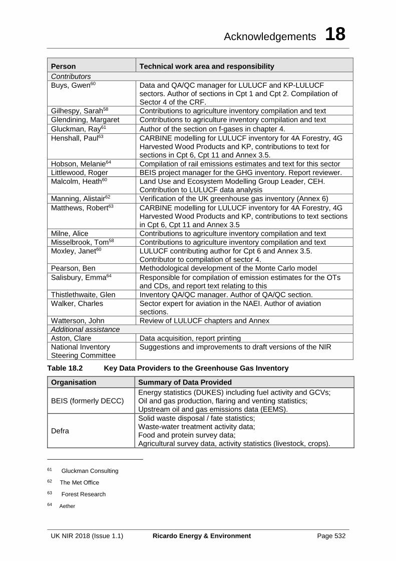
Acknowledgements 18
UK NIR 2018 (Issue 1.1) Ricardo Energy & Environment Page 532
Person Technical work area and responsibility
Contributors
Buys, Gwen60 Data and QA/QC manager for LULUCF and KP-LULUCF sectors. Author of sections in Cpt 1 and Cpt 2. Compilation of Sector 4 of the CRF.
Gilhespy, Sarah58 Contributions to agriculture inventory compilation and text
Glendining, Margaret Contributions to agriculture inventory compilation and text
Gluckman, Ray61 Author of the section on f-gases in chapter 4.
Henshall, Paul63 CARBINE modelling for LULUCF inventory for 4A Forestry, 4G Harvested Wood Products and KP, contributions to text for sections in Cpt 6, Cpt 11 and Annex 3.5.
Hobson, Melanie64 Compilation of rail emissions estimates and text for this sector
Littlewood, Roger BEIS project manager for the GHG inventory. Report reviewer.
Malcolm, Heath60 Land Use and Ecosystem Modelling Group Leader, CEH. Contribution to LULUCF data analysis
Manning, Alistair62 Verification of the UK greenhouse gas inventory (Annex 6)
Matthews, Robert63 CARBINE modelling for LULUCF inventory for 4A Forestry, 4G Harvested Wood Products and KP, contributions to text sections in Cpt 6, Cpt 11 and Annex 3.5
Milne, Alice Contributions to agriculture inventory compilation and text
Misselbrook, Tom58 Contributions to agriculture inventory compilation and text
Moxley, Janet60 LULUCF contributing author for Cpt 6 and Annex 3.5. Contributor to compilation of sector 4.
Pearson, Ben Methodological development of the Monte Carlo model
Salisbury, Emma64 Responsible for compilation of emission estimates for the OTs and CDs, and report text relating to this
Thistlethwaite, Glen Inventory QA/QC manager. Author of QA/QC section.
Walker, Charles Sector expert for aviation in the NAEI. Author of aviation sections.
Watterson, John Review of LULUCF chapters and Annex
Additional assistance
Aston, Clare Data acquisition, report printing
National Inventory Steering Committee
Suggestions and improvements to draft versions of the NIR
Table 18.2 Key Data Providers to the Greenhouse Gas Inventory
Organisation Summary of Data Provided
BEIS (formerly DECC) Energy statistics (DUKES) including fuel activity and GCVs; Oil and gas production, flaring and venting statistics; Upstream oil and gas emissions data (EEMS).
Defra
Solid waste disposal / fate statistics; Waste-water treatment activity data; Food and protein survey data; Agricultural survey data, activity statistics (livestock, crops).
61 Gluckman Consulting
62 The Met Office
63 Forest Research
64 Aether
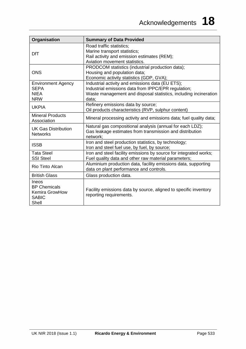
Acknowledgements 18
UK NIR 2018 (Issue 1.1) Ricardo Energy & Environment Page 533
Organisation Summary of Data Provided
DfT
Road traffic statistics; Marine transport statistics; Rail activity and emission estimates (REM); Aviation movement statistics.
ONS PRODCOM statistics (industrial production data); Housing and population data; Economic activity statistics (GDP, GVA);
Environment Agency SEPA NIEA NRW
Industrial activity and emissions data (EU ETS); Industrial emissions data from IPPC/EPR regulation; Waste management and disposal statistics, including incineration data;
UKPIA Refinery emissions data by source; Oil products characteristics (RVP, sulphur content)
Mineral Products Association
Mineral processing activity and emissions data; fuel quality data;
UK Gas Distribution Networks
Natural gas compositional analysis (annual for each LDZ); Gas leakage estimates from transmission and distribution network;
ISSB Iron and steel production statistics, by technology; Iron and steel fuel use, by fuel, by source;
Tata Steel SSI Steel
Iron and steel facility emissions by source for integrated works; Fuel quality data and other raw material parameters;
Rio Tinto Alcan Aluminium production data, facility emissions data, supporting data on plant performance and controls.
British Glass Glass production data.
Ineos BP Chemicals Kemira GrowHow SABIC Shell
Facility emissions data by source, aligned to specific inventory reporting requirements.

Acknowledgements 18
UK NIR 2018 (Issue 1.1) Ricardo Energy & Environment Page 534