Questioni di Economia e Finanza(Occasional Papers)

A risk dashboard for the Italian economy

by Fabrizio Venditti, Francesco Columba and Alberto Maria Sorrentino

Num

ber 425Fe

bru

ary

2018

The series Occasional Papers presents studies and documents on issues pertaining to

the institutional tasks of the Bank of Italy and the Eurosystem. The Occasional Papers appear

alongside the Working Papers series which are specifically aimed at providing original contributions

to economic research.

The Occasional Papers include studies conducted within the Bank of Italy, sometimes

in cooperation with the Eurosystem or other institutions. The views expressed in the studies are those of

the authors and do not involve the responsibility of the institutions to which they belong.

The series is available online at www.bancaditalia.it .

ISSN 1972-6627 (print)ISSN 1972-6643 (online)

Printed by the Printing and Publishing Division of the Bank of Italy

Questioni di Economia e Finanza(Occasional Papers)

Number 425 – February 2018

A risk dashboard for the Italian economy

by Fabrizio Venditti, Francesco Columba and Alberto Maria Sorrentino

A RISK DASHBOARD FOR THE ITALIAN ECONOMY

by Fabrizio Venditti*, Francesco Columba* and Alberto Maria Sorrentino*

Abstract

In this paper we describe an analytical framework to assess financial stability risks in the Italian economy. We use a large number of indicators, selected to take into account the peculiarities of the Italian economy, to monitor risks in seven areas: interlinkages, the credit markets, the macroeconomic environment, funding conditions, the financial markets, and the banking and insurance sectors. Based on thresholds selected on the basis of either expert judgment or historical distributions, we construct risk heatmaps and derive aggregate scores for each of the above risk categories. By providing timely information on the buildup of risks, the proposed dashboard usefully complements other analytical tools currently used for developing and implementing macroprudential policy. JEL Classification: G12, G21, G23, G28. Keywords: early warning indicators, financial stability risks, heatmaps, macroprudential policy.

Contents

1. Introduction ........................................................................................................................... 5

2. Indicators ............................................................................................................................... 6

3. Heatmaps ............................................................................................................................. 13

3.1 Risk monitoring using heatmaps ................................................................................... 13

4. Aggregate indicators ............................................................................................................ 15

5. Conclusions ......................................................................................................................... 16

Tables and Figures ................................................................................................................... 17

Bibliography ............................................................................................................................. 21

Appendix A - Risk assessment tools in other institutions ........................................................ 23

Appendix B – Thresholds designation ..................................................................................... 25

Appendix C - Aggregation of elementary information ............................................................ 29

_______________________________________

* Bank of Italy, Directorate General for Economics, Statistics and Research - Financial Stability Directorate.

1. Introduction *

The Great Financial Crisis of 2007-08 showed the potentially disruptive effects of externalities in the financial system. In some countries, for instance those characterized by excessive leverage and poor liquidity, small shocks in one particular sector can be strongly amplified, leading to fire sales and knock-on effects in other sectors with devastating consequences for economic output and employment.

Following the crisis, a debate on the merits of macroprudential policies in addressing externalities in the financial system, therefore lowering the probability and severity of financial crises, has taken center stage. As the analytical framework in the field of macroprudential policies progressed, a consensus has been reached on what data and indicators, along with expert judgment, should be used to inform the activation of such policies. Ideally, such a surveillance system should (i) monitor both financial and real economic developments, (ii) focus on the most important features of the macro-financial environment to be monitored, and (iii) provide indications on the level and direction of systemic risk, defined as the build-up of financial externalities.1

Following these broad principles, in this paper we document the construction of a risk dashboard to be used for monitoring cyclical and structural vulnerabilities in the Italian economy that may turn into risks for financial stability. The framework is intended both for internal analysis as well as for communication on financial stability issues with other parties, such as public and other institutions. The dashboard is based on many indicators (70). Coupled with warning thresholds, they are organized in a scheme that permits a quick and comprehensive evaluation of different risks, both real and financial in nature. The indicators, chosen among those that were found relevant in the literature,2 cover the main aspects of the Italian economy and are grouped in seven macro-categories: i) interlinkages, ii) credit risk, iii) macroeconomic risk, iv) funding risk, v) market risk, vi) solvency and profitability risk in the banking sector, and vii) solvency and profitability risk in the insurance sector. We chose these categories for two reasons. First, they map most sources of systemic risk, which historically stem from: i) large reciprocal exposure among financial institutions, ii) excessive risk taking by households and firms, iii) adverse macroeconomic conditions that could impact the ability of agents to service their debt, iv) excessive maturity transformation and rollover risk in the banking sector, v) large changes in asset prices, vi) fragilities in the capital structure and in the ability to generate profits in banks and (vii) insurance firms. Second, we tried to make our risk dashboard as comparable as possible in terms of information content with that published by the European Systemic Risk Board (ESRB)3, whose assessment on systemic risk provides an

* We thank Massimiliano Affinito, Alessandro Allegri, Michele Leonardo Bianchi, Martina Bignami, GiuseppeCascarino, Maurizio Cassi, Alessio Ciarlone, Fabio Coluzzi, Antonio Di Cesare, Roberto Felici, Roberta Fiori, Cristina Floccari, Antonella Foglia, Maddalena Galardo, Ivano Galli, Giovanni Guazzarotti, Eleonora Iachini, Gaetano Marseglia, Pamela Minzera, Salvatore Muzzicato, Stefano Neri, Stefano Nobili, Marcello Pericoli, Stefano Piersanti, Cristiana Rampazzi, Silvia Sacco, Silvia Vori, Francesco Zollino and seminar participants at the Bank of Italy Workshop Macroprudential Analyses and Supervision (October 2017). We are solely responsible for any and all errors. The views expressed herein are ours and do not necessarily reflect those of the Bank of Italy. 1 See Adrian et al., 2013. 2 See Mencía and Saurina (2016), Aikman et al. (2015), Drehmann et al. (2014), Krishnamurthy and Vissing-Jorgensen (2014), Schularick and Taylor (2012). 3 The ESRB also uses seven categories: i) Interlinkages and composite measures of systemic risk, ii) macro risk, iii) credit risk, iv) funding and liquidity, v) market risk, vi) profitability and solvency, and vii) structural risk. Appendix Aprovides a more detailed comparison of the framework herein developed and those used by other international institutions.

5

important input both in the regular monitoring of financial stability in the European Union and in the design of EU stress test scenarios.

The main output of the analysis is a set of heatmaps that allows us to keep track of the level and evolution of risks as signaled by individual indicators.4 Heatmaps provide a timely snapshot of the macro-financial conditions of the economy and serve as a useful basis for a discussion on the appropriateness of the macroprudential stance. The information provided by the heatmaps is very granular, so that filtering out the main trends that come from the individual series can be rather challenging. Hence, in a second step, we obtain a more synthetic view on risk developments by pooling individual indicators into aggregate indexes for the main macro-categories. The process of aggregation entails a trade-off between magnifying common tendencies in the data and losing important information on the nature and level of risks. The aggregate indicators are then used to build time heatmaps (the second output of the analysis) where the colors are indicative of the tendency, rather than of the level, of risk.

The note is organized as follows: Sections 2 and 3 provide a description of the data collected in the risk dashboard and of the resulting heatmaps. Section 4 describes the time heatmaps. In Appendix A we compare the risk reporting framework herein developed with those set up by the European Central Bank (ECB), by the European Banking Authority (EBA) and by the European Systemic Risk Board (ESRB). In Appendix B and C we provide the technical aspects of the process of thresholds selection and of the aggregation process described in Section 4.5

The monitoring of risks to financial stability developed in this work, properly informed by the judgment of experts, will contribute to guide the implementation of macroprudential policy by the Bank of Italy.6

2. Indicators

The risk dashboard is structured according to seven macro-categories: 1. Inter-linkages, including market based indicators of interdependencies and data on

exposure concentration; 2. Credit risks, including data on the stock, flow and price of credit to non-financial

corporations (NFCs) and households (HHs), and data on the real estate sector; 3. Macroeconomic risks, including data on economic output, interest rates, inflation, and

debt levels; 4. Funding risks, including data on the sources and costs of bank funding, indicators on

asset encumbrance and on maturity mismatch; 5. Market risks, including volatility indicators for the main markets, price to earnings

ratio for the stock market and indicators of systemic liquidity; 6. Solvency and profitability of the banking sector, including returns and efficiency ratios

as well as capital ratios;

4 Heatmaps are a graphical representation of the data where the individual values contained in an array are associated to colors that allow an immediate assessment of risks. 5 Two separate Annexes contain further details on the single indicators as well as a comprehensive set of graphs. 6 EU legislation assigns to the Bank of Italy the power of implementing macroprudential instruments in the banking sector. The Bank of Italy is responsible for the application of instruments such as countercyclical capital buffers and capital buffers for global and national systemically important credit institutions. It can set higher capital requirements for banks in relation to their exposure towards specific sectors. The Bank of Italy can also use macroprudential instruments not harmonized by EU legislation in order to prevent or mitigate risks to the stability of the financial system.

6

7. Solvency and profitability of the insurance sector, including indicators of profitabilityand capital ratios computed by IVASS.

The selection of indicators within each risk category is largely built on the literature on systemic risk and on the experience of other institutions that play a role in ensuring financial stability. Again, we used the ESRB Risk Dashboard as reference benchmark and, where possible, complemented it with indicators developed and used internally at the Bank of Italy (for instance, we include an indicator of systemic liquidity risk tailored on the Italian economy, see Table 5).

Interlinkages This section of the risk dashboard includes a set of indicators and interlinkage measures across financial markets. This category is composed of six indicators, grouped in two sub-categories (see Table 1): market indicators and non-market indicators.

Table 1: indicators in the interlinkages category

The first sub-category7 includes the Delta-CoVaR (indicator 1) and the Joint Probability of Default (indicator 2). The Delta-CoVaR is an indicator of systemic risk computed according to the methodology proposed by Adrian and Brunnermeier (2016). It measures the average impact of a bank in distress on the market capitalization of the reference system.8 The second indicator for the market sub-category is the Joint Probability of Default (indicator 2) computed according to the methodology proposed by Segoviano and Goodhart (2009). It reports the probability of simultaneous default by two or more large and complex banking groups within a horizon of one year. In the second sub-category (non-market indicators) we keep track of international inter-linkages of Italian banks and of exposure concentration. International linkages are monitored through the ratio of banks’ cross-border claims to total assets (indicator 3) and by the ratio of foreign currency loans of Italian banks on total loans (indicator 4). The remaining two indicators focus on two counterparty sectors that have proven to be important in past financial crises: HH’s mortgage loans as a percentage of total credit (indicator 5, see Cecchetti, 2008), and exposure to the general government as a percentage of total assets (indicator 6).

Credit risk Credit risk can be defined as the risk of losses for the financial sector due to the inability of counterparties to meet their obligations. This section of the dashboard therefore analyzes the ability of the non-financial private sector (NFCs and HHs) to repay its debt and to obtain financing at sustainable costs. It also monitors current conditions in the real estate sector, a sector that

7 Systemic risk indicators based on market data are useful timely warning signals of financial instability, Mencía and Saurina (2016). Although a large number of market based systemic risk indicators have been proposed in the literature (see for instance http://vlab.stern.nyu.edu/en/welcome/risk/) in the risk dashboard we only keep track of market indicators that are estimated internally at the Bank of Italy, also to guarantee continuity and timely updates. 8 The Delta-CoVaR of Italian banks is estimated by using a closed form formula. See Bianchi and Sorrentino (2017).

MacroCategory # Indicator Indicator SubCategory1 Delta-Covar (per cent)2 Joint Probability of Default (per cent)3 Cross-border claims of Italian banks/Total Assets (per cent)4 Foreign Currency Loans/Total Loans (per cent)5 MFI Loans For House Purchase/Total Private Credit (per cent)6 Exposure to Government/Total Assets (per cent)

Interlinkages

Market

Non-Market

7

plays a crucial role in financial stability since investments in real estate are highly illiquid, leveraged and “lumpy”. The credit risk section is composed of 19 times series (see Table 2).

First, we collect information on the cost at which both NFCs and HHs obtain financing as well as information on loan volumes. In particular, we include data on interest rates of loans extended by banks (indicators 7 and 15) and on the growth rates of bank loans (indicators 10 and 17). The low cost of borrowing is a two-edged sword. It facilitates debt sustainability but may also spur excessive borrowing, leaving debtors vulnerable to future increases in borrowing costs and may lead to loan defaults, higher provisioning needs, and losses for their creditors.9 A similar reasoning applies to loan growth: in periods of sustained growth, credit may be extended to “unworthy” borrowers, increasing the risk of future loan provisioning needs and losses for banks. On the other hand, low loan growth rates may signal constraints on economic growth from the financial sector.

Table 2: indicators in the credit risk category

Lending margins (indicators 8 and 16) are the spread between interest rates charged by banks on loans and those paid on deposits. Inter alia, they are a measure of bank profitability. Low margins may lead to excessive borrowing thus impairing the sustainability of a bank’s business model. High margins, on the other hand, may adversely affect access to credit. We also include standard measures of backward looking/historical measures of credit risk, such as bad debts and NPL ratios (indicators 11 and 12 for NFCs and indicators 19 and 20 for HHs)10. Given the importance of debt in amplifying financial shocks, we include two measures of leverage for NFCs (the ratio of financial debt to total assets, indicator 13, and the ratio of financial debt to GDP, indicator 14) while for HHs leverage is measured as the ratio of debt to disposable income (indicator 21). Changes to the credit standards applied to loans to NFCs and to mortgage loans to HHs (indicators 9 and 18), derived from the Bank Lending Survey, subsume the information about the terms of obtaining

9 See Borio and Lowe (2004) and Schularick and Taylor (2012) on excessive credit growth and financial crisis; Mian and Sufi (2009) and Mayer et al (2009) on the risks posed by rapid borrowing by risky borrowers. 10 See Accornero et al. (2017) for an extensive review of the literature on the relation between NPLs, credit flows and banking performance.

MacroCategory # Indicator Indicator SubCategory7 Interest rate on Loans, NFCs (pp)8 MFIs lending margins on loans, NFCs (pp)9 Changes in Credit Standards for Loans, NFCs (balances)

10 Bank Loans, NFCs (y-o-y % change)11 New NPL/Outstanding Loans, NFCs (per cent)12 New Bad Debts/Outstanding Loans, NFCs (per cent)13 Firms Leverage (per cent)14 Firms Financial Debt/Gdp (per cent)15 Interest Rate on Loans for house purchase, HH (pp)16 MFIs lending margins on loans for house purchase, HH (pp)17 Bank Loans, HH (y-o-y % change)18 Changes in Credit Standards for Mortgages, HH (balances)19 New Bad Debts/Outstanding Loans, HH (per cent)20 New NPL/Outstanding Loans, HH (per cent)21 Household Loans/Income ratio, HH (per cent)22 House Prices, % deviation from trend (Index, 2010=100)23 Real Estate Agents' Expectations for House Prices in the current quarte24 Transactions in Residential Property (Index, 2010=100)25 Transactions in Non-Residential Property (Index, 2010=100)

Credit

NFCs

Real Estate

HHs

8

loans from banks. These indicators capture both changes in credit standards endogenously related to economic developments as well as autonomous/exogenous credit supply restraints.

Turning to the real estate market, we look at both prices and volumes. As the risk of a credit bubble is reinforced by increasing residential property prices, we keep track of both prices deviations from their historical tendencies and price expectations (indicators 22 and 23).11 We also monitor residential (indicator 24) and non-residential property (indicator 25) transactions.

Macroeconomic risk This section includes standard macroeconomic variables that could signal the build-up of risks broadly stemming from macroeconomic developments. These can pose financial stability risks to the extent that low growth, high debt levels, and high financing costs contribute to making debtor positions unsustainable.

The first group includes output indicators, i.e. the unemployment rate (indicator 26) the Composite Purchasing Managers Index (indicator 27), a composite index that summarizes the results of a survey of purchasing managers,12 and real GDP growth (indicator 28). Monitoring output is important because major risks to financial stability, such as credit and solvency risk, typically build up in periods of expansions and materialize in recessions, when economic agents experience difficulties in repaying debt and investors demand higher premiums in exchange for capital.

Table 3: indicators in the macroeconomic risk category

Turning to the debt sub-category, we also include the domestic credit-to-GDP gap (indicator 29) which is an early warning signal of credit bubbles.

For this reason, this is the main indicator that is monitored when calibrating the banking sector’s countercyclical capital buffer .13 Given the crucial role of the government sector in ensuring

11 See Cecchetti (2008) and Reinhart and Rogoff (2010) for studies on real estate prices as key sources of financial instability. 12 The resulting PMI figure is calculated by taking the percentage of respondents that reported better conditions than the previous month and adding to that total half of the percentage of respondents that reported no change in conditions. 13 See Alessandri et al. (2015), “A note on the implementation of a Countercyclical Capital Buffer in Italy”, Bank of Italy Occasional Papers, 278.

MacroCategory # Indicator Indicator SubCategory26 Unemployment Rate (per cent)27 Purchasing Manager Index-Composite (balances)28 GDP Growth (y-o-y, per cent)29 Total Credit/Gdp Gap (per cent)30 Public Debt/Gdp ratio (per cent)31 Deficit/Gdp ratio (per cent)32 Aggregate Debt/GDP ratio (per cent)33 Scheduled redemption of gov. debt (ratio to GDP, per cent)34 Current Account/GDP ratio (per cent)35 Spread BTP-BUND (per cent)36 Real Short Term Interest Rate (per cent)37 Real Long Term Interest Rate (per cent)38 Consumer Price Inflation (y-o-y % change)39 Inflation Expectations 6 quarters ahead (y-o-y % change)40 GDP deflator (y-o-y % change)

MACRO

Output

Debt

Rates

Inflation

9

financial stability, the dashboard also includes the debt-to-GDP ratio (indicator 30), the deficit-to-GDP ratio (indicator 31), the aggregate debt-to-GDP ratio (indicator 32) and data on forthcoming sovereign debt redemptions of marketable securities at the one year horizon (indicator 33). The current account balance (indicator 34), which is influenced by developments in competitiveness vis-à-vis other economies and determines the net international position, is also included.

Since nominal and real financing costs determine the sustainability of debt, we collect statistics on interest rates and inflation. In particular, we monitor the spread between Italian and German sovereign bond (indicator 35) as well as the real short- and long-term rates (indicators 36 and 37). Since unexpected changes in the rate of inflation affect the real burden of debt, redistributing it from creditors to debtors, we include in the dashboard consumer price inflation (indicator 38), inflation expectations six quarters ahead (indicator 39) and the GDP deflator (indicator 40).

Funding risk This section of the dashboard comprises a number of indicators to measure funding and liquidity conditions in the financial sector.14 We select data on funding sources, their stability, the availability of collateral and differentials in the rates at which Italian banks fund themselves compared to banks in other partner countries.

Indicators on the sources of funding are the share of funding from central banks, as well as from foreign and long-term investors. The former indicates problems in obtaining founds from traditional sources (indicator 41). The share of foreign debt over total funding (indicator 42) measures the dependence of the banking system on external credit. Finally, the share of funding accounted for by long-term debt instruments (indicator 43) provides information on the ability of banks to tap markets for instruments other than traditional deposits, and on the risk perception of investors on the banking sector.

Table 4: indicators in the funding risk category

Regarding funding via deposits, banks with higher loan-to-deposit ratios or larger funding gaps (between loans on the one hand and deposits plus securities on the other) rely more heavily on the volatile wholesale funding markets (indicators 44 and 46). Those banks are more exposed to liquidity risk, as measured by the net liquidity index (indicator 45) which is based on unencumbered liquid assets and expected cash flows over a one-month horizon. The availability of assets to be used as collateral in repo transactions is measured by the ratio of assets that are available for collateralization to total assets (indicator 47). Finally, the spread between unsecured and secured debt (indicator 48) measures the perceived riskiness of banks. Hence, this indicator increases when markets become skittish about the health of the banking sector.15 Similarly, the

14 See Mencía and Saurina (2016), Hahm et al (2013), Krishnamurthy and Vissing-Jorgensen (2013) and Brunnermeier and Oehmke (2013) for studies on funding and liquidity as a key driver of systemic risk. 15 See Greenwood and Hanson (2013).

MacroCategory # Indicator Indicator SubCategory41 Central Bank Funding/Total Funding (per cent)42 Foreign Debt/Total Funding (per cent)43 Long Term Issuance/Total Funding (per cent)44 Loan/Deposit ratio (per cent)45 Banks Net Liquidity/Total Assets (per cent)46 Funding Gap (per cent)47 Securities To Collateralize Ratio (per cent) Encumbrance48 Secured-Unsecured Interbank Rate Spread (bp)49 Covered Bonds ITA/GER Spread (bp)50 Bank 5YBonds ITA/GER Spread (bp)

FUNDING

Sources

Stability

Spreads

10

spreads between similar bank bonds issued by Italian and German institutions (indicators 49 and 50) measure funding tensions.

Market risk Market risk is the risk of losses arising from movements in financial market prices. The indicators in this category are measures of market volatility, market valuations and market liquidity.16

The first indicator in this section is the CBOE Volatility Index (VIX, indicator 51), also referred to as the “investor fear gauge”, a measure of market expectations of near-term volatility (30-day volatility) based on S&P 500 stock index option prices. This volatility is meant to be forward looking, as it is calculated from both call and put options, and is widely used as measure of market risk. We also include the European counterpart, the VSTOXX (indicator 55). Currency risk in the market for major currencies is measured by exchange rate implied volatilities (indicators 52 to 54). The indicators reflect the volatility of foreign currency interest rates implied by at-the-money options prices observed in the market for EURO/YEN, EURO/USD and YEN/USD exchange rates, based on a three-month maturity. Exchange rate fluctuations typically increase sharply in times of crises.

Table 5: indicators in the market risk category

Market valuations are captured by the price-to-earnings ratio (indicator 56), that is the ratio between a company’s market value and its profitability. Very high values may indicate market overvaluation, raising the probability of a price correction.

In order to capture signs of liquidity stress we rely on the the Bank of Italy’s Systemic Liquidity Index (indicator 57).17 This is a composite index obtained as the aggregation of three indices representative of three market segments in which Italian banks are particularly active: the money market (indicator 58), the Italian government bond market (indicator 59), and the equity and corporate market (indicator 60). These indicators tend to increase in times of financial distress. They reached their maximum levels in the period after the Lehman default (end of 2008) and during the sovereign debt crisis (end of 2011).

Profitability and solvency: banks This section comprises a number of indicators focusing on the profitability and solvency of the banking sector (data are drawn from supervisory reports).

16 See Brunnermeier and Sannikov (2014) for studies on market volatility and financial stability. 17 For a complete discussion of the liquidity indicators, please refer to Iachini, Eleonora, and Stefano Nobili, "An indicator of systemic liquidity risk in the Italian financial markets," Banca d'Italia, Occasional Papers (2014).

MacroCategory # Indicator Indicator SubCategory51 CBOE-VIX (index)52 EURO/YEN 3M VOLATILITY (bp)53 EURO/USD 3M VOLATILITY (bp)54 YEN/USD 3M VOLATILITY (bp)55 VSTOXX VOLATILITY (index)56 Price to Earnings (ratio) Valuation57 Systemic Liquidity (index)58 Money Mkt Liquidity (index)59 Gov. Bonds Liquidity (index)60 Equities/Corporate Liquidity (index)

MARKET

Volatility

Liquidity

11

Table 6: indicators in the profitability and solvency (banks) category

Indicators of profitability are: return on tangible equity (ROTE, indicator 61), the cost-to-income ratio (indicator 62) and loan loss provisions to gross operating profits (indicator 63). ROTE, the most popular indicator of profitability, measures how companies generate income from shareholders’ funds (net of goodwill impairments). The cost-to-income ratio relates company costs to income; this is a measure of efficiency in that the lower the ratio the more efficient a bank is. Finally, loan loss provisions over gross operating profits allow us to assess how operating margins are affected by the yearly flow of provisions. Indicators of bank solvency are the CET1 ratio, measured as the ratio of Core Equity Tier 1 (CET1) to risk weighted assets (indicator 64), and the leverage indicator, the ratio of equity to total assets (indicator 65).18 Profitability and solvency: insurance This section of the dashboard focuses on the financial performance and solvency of the insurance sector. Rather than being based on the underlying indicators, it includes composite indicators (scores) that range from 1 to 10 (indicating increasing risks) and are developed by IVASS.19

Table 7: indicators in the profitability and solvency (insurance) category

The first indicator (indicator 66) is the score based on the combined ratio for non-life insurance activities. Like the cost-to-income ratio for banks, the combined ratio represents the evolution of costs as measured by the sum of operating expenses and insurance-related claims in proportion to net premiums. Next is the score based on the return on equity (indicator 67) for all insurance segments. The solvency score (indicator 68) is based on the ratio of available capital to required solvency capital, the latter being set by the regulators in accordance with the “Solvency II” framework. The last two indicators (indicators 69 and 70) are measured by the change in premiums for the life and non-life segments. Sustained as well as weak changes represent a risk: the former might signal an underpricing of risk, while the latter might lead to profitability problems.

18 See Diamond and Rajan (2001) and Berger and Bouwman (2013) for studies on capital levels, leverage and implications for financial fragility. 19 Notice that in computing these scores, all risks are transformed into right-tailed risks, so that increasing values in the 1-10 scale indicate increasing risks. For instance low ROEs are associated with higher risks and these are measured by higher scores.

MacroCategory # Indicator Indicator SubCategory61 Return on Tangible Equity (per cent)62 Cost/Income ratio (per cent)63 Loan Loss Provisions/Gross Op. Profits (per cent)64 CET1 ratio (per cent) Solvency65 LEVERAGE (per cent)

ProfitabilityPROFITABILITY/SOLVENCY BANKS

MacroCategory # Indicator Indicator SubCategory66 Combined-Non Life (index) Profitability67 ROE (index)68 Solvency (index) Solvency69 Change Premium Life (index)70 Change Premium Non- Life (index)

PROFITABILITY/SOLVENCY INSURANCE

Overall

12

3. Heatmaps

The indicators collected in the dashboard and described in the previous section are organized in risk heatmaps. Heatmaps are visual tools designed to assign a risk level to each indicator. We use a three-color scale (green, yellow and red) to signal whether, according to the information provided by the indicator, a risk is negligible, medium or high. The thresholds that separate the colors can be chosen either on the basis of the historical distribution of the indicators (i.e. based on specific percentiles of the indicator’s distribution) or on the basis of specific values chosen judgmentally. In the first method the current level of the indicator is compared with its own history in order to assign a risk level. This is suitable for time series indicators that are sufficiently long and that have gone through periods of stress so that extreme values (be they low or high) can signal an increasing level of risk. The second method is more appropriate for indicators where thresholds have been determined either by generally accepted practices (e.g. deficit-to-GDP ratios, inflation targets, etc.) or by other statistical criteria. It is clear that, within a system of heatmaps, the choice of the threshold is crucial. Thresholds need to strike a trade-off between being sufficiently conservative (so as to raise warning signs in periods of stress) but at the same time realistically reflecting the features of the economy that is being monitored. To give an example that is tailored to Italy, thresholds for GDP growth need to be relatively ambitious but must also take into account the impact of adverse demographic developments as well as the link between productivity and growth.20 For this reason the process of choosing the thresholds was conducted in consultation with a large pool of sector experts within the Bank of Italy. Experts chose the thresholds by examining historical developments as well as international practices and relied on both statistical criteria and judgment.21

The heatmaps for the different risk categories are presented in Tables 8 to 14. They are structured as follows: in the first two columns we report a sequential number and the name of the series. A first block of colored cells follows, containing data on the latest quarters. A second block of colored cells shows the latest monthly observations. Finally, on the right hand side, we report the thresholds that are used to color the cells. Having the thresholds together with the data is useful for two reasons: first, they allow the reader to understand the nature of the risk of a given indicator,22 and second, comparing them with the actual data gives an idea of the distance of the indicators from the nearest threshold.

3.1 Risk monitoring using heatmaps

In this sub-section we provide a brief example of how heatmaps can be used to obtain a bird’s-eye view on risks and to form a first judgment on rising vulnerabilities.

As of February 2017 (the cutoff for the information contained in Tables 8 to 14), systemic risk, as measured by market indicators, had fallen slightly thanks to the low level of stock market volatility, while risks from cross-border and cross-sectorial exposures remained contained (Table 8).

20 See Appendix B. 21 A similar process is adopted by all international organizations that produce risk heatmaps. 22 Indicators can be broken down into three sub-categories: (1) indicators that signal an increase in risk when they are very high, i.e. when they reach the right tail of their distribution (referred to as right-tail risks) (2) indicators that signal an increase in risk when they are very low, i.e. when they reach the left tail of their distribution (referred to as left-tail risks), (3) indicators that signal an increase in risk when they are either very high or very low, i.e. when they reach either tail of their distribution (referred to as two-tail risks).

13

Turning to Credit Risk, Table 9 shows that in the NFC sector, bank loans recorded a timid recovery, benefitting from low and stable interest rates and favorable supply conditions. At the same time, leverage remained broadly stable while credit quality, measured by the new NPL ratio, kept improving. As mortgage rates remained at historical lows, lending to households increased briskly, but this did not translate into a significant increase in the debt-to-income ratio or into a worsening of credit quality. Finally, the real estate sector showed a slow recovery, but risks to financial stability stemming from this sector remained low overall. Interest rates were very low by historical standards and therefore marked in red; yet, given the weak credit growth, the risk that they fuel a credit bubble is highly unlikely. As for broader macroeconomic risks (Table 10) the heatmaps indicate that improving business cycle conditions did not yet translate into a narrowing of the credit-to-GDP gap, which remained deeply negative. Renewed concerns about the stability of the monetary union, fueled by geopolitical uncertainties, pushed up the Btp-Bund spread, which, however, remained below alert levels. Favored by very low nominal and real rates, public and aggregate debt deleveraging proceeded, albeit slowly. Finally, Italy’s external position benefitted from increasing current account surpluses. Standard indicators of funding conditions (Table 11) signaled some difficulties for Italian banks in obtaining funds. First, banks relied significantly on central bank funding, an indication of persistent market fragmentation. Second, secured/unsecured spreads displayed significant strains at the turn of the year. Third, the share of longer-term funding remained persistently low. Market volatility remained compressed at the beginning of 2017 (Table 12), despite some tensions in the market liquidity of government and corporate bonds at the end of 2016. Profitability in the banking sector remained worryingly low, yet solvency improved mildly (Table 13). Finally, in the insurance sector profitability was stable and capital strength high (Table 14). Summarizing, the main messages emerging from the heatmaps are that at the beginning of 2017 leverage in all economic sectors was either falling or stable, debt sustainability benefitted from substantial monetary accommodation, credit quality improved and balance sheet repair in the banking sector proceeded, albeit slowly. At the same time, funding conditions worsened and Italian financial markets proved susceptible/vulnerable to geopolitical tensions. Risks appear to be at medium levels, but monetary accommodation plays a big role in curbing them, raising an important question regarding what will happen once the course of interest rates is reversed. A comparison of this assessment with the Executive Summary of the Financial Stability Report (FSR) published by Bank of Italy at the end of April (largely based on a similar information set) reveals important differences. The picture painted by the heatmaps, for instance, does not capture some important forward-looking and judgmental elements that form the risk assessment in the Bank of Italy’s FSR, namely the rise of geopolitical tensions at the beginning of 2017, the uncertainty regarding the course of fiscal policy in the US under the Trump administration and the risks of increasing interest rates in most advanced economies. Although such risks could be detected by “ad hoc” indicators (think for instance of measures of political uncertainty based on polls), their relevance for the Italian economy is likely episodic and the inclusion of such indicators in the dashboard unwarranted.

14

This simple example points to a critical trade-off in the setup of a financial stability monitoring tool. On the one hand, following “too many” indicators provides insurance against the risk of missing important information, but it implies a cost in terms of signal extraction from a large information set. In other words, the task of distilling what is relevant from what is not relevant in a very large dashboard could become daunting. On the other hand, relying on a narrow, albeit stable, information set simplifies the assessment at the cost of excluding potentially relevant information. Two messages emerge from this discussion. First, although we have based our risk dashboard on a number of core indicators that we expect to remain relevant for the Italian economy, the list of indicators needs to be regularly reviewed and updated, also to keep track of structural changes in the economy. Second, heatmaps need to be used sensibly, that is, as a (data-based) starting point for an assessment of risks, to be complemented and informed by judgmental elements.

4. Aggregate indicators

The last analytical tool that we develop is a set of aggregate indicators that tries to capture the main trends within each risk category.23

The aggregation of individual indicators requires solving a number of conceptual challenges. We briefly summarize them here and refer the reader to Appendix C for a more detailed explanation. First, since the indicators collected have different frequencies, we aggregate all of them on a monthly basis, interpolating data when needed. Second, we give zero weight to missing values which implies that, at the beginning of the sample, longer time series are relatively over-represented. The third issue pertains to the fact that the risk nature of each indicator is different, i.e. for some indicators risks are in both sides of the distribution (“two-tailed”), while for others risks are either “right-tailed” or “left-tailed” (see Appendix C for further details). Finally, a set of weights must be chosen to aggregate the variables. While we have experimented with a number of options, the results that we obtain do not differ much with respect to the weighting scheme used. Hence we aggregate using equal weights and standardize the series. All these steps imply a “cost” so that the resulting aggregate indicators are more informative on the evolution than on the level of risks. Yet, the analysis in Appendix C shows that these indexes have the desirable property of leading the business cycle by some quarters, in the sense that an unexpected increase in their value portends a fall in industrial production.

The aggregate indicators as of February 2017 are shown in Table 15. In the Table we assign different shades of blue to the values to indicate risks that are diminishing (light blue), stable (standard blue) or rising (dark blue). The colors are assigned through a rule of thumb that proved useful in characterizing the evolution of risks during the Great Recession and the Sovereign Debt Crisis. In particular, we compare the three-month change in each aggregate index with its standard deviation. If the change is larger/lower than the standard deviation by a given factor (20%) we shade it light/dark blue, otherwise we categorize it as standard blue. Consistent with the idea that these indicators measure more the direction than the intensity of risks, we do not report the specific values of the indicators but only the colors.

The heatmap for the aggregate indicators confirms the broad tendency highlighted by the individual heatmaps. In particular, in the latest months credit risk indicators point towards a slight improvement while funding risk suggest a deterioration of risk, consistently with higher reliance

23 At the time this paper was written, data limitations relating to structural breaks in the series did not allow us to compute aggregate indicators for the category “Profitability and solvency: banks”.

15

on Central Bank funding, higher secured-unsecured spreads and lower long-term issuance. For all the other categories risks appear to be stable.

5. Conclusions

In this note we have developed a risk dashboard for the Italian economy composed of 70 indicators grouped into 7 different risk categories. Using thresholds selected on the basis of either expert judgment or historical distributions, we have organized the available information set in risk heatmaps, which provide a useful visual tool for monitoring risks in the main economic sectors as well as in the financial markets. Aggregate indicators are also developed.

Since financial crises erupt from the complex interaction of economic agents, the surveillance tool that we have built is not intended to predict exactly the timing or the severity of financial crises. Rather, it is intended to identify in real time any rising tensions in the financial system and in the main economic sectors, and to offer policy makers comprehensive information that they can use in discussing and developing follow-up policies if needed. Also, this tool cannot replace a subjective assessment of financial stability risks. While such assessment has to start from the data, it needs to go beyond, adding to the static picture painted by the heatmaps a crucial forward-looking component.

16

Table 8: Interlinkages

Table 9: Credit risk

Indicator 2016 2016 2016 2016 2017 2017 2017 2017n° 3 6 9 12 3 1 2 31 Delta-Covar (per cent) -6,20 -5,32 -4,82 -4,26 -6,03 -4,502 Joint Probability of Default (per cent) 1,44 1,39 1,43 1,58 1,40 1,33 1,47 2,01 4,263 Cross-border claims of Italian banks/Total Assets (per cent) 6,80 7,02 6,64 6,88 7,13 6,98 7,28 9,32 10,304 Foreign Currency Loans/Total Loans (per cent) 0,83 0,81 0,84 0,99 1,29 3,195 MFI Loans For House Purchase/Total Private Credit (per cent) 23,41 23,53 23,71 23,85 24,02 23,95 24,10 25,00 45,006 Exposure to Government/Total Assets (per cent) 17,25 17,40 17,17 16,64 16,79 16,74 16,85 10,00 20,00

THRESHOLDS

Indicator 2016 2016 2016 2016 2017 2017 2017 2017n° 3 6 9 12 3 1 2 37 Interest rate on Loans, NFCs (pp) 2,40 2,22 2,02 1,95 1,95 1,95 1,90 1,99 2,79 3,39 4,22 5,138 MFIs lending margins on loans, NFCs (pp) 0,90 0,74 0,55 0,48 0,75 0,76 0,67 0,82 4,00 8,009 Changes in Credit Standards for Loans, NFCs (balances) -18,75 -18,75 -6,25 0,00 0,00 -30,00 -15,00 15,00 30,00

10 Bank Loans, NFCs (y-o-y % change) -0,15 0,12 -0,01 0,36 0,53 0,93 0,12 -2,00 0,00 6,00 12,0011 New NPL/Outstanding Loans, NFCs (per cent) 4,37 4,50 4,07 3,61 3,60 6,2012 New Bad Debts/Outstanding Loans, NFCs (per cent) 4,08 3,64 3,49 3,88 1,70 3,5013 Firms Leverage (per cent) 43,89 44,96 44,94 43,79 44,37 48,0114 Firms Financial Debt/Gdp (per cent) 76,49 76,81 76,58 78,47 82,4215 Interest Rate on Loans for house purchase, HH (pp) 2,31 2,19 2,04 1,99 2,06 2,03 2,10 2,06 2,69 3,35 3,83 4,7816 MFIs lending margins on loans for house purchase, HH (pp) 1,35 1,17 1,03 0,96 1,29 1,28 1,31 1,27 4,00 8,0017 Bank Loans, HH (y-o-y % change) 1,10 1,48 1,67 1,86 -2,00 0,00 6,00 12,0018 Changes in Credit Standards for Mortgages, HH (balances) -12,50 -6,25 -18,75 0,00 0,00 -30,00 -15,00 15,00 30,0019 New Bad Debts/Outstanding Loans, HH (per cent) 1,56 1,55 1,42 1,68 1,00 1,7020 New NPL/Outstanding Loans, HH (per cent) 1,91 1,88 1,66 1,52 2,20 2,7021 Household Loans/Income ratio, HH (per cent) 61,80 61,77 61,69 61,74 75,00 150,0022 House Prices, % deviation from trend (Index, 2010=100) -2,57 -1,60 -0,75 -0,02 -4,19 -0,46 1,64 3,0523 Real Estate Agents' Expectations for House Prices (balances) -32,90 -28,30 -37,50 -28,60 -50,00 -25,00 25,00 50,0024 Transactions in Residential Property (Index, 2010=100) 81,51 86,50 87,41 90,43 68,52 96,35 103,00 125,2925 Transactions in Non-Residential Property (Index, 2010=100) 75,89 80,93 85,63 85,01 70,09 92,97 107,23 143,99

THRESHOLDS

17

Table 10: Macroeconomic risk

Table 11: Funding risk

Indicator 2016 2016 2016 2016 2017 2017 2017 2017n° 3 6 9 12 3 1 2 326 Unemployment Rate (per cent) 11,59 11,59 11,63 11,81 11,67 11,81 11,53 11,67 8,00 11,0027 Purchasing Manager Index-Composite (balances) 53,30 52,17 51,73 52,47 53,80 52,80 54,80 40,00 50,0028 GDP Growth (y-o-y, per cent) 1,06 0,84 1,04 1,03 0,85 0,00 1,0029 Total Credit/Gdp Gap (per cent) -14,33 -13,92 -14,08 -1,54 3,84 7,98 12,1630 Public Debt/Gdp ratio (per cent) 134,82 135,42 132,73 132,62 60,00 100,0031 Deficit/Gdp ratio (per cent) -2,61 -2,43 -2,45 -2,44 -3,00 -1,0032 Aggregate Debt/GDP ratio (per cent) 255,99 256,94 254,12 253,44 200,00 300,0033 Scheduled redemption of gov. debt (ratio to GDP, per cent) 19,53 20,58 20,23 19,62 20,12 20,60 19,82 19,93 20,00 30,0034 Current Account/GDP ratio (per cent) 0,69 2,74 3,78 3,02 -4,00 -1,00 6,00 10,0035 Spread BTP-BUND (per cent) 1,17 1,31 1,29 1,62 1,78 1,64 1,91 2,24 3,3836 Real Short Term Interest Rate (per cent) -0,15 -0,42 -0,86 -1,34 -1,51 -1,51 -1,51 -1,00 -0,47 0,57 1,7737 Real Long Term Interest Rate (per cent) -0,43 -0,59 -0,74 -0,68 -0,76 -0,76 -0,76 -0,35 0,04 1,27 2,0138 Consumer Price Inflation (y-o-y % change) 0,00 -0,30 -0,07 0,17 1,30 1,00 1,60 1,30 0,50 1,50 2,50 3,0039 Inflation Expectations 6 quarters ahead (y-o-y % change) 1,20 1,10 0,80 0,90 1,40 0,50 1,50 2,50 3,0040 GDP deflator (y-o-y % change) 1,18 0,78 0,52 0,72 0,50 1,50 2,50 3,00

THRESHOLDS

Indicator 2016 2016 2016 2016 2017 2017 2017 2017n° 3 6 9 12 3 1 2 341 Central Bank Funding/Total Funding (per cent) 4,81 5,03 5,71 6,09 6,46 6,51 6,41 2,00 6,0042 Foreign Debt/Total Funding (per cent) 10,21 10,19 9,69 9,77 9,57 9,42 9,72 18,26 19,6343 Long Term Issuance/Total Funding (per cent) 0,23 0,29 0,22 0,21 0,40 0,37 0,43 0,07 0,4344 Loan/Deposit ratio (per cent) 108,44 107,09 106,62 104,71 104,40 104,49 104,31 147,77 158,2545 Banks Net Liquidity/Total Assets (per cent) 9,95 10,79 11,80 11,47 10,39 9,94 10,85 3,00 6,0046 Funding Gap (per cent) 9,02 9,37 8,70 5,98 15,66 18,9847 Securities To Collateralize Ratio (per cent) 83,18 80,56 80,72 77,04 67,19 67,19 52,24 79,5748 Secured-Unsecured Interbank Rate Spread (bp) 4,76 5,90 6,55 11,21 8,75 10,96 6,54 5,21 9,8649 Covered Bonds ITA/GER Spread (bp) 62,92 37,26 30,41 48,81 52,10 52,53 51,68 141,17 293,7350 Bank 5YBonds ITA/GER Spread (bp) 23,57 18,27 35,83 34,80 40,50 44,70 36,30 190,25 342,73

THRESHOLDS

18

Table 12: Market risk

Table 13: Profitability and solvency: banks

Table 14: Profitability and solvency: insurance

Indicator 2016 2016 2016 2016 2017 2017 2017 2017n° 3 6 9 12 3 1 2 351 CBOE-VIX (index) 20,69 15,61 13,25 14,04 11,71 11,70 11,53 11,90 20,39 26,4452 EURO/YEN 3M VOLATILITY (bp) 10,83 12,16 12,41 11,47 12,16 11,10 13,22 12,18 12,28 15,0353 EURO/USD 3M VOLATILITY (bp) 10,35 9,88 8,44 9,37 9,67 9,61 10,14 9,26 10,65 12,7254 YEN/USD 3M VOLATILITY (bp) 10,69 11,43 12,55 11,76 11,50 12,60 11,80 10,11 11,26 13,7455 VSTOXX VOLATILITY (index) 28,51 25,74 20,76 19,37 15,50 15,98 15,54 14,99 24,72 31,5756 Price to Earnings (ratio) 12,31 12,22 11,40 11,22 11,98 12,35 11,62 11,98 4,80 9,74 19,62 24,5557 Systemic Liquidity (index) 0,08 0,05 0,07 0,10 0,10 0,10 0,09 0,18 0,5258 Money Mkt Liquidity (index) 0,35 0,30 0,37 0,14 0,18 0,23 0,14 0,67 0,7859 Gov. Bonds Liquidity (index) 0,54 0,47 0,49 0,57 0,57 0,59 0,56 0,55 0,7460 Equities/Corporate Liquidity (index) 0,66 0,60 0,57 0,63 0,64 0,65 0,64 0,58 0,79

THRESHOLDS

Indicator 2016 2016 2016 2016 2017 2017 2017 2017n° 3 6 9 12 3 1 2 361 Return on Tangible Equity (per cent) 3,53 3,72 2,20 4,00 7,0062 Cost/Income ratio (per cent) 69,19 67,21 67,10 60,00 80,0063 Loan Loss Provisions/Gross Op. Profits (per cent) 66,82 71,53 79,00 50,00 100,0064 CET1 ratio (per cent) 11,50 11,60 11,90 7,00 10,5065 LEVERAGE (per cent) 5,60 5,70 5,80 4,00 5,00

THRESHOLDS

Indicator 2016 2016 2016 2016 2017 2017 2017 2017n° 3 6 9 12 3 1 2 366 Combined-Non Life (index) 1,00 1,00 1,00 4,00 8,0067 ROE (index) 3,50 3,50 3,50 4,00 8,0068 Solvency (index) 3,00 3,00 3,50 4,00 8,0069 Change Premium Life (index) 2,00 6,00 5,00 4,00 8,0070 Change Premium Non- Life (index) 3,00 3,00 2,00 4,00 8,00

THRESHOLDS

19

Table 15: Aggregate risk indicators

2016 2016 2016 2016 2016 2016 2016 2016 2016 2017 2017 20174 5 6 7 8 9 10 11 12 1 2 3

InterlinkagesCredit RiskMacroeconomic RiskFunding RiskMarket RiskProfitability and Solvency of Insurances

20

Bibliography

Accornero, M., P. Alessandi, L. Carpinelli and A.M. Sorrentino (2017). Non-performing loans and the supply of bank credit: evidence from Italy, Bank of Italy, Occasional Paper No. 374.

Adrian, T. and M.K. Brunnermeier (2016). CoVaR, American Economic Review, 106 (7), 1705-1741.

Adrian, T., D. Covitz and N. Liang (2013). Financial stability monitoring, Finance and Economics Discussion Series 2013-21, Board of Governors of the Federal Reserve System (U.S.).

Adrian, T., D. Covitz and N. Liang (2014). Financial Stability Monitoring, Staff Report no. 601, June 2014 .

Aikman, D., M.T. Kiley, S.J. Lee, M.G. Palumbo, and M.N. Warusawitharana (2015). Mapping Heat in the U.S. Financial System, Finance and Economics Discussion Series 2015-059.

Alessandri, P, Bologna, P.L., Fiori, R. and E. Sette (2015). A note on the implementation of the countercyclical capital buffer in Italy, Bank of Italy, Occasional Papers No. 278.

Berger, A.N. and C.H.S. Bouwman (2013). How does capital affect bank performance during financial crises?, Journal of Financial Economics, vol. 109.

Bianchi, M.L. and A.M. Sorrentino (2017). Measuring the CoVaR: an empirical analysis, Working Paper.

Borio, C. and P. Lowe (2004). Securing sustainable price stability. Should credit come back from the wilderness?, BIS Working Papers No 157.

Brunnermeier, M. and M. Oehmke (2013). The maturity rat race, Journal of Finance, vol. 68(2), 483-521.

Brunnermeier, M. and Y. Sannikov (2014). A macroeconomic model with a financial sector, American Economic Review, 104(2), 379-421.

Cecchetti, S. G. (2008). Measuring the macroeconomic risks posed by asset price booms, in: Asset Prices and Monetary Policy, 9-43. National Bureau of Economic Research, Inc.

Ciocchetta, F., W. Cornacchia, R. Felici, M. Loberto, (2016). Assessing Financial Stability Risks from the Real Estate Market in Italy, Bank of Italy, Occasional Paper No. 323.

Diamond, D.W. and R.G. Rajan (2001). Liquidity risk, liquidity creation, and financial fragility: a theory of banking, Journal of Political Economy, vol 109(2), 287-327, April.

Drehmann, M. and T. Kostas (2014). The credit-to-GDP gap and countercyclical capital buffers: questions and answers, BIS Quarterly Review, March.

Greenwood, R. and S.G. Hanson (2013). Issuer quality and corporate bond returns, Review of Financial Studies 26, no. 6: 1483–1525.

Hahm, J.H., H.S. Shin, and K. Shin (2013). Noncore bank liabilities and financial vulnerability, Journal of Money, Credit and Banking, 45(s1), 3-36, August.

Krishnamurthy, A. and A. Vissing-Jorgensen (2013). Short-term debt and financial crises: what we can learn from U.S. Treasury supply, Working Paper.

Lo Duca, M. and T. Peltonen (2011). Macrofinancial vulnerabilities and future financial stress: assessing systemic risks and predicting systemic events, BIS Papers chapters, in: Bank for International Settlements (ed.), Macroprudential regulation and policy, volume 60, 82-88.

21

Mayer, C., K. Pence, and S.M. Sherlund (2009). The rise in mortgage defaults, Journal of Economic Perspectives, 23(1), 23-50.

Mencia, J. and S.J. Saurina (2016). Macroprudential Policy: Objectives, Instruments and Indicators. Banco de Espana Occasional Paper No. 1601.

Mian and Sufi (2009). The consequence of mortgage credit expansion: Evidence from the US mortgage default crisis, Quarterly Journal of Economics, vol 124(4), 1449-1496.

Reinhart, C.M. and K.S. Rogoff (2010). This Time is Different: Eight Centuries of Financial Folly, Princeton University Press, Princeton, N.J.

Schularick, M. and A.M. Taylor (2012). Credit booms gone bust: monetary policy, leverage cycles, and financial crises, 1870-2008, American Economic Review, American Economic Association, vol. 102(2), 1029-61, April.

Segoviano, M.A. and C. Goodhart (2009). Banking Stability Measures, IMF Working Paper, 09/4.

22

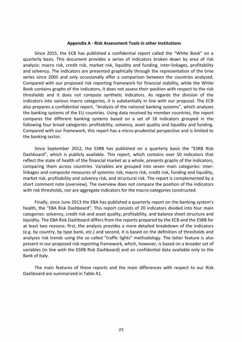
Appendix A - Risk Assessment Tools in other Institutions

Since 2015, the ECB has published a confidential report called the “White Book” on a quarterly basis. This document provides a series of indicators broken down by area of risk analysis: macro risk, credit risk, market risk, liquidity and funding, inter-linkages, profitability and solvency. The indicators are presented graphically through the representation of the time series since 2005 and only occasionally offer a comparison between the countries analyzed. Compared with our proposed risk reporting framework for financial stability, while the White Book contains graphs of the indicators, it does not assess their position with respect to the risk thresholds and it does not compute synthetic indicators. As regards the division of the indicators into various macro categories, it is substantially in line with our proposal. The ECB also prepares a confidential report, “Analysis of the national banking systems”, which analyzes the banking systems of the EU countries. Using data received by member countries, the report compares the different banking systems based on a set of 18 indicators grouped in the following four broad categories: profitability, solvency, asset quality and liquidity and funding. Compared with our framework, this report has a micro-prudential perspective and is limited to the banking sector.

Since September 2012, the ESRB has published on a quarterly basis the “ESRB Risk Dashboard”, which is publicly available. This report, which contains over 50 indicators that reflect the state of health of the financial market as a whole, presents graphs of the indicators, comparing them across countries. Variables are grouped into seven main categories: inter-linkages and composite measures of systemic risk, macro risk, credit risk, funding and liquidity, market risk, profitability and solvency risk, and structural risk. The report is complemented by a short comment note (overview). The overview does not compare the position of the indicators with risk thresholds, nor are aggregate indicators for the macro-categories constructed.

Finally, since June 2013 the EBA has published a quarterly report on the banking system's health, the “EBA Risk Dashboard”. This report consists of 20 indicators divided into four main categories: solvency, credit risk and asset quality, profitability, and balance sheet structure and liquidity. The EBA Risk Dashboard differs from the reports prepared by the ECB and the ESRB for at least two reasons: first, the analysis provides a more detailed breakdown of the indicators (e.g. by country, by type bank, etc.) and second, it is based on the definition of thresholds and analyzes risk trends using the so called "traffic lights" methodology. The latter feature is also present in our proposed risk reporting framework, which, however, is based on a broader set of variables (in line with the ESRB Risk Dashboard) and on confidential data available only to the Bank of Italy.

The main features of these reports and the main differences with respect to our Risk Dashboard are summarized in Table A1.

23

Table A1: Summary of other European Institutions’ Risk Assessment Tools

Institution ECB ECB ESRB EBA

Report White BookAnalysis of the national

banking systems Risk Dashboard Risk Dashboard

Frequency Quarterly Biannual Quarterly Quarterly

Risks anayzed

MacroCreditMarketLiquidit and FundingInterlinkagesProfitability Solvency

ProfitabilitySolvencyAsset Quality Liquidity and Funding

Inter-linkages and Systemic riskMacroCreditFunding and LiquidityMarketProfitability and SolvencyStructural

SolvencyCredit risk e asset qualityBalance sheet structureLiquidity

Differences with the Bank of Italy Risk Dashboard

No thresholds are usedAnalyzes only the Banking system

No thresholds are usedAnalyzes only the Banking system

24

Appendix B – Thresholds designation

A possible critique to the practice of setting the thresholds based on judgement or via very simple statistics (like percentiles) is that these thresholds could be more accurately estimated via appropriate econometric methods. Such a model, for instance, could be a threshold model where the dependent variable captures crisis periods (say GDP growth) and the right-hand side variable is the indicator whose thresholds we want to set (say credit growth). In this appendix we discuss some problems encountered when trying to estimate threshold models with the limited data sample typically available with Italian data. The issues are not only about estimated parameter accuracy, but also about the detection of the number of regimes. To put it more clearly with an example, even if we know that credit growth poses financial stability risks in both tails of the distribution (i.e. a credit crunch or a credit boom may be equally damaging to the economy), with a small sample and limited crisis periods an econometric model may not only incorrectly estimate the thresholds that determine a crunch or a bubble, but also fail to detect whether a crunch or a bubble are actually damaging.

To substantiate this point consider the following threshold model: = − ∗ ( > ) + ∗ ( < ) + ∗ ( ≤ ≤ ) +

where and are positive coefficients. This model depicts a nonlinear relationship between two variables, and . In particular, the impact of on is strongly negative in two regimes (i.e. when is either very high or very low) and mildly positive in the intermediate regime when falls between the two extreme values and . The model captures the idea that there is a discontinuity in the relationship between economic output and credit growth in periods of a credit crunch or a credit bubble. We simulate the model letting follow an AR(1) plus noise model, with an AR parameter at 0.9 and a unit standard deviation of the shocks. We then set = −2 ( ) and = 2 ( ), that is = −4.5and = 4.5, b=2 and c=0.5 and simulate the model over T=1000 time periods. We obtain the time series shown in Figure B1.

We now try to estimate the threshold model above using the simulated data. The estimation of the threshold model turns out to be quite challenging. The method requires performing a battery of break tests on various sub-samples, trying to infer the date and threshold at which these breaks occur. For instance, estimation performed on the model that generated the data in Figure B1 gives the results displayed in Table B1. Even with 1000 data points and despite correctly specifying the model, the estimated thresholds are -3.1 and 2.20, very far from the actual ones (-4.5 and 4.5). Turning to the coefficients we find that c is estimated very precisely, but the coefficient b that should be the same in the other regimes is estimated at around 1.3 in the low regime and at -0.26 in the high regime. Let us remark that 1000 data points is an unrealistic situation. In a more realistic setting we would be estimating over a more limited span of data, say the first 240 observations. This corresponds to 20 years of monthly data, the typical data sample available with Italian data. In this case the results in Table B2 show that the estimation picks only two (instead of

25

three regimes), i.e. if we were to base our analysis on this model we would conclude that credit bubbles never generate a recession and we would classify the variable of interest as posing left-tail instead of two-tail risks.

A second difficulty in using econometric methods to set up risk thresholds arises because, in a small sample, the crisis episodes that are observed are not necessarily related to all the variables that a risk dashboard ought to include. A case in point for Italy is that of house prices. While we know from historical records on financial crises that these are often preceded by a housing boom, Italy did not experience a housing boom before 2008 and the double dip recession that hit the economy between 2009 and 2014 originated from foreign shocks. If we were to fit an empirical model like the threshold model described above using housing prices, we would hardly find any relationship between the business cycle and house prices. Since this would not automatically imply that house price dynamics do not pose risks to financial stability, the choice of risk thresholds is bound to fall on (more) informal methods.

Of course, as more data become available, combining econometric methods with outside judgement may prove beneficial. Yet with a limited information set the use of judgement becomes indispensable both in classifying the nature of the risks as well as in setting thresholds for the indicators.

26

Figure B1: threshold model simulations, T=1000, = − . and = .

Table B1, Regression results, threshold models, T=1000, = − . and = .

Dependent Variable: Y Method: Threshold Regression Included observations: 1000 after adjustments Threshold type: Bai-Perron tests of L+1 vs. L sequentially determined thresholds Threshold variable: X Threshold selection: Trimming 0.15, Max. thresholds 5, Sig. level 0.05 Threshold values used: -3.062807, 1.519618

Variable Coefficient Std. Error t-Statistic Prob.

X < -3.062807 -- 150 obs

X 1.330883 0.033311 39.95269 0.0000

-3.062807 <= X < 1.519618 -- 700 obs

X 0.500000 0.050804 9.841715 0.0000

1.519618 <= X -- 150 obs

X -0.265656 0.051743 -5.134135 0.0000

R-squared 0.592312 Mean dependent var -0.992286 Adjusted R-squared 0.591494 S.D. dependent var 2.982638 S.E. of regression 1.906337 Akaike info criterion 4.131240 Sum squared resid 3623.220 Schwarz criterion 4.145963 Log likelihood -2062.620 Hannan-Quinn criter. 4.136836 Durbin-Watson stat 0.984827

0 100 200 300 400 500 600 700 800 900 1000-10

-5

0

5

10xt

0 100 200 300 400 500 600 700 800 900 1000-20

-10

0

10yt

27

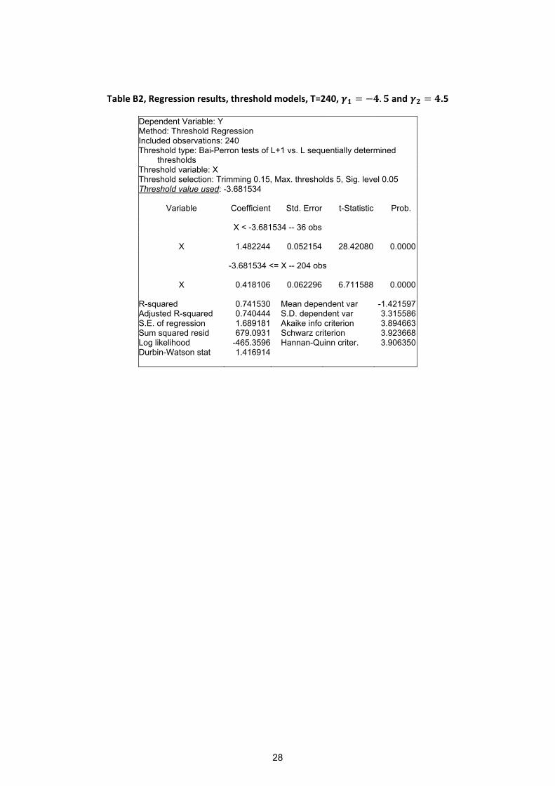
Table B2, Regression results, threshold models, T=240, = − . and = .5

Dependent Variable: Y Method: Threshold Regression Included observations: 240 Threshold type: Bai-Perron tests of L+1 vs. L sequentially determined thresholds Threshold variable: X Threshold selection: Trimming 0.15, Max. thresholds 5, Sig. level 0.05 Threshold value used: -3.681534

Variable Coefficient Std. Error t-Statistic Prob.

X < -3.681534 -- 36 obs

X 1.482244 0.052154 28.42080 0.0000

-3.681534 <= X -- 204 obs

X 0.418106 0.062296 6.711588 0.0000

R-squared 0.741530 Mean dependent var -1.421597 Adjusted R-squared 0.740444 S.D. dependent var 3.315586 S.E. of regression 1.689181 Akaike info criterion 3.894663 Sum squared resid 679.0931 Schwarz criterion 3.923668 Log likelihood -465.3596 Hannan-Quinn criter. 3.906350 Durbin-Watson stat 1.416914

28

Appendix C - Aggregation of Elementary Information

The computation of aggregate indexes on the basis of the elementary time series collected in the risk dashboard poses four conceptual and analytical challenges.

First, the indicators collected have different frequencies and different publication lags. Market variables (spreads or indicators derived from market data like the Co-VaR) are sampled daily and are available in real time. Monthly variables are characterized by different levels of timeliness, ranging from data with a very short delay such as survey data to the substantial publication lag (up to two months) that characterizes output and inflation data. Finally, quarterly national account variables are typically available only 60 to 90 days after the reference quarter. The issue of aggregating variables with mixed frequencies and different publication lags (i.e. with ragged edges) can be solved by using a range of econometric techniques with different levels of sophistication. In our analysis we have chosen to work with a common monthly frequency for all the indicators. This requires taking monthly averages of daily/weekly indicators and interpolating them through a low-pass filter at lower frequency (quarterly) variables. Furthermore, we have chosen to “balance” the data panel by employing random walk forecasts of the individual indicators. This technique ensures that the very last observation of the composite indicator provides a snapshot of the data that were actually available when the aggregate index was compiled.

The second issue regards time series length. Some indicators are indeed available for a longer time span, while others are considerably shorter. When aggregating the variables we have decided to give zero weight to the missing series. This means that at the beginning of the sample, longer time series are relatively over-represented.

The third issue pertains the fact that the risk nature of the indicators that we have selected differs according to the indicators, i.e. for some indicators risks are in both sides of the distribution (“two-tailed”), while for others risks are either “right-tailed” or “left-tailed”. This implies that prior to aggregating them, the indicators need to be transformed. This has important implications for the information that aggregate indicators provide, as the nature of the risk is lost after this transformation is performed. To illustrate this point, in Figure C1 we plot two (fictitious) time series, representing changes in credit standards (top panel), credit growth (middle panel) and their aggregation (bottom panel). The financial stability risks implied by the two variables come from both tails of the distribution. In this particular example, for instance, there are two phases in which credit standards are tightened significantly and credit growth slumps (a credit bust) and one phase when credit growth is buoyant and credit standard are very lax (credit boom). In all these phases the indicators are marked as red, since they are beyond the thresholds that indicate excessive risks. Notice that if we were to aggregate them with equal weights, the resulting aggregate indicator would be flat and marked as green, i.e. we would lose all the information on risks that they contain. This is because we are mixing risks on the left tail of the distribution of the first indicator with risks on the right tail of the distribution of the second indicator. A possible solution to this problem is to transform the indicators so as to make them “right-tailed”, i.e. to flip them around their central value, as shown in the top and central panels of Figure C2. Now, notice that the aggregate indicator (bottom panel of Figure C2) correctly identifies periods of risks, but that the “nature” of the risks is lost, i.e. upon seeing an aggregate indicator that is red we do not know whether we are in a period of credit bust or

29

credit boom. This is the price to pay when constructing composite risk indicators that pool information from variables with heterogeneous risk natures.24 A further implication of this transformation is that there is no automatic link between the aggregate indicators and macroprudential instruments. Consider, for instance, setting a countercyclical capital buffer to smooth the financial cycle. Looking at the individual variables (credit standards and credit growth) would have suggested releasing the buffer in periods of credit bust and raising them in periods of boom. The aggregate indicator, however, does not provide such clear-cut guidance: this means that while the aggregate indicators can provide useful synthetic information, their interpretation needs to be backed by a careful reading of the individual variables.

Fourth, and finally, a set of weights must be chosen to aggregate the variables. In determining a system of weights to assign to the indicators, it must first be decided whether it should depend on the optimization of a given objective function. One aspect that is often seen in the variable screening procedures and the assessment of their relative importance is the ability to anticipate a financial crisis. In this case the variable weights are obtained through a regression model where the dependent variable is a binary indicator that identifies periods of crisis (Lo Duca and Peltonen, 2011) or a variable correlated with periods of financial stress (such as the flow of new bad debts in relation to bank capital, Ciocchetta et al., 2016). This approach has the advantage of transparently specifying a “target” variable with respect to which information is selected and weighted, but it has two problems. The first is that financial crises are rare. It is therefore possible that, in the method that uses a binary dependent variable, the increasing vulnerability reported by certain indicators is ignored since the correlation between those indicators and the indicators of a crisis is very low. Another risk is that the dependent variables are backward-looking in measuring the materialization of a risk, rather than being predictive of the occurrence of a systemic event.

An alternative is to use aggregation methods that do not depend on a clear objective function. In this case, the weights may be obtained by the general formula: = ,

where the variable is a composite index obtained on the basis of M elementary indicators , . Using different specifications of and the parameter r, different aggregation schemes are obtained (simple averages, geometric averages, etc.). The advantages of using aggregation systems such as those just described are the simplicity and the independence from a discretionary target variable. However, a problem can arise when the construction of the data set is biased toward a certain sector or type of indicators, given that this feature will be reflected in the composite indicator. This problem can be solved either by excluding from the aggregation those indicators that are highly correlated with one another in the information set, or by using statistical criteria that assign lower weights to variables that are highly correlated with the others. Another issue is the level at which to stop the process of aggregation. The

24 Mencia and Saurina (2016), adopt a similar solution as the one used. Aikman et al. (2015), on the other hand, intentionally select only “right-tailed” risk indicators.

30

choice may fall on an intermediate stage (for example, at the individual risk level) or continue up to a single systemic risk indicator.25

Since our dataset is relatively balanced in terms of the number and type of indicators collected, we have chosen to use an aggregation scheme that is disconnected from a target variable (i.e. weighted averages) and to aggregate the information for each individual risk category, ending up with five aggregate risk indicators.26

In more detail, starting with the individual time series collected in the dashboard,27 the aggregation was performed in three steps:

1. The “two-tailed” and “left-tailed” indicators are transformed into “right-tailed”indicators;

2. The series are standardized (the averages are subtracted, and they are divided by thestandard deviation);

3. The series are aggregated at the category level based on the following weightingschemes:

simple average; weighted average, assigning to the variables a weight inversely proportional to the

correlation with other indicators in the same risk category; weighted average, assigning to the variables a weight inversely proportional to the

forecasting ability of a measure of economic activity.

In Figures C3 to C7 we report the results of this aggregation. In particular, in the top panels we show the composite indicators obtained with these three methods, and indicate with the grey shaded areas the two recessions identified by the Center for Economic Policy Research (CEPR) for the euro area, namely the Great Recession and the Sovereign Debt Crisis. The middle panels show the impulse response functions of the index of industrial production following a

25 The Federal Reserve Board’s risk monitoring system , for example, starts from 44 elementary indicators (Aikman et al., 2015). These are grouped into 14 categories which are included in 3 macro-groups. Starting from elementary information, pooling is obtained through a simple average. 26 Due to data limitations, for the group of indicators in the solvency-profitability groups we have not been able to construct a composite indicator as described in this section. However, since IVASS does compute such a composite indicator for the insurance sector, we rely on their indicator for the risk heatmaps. 27 Since some indicators convey similar information (think for instance of the NPL and bad debt ratios in the Credit Risk category), the aggregation analysis is performed on a subset of indicators for each category. In particular, (i) for Interlinkages we aggregate the Delta-Covar, the Joint Probability of Default, Cross Border Claims, and Government Loans, (ii) for Credit Risk we aggregate Interest rate on Loans, NFCs, Changes in Credit Standards for Loans, NFCs, Bank Loans, NFCs, Firms Leverage, New NPL/Outstanding Loans, NFCs, Interest Rate on Loans for house purchase, HH, Bank Loans, HH, Changes in Credit Standards for Mortgages, HH, New NPL/Outstanding Loans, HH, House Prices, % deviation from trend (Index, 2010=100), Transactions in Residential Property, (iii) for Macroeconomic Risk we aggregate the Unemployment Rate, GDP Growth, Total Credit/GDP Gap, Public Debt/GDP ratio, Deficit/GDP ratio, Scheduled redemption of government debt (ratio to GDP), Current Account/GDP ratio, Spread BTP-BUND, Real Long Term Interest Rate, Consumer Price Inflation, Inflation Expectations 6 quarters ahead, (iv) for Funding Risk we aggregate Central Bank Funding/Total Funding, Foreign Debt/Total Funding, Long Term Issuance/Total Funding, Loan/Deposit ratio, Banks Net Liquidity Securities To Collateralize Ratio, Secured-Unsecured Interbank Rate Spread, Covered Bonds ITA/GER Spread, Bank 5YBonds ITA/GER Spread, (v) for Market Risk we aggregate CBOE-VIX, EURO/USD 3M VOLATILITY, VSTOXX VOLATILITY, Price to Earnings, and Systemic Liquidity.

31

shock to the aggregate risk indicator in a simple bivariate Vector Auto Regression (VAR).28 The bottom panel shows the fraction of forecast error variance decomposition of industrial production attributable to the risk shock. Three results emerge from this analysis. First, all the aggregate indicators, regardless of the averaging method used, increase sharply in periods of recession. Second, no material differences emerge from the different aggregation methods, suggesting that the simplest method (simple average) is a good solution to the aggregation problem. Third, composite indicators of credit, macro, funding and market risk somewhat anticipate business cycle developments, as shown from the hump-shaped response of the industrial production index to an unexpected shock to one of these indicators. The aggregate interlinkages index, on the other hand, is poorly correlated with future economic activity. Also, this dynamic conditional correlation is relatively stronger for some composite indicators (macro and credit risk) than for others. All in all, this analysis shows that aggregate indicators constructed by (i) symmetrizing (ii) standardizing (iii) and averaging with equal weights the single indicators do contain valuable information about business cycle dynamics.

28 Structural identification is achieved through a Choleski decomposition, where the aggregate risk indicator is ordered first and the log of the industrial production index second. Results do not change materially when the order of the variables is reversed.

32

Figure C1: indicators of credit booms and busts and composite indicator

Figure C2: “symmetrized” indicators of credit booms and busts and composite indicator

33

Figure C3

Figure C4

34

Figure C5

Figure C6

35

Figure C7

36