UCGE Reports - University of Calgary | Home · In a pseudonoise (PN) spread-spectrum system, the...
131
UCGE Reports Number 20257 Department of Geomatics Engineering Interference Effects on GPS L2C Signal Acquisition and Tracking (URL: http://www.geomatics.ucalgary.ca/research/publications/GradTheses.html ) by Donghua Yao August 2007
Transcript of UCGE Reports - University of Calgary | Home · In a pseudonoise (PN) spread-spectrum system, the...

UCGE Reports
Number 20257
Department of Geomatics Engineering
Interference Effects on GPS L2C Signal
Acquisition and Tracking (URL: http://www.geomatics.ucalgary.ca/research/publications/GradTheses.html)
by
Donghua Yao
August 2007
THE UNIVERSITY OF CALGARY
Interference Effects on GPS L2C Signal Acquisition and Tracking
by
Donghua Yao
A THESIS
SUBMITTED TO THE FACULTY OF GRADUATE STUDIES
IN PARTIAL FULFILLMENT OF THE REQUIREMENTS FOR THE
DEGREE OF MASTER OF SCIENCE
DEPARTMENT OF GEOMATICS ENGINEERING
CALGARY, ALBERTA
August, 2007
© Donghua Yao 2007

iii
Abstract
GPS L2C signals are now being transmitted from the new-generation IIR-M
satellites. L2C signals are easily affected by RF and are often distorted by RF
interference. Therefore, the performance of L2C signal acquisition and tracking is
influenced by RF interference. The interferences of additive white Gaussian noise
and unwanted L2C signals are always accompanied with incoming desired L2C
signals. In this thesis, the effects of cross-correlation and additive white Gaussian
noise (AWGN) on the performances of the L2C signal acquisition and tracking are
analyzed in four parts: L2C signal detection, maximum error probability of
information data estimation, signal-to-noise ratio, and PLL tracking errors.
In L2C signal detection, a large cross-correlation value is used to estimate the
detection probabilities. Cross-correlation will affect L2C signal detection
performance. The cross-correlations increase the error probability of information
data estimation. The average signal-to-noise ratio is derived under the effects of
cross-correlation and AWGN. The SNR is reduced when there is more
cross-correlation or when the unwanted signal power from another satellite is
higher than the desired signal power. In the PLL error analysis, the PLL error is
estimated by using the linear method under the cross-correlation and AWGN.
Simulations are also done for the analyses of the cross-correlation and AWGN

iv
effects on L2C signal acquisition and tracking.

v
Acknowledgements
My foremost thanks go to my supervisors, Professor Gérard Lachapelle and
Professor Susan Skone. Their patient guidance and constant encouragement
have been invaluable and made this thesis a reality.
I am grateful to my wife and my daughter for their unconditional love, endless
support, and constant encouragement in my career. I thank also my parents and
other family members for their love and encouragement during my study.
I would like to express my thanks to research associates and graduate students,
particularly Mr. Rob Watson, for their efforts and patience during my many inquiries;
their technical feedback greatly helped to improve this thesis. I thank Wei Yu for his
help in a numerical experiment. Many thanks go to Bo Zheng, Gang Mao, Ning Luo,
Zhi Jiang, Wouter van der Wal, Changlin Ma, Jianning Qiu, Surendran
Shanmugam, Moncton Gao and Tao Hu for helpful discussions and advices. I also
thank other PLAN group members, Mark Petovello, John Schleppe, as well as
many others for their valuable assistances during the period of my study.
vi
Table of Contents
Abstract ................................................................................................................iii
Acknowledgements .............................................................................................. v
Table of Contents..................................................................................................vi
List of Tables.........................................................................................................ix
List of Figures ....................................................................................................... x
Notation .............................................................................................................. xiii
Chapter 1.............................................................................................................. 1
Introduction........................................................................................................... 1
1.1 Background ............................................................................................ 1
1.2 Radio Frequency Interference ................................................................ 3
1.2.1 Cross-Correlation Interference........................................................... 3
1.2.2 Pulsed Interference............................................................................ 4
1.2.3 Continuous Wave Interference........................................................... 5
1.2.4 AM Interference ................................................................................. 5
1.2.5 FM Interference ................................................................................. 6
1.3 Motivation and Objective ........................................................................ 7
1.4 Thesis Outline....................................................................................... 10
Chapter 2............................................................................................................ 12

vii
Cross-Correlation and White Gaussian Noise Effects on Acquisition ................. 12
2.1 L2C Code Structure .............................................................................. 12
2.2 L2C Signal Acquisition .......................................................................... 18
2.2.1 L2C Signal ....................................................................................... 19
2.2.2 Model of the Correlator Output for CM Code Acquisition ................. 20
2.2.3 Largest Cross-Correlation................................................................ 31
2.2.4 Simulation Approach for the Largest Cross-Correlation................... 41
2.2.5 Signal Detection............................................................................... 44
2.3 Conclusions .......................................................................................... 54
Chapter 3............................................................................................................ 56
Cross-Correlation and White Gaussian Noise Effects on Signal-To-Noise Ratio 56
3.1 Worst Case Performance ..................................................................... 56
3.2 Numerical Simulation for Worst Case Performance.............................. 59
3.2.1 Simulation Scheme.......................................................................... 59
3.2.2 Result Analysis ................................................................................ 60
3.3 Theoretical Analysis of Average Signal-To-Noise Ratio ........................ 63
3.4 The Numerical Simulation for Average SNR......................................... 70
3.4.1 Simulation Method ........................................................................... 70
3.4.2 Simulated Average SNR Results ..................................................... 72
3.5 Conclusions .......................................................................................... 77
Chapter 4............................................................................................................ 78
Cross-Correlation and White Gaussian Noise Effects on PLL Tracking Loops ... 78
4.1 Basic Principle of a Phase-Locked Loop .............................................. 78

viii
4.1.1 The Input Signal without Interference .............................................. 79
4.1.2 Input Signal with Additive Noise....................................................... 81
4.2 Theory of Average PLL Phase Error under Cross-Correlation and White Gaussian Noise............................................................................................... 84
4.3 Simulation of the Average PLL Phase Error under Cross-Correlation and White Gaussian Noise .................................................................................. 100
4.3.1 Simulation Scheme........................................................................ 100
4.3.2 Simulation Results and Analysis .................................................... 103
4.4 Conclusions ........................................................................................ 109
Chapter 5...........................................................................................................111
Conclusions and Recommendations .................................................................111
5.1 Conclusions .........................................................................................111
5.2 Recommendations.............................................................................. 114
REFERENCES................................................................................................. 116

ix
List of Tables
Table 2.1 Chip Positions of the CM Codes in the PN Code.......................... 17
Table 2.2 Chip Positions of the CL Codes in the PN Code........................... 18
Table 2.3 Maximum Cross-Correlation ......................................................... 43

x
List of Figures
Figure 2.1 L2C Code Generator (IS-GPS-200D 2004)................................. 13
Figure 2.2 Positions of CM and CL Code Area in the PN Code.................... 14
Figure 2.3 Positions of CM and CL Codes in the CM and CL Code Area..... 14
Figure 2.4 Related Positions of CM and CL Codes in the L2C Code ........... 15
Figure 2.5 The Chip Positions of CM and CL Codes in the L2C Code ......... 16
Figure 2.6 Chips of CM and CL Codes......................................................... 16
Figure 2.7 Variation of Cross-Correlation between Local and Incoming CM
Code with Delays Ranging from 0 to 20 TC............................................ 36
Figure 2.8 Variation of Cross-Correlation between CM and CL Code with
Delays Ranging from 0 to 20 TC............................................................. 38
Figure 2.9 Scheme to Find The Maximum Cross-Correlation ...................... 42
Figure 2.10 Generic CM Code Acquisition Model......................................... 44
Figure 2.11 Probability of Detection of Total (I+Q)C/N0 at the Antenna Output
............................................................................................................... 49
Figure 2.12 Probability of Detection of Total (I+Q)C/N0 at the Antenna Output
for 20 ms Coherent Integration Time (No Uncertainty and No Front End

xi
Filtering Effects are Considered)............................................................ 53
Figure 3.1 Method Used to Estimate the Largest Error Probability .............. 60
Figure 3.2 Maximum Error Probabilities ....................................................... 61
Figure 3.3 Maximum Error Probabilities with White Gaussian Noise and
Cross-Correlation................................................................................... 62
Figure 3.4 Average SNR Scheme Under Cross-Correlation and White
Gaussian Noise...................................................................................... 71
Figure 3.5 Average SNR with White Gaussian Noise Only .......................... 73
Figure 3.6 Average SNR with Cross-Correlation Only.................................. 74
Figure 3.7 Average SNR with Cross-Correlation and White Gaussian Noise76
Figure 4.1 Phase-Locked Loop (Viterbi 1966) .............................................. 80
Figure 4.2 Phase-Locked Loop Linear Model (Viterbi 1966) ........................ 80
Figure 4.3 Phase-Locked Loop Linear Model (with Additive Noise) (Viterbi
1966)...................................................................................................... 83
Figure 4.4 Simulated Base-band Signal for Phase-Locked Loop ............... 102
Figure 4.5 Simulated Phase-Locked Loop ................................................. 103
Figure 4.6 PLL Errors with White Gaussian Noise Only ............................. 104

xii
Figure 4.7 PLL Errors with Cross-Correlations Only................................... 105
Figure 4.8 PLL Errors with Cross-Correlations and White Gaussian Noise 106
Figure 4.9 PLL Errors with Cross-Correlations and White Gaussian Noise 109

xiii
Notation
List of Abbreviations
AM Amplitude Modulation
AWGN Additive White Gaussian Noise
BPSK Binary Phase-Shift Keying
C/A GPS Coarse/Acquisition Code
CL GPS Civil Long Code
CM GPS Civil Moderate Code
C/N0 Carrier-to-Noise density ratio
CW Continuous Wave
dB Decibel
dBW Decibel Watt
DLL Delay Locked Loop
FM Frequency Modulation
GPS Global Positioning System
L2C L2 Civil
MRSRG Multiple Return Shift Register Generator
NCO Numerical Controlled Oscillator
PLL Phase Locked Loop

xiv
PN Pseudonoise
PRN Pseudorandom Noise
PSD Power Spectral Density
P(Y) Precision Code
RF Radio Frequency
RMS Root Mean Square
SNR Signal to Noise Ratio
VCO Voltage Controlled Oscillator
List of Symbols
0N One Side PSD of thermal noise
DP Probability of Detection
faP Probability of false alarm
kP L2C signal power for satellite k
kτ Code delay of satellite k
kφ Phase offset of satellite k
Φ Standard Gaussian cumulative distribution function

1
Chapter 1
Introduction
1.1 Background
In a pseudonoise (PN) spread-spectrum system, the spreading of the message
signal is achieved by modulating it with a PN sequence before transmission. At the
receiver, the incoming signal is despread by correlating it with the local PN
sequence (Holmes 1990). Radio frequency (RF) interference may affect the link
between a transmitter and a receiver in a PN spread-spectrum system. As a PN
spread-spectrum system, the Global Positioning System (GPS) is also affected by
RF interference. RF interference on GPS signals received by a GPS receiver will
distort the signal and affect the performance of acquisition and tracking of
receivers. RF interference will cause an increase in noise in receivers and
decrease the signal to noise ratio (SNR) of signals; therefore they will affect the
detection level. If the RF interference is very large, receivers cannot acquire
signals and will lose tracking capabilities.
Many users worldwide depend on GPS for their positioning. In real-world
applications, both the accuracy and reliability of GPS under non-ideal
circumstances should be known to these users. RF interference affects both

2
accuracy and reliability of receivers and it is therefore important to study RF
interference in detail.
Generally, RF interference includes cross-correlation (wideband spread spectrum),
additive white Gaussian noise (AWGN), wideband phase/frequency modulation,
wideband pulse, narrowband continuous wave, narrowband phase/frequency
modulation, and narrowband swept continuous wave. Any radio navigation system
can be disrupted by sufficiently high power interference (Parkinson 1996).
Although receivers can take advantage of the spread spectrum of GPS codes, the
signal can be disrupted by RF interference that is beyond a certain threshold level
(Parkinson 1996).
The GPS signal consists of two components: L1 at a centre frequency of
1575.42 MHz and L2 at a centre frequency of 1227.6 MHz. The L1 signal has an
in-phase carrier component which is modulated by a 10.23 MHz clock rate
precision (P) signal and a quadrature carrier component that is modulated by a
1.023 MHz civil C/A signal (Kaplan 1996). The L2 carrier is biphase modulated by
the P code. The new L2C signal modulates the quadrature carrier component of
the L2 carrier with 1.023 MHz chip rate (Cho et al 2004). L2C uses two different PN
codes for every satellite: one is the civil moderate (CM) code, which repeats every
10,230 chips, the other is the civil long (CL) code, which repeats every
767,250 chips. The L2C signal is formed by the chip-by-chip multiplexing of the

3
CM (with data) and CL codes (Tran et al 2003).
1.2 Radio Frequency Interference
Some research studies about the effects of RF interference on receivers in the
environment of L1 with C/A code have been performed by others and are
introduced as follows.
1.2.1 Cross-Correlation Interference
Cross-correlation is a type of interference in a weak signal environment. The
cross-correlation properties of the L1 C/A and L2C codes are such that in a weak
signal environment, the presence of a strong signal may cause a cross-correlation
peak that exceeds the autocorrelation peak of the weak signal. The interference
will lead to a false alarm, because the cross-correlation peak is acquired as an
autocorrelation peak. Acquiring the incorrect cross-correlation peak will have a
negative impact on acquisition performance as the value of the Doppler frequency
and the code delay acquired are inaccurate. In the tracking loop, if the desired
signal is being tracked, the cross-correlation of C/A code causes more tracking
errors, in the situation of Doppler crossovers and large Doppler offsets between
two satellites. Cross-correlation errors are affected by, amongst others, correlator
spacing, integration time, and tracking loop filtering (Zhu & van Graas 2005).

4
Generally, in the analyses of C/A codes, C/A codes are assumed to be random.
The power spectral density (PSD) of the signals is assumed to be 2)/)(sin( xx . In
theory, 2)/)(sin( xx is the PSD of codes that are maximal length PN codes and
have very long periods. The C/A codes are not the maximal length PN codes and
do not have sufficiently long periods to be considered purely random. Therefore
the C/A codes have different autocorrelation and cross-correlation properties
compared with random codes (Kumar et al 1999). Moreover, if the Doppler
frequency differences are well outside the tracking loop bandwidth,
cross-correlation errors will reach maximum values (Zhu & van Graas 2005)
1.2.2 Pulsed Interference
The effects of pulsed interference on receivers can vary widely depending on the
characteristics of the interfering signal (peak power, duty cycle, pulse width) and
the exact implementation of the receiver (Hegarty et al 2000). But in the situation of
low power pulsed interference, the noise power variation is only affected minimally
by coherent and non-coherent integration, and the low power pulsed interference
effect on the noise power is negligible (Deshpande et al 2004a). The low power
pulsed interference has no effect on the signal processing section (Deshpande et
al 2004a).
5
1.2.3 Continuous Wave Interference
Continuous wave (CW) interference will also cause loss of lock in a signal tracking
loop. In acquisition mode, the probability of detection can be strongly decreased by
CW interference. The C/A code has a few strong lines in the PSD above the
2)/)(sin( xx envelope (nearly 8 dB above), which makes it more vulnerable to a
continuous wave RF interference at these line frequencies than its maximum
length PN sequence counterpart (Kaplan 1996). The reason is that the incoming
CW interference power spread by the local code replica is not the same as the
ideal PSD envelope. For the line frequencies with higher PSD than the envelope,
the real CW interference powers (after spreading) are larger than the ideal powers.
Deshpande (2004a) demonstrates that for acquisition, although the continuous
wave interference results in an increase in noise power when the coherent
integration time and non-coherent integration time are increased, the SNR can still
be raised by increasing the coherent and non-coherent integration time. With
longer coherent and non-coherent integration time, receivers are able to tolerate
more continuous wave interference power.
1.2.4 AM Interference
An AM signal is a continuous wave signal whose amplitude varies as a function of
the modulating signal. The amount of modulation present in the signal is

6
determined by the modulation depth. The correlation process in acquisition and
tracking spreads the interference signal and decreases the signal power to reduce
the effect of the interference signal. In the presence of AM interference, the noise
power increases for higher modulation depths because more modulation signals
are present. The noise power increase raises the detection threshold, thereby
reducing the possibility of acquisition. Therefore, with an increase of the
interference power at different modulation depths, the SNR decreases and the
successful acquisition percentage decreases (Deshpande et al 2004b). After
correlation, the de-spread interference signal causes non-Gaussian noise. This
increases the noise with an increase in the pre-detection integration period. But
the SNR increases with an increase of the coherent integration time. The longer
coherent integration time provides better tolerance to high noise power
(Deshpande et al 2004b).
1.2.5 FM Interference
An FM signal is a CW signal whose frequency varies as a function of the
modulating signal. Higher deviations of frequency result in the increase of noise
power. Longer coherent integration times can increase the signal peak and allow
successful acquisition. Non-coherent integration can improve the interference
tolerance. For example, a coherent integration time of 20 ms is sufficient to tolerate

7
10 dB of interference power. A non-coherent integration factor of five and a
coherent integration time beyond 8 ms can tolerate 20 dB interference power
(Deshpande et al 2004b). By increasing the non-coherent integration factor,
non-coherent integration improves the interference tolerance to 30 dB
(Deshpande et al 2004b).
1.3 Motivation and Objective
The first new generation GPS IIR-M satellite was launched in September 2005.
From this satellite, two signals are transmitted: L1 (including L1 C/A code, P(Y)
code and M code) and L2 (L2C code, P(Y) and M code). A new L2 civil signal has
been developed which is especially designed to provide better cross-correlation
interference protection relative to the current C/A codes. Therefore, it is important
to consider the cross-correlation interference and white Gaussian noise
interference on this new signal.
The major objective of this thesis is to analyse the effects of the cross-correlation
and white Gaussian noise interference on L2C acquisition and tracking
performance. This includes
1. Evaluate the ability of detection under the AWGN and cross-correlation,
especially under the weak signal environment.

8
2. Estimate the maximum error probability of information data estimation,
especially under the weak desired incoming signal.
3. Estimate the average signal-to-noise ratio of the correlator output after
integration under the normal or weak desired signal.
4. Evaluate the phase locked loop error with cross-correlation and AWGN
combined and the error changes with cross-correlations under weak desired
signal.
To achieve the objectives, the following tasks are carried out in this thesis:
1. To analyse the L2C signal structure including properties of the CM and CL
codes and how the CM and CL codes combine into the L2C code.
2. To theoretically analyse the effects of L2C cross-correlations and AWGN
interferences on L2C signal detection.
3. To estimate the error probability of the information (navigation) data estimation
under the worst cross-correlation and AWGN effects and the average SNR of
the correlator output under cross-correlation and AWGN.
4. To theoretically derive the PLL jitter of L2C cross-correlation and white
Gaussian noise, and analyse the tracking loop performance under different
noise power and cross-correlation in the weak signal environment.

9
5. To generate the simulated cross-correlation data of L2C signal and AWGN
data.
6. To process the L2C signals with cross-correlation interference and AWGN
interference by using base-band simulation method including probability of
detection, average SNR of correlator output and PLL jitter.
7. To analyse the differences between the theoretical results and the output of the
base-band simulation.
To realize the objectives, the theoretical analyses of the interference effects will
first be carried out: analysing the effects of cross-correlation interference on L2C
acquisition, error probability of the information estimation and PLL tracking
performance, determining the L2C acquisition, error probability and PLL tracking
performance with AWGN interference.
Second, a base-band simulation for L2C cross-correlation and AWGN interference
is provided. In the simulation, the error probability and the SNR of the correlator
output with and without cross-correlation are considered. In the PLL tracking loops,
the PLL errors are simulated with and without cross-correlation.
Finally, the differences between the simulation and the theoretical results are
analysed taking into account the limitations of the theoretical models.

10
1.4 Thesis Outline
In Chapter 2 of this thesis, the L2C signal structure, the output of correlator and
L2C cross-correlation and AWGN interference effects on L2C signal detection are
analysed.
The error probability of information data estimation under worst cross-correlation
effects and the SNR of the correlator output with cross-correlation and AWGN
interference are analysed in Chapter 3. A simulation is used to support this
analysis. The SNR of the correlator output is derived theoretically. Then according
to the SNR theoretical model, the SNR as a function of L2C signal power from
other satellites is computed. In the later simulation part, by using simulated
cross-correlation and white Gaussian noise interference data, the SNR is
computed under the presence of cross-correlation and AWGN. Lastly, results of
theoretical SNR derivations and simulated SNR are analysed.
The L2C cross-correlation and AWGN interference effects on PLL tracking loops
are studied in Chapter 4. In this part, the PLL jitter is derived under the
cross-correlation and AWGN interference. Furthermore, throughout the theoretical
model, the theoretical PLL error is calculated. Then, by using second order PLL
tracking loops and simulated cross-correlation and AWGN interference data, the
PLL errors are simulated. At the end of the chapter, the results of theoretical and

11
simulated PLL errors are analysed.
Chapter 5 contains conclusions and recommendations.

12
Chapter 2
Cross-Correlation and White Gaussian Noise Effects on
Acquisition
In this chapter, the structure of the L2C signal is analysed and the model of
correlator output is derived. Given that during acquisition the most important task is
to detect a desired L2C signal in the input signals, the probability of detection in
L2C acquisition is also estimated.
2.1 L2C Code Structure
The new signal is modulated on the L2 carrier at a frequency of 1227.60 MHz. The
new signal structure was augmented by the addition of the enhanced L2C code.
The L2C signal is composed of two multiplexed code signals, which include the
moderate length code (CM) signal with a 10,230 chip sequence repeating every
20 ms, and the long length code (CL) signal which has a 767,250 chip sequence
repeating every 1.5 seconds (Fontana et al 2001). Thus, the CL code is 75 times
longer than CM code. Both CM and CL codes are generated from a single multiple
return shift register generator (MRSRG) (Holmes 1990). Figure 2.1 shows the L2C
code generator (IS-GPS-200D 2004). Its polynomial is
27242119161311965431 xxxxxxxxxxxx ++++++++++++ (IS-GPS-200D

13
2004). This polynomial is considered to be a “primitive polynomial” (Peterson 1962)
and the output sequence produced by the MRSRG is an m-sequence (Holmes
1990). That is, the output sequence is a PN code with maximal length of 1227 − .
Simulation studies confirm that every CM code or CL code is a part of the same PN
code sequence that is shown in Table 2.1 and 2.2.
Figure 2.1 L2C Code Generator (IS-GPS-200D 2004)
Assuming that the PN code begins from the CM code with PRN 1, Figure 2.2
shows the positions of the CM and CL code area in the PN code. The area from
CM1 to CL37 occupies about one-third of the PN code sequence.
14
Figure 2.2 Positions of CM and CL Code Area in the PN Code
Figure 2.3 shows that CM codes are distributed in order of PRN number. There is
an interval between any two adjacent CM codes, except for CM4 to CM5 and
CM34 to CM35, but there is no overlap. Also, CL codes are distributed in order of
PRN number, with an interval between any two adjacent CL codes.
Figure 2.3 Positions of CM and CL Codes in the CM and CL Code Area
0 %100
CM CL
%46.0 %9.1 %3.33
1CM 2CM 3CM 4CM 5CM 6CM 33CM 34CM 35CM 36CM 37CM
CM Area
CL Area
1CL 2CL 3CL 4CL 37CL36CL35CL34CL
0 %100
CM CL
%46.0 %9.1 %3.33

15
Table 2.1 provides the chip positions of CM codes in the PN code and Table 2.2
gives the chip positions of CL codes in the same PN code. Table 2.1 shows that
there is no interval between CM4 and CM5 and between CM34 and CM35.
The navigation data (CNAV) on L2C is a stream of 50 symbols per second (sps).
This stream is modulo-2 added and synchronized to a CM code of 10,230 chips
(20 ms) which has a chip rate of 511.5 Kchips/s. The CL code has the same chip
rate of 511.5 Kchips/s. A combined sequence is generated at 1.023 Mchips/s via
chip-by-chip multiplexing of 75 CM codes with one CL code (the odd chips of the
combined sequence are the chips of the CM code, while the chips of the CL code
constitute the even chips of the combined sequence). Subsequently, this
sequence is Binary Phase-Shift Keying (BPSK) modulated on the L2 carrier
frequency of 1227.6 MHz to generate the GPS L2C signal. For an L2C code, the
related positions of the CM and the CL codes are shown in Figure 2.4. Figure 2.5
displays the first 8 chips of an L2C code.
Figure 2.4 Related Positions of CM and CL Codes in the L2C Code
One period of CL code
CM CM CM CM CM
1 2 3 4 75

16
Figure 2.5 The Chip Positions of CM and CL Codes in the L2C Code
If the CM and CL codes are considered separately, Figure 2.6 gives the CM code
and CL codes respectively.
Figure 2.6 Chips of CM and CL Codes
The CM code is interspersed with zeros: for instance, the CM code starts with the
first chip of the CM code followed by a zero, followed by the second chip of CM
code, etc. The CL code is also interspersed with zeros but the CL code starts with
a zero, followed by the first chip of the CL code, followed by another zero, then
followed by the second chip of the CL code, etc. Now the real CM code includes
20,460 chips. Half of them are zeros. The real CL code includes 1,534,500 chips
and half of them are also zeros.
CM0 CM1 0 CM2 0 0 CM3 0
0 CL0 0 CL1 0 CL2 0 CL3
CM0 CM1 CL1 CM2 CL2CL0 CM3 CL3

17
Table 2.1 Chip Positions of the CM Codes in the PN Code
PRN Start Chip End Chip PRN Start Chip End Chip
CM1 1 10230 CM20 358159 368388
CM2 24669 34898 CM21 368563 378792
CM3 46159 56388 CM22 379671 389900
CM4 58357 68586 CM23 390029 400258
CM5 68587 78816 CM24 407162 417391
CM6 79923 90152 CM25 420550 430779
CM7 93620 103849 CM26 445145 455374
CM8 107201 117430 CM27 455377 465606
CM9 131569 141798 CM28 465704 475933
CM10 174842 185071 CM29 485565 495794
CM11 204213 214442 CM30 502101 512330
CM12 215951 226180 CM31 513281 523510
CM13 243924 254153 CM32 525874 536103
CM14 254666 264895 CM33 545269 555498
CM15 267233 277462 CM34 555504 565733
CM16 287283 297512 CM35 565734 575963
CM17 314872 325101 CM36 576174 586403
CM18 328577 338806 CM37 609080 619309
CM19 345852 356081

18
Table 2.2 Chip Positions of the CL Codes in the PN Code
PRN Start Chip End Chip PRN Start Chip End Chip
CL1 2572874 3340123 CL20 25086060 25853309
CL2 3611748 4378997 CL21 25860042 26627291
CL3 4776698 5543947 CL22 26632841 27400090
CL4 5549911 6317160 CL23 27404480 28171729
CL5 6600950 7368199 CL24 28479640 29246889
CL6 7693046 8460295 CL25 29461932 30229181
CL7 8490864 9258113 CL26 30527913 31295162
CL8 9813391 10580640 CL27 31463955 32231204
CL9 11318511 12085760 CL28 32255663 33022912
CL10 12301506 13068755 CL29 33084255 33851504
CL11 13089158 13856407 CL30 34138540 34905789
CL12 13856747 14623996 CL31 35770969 36538218
CL13 15831362 16598611 CL32 36613325 37380574
CL14 17989992 18757241 CL33 38779316 39546565
CL15 18836507 19603756 CL34 39872698 40639947
CL16 20185827 20953076 CL35 40649710 41416959
CL17 20963478 21730727 CL36 43057237 43824486
CL18 22095019 22862268 CL37 43893760 44661009
CL19 23196321 23963570
2.2 L2C Signal Acquisition
The CL code period is 1.5 seconds. Direct acquisition of the CL code is therefore
difficult. Since the CM code period is 20 ms, a good way to acquire the L2C signal
19
is to acquire and track the CM code first, then the known relationship between CM
and CL code can be used to acquire and track CL code.
2.2.1 L2C Signal
If there are K satellites, the k-th navigation data signal )(tdk is a sequence of unit
amplitude, positive and negative rectangular pulses with duration T (T =20 ms is
the pre-integration time). The data signal )(tdk can be expressed as (Pursley
1977)
∑∞
−∞=−=
lTlkk lTtpdtd )()( , . (2-1)
Here, 1)( =tpT for Tt <≤0 and 0)( =tpT otherwise, and }1,1{, −+∈lkd . The
k-th L2C code comprises moderate and long code segments termed )(tCMk and
)(tCLk . The )(tCMk code consists of a 20 ms periodic sequence of unit amplitude,
positive and negative rectangular pulses of duration cT ( cT =1/20460 ms). The
)(tCLk code has identical characteristics, but has a 1.5 s repetition period. If kP
represents the signal powers then the L2C signal transmitted from the k-th satellite
is
]2cos[)]()()([2 2 kLkkkkk tftCLtCMtdPS θπ ++= . (2-2)
where kP is the L2C signal power from satellite k, kP2 is the amplitude of L2C
20
signal, )(tdk is the navigation data on the CM code and 2Lf is the L2 carrier
frequency. The variable kθ is the carrier phase, )(tCM k represents the CM code
and )(tCLk represents the CL code.
Considering that there are several satellites in view simultaneously and that there
is channel noise which can be assumed to be )(tn (an additive white Gaussian
noise (AWGN) with a two-sided spectral density 2/0N ), the received signal can be
written as
)(])(2cos[
)]()()([2)(
2
1
tntff
tCLtCMtdPtr
kdkL
K
kkkkkkkk
+++×
−+−−= ∑=
φπ
τττ. (2-3)
where K is the number of satellites in view, df is the Doppler frequency of the
incoming signal and kdLkk ff τπθφ )(2 2 +−= where kτ is the code time delay.
2.2.2 Model of the Correlator Output for CM Code Acquisition
Assuming that the local signal includes the carrier and CM code replica, the local
CM replica is )(tCMi which is one period of the CM code. The local in-phase
carrier is ])ˆ(2cos[ 2 tff diL +π and the local quadrature phase carrier is
])ˆ(2sin[ 2 tff diL +π . Here, dif̂ is the Doppler estimate for the local carrier. This
estimate is in the range –4 kHz to +4 kHz, with a search step of about 33 Hz (the
pre-integration time is 20 ms). The step is equal to 2/(3T) (Kaplan 1996) to find the

21
raw incoming Doppler. A circular correlation method is then used to find the code
delay. This is achieved by first multiplying the incoming signal with the local
in-phase carrier and quadrature phase carriers and correlating them with the local
replica )(tCMi .
The correlator outputs are
dttfftCMtrI diLi
T
i ])ˆ(2cos[)()( 20
+= ∫ π . (2-4)
dttfftCMtrQ diLi
T
i ])ˆ(2sin[)()( 20
+= ∫ π . (2-5)
which can be rewritten as
dttfftCM
tntffmTtCLtCMtdPI
diLi
T K
kkdkLkkkkkkki
])ˆ(2cos[)(
)(])(2cos[)]()()([2
2
0 12
+×
⎭⎬⎫
⎩⎨⎧
+++−++−−= ∫ ∑=
π
φπτττ
(2-6)
dttfftCM
tntffmTtCLtCMtdPQ
diLi
T
kdkL
K
kkkkkkkki
])ˆ(2sin[)(
)(])(2cos[)]()()([2
2
02
1
+×
⎭⎬⎫
⎩⎨⎧
+++−++−−= ∫ ∑=
π
φπτττ
(2-7)
where m = 0, 1, 2, 3,…, 74. Because the integration time is 20 ms, every 20 ms
there is an integration output. For local CM code, the integration from 1 to T (T=20
ms) is one CM code period, but for incoming CL code, the integration from 1 to T is

22
only 1/75 period of CL code. Supposing the code delay is zero, the integration of
incoming CL code is not only from )0(kCL to )(TCLk , it is also possible from
)(TCLk to )2( TCLk , from )2( TCLk to )3( TCLk ,..., and from )74( TCLk to
)75( TCLk . That is from )0( mTCLk + to )( mTTCLk + , m = 0, 1, 2, 3,…, 74, or
integration is on )( mTtCLk + , t is from 0 to T, m = 0, 1, 2, 3,…, 74. Now if there is
a code delay kτ , the integration will be on )( kk mTtCL τ−+ , t is from 0 to T, m =
0, 1, 2, 3,…, 74. When m=0 and t is from 0 to T, the incoming )( kk tCL τ−
includes the last part of CL code (from )75( kk TCL τ− to )75( TCLk ) and the first
part of CL code (from )0(kCL to )( kk TCL τ− ). In fact
)()75( kkkk tCLTtCL ττ −=−+ . The mT and code delay kτ can give which part of
CL code is correlated with the local CM code.
According to Viterbi (1966), supposing the AWGN )(tn has been passed through
a symmetric wideband bandpass filter with centre frequency 0ω (where 0ω is the
incoming desired signal frequency), a band-limited WGN )(tnb is given which can
be expressed as
]cos)(sin)([2)( 0201 ttnttntnb ωω += . (2-8)
where )(1 tn and )(2 tn are independent Gaussian processes of zero mean and
same identical spectral densities as the spectral density of )(tn but their centre
frequency is about zero. The processes )(1 tn and )(2 tn are also band-limited

23
WGN (Holmes 1990).
The components I and Q can be written as
Ik
kkkkkkkk
K
ki n
TfTfmTLMdPI +
∆∆
∆+= ∑= π
πφττ )sin()cos()] ,()([2/1
. (2-9)
Qk
kkkkkkkk
K
ki n
TfTfmTLMdPQ +
∆∆
∆+= ∑= π
πφττ )sin()sin()] ,()([2/1
. (2-10)
where In and Qn are centred Gaussian correlator output noise with power
8022 TN
nQnI == σσ . ∫ −=T
ikkkk dttCMtCMM0
)()()( ττ is the cross-correlation
between )( kk tCM τ− and )(tCMi , ∫ −+=T
ikkkk dttCMmTtCLmTL0
)()() ,( ττ is the
cross-correlation between )( kk mTtCL τ−+ and )(tCMi , kτ is the difference
between the local delay and the incoming code delay, kφ∆ is the difference
between phases of the local carrier and of the incoming signal carrier, and kf∆ is
the difference between the frequency of the local carrier and that of the incoming
carrier.
The centred Gaussian correlator output noise power is derived from the following
formulas:
})ˆ)ˆ(2cos()()({0
22 ∫ ++=
T
idiLinI dttfftCMtnVar φπσ . (2-11)

24
})ˆ)ˆ(2sin()()({0
22 ∫ ++=
T
idiLinQ dttfftCMtnVar φπσ . (2-12)
where { } 222 )]([)())(()( XEXEXEXEXVar −=−= , such that
0)ˆ)ˆ(2cos()()}({})ˆ)ˆ(2cos()()({0
20
2 =++=++ ∫∫T
idiLi
T
idiLi dttfftCMtnEdttfftCMtnE φπφπ
and
0)ˆ)ˆ(2sin()()}({})ˆ)ˆ(2sin()()({0
20
2 =++=++ ∫∫T
idiLi
T
idiLi dttfftCMtnEdttfftCMtnE φπφπ .
Therefore
⎭⎬⎫
⎩⎨⎧
++= ∫ 2
02
2 })ˆ)ˆ(2cos()()(T
idiLinI dttfftCMtnE φπσ . (2-13)
⎭⎬⎫
⎩⎨⎧
++= ∫ 2
02
2 })ˆ)ˆ(2sin()()(T
idiLinQ dttfftCMtnE φπσ . (2-14)
This result can be expressed as

25
8
)()(4
)]ˆˆ2(cos)ˆˆ2()[sin()(4
)()()]ˆˆ2cos()ˆˆ2cos()(22
1
)ˆˆ2sin()ˆˆ2sin()(22
1[
)()()]ˆˆ2cos()ˆˆ2cos()()(21
)ˆˆ2sin()ˆˆ2sin()()(21[
)()]ˆˆ2cos()(21)ˆˆ2sin()(
21[2
)()]ˆˆ2cos()(21)ˆˆ2sin()(
21[2
)ˆ)ˆ(2cos()()()ˆ)ˆ(2cos()()(
0
0
0
0
220
0
0 0
0
22
0 011
210
210
T
0
T
022
2
TN
dttCMtCMN
dttftftCMtCMN
dtdssCMtCMsftfstN
sftfstN
dtdssCMtCMsftfsntn
sftfsntnE
dssCMsfsnsfsn
dttCMtftntftnE
dssffsCMsndttfftCMtnE
T
ii
T
idiidiii
iiidiidi
T T
idiidi
iiidiidi
T T
idiidi
iidiidi
T
iidiidi
T
idiLiidiLinI
=
=
+++=
++−
+++−=
++
+++=
⎭⎬⎫
+++−
⎩⎨⎧
⋅+++−=
⎭⎬⎫
⎩⎨⎧
++++=
∫
∫
∫ ∫
∫ ∫
∫
∫
∫ ∫
φπφπ
φπφπδ
φπφπδ
φπφπ
φπφπ
φπφπ
φπφπ
φπφπσ
(2-15)
In the above equation, )(1 tn and )(2 tn are independent Gaussian processes with
respect to each other, so 0)]()([ 21 =sntnE . Half of the )(tCMi chips are assumed
to be zeros, and the property ∫ =T
iiTdttCMtCM
0 2)()( is used. The double frequency
component is ignored, because T
ff diL1)ˆ( 2 >>+ and is filtered out.
With similar reasoning, Equation (2-14) can also be written as

26
802 TN
nQ =σ . (2-16)
Suppose the difference between the local code delay and the desired incoming
code delay is zero ( 0=iτ ) and the desired PRN is i, the correlation between the
i-th received desired signal and the local signal (when ik = ) is
Tf
TfmTLMdPIi
iiiiiiiiid ∆
∆∆+=
ππφττ )sin()cos()] ,()([2/ 0, . (2-17)
Tf
TfmTLMdPQi
iiiiiiiiid ∆
∆∆+=
ππφττ )sin()sin()] ,()([2/ 0, . (2-18)
Considering the property 2
)()()(0
TdttCMtCMMT
iiii == ∫τ (e.g. considering that
half of the chips of CM code are zero), and the property
0)()() ,(0
=+= ∫T
iiii dtmTtCLtCMmTL τ (e.g. considering the chips with value zero),
Equations (2-17) and (2-18) can be rewritten as
Tf
TfdTPIi
iiiiid ∆
∆∆=
ππφ )sin()cos(
22/ 0, . (2-19)
Tf
TfdTPQi
iiiiid ∆
∆∆=
ππφ )sin()sin(
22/ 0, . (2-20)
and the iI and iQ can be written as

27
I
1
0,
)sin()cos()] ,()()([2/
)sin()cos(2
2/
nTf
TfmTLMtdP
TfTfdTPI
k
kK
ikk
kkkkkkkk
i
iiiii
+∆∆
∆+−
+∆∆
∆=
∑≠= π
πφτττ
ππφ
. (2-21)
Q
k
kK
ikk
kkkkkkkk
i
iiiii
nTf
TfmTLMtdP
TfTfdTPQ
+∆∆
∆+−
+∆∆
∆=
∑≠= π
πφτττ
ππφ
)sin()cos()] ,()()([2/
)sin()sin(2
2/
1
0,
. (2-22)
The CM code can be defined as (Pursley 1977)
∑∞
−∞=−=
jcTc
Mjkk jTtpatCM )()( , . (2-23)
where 1)( =tPTc for cTt <≤0 , and 0)( =tPTc otherwise. If the CM and CL codes
are considered separately, from Figure 2.6, the chips of the real CM code include
zeros when the chip number is even. Therefore 0, =Mjka when j is even.
Otherwise Mjka , is the sequence of code chips in the set [+1, -1] which has a period
cTTN /= . cT is the duration of a chip.
The CL code can be defined as (Pursley 1977)
∑∞
−∞=−=
jcTc
Ljkk jTtpatCL )()( , . (2-24)
where the chips of real CL code include zeros when the chip number is odd, i.e.
0, =Ljka when j is odd. In other cases L
jka , is also the sequence of code chips
in the set [+1, -1], which has a period ccLL TTTTNN /75/ == . cT is also the

28
duration of a CL chip. Equations (2-21) and (2-22) can be rewritten as
Ik
kkCk
Lik
K
ikk
kM
ikkkM
ikkki
iiiii
nTf
TfmNTR
RdRdPTf
TfdTPI
+∆∆
∆+
++∆∆
∆= ∑≠=
−
ππφτ
ττππφ
)sin()cos()],(
)(ˆ)([2/)sin()cos(2
2/
,
1,0,,1,0,
(2-25)
Qk
kkCk
Lik
K
ikk
kM
ikkkM
ikkki
iiiii
nTf
TfmNTR
RdRdPTf
TfdTPQ
+∆∆
∆+
++∆∆
∆= ∑≠=
−
ππφτ
ττππφ
)sin()sin()],(
)(ˆ)([2/)sin()sin(2
2/
,
1,0,,1,0,
(2-26)
where the continuous-time partial cross-correlation is defined as (Pursley 1977)
∫ −=k
dttCMtCMR ikkkM
ik
τ
ττ0
, )()()( . (2-27)
∫ −=NTc
ikkkM
ik
k
dttCMtCMRτ
ττ )()()(ˆ, . (2-28)
for Tk ≤≤τ0 . Because of the code delay kτ , kd may take a different value 1,−kd
or 0,kd (+1 or -1).
The continuous-time partial cross-correlation between the CM code CL code is
defined by
∫ −+=NTc
ikCkCkL
ik dttCMmNTtCLmNTR0
, )()(),( ττ . (2-29)

29
where m = 0, 1, 2, …, 74. The length of the CL code is 75 times that of CM code.
When the code delay is fixed, the cross-correlation between the CM and CL code
has 75 possibilities because of the 75 different values of m.
According to Pursley (1977), for Tk <≤ τ0 , there is an l that fits
TTllT ckc <+≤≤≤ )1(0 τ , so the continuous-time partial cross-correlation can be
expressed as
))](()1([)()( ,,,, ckikikcikkM
ik lTNlCNlCTNlCR −−−−++−= ττ . (2-30)
))](()1([)()(ˆ,,,, ckikikcikk
Mik lTlClCTlCR −−++= ττ . (2-31)
where
⎪⎪⎪
⎩
⎪⎪⎪
⎨
⎧
≥
<≤−
−≤≤
= ∑
∑
+−
=−
−−
=+
N |l| ,0
01 ,
10 ,
)(1
0,,
1
0,,
,
lN
j
Mji
Mljk
lN
j
Mlji
Mjk
ik lNaa
Nlaa
lC . (2-32)
Given Equations (2-23) and (2-24), the cross-correlation function between CL and
CM can be written as
dtnTtPajTmNTtPa
dttCMmNTtCLmNTR
cTcMni
NT
j nkccTc
Ljk
NT
ikckckL
ik
C
C
⋅−⋅⋅−−+⋅=
−+=
∫ ∑ ∑
∫∞
−∞=
∞
−∞=
][][
)()(),(
,0
,
0,
τ
ττ.

30
From time 0 to time CNTT = , there are N chips. The integration can be done on
every chip time. Furthermore, supposing a code delay ττ ∆+= ck lT , and because
the τ∆ may not be zero, the code chip of the incoming signal is not matched with
a chip of the local signal. The correlations on the two parts are different. The
integration on every local chip time can be on the two different incoming chips.
Therefore the integration can be divided into two parts: one is from the beginning of
the chip time to τ∆ , and the other from τ∆ to the end of the chip time CT . This
cross-correlation function can be written as
∑ ∫ ∑
∫ ∑∑
∑ ∫ ∑ ∑
−
=
+
∆+
∞
−∞=
∆+ ∞
−∞=
−
=
=
+ ∞
−∞=
∞
−∞=
∆−−−++
∆−−−+=
−∆−−−+=
1
0
)1(
,,
,
1
0,
1-N
0r
)1(
,,,
][
][
][][),(
N
r
Tcr
rTc jcccTc
Ljk
Mri
rTc
rTccccTc
j
Ljk
N
r
Mri
Tcr
rTc j ncTc
MnicccTc
Ljkck
Lik
dtlTjTmNTtPaa
dtlTjTmNTtPaa
dtnTtPalTjTmNTtPamNTR
τ
τ
τ
τ
ττ
.
where 10 −≤≤ Nl , cT<∆≤ τ0 .
In the chip time range from crT to cTr )1( + , 1][ =− cTc nTtP when rn = .
Therefore Mri
Mni aa ,, = . But on the same time interval [ crT , cTr )1( + ],
1][ =∆−−−+ τcccTc lTjTmNTtP when cccc TlTjTmNTt <∆−−−+≤ τ0 . This
condition requires that the time interval be divided into two parts: [ crT , τ∆+crT ]
and [ τ∆+crT , cTr )1( + ]. In the two time intervals, j will take different values. In
the first part, τ∆+<≤ cc rTtrT , 1−−+= lmNrj . In the second part,

31
cc TrtrT )1( +<≤∆+ τ , lmNrj −+= . Therefore, the cross-correlation function
between the CM and CL code can be written as
)()],()1,([),(
)(][
)(
][
][),(
,,,
1
0,,
1
01,,
1
0,,
1
0,,
1
01,,
1
0
)1(
,,
1
01,,
1
0
)1(
,,
,
1
0,,
ckikikcik
ck
N
r
LlmNrk
Mri
N
r
LlmNrk
Mri
N
rc
LlmNrk
Mri
N
rc
LlmNrk
Mri
N
r
LlmNrk
Mri
N
r
Tcr
rTc
LlmNrk
Mri
N
r
rTc
rTc
LlmNrk
Mri
N
r
Tcr
rTc jcccTc
Ljk
Mri
rTc
rTccccTc
j
Ljk
N
r
MriCk
Lik
lTlmWlmWTlmW
lTaaaaTaa
Taaaa
dtaadtaa
dtlTkTmNTtPaa
dtlTjTmNTtPaamNTR
−⋅−++⋅=
−⋅−+⋅=
∆−⋅+∆⋅=
+=
∆−−−++
∆−−−+=
∑∑∑
∑∑
∑ ∫∑ ∫
∑ ∫ ∑
∫ ∑∑
−
=−+
−
=−−+
−
=−+
−
=−+
−
=−−+
−
=
+
∆+−+
−
=
∆+
−−+
−
=
+
∆+
∞
−∞=
∆+ ∞
−∞=
−
=
τ
τ
ττ
τ
ττ
τ
τ
τ
τ
. (2-33)
where
10,),(1
0,,, −≤≤= ∑
−
=−+ NlaalmW
N
r
LlmNrk
Mriik , ττ ∆=− ck lT , =m 0, 1, 2, …, 74.
when 75=m , Llrk
LlNrk aa −−+ = ,75, .
2.2.3 Largest Cross-Correlation
The cross-correlation components are considered: )(,1, kM
ikk Rd τ− , )(ˆ,0, k
Mikk Rd τ and
),(, CkL
ik mNTR τ . Because the code delay kτ can be changed in the range of 0 to T
and m can be taken to be 0, 1, 2,…,74, the values of )(,1, kM
ikk Rd τ− , )(ˆ,0, k
Mikk Rd τ and
),(, CkL
ik mNTR τ vary with kτ and m. In the worst-case scenario

32
),()(ˆ)( ,,0,,1, CkL
ikkM
ikkkM
ikk mNTRRdRd τττ ++− will have the largest absolute values; in
such cases the effect of the cross-correlation is maximum.
The chips in the CM code with even numbers and the chips in the CL code with odd
numbers are all zeros. For the continuous time partial cross-correlations )(, kM
ikR τ ,
)(ˆ, k
MikR τ , and ),(, Ck
Lik mNTR τ , because N is an even number the following are
derived for cases in which l is an odd number.
0)(1
0,,, == ∑
−−
=+
lN
j
Mlj
Mjkik aalC , 0)(
1
0,,, ==− ∑
−
=+−
l
j
Mji
MNljkik aaNlC and
0)1,(1
01,,, ==+ ∑
−
=−−+
N
r
LlmNrk
Mriik aalmW .
The three continuous time cross-correlations
))](()1([)()( ,,,, ckikikcikkM
ik lTNlCNlCTNlCR −−−−++−= ττ ,
))](()1([)()(ˆ,,,, ckikikcikk
Mik lTlClCTlCR −−++= ττ , and
)()],()1,([),( ),( ,,,, ckikikcikCkL
ik lTlmWlmWTlmWmNTR −⋅−++⋅= ττ
can be rewritten as
ττ ∆⋅−+= )1()( ,, NlCR ikkM
ik . (2-34)
ττ ∆⋅+= )1()(ˆ,, lCR ikk
Mik . (2-35)

33
)(),( ),( ,, ττ ∆−⋅= cikCkL
ik TlmWmNTR . (2-36)
where ck lT−=∆ ττ , cT≤∆≤ τ0 .
For cases in which l is an even number the following expressions are derived.
0)1(2
01,,, ==+ ∑
−−
=++
lN
j
Mlji
Mjkik aalC , 0)1(
0,1,, ==−+ ∑
=+−−
l
j
Mji
MNljkik aaNlC and
0),(1
0,,, == ∑
−
=−+
N
r
LlmNrk
Mriik aalmW .
The three continuous time cross-correlations can be rewritten as
)()()( ,, ττ ∆−⋅−= cikkM
ik TNlCR . (2-37)
)()()(ˆ,, ττ ∆−⋅= cikk
Mik TlCR . (2-38)
ττ ∆⋅+= )1,( ),( ,, lmWmNTR ikCkL
ik . (2-39)
where ck lT−=∆ ττ , cT≤∆≤ τ0 .Given the first two terms of the cross-correlation
),()(ˆ)( ,,0,,1, CkL
ikkM
ikkkM
ikk mNTRRdRd τττ ++− , and assuming that l is an even number,
the cross-correlation between the local and incoming CM code (with navigation
data) can be written as follows when taking Equations (2-37) and (2-38) into
account:

34
⎩⎨⎧
−=∆−⋅−−
=∆−⋅+−=
∆−⋅+∆−⋅−=+
−−
−−
−−
0,1,,,1,
0,1,,,1,
,0,,1,,0,,1,
);()]()([);()]()([
)()()()()(ˆ)(
kkcikikk
kkcikikk
cikkcikkkM
ikkkM
ikk
ddTlCNlCdddTlCNlCd
TlCdTNlCdRdRd
ττ
ττττ
.
The above equation shows that the cross-correlation between the local and
incoming CM code is a straight line over the time area [ ClT , CTl )1( + ]. When
0,1, kk dd =− , the slope of the line is )]()([ ,,1, lCNlCd ikikk +−− − . When 0,1, kk dd −=− ,
the slope is )]()([ ,,1, lCNlCd ikikk −−− − . When Ck lT=τ (e.g. 0=∆τ on the left
boundary) the cross-correlation reaches its extreme value of
cikikk TlCNlCd )]()([ ,,1, +−− or cikikk TlCNlCd )]()([ ,,1, −−− . On the right boundary,
when Ck Tl )1( +=τ (e.g. CT=∆τ ) the cross-correlation is zero.
Assuming that l is an odd number, from Equations (2-34) and (2-35) the
cross-correlation between the local and incoming CM code with navigation data
can be written as
⎩⎨⎧
−=∆⋅+−−+
=∆⋅++−+=
∆⋅++∆⋅−+=+
−−
−−
−−
0,1,,,1,
0,1,,,1,
,0,,1,,0,,1,
;)]1()1([;)]1()1([
)1()1()(ˆ)(
kkikikk
kkikikk
ikkikkkM
ikkkM
ikk
ddlCNlCdddlCNlCd
lCdNlCdRdRd
ττ
ττττ
.
The cross-correlation between the two codes is also a straight line over the time
interval [ ClT , CTl )1( + ]. When 0,1, kk dd =− , the slope of the line is
)]1()1([ ,,1, ++−+− lCNlCd ikikk . When 0,1, kk dd −=− , the slope is
)]1()1([ ,,1, +−−+− lCNlCd ikikk . At the left boundary, when 0=∆τ , the
cross-correlation is zero. At the right boundary, when CT=∆τ , the

35
cross-correlation reaches its extreme value, namely
Cikikk TlCNlCd )]1()1([ ,,1, ++−+− , or Cikikk TlCNlCd )]1()1([ ,,1, +−−+− . Through
these analyses, we know that the cross-correlation between the local and
incoming CM code from another satellite will have many cases of extreme values.
In the code delay period [0, T ], when the code delay is an even integer multiple of
CT , Ck lT=τ , =l 0, 2, 4,…, 2−N is an even number and the cross-correlation
reaches the following extreme value
CkiCikikk TTlCNlCd ⋅=+−− λ)]()([ ,,1, .
or
CkiCikikk TTlCNlCd ⋅=−−− λ̂)]()([ ,,1, .
When the code delay is an odd integer multiple of CT , Ck lT=τ , =l 1, 3, 5,…,
1−N is an odd number, and the cross-correlation becomes zero. Therefore, the
maximum value of the cross-correlation )(ˆ)( ,0,,1, kM
ikkkM
ikk RdRd ττ +− is the highest
one of these extreme values.

36
Figure 2.7 Variation of Cross-Correlation between Local and Incoming CM
Code with Delays Ranging from 0 to 20 TC
Figure 2.7 displays the simulated cross-correlation between the local CM code for
PRN=1 and the incoming CM code for PRN=2. This figure gives only the
cross-correlation with code delay [0, CT20 ]. The relative cross-correlation is the
value of the cross-correlation related to the value of the auto-correlation. It shows
that when the code delay is an odd integer multiple of CT , the cross-correlation is
zero. When the code delay is an even integer multiple of CT , the cross-correlation
takes its extreme value.

37
The cross-correlation between the local and incoming CM code is affected by the
navigation data. Assuming that the navigation data 1,−kd and 0,kd can be 1 or -1
with the same probabilities, any value of the cross-correlation can be positive or
negative, so the cross-correlation between the local and incoming CM code with
navigation data is symmetrical. The maximum cross-correlation (should be
positive) equals the absolute value of the minimum cross-correlation.
Now, consider the cross-correlation between a local CM code and an incoming CL
code from another satellite. Given the last term of the cross-correlation
),()(ˆ)( ,,0,,1, CkL
ikkM
ikkkM
ikk mNTRRdRd τττ ++− and assuming l is an even number, from
Equation (2-39), the cross-correlation between the local CM code and the
incoming CL code can be written as
ττ ∆⋅+= )1,( ),( ,, lmWmNTR ikCkL
ik .
This cross-correlation is a straight line in the time interval [ ClTmT + ,
CTlmT )1( ++ ]. The slope of the line is )1,(, +lmW ik . The cross-correlation reaches
the extreme value Cik TlmW ⋅+ )1,(, at the right boundary CT=∆τ , Ck Tl )1( +=τ .
At the left boundary, the cross-correlation becomes zero ( 0=∆τ , Ck lT=τ ).
Assuming that l is an odd number, from Equation (2-36), the cross-correlation
can be given by

38
)(),( ),( ,, ττ ∆−⋅= cikCkL
ik TlmWmNTR .
The cross-correlation is also a straight line in the time interval [ ClTmT + ,
CTlmT )1( ++ ]. The slope of the line is ),(, lmW ik . The cross-correlation reaches
the extreme value Cik TlmW ⋅),(, on the left boundary. On the right boundary, the
cross-correlation becomes zero.
Figure 2.8 Variation of Cross-Correlation between CM and CL Code with
Delays Ranging from 0 to 20 TC
Figure 2.8 displays the cross-correlation between the local CM code for PRN=1
and incoming CL code for PRN=2 with the code delay only ranging from 0 to 20 CT .
39
When the code delay is an odd integer multiple of CT , Ck lT=τ , =l 1, 3, 5,…,
1−N is an odd number, =m 0, 1, 2,…,74, and the cross-correlation
),(, CkL
ik mNTR τ takes its extreme value:
CkiCik TTlmW ⋅=⋅ η),(, .
The cross-correlation ),(, CkL
ik mNTR τ becomes zeros when the code delay is an
even integer multiple of CT , Ck lT=τ , =l 0, 2, 4,…, and 2−N is an odd integer.
The maximum value of the cross-correlation ),(, CkL
ik mNTR τ is the largest one of
these extreme values.
Because there are no navigation data on the incoming CL code, the
cross-correlation ),(, CkL
ik mNTR τ may not be symmetrical, so the maximum
(positive) value of ),(, CkL
ik mNTR τ may be different from the absolute minimum
value (the minimum value should be negative) of ),(, CkL
ik mNTR τ .
The cross-correlations )(ˆ)( ,0,,1, kM
ikkkM
ikk RdRd ττ +− and ),(, CkL
ik mNTR τ are all
straight lines in any one range of [ ClTmT + , CTlmT )1( ++ ]. Therefore, the
summation of the cross-correlations )(ˆ)( ,0,,1, kM
ikkkM
ikk RdRd ττ +− and ),(, CkL
ik mNTR τ
is also a straight line in the same range.
The maximum value of ),()(ˆ)( ,,0,,1, CkL
ikkM
ikkkM
ikk mNTRRdRd τττ ++− for all values of
l and m can be found by comparing )(ˆ)( ,0,,1, kM
ikkkM
ikk RdRd ττ +− and

40
),(, CkL
ik mNTR τ values. When )(ˆ)( ,0,,1, kM
ikkkM
ikk RdRd ττ +− reaches its extreme value
Cik T,λ or Cik T,λ̂ , ),(, CkL
ik mNTR τ becomes zero; when ),(, CkL
ik mNTR τ reaches its
extreme value Cik T,η , )(ˆ)( ,0,,1, kM
ikkkM
ikk RdRd ττ +− becomes zero. Therefore the
maximum value of CCkL
ikkM
ikkkM
ikk TmNTRRdRd )],()(ˆ)([ ,,0,,1, τττ ++− is defined by
[ ]{ }
}ˆ,max{
}),ˆmax(,),max(max{
),()(ˆ)(max
,k,i
,,,,
,,0,,1,,
ik
ikikikik
CCkL
ikkM
ikkkM
ikkik TmNTRRdRd
θθ
ηληλ
τττγ
=
=
++= −
where ),max( ,,, ikikik ηλθ = or ),ˆmax(ˆ,,, ikikik ηλθ = .
Therefore, to choose the maximum value of
),()(ˆ)( ,,0,,1, CkL
ikkM
ikkkM
ikk mNTRRdRd τττ ++− is equivalent to choosing
)}max(),ˆmax(),max{max(},ˆ,max{ ,,,,,, ikikikikikik ηλλθθγ == . (2-40)
By using a similar approach, the minimum value of
CCkL
ikkM
ikkkM
ikk TmNTRRdRd )],()(ˆ)([ ,,0,,1, τττ ++− for all values of l and m is defined
by
[ ]{ }
}ˆ,min{ }),ˆmin(,),min(min{
),()(ˆ)(minˆ
,ik,
,,,,
,,0,,1,,
ik
ikikikik
CCkL
ikkM
ikkkM
ikkik TmNTRRdRd
µµηληλ
τττγ
=
=
++= −
where ),min( ,,, ikikik ηλµ = or ),ˆmin(ˆ ,,, ikikik ηλµ = .

41
Therefore, to choose the minimum value of ),()(ˆ)( ,,0,,1, CkL
ikkM
ikkkM
ikk mNTRRdRd τττ ++−
is equivalent to choosing
)}min(),ˆmin(),min{min(},ˆ,min{ˆ ,,,,,, ikikikikikik ηλλµµγ == . (2-41)
Because the ik ,λ and ik ,λ̂ are symmetrical, Equation (2-41) can be written as
)}min(|,ˆ|max|,|maxmin{},ˆ,min{ˆ ,,,,,, ikikikikikik ηλλµµγ −−== . (2-42)
Finally, the largest cross-correlation is the larger value of ik ,γ and |ˆ| ,ikγ .
2.2.4 Simulation Approach for the Largest Cross-Correlation
In the simulation, Matlab is used to do the numerical experiment. The purpose of
the simulation is to find the largest absolute value of the cross-correlation. First
step is to generate local CM code and incoming CM and CL code. Then, the
outputs of cross-correlations are simulated with several different variations. Code
delays CCCk TTT 20460...,,2 ,=τ are simulated because the extreme values of
cross-correlation only take place in these cases, with navigation data transitions
and the cross-correlations between local CM code and the incoming CM and CL
code for different 74,...,2 ,1 ,0 ; =mm . At last, these outputs of cross-correlations
are compared to obtain the one with largest absolute value.

42
Figure 2.9 Scheme to Find The Maximum Cross-Correlation
Figure 2.9 displays the simulation process. The code delay is only taken as an
integer multiple of CT . In this way, one can obtain the extreme values of the
cross-correlation; by comparing these extreme values, the maximum and
minimum values are obtained. For the incoming CM code, there are data
transitions to consider. Two cases are analysed here: with and without data
transition. On the incoming CL code, there is no data. After integration, it is
necessary to compare the maximum and minimum absolute values of the
cross-correlation because the cross-correlation between the incoming CL code
and local CM code is not symmetrical.
Table 2.3 displays the result of the maximum cross-correlation where 1=i was
chosen.
CM Code Delay (Tc)1,2,…20460
CL Code Delay (Tc)1,2,…20460 m = 0,1,…,74
Data Transition on CM Code
L2C Code ⊗
Local CMCode
∑T
Max() Min()
)(ABSMax

43
Table 2.3 Maximum Cross-Correlation
k kτ m 1,ˆkγ 1,kγ CM-CL CM-CM
2 10414 74 -446 418 Yes No
3 5670 11 -450 410 Yes No
4 18776 10 -450 406 Yes No
5 10710 58 -430 400 Yes No
Explanation: Yes: With largest cross-correlation. No: Without largest cross-correlation
From Table 2.3, after comparing the cross-correlations, it is found that the largest
absolute cross-correlation values between the local CM code and incoming CL
code are greater than the largest cross-correlation between the local and incoming
CM code. The cross-correlation with the largest absolute value is negative (Local
PRN=1, for incoming CM and CL code, PRN=2, 3, 4, 5). After comparing all largest
absolute cross-correlations with each other, the largest value is the
cross-correlation between the local CM code (with PRN=26) and incoming CL
code (with PRN=4) where 570ˆ 26,4 −=γ and the cross-correlation is -31.1 dB.
44
2.2.5 Signal Detection
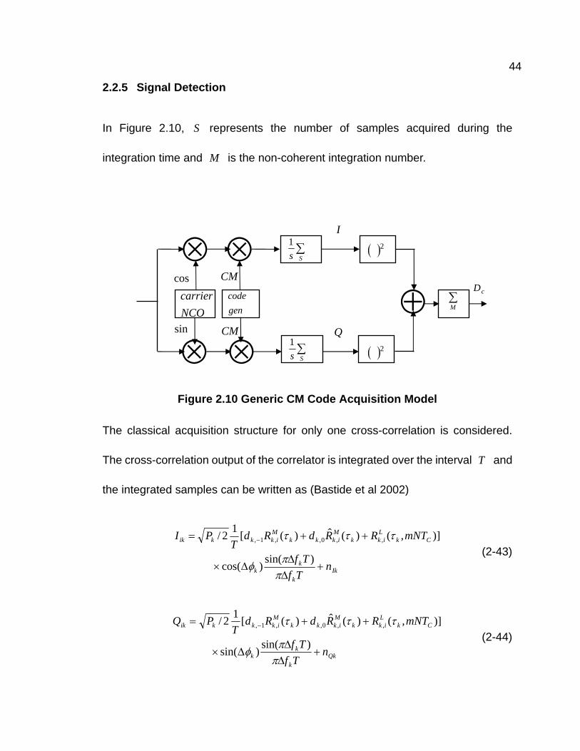
In Figure 2.10, S represents the number of samples acquired during the
integration time and M is the non-coherent integration number.
Figure 2.10 Generic CM Code Acquisition Model
The classical acquisition structure for only one cross-correlation is considered.
The cross-correlation output of the correlator is integrated over the interval T and
the integrated samples can be written as (Bastide et al 2002)
Ik
k
kk
CkL
ikkM
ikkkM
ikkkik
nTf
Tf
mNTRRdRdT
PI
+∆∆
∆×
++= −
ππφ
τττ
)sin()cos(
)],()(ˆ)([12/ ,,0,,1,
(2-43)
Qk
k
kk
CkL
ikkM
ikkkM
ikkkik
nTf
Tf
mNTRRdRdT
PQ
+∆∆
∆×
++= −
ππφ
τττ
)sin()sin(
)],()(ˆ)([12/ ,,0,,1,
(2-44)
⊗
⊗
NCOcarrier
sin
cos
⊗
⊗gencode
∑Ss
1
∑Ss
1
( )2
( )2
CM
CM
Q
I
⊕ ∑M
cD

45
where there is a factor T1 in every equation (considered the normalized
cross-correlation for the integration time T ), and Ikn and Qkn are centred
Gaussian correlator output noise with power T
Nn 8
02 =σ .
Signal acquisition can include coherent and non-coherent integration. Coherent
integration is the correlation between incoming signal and local replica. When the
signal code phase and frequency offset are matched, the SNR of the predetection
integration is enhanced. The longer the predetection integration time, the larger
the value of SNR for the integrator output. Because the band-limited white
Gaussian noise is random and its mean is zero, it can be reduced over the
integration time. Generally, the CM code predetection integration interval is 20 ms.
This integration time is long enough for the signal to be detected, because the
SNR can be relatively large for the case of a 20 ms integration time. Sometimes if
the incoming signal is very weak, for example indoor signal reception,
non-coherent integration can be added to improve the SNR. Although
non-coherent integration suffers from a squaring loss, it still increases the SNR.
The hypothesis test of the signal detection includes (Bastide et al 2002):
Hypothesis H0 (the desired signal is not present) and Hypothesis H1 (the desired
signal is present). The test statistic is compared to a threshold. The detection
decision will be made under a false alarm probability faP and detection probability
dP . The relevant test statistic is

46
∑ +=M
ii QID )( 22 . (2-45)
where M is the non-coherent time number. This test statistic includes coherent and
non-coherent integration.
Next, signal detection is analysed for the cases of band-limited WGN effects only
and one cross-correlation combined with band-limited WGN effects.
2.2.5.1 Band-Limited WGN Effects Only on Signal Detection
Hypothesis H0: no desired signal
Considering only the white Gaussian noise, the test statistic can be written as
(Bastide et al 2002)
∑ +=M
QkIk nnD )( 220 . (2-46)
Because Ikn and Qkn represent the Gaussian distribution, then 2nnD σ is a
central 2χ (chi square) distribution, and 2M represents the degrees of freedom of
the central 2χ chi square distribution.
The false alarm probability is given as follows (Bastide et al 2002):
∫∞
=>=Th
Dnfa duupThDPn
)(}Pr{ . (2-47)
where Th is the threshold, faP is false alarm probability, and )(uPnD is the
probability density function of the test statistic and of the central 2χ distribution. If

47
the faP value is chosen as 310−=faP , the classical value, then from the central
2χ distribution the Th value is determined with different M values by calculating
the inverse function of Equation (2-47). If 310−=faP and M is 1, from the central
2χ distribution, the threshold Th is about 13.8. When M is 2, the threshold Th
should be about 18.5. And when M is 3, the threshold Th is about 22.5. The
error is less than 0.05.
Hypothesis H1: a desired signal is present
In the case of a useful signal with white Gaussian noise being present, from
Equations (2-17) and (2-18) and considering the factor T1 , the test statistic is
derived as follows (Bastide et al 2002).
⎪⎭
⎪⎬⎫
⎥⎦
⎤⎢⎣
⎡+
∆∆
∆+++
⎩⎨⎧
⎥⎦
⎤⎢⎣
⎡+
∆∆
∆++= ∑2
0,
2
0,
)sin()sin()]()([12/
)sin()cos()]()([12/
Qki
iiiiiiii
MIk
i
iiiiiiiis
nTf
TfmTLMdT
P
nTf
TfmTLMdT
PD
ππφττ
ππφττ
(2-48)
2/ nsD σ is a non-central 2χ distribution. The degree of freedom is 2M. The
expected value of the non-centrality parameter is given as (Bastide et al 2002)
2
2
0
)sin()]()([4⎟⎟⎠
⎞⎜⎜⎝
⎛∆∆
++=Tf
TfmTLMdTN
MP
i
iiiiii
is π
πττλ . (2-49)
where the function )]()([ iiiii mTLMd ττ ++ is the autocorrelation between the
local CM code and the desired incoming L2C signal.

48
From the analysis above, it is clear that the probability of the detection is related to
a non-central 2χ distribution and the detection threshold Th . The value of the
non-centrality parameter shows that the non-central 2χ distribution depends on
the carrier-to-noise density ratio ( 0/ NC ) (here, it is 0/ NPi ), pre-detection
integration time T , non-coherent integration number M , the difference between
the frequency of the local carrier and the desired incoming carrier, the difference
between phase of the local carrier and of the desired incoming signal carrier, and
the difference between the local code delay and the desired incoming code delay.
If one only considers that the difference between the local code delay and the
desired incoming code delay is zero ( 0=iτ ), the difference between the phase of
the local carrier and that of the desired incoming signal carrier is zero ( 0=∆ iφ ) and
the difference between the frequency of the local carrier and of the desired
incoming carrier is zero ( 0=∆ if ). Equation (2-48) can then be written as follows
(considering Equations (2-19) and (2-20)).
∑⎪⎭
⎪⎬⎫
⎪⎩
⎪⎨⎧
⎥⎦⎤
⎢⎣⎡ ++⎥⎦
⎤⎢⎣⎡ +=
MQkiiIkiis ndPndPD
2
0,
2
0, 212/
212/ . (2-50)
Equation (2-49) can be written as
0N
MTPis =λ . (2-51)

49
Figure 2.11 Probability of Detection of Total (I+Q)C/N0 at the Antenna Output
Figure 2.11 displays the probability of detection depending on the total (I+Q)C/N0
at the antenna output. When the probability of false alarm (Pfa) is chosen as 0.001,
the relationship between the probability of detection and the C/N0 ranging from
20 dB-Hz to 33 dB-Hz is shown. The pre-detection integration T is 20 ms. The
three curves express the relationship with the non-coherent integration number
M=1, 2 and 3. In the figure, the effects of front-end are not considered and the code,
frequency, and phase uncertainties are assumed to be zero. More non-coherent

50
integrations will yield higher detection capabilities if the effects of code Doppler can
be ignored. The non-coherent integration with M=3 has a 3 to 4 dB-Hz better ability
to detect the desired signal; that is, with a C/N0 which can be 3 to 4 dB-Hz lower
than the one with M=1. Under the weak desired signal environment, when M=1,
the probability of detection can reach 0.9 with C/N0 equal to 30.8 dB-Hz. When
C/N0 equals 29.9 dB-Hz, the probability of detection can reach 0.8. When M=3, the
probability of detection can be 0.9 with C/N0 equal to 27.1 dB-Hz and 0.8 with C/N0
equal to 26.3 dB-Hz
2.2.5.2 Band-Limited WGN and One Cross-Correlation Effects on Signal
Detection
Hypothesis H0: no desired signal
If a cross-correlation interference peak is considered (the worst case of
cross-correlation), the test statistic becomes (Bastide et al 2002)
⎪⎭
⎪⎬⎫
⎥⎦
⎤⎢⎣
⎡+∆
∆∆
+++
⎪⎩
⎪⎨⎧
⎥⎦
⎤⎢⎣
⎡+∆
∆∆
++=
−
−∑2
,,0,,1,
2
,,0,,1,,0
)sin()sin()],( )(ˆ)([12/
)cos()sin()],( )(ˆ)([12/
Qkkk
kCk
Likk
Mikkk
Mikkk
MIkk
k
kCk
Likk
Mikkk
Mikkkc
nTf
TfmNTRRdRdT
P
nTf
TfmNTRRdRdT
PD
φππτττ
φππτττ
(2-52)
2,0 / ncD σ is a non-central 2χ distribution. The degree of freedom is 2M. The

51
non-centrality parameter of the 2χ distribution is calculated as follows (Bastide et
al 2002).
22
,,0,,1,0
22,,0,,1,
2,,0,,1,
)sin()],( )(ˆ)([4
/}))sin()sin()],( )(ˆ)([12/(
))cos()sin()],( )(ˆ)([12/{(
⎟⎟⎠
⎞⎜⎜⎝
⎛∆∆
++=
∆∆∆
+++
∆∆∆
++=
−
−
−∑
TfTfmNTRRdRd
TNMP
TfTfmNTRRdRd
TP
TfTfmNTRRdRd
TP
k
kCk
Likk
Mikkk
Mikk
k
nkk
kCk
Likk
Mikkk
Mikkk
Mk
k
kCk
Likk
Mikkk
Mikkkc
ππτττ
σφππτττ
φππτττλ
(2-53)
where the function 2,,0,,1,2 )],( )(ˆ)([1
CkL
ikkM
ikkkM
ikk mNTRRdRdT
τττ ++− is the
normalized cross-correlation between the local CM code and the k-th incoming
L2C signal. The false alarm probability must be associated with a precise
2,,0,,1,2
0
)],( )(ˆ)([ CkL
ikkM
ikkkM
ikkk mNTRRdRdTN
P τττ ++− that represents the worst real
case. From Section 2.2.4, the worst cross-correlation of
2,,0,,1,2 )],( )(ˆ)([1
CkL
ikkM
ikkkM
ikk mNTRRdRdT
τττ ++− is -31.1 dB. Then, the term
2,,0,,1,2
0
)],( )(ˆ)([ CkL
ikkM
ikkkM
ikkk mNTRRdRdTN
P τττ ++− can be chosen as 11.7dB-Hz,
( HzdBNPk −= 8.42
0
), which is the worst L2C case for a 20 ms pre-detection
integration.
Hypothesis H1: a desired signal is present

52
If, in the case of the useful signal, cross-correlation and white Gaussian noise are
present, the test statistic is given as follows (Bastide et al 2002).
}))sin()sin()],( )(ˆ)([12/(
)sin()sin()]()([12/(
))cos()sin()],( )(ˆ)([12/
)cos()sin()]()([12/{(
2,,0,,1,
2,,0,,1,
Qkkk
kCk
Likk
Mikkk
Mikkk
ii
iiiiiii
Ikkk
kCk
Likk
Mikkk
Mikkk
Mi
i
iiiiiiis
nTf
TfmNTRRdRdT
P
TfTfmTLMd
TP
nTf
TfmNTRRdRdT
P
TfTfmTLMd
TPD
+∆∆∆
+++
∆∆∆
+++
+∆∆∆
+++
∆∆∆
++=
−
−
∑
φππτττ
φππττ
φππτττ
φππττ
(2-54)
2/ nsD σ is a non-central 2χ distribution and the degree of freedom is 2M. The
expected value of the non-centrality parameter is (Bastide et al, 2002)
2
2,,0,,1,
0
22
0
)sin()],( )(ˆ)([4
)sin()]()([4
⎟⎟⎠
⎞⎜⎜⎝
⎛∆∆
+++
⎟⎟⎠
⎞⎜⎜⎝
⎛∆∆
++=
− TfTfmNTRRdRd
TNMP
TfTfmTLMd
TNMP
k
kCk
Likk
Mikkk
Mikk
k
i
iiiiii
is
ππτττ
ππττλ
(2-55)
where the function )]()([1iiiii mTLMd
Tττ ++ is the normalized autocorrelation
between the local CM code and the desired incoming L2C code. If iτ is assumed
to be zero, )(1ii mTL
Tτ+ is equal to zero and )(1
iiMT
τ is equal to 21 .

53
Figure 2.12 Probability of Detection of Total (I+Q)C/N0 at the Antenna Output
for 20 ms Coherent Integration Time (No Uncertainty and No Front End
Filtering Effects are Considered)
In this case, results are almost identical to the case shown in Figure 2.11 except
that the cross-correlation false alarm probability is 0.001. In Figure 2.12, the false
alarm probability (Pfa) is still 0.001, but the worst cross-correlation case has been
considered. Pre-integration time is 20 ms. The non-coherent integration number is
M=1,2 and 3. The effects of the front-end are not considered and the code,
frequency, and phase uncertainties are assumed to be zero. Additional
non-coherent integration will result in better detection if the Doppler effects on

54
incoming code can be ignored. The non-coherent method with M=3 has a 3 to
4 dB-Hz higher ability to detect the desired signal than the one with M=1.
Comparing Figure 2.11 with Figure 2.12, with the presence of cross-correlation the
detection probabilities are degraded. With the same non-coherent integration
number M, the detection capability under band-limited WGN only is about 1 dB-Hz
higher than the detection capabilities under one worst cross-correlation and
band-limited WGN combined. Under the weak desired signal environment, when
M=1, the probability of detection can reach 0.9 with C/N0=31.7 dB-Hz and 0.8 with
C/N0=30.8 dB-Hz. When M=3, the probability of detection can reach 0.9 with
C/N0=28.1 dB-Hz and 0.8 with C/N0=27.4 dB-Hz. The detection probabilities are
mostly decreased by approximately 0.20 for M=1 at C/N0=29 dB-Hz, by
approximately 0.21 for M=2 at C/N0=27 dB-Hz, and by approximately 0.22 for M=3
at C/N0=26 dB-Hz.
2.3 Conclusions
The CM and CL codes of the L2C signal are generated from one PN code with
maximal length of 1227 − . The largest cross-correlation of -31.1 dB is between a
local CM code (PRN=26) and incoming CL code (PRN=4). For any
cross-correlation of the local and incoming CM code, when the code delay is an
odd integer multiple of T the cross-correlation is zero. When the code delay is an
even integer multiple of T , the cross-correlation reaches its extreme values. For

55
any cross-correlation of the local CM code and incoming CL code, when the code
delay is an odd integer multiple of T the cross-correlations have extreme values.
When the code delay is an even integer multiple of T , the cross-correlations are
zero. Under band-limited WGN only, the non-coherent integration with M=3 has a
3 to 4 dB-Hz better ability to detect the desired signal than the case for M=1. Under
band-limited WGN and one worst case cross-correlation combined, the
non-coherent integration with non-coherent integration number M=3 also has a 3
to 4 dB-Hz better ability to detect the desired signal than the one with M=1. Under
the weak desired signal environment, with the same non-coherent integration
number M, the detection capabilities under band-limited WGN only is about
1 dB-Hz higher than the detection capabilities under one worst cross-correlation
and band-limited WGN combined.

56
Chapter 3
Cross-Correlation and White Gaussian Noise Effects on
Signal-To-Noise Ratio
The signal-to-noise ratio is a critical parameter in receivers. The SNR of the
incoming signal and the SNR of the output of the correlator affect the detection
performance. After decoding and wiping-off the code on the desired incoming
signal, the output of a correlator includes the desired signal, cross-correlations
with unwanted signals, and the spread band-limited WGN in the cases being
considered. The cross-correlations cause SNR degradation as compared to the
situation without cross-correlations.
3.1 Worst Case Performance
For the L2C signal, given the analysis in Chapter 2, consider that there are several
satellites in view simultaneously. If the Doppler effects are not considered
( 0=∆=∆ ki ff ) and the local carrier is matched with the incoming desired signal
( 0=∆ iφ ), Equation (2-25) can be written as
IkCkL
ik
K
ikk
kM
ikkkM
ikkkiii
nmNTR
RdRdPdTPI
+∆+
++= ∑≠=
−
)cos()],(
)(ˆ)([2/2
2/
,
1,0,,1,0,
φτ
ττ. (3-1)
Now consider the cross-correlation terms in Equation (3-1):

57
)cos()],()(ˆ)([2/ ,1
,0,,1, kCkL
ik
K
ikk
kM
ikkkM
ikkk mNTRRdRdP φτττ ∆++∑≠=
− .
),(, mv kik τ is defined by
)cos()],()(ˆ)([),( ,,0,,1,, kCkL
ikkM
ikkkM
ikkkik mNTRRdRdmv φττττ ∆++= − . (3-2)
In Equation (3-2), when the difference between the phase of the local carrier and
that of the incoming signal carrier become zero ( 0=∆ kφ ), the largest value of
)cos( kφ∆ occurs ( 1)cos( =∆ kφ ).
The output of a correlator is sent to a discriminator. If a discriminator of type
ii QIsign ⋅=Ψ )()(θ is used, )( iIsign is critical. In Equation (3-1), if the sign of iI
is different from that of 0,id under the effects of cross-correlation and white
Gaussian noise, errors of information data estimation occur. These error
probabilities are defined by )1|0( 0, −=> iir dIP and )1|0( 0, +=< iir dIP (Pursley
1977). When 10, −=id , the maximum error probability for the information data
estimation corresponds to the maximum value of ),(, mv kik τ for each ik ≠ . When
10, =id , the maximum error probability for the information data estimation
corresponds to the minimum value of ),(, mv kik τ for each ik ≠ .
According to the analyses in Chapter 2, if 10, −=id , the maximum value of the
cross-correlation can be estimated by

58
)}max(),ˆmax(),max{max( ,,,, ikikikik ηλλγ = .
If 10, =id , the minimum value of the cross-correlation can be estimated by
)}min(|,ˆ|max|,|maxmin{ˆ ,,,, ikikikik ηλλγ −−= .
Finally, the worst case is to choose the larger values of ik ,γ and |ˆ| ,ikγ . When ik ,γ
is larger, the condition 10, −=id is considered. When |ˆ| ,ikγ is larger, the condition
10, =id is considered.
Suppose that
}|ˆ|2
,2
max{ ,, Cikk
Cikk TPTP γγ=Λ ,
and this is the worst case of cross-correlation.
If the cross-correlation is generated from more than one signal, that is 3≥K , and
noting that ik ,γ is not symmetrical according to Equation (3-1), the expressions
Cikk
K
ikk
TP,
1 2γ∑
≠=
and Cikk
K
ikk
TP |ˆ|2 ,
1
γ∑≠=
can be compared. When Cikk
K
ikk
TP,
1 2γ∑
≠=
is
larger, 10, −=id is considered. When Cikk
K
ikk
TP |ˆ|2 ,
1
γ∑≠=
is larger, 10, =id is
considered. Now
}|ˆ|2
,2
max{ ,1
,1
Cikk
K
ikk
Cikk
K
ikk
TPTP γγ ∑∑≠=
≠=
=Λ . (3-3)

59
The maximum value of probability maxP can be given by (Pursley 1977)
}/)]
|ˆ|2 ,
2max(1{[1
}/)]8(1{[1
0,
1
,
1
0max
NTPPP
NPP
N
NTPPT
P
ii
kikK
ikki
kikK
ikk
ii
γγ∑∑≠=
≠=
−Φ−=
Λ−Φ−=
(3-4)
where Φ is the standard Gaussian cumulative distribution function.
3.2 Numerical Simulation for Worst Case Performance
For the worst-case performance, because the largest cross-correlation is
considered, the cross-correlation is not variable. The output of the correlator is
sent to the discriminator, thus the sign of the in-phase component is critical. If the
evaluation of the in-phase component sign is different from in the real case, a
tracking error will occur. When 10, −=id or 10, =id , the largest positive
cross-correlation or the largest negative cross-correlation will lead to more effects
on the information data estimation of desired signal.
3.2.1 Simulation Scheme
The simulation scheme is shown in Figure 3.1. In the simulation, by using Matlab,
the incoming signal is simulated which includes the desired signal (CM code) and
band-limited WGN. Then, the integration is done after the correlation between the
local CM code and incoming signal. After integration, a minimum cross-correlation

60
(the absolute value is the largest from the simulation in Chapter 2) is added to the
output of the integration. Because the minimum cross-correlation is used, 0,1d is
chosen to be +1. If the output iI is negative which is different with the sign of the
desired signal, an error of information data estimation occurs. Here, in the
simulation, K is chosen to be 1, 3, and 5, which means no cross-correlation, two
cross-correlations, and four cross-correlations. Then, the error probability of
information data estimation is calculated under different C/N0 including under the
weak desired signal.
Figure 3.1 Method Used to Estimate the Largest Error Probability
3.2.2 Result Analysis
Figure 3.2 displays the maximum error probabilities of information data estimation
for the worst cases. In this figure, the lowest two curves are the maximum error
probabilities for the theoretical value and simulated result with band-limited WGN
Desired Signal (CM Code)
White Gaussian Noise
⊗Local CM
∑T
Min Cross- Correlation
⊕ ⊕ <0

61
only (K=1). The other curves are the theoretical results and simulation results with
band-limited WGN and two worst cross-correlations (K=3), and the results with
four cross-correlations (K=5).
Figure 3.2 Maximum Error Probabilities
In the simulation, the maximum error probabilities of information data estimation
increase with the reduction of the C/N0. When the C/N0 is less than 26 dB-Hz, the
maximum error probabilities cannot be ignored. From the figure, when there are
cross-correlations, the error probabilities are larger than the case with band-limited
WGN only. In the case above, the power of the desired signal is the same as the

62
power of the undesired signal power. The difference of the error probabilities
generated by the cross-correlations is not very great. The main effect on maximum
error probabilities comes from band-limited WGN.
Figure 3.3 shows that when C/N0 is chosen to be 26 dB-Hz, the maximum error
probabilities vary with the ratio of the desired signal power to the undesired signal
powers.
Figure 3.3 Maximum Error Probabilities with White Gaussian Noise and
Cross-Correlation
The results in Figure 3.3 show that when the ratio (in dB) of Pi power to Pk power is

63
less than about -8 dB, the effects of cross-correlations on the maximum error
probabilities become very large, especially when 4≥K . That is, under the
situation of weak desired signal (C/N0 is 26 dB-Hz), the strong undesired signal
(about 8 dB larger or more than the desired signal), which leads to the large
cross-correlation, is a significant source of the information data estimation error
probabilities.
3.3 Theoretical Analysis of Average Signal-To-Noise Ratio
In Equation (3-1), 0,id can be +1 or -1. The two probabilities are considered
symmetrical. There is no loss in generality in assuming 10, +=id ; thus the desired
signal component of iI is2
2/ TPi .
To get the average signal-to-noise ratio, it is necessary to derive the variance of the
noise. First, the average of the iI can be written as
∫
∑
+++
∆−+
++=
≠=
−
T
idiLi
kCkL
ik
K
ikk
kM
ikkkM
ikkkii
dttfftCMtnE
EmNTRE
REdEREdEPTPIE
02
,
1,0,,1,
)ˆ)ˆ(2cos()())((
))(cos())]((
))(ˆ()())(()([2/2
2/)(
φπ
φτ
ττ
(3-5)
Suppose that kφ∆ and kτ are uniformly distributed in the range [0, π2 ] and [0,T ].
Because ))(cos( kE φ∆ and ))(( tnE are equal to zero, Equation (3-5) can be written
as

64
2
2/)( TPIE ii = . (3-6)
The 2iI average is
}])ˆ)ˆ(2cos()()({[
})ˆ)ˆ(2cos()()(
)cos()],()(ˆ)([2/2{
)}cos()],()(ˆ)([2/
)cos()],()(ˆ)([2/{
})ˆ)ˆ(2cos()()(2
2/2{
)}cos()],()(ˆ)([2/2
2/2{8
)(
0
22
02
,1
,0,,1,
,1
,0,,1,
,1
,0,,1,
02
,1
,0,,1,
22
∫
∫
∑
∑
∑
∫
∑
+++
++
⋅∆+++
∆++
⋅∆+++
++⋅+
∆++⋅+=
≠=
−
≠=
−
≠=
−
≠=
−
T
idiLi
T
idiLi
kCkL
ik
K
ikk
kM
ikkkM
ikkk
kCkL
ik
K
ikk
kM
ikkkM
ikkk
kCkL
ik
K
ikk
kM
ikkkM
ikkk
T
idiLii
kCkL
ik
K
ikk
kM
ikkkM
ikkkii
i
dttfftCMtnE
dttfftCMtn
mNTRRdRdPE
mNTRRdRdP
mNTRRdRdPE
dttfftCMtnTPE
mNTRRdRdPTPETPIE
φπ
φπ
φτττ
φτττ
φτττ
φπ
φτττ
(3-7)
In Equation (3-7), 0))(cos( =∆ kE φ and 0))(( =tnE , so the cross terms are zero
as follows:
0)}cos()],()(ˆ)([2/2
2/2{ ,1
,0,,1, =∆++⋅∑≠=
− kCkL
ik
K
ikk
kM
ikkkM
ikkki mNTRRdRdPTPE φτττ .

65
0})ˆ)ˆ(2cos()()(2
2/2{0
2 =++⋅ ∫T
idiLii dttfftCMtnTPE φπ .
0})ˆ)ˆ(2cos()()(
)cos()],()(ˆ)([2/2{
02
,1
,0,,1,
=++
⋅∆++
∫
∑≠=
−
T
idiLi
kCkL
ik
K
ikk
kM
ikkkM
ikkk
dttfftCMtn
mNTRRdRdPE
φπ
φτττ
Considering these zero terms, Equation (3-7) can be rewritten as
}])ˆ)ˆ(2cos()()({[
)}cos()],()(ˆ)([2
)cos()],()(ˆ)([2
{8
)(
2
02
,1
,0,,1,
,1
,0,,1,
22
∫
∑
∑
+++
∆++
⋅∆+++=
≠=
−
≠=
−
T
idiLi
jCjL
ij
K
ijj
jM
ijjjM
ijjj
kCkL
ik
K
ikk
kM
ikkkM
ikkki
i
dttfftCMtnE
mNTRRdRdP
mNTRRdRdPETPIE
φπ
φτττ
φτττ
(3-8)
In Equation (3-8), there are still cross terms in the cross-correlation term. If we take
0)( 1, =−kdE , 0)( 0, =kdE , 0)()()( 0,1,0,1, == −− jkjk dEdEddE ,
0)()()( 1,1,1,1, == −−−− jkjk dEdEddE , kj ≠ , 0)()()( 0,0,0,0, == jkjk dEdEddE , kj ≠ ,
1)()( 0,0,1,1, ==−− kkkk ddEddE , 0))(cos())(cos())cos()(cos( =∆∆=∆∆ jkjk EEE φφφφ ,
kj ≠ , 0)()()( 0,1,0,1, == −− kkkk dEdEddE and 21))((cos2 =∆ kE φ into account, the
following terms are all zero, where kj ≠ :
0)](cos)(ˆ)([ 2,0,,1, =∆− kk
Mikkk
Mikk RdRdE φττ .

66
0)](cos),()([ 2,,1, =∆− kCk
Likk
Mikk mNTRRdE φττ .
0)](cos),()(ˆ[ 2,,0, =∆ kCk
Likk
Mikk mNTRRdE φττ .
0)]cos()cos()(ˆ)([ ,0,,1, =∆∆− jkkM
ijjkM
ikk RdRdE φφττ .
0)]cos()cos(),()([ ,,1, =∆∆− jkCjL
ijkM
ikk mNTRRdE φφττ .
0)]cos()cos(),()(ˆ[ ,,0, =∆∆ jkCjL
ijkM
ikk mNTRRdE φφττ .
0)]cos()cos()()([ ,1,,1, =∆∆−− jkkM
ijjkM
ikk RdRdE φφττ .
0)]cos()cos()(ˆ)(ˆ[ ,0,,0, =∆∆ jkkM
ijjkM
ikk RdRdE φφττ .
0)]cos()cos(),(),([ ,, =∆∆ jkCjL
ijCkL
ik mNTRmNTRE φφττ .
The 2iI average can be written as
8
])),(())(ˆ())(([48
)(
0
2,
2,
2,
1
22
TN
mNTREREREPTPIE CkL
ikkM
ikkM
ik
K
ikk
kii
+
+++= ∑≠=
τττ
(3-9)
Therefore, the variance of the noise component of iI is
8
])),(())(ˆ())(([4
)]([)(})]({[)(
02,
2,
2,
1
222
TNmNTREREREPIEIEIEIEIVar
CkL
ikkM
ikkM
ik
K
ikk
k
iiiii
+++=
−=−=
∑≠=
τττ (3-10)
Equation (3-10) can be rewritten as (Pursley 1977)

67
8})],([1)](ˆ[)]({[
4
8})],([1)](ˆ[)]({[
4)(
02,
1
0
2,
2,
1
)1(1
0
02,
1
0
2,
2,
1 0
TNdmNTRN
RRT
P
TNdmNTRN
RRT
PIVar
kCkL
ik
N
mLk
Mikk
Mik
K
ikk
Tcl
lTc
N
l
k
kCkL
ik
N
mLk
Mikk
Mik
K
ikk
Tk
i
L
L
+++=
+++=
∑∑ ∫∑
∑∑ ∫
−
=≠=
+−
=
−
=≠=
ττττ
ττττ
(3-11)
The integration kCkL
ik
N
mLk
Mikk
Mik
Tl
lT
dmNTRN
RRLC
C
ττττ })],([1)](ˆ[)]({[ 2,
1
0
2,
2,
)1(
∑∫−
=
+
++ can be
derived separately as follows. The first term (from Equation (2-30)) is
)]1()1()()([3
)(
)]()1([3
)]()1()[()(
)})](()1([)({))((
2,,,
2,3
3
2,,
3
3,,,
32,
2,,,
)1(2
,
)1(
+−++−−+−=
−−−++
−−−+−+−=
−−−−++−= ∫∫++
NlCNlCNlCNlCN
NT
NlCNlCT
TNlCNlCNlCTNlC
dlTNlCNlCTNlCdR
ikikikikc
ikikc
cikikikcik
kckikikcik
Tl
lTkk
Mik
Tl
lT
C
C
C
C
ττττ
(3-12)
The second term (from Equation (2-31)) is
)]1()1()()([3
)(
)]()1([3
)]()1()[()(
)})](()1([)({))(ˆ(
2,,,
2,3
3
2,,
3
3,,,
32,
2,,,
)1(2
,
)1(
++++=
−++
−++=
−−++= ∫∫++
lClClClCN
NT
lClCT
TlClClCTlC
dlTlClCTlCdR
ikikikikc
ikikc
cikikikcik
kckikikcik
Tl
lTkk
Mik
Tl
lT
C
C
C
C
ττττ
(3-13)
68
The third term (from Equation (2-33)) is
)]1,()1,(),(),([13
)(
})],()1,([3
)],()1,()[,(),({1
)})](,(
)1,([),({1)),((1
2,,,
2,
1
03
3
2,,
3
3,,,
32,
1
0
2,
,,
)1(1
0
2,
)1(1
0
++++=
−++
−++=
−−
++=
∑
∑
∫∑∫∑
−
=
−
=
+−
=
+−
=
lmWlmWlmWlmWNN
NT
lmWlmWT
TlmWlmWlmWTlmWN
dlTlmW
lmWTlmWN
dmNTRN
ikikikik
N
mL
c
ikikc
cikikikcik
N
mL
kckik
ikcik
Tl
lT
N
mLkCk
Lik
Tl
lT
N
mL
L
L
C
C
LC
C
L
ττ
ττ
(3-14)
Taking Equations (3-12), (3-13) and (3-14) into account, Equation (3-11) can be
rewritten as
8
][12
)( 0,,
13
2 TNrrPN
TIVar Lik
Mik
K
ikk
ki ++= ∑≠=
. (3-15)
where
)}1()1()()(
)1()1()()({
2,,,
2,
2,,,
2,
1
0,
+++++
+−++−−+−= ∑−
=
lClClClC
NlCNlCNlCNlCr
ikikikik
ikikikik
N
l
Mik and
)}1,()1,(),(),({1 2,,,
2,
1
0
1
0, ++++= ∑∑
−
=
−
=
lmWlmWlmWlmWN
r ikikikik
N
l
N
mL
Lik
L
.
For the CM code, the chips with an even number are zero; therefore, either
)(, NlC ik − or )1(, +− NlC ik must be zero. The product of )(, NlC ik − and

69
)1(, +− NlC ik is zero. For the same reason, either )(, lC ik or )1(, +lC ik must be
zero, such that )1()( ,, +lClC ikik equals zero.
For the CL code, the chips with an odd number are zero; therefore either ),(, lmW ik
or )1,(, +lmW ik must be zero. The product )1,(),( ,, +lmWlmW ikik equals zero and
Mikr , and L
ikr , can be rewritten as
)}1()()1()({ 2,
2,
2,
2,
1
0, ++++−+−= ∑
−
=
lClCNlCNlCr ikikikik
N
l
Mik and
)}1,(),({1 2,
2,
1
0
1
0, ++= ∑∑
−
=
−
=
lmWlmWN
r ikik
N
l
N
mL
Lik
L
.
where
)1()( 2,
1
0
2,
1
0
+−=− ∑∑−
=
−
=
NlCNlC ik
N
lik
N
l
, )1()( 2,
1
0
2,
1
0
+= ∑∑−
=
−
=
lClC ik
N
lik
N
l
and
)1,(1),(1 2,
1
0
1
0
2,
1
0
1
0
+= ∑∑∑∑−
=
−
=
−
=
−
=
lmWN
lmWN ik
N
l
N
mLik
N
l
N
mL
LL
.
Therefore, from the derivation above and Pursley (1977), the average
signal-to-noise ratio (SNR) is
210
,,1
13 }][)23{()(
22/ −
≠=
− ++== ∑ TPNrr
PPNIVarTPSNR
i
Lik
Mik
K
ikk i
kii . (3-16)

70
3.4 The Numerical Simulation for Average SNR
In the numerical simulation of the average SNR, there are cross-correlation and
band-limited WGN effects. Three cases are considered here. The first is the
situation with band-limited WGN only. The second has cross-correlation only. The
third has cross-correlation and band-limited WGN combined.
3.4.1 Simulation Method
SNR is a critical parameter in GPS receivers. The SNR of the correlator output
affects the performances of acquisition and of the tracking loop. In this simulation
section, the SNR evaluation is done according to the statistical average value over
a pre-integration period. The code delays and phase offsets between the local
replica and incoming signals from other satellites are supposed to be independent.
They are random variables uniformly distributed in the pre-integration time period
[0, T] and a phase period [0, π2 ]. For the long incoming CL code, there are also
75 cross-correlation possibilities, for which 74... ,2 ,1 ,0=m . The incoming signal
includes a desired signal which the local replica matches very well, the signals
from other satellites, and band-limited WGN. The undesired signals have different
code delays because of the different distances from different satellites to the
receiver, and different phase offsets due to the differences between the local and
the remote clocks. Figure 3.4 shows the incoming signal simulation, correlation

71
model, and SNR calculation method.
Figure 3.4 Average SNR Scheme Under Cross-Correlation and White
Gaussian Noise
Here, by using Matlab, the local signal is the CM code with PRN=1. The desired
signal is also the incoming CM code with PRN=1. Because the local and incoming
desired CM code are matched exactly, and considering the zero chips in the CM
and CL code, the correlation between the incoming CL code with PRN=1 and the
local CM code with PRN=1 is zero. It is not necessary to put the CL code in the
incoming desired signal. The undesired signals include the incoming CM and CL
code with PRN=2, 3, 4, 5. There are code delays and phase offsets in the incoming
signal. For the incoming CL code, there is one more parameter 74... ,2 ,1 ,0=m ,
because the CL code is a long code, which is 75 times the CM code. There are
navigation data on the incoming CM code. The data 1,−kd and 0,kd can be +1 or
Desired Signal
Undesired Signals
White Gaussian Noise
⊕ ⊗Local Signal
∑
Var
Mean
/ SNR

72
-1. The probabilities of having +1 or -1 are equal. The incoming signal is generated
which includes desired signal, undesired signals and band-limited WGN. The
incoming signal is correlated with the local signal and is integrated. Then, the
output average and output variance are calculated. Finally, the SNR is the output
average divided by the root square of output variance. The simulations include the
SNR with band-limited WGN only, cross-correlations only, and band-limited WGN
and cross-correlations combined
3.4.2 Simulated Average SNR Results
When there are no cross-correlation effects, Equation (3-16) can be rewritten as
21
0
][N
TPSNR i= . If it is presented in dB, then )(log10)(log10 01010 NTPSNR i −= .
There is no loss in generality in assuming 1=i .

73
Figure 3.5 Average SNR with White Gaussian Noise Only
Figure 3.5 shows the variation of SNR under the band-limited WGN only with the
power of the desired incoming signal. The red line is the theoretical result and the
blue line is the simulation result. From the IS-GPS-200D specifications, the L2C
power is -160 dBW. Therefore, the simulation area is in the region where the signal
power is less than -160 dBW. The SNR is reduced from 26 dB to 6 dB with the
deduction of the desired incoming signal power from -160 dBW to -180 dBW. The
RMS error of the simulation from Figure 3.5 is less than 0.19 dB.

74
Figure 3.6 Average SNR with Cross-Correlation Only
Figure 3.6 shows the simulation results under the cross-correlations only. In this
situation, Equation (3-16) can be rewritten as 21
,,1
13 ]}[)23{( −
≠=
− += ∑ Lik
Mik
K
ikk i
k rrPPNSNR . If
it is presented in dB, then
⎟⎟⎠
⎞⎜⎜⎝
⎛−
⎥⎥⎥
⎦
⎤
⎢⎢⎢
⎣
⎡+−⎥⎦
⎤⎢⎣⎡=
⎟⎟⎠
⎞⎜⎜⎝
⎛−
⎥⎥⎥⎥⎥
⎦
⎤
⎢⎢⎢⎢⎢
⎣
⎡
+=
∑
∑
≠=
≠=
i
kLik
Mik
K
ikk
i
k
Lik
Mik
K
ikk
PPrrN
PP
rr
NSNR
10,,1
103
10
10
,,1
3
10
log10][log1023log10
log10][
23
log10
(3-17)

75
In the simulation, powers from other undesired signals are supposed to be the
same ( ikPP ik ≠= , ). In Figure 3.6, the ratio of the undesired signal power to
desired signal power ranges from 1 to 100. From Equation (3-17), the relationship
between SNR in dB and the ratio of undesired signal power to desired signal power
is logarithmic. Because the differences between different average
cross-correlations are small, the second term in Equation (3-17) is also changed
with the logarithm of cross-correlation number if kP remains constant. The
greatest RMS error of the simulation in the four cases (K = 2, 3, 4, 5) is less than
0.23 dB.
Figure 3.7 describes the simulated average SNR results under the
cross-correlations and band-limited WGN. Equation (3-16) can be rewritten as (in
dB)
⎥⎥⎥⎥⎥
⎦
⎤
⎢⎢⎢⎢⎢
⎣
⎡
+
+
−=
∑≠=
TPN
N
rrPP
SNRi
Lik
Mik
K
ikk i
k
0
3
,,1
10
23
][
log10 . (3-18)
In this simulation, the band-limited WGN and desired incoming signal remain
constant. The ratio of undesired signal power and desired signal power is from 1 to
100. There are four cases (K = 2, 3, 4, 5). When K = 2 (that is only one
cross-correlation), if the ratio i
k
PP ranges from 1 to 100 (increase of about 20 dB),

76
the SNR decreases by about 3.5 dB. When K = 5 (four cross-correlations), in the
same range, the SNR decreases by about 7.5 dB.
Figure 3.7 Average SNR with Cross-Correlation and White Gaussian Noise
Figure 3.5 shows that when the desired incoming signal power is -160 dBW, the
SNR is about 26 dB. In Figure 3.7, on the left hand side, when the unwanted signal
power is almost same as the desired signal power, the SNR is near 26 dB. The two
results are consistent. The effects from the cross-correlations can be ignored
compared to the effects of band-limited WGN. As the ratio of unwanted to desired
signal power increases, Figure 3.7 shows that the cross-correlations also increase

77
their effects on the SNR results.
3.5 Conclusions
The analyses of cross-correlation and band-limited WGN effects on SNR and
worst case performance demonstrate the following. If the power of the desired
signal is the same as the power of the undesired signal, the maximum error
probability difference generated by the cross-correlations is small. The main
effects on maximum error probabilities come from the effects of band-limited WGN.
In urban areas, the GPS signal can be attenuated by buildings and its strength can
be decreased about 32 dBW (Tang and Dodds 2006). Under the weak desired
signal situation, if the undesired signal power is larger than the desired signal
power (more than 8 dB), the maximum error probability increases rapidly,
especially when 4≥K .
In SNR analyses, if there are no cross-correlations, SNR varies linearly with the
desired signal power in dBW. If there is no white Gaussian noise, SNR changes
with the logarithm of the cross-correlation number or with the logarithm of the ratio
of undesired to desired signal power. If the band-limited WGN and desired
incoming signal remain constant, under the high ratio of the undesired signal
power to desired signal power, cross-correlation becomes the main factor to affect
the SNR result.
78
Chapter 4
Cross-Correlation and White Gaussian Noise Effects on
PLL Tracking Loops
Functioning as an automatic phase control system, the phase-locked loop is a
closed-loop tracking system capable of tracking the phase of a received signal that
has a residual carrier component. The system synchronizes the phase or
frequency of its output signal with that of the input signal. When the output signal of
the PLL is synchronized with the input signal, an arrangement often referred to as
locked state (Best 2003), the phase error between output signal and input signals
is zero. Any cross-correlation in the input of the PLL will affect the PLL
performance. In this chapter, it is described how the cross-correlations affect such
performance.
4.1 Basic Principle of a Phase-Locked Loop
In a phase-locked loop, if a phase error accumulates, a control signal acts on the
oscillator in such a way that the phase error is reduced. In this system, the phase of
the output signal is locked to the phase of the reference signal.

79
4.1.1 The Input Signal without Interference
According to Viterbi (1966), a phase-locked loop consists of three major
components: a multiplier, a linear time-invariant loop filter, and a voltage-controlled
oscillator. Figure 4.1 shows the phase-locked loop for the condition of no
interference in the input signal, where )(sin2 tA θ is the input signal, 2A
is the input signal power, and )('cos2 1 tK θ is the VCO output signal. The
term 1K is the root-mean-square amplitude of the VCO output signal (Viterbi,
1966) and )(te is the control signal to the VCO. When )(te equals zero, the
VCO generates a constant-frequency sinusoid with frequency 0ω . Under the
control signal )(te , the VCO frequency is )(20 teK+ω . The term 2K is the
proportionality constant in radians per second per volt. Then one has (Equation
(4-1) to (4-12) are taken from Viterbi (1966)):
)()('20 teK
dttd
+= ωθ . (4-1)
The output of the multiplier is:
)]}(')(sin[)](')({sin[)('cos2)(sin2)( 11 ttttAKtKtAtx θθθθθθ ++−=⋅= .
The summation component is eliminated by the filter-VCO combination. The
output of the linear filter is duutfuxtet
)()()(0
−= ∫ and )(tf is the impulse
response of the filter.

80
Figure 4.1 Phase-Locked Loop (Viterbi 1966)
Suppose that ttt 01 )()( ωθθ −= and ttt 02 )(')( ωθθ −= . The phase error is then
)()()( 21 ttt θθφ −= . When )(tφ is small compared with 1 radian, the approximation
)()(sin tt φφ = can be used. Then one has the linear equation
duuutfAKdt
tddt
tddt
tddt
td t
)()()()()()(
0
121 φθθθφ−−=−= ∫ (4-2)
where 21KKK = is the loop gain. Figure 4.2 describes this linear model.
Figure 4.2 Phase-Locked Loop Linear Model (Viterbi 1966)
Assuming the existence of the following Laplace transforms
X LinearFilter
VCO
)(sin2 tA θ )(tx
)(te)('cos2 1 tK θ
+ Linear Filter
∫t
0
)(1 tθ )(tφ
dttd )(2θ
)(2 tθ
AK+
−

81
0)(Re ;)()(~1
01 ≥= −
∞
∫ saldtets stθθ and
0)(Re ;)()(~
0
≥= −∞
∫ saldtets stφφ ,
the Equation (4-2) can be written as )(~/)(1
1)(~1 s
ssAKFs θφ
+= and
)(~/)(1
/)()(~12 s
ssAKFssAKFs θθ
+= , where )(sF is the transfer function of the linear filter.
The closed-loop transfer function is
ssAKF
ssAKFsssH
/)(1/)(
)(~)(~
)(1
2
+==
θθ . (4-3)
4.1.2 Input Signal with Additive Noise
Suppose that the input signal includes additive thermal noise which is a zero-mean
wideband Gaussian process, where the white noise has been passed through a
symmetric wide-band bandpass filter with centre frequency 0ω and a flat
passband that passes only frequencies below 02ω rad/sec. The Gaussian
process can then be expressed as
)]cos()()sin()([2)( 0201 ttnttntn ωω += . (4-4)
where )(1 tn and )(2 tn are independent Gaussian processes of zero mean and
with two-sided spectral densities of 2/0N .

82
The received signal is
)}cos()()sin()()](sin[{2)()(sin2 020110 ttnttnttAtntA ωωθωθ +++=+ . (4-5)
Multiplying by the output signal of the VCO, the output of the multiplier is
)](2cos[)()](2sin[)()]()(2sin[ )(cos)()(sin)()]()(sin[)(
202120112101
221211211
tttnKtttnKtttAKttnKttnKttAKtx
θωθωθθωθθθθ
++++++++−−=
.
The terms with the frequency 02ω rad/sec may be neglected. The filtered
multiplier output is
duutfuunuunuAKtet
)()](cos)()(sin)()(sin[)( 22210
1 −+−= ∫ θθφ .
If one defines )(cos)()(sin)()(' 2221 ttnttntn θθ +−= , then one has
duutfunuAKdt
tddt
td t
)()](')(sin[)()(
0
1 −+−= ∫ φθφ . (4-6)
If the phase error )(tφ is small, then )()(sin tt φφ = . Equation (4-6) becomes linear
duutfunuAKdt
tddt
td t
)()](')([)()(
0
1 −+−= ∫ φθφ . (4-7)
Figure 4.3 displays the model of Equation (4-7). According to Viterbi (1966),
because of the white Gaussian noise, the spectral density of the phase error is
)(/)(1
/)()(2
ωωω
ωωωφ nSiAKF
iKFS+
= . (4-8)

83
where )(ωnS is the noise spectral density.
Figure 4.3 Phase-Locked Loop Linear Model (with Additive Noise) (Viterbi
1966)
Given that ssAKF
ssAKFsH/)(1
/)()(+
= and 2/)( 0NSn =ω , Equation (4-8) becomes
22
0 )(2
)( ωωφ iHA
NS = . (4-9)
The phase error variance due to noise is
πωω
πωωσφ 2
)(2
)(2
2
0202
202 diH
ANdiH
AN
∫∫∞∞
∞−
== . (4-10)
where 0N is the one-sided power spectral density of the white Gaussian noise
and 2A is the desired signal power. If the loop-noise bandwidth is defined as
πωω
2)( 2
0
diHBn ∫∞
= . (4-11)
+ Linear Filter
∫t
0
)(1 tθ )(tφ
dttd )(2θ
)(2 tθ
K+A
)(' tn
+−

84
the phase error variance can be rewritten as
202
ABN n=φσ . (4-12)
4.2 Theory of Average PLL Phase Error under Cross-Correlation
and White Gaussian Noise
If one assumes the PRN of the desired signal 1=i , there is no loss in generality.
The quadrature-phase component of correlation and integration can be expressed
by
dtttCMtndttCMmTtCL
dttCMtCMtdPTPd
dtttCMtnt
mTtCLtCMtdPQ
c
T
kkk
T
kkkk
T
k
K
k
ckc
T K
kkkkkkkk
)ˆsin()()()sin(])()(
)()()([2/)sin(8/
)ˆsin()()}()cos(
)]()()([2{
110
10
102
110,1
11
0 11
φωφτ
ττφ
φωφω
τττ
++∆−++
−−+∆=
+++×
−++−−=
∫∫
∫∑
∫ ∑
=
=
.
(4-13)
where 01 ≠∆φ
Given the discriminator (using this discriminator is because it can be considered as
linear function when the phase error is small)
11)()( QIsign ⋅=Ψ θ . (4-14)
the output of the discriminator is
85
)()()()sin(8/ˆ
)ˆsin()()(ˆ)sin()()(
)()()(2/ˆ)sin(8/ˆ)(
110,10,1
110
0,110
102
0,1110,10,1
kGkLkM
c
T
kkk
T
kkkk
T
k
K
k
TPdd
dtttCMtnddttCMmTtCL
dttCMtCMtdPdTPdd
τττφ
φωφτ
ττφθ
Λ+Λ+Λ+∆=
++∆⎭⎬⎫
−++
⎩⎨⎧
−−+∆=Ψ
∫∫
∫∑=
.
(4-15)
where 0,1d̂ is the estimation of )( 1Isign . In fact, for L2C, it is the estimation of the
navigation data on the desired incoming CM code:
)ˆsin()0,(2/ˆ
)ˆsin(])()()([2/ˆ)(
1,2
0,1
102
0,1
kkMkk
K
k
kkkkk
T
k
K
kkM
ZPd
dttCMtCMtdPd
φτ
φτττ
∆=
∆−−=Λ
∑
∫∑
=
=
.
)ˆsin()0,(2/ˆ
)ˆsin(])()([2/ˆ)(
1,2
0,1
102
0,1
kkLkk
K
k
kkk
T
k
K
kkL
ZPd
dttCMmTtCLPd
φτ
φττ
∆=
∆−+=Λ
∑
∫∑
=
= .
dtttCMtnd c
T
kG )ˆsin()()(ˆ)( 110
0,1 φωτ +=Λ ∫ .
The first term in Equation (4-15) is the signal needed by the PLL tracking loop. The
other three terms are the interferences generated by cross-correlations and white
Gaussian noise. The autocorrelation function of the interferences is
{ }
)()()( )]()([)]()([)]()([ )]()()()][()()([ )(
M
vRvRvRvEvEvEvvvEvR
GLM
kGkGkLkLkMk
kGkLkMkGkLkM
++=+ΛΛ++ΛΛ++ΛΛ=+Λ++Λ++ΛΛ+Λ+Λ=
ττττττττττττ
(4-16)

86
Given that 0)( 1, =−kdE , 0)( 0, =kdE and 0))(( =tnE , then 0))(( =Λ kME τ and
0))(( =Λ kGE τ . In Equation (4-16), )( )( ),( kGkLkM and τττ ΛΛΛ are assumed to be
white over the entire loop bandwidth region of interest (Huang 1998), They are
independent with each other; therefore 0))()(( =+ΛΛ νττ kMkLE ,
0))()(( =+ΛΛ νττ kMkGE , 0))()(( =+ΛΛ νττ kLkME , 0))()(( =+ΛΛ νττ kLkGE ,
0))()(( =+ΛΛ νττ kGkME and 0))()(( =+ΛΛ νττ kGkLE .
Given the autocorrelation function of interference, the one-sided power spectral
density of the interference can be expressed as:
GL
G
NT
NTL
NT
NTM
NT
NT
NT
NT
dvvRdvvRdvvRdvvRC
C
C
C
C
C
C
C
µµµ
µ
++=
++== ∫∫∫∫−−−−
M
)(2)(2)(2)(2. (4-17)
The autocorrelation function )(νGR of the component AWGN can be expressed
as (Huang 1998)

87
|)|(
8
)]ˆ22cos(21
21)[()(
2
)ˆ(sin)()(2
)ˆsin()ˆsin()()()(2
)ˆsin()ˆsin()()()()([
])ˆsin()()()ˆsin()()([
)]()([)(
0
111||
0
12
10
||
11110
||
||0
1111
||
||0
11
||
||11
0
ν
φω
φω
φωφωδ
φωφω
φωφω
νττν
ν
ν
ν
ν
ν
ν
ν
ν
−=
+−=
+=
++−=
++=
++=
+ΛΛ=
∫
∫
∫∫
∫∫
∫∫
+
+
+
C
c
NT
c
NT
cc
NTNT
cc
NTNT
c
NT
c
NTkGkGG
NTN
dtttCMtCMN
dtttCMtCMN
dtduutuCMtCMutN
dtduutuCMtCMuntnE
duuuCMundtttCMtnE
ER
C
C
CC
CC
CC
. (4-18)
Because the component of the AWGN )( kG τΛ is white over the loop filter region
of interest and the autocorrelation function is zero at CNT≥||ν (Huang 1998), the
one-side power spectral density of )( kG τΛ can be expressed as
20
0
00
0
)(4
])()([4
|)|(8
2)(2
C
C
NT
CNT
C
NT
NTG
NT
NTG
NTN
dvvNTdvvNTN
dvvNTNdvvR
C
C
C
C
C
C
=
−++=
−==
∫∫
∫∫
−
−−
µ
. (4-19)
By a similar process, the component of the cross-correlation between the local and
incoming CM code is considered. The autocorrelation function of the component
)( kM τΛ can be expressed as (Huang 1998)

88
)],()0,([4
)]()([)( 1,1,2
vZZEPvEvR kMkk
Mk
kK
kkMkMM ττττ ∑
=
=+ΛΛ= . (4-20)
where (Huang 1998)
)(ˆ)()()()()0,( 1,0,1,1,10
1, kMkkk
Mkkkkkk
NT
kMk RdRddttCMtCMtdZ
C
τττττ +=−−= −∫ . (4-21)
)|,|,(),|,(||)[|,(
),||,(),|,(|)[|,(|
)()()(),(
1,1,1,0,
1,0,1,1,
1
||
||1,
kkkkkCkkkk
kCkkkkkkkk
kkkk
vNT
vk
Mk
vQdNTvQdvBNTvQdvQdvB
dttCMtCMtdvZC
ττττττττττ
τττ
+++
++=
−−=
−
+
∫. (4-22)
with 1),( =βαB for βα ≤≤0 and 0),( =βαB for other cases, and
∫ −=β
α
γγβα dttCMtCMQ kk )()(),,( 11, . The average of )0,(1, kMkZ τ times ),(1, ντ k
MkZ
becomes
89
{
}
)},|,vmax{|},|,v(min{|
)](ˆ)()|,(|[)()(ˆ))(ˆ(
)]|,|,()(ˆ
)()(ˆ))(ˆ|)[(|,()],|,(|)(ˆ
),|,(|)()()(ˆ))(ˆ)[(|,(|
)]|,|,(),,0(),,()[(ˆ|)|,(
)],,0()(ˆ),,()(ˆ
),|,(|)(ˆ),|,(|)()[|,(|
),|,(|)(ˆ|)|,(
)],||,()(ˆ),|,(|)()[|,(|
)]}|,|,( ),|,(||)[|,()],||,( ),|,(|)[|,(|)]{(ˆ)([)],()0,([
kkk1,
1,1,1,1,2
1,
1,1,
1,1,2
1,1,1,
1,1,1,1,2
1,
1,1,1,1,
1,1,1,1,
1,1,1,1,
1,1,
1,1,1,1,
1,1,
1,0,1,0,
1,1,1,0,1,1,1,1,
τττττττττ
τττ
τττττττ
τττττττ
ττττττττ
ττττττ
τττττττ
ττττ
τττττττ
ττττττττττττττ
k
kMkk
Mkkk
Mkk
Mkk
Mk
kkkkMk
kMkk
Mkk
Mkkkkkk
Mk
kkkkMkk
Mkk
Mkk
Mkk
kkkkkkkCkkkMkk
kkkkMkkCkkk
Mk
kkkkMkkkkk
Mkk
kCkkkMkk
kCkkkMkkkkk
Mkk
kkkk
kCkkkkkCkkk
kkkkkkMkkk
Mkkk
Mkk
Mk
QRRvBRRR
vQR
RRRvBvQR
vQRRRRvB
vQQNTQRvB
QRNTQR
vQRvQRvB
NTvQRvB
NTvQRvQRvB
vQdNTvQdvBNTvQd
vQdvBRdRdEvZZE
×−++=
−++
−++=
−+
++
+−=
+
+++=
++++
+= −−
.
(4-23)
According to Huang (1998), the interference )( kM τΛ is assumed to be white in
the loop bandwidth region and the autocorrelation function is zero at CNT≥||ν .
The power spectral density Mµ can be written as
MC
M
NT
NTM I
NTPdvvR
C
C4
)(23
1== ∫−
µ . (4-24)
where
)]}(),([)](),([)](),([C
)](),(2[)](),([2C
)]()(),(2[{31
1,1,1,1,1,k,1
1,1,1,k,1
1,1,1,1
1
02
NlClCNlCNlClClNlDNlClDl
NlDNlNClCPPI
kkkkk
kkk
kkkk
N
l
K
kM
−Θ−−−Θ+Θ
+−−+
+−−−= ∑∑−
==
ψψ
ψ
. (4-25)

90
with
)1()1()()1(
21
)1()(21)()()](),([
+++++
++=
lBlAlBlA
lBlAlBlAlBlAψ. (4-26)
)1()(
41)()1(
43
)1()1(43)()(
45)](),([
++++
+++=Θ
lBlAlBlA
lBlAlBlAlBlA. (4-27)
and
⎪⎪⎪
⎩
⎪⎪⎪
⎨
⎧
≥
<≤
≤≤+
= −
+−
=
+
−−
=
∑
∑
N|l| 0,
0lN-1 ,
1-Nl0 ,)(
)( ,1,
1
0
,1,
1
0
1,M
jM
ljk
lN
j
Mlj
Mjk
lN
j
k aja
aalj
lD . (4-28)
Let us now consider the cross-correlation component between the local CM code
and incoming CL code. The autocorrelation function of the component )( kL τΛ
can be written as
)],()0,([4
)]()([)( 1,1,2
vZZEPvEvR kLkk
Lk
kK
kkLkLL ττττ ∑
=
=+ΛΛ= . (4-29)
where νν ∆+= CqT , CT≤∆≤ ν0 , and
))](,()1,([),(
)()()0,(
1,1,1,
10
1,
CkkkCk
kk
NT
kLk
lTlmWlmWTlmW
dttCMmTtCLZC
−−++=
−+= ∫τ
ττ. (4-30)
91
dtlTjTmNTtPaa
dtlTjTmNTtPaa
dtnTtPajTmNTtPa
dtnTtPajTmNTtPa
dtnTtPajTmNTtPa
dtnTtPajTmNTtPa
dtnTtPajTmNTtPa
dtnTtPajTmNTtPa
dttCMmTtCLvZ
kCCCTL
jkj
MqN
vTqN
TqN
kCCCTL
jkj
Mq
Tq
vqT
CTMn
nkCCT
Ljk
j
Tr
rT
qN
qr
CTMn
nkCCT
Ljk
j
vTqN
TqN
CTMn
nkCCT
Ljk
j
Tq
v
CTMn
nkCCT
Ljk
j
TqN
Tq
CTMn
nkCCT
Ljk
j
vqTNT
v
CTMn
nkCCT
Ljk
j
vNT
v
kk
vNT
vk
Lk
C
C
C
C
C
C
CC
C
C
CC
C
C
CC
C
CC
C
C
CC
CC
CC
C
C
)(
)(
)()(
)()(
)()(
)()(
)()(
)()(
)()(),(
,,1
)(
)(
,,1
)1(
,1,
)1(1
1
,1,
)(
)(
,1,
)1(
qT
,1,
)(
)1(
,1,qT
,1,
||
||
1
||
||1,
C
C
τ
τ
τ
τ
τ
τ
τ
τ
ττ
∆−−−+
+∆−−−+
+−−−+=
−−−+
+−−−+
+−−−+=
−−−+=
−−−+=
−+=
∑∫
∑∫
∑∑∫∑
∑∑∫
∑∑∫
∑∑∫
∑∑∫
∑∑∫
∫
∞
−∞=+
∆++
+
∞
−∞=
+
∆+
∞
−∞=
∞
−∞=
+−+
+=
∞
−∞=
∞
−∞=
∆++
+
∞
−∞=
∞
−∞=
+
∆+
∞
−∞=
∞
−∞=
+
+
∞
−∞=
∞
−∞=
∆++
∆+
∞
−∞=
∞
−∞=
+
+
.
(4-31)
In the next analyses the average value of )],()0,([ 1,1, vZZE kLkk
Lk ττ will be estimated
for ττ ∆+= Ck lT from 0 to T, that is for l from 0 to N-1 and τ∆ from 0 to Tc.
),(1, vZ kLk τ will take two different values in the different ranges CT≤∆≤∆ τν and
ντ ∆≤∆≤0 . Therefore the integration for τ∆ from 0 to Tc should be divided into
two parts on CT≤∆≤∆ τν and ντ ∆≤∆≤0 . After integrations are conducted
separately, the two results should be added. Considering Equation (4-31) in the
two ranges separately, when CT≤∆≤∆ τν Equation (4-31) can be written as
92
vqlmHqNlmHqlmWqlmWTqlmW
vaa
aaaa
Taaaa
vaa
Taavaa
dtadtaa
dtaa
dtaadtaa
dtlTjTmNTtPaavZ
kk
kkkCk
LlmNqk
Mq
LlmNqNk
MqNk
LlmNrk
Mr
qN
qr
CL
lmNrkMr
qN
qrk
LlmNrk
Mr
qN
qr
LlmNqNk
MqN
kCL
lmNqkMqk
LlmNqk
Mq
LlmNrk
Tr
rT
LlmNrk
rT
rT
Mr
qN
qr
LlmNqNk
MqN
vTqN
TqN
LlmNqk
Mq
Tq
qT
LlmNqk
Mq
qT
vqT
kCCCTL
jkj
Tr
rT
Mr
qN
qrk
Lk
C
kC
kC
C
C
C
C
kC
kC
C
C
C
C
∆⋅+−++
+∆⋅−++⋅=
∆⋅
−+∆⋅
−⋅+∆⋅=
∆⋅
+∆−+∆−∆
++=
++
+∆−−−+=
−−+
−−+++−+
−+
=
−+
−+
=−−+
−+
=
−−+++
−+−−+
−+
+
∆+−−+
∆+−+
+=
−−+++
∆++
+
−+
+
∆+−−+
∆+
∆+
∞
−∞=
+−+
+=
∑
∑∑
∫∫∑
∫
∫∫
∑∫∑
)],1,(),1,([ )],,(),1,([),,(
]
[
)]()(
][
)(),(
1,1,
1,1,1,
1,,1
1,,1,,1
1
,,1
1
1,,1
1
1,,1
,,11,,1
,
)1(
1,,1
1
1
1,,1
)(
)(
,,1
)1(
1,,1
,
)1(
,1
1
11,
τ
τ
τ
ττ
ττ
τ
τ
τ
τ
. (4-32)
where ∑−+
=−+=
1
,,11, ),,(qN
qr
LlmNrk
Mrk aaqlmW , L
lmNqkM
qk aaqlmH −+= ,,11, ),,( .
When ντ ∆≤∆≤0 , Equation (4-31) can be written as

93
vqlmHqNlmHqlmWqlmWTqlmW
vaa
aaaa
Taaaa
vaa
aavTaa
dtadtaa
dtaa
dtaadtaa
dtlTjTmNTtPaavZ
kk
kkkCk
LlmNqk
Mq
LlmNqNk
MqNk
LlmNrk
Mr
qN
qr
CL
lmNrkMr
qN
qrk
LlmNrk
Mr
qN
qr
kL
lmNqNkM
qN
kL
lmNqNkM
qNCL
lmNqkMq
LlmNrk
Tr
rT
LlmNrk
rT
rT
Mr
qN
qr
LlmNqNk
MqN
vTqN
TqN
LlmNqNk
MqN
TqN
TqN
LlmNqk
Mq
Tq
vqT
kCCCTL
jkj
Tr
rT
Mr
qN
qrk
Lk
C
kC
kC
C
C
kC
kC
C
C
C
C
C
C
∆⋅−+
+∆⋅+−+++⋅=
∆⋅
−+∆⋅
−⋅+∆⋅=
∆−∆⋅
+∆+∆−
++=
++
+∆−−−+=
−+
−+++−+
+
+=
−+
−+
=−−+
+
+=
−+++
−−+++−+
−+
+
∆+−−+
∆+−+
+=
−+++
∆++
∆++
−−+++
∆++
+−+
+
∆+
∞
−∞=
+−+
+=
∑
∑∑
∫∫∑
∫
∫∫
∑∫∑
)],,(),,([ )]1,,()1,1,([),,(
]
[
)(
)(
][
)(),(
1,1,
1,1,1,
,,1
,,1,,11
,,1
1
1,,11
,,1
1,,1,,1
,
)1(
1,,1
1
1
,,1
)(
)(
1,,1
)(
)(,,1
)1(
,
)1(
,1
1
11,
τ
τ
τ
τ
τ
ττ
τ
τ
τ
τ
. (4-33)
Therefore, when CT≤∆≤∆ τν , the average )0,(1, kLkZ τ times ),(1, vZ k
Lk τ becomes
{
}
kCkkk
kkCk
kkCk
kkkk
CkCkkk
CkCkkk
Ckk
Tl
vlT
N
l
N
mCL
kk
CkkkCk
CkkkCkkLkk
Lk
dvlTqlmHqNlmHlmWlmWvTqlmH
qNlmHlmWlT
qlmWqlmWlmWlmWlTTqlmWqlmWlmWlTTlmWlmWqlmW
TqlmWlmWNTN
vqlmHqNlmHlTqlmWqlmWTqlmW
lTlmWlmWTlmWEvZZE
C
C
L
ττ
τ
ττ
ττττ
})()],1,(),1,([ )]0,,()0,1,([)],1,(
),1,([)0,,()(
)],,(),1,([)]0,,()0,1,([ )()],,(),1,()[0,,( )()]0,,()0,1,()[,,(
),,()0,,({1
})],1,(),1,([ )()],,(),1,([),,({
)})](0,,()0,1,([)0,,({)],()0,([
1,1,
1,1,1,
1,1,2
1,1,1,1,
1,1,1,
1,1,1,
21,1,
)1(1
0
1
0
1,1,
1,1,1,
1,1,1,1,1,
∆⋅−⋅+−++
⋅−++∆⋅⋅+
−++⋅+−
⋅−+⋅−+
+−⋅⋅−+
+−⋅⋅−+
+⋅=
∆⋅+−++
+−⋅−++⋅
⋅−−++⋅=
∫∑∑+
∆+
−
=
−
=
.
(4-34)

94
After integration, in the range CT≤∆≤∆ τν , the autocorrelation function can be
written as
})(21)],1,(
),1,()][0,,()0,1,([ )()],1,(),1,([)0,,(
)(31)],,(),1,([)]0,,()0,1,([
2)()],,(),1,()[0,,(
2)()]0,,()0,1,()[,,(
][),,()0,,({4
1
)],()0,([4
)(
221,
1,1,1,
1,1,1,
331,1,1,1,
221,1,1,
221,1,1,
21,1,
1
0
1
02
1,1,2
vvTqlmH
qNlmHlmWlmWvTvTqlmHqNlmHlmW
vTqlmWqlmWlmWlmW
TvTqlmWqlmWlmW
TvTlmWlmWqlmW
vTTqlmWlmWPNTN
vZZEPvR
Ck
kkk
CCkkk
Ckkkk
CCkkk
CCkkk
CCkkk
N
l
N
m
K
kCL
kLkk
Lk
kK
kLa
L
∆⋅∆−⋅+
−++−+
+∆−⋅∆⋅⋅+−++⋅
+∆−⋅−+⋅−+
+⋅∆−⋅−+
+⋅∆−⋅−+
+∆−⋅=
=
∑∑∑
∑−
=
−
==
=
ττ
.
(4-35)
When ντ ∆≤∆≤0 , the average )0,(1, kLkZ τ times ),(1, vZ k
Lk τ becomes
{
}
kCkk
kkk
CkkkCk
kkkk
CkCkkk
CkCkkk
Ckk
vlT
lT
N
l
N
mCL
kk
CkkkCk
CkkkCkkLkk
Lk
dvlTqlmHqNlmHlmWlmW
vTqlmHqNlmHlmWlT
qlmWqlmWlmWlmWlTTqlmWqlmWlmW
lTTlmWlmWqlmW
TqlmWlmWNTN
vqlmHqNlmHlTqlmWqlmWTqlmW
lTlmWlmWTlmWEvZZE
C
C
L
ττ
τ
ττ
ττττ
})()],,( ),,()][0,,()0,1,([
)],,(),,([)0,,()(
)]1,,()1,1,([)]0,,()0,1,([ )()]1,,()1,1,()[0,,(
)()]0,,()0,1,()[,,(
),,()0,,({1
})],,(),,([ )()]1,,()1,1,([),,({
)})](0,,()0,1,([)0,,({)],()0,([
1,
1,1,1,
1,1,1,2
1,1,1,1,
1,1,1,
1,1,1,
21,1,
1
0
1
0
1,1,
1,1,1,
1,1,1,1,1,
∆⋅−⋅
−+−+
+∆⋅⋅−+⋅+−
⋅+−++⋅−+
+−⋅⋅+−++
+−⋅⋅−+
+⋅=
∆⋅−+
+−⋅+−+++⋅
⋅−−++⋅=
∫∑∑∆+−
=
−
=
.
(4-36)

95
After integration, in the range ντ ∆≤∆≤0 , the autocorrelation function can be
written as
}21)],,(),,([)]0,,()0,1,([
)],,(),,([)0,,( 31)]1,,()1,1,([)]0,,()0,1,([
2)]1,,()1,1,()[0,,(
2)]0,,()0,1,()[,,(
),,()0,,({4
1
)],()0,([4
)(
31,1,1,1,
21,1,1,
31,1,1,1,
21,1,1,
21,1,1,
21,1,
1
0
1
02
1,1,2
vqlmHqNlmHlmWlmW
vTqlmHqNlmHlmW
vqlmWqlmWlmWlmW
TvqlmWqlmWlmW
TvlmWlmWqlmW
vTqlmWlmWPNTN
vZZEPvR
kkkk
Ckkk
kkkk
Ckkk
Ckkk
Ckkk
N
l
N
m
K
kCL
kLkk
Lk
kK
kLb
L
∆⋅−+⋅−+
+∆⋅⋅−+⋅
+∆⋅⋅+−++⋅−+
+⋅∆⋅+−++
+⋅∆⋅−+
+∆⋅⋅=
=
∑∑∑
∑−
=
−
==
=
ττ
.
(4-37)
Therefore the autocorrelation function )(νLR of the component )( kL τΛ can be
written as )()()( ννν LbLaL RRR += . Given that )( kL τΛ is white in the loop
bandwidth region of interest and the autocorrelation function is zero at CNT≤||ν
(Huang 1998), the one-side power spectral density of the component )( kL τΛ can
be written as

96
dvqTvqlmHqNlmHlmWlmW
qTvTqlmHqNlmHlmW
qTvqlmWqlmWlmWlmW
TqTvqlmWqlmWlmW
TqTvlmWlmWqlmW
qTvTqlmWlmWPNTN
dvqTvqTvTqlmH
qNlmHlmWlmWqTvTqTvTqlmHqNlmHlmW
qTvTqlmWqlmWlmWlmW
TqTvTqlmWqlmWlmW
TqTvTlmWlmWqlmW
qTvTTqlmWlmWPNTN
dvvRdvvRdvvRvRdvvR
Ckkkk
CCkkk
Ckkkk
CCkkk
CCkkk
CCkk
Tq
qTk
N
l
N
m
K
k
N
qCL
CCCk
kkk
CCCCkkk
CCkkkk
CCCkkk
CCCkkk
CCCkk
Tq
qTk
N
l
N
m
K
k
N
qCL
Lb
NT
La
NT
LbLa
NT
NTL
NT
NTL
C
C
L
C
C
L
CCC
C
C
C
})(21)],,(),,([)]0,,()0,1,([
)()],,(),,([)0,,(
)(31)]1,,()1,1,([)]0,,()0,1,([
2)()]1,,()1,1,()[0,,(
2)()]0,,()0,1,()[,,(
)(),,()0,,({1
)}(])([21)],1,(
),1,()][0,,()0,1,([ )]([)()],1,(),1,([)0,,(
])([31)],,(),1,([)]0,,()0,1,([
2])([)],,(),1,()[0,,(
2))(()]0,,()0,1,()[,,(
)]([),,()0,,({1
)(4)(4)]()([2)(2
31,1,1,1,
21,1,1,
31,1,1,1,
21,1,1,
21,1,1,
21,1,
)1(1
0
1
02
1
0
221,
1,1,1,
1,1,1,
331,1,1,1,
221,1,1,
221,1,1,
21,1,
)1(1
0
1
02
1
0
00
−⋅−+⋅−+
+−⋅⋅−+⋅
+−⋅⋅+−++⋅−+
+⋅−⋅+−++
+⋅−⋅−+
+−⋅⋅
+−⋅−−⋅+
−++−+
+−−⋅−⋅⋅+−++⋅
+−−⋅−+⋅−+
+⋅−−⋅−+
+⋅−−⋅−+
+−−⋅=
+=+==
∫∑∑∑∑
∫∑∑∑∑
∫∫∫∫
+−
=
−
==
−
=
+−
=
−
==
−
=
−−
µ
.
(4-38)
After integration, Equation (4-38) becomes

97
LL
C
kkk
kkk
kkk
kkk
kkkk
kk
kkkk
kkk
N
l
N
m
K
k
N
qL
C
Ckkk
Ckkk
Ckkkk
Ckk
Ckkk
N
l
N
m
K
k
N
qCL
Ckkk
Ckkk
Ckk
CkkCkk
Ckkk
N
l
N
m
K
k
N
qCLL
INN
TP
qlmHqNlmHlmW
qlmHqNlmHlmW
qlmHqNlmHlmW
qlmHqNlmHlmW
qlmWqlmWlmWlmW
qlmWlmW
qlmWlmWqlmWlmW
qlmWlmWPNN
T
TqlmHqNlmHlmW
TqlmHqNlmHlmW
TqlmWqlmWlmWlmW
TlmWqlmW
TqlmWlmWPNTN
TqlmHqNlmHlmW
TqlmHqNlmHlmW
TqlmWlmW
TqlmWlmWTlmWqlmW
TqlmWlmWPNTN
L
L
L
4
}21)],,(),,([)0,1,(
65)],,(),,([)0,,(
21)],1,(),1,()[0,1,(
61)],1,(),1,([)0,,(
31)]1,,()1,1,([)]0,,()0,1,([
),1,()0,1,( 31),1,()0,,(),,()0,1,(
35),,()0,,({
4
}81)],,(),,([)0,1,(
245)],,(),,([)0,,(
121)]1,,()1,1,([)]0,,()0,1,([
61)0,1,(),,(
31),,()0,,({1
}81)],1,(),1,()[0,1,(
241)],1,(),1,([)0,,(
41),1,()0,1,(
121),1,()0,,(
121)0,1,(),,(
121),,()0,,({1
31
1,1,1,
1,1,1,
1,1,1,
1,1,1,
1,1,1,1,
1,1,
1,1,1,1,
1,1,
1
0
1
02
1
0
3
41,1,1,
41,1,1,
41,1,1,1,
41,1,
41,1,
1
0
1
02
1
0
41,1,1,
41,1,1,
21,1,
41,1,
41,1,
41,1,
1
0
1
02
1
0
=
⋅−+⋅+
+⋅−+⋅
+⋅+−+++
+⋅+−++⋅
+⋅+−++⋅++
+⋅++
++++
+⋅=
⋅−+⋅+
+⋅−+⋅
+⋅+−++⋅++
++
+⋅
+⋅+−+++
+⋅+−++⋅
+⋅++
++++
+⋅=
∑∑∑∑
∑∑∑∑
∑∑∑∑
−
=
−
==
−
=
−
=
−
==
−
=
−
=
−
==
−
=
µ
.
(4-39)

98
where
}21)],,(),,([)0,1,(
65)],,(),,([)0,,(
21)],1,(),1,()[0,1,(
61)],1,(),1,([)0,,(
31)]1,,()1,1,([)]0,,()0,1,([
),1,()0,1,( 31),1,()0,,(),,()0,1,(
35),,()0,,({
1,1,1,
1,1,1,
1,1,1,
1,1,1,
1,1,1,1,
1,1,
1,1,1,1,
1,1,1
1
0
1
02
1
0
⋅−+⋅+
+⋅−+⋅
+⋅+−+++
+⋅+−++⋅
+⋅+−++⋅++
+⋅++
++++
+⋅= ∑∑∑∑−
=
−
==
−
=
qlmHqNlmHlmW
qlmHqNlmHlmW
qlmHqNlmHlmW
qlmHqNlmHlmW
qlmWqlmWlmWlmW
qlmWlmW
qlmWlmWqlmWlmW
qlmWlmWPPI
kkk
kkk
kkk
kkk
kkkk
kk
kkkk
kkk
N
l
N
m
K
k
N
qL
L
. (4-40)
Because local CM chips with even number and incoming CL chips with odd
number are all zeros, and N is an even number, one of ),,(1, qlmWk and
)0,1,(1, +lmWk is zero. Therefore, in Equation (4-40), 0),,()0,1,( 1,1, =+ qlmWlmW kk .
For the same reason, one has
0),1,()0,,( 1,1, =+ qlmWlmW kk ,
0)],1,(),1,()[0,,( 1,1,1, =+−++ qlmHqNlmHlmW kkk ,
0)],,(),,()[0,1,( 1,1,1, =−++ qlmHqNlmHlmW kkk ,
and

99
)],1,()0,1,([ )],,()0,,([ 1,1,1
1-N
0l
1-N
0m1,1,
1
1-N
0l
1-N
0m
LL
qlmWlmWPPqlmWlmW
PP
kkk
kkk +⋅+= ∑∑∑∑
==== ,
0
)]}1,,()0,,([
)]1,1,()0,1,([ {3
)]1,,()0,,()1,1,()0,1,([ 3
31)]1,,()1,1,([)]0,,()0,1,([
1,1,
1-N
0l
1-N
0m
1,1,
1-N
0l
1-N
0m1
1,1,1,1,1
1-N
0l
1-N
0m
1,1,1,1,1
1-N
0l
1-N
0m
L
L
L
L
=
+⋅−
++⋅+=
+⋅−++⋅+=
⋅+−++⋅++
∑∑
∑∑
∑∑
∑∑
==
==
==
==
qlmWlmW
qlmWlmWP
P
qlmWlmWqlmWlmWP
P
qlmWqlmWlmWlmWPP
kk
kkk
kkkkk
kkkkk
,
)],1,(),1,()[0,1,(
)],,(),,()[0,,(
1,1,1,1
1-N
0l
1-N
0m
1,1,1,1
1-N
0l
1-N
0m
L
L
qlmHqNlmHlmWPP
qlmHqNlmHlmWPP
kkkk
kkkk
+−+++=
−+
∑∑
∑∑
==
==
.
Therefore, Equation (4-40) can be rewritten as
)]},,(),,([)0,,(
34
),,()0,,(38{
1,1,1,
1,1,1
1
0
1
02
1
0
qlmHqNlmHlmW
qlmWlmWPPI
kkk
kkk
N
l
N
m
K
k
N
qL
L
−+⋅
+= ∑∑∑∑−
=
−
==
−
= . (4-41)
The one-sided power spectral density of the components )( kM τΛ , )( kL τΛ and
)( kG τΛ is
4
)(44
2
03
13
1
M
CL
L
CM
C
GL
NTNINN
TPINTP
++=
++= µµµµ. (4-42)
Referring to Equations (4-9) to (4-12), and given the desired signal power

100
8/)( 21 CNTP , the PLL phase error is
22
2221
033
21
2
]222[
8/)(
nC
nLM
nLL
CM
C
C
n
BPNI
NNTI
NT
NTPB
φφ
φφφ
φ
σσ
σσσ
µσ
+=
++=
⋅++=
⋅=
. (4-43)
where nB is the PLL loop-noise bandwidth, nMC
M BINT
32 2=φσ , nL
L
CL BI
NNT
32 2=φσ ,
nn BPN
1
02 2=φσ and 222
LMC φφφ σσσ += .
4.3 Simulation of the Average PLL Phase Error under
Cross-Correlation and White Gaussian Noise
The PLL phase error in the above analyses includes the effects of white Gaussian
noise and of the cross-correlation. In the following simulation, the interferences are
first considered separately, then as a combined effect.
4.3.1 Simulation Scheme
In the simulation, the local CM code is assumed to match the desired incoming CM
code well, with no code delay between the local CM code and the incoming CM
code. This simulation includes two parts: input signal simulation and PLL
simulation. Assuming that the signal is on baseband, the simulated signal includes

101
the desired signal, undesired signals from other satellites, and AWGN. In the
simulation of the signal, the code delays between the local CM code and incoming
CM and CL codes are considered to be random parameters uniformly distributed in
the range [0, T]. For the incoming CM codes, there are navigation data that have
random values of +1 or -1 on the CM codes, depending on the code delays. For the
incoming CL codes, the m parameters are also considered to be random values
uniformly distributed in the range [0, 74]. The phase differences between the local
carrier and those of undesired signals are also considered to be random
parameters, and they are uniformly distributed in the range [0, π2 ]. After the
incoming signal is simulated, it is multiplied with a local signal. Then the output of
this correlation is sent to the simulated PLL tracking loop.

102
Figure 4.4 Simulated Base-band Signal for Phase-Locked Loop
The first simulation process is shown in Figure 4.4. This simulation is to generate
the I and Q components as the input of phase locked loop. By using Matlab, first,
the L2C code is generated by the summation of CM and CL code. The CM code is
simulated with code delay, and it includes navigation data. The CL code is also
simulated with the same code delay, and m is a random value ranging from 0 to 74.
Then the incoming L2C code is multiplied by the local CM code. After correlation
and integration, the output is multiplied by the sine of the phase difference and the
cosine of the phase difference to generate quadrature-phase and in-phase
components.
Figure 4.5 shows that the simulated PLL tracking loop includes a discriminator,
CL code M=0,1..74
Code Delay
Incoming Phase
CM code Nav Data
Local Phase
⊕+−
Local CM code
⊗
sin() andcos()
∑ ⊗⊕QandI

103
loop filter, and NCO. In this simulation, by using Matlab, the discriminator
QIsign ⋅=Ψ )( is used. This discriminator is used because it can be analysed
theoretically by using linear method. The product of the sign estimation of the
in-phase component and quadrature-phase component is sent to the loop filter to
generate a control signal. This output of the filter controls the NCO to produce a
phase prediction )(2 tθ . Here, the loop noise bandwidth is set to be a typical value
10 Hz.
Figure 4.5 Simulated Phase-Locked Loop
4.3.2 Simulation Results and Analysis
In this section, three situations are discussed: the PLL error under the white
Gaussian noise only, the PLL error under the cross-correlations only, and the PLL
error under the two types of interferences combined.
I
Q
Sign() ⊗ Filter
NCO )(te)(2 tθ

104
Figure 4.6 PLL Errors with White Gaussian Noise Only
Figure 4.6 shows the PLL error under white Gaussian noise only. The
carrier-to-noise ratio is 25 to 45 dB-Hz; the phase-locked loop noise bandwidth nB
is 10 Hz. The PLL error is small in the normal situation (C/N0 is about 42 dB-Hz),
that is about 2 to 3 degrees. In the range C/N0 from 45 to 34 dB-Hz, the PLL error
increases slowly and the difference is less than 4 dB-Hz. Under high band-limited
WGN (C/N0 less than 34 dB-Hz), the PLL error is more than 5 degrees and grows
rapidly with the decrease of C/N0. In the range 34 to 25 dB-Hz, the PLL error
increases to almost 10 degrees. When the C/N0 is reduced to almost 25 dB-Hz,
the PLL error reaches 15 degrees. Finally, when the C/N0 is 25 dB-Hz, the PLL
error is divergent, and the loop loses lock. In Figure 4.6, the difference between the

105
theoretical value and simulation value becomes large with a decrease of C/N0, and
the effect of the non-linear phase-locked loop is obvious.
Figure 4.7 PLL Errors with Cross-Correlations Only
Figure 4.7 displays the PLL error with the cross-correlations only. When the ratio
ki PP / is in the range [-10 0], the PLL error is less than 1.7 degrees. If the ratio
ki PP / lies in the range [-20 -10], the PLL error increases rapidly. In the range [-20
0], if there is only one cross-correlation, the PLL error increases only to
2.2 degrees, while under the four cross-correlations, the PLL error increases up to
4.5 degrees. Therefore, under the situation with more high power undesired
signals, the cross-correlation effect is large. When the signal power difference

106
between the desired and the unwanted signal is small, the effect of
cross-correlation is minor. But with an increase of the undesired signal power, the
power difference grows and the PLL error increases rapidly. The cross-correlation
effect grows rapidly. The difference between the theoretical value and simulation
value becomes large with a decrease of the ratio ki PP / , and the effect of the
non-linear phase-locked loop is also obvious.
Figure 4.8 PLL Errors with Cross-Correlations and White Gaussian Noise
Figure 4.8 shows the PLL error under cross-correlations and band-limited WGN
combined. In this simulation, the C/N0 is 42.8 dB-Hz. The PLL error increases
when the ratio ki PP / is reduced. When the ratio ki PP / equals 0 dB on the right

107
hand side in the figure, the theoretical values differ from the simulation values. The
reason is that there is a non-linear effect in the simulation under this C/N0 level.
When C/N0 is 42.8 dB-Hz, the difference between the simulated PLL error and
theoretical PLL error is small. Figure 4.6 reflects the difference. In Figure 4.9, if the
C/N0 is chosen to be 30 dB-Hz, the difference is obvious. This phenomenon can be
compared with the situation in Figure 4.6. Because of the non-linearity in the
simulations, the difference between the simulation and the theoretical value
increases when the C/N0 decreases. So the large difference between the
simulation and theoretical results is due to the non-linearity of the phase-locked
loop under the lower C/N0. When there is no band-limited WGN, as shown in
Figure 4.7, the PLL errors increase to 2.2 degrees with one cross-correlation, and
4.5 degrees with four cross-correlations. But if there is band-limited WGN, as
shown in Figure 4.8, when the C/N0=42.8 dB-Hz the PLL errors increase to
1.2 degrees with one cross-correlation, and to 3.5 degrees with four
cross-correlations. If the band-limited WGN becomes larger, as shown in Figure
4.9, and C/N0=30 dB-Hz, the PLL errors increase to 0.4 degrees with one
cross-correlation, and to 1.7 degrees with four cross-correlations. The reason is
that the band-limited WGN increases and becomes an overwhelming factor that
affects the performance of the phase-locked loop, even as the ratio ki PP /
reaches -20 dB. Because from Figure 4.6, when C/N0=30 dB-Hz, the PLL error
affected by band-limited WGN only is about 8 degrees, while from Figure 4.7, even
for ki PP / is -20 dB (the worst case in Figure 4.7) the PLL error affected by
cross-correlation only is from 2 to 5 degrees depending on the cross-correlation
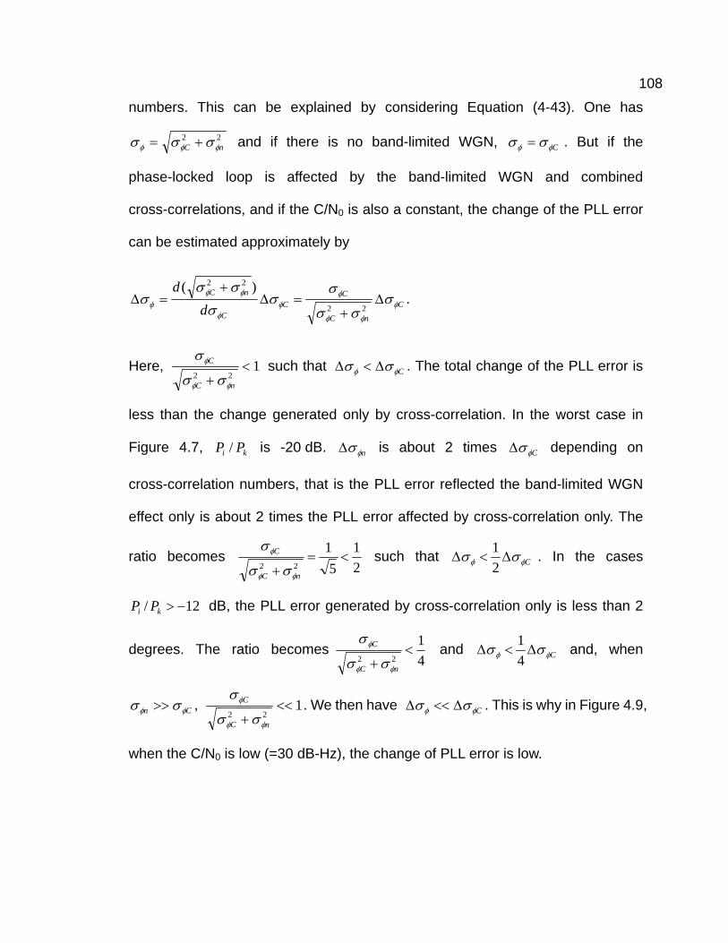
108
numbers. This can be explained by considering Equation (4-43). One has
22nC φφφ σσσ += and if there is no band-limited WGN, Cφφ σσ = . But if the
phase-locked loop is affected by the band-limited WGN and combined
cross-correlations, and if the C/N0 is also a constant, the change of the PLL error
can be estimated approximately by
C
nC
CC
C
nC
dd
φ
φφ
φφ
φ
φφφ σ
σσ
σσ
σσσ
σ ∆+
=∆+
=∆22
22 )(.
Here, 122<
+ nC
C
φφ
φ
σσ
σ such that Cφφ σσ ∆<∆ . The total change of the PLL error is
less than the change generated only by cross-correlation. In the worst case in
Figure 4.7, ki PP / is -20 dB. nφσ∆ is about 2 times Cφσ∆ depending on
cross-correlation numbers, that is the PLL error reflected the band-limited WGN
effect only is about 2 times the PLL error affected by cross-correlation only. The
ratio becomes 21
51
22<=
+ nC
C
φφ
φ
σσ
σ such that Cφφ σσ ∆<∆
21 . In the cases
12/ −>ki PP dB, the PLL error generated by cross-correlation only is less than 2
degrees. The ratio becomes41
22<
+ nC
C
φφ
φ
σσ
σ and Cφφ σσ ∆<∆
41 and, when
Cn φφ σσ >> , 122<<
+ nC
C
φφ
φ
σσ
σ. We then have Cφφ σσ ∆<<∆ . This is why in Figure 4.9,
when the C/N0 is low (=30 dB-Hz), the change of PLL error is low.

109
Figure 4.9 PLL Errors with Cross-Correlations and White Gaussian Noise
4.4 Conclusions
In this chapter, the PLL jitter was theoretically derived. To justify the theoretical
results, a simulation is carried out to compare the theoretical derivation. The
results describe the changes of PLL errors in three situations. Under band-limited
WGN only, when the C/N0 is normal (equal to 42.8 dB-Hz), the theoretical and
simulation value match well. Under a low C/N0, because of the non-linear nature of
a phase-locked loop, the differences between theoretical and simulation results
become large. Under the cross-correlations only, the PLL error increases rapidly
with the decrease of ki PP / when 10/ −<ki PP dB. Under the band-limited WGN

110
and cross-correlations combined, when the band-limited WGN becomes large (low
C/N0), the changes of PLL error generated by cross-correlations increase slowly as
a function of ki PP / . The reason is that the effects of large band-limited WGN
overwhelm the effects of cross-correlations.

111
Chapter 5
Conclusions and Recommendations
5.1 Conclusions
The main purpose of this thesis is to study the effects of RF interferences, such as
cross-correlations and white Gaussian noise, on GPS L2C signal acquisition and
carrier tracking, using both theoretical and simulated studies. The research is
focused on the CM code acquisition and tracking under RF interference.
The probability of CM code detection under cross-correlation and white Gaussian
noise was derived and simulated. Under the band-limited WGN only or the
band-limited WGN and one worst cross-correlation combined, the non-coherent
integration with M=3 has a 3 to 4 dB-Hz better ability to detect the desired signal
than the one with M=1. With the same non-coherent integration number M, the
detection abilities under band-limited WGN only is about 1 dB-Hz higher than the
detection abilities under one worst cross-correlation and band-limited WGN
combined. The worst-case cross-correlation was derived theoretically. The
worst-case cross-correlation is between a local CM code (PRN=26) and incoming
CL code (PRN=4), with a value of -31.1 dB. The practical calculation is done and
the worst cross-correlation case is used in CM code detection and the sign
evaluation of the in-phase component.
The error probability of information data estimation in the worst case is derived
under cross-correlation and white Gaussian noise combined. When the power of

112
the desired signal is the same as the power of the undesired signal, the difference
of the maximum error probabilities of information data estimation generated by the
cross-correlations is not very large. The main effect on maximum error
probabilities comes from band-limited WGN. Under the situation of a weak desired
signal, if the unwanted signal power is higher than the desired signal power (more
than 8 dB), the maximum error probabilities of information data estimation grow
very fast with the decrease of the ratio Pi/Pk, especially when 4≥K .
The SNR simulation results support the SNR theoretical derivation well. Under the
band-limited WGN only, the SNR is linearly reduced from 26 dB to 6 dB with the
reduction of the desired incoming signal power from -160 dBW to -180 dBW. The
RMS error of the simulation from Figure 3.5 is less than 0.19 dB. When the desired
incoming signal power is -160 dBW, the SNR is about 26 dB. Under the
cross-correlations and band-limited WGN combined, when the unwanted signal
power is almost the same as the desired signal power, the SNR is near 26 dB. The
two results are almost the same. The effects from the cross-correlations can be
ignored as compared to the effects of band-limited WGN. With an increase in the
ratio of the unwanted signal power to the desired signal, the cross-correlations
become an important factor on the SNR result. It cannot be ignored compared to
the effects of band-limited WGN.
In PLL performance analyses of both theory and simulation, it is assumed that the
DLL tracking is ideal. The local CM code exactly matches the incoming CM code,
and there is no error from DLL tracking to affect the PLL performance. There are

113
estimation errors in the PLL performance analyses, especially in the situation of
low C/N0 or low ratio of desired signal power to unwanted signal power from other
satellites ki PP / . The estimation errors occur because in the theoretical model,
only linear status is considered. The model is assumed only in the small phase
error environment. The phase error φ is used instead of its sinusoid. So when the
phase error becomes large under strong interference, the simulation results
display the non-linear property of PLL. Then the estimation error is generated and
grows large when the interferences become strong; but if we compare the
estimation errors with the PLL errors, it is still small.
In the analyses of PLL performance, under the band-limited WGN only, the PLL
error for simulations match the theoretical result very well when the C/N0 is normal
(=42.8 dB-Hz). With the decrease of C/N0, the difference between the simulation
result and theoretical result becomes large because of the non-linear property of
the PLL tracking loop. Under the cross-correlations only, the PLL error increases
rapidly with the decrease of ki PP / when 10/ −<ki PP dB. Because of the PLL’s
non-linear property, the estimation error becomes large when ki PP / is low. In the
situation of the two interferences combined, because the band-limited WGN is
larger than cross-correlation in general, especially under the low C/N0 (=30 dB-Hz),
the PLL error comes mainly from the band-limited WGN effects. The estimation
error becomes large because of the non-linear PLL property. Therefore the
simulation results and theoretical results are considered separately when the
estimation error made by nonlinear property is larger than the error made by

114
cross-correlation.
5.2 Recommendations
Considering the findings from this thesis, it is recommended that advanced
research be performed in the following areas.
First, CL code acquisition and tracking should be studied, because only CM code
acquisition and tracking is studied in this thesis. The CL code is long, with a 1.5 s
period. There is no navigation data on the CL code. If the CL code is analysed, a
longer coherent integration time can be used, helping to increase SNR in signal
detection.
Second, DLL tracking performance should be considered, because in this thesis
only PLL performance is analysed and it is assumed that the DLL tracking is
correct. In the real-world case, PLL tracking and DLL tracking errors affect the PLL
and DLL tracking performance and vice versa, such that considering only one of
them is not sufficient. If there are errors in the two tracking loops under
cross-correlations and white Gausssian noise conditions, performance of the PLL
should be different than the results for which only PLL error is considered.
The SNR analysis is done under the assumption that there is no code delay and no
carrier offset for the desired signal. The worst case of cross-correlations and the
average SNR is studied in the ideal situation. In fact, in the normal situation, there
is not only code delay, but also carrier offset for the desired signal. There is loss of
desired signal power, and the average SNR should be degraded.
115
Third, the discriminator should be studied further, because in this thesis only one
type of discriminator is analysed and the linear model in used in small phase error
conditions. If other discriminators are considered, can the linear model be used? If
the discriminator must be analysed in non-linear status, can the non-linear model
be simplified so as to analyse the PLL or DLL performance theoretically? These
are questions that should be addressed.

116
REFERENCES
Bastide, F., O. Julien, C. Macabiau, and B. Roturier, (2002) “Analysis of L5/E5 Acquisition, Tracking and Data Demodulation Thresholds,” in Proceeding of ION 24-27 September, Portland, OR, pp. 2196-2207, U.S. Institute of Navigation, Fairfax, VA
Best, R. E. (2003), Phase-Locked Loops Design, Simulation, and Applications, McGraw-Hill, New York
Cho, D. J., C. Park, and S. J. Lee, (2004) “An Assisted GPS Acquisition Method using L2 Civil Signal in Weak Signal Environment,” The 2004 International Symposium on GPS/GNSS 6-8 December, Sydney, Australia
Deshpande, S. and M.E. Cannon (2004a) “Interference Effects on the GPS Signal Acquisition,” in Proceeding of ION NTM 26-28 January, San Diego, CA, pp. 1027-1036, U.S. Institute of Navigation, Fairfax, VA
Deshpande, S. (2004b) “Modulated Signal Interference in GPS Acquisition,” in Proceeding of ION 21-24 September, Long Beach, CA, pp. 76-86, U.S. Institute of Navigation, Fairfax, VA
Fontana, R.D., W. Cheung, P. M. Novak, and T. A. Stansell (2001) “The New L2 Civil Signal,” in Proceeding of ION 11-14 September, Salt Lake City, UT, pp. 617-631, U.S. Institute of Navigation, Fairfax, VA
Hegarty, C., A. J. Van Dierendonck, D. Bobyn, M. Tran, T. Kim, and J. Grabowski (2000) “Suppression of Pulsed Interference through Blanking,” in Proceeding of the IAIN World Congress in Assoiation with the U.S. ION Annual Meeting 26-28 June, San Diego, CA, pp. 399-408, U.S. Institute of Navigation, Fairfax, VA
Holmes, J. K. (1990), Coherent Spread Spectrum Systems, Wiley & Sons, New York, NY
Huang, W., I. Andonovic, and M. Nakagawa (1998) “PLL Performance of DS-CDMA Systems in the Presence of Phase Noise, Multiuser Interference, and Additive Gaussian Noise,” IEEE Transactions on Communications, Volume 46, No. 11, November, pp. 1507-1515
IS-GPS-200D (2004) NAVSTAR GPS Space Segment / Navigation User Interfaces, Space and Missile Systems Center (SMC) and Navstar GPS Joint Program Office (SMC/GP)

117
Kaplan, E.D. (1996), Understanding GPS: Principles and Applications, Artech House, Norwood, MA
Kumar, R., S. H. Raghavan, M. Zeitzew, P. Munjal and S. Lazar (1999) “Analysis of Code Cross Correlation Noise in GPS Receivers Operating in Augmented GPS Systems,” in Proceeding of ION NTM 25-27 January, San Diego, CA, pp. 295-304, U.S. Institute of Navigation, Fairfax, VA
Parkison, B.W. and J.J. Spilker Jr (1996), Global Positioning System: Theory and Applications, American Institute of Aeronautics and Astronautics, Washington
Peterson, W. W. (1962) Error-Correcting Codes, The M.I.T. Press
Pursley, M. B. (1977) “Performance Evaluation for Phase-Coded Spread-Spectrum Multiple-Access Communication—Part I: System Analysis,” IEEE Transactions on Communications, Volume 25, No. 8, August, pp. 795-799
Tang, B. and D. E. Dodds (2006) “Weak Signal GPS Synchronization For Locating In-Building Cellular Telephones,” IEEE CCECE/CCGEI, pp. 928-931
Tran, M. and C. Hegarty (2003) “Performance Evaluations of the New GPS L5 and L2 Civil (L2C) Signals,” in Proceeding of ION NTM 22-24 January, Anaheim, CA, pp. 521-535, U.S. Institute of Navigation, Fairfax, VA
Viterbi, Andrew J. (1966) Principles of Coherent Communication, McGraw-Hill, Inc.
Zhu, Z. and F. van Graas (2005) “Effects of Cross Correlation on High Performance C/A Code Tracking,” in proceedings of ION NTM 24-26 January, San Diego, CA, pp. 1053-1061, U.S. Institute of Navigation, Fairfax, VA