UCGE Reports Number 20266

Department of Geomatics Engineering A vector-based geographical cellular automata model to mitigate scale sensitivity and to allow objects’ geometric

transformation (URL: http://www.geomatics.ucalgary.ca/research/publications/GradTheses.html)

by

Niandry Leet Moreno

February, 2008

UNIVERSITY OF CALGARY

A vector-based geographical cellular automata model to mitigate scale

sensitivity and to allow objects’ geometric transformation

by

Niandry Leet Moreno

A THESIS

SUBMITTED TO THE FACULTY OF GRADUATE STUDIES

IN PARTIAL FULFILLMENT OF THE REQUIREMENTS FOR THE

DEGREE OF Doctor of Philosophy

DEPARTMENT OF GEOMATICS ENGINEERING

CALGARY, ALBERTA

February, 2008

© Niandry Leet Moreno 2008

i

Abstract

Raster-based cellular automata (CA) models have been increasingly used over the last

decades to simulate a wide range of spatial phenomena, but recent studies have illustrated

that they are scale sensitive, that is their results vary with the cell size and neighbourhood

configuration. Two solutions have been proposed to mitigate this problem: a sensitivity

analysis to determine the most appropriate cell size and neighbourhood configuration that

capture the dynamics of the study area, and the implementation of an object or vector-

based cellular automata model independent of the cell size and the neighbourhood

configuration. Several researchers have begun to implement vector-based CA models that

define space based on the GIS (Geographic Information Systems) vector model, but these

models have several limitations. First, the polygons and the neighbouring relationships

are mainly based on Voronoi boundaries which are automatically defined in the model.

The polygons do not necessarily correspond to meaningful entities and spatial

relationships; characteristics such as attractivity, connectivity or accessibility are not

taken into account. Second, their sensitivity to the neighbourhood configuration has not

been tested; the number and distribution of the neighbours determine the change of state

of an object, therefore their selection could affect the simulation outcomes. Finally, these

models do not allow the change of shape of the objects, which represent an essential

component of their spatial evolution through time.

ii

In this research, a new vector-based cellular automata (VecGCA) model is proposed to

overcome the cell size and neighbourhood configuration sensitivity of the classical raster-

based CA models and the limitations of the previous implementations of vector-based CA

models. In the VecGCA model, space is represented as a collection of geographic objects

where each object corresponds to a real-world entity of irregular shape and size (e.g. a

forest, a city, a lake). Each geographic object has its own geometric representation

(polygon) which evolves through time according to a transition function that depends on

the influence of its neighbours. This evolution is expressed by the change of shape and

size of the objects and it is performed using a geometric transformation procedure. This

procedure reduces the area of an object in the region nearest to the neighbour that exerts

an influence on it and increases the area of that neighbour.

Two neighbourhood definitions were tested: a buffer of influence and a dynamic

neighbourhood. In the first case, the neighbourhood is considered as the region of

influence on each geographic object, where the neighbours are all geographic objects

located within the region of influence; the transition function determines the area of an

object that must change state for the state of its neighbours. In the dynamic

neighbourhood, the neighbourhood is the whole geographic space and the neighbours are

defined based on the properties of each geographic object; two objects are neighbours if

they are separated by 0, 1 or more objects whose states favour the state transition between

them. The transition function defines the distance, from the closest point to the neighbour

iii

to a point in its interior, where the influence of that neighbour is equal to a threshold

value, which represents the resistance of an object to change state.

The model was used to simulate land-use/land-cover changes in two regions of different

landscape complexity, in southern Quebec and southern Alberta, Canada. The results

obtained show that VecGCA represents well the dynamics in the study areas through an

adequate evolution of the geometry of the geographic objects which are independent of

the cell size. The geometric transformation procedure introduced in VecGCA executes

the change of shape of a geographic object by changing its state in a portion of its

surface, allowing a more realistic representation of the evolution of the landscape.

Additional results reveal that when using the first neighbourhood definition, VecGCA is

sensitive to the neighbourhood size and that this sensitivity varies with the landscape

configuration. When applying a dynamic neighbourhood, the land-use patterns generated

by the model are very similar to the reference maps in each study area. With the

implementation of a dynamic neighbourhood, VecGCA becomes independent of spatial

scale, including both cell size and neighbourhood configuration.

iv

Acknowledgements

I would like to express my sincere thanks and appreciation to my supervisor Dr. Danielle

J. Marceau for her continuous support, enthusiasm, dedication, encouragement and

guidance during research. It was a pleasure to work under her supervision.

Many thanks go to all my colleagues in the Geocomputing Laboratory for their help,

advice, encouragement, and friendship. Special thanks to Dr. André Ménard, Jean-

Gabriel Hasbani and Fang Wang for their valuable suggestions and discussions about my

research.

To my professors and friends at the Simulation and Modelling Centre of the University of

Los Andes, Venezuela, thank you for their constant guidance.

To my great husband Jose Gregorio, thank you very much, I love you. Your help and

support cannot be described by words. My little Isabella, you are my inspiration, you

pushed to complete this work; I love you so much. And thanks to my parents for their

love and support throughout my life.

This research was funded by scholarships obtained from the Organization of American

States (OAE), the Department of Geography at the University of Montreal, the

v

Department of Geomatics Engineering at the University of Calgary and the University of

Los Andes, Venezuela. My research was also supported by a NSERC (Natural Sciences

and Engineering Research Council) research grant awarded to my supervisor.

vi

Dedication

To

Jose Gregorio and Isabella

vii

Table of contents Abstract................................................................................................................................ i

Acknowledgements............................................................................................................ iv

Dedication.......................................................................................................................... vi

Table of contents .............................................................................................................. vii

List of Tables ..................................................................................................................... ix

List of Figures ................................................................................................................... xi

List of abbreviations and symbols .................................................................................. xiii

INTRODUCTION.............................................................................................................. 1 1.1 Scale sensitivity of the raster-based CA models................................................................ 6 1.2 Solutions proposed to overcome the scale sensitivity in the raster-based CA models.10 1.3 Problem statement and research objectives .................................................................... 15 1.4 Research scope ................................................................................................................... 17 1.5 Assumptions and limitations............................................................................................. 17 1.6 Thesis outline ..................................................................................................................... 18

DESCRIPTION OF VecGCA MODEL AND COMPARISON WITH A RASTER-BASED CA MODEL........................................................................................................ 20

2.1 Conceptual model .............................................................................................................. 20 2.1.1 Procedure of geometric transformation.......................................................................................25

2.2 Implementation.................................................................................................................. 27 2.2.1 Simulation algorithm ..................................................................................................................34 2.2.2 Geometric transformation algorithm...........................................................................................38

2.3 Comparison of VecGCA and a raster-based CA model to simulate land-use changes41 2.3.1 Land-use change modelling ........................................................................................................41 2.3.2 Study area and dataset.................................................................................................................44 2.3.3 Definition of the VecGCA model ...............................................................................................46 2.3.4 Definition of the raster-based CA model ....................................................................................52 2.3.5 Model simulations.......................................................................................................................54 2.3.6 Results.........................................................................................................................................56

2.4 Discussion ........................................................................................................................... 64 PERFORMANCE IMPROVEMENT OF THE GEOMETRIC TRANSFORMATION PROCEDURE AND SENSITIVITY ANALYSIS OF VecGCA TO THE NEIGHBOURHOOD SIZE............................................................................................. 66

3.1 Update of VecGCA model................................................................................................. 66 3.1.1 Simulation procedure..................................................................................................................68

viii

3.2 Sensitivity analysis of VecGCA to the neighbourhood size............................................ 72 3.2.1 Study areas..................................................................................................................................73 3.2.2 The land-use/land-cover VecGCA model...................................................................................75 3.2.3. Model simulation .......................................................................................................................75 3.2.4 Results.........................................................................................................................................76

3.3. Discussion .......................................................................................................................... 88 DYNAMIC NEIGHBOURHOOD IN VecGCA.............................................................. 91

4.1 Dynamic neighbourhood definition and update of VecGCA......................................... 91 4.2 Land-use change VecGCA models using a dynamic neighbourhood ......................... 100

4.2.1 Study areas................................................................................................................................100 4.2.2 The land-use VecGCA model ...................................................................................................101 4.2.3 Model simulations.....................................................................................................................102 4.2.4 Results.......................................................................................................................................103

4.3 Discussion ......................................................................................................................... 108 CONCLUSION............................................................................................................... 111

5.1 Recommendations for future work ................................................................................ 114 REFERENCES .............................................................................................................. 116

APPENDIX A................................................................................................................. 125

ix

List of Tables

Table 2.1. Transition probabilities defined from the comparison of the two vector land-use maps of 1999 and 2002 for a temporal resolution of three years ...……….

49

Table 2.2. Threshold values indicating the minimum influence that a polygon must exert on another to produce a geometric transformation ...……...………………….

51

Table 2.3. Transition probabilities for the raster-based CA model of 30 m (W=Water, F=Forest, A=Agriculture, U=Urban) ...………………………………...

53

Table 2.4. Transition probabilities for the raster-based CA model of 100 m (W=Water, F=Forest, A=Agriculture, U=Urban) …...……………………………...

54

Table 2.5. Statistics describing the simulation outcomes of the VecGCA model and the raster-based CA models, and comparison with the 2002 raster land-use map (F=Forest, A=Agriculture) …………………………………………………….

57

Table 2.6. Proportion of simulated area that coincides with the state of the system in 2002 for each land use …………………………………………………………...

59

Table 2.7. Statistics describing the simulation outcomes of the VecGCA model and the raster-based CA models for 2032 (F=Forest, A=Agriculture) ….………….

62

Table 3.1. Average computation time of the procedures called in the new implementation of the model ….…………………………………..………………..

80

Table 3.2. Proportion of land-use/land-cover (%) in the Maskoutains region using different neighbourhood sizes …………………………………………………….

81

Table 3.3. Proportion of land-use/land-cover (%) in the Elbow river watershed using different neighbourhood sizes …..…………………………………………..

82

Table 4.1. Matrix of favourable states for land-use transitions in Maskoutains region ……………………………………………………………………………….

102

Table 4.2. Matrix of favourable states for land-use transitions in Elbow river watershed …………………………………………………………………………...

102

Table 4.3. Proportion of land uses for 2002 produced by VecGCA and percentage

x

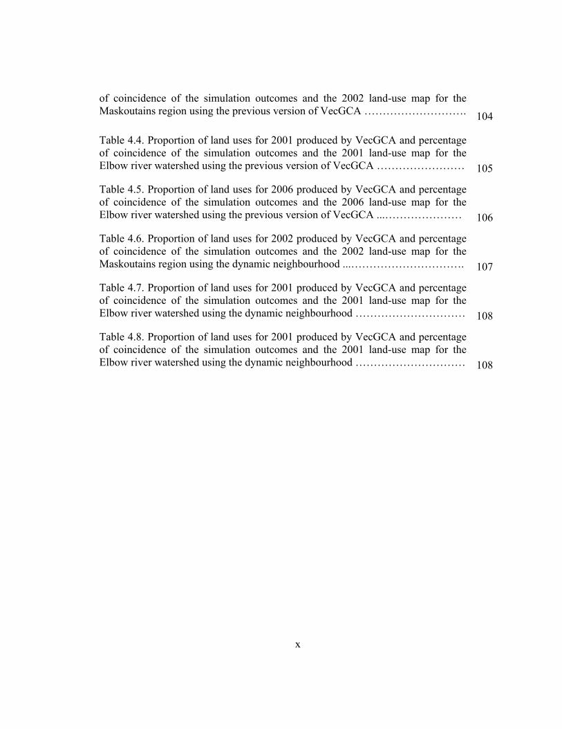
of coincidence of the simulation outcomes and the 2002 land-use map for the Maskoutains region using the previous version of VecGCA ……………………….

104

Table 4.4. Proportion of land uses for 2001 produced by VecGCA and percentage of coincidence of the simulation outcomes and the 2001 land-use map for the Elbow river watershed using the previous version of VecGCA ……………………

105

Table 4.5. Proportion of land uses for 2006 produced by VecGCA and percentage of coincidence of the simulation outcomes and the 2006 land-use map for the Elbow river watershed using the previous version of VecGCA ...…………………

106

Table 4.6. Proportion of land uses for 2002 produced by VecGCA and percentage of coincidence of the simulation outcomes and the 2002 land-use map for the Maskoutains region using the dynamic neighbourhood ...………………………….

107

Table 4.7. Proportion of land uses for 2001 produced by VecGCA and percentage of coincidence of the simulation outcomes and the 2001 land-use map for the Elbow river watershed using the dynamic neighbourhood …………………………

108

Table 4.8. Proportion of land uses for 2001 produced by VecGCA and percentage of coincidence of the simulation outcomes and the 2001 land-use map for the Elbow river watershed using the dynamic neighbourhood …………………………

108

xi

List of Figures

Figure 1.1. Illustration of Conway’s “Game Life” ...……………………………….. 3

Figure 2.1. Geographic space composing by five objects: a, b, c, d and e. The neighbourhood around a is defined by r and the neighbours of a are the objects b and d ……………………………………………………………..………………...

22

Figure 2.2. Illustration of a performed of geometrical transformation procedure …. 27

Figure 2.3. UML diagram of the library of components that defines the VecGCA model ……………………………………………………………….........................

29

Figure 2.4. Simulation flow chart of VecGCA model ..……………………………. 37

Figure 2.5. Flow chart of geometric transformation in VecGCA ……..……………. 40

Figure 2.6. Land-use map of the Maskoutains region: (a) 1999, and (b) 2002 …….. 46

Figure 2.7. The 2002 land-use maps and the land use spatial distribution generated by the VecGCA model and the raster-based CA models in 2002 ...………………...

60

Figure 2.8. Proportion of forested and agricultural area calculated on the simulation outcomes of the VecGCA and the 30 m and 100 m raster-based CA models ………

61

Figure 3.1. Improved implementation of the geometrical transformation procedure.. 71

Figure 3.2 Land-use maps of the Elbow river watershed: (a) 1996, and (b) 2001 …. 74

Figure 3.3. The 1999 vector land-use/land-cover map of the Maskoutains sub-region and the spatial distribution generated by the VecGCA for the year 2002 using the first and the improved implementations of the model …...……………….

78

Figure 3.4. Schematic representation of the landscape configuration of the Maskoutains region where the objects have only one neighbour for different neighbourhood sizes …………………………………………………………………

84

Figure 3.5. Schematic representation of the Elbow river landscape configuration where the objects have several neighbours; when the neighbourhood size increases the number of neighbours and the neighbours’ area within the neighbourhood also increase ……..…........................................................................................................

85

xii

Figure 3.6. Simulation outcomes for the Maskoutains region for 2002 using different neighbourhood sizes ...…………………………………………………...

86

Figure 3.7. Simulation outcomes for the Elbow river watershed for 2001 using different neighbourhood sizes ..………………………………………………...….

87

Figure 4.1. Geographic space composed by six geographic objects. The geographic object A has four neighbours: the adjacent objects B, C and D, and non adjacent object E ……………………………………………………………………………...

93

Figure 4.2. Influence function used to implement the dynamic neighbourhood ….. 95

Figure 4.3. Schematic representation of the distance calculated from the transition function that defines the buffer size to be built around each neighbour to take a portion of a central object (geometric transformation procedure described in the section 3.1.1) ………………..……………………………………………………….

99

xiii

List of abbreviations and symbols

CA Cellular automata

GCA Geographical cellular automata

VecGCA Vector-based geographical cellular automata

GIS Geographic information systems

MAS Multi-agent system

fa Transition function of object a

gab Influence of the object a on the object b

λab Threshold value to change from the b’s state to a’s state

Aa Area of the object a

Pb→a Probability to change from b’s state to a’s state

dab Distance between the centroid of the object a and the centroid of the

object b

dminab Minimum distance between the object a and the object b

Chapter 1 1

1

CHAPTER 1

INTRODUCTION

Cellular Automata (CA) are dynamic systems defined by a large tessellation of finite-

state cells whose states are updated at discrete time steps according to deterministic or

probabilistic rules, which dictate how the state of each cell might change based on the

state of its neighbouring cells. They were introduced by Ulam and Von Neumann in the

1940’s to investigate self-reproductive systems (Von Neumann 1966). Formally, a CA is

defined by five basic elements: space, set of states, neighbourhood, transition rules and

time. In the classic definition of CA, space is defined as an infinite and regular

tessellation of cells of discrete states. Each cell can take one state from a set of states that

defines the outcomes of the system. The state of any cell depends on the states and

configurations of other cells in the neighbourhood of that cell, where the neighbourhood

is the adjacent set of cells to that cell. Transitions rules (also known as transition

functions) drive the change of state in each cell; they are usually specified as a table of

Chapter 1 2

2

rules that define the next state of a cell for each possible configuration of neighbourhood.

Finally, time represents the minimum necessary time interval for a cell to change state.

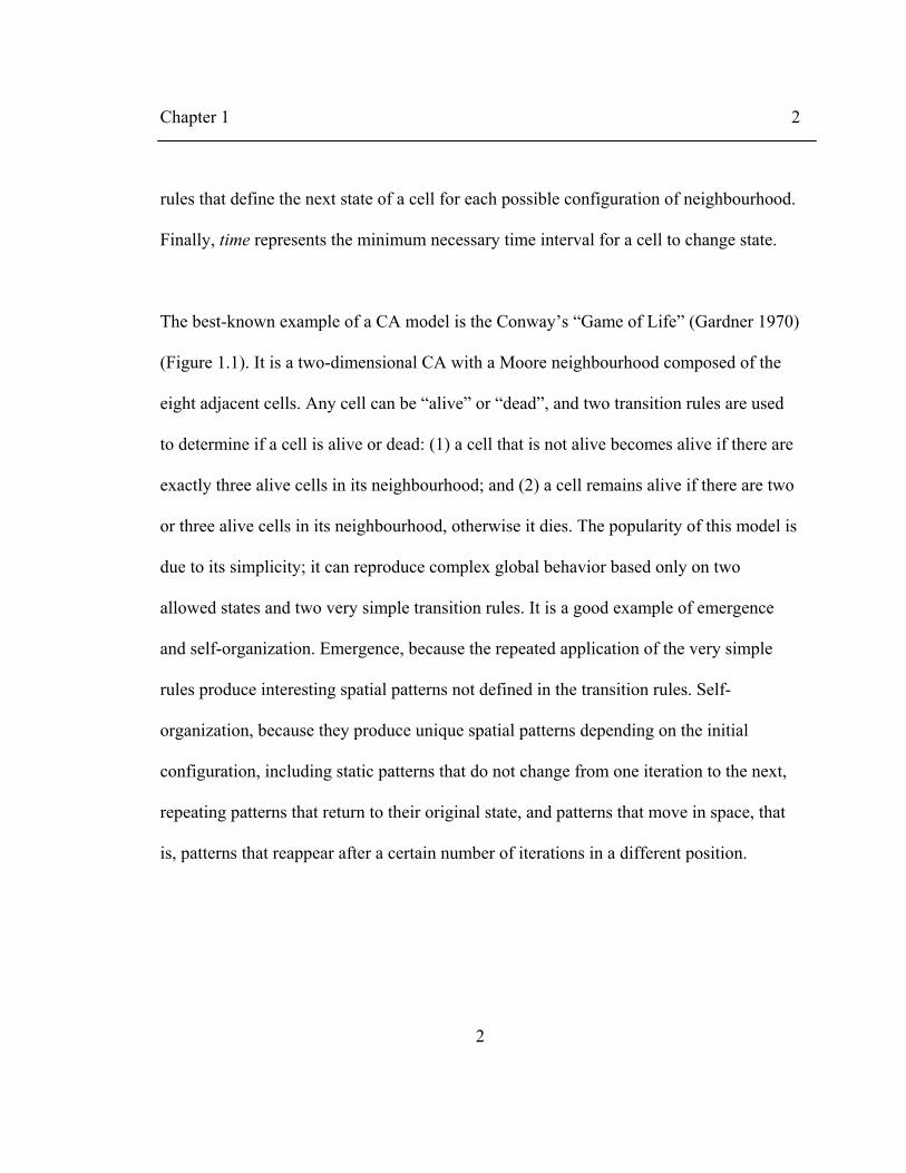
The best-known example of a CA model is the Conway’s “Game of Life” (Gardner 1970)

(Figure 1.1). It is a two-dimensional CA with a Moore neighbourhood composed of the

eight adjacent cells. Any cell can be “alive” or “dead”, and two transition rules are used

to determine if a cell is alive or dead: (1) a cell that is not alive becomes alive if there are

exactly three alive cells in its neighbourhood; and (2) a cell remains alive if there are two

or three alive cells in its neighbourhood, otherwise it dies. The popularity of this model is

due to its simplicity; it can reproduce complex global behavior based only on two

allowed states and two very simple transition rules. It is a good example of emergence

and self-organization. Emergence, because the repeated application of the very simple

rules produce interesting spatial patterns not defined in the transition rules. Self-

organization, because they produce unique spatial patterns depending on the initial

configuration, including static patterns that do not change from one iteration to the next,

repeating patterns that return to their original state, and patterns that move in space, that

is, patterns that reappear after a certain number of iterations in a different position.

Chapter 1 3

3

Figure 1.1. Illustration of Conway’s “Game of Life”

In 1984, Stephen Wolfram presented the CA model as a modelling paradigm for complex

systems due to its capacity to generate complex patterns from simple local iterations. He

studied the complex behaviour produced by a very simple class of CA (one-dimensional,

two-states CA) capable of universal computation (Turing machine) and suggested that the

complexity in nature could be generated by the same principle, that is the cooperation of

many simple identical components. In his book “A New Kind of Science” (Wolfram

2002), he argues that simple programs, such as CA, are able to capture the essence of

almost any complex system.

Chapter 1 4

4

Theoretical applications of CA, such as the Game of Life or the CA model presented by

Wolfram (1984) that reproduces the Turing machine, generally consist in taking a given

rule and discovering its properties, referred to as the forward problem (Gutowitz 1990).

This approach is generally applied in formal language theory, computation theory,

physics and mathematics. In social and natural sciences, most applications follow an

inverse approach, which consists in discovering the rules that produce the observed

patterns in the studied phenomenon, and frequently in using these rules to forecast its

future behavior.

Due to their computational simplicity and their explicit representation of space and time,

CA models constitute a powerful tool to model complex natural and human systems.

However, the classical definition of CA assumes certain characteristics that make their

application difficult for simulating real-world phenomena:

1. the transition rules are uniformly applied to all cells at fixed time intervals;

2. the same neighbourhood is defined for all cells, and

3. every change in state must be local, that is the transition rules define the change of

state of a single cell based on its neighbourhood configuration.

To overcome these limitations, several CA extensions have been proposed. In a pioneer

work, Couclelis (1985) presented a model allowing the separation of the neighbourhood

Chapter 1 5

5

set and the transition rules for each cell. Takeyama and Couclelis (1997) developed a

mathematical framework, called Geo-Algebra, which expresses the modelling paradigm

of CA in the form of map equations. In addition, Geo-Algebra generalizes the structure of

standard CA to accept arbitrary, spatially variant neighbourhoods and transition rules.

Other studies conducted by White et al. (1997) and O’Sullivan (2001a) extend the

definition of neighbourhood as the set of all cells (adjacent or not) that influence the state

of a particular cell, defined as a radius of influence and as a graph of influence,

respectively. Additionally, White et al. (1997) introduced the use of constrained CA

where a CA model is linked to an external sub-model that defines the number of cells that

change state at each time step.

Others authors have contributed to improve different aspects related to CA modelling,

including model calibration and validation (Li and Yeh 2000; Li and Yeh 2002; Wu

2002; Liu and Phinn 2003; Li and Yeh 2004; Straatman et al. 2004; Dietzel and Clarke

2007; Hasbani and Marceau 2007), neighbourhood definition, and the analysis of

neighbourhood relationships (O’Sullivan 2001a,b; Verburg et al. 2004).

Thanks to all these advances, in the last few years, numerous studies involving the

application of CA in a geographic context have been undertaken. Geographic cellular

automata (GCA) have been used to simulate land-use and land-cover changes (Li and

Chapter 1 6

6

Yeh 2002; Wu 2002; Almeida et al. 2003; Ménard and Marceau 2007), fire propagation

(Berjak and Hearne 2002; Favier et al. 2004; Yassemi et al. 2007), vegetal succession

(Soares-Filho et al. 2002; Rietkerk et al. 2004), and urban growth and development

(White 1998; Li and Yeh 2000; Liu and Phinn 2003; Dietzel and Clarke 2005; Lau and

Kam 2005).

All these applications have been done using a discrete space representation and a regular

tessellation of cells of same size and shape similar to the Geographic Information System

(GIS) raster model. However, recent studies have demonstrated that such raster-based CA

models are sensitive to spatial scale, that is the simulation outcomes might vary with the

cell size and the neighbourhood configuration.

1.1 Scale sensitivity of the raster-based CA models

Many factors must be considered when elaborating a CA model; the spatial scale is

certainly amongst the most important. Scale generally represents the window of

perception through which reality is observed (Marceau 1999). In a GCA, spatial scale is

defined by three components: the spatial extent, the cell size and the neighbourhood

configuration. The spatial extent corresponds to the geographic area to be modelled. The

cell size specifies the area covered by each cell. The neighbourhood configuration

determines the distribution and number of neighbours that have an influence in the

Chapter 1 7

7

change of state of a cell. Selecting the appropriate value for these components is a key

step in the definition of a GCA. If this selection is wrong, the model cannot adequately

capture the dynamics of the study area. The problem is that the selection of cell size and

neighbourhood configuration is generally arbitrary; they are usually determined by a

mixture of data availability, intuition, computing and resource considerations, trial and

error, and information about spatial unit size or influence. There are no standard methods

to determine the appropriate cell size that represents key entities of a study area, or to

identify the best neighbourhood configuration that drives the change of state of a cell.

Several researchers have studied the effect of the cell size and neighbourhood

configuration in the simulation outcomes of raster-based CA models. Jenerette and Wu

(2001) developed a Markov-cellular automata model to simulate land-use changes in the

central Arizona – Phoenix region, USA, and performed simulation using two spatial

resolutions of 250 m and 75 m. Their results revealed that the resolution affects the

ability of the model to simulate land-use changes, the coarser resolution generating more

realistic spatial patterns than the finer resolution.

Chen and Mynett (2003) investigated the impact of cell size and neighbourhood

configuration in a raster-based CA prey-predator model (EcoCA). They tested four

different scenarios (two cell sizes and two neighbourhood configurations) and observed

Chapter 1 8

8

that the cell size affects the spatial patterns generated by the model, while the

neighbourhood configuration influences both the spatial patterns and the system stability.

A smaller cell size produces more segmented spatial patterns although the general

statistics (mean and standard deviation of population density) do not show significant

differences. They propose to use the spatial scale of relevance in the ecosystem under

study as cell size and the standard Moore neighbourhood in order to achieve a consistent

model behavior independent of the cell size. Spatial auto-correlation and Wavelet

analysis are proposed as methods to find the relevant spatial scale in the studied

ecosystem.

Jantz and Goetz (2005) presented the results of a sensitivity analysis of a cellular urban

land-use change model, SLEUTH, by testing its performance when the cell size is

changed. SLEUTH is a CA-based urban growth model coupled with a land-cover change

model that simulates the urban dynamics using four growth rules: spontaneous new

growth, new spreading centre growth, edge growth and road-influence growth. Four cell

sizes were tested (45 m, 90 m, 180 m, and 360 m) and four separate calibration

procedures were performed, one for each cell size. Their results showed that SLEUTH

was able to capture the rate of growth across all cell sizes, but its ability to replicate urban

growth patterns varies with the cell size. They suggest performing a sensitivity analysis to

Chapter 1 9

9

assess the impact of the cell size on the simulation outcomes and to identify the cell size

with which the model can better capture the dynamics of the study area.

In a study undertaken to assess the spatial scale sensitivity in a land-use change CA

model, Ménard and Marceau (2005) tested five different cell sizes (30 m, 100 m, 200 m,

500 m and 1000 m) and six neighbourhood configurations (Moore, Von Neumann and

three circulars, of approximately two-cell, three-cell and five-cell radius), which create

thirty different scenarios. Their results demonstrated that the choice of cell size and

neighbourhood configuration has a considerable impact on the simulation results in terms

of land-cover area and spatial patterns. They also revealed that using the finest resolution

available is not always the best selection. In that model, 30 m resolution generates a

highly fragmented landscape that does not correspond to a realistic dynamics in the study

area. The authors propose to systematically conduct a sensitivity analysis to identify the

appropriate cell size and neighbourhood configuration and advocate the development of

an object-based CA model to mitigate scale sensitivity.

Kocabas and Dragicevic (2006) explored the impact of changing the cell size and

neighbourhood configuration on the outcomes of a raster-based CA urban growth model.

Two neighbourhood types (rectangular and circular) and 54 neighbourhood sizes were

used. Four spatial resolutions were also tested (50 m, 100 m, 150 m and 250 m) for a total

Chapter 1 10

10

of 432 scenarios being evaluated. A visual inspection of the simulation outcomes showed

that different neighbourhood types generate different spatial patterns for the same

neighbourhood size. Also, decreasing the spatial resolution produces different spatial

patterns in the simulation results for the same neighbourhood size. Changing the spatial

resolution did not produce significant changes in the Kappa index, but changes were

significant when neighbourhood size and type vary. Finally, the analysis of spatial

metrics showed that both neighbourhood sizes and types have a strong influence on the

simulation outcomes and that the spatial resolution affects the spatial patterns generated

by the model. The authors proposed to conduct a sensitivity analysis approach combining

qualitative and quantitative measures to improve the accuracy, precision and relevance of

the simulation outcomes of a CA model.

1.2 Solutions proposed to overcome the scale sensitivity in the raster-

based CA models

Most of the researchers who have investigated the spatial sensitivity in raster-based CA

models advocate the application of a sensitivity analysis to determine the appropriate cell

size and neighbourhood configuration that adequately capture the dynamics of the system

under study (Jenerette and Wu 2001; Jantz and Goetz 2005; Ménard and Marceau 2005;

Kocabas and Dragicevic 2006; Samat 2006). However, this procedure has limitations.

First, the sensitivity analysis is performed on a sub-set of the possible combinations of

Chapter 1 11

11

cell size and neighbourhood configurations. Testing all possible combinations is

practically impossible and the choice of such combinations remains arbitrary. Second,

sensitivity analysis can guide the choice of cell size and neighbourhood configuration in a

particular application, but does not solve the problem of scale sensitivity. Each new

application will require a sensitivity analysis, which is time consuming and still

imprecise.

Another solution, advocated by Ménard and Marceau (2005), is the development of

alternative CA models, such as vector- or object-based models where space is defined as

a collection of irregular entities that correspond to real entities composing the study area

which evolve through time. The evolution of an object is then driven by the behaviour of

the represented real entity, which is independent of scale. For example, an object

representing a city expands when its population increases and this behaviour is the same

at any spatial scale.

Some researchers have begun to implement irregular space in CA models through the

use of Voronoi polygons (Flache and Hegselmann 2001; Shi and Pang 2000). In these

models, space is represented by a Voronoi spatial model generated from a collection of

spatial objects (i.e. point, line or area); the neighbourhood relationships are defined with

the Voronoi boundaries, that is two spatial objects are neighbours if they share a common

Chapter 1 12

12

Voronoi boundary. These Voronoi-based CA models allow the representation of irregular

space and different neighbourhood configuration (number and distribution of neighbours)

for each spatial object. However, this approach also has some limitations. A Voronoi

polygon represents a region grouping the set of points closest to a spatial object, but it

does not necessarily correspond to a real-world entity. In addition, the neighbourhood

relationships are automatically generated by the model and cannot be explicitly defined

by the user.

In other studies, the GIS vector format is used to define space, where each polygon

represents a real-world entity. Two models have been presented using this approach: the

vector CA of Hu and Li (2004) and the iCity model proposed by Stevens et al. (2007).

The vector CA model is an extended CA model based on geographic objects, where a

geographic object is the conceptual representation of a real entity such as a city, a farm, a

land parcel, or a school. Each geographic object has a spatial representation under the

Cartesian coordinate system (a point, a line, a polyline or a polygon). Neighbourhood

relationships among geographic objects are defined using Voronoi diagrams. The

transition rules determine the next state of a geographic object, based on the state and

area of its neighbours, the distance between a geographic object and its neighbours, and

the length of their common border.

Chapter 1 13

13

The iCity model extends the traditional formalization of CA to include an irregular spatial

structure, asynchronous urban growth (different development time for each land use), and

a high spatio-temporal resolution to aid in spatial decision making for urban planning.

Space is defined as a collection of irregular cadastral land parcels and the neighbourhood

considers both Voronoi boundaries and connectivity among objects. Each parcel has an

attribute representing its level of development from fully undeveloped to fully developed

land. The appearance of new parcels is based on a set of predefined parcels that change

state from undeveloped to develop.

These two models present two disadvantages. The first one is the lack of an explicit

definition of the neighbourhood relationships. They are mainly determined by the

Voronoi boundaries, which are automatically generated from the vector map that

represents space. The second disadvantage is that the models do not implement the

change of shape of objects that continuously occur in the real world and that should be

taken into account. For example, urbanization involves the expansion of urban areas at

the expense of non-developed areas, which produces geometrical transformations in the

urban and non-urban patches that define that geographic area. Similar transformations

characterize deforestation or any other land-use/land-cover change processes.

Chapter 1 14

14

To overcome the neighbourhood configuration sensitivity in CA models, various

approaches have been proposed. In the raster-based CA models, an enlarged circular

neighbourhood was introduced by White (1993) that incorporates a weighting function

depending on distance. The circular neighbourhood treats all directions equally, so it

eliminates the sources of differences in the distance between the neighbourhood and the

central cell. However, the radius of the circle still affects the modelling results. Verburg

et al. (2004) proposed a method to analyse the neighbourhood interactions based on an

empirical analysis of changes in land-use patterns. This method calculates a measure of

the over- or under-representation of different land-use types in the neighbourhood of a

specific location. This measure, called the enrichment factor, is defined by the occurrence

of a land-use type in the neighbourhood of a location relative to the occurrence of this

land-use type in the whole study area. The method was applied in the Netherlands and the

results shown that neighbourhood interactions among land-use types differ in different

parts of the study area. The authors suggested parameterizing CA models using derived

neighbourhood characteristics. Stewart-Cox et al. (2005) used two kinds of

neighbourhood in their raster-based CA model, global and local, for simulating

pollination and seed setting process. They achieved more realistic results when compared

to using one uniform neighbourhood. However, the configuration of the local

neighbourhood still influences the modelling results.

Chapter 1 15

15

In vector-based CA models, no research has been done to test the sensitivity to the

neighbourhood configuration. Moreover, as previously mentioned, the neighbourhood in

these models is principally defined using Voronoi boundaries, which cannot represent

specific neighbourhood relationship among objects such as connectivity, accessibility or

attractivity, because they are automatically generated from the vector map that represents

space.

1.3 Problem statement and research objectives

The following problem statement can be derived from the previous discussion about CA

models, their applications and limitations: raster-based CA models are sensitive to the

cell size and the neighbourhood configuration, and the solutions proposed so far are still

incomplete. While a sensitivity analysis might guide the selection of cell size and

neighbourhood configuration, it does not remove the problem of scale sensitivity. In

addition, the vector-based CA models recently proposed do not implement the change of

shape of the spatial objects that define geographic space, their neighbourhood based on

Voronoi boundaries limits the neighbouring relationships among objects, and their

sensitivity to the neighbourhood configuration has not been evaluated.

Based on this problem statement, the primary objective of this research is to develop a

new vector-based CA model that overcomes the problem of spatial scale sensitivity of

Chapter 1 16

16

classical raster-based CA models and of recent implementations of vector CA by

allowing an irregular space tessellation where the neighbourhood definition and the

transition functions are associated to the real properties of each geographic object within

the study area, and that allows the geometric transformation of the geographic objects as

a result of the transition functions.

In order to reach this objective, the incremental development of a new vector-based

geographical CA model, called VecGCA, is presented, first to address the issue of cell

size sensitivity, to define explicitly the neighbourhood configuration and to allow the

change of shape of the objects, and second, to overcome the sensitivity to the

neighbourhood configuration.

The major contributions of this research are summarized below:

1. Using the space definition presented in the previous vector-based CA model, a

new geometric transformation procedure is developed to allow the change of

shape of the geographic objects and to represent their evolution through time.

2. A new neighbourhood definition is presented that removes the concept of fixed

distance to identify the neighbouring relationship among geographic objects. The

new neighbourhood definition overcomes the sensitivity to the neighbourhood

configuration of the classical raster-based CA models.

Chapter 1 17

17

1.4 Research scope

The scope of this research is:

1. To design and implemented a new vector-based geographical cellular automata

model to allow geometric transformations of polygons and to overcome the scale

sensitivity of the classical raster-based CA models.

2. To test the model using real data to simulate land-use changes in two specific

study areas.

3. To compare the obtained results with the results of a classical raster-based CA

model and to analyze the generated spatial patterns by VecGCA compared with

the reference land-use maps available for each study area.

1.5 Assumptions and limitations

The following assumptions and limitations of this research are:

• The land-use change models implemented to test the new VecGCA model were

defined based on transition probabilities between different land uses present in

each study area; others factors such as land fertility, distance to river or road,

slope, have not been considered. We assumed that the changes of landscape

configuration observed in the historical data represent the dynamics of the study

Chapter 1 18

18

area; therefore transition probabilities are calculated from the comparison of

historical land-use maps.

• The available data for each study area is limited (two land-use maps for the

Maskoutains region, and three for the Elbow river watershed). The calibration and

validation of the land-use change models were made using the same data.

• The developed model is limited to applications were the geographic objects are

represented as polygons; other representations as points or lines have not been

implemented.

1.6 Thesis outline

This thesis is organized into five chapters. In Chapter 2, the Vector-based geographic

cellular automata (VecGCA) model is introduced. This chapter contains a detailed

description of the first version of the VecGCA model including the conceptual model and

the implementation details. The methodology applied to simulate land-use changes and

the comparison with a raster-based CA model is described, followed by a description of

the results and a presentation of some limitations of the model.

Chapter 3 describes an improved version of the VecGCA model and presents a sensitivity

analysis to the neighbourhood size. The improved version includes a new implementation

of the geometric transformation procedure to reduce the computation time and other

Chapter 1 19

19

limitations described in Chapter 2. Two land-use change models are implemented to

assess the performance of the model associated with the spatial complexity of the

landscape and its sensitivity to the neighbourhood size. The methodology for the

definition of these models is described, and the results and limitations are presented.

In Chapter 4, a dynamic neighbourhood is described and the update of the VecGCA

model is presented. The methodology to define two land-use change models and testing

the new neighbourhood definition is presented. The results and interpretation are

provided at the end of the chapter. Finally, the general conclusions from this research and

recommendations for future work are presented in Chapter 5.

Chapter 2 20

20

CHAPTER 2

DESCRIPTION OF VecGCA MODEL AND COMPARISON WITH A RASTER-BASED CA MODEL

This chapter presents a new vector-based geographic cellular automata model (VecGCA),

its conceptual model and the details of its implementation. The first version of VecGCA

is proposed to overcome the cell size sensitivity of the raster-based CA models, to define

explicitly the neighbourhood in the model and to allow the change of shape of the

geographic objects. A test of the model to simulate land-use changes in the Maskoutains

region, in Quebec, and the comparison with a raster-based CA model are also presented.

2.1 Conceptual model

VecGCA is an extension of the classical CA models; it is defined by the same five basic

elements: space, set of states, neighbourhood, transition functions and time. However,

Chapter 2 21

21

the space, neighbourhood and transition functions are redefined in order to overcome the

sensitivity to the cell size in the raster-based CA models, to define explicitly the

neighbourhood and to allow the geometric transformation of the objects.

In VecGCA, space is composed of a collection of georeferenced geographic objects of

irregular shape that represent real-world entities. Each geographic object is represented as

a polygon that is in a specific state and can define its proper transition function and

neighbourhood. Each geographic object is connected to each other through adjacent sides

composing the whole space of a study area.

The neighbourhood is a key component of the model, because it defines which objects

determine the change of shape of a central object. In geographic applications, such as

land-use/land-cover changes or urban development, a geographic entity is generally

influenced by adjacent or non-adjacent entities separated by a distance d. In this first

version of VecGCA, the neighbourhood is defined as an external buffer (region of

influence) around each geographic object and the neighbours are all the objects (adjacent

or non-adjacent) that are totally or partially within the region of influence (Figure 2.1).

The size of the buffer that delineates the region of influence is expressed in length units

and is explicitly defined by the user.

Chapter 2 22

22

Figure 2.1. Geographic space composed of five objects: a, b, c, d and e. The neighbourhood around a is defined by r and the neighbours of a are the objects b and d

Each neighbour exerts an influence on the central object that can produce a change of

shape regulated by the transition function, which is evaluated for each neighbour of the

geographic object. This transition function quantifies the area that changes state from the

state of the central object to the state of its neighbours. That area is related to the area of

the neighbour within the neighbourhood and its influence on the specific geographic

object (Equation 2.1). The transition function has 0 as lower limit, when the influence of

the neighbour is smaller than a threshold value (λ), and the total area of the geographic

object as upper limit, when the whole area of the geographic object changes state. The

Chapter 2 23

23

threshold value represents the resistance of a geographic object to change state for the

state of its neighbour.

( )abab gtAftf ,)()1( =+ (2.1)

where

fb is the transition function of object b,

A(t)a is the area of the neighbour a within the neighbourhood of the object b at

time t, and

gab is the influence of the neighbour a on the object b.

The influence quantifies the pressure of a neighbour on the central object to take a portion

of its surface. Its value varies between 0 and 1, where 0 indicates no influence and 1 the

highest influence. The influence value is defined by three main parameters: the

neighbours’ area within the neighbourhood, the probability that a geographic object

changes its state for the state of its neighbours, and the distance between a neighbour and

a geographic object (Equation 2.2). In order to consider distances greater than 0 and to

give relevance to adjacent and non-adjacent neighbours, the distance between the

centroids of the polygons is used. Other parameters could be included to represent

specific aspects of the dynamics of the study area.

Chapter 2 24

24

( )ababaab dPtAgg ,,)( →= (2.2)

where

gab is the influence of the neighbour a on the object b,

A(t)a is the area of the neighbour a within the neighbourhood of the object b at

time t,

Pb→a is the probability to change from the b’s state to a’s state,

dab is the distance between the centroid of the neighbour a and the centroid of the

object b.

The change of state of a portion or the totality of the geographic object calculated in the

transition function is performed in the procedure of geometric transformation. This

procedure is called n times, one for each neighbour which transition function is greater

than zero. The execution order is descendant from the neighbour having the highest

influence to the neighbour having the lowest influence. The geometric transformations

are synchronous; all geographic objects composing a study area are considered during the

same time step and their changes of shape are executed as needed.

Chapter 2 25

25

2.1.1 Procedure of geometric transformation

The evolution of an object consists in its change of shape and size through time. These

changes are performed in the geometric transformation procedure. This procedure

reduces the area of the geographic object in a quantity (expressed in area unit and

calculated in the transition function) from the region nearest to the corresponding

neighbour. The principle is to remove small portions of the geographic object at the

frontier with its neighbour until the area calculated in the transition function is removed.

The problem is to determine the shape and size of these small portions to be removed

from the geographic object. The solution applied in this first version of the VecGCA

model is to rasterize the geographic object, using a regular grid which resolution is

defined by the user, and eliminate the necessary cells (nearest to each respective

neighbour) to satisfy the area that has been calculated by the transition function. The

number of cells to be eliminated is given by Equation 2.3.

2)()1(

RtfNc b +

= (2.3)

where

Nc is the number of cells that change state,

fb is the transition function of object b, and

Chapter 2 26

26

R is the resolution of rasterization.

The removed cells define a new object that is later combined to the corresponding

neighbour. The cells that remain in the state of the geographic object are vectorized and

define the new geometric representation of the geographic object.

A hypothetical example illustrating this procedure is presented in Figure 2.2. The

polygon b is a neighbour of the object a and exerts an influence on it (Fig. 2.2.a). Let us

suppose that a’s state is 0, that b’s state is 1, Ab= 2 m2, P0→1= 0.8, dab= 2.2 m and λ0→1=

0.6. Let us also suppose that ( ){ }65.02.2,8.0,2| =∃ gg , then as 6.065.0 ≥ , a region of

a will change its state to the state of b. The area of this region is calculated using the

transition function of a. a is transformed into a raster format (Fig. 2.2.b) and the number

of cells corresponding to the area that must change state is calculated. Let us suppose that

( ){ }2 21.065.0 ,2| mff =∃ and the resolution of rasterization is 0.1 m, then

21) 1.0/( 21.0 22 == mmNc . The cells of a that are nearest to the neighbour b are

assigned the state of b until the number of cells previously calculated is reached (Fig.

2.2.c). a is transformed into a vector format again and a new polygon is created with the

area that has changed and incorporated to b (Fig. 2.2.d). The topology of each polygon is

updated after each geometric transformation.

Chapter 2 27

27

Figure 2.2. Illustration of a performed geometrical transformation procedure

2.2 Implementation

The design of the VecGCA model was done using the Oriented-Object Methodology

(OOM) and implemented in Java. Our library uses two additional libraries: OpenMap

Chapter 2 28

28

library (OpenMap 2005) for the handling and display of shape files, and JTS Topology

Suite (JTS 2004) for the handling of geometric objects (points, lines, polygons,

polylines), buffer construction and geometric operations (intersection, difference, union,

etc).

The VecGCA model is presented as a library of software organized into four packages

(Figure 2.3):

1. Conceptual model. It includes the set of main classes composing VecGCA, the

geographic space and other additional classes that support the procedure of

geometric transformation of polygons.

2. Graphic. It is a set of classes that display the collection of geographic objects that

define space; these classes are implemented as subclasses of JFrame of the

package java.swign.

3. Utilities. It includes additional classes that allow the handling of raster data and

the calculation of the transition probabilities and thresholds from the comparison

of two raster maps of different dates.

4. Interface. It contains classes that transform data from shape files to geographic

objects and vice versa, using OpenMap and JTS libraries.

Chapter 2 29

29

Figure 2.3. UML diagram of the library of components that defines the VecGCA model

Description of the Conceptual model package

The classes contained in this package are:

1. VecGCA. It is the primary class in the VecGCA model. It allows the definition of

the model that represents the system under study. It has a collection of attributes

that document the model: its name, the description of the system and the time unit

that defines the evolution of the system. Another set of attributes describe the

characteristics associated with space (defined as a collection of geographic

Chapter 2 30

30

objects), and the resolution used in the procedure of geometric transformation.

The methods of this class allow the handling of all attributes, the main control of

the simulation model, and the execution of the geometric transformation

procedure on geographic objects. Details of the simulation and the geometric

transformation procedure are described in the sections 2.2.1 and 2.2.2,

respectively.

2. GeographicObject. It defines each geographic object of the VecGCA model, its

behavior, its neighbourhood, and the transition function. The attributes of this

class store the information related to the actual state of the geographic object, its

geometry, its neighbourhood size and its neighbours’ list; it also stores the

information about its behavior associated with the possible changes, such as the

probabilities of transition and the threshold values. Some attributes are static

(such as state, neighbourhood, probabilities of transition and threshold), while

others are updated through the simulation (neighbours and geometry). The

methods of this class update the dynamic attributes and execute the evolution of

the geographic object.

3. Neighbour. In order to reduce the computation time, this class was implemented

to store information of the neighbours of a geographic object directly with the

object. The attributes of this class include the identifier of the neighbour, its state,

the area within the neighbourhood, the distance between the objects, the influence

Chapter 2 31

31

value, and the area to change from the object’s state to the neighbour’s state.

Simple methods were implemented to handle (read and update) these attributes.

4. VectortoRaster. This class with the next class (RastertoVector) supports the

procedure of geometric transformation. It executes the transformation of data

from a standard vector format (shape file) to a standard matrix format (raster

format), called rasterization. The rasterization is a simple process that consists of

overlaying a regular grid on top of the vector file and to assign to each cell the

value associated to the polygon that contains it. The algorithm used in this model

is the scan-line algorithm, commonly applied in computer graphics to convert

vector maps to raster images (Healey et al. 1998).

5. RastertoVector. This class executes the transformation of data from a matrix

format to a vector format, called vectorization. The vectorization process is more

complicated. It consists in extracting, from a raster image, sequences of vectors

that represent polygons, lines or isolated points. The algorithm used in this model

is a variation of the algorithm presented by Parker (1988) where the vectors are

constructed in the border of each cell producing a stair effect in the polygons, but

reducing the border and overlay problems between the adjacent polygons and

preserving the integrity of the geographic space.

Chapter 2 32

32

Description of the Graphic package

The classes in this package are:

1. Palette. It is a basic class that assigns a colour, expressed as a java.awt.Color, to a

value or value interval.

2. FrameShape. It is a basic window based on the OpenMap library (OpenMap

2005) to display a shape file using a specific palette.

3. FrameGeometriesJTS and PanelJTS. These are simple classes based on Graphic

User Interface (GUI) components of Java that display a list of geographic objects

which can be instances of GeometryValue or GeographicObject classes.

Description of the Utilities package

The classes in this package are designed to support the parameterization of the VecGCA

model and to analyse its results. These classes are:

1. Thresholds. Using two raster maps, this class calculates the transition probabilities

and threshold values that define the resistance to change from a state X to a state

Y, according to the procedure described in the section 2.3.2.

2. ResultAnalysis. From a sequence of dated shape files or text files in WKT (Well-

Known Text) format, this class calculates for each possible state the coverage

(area and proportion), the number of polygons and the mean, minimum and

Chapter 2 33

33

maximum area of these polygons. The WKT format is defined in the OGC

Standards (Open Geospatial Consortium, Int).

3. VisualAnalysis. This class supports the comparison of two lists of geographic

objects and calculates the correspondence between them. This is similar to an

overlay of two vector maps, but details of each object are presented, that is for

each object the changes of state and area are calculated. For example, the area of

an object in the first map, which state is forest, corresponds in the second map to

80% forest, 15% agriculture and 5% urban area.

4. RasterMatrix. It is an additional class to read a raster map from an ASCII file in a

two-dimensional array.

Description of the Interface package

The classes composing this package are used to read the initial conditions of the model

and store the state of the system (map corresponding to the geographic space) at any time

step. These classes are:

1. GeometryValue. This class is designed to write the information contained in a

shape file using the classes defined in the JTS library (JTS 2004). It has two

attributes, one to describe the geometry of an object (geometry) and another

associated to its state (value).

Chapter 2 34

34

2. LoaderShapeFile. Based on the OpenMap library (OpenMap 2005), this class

reads shape files and builds a list of objects of type GeometryValue which is used

to define the initial conditions in the VecGCA model.

3. SaveShapeFile. It translates a list of GeometryValue objects to a shape file.

4. SaveJTS. This class was designed to store the geographic space of the model in

text files using the WKT representation of geometries.

5. LoaderJTS. This is a complement of the above class; it reads text files that store

the geographic space in WKT representation and builds a list of objects of type

GeometryValue which is used to define the initial conditions of the model.

All these classes support the definition, simulation, visualization and result analysis of the

VecGCA model, but the model’s core is the VecGCA class that executes the evolution of

the system under study. The following sections present the details of the simulation and

the geometric transformation algorithms that execute that evolution.

2.2.1 Simulation algorithm

The simulation procedure controls the evolution of the geographic space through time. In

VecGCA, space is implemented as a list of geographic objects. In this procedure, each

element of the list of geographic objects is reviewed to determine what are the neighbours

(update_neighbourhood procedure) and if there are neighbours that exert an influence

Chapter 2 35

35

higher than a threshold value. In such a case, the area to be changed is calculated and the

geometric transformation procedure is executed on the geographic object that is

reviewed. Finally, a procedure to check the topology of the whole geographic space is

performed; this procedure removes possible errors introduced by the rasterization and

vectorization procedure. Figure 2.4 presents a flow chart of this procedure.

The update_neighbourhood procedure built a buffer around a geographic object and

checks which geographic objects are within this buffer (by intersection). When a

geographic object is within the buffer, the influence value is calculated, and this

information is added to the neighbours’ list of the geographic object that is being

reviewed. The detailed algorithm of this procedure is presented below.

Let g be the geographic object to be reviewed. Let p be the polygon that

represents the geometry of g. Let buffer be the polygon that defines the

neighbourhood of g. Let centre be an auxiliary variable to store the centroid of p.

For each geographic object of the geographic space that defines the vector-based

cellular automata model do:

1. Intersect the geometry of this geographic object with buffer.

2. If the intersection is not empty then this geographic object is a neighbour of

g; do:

Chapter 2 36

36

2.1. Calculate the distance between the centroid of this neighbour and centre.

2.2. Calculate the intersection area.

2.3. Calculate the influence of this neighbour on g and the area to change

according to the transition function of g.

2.4. Create a new Neighbour object with the following attributes: the id and

state of the neighbouring object, the area calculated in 2.2, the distance

between the neighbour and g calculated in 2.1, and the influence and area

to change calculated in 2.3

2.5. Add this new Neighbour object to the neighbours’ list of g.

Chapter 2 37

37

Figure 2.4. Simulation flow chart of VecGCA

Chapter 2 38

38

2.2.2 Geometric transformation algorithm

The geometrical transformation procedure is responsible for the change of shape of the

geographic objects. Its implementation includes a rasterization and vectorization process

to control the quantity of area that changes state in the appropriated section of the

polygon. The topological relationships between each polygon are calculated at each

geometric transformation to preserve the integrity of the geographic space. Figure 2.5

presents a flow chart of the geometrical transformation procedure implemented in

VecGCA model. This procedure encompasses the following steps:

1. Rasterize the geographic object into a matrix, which dimensions are defined by

the minimum bounding box in the neighbourhood of the geographic object. Each

cell’s value corresponds to the identification number (ID) of each geographic

object.

2. If some neighbours of the geographic object have an area calculated in the

simulation procedure greater than 0, than the cells nearest to this neighbour are

assigned the ID of the neighbour.

3. If some cells change state, then vectorize the cells corresponding to the

geographic object and assign this new geometric representation to the geographic

object.

Chapter 2 39

39

4. If some neighbours of the geographic object have an area calculated in the

simulation procedure greater than 0, then vectorize the cells corresponding to the

ID of the neighbour, join this new polygon with the geometric representation of

the neighbour, and assign this new geometric representation to the neighbour.

Chapter 2 40

40

Figure 2.5. Flow chart of the geometric transformation procedure in VecGCA

Chapter 2 41

41

2.3 Comparison of VecGCA and a raster-based CA model to simulate

land-use changes

VecGCA was tested using real data to simulate the land-use changes in the Maskoutains,

an agroforested region in southern Quebec, Canada. The results were compared with

those obtained with a raster-based CA model applied to the same study area under the

same conditions. This section presents an overview of land-use change modelling and

describes the methodology used to test the model as a tool to simulated land-use changes

and the results that were obtained.

2.3.1 Land-use change modelling

Land-use change models are useful tools for understanding the causes and consequences

of land conversion, the interactions between socio-economic and biophysical forces that

influence the rate and spatial pattern of land-use changes. Two categories of models can

be identified for the study of land-use changes. The first group is the spatially explicit

models at highly disaggregate scales, developed by geographers and natural scientists to

study land-use changes by direct observation, using remote sensing data and GIS

modelling (Jenerette and Wu, 2001; Wu, 2002; Almeida et al., 2003, Ménard and

Marceau, 2007). The second group is the models, generally developed in the social

Chapter 2 42

42

sciences, to study the individual behaviour in human-environment interactions at the

micro-scale (Irwin and Geoghegan, 2001; Parker et al., 2003; Moreno et al., 2007).

Verburg et al. (2004) distinguish six important features that must be considered to model

land-use changes: (1) level of analysis; (2) cross-scale dynamics; (3) driving factors; (4)

spatial interaction and neighbourhood effects; (5) temporal dynamics; and (6) level of

integration.

The level of analysis defines the scale of analysis used to define the model (micro-scale

or macro-scale as mentioned below). In addition, land use is the result of multiple

processes that act over different scales (cross-scale dynamics). At each scale, different

processes dominate land-use changes. Most land-use models are based on one scale or

level exclusively, but others models are structured hierarchically to consider multiple

levels into the land-use dynamics and to represent the cross-scale dynamics (White and

Engelen, 2000; White, 2005).

A key element in the development of realistic models of land-use change is the

identification of the most important drivers of change and how to best represent these

drivers in the model. Land-use change is often modelled as a function of a selection of

socio-economic and biophysical variables that act as driving forces of the land-use

Chapter 2 43

43

change. Driving forces are often considered exogenous to the land-use system to facilitate

modelling, and they are modelled as external subsystems linked to the land-use model

(level of integration). In addition, these drivers are scale dependent, that is at different

scales of analysis different drivers have a dominant influence on the land-use systems

(Veldkamp and Lambin, 2001).

Land use models are dynamic systems that reproduce the evolution of a land-use system

through a time period (temporal dynamics). Generally, the land-use changes generated by

the model are not predictable; they may depend on the initial conditions, and random

events associated to the driving forces. However, the land-use patterns generated by the

land-use models exhibit generally high spatial autocorrelation due to the spatial

interactions between the land-use types themselves over a short or long distance, or

through different scales.

CA models are a very common approach used to simulate land-use changes, because they

are spatially explicit dynamic systems that can represent all the features mentioned

previously. The early CA models were defined at one scale (Clarke and Gaydos, 1998;

Jenerette and Wu, 2001), but advances in constrained CA models (White and Engelen,

2000; Straatman et al., 2004), coupled MAS-CA models (Parker et al., 2003; Moreno et

al., 2007) and in multi-scale CA models (White, 2005) have allowed representing the

Chapter 2 44

44

cross-scale dynamics in land-use systems. In addition, CA are defined based on local

interactions of cells, therefore they can represent the spatial interactions and

neighbourhood effects present in a land- use systems. However, the scale sensitivity of

the raster-based CA models is a disadvantage of this approach. We propose a new

VecGCA model to overcome the scale sensitivity of the raster-based CA models, that

retains all properties of the classical CA to represent the land-use dynamics.

In the following sections, a simple land-use change model is presented to test the new

approach. The VecGCA land-use change model is based on transition probabilities of

land uses and it simulates the dynamics in the study area by assuming that these

probabilities remained constant over time. This approach is similar to the early models of

land-use changes which were simple grid-based Markov models (Ives et al. 1998). In

order to compare the simulation outcomes with the results obtained using a traditional

raster-based CA model, the implemented raster-based CA models are also simple models

based in transition probabilities of land uses. The development of a more realistic land-

use change model will be done when the new approach will have been tested.

2.3.2 Study area and dataset

The study area is the Maskoutains regional county municipality that covers an extent of

1312 km2. In this region, two dominant land uses/land covers can be observed:

Chapter 2 45

45

agriculture and forest. The fertility of the land and its proximity to the Montreal City

market create a situation that is highly favourable for agriculture, but also generates high

pressure on the forest remnants in the region. Between 1999 and 2002, the region has lost

23 km2 of forested area, which corresponds to a decline of 10.5% (Soucy-Gonthier et al.

2003). The Maskoutains region was chosen for this study because of the availability of

geographic data and the previous knowledge about the dynamics of land-use changes in

this region (Ménard and Marceau 2007), which facilitate the implementation and testing

of the VecGCA model.

The main data sources are two land-use maps of the Maskoutains region originating from

the classification of Landsat Thematic Mapper (TM) images acquired in 1999 and 2002

(Figure 2.6) (Soucy-Gonthier et al. 2003). The images have an original spatial resolution

of 30 m and the land-use classes are forest, agriculture, urban areas and water (classes 1,

2, 3 and 4). These maps were transformed in a vector format using the Raster to Polygon

conversion tool in ArcGIS 9.0 (ESRI 2005).

Chapter 2 46

46

Figure 2.6. Land-use map of the Maskoutains region: (a) 1999, and (b) 2002

2.3.3 Definition of the VecGCA model

To apply the VecGCA model to a specific study area, the neighbourhood, the influence

function, and the transition function that represents the dynamics of that study area must

be determined. The neighbourhood is defined as an external buffer of 30 m around each

geographic object in order to establish a comparison with the Moore neighbourhood in

(a) (b)

..

Chapter 2 47

47

the raster-based CA model with a cell size of 30 m that corresponds to the original

resolution of the raster land-use maps.

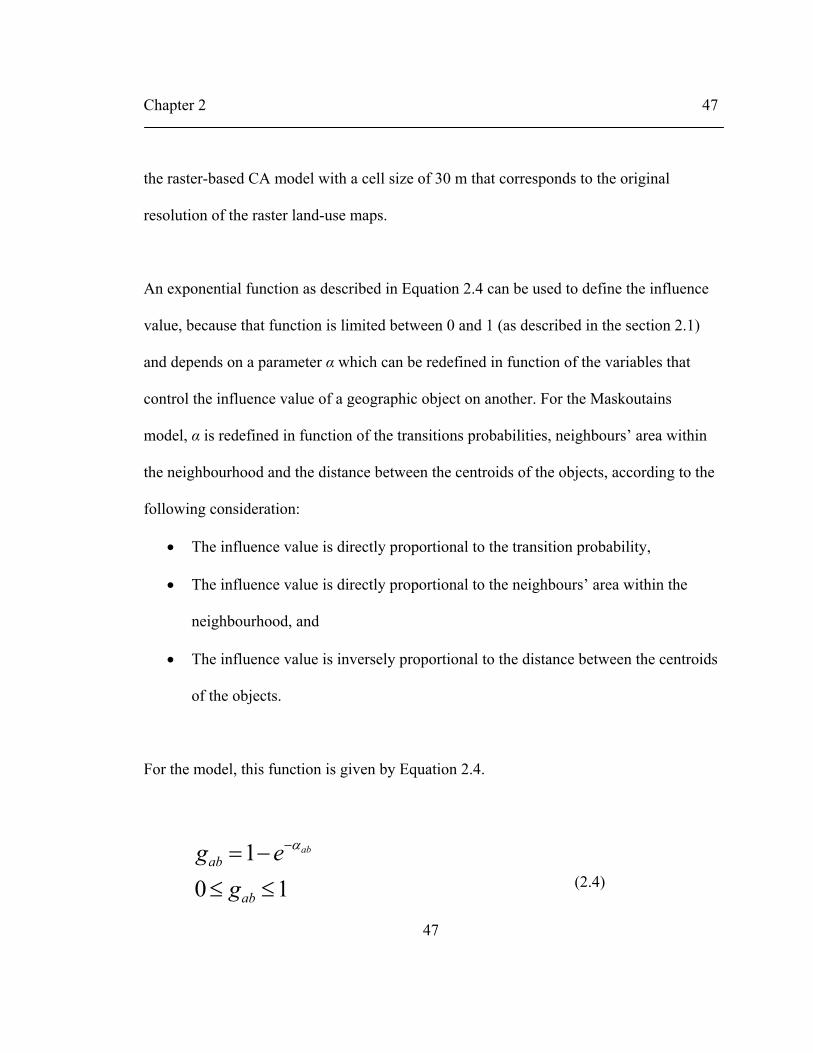
An exponential function as described in Equation 2.4 can be used to define the influence

value, because that function is limited between 0 and 1 (as described in the section 2.1)

and depends on a parameter α which can be redefined in function of the variables that

control the influence value of a geographic object on another. For the Maskoutains

model, α is redefined in function of the transitions probabilities, neighbours’ area within

the neighbourhood and the distance between the centroids of the objects, according to the

following consideration:

• The influence value is directly proportional to the transition probability,

• The influence value is directly proportional to the neighbours’ area within the

neighbourhood, and

• The influence value is inversely proportional to the distance between the centroids

of the objects.

For the model, this function is given by Equation 2.4.

101≤≤−= −

ab

ab

geg abα

(2.4)

Chapter 2 48

48

where

gab is the influence of the neighbour a on the object b, and

αab is defined in Equation 2.5

abaabab dtAP /)(*→=α (2.5)

where

Pb→a is the probability to change from b’s state to a’s state,

A(t)a is the area of the neighbour a within the neighbourhood of the object b at

time t, and

dab is the distance between the centroid of the neighbour a and the centroid of the

object b.

Transition probabilities are defined from the comparison of the two land-use maps of

1999 and 2002. They are calculated according to Equation 2.6.

∑=

→

→→ = 4

1iiX

YXYX

A

AP (2.6)

where

PX→Y is the transition probability from state X to state Y,

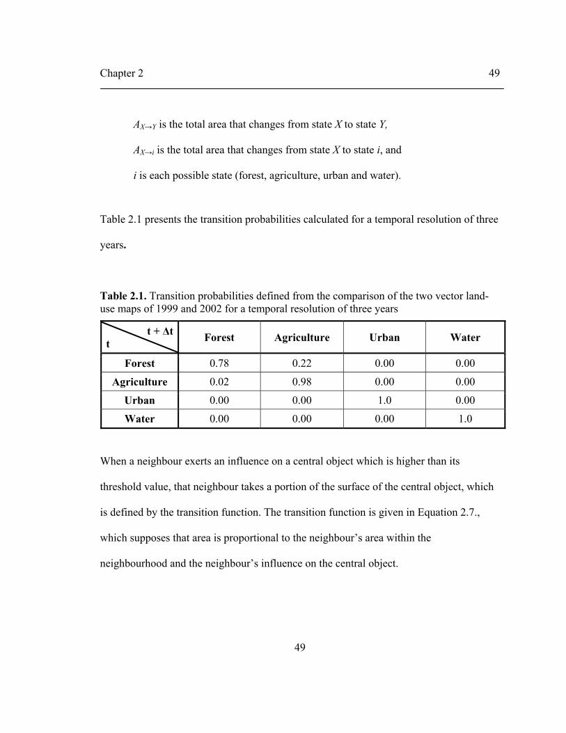
Chapter 2 49

49

AX→Y is the total area that changes from state X to state Y,

AX→i is the total area that changes from state X to state i, and

i is each possible state (forest, agriculture, urban and water).

Table 2.1 presents the transition probabilities calculated for a temporal resolution of three

years.

Table 2.1. Transition probabilities defined from the comparison of the two vector land-use maps of 1999 and 2002 for a temporal resolution of three years

t + Δt t Forest Agriculture Urban Water

Forest 0.78 0.22 0.00 0.00

Agriculture 0.02 0.98 0.00 0.00

Urban 0.00 0.00 1.0 0.00

Water 0.00 0.00 0.00 1.0

When a neighbour exerts an influence on a central object which is higher than its

threshold value, that neighbour takes a portion of the surface of the central object, which

is defined by the transition function. The transition function is given in Equation 2.7.,

which supposes that area is proportional to the neighbour’s area within the

neighbourhood and the neighbour’s influence on the central object.

Chapter 2 50

50

⎩⎨⎧ ≥

=caseother 0

if *)( abababab

ggtAf

λ (2.7)

where

fb is the transition function of object b,

A(t)a is the area of the neighbour a within the neighbourhood of the object b at

time t, and

λab is a threshold value that represents the resistance of the geographic object b to

change its state for the state of its neighbour a.

Threshold value can be defined as the probability that a geographic object does not

change its state to state X although all its neighbours are in state X. Equation 2.8 provides

the threshold value:

max1 Pab −=λ (2.8)

where Pmax is the probability that a geographic object b changes its state to the state of the

geographic object a when all its neighbours are in the state of a.

Since the neighbourhood configurations for irregular polygons are infinite, a simplified

situation for the calculation of the threshold values was applied, where all the polygons

are considered as squares of same size, connected to each other as cells in the raster

Chapter 2 51

51

model. Then Pmax is the probability that a geographic object changes its state from state X

to state Y when its eight neighbours are in state Y. This probability was calculated from

the comparison of the two raster land-use maps (1999 and 2002) and it is given by the

number of cells in state X in 1999 that have changed to state Y in 2002, while having

eight cells in state Y in its neighbourhood, divided by the total number of cells in state X

with the same neighbourhood in 1999.

Table 2.2 presents the threshold values calculated for the model. This procedure is

implemented in the class Thresholds of the package Utilities and can be used to

determine the threshold values in any model from two raster images of different dates.

The threshold values for the transitions between the same states have been assigned to 1,

since they are not considered as changes of state.

Table 2.2. Threshold values indicating the minimum influence that a polygon must exert on another to produce a geometric transformation

t + Δt t Forest Agriculture Urban Water

Forest 1.00 0.11 1.00 1.00

Agriculture 0.37 1.00 1.00 1.00

Urban 1.00 1.00 1.00 1.00

Water 1.00 1.00 1.00 1.00

Chapter 2 52

52

The original resolution (30 m) of the available land-use maps was chosen for the

rasterization procedure, to ensure that all objects can be represented in the raster format.

2.3.4 Definition of the raster-based CA model

Two raster-based CA models were also implemented to compare results with those

obtained using the VecGCA model. These models differ only in their spatial resolution.

First, a resolution of 30 m was chosen to provide a direct comparison with the VecGCA

model, in which land-use data at their original resolution of 30 m are used to establish the

initial conditions of the model. Second, a resolution of 100 m was also used based on the

results previously obtained in a scale sensitivity analysis conducted by Ménard and

Marceau (2005), which indicates that 100 m is the best resolution to represent the

dynamics of the study area.

Space was defined as a regular grid corresponding to a raster land-use map. Each cell can

be in one of four states, namely forest, agriculture, urban or water, but only two changes

of state have been considered in this region: forest to agriculture and agriculture to forest.

The Moore neighbourhood was chosen to represent the influence of first-order adjacent

cells on a cell. Probabilistic rules were calculated from the comparison between two land-

use maps (1999 and 2002), according to the procedure described in Ménard and Marceau

(2005), where a forested cell that has n agricultural cells in its neighbourhood has a

Chapter 2 53

53

probability of changing to agriculture equal to the number of forested cells with n

agricultural neighbours that have changed to agriculture between 1999 and 2002, divided

by the total number of forested cells with the same neighbourhood in 1999. Tables 2.3

and 2.4 present the transition probabilities calculated using the raster land-use maps at 30

m and 100 m spatial resolution, respectively.

Table 2.3. Transition probabilities for the raster-based CA model of 30 m (W=Water, F=Forest, A=Agriculture, U=Urban)

Number of neighbours whose previous state is equal to the cell’s next state Transition

0 1 2 3 4 5 6 7 8

F → F 0.096 0.175 0.195 0.280 0.424 0.547 0.602 0.683 0.880

F → A 0.000 0.326 0.411 0.475 0.590 0.741 0.818 0.841 0.929

A → F 0.000 0.111 0.174 0.265 0.357 0.498 0.528 0.507 0.638

A → A 0.799 0.770 0.678 0.677 0.713 0.795 0.864 0.910 0.991

U → U 0.882 0.888 0.920 0.918 0.944 0.986 0.990 0.996 1.000

W → W 0.900 0.954 0.979 0.910 0.888 0.938 0.988 0.998 1.000

Transition probabilities which values are zero (0) are not included in the tables. The

transition probability from forest to agriculture with 0 agricultural neighbours and from

agriculture to forest with 0 forested neighbours has been assigned a value of 0, because

they do not correspond to any significant ecological phenomena. Since a pseudo-random

number generator was used to implement the probabilistic rules, ten replicas of each

Chapter 2 54

54

simulation were performed using the raster-based CA model and the mean results were

considered in the comparison with the VecGCA model.

Table 2.4. Transition probabilities for the raster-based CA model of 100 m (W=Water, F=Forest, A=Agriculture, U=Urban)

Number of neighbours whose previous state is equal to the cell’s next state Transition

0 1 2 3 4 5 6 7 8

F → F 0.196 0.342 0.478 0.541 0.650 0.762 0.804 0.868 0.928

F → A 0.000 0.142 0.208 0.260 0.368 0.481 0.555 0.693 0.832

A → F 0.000 0.039 0.078 0.121 0.214 0.323 0.360 0.403 0.661

A → A 0.577 0.712 0.743 0.735 0.825 0.909 0.939 0.969 0.995

U → U 0.923 0.952 0.951 0.979 0.990 0.991 0.997 0.997 1.000

W → W 0.980 0.964 0.978 0.951 0.959 1.000 1.000 0.000 0.000

2.3.5 Model simulations

Two simulation periods were considered in the study:

1. From 1999 to 2002 in order to compare the results of the VecGCA model and the

raster-based CA models with the 2002 land-use map. The 1999 land-use maps (in

raster and vector formats) were used to establish the initial conditions in the raster-

based CA models and the VecGCA model. A temporal resolution of one year was

chosen and the transition probabilities for this temporal resolution were calculated

from the transition probabilities of three years using the exponential method

Chapter 2 55

55

presented by Yeh and Li (Yeh and Li 2006) where the transition probability P

calculated for a time step t is substituted by Pn for a time step T where T = n*t.

2. From 2002 to 2032 in order to observe the performance of the VecGCA when

executed over a longer period of time (10 time units) and to compare its results with

the results obtained with the raster-based CA models. The 2002 land-use maps (in

raster and vector formats) were used to determine the initial conditions of each model.

A temporal resolution of three years was used for the simulations.

Validation of the first simulation period was done by comparing the simulation outcomes

of the VecGCA model with the 2002 vector land-use map, the 30 m raster-based CA

model outcomes with the 2002 30 m raster land-use map, and the 100 m raster-based CA

model outcomes with the 2002 100 m raster land-use map. The results obtained for the

second simulation period have not been quantitatively validated since our purpose was to

evaluate the performance of the VecGCA model in comparison to the raster CA models

over a longer period of time.

In order to compare the simulation outcomes produced by the VecGCA model and the

raster-based CA models, a landscape analysis using Fragstats 3.3., a computer software

program designed to compute a variety of landscape metrics for categorical map patterns

(McGarigal et al. 1995), was done on the raster-based CA results. The number of patches

Chapter 2 56

56

for each land use was calculated on the raster maps generated by the raster-based CA

models and compared with the number of polygons produced by the VecGCA model.

2.3.6 Results

The first section presents the simulation results obtained from 1999 to 2002. The second

section describes the possible states of the system in the following 30 years,

corresponding to simulations conducted from 2002 to 2032.

Simulation results for the period 1999 to 2002

The results produced by the VecGCA model and the raster-based CA models were

compared with the 2002 vector land-use map and the 2002 30 m and 100 m raster land-

use maps, respectively, to assess the capacity of the models to effectively capture the

dynamics of the study area (Table 2.5). The three models reveal a proportion of land use

very similar to the corresponding reference map. The VecGCA model produced 14.92 %

forested area for 2002 versus 14.83 % presents in the reference 2002 vector land-use

map; the 30 m and 100 m raster-based CA produced 14.84 % and 14.86 % of forested

area for 2002 versus, respectively, compared with 14.86 % and 14.86 % present in the

reference 2002 30 m and 100 m raster land-use maps. However, the landscape

configuration is quite different. With the 30 m raster-based CA, the number of forested

and agricultural patches considerably increases from 1453 in 1999 to 2727 in 2002 and

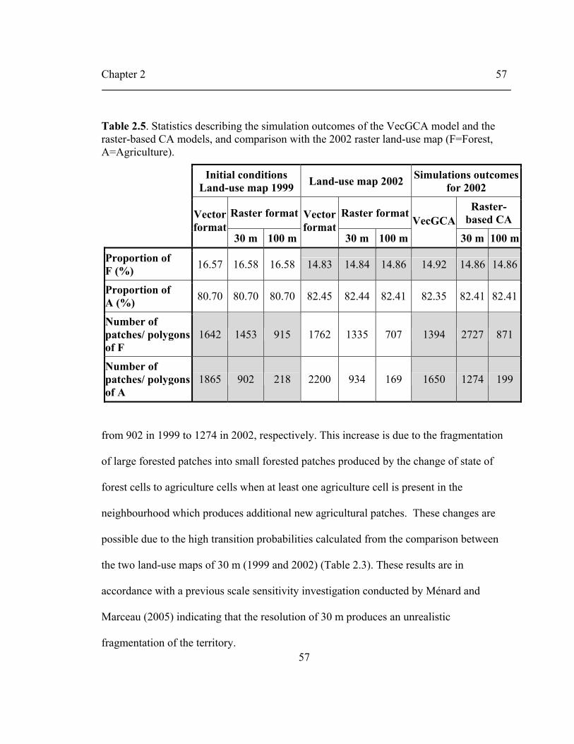
Chapter 2 57

57

Table 2.5. Statistics describing the simulation outcomes of the VecGCA model and the raster-based CA models, and comparison with the 2002 raster land-use map (F=Forest, A=Agriculture).

Initial conditions Land-use map 1999 Land-use map 2002 Simulations outcomes

for 2002

Raster format Raster format Raster-based CA

Vector format

30 m 100 m

Vector format

30 m 100 m VecGCA

30 m 100 m

Proportion of F (%) 16.57 16.58 16.58 14.83 14.84 14.86 14.92 14.86 14.86

Proportion of A (%) 80.70 80.70 80.70 82.45 82.44 82.41 82.35 82.41 82.41

Number of patches/ polygons of F

1642 1453 915 1762 1335 707 1394 2727 871

Number of patches/ polygons of A

1865 902 218 2200 934 169 1650 1274 199

from 902 in 1999 to 1274 in 2002, respectively. This increase is due to the fragmentation

of large forested patches into small forested patches produced by the change of state of

forest cells to agriculture cells when at least one agriculture cell is present in the

neighbourhood which produces additional new agricultural patches. These changes are

possible due to the high transition probabilities calculated from the comparison between

the two land-use maps of 30 m (1999 and 2002) (Table 2.3). These results are in

accordance with a previous scale sensitivity investigation conducted by Ménard and

Marceau (2005) indicating that the resolution of 30 m produces an unrealistic

fragmentation of the territory.

Chapter 2 58

58

With the two other models, the number of patches/polygons decreases with time

producing a less fragmented landscape (Table 2.5). This can be explained by the

disappearance of forested patches absorbed by large agricultural patches. In the 100 m

raster-based CA model, the numbers of forested and agricultural patches decrease from

915 in 1999 to 871 in 2002 and from 218 in 1999 to 199 in 2002, respectively. This

behavior is associated with the high transition probabilities from forest to agriculture

when the number of agricultural neighbours is higher than 5. In VecGCA, the number of

forested and agricultural patches (polygons) decreases from 1642 in 1999 to 1394 in 2002

and from 1865 in 1999 to 1650 in 2002, respectively. The disappearance of forested

patches absorbed by large agricultural patches is explained by the high pressure that

receives a forested object with an agricultural neighbour that covers its entire

neighbourhood.

However, a difference between the results produced by the VecGCA model and the 100

m raster-based CA model can be observed when an overlay of the 2002 vector and 100 m

raster land–use maps with the corresponding simulation outcomes is performed (Table

2.6). The forest and agricultural patches produced by VecGCA coincide with the real

forested and agricultural patches in the study area in a slightly greater proportion than the

patches generated by the 100 m raster-based CA model. These results can by explained

Chapter 2 59

59

Table 2.6. Proportion of simulated area that coincides with the state of the system in 2002 for each land use

% coincident with the reference map Land use VecGCA 100 m raster-based CA

Forest 80.61 77.97

Agriculture 96.26 93.04

Others 98.54 97.86

by the capacity of VecGCA to reproduce the evolution of the objects by their change of

shape, whereas the patches produced by the raster-based CA model are created by the

agglomeration of individual cells changing state. The outcomes of VecGCA, obtained

from the original spatial distribution of the land-use map, present a spatial distribution

that is more similar to the state of the landscape in 2002 than the outcomes produced by

the raster model although the cell size of 100 m has been identified as the most

appropriate in a previous sensitivity analysis (Ménard and Marceau 2005).

A zoom on a small portion of the study area illustrates the detailed spatial distribution

produced by VecGCA and the raster-based CA models (Fig. 2.7). The landscape

generated by VecGCA is characterized by large patches of well-defined boundaries, in

comparison with the diffuse boundaries and a high landscape fragmentation produced by

both raster-based CA models.

Chapter 2 60

60

Figure 2.7. The 2002 land-use maps and the land-use spatial distribution generated by the VecGCA model and the raster-based CA models in 2002

Simulation results for the period 2002 to 2032

The simulation results for the period 2002-2032 reveal that the three models generate a

similar trend, namely a decrease in forested areas and an increase in agricultural areas

(Fig. 2.8), but in different proportions.

30 m raster land-use map for 2002 30 m raster-based CA result for 2002

100 m raster land-use map for 2002 100 m raster-based CA result for 2002

vector land-use map for 2002 VecGCA results for 2002

Chapter 2 61

61

0

2

4

6

8

10

12

14

16

2002 2005 2008 2011 2014 2017 2020 2023 2026 2029 2032

Time (years)

Prop

ortio

n (%

)

76

78

80

82

84

86

88

90

92

94

96

Forest 30 m raster-based CAForest 100 m raster-based CAForest vecGCA

Agriculture 30 mraster-based CAAgriculture 100 mraster-based CAAgriculture vecGCA

Figure 2.8. Proportion of forested and agricultural area calculated on the simulation outcomes of VecGCA and the 30 m and 100 m raster-based CA models

With the VecGCA model, the decrease in forested areas is lower in comparison to the

decrease shown in both raster-based CA models; consequently the increase in agricultural

area is also lower. In the VecGCA model, the proportion of forested area is reduced from

14.83 % in 2002 to 7.58% in 2032 and the proportion of agricultural area is increased

from 82.45 % in 2002 to 89.69 % in 2032, whereas with the raster-based CA models the

reduction in forested area is from 14.84% to 4.30% for the 30 m model and from 14.86%

to 3.58% for the 100 m model, while the increase in agricultural area is from 82.44 % to

92.98 % and from 82.41 % to 93.69 % for the 30 m model and the 100 m model,

respectively (Table 2.7). These results can be explained by the fact that with the VecGCA

model, the decrease in forested area is determined by the change of state in only a portion

Chapter 2 62

62

Table 2.7. Statistics describing the simulation outcomes of the VecGCA model and the raster-based CA models for 2032 (F= Forest, A=Agriculture)

Initial conditions Land-use map 2002

Simulation outcomes for 2032

Raster format Raster-based CA

Vector format 30 m 100 m

VecGCA 30 m 100 m

Proportion of F (%) 14.83 14.84 14.86 7.58 4.30 3.58

Proportion of A (%) 82.45 82.44 82.41 89.69 92.98 93.69

Number of patches/ polygons of F 1762 1335 707 1659 9753 474

Number of patches/ polygons of A 2200 934 169 1359 628 83

of the forested polygons produced by the influence exerted by the agricultural polygon

neighbours at each time step. In comparison, in both raster-based CA models, the

decrease in forested area is associated to the change of state of forested cells in the

totality of their surface.

However, the landscape configuration produced by each model is different as revealed by

the number of forested and agricultural patches/polygons (Table 2.7). With the 30 m

raster-based CA model, the number of forested patches considerably increases from 1335

in 2002 to 9753 in 2032, while the number of agricultural patches decreases from 934 to

628 due to the agglomeration of agricultural patches. However, the 30 m raster-based CA

model generates a considerably more fragmented landscape than the one produced by the

Chapter 2 63

63

100 m raster-based CA and the VecGCA model. The fragmentation in the 30 m raster-

based CA model is due to the division of large forested patches into small ones produced

by the change of state of forest cells to agriculture cells when at least one agriculture cell

is present in the neighbourhood. For the other two models, the reduction in the number of

forested and agricultural patches/polygons is due to the disappearance of forested

patches/polygons absorbed by large agricultural patches/polygons and the agglomeration

or union of agricultural patches/polygons. In VecGCA, the number of forested and

agricultural polygons decreases from 1762 in 2002 to 1659 in 2032 and from 2200 in

2002 to 1359 in 2032, respectively. A similar behaviour is provided by the 100 m raster-

based CA model; the number of forested patches decreases from 707 in 2002 to 474 in

2032, while the number of agricultural patches decreases from 169 in 2002 to 83 in 2032.

The models display the same behavior for both simulation periods. The 30 m raster-based

CA model produces a highly fragmented landscape that does not realistically represent

the dynamics in the study area. These results are in agreement with those obtained in a

previous study (Ménard and Marceau 2005) indicating that 30 m is not an adequate cell

size for simulating the dynamics in the Maskoutains region and that the best cell size is

100 m. The 100 m raster-based CA and the VecGCA models both capture well the

dynamics of the study area. However, there is no need to perform a cell size sensitivity

Chapter 2 64

64

analysis with VecGCA since the polygons correspond to the real distribution of land-use

patches in the landscape.

2.4 Discussion

The results obtained reveal that VecGCA produces an adequate evolution of the

geographic objects, generating realistic spatial patterns when compared to the reference

land-use map. These results are independent of the cell size and no sensitivity analysis is

required to determine neither the initial spatial distribution nor the cell size of the model.

However, some limitations are still present in the model.

First, the rasterization used in the geometric transformation procedure introduces two

problems: the selection of the cell size is arbitrary and affects the simulation outcomes. In

addition, the rasterization produces a staircase effect on the polygons’ border, generating

errors in the delineation of the objects. A solution to overcome this problem is to replace

the rasterization by a procedure that only uses vectors, where the portion removed from a

geographic object is an irregular polygon whose borders conserve the initial definition of

the objects.

An issue that is not addressed in the first version of VecGCA is the possible sensitivity to

the neighbourhood definition. Several questions such as: Is VecGCA sensitive to the

Chapter 2 65

65

neighbourhood size? How to determine the appropriate neighbourhood size for a specific

study area? Should the neighbourhood size be constant or variable around a geographic

object? must be investigated. Finally, the appearance of new isolated polygons simulating

the emergence of land-use patches is not included in VecGCA. Nevertheless, in this

version of the model new polygons appear when a geographic object is divided into

several objects due to the influence of its neighbours, or because a non-adjacent

neighbour produces a geometric transformation.

The first version of VecGCA model overcomes the cell size sensitivity of the raster-based

CA models; it defines the neighbourhood as an influence zone that represents

neighbouring relationships more realistically than the Voronoi boundaries, and it allows

the change of shape of geographic objects through time. The second step is to investigate

its sensitivity to the neighbourhood size and if it is sensitive, to propose solutions to

overcome this problem. In addition, the technical limitations introduced by the

rasterization procedure should be removed to guarantee the good performance of the

model. This is the subject of the following chapter.

Chapter 3 66

66

CHAPTER 3

PERFORMANCE IMPROVEMENT OF THE GEOMETRIC TRANSFORMATION PROCEDURE AND SENSITIVITY ANALYSIS OF VecGCA TO THE NEIGHBOURHOOD SIZE

This chapter describes an improved version of VecGCA that overcomes the limitations

present in the first version that were introduced by the rasterization process used in the

geometric transformation procedure. In addition, a sensitivity analysis of VecGCA to the

neighbourhood configuration is performed using two different study areas: Maskoutains

region, Quebec, and Elbow river watershed, Alberta.

3.1 Update of VecGCA model

In the first implementation of the VecGCA model, a rasterization and vectorization

process was executed to control the appropriate area that changes state in a specific

Chapter 3 67

67

section of the geographic object (Figure 2.2). The procedure consisted in rasterizing the

geographic object, using a regular grid whose resolution was defined by the user, and

eliminating the nearest cells to each respective neighbour to satisfy the area that changes

state. The remaining cells that composed the geographical object were converted to the

vector format again and the removed cells defined a new area that was vectorized and

added to the corresponding neighbour. This procedure has two limitations: the resolution

chosen to execute the rasterization is arbitrary and the simulation outcomes vary with the

cell size. Also, the rasterization process produces a staircase effect on the polygons’

border that introduces errors in the real definition of the objects. In addition, the VecGCA

model is computationally intensive due to the handling of a large number of polygons

that can compose a study area and the update of their topological relationships after each

geometrical transformation during the simulation.

An improved implementation of the VecGCA geometrical transformation procedure is

presented here to overcome the limitations introduced by the rasterization procedure and

to reduce the computation time. This implementation involves a new definition of the

geometrical transformation procedure in which the rasterization procedure has been

replaced by the definition of an external buffer around the neighbours, which intersection

with the geographic object defines the area to be removed from that geographic object

and added to its neighbours. Also, some modifications of the simulation procedure were

Chapter 3 68

68

made to reduce the number of geometric operations and consequently to decrease the

computation time required to conduct the simulations.

3.1.1 Simulation procedure

The simulation procedure presented in the section 2.2.1 was updated to reduce the

computation time. At each time step, the updated simulation procedure calls three

additional procedures:

1. Update neighbourhood procedure: it evaluates and updates the neighbourhood and

neighbours of each geographic object.

2. Geometric transformation procedure: it executes the change of shape on each

geographic object where the influence of its neighbours is higher than a threshold

value that represents the resistance of a geographic object to change state for the state

of its neighbour.

3. Simplify space procedure: it joins adjacent polygons having the same state and

behavior, reducing the number of geographic objects that compose the geographic

space.

Update neighbourhood procedure

As mentioned in the section 2.2 (implementation), each geographic object has two

attributes that define the neighbourhood size (external buffer size) and the neighbours’

Chapter 3 69

69

list, respectively. In the neighbours’ list, the geographic object stores information about

all its neighbours: identification, state, distance between the centroid of the geographic

object and the centroid of the neighbour object, area of the neighbour within the

neighbourhood, neighbour’s influence on the geographic object, and area of the object

that must change for its neighbour’s state. The procedure builds an external buffer around

each geographic object and calculates which other objects are located inside this buffer.

To check if a geographical object is located inside the buffer, a condition is evaluated

before executing the intersection between the objects. This condition consists in

calculating the coordinates of the minimum bounding box around the buffer and the

coordinates of the minimum bounding box around the neighbour. If this evaluation

indicates an intersection of the two minimum bounding boxes, then the neighbour is

retained. Otherwise, it is discarded.

If a geographic object is found inside the buffer, the distance between the centroids, the

intersection area of the neighbour object and the neighbourhood, the influence, and the

area to change are calculated, and all this information is stored in the neighbours’ list of

the geographic object. In addition, the geographic object is stored as a neighbour of its

neighbours, but only the identification, state and distance between centroids are kept. The

other information about the intersection area, the influence and the area to change are

updated when the neighbour is examined as a central geographic object.

Chapter 3 70

70

Two conditions are evaluated before calculating the area of a geographic object to change

for the state of its neighbour:

1. If two geographical objects A and B are neighbours and A exerts an influence on B,

and B exerts an influence on A, only the highest influence between the two objects is

considered as producing a geometric transformation;

2. If this influence is higher than a threshold value, the area to change is calculated

according to the transition function; otherwise the area to change is assigned the value

0.

This updated implementation examines all geographic objects before executing any

geometric transformation.

Geometric transformation procedure

The geometrical transformation procedure reduces the area of geographic objects

(calculated by the transition function) from the region nearest to the corresponding

neighbour. The reduced area creates a new polygon that is added to the corresponding

neighbour.

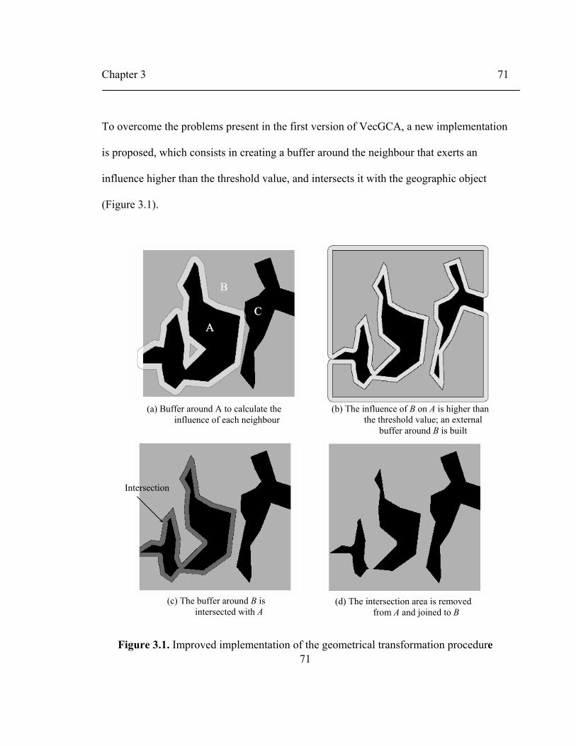
Chapter 3 71

71

To overcome the problems present in the first version of VecGCA, a new implementation

is proposed, which consists in creating a buffer around the neighbour that exerts an

influence higher than the threshold value, and intersects it with the geographic object

(Figure 3.1).

Figure 3.1. Improved implementation of the geometrical transformation procedure

(a) Buffer around A to calculate the influence of each neighbour

AA CC

BB

(c) The buffer around B is intersected with A

Intersection

(b) The influence of B on A is higher than the threshold value; an external

buffer around B is built

(d) The intersection area is removed from A and joined to B

Chapter 3 72

72

The intersection area is removed from the geographic object to create a new geographic

object that is subsequently joined to the corresponding neighbour in the simplify space

procedure (described below). The buffer size is automatically adjusted to guarantee that

the intersection area corresponds to at least 95% of the area calculated by the transition

function. The procedure is executed for each neighbour whose influence is higher than

the threshold value, starting with the neighbour having the highest influence. This

implementation is conceptually more elegant; it is expected that it will considerably

reduce the computation time and remove the staircase effect that was present in the first

version of the model.

Simplify space procedure

When all the geometric transformations are executed, the simplify space procedure is

called. This procedure checks the whole geographic space and joins adjacent geographic

objects with the same state and behavior, producing new geographic objects whose area

is the sum of those adjacent polygons.

3.2 Sensitivity analysis of VecGCA to the neighbourhood size

VecGCA overcomes the cell size sensitivity of the raster-based CA models, but its

sensitivity to the neighbourhood configuration has not been evaluated. This is important

Chapter 3 73

73

since the neighbourhood size is used to define the influence and the transition functions

of the model.

Two land-use change models in two regions of different complexity (different polygon

distributions, different aerial extensions and numbers of polygons, and different numbers

of land-use classes), in southern Quebec and in southern Alberta, in Canada, were

developed in order to test the improved implementation of the VecGCA geometric

transformation procedure and to assess its performance. In addition, a sensitivity analysis

to the neighbourhood configuration is conducted to determine the impact on the

simulation outcomes of the VecGCA model. While the use of a vector-based approach

overcomes the sensitivity to cell size, our hypothesis is that it does not address the

possible sensitivity to neighbourhood configuration. This aspect needs to be evaluated

before proper solutions can be investigated.

3.2.1 Study areas

The first study area is the Maskoutains region, described in the section 2.3.1. The second

study area is the Elbow river watershed. This area comprises all the land area drained by

the Elbow River and its tributaries, which covers approximately 1238 km2. In this region,

a greater variety of land uses/land covers can be observed: forest, agriculture, vegetated

land (shrubs and other vegetation different from agricultural land), construction and open

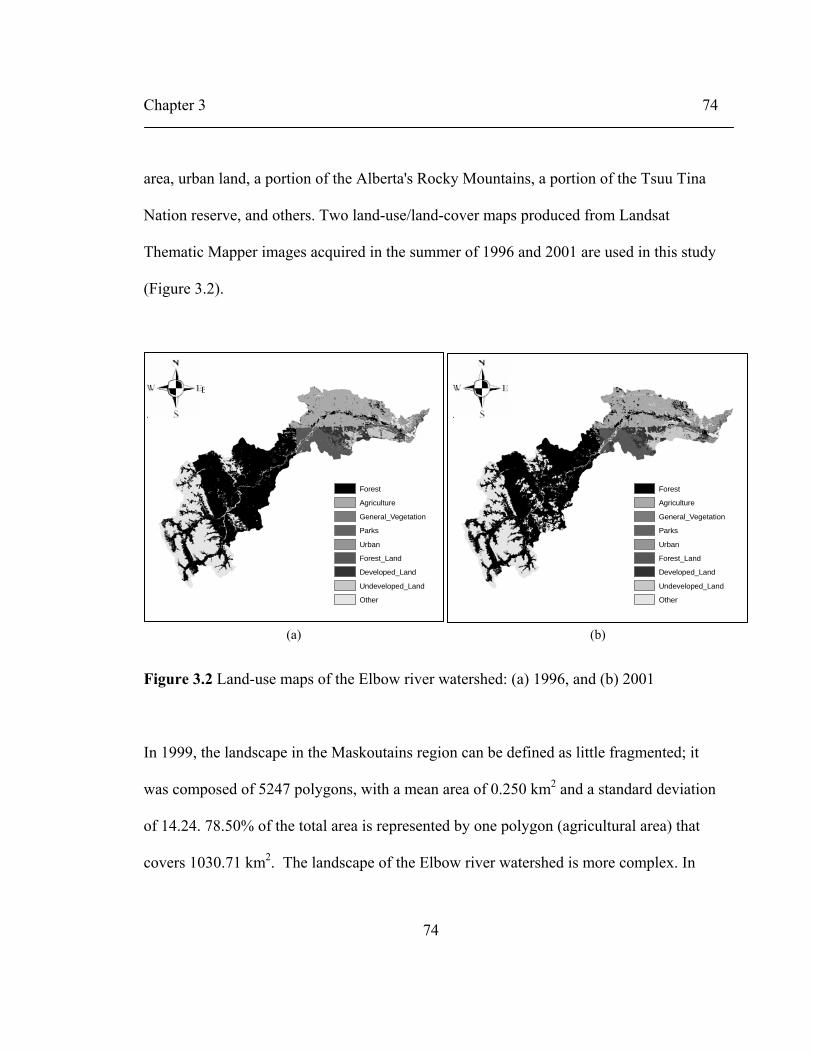
Chapter 3 74

74

area, urban land, a portion of the Alberta's Rocky Mountains, a portion of the Tsuu Tina

Nation reserve, and others. Two land-use/land-cover maps produced from Landsat

Thematic Mapper images acquired in the summer of 1996 and 2001 are used in this study

(Figure 3.2).

Figure 3.2 Land-use maps of the Elbow river watershed: (a) 1996, and (b) 2001

In 1999, the landscape in the Maskoutains region can be defined as little fragmented; it

was composed of 5247 polygons, with a mean area of 0.250 km2 and a standard deviation

of 14.24. 78.50% of the total area is represented by one polygon (agricultural area) that

covers 1030.71 km2. The landscape of the Elbow river watershed is more complex. In

Forest

Agriculture

General_Vegetation

Parks

Urban

Forest_Land

Developed_Land

Undeveloped_Land

Other

(a) (b)

. .Forest

Agriculture

General_Vegetation

Parks

Urban

Forest_Land

Developed_Land

Undeveloped_Land

Other

Chapter 3 75

75

1996, it was composed of 7195 polygons of smaller extent compared to the Maskoutains

region (mean area of 0.172 km2 and standard deviation of 6.67).

3.2.2 The land-use/land-cover VecGCA model

The model used to simulate the dynamics in both study areas is the same as described in

the section 2.3.2. Space is defined as a collection of patches of different land uses/land

covers, where each patch corresponds to a polygon of the vector land-use/land-cover map

of the study area. The initial conditions were determined by the maps of 1999 and 1996

for the Maskoutains region and the Elbow river watershed, respectively.

The transition probabilities for the Elbow river watershed for a temporal resolution of

five years were calculated from the comparison of the two land-use/land-cover maps of

1996 and 2001, according to the procedure described in the section 2.3.2.

3.2.3. Model simulation

To determine the performance of the VecGCA model, one simulation in each study area

was run over ten time units and a neighbourhood size of 30 m. The computation time for

the three procedures (update neighbourhood, geometrical transformation and simplify

space) called from the simulation procedure were calculated. All simulations were

Chapter 3 76

76

performed on a DELL Dimension DXPO51, Intel ® Pentium ® Dual CPU (3.20 GHz

and 3.19 GHz), 2.00 GB of RAM.

To test the sensitivity of the model to the neighbourhood configuration, four simulations

for each study area were performed and their results were compared. Each simulation is

associated to a different neighbourhood size: 30 m, which is the original resolution of the

land-use/land-cover maps; 10 m, a small neighbourhood size which is 1/3 of the original

resolution; and two larger neighbourhood sizes (60 m and 120 m), corresponding

respectively to two and four times the original resolution of the land-use/land-cover

maps. All the simulations were performed from 1999 to 2002 for the Maskoutains region

and from 1996 to 2001 for the Elbow river watershed and compared to the land-use/land-

cover maps of the two areas for the years 2002 and 2001, respectively. The temporal

resolution was one year.

3.2.4 Results

The first section presents the performance assessment of the model when used to simulate

land-use/land-cover changes in the two study areas. The second section describes the

simulation outcomes of VecGCA for the Maskoutains region and the Elbow river

watershed obtained with different neighbourhood sizes.

Performance improvement of the model

Chapter 3 77

77

Two aspects were evaluated to determine the performance of the model: the adequate

representation of the entities composing the landscape and the computation time.

Figure 3.3 presents a section of the 1999 land-use map of the Maskoutains region and the

simulation outcomes obtained for 2001 using the first and the improved implementations

of VecGCA. A first observation is that although both models start with the same initial

conditions and produce a similar spatial distribution, the first implementation produces a

staircase effect on the polygon’s borders due to the rasterization process used in the

geometrical transformation procedure. This rasterization process also introduces some

error in the boundary’s definition of the entities composing the study area due to the

arbitrary selection of the cell size for the rasterization. In comparison, the improved

implementation generates a spatial distribution of well-defined polygons that preserves

the border definition as observable in the initial conditions, removing the staircase effect

and the error introduced by the arbitrary selection of the cell size used in the rasterization

process.

Chapter 3 78

78

Figure 3.3. The 1999 vector land-use/land-cover map of the Maskoutains sub-region and the spatial distribution generated by VecGCA for the year 2002 using the first and the improved implementations of the model

Chapter 3 79

79

In addition, a considerable reduction in the computation time between both

implementations has been achieved, from 11.87 hours for one iteration to 13.14 hours for

ten iterations in the Maskoutains region. This reduction of time can be explained by the

optimization of the update neighbourhood procedure and the new implementation of the

geometric transformation procedure that remove all operations of rasterization and

vectorization.

When comparing the new implementation for the two study areas, the total computation

time of the model (for ten iterations) is approximately the same, namely 13.14 hours for

the Maskoutains region and 13.32 hours for the Elbow river watershed, with an average

time of 1.31 hour per iteration in both models. However, the computation time for each

procedure is different in each study area (Table 3.1). An analysis of these results indicates

that the computation time of the VecGCA model depends on the number of possible

changes of state and the fragmentation of the study area. A number of 36 possible land-

use/land-cover changes can be found in the Elbow river watershed compared to only two

in the Maskoutains region. Therefore there are more possible changes of shape to be

executed in the Elbow river watershed and the average computation time for the

geometrical transformation procedure is longer in this region than it is in the Maskoutains

region (59.5 min compared to 21.0 min).

Chapter 3 80

80

The update neighbourhood and simplify space procedures execute many geometrical

operations of intersection and join among adjacent and near polygons. Therefore for

regions composed of a large matrix containing numerous small patches the computation

time associated to these procedures is expected to be generally high. This is the case for

the Maskoutains region, where 78.50% of the total area is covered by one large polygon

of agricultural area. Since the landscape in the Elbow river watershed is more

fragmented, the computation time for these two procedures is shorter in comparison to

the computation time for the Maskoutains region (10.9 and 9.5 min vs. 24.6 and 33.2

min) (Table 3.1).

Table 3.1. Average computation time of the procedures called in the new implementation of the model

Average computation time (minutes) Procedure Maskoutains region Elbow river watershed

Update neighbourhood 24.6 10.9

Geometrical transformation 21.0 59.5

Simplify space 33.2 9.5

Sensitivity to the neighbourhood configuration

Simulations were performed for each study area with neighbourhood sizes of 10 m, 30 m,

60 m and 120 m. In the Maskoutains region, the results reveal that when using the

neighbourhood sizes of 10 m and 30 m, the simulated proportion of forested and

agricultural land for 2002 differs in less than 2% of the proportion calculated from the

Chapter 3 81

81

2002 land-use/land-cover map. When using the neighbourhood sizes of 60 m and 120 m,

the difference between the simulated land-use/land-cover proportions for 2002 and the

calculated proportions from the 2002 map is higher and might exceed 8% (Table 3.2).

Table 3.2. Proportion of land-use/land-cover (%) in the Maskoutains region using different neighbourhood sizes

Simulation outcomes

1999 2000 2001 2002

2002 simulation outcome – 2002 land-use map

Neighbourhood 10 m 16.57 16.38 16.30 16.22 1.39

Neighbourhood 30 m 16.57 16.03 15.44 14.59 -0.24

Neighbourhood 60 m 16.57 16.02 14.90 12.16 -2.67

Neighbourhood 120 m 16.57 12.40 9.43 6.37 -8.46 Fore

st

Reference map 16.57 - - 14.83 0

Neighbourhood 10 m 80.70 80.89 80.98 81.05 -1.4

Neighbourhood 30 m 80.70 81.25 81.84 82.68 0.23

Neighbourhood 60 m 80.70 81.25 82.38 85.11 2.66

Neighbourhood 120 m 80.70 84.88 87.84 90.91 8.46 Agr

icul

ture

Reference map 80.70 - - 82.45 0

The neighbourhood size has a less pronounced impact on the simulation outcomes in the

Elbow river watershed (Table 3.3). The largest difference (2.08 percentage points) is

found for the agricultural land-use class using a neighbourhood size of 120 m. For all

other classes, the simulated and calculated proportions differ by less than 1.5 percentages

points when using different neighbourhood sizes. These results can be explained by the

Chapter 3 82

82

fact that the influence function (Equation 2.4) and the transition function (Equation 2.5)

are directly proportional to the neighbours’ area within the neighbourhood. The

neighbours’ area varies with the neighbourhood size and the landscape configuration. In

the Maskoutains region, the majority of the objects have only one neighbour; they are

small forested patches located inside a large matrix of agricultural land (Figure 3.4). The

influence of the agriculture matrix on the small forested patches and the area that changes

from forest to agriculture (calculated from the transition function) increase when the

neighbourhood size increases.

Table 3.3. Proportion of land-use/land-cover (%) in the Elbow river watershed using different neighbourhood sizes

1996 1997 1998 1999 2000 2001

2001 simulation outcome – 2001 land-use map

Neigh. 10 m 44.45 44.62 44.58 44.44 44.42 44.39 0.04

Neigh. 30 m 44.45 44.49 44.36 44.15 44.11 43.46 -0.89

Neigh. 60 m 44.45 44.97 44.84 44.72 43.62 43.58 -0.77

Neigh. 120 m 44.45 45.53 45.35 45.08 44.86 43.53 -0.82 Fore

st

Reference map 44.45 - - - - 44.35 0

Neigh. 10 m 15.39 15.33 15.28 15.26 15.24 15.21 1.73

Neigh. 30 m 15.39 15.41 15.30 15.40 15.36 15.35 1.87

Neigh. 60 m 15.39 15.58 15.51 15.40 15.35 15.32 1.84

Neigh. 120 m 15.39 15.74 15.77 15.60 15.56 15.56 2.08 Agr

icul

ture

Reference map 15.39 - - - - 13.48 0

Chapter 3 83

83

Neigh. 10 m 1.98 1.85 1.82 1.82 1.80 1.79 0.11 Neigh. 30 m 1.98 1.61 1.48 1.45 1.43 1.54 -0.14 Neigh. 60 m 1.98 1.32 1.19 1.18 1.39 1.36 -0.32 Neigh. 120 m 1.98 0.82 0.48 0.28 0.25 0.33 -1.35 V

eget

atio

n

Reference map 1.98 - - - - 1.68 0

Neigh. 10 m 0.87 0.81 0.78 0.75 0.73 0.74 -0.08

Neigh. 30 m 0.87 0.74 0.67 0.62 0.61 0.60 -0.22

Neigh. 60 m 0.87 0.72 0.67 0.66 0.64 0.56 -0.26

Neigh. 120 m 0.87 0.71 0.66 0.62 0.62 0.61 -0.21

Park

s

Reference map 0.87 - - - - 0.82 0

Neigh. 10 m 1.56 1.60 1.61 1.63 1.63 1.67 -0.63

Neigh. 30 m 1.56 1.66 1.69 1.71 1.72 1.72 -0.58

Neigh. 60 m 1.56 1.67 1.69 1.69 1.70 1.75 -0.55

Neigh. 120 m 1.56 1.66 1.68 1.70 1.70 1.70 -0.6 Urb

an

Reference map 1.56 - - - - 2.30 0

Neigh. 10 m 6.80 6.78 6.75 6.74 6.72 6.73 0.86

Neigh. 30 m 6.80 6.79 6.66 6.61 6.60 6.59 0.72

Neigh. 60 m 6.80 6.79 6.71 6.64 6.63 6.62 0.75

Neigh. 120 m 6.80 6.81 6.77 6.72 6.50 6.46 0.59

Fore

st in

Tsu

T

ina

Nat

ion

rese

rve

Reference map 6.80 - - - - 5.87 0

Neigh. 10 m 3.04 3.03 3.01 2.99 2.99 2.97 -0.25

Neigh. 30 m 3.04 3.01 3.07 3.07 3.06 3.05 -0.17

Neigh. 60 m 3.04 3.03 2.95 2.97 2.96 2.97 -0.25

Neigh. 120 m 3.04 3.00 2.94 2.94 2.78 2.64 -0.58

Dev

elop

ed la

nd in

T

su T

ina

Nat

ion

rese

rve

Reference map 3.04 - - - - 3.22 0

Chapter 3 84

84

Neigh. 10 m 2.88 2.92 2.96 2.99 3.01 3.05 -0.47

Neigh. 30 m 2.88 2.92 3.00 3.05 3.07 3.09 -0.43

Neigh. 60 m 2.88 2.91 3.07 3.11 3.13 3.14 -0.38

Neigh. 120 m 2.88 2.92 3.01 3.07 3.44 3.63 0.11

Und

evel

oped

la

nd in

Tsu

Tin

a N

atio

n re

serv

e

Reference map 2.88 - - - - 3.52 0

Figure 3.4. Schematic representation of the landscape configuration of the Maskoutains region where the objects have only one neighbour for different neighbourhood sizes

The landscape configuration for the Elbow river watershed is different. Each geographic

object has several neighbours of different states where an increase of the neighbourhood

size can produce an increase of the neighbours’ area within the neighbourhood as well as

an increase in the number of neighbours (Figure 3.5). The increase of the neighbours’

area is less important than the one produced in a landscape composed of a large matrix

containing numerous small objects, such as in the Maskoutains region. Consequently, the

increase of influence and the area to change from the object’ state to the neighbour’s state

5 2

1

6

4

3

Chapter 3 85

85

is often not significant when the neighbourhood size increases. When the number of

neighbours increases, the influence and the area to change for the neighbours present in

the neighbourhood do not increase significantly due to the fact that these neighbours are

distant geographic objects separated by other objects. Therefore, in this landscape

configuration the simulation outcomes are less sensitive to the neighbourhood size.

Figure 3.5. Schematic representation of the Elbow river landscape configuration where the objects have several neighbours; when the neighbourhood size increases the number of neighbours and the neighbours’ area within the neighbourhood also increase

Additionally, in both landscape configurations, coarser neighbourhood sizes produce a

landscape that is less fragmented because small geographic objects (forested patches)

tend to disappear quickly, absorbed by the larger geographic objects of agricultural land

(Figures 3.6 and 3.7).

1 2

10

9 16 17

18

11 3

4

5

6

7 8

14 13 12

15

Chapter 3 86

86

Figure 3.6. Simulation outcomes for the Maskoutains region for 2002 using different neighbourhood sizes

Neighbourhood size = 10 m Neighbourhood size = 30 m

Neighbourhood size = 60 m Neighbourhood size = 120 m

Chapter 3 87

87

Figure 3.7. Simulation outcomes for the Elbow river watershed for 2001 using different neighbourhood sizes

Neighbourhood size = 10 m Neighbourhood size = 30 m

Neighbourhood size = 60 m Neighbourhood size = 120 m

Chapter 3 88

88

3.3. Discussion

The results show that the improved version of VecGCA considerably reduces the

computation time; it also removes the problems introduced by the rasterization process

used in the geometric transformation procedure, that is the staircase effect in the

polygon’s border and the arbitrary selection of the resolution used in the rasterization.

However, the computation time remains long when compared to the simulation time for a

raster-based CA model. For example 13.14 hours for ten iterations are required by the

Maskoutains region VecGCA model versus approximately two hours for the same

simulation using a 100 m raster-based CA model.

Nevertheless, if we consider the time needed for the calibration and sensitivity analysis to

cell size of a raster-based CA model, the computation time of VecGCA remains

reasonable. For example, Clark and Gaydos (1998) reported that the calibration of

SLEUTH to study the urban growth in San Francisco, California, required hundreds of

hours of CPU time. In a hypothetical example where the time required to calibrate a

simple raster-based CA model is one hour and the simulation time is two hours for ten

iterations, if a sensitivity analysis necessitates testing 25 scenarios (5 cell sizes and 5

neighbourhood configurations), the total computation time will be 75 hours for that

model.

Chapter 3 89

89

Using VecGCA, conducting a sensitivity analysis to cell size is not necessary. The

calibration process includes testing the influence and transition functions to guarantee

that they well capture the dynamics in the study area. This is done by executing the

model for a few iterations and comparing the results with the available dataset for the

study area. In this project, to calibrate VecGCA for the Maskoutains region, simulations

were performed from 1999 to 2002 using a time step of three years, and the results were

compared with the 2002 land-uses map; the time required for the calibration of this

region was approximately three hours and the total computation time was approximately

17 hours. Similar times were required to calibrate and run the Elbow river watershed

VecGCA model. The calibration was done from 1996 to 2001 with a temporal resolution

of five years and the results were compared with the 2001 land-use map.

Another aspect evaluated in this chapter is the sensitivity of VecGCA to the

neighbourhood configuration. The results revealed that the model is sensitive to the

neighbourhood size and this sensitivity depends on the landscape configuration of the

study area. The problem is to define how to control or remove this sensitivity. Two

possible solutions are envisioned to address this problem:

1. The definition of the influence and transition functions independently of the

neighbours’ area within the neighbourhood. In this case, the neighbourhood is used

Chapter 3 90

90

only to determine what are the neighbours of a central object. The increase or

decrease of the neighbourhood size can increase or decrease the number of

neighbours, but it does not modify the influence value of a neighbour or its area to

change calculated in the transition function.

2. A dynamic neighbourhood adapted to each geographic object where the neighbours

are defined by no-geometric properties. In this neighbourhood, there are no

limitations of distance; the neighbourhood is the whole geographic space.

Our hypothesis is that the second option is the best solution, because it removes the

definition of fixed distance and considers all possible distances in only one

neighbourhood definition. In the next chapter, a dynamic neighbourhood is introduced in

the VecGCA model in order to remove its sensitivity to the neighbourhood configuration.

Chapter 4 91

91

CHAPTER 4

DYNAMIC NEIGHBOURHOOD IN VecGCA

This chapter describes the characteristics of a new neighbourhood definition proposed to

overcome the neighbourhood size sensitivity present in the previous version of VecGCA.

The new neighbourhood involves the redefinition of the influence and transition

functions of VecGCA. A test of the model to simulate land-use changes in two different

study areas and the comparison with the previous version of VecGCA are presented.

4.1 Dynamic neighbourhood definition and update of VecGCA

The dynamic neighbourhood proposed in this research is a neighbourhood that changes

through time; there is no distance or fixed area that delineates it and it is specific to each

geographic object. The neighbourhood includes the whole geographic space, and the

Chapter 4 92

92

neighbourhood relationships between two objects are defined according to the properties

of each geographic object. Objects a and b are neighbours if they are separated by 0, 1 or

more objects whose states are favourable to the change of state from a to b. A n x m

binary matrix describes if a state X is favourable to the transition from the state Y to Z,

where n is the number of possible states of a geographic object and m is the number of

possible transitions in the model. In this matrix, the 1 values indicate that a state X is

favourable to a transition and the 0 values indicate the opposite.

For example, let us suppose a geographic space as defined in Figure 4.1, composed of six

geographic objects that represent patches of different land uses/land covers (U =

undeveloped land, D = developed land, P = park, C = commercial land and W = water).

Let us suppose that the possible transitions are U to D, U to C, U to P, P to D, and P to C.

Let us suppose that the matrix M represents the favourable states to the transitions in the

model.

U D C P W U → D 0 0 1 1 1 U → C 0 0 1 1 0 U → P 0 0 0 0 1 P → D 0 0 1 0 0

M =

P → C 0 1 0 0 0

Chapter 4 93

93

Figure 4.1. Geographic space composed of six geographic objects. The geographic object a has four neighbours: the adjacent objects b, c and d, and the non-adjacent object e.

This matrix indicates for example, that commercial land is favourable to the transition

from undeveloped land to developed land, from undeveloped land to commercial land

and from park to developed land. Using this matrix, we can say that the neighbours of

object a in Figure 4.1 are the adjacent objects b, c, d and the non-adjacent object e. e is

neighbour of a for two reasons: first because e and a are separated by b that is a

commercial land and this state is favourable to the transition from undeveloped to

developed land; second, because e and a are separated by the objects c and d that are in

the states water and park, respectively, and these states are favourable to the transition

from undeveloped to developed land. However, we cannot say that a is neighbour of e,

because the transition from developed to undeveloped land is not possible. This matrix is

obtained from the analysis of historical spatial data that reveals when a change of state of

a geographical object has occurred due to the influence of its non-adjacent neighbours

Chapter 4 94

94

and what are the states of these intermediate objects. The procedure to calculate this

matrix is described in the methodology section.

In the previous version of the VecGCA model, each neighbour exerts an influence on the

central object producing its change of shape if this influence is higher than a threshold

value (λ) that represents the resistance of the geographic object to change state for the

state of its neighbour. This influence value is constant on the whole surface of the central

object. The transition function quantifies the area of the central object that changes its

state for the neighbour’s state.

With the dynamic neighbourhood definition, the influence value is variable on the surface

of the central object. The influence value increases when the neighbour is closer to the

central object; the maximum value (gmax) is obtained in the object’s border and decreases

inside the object. Additionally, two considerations remain from the definition presented

in the sections 2.1 and 2.3.3: the influence function must be limited between 0 and 1, and

the influence function must be defined in function of the variables that determine the

pressure of a geographic object on another.

According to the results obtained in the previous version of the model, an exponential

function (Equation 2.4) can represent the influence function into the model. However,

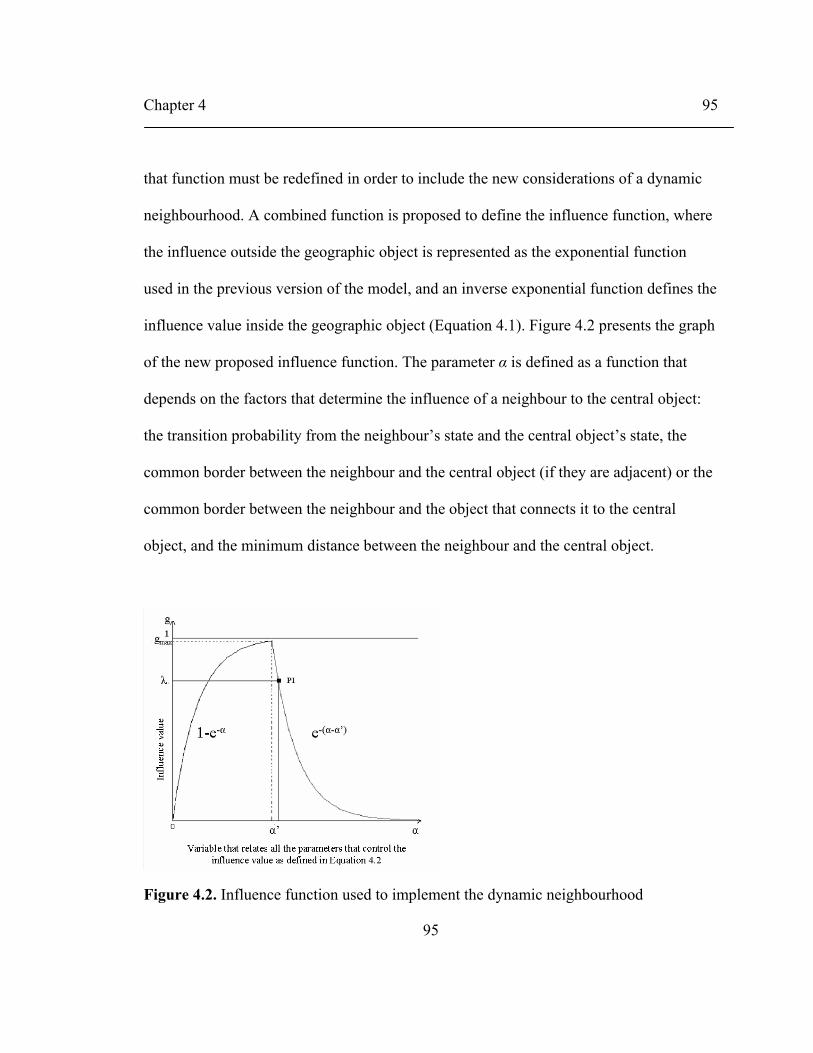
Chapter 4 95

95

that function must be redefined in order to include the new considerations of a dynamic

neighbourhood. A combined function is proposed to define the influence function, where

the influence outside the geographic object is represented as the exponential function

used in the previous version of the model, and an inverse exponential function defines the

influence value inside the geographic object (Equation 4.1). Figure 4.2 presents the graph

of the new proposed influence function. The parameter α is defined as a function that

depends on the factors that determine the influence of a neighbour to the central object:

the transition probability from the neighbour’s state and the central object’s state, the

common border between the neighbour and the central object (if they are adjacent) or the

common border between the neighbour and the object that connects it to the central

object, and the minimum distance between the neighbour and the central object.

Figure 4.2. Influence function used to implement the dynamic neighbourhood

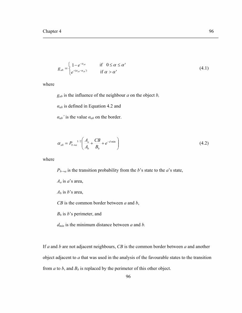
Chapter 4 96

96

⎩⎨⎧

>≤≤−

=−−

−

' if '0 if 1

)'( αααα

αα

α

abab

ab

ee

gab (4.1)

where

gab is the influence of the neighbour a on the object b,

αab is defined in Equation 4.2 and

αab’ is the value αab on the border.

⎟⎟⎠

⎞⎜⎜⎝

⎛++= −

→min2/1 d

bb

aabab e

BCB

AAPα (4.2)

where

Pb→a is the transition probability from the b’s state to the a’s state,

Aa is a’s area,

Ab is b’s area,

CB is the common border between a and b,

Bb is b’s perimeter, and

dmin is the minimum distance between a and b.

If a and b are not adjacent neighbours, CB is the common border between a and another

object adjacent to a that was used in the analysis of the favourable states to the transition

from a to b, and Bb is replaced by the perimeter of this other object.

Chapter 4 97

97

As Aa / Ab can be very large if a is larger than the central object, a factor is introduced to

regulate this value between 0 and 1. Equation 4.2 is rewritten as Equation 4.3.

30

min

min

max

2/1

≤≤

⎟⎟⎟⎟

⎠

⎞

⎜⎜⎜⎜

⎝

⎛

++= −→

α

α d

b

b

a

abab eBCB

AAAA

P (4.3)

where

Amax is the largest object’s area within the whole geographic space, and

Amin is the smallest object’s area.

If the influence on the object’s border is higher than λ, then the geometrical

transformation procedure is performed. The area that changes is not specified in the

transition function as in the previous version. Instead, the transition function determines

exactly the buffer size that is used in the geometrical transformation procedure to take a

portion of the central object and add it to the corresponding neighbour. This buffer size is

calculated from the point where the influence value inside the central object is equal to λ

(corresponding to P1 in Figure 4.2). Therefore, the transition function is derived from the

influence function. The transition function calculates the value of dmin for which the

influence value is equal to the threshold value (λ) when αab is higher than αab’, that is the

Chapter 4 98

98

influence inside the object. From Equation 4.1, αab can be defined by Equation 4.4, and

by replacing (4.3) in (4.4)

)(' λαα Lnabab −= (4.4)

)('min

min

max

2/1 λα LneBCB

AAAA

P abd

b

b

a

ab −=

⎟⎟⎟⎟

⎠

⎞

⎜⎜⎜⎜

⎝

⎛

++ −→ (4.5)

dmin can be found from Equation 4.5 and defines the transition function (Equation 4.6).

( )⎥⎥⎥⎥

⎦

⎤

⎢⎢⎢⎢

⎣

⎡

−−−−=→ b

b

a

abab

ab BCB

AAAA

LnP

Lnf

min

max2/1 )('1 λα (4.6)

where

fab is the transition function that determines the size of the buffer that is built

around a to take a portion of b.

To clarify the transition function concept, Figure 4.3 presents a hypothetical example

where the transition function of a geographic object is calculated. Let us suppose a

Chapter 4 99

99

geographic space composed of four geographic objects a, b, c and d. Let us suppose that

b, c and d exert an influence on a that is higher than the threshold values. Therefore the

transition function is calculated for bc, ca and da to determine the buffer size that must be

built around c, c and d to take a portion of a. For b, the buffer size is defined by fba,

calculated from the Equation 4.6, and represents the distance from any point on the

border of a, because a and b are adjacent, to a point in its interior where gba = λba. For c

and d, the buffer size is defined by fca and fda, respectively. They are also calculated from

Equation 4.6 and represent the distances from the closest point of c to a to a point in the

interior of a where gca = λca, and from the closest point of d to a to a point in the interior

of a where gda = λda.

Figure 4.3. Schematic representation of the distance calculated from the transition function that defines the buffer size to be built around each neighbour to take a portion of a central object (geometric transformation procedure described in the section 3.1.1).

ab

cd

fca fda

fba

Influence value (inside the object)

Higher Lowerλab λac λad

Chapter 4 100

100

4.2 Land-use change VecGCA models using a dynamic neighbourhood

To test the dynamic neighbourhood and to determine if it overcomes the sensitivity to the

neighbourhood size that is present in the previous version of VecGCA, two land-use

VecGCA models have been built for two regions of varying landscape configuration in

Canada. The results were compared with the ones obtained using the previous version of

VecGCA.

4.2.1 Study areas

The first study area is the Maskoutains region described in the section 2.3.1. The second

study area is a sub-region of the Elbow river watershed, located in Southwest Alberta,

Canada, which covers approximately 731 km2. The subregion was selected from the

study area described in the section 3.2.1, where a portion corresponding to the Alberta's

Rocky Mountains was excluded because significant changes were not observed when the

available data was analyzed. Three land-use maps generated from Landsat Thematic

Mapper images acquired in the summer of 1996, 2001 and 2006 were available for that

region. A reclassification from the land uses described in the section 3.2.1 was done to

focus on the main classes: forest, agriculture, urban, water and the Tsuu Tina Nation

Land. The dynamics inside the Tsuu Tina Nation Land has not been studied; therefore

there are no visible changes in this area.

Chapter 4 101

101

4.2.2 The land-use VecGCA model

In VecGCA, space is represented as a collection of patches of different land uses, where

each patch corresponds to a polygon of the vector land-use map of the study area. The

influence function and the transition function are given in Equations 4.1 and 4.6,

respectively.

The transition probabilities and threshold values are obtained from the comparison of two

land-use maps of different dates and are calculated as described in the section 3.2.2. The

binary matrix that describes if a state X is favourable to the transition from the state Y to Z

is obtained from the comparison of two historical vector land-use maps. This procedure

checks when an object A changes, in a portion or in the totality of its surface, from the

state Y to the state Z without having adjacent objects in the Z state. The procedure is

looking for the closest object in the state Z; the objects that separate the object A from

this closest object are considered intermediate objects, and the states of these

intermediate objects are considered favourable states to the transition from Y to Z. Tables

4.1 and 4.2 present the matrix corresponding to the Maskoutains region and the eastern

subregion of the Elbow river watershed, respectively.

Chapter 4 102

102

Table 4.1. Matrix of favourable states for land-use transitions in the Maskoutains region

Land uses Transitions Forest Agriculture Urban Water

F → A 0 0 0 1

A → F 0 0 0 1

Table 4.2. Matrix of favourable states for land-use transitions in the Elbow river watershed

Land uses Transitions

Forest Agriculture Urban Water Reserve

F → A 0 0 1 1 0

F → U 0 1 0 1 0

A → F 0 0 1 1 0

A → U 1 0 0 1 0

U → F 0 1 0 1 0

U → A 1 0 0 0 0

4.2.3 Model simulations

Five simulations on each study area were performed to compare the results of the

dynamic neighbourhood with the results obtained using the previous version of VecGCA

(for four different neighbourhood sizes: 10 m, 30 m, 60 m and 120 m) and the reference

land-use/land-cover maps of the two areas. The simulations were run from 1999 to 2002

for the Maskoutains region and the results were compared with the 2002 land-use/land-

cover map. For the Elbow river watershed, the simulations were performed from 1996 to

Chapter 4 103

103

2006, and the results obtained were compared with the 2001 and 2006 land-use/land-

cover maps. The temporal resolution of the simulations is one year.

4.2.4 Results

When using the previous version of VecGCA in the Maskoutains region, the simulated

proportion of forested and agricultural land for 2002 varies up to 10 percentage points

(Table 2.4) when the neighbourhood size varies from 10 m to 120 m. For example, the

proportion of forested area is 16.22% using a neighbourhood size of 10 m, in comparison

to 6.37% when using 120 m as the neighbourhood size. A comparison of these results

with the proportion and distribution of land uses present in the 2002 land-use map

suggests that 30 m is a good neighbourhood size to simulate the dynamics in this area. A

spatial overlay of the 2002 land-use map and the simulation results for 2002 reveals that

when using a neighbourhood size of 10 m, 97.49 % of agricultural area generated by

VecGCA coincides with the agricultural area present in the 2002 land-use map, in

comparison with 89.71% when a neighbourhood size of 120 m is used (Table 4.3). For

the forested area, the obtained results are opposite; the coincident proportion is smallest

when the neighbourhood size is 10 m (Table 4.3). These results can be explained by the

fact that when the neighbourhood size increases, small forested patches disappear due to

the high influence of the agricultural area.

Chapter 4 104

104

Table 4.3. Proportion of land uses for 2002 produced by VecGCA and percentage of coincidence of the simulation outcomes and the 2002 land-use map for the Maskoutains region using the previous version of VecGCA

Buffer neighbourhood 10 m 30 m 60 m 120 m

2002 land-use map

Forest 16.22 14.59 12.16 6.37 14.83 Land-use proportion (%) Agriculture 81.05 82.68 85.11 90.91 82.45

Forest 79.02 80.61 81.46 86.45 - % coincident with the reference map Agriculture 97.49 96.26 94.19 89.71 -

For the Elbow river watershed, the simulation outcomes were compared with the

proportion of land use and spatial distribution of patches calculated from two land-use

maps corresponding to 2001 and 2006. In both cases, the results obtained are similar; the

proportions of agricultural and urban areas slightly increase with the neighbourhood size

while it is the opposite for the proportion of forested area (Tables 4.4. and 4.5).

The proportion of forested land for 2001 using a neighbourhood size of 10 m is 44.65%

in comparison to 42.54% using 120 m as the neighbourhood size (Table 4.4). For 2006,

the proportion of forested area is 44.58% and 41.39% using a neighbourhood size of 10

m and 120 m respectively (Table 4.5). As mentioned is the previous chapter, these results

indicate that for the Elbow river watershed the previous version of VecGCA is less

sensitive to the variation of the neighbourhood size than it is in the Maskoutains region.

The sensitivity varies with the landscape configuration because the influence and the

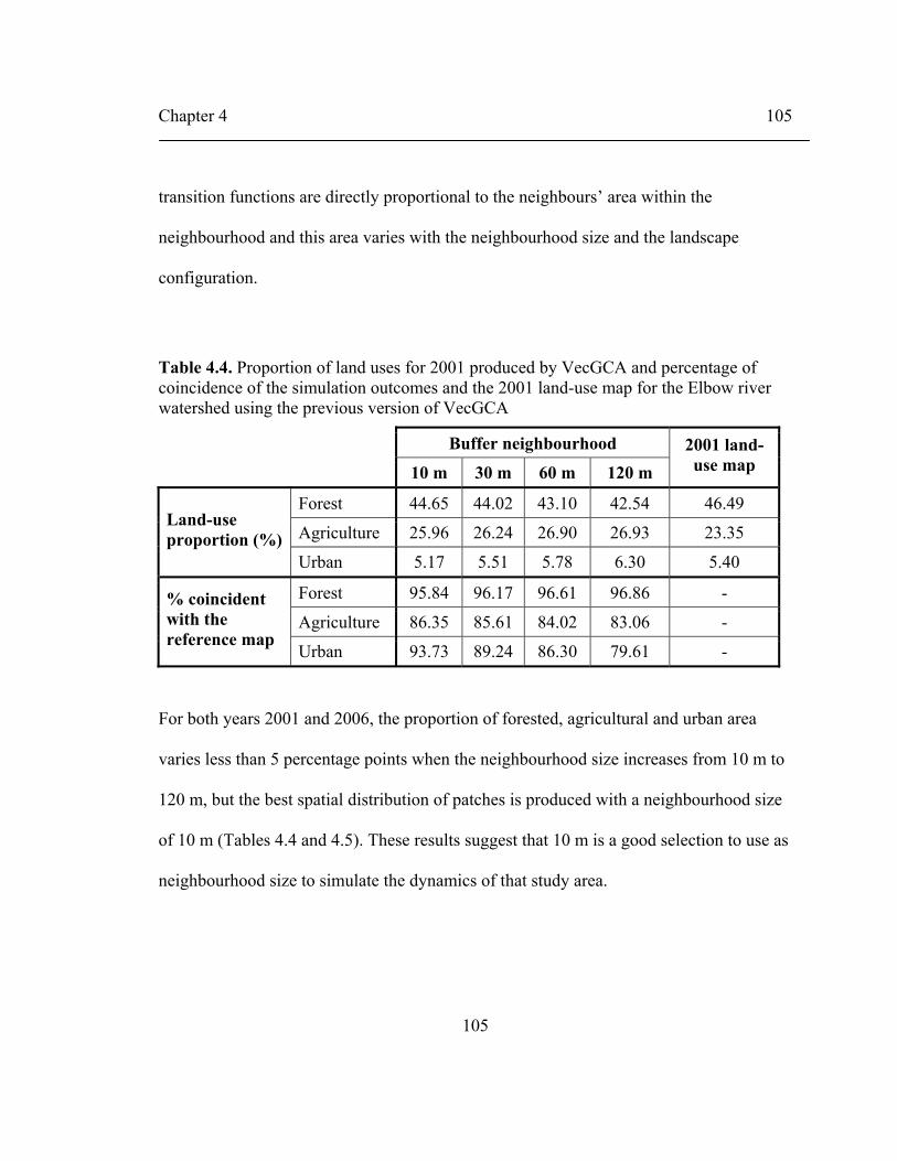
Chapter 4 105

105

transition functions are directly proportional to the neighbours’ area within the

neighbourhood and this area varies with the neighbourhood size and the landscape

configuration.

Table 4.4. Proportion of land uses for 2001 produced by VecGCA and percentage of coincidence of the simulation outcomes and the 2001 land-use map for the Elbow river watershed using the previous version of VecGCA

Buffer neighbourhood 10 m 30 m 60 m 120 m

2001 land-use map

Forest 44.65 44.02 43.10 42.54 46.49

Agriculture 25.96 26.24 26.90 26.93 23.35 Land-use proportion (%)

Urban 5.17 5.51 5.78 6.30 5.40

Forest 95.84 96.17 96.61 96.86 -

Agriculture 86.35 85.61 84.02 83.06 - % coincident with the reference map

Urban 93.73 89.24 86.30 79.61 -

For both years 2001 and 2006, the proportion of forested, agricultural and urban area

varies less than 5 percentage points when the neighbourhood size increases from 10 m to

120 m, but the best spatial distribution of patches is produced with a neighbourhood size

of 10 m (Tables 4.4 and 4.5). These results suggest that 10 m is a good selection to use as

neighbourhood size to simulate the dynamics of that study area.

Chapter 4 106

106

Table 4.5. Proportion of land uses for 2006 produced by VecGCA and percentage of coincidence of the simulation outcomes and the 2006 land-use map for the Elbow river watershed using the previous version of VecGCA

Buffer neighbourhood 10 m 30 m 60 m 120 m

2006 land-use map

Forest 44.58 43.67 42.28 41.39 45.01

Agriculture 25.99 26.27 27.27 27.19 24.98 Land-use proportion (%)

Urban 5.21 5.83 6.23 7.19 6.18

Forest 94.58 95.20 96.09 96.49 -

Agriculture 88.11 87.28 85.05 80.61 - % coincident with the reference map

Urban 93.84 85.99 81.90 72.48 -

Using the dynamic neighbourhood, the results obtained for both regions reveal a good

performance of the model independently of the landscape configuration. For the

Maskoutains region, the proportion of forested and agricultural land differs by less than 1

percentage point of the proportion calculated from the 2002 land-use map (Table 4.6).

Additionally, a spatial overlay of the simulation outcomes and the 2002 land-use map

shows that the spatial distribution of patches produced by the dynamic neighbourhood

corresponds to 83.60 % and 96.48 % of the spatial distribution of forested and

agricultural patches, respectively that is present in the 2002 land-use map (Table 4.6).

Chapter 4 107

107

Table 4.6. Proportion of land uses for 2002 produced by VecGCA and percentage of coincidence of the simulation outcomes and the 2002 land-use map for the Maskoutains region using the dynamic neighbourhood

Dynamic neighbourhood 2002 land-use map

Forest 14.27 14.83 Land-use proportion (%) Agriculture 83.00 82.45

Forest 83.60 - % coincident with the reference map Agriculture 96.48 -

For the Elbow river watershed, the simulation results obtained are very similar to the

landscape configuration represented on the 2001 land-use map. The proportion of

forested land for 2001 corresponds to 44.25% in comparison to 46.49% of forested land

calculated from the 2001 land-use map (Table 4.7). In general, the proportion of land

uses generated by VecGCA varies by less than 3 percentage points when compared to the

2001 land-use map. Additionally, the results reveal a high correspondence of the

landscape generated by VecGCA using a dynamic neighbourhood and the landscape

present in the 2001 land-use map. A proportion of 96.15 %, 86.17 % and 88.18 %

respectively corresponds to the forested, agricultural and urban patches present in the

2001 land-use map (Table 4.7). The same analysis performed using the 2006 land-use

map (Table 4.8) leads to similar results which suggests that the model captures very well

the dynamics in the region.

Chapter 4 108

108

Table 4.7. Proportion of land uses for 2001 produced by VecGCA and percentage of coincidence of the simulation outcomes and the 2001 land-use map for the Elbow river watershed using the dynamic neighbourhood

Dynamic neighbourhood 2001 land-use map

Forest 44.25 46.49

Agriculture 25.87 23.35 Land-use proportion (%)

Urban 5.66 5.40

Forest 96.15 -

Agriculture 86.17 - % coincident with the reference map

Urban 88.18 -

Table 4.8. Proportion of land uses for 2006 produced by VecGCA and percentage of coincidence of the simulation outcomes and the 2006 land-use map for the Elbow river watershed using the dynamic neighbourhood

Dynamic neighbourhood 2006 land-use map

Forest 44.22 45.01

Agriculture 25.54 24.98 Land-use proportion (%)

Urban 6.02 6.18

Forest 94.85 -

Agriculture 88.22 - % coincident with the reference map

Urban 85.10 -

4.3 Discussion

The results obtained with the implementation of a dynamic neighbourhood in VecGCA

demonstrate that the model can adequately represent the dynamics in two study areas. In

Chapter 4 109

109

addition, the neighbourhood definition removes the neighbourhood size sensitivity of

VecGCA because the buffer of influence associated with each geographic object has been

eliminated. The neighbourhood’s area is now the whole geographic space. Therefore a

geographic object could be a neighbour of all other geographic objects that compose

space. For example, in a geographic space composed of 100 geographic objects, a

geographic object could have from zero to ninety-nine neighbours. A dynamic

neighbourhood allows representing all possible neighbourhood sizes in a unique

neighbourhood configuration. The neighbours of a geographic space can be adjacent or

separated by a minimum distance of 10 m, 50 m, 1 km or any other distance where the

limit is the extension of the geographic space.

In terms of computation time, the dynamic neighbourhood increases the number of

geometric operations executed in the update neighbourhood procedure. In this procedure,

the whole geographic space must be reviewed for each geographic object to determine its

neighbours. In addition, the number of calls to the geometrical transformation procedure

also increases, because the number of neighbours for each geographic object that can

produce a change of shape could be high. For the Maskoutains region, the computation

time was approximately 48 hours, including six hours of calibration (as described in

Section 3.3) and 42 hours of simulation time (for three iterations from 1999 to 2002). For

the Elbow river watershed model, the calibration time was approximately 8 hours (as

Chapter 4 110

110

described in Section 3.3) and 52 hours of simulation time (for ten iterations from 1996 to

2006). However, using VecGCA with a dynamic neighbourhood eliminates the

computation time associated to the sensitivity analysis that should be conducted to

determine the best combination of cell size and neighbourhood configuration, which is a

considerable advantage.

Chapter 5 111

111

CHAPTER 5

CONCLUSION

The objective of this research was to propose a new vector-based cellular automata model

that overcomes the scale sensitivity of the classic raster-based cellular automata models

and the limitations of the previous implementations of vector-based CA models. An

incremental development of VecGCA model was presented. Three versions of the model

were tested with real data to simulate land-use/land-cover changes in two regions of

different landscape configuration in Canada and satisfactory results were reached.

The first version of VecGCA introduced the new definitions of space, neighbourhood and

transition function to overcome the cell size sensitivity and to allow the change of shape

of geographic objects. In this version, a procedure that encompasses a rasterization and

vectorization procedure was implemented to execute the geometric transformation of

Chapter 5 112

112

geographic objects. The model was tested to simulate land-use changes in an agroforested

area in southern Quebec, the Maskoutains region. The results revealed that VecGCA

produces an adequate evolution of the geometry of the objects, producing realistic

patterns similar to the reference land-use map. Its initial spatial distribution corresponds

to the real patches of the study area. In comparison, when using a raster-based CA model,

a sensitivity analysis must be conducted to determine the cell size that best represents the

dynamics of the study area and to generate the initial distribution associated to this cell

size. Nevertheless, the first version of VecGCA had some limitations introduced by the

rasterization procedure used in the geometric transformation procedure: the use of an

arbitrary cell size, and the staircase effect in the border of the object. This resulted in the

loss of precision in the definition of the geographic objects in the simulation outcomes as

well as the disappearance of whole objects that were too small to be represented by the

chosen cell size.

A second version of the VecGCA was implemented to resolve these technical problems

introduced by the rasterization process. The rasterization procedure was removed and

replaced by an external buffer built around each neighbour to remove the area calculated

in the transition function from a geographic object and join it to the neighbour that exerts

an influence on that object. This implementation generates a more realistic representation

Chapter 5 113

113

of the polygons composing the landscape, and considerably reduces the computation

time.

A sensitivity analysis to the neighbourhood size was done using the second version of

VecGCA model to simulate the land-use changes in two regions of different spatial

complexity. The results demonstrated that the model remains sensitive to the

neighbourhood configuration and that the sensitivity depends on the landscape

configuration. A dynamic neighbourhood was proposed to overcome this problem.

Finally, a third version of the model was developed to include the dynamic

neighbourhood definition. In this definition, the neighbourhood relationships among

objects are described semantically, the buffer of influence is removed, and the

neighbourhood is not associated to a fixed distance. An object A is neighbour of another

object B if they are adjacent or they are separated by other objects which states are

favourable to the change of state from A to B. The principal advantage of this new

neighbourhood definition is that it is independent of a fixed influence zone and it uses the

whole geographic space to evaluate which geographic objects exert an influence on

others to generate a geometric transformation or change of shape. The results revealed

that the dynamic neighbourhood implemented in VecGCA produces spatial patterns very

similar to the reference land-use maps for two study areas of different spatial complexity,

which suggest that it is independent of the landscape configuration.

Chapter 5 114

114

The final version of VecGCA model overcomes the scale sensitivity of the raster-based

CA models by allowing the representation of space as a collection of geographic objects

where each object corresponds to a real entity of irregular shape and size (e.g. a forest, a

city, a lake), which behaviour is independent of scale, and by including a new

neighbourhood definition that encompasses all possible neighbourhood configurations in

a unique dynamic neighbourhood. In addition, the implementation of the evolution of the

geographic objects through geometric transformations (changes in shape and size) offers

a major improvement compared to the previous developed vector-based CA model.

5.1 Recommendations for future work

The first step for future work is to improve the implementation of VecGCA to reduce the

computation time and ensure that VecGCA becomes an attractive and useful tool to

simulate land-use/land-cover changes or other spatio-temporal phenomena that imply

geometric transformations of objects. Two options are evaluated:

1. Optimization of the source code. Check the source code to reduce the number of

loops, calls to recursive procedures, repeated calculations of areas, intersections,

differences, etc.

2. Use a spatial database management system that handles the geometry of the

geographic objects. In the actual implementation of VecGCA, the geographic

Chapter 5 115

115

objects list is handled in RAM memory and all geometry operations are

performed using the available classes in JTS library. However, using a spatial

database to store the geographic objects with a spatial index on their geometry

attributes should reduce the computation time involved in the geometric

operations (intersection, difference and union).

VecGCA was tested to simulate the land-use/land-cover changes in two regions of

varying landscape configuration in Canada. These models were defined based on

transition probabilities calculated from historical data, and factors such as distance to

main roads or global constraints were not considered. Future work will be conducted to

calibrate VecGCA including additional parameters in the influence and transition

functions (Equations 4.1, 4.2 and 4.6). A methodology will be introduced to determine

the key factors that define the dynamics in the study area and how these factors can be

included in the influence and the transition functions.

References 116

116

REFERENCES

Almeida, C. M. d., Batty, M., Monteiro, A. M. V., Câmara, G., Soares-Filho, B. S.,

Cerqueira, G. C., and Pennachin, C. L. (2003). "Stochastic cellular automata

modeling of urban land use dynamics: empirical development and estimation."

Computers, Environment and Urban Systems, 27, 481-509.

Berjak, S. G., and Hearne, J.W. (2002). “An improved cellular automaton model for

simulating fire in a spatially heterogeneous Savanna system.” Ecological

Modelling, 148(2): 133-151.

Chen, Q., and Mynett, A. E. (2003). "Effects of cells size and configuration in cellular

automata based prey-predator modeling." Simulation Modelling Practice and

Theory, 11, 609-625.

Clarke, K., Brass, J., and Riggan, P. (1994). "A cellular automata model of wildfire

propagation and extinction." Photogrammetric Engineering and Remote Sensing,

60, 1355-1367.

Clarke, K. , and Gaydos, L. (1998). "Loose coupling a cellular automaton model and

GIS: Long-Term Growth Prediction for San Francisco and Washington /

References 117

117

Baltimore." International Journal of Geographical Information Science, 12(7),

699-714.

Couclelis, H. (1985). "Cellular worlds: a framework for modeling micro-macro

dynamics." Environment and Planning A, 17, 585-596.

Dietzel, C., and Clarke, K. (2005). "The effect of disaggregating land use categories in

cellular automata during model calibration and forecasting." Computers,

Environment and Urban Systems, 30(1): 78-101.

Dietzel, C., and Clarke, K. (2007). "Toward optimal calibration of the SLEUTH land use

change model." Transaction in GIS, 11(1): 29-45.

ESRI. (2005). "ArcGIS 9. Desktop GIS.

<http://www.esri.com/software/arcgis/about/desktop.html>."

Favier, C., Chave, J., Fabing, A., Schwartz, D., and Dubois, M. A. (2004). "Modelling

forest-savanna mosaic dynamics in man-influenced environments: effects of fire,

climate and soil heterogeneity." Ecological Modelling, 171, 85-102.

Flache, A., and Hegselmann, R. (2001). "Do irregular grids make a difference? Relaxing

the spatial regularity assumption in cellular models of social dynamics." Journal

of Artificial Societies and Social simulation, 4(4),

http://jasss.soc.surrey.ac.uk/4/4/6.html.

Gardner, M. (1970). "Mathematical Games", Scientific American, 223(10):120-123.

Gutowitz, H. (1990). “Introduction”. Physica D, 45, vii-xiv.

References 118

118

Hasbani, J.-G. and Marceau, D.J. (2007). “Calibration of a cellular automata model to

simulate land-use changes in the Calgary region.” In the Geo-Tech Event, 14-17

May 2007, Calgary, Alberta.

Healey, R., Dowers, S., Gittings, B., and Mineter, M. (1998). Parallel Processing

Algorithms for GIS, Taylor & Francis, London.

Hu, S., and Li, D. (2004). "Vector Cellular Automata Based Geographical Entity." 12th

International Conference on Geoinformatics - Geoespatial Information Research:

Bridging the Pacific and Atlantic, 7-9 June 2004, University of Gävle, Sweden,

249-256.

Irwin, E.G., and Geoghegan, J. (2001). “Theory, data, methods: developing spatially

explicit economic models of land use change.” Agriculture, Ecosystems and

Environment, 85: 7-23.

Ives, A. R., Turner, M.G., and Pearson, S.M. (1998). “Local explanations of landscape

patterns: can analytical approaches approximate simulation models of spatial

processes?” Ecosystems, 1, 35-51.

Jantz, C. A., and Goetz, S. J. (2005). "Analysis of scale dependencies in an urban land-

use-change model." International Journal of Geographical Information Science,

19(2), 217-241.

Jenerette, G. D., and Wu, J. (2001). "Analysis and simulation of land-use change in the

central Arizona-Phoenix region, USA." Landscape Ecology, 16, 611-626.

References 119

119

JTS. (2004). "JTS Technology Suite." Vivid Solutions, Victoria, British Columbia,

Canada. [WWW page] URL http://www.vividsolutions.com/jts/jtshome.htm

Kocabas, V., and Dragicevic, S. (2006). "Assessing cellular automata model behaviour

using a sensitivity analysis approach." Computers, Environment and Urban

Systems, 30(6), 921-953.

Lau, K. H., and Kam, B. H. (2005). "A cellular automata model for urban land-use

simulation." Environment and Planning B: Planning and Design, 32, 247-263.

Li, X., and Yeh, A. G.-o. (2000). "Modelling sustainable urban development by the

integration of constrained cellular automata and GIS." International Journal of

Geographical Information Science, 14(2), 131-152.

Li, X., and Yeh, A. G.-o. (2002). "Neural-network-based cellular automata for simulating

multiple land use changes using GIS." International Journal of Geographical

Information Science, 16(4), 323-343.

Li, X., and Yeh, A. G.-o. (2004). "Data mining of cellular automata’s transition rules."

International Journal of Geographical Information Science, 18(8), 723-744.

Liu, Y., and Phinn, S. R. (2003). "Modelling urban development with cellular automata

incorporating fuzzy-set approaches." Computers, Environment and Urban

Systems, 27, 637-658.

Marceau, D.J. (1999). “The scale issue in the social and natural sciences.” Canadian

Journal of Remote Sensing, 25(4), 347-356.

References 120

120

McGarigal, K., Marks, B., Ene, E., and Holmes, C. (1995). "Fragstats .

http://www.umass.edu/landeco/research/fragstats/fragstats.html." University of

Massachusetts.

Ménard, A., and Marceau, D. (2005). "Exploration of spatial scale sensitivity in

geographic cellular automata." Environment and Planning B: Planning and

Design, 32, 693-714.

Ménard, A., and Marceau, D. (2007). "Simulating the impact of forest management

scenarios in an agricultural landscape of southern Quebec, Canada, using a

geographic cellular automata." Landscape and Urban Planning, 79(3-4), 253-265.

Moreno, N., Quintero, R., Ablan, M., Barros, R., Dávila, J., Ramírez, H., Tonella, G., and

Acevedo, M.F. (2007). “Biocomplexity of deforestation in the Caparo tropical

forest reserve in Venezuela: An integrated multi-agent and cellular automata

model.” Environmental Modelling and Software, 22(5), 664-673.

O'Sullivan, D. (2001a). "Exploring Spatial Process Dynamics Using Irregular Cellular

Automaton Models." Geographical Analysis, 33(1), 1-18.

O'Sullivan, D. (2001b). "Graph-cellular automata: a generalized discrete urban and

regional model." Environment and Planning B: Planning and Design, 28, 687-

705.

Open Geospatial Consortium, Inc (n.d) “OpenGIS Specification (Standrads)”. [WWW

page] URL http://www.opengeospatial.org/standards

References 121

121

OpenMap. (2005). "OpenMapTM. Open Systems Mapping Technology." BBN

Technologies. [WWW page]. URL http://openmap.bbn.com

Parker, D. C., Manson, S. M., Janssen, M. A., Hoffmann, M. J., and Deadman, P. (2003).

"Multi-agent Systems for the Simulation of Land-Use and Land-cover Change: A

review." Annals of the Association of American Geographers, 93(2), 314-337.

Parker, J. R. (1988). "Extracting Vectors from Raster Images." Comput. & Graphics,

12(1), 75-79.

Rietkerk, M., Dekker, S. C., Ruiter, P. C. d., and Koppel, J. v. d. (2004). "Self-Organized

Patchiness and Catastrophic Shifts in Ecosystems." Review, 305, 1926-1929.

Samat, N. (2006). “Characterizing the scale sensitivity of the cellular automata simulated

urban growth: A case study of the Seberang Perai Region, Penang State,

Malaysia.” Computers, Environment and Urban Systems, 30, 905-920.

Shi, W., and Pang, M. Y. C. (2000). "Development of Voronoi-based cellular automata -

an integrated dynamic model for Geographical Information Systems."

International Journal of Geographical Information Science, 14(5), 455-474.

Soares-Filho, B.S., Cerqueira, G.C., and Pennachin, C.L. (2002). “DINAMIC ─ a

stochastic cellular automata model designed to simulate the landscape dynamics

in an Amazonian colonization frontier.” Ecological Modelling, 154( 3, 1): 217-

235.

References 122

122

Soucy-Gonthier N, Marceau D, Delage M, Cogliastro A, Domon G, Bouchard A, 2003

Détection de l'évolution des superficies forestières en Montérégie entre juin 1999

et août 2002 à partir d'images satellitaires Landsat TM [Survey of the evolution

of forested areas in the Monteregie region, June 1999 - August 2002, from

Landsat-TM remote sensing images], report presented to the Agence Forestière de

la Montérégie; copy available from the authors

Stevens, D., Dragicevic, S., and Rothley, K. (2007). "iCity: A GIS-CA modelling tool for

urban planning and decision making." Environmental Modelling & Software, 22,

761-773.

Stewart-Cox, J., Britton, N., and Mogie, M. (2005). "Pollen limitation or mate search

need not induce an Allee effect." Bulletin of Mathematical Biology, 67, 1049-

1079.

Straatman B, White R, Engelen G, 2004, "Towards an automatic calibration procedure

for constrained cellular automata." Computers, Environment and Urban Systems,

28, 149-170.

Takeyama, M., and Couclelis, H. (1997). "Map dynamics: integrating cellular automata

and GIS through Geo-Algebra." International Journal of Geographical

Information Science, 11(1), 73-91.

Thiéry, J. M., D'Herbes, H. M., and Valentin, C. (1995). "A model simulating the genesis

of banded vegetation patterns in Niger." Journal of Ecology, 83, 497-507.

References 123

123

Veldkamp, A., and Lambin, E.F. (2001). “Predicting land-use change.” Agriculture,

Ecosystems and Environment, 85, 1-6.

Verburg, P. H., Nijs, T. C. M. d., Eck, J. R. v., Visser, H., and Jong, K. d. (2004). "A

method to analyze neighbourhood characteristics of land use patterns."

Computers, Environment and Urban Systems, 28, 667-690.

Verburg., P.H., Schot, P.P., Dijst, M.J., and Veldkamp, A. (2004). “Land use change

modeling: current practice and research priorities.” GeoJurnal, 61, 309-324.

Von Neumann, J. (1966). Theory of self reproducing automata, University of Illinois

Press, Illinois.

White, R. (1993). "Cellular automata and fractal urban form: a cellular modelling

approach to the evolution of urban land-use patterns." Environment and Planning

A, 25, 1175-1199.

White, R. (1998). "Cities and Cellular Automata." Discrete dynamics in Nature and

Society, 2, 111-125.

White, R. (2005). “Modelling multi-scale processes in a cellular automata framework.”

Complex Artificial Environments, Springer-Verlag, 165-178.

White, R., Engelen, G., and Uljee, I. (1997). "The use of constrained cellular automata

for high-resolution modelling of urban land-use dynamics." Environment and

Planning B: Planning and Design, 24, 323-343.

References 124

124

White, R., and Engelen, G. (2000). "High-resolution integrated modeling of the spatial

dynamics of urban and regional systems.” Computer, Environment and Urban

System, 24, 383-400.

Wolfram, S. (1984). "Cellular automata as models of complexity." Nature, 311, 419-424.

Wolfram, S. (2002). A New Kind of Science, Wolfram Media, Inc.

Wu, F. (2002). "Calibration of stochastic cellular automata: the application to rural-urban

land conversions." International Journal of Geographical Information Science,

16(8), 795-818.

Yassemi, S., Dragicevic, S., and Schmidt, M. (2007). “Design and implementation of an

integrated GIS-based cellular automata model to characterize forest fire

behaviour.” Ecological Modelling. In Press, available online 30 August 2007.

Yeh, A. G.-O., and Li, X. (2006). "Errors and uncertainties in urban cellular automata."

Computers, Environment and Urban Systems, 30, 10-28.

Appendix A 125

125

APPENDIX A

PUBLICATIONS

The results of this research have been published or submitted in three scientific journals,

two book chapters, and three proceedings of international conferences.

SCIENTIFIC PAPERS

Moreno, N., Ménard, A., and Marceau, D. J. (2007). VecGCA: a vector-based

geographic cellular automata model allowing geometrical transformations of

objects. Environment and Planning B: Planning and Design, vol 34, in press.

Moreno, N., and Marceau, D. J. (2007). Performance improvement and sensitivity

analysis of a new vector-based geographic cellular automata model. Submitted to

Environmental Modelling & Software in March 2007.

Moreno, N., Wang, F., and Marceau, D. J. (2007). Implementation of a dynamic

neighbourhood in a land-use vector-based geographic cellular automata model.

Appendix A 126

126

Submitted to Computers, Environment & Urban Systems in September 2007.

(invited)

BOOK CHAPTERS

Marceau, D. J., Ménard, A., and Moreno, N. (2007). Les automates cellulaires appliqués

à la simulation des changements d’utilisation du sol: Sensibilité à l’échelle

spatiale et temporelle. In M. Thériault & F. Desrosiers (Eds.), Information

géographique et dynamiques urbaines. Paris: Lavoisier – Hermes Science

Publication, In press.

Marceau, D. J., and Moreno, N. (2007). An object-based cellular automata to mitigate

scale dependency. In S. Lang, T. Blaschke & G. J. Hay (Eds.), Object-Based

Image Analysis. Springer-Verlag, In press.

CONFERENCE PROCEEDINGS

Moreno, N., and Marceau, D. J. (2007). “Performance assessment of a new vector-based

geographic cellular automata model.” Proceedings of the International

Conference on GeoComputation, 3 - 5 September, 2007, Maynooth, Ireland.

Moreno, N. and Marceau, D.J. (2007). “Modeling land-use changes using a novel vector-

based cellular automata model.” Proceedings of the 18th IASTED International

Appendix A 127

127

Conference on Modelling and Simulation, May 30 - June 1, 2007, Montreal,

Quebec.

Moreno, N., and Marceau, D. J. (2006). A vector-based cellular automata model to allow

changes of polygon shape. Proceedings of the International Conference on

Modeling and Simulation - Methodology, Tools, Software Applications, July 31 -

August 2, 2006, Calgary, Canada. pp. 85-92.