UCGE ReportsNumber 20137

Department of Geomatics Engineering

Spectral Analysis of Gravity Field Data and Errors inview of Sub-Decimetre Geoid Determination in Canada

(URL: http://www.geomatics.ucalgary.ca/GradTheses.html)

by

Olugbenga Esan

May 2000

THE UNIVERSITY OF CALGARY

Spectral Analysis of Gravity Field Data and Errors in view

of Sub-Decimeter Geoid Determination in Canada

by

Olugbenga Esan

A THESIS

SUBMITTED TO THE FACULTY OF GRADUATE STUDIES IN

PARTIAL FUFILLMENT OF THE REQUIREMENTS FOR THE DEGREE

OF MASTER OF SCIENCE

DEPARTMENT OF GEOMATICS ENGINEERING

THE UNIVERSITY OF CALGARY

CALGARY, ALBERTA, CANADA

MAY, 2000

© Oesan 2000

ii

ABSTRACT

Recent developments in the modern geodetic, geophysics and oceanographic applications

require a geoid with absolute accuracy of 10 centimetre or better and a relative accuracy of

1 part per million (ppm) of the inter-station distance. Gravity field data in Canada are

spectrally analysed with the view of refining geoid estimation methods that will yield the

above-mentioned accuracy requirements. The analysis is based on estimates of empirical

covariance functions and degree variances derived from local gravity observations, a

global geopotential model (EGM96), and topographic heights.

Numerical results for selected areas in mountainous, flat and marine areas of Canada show

that the empirical signal and error covariance functions are non-uniform and they are

highly correlated with the roughness of the topography. Gravity data and topographic

heights with 1′ spatial resolution are required for 1 cm geoid in the mountainous areas

while the same level of geoid accuracy can be achieved with 5′ data set in the flat areas. In

addition, rigorous modelling of the topographic effects with actual topographic density

values, as well as combination of the solution from the GM and Stokes's integral using

gravity data in a cap size of 10°×10° is required for accurate geoid estimation.

iii

PREFACE

This is an unaltered version of the author's Master of Science in Geomatics Engineering

thesis of the same title. The Faculty of Graduate Studies accepted this thesis in May 2000.

The faculty supervisor for this work was Dr. M. G. Sideris. Other members of the

examining committee were Dr. N. El-Sheimy and Dr. B.J. Maundy.

iv

ACKNOWLEDGEMENTS

My gratitude goes to my distinguished supervisor, Dr. Michael G. Sideris, who despite his

tight schedule has been very supportive. I am grateful for his encouragement and

constructive criticism throughout the course of my graduate studies.

Special thanks to Dr. K. P. Schwarz and Dr. J. A. R. Blais for the beneficial discussion we

had during the course of this research. I am also indebted to Mr. C. Kotsakis for his

advice, as well as for providing me with some computer programs used for the research.

I also wish to thank Mrs. Madelyn Bradley at the international student center of the

University of Calgary for her advice, which have been very useful. The advice and

assistance received from my colleagues, as well as other staffs of the department are also

acknowledged.

Financial support for this research has been provided by the Natural Sciences and

Engineering Research Council of Canada, Geodetic Survey Division of NRCan, and

NEOIDE Network of Centres of Excellence research grants to Dr. M. G. Sideris.

v

DEDICATION

I wish to dedicate this thesis to my dad, Mr. E. Oluwole Esan, who has just passed away,

as well as to my mum Mrs. Florence Esan.

vi

TABLE OF CONTENTS

Page

ABSTRACT …………………………………………… …………………………… ii

PREFACE ….……………………………………………………………………...… iii

ACKNOWLEDGEMENTS ……………………………………………………....… iv

DEDICATION ……………………………………………………………………… v

TABLE OF CONTENTS ………...………………………………………………… vi

LIST OF TABLES ….………………………………………………………………. x

LIST OF FIGURES .……………………………………………...….……………… xii

NOTATION ……………………………………………………………………….... xiv

CHAPTER

1 INTRODUCTION AND RESEARCH BACKGROUND …..…………..….. 1

1.1 BACKGROUNG AND PROBLEM STATEMENT ……………………... 1

1.2 RESEARCH OBJECTIVES ……………………………...……………..… 5

1.3 METHODOLOGY ………………………………………………..……..... 7

1.4 OUTLINE OF THESIS …………………………...………………………. 8

vii

2 GEOID ESTIMATION WITH A GEOPOTENTIAL MODEL AND

LOCAL GRAVITY DATA ……………….…………………….….………...…. 10

2.1 FORMULAS FOR GEOID COMPUTATION …………………….....….….. 11

2.2 THE SPHERICAL STOKES'S FORMULA ………………………….…….... 15

2.3 FORMULAS FOR TERRAIN CORRECTION WITH MASS PRISM

TOPOGRAPHIC MODEL …………………………………………………… 16

2.4 ANALYIS OF RESULTS FOR GM AND GRAVITY DATA

COMBINATION …………………………………………………………...... 17

2.4.1 Data Sets Used ………….………………………………….………….... 17

2.4.2 Computed Gravimetric Geoid Undulations ………….….….……...… 18

2.4.2.1 Absolute Geoid Error with respect to GPS/Levelling ………….… 19

2.4.2.2 Relative Geoid Error with respect to GPS/Levelling ……....…….. 21

2.5 THE EFFECT OF LATERAL TOPOGRAPHIC DENSITY VARIATION

ON TERRAIN CORRECTIONS AND GEOID UNDULATIONS ………… 24

3 ESTIMATION AND MODELLING OF GRAVITY FIELD COVARIANCE

AND SPECTRAL DENSITY FUNCTIONS …………………………………... 34

3.1 CONCEPTS OF COVARIANCE AND SPECTRAL DENSITY

FUNCTIONS .……………………………………………………………….. 34

3.2 LOCAL GRAVITY ANOMALY COVARIANCE FUNCTION …………… 37

3.2.1 Estimation of Empirical Covariance Function …………………...….. 39

3.2.1.1 Covariance function from actual data ……………….………...... 39

3.2.1.2 Covariance function via spectral density function …………...….. 41

3.2.2 Modelling of Gravity Anomaly Covariance Function ………..……… 43

viii

3.3 ESTIMATION OF THE GRAVITY ANOMALY POWER SPECTRAL

DENSITY FUNCTION ……….….……………………………………....... 46

3.4 RELATIONSHIP BETWEEN DEGREE VARIANCES AND

POWER SPECTRUM ………………………………………….…………… 47

4 COVARIANCE ANALYSIS FOR AREAS IN CANADA ……………..……. 49

4.1 TEST AREAS AND DATA REDUCTION ………………….…..…………. 49

4.2 ESTIMATION OF COVARIANCE FUNCTION PARAMETERS ………… 54

4.3 RESULT AND DISCUSSION ……………………….………………….….... 54

5 HIGH FREQUENCY VARIATION OF THE GRAVITY FIELD SIGNAL

SPECTRUM, AND ESTIMATION OF REQUIRED SAMPLING DENSITY

FOR LOCAL GRAVITY DATA ……………..………………………..…...…. 62

5.1 GEOID SPECTRUM FROM GM, LOCAL GRAVITY DATA AND

TOPOGRAPHIC HEIGHTS ……………………….………………………. 63

5.2 DECAY OF LOCAL GRAVITY SPECTRUM IN THE HIGH

WAVE NUMBERS ……………………………………..………………….... 67

5.3 DATA RESOLUTION REQUIREMENT FOR

GEOID ESTIMATION …………………………………………….……...... 72

6 ANALYSIS AND MODELLING OF THE GEOID ERRORS ..…………..… 76

6.1 DATA ERROR PROPAGATION ………………………………...………… 77

ix

6.2 GEOID ERROR COVARIANCE MODELS ……………………………..… 78

6.2.1 GM Coefficients Error Covariance ………………………..…..…….. 80

6.2.2 Estimation and Modelling of Gravity Data Error Covariance

Function ……………………………………………………...……… 80

6.2.2.1 Gravity Error Covariance Function Estimation Based on

Multiple Observations ………………………………...………….. 80

6.2.2.2 Gravity error Covariance Function Model …………………….... 85

6.2.3 Topographic Effect Error Covariance Model ……………….…….… 86

6.3 GEOID ERROR FROM GM COEFFICIENTS ….………………………… 86

6.4 GEOID ERROR FROM GRAVITY DATA ….……….……………...…… 87

6.5 COMBINED GEOID ERROR COVARIANCE FUNCTIONS ……..…… 90

6.5.1 Geoid Error from GM and Gravity Data ………………………….... 90

6.5.2 Comparison of Internal and External Geoid Errors ………………… 90

7 SUMMARY, CONCLUSIONS AND RECOMMEDATIONS ……………... 94

7.1 SUMMARY ……………………………………………………………….... 94

7.2 CONCLUSIONS ………………………………………………………….... 95

7.3 RECOMMENDATIONS AND FUTURE PLANS ………….…….…..…... 97

REFERENCES …………………………………….….…………………………..… 99

x

LIST OF TABLES

Table 2.1 Statistics of residual gravity anomalies and heights used for

GM and local gravity data analysis …………………...……………… 18

Table 2.2 Comparison of gravimetric geoid with GPS/levelling

derived geoid ………………………………………………………….. 19

Table 2.3 Statistics of topographic densities and heights ……………………….... 24

Table 2.4 Statistics of terrain correction with and without topographic density

variations ………………………………………..……………………... 25

Table 2.5 Statistics of geoid undulations with and without topographic density

variations ………………………….…………………………………... 26

Table 2.6 Statistics of geoid indirect effect with and without topographic density

variations ……………………………………………………….……... 32

Table 2.7 Statistics of geoid direct and indirect effect with and without

topographic density variations ………...……………………….……... 32

Table 4.1 Covariance analysis test areas and height statistics …………………... 51

Table 4.2 Statistics of reduced gravity anomalies before and after griding .…….. 52

Table 4.3 Statistics of free air gravity anomalies before and after griding ………. 53

Table 4.4 Gravity anomaly covariance function parameters for mountainous

areas ……………………………………………………………………. 59

Table 4.5 Gravity anomaly covariance function parameters for flat and marine

areas …………………………………………………………………… 60

xi

Table 4.6 Free air gravity anomaly covariance function parameters ……………. 60

Table 5.1 Local geoid decay parameters at various spectral bands for mountainous

areas ……………………………………………………….…………... 70

Table 5.2 Local geoid decay parameters at various spectral bands for flat and

marine areas ………………………………………….………………..71

Table 6.1 Parameters for external geoid error model …………………………….. 92

xii

LIST OF FIGURES

Figure 2.1 Absolute geoid accuracy versus harmonic degree expansion ……... 20

Figure 2.2 Absolute geoid accuracy versus Stokes's cap size ………...………. 20

Figure 2.3 Relative geoid accuracy versus harmonic degree expansion for

100 km baseline …………..………………………………………. 22

Figure 2.4 Relative geoid accuracy versus Stokes's cap size for 100 km

baseline ……………………………………………………………. 22

Figure 2.5 Relative geoid accuracy versus harmonic degree expansion for

500 km baseline …………...………………………………………. 23

Figure 2.6 Relative geoid accuracy versus Stokes's cap size for 500 km

baseline ………………………………………………………..…... 23

Figure 2.7 Contour plots of the topographic heights …………...……………… 27

Figure 2.8 Contour plot of terrain correction differences ……….……………. 28

Figure 2.9 Contour plot of geoid undulation differences ………..………..….. 29

Figure 2.10 Contour plot of geoid indirect effect differences ………………….. 30

Figure 2.11 Contour plot of geoid direct and indirect effect differences ……….. 31

Figure 3.1 Local covariance function parameters ………………………….….. 38

Figure 4.1 Distribution of test area blocks across Canada …………….……… 50

Figure 4.2 Empirical 1D and 2D gravity anomaly covariance function

for a rocky area ………………………………………………….… 56

xiii

Figure 4.3 Empirical 1D and 2D gravity anomaly covariance function

for a flat area …………………...……………………………….… 57

F7igure 4.4 Empirical 1D and 2D gravity anomaly covariance function

for a marine area ………………………………………………..… 58

Figure 5.1 Geoid power spectrum from various gravity signals ……...…….… 65

Figure 5.2 Geoid power spectrum from EGM96 and local gravity data ….....… 66

Figure 5.3 Geoid degree variances for a mountainous area ………….….….… 68

Figure 5.4 Geoid degree variances for a flat area ……………...…….….….… 69

Figure 5.5 Geoid degree variances for a marine area ………………..….….… 69

Figure 5.6 Local data sampling density without topographic effect ………..… 73

Figure 5.7 Local data sampling density with topographic effect ………………. 74

Figure 6.1 Geoid error degree variances of EGM96 coefficients ………….….. 79

Figure 6.2 Gravity error covariance function for a flat area …………………... 84

Figure 6.3 Gravity error covariance function for a rocky area ………………... 84

Figure 6.4 Geoid error covariance function from EGM96 coefficients …...…... 87

Figure 6.5 Geoid error covariance function from gravity data

for a flat area ……………………………………………………… 89

Figure 6.6 Geoid error covariance function from gravity data

for a mountainous area ……………………………………………. 89

Figure 6.7 GPS/levelling geoid error covariance function for a flat area .…….. 91

Figure 6.8 GPS/levelling geoid error covariance function

for a mountainous area ………………………..…………………… 92

xiv

NOTATION

∆g gravity anomaly

∆gGM gravity anomaly computed from a geopotential model

∆gr residual gravity anomaly

C terrain correction

DEM digital elevation model

N gravimetric geoid undulation

NDEM topographic indirect effect of geoid undulation

NGM geoid undulation computed from a geopotential model

N∆gr geoid undulation computed from Stokes integration

G Newton's gravitational constant

GM geopotential model

EGM earth geopotential model

R mean earth's radius

ρ topographic density

γ normal gravity on ellipsoid

ϕ latitude

λ longitude

Co variance of the covariance function

χ1/2 correlation distance

∆ϕ grid spacing in latitude direction

xv

∆λ grid spacing in longitude direction

∆x grid spacing in X-direction

∆y grid spacing in Y-direction

h topographic height

S Spherical Stokes kernel function

Std standard deviation

Var variance

rms root mean square

PSD power spectral density

GPS global positioning system

ppm part per million

F, F-1 Fourier transform operator and its inverse

H, H-1 Hankel transform operator and its inverse

FFT fast Fourier transform

u, v frequency in X and in Y direction

n, m degree and order of harmonic expansion

nmax maximum degree of harmonic expansion

nmnm s,c fully normalized geopotential coefficients

nmP fully normalized associated Legendre function

2nc degree variance of the gravity anomaly

2nó degree variance of the anomalous potential

1

CHAPTER 1

INTRODUCTION AND RESEARCH BACKGROUND

1.1 BACKGROUND AND PROBLEM STATEMENT

The demand for a high precision geoid, which is required for modern geodetic,

geophysics and oceanographic applications, has necessitated the need to refine the theory

and practical computation methods of geoid estimation. The absolute geoid accuracy

required for these modern applications are in the range of few centimetres, with a relative

accuracy of 1 part per million (ppm) of the inter-station distance. Although some major

developments have been made in precise geoid estimation, the current geoid prediction

methods and data availability are still far from meeting these high accuracy requirements.

Therefore, more improvements in the theory and practical methods of geoid

determination are needed in order to obtain centimetre level geoid and at the same time

increase the computation efficiency and data handling of the methods.

Improvement in practical geoid estimation can be achieved through a thorough

examination of existing geoid estimation methods and optimal data combination

techniques. Geoid undulations can be determined by various prediction techniques such

as least squares collocation, input output system theory, spherical harmonic expansions,

Stokes's integral solution, Molodensky's solution, or their combination. The advantage of

the least squares collocation lies in its ability to accept heterogeneous data as input

observations. The accuracy of the results relies on both the accuracy of the observations

and the reliability of the signal and error covariance functions (Moritz, 1980; Tscherning,

1984). With a given geopotential model, geoid undulations can be computed from a

spherical harmonic expansion. The solution from the geopotential model however

contains only the long wavelength information of the gravity field (Pavlis, 1997; Rapp

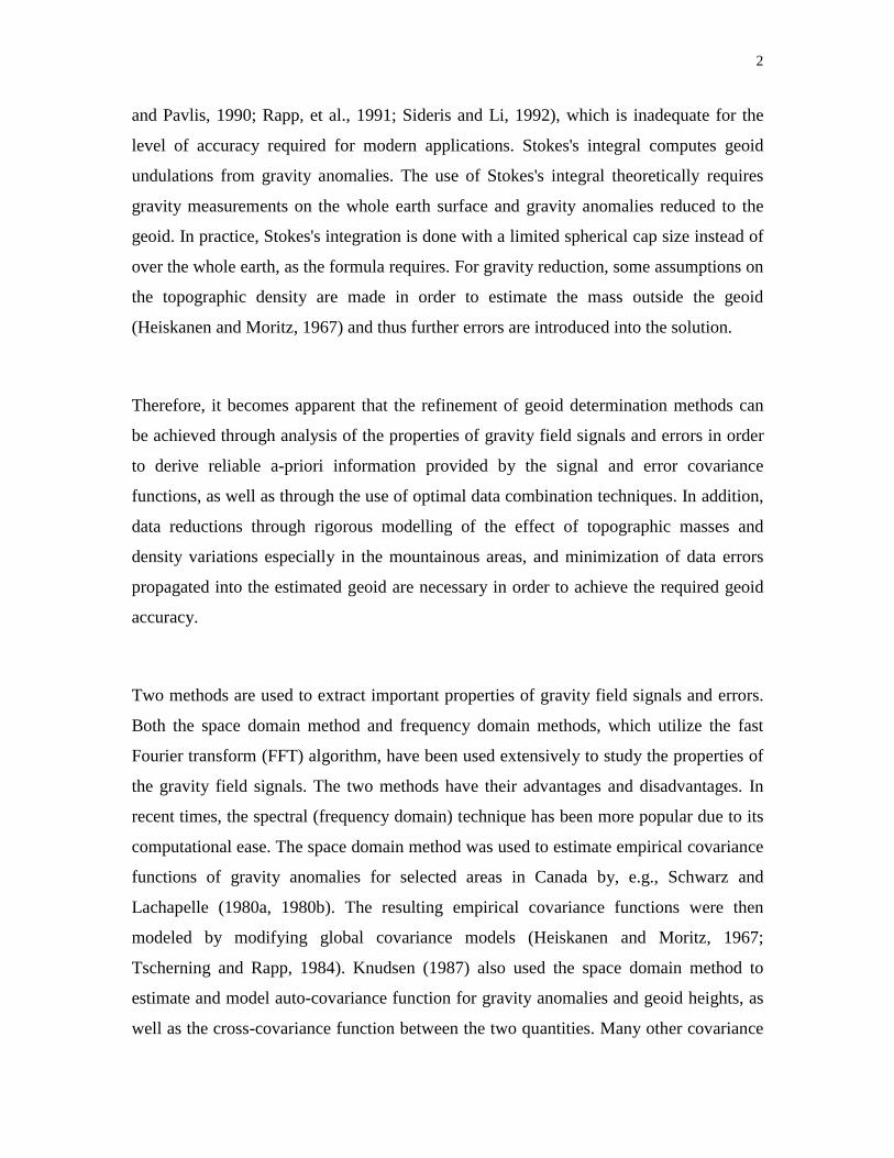
2

and Pavlis, 1990; Rapp, et al., 1991; Sideris and Li, 1992), which is inadequate for the

level of accuracy required for modern applications. Stokes's integral computes geoid

undulations from gravity anomalies. The use of Stokes's integral theoretically requires

gravity measurements on the whole earth surface and gravity anomalies reduced to the

geoid. In practice, Stokes's integration is done with a limited spherical cap size instead of

over the whole earth, as the formula requires. For gravity reduction, some assumptions on

the topographic density are made in order to estimate the mass outside the geoid

(Heiskanen and Moritz, 1967) and thus further errors are introduced into the solution.

Therefore, it becomes apparent that the refinement of geoid determination methods can

be achieved through analysis of the properties of gravity field signals and errors in order

to derive reliable a-priori information provided by the signal and error covariance

functions, as well as through the use of optimal data combination techniques. In addition,

data reductions through rigorous modelling of the effect of topographic masses and

density variations especially in the mountainous areas, and minimization of data errors

propagated into the estimated geoid are necessary in order to achieve the required geoid

accuracy.

Two methods are used to extract important properties of gravity field signals and errors.

Both the space domain method and frequency domain methods, which utilize the fast

Fourier transform (FFT) algorithm, have been used extensively to study the properties of

the gravity field signals. The two methods have their advantages and disadvantages. In

recent times, the spectral (frequency domain) technique has been more popular due to its

computational ease. The space domain method was used to estimate empirical covariance

functions of gravity anomalies for selected areas in Canada by, e.g., Schwarz and

Lachapelle (1980a, 1980b). The resulting empirical covariance functions were then

modeled by modifying global covariance models (Heiskanen and Moritz, 1967;

Tscherning and Rapp, 1984). Knudsen (1987) also used the space domain method to

estimate and model auto-covariance function for gravity anomalies and geoid heights, as

well as the cross-covariance function between the two quantities. Many other covariance

3

modelling studies have also been reported in the literature (Vassiliou and Schwarz, 1987;

Jordan, 1972; Tscherning and Rapp, 1974).

Spectral techniques provide excellent means of extracting gravity field information

contained in each of the gravity field data with the view of determining the contribution

to the gravity spectrum of each data type (Sideris, 1987; Forsberg 1984, 1986; Kotsakis

and Sideris, 1999). Analysis of the gravity field spectrum should involve critical

examination of the spectral information from each data set and from a combination of

geopotential model (GM), local gravity data and heights, which respectively provide

long, medium and short wavelengths information of the gravity field. Such analysis

would provide the necessary gravity field signal and error covariance or power spectral

density (PSD) functions required for geoid prediction techniques. In addition, estimates

of data sampling density derived from degree variances of the gravity signal would give a

better picture of the data requirement for geoid estimation with sub-decimetre accuracy.

Both the space domain and frequency domain methods need to be critically examined to

determine which method will be better in estimating the covariance functions for a local

area. It will also be necessary to know how the two methods could be combined to

achieve the best results in extracting spectral properties of the gravity field signals. In

addition, estimated PSD functions and degree variances should be thoroughly exploited

in various spectral bands to determine the geoid power contribution in various spectral

bands, as well as to estimate the data resolution required for centimetre to decimetre level

of geoid accuracy.

Investigation of the contribution to geoid undulations of the GM coefficients and errors

using the EGM96 geopotential model, in combination with local gravity in Stokes's

integral, would provide the means of optimally combining the two data types.

Consequently, the effects of truncating the degree of the spherical harmonic expansion of

the GM in favour of using larger cap size to evaluate Stokes's integral need to be

4

examined. In similar studies, an increased area of integration has been shown to improve

the results for geoid estimates (Schwarz, 1984; Sjoberg, 1987). The limit to which the cap

size should be increased is investigated in order to derive an optimal cap size for Stokes's

integral solution.

Critical analysis of the signal information from the short wavelength part of the gravity

field spectrum in which the topographic terrain corrections have a dominant role is

required in order for the centimetre geoid to be achievable. Li and Sideris (1994)

established that the discrepancy between the gravimetric geoid and GPS/levelling derived

geoid is correlated with the roughness of the topography. Therefore, rigorous modelling

of the effect of topography and density variations especially in the mountainous areas

would provide information on the recoverable geoid power in the very high spectral band.

Rigorous formulas for terrain correction have been proposed and used (Sideris 1984,

1985, 1990; Li, 1993). The effect of using mass prism topographic model and line prism

topographic model is also documented in Li (1993). In all these studies constant density

values were used for the computation of the terrain effect even in the mountainous areas.

The effect of terrain correction with actual topographic density values on the estimated

geoid needs to be examined if the sub-decimetre geoid is to be achieved especially in

areas with very rough topography.

The overall achievable accuracy of predicted geoid is limited by a number of error

sources. Of more importance are those errors in the geopotential model (GM), local

gravity anomalies g∆ , and heights, which are propagated into the geoid results through

the prediction formulas. Smaller errors due to datum biases, spherical approximation, and

the mass of the atmosphere are not considered in this study; further details can be found

in Heiskanen and Moritz (1967). Proper description of the behavior of data source errors

are provided by suitable covariance function models. While the error covariance function

from the GM can be easily derived from the error degree variances of the coefficients,

5

empirical error covariance models have to be derived for the gravity and height data that

will represent the actual error behavior for the local area. Sideris and Schwarz (1986)

documented error covariance models of gravity and height for areas located in the North

American continent. In order to derive error models for gravity and heights that will

actually represent the local area, models for areas with different topography should be

derived separately, and the overall geoid error from the data errors should be estimated

and modeled for individual areas. In addition, a thorough analysis of errors from each of

the data sources and combination of the data would provide a good picture of internal

geoid accuracy achievable with each data type and combination of the data types.

Therefore, it can be expected that spectral analysis of the gravity field data can provide

the information required for refining geoid estimation methods in order to obtain geoid

with a cm level of accuracy in a local area. Information contained in the spectrum of

different data types would provide the geoid rms power from each of the data types and

their combination. Such information will be useful in determining the optimal procedures

for combining the different data for the geoid prediction methods.

Furthermore, a thorough analysis and rigorous modelling of the effect of topography and

density variation especially in the mountainous areas would improve the short

wavelength information of the geoid in these areas.

1.2 RESEARCH OBJECTIVES

The main task of this study is to investigate how the practical geoid determination

methods could be refined especially in terms of data requirements to achieve geoid

estimates with sub-decimetre level of accuracy. Both space domain and frequency

domain methods will be used to estimate empirical covariance functions of gravity

anomaly for areas with different topographic features in order to examine their

6

correlation with the topography, as well as to investigate the use of uniform covariance

function for prediction by collocation. Spectral techniques will be used extensively to

extract the properties of local gravity field signals in various wavelength bands using the

EGM96, local gravity anomalies, topographic densities and heights. Models for the decay

of the spectrum of the gravity data at various wavelength bands will be derived and the

results compared to standard models. In addition, rigorous terrain correction formulas

will be used with lateral density variations to investigate the effect of using a constant

topographic density value for terrain corrections and geoid indirect effects computation

especially for high mountainous areas.

The role of the GM using EGM96 and local gravity data in geoid estimation will be

investigated. Maximum degree of spherical harmonic expansion of the GM coefficients

in combination with cap size of the Stokes integral will be studied to determine the effect

of truncating the harmonic series in favour of using more local gravity data.

More specifically, the overall objectives of this research will be achieved through the

following tasks:

• Derive covariance and power spectral density (PSD) functions for the gravity field

signals and errors for areas with different topography, possibly marine, flat and

mountainous areas.

• Derive estimates of the gravity and height spacing required for a given level of

accuracy for the geoid.

• Investigate the role of topographic density variations especially in mountainous areas.

• Investigate the role of the GM maximum degree of expansion, in conjunction with

Stokes integral cap size containing the local gravity data.

• Derive models for geoid errors from gravity, heights and GM, as well as the

combined geoid error separately for flat and mountainous areas.

7

1.3 METHODOLOGY

Available gravity, topographic heights and density data for Canada, as well as EGM96

coefficients will be analyzed to derive the covariance and PSD functions of the data sets.

The estimated PSD and covariance functions are used to derive corresponding degree

variances for the gravity data which are then used to estimate the required gravity data

spacing for various levels of accuracy of geoid prediction in the centimetre to decimetre

range. Covariance and PSD functions will be estimated for selected areas in the marine,

flat and mountainous areas of Canada. The results of the spectral analysis for the different

areas will then be compared to determine the average spectral properties of the gravity

field in the marine, flat and mountainous areas of Canada. Furthermore, the effect of

using actual topographic density values for terrain corrections in mountainous areas will

be investigated for areas selected in the Rocky Mountains of western Canada. Analysis

will be based on topographic density data with 30″×30″ resolution and a digital elevation

model (DEM) with 3″×3″ resolution. The results of the terrain corrections and geoid

indirect effects derived with actual topographic density values will be compared with

those obtained with a constant topographic density value.

Reduced gravity anomalies with 5′×5′ resolution in a block size of about 15o×15o and

EGM96 coefficients will be used to study the effect of truncating the harmonic expansion

of the GM model in favour of using more local gravity in a cap size for Stokes's

integration. Various values of maximum degree of spherical harmonic expansion will be

used to estimate gravity anomalies from the reference model and subsequently used to

derive various reduced gravity anomalies. For each set of estimated reduced gravity

anomalies, the corresponding geoid undulation is estimated using Stokes's integral with

varying cap size. The total geoid estimated for a given cap size and harmonic degree of

expansion is then compared to geoid undulations derived from GPS/levelling benchmarks

located within the area of analysis. In addition, the spectrum of the GM and local gravity

data will be analyzed to determine better procedures for combining the GM coefficients

with local gravity data.

8

Gravity data error covariance and PSD functions will be derived by modelling the

differences between actual measurement and predicted observations for selected areas in

flat and mountainous areas. The derived gravity error covariance models will be used to

determine the magnitude of propagated geoid undulation errors for the flat and

mountainous areas. An attempt will be made to compare internal propagated errors with

external geoid errors derived from GPS/levelling benchmarks in the flat and rocky test

areas.

1.4 THESIS OUTLINE

The thesis consists of seven chapters. The content of the next six chapters is summarized

below.

Chapter 2 outlines the methodology and equations for conventional geoid estimation. The

results of varying cap size in Stokes's integral and the maximum degree of spherical

harmonic expansion for the GM coefficients are presented. The effect of lateral density

variations on terrain correction and estimated geoid is presented as well.

In chapter 3, the basic concept of covariance and PSD estimation is discussed and

equations relating the two functions, as well as their relation to the degree variances, are

presented.

Chapter 4 discusses the results of local gravity anomaly empirical covariance functions

for areas selected across Canada in the mountainous, flat and marine test areas. A

comparison is made between the covariance functions derived from the space domain

method with actual gravity data and those from the frequency domain method using

9

gravity data on a grid. The effect of data griding on the estimated covariance estimates is

also discussed.

The variation of the gravity field spectrum at very high frequencies is discussed in

chapter 5. Numerical results for flat and mountainous test areas in Canada are presented.

In addition, the gravity data sampling density required for a level of geoid accuracy in the

decimetre to centimetre range is also presented.

In chapter 6, models for gravity and height data error covariance functions are discussed.

Numerical results of geoid error covariance from these data errors are presented for flat

and mountainous test areas. External geoid errors derived from comparison of GPS and

levelling benchmarks within the area of analysis are estimated and the results are

compared with the internally propagated geoid errors in flat and mountainous areas to

examine their correlation with the topography.

Chapter 7 summarizes the results of the whole study. Main conclusions and

recommendations for geoid estimation and further research are also discussed.

10

CHAPTER 2

GEOID ESTIMATION WITH A GEOPOTENTIAL MODEL AND LOCAL GRAVITY

DATA

This chapter discusses the role of the global geopotential model (GM), local gravity data

and their combination in conventional geoid determination methods. In practice, the long

wavelength geoid is usually estimated by a spherical harmonic expansion up to the

maximum degree and order of the given GM. The contribution from the local gravity data

is estimated by Stokes's integral with gravity anomalies in a given cap size which define

the area of integration. The evaluation of Stokes's integral by FFT requires gravity

anomalies on a regular grid. The interpolation of gravity anomalies is usually carried out

with collocation, which requires reliable a priori information provide by signal and error

covariance functions.

Section 2.1 of this chapter presents the conventional formulas for gravimetric geoid

determination using the remove restore technique. Section 2.2 outlines the FFT formulas

for evaluating the Stokes and terrain correction convolution integrals. Analysis of results

for selected areas in Canada is discussed in section 2.3. In section 2.4, the effect of lateral

topographic density variations on terrain correction and estimated geoid in mountainous

areas is discussed.

11

2.1 FORMULAS FOR GEOID COMPUTATION

The computation of the gravimetric geoid undulation is accomplished by combining

solution from three sources; a global geopotential model (GM), local gravity anomalies

∆g, and the topography represented by a Digital Elevation Model (DEM) using the

remove-restore technique. Local gravity anomalies are first reduced by removing the

effect of the topography and the long wavelength contribution from a reference field. The

effect of the topography and global field are then restored in the final expression for the

geoid undulation. The expression for the gravimetric geoid undulation could therefore be

written as

DEMrÄgGM NNNN ++= (2.1)

where GMN is the geoid undulation implied by the geopotential model, rgN∆ is the

contribution of reduced gravity anomalies, which is derived from Stokes's integration,

and DEMN is the indirect effect of the topography.

The contribution of the GM coefficients, GMN , at a point is computed by spherical

harmonic expansion series (Heiskanen and Moritz, 1967), and is given in spherical

approximation on the geoid as

( )∑∑= =

+=maxn

2n

n

0mnmnmnmGM )(sinPsinmëscosmëcRN ϕ (2.2)

12

where R is the mean radius of the earth, nmc and nms are the fully normalized harmonic

coefficients of the anomalous potential, nmP are the fully normalized associated

Legendre functions, and maxn denotes the maximum degree and order of expansion of

the GM geopotential solution.

The Stokes formula for computing the geoid undulations is given as

dó)(S),ë(gã4

RN

ó

rÄg rψϕ

π ∫∫∆= (2.3)

where ó denotes the sphere of integration, ϕ and λ are the geocentric latitude and

longitude of the data point respectively, ã is the normal gravity, rg∆ is the residual

gravity anomaly, which has been corrected for the effect of the topography and

referenced to a GM, )(Sψ is the Stokes function, and ψ denotes the spherical distance

between the data point and the computation point. Since in real world applications the

gravity data are only available in discrete point locations, the expression in (2.3) can be

rewritten for gravity anomaly data given on the sphere (Haagmans et al, 1992; Li and

Sideris, 1994) as

ëcos)(S)ë,(gã4

RN

B

l

L

l

r

ë

ëërÄg ∆∆∆= ∑∑

= =ϕψϕ

π

ϕ

ϕϕ (2.4)

where ∆ϕ and ∆λ are the grid spacing in latitude and longitude direction respectively, L

and B define the cap size and they represent the number of meridians and parallels in the

block respectively. The Stokes kernel function ),(Sψ can be expressed as

13

+

−−

+−−=

2sin

2sinin

2sin63

2sin10

2sin64

2sin

1)(S

22

2

ψψψ

ψψψ

ψ

(2.5)

where

ϕϕϕϕψ

coscos2

ëësin

2sin

2sin p

p2p22

−+

−=

(2.6)

The term rg∆ in equation (2.4) according to Helmert's second condensation reduction is

given as

GMgFAr gCgg ∆−++∆=∆ ∆δ (2.7)

where FAg∆ is the free air gravity anomaly corrected for the atmospheric attraction, C is

the classical terrain correction, g∆δ is the indirect effect on gravity which, being very

small, is neglected in this study, and GMg∆ is the gravity anomaly computed in spherical

approximation on the geoid by the spherical harmonic expansion formula

( ) ( )∑ ∑= =

+−=maxn

2n

n

0mnmnmnmGM )(sinPsinmëscosmëc1nãÄg ϕ (2.8)

14

The terrain correction C, can be expressed in planar earth approximation as

dxdydzs

)zz)(hy,x,(G)h,y,x(C

E

z

h 3

pppp

p∫∫ ∫

−−=

ρ (2.9)

where ( )212p

2p

2p )z(hy)(yx)x(s −+−+−= , G is the Newton's gravitational constant,

ρ is the topographic density, h is the topographic height, (x, y, z) represents the running

point, )h,y,x( ppp represents the computation point, and E represents the integration

area.

The indirect effect of Helmert's condensation reduction on the geoid in planar

approximation, considering the first two terms is given (Sideris, 1990) as

∫∫−

−

=

E3

pp33

pp

pp2

ppppDEM

dxdys

)]y,(xhy)(x,h)[y,x(

6ã

G

)y,(xh)y,x(ã

ðG)y,(xN

ρ

ρ

(2.10)

See Sideris (1990) and Li (1993) for the detailed expression of geoid topographic indirect

effect and its evaluation via FFT. 1D-FFT formulas for evaluating equation (2.4) are

presented in the next section. Further details on the evaluation of convolution integrals in

physical geodesy by FFT techniques can be found in Schwarz et al. (1989), Sideris

(1994), and Sideris and She (1994). It should be noted that in using the FFT formulas,

data on grids are 100% zero padded, to minimize the effect of circular convolution.

15

2.2 THE SPHERICAL STOKE'S FORMULA

The 1D FFT technique allows for the evaluation of the discrete spherical Stokes integral

without approximation (Sideris and She, 1994). The result of equation (2.4) on a certain

parallel of latitude lϕ using data along parallels of latitude jϕ can be expressed as

( ) ϕϕϕϕϕϕ ÄÄëëë,,S)cosë,Äg(ã4

R)ë,(N

L

1j

B

0iikijjijklÄgr ∑ ∑

= =

−=

ð (2.11)

Since the bracket in (2.11) contains a one-dimensional discrete convolution with respect

to λ, i.e., along a parallel, the expression for its evaluation is given for the fixed parallel

lϕ as

{ } ( ){ }

= ∑

=

−W

0ikijjijklÄg ,ë,S)cos,ëÄg(

ã4

ÄëRÄ),ë(N

rϕϕϕϕ

πϕϕ FFF 1 (2.12)

where F and 1F− denotes the 1D Fourier transform operator and its inverse, respectively.

Detail discussion on the derivation of equation (2.12) from equation (2.3) can be found in

Sideris and She (1994), and Haagmans et al. (1992). The expression in (2.12) yields the

geoid undulation for all the points on one parallel. The major advantage of using the 1D

FFT approach lies in its ability to give exactly the same result as those obtained by direct

numerical integration.

16

2.3 FORMULAS FOR TERRAIN CORRECTION WITH MASS PRISM

TOPOGRAPHIC MODEL

For a given topographic density and height data on a grid, equation (2.9) under the

assumption of uniform density within a topographic mass model, can be written as

)yT(x,)yx,(G)y,C(x1N

0n

1M

0mpp ∑∑

−

=

−

=

= ρ (2.13)

where )yT(x, is the kernel function given as, Li (1993):

hh

0

y/2)(yy

y/2)(yy

)x/2(xx

)x/2(xx

pp

p

p

psz

xyarctanz-

sz

yxarctanz-s)ln(xys)ln(yx)yx,(T

−∆+−

∆−−

∆+−

∆−−

+++=

∗

∗∗∗∗

(2.14)

In equation (2.14), x∆ and y∆ represent the grid spacing in the x and y directions

respectively, and the distance kernel 21

])zh()yy()xx[(s 2p

2p

2p −+−+−= . The

derivation of equations (2.13) and (2.14), and evaluation by 2D FFT is discussed in detail

in Li (1993, pp. 70 - 83). In this thesis, the estimation of all terrain correction is

implemented by the program originally written by Yecai Li (1993); some modifications

are made to the original program to suite the size and format of the input and output data.

Equations (2.1), (2.2) and (2.4) to constitute the set of formulas adopted in this study for

the computation of the gravimetric geoid. Specifically, equation (2.2) is used to derive the

geoid contribution with various values of the degree and order of spherical harmonic

17

expansion of the EGM96 while equation (2.4) is used to derive the geoid with various cap

sizes. Reduced gravity anomalies are derived by using equation (2.7); the reference

gravity anomalies are derived with various degree and order of spherical harmonic

expansion of the EGM96 by using equation (2.8) while the terrain corrections are derived

by using equation (2.9). The effect of change in the integration cap size on the geoid

indirect topographic effects in equation (2.10) is very small and is ignored in this study.

2.4 ANALYSIS OF RESULTS FOR GM AND GRAVITY DATA COMBINATION

2.4.1 Data Sets Used

An area between latitudes 50.0471 and 65.0471, and longitudes -128.0471 and -113.0471

)1515( 00 × located in the Alberta and British Columbia provinces is selected for analysis.

Gravity data with 5′×5′ grid spacing and 1′×1′ DEM data provided by the Geodetic

Survey Division are used. The data sets belong to the same sets of data used for

computing GSD95 geoid model (Veronneau, 1996). The gravity anomaly and geoid

undulation from the GM is computed using the software developed in the department of

Geomatics Engineering, University of Calgary by Li Y. C. (1993). The EGM96

geopotential model, which is complete to degree and order 360, is also used as the

reference field. Newly adjusted leveling data referenced to the Canadian Geodetic Datum

(CGD28) and GPS data points in the selected area are use to derive geoid undulation with

which the estimated gravimetric geoid is compared. Table 2.1 shows the statistics of the

reduced gravity anomaly data and heights used for the analysis.

18

Table 2.1: Statistics of residual gravity anomalies and heights used

for GM and local gravity data analysis

Height (m)Min Max Mean Std.

-1.83 3747.03 885.23 611Residual Gravity Anomalies (mGal)

Degreeof

ExpansionMin Max Mean Std.

30 -113.2 148.1 1.5 27.060 -123.2 149.6 0.6 26.490 -130.5 135.2 -0.1 25.2120 -136.3 136.6 0.0 24.3180 -127.1 141.9 0.0 23.0240 -141.5 127.3 0.0 21.4360 -152.6 146.1 -0.1 20.0

2.4.2 Computed Gravimetric Geoid Undulations

The geoid undulation contributions from the EGM96 and reference gravity anomalies

GMg∆ are computed with (2.2) and (2.8) respectively using 45 , 60, 90, 120, 180, 240,

and 360 spherical harmonic expansions. For each degree of expansion, the block size

used in the Stokes integration varies between 1°×1° and 15°×15°, which correspond

respectively to the smallest and largest cap sizes used in this analysis. The results of

rgN∆ are then added to the corresponding geoid contribution from the EGM96, as well as

the geoid topographic indirect effect, which is computed with all the data points in each

block.

19

2.4.2.1 Absolute Geoid Error with respect to GPS/leveling

The statistics of the standard deviation (Std) of the absolute differences between the two

types of geoid undulations at 265 GPS benchmark stations are summarized in Table 2.2.

The systematic datum differences between the gravimetric geoid and the GPS/levelling

geoid (Kotsakis and Sideris, 1999) are removed by a four-parameter transformation

equation. See Heiskanen and Moritz (1967) for details. The Std of the absolute difference

after a least-squares fit with a four-parameter model is also given (in parentheses) in

Table 2.2. Figures 2.1 and 2.2 show the graphs of absolute geoid difference Std values

against the degree of expansion and cap size, respectively.

Table 2.2: Comparison of gravimetric geoid with GPS/levelling derived geoid

before and after (in parenthesis) datum fit

Degree of Spherical Harmonic ExpansionCapSize 60

(m)90(m)

120(m)

180(m)

240(m)

360(m)

Zero 1.04 (0.94) 0.72 (0.66) 0.64 (0.59) 0.52 (0.46) 0.45 (0.39) 0.43 (0.35)

1 0.49 (0.40) 0.34 (0.31) 0.30 (0.27) 0.25 (0.20) 0.24 (0.20) 0.24 (0.20)

3 0.38 (0.31) 0.29 (0.24) 0.24 (0.19) 0.24 (0.20) 0.24 (0.19) 0.25 (0.19)

5 0.35 (0.25) 0.28 (0.22) 0.23 (0.18) 0.23 (0.20) 0.22 (0.19) 0.22 (0.19)7.5 0.32 (0.17) 0.27 (0.18) 0.22 (0.16) 0.18 (0.15) 0.18 (0.15) 0.18 (0.15)

10 0.22 (0.14) 0.20 (0.14) 0.18 (0.13) 0.15 (0.13) 0.15 (0.13) 0.15 (0.13)

12.5 0.22 (0.16) 0.19 (0.15) 0.18 (0.14) 0.15 (0.13) 0.15 (0.14) 0.15 (0.14)

15 0.21 (0.16) 0.19 (0.15) 0.18 (0.14) 0.15 (0.13) 0.15 (0.14) 0.15 (0.14)

20

Figure 2.1: Absolute geoid accuracy versus harmonic degree of expansion

Legend values are block sizes in degrees

Figure 2.2: Absolute geoid accuracy versus Stokes's cap size

Legend values are spherical harmonic degree

0.0

0.2

0.4

0.6

0.8

1.0

1.2

0 100 200 300 400

Spherical harmonic expansion (degree)

Geo

id d

iffe

ren

ce S

td (

m)

GM 1 5 10 15

0.00

0.05

0.10

0.15

0.20

0.25

0.30

0.35

0 2 4 6 8 10 12 14 16

Cap size (degrees)

Geo

id d

iffe

ren

ce S

td (

m)

90 180 360

21

As shown in Table 2.2, the gravimetric geoid computed with larger cap size, which

corresponds to more local gravity data, gives better results. Figure 2.1 shows that the

improvement in the accuracy of the geoid estimated with harmonic expansion greater

than 200 degrees and cap size of 10° ×10° or greater is negligible. Figure 2.2 shows that

the improvement in the accuracy of the computed geoid when the block size is increased

beyond 10°×10° is of the order of few mm.

Combining the results of Figure 2.1 and 2.2, it is evident that the best estimates of the

geoid can be obtained with spherical harmonic expansion of about 200 degree and

Stokes's integration with local gravity data in a capsize of 10° × 10°. Results computed

with degree of expansion greater than 200 degree and cap size greater than 10° × 10° do

not seem to improve the accuracy of the geoid estimates.

2.4.2.2 Relative Geoid Error with respect to GPS/leveling

To evaluate the relative agreement of the computed gravimetric geoid with respect to the

GPS/leveling data, relative differences are formed on baselines of 100km and 500km in

length. The relative accuracy values are the average value over the baselines with length

about ± 10km from the nominal value. The results of the Std of relative geoid differences

are plotted against the degree of spherical harmonic expansion in Figures 2.3 and 2.5 for

the 100km and 500km baselines respectively. Figures 2.4 and 2.6 show the graph of the

relative geoid Std against cap size, for 100km and 500km baselines respectively. Again

the results of Figures 2.3 to 2.6 agree with the previous results shown in Figures 2.1 and

2.2 for the Std of absolute geoid differences. In order to obtain geoid with a relative

accuracy of 1.5ppm on 100km baseline, EGM96 solution with a minimum of 200

spherical harmonic expansion, as well as Stokes's integration with local data in cap size

of 5°×5° or more is required. In Figures 2.3 and 2.5, the legend values are the cap sizes in

degrees; while in Figures 2.4 and 2.6, the legend values are spherical harmonic degree.

22

Figure 2.3: Relative geoid accuracy versus degree of expansion for 100 km baselines

Figure 2.4: Relative geoid accuracy versus Stokes's cap size for 100 km baselines

0.00

0.50

1.00

1.50

2.00

2.50

3.00

3.50

0 50 100 150 200 250 300 350 400

Spherical harmonic expansion (degree)

Geo

id r

elat

ive

dif

f. (

pp

m)

1 5 15 10

0.00

0.50

1.00

1.50

2.00

2.50

3.00

3.50

0 2 4 6 8 10 12 14 16

Cap Size (degrees)

Geo

id r

ealt

ive

dif

f. (

pp

m)

90 180 360

23

Figure 2.5: Relative geoid accuracy versus degree of expansion for 500 km baselines

Figure 2.6: Relative geoid accuracy versus Stokes's cap size for 500 km baselines

0.00

0.10

0.20

0.30

0.40

0.50

0.60

0.70

0.80

0.90

0 50 100 150 200 250 300 350 400

Spherical harmonic expansion (degree)

Geo

id r

elat

ive

dif

f. (

pp

m)

1 5 15 10

0.00

0.10

0.20

0.30

0.40

0.50

0.60

0 5 10 15 20

Cap size (degrees)

Geo

id r

elat

ive

dif

f. (

pp

m)

90 180 360

24

2.5 THE EFFECT OF LATERAL DENSITY VARIATIONS ON TERRAIN

CORRECTIONS AND GEOID UNDULATIONS

The terrain correction formula based on the mass prism or mass line model (Li, 1993) is

usually executed with constant topographic density value )gm/cm67.2( 3o =ρ for most

applications. In this section, rigorous terrain correction formulas in which the earth

topographic mass is represented by mass prisms of equal base area is used to estimate

terrain corrections with actual topographic density values, as well as with a constant

topographic density value. The effect of making the assumption of constant density

values for the terrain correction, as well as for estimating geoid undulation, is

investigated for five areas located in the Rocky Mountains of western Canada.

Table 2.3: Statistics of topographic densities and heights

SW cornercoordinate

Density (g/cm**3)

Height(m)Test

Area Lat. Long. Min Max Std Min Max StdDRKY1 49 -116 2.49 2.85 2.57 700.00 3377.00 1697.78

DRKY2 49 -120 2.49 2.90 2.68 170.00 2814.00 1281.64

DRKY3 51 -120 2.56 2.90 2.60 386.00 3506.00 1639.44

DRKY4 49 -122 2.49 2.98 2.70 0.00 2754.00 1284.57

DRKY5 51 -122 2.56 2.90 2.71 294.00 2803.00 1265.98

The terrain corrections for selected areas are computed using equations (2.13) and (2.14)

with actual topographic density values, and with constant topographic density value of

3g/cm67.2 . Table 2.3 shows the statistics of the topographic density data and heights, as

25

well as the location of the test areas. The results of the terrain corrections, and their

differences are presented in Table 2.4.

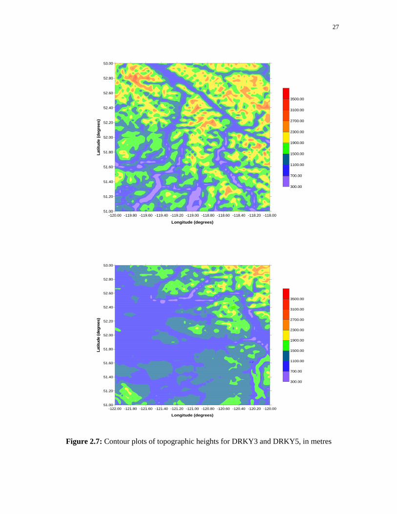
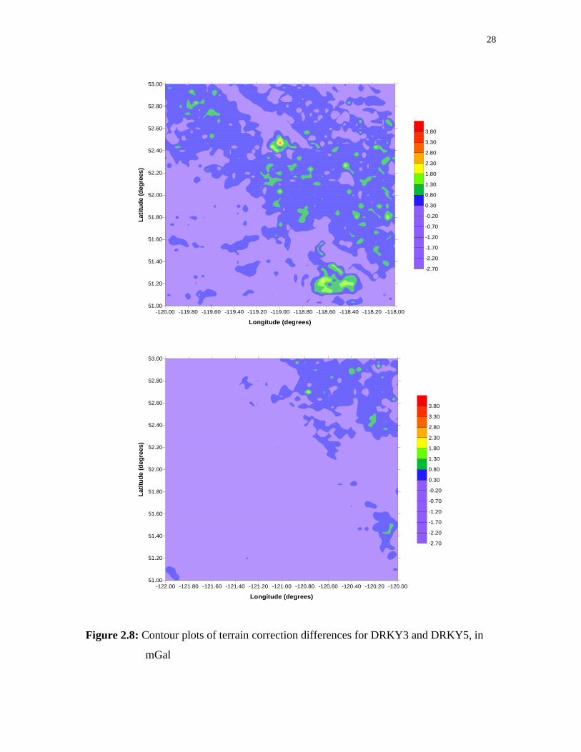
Figures 2.6 and 2.7 show contour plots of the topographic heights and the differences

between the two estimated terrain corrections. Each figure contains the plot for the areas

DRKY3 and DRKY5 at the top and bottom, respectively.

Table 2.4: Statistics of terrain corrections with and without topographic density

variations

TestArea

Without densityvariations

(mGal)

With densityvariations

(mGal)

Difference

(mGal)Min Max Std Min Max Std Min Max Std

DRKY1 0.10 50.39 6.65 0.10 50.37 6.44 -0.58 2.27 0.24

DRKY2 0.33 50.04 6.23 0.33 46.78 6.24 -1.28 3.26 0.20

DRKY3 0.82 75.27 11.35 0.82 77.99 11.64 -2.73 3.82 0.45

DRKY4 0.23 60.52 7.69 0.23 60.12 7.71 -1.95 3.18 0.22

DRKY5 0.05 46.45 5.13 0.05 48.40 5.29 -1.95 1.38 0.21

Geoid undulations are estimated with equation (2.12) using reduced gravity anomalies

that are derived with the two different terrain corrections. The result of the difference

between the geoid undulations estimated with actual topographic density and constant

topographic density is shown in Figure 2.9 for DRKY3 and DRKY5 at the top and

bottom, respectively. The Statistics of the difference is also given in Table 2.5.

26

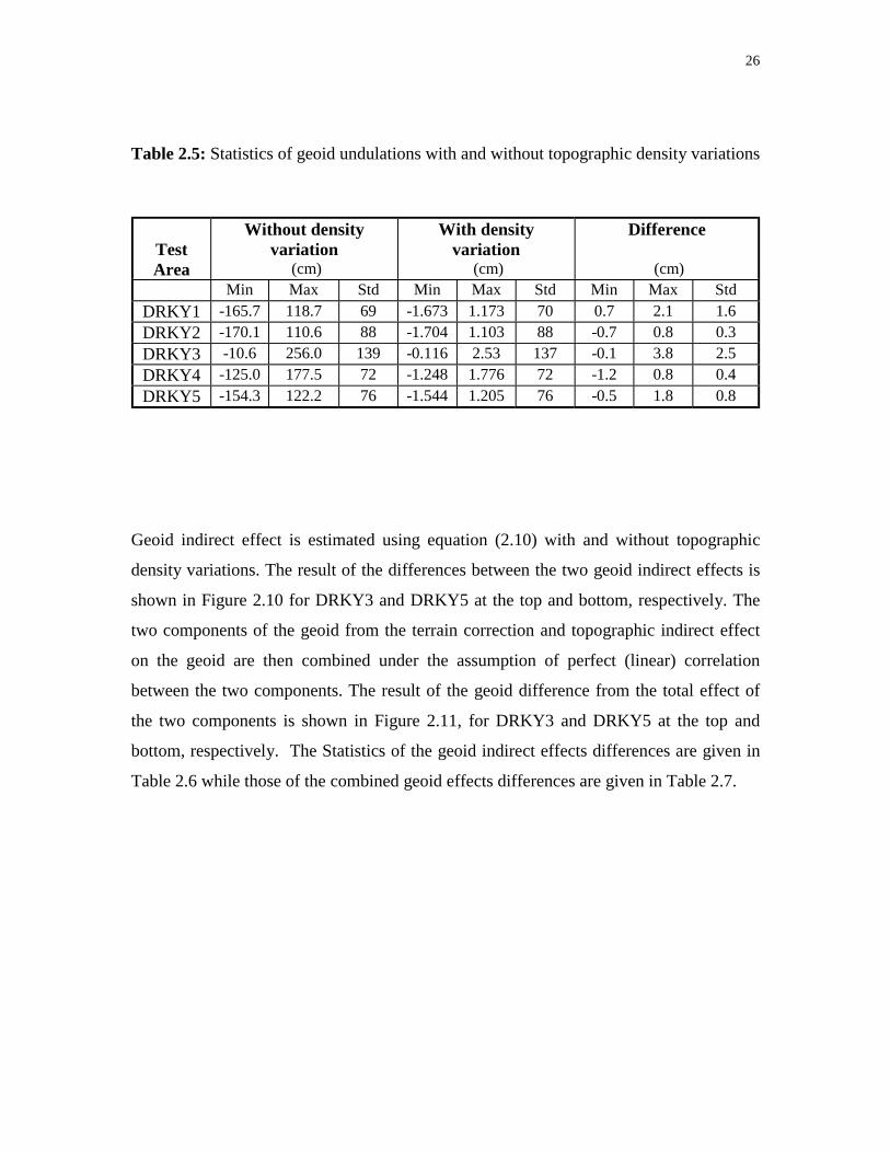
Table 2.5: Statistics of geoid undulations with and without topographic density variations

TestArea

Without densityvariation

(cm)

With densityvariation

(cm)

Difference

(cm)Min Max Std Min Max Std Min Max Std

DRKY1 -165.7 118.7 69 -1.673 1.173 70 0.7 2.1 1.6

DRKY2 -170.1 110.6 88 -1.704 1.103 88 -0.7 0.8 0.3

DRKY3 -10.6 256.0 139 -0.116 2.53 137 -0.1 3.8 2.5

DRKY4 -125.0 177.5 72 -1.248 1.776 72 -1.2 0.8 0.4

DRKY5 -154.3 122.2 76 -1.544 1.205 76 -0.5 1.8 0.8

Geoid indirect effect is estimated using equation (2.10) with and without topographic

density variations. The result of the differences between the two geoid indirect effects is

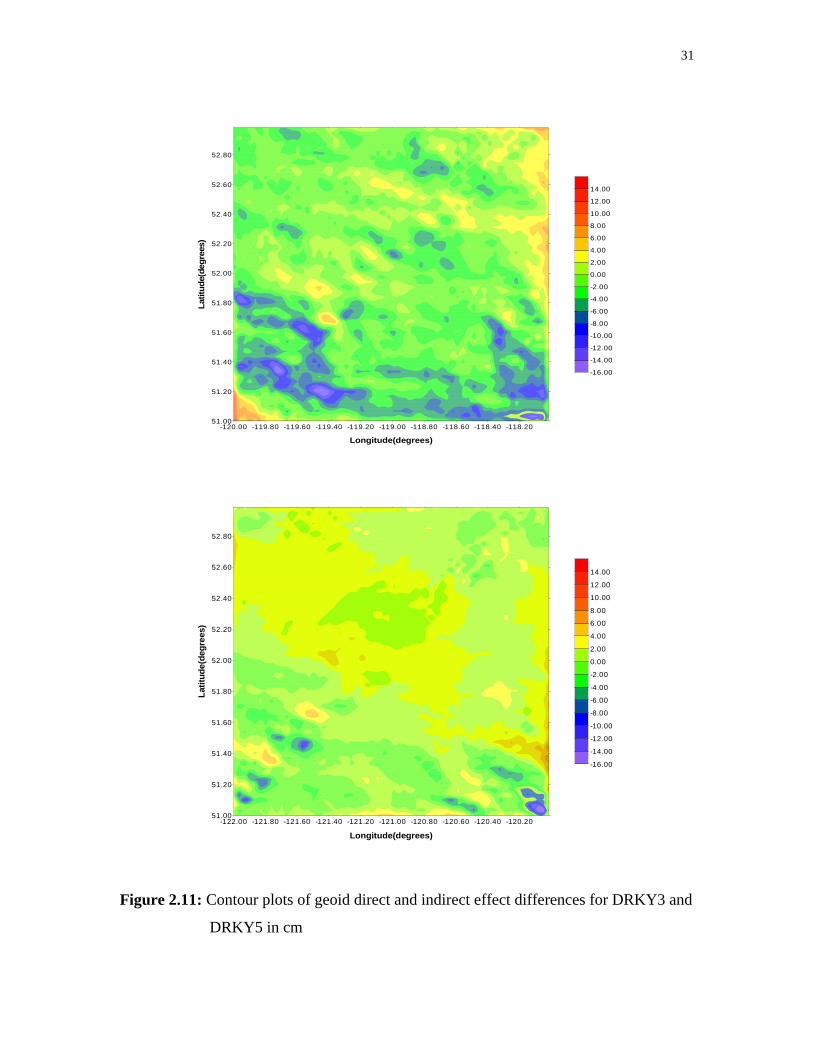
shown in Figure 2.10 for DRKY3 and DRKY5 at the top and bottom, respectively. The

two components of the geoid from the terrain correction and topographic indirect effect

on the geoid are then combined under the assumption of perfect (linear) correlation

between the two components. The result of the geoid difference from the total effect of

the two components is shown in Figure 2.11, for DRKY3 and DRKY5 at the top and

bottom, respectively. The Statistics of the geoid indirect effects differences are given in

Table 2.6 while those of the combined geoid effects differences are given in Table 2.7.

27

Figure 2.7: Contour plots of topographic heights for DRKY3 and DRKY5, in metres

-120.00 -119.80 -119.60 -119.40 -119.20 -119.00 -118.80 -118.60 -118.40 -118.20 -118.00

Longitude (degrees)

51.00

51.20

51.40

51.60

51.80

52.00

52.20

52.40

52.60

52.80

53.00

Lat

itu

de

(deg

rees

)

300.00

700.00

1100.00

1500.00

1900.00

2300.00

2700.00

3100.00

3500.00

-122.00 -121.80 -121.60 -121.40 -121.20 -121.00 -120.80 -120.60 -120.40 -120.20 -120.00

Longitude (degrees)

51.00

51.20

51.40

51.60

51.80

52.00

52.20

52.40

52.60

52.80

53.00

Lat

itude

(deg

rees)

300.00

700.00

1100.00

1500.00

1900.00

2300.00

2700.00

3100.00

3500.00

28

Figure 2.8: Contour plots of terrain correction differences for DRKY3 and DRKY5, in

mGal

-120.00 -119.80 -119.60 -119.40 -119.20 -119.00 -118.80 -118.60 -118.40 -118.20 -118.00

Longitude (degrees)

51.00

51.20

51.40

51.60

51.80

52.00

52.20

52.40

52.60

52.80

53.00

Lat

itu

de

(deg

rees

)

-2.70

-2.20

-1.70

-1.20

-0.70

-0.20

0.30

0.80

1.30

1.80

2.30

2.80

3.30

3.80

-122.00 -121.80 -121.60 -121.40 -121.20 -121.00 -120.80 -120.60 -120.40 -120.20 -120.00

Longitude (degrees)

51.00

51.20

51.40

51.60

51.80

52.00

52.20

52.40

52.60

52.80

53.00

Lat

itu

de

(deg

rees

)

-2.70

-2.20

-1.70

-1.20

-0.70

-0.20

0.30

0.80

1.30

1.80

2.30

2.80

3.30

3.80

29

Figure 2.9: Contour plots of geoid undulation differences for DRKY3 and DRKY5, in

cm

-120.00 -119.80 -119.60 -119.40 -119.20 -119.00 -118.80 -118.60 -118.40 -118.20

Longitude (degrees)

51.00

51.20

51.40

51.60

51.80

52.00

52.20

52.40

52.60

52.80

Lat

itu

de (

deg

rees

)

-0.60

-0.20

0.20

0.60

1.00

1.40

1.80

2.20

2.60

3.00

3.40

3.80

-122.00 -121.80 -121.60 -121.40 -121.20 -121.00 -120.80 -120.60 -120.40 -120.20

Longitude(degrees)

51.00

51.20

51.40

51.60

51.80

52.00

52.20

52.40

52.60

52.80

Lat

itu

de(

deg

rees)

-0.60

-0.20

0.20

0.60

1.00

1.40

1.80

2.20

2.60

3.00

3.40

3.80

30

Figure 2.10: Contour plots of geoid indirect effect differences for DRKY3 and DRKY5

in cm

-120.00 -119.80 -119.60 -119.40 -119.20 -119.00 -118.80 -118.60 -118.40 -118.20

Longitude (Degree)

51.00

51.20

51.40

51.60

51.80

52.00

52.20

52.40

52.60

52.80

Lat

itu

de

(Deg

ree)

-16.00

-14.00

-12.00

-10.00

-8.00

-6.00

-4.00

-2.00

0.00

2.00

4.00

6.00

8.00

-122.00 -121.80 -121.60 -121.40 -121.20 -121.00 -120.80 -120.60 -120.40 -120.20

Longitude (Degree)

51.00

51.20

51.40

51.60

51.80

52.00

52.20

52.40

52.60

52.80

Lat

itu

de

(Deg

ree)

-16.00

-14.00

-12.00

-10.00

-8.00

-6.00

-4.00

-2.00

0.00

2.00

4.00

6.00

8.00

31

Figure 2.11: Contour plots of geoid direct and indirect effect differences for DRKY3 and

DRKY5 in cm

-120.00 -119.80 -119.60 -119.40 -119.20 -119.00 -118.80 -118.60 -118.40 -118.20

Longitude(degrees)

51.00

51.20

51.40

51.60

51.80

52.00

52.20

52.40

52.60

52.80

Lat

itu

de(

deg

rees

)

-16.00

-14.00

-12.00

-10.00

-8.00

-6.00

-4.00

-2.00

0.00

2.00

4.00

6.00

8.00

10.00

12.00

14.00

-122.00 -121.80 -121.60 -121.40 -121.20 -121.00 -120.80 -120.60 -120.40 -120.20

Longitude(degrees)

51.00

51.20

51.40

51.60

51.80

52.00

52.20

52.40

52.60

52.80

Lat

itu

de(d

egre

es)

-16.00

-14.00

-12.00

-10.00

-8.00

-6.00

-4.00

-2.00

0.00

2.00

4.00

6.00

8.00

10.00

12.00

14.00

32

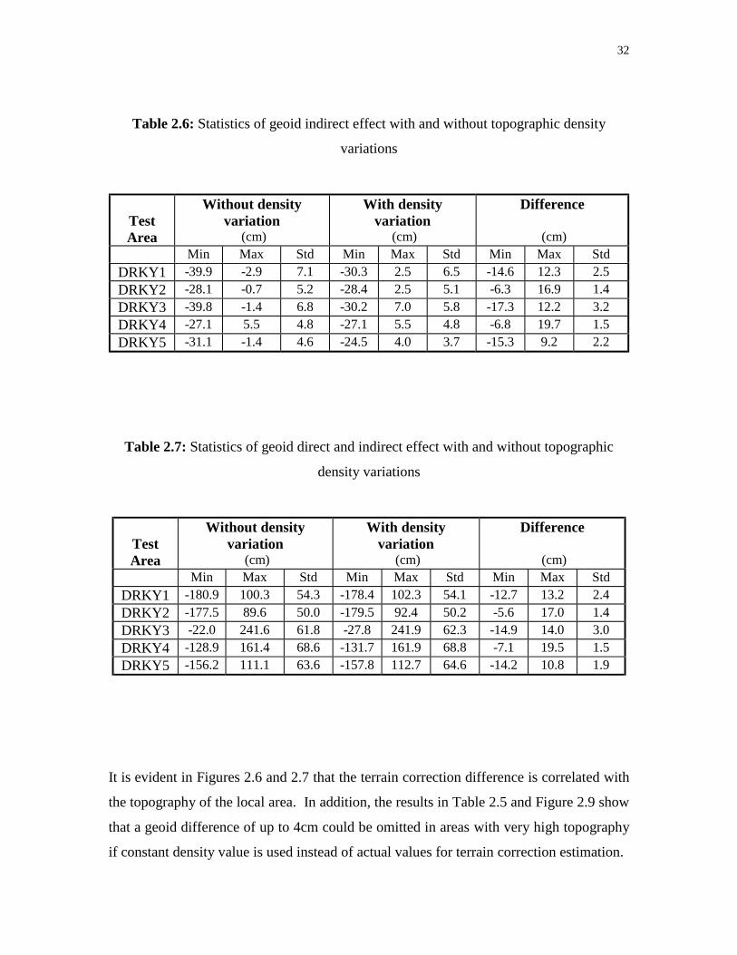
Table 2.6: Statistics of geoid indirect effect with and without topographic density

variations

TestArea

Without densityvariation

(cm)

With densityvariation

(cm)

Difference

(cm)Min Max Std Min Max Std Min Max Std

DRKY1 -39.9 -2.9 7.1 -30.3 2.5 6.5 -14.6 12.3 2.5

DRKY2 -28.1 -0.7 5.2 -28.4 2.5 5.1 -6.3 16.9 1.4

DRKY3 -39.8 -1.4 6.8 -30.2 7.0 5.8 -17.3 12.2 3.2

DRKY4 -27.1 5.5 4.8 -27.1 5.5 4.8 -6.8 19.7 1.5

DRKY5 -31.1 -1.4 4.6 -24.5 4.0 3.7 -15.3 9.2 2.2

Table 2.7: Statistics of geoid direct and indirect effect with and without topographic

density variations

TestArea

Without densityvariation

(cm)

With densityvariation

(cm)

Difference

(cm)Min Max Std Min Max Std Min Max Std

DRKY1 -180.9 100.3 54.3 -178.4 102.3 54.1 -12.7 13.2 2.4

DRKY2 -177.5 89.6 50.0 -179.5 92.4 50.2 -5.6 17.0 1.4

DRKY3 -22.0 241.6 61.8 -27.8 241.9 62.3 -14.9 14.0 3.0

DRKY4 -128.9 161.4 68.6 -131.7 161.9 68.8 -7.1 19.5 1.5

DRKY5 -156.2 111.1 63.6 -157.8 112.7 64.6 -14.2 10.8 1.9

It is evident in Figures 2.6 and 2.7 that the terrain correction difference is correlated with

the topography of the local area. In addition, the results in Table 2.5 and Figure 2.9 show

that a geoid difference of up to 4cm could be omitted in areas with very high topography

if constant density value is used instead of actual values for terrain correction estimation.

33

The effect of using actual density values is more noticeable in the computation of the

geoid indirect effect. The results in Table 2.6 and Figure 2.10 show that a difference of

up to 20 cm could be omitted in the geoid estimates. When the two geoid components are

combined, a geoid difference of 20 cm is noticed (Table 2.7 and Figure 2.11).

34

CHAPTER 3

ESTIMATION AND MODELLING OF GRAVITY FIELD COVARIANCE AND

POWER SPECTRAL DENSITY FUNCTIONS

This chapter outlines the basic concepts of covariance, correlation and power spectral

density (PSD) function estimation and the relation between the three functions. Formulas

that are used in the spectral analysis are also presented.

Section 3.1 discusses the basic concepts of covariance, correlation and power spectral

density functions; it also highlights the relationship between the three functions. In

section 3.2, formulas used for practical estimation of empirical gravity anomaly

covariance function, as well as covariance function models, are presented. Section 3.3

discusses the computation of gravity anomaly PSD function, and the relationship between

the PSD function and degree variances is presented in section 3.4.

3.1 CONCEPTS OF COVARIANCE AND SPECTRAL DENSITY FUNCTIONS

This section discusses the basic concepts of covariance, correlation and power spectral

density functions and the relation between the three functions. The derivations of the

equations relating the functions is not discussed as it can be found in many text books and

papers on the subject; see, e.g., Bendat and Piersol (1980, 1986) and Sideris (1994). The

definition of these functions is limited in this section to Cartesian coordinates with the X

axis pointing east, the Y axis pointing north and the Z axis pointing upward.

35

The covariance function y)(x,Cgh of two functions )y,g(x 11 and )y,h(x 22 , which are

sample functions of the corresponding stationary random processes, is defined as

( )( )[ ]h)y,h(xg)y,g(xEy)x,(C 2211gh −−=∆∆ (3.1)

where 12 x- xx =∆ , 12 y-y y =∆ , [ ]E is the mathematical expectation operator, and g

and h are the mean values of the functions )y,g(x 11 and )y,h(x 11 , respectively. When

the two functions )y,g(x 11 and )y,h(x 22 are identical, i.e., )y,g(x )y,h(x 2211 = , then

the result of equation (3.1) is termed auto-covariance function. Otherwise, if

)y,g(x )y,h(x 2211 ≠ , the resultant covariance is known as the cross-covariance function.

Furthermore, if y),x(Cgh ∆∆ is such that it could be replaced with (s)Cgh , where

222 yxs ∆+∆= , then the resultant covariance function is said to be isotropic.

The correlation function y)(x,R gh of two sample functions )y,g(x 11 and )y,h(x 22 is

defined as

( )( )[ ])y,h(x)y,g(xEy),x(R 2211gh =∆∆ (3.2)

where all variables have the same meaning as previously defined. For sample functions

with zero means, i.e., 0h g == , the correlation function is identical to the covariance

function, i.e., ghgh C R = . Sample functions with zero means are referred to as centred

functions. Again, if the two sample functions are identical, the correlation function in

equation (3.2) is known as the auto-correlation function. Otherwise, it is called cross-

correlation function.

36

The PSD function is defined as the frequency domain equivalent of the correlation

function. The function contains the spectrum of the mean square values of the sample

functions. For the two sample functions )y,g(x 11 and )y,h(x 22 , the PSD function

)yx,(Pgh is defined via the Fourier transform of the correlation function )yx,(R gh as

{ }y)(x,Rdxdyy)e(x,R)vu,(P ghvy)(uxj2-

ghgh F== ∫ ∫∞

∞−

∞

∞−

+π (3.3)

where the spatial frequencies u and v (also known as wave numbers) correspond to x and

y, respectively. If the two functions )y,g(x 11 and )y,h(x 22 are centered functions, then

equation (3.3) is equivalent to

{ }y)(x,Cdxdyy)e(x,C)vu,(P ghvy)(uxj2-

ghgh F== ∫ ∫∞

∞−

∞

∞−

+π (3.4)

since in this case the covariance and correlation functions are equal. Again we have auto-

power spectral density function if the two sample functions are identical and cross-power

spectral density function if otherwise.

In practice, discrete values of the sample functions are usually given on a finite plane.

Therefore, the continuous spectrum given in equation (3.3) and (3.4) becomes discrete.

The discrete Fourier transform is then applied. In addition, the expressions in (3.1) and

(3.2) are executed as summation in the x and y directions. The derivation of the

expressions for the covariance, correlation and PSD functions, and their general

applications can be found in Bendat and Piersol (1980, 1986).

37

3.2 LOCAL GRAVITY ANOMALY COVARIANCE FUNCTION

Moritz (1980) gave the basic definition of a global covariance function on a sphere as the

expected value over the sphere of the product of all pairs of gravity values located at

fixed distances apart. The local covariance function of the gravity field is defined by

Goad et al, (1984) as a special case of a global covariance function where the information

content of wavelengths longer than the extent of the local area has been removed, and the

information outside, but nearby, the area is assumed to vary in a manner similar to the

information within the area. In this section, the fundamental equations for the estimation

of local covariance functions for gravity anomalies are presented. The notation employed

in the expressions for the covariance functions follow closely the one used in Heiskanen

and Moritz (1967).

Three parameters are used to describe the characteristics of the local covariance function

of gravity field quantities. The definition of the three parameters, the variance 0C , the

correlation distance 21χ and the horizontal gravity gradient variance, are given in Moritz

(1980).

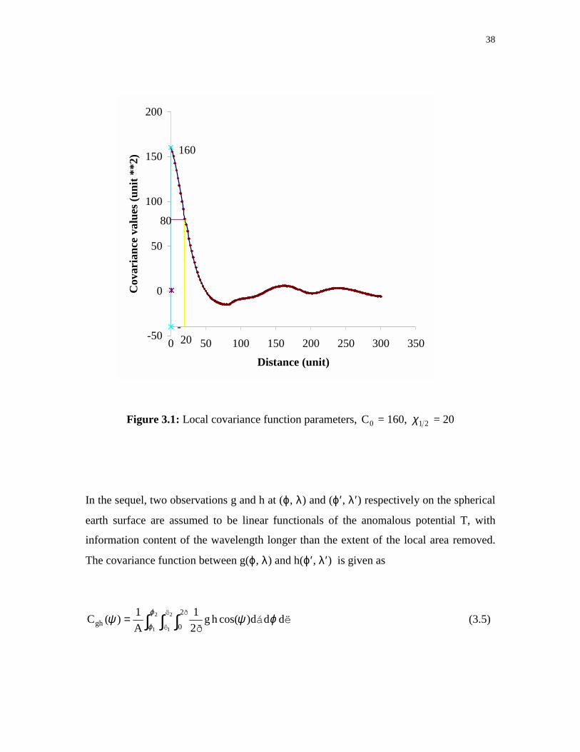
The first two parameters 0C and 21χ (Figure 3.1) are used in this study to describe the

local covariance function of the gravity anomalies. The variance 0C is the value of the

covariance for zero distance while the correlation distance 21χ is defined as the distance

at which the covariance is half of the variance value, i.e. 021 C2

1)C(÷ = .

38

Figure 3.1: Local covariance function parameters, 0C = 160, 21χ = 20

In the sequel, two observations g and h at (ϕ, λ) and (ϕ′ , λ′ ) respectively on the spherical

earth surface are assumed to be linear functionals of the anomalous potential T, with

information content of the wavelength longer than the extent of the local area removed.

The covariance function between g(ϕ, λ) and h(ϕ′ , λ′ ) is given as

dëddá)cos(hg2ð

1

A

1)(C

2

1

2

1

ë

ë

2ð

0gh ϕψψϕ

ϕ∫ ∫ ∫= (3.5)

80

20-

160

-50

0

50

100

150

200

0 50 100 150 200 250 300 350

Distance (unit)

Cov

aria

nce

val

ues

(u

nit

**2

)

39

where A is the size of the area on the unit sphere, 2121 ë,ë,,ϕϕ represents the extent of

the local area, á is the azimuth and )ëcos(ëcoscossinsin)(cos ′−′+′= ϕϕϕϕψ .

Equation (3.5) represents a homogenous and isotropic covariance function, which is

calculated as an average of the product of g and h over the local area (homogeneity) and

as an average over the azimuth (isotropy). In practice, the observations are at discrete

points in the local area and the integral reduces to numerical summation.

3.2.1 Estimation of Empirical Covariance Function

Two methods are usually employed in the estimation of the local gravity empirical

covariance function. The first method makes use of the actual data available to compute

the empirical covariance functions directly, while the second method computes the

empirical covariance functions by taking the inverse Fourier transform of PSD functions.

The former method is referred to as the direct method while the later is referred to as the

indirect method.

3.2.1.1 Covariance Function from Actual Data

This method computes the empirical covariance function directly from actual data and is

referred to as the direct method. Two formulas are presented for empirical covariance

estimation with actual gravity data. The first set of formulas estimate the isotropic

empirical covariance function of gravity data with irregular distribution. For gravity data

with a regular grid, the empirical covariance function is given by the second set of

formulas.

40

The covariance function between the function g and h given at discrete points in blocks

on the sphere is given as

∑

∑ ′′=

hg

h g

aa

)ë,h( )g(aa

)C(

ϕϕψ

,ë

(3.6)

where ga and ha represent the area of the blocks on the sphere for observation g and h,

respectively. For gravity anomalies, ig ë),g( ∆=ϕ and jg )ë,g( ∆=′′ϕ , equation (3.6)

provides an isotropic gravity anomaly covariance function.

If the gravity anomalies for example are given in blocks of equal area, then equation (3.6)

reduces to

k

kji

kg n

gg)(C∑ ∆∆

=∆∆ ψg (3.7)

where kn represents the number of products taken at a given spherical distance kψ . The

distance ψ to which product at kψ is determined is defined by

2

Ä

2

Äk

ψψψψψ +<<− (3.8)

41

where ψ∆ is a suitable interval.

In the case of gravity anomalies given on a rectangular regular grid of area size yx TT ×

and with grid spacing x∆ and y∆ in the x and y directions, respectively, the empirical

non-isotropic covariance function for gravity anomalies g∆ is estimated as

∑ ∑−

= =∆∆ ++∆∆=

1-kM

i

l-1-N

jgg

0 0

l)]jk,g(ij)][g(i,l-N

1

k-M

1l)(k,C (3.9)

where x

TM x

∆= ,

y

TN y

∆= .

3.2.1.2 Covariance Function via Spectral Density Function

The empirical covariance function could be estimated indirectly from gridded data by the

fast Fourier transform (FFT) algorithm. Since the power spectral density function is the

frequency domain equivalence of the correlation function, then for centered gravity data,

the inverse Fourier transform of the PSD function provides the corresponding covariance

function of the gravity data.

In flat earth approximation, the surface of the earth is replaced by a tangential plane. The

spherical distance )(ψ becomes the planar distance s )yxs( 222 += . In a local area, both

approximations converge to each other (Knudsen, 1987). The PSD function ( actually the

periodogram) of gravity anomaly observations is estimated by Fourier transform as

42

*v)G(u,v)G(u,v)(u,P ∆∆=∆∆ gg (3.10)

where ∆G is the Fourier transform of the gravity anomaly observations ∆g.

The two-dimensional non-isotropic covariance function y)(x,C gg∆∆ is then estimated by

taken the inverse Fourier transform of )vu,(P gg∆∆ as

∫ ∫∞

∞−

∞

∞−

+∆∆∆∆∆∆ == dxdye)vu,(P}P{v)(u,C vux(2j

gggy)

gggπ-1F (3.11)

An isotropic covariance function )(sC gg∆∆ is derived from equation (3.11) by averaging

over all azimuths as

∫ ∆∆∆∆ =π

π2

0 gg dá)yx,(C2

1)(sC gg (3.12)

For isotropic PSD function ),(ùP g∆∆g where 222 vuù += , the corresponding isotropic

covariance function ),(sC g∆∆g is obtained by the inverse Hankel transform and not with

the inverse Fourier transform; see Forsberg 1984 for details. The Hankel transform

operator H and its inverse 1−H is define for the function g as

ds)sù(sg(s)J}g(s){ )(g0 0∫∞

== Hù (3.13)

43

dù)sù(J ùg(ù)}) g(ù{) g(s0 0

1 ∫∞− == H (3.14)

where 0J is the Bessel function of order zero.

3.2.2 Modeling of the Gravity Anomaly Covariance Function

In gravity field prediction with heterogeneous gravity field data, self sufficient covariance

models are required in the estimation method. The self-sufficiency of the covariance

functions ensures that the covariance functions of the different gravity field quantities are

related through linear functional of the anomalous potential. A self sufficient covariance

function is derived by fitting empirical covariance values to some analytical function,

which is usually characterized by few parameters.

Various covariance models for gravity field signals are presented in Moritz (1980). A

number of analytical covariance functions have also been suggested and used for gravity

field approximation in flat earth approximation. See Vassiliou and Schwarz (1987) and

Jordan (1972) for details.

For spherical earth, the covariance function model is usually derived from degree a

variance model. The Tscherning/Rapp model (Tscherning and Rapp, 1974) is the most

widely used degree variance models, and is adopted in this study for covariance

modelling. Empirical covariance values are fitted to the analytical model by least squares

in an iterative procedure.

44

The covariance function )(K ψ of the anomalous potential T expanded into a harmonics

series is given in terms of Legendre polynomials as, (Moritz, 1980):

)(cosPrr

RT),T()(K n

n

2n

1n

B2n

max

ψσψ ∑=

+

′

= (3.15)

where maxn is the maximum degree and order of a global geopotential model that is used

as the reference field, T),T(2nσ are the anomalous potential degree variances, r and r′

represent the geocentric radial distances of two observation points at a (spherical)

distance ψ apart, and BR is the radius of the Bjerhammar sphere.

Since in practice the covariance function )(K ψ of the anomalous potential T cannot be

estimated directly, equation (3.5) is fitted to covariance values of gravity field data that

are linear functionals of T . The covariance of the local anomalous potential is then

derived by applying the inverse linear functional relation. The covariance function of

reduced local gravity anomalies derived from equation (3.15) can be expressed as

∑

∑∞

+=

+

=

+∆∆

∆∆+

∆∆=

1nnn

2nrr

2n

n

n

2n

2nrr

2ngg

max

max

r

)(cosPS)g,g(

)(cosP)Sg,g(c)(C

ψε

ψψr

(3.16)

where )g,g(c rr2n ∆∆ are the local gravity anomaly degree variances,

′

=rr

RS

2B , rg∆ is

the reduced gravity anomaly, and )g,g( rr2n ∆∆ε are the error degree variances of the local

gravity data.

45

The degree variances of the potential and gravity anomalies are estimated using the

Tscherning/Rapp model given as

24)2)(n1)(n(n

A)T,T(2

n +−−=σ (3.17)

)T,T(R

)1n()g,g( n2

E

22n σσ −=∆∆ (3.18)

where A is a constant which is related to the variance value in unit of mGal2. For other

quantities of the gravity field, the covariance function and degree variances can be

derived from the linear functional relation of such quantities to the anomalous potential.

Expressions for other gravity field quantities can be found in Moritz (1980).

The error degree variances of the local gravity data )g,g( rr2n ∆∆ε , is obtained by an

approximate method with the following expressions:

)ù(P1)(n

0.5n

ã2

1)g,g( n2rr

2n g∆−

+=∆∆ επε (3.19)

a

ù2

gn

n

geó)ù(P =

∆ε,

R

0.5nù n

+= (3.20)

where g

P∆ε

is the isotropic gravity error PSD function, gó is the average standard

deviation of the gravity observations, and a is a constant (a=10). A detail expression for

gravity error degree variances is given later in this thesis.

46

The fitting of the model in equation (3.16) to the empirical covariance values is done by

an adjustment of the parameters RB and A using a least square inversion method; see

Knudsen (1987) for details. In the covariance analysis that follows, the modelling of the

covariance functions is carried out with a computer program, which was originally

written by Tscherning (1975). The program has been modified to suite the data format

and error degree variance model in equation (3.19).

3.3 ESTIMATION OF THE GRAVITY ANOMALY POWER SPECTRAL DENSITY

FUNCTION

The power spectral density (PSD) function can be estimated directly from the actual data

in a grid by Fourier transform or indirectly by taken the inverse Fourier transform of

previously estimated correlation function. For gravity anomalies given at discrete points

on a plane, the PSD function can be computed directly from the data as

[ ] [ ] ∗∆∆=∆∆ )yg(x,y)g(x,v)(u,P gg FF (3.21)

where ∗ denotes complex conjugate, and F is the Fourier transform operator. Again, the

evaluation of equation (3.21) by FFT requires that the gravity anomalies be on a grid.

Further detail information on Fourier transform and its applications are found in

Bracewell (1983) and Schwarz et al. (1990).

The second method used in the estimation of power spectral density function involves

taking the Fourier transform of a previously calculated correlation function. For gravity

anomalies g∆ located at discrete points on a plane equation, (3.3) could be written as

47

}y)(x,R{v)(u,P ÄgÄgÄgÄg F= (3.22)

where F denotes two-dimensional (2D) discrete Fourier transform operator. For centered

gravity anomalies on a regular grid, the correlation function is equivalent to the

covariance function given in (3.9).

3.4 RELATIONSHIP BETWEEN DEGREE VARIANCES AND POWER SPECTRUM

Degree variances are usually used to study the variation of the gravity field in various

spectral bands because they allow easy comparison with results from global models. The

degree variances of the anomalous potential 2nó can be defined as the spectrum of the

local isotropic covariance function of this potential in spherical earth approximation.

Forsberg (1984) established a relationship between the degree variance 2nó and the

isotropic PSD function )ù(PTT of the anomalous potential for flat earth approximations

as

)ù(P2

1n

R2

1ó TT2

2n

+=

ð (3.23)

where the wave number R

2

1n

ù+

= . In the sequel, two-dimensional PSD function of the

gravity anomaly is computed first with equation (3.21) and made isotropic by averaging

along circles of constant wavelength. Then the degree variances of the anomalous

potential are estimated from

48

2n2

22n c

1)(n

Ró

−= (3.24)

where nc is the degree variances of the local gravity anomalies estimated from the

corresponding isotropic PSD function using an expression similar to (3.23) for the gravity

anomaly.

49

CHAPTER 4

COVARIANCE ANALYSIS FOR AREAS IN CANADA

This chapter discusses the results of the empirical covariance functions for local gravity

anomalies in selected areas across Canada. The preprocessing of the gravity anomaly data

is discussed in section 4.1 while the results of both the space domain and frequency

domain methods are presented and compared for all the selected areas in section 4.3. The

selected mountainous areas are located in the west, the flat areas in the east and the

marine areas in the Hudson bay, and the Pacific and Atlantic coasts of Canada. The

mountainous areas have highly varying topography with standard deviation of 450m or

higher. The flat areas are rather smooth with standard deviation usually below 200m.

4.1 TEST AREAS AND DATA REDUCTION

The results of the analysis in the sequel are based on data selected from blocks of 2o × 2o

in western (rocky areas) and eastern Canada (flat areas), and blocks of 5o × 5o in marine

areas. Figure 4.1 shows the location of all the test areas in rectangular blocks. In Table

4.1, the statistics of topographic heights, as well as the geographic local of the test areas

are presented.

50

Figure 4.1: Distribution of test area blocks across Canada

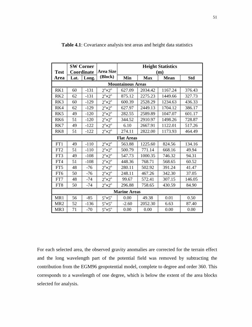
51

Table 4.1: Covariance analysis test areas and height data statistics

SW CornerCoordinate

Height Statistics(m)Test

Area Lat. Long.

Area Size(Block) Min Max Mean Std

Mountainous AreasRK1 60 -131 2o×2o 627.09 2034.42 1167.24 376.43RK2 62 -131 2o×2o 875.12 2275.23 1449.66 327.73RK3 60 -129 2o×2o 600.39 2528.29 1234.63 436.33RK4 62 -129 2o×2o 627.97 2449.13 1704.12 386.17RK5 49 -120 2o×2o 282.55 2589.89 1047.07 601.17RK6 51 -120 2o×2o 344.52 2910.97 1498.26 728.87RK7 49 -122 2o×2o 6.10 2667.91 1122.01 517.26RK8 51 -122 2o×2o 274.11 2822.00 1173.93 464.49

Flat AreasFT1 49 -110 2o×2o 563.88 1225.60 824.56 134.16FT2 51 -110 2o×2o 500.79 771.14 668.16 49.94FT3 49 -108 2o×2o 547.73 1000.35 746.32 94.31FT4 51 -108 2o×2o 448.36 768.71 568.65 60.52FT5 48 -76 2o×2o 280.11 502.92 391.24 41.47FT6 50 -76 2o×2o 248.11 467.26 342.30 37.05FT7 48 -74 2o×2o 99.67 572.41 307.15 146.05FT8 50 -74 2o×2o 296.88 758.65 430.59 84.90

Marine AreasMR1 56 -85 5o×5o 0.00 49.38 0.01 0.50MR2 52 -136 5o×5o -2.60 2052.30 6.63 87.40MR3 71 -70 5o×5o 0.00 0.00 0.00 0.00

For each selected area, the observed gravity anomalies are corrected for the terrain effect

and the long wavelength part of the potential field was removed by subtracting the

contribution from the EGM96 geopotential model, complete to degree and order 360. This

corresponds to a wavelength of one degree, which is below the extent of the area blocks

selected for analysis.

52

Table 4.2: Statistics of reduced gravity anomalies before and after gridding

(all values are in mGal)

Before GriddingAfter centering (mean = 0) and gridding

with 5′′′′ and 1′′′′ spacingMin Max Std

TestArea

IPD(′′′′)

Min Max Mean Std 5′′′′ 1′′′′ 5′′′′ 1′′′′ 5′′′′ 1′′′′Mountainous Areas

RK1 7.6 -68.5 67.6 -3.3 31.9 -70.3 -69.2 67.5 64.2 24.9 25.4RK2 7.3 -72.6 87.9 10.0 31.1 -84.4 -74.7 73.3 68.4 20.1 20.4RK3 6.9 -100.5 89.0 -3.3 43.8 -100.1 -91.1 81.2 78.0 31.6 32.1RK4 7.8 -112.0 129.1 27.8 44.2 -136.8 -120.3 96.0 77.5 30.2 30.3RK5 5.8 -122.8 147.5 -13.8 63.9 -148.6 -148.3 151.2 146.3 54.1 54.6RK6 6.0 -135.7 153.1 -2.3 80.3 -156.1 -146.1 119.9 117.3 56.7 57.5RK7 5.0 -144.7 160.2 -11.7 53.9 -134.4 -120.2 145.0 136.2 58.3 57.8RK8 5.4 -117.9 133.6 -5.3 45.5 -124.6 -115.5 131.1 130.0 43.9 44.8

Flat AreasFT1 5.9 -23.7 24.4 -1.1 7.9 -22.3 -21.4 24.8 23.2 7.3 7.3FT2 6.6 -15.7 15.7 0.3 5.6 -15.7 -13.9 14.8 13.1 5.2 5.2FT3 5.9 -16.7 20.8 0.1 6.6 -17.8 -17.0 20.0 19.8 6.4 6.3FT4 6.2 -11.3 18.8 1.4 5.4 -12.5 -12.5 17.3 16.3 5.2 5.2FT5 8.6 -28.1 26.8 -1.5 9.3 -26.5 -26.5 27.7 24.5 7.7 7.8FT6 8.6 -15.8 26.0 -2.7 6.9 -11.8 -10.7 28.4 23.8 4.6 4.5FT7 7.7 -28.7 13.1 -5.9 8.2 -23.8 -20.8 16.8 15.9 6.3 6.3FT8 8.9 -30.2 24.0 -3.7 7.8 -26.3 -20.4 26.1 21.6 6.6 6.7

Marine AreasMR1 3.0 -33.4 31.2 -0.9 58 -32.6 -30.1 -30.1 31.2 31.2 7.2MR2 3.1 -189.1 144.0 -2.7 439 -184.1 -188.9 -188.9 116.1 116.1 24.2MR3 4.6 -39.1 68.0 5.2 266 -49.4 -49.2 -49.2 64.0 64.0 12.6

Since the frequency domain method requires that data be given on a regular grid, it is

necessary to have the gravity data at some specified points. The interpolation of reduced

gravity anomalies is carried out by the Suffer software using ordinary Kriging (Blais,

1982). Predicting gravity data by collocation method (Moritz, 1980) was not employed in

53

the gridding procedure due to the amount of computation involved. Tables 4.2 and 4.3

present the statistics of the reduced and free-air gravity anomalies before and after

gridding, respectively. The average inter point distance (IPD) represent the actual data

resolution before gridding, and it is estimated as

A

NPIPD = (4.1)

where NP represents the number of data point in the selected block area, and A is the area

size. It should be noted that the gravity anomalies are also centered after gridding by

subtracting the mean value from the data.

Table 4.3: Statistics of free air gravity anomalies before and after gridding

(all values are in mGal)

Before GriddingAfter centering (mean = 0)

and gridding with 1′′′′ spacingTestArea

Min Max Mean Std Min Max StdRK1 -71.3 53.9 -7.7 28.7 -69.9 59.6 22.3RK2 -81.5 70.3 4.2 27.6 -88.0 63.5 17.8RK3 -107.0 66.5 -8.9 39.4 -101.9 63.8 28.4RK4 -122.9 90.1 16.4 40.1 -136.1 70.3 27.9RK5 -136.9 117.6 -23.3 61.2 -144.2 128.6 51.3RK6 -154.9 109.7 -19.0 5756 -155.3 97.9 2833RK7 -184.9 126.3 -19.6 2616 -161.2 126.7 2667RK8 -137.3 92.0 -11.0 1616 -134.2 100.0 1385

54

4.2 ESTIMATION OF COVARIANCE FUNCTION PARAMETERS

The essential parameters (C0 and χ1/2) are estimated for each of the test areas. The

C0 value is derived from the following equation

∑=∆=

n

1i

2i0 n

1C g (4.1)

where n is the number of gravity observations in the test area. In order to obtain 21÷ , the

covariance values at a 1′ spherical distance interval are first derived. Then a fifth order

polynomial function is fitted to the covariance functions. The 21÷ values are estimated

from the fitted polynomial function by an iterative procedure.

4.3 RESULT AND DISCUSSION

The results of the empirical covariance functions of the gravity anomalies using the space

domain method and spectral method for each of the selected areas are presented in this

section. In addition, the characteristics of the local covariance functions are discussed.

The empirical covariance function is estimated in the space domain using equation (3.7)

with 1=∆ψ arcmin. The results of the space domain empirical covariance functions are

fitted to the model in equation (3.16) with the degree variance model derived from the

Tscherning/Rapp model.

55

Empirical non-isotropic 2D covariance functions are estimated from the 2D PSDs with

equation (3.11), which is evaluated via FFT. To minimize the effect of circular

convolution (Sideris, 1994), 100% zero padding is used. The 1D isotropic covariance

functions are derived from the corresponding 2D covariance functions by averaging over

the azimuths with equation (3.12).

Figures 4.2, 4.3 and 4.4 show the graphs of the results of the space domain (SPC) and

frequency domain (FFT) methods alongside with the plots of the corresponding

covariance function model (MDL) obtained after fitting the result of the space domain

method to the covariance model. The results of the space domain method show

oscillations, which are more pronounced in some distance intervals. These oscillations are

due to few data points available for the distance interval.

Each figure (4.2, 4.3 and 4.4) shows the 1D isotropic (upper graph) and 2D non-isotropic

(lower graph) covariance function for an area in the mountainous (RK6), flat (FT2) and

marine (MR3) test areas, respectively. Tables 4.4 and 4.5 present the statistics of the

variances oC and correlation distance 21χ estimated with both space domain and Fourier

transform methods for all the selected areas.

In the mountainous areas (Table 4.4), the value of oC varies between 980mGal2 and

7000mGal2 for the space domain method after fitting with a model while the

corresponding value for the frequency domain method is much lower than expected and

varies between 420mGal2 and 3300mGal2. Estimates of the correlation distance for the

space domain method vary between 2.6′ and 4.0′ while those of the frequency domain

method vary between 3.9′ and 6.5′.

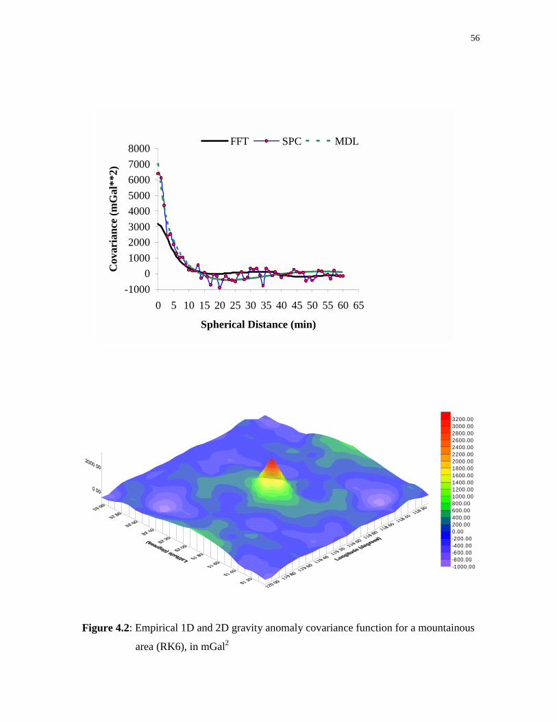
56

Figure 4.2: Empirical 1D and 2D gravity anomaly covariance function for a mountainous

area (RK6), in mGal2

-1000

0

1000

2000

3000

4000

5000

6000

7000

8000

0 5 10 15 20 25 30 35 40 45 50 55 60 65

Spherical Distance (min)

Cov

aria

nce

(m

Gal

**2)

FFT SPC MDL

-1000.00-800.00-600.00-400.00-200.000.00200.00400.00600.00800.001000.001200.001400.001600.001800.002000.002200.002400.002600.002800.003000.003200.00

57

Figure 4.3: Empirical 1D and 2D gravity anomaly covariance function for a flat area

(FT2), in mGal2

-10

-5

0

5

10

15

20

25

30

35

0 5 10 15 20 25 30 35 40 45 50 55 60 65

Spherical Distance (min)

Cov

aria

nce

(m

Gal

**2)

FFT SPC MDL

-8.00

-6.00

-4.00

-2.00

0.00

2.00

4.00

6.00

8.00

10.00

12.00

14.00

16.00

18.00

20.00

58

Figure 4.4: Empirical 1D and 2D gravity anomaly covariance function for a marine area

(MR3), in mGal2

-100-50

050

100150200250300350400

0 20 40 60 80 100 120 140 160

Spherical Distance (min)

Cov

aria

nce

(m

Gal

**2)

FFT SPC MDL

-40.00-30.00-20.00-10.000.0010.0020.0030.0040.0050.0060.0070.0080.0090.00100.00110.00120.00130.00140.00150.00

59

Table 4.4: Gravity anomaly covariance function parameters for mountainous areas

Frequency Domain Method5′′′′ Spacing 1′′′′ Spacing

Space domainmethodTest

AreaoC

(mGal2)

χ( ′ )

oC(mGal2)

χ( ′ )

oC(mGal2)

χ( ′ )

RK1 646 5.6 622 5.6 984 3.5RK2 417 3.9 404 3.9 1012 2.9RK3 1028 4.2 997 4.3 2606 3.3RK4 915 4.6 914 4.6 1646 3.3RK5 2976 4.6 2924 4.8 3882 2.6RK6 3311 4.5 3211 4.6 7026 3.2RK7 3339 6.5 3394 6.2 1675 2.8RK8 2004 5.7 1924 5.3 2059 4.0

The results of the space and frequency domain methods for the flat and marine areas

(Table 4.5) are however close with little change in the variance values and correlation

distances. For flat areas, estimates of the variance vary between 20mGal2 and 60mGal2 for

the frequency domain method and 26mGal2 and 90mGal2 for the space domain method.

The correlation distance varies between 7.3′ and 9.4′ for the frequency method while the

space domain method estimates vary between 5.2′ and 8.3′. The results for the marine

areas show that the variance values vary widely from one area to the other; the correlation

length is between 7.0′ and 10.6′, and 8.1′ and 9.4′ for the frequency and space domain

methods, respectively.

The results of the covariance function parameters estimated by frequency domain method

for referenced free air gravity anomalies in the mountainous areas are presented in Table

4.6.

60

Table 4.5: Gravity anomaly covariance function parameters for flat and marine areas

Frequency Domain5′′′′ Spacing 1′′′′ Spacing

Space DomainTestArea

oC(mGal2)

χ( ′ )

oC(mGal2)

χ( ′ )

oC(mGal2)

χ( ′ )

Flat AreasFL1 54 8.4 54 7.4 56 8.2FL2 27 8.4 27 5.2 26 7.7FL3 40 9.4 41 6.4 28 8.3FL4 27 8.3 27 5.2 27 6.4FL5 60 8.4 59 7.7 86 5.8FL6 20 7.3 21 4.6 51 6.1FL7 40 7.8 40 6.3 82 8.3FL8 44 7.6 44 6.6 55 5.2

Marine AreasMR1 52 7.0 52 7.0 74 8.1MR2 423 7.9 415 7.6 342 8.8MR3 159 10.6 157 10.5 370 9.4

Table 4.6: Free air gravity anomaly covariance function parameters

Test Area RK1 RK2 RK3 RK4 RK5 RK6 RK7 RK8

oC (mGal2) 491 309 792 770 2627 2833 2667 1384

χ ( ′ ) 5.6 3.1 4.3 4.7 4.7 4.5 5.7 4.8

κ 1.4 1.8 2.7 1.7 2.4 2.0 2.2 1.7

The results presented in Figures 4.2 to 4.4 and Tables 4.4 and 4.5 show that covariance

functions estimated by both the frequency and space domain methods vary for the

different areas selected. In the mountainous areas, the covariance functions have higher

variance value and shorter correlation distance when compared to the corresponding

61

values estimated for the flat and marine areas. It should be noted that both the frequency

and space domain methods are influenced by 'smoothing' effect, due on the one hand to

the gridding procedure employed in the frequency method an on the other hand to the

azimuth averaging employed in the space domain method. The smoothing effect depends

to a great extent on the roughness of the topography and the distribution of the data points

in the local area. The data distribution is represented by the average inter-point distance

(IPD), which is given in Tables 4.4 and 4.5. The lower the IPD value with better data

distribution, the less the smoothing effect.

In areas with rather flat topography, the empirical covariance function functions from both

space and frequency domain methods agree better in most of the test areas; for areas with

very rough topography, the covariance function from the space domain method and

frequency domain method vary widely. Again this can be attributed to the 'smoothing

effects' which is more pronounced for areas with rough topography.

The effect of the grid spacing on the covariance estimates is shown in Tables 4.4 and 4.5.

Using the frequency domain method with data on 5′ and 1′ grid, the covariance function

estimates have smaller variance value and the correlation distance with the 1′ grid data

when compared with the corresponding results for 5′ grid data.

62

CHAPTER 5

HIGH FREQUENCY VARIATION OF THE GRAVITY FIELD SIGNAL SPECTRUM,

AND ESTIMATION OF REQUIRED SAMPLING DENSITY FOR LOCAL GRAVITY

DATA

In this chapter, analysis of the spectrum of the gravity field signals is discussed.

Information from the spectrum of the gravity field data is used to derive among other

things the decay parameters for different frequency bands of the gravity field signal

spectrum, and estimate the sampling density for local gravity data and heights required to

provide a certain geoid accuracy and resolution.

The very high frequency information of the local gravity field is derived from very dense

digital elevation model data (DEM) on a 3″×3″ grid while local gravity anomalies on a

1′×1′ grid are used to derive the medium to high frequency gravity field information. The

long wavelength information characteristics of the gravity field are determined from the

EGM96 geopotential model.

The spectrum of the geoid from various gravity field signals for a selected area is first

presented in section 5.1; the geoid spectrum from EGM96 and local gravity data is

analyzed in view of the combination of GM and gravity data. In section 5.2, the results of

estimated geoid degree variances for selected areas are presented alongside the derived

variances from the Tscherning/Rapp model and degree variances with decay implied by

the Kaula rule for comparison. In addition, estimates of the decay parameter for the test

areas are presented. Section 5.3 discusses gravity data resolution requirement for various

levels of geoid accuracy in the centimetre to decimetre range.

63

5.1 GEOID SPECTRUM FROM GM, LOCAL GRAVITY DATA AND TOPOGRAPHIC

HEIGHTS

In this section, the power spectrum of the geoid represented by the degree variances 2Nó

(in cm2), is estimated for the various local geoid components. The GM geoid degree

variances are given as

( )∑=

+=n

0m

2nm

2nm22

22N sc

Rã

(GM) ó

GM (5.1)

while the geoid degree variances from gravity anomaly and terrain corrections is derived

from

2

2n2

Nã

ó ó

g=

∆ (5.2)

where 2nó is derived from equation (3.23).

Global degree variance models given by the Kaula's rule (Kaula, 1966) and the

Tscherning/Rapp model (Tscherning and Rapp, 1974) are also employed herein for

comparison. The Kaula's rule is given as

4

102n

n

1n2107.0ó

+×≈ − (5.3)

64

The Tscherning/Rapp model for Bjerhammar sphere depth 1.2km)RR( EB =− is given as

24)2)(n-1)(n-(n

99962.0104.4ó

1n102

n +×≈

+− (5.4)

The results of the geoid power spectrum derived from, the EGM96 (GM_NVAR)

complete to degree and other 360, the local gravity data (GV_NVAR), the terrain

correction (TC_NVAR), and the geoid indirect effect (IND_VAR) are shown in Figure

5.1. The data sets used for the analysis are selected from an area block of 15°×15°, which

is located in the Alberta and British Columbia provinces between latitudes 50.0471 and

65.0471, and longitudes -128.0471 and -113.047. The selected area is similar to the one

used for GM and local gravity combination analysis in chapter two of this thesis. The

statistics of the data sets are given in Table 2.1. The resolution of the local gravity data is

5′×5′, while the DEM data are interpolated on 5′×5′ grid.

Figure 5.1 shows the importance of proper modeling for all local terrain effects on the

geoid undulation signal especially in mountainous areas. Terrain correction alone can

create a geoid signal which amounts to over 10 cm (rms) for harmonic degree 150,2n < .

The corresponding value for flat areas (Kotsakis and Sideris, 1998) show that such

topographic effects should always be taken into account if a centimetre geoid is truly

desired.

It is also interesting to note (Figure 5.1) the significant amount of low-wavelength power

that the geoid indirect effect signal appears to have for harmonic degrees n > (~320) in the

selected area. It completely dominates over the geoid signal originating from the use of the

terrain correction. In particular, the geoid indirect effect shows a rms value of

approximately 1.8 cm inside the spectral band 24 < n < 2,150, while the geoid component

from the terrain correction in the same band has an average power of 10.3 cm. The local

65

free-air geoid also has a signal power at the 4.5 cm level over the spectral band 360 < n <

2,150; the geoid rms power from terrain correction and geoid indirect in the same spectral

band are 0.3 cm and 0.7 cm, respectively. All the corresponding values in the spectral

band 360 < n < 2,150, for flat test areas (Kotsakis and Sideris, 1998) are almost negligible.

The effect of using local gravity data in lager cap size for geoid estimation is again shown

in Figure 5.1. A closer look of the geoid spectrum form EGM96 and local gravity data is

shown in Figure 5.2.

Figure 5.1: Geoid power spectrum from various gravity field signals

3201.0E-05

1.0E-04

1.0E-03

1.0E-02

1.0E-01

1.0E+00

1.0E+01

1.0E+02

1.0E+03

1.0E+04

1.0E+05

1.0E+06

1.0E+07

1 10 100 1000 10000

Spherical harmonic degree

Geo

id d

egre

e va

rian

ces

(cm

**2)

GM_NVAR GV_NVAR IND_VAR TC_NVAR

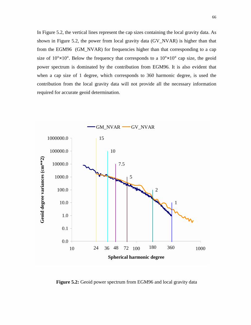
66

In Figure 5.2, the vertical lines represent the cap sizes containing the local gravity data. As

shown in Figure 5.2, the power from local gravity data (GV_NVAR) is higher than that

from the EGM96 (GM_NVAR) for frequencies higher than that corresponding to a cap

size of 10°×10°. Below the frequency that corresponds to a 10°×10° cap size, the geoid

power spectrum is dominated by the contribution from EGM96. It is also evident that

when a cap size of 1 degree, which corresponds to 360 harmonic degree, is used the

contribution from the local gravity data will not provide all the necessary information

required for accurate geoid determination.

Figure 5.2: Geoid power spectrum from EGM96 and local gravity data

15

24

10

36

7.5

48

5

72

2

180

1

3600.0

0.1

1.0

10.0

100.0

1000.0

10000.0

100000.0

1000000.0

10 100 1000

Spherical harmonic degree

Geo

id d

egre

e va

rian

ces

(cm

**2)

GM_NVAR GV_NVAR

67

5.2 THE DECAY OF THE GRAVITY FIELD SPECTRUM IN THE HIGH WAVE

NUMBERS

This section discusses the variation of the earth gravity field spectrum in medium and high

frequencies, and the results of the estimates of the decay parameters for local areas are

presented.

On a global scale, the earth gravity field spectrum has been known to obey a power decay

law in the form of

â

2n

n

áó ≈ (5.5)

where á and â are constants. The constant â describes the rate of decay of the gravity

field spectrum.

In Figure 5.1, the geoid power spectra originating from the local gravity data and the

terrain correction seem to follow a faster decaying pattern than the spectrum of the third

geoid component (indirect effect). A comparison of the geoid power 2Nó , derived from

local gravity anomalies, with global models in equations (5.3) and (5.4) is shown in

Figures 5.3, 5.4 and 5.5, respectively for mountainous, flat and marine test areas in

Canada. The test areas and gravity data are similar to those used for covariance analysis in

chapter four of this thesis. The location of these areas is shown in Figure 4.1 while the

statistics of the gravity and height data are given in Tables 4.2 and 4.1, respectively.

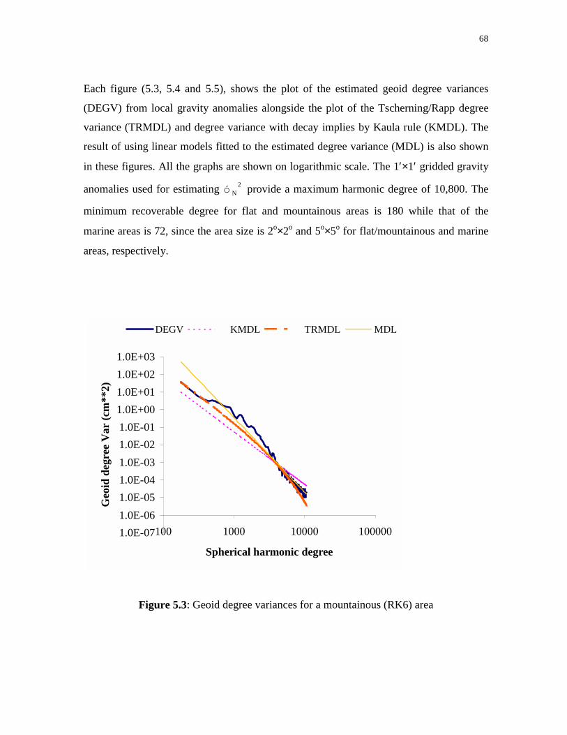
68

Each figure (5.3, 5.4 and 5.5), shows the plot of the estimated geoid degree variances

(DEGV) from local gravity anomalies alongside the plot of the Tscherning/Rapp degree

variance (TRMDL) and degree variance with decay implies by Kaula rule (KMDL). The

result of using linear models fitted to the estimated degree variance (MDL) is also shown

in these figures. All the graphs are shown on logarithmic scale. The 1′×1′ gridded gravity

anomalies used for estimating 2Nó provide a maximum harmonic degree of 10,800. The

minimum recoverable degree for flat and mountainous areas is 180 while that of the

marine areas is 72, since the area size is 2o×2o and 5o×5o for flat/mountainous and marine

areas, respectively.

Figure 5.3: Geoid degree variances for a mountainous (RK6) area

1.0E-07

1.0E-06

1.0E-05

1.0E-04

1.0E-03

1.0E-02

1.0E-01

1.0E+00

1.0E+01

1.0E+02

1.0E+03

100 1000 10000 100000

Spherical harmonic degree

Geo

id d

egre

e V

ar (

cm**

2)

DEGV KMDL TRMDL MDL

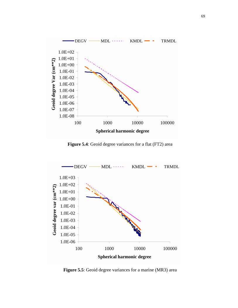
69

Figure 5.4: Geoid degree variances for a flat (FT2) area

Figure 5.5: Geoid degree variances for a marine (MR3) area

1.0E-081.0E-07

1.0E-061.0E-05

1.0E-041.0E-03

1.0E-021.0E-01

1.0E+001.0E+01

1.0E+02

100 1000 10000 100000

Spherical harmonic degree

Geo

id d

egre

e V

ar (

cm**

2)

DEGV MDL KMDL TRMDL

1.0E-06

1.0E-05

1.0E-04

1.0E-03

1.0E-02

1.0E-01

1.0E+00

1.0E+01

1.0E+02

1.0E+03

100 1000 10000 100000

Spherical harmonic degree

Geo

id d

egre

e va

r (c

m**

2)

DEGV MDL KMDL TRMDL

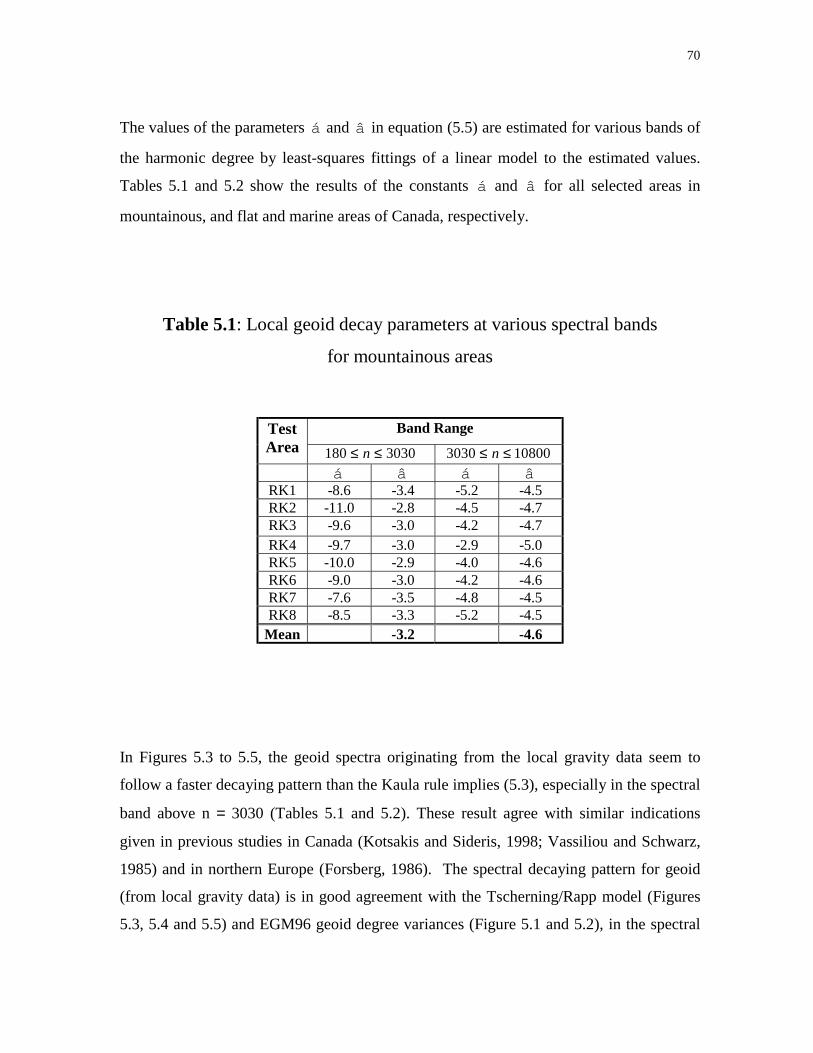
70

The values of the parameters á and â in equation (5.5) are estimated for various bands of

the harmonic degree by least-squares fittings of a linear model to the estimated values.

Tables 5.1 and 5.2 show the results of the constants á and â for all selected areas in

mountainous, and flat and marine areas of Canada, respectively.

Table 5.1: Local geoid decay parameters at various spectral bands

for mountainous areas

Band RangeTestArea 3030180 ≤≤ n 108003030 ≤≤ n

á â á âRK1 -8.6 -3.4 -5.2 -4.5RK2 -11.0 -2.8 -4.5 -4.7RK3 -9.6 -3.0 -4.2 -4.7RK4 -9.7 -3.0 -2.9 -5.0RK5 -10.0 -2.9 -4.0 -4.6RK6 -9.0 -3.0 -4.2 -4.6RK7 -7.6 -3.5 -4.8 -4.5RK8 -8.5 -3.3 -5.2 -4.5

Mean -3.2 -4.6

In Figures 5.3 to 5.5, the geoid spectra originating from the local gravity data seem to

follow a faster decaying pattern than the Kaula rule implies (5.3), especially in the spectral

band above n = 3030 (Tables 5.1 and 5.2). These result agree with similar indications

given in previous studies in Canada (Kotsakis and Sideris, 1998; Vassiliou and Schwarz,

1985) and in northern Europe (Forsberg, 1986). The spectral decaying pattern for geoid

(from local gravity data) is in good agreement with the Tscherning/Rapp model (Figures

5.3, 5.4 and 5.5) and EGM96 geoid degree variances (Figure 5.1 and 5.2), in the spectral

71

band 60 < n < 360. In addition, the local geoid spectra decay faster in high frequencies (n

> 3030) with 4.0â > for most areas.

Table 5.2: Local geoid decay parameters at various spectral bands

for flat and marine areas

a) Flat

Band RangeTestArea 3030180 ≤≤ n 108003030 ≤≤ n

á â á âFT1 -7.9 -4.1 -9.0 -3.9FT2 -9.6 -3.6 -9.4 -3.8FT3 -8.8 -3.8 -8.1 -4.2FT4 -8.3 -4.0 -9.3 -3.8FT5 -7.8 -4.1 -8.3 -4.1FT6 -9.9 -3.5 -6.4 -4.3FT7 -9.2 -3.7 -8.4 -4.1FT8 -9.5 -3.6 -9.2 -3.8

Mean -3.8 -4.0

b) Marine

Band RangeTestArea 3030180 ≤≤ n 108003030 ≤≤ n

á â á âMR1 -9.8 -3.4 -4.6 -5.0MR2 -7.2 -4.0 -9.2 -3.5MR3 -6.6 -4.4 -7.5 -4.2

72

5.3 DATA RESOLUTION REQUIREMENT FOR GEOID ESTIMATION

In order to investigate the required data spatial resolution for certain level of geoid

accuracy, gravity data and topographic heights in both the mountainous and flat areas are

analyzed separately in view of the wide difference in the gravity field signals in both areas

(Table 4.2). In this section, the estimation of spatial resolution for local gravity data and

heights required for centimetre to decimetre geoid accuracy in the mountainous and flat

areas of Canada is presented.

The contribution of the local gravity field data to the geoid can be investigated from

estimates of the geoid short wavelength power. The estimated geoid short wavelength

power contains the rms value of the local geoid signal contributed above a certain

harmonic degree on , and can be expressed as

∑∞

>

=>onn

2n2o

2N ó

ã

1)n(nó (5.6)

where )nn(ó o2N > represent the geoid rms value above certain spherical harmonic degree.

The estimated values of 2Nó for different on , which correspond to the highest harmonic

degree and consequently to the data spacing, provides a means of evaluating the data

resolution requirement for the decimetre to centimetre geoid accuracy. It should be noted

that the values of 2Nó represent only the ideal local geoid variance, since in most cases the

spherical harmonics errors of the reference field will be much larger than these values.

73

The graph of estimates of 2Nó derived from gravity data and fitted models in the selected

mountainous and flat test areas of Canada against on are shown in Figure 5.6. The

corresponding results after adding the effect of the topography are shown in Figure 5.7. In

estimating 2Nó , it is assumed that a perfect (linear) correlation exists among all the geoid

components. The plotted geoid rms values are based on the average of 2Nó estimates for

the mountainous test areas and flat test areas.

Figure 5.6: Local data sampling density for cm-dm geoid without topographic effect

0

10

20

30

40

50

60

70

80

0 5 10 15 20 25 30 35

Sampling density (arc-min)

Geo

id a

liasi

ng

erro

r (c

m)

���������������������������������������������������������������������������������������������������������������������

��� Rocky Flat

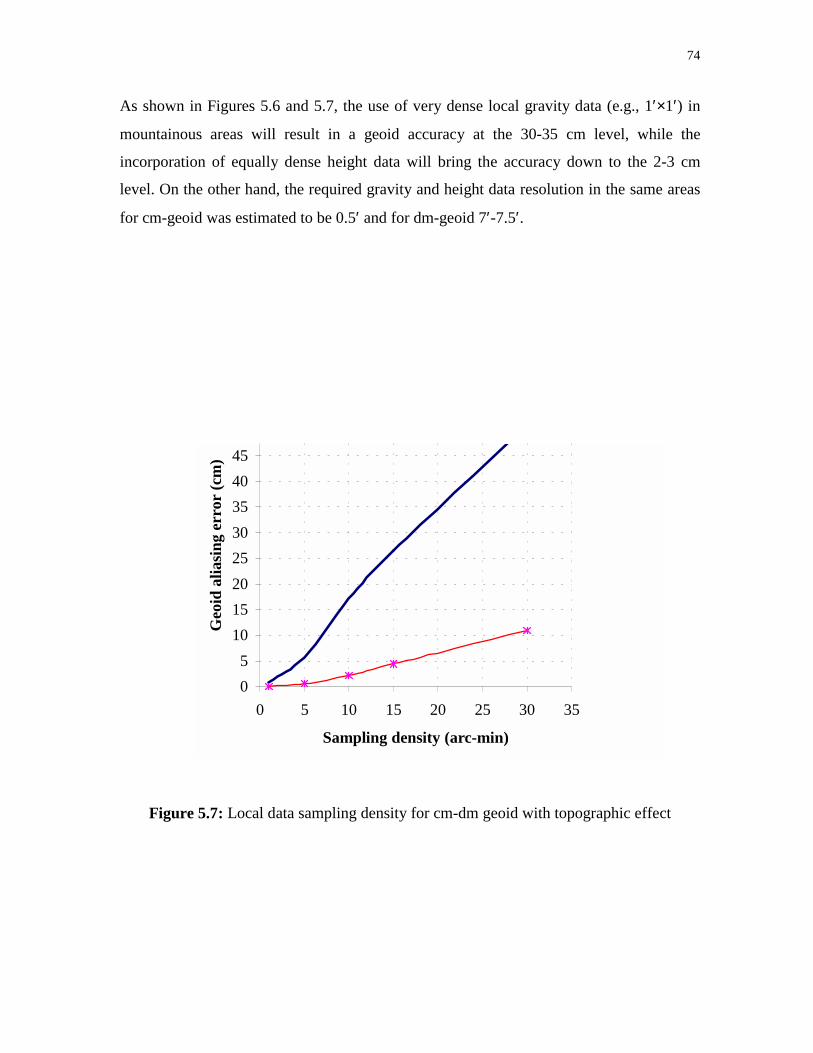
74

As shown in Figures 5.6 and 5.7, the use of very dense local gravity data (e.g., 1′×1′) in

mountainous areas will result in a geoid accuracy at the 30-35 cm level, while the

incorporation of equally dense height data will bring the accuracy down to the 2-3 cm

level. On the other hand, the required gravity and height data resolution in the same areas

for cm-geoid was estimated to be 0.5′ and for dm-geoid 7′-7.5′.

Figure 5.7: Local data sampling density for cm-dm geoid with topographic effect

0

5

10

15

20

25

30

35

40

45

0 5 10 15 20 25 30 35

Sampling density (arc-min)

Geo

id a

liasi

ng

erro

r (c

m)

75

In the flat areas of Canada, dm-geoid accuracy can be achieved without even taking terrain

effects into account, by using a local gravity grid spacing of 20′. For cm-level geoid,

gravity and terrain data should be combined with a resolution better than 6′. It should be

noted that all the above accuracy estimates refer to an average spatial behavior and

individual point errors may vary from these values.

76

CHAPTER 6

ANALYSIS AND MODELLING OF THE GEOID ERRORS

In geoid determination, a number of error sources limit the accuracy of the predicted geoid

undulations. The most significant of these errors are due to the noisy data used in the

conventional geoid estimation: the geopotential model (GM), local gravity anomalies g∆

and the heights. Smaller errors due to datum biases, spherical approximation, and the mass

of the atmosphere are usually considered to be at the noise level (Sideris and Schwarz,

1986), and are not taken into consideration in this study; further details about this class of

errors can be found in Heiskanen and Moritz (1967).

The two basic methods that are used to evaluate the accuracy of gravimetrically derived

geoid undulations, external comparison with GPS/levelling benchmarks and internal

propagation of data errors, are employed in the estimation of the geoid error covariance

functions. The methodology for the internal error propagation is similar to that employed

by Sideris and Schwarz (1986 and 1987). Absolute geoid error covariances from each

source are derived by propagation of error covariances of the data source.

Covariance models for relative geoid errors can be derived by propagating the error

covariances of absolute geoid for two baselines. Then the contribution of each data to the

relative geoid error variances and covariances can be investigated as for the absolute geoid

undulation error covariances, which is presented in the sequel. Derivation of the

expressions for the relative geoid error covariance function is contained in Sideris and

Schwarz (1986).

77

In section 6.1, the general expression for geoid error covariance propagation is presented.

This is followed by error covariance models from the GM coefficients, gravity data and

heights, which are presented in section 6.2. In sections 6.3 and 6.4, estimates of the errors

from GM coefficients and gravity data are derived for two areas selected, respectively.

Section 6.5 presents the results of the combined geoid error covariance function from both

GM and gravity data are discussed. In addition, estimates of the geoid errors derived from

comparison of gravimetric geoid and GPS/levelling derived geoid are compared with the

internally propagated geoid errors from the GM and local gravity data.

6.1 DATA ERROR PROPAGATION

Applying the theory of error propagation to the expression for geoid estimation in

equation (2.1), the error variance of the geoid undulations, under the assumption of

uncorrelated data errors, can be expressed as

2N

2N

2N

2N CGMgT

óóóó ++=∆

(6.1)

where 2NT

ó is the combined geoid error variance, 2N g

ó∆

is the geoid error variance due to

error in gravity anomaly, 2NGM

ó is the geoid error variance from the GM, and 2NC

ó is the

geoid error variance due to error in the topographic heights. Again for simplicity, equation

(6.1) represents the case where the data errors are assumed to be uncorrelated. The

expressions for these components are given (Li and Sideris, 1994) as follows:

( ) ( )22g

22g

22N )(S)(S*cos

ã4

ëRó

GMgψψσϕσ

πϕ −+

∆∆= ∆∆∆

(6.2)

78

∑∑= =

+=360

2n

2s

n

0m

2c

22N )(Ró

nmnmGMσσ (6.3)

2h

22N

ã

Gó

Cσρπ

= (6.4)

∑ ∑= =

∆ +−=360

2n

2s

n

0m

2c

222g )()1n(Gó

nmnmGMσσ (6.5)

where nmnm SC

ó,ó are the errors (standard deviations) of the normalized geopotential

coefficients of degree n and order m, hó is the error (standard deviation) of the height

measurement, )(Sψ is the Stokes's Kernel function, and )(S ψ is the summation of the

Legendre series of Stokes spherical kernel up to nmax=360. It is given as, (Li and Sideris,

1994):

)(cosP1n

12n)(S n

n

2n

max

ψψ ∑= −

+= , (6.6)

6.2 GEOID ERROR COVARIANCE FUNCTION MODELS

The geoid error covariance function NE for any data set with geoid error degree variances

2åN

ó , computed from the data, can be obtained from the following formula, (Sideris and

Schwarz, 1986):

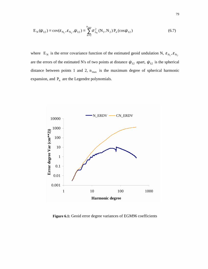
79

)(cosP )N,(N),,cov()(E 2:1n

n

2n21

2å2:1NN2:1N

max

N21ψσψεεψ ∑

=== (6.7)

where NE is the error covariance function of the estimated geoid undulation N,21 NN , εε

are the errors of the estimated N's of two points at distance 2:1ψ apart, 2:1ψ is the spherical

distance between points 1 and 2, maxn is the maximum degree of spherical harmonic

expansion, and nP are the Legendre polynomials.

Figure 6.1: Geoid error degree variances of EGM96 coefficients

0.001

0.01

0.1

1

10

100

1000

10000

1 10 100 1000

Harmonic degree

Err

or d

egre

e V

ar (

cm**

2))

N_ERDV CN_ERDV

80

6.2.1 GM Coefficients Error Covariance Function

The geoid error covariance function from the GM coefficients is derived from the error

degree variances, which is given in equation (6.3). The graph of the actual (N_ERDV) and

cumulative (CN_ERDV) geoid degree variances of the EGM96 geopotential model

coefficients plotted against spherical harmonic degree are shown in Figure 6.1. It is

evident from Figure 6.1 that the GM geoid errors are more in the long and medium

wavelength bands compared to those in the higher frequencies (above 200 harmonic

degree). See Pavlis (1997) for detail.

6.2.2 Estimation and Modelling of Gravity Data Error Covariance Function

In gravity field prediction by collocation or input output system theory (IOST) using

heterogeous data, the overal accuracy of the predicted quantity will depend on how the

error information which is contained in the error covariance or PSD function of each data

represent the reality for the local area. Well represented error covariance and PSD

functions will provide proper weights for the different data and thus improve the precision

of the prediction. In this study, an attempt is made to estimate and compare gravity error

covariance functions for two areas with different topographic features. This is necessary

especially when gravity field prediction is done in areas with diverse topography.

6.2.2.1 Gravity Error Covariance Function Based on Multiple Observations

The error covariance function of local gravity data can easily be derived for areas with

multiple gravity databases as documented in Weber and Wenzel (1983) for marine areas.

See also Esan and Sideris (1999). However, the availability of multiple gravity data over

the terrain surface is practically impossible and thus makes estimation of gravity error

81

covariance from multiple observations for such areas impossible. In the sequel, gravity

errors are obtained by comparing predicted to measured gravity anomalies in the selected

areas. The gravity anomalies g)(∆ are first corrected for terrain effect and referenced to

EGM96. The mathematics of estimating covariance function from multiple observation is

presented below.

Assuming a sufficient number of multiple and independent observations of the gravity

data, the error covariance function can be estimated from observation differences. Using

the parameters 21 g,g for true values located at two points separated by a spherical

distance 12ψ , ! for observations, å for true errors, and the subscripts lk,j,i, for the

various data sources, we can write the following expressions:

jjii1 ååg +=+= !! llkk2 ååg +=+= !! (6.8)

Defining the observation differences (dg) as,

ijji1ij åådg −=−= !! kllkkl2 åådg −=−= !! (6.9)

the expectation value for product pairs of differences at the two points can be expressed as

follows:

{ } { } { } { } { }kikjljlj2kl1ij ååEååEååEåEdgdgE +−−= å (6.10)

Equation (6.10) could be estimated as

82

{ } ∑≅ 2kl1ij2kl1ij dgdgn

1dgdgE (6.11)

Replacing expectation values by covariances, we have the following expressions:

)å,cov(å)å,cov(å-)å,cov(å-)å,cov(ådgdgn

1kilikjlj2kl1ij +≅∑ (6.12)

where n denotes the number of observations in the sources.

Error covariances can be determined in two ways. In the first case, if one of the sources

that participated in the evaluation of ij1dg also participated in the evaluation of kl2dg e.g.

ki = lj ≠ (6.13)

then using the of hypothesis of zero cross correlation between errors of different sources

and inserting equation (6.13) into (6.12), the error covariances for observations of source

i can be written as

∑≅ 2il1ijii dgdgn

1)å,cov(å (6.14)

In the other case, if both sources that participated in the evaluation of difference 1ijdg also

participated in the evaluation of the difference 2kldg , then

ki = lj = (6.15)

83

Accepting the hypothesis of equal error covariances for both sources, and combining

equations (6.15) and (6.12), the error covariances is given as

∑≅ 2ij1ijii dgdg2n

1)å,åcov( (6.16)

It should be noted that the reliability of the results of these models depend on the validity

of the hypothesis introduced. Gravity error covariance functions for the selected areas are

computed using equation (6.14). The error degree variances 2g ,n ó ∆ of the gravity anomaly

contributed to the undulations are then computed from the corresponding error PSD

function with equation (3.23).

The numerical results for two test areas in Canada are shown in Figures 6.2 and 6.3. The

two test areas each with 5o×5o block size are located in the west (latitudes 50o to 55o, and

longitudes -120o to 115− ) and in the east (latitudes 46o to 51o, and longitudes -74o to -69o)

of Canada.

The values of parameters characterizing the behavior of the covariance function (the

variance oC and correlation length 21÷ ) for the two selected areas show that while oC

values are different, the 21÷ values are similar. The variance values are about 318 mGal2

and 20 mGal2 respectively for the mountainous and flat areas. Estimated values of 21÷ in

the mountainous area is about 4′, while that of the flat area is about 4.5′.

84

Figure 6.2: Gravity error covariance function for a flat area

Figure 6.3: Gravity error covariance function for a mountainous area

-5

0

5

10

15

20

25

0 20 40 60 80 100 120 140 160

Distance (min)

Cov

aria

nce

(m

Gal

**2)

ECOV MDLC

-50

0

50

100

150

200

250

300

350

0 20 40 60 80 100 120 140 160

Distance (min)

Cov

aria

nce

(m

Gal

**2)

ECOV MDLC

85

6.2.2.2 Gravity Error Covariance Function Model

A number of error covariance models for gravity data have been suggested by different

authors. Gravity error covariance could be derived from a Gaussian error PSD function

gƌP (Sideris and Schwarz, 1986), given as

21

2/4aù-

21

onå e

2a

a)ù(P =

∆g,

R

0.5nù n

+= (6.17)

where oa is a constant with unit (mGal2) and 1a is a scaling factor. Both oa and 1a are to

be determined for each local area. The corresponding covariance function can be written

as

22:1

21

21

ø-ao:21gg:21g ea},,ååcov{)(E == ∆∆∆ ψψ , for ψ in degrees. (6.18)

The estimated gravity error covariance model derived after fitting the empirical error

covariance values with equation (6.14) is also shown in Figures 6.2 and 6.3 alongside with

the empirical covariance values for flat and mountainous areas, respectively. Estimated

values of oa and 1a of the fitted models are 318.6mGal2 and 12.0 for the mountainous

area, and 20.0mGal2 and 10.0 for the flat area.

86

6.2.3 Topographic Effect Error Covariance Model

The effect of the terrain on predicted geoid undulations is very small in areas with smooth

terrain, such as in eastern Canada. However, the terrain contribution in areas with rough

topography has a considerable effect on predicted gravity field quantities. Error due to the

topographic heights can be derived from a Gaussian covariance model given as

2

h

dg c)(E ψψ −

∆ = e , for ψ in degrees. (6.19)

where c and d are parameters (with units similar to those of a1 and oa ) that characterize

the behavior of the topographic error effect for the local area. Estimate of c and d for the

North American continent is given by Sideris and Schwarz (1986) as 5 mGal2 and 10.5,

respectively. To derive estimates of c and d, standard deviations of the gravity

observations were propagated into the error variances of the terrain correction equation,

and the result modeled using equation (6.19) Geoid error due to the topographic indirect

effect can be derived from the corresponding error variances, which is given in equation

(6.4), by using equation (6.7).

6.3 GEOID ERROR FROM GM COEFFICIENTS

The evaluation of the error contribution of the GM coefficients can be done with distance

dependent data error covariance functions derived from the error degree variances of the

GM coefficients. The contribution of the GM errors to )(C 2:1N ψ is computed from error

degree variances of the EGM96 coefficients with equation (6.3), for which the coefficients

87

and their errors are given up to degree 360, and the plot of the result is shown in Figure

6.4. The variance value is about 1300cm2 while the correlation length is about 30′.

Figure 6.4: Geoid error covariance function from EGM96 coefficients

6.4 GEOID ERROR FROM GRAVITY DATA

Since the gravity anomalies used in the computation of the geoid undulations are

referenced to the geopotential model and reduced for topographic effect, the combined

gravity error variances is derived for the harmonics of degree maxnn ≤ )360(nmax = from

the EGM96 coefficient error using equation (6.5). For maxnn > , the errors from local

gravity data and terrain effect are estimated separately. The local gravity error degree

variances is computed as

-200

0

200

400

600

800

1000

1200

1400

0 20 40 60 80 100 120 140 160

Distance (min)

Cov

aria

nce

s (c

m *

*2)

88

)ù(P1)(n

n

ðã2

1å ngg22

2g,n

2

1

∆∆∆ −

+= ,

R

nù 2

1

n

+= (6.20)

where and n starts at 361, and ggP ∆∆ is the isotropic gravity error PSD function estimated

from the corresponding error covariance function, which is derived with equation (6.14).

The corresponding geoid error covariances computed with equation (6.20) are shown in

Figures 6.5 and 6.6, respectively for flat and mountainous test areas.

The variance value of the derived geoid error covariance function is higher for the

mountainous test area compared with that from the flat area as expected. In mountainous

area, the geoid variance is estimated at about 4.8 cm2, the corresponding value in the flat

area, is about 0.18 cm2. The correlation length is 7′ for both test areas. Covariance model

of the form

22:1

21øa-

oN eaE = (6.21)

is then fitted to the derived covariance values. The values of the parameters oa and 1a of

the fitted models are estimated as 4.80 cm2, 6.7 and 0.19 cm2, 6.3 for the mountainous and

flat test areas, respectively.

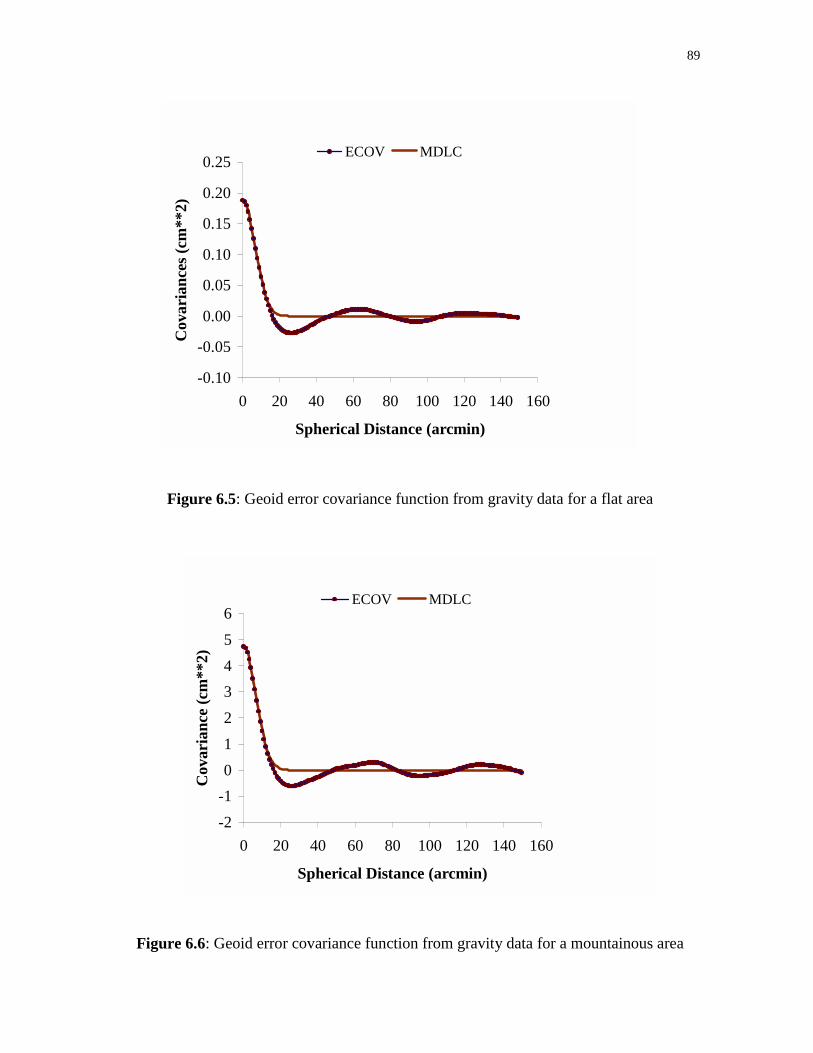
89

Figure 6.5: Geoid error covariance function from gravity data for a flat area

Figure 6.6: Geoid error covariance function from gravity data for a mountainous area

-2

-1

0

1

2

3

4

5

6

0 20 40 60 80 100 120 140 160

Spherical Distance (arcmin)

Cov

aria

nce

(cm

**2)

ECOV MDLC

-0.10

-0.05

0.00

0.05

0.10

0.15

0.20

0.25

0 20 40 60 80 100 120 140 160

Spherical Distance (arcmin)

Cov

aria

nce

s (c

m**

2)

ECOV MDLC

90

6.5 Combined Geoid Error Covariance Function

6.5.1 Geoid Error from GM and Gravity Data

The total geoid error covariance function from gravity and GM is obtained from (6.1)

where for 360n2 ≤≤ , the formula (6.4) is used to compute the errors degree variances

of the coefficients of the EGM96 geopotential model, for which the coefficients and their

errors are given up to degree 360. For 360n > , the error covariance functions are

computed with equation (6.20). The results for the two selected areas are similar to that

shown in Figure 6.2. The variance value for the total geoid error covariance function is

about 1300 cm2 while the correlation length is about 30′ for the two areas. The fact that

these values are the same for the two areas is due to the strong influence of the errors

coming from the GM which dominates the long and medium wavelength bands of the

geoid error spectrum.

6.5.2 Comparison of Internal and External Geoid Errors

Gravimetric geoid undulations are computed for the two selected areas above using the

formulas presented in chapter 2. The results of the total geoid were compared to the

GPS/leveling data on benchmarks in the two areas (80 and 112 data points for the

mountainous and flat areas, respectively). The difference between the gravimetric and

GPS/leveling derived geoid provides an estimate of the external geoid error which can be

compared to the internal propagated geoid errors. The standard geoid error derived from

the difference between the gravimetric geoid and GPS/leveling is about 19 cm and 17 cm

for the mountainous and flat areas, respectively.

91

Covariance functions for the external GPS/leveling derived geoid errors are computed

empirically for the two areas and the results are fitted with fourth order polynomial model.

The graph of the empirical error covariance functions and fitted models are shown in

Figures 6.7 and 6.8 for the flat and mountainous test areas, respectively. Values of fitted

model parameters are given in Table 6.1. The covariance function of the external geoid

error has a correlation length of about 8′ for the two areas. The variance value of the

covariance function for the mountainous area is about 344cm2 while that of the flat area is

about 302cm2.

Figure 6.7: GPS/leveling geoid error covariance function for a flat area

-300

-200

-100

0

100

200

300

400

500

0 20 40 60 80 100 120 140 160

Distance (arc-min)

Geo

id c

ovar

ian

ce (

cm**

2)

ECOV MDLC

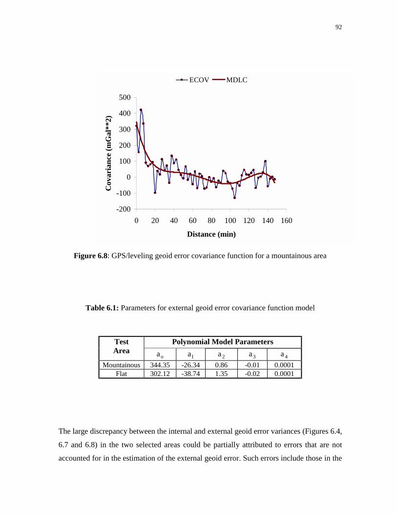
92

Figure 6.8: GPS/leveling geoid error covariance function for a mountainous area

Table 6.1: Parameters for external geoid error covariance function model

Polynomial Model ParametersTestArea

oa 1a 2a 3a 4a

Mountainous 344.35 -26.34 0.86 -0.01 0.0001Flat 302.12 -38.74 1.35 -0.02 0.0001

The large discrepancy between the internal and external geoid error variances (Figures 6.4,

6.7 and 6.8) in the two selected areas could be partially attributed to errors that are not

accounted for in the estimation of the external geoid error. Such errors include those in the

-200

-100

0

100

200

300

400

500

0 20 40 60 80 100 120 140 160

Distance (min)

Cov

aria

nce

(m

Gal

**2)

ECOV MDLC

93

leveling and GPS data, as well as datum biases (Kotsakis and Sideris, 1999). As expected,

the variance of geoid error covariance function for the western area is higher compared to

the corresponding value for the eastern area.

The reliability of the external GPS/levelling derived geoid errors depends on how accurate

the GPS and orthometric observations are. Thus it should be use as standard to test the

accuracy of the gravimetric geoid if the accuracy of the GPS and heights are know. The

internal propagated geoid errors on the other hand, provides useful information on the

relation between the gravity anomaly errors, the GM errors and the computed geoid

undulations. The reliability of the internal errors depends on how accurate the source data

errors are know. This type of error should be used in gravity field prediction with geoid

undulations as input data.

94

CHAPTER 7

7.1 SUMMARY

Gravity field data in areas with different topographic features have been analyzed to

derive characteristics of the gravity field signal and errors for local areas. Firstly, the effect

of truncating the spherical harmonic expansion of the GM coefficients in favour of using

lager cap size for Stokes's integral solution is investigated in order to derive the

appropriate combination techniques for the two data types. In addition, the effect of using

lateral density variations for terrain correction computation and geoid estimation in the

Mountainous Mountains is also investigated.

Secondly, estimates of local gravity empirical covariance functions for mountainous, flat

and mountainous areas of Canada are derived using space domain and spectral methods.

Models for the empirical covariance functions are derived for all the areas by fitting some

analytical function to the space domain empirical covariance values. In addition, the

sampling density of gravity data required for a centimetre to decimetre accuracy level of

the geoid is estimated separately for the flat and mountainous areas.

Finally, estimates of gravity error covariance function for mountainous and flat areas are

derived and compared. Geoid errors propagated form both gravity data and geopotential

model coefficient errors are also estimated; the results are then compared to the external

geoid error derived from GPS/levelling data.

95

7.2 CONCLUSION

From the analysis and results presented in this report, the following can be concluded:

A. The covariance functions for areas in Canada with similar topographic and

geophysical features are rather stationary, while the covariance functions for areas

with different topography vary widely with the topography. The results of both the

space domain and spectral method of empirical covariance determination are similar in

areas with flat terrain. The result of the two methods is very different for areas with

rough topography. The difference is attributed to the smoothing effect introduced by

the gridding procedure, and radial averaging used in the spectral method, as well as the

distance averaging used in the spatial method. The smoothing effect depends on the

roughness of the topography and the distribution of the data points in the local area.

B. The decay of the geoid spectrum in medium and high frequencies is not constant, and

it also varies with the topographic height differences. For certain areas in Canada, the

rate of decay is different from the decay implied by the Kaula rule (decay rate = 3) in

medium and high frequencies. Between 180 and 3030 harmonic degree the rate of

decay is about 3.2 while for frequencies above harmonic degree of 3030, the geoid

spectrum decay even faster at about 4.6.

C. The data resolution required for centimetre to decimetre accuracy level of geoid

estimation varies between the flat and mountainous areas. In the mountainous area, a 1

cm geoid estimate will require grid data with 1′ spacing while in the flat areas, a 5′

grid data is required to achieve the same level of accuracy.

96

D. The difference between terrain corrections estimated with constant and varying density

values is correlated with the topography of the local area. The computation of terrain

corrections with actual density values using the prism mass model for the topography

is required in the mountainous areas if the centimetre geoid is to be achieved in these

areas.

E. The best achivable accuracy of the geoid estimated by the combination of a GM with

the Stokes's integral can be obtained if the cap size used in the Stokes integral is not

less than 10°×10° and the harmonic degree of expansion not less than 200 with the

EGM96. Using larger areas and higher degrees of expansion does not neccessarily

improve the geoid accuracy.

F. The gravity error covariance function for both flat and mountainous areas of Canada

can be modeled with a function of the form 2:121øa-

o2:1g ea)ø(E =∆ , for 2:1ø in degrees,

and so can the corresponding geoid error covariance function be modeled with the

function 2

2:121ø-a

o22:1N ea)(øE = . In both cases, oa represents the variance of the error

covariance function.

G. The spectrum of the geoid error is mainly dominated by errors from the geopotential

model, consequently, for both flat and mountainous areas, the combined geoid errors

from GM coefficients and gravity data are quite similar. The results of the internal

propagated and external geoid errors disagree in both the flat and the mountainous

areas tested; estimates of the total geoid error are higher in the mountainous areas

when compared to those of the flat areas.

97

7.3 RECOMMENDATIONS AND FUTURE PLANS

The following recommendations are proposed for further research:

1) A new geoid model based on the results of the findings herein should be computed for

Canada using, e.g., a 10° ×10° cap size for Stokes's integration, variable topographic

density for rigorous modelling of the terrain correction and geoid indirect effect, and

new denser gravity anomalies and digital topographic heights. The new geoid model

should be compared to previous geoid models for Canada, as well as global models to

assess the improvement in the geoid especially in the mountainous areas of Canada.

2) To derive gravimetric geoid in mountainous areas with an absolute accuracy of 5 cm

or better, both the gravity anomalies and the digital topographic heights with 1′

resolution are require. Therefore, the present gravity data have to be improved in terms

of data coverage, density and precision.

3) As it has been pointed out in chapters 4 and 6 of this thesis, gravity field signal and

error covariance functions over Canada are not constant; it vary from one area to the

other. Further studies on the effect of using different signal and error covariance

functions for gravity field prediction in areas with different topographic features

should be done. In addition, covariance models that would provide optimal results for

gravity field approximation with heterogeneous data set should be derived separately

for the flat, mountainous and marine areas.

4) The internal geoid error derived from the propagation of both the gravity anomaly

errors and the geopotential harmonic coefficients (EGM96), provides useful

information on the relation between the gravity anomaly errors, the GM errors and the

98

computed geoid undulations. Numerical investigation to derive internal geoid

undulation errors for all in Canada should be done. The relation between the internal

errors estimates and the external accuracy estimation that are obtained by comparing

gravimetric geoid with GPS/levelling derived geoid on benchmarks should also be

investigated for all areas in Canada.

5) Error covariance models for the geoid indirect effect should be derived and the effect

on the total geoid error should be evaluated especially in the mountainous areas.

6) In order to provide a reasonable external standard for evaluating the accuracy of

gravimetric geoid undulation, it is necessary to investigate the quality (accuracy) of the

GPS and levelling observations that are used in estimating the external geoid accuracy.

This is more important in the mountainous areas, where it is believed that the accuracy

of the orthometric heights is poorer when compared to those of the flat areas.

99

REFERENCES

Balmino, G., B. Moynot, M. Sarrailh, and N. Vales. 1987. Free air gravity anomalies over

the ocean from SEASAT and GEOS-3 altimetry data. EOS Trans. AGU, Vol. 68, pp.

17-19.

Barzaghi, R., A. Fermi, S. Tarantola, and F. Sansò. 1993. Spectral techniques in inverse

Stokes and overdetermined problems. Surveys in Geophysics, Vol. 14, No. 4-5.

Bendat, J.S. and A.G. Piersol. 1986. Random data: Analysis and measurement

procedures, Second edition, John Wiley and Sons, New York.

Bendat, J.S. and A.G. Piersol. 1980. Engineering Applications of Correlation and

Spectral Analysis. John Wiley and Sons, New York.

Blais J.A.R. 1982. Synthesis of Kriging Estimation Methods. Manuscripta Geodetica Vol.

7, pp. 325 - 352.

Bottoni, G.P. and R. Barzaghi. 1993. Fast collocation. Bulletin Géodésique, Vol. 67, No.

2, pp. 119-126.

Bracewell, R.N. 1986. The Fourier transform and its applications, Second edition,

revised. McGraw-Hill, New York.

Esan, O. and M. G. Sideris. 1999. On the Role of the GM, Error Propagation, and

Optimal Combination of GM with Local Gravity Data in Precise Geoid

Determination. Report Submitted to Geodetic Survey Canada.

Forsberg, R. 1984. Local covariance functions and density distributions. OSU Report No.

356, Department of Geodetic Science and Surveying, The Ohio State University.

100

Forsberg, R. 1987. A new covariance model for inertial gravimetry and gradiometry.

Journ. of Geophys. Res., Vol. 92, No. B2, pp. 1305-1310.

Forsberg, R. 1993. Impact of airborne gravimetry on geoid determination - the Greenland

example. Bul. International. Geoid Service, No 2, pp. 32-43.

Forsberg, R. and S. Kenyon. 1995. Downward continuation of airborne gravity data. Proc.

of IAG Symposium G4, IUGG XXI General Assembly, Boulder, Colorado, July 2-14,

1995. pp. 73-80.

Haagmans, R. E. de Min and M. van Gelderen, 1992. Evaluation of Stokes' and other

integrals using 1D-FFT and a comparison with existing methods. Paper submitted to

Manuscripta Geodetica.

Hammer, S. 1983. Airborne gravity is here! Geophysics, Vol. 48, No. 2, pp. 213-223.

Heiskanen, W. A. and H. Moritz. 1967. Physical geodesy. W. H. Freeman and Company.

San Francisco.

Kaula, W.M., Theory of Satellite Geodesy, Blaisdell Publishing Co., 1966.

Kotsakis, C. and M. G. Sideris. 1998. Study of the gravity field spectrum in Canada in

view of cm-Geoid Determination. Paper presented at the Second Joint Meeting of

the Internaional Gravity Commission and the Geoid Commission Trieste, Italy, Sept.

7-12, 1998. Also submitted to Journ. of Geodesy.

Kotsakis, C. and M. G. Sideris. 1999. On the Adjustment of Combined

GPS/Levelling/Geoid Networks. Paper presented at the IV Hofine-Marusi

Symposium on Mathematical Geodesy Trento, Italy, Sept. 14 - 17 1998.

101

Li, Y.C. 1993. Optimized spectral geoid determination. UCGE Report No. 20050,

Department of Geomatics Engineering, The University of Calgary, Calgary, Alberta.

Li, J. and M.G. Sideris. 1995. Marine gravity and geoid determination by optimal

combination of satellite altimetry and shipborne gravimetry data. Paper presented at

the XXI IUGG General Assembly, July 2-14, Boulder, Colorado. Also submitted to

the Journal of Geodesy.

Li, Y.C. and M.G. Sideris. 1994. Minimization and estimation of geoid undulation errors.

Bulletin Géodésique, Vol. 68, pp. 201-219.

Moritz, H. 1980. Advanced Physical Geodesy. H. Wichmann verlag, Karlsruhe, Germany.

Pavlis, N. K. 1997. Development and applications of geopotential models. Prepared for

the Second international school for the determination and use of the geoid, Rio de

Janeiro, Brazil.

Rapp, R. H., Y. M. Wang and N. K. Pavis. 1991. The Ohio State 1991 geopotential and

sea surface topography harmonic coefficient models. OSU Report No. 410,

Department of Geodetic Science and Surveying, The Ohio State University, Ohio,

USA.

Rapp, R. H. and N. K. Pavlis, 1990. The development and analysis of geopotential

coefficient models to spherical harmonic degree 360. Journ. of Geophys. Res. Vol.

95, No. B13, pp. 21885 - 21911.

Schwarz, K. P. 1984. Data types and their spectral properties, Proceedings of Local

Gravity Field Approximation. Beijing, China, August 21 - September 4.

102

Schwarz, K.P. 1987. Geoid profiles from an integration of GPS satellite and inertia data.

Bollettino Di Geodesia e Scienze Affini. Anno XLVI, N. 2, pp. 117-131. Presented at

the International Symposium on the Definition of the Geoid, Florence, Italy, May

26-30, 1986.

Schwarz, K. P. and Y.C. Li. 1995. What can airborne gravimetry contribute to geoid

determination? Proc. of IAG Symposium G4, IUGG XXI General Assembly, Boulder,

Colorado, July 2-14, 1995. pp. 143-152.

Schwarz, K. P. and M.G. Sideris. 1985. Precise geoid heights and their use in GPS

interferometry. GSD Report NO. 85-004. Geodetic Survey Canada.

Schwarz, K. P., Sideris M. G. and R. Forsberg. 1989. The use of FFT

techniques in physical geodesy. Geophys. Journal Inter., Vol. 100, pp. 485-

514.

Schwarz, K. P. and M. Wei. 1994. Some unsolved problems in airborne gravimetry. Paper

presented at the Symposium 'Gravity and Geoid', Graz, Austria, September 11-17.

Schwarz, K. P. and M. Wei. 1992. Inertia surveying and INS/GPS integration. Lecture

Notes, Department of Geomatics Engineering, The University of Calgary, Calgary,

Alberta, Canada.

Seeber, G. 1993. Satellite Geodesy. Walter de Gruyter, Berlin, New York.

Sideris, M.G. 1987. On the application of spectral techniques to the gravimetric problem.

Proc. of the XIX IUGG General Assembly, Tome II, Vancouver, BC, August 9-22,

pp. 428-442.

103

Sideris, M.G. 1995. On the use of heterogeneous noisy data in spectral gravity field

modelling methods. Invited paper, presented at the XXII IUGG General Assembly,

Colorado, July 2-14, 1995.

Sideris , M.G. and B.B. She, (1994): A new, high-resolution geoid for Canada and part of

the U.S. by the 1D FFT method. Bulletin Geodesique Vol. 69, No 2, pp. 92-108.

Sideris, M.G. and K. P. Schwarz. 1986. The use of GPS and DOPPLER heights in NAVD.

Paper presented at the Fourth International Geodetic Symposium on Satellite

Positioning, Austin, Texas, April 28-May2, 1986.

Sideris, M.G. and K. P. Schwarz. 1987. Improvement of the medium and short features of

geopotential solutions by local gravity data. Bollettino Di Geodesia e Scienze Affini.

Anno XLVI, N. 3, pp. 206-221.

Sideris, M.G. and Y. Li. 1992. Improved geoid determination for leveling by GPS. In

Proc. of the sixth Int. Geodetic Symposium on Satellite Positioning Vol. II, pp. 873 -

882, Columbus, Ohio, March 17- 20.

Sjoberg, L. E. 1987. Progress in global gravity field approximation, Contributions to

geodetic theory and methodology. XIX general meeting of the IUGG, Vancouver,

BC, Canada, August 2-22.

Tscherning, C. C. 1975. Covariance expression for second and lower order derivatives of

the anomalous potential. Report of The Dep. of Geodetic Science No. 225, 1975.

Tscherning, C. C. 1984. Local approximation of the gravity potential by least-squares

collocation. Proceedings of the international summer school on local gravity field

approximation, Beijing, China, August 21 - September 4.

104

Tscherning, C. C. and R. H. Rapp. 1974. Closed covariance expression for gravity

anomalies, geoid undulations and deflections of the vertical implied by anomaly

degree- variance models. OSU Report No. 208, Department of Geodetic Science and

Surveying, Ohio State University.

Veronneau M., (1996) Canadian Geoid Model GSD95 and its precision. Geodetic Survey

Division Canada, internal report.

Weber G. and H. G. Wenzel. 1983. Error covariance functions of sea gravity data and

implications for geoid determination. Marine Geodesy. Vol. 7, Number 1-4

Wu, L. and M.G. Sideris. 1995. Using multiple input-single output system relationships in

post processing of airborne gravity vector data. Proc. of IAG Symposium G4, IUGG

XXI General Assembly, Boulder, Colorado, July 2-14, 1995. pp. 87-94.

Zhang, C. and J. A. R Blais. 1995. Comparison of methods for marine gravity

determination from satellite altimetry data in the Labrador Sea. Bulletin Géodésique,

Vol. 69, pp 173-180.

Zhang, C. and J. A. R Blais. 1993. Recovery of gravity distubances from satellite altimetry

by FFT techniques: a synthetic study. Manuscripta Geodaetica, Vol. 18, pp.

158-170.

Zhang, C. and M. G. Sideris. 1995. Gravity disturbances from GEOSAT data and forward

geopotential models in the Labrador Sea. IAG Symposia 113, convened and editted

by Sunkel, H. and I. Marson, Springer, pp. 317-328.