This may be the author’s version of a work that was submitted/acceptedfor publication in the following source:

Fitzgerald, Daniel, Walker, Rodney, & Campbell, Duncan(2005)A Vision Based Emergency Forced Landing System for an AutonomousUAV.In AIAC11 (Ed.) Proceedings of the Eleventh Australian InternationalAerospace Congress.AIAC11, Australia, Victoria, Melbourne, pp. 1-26.

This file was downloaded from: https://eprints.qut.edu.au/2763/

c© Copyright 2005 (please consult author)

This work is covered by copyright. Unless the document is being made available under aCreative Commons Licence, you must assume that re-use is limited to personal use andthat permission from the copyright owner must be obtained for all other uses. If the docu-ment is available under a Creative Commons License (or other specified license) then referto the Licence for details of permitted re-use. It is a condition of access that users recog-nise and abide by the legal requirements associated with these rights. If you believe thatthis work infringes copyright please provide details by email to qut.copyright@qut.edu.au

Notice: Please note that this document may not be the Version of Record(i.e. published version) of the work. Author manuscript versions (as Sub-mitted for peer review or as Accepted for publication after peer review) canbe identified by an absence of publisher branding and/or typeset appear-ance. If there is any doubt, please refer to the published source.

COVER SHEET

This is the author version of article published as: Fitzgerald, Daniel L. and Walker, Rodney A. and Campbell, Duncan A. (2005) A Vision Based Emergency Forced Landing System for an Autonomous UAV. In Proceedings Australian International Aerospace Congress Conference, Melbourne Australia, Melbourne, Australia. Copyright 2005 (please consult author) Accessed from http://eprints.qut.edu.au

A Vision Based Emergency Forced Landing System for an Autonomous UAV

Daniel Fitzgerald 1, Dr Rodney Walker 1, Dr Duncan Campbell 1

1 Airborne Avionics Research Group, Queensland University of Technology, 2 George St, GPO Box

2434, Brisbane, Australia 4000 Email: dl.fitzgerald@qut.edu.au; Contact: (07) 3864 1362

Summary: This paper introduces the forced landing problem for UAVs and presents the machine-vision based approach taken for this research. The forced landing problem, is a new field of research for UAVs and this paper will show the preliminary analysis to date. The results are based on video data collected from a series of flight trials in a Cessna 172. The aim of this research is to locate “safe” landing sites for UAV forced landings, from low quality aerial imagery. Output video image frames, will highlight the algorithm’s selected safe landing locations. The algorithms for the problem use image processing techniques and neural networks for the classification problem. It should be noted that although the system is being designed primarily for the forced landing problem for UAVs, the research can also be applied to forced landings or glider applications for piloted aircraft. Keywords: Forced landing, emergency landing, Unmanned Aerial Vehicle (UAV), machine vision, Probabilistic Neural Networks (PNN).

Introduction Human pilots perform forced landings in emergency situations that require aircraft to immediately land. An example of such an emergency could be an engine failure. UAVs are not immune to these emergencies, and as such, require a system that will allow a UAV to autonomously decide on the safest region to land in the surrounding areas during flight. The overall objective of the research is to design a system whereby, “safe” landing sites are chosen for a UAV to land in. A “safe” landing site is one that will not cause any injury to a person. Additionally, a “safe” landing site will be one that minimizes property damage. Finally, the system will try to save the UAV itself, however this is of the lowest priority. An example would be that the UAV would choose to land into a lake instead of landing onto a road with cars. The development of an autonomous UAV forced landing system is a previously unexplored research field. Garcia-Pardo, Gaurav and Montgomery [1], state that at their time of writing (May 2001) they were “unaware of a vision based safe landing system for an autonomous aerial robot.” Alternative passive solutions such as parachutes (uncontrolled descent) and other flight termination systems (such as explosive devices) have been explored, however these can still lead to human injury and property damage on the ground. These alternatives are seen to be inadequate as a solution to the UAV forced landing problem.

The motivation behind the development of a UAV forced landing system is from a UAV operations safety standpoint. Resolving these issues, is seen as being a key component for obtaining approval for UAV operations in civilian airspace, in particular above populated areas, as this process is analogous to human pilot emergency operation. Additionally, the research could also serve as a baseline for regulatory bodies, for example the Civil Aviation Safety Authority (CASA). The low-cost aspect of the system is an integral part of this research. With a low-cost landing system available, it will mean UAVs will be more accessible to potential users. This means that more UAV users will have access to a system that is aimed at the safety and preservation of human-life. The validity of this research will ultimately be determined by how well the forced landing system performs, compared with the performance of human pilots in forced landing situations. If it can be shown that this system can perform as well as a human pilot, then it can be argued that this system is an adequate safety system to allow UAV flights above populated areas. This is, of course, assuming that other UAV integration issues have been solved, for example: collision avoidance, health monitoring and mission management systems.

Forced Landing Theory

A forced landing is an unscheduled event that can occur at any time during a flight, due to some emergency that requires the aircraft to perform an emergency landing. There must still be control surface and avionics control so that the aircraft is able to maneuver to a desired landing site. There are two types of forced landings that this research has identified:

• gliding approach; and • guided parachute descent.

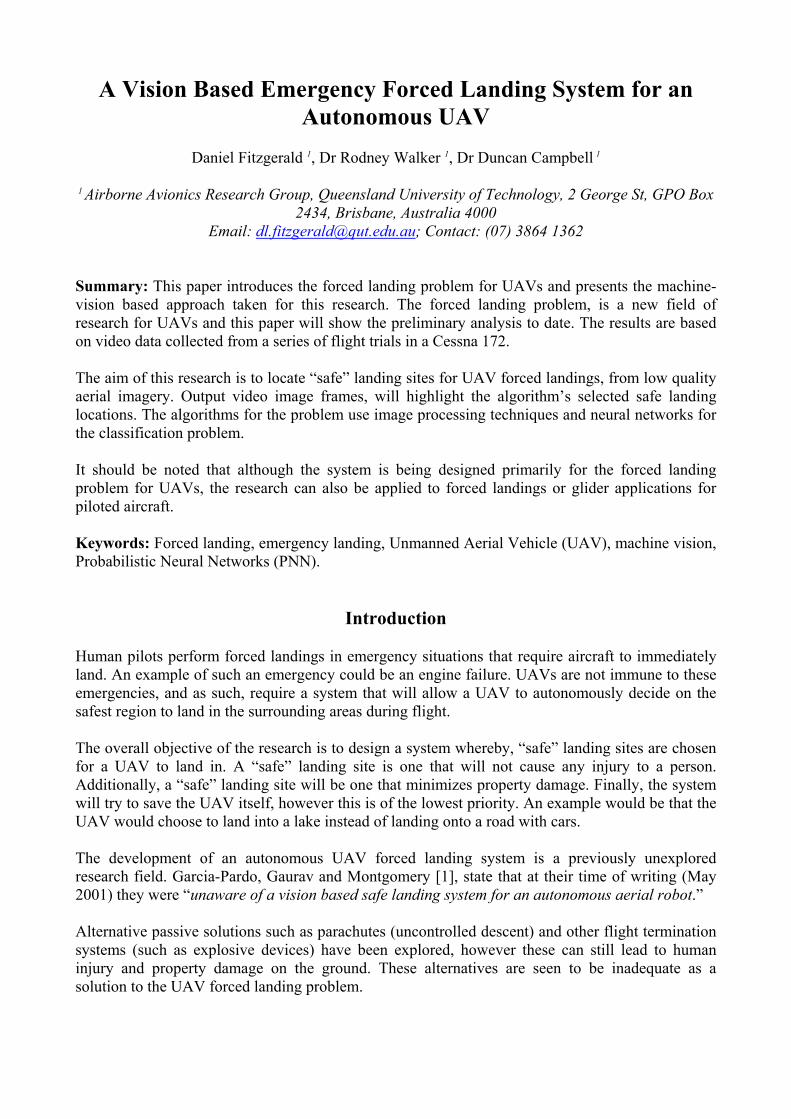
Gliding Approach The gliding approach is the type of forced landing that human pilots perform in an emergency for fixed wing aircraft. This method is based on fundamentals of flight dynamics. Assume the case where an engine has failed, resulting in a situation where there is no thrust. Now airspeed, angle of attack and descent rate must be traded-off for continued flight. If the pilot maintains an appropriate range of airspeeds, the aircraft can make a controlled descent down to the ground. This glide performance is specific to the lift to drag ratio for each individual aircraft.

α

α α - Glide Angle for a

particular aircraft

Fig. 1: Effect of Altitude on Aircraft Glide Performance

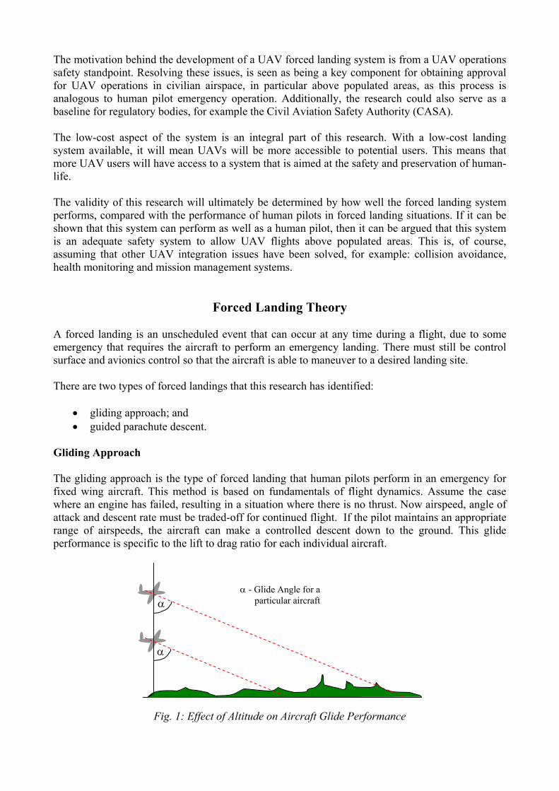
The complications are that the pilot must find a suitable landing site, within the gliding range of the aircraft. The distance that the aircraft can glide is dependant on the altitude and lift to drag ratio of the aircraft. If an aircraft is at a higher altitude than another, then the pilot has more time to decide where to land the aircraft. The lift to drag ratio is characterized by the glide angle (α), shown in Fig. 1. Wind factors must also be considered, as this can increase or decrease the maximum gliding distance achievable for an aircraft. Fig. 2 depicts the effect of wind on the decent more clearly.

original

with wind

with wind

WIND

α

α

α - Glide Angle for a particular aircraft

Fig. 2: Effect of Wind on Aircraft Glide Performance

As can be seen in the figure above, a headwind for the aircraft would result in a decrease in the aircraft’s gliding performance – gliding distance reduced. Subsequently, a tailwind would result in an improvement in the glide performance. These points highlight the importance of knowing what the wind conditions are around the aircraft. Guided Parachute Descent The other type of forced landing identified for the UAV application, is the guided parachute descent. This method involves deploying a parachute in an emergency, and then using a number of control surfaces to guide the aircraft down to a safe landing site. The control surfaces in this case can be on the UAV or can be a totally redundant system. This is different to the gliding approach described above, which relies on aircraft control surfaces being operational. It is important to note however, that a human pilot would not be able to do anything in this situation either, and this research is aimed at producing a system that uses a human pilot as the benchmark for system performance. This research is applicable to both types of UAV forced landings identified above. In each case, a system is required to identify a “safe” landing location for the UAV, and this is the aim of this research.

Forced Landing System Overview As this forced landing problem is a new area of research for UAV operations, this section will highlight some of the key components of the entire UAV forced landing system, and illustrate where in the system this particular research lies. It is anticipated, that future research will build on the foundations of the forced landing problem presented in this paper.

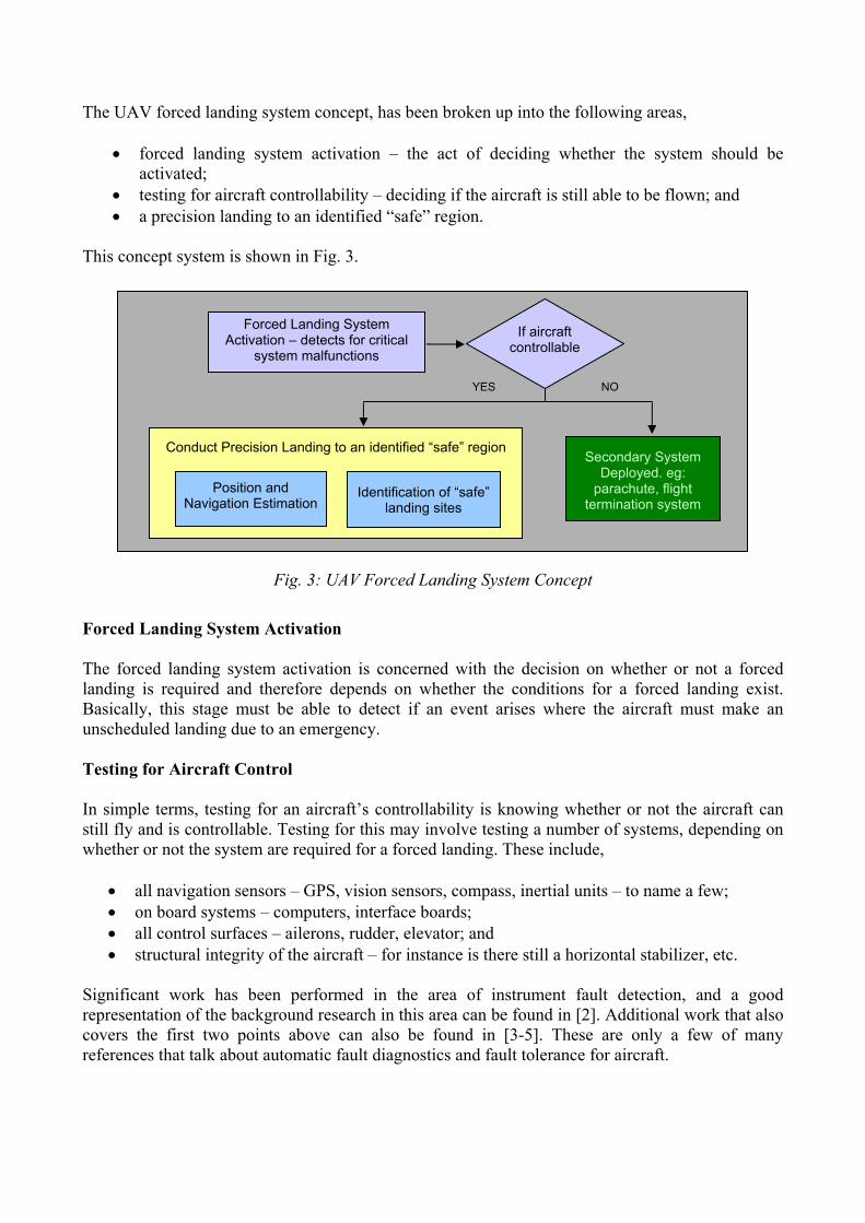
The UAV forced landing system concept, has been broken up into the following areas,

• forced landing system activation – the act of deciding whether the system should be activated;

• testing for aircraft controllability – deciding if the aircraft is still able to be flown; and • a precision landing to an identified “safe” region.

This concept system is shown in Fig. 3.

Fig. 3: UAV Forced Landing System Concept

Forced Landing System Activation The forced landing system activation is concerned with the decision on whether or not a forced landing is required and therefore depends on whether the conditions for a forced landing exist. Basically, this stage must be able to detect if an event arises where the aircraft must make an unscheduled landing due to an emergency. Testing for Aircraft Control In simple terms, testing for an aircraft’s controllability is knowing whether or not the aircraft can still fly and is controllable. Testing for this may involve testing a number of systems, depending on whether or not the system are required for a forced landing. These include,

• all navigation sensors – GPS, vision sensors, compass, inertial units – to name a few; • on board systems – computers, interface boards; • all control surfaces – ailerons, rudder, elevator; and • structural integrity of the aircraft – for instance is there still a horizontal stabilizer, etc.

Significant work has been performed in the area of instrument fault detection, and a good representation of the background research in this area can be found in [2]. Additional work that also covers the first two points above can also be found in [3-5]. These are only a few of many references that talk about automatic fault diagnostics and fault tolerance for aircraft.

NO YES

Forced Landing System Activation – detects for critical

system malfunctions

If aircraft controllable

Conduct Precision Landing to an identified “safe” region Secondary System

Deployed. eg: parachute, flight

termination system Position and

Navigation Estimation Identification of “safe”

landing sites

Precision Landing to an Identified “Safe” Region This stage is the key component of the forced landing system. It is the stage that must firstly determine where the UAV is to land, and secondly determine how exactly the UAV will navigate and land on the selected safe landing site. This research is focused on developing the algorithms that will enable a UAV to autonomously decide on the safest landing location for the UAV. This part of the system is seen to be the heart of the forced landing problem, and once solved, will enable the development of the complete forced landing system. Discussion The testing for control is crucial to the successful landing of a UAV and needs to be addressed. If the aircraft cannot be controlled, then the secondary system must be deployed (as shown in Fig. 3). The secondary system could be a parachute or an explosive flight termination system. It should be noted, that the secondary passive system described here is considered as an undesirable alternative. A passive landing system can have dangerous implications – for instance a UAV descending on a parachute, could descend into the middle of a busy freeway. However, it is believed that the system proposed here is an adequate starting point for the forced landing concept, as it is a totally new research area for UAVs. Additionally, the same problem still exists for a piloted aircraft placed in a forced landing scenario, faced with additional failures. That is, if the aircraft is not controllable, then the pilot can only hope that the plane lands somewhere where there will be minimal damage to other persons and property. The proposed forced landing system will exhibit the same, if not better performance in this situation, with the existence of the secondary safety system. The remainder of the paper will detail the development of the algorithms that will enable a UAV to autonomously decide on the safest landing location for the UAV. The methods for gathering the data required for the development of the “safe” landing site selection algorithm will be presented, followed by a detailed account of the development to date of the algorithm. Also, results for all phases of the algorithm will be presented.

Data Collection Test data was required to develop and test the algorithms for the UAV forced landing problem. The aim of the data collection was to obtain a data set that was representative of what a UAV may encounter in general operations. Data Collected Tests were performed in a Cessna 172 from Archerfield Airport, Brisbane, Australia (July 2004). The video data collected was from an approximate altitude of 2500 ft and contained differing sample datasets of the South East Queensland region. The three categories of datasets collected were from populated, rural and suburban areas.

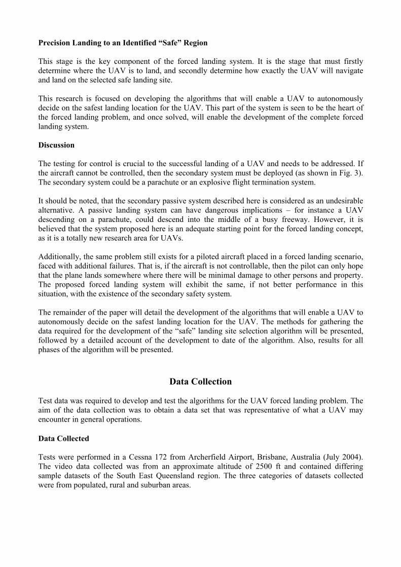
Onboard System The data-collection system consisted of a PC-104, Novatel GPS receiver, a XBow inertial unit and a XBOB-II board. The XBOB-II board was used to overlay timestamp information over the video intermittently, to synchronize between the logged data and the video data. The specific data collected, included,

• video data from the CCD camera; • aircraft Euler angles, rates and accelerations from the inertial sensor; • altitude, position and velocity information from the GPS unit; and • orientation of the camera with respect to the aircraft’s body fixed axis.

The system was mounted within the aircraft on the rear seat. This is shown in Fig. 4.

Fig. 4: Data Collection System

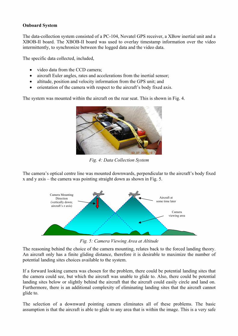
The camera’s optical centre line was mounted downwards, perpendicular to the aircraft’s body fixed x and y axis – the camera was pointing straight down as shown in Fig. 5.

Fig. 5: Camera Viewing Area at Altitude

The reasoning behind the choice of the camera mounting, relates back to the forced landing theory. An aircraft only has a finite gliding distance, therefore it is desirable to maximize the number of potential landing sites choices available to the system. If a forward looking camera was chosen for the problem, there could be potential landing sites that the camera could see, but which the aircraft was unable to glide to. Also, there could be potential landing sites below or slightly behind the aircraft that the aircraft could easily circle and land on. Furthermore, there is an additional complexity of eliminating landing sites that the aircraft cannot glide to. The selection of a downward pointing camera eliminates all of these problems. The basic assumption is that the aircraft is able to glide to any area that is within the image. This is a very safe

Camera viewing area

Camera Mounting Direction Aircraft at

some time later (vertically down; aircraft’s z axis)

assumption, as if we consider a wide-angled camera lens of say 900, an aircraft should be able to reach an area identified in this image – the glide performance of an aircraft is assumed to be approximately 450 angle of descent in this case.

Forced Landing Site Selection Algorithm – Overview

The algorithms to detect safe regions to land for the UAV forced landing problem have been approached in a way that aims to select safe landing areas, similar to that of a human pilot. Elements from the human pilot’s decision making process for landings, useful for the UAV forced landing application include,

• size of the landing site; • shape of the landing site; • surroundings of the landing site – for instance, are there buildings, fences or power lines

nearby; • slope of the landing site; and • classification of the landing site – for instance, is it a grass field or an empty road.

In addition, the algorithms must be constructed in a way, so that a solution to the algorithm is able to be found within a reasonable time frame. The forced landing site selection algorithm incorporates elements of the 5 points listed above. It has also been approached in a way that avoids unnecessary processing. For instance, there is no point identifying all grass areas in an image, if most of these are unsuitable because they are too small to land in. The algorithm has been structured as follows,

• Region Sectioning Phase; • Geometric Acceptance Phase; • Site Identification Phase; and • Final Site Selection Phase.

Region Sectioning Phase The region sectioning phase is the first step in the forced landing site selection algorithm. The aim here is to locate areas that are free of obstacles and are of the same material – for example, grass fields, bitumen or water. Two methods were trialed for this problem. The first was based on an image segmentation technique using three dimensional Gaussian probability models [6], and the second was a novel approach adopted from known image processing techniques for this particular research application. The segmentation approach to the problem was tested on the data-set and found to yield adequate results. However, this approach was found to be less computationally efficient than the second approach and therefore was abandoned. The second approach was capable of locating regions from the aerial data that were firstly, of similar texture and secondly, free of obstacles. These regions would then be input for the next phase

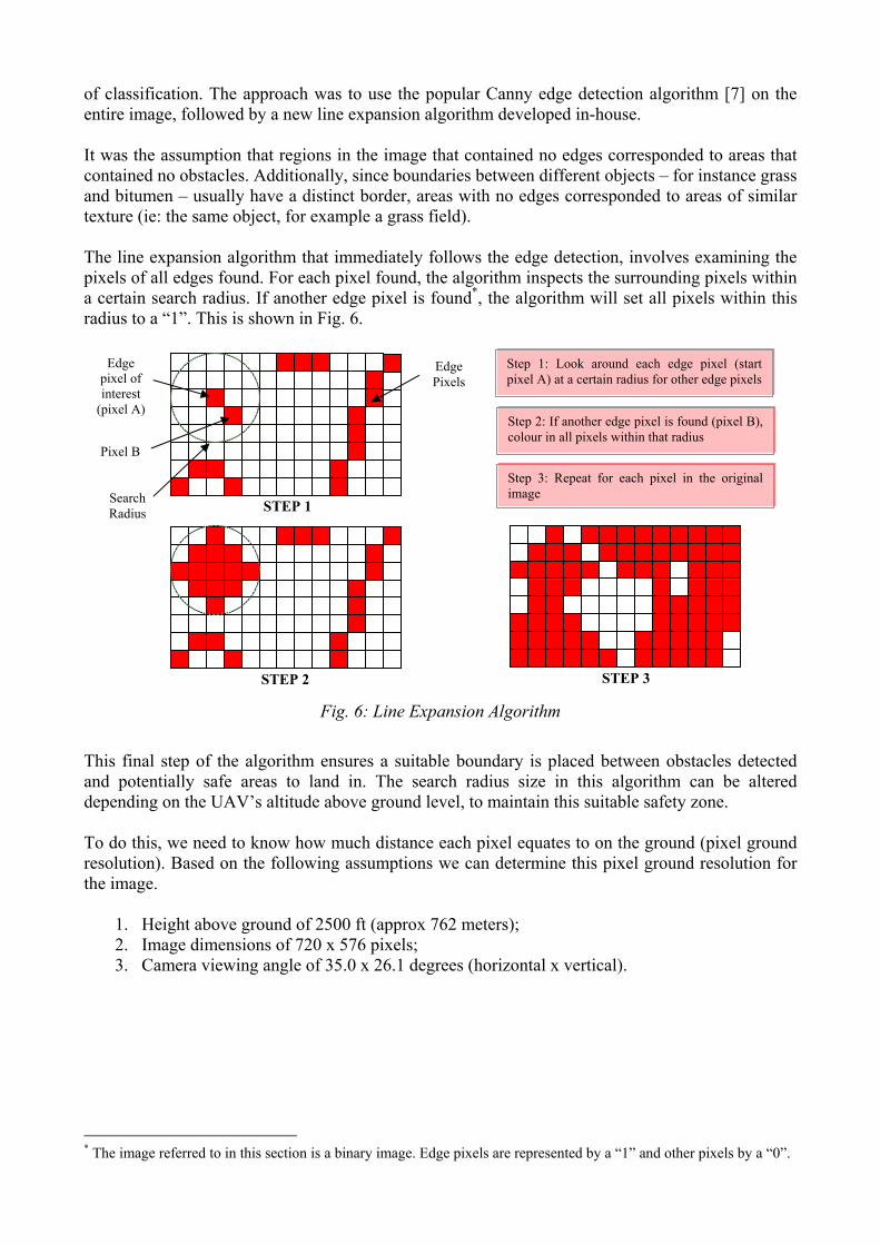
of classification. The approach was to use the popular Canny edge detection algorithm [7] on the entire image, followed by a new line expansion algorithm developed in-house. It was the assumption that regions in the image that contained no edges corresponded to areas that contained no obstacles. Additionally, since boundaries between different objects – for instance grass and bitumen – usually have a distinct border, areas with no edges corresponded to areas of similar texture (ie: the same object, for example a grass field). The line expansion algorithm that immediately follows the edge detection, involves examining the pixels of all edges found. For each pixel found, the algorithm inspects the surrounding pixels within a certain search radius. If another edge pixel is found*, the algorithm will set all pixels within this radius to a “1”. This is shown in Fig. 6.

Fig. 6: Line Expansion Algorithm

This final step of the algorithm ensures a suitable boundary is placed between obstacles detected and potentially safe areas to land in. The search radius size in this algorithm can be altered depending on the UAV’s altitude above ground level, to maintain this suitable safety zone. To do this, we need to know how much distance each pixel equates to on the ground (pixel ground resolution). Based on the following assumptions we can determine this pixel ground resolution for the image.

1. Height above ground of 2500 ft (approx 762 meters); 2. Image dimensions of 720 x 576 pixels; 3. Camera viewing angle of 35.0 x 26.1 degrees (horizontal x vertical).

* The image referred to in this section is a binary image. Edge pixels are represented by a “1” and other pixels by a “0”.

Step 1: Look around each edge pixel (start pixel A) at a certain radius for other edge pixels

STEP 3 STEP 2

STEP 1

Edge pixel of interest

(pixel A)

Edge Pixels

Step 2: If another edge pixel is found (pixel B), colour in all pixels within that radius

Step 3: Repeat for each pixel in the original image Search

Radius

Pixel B

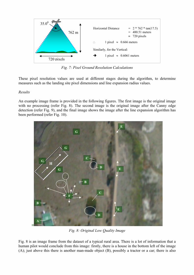
Fig. 7: Pixel Ground Resolution Calculations

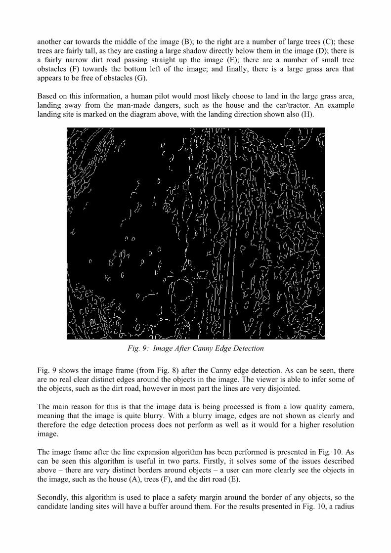
These pixel resolution values are used at different stages during the algorithm, to determine measures such as the landing site pixel dimensions and line expansion radius values. Results An example image frame is provided in the following figures. The first image is the original image with no processing (refer Fig. 8). The second image is the original image after the Canny edge detection (refer Fig. 9), and the final image shows the image after the line expansion algorithm has been performed (refer Fig. 10).

G Fig. 8: Original Low Quality Image

Fig. 8 is an image frame from the dataset of a typical rural area. There is a lot of information that a human pilot would conclude from this image: firstly, there is a house in the bottom left of the image (A); just above this there is another man-made object (B), possibly a tractor or a car; there is also

720 pixels

762 m

35.00 Horizontal Distance = 2 * 762 * tan(17.5) = 480.51 meters ≡ 720 pixels

∴ 1 pixel ≈ 0.666 meters Similarly, for the Vertical:

1 pixel ≈ 0.6061 meters

G

A

G H

B

C

D

F C

D

G

G

B

E

E

E

another car towards the middle of the image (B); to the right are a number of large trees (C); these trees are fairly tall, as they are casting a large shadow directly below them in the image (D); there is a fairly narrow dirt road passing straight up the image (E); there are a number of small tree obstacles (F) towards the bottom left of the image; and finally, there is a large grass area that appears to be free of obstacles (G). Based on this information, a human pilot would most likely choose to land in the large grass area, landing away from the man-made dangers, such as the house and the car/tractor. An example landing site is marked on the diagram above, with the landing direction shown also (H).

Fig. 9: Image After Canny Edge Detection

Fig. 9 shows the image frame (from Fig. 8) after the Canny edge detection. As can be seen, there are no real clear distinct edges around the objects in the image. The viewer is able to infer some of the objects, such as the dirt road, however in most part the lines are very disjointed. The main reason for this is that the image data is being processed is from a low quality camera, meaning that the image is quite blurry. With a blurry image, edges are not shown as clearly and therefore the edge detection process does not perform as well as it would for a higher resolution image. The image frame after the line expansion algorithm has been performed is presented in Fig. 10. As can be seen this algorithm is useful in two parts. Firstly, it solves some of the issues described above – there are very distinct borders around objects – a user can more clearly see the objects in the image, such as the house (A), trees (F), and the dirt road (E). Secondly, this algorithm is used to place a safety margin around the border of any objects, so the candidate landing sites will have a buffer around them. For the results presented in Fig. 10, a radius

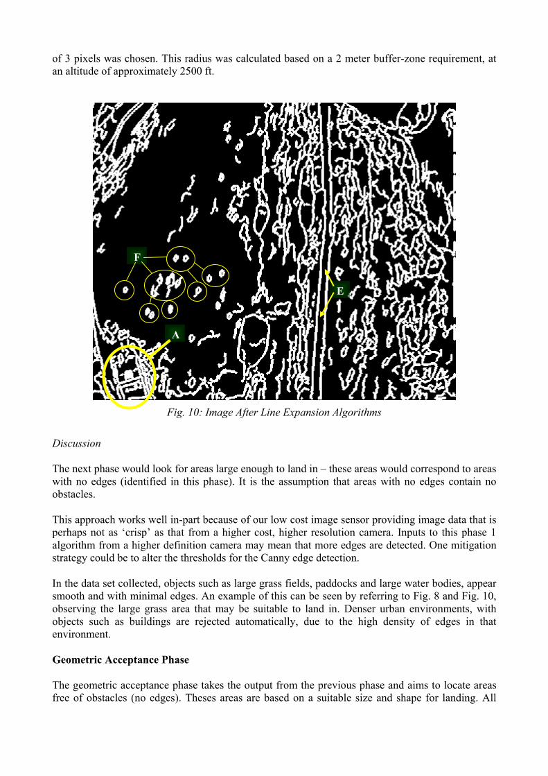
of 3 pixels was chosen. This radius was calculated based on a 2 meter buffer-zone requirement, at an altitude of approximately 2500 ft.

F

E

Fig. 10: Image After Line Expansion Algorithms

A

Discussion The next phase would look for areas large enough to land in – these areas would correspond to areas with no edges (identified in this phase). It is the assumption that areas with no edges contain no obstacles. This approach works well in-part because of our low cost image sensor providing image data that is perhaps not as ‘crisp’ as that from a higher cost, higher resolution camera. Inputs to this phase 1 algorithm from a higher definition camera may mean that more edges are detected. One mitigation strategy could be to alter the thresholds for the Canny edge detection. In the data set collected, objects such as large grass fields, paddocks and large water bodies, appear smooth and with minimal edges. An example of this can be seen by referring to Fig. 8 and Fig. 10, observing the large grass area that may be suitable to land in. Denser urban environments, with objects such as buildings are rejected automatically, due to the high density of edges in that environment. Geometric Acceptance Phase The geometric acceptance phase takes the output from the previous phase and aims to locate areas free of obstacles (no edges). Theses areas are based on a suitable size and shape for landing. All

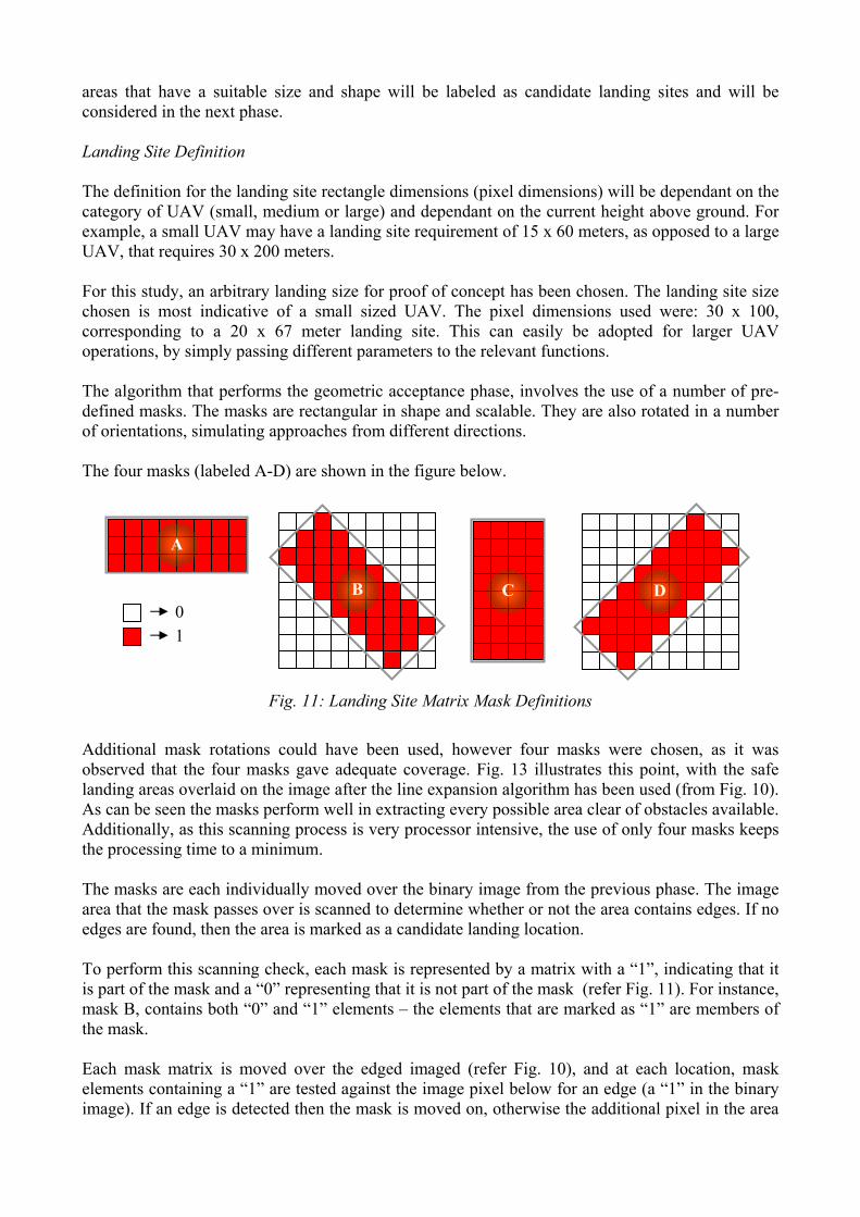
areas that have a suitable size and shape will be labeled as candidate landing sites and will be considered in the next phase. Landing Site Definition The definition for the landing site rectangle dimensions (pixel dimensions) will be dependant on the category of UAV (small, medium or large) and dependant on the current height above ground. For example, a small UAV may have a landing site requirement of 15 x 60 meters, as opposed to a large UAV, that requires 30 x 200 meters. For this study, an arbitrary landing size for proof of concept has been chosen. The landing site size chosen is most indicative of a small sized UAV. The pixel dimensions used were: 30 x 100, corresponding to a 20 x 67 meter landing site. This can easily be adopted for larger UAV operations, by simply passing different parameters to the relevant functions. The algorithm that performs the geometric acceptance phase, involves the use of a number of pre-defined masks. The masks are rectangular in shape and scalable. They are also rotated in a number of orientations, simulating approaches from different directions. The four masks (labeled A-D) are shown in the figure below.

Fig. 11: Landing Site Matrix Mask Definitions

Additional mask rotations could have been used, however four masks were chosen, as it was observed that the four masks gave adequate coverage. Fig. 13 illustrates this point, with the safe landing areas overlaid on the image after the line expansion algorithm has been used (from Fig. 10). As can be seen the masks perform well in extracting every possible area clear of obstacles available. Additionally, as this scanning process is very processor intensive, the use of only four masks keeps the processing time to a minimum. The masks are each individually moved over the binary image from the previous phase. The image area that the mask passes over is scanned to determine whether or not the area contains edges. If no edges are found, then the area is marked as a candidate landing location. To perform this scanning check, each mask is represented by a matrix with a “1”, indicating that it is part of the mask and a “0” representing that it is not part of the mask (refer Fig. 11). For instance, mask B, contains both “0” and “1” elements – the elements that are marked as “1” are members of the mask. Each mask matrix is moved over the edged imaged (refer Fig. 10), and at each location, mask elements containing a “1” are tested against the image pixel below for an edge (a “1” in the binary image). If an edge is detected then the mask is moved on, otherwise the additional pixel in the area

A

B

C

D

0 1

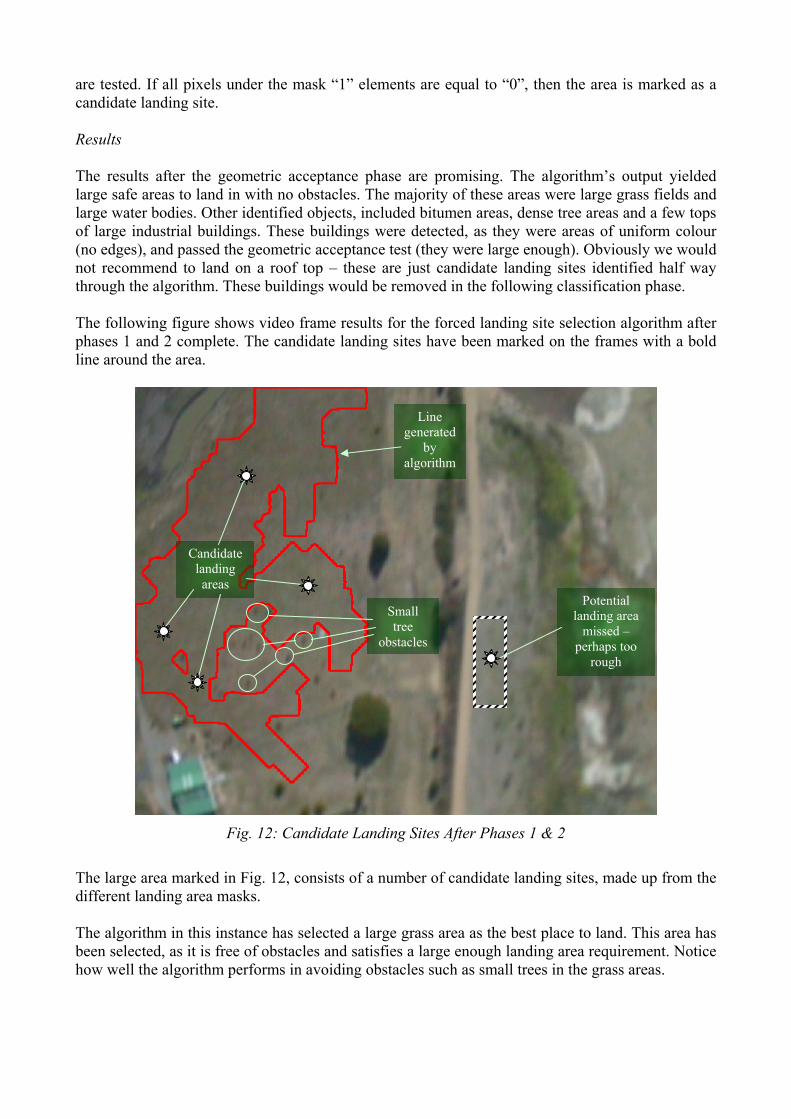
are tested. If all pixels under the mask “1” elements are equal to “0”, then the area is marked as a candidate landing site. Results The results after the geometric acceptance phase are promising. The algorithm’s output yielded large safe areas to land in with no obstacles. The majority of these areas were large grass fields and large water bodies. Other identified objects, included bitumen areas, dense tree areas and a few tops of large industrial buildings. These buildings were detected, as they were areas of uniform colour (no edges), and passed the geometric acceptance test (they were large enough). Obviously we would not recommend to land on a roof top – these are just candidate landing sites identified half way through the algorithm. These buildings would be removed in the following classification phase. The following figure shows video frame results for the forced landing site selection algorithm after phases 1 and 2 complete. The candidate landing sites have been marked on the frames with a bold line around the area.

Candidate landing areas

Small tree

obstacles

Line generated

by lgorithm

a

Potential landing area

missed – perhaps too

rough

Fig. 12: Candidate Landing Sites After Phases 1 & 2

The large area marked in Fig. 12, consists of a number of candidate landing sites, made up from the different landing area masks. The algorithm in this instance has selected a large grass area as the best place to land. This area has been selected, as it is free of obstacles and satisfies a large enough landing area requirement. Notice how well the algorithm performs in avoiding obstacles such as small trees in the grass areas.

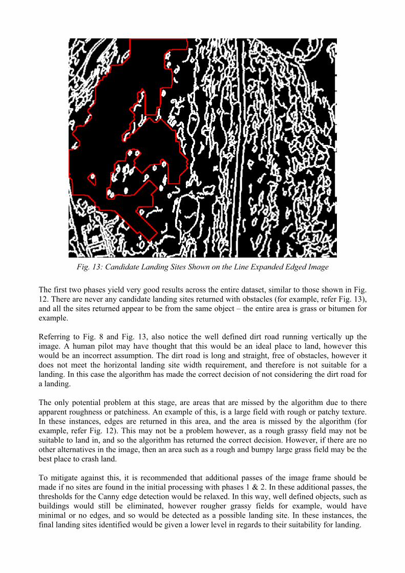
Fig. 13: Candidate Landing Sites Shown on the Line Expanded Edged Image

The first two phases yield very good results across the entire dataset, similar to those shown in Fig. 12. There are never any candidate landing sites returned with obstacles (for example, refer Fig. 13), and all the sites returned appear to be from the same object – the entire area is grass or bitumen for example. Referring to Fig. 8 and Fig. 13, also notice the well defined dirt road running vertically up the image. A human pilot may have thought that this would be an ideal place to land, however this would be an incorrect assumption. The dirt road is long and straight, free of obstacles, however it does not meet the horizontal landing site width requirement, and therefore is not suitable for a landing. In this case the algorithm has made the correct decision of not considering the dirt road for a landing. The only potential problem at this stage, are areas that are missed by the algorithm due to there apparent roughness or patchiness. An example of this, is a large field with rough or patchy texture. In these instances, edges are returned in this area, and the area is missed by the algorithm (for example, refer Fig. 12). This may not be a problem however, as a rough grassy field may not be suitable to land in, and so the algorithm has returned the correct decision. However, if there are no other alternatives in the image, then an area such as a rough and bumpy large grass field may be the best place to crash land. To mitigate against this, it is recommended that additional passes of the image frame should be made if no sites are found in the initial processing with phases 1 & 2. In these additional passes, the thresholds for the Canny edge detection would be relaxed. In this way, well defined objects, such as buildings would still be eliminated, however rougher grassy fields for example, would have minimal or no edges, and so would be detected as a possible landing site. In these instances, the final landing sites identified would be given a lower level in regards to their suitability for landing.

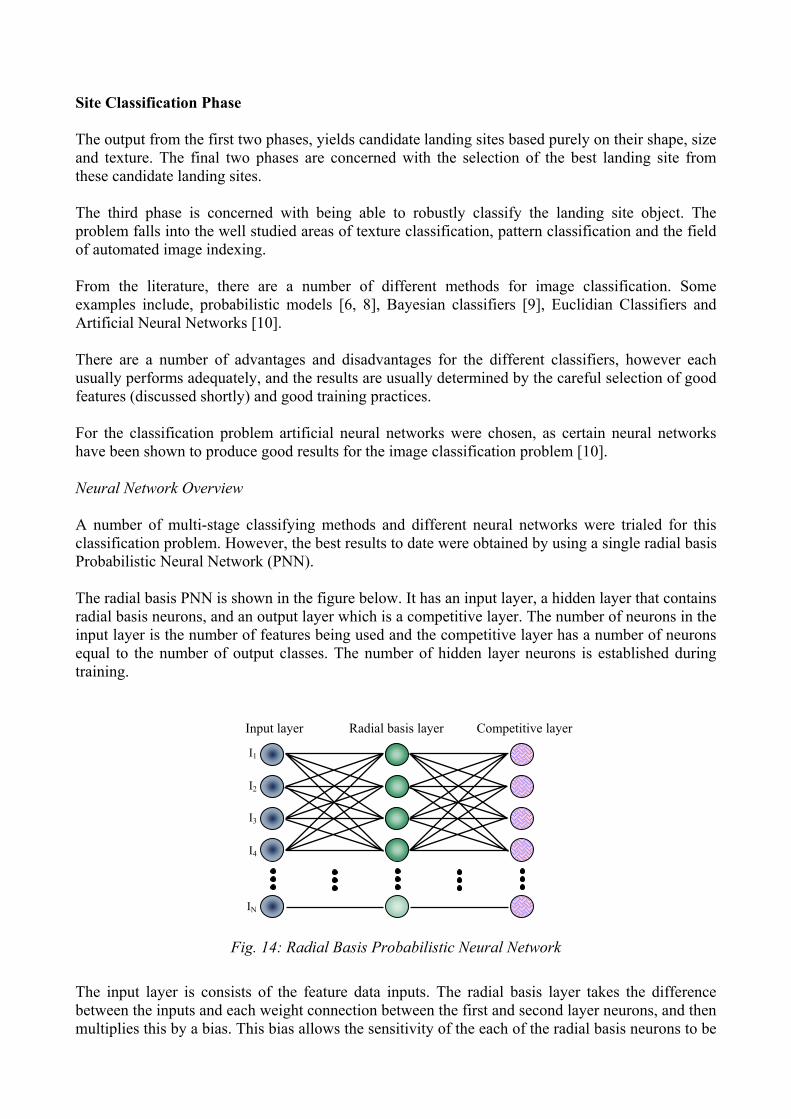
Site Classification Phase The output from the first two phases, yields candidate landing sites based purely on their shape, size and texture. The final two phases are concerned with the selection of the best landing site from these candidate landing sites. The third phase is concerned with being able to robustly classify the landing site object. The problem falls into the well studied areas of texture classification, pattern classification and the field of automated image indexing. From the literature, there are a number of different methods for image classification. Some examples include, probabilistic models [6, 8], Bayesian classifiers [9], Euclidian Classifiers and Artificial Neural Networks [10]. There are a number of advantages and disadvantages for the different classifiers, however each usually performs adequately, and the results are usually determined by the careful selection of good features (discussed shortly) and good training practices. For the classification problem artificial neural networks were chosen, as certain neural networks have been shown to produce good results for the image classification problem [10]. Neural Network Overview A number of multi-stage classifying methods and different neural networks were trialed for this classification problem. However, the best results to date were obtained by using a single radial basis Probabilistic Neural Network (PNN). The radial basis PNN is shown in the figure below. It has an input layer, a hidden layer that contains radial basis neurons, and an output layer which is a competitive layer. The number of neurons in the input layer is the number of features being used and the competitive layer has a number of neurons equal to the number of output classes. The number of hidden layer neurons is established during training.

Fig. 14: Radial Basis Probabilistic Neural Network

The input layer is consists of the feature data inputs. The radial basis layer takes the difference between the inputs and each weight connection between the first and second layer neurons, and then multiplies this by a bias. This bias allows the sensitivity of the each of the radial basis neurons to be

I2

I3

IN

I4

Input layer

I1

Radial basis layer Competitive layer

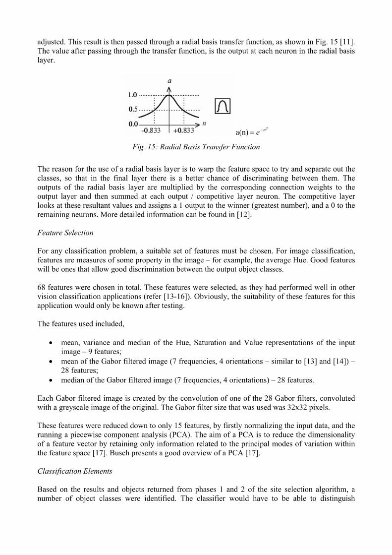
adjusted. This result is then passed through a radial basis transfer function, as shown in Fig. 15 [11]. The value after passing through the transfer function, is the output at each neuron in the radial basis layer.

2

a(n) ne −=

Fig. 15: Radial Basis Transfer Function

The reason for the use of a radial basis layer is to warp the feature space to try and separate out the classes, so that in the final layer there is a better chance of discriminating between them. The outputs of the radial basis layer are multiplied by the corresponding connection weights to the output layer and then summed at each output / competitive layer neuron. The competitive layer looks at these resultant values and assigns a 1 output to the winner (greatest number), and a 0 to the remaining neurons. More detailed information can be found in [12]. Feature Selection For any classification problem, a suitable set of features must be chosen. For image classification, features are measures of some property in the image – for example, the average Hue. Good features will be ones that allow good discrimination between the output object classes. 68 features were chosen in total. These features were selected, as they had performed well in other vision classification applications (refer [13-16]). Obviously, the suitability of these features for this application would only be known after testing. The features used included,

• mean, variance and median of the Hue, Saturation and Value representations of the input image – 9 features;

• mean of the Gabor filtered image (7 frequencies, 4 orientations – similar to [13] and [14]) – 28 features;

• median of the Gabor filtered image (7 frequencies, 4 orientations) – 28 features. Each Gabor filtered image is created by the convolution of one of the 28 Gabor filters, convoluted with a greyscale image of the original. The Gabor filter size that was used was 32x32 pixels. These features were reduced down to only 15 features, by firstly normalizing the input data, and the running a piecewise component analysis (PCA). The aim of a PCA is to reduce the dimensionality of a feature vector by retaining only information related to the principal modes of variation within the feature space [17]. Busch presents a good overview of a PCA [17]. Classification Elements Based on the results and objects returned from phases 1 and 2 of the site selection algorithm, a number of object classes were identified. The classifier would have to be able to distinguish

between these classes correctly, so that the UAV is able to land on the appropriate target. These classes are,

• grass; • trees; • water; • bitumen; and • buildings.

The classifier is shown in the figure below.

Fig. 16: Classifier Output Class Definitions

As can be seen in the figure above, there are a number of categories for both grass and water. These are then generalized after the classification process to just either grass or water. The reason for this, is by using a number of sub categories for the classification process, the overall classification accuracy is improved. Results The results presented in this section have been taken from assessing the performance of the probabilistic neural network classifier (trained on 150 sample images) against 279 test images taken from image frames of the flight data collected. These test images are rectangular areas that were manually selected and categorized by a human operator. Examples of images for each classification class are shown in Table 1. These images were then used as inputs to the neural network, and the output classification compared with the correct classification as determined by the human operator.

Candidate landing site

classifier

GREEN GRASS

BROWN GRASS

TREES

WATER - DARK BLUE GREEN

WATER - DARK BROWN GREEN

WATER - GREEN

WATER – LIGHT BROWN

GRASS

BITUMEN

BUILDING

INPUT IMAGE

REGION WATER

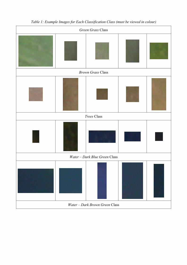
Table 1: Example Images for Each Classification Class (must be viewed in colour)

Green Grass Class

Brown Grass Class

Trees Class

Water – Dark Blue Green Class

Water – Dark Brown Green Class

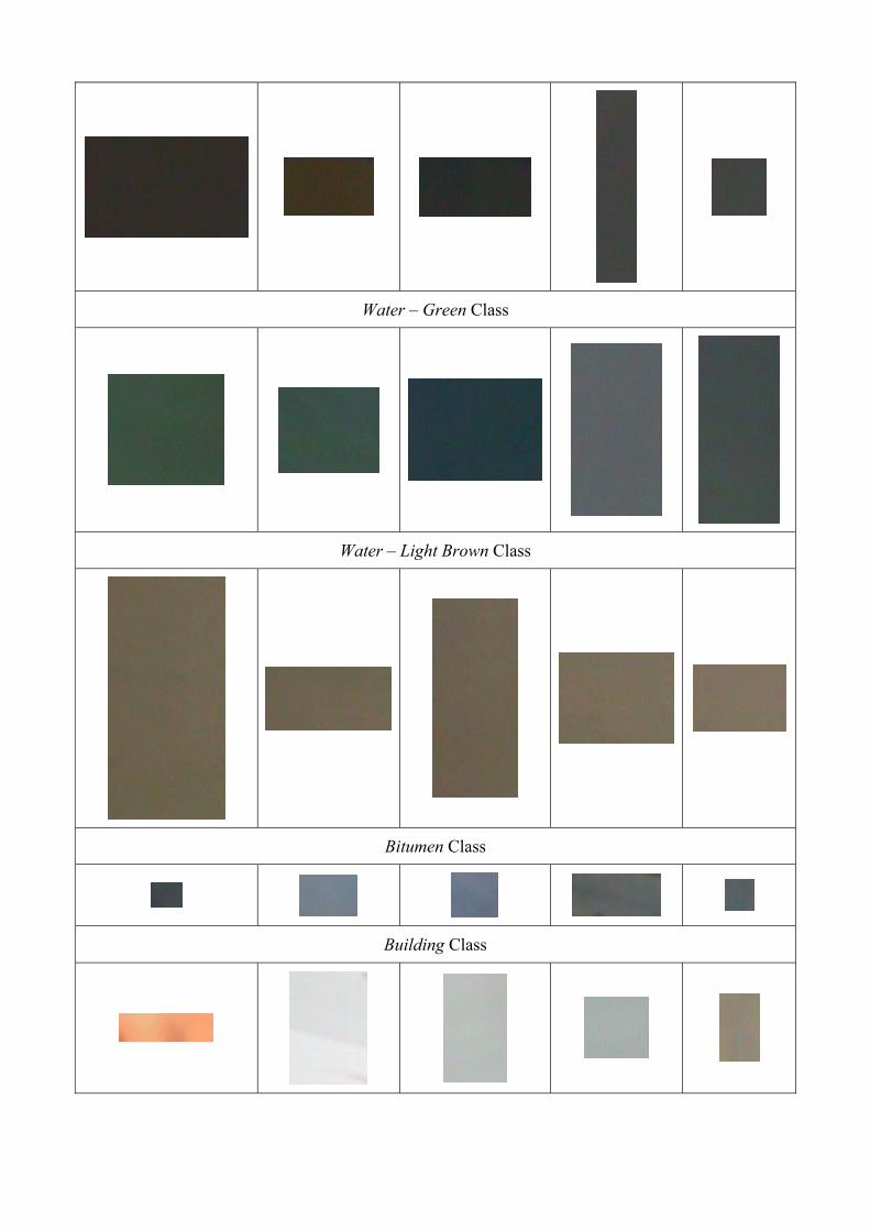
Water – Green Class

Water – Light Brown Class

Bitumen Class

Building Class

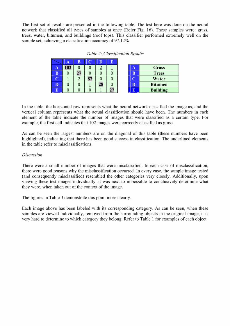
The first set of results are presented in the following table. The test here was done on the neural network that classified all types of samples at once (Refer Fig. 16). These samples were: grass, trees, water, bitumen, and buildings (roof tops). This classifier performed extremely well on the sample set, achieving a classification accuracy of 97.12%.

Table 2: Classification Results

A B C D E A 102 0 0 2 1 A Grass B 0 27 0 0 0 B Trees C 1 2 87 0 0 C Water D 0 0 1 28 0 D Bitumen E 0 0 0 1 27 E Building

In the table, the horizontal row represents what the neural network classified the image as, and the vertical column represents what the actual classification should have been. The numbers in each element of the table indicate the number of images that were classified as a certain type. For example, the first cell indicates that 102 images were correctly classified as grass. As can be seen the largest numbers are on the diagonal of this table (these numbers have been highlighted), indicating that there has been good success in classification. The underlined elements in the table refer to misclassifications. Discussion There were a small number of images that were misclassified. In each case of misclassification, there were good reasons why the misclassification occurred. In every case, the sample image tested (and consequently misclassified) resembled the other categories very closely. Additionally, upon viewing these test images individually, it was next to impossible to conclusively determine what they were, when taken out of the context of the image. The figures in Table 3 demonstrate this point more clearly. Each image above has been labeled with its corresponding category. As can be seen, when these samples are viewed individually, removed from the surrounding objects in the original image, it is very hard to determine to which category they belong. Refer to Table 1 for examples of each object.

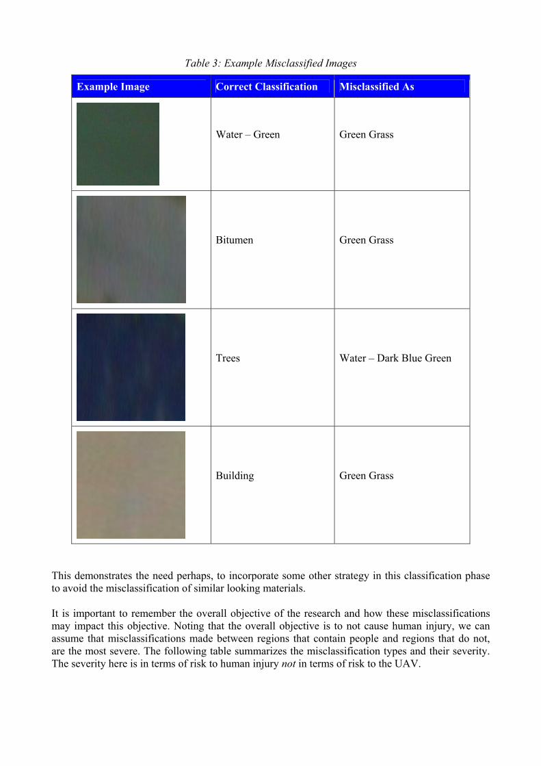
Table 3: Example Misclassified Images

Example Image Correct Classification Misclassified As

Water – Green

Green Grass

Bitumen

Green Grass

Trees

Water – Dark Blue Green

Building

Green Grass

This demonstrates the need perhaps, to incorporate some other strategy in this classification phase to avoid the misclassification of similar looking materials. It is important to remember the overall objective of the research and how these misclassifications may impact this objective. Noting that the overall objective is to not cause human injury, we can assume that misclassifications made between regions that contain people and regions that do not, are the most severe. The following table summarizes the misclassification types and their severity. The severity here is in terms of risk to human injury not in terms of risk to the UAV.

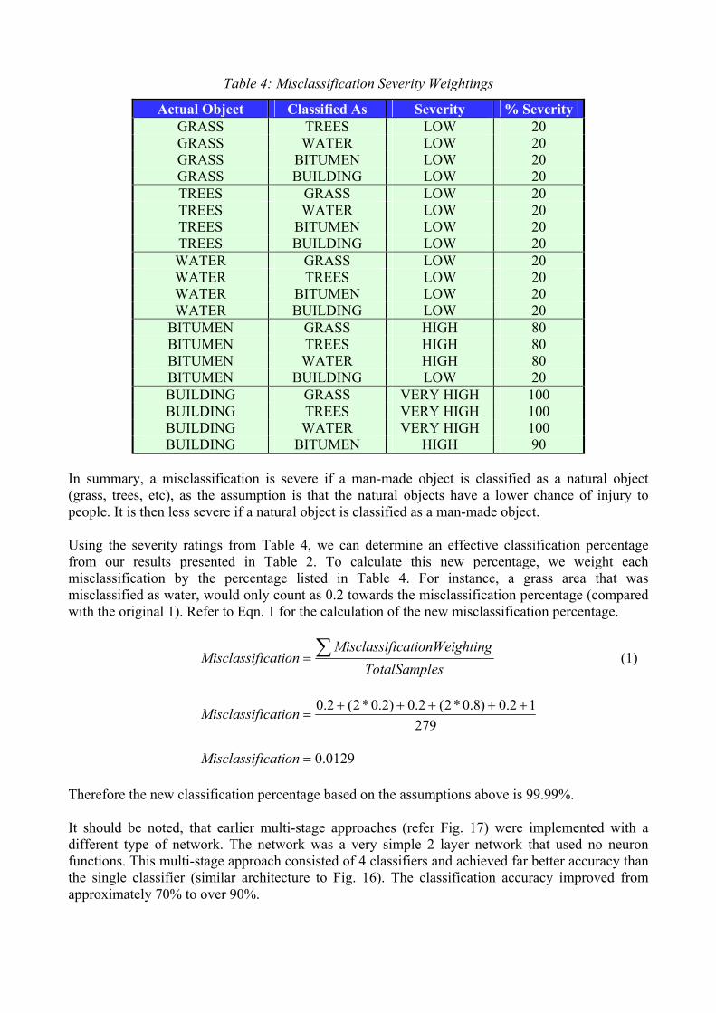
Table 4: Misclassification Severity Weightings

Actual Object Classified As Severity % Severity GRASS TREES LOW 20 GRASS WATER LOW 20 GRASS BITUMEN LOW 20 GRASS BUILDING LOW 20 TREES GRASS LOW 20 TREES WATER LOW 20 TREES BITUMEN LOW 20 TREES BUILDING LOW 20 WATER GRASS LOW 20 WATER TREES LOW 20 WATER BITUMEN LOW 20 WATER BUILDING LOW 20

BITUMEN GRASS HIGH 80 BITUMEN TREES HIGH 80 BITUMEN WATER HIGH 80 BITUMEN BUILDING LOW 20 BUILDING GRASS VERY HIGH 100 BUILDING TREES VERY HIGH 100 BUILDING WATER VERY HIGH 100 BUILDING BITUMEN HIGH 90

In summary, a misclassification is severe if a man-made object is classified as a natural object (grass, trees, etc), as the assumption is that the natural objects have a lower chance of injury to people. It is then less severe if a natural object is classified as a man-made object. Using the severity ratings from Table 4, we can determine an effective classification percentage from our results presented in Table 2. To calculate this new percentage, we weight each misclassification by the percentage listed in Table 4. For instance, a grass area that was misclassified as water, would only count as 0.2 towards the misclassification percentage (compared with the original 1). Refer to Eqn. 1 for the calculation of the new misclassification percentage.

esTotalSamplghtingicationWeiMisclassif

icationMisclassif ∑= (1)

27912.0)8.0*2(2.0)2.0*2(2.0 +++++

=icationMisclassif

0129.0=icationMisclassif

Therefore the new classification percentage based on the assumptions above is 99.99%. It should be noted, that earlier multi-stage approaches (refer Fig. 17) were implemented with a different type of network. The network was a very simple 2 layer network that used no neuron functions. This multi-stage approach consisted of 4 classifiers and achieved far better accuracy than the single classifier (similar architecture to Fig. 16). The classification accuracy improved from approximately 70% to over 90%.

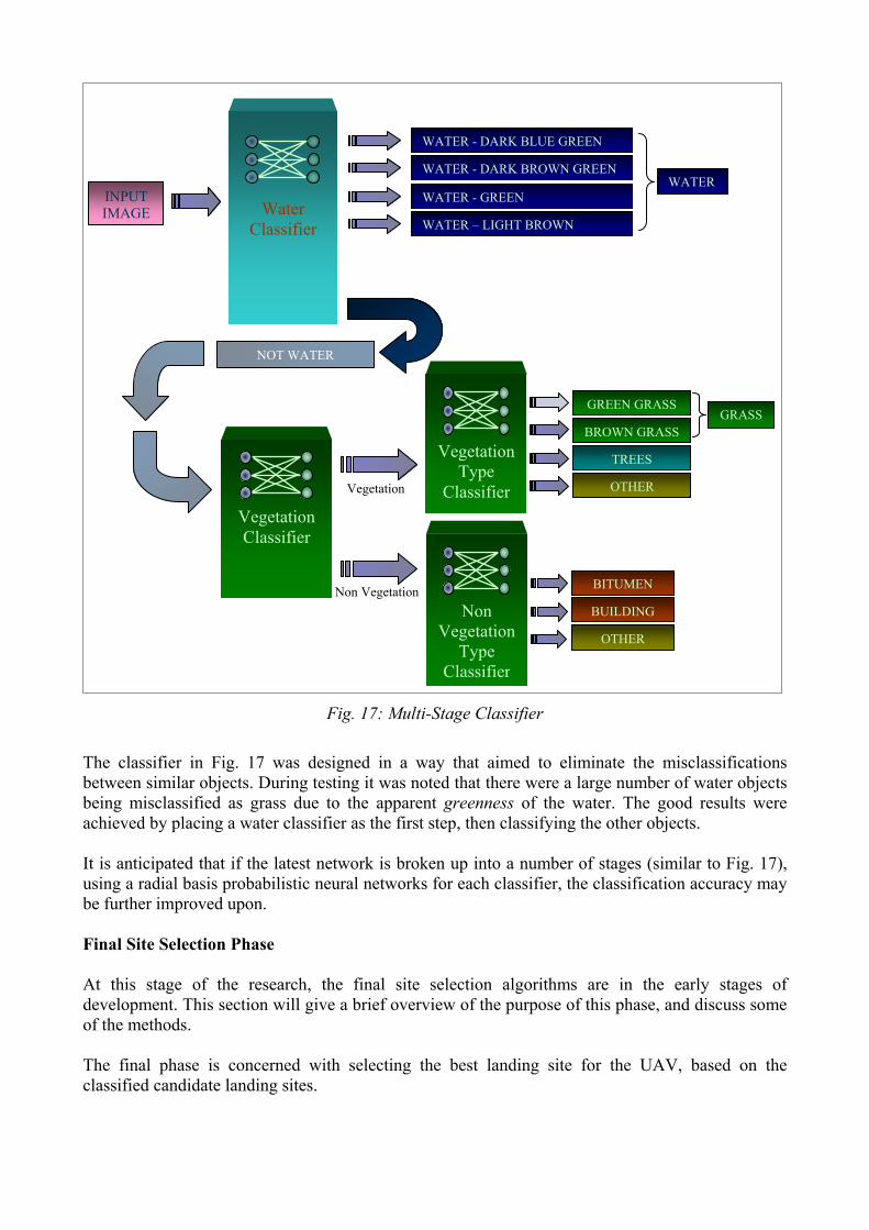
Fig. 17: Multi-Stage Classifier

The classifier in Fig. 17 was designed in a way that aimed to eliminate the misclassifications between similar objects. During testing it was noted that there were a large number of water objects being misclassified as grass due to the apparent greenness of the water. The good results were achieved by placing a water classifier as the first step, then classifying the other objects. It is anticipated that if the latest network is broken up into a number of stages (similar to Fig. 17), using a radial basis probabilistic neural networks for each classifier, the classification accuracy may be further improved upon. Final Site Selection Phase At this stage of the research, the final site selection algorithms are in the early stages of development. This section will give a brief overview of the purpose of this phase, and discuss some of the methods. The final phase is concerned with selecting the best landing site for the UAV, based on the classified candidate landing sites.

Non Vegetation

Vegetation

GREEN GRASS

BROWN GRASS

WATER - DARK BLUE GREEN

TREES

WATER - DARK BROWN GREEN

WATER - GREEN

WATER – LIGHT BROWN

BITUMEN

BUILDING

GRASS

WATER Water

Classifier

INPUT IMAGE

NOT WATER

Vegetation Type

Vegetation Classifier

Classifier OTHER

Non Vegetation

Type OTHER

Classifier

There will be a number of steps to this process. Some include,

• Weighting the sites on there suitability for landing based on their classification type – for example, a grass field would have more weighting than a water body such as a lake;

• Tracking the candidate landing site regions over a number of frames, to exclude objects with moving objects within – here some form of image averaging will be performed, then some translation and rotation of the area to compensate for the velocity of the aircraft, and finally image subtraction to locate any objects moving differently to the background;

• Observing the spatial relationships between the objects – it would be better to head for an area with a number of alternatives (multiple landing sites within close range of each other) rather than heading for just one object – this maximizes the choices at lower altitudes;

• Ensure the surroundings of the target object are suitable – for example, make sure there are no tall buildings next to a grass area chosen for landing that could hinder the UAV landing approach.

The final output, will be an image frame with the “safe” landing site selected (if one exists). If there are multiple objects left at this stage, the algorithm will rank them in order of most suitable to least suitable to land in.

Conclusions In the past decade there has been prolific growth in the number of UAVs, UAV based companies and UAV operators all around the globe. This growth however, will ultimately lead to the increase in UAV related incidents. This research has pointed out that there is a need for a forced landing system for UAVs, an area that has no attention to date. This paper has addressed the forced landing problem for UAVs. Forced landings are required, when an aircraft is unable to continue on its mission and unable to return safety home. This can occur for example if an engine failure occurs. UAVs are no different to manned aircraft, and as such require a means to be able to land safely if something does go wrong and a forced landing is required. UAVs can be smaller than manned aircraft, but can also be larger – they can cause just as much damage to persons and property, and therefore this problem must be addressed. The paper has presented a novel approach to locate “safe” landing sites for a UAV forced landing. The research has drawn upon many fields including, image based landing methodologies for spacecraft, autonomous helicopters and also in the areas of aerial mapping and surveying. The results presented have highlighted the differing successes that have been achieved to date, and discussed potential problems and recommendations for the next period of research. Results have shown the algorithm selecting candidate landing sites successfully after phases 1 and 2, and preliminary work on the classification phase has yielded promising results on the test and training datasets of 97.12 %. Issues that still need to be addressed include, the effect of time of day / lighting effects on the algorithm; the effects of changing altitudes – the work presented here was based on aerial data that was taken at approximately 2500 ft; finally, a method must be devised to verify the algorithm on a very large dataset – testing the algorithm on more than 5000 images, as opposed to 279 (the problem here is the manual classification of over 5000 images).

In conclusion, the goal as UAV researchers is to have UAVs fully integrated into civilian airspace flying over populated areas. This will never be achieved, without some kind of safety system to land the UAV in the event of a failure. It is believed that the proposed architecture and algorithms will be an ideal candidate for such a system.

Acknowledgments This research is based in the Cooperative Research Centre for Satellite Systems with financial support from the Commonwealth of Australia through the CRC Program. Additional financial support for this project has been granted by QUT and the Faculty of Built Environment Engineering, QUT. This research was supported in part by a grant of computer software from QNX Software Systems Ltd.

References [1] P. Garcia-Padro, G. Sukhatme, and J. Montgomery, "Towards vision-based safe landing for

an autonomous helicopter," 2001. [2] A. P. Oliva, "Sensor Fault Detection and Analyitical Redundency Satellite Launcher Flight

Control System," SBA Controle & Automação, vol. 9 num. 3, pp. 156-164, 1998. [3] D. H. Zhou and P. M. Frank, "Fault diagnostics and fault tolerant control," Aerospace and

Electronic Systems, IEEE Transactions on, vol. 34, pp. 420-427, 1998. [4] B. S. Pervan, D. G. Lawrence, and B. W. Parkinson, "Autonomous fault detection and

removal using GPS carrier phase," Aerospace and Electronic Systems, IEEE Transactions on, vol. 34, pp. 897-906, 1998.

[5] M. Saif and Y. Guan, "A new approach to robust fault detection and identification," Aerospace and Electronic Systems, IEEE Transactions on, vol. 29, pp. 685-695, 1993.

[6] S. Herman and E. Bellers, "Locally-adaptive processing of television images based on real-time image segmentation," presented at Consumer Electronics, 2002. ICCE. 2002 Digest of Technical Papers. International Conference on, 2002.

[7] J. F. Canny, "A computational approach to edge detection," IEEE Trans Pattern Analysis and Machine Intelligence, vol. 8, pp. 679-698.

[8] A. Singhal, J. Luo, and W. Zhu, "Probabilistic spatial context models for scene content understanding," presented at Computer Vision and Pattern Recognition, 2003. Proceedings. 2003 IEEE Computer Society Conference on, 2003.

[9] A. Vailaya, M. Figueiredo, A. Jain, and H. J. Zhang, "Content-based hierarchical classification of vacation images," presented at Multimedia Computing and Systems, 1999. IEEE International Conference on, 1999.

[10] C. G. Looney, "Pattern Recognition Using Neural Networks," Oxford University Press, 1997.

[11] Mathworks, "Matlab Neural Network Toolbox, Radial Basis Neural Networks," 2002. [12] S. Chen, C. F. N. Cowan, and P. M. Grant, "Orthogonal Least Squares Learning Algorithm

for Radial Basis Function," IEEE Transactions on Neural Networks, vol. 2, pp. 302-309, 1991.

[13] A. Vailaya and A. Jain, "Detecting sky and vegetation in outdoor images," Proceedings of SPIE-The International Society for Optical Engineering, pp. 411-420, 2000.

[14] A. K. Jain and F. Farrokhnia, "Unsupervised texture segmentation using Gabor filters," presented at Systems, Man and Cybernetics, 1990. Conference Proceedings., IEEE International Conference on, 1990.

[15] P. Kruizinga, N.Petkov, and S. E. Grigorescu, "Comparison of Texture Features based on Gabor Features," Proceedings of the 10th International Conference of Image Analysis and Processing, Venice, Italy, pp. 142-147, 1999.

[16] L. Chen, G. Lu, and D. Zhang, "Effects of different Gabor filters parameters on image retrieval by texture," Multimedia Modelling Conference, 2004. Proceedings. 10th International, pp. 273-278, 2004.

[17] A. W. Busch, "Introduction to Pattern Recognition," 2002.