UAV Coordination for Autonomous Target Tracking · a Helmsman sensitivity parameter d Distance Fb...
22
UAV Coordination for Autonomous Target Tracking Richard A. Wise * and Rolf T. Rysdyk † Autonomous Flight Systems Laboratory University of Washington, Seattle, WA 98195 This report compares several different methodologies for tracking a moving target with multiple Unmanned Aerial Vehicles (UAVs). Relative position coordination of UAVs is en- forced. The comparison considers minimization of heuristics and robustness of performance and stability when the UAVs are exposed to wind and target motion. Nomenclature a Helmsman sensitivity parameter d Distance F b Body-fixed frame g Gravity constant r Radius s Arclength position along desired path V Velocity V a Airspeed V g Inertial speed (ground speed) V w Windspeed (inertial) x, y, z Position coordinates y s Cross-track error κ(s) Curvature of desired path at position s φ Bank angle ρ Radius of curvature χ Course χ w Wind direction (‘from’ convention) ψ Heading ψ w Wind vector orientation (ψ w = χ w + π) Ψ Bearing angle of aircraft from the target (‘Clock angle’ relative to target) Subscripts and Superscripts b Body-fixed reference frame c Command e Earth reference frame hat (ˆ ·) Estimate icpt Intercept s Serret-Frenet reference frame t Target w Wind tilde (˜ ·) Relative parameter(Vehicle - Target) minus (·) - A value delayed by one time step * Research Assistant, Department of Aeronautics and Astronautics, e-mail : [email protected] † Assistant Professor, Department of Aeronautics and Astronautics, email: [email protected] 1
Transcript of UAV Coordination for Autonomous Target Tracking · a Helmsman sensitivity parameter d Distance Fb...

UAV Coordination for Autonomous Target Tracking
Richard A. Wise∗ and Rolf T. Rysdyk†
Autonomous Flight Systems Laboratory
University of Washington, Seattle, WA 98195
This report compares several different methodologies for tracking a moving target withmultiple Unmanned Aerial Vehicles (UAVs). Relative position coordination of UAVs is en-forced. The comparison considers minimization of heuristics and robustness of performanceand stability when the UAVs are exposed to wind and target motion.
Nomenclature
a Helmsman sensitivity parameterd DistanceFb Body-fixed frameg Gravity constantr Radiuss Arclength position along desired pathV VelocityVa AirspeedVg Inertial speed (ground speed)Vw Windspeed (inertial)x, y, z Position coordinatesys Cross-track errorκ(s) Curvature of desired path at position sφ Bank angleρ Radius of curvatureχ Courseχw Wind direction (‘from’ convention)ψ Headingψw Wind vector orientation (ψw = χw + π)Ψ Bearing angle of aircraft from the target
(‘Clock angle’ relative to target)
Subscripts and Superscripts
b Body-fixed reference framec Commande Earth reference framehat (·) Estimateicpt Intercepts Serret-Frenet reference framet Targetw Windtilde (·) Relative parameter(Vehicle - Target)minus (·)− A value delayed by one time step
∗Research Assistant, Department of Aeronautics and Astronautics, e-mail : [email protected]†Assistant Professor, Department of Aeronautics and Astronautics, email: [email protected]
1

τ Tangential component (to the orbit)
I. Introduction
Figure 1. Coordinated UAVs Tracking a Target
Figure [1] is an illustration of multiple UAVs coordinating to track a moving target ship. Tracking impliesmaintaining continuous knowledge of the target’s position. Each UAV must maintain its own position whiledetermining the target’s position based on onboard sensors. Tracking guidance performance is strongly cou-pled to the ability of the sensors to determine the target’s position. Poor sensor information will lead to apoor track which will lead back to poor sensor information. The combined sensor information of coordinatedUAVs provides more accurate target position determination than possible with a single UAV [2]. Thus, thereare many ongoing efforts to determine optimal methods to track a moving target with multiple autonomousUAVs.
Cost and reliability are driving factors for using multiple UAVs. The cost of a UAV is largely determinedby the quality of its sensor package and position determination package (GPS and INS). However, sendingtwo coordinated UAVs with less complex sensors can lead to a better target track than sending one with asensor that costs twice as much. Further, the probability of mission success increases as the loss of a singlevehicle in a flock of vehicles is less severe than the loss of the only vehicle sent on the mission.
A. The Desired Picture
Figure [2] represents the desired motion of two UAVs orbiting a target. The picture is relative, i.e. as seenfrom an observer that moves with the target. Notice, that the UAVs maintain a constant distance from thetarget as well as maintain a constant angular separation, even in the presence of wind. Figure [3] shows thecorresponding absolute motion of the UAVs when tracking a target that moves Easterly at constant speed.
B. The Constant Clock Angle Separation Problem
Clock angle is the bearing of the UAV position with respect to the target position:
Ψ = atan
(y − yt
x− xt
)= atan(
y
x) (1)
2

−300 −200 −100 0 100 200 300−300
−200
−100
0
100
200
300Desired Positions of the UAVs Relative to the Target
UAV1UAV2Clock Angle UAV1
UAV2
Rdes
Rdes
∆ ψdes
XTarget
Wind
Figure 2. The Desired Relative Picture
0 500 1000 1500 2000 2500−50
0
50
100
150
200
250
300
350
400
450
Position EAST
Pos
ition
NO
RT
H
Absolute Positions of the UAVs and Target
TargetUAV1UAV2
Figure 3. The Desired Absolute Picture
The requirement to maintain the clock angle difference between the UAVs while simultaneously tracking amoving target significantly increases the complexity of the tracking problem.
1. Tracking a Moving Target, No Wind
First consider Figure [4(a)] which shows the local velocity vector of a UAV relative to a moving target.The vectors are evenly spaced in time. The UAV rotates counter-clockwise about the target. When theUAV passes the target, the relative speed lessens as does the UAV clock angle rate about the target (Ψ =(|(Vuav−Vt|)τ )/r). This is seen in Figure [4(a)]: the vectors seem bunched up. When the UAV has rotatedpast the front of the target, its relative speed increases to include the target motion in the opposite direction.This higher speed results in higher clock angle rate. This is visible in Figure [4(a)] as the vectors spreadingapart.
2. Tracking a Stationary Target With Wind
Now consider the problem of target tracking in the presence of a wind field, as shown in Figure [4(b)]. Herea UAV orbits a stationary target, but with a constant wind from right to left. In Figure [4(a)], the velocityvectors are evenly spaced in time, but are bunched up when the vehicle travels against the wind and spreadout when the vehicle is with the wind. The relative speed effect is exactly the same as caused by targetmotion (Ψ = (|(Vuav −Vw|)τ )/r). Unlike the target, however, the wind also affects the vehicle dynamics.Increased ground speed due to wind will cause an additional increase in bank angle due to the coordinatedcoupling of heading rate and bank angle. High wind speeds will cause bank angle limit saturation even whenequivalently fast targets do not.
3. Tracking a Moving Target With Wind
Combining the effects of a moving target with wind may render a real UAV, with bank angle limits andresponse dynamics, incapable of maintaining or even converging to the desired circular orbit in Figure [2].
For example, assume that the wind is in a direction opposite the motion of the target. As the UAV passes thetarget, its ground speed is reduced by the wind velocity. This results in a lesser clock angle rate. Assumingthat the ground speed of the UAV remains higher than the target, the UAV should be able to continue itsorbital path. As the UAV rounds the target, its ground speed will increase by the wind speed resultingin a higher clock angle rate necessary for continued orbit. The bank angle of the UAV must increase toaccommodate, possibly to saturation. Again, this is not only due to the UAV’s increased relative speed withrespect to the target, but also due to its increased inertial speed due to the wind. This may cause the UAVto lag behind the target, diverging from the orbit, until the UAV turns back into the wind to catch back upwith the target. In other words, the control authority of the UAV is increased when it is not needed and
3

−300 −200 −100 0 100 200 300 400−300
−200
−100
0
100
200
300
400UAV Heading, spaced every 4 seconds.
High heading ratechange as UAVsround the target →
← Low heading ratechange as UAVspass the target
(a) Effect of Target Motion On Course Rate of Change
−300 −200 −100 0 100 200 300 400−300
−200
−100
0
100
200
300
400UAV Heading, spaced every 4 seconds.
High heading ratechange as UAVs headwith the wind →
← Low heading ratechange as UAVshead into the wind
(b) Effect of Wind On Course Rate of Change
Figure 4. Relative Motion Effects on Course Rate of Change
degraded just it is. Of course, if the wind were to go in the opposite direction, everything would be easier,but this cannot be expected in general.
4. Coordinated Tracking of a Moving Target With Wind
The clock angle rate is now given by:
Ψ2(t) =
(Vg(t)2 + V 2
t + 2Vg(t)Vt(t) sin(Ψ(t)− ψt(t)))τ
r(t)2(2)
For coordinated tracking, the clock angle separation must first be achieved and then held constant bymatching the clock angle rate of change. Note that clock angle rate varies with target velocity, wind velocity,and clock angle. The control logic must account for each of these factors, within the bounds of aircraftperformance (bank angle limits) and behavior (dynamics). This must be done simultaneously with trackingthe target.
5. Coordinated Tracking - Open Issues
Finally, inherent in multi-vehicle coordination are two other open issues: inter-vehicle communication andcollision avoidance. As these issue are not addressed by this paper, it is assumed that for the purposes ofcomparison, the communication is perfect and collision avoidance is handled by altitude separation.
II. Kinematic Coordinated Turn UAV Model
As with most conventional aircraft, the UAV control problem would normally involve the following de-grees of freedom : airspeed, aerodynamic side-slip angle, turn rate, and flight path angle. The availableaerodynamic control surfaces for rotation about the three body axes are the ailerons, elevator, and rudder.The propulsion (throttle) remains and will be assumed to work in conjunction with the elevator to controlaltitude and airspeed. Since this control problem addresses guidance at constant altitude, it will be assumedthat airspeed and altitude can be held (or controlled) independent of lateral-directional commands.
Aileron and rudder signals are combined to zero sideslip providing a “truly banked turn” or a ‘coordinatedturn’. Turn coordination relates the bank angle and turn rate, kinematically, as follows:
tanφ =Vg
gψ (3)
In Equation [3], note again the difference between wind and target motion. Only wind will effect this kine-matic scaling between heading rate and bank angle.
4

To account for aircraft dynamics, a command in airspeed will be assumed to have a first order responseby the UAV as follows:
Va =1
s + 1Vc (4)
A command saturation of ±20% of nominal speed is used.
Bank angle response shows a first order behavior:
φ =1
0.3s + 1φc (5)
A bank angle rate limit of ±45 deg/s is used as well as a command saturation of ±45 deg.
We will simply relate navigation over the ground via a flat earth model. As we will allow for wind, wedistinguish between heading (horizontal orientation of the body frame) and course (horizontal orientation ofthe UAV over ground, i.e. in the inertial frame).
Figure [5] is a diagram of inputs and outputs relating the control logic to the UAV motion. Note thatthe the control logic will take in (at least) UAV and target ground velocity (or position) and orbit parame-ters (radius and UAV clock angle separation) and output a course rate command and velocity command.Sensed wind information may also be used by the controller (not shown). Also note the necessity of vehiclecommunication: the speed and clock angle of both UAVs are inputs.
Sensors
V_w
chi_w
V_t
Comms From Other UAV
chi
V_a
Standoff
Distance
UAV Separation
Guidance Logic
Aircraft Model
V_w
chi_w
phi_c
V_ac
V_gV_g
V_t
r_c
chi_2
V_a2
Delta_chi_c
phi_c
V_ac
Figure 5. Information Flow To and From the Guidance Logic
6. Comparative Simulations
For all simulations, two UAVs will be required to coordinate positions while tracking the following targetspeed profiles:
1. No Wind, No Target Motion (control)
2. Constant wind, Wind Speed:UAV Speed = 0.2, Direction: from West, No Target Motion
3. No Wind, Slow Target Profile in Figure [6]
4. No Wind, Fast Target Profile in Figure [7]
5. Wind Speed:UAV Speed = 0.2, Wind Direction with Target, Slow Target Profile as in Figure [6]
6. No Wind, Target Turning in Figure [8]
5

0 50 100 150 200 250 3000
10
20
30Slow Target Speed Profile. Max tgt speed / UAV speed: 0.4
Time [sec]
Spe
ed [m
/sec
]
Target SpeedMax UAV Speed
0 500 1000 1500 2000 2500 3000−1
−0.5
0
0.5
1Slow Target Position Profile
Position East [m]
Pos
ition
Nor
th [m
]
Figure 6. Slow Target
0 50 100 150 200 250 300−30
−20
−10
0Fast Target Speed Profile. Max tgt speed / UAV speed: 1.1
Time [sec]
Spe
ed [m
/sec
]
Target SpeedMax UAV Speed
−5000 −4000 −3000 −2000 −1000 0−1
−0.5
0
0.5
1Fast Target Position Profile
Position East [m]
Pos
ition
Nor
th [m
]
Figure 7. Fast Target
0 100 200 300−5
0
5
10
15
20
25
30Turning Target Speed Profiles
Time [sec]
Spe
ed [m
/sec
]
Speed EastSpeed NorthMax UAV Speed
0 200 400 600 8000
100
200
300
400
500
600
700
800
900Turning Target Position Profile
Position East [m]
Pos
ition
Nor
th [m
]
Figure 8. Turning Target
III. Method 1 : Helmsman Behavior Based Guidance Law
A. Description
The first method is an extension of path following as developed here by Rysdyk [5]. In this work, convergingback to the desired path consists of stabilizing two degrees of freedom to zero: course angle error, and crosstrack distance. The path geometry to be followed is determined based on the target current position andheading as well as a standoff distance.
Deviations from this path produce the course angle error and cross track distance. “Good Helmsman”behavior is employed, so-called as it smoothly transitions from current path to the desired path by simulta-neously bringing cross track distance and course angle error to zero:
σs = (χ− χs)e−ays/2 − 1e−ays/2 + 1
(6)
The output, σs, is the commanded relative course with gain a. A PD control relates this to the course rate:
χs = s−κ1
χs = χ− χs
ys =∫ t
0
(Vc sin(χs)dτ
s =∫ t
0
(Vc cos(χs)(1− y−s κ1))dτ
ψc ≈ χc =(
kp(σs − χs) + ki
∫ t
0
(σs − χs)dτ
)− Vcκ2 (7)
6

Here, κ1 is the command nominal path curvature (1/rc) and κ2 is the ‘adjusted’ path curvature. For twoUAV coordination, the lead aircraft normally holds a constant stand-off distance from the target so κ1
and κ2 are equal. Based on the clock angle separation error (using another “Good Helmsman” transitionfunction), the follower aircraft adjusts κ2 as well as adjusting the cross track error used to calculate σs:ys = ys + (1/κ2 − 1/κ1). Optionally, both aircraft adjust radius oppositely (one increase, other decrease).Also, both aircraft speeds adjust (one up, one down) when speed control is available. This provides thenecessary additional degree of freedom to achieve a desired angular separation between the two UAVs.
B. Simulations
−300 −200 −100 0 100 200 300−300
−200
−100
0
100
200
300
Position EAST
Pos
ition
NO
RT
H
Relative Positions of the UAVs WRT the Target
0
0
300
300
UAV1UAV2Time Stamps
Figure 9. Helmsman: Tracking a Fixed Target With an Initial Condition Offset
Figures [9-15] resulted as the target and wind velocity profiles were changed per Section [II.6]. In eachfigure, UAV1 is the ‘lead’ UAV and UAV2 is the ‘follower’.
In Figure [9], UAV1 has the initial heading of −45 degrees. In comparison to Figure [2], UAV1 shouldhave a heading of zero degrees at this point in the orbit. An orbit correction occurs as a result, and UAV1settles on the desired orbit. UAV2 has an initial distance from the target further than the commanded orbitradius of 200 meters. Further, the clock angle between UAV1 and UAV2 is zero whereas the commandedrelative clock angle is 75 degrees. UAV2 also corrects and settles on the desired orbit with a correct separa-tion clock angle. This method is able to correct for initial condition errors. Further simulations will all startwith both UAVs having heading angles of 0 degrees and initial positions 200 meters to the South of the target.
Figure [10] shows that this method works when the target is stationary and no wind is present. Figure[11] demonstrates the effect of wind, which is clearly minor. A regular oscillation occurs for the relativeclock angle between the UAVs, but remains bounded to within 2% of the command.
In Figure [12], target forward speed has a similar effect on the relative clock angle as the wind, i.e. asmall, regular oscillation. Wind can be seen to skew the orbit patterns of the UAVs in Figure [13]. Thecompensation of UAV2 is also apparent as UAV2s radius regularly changes. The wind has also caused theclock angle to be affected in a regular pattern. The overshoot has increased to approximately 25%.
In Figure [14], the UAVs are too slow to remain near the target and fall behind. Considering the logicin Equation [7], and noting that cross-track error will grow large as the target distance increases, the head-ing rate command will quickly grow and saturate the bank angle commands of the two UAVs. Each spinsabout a tight orbit. Even when the target slows, the command does not relieve enough for UAV1 due tothe integral action winding up the command, and UAV1 continues to spin. UAV2 however, modifies itscross track error based upon the difference in clock angle. UAV1’s clock angle from the target is nearing a
7

−300 −200 −100 0 100 200 300−300
−200
−100
0
100
200
300
Position EAST
Pos
ition
NO
RT
H
Relative Positions of the UAVs WRT the Target
0 300
300
UAV1UAV2Time Stamps
0 20 40 60 80 100 120−10
−8
−6
−4
−2
0
2
4
6
8
10Deviation in Clock Angle Separation From Command
Time
Clo
ck A
ngle
Dev
iatio
n
Figure 10. Helmsman: Tracking a Fixed Target
−300 −200 −100 0 100 200 300−300
−200
−100
0
100
200
300
Position EAST
Pos
ition
NO
RT
H
Relative Positions of the UAVs WRT the Target
00
100
100
UAV1UAV2Time Stamps
Wind Speed0.2 V
0 20 40 60 80 100 120−10
−8
−6
−4
−2
0
2
4
6
8
10Deviation in Clock Angle Separation From Command
TimeC
lock
Ang
le D
evia
tion
Figure 11. Helmsman: Tracking a Fixed Target WithWind
constant, but the clock angle between UAV1 and UAV2 is increasing. This creates an increasing error signaland causes UAV2 to reduce its cross track error signal, desaturating the heading rate command.
Finally, Figure [15] demonstrates the UAV’s ability to follow a target through a turn.
IV. Method 2 : Lyapunov Vector Field Guidance Law
A. Description of the Vector Field
The second method builds upon the work done by Lawrence and Frew [3]. The guidance of the UAV to theobservation orbit is determined by building a vector field that has a stable limit cycle centered on the targetposition. The governing equations are as follows:
r =√
x2 + y2
vx = −x(r2 − r2c )− 2rrdy
vy = −y(r2 − r2c ) + 2rrdx
χcomV F = atan2(vy, vx)
∆chi com = χcomV F − ang( ~V ) (8)
Figures [16-18] visualize this vector field. Figure [16] shows the vector field surrounding a stationary target.It is clear that a path following the field vectors from any point will end up on a circle of radius equal to thespecified stand-off distance (shown in black).
To understand how the target motion effects the velocity field, the rate of change of the gradient dueto the target can be determined as follows: The area around the target is discretized into points at relativecoordinates (i, j) (i.e. target relative location is (0,0)). The gradient is calculated at each discrete point
8

−300 −200 −100 0 100 200 300−300
−200
−100
0
100
200
300
Position EAST
Pos
ition
NO
RT
H
Relative Positions of the UAVs WRT the Target
00
300
300
UAV1UAV2Time Stamps
0 50 100 150 200−10
−8
−6
−4
−2
0
2
4
6
8
10Deviation in Clock Angle Separation From Command
Time
Clo
ck A
ngle
Dev
iatio
n
Figure 12. Helmsman: Tracking a Slow Target
−300 −200 −100 0 100 200 300−300
−200
−100
0
100
200
300
Position EAST
Pos
ition
NO
RT
H
Relative Positions of the UAVs WRT the Target
00
300
300
UAV1UAV2Time Stamps
0 50 100 150 200−50
−40
−30
−20
−10
0
10
20
30
40
50Deviation in Clock Angle Separation From Command
TimeC
lock
Ang
le D
evia
tion
Figure 13. Helmsman: Tracking a Slow Target WithWind
0 500 1000 1500 2000 2500 3000 3500
−200
0
200
400
600
800
1000
1200
1400
1600
Position EAST
Pos
ition
NO
RT
H
Relative Positions of the UAVs WRT the Target
0
0
100
100
200
200
300
300
UAV1UAV2Time Stamps
0 50 100 150 200 250 300−100
−80
−60
−40
−20
0
20
40
60
80
100Deviation in Clock Angle Separation From Command
Time
Clo
ck A
ngle
Dev
iatio
n
Figure 14. Helmsman: Tracking a Fast Target
−300 −200 −100 0 100 200 300−300
−200
−100
0
100
200
300
Position EAST
Pos
ition
NO
RT
H
Relative Positions of the UAVs WRT the Target
00
300
300
UAV1UAV2Time Stamps
0 50 100 150 200 250 300−10
−8
−6
−4
−2
0
2
4
6
8
10Deviation in Clock Angle Separation From Command
Time
Clo
ck A
ngle
Dev
iatio
n
Figure 15. Helmsman: Tracking a Turning Target
9

−500 0 500 1000 1500−600
−400
−200
0
200
400
600Velocity Gradient Field, stationary target.
Position East
Pos
ition
Nor
th
Figure 16. Stationary Target Vector Field
resulting in the direction of the field vector χ(i,j)(t). A new gradient vector is calculated at the same points(i, j), but with target position delayed in time by ∆T , resulting in a new field angle χ(i,j)(t−∆T ). Rate ofchange is thus:
χ =χ(i,j)(t)− χ(i,j)(t−∆T ))
∆T(9)
Figures [17-18] show the vector field locally surrounding a target moving Easterly. In each figure, a color mapis used to indicate vector rotational rates as a percentage of the maximum possible heading rate. Far fromthe target, the color is constant and represents ψ < 0.25ψmax. Each subsequent shade darkening of the mapindicates an increase of 0.25ψmax. A dark, dashed line indicates the relative orbit around the target. Themaximum heading rate is based on Equation [3]. A heading rate of greater than 17.7 deg/sec will saturatethe bank angle command, set at 45 degrees.
In Figure [17], the target’s speed is 43% that of the UAV’s. No shade increase appears along the or-
−400 −200 0 200 400−400
−300
−200
−100
0
100
200
300
400
Velocity Gradient Field, moving target.Rate limit = 17.7 deg/s TGT:UAV spd =0.39152 Time : 33
Position East
Pos
ition
Nor
th
Figure 17. Slow Target Vector Field
200 400 600 800 1000−400
−300
−200
−100
0
100
200
300
400
Velocity Gradient Field, moving target.Rate limit = 17.7 deg/s TGT:UAV spd =1.1355 Time : 64
Position East
Pos
ition
Nor
th
Figure 18. Fast Target Vector Field
bit and thus the maximum command along the orbit remains less than 0.25ψmax. In Figure [18], the targethas speed of 110% that of the UAV. And yet, along the orbit, the shade has increased by only two incre-ments indicating a command of χc < 0.75ψmax. Indeed, the command does not increase to greater thanψmax unless the UAV is well within the specified standoff distance. Thus, assuming that no wind is present,
10

the angle command given by the vector field is within the capability of the UAV to follow for all targetspeeds for which the UAV can orbit the target.
B. Application of the Vector Field for Control Guidance
To extend the vector field angle output to the required logic output start with:
ψc ≈ χc = kp∆chi com + kd ang( ~V ) (10)
To ensure the heading rate command is still within the bounds of the UAV capability, the proportionalconstant, kp, is kept less than unity and the derivative term is set to only reduce the heading rate command.
To be able to follow a target that goes faster than the UAV, a second command is generated:
χct = k2∆(ang( ~V )− ang(θtan)
)(11)
where ang(θtan) is the angle of a line that connects the current UAV position to the tangent of a circle,centered on the target postion, of radius equal to the specified stand-off distance.
However, this command is heavily weighted, as a function of target distance, such that it only has aneffect when the UAV is distant from the target. This is the case when Equation [10] is insufficient to main-tain the UAV at stand-off distance, such as when the UAV becomes slower than the target. Conversely,the basic vector field command is weighted oppositely. This ensures that the vector field command is usedwhenever the UAV is near, and can keep up with, the target. The weighting functions are used as transitionsto avoid hard switches.
C. UAV Coordination
Assuming UAV relative velocity remains positive, angular separation can be achieved by varying UAV speedproportional to the angular separation error:
Vc = Vc0 + kRc(Ψc − (Ψ1 −Ψ2)) (12)
Note that k is negative for UAV1 and positive for UAV2. Therefore, the vehicles will change speeds equallybut oppositely (one will increase, the other decrease).
At high relative speeds, it becomes much more difficult to maintain large clock separation due to the highheading rate changes. To compensate, ΨC is reduced as a function of increasing target speed. If the targetbecomes faster than the UAV, accurate tracking becomes less of a concern than losing too much ground andtherefore losing any track of the target. In this case, the angular compensation is turned off and the speedcommand is increased to maximum speed in an attempt to minimize distance gained by the target.
D. Simulations
Figures [19-24] resulted as the target and wind velocity profiles were changed per Section [II.6]. In eachfigure, UAV1 is the ‘lead’ vehicle and UAV2 is the ‘follower’.
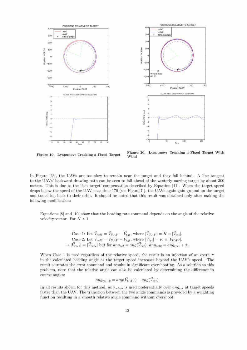
In Figure [19], it is clear that this method can meet the clock angle requirement while loitering arounda stationary target with no wind present. Note that this method reaches a zero deviation about 10 secondsslower than the Helmsman method. Figure [20] demonstrates the effect of wind. An undamped oscillationoccurs for the relative clock angle between the UAVs, but remains bounded to within 2 degrees of the com-mand, only a slightly larger oscillation amplitude than the Helmsman method.
In Figure [21], target forward speed has a similar effect on the relative clock angle as the wind, i.e. anundamped oscillation. Note that the amplitude is slightly less than for the Helmsman method. Wind canbe seen to skew the orbit patterns of the UAVs in Figure [22], but has much less of an effect than it does onthe Helmsman method.
11
−400 −200 0 200 400−400
−300
−200
−100
0
100
200
300
400
Position EAST
Pos
ition
NO
RT
H
POSITIONS RELATIVE TO TARGET
00
UAV1UAV2Time Stamps
0 10 20 30 40 50 60 70 80 90−10
−8
−6
−4
−2
0
2
4
6
8
10CLOCK ANGLE SEPARATION DEVIATION
Time
DE
VIA
TIO
N [
deg]
Figure 19. Lyapunov: Tracking a Fixed Target
−400 −200 0 200 400−400
−300
−200
−100
0
100
200
300
400
Position EAST
Pos
ition
NO
RT
H
POSITIONS RELATIVE TO TARGET
00
UAV1UAV2Time Stamps
Wind Speed0.2 V
0 50 100 150−10
−8
−6
−4
−2
0
2
4
6
8
10CLOCK ANGLE SEPARATION DEVIATION
TimeD
EV
IAT
ION
[de
g]
Figure 20. Lyapunov: Tracking a Fixed Target WithWind
In Figure [23], the UAVs are too slow to remain near the target and they fall behind. A line tangentto the UAVs’ backward-drawing path can be seen to fall ahead of the westerly moving target by about 300meters. This is due to the ’fast target’ compensation described by Equation [11]. When the target speeddrops below the speed of the UAV near time 170 (see Figure[7]), the UAVs again gain ground on the targetand transition back to their orbit. It should be noted that this result was obtained only after making thefollowing modification:
Equations [8] and [10] show that the heading rate command depends on the angle of the relativevelocity vector. For K > 1
Case 1: Let ~Vrel1 = ~VUAV − ~Vtgt, where |~VUAV | = K × |~Vtgt|.Case 2: Let ~Vrel2 = ~VUAV − ~Vtgt, where |~Vtgt| = K × |~VUAV |.
→ |~Vrel1| = |~Vrel2| but for angrel = ang(~Vrel), angrel2 = angrel1 + π.
When Case 1 is used regardless of the relative speed, the result is an injection of an extra πin the calculated heading angle as the target speed increases beyond the UAV’s speed. Theresult saturates the error command and results in significant overshooting. As a solution to thisproblem, note that the relative angle can also be calculated by determining the difference incourse angles:
angrel−b = ang(~VUAV )− ang(~Vtgt)
In all results shown for this method, angrel−b is used preferentially over angrel at target speedsfaster than the UAV. The transition between the two angle commands is provided by a weightingfunction resulting in a smooth relative angle command without overshoot.
12

−400 −200 0 200 400−400
−300
−200
−100
0
100
200
300
400
Position EAST
Pos
ition
NO
RT
H
POSITIONS RELATIVE TO TARGET
00
UAV1UAV2Time Stamps
0 50 100 150 200−10
−8
−6
−4
−2
0
2
4
6
8
10CLOCK ANGLE SEPARATION DEVIATION
Time
DE
VIA
TIO
N [
deg]
Figure 21. Lyapunov: Tracking a Slow Target
−400 −200 0 200 400−400
−300
−200
−100
0
100
200
300
400
Position EAST
Pos
ition
NO
RT
H
POSITIONS RELATIVE TO TARGET
00
UAV1UAV2Time Stamps
Wind Speed0.2 V
0 50 100 150 200−10
−8
−6
−4
−2
0
2
4
6
8
10CLOCK ANGLE SEPARATION DEVIATION
TimeD
EV
IAT
ION
[de
g]
Figure 22. Lyapunov: Tracking a Slow Target WithWind
−400 −200 0 200 400 600 800 1000−1000
−800
−600
−400
−200
0
200
400
Position EAST
Pos
ition
NO
RT
H
POSITIONS RELATIVE TO TARGET
0
100
100
200200
UAV1UAV2Time Stamps
0 50 100 150 200 250−50
−40
−30
−20
−10
0
10
CLOCK ANGLE SEPARATION DEVIATION
Time
DE
VIA
TIO
N [
deg]
Figure 23. Lyapunov: Tracking a Fast Target
−400 −200 0 200 400−400
−300
−200
−100
0
100
200
300
400
Position EAST
Pos
ition
NO
RT
H
POSITIONS RELATIVE TO TARGET
00
300
300
UAV1UAV2Time Stamps
0 50 100 150 200 250 300−10
−8
−6
−4
−2
0
2
4
6
8
10CLOCK ANGLE SEPARATION DEVIATION
Time
DE
VIA
TIO
N [
deg]
Figure 24. Lyapunov: Tracking a Turning Target
13
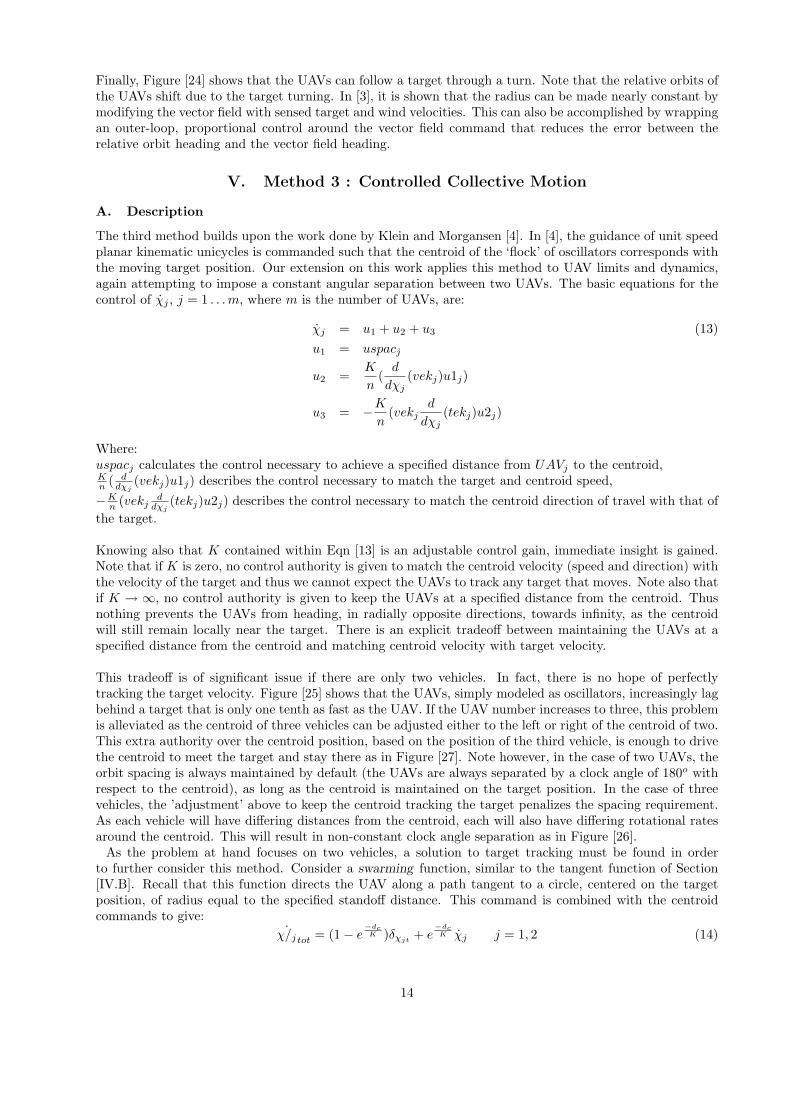
Finally, Figure [24] shows that the UAVs can follow a target through a turn. Note that the relative orbits ofthe UAVs shift due to the target turning. In [3], it is shown that the radius can be made nearly constant bymodifying the vector field with sensed target and wind velocities. This can also be accomplished by wrappingan outer-loop, proportional control around the vector field command that reduces the error between therelative orbit heading and the vector field heading.
V. Method 3 : Controlled Collective Motion
A. Description
The third method builds upon the work done by Klein and Morgansen [4]. In [4], the guidance of unit speedplanar kinematic unicycles is commanded such that the centroid of the ‘flock’ of oscillators corresponds withthe moving target position. Our extension on this work applies this method to UAV limits and dynamics,again attempting to impose a constant angular separation between two UAVs. The basic equations for thecontrol of χj , j = 1 . . . m, where m is the number of UAVs, are:
χj = u1 + u2 + u3 (13)u1 = uspacj
u2 =K
n(
d
dχj(vekj)u1j)
u3 = −K
n(vekj
d
dχj(tekj)u2j)
Where:uspacj calculates the control necessary to achieve a specified distance from UAVj to the centroid,Kn ( d
dχj(vekj)u1j) describes the control necessary to match the target and centroid speed,
−Kn (vekj
ddχj
(tekj)u2j) describes the control necessary to match the centroid direction of travel with that ofthe target.
Knowing also that K contained within Eqn [13] is an adjustable control gain, immediate insight is gained.Note that if K is zero, no control authority is given to match the centroid velocity (speed and direction) withthe velocity of the target and thus we cannot expect the UAVs to track any target that moves. Note also thatif K → ∞, no control authority is given to keep the UAVs at a specified distance from the centroid. Thusnothing prevents the UAVs from heading, in radially opposite directions, towards infinity, as the centroidwill still remain locally near the target. There is an explicit tradeoff between maintaining the UAVs at aspecified distance from the centroid and matching centroid velocity with target velocity.
This tradeoff is of significant issue if there are only two vehicles. In fact, there is no hope of perfectlytracking the target velocity. Figure [25] shows that the UAVs, simply modeled as oscillators, increasingly lagbehind a target that is only one tenth as fast as the UAV. If the UAV number increases to three, this problemis alleviated as the centroid of three vehicles can be adjusted either to the left or right of the centroid of two.This extra authority over the centroid position, based on the position of the third vehicle, is enough to drivethe centroid to meet the target and stay there as in Figure [27]. Note however, in the case of two UAVs, theorbit spacing is always maintained by default (the UAVs are always separated by a clock angle of 180o withrespect to the centroid), as long as the centroid is maintained on the target position. In the case of threevehicles, the ’adjustment’ above to keep the centroid tracking the target penalizes the spacing requirement.As each vehicle will have differing distances from the centroid, each will also have differing rotational ratesaround the centroid. This will result in non-constant clock angle separation as in Figure [26].
As the problem at hand focuses on two vehicles, a solution to target tracking must be found in orderto further consider this method. Consider a swarming function, similar to the tangent function of Section[IV.B]. Recall that this function directs the UAV along a path tangent to a circle, centered on the targetposition, of radius equal to the specified standoff distance. This command is combined with the centroidcommands to give:
˙χ/jtot = (1− e−dc
K )δχjt + e−dc
K χj j = 1, 2 (14)
14

−5 0 5 10 15 20 25 30
−15
−10
−5
0
5
10
15
Absolute Positions of UAVs, Centroid, and Target. Target:UAV Speed = 0.1
Position East
Pos
ition
Nor
th
Figure 25. Centroid : Two Oscillators Tracking a Tar-get
−20 −10 0 10 20 30
−20
−15
−10
−5
0
5
10
15
Absolute Positions of UAVs, Centroid, and Target. Target:UAV Speed = 0.1
Position East
Pos
ition
Nor
th
Figure 26. Centroid : Tracking With a Tangent Swarm-
ing Function
−10 0 10 20 30
−15
−10
−5
0
5
10
15
20
Absolute Positions of UAVs, Centroid, and Target. Target:UAV Speed = 0.1
Position East
Pos
ition
Nor
th
Figure 27. Centroid : Three Oscillators Tracking a Target
Where dc is the distance from the centroid to the target and K is an adjustable gain.
Equation [14] swarms, or brings all of the UAVs toward the target by setting the commanded headingrate to zero only if the vehicle heading is pointing along the tangent line to the target. The exponentialweighting functions avoid the use of switching by providing the emphasis on the original function (trade offvehicle spacing and centroid-target convergence) only when the distance from the centroid to the target issmall. This implies that one can reduce the gain in Equation [13] to achieve good distance separation as theswarming function complements the centroid-target convergence by definition. See Figure [26].
B. Simulations
Figures [28-33] resulted as the target and wind velocity profiles were changed per Section [II.6]. In eachfigure, the path of UAV1 is in blue, the path of UAV2 is in green, and the path of the centroid is in red.
Figure [28] demonstrates the loitering capability of this method. A slight oscillation in the clock angleoccurs. The wind, as seen in Figure [29], significantly alters the orbit patterns of the UAVs. This moves thecentroid away from the target position, detrimentally to the clock angle separation.
Figures [30 - 33], as opposed to Figures [25 - 26], demonstrate the considerable effect of adding kinematicsand dynamics to the oscillator model upon which this method is based. In each case, the variations of theclock angle separation with respect to the target is quite large. This is due to the ‘traveling’ of the centroid
15

−150 −100 −50 0 50 100 150−150
−100
−50
0
50
100
150Relative Positions of UAVs, and Centroid WRT the Target
Position EAST
Pos
ition
NO
RT
H
Figure 28. Centroid: Tracking a Fixed Target
−250 −200 −150 −100 −50 0 50 100 150−200
−150
−100
−50
0
50
100
150Relative Positions of UAVs, and Centroid WRT the Target
Position EAST
Pos
ition
NO
RT
H
Wind Speed0.2 V
Figure 29. Centroid: Tracking a Fixed Target WithWind
−300 −200 −100 0 100−200
−150
−100
−50
0
50
100
150Relative Positions of UAVs, and Centroid WRT the Target
Position EAST
Pos
ition
NO
RT
H
Figure 30. Centroid: Tracking a Slow Target
−300 −200 −100 0 100−200
−150
−100
−50
0
50
100
150Relative Positions of UAVs, and Centroid WRT the Target
Position EAST
Pos
ition
NO
RT
H
Wind Speed0.2 V
Figure 31. Centroid: Tracking a Slow Target WithWind
16

−100 0 100 200 300 400 500 600−150
−100
−50
0
50
100
150
200Relative Positions of UAVs, and Centroid WRT the Target
Position EAST
Pos
ition
NO
RT
H
Figure 32. Centroid: Tracking a Fast Target
−200 −100 0 100 200−250
−200
−150
−100
−50
0
50
100
150
200Relative Positions of UAVs, and Centroid WRT the Target
Position EAST
Pos
ition
NO
RT
H
Figure 33. Centroid: Tracking a Turning Target
with respect to the target. Maintaining the centroid on the target is the key to keeping angular separationof the UAVs with respect to the target.
Notice that the tangent swarming function keeps the UAVs within range of the fast target in Figure [32]and allows them the regain their orbit when the target slows per the profile in Figure [7]. Also note that inFigure [33], the slower target speed has reduced the clock angle oscillation amplitude, although now a cleardrift in average clock angle separation can be detected.
VI. Method 4 : ’Real-Time’ Optimization for Predictive Control
There are many fast and efficient routines for solving optimization problems, particularly if the space overwhich to optimize is convex [1]. If the optimization can be done fast enough, given computational limits, itcan be used in concert with Model Predictive Control to accurately determine future commands.
A. Using Model Predictive Control
Let time now = T and the current command = θc(T ). Due to calculation time (δt), the next command willbe available at time T + δt. If δt ≤ tf , then at each integer multiple of tf , a new command (θ(T + n tf ))will be available for use. See Figure [34]. A zero-order hold can then be used to create a piece-wise constantcommand. θc(t).
B. Formulating Tracking as Model Predictive Control
Target and/or wind speed will affect UAV relative position and speed with respect to the target. Given thiseffect, the control input that results in the desired relative future position and speed of the UAV can beprecisely determined. This assumes UAV, target, and wind field dynamics and their interactions are knownaccurately from current time until the future time. Figure [35] graphically shows how UAV position changesrelative to the target as the target moves over a small time increment. Here, the target moves incrementallengths dTx and dTy. The UAV, starting from position 1 has a clock angle δ. The UAV moves length dU(angle α) in the absolute frame and dR (angle α+β) in the relative frame, resulting in a clock angle γ. Notethat relative position 2 remains a distance R from the target. Therefore, neglecting dynamics, α representsthe commanded heading the UAV must have had at position 1 to get to position 2. Given dTx, dTy, R, andδ, α (and dR, β, γ) can be found by solving the following set of equations:
dR cos(α + β) = dU cos α− dtx
17

Determine
θ(to+tf)
to+3tfto+2tfto+tfto
Determine
θ(to+2tf)
Determine
θ(to+3tf)
Figure 34. Calculation and Data Flow
dR sin(α + β) = dU sin α− dty
R cos γ + dR cos(α + β) = dtx + R cos γ
R sin γ + dR sin(α + β) = dtx + R sin γ (15)
Note, this set is solved as an optimization problem by moving all terms in each equation to right side. Theequation solution would cause each right hand side to evaluate to zero. The optimization is to minimize thenorm of the function evaluations. If the norm is zero, the the optimal set found is also the solution to theequation set.Note also that the wind effect on relative speed can be included by modifying dTx and dTy to include therelative effects of wind in the x and y directions, respectively. For example, if the wind is adverse to theUAV in the x-direction, dTx would increase accordingly.
By solving for α at small time steps ∆t in length, it is reasonable to assume that the target and wind
dTy
2
1
1
2
2
RR
dU
γ
β
δ
dR
dTx
α
Figure 35. Relative Motions
velocities are constant over ∆t. Therefore, dTx = Vtx∆t and dTy = Vty∆t. To convert to a heading ratecommand, the heading rate is assumed proportional to the difference in subsequent calculations of heading:
α = k1(α− α−) (16)
18

To account for initial condition errors, the heading rate is modified by assuming the UAV is always drivingto maintain commanded stand-off distance:
αc = α + k2(Rc −R)/R (17)
C. Commanding Speed to Achieve Angular Separation
Along the same reasoning as the Lyapunov method, angular separation is achieved by varying UAV speedproportional to the angular separation error:
∆Vc = k3(Ψc − (Ψ1 −Ψ2)) (18)
Note that k3 is negative for UAV1 and positive for UAV2. Therefore, the vehicles will change speeds equallybut oppositely (one will increase, the other decrease).
D. Simulations
−300 −200 −100 0 100 200 300−300
−200
−100
0
100
200
300
Position EAST
Pos
ition
NO
RT
H
Relative Positions of the UAVs WRT the Target
UAV1UAV2
0 20 40 60 80 100 120−10
−8
−6
−4
−2
0
2
4
6
8
10Deviation in Clock Angle Separation From Command
Time
Clo
ck A
ngle
Dev
iatio
n
Figure 36. RTO: Tracking a Fixed Target
−300 −200 −100 0 100 200 300−300
−200
−100
0
100
200
300
Position EAST
Pos
ition
NO
RT
H
Relative Positions of the UAVs WRT the Target
UAV1UAV2
Wind Speed0.2 UAV
0 50 100 150−10
−8
−6
−4
−2
0
2
4
6
8
10Deviation in Clock Angle Separation From Command
Time
Clo
ck A
ngle
Dev
iatio
n
Figure 37. RTO: Tracking a Fixed Target With Wind
Figures [36-41] resulted as the target and wind velocity profiles were changed per Section [II.6].
Figure [36] demonstrates that this method can quickly achieve and maintain a loitering orbit about a sta-tionary target. The response time is similar to the Helmsman method. The introduction of wind results inonly a small oscillation as seen in Figure [37].
When the target speed is slow, Figure [38] shows that the motion creates an unsteady, but still smalloscillation of ±5 degrees, or twice the Lyapunov method. However, the introduction of an adverse wind(see Figure [39]) eventually results in unstable behavior in the follower UAV. Note that this behavior startswhen the lead UAV is at its lowest relative speed (most Southerly point on the relative orbit). The velocitycompensation is not enough to account for both the adverse wind and the target. The radius of the follower
19

−300 −200 −100 0 100 200 300−300
−200
−100
0
100
200
300
Position EAST
Pos
ition
NO
RT
H
Relative Positions of the UAVs WRT the Target
* 00300 *
* 300
UAV1UAV2Time Stamps
0 50 100 150 200 250 300−20
−15
−10
−5
0
5
10
15
20Deviation in Clock Angle Separation From Command
Time
Clo
ck A
ngle
Dev
iatio
n
Figure 38. RTO: Tracking a Slow Target
−300 −200 −100 0 100 200 300−300
−200
−100
0
100
200
300
Position EAST
Pos
ition
NO
RT
H
Relative Positions of the UAVs WRT the Target
UAV1UAV2
Wind Speed0.2 V
0 50 100 150−35
−30
−25
−20
−15
−10
−5
0
5
10
15
20Deviation in Clock Angle Separation From Command
TimeC
lock
Ang
le D
evia
tion
Figure 39. RTO: Tracking a Slow Target With Wind
0 2000 4000 6000 8000−300
−200
−100
0
100
200
300
Position EAST
Pos
ition
NO
RT
H
Relative Positions of the UAVs WRT the Target
UAV1UAV2
0 50 100 150 200 250 300−20
−10
0
10
20
30
40
50
60
70
80
90Deviation in Clock Angle Separation From Command
Time
Clo
ck A
ngle
Dev
iatio
n
Figure 40. RTO: Tracking a Fast Target
−300 −200 −100 0 100 200 300−300
−200
−100
0
100
200
300
Position EAST
Pos
ition
NO
RT
H
Relative Positions of the UAVs WRT the Target
* 00
* 300
* 300
UAV1UAV2Time Stamps
0 50 100 150 200 250 300−20
−15
−10
−5
0
5
10
15
20Deviation in Clock Angle Separation From Command
Time
Clo
ck A
ngle
Dev
iatio
n
Figure 41. RTO: Tracking a Turning Target
20
UAV begins to oscillate, effectively slowing its clock angle rate. The radius compensation is taxed to keepthe UAV near the specified stand-off distance and starts to overshoot considerably. By the time the followerUAV reaches its lowest relative speed, the clock separation has started to diverge quickly. This quickens theovershoots towards instability.
As stated, this method cannot work for target speeds faster than the lowest UAV speed. As an exam-ple, Figure [40] shows the unstable behavior resulting from the fast target profile.
Finally, tracking a target through a turn is demonstrated in Figure [41]. The result is similar to a theslow target in Figure [38], but with lower steady oscillations, as this target is slower. The oscillation ampli-tude is almost exactly the same as in Figure [37], which has wind speed the same magnitude as the turningtarget.
VII. Conclusion
This paper investigated four low heuristic methods for coordinated tracking of a moving target. Thefollowing summarizes the advantages and disadvantages of the each method.
Good Helmsman Behavior
• This method works the best to maintain relative clock angle and could be improved, possibly, bycommanding relative angle smaller as target or wind speed increases.
• Anti-windup methods are necessary to prevent command saturation
• This method does not take into account a target faster than the UAVs. If the initial conditions aresignificantly different from the desired orbit, convergence to the orbit occurs, but is slow.
Modified Lyapunov Vector Field
• This method produces feasible commands (within the capability of the UAV), at least when wind isnot present.
• The relative clock angle between the two UAVs oscillates whenever the target or wind speed is non-zero.
• The tangent method works well as a command when the UAV is distant from the target, such as whenthe target moves faster than the UAV.
Controlled Collective Motion
• This method works well for three, and possibly more, vehicles. For two, a possible solution was given.However, this solution had the least ability to maintain target clock angle.
• Wind is very detrimental to this method.
• Considerable work must still be done to integrate the logic of this work, based on an oscillator model,onto a real UAV.
‘Real-Time’ Optimization
• As is common with predictive control, this method depends heavily on the model used to propagatecommands. Feedback is necessary to keep initial conditions near the ’expected’ values.
• Velocity compensation for clock angle separation can lead to unstable behavior at high wind and/ortarget speeds.
• This type of method, if needed to run in actual ’real-time’, would require considerable computing powerto perform the optimization quick enough to output the needed commands.
Any method that is to work well must account for the wind and a target that, at least for some time, canoutperform the UAV.
21

Acknowledgments
This work is sponsored by AFOSR Topic AF04−T011 in cooperation with Cornell University in Ithaca,NY and the Insitu Group in Bingen, WA.
References
1Boyd, S. and Vandenberghe, L.“Convex Optimization”, Cambridge University Press, 2004.2Campbell, M. and Ousingsawat, J. “On-line Estimation and Path Planning for Multiple Vehicles in an Uncertain Envi-
ronment”, AIAA Guidance, Navigation, and Control Conference, Monterey, CA, August 2002.3Frew, E. and Lawrence, D., “Cooperative Stand-off Tracking of Moving Targets by a Team of Autonomous Aircraft”,
AIAA Guidance, Navigation, and Control Conference, San Francisco, CA, August 2005.4Klein, D. and Morgansen, K., “Controlled Collective Motion for Trajectory Tracking”, Proceedings of the American
Control Conference, 2006.5Lawrence, D., “Lyapunov Vector Fields for UAV Flock Coordination”, 2nd AIAA “Unmanned Unlimited” Aerospace
Sytems, Technology, and Operations Conference, San Diego, CA, August 2002.6Ogren, P. and Egerstedt, M., “A Control Lyapunov Function Approach to Multiagent Coordination,” IEEE Transactions
of Robotics and Automation, Vol 18, No. 5, OCT 2002.7Rysdyk, R. “UAV Path Following for Constant Line-of-Sight Target Observation,” Journal of Guidance, Navigation, and
Control, in press.8S. Stolle and R. Rysdyk, ”Flight Path Following Guidance for Unmanned Air Vehicles with Pan-tilt Camera for Target
Observation,” Digital Avionics Systems Conference, Indianapolis, IN, 2003.
22