
u x V v Flight Mechanics - Big Idea | NASA's Breakthrough...
45
1 Flight Mechanics Juan R. Cruz Atmospheric Flight and Entry Systems Branch NASA Langley Research Center x y z u w v V ! # Version 6 2 Contents Flight Mechanics 3 Basic Assumptions 4 Coordinate Systems 5 State Variables 12 Equations of Motion 18 Euler Parameters / Quaternions 32 External Forces and Moments 38 Relative Wind Angles 51 Example Aerodynamic Model 62 Flight Path Angle 74 Numerical Integration of the Equations of Motion 76 Symbols 84 References and Bibliography 89 Acknowledgements 90 Appendices
Transcript of u x V v Flight Mechanics - Big Idea | NASA's Breakthrough...
1
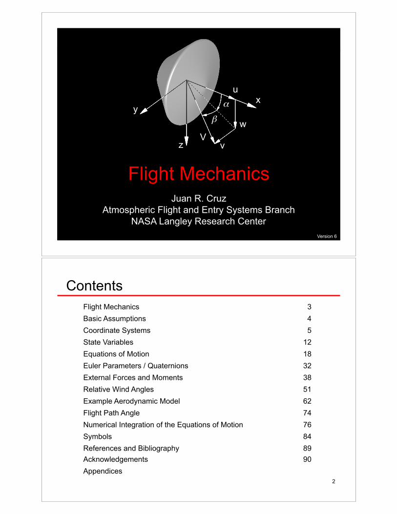
Flight Mechanics
Juan R. Cruz
Atmospheric Flight and Entry Systems Branch
NASA Langley Research Center
x y
z
u
w
v
V
!"
#"
Version 6
2
Contents
Flight Mechanics 3
Basic Assumptions 4
Coordinate Systems 5
State Variables 12
Equations of Motion 18
Euler Parameters / Quaternions 32
External Forces and Moments 38
Relative Wind Angles 51
Example Aerodynamic Model 62
Flight Path Angle 74
Numerical Integration of the Equations of Motion 76
Symbols 84
References and Bibliography 89
Acknowledgements 90
Appendices
3
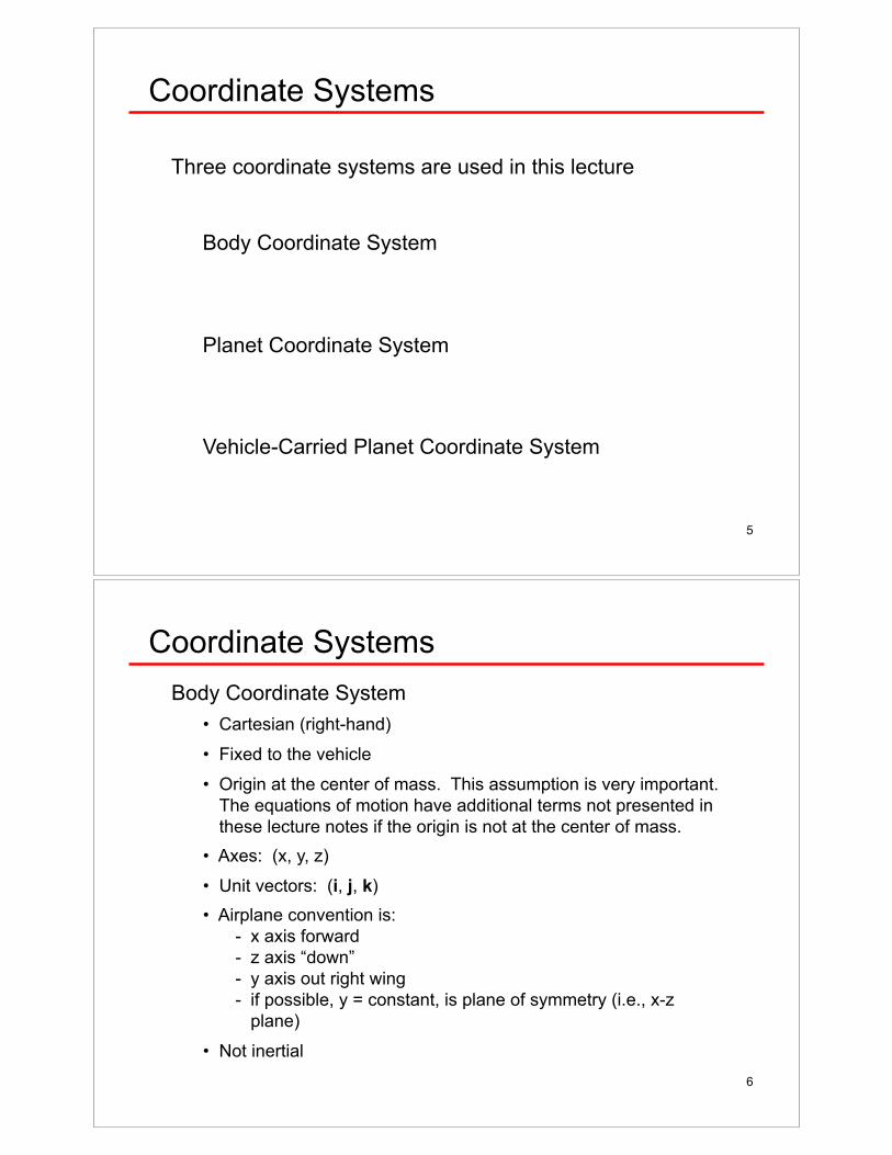
Flight Mechanics
Definition
The branch of engineering that studies the motion of
aerospace vehicles in flight when acted upon by gravitational, aerodynamic, propulsive, and other external
forces.
In this set of lectures we will focus on the flight mechanics
of entry and descent vehicles, with an emphasis on:
- deriving the necessary differential equations
- modeling gravity and aerodynamic forces
- numerically integrating the differential equations
4
Basic Assumptions
• Single, rigid, flight vehicle without rotating masses
• Constant mass properties (i.e., mass, moments of inertia, products of inertia, center of mass)
• The planet is flat and non-rotating (planet surface is
used to define an inertial coordinate system)
• No wind
• The the atmospheric density, !, is a function of the
altitude, h
Additional assumptions are listed throughout the lecture.
5
Coordinate Systems
Three coordinate systems are used in this lecture
Body Coordinate System
Planet Coordinate System
Vehicle-Carried Planet Coordinate System
6
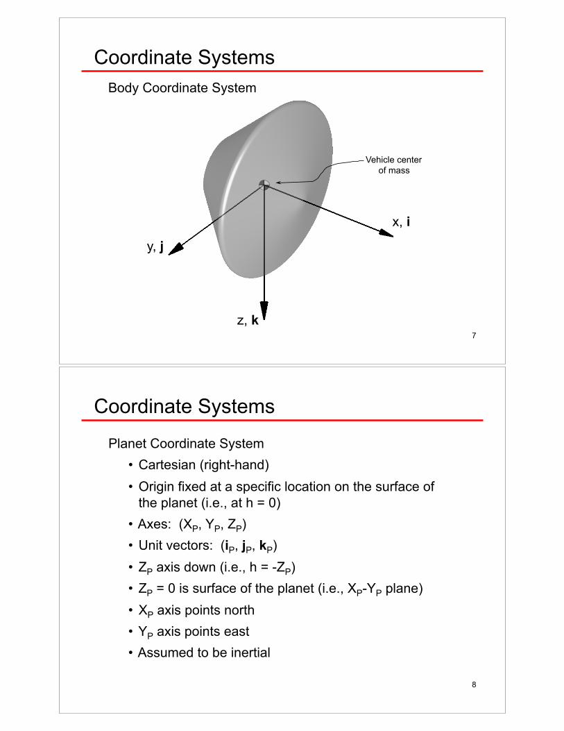
Coordinate Systems
Body Coordinate System
• Cartesian (right-hand)
• Fixed to the vehicle
• Origin at the center of mass. This assumption is very important.
The equations of motion have additional terms not presented in
these lecture notes if the origin is not at the center of mass.
• Axes: (x, y, z)
• Unit vectors: (i, j, k)
• Airplane convention is:
- x axis forward
- z axis “down”
- y axis out right wing
- if possible, y = constant, is plane of symmetry (i.e., x-z
plane)
• Not inertial
7
Coordinate Systems
Body Coordinate System
x, i
z, k
y, j
Vehicle center
of mass
8
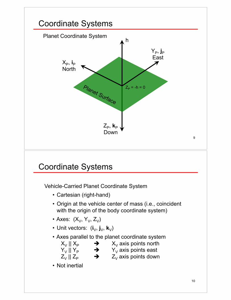
Coordinate Systems
Planet Coordinate System
• Cartesian (right-hand)
• Origin fixed at a specific location on the surface of
the planet (i.e., at h = 0)
• Axes: (XP, YP, ZP)
• Unit vectors: (iP, jP, kP)
• ZP axis down (i.e., h = -ZP)
• ZP = 0 is surface of the planet (i.e., XP-YP plane)
• XP axis points north
• YP axis points east
• Assumed to be inertial
Planet Coordinate System
9
Coordinate Systems
XP, iP
North
YP, jP
East
ZP, kP
Down
h
ZP = -h = 0
10
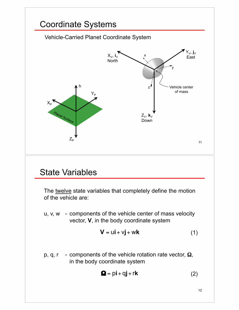
Coordinate Systems
Vehicle-Carried Planet Coordinate System
• Cartesian (right-hand)
• Origin at the vehicle center of mass (i.e., coincident
with the origin of the body coordinate system)
• Axes: (XV, YV, ZV)
• Unit vectors: (iV, jV, kV)
• Axes parallel to the planet coordinate system
XV || XP ! XV axis points north YV || YP ! YV axis points east ZV || ZP ! ZV axis points down
• Not inertial
Vehicle-Carried Planet Coordinate System
11
Coordinate Systems
XP
YP
ZP
h
XV, iV North
YV, jV East
ZV, kV
Down
x
z
y
Vehicle center
of mass
12
State Variables
The twelve state variables that completely define the motion
of the vehicle are:
u, v, w - components of the vehicle center of mass velocity
vector, V, in the body coordinate system
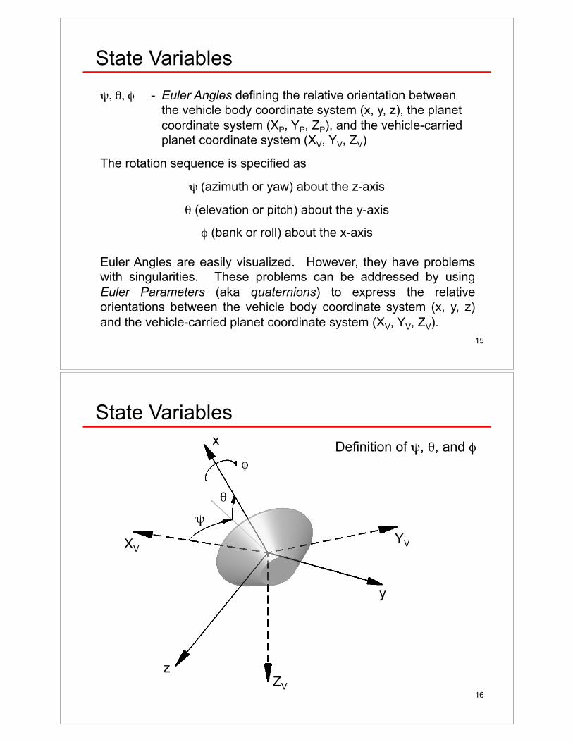
p, q, r - components of the vehicle rotation rate vector, ",
in the body coordinate system
!
V = ui+ vj+ wk
!
" = pi+ qj+ rk
(1)
(2)
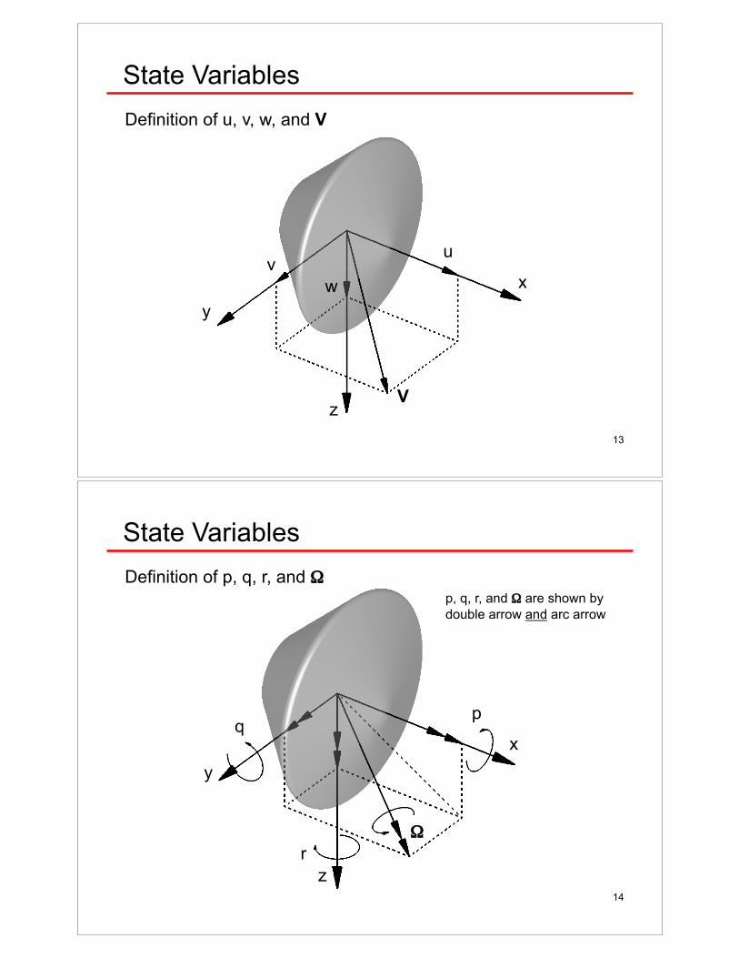
13
State Variables
u
w
v
V z
y
x
Definition of u, v, w, and V
14
State Variables
p
r
q
"#
x
z
y
p, q, r, and " are shown by
double arrow and arc arrow
Definition of p, q, r, and "#
15
State Variables
$, %, & - Euler Angles defining the relative orientation between
the vehicle body coordinate system (x, y, z), the planet
coordinate system (XP, YP, ZP), and the vehicle-carried
planet coordinate system (XV, YV, ZV)
The rotation sequence is specified as
$ (azimuth or yaw) about the z-axis
% (elevation or pitch) about the y-axis
& (bank or roll) about the x-axis
Euler Angles are easily visualized. However, they have problems
with singularities. These problems can be addressed by using
Euler Parameters (aka quaternions) to express the relative
orientations between the vehicle body coordinate system (x, y, z)
and the vehicle-carried planet coordinate system (XV, YV, ZV).
16
State Variables
Definition of $, %, and &#
YV XV
ZV
x
z
y
$
%
&
17
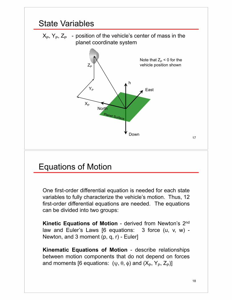
State Variables
XP, YP, ZP - position of the vehicle’s center of mass in the
planet coordinate system
XP
YP
ZP
h
Planet Surface
North
East
Down
Note that ZP < 0 for the
vehicle position shown
18
Equations of Motion
One first-order differential equation is needed for each state
variables to fully characterize the vehicle’s motion. Thus, 12
first-order differential equations are needed. The equations can be divided into two groups:
Kinetic Equations of Motion - derived from Newton’s 2nd
law and Euler’s Laws [6 equations: 3 force (u, v, w) -
Newton, and 3 moment (p, q, r) - Euler]
Kinematic Equations of Motion - describe relationships
between motion components that do not depend on forces
and moments [6 equations: ($, %, &) and (XP, YP, ZP)]
19
Equations of Motion - u, v, w
The linear momentum vector of the vehicle, p, is defined by
(3)
where m is the vehicle’s mass. From Newton’s second law
(4)
Notice the additional term " x p. This term arises because the body coordinate system is rotating. F is the external
forces vector (e.g., gravitational, aerodynamic, buoyancy,
propulsive forces).
!
p = mV
!
F =dp
dt+"#p
20
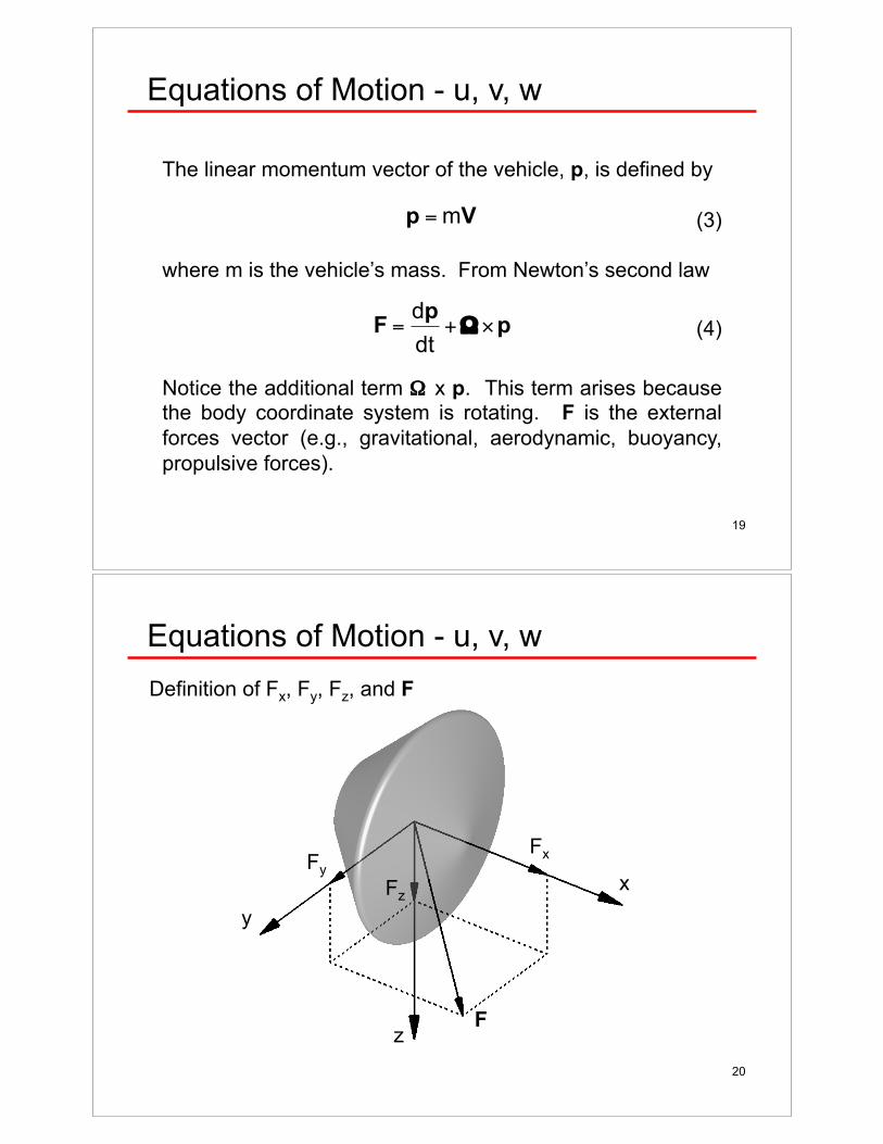
Equations of Motion - u, v, w
Fx
Fz
Fy
F z
y
x
Definition of Fx, Fy, Fz, and F
21
Performing the indicated operations on the right hand side
of equation (4) yields
(5)
Equations of Motion - u, v, w
!
F = mdu
dt+ qw " rv
#
$ %
&
' ( i+m
dv
dt+ ru" pw
#
$ %
&
' ( j
+ mdw
dt+ pv " qu
#
$ %
&
' ( k
22
Equation (5) can be rewritten in terms of its scalar
components to yield the differential equations for u, v, and
w. Fx, Fy, and Fz are the scalar components of the external forces vector.
(6)
(7)
(8)
Equations of Motion - u, v, w
!
du
dt= "qw + ru+
Fx
m
!
dv
dt= "ru+ pw +
Fy
m
!
dw
dt= "pv + qu+
Fz
m
23
The angular momentum vector, L, about the origin of the
body coordinate system (i.e., vehicle center of mass), is
given by
(9)
Where rm is the position vector of an infinitesimal mass
element dm
(10)
Equations of Motion - p, q, r
!
L = rm" #" r
m( )[ ]Vol$ dm
= # rm
•rm( ) % r
m#•r
m( )[ ]Vol$ dm
!
rm
= xmi+ y
mj+ z
mk
24
Define the moments of inertia Ixx, Iyy, and Izz as
(11)
and the products of inertia as
(12)
Beware that a different sign convention is sometimes used for the products of inertia. Also note that the moments and products of inertia as defined here are
about the vehicle’s center of mass (i.e., the body coordinate system origin).
Equations of Motion - p, q, r
!
Ixx = ym
2 + zm
2( )Vol" dm
Iyy = xm
2 + zm
2( )Vol" dm
Izz = xm
2 + ym
2( )Vol" dm
!
Ixy = xmymVol" dm
Ixz = xmzmVol" dm
Iyz = ymzmVol" dm
25
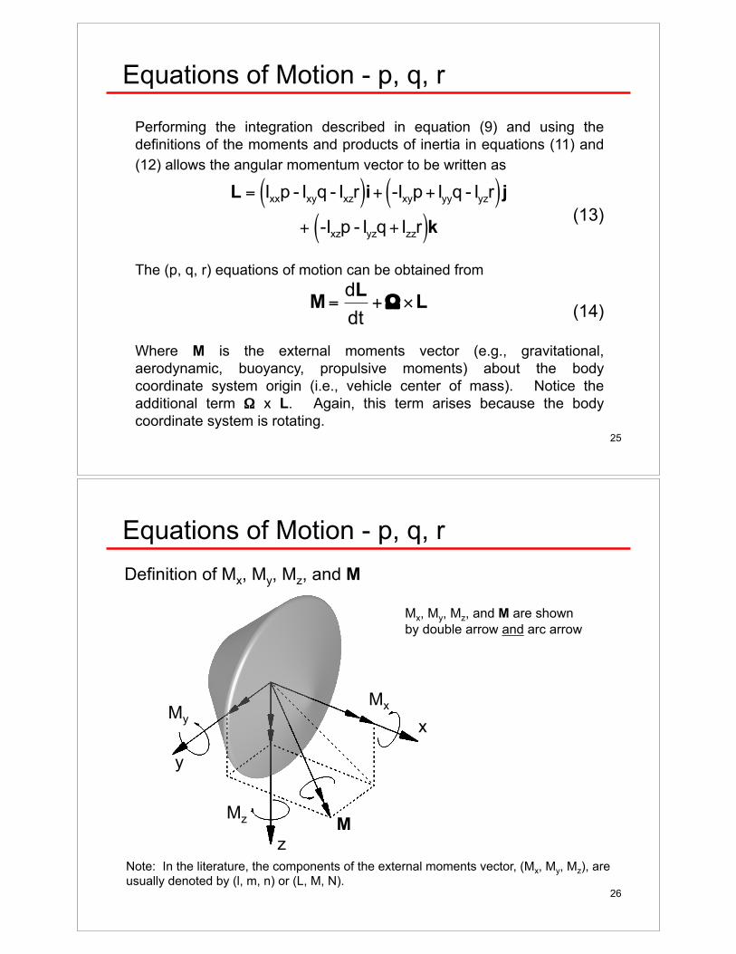
Equations of Motion - p, q, r
Performing the integration described in equation (9) and using the
definitions of the moments and products of inertia in equations (11) and
(12) allows the angular momentum vector to be written as
(13)
The (p, q, r) equations of motion can be obtained from
(14)
Where M is the external moments vector (e.g., gravitational,
aerodynamic, buoyancy, propulsive moments) about the body
coordinate system origin (i.e., vehicle center of mass). Notice the
additional term " x L. Again, this term arises because the body
coordinate system is rotating.
!
L = Ixxp - Ixyq - Ixzr( )i+ -Ixyp + Iyyq - Iyzr( ) j
+ -Ixzp - Iyzq + Izzr( )k
!
M =dL
dt+"#L
26
Equations of Motion - p, q, r
Note: In the literature, the components of the external moments vector, (Mx, My, Mz), are
usually denoted by (l, m, n) or (L, M, N).
Mx
Mz
My
M
x
z
y
Mx, My, Mz, and M are shown
by double arrow and arc arrow
Definition of Mx, My, Mz, and M
27
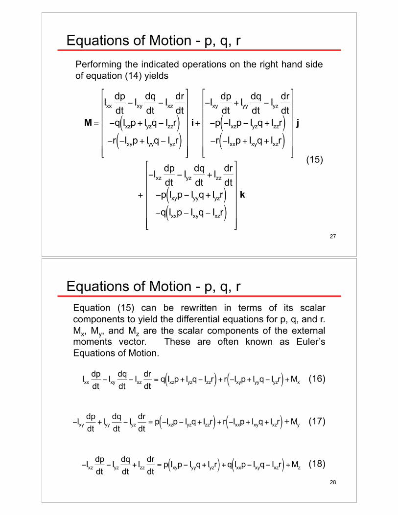
Equations of Motion - p, q, r
Performing the indicated operations on the right hand side
of equation (14) yields
(15)
!
M =
Ixx
dp
dt" Ixy
dq
dt" Ixz
dr
dt
"q Ixzp + Iyzq" Izzr( )"r "Ixyp + Iyyq" Iyzr( )
#
$
% % % % % %
&
'
( ( ( ( ( (
i+
"Ixy
dp
dt+ Iyy
dq
dt" Iyz
dr
dt
"p "Ixzp" Iyzq + Izzr( )"r "Ixxp + Ixyq + Ixzr( )
#
$
% % % % % %
&
'
( ( ( ( ( (
j
+
"Ixz
dp
dt" Iyz
dq
dt+ Izz
dr
dt
"p Ixyp" Iyyq + Iyzr( )"q Ixxp" Ixyq" Ixzr( )
#
$
% % % % % %
&
'
( ( ( ( ( (
k
28
Equations of Motion - p, q, r
Equation (15) can be rewritten in terms of its scalar
components to yield the differential equations for p, q, and r.
Mx, My, and Mz are the scalar components of the external moments vector. These are often known as Euler’s
Equations of Motion.
(16)
(17)
(18)
!
Ixx
dp
dt" Ixy
dq
dt" Ixz
dr
dt= q Ixzp + Iyzq" Izzr( ) + r "Ixyp + Iyyq" Iyzr( ) +Mx
!
"Ixy
dp
dt+ Iyy
dq
dt" Iyz
dr
dt= p "Ixzp" Iyzq + Izzr( ) + r "Ixxp + Ixyq + Ixzr( ) + My
!
"Ixz
dp
dt" Iyz
dq
dt+ Izz
dr
dt= p Ixyp" Iyyq + Iyzr( ) + q Ixxp" Ixyq" Ixzr( ) +Mz
29
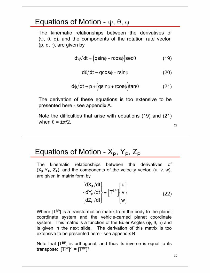
Equations of Motion - $, %, &
The kinematic relationships between the derivatives of
($, %, &), and the components of the rotation rate vector,
(p, q, r), are given by
(19)
(20)
(21)
The derivation of these equations is too extensive to be
presented here - see appendix A.
Note the difficulties that arise with equations (19) and (21)
when % = ±'/2.
!
d" dt = qsin# + rcos#( )sec$
!
d" dt = qcos# $ rsin#
!
d" dt = p + qsin" + rcos"( )tan#
30
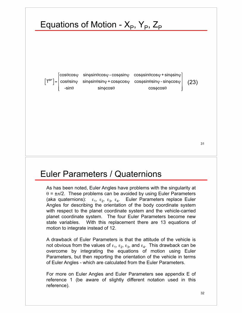
Equations of Motion - XP, YP, ZP
The kinematic relationships between the derivatives of
(XP,YP, ZP), and the components of the velocity vector, (u, v, w),
are given in matrix form by
(22)
Where [TBP] is a transformation matrix from the body to the planet
coordinate system and the vehicle-carried planet coordinate
system. This matrix is a function of the Euler Angles ($, %, &) and
is given in the next slide. The derivation of this matrix is too
extensive to be presented here - see appendix B.
Note that [TBP] is orthogonal, and thus its inverse is equal to its
transpose: [TBP]-1 = [TBP]T.
!
dXP
dt
dYP
dt
dZP
dt
"
# $
% $
&
' $
( $
= TBP[ ]
u
v
w
"
# $
% $
&
' $
( $
31
Equations of Motion - XP, YP, ZP
!
TBP[ ] =
cos"cos# sin$sin"cos# - cos$sin# cos$sin"cos#+ sin$sin#
cos"sin# sin$sin"sin#+ cos$cos# cos$sin"sin# - sin$cos#
-sin" sin$cos" cos$cos"
%
&
' ' '
(
)
* * *
(23)
32
Euler Parameters / Quaternions
As has been noted, Euler Angles have problems with the singularity at
% = ±'/2. These problems can be avoided by using Euler Parameters
(aka quaternions): (1, (2, (3, (4. Euler Parameters replace Euler
Angles for describing the orientation of the body coordinate system
with respect to the planet coordinate system and the vehicle-carried
planet coordinate system. The four Euler Parameters become new
state variables. With this replacement there are 13 equations of
motion to integrate instead of 12.
A drawback of Euler Parameters is that the attitude of the vehicle is
not obvious from the values of (1, (2, (3, and (4. This drawback can be
overcome by integrating the equations of motion using Euler
Parameters, but then reporting the orientation of the vehicle in terms
of Euler Angles - which are calculated from the Euler Parameters.
For more on Euler Angles and Euler Parameters see appendix E of
reference 1 (be aware of slightly different notation used in this
reference).
33
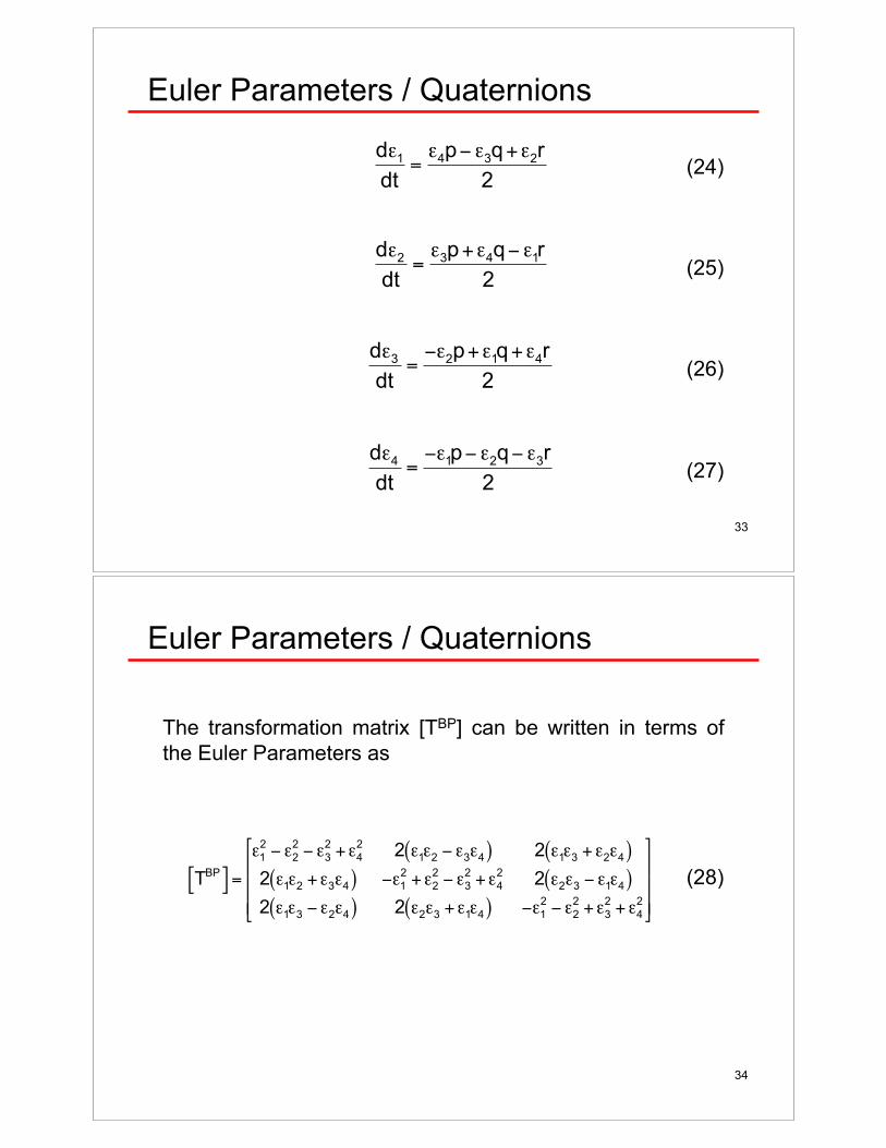
Euler Parameters / Quaternions
!
d"1
dt="4p# "3q+"2r
2
!
d"2
dt="3p+"4q# "1r
2
!
d"3
dt=#"2p+"1q+"4r
2
!
d"4
dt=#"1p# "2q# "3r
2
(24)
(25)
(26)
(27)
34
Euler Parameters / Quaternions
!
TBP[ ] =
"1
2 # "2
2 # "3
2 +"4
22 "
1"
2# "
3"
4( ) 2 "1"
3+ "
2"
4( )2 "
1"
2+"
3"
4( ) #"1
2 +"2
2 # "3
2 +"4
22 "
2"
3# "
1"
4( )2 "
1"
3# "
2"
4( ) 2 "2"
3+"
1"
4( ) #"1
2 # "2
2 +"3
2 + "4
2
$
%
& & &
'
(
) ) )
(28)
The transformation matrix [TBP] can be written in terms of
the Euler Parameters as
35
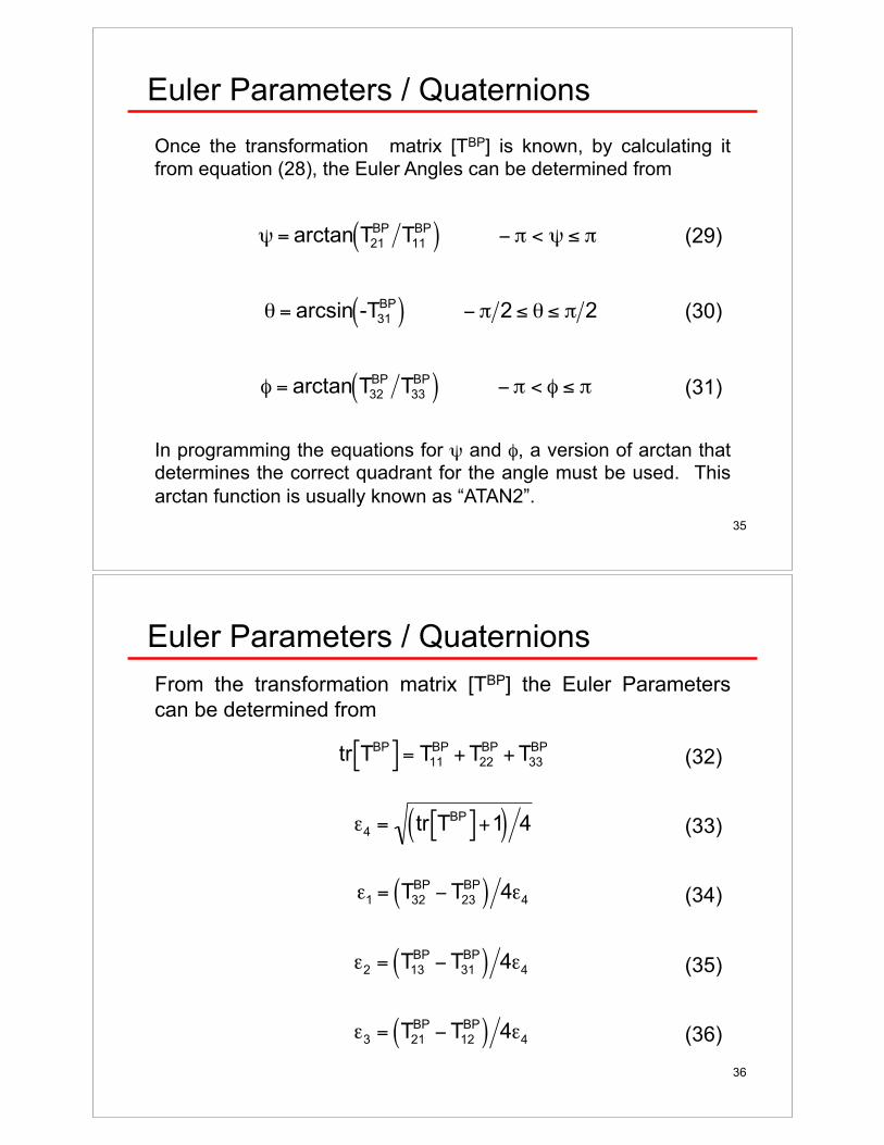
Euler Parameters / Quaternions
Once the transformation matrix [TBP] is known, by calculating it
from equation (28), the Euler Angles can be determined from
In programming the equations for $ and &, a version of arctan that determines the correct quadrant for the angle must be used. This
arctan function is usually known as “ATAN2”.
!
" = arctan T21
BPT
11
BP( ) # $ < " % $
!
" = arcsin -T31
BP( ) # $ 2 % " % $ 2
!
" = arctan T32
BPT
33
BP( ) # $ < " % $
(29)
(30)
(31)
36
Euler Parameters / Quaternions
From the transformation matrix [TBP] the Euler Parameters
can be determined from
!
tr TBP[ ] = T
11
BP + T22
BP + T33
BP
(32)
(33)
(34)
(35)
(36)
!
"4
= tr TBP[ ] +1( ) 4
!
"1
= T32
BP#T
23
BP( ) 4"4
!
"2
= T13
BP#T
31
BP( ) 4"4
!
"3
= T21
BP#T
12
BP( ) 4"4
37
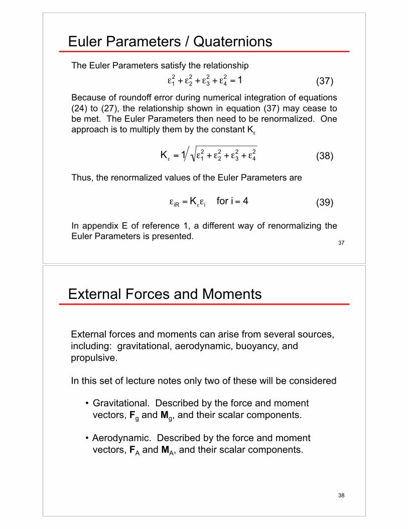
Euler Parameters / Quaternions
The Euler Parameters satisfy the relationship
Because of roundoff error during numerical integration of equations
(24) to (27), the relationship shown in equation (37) may cease to
be met. The Euler Parameters then need to be renormalized. One
approach is to multiply them by the constant K(
Thus, the renormalized values of the Euler Parameters are
In appendix E of reference 1, a different way of renormalizing the Euler Parameters is presented.
!
"1
2+ "
2
2+ "
3
2+ "
4
2= 1 (37)
(38)
(39)
!
K" = 1 "1
2+ "
2
2+ "
3
2+ "
4
2
!
"iR
= K""i for i = 4
38
External Forces and Moments
External forces and moments can arise from several sources,
including: gravitational, aerodynamic, buoyancy, and
propulsive.
In this set of lecture notes only two of these will be considered
• Gravitational. Described by the force and moment
vectors, Fg and Mg, and their scalar components.
• Aerodynamic. Described by the force and moment
vectors, FA and MA, and their scalar components.
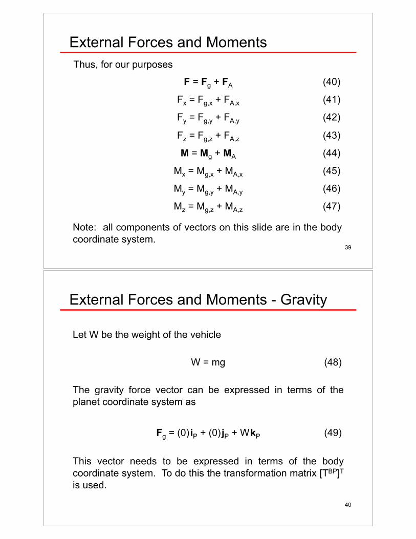
39
F = Fg + FA
Fx = Fg,x + FA,x
Fy = Fg,y + FA,y
Fz = Fg,z + FA,z
M = Mg + MA
Mx = Mg,x + MA,x
My = Mg,y + MA,y
Mz = Mg,z + MA,z
Note: all components of vectors on this slide are in the body
coordinate system.
(40)
(41)
(42)
(43)
(44)
(45)
(46)
(47)
External Forces and Moments
Thus, for our purposes
40
External Forces and Moments - Gravity
Let W be the weight of the vehicle
W = mg (48)
The gravity force vector can be expressed in terms of the
planet coordinate system as
Fg = (0) iP + (0) jP + W kP (49)
This vector needs to be expressed in terms of the body
coordinate system. To do this the transformation matrix [TBP]T
is used.
41
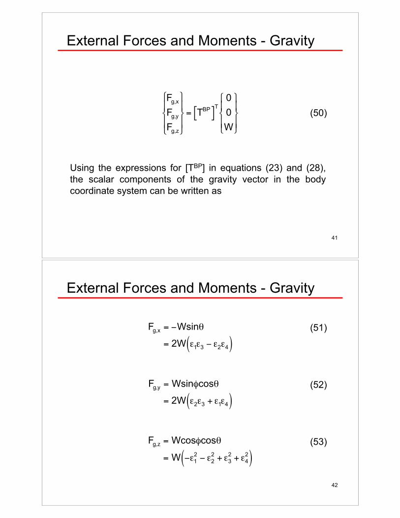
External Forces and Moments - Gravity
!
Fg,x
Fg,y
Fg,z
"
# $
% $
&
' $
( $
= TBP[ ]T
0
0
W
"
# $
% $
&
' $
( $
Using the expressions for [TBP] in equations (23) and (28),
the scalar components of the gravity vector in the body
coordinate system can be written as
(50)
42
External Forces and Moments - Gravity
!
Fg,x = "Wsin#
= 2W $1$3 " $2$4( )(51)
(52)
(53)
!
Fg,y = Wsin"cos#
= 2W $2$3 + $1$4( )
!
Fg,z = Wcos"cos#
= W $%1
2 $ %2
2 + %3
2 + %4
2( )
43
External Forces and Moments - Gravity
Notice that since we have defined the origin of the body
coordinate system to be at the center of mass of the vehicle,
the moment vector due to gravity, Mg, (and thus all its component) in the body coordinate system are zero.
Mg = 0 (54)
Mg,x = 0 (55)
Mg,y = 0 (56)
Mg,z = 0 (57)
44
External Forces and Moments - Aero
Modeling the aerodynamic forces and moments is difficult.
The end result is just that - a model.
In this set of lecture notes the aerodynamic forces and
moments are modeled as follows
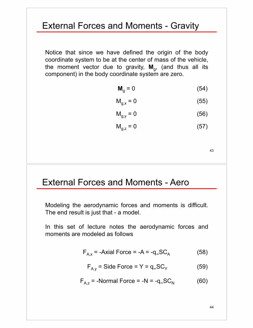
FA,x = -Axial Force = -A = -q!SCA (58)
FA,y = Side Force = Y = q!SCY (59)
FA,z = -Normal Force = -N = -q!SCN (60)
45
External Forces and Moments - Aero
A – axial force
Y – side force N – normal force
A, Y, and N, as
shown, are positive
x
N
A
z
Y
y
46
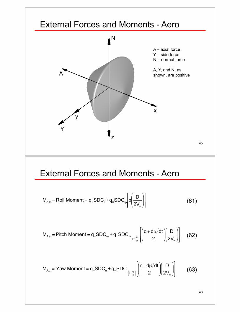
External Forces and Moments - Aero
(61)
(62)
(63)
!
MA,x = Roll Moment = q"SDCl + q"SDClpp
D
2V"
#
$ %
&
' (
)
* + +
,
- . .
!
MA,y = Pitch Moment = q"SDCm + q"SDCmq +
d#
dt
$
% &
'
( )
q + d# dt
2
$
% &
'
( )
D
2V"
$
% &
'
( )
*
+ , ,
-
. / /
!
MA,z = Yaw Moment = q"SDCn + q"SDCnr -
d#
dt
$
% &
'
( )
r * d# dt
2
$
% &
'
( )
D
2V"
$
% &
'
( )
+
, - -
.
/ 0 0
47
External Forces and Moments - Aero
Where,
(64) (airspeed)
(65)
(dynamic pressure)
Note that V! can be defined as shown in equation (64) because
we have assumed no wind, and thus the velocity components
(u, v, w) are the same as the airspeed components (u!, v
!, w
!). If
there is wind the velocity and airspeed components will not be the
same! The wind will need to be taken into account to determine
the airspeed components and the airspeed. Also, remember that
the atmospheric density, !, is a function of the altitude, h = -ZP.
!
V" = u2
+ v2
+ w2
!
q" = 1
2#V"
2
48
External Forces and Moments - Aero
Comments on Equations (58) to (63)
• The reference area for all aerodynamic coefficients is S.
• The reference length for all aerodynamic coefficients is D.
• The approach used here is to define the static aerodynamic coefficients
CA and CN in the body coordinate system as is usually done for entry
vehicles. In aircraft applications it is common to use the equivalent
static aerodynamic coefficients CL and CD (lift and drag, respectively).
The transformation between (CA, CN) and (CL, CD) is a simple one
involving the angle of attack, ). I leave it up to you to derive it.
• It is assumed here that the aerodynamic coefficients can only be
functions of the vehicle geometry, location of the vehicle center of
mass, the instantaneous value of the state variables and their
derivatives (which include the angle of attack, angle of sideslip, and
their derivatives), the Mach number, the Reynolds number, and the
Knudsen number as appropriate.
49
External Forces and Moments - Aero
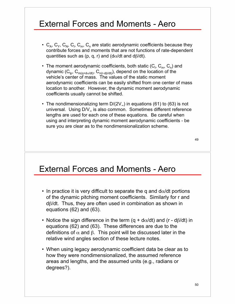
• CA, CY, CN, Cl, Cm, Cn are static aerodynamic coefficients because they
contribute forces and moments that are not functions of rate-dependent
quantities such as (p, q, r) and (d)/dt and d*/dt).
• The moment aerodynamic coefficients, both static (Cl, Cm, Cn) and
dynamic (Clp, Cm(q+d)/dt), Cn(r-d*/dt)), depend on the location of the
vehicle’s center of mass. The values of the static moment
aerodynamic coefficients can be easily shifted from one center of mass
location to another. However, the dynamic moment aerodynamic
coefficients usually cannot be shifted.
• The nondimensionalizing term D/(2V!) in equations (61) to (63) is not
universal. Using D/V! is also common. Sometimes different reference
lengths are used for each one of these equations. Be careful when
using and interpreting dynamic moment aerodynamic coefficients - be
sure you are clear as to the nondimensionalization scheme.
50
External Forces and Moments - Aero
• In practice it is very difficult to separate the q and d)/dt portions
of the dynamic pitching moment coefficients. Similarly for r and
d*/dt. Thus, they are often used in combination as shown in
equations (62) and (63).
• Notice the sign difference in the term (q + d)/dt) and (r - d*/dt) in
equations (62) and (63). These differences are due to the
definitions of ) and *. This point will be discussed later in the
relative wind angles section of these lecture notes.
• When using legacy aerodynamic coefficient data be clear as to
how they were nondimensionalized, the assumed reference
areas and lengths, and the assumed units (e.g., radians or
degrees?).
51
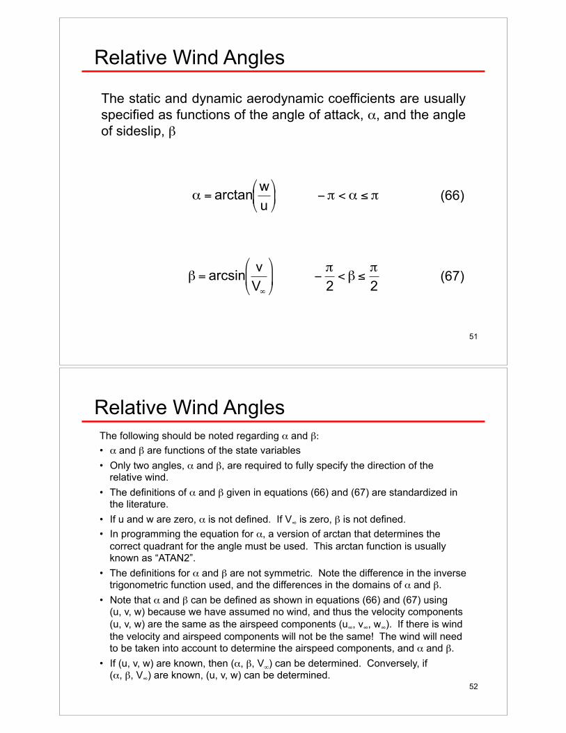
The static and dynamic aerodynamic coefficients are usually
specified as functions of the angle of attack, ), and the angle
of sideslip, *#
(66)
(67)
Relative Wind Angles
!
" = arctanw
u
#
$ %
&
' ( )* < " + *
!
" = arcsinv
V#
$
% &
'
( ) *
+
2< " ,
+
2
52
The following should be noted regarding ) and *:
• ) and * are functions of the state variables
• Only two angles, ) and *, are required to fully specify the direction of the relative wind.
• The definitions of ) and * given in equations (66) and (67) are standardized in the literature.
• If u and w are zero, ) is not defined. If V! is zero, * is not defined.
• In programming the equation for ), a version of arctan that determines the
correct quadrant for the angle must be used. This arctan function is usually known as “ATAN2”.
• The definitions for ) and * are not symmetric. Note the difference in the inverse trigonometric function used, and the differences in the domains of ) and *.
• Note that ) and * can be defined as shown in equations (66) and (67) using (u, v, w) because we have assumed no wind, and thus the velocity components
(u, v, w) are the same as the airspeed components (u!, v
!, w
!). If there is wind
the velocity and airspeed components will not be the same! The wind will need to be taken into account to determine the airspeed components, and ) and *.
• If (u, v, w) are known, then (), *, V!) can be determined. Conversely, if
(), *, V!) are known, (u, v, w) can be determined.
Relative Wind Angles
53
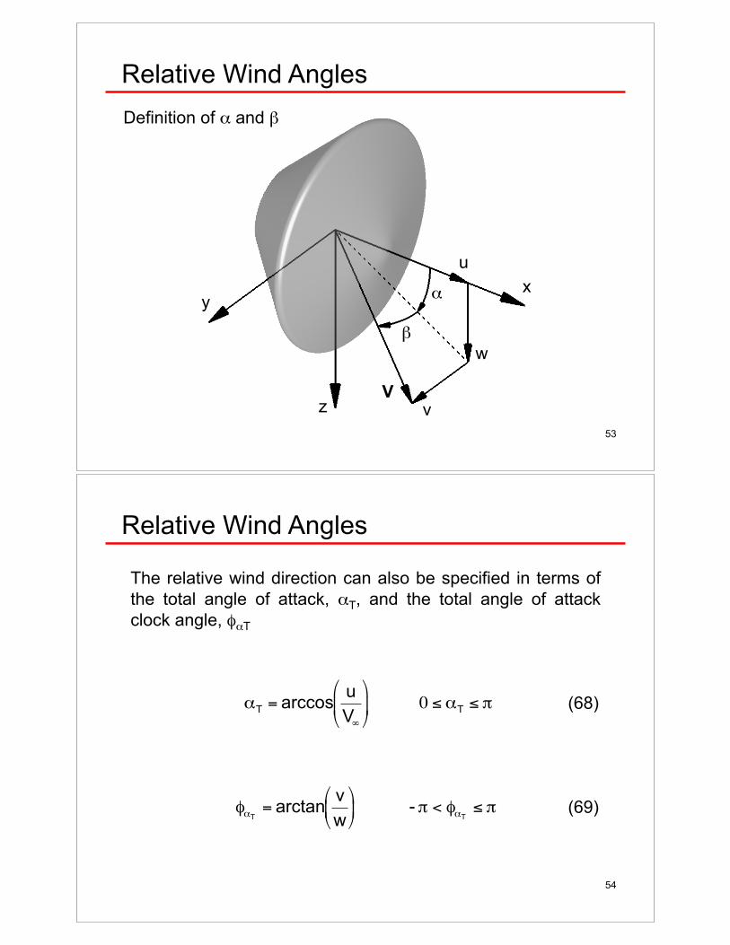
Relative Wind Angles
Definition of ) and *#
x y
z
)#
*#
u
v
w
V
54
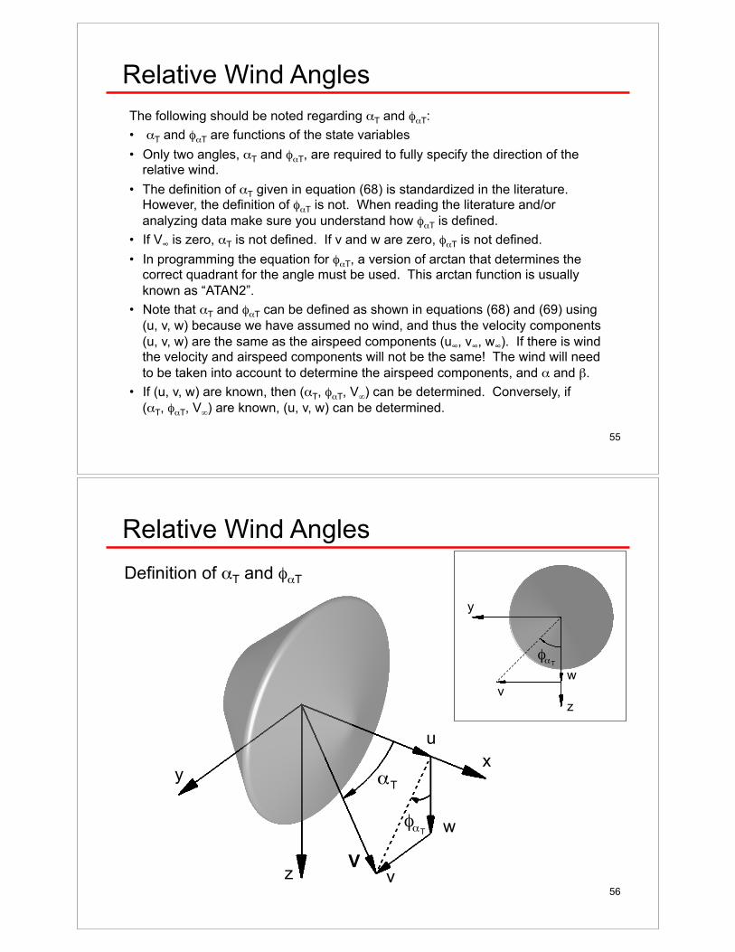
The relative wind direction can also be specified in terms of
the total angle of attack, )T, and the total angle of attack
clock angle, &)T#
(68)
(69)
Relative Wind Angles
!
"T
= arccosu
V#
$
% &
'
( ) 0 * "T
* +
!
"#T
= arctanv
w
$
% &
'
( ) - * < "#T
+ *
55
The following should be noted regarding )T and &)T:
• )T and &)T are functions of the state variables
• Only two angles, )T and &)T, are required to fully specify the direction of the relative wind.
• The definition of )T given in equation (68) is standardized in the literature. However, the definition of &)T is not. When reading the literature and/or
analyzing data make sure you understand how &)T is defined.
• If V! is zero, )T is not defined. If v and w are zero, &)T is not defined.
• In programming the equation for &)T, a version of arctan that determines the correct quadrant for the angle must be used. This arctan function is usually
known as “ATAN2”.
• Note that )T and &)T can be defined as shown in equations (68) and (69) using
(u, v, w) because we have assumed no wind, and thus the velocity components
(u, v, w) are the same as the airspeed components (u!, v
!, w
!). If there is wind
the velocity and airspeed components will not be the same! The wind will need
to be taken into account to determine the airspeed components, and ) and *.
• If (u, v, w) are known, then ()T, &)T, V!) can be determined. Conversely, if
()T, &)T, V!) are known, (u, v, w) can be determined.
Relative Wind Angles
56
Relative Wind Angles
Definition of )T and &)T#
x y
z
u
v
w
V
!
"T
!
"#T
!
"#T
z
y
w
v
57
Relative Wind Angles
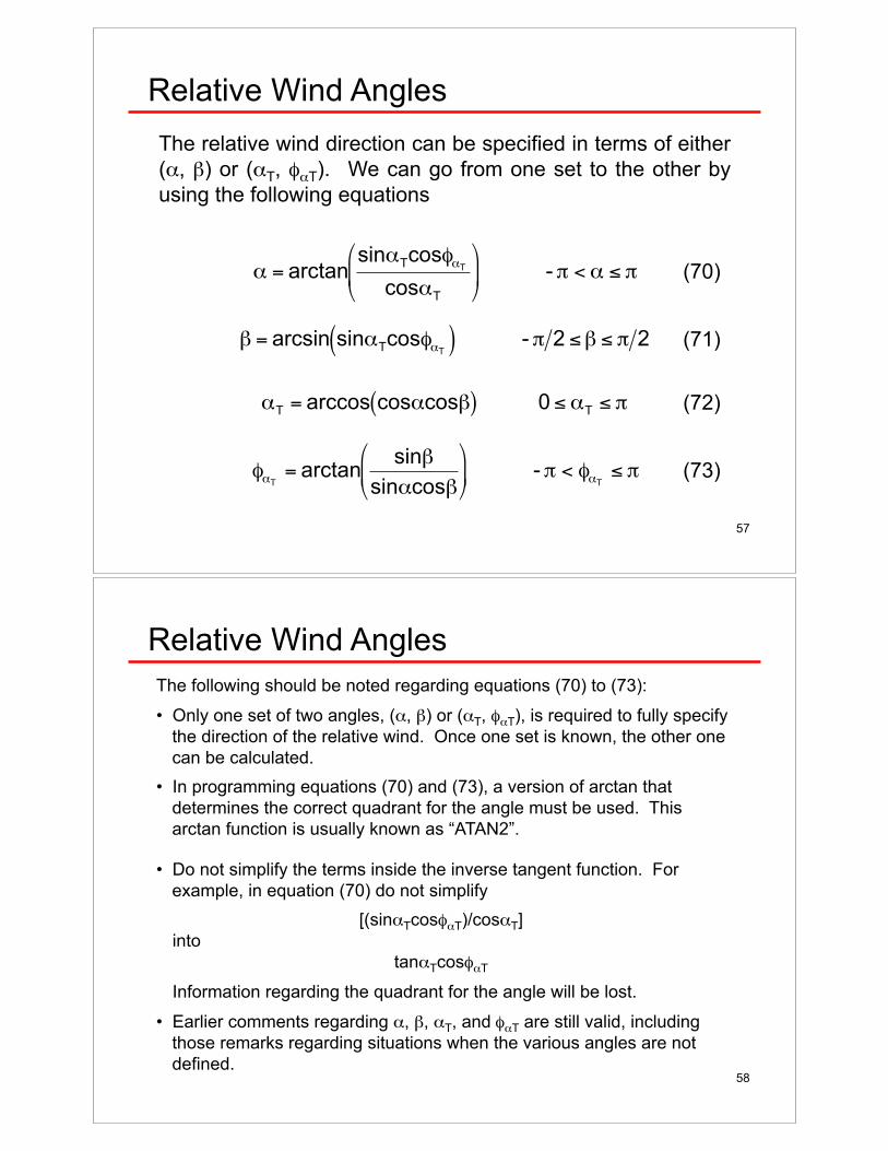
The relative wind direction can be specified in terms of either
(), *) or ()T, &)T). We can go from one set to the other by
using the following equations
!
" = arctansin"
Tcos#"T
cos"T
$
% &
'
( ) - * < " + *
!
"#T
= arctansin$
sin#cos$
%
& '
(
) * - + < "#T
, +
!
" = arcsin sin#Tcos$#T
( ) - % 2 &" & % 2
!
"T
= arccos cos"cos#( ) 0 $ "T$ %
(70)
(71)
(72)
(73)
58
The following should be noted regarding equations (70) to (73):
• Only one set of two angles, (), *) or ()T, &)T), is required to fully specify
the direction of the relative wind. Once one set is known, the other one
can be calculated.
• In programming equations (70) and (73), a version of arctan that
determines the correct quadrant for the angle must be used. This
arctan function is usually known as “ATAN2”.
• Do not simplify the terms inside the inverse tangent function. For
example, in equation (70) do not simplify
[(sin)Tcos&)T)/cos)T]
into
tan)Tcos&)T
Information regarding the quadrant for the angle will be lost.
• Earlier comments regarding ), *, )T, and &)T are still valid, including
those remarks regarding situations when the various angles are not
defined.
Relative Wind Angles
59
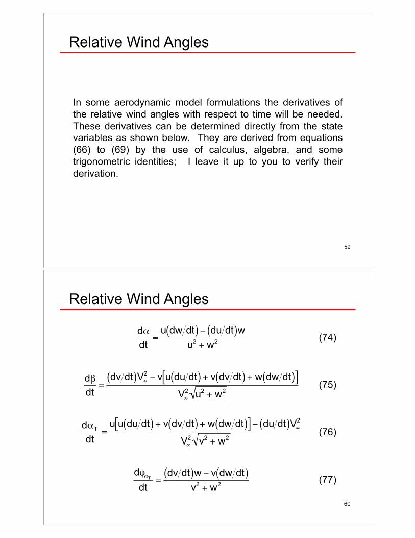
In some aerodynamic model formulations the derivatives of
the relative wind angles with respect to time will be needed.
These derivatives can be determined directly from the state variables as shown below. They are derived from equations
(66) to (69) by the use of calculus, algebra, and some
trigonometric identities; I leave it up to you to verify their
derivation.
Relative Wind Angles
60
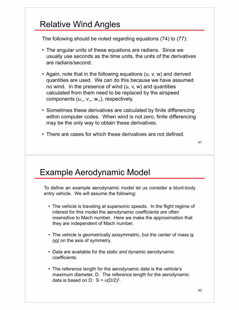
Relative Wind Angles
(74)
(75)
(76)
(77)
!
d"
dt=
u dw dt( ) # du dt( )wu
2 + w2
!
d"
dt=
dv dt( )V#
2 $ v u du dt( ) + v dv dt( ) + w dw dt( )[ ]V#
2u
2 + w2
!
d"T
dt=
u u du dt( ) + v dv dt( ) + w dw dt( )[ ] # du dt( )V$
2
V$
2v
2 + w2
!
d"#T
dt=
dv dt( )w $ v dw dt( )v
2 + w2
61
Relative Wind Angles
The following should be noted regarding equations (74) to (77):
• The angular units of these equations are radians. Since we
usually use seconds as the time units, the units of the derivatives
are radians/second.
• Again, note that in the following equations (u, v, w) and derived
quantities are used. We can do this because we have assumed
no wind. In the presence of wind (u, v, w) and quantities
calculated from them need to be replaced by the airspeed
components (u!, v
!, w
!), respectively.
• Sometimes these derivatives are calculated by finite differencing
within computer codes. When wind is not zero, finite differencing
may be the only way to obtain these derivatives.
• There are cases for which these derivatives are not defined.
62
Example Aerodynamic Model
To define an example aerodynamic model let us consider a blunt-body
entry vehicle. We will assume the following:
• The vehicle is traveling at supersonic speeds. In the flight regime of
interest for this model the aerodynamic coefficients are often
insensitive to Mach number. Here we make the approximation that
they are independent of Mach number.
• The vehicle is geometrically axisymmetric, but the center of mass is
not on the axis of symmetry.
• Data are available for the static and dynamic aerodynamic
coefficients.
• The reference length for the aerodynamic data is the vehicle’s
maximum diameter, D. The reference length for the aerodynamic
data is based on D: S = '(D/2)2.
63
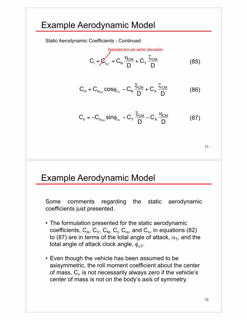
Example Aerodynamic Model
Static Aerodynamic Coefficients
• The model coordinate system has axes (+, ,, -). The + axis is
coincident with the axis of symmetry of the entry vehicle.
• The (+, ,, -) axes are parallel to the body coordinate system axes
(x, y, z), respectively.
• The center of mass of the vehicle (i.e., the origin of the body
coordinate system) is located at (+CM, ,CM, -CM) in the model
coordinate system. The vector from the origin of the model coordinate
system to the origin of the body coordinate system is rCM.
• Because the vehicle is axisymmetric, the static aerodynamic
coefficients are given as functions of the total angle of attack, )T, only,
in terms of axisymmetric aerodynamic coefficients:
CAT()T), CNT()T), ClOT()T), CmOT()T)
64
Example Aerodynamic Model
*Given our assumption of no wind, the velocity vector, V, is the same as the
airspeed vector, V!. When there is wind this will not generally be the case. It is
the airspeed velocity vector that is needed to determine the relative wind angles,
airspeed, and dynamic pressure.
Static Aerodynamic Coefficients - Continued
• Because the vehicle is axisymmetric, the aerodynamic forces vector
components specified by CAT and CNT lie in the plane specified by the
+ axis and the velocity vector V.*
• Because the vehicle is axisymmetric, the aerodynamic moment vector
component specified by CmOT()T) is perpendicular to the plane
specified by the + axis and the velocity vector V.* Also note that this
moment is about the origin, O, of the (+, ,, -) coordinate system, not
about the origin of the body coordinate system (x, y, z) which is
centered on the vehicle’s center of mass.
• Because the vehicle is axisymmetric, the roll moment coefficient about
the + axis, ClOT, is zero.
65
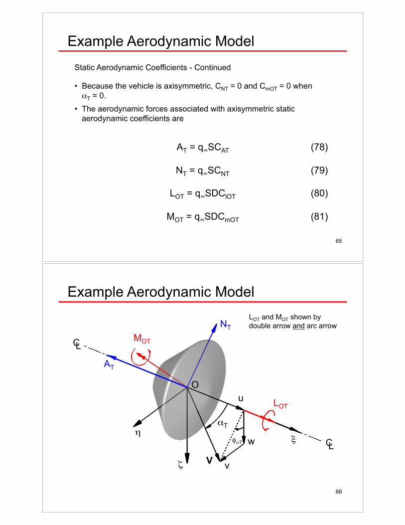
Example Aerodynamic Model
Static Aerodynamic Coefficients - Continued
• Because the vehicle is axisymmetric, CNT = 0 and CmOT = 0 when
#)T = 0.
• The aerodynamic forces associated with axisymmetric static
aerodynamic coefficients are
AT = q!SCAT
NT = q!SCNT
LOT = q!SDClOT
MOT = q!SDCmOT
(78)
(79)
(80)
(81)
66
Example Aerodynamic Model
NT
AT
MOT
LOT
+#,#
-#V
v
w
u
)T
&)T C L
C L
LOT and MOT shown by
double arrow and arc arrow
O
67
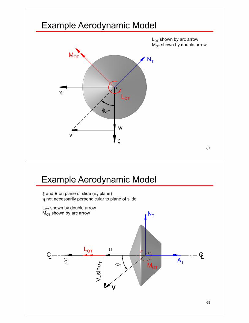
Example Aerodynamic Model
NT
MOT
LOT
,#
-#
v
w
&)T
LOT shown by arc arrow
MOT shown by double arrow
O
68
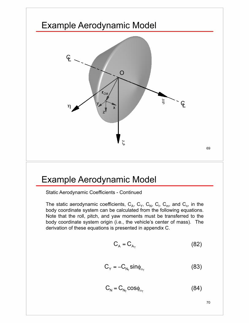
Example Aerodynamic Model
NT
MOT
LOT
+#
V
u
)T
+ and V on plane of slide ()T plane)
, not necessarily perpendicular to plane of slide
LOT shown by double arrow MOT shown by arc arrow
O
AT
V!sin)
T
C L C L
69
Example Aerodynamic Model
C L
C L +#
,#
-#
x y
z
rCM
O
70
Example Aerodynamic Model
Static Aerodynamic Coefficients - Continued
The static aerodynamic coefficients, CA, CY, CN, Cl, Cm, and Cn, in the
body coordinate system can be calculated from the following equations.
Note that the roll, pitch, and yaw moments must be transferred to the
body coordinate system origin (i.e., the vehicle’s center of mass). The
derivation of these equations is presented in appendix C.
!
CA
= CAT
(82)
(83)
(84)
!
CY
= "CNT
sin#$T
!
CN
= CNT
cos"#T
71
Example Aerodynamic Model
Static Aerodynamic Coefficients - Continued
!
Cl= C
lOT
+ CN
"CM
D+ C
Y
#CM
D(85)
(86)
(87)
!
Cm
= CmOT
cos"#T
$CN
%CM
D+ C
A
&CM
D
!
Cn
= "CmOT
sin#$T
"CY
%CM
D"C
A
&CM
D
Assumed zero per earlier discussion
72
Example Aerodynamic Model
Some comments regarding the static aerodynamic
coefficients just presented.
• The formulation presented for the static aerodynamic
coefficients, CA, CY, CN, Cl, Cm, and Cn, in equations (82)
to (87) are in terms of the total angle of attack, )T, and the total angle of attack clock angle, &)T.
• Even though the vehicle has been assumed to be
axisymmetric, the roll moment coefficient about the center
of mass, Cl, is not necessarily always zero if the vehicle’s center of mass is not on the body’s axis of symmetry.
73
Example Aerodynamic Model
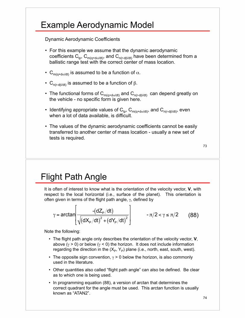
Dynamic Aerodynamic Coefficients
• For this example we assume that the dynamic aerodynamic
coefficients Clp, Cm(q+d)/dt), and Cn(r-d*/dt) have been determined from a
ballistic range test with the correct center of mass location.
• Cm(q+d)/dt) is assumed to be a function of ).
• Cn(r-d*/dt) is assumed to be a function of *.
• The functional forms of Cm(q+d)/dt) and Cn(r-d*/dt) can depend greatly on
the vehicle - no specific form is given here.
• Identifying appropriate values of Clp, Cm(q+d)/dt), and Cn(r-d*/dt), even
when a lot of data available, is difficult.
• The values of the dynamic aerodynamic coefficients cannot be easily
transferred to another center of mass location - usually a new set of
tests is required.
74
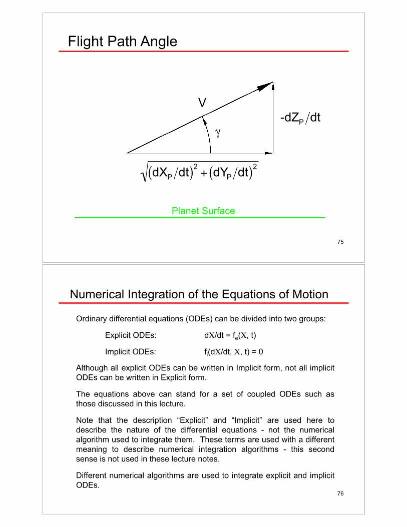
Flight Path Angle
It is often of interest to know what is the orientation of the velocity vector, V, with
respect to the local horizontal (i.e., surface of the planet). This orientation is often given in terms of the flight path angle, ., defined by
!
" = arctan- dZ
Pdt( )
dXP
dt( )2
+ dYP
dt( )2
#
$
% %
&
'
( ( - ) 2 < " * ) 2 (88)
Note the following:
• The flight path angle only describes the orientation of the velocity vector, V,
above (. > 0) or below (. < 0) the horizon. It does not include information regarding the direction in the (XP, YP) plane (i.e., north, east, south, west).
• The opposite sign convention, . > 0 below the horizon, is also commonly used in the literature.
• Other quantities also called “flight path angle” can also be defined. Be clear
as to which one is being used.
• In programming equation (88), a version of arctan that determines the
correct quadrant for the angle must be used. This arctan function is usually known as “ATAN2”.
75
Flight Path Angle
Planet Surface
!
dXP
dt( )2
+ dYP
dt( )2
!
-dZP
dt
!
V
!
"
76
Numerical Integration of the Equations of Motion
Ordinary differential equations (ODEs) can be divided into two groups:
Explicit ODEs: d//dt = fe(/, t)
Implicit ODEs: fi(d//dt, /, t) = 0
Although all explicit ODEs can be written in Implicit form, not all implicit
ODEs can be written in Explicit form.
The equations above can stand for a set of coupled ODEs such as
those discussed in this lecture.
Note that the description “Explicit” and “Implicit” are used here to
describe the nature of the differential equations - not the numerical
algorithm used to integrate them. These terms are used with a different
meaning to describe numerical integration algorithms - this second
sense is not used in these lecture notes.
Different numerical algorithms are used to integrate explicit and implicit
ODEs.
77
Numerical Integration of the Equations of Motion
For the types of flight mechanics problems discussed in this lecture…
Case 1
IF the external force and moment vectors depend only on the state
variables, and do not depend on the time derivatives of the state
variables, it is possible to write the equations of motion ODEs in explicit
form.
Case 2
IF the external force and moment vectors depend on the state variables,
and are linearly dependent on the time derivatives of the state variables,
it is possible to write the equation of motion ODEs in explicit form.
Case 3
IF the external force and moment vectors are nonlinearly dependent on
the time derivatives of the state variables, it may not be possible to write
the equations of motion ODEs in explicit form.
78
Numerical Integration of the Equations of Motion
Note the following:
• In this set of lecture notes we are only considering gravity and
aerodynamic forces and moments.
• The gravity force and moment vectors in equations (49) to (57) are
only dependent on the state variables, they do not include any time
derivatives of the state variables.
• The model described by equations (58) to (63) for the aerodynamic
force and moment vectors depend on the state variables, and linearly
on the time derivatives of the state variables through the terms d)/dt
and d*/dt in equations (62) and (63).
If we then assume that all the aerodynamic coefficients (static and
dynamic) are only functions of the state variables, and not on the time
derivatives of the state variables, then the equations of motion, including
the force and moment vectors as modeled here, fall under Case 2 in the
previous slide.
79
Numerical Integration of the Equations of Motion
Numerical Integration Algorithms
The most common numerical integration algorithms require that
the ODEs be written in explicit form
d//dt = fe(/, t)
Runge-Kutta methods are common for solving explicit ODEs.
The solver “ode45” in MATLAB uses this method.
More difficult to find are numerical integration algorithms for
ODEs written in implicit form
fi(d//dt, /, t) = 0
The solver “ode15i” in MATLAB can integrate implicit ODEs.
80
Numerical Integration of the Equations of Motion
Where am going with all this?
If you are writing your own code to solve flight mechanics problems as posed here, you will need to decide in which form you are going to, or can,
write the ODEs. Then, you will have to choose an appropriate numerical
integration algorithm.
You can always write the ODEs in implicit form, and use a numerical integration algorithm intended for use with implicit ODEs.
Sometimes additional approximations are made. Specifically, the equations
of motion ODEs will be written in “pseudo-explicit” form, with the external
force and moment vectors on the right hand side of the equations, even though these vectors may depend on time derivatives of the state variables.
A numerical integration algorithm for explicit ODEs will be used, and time
derivatives of the state variables in the right hand side of the equations will
be determined by finite differencing. Note that doing this adds an additional
level of approximation in the numerical integration of the ODEs - you will have to decide whether this approximation yields acceptable results.
81
Numerical Integration of the Equations of Motion
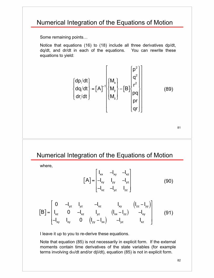
Some remaining points…
Notice that equations (16) to (18) include all three derivatives dp/dt,
dq/dt, and dr/dt in each of the equations. You can rewrite these
equations to yield:
!
dp dt
dq dt
dr dt
"
# $
% $
&
' $
( $
= A[ ])1
Mx
My
Mz
"
# $
% $
&
' $
( $ ) B[ ]
p2
q2
r2
pq
pr
qr
"
#
$ $ $
%
$ $ $
&
'
$ $ $
(
$ $ $
*
+
, , , , , , ,
-
.
/ / / / / / /
(89)
82
Numerical Integration of the Equations of Motion
where,
!
A[ ] =
Ixx "Ixy "Ixz
"Ixy Iyy "Iyz
"Ixz "Iyz Izz
#
$
% % %
&
'
( ( (
(90)
!
B[ ] =
0 "Iyz Iyz "Ixz Ixy Izz " Iyy( )Ixz 0 "Ixz Iyz Ixx " Izz( ) "Ixy
"Ixy Ixy 0 Iyy " Ixx( ) "Iyz Ixz
#
$
% % %
&
'
( ( (
(91)
I leave it up to you to re-derive these equations.
Note that equation (85) is not necessarily in explicit form. If the external
moments contain time derivatives of the state variables (for example
terms involving d)/dt and/or d*/dt), equation (85) is not in explicit form.
83
Numerical Integration of the Equations of Motion
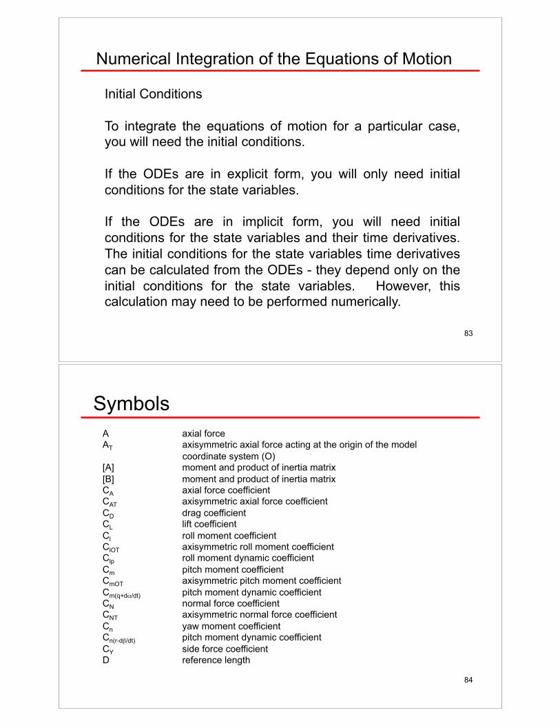
Initial Conditions
To integrate the equations of motion for a particular case, you will need the initial conditions.
If the ODEs are in explicit form, you will only need initial
conditions for the state variables.
If the ODEs are in implicit form, you will need initial
conditions for the state variables and their time derivatives.
The initial conditions for the state variables time derivatives
can be calculated from the ODEs - they depend only on the
initial conditions for the state variables. However, this calculation may need to be performed numerically.
84
Symbols
A axial force
AT axisymmetric axial force acting at the origin of the model
coordinate system (O)
[A] moment and product of inertia matrix
[B] moment and product of inertia matrix
CA axial force coefficient
CAT axisymmetric axial force coefficient
CD drag coefficient
CL lift coefficient
Cl roll moment coefficient
ClOT axisymmetric roll moment coefficient
Clp roll moment dynamic coefficient
Cm pitch moment coefficient
CmOT axisymmetric pitch moment coefficient
Cm(q+d)/dt) pitch moment dynamic coefficient
CN normal force coefficient
CNT axisymmetric normal force coefficient
Cn yaw moment coefficient
Cn(r-d*/dt) pitch moment dynamic coefficient
CY side force coefficient
D reference length
85
Symbols
F external forces vector
FA aerodynamic force vector
FA,x, FA,y, FA,z components of the aerodynamic force vector, FA, in the body
coordinate system
Fg gravitational force vector
Fg,x, Fg,y, Fg,z components of the gravitational force vector, Fg, in the body
coordinate system
Fx, Fy, Fz components of the external forces vector, F, in the body
coordinate system
fe, fi functions
g acceleration of gravity
h altitude
Ixx, Iyy, Izz moments of inertia about the vehicle’s center of mass
Ixy, Ixz, Iyz products of inertia about the vehicle’s center of mass
i, j, k unit vectors for the body coordinate system
iP, jP, kP unit vectors for the planet coordinate system
iV, jV, kV unit vectors for the vehicle-carried planet coordinate system
K( renormalizing factor for the Euler Parameters
L angular momentum vector
LOT axisymmetric roll moment acting at the origin of the model
coordinate system
86
Symbols
M external moments vector about the body coordinate system origin
(i.e., vehicle center of mass)
MA aerodynamic moment vector about the body coordinate system
origin (i.e., vehicle center of mass)
MA,x, MA,y, MA,z components of the aerodynamic moment vector, MA, in the body
coordinate system
Mg gravitational moment vector about the body coordinate system
origin (i.e., vehicle center of mass) – zero in the present
discussion
Mg,x, Mg,y, Mg,z components of the aerodynamic moment vector, Mg, in the body
coordinate system – zero in the present discussion
MOT axisymmetric pitch moment acting at the origin of the model
coordinate system (O)
Mx, My, Mz components of the external moments vector, M, in the body
coordinate system
m vehicle mass
N normal force
NT axisymmetric normal force acting at the origin of the model
coordinate system (O)
p linear momentum vector
p, q, r components of the vehicle rotation rate vector, ", in the body
coordinate system
87
Symbols
q!
dynamic pressure
rCM vector from the origin of the model coordinate system (O) to the
origin of the body coordinate system (center of mass)
rm position vector of an infinitesimal mass element dm
S reference area
[TBP] rotation matrix from the body to the planet coordinate system and
the vehicle-carried planet coordinate system
element i, j = 1,2,3 of the matrix [TBP]
t time
u, v, w components of the vehicle center of mass
velocity vector, V, in the body coordinate system
u!, v
!, w
! components of the vehicle center of mass airspeed vector, V
!, in
the body coordinate system; same as (u, v, w) when there is no
wind
V velocity vector of the vehicle center of mass; same as V! when
there is no wind
V!
airspeed vector of the vehicle center of mass; same as V when
there is no wind
V!
airspeed
W vehicle weight
XP, YP, ZP planet coordinate system axes
88
Symbols
XV, YV, ZV vehicle-carried planet coordinate system axes
x, y, z body coordinate system axes
xm, ym, zm components of the position vector, rm, in the body coordinate
system
Y side force
) angle of attack
)T total angle of attack
*! angle of sideslip
. flight path angle
(1, (2, (3, (4 Euler Parameter
(1R, (2R, (3R, (4R renormalized Euler Parameter#
%! elevation (pitch) Euler Angle
+, ,, - model axes
+CM, ,CM, -CM location of the vehicle’s center of mass in the model axes
! atmospheric density
&! bank (roll) Euler Angle
&)T total angle of attack clock angle
/ generic state variable#
$ azimuth (yaw) Euler Angle
" vehicle rotation rate vector
89
References and Bibliography References
1) Anon.: Recommended Practice for Atmospheric and Space Flight Vehicle Systems, American
National Standard, ANSI/AIAA R-004-1992, AIAA, Washington, DC, 1992.
Bibliography
B1) Minkler, G. and Minkler, J.: Aerospace Coordinate Systems and Transformations, Magellan Book
Co., , Baltimore, MD, 1990.
B2) Kuipers, J. B.: Quaternions and Rotation Sequences - A Primer with Applications to Orbits,
Aerospace, and Virtual Reality, Princeton University Press, Princeton, NJ, 1999.
B3) Etkin, B.: Dynamics of Flight, Stability and Control, John Wiley & Sons, Inc., New York, NY, 1959.
B4) Etkin, B.: Dynamics of Atmospheric Flight, Dover Publications, Inc., Mineola, NY, 1972. (Updated
version of B3 above, available in paperback Dover edition.)
B5) Tewari, A.: Atmospheric and Space Flight Dynamics, Modeling and Simulation with MATLAB® and
Simulink®, Birkhäuser, Boston, MA, 2007.
B6) Gallais, P.: Atmospheric Re-Entry Vehicle Mechanics, Springer-Verlag, Berlin, Germany, 2007.
B7) Hirschel, E. H. and Weiland, C.: Selected Aerothermodynamic Design Problems of Hypersonic
Flight Vehicles, Springer-Verlag, Berlin, Germany, 2009.
B8) Zipfel, P. H.: Modeling and Simulation of Aerospace Vehicle Dynamics, Second Edition,
AIAA, Reston, VA, 2007.
B9) Wright, J.: A Compilation of Aerodynamic Nomenclature and Axes Systems, NOLR 1241, United
States Naval Ordnance Laboratory, White Oak, MD, 1962.
90
Acknowledgements
Mark Schoenenberger of NASA Langley Research Center
and Richard Powell of Analytical Mechanics Associates
provided numerous comments that were helpful in creating these lecture notes. Their help is gratefully acknowledged.


