
U. S. ARMY AVIATION MATERIEL LABORATORIES … · Kaman Electronics Systems Division September 1966...
208
p USAAVLABS TECHNICAL REPORT 66-71 APPLICATION OF FLUIDICS TO AUTOMATIC FLIGHT CONTROL By E. M. Dexter S. D. Wills C. V. DiCamillo Bowles Engineering Corporation L. A. Kaufman C. Van Dusen Kaman Electronics Systems Division September 1966 U. S. ARMY AVIATION MATERIEL LABORATORIES FORT EOSTIS, VIRGINIA CONTRACT DA 44-177-AMC-202(T) BOWLES ENGINEERING CORPORATION SILVER SPRING, MARYLAND Distribution of this document is unlimited 0/n- D D C ,-pfprprin Hf? JM1 2 7 1957 _ C r
Transcript of U. S. ARMY AVIATION MATERIEL LABORATORIES … · Kaman Electronics Systems Division September 1966...
p
USAAVLABS TECHNICAL REPORT 66-71
APPLICATION OF FLUIDICS TO AUTOMATIC FLIGHT CONTROL
By
E. M. Dexter S. D. Wills
C. V. DiCamillo
Bowles Engineering Corporation
L. A. Kaufman C. Van Dusen
Kaman Electronics Systems Division
September 1966
U. S. ARMY AVIATION MATERIEL LABORATORIES FORT EOSTIS, VIRGINIA
CONTRACT DA 44-177-AMC-202(T)
BOWLES ENGINEERING CORPORATION
SILVER SPRING, MARYLAND
Distribution of this document is unlimited
0/n-
D D C ,-pfprprin Hf?
JM1 2 7 1957 _
C
r

I -I
Disclaimers
The findings in this report are not to be construed as an official Depart- ment of the Army position unless so designated by other authorized documents.
When Government drawings, specifications, or other data are used for any purpose other than in connection with a deünitely related Government procurement operation, the United States Government thereby incurs no responsibility nor any obligation whatsoever; and the fact that the Govern- ment may have formulated, furnished, or in any way supplied the said drawings, specifications, or other data is not to be regarded by impli- cation or otherwise as in any manner licensing the holder or any other person or corporation, or conveying any rights or permission, to manu- facture, use, or sell any patented invention that may in any way be related thereto.
Trade names cited in this report do not constitute an official endorse- ment or approval of the use of such commercial hardware or software.
Disposition Instructions
Destroy this report when no longer needed. Do not return it to originator.
CFSTI W':|Tt SECTION
HOC BUFF SECTIflH r
UNANNOUNCED n
Jl'SriMCOIOfl
Di'fHBtnCu.AYHIUBlLITY CODEi
BIST. , AVAIL, sa. or SfLCIAL
/ 1

DEPARTMENT OF THE ARMY U. S. ARMY AVIATION MATERIEL LADORATORIES
FORT EUSTIS. VIRGINIA 23604
This report has been reviewed by the U. S. Army
Aviation Materiel Laboratories and is considered
to be technically sound. The report is published
for the exchange of information and the stimulation
of ideas.

Ta«k 1P121401A14186 Coatracr DA 44-177-AMC-202 (T) USAAVLAES Technical Report 66-71
September 1966
APPLICATION OF FLUIDICS TO AUTOMATIC FLIGHT CONTROL
by
E. M. Dexter S. D. Wills
C. V. DiCamillo Bowles Engineering Corporation
L. A. Kaufman C. Van Dusen
Kaman Electronics Systems Division
Prepared by
Bowles Engineering Corporation Silver Spring, Maryland
For
U.S. Army Aviation Materiel Laboratories Fort Eustis, Virginia
Distribution of this document is unlimited

BLANK PAGE
.'•i

SUMMARY
Y // ■ This report evaluates the feasibility and desirability of a fluidic
Automatic Flight Control System. The study is carried out in four parts: (1) a description of the basic flight control system and fluidic compo- nents; (2) the definition and requirements for an automatic flight control; (3) a proposed fluidic system; and (4) an evaluation of the proposed system with a comparison with an existing Automatic Flight Control System.
The automatic flight control provides assistance to the pilot to improve the handling qualities of the aircraft as well as provides an autopilot. In each case the system utilized is composed of sensors, such as vehicle attitude or rate of motion; computers and amplifiers to combine and modify the sensor information; and power devices to drive the thrust mechanisms. Fluidic devices, fluid computers, and sensors without moving parts have been demonstrated which provide the functions of sensing, computation, and amplification.
The Automatic Flight Control System (AFCS) to be implemented consists of open loop damping (OLD) systems, stability augmentation systems (SAS) and an autopilot. Each mode of control - pitch, yaw, roll, and translation is similar in function. ._ -^,
The open loop damping is a technique for improving the handling qualities of the aircraft to some extent without sensing aircraft motion. The pilot's controller input is sensed, modified in the computer, and used to change the input signal to the force producing member (e.g. , blade pitch).
The stability augmentation system uses aircraft motion sensing to provide improved handling qualities. Motion sensor input, as well as the pilot's controller input, is modified in the computer to change the pilot's Input to the force -oroducing member.
Tht, mechanism for introducing the corrective change in a mechanical transmission is a variable-length actuator with a servo drive. In the so- called fly-by-wire system, the pilot's controller output is an electrical signal used to drive a remote electro-hydraulic actuator. In this case the corrective signals are introduced in the electrical network.
In the autopilot mode the aircraft attitude is sensed. This is compared with the pilot's setting and used in a separate servo to supplant the pilot's input. The SAS remain in operation.
iii
/
>

i i
\.A-N ^ ^
\l The portion of the complete AFCS chosen for implementation is the pitch axis of a fly-by-wire system. For the Fluidic system under consideration in this report,a fluid signal transmission system is the equivalent of the conventional fly-by-wire system.
The proposed fluidic control has hydraulic OLD and SAS, and a pneumatic autopilot. These fluids were chosen primarily for compatibility with the power drive and response, respectively.
The fluidic nonredundanc single-axis system was estimated to weigh 27.35 pounds and consume 790 watts at maximum power output. A comparable portion of an electronic system (AN/ASW - 12(V) system) weighs 21.9 pounds and consumes 655 watts at maximum power.
The reliability comparison, which for the fluidic components was based on estimated failure rates, shows better performance tor the fluidic system. Because of the relative newness of the fluidic art, no extensive data is available to support the reliability claims. Howevtr, the assumptions are believed to be conservative. It is noted that if the electronic system is made sufficiently redundant to match the projected fluidic system reliability, the fluidic system will weigh 0.6 that of the electronic system.
iv

FOREWORD
The advent of fluid computing devices and sensors with no moving parts (fluidics) has stimulated interest in a wide range of potential applications.
The purpose of this study is to evaluate the feasibility and desirability of applying this new technology to Automatic Flight Control Systems for V/STOL aircraft and helicopters.
The project was performed under the technical direction of Mr. George W. Fosdick, the designated representative of the Contracting Officer, of the U. S. Army Aviation Materiel Laboratories.
The project was organized at Bowles Engineering under the direction of the Chief Engineer, Mr. Edwin M. Dexter. The Project Manager was Mr, Saul D. Wills. The engineering staff included Mr. John R. Colston and Mr. Carmine V. DiCamillo.
As subcontractor, Kaman Electronics Systems Division, under the leader- ship of Mr. L. A. Kaufman, supplied the background and technical data on the helicopter and V/STOL aircraft control systems.
Information from Cadillac Gage Company and Vickers Incorporated appears in the discussion on digital actuators.

TABLE OF CONTENTS
Page
SUMMARY ill
FOREWORD v
LIST OF ILLUSTRATIONS vlii
LIST OF TABLES xli
LIST OF SYMBOLS xiv
INTRODUCTION 1
CONCLUSIONS 3
RECOMMENDATIONS 4
SECTION 1. THE ELEMENTS OF FLUID COMPUTING SYSTEMS 5
VEHICLE MOTION SENSORS o SIGNAL-PROCESSING AND AMPLIFICATION COMPONENTS 9
SECTION 2. DEFINITION AND RE ^UIREMENTS OF AN AUTOMATIC FLIGHT CONTROL SYSTEM 25
FUNCTIONS OF THE AUTOMATIC FLIGHT CONTROL SYSTEM 25 STABILITY AUGMENTATION SYSTEM 26 ATTITUDE CONTROL AND OTHER FUNCTIONS .... 26 REVIEW OF AUTOMATIC FLIGHT CONTROL SYSTEMS . . 26 FLY-BY-WIRE IMPLEMENTATION 37 AUTOMATIC FLIGHT CONTROL SYSTEMS FOR PITCH/ROLL, YAW, AND THRUST AXES 39 PITCH/ROLL AXES 39 YAW AXIS 45 THRUST AXIS 45 OPEN LOOP DAMPING 53 STABILITY AUGMENTATION SYSTEM 54 AUTOPILOT 58
vi
Page
SECTION 3. FLUID IMPLEMENTATION OF THE AUTOMATIC FLIGHT CONTROL SYSTEM 68
SELECTION OF FLUIDS 68 PRIMARY CONTROL SYSTEM 70 AUTOPILOT SYSTEM 95
SECTION 4. AN EVALUATION OF THE PROPOSED FLUIDIC AUTOMATIC FLIGHT CONTROL SYSTEM 135
WEIGHT AND SIZE 135 POWER REQUIREMENTS 136
BIBLIOGRAPHY 157
DISTRIBUTION 159
APPENDIX I. REVIEW OF PRINCIPLES OF STABILITY AUGMENTA- TION AND ATTITUDE CONTROL 161
APPENDIX II. TEN-STAGE, SYNCHRONOUS, UP-DOWN BINARY COUNTER 181
APPENDIX III. TYPICAL RESPONSE CALCULATION IN FLUID CIRCUIT ANALYSIS 185
vil

LIST OF ILLUSTRATIONS
Figure Page
1 Typical Aircraft Control Arrangement 6
2 Basic Vortex Rate Sensor Configuration 8
3 Stream Interaction Amplifiers 10
4 Stream Interaction Amplifiers 12
5 Boundary Layer Control Amplifier 14
6 Boundary Layer Logic Elements 16
7 Vortex Amplifiers 17
8 Turbulence Amplifier 20
9 Silhouette of Six-Stage Analog Amplifier 21
10 Self-Matching Elements 22
11 Three-Stage Unvented Amplifier 23
12 Response of Vehicle to a Pull and Hold Command 28 With Various Degrees of Stabilization
13 Pure Rate Stabilization 29
14 Shaped Rate Stabilization • 30
15 Open Loop Damping 32
16 OLD-SAS Mechanical Implementation and Control 33 System Block Diagram
17 Attitude Hold With Shaped Rate Stabilization 34
18 Mechanical Implementation of Pilot Controller 36
19 Fly-By-Wire Implementation of AFCS 38
viii

Figure Page
20 Flight Control System Configurations 40
21 Pitch/Roll Systems - Fly-By-Wire Arrangement 41
22 Pitch Vehicle Translation Input Logic 43
23 Pitch/Roll Systems - Conventional Primary Controls 44
24 Yaw System - Fly-By-Wire Arrangement 46
25 Yaw System - Conventional Primary Control System 47
26 Thrust System - Fly-By-Wire Control System 48
27 Primary Control Coupler for Tilt-Wing VTOL 50
28 Pitch Axis - System Functional Requirements 60
29 Primary Control and Stability Augmentation Functions 71
30 Primary Control Circuit 72
31 Control Mode Selector 74
32 Open Loop Damping Function (Shaping Network #1) 75
33 Pilot Input Shaping for SAS (Shaping Network #2) 78
34 SAS With Shaping Network #3 79
35 Displacement Transducer 81
36 Displacement Transducer Characteristic 82
37 Pressure Displacement Characteristics of Displacement 83 Transducer
38 Gain as a Function of Supply Pressure for a Center 85 Dump Type Hydraulic Analog Amplifier
39 Viscosity - Pressure Gain Characteristics for Center 86 Dump Hydraulic Analog Amplifier (2614)
ix
/

Figure
40 Summing Amplifier Characteristics
41 Differential Operation of Limiting Amplifier
42 Vortex Inductive Lag
43 Vortex Rate Sensor
44 Attitude Sensing by FM Integration
45 Change of Pitch Attitude Reference
46 Attitude Gyro Circuit
47 Autopilot Block Diagram
48 Mechanical Implementation of Pilot Controller
49 Force Transducer
50 Force Integration - Rate Logic
51 Pulse Former and Synchronizer
52 Timing Pulse Gonerator Circuit
53 Seven-Stage Compare Logic
54 Eight-Stage Digital Actuator (Lever Adder Principle)
55 Digital Elements
56 Modified Lever Adder (Top View)
57 Mid position Operation
58 Three-Way Transfer Valve
59 Cascaded Control Power Flow Path Primary Control and Stability Augmentation Systems
Page
88
89
92
96
98
99
101
102
107
112
114
116
118
.24
126
128
129
131
132
140

Figure Page
60 AFCS Block Diagram - Attitude Control 162
61 AFCS Block Diagram With Simplified Characteristics 163
62 Effect of Stability Augmentation 165
63 Vehicle Response to Shaped Rate Feedback 167
64 Open Loop Damping 168
65 Stability Augmentation With Attitude Control 171
66 Attitude Response 173
67 Means for Establishing the Attitude Control 174
68 Translational Velocity Control 176
69 Simplified Transition Control 177
70 Response of Velocity Control System 178
71 Control Force Steering 179
72 Ten-Stage, Synchronous, Up-Down Binary Counter 183
xi

. Table
I
II
III
IV
V
VI
VII
VIII
K
X
XI
XII
XIII
XIV
XV
XVI
XVII
XVIII
XK
LIST OF TABLES
Army Autopilot Setting Functions
Control Actuator Characteristics
Pilot Controller Requirements
Open Loop Damping Coupler Characteristics
Rate Gyro Characteristics
Stability Augmentation Shaping Network
Page
35
51
52
55
56
57
Open Loop Damping Coupler Characteristics•• SAS Mode 59
Autopilot Servo Characteristics
Attitude Gyro Characteristics
Autopilot Servo Characteristics -Attitude Control
Pilot Controller Force Transducer Characteristics
Force Integrator Characteristics
Weight of Fluldic Primary Control, OLD and SAS, Pitch Axis
Weight of Autopilot System, Pitch Axis
Power Consumption
Fluid Primary Control System Reliability
Fluid Stability Augmentation System Reliability
Fluid Autopilot - Attitude Hold System Reliability
Weight and Power, Electro-Hydraulic Primary and Stability Augmentation System
61
63
64
66
67
137
138
141
146
148
150
151
xii

Table Page
XX Weight and Power, Electro-Hydraulic Autopilot, 152 Attitude Control System
XXI Fluid Versus Electronic Systems Nonredundant 153 Single Axis
XXII Cooper Rating Scale 170
xiii
/
'i

LIST OF SYMBOLS
A Inside cross-sectional area of line, square inches
a Nozzle cross-sectional area, square inches
C Fluid capacitance. In. Vpsi
C Fluid viscosity, centipoises
D Line inside diameter, inches
d Nozzle hydraulic diameter, inches
db 20 log _ gain ratio, decibels
F Cpen loop damping compensator transfer function
g Acceleration of gravity, inches per second squared
I Fluid inductance, psi in.Vsec2
K (1=1,2,3, etc. ) transfer function static gain constant
L Line length, inches
m Vehicle mass, pounds
P Fluid pressure, psi
p s
Supply pressure, psi
pd Line pressure, psi
p+ Power jet pressure, psi
R Fluid resistance. psi in.3/ sec
R Rate sensor radius, inches o
s LaPlace operator. seconds
xiv
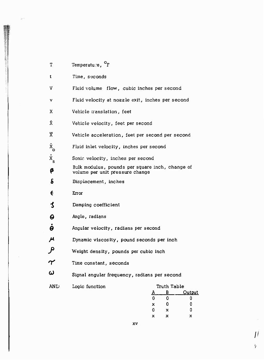
T Temperatu :e, 0F
t Time, seconds
V Fluid volume flow, cubic inches per second
v Fluid velocity at nozzle exit, inches per second
X Vehicle translation, feet
X Vehicle velocity, feet per second
J? Vehicle acceleration, feet per second per second • X Fluid inlet velocity, inches per second •
X Sonic velocity, inches per second
_ Bulk modulus, pounds per square inch, change of T volume per unit pressure change
£ Displacement, inches
6 Error
"^ Damping coefficient
Q Angle, radians • 0 Angular velocity, radians per second
/4 Dynamic viscosity, pound seconds per Inch
j Weight density, pounds per cubic Inch
T^ Time constant, seconds
^ Signal angular frequency, radians per second
AND Logic function Truth Table A B Output 0 0 0 x 0 0 0 x 0 X X X
XV
/'
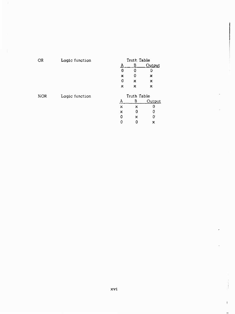
OR
NOR
Logic function Truth Table A_ B Output 0 0 0 X 0 X
0 X X
X x X
Logic function Truth Table A B Output X X 0 X 0 0 0 X 0 0 0 X
xvi

INTRODUCTION
This report is divided into four sections:
Section 1 - The Elements of Fluid Computing Systems.
Section 2 - Definition and Requirements of an Automatic Flight Control System.
Section 3 - Fluid Implementation of the Automatic Flight Control System.
Section 4 - An Evaluation of the Proposed Fluidic Automatic Flight Control System.
Section 1 describes the basic Automatic Flight Control System and the role that fluidics might offer in improving the system. Typical fluidic elements are described to give the reader an idea of what fluidics is all about.
Section 2 describes the function of the Automatic Flight Control System which includes the stability augmentation system as well as the auto- pilot. Specifications are given for a typical system.
Section 3 is the implementation of the Automatic Flight Control System with fluidic components. Of first consideration is the choice of operating fluid. It is concluded that the stability augmentation system is most desirable if it is proportional and uses hydraulic fluid. This decision is based primarily on compatibility with the existing equipment. The auto- pilot is digital and uses air as the working fluid. This decision is based primarily on power consumption due to the large number of fluid elements. The remainder of this section is a detailed description of each portion of the fluid circuitry.
Section 4 is the evaluation of the fluidic Automatic Flight Control System. This evaluation includes size, weight, power, reliability, maintainability, and response to environmental factors. Each basic component is considered in detail, and then the fluid system is compared to an existing electronic system.

Throughout the report, each section is related to the overall effort by a suitable introduction. This is to allow sections of the report to be read out of context by those specifically interested in one section, or alternately, to allow the opportunity to read only the introductions to obtain an appreciation of the general aspects of this study.

CONCLUSIONS
The study has shown that fluidic systems do offer another approach to automatic flight control and that the functional and dynamic performance requirements can be obtained. The areas of improvement offered appear to be cost and reliability, both of which need to be supported by actual experience before their value can be determined.
OPEN LOOP DAMPING AND STABILITY AUGMENTATION SYSTEM
The analysis indicates that the proposed fluidic control can meet the performance requirements specified. The proposed nonredundant fluidic system is 18 percent heavier and requires 47 percent more power (at maximum power output) than the electro-hydraulic system. The predicted reliability of the fluidic system is 0.9998 compared to a reliability of 0.9956 for a nonredundant electronic system for the same period.
A problem in the hydraulic SAS will be the cold start requirement. High fluid viscosity requires special fluidic element designs, high pressure and/or large nozzle sizes with the attendant high power consumption.
AUTOPILOT
The analysis indicates that the proposed fluidic system can meet the functional an^ dynamic response specifications.
The pneumatic fluidic autopilot is estimated to weigh 17.25 pounds compared to the 13.3 pounds for the electronic system. The estimated power consumption is 100 watts compared to the 185 watts for the nonredundant electronic subsystem.
/

RECOMMENDATIONS
It is recommended that development be carried on in the following areas:
1. A fluidic (hydraulic) stability augmentation system.
2. A fluidic (hydraulic) open loop damping system.
3. A fluidic (pneumatic) attitude hold system.
It is further recommended that research and development be carried on in the following areas:
1. Establishment of a reliability program with the objective of substantiating the expected reliabilities. The program would commence with a test program to be followed by a development program to obviate the failures noted.
2. Optimization of the hydraulic rate sensor and amplifiers to reduce the required flow rate. This development requires consideration of viscous losses and the match;ng of threshold to that required in the stability augmentation system.
3. Development of a fluid-controlled servo valve (or actuator assembly) requiring low power control input signals.
4. Development of a pneumatically operated digital actuator.
The first three of these research items can be covered by a program to develop a hydraulic stability augmentation system.

SECTION 1
THE ELEMENTS OF FLUID COMPUTING SYSTEMS
Typically, aircraft control systems include the pilot's controller, and a power boost, whose output drives the force-producing member. In more sophisticated systems, control forces are introduced from the stability augmenting system through a free-floating actuator which acts in the link from the power boost to the force-producing member. Figure I. Both the power boost and series actuator are hydraulically powered devices.
What opportunities would be offered if the control system were composed of fluid sensors and computing elements? If hydraulic sensors and computation were used, an Interface might be removed or simplified. Further, the fluid sensors and computation themselves may prove to be more reliable. It has become a rule in the application of fluid systems that if the input and output of a computer can be obtained in the same working fluid, then it is likely that fluid systems will offer advantages.
Each element of the AFCS falls into one of three fundamental classes of components:
1. Vehicle motion sensors.
2. Signal processing and amplification components.
3. Interface devices.
Succeeding paragraphs of this section provide a summary description of the fluid devices in each class which, in subsequent report sections, will be used to implement the fluid system defined in this repc-4-.
VEHICLE MOTION SENSORS
Two distinct types of angular motion sensing functions are performed in the fully implemented AFCS. They include a rate-sensing function and an attitude-sensing function. In a conventionally mechanized system, these functions are normally supplied by a form of gyroscope in which the precessional tendency of a spinning rotor in response to vehicle turning motions is sensed. In effect, the change in rotor angular momentum due to the turning input of the vehicle is measured and

Control
U o JL
i Power
Boost
////////////
Stability Augmenta- tion
Servo
Control Actuator
Figure 1. TYPICAL AIRCRAFT CONTROL ARRANGEMENT
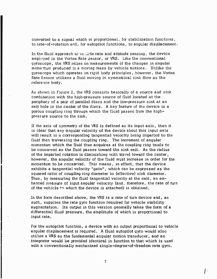
converted to a signal which is proportional, for stabilization functions, to rate-of-rotation and, for autopilot functions, to angular displacement.
In the fluid approach to vehicle rate and attitude sensing, the device employed is the Vortex Rate oensor, or VRS. Like the conventional gyroscope, the VRS relies on measurements of the changes in angular momeatum produced in a moving mass by vehicle motions. Unlike the gyroscope which operates on rigid body principles, however, the Vortex Rate Sensor utilizes a fluid moving in symmetrical sink flow as the reference body.
As shown in Figure 2, the VRS consists basically of a source and sink combination with the high-pressure source of fluid located at the periphery of a pair of parallel discs and the low-pressure sink at an exit hole in the center of the discs. A key feature of the device is a porous coupling ring through which the fluid passes from the high- pressure source to the sink.
If the axis of symmetry of the VRS is defined as its input axis, then it is clear that any angular velocity of the device about this input axis will result in a corresponding tangential velocity being imparted to the fluid then traversing the coupling ring. The increment of angular momentum which the fluid thus acquires at the coupling ring tends to be conserved as the fluid passes toward the sink exit. As the radius of the imparted rotation is diminishing with travel toward the center, however, the angular velocity of the fluid must increase in order for the momentum to be conserved. This means, in effect, that the device exhibits a tangential velocity "gain", which can be expressed as the squared ratio of coupling ring diameter to (effective) sink diameter. Thus, by measuring the fluid tangential velocity at the exit, an en- hanced measure of input angular velocity (and, therefore, the rate of turn of the vehicle to which the device is attached) is obtained.
In the form described above, the VRS is a rate of turn device and, as such, supplies the rate gyro function required for vehicle stability augmentation. Its output in this version generally takes the form of a differential fluid pressure, the amplitude of which is proportional to input rate.
For the autopilot function, a device with an output proportional to vehicle angular displacement is required. A fluid autopilot gyro would also utilize a VRS as the fundamental angular motion transducer, and an integrator would be provided identical in function to that which is used with a conventionally mechanized single-degree-of-freedom rate gyro.

Disc
^SSSVSWASSSfc
\\svsss\s\\ssss\ss
Disc Coupling
Ring
Note: P1 > P
Figure 2 , Section A-A
BASIC VORTEX RATE SENSOR CONFIGURATION
8

In the case of the VRS, a fluid analog integrator with a wide range of available time constants is practical. Like its electrical counterpart, this consists of a high-gain amplifier with feedback. Even more attractive, however, from the viewpoint of compatibility with trim or navigation system inputs is a digital form of integrator. Here, each of a pair of push-pull pressure signals de"eloped at the rate sensor output is used as the input to a pressure-controlled oscillator whose output frequency is a direct function of input pressure. The difference frequency of the oscillators thus provides a measure of VRS input rate and, when summed in a forward-backward counter, supplies a pulse count propor- tional to VRS input angular displacement.
SIGNAL-PROCESSING AND AMPLIFICATION COMPONENTS
Central to the concept of a fluid control system is the amplifier function, be it analog or digital, and among the many forms of fluid gain elements evolved in the past few years, four basic types can be distinguished:
1. Stream interaction amplifiers.
2. Boundary layer control amplifiers.
3. Vortex amplifiers.
4. Turbulence amplifiers.
These devices, through the use of appropriate fluid circuitry including the fluid equivalents of resistance, capacitance and inductance, can be interconnected and used in various combinations to obtain a very wide variety of control system functions. A brief discussion of the operating principles of each basic amplifier type follows, together with a discussion of fluid impedance parameters.
Stream Interaction Amplifiers
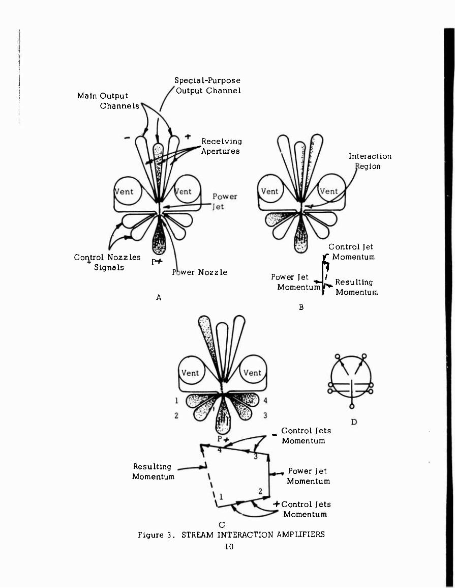
Figure 3 illustrates a stream interaction amplifier. Fluid under pressure P+ is supplied to the "power nozzle" and exhausts as a "power jet" into an "interaction region. " The power jet passes through the inter- action region and enters one or more "receiving apertures" which are entrances to the "output channels" of the amplifier. The amplifier illustrated in Figure 3 usually operates with the two outer output channels connected as push-pull outputs. Thus, the difference of pressure in these two channels represents the amplifier's "Output Pressure Signal."
Main Output Channels
Special-Purpose Output Channel
Receiving Apertures
Control Nozzles p. Signals Power Nozzle
Interaction eg ion
ft
Control Jet Momentum
Power Jet Momentum
B
^ Resulting Momentum
Resulting Momentum
^ Control Jets Momentum
^^ Power Jet Momentum
-♦•Control Jets Momentum
Figure 3. STREAM INTERACTION AMPLIFIERS 10

One or more control nozzles are provided, discharging control jets at approximately right angles to the power jet. The momenta of power jet and control jets add vectorially, establishing a new flow path for the power jet. Consequently, the distribution of power jet flow to each receiving aperture is changed and the output signal changes. The change of output signal amplitude divided by the causative change of input signal is the amplifier gain.
output change Gain = —
control change
Each amplifier can be considered to have a mass flow gain, Gm; a volumetric Low gain, GQ; a pressure gain, Gp; and various types of power gain, Gp (hydraulic power, thermal power for heating and cooling, enthalpy power, power including chemical energy, etc.). In each case, the same characteristic must be used as a basis of measurement for both control and output signals.
Figure 3C illustrates how a simple multiple-control nozzle system can be used to accomplish a summation of positive and negative input signals.
Figure 3D is the line symbol of the stream interaction amplifier.
Figure 4 illustrates several variations of such stream int3raction amplifiers, including the following:
4A Subsonic unvented analog amplifiers.
4B Supersonic free surface power jet.
4C Subsonic crossover amplifiers.
4D Subsonic analog amplifier with external feedback.
Figure 4D is of importance because it illustrates the feasibility of feedback techniques by which, with appropriate feedback impedance, a variety of transfer functions could be achieved.
Boundary Layer Oontrol Amplifiers
The Boundary Layer Oontrol or Wall Interaction Amplifier utilizes pressure fields between the power jet and adjacent walls to control the power jet flow path to the receiving aperture system. Such amplifiers use fluid
11

A. Subsonic Unvented Analog Amplifier
B. Supersonic Free Surface Power Jet
C , Subsonic Crossover Amplifier
D. Subsonic Analog Amplifier With External Feedback
Figure 4. STREAM INTERACTION AMPLIFIERS
12

entrainment characteristics and the interaction region sidewall contour to provide the desired "internal" feedback characteristics. Figure 5A shows a power jet issuing from a subsonic nozzle into an interaction region. The jet entrains fluid from the interaction region. Makeup fluid to replace entrained fluid is obtained by:
1. Flow from the downstream regions.
2 Recirculation of flow from the power jet.
3. Flow from vents leading to a reference pressure region.
4. Flow from control nozzles supplied by an input signal source.
In the two-dimensional model Illustrated in Figure 5, the power jev. extends between the top and bottom cover plates and so isolates the right portion of the interaction region from the left portion of the interaction region.
In Figure 5A,sufficient makeup flow is provided that the power jet is centered.
In Figure SB^he power jet is driven to the right by a left side control signal. Availability of makeup fluid to the right side "bubble" from downstream regions is limited by the power jet location relative to the sidewall. This is a positive feedback action which lowers the right side bubble pressure.
In Figure SC/an increase of the left side control signal strength drives the power jet farther to the right, sealing the right side bubble. For such a flow condition, the feedback is now sufficient that the left side control signal can be discontinued and the power jet will remain locked to the right sidewall, providing a memory.
In Figure 5D,a further increase of left side control signal drives the power jet farther to the right. In this position, some of the power jet is scooped off and fed back to the right side bubble, increasing its pressure and so limiting further power jet deflection. This corresponds to a negative feedback characteristic.
Thus, the interaction region contour can be designed to provide positive and/or negative feedback characteristics as desired without the need for external feedback paths.
13

Figure 5. BOUNDARY LAYER CONTROL AMPLIFIER
14
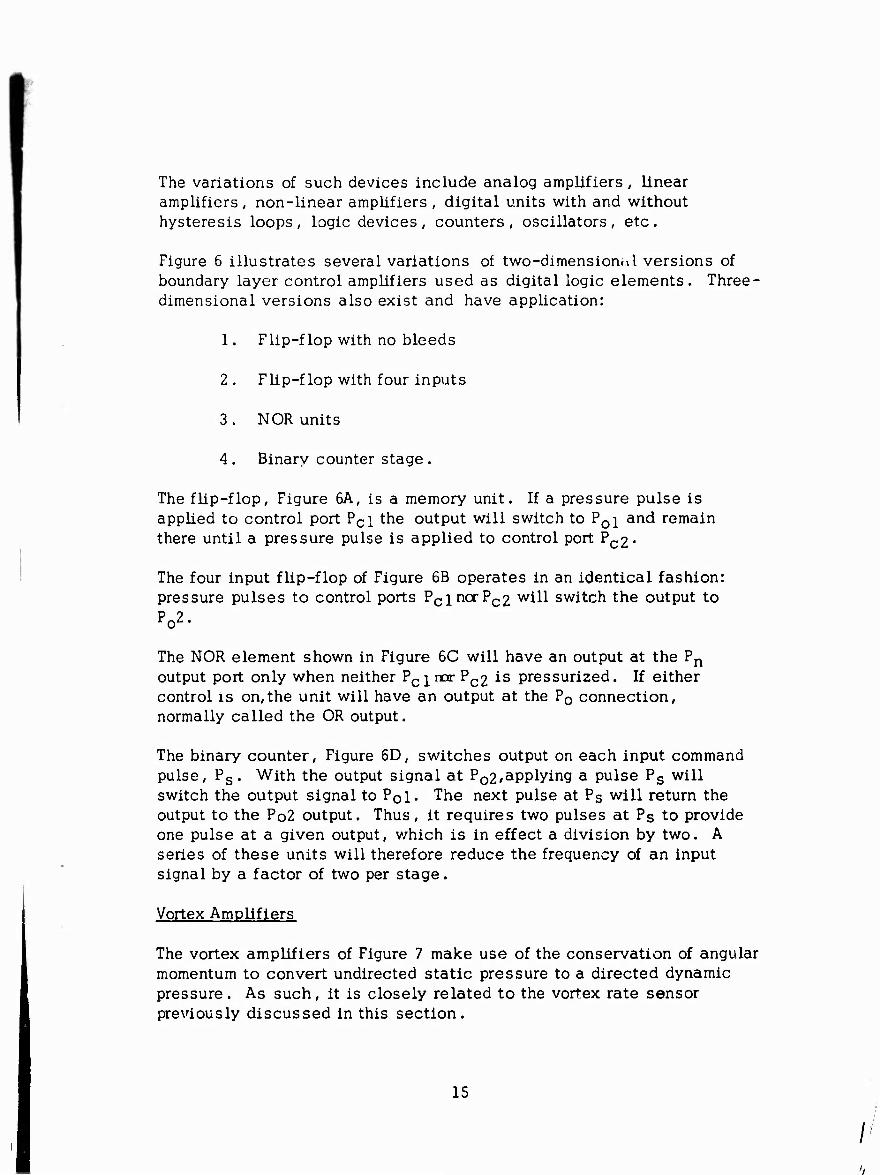
The variations of such devices include analog amplifiers, linear amplifiers , non-linear amplifiers , digital units with and without hysteresis loops, logic devices, counters, oscillators, etc.
Figure 5 illustrates several variations of two-dimensionol versions of boundary layer control amplifiers used as digital logic elements. Three- dimensional versions also exist and have application:
1. Flip-flop with no bleeds
2 . Flip-flop with four inputs
3 . NOR units
4 . Binary counter stage .
The flip-flop, Figure 6A, is a memory unit. If a pressure pulse is applied to control port Pci the output will switch to P0i and remain there until a pressure pulse is applied to control port Pc2'
The four input flip-flop of Figure 6B operates in an identical fashion: pressure pulses to control ports Pclncx^c2 w^ switch the output to P 2
The NOR element shown in Figure 6C will have an output at the Pn
output port only when neither PcinarPc2 is pressurized. If either control is on,the unit will have an output at the P0 connection, normally called the OR output.
The binary counter. Figure 6D, switches output on each input command pulse, Ps. With the output signal at Po2/aPPlyin9 a pulse Ps will switch the output signal to PQI« The next pulse at Ps will return the output to the Po2 output. Thus, it requires two pulses at Ps to provide one pulse at a given output, v/hich is in effect a division by two. A series of these units will therefore reduce the frequency of an input signal by a factor of two per stage.
Vortex Amplifiers
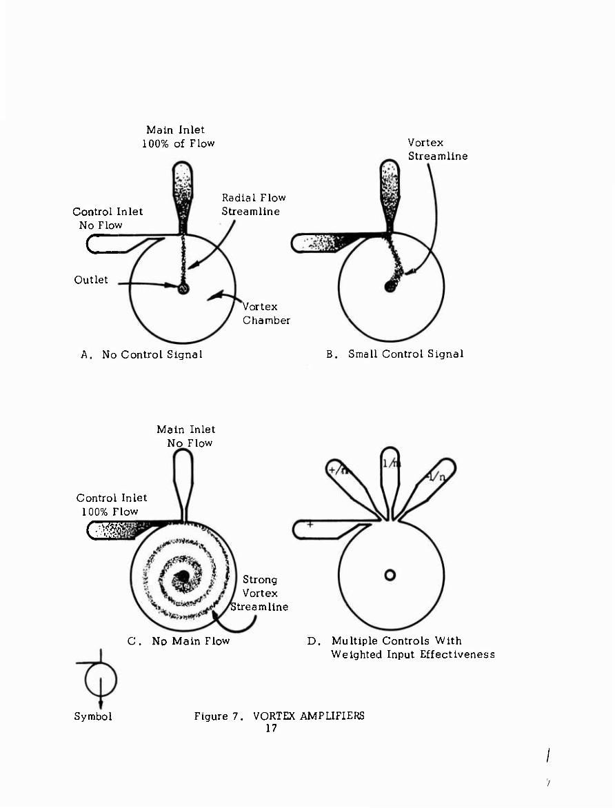
The vortex amplifiers of Figure 7 make use of the conservation of angular momentum to convert undirected static pressure to a directed dynamic pressure. As such, it is closely related to the vortex rate sensor previously discussed in this section.
15

Po2 Po!
Pel Pc2
P+
Poi P02
Pci Pc2
■ Pea .Pc4
P+
Unvented Flip-Flop B
Four-Input Unvented Flip-Flop
Po Pn Poi P02
P+
P+ Ps
C NOR
D Binary Counter
Stage
Figure 6. BOUNDARY LAYER LOGIC ELEMENTS
16
Main Inlet 100% of Flow
Control Inlet No Flow
c Outlet
Radial Flow Streamline
Vortex Chanber
Vortex Streamline
A. No Control Signal B. Small Control Signal
Main Inlet No Flow
Control Inlet 100% Flow
rtw- ■iii'tfY
Symbol
Strong Vortex
Streamline
C. Np Main Flow D. Multiple Controls With Weighted Input Effectiveness
Figure 7. VORTEX AMPLIFIERS 17

In general, fluid is introduced at the periphery of a circular cross section and flows toward a centrally located outlet. A control signal establishes the angle between a radius of the cylinder and the flow streamline.
In Figure 7A the fluid flow is radial and no vortex exists. In Figure 7B a control signal is provided,introducing angular momentum for the fluid flow and producing a new streamline angle.
In Figure 7C all of the fluid flow is introduced with maximum circum- ferential velocity components producing a maximum strength vortex.
In Figure 7D provision is made for introduction of multiple control signals of selected weighting.
The output signal of the device can take many forms. For example, it can be the pressure drop between inlet and outlet locations for cases where such pressure drop is dependent upon the rate at which the fluid spins. This pressure drop is limited by a Mach 1 condition at the discharge location for compressible fluids and by the cavitation number (local static pressure compared with vaporization pressure) for incompressible fluids. Thus, the pressure drop in this device, which is controllable by the vortex action, is limited in the case of compressible fluids to a much lower value than in the case of incompressible fluids.
Another form of output signal is the mass flow rate of such amplifiers.
Another form of output signal is provided by devices (located at the outlet) which examine the various components of the exit velocity vector as exhibited by flow path, directed pressure, selective impedarce characteristics, etc. Such devices can provide extreme sensitivity and can provide measurement of output signals related to the input signal not only by a gain factor but also by derivative or integration relationships. Such readout devices are proprietary designs.
There are many variations of vortex amplifiers. In general, such amplifiers exhibit a signal phase shift dependent upon the fluid transport time from inlet location to outlet location. This phaje shift or lag is significant in many applications and must be considered in the design.
Turbulence Amplifiers
The turbulence (or Bell) amplifier was first used by Bell in 1886. Subsequently, it was used by others in Europe, by Hall (U. S. Patent 1,628,723), and by Auger for various purposes. In this amplifier,
18

Figure 8, a laminar jet Is provided with a receiving aperture. When a control signal Is Introduced at the power nozzle exit, the power jet Is triggered and becomes turbulent, decreasing the flow to, and pressure developed In, the receiving aperture. This action Is analog In nature but saturate- so that It can be used as a digital device where desired. Turbulence can be introduced by sound as a control signal so that the amplifier has found use as a phonometer.
Such amplifiers have most frequently found use at low pressure levels for logic circuitry. Here, a limitation will be found in that they are fundamentally NOR-type elements.
Interconnections, Impedance, and Circuit Parameters
As with any amplification technique, it is desirable to be able to inter- connect and stage amplifiers. This is feasible with fluid amplifiers. It is further useful to be able to provide shaping networks, feedback, etc., in order to accomplish the desired control function. This, too, has been accomplished with fluid amplifiers.
Figure 9 shows a six-stage pressure amplifier having a pressure gain of 4000. The output of one stage provides a control signal for the next stage. In this system, not all of the first-stage amplifier's flow is delivered to the second-stage controls. Some of the first-stage flow escapes through vents to a reference pressure sump and is used as a supply for another ^wer pressure level system or is discarded.
Figure 10 shows several digital elements provided with such vents. These devices are termed "self-matching", as they match themselves to the load impedance without changing control characteristics whether the load is a dead-ended chamber, a piston, or a discharge nozzle.
Figure 11 shows a three-stage unvented amplifier. In this device, all of the first-stage input is delivered as a push-pull control signal to the second stage. Similarly, all of the first- and second-stage input is delivered as a push-pull control signal to the third stage. As would be imagined, design of unvented systems is more demanding and specific than design of vented systems.
Just as electrical circuits have impedance characteristics, so too, fluid circuits have their resistance, capacitance, and inertance. Fluid Impedance is more complex than conventional electrical impedance and lacks the storehouse of prior art available to the electrical engineer.
19
/
Main Flow
Control Signal
\ll Output Aperture
A. No Signal B. Small Signal X^:
Large Signal
*>
~/T ^
D. Two Signals Simultaneously
Figures. TURBULENCE AMFUHER
20

3rcJ Stage
4th Stage
2nd Stage
1st Stage
5th Stage
6th Stage
Inputs Figure 9. SILHOUETTE OF S
2
Out
X-STAGE ANALOG AMPLIFIER

Vent
Output
.»-Vent
• Control
(1) Flip-Flop
Outputs OR NOR
Vent
Controls
(2) OR-NOR
Output 0
Output 1
Vent
Vent
Reset
Vent
Vent
Set Input Pulse
(3) Binary Counter Stage
Figure 10. SEL^-MATCHING ELEMENTS
22

+ Output - Output
Figure 11. THREE-STAGE UNVENTED AMPLIFIER
23

In general, a fluid resistance is a passageway having a large surface area compared to flow cross-sectional area. However, dynamic flow patterns can also provide a fluid resistance.
Compressibility provides an analog of the electrical "capacitance to ground". However, other fluid capacitance to ground affects are provided by: change of phase (gas-liquid-gas), gravitational effects (water column), deformable volume (bellows), release of chemical energy, etc. An "in-line" capacitance effect is provided by a flexible diaphragm which completely blocks any d.c. flow.
An analog to electrical inductance is tluid Anertance, a tendency to preserve the velocity status quo.
In general, it has been found that fluid controls can provide any function desired that can be provided with electrical circuitry. The fluid system is limited in response speed by signal transmission speed of the order of the speed of sound, whereas electronics is limited by the speed of light. In general, internal control systems do not need or make use of the transmission speed available from electronics. The low cost and high reliability, ruggedness and tolerance of extreme environment offered by fluid systems insure their contribution to the controls field.
24

SECTION 2
DEFINITION AND REQUIREMENTS OF AN AUTOMATIC FLIGHT CONTROL SYSTEM
FUNCTIONS OF THE AUTOMATIC FLIGHT CONTROL SYSTEM
The general inadequacy of most helicopters and VTOL aircraft in providing pleasant handling qualities is a well-known fact. The presence of poor handling qualities in helicopters has inhibited the development of wide- spread instrument flight rules (IFR) capability and has been corrected recently through the incorporation of stability augmentation systems (Ref- erence 1). The CH-47A, for example, employs a dual redundant stability augmentation system, since helicopter handling qualities are quite mar- ginal without artificial stabilization.
With an increasing emphasis on VTOL aircraft types, the handling qualities problem has become even more severe. The incidental damping in pitch and roll, available in helicopter rotors at low speeds, has virtually van- ished in VTOL aircraft. The XV-4A, Lockheed Hummingbird, for example, is reported (Reference 2 ) to have exhibited strong divergent oscillations in stick-fixed pitch and roll attitude response, having a time to double ampli- tude of the order of 1 second. To permit experimentation at low speeds (in VTOL configuration), this aircraft was equipped with a stability augmenta- tion system.
The fundamental basis for the lack of adequate handling qualities is in- sufficient inherent damping relative to the available, necessary control power (Reference 3 ). The effect of inadequate damping is to introduce a requirement for substantial anticipatory pilot response. Whereas the con- ventional fixed-wing aircraft can be stabilized with virtually no quicken- ing, the helicopter and VTOL aircraft require substantial pilot lead (Ref- erence 1).
The need for the pilot to respond not only to attitude errors, but to rate of change of attitude as well, represents a substantial burden. Taken in com- bination with other stringent mission requirements (poor visibility, weapon launching, flight in close proximity to the ground, etc.), this burden can, in fact, exceed the capacity of the pilot.
Desirable handling qualities may be obtained through the use of stability augmentation systems. These systems have as an objective the reduction of pilot effort to a level where he operates as a purely proportional device— providing control inputs which are directly proportional to displacement
25
/
attitude errors. Control systems which can reduce the operator's control input requirements to those of a purely proportional device are regarded as optimum from the point of view of reduction of operator burden (Reference 4 )
STABILITY AUGMENTATION SYSTEM
The stability augmentation system introduces corrective motions to the air- craft control system which are generally functions of the angular rate of the vehicle about each axis of the aircraft. The system is usually implemented such that these motions are not r ^^ted at the pilot controls and, furthei, are limited in maximum displacement to a small fraction of the total control available (for safety reasons). The overall effect is an increase in stability which makes the vehicle easier to fly. A well designed stability augmen- tation system does, in fact, reduce pilot response requirements to those of a proportional amplifier (Reference 1).
The function of the stability augmentation system is therefore seen to be associated with the short-period requirements of vehicle attitude control and is an equalization technique for otherwise undesirable handling quali- ties. To the extent that the specific vehicle deviates from acceptable handling quality standards (References 3,5, and 6), the role of the stability augmentation system in achieving satisfactory flight can vary from being a desirable (but unessential) adjunct to the aircraft to being a vital element of the aircraft, directly affecting safety in flight. This spec- trum of need is accompanied by a compatible spectrum of equipment reli- ability requirements.
ATTITUDE CONTROL AND OTHER FUNCTIONS
In contrast to the stability augmentation system, which makes the vehicle easier to fly, attitude controls maintain the pitch, roll, and heading of the vehicle in response to the pilot's command. The attitude control is incor- porated with other autoi latic navigation functions, such as doppler speed measurements, to perform more complicated mission requirements.
REVIEW OF AUTOMATIC FLIGHT CONTROL SYSTEMS
The objective of this section is to review the well known concepts of heli- copter automatic flight controls for those who are unfamiliar with the basic techniques. A somewhat more detailed analysis is given in Appendix I.
26
To illustrate these techniques, the performance of an aircraft is described for a variety of controls, of increasing complexity, to a pull and hold com- mand. These are summarized in Figure 12, where the aircraft attitude is plotted as a function of time.
Unaugmented System
The response of an unaugmented system is characteristically one of con- tinuous acceleration, as indicated by the continuously increasing slope of the curve in Figure 12. This is obviously a difficult vehicle to fly.
Pure Rate Stabilization
A basic form of stability augmentation is the addition of a rate signal feed- back to effect a rate of rotation proportional to the pilot's input. A mech- anization of this system is shown in Figure 13. The rate gyro signal drives the stability augmentation servo to oppose the pilot's input so that the con- trol deflection is reduced as the rate is increased.
The augmented response shows the attainment of a steady-state angular rate whose final value is determined by the ratio of the input to the feedback control sensitivity.
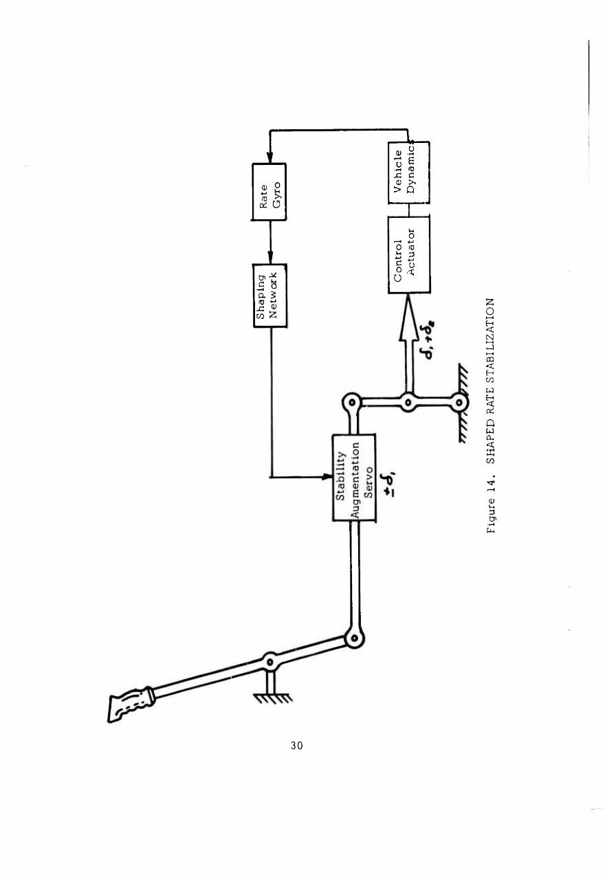
Shaped Rate Stabilization
While the angular rate feedback system is able to satisfy minimum handling qualities criteria, additional dynamic transfer characteristics are required in the feedback control to obtain more nearly optimum characteristics, i.e. , more responsive control. This additional circuit is shown in Figure 14. As in rate stabilization circuit, the feedback opposes the input. However, the lag-lead circuit prevents the high frequency (quick motion^) from being fed back. This allows the high-frequency component of the pilot's input to pass directly to the output unopposed. The result is a high initial re- sponse which allows the system to arrive at the desired attitude more quickly.
Also, the lag-lead shaping circuit effects a degree of attitude hold so that for short periods the input results in near attitude command, as shown in Figure 12.
The improvement in performance is considerable for a minor addition of complexity.
27
r. o
tu -a 3
<. <
UH
28

' H ö H*
v 6 —[ 10
Q) Q
1 > 1
1 . 1 n 0 O *J «3 2 c => P.o Ü <
o I—(
N
i—i
<; H
M
2 W oc
0) u
& -•-I
29
//
v. 1
OJ o
cS Ü
V
o>^ 5 ö a 5 ro ti x £ w ^
(D .ä
Ü S ^J (D Ä C 0) >! > Q
1
r" ̂ o
—< -t-l 0 ID
ontr
A
ctu
u
o 1—<
H <
CQ < H CO
W H
P W
w
0)
30

The Open Loop Damping System
It is of interest to note that an equivalent transfer characteristic between rate and pilot control can be achieved without resort to feedback control by operation on the pilot control output through the stability augmentation servo actuator and shaping network, Figure 15. This is a compensation or open loop technique. It is for this reason that "open loop damping", or OLD, is used as a descriptor.
In effect, the OLD circuit anticipates the rate of motion that is expected from a given input. This estimated rate is fed back to oppose the pilot's input. The result is similar to rate stabilization.
There is, however, a major functional difference between the rate stabiliza- tion system and the OLD technique. The OLD system does not respond to external disturbances. On the other hand, the OLD is able to reduce the pilot's burden in his response to these disturbances, as has been found in fixed- and moving-base simulator studies conducted recently by Northrop Norair (Reference 8).
Combined Open Loop Damping and Stability Augmentation System
The combination of the OLD and SAS with an additional shaping network pro- vides a useful combination. The position transducer, which was added for the OLD system, can be used to improve the sensitivity of the stability augmentation system.
In a transient maneuver, it is desirable to cancel the rate gyro signal so that the pilot's command is not opposed by the rate feedback signal. With- out this, the control is much less responsive, though usable.
An implementation of the combined OLD-SAS systems is shown in Figure 16 .
Attitude Hold-Autopilot Function
The attitude hold function is effected by the addition of an attitude gyro which drives an actuator in the pilot's input circuit as shown in Figure 17. In this mode of operation, the autopilot input supplants the normal pilot input. In this mode, the pilot's input signal is used to bias or set the autopilot reference. Alternately, there are other sources of autopilot set- ting information. These are outlined in Table I .
A diagram of a representative single axis AFCS is shown in Figure 18, with the addition of a mechanical clutch and spring arrangement and a force trans- ducer. The operation of this system is as follows:
31

t (0 |
0)
ü Id 1 "^ ID I x: c
0) > > p
r^ — (DO
-Q C C fD <U 0)
S co en CO
-S o a ? (D +J X 0) CO 2
+1
u l-H
< Q OH
O
2: w (X,
O
LO
cn
> ■9- X 6 ü
Q. (D W
w u
32 ^2W

I 0) o (D S a: ü
V
a ? (D f. X ® CO Z
o v -^
fl) >•
n P r . 1 ^ o 0 ^ > (0 !s 3 0) ^.
03 U •t
p
u 2 CQ
w H
CO
i O u p <
O i—i H < H
W
i—i
< U i—i
K U w 2
CO I
p O
U3
0) u 3 Cn
33
/'

**H 0) fi f u fD 1
-C C I
1 ^ >, P I 1
I-* I •—* o 1 o -*-< 1 >-• (D I
o 3 u 1
U <
o I—I
N
H CO
W H
P W a,
CO
X H
Q .-) O
w Q
H I— H H <;
NWVWV^^
34

TABLE I ARMY AUTOPILOT SETTING FUNCTIONS
Function Mission Data
Source
Attitude/heading
Heading (only)
Ground velocity
Terrain following
Altitude control
Station keeping
Approach and landing systems
Hover control
Control stick steering
Weapon launching; radar surveillance; long dura- tion flights
Weapon launching (SS-11)
Long periods of low speed flight (aerial crane)
Nap-of-the-earth flight
Transport/utility- - long duration flights
Tight formation flights
All weather flight
Cargo sling loading
Nap-of-the-earth flight
Vertical gyro, compass system
Compass system
Doppler radar, inertial naviga- tion system
Forward scanning radar altimeter
Barometric alti- tude sensor
Station keeping radar
VOR/ILS (stateside)
Cable angle sen- sor
Electro-fluid transducer
35

3 >
c o ■r-t *-> o 2
0)
10 c
o w c o
.^4 o (0 M-4
o •o > c T3 fO 3 < 2 [JL,
0)
o b c o ü
■CZJ ^=€)
o> 1»! c ••-4 o a 5 (0 •»■J
£ 0) CO 2
? D> t. . C
-i-i Ö a ? (D ■u
x: (1) co 2
J
a;
O H
o ü
IX,
O
2 H <,
W
u:
i—i
.-i <:
<q
ü w 2
(U 00
© CQ j, 0__ 3
-Ü A^W
D -^ <C (X,
T5^^ \\\\\\V

Unaugmented
With all the OLD^AS, and autopilot functions Off, the pilot controller operates the control actuator directly. With the air brake Off,the pilot's control is spring centered at the spring rate determine ly the low rate spring since the high rate spring centering system essentially holds the upper pivot fixed. Also, both servos are fixed at center. The pilot there- fore has direct control.
Open Loop Damping
With switch 1 engaged, the displacement transducer and OLD circuit provide an augmentation signal that extends or retracts the stability aug- mentation to oppose the pilot's input.
Stability Augmentation System
With switch 1 disengaged and switch 2 engaged, the rate sensor and displacement transducer signals are introduced to provide shaped rate stabilization.
Autopilot
With switches 2 and 3 engaged, the autopilot function is added to the SAS. Engaging switch 3 actuates the air brake, locking the lower ^ivot at center position. The pilot's controller is now spring centered with the high rate spring, a stiff system. The attitude and/or other navigation functions now supplant the pilot's normal input. However, if the pilot applies a force to the controller, a force is transmitted through and is measured by the force transducer. The time duration of the applied force is accumulated, by integration, to reset the reference. If sufficient force is exerted (well within the pilot's ability), the spring can be overcome to operate the control actuator directly.
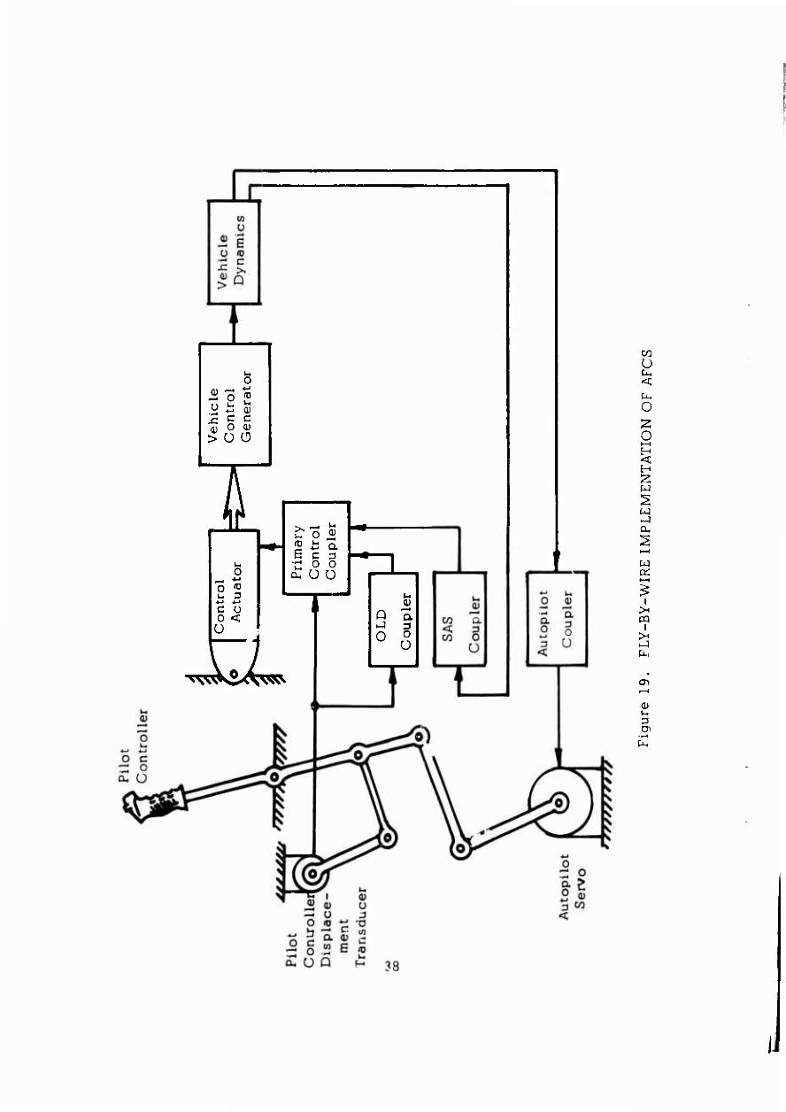
FLY-BY-WIRE IMPLEMENTATION
The fly-by-wire implementation of the AFCS is characterized by the trans- mission of the control signals by electrical or fluid means. A simplified system schematic is shown in Figure 19 . In the case at hand, the input to the control actuator is a fluid signal rather than a mechanical drive. The primary coupler takes the place of the stability augmentation servo of the mechanical implementation. In other respects, the implementation is very similar. The displacement transducer, OLD, SAS, autopilot, and auto- pilot servo have identical inputs and outputs.
37
/
^ 1 0 ü o (0 f
\ 0t 4-» 0) 1 r c c I a) u 0) i > ü 0
I O
, ■*->
4-1 4-1
c u o <
•« o ^ 2 i3 Q. E C 3 u 0 0
£ U ü
^VAKS^WN
>-• 1 a 1 Q al -^ 3 1 o 0 1
U
CO
U <c u-, O
O >—< H <
>—i
M
i
I
CD
0) 1-,
3
Pu,

The fly-by-wire implementation contains all of the functions of the mechan- ical implementation that would be considered from a fluid system point of view. Therefore, the fly-by-wire implementation will be considered as a basis of discussion for this study, since it presents a greater opportunity to investigate the fluid system approach.
AUTOMATIC FLIGHT CONTROL SYSTEMS FOR PITCH/ROLL, YAW, AND THRUST AXES
Each control axis of the AFCS may be made up by combination of the pri- mary control system, stability augmentation system, open loop damping, and autopilot subsystems as shown in Figure 20. The arrangement of each axis is shown in Figures 21 through 26, starting with the pitch and roll axes, which are essentially identical from the functional point of view.
PITCH/ROLL AXES
In Figure 21 the output of the pilot controller displacement transducer is fed to the primary control coupler for scaling and calibration, and thence to a control actuator which is connected within the vehicle such thai its displacement produces vehicle pitch/roll control moments.
The superposition of higher order functions by the addition of couplers is shov/n for OLD,. SAS, and autopilot control modes. Without an SAS coupler, the form for the OLD shaping network transfer function is that of a simple lag network (see Appendix I). With the SAS coupler operative, the role of the OLD shaping network changes (since stick-fixed damping is achieved with röte gyro signaling). It furnishes a dynamic cancellation of the rate gyro signal during maneuvers,as in typical series servo systems (Refer- ence 9 ). In this capacity, it is necessary for the OLD shaping network output to be reversed in polarity (i.e. , to add to pilot control) and to lead, rather than lag, the pilot controller motion. In this way, the shap- ing network output is able to overcome the rate gyro signals which tend to prevent maneuvers, thereby maintaining vehicle control sensitivity.
The shaping network used in the SAS coupler is designed to modify the rate gyro output, such that it approximates the incorporation of equivalent atti- tude displacement data (Reference 7 ).
In the autopilot mode of operation, the pilot's input is a bias to the atti- tude control. The pilot's controller is driven by the attitude servo; how- ever, the controller servo can be overridden by the pilot A force applied to the controller produces the bias effect.
39

I JL
n .r m i U 1
1 <1) T* 1 Ni _L 1 1 0) ^ 1 > Q
CO *
^ i M i 1 CO ■■
lot
sio
n
ion
s 2; 2 H n 1
1 "] % 1
topi
Mis
; an
ct
g D
^ ^•oC 0) 1 ^ u.
cle
Mom
»r
ce
ator 1 ^ 53
-< U 1-
Veh
C
ontr
ol
or F
G
ene 2
w H
CO . 1
A O T . " 1 K 1 X ' H a A fw—1 2;
i i Q y^ 0
% i Ü ! (0 4 1 >, 1 H
- /^k- 2 ^ * T Pu,
i o T . ü /W-. o 1 J- vXr* 1
5 + 0)
1 E 6 ! 3 1 u Q 5 1 ^ H-J (0
1 1 0
H 1 ' 1 w
•
o L- J3 IOC
1 1 ^ 0
1 1
40

H
W
M Ü
s I u B
CO
CO
QJ
PL,
> ^ &. ^ M
41

The mechanical Implementation of the pilot's controller is shown in Figure 18. When the autopilot mode is selected, the air brake comes On, locking the lower pivot. The pilot controller is now driven by the servo shown in series with the high spring rate—a stiff system. When the pilot exerts a force on the controller, the force transducer output is the bias signal to the autopilot loop.
In reference to Figure 21, this bias signal is integrated to reset the atti- tude reference in the autopilot coupler.
In the same fashion, the input from other commands can bias the autopilot. For example, vehicle translation data are obtained as outputs from the navigation equipment. For the roll axis, the translational data are related to course error in cruise conditions. By commanding a roll angle to null this error, the vehicle performs turning maneuvers until it holds the desired course. For vehicles engaged in hoveling missions (e.g., cargo slinging), the translational control data for roll (or pitch) may be changed to lateral (or longitudinal) ground velocity (as measured by a doppler radar, for example).
In contrast to the relatively simple coupling of translational data into the roll autopilot control, the pitch axis coupling is somewhat more complex. The additional complexity results from the fact that in low speed flight the pitch attitude controls longitudinal translation (only), whereas in cruise flight it is an effective means for control of vertical translation,especially in higher performance VTOL. It is therefore necessary to weight the role of the vehicle pitch control versus vehicle thrust control in achieving altitude con- trol, as shown in Figure 22. The speed logic function shown in this figure makes the pitch axis progressively ineffectual in maintaining altitude as speed is decreased, while simultaneously utilizing the thrust axis to a greater extent. The speed logic function is particularly important in auto- matic terrain following modes as a means for selecting the best combina- tion of pitch and thrust variation to achieve terrain clearance at specific flight conditions.
The differences in configuration between fly-by-wire primary control sys- tem may be noted by comparison of Figure 23 with Figure 21. Figure 23 represents the system of Figure 21 with the fly-by-wire control system deleted. It is apparent that both systems use identical functional build- ing blocks. (The use of a primary control coupler is still a general require- ment in the conventional primary control system version, since control blending may still be required; i.e., where the control actuator cannot be installed in the body-axis-oriented portion of the control system.)
42
1_

OJ
o 0
CM
■M <u -1 3 a 0
C7>
0 'w'
TD •-<
iä CPX
•r-l C) 0) *->
^ a,
1
# i
a>
tud
4-> ■r* !D
! *■' Q <
TT cv;
o 0) ♦J u ■l-J
3 a *->
3
3 *"■'
o OT —J
T3 0) ^
■M
x: 4->
m w
(11 d ^
X
i
Ü Ü
O i—•
s CO
H
w > K Ü H
CM OJ
0) u 3
43
/

..*'■
I-
g -I
O Ü
<:
3 a,
<;
o I—I H
w >
O Ü
CO
w H
CO
Ü H
CO CM
0) u

YAW AXIS
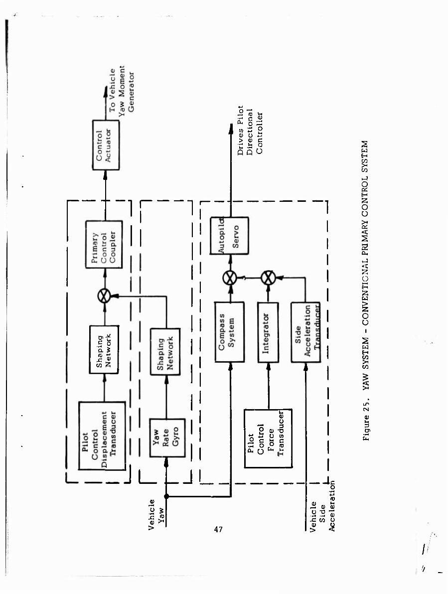
The yaw axis schematic of Figure 24 shows a close functional similarity to the pitch/roll axes of Figures 21 and 23. The notable differences are the omission of translational control inputs (since the yaw axis does not con- trol vehicle translation) and the use of a side acceleration input for turn coordination. In every other respect, the system arrangement is a strong analog of the pitch/roll configuration. Figure 25, therefore, shows changes to the yaw system, as it would be applied to conventional primary control systems, which are similar to the pitch/roll axes changes.
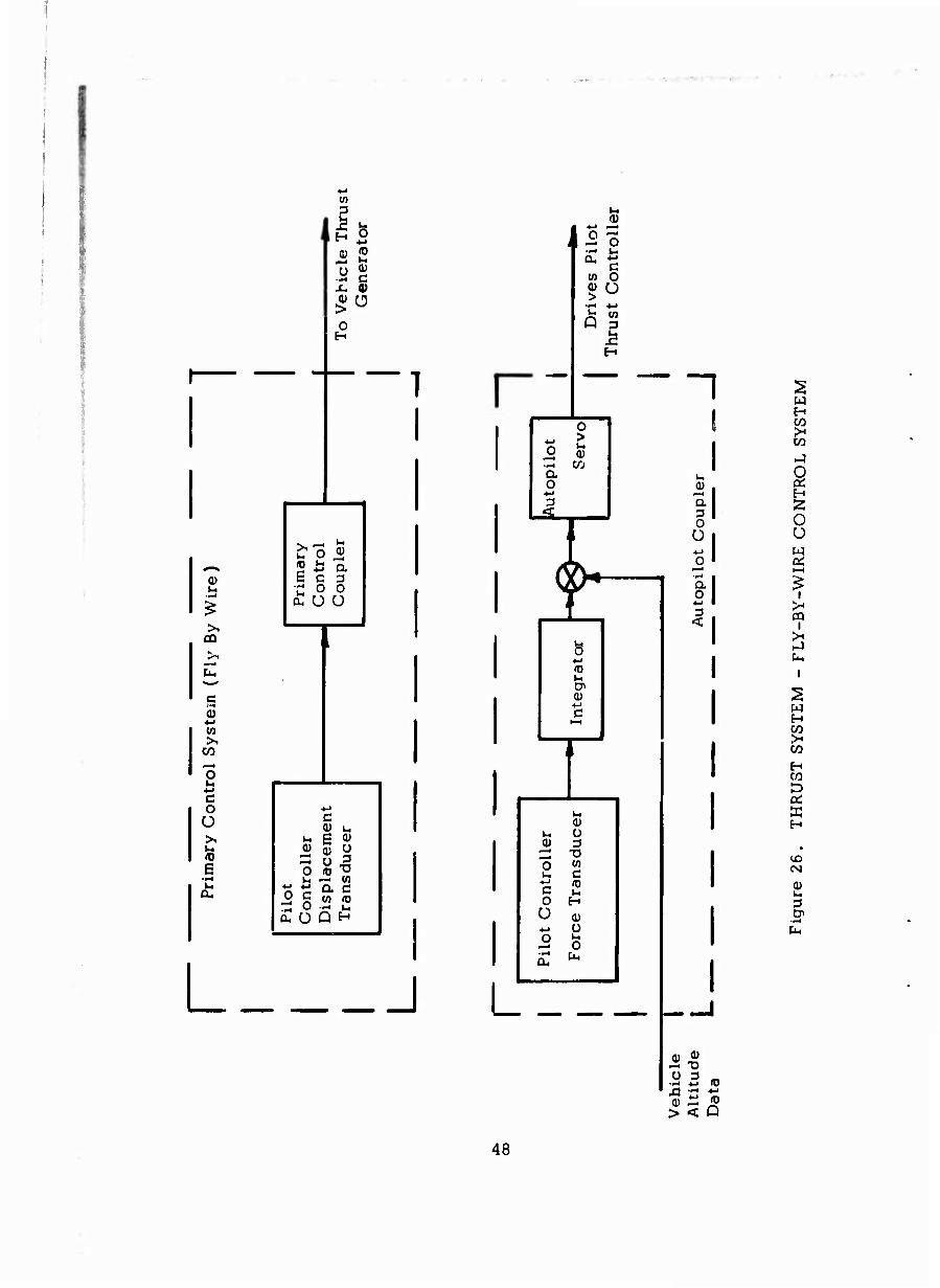
THRUST AXIS
By thrust axis is meant direct vehicle lift control. In helicopters, this is achieved by rotor collective pitch change; in VTOL aircraft, by any number of different techniques (tilt wing, tilt engine, jet diversion, etc.). Direct lift is a necessary condition cor pure vertical flight. Under such conditions, the control of vehicle vertical translation can be achieved only by thrust control. Figure 26 shows how the direct lift, or thrust axis, may be controlled by vehicle altitude data. It is more desirable to control alti- tude in cruise flight through pitch attitude than through direct lift. The role of a speed logic system in weighting the role of the two controls has been cited (see Figure 22).
The automatic control of vertically rising aircraft has not yet demonstrated a need for a stability augmentation system for thrust conUol. Therefore, none is shown in Figure 26. Instead, the thrust control system is entirely an autopilot function. In a conventional primary control system, the sys- tem reduces to only the autopilot coupler, i.e., to the lower block of Figure 26.
Component Specifications
The previous section has shown that the AFCS is generally the combination of five subsystems used in varying degrees in the control: the primary control, the primary control coupler, the open loop damping, the stability augmentation system, and the autopilot subsystem. These are shown in Figure 19.
Since there is a marked parallelism in system construction (e.g., three essentially identical stability augmentation axes), the ability of fluid systems to achieve the performance requirements outlined above can be assessed by a detailed analysis of one axis only: the longitudinal
45

0) § ü e
JC 0
<ü Ä (0
0) "^ i c O ^ 0) H >S Ü
r
1
i >-• 1 \o2\ ^2 1 c 3 1
| ü < j
1
o n v z: c - a.oo m ♦■• •M S O C > Q) O
"I
o h c o ü
a r" u
CU
0 o,
Con
trol
ler
Dis
plac
emen
t T
rans
duce
r
<n 1 w s l 2 <u 1 a ^
6 w
o ^ üw
i
+-•
(-. Di 0)
a o ü
Q. o
■M
C 0
u
u 4-> 3 (D n
Q) u to TD 0) c
H
W
w Ü
2 <
2
I >H PQ
I
2 w H
I CM
D
46
c: o (0
0)
0) o
d<
> w
ö 1 1 a ^ 1
(0 4-1 1
JZ 0) CO Z
1 1
r'JL-JL 0)
x: « >
o^ »H •« c UJ a. S .—1
w S o <1) u •M
> (U c f- »-< o u —« Q Q U
p^-" »-* 1 0) 1 Ü
o 4-1
3 0) -o
1 +-> Ü w 10 1 -H
c o £ S a, Ü H
47
o (0
x: co o
w H
CO
2 H
o Ü
>: <;
S a.
►-< H
W
O o
2 w
CO
I CM
0) 1-1 3
/'
»Is ® Ü
o H
0)
CQ
S 0)
4-1 w
CO
o
c o Ü
S u a,
u o «
6 C 3 •r; o o cu U Ü
0)
c
u — m
0 C w ro
cC Ü P H
1 n
u
a O
< r b *-' 10 u Oi 0)
■♦-' c t—4
1
t~> a>
u o QJ 3 S "O O w
u C ti (D C ü O H Ü a) ♦J Ü o fe -= 0
a, ^
» • — —
"I o I
a o 3
2% Ü 3 _
2 w H
O Ü w oi
CD I
2 w H
CO
H CO
g H
ID CSJ
CU
3
> < Q
48

•^A
(pitch) axis, for example. Through a comparison with the other axes of control (including the use of conventional primary controls^ it is evident that this control axis is a compendium of all of the other axes of control. The quantitative analysis of this axis should therefore be a necessary and sufficient exercise for evaluation of fluid device feasibility.
The following paragraphs accordingly present the quantitative requirements for longitudinal (pitch) axis control. These requirements are then sum- marized in Figure 28.
Primary Control
The major components of the fly-by-wire system are the actuator, the pri- mary control coupler, and the pilot control column with displacement trans- ducer (see Figure 19). The control actuator characteristics are determined by the following major parameters:
Stall Force Free Speed Response Resolution Stroke Linearity
The values for the performance requirements of the control actuator in the fly-by-wire application are given in the first column of Table II, The stall force is the maximum force that can be sustained. The free speed is the maximum velocity to a step input. The response is characterized by the natural frequency of the control actuator and the degree of damping. Note that at 180 radians per second with a damping ratio of 0.5,the response is limited to about this frequency, falling off very rapidly as the frequency is increased thereafter.
This same control actuator could be used in a conventional system to intro- duce the stability augmentation signal by interposing this actuator in series with the push rod. The only modification would be a limiting of its stroke at + 1/4 inch as required by the restricted authority concept. The perform- ance requirements for this application are given in the right column of Table II . Note thct the pprformance is identical. Rdcience 7 gives a good quantitative estimate of these parameters for the conventional control.
The pilot controller specifications. Table HI, include maximum travel, reso- lution, and linearity. The resolution and linearity requirements are of pri- mary significance to this study because they define the performance of the mechanical fluid interface. The displacement stated is for a side-arm
49
■
//

10
■M
o h c o Ü
4-1 O c o N
u O X
0 +-> DC na
3
H
T
O
•M u
c o t-H
(1) > D
4-> ■ ft
0 u <
0) s: .—I <j o 4->
Ü cu
T
2 is a B c :i u 0 0
cu ü U
J
0)
o u *-> c o U
(0 c
T3
Ho
o o
c
c 0) <U Ü U 3
2 2 J Ü P H
C
a.
u
o b c o Ü
c
S a <u c u z (OX
^ '-
c 6
C o - •
c 0) Ü 3
cn
Q ü Q H
0) >
-(-4 o O (U 0) 3
■M O
0 <c Ü x: -t-J u M-l ■tj
a,
o >
I—I H a: O
a. P O U
o H
o Ü
<
S CL,
(1) l-H
3
O
a,
50

TABLE II CONTROL ACTUATOR CHARACTERISTICS
Fly-by-Wire Conventional Con- parameter Application (b) trol Application (c)
Stall force 750 lb. 750 lb.
Free speed 16 m./sec. 4 in./sec.
Natural frequency (a) 180 rad/sec. 180 rad/sec.
Damping ratio (a) 0.5 to 0.7 0.5 to 0.7
Resolution 0.005 in. 0.005 in.
Stroke ±1 in. + 1/4 in.
Linearity (deviation 2.0% 2.0% from sL .ight line)
(a) Closed loop position servo frequency response with no load (b) Full authority actuator (c) Limited authority actuator in series with boost actuator
51

•-
TABLE III PILOT CONTROLLER REQUIREMENTS
Parameter Nominal Value
Maximum travel + 2 in.
Resolution (% of full stroke) 0.5%
Linearity (deviation from 2.0% straight line)
52

Controller. The mechanization of a conventional controller poses no great- er problems than that for a side-arm controller; hence establishment of feasibility of the side-arm controller implies feasibility of the conventional controller.
The requirements of the primary control coupler are uniquely related to the specific aircraft in which the system is used. For example, Figure 27 shows a possible arrangement which would exist in a tilt-wing VTOL, in which the primary control coupler transforms pilot control axis outputs into vehicle control actuator outputs. The schematic is presented to demon- strate that this system element will, in general, require customized design. To proceed with the objectives of this program, however, it would appear acceptable to assume that the transformation of pilot controller axes to vehicle actuator axes has a 1:1 correspondence. Thus, for the purposes of this study, the pitch axis primary control coupler is regarded as a scal- ing device (only) which coordinates the pilot controller output signal such that full signal output from the pilot controller produces the full stroke available in the control actuator.
OPEN LOOP DAMPING
The open loop damping (OLD) coupler accepts the pilot controller output position signal. The output of the OLD coupler is a dynamically shaped signal which modifies the otherwise linear input to the primary control coupler. Since it is desirable for the OLD coupler output to have a zero steady-state output for any position of the pilot controller, blocking or washout is a specific requirement for the OLD coupler. A second require- ment is for a limitation of authority such that under no condition can the OLD coupler output ever exceed more than a small percent of the maximum pilot controller output. Finally, the OLD shaping network must furnish the fundamental lagging characteristic of equation 2. When all of these require- ments are combined, the form of the resulting transfer function is
F = - KT] S
(T1S+ 1)(T2S+ 1) (1)
which, for pilot control frequency pass band, approximates as follows:
T=WtfTir~ - (2)
This has the same characteristic as equation 11 (in Appendix I).
53

The maximum value of F, for any input, must be limited in authority. Au- thority limitation and other requirements are estimated in Table IV.
STABILITY AUGMENTATION SYSTEM
The stability augmentation coupler contains attitude rate sensing and shap- ing networks to enhance its performance (equation 10, Appendix I). The attitude rate sensor characteristics are defined by the following param- eters: resolution, linearity, range, response. Much work has been com- pleted in tha development of miniature electro-mechanical sensors which have been used for stability augmentation. It „u a well-known fact that the available characteristics in these rate gyros exceed, substantially, the actual system requirements.
Based on much of the work performed in Reference 7 and on experience with operational aircraft, the estimates of Table V have been generated as real- istic requirements for an attitude rate sensor used solely for stability c.ug- mentation. Of special consideration is the permissible threshold of 0.2 deg/sec cited in Table V, as compared with figures of less than 0.05 dog/ sec furnished in electro-mechanical units. The adequacy of this level of accuracy may be appreciated by considering a typical attitude hold situa- tion (whether the attitude is controlled automatically or manually). Assume that the attitude hold loop is stabilized at a control (or natural) frequency of 3 rad/sec (typical of many system settings) and that an accuracy of 1 degree (peak-to-peak) is being achieved. It would then follow that the peak velocity corresponding to this stabilization task would be 1.5 deg/ sec, which is well above the rate gyro threshold.
In order to optimize handling qualities, it is desirable to shape the out- put of the rate gyro (as described in Appendix I). The form of the transfer function is
^'-rtfrr'- (3)
Values for the various parameters are presented in Table VI.
When the stability augmentation mode is operative, the OLD coupler is modified to provide a signal to cancel the rate gyro signal as discussed on page 31. Thus,
(TV S+l) ' [qi
54

TABLE IV
OPEN LOOP DAMPING COUPLER CHARACTERISTICS
Parameter Nominal Value
Washout time constant 'i 10 sec.
Lag time constant TS ^ sec.
Gain (a) k 0.5
Authority (b) 15%
(a) Gain is expressed as quasi-steady-state ratio of OLD output to in- put, K of equation 2 on page 53.
(b) Authority is maximum output of OLD coupler in relation to total control range.
55

TABLE V RATE GYRO CHARACTERISTICS
Parameter
Range
Threshold
Linearity
Frequency response
Phase shift
Amplitude response
Resonance
Scale factor
Nominal Value
+_ 40 deg/sec.
0.2 deg/sec.
2.0%
Less than 10 deg. @ 1 ops
Within + 1 db to 1 ops
Less than + 3 db
Fall output of rate gyro to be equal to full output of pilot controller displacement transducer
56

TABLE VI STABILITY AUGMENTATION SHAPING NETWORK
Parameter Nominal Value
Static gain 10
Lag time constant T^ 2.0 sec.
Lead tima constant ^s 0,2 sec.
Output limiting Less than or equal to 15% of maxi- mum input signal
Washout network (pitch) Cascade with lag/lead. Washout time constant--5 sec.
57
•i

Appropriate values for the OLD coupler shaping network parameters are out- lined in Table VII.
AUTOPILOT
A composite diagram of the automatic flight control is presented in Figure 28. This diagram shows how the major building blocks are integrated in a quantitative sense to furnish the following functions:
Primary control Open loop damping Stability augmentation Autopilot servo Attitude control Trim control Navigational control (as an example of typical coupling requirements)
The primary control, OLD, and stability augmentation have been discussed. The following paragraphs of this section cover the performance requirements of the autopilot system.
Autopilot Servo
As shown in Figure 19, the autopilot supplants the pilot input. The auto- pilot servo is used both as a centering spring and as a motor drive. When used in a fly-by-wire system, the centering spring forces would be chosen at the lowest levels consistent with the provision of definite feel. In a conventional system, somewhat higher spring forces would be required to maintain a suitable margin relative to the larger level of friction inherent in such systems. TableVIII outlines the major design characteristics of the autopilot servo needed to furnish a suitable manual trim system. The left column refers to the fly-by-wire system with a stroke of + 2 inches, and the right column refers to a conventional column with a + 8-inch stroke.
Attitude Control
The attitude control function is achieved by feeding attitude errors to the attitude servo. The attitude error is generated as the d iference between a reference signal and the measured attit de of the aircraft,as discussed previously.
The attitude sensor should have a drift of less than 0.5 degree over a period of 6 minutes to ensure reasonably precise attitude stability. With
58
L

TABLE VII OPEN LOOP DAMPING COUPLER CHARACTERISTICS - SAS MODE
Parameter Nominal Value
Washout time constant TY 1 sec.
Gain (a) k' 0.5
Authority (b) 15%
(a) See Note a, Table IV (b) See Note b. Table IV
59
/

n>
CO H
w
w (X I—I
a w
o Ü
PL,
w CO
CO
K
CD CM
09
0»

Preload
Trim rate (a)
0.5 lb.
0.50 in./sec. (c)
0.5 to 1.5 lb.
2.0 in./sec. (e)
Time for fast trim 1.0 sec. 1.0 sec.
(a) Measured at center of pilot grip. (b) Based on MIL-H-8501A. (c) Using the maximum stroke of 2 in. (Table III ).
This implies a time to trim from hardover to hardover of 8 sec. (d) For first in. of travel of pilot grip. (e) Based on maximum assumed travel of + 8 in.; yields 8-sec. hard-
over to hardover trim time.
TABLE VIII AUTOPILOT SERVO CHARACTERISTICS
Parameter
Spring gradient (a)
Autopilot Servo for Fly-By-Wire Application
Autopilot Servo Conventional
Control Application (b)
1 lb/in. 0.5 to 2.0 lb/in. (d) -i
61
i

such accuracy, and with a reasonably precise servo system, the vehicle static accuracy may be maintained within + ] degree, which should suffice for a)l of the functions listed in Table I .
i
For translationd control functions, which cover the bulk, of the requirements of Table I , the verticality* time scale may be related to the response char- acteristic of the closed loop translational control system. These response characteristics are largely a function of the lags associated with the accel- eration of the mass of the vehicle with the available vehicle propulsive force. In typical path control tasks (e.g., automatic course control) the natural frequency of the stabilized vehicle is of the order of 0.1 rad/sec. , or a period of the order of 60 seconds or more. In order to render the effects of long-term gyro drift negligible on the control of the vehicle, it would follow that the verticality accuracy, 0.5 degree, should be main- tained for a period of at least 5 to 10 times the response time of the con- trol loop. This would place the long-term requirement for gyro verticality in the region of 6 minutes or so--insofar as translational control require- ments are concerned.
For weapon launching and radar surveillance tasks, the verticality time period may be directly related to the control task itself. This would appear to imply a time span substantially less than that demanded by the trans- lational control. Stated conversely, a gyro capable of maintaining verti- cality for 6 minutos or so would be more than adequate for these functions. However, a degree of precision of the qyro system exceeding the typical 0.5 degree accuracy for peüods of up to 1 minute would appear to be a good design objective.
Other major characteristics of the attitude sensor are covered in TablelX .
The transformation of attitude error into control output lies generally in the range of + 10 degrees of attitude error equal to full control. Also, servo threshold is generally held to the order of 0.05 degree of attitude error. Characteristics of the autopilot servo required to achieve these levels of performance are listed in Table X. When combined with the requirements for manual trim (Table VIII) the autopilot servo is uniquely defined.
* Verticality is the degree to which the gyro maintains a vertical reference.
62
-

TABLE DC ATTITUDE GYRO CHARACTERISTICS
Parameter Nominal Value
Verticality (a)
Range (full signal output)
Frequency response
Phase shift
Amplitude response
Resonance (b)
+ 0.5 deg. for a period of 6 min, + 0.1 deg. for a period of 1 min,
for weapon launching and/or surveillance
+ 45 deg.
Less than 10 deg. @ 1 cps
Within + 3 db to 1 cps
Less than + 3 db
Linearity 2.0%
(a) Verticality is the degree to which the attitude gyro maintains a vertical reference.
(b) Output amplitude signal generated by a resonant condition.
63

TABLE X AUTOPILOT SERVO CHARACTERISTICS-ATTITUDE CONTROL
Parameter
Natural frequency
Damping ratio
Maximum stroke
Maximum force
Free speed
Resolution
Scale factor
Nominal Value (a)
30 rad/sec.
0.5 to 0 .7
+ 2 in.
2.0 lb.
2 in/sec.
0.010 in.
Maximum stroke shall be achieved for signal inputs equivalent to + 10 deg. of attitude error.
(a) All values are referenced to pilot control grip travel.
64

Control Force Steering
The control force steering function uses a pilot controller force transducer and integrator, Figure 18, to bias the attitude gyro signal. Typical scal- ing is such that full pilot effort, in this case + 2 pounds, can achieve a maneuver rate of the order of 45 degrees per second or less (and most probably, considerably less).
Prior to engagement of the autopilot, it is necessary to synchronize the attitude reference to the prevailing attitude. This is normally achieved by the use of an integrator, as shown in Figure 28. The quantitative details of the synchronization function are reserved for later discussion.
Since the integrator is used in this dual capacity, synchronization as well as force integration, it is desirable to keep the sensitivity of the force transducer relatively low, while making the integration rate as high as practical. Keeping this consideration in mind, the characteristics of Tables XI andXII represent a reasonable compromise between these two functional requirements. Incorporated in TableXII are the synchronization characteristics of the force integrator.
Navigation Control
Navigation control is achieved by interposition of a coupler between the output of a navigational aid system and the autopilot servo. The coupler output, as shown in Figure 28,then becomes the attitude reference for the autopilot.
Implicit in the function of the navigation coupler is a conversion process in which the electric signal output of the navigation aid is transformed into a fluid signal.
65

TABLE XI PILOT CONTROLLER FORCE TRANSDUCER CHARACTERISTICS
Parameter Nominal Value
Range
Preload
Spring gradient
Scale factor
+ 2.0 lb.
0.5 lb.
20.0 lb./in.
Maximum output should be 5% of maximum attitude gyro output
65

TABLE XII FORCE INTEGRATOR CHARACTERISTICS
Parameter Value
Integration rate Ky
Integration time constant
Maximum rate
Threshold
20 sec.
0 .05 sec.
A signal output rate equivalent to an attitude rate of 45 deg/sec.
r ^uivalent to the signal generated by a force transducer output of 0.1 lb.
Synchronization
Loop natural frequency
Damping ratio
20 rad/sec
0.5
67

SECTION 3
FLUID IMPLEMENTATION OF THE AUTOMATIC FLIGHT CONTROL SYSTEM
In summary, Section 2 has shown that a fluid implementation of the pitch axis will demonstrate all of the functions necessary for the full Automatic Flight Control System. The quantitative analysis of the pitch axis control is therefore a sufficient exercise for the evaluation of fluid system feasi- bility. Further, the demonstration of a fly-by-wire system allows the evaluation of the maximum number of fluid components but does not pre- clude the use of a mechanical primary system with fluid stability augmen- tation. Section 2 also includes the specifications for the pitch axis con- trol which are summarized in block diagram form in Figure 28.
The objective of Section 3 is to propose a fluid implementation of the pitch axis Automatic Flight Control System and to show that the problem system is capable of providing the specified performance. The system will be evalu- ated in Section 4 for size, weight, power, and potential reliability. Before considering the implementation of the circuits, it is necessary to select the working fluid. A decision to use hydraulic fluid for the primary control, open loop damping, and stability augmentation system and to use air in the autopilot is based primarily on fluid compatibility with existing functions and power consumption. Further, an analog approach was selected for the stability augmentation system and a digital approach for the attitude con- trol and other functions. A general discussion of these selections precedes a detailed description of the fluid circuitry.
SELECTION OF FLUIDS
The functions of the Automatic Flight Control System fall into two groups:
1. Primary control, open loop damping, stability augmentation.
2. Autopilot.
Referring to Figure 19 of Section 2, the primary control involves a power actuator with high stiffness requirements, while the autopilot involves low force actuation.
The primary system is, by present practices, often actuated hydraulically for time-proven reasons which involve safety, efficiency, response, and stiffness. The use of hydraulics, therefore, in the control circuitry avoids
68

dependency on two power supplies. In addition, in helicopter applications where the hydraulic pump is driven by the rotor, the hydraulic supply is independent of the main power plant; hence, the primary control functions would be available even in the event of propulsion engine failure or shut- down. This is a desirable feature to ensure that the pilot maintains control of the craft during emergency conditions. The stability augmentation system having a reliability requirement no less than that of the primary system is deserving of the same treatment.
The required accuracy of the primary control, open loop damping, and sta- bility augmentation system is compatible with fluid analog systems. Accu- racy of an analog fluid system is primarily related to the amplitude of the noise signal compared to the maximum signal. This defines the limiting resolution or accuracy. In state-of-the-art fluid analog systems the noise is about 1 percent of the maximum signal, which is adequate to meet the specifications.
One possible deterrent to the hydraulic system is the high fluid viscosity at cold startup. Fluid systems are contingent on obtaining high fluid ve- locities. If oils such as MIL-5606 are used in fluid amplifiers of reasonable size (.0008 in. power nozzles) for this application, designs with increased channel sizes to reduce pressure losses and high pressures (300 psi) will be required.
Examination of the autopilot reveals the need for high resolution and long- term integrations. Analog systems do not have sufficient resolution for the autopilot. Also, long-term analog integration requires large tanks for energy storage. The solution to this dilemma is a frequency modulation digital approach which will be described in detail later. Briefly, digital systems offer high resolution, limited only by the information storage ca- pacity, an I excellent long-term integrations. Information converted to a frequency can be integrated by counting. The counter has perfect memory. Functionally, therefore, the FM-digital approach offers a solution. The choice of air as the autopilot working fluid is based on power consumption. There are a large number of elements in the digital system, and power consumption would be prohibitive if high-pressure hydraulic fluid were used.
A survey of the other autopilot functions shows, with the exception of the servo, that all the other functions lend themselves well to the digital approach. The alternative, a digital-to-analog conversion, will only cause a loss of accuracy which was gained by using the digital system and also will introduce a complex circuit in the control. The approach taken will be to consider the entire autopilot as pneumatic digital and to discuss concep- tual models of a digital servo actuator.
69
/
V

These arguments show the desirability of using hydraulic analog circuitry for the primary, open loop damping, and stability augmentation system functions and pneumatic digital circuitry for the autopilot functions.
PRIMARY CONTROL SYSTEM
A schematic diagram of the primary control, open loop damping circuit and stability augmentation circuit is shown in Figure 29. (For a discussion of fluid devices and symbols, refer to Section 1.) Each major block will be described in detail below.
The primary control circuit of this subsystem is isolated and shown in Figure 30. This is a servo positioning system with its input at the pilot controller and a proportional position output at the actuator.
The circuit consists of the input displacement transducer (a fluid potenti- ometer); four fluid amplifiers, shown in Figure 30 in schematic form; and the actuator with a displacement transducer. Briefly, the units shown have a power input and two output legs which operate in push-pull fashion. Three of the units have four control inputs which normally operate with two pairs of push-pull signals.
In Figure 30 a displacement of the pilot controller moves the displacement transducer. The displacement transducer is a fluid potentiometer which transmits a differential hydraulic pressure signal proportional to the input displacement. This signal passes through two couplers and into the control actuator error summer. The error signal drives the first-stage servo valve, which is a fluid power amplifier. This in turn positions the second-stage servo valvejWhich is of the spool type with spool position feedback. The actuator motion causes the feedback displacement transducer to send a signal to the error summer to cancel the error signal. Note that this ap- proach uses the existing control actuator with the addition of the fluid displacement transducer and the fluid-operated servo valve.
Coupling to OLD and SAS consists of transmitting the input signal from the pilot control displacement to shaping networks #1 and #2 (Figure 28 ) and the subsequent modification of the input signal by the addition (or subtraction) of the stabilizing signals from the OLD and SAS circuits (see Figures 19 and 28). The modified signal next enters the primary coupler. In a multiaxis control circuit,the primary coupler serves to meet cross- coupling requirements where the displacement of more than one actuator is required to control each axis. Hence, the pilot demand for a pitch maneuver requires the coordination of several actuators, and, likewise, a demand from other axes of control requires a motion of the pitch actuator.
70

7]
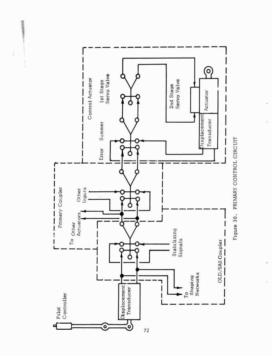
■CD

In this single-axis control system there will be no other actuations nor other inputs to the pitch actuator; however, the primary coupler is shown with a fan-out of the pitch command signal to provide for other actuators and a summing point to provide for inputs from other axes of control.
Mode Selection
Section 2 of this report describes the problems of flight control and the various degrees of pilot assistance: open loop damping, stability augmen- tation, and automatic flight control. These are available on command. Figure 3 1 shows a conceptual sketch of the pilot controller and the control mode selector. The control mode selector is the implementation of the Automatic Flight Control System selector panel shown as a number of switches in Figure 28. Since not all combinations of these switch positions are permissible combinations, the mode selector is controlled by a single lever which allows only the five permissible switch combina- tions shown.
The minimum level of flight control for normal operation is the stability augmentation system which permits pilot control with rate stabilization of the vehicle. The next higher level of flight control is the attitude con- trol mode. In this mode the rate stabilized vehicle is under automatic flight control from the attitude gyro with pilot option either to change the attitude reference or manually to override the Automatic Flight Control System. The highest level of flight control is the navigational control mode. In this mode the rate stabilized vehicle is under automatic flight control of a mission navigational aid in addition to the attitude gyro. The pilot, however, can change the automatic flight control reference or manu- ally override the Automatic Flight Control System. The two modes of flight control for emergency operation are the primary control mode and the open loop damping mode. As mentioned previously, the primary control is un- stable and is used only as a last resort. The open loop damping system shapes the pilot input signal and considerably improves vehicle handling qualities; however, since it does not respond to external disturbances, it is less desirable than the stability augmentation system.
Open Loop Damping
The mode selector switch serves to introduce either the OLD circuit or thn SAS circuit into the primary control through the OLD/SAS coupler. The performance requirements for this circuit are specified in Section 2 of this report and are summarized in Figure 28.
The circuit: to provide the open loop damping function is shown in Figure 32. This is a shaping network to provide a simple lag at T2 = 1 second and
73
11

Trim Switcn
Pilot Controller
. Control ^^__^^—j^Ac t u a t or
C 7
[_0, Open Loop Damping (Includes P)
__P, Primary Control Only
S, Stability Augmentation System (Includes P)
A, Attitude Control (Includes S) N, Navigational Control (Includes A)
For Emergency Operation
—For Normal Operation
Figure 31. CONTROL MODE SELECTOR
74

O
LD
+ o
N
O i—t
H Ü
D
Ö *
Q 5
O S
SI 2 a
CO
t-l
3 CT

washout for signal durations longer than T^ = 10 seconds.
The signal from the pilot controller displacement transducer is introduced into the circuit through a pair of in-line orifices to limit input flow. Next, a variable orifice is shunted across the two lines to provide a means for adjusting loop gain. The time constants are achieved using vortex induc- tance lag. The 10-second washout is attained using a vortex inductor in each signal line and feeding the vortex outputs differentially into a dif- ferential summing amplifier. The input signal is also fed directly into the summing amplifier in the opposite polarity. The two di'ferential signal levels are initially set for cancellation at steady-state conditions. This perfect cancellation occurs only over the low-frequency range for which the vortex inductors do not attenuate their output signals. Therefore, washout occurs from steady state to the 10-second break frequency of the vortex inductors. Above this frequency, cancellation does not occur in the summing amplifier, and the input signal is passed unattenuated.
The output from the first summing amplifier is fed differentially into a second set of vortex inductors of l-second time constant to provide wash- out above the l-second period. A final active amplification stage is pro- vided to compensate for the DC attenuation characteristics of the pressure shaping networks. The output of this final amplifier is supplied to the mode selection switch shown in Figure 28 and is available to be summed into the OLD/SAS coupler whenever the pilot engages the OLD mode of control. Note that the switch output feeds through a fluid limiter in order to meet the limited authority requirement p.aced on the stability augmentation functions.
The time constants for this shaping network were obtained by using the inductive property of a vortex. This particular selection was made be- cause (1) this mode has no moving parts and (2) the unit can be made quite compact to obtain time constants in the range of interest. An alter- nate approach is to use the inductive properties of a length of hydraulic line. With this approach,large diameters are required to obtain the low resistance to inductance ratios required. Another alternate approach is to use the capacitive properties of a shunt hydraulic accumulator across the two signal lines. To use this would require a double-action hydraulic cylinder with an internal, spring-centered piston. This approach involves problems with moving parts, seals, friction, and leaks. As can be seen, the vortex time constant seems to be the most trouble free.
Stability Augmentation System
In the stability augmentation mode the OLD/SAS coupler introduces the shap- ing network #2 and the attitude signal from the rate gyro, as shown in Figure 28 .
76
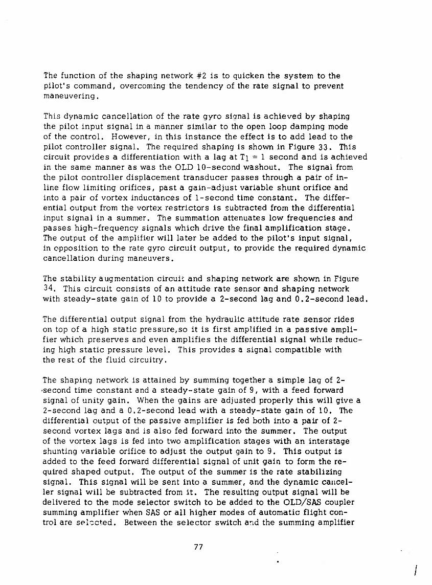
The function of the shaping network #2 is to quicken the system to the pilot's command, overcoming the tendency of the rate signal to prevent maneuvering.
This dynamic cancellation of the rate gyro signal is achieved by shaping the pilot input signal in a manner similar to the open loop damping mode of the control. However, in this instance the effect is to add lead to the pilot controller signal. The required shaping is shown in Figure 33. This circuit provides a differentiation with a lag at Ti = 1 second and is achieved in the same manner as was the OLD 10-second washout. The signal from the pilot controller displacement transducer passes through a pair of in- line flow limiting orifices, past a gain-adjust variable shunt orifice and into a pair of vortex inductances of 1-second time constant. The differ- ential output from the vortex restrictors is subtracted from the differential input signal in a summer. The summation attenuates low frequencies and passes high-frequency signals which drive the final amplification stage. The output of the amplifier will later be added to the pilot's input signal, in opposition to the rate gyro circuit output, to provide the required dynamic cancellation during maneuvers.
The stability augmentation circuii: and shaping network are shown in Figure 34. This circuit consists of an attitude rate sensor and shaping network with steady-state gain of 10 to provide a 2-second lag and 0.2-second lead.
The differential output signal from the hydraulic attitude rate sensor rides on top of a high static pressure,so it is first amplified in a passive ampli- fier which preserves and even amplifies the differential signal while reduc- ing high static pressure level. This provides a signal compatible with the rest of the fluid circuitry.
The shaping network is attained by summing together a simple lag of 2- •second time constant and a steady-state gain of 9, with a feed forward signal of unity gain. When the gains are adjusted properly this will give a 2-second lag and a 0.2-second lead with a steady-state gain of 10. The differential output of the passive amplifier is fed both into a pair of 2- second vortex lags and is also fed forward into the summer. The output of the vortex lags is fed into two amplification stages with an interstage shunting variable orifice to adjust the output gain to 9. This output is added to the feed forward differential signal of unit gain to form the re- quired shaped output. The output of the summer is the rate stabilizing signal. This signal will be sent into a summer, and the dynamic cancel- ler signal will be subtracted from it. The resulting output signal will be delivered to the mode selector switch to be added to the OLD/SAS coupler summing amplifier when SAS or all higher modes of automatic flight con- trol are selected. Between the selector switch and the summing amplifier
77

Di O
K )i
<
Cd
O
Ü
OH 4»
w o H ^ D 0)
i—i cn
H 5 2 ^ D-, CO
on CO
0) M
Di
78
■

u -f
CM + CM
^ CM
-Q -a ^iQd
)(
Ü
ÜN|Ü
W
C 2
CO
H i—<
CO
CO
0)
79

.
there Is a limiter to insure that the SAS input to the summer is of limited authority.
Components of the Primary Open Loop Damping and Stability Augmentation Systems
Displacement Transducer
This mechanical-to-fluid interface to convert the pilot's controller output to a hydraulic signal is shown in Figure 35. It is a valve in which a slid- ing member varies a pair of orifice areas in inverse relationship. These orifices divide the flow from a constant pressure source to two outlets. The two outlets direct flow to the control ports of a fluid amplifier. In this way a differential pressure signal which is porportional to the valve slider position is impressed on the fluid amplifier control ports.
An analysis of this component has shown that a linearity deviation of 1/2 of 1 percent occurs when the orifice sizes have changed by + 0.376 of the center position area. Thus, the linearity is sufficient for the primary control application specified in Table III. Curves showing gain and linearity are given in Figures 36 and 37.
Hydraulic Analog Amplifier
The configuration of the hydraulic analog amplifier is essentially the same as its pneumatic counterpart, although some differences in internal dimen- sioning are made to reduce viscous losses to improve the performance with oil.
Fluid amplifiers exhibit performance degradation with reduced Reynolds num- bers. The reduction in performance change is due to pressure losses in channels. It would be expected, therefore, that low pressures, leading to low flow velocities and laminar conditions, and high viscosities will attenu- ate the performance. All of these stem from the fact that fluid amplifiers operate in flowing systems. The output pressure, even in a fluid amplifier that drives a load that has no flow, is the result of a pressure recovered from a velocity. In valve systems the response may be sluggish due to the slow fluid velocities;but with a non-flowing output, the output pres- sure can approach that of the supply. In fluidic systems the velocity of the power jet may be severely reduced from the expected value by low pres- sures or high viscosity. As a result, the recovery pressure in the receivers will be reduced.
80

ü Q CO 2:
w
w Q
LO
CO
81
/i

Figure 36
V^2 ^supply
P1 = Left Output (To Orifice ) P2 = Right Output (To Orifice )
= Supply Pressure Am = Orifice Area at Mid
Position A= Orifice Area at Any
Position
DISPLACEMENT TRANSDUCER CHARACTERISTIC 82

Percent Deviation of Differential Pressure Signal From A Linear Pressure 1 +
I i
f i
IT 00
I
öS o
f CM
-I -~P
Displacement Relationship
CO
o
I
Figure 37. PRESSURE DISPLACEMENT CHARACTERISTICS OF DISPLACEMENT TRANSDUCER
83

An example of a specific amplifier performance is given in Figures 38 and 39. For this example, a worst case is chosen. First, the amplifier is a center dump unit specifically designed for turbulent condition performance. Second, the loads are orifices equal to the control nozzle sizes at the end of long narrow channels.
The basis for operation of the center dump amplifier is that the uniform velocity across the exit of the power nozzle becomes triangular down- stream at the receivers, Reference 10. The receivers "see" the pressure level at their locations. A very steep slope in the velocity profile yields high gain. As the pressure drops and the fluid viscosity increases, the velocity distribution at the nozzle exit becomes triangular because of high losses along the power nozzle walls. As a result, the velocity gradient at the receivers becomes less pronounced and the gain is reduced. Also, the low pressure and high viscosity increase the losses in the receiver channels, further decreasing the amplifier performance.
The solid curve in Figure 38 shows the ainplifier performance on 5606 oil, a light aircraft grade. Note that the supply pressure must be increased to about 200 psi before a stable gain is obtained. Above 200 psi the gain is not sensitive to supply pressure.
Increasing the viscosity by using a heavier oil and then reducing the oil temperature gives a spread of performance at 50-psi supply pressure from a gain of about 2.5, at a viscosity of 10 centipoises to a gain of less than 0.5 at a viscosity of 200 centipoi. es. These data are plotted in Figure 39 with extrapolated values for 100 and 300 psi.
For reference, the viscosity of 5606 oil is about 10,000 centipoises at -65F, a startup specification. As a result of this startup specification, single splitter amplifiers (such as Figure 6) increased receiver channel sizes, shorter power nozzles, and high pressure operation will be required. With these modifications it is anticipated that -65F operation can be achieved at 300 psi.
Pneumatic fluid amplifiers are linear within + 1 percent and have a 5 0-to-l signal-to-noise ratio. Hydraulic fluid amplifiers have substantially the same linearity but better signal-to-noise ratio. Values of 600-to-l have been measured. The required 200-to-l range for the stability augmentation system seems more easily achievable in a hydraulic circuit than in a pneu- matic one. This figure is derived from the specifications for the rate gyro. Table V. Since the rate gyro signal must be amplified, the amplifier must not degrade the information. The rate gyro has a required range of 4 0 de- grees per second and a threshold of 0.2 degree per second. The resultant signal noise ratio is 200 (40 r 0.2).
84

700.
600-
500--
a 40Of
+ DM
p 3004- a
QJ u
0) N g 2004-
0)
o OH
100-.
/
®
2190 Oil @ 85F /i= 175 cp
-2190 Oil @ 105F yu= 80 cp
2190 Oil @ 140oF yu = 35 cp
5606 Oil @ 80° ro 110oF
yu = 10 cp
Hydraulic Fluid Amplifiers (2614) Power Nozzle Size .020 x .040 inch
0 12 3 4 Pressure Gain
Figure 38. GAIN AS A FUNCTION OF SUPPLY PRESSURE FOR A CENTER DUMP TYPE HYDRAULIC ANALOG AMPLIFIER
85

a,
D Q cc w H S UJ
U oi O UH
CO —
u -^ 1—1 ^H H ^
Ul W oj a; 01 2- 0 H w a ü ^
■^ rf t^ 4-» J •—' C a HJ 0) S Q- U
^ Ü U; <o 0 u
0^ IJl y ^ > g<
co U CO 3 a: P ^ ^
1 Q >H >H H X t—i
CO 0 U CO ►—1
>
(D CO
(U u. 3 CT
[iH CO CSJ
86

The frequency response of the 20-by-40-mil size amplifier is in the order of 1 kilocycle. The transport time for this amplifier with a hydraulic supply pressure (P+) of 300 psi is approximated by a time delay of 0.0005 second.
Hydraulic Summing Amplifier
The summing amplifier configuration is the same as the amplifier discussed above except that two pairs of control nozzles are used to sum two differ- ential pressure signals. A silhouette of this type of amplifier is shown in Figure 40.
The accuracy of the summing amplifier depends to a large extent on the relative bias levels of the two pairs of signals. Correctly biased, a summing accuracy of 5 percent can be achieved. This figure represents the maximum deviation of the differential output pressure from the computed value compared to the maximum differential output. Future development may increase this accuracy to an estimated 2 percent. The 2-percent ac- curacv is suitable for summing the primary signal with the open loop damp- ing or stability augmentation signals. (See Tables IV and V for characteristic linearities of existing systems.)
Fluid Limiter
The limiting function is accomplished through the use of a saturating am- plifier (Figure 4l). A saturating amplifier is a pressure amplifier in which the saturating characteristic is obtained at some sacrifice of gain. The saturating effect is produced by limiting the pewer jet deflection so that at maximum deflection the newer jet is directed at one of the receivers. This is accomplished by introducing the control signal at an angle less than perpendicular to the power jet. Since only a vertical component of the control signal jet momentum acts to deflect the power jet, the result is low gain and limited deflection. The selected power jet pressure deter- mines the maximum output signal available from the amplifier.
The dynamic response of this amplifier with 20-by"40-mil nozzle sizes would be in the order of 1 kilocycle. The transport time with a hydraulic supply pressure of 300 psi is approximated by a time delay of 0.0005 sec- ond.
Hydraulic Rate Sensor
In the vortex rate gyro the flow of fluid is radially inward through a drive ring to the axial exit ports at the center. When the sensor is turned, the drive ring imparts a tangential component of velocity to the flow. The function of the vortex flow field is to amplify the tangential component of velocity. Since, by the law of conservation of angular momentum, the
87

+ r ^ —
t f? XZ 1 APcl = Differential Input 1
P6+
Apc2 = Differential Input 2
^PQ = Differential Output P+ = Supply Pressure
^pc2
APcl 1
Silhouette
AP cl
Figure 40. SUMMING AMPLIFIER CHARACTERISTICS
88

P+ = Supply Pressure P^,, = Control Pressure
C A P = Control Pressure pCB r-OA = Output Pressure
OB - Output Pressure AP^=P^A-P^D = Control Differential
C UA ÜB _ Pressure
APn=PnA-Pnn = Output Differential U UA UD _
Pressure
Increasing P CB Increasing P
(Single Sided Operation) CA
Figure 41. DIFFERENTIAL OPERATION OF LIMITING AMPLIFIER
89

product of tangential velocity and radius remains constant, the tangential velocity increases as the center is approached. The effect is a spin of the fluid column in the outlet. The amplified velocity can be readily detected at the output by sensing the helix angle of flow in the output or by measuring the tangential component of velocity. The method of detec- tion is a prime consideration. Other appropriate design compromises, to meet the specifications, include the selection of
1. Diameter of the vortex flow field.
2. The height of the unit.
3. Exit diameter.
4. Flow.
Referring to the specifications,
1. High response requires a small diameter and/or high flow.
2. The threshold level is degraded with increasing flow rate, since more turbulence is generated.
3. A high gain, psi per radian per second, requires a large diam- eter.
Preliminary calculations indicate that the unit will have a 2-inch diam- eter, a 0.040-inch height and a flow of 2.0 gpm. The pressure drop across the unit will be about 100 psi. This unit will have a response of 0.002 second, or about 100 cps under these conditions, which will meet the response requirement of Table V .
A major consideration is the type of detector used. Limiting our discus- sion to unclassified techniques, the following comments are appropriate. Angle-of-attack detectors to sense the helix angle of flow in the outlet pose significant problems because of the small port sizes inherent in such detectors. It is imperative that detector techniques be used that accept a larger portion of the total flow. One approach is described below.
This detector is composed of a slot in the exit tube and downstream, the slot and the receivers being in the same arrangement as in a fluid analog am- plifier. The direction of flow issuing from the slot, a nozzle, is affected by the spin in the exit tube. This results in an associated output differ- ential pressure,/^ , in the pair of receivers downstream. The threshold level obtained from air tests of this detector was measured at 0.01 degree
90

per second. Again, this detector utilizes a large portion of the flow from the sensor compared to the wing or tube type flow angle detectors.
A major problem in all fluid sensors with a small-time response is the threshold level, which in this case is specified at 0.2 degree per sec- ond (Table V). The'threshold is determined by flow turbulence. The major source of noise is in the inlet flow condition. The fluid manifold must be designed to attain a dynamically uniform condition at the drive ring. The frequency of the noise is a major consideration. Since most of the noise is systematic, of sinusoidal nature, the frequencies above the response regime can be averaged without destroying the signal. Because of the small size of the unit and the high flow velocities, it is expected that the noise will be well above 100 cps. This can be filtered without destroying the information frequency range required.
However, the threshold will more likely be limited by the amplifiers. With a specified threshold of 0.2 degree per second and a range of 40 degrees per second, the implied noise-signal ratio is 0.2/40 or 0.5 percent. The normal amplifier noise-signal ratio is about 2 percent. Therefore, dif- ficulties in meeting this specification should be expected.
The drive ring of most units has been of porous materials or wire mesh. These are, in effect,filters. Contamination will affect the flow distribu- tion through the wall; this will result in output noise and eventual degra- dation of the system gain and response. A unit with a radial vane drive ring is suggested. The spacing is to be compatible with subsequent fluid circuitry so that no portion of the system will aggravate contamination conditions.
Shaping Networks
The implementation of shaping networks requires the use of capacitive or inductive impedance with resistance. In compressible fluid systems a volume and associated resistance serve as a mechanism to store energy. In hydraulic systems the vortex flywheel provides an energy storage mechanism.
A vortex unit is shown schematically in Figure 42. The measure of per- formance of this unit is the dynamic relationship between the output flow resulting from an input pressure, P^. It can be shown that the vortex characteristic is
^Vo G V2 = Exit: velocity A p = TS + 1 Pi = Inlet pressure
1 T = Time constant G = Gain S = d/dt, time-wise differentia-
tion 91

Figure 42. VORTEX INDUCTIVE LAG
92

where
u 1 . a2 ,,
C2 + a-7 K2
T a2 = 2KV —V G v aiz
For example,
If ?! = 100 psi
P2 = 40 psi ai=a2 = 0.0008 in2
t = 0.080 in rl = 2 in r2 G T
= 0.020 in. , 4 54 m/sec. 4•0H psi
= 3.94 sec.
Therefore, the unit assumed has a time constant of 3.94 seconds in a reasonable size, indicating the practicality of using the vortex lag in shaping networks.
Hydraulic Actuator
The actuator is envisioned as an assembly including servo valve and feed- back device. The feedback device may be either mechanical or a fluid transducer similar to the input transducer (see Figure 35) and built into the actuator. The servo valve may be either single or double staged. The single-stage valve,, spool type, requires high driving pressures, which in turn demands high fluid amplifier operating pressures with consequent high power consumption. By utilizing the gain of a two-stage servo valve, a more economical use of control power is attained.
There are no theoretical reasons why an actuator of this type cannot be made to equal the performance of presently used power boost or electrically con- trolled actuators.
Response of the Primary, Open Loop Damping and Stability Augmentation System
The system specifications for the stability augmentation system, which were obtained from electronic system requirements, give a maximum phase shift of 10 degrees at 1 cycle per second for the rate sensor, followed by
93

a shaping network that attenuates high frequency response after 1 cycle per second (see Tables V and VI). In total, therefore, the combination of rate sensor and shaping network have a phase shift of 55 degrees at 1 cycle per second.
The response of the SAS will include an estimated 10 amplifiers, or equiva- lent, and the rate sensor (see Figure 29).
The estimate rate sensor response is about 0.002 second (see page 90). If we assume 10 amplifiers at a delay of 0.0005 second, the total am- plifier delay is 0.005 second. The system la., from the rate sensor to the SAS servo is 0.007 second. The resulting phase shift is 2.52 degrees at 1 cycle per second, which is much better than required.
It is interesting to note that the implementation with fluid computation can- not be considered on a one-for-one basis with the electronic system, since the transmission and amplification in the fluid system take appreciable time.
Regrouping of requirements is necessary. Appendix III gives additional details on fluid element response characteristics.
Operational Factors
The most critical factor in fluid system operation is the sensitivity to dirt accumulation. High-pressure hydraulic systems will no doubt work at a distinct advantage, having high fluid momentum to carry particles away. The saving point is that the minimum port size in hydraulic fluid systems will be large. Particles, because of filters now in place, will be much smaller than the minimum port sizes. The infant mortality will no doubt be most critical, since particles lodged in the system at startup will be large enough to cause failure.
Once a failure has occurred, it may be possible to back-flow the circuits while in place, but replacement appears preferable. The circuits should therefore be easily replaceable. Cleaning, once they are removed, is feasible.
Cold start might cause difficulties; but since the oil temperature is adequate for current systems, it appears likely that it will be adequate for fluid systems.
The installation design should place the fluid circuits contiguous to the hottest location in the hydraulic system; e.g. , pump regulator discharge. The circuits should be of heat-conductive material and should be mounted so that there is a maximum heat conduction. This will alleviate warmup or freezing difficulties.
94

The fluid circuits will have to be submerged. This does not mean that they must be located in the bottom of the sump, but only that the drain arrange- ments must prevent air from reaching the amplifier interaction region.
The critical components of the fluid system are the orifices and fluid ele- ments. These should be in integral housings isolated by filters from the power system. The parting line should be between the filters and power supply. In such a construction the replaceable fluid circuits can be pro- tected to a maximum extent during assembly.
Another necessary feature is pressure test points for troubleshooting. These should not enter the fluid circuit directly but should also enter through a filter.
These considerations define a modular circuit construction with filtering, mounted on a manifold block contiguous with the return hydraulic flow line. The manifold and circuit will be contained in a jacke^possibly with quick disconnects brought out for circuit checks.
AUTOPILOT SYSTEM
The autopilot control system performs the functions related to navigation and mission requirements. These functions are shown in the lower half of Figure 28.
The primary component of the autopilot is the attitude hold control. In the proposed system, the attitude reference is derived from an integration of a rate gyro signal. This integration is performed by converting the sen- sor signal to a pulse rate and subsequently counting pulses - a digital integration - to measure attitude.
The following section describes the basic concept of this approach; tech- niques for resetting the reference or command attitude; and a technique for "erecting" the attitude gyro as drift occurs.
Attitude Control
The first element of the fluid attitude hold circuit is the vortex rate sen- sor shown schematically in Figure 43. In this device fluid enters through the drive ring which imparts the sensed angular velocity to fluid as a tan- gential velocity. As the fluid spirals into the center outlet,this tangential velocity is increased through the principle of conservation of momentum. Pickup probes in the outlet sense the spin of the fluid and deliver a push- pull output pressure proportional to the input rate of turn. When
95

-.
* 0
Figure 43. VORTEX RATE SENSOR Schematic Diagram
96

no rate of turn is applied, the two output legs have identical pressure levels If an angular rate is applied, the output pressure from one leg will increase while the other will decrease. If the rate of turn is applied in the opposite direction, the output pressure differential will be reversed. The pressure and flow levels of this signal are extremely small. Experience has shown that considerable distortion and loss of resolution would result if this sig- nal were amplified with proportional amplifier stages due to inherent signal- to-noise ratio limitations. Maximum retention of signal information is achieved by converting the two pressure signals into frequency signals through the use of a pair of pressure controlled oscillators (PCO). Once the pressure signals have been converted to frequency signals (also of a very low level), the frequency signals can be amplified to a useful level with a pair of proportional amplifiers (AMP). Any distortion in the ampli- fication process will only distort the wave shape; it cannot alter the fre- quency which is now the carrier of the desired information.
In the digital attitude control system each output leg of the vortex rate sensor is coupled directly to a pressure-controlled oscillator. Figure 44 shows a portion of the attitude hold circuit. Each pressure-controlled oscillator operates at a frequency proportional to its probe pressure. There- fore, there is a direct correlation between the input rate, in degrees per second, and the difference frequency, in cycles per second, at the output of the oscillators. The difference count rate is a measure of the input rate in degrees per second. The total difference count is a measure of the angular deflection, since the difference counts are proportional to the degrees of deflection. Note in the example of Figure 44 that the pressure pulses at the output of the pressure-controlled oscillators are uniform until a rate of turn is applied. With rate applied, one frequency increases, the other decreases. The total count difference of one, generat- ed over this period, is related to an attitude change by the system gain.
The difference count is measured by continuous subtraction of two parallel binary counters or by a single counter that has the ability to count up or down,depending on the sign of the input signal. A device which can count up or down (add or subtract) is termed an up-down counter. In either case the output will be a binary code which will indicrte the direction and mag- nitude of the course error. The error counts are then fed through a posi- tion control circuit to a digital autopilot servo actuator which then pro- duces corrective signals through the pilot's control stick (see Figure 19).
In the system described above, the counters form thj attitude register, producing error signals when there is a deviation from the preset attitude.
A method of changing the preset attitude is indicated in Figure 45 in the form of a force transducer controlled by the pilot's stick. In the autopilot
97
'l

Pressure 9 Total Count;
10 Total Count:
PCU | Counter
* tm —^
t PCO rionntpr i
"
Count Difference (Attitude Error)
Figure 44. ATTITUDE SENSING BY FM INTEGRATION
98

o
-a 3
M u
M w a: w Q ID H
U H >—t a,
O w Ü <
Ü
0) IM a
99

mode the pilot's control is made stiff by engaging the brake shown in Figure 18. This allows the pilot to apply a force with little movement to the force transducer. The transducer produces fluid signals related to the magnitude and sense of the force applied. These signals gate pulses to drive the up or down counter, depending on the sense of the force, to change the net count in t; ? counters. The pulse rdte depends on the ap- plied force,and the total attitude changes depend on the duration of the applied force. Thus, the force is integrated with time to produce the attitude reference change. This trimming is described for a control force steering. The manual trim can be introduced in the same manner.
The same technique is proposed to correct for gyro drift. The highly damped pendulum circuit shown in Figure 46 is a drift compensating circuit. The pendulum is the reference, and the pendulum case is maintained at the atti- tude stored in the attitude register. Any error between the pendulum and its case introduces slow corrective counts. These counts are fast enough to correct drift, yet slow enough to avoid ^nror buildup due to acceleration forces acting on the pendulum, a standui .echnique use for erection.
Velocity signals from the doppler radar can be introduced to the fluid system in the same manner.
Autopilot Circuit
The foregoing has described briefly the basic technique for implementing the fluid autopilot attitude control. Figure 28. This system includes the attitude sensor (an integrated rate technique); techniques for resetting the reference by pilot input, erection system, or navigational aids; and a digital autopilot servo.
The introduction to this section has shown that the autopilot should use air as the working fluid because of the large number of units and the attendant high power consumption if hydraulic fluid were used.
The following is a description of the fluid autopilot. The circuit block diagram is shewn in Figure 47. The basic functions performed by this circuit are attitude sensing, attitude reference control, coupling-to-navi- gation aids, and trim functions. The output of this circuit drives the auto- pilot servo actuator. Figure 19.
Attitude Gyro
The attitude sensing function is depicted in Figure 28 as the attitude gyro block, with attitude angle 0 as the input and signal H as the output. In the circuit diagram (Figure 47),the attitude angle is determined by the
100

i—I
U O cc >H
0 w Q
H )—I
H H <
<X3
0) 3
101

(o) f
I» s a
K B
III 4 a
is
(I J do do TT TT
II
rH :? «
1 I
[TE
i
s I
3
s
^
^
•mm
< Ü
Q
ü O CQ
H o H-l 1—C
OH
O
<
1^ T
a>
102

integration of angular rate of pitch as described in page 120. The attitude error is the output of the H register which includes the up-down counting function.
Attitude Reference
A pendulum is used as a long-term reference to correct the H register for slow rates below the threshold of the attitude gyro. The output of the H register drives the pendulum rotation actuator to position the pendulum case to the angle corresponding to the binary coded attitude signal. If this is the true attitude, the pendulum will plumb down the center of the case. Any error will cause the pendulum to lie closer to one wall than the other. This will generate a pendulum position error signal which will introduce a slow corrective count into the H register. As has been shown, the atti- tude has been sensed and transformed into a compatible fluid signal in the form of the binary coded output of the H register.
One technique for changing attitude reference is indicated in Figure 28. The pilot controller force transducer drives an integrator when the autopilot switch is in the "on" position. The effect is that a pilot input force, Fp, produces a signal, Ji, which is then introduced into the integrator as a time rate of integration. As long as the integration rate signal is present, the output, J, of the integrator changes by the prescribed rate. This out- put signal is the attitude reference change signal. In Figure 47 the ligital force transducer is depicted as a device which puts out stepped signals proportional to the applied force level. These signals are fed into a force integration rate logic whose output is a pulse rate proportional to the force level input. The J register, another up-down binary counter, is the atti- tude reference integrator. The difference count stored in the J register is the binary coded form of the attitude reference. The pulse rate output from the force integration rate logic is fed into the J register to change the stored count, thereby changing the attitude reference.
Navigation Coupler
The function of coupling to navigational aids is depicted in Figure 28 as a navigational aid input feeding into a navigation coupler. The various navigational aids are given in Table I . In general, the navigation aids are electronic sensing devices, and in order to make them compatible with the digital fluid circuitry they are connected to two-line fluid interfacing devices. One signal line generates a fluid frequency signal proportional to a positive error sensed by the navigational aid, the other line generates a fluid frequency signal proportional to a negative error sensed by the navigational aid. The circuit is arranged such that only one line transmits a frequency signal at a time; and further, for no sensed navigational error, the frequency output from both lines is zero. Note that this performance is somewhat different from that of the attitude gyro. The attitude gyro
103

produces a frequency output on both lines at all times, and both outputs would change (one increasing, the other decreasing) for any sensed angular rate of pitch.
The navigation coupling circuit, shown in figure 47, consists of taking the frequency signals and putting them through a pulse former and syn- chronizer to make them compatible with the rest of the autopilot circuitry. The output pulses from the pulse former and synchronizer are fed into the J register, which in the navigational mode becomes a general reference register and accepts inputs from either the navigation coupler or the pilot controller force transducer.
Timing Pulse Generator
At this time it becomes necessary to mention one component required by the digital logic which was not mentioned in the system functional require- ments; namely, the timing pulse generator and pulse sealer, or, as it is more commonly known, the clock. A clock is required in this type of digital circuitry for several functional reasons. First, it establishes pulse rates as references for digital integration rates or digital actuation rates. Next, it establishes a single source of well-formed, controlled width and amplitude pulses to assure the proper operation of the various digital elements. Finally, it serves to synchronize the operation of all the circuit elements and thereby prevent loss of count which might otherwise result from the appearance of coincident pulses.
The clock sends out alternate up and down count pulses at the following pulse rates: 100, 50, 25, 12.5, and 0.4 pulses per second. These are sent to the various synchronizer, integration rate, and actuation rate cir- cuits to establish the four levels of integration and actuation. The 0.4- pulse-per-second rate is required only by the pendulum long-term refer- ence and limits the rate at which the pendulum can apply a correction to the H register.
Compare Circuits
Another function not explicitly specified in the functional requirements of Figure 28 is the comparison and pulse gating logic. This function is shown schematically in Figure 28 as the error summing points. With digital logic the error summation function becomes a comparison function as shown in Figure 47. The contents of the H register (binary coded attitude signal) are compared with the contents of the J register (binary coded attitude reference signal) in the compare circuits. Any inequality will open one or more of the pulse gates and deliver a train of correcting pulses to the autopilot servo actuator. The correcting pulses are delivered at a rate
104

proportional to the error with a maximum rate of 100 pulses per second for an error of eight binary bits or greater. The correcting pulses sent to the autopilot servo are also sent to the J register where they work to reduce the comparison error to zero. Thus, by c osing the loop we obtain an autopilot servo actuator displacement proportion to error count.
Autopilot Servo Actuator
The autopilot servo actuator is a form of digital stepping actuator. It con- sists of an eight-stage up-down binary counter to store the binary coded position; eight actuator drivers to power the eight digital actuator stages; and an eight-stage digital actuator. The details of the actuator will be discussed in a later section, but let it suffice to say that it consists of eight pistons operating in an additive fashion such that each contributes an effective stroke equal to its binary coded weight. The actuator exten- sion is proportional to the count stored in the binary position counter.
Slow Trim
There are two additional techniques for introducing an attitude reference change, both originating from a pilot command: stick rate trim (slow trim) and stick position trim (quick trim). These are operative only when the autopilot functions (Automatic Flight Control Modes) are not operative.
Slow trim can be described as the mode wherein the pilot releases the con- trol stick and merely presses the trim switch (at the top of the control stick) in the desired direction of trim. So long as the pilot depresses the trim switch, the control stick will slowly move in that direction at constant speed. When the desired trim is attained, the pilot releases the switch.
Quick Trim
Quick trim can be described as the mode wherein the pilot, not being satisfied with the force-free control stick neutral position, grasps the control stick and displaces it to a position of satisfactory trim. If at this moment the pilot would release the control stick, the vehicle would return to the unsatisfactory trim condition, since the control stick would return to its original position. Instead,the pilot presses and releases the quick trim button. In doing so, he has established a new, force-free , neutral position in the present stick location. Upon release, the control stick remains in the new trimmed position.
These two trim modes are shown in Figure 47. The slow trim is achieved by gating a slow pulse rate (21.5 pulses per second) into the autopilot servo actuator. Therefore, the servo actuator moves at a steady rate. The
105

quick trim is achieved by gating the output from the force integration rate logic directly to the autopilot servo actuator. When quick trim is required, the pilot is holding the control stick against a restoring force. The force transducer senses this force and sends out an integration signal. Pressing the quick trim button gates this integration signal to the autopilot servo actuator in such polarity as to move the actuator to relieve the stick force . When the stick force approaches zero, the force transducer turns off the integration signal. Hence, the autopilot servo, driven by the output of the force transducer, has moved such as to establish a new force-free null at the present stick position.
Autopilot Subc.i.rcuits
The foregoing has described in general terms the operation of the autopilot system. The objective of the following is to describe in detail the proposed implementation of the autooilot. This description will include the follow- ing items:
Pilot Controller Force Transducer Force Integration Rate Logic Navigation Coupler Pulse Former and Synchronizer Timing Pulse Generator Circuit Trim Circuits Attitude Gyro Circuit Attitude Reference Integrator Compare Circuitry and Pulse Gating Logic Autopilot Servo Actuator Pneumatic Digital Elements Pneumatic Actuator Pendulum Assembly Autopilot Response Operational Factors
Pilot Controller
The mechanical implementation of the pilot controller is shown in Figure 48.
The pilot controller is a linkage with a fixed pivot and is thence connected to the displacement transducer and thereby over the control actuator. The displacement transducer requires little or no force to move or to hold in position. All the pilot controller forces are generated by the second link- age train shown.
106

w 1-1
9 H
O Ü
O
o I—I H <
w
i—t
< ü
2
00
u 3
W^^v
107
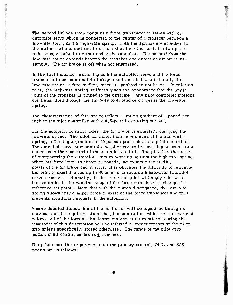
The second linkage train contains a force transducer in series with an autopilot servo which is connected to the center of a crossbar between a low-rate spring and a high-rate spring. Both the springs are attached to the airframe at one end and to a pushrod at the other end, the two push- rods being attached to either end of the crossbar. The pushrod from the low-rate spring extends beyond the crossbar and enters an air brake as- sembly. The air brake is off when not energized.
In the first instance, assuming both the autopilot servo and the force transducer to be inextensible linkages and the air brake to be off, the low-rate spring is free to flex, since its pushrod is not bound. In relation to it, the high-rate spring stiffness gives the appearance that the upper joint of the crossbar is pinned to the airframe. Any pilot controller motions are transmitted through the linkages to extend or compress the low-rate spring.
The characteristics of this spring reflect a spring gradient of 1 pound per inch to the pilot controller with a 0.5-pound centering preload.
For the autopilot control modes, the air brake is actuated, clamping the low-rate spring. The pilot controller then moves against the high-rate spring, reflecting a gradient of 20 pounds per inch at the pilot controller. The autopilot servo now controls the pilot controller and displacement trans- ducer under the command of the autopilot control. The pilot, has the option of overpowering the autopilot servo by working against the high-rate spring. When his force level is above 20 pounds, he exceeds the holding power of the air brake and it slips. This obviates the difficulty of requiring the pilot to exert a force up to 80 pounds to reverse a hard-over autopilot servo maneuver. Normally, in this mode the pilot will apply a force to the controller in the working range of the force transducer to change the reference set point. Note that with the clutch disengaged, the low-rate spring allows only a minor force to exist at the force transducer and thus prevents significant signals in the autopilot.
A more detailed discussion of the controller will be organized through a statement of the requirements of the pilot controller, which are summarized below. All of the forces, displacements and rates mentioned during the remainder of this description will be referred ^c measurements at the pilot grip unless specifically stated otherwise. The range of the pilot grip motion in all control modes is + 2 inches.
The pilot controller requirements for the primary control, OLD, and SAS modes are as follows:
108

1. The pilot initiates all commands by positioning the pilot con- troller which in turn moves the displacement transducer.
2. The pilot controller exhibits a low spring gradient of 1 pound per inch.
3. At any force-free null position, the pilot controller will be cen- tered by a 0.5-pound preload force. This centering force is necessary to prevent the stick from moving under its own weight or under acceleration forces.
4. The pilot controller can be slow trimmed at a constant rate of 0.25 inch per second.
5. The pilot controller can be quick trimmed by displacing it to any position and establishing a new force-free null at that position. It is estimated that to change the null from centered stick to hard-over stick might take 3 seconds.
6. The automatic flight controllers initiate all normal commands through the displacement of the autopilot servo actuator. The autopilot servo actuator is connected to the base of the pilot controller, which in turn is connected to the pilot controller displacement trans- ducer. A displacement of the autopilot servo actuator moves both the pilot controller and the displacement transducer. It is the output of the displacement transducer which becomes a com- mand input to the control actuator in all instances.
7. The pilot at all times has the option of overriding the automatic flight modes by overpowering the autopilot servo forces on the pilot controller.
8. The pilot can change the reference set point with a pilot controller force input which is sensed by the force transducer.
9. In order to isolate the functions of the force transducer, require- ment 8, and the displacement transducer, requirement 2, the pilot controller need have a high spring gradient of about 20 pounds per inch during autopilot modes. If this were not true, any attempt to change the attitude leference set point by way of the force transducer would also appreciably change the attitude directly through the displacement transducer.
The controller configuration with the clutch disengaged clearly meets requirements 1,2, and 3.
109
/

!
The slow trim feature, requirement A, is the ability to change the null positiOii transducer output by changing the length of the servo, Figure 47. Depressing the slow trim switch gates pulses to the servo actuator to ex- tend or retract as required.
For quick trim the low-level force in the force transducer plays a part. When the pilot controller is forced against the low-rate spring, this force is transmitted through the force transducer. When the quick-trim button is pressed, the force transducer integration logic sends a train of pulses to the autopilot servo, causing it to change its length to relieve the spring force and thereby locating a new force-free null at the present stick posi- tion. The trim functions, requirements 4 and 5, for primary control OLD and SAS modes are therefore met by the configuration.
The requirement for autopilot control, requirement 6, is clearly met by the system with the clutch engaged. A slipping clutch meets requirement 7. To meet requirement 8 the force transducer has an input idnge of + 2 pounds force which corresponds to a maximum integration rate (measured as pilot controller velocity due to autopilot servo extension) of + 2 inches per second.
For the sake of completeness at this point, it becomes necessary to de- scribe an alternate method of changing the reference set point. The cir- cuitry. Figure 47 , is so designed that the reference J register will always follow the attitude H register when the autopilot functions are not engaged. This characteristic provides bumpless switching into or out of autopilot control. Therefore, the pilot can use this property for his benefit by momentarily switching out of autopilot mode, manually navigating to the new reference condition, and reengaging the autopilot mode. In this fashion, the autopilot will hold the vehicle attitude existing at the instant of switching.
The requirement for isolation, requirement 9, is demonstrated as follows: with a pilot controller spring gradient of 20 pounds per inch and a force transducer range of + 2 pounds, an initial application of maximum force will only cause 0.1-inch deflection of the pilot controller,which is 2.5 percent of the + 2-inch range of the displacement transducer. The inte- grated output of the force transducer will generate maximum error signal to the autopilot servo. Hence, through the extension of the autopilot servo at slewing velocity, the pilot controller will be moved at the rate of 2 inches per second so long as the pilot force remains. The initial pilot controller displacement is equivalent to the force integration for a 0.05- second period which is "less than the twinkling of an eye" (beyond the pilot's visual perception, hence beyond his ability to respond).
110
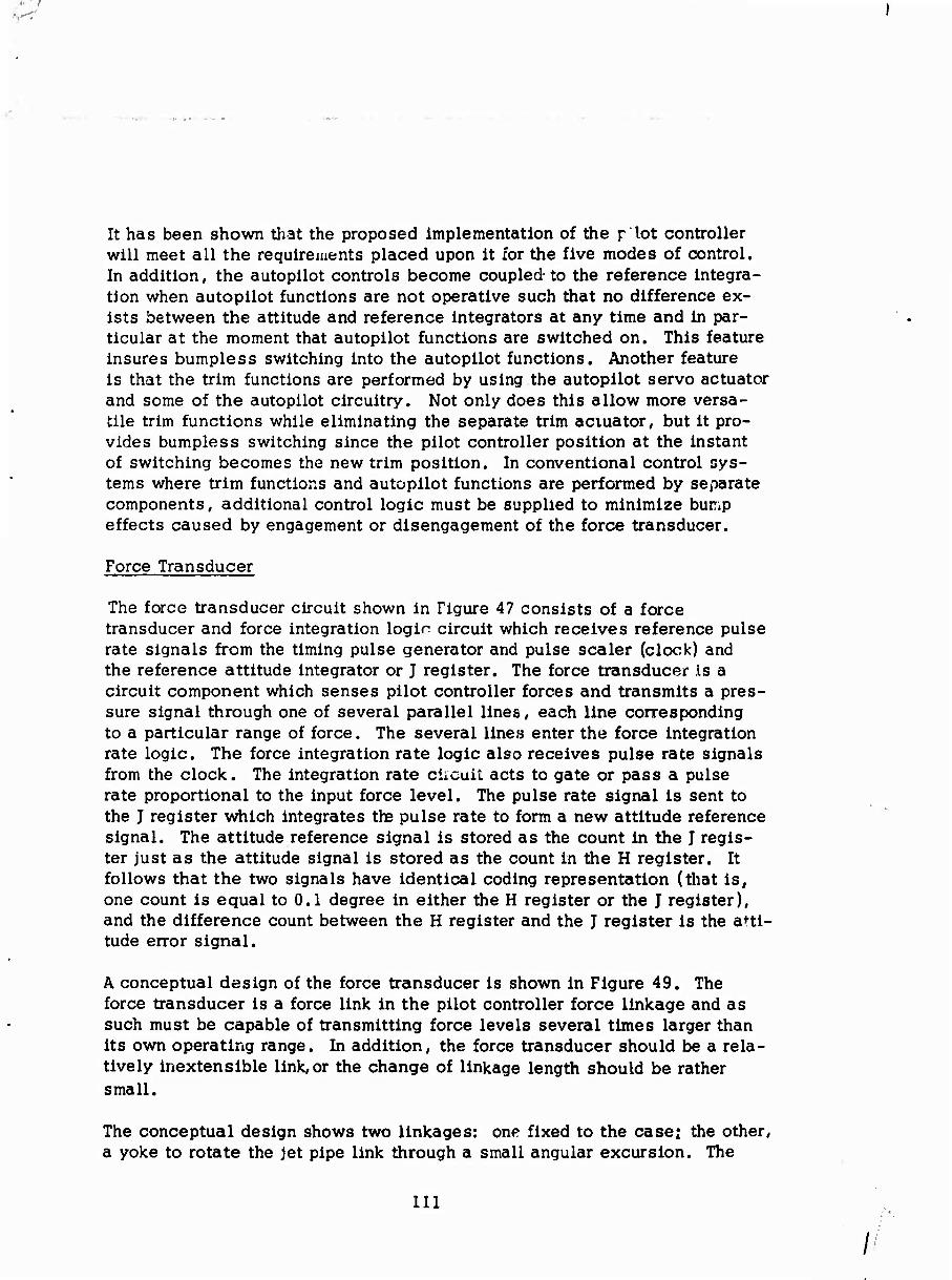
It has been shown that the proposed implementation of the F lot controller will meet all the requirements placed upon it for the five modes of control. In addition, the autopilot controls become coupled to the reference integra- tion when autopilot functions are not operative such that no difference ex- ists between the attitude and reference integrators at any time and in par- ticular at the moment that autopilot functions are switched on. This feature insures bumpless switching into the autopilot functions. Another feature is that the trim functions are performed by using the autopilot servo actuator and some of the autopilot circuitry. Not only does this allow more versa- tile trim functions while eliminating the separate trim actuator, but it pro- vides bumpless switching since the pilot controller position at the instant of switching becomes the new trim position. In conventional control sys- tems where trim functions and autopilot functions are performed by separate components, additional control logic must be supplied to minimize bump effects caused by engagement or disengagement of the force transducer.
Force Transducer
The force transducer circuit shown in Figure 47 consists of a force transducer and force integration logir circuit which receives reference pulse rate signals from the timing pulse generator and pulse sealer (clock) and the reference attitude integrator or J register. The force transducer Is a circuit component which senses pilot controller forces and transmits a pres- sure signal through one of several parallel lines, each line corresponding to a particular range of force. The several lines enter the force integration rate logic. The force integration rate logic also receives pulse rate signals from the clock. The integration rate ciicuit acts to gate or pass a pulse rate proportional to the input force level. The pulse rate signal is sent to the J register which integrates the pulse rate to form a new attitude reference signal. The attitude reference signal is stored as the count in the J regis- ter just as the attitude signal is stored as the count in the H register. It follows that the two signals have identical coding representation (that is, one count is equal to 0.1 degree in either the H register or the J register), and the difference count between the H register and the J register is the alti- tude error signal.
A conceptual design of the force transducer is shown in Figure 49. The force transducer is a force link in the pilot controller force linkage and as such must be capable of transmitting force levels several times larger than its own operating range. In addition, the force transducer should be a rela- tively inextensible link, or the change of linkage length should be rather small.
The conceptual design shows two linkages: onp fixed to the case; the other, a yoke to rotate the jet pipe link through a small angular excursion. The
111

■
? C Ä 0 T) a 0) m +-< 0) (0 b o Ü n Ü c
(0
(0 1 w c J3 0) (7> w >
a 4-) H (I> (0 3 3 Ü c O. CT H Oi ♦J •^< •F-«
3 PM »«-i w 0
1 OS M U
1 Q CO in
• l
2 S
m H ". i ^ W ( Q.
g O m O
CK
m C OJ 1' • + O)
1/5 Q "tj*
• 0} + it 3
a (JU,
<u ü 8 T3 0)
E w C (D it H
■'
112

ys
-I /•'-j«*r* ,
jet pipe link is spring-centered by a pair of spring pins. Over the operat- ing range of + 2 pounds the jet pipe makes its full angular excursion; for greater forces the link rests against a mechanical stop and the transducer moves as a rigid linkage. Air pressure is supplied to the jet pipe and sub- sequently recovered in one of the nine receivers. For various force level inputs the jet is directed to and received by the corresponding receiver, with a central receiver provided to vent the air jet for zero force input. The other eight receivers are connected to signal lines which go into the force integration-rate logic circuit.
Force Integration Rate Logic
The force integration rate logic. Block 5 of Figure 47, is shown in Figure 50. Its two groups of input signals consist of force level signals from the force transducer and up and down pulses at four pulse rates from the timing pulse generator circuit. The function of the force integration rate logic is to relate pulse rates to force signals and to merge the pulse rates into a net up pulse rate or a net down pulse rate. The relating of force to pulse rate is achieved by using the force level signals as gating signals to open AND gates which then pass clock pulses. All the up pulses are merged into an up-OR and likewise all the down pulses into a down-OR. Since the various up pulses, for instance, are coincident, it is possible to open more than one AND gate,with the resultant output being that of the highest pulse rate, not the sum of the pulse races. For example, a series of pulses at the 12.5-pulse-per-second rate will fall, time-wise, on every other pulse from the 25-pulse-per-second input. As a result, the output OR will run at only the higher pulse rate. Since the input signal rates from the pulse sealer are multiples of two, there will not be any additive effect. The out- put from the force integration rate logic is sent to a switch. When the auto- pilot loop functions are engaged, the force integration rate output is sent into the attitude reference register (J register). When autopilot functions are not engaged, the output is sent to the quick trim circuit.
Navigr Jon C nipler
The novigcUon coupler accepts inputs from the mission electronic sensors or v ntroilers and converts these to a pneumatic signal for processing in the pulse former and synchronizer.
Electric to pneumatic conversion is rapidly performed by a torque motor and jet pipe. This approach leads to an implementation identical to the force integration logic where pulse rates are generated roughly in proportion to the error and of a polarity indicated by which of the two lines carries the error signal.
113
I- -.
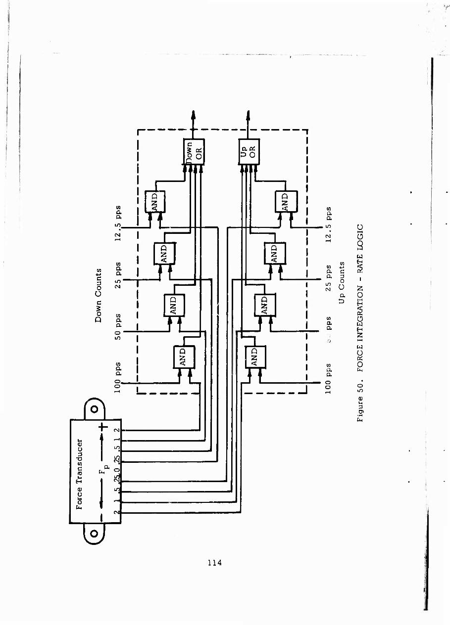
w ■M c 3 O Ü c
I o
HI
w a a
OJ
(A a a
a a o • IT)
en a a o o
o
w C
0) O
CM
4 ^H
a o K3 I^I
^
HJ
c
«
X I
Q 2
un Q
n rL
• ■«
laoi bo •I
Q
n Q 2
n Q 2
rr U
Q 2
Jl
en a a m
tn a a
w a a
4->
d a o Ü a D
w a a o o
Ü i—i o 9 M H
2 O H
Ü w H 2 i—i
w
2 o
ffl )->
cn
114

The possibility of obtaining a frequency signal from the electronic sensor or of using only one correction rete to simplify the system should h?t be overlooked.
Another approach is to use the jet pipe outputs to drive two pressure con- trolled oscillators, one for each polarity. The result will be a frequency in one or the other output lino, indicating the polarity and magnitude of the error. These signals can be used with the circuit in the pulse former and synchronizer.
Pulse Former and Synchronizer
The details of the pulse former and synchronizer circuit are shown in Figure 51. Its function is to receive a frequency signal from an input device and change it into an equivalent pulse rate such that the output pulses are synchronized by the clock.
The inputs are the PCO outputs, an up frequency and a down frequency; and the output consists of up command pulses and down command pulses syn- chronized by the clock. The pulse former and synchronizer consists of a pair of identical circuits, one for up counts and one for down counts. For this discussion, it will suffice to describe one of the circuits.
The frequency signal is first fed into a digital inverter-amplifier (I/A). The inverter-amplifier has a single input and two outputs. When no input is present, an output signal comes from the inverter output; when an input is present, an output signal comes from the amplifier output. For a one-cycle period of input, the output is alternately from the inverter or amplifier out- put. Thus, the frequency cycle has been transformed into two square waves, one out of phase with the other.
These two square waves are sent into a NOR gate, the inverter signal being sent in directly, the amplifier signal being first delayed. A NOR gate gives an output signal when none of its input signals are present. When the I/A switches from inverter output to amplifier output, the inverter signal to the NOR gage disappears immediately, while the amplifier signal is de- layed in appearing. During this delay time neither signal is present, so the NOR gate puts out a pressure signal. When the amplifier signal ar- rives, the NOR output goes to zero. A pressure pulse has been developed of pulse width equal to the time delay. When the I/A switches from am- plifier output to inverter output, the effect of the time delay is to overlap the inputs to the NOR gate, so no pulse is formed. Thus far, a leading edge pulse former has been demonstrated.
115

■ I
M
Ü
CO
Q
<
w
2 O u, w
a.
0)
116
^.—<**»;, -» , . - ■
The output pulse Is still randomly timed and is unsuitable for the computa- tional circuitry. Next, it has to be synchronized with the clock. This is accomplished by storing it in a flip-flop until the next clock pulse arrives. The flip-flop is a settable element which remains switched into the state corresponding to its last pulse input. When the SET-ONE (SI) input is pulsed, the output switches (or remains if it is there already) to the ONE output. The SET-ZERO (SO) input switches the output to the ZERO output. The output pulse from the NOR gate is the SET-ONE input and switches the flip-flop to the ONE state. The ONE output from the flip-flop opens an AND gate for the next clock pulse. The AND gate receives clock pulses at the maximum rate - 100 pps. The next clock pulse passes through the AND gate and is sent out of the pulse former and synchronizer as an output count. This pulse is also fed into the SET-ZERO input of the flip-flop which turns off the ONE output and consequently closes the AND gate to further input pulses. Only one clock pulse is sent out each time the AND gate is open. Since the maximum output rate is limited by the clock pulse rate to 100 pps, the maximum input rate is limited to 100 cps.
Timing Pulse Generator Circuit
The timing pulse generator circuit schematic is shown in Figure 52. The clock components are an oscillator, a binary sealer or nine-stage syn- chronous binary counter, a number of pulse former stages, and a number of pulse delayers and amplifiers.
The requirements placed on the clock are as follows:
1. To produce noise-free pulses of controlled amplitude, pulse width, pulse repetition rate, and pulse timing.
2. To produce a family of up pulses of 100, 50, 25, 12.5, and 0.39 pps repetition rate such that the lower rate pulses are in exact synchronism with the 100 pps up pulses.
3. To produce a similar family of down pulses of 100, 50, 25, 12.5, and 0.39 pps repetition rate such that the lower rate pulses are in exact synchronism with the 100 pps down pulses and further that the down pulses lag behind the up pulses by exactly 0.005 second (in other words, the 100 pps down pulses are spaced equidistant between the 100 pps up pulses.)
The frequency reference is a fluid oscillator. This can be either an analog or digital amplifier being fed back positively through either a tuned circuit or sonic time delay line. Its output waveform is either a square wave from
117

j
t
1 ^ |— p h a
r\ r^- ■■
m a
1 <3- » 1 oi i o r i ! CD
CD
Q
. ['•^ "^ i-j-^ K 1 •
o O
u . ^ Q ■ L. i i J Ü
o o
CÜ
W IS a
[£j 1 a f-cT"
o 2
n ^M P
1 h oo 1 ^ o o
• CM p— | CM 2
—1
(U
C D O
o >, ii
C
1 • O "*
S3 < 1— P L, ' CL,
h <*5
O «
Ü 2 t-H
CO j Q.
r * a ^
2 k- -• in
CM • o ^o
P f •^ aH
m W r^— LO
CM . CM
W 3 O c 0 u u c w
& i
M in •
o -*
LO
< — P
CVJ
O
-«-I
1 UH
, LJ o in
t/)
a ^1 ij o i
2 1
P o — ■»->
CO
55
o
" o i o o |
1 !
< i P
Osc
illa
tor
200
cps
a w i a : 1 o 2 !
a a ^
P o o 1 "■ •4 i ■--i
118

a digital amplifier or a sine wave from an analog amplifier. In either case the output is a 200-cycle-per-second signal adequate to drive a binary counter.
The binary counter for this application need not be bidirectional nor bit par- allel resetting but merely up counting and synchronous. This can be achieved by a simplification of the up-down synchronous binary counter de- scribed in Appendix II. Each successive counter stage puts out square waves of half the frequency of the previous stage. These square wave signals become the input to trailing edge differentiators (or pulse formers) at each of five counter stages.
At these five counter stages the ONE output and the delayed ZERO output are the inputs to a NOR gate. The NOR gate output is a pulse each time the binary counter stage switches from ONE to ZERO. (The pulse former princi- ple was described in relation to the pulse former and synchronizer circuit.) These NOR gate outputs at 100, 50, 25, 12.5, and 0.39 pps become the up pulses. These are delivered to the circuit elements as required. The up pulses at each pulse rate are also delivered to half pulse-time delays and to digital amplifiers which delay all the pulses 0.005 second, amplify them to compensate for the attenuation characteristic of the delay, and deliver them as the down counts to the circuit elements as required. The destination of the various pulse rate signals is shown in Figure 47.
Trim Circuits
The trim functions consist of constant rate or slow trim and force-free null- ing of the pilot controller or quick trim. Both of these modes are operative only when the autopilot is off. These functions are shown on Figure 47 where the autopilot servo actuator receives inputs from the trim circuits when the autopilot mode selector switch is in the off position.
The slow trim is achieved by sending a gating signal to either the up or down AND gate to pass the corresponding directed clock pulse signals at a rate of 12.5 pps. This rate is equal to the slowest force transducer rate and will trim the pilot controller from center to hard-over in 8 seconds.
The quick trim is achieved by sending a "go" or actuating signal to open both the up and down AND gates to the force transducer circuit output. In the quick trim mode, the pilot controller is held displaced against a stick force. The resulting force integration rate logic will cause the autopilot servo actuator to move in a direction to relax the stick force to zero, there- by establishing a new force-free null. The estimated time to reach equi- libruim in a null shift from center to hard-over is from 2 to 3 seconds.
119
//
>

Attitude Gvro Circuit
The attitude gyro circuit is shown in the lower left comer of Figure 47. It shows both the angular rate of pitch sensor circuit which senses angular rates from the threshold (0.03 degree per second or lower) to a maximum rate of 10 degrees per second and the pendulum long-term reference which senses aircraft angular error to within +0.05 degree and applies correc- tion at a maximum rate of 0.033 degree per second. Both signals are sent to the attitude register, or H register, which stores the binary coded atti- tude signal.
Referring to Figure 46 and page 100, the integrated rate of change of pitch signal stored in the H register is the computed attitude of the aircraft. Outputs of the H register position the pendulum case. If the computed atti- tude is correct, the pendulum case will be vertical. Over a long period the pendulum will also average a vertical position. If a difference exists, a very slow correction rate will be introduced into the H register to, in effect, erect the gyro.
The two frequency signals are respectively referred to as an up signal and a down signal; the up signal being the frequency which increases with angular rate of direction to cause the forward end of the vehicle to go up, the down signal being the frequency which increases with angular rate of direction to cause the forward end of the vehicle to go down.
The two frequency signals are sent into a pulse former and a synchronizer circuit described on page 115. This is a buffer which sends out a properly timed pulse for each cycle of frequency input.
The two pulse rate signals pass fir^t through OR gates and thence into the attitude rate integrator of H register, a ten-stage, synchronous, up-down binary counter. The OR gate is a digital circuit element allowing signals from more than one source to pass into the binary counter. "When the atti- tude gyro senses no angular rate of pitch, the up count pulse rate is equal to the down count pulse rate and there is no change in the stored count in the binary counter. When the rate gyro senses an angular rate of pitch,the two pulse rates are not equal and the stored count in the binary counter changes. The binary counter stores the attitude in the form of binary coded pressure level signals at the outputs of each counter stage; a pressure level at the "one" output indicating the presence of that bit, a pressure level at the "zero" output indicating the absence of that bit.
The binary counter selected has ten stages and a storage capacity of 210= 1024 counts. The specification for the attitude gyro requires a range of + 45 degrees or 90 degrees total. The scaling convention established is
120

#»-«•
to have 90 degrees equal to 900 binary bits or 1 binary bit equal to 0.1 degree. Therefore, the rate sensor maximum output of 100 pps is equal to an angular rate of 10 degrees per second.
The output of each stage of the attitude rate integrator is amplified by an actuator driver and fed into the pendulum rotation actuator. This is shown in detail in Figure 47. The actuator drivers are analog amplifiers which boost the output pressure level sufficiently to drive a digital actuator. The pendulum rotation actuator is a ten-stage digital actuator of the same type as the autopilot servo actuator. It consists of ten actuator stages^ach of which contributes a stroke proportional to its digital weight. The output displacements add together to produce an analog representation of the digital code. Figure 57. This actuator serves to rotate the pendulum case by the attitude angle stored in the attitude rate integrator. Originally, the pendulum case is oriented such that when the attitude signal (in the attitude rate integrator) is zero degrees and the true vehicle attitude is zero degrees the pendulum will plumb through the centerline of the case. The pendulum is a reference to ground and as such it swings through the same angle relative to the vehicle as the vehicle makes relative to the ground. This is the true attitude angle. The pendulum casein the other hand,is referenced to the vehicle and It follows the attitude angle stored in the attitude rate integrator. Any difference between the true attitude angle and the stored attitude angle manifests itself as a pendulum mis- alignment relative to the case cinlarline.
The rondulum serves as a flapper between a pair of nozzles built into the cast. When the pendulum is as much as +0.05 degree off the case center- line,the pressure difference measured by the flapper nozzles becomes suf- ficient to apply corrective action. The differential pressure signal from the flapper nozzles is fed into an orifice-volume filter which suppresses high frequency signals due to accelerations and vibrations. The filtered output signal is sent to a saturating amplifier. The saturating amplifier is a proportional amplifier which is capable of be;ng severely overdriven beyond the proportional band while it remains constant at the maximum signal level.
The two outputs from the saturating amplifier eacl are fed into an AND gate. The AND gate will pass a pressure pulse, providing a pressure level is on the other input. The pressure level signals come from the saturating am- plifier which is operated at such a level that 75 percent of maximum output signal is too small to open either AND gate. When the input differential pressure to the saturating amplifier is small or zero, each output signal is too small to open either AND gate. However, an off-center pendulum condition will cause an appreciable input differential pressure. This, in turn, will drive the proper output to a level sufficient to open one AND gate to provide corrective action.
121
/

The clock supplies up and down pulses to the AND gates at the rate of 0.39 pps. This approximately corresponds to a long-term correction rate of 0.03 degree per second or 2 degrees per minute. In conventional gyro systems, this limit is placed on pendulum correction rates to suppress pendulum coupling with phugoid oscillations. When an AND gate is open, the clock pulses pass through and are sent into the attitude rate integrator through the respective OR gate. This changes the attitude count stored in the inte- grator and thereby corrects the position of the case relative to the pendulum,
Attitude Reference Integrator
The attitude reference integrator, the J register, is the control reference for autopilot functions. This consists of a ten-stage synchronous up-down binaiy counter of operational specification identical to the attitude register (H register). See Appendix II. The stored count in the J register is the reference which the attitude register follows, and the difference count be- tveen the two registers is the error signal. The output of these two regis- ters is compared in a compare circuit which sends out correction pulses to the autopilot servo to reduce the compare error to zero.
Compare Circuitry and Pulse Gating Logic
The outer loop error signal is manifest as a non-cornpare between the H register and the J register. The compare is made on two levels: a coarse compare and a fine compare. The coarse compare circuit is a relatively slow circuit which detects compare errors of eight counts or greater and acts to correct the error at the rate of 100 pps. The fine compare circuit detects compare errors of four counts, two counts and one count and cor- rects at the rates of 50 pps, 25 pps, and 12.5 pps, respectively. The gating logic works in conjunction with the two compare circuits to send the correcting pulses to both the autopilot servo reference register and nega- tively to the J register. In this manner, the count of correcting pulse is equal to the error count »since the correcting count subtracts from the J register until the compare error is subtracted out. Hence, the displacement of the autopilot servo is proportional to the error signal.
The compare is made on a stage-by-stage basis comparing a stage of the H register with the corresponding stage of the J register. The fine compar- ison is made by entering the ONE output of the H register and the ZERO out- put of the corresponding J register in a NOR gate. The NOR gate will pro- duce an output signal only frr no input signals present; therefore, the ab- sence of ZERO from H and OVE from J indicates the presence of ONE from H and ZERO from J; hence,H is greater than J. The output from the NOR gate is the signal which opens the corresponding AND gate to permit corrective pulses to pass. The same type of comparison is made between the ZERO
122

output of the H register and the ONE output of the J register to establish if J is greater than H. Notice that for fine compare each stage compare inde- pendently controls a J greater, an H greater, an AND gate, and a corre- sponding output.
With the coarse compare, stages 4 through 10 of both the H register and the J register are compared and the comparison yields only one output (either H is greater, J is greater) or no output (equality). This coarse compare circuit is shown in Figure 52, including stages 4 through 10 of the H and J registers. The logic here is to compare the two registers stage by stage, starting with the last stage. As soon as a stage inequality is found there is no need to continue the comparison, and all lower stages compared are inhibited.
The comparison starts at the tenth stage by comparing the two ZERO outputs in an AND-EXCLUSIVE OR gate. This element functions as follows: if neither inputs are present, no outputs occur; if either but not both inputs are pres- ent, an OR output is produced; if both inputs are present, an AND output is produced. The AND output indicates two zeros; hence, equality and the stage inequality NOR gates are inhibited. When an inequality exists it indicates that one of the ONE outputs is not present. The absence of a ONE output from the J register stage causes an output signal from the cor- responding NOR gate to indicate that H is greater, and vice versa.
Only one greater-than signal is generated in the entire circuit at one time, since one inequality inhibits further compares. The output of each H greater compare and those of each J greater compare are gated together in OR gates to produce a single H greater output and a single J greater output. The presence of one of these signals opens the corresponding AND gate to pass pulses at 100 pps to correct the compare error.
The pulse gating circuitry has already been described along with the com- pare logic description. There are four gating pulse rates, and it is possible to have an output at each pulse rate. These pulses combine in the follow- ing two modes; like signs superpose and unlike signs subtract. For ex- ample, if H greater outputs occurred at 100 pps and 50 pps, the gross H greater pulse rate would be the greater of the rates or 100 pps; and if J greater output occurred at 25 pps with equality (no output at 12.5 pps), the net effect would be an up count (H greater) at 100 pps and a down count (J greater) at 25 pps or a differential up count at 75 pps. When the auto- pilot selector switch is in the ON position, this error count is delivered to the autopilot servo reference register.
123
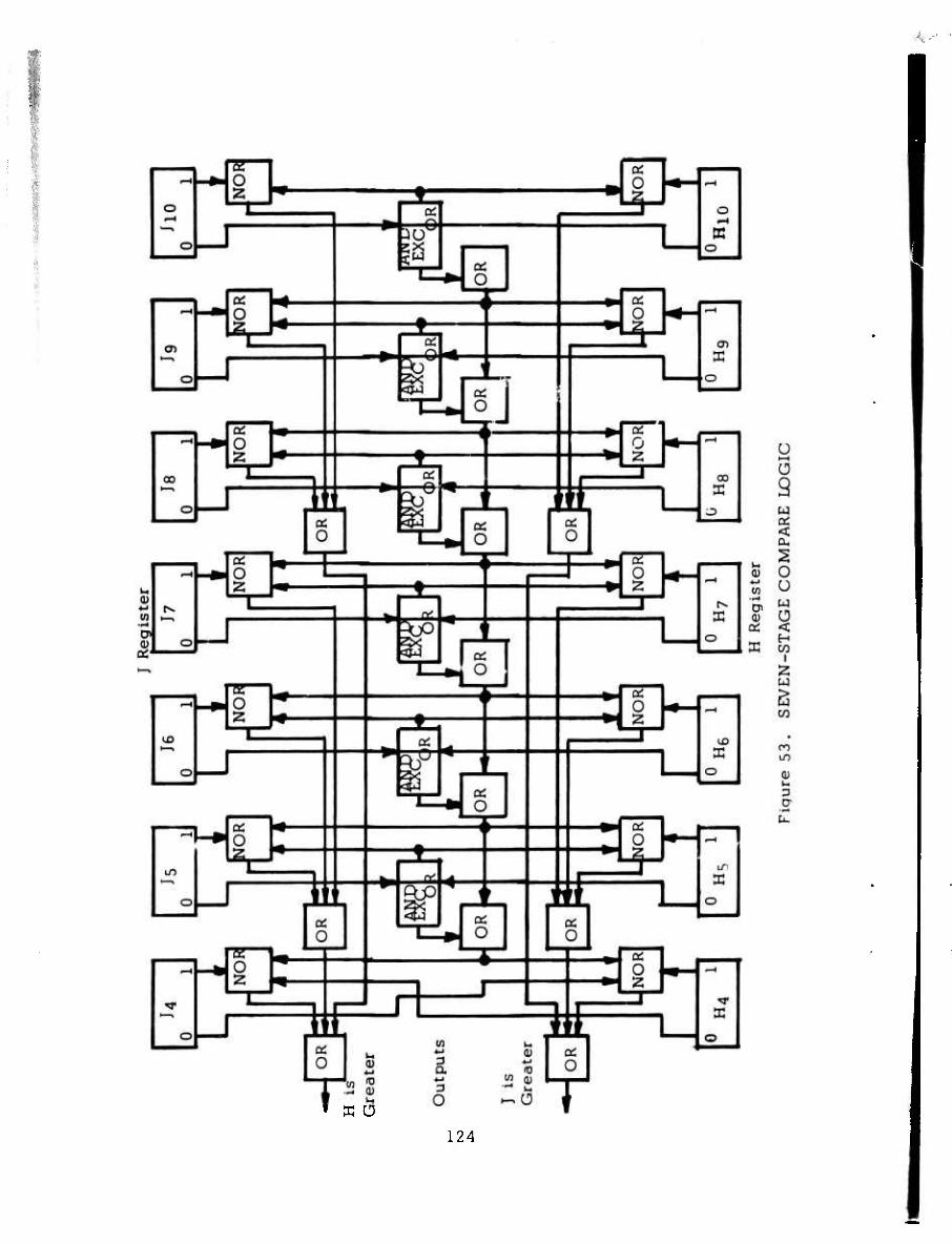
<■
X o 124
Autopilot Servo Actuator
The autopilot servo actuator requires digital operation to meet the resolu- tion requirements. Since actuation forces are quite low, pnermatic actu- ation seemed to be expedient.
One approach considered is a pneumatic stepping actuator. This actuator would have to complete its motion in 0.010 second. This approach would require either considerable mechanical complexity such as ratchet and pawls to limit steps or else very high pneumatic pressures to achieve the step- ping speed and also to be rigid against external forces su .h as the pilot overriding the autopilot servo. If such a device were forced sufficiently to slip a step, it would continue to slip, thereby losing reference. In general, this concept did not seem easily adaptable to this system.
Another approach considered was to use an analog actuator with a digital feedback signal. The feedback could be in the form of pulses to acknowl- edge the error signal by a countdown technique. However, problems would arise in detecting actuator direction. Two or three pulse lines could be used as a feedback to establish direction positively. This would Involve complicated decoding logic and very close tolerances to fabricate the me- chanical pulse generator. The three-line feedback device approaches the complexity of a position coded device. A sizable shaft force can cause the actuator to slip one set of pulses and lose reference.
Another approach is to use an analog actuator with a binary coded feedback from a metallic punch coded tape. With this arrangement the actuator could not lose reference, since each position is coded. Considering an eight bit coding and 200 actuator positions, if the holes on the tape were on 0.1- inch centers as per perforated paper tape specifications, then the coded metallic tape would be about 1 inch wide and 20 inches long. This system would involve the use of mechanical gearing between the actuator and the tape and a pair of tape takeup reels. Although this concept is workable, it is of considerable mechanical complexity.
The principle selected to demonstrate the autopilot servo actuator is the lever adder principle. An eight-stage digital actuator, based on the lever adder principle, is shown in Figure 54. This consists of eight double-act- ing pistons driven to either end of stroke by the amplified outputs from a binary counter. All piston strokes are equal. The least significant piston rod is connected to one end of a crossbar, the other end of the crossbar being a hinge to ground. The stroke of the midpoint of the crossbar is equal to half the piston stroke. The next least significant piston rod is connected to one end of a second crossbar, the other end of the crossbar being linked to the midpoint of the first crossbar. The midpoint of the second crossbar moves half stroke for full displacement of the second
125
/
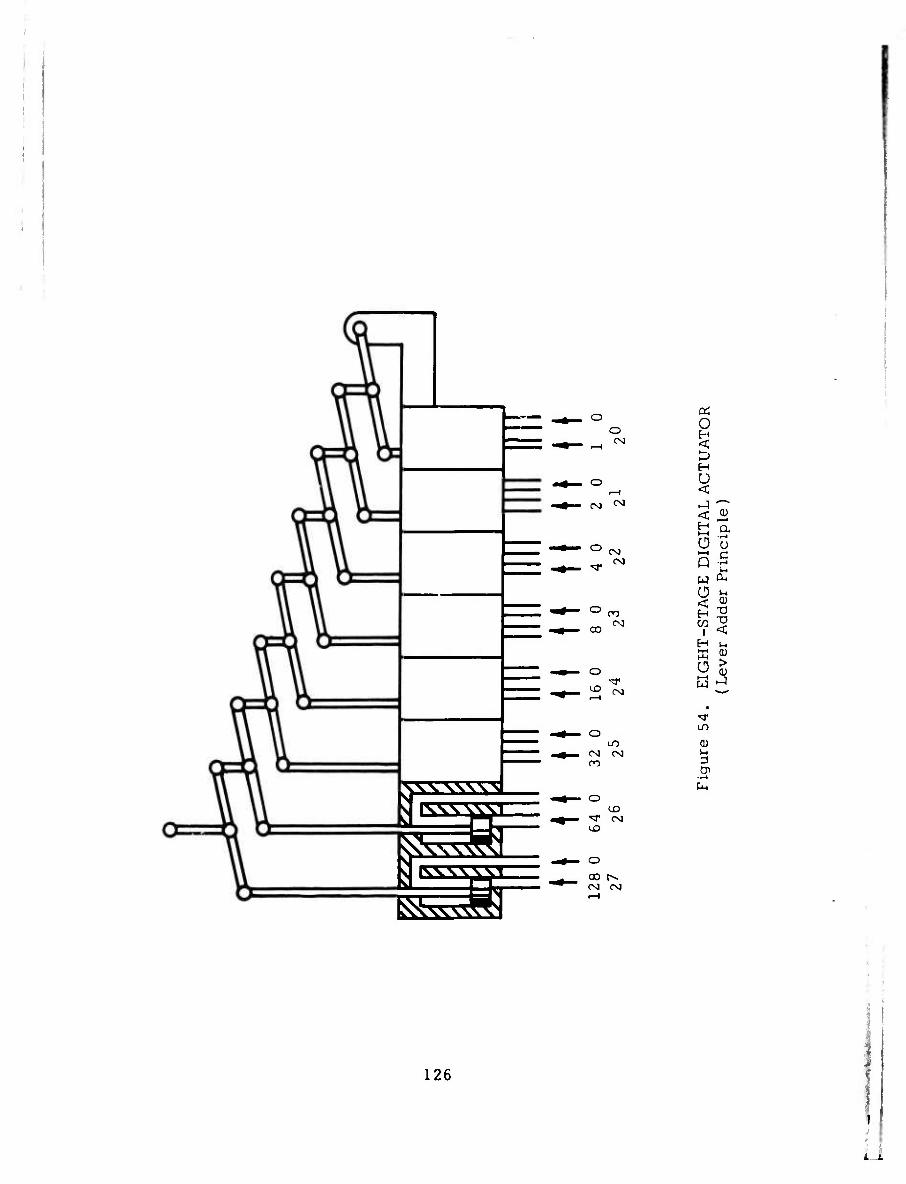
■VAWSSM
^KSSSSSI
^^ i^-s
o o
cd O H
^ ^ < ^ H
o u r—1 <
OJ OJ KJ -7- < %
O Ä, Ö 2- ü 5 v-' CM ,-, c
T ^ Q-§ w c^ O !-
0^ CM w 5 00 1 <
H i-, E 2^
O Ü >
^H
■^T LD
O LD 03
O) CM u oo 3
Di •-1
tL. o
U3 ^T CM U3
O
00 t^ CM CM
126
li
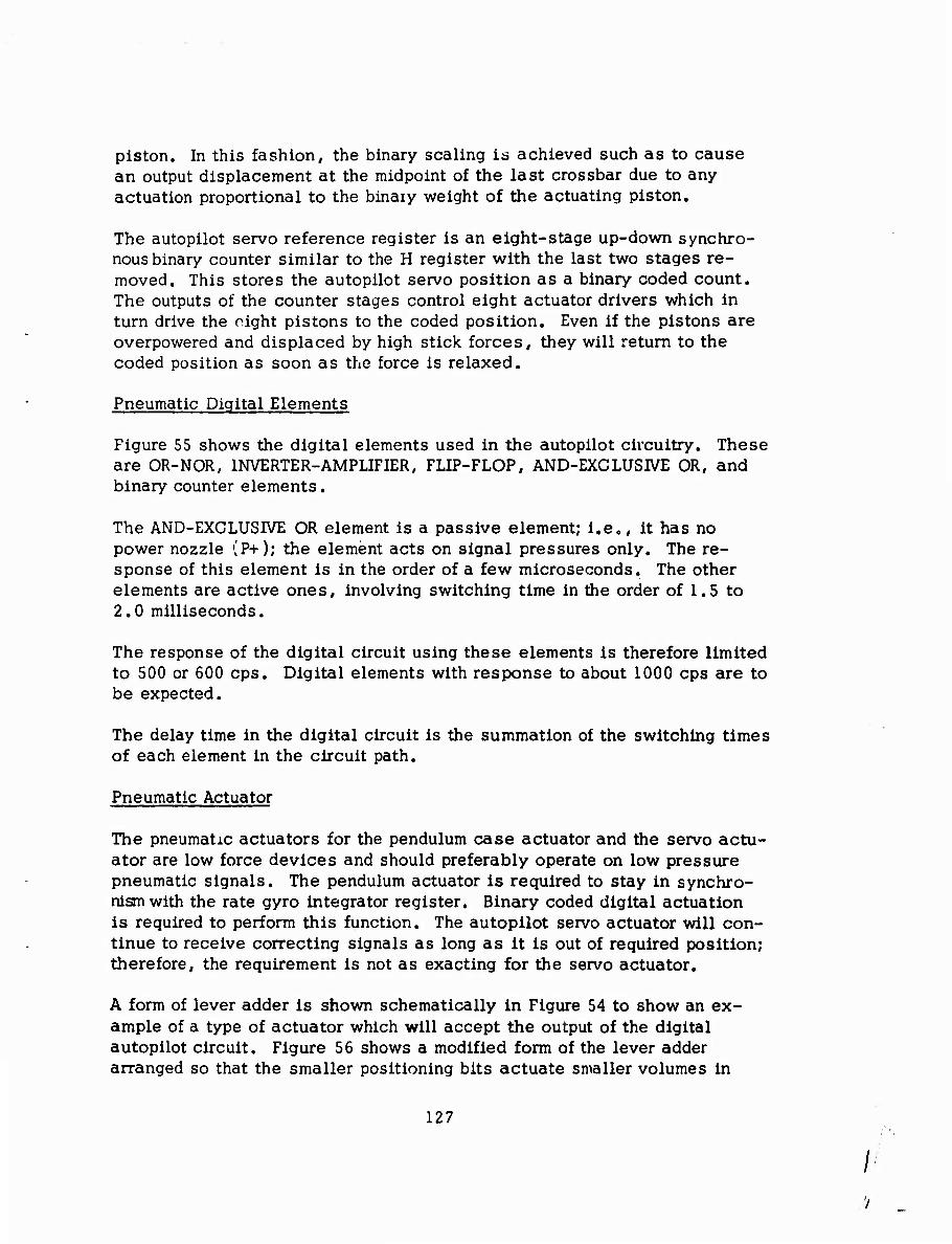
piston. In this fashion, the binary scaling is achieved such as to cause an output displacement at the midpoint of the last crossbar due to any actuation proportional to the binary weight of the actuating piston.
The autopilot servo reference register is an eight-stage up-down synchro- nous binary counter similar to the H register with the last two stages re- moved. This stores the autopilot servo position as a binary coded count. The outputs of the counter stages control eight actuator drivers which in turn drive the oight pistons to the coded position. Even if the pistons are overpowered and displaced by high stick forces, they will return to the coded position as soon as the force is relaxed.
Pneumatic Digital Elements
Figure 55 shows the digital elements used in the autopilot circuitry. These are OR-NOR, INVERTER-AMPLIFIER, FLIP-FLOP, AND-EXCLUSIVE OR, and binary counter elements.
The AND-EXCLUSIVE OR element is a passive element; i.e., it has no power nozzle (P+); the element acts on signal pressures only. The re- sponse of this element is in the order of a few microseconds. The other elements are active ones, involving switching time in the order of 1.5 to 2.0 milliseconds.
The response of the digital circuit using these elements is therefore limited to 500 or 600 ops. Digital elements with response to about 1000 cps are to be expected.
The delay time in the digital circuit is the summation of the switching times of each element in the circuit path.
Pneumatic Actuator
The pneumatic actuators for the pendulum case actuator and the servo actu- ator are low force devices and should preferably operate on low pressure pneumatic signals. The pendulum actuator is required to stay in synchro- nism with the rate gyro integrator register. Binary coded digital actuation is required to perform this function. The autopilot servo actuator will con- tinue to receive correcting signals as long as it is out of required position; therefore, the requirement is not as exacting for the servo actuator.
A form of lever adder is shown schematically in Figure 54 to show an ex- ample of a type of actuator which will accept the output of the digital autopilot circuit. Figure 56 shows a modified form of the lever adder arranged so that the smaller positioning bits actuate smaller volumes in
127

•,-•
OR-NOR Inverter-Amplifier
AND-EXCLUSIVE OR
Flip-Flop Binary Counter
Figure 55. DIGITAL ELEMENTS
128

.-■
128 Weight 1 Dia 2 Stioke
64 Weight 1 Dia 2 Stroke
8 Weight 1/2 Dia 1/2 Stroke
4 Weight 1/2 Dia 1/2 Stroke db
tput
0 32 Weight 5/8 Dia 1 Stroke
0 16 Weight 5/8 Dia 1 Stroke
2 Weight Y^-» 5/8 Stroke W 1/4 Stroke
1 Weight 5/16 Dia
JJ\ 1/4 Stroke
Figure 56 . MODIFIED LEVER ADDER (Top View)
129 \

order to achieve faster response on the lesser bits. If the driving am- plifiers are sized to achieve a greatest bit response at least equal to the required slewing rate, i.e. , full stroke in 2 seconds, the smallest bit is actuated in 25 milliseconds. This value is obtained by scaling the great- est bit time by the stroke and area ratios shown in Figure 56 (5/16 the diameter of approximately 1/10 the area and 1/8 the stroke).
There are several other approaches to digital positioning. In one design a series of interlocking pistons are arranged to receive pressure, each from its unique port. Each port represents a bit of binary information. Pressure admitted to a port separates twc pistons by a predetermined amount con- trolled by the length of the tongue of the adjacent lower bit piston. In this way the piston movements are additive. A biasing force from system pres- sure acting on the smaller piston area at the rod end returns the pistons when actuating pressure is removed from any of the signal ports. Figure 57 shows the digital actuator concept of Vickers, Inc., and a similar unit, differing in many details, manufactured by Cadillac Gage.
Actuators of this design are used in high-pressure hydraulic circuitry. The digital information is electrical and is introduced through solenoid oper- ated valves, such as the Cadillac Gage three-way transfer wave, Figure 58, It is possible to operate such an actuator through pneumatically con- trolled transfer valves. The assembly, as presently fabricated, is too heavy and bulky for the autopilot system. A smaller lightweight unit de- signed for low-pressure operation is a feasible solution.
Another approach is a conventional actuator used with a digital feedback device. A compare register must be added to the circuit to monitor the feedback signals against the input signals.
Force Transducer
The force transducer concept is shown in Figure 49. This unit will not contribute a time delay except for the effect of the length of transmission to the force rate integration circuit. See the subsection on transmission lines below.
Pendulum Assembly
The pendulum attitude reference is meant to supply long-term correction signals to the attitude rate integrator at a rate of one pulse every 3 sec- onds. The response of this component does not affect the system response.
130

E 0) Ü
JO a w
c
o I—« H
w a. O
O i—i H t-H CO
O CL,
Q
u->
cn ■f->
u-,
131
//

Vent Control Pressure
Figure 58 . THREE-WAY TRANSFER VALVE
132

Autopilot Response
The required response of the autopilot is indicated by the specifications for the gyro and the autopilot servo for an electronic system given in Tables DC and X respectively.
The fluid system response, which includes the rate sensor and circuitry, should be comparable to the attitude gyro in the electronic system.
The autopilot circuit accumulates delays from the total of digital elements in the signal path. The delays in the path of a signal from the rate sensor in the autopilot to the autopilot servo actuator are tabulated below:
Rate sensor (pneumatic) 0.028 sec Pressure-controlled oscillators and amplifiers Negligible Pulse former and synchronizer: three active elements 0.006 sec One OR-NOR element 0.002 sec Attitude integrator, "H" register: five active elements 0.010 sec Fine compare circuit: three active elements 0.006 sec One OR-NOR üiement 0.002 sec Actuator position register: five active elements 0.010 sec Output driver amplifier Negligible
TOTAL 0.064 sec
The response indicated by this tabulation, 0.064 second, is equivalent to a phase lag of 23 degrees at 1 cycle per second. This is greater than the specified 10 degrees given in Table DC.
The autopilot servo response is given as a natural frequency of 30 radians per second or 5 cycles per second. It is evident that the lack of response of the fluid gyro circuit can be compensated by a slight improvement in the proposed digital autopilot servo over the autopilot servo of Table X .
The proposed digital system will exhibit time delays and time constants but negligible resonance. It appears likely that the element moving time of a digital unit could be made at least 30 milliseconds. Therefore, it is safe to assume that the overall system can be made compatible with the overall specifications.
Operational Factors
The pneumatic circuits appear to be more prone to contamination difficulty. The lower pressures used preclude major self-cleaning. However, again the particle-size from the filtered air system is much smaller than the min- imum orifice. Industry standards using shop air and 40-micron filtration specify orifices no less than 0.010 inch in diameter. The pneumatic system
133
'/

orifices are to be no smaller. Infant mortality is the major problem to be considered, assuring that adequate tist time has been allowed after as- sembly on refit for the problems to appear.
The pneumatic system may also suffer from icing unless precautions are taken. An approach such as the following is suggested. Mount the pneu- matic system, metal units, on some portion of the exhaust gas system. Power the unit with a shaft-driven fan in an enclosed system using recir- culating air as much as possible.
Again, the circuit orifice adjustment structure should be easily replaceable with self-contained filters as described for the hydraulic system, page 94 ,
i 134

SECTION 4
AN EVALUATION OF THE PROPOSED FLUIDIC AUTOMATIC FLIGHT CONTROL SYSTEM
This section evaluates the weight, size, power, and reliability charac- teristics of the fluid automatic flight controls implemented in the preced- ing section. The results of this evaluation are then compared with the electronic systems performing equivalent functions.
The results of this comparison are summarized on Table XXI, which indicates considerable advantage for the fluid systems in reliability and cost. The fluid nonredundant system is indicated to be 25 percent heavier and require 20 percent more power than the nonredundant electronic system.
However, the addition of parallel redundancy to upgrade the reliability of the electronic systems to that of the fluid system approximately doubles the weight, power consumption and cost of the electronic system, The weight of the fluid system now becomes 40 percent less than the electronic systen^and the power consumption becomes 37 percent less and the cost about 1/3 that of the electronic system.
WEIGHT AND SIZE
The weight and size of fluid systems are factors which will undergo major changes within the next few years. The estimates given here are for realizable element sizes and packaging based on the present state of development of fluid dsvices.
The primary control circuit (see Figures 19 and 29), the open loop damping circuit, and the stability augmentation circuit are assumed to be fabricated in a lightweight metal alloy. About 15 analog fluid amplifiers are required in total for these circuits. These elements can be fabricated in a pair of 5-inch-by-6-inch plates on a common manifold, which will be 1/2 inch thick overall. Based on the weight of sample units at Bowles Engineering Corp. , this assembly is estimated to weigh 1. 3 pounds. The hydraulic fluid in the manifold and in the volumes adjacent to the circuits, the submerging fluid, will occupy a volume of 5 inches by 6 inches by 0.75 inch. The weight of the fluid is 0.67 pound. To this must be added the weight of the rate sensor
135

(page 87), input transducer (page 80), actuator (page 93), and associated hydraulic fluid. The overall SAS weight is tabulated in Table XIII.
In high pressure aircraft systems it will be advisable to use a hydraulic motor-pump converter to supply the low pressure control flow. This hydraulic motor-pump converter will weigh 3.2 pounds and will have the capacity for the pitch, yaw, roll and thrust axis. Figures 21 through 26. All of the converter weight is charged against the fluid system even though some electrical capacity can be diminished. As will be shown, the electrical power consumption reduction is not significant.
The autopilot circuits contain 339 digital elements and 18 driver stages which are larger in size than the logic elements. Approximately 40 logic elements will fit on a 6-inch-by-8-inch plate. It is assumed that seven circuit plates will be required for these circuits. The plates and manifolds sandwiched into one assembly will be in the order of 1.25 irch thick. It is further assumed that these circuit plates will be fabricaed in a lightweight metal alloy. Weights of laboratory samples indicate a total weight of the plates plus manifolds of 5.00 pounds.
The weight of the shaft-driven fan, which appears to be the most satisfactory power supply, is not charged against the fluid system. The weight of the portion of the electrical power generator used for the auto- pilot is converted to a shaft-driven two-stage fan. Note that the fan weight for a given power is much less than a generator and also that the fluid power is less than the electrical power. The total weight of the autopilot pitch axis control circuit is tabulated in Table XIV.
POV/ER REQUIREMENTS
Primary Control and Stability Augmentation
The element size and operating pressure determine the power consump- tion of the fluid amplifier. These elements may be sized over a large range, limited by size and weight considerations on one hand and sensitivity to viscosity and particle contamination on the other.
The operating pressure of each amplifier in the circuit is dictated by system considerations. A high pressure output requirement from the final or driver stage of a system will multiply the number of amplifying stages required as well as the pressures and flows at which they operate. This particularly affects the few amplifying stages preceding the driver stage.
136

TABLE XIII WEIGHT OF FLUIDIC PRIMARY CONTROL. OLD AND SAS. PITCH AXIS
Item Weight in Pounds
Displacement Transducer 1.5
Circuit Plate and Manifold 1.3
Rate Sensor
Actuator
Filter
Tubing and Fittings
Hydraulic Motor-Pump Converter (weight per axis)
Hydraulic Fluid
TOTAL 10.9
0. .5
4. .5
0. ,3
1. 2
0. ,8
o. 8
137

TABLE XIV WEIGHT OF AUTOPILOT SYSTEM . PITCH AXIS
Item Weight in Pounds
Rate Sensor 1. 50
Navigation Interface 1. 00
Circuit Plates (4) 5.00
Pendulum-Actuator Assembly 2.00
Force Transducer 1.00
Spring and Brake Assembly 1.25
Servo Actuator 2.50
Tubing and Fittings 2.00
Filters and Pressure Regulator 1. 00
TOTAL 17.25
138

The power requirement of a control system is affected by an additional major factor, the system supply pressure. To illustrate this point, a single hydraulic fluid amplifier will be considered. This amplifier is to operate at a pressure of 200 psi consuming 10 watts of hydraulic power. If this amplifier is supplied from a 1000-psi source, the pressure must be dropped by a reducer or restrictor in series with the amplifier. The total power dissipated is five times as great as for the 200-psi case. This amplifier and restrictor, then, will require the consumption of 50 watts when supplied from a 1000-psi source.
The example given above indicates the importance of considering the relations of power supply and circuit configuration in the design of fluid control systems. This is of particular importance when the available supply pressure is high. For minimum power consumption the circuits should be designed to cascade the flow (see Figure 59); and the power supply should be from a dual pressure source, a high pressure to furnish muscle and a low pressure to furnish control flow.
For the purposes of the present estimate, it is assumed that a 3Q0-psi hydraulic source is available in addition to the high pressure supply. The low pressure source is assumed to be the output of a converter, by a hydraulic motor from the high pressure supply.
The fluid amplifiers are assumed to have an 8-by-24-mil power nozzle. The rate sensor requires a flow of 2 gpm. This flow is more than that required for the balance of the SAS and primary control. The circuit is arranged to cascade flow from the power supply as shown in Figure 59.
The power requirement for the composite primary control and stability augmentation circuit is then determined by the rate sensor flow. The flow of 2 gpm supplied at 300 psi represents 0.35 horsepower or 260 watts. This does not include the power required to drive the actuator which uses variable power to a maximum of 430 watts. The total maximum power is then 690 watts i^r the primary plus SAS (see Table XV).
Autopilot
The pneumatic autopilot circuit is based on operation from a 5-psi-out- put two-stage shaft-driven fan. This pressure is sufficient to drive the ,oervo actuator and the pendulum actuator. The digital fluid elements will operate at 1 psi. Using 7-by-15-mil nozzle size digital amplifiers.
139

a a. 3
CO
o u 3 w w. 0)
.3
M M O O (0
4-> Xi •D •K3 3 o < k.
-3
i
u 0)
ö 1 t 1 W 3 CO
♦ h
-3
-d >.ö ^
12 a 6 3 £5
1
w c
<
■r-4
a CO x:
CO
a J
0 i ü
3 t! "O 3 m
Inp
ran
! H
4
I
CT c
0) 4-t
•w4
a (0 (0
DC x: CO
-2
1 -M
1^
Rat
e S
enso
r
o a:
O Ü
<:
S a. 33
CU CO
Sg
CO
w H CO
1^,
OS w
O
<; H
M 2
g H
u ^
H
Q M Q < U CO <: ü
3
H CO
Q
140

TABLE XV
POWER CONSUMPTION
Required Pressure
Supply Pressure Flow Power
Hydraulic-Primary and Stability Augmentation
Rate Sensor (1) 50 psi 300 psi 2 gpm 260 watts Circuitry (1) 25C 300 1.8 gpm 234 watts
Cascaded System 300 psi 300 psi 2 gpm 260 watts Actuator Variable 3,000 psi Variable 430 watts max (2) Total - Cascaded 690 watts max
System
Pneumatic Auto- pilot, Attitude Control
Rate Sensor (1) 2 psi 5 psi 4.4 scfm 79 watts Logic Circuitry (l) 1 psi 5 psi 4.32 scfm 78 watts
Cascaded Circuit 3 psi 5 psi 4.4 scfm 79 watts Driver Stages 5 psi 5 psi 1,17 scfm 21 watts Total-Cascaded 5.57 scfm 100 watts
System
(1) Requirements for individual items; when combined in a cascaded system as shown in Figure 59, the total power requirement is reduced.
(2) The same power as in the electro-hydraulic actuator used for a system comparison, Table XIX.
141

4.32 s :fm* airflow is required for the 339 elements (see page 136). The driver elements must supply sufficient flow to drive the actuators at the required speeds. The actuator flow is estimated by determining the area required to yield a force of 2 pounds when supplied 2.5 psi air (50 percent of the driver amplifier supply pressure, the approximate pressure recovery), and from this area the volume swept at a piston speed of 2 inches per second (see autopilot servo characteristics. Table VIII). This flow rate is the requirement of each of the 18 driver stages; 10 for the pendulum actuator and 8 for the autopilot servo. The total flow required for these drivers calculates to 1.17 scfm. The rate sensor requires 4.4 scfm. The total flow required for the autopilot circuits is 9.89 scfm. The total power required to deliver this airflow at 5 psi is 170 watts, allowing 15 percent for compressor friction losses. By cascading the flow in a manner similar to that described for the hydraulic circuits,the power requirement is 100 watts.
Table XV summarizes the power requirements for the fluid systems.
Reliability
A basic problem arises in approaching the analysis of the reliability of fluid devices. This problem must be resolved before proceeding with the analysis.
Electronic devices used thus far are characterized by an essentially random failure pattern in which failure is constant with time. Certain burn-in sequences are sometimes employed to eliminate infant mortality. Overhaul and renewal techniques are sometimes required to deal with wearout, especially in electro-mechanical devices. However, to the largest extent, the failure pattern is random, and there are sufficient data available for predicting the reliability of new electronic components.
For fluid devices this failure pattern has not been determined. Life tests performed at Bowles Engineering Corporation on digital and analog elements, after debugging, have shown only one failure. Examination showed metal chips in the fluid passage, the result of careless fabrication. The unit that failed is an early model; it has not failed since, in over 2 years of continuous operation. Thus far, the total element hours of the life tests is just under 30,000. Other modes of failure have been noted which are related to fabrication techniques.
*scfm is the cubic feet of air per minute at standard conditions of 14.7 psia and 70°F.; 1 scfm is 0.07 pound per minute.
142
i
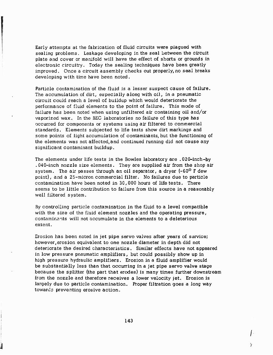
Early attempts at the fabrication of fluid circuits were plagued with sealing problems. Leakage developing in the seal between the circuit plate and cover or manifold will have the effect of shorts or grounds in electronic circuitry. Today the sealing techniques have been greatly improved. Once a circuit assembly checks out properly,no seal breaks developing with time have been noted.
Particle contamination of the fluid is a lesser suspect cause of failure. The accumulation of dirt, especially along with oil, in a pneumatic circuit could reach a level of buildup which would deteriorate the performance of fluid elements to the point of failure. This mode of failure has been noted when using unfiltered air containing oil and/or vaporized wax. In the BEG laboratories no failure of this type has occurred for components or systems using air filtered to commercial standards. Elements subjected to life tests show dirt markings and some points of light accumulation of contaminants, but the functioning of the elements was not affected,and continued running did not cause any significant contaminant buildup.
The elements under life tests in the Bowles laboratory are .020-inch-by .040-inch nozzle size elements. They are supplied air from the shop air system. The air passes through an oil separator, a dryer (-60° F dew point), and a 25-micron commercial filter. No failures due to particle contamination have been noted in 30,000 hours of life tests. There seems to be little contribution to failure from this source in a reasonably well filtered system.
By controlling particle contamination in the fluid to a level compatible with the size of the fluid element nozzles and the operating pressure, contaminants will not accumulate in the elements to a deleterious extent.
Erosion has been noted in jet pipe servo valves after years of service; however,erosion equivalent to one nozzle diameter in depth did not deteriorate the desired characteristics. Similar effects have not appeared in low pressure pneumatic amplifiers, but could possibly show up in high pressure hydraulic amplifiers. Erosion in a fluid amplifier would be substantially less than that occurring in a jet pipe servo valve stage because the splitter (the part that erodes) is many times further downstream from the nozzle and therefore receives a lower velocity jet. Erosion is largely due to particle contamination. Proper filtration goes a long way towards preventing erosive action.
143

This discussion serves to show that time dependent failures will not likely be a factor in the reliability of fluid systems. Burn-in techniques at startup and replacement at specified periods should eliminate time dependent failures. The middle life of a component can therefore be assumed to have a random failure rate pattern.
Estimates of the failure rate of fluid elements have been made by others (References 11 and 12). Another estimate made at this point would have to be based on much the same material,since life tests have not yet accumulated sufficient data for better estimates. The reliability estimate given below is based on existing failure rate d^ta and by estimates when there are no existing data.
Each system is treated as a series of reliability blocks.
Primary Control System
The primary control system consists of the following reliability blocks (see Figures 18, 19, and 35):
Input transducer
Fluid amplifiers
Lines and fittings
Actuator -
Servo valve
Hydraulic actuator
Feedback device
The comparison of electronic and fluid power systems shows nearly equal reliability and hence is not considered. First,the high pressure hydraulic power is common to both. Second,the high pressure to low pressure converter has a reliability comparable with a generator; a failure rate of about 200/10° operating hours, Reference 13. The converter in the fluid system serves the same function as the generator in the electronic system (see page 139).
144

The input transducer consists of a spool with two tapered slots working in a sleeve. This is similar to a manually operated spool valve which has a failure rate of I.O/IO^ per million operating hours (Reference 13).
The fluid amplifier in one estimate has a failure rate of 0.0311/106
hours (Reference 12),and in another estimate this value is 0.50/106 hours (Reference 11). Since the latter is based on the failure rate of a gasket which is O.OS/lO^ hours (Reference 14), a use factor* of 10 must have been included. The two estimates are then in fair agreement. In this estimate the larger value will be used.
The hydraulic lines and fittings may be considered as assemblies of one hose with two fittings or connectors. The failure rates are:hose - 0.595/106 hours (Reference 15); fitting - 0.451/106 hours (Reference 14); and the assembly - 1.497/10^ hours. These values include the aircraft use factor.
The actuator is made up of three major parts: the servo valve, the hydraulic actuator, and the feedback device. This assembly can be designed similar to those presently in use. The difference is in the input, which is a fluid differential pressure rather than the mechanical input. It is estimated that the actuator failure rate will be similar to that presently assigned, 35.6/106 hours (Reference 14). It is of note that the required reliability for a mechanical primary system has been sei: at a value better than 35.6 x 10^ hours and therefore requires parallel redundant actuators. This evaluation,however,is based on a nonredundant comparison.
The reliability determination is shown in Table XVI The overall system failure rate is 50.594/106 hours. The calculated rei:«hility for 10 hours of operation is 0.99949406.
A calculated value for the failure rate of a power boost-mechanical control must be at least the 35.6/106 hours of the actuator. Adequate reliability by today's standards is achieved only with parallel redundant actuators. The fluid system may be made entirely parallel redundant, still weigh less than the mechanical system and gain a reliability approaching that of the power boost system.
*A "use factor" is the ratio between field experience and laboratory test experience. The ratio is normally characterized by the service (e.g., aircraft, marine, industrial use, etc.).
145

TABLE XVI FLUH) PHIMARY CONTROL SYSTEM RELIABILITY
Failure Rate Per 106 Hours Part No. of Items Unit Total
10.f) 10.0 0,5 2.0 1,497 2.994
33.6 35.6 50.594
50.594/106 hours 0.000050594 per hour
Displacement Transducer 1 Fluid Amplifier 4 Lines and Fittings 2 Actuator 1
Failure Rate
Reliability, R = e ~ K t
For 10 hours of operation t = 10
R=e-0.00050594 =0.99949406
146

Stability Augmentation System
The stability augmentation system consists of three reliability blocks: the rate sensor, the fluid amplifiers, and the lines and fittings plus the primary control system.
The failure rate of these blocks has been discussed with the exception of the rate sensor. The failure rate of this unit is taken as 1.66/10° hours (Reference u).
The reliability determination for the SAS system is shown in Table XVII. The overall failure rate is 63. 736/106 hours. The reliability for 2 hours of operation is 0.99987.
The open loop damping circuit has no rate sensor and fewer amplifiers. Its reliability would be somewhat better than that of the SAS circuit.
Autopilot, Attitude Control
The attitude hold system is the most complex and therefore the least reliable of the autopilot controls. Therefore, this system is chosen as indicative of the autopilot reliability. In addition, 331 out of the 357 fluid amplifiers in the autopilot circuit are required for the attitude hold function.
The components of the attitude hold system are divided into seven reliability blocks: the rate sensor, the fluid amplifiers, the lines and fittings, "O" ring ciicuit plate gaskets, the pendulum assembly, the pendulum actuator, and the servo actuator plus the primary and SAS.
The first three of these blocks have been discussed above.
The pendulum assembly contains a pendulum supported by a flat flexure spring and two orifices metered by the pendulum. Airborne springs have a failure rate of 0.11/10^ hours (Reference 14); orifices, variable - 0.55/10" hours (Reference 13). Based on these figures and allowing for structural failures, the estimated failure rate for the pendulum assembly is 2.0/10^ hours.
The actuators will be more complex than a two-cylinder unit with linkage - 13.28/10^ hours (Reference 11), and will probably be more susceptible to failure than the hydraulic control actuator - 35.6/10^ hours (Reference 14). The failure rate for the digital actuators is estimated at 100/106 hours.
147
TABLE XVII FLUID STABILITY AUGMENTATION SYSTEM RELIABILITY
Failure Rate Per 106 Hours Part No. of Items Unit Total
Rate Sensor 1 1.66 1.66 Fluid Amplifiers 5 .50 2.50 Lines and Fittings 6 1.497 8.982
13.142 Failure Rate, Primary Control System 50.594
63.736
Failure Rate =63.736/106 hours :0.000063736/hour
Reliability, R = e-\t
For 2 hours of operation t = 2
R=e-0.000127472 =0.99987
148
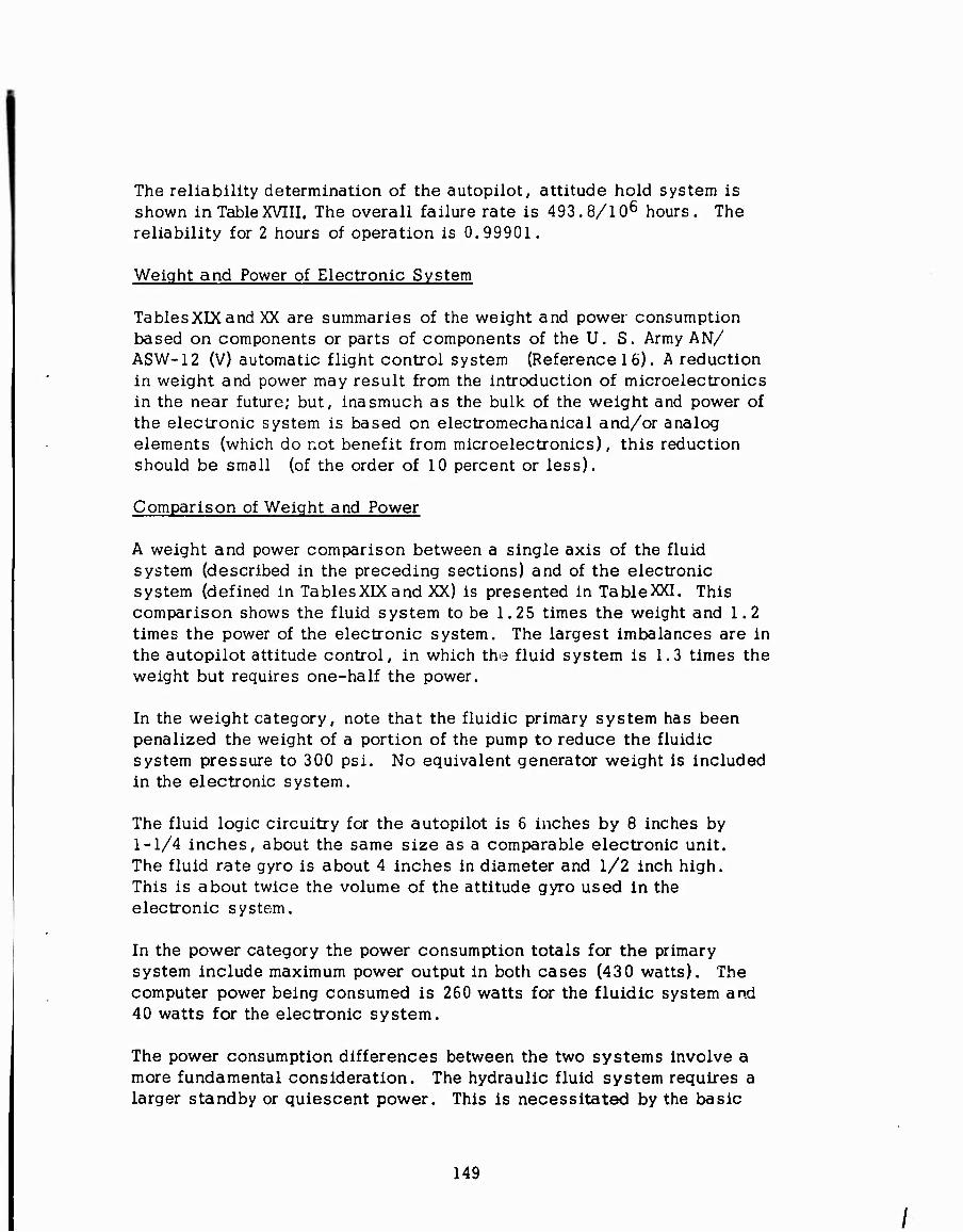
The reliability determination of the autopilot, attitude hold system is shown in Table XVIII. The overall failure rate is 493. 8/106 hours. The reliability for 2 hours of operation is 0.99901.
Weight and Power of Electronic System
TablesXIXand XX are summaries of the weight and power consumption based on components or parts of components of the U. S. Army AN/ ASW-12 (V) automatic flight control system (Reference 16). A reduction in weight and power may result from the introduction of microelectronics in the near future; but, inasmuch as the bulk of the weight and power of the electronic system is based on electromechanical and/or analog elements (which do not benefit from microelectronics), this reduction should be small (of the order of 10 percent or less).
Comparison of Weight and Power
A weight and power comparison between a single axis of the fluid system (described in the preceding sections) and of the electronic system (defined in TablesXIXand XX) is presented in TableXXI. This comparison shows the fluid system to be 1.25 times the weight and 1.2 times the power of the electronic system. The largest imbalances are in the autopilot attitude control, in which the fluid system is 1.3 times the weight but requires one-half the power.
In the weight category, note that the fluidic primary system has been penalized the weight of a portion of the pump to reduce the fluidic system pressure to 300 psi. No equivalent generator weight is included in the electronic system.
The fluid logic circuitry for the autopilot is 6 inches by 8 inches by 1-1/4 inches, about the same size as a comparable electronic unit. The fluid rate gyro is about 4 inches in diameter and 1/2 inch high. This is about twice the volume of the attitude gyro used in the electronic system.
In the power category the power consumption totals for the primary system include maximum power output in both cases (430 watts). The computer power being consumed is 260 watts for the fluidic system and 40 watts for the electronic system.
The power consumption differences between the two systems involve a more fundamental consideration. The hydraulic fluid system requires a larger standby or quiescent power. This is necessitated by the basic
149
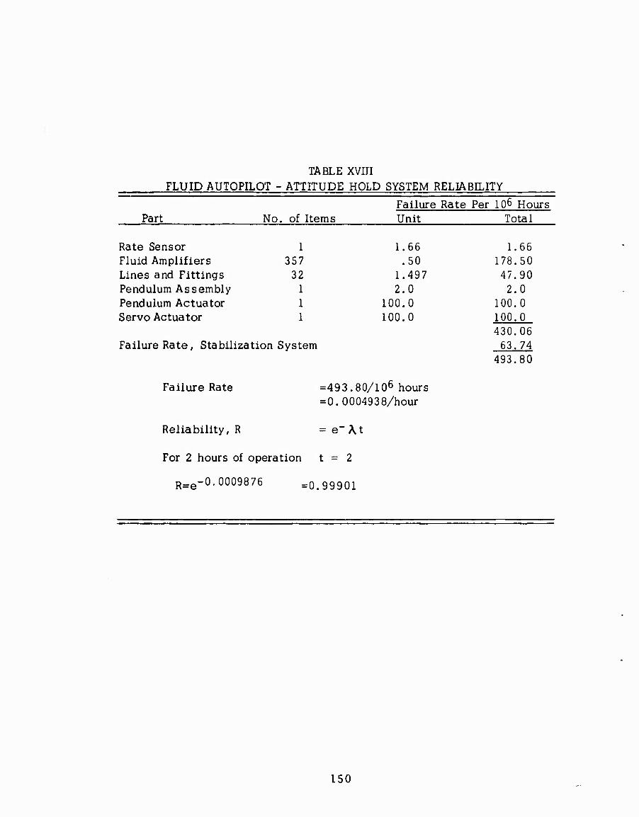
TABLE XVIII FLUID AUTOPILOT - ATTITUDE HOLD SYSTEM RELIABILITY
Failure Rate Per 106 Hours Part No. of Items Unit Total
Rate Sensor 1 1.66 1.66 Fluid Amplifiers 357 .50 178.50 Lines and Fittings 32 1.497 47.90 Pendulum Assembly 1 2.0 2.0 Pendulum Actuator 1 100.0 100.0 Servo Actuator 1 100.0 100.0
Failure Rate, Stabilization System 430.06 63.74
493.80
Failure Rate =493.80/106 hours = 0.0004938/hour
Reliability, R = e-A.t
For 2 hours of operation t = 2
R=e -0.0009876 =0.99901
150

TABLE XIX WEIGHT AND POWER,
ELECTRO-HYDRAULIC PRIMARY AND STABILITY AUGMENTATION SYSTEM 1 ■ -
Weiqht Power Component (lb.) (watts)
Pilot Controller Displacement 1.3 negligible Transducer (1)
Attitude Rate Gyro (2) 0.8 35
Amplifier Assembly (3) 1.5 5
Control Actuator (Electro-Hydraulic) 5 430 (4)
TOTAL 8.6 470
NOTES:
1. Consists of AN/ASW-12(V) rotary motion transducer (0.3 lb.) and suitable control stick assembly (1.0 lb. , estimate).
2. Based on typical sub-miniature electro- mechanical rate gyro characteristics.
3. Estimated as an assembly of AN/ASW-12(V) sub-components: preamplifier of electro-mechanical rotary actuator, demodulator of attitude reference control and miscellaneous elements.
4. Equivalent hydraulic power consumption at maximum actuator power output.
151

,
TABLE XX WEIGHT AND POWER,
ELECTRO-HYDRAULIC AUTOPILOT, ATTITUDE CONTROL SYSTEM
Component (1) Weight
(lb.) Power
(watts)
Pilot Force Transducer
Attitude Gyro
Integrator (2)
Autopilot Servo Actuator
TOTAL
1.0
5.8
1.5
5.0
13.3
negligible
100
30
55
185
NOTES;
1. All components are existing AN/ASW-12(V) units.
2. This unit can combine force integration and trim functions
152
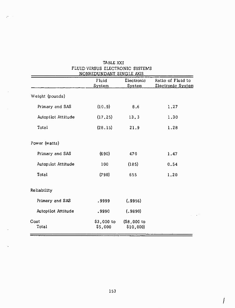
TABLE XXI FLUID VERSUS ELECTRONIC SYSTEMS
NONREDUNDANT SINGLE AXIS
Fluid Electronic Ratio of Fluid to System System Electronic System
Weight (pounds)
Primary and SAS (10.9) 8.6 1.27
Autopilot Attitude (17.25) 13.3 1.30
Total (28.15) 21.9 1.28
Power (watts)
Primary and SAS (690) 47 0 1.47
Autopilot Attitude 100 (185) 0.54
Total (790) 655 1.20
Reliability
Primary and SAS .9999 (.9956)
Autopilot Attitude .9990 (.9890)
Cost $3,000 to ($8,000 to Total $5,000 $10,000)
153

fact that continuous fluid flow through all of the system elements must be maintained in order for the system to function. This characteristic of the fluid system is somewhat analogous to the class A electronic amplifier in which a relatively large standby power is used in proportion to the useful output power. But, whereas the use of low quiescent power techniques (class B and class C amplifiers) have been achieved in electronic systems, it is as yet too early for this position to have been achieved in fluid systems - except where digital techniques can be used on a practical basis in the system design. The power consumption of the fluid system autopilot, which j^ digital, thus approaches one-half the electronic system power consumption level, while the primary and SAS power consumption is almost 50 percent greater (see Table XM),
Reliability of Electronic Systems
The reliability of an electronic stability augmentation system, based on AN/ASW-12(V) Reference 16, is 0.9956 for a nonredundant system and 2- hour mission time.
On the same basis the reliability of an electronic autopilot, attitude hold system is 0.9890.
Comparison of Reliability
The equivalent nonredundant reliabilities of the electronic systems based on the AN/ASW-12(V) system of Reference 16 and the fluid AFCS are also given in Table XXL
An evaluation of fluid versus electronic circuits on the basis of equivalent reliability would require the multiplication of the various factors for the electronic system by a factor of at least two. For example, where the weight of the fluid system is given as 1.2 times that of the electronic system, this ratio becomes 0.6 when compared to the redundant electronic system required to match the predicted fluid reliability.
The reliability of the pneumatic system blower supply may be better than the electronic system generator. The blower failures are. Reference 13, generally less than 100/10° hours. However,if pressure regulation is required the reliabilities will be similar. This latter case is assumed.
154

Costs
The costs which are itemized below are estimated on .he basis of a quantity of 100. This is a suffic-.at number in the case of the fluid circuits to reduce the costs of tooling to a fraction of the circuit costs. This number also allows other fixture preparation to aircraft like cost- quantity relationships.
The estimates are based on light metal construction, machined manifolds, "O" ring sealing, and finishes compatible with the trade.
Primary and Stability Augmentation System Cost $
1 ea Displacement Transducer 200
1 ea Circuit Plate - 15 Elements 100
1 ea Manifold 200
w/15 Valves @$20 300 500
1 ea Rate Sensor 200
1 ea Enclosure w/Fittings 200
Misc Fittings, Filters 50
1/4 ea Hydraulic Motor Pump @ 200 50
Components 1300
Assembly and Test 300
1600 1600
Autopilot Axis
1 ea Rate Sensor 100
1 ea Electro/Fluid Interface 100
4 ea Circuit Plates @100 400
155

4 ea Manifold @100 400
1 ea Pendulum and Digital Actuator 400
1 ea Force Transducer 200
1 ea Spring and Brake System 200
1 ea Autopilot Servo Actuator 350
Misc Tubing, Fittings, Filters, Regulator 50
Components 2250
Assembly and Test 700
2950 2950
4550
A cost spread of $3,000 to $5,000 is included in Table XXL The electronic system costs are for a comparable portion of the AN/ASW-12(V) system.
156

BIBLIOGRAPHY
1. Kaufman, L. A. and Schultz, E. R. , VTOL Automatic Flight Control, Proceedings of the 19th Annual Forum of the American Helicopter Society, May 1963.
2. Naumann, E. A. and Schmier, H. , Design and Development of the Stability Augmentation System for the Lockheed Army XV-4A, Proceedings of the 20th Annual Forum of the American Helicopter Society, May 1964.
3. TapscoU, R. J. , "Helicopter and VTOL Aircraft: Criteria for Control and Response Characteristics in Hovering and Low Speed Flight," Aerospace Engineering. Volume 19, Number 6, June 1960.
4. Birmingham, H.P. and Taylor, F. V. , A Human Engineering Approach to the Design of Man-Operated Continuous Control Systems, ONR Symposium ACR-11, October 1955.
5. MIL-H-8501A, Helicopter Flying and Ground Handling Qualities, General Reguirements for, 7 September 1961.
6. Reeder, J. P., Handling Qualities Experience with Several VTOL Research Aircraft, NASA Conference on V/STOL Aircraft, Langley Research Center, 17-18 November 1960.
7. Van Train, J. , Automatic Flight Control System for Army VTOL/STOL Aircraft, Kaman Aircraft Company, Electronic Systems Division, Bloomfield, Connecticut, Report No. G-198, June 1964, Document No. AD 442 692.
8. Morris, W. B. , All Mechanical Primary Flight Control System for VTOL/STOL Aircraft. S.A.E. National Aeronautic Meeting-508D, April 1962, Society of Automotive Engineers, 485 Lexington Avenue, New York, New York.
9. Kaufman, L., "Helicopter Control Stick Steering," Sperry Engineering Review, Volume II, Number 3, October 1958, Sperry Gyroscope Co., Great Neck, Long Island, New York.
157

I
10. Dexter, E. M. , Analog Pure Fluid Amplifiers, A.S.M.E. Symposium, Fluid Jet Control Devices, November 20, 1962, page 41, American Society of Mechanical Engineers, 29 West 39th Street, New York, New York.
11. Fluid Technology State of the Art-R-ED 5195. Honeywell, Minneapolis, Minnesota, July 1964, Document No. AD 353 636,
12. Fox, H. L. , A Comparison of the Reliability of Electronics Components and Pure Fluid Amplifiers, Proceedings of the Fluid Amplification Symposium, Sperry Utah Co. , 322 North 21st West, Salt Lake City, Utah, October 1962, Document No. AD 29 7 935.
13. BuWeps Failure Rate Data Program, Table A. Electrical-Electronic Component Part Cross-References, page 2.07-2.212; Table B. Mechanical, Hydraulic, Pneumatic, Pyrotechnic, Miscellaneous, Component Part Cross-References, page 2.213- 2.371, September 1, 1964, Officer in Charge, CodeE6, U. S. Naval Fleet Missile Systems Analysis and Evaluation Group, Corona, California.
14. A Summary of Component Failure Rate and Weighting Function Data and Their Use in Systems Preliminary Design, Wright Air Development Division, Air Research and Development Command, United States Air Force, Wright Patterson Air Force Base, Ohio, WADC Technical Report 57-668, Document No. AD 142 120.
15. Earles, D. R. and Eddins, M. F. , Reliability Engineering Data Series, Failure Rates, Reliability Analysis Section; Research and Development Division,AVCO Corporation, Wilmington, Massachusetts, April 1962, Document No. 269358.
16. Final Progress Report on the Development of an Automatic Flight Control System AN/ASW-12(V), Sperry Phoenix Company Report No. LJ-1263-0070, April 1961, Sperry Phoenix Company, Dear Valley Road at 19th Avenue, Box 2529, Phoenix, Arizona.
17. Kaufman, L. and Peress, K. , A Review of Methods for Predicting Helicopter Longitudinal Response, Journal of the Aeronautical Sciences, Volume 23 Number 3, March 1956.
158

APPENDIX I
REVIEW OF PRINCIPLES OF STABILITY AUGMENTATION AND ATTITUDE CONTROL
This appendix describes the role of the stability augmentation system and attitude control in providing desirable handling qualities. To achieve this objective with clarity, certain simplifying assumptions are used such that the combination of vehicle dynamics and stability augmentation system dynam- ics results in a simple second-order system.
The vehicle dynamic response can be assumed to be that of pure inertia; i.e., control motion produces a directly proportional angular acceleration of the vehicle. Although the actual vehicle response is considerably more complex, this approximation is quite accurate for short-period, small- displacement response of helicopters and VTOL aircraft in the low-speed regime, which is of particular importance here (References 1, 16, 17).
Figure 60 is a block diagram of the basic stability augmentation system. The input is the control motion, §-. Tn this analysis, the control motion can be assumed to be furnished by the pilot. Further, since small displace- ment control Is considered, ^9 is the perturbation about a trimmed atti- tude.
The feedback signal is the displacement, $ . The loop error is the dif- ference between the input, S-, and the signal, $ ; i.e.,
£/" V Si ' (5)
The signal, S , , is related to attitude Q as folk /s: 1 wo
S, « KjSOo . (6)
The feedback control transfer function neglects secondary effects, such as servo dynamics, and provides a control displacement, 8,» which is direc- tly proportional to rate of change of attitude. The operator, s, denotes time-wise differentiation; i.e. , s = d/dt.
These values are shown in Figure 61. Also, the loop error is related to output attitude, A , as follows: vo
161

s:
>
S H
o Ü w Q
H i—<
H
Ü
Ü
DQ
Ü
*•
«0 o
0) u
P.,
T3 C T 6 S o Ü
w5»
3 a
162

to
&
J
to
I'i
Ü I—I H •—t
W H Ü
Ü P w IJU,
CU
H
3 o Q
8 m en Ü
to
3
163

^«■giCc. (7)
If equations (6) and (7) are substituted into equation (5) and the resulting equation simrlified, one achieves the following result:
I
öo _ K,
sitivity, eq
6* «. x
(8)
With k , the feedback sensitivity, equal to zero, equation 8 reduces to
st ?' (9,
which is the assumed unstabilized vehicle response.
Differences between the augmented and unaugmented response of the ve- hicle are demonstrated in Figure 62 for a pull and hold maneuver; i.e., a step input of S9« The augmented response shows the attainment of a steady-state angular rate whose final value is determined by the ratio of the step input, $. , to the feedback control sensitivity, k . The tran- sient response in achieving this steady-state rate is that of a first-order exponential rise, in which approximately 63 percent of the final steady- state velocity is achieved in the characteristic time, -—— seconds.
K Kj
The unaugmented response shows a linear increase of attitude rate with time, the sensitivity of the response, or slope of the curve, being the un- stabilized helicopter control sensitivity K.
The ability to achieve a continuous concave downward shape to the angu- lar rate/time curve satisfies MIL-H-8501A (Reference 5 ). On the other hand, the unaugmented characteristic does not satisfy MIL-H-8501A, since the curve never becomes concave downward. In a more typical case, the response may actually become convex as shown dotted in Figure 62.
Returning to the augmented vehicle response, it is evident that the feed- back control system allows the achievement of a steady-state angular velocity proportional to pilot stick motion by adding corrective control, § , furnished by the stability augmentation servo, to the pilot input, g , as shown in Figure 61. This feedback control is able to arrest the
angular acceleration of the vehicle as a function of the characteristic time, T * -j^-j; seconds.
164

Ki = 0 More Typical Vehicle
K1 = 0 Simplified Characteristics
&
.03a
4%
5.
s.
Sz*St Time
Figure 62 . EFFECT OF STABILITY AUGMENTATION
165

While the angular rate feedback system is able to satisfy minimum han- dling qualities criteria (Reference 5, MIL-H-8501A), additional dynamic transfer characteristics are desired to obtain more nearly optimum charac- teristics (Reference 7 ). An improved characteristic is obtained by the use of a lag-lead network in series with the rate sensor (Figure 63). The transfer function of the feedback signal becomes
ii- « K.S (T,S^ with T, »T. . (10)
This response shaping attenuates the high frequency components of the rate signal while passing the low frequency components at a relatively high gain. As a result, the pilot's pull and hold input command is initially un- opposed and effects a high initial acceleration, which is subsequently opposed to a high degree. Note in Figure 63c the high initial rate, d , and the low steady rate thereafter. The integration of rate, vehicle atti- tude, shows a rapid initial change followed by a very slow change with time. The illusion created is that the response to the input is nearly atti- tude control rather than rate control, a significantly easier pilot task.
It is of interest to note that an equivalent transfer characteristic between attitude and pilot control can be achieved without resort to feedback con- trol, but rather by direct operation on pilot control output (References 7 and 8). Figure 64 is a schematic of such a system. It may be noted
that the technique illustrated in Figure 64 is a compensation or open loop technique. It is for this reason that the term "open loop damping," or OLD, is used as a descriptor.
If the compensator dynamic characteristic, F, of Figure 64 is chosen, as follows:
F s—rT~ . (n)
it would then follow that
— 4- I K,K
I Po _ K
^0 (12)
or exactly the same characteristic as that of the rate stabilization system (see equation 8)).
The major functional difference between the rate stabilization system and the open loop damping, or OLD technique, is that the OLD system does not respond to external disturbances (i.e. , turbulence). On the i ther hand,
166

Vehicle Dynamics
Input 4v x S2
Output
Command Attitude
Shaped Rate Feedback
KiS (TiS + 1 ) (a) T2S + 1 )
where T2 >> Ti
Vehicle Attitude
9
(b)
Vehicle Rate
9
Input Command
(d)
Figure 63, VEHICLE RESPONSE TO SHAPED RATE FEEDBACK
167

i
2
Q CU
O
2 w a, O
168

OLD is able to reduce pilot burden in response to these disturbances. It has been found in fixed and moving base simulator studies, conducted recently by Northrop Norair, that Cooper ratings of 1.5 to 2.0 could be achieved consistently by using the OLD technique. The Cooper Rating Scale for evaluation of pilot opinion is presented in Table XXII. The OLD technique has been advanced primarily as a means for minimization of sys- tem complexity, especially with reference to the elimination of rate gyros.
The block diagram of the attitude control and stability augmentation system is shown in Figure 65. Note that the rate stabilized vehicle transfer func- tion (equation (8)) is used as the equivalent of the vehicle with ra^e feed- back control. The pilot's input command is now the attitude reference,
ref
The error, £ , is defined as the difference between the desired reference attitude, Q ,, and the actual attitude, 0 :
ref o
£ = öref -e0. (is) Using the relationships
and %= .^o Kl — ' (14)
one can demonstrate that
5(V^) ' Ö. dj.
where 'ei
(15)
CO* « K^K (16) and r « ^ . (i7) Some characteristics of equation (15) are worthy of note. First, the re- sponse is that of a second-order system with a static sensitivity of unity. Second, the natural frequency of the second-order system, (j , is a func- tion of the product of the vehicle control sensitivity, K, and the displace- ment feedback, k . Third, the damping of the system is governed by the
169

w 1-1 < O
u
w a. O O Ü
T3
5^
2 in O .C «mow
a. ^ < aj
o ■-I 4-1
a
Ü W (D Q
■PH C
I«
Q) > Di •M C O -•H
4-1
(0 ^ a <
en Cn C C o
•M -iH ■M •M 10 •H IH T3 0) C a 0 OÜ
www 0) 0) <u
>H >H >H
m tn ui 0) 0) 0)
>H >H >H
6
E •r-l 4-> a o >,
i—i
0) o
Ü c
c (0 w
c a '-* —• © 12
w Ü
E i o u ui to
x: Jo
^ ü
4->
ü in > (0
4-> C Ü
^ 2 t
^H OJ CO
b 4->
Ü (0 CO
(O CO
c o
2 w i ö o a 2 O
w w en 0) 0) 0)
>H >H >H
l c
XI D O Q
in --j Ü 2
m 5
^ S
X! (O ^
(O -H
»0(0 XI 4J Q.
2 S «
XJ
O Q
0) Cn
E
*-> c 0 o
Ü Ü (O c;
w E ^ < a^
a J3 c o (0 0 4-»
(0 4-) -M
i-, CD 'S 0 O c a o o o < Ü
■^ m U3
>, IH o
•M Ü (O m in -^ 4J
(D in ß P
c -2 4-1
O» (0 j-. «-. CD 0) E a w O
J3 3 Ü
Q
o 2
i
E (D
o o
o o
0)
XI (0
« c t3i o C Ü
c 3 I
^H +3 ^H •—< ^ ^ ^ ^ to r* ^ ra 4-1 X 4-1 4->
<D Ü 0 OJ Ü >, ü Ü Ü o o Ü (0 £ (0 (0
0) c c P Di ^ !=>
oo en
^^ XI !0
4-1
a Ü Ü (0 c
o
o
.2 ^ > o.
ire tn 0 in O a
c o
o 2
ä in
o en a £ 3 ro O 2 O ^ ß in 2 0 0)
ü -■H X! a o b in fO 4-> fO Ü
170
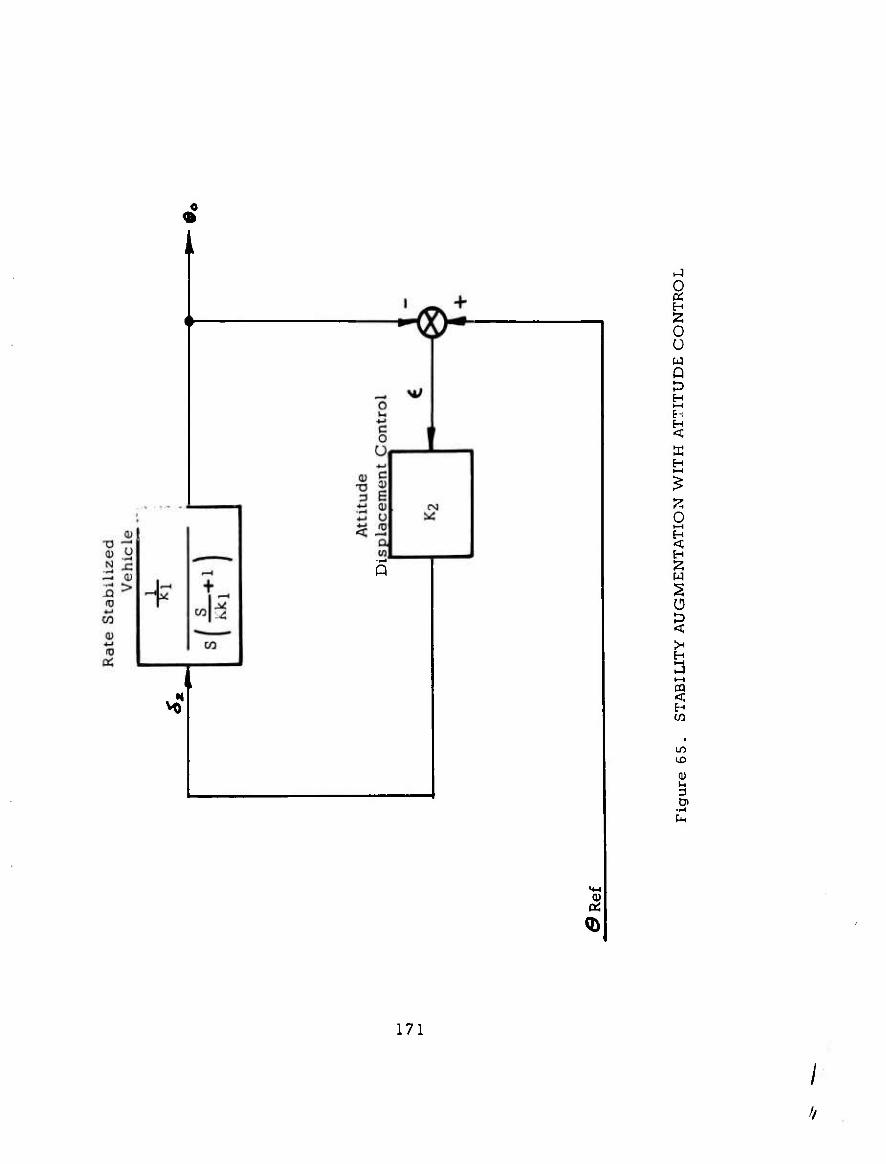
•*
^
§ H
o u w Q
K H
2 < w
Ü
§
K u-)
171

ratio of the rate feedback to the displacement feedback, Q . In fact, the damping ratio is defined by the relation
^= ÜJ±>a . (is)
An illustration of the response of the attitude to a step change in attitude reference is presented in Figure 66.
It is emphasized that all of these results are based on the use of the sim- plified vehicle response characteristic and the conditions under which this characteristic tends to approximate actual vehicle response with good accuracy (References 7, 16).
Experience has demonstrated that for relatively large values of Cc) (i.e., of the order of 3 to 4 radians per second), the approximations usea above are quite good, provided that serv- ^ ural frequency (both stability aug- mentation and attitude) is greater than 5 <*) .
n
The difference between stability augmentation and the combinatioii of stability augmentation and attitude control is now apparent. The & Lability augmentation is able to reduce an acceleration response (equation (9)) to a rate response (equation (8)); the combination control reduces the rate response to a displacement response. The command for the stability aug- mentation is a control deflection, 'i ; the command for the attitude con- trol is a signal reference, 9 f.
To complete this review, the means for control of reference attitude require discussion. There are three different generic means for establishing the reference attitude for the attitude control illustrated in Figure 65. Two of
these techniques are pilot-operated. Through a "black box," which is able to produce compatible signal outputs, the pilot may establish a desired attitude level by setting a graduated dial. For ease in operation, the ref- erence producing transducer can, alternatively, be integrated into the control system so as to respond to forces applied to the controls - control force steering. Either of these methods has the same objective: to permit the pilot to select a desired reference attitude and thereby also to permit him to change this reference from time to time in accordance with his flight plans.
In contrast to the direct pilot control of the attitude reference is the cou- pling of the attitude control to a sensor capable of measuring vehicle trans- lation as indicated in Figure 67. This arrangement makes the reference attitude,^ f, a direct and continuous function of vehicle translation. In the generic sense, then, this operation is an automatic control of vehicle
172

Q*
ÖRef
Time.
ÖRef
Figure 66. ATTITUDE RESPONSE
173
//

I c 0
-F-4 •M In fD o *—' w w d c 0) (0 co H
■M c <u 6 ^ o U i_ (D >. aO w
M-i
Q
a;
y
l-l
(U (U a u D c O 0)
Ü cu tt-(
a: 1 C o ± .r*
¥ +■' I (D X ^ W~ W
^^ c ro
c H
Ü X o
03
CTi S UD C r-t 0) S 0) ll U w l-l (1) b >. 3 0)
■t-l PL) 7J _ Cn PL,
atro
er
in
o ^ Ü w
U.- "T J
174
§ H
O Ü w Q
H i—i
H H <. W ^C H
Ü I—I
w I—1
PQ <, H CO M
Pi O
w

translation through vehicle rotation.
An example of a vehicle translational control system is the velocity control system shown in Figure 68. The stabilized autopilot obeys equation (15). The simplified relation between vehicle translation, x , and vehicle rota- tion, 0 , is obtained by using Newton's law, assuming that vehicle drag is negligible (as in low-speed flight) and that the unbalanced force is the vehicle vertical thrust tilted through the angle 9 :
mgÖo Ä TnXo i (19)
whence, *o 3 ä- = T • (20)
It is desirable to further simplify the system of Figure 68 as illustrated in Figure 69. Implied in this assumption is the fact that the attitude response, characterized hy (j , is much more rapid than that of the overall velocity control system.
Using a similar analytical approach, as in the previous derivation of sta- bility augmentation and attitude control transfer functions, one may demon- strate that the relation between vehicle velocity, x , and the desired ref- erence velocity, x ., is giv^n by the following relation:
4^-s-! (2i) This is the characteristic response of a first-order system, as illustrated in Figure 70, and shows how the desired reference velocity is achieved through continuous, automatic variation of reference attitude.
Returning to the control force steering system. Figure 71, illustrates the general arrangement of the system. The force transducer may be regarded as a strain gage mounted to the control column. When forces are applied to the column (against the reaction of the attitude control servo), a signal is applied to an integrator, such that the reference attitude becomes the time integral of the applied force, F; i.e.,
Ä-pf = / « Fttt + CONSTANT, (22) -/•
in which OC is a proportionality constant established to yield a comfortable response characteristic. If both sides of equation (22) are differentiated, the following result is obtained:
175

&
-1
§
o Ü >* H »—i
u Q i-.
>
<
O
2
to
u
176

•X
w
<b*
ä
§
O Ü
2 H i—»
CO 2
Q w i—«
a, i—i
CO
3
177
//

?,
^Refi
03XRefT— 0 -H \~rr.-t- gk3
Time
^Ref Refi
©Rd
Figure 70. RESPONSE OF VELOCITY CONTROL SYSTEM
178
1
J

cu
i
M 0) u 3
(u -a U OT ^ c O a u. ^
H
Ü
2 w w H W U
O
g H
O Ü
T
4-. ^
S o a. tu
179

^efÄ «F. (23)
Equation (23) states that the rate of change of reference attitude is directly proportional to the applied force. By resort to equation (15),
(24)
If the natural frequency, CJ , is relatively high, equation (24)says, in effect, that the vehicle follows the applied force at a rate proportional to the applied force.
Thus, the control force steering system permits command of new attitude by the application of force to the primary controls, with the aircraft picking up a rate of change of attitude proportional to the applied force. When the force is removed, the vehicle will be stabilized.at the attitude reference prevail- ing at that time.
180

APPENDIX II
TEN-STAGE. SYNCHRONOUS, UP-DOWN BINARY COUNTER
REQUIREMENTS
Of the several binary counter configurations, it was decided that a ten- stage, synchronous, up-down, bit-parallel reset binary counter was re- quired in this application. This decision was made after reviewing the performance obtainable from the various, less complicated binary counter configurations. At this time it is well to review the thinking leading up to this decision.
This basic building block for binary counters is a single-stage binary count- er (see Section l). This has a count input and two outputs. One output is arbitrarily selected as the ONE output; the other is the ZERO output. In addition, there is a reset function, but it is not of interest in this discus- sion.
The simplest binary counter is formed by cascading the number of stages such that the zero output of each stage feeds into the count input of the suc- cessive stage. Such a counter is a serial, up counter. It will not meet the requirement of both positive and negative integration rates. A pair of up counters can be used,with one receiving down counts. The integrated value becomes the difference between the two counts. This would require a rather complicated circuit to decode. Also, when the up counters reach the maximum count, they roll over (return to zero); hence, the coded information becomes ambiguous. These arguments substantiate the need for an up-down counter.
When a pulse enters a serial counter, it propagates from the least signifi- cant stage toward the most significant stage. Using a 0.002 second as the propagation rate per stage, it will take 0.020 second for a pulse to propagate through ten serial counter stages. Since the counting is at a rate up to 100 pps, it is possible to have three pulses propagating through a serial counter at one time. Until a pulse has completed its propagation, the counter output is in error (and it can be considerably in error). A simple example will demonstrate this point. Assume that at time t=000, register R = 011. A count is entered into the register at t - 000; at t = 0.002, R = 010; at t = 0.004, R = 000; at t = 0.006. R = 011. In this example, when one has added to three, the register went to zero during the serial counting before coming out with the correct value of four. Using a serial
181
/

binary counter in this application would result in the output being grossly in error most of the time. Clearly a lynchronous output binary counter is required.
IMPLEMENTATION
Figure 72 depicts a ten-stage,synchronous,up-down binary counter. Rather than describe it piece by piece, the generalizations upon which its design was based will be pointed out.
1. The input up and down pulses come in on separate lines and for the most part are processed by two separate but identical circuits.
2. The input pulses are amplified (for fan-ouc purposes), inverted (for logical purposes), and simultaneously fed to all ten stages.
3. Each stage has an up gate and a down gate which have previous knowl- edge as to whether or not to accept the pulse.
4. All gates which are receptive accept the pulse and feed it into the binary counter by way of an OR gate.
5. All binary counters which have to change count do so at the same instant. Except for the switching transient the register always stores a completed count, whether it be the previous count or the new count.
6. With the advent of the new count the up and down gates are reset for the next input pulse.
This type of counting replaces the carry and borrow with anticipation logic where each counter stage anticipates whether or not to change state on the next count based on the present stored count. The anticipation laws are quite simply stated below:
7. The first-stage changes count for all new counts, whether up or down.
8. For any other stage a change of count will occur for a new up pulse only if all lower weight stages are presently set to one.
9. For any other stage a change of count will oscur for a new down pulse only if all lower weight stages are presently set to zero.
Now referring to the circuit^t is noted that each incoming pulse passes through either an amplifier and an inverter in that order or in the reverse
182

2
I Q
i a.
O
o a K Ü
w
w
CO I
w H
PC W H
P O Ü
a
i—i DQ
^mn^ ^ng^
IT 183

order to result in a pulse inversion. Now the pulse looks like a notch or short period of no pressure in an otherwise steady static pressure. The inverter pulse (notch) is simultaneously transmitted to a NOR gate at each counter stage (the inverter at the first stage can be viewed as a NOR gate with no other inhibiting input). At all NOR gates which are inhibited by another input signal the inverter pulse does not alter the output; at all NOR gates where inhibiting signals are absent, the momentary absence of pres- sure causes a momentary output (pulse ), from the NOR gate, through the OR gate, and into the binary counter. The binary counters so pulsed each change count. The new stored count changes the inhibit signals to the NOR gates and the counter is ready for the next pulse. The inhibit signals for each stage NOR gate are generated by gating together with OR gates all the ONE outputs of the previous stages and all the ZERO outputs of the pre- vious stages. The presence of a single ONE output on previous stages will inhibit the down pulse from passing the NOR gate. The presence of a single ZERO output on previous stages will inhibit the up pulse from passing the NOR gate. As can be seen, the presence of a single ZERO is the indication of the absence of a ONE; likewise, the absence of all ZERO'S indicates the presence of all ONE'S and the inhibit signal is removed.
MODIFICATIONS FOR USE AS TIMING PULSE GENERATOR
The synchronous,up-down counter can be simplified for use in the timing pulse generator. The simplifications consist of removing the tenth counter stage, the down count and down count reset logic (approximately half of the logic elements exclusive of the binary counters), and removing the OR gates just below each binary counter stage; now the output of each binary counter stage becomes a pair of complementing square waves, one being on when the other is off. Each successive counter stage puts out square waves of half the frequency of the previous stage.
184

.... ,*•"
APPENDIX III
TYPICAL RESPONSE CALCULATION IN FLUID CIRCUIT ANALYSIS
The response calculations for a typical fluid circuit shown below involve capacitance, the ability of the fluid to store energy; inductance, the fluids inertia; resistance, the relationship between flow and pressure; and sonic velocity, the speed of a pressure wave in a pipe. These basic character- istics are defined below.
Fluid Resistance, R
The fluid resistance equation is the linearized form of the orifice equation:
V«aC V^7- (25)
C ., the orifice coefficient, is assumed unity in value for a nozzle.
To lineorize ,!. e ; ^tion the partial derivative of flow with respect to pressur droo is taken to be constant for small signal changes:
inverting,
(26)
(27)
-■■
185
/
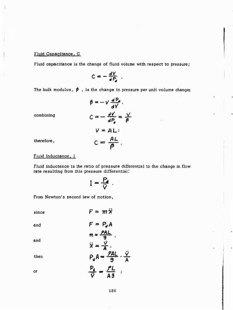
Fluid Capacitance, C
Fluid capacitance is the change of fluid volume with respect to pressure;
The bulk modulus, (3 , is the change in pressure per unit volume change:
combining /* ^ ^v _ _^
therefore,
Fluid Inductance, I
V = AL;
Fluid inductance is the ratio of pressure differential to the change in flow rate resulting from this pressure differential!
! = -&. V
From Newton's second law of motion,
since F — T77X
and
and
then
or
F= P^
m» -g ■■-,
• •
A
i
186
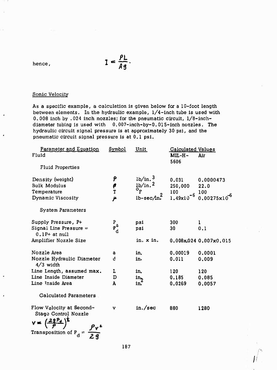
hence, n.
Sonic Velocity
As a specific example, a calculation is given below for a 10-foot length between elements. In the hydraulic example, 1/4-inch tube is used with 0.008 inch by .024 inch nozzles; for the pneumatic circuit, l/8-inch- diameter tubing is used with 0.007-inch-by-0. 015-inch nozzles. The hydraulic circuit signal pressure is at approximately 30 psi, and the pneumatic circuit signal pressure is at 0.1 psi.
Parameter and Equation Symbol Unit Calculated Values Fluid MIL-H-
5606 Air
Fluid Properties
Density (weight) ? lb/in.3 0.031 0.0000473
Bulk Modulus P lb/in.2 250,000 22.0
Temperature T 0F 2 lb-sec/in.
100 100 0.00275x10 Dynamic Viscosity /* 1.49x10"
System Parameters
Supply Pressure, P+ Ps psi 300 1
Signal Line Pressure = Pd psi 30 0.1
0.1P+ at null Amplifier Nozzle Size in. x in. 0.008X.024 0.007x0.01
Nozzle Area a in. 0.00019 0.0001 Nozzle Hydraulic Diameter d in. 0.011 0.009
4/3 width Line Length, assumed max. L in. 120 120 Line Inside Diameter D
in. 0.185 0.085
Line Tnside Area A 0.0269 0.0057
Calculated Parameters
Flow Velocity at Second- Stage Control Nozzle m
Transposition of P , = d
187
in./sec 880 1280
//

Parameter and Equation Symbol Fluid
Volume Flow, first to second stage V = av
Sonic Velocity
X = s W1
Symbol Unit Calculated Values MIL-H- Air 5606
• V in.3/sec 0.167 0.128
• in./sec 56,000 13,400
♦Transmission Line Effects
Sonic Delay
^5
Orifice-Volume, Capacitive Time Constant
= R x C x 2 (Orifice at •C each end of line)
«?) Orifice-Inductance Time
Constant 1^= 1/2K
X, 4A [f)l,J Line Loss, Laminar Flow
AP, = TT P4
r »X
AP,
sec
sec
sec
psi
0.00214 0.0090
0.00236 0.0222
0.00048 0.00082
1.03 0.002
*No long transmission lines are used in the system with the exception of the hydraulic lines from the pilot input position transducer to the amplifier package. See "Fluid Impedance," below, for derivation of R, C, and I.
Summarizing
Average line loss R-C time constant L/R time constant Transmission time delay
Hydraulic 1.03 psi 0.00236 sec 0.00048 sec 0.002 sec
Pneumatic 0.002 psi 0.0222 sec 0.00082 sec 0.009 sec
188

•«».
The effect of line loss is the attenuation of the signals. This attenuation has no effect on the pneumatic digital system but will reduce maximum hy- draulic signals by about 1.0 oercent for the 10-foot line length. No prob- lem is created by this effect within the amplifier package,since the line lengths between elements are kept small. The major effect is in the trans- mission of command signals in the primary circuit from the displacement transducer to the Af'CS. Here the attenuation is a change in signal range and must be compensated by a designed relationship between input and feedback device or by adding restrictions in the feedback lines of the me- chanical to fluid transducer to match those in the input lines.
The capacitive effect results in a time delay for the transmission of pneu- matic digital signals. The inductive effect is negligible in the pneumatic circuit. These effects are both small in the hydraulic control system and are nearly equal. This fact presents the possibility of matching the hy- draulic line impedance to the load to eliminate the reactance effects.
189
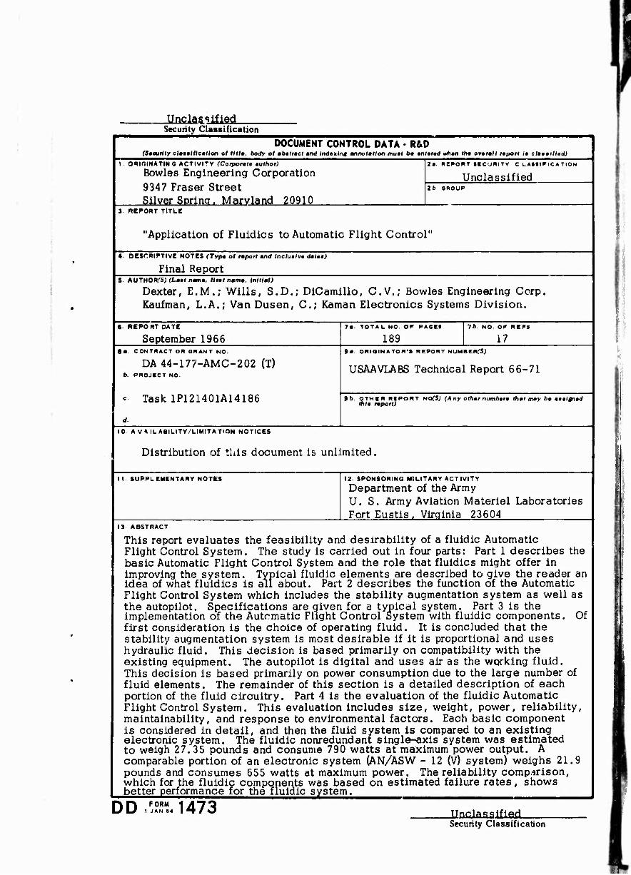
-Ilnglassiüeci Security Classification
DOCUMENT CONTROL DATA • R&D (Stcurlly elmttlllcallon ol till», body of ab*(r«cr and indexing annolallon mutt be entered «/hen (he overa/l report i« clmtmilied)
\. ORIGINATING ACTIV/ITY (Corporate author;
Bowles Engineering Corporation 9347 Fräser Street
Silver Soring. Maryland 20910
2a REPORT SECURITY C L ASSI Fl C A TION
Unclassified 2b GROUP
3 REPORT TITLE
"Application of Fluidics to Automatic Flight Control"
4 DESCRIPTIVE NOTES (Type of «port and tnc/u((ve dateaj
Final Report 5- AUTHORfS; fLaet name, ft rat name, Initial)
Dexter, E.M.; Wills, S.D.; DiCamillo, C.V.; Bowles Engineering Corp. Kaufman, L.A.; Van Dusen, C; Kaman Electronics Systems Division.
6 REPORT DATE
September 1966 8a. CONTRACT OR GRANT NO.
DA 44-177-AMC-202 (T) b. PROJECT NO.
*■ Task 1P121401A14186
d
7a. TOTAL NO. OF PAGES
189 7b. NO. OF REFS
17 9a. ORIGINATOR'S REPORT NUMBERfSj
USAAVLABS Technical Report 66-71
9b. OTHER REPORT NOfS; CAny other numbera that may be aetlgned Chta rape ft)
10. AVAILABILITY/LIMITATION NOTICES
Distribution of this document is unlimited.
11 SUPPLEMENTARY NOTES 12 SPONSORING MILITARY ACTIVITY
Department of the Army U. S. Army Aviation Materiel Laboratories Fort Eustis . Virginia 23604
13 ABSTRACT
Of
This report evaluates the feasibility and desirability of a fluidic Automatic Flight Control System. The study is carried out in four parts: Part 1 describes the basic Automatic Flight Control System and the role that fluidics might offer in improving the system. Typical fluidic elements are described to give the reader an idea of what fluidics is all about. Part 2 describes the function of the Automatic Flight Control System which includes the stability augmentation system as well as the autopilot. Specifications are given for a typical system. Part 3 is the implementation of the Automatic Flight Control System with fluidic components, first consideration is the choice of operating fluid. It is concluded that the stability augmentation system is most desirable if it is proportional and uses hydraulic fluid. This decision is based primarily on compatibility with the existing equipment. The autopilot is digital and uses air as the working fluid. This decision is based primarily on power consumption due to the large number of fluid elements. The remainder of this section is a detailed description of each portion of the fluid circuitry. Part 4 is the evaluation of the fluidic Automatic Flight Control System. This evaluation includes size, weight, power, reliability, maintainability, and response to environmental factors. Each basic component is considered in detail, and then the fluid system is compared to an existing electronic system. The fluidic nonredundant single-axis system was estimated to weigh 27.35 pounds and consume 790 watts at maximum power output. A comparable portion of an electronic system (AN/ASW - 12 (V) system) weighs 21.9 pounds and consumes 655 watts at maximum power. The reliability comp^rison, which for the fluidic components was based on estimated failure rates, shows better performance for the fluidic system.
DD FORM 1 JAN 84 1473 .Unclassified
Security Classification

Unclnsalflflri Security CUaslfication
u KIV WORDS
Fluidlcs Fluerics Fluid Amplifiers Flight Control Stability Augmentation System Helicopters V/STOL Aircraft
UNK A
NOLK WT
LINK •
MOLI WT LINK C
NOLI »>T
INSTRUCTIONS 1. ORIOINATINO ACTIVITY: Bntar th* namt and addraaa of th« contractor, «ubeontractor, grantaa, Daputmant of Do- font« activity or othar organliatlon fceiporata author; laaulni tha raport. 3a. REPORT SBCURTY CLASSIFICATIONS Entar tha ovar- all «acurlty claailflcatlon of tha raport. Indlcata whathar "Raatrlctad Data" la Ineludad Marking la to ba In accord- ance with approprlata aacurlty ragulatlona. 2b. GROUP: Automatic downgradlni la apaclflad In DoD Dl- ractlve 5200.10 and Armad Porcaa Induatrlal Manual. Entar tha group numbar, Alao, whan appllcabta, ahow that optional markinga havn bean uaad for Oroup 3 and Group 4 at author- Itad.
3. REPORT TITLE: Entar tha complata raport tltla In all capital lattara. Tltlaa In all caaaa ahould ba unclaaalflad. If a meaningful tltla cannot ba aalactad without clatalflea- tlon, ahow tltla daaalflcatlon In all capltsla In paranthaala Immediately following tha tltla. 4. DESCRIPTIVE NOTES: If approprlata, enter tha type of report, e.g.. Interim, prograaa, aummary, annual, or final. Give the Inclualvc datca whan a apaelflc reporting period la covered. 5. AUTHOR(S): Enter tha n«m»(a) of authoKa) aa thown on or In the report. Enter taat name, flrat name, middle Initial. If n-.iUtary, ahow rank and branch of narvlca. Tha name of the principal «uthor la an abaoluta minimum requirement. 6. REPORT DATE: Entar tha data of th« report aa day, month, year; or month, yean If more than one data appeara on the report, ute data of publication. 7a. TOTAL NUMBER OP PAGES: Tha total page count «hould follow normal pagination procaduraa, ta,, entar tha number of pagea containing Information, 7b. NUMBER OF REFERENCE» Entar the total numbar of referencea cited In the report. 8«. CONTRACT OR GRANT NUMBER: If approprlata, antnr the applicable number of th« contract or grant under which the report waa written. 8h, 8c. b Id. PROJECT NUMBER: Entar the appropriate military department Identification, auch aa project number, aubprojact number, ayalam numbara, taak numbar, etc. 9a. ORIGINATOR'S REPORT NUMBER(S): Enter the offi- cial raport number by which tha document will ba Identified and controlled by the originating activity. Thla numbar muat be unique to thla report. 9b. OTHER REPORT NUMBER(S): If th« report haa been aaalgned any other report numbara (vlthrt hy tho originator or by (he »pontor), alao enter thla.numb«r(a), ID. AVAILABILITY/LIMITATION NOTICES: Enter any Urn- Uatlona on further dlaaamlnatlon of tha report, other than thoae
Impoaed by aacurlty daaalflcatlon, ualng atandard atatamanta auch aa:
(I)
(2)
(3)
(4)
"Qualified requaatara may obtain coplaa of thla raport from DDC" "Foreign announcement and dlaaamlnatlon of thla raport by DOC la not authorised." "U. S. Government agenclaa may obtain copiea of thla raport directly from DDC. Other qualified DDC uaara ahall raqueat through
>i
"U. S. military agenclaa may obtain coplea of thla report directly from DDC Other qualified uaara ahall requeat through
(5) "All dlatrlbutlon of thla raport la controlled. Qual- ified DDC uaara ahall raqueat through
If the report haa been furnlahed to the Office of Technical Servlcea, Department of Commerce, for aale to the public, Indi- cate thla fact and entar tha price. If known. IL SUPPLEMENTARY NOTES: Uae for addition«! explana- tory notea. 12. SPONSORING MILITARY ACTIVITY: Enter the name of the departmental project office or laboratory aponaorlng (pay ing lor) tha reaearch and development Include a^dreaa. 13- ABSTRACT: Enter an abatract giving a brief and factual aummary of tha document Indicative of the report, even though It may alao appear elaewhere In the body of tha technical re- port. If additional apace la required, a continuation aheet ahall be attached.
It Ik highly dealrable that tha abatract of claaalfled reporta be unclaaalfled. Each paragraph of tha abatract ahall end with an Indication of the military aacurlty daaalflcatlon of the In- formation In the paragraph, repreaented aa (Ti), (S), (C). or ft/;.
There la no limitation on the length of the abatract. How- over, the auggaated length la from ISO to 23S worda.
14. KEY WORDS: Key worda are technically meaningful tertna or abort phraaea that characterise a report and may be uaad aa Index entrlea for cataloging the report- Key worda must be aetected ao that no aacurlty daaalflcatlon la required. Identi- fier«, auch aa equipment model dealgnatlon, trade name, military project code name, geographic location, may be uaad aa key worda but will be followed by an Imllcatlon of technical con- text. The aaalgnment of link«, rulea, and welghta la optional.
Ilaslaaalflfld Security ClMilflcation 6141-66