U RAL ELECTRICI

SCHENECTADY, NFW YORK~

TECHNICAL REPORT VTME ESTIMATION OF PERIODIC SIGNALS IN NOISE

T. G. Kincaid and H. J. Scudder, Mf

Contract No. NOrr-4692(0O)A

421

F~ebruary 1968

Office of Naval Research 01~

This document has been approved for pubicrelease and sale; its distribution is unlimited,

CL kA PI N HiU St S-68-1019

3

TECHNICAL REPORT

TO

OFFICE OF NAVAL RESEARCH

THE ESTIMATION OF PERIODIC SIGNALS IN NOISE

T.G. Kincaid and H.J. Scudder, I

Contract No. NOnr-4692(00)

February 1968

This document has been approved for publicrelease and sale; its distribution is unlimited.

Research and Development CenterGENERAL ELECTRIC COMPANY

Schenectady, New York 12301

S-68-1019

ABSTRACT

This report presents two methods for the estimation of a periodic signalin additive noise. Both methods assume that only a finite time sample of thesignal plus noise is available for processing. The estimate of the signal ischosen to minimize the mean square error between the estimate and the sampleof signal plus noise. This is also a maximum likelihood estimate if the noiseis white and Gaussian.

The first method is frequency domain analysis. Estimates for theperiod of the signal and the complex amplitudes of its harmonics are derived.

The second method is time domain analysis. Estimates for the periodof the signal and for the waveform of one period are derived.

Under the assumption of white noise and large signal-to-noise ratio,formulas for the expected values and variances of the period estimates arederived. The estimates for the period are found to be the same by both methods.The estimate is unbiased and has a variance inversely proportional to thesignal-to-noise ratio, and inversely proportional to the cube of the number ofperiods in the given sample. The expected values of the estimates of the wave-form itself are derived, and the estimates are found to be biased.

Ii

TABLE OF CONTENTS

Page

I. INTRODUCTION- -------------------------------- 1

T. THE FREQUENCY DOMAIN APPROACH 3---------------3

A. The Estimates of the Period and Fourier Coefficients ----- 3B. The Resolution of the Period Estimate - --------------- 4C. The Expectation and Variance of the Period Estimate ----- 5D. The Expectations of the Fourier Coefficient Estimates ---- 6

I. THE TIIME DOMAIN APPROACH- --------------------- 6

A. The Estimate of the Waveform for a Fixed Period ------- 7B. The Estimate of the Period 8----------------------8C. The Expected Value of the Waveform Estimate --------- 9

IV. CONCLUSION- --------------------------------- 10

APPENDICES (A through G) ---------------------------- 11-30

REFERENCES ------------------------------------- 31

iii

THE ESTIMATION OF PERIODIC SIGNALS IN NOISE

T. G. Kincaid* and H. J. Scudder, III

I. INTRODUCTION

In this report we conside?" the problem of estimating a periodic signalin additive noise. Although this iij a special application of the establishedtheory of parameter estimation, (1, 2) periodic signals deserve a detailed treat-ment because of their frequent occurrence. For example, the results of thisstudy are useful in the analysis of sounds produced by rotating machinery. Inthis application, good signal estimates can be used for source identification ormalfunction diagnosis.

We shall assume that a finite time sample o- the signal plus noise isavailable for inspection. We shall show two methods of forming the estimateof the periodic signal which minimizes the mean square error between thisestimate and the given time sample of signal plus noise. (It is well known thatthe minimum mean square error estimator is also a maximum likelihood esti-mator if the noise is white and Gaussian. ) The first method uses a frequencydomain approach, while the second method works in the time domain.

In the frequency domain method, the first step is to estimate the periodby summing the power spectrum of the data at harmonics of a sequence of trialfundamental frequencies. The period of the fundamental which gives the largestsum is the estimate. The Fourier coefficients of desired waveform are thenestimated from the values of the Fourier transform of the data at harmonics ofthe estimated fundamental.

In the time domain method, the period and the waveforrn are estimatedsimultaneously. The technique is simply to choose a trial period P, divide thedata into P length sections, and average the sections. The trial period whichproduces the average waveform with the largest energy is the estimate of thetime period, and the average waveform is the estimate of the true waveform.

tUnder the assumption of white noise and large signal-to-noise ratio,formulas for appropriate statistics of the estimates are deived for both methods.The mean and variance of the period e-timates are found to be the same by bothmethods. The mean is found to be unbiased. The var::ice is found to be inverselyproportional to the signal-to-noise ratio and inversely proportional to the cubeof the number of periods in the data sample. Formulas for the mean of theFourier coefficients are derived for the frequency domain estimates, and it isfound that these estimates are biased. In the time domain approach, it isnecessary to assume a noise distribution to compute the mean of the waveformestimate. On the assumption of Gaussian noise, this estimate is shown to be

*General Electric Company, Heavy Military Electronics Department, Syracuse,New York.

~-1-

biased.

In this report tk,- following notation will be used.

? (t) denotes a function aefined on the interval -- <t<, and is a theoreticalideal,

f(t) denotes a function which is equal to T(t) on a finite interval T, and

zero elsewhere, and is the real signal we must work with.

0 for lxl> 1 /2

rect(x) = 1/& for lxi = 1/2

! for Ixl<1/2

si Lx for xJ0Tux

sinc(x) =1 for x=O

(rect and sinc are a Fourier transform pair);

6(t) denotes the Dirac delta function;

{0frt<O and t>x

gx(t) = for 0t< ,x the gate function;

* between functions denotes convolution;

* as a superscript denotes complex conjugation;

E is an expectation (ensemble averaging) operator.

In general, where small letters are used for time functions, thecorresponding capitals are used for thleir Fourier transforms.

Formally, we initiate our analysis with the following assumptions:

(i) Wi{() = Z(t) + i(t) has bandwidth B Hz;1.(ii) xo(t) is periodic with period P 0>>B, i. e., many harmonics;

(iii) ' (t) is a sample function of a zero mean wide sense stationaryrandom process with covariance function R(t-s) and PowerSpectrum P(f);

(iv) For band-limited white noise, R(t-s) a 2 sinc(2Bt) and P(f)aY22rec fI

(v) 0(t) =n w°(t-nP°) (see Ref. 3)

-2-

where wo(t) = 0; for t<O, t :Po.

(vi) JPC wo(t)dt>>a0

i. e., large signal-to-noise ratio.

(vii) z(t) is known on an interval of length T>>P0i. e., many periods.

II. THE FREQUENCY DOMAIN APPROACH

In the frequency domain approach we begin by characterizing the un-known periodic waveform Z0(t) as a Fourier series. The optimization procedurethen yields estimators of the period P 0 and Fourier coefficients cok Of xo(t).

A. The Estimates of the Period and Fourier Coefficients

Any periodic signal x(t) can be written as a Fourier series as follows

j2rrkt/PSck e . (/-'k

As our estimate of 0 (t) , we seek the particular periodic signal X(t) = R(t) whichminimizes the mean square error between ~(t) and the observed data _'(t) on theinterval -T/2 < t _< T/2. That error is given by

1 fT/2 Zt) 1

L f-T2 t) - '(t)] 2 dt . (2)

In Appendix A it is shown that the estimates of the perioa P and the Fouriercoefficients 8k of X(t) are determined as follows.

First compute Z(f), the Fourier transform of z(t). Then P is the valueof P which maximizes the expression

T KV (P) = ;F Z I Z (k /p)12 (3)

k=1

where K is tho total number of harmonics that can be accommodated by thebandwidth of z(t). The Fourier coefficient estimates k are the values of ckgiven by

ck = ak + J Ak (4)

-3-

where1

ak = Zr (k/P) (5)1 zi (6)

bk = Zi (k/P)(6

Zr(f) and Zi(f) are, respectively, the real and imaginary parts of Z(f). Theestimate i(t) of the unknown waveform can then be generated by the relation

A(t) =. CkkeJ2n~kt/P (7)

k

These estimates are independent of the noise covariance R(t-s).

The estimates are intuitively what we would expect. The period isestimated by summing the values of the power spectrum of z(t) at the harmonicsof the fundamental frequency 1/P. When plotted as a function of P, one wouldexpect this sum to be greatest when P is close to the true period. The Fouriercoefficients of x0(t) are then just l/T the values of the Fourier transform atharmonics of the estimated fundamental frequency.

B. The Resolution of the Period Estimate

In practice, V(P) cannot be tested for a maximum at every value of P.Usually P0 is known approximately (from auto-correlation or power spectrumdata), so that a range of values of P to be tested can be established. In orderto reduce the computing time, it is desirable to test as few values of P asnecessary within that range. How far apart can we choose the test values of Pwithout danger of missing the maximum of V(P)? To answer this question weneed to know the behavior of V(P) in the vicinity of the maximum.

Since the Fourier transform is a linear operation, the assumption ofa large signal-to-noise ratio carries over into the frequency domain. Thusthe gross behavior of V(P) in the vicinity of the maximum will be dominated bythe signal, and we can study that behavior adequately by considering the idealcase in which there is no noise. In Appendix B the noise free behavior of V(P)is studied in a region AP about P 0 . For h<<P0 it is shown that

K

V(Po + h) -= 1cok, 2 sinc2 (8)k=l0

Equation (8) shows that in the vicinity of P0 the noise-free V(P) is a weightedsum of squared sinc functions, centered on P 0 . The widths of the main lobesof the sinc functions are inversely proportional to k, each lobe going to zero ath =P0/kT. The "roll off" of V(P) in the immediate vicinity of P0 is controlledby the narrowest of these squared sinc functions. This is the term in Eq. (8)for which k=K. Thus, in order not to miss the maximum, V(P) should be

-4-

sampled at intervals not larger than

AP =(9)KT

We shall call the quantity AP given by Eq. (9) the resolution of the periodestimator.

Since K is the total number of harmonics in %(t), it is appropriate todefine the bandwidth B0 of i0(t) to be K/P 0 . Then Eq. (9) can be written

AP = (10)B0T

Equation (10) is satisfying in its simplicity. It says that the resolutionof the period estimator is equal to the true period divided by an appropriatelydefined time bandwidth product. The resolution does not depend upon the detailedstructure of the periodic waveform.

C. The Expectation and Variance of the Period Estimate

Because of the noise, we cannot expect the maximum of V(P) to lieexactly at P 0. As a measure of how close P is likely to come to P0 , we shallcompute the expectation and the variance of the random variable P. We proceedas follows. (4)

V(P) is a well-behaved function of P. Thus we can expand V(P) in aTaylor series about the true period P 0.

V(P) = V(P 0 + h) = V(P 0 ) + V'(P 0 ) h + V"(P 0 ) -i2 (11)

We shall only investigate the region h << P0 , so we can neglect terms of higherthan second order in h. The maximum of V(P) may be found by taking thederivative of V(P) and equating it to zero.

V'(P) = 0 = V(Po) + V"(P 0) h . (12)

Solving Eq. (12) for h, we find that to a first approximation

V'(PO)P0 - Vl IWO) • 13)

In Appendix C it is shown that the expectation of P as given by Eq. (13) is

EP= Po (14)

i. e., the estimate is unbiased.

-5-

It is also shown in Appendix C that the variance of P as given by Eq.(13) is

I o__3

Var P 2 o j-, 3 E' 1 (15)

where B2w is the second moment of the spectrum of wo(t), defined by Eq. (C25),

and Ew is the energy of wo(t), defined by Eq. (C26). Equation (15) shows thatthe variance of P decreases as the inverse cube of the length of the data sampleT, and that it decreases as the inverse of the signal-to-noise ratio E w / a .

D. The Expectations of the Fourier Coefficient Estimates

The estimates of the complex Fourier coefficients of the oignal are,by Eqs. (4), (5), and (6)

1 Xo

T k o k o 2 " p

Thus

1 ,X k k2 2TT2 T2 k (P2PO) 2E C X0 E +.. +

k T P4 13 PO 2 0-

1 0k 2 !,2 2 a

21TO POT BBw Ew

We see that the estimates of the Fourier coefficients are biased, but that thebias approaches 0 as T--, and decreases as the signal-to-nise ratio increases.

III. THE TIME DOMAIN APPROACH

We shall assume in this analysis that '~(t), the periodic signal plusnoise, is known on an interval 0.<t<T. Let gT(t) be the gate function defined irnthe Introduction. Then

z (t) = 'g(t) gT (t)

is the known signal, and

xo(t) ot) -T(t)

-6-

is the true periodic waveform obscured by noise

no(t) = io(t) gT(t)

on this interval. In this approach we shall find an estimate w^(t) of wo(t), thewaveform of one period of ' (t); and we shall find an estimate P of P 0, the periodof 30(t). These two estimates give an estimate i(t) of xO(t). We shall chooseas our estimate V(t) the particular x(t) which minimizes the mean square error

L= f [z(t) - x(t)]2 dt (17)

We shall also determine the mean and variance of P, and the mean of WR(t) underthe assumption of Gaussian noise.

A. The Estimate of the Waveform for a Fixed Period

In this section we assume a fixed period P and find a periodic waveformwhich minimizes L. To simplify the analysis we shall minimize L over a sectionof data NP long, rather than T. The integer N is chosen so that the intervalNP is as large as possible i. e., NP 4 T < (N+I)P. Thus we shall actually findthe periodic waveform X^p(t) which minimizes

1fNP

L = 1-- [z(t) - x(t)]2 dt (18)

Let -Cvp(t) be one period of )?p(t). In Appendix D it is shown that

N-IMp(t) z(t + nP) gp(t); NP T < (N + 1) P (19)

n=0

This equation says that 'p(t) is the average of N successive P length sectionsof z(t). This result is intuitively what one would expect. As successive Plength intervals are averaged the periodic component remains constant whilethe noise tends to average to zero.

It is of interest to examine the error in the estimate 'vp(t) caused byrestricting the data to a duration NP. It is shown in Appendix D that the dif-ference between vp(t) given by Eq. (19) and the estimate w (t) which minimizesL given by Eq. (17) is

W -(t 'p(t) = N [z(t + NP) - wp(t)] 0 t < (T - NP){0l I (20)

0 ;(T - NP) t<T

-7-

This error is the difference between averaging the left over "tail" of the datainto the estimate. Since the amplitude of error is inversely proportional toN+I, our introductory assumption that T >> P makes this error small. Byneglecting this error we not only simplify the analysis but eliminate an untidydiscontinuity in W.p(t) at t=T-NP.

B. The Estimate of the Period

Now that we have learned how to form WRp(t) for an arbitrary P, weshall find an estimate P for the true period P 0. By our stated criterion, werequire P to be that P which minimizes Lp as given by Eq. (18). It appearsimpossible to get any satisfaction by setting the derivative of Lp with respectto P equal to zero. The P is tied up inside the x(t) in an unknown manner andcannot be brought out. The best technique appears to be brutu force computationof L as a function of P, and to choose the P which minimizes L as P.

However, it is not necessary to actually go through the computation ofLp for each P in order to minimize Lp. It is sufficient to compute the energyof the estimate W^p(t) for each P. Then the P for which this energy is a maximumis the estimate P of the true period P 0.

To show this, we first define the error signal estimate

ep(t) = z(t) - x^p(t) .(21)

In Appendix E it is shown that p(t) is orthogonal to p(t), viz.,

NP

f0 NP(t) ep(t) dt = 0 (22)

Now, our objective was to choose P to minimize the mean square error signal,Lp.

.1 NPLp = J [z(t) - -p(t)]2 dt

s 2t stNP rNPN _ j z(t)dt - 2 [Xp(t) + ep(t)] Xp(t) dt + 2p(t) dtNP 0 fN

z 2 7 z2(t) dt - fN (t) dt . (23)0

Since the first term is very nearly a constant for a small range of P, Lp willbe a minimum when the second term is a maximum. (5) Thus P is the value ofP which maximizes the exipression

-8-

0N P P

V(P) X(t) dt = P Vp(t) dt (24)00

The choice of notation is deliberate. In Appendix F it is shown that Eqs. (24)and (3) are equivalent definitions of V(P).

Since the estimator of the period is the same for both the time andfrequency domain approaches, the resolution of the period estimator is givenby Eq. (9) cr Eq. (10). Similarly, the expectation and variance of the estimateare given by Eqs. (14) and (15), respectively.

C. The Expected Value of the Waveform Estimate

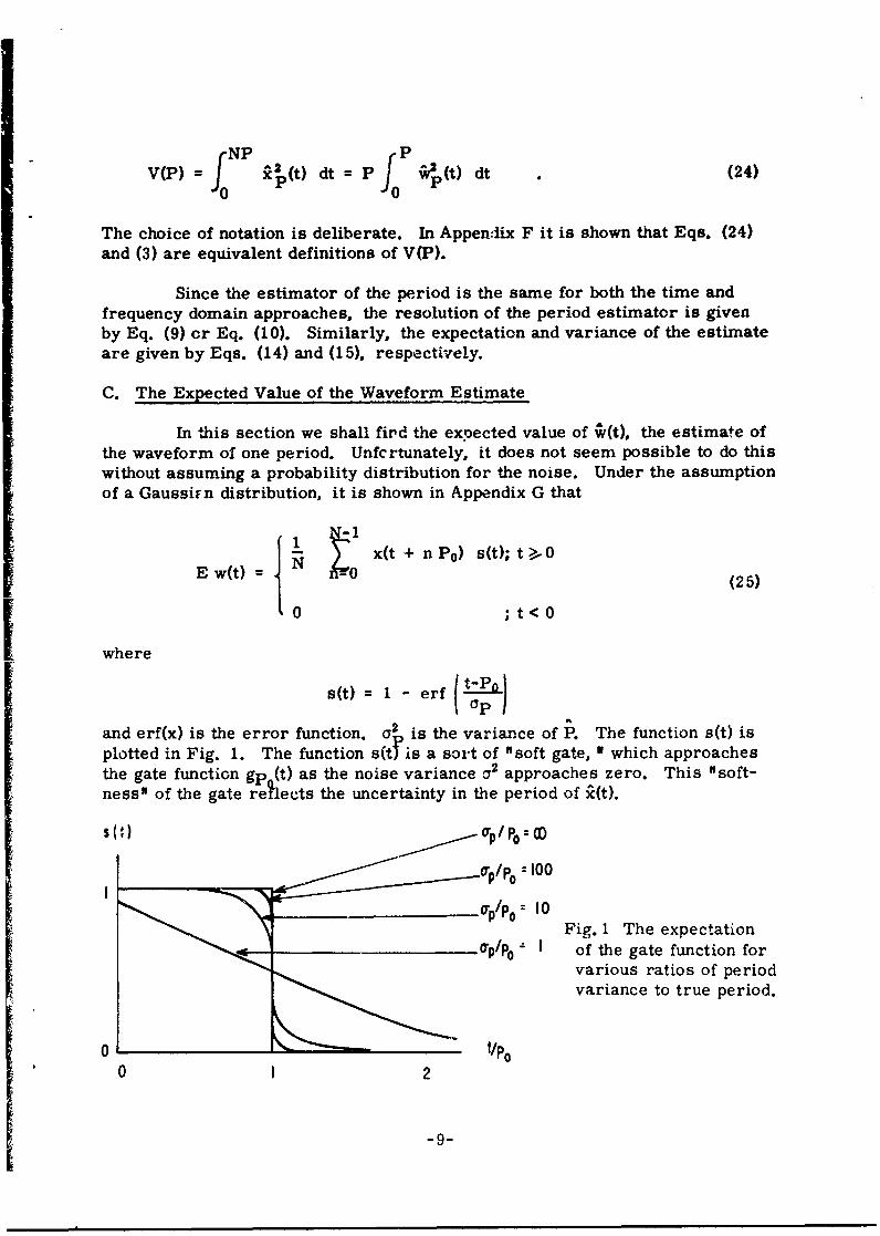
In this section we shall fird the expected value of 4(t), the estimate ofthe waveform of one period. Unfcrtunately, it does not seem possible to do thiswithout assuming a probability distribution for the noise. Under the assumptionof a Gaussi~n distribution, it is shown in Appendix G that

Ew(t) = x(t + nPo) s(t); t> 0E w1)- 25)

whr 0 ;t<0where

s(t) = 1 - erf (t-PO)

and erf(x) is the error function, a 2 is the variance of P. The function s(t) isplotted in Fig. 1. The function s(tyis a sort of "soft gate, " which approachesthe gate function gp (t) as the noise variance a2 approaches zero. This "soft-ness" of the gate reflects the uncertainty in the period of i(t).

SCI) P/ O:D

p/Po :10

Fig. 1 The expectation0"p/p0_: I of the gate function for

various ratios of periodvariance to true period.

0 t/Po0 2

-9-

IV. CONCLUSION

Two methods of finding the least mean square estimate of a periodicfunction in noise have been derived. These have been labeled the frequencydomain and time domain methods. Under appropriate assumptions about thenoise, formulas for the expectation and variance of the period estimate, and theexpectation of the waveform estimates have been found. The variances of thewaveform estimates were not found.

Of the two methods, the authors have found the time domain methodmore satisfactory if it is not necessary to compute the Fourier transform forother reasons. If n data waveform samples are available, and it is desired tosearch m periods for a maximum, then the time required is proportional to inn.The time domain method has the additional feature that the estimates can bemade in one pass through the data. This is important if the data are stored ontape, or some other slow memory.

When the Fourier transform of the data has to be computed anyway forreasons other than waveform egtimation, the frequency domain method isadvantageous. Taking the Fourier transform of n data points requires a timeproportional to n log n, assuming the fast Fourier transform is used. Then,once the power spectrum is formed, it can be searched exhaustively for evidenceof periodicities. This search requires mh operations, where h is the averagenumber ol harmonics summed on each period tested. This is essentially atwo-pass system. On the first pass the data are Fourier transformed, and onthe second pass the power spectrum is searched.

It is worth noting that the period estimator also serves as a suboptimaldetector of periodic waveforms. When there are a large number of strongharmonics, it is somewhat more sensitive than a spectrogram, which does notsum the harmonics. The optimum tetector takes advantage of the waveformestimate in an estimator-correlator configuration. This will be shown by theauthors in a forthcoming report.

-10-

APPENDIX A

We wish to verify that P is the value of P which maximizes V(P) givenby Eq. (3), and that Ak is the value of ck given by Eq. (4) of the main text.

From Eqs. (1) and (2) we have that

L= T/ z2(t)-2z(t ck e +J-2"ktP j21-(k+t/Pd

(Al)Thus,

L T/2 CP 1 +sinc (k+' T /P!T L -T/2 Lk

2 rT/ 2 j2Trkt/P2 k f-T/2 z(t) e dt . (A2)

If we definefT/2 -i2T kt/P

Z(k/P) = T/2 z(t) e - dt, (A3)

the Fourier transform of the input z(t) at frequency k/P, and we use theassumption T>>P, then

L/ z2 (t)dt + Ick 2 - 2 c Z*(k/P) (A4)T -T/2 L Itcd T k k

since only the diagonal terms of the double sum make major contributions.Le' ck = ak + jbk, and note that bk = b-k, ak = a-k.

Then

L - T/2 z2(t)dt - ka2 + b'- 2 [ak Zrk/P)-bkZi(k/P)]

Minimizing with respect to the ak and bk yieldsZr Z.

ak = -Z-(k/P) bk = (k/P) (A5)

Substituting, we find

T I T/2 Z2(t)dt + 1\. ,Z(k/ P), 1 2 iZ(k!P) 12

T - -T/2 T Z k- k

I -IIk

or

'(J/2ztdt ~ Z'k /)1 (A6) .T/2

Since the first term on the right of Eq. (A6) is a constant, L isminimized when the second term on the right is maximized. Since z(t) has somefinite practical bandwidth, it is n-at necessary to sum over all k, but rather tosome upper limit K. Thus the value of P which maximizes V(P) is given byEq. (3). Equations (A5) give the values of ak and bk which minimize L for anychoice of P. Thus L is minimized with respect to both P and ck when ck = Ck,as given by Eq. (4).

-12-

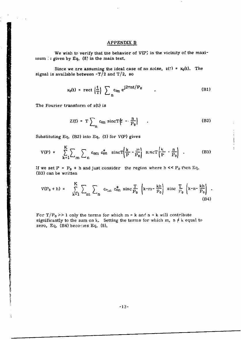
APPENDIX B

We wish to verify that the behavior of V(P, in the vicinity of the maxi-mum : given by Eq. (8 in the main text.

Since we are assuming the ideal case of no noise, z() = xo(t). Thesignal is available between -T/2 and T/2, so

xo(t) = rect (TL) Z con ej2Trnt/Po (Bl)n

The Fourier transform of z(t) is

Z(f) = T Z con sincTIf -. - (B2)n0

Substituting Eq. (B2) into Eq. (3) for V(P) gives

K 1 k : i n~V(P) = Z m CZ m Con sincT p P-i s~ncT (p P0 (B3)

k=I m En

If we set P = P0 + h and just consider the region where h << Po thlen Eq.

(B3) can be written

K hV(P + h) = 7 C~ihl C0n sinc0 k-m- sinc!-.o k-n- L

k=1l m EnPOP p0O

(B4)

For T/Po >> 1 only the terms for which m = k and n = k will contributesignificantly to the sum on k. Setting the terms for which m, n J k equal tozero, Eq. (B4) becorles Eq. (8).

-13-

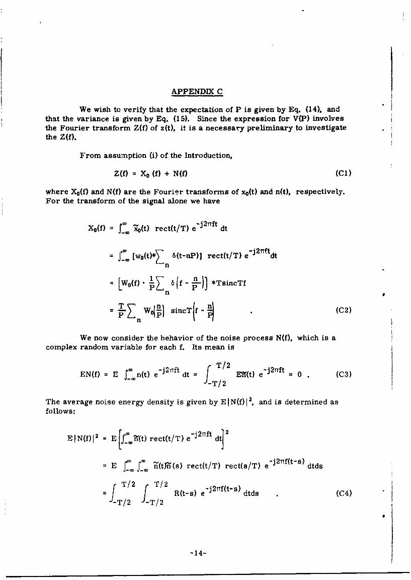
APPENDIX C

thetheWe wish to verify that the expectation of P is given by Eq. (14). andthat tevariance is given by Eq. (15). Since the expression for V(P) involves

teFourier transform Z(f) of z(t), it is a necessary preliminary to investigateteZ f).

From assumption (i) of the Introduction,

Z (f) = X0 (f) + N (f) (Cl)

where X0 (f) and N(f) are the Fourier transforms of x0(t) and n(t), respectively.For the transform of the signal alone we have

XO(f = J- cc x(t) rect(t/T) e jftdt

= NO[Ot* 6tnj ettT j2rrftL. En

= [wO~f) - L 6 (f- -L)] *TsincTfn A

TZ W0(!) sincTtf-' (C2)n

We now consider the behavior of the noise process N(f), which is acomplex random variable for each f. Its mean is

EN(f) = E n~)e,2~tdt T/2 E?(t) e -j2fft = 0 * (C3)

The average noise energy density is given by E I N(f) 12 , and is determined asfollows:

E IN(f) 12 = E W(t) rect(t/T) e j 2Tft dt]2

= E C0Mns)rect(t/T) rect(s/T) e -j2rrf(t-s) dd

=fT/2 T/2 R~-)e-j2rf(t-s) dts(CO)-T/2 f-T/2

-14-

For band-limited white noise

EIN(f) 2 = f Jrect(t/T) rect(s/T)o2 sinc[2B(t-s)] e-j2 f( - ) dtds

= .2 rM ds rect(s/T) ej 2 r f - [sxnc(2Bs)*rect(s/T) e + j 2*

f s (C5)

Taking the Fourier transform of the convolution, and integrating over s first,we get

EIN(f)12 = 2!B J'D sinc2 T(f-g) rect(24) dg . (C6)

A plot of 1/T E I N(f) 2 the average power density of the time limited noise, isshown in Fig. C-1 for several different BT products. Note that as BT-' - thisfunction approaches the "rect, N and for BT > 10 a Urect" is a good approxima-tion to the actual power density. This can be seen directly from Eq. (C6) bynoting that compared to the Orect" function the squared wsinc" function isbecoming very narrow, i. e. , approaching an impulse as BT- -. Since this"impulse" has area I/T, we can use the approximation

EIN(f) 1 = 2 rec- . (C7)

With these preliminaries taken care of, we can now turn Lo the verification ofEqs. (14) and (15).

29 OT1a 10

T- 5

B U 9

Fig. C-I Average power density of band-limitedwhite noise for various BT products.

-15-

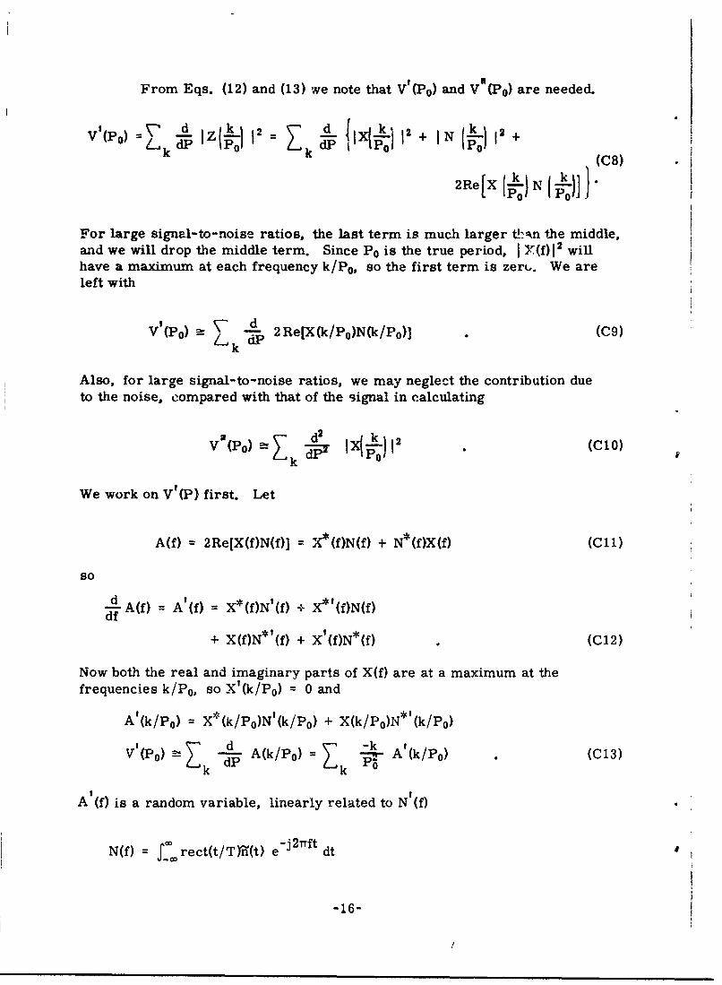
From Eqs. (12) and (13) we note that VI(Po) and V"(Po) are needed.

kk (C8)

2Re[X I--)NI k

For large signal-to-noise ratios, the last term is much larger t!i.n the middle,and we will drop the middle term. Since P 0 is the true period, I (f) 12 willhave a maximum at each frequency k/P 0 , so the first term is zero. We areleft with

V (P°) =" P2Re[X(k/P°)N(k/P°)] .(C9)

k

Also, for large signal-to-noise ratios, we may neglect the contribution dueto the noise, compared with that of the signal in calculating

P0

k P

We work on V'(P) first. Let

A(f) = 2Re[X(f)N(f)] =X'-(f)N(f) + N*(f)X(f) (Cll)

so

ddf A(f) = A'(f) = X*(f)N'(f) + X'fNf

+ X(f)N*'(f) + X'(f)N*(f) (C12)

Now both the real and imaginary parts of X(f) are at a maximum at thefrequencies k/Po, so X'(k/P 0 ) = 0 and

A'(k/Po) X*(k/Po)N'(k/Po) + X(k/Po)N* (k/Po)

V'(PO) d A(k/Po)= -p' A (k/Po) (C13)k d Ak k 0

A (f) is a random variable, linearly related to NI(f)

N(f) = c rect(t/T)-n(t) e - j21 ft dt

-16-

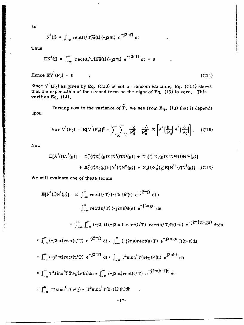
soIN I(f) =frect(t/Tiin(t) (-j2Tnt) e -j2nft dt

Thus

EN I(f) £ rect(t/T)E-n(t) (-j2Trt) e j2Tlft dt = 0

Hence EV (Po) =0 (C14)

Since V"(Po) as given by Eq. (CIO) is not a random variable, Eq. (C14) showsthat the expectation of the second term on the right of Eq. (13) is zero. Thisverifies Eq. (14).

Turning now to the variance of P, we see from Eq. (13) that it dependsupon

Var V'(Po) = E[V'(p 0 )]2 k -t [A, EA( k 1A'11-fl ] 15kL t'- 0 Pj P

Now

E[A'(f)A'(g)] = X0*(f)X*(g)E[N'(f)N'(g)] + X0(f) XK0 (g)E(N'*(f)N'*(g)]I + ~X*(f)Xo(g)E[N'(f)N*(g)] + Xo(f)X*(g)E[N '*(f)N'(g)j .(C16)

We will evaluat-e one of these terms

E[N'(f)N'(g)] =E '~ rect(t/T) (-j2Trrti(t) e - 2 Trft dt.

j00rect(s/T)(-j2Trs)?f(s) e- ~g ds

-jcnt (CDs 3j2T(ft+gs)j~ J(-2t)(jT rent(t/T) rect(s/T)R(t-s) e dtds

-. C -j, j-'t~rc~/T dt.- J0(' (-j2Ts)rect(s/T) e j2 'gs R(t-s)ds

-0 ~ -j2rrt)rect(t/T) e- 2 1rrft it * J" T 2 Sinc'T(h+g)P(h) ej2 Th ht

QT jTsinc'T(h+g)P(h)dh. J' (-j2Trt)rect(t/T) ej 2 f cit

-0 Tf T2sinc'T(h+g) * T 2 sincIT(h-f)P(h)dh

-17-

Substituting for P(h) from assumption (iv) in the Intrcduction,

2 32

E[N (f)N (g)J - T3 sinc"T(g+f) rect(g/2B) rect(f/2B) (C17)

because the sinc function behaves similar to a 6 function for large BT. Sincethe above is real, E[N*(f)N*(g)] = E[N'(f)N'(g)]. In a similar manner,

*1 2

E[N'(f)N*'(g)] = E[N*'(f)N'(g)] a 2- T3sinc"T(f-g) rect(g/2B) rect(f/2B)2B

(C18)Thus

E[A'(f)A'(g)] -t X(f)X ,(g) + Xo(f)Xo(g)] sinc"T(f+g)

+ [Xo(f)X~o(g) + X*(f)Xo(g)] sinc"T(f-g)j

2" rect(f/2B) rect(g/2B) .(C19)2TB

For f=g,

a2T 3

+ 2Re[X6(f)- sinc"(2Tf) rect(f/2B) (C20)

For f = -g we get the same expression, so

Var V'(P) a 2 r21Xo 12 +Ik BPoIPo PO 2B 3

2Re x2 '(2T3 .ic 2-j+ 7 k t E A ,

Ikh<BPo it- 0 PO

IkI / It

where we have summed over both diagonals separately. We may neglect thelast two sets of terms, in comparison with the first since they are down by afactor of at least P 0/T. Thus

I 2rT T' G2 2 k2I(~2Var V(P) T3 B) I<B kXo]' (C21)

-18-

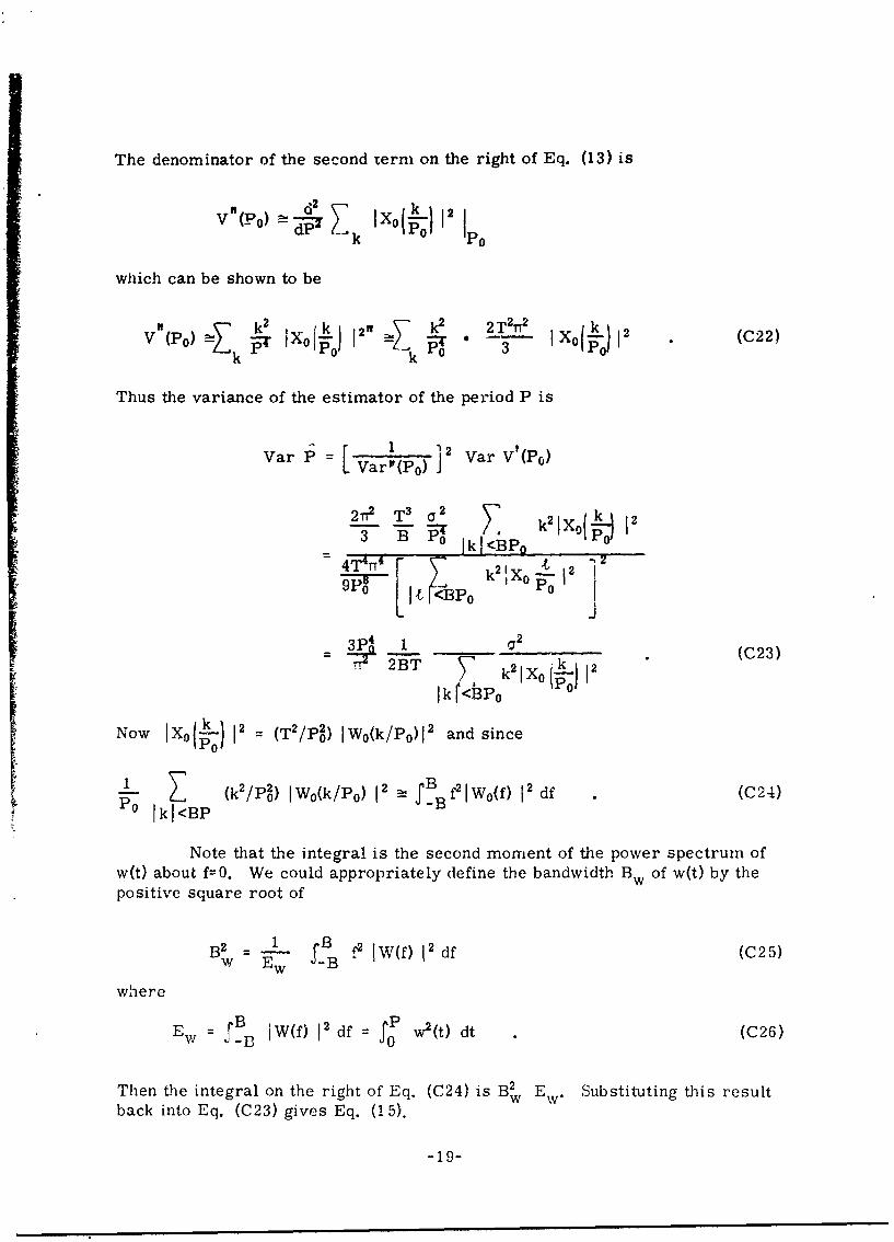
The denominator of the second term on the right of Eq. (13) is

V"(PO) P k Ix o

which can be shown to be

IXO 12, k * 2T 2r Ik_2

O(P) k l k ' 3 Xo

Thus the variance of the estimator of the period P is

Var 1P 12 [a 1 2

Var"(Po) J Var V'(Po)

2rn-2 T3 a 2 k21o~3 B o kk<BP O 12

.4 VIrBP k2 "Xo o0

L-I k' 11 <BE

4 2T TT k2I XO (-0 12 (C23)

lkkBPNowD 20p

Now X0-L-)12 = (T 2 /p2) IW 0(k/P 0 )1 2 and since

! (k2/P2) IWo(k/Po) 12 -- 12 lWo(f) 1 df (C24)P0 kI<BP

Note that the integral is the second moment of the power spectrum ofw(t) about f-0. We could appropriately define the bandwidth Bw of w(t) by thepositive square root of

B = 1 B ff2l W(f)l 2 df (C25)w Ew JB

where

W - W(f) 12 df fP w2(t) dt (C26)

Then the integral on the right of Eq. (C24) is B2 Ew . Substituting this resultback into Eq. (C23) gives Eq. (1 5).

-19-

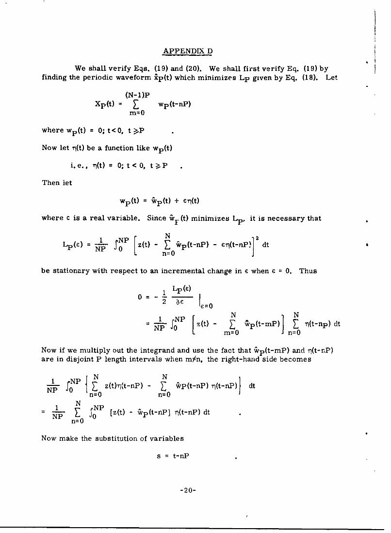
APPENDIX D

We shall verify Eqs. (19) and (20). We shall first verify Eq. (19) byfinding the periodic waveform lp(t) which minimizes Lp given by Eq. (18). Let

(N-1)PXp(t) = Z wp(t-nP)

m=0

where wp(t) = 0; t<0, t >.P

Now let i(t) be a function like wp(t)

i.e., T(t) = 0;t<0, t>P

Then iet

Wp(t) = 'Vp(t) + CII(t)

where c is a real variable. Since ^ Fy(t) minimizes Lp, it is necessary that

N .2

Lp K 1 JNP z(t) - T 1 Vp(t-nP) - eTI(t-nP) dt

be stationary with respect to an incremental change in - when e = 0. Thus

I Lp (C0=I

2 6 [E =O

1 P [ N NJ1 z(t) - Z ;Vp(t-mP)n Z n(t-np) dt

Now if we multiply out the integrand and use the fact that w.p(t-mP) and i,(t-nP)are in disjoint P length intervals when m/n, the right-hand side becomes

4N NR-'P" z(t)r,(t-nP) - Cvp(t-nP) n(t-nP) dtn=0 n=0

1 N NPNP J [z(t) - vp(t-nP] n(t-nP) dt

n=0

Now make the substitution of variables

s = t-nP

-20-

Then the integral becomes

N!

1 N NP-nP" 1 nP [z(s+nP)- Vp(s)] n(s)ds

Since T(s) is zero except in the interval O.< s < P, this expression can bewritten

N-1

NP n JO [z(s4nP)-v'p(s)] ri(s)dsn= 0

Taking the summation back inside the first integral, and making useof the gate function notation, the expression becomes

z(t+nP) gp(t) - N~p(t) n(t) dtNPn=0

clear that if this expression is to be zero for all possible r,(t), then it is requiredthat

1 N-1Vp (t) = !R L z (t+nP) 9P t)

n= 0

Or, stated in another form

4 iN-1wN e-1 z(t+nP) ;0 < t < P (Dl)

n=0

which is Eq. (19). This is indeed a minimum since

'P (C )>0 for n(t) $ 0

In order to verify Eq. (20) it is necessary to first repeat the aboveminimization process over the data intervals T, rather than NP. The result is

NN, 0 (D2)P

wV P(t) nO(2IN-1

N T " z(t+nP) ; 0 <t <P

n= 0

-21-

This equation shows that .rp(t) differs from wp(t) only in that the "left-over"portion of z(t) between NP and 'r has been averaged in also. The error betweenthe two estimates is given by

-1 N 1 N-Iz z(t-inP) - z(t+nP) ;,< Ot <(T-NP)

n=0 n= 0

_ Nz z(t+NP) + -+ N z(t+nP) 0 .t < (T-NP)

1r 0

1 Lr z(t+NP) - 1-N t<(-PN+l I LZ z(t+nP)] .t<(-P

n= (

1 ~ [z(t+NP) - WrP(t)] 0 Ot <(T-NP)

and zero elsewhere. This is Eq. (20).

-22-

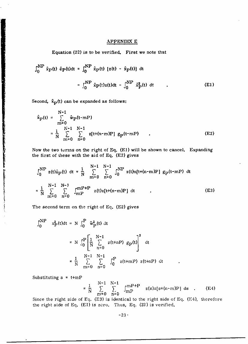
APPENDIX E

Equation (22) is to be verified. First we note that

NP Tfo ip(t) ep(t)dt = j0 xp(t) [z(t) - Xp(t)] dt

=rNP xp(t)z(t)dt - NP0I' (t) dt (El)

Second, Xp(t) can be expanded as follows:

N-IXp(t) = " Wvp(t-mP)

m=0

1 N-i N-iZ Z. zft+(n-m)P] gp(t-mP) (E2)

m=0 n=O

Now the two terms on the right of Eq. (El) will be shown to cancel. Expandingthe first of these with the aid of Eq. (E2) gives

NP 1 N-I N-I NPSN z(t)xp(t) dt = R Z J_ z(t)z[t+(n-m)P] gp(t-mP) dtm=0 n=0

N-1 N-1 = =

N- N- mP+P z(t)z[t+(n-m)P] dt (M)

m=0 n=0

The second term on the right of Eq. (E2) gives

JNP 4p(t)dt = N P V,(t) dt

= N 0 z(t+nP) gP(t dt

- N-i N-iN N-1 z(t+mP) z(t+nP) dtm=O n=0

Substituting s = t+mPN-i N-i

N1 N N- imP+ P z(s)z[s+(n-m)P] ds . (E4)m=0 n=0

Since the right side of Eq. (E3) is identical to the right side of Eq. (E4), therefore

the right side of Eq. (El) is zero. Thus, Eq. (22) is verified.

-23-

APPENDIX F

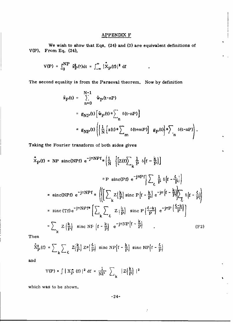
We wish to show that Eqs. (24) and (3) are equivalent definitions ofV(P). From Eq. (24),

v(P)=rNP M6= i Xp(f)1' d

The second equality is from the Parseval theorem. Now by definition

N-1ip(t) = }" 'Vp(t-nP)

n=0

= gNp(t)[wp(t)* 6(t-nP)]n

= gNplt) N 6n

Taking the Fourier transform of both sides gives

4~(f) =NP sinc(NPf) ei'n(* Z(f)e 1 I (f -

kk({ P ' sincfk' Ze- & f-k} v f-)'

sinc(NPf) e - j r rNPf Z sinc P (f - h) e1If - 6 (f -

sine(Tf)e - rTNPf* [Z z sinep(--k) e -t k-)}

Z Ik(k sinc NP (f -) e-JN P(fI- (F2)

Then

X, (f) = Zk z4 Z k ) Z*( j sinc NP(f - sinc NP(f -

and

(p) X A~ (f) 12 df NP Zk 12

which was to be shown.

-24-

APPENDIX G

AIn this Appendix we shall verify Eq. (25). Once a P has been chosen

as the period estimate, the waveform estimate is

I N-iv(t) = Z z(t+nP) gj(t) (Gi)

n= 0

Letting P z po+fi, we can expand z in a Taylor series about Po.

1 N-1wt) N n0 [z(t+nP°) + z'(t+nPO)nh +'"] gp(t)

For large signal-to-noise ratio, we can assume that nh C< 1, in which case

wi(t) 1 f N [z(t+nPo)] gp(t)N n-O

The expectation of 'v(t) is then

= N-IE~v(t) N 1 x(t+nPo) Egf,(t) + E[n(t+nPo) g;(t)] . (G2)

N n=O

I Now we shall evaluate each of the expectations on the right separately.

Eg(t) = f,. gpw(t)p()dP,

where p(P) is the density function of the period estimate. Unfortunately, it isnecessary to have a probability distribution for P to evaluate Egp(t). Therefore,we shall proceed with the assumption that the noise is Gaussian. Let

A

From Eq, (13) we have that

V"(P 0 )

By our approximations V"(P 0 ) is given by Eq. (C9) and is not a function of thenoise. However, Eqs. (C8) and (C7) show V'(P 0 ) to be a linear function of thenoise. Thus 1 is (to a first approximation) a Gaussian random variable, withzero mean and variance 2 given by Eq. (15). Then

P (P) = ' OP (P)

-25-

where p is the Gaussian density function with mean P0 and variance o2 ThenPl

LEpgL (t g(t) rpp 0, o p (P)dP

For any t<O, g(.) = 3.

For any t>O,g It =1 for > t

gj,(t) 0 for P<t

Hence,Eg(t) = tp (P)dP for tDO

O for t<O

Substituting x = (P-Po)/op gives

g ft' P cp 1(x)dx for t:O

Egj,(t) cr

l0 for t<O

1 - * (tP-) for W

0 for t<O

where # is the Gaussian distribution function. This allows us to evaluate thefirst term of Eq. (G2). The second term of Eq. (G2) is

E[n(t+nP o) A (0)]

which is essentially the average value of the noise over an interval P. Since theexpected value of the noise is zero, it is reasonable to expect this term to benearly zero. Hence

N-1

-x(t+nPO)

EWNr(t) n=O P

0 for t<O

-26-

REFERENCES AND FOOTNOTES

1. H. D. Brunk, An Introduction to Mathematical Statistics, Ginn and Co.,Boston (1960), Chap. 8.

2. M. Fisz, Probability Theory and Mathematical Statistics, John Wiley andSons, Inc.. New York (1963), Chap. 13,

3. All summations are from -- to - unless otherwise indicated.

4. This method was suggested by Helstrom's treatment of a similar case.See C. W. Helstrom, Statistical Theory of Siknal Detection, Pergamon Press,New York (1960), p. 231.

5. It can be shown that the change in the first term with P becojLi C importantwhen z2(NP) exceeds the mean square value of z(t) by a factor of N2 ormore.

-27-

UNCLASSIFIEDSpenivi C ax-ificaucinf

DOCUMENT CONTROL DATA.- R & D(Security. cleaifictioni .1 fill*. bo"y Of abeffliCt and ibdnannotae~tioen must be eitoreg Wh". the overall target is Claeaiftod)

9. I CJRIa,..A TING AC 7vITY (Coporteeauthor) 2.. REPORT SECURITY CLASSIFICATION

Research and Development Center- K-1 UnclassifiedGeneral Electric Company 2b GROUP

Schenectady- New York 123013 REPORT TI F

THE ESTIMATION OF PERIODIC SIGNALS TN NOISE

4 fr'rC-P1IVE NOTES (Type 0 oftet and incluiin dates)

Technical ReportI AU T ORIS (First nemre. middle* initial, sot name)

Thomas G. KincaidHenry J. Scudder, mI

6 Pf P0.1 ATE IaM TOTAL 11O OF PAGES 17b. No OF, REais

February 1968 3go. CON'MALT OR GRANT P40 Se RIGINATOWS REPORT NUMS9RI1S)

NOnr-4692(00)III 6010 _C -jo -68-1019

Sb OTHER REPORT NO(S) (Any orl*fet inee dIat may &a aesidisdthis report)

d.

.OISI AIPUJON STATFUENTI

This documnr has been approved for public release and sale; its distribution isunlimited.

I' hJPP . ?1AR NO0TES 12 SPONSORING MILITARY ACTI VITY

Department of the Navy,Office of Naval Research,

ThisWashington, D. C. 20360repor preentstwo ethos for the estimation of a periodic signal inf

~additive noise. Both methods assume that only a finite time sample of the signal plusnoise is available for processing. The estimate of the signal is chosen to minimizethe mean square error between the estimate and the sample of signal plus noise.This is also a maximum likelihood estimate if the noise is white and Gaussian.

The first method is fr' quency domain analysis. Estimates for the period of thesignal and the complex amplitudes of its harmonics are derived.

The second method is time domain analysis. Estimates for the period of thesignal and for the waveform of one period are derived.

Under the assumption of white noise and large signal-to-noise ratio, formulasfor the expected values and variances of the period estimates are derived. Theestimates for the period are found to be the same by both methods. The estimate isunbiased and has a variance inversely proportional to the signal- to-noise ratio, andinversely proportional to the cube of the number of periods in the given sample. Theexpected values .jf the estimates of the waveform itself are derived, and theestimates are found to be biased.

D D NORM..1473 UNCLASSIFIED

UNCLASSIFIEDSecurmt cla-siaif ation

14 K *RSLINK A LiNK 0 LINK C

FOOLE 3 K W Y _R)EJI OLE *T

Signal TheoryEstimation TheoryI

4

UNCIAsSTT~pI

S*Cu~tY libs'(ICII