
_tzLnsgqDa
617
-
Upload
tariq-aziz -
Category
Documents
-
view
1.487 -
download
21
Transcript of _tzLnsgqDa

PART
THE BASIC
REGRESSION MODEL

1 CHAPTER
An Overview of Regression Analysis
1.1 What Is Econometrics?
1.2 What Is Regression Analysis?
1.3 The Estimated Regression Equation
1.4 A Simple Example of Regression Analysis
1.5 Using Regression to Explain Housing Prices
1.6 Summary and Exercises
1.1 What Is Econometrics?
"Econometrics is too mathematical; it's the reason my best friend isn't majoring in economics."
"There are two things you don't want to see in the making—sausage and econometric research. "1
"Econometrics may be defined as the quantitative analysis of actual eco-nomic phenomena. " 2
"It's my experience that 'economy-tricks' is usually nothing more than a justification of what the author believed before the research was begun."
Obviously, econometrics means different things to different people. To begin-ning students, it may seem as if econometrics is an overly complex obstacle to an otherwise useful education. To skeptical observers, econometric results should be trusted only when the steps that produced those results are com-pletely known. To professionals in the field, econometrics is a fascinating set
1. Attributed to Edward E. Learner. 2, Paul A. Samuelson, T. C. Koopmans, and J. R. Stone, "Repo rt of the Evaluative Committee for Econometrica," Econometrica, 1954, p. 141.
3
4 PART I • THE BASIC REGRESSION MODEL
of techniques that allows the measurement and analysis of economic phe-nomena and the prediction of future economic trends.
You're probably thinking that such diverse points of view sound like the statements of blind people trying to describe an elephant based on what they happen to be touching, and you're partially right. Econometrics has both a formal definition and a larger context. Although you can easily memorize the formal definition, you'll get the complete picture only by understanding the many uses of and alternative approaches to econometrics.
That said, we need a formal definition. Econometrics, literally "economic measurement," is the quantitative measurement and analysis of actual eco-nomic and business phenomena. It attempts to quantify economic reality and bridge the gap between the abstract world of economic theory and the real world of human activity. To many students, these worlds may seem far apart. On the one hand, economists theorize equilibrium prices based on carefully conceived marginal costs and marginal revenues; on the other, many firms seem to operate as though they have never heard of such con-cepts. Econometrics allows us to examine data and to quantify the actions of firms, consumers, and governments. Such measurements have a number of different uses, and an examination of these uses is the first step to under-standing econometrics.
1.1.1 Uses of Econometrics
Econometrics has three major uses:
1. describing economic reality
2. testing hypotheses about economic theory
3. forecasting future economic activity
The simplest use of econometrics is description. We can use econometrics to quantify economic activity because econometrics allows us to put num-bers in equations that previously contained only abstract symbols. For exam-ple, consumer demand for a particular commodity often can be thought of as a relationship between the quantity demanded (Q) and the commodity's price (P), the price of a substitute good (P S), and disposable income (Yd). For most goods, the relationship between consumption and disposable income is expected to be positive, because an increase in disposable income will be associated with an increase in the consumption of the good. Econometrics actually allows us to estimate that relationship based upon past consump-tion, income, and prices. In other words, a general and purely theoretical functional relationship like:
CHAPTER 1 • AN OVERVIEW OF REGRESSION ANALYSIS 5
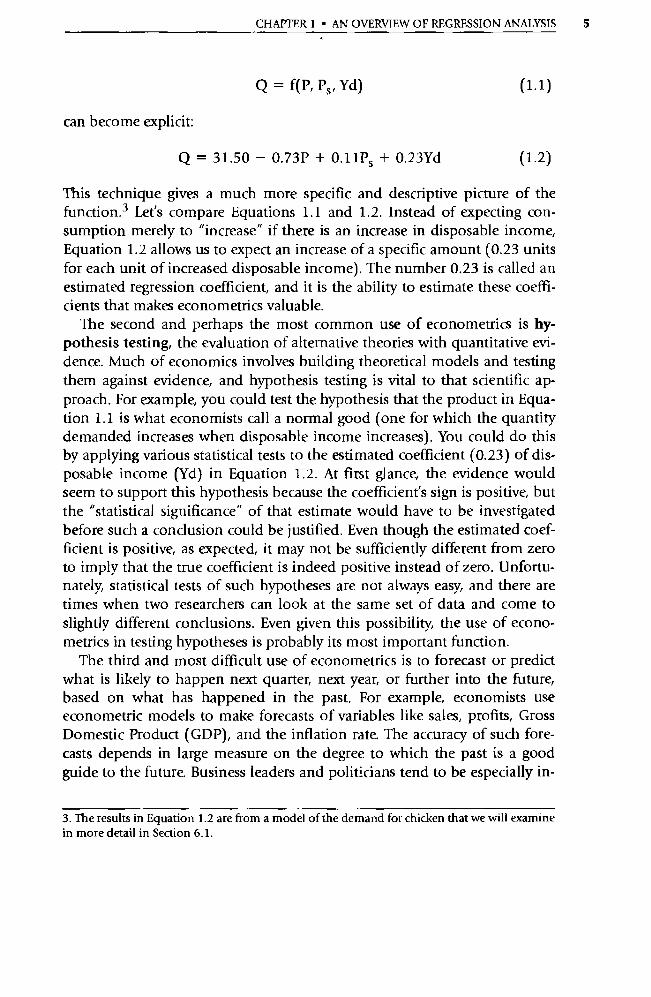
Q = f(P, Ps , Yd) (1.1)
can become explicit:
Q=31.50 -0.73P+O.11Ps +0.23Yd (1.2)
This technique gives a much more specific and descriptive picture of the function. 3 Let's compare Equations 1.1 and 1.2. Instead of expecting con-sumption merely to "increase" if there is an increase in disposable income, Equation 1.2 allows us to expect an increase of a specific amount (0.23 units for each unit of increased disposable income). The number 0.23 is called an estimated regression coefficient, and it is the ability to estimate these coeffi-cients that makes econometrics valuable.
The second and perhaps the most common use of econometrics is hy-pothesis testing, the evaluation of alternative theories with quantitative evi-dence. Much of economics involves building theoretical models and testing them against evidence, and hypothesis testing is vital to that scientific ap-proach. For example, you could test the hypothesis that the product in Equa-tion 1.1 is what economists call a normal good (one for which the quantity demanded increases when disposable income increases). You could do this by applying various statistical tests to the estimated coefficient (0.23) of dis-posable income (Yd) in Equation 1.2. At first glance, the evidence would seem to suppo rt this hypothesis because the coefficient's sign is positive, but the "statistical significance" of that estimate would have to be investigated before such a conclusion could be justified. Even though the estimated coef-ficient is positive, as expected, it may not be sufficiently different from zero to imply that the true coefficient is indeed positive instead of zero. Unfortu-nately, statistical tests of such hypotheses are not always easy, and there are times when two researchers can look at the same set of data and come to slightly different conclusions. Even given this possibility, the use of econo-metrics in testing hypotheses is probably its most impo rtant function.
The third and most difficult use of econometrics is to forecast or predict what is likely to happen next qua rter, next year, or further into the future, based on what has happened in the past. For example, economists use econometric models to make forecasts of variables like sales, profits, Gross Domestic Product (GDP), and the inflation rate. The accuracy of such fore-casts depends in large measure on the degree to which the past is a good guide to the future. Business leaders and politicians tend to be especially in-
3. The results in Equation 1.2 are from a model of the demand for chicken that we will examine in more detail in Section 6.1.
6 PART I • THE BASIC REGRESSION MODEL
terested in this use of econometrics because they need to make decisions about the future, and the penalty for being wrong (bankruptcy for the entre-preneur and political defeat for the candidate) is high. To the extent that econometrics can shed light on the impact of their policies, business and government leaders will be better equipped to make decisions. For example, if the president of a company that sold the product modeled in Equation 1.1 wanted to decide whether to increase prices, forecasts of sales with and with-out the price increase could be calculated and compared to help make such a decision. In this way, econometrics can be used not only for forecasting but also for policy analysis.
1.1.2 Alternative Econometric Approaches
There are many different approaches to quantitative work. For example, the fields of biology, psychology, and physics all face quantitative questions sim-ilar to those faced in economics and business. However, these fields tend to use somewhat different techniques for analysis because the problems they face aren't the same. "We need a special field called econometrics, and text-books about it, because it is generally accepted that economic data possess certain properties that are not considered in standard statistics texts or are not sufficiently emphasized there for use by economists. " 4
Different approaches also make sense within the field of economics. The kind of econometric tools used to quantify a particular function depends in part on the uses to which that equation will be put. A model built solely for descriptive purposes might be different from a forecasting model, for exam-ple.
To get a better picture of these approaches, let's look at the steps necessary for any kind of quantitative research:
1. specifying the models or relationships to be studied
2. collecting the data needed to quantify the models
3. quantifying the models with the data
Steps 1 and 2 are similar in all quantitative work, but the techniques used in step 3, quantifying the models, differ widely between and within disci-plines. Choosing the best technique for a given model is a theory-based skill that is often referred to as the "a rt" of econometrics. There are many alterna-tive approaches to quantifying the same equation, and each approach may
4. Clive Granger, "A Review of Some Recent Textbooks of Econometrics," Journal of Economic Literature, March 1994, p. 117.
CHAII'ER 1 • AN OVERVIEW OF REGRESSION ANALYSIS 7
give somewhat different results. The choice of approach is left to the individ-ual econometrician (the researcher using econometrics), but each researcher should be able to justify that choice.
This book will focus primarily on one particular econometric approach: single-equation linear regression analysis. The majority of this book will thus concentrate on regression analysis, but it is impo rtant for every econometri-cian to remember that regression is only one of many approaches to econo-metric quantification.
The importance of critical evaluation cannot be stressed enough; a good econometrician can diagnose faults in a particular approach and figure out how to repair them. The limitations of the regression analysis approach must be fully perceived and appreciated by anyone attempting to use regression analysis or its findings. The possibility of missing or inaccurate data, incor-rectly formulated relationships, poorly chosen estimating techniques, or im-proper statistical testing procedures implies that the results from regression analyses should always be viewed with some caution.
1.2 What Is Regression Analysis?
Econometricians use regression analysis to make quantitative estimates of economic relationships that previously have been completely theoretical in nature. After all, anybody can claim that the quantity of compact discs de-manded will increase if the price of those discs decreases (holding everything else constant), but not many people can put specific numbers into an equa-tion and estimate by how many compact discs the quantity demanded will in-crease for each dollar that price decreases. To predict the direction of the change, you need a knowledge of economic theory and the general character-istics of the product in question. To predict the amount of the change, though, you need a sample of data, and you need a way to estimate the relationship. The most frequently used method to estimate such a relationship in econo-metrics is regression analysis.
1.2.1 Dependent Variables, Independent Variables, and Causality
Regression analysis is a statistical technique that attempts to "explain" movements in one variable, the dependent variable, as a function of move-ments in a set of other variables, called the independent (or explanatory) variables, through the quantification of a single equation. For example in Equation 1.1:
Q = f(P, Ps , Yd) (1.1)
8 PART I ■ THE BASIC REGRESSION MODEL •
Q is the dependent va riable and P, P S, and Yd are the independent va riables. Regression analysis is a natural tool for economists because most (though not all) economic propositions can be stated in such single-equation functional forms. For example, the quantity demanded (dependent va riable) is a func-tion of price, the prices of substitutes, and income (independent variables).
Much of economics and business is concerned with cause-and-effect propositions. If the price of a good increases by one unit, then the quantity demanded decreases on average by a ce rtain amount, depending on the price elasticity of demand (defined as the percentage change in the quantity de-manded that is caused by a one percent change in price). Similarly, if the quantity of capital employed increases by one unit, then output increases by a certain amount, called the marginal productivity of capital. Propositions such as these pose an if-then, or causal, relationship that logically postulates that a dependent variable's movements are causally determined by move-ments in a number of specific independent variables.
Don't be deceived by the words dependent and independent, however. Al-though many economic relationships are causal by their very nature, a regres-sion result, no matter how statistically significant, cannot prove causality. All regression analysis can do is test whether a significant quantitative relationship exists. Judgments as to causality must also include a healthy dose of economic theory and common sense. For example, the fact that the bell on the door of a flower shop rings just before a customer enters and purchases some flowers by no means implies that the bell causes purchases! If events A and B are related statistically, it may be that A causes B, that B causes A, that some omitted factor causes both, or that a chance correlation exists between the two.
The cause-and-effect relationship is often so subtle that it fools even the most prominent economists. For example, in the late nineteenth century, English economist Stanley Jevons hypothesized that sunspots caused an in-crease in economic activity. To test this theory, he collected data on national output (the dependent variable) and sunspot activity (the independent vari-able) and showed that a significant positive relationship existed. This result led him, and some others, to jump to the conclusion that sunspots did in-deed cause output to rise. Such a conclusion was unjustified because regres-sion analysis cannot confirm causality; it can only test the strength and direc-tion of the quantitative relationships involved.
1.2.2 Single -Equation Linear Models
The simplest single-equation linear regression model is:
Y = 130 + 131X (1.3)
CHAPTER 1 • AN OVERVIEW OF REGRESSION ANALYSIS 9
Equation 1.3 states that Y, the dependent va riable, is a single-equation linear function of X, the independent variable. The model is a single-equation model because no equation for X as a function of Y (or any other variable) has been specified. The model is linear because if you were to plot Equation 1.3 on graph paper, it would be a straight line rather than a curve.
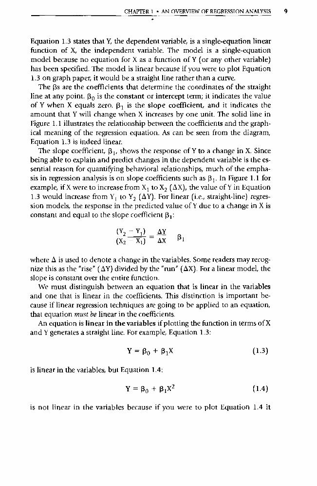
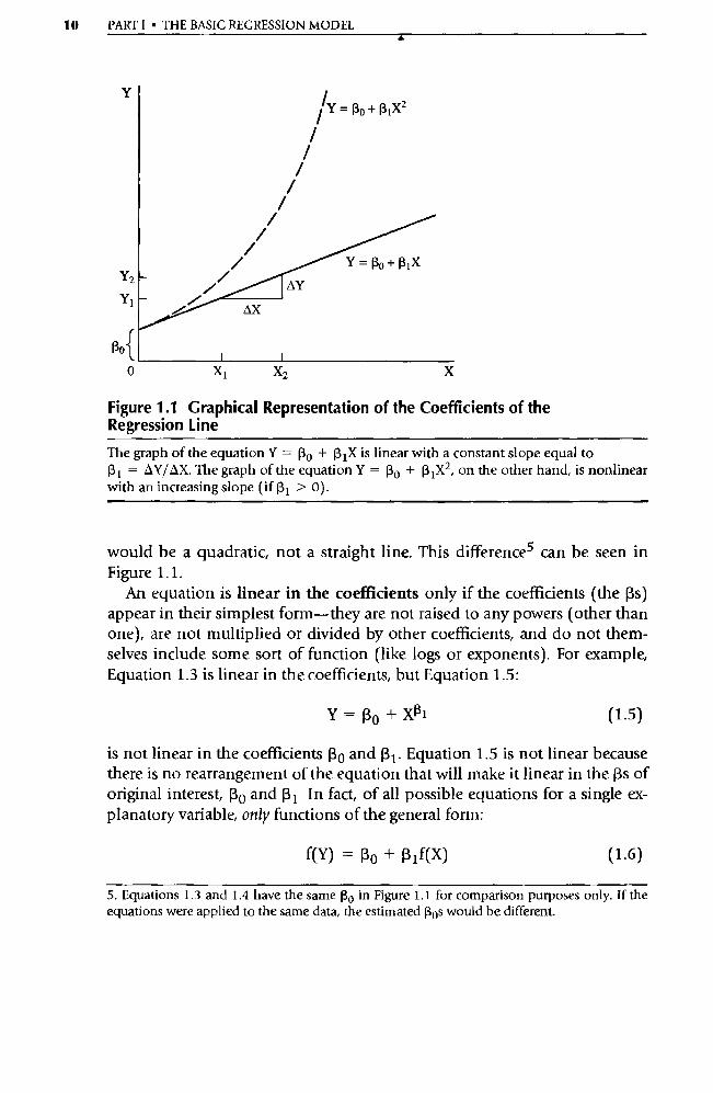
The [3s are the coefficients that determine the coordinates of the straight line at any point. Ro is the constant or intercept term; it indicates the value of Y when X equals zero. 13 1 is the slope coefficient, and it indicates the amount that Y will change when X increases by one unit. The solid line in Figure 1.1 illustrates the relationship between the coefficients and the graph-ical meaning of the regression equation. As can be seen from the diagram, Equation 1.3 is indeed linear.
The slope coefficient, [3 1 , shows the response of Y to a change in X. Since being able to explain and predict changes in the dependent variable is the es-sential reason for quantifying behavioral relationships, much of the empha-sis in regression analysis is on slope coefficients such as (3 1 . In Figure 1.1 for example, if X were to increase from X 1 to X2 (AX), the value of Y in Equation 1.3 would increase from Y 1 to Y2 (AY). For linear (i.e., straight-line) regres-sion models, the response in the predicted value of Y due to a change in X is constant and equal to the slope coefficient 13 1 :
(Y2 — Y1) AY (X2 _ X1 ) = AX 131
where 0 is used to denote a change in the variables. Some readers may recog-nize this as the "rise" (AY) divided by the "mn" (AX). For a linear model, the slope is constant over the entire function.
We must distinguish between an equation that is linear in the variables and one that is linear in the coefficients. This distinction is impo rtant be-cause if linear regression techniques are going to be applied to an equation, that equation must be linear in the coefficients.
An equation is linear in the variables if plotting the function in terms of X and Y generates a straight line. For example, Equation 1.3:
Y = Ro + 13 1 X
is linear in the variables, but Equation 1.4:
Y = Ro + R1X2
(1.3)
(1.4)
is not linear in the variables because if you were to plot Equation 1.4 it
10 PARTI • THE BASIC REGRESSION MODEL ^.
^Y= Ro + R1X2
^ /
/
/ / /
/ /
/
= Ro + R i x
/ / AY
Y1
Ro{ 0
X1 X2 X
Figure 1.1 Graphical Representation of the Coefficients of the
Regression Line
The graph of the equation Y = Ro + 13 1 X is linear with a constant slope equal to
13 1 = AY/AX. The graph of the equation Y = R o + R1X2, on the other hand, is nonlinear with an increasing slope (if 13 1 > 0).
would be a quadratic, not a straight line. This difference 5 can be seen in Figure 1.1.
An equation is linear in the coefficients only if the coefficients (the (3s)
appear in their simplest form—they are not raised to any powers (other than
one), are not multiplied or divided by other coefficients, and do not them-selves include some so rt of function (like logs or exponents). For example,
Equation 1.3 is linear in the coefficients, but Equation 1.5:
Y =Ro +XR1
is not linear in the coefficients Ro and R 1 . Equation 1.5 is not linear because there is no rearrangement of the equation that will make it linear in the (3s of original interest, Ro and 13 1 In fact, of all possible equations for a single ex-planatory variable, only functions of the general form:
f(Y) = Ro + R 1 f(X) (1.6)
Y
Y2
(1.5)
5. Equations 1.3 and 1.4 have the same Ro in Figure 1.1 for comparison purposes only. If the equations were applied to the same data, the estimated Ros would be different.
CHAPtER 1 • AN OVERVIEW OF REGRESSION ANALYSIS 11
•
are linear in the coefficients (3 0 and 13 1 . In essence, any so rt of configuration of the Xs and Ys can be used and the equation will continue to be linear in the coefficients. However, even a slight change in the configuration of the 13s will cause the equation to become nonlinear in the coefficients.
Although linear regressions need to be linear in the coefficients, they do not necessarily need to be linear in the variables. Linear regression analysis can be applied to an equation that is nonlinear in the variables if the equa-tion can be formulated in a way that is linear in the coefficients. Indeed, when econometricians use the phrase "linear regression," they usually mean "regression that is linear in the coefficients." 6
1.2.3 The Stochastic Error Term
Besides the variation in the dependent variable (Y) that is caused by the in-dependent variable (X), there is almost always variation that comes from other sources as well. This additional variation comes in part from omitted explanatory variables (e.g., X2 and X3 ). However, even if these extra variables are added to the equation, there still is going to be some variation in Y that simply cannot be explained by the model. 7 This variation probably comes from sources such as omitted in fluences, measurement error, incorrect func-tional form, or purely random and totally unpredictable occurrences. By random we mean something that has its value determined entirely by chance.
Econometricians admit the existence of such inherent unexplained varia-tion ("error") by explicitly including a stochastic (or random) error term in their regression models. A stochastic error term is a term that is added to a regression equation to introduce all of the variation in Y that cannot be ex-plained by the included Xs. It is, in effect, a symbol of the econometrician's ignorance or inability to model all the movements of the dependent variable.
6. The application of regression analysis to equations that are nonlinear in the va riables is cov-ered in Chapter 7 The application of regression techniques to equations that are nonlinear in the coefficients, however, is much more difficult.
7 The exception would be the extremely rare case where the data can be explained by some sort of physical law and are measured perfectly. Here, continued variation would point to an omit-ted independent va riable. A similar kind of problem is often encountered in astronomy, where planets can be discovered by noting that the orbits of known planets exhibit variations that can be caused only by the gravitational pull of another heavenly body. Absent these kinds of physi-cal laws, researchers in economics and business would be foolhardy to believe that all variation in Y can be explained by a regression model because there are always elements of error in any attempt to measure a behavioral relationship.
12 PART I • THE BASIC REGRESSION MODEL
The error term (sometimes called a disturbance term) is usually referred to with the symbol epsilon (e), although other symbols (like u or v) are some-times used.
The addition of a stochastic error term (e) to Equation 1.3 results in a typ-ical regression equation:
Y = R0 +R iX +e (1.7)
Equation 1.7 can be thought of as having two components, the deterministic component and the stochastic, or random, component. The expression
RO + 13 1 X is called the deterministic component of the regression equation be-cause it indicates the value of Y that is determined by a given value of X, which is assumed to be nonstochastic. This deterministic component can also be thought of as the expected value of Y given X, the mean value of the Ys associated with a particular value of X. For example, if the average height of all 14-year-old girls is 5 feet, then 5 feet is the expected value of a girl's height given that she is 14. The deterministic pa rt of the equation may be written:
E(YIX) = 13 0 + 13 1 X (1.8)
which states that the expected value of Y given X, denoted as E(YIX), is a lin-ear function of the independent va riable (or variables if there are more than one). 8
Unfortunately, the value of Y observed in the real world is unlikely to be exactly equal to the deterministic expected value E(YIX). After all, not all 14-year-old girls are 5 feet tall. As a result, the stochastic element (e) must be added to the equation:
Y =E(YIX)+ e=(30+R1X+e (1.9)
8. This property holds as long as E(€IX) = 0 [read as "the expected value of X, given epsilon" equals zero], which is true as long as the Classical Assumptions (to be outlined in Chapter 4) are met. It's easiest to think of E(e) as the mean of E, but the expected value operator E techni-cally is a summation of all the values that a function can take, weighted by the probability of each value. The expected value of a constant is that constant, and the expected value of a sum of variables equals the sum of the expected values of those variables.
CHAPTER 1 • AN OVERVIEW OF REGRESSION ANALYSIS 13
The stochastic error term must be present in a regression equation because there are at least four sources of variation in Y other than the variation in the included Xs:
1. Many minor influences on Y are omitted from the equation (for example, because data are unavailable).
2. It is virtually impossible to avoid some so rt of measurement error in at least one of the equation's variables.
3. The underlying theoretical equation might have a different func-tional form (or shape) than the one chosen for the regression. For example, the underlying equation might be nonlinear in the vari-ables for a linear regression.
4. All attempts to generalize human behavior must contain at least some amount of unpredictable or purely random variation.
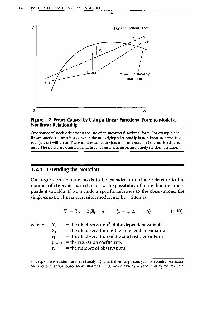
To get a better feeling for these components of the stochastic error term, let's think about a consumption function (aggregate consumption as a func-tion of aggregate disposable income). First, consumption in a particular year may have been less than it would have been because of uncertainty over the future course of the economy. Since this uncertainty is hard to measure, there might be no variable measuring consumer uncertainty in the equa-tion. In such a case, the impact of the omitted variable (consumer uncer-tainty) would likely end up in the stochastic error term. Second, the ob-served amount of consumption may have been different from the actual level of consumption in a particular year due to an error (such as a sampling error) in the measurement of consumption in the National Income Ac-counts. Third, the underlying consumption function may be nonlinear, but a linear consumption function might be estimated. (To see how this incor-rect functional form would cause errors, see Figure 1.2.) Fourth, the con-sumption function attempts to portray the behavior of people, and there is always an element of unpredictability in human behavior. At any given time, some random event might increase or decrease aggregate consumption in a way that might never be repeated and couldn't be anticipated.
These possibilities explain the existence of a difference between the ob-served values of Y and the values expected from the deterministic component of the equation, E(Y I X) . These sources of error will be covered in more detail in the following chapters, but for now it is enough to recognize that in econo-metric research there will always be some stochastic or random element, and, for this reason, an error term must be added to all regression equations.
14 PART I • THE BASIC REGRESSION MODEL
Y
0 X
Figure 1.2 Errors Caused by Using a Linear Functional Form to Model a Nonlinear Relationship
One source of stochastic error is the use of an incorrect functional form. For example, if a linear functional form is used when the underlying relationship is nonlinear, systematic er-rors (the es) will occur. These nonlinearities are just one component of the stochastic error term. The others are omitted va riables, measurement error, and purely random va riation.
1.2.4 Extending the Notation
Our regression notation needs to be extended to include reference to the number of observations and to allow the possibility of more than one inde-pendent variable. If we include a specific reference to the observations, the single-equation linear regression model may be written as:
Yi — R Ei (1= 1, 2, , n) (1.10)
where: Yi = the ith observations of the dependent va riable Xi = the ith observation of the independent variable Ei = the ith observation of the stochastic error term Ro, R1 = the regression coefficients n = the number of observations
9. A typical observation (or unit of analysis) is an individual person, year, or count ry. For exam- ple, a series of annual obse rvations starting in 1950 would have Y 1 = Y for 1950, Y2 for 1951, etc.

CHA1'I'ER 1 • AN OVERVIEW OF REGRESSION ANALYSIS 15
This equation is actually n equations, one for each of the n observations:
Yl = RO + 131 X1 + E1 Y2 = RO + R 1 X2 + E2
Y3 = 130 + 131 X3 + E3
Yn — Ro + 131Xn + En
That is, the regression model is assumed to hold for each observation. The coefficients do not change from observation to observation, but the values of Y, X, and e do.
A second notational addition allows for more than one independent vari-able. Since more than one independent va riable is likely to have an effect on the dependent variable, our notation should allow these additional explana-tory Xs to be added. If we define:
Xli = the ith observation of the first independent variable X2i = the ith observation of the second independent variable X3i = the ith observation of the third independent va riable
then all three va riables can be expressed as determinants of Y in a multivari-ate (more than one independent variable) linear regression model:
Yi =13o+131Xii+132X2i+133X3i+Ei (1.11)
The meaning of the regression coefficient 131 in this equation is the impact of a one unit increase in X 1 on the dependent variable Y, holding constant the other included independent va riables (X2 and X3). Similarly, R2 gives the im-pact of a one-unit increase in X2 on Y, holding X 1 and X3 constant. These multivariate regression coefficients (which are parallel in nature to pa rtial derivatives in calculus) serve to isolate the impact on Y of a change in one variable from the impact on Y of changes in the other variables. This is possi-ble because multivariate regression takes the movements of X2 and X3 into account when it estimates the coefficient of X 1 . The result is quite similar to what we would obtain if we were capable of conducting controlled labora-tory experiments in which only one variable at a time was changed.
In the real world, though, it is almost impossible to run controlled experi-ments, because many economic factors change simultaneously, often in oppo-site directions. Thus the ability of regression analysis to measure the impact of one variable on the dependent va riable, holding constant the influence of the other variables in the equation, is a tremendous advantage. Note that if a va riable is not included in an equation, then its impact is not held constant in the estimation of the regression coefficients. This will be discussed further in Chapter 6.
16 PARTI • THE BASIC REGRESSION MODEL
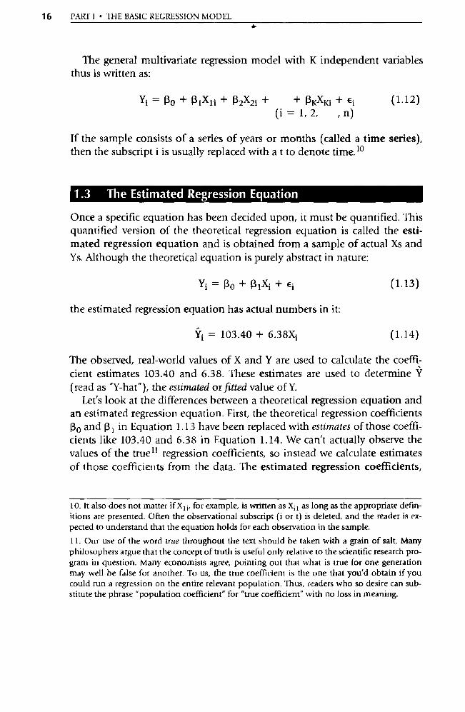
The general multivariate regression model with K independent va riables thus is written as:
Yi = RO + R1Xli 132X2i + + RxXxi + Ei (i = 1, 2, , n)
(1.12)
If the sample consists of a series of years or months (called a time series), then the subscript i is usually replaced with a t to denote time. 10
1.3 The Estimated Regression Equation
Once a specific equation has been decided upon, it must be quantified. This quantified version of the theoretical regression equation is called the esti-mated regression equation and is obtained from a sample of actual Xs and Ys. Although the theoretical equation is purely abstract in nature:
Yi —Q0+R1Xi+ E i
the estimated regression equation has actual numbers in it:
(1.13)
Yi = 103.40 + 6.38Xi (1.14)
The observed, real-world values of X and Y are used to calculate the coeffi-cient estimates 103.40 and 6.38. These estimates are used to determine Y
(read as "Y-hat"), the estimated or fitted value of Y. Let's look at the differences between a theoretical regression equation and
an estimated regression equation. First, the theoretical regression coefficients
Ro and 13 1 in Equation 1.13 have been replaced with estimates of those coeffi-cients like 103.40 and 6.38 in Equation 1.14. We can't actually observe the values of the truell regression coefficients, so instead we calculate estimates of those coefficients from the data. The estimated regression coefficients,
10. It also does not matter if X 11, for example, is written as X, i as long as the appropriate defin-itions are presented. Often the observational subscript (i or t) is deleted, and the reader is ex-pected to understand that the equation holds for each obse rvation in the sample.
11. Our use of the word true throughout the text should be taken with a grain of salt. Many philosophers argue that the concept of truth is useful only relative to the scientific research pro-gram in question. Many economists agree, pointing out that what is true for one generation may well be false for another. To us, the true coefficient is the one that you'd obtain if you could run a regression on the entire relevant population. Thus, readers who so desire can sub-stitute the phrase "population coefficient" for "true coefficient" with no loss in meaning.

CHAPTER 1 - AN OVERVIEW OF REGRESSION ANALYSIS 17
more generally denoted by Ro and Il i (read as "beta-hats"), are empirical best guesses of the true regression coefficients and are obtained from data from a sample of the Ys and Xs. The expression
Ÿi =RO +R1Xi (1.15)
is the empirical counterpart of the theoretical regression Equation 1.13. The calculated estimates in Equation 1.14 are examples of estimated regression coefficients 13o and R 1 . For each sample we calculate a different set of esti-mated regression coefficients.
Yi is the estimated value of Yi, and it represents the value of Y calculated from the estimated regression equation for the ith observation. As such, Y i is our predication of E(Yi I Xi) from the regression equation. The closer Y i is to Yi, the better the fit of the equation. (The word fit is used here much as it would be used to describe how well clothes fit.)
The difference between the estimated value of the dependent va riable (Yi) and the actual value of the dependent variable (Y i) is defined as the residual (ei):
ei = Yi — Yi (1.16)
Note the distinction between the residual in Equation 1.16 and the error term:
Ei = Yi — E(Yi I Xi) (1.17)
The residual is the difference between the observed Y and the estimated re-gression line (Y), while the error term is the difference between the observed Y and the true regression equation (the expected value of Y). Note that the er-ror term is a theoretical concept that can never be observed, but the residual is a real-world value that is calculated for each observation every time a re-gression is mn. Most regression techniques not only calculate the residuals but also attempt to select values of Ro and R that keep the residuals as low as possible. The smaller the residuals, the better the fit, and the closer the Ys will be to the Ys.
All these concepts are shown in figure 1.3. The (X, Y) pairs are shown as points on the diagram, and both the true regression equation (which cannot be seen in real applications) and an estimated regression equation are in-cluded. Notice that the estimated equation is close to but not equivalent to the true line. This is a typical result. For example, Y 6 , the computed value of Y

• / /• •
Y
Y6
r e6 Y6
X X6
Ÿ; = Ro + OiXi (Estimated Line)
•
e6 {
.//
• • /.
E6 / •
I• • E(Y; IXi) = po + oixi • (True Line)
po
Ro
0
18 PART I • THE BASIC REGRESSION MODEL
Figure 1.3 True and Estimated Regression Lines
The true relationship between X and Y (the solid line) cannot typically be observed, but the estimated regression line (the dotted line) can. The difference between an observed data point (for example, i = 6) and the true line is the value of the stochastic error term (€6). The difference between the observed Y6 and the estimated value from the regression line (Y6) is the value of the residual for this observation, e 6 .
for the sixth observation, lies on the estimated (dashed) line, and it differs from Y6, the actual observed value of Y for the sixth observation. The differ-ence between the observed and estimated values is the residual, denoted by e6 . In addition, although we usually would not be able to see an observation of the error term, we have drawn the assumed true regression line here (the solid line) to see the sixth observation of the error term, €6 , which is the dif-ference between the true line and the observed value of Y, Y6.
Another way to state the estimated regression equation is to combine Equations 1.15 and 1.16, obtaining:
Yi=Ro+RiX;+ei (1.18)
Compare this equation to Equation 1.13. When we replace the theoretical re-gression coefficients with estimated coefficients, the error term must be re-placed by the residual, because the error term, like the regression coefficients po and R I , can never be observed. Instead, the residual is observed and mea-sured whenever a regression line is estimated with a sample of Xs and Ys. In
CHAPTER 1 • AN OVERVIEW OF REGRESSION ANALYSIS 19
this sense, the residual can be thought of as an estimate of the error term, and e could have been denoted as ê.
The following chart summarizes the notation used in the true and esti-mated regression equations:
True Regression Equation Estimated Regression Equation
130
Ro 13 1
131 Ei e ;
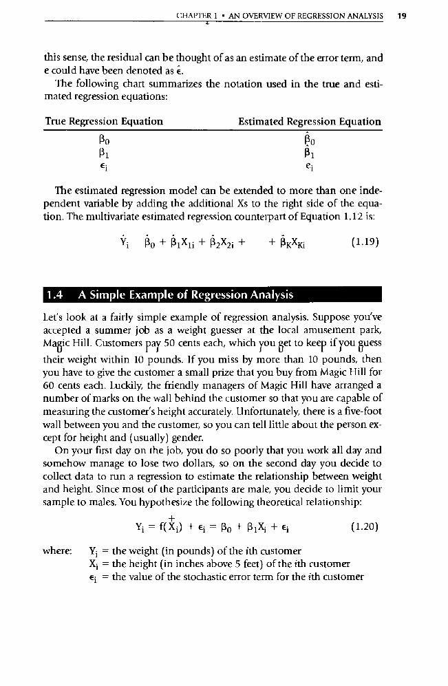
The estimated regression model can be extended to more than one inde-pendent variable by adding the additional Xs to the right side of the equa-tion. The multivariate estimated regression counterpart of Equation 1.12 is:
Yi 130 + 131 X1i + R2X2i +
+ RKXKi (1.19)
1.4 A Simple Example of Regression Analysis
Let's look at a fairly simple example of regression analysis. Suppose you've accepted a summer job as a weight guesser at the local amusement park, Magic Hill. Customers pay 50 cents each, which you get to keep if you guess
their weight within 10 pounds. If you miss by more than 10 pounds, then you have to give the customer a small prize that you buy from Magic Hill for 60 cents each. Luckily, the friendly managers of Magic Hill have arranged a number of marks on the wall behind the customer so that you are capable of measuring the customer's height accurately. Unfortunately, there is a five-foot wall between you and the customer, so you can tell little about the person ex-cept for height and (usually) gender.
On your first day on the job, you do so poorly that you work all day and somehow manage to lose two dollars, so on the second day you decide to collect data to run a regression to estimate the relationship between weight and height. Since most of the pa rticipants are male, you decide to limit your sample to males. You hypothesize the following theoretical relationship:
+ Yi =f( X i ) + Ei- 13o + 13 1 X; + Ei (1.20)
where: Y; = the weight (in pounds) of the ith customer Xi = the height (in inches above 5 feet) of the ith customer Ei = the value of the stochastic error term for the ith customer
20 PART I • THE BASIC REGRESSION MODEL
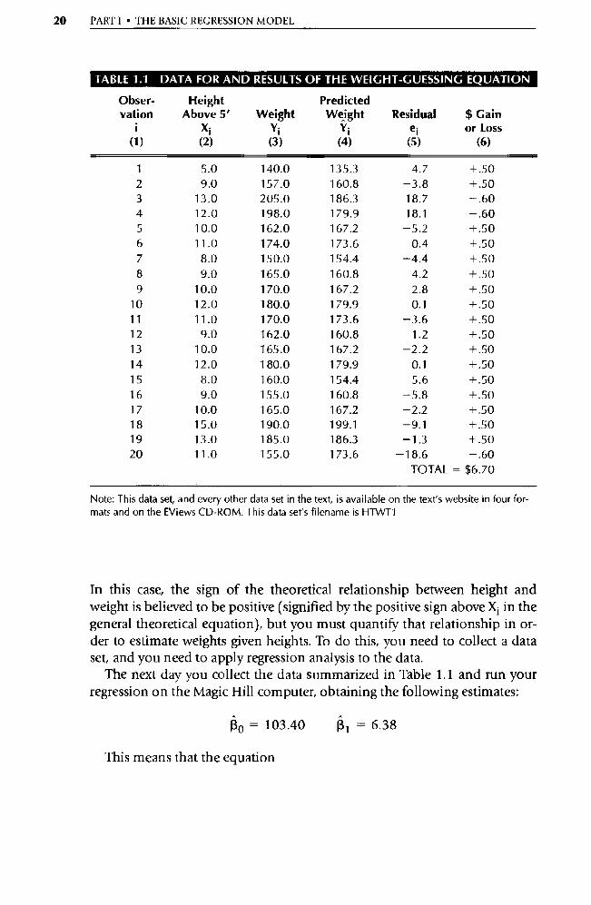
TABLE 1.1 DATA FOR AND RESULTS OF THE WEIGHT-GUESSING EQUATION
Obser- vation
Height Above 5'
Xi Weight
Yi
Predicted Weight
Yi Residual
ei $ Gain or Loss
(1) (2) (3) (4) (5) (6)
1 5.0 140.0 135.3 4.7 +.50 2 9.0 157.0 160.8 -3.8 +.50 3 13.0 205.0 186.3 18.7 -.60 4 12.0 198.0 179.9 18.1 -.60 5 10.0 162.0 167.2 -5.2 +.50 6 11.0 174.0 173.6 0.4 +.50 7 8.0 150.0 154.4 -4.4 +.50 8 9.0 165.0 160.8 4.2 +.50 9 10.0 170.0 167.2 2.8 +.50
10 12.0 180.0 179.9 0.1 +.50 11 11.0 170.0 173.6 -3.6 +.50 12 9.0 162.0 160.8 1.2 +.50 13 10.0 165.0 167.2 -2.2 +.50 14 12.0 180.0 179.9 0.1 +.50 15 8.0 160.0 154.4 5.6 +.50 16 9.0 155.0 160.8 -5.8 +.50 17 10.0 165.0 167.2 -2.2 +.50 18 15.0 190.0 199.1 -9.1 +.50 19 13.0 185.0 186.3 -1.3 +.50 20 11.0 155.0 173.6 -18.6 -.60
TOTAL = $6.70
Note: This data set, and every other data set in the text, is available on the text's website in four for-mats and on the EViews CD-ROM. This data set's filename is HTWT1
In this case, the sign of the theoretical relationship between height and weight is believed to be positive (signified by the positive sign above X i in the general theoretical equation), but you must quantify that relationship in or-der to estimate weights given heights. To do this, you need to collect a data set, and you need to apply regression analysis to the data.
The next day you collect the data summarized in Table 1.1 and run your regression on the Magic Hill computer, obtaining the following estimates:
Ro = 103.40 RI = 6.38
This means that the equation
• •
• •
• Observations
X Y-hats
= 103.40 + 6.38X;
CHAPTER 1 • AN OVERVIEW OF REGRESSION ANALYSIS
1 1 I I I 1 I I 1 I I 1 1 1 1
1 2 3 4 5 6 7 8 9 10 11 12 13 14 15 X Height (over five feet in inches)
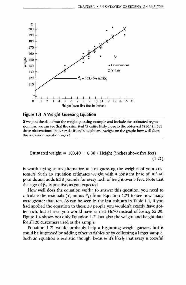
Figure 1.4 A Weight-Guessing Equation
Y 200
190
180
170
160
yao 150
140
130
120
110
If we plot the data from the weight-guessing example and include the estimated regres-sion line, we can see that the estimated Ys come fairly close to the observed Ys for all but
three obse rvations. Find a male friend's height and weight on the graph; how well does
the regression equation work?
Estimated weight = 103.40 + 6.38 • Height (inches above five feet)
(1.21)
is worth trying as an alternative to just guessing the weights of your cus-tomers. Such an equation estimates weight with a constant base of 103.40
pounds and adds 6.38 pounds for every inch of height over 5 feet. Note that
the sign of R 1 is positive, as you expected. How well does the equation work? To answer this question, you need to
calculate the residuals (Y1 minus Ÿi) from Equation 1.21 to see how many were greater than ten. As can be seen in the last column in Table 1.1, if you
had applied the equation to these 20 people you wouldn't exactly have got-ten rich, but at least you would have earned $6.70 instead of losing $2.00.
Figure 1.4 shows not only Equation 1.21 but also the weight and height data
for all 20 customers used as the sample. Equation 1.21 would probably help a beginning weight guesser, but it
could be improved by adding other variables or by collecting a larger sample.
Such an equation is realistic, though, because it's likely that every successful
22 PART I • THE BASIC REGRESSION MODEL
weight guesser uses an equation like this without consciously thinking about that concept.
Our goal with this equation was to quantify the theoretical weight/height equation, Equation 1.20, by collecting data (Table 1.1) and calculating an es-timated regression, Equation 1.21. Although the true equation, like observa-tions of the stochastic error term, can never be known, we were able to come up with an estimated equation that had the sign we expected for R I and that helped us in our job. Before you decide to quit school or your job and try to make your living guessing weights at Magic Hill, there is quite a bit more to learn about regression analysis, so we'd better move on.
1.5 Using Regression to Explain Housing Prices
As much fun as guessing weights at an amusement park might be, it's hardly a typical example of the use of regression analysis. For every regression run on such an off-the-wall topic, there are literally hundreds run to describe the reaction of GDP to an increase in the money supply, to test an economic theory with new data, or to forecast the effect of a price change on a firm's sales.
As a more realistic example, let's look at a model of housing prices. The purchase of a house is probably the most important financial decision in an individual's life, and one of the key elements in that decision is an appraisal of the house's value. If you overvalue the house, you can lose thousands of dollars by paying too much; if you undervalue the house, someone might outbid you.
All this wouldn't be much of a problem if houses were homogeneous products, like corn or gold, that have generally known market prices with which to compare a particular asking price. Such is hardly the case in the real estate market. Consequently, an impo rtant element of every housing pur-chase is an appraisal of the market value of the house, and many real estate appraisers use regression analysis to help them in their work.
Suppose your family is about to buy a house in Southern California, but you're convinced that the owner is asking too much money. The owner says that the asking price of $230,000 is fair because a larger house next door sold for $230,000 about a year ago. You're not sure it's reasonable to compare the prices of different-sized houses that were purchased at different times. What can you do to help decide whether to pay the $230,000?
Since you're taking an econometrics class, you decide to collect data on all local houses that were sold within the last few weeks and to build a re-
CHAPTER 1 • AN OVERVIEW OF REGRESSION ANALYSIS 23
gression model of the sales prices of the houses as a function of their sizes. 12 Such a data set is called cross-sectional because all of the observa-tions are from the same point in time and represent different individual economic entities (like countries, or in this case, houses) from that same point in time.
To measure the impact of size on price, you include the size of the house as an independent variable in a regression equation that has the price of that house as the dependent va riable. You expect a positive sign for the coefficient of size, since big houses cost more to build and tend to be more desirable than small ones. Thus the theoretical model is:
+ Pi = f( S i) + Ei = Ro + Risi + Ei
where: Pi = the price (in thousands of $) of the ith house Si = the size (in square feet) of that house Ei = the value of the stochastic error term for that house
(1.22)
You collect the records of all recent real estate transactions, find that 43 lo-cal houses were sold within the last 4 weeks, and estimate the following re-gression of those 43 observations:
Pi = 40.0 + 0.138Si (1.23)
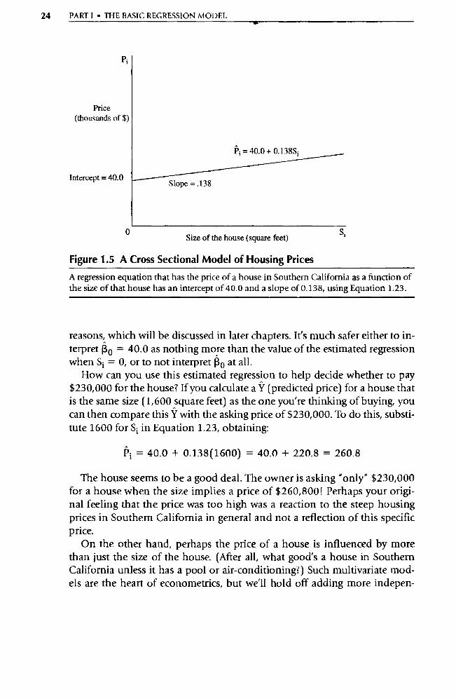
What do these estimated coefficients mean? The most impo rtant coefficient is R1 = 0.138, since the reason for the regression is to find out the impact of size on price. This coefficient means that if size increases by 1 square foot, price will increase by 0.138 thousand dollars ($138). R1 thus measures the change in Pi associated with a one-unit increase in S i . It's the slope of the re-gression line in a graph like Figure 1.5.
What does 11 0 = 40.0 mean? Ro is the estimate of the constant or intercept term. In our equation, it means that price equals 40.0 when size equals zero. As can be seen in Figure 1.5, the estimated regression line intersects the price axis at 40.0. While it might be tempting to say that the average price of a va-cant lot is $40,000, such a conclusion would be unjustified for a number of
12. It's unusual for an economist to build a model of price without induding some measure of quantity on the right-hand side. Such models of the price of a good as a function of the attrib-utes of that good are called hedonic models and will be discussed in greater depth in Section 11.7 The interested reader is encouraged to skim the first few paragraphs of that section before continuing on with this example.
= 40.0 +0.138S;
Slope = .138
Pi
Price (thousands of $)
Intercept = 40.0
24 PART I • THE BASIC REGRESSION MODEL
0 Size of the house (square feet) S`
Figure 1.5 A Cross Sectional Model of Housing Prices
A regression equation that has the price of a house in Southern California as a function of the size of that house has an intercept of 40.0 and a slope of 0.138, using Equation 1.23.
reasons, which will be discussed in later chapters. It's much safer either to in-terpret Ro = 40.0 as nothing more than the value of the estimated regression when Si = 0, or to not interpret 13o at all.
How can you use this estimated regression to help decide whether to pay $230,000 for the house? If you calculate a Î' (predicted price) for a house that is the same size (1,600 square feet) as the one you're thinking of buying, you can then compare this Y with the asking price of $230,000. To do this, substi-tute 1600 for S i in Equation 1.23, obtaining:
Pi = 40.0 + 0.138(1600) = 40.0 + 220.8 = 260.8
The house seems to be a good deal. The owner is asking "only" $230,000 for a house when the size implies a price of $260,800! Perhaps your origi-nal feeling that the price was too high was a reaction to the steep housing prices in Southern California in general and not a reflection of this specific price.
On the other hand, perhaps the price of a house is influenced by more than just the size of the house. (After all, what good's a house in Southern California unless it has a pool or air-conditioning?) Such multivariate mod-els are the heart of econometrics, but we'll hold off adding more indepen-
CHAPTER 1 • AN OVERVIEW OF REGRESSION ANALYSIS 25
dent variables to Equation 1.23 until we return to this housing price example later in the text.
1.6 Summary
1. Econometrics, literally "economic measurement," is a branch of eco-nomics that attempts to quantify theoretical relationships. Regression analysis is only one of the techniques used in econometrics, but it is by far the most frequently used.
2. The major uses of econometrics are description, hypothesis testing, and forecasting. The specific econometric techniques employed may vary depending on the use of the research.
3. While regression analysis specifies that a dependent va riable is a func-tion of one or more independent va riables, regression analysis alone cannot prove or even imply causality.
4. Linear regression can only be applied to equations that are linear in the coefficients, which means that the regression coefficients are in their simplest possible form. For an equation with two explanatory variables, this form would be:
f(Yi) — Ro + R1f(X1i) + 132f(X2i) + Ei
5. A stochastic error term must be added to all regression equations to account for variations in the dependent variable that are not ex-plained completely by the independent variables. The components of this error term include: a. omitted or left-out variables b. measurement errors in the data c. an underlying theoretical equation that has a different functional
form (shape) than the regression equation d. purely random and unpredictable events
6. An estimated regression equation is an approximation of the true equation that is obtained by using data from a sample of actual Ys and Xs. Since we can never know the true equation, econometric analysis focuses on this estimated regression equation and the esti-mates of the regression coefficients. The difference between a particu-lar observation of the dependent variable and the value estimated from the regression equation is called the residual.
26 PART I • THE BASIC REGRESSION MODEL
Exercises
(Answers to even -numbered exercises are in Appendix A.)
1. Write the meaning of each of the following terms without referring to the book (or your notes), and compare your definition with the ver-sion in the text for each: a. stochastic error term b. regression analysis c. linear in the variables d. slope coefficient e. multivariate regression model f. expected value g. residual h. linear in the coefficients
2. Use your own computer's regression so ftware and the weight (Y) and height (X) data from Table 1.1 to see if you can reproduce the esti-mates in Equation 1.21. There are three different ways to load the data: You can type in the data yourself, you can open datafile H1WT1 on the EViews CD, or you can download datafile HTWT1 (in any of four formats: SAS, EXCEL, SHAZAM, and ASCII) from the text's web-site: www.awlonline.com/studenmund/ Once the datafile is loaded, then run Y = f(X), and your results should match Equation 1.21. Dif-ferent programs require different commands to run a regression. For help in how to do this with EViews, for example, see the answer to this question in Appendix A.
3. Decide whether you would expect relationships between the follow-ing pairs of dependent and independent variables (respectively) to be positive, negative, or ambiguous. Explain your reasoning. a. Aggregate net investment in the U.S. in a given year and GDP in
that year. b. The amount of hair on the head of a male professor and the age of
that professor. c. The number of acres of wheat planted in a season and the price of
wheat at the beginning of that season. d. Aggregate net investment and the real rate of interest in the same
year and country. e. The growth rate of GDP in a year and the average hair length in that
year. f. The quantity of canned heat demanded and the price of a can of
heat.
CHAPTER 1 • AN OVERVIEW OF REGRESSION ANALYSIS 27
4. Let's return to the height/weight example in Section 1.4: a. Go back to the data set and identify the three customers who
seem to be quite a distance from the estimated regression line. Would we have a better regression equation if we dropped these customers from the sample?
b. Measure the height of a male friend and plug it into Equation 1.21. Does the equation come within ten pounds? If not, do you think you see why? Why does the estimated equation predict the same weight for all males of the same height when it is obvious that all males of the same height don't weigh the same?
c. Look over the sample with the thought that it might not be ran-domly drawn. Does the sample look abnormal in any way? (Hint: Are the customers who choose to play such a game a random sam-ple?) If the sample isn't random, would this have an effect on the regression results and the estimated weights?
d. Think of at least one other factor besides height that might be a good choice as a variable in the weight/height equation. How would you go about obtaining the data for this variable? What would the expected sign of your variable's coefficient be if the vari-able were added to the equation?
5. Continuing with the height/weight example, suppose you collected data on the heights and weights of 29 more customers and estimated the following equation:
= 125.1 + 4.03X; (1.24)
where: Y; = the weight (in pounds) of the ith person X; = the height (in inches over five feet) of the ith person
a. Why aren't the coefficients in Equation 1.24 the same as those we estimated previously (Equation 1.21)?
b. Compare the estimated coefficients of Equation 1.24 with those in Equation 1.21. Which equation has the steeper estimated relation-ship between height and weight? Which equation has the higher intercept? At what point do the two intersect?
c. Use Equation 1.24 to "predict" the 20 o riginal weights given the heights in Table 1.1. How many weights does Equation 1.24 miss by more than ten pounds? Does Equation 1.24 do better or worse than Equation 1.21? Could you have predicted this result beforehand?
d. Suppose you had one last day on the weight-guessing job. What equation would you use to guess weights? (Hint: There is more than one possible answer.)
28 PART I • THE BASIC REGRESSION MODEL s
6. Not all regression coefficients have positive expected signs. For example, a Sports Illustrated article by Jaime Diaz reported on a study of golfing putts of various lengths on the Professional Golfers Association (PGA) Tour. 13 The article included data on the percentage of putts made (P i) as a function of the length of the putt in feet (L i). Since the longer the putt, the less likely even a professional is to make it, we'd expect L i to have a negative coefficient in an equation explaining P i . Sure enough, if you estimate an equation on the data in the arti cle, you obtain:
P; = f(L i) = 83.6 — 4.1L; (1.25)
a. Carefully write out the exact meaning of the coefficient of L i . b. Use Equation 1.25 to determine the percent of the time you'd expect
a PGA golfer to make a 10-foot putt. Does this seem realistic? How about a 1-foot putt or a 25-foot putt? Do these seem as realistic?
c. Your answer to pa rt b should suggest that there's a problem in apply-ing a linear regression to these data. What is that problem? (Hint: If you're stuck, first draw the theoretical diagram you'd expect for P i as a function of Li, then plot Equation 1.25 onto the same diagram.)
d. Suppose someone else took the data from the a rticle and estimated:
P; = 83.6 -4.1L; +e;
Is this the same result as that in Equation 1.25? If so, what definition do you need to use to convert this equation back to Equation 1.25?
7. Return to the housing price model of Section 1.5 and consider the fol-lowing equation:
Si = 72.2 + 5.77Pi (1.26)
where: Si = the size (in square feet) of the ith house Pi = the price (in thousands of $) of that house
a. Carefully explain the meaning of each of the estimated regression coefficients.
b. Suppose you're told that this equation explains a significant por-tion (more than 80 percent) of the variation in the size of a house. Have we shown that high housing prices cause houses to be large? If not, what have we shown?
c. What do you think would happen to the estimated coefficients of
13. Jaime Diaz, "Perils of Putting," Sports Illustrated, April 3, 1989, pp. 76-79.
CHAPTER 1 • AN OVERVIEW OF REGRESSION ANALYSIS 29
this equation if we had measured the price va riable in dollars in-stead of in thousands of dollars? Be specific.
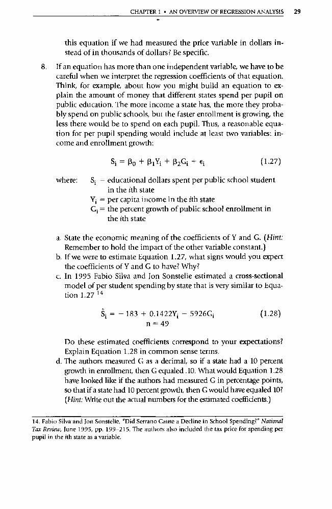
8. If an equation has more than one independent va riable, we have to be careful when we interpret the regression coefficients of that equation. Think, for example, about how you might build an equation to ex-plain the amount of money that different states spend per pupil on public education. The more income a state has, the more they proba-bly spend on public schools, but the faster enrollment is growing, the less there would be to spend on each pupil. Thus, a reasonable equa-tion for per pupil spending would include at least two variables: in-come and enrollment growth:
Si = Rp + R lYi + r32Gi + Ei (1.27)
where: Si = educational dollars spent per public school student in the ith state
IT; = per capita income in the ith state Gi = the percent growth of public school enrollment in
the ith state
a. State the economic meaning of the coefficients of Y and G. (Hint: Remember to hold the impact of the other va riable constant.)
b. If we were to estimate Equation 1.27, what signs would you expect the coefficients of Y and G to have? Why?
c. In 1995 Fabio Silva and Jon Sonstelie estimated a cross-sectional model of per student spending by state that is very similar to Equa- tion 1.27 14
S i = — 183 + 0.1422Y1 — 5926G 1 (1.28) n = 49
Do these estimated coefficients correspond to your expectations? Explain Equation 1.28 in common sense terms.
d. The authors measured G as a decimal, so if a state had a 10 percent growth in enrollment, then G equaled .10. What would Equation 1.28 have looked like if the authors had measured G in percentage points, so that if a state had 10 percent growth, then G would have equaled 10? (Hint: Write out the actual numbers for the estimated coefficients.)
14. Fabio Silva and Jon Sonstelie, "Did Serrano Cause a Decline in School Spending?" National Tax Review, June 1995, pp. 199-215. The authors also included the tax price for spending per pupil in the ith state as a variable.

30 PART I • THE BASIC REGRESSION MODEL
9. Your friend estimates a simple equation of bond prices in different years as a function of the interest rate that year (for equal levels of risk) and obtains:
Yi = 101.40 — 4.78X1
where: Y; = U.S. government bond prices (per $100 bond) in the ith year
X; = the federal funds rate (percent) in the ith year
a. Carefully explain the meanings of the two estimated coefficients. Are the estimated signs what you would have expected?
b. Why is the left-hand variable in your friend's equation Y and not Y? c. Didn't your friend forget the stochastic error term in the estimated
equation? d. What is the economic meaning of this equation? What criticisms
would you have of this model? (Hint: The federal funds rate is a rate that applies to overnight holdings in banks.)
10. Housing price models can be estimated with time-series as well as cross-sectional data. If you study aggregate time-series housing prices (see Table 1.2 for data and sources), you have:
Pt = f(GDP) = 7404.6 + 19.8Yt n = 31 (annual 1964-1994)
where : Pt = the nominal median price of new single-family houses in the U.S. in year t
Yt = the U.S. GDP in year t (billions of current $)
a. Carefully interpret the economic meaning of the estimated coeffi-cients.
b. What is Yt doing on the right side of the equation? Shouldn't it be on the left side?
c. Both the price and GDP va riables are measured in nominal (or cur-rent, as opposed to real, or inflation-adjusted) dollars. Thus a ma-jor portion of the excellent explanatory power of this equation (more than 99 percent of the variation in P t can be explained by Yt alone) comes from capturing the huge amount of inflation that took place between 1964 and 1994. What could you do to elimi-nate the impact of in flation in this equation?
d. GDP is included in the equation to measure more than just infla-tion. What factors in housing prices other than inflation does the

CHAPTER 1 • AN OVERVIEW OF REGRESSION ANALYSIS 31
TABLE 1.2 DATA FOR THE TIME-SERIES MODEL OF HOUSING PRICES
t Year Price(P t) GDP(Yt)
1 1964 18,900 648.0 2 1965 20,000 702.7 3 1966 21,400 769.8 4 1967 22,700 814.3 5 1968 24,700 889.3 6 1969 25,600 959.5 7 1970 23,400 1010.7 8 1971 25,200 1097.2 9 1972 27,600 1207.0
10 1973 32,500 1349.6 11 1974 35,900 1458.6 12 1975 39,300 1585.9 13 1976 44,200 1768.4 14 1977 48,800 1974.1 15 1978 55,700 2232.7 16 1979 62,900 2488.6 17 1980 64,600 2708.0 18 1981 68,900 303 0.6 19 1982 69,300 3149.6 20 1983 75,300 3405.0 21 1984 79,900 3777.2 22 1985 84,300 4038.7 23 1986 92,000 4268.6 24 1987 104,500 4539.9 25 1988 112,500 4900.4 26 1989 120,000 5250.8 2 7 1990 122,900 5546.1 28 1991 120,000 5724.8 29 1992 121,500 6020.2 30 1993 126,500 6343.3 31 1994 130,000 6736.9
= the nominal median price of new single family houses in the U.S. in year t. (Source: The Statistical Abstract of the U.S.)
Yt = the U.S. GDP in year t (billions of current dollars). (Source: The Economic Report of the President)
Note: EViews filename = HOUSE1
GDP variable help capture? Can you think of a variable that might do a better job?
11. The distinction between the stochastic error term and the residual is one of the most difficult concepts to master in this chapter. a. List at least three differences between the error term and the residual.
32 PART I • THE BASIC REGRESSION MODEL
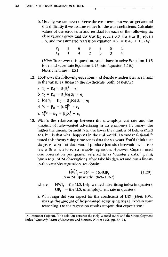
b. Usually, we can never observe the error term, but we can get around this difficulty if we assume values for the true coefficients. Calculate values of the error term and residual for each of the following six observations given that the true 13 0 equals 0.0, the true 13 1 equals 1.5, and the estimated regression equation is Y i = 0.48 +
Yi 2 6 3 8 5 4 Xi 1 4 2 5 3 4
(Hint: To answer this question, you'll have to solve Equation 1.13 for E and substitute Equation 1.15 into Equation 1.16.) Note: filename = EX1
12. Look over the following equations and decide whether they are linear in the va riables, linear in the coefficients, both, or neither.
a.Yi=13o+13 Xi + Ei
b.Yi =130 +(3 1 logXi + ei
c. log Yi Ro + 13 1 1og Xi + Ei
d.Yi =[30 +R 142 + Ei
e.Y13° =R1+132X? + E;
13. What's the relationship between the unemployment rate and the amount of help-wanted advertising in an economy? In theory, the higher the unemployment rate, the lower the number of help-wanted ads, but is that what happens in the real world? Damodar Gujarati l5
tested this theory using time-series data for six years. You'd think that six years' worth of data would produce just six observations, far too few with which to run a reliable regression. However, Gujarati used one observation per qua rter, referred to as "quarterly data," giving him a total of 24 observations. If we take his data set and run a linear-in-the-variables regression, we obtain:
HWIt = 364 - 46.4URt (1.29) n = 24 (quarterly 1962-1967)
where: HWIt = the U.S. help-wanted advertising index in qua rter t URt = the U.S. unemployment rate in qua rter t
a. What sign did you expect for the coefficient of UR? (Hint: HWI rises as the amount of help-wanted advertising rises.) Explain your reasoning. Do the regression results suppo rt that expectation?
15. Damodar Gujarati, "The Relation Between the Help-Wanted Index and the Unemployment Index," Quarterly Review of Economics and Business, Winter 1968, pp. 67-73.
CHAPTER 1 • AN OVERVIEW OF REGRESSION ANALYSIS 33
b. This regression is linear both in the coefficients and in the vari-ables. Think through the underlying theory involved here. Does the theory suppo rt such a linear-in-the-variables model? Why or why not?
c. The model includes only one independent variable. Does it make sense to model the help-wanted index as a function of just one variable? Can you think of any other va riables that might be im-portant?
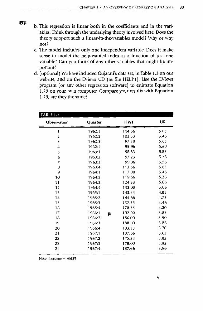
d. (optional) We have included Gujarati's data set, in Table 1.3 on our website, and on the EViews CD (as file HELP1). Use the EViews program (or any other regression software) to estimate Equation 1.29 on your own computer. Compare your results with Equation 1.29; are they the same?
TABLE 1.3
Observation Quarter HWI UR
1 1962:1 104.66 5.63
2 1962:2 103.53 5.46
3 1962:3 97.30 5.63
4 1962:4 95.96 5.60
5 1963:1 98.83 5.83
6 1963:2 97.23 5.76 7 1963:3 99.06 5.56 8 1963:4 113.66 5.63 9 1964:1 117.00 5.46
10 1964:2 119.66 5.26
11 1964:3 124.33 5.06 12 1964:4 133.00 5.06 13 1965:1 143.33 4.83 14 1965:2 144.66 4.73 15 1965:3 152.33 4.46 16 1965:4 178.33 4.20 17 1966:1 192.00 3.83
18 1966:2 186.00 3.90
19 1966:3 188.00 3.86
20 1966:4 193.33 3.70
21 1967:1 187.66 3.63
22 1967:2 175.33 3.83
23 1967:3 178.00 3.93
24 1967:4 187.66 3.96
Note: filename = HELP1
2 CHAPTER
Ordinary Least Squares
2.1 Estimating Single-Independent-Variable Models with OLS
2.2 Estimating Multivariate Regression Models with OLS
2.3 Evaluating the Quality of a Regression Equation
2.4 Describing the Overall Fit of the Estimated Model
2.5 An Example of the Misuse of 11 2
2.6 Summary and Exercises
The bread and butter of regression analysis is the estimation of the coeffi-cients of econometric models with a technique called Ordinary Least Squares (OLS). The first two sections of this chapter summarize the reasoning behind and the mechanics of OLS. Regression users usually rely on computers to do the actual OLS calculations, so the emphasis here is on understanding what OLS attempts to do and how it goes about doing it.
How can you tell a good equation from a bad one once it has been esti-mated? One factor is the extent to which the estimated equation fits the ac-tual data. The rest of the chapter is devoted to developing an understanding of the most commonly used measures of this fit: R 2 and the adjusted R2 , R2, pronounced R-bar-squared. The use of 11 2 is not without perils, however, so the chapter concludes with an example of the misuse of this statistic.
2.1 Estimating Single-Independent-Variable Models with OLS
The purpose of regression analysis is to take a purely theoretical equation like:
Yi=i3o+RiXi+ Ei
and use a set of data to create an estimated equation like:
itri -- k +RiXi
(2.1)
(2.2)
34
CHAPTER 2 • ORDINARY LEAST SQUARES 35
where each "hat" indicates a sample estimate of the true population value. (In the case of Y, the "true population value" is E[YjX].) The purpose of the estimation technique is to obtain numerical values for the coefficients of an otherwise completely theoretical regression equation.
The most widely used method of obtaining these estimates is Ordinary Least Squares (OLS). OIS has become so standard that its estimates are presented as a point of reference even when results from other estimation techniques are used. Ordinary Least Squares is a regression estimation technique that calcu-lates the 13s so as to minimize the sum of the squared residuals, thus:'
OLS minimizes E e? (i = 1, 2, , n) (2.3) = 1
Since these residuals (e is) are the differences between the actual Ys and the estimated Ys produced by the regression (the Ÿs in Equation 2.2), Equation 2.3 is equivalent to saying that OIS minimizes E (Yi if.i) 2
2.1.1 Why Use Ordinary Least Squares?
Although OIS is the most-used regression estimation technique, it's not the only one. Indeed, econometricians have invented what seems like zillions of dif-ferent estimation techniques, a number of which we'll discuss later in this text.
There are at least three impo rtant reasons for using OLS to estimate regres-sion models:
1. OLS is relatively easy to use.
2. The goal of minimizing Ee; is quite appropriate from a theoretical point of view.
3. OLS estimates have a number of useful characteristics.
The first reason for using OLS is that it's the simplest of all econometric es-timation techniques. Most other techniques involve complicated nonlinear
1. The summation symbol, E, means that all terms to its right should be added (or summed) over the range of the i values attached to the bottom and top of the symbol. In Equation 2.3, for example, this would mean adding up e; for all integer values between 1 and n:
e?= +eZ+ + en
i =1
Often the E notation is simply written as E as in Equation 2.5, and it is assumed that the
summation is over all obse rvations from i = 1 to i = n. Sometimes, the i is omitted entirely, as in Equation 2.16, and the same assumption is made implicitly. For more practice in the basics of summation algebra, see Exercise 2.
36 PART I • THE BASIC REGRESSION MODEL
formulas or iterative procedures, many of which are extensions of OLS itself. In contrast, OLS estimates are simple enough that, if you had to, you could compute them without using a computer or a calculator (for a single-independent-variable model).
The second reason for using OLS is that minimizing the summed, squared residuals is an appropriate theoretical goal for an estimation technique. To see this, recall that the residual measures how close the estimated regression equation comes to the actual observed data:
ei = Yi —Ÿi (i = 1, 2, . , n) (1.16)
Since it's reasonable to want our estimated regression equation to be as close as possible to the observed data, you might think that you'd want to mini-mize these residuals. The main problem with simply totaling the residuals and choosing that set of j3s that minimizes them is that e i can be negative as well as positive. Thus, negative and positive residuals might cancel each other out, allowing a wildly inaccurate equation to have a very low Ee i . For exam-ple, if Y 100,000 for two consecutive observations and if your equation predicts 1.1 million and —900,000, respectively, your residuals will be +1 million and —1 million, which add up to zero!
We could get around this problem by minimizing the sum of the absolute values of the residuals, but this approach has problems as well. Absolute val-ues are difficult to work with mathematically, and summing the absolute val-ues of the residuals gives no extra weight to extraordinarily large residuals. That is, it often doesn't matter if a number of estimates are off by a small amount, but it's impo rtant if one estimate is off by a huge amount. For exam-ple, recall the weight-guessing equation of Chapter 1; you lost only if you missed the customer's weight by 10 or more pounds. In such a circumstance, you'd want to avoid large residuals.
Minimizing the summed squared residuals gets around these problems. Squared functions pose no unusual mathematical difficulties in terms of ma-nipulations, and the technique avoids canceling positive and negative residu-als because squared terms are always positive. In addition, squaring gives greater weight to big residuals than it does to smaller ones because e; gets rel-atively larger as e i increases. For example, one residual equal to 4.0 has a greater weight than two residuals of 2.0 when the residuals are squared (4 2 = 16 vs. 2 2 + 22 = 8).
The final reason for using OLS is that its estimates have at least three desir-able characteristics:
1. The estimated regression line (Equation 2.2) goes through the means of Y and X. That is, if you substitute Y and X into Equation 2.2, the equation holds exactly: Yi = 130 + RIXi.

CHAPTER 2 • ORDINARY LEAST SQUARES 37
2. The sum of the residuals is exactly zero.
3. OLS can be shown to be the "best" estimator possible under a set of fairly restrictive assumptions.
An estimator is a mathematical technique that is applied to a sample of data to produce real-world numerical estimates of the true population re-gression coefficients (or other parameters). Thus, Ordinary Least Squares is an estimator, and a (3 produced by OLS is an estimate.
2.1.2 How Does OLS Work?
How would OLS estimate a single-independent-variable regression model like Equation 2.1?
Yi =R0+R1Xi+ Ei
OLS selects those estimates of 13 o and 13 1 that minimize the squared residuals, summed over all the sample data points:
n n = (Y1 — Ÿi)2 (i = 1, 2, , n) (2.4)
i=1 i= 1
However, Ÿi = (30 + 13X11, so OLS actually minimizes
Ee, = (Yi 113(i)2 (2.5)
by choosing the (3s that do so. In other words, OLS yields the (is that mini-mize Equation 2.5. For an equation with just one independent variable, these coefficients are 2 :
R1 =
n _ _
((Xi X) (Y ` Y)) i = 1
(2.6)
E(Xi — _X) 2 i = 1
and, given this estimate of (3 i ,
(2.1)
2. For those with a moderate grasp of calculus and algebra, the derivation of these equations is informative. See Exercise 12.
Ro =Y -RIX (2.7)
38 PART I • THE BASIC REGRESSION MODEL a
where X = the mean of X, or 1X/n, and Ÿ = the mean of Y, or E Y/n. What do these equations mean? Equation 2.6 sets R1 equal to the joint
variation of X and Y (around their means) divided by the variation of X around its mean. It measures the portion of the variation in Y that is associ-ated with variations in X. Equation 2.7 defines 13 0 to ensure that the regres-sion equation does indeed pass through the means of X and Y. In addition, it can be shown that Equations 2.6 and 2.7 provide (3s that minimize the summed square residuals. Note that for each different data set, we'll get dif-ferent estimates of R1 and 130, depending on the sample.
2.1.3 Total, Explained, and Residual Sums of Squares
Before going on, let's pause to develop some measures of how much of the vari-ation of the dependent variable is explained by the estimated regression equa-tion. A comparison of the estimated values with the actual values can help the researcher get a feeling for the adequacy of the hypothesized regression model.
Various statistical measures can be used to assess the degree to which the Ys approximate the corresponding sample Ys, but all of them are based on the de-gree to which the regression equation estimated by OLS explains the values of Y better than a naive estimator, the sample mean, denoted by Y. That is, econo-metricians use the squared va riations of Y around its mean as a measure of the amount of variation to be explained by the regression. This computed quantity is usually called the total sum of squares, or TSS, and is written as:
TSS = (Yi Y_) 2 (2.8) i =1
For Ordinary Least Squares, the total sum of squares has two components, that variation which can be explained by the regression and that which cannot:
(Yi Y)2= Or, - Y) 2+ ^ei
Total Sum = Explained + Residual of
Sum of
Sum of Squares Squares
Squares
(TSS)
(ESS)
(RSS)
This is usually called the "decomposition of variance."
(2.9)
Y
Ÿ
X
CHAPTER 2 • ORDINARY LEAST SQUARES 39
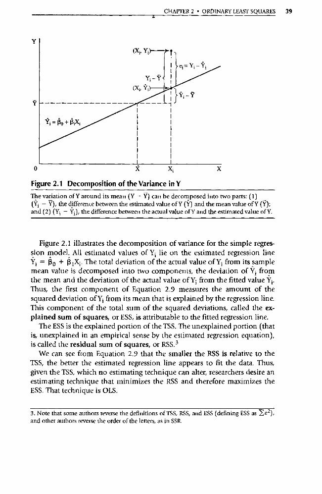
Figure 2.1 Decomposition of the Variance in Y
The variation of Y around its mean (Y — Y) can be decomposed into two pa rts: (1) (Y1 — Y), the difference between the estimated value of Y (Ÿ) and the mean value of Y (Ÿ); and (2) (Yi — Yi), the difference between the actual value of Y and the estimated value of Y.
Figure 2.1 illustrates the decomposition of variance for the simple regres-sion model. All estimated values of Y i lie on the estimated regression line Yi = 130 + 131X1. The total deviation of the actual value of Y i from its sample mean value is decomposed into two components, the deviation of Yi from the mean and the deviation of the actual value of Yi from the fitted value Thus, the first component of Equation 2.9 measures the amount of the squared deviation of Yi from its mean that is explained by the regression line. This component of the total sum of the squared deviations, called the ex-plained sum of squares, or ESS, is attributable to the fitted regression line.
The ESS is the explained po rtion of the TSS. The unexplained portion (that is, unexplained in an empirical sense by the estimated regression equation), is called the residual sum of squares, or RSS. 3
We can see from Equation 2.9 that the smaller the RSS is relative to the TSS, the better the estimated regression line appears to fit the data. Thus, given the TSS, which no estimating technique can alter, researchers desire an estimating technique that minimizes the RSS and therefore maximizes the ESS. That technique is OLS.
3. Note that some authors reverse the definitions of TSS, RSS, and ESS (defining ESS as Ee 2 ), and other authors reverse the order of the letters, as in SSR.
40 PART I • THE BASIC REGRESSION MODEL •
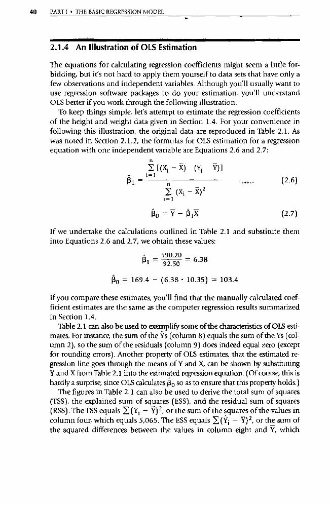
2.1.4 An Illustration of OLS Estimation
The equations for calculating regression coefficients might seem a little for-bidding, but it's not hard to apply them yourself to data sets that have only a few observations and independent variables. Although you'll usually want to use regression software packages to do your estimation, you'll understand OLS better if you work through the following illustration.
To keep things simple, let's attempt to estimate the regression coefficients of the height and weight data given in Section 1.4. For your convenience in following this illustration, the original data are reproduced in Table 2.1. As was noted in Section 2.1.2, the formulas for OLS estimation for a regression equation with one independent variable are Equations 2.6 and 2.7:
n
/ [(Xi — X) (Yi Y) ] i =1
R1 = n
/ (Xi — X) 2 i =1
Ro =Y — R1X
If we undertake the calculations outlined in Table 2.1 and substitute them into Equations 2.6 and 2.7, we obtain these values:
590.20 — 6.38 R 1
— 92.50
(30 = 169.4 — (6.38 • 10.35) = 103.4
If you compare these estimates, you'll find that the manually calculated coef-ficient estimates are the same as the computer regression results summarized in Section 1.4.
Table 2.1 can also be used to exemplify some of the characteristics of OLS esti-mates. For instance, the sum of the Ys (column 8) equals the sum of the Ys (col-umn 2), so the sum of the residuals (column 9) does indeed equal zero (except for rounding errors). Another property of OLS estimates, that the estimated re-gression line goes through the means of Y and X, can be shown by substituting
and X from Table 2.1 into the estimated regression equation. (Of course, this is hardly a surprise, since OLS calculates RU so as to ensure that this property holds.)
The figures in Table 2.1 can also be used to derive the total sum of squares (TSS), the explained sum of squares (ESS), and the residual sum of squares (RSS). The TSS equals (Y; — Y) 2 , or the sum of the squares of the values in column four, which equals 5,065. The ESS equals (Y ; — Ÿ) 2, or the sum of the squared differences between the values in column eight and Y, which
(2.6)
(2.7)
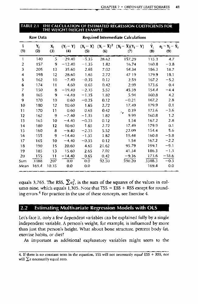
CHAPTER 2 • ORDINARY LEAST SQUARES 41
TABLE 2.1 THE CALCULATION OF ESTIMATED REGRESSION COEFFICIENTS FOR THE WEIGHT/HEIGHT EXAMPLE
Raw Data Required Intermediate Calculations
(1) Yi XI (2) (3)
(Yi - Y) (4)
(Xi - X) (5)
(Xi - X) 2 (6)
(Xi - X)(Yi - Ÿ) Ÿ i (7) (8)
ei -Yi - Ÿi (9)
1 140 5 -29.40 -5.35 28.62 15 7.2 9 135.3 4.7 2 157 9 -12.40 -1.35 1.82 16.74 160.8 -3.8 3 205 13 35.60 2.65 7.02 94.34 186.3 18.7 4 198 12 28.60 1.65 2.72 47 19 179.9 18.1 5 162 10 -7.40 -0.35 0.12 2.59 167.2 -5.2 6 174 11 4.60 0.65 0.42 2.99 173.6 0.4 7 150 8 -19.40 -2.35 5.52 45.59 154.4 -4.4 8 165 9 -4.40 -1.35 1.82 5.94 160.8 4.2
9 170 10 0.60 -0.35 0.12 -0.21 167.2 2.8
10 180 12 10.60 1.65 2.72 17.49 179.9 0.1
11 170 11 0.60 0.65 0.42 0.39 173.6 -3.6
12 162 9 -7.40 -1.35 1.82 9.99 160.8 1.2 13 165 10 -4.40 -0.35 0.12 1.54 167.2 2.8 14 180 12 10.60 1.65 2.72 17.49 179.9 0.1 15 160 8 -9.40 -2.35 5.52 22.09 154.4 5.6 16 155 9 -14.40 -1.35 1.82 19.44 160.8 -5.8
17 165 10 -4.40 -0.35 0.12 1.54 167.2 -2.2
18 190 15 20.60 4.65 21.62 95.79 199.1 -9.1
19 185 13 15.60 2.65 7.02 41.34 186.3 -1.3
20 155 11 -14.40 0.65 0.42 -9.36 173.6 -18.6 Sum 3388 207 0.0 0.0 92.50 590.20 3388.3 -0.3 Mean 169.4 10.35 0.0 0.0 169.4 0.0
equals 3,765. The RSS, Se;, is the sum of the squares of the values in col-umn nine, which equals 1,305. Note that TSS = ESS + RSS except for round-ing errors. 4 For practice in the use of these concepts, see Exercise 4.
2.2 Estimating Multivariate Regression Models with OLS
Let's face it, only a few dependent variables can be explained fully by a single independent variable. A person's weight, for example, is influenced by more than just that person's height. What about bone structure, percent body fat, exercise habits, or diet?
As important as additional explanatory variables might seem to the
4. If there is no constant term in the equation, TSS will not necessarily equal ESS + RSS, nor will E necessarily equal zero.
42 PART I • THE BASIC REGRESSION MODEL s
height/weight example, there's even more reason to include a variety of inde-pendent variables in economic and business applications. Although the quantity demanded of a product is certainly affected by price, that's not the whole story. Advertising, aggregate income, the prices of substitutes, the in-fluence of foreign markets, the quality of customer service, possible fads, and changing tastes all are important in real-world models. As a result, we feel that it's vital to move from single-independent-variable regressions to multi-variate regression models, equations with more than one independent variable.
2.2.1 The Meaning of Multivariate Regression Coefficients
The general multivariate regression model with K independent va riables can be represented by Equation 1.12:
Yi 13o +R1X1i+ 02X2i + + RKXKi + E i (1.12)
where i, as before, goes from 1 to n and indicates the observation number. Thus, X11 indicates the ith observation of independent va riable X 1 , while X21 indicates the ith observation of another independent va riable, X2 .
The biggest difference between a single-independent-variable regression model and a multivariate regression model is in the interpretation of the lat-ter's slope coefficients. These coefficients, often called partials regression coef-ficients, are defined to allow a researcher to distinguish the impact of one variable on the dependent va riable from that of other independent va riables.
Specifically, a multivariate regression coefficient indicates the change in the dependent variable associated with a one-unit increase in the in-dependent variable in question holding constant the other independent variables in the equation.
This last italicized phrase is a key to understanding multiple regression (as multivariate regression is often called). The coefficient Ri measures the im-pact on Y of a one-unit increase in X 1 , holding constant X2, X3 , and XK but not holding constant any relevant va riables that might have been omitted
5. The term "partial regression coefficient" will seem especially appropriate to those readers who have taken calculus, since multivariate regression coefficients correspond to pa rtial deriva-tives. Indeed, in Equation 1.12 the partial derivative of Y 1 with respect to Xli is p i , etc.

CHAPTER 2 • ORDINARY LEAST SQUARES 43 w
from the equation (e.g., XK+1). The coefficient Ro is the value of Y when all the Xs and the error term equal zero. As we'll learn in Section 7.1, you should always include a constant term in a regression equation, but you should not rely on estimates of (3 0 for inference.
As an example of multivariate regression, let's consider the following an-nual model of the per capita demand for beef in the United States:
Bt = 37.54 — 0.88Pt + 11.9Ydt (2.10)
where: Bt = the per capita consumption of beef in year t (in pounds per person)
Pt = the price of beef in year t (in cents per pound) Ydt = the per capita disposable income in year t (in thousands of
dollars)
The estimated coefficient of income, 11.9, tells us that beef consumption will increase by 11.9 pounds per person if per capita disposable income goes up by $1,000, holding constant the price of beef. The ability to hold price con-stant is crucial because we'd expect such a large increase in per capita income to stimulate demand, therefore pushing up prices and making it hard to dis-tinguish the effect of the income increase from the effect of the price increase. The multivariate regression estimate allows us to focus on the impact of the income variable by holding the price variable constant.
Note, however, that the equation does not hold constant other possible variables (like the price of a substitute) because these va riables are not in-cluded in Equation 2.10. Before you move on to the next section, take the time to think through the meaning of the estimated coefficient of P in Equation 2.10; do you agree that the sign and relative size fit with economic theory?
2.2.2 OLS Estimation of Multivariate Regression Models
The application of OLS to an equation with more than one independent vari-able is quite similar to its application to a single-independent-variable model. To see this, let's follow the estimation of the simplest possible multi-variate model, one with just two independent variables:
Yi — RO + R1Xli + R2X2i + E i (2.11)
The goal of OLS is to choose those (3s that minimize the summed square residuals, but now these residuals are from a multivariate model. For Equa-tion 2.11, OLS would minimize:
44 PART I • THE BASIC REGRESSION MODEL
Ee? = (Yi — Yi)2 = (Yi — R O — R1X1i R2X2i)2 (2.12)
While OLS estimation of multivariate models is identical in general approach to that of single-independent-variable models, the equations themselves are more cumbersome. For Equation 2.11, the estimated coefficients are:
(Dxl )(Ex2) — (EYx2 )(Ex l x2 ) 13 1 =
(Ixi)(Exi) (Ex1x2) 2
(Eyx2)(Exl) — (EYx1)(Ex1x2) P2 =
(Exi)(Exi) (Ex1x2) 2
Ro = Y RIXI — R2X2
where lower case va riables indicate deviations from the mean, as in y = Y; — Ÿ; x1 = Xti X 1 ; and x2 = X2i - X2.
For the reader who is just about to throw this book away because of the complexity of the previous equations, there's both bad and good news. The bad news is that Equations 2.13 through 2.15 are for a regression model with only two independent variables; with three or more, the situation really gets out of hand! The good news is that numerous user-friendly computer pack-ages can calculate all of the above in less than a second of computer time. In-deed, only someone lost in time or stuck on a desert island would bother es-timating a multivariate regression model without a computer. The rest of us will use EViews, SHAZAM, SAS, TSP, RATS, BIOMED, MINITAB, or any of the other commercially available regression packages. The purpose of presenting these equations is to help you understand what multivariate estimation in-volves, not to teach you how to do it without a computer.
(2.13)
(2.14)
(2.15)
2.2.3 An Example of a Multivariate Regression Model
As an example of the estimation of a multivariate regression model, let's re-turn to the beef demand equation of the previous section, Equation 2.10:
Bt = 37.54 — 0.88Pt + 11.9Ydt (2.10)
where: Bt = the per capita consumption of beef in year t (in pounds per person)
Pt = the price of beef in year t (in cents per pound) Ydt = the per capita disposable income in year t (in thousands of
dollars)
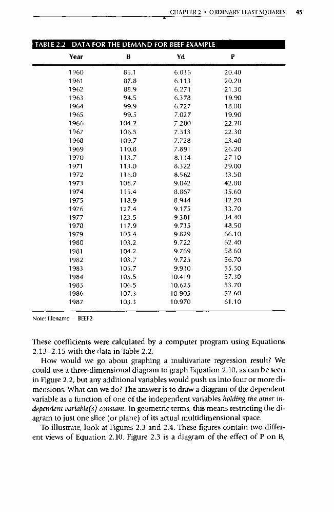
CHAFFER 2 • ORDINARY LEAST SQUARES 45
TABLE 2.2 DATA FOR THE DEMAND FOR BEEF EXAMPLE
Year B Yd P
1960 85.1 6.036 20.40 1961 87.8 6.113 20.20 1962 88.9 6.271 21.30 1963 94.5 6.3 78 19.90 1964 99.9 6.727 18.00 1965 99.5 7.02 7 19.90 1966 104.2 7.280 22.20 1967 106.5 7.513 22.30 1968 109.7 7.728 23.40 1969 110.8 7.891 2 6.2 0 1970 113.7 8.134 27 10 1971 113.0 8.322 29.00 1972 116.0 8.562 33.50 1973 108.7 9.042 42.80 1974 115.4 8.867 35.60 1975 118.9 8.944 32.20 1976 127.4 9.175 33.70 1977 123.5 9.381 34.40 1978 117.9 9.735 48.50 1979 105.4 9.829 66.10 1980 103.2 9.722 62.40 1981 104.2 9.769 58.60
1982 103.7 9.725 56.70 1983 105.7 9.930 55.50 1984 105.5 10.419 57.30 1985 106.5 10.625 53.70 1986 107.3 10.905 52.60 1987 103.3 10.970 61.10
Note: filename = BEEF2
These coefficients were calculated by a computer program using Equations 2.13-2.15 with the data in Table 2.2.
How would we go about graphing a multivariate regression result? We could use a three-dimensional diagram to graph Equation 2.10, as can be seen in Figure 2.2, but any additional va riables would push us into four or more di-mensions. What can we do? The answer is to draw a diagram of the dependent variable as a function of one of the independent variables holding the other in-dependent variable(s) constant. In geometric terms, this means restricting the di-agram to just one slice (or plane) of its actual multidimensional space.
To illustrate, look at Figures 2.3 and 2.4. These figures contain two differ-ent views of Equation 2.10. Figure 2.3 is a diagram of the effect of P on B,
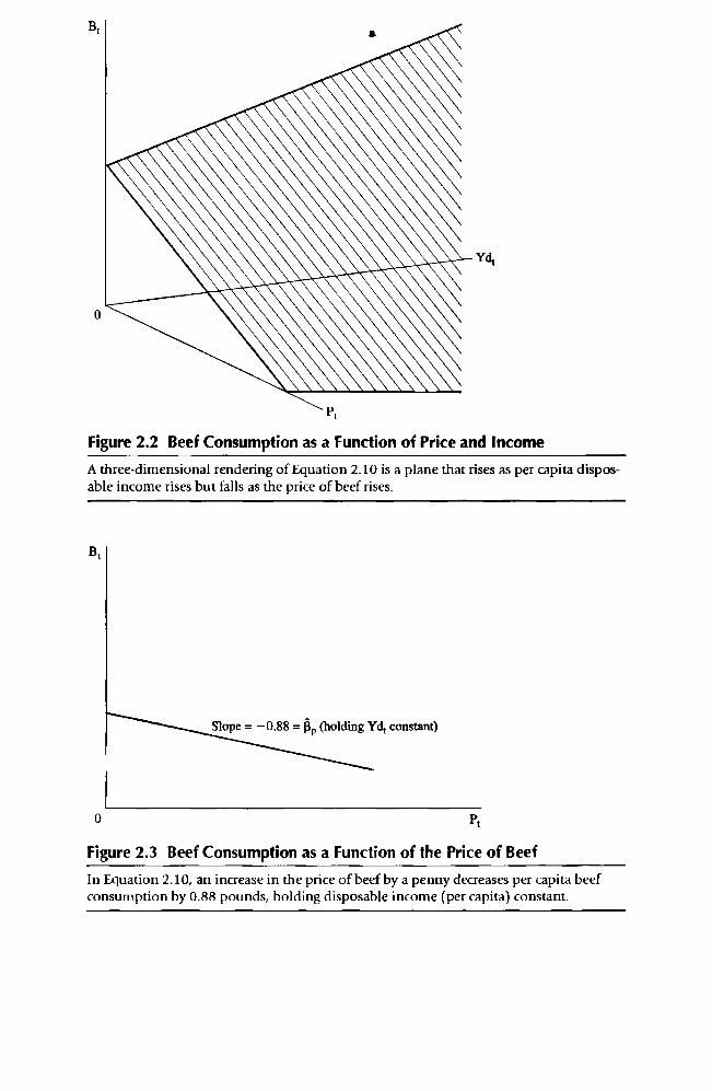
a
Figure 2.2 Beef Consumption as a Function of Price and Income
A three-dimensional rendering of Equation 2.10 is a plane that rises as per capita dispos-able income rises but falls as the price of beef rises.
B t
Slope = —0.88 = llp (holding Ydt constant)
0 Pt
Figure 2.3 Beef Consumption as a Function of the Price of Beef
In Equation 2.10, an increase in the price of beef by a penny decreases per capita beef consumption by 0.88 pounds, holding disposable income (per capita) constant.
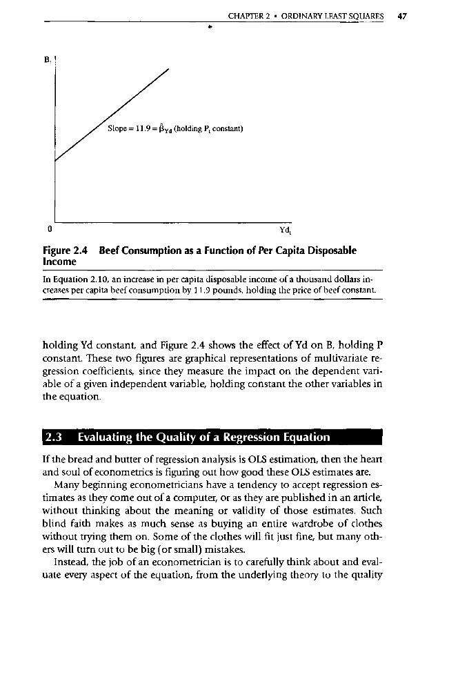
CHAPTER 2 • ORDINARY LEAST SQUARES 47
B,
Slope = 11.9 = (3yd (holding Pt constant)
0 Yd^
Figure 2.4 Beef Consumption as a Function of Per Capita Disposable
Income
In Equation 2.10, an increase in per capita disposable income of a thousand dollars in-creases per capita beef consumption by 11.9 pounds, holding the price of beef constant.
holding Yd constant, and Figure 2.4 shows the effect of Yd on B, holding P constant. These two figures are graphical representations of multivariate re-gression coefficients, since they measure the impact on the dependent vari-able of a given independent variable, holding constant the other variables in
the equation.
2.3 Evaluating the Quality of a Regression Equation
If the bread and butter of regression analysis is OLS estimation, then the heart
and soul of econometrics is figuring out how good these OLS estimates are.
Many beginning econometricians have a tendency to accept regression es-timates as they come out of a computer, or as they are published in an a rticle, without thinking about the meaning or validity of those estimates. Such
blind faith makes as much sense as buying an entire wardrobe of clothes
without trying them on. Some of the clothes will fit just fine, but many oth-ers will turn out to be big (or small) mistakes.
Instead, the job of an econometrician is to carefully think about and eval-uate every aspect of the equation, from the underlying theory to the quality

48 PARTI • THE BASIC REGRESSION MODEL 4
of the data, before accepting a regression result as valid. In fact, most good econometricians spend quite a bit of time thinking about what to expect from an equation before they estimate that equation.
Once the computer estimates have been produced, however, it's time to evaluate the regression results. The list of questions that should be asked dur-ing such an evaluation is long. For example:
1. Is the equation supported by sound theory?
2. How well does the estimated regression as a whole fit the data?
3. Is the data set reasonably large and accurate?
4. Is OLS the best estimator to be used for this equation?
5. How well do the estimated coefficients correspond to the expectations developed by the researcher before the data were collected?
6. Are all the obviously impo rtant variables included in the equation?
7 Has the most theoretically logical functional form been used?
8. Does the regression appear to be free of major econometric problems?
The goal of this text is to help you develop the ability to ask and appropri-ately answer these kinds of questions. In fact, the number in front of each question above roughly corresponds to the chapter in which we'll address the issues raised by that question. Since this is Chapter 2, it'll come as no surp rise to you to hear that the rest of the chapter will be devoted to the second of these topics, the overall fit of the estimated model.
2.4 Describing the Overall Fit of the Estimated Model
Let's face it, we expect that a good estimated regression equation will explain the variation of the dependent variable in the sample fairly accurately. If it does, we say that the estimated model fits the data well.
Looking at the overall fit of an estimated model is useful not only for eval-uating the quality of the regression, but also for comparing models that have different data sets, functional forms, or combinations of independent vari-ables. We can never be sure that one estimated model represents the truth any more than another, but evaluating the quality of the fit of the equation is one ingredient in a choice between different formulations of a regression model. The simplest commonly used measure of that fit is the coefficient of determination, R2.

CHAPTER 2 • ORDINARY LEAST SQUARES 49
2.4.1 R2, The Coefficient of Determination
The coefficient of determination is the ratio of the explained sum of squares to the total sum of squares:
2 _ ESS _ RSS ^e2
R TSS 1 TSS — 1 E (Y1 17)2
The higher R2, the closer the estimated regression equation fits the sample data. Measures of this type are called "goodness of fit" measures. Since TSS, RSS, and ESS are all nonnegative (being squared deviations), and since ESS < TSS, R2 must lie in the interval
0 R2 is1 (2.17)
A value of R2 close to one shows an excellent overall fit, whereas a value near zero shows a failure of the estimated regression equation to explain the val-ues of Y; better than could be explained by the sample mean Ÿ. In other words, R2 can be defined by the percentage of the va riation of Y around Ÿ that is explained by the regression equation. Since OLS selects the parameter estimates that minimize RSS, OLS provides the largest possible R 2, given the linear specification of the model.
Figures 2.5 through 2.7 demonstrate some extremes. Figure 2.5 shows an X and Y that are unrelated. The fitted regression line might as well be Y = Y, the same value it would have if X were omitted. As a result, the estimated lin-ear regression is no better than the sample mean as an estimate of Y i. The ex-plained portion, ESS, = 0, and the unexplained po rtion, RSS, equals the total squared deviations TSS; thus, R 2 = 0. In this case, the residuals are large rela-tive to the deviations in Y from its mean, implying that a regression line is not useful in describing the relationship between X and Y.
Figure 2.6 shows a relationship between X and Y that can be "explained" quite well by a linear regression equation: the value of R 2 is .95. This kind of result is typical of a time-series regression with a good fit. Most of the varia-tion has been explained, but there still remains a po rtion of the variation that is essentially random or unexplained by the model. Goodness of fit is relative to the topic being studied. If the sample is cross-sectional, an R 2 of .50 might be considered a good fit. In other words, there is no simple method of deter-mining how high R2 must be for the fit to be considered satisfactory. Instead, knowing when R2 is relatively large or small is a matter of experience. It should be noted that a high R2 does not imply that changes in X lead to changes in Y, as there may be an underlying variable whose changes lead to changes in both X and Y simultaneously.
(2.16)

• • • • • • • •
Regression Line
• R2 =0 • • • • •
•
0 X
Figure 2.5
X and Y are not related; in such a case, R 2 would be O.
Y
Y
Y
Y
0 X
Figure 2.6
A set of data for X and Y that can be "explained" quite well with a regression line (R 2 = .95).
R2 = 1
0 X
Figure 2.7
A perfect fit: all the data points are on the regression line, and the resulting R 2 is 1.
50
CHAPTER 2 • ORDINARY LEAST SQUARES 51
Figure 2.7 shows a perfect fit of R 2 = 1. Such a fit implies that no estima-tion is required. The relationship is completely deterministic, and the slope and intercept can be calculated from the coordinates of any two points. In fact, reported equations with Res equal to (or very near) one should be viewed with suspicion; they very likely do not explain the movements of the dependent variable Y in terms of the causal proposition advanced, even though they explain them empirically.
2.4.2 R2 , The Adjusted R2
A major problem with R2 is that adding another independent variable to a particular equation can never decrease R 2 That is, if you compare two identi-cal regressions (same dependent variable and independent variables), except that one has an additional independent variable, the equation with the greater number of independent variables will always have a better (or equal) fit as measured by R2 To see this, recall the equation for R 2, Equation 2.16:
R2 = — RSS = 1 _ Ee
TSS E (Y1
— Y) 2
Since the dependent variable has not changed, TSS is still the same. Also, since OLS ensures that adding a va riable will not increase the summed squared residuals, RSS will only decrease or stay the same. 6 If RSS decreases, RSS/TSS will also decrease and 1 — RSS/TSS will increase. Thus, adding a variable to an equation virtually guarantees that R 2 will increase.
Perhaps an example will make this clear. Let's return to our weight guess-ing regression, Equation 1.21:
Estimated weight = 103.40 + 6.38 • Height (over five feet)
The R2 for this equation is .74. If we now add a completely nonsensical variable to the equation (say, the campus post office box number of each in-dividual in question), then it turns out that the results become:
Estimated weight = 102.35 + 6.36 (height > five feet) + 0.02 (box#)
but the R2 for this equation is .75! Thus, an individual using R 2 alone as the measure of the quality of the fit of the regression would choose the second version as better fitting.
(2.16)
6. You know that RSS will never increase because the OLS program could always set the coefficient of the added va riable equal to zero, thus giving the same fit as the previous equation. The coefficient of the newly added variable being zero is the only circumstance in which R 2 will stay the same when a variable is added. Otherwise, R2 will always increase when a va riable is added to an equation.
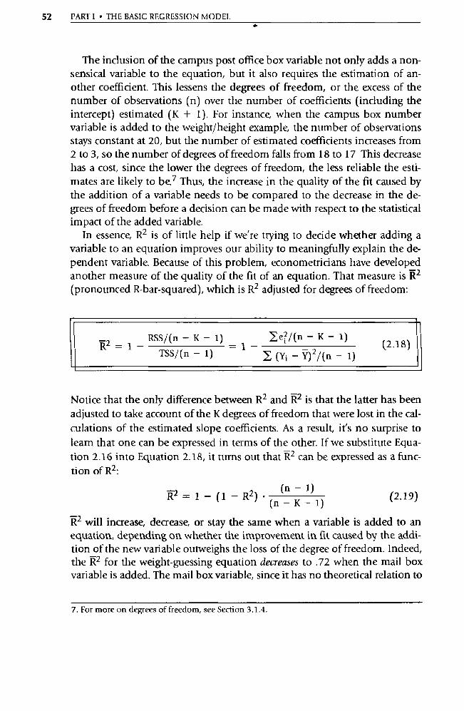
52 PART I • THE BASIC REGRESSION MODEL
The inclusion of the campus post office box va riable not only adds a non-sensical variable to the equation, but it also requires the estimation of an-other coefficient. This lessens the degrees of freedom, or the excess of the number of observations (n) over the number of coefficients (including the intercept) estimated (K + 1). For instance, when the campus box number variable is added to the weight/height example, the number of observations stays constant at 20, but the number of estimated coefficients increases from 2 to 3, so the number of degrees of freedom falls from 18 to 17 This decrease has a cost, since the lower the degrees of freedom, the less reliable the esti-mates are likely to be. 7 Thus, the increase in the quality of the fit caused by the addition of a va riable needs to be compared to the decrease in the de-grees of freedom before a decision can be made with respect to the statistical impact of the added variable.
In essence, R2 is of little help if we're trying to decide whether adding a variable to an equation improves our ability to meaningfully explain the de-pendent variable. Because of this problem, econometricians have developed another measure of the quality of the fit of an equation. That measure is 1i 2
(pronounced R-bar-squared), which is R2 adjusted for degrees of freedom:
RSS/(n - K - 1) Ie? /(n - K - 1) 2 R 1 - TSS/(n - 1) = 1
(Y1 - Y) 2/(n - 1) (2.18)
Notice that the only difference between R 2 and R2 is that the latter has been adjusted to take account of the K degrees of freedom that were lost in the cal-culations of the estimated slope coefficients. As a result, it's no surprise to learn that one can be expressed in terms of the other. If we substitute Equa-tion 2.16 into Equation 2.18, it turns out that R2 can be expressed as a func-tion of R2 :
R2 =1—(1—R2)• (n—K-1) (2.19)
R2 will increase, decrease, or stay the same when a va riable is added to an equation, depending on whether the improvement in fit caused by the addi-tion of the new variable outweighs the loss of the degree of freedom. Indeed, the 11.2 for the weight-guessing equation decreases to .72 when the mail box variable is added. The mail box variable, since it has no theoretical relation to
(n — 1)
7. For more on degrees of freedom, see Section 3.1.4.

CHAPTER 2 • ORDINARY LEAST SQUARES 53
weight, should never have been included in the equation, and the 112 mea-sure suppo rts this conclusion.
The highest possible R2 is 1.00, the same as for R 2 The lowest possible R2, however, is not .00; if R 2 is extremely low, R2 can be slightly negative. To see this, substitute 0 for R2 into Equation 2.19.
R2 can be used to compare the fits of equations with the same dependent variable and different numbers of independent variables. Because of this property, most researchers automatically use k2 instead of R2 when evaluat-ing the fit of their estimated regression equations. In fact, R 2 has become so popular that it replaces R 2 in most reported regression results.
Finally, a warning is in order. Always remember that the quality of fit of an estimated equation is only one measure of the overall quality of that regres-sion. As mentioned above, the degree to which the estimated coefficients conform to economic theory and the researcher's previous expectations about those coefficients are just as important as the fit itself. For instance, an estimated equation with a good fit but with an implausible sign for an esti-mated coefficient might give implausible predictions and thus not be a very useful equation. Other factors, such as theoretical relevance and usefulness, also come into play. Let's look at an example of these factors.
2.5 An Example of the Misuse of R 2
Section 2.4 implies that the higher the overall fit of a given equation, the bet-ter. Unfortunately, many beginning researchers assume that if a high R 2 (or R2) is good, then maximizing R 2 is the best way to maximize the quality of an equation. Such an assumption is dangerous because a good overall fit is only one measure of the quality of an equation.
Perhaps the best way to visualize the dangers inherent in maximizing R 2 without regard to the economic meaning or statistical significance of an
equation is to look at an example of such misuse. This is impo rtant because it is one thing for a researcher to agree in theory that "R 2 maximizing" is bad, and it is another thing entirely for that researcher to avoid subconsciously maximizing R2 on projects. It is easy to agree that the goal of regression is not to maximize R2, but many researchers find it hard to resist that temptation.
As an example, assume that you've been hired by the State of California to help the legislature evaluate a bill to provide more water to Southern Califor-nia. 8 This issue is important because a decision must be made whether or not
8. The principle involved in this section is the same one that was discussed during the actual re-search, but these coefficients are hypothetical because the complexities of the real equation are irrelevant to our points.
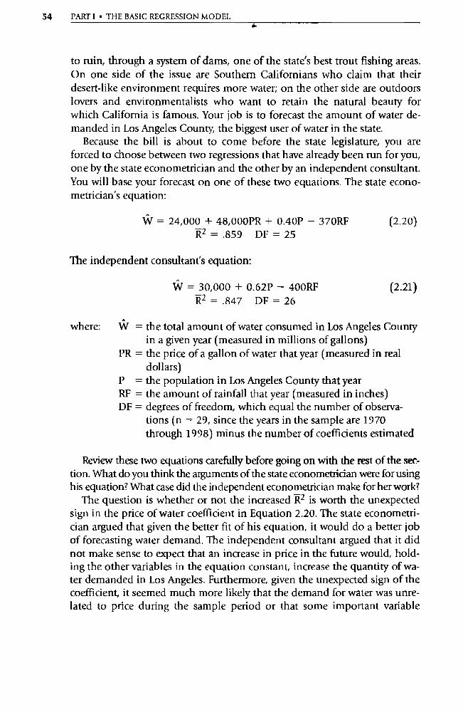
54 PART I • THE BASIC REGRESSION MODEL
to ruin, through a system of dams, one of the state's best trout fishing areas. On one side of the issue are Southern Californians who claim that their desert-like environment requires more water; on the other side are outdoors lovers and environmentalists who want to retain the natural beauty for which California is famous. Your job is to forecast the amount of water de-manded in Los Angeles County, the biggest user of water in the state.
Because the bill is about to come before the state legislature, you are forced to choose between two regressions that have already been mn for you, one by the state econometrician and the other by an independent consultant. You will base your forecast on one of these two equations. The state econo-metrician's equation:
W = 24,000 + 48,000PR + 0.40P — 370RF (2.20) R2 = .859 DF = 25
The independent consultant's equation:
W = 30,000 + 0.62P — 400RF (2.21) R2 =.847 DF =26
where: W = the total amount of water consumed in Los Angeles County in a given year (measured in millions of gallons)
PR = the price of a gallon of water that year (measured in real dollars)
P = the population in Los Angeles County that year RF = the amount of rainfall that year (measured in inches) DF = degrees of freedom, which equal the number of observa-
tions (n = 29, since the years in the sample are 1970 through 1998) minus the number of coefficients estimated
Review these two equations carefully before going on with the rest of the sec-tion. What do you think the arguments of the state econometrician were for using his equation? What case did the independent econometrician make for her work?
The question is whether or not the increased 11 2 is worth the unexpected sign in the price of water coefficient in Equation 2.20. The state econometri-cian argued that given the better fit of his equation, it would do a better job of forecasting water demand. The independent consultant argued that it did not make sense to expect that an increase in price in the future would, hold-ing the other variables in the equation constant, increase the quantity of wa-ter demanded in Los Angeles. Furthermore, given the unexpected sign of the coefficient, it seemed much more likely that the demand for water was unre-lated to price during the sample period or that some impo rtant variable
CHAPTER 2 • ORDINARY LEAST SQUARES 55
(such as real per capita income) had been left out of both equations. Since the amount of money spent on water was fairly low compared with other ex-penditures during the sample years, the consultant pointed out, it was possi-ble that the demand for water was fairly price inelastic. The economic argu-ment for the positive sign observed by the state econometrician is difficult to justify; it implies that as the price of water goes up, so does the quantity of water demanded.
Was this argument simply academic? The answer, unfortunately, is no. If a forecast is made with Equation 2.20, it will tend to overforecast water de-mand in scenarios that foresee rising prices and underforecast water demand with lower price scenarios. In essence, the equation with the better fit would do a worse job of forecasting. 9
Thus, a researcher who uses R 2 as the sole measure of the quality of an equation (at the expense of economic theory or statistical significance) in-creases the chances of having unrepresentative or misleading results. This practice should be avoided at all costs. No simple rule of econometric esti-mation is likely to work in all cases. Instead, a combination of technical competence, theoretical judgment, and common sense makes for a good econometrician.
To help avoid the natural urge to maximize R 2 without regard to the rest of the equation, you might find it useful to imagine the following conversation:
You: Sometimes, it seems like the best way to choose between two models is to pick the one that gives the highest R 2 .
Your Conscience: But that would be wrong. You: I know that the goal of regression analysis is to obtain dependable es-
timates of the true population coefficients and not to get a high R 2, but my results "look better" if my fit is good.
Your Conscience: Look better to whom? It's not at all unusual to get a high R2 but find that some of the regression coefficients have signs that are con-trary to theoretical expectations.
You: Well, I guess I should be more concerned with the logical relevance of the explanatory variables than with the fit, huh?
Your Conscience: Right! If in this process we obtain a high R 2, well and good, but if R2 is high, it doesn't mean that the model is good.
You: Amen.
9. A couple of caveats to this example are in order. First, the purpose of the rainfall va riable in both equations was to explain past behavior. For forecasting purposes, average rainfall figures would likely be used because future rainfall would not be known. Second, the income va riable suggested by the independent consultant turned out to have a relatively small coefficient. This is because water expenditure is so minor in relation to the overall budget that the demand for water turned out to be fairly income inelastic as well as fairly price inelastic.
56 PARTI • THE BASIC REGRESSION MODEL
2.6 Summary
1. Ordinary Least Squares (OLS) is the most frequently used method of obtaining estimates of the regression coefficients from a set of data. OLS chooses those (3s that minimize the summed squared residuals (se?) for a particular sample.
2. The coefficient of determination, R 2, is the simplest measure of the degree of statistical fit of an estimated equation. It can be thought of as the percentage of the variation of Y around its mean that has been explained by a particular regression equation and is defined as the ex-plained sum of squares (ESS) divided by the total sum of squares (TSS). A major fault of R2 is that it always increases (technically, never decreases) when a variable is added to an equation.
3. R-bar-squared (112) is the coefficient of determination (R 2) adjusted for degrees of freedom. 11. 2 increases when a variable is added to an equation only if the improvement in fit caused by the addition of the new variable more than offsets the loss of the degree of freedom that is used up in estimating the coefficient of the new variable. As a result, most researchers will automatically use R 2 instead of R2 when evalu-ating the fit of their estimated regression equations.
4. Always remember that the quality of fit of an estimated equation is only one of the measures of the overall quality of that regression. The degree to which the estimated coefficients conform to economic the-ory and expectations developed by the researcher before the data were collected is at least as impo rtant as the size of R2 itself.
Exercises
(Answers to even-numbered exercises are in Appendix A.)
1. Write the meaning of each of the following terms without referring to the book (or your notes), and compare your definition with the ver-sion in the text for each: a. ordinary least squares b. the meaning of a multivariate regression coefficient c. total, explained, and residual sums of squares d. coefficient of determination e. degrees of freedom f. R2
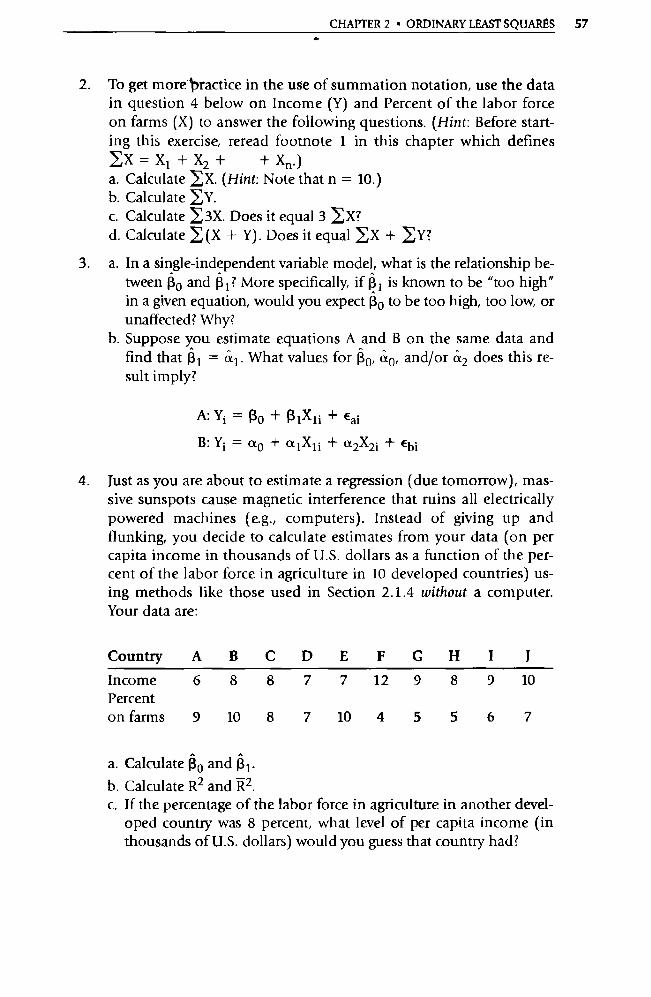
CHAPTER 2 • ORDINARY LEAST SQUARES 57
2. To get more 'Practice in the use of summation notation, use the data in question 4 below on Income (Y) and Percent of the labor force on farms (X) to answer the following questions. (Hint: Before start-ing this exercise, reread footnote 1 in this chapter which defines EX=X1 + X2 + +Xn.) a. Calculate X. (Hint: Note that n = 10.) b. Calculate EY. c. Calculate E3X. Does it equal 3 IX? d. Calculate (X + Y). Does it equal EX + EY?
3. a. In a single-independent variable model, what is the relationship be-tween âo and R1? More specifically, if Q1 is known to be "too high" in a given equation, would you expect 13 o to be too high, too low, or unaffected? Why?
b. Suppose you estimate equations A and B on the same data and find that R1 = â l . What values for 1 o
, &o, and/or 612 does this re-
sult imply?
A:Yi = RO + R1Xli + Eai
B:Yi = oto + a1Xi + a2X2i + Ebi
4. Just as you are about to estimate a regression (due tomorrow), mas-sive sunspots cause magnetic interference that ruins all electrically powered machines (e.g., computers). Instead of giving up and flunking, you decide to calculate estimates from your data (on per capita income in thousands of U.S. dollars as a function of the per-cent of the labor force in agriculture in 10 developed countries) us-ing methods like those used in Section 2.1.4 without a computer. Your data are:
Country A B C D E F G H I J
Income Percent on farms
6
9
8
10
8
8
7
7
7
10
12
4
9
5
8
5
9
6
10
7
a. Calculate (3 0 and (1 1. b. Calculate R2 and R2 . c. If the percentage of the labor force in agriculture in another devel-
oped country was 8 percent, what level of per capita income (in thousands of U.S. dollars) would you guess that count ry had?
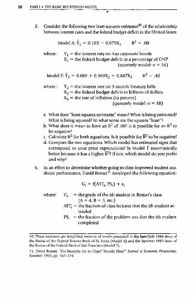
58 PART I • THE BASIC REGRESSION MODEL
5. Consider the following two least-squares estimates 10 of the relationship between interest rates and the federal budget deficit in the United States:
Model A: Yl = 0.103 — 0.079X 1 R2 = .00
where: Y 1 = the interest rate on Aaa corporate bonds X 1 = the federal budget deficit as a percentage of GNP
(quarterly model: n = 56)
Model T: Y2 = 0.089 + 0.369X2 + 0.887X3 R2 = .40
where : Y2 = the interest rate on 3-month Treasury bills X2 = the federal budget deficit in billions of dollars X3 = the rate of inflation (in percent)
(quarterly model: n = 38)
a. What does "least-squares estimates" mean? What is being estimated? What is being squared? In what sense are the squares "least"?
b. What does it mean to have an R2 of .00? Is it possible for an R2 to be negative?
c. Calculate R 2 for both equations. Is it possible for R 2 to be negative? d. Compare the two equations. Which model has estimated signs that
correspond to your prior expectations? Is Model T automatically better because it has a higher R 2 ? If not, which model do you prefer and why?
6. In an effort to determine whether going to lass improved student aca-demic performance, David Romerll developed the following equation:
Gi = f(ATTi, PSi) + Ei
where: Gi = the grade of the ith student in Romer s class (A = 4, B = 3, etc.)
ATTi = the fraction of class lectures that the ith student at-tended
PS i = the fraction of the problem sets that the ith student completed
10. These estimates are simplified versions of results presented in the June/July 1984 issue of the Review of the Federal Reserve Bank of St. Louis (Model A) and the Summer 1983 issue of the Review of the Federal Bank of San Francisco (Model T).
11. David Romer, "Do Students Go to Class? Should They?" Journal of Economic Perspectives, Summer 1993, pp. 167-174.
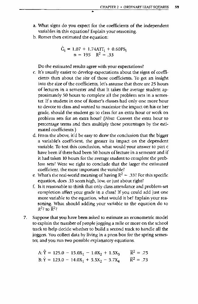
CHAPTER 2 • ORDINARY LEAST SQUARES 59
a. What signs do you expect for the coefficients of the independent variables in this equation? Explain your reasoning.
b. Romer then estimated the equation:
Gi = 1.07 + 1.74ATTi + 0.60PSi n= 195 R2 =.33
Do the estimated results agree with your expectations? c. It's usually easier to develop expectations about the signs of coeffi-
cients than about the size of those coefficients. To get an insight into the size of the coefficients, let's assume that there are 25 hours of lectures in a semester and that it takes the average student ap-proximately 50 hours to complete all the problem sets in a semes-ter. If a student in one of Romer s classes had only one more hour to devote to class and wanted to maximize the impact on his or her grade, should the student go to class for an extra hour or work on problem sets for an extra hour? (Hint: Convert the extra hour to percentage terms and then multiply those percentages by the esti-mated coefficients.)
d. From the above, it'd be easy to draw the conclusion that the bigger a variable's coefficient, the greater its impact on the dependent variable. To test this conclusion, what would your answer to pa rt c have been if there had been 50 hours of lecture in a semester and if it had taken 10 hours for the average student to complete the prob-lem sets? Were we right to conclude that the larger the estimated coefficient, the more impo rtant the variable?
e. What's the real-world meaning of having R 2 = .33? For this specific equation, does .33 seem high, low, or just about right?
f. Is it reasonable to think that only class attendance and problem-set completion affect your grade in a class? If you could add just one more variable to the equation, what would it be? Explain your rea-soning. What should adding your variable to the equation do to R2 ? to R2 ?
7. Suppose that you have been asked to estimate an econometric model to explain the number of people jogging a mile or more on the school track to help decide whether to build a second track to handle all the joggers. You collect data by living in a press box for the spring semes-ter, and you run two possible explanatory equations.
A:Ÿ = 125.0 — 15.0X 1 — 1.0X2 + 1.5X3 R2 . 75
B:Y = 123.0 — 14.0X 1 + 5.5X2 — 3.7X4 RZ = .73

60 PART I • THE BASIC REGRESSION MODEL ^
where: Y = the number of joggers on a given day X 1 = inches of rain that day X2 = hours of sunshine that day X3 = the high temperature for that day (in degrees F) X4 = the number of classes with term papers due the next
day
a. Which of the two (admittedly hypothetical) equations do you pre-fer? Why?
b. How is it possible to get different estimated signs for the coefficient of the same va riable using the same data?
8. David Katz 12 studied faculty sala ries as a function of their "productiv-ity" and estimated a regression equation with the following coefficients:
Si = 11,155 + 230B1 + 18Ai + 102E1 + 489Di + 189Y1 +
where: Si = the salary of the ith professor in dollars per year Bi = the number of books published, lifetime Ai = the number of articles published, lifetime El = the number of "excellent" articles published, lifetime
Di = the number of dissertations supervised Yi = the number of years teaching experience
a. Do the signs of the coefficients match your prior expectations? b. Do the relative sizes of the coefficients seem reasonable? c. Suppose a professor had just enough time (after teaching, etc.) to
write a book, write two excellent articles, or supervise three disser-tations. Which would you recommend? Why?
d. Would you like to reconsider your answer to pa rt b above? Which coefficient seems out of line? What explanation can you give for that result? Is the equation in some sense invalid? Why or why not?
9. What's wrong with the following kind of thinking: "I understand that R2 is not a perfect measure of the quality of a regression equation be-cause it always increases when a va riable is added to the equation. Once we adjust for degrees of freedom by using R 2, though, it seems to me that the higher the R 2 , the better the equation.
12. David A. Katz, "Faculty Salaries, Promotions, and Productivity at a Large University," Amer-ican Economic Review, June 1973, pp. 469-477 Katz's equation induded other variables, as well, as indicated by the "+ • • • " at the end of the equation.
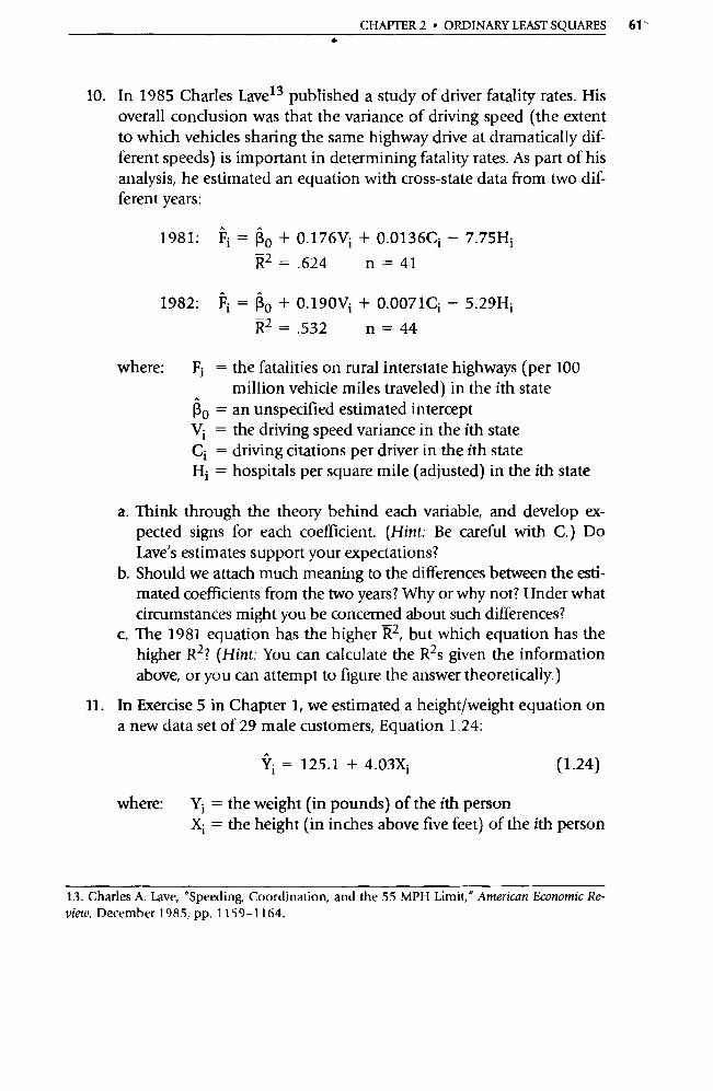
CHAPTER 2 • ORDINARY LEAST SQUARES 61
10. In 1985 Charles Lave 13 published a study of driver fatality rates. His overall conclusion was that the va riance of driving speed (the extent to which vehicles sharing the same highway drive at dramatically dif-ferent speeds) is impo rtant in determining fatality rates. As pa rt of his analysis, he estimated an equation with cross-state data from two dif-ferent years:
1981: Fi = + 0.176Vi + 0.0136C; — 7.75H;
R2 =.624 n=41
1982: Fi =(3p+ 0.190V; +0.0071C; -5.29H;
R2 =.532 n=44
where: Fi = the fatalities on rural interstate highways (per 100 million vehicle miles traveled) in the ith state
Ro = an unspecified estimated intercept Vi = the driving speed variance in the ith state Ci = driving citations per driver in the ith state Hi = hospitals per square mile (adjusted) in the ith state
a. Think through the theory behind each va riable, and develop ex-pected signs for each coefficient. (Hint: Be careful with C.) Do Lave's estimates suppo rt your expectations?
b. Should we attach much meaning to the differences between the esti-mated coefficients from the two years? Why or why not? Under what circumstances might you be concerned about such differences?
c. The 1981 equation has the higher R 2, but which equation has the higher R2 ? (Hint: You can calculate the R 2s given the information above, or you can attempt to figure the answer theoretically.)
11. In Exercise 5 in Chapter 1, we estimated a height/weight equation on a new data set of 29 male customers, Equation 1.24:
= 125.1 + 4.03X; (1.24)
where: Yi = the weight (in pounds) of the ith person Xi = the height (in inches above five feet) of the ith person
13. Charles A. Lave, "Speeding, Coordination, and the 55 MPH Limit," American Economic Re-view, December 1985, pp. 1159-1164.

62 PART I • THE BASIC REGRESSION MODEL
Suppose that a friend now suggests adding Fi , the percent body fat of the ith person, to the equation.
a. What is the theory behind adding F ; to the equation? How does the meaning of the coefficient of X change when you add F?
b. Assume you now collect data on the percent body fat of the 29 males and estimate:
Yi = 120.8 + 4.11Xi + 0.28Fi (2.22)
Do you prefer Equation 2.22 or Equation 1.24? Why? c. Suppose you learn that the R 2 of Equation 1.24 is .75 and the R2 of
Equation 2.22 is .72. Which equation do you prefer now? Explain your answer.
d. Suppose that you learn that the mean of F for your sample is 12.0. Which equation do you prefer now? Explain your answer.
12. For students with a background in calculus, the derivation of Equa-tions 2.6 and 2.7 is useful. Derive these two equations by carrying out the following steps. (Hint: Be sure to write out each step of the proof; if you get stuck, compare your answer to that in the back of the book.) a. Differentiate Equation 2.5 with respect to RD and then with respect
to R 1 .
b. Set these two derivatives equal to zero, thus creating what are called the "normal equations."
c. Solve the normal equations for (i 1, obtaining Equation 2.6. d. Solve the normal equations for (30, obtaining Equation 2.7.
13. To get more practice in using EViews or your computer's regression program, estimate Equation 2.10 using the data from Table 2.2 (or the BEEF2 datafile on the website or the EViews disk). Can you replicate the results in the text? What are R 2 and R2?
3 CHAPTER
Learning to Use Regression Analysis
3.1 Steps in Applied Regression Analysis
3.2 Using Regression Analysis to Pick Restaurant Locations
3.3 Summary and Exercises
From a quick reading of Chapter 2, it'd be easy to conclude that regression analysis is little more than the mechanical application of a set of equations to a sample of data. Such a notion would be similar to deciding that all there is to golf is hitting the ball well. Golfers will tell you that it does little good to hit the ball well if you've used the wrong club or have hit the ball toward a trap, tree, or pond. Similarly, experienced econometricians spend much less time thinking about the OLS estimation of an equation than they do about a number of other factors. Our goal in this chapter is to introduce some of these "real world" concerns.
The first section, an overview of the six steps typically taken in applied re-gression analysis, is the most important in the chapter. We believe that the ability to learn and understand a specific topic, like OLS estimation, is en-hanced if the reader has a clear vision of the role that specific topic plays in the overall framework of regression analysis. In addition, the six steps make it hard to miss the crucial function of theory in the development of sound econometric research.
This is followed by a complete example of how to use the six steps in ap-plied regression, a location analysis for the "Woodÿ s" restaurant chain that is based on actual company data and to which we will return in future chapters to apply new ideas and tests.
3.1 Steps in Applied Regression Analysis
Although there are no hard and fast rules for conducting econometric re- search, most investigators commonly follow a standard method for applied regression analysis. The relative emphasis and effort expended on each step
63
64 PARTI • THE BASIC REGRESSION MODEL
may vary, but normally all the steps are considered necessary for successful research. Note that we don't discuss the selection of the dependent variable; this choice is determined by the purpose of the research. After that, it is logi-cal to follow this sequence:
1. Review the literature and develop the theoretical model.
2. Specify the model: Select the independent va riables and the func-tional form.
3. Hypothesize the expected signs of the coefficients.
4. Collect the data.
5. Estimate and evaluate the equation.
6. Document the results.
The purpose of suggesting these steps is not to discourage the use of inno-vative or unusual approaches but rather to develop in the reader a sense of how regression ordinarily is done by professional economists and business analysts.
3.1.1 Step 1: Review the literature and Develop the Theoretical Model
The first step in any applied research is to get a good theoretical grasp of the topic to be studied. That's right, the best data analysts don't start with data; they start with theory. This is because many econometric decisions, ranging from which variables to use to which functional form to employ, are deter-mined by the underlying theoretical model. It's virtually impossible to build a good econometric model without a solid understanding of the topic you're studying.
For most topics, this means that it's sma rt to review the scholarly literature before doing anything else. If a professor has investigated the theory behind your topic, you want to know about it. If other researchers have estimated equations for your dependent va riable, you might want to apply one of their models to your data set. On the other hand, if you disagree with the ap-proach of previous authors, you might want to head off in a new direction. In either case, you shouldn't have to "reinvent the wheel"; you should start your
CHAPTER 3 • LEARNING TO USE REGRESSION ANALYSIS 65
investigation where earlier researchers left off. Any academic paper on an em-pirical topic should begin with a summary of the extent and quality of previ-ous research.
The most convenient approaches to reviewing the literature are to obtain several recent issues of the Journal of Economic Literature or a business-ori-ented publication of abstracts, or to run an Internet search on your topic. Us-ing these resources, find and read several recent a rticles on your topic. Pay at-tention to the bibliographies of these a rticles. If an older article is cited by a number of current authors, or if its title hits your topic on the head, trace back through the literature and find this a rticle as well. We'll have more ad-vice on reviewing the literature in Chapter 11.
In some cases, a topic will be so new or so obscure that you won't be able to find any a rticles on it. What then? We recommend two possible strategies. First, try to transfer theory from a similar topic to yours. For example, if you're trying to build a model of the demand for a new product, read a rticles that analyze the demand for similar, existing products. Second, if all else fails, pick up the telephone and call someone who works in the field you're investigating. For example, if you're building a model of housing in an unfa-miliar city, call a real estate agent who works there.
3.1.2 Step 2: Specify the Model: Select the Independent Variables and the Functional Form
The most important step in applied regression analysis is the specification of the theoretical regression model. After selecting the dependent variable, the following components should be specified:
1. the independent va riables and how they should be measured,
2. the functional (mathematical) form of the variables, and
3. the type of stochastic error term.
A regression equation is specified when each of these elements has been treated appropriately. We'll discuss the details of these specification decisions in Chapters 6, 7, and 4, respectively.
Each of the elements of specification is determined primarily on the basis of economic theory, rather than on the results of an estimated regression equation. A mistake in any of the three elements results in a specification er-ror. Of all the kinds of mistakes that can be made in applied regression analysis, specification error is usually the most disastrous to the validity of the estimated equation. Thus, the more attention paid to economic theory at

66 PART I • THE BASIC REGRESSION MODEL
the beginning of a project, the more satisfying the regression results are likely to be.
The emphasis in this text is on estimating behavioral equations, those that describe the behavior of economic entities. We focus on selecting indepen-dent variables based on the economic theory concerning that behavior. An explanatory variable is chosen because it is a theoretical determinant of the dependent va riable; it is expected to explain at least pa rt of the variation in the dependent variable. Recall that regression gives evidence but does not prove economic causality. Just as an example does not prove the rule, a re-gression result does not prove the theory.
There are dangers in specifying the wrong independent variables. Our goal should be to specify only relevant explanatory variables, those expected theo-retically to assert a "significant" influence on the dependent va riable. Vari
-ables suspected of having little effect should be excluded unless their possi-ble impact on the dependent variable is of some particular (e.g., policy) interest.
For example, an equation that explains the quantity demanded of a con-sumption good might use the price of the product and consumer income or wealth as likely variables. Theory also indicates that complementary and sub-stitute goods are impo rtant. Therefore, you might decide to include the prices of complements and substitutes, but which complements and substitutes? Of course, selection of the closest complements and/or substitutes is appropri-ate, but how far should you go? The choice must be based on theoretical judgment.
When researchers decide that, for example, the prices of only two other goods need to be included, they are said to impose their priors (i.e., previous theoretical belief) or their working hypotheses on the regression equation. Imposition of such priors is a common practice that determines the number and kind of hypotheses that the regression equation has to test. The danger is that a prior may be wrong and could diminish the usefulness of the esti-mated regression equation. Each of the priors therefore should be explained and justified in detail.
Some concepts (for example, gender) might seem impossible to include in an equation because they're inherently qualitative in nature and can't be quantified. These va riables can be quantified by using dummy (or binary) variables. A dummy variable takes on the values of one or zero depending on whether a specified condition holds. We'll discuss dummy variables in de-tail in Chapters 7 and 13.
As an illustration, suppose that Yi represents the salary of the ith high school teacher, and that the salary level depends primarily on the type of de-gree earned and the experience of the teacher. All teachers have a B.A., but
where: Xii =
X2i = the number of years of teaching experience of the ith teacher
{ 1 if the ith teacher has an M.A. 0 otherwise
CHAPTER 3 • LEARNING TO USE REGRESSION ANALYSIS 67
some also have an M.A. An equation representing the relationship between earnings and the type of degree might be:
Yi R O + 01Xli + P2X2i + E i (3.1)
The variable X 1 only takes on values of zero or one, so X 1 is called a dummy variable, or just a "dummy." Needless to say, the term has generated many a pun. In this case, the dummy variable represents the condition of having a master's degree. The coefficient j3 1 indicates the additional salary that can be attributed to having an M.A., holding teaching experience constant.
3.1.3 Step 3: Hypothesize the Expected Signs of the Coefficients
Once the variables are selected, it is important to carefully hypothesize the signs you expect their regression coefficients to have based on the underlying theory. For example, in the demand equation for a final consumption good, the quantity demanded (Q d) is expected to be inversely related to its price (P) and the price of a complementary good (P c ), and positively related to consumer income (Y) and the price of a substitute good (Ps). The first step in the written development of a regression model usually is to express the equa-tion as a general function:
— + — + Qd = f( P, Y, Pc, Ps ) + E (3.2)
The signs above the variables indicate the hypothesized sign of the respective regression coefficient in a linear model.
In many cases, the basic theory is general knowledge, so that the reasons for each sign need not be discussed. However, if any doubt surrounds the se-lection of an expected sign, you should document the opposing forces at work and the reasons for hypothesizing a positive or negative coefficient.
3.1.4 Step 4: Collect the Data
Data collection may begin after the specification of the regression model. This step entails more than a mechanical recording of data, though, because
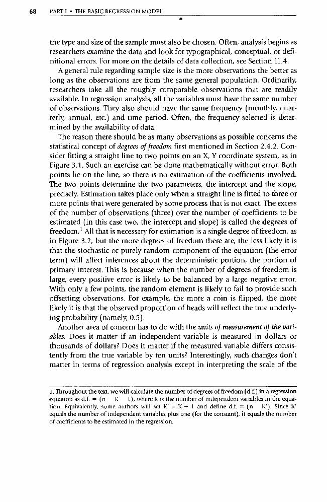
68 PARTI • THE BASIC REGRESSION MODEL
the type and size of the sample must also be chosen. Often, analysis begins as researchers examine the data and look for typographical, conceptual, or defi-nitional errors. For more on the details of data collection, see Section 11.4.
A general rule regarding sample size is the more observations the better as long as the observations are from the same general population. Ordinarily, researchers take all the roughly comparable observations that are readily available. In regression analysis, all the va riables must have the same number of observations. They also should have the same frequency (monthly, quar-terly, annual, etc.) and time period. Often, the frequency selected is deter-mined by the availability of data.
The reason there should be as many observations as possible concerns the statistical concept of degrees of freedom first mentioned in Section 2.4.2. Con-sider fitting a straight line to two points on an X, Y coordinate system, as in Figure 3.1. Such an exercise can be done mathematically without error. Both points lie on the line, so there is no estimation of the coefficients involved. The two points determine the two parameters, the intercept and the slope, precisely. Estimation takes place only when a straight line is fitted to three or more points that were generated by some process that is not exact. The excess of the number of observations (three) over the number of coefficients to be estimated (in this case two, the intercept and slope) is called the degrees of freedom.' All that is necessary for estimation is a single degree of freedom, as in Figure 3.2, but the more degrees of freedom there are, the less likely it is that the stochastic or purely random component of the equation (the error term) will affect inferences about the deterministic po rtion, the portion of primary interest. This is because when the number of degrees of freedom is large, every positive error is likely to be balanced by a large negative error. With only a few points, the random element is likely to fail to provide such offsetting observations. For example, the more a coin is flipped, the more likely it is that the observed propo rtion of heads will reflect the true underly-ing probability (namely, 0.5).
Another area of concern has to do with the units of measurement of the vari-ables. Does it matter if an independent va riable is measured in dollars or thousands of dollars? Does it matter if the measured variable differs consis-tently from the true variable by ten units? Interestingly, such changes don't matter in terms of regression analysis except in interpreting the scale of the
1. Throughout the text, we will calculate the number of degrees of freedom (d.f.) in a regression equation as d.f. = (n K 1), where K is the number of independent variables in the equa- tion. Equivalently, some authors will set K' = K + 1 and define d.f. = (n K'). Since K' equals the number of independent va riables plus one (for the constant), it equals the number of coefficients to be estimated in the regression.
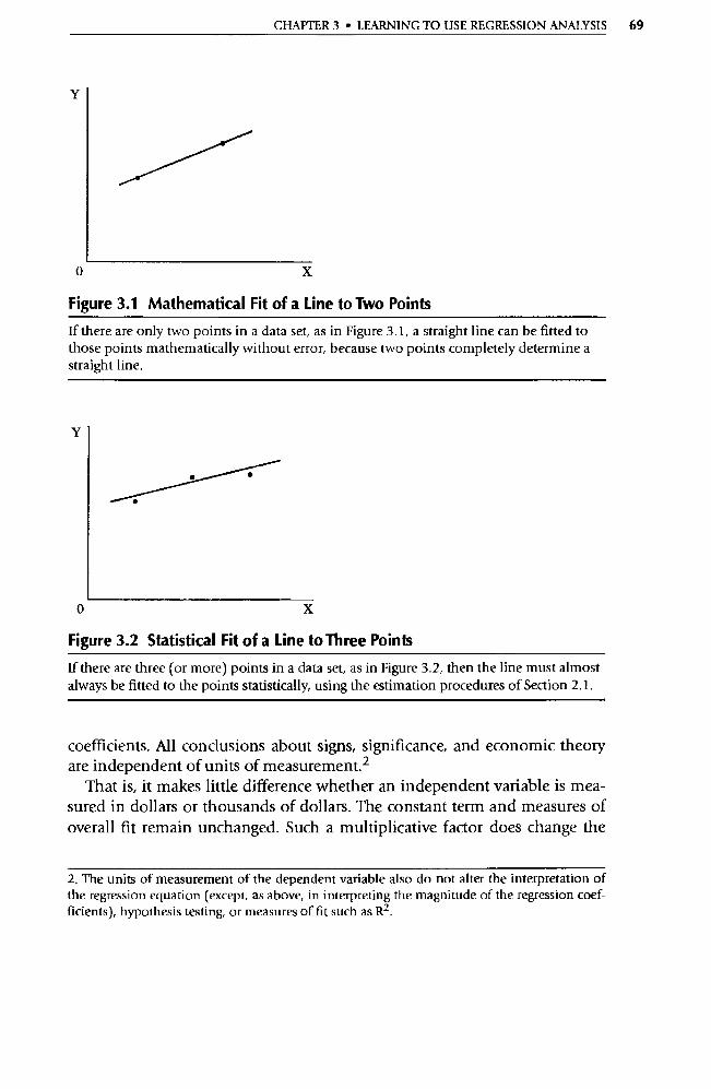
CHAPTER 3 • LEARNING TO USE REGRESSION ANALYSIS 69
Y
Y
o X
Figure 3.1 Mathematical Fit of a Line to Two Points
If there are only two points in a data set, as in Figure 3.1, a straight line can be fitted to those points mathematically without error, because two points completely determine a straight line.
•
•
o X
Figure 3.2 Statistical Fit of a Line to Three Points
If there are three (or more) points in a data set, as in Figure 3.2, then the line must almost always be fitted to the points statistically, using the estimation procedures of Section 2.1.
coefficients. All conclusions about signs, significance, and economic theory are independent of units of measurement. 2
That is, it makes little difference whether an independent va riable is mea-sured in dollars or thousands of dollars. The constant term and measures of overall fit remain unchanged. Such a multiplicative factor does change the
2. The units of measurement of the dependent va riable also do not alter the interpretation of the regression equation (except, as above, in interpreting the magnitude of the regression coef-ficients), hypothesis testing, or measures of fit such as R2.

70 PARTI • THE BASIC REGRESSION MODEL
slope coefficient, but only by the exact amount necessary to compensate for the change in the units of measurement of the independent variable. Simi-larly, a constant factor added to a variable alters only the intercept term with-out changing the slope coefficient itself.
As an example, recall the weight/height regression of Section 1.4. The ex-planatory variable was measured as inches above 5 feet, so that 5 feet, or 60 inches, was a constant factor that was subtracted from each obse rvation. If we reestimate the equation with the absolute height in inches (Z) as the inde-pendent variable, we get:
= —279.2 + 6.38Z; (3.3)
Since the original equation was
Yi = 103.4 + 6.38Xi (3.4)
only the constant term has changed, and for each height we would obtain the same estimated weight. To see this, substitute 60 for Z and 0 for X; Y = 103.4 in both cases! The essential relationship between Y and Z is the same as be-tween Y and X. That is, adding a constant to a va riable will not change the slope coefficients of a linear equation (but it will in most equations that are nonlinear in the coefficients).
3.1.5 Step 5: Estimate and Evaluate the Equation
The Ordinary Least Squares (OLS) technique, discussed in Section 2.1, is the method typically used to estimate econometric equations. Where alternative techniques might be appropriate, estimates from the alternatives should be compared to OLS estimates. The alternatively estimated equations must be evaluated carefully and judgment applied before a choice is made.
Once the model has been estimated, the results should be checked for er-rors. Data transformations and coefficient estimation are usually done in the same computer program, so it is wise to obtain a printout of the data set ex-actly as it was used in the regression estimation. Check one or two values of any variables that were transformed. If these values are correct, it may be as-sumed that the computer did not make any mistakes transforming the rest of the observations. Also obtain a printout or a plot of the data and look for outliers. An outlier is an obse rvation that lies outside the range of the rest of the observations. Looking for outliers is a very economical way to look for data entry or transcription errors. It's also a good habit to make sure that the mean, maximum, and minimum of each variable seem reasonable.
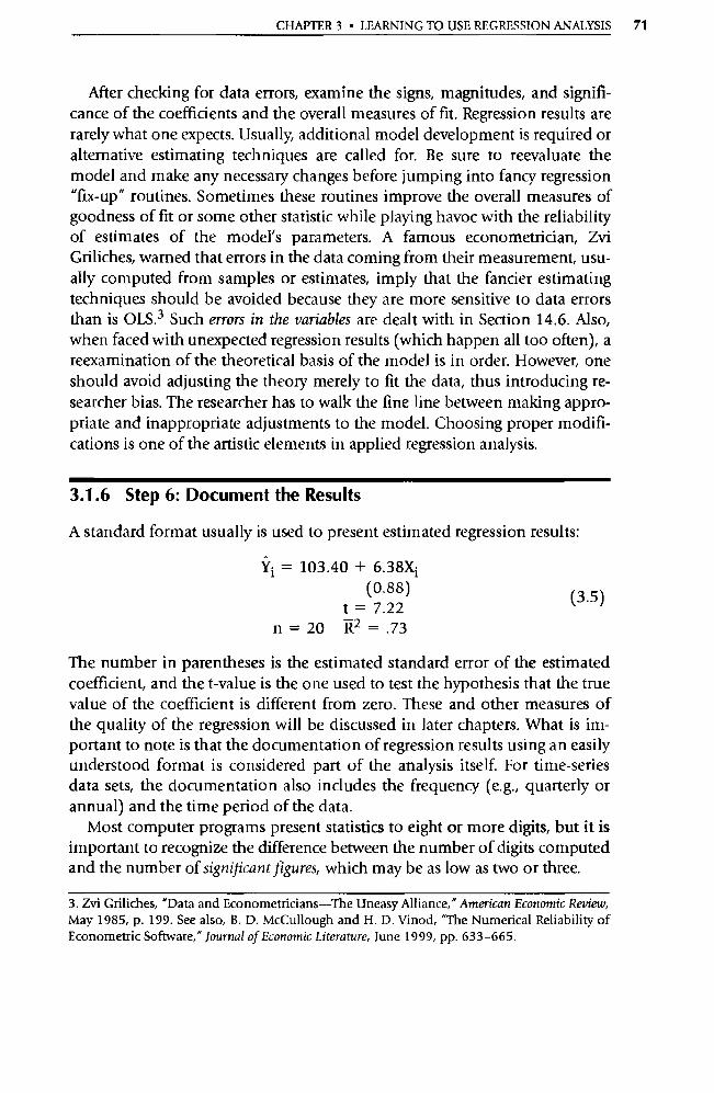
CHAPTER 3 • LEARNING TO USE REGRESSION ANALYSIS 71
After checking for data errors, examine the signs, magnitudes, and signifi-cance of the coefficients and the overall measures of fit. Regression results are rarely what one expects. Usually, additional model development is required or alternative estimating techniques are called for. Be sure to reevaluate the model and make any necessary changes before jumping into fancy regression "fix-up" routines. Sometimes these routines improve the overall measures of goodness of fit or some other statistic while playing havoc with the reliability of estimates of the model's parameters. A famous econometrician, Zvi Griliches, warned that errors in the data coming from their measurement, usu-ally computed from samples or estimates, imply that the fancier estimating techniques should be avoided because they are more sensitive to data errors than is OLS. 3 Such errors in the variables are dealt with in Section 14.6. Also, when faced with unexpected regression results (which happen all too often), a reexamination of the theoretical basis of the model is in order. However, one should avoid adjusting the theory merely to fit the data, thus introducing re-searcher bias. The researcher has to walk the fine line between making appro-priate and inappropriate adjustments to the model. Choosing proper modifi-cations is one of the artistic elements in applied regression analysis.
3.1.6 Step 6: Document the Results
A standard format usually is used to present estimated regression results:
Yi = 103.40 + 6.38Xi (0.88)
t = 7.22 n=20 R2 =.73
The number in parentheses is the estimated standard error of the estimated coefficient, and the t-value is the one used to test the hypothesis that the true value of the coefficient is different from zero. These and other measures of the quality of the regression will be discussed in later chapters. What is im-portant to note is that the documentation of regression results using an easily understood format is considered pa rt of the analysis itself. For time-series data sets, the documentation also includes the frequency (e.g., quarterly or annual) and the time period of the data.
Most computer programs present statistics to eight or more digits, but it is important to recognize the difference between the number of digits computed and the number of significant figures, which may be as low as two or three.
(3.5)
3. Zvi Griliches, "Data and Econometricians—The Uneasy Alliance," American Economic Review, May 1985, p. 199. See also, B. D. McCullough and H. D. Vinod, "The Numerical Reliability of Econometric Software," Journal of Economic Literature, June 1999, pp. 633-665.
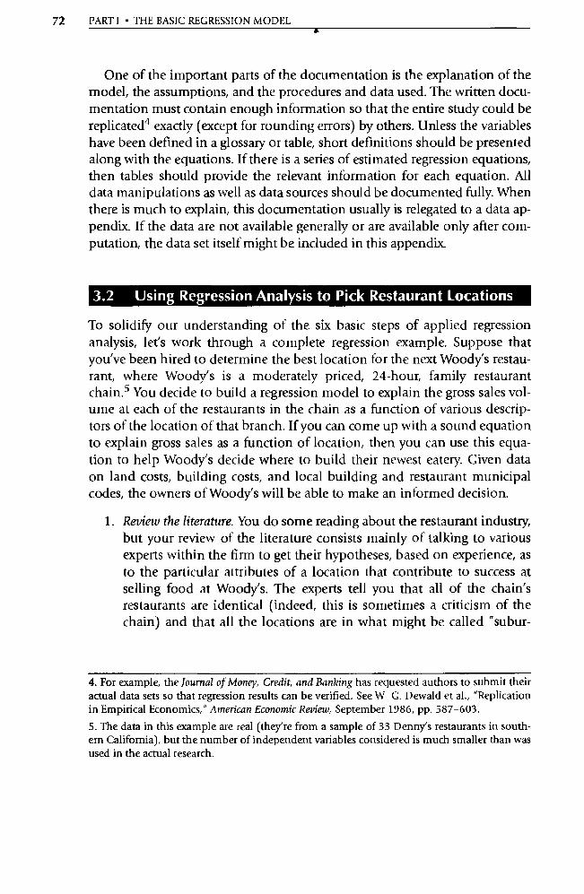
72 PART I • THE BASIC REGRESSION MODEL •
One of the important parts of the documentation is the explanation of the model, the assumptions, and the procedures and data used. The written docu-mentation must contain enough information so that the entire study could be replicated 4 exactly (except for rounding errors) by others. Unless the variables have been defined in a glossary or table, sho rt definitions should be presented along with the equations. If there is a series of estimated regression equations, then tables should provide the relevant information for each equation. All data manipulations as well as data sources should be documented fully. When there is much to explain, this documentation usually is relegated to a data ap-pendix. If the data are not available generally or are available only after com-putation, the data set itself might be included in this appendix.
3.2 Using Regression Analysis to Pick Restaurant Locations
To solidify our understanding of the six basic steps of applied regression analysis, let's work through a complete regression example. Suppose that you've been hired to determine the best location for the next Woody's restau-rant, where Woody's is a moderately priced, 24-hour, family restaurant chain. 5 You decide to build a regression model to explain the gross sales vol-ume at each of the restaurants in the chain as a function of various descrip-tors of the location of that branch. If you can come up with a sound equation to explain gross sales as a function of location, then you can use this equa-tion to help Woody's decide where to build their newest eatery. Given data on land costs, building costs, and local building and restaurant municipal codes, the owners of Woody's will be able to make an informed decision.
1. Review the literature. You do some reading about the restaurant industry, but your review of the literature consists mainly of talking to various expe rts within the firm to get their hypotheses, based on experience, as to the particular attributes of a location that contribute to success at selling food at Woody's. The expe rts tell you that all of the chain's restaurants are identical (indeed, this is sometimes a criticism of the chain) and that all the locations are in what might be called "subur-
4. For example, the Journal of Money, Credit, and Banking has requested authors to submit their actual data sets so that regression results can be verified. See W G. Dewald et al., "Replication in Empirical Economics," American Economic Review, September 1986, pp. 587-603.
5. The data in this example are real (they're from a sample of 33 Denny's restaurants in south-ern California), but the number of independent va riables considered is much smaller than was used in the actual research.
CHAPTER 3 • LEARNING TO USE REGRESSION ANALYSIS 73
ban, retail, or residential" environments (as distinguished from central cities or rural areas, for example). Because of this, you realize that many of the reasons that might help explain differences in sales volume in other chains do not apply in this case because all the Woody's locations are similar. (If you were comparing Woody's to another chain, such variables might be appropriate.)
In addition, discussions with the people in the Woody's strategic planning department convince you that price differentials and con-sumption differences between locations are not as impo rtant as is the number of customers a particular location attracts. This causes you to be concerned for a while because the variable you had planned to study originally, gross sales volume, would vary as prices changed be-tween locations. Since your company controls these prices, you feel that you would rather have an estimate of the "potential" for such sales. As a result, you decide to specify your dependent variable as the number of customers served (measured by the number of checks or bills that the waiters and waitresses handed out) in a given location in the most recent year for which complete data are available.
2. Specify the model: Select the independent variables and the functional form. Your discussions and personal investigations lead to a number of sug-gested variables that should help explain the attractiveness of a particu-lar site to potential customers. After a while, you realize that there are three major determinants of sales (customers) on which virtually every-one agrees. These are the number of people who live near the location, the general income level of the location, and the number of direct com-petitors close to the location. In addition, there are two other good sug-gestions for potential explanatory va riables. These are the number of cars passing the location per day and the number of months that the particular restaurant has been open. After some serious consideration of your alternatives, you decide not to include the last possibilities. All the locations have been open long enough to have achieved a stable clien-tele, so the number of months open would not be likely to be impor-tant. In addition, data are not available for the number of passing cars for all the locations. Should population prove to be a poor measure of the available customers in a location, you'll have to decide whether to ask your boss for the money to collect complete traffic data.
The exact definitions of the independent variables you decide to in-clude are:
N = Competition: the number of direct market competitors within a two-mile radius of the Woody's location
74 PART I • THE BASIC REGRESSION MODEL
P = Population: the number of people living within a three- mile radius of the Woody's location
I = Income: the average household income of the popula- tion measured in variable P
Since you have no reason to suspect anything other than a linear functional form and a typical stochastic error term, that's what you decide to use.
3. Hypothesize the expected signs of the coefficients. After thinking about which variables to include, you expect hypothesizing signs will be easy. For two of the variables, you're right. Everyone expects that the more competition, the fewer customers (holding constant the popula-tion and income of an area), and also that the more people that live near a particular restaurant, the more customers (holding constant the competition and income). You expect that the greater the income in a particular area, the more people will choose to eat away from home and the more people will choose to eat in a family restaurant instead of in the lower-priced fast-food chains. However, people in especially high-income areas might want to eat in a restaurant that has more "at-mosphere" than a family restaurant. Some investigation reveals that it is virtually impossible to get zoning clearance to build a 24-hour facil-ity in a "ritzy" residential neighborhood. You remain slightly worried that the income variable might not be as unambiguous a measure of the appeal of a location as you had thought. To sum, you expect:
— + + Yi = f(Ni, Pi, Ii) + Ei = RO + ¢nNi + RpPi + RIIi + Ei (3.6)
where the signs above the va riables indicate the expected impact of that particular independent va riable on the dependent va riable, holding constant the other two explanatory va riables, and Ei is a typical stochas-tic error term.
4. Collect the data. You want to include every local restaurant in the Woody's chain in your study, and, after some effo rt, you come up with data for your dependent variable and all your independent va riables for all 33 locations. You're confident that the quality of your data is ex-cellent for three reasons: each manager measured each va riable identi-cally, you've included each restaurant in the sample, and all the infor-mation is from the same year. [The data set is included in this section (Table 3.1), along with a sample computer output for the regression es-timated (Table 3.2).]
CHA1'l'ER 3 • LEARNING TO USE REGRESSION ANALYSIS 75
5. Estimate and evaluate the equation. You take the data set and enter it into the computer. You then run an OLS regression on the data, but you do so only after thinking through your model once again to see if there are hints that you've made theoretical mistakes. You end up admitting that although you cannot be sure you are right, you've done the best you can, and so you estimate the equation, obtaining:
= 102,192
t =
9075N ; (2053) —4.42
+ 0.355P ; (0.073) 4.88
+ 1.288I ; (0.543) 2.37
(3.7)
n=33 R2 =.579
This equation satisfies your needs in the sho rt run. In particular, the es-timated coefficients in the equation have the signs you expected. The overall fit, although not outstanding, seems reasonable for such a di-verse group of locations. To predict sales at potential locations, you ob-tain the values of N, P, and I for each location and then plug them into Equation 3.7 Other things being equal, the higher the predicted Y, the better the location from Woody's point of view.
6. Document the results. The results summarized in Equation 3.7 meet our documentation requirements. (Note that we include the standard er-rors of the estimated coefficients and t-values 6 for completeness even though we won't make use of them until Chapter 5.) However, it's not easy for a beginning researcher to wade through a computer's regres-sion output to find all the numbers required for documentation. You'll probably have an easier time reading your own computer system's printout if you take the time to "walk through" the sample computer output for the Woody's model on the previous two pages. This sample output was produced by the EViews computer program, but it's similar to those produced by SAS, SHAZAM, TSP, and others.
Page one of the computer output summarizes the input data. The first items listed are the actual data. These are followed by a table of the sim- ple correlation coefficients between all pairs of variables in the data set.
The second page summarizes the OLS estimates generated from the data. It starts with a listing of the estimated coefficients, their estimated
6. Throughout the text, the number in parentheses below a coefficient estimate will be the stan-dard error of that estimated coefficient. Some authors put the t-value in parentheses, though, so be alert when reading journal a rticles or other books.
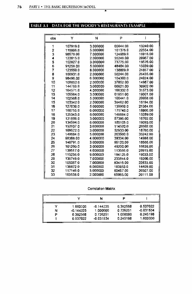
Y N P I
Y 1.000000 -0.144225 0.392568 0.537022 N -0.144225 1.000000 0.726251 -0.031534 P 0.392568 0.726251 1.000000 0.245198 I 0.537022 -0.031534 0.245198 1.000000
76 PART I • THE BASIC REGRESSION MODEL
TABLE 3.1 DATA FOR THE WOODY'S RESTAURANTS EXAMPLE
obs Y N P I
1 107919.0 3.000000 65044.00 13240.00 2 118866.0 5.000000 101376.0 22554.00 3 98579.00 7.000000 124989.0 16916.00 4 122015.0 2.000000 55249.00 20967.00 5 152827.0 3.000000 73775.00 19576.00 6 91259.00 5.000000 48484.00 15039.00 7 123550.0 8.000000 138809.0 21857.00 8 160931.0 2.000000 50244.00 26435.00 9 98496.00 6.000000 104300.0 24024.00 10 108052.0 2.000000 37852.00 14987.00 11 144788.0 3.000000 66921.00 30902.00 12 164571.0 4.000000 166332.0 31573.00 13 105564.0 3.000000 61951.00 19001.00 14 102568.0 5.000000 100441.0 20058.00 15 103342.0 2.000000 39462.00 16194.00 16 127030.0 5.000000 139900.0 21384.00 17 166755.0 6.000000 171740.0 18800.00 18 125343.0 6.000000 149894.0 15289.00 19 121886.0 3.000000 57386.00 16702.00 20 134594.0 6.000000 185105.0 19093.00 21 152937.0 3.000000 114520.0 26502.00 22 109622.0 3.000000 52933.00 18760.00 23 149884.0 5.000000 203500.0 33242.00 24 98388.00 4.000000 39334.00 14988.00 25 140791.0 3.000000 95120.00 18505.00 26 101260.0 3.000000 49200.00 16839.00 27 139517.0 4.000000 113566.0 28915.00 28 115236.0 9.000000 194125.0 19033.00 29 136749.0 7.000000 233844.0 19200.00 30 105067.0 7.000000 83416.00 22833.00 31 136872.0 6.000000 183953.0 14409.00 32 117146.0 3.000000 60457.00 20307.00 33 163538.0 2.000000 65065.00 20111.00
Correlation Matrix
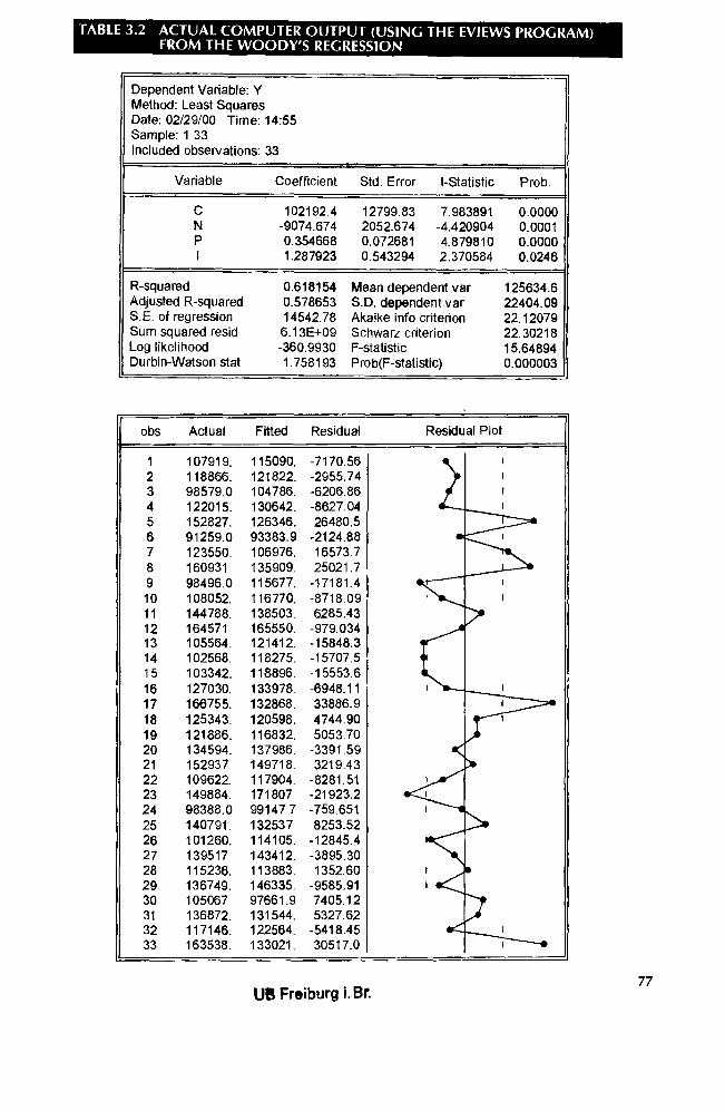
TABLE 3.2 ACTUAL COMPUTER OUTPUT (USING THE EVIEWS PROGRAM) FROM THE WOODY'S REGRESSION
Dependent Variable: Y Method: Least Squares Date: 02/29/00 Time: 14:55 Sample: 1 33 Included observations: 33
Variable Coefficient Std. Error t-Statistic Prob.
C 102192.4 12799.83 7.983891 0.0000 N -9074.674 2052.674 -4.420904 0.0001 P 0.354668 0.072681 4.879810 0.0000 I 1.287923 0.543294 2.370584 0.0246
R-squared 0.618154 Mean dependent var 125634.6 Adjusted R-squared 0.578653 S.D. dependent var 22404.09 S.E. of regression 14542.78 Akaike info criterion 22.12079 Sum squared resid 6.13E+09 Schwa rz criterion 22.30218 Log likelihood -360.9930 F-statistic 15.64894 Durbin-Watson stat 1.758193 Prob(F-statistic) 0.000003
obs Actual Fitted Residual Residual Plot
1 107919. 115090. -7170.56
2 118866. 121822. -2955.74
3 98579.0 104786. -6206.86
4 122015. 130642. -8627.04
5 152827. 126346. 26480.5
6 91259.0 93383 . 9 -2124 . 88
7 123550. 106976. 16573.7 8 160931 135909. 25021.7 9 98496.0 115677. - 17181.4
10 108052. 116770. - 8718.09
11 144788. 138503. 6285.43 .
12 164571 165550. -979.034 13 105564. 121412. - 15848.3 14 102568. 118275. - 15707.5 15 103342. 118896. - 15553.6 16 127030. 133978. -6948.11
17 166755. 132868. 33886.9 18 125343. 120598. 4744.90
19 121886. 116832. 5053.70 20 134594. 137986. -3391.59 21 152937 149718. 3219.43 ► 22 109622. 117904. - 8281.51 23 149884. 171807 -21923.2 24 98388.0 99147 7 - 759.651
25 140791. 132537 8253.52 Ill■ 26 101260. 114105. - 12845.4 27 139517 143412. -3895.30 1
28 115236. 113883. 1352.60 1 29 136749. 146335. -9585.91 ^
,
30 31
105067 136872.
97661.9 131544.
7405.12 5327.62 IIP
32 117146. 122564. - 5418.45 .ii
33 163538. 133021. 30517.0
77 UB Freiburg i. Br.
78 PART I • THE BASIC REGRESSION MODEL a
standard errors, and the associated t-values, and follows with R 2, R2, the standard error of the regression, RSS, and the F-ratio. This is fol-lowed by a listing of the observed Ys, the predicted Ys, and the residu-als for each observation. Numbers followed by "E+06" or "E-01" are expressed in a scientific notation indicating that the printed decimal point should be moved six places to the right or one place to the left, respectively.
In future chapters, we'll return to this example in order to apply var-ious tests and ideas as we learn them.
3.3 Summary
1. Six steps typically taken in applied regression analysis are: a. Review the literature and develop the theoretical model. b. Specify the model: Select the independent variables and the func-
tional form. c. Hypothesize the expected signs of the coefficients. d. Collect the data. e. Estimate and evaluate the equation. f. Document the results.
2. A dummy variable takes on only the values of one or zero, depending on whether or not some condition is met. An example of a dummy variable would be X equals 1 if a particular individual is female and 0 if the person is male.
Exercises
(Answers to even-numbered exercises are in Appendix A.)
1. Write the meaning of each of the following terms without referring to the book (or your notes), and compare your definition with the ver-sion in the text for each: a. the six steps in applied regression analysis b. dummy variable c. cross-sectional data set d. specification error e. degrees of freedom
2. Contrary to their name, dummy va riables are not easy to understand without a little bit of practice: a. Specify a dummy va riable that would allow you to distinguish be-
CHAPTER 3 • LEARNING TO USE REGRESSION ANALYSIS 79
tween undergraduate students and graduate students in your econo-metrics class.
b. Specify a regression equation to explain the grade (measured on a scale of 4.0 for an A) each student in your class received on his or her first econometrics test (Y) as a function of the student's grade in a previous course in statistics (G), the number of hours the student studied for the test (H), and the dummy variable you created above (D). Are there other variables you would want to add? Explain your answer.
c. What is the hypothesized sign of the coefficient of D? Does the sign depend on the exact way in which you defined D? (Hint: In partic-ular, suppose that you had reversed the definitions of one and zero in your answer to pa rt a.) How?
d. Suppose that you collected the data and ran the regression and found an estimated coefficient for D that had the expected sign and an absolute value of 0.5. What would this mean in real-world terms? By the way, what would have happened if you had only un-dergraduates or only graduate students in your class?
3. Do liberal a rts colleges pay economists more than they pay other pro-fessors? To find out, we looked at a sample of 2,929 small-college fac-ulty members and built a model of their salaries that included a num-ber of variables, four of which were (standard errors in parentheses):
= 36,721 + 817Mi + 426A1 + 406Ri + 3539T, + (259) (456) (24) (458)
R2 = .77 n = 2929
(3.8)
where: Si = the salary of the ith college professor Mi = a dummy variable equal to 1 if the ith professor is a
male and 0 otherwise Ai = a dummy variable equal to 1 if the ith professor is
African American and 0 otherwise Ri = the years in rank of the ith professor Ti = a dummy variable equal to 1 if the ith professor
teaches economics and 0 otherwise
a. Carefully explain the meaning of the estimated coefficient of M. b. The equation indicates that African Americans earn $426 more
than members of other ethnic groups, holding constant the other variables in the equation. Does this coefficient have the sign you expected? Why or why not?
80 PART I ■ THE BASIC REGRESSION MODEL
c. Is R a dummy va riable? If not, what is it? Carefully explain the meaning of the coefficient of R.
d. What's your conclusion? Do economists earn more than other pro-fessors at liberal a rts colleges? Explain.
e. Assume that your professor is a white, male economist who has been an assistant professor at your college for three years. How much money does the equation predict that he is earning? (Hint: As tempting as it might be, please don't ask your professor how much he or she earns.)
4. Return to the Woody's regression example of Section 3.2. a. In any applied regression project there is the distinct possibility
that an impo rtant explanatory variable has been omitted. Reread the discussion of the selection of independent variables and come up with a suggestion for an independent variable that has not been included in the model (other than the variables already men-tioned). Why do you think this variable was not included?
b. What other kinds of criticisms would you have of the sample or independent variables chosen in this model?
5. Suppose you were told that, while data on traffic for Equation 3.7 are still too expensive to obtain, a variable on traffic, called T i, is available that is defined as 1 if more than 15,000 cars per day pass the restau-rant and 0 otherwise. Further suppose that when the new variable (T i) is added to the equation the results are:
Yi = 95,236 — 7307Ni + 0.320Pî + 1.28Iî + 10,994T1 (3.9) (2153) (0.073) (0.51) (5577)
t = —3.39 4.24 2.47 1.97 n=33 R2 =.617
a. What is the expected sign of the coefficient of the new variable? b. Would you prefer this equation to the original one? Why? c. Does the fact that R2 is higher in Equation 3.9 mean that it is neces-
sarily better than Equation 3.7?
6. Suppose that the population va riable in Section 3.2 had been defined in different units as in:
P = Population: thousands of people living within a three-mile radius of the Woody's location
a. Given this definition of P, what would the estimated slope coeffi-cients in Equation 3.7 have been?
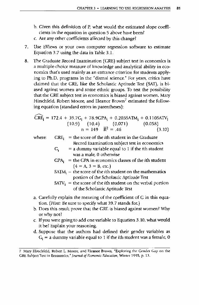
CHAPTER 3 • LEARNING TO USE REGRESSION ANALYSIS 81
b. Given this definition of P, what would the estimated slope coeffi-cients in the equation in question 5 above have been?
c. Are any other coefficients affected by this change?
7. Use EViews or your own computer regression software to estimate Equation 3.7 using the data in Table 3.1.
8. The Graduate Record Examination (GRE) subject test in economics is a multiple-choice measure of knowledge and analytical ability in eco-nomics that's used mainly as an entrance criterion for students apply-ing to Ph.D. programs in the "dismal science." For years, critics have claimed that the GRE, like the Scholastic Aptitude Test (SAT), is bi-ased against women and some ethnic groups. To test the possibility that the GRE subject test in economics is biased against women, Ma ry
Hirschfeld, Robert Moore, and Eleanor Brown 7 estimated the follow-ing equation (standard errors in parentheses):
GREi = 172.4 + 39.7G1 + 78.9GPAi + 0.203SATMi + 0.110SATVi (10.9) (10.4) (0.071) (0.058)
n = 149 R2 = .46 (3.10)
where: GRE; = the score of the ith student in the Graduate Record Examination subject test in economics
Gi = a dummy variable equal to 1 if the ith student was a male, 0 otherwise
GPA; = the GPA in economics dasses of the ith student (4 = A, 3 = B, etc.)
SATMi = the score of the ith student on the mathematics portion of the Scholastic Aptitude Test
SATVi = the score of the ith student on the verbal po rtion of the Scholastic Aptitude Test
a. Carefully explain the meaning of the coefficient of G in this equa-tion. (Hint: Be sure to specify what 39.7 stands for.)
b. Does this result prove that the GRE is biased against women? Why or why not?
c. If you were going to add one va riable to Equation 3.10, what would it be? Explain your reasoning.
d. Suppose that the authors had defined their gender va riables as Gi = a dummy variable equal to 1 if the ith student was a female, 0
7 Mary Hirschfeld, Robert L. Moore, and Eleanor Brown, "Exploring the Gender Gap on the GRE Subject Test in Economics," Journal of Economic Education, Winter 1995, p. 13.
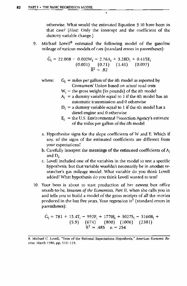
82 PARTI • THE BASIC REGRESSION MODEL
otherwise. What would the estimated Equation 3.10 have been in that case? (Hint: Only the intercept and the coefficient of the dummy variable change.)
9. Michael Lovell 8 estimated the following model of the gasoline mileage of various models of cars (standard errors in parentheses):
= 22.008 — 0.002W1 — 2.76Aî + 3.28Di + 0.415E1 (0.001) (0.71) (1.41) (0.097)
R2 =.82
where: Gi = miles per gallon of the ith model as reported by Consumers' Union based on actual road tests
Wi = the gross weight (in pounds) of the ith model Ai = a dummy variable equal to 1 if the ith model has an
automatic transmission and 0 otherwise D; = a dummy variable equal to 1 if the ith model has a
diesel engine and 0 otherwise E; = the U.S. Environmental Protection Agency's estimate
of the miles per gallon of the ith model
a. Hypothesize signs for the slope coefficients of W and E. Which if any, of the signs of the estimated coefficients are different from your expectations?
b. Carefully interpret the meanings of the estimated coefficients of A; and Di .
c. Lovell included one of the variables in the model to test a specific hypothesis, but that variable wouldn't necessarily be in another re-searcher's gas mileage model. What variable do you think Lovell added? What hypothesis do you think Lovell wanted to test?
10. Your boss is about to start production of her newest box office smash -to -be, Invasion of the Economists, Pa rt II, when she calls you in and tells you to build a model of the gross receipts of all the movies produced in the last five years. Your regression is 9 (standard errors in parentheses):
= 781 + 15.4T1 — 992F; + 1770J1 + 3027Si — 3160B 1 + (5.9) (674) (800) (1006) (2381)
R2 = .485 n = 254
8. Michael C. Lovell, "Tests of the Rational Expectations Hypothesis," American Economic Re-view, March 1986, pp. 110-124.
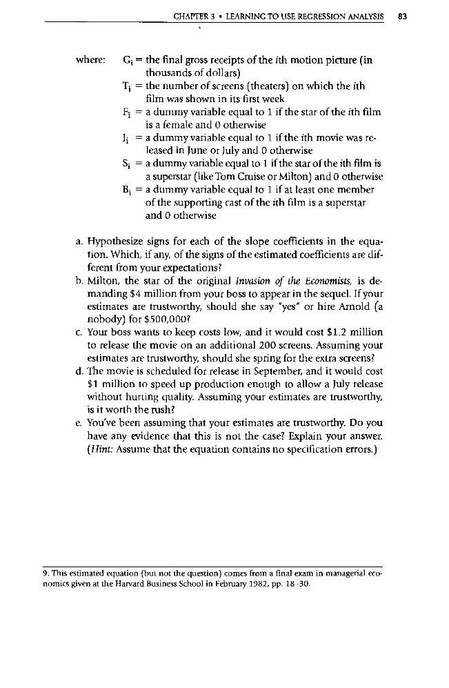
CHAPTER 3 • LEARNING TO USE REGRESSION ANALYSIS 83
where: Gi = the final gross receipts of the ith motion picture (in thousands of dollars)
Ti = the number of screens (theaters) on which the ith film was shown in its first week
Fi = a dummy variable equal to 1 if the star of the ith film is a female and 0 otherwise
Ji = a dummy variable equal to 1 if the ith movie was re-leased in June or July and 0 otherwise
Si = a dummy va riable equal to 1 if the star of the ith film is a superstar (like Tom Cruise or Milton) and 0 otherwise
Bi = a dummy variable equal to 1 if at least one member of the supporting cast of the ith film is a superstar and 0 otherwise
a. Hypothesize signs for each of the slope coefficients in the equa-tion. Which, if any, of the signs of the estimated coefficients are dif-ferent from your expectations?
b. Milton, the star of the original Invasion of the Economists, is de-manding $4 million from your boss to appear in the sequel. If your estimates are trustworthy, should she say "yes" or hire Arnold (a nobody) for $500,000?
c. Your boss wants to keep costs low, and it would cost $1.2 million to release the movie on an additional 200 screens. Assuming your estimates are trustworthy, should she spring for the extra screens?
d. The movie is scheduled for release in September, and it would cost $1 million to speed up production enough to allow a July release without hurting quality. Assuming your estimates are trustworthy, is it worth the rush?
e. You've been assuming that your estimates are trustworthy. Do you have any evidence that this is not the case? Explain your answer. (Hint: Assume that the equation contains no specification errors.)
9. This estimated equation (but not the question) comes from a final exam in managerial eco-nomics given at the Harvard Business School in February 1982, pp. 18-30.

4 CHAPTER
The Classical Model
4.1
The Classical Assumptions
4.2
The Normal Distribution of the Error Term
4.3
The Sampling Distribution of (3
4.4
The Gauss—MarkovTheorem and the Properties of OLS Estimators
4.5 Standard Econometric Notation
4.6 Summary and Exercises
The classical model of econometrics has nothing to do with ancient Greece or even the classical economic thinking of Adam Smith. Instead, the term classical refers to a set of fairly basic assumptions required to hold in order for OLS to be considered the "best" estimator available for regression models. When one or more of these assumptions do not hold, other estimation tech-niques sometimes may be better than OLS.
As a result, one of the most important jobs in regression analysis is to decide whether the classical assumptions hold for a particular equation. If so, the OLS estimation technique is the best available. Otherwise, the pros and cons of al-ternative estimation techniques must be weighed. These alternatives are usually adjustments to OLS that take account of the particular assumption that has been violated. In a sense, most of the rest of this book deals in one way or an-other with the question of what to do when one of the classical assumptions is not met. Since econometricians spend so much time analyzing violations of them, it is crucial that they know and understand these assumptions.
4.1 The Classical Assumptions
The Classical Assumptions must be met in order for OLS estimators to be the best available. Because of their impo rtance in regression analysis, the as- sumptions are presented here in tabular form as well as in words. Subsequent
84
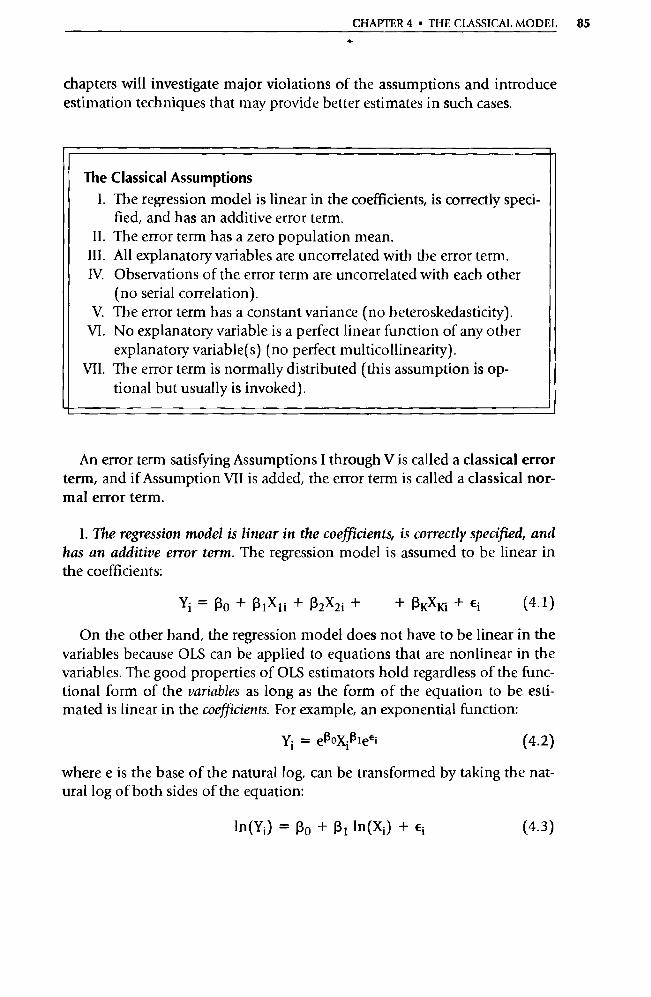
CHAPTER 4 • THE CLASSICAL MODEL 85
chapters will investigate major violations of the assumptions and introduce estimation techniques that may provide better estimates in such cases.
The Classical Assumptions I. The regression model is linear in the coefficients, is correctly speci-
fied, and has an additive error term. II. The error term has a zero population mean.
III. All explanatory va riables are uncorrelated with the error term. IV. Observations of the error term are uncorrelated with each other
(no serial correlation). V. The error term has a constant variance (no heteroskedasticity).
VI. No explanatory variable is a perfect linear function of any other explanatory variable(s) (no perfect multicollinearity).
VII. The error term is normally distributed (this assumption is op-tional but usually is invoked).
An error term satisfying Assumptions I through V is called a classical error term, and if Assumption VII is added, the error term is called a classical nor-mal error term.
I. The regression model is linear in the coefficients, is correctly specified, and has an additive error term. The regression model is assumed to be linear in the coefficients:
Yi = Ro + RlXli + R2X2i + + RKXKi + Ei (4.1)
On the other hand, the regression model does not have to be linear in the variables because OLS can be applied to equations that are nonlinear in the variables. The good properties of OLS estimators hold regardless of the func-tional form of the variables as long as the form of the equation to be esti-mated is linear in the coefficients. For example, an exponential function:
Yi = eRoXi11eEi (4.2)
where e is the base of the natural log, can be transformed by taking the nat-ural log of both sides of the equation:
ln(Yi) = Ro + Ri ln(Xi) + Ei (4.3)
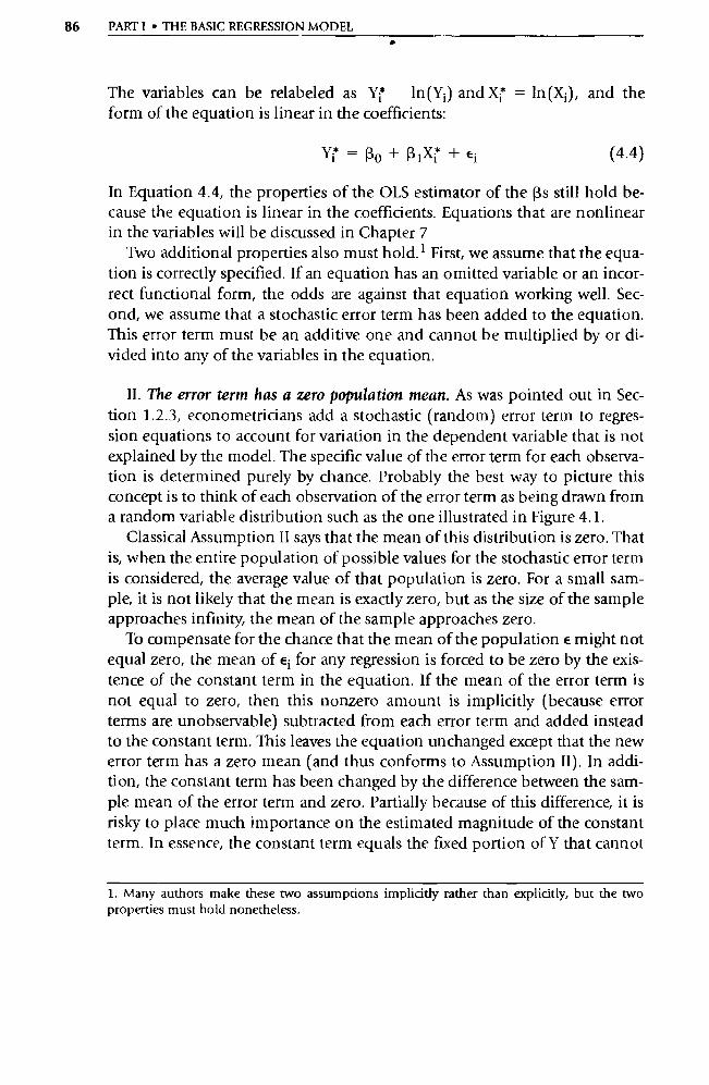
86 PARTI • THE BASIC REGRESSION MODEL w
The variables can be relabeled as Yi ln(Yi) and X; = In (Xi), and the form of the equation is linear in the coefficients:
Yi — R0 + R1Xi + Ei (4.4)
In Equation 4.4, the properties of the OLS estimator of the 13s still hold be-cause the equation is linear in the coefficients. Equations that are nonlinear in the variables will be discussed in Chapter 7
Two additional properties also must hold. 1 First, we assume that the equa-tion is correctly specified. If an equation has an omitted variable or an incor-rect functional form, the odds are against that equation working well. Sec-ond, we assume that a stochastic error term has been added to the equation. This error term must be an additive one and cannot be multiplied by or di-vided into any of the variables in the equation.
II. The error term has a zero population mean. As was pointed out in Sec-tion 1.2.3, econometricians add a stochastic (random) error term to regres-sion equations to account for variation in the dependent variable that is not explained by the model. The specific value of the error term for each observa-tion is determined purely by chance. Probably the best way to picture this concept is to think of each observation of the error term as being drawn from a random variable distribution such as the one illustrated in Figure 4.1.
Classical Assumption II says that the mean of this distribution is zero. That is, when the entire population of possible values for the stochastic error term is considered, the average value of that population is zero. For a small sam-ple, it is not likely that the mean is exactly zero, but as the size of the sample approaches infinity, the mean of the sample approaches zero.
To compensate for the chance that the mean of the population E might not equal zero, the mean of Ei for any regression is forced to be zero by the exis-tence of the constant term in the equation. If the mean of the error term is not equal to zero, then this nonzero amount is implicitly (because error terms are unobservable) subtracted from each error term and added instead to the constant term. This leaves the equation unchanged except that the new error term has a zero mean (and thus conforms to Assumption II). In addi-tion, the constant term has been changed by the difference between the sam-ple mean of the error term and zero. Partially because of this difference, it is risky to place much impo rtance on the estimated magnitude of the constant term. In essence, the constant term equals the fixed po rtion of Y that cannot
1. Many authors make these two assumptions implicitly rather than explicitly, but the two properties must hold nonetheless.
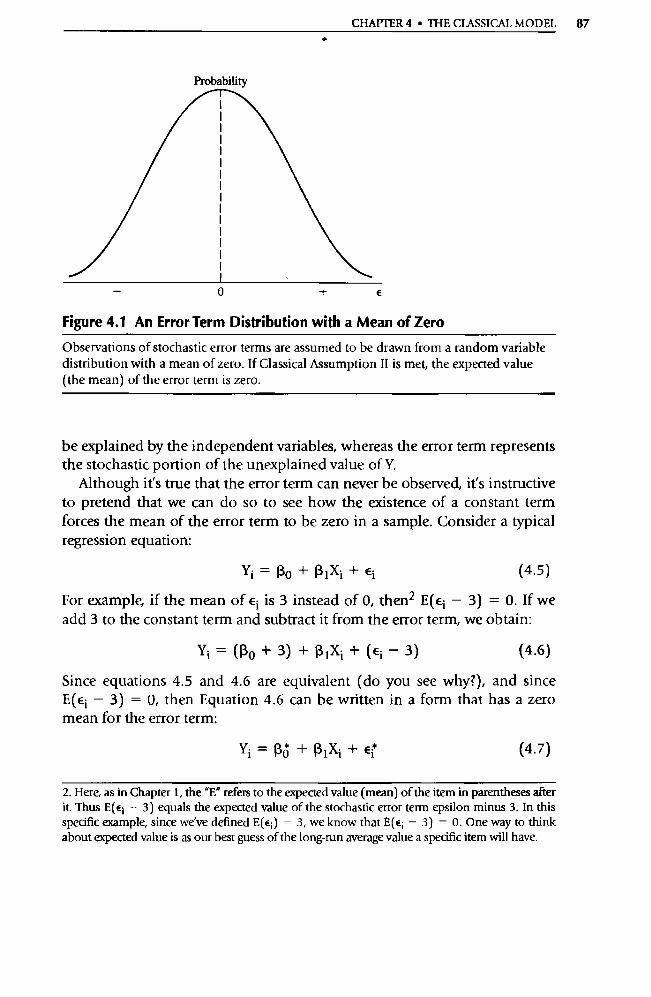
CHAPTER 4 • THE CLASSICAL MODEL 87
Probability
0 E
Figure 4.1 An Error Term Distribution with a Mean of Zero
Observations of stochastic error terms are assumed to be drawn from a random variable distribution with a mean of zero. If Classical Assumption II is met, the expected value (the mean) of the error term is zero.
be explained by the independent va riables, whereas the error term represents the stochastic po rtion of the unexplained value of Y.
Although it's true that the error term can never be observed, it's instructive to pretend that we can do so to see how the existence of a constant term forces the mean of the error term to be zero in a sample. Consider a typical regression equation:
Yi=Ro+RIXi+ Ei (4.5)
For example, if the mean of Ei is 3 instead of 0, then 2 E(Ei — 3) = 0. If we add 3 to the constant term and subtract it from the error term, we obtain:
Yi = ((30 +3) +(31Xi+ (€i 3) (4.6)
Since equations 4.5 and 4.6 are equivalent (do you see why?), and since E(Ei — 3) = 0, then Equation 4.6 can be written in a form that has a zero mean for the error term:
Yi = Pô + R 1 Xi + El (4.7)
2. Here, as in Chapter 1, the "E" refers to the expected value (mean) of the item in parentheses after it. Thus E(e ; — 3) equals the expected value of the stochastic error term epsilon minus 3. In this specific example, since we've defined E(e i ) = 3, we know that E(ei — 3) = O. One way to think about expected value is as our best guess of the long-run average value a specific item will have.
88 PART I • THE BASIC REGRESSION MODEL
where Rô = Ro + 3 and ei = Ei — 3. As can be seen, Equation 4.7 conforms to Assumption II. This form is always assumed to apply for the true model. Therefore, the second classical assumption is assured as long as there is a constant term included in the equation. This statement is correct as long as all other classical assumptions are met.
III. All explanatory va riables are uncorrelated with the error term. It is as-sumed that the observed values of the explanatory variables are determined independently of the values of the error term. Explanatory variables (Xs) are considered to be determined outside the context of the regression equation in question.
If an explanatory variable and the error term were instead correlated with each other, the OLS estimates would be likely to attribute to the X some of the variation in Y that actually came from the error term. If the er-ror term and X were positively correlated, for example, then the estimated coefficient would probably be higher than it would otherwise have been (biased upward), because the OLS program would mistakenly attribute the variation in Y caused by e to have been caused by X instead. As a result, it's important to ensure that the explanatory variables are uncorrelated with the error term.
An important economic application that violates this assumption is any model that is simultaneous in nature. In most economic applications, there are several related propositions that, when taken as a group, suggest a system of regression equations. In most situations, interrelated equations should be considered simultaneously instead of separately. Unfortunately, such simul-taneous systems violate Classical Assumption III.
To see why, let's look at an example. In a simple Keynesian macroeco-nomic model, an increase in consumption (caused perhaps by an unex-pected change in tastes) will increase aggregate demand and therefore aggregate income. An increase in income, however, will also increase con-sumption; so, income and consumption are interdependent. Note, however, that the error term in the consumption function (which is where an unex-pected change in tastes would appear) and an explanatory variable in the consumption function (income) have now moved together. As a result, Classical Assumption III has been violated; the error term is no longer un-correlated with all the explanatory variables. This will be considered in more detail in Chapter 14.
IV. Observations of the error term are uncorrelated with each other. The ob-servations of the error term are drawn independently from each other. If a systematic correlation exists between one observation of the error term and
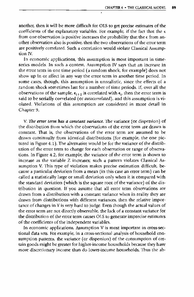
CHAPTER 4 • THE CLASSICAL MODEL 89
another, then it will be more difficult for OLS to get precise estimates of the coefficients of the explanatory variables. For example, if the fact that the E
from one observation is positive increases the probability that the E from an-other observation also is positive, then the two observations of the error term are positively correlated. Such a correlation would violate Classical Assump-tion IV.
In economic applications, this assumption is most impo rtant in time-series models. In such a context, Assumption IV says that an increase in the error term in one time period (a random shock, for example) does not show up in or affect in any way the error term in another time period. In some cases, though, this assumption is unrealistic, since the effects of a random shock sometimes last for a number of time periods. If, over all the observations of the sample, Et+ I is correlated with Et, then the error term is said to be serially correlated (or autocorrelated), and this assumption is vi-olated. Violations of this assumption are considered in more detail in Chapter 9.
V. The error term has a constant variance. The variance (or dispersion) of the distribution from which the observations of the error term are drawn is constant. That is, the observations of the error term are assumed to be drawn continually from identical distributions (for example, the one pic-tured in Figure 4.1). The alternative would be for the variance of the distrib-ution of the error term to change for each observation or range of observa-tions. In Figure 4.2, for example, the variance of the error term is shown to increase as the variable Z increases; such a pattern violates Classical As-sumption V. This type of violation makes precise estimation difficult, be-cause a particular deviation from a mean (in this case an error term) can be called a statistically large or small deviation only when it is compared with the standard deviation (which is the square root of the variance) of the dis-tribution in question. If you assume that all error term observations are drawn from a distribution with a constant variance when in reality they are drawn from distributions with different variances, then the relative impor-tance of changes in Y is very hard to judge. Even though the actual values of the error term are not directly observable, the lack of a constant variance for the distribution of the error term causes OLS to generate imprecise estimates of the coefficients of the independent variables.
In economic applications, Assumption V is most important in cross-sec-tional data sets. For example, in a cross-sectional analysis of household con-sumption patterns, the variance (or dispersion) of the consumption of cer-tain goods might be greater for higher-income households because they have more discretionary income than do lower-income households. Thus the ab-
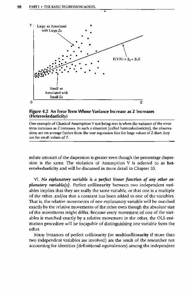
E(YIX) = f30 + R iz
Large es Associated with Large Zs
N1/4 . • •
• •
Small es Associated with
Small Zs
• • •
90 PART I • THE BASIC REGRESSION MODEL •
Figure 4.2 An Error Term Whose Variance Increase as Z Increases (Heteroskedasticity)
One example of Classical Assumption V not being met is when the va riance of the error term increases as Z increases. In such a situation (called heteroskedasticity), the observa-tions are on average farther from the true regression line for large values of Z than they are for small values of Z.
solute amount of the dispersion is greater even though the percentage disper-sion is the same. The violation of Assumption V is referred to as het-eroskedasticity and will be discussed in more detail in Chapter 10.
VI. No explanatory variable is a perfect linear function of any other ex-planatory variable(s). Perfect collinearity between two independent vari-ables implies that they are really the same variable, or that one is a multiple of the other, and/or that a constant has been added to one of the variables. That is, the relative movements of one explanatory variable will be matched exactly by the relative movements of the other even though the absolute size of the movements might differ. Because every movement of one of the vari-ables is matched exactly by a relative movement in the other, the OLS esti-mation procedure will be incapable of distinguishing one variable from the other.
Many instances of perfect collinearity (or multicollinearity if more than two independent variables are involved) are the result of the researcher not accounting for identities (definitional equivalences) among the independent
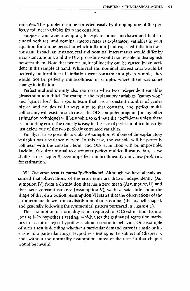
CHAPTER 4 • THE CLASSICAL MODEL 91 •
variables. This problem can be corrected easily by dropping one of the per-fectly collinear variables from the equation.
Suppose you were attempting to explain home purchases and had in-cluded both real and nominal interest rates as explanatory variables in your equation for a time period in which inflation (and expected inflation) was constant. In such an instance, real and nominal interest rates would differ by a constant amount, and the OLS procedure would not be able to distinguish between them. Note that perfect multicollinearity can be caused by an acci-dent in the sample at hand. While real and nominal interest rates would be perfectly multicollinear if inflation were constant in a given sample, they would not be perfectly multicollinear in samples where there was some change in inflation.
Perfect multicollinearity also can occur when two independent variables always sum to a third. For example, the explanatory variables "games won" and "games lost" for a spo rts team that has a constant number of games played and no ties will always sum to that constant, and perfect multi-collinearity will exist. In such cases, the OLS computer program (or any other estimation technique) will be unable to estimate the coefficients unless there is a rounding error. The remedy is easy in the case of perfect multicollinearity: just delete one of the two perfectly correlated variables.
Finally, it's also possible to violate Assumption VI if one of the explanatory variables has a variance of zero. In this case, the variable will be perfectly collinear with the constant term, and OLS estimation will be impossible. Luckily, it's quite unusual to encounter perfect multicollinearity, but, as we shall see in Chapter 8, even imperfect multicollinearity can cause problems for estimation.
VII. The error term is normally distributed. Although we have already as-sumed that observations of the error term are drawn independently (As-sumption IV) from a distribution that has a zero mean (Assumption II) and that has a constant variance (Assumption V), we have said little about the shape of that distribution. Assumption VII states that the observations of the error term are drawn from a distribution that is normal (that is, bell shaped, and generally following the symmetrical pattern portrayed in Figure 4.1).
This assumption of normality is not required for OLS estimation. Its ma-jor use is in hypothesis testing, which uses the estimated regression statis-tics to accept or reject hypotheses about economic behavior. One example of such a test is deciding whether a particular demand curve is elastic or in-elastic in a particular range. Hypothesis testing is the subject of Chapter 5, and, without the normality assumption, most of the tests in that chapter would be invalid.

92 PARTI • THE BASIC REGRESSION MODEL
4.2 The Normal Distribution of the Error Term
In this section we briefly introduce the concept of the normal dist ribution and explain why the Central Limit Theorem tends to justify the assumption of normality for a stochastic error term.
The only assumption that is optional to the definition of the classical model is that the error term is normally distributed. It is usually advisable to add the assumption of normality to the other six assumptions for two reasons:
1. The error term Ei can be thought of as the composite of a number of minor influences or errors. As the number of these minor influences gets larger, the distribution of the error term tends to approach the nor-mal distribution. This tendency is called the Central Limit Theorem.
2. The t-statistic and the F-statistic, which will be developed in Chapter 5, are not truly applicable unless the error term is normally distributed.
4.2.1 The Normal Distribution
The normal dist ribution is a symmetrical, continuous, bell-shaped curve. The parameters that describe normal dist ributions and allow us to differentiate be-tween various normal distributions are the mean (µ, the measure of cen tral ten-dency), and the variance (Q2, the measure of dispersion). Two such normal dis-tributions are shown in Figure 4.3. In normal distribution I, the mean is 0 and the variance is 1; in normal distribution II, the mean is 2, and the va riance is 0.5.
A quick look at Figure 4.3 shows how normal distributions differ when the means and variances are different. When the mean is different, the entire dis-tribution shifts. For example, distribution II is to the right of dist ribution I because its mean, 2, is greater than the mean of distribution I. When the vari-ance is different, the distribution becomes fatter or skinnier. For example, distribution II is distributed more compactly around its mean than is distrib-ution I because distribution II has a smaller variance. Observations drawn at random from distribution II will tend to be closer to the mean than those drawn from distribution I, while distribution I will tend to have a higher like-lihood of observations quite far from its mean.
In Figure 4.3, distribution I represents what is called the standard normal distribution because it is a normal dis tribution with a mean equal to zero and a variance equal to one. This is the usual dist ribution given in statistical tables, such as Table B -7 in the back of this book. Often the parameters of a normal distribution will be listed in a compact summary form: N(µ, (3- 2 ). For distribution I, this notation would be N(0,1) and would stand for a normal distribution with mean zero and variance one.
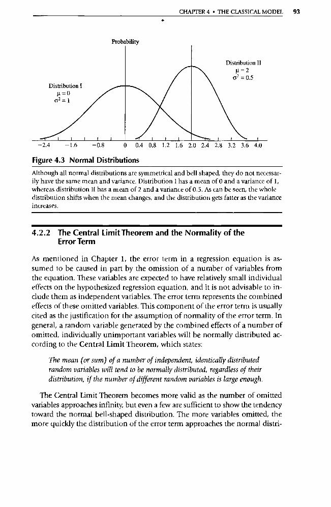
CHAPTER 4 • THE CLASSICAL MODEL 93 •
Probability
Distribution II
pAliti=2 0.5
Distribution I u = o
62 =
—2.4 —1.6 —0.8
0.4 0.8 1.2 1.6 2.0 2.4 2.8 3.2 3.6 4.0
Figure 4.3 Normal Distributions Although all normal distributions are symmetrical and bell shaped, they do not necessar-ily have the same mean and variance. Distribution I has a mean of 0 and a variance of 1, whereas distribution II has a mean of 2 and a va riance of 0.5. As can be seen, the whole distribution shifts when the mean changes, and the distribution gets fatter as the variance increases.
4.2.2 The Central Limit Theorem and the Normality of the Error Term
As mentioned in Chapter 1, the error term in a regression equation is as-sumed to be caused in pa rt by the omission of a number of variables from the equation. These variables are expected to have relatively small individual effects on the hypothesized regression equation, and it is not advisable to in-clude them as independent variables. The error term represents the combined effects of these omitted variables. This component of the error term is usually cited as the justification for the assumption of normality of the error term. In general, a random variable generated by the combined effects of a number of omitted, individually unimportant variables will be normally distributed ac-cording to the Central Limit Theorem, which states:
The mean (or sum) of a number of independent, identically distributed random variables will tend to be normally distributed, regardless of their distribution, if the number of different random variables is large enough.
The Central Limit Theorem becomes more valid as the number of omitted variables approaches infinity, but even a few are sufficient to show the tendency toward the normal bell-shaped dist ribution. The more variables omitted, the more quickly the distribution of the error term approaches the normal distri-

0
-1.0
Rel
ativ
e F
req
uenc
y 0.5
0.4
0.3
0.2
0.1
94 PART I • THE BASIC REGRESSION MODEL
>, 0.5 ^
0.4
ri 0.3
0.2
Ix 0.1
0 I I I I I -1.0 -0.8 -0.6 -0.4 -0.2 0 0.2 0 4 0.6 0.8 1.0
Figure 4.4 Relative Frequency of the Error Term as an Average of 2 Omitted Variables: 10 Observations
I
-0.8 -0.6 -0.4 -0.2 0 0.2 0.4 0.6 0.8 1.0 E i
Figure 4.5 Relative Frequency of the Error Term as an Average of 10 Omit-ted Variables: 10 Observations
Ei
As the number of different omitted va riables increases, the dist ribution of the sum of those variables approaches the normal dist ribution. This tendency (called the Central
Limit Theorem) can be seen in Figures 4.4 and 4.5. As the number of omitted variables
increases from 2 to 10, the dist ribution of their average does indeed become more sym-metrical and bell shaped.
bution because the various omitted va riables are more likely to cancel out extreme observations. As a result, it is good econometric practice to assume a normally distributed stochastic error term in a regression that must omit a number of minor unrelated influences. Purposely omitting a few vari-ables to help achieve normality for the error term, however, should never be considered.
Let's look at an example of the Central Limit Theorem and how the error term tends to be normally distributed if the number of omitted variables is large enough. First, suppose that only two potentially relevant va riables are so minor that they are not included in an equation. Figure 4.4 shows 10 com-puter-generated observations of a stochastic error term that is the sum of two
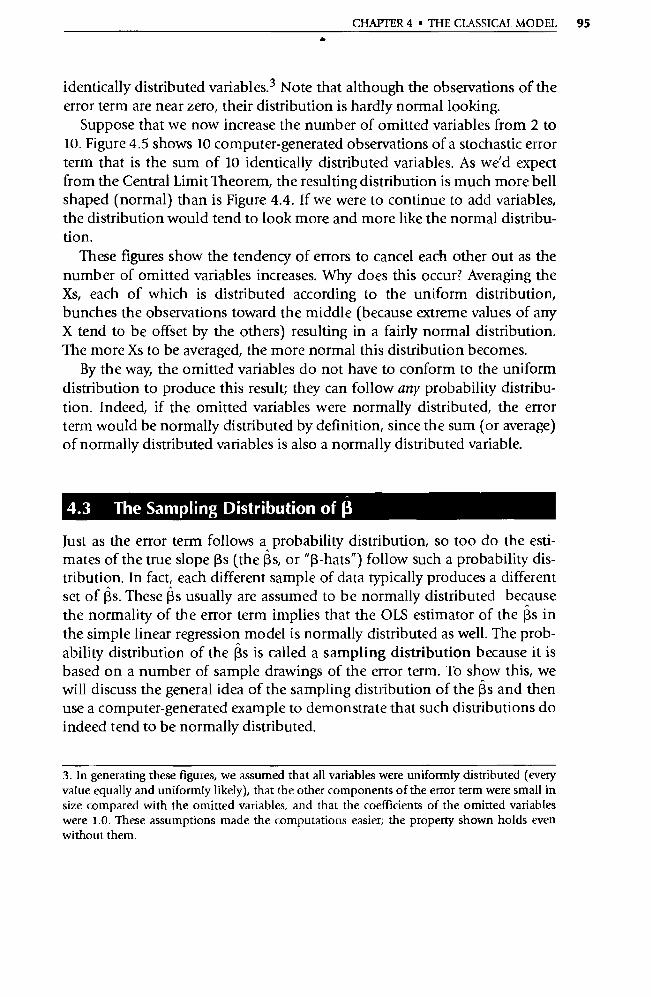
CHAPTER 4 • THE CLASSICAL MODEL 95
identically distributed variables. 3 Note that although the observations of the error term are near zero, their distribution is hardly normal looking.
Suppose that we now increase the number of omitted variables from 2 to 10. Figure 4.5 shows 10 computer-generated observations of a stochastic error term that is the sum of 10 identically distributed variables. As we'd expect from the Central Limit Theorem, the resulting dist ribution is much more bell shaped (normal) than is Figure 4.4. If we were to continue to add variables, the distribution would tend to look more and more like the normal distribu-tion.
These figures show the tendency of errors to cancel each other out as the number of omitted variables increases. Why does this occur? Averaging the Xs, each of which is distributed according to the uniform distribution, bunches the observations toward the middle (because extreme values of any X tend to be offset by the others) resulting in a fairly normal distribution. The more Xs to be averaged, the more normal this dist ribution becomes.
By the way, the omitted va riables do not have to conform to the uniform distribution to produce this result; they can follow any probability distribu-tion. Indeed, if the omitted variables were normally distributed, the error term would be normally distributed by definition, since the sum (or average) of normally distributed variables is also a normally distributed va riable.
4.3 The Sampling Distribution of 0 Just as the error term follows a probability distribution, so too do the esti-mates of the true slope Rs (the (3s, or "(3-hats") follow such a probability dis-tribution. In fact, each different sample of data typically produces a different set of (3s. These 13s usually are assumed to be normally distributed because the normality of the error term implies that the OLS estimator of the (3s in the simple linear regression model is normally distributed as well. The prob-ability distribution of the (3s is called a sampling distribution because it is based on a number of sample drawings of the error term. To show this, we will discuss the general idea of the sampling distribution of the (3s and then use a computer-generated example to demonstrate that such distributions do indeed tend to be normally distributed.
3. In generating these figures, we assumed that all va riables were uniformly distributed (every value equally and uniformly likely), that the other components of the error term were small in size compared with the omitted variables, and that the coefficients of the omitted variables were 1.0. These assumptions made the computations easier; the property shown holds even without them.

96 PAU I • THE BASIC REGRESSION MODEL e
4.3.1 Sampling Distributions of Estimators
Recall that an estimator is a formula, such as the OLS formula in Equation 2.13, that tells you how to compute 13k, and an estimate is the value of i3k computed by that formula. We have noted that the purpose of regression analysis is to obtain good estimates of the true (or population) coefficients of an equation from a sample of that population. In other words, given an equation like:
Yi = Ro + R1XIi R2X2i Ei (4.8)
we want to estimate [3s by taking a sample of the population and calculating those estimates (typically by OLS if the classical assumptions are met). Since re-searchers usually have only one sample, beginning econometricians often as-sume that regression analysis can produce only one estimate of the (3s. In reality, each different sample from a given population will produce a different set of es-timates of the Ps. For example, one sample might produce an estimate consider-ably higher than the true p whereas another might come up with a R that is lower. We need to discuss the properties of the distribution of these (3s, even though in most real applications we will encounter only a single draw from it.
A simplified example will help clarify this point. Suppose you were at-tempting to estimate the average age of your class from a sample of the class; let's say that you were trying to use a sample of 5 to estimate the average age of a class of 30. Your estimate would obviously depend on the exact sample you picked. If your random sample accidentally included the five youngest or the five oldest people in the class, then your estimated age would be dramat-ically different from the one you would get if your random sample were more centered. In essence, then, there is a distribution of all the possible estimates that will have a mean and a variance just as the distribution of error terms does. To illustrate this concept, assume that the population is distributed uniformly between 19 and 23. Here are three samples from this population:
sample 1: 19, 19, 20, 22, 23; mean = 20.6 sample 2: 20, 21, 21, 22, 22; mean = 21.2 sample 3: 19, 20, 22, 23, 23; mean = 21.4
Each sample yields an estimate of the true population mean (which is 21), and the distribution of the means of all the possible samples has its own mean and variance. For a "good" estimation technique, we would want the mean of the distribution of sample estimates to be equal to the true popula-tion mean. This is called unbiasedness. Although the mean of our three sam-ples is a little over 21, it seems likely that if we took enough samples, the mean of our group of samples would eventually equal 21.0.
An unbiased estimator is an estimator whose sampling distribution has as its expected value the true value of 13.
E(Rk) — Pk (4.9)
CHAPTER 4 • THE CLASSICAL MODEL 97
In a similar way, the (3s estimated by OLS for Equation 4.8 form a distribu-tion of their own. Each sample of observations of Y and the Xs will produce different (3s, but the distribution of these estimates for all possible samples has a mean and a variance like any distribution. When we discuss the proper-ties of estimators in the next section, it will be impo rtant to remember that we are discussing the properties of the distribution of estimates generated from a number of samples (a sampling distribution).
Properties of the Mean
A desirable property of a distribution of estimates is that its mean equals the true mean of the variable being estimated. An estimator that yields such esti-mates is called an unbiased estimator.
Only one value of R is obtained in practice, but the property of unbiasedness is useful because a single estimate drawn from an unbiased dist ribution is more likely to be near the true value (assuming identical variances of the (3s) than one taken from a dist ribution not centered around the true value. If an estimator produces (3s that are not centered around the true (3, the estimator is referred to as a biased estimator.
We cannot ensure that every estimate from an unbiased estimator is better than every estimate from a biased one because a particular unbiased esti-mate4 could, by chance, be farther from the true value than a biased estimate might be. This could happen by chance, for example, or because the biased estimator had a smaller variance. Without any other information about the distribution of the estimates, however, we would always rather have an unbi-ased estimate than a biased one.
Properties of the Variance
Just as we would like the distribution of the (3s to be centered around the true population 13, so too would we like that distribution to be as narrow (or pre-
4. Technically, since an estimate has just one value, an estimate cannot be unbiased (or biased). On the other hand, the phrase "estimate produced by an unbiased estimator" is cumbersome, especially if repeated 10 times on a page. As a result, many econometricians use "unbiased esti-mate" as shorthand for "a single estimate produced by an unbiased estimator."
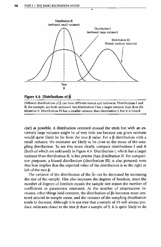
Distribution I (unbiased, large variance)
Distribution III (biased, medium vari ance)
98 PART I • THE BASIC REGRESSION MODEL
Distribution H (unbiased, small variance)
True
R
Figure 4.6 Distributions of (3
Different dist ributions of R can have different means and va riances. Distributions I and II, for example, are both unbiased, but dist ribution I has a larger va riance than does dis-tribution II. Distribution Ill has a smaller variance than dist ribution I, but it is biased.
cise) as possible. A dist ribution centered around the truth but with an ex-tremely large variance might be of very little use because any given estimate would quite likely be far from the true 13 value. For a 13 distribution with a small variance, the estimates are likely to be close to the mean of the sam-pling distribution. To see this more clearly, compare distributions I and II (both of which are unbiased) in Figure 4.6. Distribution I, which has a larger variance than distribution II, is less precise than dist ribution II. For compari-son purposes, a biased distribution (dist ribution III) is also pictured; note that bias implies that the expected value of the distribution is to the right or left of the true 13.
The variance of the distribution of the 13s can be decreased by increasing the size of the sample. This also increases the degrees of freedom, since the number of degrees of freedom equals the sample size minus the number of coefficients or parameters estimated. As the number of observations in-creases, other things held constant, the distribution of Rs becomes more cen-tered around its sample mean, and the variance of the sampling distribution tends to decrease. Although it is not true that a sample of 15 will always pro-duce estimates closer to the true 13 than a sample of 5, it is quite likely to do
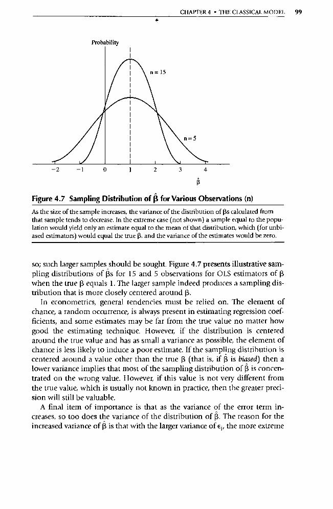
CHAPTER 4 • THE CLASSICAL MODEL 99
Probability
R
Figure 4.7 Sampling Distribution of R for Various Observations (n)
As the size of the sample increases, the va riance of the dist ribution of (3s calculated from that sample tends to decrease. In the extreme case (not shown) a sample equal to the popu-lation would yield only an estimate equal to the mean of that distribution, which (for unbi-ased estimators) would equal the true 13, and the va riance of the estimates would be zero.
so; such larger samples should be sought. Figure 4.7 presents illustrative sam-pling distributions of (3s for 15 and 5 observations for OLS estimators of [3 when the true 13 equals 1. The larger sample indeed produces a sampling dis-tribution that is more closely centered around 13.
In econometrics, general tendencies must be relied on. The element of chance, a random occurrence, is always present in estimating regression coef-ficients, and some estimates may be far from the true value no matter how good the estimating technique. However, if the distribution is centered around the true value and has as small a variance as possible, the element of chance is less likely to induce a poor estimate. If the sampling distribution is centered around a value other than the true 13 (that is, if R is biased) then a lower variance implies that most of the sampling distribution of R is concen-trated on the wrong value. However, if this value is not very different from the true value, which is usually not known in practice, then the greater preci-sion will still be valuable.
A final item of impo rtance is that as the variance of the error term in-creases, so too does the variance of the distribution of (3. The reason for the increased variance of R is that with the larger variance of ei, the more extreme
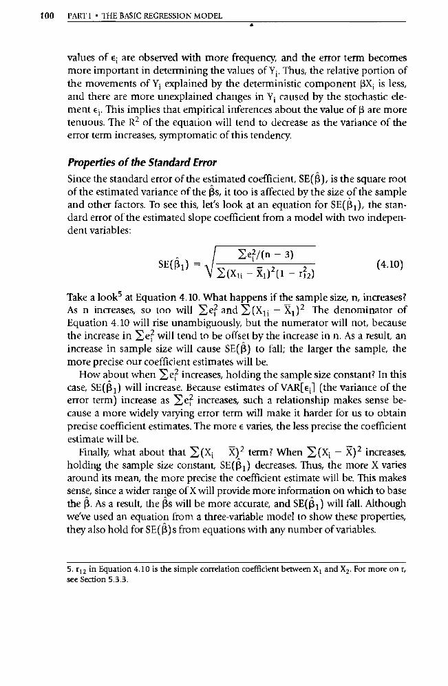
100 PART I • THE BASIC REGRESSION MODEL
values of Ei are observed with more frequency, and the error term becomes
more impo rtant in determining the values of Yi . Thus, the relative po rtion of the movements of Yi explained by the deterministic component 13X i is less, and there are more unexplained changes in Yi caused by the stochastic ele-ment Ei. This implies that empirical inferences about the value of 13 are more tenuous. The R2 of the equation will tend to decrease as the variance of the
error term increases, symptomatic of this tendency.
Properties of the Standard Error
Since the standard error of the estimated coefficient, SE0), is the square root
of the estimated variance of the 13s, it too is affected by the size of the sample
and other factors. To see this, let's look at an equation for SE(13 1 ), the stan-dard error of the estimated slope coefficient from a model with two indepen-dent variables:
SE(R I) = + ^e?/(n 2 3)
2 (4.10) G(X11 — R1 ) 2 (1 — r12)
Take a looks at Equation 4.10. What happens if the sample size, n, increases? As n increases, so too will le; and E(X1i — X 1 ) 2 The denominator of Equation 4.10 will rise unambiguously, but the numerator will not, because the increase in le? will tend to be offset by the increase in n. As a result, an
increase in sample size will cause SE( f1) to fall; the larger the sample, the
more precise our coefficient estimates will be.
How about when le? increases, holding the sample size constant? In this case, SE(13 1 ) will increase. Because estimates of VAR[€ ] (the variance of the
error term) increase as Ee; increases, such a relationship makes sense be-cause a more widely varying error term will make it harder for us to obtain
precise coefficient estimates. The more E varies, the less precise the coefficient estimate will be.
Finally, what about that E (Xi X) 2 term? When E (Xi — 30 2 increases, holding the sample size constant, SE((3 1 ) decreases. Thus, the more X va ries around its mean, the more precise the coefficient estimate will be. This makes
sense, since a wider range of X will provide more information on which to base
the R. As a result, the 13s will be more accurate, and SE(13 1 ) will fall. Although we've used an equation from a three-variable model to show these properties,
they also hold for SE(13)s from equations with any number of variables.
5. r12 in Equation 4.10 is the simple correlation coefficient between X 1 and X2. For more on r, see Section 5.3.3.
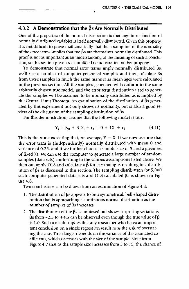
CHAPTER 4 • THE CLASSICAL MODEL 101
4.3.2 A Demonstration that the Rs Are Normally Distributed
One of the properties of the normal distribution is that any linear function of normally distributed va riables is itself normally distributed. Given this property, it is not difficult to prove mathematically that the assumption of the normality of the error terms implies that the Rs are themselves normally distributed. This proof is not as impo rtant as an understanding of the meaning of such a conclu-sion, so this section presents a simplified demonstration of that property.
To demonstrate that normal error terms imply normally distributed 13s, we'll use a number of computer-generated samples and then calculate (3s from these samples in much the same manner as mean ages were calculated in the previous section. All the samples generated will conform to the same arbitrarily chosen true model, and the error term distribution used to gener-ate the samples will be assumed to be normally distributed as is implied by the Central Limit Theorem. An examination of the distribution of 13s gener-ated by this experiment not only shows its normality, but is also a good re-view of the discussion of the sampling distribution of 13s.
For this demonstration, assume that the following model is true:
Yi — 13 0 +R 1 Xi + Ei=0+ 1Xi+Ei (4.11)
This is the same as stating that, on average, Y = X. If we now assume that the error term is (independently) normally distributed with mean 0 and variance of 0.25, and if we further choose a sample size of 5 and a given set of fixed Xs, we can use the computer to generate a large number of random samples (data sets) conforming to the various assumptions listed above. We then can apply OLS and calculate a 13 for each sample, resulting in a distrib-ution of 13s as discussed in this section. The sampling distribution for 5,000 such computer-generated data sets and OLS-calculated 13s is shown in Fig-ure 4.8.
Two conclusions can be drawn from an examination of Figure 4.8:
1. The distribution of Rs appears to be a symmetrical, bell-shaped distri-bution that is approaching a continuous normal distribution as the number of samples of 13s increases.
2. The distribution of the (3s is unbiased but shows surprising variations. 13s from -2.5 to +4.5 can be observed even though the true value of l3 is 1.0. Such a result implies that any researcher who bases an impor-tant conclusion on a single regression result runs the risk of overstat-ing the case. This danger depends on the variance of the estimated co-efficients, which decreases with the size of the sample. Note from Figure 4.7 that as the sample size increases from 5 to 15, the chance of
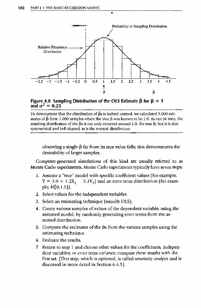
102 PART I • THE BASIC REGRESSION MODEL •
Probability or Sampling Distribution
^
Relative Frequency Distribution
—2.5 —2 —1.5 —1 —0.5 0 0.5 1 15 2 25 3 3.5 4 4.5
R
Figure 4.8 Sampling Distribution of the OLS Estimate (3 for R = 1
and cr2 = 0.25
To demonstrate that the distribution of Rs is indeed normal, we calculated 5,000 esti-mates of l3 from 5,000 samples where the true 13 was known to be 1.0. As can be seen, the
resulting distribution of the Rs is not only centered around 1.0, the true 13, but it is also
symmetrical and bell shaped, as is the normal dis tribution.
observing a single R far from its true value falls; this demonstrates the desirability of larger samples.
Computer-generated simulations of this kind are usually referred to as Monte Carlo experiments. Monte Carlo experiments typically have seven steps:
1. Assume a "true" model with specific coefficient values (for example, Y = 3.0 + 1.2X 1 5.3X2) and an error term distribution (for exam- ple, N[0,1.0]).
2. Select values for the independent va riables.
3. Select an estimating technique (usually OLS).
4. Create various samples of values of the dependent variable, using the assumed model, by randomly generating error terms from the as-sumed distribution.
5. Compute the estimates of the Ps from the various samples using the estimating technique.
6. Evaluate the results.
7 Return to step 1 and choose other values for the coefficients, indepen-dent variables, or error term variance; compare these results with the first set. (This step, which is optional, is called sensitivity analysis and is discussed in more detail in Section 6.4.5).
CHAPTER 4 • THE CLASSICAL MODEL 103
4.4 The Gauss—Markov Theorem and the Properties of OLS Estimators
The Gauss-Markov Theorem proves two impo rtant properties of OLS estima-tors. This theorem is proven in all advanced econometrics textbooks and readers interested in the proof should see Exercise 8 and its answer in Appen-dix A. For a regression user, however, it's more impo rtant to know what the theorem implies than to be able to prove it. The Gauss-Markov Theorem states that:
Given Classical Assumptions I through VI (Assumption VII, normality, is not needed for this theorem), the Ordinary Least Squares estimator of Rk is the minimum variance estimator from among the set of all lin-ear unbiased estimators of (3k, for k = 0, 1, 2, , K.
The Gauss-Markov Theorem is perhaps most easily remembered by stat-ing that "OLS is BLUE" where BLUE stands for "Best (meaning minimum variance) Linear Unbiased Estimator." Students who might forget that "best" stands for minimum variance might be better served by remembering "OLS is MvLUE," but such a phrase is hardly catchy or easy to remember.
If an equation's coefficient estimation is unbiased (that is, if each of the es-timated coefficients is produced by an unbiased estimator of the true popula-tion coefficient), then:
E( (-3k) = 13 k (k = 0, 1, 2, , K)
Best, as mentioned above, means that each (3k has the smallest va riance pos-sible (in this case, out of all the linear unbiased estimators of 13 k). An unbi-ased estimator with the smallest variance is called efficient, and that estima-tor is said to have the property of efficiency.
The Gauss-Markov Theorem requires that just the first six of the seven clas-sical assumptions be met. What happens if we add in the seventh assump-tion, the assumption that the error term is normally distributed? In this case, the result of the Gauss-Markov Theorem is strengthened because the OLS es-timator can be shown to be the best (minimum variance) unbiased estimator out of all the possible estimators, not just out of the linear estimators. In other words, if all seven assumptions are met, OLS is "BUE." It also turns out that the OLS estimator is equivalent to another estimation technique, the maximum likelihood estimator (which we will discuss in Chapter 13).

104 PART I • THE BASIC REGRESSION MODEL
Given all seven classical assumptions, the OLS coefficient estimators can be shown to have the following properties:
1. They are unbiased. That is, E0) is (3. This means that the OLS estimates of the coefficients are centered around the true population values of the parameters being estimated.
2. They are minimum variance. The distribution of the coefficient estimates around the true parameter values is as tightly or narrowly distributed as is possible for an unbiased distribution. No other unbiased estima-tor has a lower variance for each estimated coefficient than OLS.
3. They are consistent. As the sample size approaches infinity, the esti-mates converge on the true population parameters. Put differently, as the sample size gets larger, the variance gets smaller, and each estimate approaches the true value of the coefficient being estimated.
4. They are normally distributed. The Rs are N((3, VARaII). Thus various statistical tests based on the normal distribution may indeed be ap-plied to these estimates, as will be done in Chapter 5.
If the seven classical assumptions are met and if OLS is used to calculate the (3s, then it can be stated that an estimated regression coefficient is an un-biased, minimum variance estimate of the impact on the dependent va riable of a one-unit increase in a given independent variable, holding constant all other independent variables in the equation. Such an estimate is drawn from a distribution of estimates that is centered around the true population coeffi-cient and has the smallest possible variance for such unbiased dist ributions.
4.5 Standard Econometric Notation
Whereas Section 4.3 portrayed graphically the notions of central tendency and dispersion, this section presents the standard notation used throughout the econometrics literature for these concepts.
The measure of the central tendency of the sampling dist ribution of (3, which can be thought of as the mean of the Rs, is denoted as E(f3), read as "the expected value of beta-hat." The expected value of a random va riable is the population mean of that variable (with observations weighted by the probability of observation).
The variance of R is the typical measure of dispersion of the sampling dis-tribution of f3. The variance has several alternative notational representa-tions, including VAR(f3 ) and Π2 (13). Each of these is read as the "variance of beta-hat" and represents the degree of dispersion of the sampling distribu-tion of f3.

Bernhard
TextBox
p 105 is missing
106 PART I + THE BASIC REGRESSION MODEL
that the variance of the true 13, r 2 (13), is zero, since there is only one true Pk with no distribution around it. Thus, the estimated variance of the estimated coefficient is defined and observed, the true variance of the estimated coeffi-cient is unobservable, and the true variance of the true coefficient is zero. The square root of the estimated variance, or the coefficient estimate, is the stan-dard error of (3, SE((3 k), which we will use extensively in hypothesis testing.
4.6 Summary
1. The seven Classical Assumptions state that the regression model is linear with an error term that has a mean of zero, is uncorrelated with the explanatory variables and other observations of the error term, has a constant va riance, and is normally distributed (optional). In ad-dition, explanatory va riables must not be perfect linear functions of each other.
2. The two most impo rtant properties of an estimator are unbiasedness and minimum variance. An estimator is unbiased when the expected value of the estimated coefficient is equal to the true value. Minimum variance holds when the estimating dist ribution has the smallest vari-ance of all the estimators.
3. Given the Classical Assumptions, OLS can be shown to be the mini-mum variance, linear, unbiased estimator (or BLUE, for best linear unbiased estimator) of the regression coefficients. This is the Gauss-Markov Theorem. When one or more of the classical proper-ties do not hold (excluding normality), OLS is no longer BLUE, al-though it still may provide better estimates in some cases than the al-ternative estimation techniques discussed in subsequent chapters.
4. Because the sampling dist ribution of the OLS estimator of (3k is BLUE, it has desirable properties. Moreover, the variance, or the degree of dispersion of the sampling distribution of (3k, decreases as the num-ber of observations increases.
5. An OLS-estimated regression coefficient from a model that meets the classical assumptions is an unbiased, minimum variance estimate of the impact on the dependent variable of a one-unit increase in the in-dependent variable in question, holding constant the other indepen-dent variables in the equation.
6. There is a standard notation used in the econometric literature. Table 4.1 presents this fairly complex set of notational conventions for use
CHAPTER 4 • THE CLASSICAL MODEL 107
in regression analysis. This table should be reviewed periodically as a refresher.
Exercises
(Answers to even-numbered exercises are in Appendix A.)
1. Write the meaning of each of the following terms without referring to the book (or to your notes), and compare your definition with the version in the text for each: a. the Classical Assumptions b. classical error term c. standard normal distribution d. the Central Limit Theorem e. unbiased estimator f. BLUE g. sampling distribution
2. Which of the following pairs of independent variables would violate Assumption VI? (That is, which pairs of variables are perfect linear functions of each other?) a. right shoe size and left shoe size (of students in your class) b. consumption and disposable income (in the United States over the
last 30 years) c. Xi and 2Xi d. Xi and (Xi) 2
3. Consider the following estimated regression equation (standard er-rors in parentheses):
Yt = —120 + 0.10Ft + 5.33Rt R2 =.50 (0.05) (1.00)
where: Yt = the corn yield (bushels/acre) in year t Ft = fertilizer intensity (pounds/acre) in year t Rt = rainfall (inches) in year t
a. Carefully state the meaning of the coefficients 0.10 and 5.33 in this equation in terms of the impact of F and R on Y.
b. Does the constant term of —120 really mean that negative amounts of corn are possible? If not, what is the meaning of that estimate?
c. Suppose you were told that the true value of RF is known to be 0.20. Does this show that the estimate is biased? Why or why not?
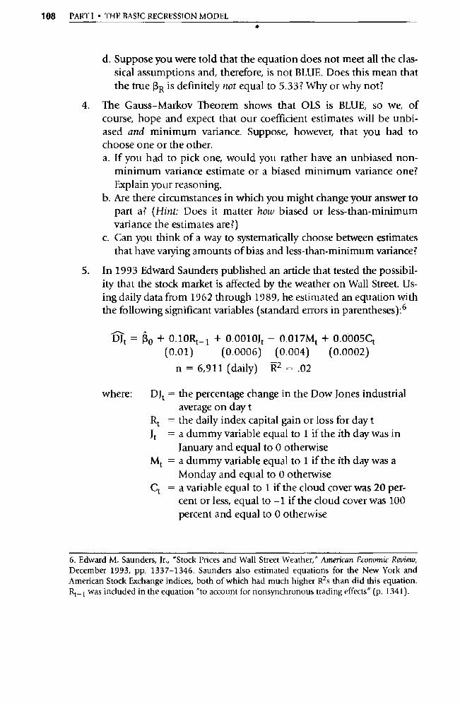
108 PARTI • THE BASIC REGRESSION MODEL
d. Suppose you were told that the equation does not meet all the clas-sical assumptions and, therefore, is not BLUE. Does this mean that the true RR is definitely not equal to 5.33? Why or why not?
4. The Gauss-Markov Theorem shows that OLS is BLUE, so we, of course, hope and expect that our coefficient estimates will be unbi-ased and minimum variance. Suppose, however, that you had to choose one or the other. a. If you had to pick one, would you rather have an unbiased non-
minimum variance estimate or a biased minimum variance one? Explain your reasoning.
b. Are there circumstances in which you might change your answer to part a? (Hint: Does it matter how biased or less-than-minimum variance the estimates are?)
c. Can you think of a way to systematically choose between estimates that have varying amounts of bias and less-than-minimum variance?
5. In 1993 Edward Saunders published an artide that tested the possibil-ity that the stock market is affected by the weather on Wall Street. Us-ing daily data from 1962 through 1989, he estimated an equation with the following significant variables (standard errors in parentheses): 6
DJt = Ro + 0.10Rt_ 1 + 0.0010Jt - 0.017Mt + 0.0005Ct (0.01) (0.0006) (0.004) (0.0002)
n = 6,911 (daily) R2 = .02
where: DJt = the percentage change in the Dow Jones industrial average on day t
Rt = the daily index capital gain or loss for day t Jt = a dummy variable equal to 1 if the ith day was in
January and equal to 0 otherwise Mt = a dummy variable equal to 1 if the ith day was a
Monday and equal to 0 otherwise Ct = a variable equal to 1 if the cloud cover was 20 per-
cent or less, equal to -1 if the cloud cover was 100 percent and equal to 0 otherwise
6. Edward M. Saunders, Jr., "Stock Prices and Wall Street Weather," American Economic Review, December 1993, pp. 1337-1346. Saunders also estimated equations for the New York and American Stock Exchange indices, both of which had much higher R es than did this equation. Rt _ t was included in the equation "to account for nonsynchronous trading effects" (p. 1341).
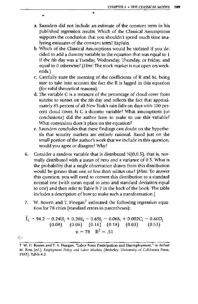
CHAPTER 4 • THE CLASSICAL MODEL 109
a. Saunders did not include an estimate of the constant term in his published regression results. Which of the Classical Assumptions supports the conclusion that you shouldn't spend much time ana-lyzing estimates of the constant term? Explain.
b. Which of the Classical Assumptions would be violated if you de-cided to add a dummy variable to the equation that was equal to 1 if the ith day was a Tuesday, Wednesday, Thursday, or Friday, and equal to 0 otherwise? (Hint: The stock market is not open on week-ends.)
c. Carefully state the meaning of the coefficients of R and M, being sure to take into account the fact the R is lagged in this equation (for valid theoretical reasons).
d. The variable C is a measure of the percentage of cloud cover from sunrise to sunset on the ith day and reflects the fact that approxi-mately 85 percent of all New York's rain falls on days with 100 per-cent cloud cover. Is C a dummy variable? What assumptions (or conclusions) did the author have to make to use this va riable? What constraints does it place on the equation?
e. Saunders concludes that these findings cast doubt on the hypothe-sis that security markets are entirely rational. Based just on the small portion of the author's work that we include in this question, would you agree or disagree? Why?
6. Consider a random variable that is distributed N(0,0.5), that is, nor-mally distributed with a mean of zero and a va riance of 0.5. What is the probability that a single observation drawn from this dis tribution would be greater than one or less than minus one? [Hint: To answer this question, you will need to convert this distribution to a standard normal one (with mean equal to zero and standard deviation equal to one) and then refer to Table B-7 in the back of the book. The table includes a desc ription of how to make such a transformation.]
7. W. Bowen and T. Finegan 7 estimated the following regression equa-tion for 78 cities (standard errors in parentheses):
Li
- 94.2 — 0.24Ui + 0.20E; — 0.69Ii — 0.06Si + 0.002Ci — 0.80D i (0.08) (0.06) (0.16) (0.18) (0.03) (0.53)
n=78 R2 =.51
7 W. G. Bowen and T. A. Finegan, "Labor Force Pa rticipation and Unemployment," in Arthur M. Ross (ed.), Employment Policy and Labor Markets (Berkeley: University of California Press, 1965), Table 4-2.
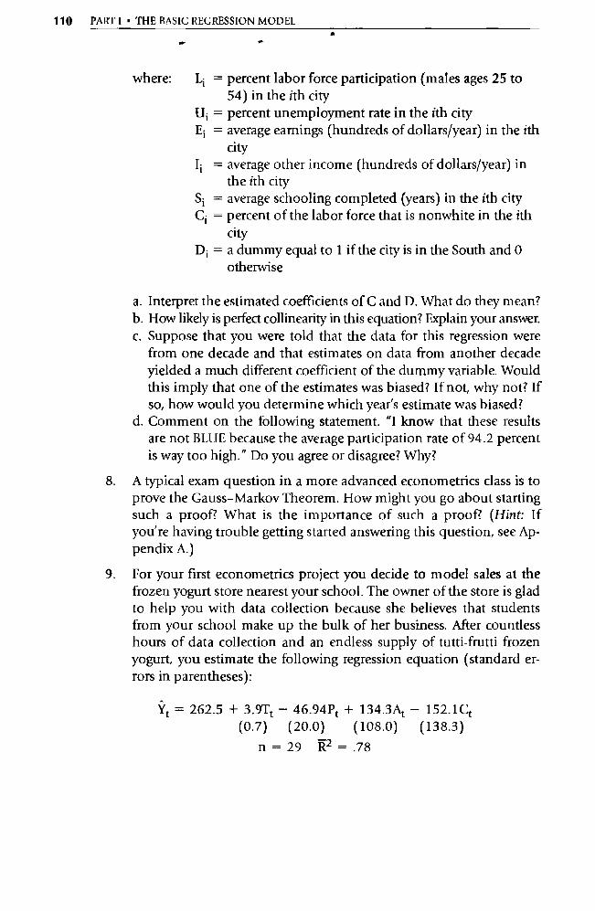
110 PART I • THE BASIC REGRESSION MODEL
s P
where: Li = percent labor force pa rticipation (males ages 25 to 54) in the ith city
Ui = percent unemployment rate in the ith city Ei = average earnings (hundreds of dollars/year) in the ith
city Ii = average other income (hundreds of dollars/year) in
the ith city Si = average schooling completed (years) in the ith city Ci = percent of the labor force that is nonwhite in the ith
city Di = a dummy equal to 1 if the city is in the South and 0
otherwise
a. Interpret the estimated coefficients of C and D. What do they mean? b. How likely is perfect collinearity in this equation? Explain your answer. c. Suppose that you were told that the data for this regression were
from one decade and that estimates on data from another decade yielded a much different coefficient of the dummy variable. Would this imply that one of the estimates was biased? If not, why not? If so, how would you determine which year's estimate was biased?
d. Comment on the following statement. "I know that these results are not BLUE because the average pa rticipation rate of 94.2 percent is way too high." Do you agree or disagree? Why?
8. A typical exam question in a more advanced econometrics class is to prove the Gauss-Markov Theorem. How might you go about starting such a proof? What is the impo rtance of such a proof? (Hint: If you're having trouble getting started answering this question, see Ap-pendix A.)
9. For your first econometrics project you decide to model sales at the frozen yogurt store nearest your school. The owner of the store is glad to help you with data collection because she believes that students from your school make up the bulk of her business. After countless hours of data collection and an endless supply of tutti-frutti frozen yogurt, you estimate the following regression equation (standard er-rors in parentheses):
Yt = 262.5 + 3.9Tt — 46.94Pt + 134.3At — 152.1 Ct (0.7) (20.0) (108.0) (138.3)
n= 29 R2=.78
CHAPTER 4 • THE CLASSICAL MODEL 111
where: Yt = the total number of frozen yogurts sold during the tth two-week time period
Tt = average high temperature (in degrees F) during period t Pt = the price of frozen yogurt (in dollars) at the store in
period t At = a dummy variable equal to 1 if the owner places an ad
in the school newspaper during period t, 0 otherwise Ct = a dummy variable equal to 1 if your school is in regu-
lar session in period t (early September through early December and early January through late May), 0 otherwise
a. This is a demand equation without any supply equation specified. Does this violate any of the Classical Assumptions? What kind of judgments do you have to make to answer this question?
b. What is the real-world economic meaning of the fact that the esti-mated coefficient of At is 134.3? Be specific.
c. You and the owner are surprised at the sign of the coefficient of C. Can you think of any reason for this sign? (Hint: Assume that your school has no summer session.)
d. If you could add one variable to this equation, what would it be? Be specific.
10. The middle third of this text (Chapters 6 through 11) concentrates on analyzing violations of the six Classical Assumptions required to prove the Gauss-Markov Theorem. If you're going to understand these chapters, it's good advice to know the Classical Assumptions cold before you start them. (It turns out to be fairly difficult to make sense of a whole chapter about the violation of a particular assump-tion if you're not really sure what that assumption is all about!) To help accomplish this task, complete the following exercises: a. Write out the Classical Assumptions without looking at your book
or notes. (Hint: Don't just say them to yourself in your head—put pen or pencil to paper!)
b. After you've completed writing out all six assumptions, compare your version with the text's. What differences are there? Are they impo rtant?
c. Get together with a classmate and take turns explaining the as-sumptions to each other. In this exercise, try to go beyond the defi-nition of the assumption to give your classmate a feeling for the real-world meaning of each assumption.
5 CHAPTER
Hypothesis Testing
5.1 What Is Hypothesis Testing?
5.2 The t-Test
5.3 Examples of t Tests
5.4 Limitations of the t-Test
5.5 The F-Test of Overall Significance
5.6 Summary and Exercises
The most important use of econometrics for many researchers is in testing their theories with data from the real world, so hypothesis testing is more meaningful to them than are the other major uses of econometrics (descrip-tion and forecasting). This chapter starts with a brief introduction to the topic of hypothesis testing. We then examine the t-test, the statistical tool typ-ically used for hypothesis tests of individual regression coefficients, and the F-test of overall significance.
We are merely returning to the essence of econometrics—an effo rt to quantify economic relationships by analyzing sample data—and asking what conclusions we can draw from this quantification. Hypothesis testing goes beyond calculating estimates of the true population parameters to a much more complex set of questions. Hypothesis testing determines what we can learn about the real world from a sample. Is it likely that our result could have been obtained by chance? Can our theories be rejected using the results generated by our sample? If our theory is correct, what are the odds that this particular sample would have been observed?
Hypothesis testing and the t-test should be familiar topics to readers with strong backgrounds in statistics, who are encouraged to skim this chapter and focus only on those applications that seem somewhat new. The develop-ment of hypothesis testing procedures is explained here in terms of the re-gression model, however, so pa rts of the chapter may be instructive even to those already skilled in statistics. Students with a weak background in statis-tics are encouraged to read Chapter 16 before beginning Chapter 5.
112
CHAPTER 5 • HYPOTHESIS TESTING 113
Our approach will be classical in nature, since we assume that the sample data are our best and only information about the population. An alternative, Bayesian statistics, adds prior information to the sample to draw statistical inferences. 1
5.1 What Is Hypothesis Testing?
Hypothesis testing is used in a variety of settings. The Food and Drug Admin-istration (FDA), for example, tests new products before allowing their sale. If the sample of people exposed to the new product shows some side effect sig-nificantly more frequently than would be expected to occur by chance, the FDA is likely to withhold approval of marketing that product. Similarly, economists have been statistically testing various relationships between con-sumption and income for half a century; theories developed by John May-nard Keynes and Milton Friedman, among others, have been tested on macroeconomic and microeconomic data sets.
Although researchers are always interested in learning whether the theory in question is supported by estimates generated from a sample of real-world observations, it's almost impossible to prove that a given hypothesis is correct. All that can be done is to state that a particular sample conforms to a particu-lar hypothesis. Even though we cannot prove that a given theory is "correct" using hypothesis testing, we can often reject a given hypothesis with a ce rtain degree of confidence. In such a case, the researcher concludes that it is very unlikely the sample result would have been observed if the hypothesized the-ory were correct. If there is conflicting evidence on the validity of a theory, the question is often put aside until additional data or a new approach shed more light on the issue.
Let's begin by investigating three topics that are central to the application of hypothesis testing to regression analysis:
1. the specification of the hypothesis to be tested,
1. Bayesian econometrics combines estimates generated from samples with estimates based on prior theory or research. For example, suppose you attempt to estimate the marginal propensity to consume (MPC) with the coefficient of income in an appropriately specified consumption regression equation. If your prior belief is that the MPC is 0.9 and if the estimated coefficient from your sample is 0.8, then a Bayesian estimate of the MPC would be somewhere between the two, depending on the strength of your belief. Bayesians, by being forced to state explicitly their prior expectations, tend to do most of their thinking before estimation, which is a good habit for a number of impo rtant reasons. For more on this approach, see Dale Poi ri er, Interme-diate Statisics and Econometrics: A Comparative Approach (Camb ridge, MA: MIT Press, 1995).
114 PARTI • THE BASIC REGRESSION MODEL
2. the decision rule to use in deciding whether to reject the hypothesis in question, and
3. the kinds of errors that might be encountered if the application of the decision rule to the appropriate statistics yields an incorrect inference.
5.1.1 Classical Null and Alternative Hypotheses
The first step in hypothesis testing is to state explicitly the hypothesis to be tested. To ensure fairness, the researcher should specify the hypothesis before the equation is estimated. The purpose of prior theoretical work is to match the hypothesis to the underlying theory as completely as possible. Hypothe-ses formulated after generation of the estimates are at times justifications of particular results rather than tests of their validity. As a result, most econome-tricians take pains to specify hypotheses before estimation.
In making a hypothesis, you must state carefully what you think is not true and what you think is true. These reflections of the researcher's expectations about a particular regression coefficient (or coefficients) are summarized in the null and alternative hypotheses. The null hypothesis is typically a state-ment of the range of values of the regression coefficient that would be ex-pected to occur if the researcher's theory were not correct. The alternative hy-pothesis is used to specify the range of values of the coefficient that would be expected to occur if the researcher's theory were correct. The word null also means "zero, and the null hypothesis can be thought of as the hypothesis that the researcher does not believe. 2 The reason it's called a null or zero hy-pothesis is that a variable would not be included in an equation if its ex-pected coefficient were zero.
We set up the null and alternative hypotheses in this way so we can make rather strong statements when we reject the null hypothesis. It is only when we define the null hypothesis as the result we do not expect that we can con-trol the probability of rejecting the null hypothesis accidentally when it is in fact true. The converse does not hold. That is, we can never actually know the probability of agreeing accidentally that the null hypothesis is correct when it
2. Researchers occasionally will have to switch the null and alternative hypotheses. For in-stance, some tests of rational expectations theory have put the preferred hypothesis as the null hypothesis in order to make the null hypothesis a specific value. In such cases of tests of spe-cific nonzero values, the reversal of the null and alternative hypotheses is regrettable but un-avoidable. An example of this kind of reversal is a two-sided null hypothesis involving a non-zero value, as in the second example in Section 5.3.2. Except for these rare cases, all null hypotheses in this text will be the result we expect not to occur.

CHAFFER 5 • HYPOTHESIS TESTING 115
is in fact false. As a result, we can never say that we accept the null hypothesis; we always must say that we cannot reject the null hypothesis, or we put the word "accept" in quotes.
Hypotheses in econometrics usually do not specify particular values, but instead they state the particular signs that the researcher expects the esti-mated coefficients to take. We typically hypothesize that a particular coeffi-cient will be positive (or negative). In such cases, the null hypothesis repre-sents what is expected not to occur, but that expectation is now a range; the same is true for the alternative hypothesis.
The notation used to refer to a null hypothesis is "H 0:," and this notation is followed by a statement of the value or range of values you do not expect the particular parameter to take. If, for example, you expect a negative coeffi-cient, then the correct null hypothesis is:
Ho : 13 ? 0 (the values you do not expect)
The alternative hypothesis is expressed by "HA: followed by the parameter value or values you expect to observe:
HA: 13 < 0 (the values you expect to be t rue)
Another way to state the null and alternative hypotheses is to test the null hypothesis that 13 is not significantly different from zero in either direction. In this second approach, the null and alternative hypotheses would be:
Ho: R=o HA: I:3 O
Since the alternative hypothesis has values on both sides of the null hypothe-sis, this approach is called a two-sided test (or two - tailed test) to distinguish it from the one -sided test of the previous example (in which the alternative hy-pothesis was only on one side of the null hypothesis). 3
3. Some researchers prefer to use a two-tailed test around zero for this hypothesis because they feel that the dassical approach requires the null hypothesis to contain a single value. We feel that the use of a two-tailed test in such a circumstance is a mistake. However, we have no quarrel with using 13 = 0 as the null hypothesis as long as the alte rnative hypothesis remains the same. These two versions of the null hypothesis give identical answers because to test a null hypothesis that is a range like 13 <_ 0, you must focus on the value in that range that is closest to the range implied by the alte rnative hypothesis. If you can reject that value, you can reject values that are farther away as well. Truncating the range of the null hypothesis in this way has no practical importance.
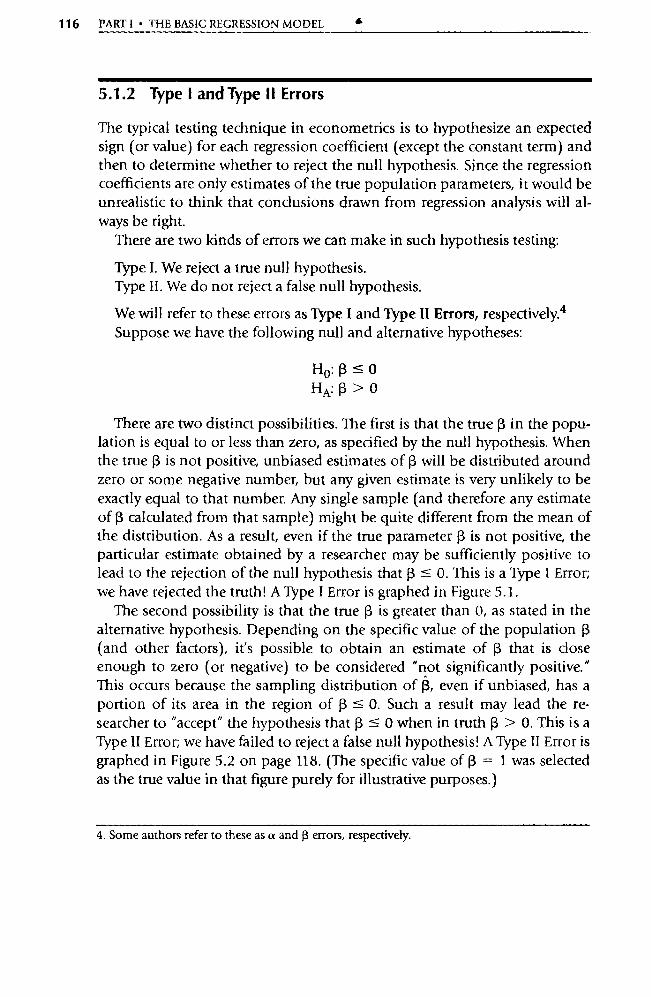
116 PART I • THE BASIC REGRESSION MODEL ^
5.1.2 Type I and Type II Errors
The typical testing technique in econometrics is to hypothesize an expected sign (or value) for each regression coefficient (except the constant term) and then to determine whether to reject the null hypothesis. Since the regression coefficients are only estimates of the true population parameters, it would be unrealistic to think that conclusions drawn from regression analysis will al-ways be right.
There are two kinds of errors we can make in such hypothesis testing:
Type I. We reject a true null hypothesis. Type II. We do not reject a false null hypothesis.
We will refer to these errors as Type I and Type II Errors, respectively. 4 Suppose we have the following null and alternative hypotheses:
Ho : j3 5-0 HA: (3 >0
There are two distinct possibilities. The first is that the true 13 in the popu-lation is equal to or less than zero, as specified by the null hypothesis. When the true 0 is not positive, unbiased estimates of 13 will be distributed around zero or some negative number, but any given estimate is very unlikely to be exactly equal to that number. Any single sample (and therefore any estimate of R calculated from that sample) might be quite different from the mean of the distribution. As a result, even if the true parameter R is not positive, the particular estimate obtained by a researcher may be sufficiently positive to lead to the rejection of the null hypothesis that 13 < O. This is a Type I Error; we have rejected the truth! A Type I Error is graphed in Figure 5.1.
The second possibility is that the true 0 is greater than 0, as stated in the alternative hypothesis. Depending on the specific value of the population p (and other factors), it's possible to obtain an estimate of (3 that is close enough to zero (or negative) to be considered "not significantly positive."
This occurs because the sampling distribution of R, even if unbiased, has a
portion of its area in the region of 0 s O. Such a result may lead the re-searcher to "accept" the hypothesis that 0 < 0 when in truth (3 > O. This is a Type II Error; we have failed to reject a false null hypothesis! A Type II Error is
graphed in Figure 5.2 on page 118. (The specific value of 0 = 1 was selected
as the true value in that figure purely for illustrative purposes.)
4. Some authors refer to these as a and f3 errors, respectively.
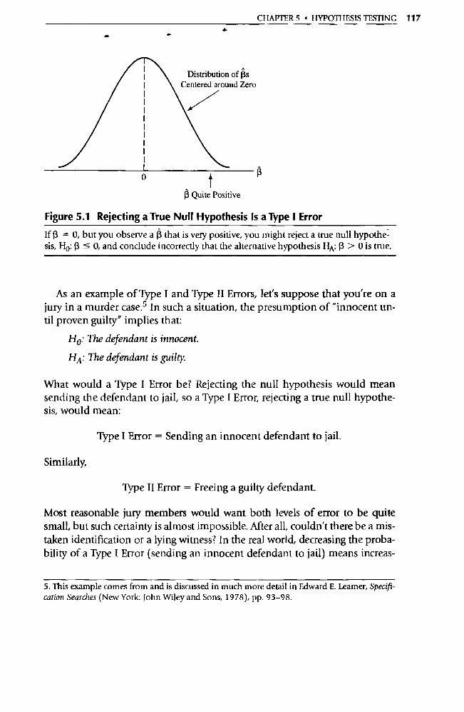
Distribution of As Centered around Zero
T R Quite Positive
0 â
CHAPTER 5 • HYPOTHESIS TESTING 117
Figure 5.1 Rejecting a True Null Hypothesis Is a Type 1 Error
If 13 = 0, but you observe a R that is very positive, you might reject a true null hypothe: sis, Ho: 13 <— 0, and conclude incorrectly that the alternative hypothesis H A: 13 > 0 is true.
As an example of Type I and Type II Errors, let's suppose that you're on a jury in a murder case. 5 In such a situation, the presumption of "innocent un-til proven guilty" implies that:
Ho: The defendant is innocent.
HA: The defendant is guilty.
What would a Type I Error be? Rejecting the null hypothesis would mean sending the defendant to jail, so a Type I Error, rejecting a true null hypothe-sis, would mean:
Type I Error = Sending an innocent defendant to jail.
Similarly,
Type II Error = Freeing a guilty defendant.
Most reasonable ju ry members would want both levels of error to be quite small, but such certainty is almost impossible. After all, couldn't there be a mis-taken identification or a lying witness? In the real world, decreasing the proba-bility of a Type I Error (sending an innocent defendant to jail) means increas-
5. This example comes from and is discussed in much more detail in Edward E. Learner, Specifi-cation Searches (New York: John Wiley and Sons, 1978), pp. 93-98.

Distribution of (3s Centered around One
118 PART I • THE BASIC REGRESSION MODEL
t o
3 Negative (or positive but close to zero)
1.0
Figure 5.2 Failure to Reject a False Null Hypothesis Is a Type II Error
If 13 = 1, but you observe a R that is negative or close to zero, you might fail to reject a false null hypothesis, Hp: R 0, and incorrectly ignore that the alternative hypothesis, HA. (3 > 0, is true.
ing the probability of a Type II Error (freeing a guilty defendant). If we never sent an innocent defendant to jail, we'd be freeing quite a few murderers!
5.1.3 Decision Rules of Hypothesis Testing
In testing a hypothesis, a sample statistic must be calculated that allows the null hypothesis to be "accepted" or rejected depending on the magnitude of that sample statistic compared with a preselected critical value found in tables such as those at the end of this text; this procedure is referred to as a decision rule.
A decision rule is formulated before regression estimates are obtained. The range of possible values of R is divided into two regions, an "acceptance" re-gion and a rejection region, where the terms are expressed relative to the null hypothesis. To define these regions, we must determine a critical value (or, for a two-tailed test, two critical values) of (3. Thus, a critical value is a value that divides the "acceptance" region from the rejection region when testing a null hypothesis. Graphs of these "acceptance" and rejection regions are presented in Figures 5.3 and 5.4.
To use a decision rule, we need to select a critical value. Let's suppose that the critical value is 1.8. If the observed (3 is greater than 1.8, we can reject the null hypothesis that 13 is zero or negative. To see this, take a look at the one-sided test in Figure 5.3. Any 13 above 1.8 can be seen to fall into the rejection region,
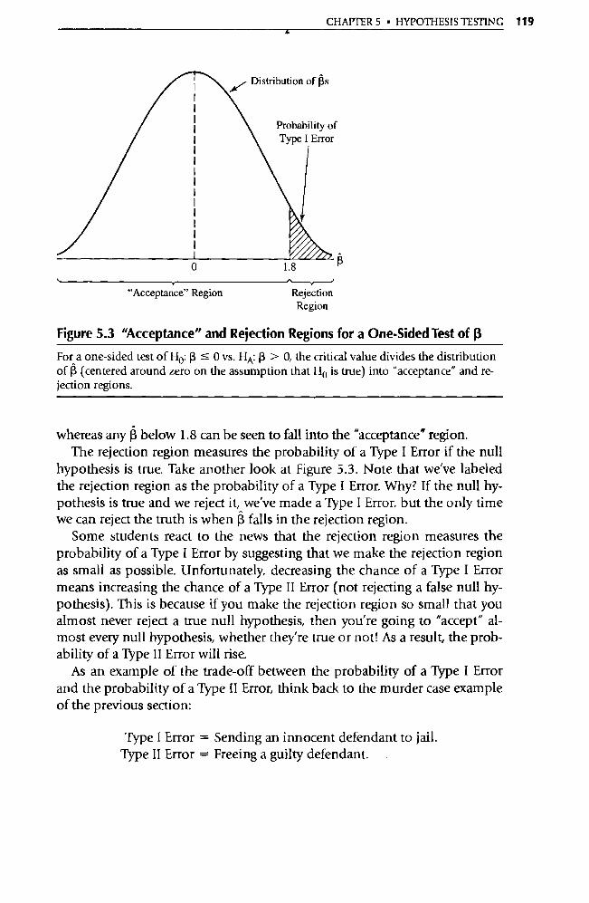
CHAPTER 5 • HYPOTHESIS TESTING 119
18
Rejection Region
"Acceptance" Region
Figure 5.3 "Acceptance" and Rejection Regions for a One-Sided Test of R
Fora one-sided test of Ho: 13 <_ 0 vs. HA: 13 > 0, the critical value divides the distribution of 13 (centered around zero on the assumption that H o is true) into "acceptance" and re-jection regions.
whereas any R below 1.8 can be seen to fall into the "acceptance" region. The rejection region measures the probability of a Type I Error if the null
hypothesis is true. Take another look at Figure 5.3. Note that we've labeled the rejection region as the probability of a Type I Error. Why? If the null hy-pothesis is true and we reject it, we've made a Type I Error, but the only time we can reject the truth is when R falls in the rejection region.
Some students react to the news that the rejection region measures the probability of a Type I Error by suggesting that we make the rejection region as small as possible. Unfortunately, decreasing the chance of a Type I Error means increasing the chance of a Type II Error (not rejecting a false null hy-pothesis). This is because if you make the rejection region so small that you almost never reject a true null hypothesis, then you're going to "accept" al-most every null hypothesis, whether they're true or not! As a result, the prob-ability of a Type II Error will rise.
As an example of the trade-off between the probability of a Type I Error and the probability of a Type II Error, think back to the murder case example of the previous section:
Type I Error = Sending an innocent defendant to jail. Type II Error = Freeing a guilty defendant.
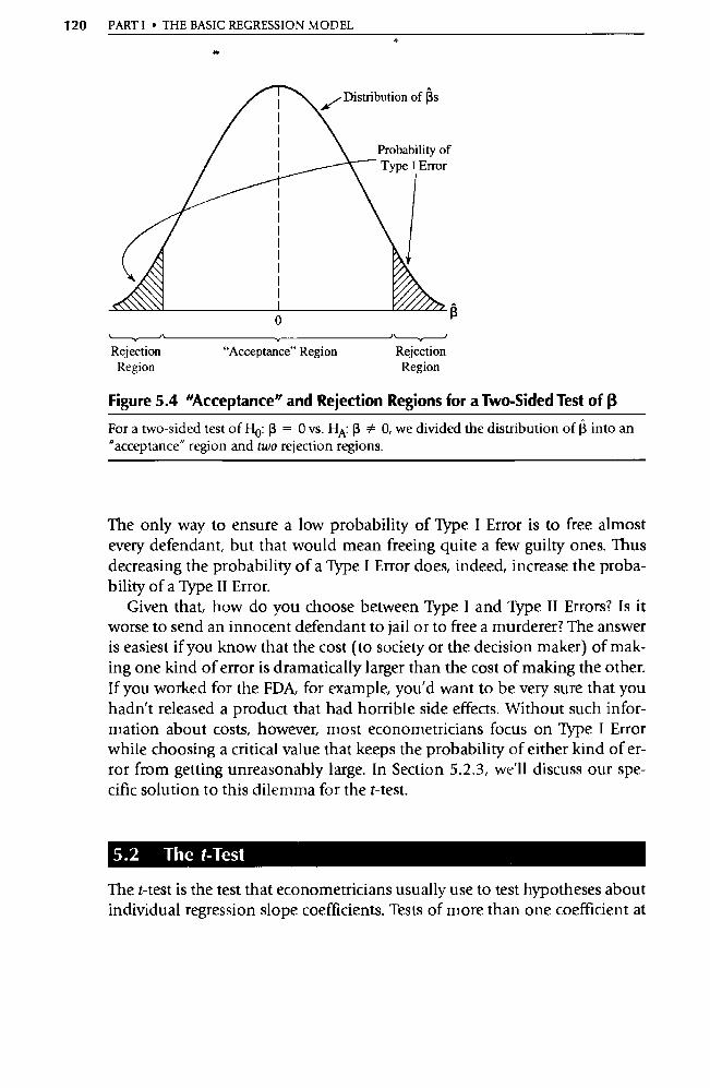
Distribution of (is
Probability of Type I Error
Rejection
"Acceptance" Region
Rejection Region
Region
120 PART I • THE BASIC REGRESSIONI MODEL
Figure 5.4 "Acceptance" and Rejection Regions for a Two-Sided Test of R For a two-sided test of Hp: (3 = 0 vs. HA: (3 0, we divided the distribution of (3 into an "acceptance" region and two rejection regions.
The only way to ensure a low probability of Type I Error is to free almost every defendant, but that would mean freeing quite a few guilty ones. Thus decreasing the probability of a Type I Error does, indeed, increase the proba-bility of a Type II Error.
Given that, how do you choose between Type I and Type II Errors? Is it worse to send an innocent defendant to jail or to free a murderer? The answer is easiest if you know that the cost (to society or the decision maker) of mak-ing one kind of error is dramatically larger than the cost of making the other. If you worked for the FDA, for example, you'd want to be very sure that you hadn't released a product that had hor rible side effects. Without such infor-mation about costs, however, most econometricians focus on Type I Error while choosing a critical value that keeps the probability of either kind of er-ror from getting unreasonably large. In Section 5.2.3, we'll discuss our spe-cific solution to this dilemma for the t-test.
5.2 The t-Test
The t-test is the test that econometricians usually use to test hypotheses about individual regression slope coefficients. Tests of more than one coefficient at
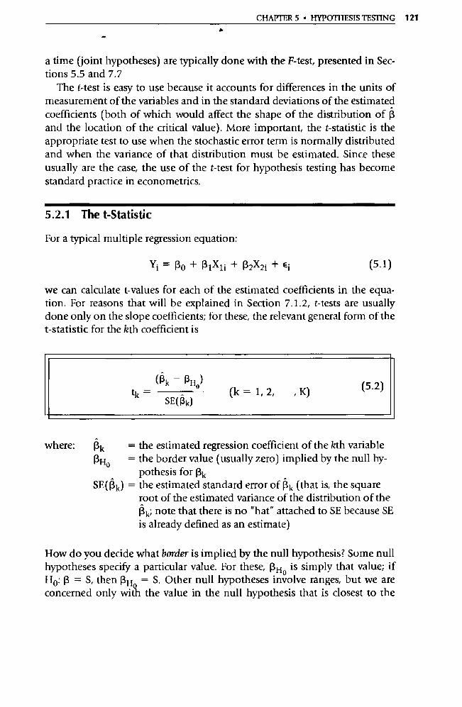
(Rk — RH) tk = ° (k = 1, 2, , K)
SE(Rk)
(5.2)
CHAPTER 5 • HYPOTHESIS TESTING 121
a time (joint hypotheses) are typically done with the F-test, presented in Sec-tions 5.5 and 7.7
The t-test is easy to use because it accounts for differences in the units of
measurement of the variables and in the standard deviations of the estimated
coefficients (both of which would affect the shape of the distribution of 13
and the location of the critical value). More important, the t-statistic is the
appropriate test to use when the stochastic error term is normally distributed
and when the variance of that distribution must be estimated. Since these
usually are the case, the use of the t-test for hypothesis testing has become
standard practice in econometrics.
5.2.1 The t-Statistic
For a typical multiple regression equation:
YiRo + RtXi^ + R2X2i + Es (5.1)
we can calculate t-values for each of the estimated coefficients in the equa-tion. For reasons that will be explained in Section 7.1.2, t - tests are usually done only on the slope coefficients; for these, the relevant general form of the
t-statistic for the hth coefficient is
where: 13 k = the estimated regression coefficient of the hth va riable
RH0
= the border value (usually zero) implied by the null hy- pothesis for 13k
SE(K) = the estimated standard error of Rk (that is, the square root of the estimated variance of the dist ribution of the Rk; note that there is no "hat" attached to SE because SE is already defined as an estimate)
How do you decide what border is implied by the null hypothesis? Some null hypotheses specify a particular value. For these, 13 110 is simply that value; if Ho : 13 = S, then 13 H = S. Other null hypotheses involve ranges, but we are concerned only with the value in the null hypothesis that is closest to the
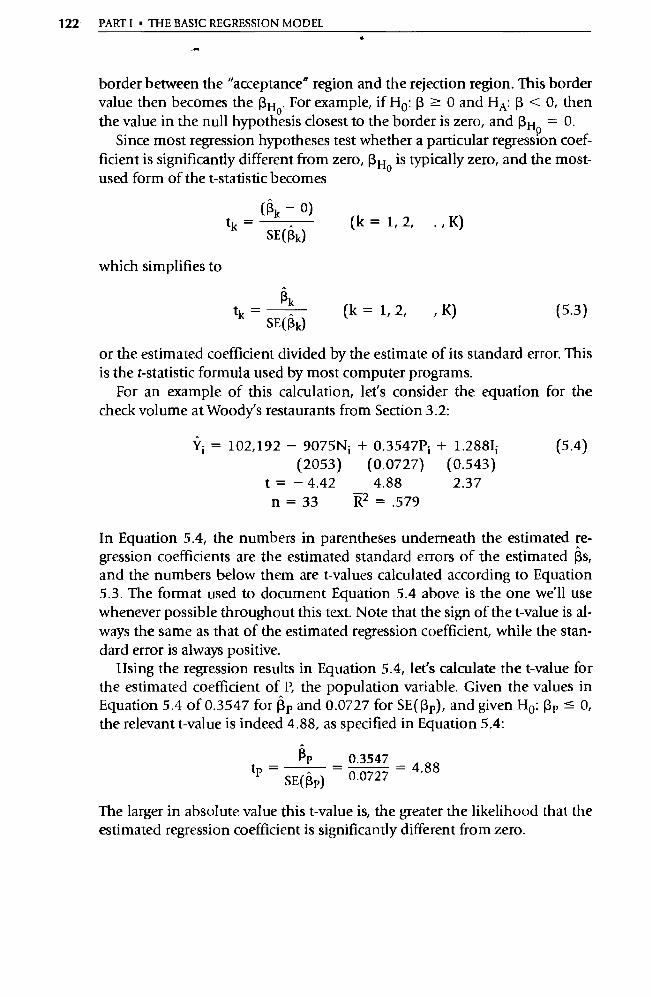
122 PARTI • THE BASIC REGRESSION) MODEL
border between the "acceptance" region and the rejection region. This border value then becomes the 13 H0. For example, if H o : (3 > 0 and HA: 13 < 0, then the value in the null hypothesis closest to the border is zero, and PHo = 0.
Since most regression hypotheses test whether a particular regression coef-ficient is significantly different from zero, 3H0 is typically zero, and the most-used form of the t-statistic becomes
tk = 0
(Rk ) (k = 1, 2, . , K) SE(13k)
which simplifies to
tk =
(k = 1, 2, , K) (5.3) SE(Rk)
or the estimated coefficient divided by the estimate of its standard error. This is the t-statistic formula used by most computer programs.
For an example of this calculation, let's consider the equation for the check volume at Woodÿ s restaurants from Section 3.2:
Y; = 102,192 — 9075N 1 (2053)
t = - 4.42
n=33
+ 0.3547Pî (0.0727)
4.88 R2 =.579
+ 1.288I ; (0.543)
2.37
(5.4)
In Equation 5.4, the numbers in parentheses underneath the estimated re-gression coefficients are the estimated standard errors of the estimated Rs, and the numbers below them are t-values calculated according to Equation 5.3. The format used to document Equation 5.4 above is the one we'll use whenever possible throughout this text. Note that the sign of the t-value is al-ways the same as that of the estimated regression coefficient, while the stan-dard error is always positive.
Using the regression results in Equation 5.4, let's calculate the t-value for the estimated coefficient of P, the population va riable. Given the values in Equation 5.4 of 0.3547 for 4 and 0.0727 for SE(P p), and given Ho: (3p 0, the relevant t-value is indeed 4.88, as specified in Equation 5.4:
RP 0.3547
tp = SE(pp) = 0.0727 = 4.88
The larger in absolute value this t-value is, the greater the likelihood that the estimated regression coefficient is significantly different from zero.

CHAPTER 5 • HYPOTHESIS TESTING 123
5.2.2 The Critical t-Value and the t-Test Decision Rule
To decide whether to reject or not to reject a null hypothesis based on a calcu-lated t-value, we use a critical t-value. A critical t-value is the value that distin-guishes the "acceptance" region from the rejection region. The critical t-value, tc, is selected from a t-table (see Statistical Table B-1 in the back of the book) depending on whether the test is one sided or two sided, on the level of Type I Error you specify and on the degrees of freedom, which we have defined as the number of observations minus the number of coefficients estimated (includ-ing the constant) or n — K — 1. The level of Type I Error in a hypothesis test is also called the level of significance of that test and will be discussed in more de-tail later in this section. The t-table was created to save time during research; it consists of critical t-values given specific areas underneath curves such as those in Figure 5.3 for Type I Errors. A critical t-value is thus a function of the proba-bility of Type I Error that the researcher wants to specify.
Once you have obtained a calculated t-value and a critical t-value, you reject the null hypothesis if the calculated t-value is greater in absolute value than the critical t-value and if the calculated t-value has the sign implied by HA.
Thus, the rule to apply when testing a single regression coefficient is that you should:
Reject H o if ItkI > t c and if tk also has the sign implied by HA.
Do Not Reject H o otherwise.
This decision rule works for calculated t-values and critical t-values for one-sided hypotheses around zero:
Ho : 13k <- 0 HA: 13k > 0
Ho: (3k>0 HA. 13k < 0
for two-sided hypotheses around zero:
Ho : 13k = 0 HA. 13k 0
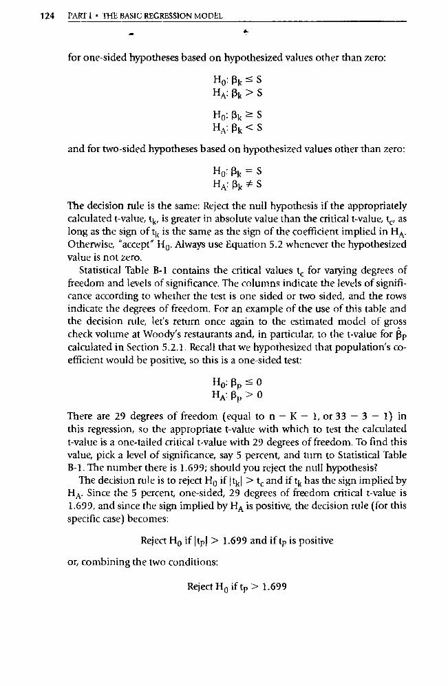
124 PART I • THE BASIC REGRESSION MODEL
for one-sided hypotheses based on hypothesized values other than zero:
H0:Rk S HA: Pk > S
Ho: Rk ? S HA: Rk<S
and for two-sided hypotheses based on hypothesized values other than zero:
Ho: [3k=S HA: Pk*S
The decision rule is the same: Reject the null hypothesis if the appropriately calculated t-value, tk, is greater in absolute value than the critical t-value, t c, as long as the sign of tk is the same as the sign of the coefficient implied in HA. Otherwise, "accept" H o. Always use Equation 5.2 whenever the hypothesized value is not zero.
Statistical Table B-1 contains the critical values t c for varying degrees of freedom and levels of significance. The columns indicate the levels of signifi-cance according to whether the test is one sided or two sided, and the rows indicate the degrees of freedom. For an example of the use of this table and the decision rule, let's return once again to the estimated model of gross check volume at Woodÿ s restaurants and, in particular, to the t-value for j3p calculated in Section 5.2.1. Recall that we hypothesized that population's co-efficient would be positive, so this is a one-sided test:
Ho:(3 P < 0
HA: j3 p >0
There are 29 degrees of freedom (equal to n — K — 1, or 33 — 3 — 1) in this regression, so the appropriate t-value with which to test the calculated t-value is a one-tailed critical t-value with 29 degrees of freedom. To find this value, pick a level of significance, say 5 percent, and turn to Statistical Table B-1. The number there is 1.699; should you reject the null hypothesis?
The decision rule is to reject H o if Itk l > tc and if tk has the sign implied by HA. Since the 5 percent, one-sided, 29 degrees of freedom critical t-value is 1.699, and since the sign implied by HA is positive, the decision rule (for this specific case) becomes:
Reject Hp if Itpl > 1.699 and if tp is positive
or, combining the two conditions:
Reject 11 0 if tp > 1.699
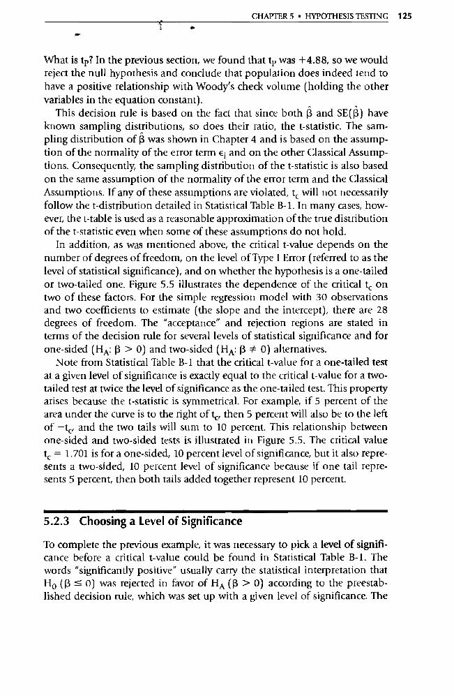
CHAI'l'ER 5 • HYPOTHESIS TESTING 125
s
What is tp? In the previous section, we found that tp was +4.88, so we would reject the null hypothesis and conclude that population does indeed tend to have a positive relationship with Woodÿ s check volume (holding the other variables in the equation constant).
This decision rule is based on the fact that since both R and SE( .13) have known sampling distributions, so does their ratio, the t-statistic. The sam-pling distribution of 13 was shown in Chapter 4 and is based on the assump-tion of the normality of the error term e; and on the other Classical Assump-tions. Consequently, the sampling distribution of the t-statistic is also based on the same assumption of the normality of the error term and the Classical Assumptions. If any of these assumptions are violated, t c will not necessarily follow the t-distribution detailed in Statistical Table B-1. In many cases, how-ever, the t-table is used as a reasonable approximation of the true distribution of the t-statistic even when some of these assumptions do not hold.
In addition, as was mentioned above, the critical t-value depends on the number of degrees of freedom, on the level of Type I Error (referred to as the level of statistical significance), and on whether the hypothesis is a one-tailed or two-tailed one. Figure 5.5 illustrates the dependence of the critical t c on two of these factors. For the simple regression model with 30 observations and two coefficients to estimate (the slope and the intercept), there are 28 degrees of freedom. The "acceptance" and rejection regions are stated in terms of the decision rule for several levels of statistical significance and for one-sided (HA: (3 > 0) and two-sided (H A: 13 0) alternatives.
Note from Statistical Table B-1 that the critical t-value for a one-tailed test at a given level of significance is exactly equal to the critical t-value for a two-tailed test at twice the level of significance as the one-tailed test. This property arises because the t-statistic is symmetrical. For example, if 5 percent of the area under the curve is to the right of t c, then 5 percent will also be to the left of —te, and the two tails will sum to 10 percent. This relationship between one-sided and two-sided tests is illustrated in Figure 5.5. The critical value tc = 1.701 is for a one-sided, 10 percent level of significance, but it also repre-sents a two-sided, 10 percent level of significance because if one tail repre-sents 5 percent, then both tails added together represent 10 percent.
5.2.3 Choosing a Level of Significance
To complete the previous example, it was necessary to pick a level of signifi-cance before a critical t-value could be found in Statistical Table B-1. The words "significantly positive" usually car ry the statistical interpretation that Ho ((3 <_ 0) was rejected in favor of HA (13 > 0) according to the preestab-lished decision rule, which was set up with a given level of significance. The
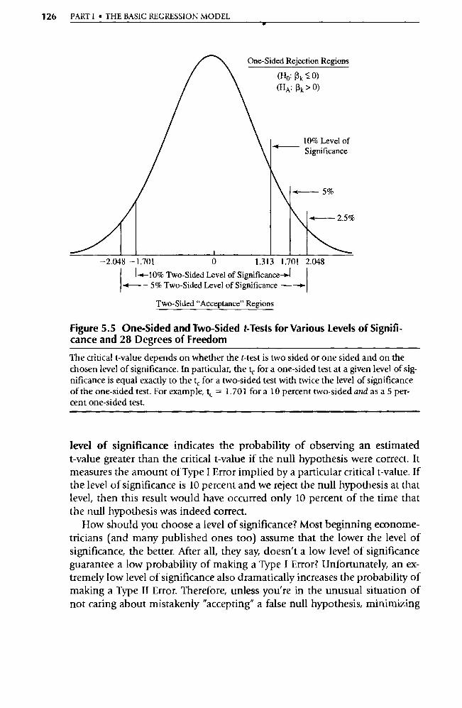
One-Sided Rejection Regions
(Ho: l k 0) (HA: Rk > 0)
10% Level of Significance
126 PARTI • THE BASIC REGRESSION MODEL sr
-2.048 -1.701 0 1.313 1.701 2.048 1E-10% Two-Sided Level of Significance
-4---- 5% Two-Sided Level of Significance ->
Two-Sided "Acceptance" Regions
Figure 5.5 One-Sided and Two-Sided t Tests for Various Levels of Signifi-cance and 28 Degrees of Freedom
The critical t-value depends on whether the t-test is two sided or one sided and on the chosen level of significance. In pa rticular, the t c for a one-sided test at a given level of sig-nificance is equal exactly to the t, for a two-sided test with twice the level of significance of the one-sided test. For example, t c = 1.701 for a 10 percent two-sided and as a 5 per-cent one-sided test.
level of significance indicates the probability of observing an estimated t-value greater than the critical t-value if the null hypothesis were correct. It measures the amount of Type I Error implied by a particular critical t-value. If the level of significance is 10 percent and we reject the null hypothesis at that level, then this result would have occurred only 10 percent of the time that the null hypothesis was indeed correct.
How should you choose a level of significance? Most beginning econome-tricians (and many published ones too) assume that the lower the level of significance, the better. After all, they say, doesn't a low level of significance guarantee a low probability of making a Type I Error? Unfortunately, an ex-tremely low level of significance also dramatically increases the probability of making a Type II Error. Therefore, unless you're in the unusual situation of not caring about mistakenly "accepting" a false null hypothesis, minimizing
CHAPTER 5 • HYPOTHESIS TESTING 127
the level of significance is not good standard practice. Instead, we recommend using a 5 percent level of significance except in
those circumstances when you know something unusual about the relative costs of making Type I and Type II Errors. If we can reject a null hypothesis at the 5 percent level of significance, we can summarize our results by saying that the coefficient is "statistically significant" at the 5 percent level. Since the 5 percent level is arbitrary, we shouldn't jump to conclusions about the value of a variable simply because its coefficient misses being significant by a small amount; if a different level of significance had been chosen, the result might have been different.
Some researchers avoid choosing a level of significance by simply stating the lowest level of significance possible for each estimated regression coeffi-cient. Such a use of the t-value should be regarded as a descriptive rather than a hypothesis-testing use of statistics.
Now and then researchers will use the phrase "degree of confidence" or "level of confidence" when they test hypotheses. What do they mean? The level of confidence is nothing more than 100 percent minus the level of signifi-cance. Thus a t-test for which we use a 5 percent level of significance can also be said to have a 95 percent level of confidence. Since the two terms have identical meanings, for all intents and purposes, we will tend to use level of significance throughout this text. Another reason we prefer the term level of significance to level of confidence is to avoid any possible confusion with the related concept of confidence intervals.
5.2.4 Confidence Intervals
A confidence interval is a range within which the true value of an item is likely to fall a specified percentage of the time. 6 This percentage is the level of confidence associated with the level of significance used to choose the critical t-value in the interval. For an estimated regression coefficient, the confidence interval can be calculated using the two-sided critical t-value and the stan-dard error of the estimated coefficient:
Confidence interval = R ± t c • SE(R) (5.5)
As an example, let's return to Equation 5.4 and our t-test of the significance of the estimate of the coefficient of population in that equation:
6. Although it is common usage to call this interval a "confidence inte rval," it technically is a "prediction inte rval.
128 PARTI • THE BASIC REGRESSION MODEL
Y; = 102,192 — 9075N 1 (2053)
t = —4.42
+ 0.3547131 (0.0727) 4.88
+ 1.288I ; (0.543) 2.37
(5.4)
n=33 R2 =.579
What would a 90 percent confidence interval for (3 look like? Well, j3p = 0.3547 and SE(j3 P ) = 0.0727, so all we need is a 90 percent two-sided critical t-value for 29 degrees of freedom. As can be seen in Statistical Table B-1, this tc = 1.699. Substituting these values into Equation 5.5, we get:
90 percent confidence interval around 4p = 0.3547 ± 1.699 • 0.0727 = 0.3547 ± 0.1235
In other words, we expect that 90 percent of the time the true coefficient will fall between 0.2312 and 0.4782.
There's an interesting relationship between confidence intervals and two-sided hypothesis testing. It turns out that if a hypothesized border value, OH°, falls within the 90 percent confidence interval for an estimated coefficient, then we will not be able to reject the null hypothesis at the 10 percent level of significance in a two-sided test. If, on the other hand, j3 Ho falls outside the 90 percent confidence inte rval, then we can reject the null hypothesis.
Perhaps the most impo rtant econometric use of confidence intervals is in forecasting. Many decision makers find it practical to be given a forecast of a range of values into which the forecasted item is likely to fall some percentage of the time. In contrast, decision makers find that a specific point forecast pro-vides them with little information about the reliability or variability of the fore-cast. For more on this application of confidence intervals, see Section 15.2.3.
5.3 Examples of t-Tests
5.3.1 Examples of One-Sided t-Tests
The most common use of the one-sided t-test is to determine whether a re-gression coefficient has the sign predicted by theory. Let's face it, if you expect a positive sign for a coefficient and you get a negative 0, it's hard to reject the possibility that the true j3 might be negative (or zero). On the other hand, if you expect a positive sign and get a positive (3, things get a bit tricky. If $3 is positive, but fairly close to zero, then a one-sided t-test should be used to de-termine whether the R is different enough from zero to allow the rejection of the null hypothesis. Recall that in order to be able to control the amount of Type I Error we make, such a theory implies an alternative hypothesis of

CHAPTER 5 • HYPOTHESIS TESTING 129
HA: 13 > 0 (the expected sign) and a null hypothesis of Ho : R 5- O. Let's look at some complete examples of these kinds of one-sided t-tests.
Consider a simple model of the aggregate retail sales of new cars that hypothesizes that sales of new cars (Y) are a function of real disposable in-come (X 1 ) and the average retail price of a new car adjusted by the consumer price index (X2). Suppose you spend some time reviewing the literature on the automobile industry and are inspired to test a new theory. You decide to add a third independent variable, the number of spo rts utility vehicles sold (X3 ), to take account of the fact that some potential new car buyers now buy car-like trucks instead. You therefore hypothesize the following model:
+ Y = f(X1, X2, X 3 ) + e (5. 6 )
13 1 is expected to be positive and 13 2 and 0.3 , negative. This makes sense, since you'd expect higher incomes, lower prices, or lower numbers of sports utility vehicles sold to increase new cars sales, holding the other va riables in the equa-tion constant. Although in theory a single test for all three slope coefficients could be applied here, nearly every researcher examines each coefficient sepa-rately with the t-test. The four steps to use when working with the t-test are:
1. Set up the null and alte rnative hypotheses.
2. Choose a level of significance and therefore a critical t-value.
3. Run the regression and obtain an estimated t-value (or t-score).
4. Apply the decision rule by comparing the calculated t-value with the critical t-value in order to reject or "accept" the null hypothesis.
1. Set up the null and alternative hypotheses. 7 From Equation 5.6, the one-sided hypotheses are set up as:
1. Ho: (3 1 <<-0
HA: (31 >0
2. Ho: 132 j 0
HA: (32 <0
3. Ho : (3 3 ? 0
HA : 133 < 0
7. Recall from footnote 3 that a one-sided hypothesis can be stated either as H o: 13 0 or Ho: 13 = 0 because the value used to test H o : 13 s 0 is the value in the null hypothesis closest to the border between the acceptance and the rejection regions. When the amount of Type I Error is calculated, this border value of R is the one that is used because, over the whole range of 13 <_ 0, the value R = 0 gives the maximum amount of Type I Error. The classical approach lim-its this maximum amount to a preassigned level, the chosen level of significance.
130 PARTI • THE BASIC REGRESSION MODEL
Remember that a t-test typically is not run on the estimate of the con-stant term Bo.
2. Choose a level of significance and therefore a critical t-value. Assume that you have considered the various costs involved in making Type I and Type II Errors and have chosen 5 percent as the level of significance with which you want to test. There are 10 observations in the data set that is going to be used to test these hypotheses, and so there are 10 — 3 — 1 = 6 degrees of freedom. At a 5 percent level of signifi-cance (or a 95 percent level of confidence), the critical t-value, t c, can be found in Statistical Table B-1 to be 1.943. Note that the level of sig-nificance does not have to be the same for all the coefficients in the same regression equation. It could well be that the costs involved in an incorrectly rejected null hypothesis for one coefficient are much higher than for another, and so lower levels of significance would be used. In this equation, though, for all three variables:
tc = 1.943
3. Run the regression and obtain an estimated t-value. You now use the data (annual from 1990 to 1999) to run the regression on your computer's OLS package, getting:
Yt = 1.30 + 4.91X1t + 0.00123X2t — 7.14X3t (2.38) (0.00022) (71.38)
t = 2.1 5. 6 — 0.1
(5.7)
where: Y = new car sales (in hundreds of thousands of units) in year t
X1 = real U.S. disposable income (in hundreds of billions of dollars)
X2 = the average retail price of a new car in year t (in dollars) X3 = the number of spo rts utility vehicles sold in year t (in
millions)
Once again, we use our standard documentation notation, so the figures in parentheses are the estimated standard errors of the s. The t-values to be used in these hypothesis tests are printed out by most standard OLS programs, because the programs are written to test the null hypothesis that (3 = 0 (or, equivalently, (3 or 0). If the pro-gram does not calculate the t-scores automatically, one may plug the
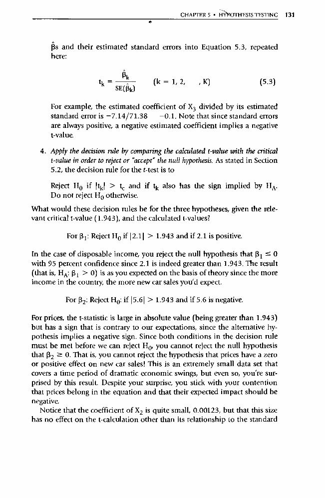
CHAPTER 5 • HYPOTHESIS TESTING 131
(3s and their estimated standard errors into Equation 5.3, repeated here:
tk = 1.1c (k = 1, 2, , K) (5.3)
SE( 130
For example, the estimated coefficient of X3 divided by its estimated standard error is —7.14/71.38 —0.1. Note that since standard errors are always positive, a negative estimated coefficient implies a negative t-value.
4. Apply the decision rule by comparing the calculated t-value with the critical t-value in order to reject or "accept" the null hypothesis. As stated in Section 5.2, the decision rule for the t-test is to
Reject Ho if ttk! > tc and if tk also has the sign implied by HA.
Do not reject H o otherwise.
What would these decision rules be for the three hypotheses, given the rele-vant critical t-value (1.943), and the calculated t-values?
For 13 1 : Reject H o if 12.11 > 1.943 and if 2.1 is positive.
In the case of disposable income, you reject the null hypothesis that (3 1 <— 0 with 95 percent confidence since 2.1 is indeed greater than 1.943. The result (that is, HA: 131 > 0) is as you expected on the basis of theory since the more income in the country, the more new car sales you'd expect.
For 13 2 : Reject H o : if 15.61 > 1.943 and if 5.6 is negative.
For prices, the t-statistic is large in absolute value (being greater than 1.943) but has a sign that is contrary to our expectations, since the alternative hy-pothesis implies a negative sign. Since both conditions in the decision rule must be met before we can reject H o, you cannot reject the null hypothesis that 13 2 ? O. That is, you cannot reject the hypothesis that prices have a zero or positive effect on new car sales! This is an extremely small data set that covers a time period of dramatic economic swings, but even so, you're sur-prised by this result. Despite your surprise, you stick with your contention that prices belong in the equation and that their expected impact should be negative.
Notice that the coefficient of X2 is quite small, 0.00123, but that this size has no effect on the t-calculation other than its relationship to the standard
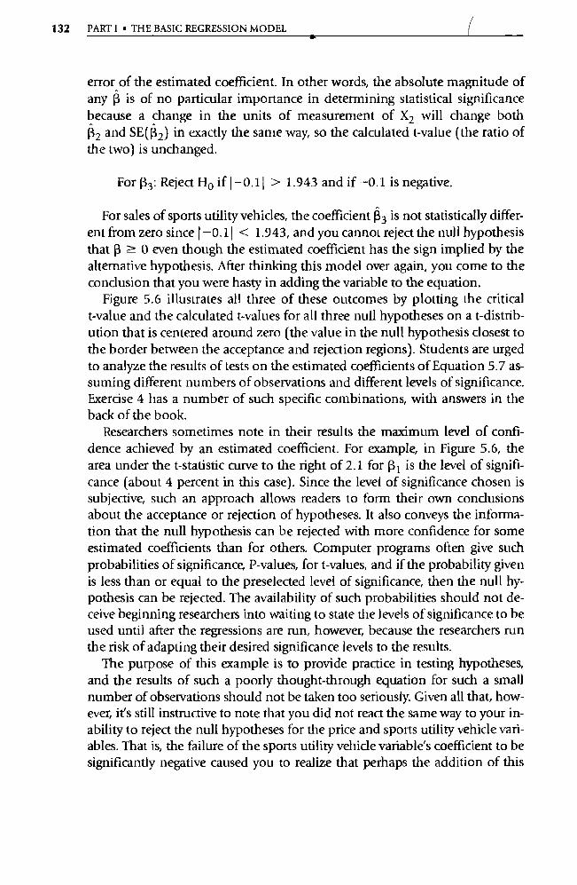
132 PARTI • THE BASIC REGRESSION MODEL
error of the estimated coefficient. In other words, the absolute magnitude of any 13 is of no particular impo rtance in determining statistical significance because a change in the units of measurement of X2 will change both
â 2 and SE02) in exactly the same way, so the calculated t-value (the ratio of the two) is unchanged.
For [3 3 : Reject H p if —0.11 > 1.943 and if —0.1 is negative.
For sales of spo rts utility vehicles, the coefficient R3 is not statistically differ-ent from zero since I —0.11 < 1.943, and you cannot reject the null hypothesis
that 13 ? 0 even though the estimated coefficient has the sign implied by the
alternative hypothesis. After thinking this model over again, you come to the
conclusion that you were hasty in adding the variable to the equation.
Figure 5.6 illustrates all three of these outcomes by plotting the critical
t-value and the calculated t-values for all three null hypotheses on a t-distrib-ution that is centered around zero (the value in the null hypothesis closest to
the border between the acceptance and rejection regions). Students are urged
to analyze the results of tests on the estimated coefficients of Equation 5.7 as-suming different numbers of observations and different levels of significance.
Exercise 4 has a number of such specific combinations, with answers in the
back of the book. Researchers sometimes note in their results the maximum level of confi-
dence achieved by an estimated coefficient. For example, in Figure 5.6, the
area under the t-statistic curve to the right of 2.1 for 13 1 is the level of signifi-cance (about 4 percent in this case). Since the level of significance chosen is
subjective, such an approach allows readers to form their own condusions
about the acceptance or rejection of hypotheses. It also conveys the informa-tion that the null hypothesis can be rejected with more confidence for some
estimated coefficients than for others. Computer programs often give such
probabilities of significance, P-values, for t-values, and if the probability given
is less than or equal to the preselected level of significance, then the null hy-pothesis can be rejected. The availability of such probabilities should not de-ceive beginning researchers into waiting to state the levels of significance to be
used until after the regressions are run, however, because the researchers run
the risk of adapting their desired significance levels to the results.
The purpose of this example is to provide practice in testing hypotheses,
and the results of such a poorly thought-through equation for such a small
number of observations should not be taken too seriously. Given all that, how-ever, it's still instructive to note that you did not react the same way to your in-ability to reject the null hypotheses for the price and sports utility vehide vari-ables. That is, the failure of the spo rts utility vehicle variable's coefficient to be
significantly negative caused you to realize that perhaps the addition of this
^
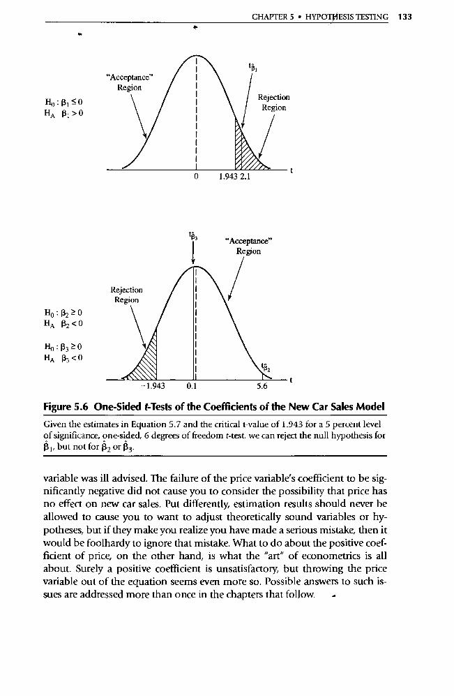
CHAPTER 5 • HYPOTJ ESIS TESTING 133
t113
Ho : Ri <_ 0 HA Ri >0
1.943 2.1
"Acceptance" Region
Ho: 132>0
HA 132 < 0
Ho :13 3 > 0
HA 133 < 0
—1.943 —0.1
5.6
Figure 5.6 One-Sided t Tests of the Coefficients of the New Car Sales Model
Given the estimates in Equation 5.7 and the critical t-value of 1.943 for a 5 percent level of significance, one-sided, 6 degrees of freedom t-test, we can reject the null hypothesis for (3 t , but not for (32 or R3.
variable was ill advised. The failure of the price variable's coefficient to be sig-nificantly negative did not cause you to consider the possibility that price has no effect on new car sales. Put differently, estimation results should never be allowed to cause you to want to adjust theoretically sound va riables or hy-potheses, but if they make you realize you have made a serious mistake, then it would be foolhardy to ignore that mistake. What to do about the positive coef-ficient of price, on the other hand, is what the "art" of econometrics is all about. Surely a positive coefficient is unsatisfactory, but throwing the price variable out of the equation seems even more so. Possible answers to such is-sues are addressed more than once in the chapters that follow. -
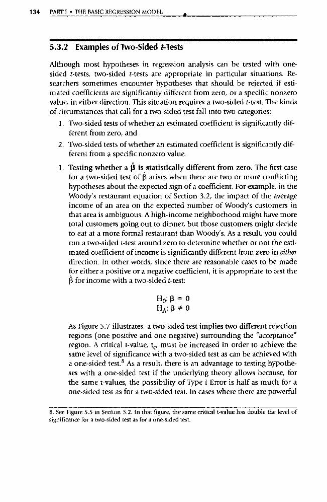
134 PART I • THE BASIC REGRESSION MODEL a
5.3.2 Examples of Two-Sided t-Tests
Although most hypotheses in regression analysis can be tested with one-sided t-tests, two-sided t-tests are appropriate in particular situations. Re-searchers sometimes encounter hypotheses that should be rejected if esti-mated coefficients are significantly different from zero, or a specific nonzero value, in either direction. This situation requires a two-sided t-test. The kinds of circumstances that call for a two-sided test fall into two categories:
1. Two-sided tests of whether an estimated coefficient is significantly dif-ferent from zero, and
2. Two-sided tests of whether an estimated coefficient is significantly dif-ferent from a specific nonzero value.
1. Testing whether a (3 is statistically different from zero. The first case for a two-sided test of R arises when there are two or more conflicting hypotheses about the expected sign of a coefficient. For example, in the Woody's restaurant equation of Section 3.2, the impact of the average income of an area on the expected number of Woody's customers in that area is ambiguous. A high-income neighborhood might have more total customers going out to dinner, but those customers might decide to eat at a more formal restaurant than Woody's. As a result, you could mn a two-sided t-test around zero to determine whether or not the esti-mated coefficient of income is significantly different from zero in either direction. In other words, since there are reasonable cases to be made for either a positive or a negative coefficient, it is appropriate to test the j3 for income with a two-sided t-test:
Ho: (3=0 HA: (3# 0
As Figure 5.7 illustrates, a two-sided test implies two different rejection regions (one positive and one negative) surrounding the "acceptance" region. A critical t-value, t c, must be increased in order to achieve the same level of significance with a two-sided test as can be achieved with a one-sided test. 8 As a result, there is an advantage to testing hypothe-ses with a one-sided test if the underlying theory allows because, for the same t-values, the possibility of Type I Error is half as much for a one-sided test as for a two-sided test. In cases where there are powerful
S. See Figure 5.5 in Section 5.2. In that figure, the same critical t-value has double the level of significance for a two-sided test as for a one-sided test.
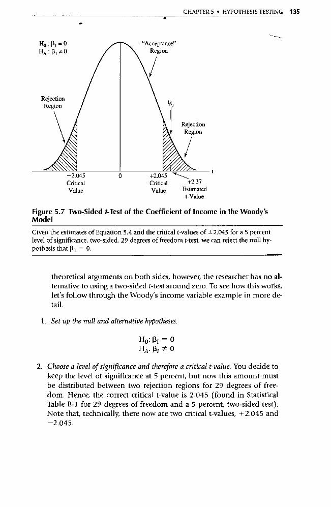
CHAI'I ER 5 • HYPOTHESIS TESTING 135 •
Ho : 13 1 = 0 "Acceptance" HA : R1 * 0 Region
—2.045 0 +2.045 ^\ Critical Critical +2.37 Value Value Estimated
t-Value
Figure 5.7 Two-Sided t-Test of the Coefficient of Income in the Woody's
Model
Given the estimates of Equation 5.4 and the critical t-values of ±2.045 for a 5 percent
level of significance, two-sided, 29 degrees of freedom t-test, we can reject the null hy-pothesis that (3 t = 0.
theoretical arguments on both sides, however, the researcher has no al-ternative to using a two-sided t-test around zero. To see how this works, let's follow through the Woody's income va riable example in more de-tail.
1. Set up the null and alternative hypotheses.
Ho : (3 1 = 0 HA. O
2. Choose a level of significance and therefore a critical t-value. You decide to keep the level of significance at 5 percent, but now this amount must be distributed between two rejection regions for 29 degrees of free-dom. Hence, the correct critical t-value is 2.045 (found in Statistical Table B-1 for 29 degrees of freedom and a 5 percent, two-sided test). Note that, technically, there now are two critical t-values, +2.045 and —2.045.
136 PART I • THE BASIC REGRESSION MODEL
3. Run the regression and obtain an estimated t-value. Since the value implied by the null hypothesis is still zero, the estimated t-value of +2.37 given in Equation 5.4 is applicable.
4. Apply the decision rule by comparing the calculated t-value with the critical t-value in order to reject or "accept" the null hypothesis. We once again use the decision rule stated in Section 5.2, but since the alternative hypoth-esis specifies either sign, the decision mle simplifies to:
For RI Reject H o if 12.371 > 2.045
In this case, you reject the null hypothesis that (3 1 equals zero because 2.37 is greater than 2.045 (see Figure 5.7). Note that the positive sign implies that, at least for Woody's restaurants, income increases cus-tomer volume (holding constant population and competition). Given this result, we might well choose to mn a one-sided t-test on the next year's Woody's data set. For more practice with two-sided t-tests, see Ex-ercise 6.
2. Two-sided t-tests of a specific nonzero coefficient value. The second case for a two-sided t-test arises when there is reason to expect a specific nonzero value for an estimated coefficient. For example, if a previous researcher has stated that the true value of some coefficient almost surely equals a particular number, RHo , then that number would be the one to test by creating a two-sided t-test around the hypothesized value, RH . To the extent that you feel that the hypothesized value is theoretically correct, you also violate the normal practice of using the null hypothesis to state the hypothesis you expect to reject 9
In such a case, the null and alte rnative hypotheses become:
H0: Rk = RH0
HA. Rk * 13H0
where R Ho is the specific nonzero value hypothesized.
9. Instead of being able to reject an incorrect theory based on the evidence, the researcher who violates the normal practice is reduced to "not rejecting" the R value expected to be true. This makes a big difference because to "accept" H o is merely to say that H o is not rejected by the data. However, there are many theories that are not rejected by the data, and the researcher is left with a regrettably weak conclusion. One way to accommodate such violations is to increase the level of significance, thereby increasing the likelihood of a Type I Error.
a
CHAPTER 5 • HYPOTHESIS TESTING 137
Since the hypothesized (3 value is no longer zero, the formula with which to calculate the estimated t-value is Equation 5.2, repeated here:
(Rk — aH) tk =
a (k = 1, 2, , K) (5.2)
SE(k)
This t-statistic is still distributed around zero if the null hypothesis is correct, because we have subtracted [3 H0 from the estimated regression coefficient whose expected value is supposed to be pH when H o is true. Since the t-statistic is still centered around zero, the decision rules developed earlier are still applicable. In other words, the techniques used above are precisely the same as for a two-sided t-test of a specific nonzero coefficient. For practice with this kind of t-test, see Exercise 6.
5.3.3 The t-Test of the Simple Correlation Coefficient, r
From the previous sections, it'd be easy to get the impression that the t-test is used only for tests of regression coefficients, but that's hardly the case. It turns out that there is a variety of applications for the t-test that don't in-volve Rs.
The most immediately useful of these applications is a t-test of the simple correlation coefficient. The simple correlation coefficient, r, is a measure of the strength and direction of the linear relationship between two variables. The simple correlation coefficient between X 1 and X2 is:
E[(Xli — X1)(X2i X2)] r12 = '/
X1) 2 (X21 — X2) 2 (5.8)
If two variables are perfectly positively correlated, then r = +1. To see this, assume that X 11 = X2 i and substitute into Equation 5.8:
— X 1 )(X 1i X1)] r12 = 1 /
X1) 2 (X1i — X1) 2
E[(X 1i X1) 2 ] = +1 E[(Xli - X1) 2]
(5.9)
138 PARTI • THE BASIC REGRESSION MODEL •
If two variables are perfectly negatively correlated, then r = —1. To see this, substitute X2i = -X 1 1 into Equation 5.8:
[(X1i — X 1 )( -Xli + Xl)] r12 = ,/
V nX1i X1) 2 E( -X1i + X 1 ) 2
-E[(X 1 , - X1) 2 ] = -1
E[(X1i - X1) 2]
If two variables are totally uncorrelated, then r = 0. One of the major uses of the simple correlation coefficient r is to test the
hypothesis that two explanatory va riables are correlated in a less than perfect but still significant (multicollinear) way. For imperfect multicollinearity to occur in this two-variable case, the simple correlation coefficient must be fairly large in the direction indicated by theory. In order to test this hypothe-sis, r can be converted into a t-statistic using:
rVn — 2 t V(1
- r2) (5.11)
where n is the size of the sample. The statistic defined in Equation 5.11 fol-lows the t-distribution with n — 2 degrees of freedom. Since t is directly re-lated to r, a large positive r will convert into a large positive t, and so on.
Tests of hypotheses about t (and therefore about r) can be undertaken us-ing the critical t-values and decision rules outlined in Section 5.2 and Statisti-cal Table B-1. For example, suppose you encounter a simple correlation coef-ficient of 0.946 between two va riables you expect to be positively correlated in a data set with 28 observations. In this case,
Ho : r <- 0 HA: r> 0
and we can reject the null hypothesis of no positive correlation if the calcu-lated t-score is larger in absolute value than the critical t-value of 1.706 (for 26 degrees of freedom at the 5 percent, one-sided level of significance) and if t has the positive sign implied by the alternative hypothesis. If we substitute r = 0.946 and n = 28 into Equation 5.11, we obtain 14.880, and the null hy-
(5.10)
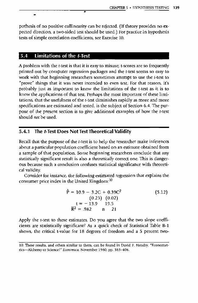
CHAPTER 5 • HYPOTHESIS TESTING 139
pothesis of no positive coIlinearity can be rejected. (If theory provides no ex-pected direction, a two-sided test should be used.) For practice in hypothesis tests of simple correlation coefficients, see Exercise 10.
5.4 Limitations of the t -Test
A problem with the t-test is that it is easy to misuse; t-scores are so frequently printed out by computer regression packages and the t-test seems so easy to work with that beginning researchers sometimes attempt to use the t-test to "prove" things that it was never intended to even test. For that reason, it's probably just as important to know the limitations of the t-test as it is to know the applications of that test. Perhaps the most impo rtant of these limi-tations, that the usefulness of the t-test diminishes rapidly as more and more specifications are estimated and tested, is the subject of Section 6.4. The pur-pose of the present section is to give additional examples of how the t-test should not be used.
5.4.1 The t-Test Does Not Test Theoretical Validity
Recall that the purpose of the t-test is to help the researcher make inferences about a particular population coefficient based on an estimate obtained from a sample of that population. Some beginning researchers conclude that any statistically significant result is also a theoretically correct one. This is danger-ous because such a conclusion confuses statistical significance with theoreti-cal validity.
Consider for instance, the following estimated regression that explains the consumer price index in the United Kingdom:'°
P = 10.9 — 3.2C + 0.39C2 (5.12) (0.23) (0.02)
t = - 13.9 19.5 17t2 = .982 n 21
Apply the t-test to these estimates. Do you agree that the two slope coeffi- cients are statistically significant? As a quick check of Statistical Table B-1 shows, the critical t-value for 18 degrees of freedom and a 5 percent two-
10. These results, and others similar to them, can be found in David F. Hendry, "Economet-rics—Alchemy or Science?" Economica, November 1980, pp. 383-406.
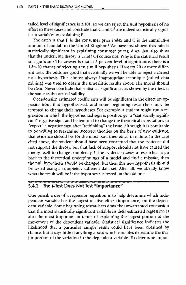
140 PARTI • THE BASIC REGRESSION MODEL
tailed level of significance is 2.101, so we can reject the null hypothesis of no effect in these cases and conclude that C and C 2 are indeed statistically signif-icant variables in explaining P.
The catch is that P is the consumer price index arid C is the cumulative amount of rainfall in the United Kingdom! We have jhst shown that rain is statistically significant in explaining consumer prices; does that also show that the underlying theory is valid? Of course not. Why is the statistical result so significant? The answer is that at 5 percent level of significance, there is a 1-in-20 chance of rejecting a true null hypothesis. If we try 20 or more differ-ent tests, the odds are good that eventually we will be able to reject a correct null hypothesis. This almost always inappropriate technique (called data mining) was used to obtain the unrealistic results above. The moral should be clear: Never conclude that statistical significance, as shown by the t-test, is the same as theoretical validity.
Occasionally, estimated coefficients will be significant in the direction op-posite from that hypothesized, and some beginning researchers may be tempted to change their hypotheses. For example, a student might run a re-gression in which the hypothesized sign is positive, get a "statistically signifi-cant" negative sign, and be tempted to change the theoretical expectations to "expect" a negative sign after "rethinking" the issue. Although it is admirable to be willing to reexamine incorrect theories on the basis of new evidence, that evidence should be, for the most pa rt, theoretical in nature. In the case cited above, the student should have been concerned that the evidence did not support the theory, but that lack of suppo rt should not have caused the theory itself to change completely. If the evidence causes a researcher to go back to the theoretical underpinnings of a model and find a mistake, then the null hypothesis should be changed, but then this new hypothesis should be tested using a completely different data set. After all, we already know what the result will be if the hypothesis is tested on the old one.
5.4.2 The t Test Does Not Test "Importance"
One possible use of a regression equation is to help determine which inde-pendent variable has the largest relative effect (impo rtance) on the depen-dent variable. Some beginning researchers draw the unwarranted conclusion that the most statistically significant va riable in their estimated regression is also the most impo rtant in terms of explaining the largest portion of the movement of the dependent variable. Statistical significance indicates the likelihood that a particular sample result could have been obtained by chance, but it says little if anything about which variables determine the ma-jor portion of the variation in the dependent variable. To determine impor-
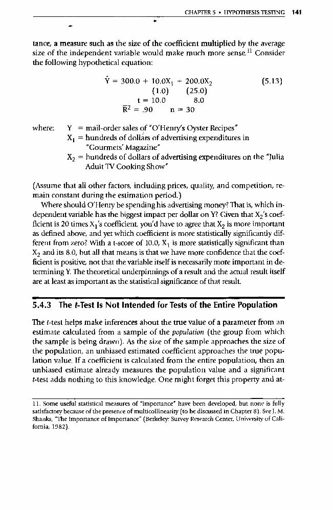
CHAPTER 5 • HYPOTHESIS TESTING 141
SD-
tance, a measure such as the size of the coefficient multiplied by the average size of the independent va riable would make much more sense. 11 Consider the following hypothetical equation:
= 300.0 + 10.0X 1 (1.0)
t = 10.0
+ 200.0X2 (25.0)
8.0
(5.13)
R2 =.90 n=30
where: Y = mail-order sales of "O'Henry's Oyster Recipes" X1 = hundreds of dollars of advertising expenditures in
"Gourmets' Magazine" X2 = hundreds of dollars of advertising expenditures on the "Julia
Adult TV Cooking Show"
(Assume that all other factors, including prices, quality, and competition, re-main constant during the estimation period.)
Where should O'Henry be spending his advertising money? That is, which in-dependent va riable has the biggest impact per dollar on Y? Given that X 2's coef-ficient is 20 times X 1 's coefficient, you'd have to agree that X2 is more important as defined above, and yet which coefficient is more statistically significantly dif-ferent from zero? With a t-score of 10.0, X 1 is more statistically significant than X2 and its 8.0, but all that means is that we have more confidence that the coef-ficient is positive, not that the va riable itself is necessarily more impo rtant in de-termining Y. The theoretical underpinnings of a result and the actual result itself are at least as impo rtant as the statistical significance of that result.
5.4.3 The t-Test Is Not Intended for Tests of the Entire Population
The t-test helps make inferences about the true value of a parameter from an estimate calculated from a sample of the population (the group from which the sample is being drawn). As the size of the sample approaches the size of the population, an unbiased estimated coefficient approaches the true popu-lation value. If a coefficient is calculated from the entire population, then an unbiased estimate already measures the population value and a significant t-test adds nothing to this knowledge. One might forget this property and at-
11. Some useful statistical measures of "impo rtance" have been developed, but none is fully satisfactory because of the presence of multicollinearity (to be discussed in Chapter 8). See J. M. Shanks, "The Impo rtance of Impo rtance" (Berkeley: Survey Research Center, Universi ty of Cali-fornia, 1982).

142 PARTI • THE BASIC REGRESSION MODEL
tach too much importance to t-sores that have been obtained from samples that approximate the population in size. All the t-test does is help decide how likely it is that a particular small sample will cause a researcher to make a mistake in rejecting hypotheses about the true population parameters.
This point can perhaps best be seen by remembering that the t-score is the estimated regression coefficient divided by the standard error of the estimated regression coefficient. If the sample size is large enough to approach the popu-lation, then the standard error will fall close to zero because the dist ribution of estimates becomes more and more narrowly distributed around the true para-meter (if this is an unbiased estimate). The standard error will approach zero as the sample size approaches infinity. Thus, the t-score will eventually become:
13 t=—=00 0
The mere existence of a large t-score for a huge sample has no real substan-tive significance because if the sample size is large enough, you can reject al-most any null hypothesis! It is true that sample sizes in econometrics can never approach infinity, but many are quite large; and others, even though fairly small, are not really samples of a population but contain the entire population in one data set. 12
5.5 The F-Test of Overall Significance
Although the t-test is invaluable for hypotheses about individual regression coefficients, it can't be used to test hypotheses about more than one coeffi-cient at a time. Such a limitation is unfortunate, since it's possible to imagine quite a few interesting hypotheses that involve more than one coefficient. For example, suppose you wanted to test the hypothesis that two regression coef-ficients were equal to each other? In such a situation, most researchers would use a different statistical test, the F-test.
The F-test is a method of testing a null hypothesis that includes more than one coefficient; it works by determining whether the overall fit of an equa-tion is significantly reduced by constraining the equation to conform to the null hypothesis. If the fit is significantly reduced, then we can reject the null hypothesis. If the fit is not reduced significantly, then we can't reject the null hypothesis. The F-test is used most frequently in econometrics to test the overall significance of a regression equation, the topic of this section. We'll investigate other uses of the F-test in Section 7.7.
12. D. N. McCloskey, "The Loss Function Has Been Mislaid: The Rhetoric of Significance Tests," American Economic Review, May 1985, p. 204.
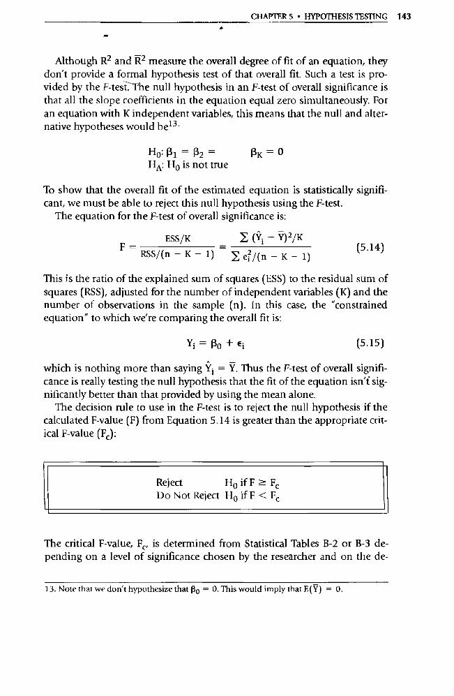
CHAPTER 5 • HYPOTHESIS TESTING 143
Although R2 and R2 measure the overall degree of fit of an equation, they don't provide a formal hypothesis test of that overall fit. Such a test is pro-vided by the F-teshe null hypothesis in an F-test of overall significance is that all the slope coefficients in the equation equal zero simultaneously. For an equation with K independent variables, this means that the null and alter-native hypotheses would be 13 *
Ho: R1=(32= 13K= 0 HA: Ho is not true
To show that the overall fit of the estimated equation is statistically signifi-cant, we must be able to reject this null hypothesis using the F-test.
The equation for the F-test of overall significance is:
ESS/K E (Yi - Y) 2/K F 5.14 ( )
This is the ratio of the explained sum of squares (ESS) to the residual sum of squares (RSS), adjusted for the number of independent va riables (K) and the number of observations in the sample (n). In this case, the "constrained equation" to which we're comparing the overall fit is:
Yi = (30 + Ei (5.15)
which is nothing more than saying Y i = Y. Thus the F-test of overall signifi-cance is really testing the null hypothesis that the fit of the equation isn't sig-nificantly better than that provided by using the mean alone.
The decision rule to use in the F-test is to reject the null hypothesis if the calculated F-value (F) from Equation 5.14 is greater than the appropriate crit-ical F-value (Fc):
Reject H0 if F ? Fc Do Not Reject H0 if F < Fc
The critical F-value, Fc, is determined from Statistical Tables B-2 or B-3 de- pending on a level of significance chosen by the researcher and on the de-
RSS/(n — K — 1)
^ e; /(n — K — 1)
13. Note that we don't hypothesize that 0 0 = 0. This would imply that E(Ÿ) = 0.
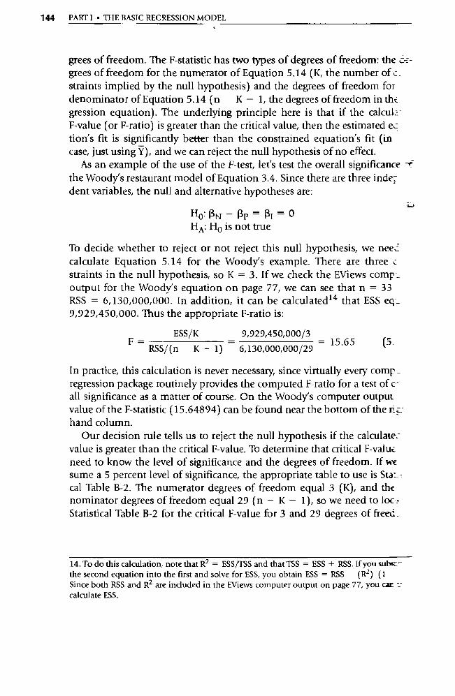
144 PARTI • THE BASIC REGRESSION MODEL
grees of freedom. The F-statistic has two types of degrees of freedom: the ,±-,-:- grees of freedom for the numerator of Equation 5.14 (K, the number of c: straints implied by the null hypothesis) and the degrees of freedom for denominator of Equation 5.14 (n K — 1, the degrees of freedom in the gression equation). The underlying principle here is that if the calculL -F-value (or F-ratio) is greater than the critical value, then the estimated ec. tion's fit is significantly better than the constrained equation's fit (in case, just using Ÿ), and we can reject the null hypothesis of no effect.
As an example of the use of the F-test, let's test the overall significance the Woody's restaurant model of Equation 3.4. Since there are three inde' dent variables, the null and alternative hypotheses are:
Ho: RN = Bp=(31=0 HA: Ho is not true
To decide whether to reject or not reject this null hypothesis, we nee. calculate Equation 5.14 for the Woody's example. There are three c straints in the null hypothesis, so K = 3. If we check the EViews comp _ output for the Woody's equation on page 77, we can see that n = 33 RSS = 6,130,000,000. In addition, it can be calculated 14 that ESS eq_ 9,929,450,000. Thus the appropriate F-ratio is:
ESS/K 9,929,450,000/3
F RSS/(n K — 1) 6,130,000,000/29 = 15.65 (5 .
In practice, this calculation is never necessary, since virtually every comp _ regression package routinely provides the computed F-ratio for a test of c -all significance as a matter of course. On the Woody's computer output value of the F-statistic (15.64894) can be found near the bottom of the ri hand column.
Our decision rule tells us to reject the null hypothesis if the calculate: value is greater than the critical F-value. To determine that critical F-value. need to know the level of significance and the degrees of freedom. If W€ sume a 5 percent level of significance, the appropriate table to use is Star_ - cal Table B-2. The numerator degrees of freedom equal 3 (K), and the nominator degrees of freedom equal 29 (n — K — 1), so we need to loc. Statistical Table B-2 for the critical F-value for 3 and 29 degrees of freed_
14. To do this calculation, note that R 2 = ESS/TSS and that TSS = ESS + RSS. If you sum the second equation into the first and solve for ESS, you obtain ESS = RSS (R2 ) (1 Since both RSS and R2 are included in the EViews computer output on page 77, you cat calculate ESS.
CHAPTER 5 • HYPOTHESIS TESTING 145
As the reader can verify, 15 Fc = 2.93 is well below the calculated F-value of 15.65, so we can reject the null hypothesis and conclude that the Woodÿ s equation does indeed have a significant overall fit.
Two final comments about the F-test of overall significance are in order. First, if there is only one independent variable, then an F-test and a t-test of whether the slope coefficient equals zero will always produce the same an-swer. (Indeed, it can be shown mathematically that the two tests are identi-cal.) This property does not hold if there are two or more independent vari-ables. In such a situation, an F-test could determine that the coefficients jointly are not significantly different from zero even though a t-test on one of the coefficients might show that individually it is significantly different from zero (or vice versa).
Finally, the F-statistic can be shown to be a direct function of R 2 The larger R2 is, the larger the F-ratio. Thus the F-test of overall significance is a test of the significance of R 2 itself. For more on this property, see Exercise 8.
5.6 Summary
1. Hypothesis testing makes inferences about the validity of specific eco-nomic (or other) theories from a sample of the population for which the theories are supposed to be true. The four basic steps of hypothe-sis testing (using a t-test as an example) are: a. Set up the null and alte rnative hypotheses. b. Choose a level of significance and, therefore, a critical t-value. c. Run the regression and obtain an estimated t-value. d. Apply the decision rule by comparing the calculated t-value with
the critical t-value in order to reject or "accept" the null hypothesis.
2. The null hypothesis states the range of values that the regression coef-ficient is expected to take on if the researcher's theory is not correct. The alternative hypothesis is a statement of the range of values that the regression coefficient is expected to take if the researcher's theory is correct.
3. The two kinds of errors we can make in such hypothesis testing are:
Type I: We reject a null hypothesis that is true.
15. Note that this critical F-value must be interpolated. The critical value for 30 denominator degrees of freedom is 2.92, and the critical value for 25 denominator degrees of freedom is 2.99. Since both numbers are well below the calculated F-value of 15.65, however, the interpo-lation isn't necessary to reject the null hypothesis. As a result, many researchers don't bother with such interpolations unless the calculated F-value is inside the range of the interpolation.

ESS /K E (Y; Y) 2 /K F =
RSS/(n — K 1) E e;/(n — K 1)
146 PART I • THE BASIC REGRESSION MODEL
Type II: We do not reject a null hypothesis that is false.
4. A decision rule states critical t-values above or below which observed sample t-values will lead to the rejection or "acceptance" of hypothe-ses concerning population parameters. Critical values are selected from a t-distribution table, depending on the chosen level of signifi-cance, the degrees of freedom involved, and the specifics of the partic-ular hypothesis.
5. The t-test tests hypotheses about individual coefficients from regres-sion equations. The general form for the t-statistic is
(Rk PH 0 ) ) tk = (k = 1, 2, , K)
SE(Rk)
In many regression applications, (3 H0 is zero. Once you have calcu-lated a t-value and chosen a critical t-value, you reject the null hypoth-esis if the t-value is greater in absolute value than the critical t-value and if the t-value has the sign implied by the alternative hypothesis.
6. The t-test is easy to use for a number of reasons, but care should be taken when using the t-test to avoid confusing statistical significance with theoretical validity or empirical impo rtance.
7. The F-test is a method of testing a null hypothesis that includes more than one coefficient. The F-test is used most frequently in economet-rics to test the overall significance of a regression equation with the following equation:
Once you've calculated an F and chosen a critical F-value, F e then you can reject the null hypothesis that implies that the overall fit of an equation is not significant if F
Exercises
(Answers to even-numbered exercises are in Appendix A.)
1. Write the meaning of each of the following terms without referring to the book (or your notes), and compare your definition with the ver-sion in the text for each. a. null hypothesis
CHAPTER 5 • HYPOTHESIS TESTING 147
b. alternative hypothesis c. Type I Error d. level of significance e. two-sided test f. decision rule g. critical value h. t-statistic i. t-test of the simple correlation coefficient j. F-test k. confidence interval
2. Create null and alternative hypotheses for the following coefficients: a. the impact of height on weight (Section 1.4) b. all the coefficients in Equation A in Exercise 7, Chapter 2 c. all the coefficients in Y = f(X 1 , X2 , and X3) where Y is total gasoline
used on a particular trip, X 1 is miles traveled, X2 is the weight of the car, and X3 is the average speed traveled
d. the impact of the decibel level of the grunt of a shot-putter on the length of the throw involved (shot-putters are known to make loud noises when they throw, but there is little theory about the impact of this yelling on the length of the put). Assume all relevant "non-grunt" variables are included in the equation.
3. Think of examples other than the ones in this chapter in which: a. It would be more important to keep Type I Error low than to keep
Type II Error low. b. It would be more important to keep Type II Error low than to keep
Type I Error low.
4. Return to Section 5.3 and test the hypotheses implied by Equation 5.6 with the results in Equation 5.7 for all three coefficients under the fol-lowing circumstances: a. 10 percent significance and 15 observations b. 90 percent confidence and 28 observations c. 99 percent confidence and 10 observations
5. Return to Section 5.2 and test the appropriate hypotheses with the re-sults in Equation 5.4 for all three coefficients under the following cir-cumstances: a. 5 percent significance and 6 degrees of freedom b. 90 percent confidence and 29 degrees of freedom c. 99 percent confidence and 2 degrees of freedom
6. Using the techniques of Section 5.3, test the following two-sided hy-potheses:

148 PART I • THE BASIC REGRESSION MODEL
a. For Equation 5.13, test the hypothesis that:
H0 :13 2 = 160.0 HA: R2 0 160.0
at the 5 percent level of significance. b. For Equation 5.4, test the hypothesis that:
Ho: 13 3 = 0 HA: P300
at the 99 percent level of confidence. c. For Equation 5.7, test the hypotheses that:
Ho: R2 = 0 HA: R2 0
at the 5 percent level of significance.
7 For all three tests in Exercise 6, under what circumstances would you worry about possible violations of the principle that the null hypoth-esis contains that which you do not expect to be true? In pa rticular, what would your theoretical expectations have to be in order to avoid violating this principle in Exercise 6a?
8. It turns out that the F-ratio can be expressed as a function of R 2 . a. As an exercise, substitute Equation 2.16 into Equations 5.14 to de-
rive the exact relationship between F and R 2 b. If one can be expressed as a function of the other, why do we need
both? What reason is there for computer regression packages to typically print out both R 2 and the F-ratio?
9. Test the overall significance of equations that have the following F-values (Using Statistical Table B-2): a. F = 5.63 with
4 degrees of freedom in the numerator and 30 degrees of freedom in the denominator
b. F = 1.53 with
3 degrees of freedom in the numerator and 24 degrees of freedom in the denominator
c. F = 57.84 with 5 degrees of freedom in the numerator and 60 degrees of freedom in the denominator
10. Given the following simple correlation coefficients between two ex-planatory variables, use the t-test (and Equation 5.11) to test the pos-sibility of significant collinearity in the specified circumstances: a. r = .905, n = 18, 5 percent level, positive expected relationship b. r = .958, n = 27, 2.5 percent level, positive expected relationship
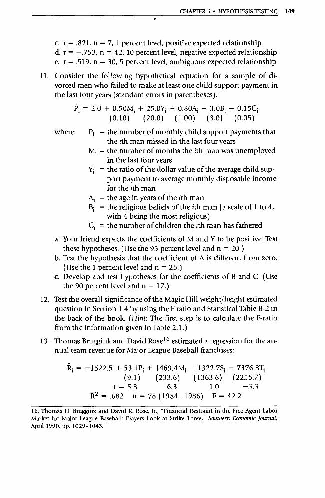
CHAPTER 5 • HYPOTHESIS TESTING 149
c. r = .821, n = 7, 1 percent level, positive expected relationship d. r = —.753, n = 42, 10 percent level, negative expected relationship e. r = .519, n = 30, 5 percent level, ambiguous expected relationship
11. Consider the following hypothetical equation for a sample of di-vorced men who failed to make at least one child support payment in the last four years- (standard errors in parentheses):
P; = 2.0+0.50Mî +25.0Yî +0.80A1 +3.0Bî -0.15Cî (0.10) (20.0) (1.00) (3.0) (0.05)
where: Pî = the number of monthly child suppo rt payments that the ith man missed in the last four years
Mi = the number of months the ith man was unemployed in the last four years
Y; = the ratio of the dollar value of the average child sup-port payment to average monthly disposable income for the ith man
A; = the age in years of the ith man B; = the religious beliefs of the ith man (a scale of 1 to 4,
with 4 being the most religious) C; = the number of children the ith man has fathered
a. Your friend expects the coefficients of M and Y to be positive. Test these hypotheses. (Use the 95 percent level and n = 20.)
b. Test the hypothesis that the coefficient of A is different from zero. (Use the 1 percent level and n = 25.)
c. Develop and test hypotheses for the coefficients of B and C. (Use the 90 percent level and n = 17.)
12. Test the overall significance of the Magic Hill weight/height estimated question in Section 1.4 by using the F ratio and Statistical Table B-2 in the back of the book. (Hint: The first step is to calculate the F-ratio from the information given in Table 2.1.)
13. Thomas Bruggink and David Rose 16 estimated a regression for the an-nual team revenue for Major League Baseball franchises:
Rî = —1522.5 + 53.1P î + 1469.4M; + 1322.7S; — 7376.3T;
(9.1) (233.6) (1363.6) (2255.7)
t = 5.8 6.3 1.0 — 3.3 R2 = .682 n = 78 (1984-1986) F = 42.2
16. Thomas H. Bruggink and David R. Rose, Jr., "Financial Restraint in the Free Agent Labor Market for Major League Baseball: Players Look at Strike Three," Southern Economic Journal, April 1990, pp. 1029-1043.
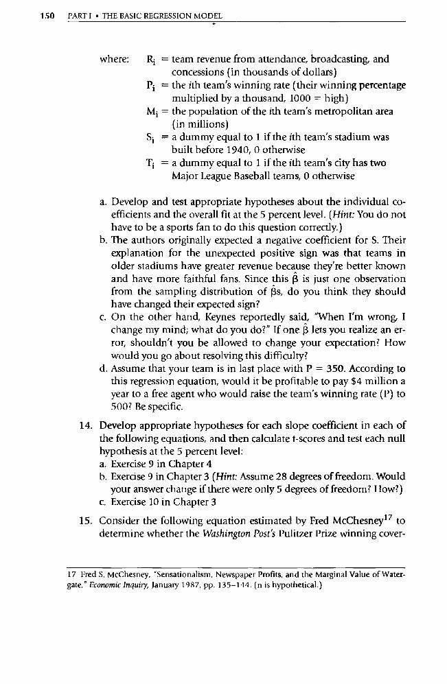
150 PARTI • THE BASIC REGRESSION MODEL
where: Ri = team revenue from attendance, broadcasting, and concessions (in thousands of dollars)
Pi = the ith team's winning rate (their winning percentage multiplied by a thousand, 1000 = high)
Mi = the population of the ith team's metropolitan area (in millions)
Si = a dummy equal to 1 if the ith team's stadium was built before 1940, 0 otherwise
Ti = a dummy equal to 1 if the ith team's city has two Major League Baseball teams, 0 otherwise
a. Develop and test appropriate hypotheses about the individual co-efficients and the overall fit at the 5 percent level. (Hint: You do not have to be a spo rts fan to do this question correctly.)
b. The authors originally expected a negative coefficient for S. Their explanation for the unexpected positive sign was that teams in older stadiums have greater revenue because they're better known and have more faithful fans. Since this R is just one observation from the sampling distribution of Rs, do you think they should have changed their expected sign?
c. On the other hand, Keynes reportedly said, "When I'm wrong, I change my mind; what do you do?" If one 13 lets you realize an er-ror, shouldn't you be allowed to change your expectation? How would you go about resolving this difficulty?
d. Assume that your team is in last place with P = 350. According to this regression equation, would it be profitable to pay $4 million a year to a free agent who would raise the team's winning rate (P) to 500? Be specific.
14. Develop appropriate hypotheses for each slope coefficient in each of the following equations, and then calculate t-scores and test each null hypothesis at the 5 percent level: a. Exercise 9 in Chapter 4 b. Exercise 9 in Chapter 3 (Hint: Assume 28 degrees of freedom. Would
your answer change if there were only 5 degrees of freedom? How?) c. Exercise 10 in Chapter 3
15. Consider the following equation estimated by Fred McChesney i7 to determine whether the Washington Post's Pulitzer Prize winning cover-
17 Fred S. McChesney, "Sensationalism, Newspaper Profits, and the Marginal Value of Water-gate," Economic Inquiry, January 1987, pp. 135-144. (n is hypothetical.)
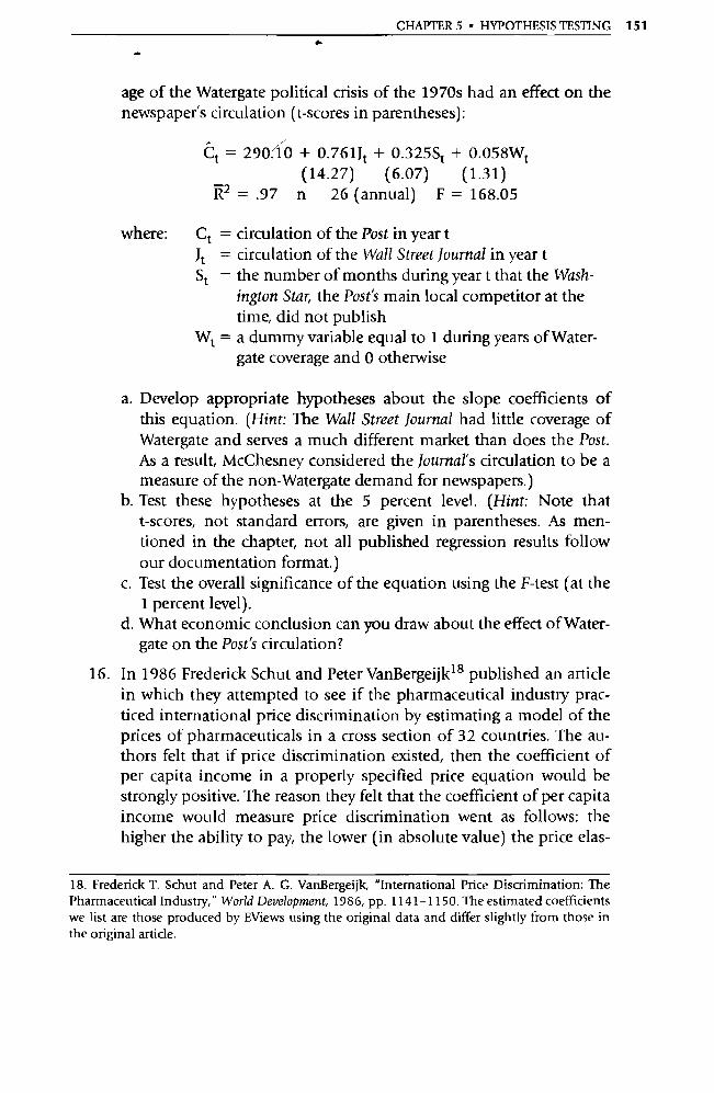
CHAPTER 5 • HYPOTHESIS TESTING 151
age of the Watergate political crisis of the 197Os had an effect on the newspaper's circulation (t-scores in parentheses):
Ct = 2900 + 0.761Jt + 0.325St + 0.058Wt (14.27) (6.07) (1.31)
R2 = .97 n 26 (annual) F = 168.05
where: Ct = circulation of the Post in year t Jt = circulation of the Wall Street Journal in year t St = the number of months during year t that the Wash-
ington Star, the Post's main local competitor at the time, did not publish
Wt = a dummy variable equal to 1 during years of Water-gate coverage and 0 otherwise
a. Develop appropriate hypotheses about the slope coefficients of this equation. (Hint: The Wall Street Journal had little coverage of Watergate and serves a much different market than does the Post. As a result, McChesney considered the Journal's circulation to be a measure of the non-Watergate demand for newspapers.)
b. Test these hypotheses at the 5 percent level. (Hint: Note that t-scores, not standard errors, are given in parentheses. As men-tioned in the chapter, not all published regression results follow our documentation format.)
c. Test the overall significance of the equation using the F-test (at the 1 percent level).
d. What economic conclusion can you draw about the effect of Water-gate on the Post's circulation?
16. In 1986 Frederick Schut and Peter VanBergeijk 18 published an article in which they attempted to see if the pharmaceutical industry prac-ticed international price discrimination by estimating a model of the prices of pharmaceuticals in a cross section of 32 countries. The au-thors felt that if price discrimination existed, then the coefficient of per capita income in a properly specified price equation would be strongly positive. The reason they felt that the coefficient of per capita income would measure price discrimination went as follows: the higher the ability to pay, the lower (in absolute value) the price elas-
18. Frederick T. Schut and Peter A. G. VanBergeijk, "International Price Disc rimination: The Pharmaceutical Industry," World Development, 1986, pp. 1141-1150. The estimated coefficients we list are those produced by EViews using the original data and differ slightly from those in the original article.
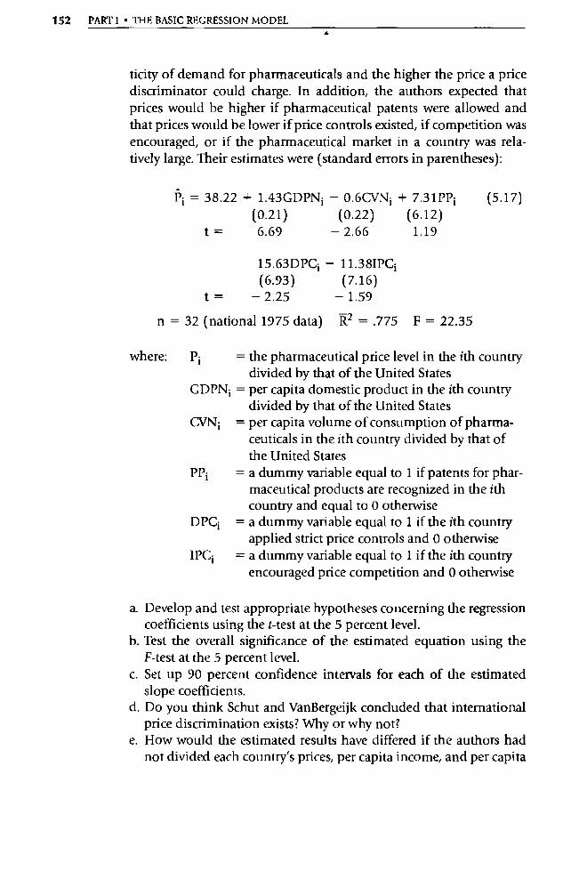
152 PARTI • THE BASIC REGRESSION MODEL
ticity of demand for pharmaceuticals and the higher the price a price discriminator could charge. In addition, the authors expected that prices would be higher if pharmaceutical patents were allowed and that prices would be lower if price controls existed, if competition was encouraged, or if the pharmaceutical market in a count ry was rela-tively large. Their estimates were (standard errors in parentheses):
(5.17) Pi = 38.22 + 1.43GDPNi — 0.6CVN i + 7.31PPi (0.21) (0.22) (6.12)
t = 6.69 — 2.66 1.19
15.63DPCi — 11.38IPCi
(6.93) (7.16)
— 2.25 — 1.59
n = 32 (national 1975 data) 12 = .775 F = 22.35
t=
where: Pi = the pharmaceutical price level in the ith count ry divided by that of the United States
GDPN; = per capita domestic product in the ith count ry divided by that of the United States
CVNi = per capita volume of consumption of pharma-ceuticals in the ith count ry divided by that of the United States
PPi = a dummy va riable equal to 1 if patents for phar- maceutical products are recognized in the ith country and equal to 0 otherwise
DPCi = a dummy variable equal to 1 if the ith count ry applied strict price controls and 0 otherwise
IPCi = a dummy va riable equal to 1 if the ith count ry encouraged price competition and 0 otherwise
a. Develop and test appropriate hypotheses concerning the regression coefficients using the t-test at the 5 percent level.
b. Test the overall significance of the estimated equation using the F-test at the 5 percent level.
c. Set up 90 percent confidence intervals for each of the estimated slope coefficients.
d. Do you think Schut and VanBergeijk concluded that international price discrimination exists? Why or why not?
e. How would the estimated results have differed if the authors had not divided each country's prices, per capita income, and per capita

CHAPTER 5 • HYPOTHESIS TESTING 153
pharmaceutical consumption by that of the United States? Explain your answer.
f. Reproduce their regression results by using the EViews computer program (datafile DRUGS5) or your own computer program and the data from Table 5.1.
TABLE 5.1 DATA FOR THE PHARMACEUTICAL PRICE DISCRIMINATION EXERCISE
Country P GDPN CV N CVN PP IPC DPC
Malawi 60.83 4.9 0.014 2.36 0.6 1 0 0
Kenya 50.63 6.56 0.07 6.27 1.1 1 0 0 India 31.71 6.56 18.66 282.76 6.6 0 0 1
Pakistan 38.76 8.23 3.42 32.9 10.4 0 1 1
Sri Lanka 15.22 9.3 0.42 6.32 6.7 1 1 1
Zambia 96.58 10.3 0.05 2.33 2.2 1 0 0
Thailand 48.01 13.0 2.21 19.60 11.3 0 0 0
Philippines 51.14 13.2 0.77 19.70 3.9 1 0 0
South Korea 435.10 20.7 2.20 16.52 13.3 0 0 0 Malaysia 70.74 21.5 0.50 5.58 8.9 1 0 0 Colombia 48.07 22.4 1.56 11.09 14.1 0 1 0
Jamaica 46.13 24.0 0.21 0.96 22.0 1 0 0
Brazil 63.83 25.2 10.48 50.17 21.6 0 1 0
Mexico 69.68 34.7 7.77 28.16 27.6 0 0 0
Yugoslavia 48.24 36.1 3.83 9.42 40.6 0 1 1
Iran 70.42 37.7 3.27 15.33 21.3 0 0 0 Uruguay 65.95 39.6 0.44 1.30 33.8 0 0 0
Ireland 73.58 42.5 0.57 1.49 38.0 1 0 0
Hungary 57.25 49.6 2.36 4.94 47.8 0 1 1
Poland 53.98 50.1 8.08 15.93 50.7 0 1 1
Italy 69.01 53.8 12.02 26.14 45.9 0 0 1
Spain 69.68 55.9 9.01 16.63 54.2 0 0 0
United Kingdom 71.19 63.9 9.96 26.21 38.0 1 1 1
Japan 81.88 68.4 28.58 52.24 54.7 0 0 1
Austria 139.53 69.6 1.24 3.52 35.2 0 0 0
Netherlands 137.29 75.2 1.54 6.40 24.1 1 0 0 Belgium 101.73 77.7 3.49 4.59 76.0 1 0 1
France 91.56 81.9 25.14 24.70 101.8 1 0 1 Luxembourg 100.27 82.0 0.10 0.17 60.5 1 0 1 Denmark 157.56 82.4 0.70 2.35 29.5 1 0 0
Germany, West 152.52 83.0 24.29 28.95 83.9 1 0 0
United States 100.00 100.0 100.00 100.00 100.0 1 1 0
Source: Frederick T. Schut and Peter A.G. VanBergeijk, "International Price Discrimination: The Pharmaceutical Industry," World Development, 1986, p. 1144.
Note: filename = DRUGS5

II PA RT
VIOLATIONS OF THE
CLASSICAL ASSUMPTIONS

6 CHAPTER
Specification: Choosing the Independent Variables
6.1 Omitted Variables
6.2 Irrelevant Variables
6.3 An Illustration of the Misuse of Specification Criteria
6.4 Specification Searches
6.5 Lagged Independent Variables
6.6 An Example of Choosing Independent Variables
6.7 Summary and Exercises
6.8 Appendix: Additional Specification Criteria
Before any equation can be estimated, it must be completely specified. Speci-fying an econometric equation consists of three parts: choosing the correct independent variables, the correct functional form, and the correct form of the stochastic error term.
A specification error results when any one of these choices is made incor-rectly. This chapter is concerned with only the first of these, choosing the variables; the second and third will be taken up in later chapters.
That researchers can decide which independent va riables to include in re-gression equations is a source of both strength and weakness in economet-rics. The strength is that the equations can be formulated to fit individual needs, but the weakness is that researchers can estimate many different speci-fications until they find the one that "proves" their point, even if many other results disprove it. A major goal of this chapter is to help you understand how to choose variables for your regressions without falling prey to the vari-ous errors that result from misusing the ability to choose.
The primary consideration in deciding if an independent va riable belongs in an equation is whether the variable is essential to the regression on the ba-sis of theory. If the answer is an unambiguous yes, then the variable definitely
156
CHAPTER 6 • SPECIFICATION: CHOOSING THE INDEPENDENT VARIABLES 157
AO
should be included in the equation, even if it seems to be lacking in statisti-cal significance. If theory is ambivalent or less emphatic, a dilemma arises. Leaving a relevant variable out of an equation is likely to bias the remaining estimates, but including an irrelevant variable leads to higher variances of the estimated coefficients. Although we'll develop statistical tools to help us deal with this decision, it's difficult in practice to be sure that a variable is rele-vant, and so the problem often remains unresolved.
We devote the fourth section of the chapter to specification searches and the pros and cons of various approaches to such searches. For example, tech-niques like stepwise regression procedures and sequential specification searches often cause bias or make the usual tests of significance inapplicable, and we do not recommend them. Instead, we suggest trying to minimize the number of regressions estimated and relying as much as possible on theory rather than statistical fit when choosing variables. There are no pat answers, however, and so the final decisions must be left to each individual researcher.
6.1 Omitted Variables
Suppose that you forget to include all the relevant independent variables when you first specify an equation (after all, no one's perfect!). Or suppose that you can't get data for one of the variables that you do think of. The result in both these situations is an omitted variable, defined as an important ex-planatory variable that has been left out of a regression equation.
Whenever you have an omitted (or left-out) variable, the interpretation and use of your estimated equation become suspect. Leaving out a relevant vari-able, like price from a demand equation, not only prevents you from getting an estimate of the coefficient of price but also usually causes bias in the esti-mated coefficients of the variables that are in the equation.
The bias caused by leaving a variable out of an equation is called omitted variable bias (or, more generally, specification bias.) In an equation with more than one independent va riable, the coefficient (3 k represents the change in the dependent variable Y caused by a one-unit increase in the independent variable Xk, holding constant the other independent variables in the equa-tion. If a variable is omitted, then it is not included as an independent vari-able, and it is not held constant for the calculation and interpretation of (3k. This omission can cause bias: It can force the expected value of the estimated coefficient away from the true value of the population coefficient.
Thus, omitting a relevant variable is usually evidence that the entire esti-mated equation is suspect because of the likely bias in the coefficients of the variables that remain in the equation. Let's look at this issue in more detail.
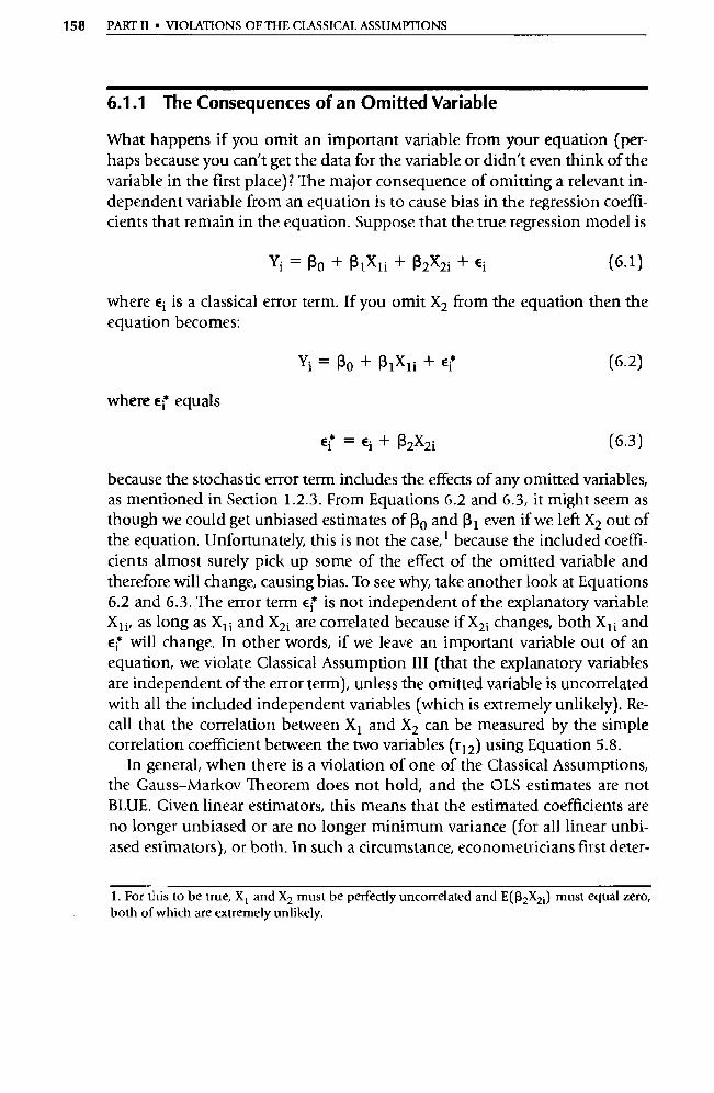
158 PART II • VIOLATIONS OF THE CLASSICAL ASSUMPTIONS
6.1.1 The Consequences of an Omitted Variable
What happens if you omit an impo rtant variable from your equation (per-haps because you can't get the data for the variable or didn't even think of the variable in the first place)? The major consequence of omitting a relevant in-dependent variable from an equation is to cause bias in the regression coeffi-cients that remain in the equation. Suppose that the true regression model is
Yi = R O + R 1X1 i + R2X2i + Ei
where Ei is a classical error term. If you omit X2 from the equation then the equation becomes:
Yi = Ro + 131X + Ei (6.2)
where Ei equals
Ei = Ei + R2X2i (6.3)
because the stochastic error term includes the effects of any omitted va riables, as mentioned in Section 1.2.3. From Equations 6.2 and 6.3, it might seem as though we could get unbiased estimates of 3 o and 13 1 even if we left X2 out of the equation. Unfortunately, this is not the case, 1 because the included coeffi-cients almost surely pick up some of the effect of the omitted variable and therefore will change, causing bias. To see why, take another look at Equations 6.2 and 6.3. The error term Ei is not independent of the explanatory va riable X 1 i, as long as Xli and X2i are correlated because if X2 i changes, both X li and Ei will change. In other words, if we leave an impo rtant va riable out of an equation, we violate Classical Assumption III (that the explanatory va riables are independent of the error term), unless the omitted va riable is uncorrelated with all the included independent variables (which is extremely unlikely). Re-call that the correlation between X 1 and X2 can be measured by the simple correlation coefficient between the two va riables (r 12) using Equation 5.8.
In general, when there is a violation of one of the Classical Assumptions, the Gauss-Markov Theorem does not hold, and the OLS estimates are not BLUE. Given linear estimators, this means that the estimated coefficients are no longer unbiased or are no longer minimum variance (for all linear unbi-ased estimators), or both. In such a circumstance, econometricians first deter-
(6.1)
1. For this to be true, X 1 and X2 must be perfectly uncorrelated and E(132X2i) must equal zero, both of which are extremely unlikely.
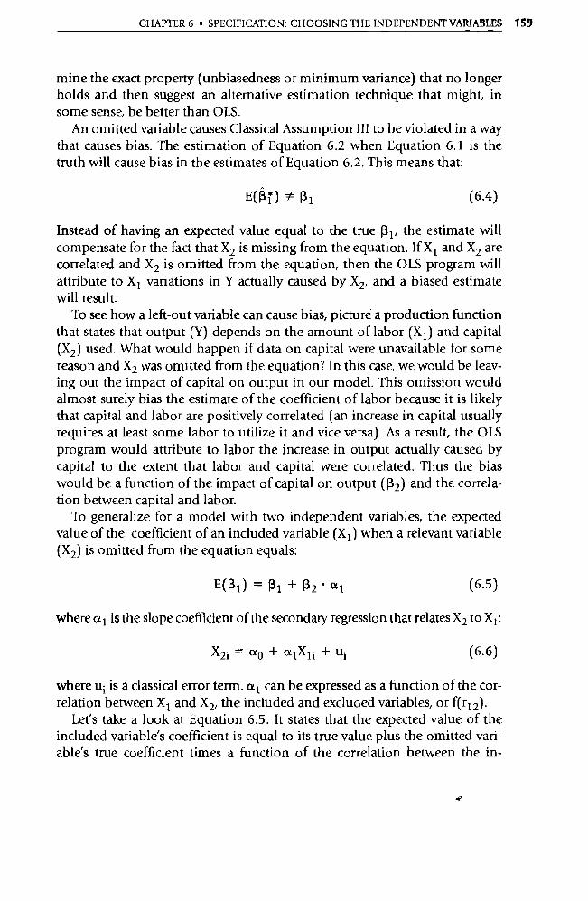
CHAPTER 6 • SPECIFICATION: CHOOSING THE INDEPENDENT VARIABLES 159
mine the exact property (unbiasedness or minimum va riance) that no longer holds and then suggest an alternative estimation technique that might, in some sense, be better than OLS.
An omitted variable causes Classical Assumption III to be violated in a way that causes bias. The estimation of Equation 6.2 when Equation 6.1 is the truth will cause bias in the estimates of Equation 6.2. This means that:
E(Ri) # RI
Instead of having an expected value equal to the true R1, the estimate will compensate for the fact that X2 is missing from the equation. If X 1 and X2 are correlated and X2 is omitted from the equation, then the OLS program will attribute to X 1 variations in Y actually caused by X2, and a biased estimate will result.
To see how a left-out variable can cause bias, picture a production function that states that output (Y) depends on the amount of labor (X 1 ) and capital (X2) used. What would happen if data on capital were unavailable for some reason and X2 was omitted from the equation? In this case, we would be leav-ing out the impact of capital on output in our model. This omission would almost surely bias the estimate of the coefficient of labor because it is likely that capital and labor are positively correlated (an increase in capital usually requires at least some labor to utilize it and vice versa). As a result, the OLS program would attribute to labor the increase in output actually caused by capital to the extent that labor and capital were correlated. Thus the bias would be a function of the impact of capital on output (3 2) and the correla-tion between capital and labor.
To generalize for a model with two independent variables, the expected value of the coefficient of an included variable (X 1 ) when a relevant variable (X2) is omitted from the equation equals:
E(13 1) = 01 + 132 • al (6.5)
where a l is the slope coefficient of the secondary regression that relates X2 to X1 :
X2i= a0 +a lXli +ui (6.6)
where ui is a classical error term. a l can be expressed as a function of the cor-relation between X 1 and X2, the included and excluded va riables, or f(r12).
Let's take a look at Equation 6.5. It states that the expected value of the included variable's coefficient is equal to its true value plus the omitted vari-able's true coefficient times a function of the correlation between the in-
(6.4)
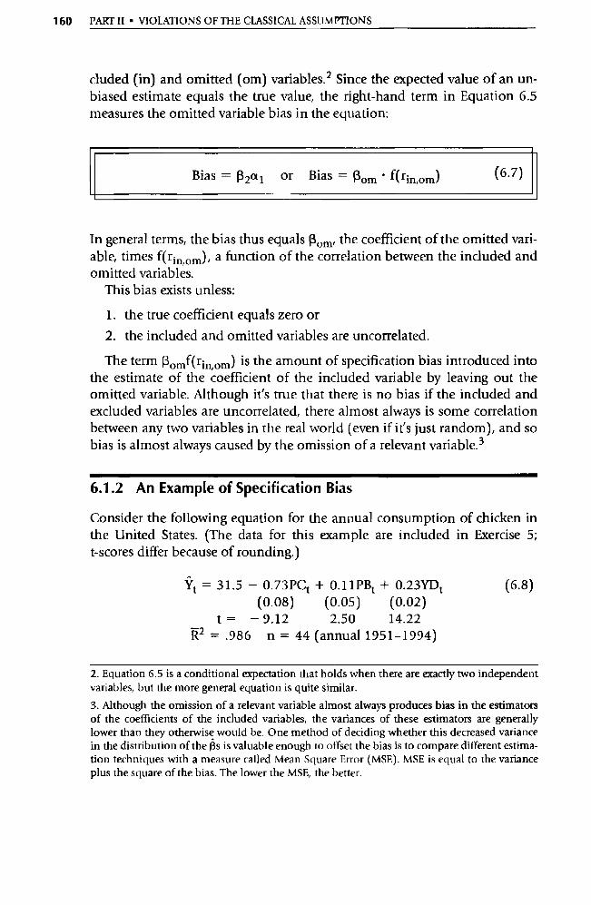
160 PART II • VIOLATIONS OF THE CLASSICAL ASSUMPTIONS
cluded (in) and omitted (om) variables. 2 Since the expected value of an un-biased estimate equals the true value, the right-hand term in Equation 6.5 measures the omitted variable bias in the equation:
Bias = 13 2a 1 or Bias = Rom • f(rin,om)
(6.7)
In general terms, the bias thus equals Rom, the coefficient of the omitted vari-able, times f(rin,om), a function of the correlation between the included and omitted variables.
This bias exists unless:
1. the true coefficient equals zero or 2. the included and omitted variables are uncorrelated.
The term Romf(rin,om) is the amount of specification bias introduced into the estimate of the coefficient of the included variable by leaving out the omitted variable. Although it's true that there is no bias if the included and excluded variables are uncorrelated, there almost always is some correlation between any two variables in the real world (even if it's just random), and so bias is almost always caused by the omission of a relevant variable. 3
6.1.2 An Example of Specification Bias
Consider the following equation for the annual consumption of chicken in the United States. (The data for this example are included in Exercise 5; t-scores differ because of rounding.)
Ÿt = 31.5 — 0.73PCt + 0.11PBt + 0.23YDt (6.8)
(0.08) (0.05) (0.02)
t = — 9.12 2.50 14.22 R2 = .986 n = 44 (annual 1951-1994)
2. Equation 6.5 is a conditional expectation that holds when there are exactly two independent variables, but the more general equation is quite similar. 3. Although the omission of a relevant variable almost always produces bias in the estimators of the coefficients of the included va riables, the va riances of these estimators are generally lower than they otherwise would be. One method of deciding whether this decreased variance in the distribution of the (3s is valuable enough to offset the bias is to compare different estima-tion techniques with a measure called Mean Square Error (MSE). MSE is equal to the va riance plus the square of the bias. The lower the MSE, the better.
CHAPTER 6 • SPECIFICATION: CHOOSING THE INDEPENDENT VARIABLES 161
where: Yt = per capita chicken consumption (in pounds) in year t PCt = the price of chicken (in cents per pound) in year t PBt = the price of beef (in cents per pound) in year t YDt = U.S. per capita disposable income (in hundreds of dollars)
in year t
This equation is a simple demand for chicken equation that includes the prices of chicken and a close substitute (beef) and an income variable. Note that the signs of the estimated coefficients agree with the signs you would have hypothesized before seeing any regression results.
If we estimate this equation without the price of the substitute, we obtain:
Yt 32.9 — 0.70PCt + 0.27YDt
(0.08) (0.01)
t = — 8.33 45.91 R2 = .984 n = 44 (annual 1951-1994)
(6.9)
Let's compare Equations 6.8 and 6.9 to see if dropping the beef price va riable had an impact on the estimated equations. If you compare the overall fit, for example, you can see that R 2 fell slightly from .986 to .984 when PB was dropped, exactly what we'd expect to occur when a relevant variable is omitted.
More important, from the point of view of showing that an omitted vari-able causes bias, let's see if the coefficient estimates of the remaining vari-ables changed. Sure enough, dropping PB caused 14 c to go from —0.73 to —0.70 and caused 4-E, to go from 0.23 to 0.27 The direction of this bias, by the way, is considered positive because the biased coefficient of PC ( —0.70) is more positive (less negative) than the suspected unbiased one ( —0.73) and the biased coefficient of YD (0.27) is more positive than the suspected unbiased one of (0.23).
The fact that the bias is positive could have been guessed before any regres-sions were mn if Equation 6.7 had been used. The specification bias caused by omitting the price of beef is expected 4 to be positive because the expected sign of the coefficient of PB is positive and because the expected correlation between the price of beef and the price of chicken itself is positive:
4. It is important to note the distinction between expected bias and any actual observed differ-ences between coefficient estimates. Because of the random nature of the error term (and hence the (s), the change in an estimated coefficient brought about by dropping a relevant va riable from the equation will not necessarily be in the expected direction. Biasedness refers to the central tendency of the sampling distribution of the (3' 3s, not to every single drawing from that distribu-tion. However, we usually (and justifiably) rely on these general tendencies. Note also that Equa-tion 6.8 has three independent va riables whereas Equation 6.7 was derived for use with equations with exactly two. However, Equation 6.7 represents a general tendency that is still applicable.

162 PART II • VIOLATIONS OF THE CLASSICAL ASSUMPTIONS
Expected bias in RPc = 13PB • f(rpc,pB) = (+) (+) = (+)
Similarly for YD:
Expected bias in RYD = RPB • f(rYD,PB) = (+) (+) _ (+)
Note that both correlation coefficients are anticipated to be (and actually are) positive. To see this, think of the impact of an increase in the price of chicken on the price of beef and then follow through the impact of any in-crease in income on the price of beef.
To sum, if a relevant variable is left out of a regression equation 1. there is no longer an estimate of the coefficient of that variable in the
equation, and 2. the coefficients of the remaining variables are likely to be biased.
Although the amount of the bias might not be very large in some cases (when, for instance, there is little correlation between the included and ex-cluded variables), it is extremely likely that at least a small amount of specifi-cation bias will be present in all such situations.
6.1.3 Correcting for an Omitted Variable
In theory, the solution to a problem of specification bias seems easy: Simply add the omitted variable to the equation. Unfortunately, that's more easily said than done, for a couple of reasons.
First, omitted variable bias is hard to detect. As mentioned above, the amount of bias introduced can be small and not immediately detectable. This is especially true when there is no reason to believe that you have mis-specified the model. Some indications of specification bias are obvious (such as an estimated coefficient that is significant in the direction opposite from that expected), but others are not so clear. Could you tell from Equation 6.9 alone that a variable was missing? The best indicators of an omitted relevant variable are the theoretical underpinnings of the model itself. What variables must be included? What signs do you expect? Do you have any notions about the range into which the coefficient values should fall? Have you accidentally left out a variable that most researchers would agree is important? The best way to avoid omitting an impo rtant variable is to invest the time to think carefully through the equation before the data are entered into the computer.
A second source of complexity is the problem of choosing which variable to add to an equation once you decide that it is suffering from omitted vari-able bias. That is, a researcher faced with a clear case of specification bias
CHAPTER 6 • SPECIFICATION: CHOOSING THE INDEPENDENT VARIABLES 163
(like an estimated (3 that is significantly different from zero in the unexpected direction) will often have no clue as to what variable could be causing the problem. Some beginning researchers, when faced with this dilemma, will add all the possible relevant variables to the equation at once, but this process leads to less precise estimates, as will be discussed in the next section. Other beginning researchers will test a number of different variables and keep the one in the equation that does the best statistical job of appearing to reduce the bias (by giving plausible signs and satisfactory t-values). This tech-nique, adding a "left-out" va riable to "fix" a strange-looking regression result, is invalid because the variable that best corrects a case of specification bias might do so only by chance rather than by being the true solution to the problem. In such an instance, the "fixed" equation may give superb statistical results for the sample at hand but then do terribly when applied to other samples because it does not describe the characteristics of the true popula-tion.
Dropping a variable will not help cure omitted variable bias. If the sign of an estimated coefficient is different from expected, it cannot be changed to the expected direction by dropping a variable that has a t-score lower (in ab-solute value) than the t-score of the coefficient estimate that has the unex-pected sign. Furthermore, the sign in general will not likely change even if the variable to be deleted has a large t-score. 5
If the estimated coefficient is significantly different from our expectations (either in sign or magnitude), then it is extremely likely that some so rt of specification bias exists in our model. Although it is true that a poor sample of data or a poorly theorized expectation may also yield statistically signifi-cant unexpected signs or magnitudes, these possibilities sometimes can be eliminated.
If an unexpected result leads you to believe that you have an omitted vari-able, one way to decide which variable to add to the equation is to use ex-pected bias analysis. Expected bias is the likely bias that omitting a particular variable would have caused in the estimated coefficient of one of the in-cluded variables. It can be estimated with Equation 6.7:
Expected bias = Rom - f(rin,om) (6.7)
If the sign of the expected bias is the same as the sign of your unexpected re- sult, then the variable might be the source of the apparent bias. If the sign of the expected bias is not the same as the sign of your unexpected result, how-
5. Ignazio Visco, "On Obtaining the Right Sign of a Coefficient Estimate by Omitting a Va riable from the Regression, Journal of Econometrics, February 1978, pp. 115-117.
164 PART II • VIOLATIONS OF THE CLASSICAL ASSUMPTIONS .
ever, then the va riable is extremely unlikely to have caused your unexpected result. Expected bias analysis should be used only when an equation has ob-vious bias (like a coefficient that is significant in an unexpected direction) and only when you're choosing between theoretically sound potential vari-ables.
As an example of expected bias analysis, let's return to Equation 6.9, the chicken demand equation without the beef price variable. Let's assume that you had expected the coefficient of Rpc to be in the range of —1.0 and that you were surprised by the unexpectedly positive coefficient of PC in Equation 6.9. (As you can see by comparing Equations 6.8 and 6.9, your expectation was reasonable, but you can never be sure of this fact in practice.)
This unexpectedly positive result could not have been caused by an omit-ted variable with negative expected bias but could have been caused by an omitted variable with positive expected bias. One such variable is the price of beef. The expected bias in RPC due to leaving out PB is positive since both the expected coefficient of PB and the expected correlation between PC and PB are positive:
Expected bias in Rpc = NB ' f(rPC,PB) = (+) (+) = (+)
Hence the price of beef is a reasonable candidate to be omitted variable in Equation 6.9.
Although you can never actually observe bias (since you don't know the true (3), the use of this technique to screen potential causes of specification bias should reduce the number of regressions run and therefore increase the statistical validity of the results. This technique will work best when only one (or one kind of) variable is omitted from the equation in question. With a number of different kinds of variables omitted simultaneously, the impact on the equation's coefficients is quite hard to specify.
A brief warning: It may be tempting to conduct what might be called "residual analysis" by examining a plot of the residuals in an attempt to find patterns that suggest va riables that have been accidentally omitted. A major problem with this approach is that the coefficients of the estimated equation will possibly have some of the effects of the left-out variable already altering their estimated values. Thus, residuals may show a pattern that only vaguely resembles the pattern of the actual omitted variable. The chances are high that the pattern shown in the residuals may lead to the selection of an incor- rect variable. In addition, care should be taken to use residual analysis only to choose between theoretically sound candidate variables rather than to generate those candidates.

Q2 VAR(R 1 ) _
(x i - XI) 2 (6.14)
CHAPTER 6 • SPECIFICATION: CHOOSING THE INDEPENDENT VARIABLES 165
6.2 Irrelevant Variables
What happens if you include a variable in an equation that doesn't belong there? This case, irrelevant variables, is the converse of omitted variables and can be analyzed using the model we developed in Section 6.1. Whereas the omitted variable model has more independent variables in the true model than in the estimated equation, the irrelevant variable model has more inde-pendent variables in the estimated equation than in the true one.
The addition of a variable to an equation where it doesn't belong does not cause bias, but it does increase the variances of the estimated coefficients of the included variables.
6.2.1 Impact of Irrelevant Variables
If the true regression specification is
Y; =Ro +R I X1i + Ei
but the researcher for some reason includes an extra va riable,
Yi= Ro+R1X1i+ R2X2i + E1 *
the misspecified equation's error term can be seen to be:
** Ei = Ei 2 2i
(6.10)
(6.11)
(6.12)
Such a mistake will not cause bias if the true coefficient of the extra (or irrele-vant) variable is zero. In that case, Ei = * That is, RI in Equation 6.11 is unbiased when R2 = O.
However, the inclusion of an irrelevant va riable will increase the variance of the estimated coefficients, and this increased variance will tend to decrease the absolute magnitude of their t-scores. Also, an irrelevant variable usually will decrease the R 2 (but not the R 2). In a model of Y on X 1 and X2, the vari-ance of the OLS estimator of RI is:
Q 2 VAR(R1) - (1 - ri2) (X1 X1) 2
If the irrelevant variable is not in the equation (or if r 12 = 0), then:
(6.13)
166 PART II • VIOLATIONS OF THE CLASSICAL ASSUMPTIONS
Thus, although the irrelevant variable causes no bias, it causes problems for the regression because it reduces the precision of the regression.
To see why this is so, try plugging a nonzero value (between +1.0 and -1.0) for r 12 into Equation 6.13 and note that VAR(R 1 ) has increased when compared to Equation 6.14. The equation with an included variable that does not belong in the equation usually has lower t-scores and a lower R 2 than it otherwise would. The property holds, by the way, only when r 12 ± 0, but since this is the case in virtually every sample, the conclusion of increased vari-ance due to irrelevant variables is a valid one. Table 6.1 summarizes the conse-quences of the omitted variable and the included irrelevant variable cases:
TABLE 6.1 EFFECT OF OMITTED VARIABLES AND IRRELEVANT VARIABLES ON THE COEFFICIENT ESTIMATES
Effect on Coefficient Estimates
Omitted Variable
Irrelevant Variable
Bias
Yes*
No
Variance
Decreases*
Increases*
*Unless ru = O.
6.2.2 An Example of an Irrelevant Variable
Let's return to the equation from Section 6.1 for the annual consumption of chicken and see what happens when we add an irrelevant variable to the equation. The original equation was:
Yt = 31.5 - 0.73PCt + 0.11PBt + 0.23YDt
(0.08) (0.05) (0.02)
t = - 9.12 2.50 14.22 R2 = .986 n = 44 (annual 1951-1994)
(6.8)
Suppose you hypothesize that the demand for chicken also depends on R, the interest rate (which, perhaps, confuses the demand for a nondurable good with an equation you saw for a consumer durable). If you now estimate the equation with the interest rate included, you obtain:
Yt = 30.0 - 0.73PCt + 0.12PBt + 0.22YDt + 0.17Rt
(0.08) (0.06) (0.02) (0.21)
t = - 9.10 2.08 11.05 0.82 R2 = .985 n = 44 (annual 1951-1994)
(6.15)
CHAPTER 6 • SPECIFICATION: CHOOSING THE INDEPENDENT VARIABLES 167
A comparison of Equations 6.8 and 6.15 will make the theory in Section 6.2.1 come to life. First of all, R 2 has fallen slightly, indicating the reduction in fit adjusted for degrees of freedom. Second, none of the regression coeffi-cients from the original equation changed significantly; compare these re-sults with the larger differences between Equations 6.8 and 6.9. Further, slight increases in the standard errors of the estimated coefficients took place. Finally, the t-score for the potential va riable (the interest rate) is very small, indicating that it is not significantly different from zero. Given the theoretical shakiness of the new variable, these results indicate that it is irrelevant and never should have been included in the regression.
6.2.3 Four Important Specification Criteria
We have now discussed at least four valid criteria to help decide whether a given variable belongs in the equation. We think these criteria are so impor-tant that we urge beginning researchers to work through them every time a variable is added or subtracted.
1. Theory: Is the variable's place in the equation unambiguous and theoretically sound?
2. t-Test: Is the variable's estimated coefficient significant in the ex-pected direction?
3. R2 • Does the overall fit of the equation (adjusted for degrees of freedom) improve when the variable is added to the equation?
4. Bias: Do other va riables' coefficients change significantly when the variable is added to the equation?
If all these conditions hold, the variable belongs in the equation; if none of them do, the va riable is irrelevant and can be safely excluded from the equa-tion. When a typical omitted relevant va riable is included in the equation, its inclusion probably will increase R2 and change other coefficients. If an irrele-vant variable, on the other hand, is included, it will reduce R 2, have an in-significant t-score, and have little impact on the other va riables' coefficients.
In many cases, all four criteria do not agree. It is possible for a variable to have an insignificant t-score that is greater than one, for example. In such a case, it can be shown that R 2 will go up when the variable is added to the equation and yet the t-score will still be insignificant.

168 PART II • VIOLATIONS OF THE CLASSICAL ASSUMPTIONS
Whenever the four criteria for whether a va riable should be included in an equation disagree, the econometrician must use careful judgment and should not rely on a single criterion like k2 to determine the specification. Re-searchers should not misuse this freedom by testing various combinations of variables until they find the results that appear to statistically suppo rt the point they want to make. All such decisions are a bit easier when you realize that the single most impo rtant determinant of a variable's relevance is its the-oretical justification. No amount of statistical evidence should make a theo-retical necessity into an "irrelevant" variable. Once in a while, a researcher is forced to leave a theoretically impo rtant variable out of an equation for lack of a better alternative; in such cases, the usefulness of the equation is limited.
6.3 An Illustration of the Misuse of Specification Criteria
At times, the four specification criteria outlined in the previous section will lead the researcher to an incorrect condusion if those criteria are applied blindly to a problem without the proper concern for economic principles or common sense. In pa rticular, a t-score can often be insignificant for reasons other than the presence of an irrelevant variable. Since economic theory is the most impo rtant test for including a va riable, an example of why a vari-able should not be dropped from an equation simply because it has an in-significant t-score is in order.
Suppose you believe that the demand for Brazilian coffee in the United States is a negative function of the real price of Brazilian coffee (PO and a positive function of both the real price of tea (P t) and real disposable income in the United States (Yd). 6 Suppose further that you obtain the data, run the implied regression, and observe the following results:
COFFEE = 9.1 + 7.8Pbc + 2.4P1 + 0.0035Yd
(15.6) (1.2) (0.0010)
t = 0.5 2.0 3.5 R2 = .60 n= 25
(6.16)
The coefficients of the second and third va riables, Pt and Yd, appear to be fairly significant in the direction you hypothesized, but the first va riable, Pbc, appears to have an insignificant coefficient with an unexpected sign. If you
6. This example was inspired by a similar one concerning Ceylonese tea published in Potluri Rao and Roger LeRoy Miller, Applied Econometrics (Belmont, California: Wadsworth, 1971), pp. 38-40. This book is now out of print.
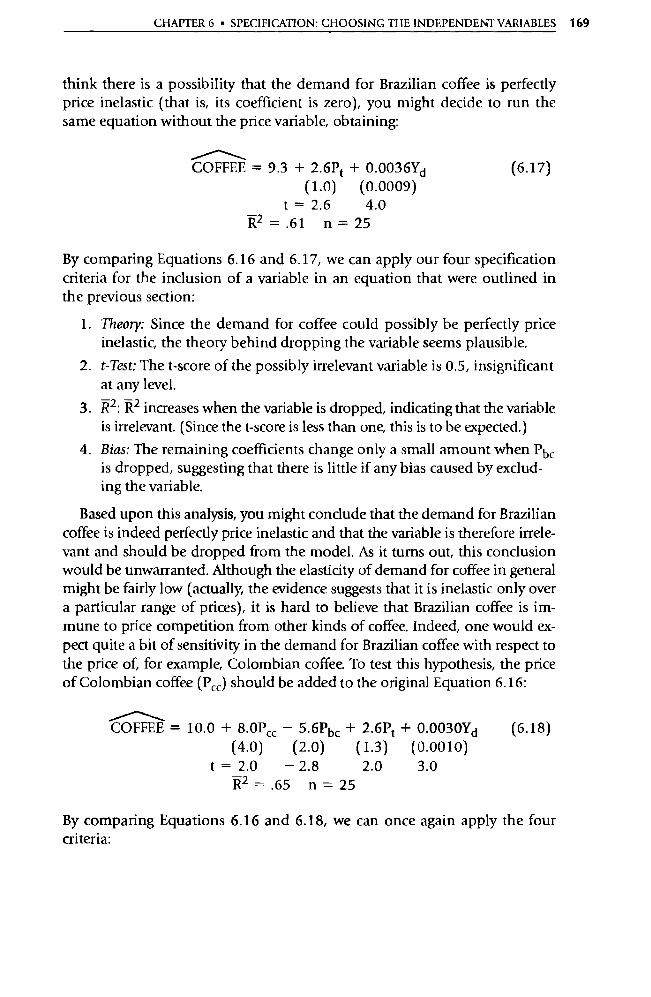
CHAPTER 6 • SPECIFICATION: CHOOSING THE INDEPENDENT VARIABLES 169
think there is a possibility that the demand for Brazilian coffee is perfectly price inelastic (that is, its coefficient is zero), you might decide to run the same equation without the price va riable, obtaining:
COFFEE = 9.3 + 2.6Pt + 0.0036Yd (6.17)
(1.0) (0.0009)
t = 2.6 4.0 R2 =.61 n=25
By comparing Equations 6.16 and 6.17, we can apply our four specification criteria for the inclusion of a variable in an equation that were outlined in the previous section:
1. Theory: Since the demand for coffee could possibly be perfectly price inelastic, the theory behind dropping the variable seems plausible.
2. t-Test: The t-score of the possibly irrelevant variable is 0.5, insignificant at any level.
3. R2 : R2 increases when the variable is dropped, indicating that the va riable is irrelevant. (Since the t-score is less than one, this is to be expected.)
4. Bias: The remaining coefficients change only a small amount when Pbc is dropped, suggesting that there is little if any bias caused by exclud-ing the variable.
Based upon this analysis, you might conclude that the demand for Brazilian coffee is indeed perfectly price inelastic and that the va riable is therefore irrele-vant and should be dropped from the model. As it turns out, this conclusion would be unwarranted. Although the elasticity of demand for coffee in general might be fairly low (actually, the evidence suggests that it is inelastic only over a particular range of prices), it is hard to believe that Brazilian coffee is im-mune to price competition from other kinds of coffee. Indeed, one would ex-pect quite a bit of sensitivity in the demand for Brazilian coffee with respect to the price of, for example, Colombian coffee. To test this hypothesis, the price of Colombian coffee (P cc) should be added to the original Equation 6.16:
COFFEE = 10.0 + 8.0Pcc — 5.6Pbc + 2.6Pt + 0.0030Yd (6.18) (4.0) (2.0) (1.3) (0.0010)
t = 2.0 — 2.8 2.0 3.0 R2 =.65 n=25
By comparing Equations 6.16 and 6.18, we can once again apply the four criteria:
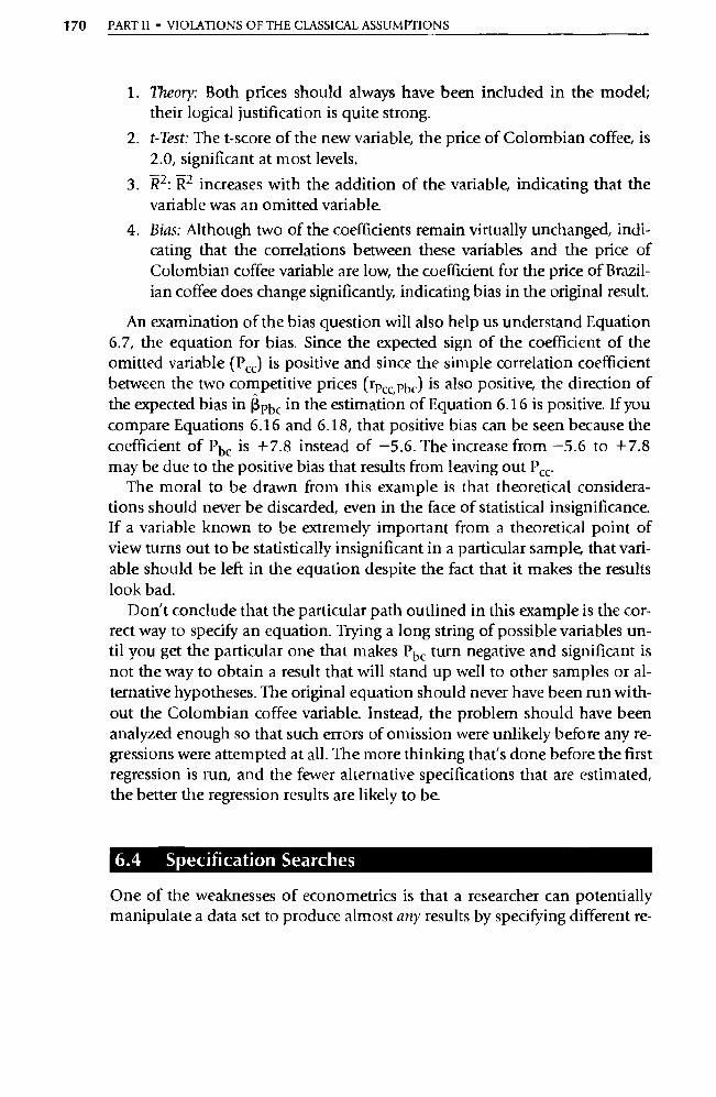
170 PART II • VIOLATIONS OF THE CLASSICAL ASSUMPTIONS
1. Theory: Both prices should always have been included in the model; their logical justification is quite strong.
2. t-Test: The t-score of the new variable, the price of Colombian coffee, is 2.0, significant at most levels.
3. 172 2 : R2 increases with the addition of the variable, indicating that the variable was an omitted variable.
4. Bias: Although two of the coefficients remain virtually unchanged, indi-cating that the correlations between these va riables and the price of Colombian coffee va riable are low, the coefficient for the price of Brazil-ian coffee does change significantly, indicating bias in the o riginal result.
An examination of the bias question will also help us understand Equation 6.7, the equation for bias. Since the expected sign of the coefficient of the omitted variable (POE) is positive and since the simple correlation coefficient between the two competitive prices (rpcc,Pbc) is also positive, the direction of the expected bias in RPbc in the estimation of Equation 6.16 is positive. If you compare Equations 6.16 and 6.18, that positive bias can be seen because the coefficient of Pbc is +7.8 instead of —5.6. The increase from —5.6 to +7.8 may be due to the positive bias that results from leaving out P OET
The moral to be drawn from this example is that theoretical considera-tions should never be discarded, even in the face of statistical insignificance. If a variable known to be extremely impo rtant from a theoretical point of view turns out to be statistically insignificant in a particular sample, that vari-able should be left in the equation despite the fact that it makes the results look bad.
Don't conclude that the particular path outlined in this example is the cor-rect way to specify an equation. Trying a long string of possible va riables un-til you get the particular one that makes P bc turn negative and significant is not the way to obtain a result that will stand up well to other samples or al-ternative hypotheses. The o riginal equation should never have been run with-out the Colombian coffee va riable. Instead, the problem should have been analyzed enough so that such errors of omission were unlikely before any re-gressions were attempted at all. The more thinking that's done before the first regression is run, and the fewer alternative specifications that are estimated, the better the regression results are likely to be.
6.4 Specification Searches
One of the weaknesses of econometrics is that a researcher can potentially manipulate a data set to produce almost any results by specifying different re-
CHAPTER 6 • SPECIFICATION: CHOOSING THE INDEPENDENT VARIABLES 171
gressions until estimates with the desired properties are obtained. Thus, the integrity of all empirical work is potentially open to question.
Although the problem is a difficult one, it makes sense to attempt to mini-mize the number of equations estimated and to rely on theory rather than statistical fit as much as possible when choosing variables. Theory, not statis-tical fit, should be the most impo rtant criterion for the inclusion of a variable in a regression equation. To do otherwise runs the risk of producing incorrect and/or disbelieved results. We'll try to illustrate this by discussing three of the most commonly used incorrect techniques for specifying a regression equa-tion. These techniques produce the best specification only by chance. At worst, they are possibly unethical in that they misrepresent the methods used to obtain the regression results and the significance of those results.
6.4.1 Data Mining
Almost surely the worst way to choose a specification is to simultaneously try a whole series of possible regression formulations and then choose the equa-tion that conforms the most to what the researcher wants the results to look like. In such a situation, the researcher would estimate virtually every possi-ble combination of the various alternative independent variables, and the choice between them would be made on the basis of the results. This practice of simultaneously estimating a number of combinations of independent variables and selecting the best from them ignores the fact that a number of specifications have been examined before the final one. To oversimplify, if you are 95 percent confident that a regression result didn't occur by chance and you run more than 20 regressions, how much confidence can you have in your result? Since you'll tend to keep regressions with high t-scores and discard ones with low t-scores, the reported t-scores overstate the degree of statistical significance of the estimated coefficients.
Furthermore, such "data mining" and "fishing expeditions" to obtain de-sired statistics for the final regression equation are potentially unethical methods of empirical research. These procedures include using not only many alternative combinations of independent variables but also many func-tional forms, lag structures, and what are offered as "sophisticated" or "ad-vanced" estimating techniques. "If you just torture the data long enough, they will confess. " 7 In other words, if enough alternatives are tried, the chances of
7. Thomas Mayer, "Economics as a Hard Science: Realistic Goal or Wishful Thinking?" Economic Inquiry, April 1980, p. 175.
172 PART II • VIOLATIONS OF THE CLASSICAL ASSUMPTIONS
obtainirtg the results desired by the researcher are increased tremendously, but the final result is essentially worthless. The researcher hasn't found any scientific evidence to suppo rt the original hypothesis; rather, prior expecta-tions were imposed on the data in a way that is essentially misleading.
6.4.2 Stepwise Regression Procedures
A stepwise regression involves the use of a computer program to choose the independent variables to be included in the estimation of a particular equa-tion. The computer program is given a "shopping list" of possible indepen-dent variables, and then it builds the equation in steps. It chooses as the first explanatory variable the one that by itself explains the largest amount of the variation of the dependent variable around its mean. It chooses as the second variable the one that adds the most to R 2 , given that the first variable is al-ready in the equation. The stepwise procedure continues until the next vari-able to be added fails to achieve some researcher-specified increase in R 2 (or all the variables are added). The measure of the supposed contribution of each independent variable is the increase in R 2 (which is sometimes called the "R2 delete") caused by the addition of the variable.
Unfortunately, any correlation among the independent variables (called multicollinearity, which we will take up in more detail in Chapter 8) causes this procedure to be deficient. To the extent that the variables are related, it becomes difficult to tell the impact of one variable from another. As a result, in the presence of multicollinearity, it's impossible to determine unambigu-ously the individual contribution of each variable enough to say which one is more important and thus should be included first. 8 Even worse, there is no necessity that the particular combination of variables chosen has any theoret-ical justification or that the coefficients have the expected signs.
Because of these problems, most econometricians avoid stepwise proce-dures. The major pitfalls are that the coefficients may be biased, the calculated t-values no longer follow the t-distribution, relevant variables may be ex-cluded because of the arbitrary order in which the selection takes place, and
8. Some programs compute standardized beta coefficients, which are the estimated coefficients for an equation in which all variables have been standardized by subtracting their means from them and by dividing them by their own standard deviations. The higher the beta of an inde-pendent va riable is in absolute value, the more impo rtant it is thought to be in explaining the movements in the dependent variable. Unfortunately, beta coefficients are deficient in the pres-ence of multicollinearity, as are partial correlation coefficients, which measure the correlation between the dependent variable and a given independent variable holding all other indepen-dent variables constant.
CHAPTER 6 • SPECIFICATION: CHOOSING THE INDEPENDENT VARIABLES 173
the signs of the estimated coefficients at intermediate or final stages of the routine may be different from the expected signs. Using a stepwise procedure is an admission of ignorance concerning which va riables should be entered.
6.4.3 Sequential Specification Searches
To their credit, most econometricians avoid data mining and stepwise regres-sions. Instead, they tend to specify equations by estimating an initial equa-tion and then sequentially dropping or adding variables (or changing func-tional forms) until a plausible equation is found with "good statistics." Faced with knowing that a few variables are relevant (on the basis of theory) but not knowing whether other additional variables are relevant, inspecting R 2
and t-tests for all variables for each specification appears to be the generally accepted practice. Indeed, it would be easy to draw from a casual reading of the previous sections the impression that such a sequential specification search is the best way to go about finding the "truth." Instead, as we shall see, there is a vast difference in approach between a sequential specification search and our recommended approach.
The sequential specification search technique allows a researcher to esti-mate an undisclosed number of regressions and then present a final choice (which is based upon an unspecified set of expectations about the signs and significance of the coefficients) as if it were the only specification estimated. Such a method misstates the statistical validity of the regression results for two reasons:
1. The statistical significance of the results is overestimated because the estimations of the previous regressions are ignored.
2. The set of expectations used by the researcher to choose between vari-ous regression results is rarely if ever disclosed. Thus the reader has no way of knowing whether or not all the other regression results had op-posite signs or insignificant coefficients for the impo rtant variables.
Unfortunately, there is no universally accepted way of conducting sequen-tial searches, primarily because the appropriate test at one stage in the proce-dure depends on which tests were previously conducted, and also because the tests have been very difficult to invent. One possibility is to reduce the de-grees of freedom in the "final" equation by one for each alternative specifica-
9. As mentioned in Chapter 5, Bayesian regression is a technique for dealing systematically with these prior expectations. For more on this issue, see Edward E. Learner, Specification Searches (New York: Wiley), 1978.
174 PART II • VIOLATIONS OF THE CLASSICAL ASSUMPTIONS
tion attempted. This• procedure is far from exact, but it does impose an ex-plicit penalty for specification searches.
More generally, we recommend trying to keep the number of regressions estimated as low as possible; to focus on theoretical considerations when choosing variables, functional forms, and the like; and to document all the various specifications investigated. That is, we recommend combining parsi-mony (using theory and analysis to limit the number of specifications esti-mated) with disclosure (reporting all the equations estimated).
There is another side to the story, however. Some researchers feel that the true model will show through if given the chance and that the best statistical results (including signs of coefficients, etc.) are most likely to have come from the true specification. The problem with this philosophy is that the ele-ment of chance is ordinarily quite strong in any given application. In addi-tion, reasonable people often disagree as to what the "true" model should look like. As a result, different researchers can look at the same data set and come up with very different "best" equations. Because this can happen, the distinction between good and bad econometrics is not always as clear cut as is implied by the previous paragraphs. As long as researchers have a healthy respect for the dangers inherent in specification searches, they are very likely to proceed in a reasonable way.
The lesson to be learned from this section should be quite clear. Most of the work of specifying an equation should be done before even attempting to estimate the equation on the computer. Since it is unreasonable to expect re-searchers to be perfect, there will be times when additional specifications must be estimated; however, these new estimates should be thoroughly grounded in theory and explicitly taken into account when testing for signifi-cance or summarizing results. In this way, the danger of misleading the reader about the statistical properties of estimates is reduced.
6.4.4 Bias Caused by Relying on the t -Test to Choose Variables
In the previous section, we stated that sequential specification searches are likely to mislead researchers about the statistical properties of their results. In particular, the practice of dropping a potential independent va riable simply because its t-score indicates that its estimated coefficient is insignificantly dif-ferent from zero will cause systematic bias in the estimated coefficients (and their t-scores) of the remaining variables. 10
10. For a number of better techniques, including sequential or "pretest" estimators and "Stein-rule" estimators, see George G. Judge, W. E. Griffiths, R. Carter Hill, Helmut Lutkepohl, and Tsoung-Chao Lee, The Theory and Practice of Econometrics (New York: Wiley, 1985).
CHAPTER 6 • SPECIFICATION: CHOOSING THE INDEPENDENT VARIABLES 175
Say the hypothesized model for a particular dependent va riable is:
Yi = Ro + 13 1X11 + 132X2i + Ei (6.19)
Assume further that, on the basis of theory, we are ce rtain that X 1 belongs in the equation but that we are not as ce rtain that X2 belongs. Even though we have stressed four criteria to determine whether X2 should be included, many inexperienced researchers just use the t-test on f'' 2 to determine whether X2 should be included. If this preliminary t-test indicates that 1 2 is significantly different from zero, then these researchers leave X2 in the equation, and they choose Equation 6.19 as their final model. If, however, the t-test does not in-dicate that 1. 2 is significantly different from zero, then such researchers drop X2 from the equation and consider Y as a function of X 1 .
Two kinds of mistakes can be made using such a system. First, X2 can some-times be left in the equation when it does not belong there, but such a mistake does not change the expected value of R1. Second, X2 can sometimes be dropped from equation when it belongs, and then the estimated coefficient of X1 will be biased by the value of the true 132 to the extent that X 1 and X2 are cor-related. In other words, 13 1 will be biased every time X2 belongs in the equation and is left out, and X2 will be left out every time that its estimated coefficient is not significantly different from zero. That is, the expected value of 1 3 1 will not equal the true (3 1 , and we will have systematic bias in our equation
E01) = RI + 132 • f(rxl,x2) P # R1 (6.20)
where P indicates the probability of an insignificant t-score. It is also the case that the t-score of (3- 1 no longer follows the t-distribution. In other words, the t-test is biased by sequential specification searches.
Since most researchers consider a number of different variables before set-tling on the final model, someone who relies on the t-test alone is likely to encounter this problem systematically.
6.4.5 Scanning and Sensitivity Analysis
Throughout this text, we've encouraged you to estimate as few specifications as possible and to avoid depending on fit alone to choose between those specifications. If you read the current economics literature, however, it won't take you long to find well-known researchers who have estimated five or more specifications and then have listed all their results in an academic jour-nal article. What's going on?
In almost every case, these authors have employed one of the two follow-ing techniques:
176 PART II • VIOLATIONS OF THE CLASSICAL ASSUMPTIONS
1. Scanning to develop a testable theory
2. Sensitivity analysis
Scanning involves analyzing a data set not for the purpose of testing a hy-pothesis but for the purpose of developing a testable theory or hypothesis. A researcher who is scanning will run quite a few different specifications, will select the specifications that fit best, and then will analyze these results in the hopes that they will provide clues to a new theory or hypothesis. As a means for stimulating fresh thinking or influencing thinking about substantive is-sues, scanning may have even more potential than does classical hypothesis testing. 11
Be careful, however; before you can "accept" a theory or hypothesis, it should be tested on a different data set (or in another context) using the hy-pothesis testing techniques of this text. A new data set must be used because our typical statistical tests have little meaning if the new hypotheses are tested on the old data set; after all, the researcher knows ahead of time what the results will be! The use of such dual data sets is easiest when there is a plethora of data. This sometimes is the case in cross-sectional research projects but rarely is the case for time-series research.
Sensitivity analysis consists of purposely running a number of alternative specifications to determine whether particular results are robust (not statisti-cal flukes). In essence, we're trying to determine how sensitive a particular re-sult is to a change in specification. Researchers who use sensitivity analysis run (and report on) a number of different specifications and tend to discount a result that appears significant in some specifications and insignificant in others. Indeed, the whole purpose of sensitivity analysis is to gain confidence that a particular result is significant in a variety of alternative specifications and is not based on a single specification that has been estimated on only one data set. For a simple example of sensitivity analysis, see Exercise 15 at the end of the chapter.
6.5 Lagged Independent Variables
Virtually all the regressions we've studied so far have been "instantaneous" in nature. In other words, they have included independent and dependent vari-ables from the same time period, as in:
11. For an excellent presentation of this argument, see Lawrence H. Summers, "The Scientific Il-lusion in Empirical Macroeconomics," Scandinavian Journal of Economics, 1991, pp. 129-148. For a number of related points of view, see David F. Hendry, Edward E. Learner, and Dale J. Poirer, A Conversation on Econometric Methodology, Institute of Statistics and Decision Sciences, Duke University, 1989, 144 pages.
CHAPTER 6 • SPECIFICATION: CHOOSING THE INDEPENDENT VARIABLES 177
o■
Yt = Ro+ 13 1 Xlt + R2X2t + Et (6.21)
where the subscript t is used to refer to a particular point in time. If all vari-ables have the same subscript, then the equation is instantaneous.
Some beginning researchers, when choosing their independent va riables, jump to the mistaken conclusion that all regressions should follow the pat-tern of Equation 6.21 and contain only variables that come from the same time period. Such a conclusion ignores the fact that not all economic or busi-ness situations imply such instantaneous relationships between the depen-dent and independent variables. In many cases we must allow for the possi-bility that time might elapse between a change in the independent variable and the resulting change in the dependent variable. The length of this time between cause and effect is called a lag. Many econometric equations include one or more lagged independent variables like X 1t_ 1 , where the subscript t — 1 indicates that the observation of X 1 is from the time period previous to time period t, as in the following equation:
Yt = Ro + R1Xlt-1 + 02X2t + Et (6.22)
In this equation, X 1 has been lagged by one time period, but the relationship between Y and X2 is still instantaneous.
For example, think about the process by which the supply of an agricultural product is determined. Since agricultural goods take time to grow, decisions on how many acres to plant or how many eggs to let hatch into egg-producing hens (instead of selling them immediately) must be made months if not years before the product is actually supplied to the consumer. Any change in an agricultural market, such as an increase in the price that the farmer can earn for providing cotton, has a lagged effect on the supply of that product:
+ — Ct = f(PCt_1, PFt) + Et = Ro + 131PCt-1 + 132PFt + Et (6.23)
where: Ct = the quantity of cotton supplied in year t PCt_ 1 = the price of cotton in year t — 1 PFt = the price of farm labor in year t
Note that this equation hypothesizes a lag between the price of cotton and the production of cotton, but not between the price of farm labor and the production of cotton. It's reasonable to think that if cotton prices change, farmers won't be able to react immediately because it takes a while for cotton to be planted and to grow.
The meaning of the regression coefficient of a lagged variable is not the same as the meaning of the coefficient of an unlagged variable. The estimated
178 PART II • VIOLATIONS OF THE CLASSICAL ASSUMPTIONS
coefficient of a lagged X measures the change in this year's Y attributed to a one-unit increase in last year's X (holding constant the other Xs in the equa-tion). Thus 13 1 in Equation 6.23 measures the extra number of units of cotton that would be produced this year as a result of a one-unit increase in last year's price of cotton, holding this year's price of farm labor constant.
If the lag structure is hypothesized to take place over more than one time period, or if a lagged dependent va riable is included on the right-hand side of an equation, the question becomes significantly more complex. Such cases, called distributed lags, will be dealt with in Chapter 12.
6.6 An Example of Choosing Independent Variables
It's time to get some experience choosing independent va riables. After all, every equation so far in the text has come with the specification already de-termined, but once you've finished this course you'll have to make all such specification decisions on your own. In future chapters, we'll use a technique called "interactive regression learning exercises" to allow you to make your own actual specification choices and get feedback on your choices. To sta rt, though, let's work through a specification together.
To keep things as simple as possible, we'll begin with a topic near and dear to your heart, your GPA! Suppose a friend who attends a small liberal a rts college surveys all 25 members of her econometrics class, obtains data on the variables listed below, and asks for your help in choosing a specification:
GPAi = the cumulative college grade point average on the ith student on a four-point scale
HGPA; = the cumulative high school grade point average of the ith stu-dent on a four-point scale
MSAT; = the highest score earned by the ith student on the math section of the SAT test (800 maximum)
VSAT; = the highest score earned by the ith student on the verbal section of the SAT test (800 maximum)
SAT; = MSAT; + VSAT; GREK; = a dummy variable equal to 1 if the ith student is a member of a
fraternity or sorority, 0 otherwise HRS; = the ith student's estimate of the average number of hours spent
studying per course per week in college PRN; = a dummy va riable equal to 1 if the ith student graduated from a
private high school, 0 otherwise
CHAPTER 6 • SPECIFICATION: CHOOSING THE INDEPENDENT VARIABLES 179
•
JOCKi = a dummy variable equal to 1 if the ith student is or was a mem-ber of a varsity intercollegiate athletic team for at least one sea-son, 0 otherwise
lnEXi = the natural log of the number of full courses that the ith student has completed in college.
Assuming that GPAi is the dependent variable, which independent vari-ables would you choose? Before you answer, think through the possibilities carefully. What are the expected signs of each of the coefficients? How strong is the theory behind each variable? Which variables seem obviously impor-tant? Which variables seem potentially irrelevant or redundant? Are there any other variables that you wish your friend had collected?
To get the most out of this example, you should take the time to write down the exact specification that you would run:
GPAi = f(?, ?, ?, ?, ?) + E
It's hard for most beginning econometricians to avoid the temptation of in-cluding all the above variables in a GPA equation and then dropping any variables that have insignificant t-scores. Even though we mentioned in the previous section that such a specification search procedure will result in bi-ased coefficient estimates, most beginners don't trust their own judgment and tend to include too many variables. With this warning in mind, do you want to make any changes in our proposed specification?
No? OK, let's compare notes. We believe that grades are a function of a stu-dent's ability, how hard the student works, and the student's experience tak-ing college courses. Consequently, our specification would be:
+ + + CPA; = f(HGPAi, HRSi, lnEXi) + E
We can already hear you complaining! What about SATs, you say? Everyone knows they're impo rtant. How about jocks and Greeks? Don't they have lower GPAs? Don't prep schools grade harder and prepare students better than public high schools?
Before we answer, it's impo rtant to note that we think of specification choice as choosing which variables to include, not which variables to exclude. That is, we don't assume automatically that a given variable should be in-cluded in an equation simply because we can't think of a good reason for dropping it.
Given that, however, why did we choose the variables we did? First, we think that the best predictor of a student's college GPA is his or her high school GPA. We have a hunch that once you know HGPA, SATs are redun-
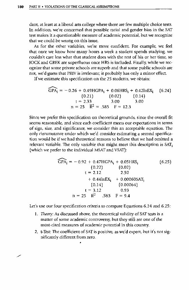
180 PART II • VIOLATIONS OF THE CLASSICAL ASSUMPTIONS
dant, at least at a liberal a rts college where there are few multiple choice tests. In addition, we're concerned that possible racial and gender bias in the SAT test makes it a questionable measure of academic potential, but we recognize that we could be wrong on this issue.
As for the other variables, we're more confident. For example, we feel that once we know how many hours a week a student spends studying, we couldn't care less what that student does with the rest of his or her time, so JOCK and GREK are superfluous once HRS is included. Finally, while we rec-ognize that some private schools are superb and that some public schools are not, we'd guess that PRIV is irrelevant; it probably has only a minor effect.
If we estimate this specification on the 25 students, we obtain:
GPAi = — 0.26 + 0.49HGPA; + 0.06HRS i + 0.421nEXi (6.24)
(0.21) (0.02) (0.14)
t = 2.33 3.00 3.00 n = 25 R2 =.585 F= 12.3
Since we prefer this specification on theoretical grounds, since the overall fit seems reasonable, and since each coefficient meets our expectations in terms of sign, size, and significance, we consider this an acceptable equation. The only circumstance under which we'd consider estimating a second specifica-tion would be if we had theoretical reasons to believe that we had omitted a relevant variable. The only variable that might meet this description is SAT i
(which we prefer to the individual MSAT and VSAT):
GPAi = — 0.92 + 0.47HGPA; + 0.05HRS;
(0.22) (0.02)
t = 2.12 2.50 + 0.441nEX; + 0.00060SATi
(0.14) (0.00064)
t = 3.12 0.93 n=25 R2 .583 F=9.4
(6.25)
Let's use our four specification criteria to compare Equations 6.24 and 6.25:
1. Theory: As discussed above, the theoretical validity of SAT tests is a matter of some academic controversy, but they still are one of the most-cited measures of academic potential in this count ry.
2. t-Test: The coefficient of SAT is positive, as we'd expect, but it's not sig-nificantly different from zero.
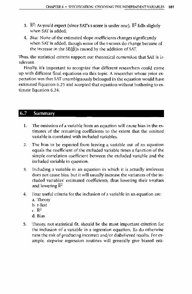
CHAPTER 6 • SPECIFICATION: CHOOSING THE INDEPENDENT VARIABLES 181
3. R2 : As you'd expect (since SATs t-score is under one), R 2 falls slightly when SAT is added.
4. Bias: None of the estimated slope coefficients changes significantly when SAT is added, though some of the t-scores do change because of the increase in the SE(13)s caused by the addition of SAT.
Thus, the statistical criteria suppo rt our theoretical contention that SAT is ir-relevant.
Finally, it's important to recognize that different researchers could come up with different final equations on this topic. A researcher whose prior ex-pectation was that SAT unambiguously belonged in the equation would have estimated Equation 6.25 and accepted that equation without bothering to es-timate Equation 6.24.
6.7 Summary
1. The omission of a variable from an equation will cause bias in the es-timates of the remaining coefficients to the extent that the omitted variable is correlated with included variables.
2. The bias to be expected from leaving a variable out of an equation equals the coefficient of the excluded variable times a function of the simple correlation coefficient between the excluded variable and the included variable in question.
3. Including a variable in an equation in which it is actually irrelevant does not cause bias, but it will usually increase the variances of the in-cluded variables' estimated coefficients, thus lowering their t-values and lowering R2
4. Four useful criteria for the inclusion of a variable in an equation are: a. Theory b. t-Test c. R2 d. Bias
5. Theory, not statistical fit, should be the most impo rtant criterion for the inclusion of a variable in a regression equation. To do otherwise runs the risk of producing incorrect and/or disbelieved results. For ex-ample, stepwise regression routines will generally give biased esti-
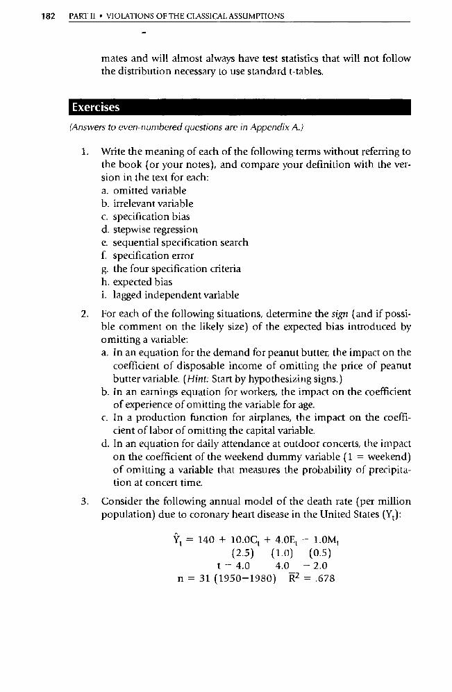
182 PART II • VIOLATIONS OF THE CLASSICAL ASSUMPTIONS
mates and will almost always have test statistics that will not follow the distribution necessary to use standard t-tables.
Exercises
(Answers to even-numbered questions are in Appendix A.)
1. Write the meaning of each of the following terms without referring to the book (or your notes), and compare your definition with the ver-sion in the text for each: a. omitted variable b. irrelevant variable c. specification bias d. stepwise regression e. sequential specification search f. specification error g. the four specification criteria h. expected bias i. lagged independent variable
2. For each of the following situations, determine the sign (and if possi-ble comment on the likely size) of the expected bias introduced by omitting a variable: a. In an equation for the demand for peanut butter, the impact on the
coefficient of disposable income of omitting the price of peanut butter variable. (Hint: Start by hypothesizing signs.)
b. In an earnings equation for workers, the impact on the coefficient of experience of omitting the variable for age.
c. In a production function for airplanes, the impact on the coeffi-cient of labor of omitting the capital variable.
d. In an equation for daily attendance at outdoor conce rts, the impact on the coefficient of the weekend dummy variable (1 = weekend) of omitting a variable that measures the probability of precipita-tion at conce rt time.
3. Consider the following annual model of the death rate (per million population) due to coronary heart disease in the United States (Y t):
Yt = 140 + 10.0Ct + 4.0Et — 1.0Mt
(2.5) (1.0) (0.5)
t = 4.0 4.0 — 2.0 n = 31 (1950-1980) R2 = .678

CHAPTER 6 • SPECIFICATION: CHOOSING THE INDEPENDENT VARIABLES 183
where: Ct = per capita cigarette consumption (pounds of to- bacco) in year t
Et = per capita consumption of edible saturated fats (pounds of butter, margarine, and lard) in year t
Mt = per capita consumption of meat (pounds) in year t
a. Create and test appropriate null hypotheses at the 10 percent level. What, if anything, seems to be wrong with the estimated coefficient of M?
b. The most likely cause of a coefficient that is significant in the unex-pected direction is omitted va riable bias. Which of the following variables could possibly be an omitted variable that is causing m's unexpected sign? Explain.
Bt = per capita consumption of hard liquor (gallons) in year t Ft = the average fat content (percentage) of the meat that was
consumed in year t Wt = per capita consumption of wine and beer (gallons) in year t Rt = per capita number of miles run in year t Ht = per capita open-heart surgeries in year t Ot = per capita amount of oat bran eaten in year t
c. If you had to choose one variable to add to the equation, what would it be? Explain your answer. (Hint: You're not limited to the variables listed in part b above.)
4. Assume that you've been hired by the surgeon general of the United States to study the determinants of smoking behavior and that you es-timate the following cross-sectional model based on data from 1988 for all 50 states (standard errors in parentheses) 12 :
= 100 — 9.0Eî + 1.04 — 0.04T1 — 3.0Vî + 1.5Rî (6.26) (3.0) (1.0) (0.04) (1.0) (0.5)
t = — 3.0 1.0 — 1.0 — 3.0 3.0
R2 = .50 n = 50 (states)
where: Ci = the number of cigarettes consumed per day per per- son in the ith state
12. This question is generalized from a number of similar studies, including John A. Bishop and Jang H. Yoo, "The Impact of the Health Scare, Excise Taxes, and Advertising on Cigarette Demand and Supply," Southern Economic Journal, January 1988, pp. 402 -411.
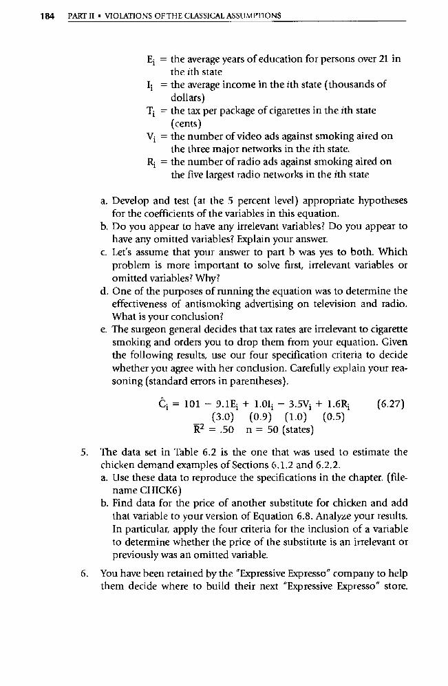
184 PART II • VIOLATIONS OF THE CLASSICAL ASSUMPTIONS
E; = the average years of education for persons over 21 in the ith state
= the average income in the ith state (thousands of dollars)
Ti = the tax per package of cigarettes in the ith state (cents)
V; = the number of video ads against smoking aired on the three major networks in the ith state.
R; = the number of radio ads against smoking aired on the five largest radio networks in the ith state
a. Develop and test (at the 5 percent level) appropriate hypotheses for the coefficients of the variables in this equation.
b. Do you appear to have any irrelevant variables? Do you appear to have any omitted variables? Explain your answer.
c. Let's assume that your answer to pa rt b was yes to both. Which problem is more impo rtant to solve first, irrelevant variables or omitted variables? Why?
d. One of the purposes of running the equation was to determine the effectiveness of antismoking advertising on television and radio. What is your conclusion?
e. The surgeon general decides that tax rates are irrelevant to cigare tte smoking and orders you to drop them from your equation. Given the following results, use our four specification criteria to decide whether you agree with her conclusion. Carefully explain your rea-soning (standard errors in parentheses).
C; = 101 —9.1E; + 1.0I ; -3.5V; + 1.6Rî (6.27) (3.0) (0.9) (1.0) (0.5)
R2 = .50 n = 50 (states)
5. The data set in Table 6.2 is the one that was used to estimate the chicken demand examples of Sections 6.1.2 and 6.2.2. a. Use these data to reproduce the specifications in the chapter. (file-
name CHICK6) b. Find data for the price of another substitute for chicken and add
that variable to your version of Equation 6.8. Analyze your results. In particular, apply the four criteria for the inclusion of a variable to determine whether the price of the substitute is an irrelevant or previously was an omitted variable.
6. You have been retained by the "Expressive Expresso" company to help them decide where to build their next "Expressive Expresso" store.
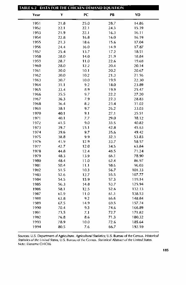
TABLE 6.2 DATA FOR THE CHICKEN DEMAND EQUATION
Year Y PC PB YD
1951 21.8 25.0 28.7 14.86 1952 22.1 22.1 24.3 15.39 1953 21.9 22.1 16.3 16.11 1954 22.8 16.8 16.0 16.19 1955 21.3 18.6 15.6 17.04 1956 24.4 16.0 14.9 17.87 1957 25.4 13.7 17.2 18.51 1958 28.0 14.0 21.9 18.84 1959 28.7 11.0 22.6 19.68 1960 28.0 12.2 20.4 20.14 1961 30.0 10.1 20.2 20.67 1962 30.0 10.2 21.3 21.56 1963 30.7 10.0 19.9 22.30 1964 31.1 9.2 18.0 23.89 1965 33.4 8.9 19.9 25.47 1966 35.5 9.7 22.2 27.20 1967 36.3 7.9 22.3 28.83 1968 36.4 8.2 23.4 31.02 1969 38.1 9.7 26.2 33.03 1970 40.1 9.1 27.1 35.51 1971 40.1 7.7 29.0 38.12 1972 41.5 9.0 33.5 40.82 1973 39.7 15.1 42.8 45.63 1974 39.6 9.7 35.6 49.42 1975 38.8 9.9 32.3 53.83 1976 41.9 12.9 33.7 58.57 1977 42.7 12.0 34.5 63.84 1978 44.8 12.4 48.5 71.24 1979 48.3 13.9 66.1 78.90 1980 48.4 11.0 62.4 86.97 1981 50.4 11.1 58.6 96.03 1982 51.5 10.3 56.7 101.33 1983 52.6 12.7 55.5 107.77 1984 54.5 15.9 57.3 119.14
1985 56.3 14.8 53.7 125.94 1986 58.1 12.5 52.6 132.13 1987 61.9 11.0 61.1 138.53 1988 63.8 9.2 66.6 148.84 1989 67.5 14.9 69.5 157.74 1990 70.4 9.3 74.6 166.89 1991 73.5 7.1 72.7 171.82 1992 76.8 8.6 71.3 180.32 1993 78.9 10.0 72.6 185.64 1994 80.5 7.6 66.7 192.59
Sources: U.S. Department of Agriculture. Agricultural Statistics; U.S. Bureau of the Census. Historical Statistics of the United States, U.S. Bureau of the Census. Statistical Abstract of the United States. Note: filename CHICK6
185
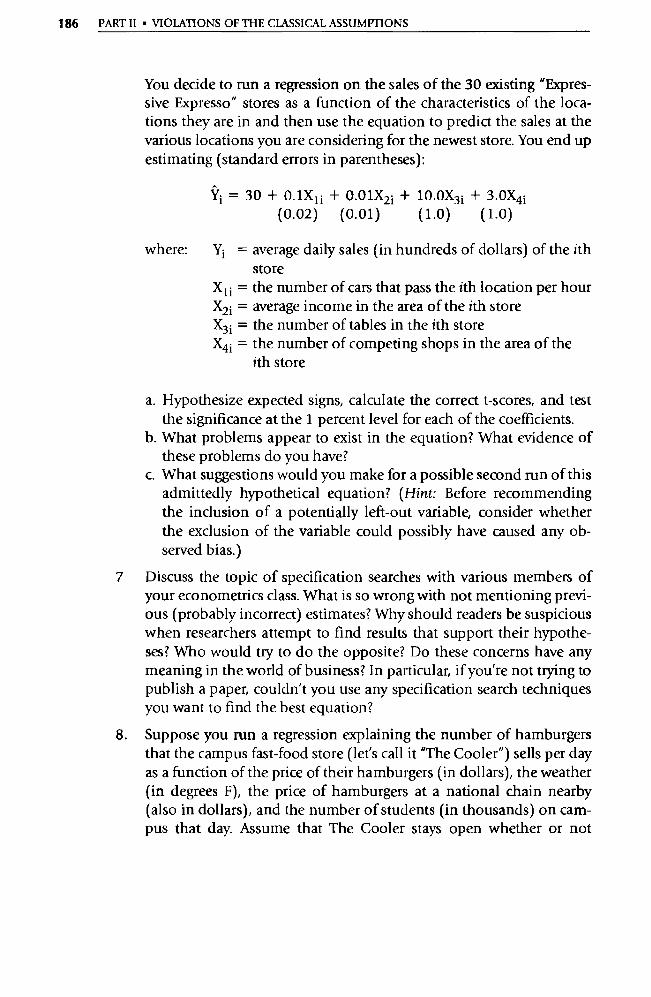
186 PART II • VIOLATIONS OF THE CLASSICAL ASSUMPTIONS
You decide to run a regression on the sales of the 30 existing "Expres-sive Expresso" stores as a function of the characteristics of the loca-tions they are in and then use the equation to predict the sales at the various locations you are considering for the newest store. You end up estimating (standard errors in parentheses):
Yi = 30+0.1X 1 1 +0.01X21+ 10.0X3 1 +3.0X41 (0.02) (0.01) (1.0) (1.0)
where: Yi = average daily sales (in hundreds of dollars) of the ith store
Xli = the number of cars that pass the ith location per hour X21 = average income in the area of the ith store X31 = the number of tables in the ith store X41 = the number of competing shops in the area of the
ith store
a. Hypothesize expected signs, calculate the correct t-scores, and test the significance at the 1 percent level for each of the coefficients.
b. What problems appear to exist in the equation? What evidence of these problems do you have?
c. What suggestions would you make for a possible second run of this admittedly hypothetical equation? (Hint: Before recommending the inclusion of a potentially left-out variable, consider whether the exclusion of the va riable could possibly have caused any ob-served bias.)
7 Discuss the topic of specification searches with various members of your econometrics lass. What is so wrong with not mentioning previ-ous (probably incorrect) estimates? Why should readers be suspicious when researchers attempt to find results that support their hypothe-ses? Who would try to do the opposite? Do these concerns have any meaning in the world of business? In pa rticular, if you're not trying to publish a paper, couldn't you use any specification search techniques you want to find the best equation?
8. Suppose you mn a regression explaining the number of hamburgers that the campus fast-food store (let's call it "The Cooler") sells per day as a function of the price of their hamburgers (in dollars), the weather (in degrees F), the price of hamburgers at a national chain nearby (also in dollars), and the number of students (in thousands) on cam-pus that day. Assume that The Cooler stays open whether or not

CHAPTER 6 • SPECIFICATION: CHOOSING THE INDEPENDENT VARIABLES 187
school is in session (for staff, etc.). Unfortunately, a lightning bolt strikes the computer and wipes out all the memory and you cannot tell which independent variable is which! Given the following regres-sion results (standard errors in parentheses):
Ÿi = 10.6 + 28.4X 11 + 12.7X21 +0.61X31 -5.9X41 (2.6) (6.3) (0.61) (5.9)
R2 =.63 n=35
a. Attempt to identify which result corresponds to which variable. b. Explain your reasoning for pa rt a above. c. Develop and test hypotheses about the coefficients assuming that
your answer to pa rt a is correct. What suggestions would you have for changes in the equation for a rerun when the computer is back up again?
9. Most of the examples in the text so far have been demand-side equa-tions or production functions, but economists often also have to quantify supply-side equations that are not true production func-tions. These equations attempt to explain the production of a product (for example, Brazilian coffee) as a function of the price of the prod-uct and various other attributes of the market that might have an im-pact on the total output of growers. a. What sign would you expect the coefficient of price to have in a
supply-side equation? Why? b. What other variables can you think of that might be impo rtant in a
supply-side equation? c. Many agricultural decisions are made months (if not a full year or
more) before the results of those decisions appear in the market. How would you adjust your hypothesized equation to take account of these lags?
d. Given all the above, carefully specify the exact equation you would use to attempt to explain Brazilian coffee production. Be sure to hypothesize the expected signs, be specific with respect to lags, and try to make sure you have not omitted an impo rtant independent variable.
10. If you think about the previous question, you'll realize that the same dependent variable (quantity of Brazilian coffee) can have different expected signs for the coefficient of the same independent variable (the price of Brazilian coffee), depending on what other variables are in the regression.
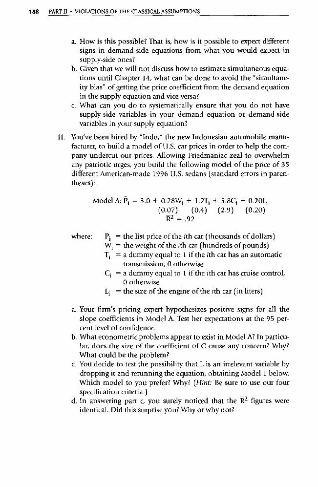
188 PART II • VIOLATIONS OF THE CLASSICAL ASSUMPTIONS
a. How is this possible? That is, how is it possible to expect different signs in demand-side equations from what you would expect in supply-side ones?
b. Given that we will not discuss how to estimate simultaneous equa-tions until Chapter 14, what can be done to avoid the "simultane-ity bias" of getting the price coefficient from the demand equation in the supply equation and vice versa?
c. What can you do to systematically ensure that you do not have supply-side variables in your demand equation or demand-side variables in your supply equation?
11. You've been hired by "Indo," the new Indonesian automobile manu-facturer, to build a model of U.S. car prices in order to help the com-pany undercut our prices. Allowing Friedmaniac zeal to overwhelm any patriotic urges, you build the following model of the price of 35 different American-made 1996 U.S. sedans (standard errors in paren-theses):
Model A: Pi = 3.0 + 0.28Wî + 1.2T1 + 5.8Cî + 0.20Lî (0.07) (0.4) (2.9) (0.20)
R2 =.92
where: Pi = the list price of the ith car (thousands of dollars) Wi = the weight of the ith car (hundreds of pounds) Ti = a dummy equal to 1 if the ith car has an automatic
transmission, 0 otherwise Ci = a dummy equal to 1 if the ith car has cruise control,
0 otherwise Li = the size of the engine of the ith car (in liters)
a. Your firm's pricing expert hypothesizes positive signs for all the slope coefficients in Model A. Test her expectations at the 95 per-cent level of confidence.
b. What econometric problems appear to exist in Model A? In particu-lar, does the size of the coefficient of C cause any concern? Why? What could be the problem?
c. You decide to test the possibility that L is an irrelevant variable by dropping it and rerunning the equation, obtaining Model T below. Which model to you prefer? Why? (Hint: Be sure to use our four specification criteria.)
d. In answering pa rt c, you surely noticed that the R 2 figures were identical. Did this surp rise you? Why or why not?
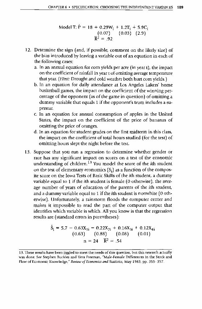
CHAPTER 6 • SPECIFICATION: CHOOSING THE INDEPENDENT VARIABLES 189
Model T: P = 18 + 0.29W î + 1.2Tî 4- 5.9C î (0.07) (0.03) (2.9)
R2 =.92
12. Determine the sign (and, if possible, comment on the likely size) of the bias introduced by leaving a variable out of an equation in each of the following cases: a. In an annual equation for corn yields per acre (in year t), the impact
on the coefficient of rainfall in year t of omitting average temperature that year. (Hint: Drought and cold weather both hurt corn yields.)
b. In an equation for daily attendance at Los Angeles Lakers' home basketball games, the impact on the coefficient of the winning per-centage of the opponent (as of the game in question) of omitting a dummy variable that equals 1 if the opponent's team includes a su-perstar.
c. In an equation for annual consumption of apples in the United States, the impact on the coefficient of the price of bananas of omitting the price of oranges.
d. In an equation for student grades on the first midterm in this class, the impact on the coefficient of total hours studied (for the test) of omitting hours slept the night before the test.
13. Suppose that you run a regression to determine whether gender or race has any significant impact on scores on a test of the economic understanding of children. 13 You model the score of the ith student on the test of elementary economics (S 1 ) as a function of the compos-ite score on the Iowa Tests of Basic Skills of the ith student, a dummy variable equal to 1 if the ith student is female (0 otherwise), the aver-age number of years of education of the parents of the ith student, and a dummy va riable equal to 1 if the ith student is nonwhite (0 oth-erwise). Unfortunately, a rainstorm floods the computer center and makes it impossible to read the pa rt of the computer output that identifies which variable is which. All you know is that the regression results are (standard errors in parentheses):
Si =5.7-0.63X 11 -0.22X21 +0.16X31 +0.12X41 (0.63) (0.88) (0.08) (0.01)
n=24 R2 =.54
13. These results have been jiggled to meet the needs of this question, but this research actually was done. See Stephen Buckles and Vera Freeman, "Male-Female Differences in the Stock and Flow of Economic Knowledge," Review of Economics and Statistics, May 1983, pp. 355-357.
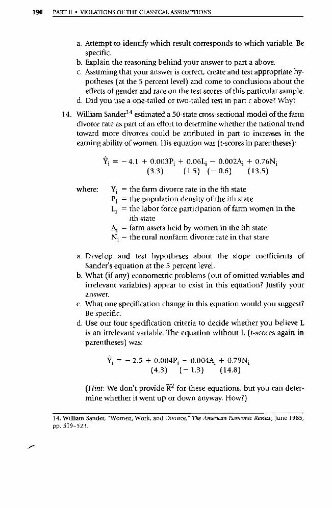
190 PART II ■ VIOLATIONS OF THE CLASSICAL ASSUMPTIONS
a. Attempt to identify which result corresponds to which variable. Be specific.
b. Explain the reasoning behind your answer to part a above. c. Assuming that your answer is correct, create and test appropriate hy-
potheses (at the 5 percent level) and come to conclusions about the effects of gender and race on the test scores of this particular sample.
d. Did you use a one-tailed or two-tailed test in pa rt c above? Why?
14. William Sander14 estimated a 50-state cross-sectional model of the farm divorce rate as pa rt of an effo rt to determine whether the national trend toward more divorces could be attributed in pa rt to increases in the earning ability of women. His equation was (t-scores in parentheses):
= — 4.1 + 0.003P; + 0.O6L; — 0.002Aî + 0.76Ni (3.3) (1.5) (— 0.6) (13.5)
where: Y; = the farm divorce rate in the ith state P; = the population density of the ith state L; = the labor force pa rticipation of farm women in the
ith state A; = farm assets held by women in the ith state Ni = the rural nonfarm divorce rate in that state
a. Develop and test hypotheses about the slope coefficients of Sander's equation at the 5 percent level.
b. What (if any) econometric problems (out of omitted variables and irrelevant variables) appear to exist in this equation? Justify your answer.
c. What one specification change in this equation would you suggest? Be specific.
d. Use our four specification criteria to decide whether you believe L is an irrelevant variable. The equation without L (t-scores again in parentheses) was:
= — 2.5 + 0.004P; — 0.004A; + 0.79N; (4.3) (— 1.3) (14.8)
(Hint: We don't provide R2 for these equations, but you can deter-mine whether it went up or down anyway. How?)
14. William Sander, "Women, Work, and Divorce," The American Economic Review, June 1985, pp. 519-523.
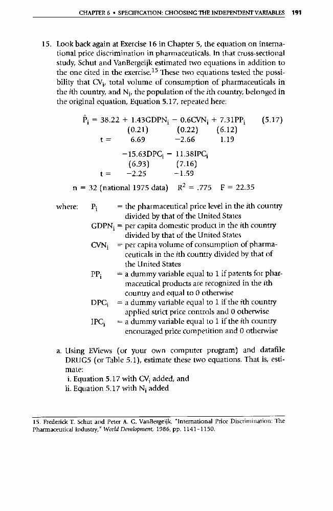
Pi = 38.22 + 1.43GDPNi — 0.6CVNi + 7.31PPi (0.21) (0.22) (6.12)
t = 6.69 —2.66 1.19
—15.63DPCi — 11.38IPCi (6.93) (7.16)
—2.25 —1.59
n = 32 (national 1975 data) R 2 = .775 F = 22.35
(5.17)
t=
CHAPTER 6 • SPECIFICATION: CHOOSING THE INDEPENDENT VARIABLES 191
15. Look back again at Exercise 16 in Chapter 5, the equation on interna-tional price discrimination in pharmaceuticals. In that cross-sectional study, Schut and VanBergeijk estimated two equations in addition to the one cited in the exercise. 15 These two equations tested the possi-bility that CVi, total volume of consumption of pharmaceuticals in the ith country, and Ni, the population of the ith count ry, belonged in the original equation, Equation 5.17, repeated here:
where: Pi = the pharmaceutical price level in the ith count ry divided by that of the United States
GDPNi = per capita domestic product in the ith count ry divided by that of the United States
CVNi = per capita volume of consumption of pharma-ceuticals in the ith country divided by that of the United States
PPi = a dummy variable equal to 1 if patents for phar- maceutical products are recognized in the ith country and equal to 0 otherwise
DPCi = a dummy variable equal to 1 if the ith count ry applied strict price controls and 0 otherwise
IPCi = a dummy variable equal to 1 if the ith count ry encouraged price competition and 0 otherwise
a. Using EViews (or your own computer program) and datafile DRUGS (or Table 5.1), estimate these two equations. That is, esti-mate: i. Equation 5.17 with CVi added, and
ii. Equation 5.17 with N i added
15. Frederick T. Schut and Peter A. G. VanBergeijk, "International Price Discrimination: The Pharmaceutical Industry," World Development, 1986, pp. 1141-1150.
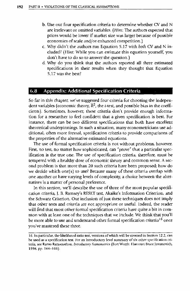
192 PART II • VIOLATIONS OF THE CLASSICAL ASSUMPTIONS
b. Use our four specification criteria to determine whether CV and N are irrelevant or omitted variables. (Hint: The authors expected that prices would be lower if market size was larger because of possible economies of scale and/or enhanced competition.)
c. Why didn't the authors run Equation 5.17 with both CV and N in-cluded? (Hint: While you can estimate this equation yourself, you don't have to do so to answer the question.)
d. Why do you think that the authors reported all three estimated specifications in their results when they thought that Equation 5.17 was the best?
6.8 Appendix: Additional Specification Criteria
So far in this chapter, we've suggested four criteria for choosing the indepen-dent variables (economic theory, R2, the t-test, and possible bias in the coeffi-cients). Sometimes, however, these criteria don't provide enough informa-tion for a researcher to feel confident that a given specification is best. For instance, there can be two different specifications that both have excellent theoretical underpinnings. In such a situation, many econometricians use ad-ditional, often more formal, specification criteria to provide comparisons of the properties of the alternative estimated equations.
The use of formal specification criteria is not without problems, however. First, no test, no matter how sophisticated, can "prove" that a particular spec-ification is the true one. The use of specification criteria, therefore, must be tempered with a healthy dose of economic theory and common sense. A sec-ond problem is that more than 20 such criteria have been proposed; how do we decide which one(s) to use? Because many of these criteria overlap with one another or have varying levels of complexity, a choice between the alter-natives is a matter of personal preference.
In this section, we'll describe the use of three of the most popular specifi-cation criteria, J. B. Ramseÿ s RESET test, Akaiké s Information Criterion, and the Schwarz Criterion. Our inclusion of just these techniques does not imply that other tests and criteria are not appropriate or useful. Indeed, the reader will find that most other formal specification criteria have quite a bit in com-mon with at least one of the techniques that we include. We think that you'll be more able to use and understand other formal specification criteria 16 once you've mastered these three.
16. In particular, the likelihood ratio test, versions of which will be covered in Section 12.2, can be used as a specification test. For an introductory level summary of s ix other specification cri-teria, see Ramu Ramanathan, Introductory Econometrics (Fort Worth: Harcou rt Brace Jovanovich, 1998, pp. 164-166).
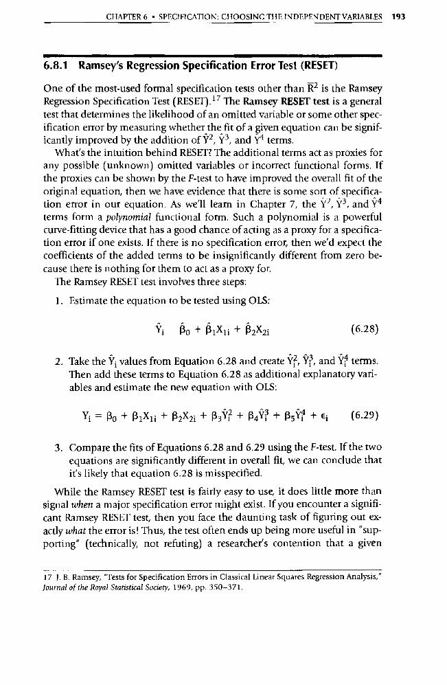
CHAPTER 6 • SPECIFICATION: CHOOSING THE INDEPENDENT VARIABLES 193
6.8.1 Ramsey's Regression Specification Error Test (RESET)
One of the most-used formal specification tests other than R2 is the Ramsey Regression Specification Test (RESET). 17 The Ramsey RESET test is a general test that determines the likelihood of an omitted variable or some other spec-ification error by measuring whether the fit of a given equation can be signif-icantly improved by the addition of Y2 , Ÿ3, and Y4 terms.
What's the intuition behind RESET? The additional terms act as proxies for any possible (unknown) omitted variables or incorrect functional forms. If the proxies can be shown by the F-test to have improved the overall fit of the original equation, then we have evidence that there is some sort of specifica-tion error in our equation. As we'll learn in Chapter 7, the Y2, Y3 , and Y4
terms form a polynomial functional form. Such a polynomial is a powerful curve-fitting device that has a good chance of acting as a proxy for a specifica-tion error if one exists. If there is no specification error, then we'd expect the coefficients of the added terms to be insignificantly different from zero be-cause there is nothing for them to act as a proxy for.
The Ramsey RESET test involves three steps:
1. Estimate the equation to be tested using OLS:
RlXti + 12X2i (6.28)
2. Take the Ÿi values from Equation 6.28 and create Ÿ; , Îi3, and Y4 terms. Then add these terms to Equation 6.28 as additional explanatory vari-ables and estimate the new equation with OLS:
Yi=RO+RIXli+ R2X2i + R3Y? + ¢4Y3 + R5Y4+ E i (6.29)
3. Compare the fits of Equations 6.28 and 6.29 using the F-test. If the two equations are significantly different in overall fit, we can conclude that it's likely that equation 6.28 is misspecified.
While the Ramsey RESET test is fairly easy to use, it does little more than signal when a major specification error might exist. If you encounter a signifi-cant Ramsey RESET test, then you face the daunting task of figuring out ex-actly what the error is! Thus, the test often ends up being more useful in "sup-porting" (technically, not refuting) a researcher's contention that a given
17 J. B. Ramsey, "Tests for Specification Errors in Classical Linear Squares Regression Analysis," Journal of the Royal Statistical Society, 1969, pp. 350 -371.
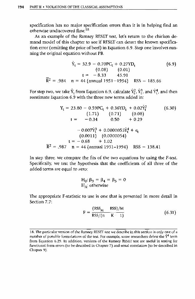
(RSSM RSS) /M F =
RSS/(n K - 1) (6.31)
194 PART II • VIOLATIONS OF THE CLASSICAL ASSUMPTIONS
specification has no major specification errors than it is in helping find an otherwise undiscovered flaw. 18
As an example of the Ramsey RESET test, let's return to the chicken de-mand model of this chapter to see if RESET can detect the known specifica-tion error (omitting the price of beef) in Equation 6.9. Step one involves run-ning the original equation without PB.
Yt = 32.9 - 0.70PCt + 0.27YDt
(0.08) (0.01) _ t = - 8.33 45.91 R = .984 n = 44 (annual 1951-1994) RSS = 185.66
(6.9)
For step two, we take Ÿt from Equation 6.9, calculate Ÿi , Ÿ3, and Îr4, and then reestimate Equation 6.9 with the three new terms added in:
Yt = 23.80 - 0.59PCt + 0.36YDt + 0.02Yi
(1.71) (0.71) (0.08) t = — 0.34 0.50 + 0.29
- 0.007 + 0.0000055Y4 + et (0.0011) (0.0000054)
t = -0.68 +1.02 R2 = .987 n = 44 (annual 1951-1994) RSS = 138.41
(6.30)
In step three, we compare the fits of the two equations by using the F-test. Specifically, we test the hypothesis that the coefficients of all three of the added terms are equal to zero:
H0: 133—R4—R5=0
HA: otherwise
The appropriate F-statistic to use is one that is presented in more detail in Section 7.7:
18. The particular version of the Ramsey RESET test we describe in this section is only one of a number of possible formulations of the test. For example, some researchers delete the ÿ4 term from Equation 6.29. In addition, versions of the Ramsey RESET test are useful in testing for functional form errors (to be described in Chapter 7) and serial correlation (to be described in Chapter 9).
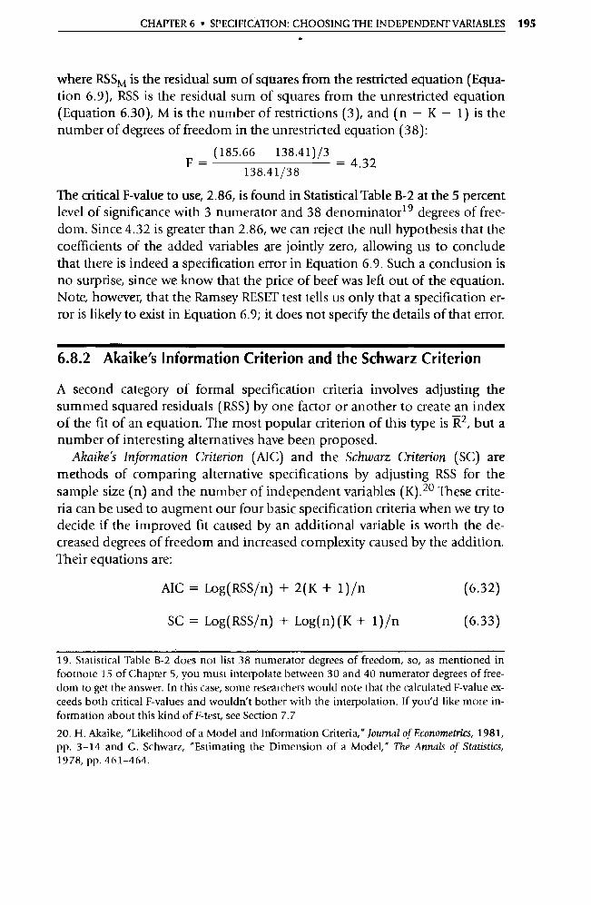
CHAPTER 6 • SPECIFICATION: CHOOSING THE INDEPENDENT VARIABLES 195
where RSSM is the residual sum of squares from the restricted equation (Equa-tion 6.9), RSS is the residual sum of squares from the unrestricted equation (Equation 6.30), M is the number of restrictions (3), and (n — K — 1) is the number of degrees of freedom in the unrestricted equation (38):
(185.66 138.41) /3 F = = 4.32
138.41/38
The critical F-value to use, 2.86, is found in Statistical Table B-2 at the 5 percent level of significance with 3 numerator and 38 denominator 19 degrees of free-dom. Since 4.32 is greater than 2.86, we can reject the null hypothesis that the coefficients of the added variables are jointly zero, allowing us to conclude that there is indeed a specification error in Equation 6.9. Such a conclusion is no surprise, since we know that the price of beef was left out of the equation. Note, however, that the Ramsey RESET test tells us only that a specification er-ror is likely to exist in Equation 6.9; it does not specify the details of that error.
6.8.2 Akaike's Information Criterion and the Schwarz Criterion
A second category of formal specification criteria involves adjusting the summed squared residuals (RSS) by one factor or another to create an index of the fit of an equation. The most popular criterion of this type is R 2, but a number of interesting alternatives have been proposed.
Ahaihe's Information Criterion (AIC) and the Schwarz Criterion (SC) are methods of comparing alternative specifications by adjusting RSS for the sample size (n) and the number of independent variables (K). 2° These crite-ria can be used to augment our four basic specification criteria when we try to decide if the improved fit caused by an additional variable is worth the de-creased degrees of freedom and increased complexity caused by the addition. Their equations are:
AIC = Log(RSS /n) + 2(K + 1)/n (6.32)
SC = Log(RSS/n) + Log(n)(K + 1)/n (6.33)
19. Statistical Table B-2 does not list 38 numerator degrees of freedom, so, as mentioned in footnote 15 of Chapter 5, you must interpolate between 30 and 40 numerator degrees of free-dom to get the answer. In this case, some researchers would note that the calculated F-value ex-ceeds both critical F-values and wouldn't bother with the interpolation. If you'd like more in-formation about this kind of F-test, see Section 7.7
20. H. Akaike, "Likelihood of a Model and Information Criteria," Journal of Econometrics, 1981, pp. 3-14 and G. Schwarz, "Estimating the Dimension of a Model," The Annals of Statistics, 1978, pp. 461-464.
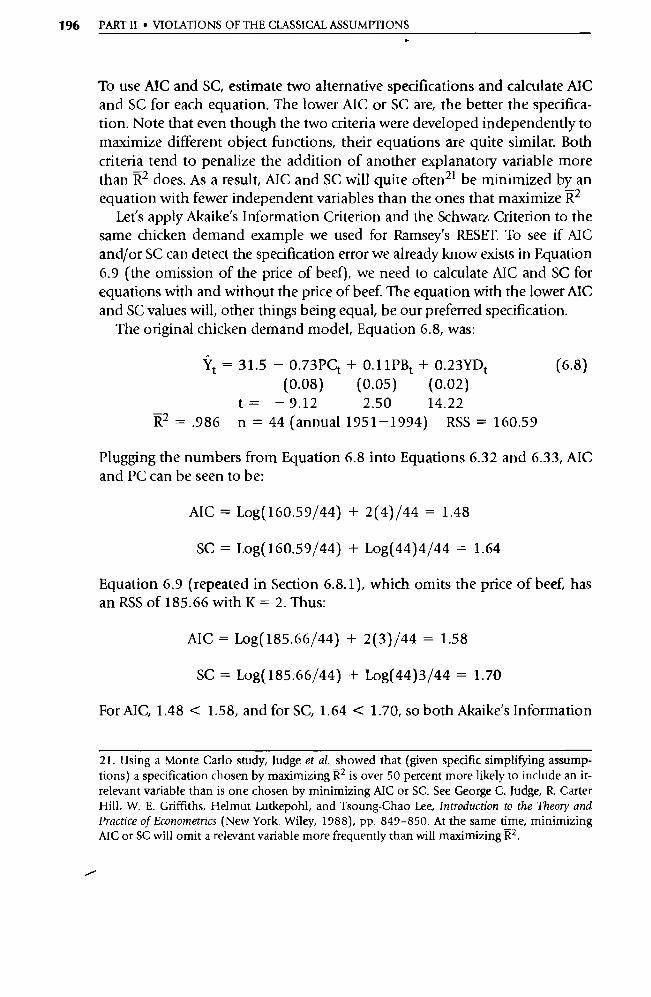
196 PART II • VIOLATIONS OF THE CLASSICAL ASSUMPTIONS
To use AIC and SC, estimate two alternative specifications and calculate AIC and SC for each equation. The lower AIC or SC are, the better the specifica-tion. Note that even though the two criteria were developed independently to maximize different object functions, their equations are quite similar. Both criteria tend to penalize the addition of another explanatory variable more than R2 does. As a result, AIC and SC will quite often 21 be minimized by an equation with fewer independent variables than the ones that maximize R2
Let's apply Akaike's Information Criterion and the Schwarz Criterion to the same chicken demand example we used for Ramseÿ s RESET. To see if AIC and/or SC can detect the specification error we already know exists in Equation 6.9 (the omission of the price of beef), we need to calculate AIC and SC for equations with and without the price of beef. The equation with the lower AIC and SC values will, other things being equal, be our preferred specification.
The original chicken demand model, Equation 6.8, was:
Ÿt = 31.5 — 0.73PCt + 0.11PBt + 0.23YDt (6.8) (0.08) (0.05) (0.02)
t = —9.12 2.50 14.22 R2 = .986 n = 44 (annual 1951-1994) RSS = 160.59
Plugging the numbers from Equation 6.8 into Equations 6.32 and 6.33, AIC and PC can be seen to be:
AIC = Log(160.59/44) + 2(4)/44 = 1.48
SC = Log(160.59/44) + Log(44)4/44 = 1.64
Equation 6.9 (repeated in Section 6.8.1), which omits the price of beef, has an RSS of 185.66 with K = 2. Thus:
AIC = Log(185.66/44) + 2(3)/44 = 1.58
SC = Log(185.66/44) + Log(44)3/44 = 1.70
For AIC, 1.48 < 1.58, and for SC, 1.64 < 1.70, so both Akaike's Information
21. Using a Monte Carlo study, Judge et al. showed that (given specific simplifying assump-tions) a specification chosen by maximizing R 2 is over 50 percent more likely to include an ir-relevant variable than is one chosen by minimizing AIC or SC. See George C. Judge, R. Ca rter Hill, W. E. Griffiths, Helmut Lutkepohl, and Tsoung-Chao Lee, Introduction to the Theory and Practice of Econometrics (New York: Wiley, 1988), pp. 849-850. At the same time, minimizing AIC or SC will omit a relevant va riable more frequently than will maximizing R2.
CHAPTER 6 • SPECIFICATION: CHOOSING THE INDEPENDENT VARIABLES 197
Criterion and the Schwarz Criterion provide evidence that Equation 6.8 is preferable to Equation 6.9. That is, the price of beef appears to belong in the equation. In practice, these calculations may not be necessary because AIC and SC are automatically calculated by some regression software packages, including EViews.
As it turns out, then, all three new specification criteria indicate the pres-ence of a specification error when we leave the price of beef out of the equa-tion. This result is not surprising, since we purposely left out a theoretically justified variable, but it provides an example of how useful these criteria could be when we're less than sure about the underlying theory.
Note that AIC and SC require the researcher to come up with a particular alternative specification, whereas Ramseÿ s RESET does not. Such a distinc-tion makes RESET easier to use, but it makes AIC and SC more informative if a specification error is found. Thus our additional specification criteria serve different purposes. RESET is most useful as a general test of the existence of a specification error, whereas AIC and SC are more useful as means of compar-ing two or more alternative specifications.
7 CHAPTER
Specification: Choosing a Functional Form
7.1
The Use and Interpretation of the Constant Term
7.2
Alternative Functional Forms
7.3
Problems with Incorrect Functional Forms
7.4
Using Dummy Variables
7.5
Slope Dummy Variables
7.6
Summary and Exercises
7.7
Appendix: More Uses for the F-Test
Even after you've chosen your independent va riables, the job of specifying the equation is not over. The next step is to choose the functional form of the relationship between each independent variable and the dependent variable. Should the equation go through the origin? Do you expect a curve instead of a straight line? Does the effect of a variable peak at some point and then start to decline? An affirmative answer to any of these questions suggests that an equation other than the standard "linear in the variables" model of the previ-ous chapters might be appropriate. Such alternative specifications are impor-tant for two reasons: a correct explanatory variable may well appear to be in-significant or to have an unexpected sign if an inappropriate functional form is used, and the consequences of an incorrect functional form for interpreta-tion and forecasting can be severe.
Theoretical considerations usually dictate the form of a regression model. The basic technique involved in deciding on a functional form is to choose the shape that best exemplifies the expected underlying economic or business prin-ciples and then to use the mathematical form that produces that shape. To help with that choice, this chapter contains plots of the most commonly used func-tional forms along with the mathematical equations that correspond to each.
The chapter begins with a brief discussion of the constant term. In pa rt icu-lar, we suggest that the constant term should be retained in equations even if
198
CHAPTER 7 • SPECIFICATION: CHOOSING A FUNCTIONAL FORM 199
theory suggests otherwise, and that estimates of the constant term should not be relied on for inference or analysis. The chapter concludes with a discus-sion of dummy variables and, in pa rticular, the use of dummy variables to al-low the coefficients of independent variables to differ for qualitative condi-tions (slope dummies).
7.1 The Use and Interpretation of the Constant Term
In the linear regression model, 13o is the intercept or constant term. It is the expected value of Y when all the explanatory variables (and the error term) equal zero. At times, 13o is of theoretical impo rtance. Consider, for example, the following cost equation:
Ci_ Ro +R1Qi+ Ei
where C i is the total cost of producing level of output Q i . The term R1Qi rep-resents the total variable cost associated with output level Q i, and Ro repre-sents the total fixed cost, defined as the cost when output Q i = O. Thus, a re-gression equation might seem useful to a researcher who wanted to determine the relative magnitudes of fixed and variable costs. This would be an example of relying on the constant term for inference.
On the other hand, the product involved might be one for which it is known that there are few if any fixed costs. In such a case, a researcher might want to eliminate the constant term; to do so would conform to the notion of zero fixed costs and would conserve a degree of freedom (which would presumably make the estimate of 13 1 more precise). This would be an exam-ple of suppressing the constant term.
Neither suppressing the constant term nor relying on it for inference is ad-visable, however, and reasons for these conclusions are explained in the fol-lowing sections.
7.1.1 Do Not Suppress the Constant Term
Chapter 4 explained that Assumption II (the error term has an expected value of zero) requires that the constant term absorb any nonzero mean that the observations of the error term might have in a given sample. Thus, suppress-ing the constant term can lead to a violation of this Classical Assumption. The only time that this assumption would not be violated by leaving out the intercept term is when the mean effect of the unobserved error term (without a constant term) is zero over all the observations.
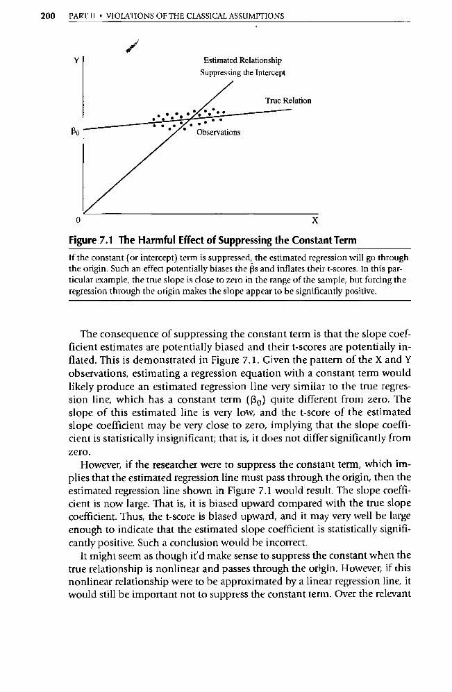
200 PART II • VIOLATIONS OF THE CLASSICAL ASSUMPTIONS
Estimated Relationship Suppressing the Intercept
Figure 7.1 The Harmful Effect of Suppressing the Constant Term
If the constant (or intercept) term is suppressed, the estimated regression will go through the origin. Such an effect potentially biases the (3s and inflates their t-scores. In this par-ticular example, the true slope is close to zero in the range of the sample, but forcing the regression through the origin makes the slope appear to be significantly positive.
The consequence of suppressing the constant term is that the slope coef-ficient estimates are potentially biased and their t-scores are potentially in-flated. This is demonstrated in Figure 7.1. Given the pattern of the X and Y observations, estimating a regression equation with a constant term would likely produce an estimated regression line very similar to the true regres-sion line, which has a constant term ((3 e) quite different from zero. The slope of this estimated line is very low, and the t-score of the estimated slope coefficient may be very close to zero, implying that the slope coeffi-cient is statistically insignificant; that is, it does not differ significantly from zero.
However, if the researcher were to suppress the constant term, which im-plies that the estimated regression line must pass through the origin, then the estimated regression line shown in Figure 7.1 would result. The slope coeffi-cient is now large. That is, it is biased upward compared with the true slope coefficient. Thus, the t-score is biased upward, and it may very well be large enough to indicate that the estimated slope coefficient is statistically signifi-cantly positive. Such a conclusion would be incorrect.
It might seem as though it'd make sense to suppress the constant when the true relationship is nonlinear and passes through the origin. However, if this nonlinear relationship were to be approximated by a linear regression line, it would still be impo rtant not to suppress the constant term. Over the relevant
CHAPTER 7 • SPECIFICATION: CHOOSING A FUNCTIONAL FORM 201
range of the observations (that is, the sample range), the estimated regression line with the constant suppressed doesn't provide an adequate approxima-tion of the true regression line, compared with an estimated regression equa-tion that includes the constant term. It is a legitimate exercise in applied econometrics to use linear approximations of nonlinear functional forms; suppressing the constant term doesn't permit an accurate approximation over the sample range of observations.
Thus, even though some regression packages allow the constant term to be suppressed (set to zero), the general rule is: Don't, even if theory specifically calls for it.
7.1.2 Do Not Rely on Estimates of the Constant Term
It would seem logical that if it's a bad idea to suppress the constant term, then the constant term must be an impo rtant analytical tool to use in evalu-ating the results of the regression. Unfortunately, there are at least two rea-sons that suggest that the intercept should not be relied on for purposes of analysis or inference.
First, the error term is generated, in pa rt, by the omission of a number of marginal independent variables, the mean effect of which is placed in the constant term. The constant term acts as a garbage collector, with an un-known amount of this mean effect being dumped into it. The constant term's estimated coefficient may be different from what it would have been without performing this task, which is done for the sake of the equation as a whole. As a result, it's meaningless to run a t-test on j3 o .
Second, the constant term is the value of the dependent variable when all the independent variables and the error term are zero, but the values of vari-ables used for economic analysis are usually positive. Thus, the origin often lies outside the range of sample observations (as can be seen in Figure 7.1). Since the constant term is an estimate of Y when the Xs are outside the range of the sample observations, estimates of it are tenuous. Estimating the con-stant term is like forecasting beyond the range of the sample data, a proce-dure that inherently contains greater error than within-sample forecasts. For more on this, see Chapter 15.
7.2 Alternative Functional Forms
The choice of a functional form for an equation is a vital pa rt of the specifica-tion of that equation. The use of OLS requires that the equation be linear in the coefficients, but there is a wide variety of functional forms that are linear in the coefficients while being nonlinear in the variables. Indeed, in previous
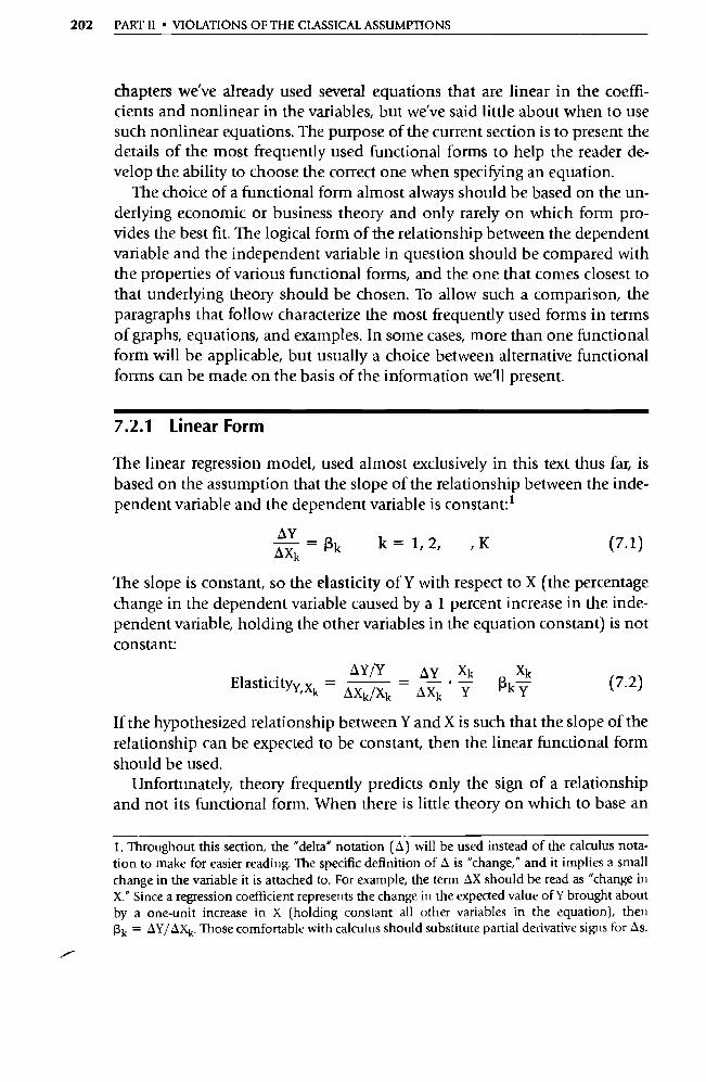
202 PART II • VIOLATIONS OF THE CLASSICAL ASSUMPTIONS
chapters we've already used several equations that are linear in the coeffi-cients and nonlinear in the variables, but we've said little about when to use
such nonlinear equations. The purpose of the current section is to present the
details of the most frequently used functional forms to help the reader de-velop the ability to choose the correct one when specifying an equation.
The choice of a functional form almost always should be based on the un-derlying economic or business theory and only rarely on which form pro-vides the best fit. The logical form of the relationship between the dependent
variable and the independent va riable in question should be compared with the properties of various functional forms, and the one that comes closest to
that underlying theory should be chosen. To allow such a comparison, the
paragraphs that follow characterize the most frequently used forms in terms
of graphs, equations, and examples. In some cases, more than one functional
form will be applicable, but usually a choice between alternative functional
forms can be made on the basis of the information we'll present.
7.2.1 Linear Form
The linear regression model, used almost exclusively in this text thus far, is
based on the assumption that the slope of the relationship between the inde-pendent variable and the dependent variable is constant: 1
OXk = 13k k = 1, 2, , K (7.1)
The slope is constant, so the elasticity of Y with respect to X (the percentage
change in the dependent variable caused by a 1 percent increase in the inde-pendent variable, holding the other variables in the equation constant) is not
constant:
ElasticityY Xk = k^Xk = AXk • Ÿ Rk
Xk (7.2)
If the hypothesized relationship between Y and X is such that the slope of the
relationship can be expected to be constant, then the linear functional form
should be used. Unfortunately, theory frequently predicts only the sign of a relationship
and not its functional form. When there is little theory on which to base an
AY
1. Throughout this section, the "delta" notation (A) will be used instead of the calculus nota-tion to make for easier reading. The specific definition of A is "change," and it implies a small change in the variable it is attached to. For example, the term AX should be read as "change in X." Since a regression coefficient represents the change in the expected value of Y brought about by a one-unit increase in X (holding constant all other variables in the equation), then 13k = AY/AXk. Those comfortable with calculus should substitute pa rtial derivative signs for As.
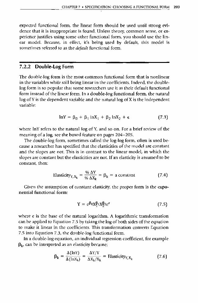
CHAPTER 7 • SPECIFICATION: CHOOSING A FUNCTIONAL FORM 203
expected functional form, the linear form should be used until strong evi-dence that it is inappropriate is found. Unless theory, common sense, or ex-perience justifies using some other functional form, you should use the lin-ear model. Because, in effect, it's being used by default, this model is
sometimes referred to as the default functional form.
7.2.2 Double-Log Form
The double-log form is the most common functional form that is nonlinear
in the variables while still being linear in the coefficients. Indeed, the double-log form is so popular that some researchers use it as their default functional
form instead of the linear form. In a double-log functional form, the natural
log of Y is the dependent variable and the natural log of X is the independent
variable:
InY = Ro + RI 1nX 1 + 13 2 lnX2 + e (7.3)
where lnY refers to the natural log of Y, and so on. For a brief review of the meaning of a log, see the boxed feature on pages 204-205.
The double-log form, sometimes called the log-log form, often is used be-cause a researcher has specified that the elasticities of the model are constant
and the slopes are not. This is in contrast to the linear model, in which the
slopes are constant but the elasticities are not. If an elasticity is assumed to be
constant, then:
% AY
ElasticityY, Xk = % AXk
= (3k = a constant (7.4)
Given the assumption of constant elasticity, the proper form is the expo-nential functional form:
Y = eRaX 1 iX92eE (7.5)
where e is the base of the natural logarithm. A logarithmic transformation
can be applied to Equation 7.5 by taking the log of both sides of the equation
to make it linear in the coefficients. This transformation converts Equation
7.5 into Equation 7.3, the double-log functional form.
In a double-log equation, an individual regression coefficient, for example
13k, can be interpreted as an elasticity because:
(1nY) DY/Y 13 k
— Onx ( l = Elasticityy xk (7.6)
k) zx k/x k

What Is a Log?
What the heck is a log? If e (a constant equal to 2 71828) t power" produces x, then b is the log of x:
Thus, a log (or logarithm) is the exponent to which a given base must be taken in order to produce a specific number. While logs come in more than one variety, we'll use only natural logs (logs to the base e) in this text. The symbol for a natural log is "ln," so ln(x) = b means that (2.71828) b
= x or, more simply,
ln(x)
For example, since e2 = (2.71828) 2 7.389, we can state that:
ln(7.389)
Thus, the natural log of 7.389 is 2i Two is the power of e that produces 7.389. Let's look at some other natural log calculations:
ln(100) 4.605 ln(1000) = 6.908 ln(10000) 9.210 ln(100000) = 1 1.513 ln(1000000) 13.816
204 PART II • VIOLATIONS OF THE CLASSICAL ASSUMPTIONS
Since regression coefficients are constant, the condition that the model have a constant elasticity is met by the double-log equation.
The way to interpret [3 k in a double-log equation is that if Xk increases by 1 percent while the other Xs are held constant, then Y will change by (3k per-cent. Since elasticities are constant, the slopes are now no longer constant.
Figure 7.2 is a graph of the double-log function (ignoring the error term). The panel on the left shows the economic concept of a production function (or an indifference curve). Isoquants from production functions show the
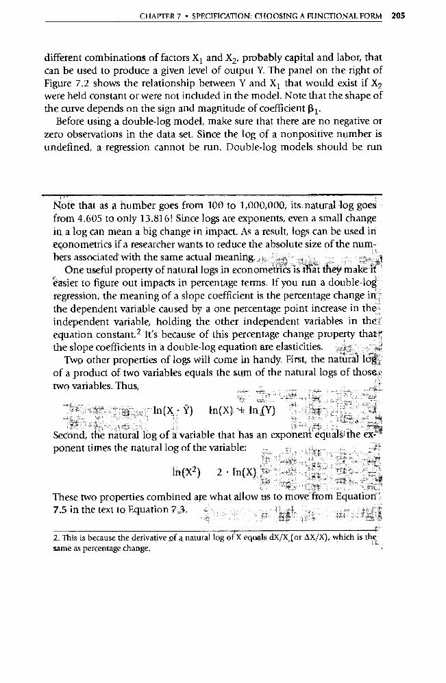
ln(X • Y) ln(X) + In (Y)
CHAPTER 7 • SPECIFICATION: CHOOSING A FUNCTIONAL FORM 205
different combinations of factors X 1 and X2, probably capital and labor, that can be used to produce a given level of output Y. The panel on the right of Figure 7.2 shows the relationship between Y and X 1 that would exist if X2
were held constant or were not included in the model. Note that the shape of the curve depends on the sign and magnitude of coefficient 13 1 .
Before using a double-log model, make sure that there are no negative or zero observations in the data set. Since the log of a nonpositive number is undefined, a regression cannot be run. Double-log models should be run
Note that as a number goes from 100 to 1,000,000, its natural log goes from 4.605 to only 13.816! Since logs are exponents, even a small change, in a log can mean a big change in impact. As a result, logs can be used in econometrics if a researcher wants to reduce the absolute size of the num-bers associated with the same actual meaning.
One useful property of natural logs in econometrics is that they make it
easier to figure out impacts in percentage terms. If you run a double-log regression, the meaning of a slope coefficient is the percentage change in the dependent variable caused by a one percentage point increase in the independent variable, holding the other independent variables in the equation constant. 2 It's because of this percentage change property that the slope coefficients in 'a double-log equation are elasticities.
Two other properties of logs will come in handy. First, the natural log of a product of two variables equals the sum of the natural logs of those
two variables. Thus,
Second, the natural log of a variable that has an exponent equals the ex-ponent times the natural log of the variable:
ln(X2) 2 • In(X)
These two properties combined are what allow us to move from Equation 7.5 in the text to Equation 7.3.
2. This is because the derivative of a natural log of X equals dX/X (or 8X/X), which is the same as percentage change.
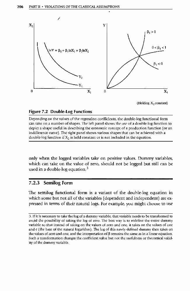
206 PART II • VIOLATIONS OF THE CLASSICAL ASSUMPTIONS
X2
0 X I
(Holding X2 constant)
Figure 7.2 Double-Log Functions
Depending on the values of the regression coefficients, the double-log functional form can take on a number of shapes. The left panel shows the use of a double-log function to depict a shape useful in describing the economic concept of a production function (or an indifference curve). The right panel shows various shapes that can be achieved with a double-log function if X2 is held constant or is not included in the equation.
only when the logged variables take on positive values. Dummy variables, which can take on the value of zero, should not be logged but still can be used in a double-log equation. 3
7.2.3 Semilog Form
The semilog functional form is a variant of the double-log equation in which some but not all of the variables (dependent and independent) are ex- pressed in terms of their natural logs. For example, you might choose to use
3. If it is necessary to take the log of a dummy variable, that variable needs to be transformed to avoid the possibility of taking the log of zero. The best way is to redefine the entire dummy variable so that instead of taking on the values of zero and one, it takes on the values of one and e (the base of the natural logarithm). The log of this newly defined dummy then takes on the values of zero and one, and the interpretation of 3 remains the same as in a linear equation. Such a transformation changes the coefficient value but not the usefulness or theoretical valid-ity of the dummy variable.
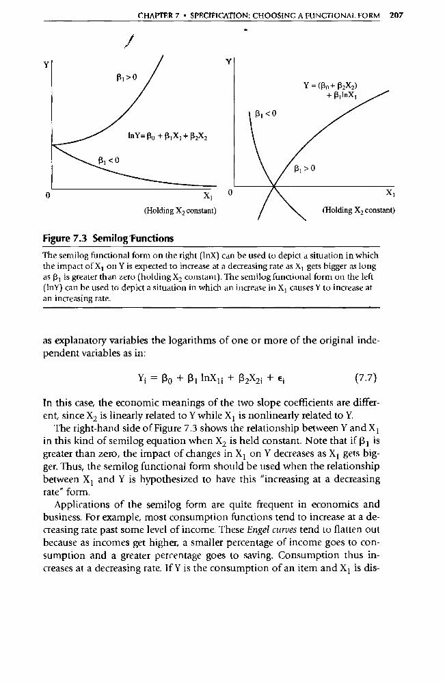
CHAPTER 7 • SPECIFICATION: CHOOSING A FUNCTIONAL FORM 207
Y Y
0 Xi
(Holding X2 constant)
0 X i
(Holding X2 constant)
Figure 7.3 Semilog -Functions
The semilog functional form on the right (1nX) can be used to depict a situation in which the impact of X 1 on Y is expected to increase at a decreasing rate as X 1 gets bigger as long as R1 is greater than zero (holding X2 constant). The semilog functional form on the left (1nY) can be used to depict a situation in which an increase in X 1 causes Y to increase at an increasing rate.
as explanatory variables the logarithms of one or more of the original inde-pendent variables as in:
Yi= Ro + Rl 1nXli+R2X2i+ ei (7.7)
In this case, the economic meanings of the two slope coefficients are differ-ent, since X2 is linearly related to Y while X 1 is nonlinearly related to Y.
The right-hand side of Figure 7.3 shows the relationship between Y and X 1 in this kind of semilog equation when X2 is held constant. Note that if 13 1 is
greater than zero, the impact of changes in X 1 on Y decreases as X 1 gets big-ger. Thus, the semilog functional form should be used when the relationship between X 1 and Y is hypothesized to have this "increasing at a decreasing rate" form.
Applications of the semilog form are quite frequent in economics and business. For example, most consumption functions tend to increase at a de-creasing rate past some level of income. These Engel curves tend to flatten out because as incomes get higher, a smaller percentage of income goes to con-sumption and a greater percentage goes to saving. Consumption thus in-creases at a decreasing rate. If Y is the consumption of an item and X 1 is dis-
208 PART II • VIOLATIONS OF THE CLASSICAL ASSUMPTIONS
posable income (with X2 standing for all the other independent va riables), then the use of the semilog functional form is justified whenever the item's consumption can be expected to tail off as income increases.
For example, recall the chicken consumption Equation 6.8 from the previ-ous chapter.
Ÿt = 31.5 - 0.73PCt + 0.11PBt + 0.23YDt
(0.08) (0.05) (0.02)
t = - 9.12 2.50 14.22 R2 = .986 n = 44 (annual 1951-1994)
If we substitute the log of disposable income (LYD) for disposable income in Equation 6.8, we get:
Yt = - 6.94 - 0.57PCt + 0.25PBt + 12.2LYDt (7.8)
(0.19) (0.11) (2.81)
t = - 3.05 2.19 4.35 R2 = .942 n = 44 (annual 1951-1994)
In Equation 7.8, the independent va riables indude the two price variables (PC and PB) and the log of disposable income. Equation 7.8 would be appro-priate if we hypothesize that as income rises, consumption will increase at a decreasing rate. For other products, perhaps like yachts or summer homes, no such decreasing rate could be hypothesized, and the semilog function would not be appropriate.
Note from Equation 7.7 that various combinations of the functional forms are possible. Thus the form taken by X 1 may be different from the form taken by X2 . In addition, Y may assume yet another different functional form. 4
Not all semilog functions have the log on the right-hand side of the equa-tion, as in Equation 7.7 The alternative semilog form is to have the log on the left-hand side of the equation. This would mean that the natural log of Y would be a function of unlogged values of the Xs, as in:
1nY = Ro + R 1X1 + 132x2 + E (7.9)
(6.8)
4. One example of such a combination functional form is called the translog function. The translog function combines three different functional forms to come up with an equation for estimating various kinds of cost functions. For more on the translog function, see Laurits R. Christensen and William H. Greene, "Economies of Scale in U.S. Electrical Power Generation," Journal of Political Economy, August 1976, pp. 655-676.
CHAPTER 7 • SPECIFICATION: CHOOSING A FUNCTIONAL FORM 209
This model has neither a constant slope nor a constant elasticity, but the co-efficients do have a very useful interpretation. If X 1 increases by one unit, then Y will change in percentage terms. Specifically, Y will change by R1 100 percent, holding X2 constant, for every unit that X 1 increases. The left-hand side of Figure 7.3 shows such a semilog function.
This fact means that the 1nY semilog function of Equation 7.9 is perfect for any model in which the dependent variable adjusts in percentage terms to a unit change in an independent variable. The most common economic and business application of Equation 7.9 is in a model of salaries of individuals, where firms often give annual raises in percentage terms. In such a model Y would be the salary of the ith employee, and X 1 would be the experience of the ith worker. Each year X 1 would increase by one, and 13 1 would measure the percentage raises given by the firm. For more on this example of a left-side semilog functional form, see Exercise 4 at the end of the chapter.
Note that we now have two different kinds of semilog functional forms, creating possible confusion. As a result, many econometricians use phrases like "right-side semilog" or "lin-log functional form" to refer to Equation 7.7 while using "left-side semilog" or "log-tin functional form" to refer to Equa-tion 7.9.
7.2.4 Polynomial Form
In most cost functions, the slope of the cost curve changes as output changes. If the slopes of a relationship are expected to depend on the level of the vari-able itself (for example, change sign as output increases) then a polynomial model should be considered. Polynomial functional forms express Y as a function of independent variables, some of which are raised to powers other than one. For example, in a second-degree polynomial (also called a qua-dratic) equation, at least one independent variable is squared:
Yi = R O + ROCH + R2(X1i) 2 + 133X2i + E i (7.10)
Such a model can indeed produce slopes that change as the independent variables change. The slopes of Y with respect to the Xs in Equation 7.10 are:
OX = p i + 213 2X 1 and LX = R3 (7.11)
Note that the first slope depends on the level of X 1 and the second slope is ;onstant. If this were a cost function, with Y being the average cost of produc-
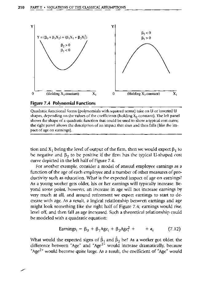
R2 < 0 p 1 >0
210 PART II • VIOLATIONS OF THE CLASSICAL ASSUMPTIONS
Y Y
Y = (Ro + R3X2) + (R1X1 + 132X?)
R2> 0 13 1 <o
0 (Holding X2 constant) X 1 0 (Holding X2 constant) X 1
Figure 7.4 Polynomial Functions
Quadratic functional forms (polynomials with squared terms) take on U or inverted U shapes, depending on the values of the coefficients (holding X2 constant). The left panel shows the shape of a quadratic function that could be used to show a typical cost curve; the right panel allows the description of an impact that rises and then falls (like the im-pact of age on earnings).
tion and X 1 being the level of output of the firm, then we would expect 131 to be negative and 13 2 to be positive if the firm has the typical U-shaped cost curve depicted in the left half of Figure 7.4.
For another example, consider a model of annual employee earnings as a function of the age of each employee and a number of other measures of pro-ductivity such as education. What is the expected impact of age on earnings? As a young worker gets older, his or her earnings will typically increase. Be-yond some point, however, an increase in age will not increase earnings by very much at all, and around retirement we expect earnings to start to de-crease with age. As a result, a logical relationship between earnings and age might look something like the right half of Figure 7.4; earnings would rise, level off, and then fall as age increased. Such a theoretical relationship could be modeled with a quadratic equation:
Earnings i = Ro + R l Agei + 13 2Age; +
+ Ei (7.12)
What would the expected signs of R 1 and 132 be? As a worker got older, the difference between "Age" and "Age 2 " would increase dramatically, because "Age2 " would become quite large. As a result, the coefficient of "Age" would
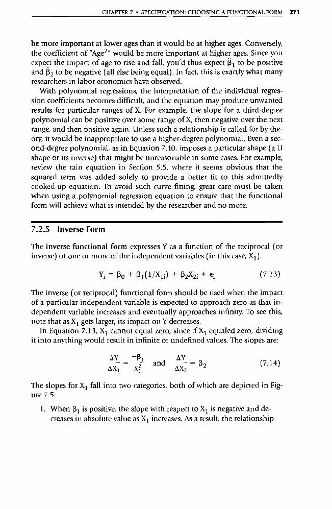
CHAPTER 7 • SPECIFICATION: CHOOSING A FUNCTIONAL FORM 211
be more important at lower ages than it would be at higher ages. Conversely, the coefficient of "Age e " would be more important at higher ages. Since you expect the impact of age to rise and fall, you'd thus expect R 1 to be positive and R2 to be negative (all else being equal). In fact, this is exactly what many researchers in labor economics have observed.
With polynomial regressions, the interpretation of the individual regres-sion coefficients becomes difficult, and the equation may produce unwanted results for particular ranges of X. For example, the slope for a third-degree polynomial can be positive over some range of X, then negative over the next range, and then positive again. Unless such a relationship is called for by the-ory, it would be inappropriate to use a higher-degree polynomial. Even a sec-ond-degree polynomial, as in Equation 7.10, imposes a particular shape (a U shape or its inverse) that might be unreasonable in some cases. For example, review the rain equation in Section 5.5, where it seems obvious that the squared term was added solely to provide a better fit to this admittedly cooked-up equation. To avoid such curve fitting, great care must be taken when using a polynomial regression equation to ensure that the functional form will achieve what is intended by the researcher and no more.
7.2.5 Inverse Form
The inverse functional form expresses Y as a function of the reciprocal (or inverse) of one or more of the independent variables (in this case, X 1 ):
Yi = Ro + R1( 1 /X1i) + R2X2i + Ei (7.13)
The inverse (or reciprocal) functional form should be used when the impact of a particular independent variable is expected to approach zero as that in-dependent variable increases and eventually approaches infinity. To see this, note that as X 1 gets larger, its impact on Y decreases.
In Equation 7.13, X 1 cannot equal zero, since if X 1 equaled zero, dividing it into anything would result in infinite or undefined values. The slopes are:
AY — R1 AY
OXl =
Xz and OX2 = R2 (7.14)
The slopes for X 1 fall into two categories, both of which are depicted in Fig-ure 7.5:
1. When R1 is positive, the slope with respect to X 1 is negative and de-creases in absolute value as X 1 increases. As a result, the relationship
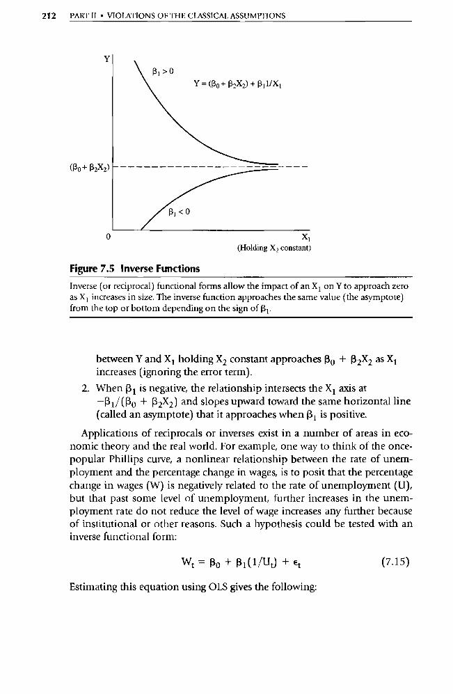
212 PART II • VIOLATIONS OF THE CLASSICAL ASSUMPTIONS
Y
(Ro + 132X2)
> 0
Y = (Ro + 132X2) + R i 1/X 1
< 0
o
X i (Holding X2 constant)
Figure 7.5 Inverse Functions
Inverse (or reciprocal) functional forms allow the impact of an X 1 on Y to approach zero as X 1 increases in size. The inverse function approaches the same value (the asymptote)
from the top or bottom depending on the sign of 13 1 .
between Y and X 1 holding X2 constant approaches 13 o + 132X2 as X1 increases (ignoring the error term).
2. When 131 is negative, the relationship intersects the X 1 axis at 131 ^ (13o + 13 2X2) and slopes upward toward the same horizontal line
(called an asymptote) that it approaches when 13 1 is positive.
Applications of reciprocals or inverses exist in a number of areas in eco-nomic theory and the real world. For example, one way to think of the once-popular Phillips curve, a nonlinear relationship between the rate of unem-ployment and the percentage change in wages, is to posit that the percentage
change in wages (W) is negatively related to the rate of unemployment (U),
but that past some level of unemployment, further increases in the unem-ployment rate do not reduce the level of wage increases any further because
of institutional or other reasons. Such a hypothesis could be tested with an
inverse functional form:
Wt = 13 o + 13 1( 1 /Ut) + Et (7.15)
Estimating this equation using OLS gives the following:

CHAPTER 7 • SPECIFICATION: CHOOSING A FUNCTIONAL FORM 213
Wt = 0.00679 + 0.1842(1 /U0 (0.0590)
t = 3.20 R2 =.397
(7.16)
This indicates that W and U are related in a way similar to that hypothesized (as shown in Figure 7.5 when 13 1 is positive), but it doesn't provide any evi-dence that the inverse functional form is the best way to depict this particular theory. For more on this example, see Exercise 5.
7.3 Problems with Incorrect Functional Forms
The best way to choose a functional form for a regression model is to choose a specification that matches the underlying theory of the equation. In a ma-jority of cases, the linear form will be adequate, and for most of the rest, common sense will point out a fairly easy choice from among the alterna-tives outlined above. Table 7.1 contains a summary of the properties of the various alternative functional forms.
Once in a while, however, a circumstance will arise in which the model is logically nonlinear in the variables, but the exact form of this nonlinearity is hard to specify. In such a case, the linear form is not correct, and yet a choice between the various nonlinear forms cannot be made on the basis of eco-nomic theory. Even in these cases, however, it still pays (in terms of under-standing the true relationships) to avoid choosing a functional form on the basis of fit alone.
For example, recall the estimated Phillips curve in Equation 7.16. Al-though the negative relationship between unemployment and inflation (us-ing the percentage increase in wages as a proxy) implied by the Phillips curve suggests a downward-sloping nonlinear curve, there are a number of other functional forms that could produce such a curve. In addition to the inverse relationship that was actually used, the double-log form and various semilog and exponential forms could also give shapes that would fit the hypothesis fairly well. If all the functional forms are so similar, and if theory does not specify exactly which form to use, why should we try to avoid using goodness of fit over the sample to determine which equation to use? This section will highlight two answers to this question:
1. Res are difficult to compare if the dependent variable is transformed.
2. An incorrect functional form may provide a reasonable fit within the sample but have the potential to make large forecast errors when used outside the range of the sample.
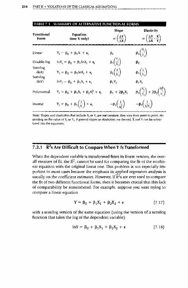
214 PART II • VIOLATIONS OF THE CLASSICAL ASSUMPTIONS
TABLE 7.1 SUMMARY OF ALTERNATIVE FUNCTIONAL FORMS
Functional Form
Equation (one X only)
Slope
(AX)
Elasticity
_ (AY X — ( AY Y
Linear Yi = Po + 13,Xi + ei
Double-log InY i = Ro + R, InX i + e i
Semilog (InX) Y i = Ro = R1 InX i + ei
Semilog (InY) InY i = Ro + R1 Xi + ei
Polynomial Y i = (30 + 13 1 X 1 + 132 X? + Ei
131 X i
R , + 2 R2 X i (31(7-i)+ 2132(Yi )
—R, XiYi1 /l Inverse Y i = Ro + R1. ) + e i
Note: Slopes and elasticities that include X i or Y i are not constant; they vary from point to point, de-pending on the value of X i or Y. If general slopes or elasticities are desired, X and Y can be substi-tuted into the equations.
7.3.1 Res Are Difficult to Compare When Y Is Transformed
When the dependent variable is transformed from its linear version, the over-all measure of fit, the R 2, cannot be used for comparing the fit of the nonlin-ear equation with the o riginal linear one. This problem is not especially im-portant in most cases because the emphasis in applied regression analysis is usually on the coefficient estimates. However, if R es are ever used to compare the fit of two different functional forms, then it becomes crucial that this lack of comparability be remembered. For example, suppose you were trying to compare a linear equation
Y— RO +(3 1X1+R2X2 + E (7.17)
with a semilog version of the same equation (using the version of a semilog function that takes the log of the dependent variable):
1nY = Ro + R1X1 + 132X2 + E (7.18)
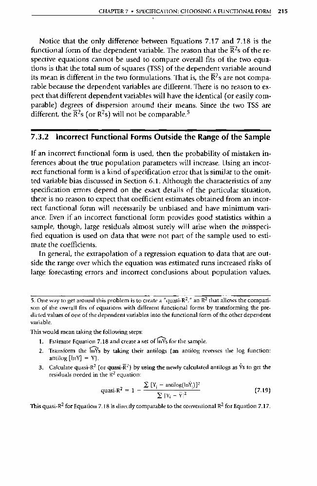
CHAPTER 7 • SPECIFICATION: CHOOSING A FUNCTIONAL FORM 215
Notice that the only difference between Equations 7.17 and 7.18 is the functional form of the dependent variable. The reason that the Res of the re-spective equations cannot be used to compare overall fits of the two equa-tions is that the total sum of squares (TSS) of the dependent variable around
its mean is different in the two formulations. That is, the R es are not compa-rable because the dependent variables are different. There is no reason to ex-pect that different dependent variables will have the identical (or easily com-parable) degrees of dispersion around their means. Since the two TSS are
different, the Res (or Res) will not be comparable. 5
7.3.2 Incorrect Functional Forms Outside the Range of the Sample
If an incorrect functional form is used, then the probability of mistaken in-ferences about the true population parameters will increase. Using an incor-rect functional form is a kind of specification error that is similar to the omit-ted variable bias discussed in Section 6.1. Although the characteristics of any specification errors depend on the exact details of the particular situation, there is no reason to expect that coefficient estimates obtained from an incor-rect functional form will necessarily be unbiased and have minimum vari-ance. Even if an incorrect functional form provides good statistics within a sample, though, large residuals almost surely will arise when the misspeci-fled equation is used on data that were not pa rt of the sample used to esti-mate the coefficients.
In general, the extrapolation of a regression equation to data that are out-side the range over which the equation was estimated runs increased risks of large forecasting errors and incorrect conclusions about population values.
5. One way to get around this problem is to create a "quasi-R 2 ," an R2 that allows the compari-son of the overall fits of equations with different functional forms by transforming the pre-dicted values of one of the dependent variables into the functional form of the other dependent
variable. This would mean taking the following steps:
1. Estimate Equation 7.18 and create a set of InYs for the sample.
2. Transform the Qs by taking their antilogs (an antilog reverses the log function:
antilog [1nY] = Y).
3. Calculate quasi-R 2 (or quasi-R2 ) by using the newly calculated antilogs as Ys to get the
residuals needed in the R 2 equation:
quasi-R2 = 1 (7.19) [Y. — Y] 2
This quasi-R2 for Equation 7.18 is directly comparable to the conventional R 2 for Equation 7.17.
^ [Yi — antilog(1nYi )1 2
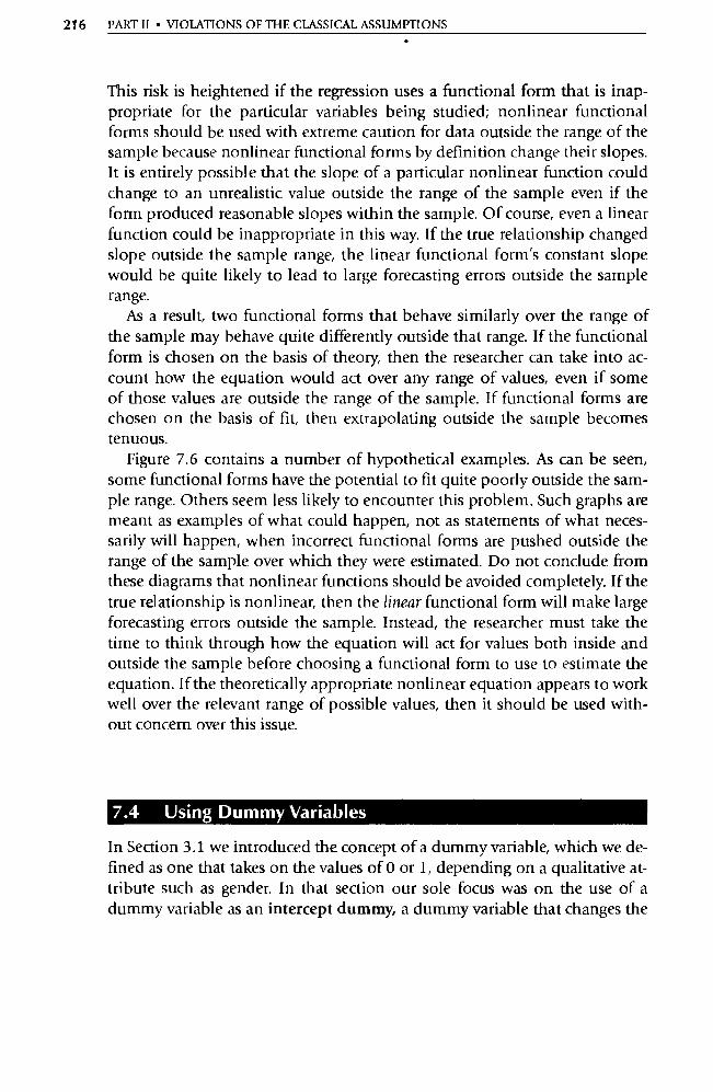
216 PART II • VIOLATIONS OF THE CLASSICAL ASSUMPTIONS
This risk is heightened if the regression uses a functional form that is inap-propriate for the particular variables being studied; nonlinear functional forms should be used with extreme caution for data outside the range of the sample because nonlinear functional forms by definition change their slopes. It is entirely possible that the slope of a particular nonlinear function could change to an unrealistic value outside the range of the sample even if the form produced reasonable slopes within the sample. Of course, even a linear function could be inappropriate in this way. If the true relationship changed slope outside the sample range, the linear functional form's constant slope would be quite likely to lead to large forecasting errors outside the sample range.
As a result, two functional forms that behave similarly over the range of the sample may behave quite differently outside that range. If the functional form is chosen on the basis of theory, then the researcher can take into ac-count how the equation would act over any range of values, even if some of those values are outside the range of the sample. If functional forms are chosen on the basis of fit, then extrapolating outside the sample becomes tenuous.
Figure 7.6 contains a number of hypothetical examples. As can be seen, some functional forms have the potential to fit quite poorly outside the sam-ple range. Others seem less likely to encounter this problem. Such graphs are meant as examples of what could happen, not as statements of what neces-sarily will happen, when incorrect functional forms are pushed outside the range of the sample over which they were estimated. Do not conclude from these diagrams that nonlinear functions should be avoided completely. If the true relationship is nonlinear, then the linear functional form will make large forecasting errors outside the sample. Instead, the researcher must take the time to think through how the equation will act for values both inside and outside the sample before choosing a functional form to use to estimate the equation. If the theoretically appropriate nonlinear equation appears to work well over the relevant range of possible values, then it should be used with-out concern over this issue.
7.4 Using Dummy Variables
In Section 3.1 we introduced the concept of a dummy va riable, which we de-fined as one that takes on the values of 0 or 1, depending on a qualitative at-tribute such as gender. In that section our sole focus was on the use of a dummy variable as an intercept dummy, a dummy variable that changes the
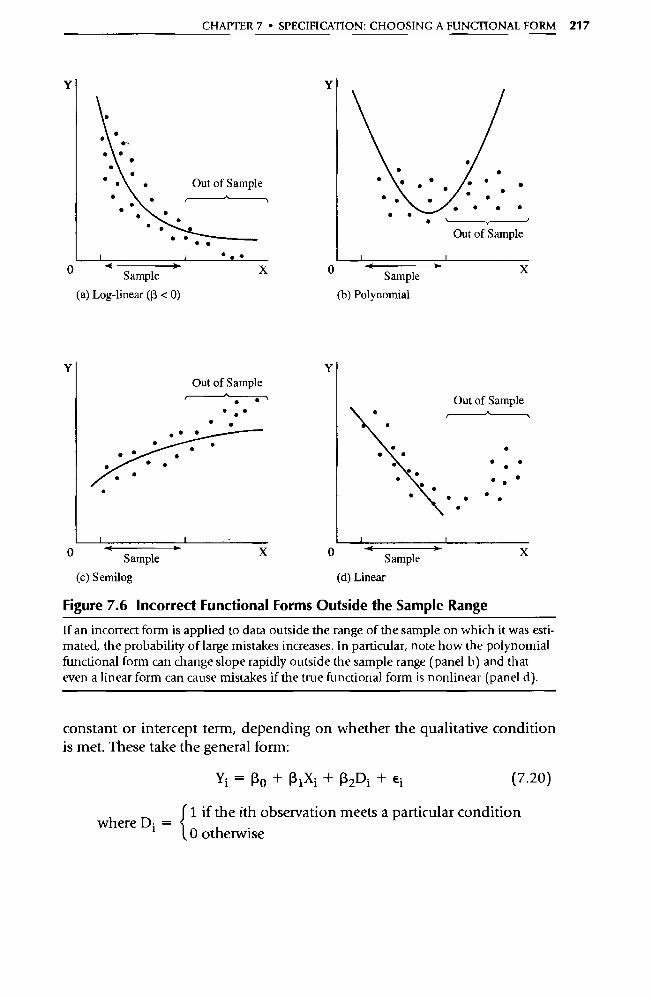
X 0 < Sample•
(a) Log-linear ((3 < 0)
X 0 • Sample
(b) Polynomial
• • • • • •
•
• X 0 Sample
(c) Semilog
X 0 Sample
(d) Linear
Y Y
Y Y
Figure 7.6 Incorrect Functional Forms Outside the Sample Range
• • •
Out of Sample
•
• • • ..
• Out of Sample
Out of Sample •
• • • •_ •
• •
Out of Sample
CHAPTER 7 • SPECIFICATION: CHOOSING A FUNCTIONAL FORM 217
If an incorrect form is applied to data outside the range of the sample on which it was esti-mated, the probability of large mistakes increases. In particular, note how the polynomial functional form can change slope rapidly outside the sample range (panel b) and that even a linear form can cause mistakes if the true functional form is nonlinear (panel d).
constant or intercept term, depending on whether the qualitative condition is met. These take the general form:
Yi = RQ+R1Xi+Q2Di+ Ei (7.20)
J 1 if the ith observation meets a particular condition where D i =
0 otherwise
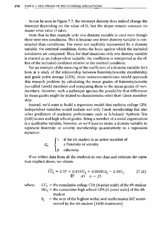
218 PART II • VIOLATIONS OF THE CLASSICAL ASSUMPTIONS
As can be seen in Figure 7.7, the intercept dummy does indeed change the intercept depending on the value of D, but the slopes remain constant no matter what value D takes.
Note that in this example only one dummy variable is used even though there were two conditions. This is because one fewer dummy variable is con-structed than conditions. The event not explicitly represented by a dummy variable, the omitted condition, forms the basis against which the included conditions are compared. Thus, for dual situations only one dummy variable is entered as an independent variable; the coefficient is interpreted as the ef-fect of the included condition relative to the omitted condition.
For an example of the meaning of the coefficient of a dummy variable, let's look at a study of the relationship between fraternity/sorority membership and grade point average (GPA). Most noneconometricians would approach this research problem by calculating the mean grades of fraternity/sorority (so-called Greek) members and comparing them to the mean grades of non-members. However, such a technique ignores the possibility that differences in mean grades might be related to characteristics other than Greek member-ship.
Instead, we'd want to build a regression model that explains college GPA. Independent variables would include not only Greek membership but also other predictors of academic performance such as Scholastic Aptitude Test (SAT) scores and high school grades. Being a member of a social organization is a qualitative variable, however, so we'd have to create a dummy variable to represent fraternity or sorority membership quantitatively in a regression equation:
1 if the ith student is an active member of Gi a fraternity or sorority
t o otherwise
If we collect data from all the students in our class and estimate the equa-tion implied above, we obtain:
CGi = 0.37 + 0.81HGi + 0.00001Si — 0.38Gi (7.21) R2 .45 n = 25
where: CG i = the cumulative college GPA (4-point scale) of the ith student HGi = the cumulative high school GPA (4-point scale) of the ith
student Si = the sum of the highest verbal and mathematics SAT scores
earned by the ith student (1600 maximum)
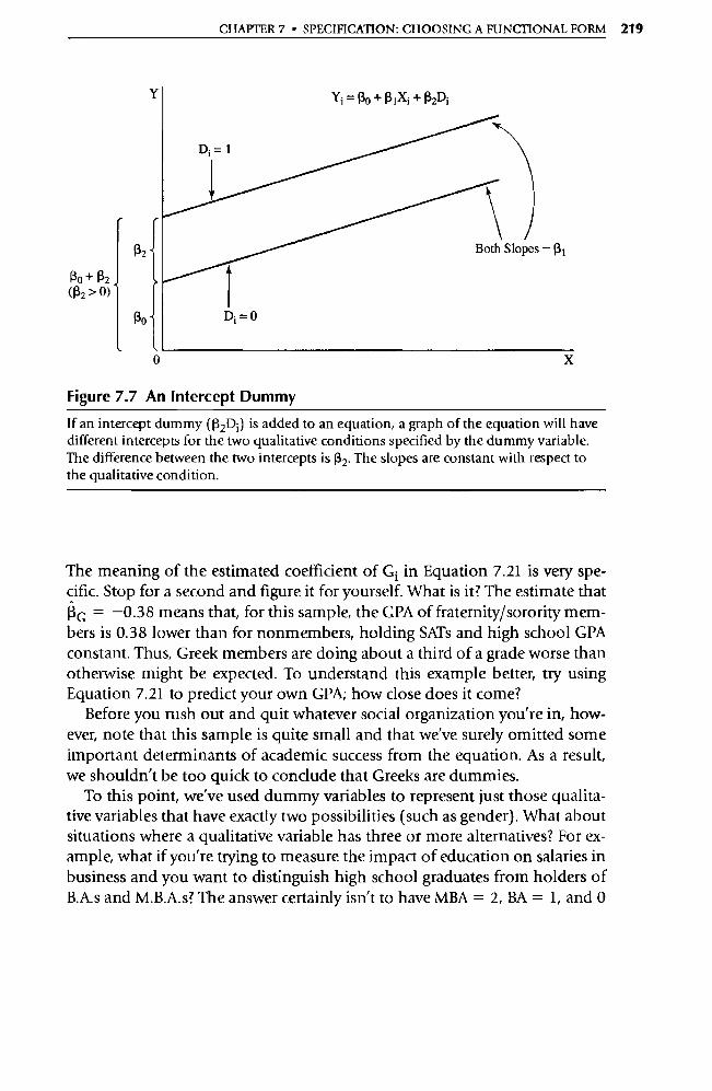
CHAPTER 7 • SPECIFICATION: CHOOSING A FUNCTIONAL FORM 219
Ro + Rz (R2 > 0)
X
Figure 7.7 An Intercept Dummy
If an intercept dummy (13 2 D;) is added to an equation, a graph of the equation will have different intercepts for the two qualitative conditions specified by the dummy variable. The difference between the two intercepts is 132. The slopes are constant with respect to the qualitative condition.
The meaning of the estimated coefficient of Gi in Equation 7.21 is very spe-cific. Stop for a second and figure it for yourself. What is it? The estimate that RG = —0.38 means that, for this sample, the GPA of fraternity/sorority mem-bers is 0.38 lower than for nonmembers, holding SATs and high school GPA constant. Thus, Greek members are doing about a third of a grade worse than otherwise might be expected. To understand this example better, try using Equation 7.21 to predict your own GPA; how close does it come?
Before you rush out and quit whatever social organization you're in, how-ever, note that this sample is quite small and that we've surely omitted some important determinants of academic success from the equation. As a result, we shouldn't be too quick to conclude that Greeks are dummies.
To this point, we've used dummy variables to represent just those qualita-tive variables that have exactly two possibilities (such as gender). What about situations where a qualitative variable has three or more alternatives? For ex-ample, what if you're trying to measure the impact of education on salaries in business and you want to distinguish high school graduates from holders of B.A.s and M.B.A.s? The answer certainly isn't to have MBA = 2, BA = 1, and 0
220 PART IT • VIOLATIONS OF THE CLASSICAL ASSUMPTIONS
otherwise, because we have no reason to think that the impact of having an M.B.A. is exactly twice that of having a B.A. when compared to having no col-lege degree at all. If not that, then what?
The answer is to create one less dummy variable than there are alternatives and to use each dummy to represent just one of the possible conditions. In the salary case, for example, you'd create two variables, the first equal to 1 if the employee had an M.B.A. (0 otherwise) and the second equal to 1 if the employee's highest degree was a B.A. (and 0 otherwise). As before, the omit-ted condition is represented by having both dummies equal to zero. This way you can measure the impact of each degree independently, without having to link the impacts of having an M.B.A. and a B.A.
A dummy variable that has only a single obse rvation with a value of one while the rest of the obse rvations are zeroes (or vice versa) is to be avoided unless the variable is required by theory. Such a "one-time dummy" acts merely to eliminate that obse rvation from the data set, improving the fit arti-ficially by setting the dummy's coefficient equal to the residual for that obser-vation. One would obtain exactly the same estimates of the other coefficients if that observation were deleted, but the deletion of an obse rvation is rarely, if ever, appropriate. Finally, dummy variables can be used as dependent vari-ables; this possibility is covered in an entire chapter, Chapter 13.
7.5 Slope Dummy Variables
Until now, every independent variable in this text has been multiplied by ex-actly one other item, the slope coefficient. To see this, take another look at Equation 7.20:
Yi= Ro +RIXi+R2Di+ Ei (7.20)
In this equation X is multiplied only by R1, and D is multiplied only by 13 2, and there are no other factors involved.
This restriction does not apply to a new kind of variable called an interac-tion term. An interaction term is an independent variable in a regression equation that is the multiple of two or more other independent va riables. Each interaction term has its own regression coefficient, so the end result is that the interaction term has three or more components, as in 03X; Di . Such interaction terms are used when the change in Y with respect to one indepen-dent variable (in this case X) depends on the level of another independent variable (in this case D). For an example of the use of interaction terms that do not involve dummy variables, see Exercise 14.
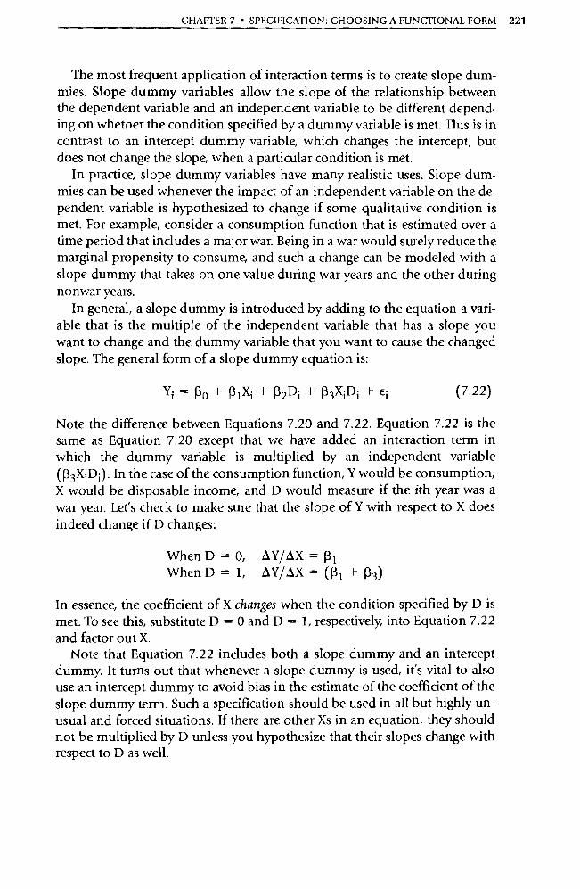
CHAPTER 7 • SPECIFICATION: CHOOSING A FUNCTIONAL FORM 221
The most frequent application of interaction terms is to create slope dum-mies. Slope dummy variables allow the slope of the relationship between the dependent variable and an independent variable to be different depend-ing on whether the condition specified by a dummy variable is met. This is in contrast to an intercept dummy variable, which changes the intercept, but does not change the slope, when a particular condition is met.
In practice, slope dummy variables have many realistic uses. Slope dum-mies can be used whenever the impact of an independent variable on the de-pendent variable is hypothesized to change if some qualitative condition is met. For example, consider a consumption function that is estimated over a time period that includes a major war. Being in a war would surely reduce the marginal propensity to consume, and such a change can be modeled with a slope dummy that takes on one value during war years and the other during nonwar years.
In general, a slope dummy is introduced by adding to the equation a vari-able that is the multiple of the independent va riable that has a slope you want to change and the dummy variable that you want to cause the changed slope. The general form of a slope dummy equation is:
Yi = Ro + R1Xi + R2D1 + 13 3X; D i + e; (7.22)
Note the difference between Equations 7.20 and 7.22. Equation 7.22 is the same as Equation 7.20 except that we have added an interaction term in which the dummy va riable is multiplied by an independent variable (33XiDi ). In the case of the consumption function, Y would be consumption, X would be disposable income, and D would measure if the ith year was a war year. Let's check to make sure that the slope of Y with respect to X does indeed change if D changes:
When D = 0, AY/AX = R i
When D = 1, AY/AX = (RI + 133)
In essence, the coefficient of X changes when the condition specified by D is met. To see this, substitute D = 0 and D = 1, respectively, into Equation 7.22 and factor out X.
Note that Equation 7.22 includes both a slope dummy and an intercept dummy. It turns out that whenever a slope dummy is used, it's vital to also use an intercept dummy to avoid bias in the estimate of the coefficient of the slope dummy term. Such a specification should be used in all but highly un-usual and forced situations. If there are other Xs in an equation, they should not be multiplied by D unless you hypothesize that their slopes change with respect to D as well.
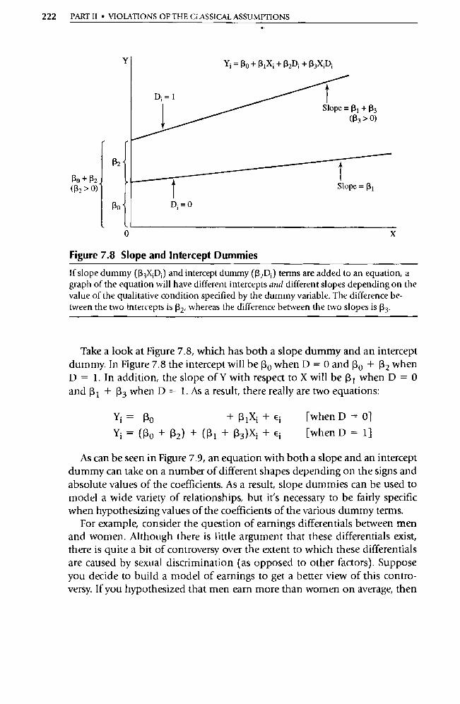
222 PART II • VIOLATIONS OF THE CLASSICAL ASSUMPTIONS
Ro + 132 (R2 > 0)
X
Figure 7.8 Slope and Intercept Dummies
If slope dummy 03 3Xi D; ) and intercept dummy (p2Di ) terms are added to an equation, a graph of the equation will have different intercepts and different slopes depending on the value of the qualitative condition specified by the dummy variable. The difference be- tween the two intercepts is 13 2, whereas the difference between the two slopes is 133 .
Take a look at Figure 7.8, which has both a slope dummy and an intercept dummy. In Figure 7.8 the intercept will be 1 o when D = 0 and 13 0 + R2 when D = 1. In addition, the slope of Y with respect to X will be 13 1 when D = 0 and 13 1 + 133 when D = 1. As a result, there really are two equations:
Yi RO + 13 1Xi + Ei [when D = 0]
Yi = ( Ro + 132) + ( 3 1 + 133)Xi + E i [when D = 1 ]
As can be seen in Figure 7.9, an equation with both a slope and an intercept dummy can take on a number of different shapes depending on the signs and absolute values of the coefficients. As a result, slope dummies can be used to model a wide variety of relationships, but it's necessary to be fairly specific when hypothesizing values of the coefficients of the various dummy terms.
For example, consider the question of earnings differentials between men and women. Although there is little argument that these differentials exist, there is quite a bit of controversy over the extent to which these differentials are caused by sexual discrimination (as opposed to other factors). Suppose you decide to build a model of earnings to get a better view of this contro-versy. If you hypothesized that men earn more than women on average, then
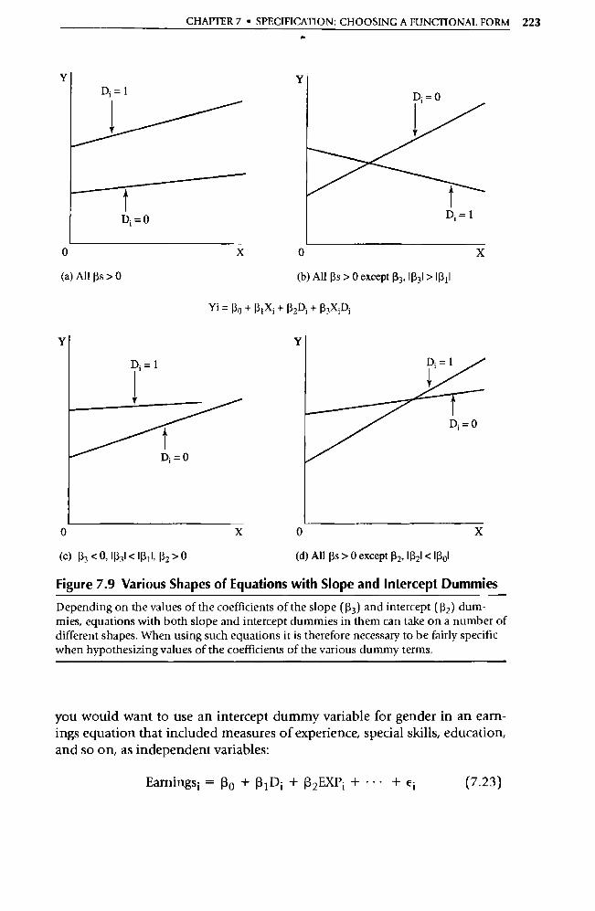
Y D; = 1
^
Di =O
0
(a) All 13s > 0
(b) All 13s > 0 except 133 , 113 3 1 > 113 1 1
Yi = Ro + R1X1 + R2Di + R 3X;D;
0 X
(c) 133 < 0, 11331 < Ili 1 1, 132 > 0 (d) All 13s > 0 except 132, 11321 < 113 01
Y
I D; = 1
D; = O
CHAPTER 7 • SPECIFICATION: CHOOSING A FUNCTIONAL FORM 223
Figure 7.9 Various Shapes of Equations with Slope and Intercept Dummies
Depending on the values of the coefficients of the slope (13 3) and intercept (13 2) dum-mies, equations with both slope and intercept dummies in them can take on a number of different shapes. When using such equations it is therefore necessary to be fairly specific when hypothesizing values of the coefficients of the various dummy terms.
you would want to use an intercept dummy va riable for gender in an earn-ings equation that included measures of experience, special skills, education, and so on, as independent variables:
Earningsi = Ro + + R2 EXP i + • • + ei (7.23)
224 PART II • VIOLATIONS OF THE CLASSICAL ASSUMPTIONS
•
where: D; = 1 if the ith worker is male and 0 otherwise EXP; = the years experience of the ith worker Ei = a classical error term
In Equation 7.23, (3 1 would be an estimate of the average difference between males and females holding constant their experience and the other factors in the equation. Equation 7.23 also forces the impact of increases in experience (and the other factors in the equation) to have the same effect for females as for males because the slopes are the same for both genders.
If you hypothesized that men also increase their earnings more per year of experience than women, then you would include a slope dummy as well as an intercept dummy in such a model:
Earnings; = 130 + 3 1Di + 13 2EXP; + 133 D; EXP; + + Ei (7.24)
In Equation 7.24, 33 would be an estimate of the differential impact of an ex-tra year of experience on earnings between men and women. We could test the possibility of a positive true R3 by running a one-tailed t-test on R 3 . If R3 were significantly different from zero in a positive direction, then we could reject the null hypothesis of no difference due to gender in the impact of ex-perience on earnings, holding constant the other variables in the equation. 6
Such an equation would be described by panel a in Figure 7.9.
7.6 Summary
1. Do not suppress the constant term even if it appears to be theoreti-cally likely to equal zero. On the other hand, don't rely on estimates of the constant term for inference even if it appears to be statistically significant.
2. The choice of a functional form should be based on the underlying eco-
6. Another approach to this problem is to use the Chow test suggested at the very end of Sec-tion 7.7 (the appendix on the F-test). To apply the Chow test to the question of earnings differ-entials between genders, use Equation 7.24 as the unconstrained equation (with all indepen-dent variables also having slope dummy formulations) and
Earnings; = (3o + f3 1 EXP; + + e; (7.25)
as the constrained equation for the full data set and for each gender separately. If the F-test shows that the fit of Equation 7.24 is significantly better than the fit of Equation 7.25, then we would reject the null hypothesis of equivalence between the male and female slope coefficients in the earnings equation.
CHAPTER 7 • SPECIFICATION: CHOOSING A FUNCTIONAL FORM 225
nomic theory to the extent to which theory suggests a shape similar to that provided by a particular functional form. A form that is linear in the variables should be used until a specific hypothesis suggests otherwise.
3. Functional forms that are nonlinear in the variables include the dou-ble-log form, the semilog form, the polynomial form, and the inverse form. The double-log form is especially useful if the elasticities in-volved are expected to be constant. The semilog and inverse forms have the advantage of allowing the effect of an independent variable to tail off as that variable increases. The polynomial form is useful if the slopes are expected to depend on the level of an independent vari-able, but polynomials of degree higher than two should be avoided unless the underlying theory specifically calls for them.
4. The use of nonlinear functional forms has a number of potential prob-lems. In particular, the k 2s are difficult to compare if Y has been trans-formed, and the residuals are potentially large if an incorrect func-tional form is used for forecasting outside the range of the sample.
5. A slope dummy is a dummy variable that is multiplied by an inde-pendent variable to allow the slope of the relationship between the dependent variable and the particular independent variable to change, depending on whether or not a particular condition is met.
Exercises
(Answers to even-numbered exercises in Appendix A.)
1. Write out the meaning of each of the following terms without refer-ring to the book (or your notes), and compare your definition with the version in the text for each: a. elasticity b. double-log functional form c. semilog functional form d. polynomial functional form e. inverse functional form f. slope dummy g. natural log h. omitted condition
2. For each of the following pairs of dependent (Y) and independent (X) variables, pick the functional form that you think is likely to be ap-
226 PART II • VIOLATIONS OF THE CLASSICAL ASSUMPTIONS
propriate, and then explain your reasoning (assume that all other rel-evant independent variables are included in the equation): a. Y = sales of shoes
X = disposable income b. Y = the attendance at the Hollywood Bowl outdoor symphony
concerts on a given night X = whether the orchestra's most famous conductor was scheduled
to conduct that night c. Y = aggregate consumption of goods and services in the United
States X = aggregate disposable income in the United States
d. Y = the money supply in the United States X = the interest rate on Treasury Bills (in a demand function)
e. Y = the average cost of production of a box of pasta X = the number of boxes of pasta produced
f. How would your answer to pa rt e change if you knew there was a significant outlier due to a capacity constraint and a rush order one year?
3. Can either (or both) of the following be estimated with OLS? Why?
a. Yi = (3 o41 XRf eui
b. Yi = el3( )t + ui
where u i is a typical classical error term and e is the base of the nat-ural logarithm.
4. Consider the following estimated semilog equation (standard errors are in parentheses):
1nSALi = 8.10 + 0.100EDi + 0.110EXPi (0.025) (0.050)
R2 =.48 n=28
where: 1nSALi = the log of the salary of the ith worker ED i = the years of education of the ith worker EXPi = the years of experience of the ith worker
a. Make appropriate hypotheses for signs, calculate t-scores, and test your hypotheses.
b. What is the economic meaning of the constant in this equation? c. Why do you think a left-side semilog functional form is used in
this model? More specifically, what are the slopes of salary with re-spect to education and experience?

CHAI'I'ER 7 • SPECIFICATION: CHOOSING A FUNCTIONAL FORM 227
d. Suppose you ran the linear version of this equation and obtained an R2 of .46. What can you conclude from this result?
5. The Phillips curve discussed in Section 7.2.5 is a good example of the use of econometrics to develop, refine, and test theory. The curve was originally "discovered" in an empirical study and once was firmly be-lieved to be true. Today, the Phillips curve is not as highly regarded as it used to be, in pa rt because of empirical results. Since data for esti-mating a Phillips curve are readily available, you can test the validity of the Phillips curve yourself. a. Search the literature (starting with the Journal of Economic Litera-
ture) and follow the controversy surrounding the topic of the Phillips curve and its estimation. 7
b. Review the possible functional forms summarized in Section 7.2. What else besides an inverse function could have been used to esti-mate the model?
c. Collect data and compare alternative functional forms for the Phillips curve.
d. From the middle 1970s to the early 1980s, a Phillips curve esti-mated from data on the U.S. economy might have shown a positive slope. What inference should you draw from such an unexpected sign? Why?
6. In an effort to explain regional wage differentials, you collect wage data from 7,338 unskilled workers, divide the count ry into four re-gions (Northeast, South, Midwest, and West), and estimate the fol-lowing equation (standard errors in parentheses):
Yî = 4.78 — 0.038Eî — 0.041Si 0.048Wî (0.019) (0.010) (0.012)
R2 =.49 n = 7,338
where: Yî = the hourly wage (in dollars) of the ith unskilled worker Ei = a dummy variable equal to 1 if the ith worker lives in
the Northeast and 0 otherwise Si = a dummy variable equal to 1 if the ith worker lives in
the South and 0 otherwise Wi = a dummy variable equal to 1 if the ith worker lives in
the West and 0 otherwise
7 For example, see Nancy Wulwick, "Phillips' Approximate Regression," in Neil de Marchi and Christopher Gilbert, eds. History and Methodology of Econometrics (Oxford: Clarendon Press, 1989), pp. 170-188. This book contains many other interesting articles on econometrics.
228 PART H • VIOLATIONS OF THE CLASSICAL ASSUMPTIONS
a. What is the omitted condition in this equation? b. If you add a dummy variable for the omitted condition to the
equation without dropping E i, Si , or Wi, what will happen? c. If you add a dummy variable for the omitted condition to the
equation and drop Ei, what will the sign of the new variable's esti-mated coefficient be?
d. Which of the following three statements is most correct? Least cor-rect? Explain your answer. i. The equation explains 49 percent of the variation of Y around
its mean with regional variables alone, so there must be quite a bit of wage variation by region.
ii. The coefficients of the regional va riables are virtually identical, so there must not be much wage variation by region.
iii.The coefficients of the regional variables are quite small com-pared with the average wage, so there must not be much wage variation by region.
e. If you were going to add one variable to this model, what would it be? Justify your choice.
7. V. N. Murti and V. K. Sastri 8 investigated the production characteris-tics of various Indian industries, including cotton and sugar. They specified Cobb-Douglas production functions for output (Q) as a double-log function of labor (L) and capital (K)
1nQi = Ro + (i 1 1nLi + (i2lnKi + ei
and obtained the following estimates (standard errors in parentheses):
Ro
Industry
Cotton 0.97 0.92 0.12 .98 (0.03) (0.04)
Sugar 2.70 0.59 0.33 .80 (0.14) (0.17)
a. Hypothesize and test appropriate null hypotheses at the 5 percent level of significance. (Hint: This is much harder than it looks!)
01 R2 R2
8. V. N. Murti and V. K. Sastri, "Production Functions for Indian Industry," Econometrica, April 1957, pp. 205-221.
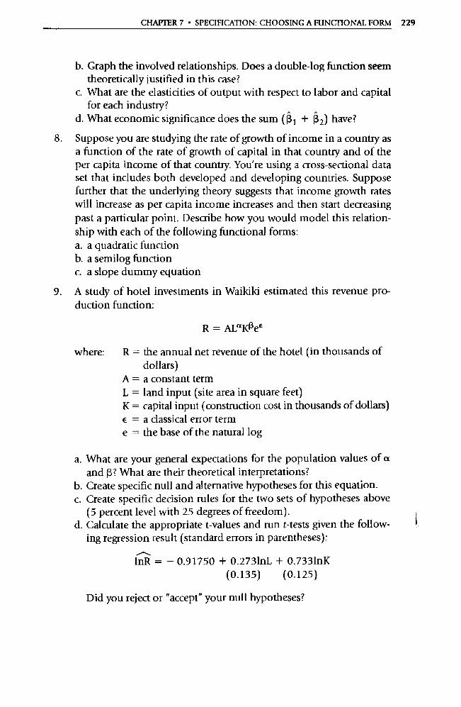
CHAPTER 7 • SPECIFICATION: CHOOSING A FUNCTIONAL FORM 229
b. Graph the involved relationships. Does a double-log function seem theoretically justified in this case?
c. What are the elasticities of output with respect to labor and capital for each industry?
d. What economic significance does the sum ((3 1 + R2) have?
8. Suppose you are studying the rate of growth of income in a count ry as a function of the rate of growth of capital in that count ry and of the per capita income of that country. You're using a cross-sectional data set that includes both developed and developing countries. Suppose further that the underlying theory suggests that income growth rates will increase as per capita income increases and then start decreasing past a particular point. Describe how you would model this relation-ship with each of the following functional forms: a. a quadratic function b. a semilog function c. a slope dummy equation
9. A study of hotel investments in Waikiki estimated this revenue pro-duction function:
R = AL°tKReE
where: R = the annual net revenue of the hotel (in thousands of dollars)
A = a constant term L = land input (site area in square feet) K = capital input (construction cost in thousands of dollars) E = a classical error term e = the base of the natural log
a. What are your general expectations for the population values of a and (3? What are their theoretical interpretations?
b. Create specific null and alternative hypotheses for this equation. c. Create specific decision rules for the two sets of hypotheses above
(5 percent level with 25 degrees of freedom). d. Calculate the appropriate t-values and run t-tests given the follow-
ing regression result (standard errors in parentheses):
1nR = — 0.91750 + 0.2731nL + 0.7331nK (0.135) (0.125)
Did you reject or "accept" your null hypotheses?

230 PART II • VIOLATIONS OF THE CLASSICAL ASSUMPTIONS
e. Is this result surprising? If you were going to build a Waikiki hotel, what input would you most want to use for investment? Is there an additional piece of information you would need to know before you could answer?
10. William Comanor and Thomas Wilson 9 specified the following re-gression in their study of advertising's effect on the profit rates of 41 consumer goods firms:
PR; = Ro + 13 1 ADV; /SALES ; + (32 1nCAP; + (33 1nES; + (i4 1nDG; + Ei
where: PR; = the profit rate of the ith firm ADV; = the advertising expenditures in the ith firm (in
dollars) SALES; = the total gross sales of the ith firm (in dollars) CAP; = the capital needed to enter the ith firm's market
at an efficient size ES; = the degree to which economies of scale exist in
the ith firm's industry DG; = percent growth in sales (demand) of the ith firm
over the last 10 years In = natural logarithm E; = a classical error term
a. Hypothesize expected signs for each of the slope coefficients. b. Note that there are two different kinds of nonlinear (in the vari-
ables) relationships in this equation. For each independent vari-able, determine the shape that the chosen functional form implies, and state whether you agree or disagree with this shape. Explain your reasoning in each case.
c. Comanor and Wilson state that the simple correlation coefficient between ADV;/SALES; and each of the other independent variables is positive. If one of these remaining variables were omitted, in which direction would R1 likely be biased?
11. Suggest the appropriate functional forms for the relationships be-tween the following variables. Be sure to explain your reasoning: a. The age of the ith house in a cross-sectional equation for the sales
price of houses in Cooperstown, New York. (Hint: Cooperstown is known as a lovely town with a number of elegant historic homes.)
9. William S. Comanor and Thomas A. Wilson, "Advertising, Market S tructure and Perfor-mance," Review of Economics and Statistics, November 1967, p. 432.
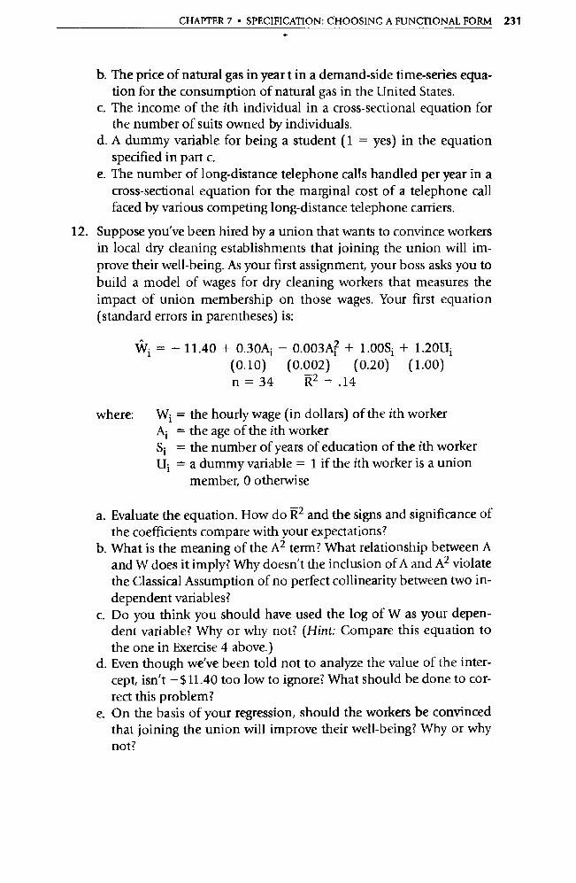
CHAPTER 7 • SPECIFICATION: CHOOSING A FUNCTIONAL FORM 231
b. The price of natural gas in year t in a demand-side time-series equa-tion for the consumption of natural gas in the United States.
c. The income of the ith individual in a cross-sectional equation for the number of suits owned by individuals.
d. A dummy variable for being a student (1 = yes) in the equation specified in part c.
e. The number of long-distance telephone calls handled per year in a cross-sectional equation for the marginal cost of a telephone call faced by various competing long-distance telephone carriers.
12. Suppose you've been hired by a union that wants to convince workers in local d ry cleaning establishments that joining the union will im-prove their well-being. As your first assignment, your boss asks you to build a model of wages for d ry cleaning workers that measures the impact of union membership on those wages. Your first equation (standard errors in parentheses) is:
W; _ — 11.40 + 0.30A; — 0.003A? + 1.00S ; + 1.20U; (0.10) (0.002) (0.20) (1.00) n=34 R2 =.14
where: W; = the hourly wage (in dollars) of the ith worker A; = the age of the ith worker S; = the number of years of education of the ith worker U; = a dummy va riable = 1 if the ith worker is a union
member, 0 otherwise
a. Evaluate the equation. How do 112 and the signs and significance of the coefficients compare with your expectations?
b. What is the meaning of the A2 term? What relationship between A and W does it imply? Why doesn't the inclusion of A and A 2 violate the Classical Assumption of no perfect collinearity between two in-dependent variables?
c. Do you think you should have used the log of W as your depen-dent variable? Why or why not? (Hint: Compare this equation to the one in Exercise 4 above.)
d. Even though we've been told not to analyze the value of the inter-cept, isn't — $11.40 too low to ignore? What should be done to cor-rect this problem?
e. On the basis of your regression, should the workers be convinced that joining the union will improve their well-being? Why or why not?
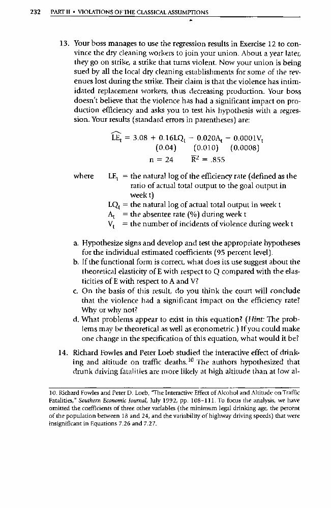
232 PART II • VIOLATIONS OF THE CLASSICAL ASSUMPTIONS
13. Your boss manages to use the regression results in Exercise 12 to con-vince the d ry cleaning workers to join your union. About a year later, they go on strike, a strike that turns violent. Now your union is being sued by all the local dry cleaning establishments for some of the rev-enues lost during the strike. Their claim is that the violence has intim-idated replacement workers, thus decreasing production. Your boss doesn't believe that the violence has had a significant impact on pro-duction efficiency and asks you to test his hypothesis with a regres-sion. Your results (standard errors in parentheses) are:
LEt = 3.08 + 0.16LQt — 0.020At — 0.0001Vt
(0.04) (0.010) (0.0008)
n=24 R2 =.855
where LEt = the natural log of the efficiency rate (defined as the ratio of actual total output to the goal output in week t)
LQt = the natural log of actual total output in week t At = the absentee rate (%) during week t Vt = the number of incidents of violence during week t
a. Hypothesize signs and develop and test the appropriate hypotheses for the individual estimated coefficients (95 percent level).
b. If the functional form is correct, what does its use suggest about the theoretical elasticity of E with respect to Q compared with the elas-ticities of E with respect to A and V?
c. On the basis of this result, do you think the cou rt will conclude that the violence had a significant impact on the efficiency rate? Why or why not?
d. What problems appear to exist in this equation? (Hint: The prob-lems may be theoretical as well as econometric.) If you could make one change in the specification of this equation, what would it be?
14. Richard Fowles and Peter Loeb studied the interactive effect of drink-ing and altitude on traffic deaths. 10 The authors hypothesized that drunk driving fatalities are more likely at high altitude than at low al-
10. Richard Fowles and Peter D. Loeb, "The Interactive Effect of Alcohol and Altitude on Traffic Fatalities," Southern Economic Jou rnal, July 1992, pp. 108-111. To focus the analysis, we have omitted the coefficients of three other va riables (the minimum legal drinking age, the percent of the population between 18 and 24, and the variability of highway driving speeds) that were insignificant in Equations 7.26 and 7.27.
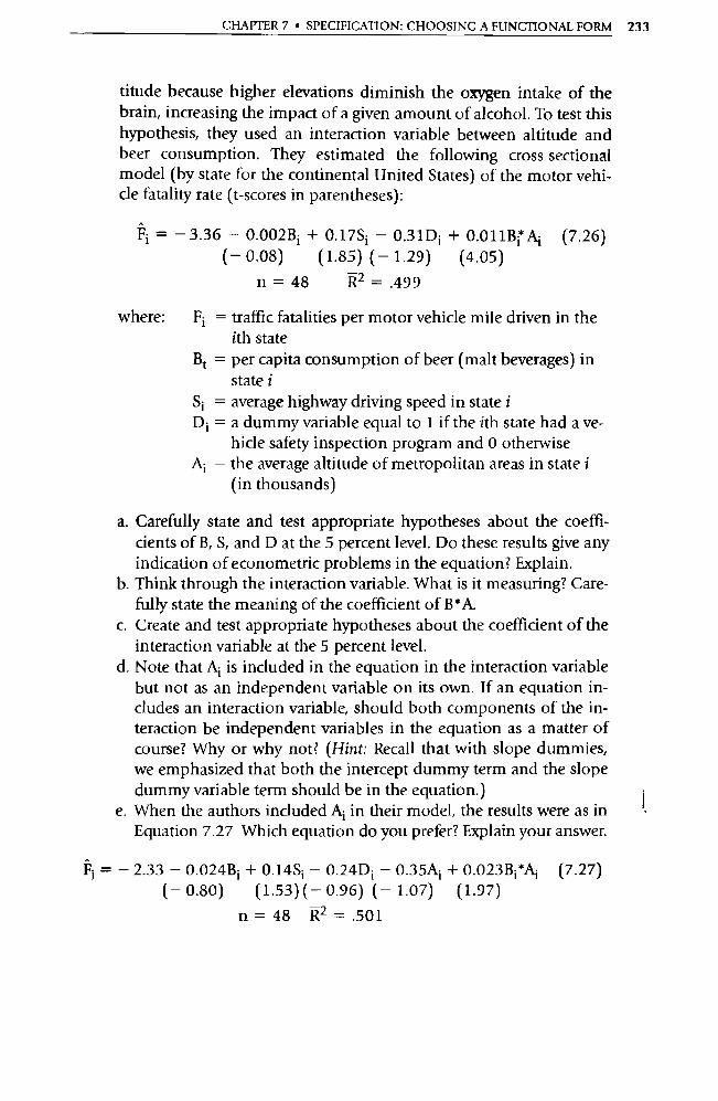
CHAPTER 7 • SPECIFICATION: CHOOSING A FUNCTIONAL FORM 233
titude because higher elevations diminish the oxygen intake of the brain, increasing the impact of a given amount of alcohol. To test this hypothesis, they used an interaction variable between altitude and beer consumption. They estimated the following cross-sectional model (by state for the continental United States) of the motor vehi-cle fatality rate (t-scores in parentheses):
Fi =- 3.36 - 0.002B;+0.17S î -0.31Di +0.011B;Ai (7.26) (— 0.08) (1.85) (— 1.29) (4.05)
n=48 R2 =.499
where: Fi = traffic fatalities per motor vehicle mile driven in the ith state
Bt = per capita consumption of beer (malt beverages) in state i
Si = average highway driving speed in state i D ; = a dummy variable equal to 1 if the ith state had a ve-
hicle safety inspection program and 0 otherwise Ai = the average altitude of metropolitan areas in state i
(in thousands)
a. Carefully state and test appropriate hypotheses about the coeffi-cients of B, S, and D at the 5 percent level. Do these results give any indication of econometric problems in the equation? Explain.
b. Think through the interaction variable. What is it measuring? Care-fully state the meaning of the coefficient of B *A.
c. Create and test appropriate hypotheses about the coefficient of the interaction variable at the 5 percent level.
d. Note that A ; is included in the equation in the interaction variable but not as an independent variable on its own. If an equation in-cludes an interaction variable, should both components of the in-teraction be independent variables in the equation as a matter of course? Why or why not? (Hint: Recall that with slope dummies, we emphasized that both the intercept dummy term and the slope dummy variable term should be in the equation.)
e. When the authors included A i in their model, the results were as in Equation 7.27 Which equation do you prefer? Explain your answer.
Fi = - 2.33 — 0.024Bî + 0.14Si — 0.24D i — 0.35A; + 0.023B; *Ai (7.27) (— 0.80) (1.53)(— 0.96) (— 1.07) (1.97)
n=48 R2=.501
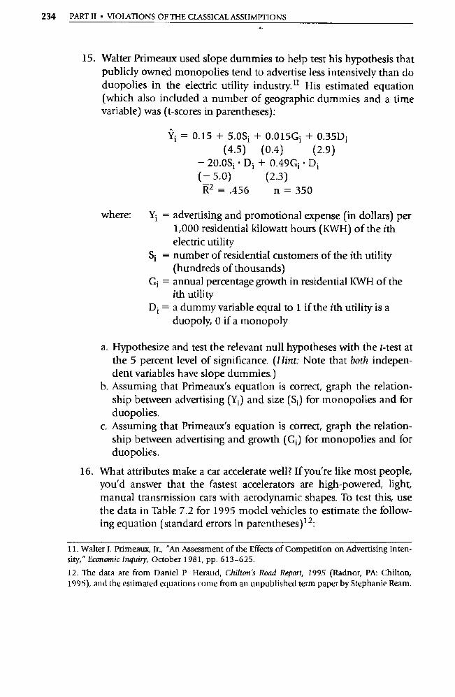
234 PART II • VIOLATIONS OF THE CLASSICAL ASSUMPTIONS •
15. Walter Primeaux used slope dummies to help test his hypothesis that publicly owned monopolies tend to advertise less intensively than do duopolies in the electric utility industry." His estimated equation (which also included a number of geographic dummies and a time variable) was (t-scores in parentheses):
=0.15+5.0Si +0.015G; +0.35Di
(4.5) (0.4) (2.9) —20.0S i •Di + 0.49G1 •D i (— 5.0) (2.3)
R2 =.456 n=350
where: Y; = advertising and promotional expense (in dollars) per 1,000 residential kilowatt hours (KWH) of the ith electric utility
Si = number of residential customers of the ith utility (hundreds of thousands)
Gi = annual percentage growth in residential KWH of the ith utility
D i = a dummy variable equal to 1 if the ith utility is a duopoly, 0 if a monopoly
a. Hypothesize and test the relevant null hypotheses with the t-test at the 5 percent level of significance. (Hint: Note that both indepen-dent variables have slope dummies.)
b. Assuming that Primeaux's equation is correct, graph the relation-ship between advertising (Yi ) and size (Si ) for monopolies and for duopolies.
c. Assuming that Primeaux's equation is correct, graph the relation-ship between advertising and growth (G i) for monopolies and for duopolies.
16. What attributes make a car accelerate well? If you're like most people, you'd answer that the fastest accelerators are high-powered, light, manual transmission cars with aerodynamic shapes. To test this, use the data in Table 7.2 for 1995 model vehicles to estimate the follow-ing equation (standard errors in parentheses) 12 :
11. Walter J. Primeaux, Jr., "An Assessment of the Effects of Competition on Advertising Inten-sity," Economic Inquiry, October 1981, pp. 613-625.
12. The data are from Daniel P Heraud, Chilton's Road Repo rt, 1995 (Radnor, PA: Chilton, 1995), and the estimated equations come from an unpublished term paper by Stephanie Ream.
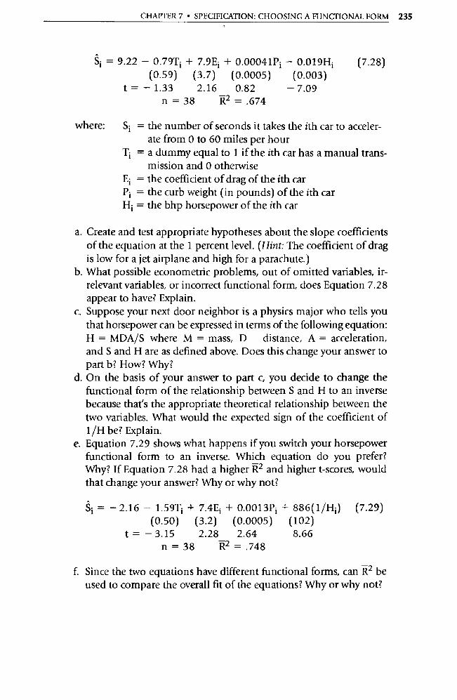
CHAPTER 7 • SPECIFICATION: CHOOSING A FUNCTIONAL FORM 235
Si= 9.22 -0.79Ti +7.9Ei +0.00041Pi -0.019Hî (0.59) (3.7) (0.0005) (0.003)
t = — 1.33 2.16 0.82 — 7.09 n=38 R2 =.674
(7.28)
where: Si = the number of seconds it takes the ith car to acceler- ate from 0 to 60 miles per hour
Ti = a dummy equal to 1 if the ith car has a manual trans-mission and 0 otherwise
Eî = the coefficient of drag of the ith car Pi = the curb weight (in pounds) of the ith car Hi = the bhp horsepower of the ith car
a. Create and test appropriate hypotheses about the slope coefficients of the equation at the 1 percent level. (Hint: The coefficient of drag is low for a jet airplane and high for a parachute.)
b. What possible econometric problems, out of omitted va riables, ir-relevant va riables, or incorrect functional form, does Equation 7.28
appear to have? Explain. c. Suppose your next door neighbor is a physics major who tells you
that horsepower can be expressed in terms of the following equation: H = MDA/S where M = mass, D distance, A = acceleration, and S and H are as defined above. Does this change your answer to part b? How? Why?
d. On the basis of your answer to pa rt c, you decide to change the functional form of the relationship between S and H to an inverse because that's the appropriate theoretical relationship between the two variables. What would the expected sign of the coefficient of 1/H be? Explain.
e. Equation 7.29 shows what happens if you switch your horsepower functional form to an inverse. Which equation do you prefer? Why? If Equation 7.28 had a higher R2 and higher t-scores, would that change your answer? Why or why not?
Si = — 2.16 — 1.59T1 + 7.4Eî + 0.0013Pî + 886(1/Hi) (7.29) (0.50) (3.2) (0.0005) (102)
t = — 3.15 2.28 2.64 8.66 n=38 R2 =.748
f. Since the two equations have different functional forms, can R 2 be used to compare the overall fit of the equations? Why or why not?
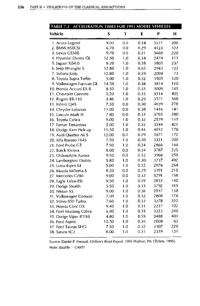
236 PART II • VIOLATIONS OF THE CLASSICAL ASSUMPTIONS
TABLE 7.2 ACCELERATION TIMES FOR 1995 MODEL VEHICLES
Vehicle S T E P H
1. Acura Legend 9.00 0.0 0.34 3571 200 2. BMW 850CSi 6.70 0.0 0.29 4123 322 3. Lexus GS300 9.70 0.0 0.31 3660 220 4. Hyundai Elantra GL 12.50 1.0 0.34 2474 113 5. Jaguar XJS4.0 8.20 1.0 0.38 3805 237 6. Jeep Wrangler S 12.80 1.0 0.65 2943 123 7 Subaru Justy 12.80 1.0 0.39 2004 73 8. Toyota Supra Turbo 5.00 1.0 0.32 3505 320
9. Volkswagen Eurovan GL 14.50 1.0 0.36 3814 110 10. Honda Accord EX-R 8.50 1.0 0.33 3009 145
11. Chevrolet Corvette 5.20 1.0 0.33 3514 405
12. Bugatti EB-110 3.46 1.0 0.29 3571 560
13. Infiniti Q45 7.50 0.0 0.30 4039 278
14. Chrysler Lebaron 11.00 0.0 0.38 1416 141
15. Lincoln Mark III 7.80 0.0 0.33 3765 280
16. Toyota Celica 9.00 1.0 0.32 2579 135
17 Ferrari Testarossa 5.00 1.0 0.32 3344 421
18. Dodge Ram Pick-up 11.50 1.0 0.44 4032 170
19. Audi Quattro A6 S 12.00 0.0 0.29 3671 172
20. Alfa Romeo 164S 7.50 1.0 0.30 3351 200
21. Ford Probe GT 7.90 1.0 0.34 2866 164
22. Buick Riviera 8.00 0.0 0.34 3787 225
23. Oldsmobile Aurora 9.50 0.0 0.32 3966 250
24. Lamborghini Diablo 5.80 1.0 0.30 3737 492
25. Lotus Esprit S4 5.00 1.0 0.32 2976 264
26. Mazda Millenia S 8.20 0.0 0.29 3391 210
27 Mercedes C280 9.00 0.0 0.32 3291 158
28. Eagle Talon ESi 9.50 1.0 0.29 2835 140
29. Dodge Stealth 5.50 1.0 0.33 3792 315
30. Nissan XS 9.00 1.0 0.36 2937 138
31. Volkswagen Corrado 7.00 1.0 0.32 2808 178
32. Volvo 850 Turbo 7.60 1.0 0.32 3278 222
33. Honda Civic DX 9.40 1.0 0.31 2227 102
34. Ford Mustang Cobra 6.80 1.0 0.35 3223 240
35. Dodge Viper RT/10 4.80 1.0 0.55 3488 400
36. Ford Aspire 12.50 1.0 0.36 2004 63
37 Ford Taurus SHO 7.50 1.0 0.32 3307 220
38. Saturn SC2 8.00 1.0 0.31 2359 124
Source: Daniel P. Heraud, Chilton's Road Report, 1995 (Radnor, PA: Chilton, 1995).
Note: datafile = CARS7
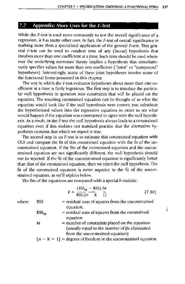
CHAPTER 7 • SPECIFICATION: CHOOSING A FUNCTIONAL FORM 237
7.7 Appendix: More Uses for the F Test
While the F-test is used more commonly to test the overall significance of a regression, it has many other uses. In fact, the F-test of overall significance is nothing more than a specialized application of the general F-test. This gen-eral F-test can be used to conduct tests of any (linear) hypothesis that involves more than one coefficient at a time. Such tests should be used when-ever the underlying economic theory implies a hypothesis that simultane-ously specifies values for more than one coefficient ("joint" or "compound" hypotheses). Interestingly, many of these joint hypotheses involve some of the functional forms presented in this chapter.
The way in which the F-test evaluates hypotheses about more than one co-efficient at a time is fairly ingenious. The first step is to translate the particu-lar null hypothesis in question into constraints that will be placed on the equation. The resulting constrained equation can be thought of as what the equation would look like if the null hypothesis were correct; you substitute the hypothesized values into the regression equation in order to see what would happen if the equation was constrained to agree with the null hypoth-esis. As a result, in the F-test the null hypothesis always leads to a constrained equation even if this violates our standard practice that the alternative hy-pothesis contains that which we expect is true.
The second step in an F-test is to estimate this constrained equation with OLS and compare the fit of this constrained equation with the fit of the un-constrained equation. If the fits of the constrained equation and the uncon-strained equation are not significantly different, the null hypothesis should not be rejected. If the fit of the unconstrained equation is significantly better than that of the constrained equation, then we reject the null hypothesis. The fit of the constrained equation is never superior to the fit of the uncon-strained equation, as we'll explain below.
The fits of the equations are compared with a special F-statistic:
(RSSM — RSS) /M
F RSS/(n K 1) (7.30)
where: RSS = residual sum of squares from the unconstrained equation.
RSSM = residual sum of squares from the constrained equation
M = number of constraints placed on the equation (usually equal to the number of (3s eliminated from the unconstrained equation)
(n — K — 1) = degrees of freedom in the unconstrained equation
238 PART II • VIOLATIONS OF THE CLASSICAL ASSUMPTIONS
RSSM is always greater than or equal to RSS; imposing constraints on the coefficients instead of allowing OLS to select their values can never decrease the summed squared residuals. (Recall that OLS selects that combination of values of the coefficients that minimizes RSS.) At the extreme, if the uncon-strained regression yields exactly the same estimated coefficients as does the constrained regression, then the RSS are equal, and the F-statistic is zero. In this case, H o is not rejected because the data indicate that the constraints ap-pear to be correct. As the difference between the constrained coefficients and the unconstrained coefficients increases, the data indicate that the null hy-pothesis is less likely to be true. Thus, when F gets larger than the critical F-value, the hypothesized rest rictions specified in the null hypothesis are re-jected by the test.
The decision rule for the F-test is:
Reject H o if F ? F^ Do Not Reject H oif F < Fc
where Fc is the critical F-value found in the appropriate F-table. As an example, let's look at a linearized annual Cobb-Douglas production
function for the United States:
Qt = Ro + R1 Lt + R2Kt +Et (7.31)
where: Qt = the natural log of total output in the United States in year t
Lt = the natural log of labor input in the United States in year t
Kt = the natural log of capital input in the United States in year t
Et = a well-behaved stochastic error term
One of the properties of such a double-log equation is that the coefficients
of Equation 7.31 can be used to test for constant returns to scale. (Constant
returns to scale refers to a situation in which a given percentage increase in
inputs translates to exactly that percentage increase in output.) It can be
shown that a Cobb-Douglas production function with constant returns to
scale is one where 13 1 and 132 add up to exactly one, so the null hypothesis to
be tested is:
Ho: (31 + (32 = 1
HA: otherwise
To test this null hypothesis with the F-test, we must run regressions on the
unconstrained Equation 7.31 and an equation that is constrained to conform
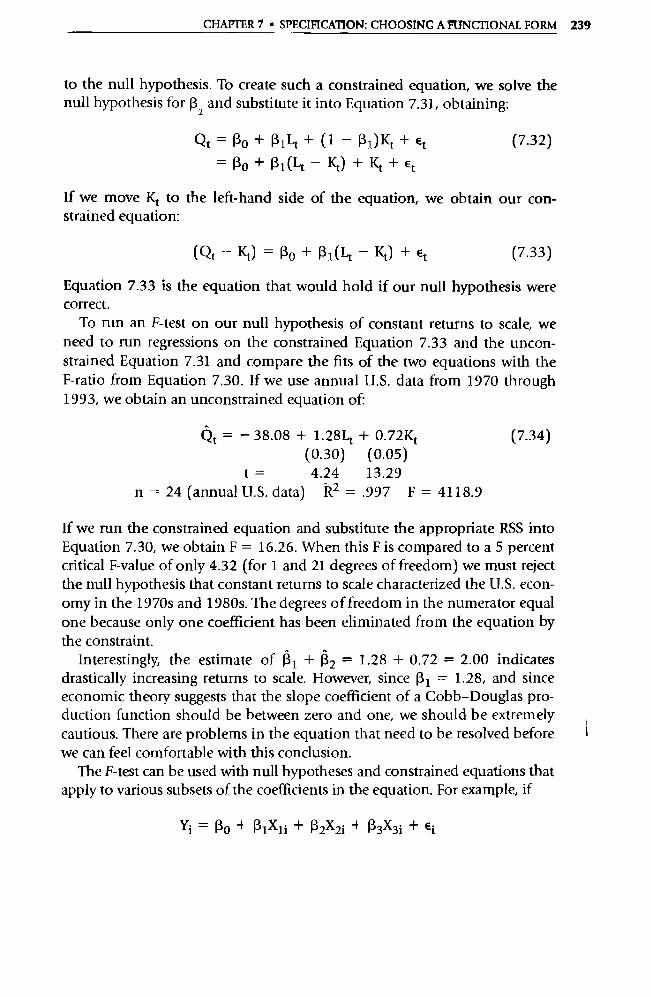
CHAPTER 7 • SPECIFICATION: CHOOSING A FUNCTIONAL FORM 239
to the null hypothesis. To create such a constrained equation, we solve the null hypothesis for 13 2 and substitute it into Equation 7.31, obtaining:
Qt = Po + + ( 1 - 131)K+ €t (7.32)
= Ro + 13 1 (4 - Kt) + Kt+ Et
If we move Kt to the left-hand side of the equation, we obtain our con-strained equation:
(Qt - Kt) = Ro + 13 1(E1 - Kt) + Et (7.33)
Equation 7.33 is the equation that would hold if our null hypothesis were correct.
To run an F-test on our null hypothesis of constant returns to scale, we need to mn regressions on the constrained Equation 7.33 and the uncon-strained Equation 7.31 and compare the fits of the two equations with the F-ratio from Equation 7.30. If we use annual U.S. data from 1970 through 1993, we obtain an unconstrained equation of:
Qt = - 38.08 + 1.284 + 0.72Kt (0.30) (0.05)
t = 4.24 13.29 n = 24 (annual U.S. data) R2 = .997 F = 4118.9
(7.34)
If we run the constrained equation and substitute the appropriate RSS into Equation 7.30, we obtain F = 16.26. When this F is compared to a 5 percent critical F-value of only 4.32 (for 1 and 21 degrees of freedom) we must reject the null hypothesis that constant returns to scale characterized the U.S. econ-omy in the 1970s and 1980s. The degrees of freedom in the numerator equal one because only one coefficient has been eliminated from the equation by the constraint.
Interestingly, the estimate of 131 + 13 2 = 1.28 + 0.72 = 2.00 indicates drastically increasing returns to scale. However, since 13 1 = 1.28, and since economic theory suggests that the slope coefficient of a Cobb-Douglas pro-duction function should be between zero and one, we should be extremely cautious. There are problems in the equation that need to be resolved before we can feel comfortable with this conclusion.
The F-test can be used with null hypotheses and constrained equations that apply to various subsets of the coefficients in the equation. For example, if
Yi = Ro + R1X1i+R2X2i+R3X3i+Ei
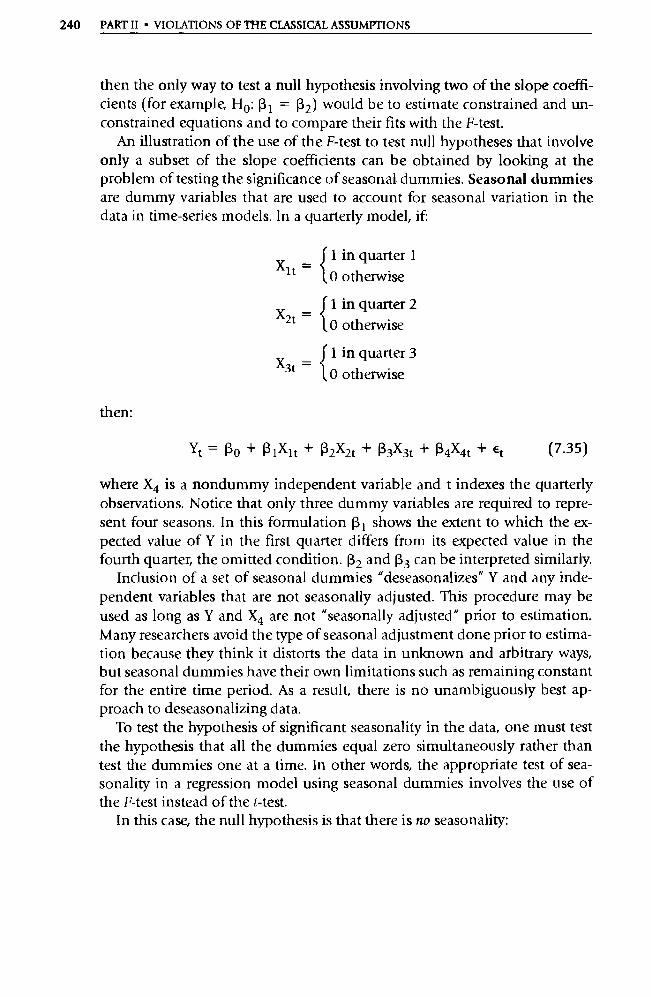
Xlt
X2t
X3t
then:
240 PART II • VIOLATIONS OF THE CLASSICAL ASSUMPTIONS
then the only way to test a null hypothesis involving two of the slope coeffi-cients (for example, H o : 13 1 = [3 2 ) would be to estimate constrained and un-constrained equations and to compare their fits with the F-test.
An illustration of the use of the F-test to test null hypotheses that involve only a subset of the slope coefficients can be obtained by looking at the problem of testing the significance of seasonal. dummies. Seasonal dummies are dummy variables that are used to account for seasonal variation in the data in time-series models. In a quarterly model, if:
(1 in quarter 1
t 0 otherwise
1 in quarter 2 0 otherwise
1 in quarter 3
0 otherwise
Yt — Ro + R1Xlt + R2X2t + R3X3t + R4X4t + Et (7.35)
where X4 is a nondummy independent variable and t indexes the quarterly observations. Notice that only three dummy variables are required to repre-sent four seasons. In this formulation 13 1 shows the extent to which the ex-pected value of Y in the first qua rter differs from its expected value in the fourth qua rter, the omitted condition. R2 and 13 3 can be interpreted similarly.
Inclusion of a set of seasonal dummies "deseasonalizes" Y and any inde-pendent variables that are not seasonally adjusted. This procedure may be used as long as Y and X4 are not "seasonally adjusted" prior to estimation. Many researchers avoid the type of seasonal adjustment done prior to estima-tion because they think it distorts the data in unknown and arbitrary ways, but seasonal dummies have their own limitations such as remaining constant for the entire time period. As a result, there is no unambiguously best ap-proach to deseasonalizing data.
To test the hypothesis of significant seasonality in the data, one must test the hypothesis that all the dummies equal zero simultaneously rather than test the dummies one at a time. In other words, the appropriate test of sea-sonality in a regression model using seasonal dummies involves the use of the F-test instead of the t-test.
In this case, the null hypothesis is that there is no seasonality:
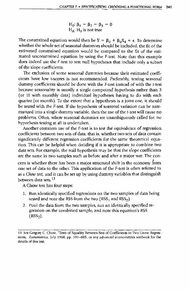
CHAPTER 7 • SPECIFICATION: CHOOSING A FUNCTIONAL FORM 241
HO: R1 = R2 = R3 =0 HA: Ho is not true
The constrained equation would then be Y = Ro + R4X4 + E. To determine whether the whole set of seasonal dummies should be included, the fit of the estimated constrained equation would be compared to the fit of the esti-mated unconstrained equation by using the F-test. Note that this example does indeed use the F-test to test null hypotheses that include only a subset of the slope coefficients.
The exclusion of some seasonal dummies because their estimated coeffi-cients have low t-scores is not recommended. Preferably, testing seasonal dummy coefficients should be done with the F-test instead of with the t-test because seasonality is usually a single compound hypothesis rather than 3 (or 11 with monthly data) individual hypotheses having to do with each quarter (or month). To the extent that a hypothesis is a joint one, it should be tested with the F-test. If the hypothesis of seasonal variation can be sum-marized into a single dummy variable, then the use of the t-test will cause no problems. Often, where seasonal dummies are unambiguously called for, no hypothesis testing at all is undertaken.
Another common use of the F-test is to test the equivalence of regression coefficients between two sets of data, that is, whether two sets of data contain significantly different regression coefficients for the same theoretical equa-tion. This can be helpful when deciding if it is appropriate to combine two data sets. For example, the null hypothesis may be that the slope coefficients are the same in two samples such as before and after a major war. The con-
cern is whether there has been a major structural shift in the economy from one set of data to the other. This application of the F-test is often referred to as a Chow test, and it can be set up by using dummy variables that distinguish between data sets. 13
A Chow test has four steps:
1. Run identically specified regressions on the two samples of data being tested and note the RSS from the two (RSS 1 and RSS2 ).
2. Pool the data from the two samples, run an identically specified re-gression on the combined sample, and note this equation's RSS (RSST) .
13. See Gregory C. Chow, "Tests of Equality Between Sets of Coefficients in Two Linear Regres-sions, Econometrica, July 1960, pp. 591-605, or any advanced econometrics textbook for the details of this test.
242 PART II • VIOLATIONS OF THE CLASSICAL ASSUMPTIONS s
3. Calculate the following F-statistic:
F = (RSS 1 + RSS2)/(N 1 + N2 2K - 2)
where: K = the number of independent variables N 1 = the number of observations in sample 1 N2 = the number of observations in sample 2
(RSST — RSS 1 — RSS2 ) /(K + 1) (7.36)
4. Reject the null hypothesis that the two sets of regression coefficients are equivalent if F > F c, where Fc is the critical F-value for (K + 1) nu-merator and (N 1 + N2 - 2K — 2) denominator degrees of freedom.
8 CHAPTER
Multicollinearity
8.1
Perfect versus Imperfect Multicollinearity
8.2
The Consequences of Multicollinearity
8.3
The Detection of Multicollinearity
8.4
Remedies for Multicollinearity
8.5
Choosing the Proper Remedy
8.6
Summary and Exercises
8.7
Appendix: The SAT Interactive Regression Learning Exercise
The next three chapters deal with violations of the Classical Assumptions and remedies for those violations. This chapter addresses multicollinearity; the next two chapters are on serial correlation and heteroskedasticity. For each of these three problems, we will attempt to answer the following questions:
1. What is the nature of the problem?
2. What are the consequences of the problem?
3. How is the problem diagnosed?
4. What remedies for the problem are available?
Strictly speaking, perfect multicollinearity is the violation of the assump-tion that no independent variable is a perfect linear function of one or more other independent variables (Classical Assumption VI). Perfect multi-collinearity is rare, but severe imperfect multicollinearity (where two or more independent variables are highly correlated in the particular data set being studied), although not violating Classical Assumption VI, still causes sub-stantial problems.
Recall that the coefficient (3k can be thought of as the impact on the de-pendent variable of a one-unit increase in the independent variable Xk, hold-ing constant the other independent variables in the equation. But if two ex-planatory variables are significantly related in a particular sample, whenever one changes, the other will tend to change too, and the OLS computer pro-
243
244 PART H • VIOLATIONS OF THE CLASSICAL ASSUMPTIONS
gram will find it difficult to distinguish the effects of one va riable from the effects of the other. Since the Xs can move together more in one sample than they do in another, the severity of multicollinearity can vary tremendously.
In essence, the more highly correlated two (or more) independent vari-ables are, the more difficult it becomes to accurately estimate the coefficients of the true model. If two variables move identically, then there is no hope of distinguishing between the impacts of the two; but if the variables are only roughly correlated, then we still might be able to estimate the two effects ac-curately enough for most purposes.
8.1 Perfect versus Imperfect Multicollinearity
8.1.1 Perfect Multicollinearity
Perfect multicollinearity l violates Classical Assumption VI, which specifies that no explanatory variable is a perfect linear function of any other explana-tory variables. The word perfect in this context implies that the variation in one explanatory variable can be completely explained by movements in an-other explanatory va riable. Such a perfect linear function between two inde-pendent variables would be:
X1i = ao + 0E1X2i
where the as are constants and the Xs are independent va riables in:
Yi = R O + R1Xli + R2X2i + Ei
Notice that there is no error term in Equation 8.1. This implies that X 1 can be exactly calculated given X2 and the equation. Examples of such perfect linear relationships would be:
3X21 or XII =6 +X2i or X11 = 2+4X2 i (8.3)
Figure 8.1 shows a graph of explanatory variables that are perfectly corre- lated. As can be seen in Figure 8.1, a perfect linear function has all data
(8.1)
(8.2)
1. The word collinearity describes a linear correlation between two independent va riables, and multicollinearity indicates that more than two independent va riables are involved. In common usage, multicollinearity is used to apply to both cases, and so we'll typically use that term in this text even though many of the examples and techniques discussed relate, strictly speaking, to collinearity.

CHAPTER 8 • MULTICOLLINEARITY 245
X i
o X2
Figure 8.1 Perfect Multicollinearity
With perfect multicollinearity, an independent va riable can be completely explained by the movements of one or more other independent variables. Perfect multicollinearity can usually be avoided by careful screening of the independent variables before a regression is run.
points on the same straight line. There is none of the va riation that accompa-nies the data from a typical regression.
Some examples of perfect multicollinearity were briefly mentioned in Sec-tion 4.1. Recall what happens when nominal and real interest rates are both included as explanatory variables in an equation. Usually, the relationship between nominal and real interest rates continually changes because the dif-ference between the two, the rate of inflation, is always changing. If the rate of inflation somehow was constant (during extremely s trict price controls, for instance), then the difference between the two would be constant, the two would be perfectly linearly related, and perfect multicollinearity would result:
int = irt + inft = irt + a (8.4)
where: in = the nominal (or money) interest rate in time t in = the real interest rate in time t inft = the rate of inflation in time t a = the constant rate of inflation
What happens to the estimation of an econometric equation where there is perfect multicollinearity? OLS is incapable of generating estimates of the re-
246 PART II • VIOLATIONS OF THE CLASSICAL ASSUMPTIONS
gression coefficients, and most OIS computer programs will print out an er-ror message in such a situation. Using Equation 8.2 as an example, we theo-retically would obtain the following estimated coefficients and standard er-rors:
R I = indeterminate SE((3 1 ) = co
(8.5)
R2 = indeterminate SE((3 2) = co
(8.6)
Perfect multicollinearity ruins our ability to estimate the coefficients because the two variables cannot be distinguished. You cannot "hold all the other in-dependent variables in the equation constant" if every time one va riable changes, another changes in an identical manner.
Fortunately, instances in which one explanatory variable is a perfect linear function of another are rare. More impo rtant, perfect multicollinearity should be fairly easy to discover before a regression is mn. You can detect perfect multicollinearity by asking whether one variable equals a multiple of another or if one variable can be derived by adding a constant to another. If so, then one of the variables should be dropped because there is no essential difference between the two.
A special case related to perfect multicollinearity occurs when a variable that is definitionally related to the dependent variable is included as an inde-pendent variable in a regression equation. Such a dominant variable is by definition so highly correlated with the dependent variable that it completely masks the effects of all other independent variables in the equation. In a sense, this is a case of perfect collinearity between the dependent and an in-dependent variable.
For example, if you include a variable measuring the amount of raw mate-rials used by the shoe industry in a production function for that industry, the raw materials variable would have an extremely high t-score, but otherwise important variables like labor and capital would have quite insignificant t-scores. Why? In essence, if you knew how much leather was used by a shoe factory, you could predict the number of pairs of shoes produced without knowing anything about labor or capital. The relationship is definitional, and the dominant variable should be dropped from the equation to get reason-able estimates of the coefficients of the other variables.
A dominant variable involves a tautology; it is defined in such a way that you can calculate the dependent va riable from it without any knowledge of the underlying theory. Be careful, though; dominant variables shouldn't be confused with highly significant or impo rtant explanatory variables. Instead, they should be recognized as being virtually identical to the dependent vari-
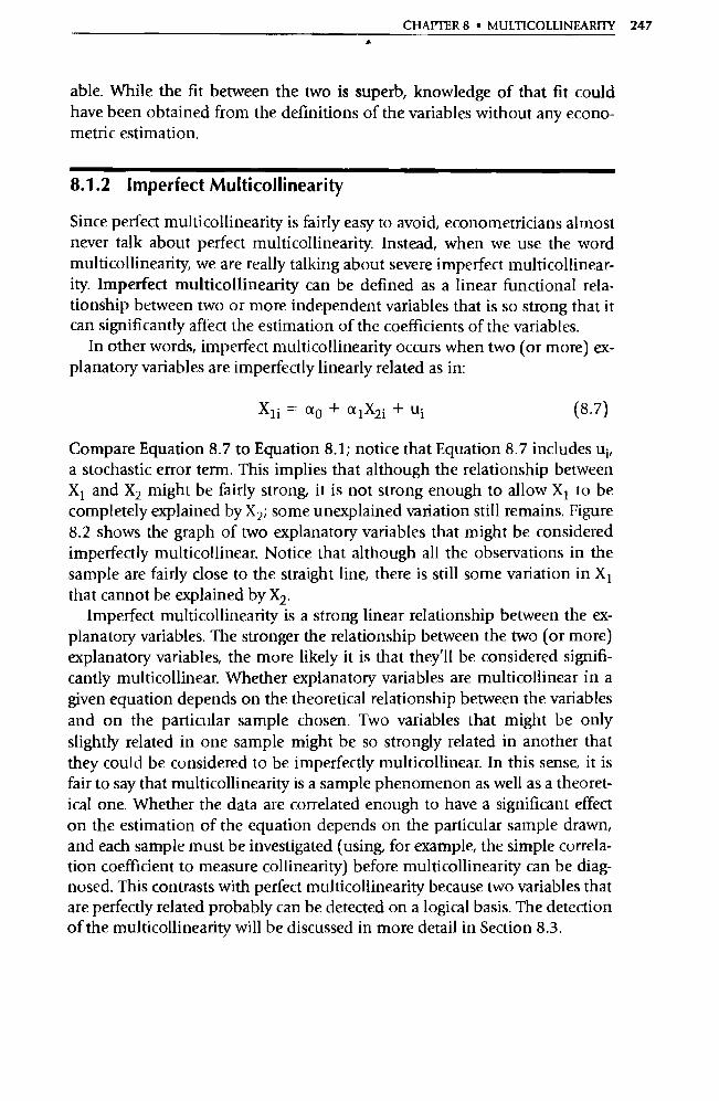
CHAPTER 8 • MULTICOLLINEARITY 247
able. While the fit between the two is superb, knowledge of that fit could have been obtained from the definitions of the variables without any econo-metric estimation.
8.1.2 Imperfect Multicollinearity
Since perfect multicollinearity is fairly easy to avoid, econometricians almost never talk about perfect multicollinearity. Instead, when we use the word multicollinearity, we are really talking about severe imperfect multicollinear-ity. Imperfect multicollinearity can be defined as a linear functional rela-tionship between two or more independent variables that is so strong that it can significantly affect the estimation of the coefficients of the variables.
In other words, imperfect multicollinearity occurs when two (or more) ex-planatory variables are imperfectly linearly related as in:
XII =ao+a lX2i+Ui (8.7)
Compare Equation 8.7 to Equation 8.1; notice that Equation 8.7 includes u i , a stochastic error term. This implies that although the relationship between X 1 and X2 might be fairly strong, it is not strong enough to allow X 1 to be completely explained by X2 ; some unexplained variation still remains. Figure 8.2 shows the graph of two explanatory variables that might be considered imperfectly multicollinear. Notice that although all the observations in the sample are fairly close to the straight line, there is still some variation in X 1
that cannot be explained by X2.
Imperfect multicollinearity is a strong linear relationship between the ex-planatory variables. The stronger the relationship between the two (or more) explanatory variables, the more likely it is that they'll be considered signifi-cantly multicollinear. Whether explanatory variables are multicollinear in a given equation depends on the theoretical relationship between the variables and on the particular sample chosen. Two variables that might be only slightly related in one sample might be so strongly related in another that they could be considered to be imperfectly multicollinear. In this sense, it is fair to say that multicollinearity is a sample phenomenon as well as a theoret-ical one. Whether the data are correlated enough to have a significant effect on the estimation of the equation depends on the particular sample drawn, and each sample must be investigated (using, for example, the simple correla-tion coefficient to measure collinearity) before multicollinearity can be diag-nosed. This contrasts with perfect multicollinearity because two va riables that are perfectly related probably can be detected on a logical basis. The detection of the multicollinearity will be discussed in more detail in Section 8.3.
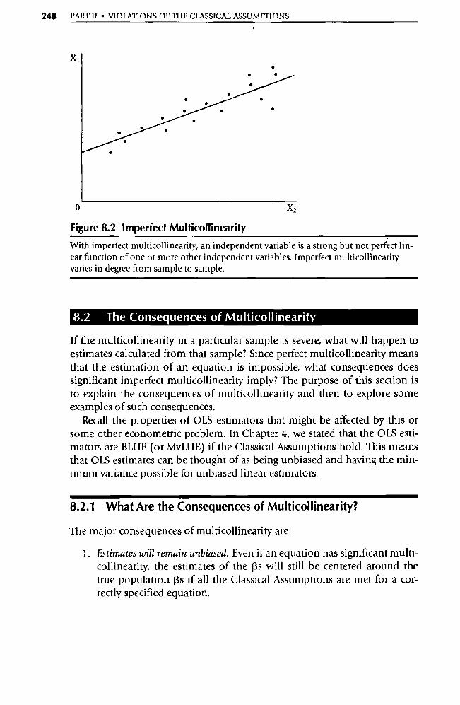
248 PART II • VIOLATIONS OF THE CLASSICAL ASSUMPTIONS
X ^
0 X2
Figure 8.2 Imperfect Multicollinearity
With imperfect multicollinearity, an independent va riable is a strong but not perfect lin-ear function of one or more other independent variables. Imperfect multicollinearity
varies in degree from sample to sample.
8.2 The Consequences of Multicollinearity
If the multicollinearity in a particular sample is severe, what will happen to estimates calculated from that sample? Since perfect multicollinearity means that the estimation of an equation is impossible, what consequences does significant imperfect multicollinearity imply? The purpose of this section is to explain the consequences of multicollinearity and then to explore some examples of such consequences.
Recall the properties of OLS estimators that might be affected by this or some other econometric problem. In Chapter 4, we stated that the OLS esti-mators are BLUE (or MvLUE) if the Classical Assumptions hold. This means that OLS estimates can be thought of as being unbiased and having the min-imum variance possible for unbiased linear estimators.
8.2.1 What Are the Consequences of Multicollinearity?
The major consequences of multicollinearity are:
1. Estimates will remain unbiased. Even if an equation has significant multi-collinearity, the estimates of the 13s will still be centered around the
true population 13s if all the Classical Assumptions are met for a cor-rectly specified equation.
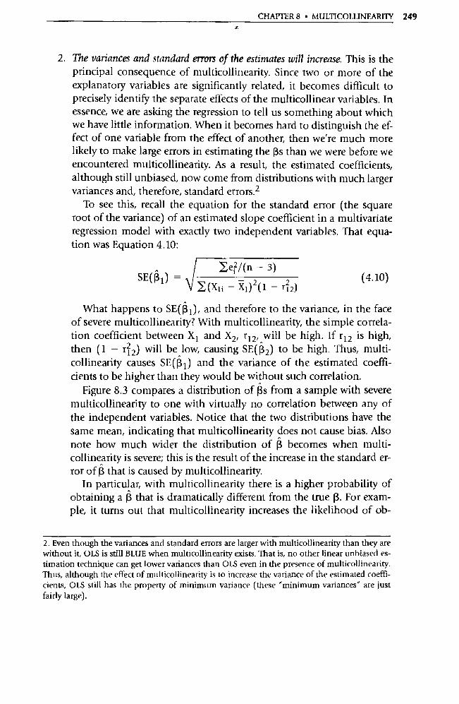
CHAPTER 8 • MULTICOLLINEARITY 249 r.
2. The variances and standard errors of the estimates will increase. This is the principal consequence of multicollinearity. Since two or more of the explanatory variables are significantly related, it becomes difficult to precisely identify the separate effects of the multicollinear variables. In essence, we are asking the regression to tell us something about which we have little information. When it becomes hard to distinguish the ef-fect of one variable from the effect of another, then we're much more likely to make large errors in estimating the (3s than we were before we encountered multicollinearity. As a result, the estimated coefficients, although still unbiased, now come from distributions with much larger variances and, therefore, standard errors. 2
To see this, recall the equation for the standard error (the square root of the variance) of an estimated slope coefficient in a multivariate regression model with exactly two independent variables. That equa-tion was Equation 4.10:
SE _ Ie? /(n — 3)
4.10
( R 1) — E(X1i — X 1 ) 2 (1 — r12)
( )
What happens to SE( 1 . 1 ), and therefore to the variance, in the face of severe multicollinearity? With multicollinearity, the simple correla-tion coefficient between X 1 and X2, r12 , will be high. If r 12 is high, then (1 — r1 2) will be low, causing SE(13 2) to be high. Thus, multi-collinearity causes SE(13 1 ) and the variance of the estimated coeffi-cients to be higher than they would be without such correlation.
Figure 8.3 compares a dist ribution of 13s from a sample with severe multicollinearity to one with virtually no correlation between any of the independent variables. Notice that the two distributions have the same mean, indicating that multicollinearity does not cause bias. Also note how much wider the distribution of 13 becomes when multi-collinearity is severe; this is the result of the increase in the standard er-ror of (3 that is caused by multicollinearity.
In particular, with multicollinearity there is a higher probability of obtaining a 13 that is dramatically different from the true 13. For exam-ple, it turns out that multicollinearity increases the likelihood of ob-
2. Even though the va riances and standard errors are larger with multicollinearity than they are without it, OIS is still BLUE when multicollinearity exists. That is, no other linear unbiased es-timation technique can get lower variances than OLS even in the presence of multicollinearity. Thus, although the effect of multicollinearity is to increase the variance of the estimated coeffi-cients, OLS still has the property of minimum variance (these "minimum variances" are just fairly large).
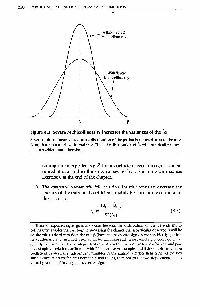
13
Without Severe ^'Multicollinearity
250 PART II • VIOLATIONS OF THE CLASSICAL ASSUMPTIONS
Figure 8.3 Severe Multicollinearity Increases the Variances of the (3s
Severe multicollinearity produces a dist ribution of the 13s that is centered around the true 13 but that has a much wider variance. Thus, the distribution of 13s with multicollinearity is much wider than otherwise.
taining an unexpected signa for a coefficient even though, as men-tioned above, multicollinearity causes no bias. For more on this, see Exercise 6 at the end of the chapter.
3. The computed t -scores will fall. Multicollinearity tends to decrease the t-scores of the estimated coefficients mainly because of the formula for the t-statistic:
( Rk - RHo) tk =
SE(Pk) (8.8)
3. These unexpected signs generally occur because the distribution of the 13s with multi-collinearity is wider than without it, increasing the chance that a particular observed 13 will be on the other side of zero from the true 13 (have an unexpected sign). More specifically, particu-lar combinations of multicollinear variables can make such unexpected signs occur quite fre-quently. For instance, if two independent variables both have positive true coefficients and pos-itive simple correlation coefficients with Y in the observed sample, and if the simple correlation coefficient between the independent va riables in the sample is higher than either of the two simple correlation coefficients between Y and the Xs, then one of the two slope coefficients is virtually assured of having an unexpected sign.

Bernhard
TextBox
p 251 is missing

252 PART II • VIOLATIONS OF THE CLASSICAL ASSUMPTIONS
tain the same pattern of multicollinearity in the forecast period that they demonstrated in the sample.
Similarly, if an explanatory va riable in an equation is not multi-collinear (also called orthogonal) with the other va riables, then the es-timation of its coefficient and standard error usually will not be af-fected. It's unusual to find an explanatory variable that's totally uncorrelated with any other explanatory variable. If this were to occur, though, then the multicollinearity in the rest of the equation would not change the estimated coefficient or the t-score of the nonmulti-collinear variable.
8.2.2 Two Examples of the Consequences of Multicollinearity
To see what severe multicollinearity does to an estimated equation, let's look at a hypothetical example. Suppose you decide to estimate a "student con-sumption function." After the appropriate preliminary work, you come up with the following hypothesized equation:
+ + CO ; = f(Ydi,LAi)+ ei= Ro +R1Ydi+ f3 2 LA; + e; (8.9)
where: CO; = the annual consumption expenditures of the ith student on items other than tuition and room and board
Yd; = the annual disposable income (including gifts) of that stu-dent
LA; = the liquid assets (savings, etc.) of the ith student e; = a stochastic error term
You then collect a small amount of data from people who are sitting near yoü in class:
Student CO; Yd; LA;
Mary $2000 $2500 $25000 Robby 2300 3000 31000 Jim 2800 3500 33000 Giorgio 3800 4000 39000 Colleen 3500 4500 48000 Jennifer 5000 5000 54000 Harwood 4500 5500 55000
Note: filename CONS8
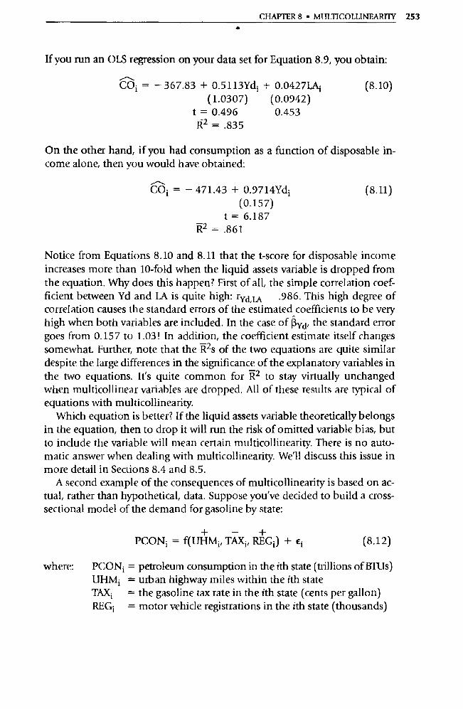
CHAPTER 8 • MULTICOLLINEARITY 253
If you run an OLS regression on your data set for Equation 8.9, you obtain:
COi = — 367.83 + 0.5113Ydi + 0.0427LAi (1.0307) (0.0942)
t = 0.496 0.453 R2 =.835
(8.10)
On the other hand, if you had consumption as a function of disposable in-come alone, then you would have obtained:
COi = — 471.43 + 0.9714Yd i (0.157)
t = 6.187 R2 =.861
(8.11)
Notice from Equations 8.10 and 8.11 that the t-score for disposable income increases more than 10-fold when the liquid assets variable is dropped from the equation. Why does this happen? First of all, the simple correlation coef-ficient between Yd and LA is quite high: ryd,LA .986. This high degree of correlation causes the standard errors of the estimated coefficients to be very high when both variables are included. In the case of Ryd, the standard error goes from 0.157 to 1.03 ! In addition, the coefficient estimate itself changes somewhat. Further, note that the Res of the two equations are quite similar despite the large differences in the significance of the explanatory variables in the two equations. It's quite common for R 2 to stay virtually unchanged when multicollinear variables are dropped. All of these results are typical of equations with multicollinearity.
Which equation is better? If the liquid assets variable theoretically belongs in the equation, then to drop it will run the risk of omitted va riable bias, but to include the va riable will mean ce rtain multicollinearity. There is no auto-matic answer when dealing with multicollinearity. We'll discuss this issue in more detail in Sections 8.4 and 8.5.
A second example of the consequences of multicollinearity is based on ac-tual, rather than hypothetical, data. Suppose you've decided to build a cross-sectional model of the demand for gasoline by state:
+ — + PCONi = f(UHMi, TAXi, REG;) + Ei (8.12)
where: PCON; = petroleum consumption in the ith state (trillions of BTUs) UHM; = urban highway miles within the ith state TAXi = the gasoline tax rate in the ith state (cents per gallon) REGi = motor vehicle registrations in the ith state (thousands)
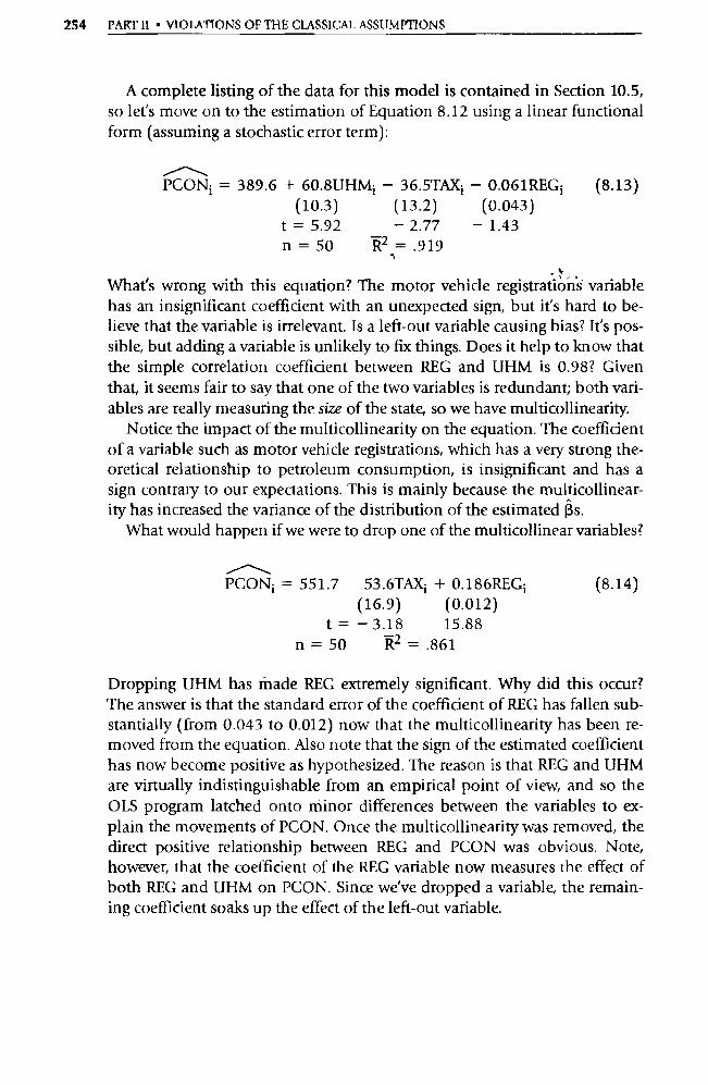
254 PART II • VIOLATIONS OF THE CLASSICAL ASSUMPTIONS
A complete listing of the data for this model is contained in Section 10.5, so let's move on to the estimation of Equation 8.12 using a linear functional form (assuming a stochastic error term):
PCONi = 389.6 + 60.8UHMi — 36.5TAXi — 0.061REGi
(10.3) (13.2) (0.043)
t = 5.92 — 2.77 — 1.43
n=50 R2 =.919
(8.13)
What's wrong with this equation? The motor vehicle registrations va riable has an insignificant coefficient with an unexpected sign, but it's hard to be-lieve that the variable is irrelevant. Is a left-out variable causing bias? It's pos-sible, but adding a variable is unlikely to fix things. Does it help to know that the simple correlation coefficient between REG and UHM is 0.98? Given that, it seems fair to say that one of the two variables is redundant; both vari-ables are really measuring the size of the state, so we have multicollinearity.
Notice the impact of the multicollinearity on the equation. The coefficient of a va riable such as motor vehicle registrations, which has a very strong the-oretical relationship to petroleum consumption, is insignificant and has a sign contrary to our expectations. This is mainly because the multicollinear-ity has increased the variance of the distribution of the estimated (3s.
What would happen if we were to drop one of the multicollinear va riables?
PCONi = 551.7 53.6TAXi + 0.186REGi
(16.9) (0.012)
t = — 3.18 15.88 n= 50 R2 =.861
(8.14)
Dropping UHM has made REG extremely significant. Why did this occur? The answer is that the standard error of the coefficient of REG has fallen sub-stantially (from 0.043 to 0.012) now that the multicollinearity has been re-moved from the equation. Also note that the sign of the estimated coefficient has now become positive as hypothesized. The reason is that REG and UHM are virtually indistinguishable from an empirical point of view, and so the OLS program latched onto minor differences between the va riables to ex-plain the movements of PCON. Once the multicollinearity was removed, the direct positive relationship between REG and PCON was obvious. Note, however, that the coefficient of the REG variable now measures the effect of both REG and UHM on PCON. Since we've dropped a variable, the remain-ing coefficient soaks up the effect of the left-out variable.

CHAPTER 8 • MULTICOLLINEARITY 255
Either UHM or REG could have been dropped with similar results because the two variables are, in a quantitative sense, virtually identical as indicated by the high simple correlation coefficient between them. In this case, REG was judged to be theoretically superior to UHM. Even though R 2 fell when UHM was dropped, Equation 8.14 should be considered superior to Equa-tion 8.13. This is an example of the point, first made in Chapter 3, that the fit of the equation is not the most impo rtant criterion to be used in determining its overall quality.
8.3 The Detection of Multicollinearity
How do we decide whether an equation has a severe multicollinearity problem? A first step is to recognize that some multicollinearity exists in every equation. It's virtually impossible in a real-world example to find a set of explanatory vari-ables in which the explantatory va riables are totally uncorrelated with each other. Our main purpose in this section will be to learn to determine how much multicollinearity exists in an equation, not whether any multicollinearity exists.
A second key point is that multicollinearity is a sample phenomenon as well as a theoretical one. That is, the severity of multicollinearity in a given equation can change from sample to sample depending on the characteristics of the sample. As a result, the theoretical underpinnings of the equation are not quite as important in the detection of multicollinearity as they are in the detection of an omitted variable or an incorrect functional form. Instead, we tend to rely more on data-oriented techniques to determine the severity of the multicollinearity in a given sample. Of course, we can never ignore the theory behind an equation. The trick is to find variables that are theoretically relevant (for meaningful interpretation) and that are also statistically non-multicollinear (for meaningful inference).
Because multicollinearity is a sample phenomenon, and the level of dam-age of its impact is a matter of degree, many of the methods used to detect it are informal tests without critical values or levels of significance. Indeed, there are no generally accepted, true statistical tests for multicollinearity. Most researchers develop a general feeling for the severity of multicollinearity in an estimated equation by looking at a number of the characteristics of that equation. Let's examine two of the most-used of those characteristics.
8.3.1 High Simple Correlation Coefficients
One way to detect severe multicollinearity is to examine the simple correlation coefficients between the explanatory va riables. If an r is high in absolute value,
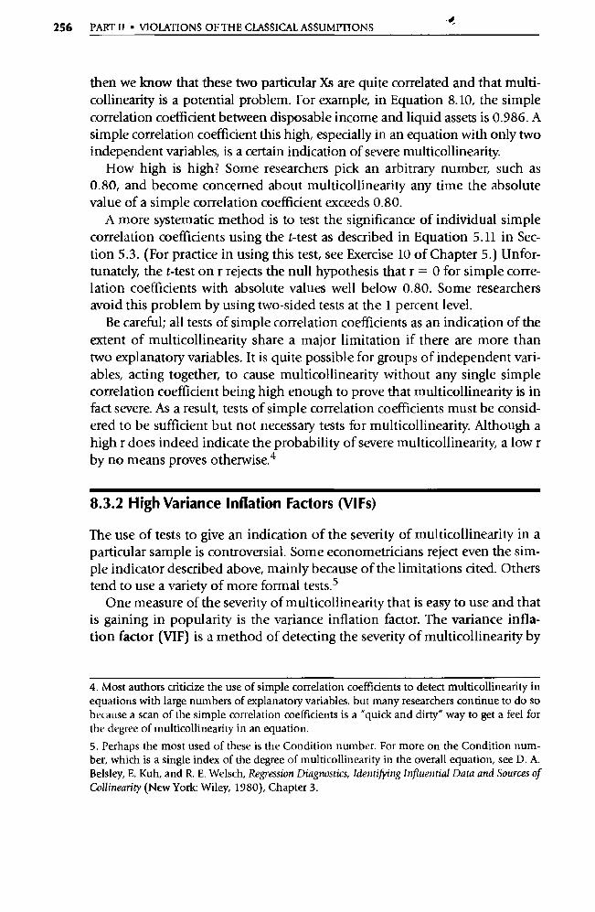
256 PART II • VIOLATIONS OF THE CLASSICAL ASSUMPTIONS
then we know that these two particular Xs are quite correlated and that multi-collinearity is a potential problem. For example, in Equation 8.10, the simple correlation coefficient between disposable income and liquid assets is 0.986. A simple correlation coefficient this high, especially in an equation with only two independent variables, is a ce rtain indication of severe multicollinearity.
How high is high? Some researchers pick an arbitrary number, such as 0.80, and become concerned about multicollinearity any time the absolute value of a simple correlation coefficient exceeds 0.80.
A more systematic method is to test the significance of individual simple correlation coefficients using the t-test as described in Equation 5.11 in Sec-tion 5.3. (For practice in using this test, see Exercise 10 of Chapter 5.) Unfor-tunately, the t-test on r rejects the null hypothesis that r = 0 for simple corre-lation coefficients with absolute values well below 0.80. Some researchers avoid this problem by using two-sided tests at the 1 percent level.
Be careful; all tests of simple correlation coefficients as an indication of the extent of multicollinearity share a major limitation if there are more than two explanatory variables. It is quite possible for groups of independent vari-ables, acting together, to cause multicollinearity without any single simple correlation coefficient being high enough to prove that multicollinearity is in fact severe. As a result, tests of simple correlation coefficients must be consid-ered to be sufficient but not necessary tests for multicollinearity. Although a high r does indeed indicate the probability of severe multicollinearity, a low r by no means proves otherwise. 4
8.3.2 High Variance Inflation Factors (VIFs)
The use of tests to give an indication of the severity of multicollinearity in a particular sample is controversial. Some econometricians reject even the sim-ple indicator described above, mainly because of the limitations cited. Others tend to use a variety of more formal tests. 5
One measure of the severity of multicollinearity that is easy to use and that is gaining in popularity is the variance inflation factor. The variance infla-tion factor (VIF) is a method of detecting the severity of multicollinearity by
4. Most authors criticize the use of simple correlation coefficients to detect multicollinearity in equations with large numbers of explanatory variables, but many researchers continue to do so because a scan of the simple correlation coefficients is a "quick and dirty" way to get a feel for the degree of multicollinearity in an equation.
5. Perhaps the most used of these is the Condition number. For more on the Condition num-ber, which is a single index of the degree of multicollinearity in the overall equation, see D. A. Belsley, E. Kuh, and R. E. Welsch, Regression Diagnostics, Identifying Influential Data and Sources of Collinearity (New York: Wiley, 1980), Chapter 3.
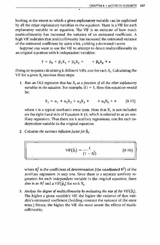
CHAPTER 8 • . MULTICOLLINEARITY 257
looking at the extent to which a given explanatory va riable can be explained by all the other explanatory variables in the equation. There is a VIF for each explanatory variable in an equation. The VIF is an estimate of how much multicollinearity has increased the va riance of an estimated coefficient. A high VIF indicates that multicollinearity has increased the estimated variance of the estimated coefficient by quite a bit, yielding a decreased t-score.
Suppose you want to use the VIF to attempt to detect multicollinearity in an original equation with k independent variables:
Y =Ro+R1X1 + 82X2+ + (3kXk + e
Doing so requires calculating k different VIFs, one for each X i . Calculating the VIF for a given Xi involves three steps:
1. Run an OLS regression that has X i as a function of all the other explanatory variables in the equation. For example, if i = 1, then this equation would be:
X 1 = a 1 + a2X2 + a3X3 + + akXk + y (8.15)
where v is a typical stochastic error term. Note that X 1 is not included on the right-hand side of Equation 8.15, which is referred to as an aux-iliary regression. Thus there are k auxiliary regressions, one for each in-dependent variable in the original equation.
2. Calculate the variance inflation factor for Ri:
VIF(R i) = 1 2 (8.16) (1 — R; )
where R; is the coefficient of determination (the unadjusted R 2) of the auxiliary regression in step one. Since there is a separate auxiliary re-gression for each independent variable in the original equation, there also is an R; and a VIF((3 ; ) for each Xi .
3. Analyze the degree of multicollinearity by evaluating the size of the VIF(I ) The higher a given variable's VIF, the higher the variance of that vari-able's estimated coefficient (holding constant the variance of the error term.) Hence, the higher the VIF, the more severe the effects of multi-collinearity.
258 PART II • VIOLATIONS OF THE CLASSICAL ASSUMPTIONS
Why will a high VIF indicate multicollinearity? The VIF(R i) can be thought of as the ratio of the estimated va ri ance of (3 i to what the variance would be with no correlation between X i and the other Xs in the equation. How high is high? An R? of one, indicating perfect multicollinearity, pro-duces a VIF of infinity, whereas an R? of zero, indicating no multicollinear-ity at all, produces a VIF of one. While there is no table of formal critical VIF values, a common rule of thumb is that if VIF(13 i) > 5, the multicollinearity is severe.
For example, let's return to Equation 8.10 and calculate the VIFs for both independent variables. Both VIFs equal 36, confirming the quite severe mul-ticollinearity we already know exists. It's no coincidence that the VIFs for the two variables are equal. In an equation with exactly two independent vari-ables, the two auxiliary equations will have identical Ri s, leading to equal VIFs. 6
Thus, the VIF is a method of detecting multicollinearity that takes into ac-count all the explanatory variables at once. Some authors and statistical soft-ware programs replace the VIF with its reciprocal, (1 R;), called tolerance, or TOL. Whether we calculate VIF or TOL is a matter of personal preference, but either way, the general approach is the most comprehensive multi-collinearity detection technique we've discussed in this text.
Unfortunately, there are a couple of problems with using VIFs. First, as mentioned, there is no hard-and-fast VIF decision rule. Second, it's possible to have multicollinear effects in an equation that has no large VIFs. For in-stance, if the simple correlation coefficient between X 1 and X2 is 0.88, multi-collinear effects are quite likely, and yet the VIF for the equation (assuming no other Xs) is only 4.4.
In essence, then, the VIF is a sufficient but not necessary test for multi-collinearity, just like the other test described in this section. Indeed, as is probably obvious to the reader by now, there is no test that allows a re-searcher to reject the possibility of multicollinearity with any real certainty.
8.4 Remedies for Multicollinearity
What can be done to minimize the consequences of severe multicollinearity? There is no automatic answer to this question because multicollinearity is a phenomenon that could change from sample to sample even for the same
6. Another use for the Res of these auxiliary equations is to compare them with the overall equation's R2 . If an auxiliary equation's R2 is higher, it's yet another sign of multicollinearity.
CHAPTER 8 • MULTICOLLINEARITY 259 •
specification of a regression equation. The purpose of this section is to out-line a number of alternative remedies for multicollinearity that might be ap-propriate under ce rtain circumstances.
8.4.1 Do Nothing
The first step to take once severe multicollinearity has been diagnosed is to decide whether anything should be done at all. As we'll see, it turns out that every remedy for multicollinearity has a drawback of some so rt, and so it of-ten happens that doing nothing is the correct course of action.
One reason for doing nothing is that multicollinearity in an equation will not always reduce the t-scores enough to make them insignificant or change the (3s enough to make them differ from expectations. In other words, the mere existence of multicollinearity does not necessarily mean anything. A remedy for multicollinearity should be considered only if the consequences cause insignificant t-scores or unreliable estimated coefficients. For example, it's possible to observe a simple correlation coefficient of .97 between two ex-planatory variables and yet have each individual t-score be significant. It makes no sense to consider remedial action in such a case, because any rem-edy for multicollinearity would probably cause other problems for the equa-tion. In a sense, multicollinearity is similar to a non-life-threatening human disease that requires general anesthesia to operate on the patient: The risk of the operation should be undertaken only if the disease is causing a signifi-cant problem.
A second reason for doing nothing is that the deletion of a multicollinear variable that belongs in an equation is fairly dangerous because it will cause specification bias. If we drop such a va riable, then we are purposely creating bias. Given all the effo rt typically spent avoiding omitted variables, it seems foolhardy to consider running that risk on purpose. As a result, experienced econometricians often will leave multicollinear va riables in equations de-spite low t-scores.
The final reason for considering doing nothing to offset multicollinearity is a theoretical one that would apply to all equations. Every time a regression is rerun, we risk encountering a specification that fits because it accidentally works for the particular data set involved, not because it is the truth. The larger the number of experiments, the greater the chances of finding the acci-dental result. In addition, when there is significant multicollinearity in the sample, the odds of strange results increase rapidly because of the sensitivity of the coefficient estimates to slight specification changes. Thus, the case against sequential specification searches outlined in Chapter 6 is even stronger in the face of severe multicollinearity.
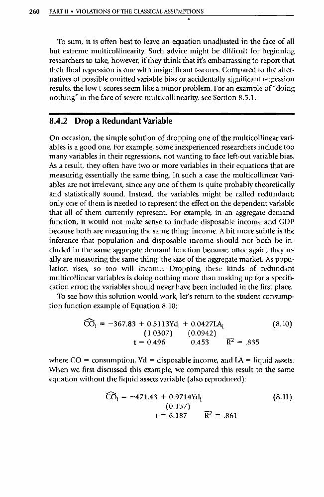
260 PART II • VIOLATIONS OF THE CLASSICAL ASSUMPTIONS
To sum, it is often best to leave an equation unadjusted in the face of all but extreme multicollinearity. Such advice might be difficult for beginning researchers to take, however, if they think that it's embarrassing to report that their final regression is one with insignificant t-scores. Compared to the alter-natives of possible omitted variable bias or accidentally significant regression results, the low t-scores seem like a minor problem. For an example of "doing nothing" in the face of severe multicollinearity, see Section 8.5.1.
8.4.2 Drop a Redundant Variable
On occasion, the simple solution of dropping one of the multicollinear vari-ables is a good one. For example, some inexperienced researchers include too many variables in their regressions, not wanting to face left-out variable bias. As a result, they often have two or more va riables in their equations that are measuring essentially the same thing. In such a case the multicollinear vari-ables are not irrelevant, since any one of them is quite probably theoretically and statistically sound. Instead, the variables might be called redundant; only one of them is needed to represent the effect on the dependent variable that all of them currently represent. For example, in an aggregate demand function, it would not make sense to include disposable income and GDP because both are measuring the same thing: income. A bit more subtle is the inference that population and disposable income should not both be in-cluded in the same aggregate demand function because, once again, they re-ally are measuring the same thing: the size of the aggregate market. As popu-lation rises, so too will income. Dropping these kinds of redundant multicollinear variables is doing nothing more than making up for a specifi-cation error; the va riables should never have been included in the first place.
To see how this solution would work, let's return to the student consump-tion function example of Equation 8.10:
COi = —367.83 + 0.5113Ydi + 0.0427LAi (1.0307) (0.0942)
t = 0.496 0.453 R2 = .835
(8.10)
where CO = consumption, Yd = disposable income, and LA = liquid assets. When we first discussed this example, we compared this result to the same equation without the liquid assets variable (also reproduced):
COi = —471.43 + 0.9714Ydi (0.157)
t = 6.187 R2 =.861
(8.11)
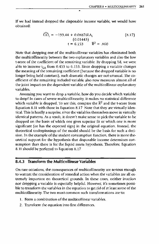
CHAPTER 8 • MULTICOLLINEARITY 261
If we had instead dropped the disposable income va riable, we would have obtained:
CO i = — 199.44 + 0.08876LAi (0.01443)
t = 6.153 R2 = .860
(8.17)
Note that dropping one of the multicollinear variables has eliminated both the multicollinearity between the two explanatory variables and also the low t-score of the coefficient of the remaining variable. By dropping Yd, we were able to increase t uk from 0.453 to 6.153. Since dropping a variable changes the meaning of the remaining coefficient (because the dropped variable is no longer being held constant), such dramatic changes are not unusual. The co-efficient of the remaining included variable also now measures almost all of the joint impact on the dependent variable of the multicollinear explanatory variables.
Assuming you want to drop a va riable, how do you decide which variable to drop? In cases of severe multicollinearity, it makes no statistical difference which variable is dropped. To see this, compare the 11 2 and the t-score from Equation 8.11 with those in Equation 8.17 Note that they are virtually iden-tical. This is hardly a surp rise, since the variables themselves move in virtually identical patterns. As a result, it doesn't make sense to pick the va riable to be dropped on the basis of which one gives superior fit or which one is more significant (or has the expected sign) in the original equation. Instead, the theoretical underpinnings of the model should be the basis for such a deci-sion. In the example of the student consumption function, there is more the-oretical suppo rt for the hypothesis that disposable income determines con-sumption than there is for the liquid assets hypothesis. Therefore, Equation 8.11 should be preferred to Equation 8.17
8.4.3 Transform the Multicollinear Variables
On rare occasions, the consequences of multicollinearity are serious enough to warrant the consideration of remedial action when the variables are all ex-tremely impo rtant on theoretical grounds. In these cases, neither inaction nor dropping a variable is especially helpful. However, it's sometimes possi-ble to transform the variables in the equation to get rid of at least some of the multicollinearity. The two most common such transformations are to:
1. Form a combination of the multicollinear variables. 2. Transform the equation into first differences.
262 PART II • VIOLATIONS OF THE CLASSICAL ASSUMPTIONS
The technique of forming a combination of two or more of the multi-collinear variables consists of creating a new variable that is a function of the multicollinear va riables and using the new variable to replace the old ones in the regression equation.
For example, if X 1 and X2 are highly multicollinear, a new variable, X3 = X 1 + X2 (or more generally, any linear combination of the two variables like k1 X 1 + k2X2) might be substituted for both of the multicollinear variables in a reestimation of the model. This technique is especially useful if the equa-tion is going to be for forecasting, since the multicollinearity outside the sample might not exist or might not follow the same pattern that it did in-side the sample.
A major disadvantage of the technique is that both portions of the combi-nation variable are forced to have the same coefficient in the reestimated equation. For example, if X3i = X1i + X21:
Yi Ro+ R3X3i + Ei_ Ro + R3(X1i+X2i) + E i (8.18)
Care must be taken not to include (in a combination) va riables with differ-ent expected coefficients (such as different expected signs) or dramatically different mean values (such as different orders of magnitude) without adjust-ing for these differences by using appropriate constants (ks) in the more gen-eral equation X3 = k1X1 + k2X2 .
The second kind of transformation to consider as a possible remedy for se-vere multicollinearity is to switch the functional form of the equation to first differences. A first difference is nothing more than the change in a variable from the previous time period to the current time period (which we've re-ferred to as "delta" or A). That is, we shall define a first difference as:
OXt=Xt — Xt- 1
If an equation (or some of the va riables in an equation) is switched from its normal specification to a first difference specification, it's quite likely that the degree of multicollinearity will be significantly reduced for two reasons. First, any change in the definitions of the variables (except a simple linear change) will change the degree of multicollinearity. Second, multicollinearity takes place most frequently (although certainly not exclusively) in time-series data, in which first differences are far less likely to move steadily upward than are the aggregates from which they are calculated. For example, although GDP might grow only 5 or 6 percent from year to year, the change in GDP (or the first difference) could fluctuate severely.
Although the severity of multicollinearity sometimes can be diminished
CHAI'lER 8 • MULTICOLLINEARITY 263
by switching to first differences, changing the functional form of an equation simply to avoid multicollinearity is almost never worth the possible theoreti-cal complications. For example, modeling capital stock is not the same as modeling the change in capital stock, which is investment, even though one equation can be derived from the other. If the basic purpose of running the regression were to model first differences, then the model should have been specified that way in the first place.
Using first differences has one unexpected advantage, however. This in-volves the concept of a nonstationary time series, or a time series that has a sig-nificant trend of some sort (for example, a rapidly increasing mean or vari-ance over time). Evidence of multicollinearity in a time series is often evidence that a number of the independent variables are nonstationary. By coincidence, one possible (though inefficient) remedy for nonstationary vari-ables is to convert to first differences, so first differences are possible reme-dies for both multicollinearity and nonstationarity. Thus, beginning econo-metricians who use first differences to "cure" multicollinearity sometimes are doing the right thing for the wrong reason! We'll discuss nonstationarity in more detail in Chapter 12.
8.4.4 Increase the Size of the Sample
Another way to deal with multicollinearity is to attempt to increase the size of the sample to reduce the degree of multicollinearity. Although such in-creases may be impossible when limitations of some so rt exist, they are use-ful alternatives to be considered when they are feasible.
The idea behind increasing the size of the sample is that a larger data set (often requiring new data collection) will allow more accurate estimates than a small one, since the large sample normally will reduce somewhat the vari-ance of the estimated coefficients, diminishing the impact of the multi-collinearity.
For most economic and business applications, however, this solution isn't feasible. After all, samples typically are drawn by getting all the available data that seem comparable. As a result, new data are generally impossible or quite expensive to find. Going out and generating new data is much easier in an ex-perimental situation than it is when the samples must be generated by the passage of time.
One way to increase the sample is to pool cross-sectional and time-series data. Such a combination of data sources usually consists of the addition of cross-sectional data (typically nonmulticollinear) to multicollinear time-series data, thus potentially reducing the multicollinearity in the total sam-ple. The major problem with this pooling is in the interpretation and use of
264 PART II • VIOLATIONS OF THE CLASSICAL ASSUMPTIONS
the estimates that are generated. Unless there is reason to believe that the un-derlying theoretical model is the same in both settings, the parameter esti-mates obtained will be some so rt of joint functions of the true time-series model and the true cross-sectional model. In general, combining different kinds of data is not recommended as a means of avoiding multicollinearity. In most cases, the unknown interpretation difficulties are worse than the known consequences of the multicollinearity.
8.5 Choosing the Proper Remedy
Of all the remedies listed, how do you go about making a choice? There is no automatic answer to this question; an adjustment for multicollinearity that might be useful in one equation could be inappropriate in another. As a re-sult, all that this section can accomplish is to illustrate general guidelines to follow when attempting to rid an equation of severe multicollinearity.
8.5.1 Why Multicollinearity Often Should Be Left Unadjusted
Our first case provides an example of the idea that multicollinearity is often best left unadjusted. Suppose you work in the marketing department of a hy-pothetical soft drink company and you build a model of the impact on sales of your firm's advertising:
St = 3080 — 75,000Pt + 4.23At — 1.04Bt (8.19) (25,000) (1.06) (0.51)
t = - 3.00 3.99 — 2.04 R2 =.825 n=28
where: St = sales of the soft drink in year t Pt = average relative price of the d rink in year t At = advertising expenditures for the company in year t Bt = advertising expenditures for the company's main competitor
in year t
Assume that there are no left-out va riables. All variables are measured in real dollars; that is, the nominal values are divided, or deflated, by a price index.
On the face of it, this is a reasonable-looking result. Estimated coefficients are significant in the directions implied by the underlying theory, and both the overall fit and the size of the coefficients seem acceptable. Suppose you
CHAPTER 8 • MULTICOLLINEARITY 265
now were told that advertising in the soft drink industry is cutthroat in nature and that firms tend to match their main competitor's advertising expendi-tures. This would lead you to suspect that significant multicollinearity was possible. Further suppose that the simple correlation coefficient between the two advertising variables is 0.974.
Such a correlation coefficient is evidence that there is severe multi-collinearity in the equation, but there is no reason even to consider doing anything about it, because the coefficients are so powerful that their t-scores remain significant, even in the face of severe multicollinearity. Unless multi-collinearity causes problems in the equation, it should be left unadjusted. To change the specification might give us better-looking results, but the adjust-ment would decrease our chances of obtaining the best possible estimates of the true coefficients. Although it's certainly lucky that there were no major problems due to multicollinearity in this example, that luck is no reason to try to fix something that isn't broken.
When a variable is dropped from an equation, its effect will be absorbed by the other explanatory variables to the extent that they are correlated with the newly omitted variable. It's likely that the remaining multicollinear vari-able(s) will absorb virtually all the bias, since the variables are highly corre-lated. This bias may destroy whatever usefulness the estimates had before the variable was dropped.
For example, if a variable, say B, is dropped from the equation to fix the multicollinearity, then the following might occur:
St = 2586 — 78,000Pt + 0.52At
(24,000) (4.32)
t = — 3.25 0.12 R2 =.531 n= 28
(8.20)
What's going on here? The company's advertising coefficient becomes less in-stead of more significant when one of the multicollinear variables is dropped. To see why, first note that the expected bias on (3 A is negative be-cause the product of the expected sign of the coefficient of B and of the corre-lation between A and B is negative:
Bias = RB • f(rA,B) = (-) (+)
(8.21)
Second, this negative bias is strong enough to decrease the estimated coeffi-cient of A until it is insignificant. Although this problem could have been avoided by using a relative advertising variable (A divided by B, for instance), that formulation would have forced identical absolute coefficients on the two
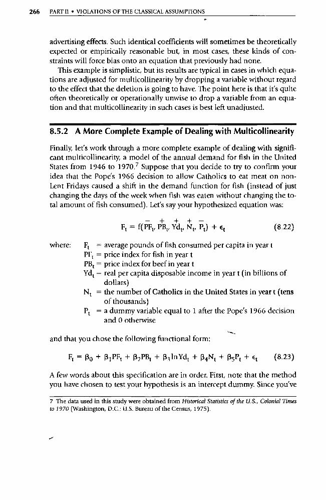
266 PART II • VIOLATIONS OF THE CLASSICAL ASSUMPTIONS
advertising effects. Such identical coefficients will sometimes be theoretically expected or empirically reasonable but, in most cases, these kinds of con-straints will force bias onto an equation that previously had none.
This example is simplistic, but its results are typical in cases in which equa-tions are adjusted for multicollinearity by dropping a variable without regard to the effect that the deletion is going to have. The point here is that it's quite often theoretically or operationally unwise to drop a variable from an equa-tion and that multicollinearity in such cases is best left unadjusted.
8.5.2 A More Complete Example of Dealing with Multicollinearity
Finally, let's work through a more complete example of dealing with signifi-cant multicollinearity, a model of the annual demand for fish in the United States from 1946 to 1970. 7 Suppose that you decide to try to confirm your idea that the Pope's 1966 decision to allow Catholics to eat meat on non-Lent Fridays caused a shift in the demand function for fish (instead of just changing the days of the week when fish was eaten without changing the to-tal amount of fish consumed). Let's say your hypothesized equation was:
— + + + — Ft = f(PFt, PBt, Ydt, Nt, Pt) + et (8.22)
where: Ft = average pounds of fish consumed per capita in year t PFt = price index for fish in year t PBt = price index for beef in year t Ydt = real per capita disposable income in year t (in billions of
dollars) Nt = the number of Catholics in the United States in year t (tens
of thousands) Pt = a dummy variable equal to 1 after the Pope's 1966 decision
and 0 otherwise
and that you chose the following functional form:
Ft = RO + 13 1 PFt + I3 2PBt + 133 1nYdt + 134Nt + 13 5 Pt + et (8.23)
A few words about this specification are in order. First, note that the method you have chosen to test your hypothesis is an intercept dummy. Since you've
7 The data used in this study were obtained from Historical Statistics of the U.S., Colonial Times to 1970 (Washington, D.C.: U.S. Bureau of the Census, 1975).
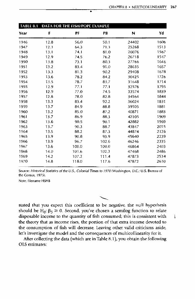
CHAPTER 8 • MULTICOLLINEARITY 267
TABLE 8.1 DATA FOR THE FISH/POPE EXAMPLE
Year F PF PB N Yd
1946 12.8 56.0 50.1 24402 1606 1947 12.3 64.3 71.3 25268 1513 1948 13.1 74.1 81.0 26076 1567 1949 12.9 74.5 76.2 26718 1547 1950 13.8 73.1 80.3 27766 1646 1951 13.2 83.4 91.0 28635 1657 1952 13.3 81.3 90.2 29408 1678 1953 13.6 78.2 84.2 30425 1726 1954 13.5 78.7 83.7 31648 1714 1955 12.9 77.1 77.1 32576 1795 1956 12.9 77.0 74.5 33574 1839 1957 12.8 78.0 82.8 34564 1844 1958 13.3 83.4 92.2 36024 1831 1959 13.7 84.9 88.8 39505 1881 1960 13.2 85.0 87.2 40871 1883 1961 13.7 86.9 88.3 42105 1909 1962 13.6 90.5 90.1 42882 1969 1963 13.7 90.3 88.7 43847 2015 1964 13.5 88.2 87.3 44874 2126 1965 13.9 90.8 93.9 45640 2239 1966 13.9 96.7 102.6 46246 2335 1967 13.6 100.0 100.0 46864 2403 1968 14.0 101.6 102.3 47468 2486 1969 14.2 107.2 111.4 47873 2534 1970 14.8 118.0 117.6 47872 2610
Source: Historical Statistics of the U.S., Colonial Times to 1970 (Washington, D.C.: U.S. Bureau of the Census, 1975).
Note: filename FISH8
stated that you expect this coefficient to be negative, the null hypothesis should be H0: R5 _> 0. Second, you've chosen a semilog function to relate disposable income to the quantity of fish consumed; this is consistent with j the theory that as income rises, the po rtion of that extra income devoted to the consumption of fish will decrease. Leaving other valid criticisms aside, let's investigate the model and the consequences of multicollinearity for it.
After collecting the data (which are in Table 8.1), you obtain the following OIS estimates:

268 PART' II • VIOLATIONS OF THE CLASSICAL ASSUMPTIONS
Ft 1.99 + 0.039PFt — 0.00077PBt + 1.771nYdt
(0.031) (0.02020) (1.87) t = 1.27 — 0.0384 0.945
— 0.0031Nt — 0.355Pt
(0.0033) (0.353) t= —0.958 —1.01
R2 =.666 n=25
(8.24)
This result is not encouraging, since you don't have to Iook at a t-table to know that none of your estimated coefficients is significant. In addition, three of your coefficients have unexpected signs. Your problems could have been caused, for example, by omitted variables (biasing the coefficients), ir-relevant variables (not belonging in the equation), or multicollinearity (a good guess, since this is the topic of the current chapter).
Where do you sta rt? If you have confidence in your review of the literature and the theoretical work you did before estimating the equation, a good place would be to see if there are any signs of multicollinearity. Supporting this decision is the R2 of .666 (an ominous number in a religious regression), which seems fairly high for such unanimously insignificant t-scores.
One measure of severe multicollinearity is the size of the simple correla-tion coefficients. Looking at the variables without knowing those statistics, which pairs (or sets) of variables look likely to be significantly correlated? It appears that per capita disposable income and the number of Catholics are quite likely to be highly correlated in virtually any time-series sample from the United States, and both appear to have been included in the equation to measure buying power. Sure enough, the correlation coefficient between N t
and lnYdt is .946. In addition, it's not unreasonable to think that food prices might move to-
gether. Since the prices that we observe are equilibrium prices, supply and de-mand shocks might affect beef and fish price indices in similar ways. For exam-ple, an oil spill that makes fish unmarketable will admittedly raise the price of fish, but that increase will almost surely shi ft the demand for beef upward, thus increasing the price of beef. Thus it is quite possible for prices of substitutes to tend to move together. As it turns out, the simple correlation coefficient be-tween the two price variables is .958. With multicollinearity of this severity be-tween two va riables with opposite expected signs, it is no surp rise that the two coefficients "switched signs." As multicollinearity increases, the dist ribution of the j3s widens, and the probability of observing an unexpected sign increases.
The second method of detecting multicollinearity, the size of the va riance inflation factors, also indicates severe problems. All the VIFs for Equation 8.24 except VIF are well above the VIF > 5 indicator of severe multicollinearity:
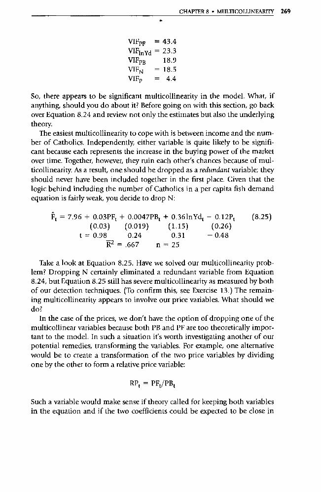
CHAPTER 8 • MULTICOLLINEARITY 269
VIFPp = 43.4
VIF1nYd = 23.3 VIFPB 18.9 VIFN = 18.5 VIFp = 4.4
So, there appears to be significant multicollinearity in the model. What, if anything, should you do about it? Before going on with this section, go back over Equation 8.24 and review not only the estimates but also the underlying theory.
The easiest multicollinearity to cope with is between income and the num-ber of Catholics. Independently, either variable is quite likely to be signifi-cant because each represents the increase in the buying power of the market over time. Together, however, they ruin each other's chances because of mul-ticollinearity. As a result, one should be dropped as a redundant variable; they should never have been included together in the first place. Given that the logic behind including the number of Catholics in a per capita fish demand equation is fairly weak, you decide to drop N:
Ft = 7.96 + 0.03PFt + 0.0047PBt + 0.36lnYdt — 0.12Pt
(0.03) (0.019) (1.15) (0.26)
t = 0.98 0.24 0.31 — 0.48 R2 = .667 n = 25
(8.25)
Take a look at Equation 8.25. Have we solved our multicollinearity prob-lem? Dropping N certainly eliminated a redundant variable from Equation 8.24, but Equation 8.25 still has severe multicollinearity as measured by both of our detection techniques. (To confirm this, see Exercise 13.) The remain-ing multicollinearity appears to involve our price variables. What should we do?
In the case of the prices, we don't have the option of dropping one of the multicollinear variables because both PB and PF are too theoretically impor-tant to the model. In such a situation it's worth investigating another of our potential remedies, transforming the variables. For example, one alternative would be to create a transformation of the two price variables by dividing one by the other to form a relative price variable:
RPt = PFt/PBt
Such a variable would make sense if theory called for keeping both variables in the equation and if the two coefficients could be expected to be close in
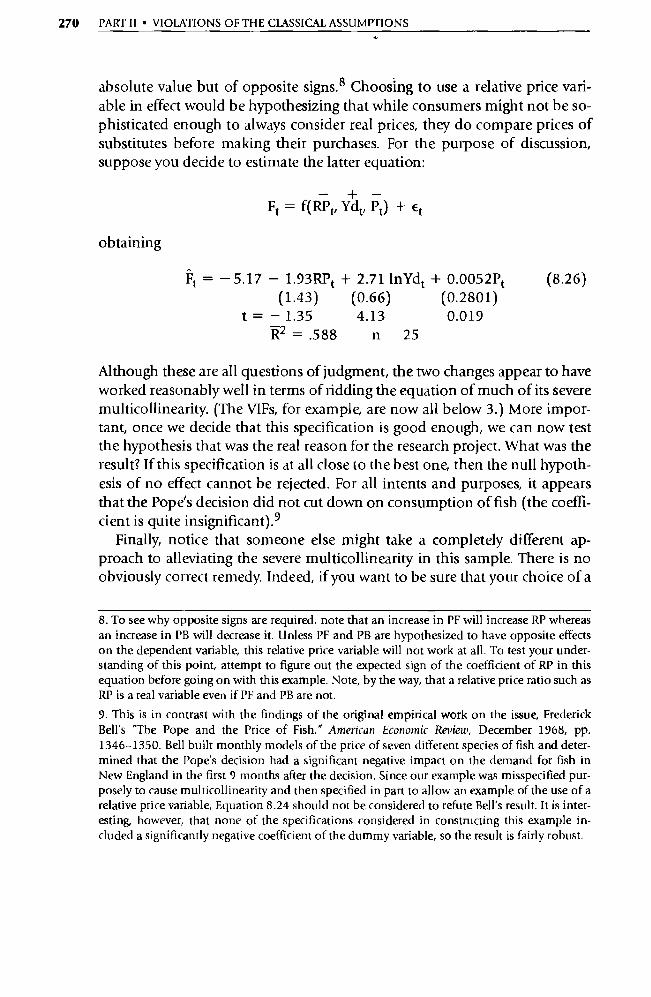
obtaining
Ft = - 5.17 — 1.93RPt + 2.71 1nYdt + 0.0052Pt (1.43) (0.66) (0.2801)
t = —1.35 4.13 0.019 R2 = .588 n 25
(8.26)
270 PART II • VIOLATIONS OF THE CLASSICAL ASSUMPTIONS
absolute value but of opposite signs. 8 Choosing to use a relative price vari-able in effect would be hypothesizing that while consumers might not be so-phisticated enough to always consider real prices, they do compare prices of substitutes before making their purchases. For the purpose of discussion, suppose you decide to estimate the latter equation:
— + —
Ft = f(RPr Ydt, Pt) + Et
Although these are all questions of judgment, the two changes appear to have worked reasonably well in terms of ridding the equation of much of its severe multicollinearity. (The VIFs, for example, are now all below 3.) More impor-tant, once we decide that this specification is good enough, we can now test the hypothesis that was the real reason for the research project. What was the result? If this specification is at all close to the best one, then the null hypoth-esis of no effect cannot be rejected. For all intents and purposes, it appears that the Pope's decision did not cut down on consumption of fish (the coeffi-cient is quite insignificant).
Finally, notice that someone else might take a completely different ap-proach to alleviating the severe multicollinearity in this sample. There is no obviously correct remedy. Indeed, if you want to be sure that your choice of a
8. To see why opposite signs are required, note that an increase in PF will increase RP whereas an increase in PB will decrease it. Unless PF and PB are hypothesized to have opposite effects on the dependent variable, this relative price va riable will not work at all. To test your under-standing of this point, attempt to figure out the expected sign of the coefficient of RP in this equation before going on with this example. Note, by the way, that a relative price ratio such as RP is a real variable even if PF and PB are not. 9. This is in contrast with the findings of the o riginal empirical work on the issue, Frederick Bell's "The Pope and the Price of Fish," American Economic Review, December 1968, pp. 1346-1350. Bell built monthly models of the price of seven different species of fish and deter-mined that the Pope's decision had a significant negative impact on the demand for fish in New England in the first 9 months after the decision. Since our example was misspecified pur-posely to cause multicollinearity and then specified in part to allow an example of the use of a relative price va riable, Equation 8.24 should not be considered to refute Bell's result. It is inter-esting, however, that none of the specifications considered in constructing this example in-cluded a significantly negative coefficient of the dummy va riable, so the result is fairly robust.
CHAPTER 8 • MULTICOLLINEARITY 271
specification did not influence your inability to reject the null hypothesis about (3 P, you might see how sensitive that conclusion is to an alte rnative ap-proach toward fixing the multicollinearity. (In such a case, both results would have to be part of the research repo rt.)
8.6 Summary
1. Perfect multicollinearity is the violation of the assumption that no ex-planatory variable is a perfect linear function of other explanatory variable(s). Perfect multicollinearity results in indeterminate esti-mates of the regression coefficients and infinite standard errors of those estimates.
2. Imperfect multicollinearity, which is what is typically meant when the word "multicollinearity" is used, is a linear relationship between two or more independent variables that is strong enough to significantly affect the estimation of that equation. Multicollinearity is a sample phenomenon as well as a theoretical one. Different samples can ex-hibit different degrees of multicollinearity.
3. The major consequence of severe multicollinearity is to increase the variances of the estimated regression coefficients and therefore de-crease the calculated t-scores of those coefficients. Multicollinearity causes no bias in the estimated coefficients, and it has little effect on the overall significance of the regression or on the estimates of any
15mmnitieallinear euplanaiory variables. 4. Severe multicollinearity causes difficulty in the identification of the
separate effects of the multicollinear variables in a regression equa-tion. In addition, coefficient estimates become very sensitive to changes in specification in the presence of multicollinearity.
5. Since multicollinearity exists, to one degree or another, in virtually every data set, the question to be asked in detection is how severe the multicollinearity in a particular sample is.
6. Two useful methods for the detection of severe multicollinearity are: a. Are the simple correlation coefficients between the explanatory
variables high? b. Are the va riance inflation factors high?
If either of these answers is yes, then multicollinearity certainly exists, but multicollinearity can also exist even if the answers are no.
272 PART II • VIOLATIONS OF THE CLASSICAL ASSUMPTIONS
7. The four most common remedies for multicollinearity are: a. Do nothing (and thus avoid specification bias). b. Drop a redundant variable. c. Transform the multicollinear variables or the equation. d. Increase the size of the sample.
8. Quite often, doing nothing is the best remedy for multicollinearity. If the multicollinearity has not decreased t-scores to the point of in-significance, then no remedy should even be considered. Even if the t-scores are insignificant, remedies should be undertaken cautiously, because all impose costs on the estimation that may be greater than the potential benefit of ridding the equation of multicollinearity.
Exercises
(Answers to even-numbered exercises are in Appendix A.)
1. Write the meaning of each of the following terms without referring to the book (or your notes), and then compare your definition with the version in the text for each: a. perfect multicollinearity b. severe imperfect multicollinearity c. dominant variable d. combination variable e. first difference f. variance inflation factor g. redundant variable
2. Beginning researchers quite often believe that they have multi-collinearity when they've accidentally included in their equation two or more explanatory variables that basically serve the same pur-pose or are, in essence, measuring the same thing. Which of the fol-lowing pairs of variables are likely to include such a redundant vari-able? a. GDP and NDP in a macroeconomic equation of some sort b. the price of refrigerators and the price of washing machines in a
durable goods demand function c. the number of acres harvested and the amount of seed used in an
agricultural supply function d. long-term interest rates and the money supply in an investment
function
CHAPTER 8 • MULTICOLLINEARTTY 273
3. A researcher once attempted to estimate an asset demand equation that included the following three explanatory variables: current wealth Wl, wealth in the previous quarter Wt_1, and the change in wealth AWt = Wt Wt_ 1 . What problem did this researcher en-counter? What should have been done to solve this problem?
4. In each of the following situations, determine whether the variable in-volved is a dominant variable: a. games lost in year t in an equation for the number of games won in
year t by a baseball team that plays the same number of games each year
b. number of Woody's restaurants in a model of the total sales of the entire Woody's chain of restaurants
c. disposable income in an equation for aggregate consumption ex-penditures
d. number of tires purchased in an annual model of the number of automobiles produced by a Big Three automaker that does not make its own tires
e. number of acres planted in an agricultural supply function
5. The formation of linear combinations is an arbitrary process. For ex-ample, one possible linear combination between liquid assets and disposable income in Section 8.4.3 could be X3i = 10(Ydi) + LA; be-cause the mean of the liquid assets variable is almost exactly 10 times the mean of the disposable income va riable. To ensure that one does not overwhelm the other, an adjustment by a factor of 10 makes sense. Other researchers prefer to regress one of the explanatory vari-ables on the other. In this case, we also obtain evidence that a multi-ple of 10 makes sense:
LÂt = — 2428.6 + 10.786Ydt (0.8125)
t = 13.274 R2 = .967
Use this same general technique to form linear combinations of the following variables: a. height and weight in Table 1.1 (assume both are explanatory Xs) b. P and I from the Woody's data set in Table 3.1 c. Y and Yd in Table 6.2 (assume both are explanatory Xs)
6. You've been hired by the Dean of Students Office to help reduce dam-age done to dorms by rowdy students, and your first step is to build a

274 PART II • VIOLATIONS OF THE CLASSICAL ASSUMPTIONS
cross-sectional model of last term's damage to each dorm as a func-tion of the attributes of that dorm:
D i = 210 + 733F1 - 0.805Si + 74.0A1 (253) (0.752) (12.4)
n = 33 R2 .84
where: Di = the amount of damage (in dollars) done to the ith dorm last term
F1 = the percentage of the ith dorm residents who are frosh
Si = the number of students who live in the ith dorm Ai = the number of incidents involving alcohol that were
reported to the Dean of Students Office from the ith dorm last term (incidents involving alcohol may or may not involve damage to the dorm)
a. Hypothesize signs, calculate t-scores, and test hypotheses for this result (5 percent level).
b. What problems (left-out variables, irrelevant variables, or multi-collinearity) appear to exist in this equation? Why?
c. Suppose you were now told that the simple correlation coefficient between S i and Ai was 0.94; would that change your answer? How?
d. Is it possible that the unexpected sign of Rs could have been caused by multicollinearity? Why?
7. Suppose your friend was modeling the impact of income on con-sumption in a quarterly model and discovered that income's impact on consumption lasts at least a year. As a result, your friend estimated the following model:
et = + RiYdt + 132Ydc- 1 + 133Ydt-2 + 134Ydt-3 + Et
a. Would this equation be subject to perfect multicollinearity? b. Would this equation be subject to imperfect multicollinearity? c. What, if anything, could be done to rid this equation of any multi-
collinearity it might have? (One answer to this question, the au-toregressive approach to distributed lags, will be covered in Chap-ter 12.)
8. In 1998, Mark McGwire hit 70 homers to break Roger Maris' old record of 61, and yet McGwire wasn't voted the Most Valuable

CHAPTER 8 • MULTICOLLINEARITY 275
Player (MVP) in his league. To try to understand how this hap-pened, you collect the following data on MVP votes, batting average (BA), home runs (HR), and runs batted in (RBI) from the 1998 Na-tional League:
Name Votes (V) BA HR RBI
Sosa 438 .308 66 158 McGwire 272 .299 70 147 Mou 215 .312 38 124 Vaughn 185 .272 50 119 Biggio 163 .325 20 88 Galarraga 147 .305 44 121 Bonds 66 .303 37 122 Jones 56 .313 34 107
Note: filename MVP8
Just as you are about to run the regression, your friend (trying to get back at you for your comments on Exercise 7) warns you that you probably have multicollinearity. a. What should you do about your friend's warning before running
the regression? + + +
b. Run the regression implied above: V = f(BA, HR, RBI) + E on the data above. What signs of multicollinearity are there?
c. What suggestions would you make for another run of this equa-tion? (If you didn't get a chance to run the equation yourself, refer to Appendix A before answering this pa rt of the question.) In par-ticular, what would you do about multicollinearity?
9. A full-scale regression model for the total annual gross sales in thou-sands of dollars of J. C. Quarter's durable goods for the last 26 years produces the following result (all measurements are in real dollars—or billions of real dollars). Standard errors are in parentheses:
SQt = — 7.2 + 200.3PCt — 150.6PQt + 20.6Yt (250.1) (125.6) (40.1) — 15.8Ct + 201.1Nt
(10.6) (103.8)

276 PART II • VIOLATIONS OF THE CLASSICAL ASSUMPTIONS
where: SQt = sales of durable goods at J. C. Quarter's in year t PCt = average price of durables in year t at J. C. Quarter's
main competition PQt = the average price of durables at J. C. Quarter's in
year t Yt = U.S. gross domestic product in year t Ct = U.S. aggregate consumption in year t Nt = the number of J. C. Quarter's stores open in year t
a. Hypothesize signs, calculate t-scores, and test hypotheses for this result (5 percent level).
b. What problems (out of omitted variables, irrelevant variables, and multicollinearity) appear to exist in this equation? Explain.
c. Suppose you were now told that the R 2 was .821, that ryc was .993, and that rpc pQ was .813. Would this change your answer to the above question? How?
d. What recommendation would you make for a rerun of this equa-tion with different explanatory variables? Why?
10. A cross-sectional regression was run on a sample of 44 states in an ef-fort to understand federal defense spending by state (standard errors in parentheses):
Si = — 148.0 + 0.841Cî — 0.0115Pî — 0.0078Eî (0.027) (0.1664) (0.0092)
where: Si = annual spending (millions of dollars) on defense in the ith state
Ci = contracts (millions of dollars) awarded in the ith state (contracts are often for many years of service) per year
Pi = annual payroll (millions of dollars) for workers in defense-oriented industries in the ith state
Ei = the number of civilians employed in defense-oriented industries in the ith state
a. Hypothesize signs, calculate t-scores, and test hypotheses for this result (5 percent level).
b. The VIFs for this equation are all above 20, and those for P and C are above 30. What conclusion does this information allow you to draw?
c. What recommendation would you make for a rerun of this equa-tion with a different specification? Explain your answer.
CHAPTER 8 • MULTICOLLINEARITY 277
11. Consider the following regression result paraphrased from a study conducted by the admissions office at the Stanford Business School (standard errors in parentheses):
;= 1.00+0.005M1+0.20B; -0.10A; +0.25S; (0.001) (0.20) (0.10) (0.10) R2 = 0.20 n = 1000
where: G; — the Stanford Business School GPA of the ith student (4 = high)
M; = the score on the graduate management admission test of the ith student (800 = high)
B; = the number of years of business experience of the ith student
A; = the age of the ith student S i = dummy equal to 1 if the ith student was an econom-
ics major and 0 otherwise
a. Theorize the expected signs of all the coefficients (try not to look at the results) and test these expectations with appropriate hypothe-ses (including choosing a significance level).
b. Do any problems appear to exist in this equation? Explain your an-swer.
c. How would you react if someone suggested a polynomial func-tional form for A? Why?
d. What suggestions (if any) would you have for another run of this equation?
12. Calculating VIFs typically involves running sets of auxiliary regres-sions, one regression for each independent variable in an equation. To get practice with this procedure, calculate the following: a. the VIFs for N, P, and I from the Woodÿ s data in Table 3.1. b. the VIFs for PB, PC, and YD from the chicken demand data in Table
6.2 (using Equation 6.8). c. the VIF for X1 in an equation where X 1 and X2 are the only inde-
pendent variables, given that the VIF for X2 is 3.8 and n = 28. d. the VIF for X 1 in an equation where X 1 and X2 are the only inde-
pendent variables, given that the simple correlation coefficient be-tween X 1 and X2 is 0.80 and n = 15.
13. Test Equation 8.25 for multicollinearity using both of our detection techniques. (Hint: This involves using the Pope/fish data set, datafile = FISH 8).
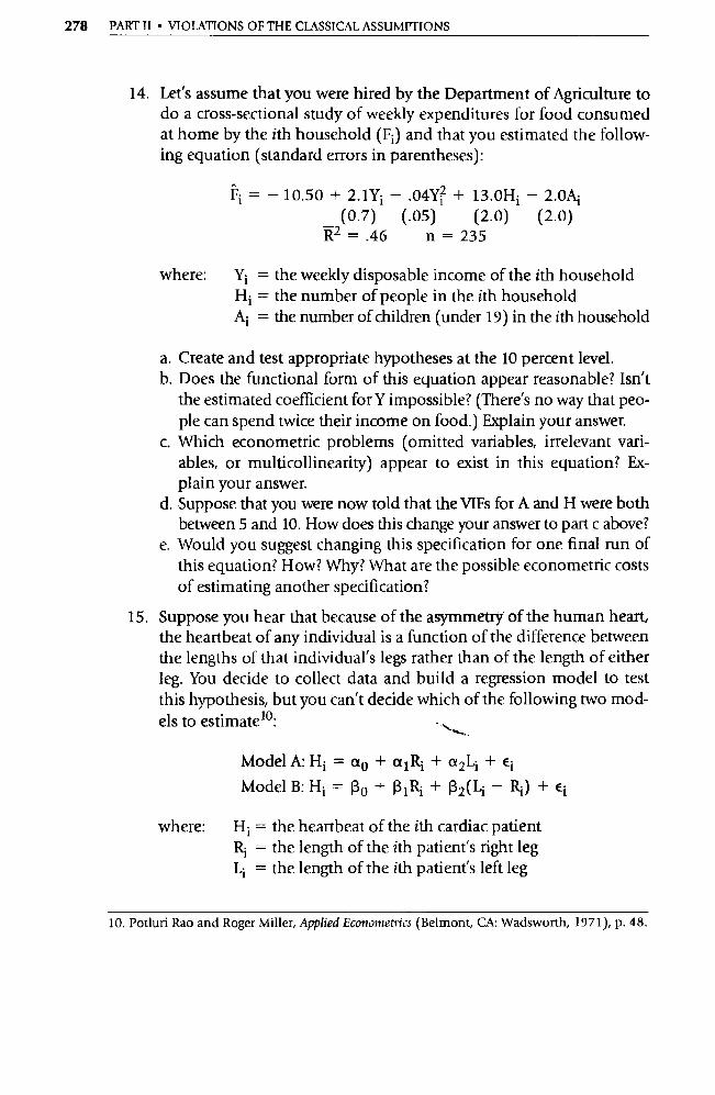
278 PART II • VIOLATIONS OF THE CLASSICAL ASSUMPTIONS
14. Let's assume that you were hired by the Department of Agriculture to do a cross-sectional study of weekly expenditures for food consumed at home by the ith household (F i) and that you estimated the follow-ing equation (standard errors in parentheses):
Fi =- 10.50+2.1Yî —.04Y?+ 13.0H î -2.0Aî (0.7) (.05) (2.0) (2.0)
R2 =.46 n=235
where: Yi = the weekly disposable income of the ith household Hi = the number of people in the ith household Ai = the number of children (under 19) in the ith household
a. Create and test appropriate hypotheses at the 10 percent level. b. Does the functional form of this equation appear reasonable? Isn't
the estimated coefficient for Y impossible? (There's no way that peo-ple can spend twice their income on food.) Explain your answer.
c. Which econometric problems (omitted variables, irrelevant vari-ables, or multicollinearity) appear to exist in this equation? Ex-plain your answer.
d. Suppose that you were now told that the VIFs for A and H were both between 5 and 10. How does this change your answer to pa rt c above?
e. Would you suggest changing this specification for one final run of this equation? How? Why? What are the possible econometric costs of estimating another specification?
15. Suppose you hear that because of the asymmetry of the human heart, the heartbeat of any individual is a function of the difference between the lengths of that individual's legs rather than of the length of either leg. You decide to collect data and build a regression model to test this hypothesis, but you can't decide which of the following two mod-els to estimate lo :
Model A: H i = a0 + a 1 Ri + a2Li + ei
Model B: Hi = Ro + R 1 Ri + 12('i - Ri) + Ei
where: H i = the heartbeat of the ith cardiac patient Ri = the length of the ith patient's right leg Li = the length of the ith patient's left leg
10. Potluri Rao and Roger Miller, Applied Econometrics (Belmont, CA: Wadsworth, 1971), p. 48.
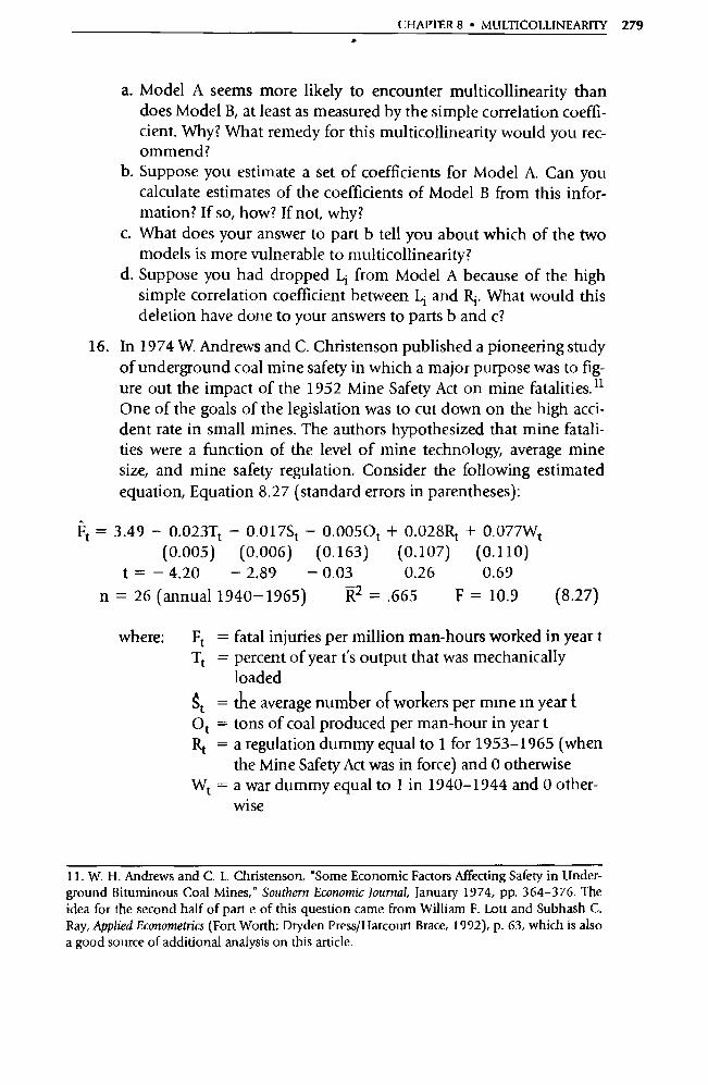
CHAPTER 8 • MULTICOLLINEARITY 279
a. Model A seems more likely to encounter multicollinearity than does Model B, at least as measured by the simple correlation coeffi-cient. Why? What remedy for this multicollinearity would you rec-ommend?
b. Suppose you estimate a set of coefficients for Model A. Can you calculate estimates of the coefficients of Model B from this infor-mation? If so, how? If not, why?
c. What does your answer to pa rt b tell you about which of the two models is more vulnerable to multicollinearity?
d. Suppose you had dropped Li from Model A because of the high simple correlation coefficient between L i and Ri . What would this deletion have done to your answers to pa rts b and c?
16. In 1974 W. Andrews and C. Christenson published a pioneering study of underground coal mine safety in which a major purpose was to fig-ure out the impact of the 1952 Mine Safety Act on mine fatalities. 11
One of the goals of the legislation was to cut down on the high acci-dent rate in small mines. The authors hypothesized that mine fatali-ties were a function of the level of mine technology, average mine size, and mine safety regulation. Consider the following estimated equation, Equation 8.27 (standard errors in parentheses):
Ft = 3.49 - 0.023Tt - 0.017S t - 0.005Ot + 0.028Rt + 0.077Wt (0.005) (0.006) (0.163) (0.107) (0.110)
t = - 4.20 - 2.89 - 0.03 0.26 0.69
n = 26 (annual 1940-1965)
R2 = .665 F = 10.9 (8.27)
where: Ft = fatal inju ries per million man-hours worked in year t Tt = percent of year is output that was mechanically
loaded
St = the average number of workers per mine in year t Ot = tons of coal produced per man-hour in year t Rt = a regulation dummy equal to 1 for 1953-1965 (when
the Mine Safety Act was in force) and 0 otherwise Wt = a war dummy equal to 1 in 1940-1944 and 0 other-
wise
11. W. H. Andrews and C. L. Christenson, Some Economic Factors Affecting Safety in Under-ground Bituminous Coal Mines," Southern Economic Journal, January 1974, pp. 364-376. The idea for the second half of pa rt e of this question came from William F. Lott and Subhash C. Ray, Applied Econometrics (Fort Worth: D ryden Press/Harcourt Brace, 1992), p. 63, which is also a good source of additional analysis on this article.
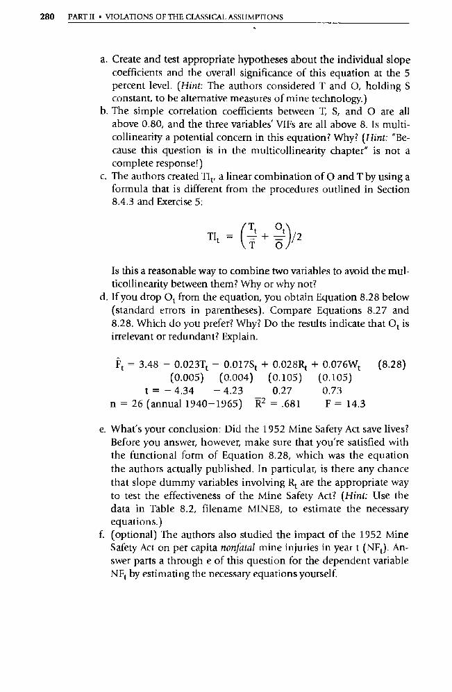
280 PART II • VIOLATIONS OF THE CLASSICAL ASSUMPTIONS
a. Create and test appropriate hypotheses about the individual slope
coefficients and the overall significance of this equation at the 5 percent level. (Hint: The authors considered T and O, holding S constant, to be alternative measures of mine technology.)
b. The simple correlation coefficients between T, S, and O are all above 0.80, and the three variables' VIFs are all above 8. Is multi-collinearity a potential concern in this equation? Why? (Hint: "Be-cause this question is in the multicollinearity chapter" is not a complete response!)
c. The authors created TI t, a linear combination of O and T by using a formula that is different from the procedures outlined in Section 8.4.3 and Exercise 5:
TIt = C Tt + Ot I^2 T O
Is this a reasonable way to combine two variables to avoid the mul-ticollinearity between them? Why or why not?
d. If you drop Ot from the equation, you obtain Equation 8.28 below (standard errors in parentheses). Compare Equations 8.27 and 8.28. Which do you prefer? Why? Do the results indicate that O t is irrelevant or redundant? Explain.
Ft = 3.48 — 0.023T1 — 0.017St + 0.028R1 + 0.076Wt (8.28) (0.005) (0.004) (0.105) (0.105)
t = — 4.34 — 4.23 0.27 0.73 n = 26 (annual 1940-1965) RZ = .681 F = 14.3
e. What's your conclusion: Did the 1952 Mine Safety Act save lives? Before you answer, however, make sure that you're satisfied with the functional form of Equation 8.28, which was the equation the authors actually published. In pa rticular, is there any chance that slope dummy variables involving Rt are the appropriate way to test the effectiveness of the Mine Safety Act? (Hint: Use the data in Table 8.2, filename MINE8, to estimate the necessary equations.)
f. (optional) The authors also studied the impact of the 1952 Mine Safety Act on per capita nonfatal mine injuries in year t (NF t). An-swer parts a through e of this question for the dependent variable NFt by estimating the necessary equations yourself.
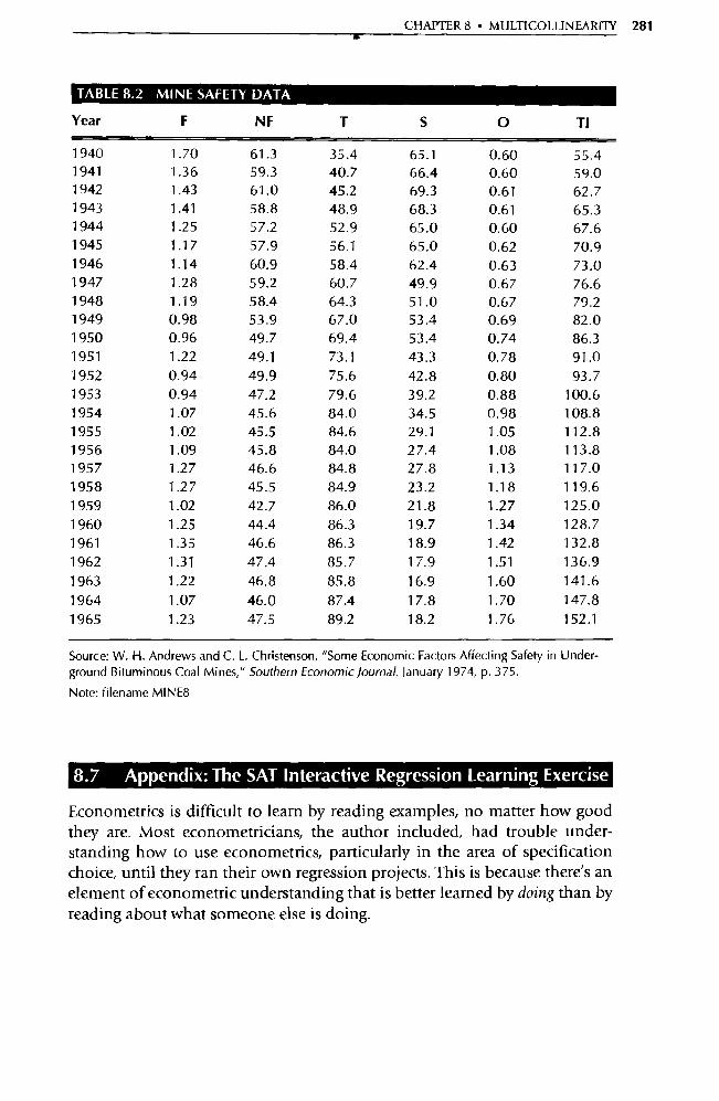
CHAPTER 8 • MULTICOLLINEARITY 281
TABLE 8.2 MINE SAFETY DATA
Year F NF T s O TI
1940 1.70 61.3 35.4 65.1 0.60 55.4 1941 1.36 59.3 40.7 66.4 0.60 59.0 1942 1.43 61.0 45.2 69.3 0.61 62.7 1943 1.41 58.8 48.9 68.3 0.61 65.3 1944 1.25 57.2 52.9 65.0 0.60 67.6 1945 1.17 57.9 56.1 65.0 0.62 70.9 1946 1.14 60.9 58.4 62.4 0.63 73.0 1947 1.28 59.2 60.7 49.9 0.67 76.6 1948 1.19 58.4 64.3 51.0 0.67 79.2 1949 0.98 53.9 67.0 53.4 0.69 82.0 1950 0.96 49.7 69.4 53.4 0.74 86.3 1951 1.22 49.1 73.1 43.3 0.78 91.0 1952 0.94 49.9 75.6 42.8 0.80 93.7 1953 0.94 47.2 79.6 39.2 0.88 100.6 1954 1.07 45.6 84.0 34.5 0.98 108.8 1955 1.02 45.5 84.6 29.1 1.05 112.8 1956 1.09 45.8 84.0 27.4 1.08 113.8 1957 1.27 46.6 84.8 27.8 1.13 117.0 1958 1.27 45.5 84.9 23.2 1.18 119.6 1959 1.02 42.7 86.0 21.8 1.27 125.0 1960 1.25 44.4 86.3 19.7 1.34 128.7 1961 1.35 46.6 86.3 18.9 1.42 132.8
1962 1.31 47.4 85.7 17.9 1.51 136.9
1963 1.22 46.8 85.8 16.9 1.60 141.6
1964 1.07 46.0 87.4 17.8 1.70 147.8 1965 1.23 47.5 89.2 18.2 1.76 152.1
Source: W. H. Andrews and C. L. Christenson, "Some Economic Factors Affecting Safety in Under-ground Bituminous Coal Mines," Southern Economic Journal, January 1974, p. 375.
Note: filename MINE8
8.7 Appendix: The SAT Interactive Regression Learning Exercise
Econometrics is difficult to learn by reading examples, no matter how good they are. Most econometricians, the author included, had trouble under-standing how to use econometrics, particularly in the area of specification choice, until they ran their own regression projects. This is because there's an element of econometric understanding that is better learned by doing than by reading about what someone else is doing.

282 PART II • VIOLATIONS OF THE CLASSICAL ASSUMPTIONS
Unfortunately, mastering the a rt of econometrics by running your own re-gression projects without any feedback is also difficult because it takes quite a while to learn to avoid some fairly simple mistakes. Probably the best way to learn is to work on your own regression project, analyzing your own prob-lems and making your own decisions, but with a more experienced econo-metrician nearby to give you one-on-one feedback on exactly which of your decisions were inspired and which were flawed (and why).
This section is an attempt to give you an opportunity to make indepen-dent specification decisions and to then get feedback on the advantages or disadvantages of those decisions. Using the interactive learning exercise of this section requires neither a computer nor a tutor, although either would certainly be useful. Instead, we have designed an exercise that can be used on its own to help to bridge the gap between the typical econometrics examples (which require no decision making) and the typical econometrics projects (which give little feedback). An additional interactive learning exercise is pre-sented in Chapter 11.
STOP!
To get the most out of the exercise, it's impo rtant to follow the instructions carefully. Reading the pages "in order" as with any other example will waste your time, because once you have seen even a few of the results, the benefits to you of making specification decisions will diminish. In addition, you shouldn't look at any of the regression results until you have specified your first equation.
8.7.1 Building a Model of Scholastic Aptitude Test Scores
The dependent variable for this interactive learning exercise is the combined SAT score, math plus verbal, earned by students in the senior class at Arcadia High School. Arcadia is an upper-middle-class suburban community located near Los Angeles, California. Out of a graduating class of about 640, a total of 65 students who had taken the SATs were randomly selected for inclusion in the data set. In cases in which a student had taken the test more than once, the highest score was recorded.
A review of the literature on the SAT shows many more psychological stud-ies and popular press a rticles than econometric regressions. Many a rticles have been authored by critics of the SAT, who maintain (among other things) that it is biased against women and minorities. In suppo rt of this argument, these critics have pointed to national average scores for women and some mi-

CHAPTER 8 • MULTICOLLINEARPTY 283
norities, which in recent years have been significantly lower than the national averages for white males. Any reader interested in reviewing a po rtion of the applicable literature should do so now before continuing on with the sec-tion. 12
If you were going to build a single-equation linear model of SAT scores, what factors would you consider? First, you'd want to include some measures of a student's academic ability. Three such variables are cumulative high school grade point average (GPA) and pa rticipation in advanced placement math and English courses (APMATH and APENG). Advanced placement (AP) classes are academically rigorous courses that may help a student do well on the SAT. More impo rtant, students are invited to be in AP classes on the basis of academic potential, and students who choose to take AP classes are reveal-ing their interest in academic subjects, both of which bode well for SAT scores. GPAs at Arcadia High School are weighted GPAs; each semester that a student takes an AP class adds one extra point to his or her total grade points. (For example, a semester grade of "A" in an AP math class counts for five grade points as opposed to the conventional four points.)
A second set of important considerations includes qualitative factors that may affect performance on the SAT. Available dummy variables in this cate-gory include measures of a student's gender (LEND), ethnicity (RACE), and native language (ESL). All of the students in the sample are either Asian or Caucasian, and RACE is assigned a value of one if a student is Asian. Asian students are a substantial proportion of the student body at Arcadia High. The ESL dummy is given a value of one if English is a student's second lan-guage. In addition, studying for the test may be relevant, so a dummy vari-able indicating whether or not a student has attended an SAT preparation class (PREP) is also included in the data.
To sum, the explanatory va riables available for you to choose for your model are:
GPAi = the weighted GPA of the ith student APMATH i = a dummy variable equal to 1 if the ith student has taken AP
math, 0 otherwise APENGi = a dummy variable equal to 1 if the ith student has taken AP
English, 0 otherwise
12. See Jay Ambert, "The SAT," American Scholar, Autumn 1982, pp. 535-542, and James Fal-lows, "The Tests and the 'Brightest': How Fair are the College Boards?" The Atlantic, February 1980, pp. 37-48. We are grateful to former Occidental student Bob Sego for his help in prepar-ing this interactive exercise.
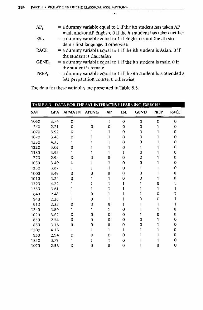
284 PART II • VIOLATIONS OF THE CLASSICAL ASSUMPTIONS
4 .
APi = a dummy va riable equal to 1 if the ith student has taken AP math and/or AP English, 0 if the ith student has taken neither
ESLi = a dummy variable equal to 1 if English is not the ith stu- dent's first language, 0 otherwise
RACEi = a dummy variable equal to 1 if the ith student is Asian, 0 if the student is Caucasian
GENDi = a dummy variable equal to 1 if the ith student is male, 0 if the student is female
PREPi = a dummy variable equal to 1 if the ith student has attended a SAT preparation course, 0 otherwise
The data for these va riables are presented in Table 8.3.
TABLE 8.3 DATA FOR THE SAT INTERACTIVE LEARNING EXERCISE
SAT GPA APMATH APENG AP ESL GEND PREP RACE
1060 3.74 0 1 1 0 0 0 0 740 2.71 0 0 0 0 0 1 0
1070 3.92 0 1 1 0 0 1 0
1070 3.43 0 1 1 0 0 1 0 1330 4.35 1 1 1 0 0 1 0
1220 3.02 0 1 1 0 1 1 0
1130 3.98 1 1 1 1 0 1 0
770 2.94 0 0 0 0 0 1 0
1050 3.49 0 1 1 0 0 1 0
1250 3.87 1 1 1 0 1 1 0
1000 3.49 0 0 0 0 0 1 0
1010 3.24 0 1 1 0 0 1 0
1320 4.22 1 1 1 1 1 0 1
1230 3.61 1 1 1 1 1 1 1
840 2.48 1 0 1 1 1 0 1
940 2.26 1 0 1 1 0 0 1
910 2.32 0 0 0 1 1 1 1
1240 3.89 1 1 1 0 1 1 0
1020 3.67 0 0 0 0 1 0 0
630 2.54 0 0 0 0 0 1 0
850 3.16 0 0 0 0 0 1 0
1300 4.16 1 1 1 1 1 1 0
950 2.94 0 0 0 0 1 1 0
1350 3.79 1 1 1 0 1 1 0
1070 2.56 0 0 0 0 1 0 0
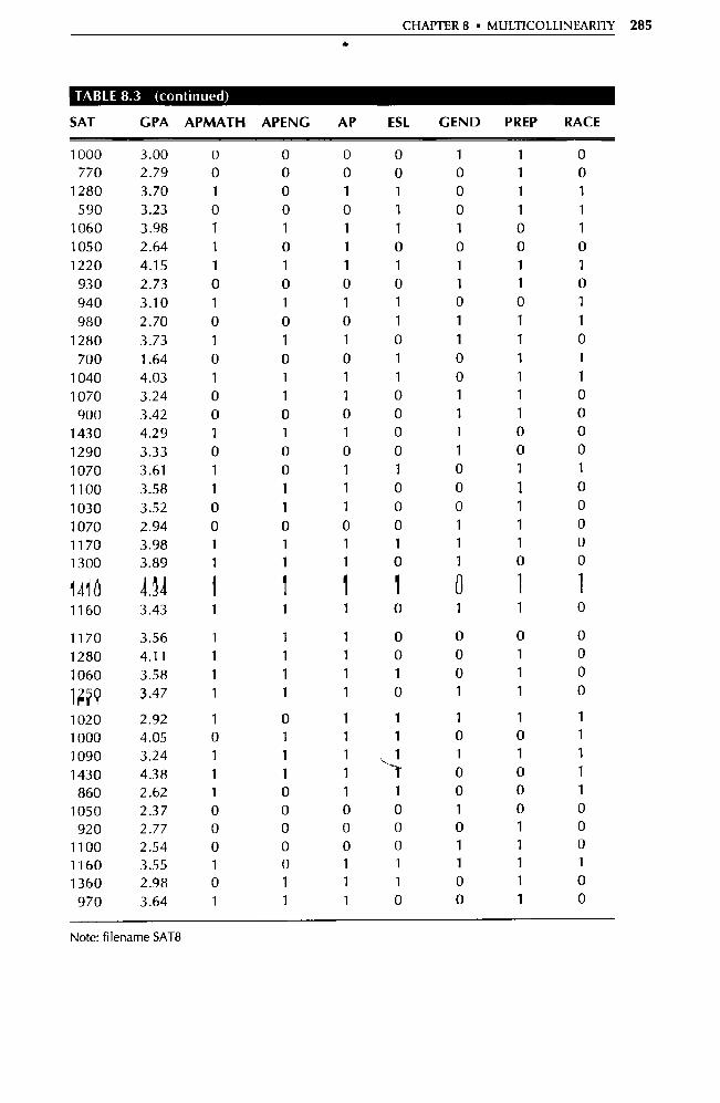
CHAPTER 8 • MULTICOLLINEARITY 285
TABLE 8.3 (continued)
SAT GPA APMATH APENG AP ESL LEND PREP RACE
1000 3.00 0 0 0 0 1 1 0
770 2.79 0 0 0 0 0 1 0
1280 3.70 1 0 1 1 0 1 1
590 3.23 0 0 0 1 0 1 1
1060 3.98 1 1 1 1 1 0 1
1050 2.64 1 0 1 0 0 0 0
1220 4.15 1 1 1 1 1 1 1
930 2.73 0 0 0 0 1 1 0
940 3.10 1 1 1 1 0 0 1
980 2.70 0 0 0 1 1 1 1
1280 3.73 1 1 1 0 1 1 0
700 1.64 0 0 0 1 0 1 1
1040 4.03 1 1 1 1 0 1 1
1070 3.24 0 1 1 0 1 1 0
900 3.42 0 0 0 0 1 1 0
1430 4.29 1 1 1 0 1 0 0
1290 3.33 0 0 0 0 1 0 0
1070 3.61 1 0 1 1 0 1 1
1100 3.58 1 1 1 0 0 1 0
1030 3.52 0 1 1 0 0 1 0
1070 2.94 0 0 0 0 1 1 0
1170 3.98 1 1 1 1 1 1 0
1300 3.89 1 1 1 0 1 0 0
1416 1.14 1 1 1 1 0 1 1 1160 3.43 1 1 1 0 1 1 0
1170 3.56 1 1 1 0 0 0 0
1280 4.11 1 1 1 0 0 1 0
1060 3.58 1 1 1 1 0 1 0
1;0 3.47 1 1 1 0 1 1 0
1020 2.92 1 0 1 1 1 1 1
1000 4.05 0 1 1 1 0 0 1
1090 3.24 1 1 1 ^ 1 1 1 1
1430 4.38 1 1 1 r
0 0 1
860 2.62 1 0 1 1 0 0 1
1050 2.37 0 0 0 0 1 0 0
920 2.77 0 0 0 0 0 1 0
1100 2.54 0 0 0 0 1 1 0
1160 3.55 1 0 1 1 1 1 1
1360 2.98 0 1 1 1 0 1 0
970 3.64 1 1 1 0 0 1 0
Note: filename SAT8
286 PART II • VIOLATIONS OF THE CLASSICAL ASSUMPTIONS
Now:
1. Hypothesize expected signs for each of these variables in an equation for the SAT score of the ith student. Examine each variable carefully; what is the theoretical content of your hypothesis?
2. Choose carefully the best set of explanatory variables. Start off by in-cluding GPA, APMATH, and APENG; what other variables do you think should be specified? Don't simply include all the variables, in-tending to drop the insignificant ones. Instead, think through the problem carefully and find the best possible equation.
Once you've specified your equation, you're ready to move to Section 8.7.2. Keep following the instructions in the exercise until you have specified your equation completely. You may take some time to think over the ques-tions contained in Section 8.7.2 or take a break, but when you return to the interactive exercise make sure to go back to the exact point from which you left rather than starting all over again. To the extent you can do it, try to avoid looking at the hints until after you've completed the entire project. The hints are there to help you if you get stuck, not to allow you to check every decision you make.
One final bit of advice: each regression result is accompanied by a series of questions. Take the time to answer all these questions, in writing if possible. Rushing through this interactive exercise will lessen its effectiveness.
8.7.2 The SAT Score Interactive Regression Exercise
To start, choose the specification you'd like to estimate, find the regression run number 13 of that specification in the following list, and then turn to that regression. Note that the simple correlation coefficient matrix for this data set is in Table 8.4 just before the results begin.
All the equations include SAT as the dependent variable and GPA, APMATH, and APENG as explanatory variables. Find the combination of ex-planatory variables (from ESL, GEND, PREP, and RACE) that you wish to in-clude and go to the indicated regression:
13. All the regression results appear exactly as they are produced by the EViews regression pack-age.
CHAPTER 8 • MULTICOLLINEARITY 287
None of them, go to regression run 8.1 ESL only, go to regression run 8.2 GEND only, go to regression run 8.3 PREP only, go to regression run 8.4 RACE only, go to regression run 8.5 ESL and GEND, go to regression run 8.6 ESL and PREP, go to regression run 8.7 ESL and RACE, go to regression run 8.8 GEND and PREP, go to regression run 8.9 GEND and RACE, go to regression run 8.10 PREP and RACE, go to regression run 8.11 ESL, GEND, and PREP, go to regression run 8.12 ESL, GEND, and RACE, go to regression run 8.13 ESL, PREP, and RACE, go to regression run 8.14 GEND, PREP, and RACE, go to regression run 8.15 All four, go to regression run 8.16
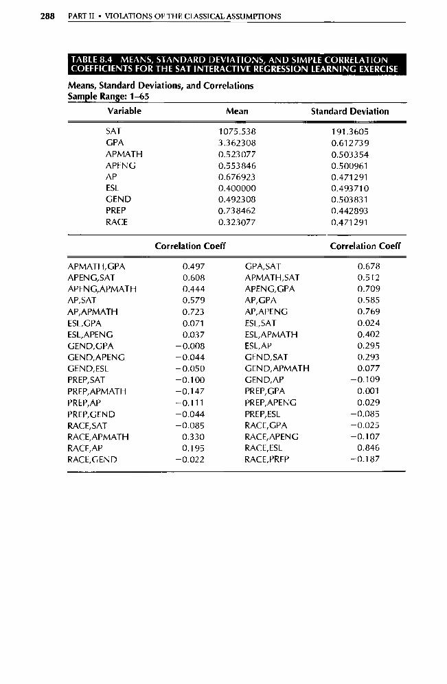
288 PART II • VIOLATIONS OF THE CLASSICAL ASSUMPTIONS
TABLE 8.4 MEANS, STANDARD DEVIATIONS, AND SIMPLE CORRELATION COEFFICIENTS FOR THE SAT INTERACTIVE REGRESSION LEARNING EXERCISE
Means, Standard Deviations, and Correlations Sample Range: 1-65
Variable Mean Standard Deviation
SAT 1075.538 191.3605 G PA 3.362308 0.612739 APMATH 0.523077 0.503354 APENG 0.553846 0.500961 AP 0.676923 0.4 712 91 ESL 0.400000 0.493 710 GEND 0.492308 0.503831 PREP 0.738462 0.442893 RACE 0.323077 0.471291
Correlation Coeff Correlation Coeff
APMATH,GPA 0.497 GPA,SAT 0.678 APENG,SAT 0.608 APMATH,SAT 0.512 APENG,APMATH 0.444 APENG,GPA 0.709 AP,SAT 0.579 AP,GPA 0.585 AP,APMATH 0.723 AP,APENG 0.769 ESL,GPA 0.071 ESL,SAT 0.024 ESL,APENG 0.037 ESL,APMATH 0.402 GEND,GPA -0.008 ESL,AP 0.295 GEND,APENG -0.044 GEND,SAT 0.293 GEND,ESL -0.050 GEND,APMATH 0.077 PREP,SAT -0.100 GEND,AP -0.109
PREP,APMATH -0.147 PREP,GPA 0.001
PREP,AP -0.111 PREP,APENG 0.029
PREP,GEND -0.044 PREP,ESL -0.085 RACE,SAT -0.085 RACE,GPA -0.025
RACE,APMATH 0.330 RACE,APENG -0.107 RACE,AP 0.195 RACE, ESL 0.846
RACE,GEND -0.022 RACE,PREP -0.187
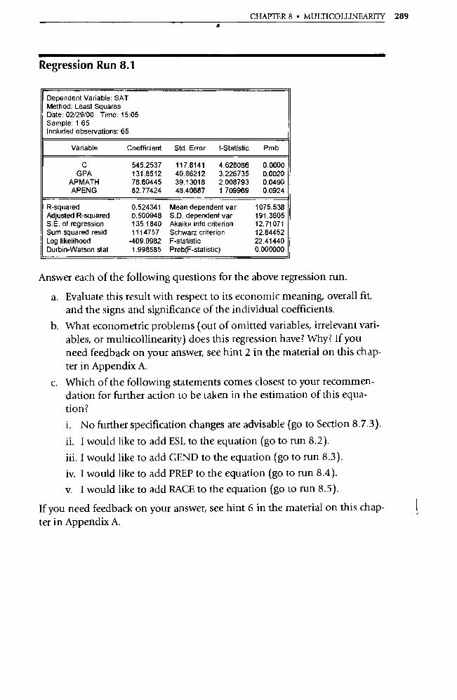
CHAPTER 8 • MULTICOLLINEARITY 289 4
Regression Run 8.1
Dependent Variable: SAT Method: Least Squares Date: 02/29/00 Time: 15:05 Sample: 1 65 Included observations: 65
Variable Coefficient Std. Error t-Statistic Prob.
C 545.2537 117.8141 4.628086 0.0000 GPA 131.8512 40.86212 3.226735 0.0020
APMATH 78.60445 39.13018 2.008793 0.0490 APENG 82.77424 48.40687 1709969 0.0924
R-squared 0.524341 Mean dependent var 1075.538 Adjusted R-squared 0.500948 S.D. dependent var 191.3605 S.E. of regression 135.1840 Akaike info criterion 12.71071 Sum squared resid 1114757 Schwa rz criterion 12.84452 Log likelihood -409.0982 F-statistic 22.41440 Durbin-Watson stat 1.998585 Prob(F-statistic) 0.000000
Answer each of the following questions for the above regression run.
a. Evaluate this result with respect to its economic meaning, overall fit, and the signs and significance of the individual coefficients.
b. What econometric problems (out of omitted variables, irrelevant vari-ables, or multicollinearity) does this regression have? Why? If you need feedback on your answer, see hint 2 in the material on this chap-ter in Appendix A.
c. Which of the following statements comes closest to your recommen-dation for further action to be taken in the estimation of this equa-tion?
i. No further specification changes are advisable (go to Section 8.7.3).
ii. I would like to add ESL to the equation (go to run 8.2).
iii. I would like to add GEND to the equation (go to run 8.3).
iv. I would like to add PREP to the equation (go to run 8.4).
v. I would like to add RACE to the equation (go to run 8.5).
If you need feedback on your answer, see hint 6 in the material on this chap-ter in Appendix A.
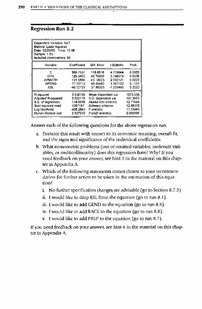
290 PART II • VIOLATIONS OF THE CLASSICAL ASSUMPTIONS
Regression Run 8.2
Dependent Variable: SAT Method: Least Squares Date: 02/29/00 Time: 15:06 Sample: 1 65 Included obse rvations: 65
Variable Coefficient Std. Error t-Statistic Prob.
C 566.7551 118.6016 4.778644 0.0000 GPA 128.3402 40 78800 3.146519 0.0026
APMATH 101.5886 43.19023 2.352121 0.0220 APENG 77.30713 48.40462 1.597102 0.1155
ESL -46.72721 37.88203 -1.233493 0.2222
R-squared 0.536105 Mean dependent var 1075.538 Adjusted R-squared 0.505179 S.D. dependent var 191.3605 S.E. of regression 134.6098 Akaike info criterion 12.71644 Sum squared resid 1087187 Schwarz criterion 12.88370 Log likelihood -408.2843 F-statistic 17.33489 Durbin-Watson stet 2.027210 Prob(F-statistic) 0.000000
Answer each of the following questions for the above regression run.
a. Evaluate this result with respect to its economic meaning, overall fit, and the signs and significance of the individual coefficients.
b. What econometric problems (out of omitted variables, irrelevant vari-ables, or multicollinearity) does this regression have? Why? If you need feedback on your answer, see hint 3 in the material on this chap-ter in Appendix A.
c. Which of the following statements comes closest to your recommen-dation for further action to be taken in the estimation of this equa-tion?
i. No further specification changes are advisable (go to Section 8.7.3).
ii. I would like to drop ESL from the equation (go to run 8.1).
iii. I would like to add GEND to the equation (go to run 8.6).
iv. I would like to add RACE to the equation (go to run 8.8).
v I would like to add PREP to the equation (go to run 8.7).
If you need feedback on your answer, see hint 6 in the material on this chap-ter in Appendix A.

CHAPTER 8 • MULTICOLLINEARITY 291 •
Regression Run 8.3
Dependent Variable: SAT Method: Least Squares Date: 02/29/00 Time: 15:07 Sample: 1 65 Included observations: 65
Variable Coefficient Std. Error t-Statistic Prob.
C 491.8225 108.5429 4.531135 0.0000 GPA 131.5798 37.29970 3.527638 0.0008
APMATH 65,04046 35.91313 1.811049 0.0751 APENG 94.10841 44.29652 2.124510 0.0378 GEND 112.0465 30.82961 3.634379 0.0006
R-squared 0.610162 Mean dependent var 1075.538 Adjusted R-squared 0.584173 S.D. dependent var 191.3605 S.E. of regression 123.3982 Akaike info criterion 12.54251 Sum squared resid 913626.4 Schwarz criterion 12.70977 Log likelihood -402.6317 F-statistic 23.47754 Durbin-Watson stat 2.104997 Prob(F-statistic) 0.000000
Answer each of the following questions for the above regression run.
a. Evaluate this result with respect to its economic meaning, overall fit, and the signs and significance of the individual coefficients.
b. What econometric problems (out of omitted variables, irrelevant vari-ables, or multicollinearity) does this regression have? Why? If you need feedback on your answer, see hint 5 in the material on this chap-ter in Appendix A.
c. Which of the following statements comes closest to your recommen-dation for further action to be taken in the estimation of this equa-tion?
i. No further specification changes are advisable (go to Section 8.7.3).
ii. I would like to add ESL to the equation (go to run 8.6).
iii. I would like to add PREP to the equation (go to run 8.9).
iv. I would like to add RACE to the equation (go to run 8.10).
If you need feedback on your answer, see hint 19 in the material on this chapter in Appendix A.
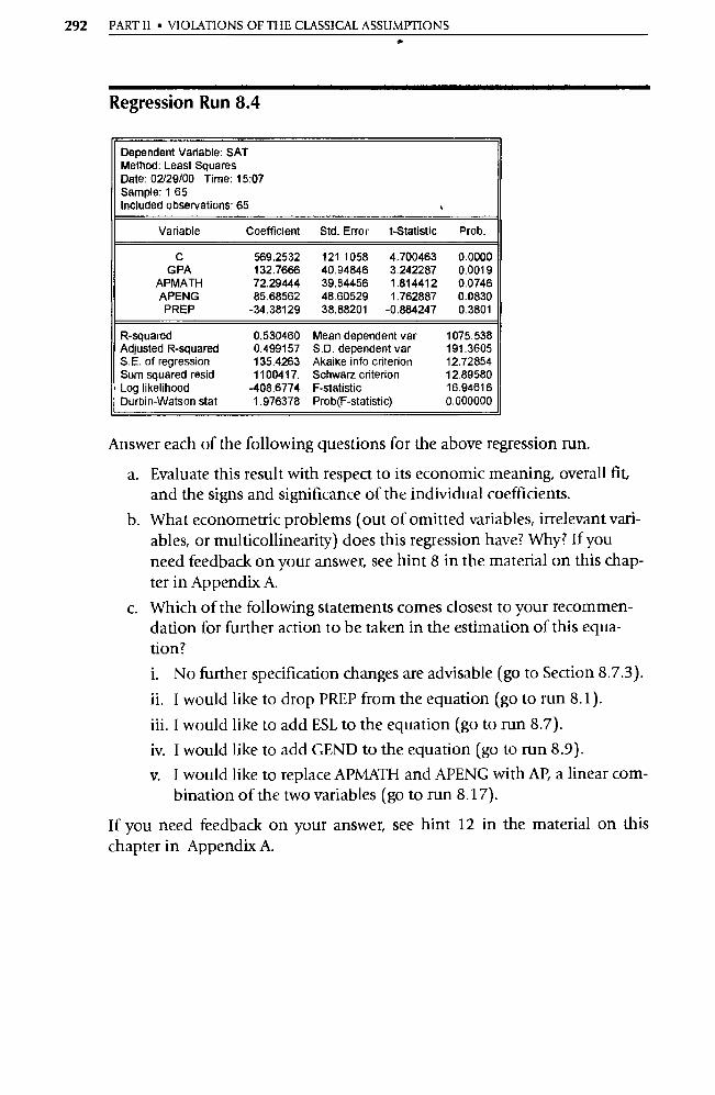
292 PART II • VIOLATIONS OF THE CLASSICAL ASSUMPTIONS
Regression Run 8.4
Dependent Variable: SAT Method: Least Squares Date: 02/29/00 Time: 15:07 Sample: 1 65 Included observations: 65 ■
Variable Coefficient Std. Error t-Statistic Prob.
C 569.2532 1211058 4.700463 0.0000 GPA 132.7666 40.94846 3.242287 0.0019
APMATH 72.29444 39.84456 1.814412 0.0746 APENG 85.68562 48.60529 1.762887 0.0830 PREP -34.38129 38.88201 -0.884247 0.3801
R-squared 0.530460 Mean dependent var 1075.538 Adjusted R-squared 0.499157 S.D. dependent var 191.3605 S.E. of regression 135.4263 Akaike info criterion 12.72854 Sum squared resid 1100417. Schwarz criterion 12.89580 Log likelihood -408.6774 F-statistic 16.94616 Durbin-Watson stat 1.976378 Prob(F-statistic) 0.000000
Answer each of the following questions for the above regression run.
a. Evaluate this result with respect to its economic meaning, overall fit, and the signs and significance of the individual coefficients.
b. What econometric problems (out of omitted variables, irrelevant vari-ables, or multicollinearity) does this regression have? Why? If you need feedback on your answer, see hint 8 in the material on this chap-ter in Appendix A.
c. Which of the following statements comes closest to your recommen-dation for further action to be taken in the estimation of this equa-tion? i. No further specification changes are advisable (go to Section 8.7.3). ii. I would like to drop PREP from the equation (go to run 8.1). iii. I would like to add ESL to the equation (go to run 8.7). iv. I would like to add GEND to the equation (go to run 8.9). v I would like to replace APMATH and APENG with AP, a linear com-
bination of the two variables (go to run 8.17).
If you need feedback on your answer, see hint 12 in the material on this chapter in Appendix A.

CHAPTER 8 • MULTICOLLINEARITY 293
Regression Run 8.5
Dependent Variable: SAT Method: Least Squares Date: 02/29/00 Time: 15:08 Sample: 1 65 Included observations: 65
Variable Coefficient Std. Error t-Statistic Prob.
C 570.8148 117.7382 4.848172 0.0000 GPA 128.2798 40.48924 3.168244 0.0024
APMATH 106.2137 42.71559 2.486533 0.0157 APENG 67.42362 48.92704 1.378044 0.1733 RACE -60.33471 39.47330 -1.528494 0.1316
R-squared 0.542168 Mean dependent var 1075.538 Adjusted R-squared 0.511646 S.D. dependent var 191.3605 S.E. of regression 133.7271 Akaike info criterion 12.70328 Sum squared resid 1072977 Schwarz criterion 12.87054 Log likelihood -407.8567 F-statistic 17.76314 Durbin-Watson stat 2.033014 Prob(F-statistic) 0.000000
Answer each of the following questions for the above regression run.
a. Evaluate this result with respect to its economic meaning, overall fit, and the signs and significance of the individual coefficients.
b. What econometric problems (out of omitted va riables, irrelevant vari-ables, or multicollinearity) does this regression have? Why? If you need feedback on your answer, see hint 3 in the material on this chap-ter in Appendix A.
c. Which of the following statements comes closest to your recommen-dation for further action to be taken in the estimation of this equa-tion? i. No further specification changes are advisable (go to Section 8.7.3).
ii. I would like to drop RACE from the equation (go to run 8.1). iii. I would like to add ESL to the equation (go to run 8.8). iv. I would like to add LEND to the equation (go to run 8.10). v I would like to add PREP to the equation (go to run 8.11).
If you need feedback on your answer, see hint 14 in the material on this chapter in Appendix A.
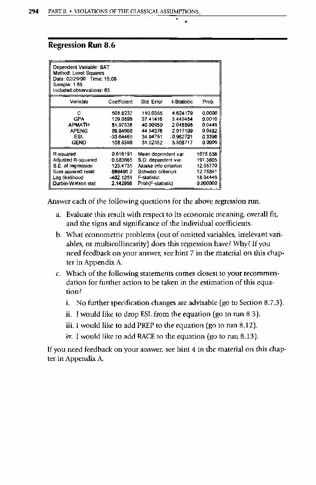
294 PART II • VIOLATIONS OF THE CLASSICAL ASSUMPTIONS
Regression Run 8.6
Dependent Variable: SAT Method: Least Squares Date: 02/29/00 Time: 15:08 Sample: 1 65 Included observations: 65
Variable Coefficient Std. Error t-Statistic Prob.
C 508.8237 110.0355 4.624179 0.0000 GPA 129.0595 37.41416 3.449484 0.0010
APMATH 81.97538 40.00950 2.048898 0.0449 APENG 89.84960 44.54376 2.017109 0.0482
ESL -33.64469 34.94751 -0.962721 0.3396 GEND 108.8598 31.02552 3.508717 0,0009
R-squared 0.616191 Mean dependent var 1075.538 Adjusted R-squared 0.583665 S.D. dependent var 191.3605 S.E. of regression 123.4735 Akaike info criterion 12.55770 Sum squared resid 899496.2 Schwarz criterion 12.75841 Log likelihood -402.1251 F-statistic 18.94449 Durbin-Watson stat 2.142956 Prob(F-statistic) 0.000000
Answer each of the following questions for the above regression run.
a. Evaluate this result with respect to its economic meaning, overall fit, and the signs and significance of the individual coefficients.
b. What econometric problems (out of omitted variables, irrelevant vari-ables, or multicollinearity) does this regression have? Why? If you need feedback on your answer, see hint 7 in the material on this chap-ter in Appendix A.
c. Which of the following statements comes closest to your recommen-dation for further action to be taken in the estimation of this equa-tion? i. No further specification changes are advisable (go to Section 8.7.3). ii. I would like to drop ESL from the equation (go to run 8.3). iii. I would like to add PREP to the equation (go to run 8.12). iv. I would like to add RACE to the equation (go to run 8.13).
If you need feedback on your answer, see hint 4 in the material on this chap-ter in Appendix A.
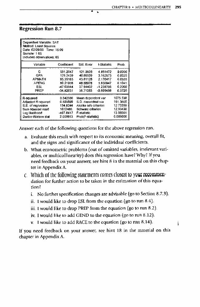
CHAPTER 8 • MULTICOLLINEARITY 295
Regression Run 8.7
Dependent Variable: SAT Method: Least Squares Date: 02/29/00 Time: 15:09 Sample: 1 65 Included observations: 65
Variable Coefficient Std. Error t-Statistic Prob.
C 591.2047 121.8609 4.851472 0.0000 GPA 129.2439 40.86539 3.162673 0.0025
- APMATH 95.35163 43.81128 2.176417 0.0335 APENG 80.21918 48.58978 1.650947 0.1041
ESL -47.03944 37.94402 -1.239706 0.2200 PREP -34.82031 38.71083 -0.899498 0.3720
R-squared 0.542380 Mean dependent var 1075.538 Adjusted R-squared 0.503599 S.D. dependent var 191.3605 S.E. of regression 134.8244 Akaike info criterion 12.73359 Sum squared resid 1072480. Schwarz criterion 12.93430 Log likelihood -407.8417 F-statistic 13.98561 Durbin-Watson stat 2.008613 Prob(F-statistic) 0.000000
Answer each of the following questions for the above regression run.
a. Evaluate this result with respect to its economic meaning, overall fit, and the signs and significance of the individual coefficients.
b. What econometric problems (out of omitted variables, irrelevant vari-ables, or multicollinearity) does this regression have? Why? If you need feedback on your answer, see hint 8 in the material on this chap-ter in Appendix A.
c. Which of the following statements comes closest to your minamcn- dation for further action to be taken in the estimation of this equa-tion?
i. No further specification changes are advisable (go to Section 8.7.3).
ii. I would like to drop ESL from the equation (go to run 8.4).
iii. I would like to drop PREP from the equation (go to run 8.2).
iv. I would like to add LEND to the equation (go to run 8.12).
v. I would like to add RACE to the equation (go to run 8.14).
If you need feedback on your answer, see hint 18 in the material on this chapter in Appendix A.
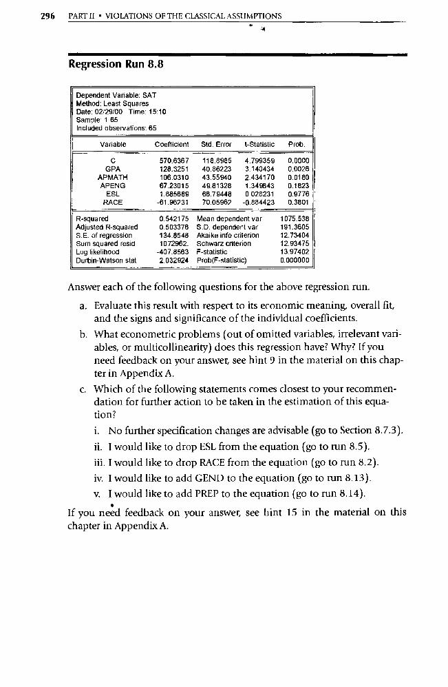
296 PART II • VIOLATIONS OF THE CLASSICAL ASSUMPTIONS s
Regression Run 8.8
Dependent Variable: SAT Method: Least Squares Date: 02/29/00 Time: 15:10 Sample: 1 65 Included observations: 65
Variable Coefficient Std. Error t-Statistic Prob.
C 570.6367 118.8985 4.799359 0.0000 GPA 128.3251 40.86223 3.140434 0.0026
APMATH 106.0310 43.55940 2.434170 0.0180 APENG 67.23015 49.81328 1.349643 0.1823
ESL 1.885689 66.79448 0 028231 0.9776 RACE -61.96231 70.05962 -0.884423 0.3801
R-squared 0.542175 Mean dependent var 1075.538 Adjusted R-squared 0.503376 S.D. dependent var 191.3605 S.E. of regression 134.8548 Akaike info criterion 12.73404 Sum squared resid 1072962. Schwa rz criterion 12.93475 Log likelihood -407.8563 F-statistic 13.97402 Durbin-Watson stat 2.032924 Prob(F-statistic) 0.000000
Answer each of the following questions for the above regression run.
a. Evaluate this result with respect to its economic meaning, overall fit, and the signs and significance of the individual coefficients.
b. What econometric problems (out of omitted variables, irrelevant vari-ables, or multicollinearity) does this regression have? Why? If you need feedback on your answer, see hint 9 in the material on this chap-ter in Appendix A.
c. Which of the following statements comes closest to your recommen-dation for further action to be taken in the estimation of this equa-tion?
i. No further specification changes are advisable (go to Section 8.7.3).
ii. I would like to drop ESL from the equation (go to run 8.5).
iii. I would like to drop RACE from the equation (go to run 8.2).
iv. I would like to add GEND to the equation (go to run 8.13).
v. I would like to add PREP to the equation (go to run 8.14).
If you need feedback on your answer, see hint 15 in the material on this chapter in Appendix A.

CHAPTER 8 • MULTICOLLINEARITY 297 a
^•
Regression Run 8.9
Dependent Variable: SAT Method: Least Squares Date: 02/29/00 Time: 15:11 Sample: 1 65 Included observations: 65
Variable Coefficient Std. Error t-Statistic Prob.
C 513.9945 111.6115 4.605210 0.0000 GPA 132.4152 37.38088 3.542326 0.0008
APMATH 59.37168 36.54919 1.624432 0.1096 APENG 96.69438 44.47540 2.174109 0.0337 GEND 111.3943 30.89564 3.605501 0.0006 PREP -31.31762 35.50451 -0.882074 0.3813
R-squared 0.615236 Mean dependent var 1075.538 Adjusted R-squared 0.582629 S.D. dependent var 191.3605 S.E. of regression 123.6270 Akaike info criterion 12.56018 Sum squared resid 901734.9 Schwa rz criterion 12.76089 Log likelihood -402.2059 F-statistic 18.86816 Durbin-Watson stat 2.065021 Prob(F-statistic) 0.000000
Answer each of the following questions for the above regression run.
a. Evaluate this result with respect to its economic meaning, overall fit, and the signs and significance of the individual coefficients.
b. What econometric problems (out of omitted variables, irrelevant vari-ables, or multicollinearity) does this regression have? Why? If you need feedback on your answer, see hint 8 in the material on this chap-ter in Appendix A.
c. Which of the following statements comes closest to your recommen-dation for further action to be taken in the estimation of this equa-tion?
i. No further specification changes are advisable (go to Section 8.7.3).
ii. I would like to drop PREP from the equation (go to run 8.3).
iii. I would like to add ESL to the equation (go to run 8.12).
iv. I would like to add RACE to the equation (go to run 8.15).
If you need feedback on your answer, see hint 17 in the material on this chapter in Appendix A.
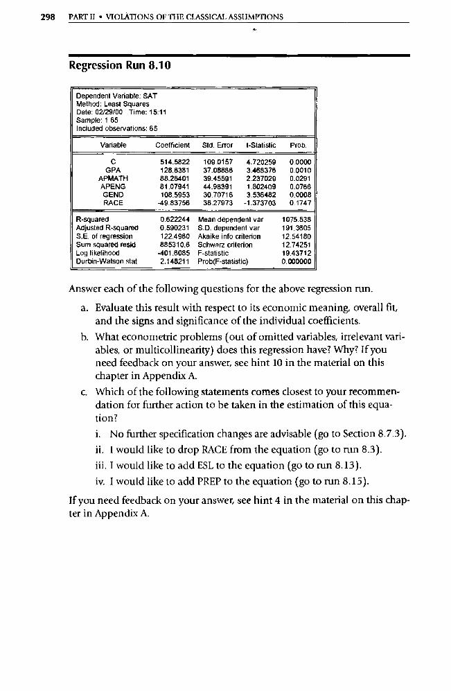
298 PART H • VIOLATIONS OF THE CLASSICAL ASSUMPTIONS
Regression Run 8.10
Dependent Variable: SAT Method: Least Squares Date: 02/29/00 Time: 15:11 Sample: 1 65 Included observations: 65
Va riable Coefficient Std. Error t-Statistic Prob.
C 514.5822 109.0157 4.720259 0.0000 GPA 128.6381 37.08886 3.468376 0.0010
APMATH 88.26401 39.45591 2.237029 0.0291 APENG 81.07941 44.98391 1.802409 0.0766 GEND 108.5953 30.70716 3.536482 0.0008 RACE -49.83756 36.27973 -1.373703 0.1747
R-squared 0.622244 Mean dependent var 1075.538 Adjusted R-squared 0.590231 S.D. dependent var 191.3605 S.E. of regression 122.4960 Akaike info criterion 12.54180 Sum squared resid 885310.6 Schwarz criterion 12.74251 Log likelihood -401.6085 F-statistic 19.43712 Durbin-Watson stat 2.148211 Prob(F-statistic) 0.000000
Answer each of the following questions for the above regression run.
a. Evaluate this result with respect to its economic meaning, overall fit, and the signs and significance of the individual coefficients.
b. What econometric problems (out of omitted variables, irrelevant vari-ables, or multicollinearity) does this regression have? Why? If you need feedback on your answer, see hint 10 in the material on this chapter in Appendix A.
c. Which of the following statements comes closest to your recommen-dation for further action to be taken in the estimation of this equa-tion?
i. No further specification changes are advisable (go to Section 8.7.3).
ii. I would like to drop RACE from the equation (go to run 8.3).
iii. I would like to add ESL to the equation (go to run 8.13).
iv. I would like to add PREP to the equation (go to run 8.15).
If you need feedback on your answer, see hint 4 in the material on this chap-ter in Appendix A.

CHAPTER 8 • MULTICOLLINEARITY 299 •
Regression Run 8.11
Dependent Variable: SAT Method: Least Squares Date: 02/29/00 Time: 15:12 Sample: 1 65 Included obse rvations: 65
Variable Coefficient Std. Error t-Statistic Prob.
C 602.4718 121.0769 4.975943 0.0000 GPA 129.0898 40.43172 3.192785 0.0023
APMATH 100.8919 42.92558 2.350391 0.0221 APENG 69.65070 48.89190 1.424586 0.1595 PREP -42.14969 38.62038 -1.091385 0.2795 RACE -65.60984 39.70586 -1.652397 0.1038
R-squared 0.551228 Mean dependent var 1075.538 Adjusted R-squared 0.513197 S.D. dependent var 191.3605 S.E. of regression 133.5147 Akaike info criterion 12.71407 Sum squared resid 1151744. Schwarz criterion 12.91478 Log likelihood -407.2071 F-statistic 14.49400 Durbin-Watson stat 2.020544 Prob(F-statistic) 0.000000
Answer each of the following questions for the above regression run.
a. Evaluate this result with respect to its economic meaning, overall fit, and the signs and significance of the individual coefficients.
b. What econometric problems (out of omitted variables, irrelevant vari-ables, or multicollinearity) does this regression have? Why? If you need feedback on your answer, see hint 8 in the material on this chap-ter in Appendix A.
c. Which of the following statements comes closest to your recommen-dation for further action to be taken in the estimation of this equa-tion? i. No further specification changes are advisable (go to Section 8.7.3). ii. I would like to drop PREP from the equation (go to run 8.5). iii. I would like to drop RACE from the equation (go to run 8.4). iv. I would like to add GEND to the equation (go to run 8.15). v. I would like to replace APMATH and APENG with AP, a linear com-
bination of the two variables (go to run 8.18).
If you need feedback on your answer, see hint 18 in the material on this chapter in Appendix A.
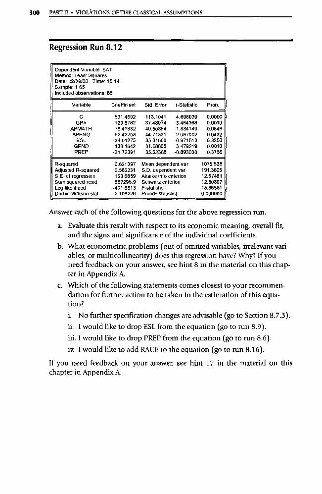
300 PART II • VIOLATIONS OF THE CLASSICAL ASSUMPTIONS
Regression Run 8.12
Dependent Variable: SAT Method: Least Squares Date: 02/29/00 Time: 15:14 Sample: 1 65 Included obse rvations: 65
Variable Coefficient Std. Error t-Statistic Prob.
C 531.4692 113.1041 4.698939 0.0000 GPA 129.8782 37.48974 3.464368 0.0010
APMATH 76.41832 40.55854 1.884149 0.0646 APENG 92.42253 44.71331 2.067002 0.0432
ESL -34.01275 35.01006 -0.971513 0.3353 GEND 108.1642 31.08865 3.479219 0.0010 PREP -31.72391 35,52388 -0.893030 0.3755
R-squared 0.621397 Mean dependent var 1075.538 Adjusted R-squared 0.582231 S.D. dependent var 191.3605 S.E. of regression 123.6859 Akaike info criterion 12.57481 Sum squared resid 887295.9 Schwarz criterion 12.80897 Log likelihood -401.6813 F-statistic 15.86581 Durbin-Watson stat 2.106229 Prob(F-statistic) 0.000000
Answer each of the following questions for the above regression run.
a. Evaluate this result with respect to its economic meaning, overall fit, and the signs and significance of the individual coefficients.
b. What econometric problems (out of omitted variables, irrelevant vari-ables, or multicollinearity) does this regression have? Why? If you need feedback on your answer, see hint 8 in the material on this chap-ter in Appendix A.
c. Which of the following statements comes closest to your recommen-dation for further action to be taken in the estimation of this equa-tion?
i. No further specification changes are advisable (go to Section 8.7.3).
ii. I would like to drop ESL from the equation (go to run 8.9).
iii. I would like to drop PREP from the equation (go to run 8.6).
iv. I would like to add RACE to the equation (go to run 8.16).
If you need feedback on your answer, see hint 17 in the material on this chapter in Appendix A.
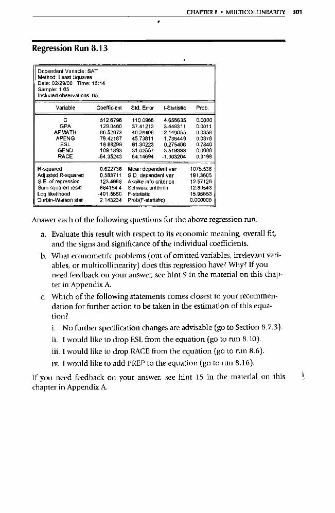
CHAPTER 8 • MULTICOLLIPIEARITY 301
f
Regression Run 8.13
Dependent Variable: SAT Method: Least Squares Date: 02/29/00 Time: 15:14 Sample: 1 65 Included observations: 65
Variable Coefficient Std. Error t-Statistic Prob.
C 512.6796 110.0966 4.656635 0.0000 GPA 129.0460 37.41213 3.449311 0.0011
APMATH 86.52973 40.26408 2.149055 0.0358 APENG 79.42187 45.73811 1.736449 0.0878
ESL 16.88299 61.30223 0.275406 0.7840 GEND 109.1893 31.02557 3.519333 0.0008 RACE -64.35243 64.14694 -1.003204 0.3199
R-squared 0.622738 Mean dependent var 1075.538 Adjusted R-squared 0.583711 S.D. dependent var 191.3605 S.E. of regression 123.4668 Akaike info criterion 12.57126 Sum squared resid 884154.4 Schwa rz criterion 12.80543 Log likelihood -401.5660 F-statistic 15.95653 Durbin-Watson slat 2.143234 Prob(F-statistic) 0.000000
Answer each of the following questions for the above regression run.
a. Evaluate this result with respect to its economic meaning, overall fit, and the signs and significance of the individual coefficients.
b. What econometric problems (out of omitted variables, irrelevant vari-ables, or multicollinearity) does this regression have? Why? If you need feedback on your answer, see hint 9 in the material on this chap-ter in Appendix A.
c. Which of the following statements comes closest to your recommen-dation for further action to be taken in the estimation of this equa-tion? i. No further specification changes are advisable (go to Section 8.7.3). ii. I would like to drop ESL from the equation (go to run 8.10). iii. I would like to drop RACE from the equation (go to run 8.6).
iv. I would like to add PREP to the equation (go to run 8.16).
If you need feedback on your answer, see hint 15 in the material on this chapter in Appendix A.
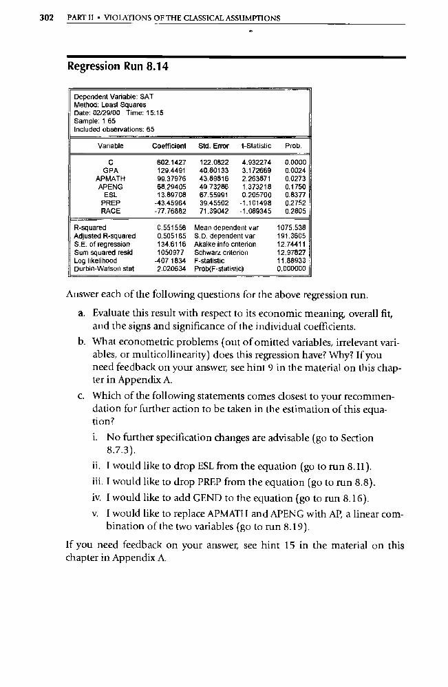
302 PART II • VIOLATIONS OF THE CLASSICAL ASSUMPTIONS
Regression Run 8.14
Dependent Va riable: SAT Method: Least Squares Date: 02/29/00 Time: 15:15 Sample: 1 65 Included obse rvations: 65
Variable Coefficient Std. Error t-Statistic Prob.
C 602.1427 122.0822 4.932274 0.0000 GPA 129.4491 40.80133 3.172669 0.0024
APMATH 99.37976 43.89816 2.263871 0.0273 APENG 68.29405 49.73286 1.373218 0.1750
ESL 13.89708 67.55991 0.205700 0.8377 PREP -43.45964 39.45502 -1.101498 0.2752 RACE -77.76882 71.39042 -1.089345 0.2805
R-squared 0.551556 Mean dependent var 1075.538 Adjusted R-squared 0.505165 S.D. dependent var 191.3605 S.E. of regression 134.6116 Akaike info criterion 12.74411 Sum squared resid 1050977 Schwarz criterion 12.97827 Log likelihood -407 1834 F-statistic 11.88933 Durbin-Watson stat 2.020634 Prob(F-statistic) 0.000000
Answer each of the following questions for the above regression run.
a. Evaluate this result with respect to its economic meaning, overall fit, and the signs and significance of the individual coefficients.
b. What econometric problems (out of omitted variables, irrelevant vari-ables, or multicollinearity) does this regression have? Why? If you need feedback on your answer, see hint 9 in the material on this chap-ter in Appendix A.
c. Which of the following statements comes closest to your recommen-dation for further action to be taken in the estimation of this equa-tion? i. No further specification changes are advisable (go to Section
8.7.3). ii. I would like to drop ESL from the equation (go to run 8.11). iii. I would like to drop PREP from the equation (go to run 8.8). iv. I would like to add GEND to the equation (go to run 8.16). v. I would like to replace APMATH and APENG with AP, a linear com-
bination of the two va riables (go to mn 8.19).
If you need feedback on your answer, see hint 15 in the material on this chapter in Appendix A.
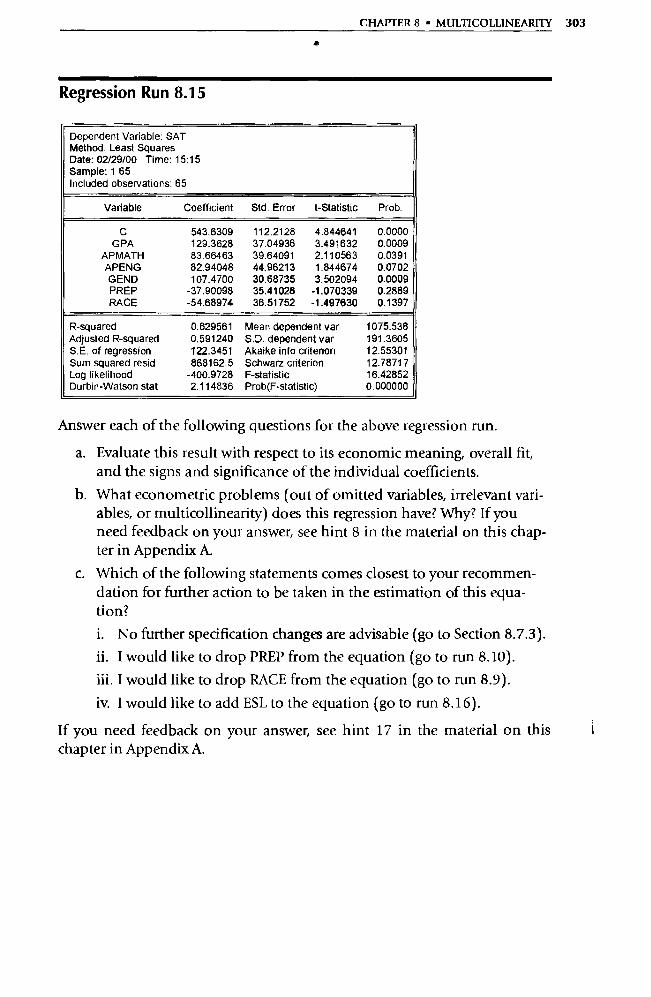
CHAFFER 8 • MULTICOLLINEARITY 303
Regression Run 8.15
Dependent Variable: SAT Method: Least Squares Date: 02/29/00 Time: 15:15 Sample: 1 65 Included observations: 65
Va riable Coefficient Std. Error t-Statistic Prob.
C 543.6309 112.2128 4.844641 0.0000 GPA 129.3628 37.04936 3.491632 0.0009
APMATH 83,66463 39.64091 2.110563 0.0391 APENG 82.94048 44.96213 1.844674 0.0702 GEND 107.4700 30.68735 3.502094 0.0009 PREP -37.90098 35.41026 -1.070339 0.2889 RACE -54.68974 36.51752 -1.497630 0.1397
R-squared 0.629561 Mean dependent var 1075.538 Adjusted R-squared 0.591240 S.D. dependent var 191.3605 S.E. of regression 122.3451 Akaike info criterion 12.55301 Sum squared resid 868162.5 Schwarz criterion 12.78717 Log likelihood -400.9728 F-statistic 16.42852 Durbin-Watson stat 2.114836 Prob(F-statistic) 0.000000
Answer each of the following questions for the above regression run.
a. Evaluate this result with respect to its economic meaning, overall fit, and the signs and significance of the individual coefficients.
b. What econometric problems (out of omitted variables, irrelevant vari-ables, or multicollinearity) does this regression have? Why? If you need feedback on your answer, see hint 8 in the material on this chap-ter in Appendix A.
c. Which of the following statements comes closest to your recommen-dation for further action to be taken in the estimation of this equa-tion?
i. No further specification changes are advisable (go to Section 8.7.3).
ii. I would like to drop PREP from the equation (go to run 8.10).
iii. I would like to drop RACE from the equation (go to run 8.9).
iv. I would like to add ESL to the equation (go to run 8.16).
If you need feedback on your answer, see hint 17 in the material on this chapter in Appendix A.
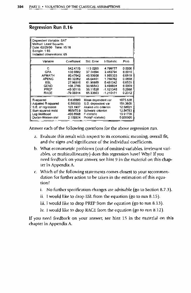
304 PART II • VIOLATIONS OF THE CLASSICAL ASSUMPTIONS
Regression Run 8.16
Dependent Va riable: SAT Method: Least Squares Date: 02/29/00 Time: 15:16 Sample: 1 65 Included observations: 65
Variable Coefficient Std. Error t-Statistic Prob.
C 542.4723 113.0203 4.799777 0.0000 GPA 130.0882 37.34094 3.483794 0.0010
APMATH 80.47642 40.53608 1.985303 0.0519 APENG 80.32262 45.64401 1.759762 0.0838
ESL 27.96510 61.95989 0.451342 0.6535 GEND 108.3766 30.96543 3.499924 0.0009 PREP -40.50116 36.11828 -1.121348 0.2668 RACE -79.06514 65.33603 -1.210131 0.2312
R-squared 0,630880 Mean dependent var 1075.538 Adjusted R-squared 0.585550 S.D. dependent var 191.3605 S.E. of regression 123.1937 Akaike info criterion 12.58021 Sum squared resid 865070.9 Schwarz criterion 12.84783 Log likelihood -400.8568 F-statistic 13.91736 Durbin-Watson scat 2.106524 Prob(F-statistic) 0.000000
Answer each of the following questions for the above regression run.
a. Evaluate this result with respect to its economic meaning, overall fit, and the signs and significance of the individual coefficients.
b. What econometric problems (out of omitted variables, irrelevant vari-ables, or multicollinearity) does this regression have? Why? If you need feedback on your answer, see hint 9 in the material on this chap-ter in Appendix A.
c. Which of the following statements comes closest to your recommen-dation for further action to be taken in the estimation of this equa-tion? i. No further specification changes are advisable (go to Section 8.7.3). ii. I would like to drop ESL from the equation (go to run 8.15). iii. I would like to drop PREP from the equation (go to run 8.13). iv. I would like to drop RACE from the equation (go to run 8.12).
If you need feedback on your answer, see hint 15 in the material on this chapter in Appendix A.
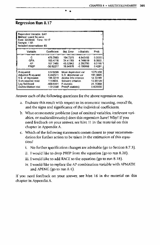
CHAPTER 8 • MULTICOLLINEARITY 305
Regression Run 8.17
Dependent Va riable: SAT Method: Least Squares Date: 02/29/00 Time: 15:17 Sample: 1 65 Included observations: 65
,
Variable Coefficient Std. Error t-Statistic Prob.
C 475.7963 104.7275 4.543185 0.0000 GPA 163.4716 34.41783 4.749619 0.0000 AP 107.7460 45.02942 2.392790 0.0198
PREP -30.92277 38.84976 -0.795958 0.4291
R-squared 0.516299 Mean dependent var 1075.538 Adjusted R-squared 0.492511 S.D. dependent var 191.3605 S.E. of regression 136.3219 Akaike info criterion 12.72748 Sum squared resid 1133604. Schwarz criterion 12.86129 Log likelihood -409.6431 F-statistic 21.70368 Durbin-Watson stat 1.912398 Prob(F-statistic) 0.000000
Answer each of the following questions for the above regression run.
a. Evaluate this result with respect to its economic meaning, overall fit, and the signs and significance of the individual coefficients.
b. What econometric problems (out of omitted variables, irrelevant vari-ables, or multicollinearity) does this regression have? Why? If you need feedback on your answer, see hint 11 in the material on this chapter in Appendix A.
c. Which of the following statements comes closest to your recommen-dation for further action to be taken in the estimation of this equa-tion? i. No further specification changes are advisable (go to Section 8.7.3). ii. I would like to drop PREP from the equation (go to run 8.20). iii. I would like to add RACE to the equation (go to run 8.18). iv. I would like to replace the AP combination variable with APMATH
and APENG (go to mn 8.4).
If you need feedback on your answer, see hint 16 in the material on this chapter in Appendix A.
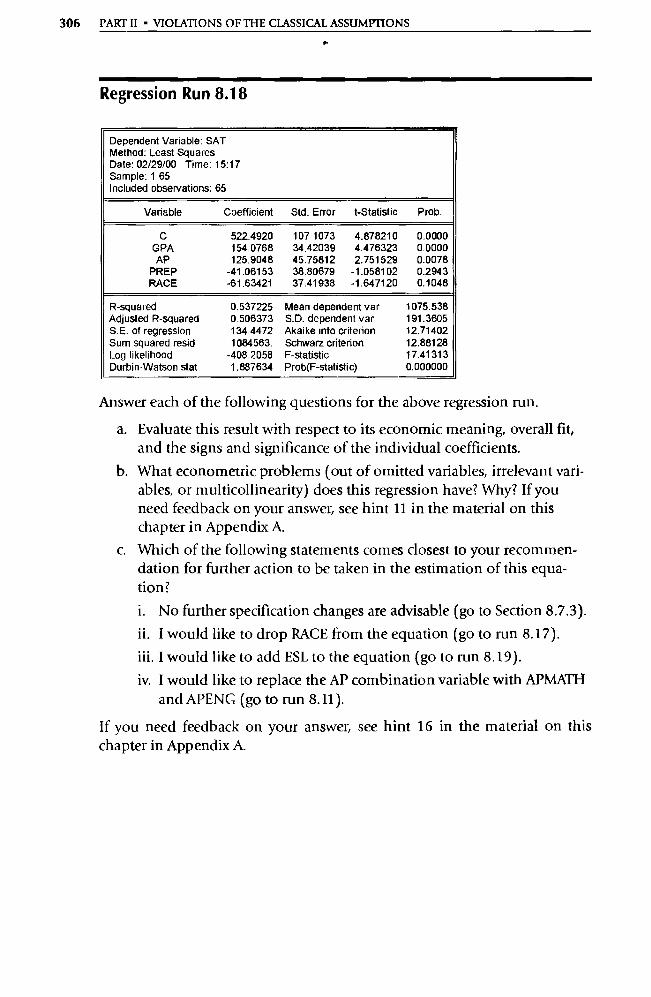
306 PART II • VIOLATIONS OF THE CLASSICAL ASSUMPTIONS
Regression Run 8.18
Dependent Variable: SAT Method: Least Squares Date: 02/29/00 Time: 15:17 Sample: 1 65 Included obse rvations: 65
Va riable Coefficient Std. Error t-Statistic Prob.
C 522.4920 1071073 4.878210 0.0000 GPA 154.0768 34.42039 4.476323 0.0000 AP 125.9048 45.75812 2.751529 0.0078
PREP -41.06153 38.80679 -1.058102 0.2943 RACE -61.63421 37.41938 -1.647120 0.1048
R-squared 0.537225 Mean dependent var 1075.538 Adjusted R-squared 0.506373 S.D. dependent var 191.3605 S. E. of regression 134.4472 Akaike info criterion 12.71402 Sum squared resid 1084563. Schwarz criterion 12.88128 Log likelihood -408.2058 F-statistic 17.41313 Durbin-Watson stat 1.887634 Prob(F-statistic) 0.000000
Answer each of the following questions for the above regression run.
a. Evaluate this result with respect to its economic meaning, overall fit, and the signs and significance of the individual coefficients.
b. What econometric problems (out of omitted variables, irrelevant vari-ables, or multicollinearity) does this regression have? Why? If you need feedback on your answer, see hint 11 in the material on this chapter in Appendix A.
c. Which of the following statements comes closest to your recommen-dation for further action to be taken in the estimation of this equa-tion? i. No further specification changes are advisable (go to Section 8.7.3). ii. I would like to drop RACE from the equation (go to run 8.17). iii. I would like to add ESL to the equation (go to run 8.19). iv. I would like to replace the AP combination variable with APMATH
and APENG (go to run 8.11).
If you need feedback on your answer, see hint 16 in the material on this chapter in Appendix A.
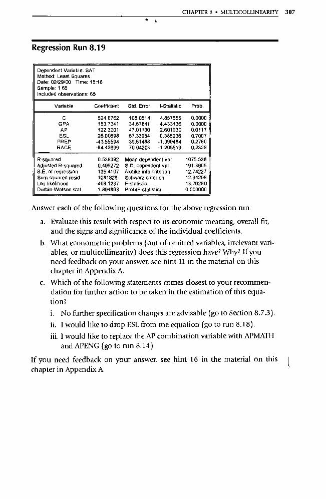
CHAPTER 8 • MULTICOLLINEARITY 307 •
Regression Run 8.19
Dependent Variable: SAT Method: Least Squares Date: 02/29/00 Time: 15:18 Sample: 1 65 Included obse rvations: 65
Va riable Coefficient Std. Error t-Statistic Prob.
C 524.8762 108.0514 4.857655 0.0000 GPA 153.7341 34.67841 4.433136 0.0000 AP 122.3201 47.01130 2.601930 0.0117 ESL 26.00898 67.33954 0.386236 0.7007
PREP -43.55594 39.61488 -1.099484 0.2760 RACE -84.43699 70.04203 -1.205519 0.2328
R-squared 0.538392 Mean dependent var 1075.538 Adjusted R-squared 0.499272 S.D. dependent var 191.3605 S.E. of regression 135.4107 Akaike info criterion 12.74227 Sum squared resid 1081828. Schwarz criterion 12.94298 Log likelihood -408.1237 F-statistic 13.76280 Durbin-Watson stat 1.894863 Prob(F-statistic) 0.000000
Answer each of the following questions for the above regression run.
a. Evaluate this result with respect to its economic meaning, overall fit, and the signs and significance of the individual coefficients.
b. What econometric problems (out of omitted variables, irrelevant vari-ables, or multicollinearity) does this regression have? Why? If you need feedback on your answer, see hint 11 in the material on this chapter in Appendix A.
c. Which of the following statements comes closest to your recommen-dation for further action to be taken in the estimation of this equa-tion? i. No further specification changes are advisable (go to Section 8.7.3). ii. I would like to drop ESL from the equation (go to run 8.18). iii. I would like to replace the AP combination variable with APMATH
and APENG (go to run 8.14).
If you need feedback on your answer, see hint 16 in the material on this chapter in Appendix A.
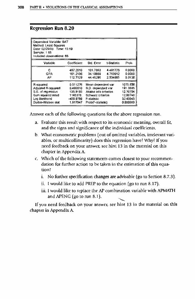
308 PART II • VIOLATIONS OF THE CLASSICAL ASSUMPTIONS
Regression Run 8.20
Dependent Variable: SAT Method: Least Squares Date: 02/29/00 Time: 15:19 Sample: 1 65 Included observations: 65
Variable Coefficient Std. Error t-Statistic Prob.
C 457.2010 101.7863 4A91773 0.0000 GPA 161.2106 34.19889 4.713912 0.0000 AP 112.7129 44.46296 2.534985 0.0138
R-squared 0.511276 Mean dependent var 1075.538 Adjusted R-squared 0.495510 S.D. dependent var 191.3605 S.E. of regression 135.9185 Akaike info criterion 12.70704 Sum squared resid 1145378. Schwarz criterion 12.80740 Log likelihood -409.9789 F-statistic 32.43043 Durbin-Watson stat 1.917047 Prob(F-statistic) 0.000000
Answer each of the following questions for the above regression run.
a. Evaluate this result with respect to its economic meaning, overall fit, and the signs and significance of the individual coefficients.
b. What econometric problems (out of omitted variables, irrelevant vari-ables, or multicollinearity) does this regression have? Why? If you need feedback on your answer, see hint 13 in the material on this chapter in Appendix A.
c. Which of the following statements comes closest to your recommen-dation for further action to be taken in the estimation of this equa-tion? i. No further specification changes are advisable (go to Section 8.7.3). ii. I would like to add PREP to the equation (go to run 8.17). iii. I would like to replace the AP combination variable with APMATH
and APENG (go to run 8.1).
If you need feedback on your answer, see hint 13 in the material on this chapter in Appendix A.
CHAPTER 8 • MULTICOLLINEARITY 309
8.7.3 Evaluating the Results from Your Interactive Exercise
Congratulations! If you've reached this section, you must have found a speci-fication that met your theoretical and econometric goals. Which one did you pick? Our experience is that most beginning econometricians end up with ei-ther regression run 8.3, 8.6, or 8.10, but only after looking at three or more regression results (or a hint or two) before settling on that choice.
In contrast, we've found that most experienced econometricians gravitate to regression run 8.6, usually after inspecting, at most, one other specifica-tion. What lessons can we learn from this difference?
1. Learn that a variable isn't irrelevant simply because its t-score is low. In our opinion, ESL belongs in the equation for strong theoretical reasons, and a slightly insignificant t-score in the expected direction isn't enough evidence to get us to rethink the underlying theory.
2. Learn to spot redundant (multicollinear) variables. ESL and RACE wouldn't normally be redundant, but in this high school, with its par-ticular ethnic diversity, they are. Once one is included in the equation, the other shouldn't even be considered.
3. Learn to spot false variables. At first glance, PREP is a tempting variable to include because prep courses almost surely improve the SAT scores of the students who choose to take them. The problem is that a stu-dent's decision to take a prep course isn't independent of his or her previous SAT scores (or expected scores). We trust the judgment of stu-dents who feel a need for a prep course, and we think that all the course will do is bring them up to the level of their peers who didn't feel they needed a course. As a result, we wouldn't expect a significant effect in either direction.
If you enjoyed and learned from this interactive regression learning exercise, you'll be interested to know that there is another in Chapter 11. Good luck!
9 CHAPTER
Serial Correlation
9.1
Pure versus Impure Serial Correlation
9.2
The Consequences of Serial Correlation
9.3
The Durbin–Watson d Test
9.4
Generalized Least Squares
9.5
Summary and Exercises
In the next two chapters we'll investigate the final component of the specifi-cation of a regression equation—choosing the correct form of the stochastic error term. Our first topic, serial correlation, is the violation of Classical As-sumption IV that different obse rvations of the error term are uncorrelated with each other. Serial correlation, also called autocorrelation, can exist in any research study in which the order of the obse rvations has some meaning. It therefore occurs most frequently in time-series data sets. In essence, serial correlation implies that the error term from one time period depends in some systematic way on error terms from other time periods. Since time-series data are used in many applications of econometrics, it's impo rtant to understand serial correlation and its consequences for OLS estimators.
The approach of this chapter to the problem of serial correlation will be similar to that used in the previous chapter. We'll attempt to answer the same four questions:
1. What is the nature of the problem?
2. What are the consequences of the problem?
3. How is the problem diagnosed?
4. What remedies for the problem are available?
9.1 Pure versus Impure Serial Correlation
9.1.1 Pure Serial Correlation
Pure serial correlation occurs when Classical Assumption IV, which assumes uncorrelated obse rvations of the error term, is violated in a correctly specified
310
Et - PEt- 1 + ut (9.1)
CHAPTER 9 • SERIAL CORRELATION 311
equation. Assumption IV implies that:
E(r, i,i) = 0 (I j)
If the expected value of the simple correlation coefficient between any two observations of the error term is not equal to zero, then the error term is said to be serially correlated. When econometricians use the term serial correla-tion without any modifier, they are referring to pure serial correlation.
The most commonly assumed kind of serial correlation is first-order serial correlation, in which the current observation of the error term is a function of the previous observation of the error term:
where: E = the error term of the equation in question p = the parameter depicting the functional relationship between
observations of the error term u = a classical (nonserially correlated) error term
The functional form in Equation 9.1 is called a first-order Markov scheme, and the new symbol, p (rho, pronounced "row"), is called the first-order autocorrelation coefficient. For this kind of serial correlation, all that is needed is for the value of one observation of the error term to directly affect the value of the next obse rvation of the error term.
The magnitude of p indicates the strength of the serial correlation in an equation. If p is zero, then there is no serial correlation (because E would equal u, a classical error term). As p approaches one in absolute value, the value of the previous obse rvation of the error term becomes more important in determining the current value of Et, and a high degree of serial correlation exists. For p to be greater than one in absolute value is unreasonable because it implies that the error term has a tendency to continually increase in ab-solute value over time ("explode"). As a result of the above, we can state that:
- 1 < p < + 1 (9.2)
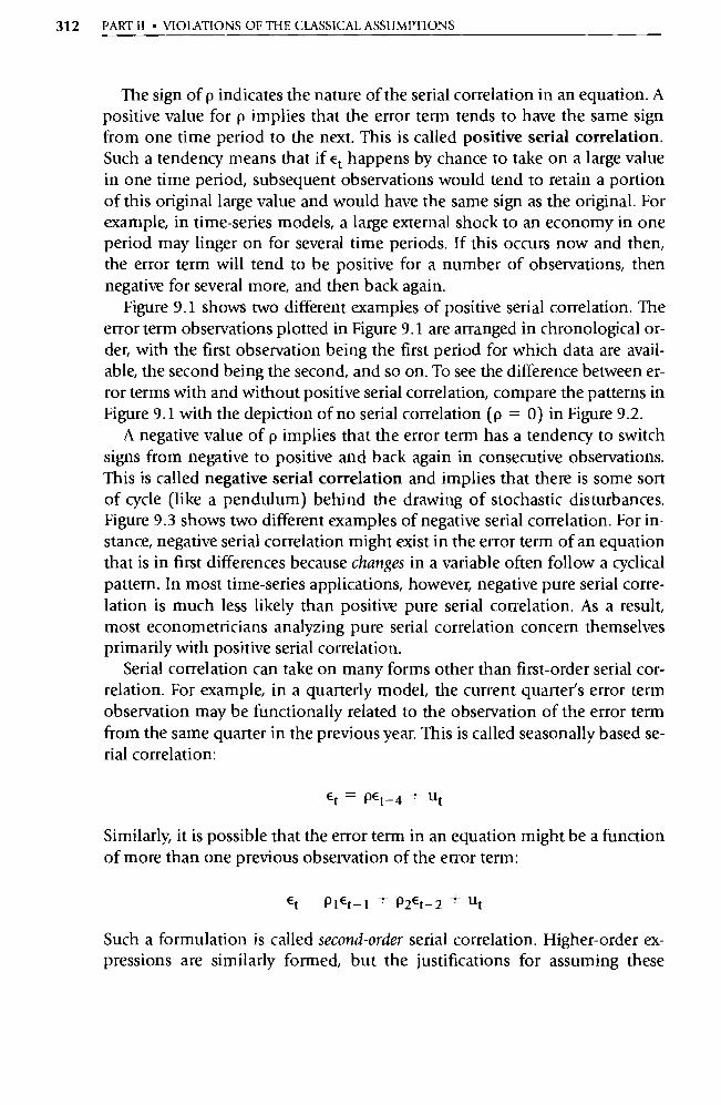
312 PART II • VIOLATIONS OF THE CLASSICAL ASSUMPTIONS
The sign of p indicates the nature of the serial correlation in an equation. A positive value for p implies that the error term tends to have the same sign from one time period to the next. This is called positive serial correlation. Such a tendency means that if Et happens by chance to take on a large value in one time period, subsequent observations would tend to retain a po rtion of this o riginal large value and would have the same sign as the original. For example, in time-series models, a large external shock to an economy in one period may linger on for several time periods. If this occurs now and then, the error term will tend to be positive for a number of observations, then negative for several more, and then back again.
Figure 9.1 shows two different examples of positive serial correlation. The error term observations plotted in Figure 9.1 are arranged in chronological or-der, with the first observation being the first period for which data are avail-able, the second being the second, and so on. To see the difference between er-ror terms with and without positive serial correlation, compare the patterns in Figure 9.1 with the depiction of no serial correlation (p = 0) in Figure 9.2.
A negative value of p implies that the error term has a tendency to switch signs from negative to positive and back again in consecutive observations. This is called negative serial correlation and implies that there is some so rt
of cycle (like a pendulum) behind the drawing of stochastic disturbances. Figure 9.3 shows two different examples of negative serial correlation. For in-stance, negative serial correlation might exist in the error term of an equation that is in first differences because changes in a variable often follow a cyclical pattern. In most time-series applications, however, negative pure serial corre-lation is much less likely than positive pure serial correlation. As a result, most econometricians analyzing pure serial correlation concern themselves primarily with positive serial correlation.
Serial correlation can take on many forms other than first-order serial cor-relation. For example, in a quarterly model, the current quarter's error term observation may be functionally related to the observation of the error term from the same qua rter in the previous year. This is called seasonally based se-rial correlation:
Et = PEt_4 + Ut
Similarly, it is possible that the error term in an equation might be a function of more than one previous observation of the error term:
Et Pi tt-1 + P2Et-2 + Ut
Such a formulation is called second-order serial correlation. Higher-order ex- pressions are similarly formed, but the justifications for assuming these
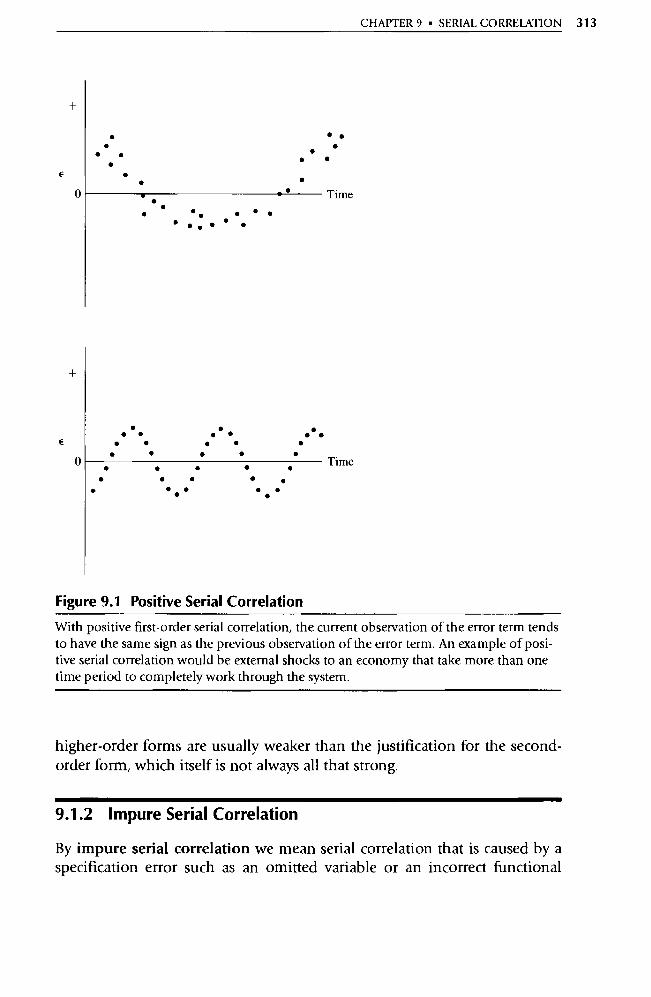
CHAPTER 9 • SERIAL CORRELATION 313
+
• • • • •
0 • . •. • • •
• • • • • •
+
• • • • • • •' • • • • • • • • • • •
• • • • • • • • • •
• • • • • • •
Figure 9.1 Positive Serial Correlation
E
E
0
• • • • •
• • • • Time
Time
With positive first-order serial correlation, the current obse rvation of the error term tends to have the same sign as the previous obse rvation of the error term. An example of posi-tive serial correlation would be external shocks to an economy that take more than one time period to completely work through the system.
higher-order forms are usually weaker than the justification for the second-order form, which itself is not always all that strong.
9.1.2 Impure Serial Correlation
By impure serial correlation we mean serial correlation that is caused by a specification error such as an omitted variable or an incorrect functional
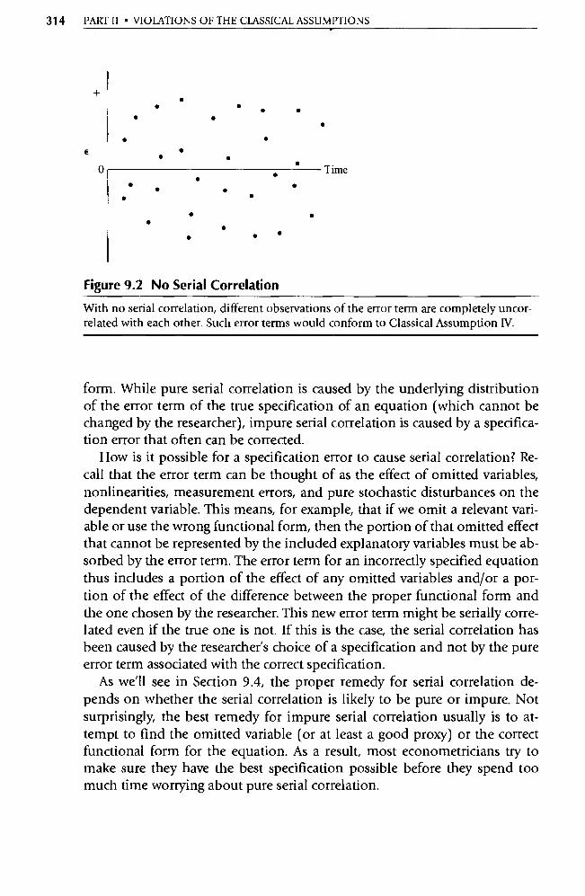
• • •
• • • •
• • •
E
o • •
• Time
• • • •
•
314 PART II • VIOLATIONS OF THE CLASSICAL ASSUMPTIONS
• • • • • •
Figure 9.2 No Serial Correlation
With no serial correlation, different obse rvations of the error term are completely uncor-related with each other. Such error terms would conform to Classical Assumption IV.
form. While pure serial correlation is caused by the underlying distribution of the error term of the true specification of an equation (which cannot be changed by the researcher), impure serial correlation is caused by a specifica-tion error that often can be corrected.
How is it possible for a specification error to cause serial correlation? Re-call that the error term can be thought of as the effect of omitted variables, nonlinearities, measurement errors, and pure stochastic disturbances on the dependent variable. This means, for example, that if we omit a relevant vari-able or use the wrong functional form, then the po rtion of that omitted effect that cannot be represented by the included explanatory variables must be ab-sorbed by the error term. The error term for an incorrectly specified equation thus includes a po rtion of the effect of any omitted variables and/or a por-tion of the effect of the difference between the proper functional form and the one chosen by the researcher. This new error term might be serially corre-lated even if the true one is not. If this is the case, the serial correlation has been caused by the researcher's choice of a specification and not by the pure error term associated with the correct specification.
As we'll see in Section 9.4, the proper remedy for serial correlation de-pends on whether the serial correlation is likely to be pure or impure. Not surprisingly, the best remedy for impure serial correlation usually is to at-tempt to find the omitted variable (or at least a good proxy) or the correct functional form for the equation. As a result, most econometricians try to make sure they have the best specification possible before they spend too much time worrying about pure serial correlation.
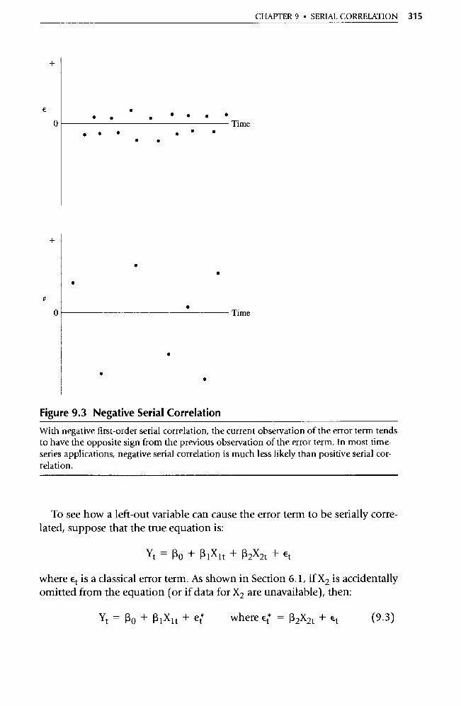
E •
Time o
+
• • • • • • Time o
•
• •
+
• •
E •
•
• •
Figure 9.3 Negative Serial Correlation
CHAPTER 9 • SERIAL CORRELATION 315
With negative first-order serial correlation, the current obse rvation of the error term tends to have the opposite sign from the previous obse rvation of the error term. In most time-series applications, negative serial correlation is much less likely than positive serial cor-relation.
To see how a left-out variable can cause the error term to be serially cone-lated, suppose that the true equation is:
Yt = Ro + R OCH + P2X2t + E t
where Et is a classical error term. As shown in Section 6.1, if X2 is accidentally omitted from the equation (or if data for X2 are unavailable), then:
Yt = Ro + RiXit + et where Et = R2X2t + Et (9.3)
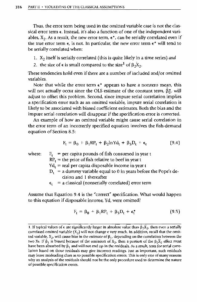
316 PART II • VIOLATIONS OF THE CLASSICAL ASSUMPTIONS
Thus, the error term being used in the omitted va riable case is not the clas-sical error term E. Instead, it's also a function of one of the independent vari-ables, X2. As a result, the new error term, e * , can be serially correlated even if the true error term e, is not. In particular, the new error term E * will tend to be serially correlated when:
1. X2 itself is serially correlated (this is quite likely in a time series) and
2. the size of a is small compared to the sizes of (3 2X2 .
These tendencies hold even if there are a number of included and/or omitted variables.
Note that while the error term E * appears to have a nonzero mean, this will not actually occur since the OLS estimate of the constant term, (30, will adjust to offset this problem. Second, since impure serial correlation implies a specification error such as an omitted variable, impure serial correlation is likely to be associated with biased coefficient estimates. Both the bias and the impure serial correlation will disappear if the specification error is corrected.
An example of how an omitted va riable might cause serial correlation in the error term of an incorrectly specified equation involves the fish-demand equation of Section 8.5:
Ft = Ro + 131RPt + 13 2 1nYdt + (33 Dt + Et (9.4)
where: Ft = per capita pounds of fish consumed in year t RPt = the price of fish relative to beef in year t Ydt = real per capita disposable income in year t Dt = a dummy variable equal to 0 in years before the Pope's de-
cision and 1 thereafter Et = a classical (nonserially correlated) error term
Assume that Equation 9.4 is the "correct" specification. What would happen to this equation if disposable income, Yd, were omitted?
Ft = Ro +R1RPt+R3Dt+ Et (9.5)
1. If typical values of a are significantly larger in absolute value than 82X2, then even a serially correlated omitted va riable (X2) will not change e very much. In addition, recall that the omit-ted variable, X2, will cause bias in the estimate of p i , depending on the correlation between the two Xs. If 0. 1 is biased because of the omission of X2, then a po rtion of the (3 2X2 effect must have been absorbed by R 1 and will not end up in the residuals. As a result, tests for serial corre-lation based on those residuals may give incorrect readings. Just as impo rtant, such residuals may leave misleading clues as to possible specification errors. This is only one of many reasons why an analysis of the residuals should not be the only procedure used to determine the nature of possible specification errors.

CHAPTER 9 • SERIAL CORRELATION 317
The most obvious effect would be that the estimated coefficients of RP and D would be biased, depending on the correlation of RP and D with Yd. A sec-ondary effect would be that the error term would now include a large po rtion of the left-out effect of disposable income on the consumption of fish. That is, EC would be a function of Et + (32 lnYdt. It's reasonable to expect that dis-posable income (and therefore its log) might follow a fairly serially corre-lated pattern:
lnYdt = f(lnYdt_ 1 ) + ut (9.6)
Why is this likely? Observe Figure 9.4, which plots the log of U.S. disposable income over time. Note that the continual rise of disposable income over time makes it (and its log) act in a serially correlated or autoregressive man-ner. But if disposable income is serially correlated (and if its impact is not small relative to E) then E * is likely to also be serially correlated, which can be expressed as:
Et = pEt 1 + ut
where p is the coefficient of serial correlation and u is a classical error term. This example has shown that it is indeed possible for an omitted variable to
In (Yd)
• •
• •
• •
0 Time
Figure 9.4 U.S. Disposable Income as a Function of Time
U.S. disposable income (and most other national aggregates) tends to increase steadily over time. As a result, such variables are serially correlated (or autocorrelated), and the omission of such a variable from an equation could potentially introduce impure serial correlation into the error term of that equation.
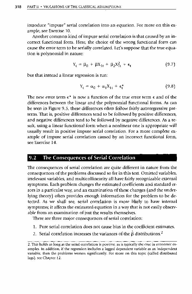
318 PART II • VIOLATIONS OF THE CLASSICAL ASSUMPTIONS
introduce "impure" serial correlation into an equation. For more on this ex-ample, see Exercise 10.
Another common kind of impure serial correlation is that caused by an in-correct functional form. Here, the choice of the wrong functional form can cause the error term to be serially correlated. Let's suppose that the true equa-tion is polynomial in nature:
Yt= Ro +RX1t+R2Xit+et
but that instead a linear regression is run:
Yt =ao +al Xlt +Et
The new error term E * is now a function of the true error term E and of the differences between the linear and the polynomial functional forms. As can be seen in Figure 9.5, these differences often follow fairly autoregressive pat-terns. That is, positive differences tend to be followed by positive differences, and negative differences tend to be followed by negative differences. As a re-sult, using a linear functional form when a nonlinear one is appropriate will usually result in positive impure serial correlation. For a more complete ex-ample of impure serial correlation caused by an incorrect functional form, see Exercise 14.
9.2 The Consequences of Serial Correlation
The consequences of serial correlation are quite different in nature from the consequences of the problems discussed so far in this text. Omitted variables, irrelevant variables, and multicollinearity all have fairly recognizable external symptoms. Each problem changes the estimated coefficients and standard er-rors in a particular way, and an examination of these changes (and the under-lying theory) often provides enough information for the problem to be de-tected. As we shall see, serial correlation is more likely to have internal symptoms; it affects the estimated equation in a way that is not easily observ-able from an examination of just the results themselves.
There are three major consequences of serial correlation:
1. Pure serial correlation does not cause bias in the coefficient estimates.
2. Serial correlation increases the variances of the R distributions. 2
(9.7)
(9.8)
2. This holds as long as the serial correlation is positive, as is typically the case in economic ex-amples. In addition, if the regression includes a lagged dependent variable as an independent variable, then the problems worsen significantly. For more on this topic (called distributed lags), see Chapter 12,
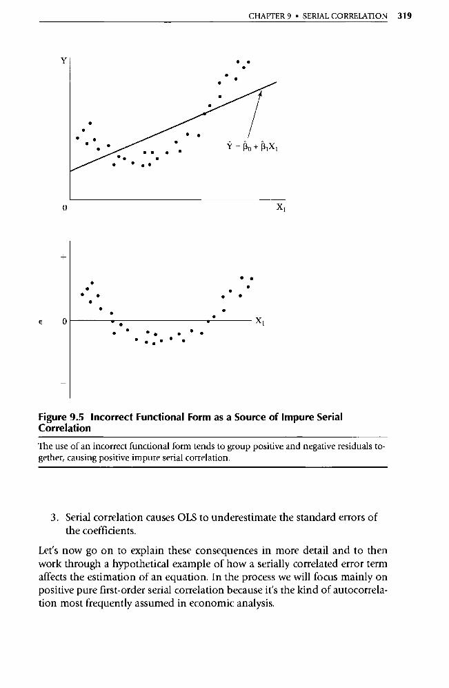
• •
• •
• •
• • • •
•
• •
• • • . • •
•
• Ÿ ° âo + 'O.RiX i
CHAPTER 9 • SERIAL CORRELATION 319
0 X 1
• • • • • •
• • . • X, •
• • • • • • • •
Figure 9.5 Incorrect Functional Form as a Source of Impure Serial Correlation
Y
The use of an incorrect functional form tends to group positive and negative residuals to-gether, causing positive impure serial correlation.
3. Serial correlation causes OLS to underestimate the standard errors of the coefficients.
Let's now go on to explain these consequences in more detail and to then work through a hypothetical example of how a serially correlated error term affects the estimation of an equation. In the process we will focus mainly on positive pure first-order serial correlation because it's the kind of autocorrela-tion most frequently assumed in economic analysis.

320 PART II • VIOLATIONS OF THE CLASSICAL ASSUMPTIONS
9.2.1 An Overview of the Consequences of Serial Correlation
The existence of serial correlation in the error term of an equation violates Classical Assumption 1V, and the estimation of the equation with OLS has at least three consequences:
1. Pure serial correlation does not cause bias in the coefficient estimates. Recall that the most important property of the OLS estimation technique is that it is minimum variance for the class of linear unbiased estimators. If the errors are serially correlated, one of the assumptions of the Gauss-Markov Theorem is violated, but this violation does not cause the coefficient estimates to be biased. Suppose that the error term of the following equation:
Yt= Ro + RiXlt+ R2X2t + Et (9.9)
is known to have pure first-order serial correlation:
et = Pet- I ± t (9.10)
where ut is a classical (nonserially correlated) error term. If Equation 9.9 is correctly specified and is estimated with OLS, then
the estimates of the coefficients of the equation obtained from the OLS estimation will be unbiased. That is,
E(Ri) = Ri and E(R2) = P2
Pure serial correlation introduces no bias into the estimation proce-dure. This conclusion doesn't depend on whether the serial correlation is positive or negative or first order. If the serial correlation is impure, how-ever, bias may be introduced by the use of an incorrect specification.
This lack of bias does not necessarily mean that the OLS estimates of the coefficients of a serially correlated equation will be close to the true coefficient values; the single estimate observed in practice can come from a wide range of possible values. In addition, the standard errors of these estimates will typically be increased by the serial correlation. This increase will raise the probability that a R will differ significantly from the true R value. What unbiased means in this case is that the dis-tribution of the (3s is still centered around the true R.
2. Serial correlation increases the variances of the (3 distributions. Although the violation of Classical Assumption IV causes no bias, it does affect the
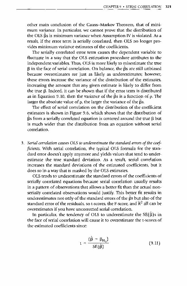
CHAPTER 9 • SERIAL CORRELATION 321
other main conclusion of the Gauss-Markov Theorem, that of mini-mum variance. In particular, we cannot prove that the distribution of the OLS j3s is minimum variance when Assumption IV is violated. As a result, if the error term is serially correlated, then OLS no longer pro-vides minimum variance estimates of the coefficients.
The serially correlated error term causes the dependent variable to fluctuate in a way that the OLS estimation procedure attributes to the independent variables. Thus, OLS is more likely to misestimate the true 13 in the face of serial correlation. On balance, the 13s are still unbiased because overestimates are just as likely as underestimates; however, these errors increase the variance of the distribution of the estimates, increasing the amount that any given estimate is likely to differ from the true j3. Indeed, it can be shown that if the error term is distributed as in Equation 9.10, then the variance of the j 3 s is a function of p. The larger the absolute value of p, the larger the variance of the [Is.
The effect of serial correlation on the distribution of the coefficient estimates is shown in Figure 9.6, which shows that the distribution of (3s from a serially correlated equation is centered around the true 13 but is much wider than the distribution from an equation without serial correlation.
3. Serial correlation causes OLS to underestimate the standard errors of the coef-ficients. With serial correlation, the typical OLS formula for the stan-dard error doesn't apply anymore and yields values that tend to under-estimate the true standard deviation. As a result, serial correlation increases the standard deviations of the estimated coefficients, but it does so in a way that is masked by the OLS estimates.
OLS tends to underestimate the standard errors of the coefficients of serially correlated equations because serial correlation usually results in a pattern of observations that allows a better fit than the actual non-serially correlated observations would justify. This better fit results in underestimates not only of the standard errors of the (3s but also of the standard error of the residuals, so t-scores, the F-score, and R 2 all can be overestimates if you have uncorrected serial correlation.
In particular, the tendency of OLS to underestimate the SE( j3)s in the face of serial correlation will cause it to overestimate the t-scores of the estimated coefficients since:
( R — RH o)
t = SE(R)
(9.11)
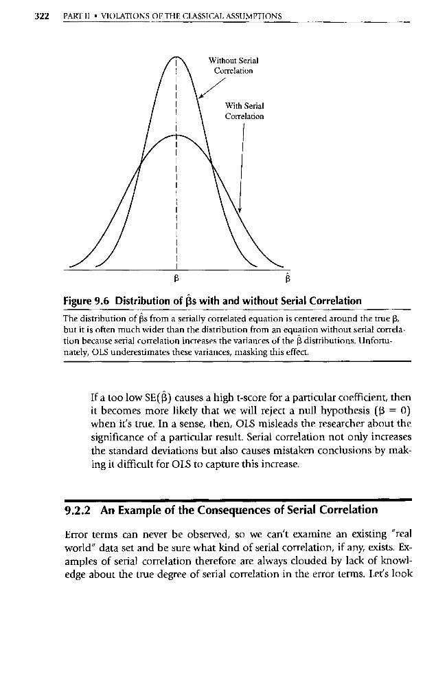
Without Serial Correlation
With Serial Correlation
322 PART II • VIOLATIONS OF THE CLASSICAL ASSUMPTIONS
13
Figure 9.6 Distribution of fis with and without Serial Correlation
The distribution of {3s from a serially correlated equation is centered around the true 13, but it is often much wider than the distribution from an equation without serial correla-tion because serial correlation increases the variances of the R distributions. Unfortu-nately, OLS underestimates these variances, masking this effect.
If a too low SE(R) causes a high t-score for a particular coefficient, then it becomes more likely that we will reject a null hypothesis ((3 = 0) when it's true. In a sense, then, OLS misleads the researcher about the significance of a particular result. Serial correlation not only increases the standard deviations but also causes mistaken conclusions by mak-ing it difficult for OLS to capture this increase.
9.2.2 An Example of the Consequences of Serial Correlation
Error terms can never be observed, so we can't examine an existing "real world" data set and be sure what kind of serial correlation, if any, exists. Ex-amples of serial correlation therefore are always clouded by lack of knowl-edge about the true degree of serial correlation in the error terms. Let's look
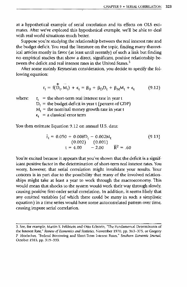
CHAPTER 9 • SERIAL CORRELATION 323
at a hypothetical example of serial correlation and its effects on OLS esti-mates. After we've explored this hypothetical example, we'll be able to deal with real world situations much better.
Suppose you're studying the relationship between the real interest rate and the budget deficit. You read the literature on the topic, finding many theoret-ical articles mostly in favor (at least until recently) of such a link but finding no empirical studies that show a direct, significant, positive relationship be-tween the deficit and real interest rates in the United States. 3
After some mainly Keynesian consideration, you decide to specify the fol-lowing equation:
+ — rt = f(Dt, Mt) + Et = Ro + RDDt + RMMt + Et (9.12)
where: rt = the short-term real interest rate in year t Dt = the budget deficit in year t (percent of GDP) Mt = the nominal money growth rate in year t Et = a classical error term
You then estimate Equation 9.12 on annual U.S. data:
ît = 0.050 + 0.008Dt — 0.002Mt (0.002) (0.001)
t = 4.00 —2.00 R2 =.60
(9.13)
You're excited because it appears that you've shown that the deficit is a signif-icant positive factor in the determination of short-term real interest rates. You worry, however, that serial correlation might invalidate your results. Your concern is in part due to the possibility that many of the involved relation-ships might take at least a year to work through the macroeconomy. This would mean that shocks to the system would work their way through slowly, causing positive first-order serial correlation. In addition, it seems likely that any omitted variables (of which there could be many in such a simplistic equation) in a time series would have some autocorrelated pattern over time, causing impure serial correlation.
3. See, for example, Ma rtin S. Feldstein and Otto Eckstein, "The Fundamental Determinants of the Interest Rate," Review of Economics and Statistics, November 1970, pp. 363-375, or Grego ry
P Hoelscher, "Federal Borrowing and Short-Term Interest Rates," Southern Economic Journal, October 1983, pp. 319-333.

324 PART II • VIOLATIONS OF THE CLASSICAL ASSUMPTIONS
Since your concern is with the estimated coefficient and standard error of the deficit variable, let's take a look at the consequences of serial correlation for your hypothetical results (with respect to D):
A. With no serial correlation:
RD = 0.008
With no serial correlation, valid inferences about the SE(13 D) = 0.002
statistical significance of 3 can be drawn from Equation t-score = 4.00
9.13's t-scores. Unfortunately, if the error term is serially correlated, we will not attain these results.
B. With serial correlation but a correct estimate of the standard error:
RD = 0.008 With serial correlation, the standard deviation increases, SE* (13 D) = 0.006 and a correct estimate of it [SE*( B D )] would decrease t-score = 1.33 the t-score. This is the result that would be printed out if
your computer program estimated "correct" SE ((3) s and t-scores.
C. With serial correlation and the OLS underestimate of the standard error:
RD = 0.008 OLS will underestimate the standard error, giving an SE(13 D) = 0.003 unrealistically high t-score. This is the result that will ac- t-score = 2.66 tually be printed out by the OLS computer program. It
masks what should be a decreased t-score.
In a real case of serial correlation, the OLS printout would look like result C not result B. In this hypothetical example, however, we've been able to do what can never be done in an actual regression. That is, we have separated the increase in the standard deviation due to serial correlation from the simulta-neous underestimate of that standard deviation by OLS. As a result, we can see that the OLS result (t = 2.66) is not a good indication of the actual signif-icance of a particular coefficient in the face of serial correlation (t = 1.33). To decide what to do, it's clear that we need to be able to test for the existence of serial correlation.
9.3 The Durbin—Watson d Test
While the first step in detecting serial correlation often is observing a pattern in the residuals like that in Figure 9.1, the test for serial correlation that is most widely used is the Durbin-Watson d test.

CHAPTER 9 • SERIAL CORRELATION 325
9.3.1 The Durbin-Watson d Statistic
The Durbin-Watson d statistic is used to determine if there is first-order se-rial correlation in the error term of an equation by examining the residuals of a particular estimation of that equation. 4 It's important to use the Durbin-Watson d statistic only when the assumptions that underlie its derivation are met:
1. The regression model includes an intercept term.
2. The serial correlation is first-order in nature:
Et = Pet-1 + ut
where p is the coefficient of serial correlation and u is a classical (non-serially correlated) error term.
3. The regression model does not include a lagged dependent va riable (discussed in Chapter 12) as an independent variable. 5
The equation for the Durbin-Watson d statistic for T observations is:
TT
d = E (et - et-1) 2/E e? 2 1
(9.14)
where the ets are the OLS residuals. Note that the numerator has one fewer observation than the denominator because an observation must be used to calculate e t _ 1 . The Durbin-Watson d statistic equals zero if there is extreme positive serial correlation, two if there is no serial correlation, and four if there is extreme negative serial correlation. To see this, put appropriate resid-ual values into Equation 9.14 for these cases:
1. Extreme Positive Serial Correlation: d = 0
In this case, et = et_ i , so (et - et-1) =0 and d=0.
4. J. Durbin and G. S. Watson, "Testing for Serial Correlation in Least-Squares Regression," Bio-metrika, 1951, pp. 159-177 The second most-used test, the Lagrange Multiplier test, is pre-sented in Chapter 12.
5. In such a circumstance, the Durbin-Watson d is biased toward 2, but the Durbin h test or other tests can be used instead; see Section 12.2.

326 PART II • VIOLATIONS OF THE CLASSICAL ASSUMPTIONS
2. Extreme Negative Serial Correlation: d = 4
In this case, e t = -et _ 1 , and (et - e t _ 1 ) Pet). Substituting into Equation 9.14, we obtain d = E (2et ) 2/1 (et ) 2 and d 4.
3. No Serial Correlation: d -= 2
When there is no serial correlation, the mean of the distribution of d is equal to two. 6 That is, if there is no serial correlation, d 2.
9.3.2 Using the Durbin—Watson d Test
The Durbin-Watson d test is unusual in two respects. First, econometricians
almost never test the one-sided null hypothesis that there is negative serial
correlation in the residuals because negative serial correlation, as mentioned
above, is quite difficult to explain theoretically in economic or business
analysis. Its existence often means that impure serial correlation has been
caused by some error of specification. Second, the Durbin-Watson test is sometimes inconclusive. Whereas pre-
viously explained decision rules always have had only "acceptance" regions and rejection regions, the Durbin-Watson test has a third possibility, called
the inconclusive region. 7 We'll discuss what to do when the test is inconclu-sive in Section 9.4.
With these exceptions, the use of the Durbin-Watson d test is quite similar to the use of the t- and F-tests. To test for positive serial correlation, the fol-lowing steps are required:
1. Obtain the OLS residuals from the equation to be tested and calculate
the d statistic by using Equation 9.14.
2. Determine the sample size and the number of explanatory va riables and then consult Statistical Tables B-4, B-5, or B-6 in Appendix B to find the
upper critical d value, d u, and the lower critical d value, d L, respectively. Instructions for the use of these tables are also in that appendix.
6. To see this, multiply out the numerator of Equation
d = [
T T T l Eq 2E(etet-1) + Eei-1 J 2 2 2
T /^ei `
1
9.14, obtaining
T T T
[ + ^ei 1 ,/lei ` 2
2 2
If there is no serial correlation, then e t and et_ 1 are not related, and, on average, E (etei_ 1 ) = 0. 7 This inconclusive region is troubling, but the development of exact Durbin-Watson tests may eliminate this problem in the near future. See William H. Greene, Econometric Analysis (New York: Macmillan, 1990), pp. 449-452. Some computer programs, including recent ver-sions of SHAZAM, allow the user the option of calculating an exact Durbin-Watson probability (of first-order serial correlation).
CHAPTER 9 • SERIAL CORRELATION 327
3. Given the null hypothesis of no positive serial correlation and a one-sided alternative hypothesis:
Ho: p O
HA: p > 0
(no positive serial correlation) (positive serial correlation)
the appropriate decision rule is:
if d < dL Reject Ho
if d > du Do Not Reject H o
if dL <- d du Inconclusive
In some circumstances, particularly first differenced equations, a two-sided d test will be appropriate. In such a case, steps 1 and 2 above are still used, but step 3 is now:
Given the null hypothesis of no serial correlation and a two-sided alter-native hypothesis:
Ho : p = O HA: p^O
(no serial correlation) (serial correlation)
the appropriate decision rule is:
if d < dL Reject H o
if d > 4 - dL Reject H o
if 4 - du > d > du Do Not Reject H o
otherwise Inconclusive
9.3.3 Examples of the Use of the Durbin—Watson d Statistic
Let's work through some applications of the Durbin-Watson test. First, turn
to Statistical Tables B-4, B-5, and B-6. Note that the upper and lower critical d
values (du and dL) depend on the number of explanatory variables (do not
count the constant term), the sample size, and the level of significance of the
test. Now set up a one-sided 95 percent confidence test for a regression with
three explanatory variables and 25 observations. As can be seen from the 5
percent table (B-4), the critical d values are d L = 1.12 and du = 1.66. As a re-sult, if the hypotheses are:
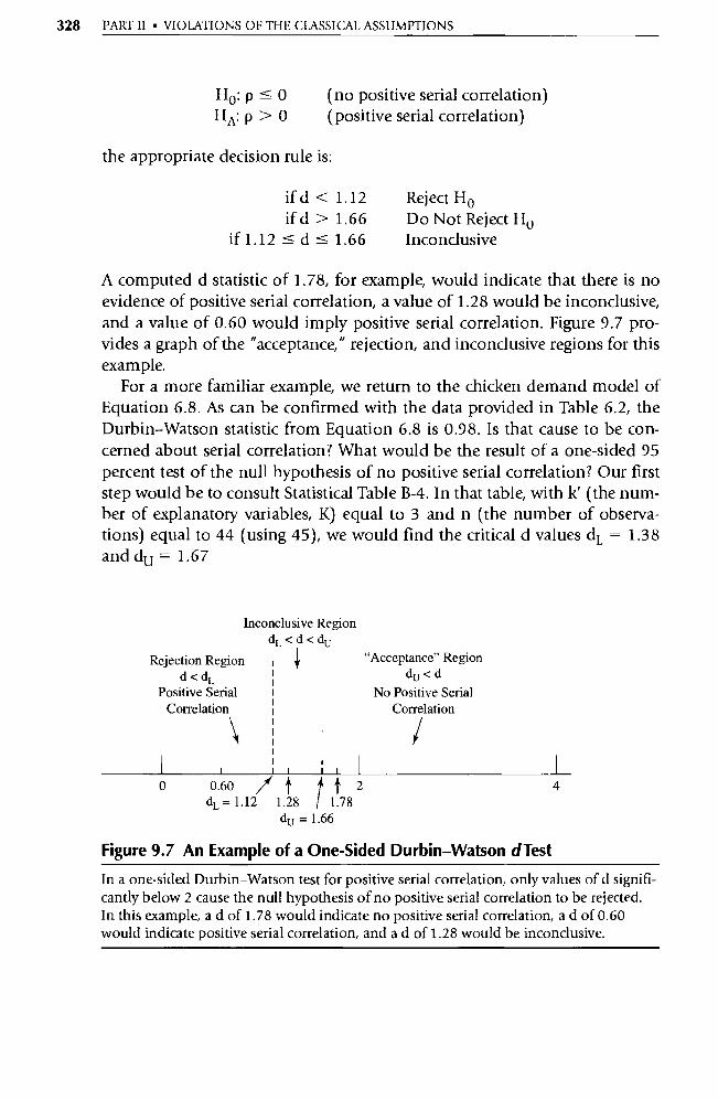
H O:p O HA: p > 0
(no positive serial correlation)
(positive serial correlation)
the appropriate decision rule is:
if d < 1.12 Reject H 0
if d > 1.66 Do Not Reject H 0
if 1.12 < d <_ 1.66 Inconclusive
A computed d statistic of 1.78, for example, would indicate that there is no
evidence of positive serial correlation, a value of 1.28 would be inconclusive,
and a value of 0.60 would imply positive serial correlation. Figure 9.7 pro-vides a graph of the "acceptance," rejection, and inconclusive regions for this
example. For a more familiar example, we return to the chicken demand model of
Equation 6.8. As can be confirmed with the data provided in Table 6.2, the
Durbin-Watson statistic from Equation 6.8 is 0.98. Is that cause to be con-cerned about serial correlation? What would be the result of a one-sided 95
percent test of the null hypothesis of no positive serial correlation? Our first
step would be to consult Statistical Table B-4. In that table, with k' (the num-ber of explanatory variables, K) equal to 3 and n (the number of observa-tions) equal to 44 (using 45), we would find the critical d values d L = 1.38 and du = 1.67
Inconclusive Region dL < d < du
Rejection Region d < dL
Positive Serial Correlation
"Acceptance" Region du < d
No Positive Serial Correlation
^
0 0.60 / it t 2 4 di, = 1.12 1.28 1.78
dU =1.66
Figure 9.7 An Example of a One-Sided Durbin-Watson dTest
328 PART II • VIOLATIONS OF THE CLASSICAL ASSUMPTIONS
In a one-sided Durbin-Watson test for positive serial correlation, only values of d signifi-cantly below 2 cause the null hypothesis of no positive serial correlation to be rejected. In this example, a d of 1.78 would indicate no positive serial correlation, a d of 0.60 would indicate positive serial correlation, and a d of 1.28 would be inconclusive.
CHAPTER 9 • SERIAL CORRELATION 329
The decision rule would thus be:
if d < 1.38 Reject H o
if d > 1.67 Do Not Reject H o if 1.38 d 1.67 Inconclusive
Since 0.98 is less than the critical lower limit of the d statistic, we would re-ject the null hypothesis of no positive serial correlation, and we would have to decide how to cope with that serial correlation.
9.4 Generalized Least Squares
Suppose that the Durbin-Watson d statistic detects serial correlation in the residuals of your equation. Is there a remedy? Some students suggest reorder-ing the observations of Y and the Xs to avoid serial correlation. They think that if this time's error term appears to be affected by last time's error term, why not reorder the data randomly to get rid of the problem? The answer is that the reordering of the data does not get rid of the serial correlation; it just makes the problem harder to detect. If €2 = f(E 1 ) and we reorder the data, then the error term observations are still related to each other, but they now no longer follow each other, and it becomes almost impossible to discover the serial correlation. Interestingly, reordering the data changes the Durbin-Watson d statistic but does not change the estimates of the coeffi-cients or their standard errors at a11. 8
Instead, the place to start in correcting a serial correlation problem is to look carefully at the specification of the equation for possible errors that might be causing impure serial correlation. Is the functional form correct? Are you sure that there are no omitted variables? In pa rticular, are there spec-ification errors that might have some pattern over time that could have intro-duced impure serial correlation into the residuals? Only after the specifica-tion of the equation has been reviewed carefully should the possibility of an adjustment for pure serial correlation be considered.
It's worth noting that if one or more of the variables increases or decreases steadily over time, as is often the case, or if the data set is logically reordered (say, according to the magnitude of one of the variables), then the Durbin-Watson statistic can help detect impure serial correlation. A signifi-
8. This can be proven mathematically, but it is usually more instructive to estimate a regression yourself, change the order of the observations, and then reestimate the regression. See Exercise 3 at the end of the chapter.
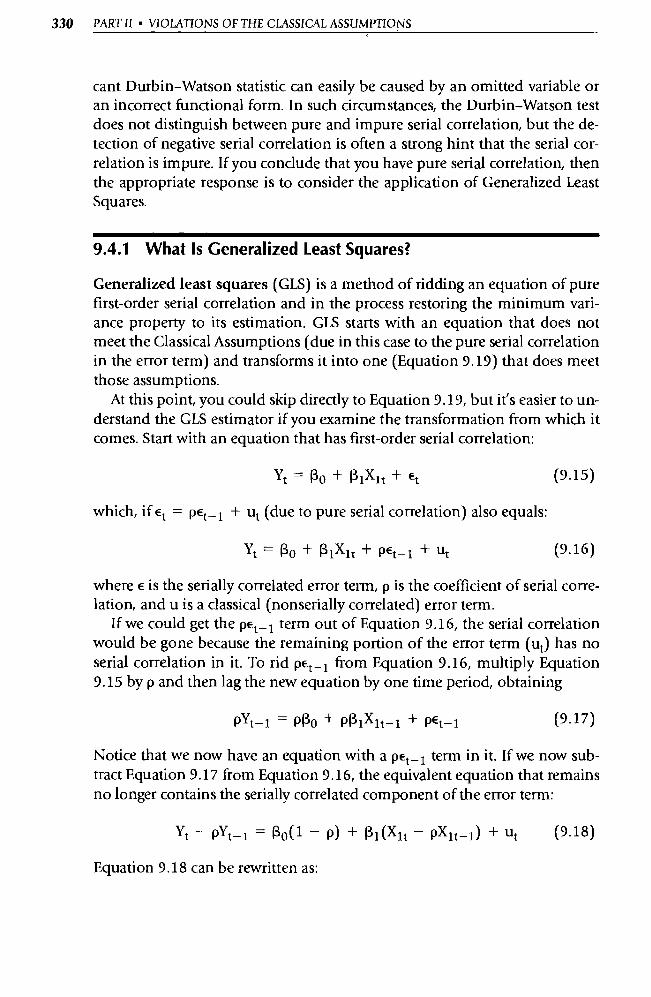
330 PART II • VIOLATIONS OF THE CLASSICAL ASSUMPTIONS
cant Durbin-Watson statistic can easily be caused by an omitted variable or an incorrect functional form. In such circumstances, the Durbin-Watson test does not distinguish between pure and impure serial correlation, but the de-tection of negative serial correlation is often a strong hint that the serial cor-relation is impure. If you conclude that you have pure serial correlation, then the appropriate response is to consider the application of Generalized Least Squares.
9.4.1 What Is Generalized Least Squares?
Generalized least squares (GLS) is a method of ridding an equation of pure first-order serial correlation and in the process restoring the minimum vari-ance property to its estimation. GLS starts with an equation that does not meet the Classical Assumptions (due in this case to the pure serial correlation in the error term) and transforms it into one (Equation 9.19) that does meet those assumptions.
At this point, you could skip directly to Equation 9.19, but it's easier to un-derstand the GLS estimator if you examine the transformation from which it comes. Start with an equation that has first-order serial correlation:
Yt - Po+R1X1t + Et
which, if Et = pEt_ 1 + ut (due to pure serial correlation) also equals:
Yt =Po +PlXlt +Pet -1 +ut
(9.15)
(9.16)
where E is the serially correlated error term, p is the coefficient of serial corre-lation, and u is a classical (nonserially correlated) error term.
If we could get the pE t _ 1 term out of Equation 9.16, the serial correlation would be gone because the remaining po rtion of the error term (ut) has no serial correlation in it. To rid pe t _ 1 from Equation 9.16, multiply Equation 9.15 by p and then lag the new equation by one time period, obtaining
PYt-1 - PPo + PR1X1t-1 + Pet-1 (9.17)
Notice that we now have an equation with a pE t _ 1 term in it. If we now sub-tract Equation 9.17 from Equation 9.16, the equivalent equation that remains no longer contains the serially correlated component of the error term:
Yt - PYt-1 - 13o( 1 - P) + R1(Xlt - PXIt- 1) + ut
Equation 9.18 can be rewritten as:
(9.18)
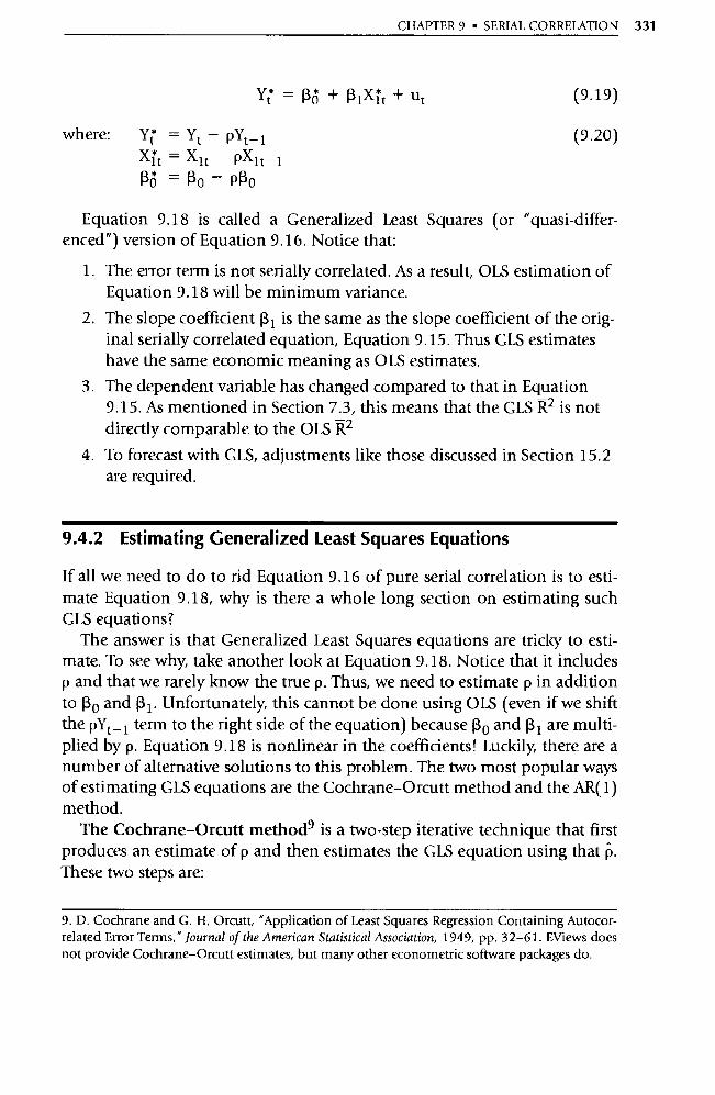
CHAPTER 9 • SERIAL CORRELATION 331
Yi = Rô + R1Xit + ut (9.19)
where: Yt - Yt - PYt - 1
Xit - X1t PX1t-1 Rô = Ro — PRo
(9.20)
Equation 9.18 is called a Generalized Least Squares (or "quasi-differ-enced") version of Equation 9.16. Notice that:
1. The error term is not serially correlated. As a result, OLS estimation of Equation 9.18 will be minimum variance.
2. The slope coefficient 13 1 is the same as the slope coefficient of the orig-inal serially correlated equation, Equation 9.15. Thus GLS estimates have the same economic meaning as OLS estimates.
3. The dependent variable has changed compared to that in Equation 9.15. As mentioned in Section 7.3, this means that the GLS R 2 is not directly comparable to the OLS R2
4. To forecast with GLS, adjustments like those discussed in Section 15.2 are required.
9.4.2 Estimating Generalized Least Squares Equations
If all we need to do to rid Equation 9.16 of pure serial correlation is to esti-mate Equation 9.18, why is there a whole long section on estimating such GLS equations?
The answer is that Generalized Least Squares equations are tricky to esti-mate. To see why, take another look at Equation 9.18. Notice that it includes p and that we rarely know the true p. Thus, we need to estimate p in addition to R o and 13 1 . Unfortunately, this cannot be done using OLS (even if we shift the pYt _ 1 term to the right side of the equation) because Ro and p i are multi-plied by p. Equation 9.18 is nonlinear in the coefficients! Luckily, there are a number of alternative solutions to this problem. The two most popular ways of estimating GLS equations are the Cochrane-Orcutt method and the AR(1) method.
The Cochrane-Orcutt method is a two-step iterative technique that first produces an estimate of p and then estimates the GLS equation using that P. These two steps are:
9. D. Cochrane and G. H. Orcutt, "Application of Least Squares Regression Containing Autocor-related Error Terms," Journal of the American Statistical Association, 1949, pp. 32-61. EViews does not provide Cochrane-Orcutt estimates, but many other econometric software packages do.
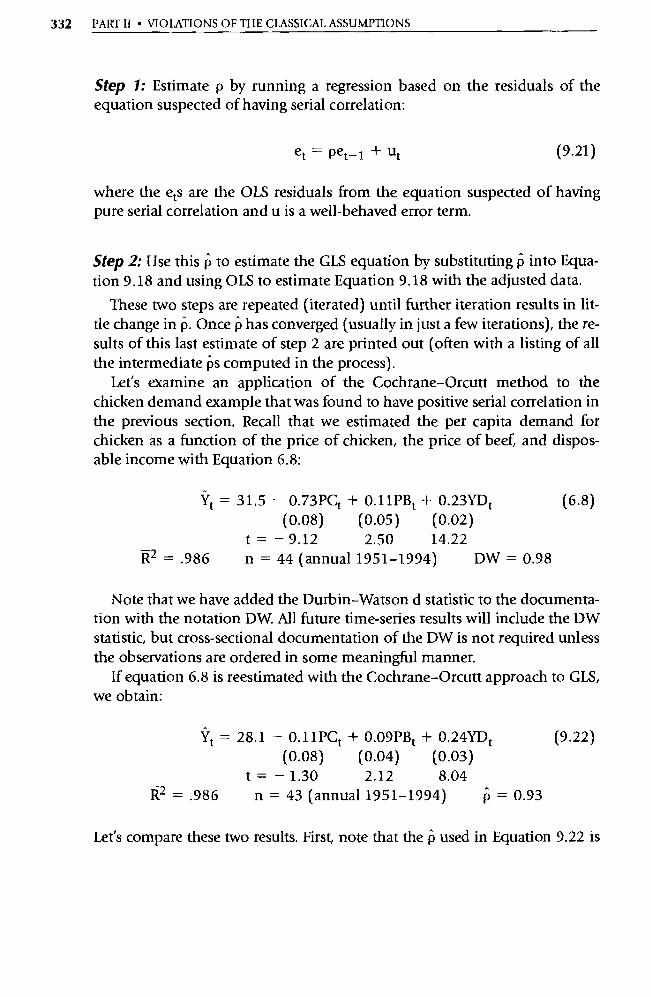
332 PART II • VIOLATIONS OF THE CLASSICAL ASSUMPTIONS
Step 1: Estimate p by running a regression based on the residuals of the equation suspected of having serial correlation:
et = Pet-1 + ut (9.21)
where the ets are the OLS residuals from the equation suspected of having pure serial correlation and u is a well-behaved error term.
Step 2: Use this p to estimate the GLS equation by substituting p into Equa-tion 9.18 and using OLS to estimate Equation 9.18 with the adjusted data.
These two steps are repeated (iterated) until further iteration results in lit-tle change in P. Once p has converged (usually in just a few iterations), the re-sults of this last estimate of step 2 are printed out (often with a listing of all the intermediate Ps computed in the process).
Let's examine an application of the Cochrane-Orcutt method to the chicken demand example that was found to have positive serial correlation in the previous section. Recall that we estimated the per capita demand for chicken as a function of the price of chicken, the price of beef, and dispos-able income with Equation 6.8:
Yt = 31.5 - 0.73PCt + 0.11PBt + 0.23YDt (0.08) (0.05) (0.02)
t = -9.12 2.50 14.22 R2 = .986 n = 44 (annual 1951-1994) DW = 0.98
(6.8)
Note that we have added the Durbin-Watson d statistic to the documenta-tion with the notation DW. All future time-series results will include the DW statistic, but cross-sectional documentation of the DW is not required unless the observations are ordered in some meaningful manner.
If equation 6.8 is reestimated with the Cochrane-Orcutt approach to GLS, we obtain:
Yt = 28.1 - 0.11 PCt + 0.09PBt + 0.24YDt
(0.08) (0.04) (0.03)
t= -1.30 2.12 8.04 R2 = .986 n = 43 (annual 1951-1994) p = 0.93
(9.22)
Let's compare these two results. First, note that the p used in Equation 9.22 is

CHAPTER 9 • SERIAL CORRELATION 333
0.93. That means that Y was actually run as YC = Y t - 0.93Yt _ 1 , PC as PCt = PCt - 0.93PCt_ i , etc. Second, note that even though serial correlation causes no bias in the estimates of the (3s, the GLS estimates of the slope coeffi-cients are different from the OLS ones. Just because two estimates have the same expected values does not mean that they will be identical.
Note that p replaces DW in the documentation of GLS estimates since the DW of Equation 9.22 is not strictly comparable with non-GLS DWs (it is bi-ased toward 2). Also note that the estimated model typically is presented in the format of Equation 9.19 without the asterisks attached to the trans-formed Y* and X* variables. Finally, note that the sample size of this regres-sion is 43 (n 1) because the first obse rvation has to be used to create the lagged values for the calculation of the quasi-differenced variables in Equa-tion 9.20.
The second way to estimate GLS equations is the AR(1) Method, which is a step-one process that estimates p, (3 0, and R 1 simultaneously. 10 In essence, the AR(1) method estimates Equation 9.18 all at once by using iterative nonlinear regression techniques that are well beyond the scope of this chap-ter. Although the AR(1) technique is more complicated, it has a number of advantages. First, the regression is on the entire data set, whereas Cochrane-Orcutt is forced to use up the first obse rvation creating the quasi-differenced variables. Second, AR(1) tends to have better-behaved SE((3)s than does Cochrane-Orcutt. Interestingly, the estimates of the slope coeffi-cients tend to be identical (depending on the convergence characteristics of the two software packages).
To compare AR(1) with Cochrane-Orcutt as alternative methods of esti-mating GLS equations, let's return to the chicken demand equation and esti-mate the equation using the AR(1) method:
Yt = 26.7 0.11PCt + 0.09PBt + 0.24YDt (9.23) (0.08) (0.04) (0.03)
t = -1.29 2.06 9.13 R2 = .995 n = 43 (annual 1951-1994) p = 0.90
Compare Equation 9.23 with Equation 9.22. Note that the estimated slope coefficients are indeed identical but that the SE(13)s differ slightly, caus-ing different t-scores. This is because of the improved properties of the AR(1)
10. To run GIS with EViews, simply add "AR(1)" to the equation as if it were an independent variable. The resulting equation is a GLS estimate where p will appear as the estimated coeffi-cient of the va riable AR(1).

334 PART II • VIOLATIONS OF THE CLASSICALASSUMPTIONS
standard errors. Which equation is better? Since the only difference between the two equations is that the AR(1) standard error estimates are superior, our recommendation is to use AR(1) procedures as long as your computer can support such nonlinear regression. This issue is hardly settled, however, be-cause Cochrane-Orcutt remains more popular than AR(1), and because an alternative to GLS, to be described in Section 9.4.3, is also gaining suppo rt .
9.4.3 Why Generalized Least Squares Shouldn't Automatically Be Used
There are a number of reasons why GLS should not be applied every time that the Durbin-Watson test indicates the likelihood of serial correlation in the residuals of an equation. Because of these reasons, it's our strong recommen-dation to avoid the use of GLS when the Durbin-Watson test is inconclusive.
1. The significant DW may be caused by impure serial correlation. When auto-correlation is detected, the cause may be an omitted va riable or a poor choice of functional form. In such a case, the best solution is to find the missing variable or the proper form. Even if these easy answers can-not be found, the application of GLS to the misspecified equation is not necessarily superior to OLS. Impure serial correlation justifies us-ing GLS only when the cause is an omitted variable that is at least rea-sonably correlated with one of the included variables. In this case, if the left-out variable cannot be found, GLS will reduce the bias some-what, because the procedure proxies for the autocorrelated po rtion of the omitted variable. In cases of uncorrelated omitted variables or im-proper functional form, it can be shown that OLS is superior to GLS for estimating an incorrectly specified equation. In all cases, of course, the best course of action is to use the correct specification.
2. The consequences of the serial correlation may be minor. GLS works well if p is close to the actual p, but p is biased in small samples, potentially causing estimation problems. Since pure serial correlation causes no bias, it's possible that the harm done to the equation by the serial cor-relation may be less than the damage done by attempting to fix that problem with a biased P. In pa rticular, when coefficient estimates seem theoretically reasonable, and when the t-scores of the various coeffi-cients are not being relied on for the retention of independent vari-ables, the harm caused by serial correlation may be minor.
3. Newey-West standard errors could be used. Not all corrections for pure se-rial correlation involve Generalized Least Squares. The Newey-West
CHAPTER 9 • SERIAL CORRELATION 335
technique directly adjusts the SE((3)s to take account of serial correla-tion without changing the (3s themselves in any way. 11 The logic be-hind Newey-West standard errors is powerful: if serial correlation does not cause bias but does impact the standard errors, then it makes sense to adjust the estimated equation in a way that changes the SE((3)s but not the 13s. Newey-West standard errors currently are estimated by only a small percentage of applied econometricians, but it seems likely that their use will increase over time.
9.5 Summary
1. Serial correlation, or autocorrelation, is the violation of Classical As-sumption IV that the observations of the error term are uncorrelated with each other. Usually, econometricians focus on first-order serial correlation, in which the current observation of the error term is as-sumed to be a function of the previous observation of the error term and a nonserially correlated error term (u):
Et — PEt -1 + ut - 1 < p < 1
where p is "rho," the coefficient of serial correction.
2. Pure serial correlation is serial correlation that is a function of the error term of the correctly specified regression equation. Impure serial corre-lation is caused by specification errors such as an omitted variable or an incorrect functional form. While impure serial correlation can be positive (0 < p < 1) or negative (-1 < p < 0), pure serial correla-tion in economics or business situations is almost always positive.
3. The major consequence of serial correlation is an increase in the vari-ances of the (3 distributions that is masked by an underestimation of those variances (and the standard errors) by OIS. Pure serial correla-tion does not cause bias in the estimates of the (3s.
4. The most commonly used method of detecting first-order serial corre-lation is the Durbin-Watson d test, which uses the residuals of an esti-
11. W. K. Newey and K. D. West, "A Simple, Positive Semi-Definite Heteroskedasticity and Auto-correlation Consistent Covariance Matrix," Econometrica, 1987, pp. 703-708. Newey-West stan-dard errors are similar in concept to SE' ((3p) on page 324. For a slightly longer discussion of a similar topic, see the discussion of heteroskedasticity-corrected standard errors in Section 10.4.
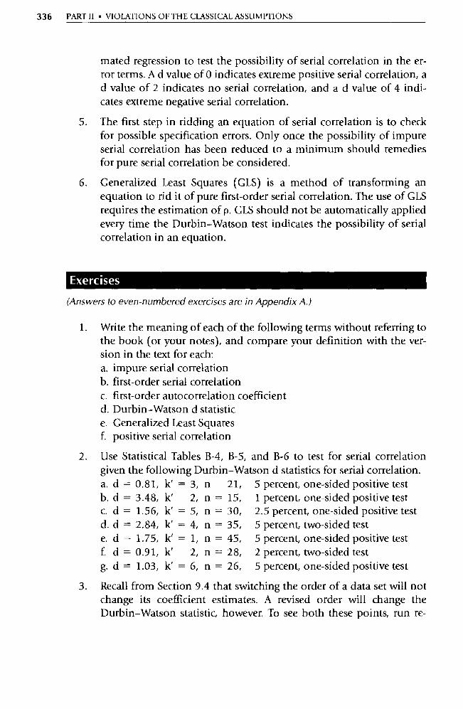
336 PART II • VIOLATIONS OF THE CLASSICAL ASSUMPTIONS
mated regression to test the possibility of serial correlation in the er- ror terms. A d value of 0 indicates extreme positive serial correlation, a d value of 2 indicates no serial correlation, and a d value of 4 indi-cates extreme negative serial correlation.
5. The first step in ridding an equation of serial correlation is to check for possible specification errors. Only once the possibility of impure serial correlation has been reduced to a minimum should remedies for pure serial correlation be considered.
6. Generalized Least Squares (GLS) is a method of transforming an equation to rid it of pure first-order serial correlation. The use of GLS requires the estimation of p. GLS should not be automatically applied every time the Durbin-Watson test indicates the possibility of serial correlation in an equation.
Exercises
(Answers to even-numbered exercises are in Appendix A.)
1. Write the meaning of each of the following terms without referring to the book (or your notes), and compare your definition with the ver-sion in the text for each: a. impure serial correlation b. first-order serial correlation c. first-order autocorrelation coefficient d. Durbin-Watson d statistic e. Generalized Least Squares f. positive serial correlation
2. Use Statistical Tables B-4, B-5, and B-6 to test for serial correlation given the following Durbin-Watson d statistics for serial correlation. a. d = b. d = c. d = d. d = e. d = f. d = g. d =
3. Recall from Section 9.4 that switching the order of a data set will not change its coefficient estimates. A revised order will change the Durbin-Watson statistic, however. To see both these points, run re-
0.81, k' = 3, n 21, 5 percent, one-sided positive test 3.48, k' 2, n = 15, 1 percent, one-sided positive test 1.56, k' = 5, n = 30, 2.5 percent, one-sided positive test 2.84, k' = 4, n = 35, 5 percent, two-sided test 1.75, k' = 1, n = 45, 5 percent, one-sided positive test 0.91, k' 2, n = 28, 2 percent, two-sided test 1.03, k' = 6, n = 26, 5 percent, one-sided positive test
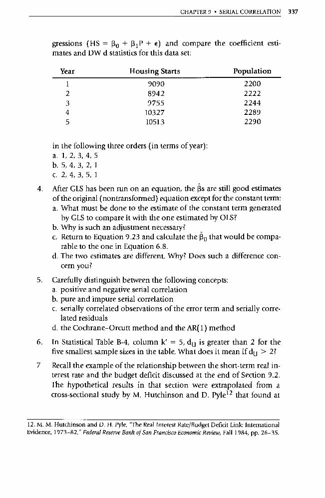
CHAPTER 9 • SERIAL CORRELATION 337
gressions (HS = 13 0 + j3 1 P + €) and compare the coefficient esti-mates and DW d statistics for this data set:
Year Housing Starts Population
1 9090 2200 2 8942 2222 3 9755 2244 4 10327 2289 5 10513 2290
in the following three orders (in terms of year): a. 1, 2, 3,4,5 b. 5, 4, 3, 2, 1 c. 2, 4, 3, 5, 1
4. After GLS has been run on an equation, the Rs are still good estimates of the o riginal (nontransformed) equation except for the constant term: a. What must be done to the estimate of the constant term generated
by GLS to compare it with the one estimated by OLS? b. Why is such an adjustment necessary? c. Return to Equation 9.23 and calculate the R0 that would be compa-
rable to the one in Equation 6.8. d. The two estimates are different. Why? Does such a difference con-
cern you?
5. Carefully distinguish between the following concepts: a. positive and negative serial correlation b. pure and impure serial correlation c. serially correlated observations of the error term and serially corre-
lated residuals d. the Cochrane-Orcutt method and the AR(1) method
6. In Statistical Table B-4, column k' = 5, d u is greater than 2 for the five smallest sample sizes in the table. What does it mean if d u > 2?
7 Recall the example of the relationship between the short-term real in-terest rate and the budget deficit discussed at the end of Section 9.2. The hypothetical results in that section were extrapolated from a cross-sectional study by M. Hutchinson and D. Pyle 12 that found at
12. M. M. Hutchinson and D. H. Pyle, "The Real Interest Rate/Budget Deficit Link: International Evidence, 1973 -82," Federal Reserve Bank of San Francisco Economic Review, Fall 1984, pp. 26 -35.
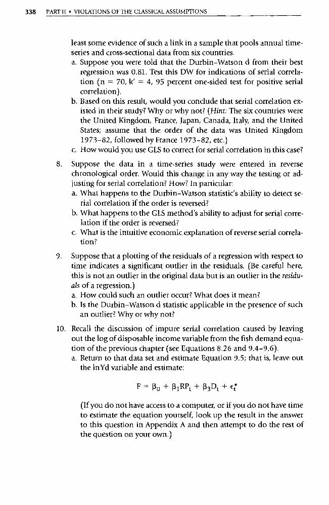
338 PART II • VIOLATIONS OF THE CLASSICAL ASSUMPTIONS
least some evidence of such a link in a sample that pools annual time-series and cross-sectional data from six countries. a. Suppose you were told that the Durbin-Watson d from their best
regression was 0.81. Test this DW for indications of serial correla-tion (n = 70, k' = 4, 95 percent one-sided test for positive serial correlation).
b. Based on this result, would you conclude that serial correlation ex-isted in their study? Why or why not? (Hint: The six countries were the United Kingdom, France, Japan, Canada, Italy, and the United States; assume that the order of the data was United Kingdom 1973-82, followed by France 1973-82, etc.)
c. How would you use GLS to correct for serial correlation in this case?
8. Suppose the data in a time-series study were entered in reverse chronological order. Would this change in any way the testing or ad-justing for serial correlation? How? In pa rticular: a. What happens to the Durbin-Watson statistic's ability to detect se-
rial correlation if the order is reversed? b. What happens to the GLS method's ability to adjust for serial corre-
lation if the order is reversed? c. What is the intuitive economic explanation of reverse serial correla-
tion?
9. Suppose that a plotting of the residuals of a regression with respect to time indicates a significant outlier in the residuals. (Be careful here, this is not an outlier in the original data but is an outlier in the residu-als of a regression.) a. How could such an outlier occur? What does it mean? b. Is the Durbin-Watson d statistic applicable in the presence of such
an outlier? Why or why not?
10. Recall the discussion of impure serial correlation caused by leaving out the log of disposable income variable from the fish demand equa-tion of the previous chapter (see Equations 8.26 and 9.4-9.6). a. Return to that data set and estimate Equation 9.5; that is, leave out
the 1nYd variable and estimate:
F = 130 + RiRPt + R3Dt + Et
(If you do not have access to a computer, or if you do not have time to estimate the equation yourself, look up the result in the answer to this question in Appendix A and then attempt to do the rest of the question on your own.)
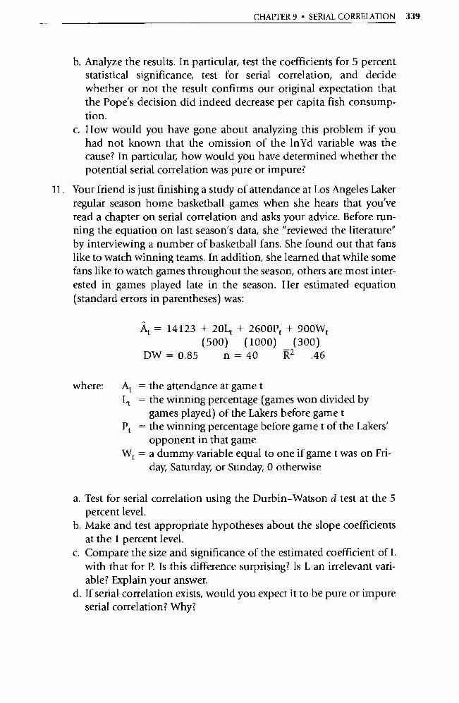
CHAPTER 9 • SERIAL CORRELATION 339
b. Analyze the results. In particular, test the coefficients for 5 percent statistical significance, test for serial correlation, and decide whether or not the result confirms our original expectation that the Pope's decision did indeed decrease per capita fish consump-tion.
c. How would you have gone about analyzing this problem if you had not known that the omission of the 1nYd variable was the cause? In pa rticular, how would you have determined whether the potential serial correlation was pure or impure?
11. Your friend is just finishing a study of attendance at Los Angeles Laker regular season home basketball games when she hears that you've read a chapter on serial correlation and asks your advice. Before run-ning the equation on last season's data, she "reviewed the literature" by interviewing a number of basketball fans. She found out that fans like to watch winning teams. In addition, she learned that while some fans like to watch games throughout the season, others are most inter-ested in games played late in the season. Her estimated equation (standard errors in parentheses) was:
At = 14123 + 20L1 + 2600Pt + 900Wt (500) (1000) (300)
DW = 0.85 n = 40 RZ .46
where: At = the attendance at game t Lt = the winning percentage (games won divided by
games played) of the Lakers before game t Pt = the winning percentage before game t of the Lakers'
opponent in that game Wt = a dummy variable equal to one if game t was on Fri-
day, Saturday, or Sunday, 0 otherwise
a. Test for serial correlation using the Durbin-Watson d test at the 5 percent level.
b. Make and test appropriate hypotheses about the slope coefficients at the 1 percent level.
c. Compare the size and significance of the estimated coefficient of L with that for P. Is this difference surprising? Is L an irrelevant vari-able? Explain your answer.
d. If serial correlation exists, would you expect it to be pure or impure serial correlation? Why?

340 PART II • VIOLATIONS OF THE CLASSICAL ASSUMPTIONS
e. Your friend omitted the first game of the year from the sample be-cause the first game is always a sellout and because neither team had a winning percentage yet. Was this a good decision?
12. In Section 2.2.3, we considered an equation for U.S. per capita con-sumption of beef for the years 1960-1987 that was kept simple for the purpose of that chapter. A more complete specification of the equation estimated on the same data produces:
Bt = -330.3 + 49.1 1nYt - 0.34PBt + 0.33PPt - 15.4Dt (9.24) (7.4) (0.13) (0.12) (4.1)
t = 6.6 - 2.6 2.7 - 3.7 R2 =.700 n = 28 DW = 0.94
where: Bt = the annual per capita pounds of beef consumed in the United States in year t
1nY = the log of real per capita disposable income in the United States in 1982 dollars
PB = average annualized real wholesale price of beef (in cents per pound)
PP = average annualized real wholesale price of pork (in cents per pound)
D = a dummy variable equal to 1 for years after 1981, 0 otherwise (an attempt to capture the increased con-sumer awareness of the health dangers of red meat)
a. Develop and test your own hypotheses with respect to the individ-ual estimated slope coefficients.
b. Test for serial correlation in Equation 9.24 using the Durbin-Watson d test at the 5 percent level.
c. What econometric problem(s) (if any) does Equation 9.24 appear to have? What remedy would you suggest?
d. You take your own advice, and apply GIS to Equation 9.24, obtaining:
At = - 193.3 + 35.2 1nYt - 0.38PBt + 0.10PPt 5.7Dt (14.1) (0.10) (0.09) (3.9)
t=2.5 -3.7 1.1 -1.5 R2 =.857 n = 28 p=0.82
(9.25)
Compare Equations 9.24 and 9.25. Which do you prefer? Why?
13. You're hired by Farmer Vin, a famous producer of bacon and ham, to test the possibility that feeding pigs at night allows them to grow
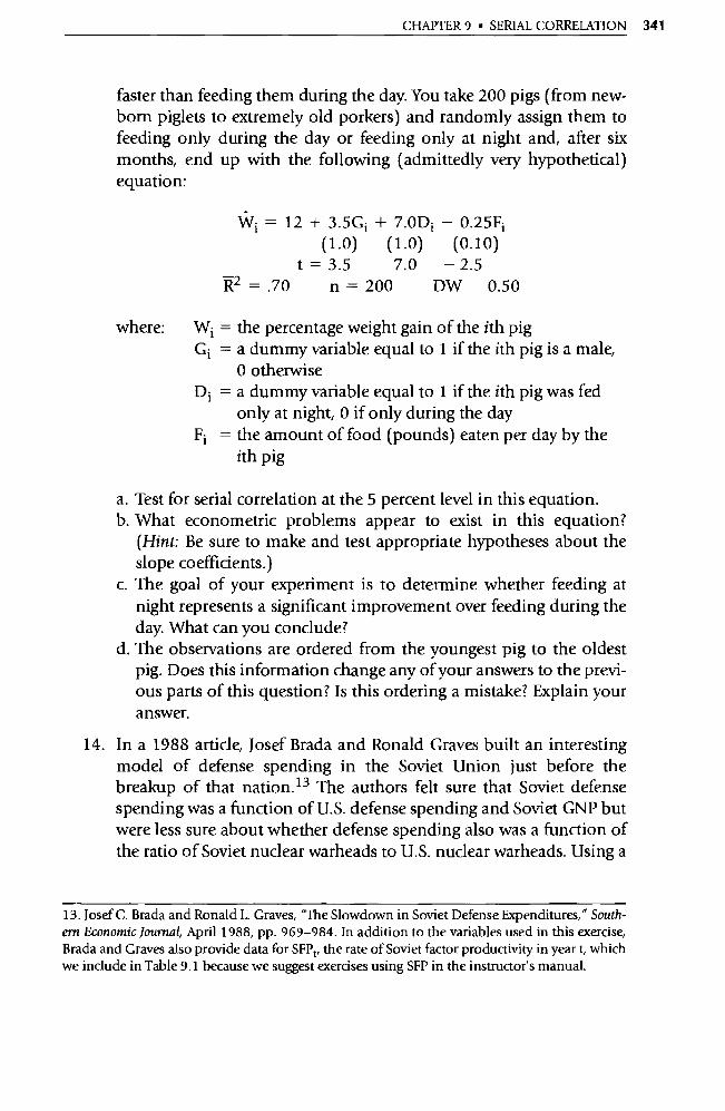
CHAPTER 9 • SERIAL CORRELATION 341
faster than feeding them during the day. You take 200 pigs (from new-born piglets to extremely old porkers) and randomly assign them to feeding only during the day or feeding only at night and, after six months, end up with the following (admittedly very hypothetical) equation:
Wi = 12 + 3.5Gi + 7.0Di — 0.25Fi
(1.0) (1.0) (0.10)
t = 3.5 7.0 — 2.5 R2 = .70 n = 200 DW 0.50
where: Wi = the percentage weight gain of the ith pig Gi = a dummy variable equal to 1 if the ith pig is a male,
0 otherwise Di = a dummy variable equal to 1 if the ith pig was fed
only at night, 0 if only during the day Fi = the amount of food (pounds) eaten per day by the
ith pig
a. Test for serial correlation at the 5 percent level in this equation. b. What econometric problems appear to exist in this equation?
(Hint: Be sure to make and test appropriate hypotheses about the slope coefficients.)
c. The goal of your experiment is to determine whether feeding at night represents a significant improvement over feeding during the day. What can you conclude?
d. The observations are ordered from the youngest pig to the oldest pig. Does this information change any of your answers to the previ-ous parts of this question? Is this ordering a mistake? Explain your answer.
14. In a 1988 article, Josef Brada and Ronald Graves built an interesting model of defense spending in the Soviet Union just before the breakup of that nation. 13 The authors felt sure that Soviet defense spending was a function of U.S. defense spending and Soviet GNP but were less sure about whether defense spending also was a function of the ratio of Soviet nuclear warheads to U.S. nuclear warheads. Using a
13. Josef C. Brada and Ronald L. Graves, "The Slowdown in Soviet Defense Expenditures," South-ern Economic Journal, April 1988, pp. 969-984. In addition to the va riables used in this exercise, Brada and Graves also provide data for SFP i, the rate of Soviet factor productivity in year t, which we include in Table 9.1 because we suggest exercises using SFP in the instructor's manual.
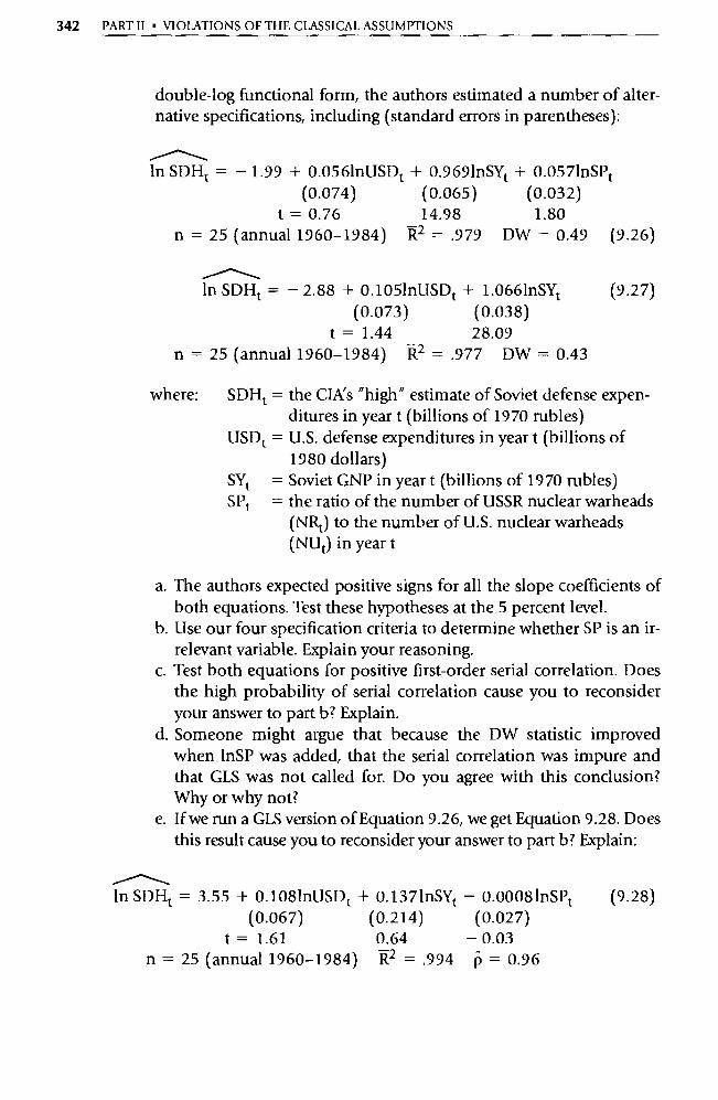
342 PART II • VIOLATIONS OF THE CLASSICAL ASSUMPTIONS
double-log functional form, the authors estimated a number of alter-native specifications, including (standard errors in parentheses):
/\ In SDHt = - 1.99 + 0.0561nUSDt + 0.9691nSYt + 0.0571nSPt
(0.074) (0.065) (0.032) t = 0.76 14.98 1.80
n = 25 (annual 1960-1984) 12 2 = .979 DW = 0.49 (9.26)
/\ ln SDHt = - 2.88 + 0.1051nUSD t + 1.0661nSYt
(0.073) (0.038) t = 1.44 28.09
n = 25 (annual 1960-1984) R2 = .977 DW = 0.43
(9.27)
where: SDHt = the CIA's "high" estimate of Soviet defense expen- ditures in year t (billions of 1970 rubles)
USDt = U.S. defense expenditures in year t (billions of 1980 dollars)
= Soviet GNP in year t (billions of 1970 rubles) = the ratio of the number of USSR nuclear warheads
(NRt) to the number of U.S. nuclear warheads (Nut) in year t
a. The authors expected positive signs for all the slope coefficients of both equations. Test these hypotheses at the 5 percent level.
b. Use our four specification criteria to determine whether SP is an ir-relevant variable. Explain your reasoning.
c. Test both equations for positive first-order serial correlation. Does the high probability of serial correlation cause you to reconsider your answer to part b? Explain.
d. Someone might argue that because the DW statistic improved when 1nSP was added, that the serial correlation was impure and that GLS was not called for. Do you agree with this conclusion? Why or why not?
e. If we run a GLS version of Equation 9.26, we get Equation 9.28. Does this result cause you to reconsider your answer to pa rt b? Explain:
/\ ln SDHt = 3.55 + 0.1081nUSDt + 0.1371nSYt
(0.067) (0.214) t = 1.61 0.64
n = 25 (annual 1960-1984) R2 = .994
- 0.00081nSPt (0.027)
- 0.03 P = 0.96
(9.28)
SYt SPt

CHAPTER 9 • SERIAL CORRELATION 343
15. Let's return to the model of Soviet defense spending of the previous exercise. Throughout that exercise, the dependent va riable is the CIA's high estimate of Soviet defense spending (SDH), but the authors also provide a "low" CIA estimate as well (SDL). Using the data from Table 9.1 or datafile DEFEND9 and either EViews or your computer's regres-sion program, answer all pa rts of Exercise 14 with 1nSDL as the de-pendent va riable instead of 1nSDH. That is, estimate versions of Equa-tions 9.26 through 9.28 with 1nSDL as the dependent variable and then use your estimates to determine the answer to each pa rt of Exer-cise 14 for the new dependent variable. Does your evaluation of the authors' conclusions change when you use this dependent variable? Why or why not?
TABLE 9.1 DATA ON SOVIET DEFENSE SPENDING
Year SDH SDL USD SY SFP NR NU
1960 31 23 200.54 232.3 7.03 415 1,734 1961 34 26 204.12 245.3 6.07 445 1,846 1962 38 29 207.72 254.5 3.90 485 1,942 1963 39 31 206.98 251.7 2.97 531 2,070 1964 42 34 207.41 279.4 1.40 580 2,910 1965 43 35 185.42 296.8 1.87 598 4,110 1966 44 36 203.19 311.9 4.10 674 4,198 1967 47 39 241.27 326.3 4.90 1,058 4,338 1968 50 42 260.91 346.0 4.07 1,270 4,134 1969 52 43 254.62 355.9 2.87 1,662 4,026 1970 53 44 228.19 383.3 4.43 2,047 5,074 1971 54 45 203.80 398.2 3.77 3,199 6,282 1972 56 46 189.41 405.7 2.87 2,298 7,100 1973 58 48 169.27 435.2 3.87 2,430 8,164 1974 62 51 156.81 452.2 4.30 2,534 8,522 1975 65 53 155.59 459.8 6.33 2,614 9,170 1976 69 56 169.91 481.8 0.63 3,219 9,518 1977 70 56 170.94 497.4 2.23 4,345 9,806 1978 72 57 154.12 514.2 1.03 5,097 9,950 1979 75 59 156.80 516.1 0.17 6,336 9,945 1980 79 62 160.67 524.7 0.27 7,451 9,668 1981 83 63 169.55 536.1 0.47 7,793 9,628 1982 84 64 185.31 547.0 0.07 8,031 10,124 1983 88 66 201.83 567.5 1.50 8,730 10,201 1984 90 67 211.35 578.9 1.63 9,146 10,630
Source: Josef C. Brada and Ronald L. Graves, "The Slowdown in Soviet Defense Expenditures," Southern Economic Journal, April 1988, p. 974.
Note: filename DEFEND9
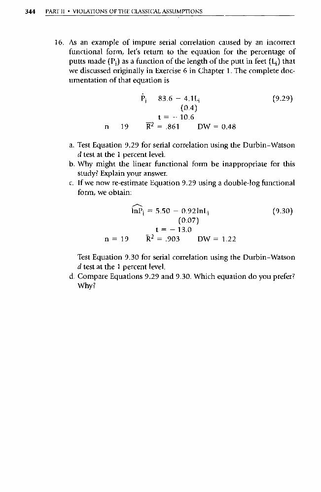
344 PART II • VIOLATIONS OF THE CLASSICAL ASSUMPTIONS
16. As an example of impure serial correlation caused by an incorrect functional form, let's return to the equation for the percentage of putts made (Pi) as a function of the length of the putt in feet (L i ) that we discussed originally in Exercise 6 in Chapter 1. The complete doc-umentation of that equation is
Pi 83.6 - 4.1Li (0.4)
t = -10.6 n 19 R2 = .861 DW =0.48
(9.29)
a. Test Equation 9.29 for serial correlation using the Durbin-Watson d test at the 1 percent level.
b. Why might the linear functional form be inappropriate for this study? Explain your answer.
c. If we now re-estimate Equation 9.29 using a double-log functional form, we obtain:
1nPi = 5.50 - 0.921nLi (0.07)
t = - 13.0 n = 19 R2 = .903 DW = 1.22
(9.30)
Test Equation 9.30 for serial correlation using the Durbin-Watson d test at the 1 percent level.
d. Compare Equations 9.29 and 9.30. Which equation do you prefer? Why?

CHAPTER 1c Heteroskedasticity
10.1 Pure versus Impure Heteroskedasticity
10.2 The Consequences of Heteroskedasticity
10.3 Testing for Heteroskedasticity
10.4 Remedies for Heteroskedasticity
10.5 A More Complete Example
10.6 Summary and Exercises
Heteroskedasticity is the violation of Classical Assumption V, which states that the observations of the error term are drawn from a distribution that has a constant variance. 1 The assumption of constant variances for different ob-servations of the error term (homoskedasticity) is not always realistic. For ex-ample, in a model explaining heights, compare a one-inch error in measur-ing the height of a basketball player with a one-inch error in measuring the height of a mouse. It's likely that error term observations associated with the height of a basketball player would come from distributions with larger vari-ances than those associated with the height of a mouse. As we'll see, the dis-tinction between heteroskedasticity and homoskedasticity is important be-cause OLS, when applied to heteroskedastic models, is no longer the minimum variance estimator (it still is unbiased, however).
In general, heteroskedasticity is more likely to take place in cross-sectional models than in time-series models. This focus on cross-sectional models is not to say that heteroskedasticity in time-series models is impossible, though.
1. Various authors spell this "heteroscedasticity, but Huston McCulloch appears to settle this controversy in favor of "heteroskedasticity" because of the word's Greek origin. See J. Huston McCulloch, "On Heteros*edasticity," Econometrica, March 1985, p. 483. Although hetero-skedasticity is a difficult word to spell, at least it's an impressive comeback when parents ask, "What'd you learn for all that money?"
345
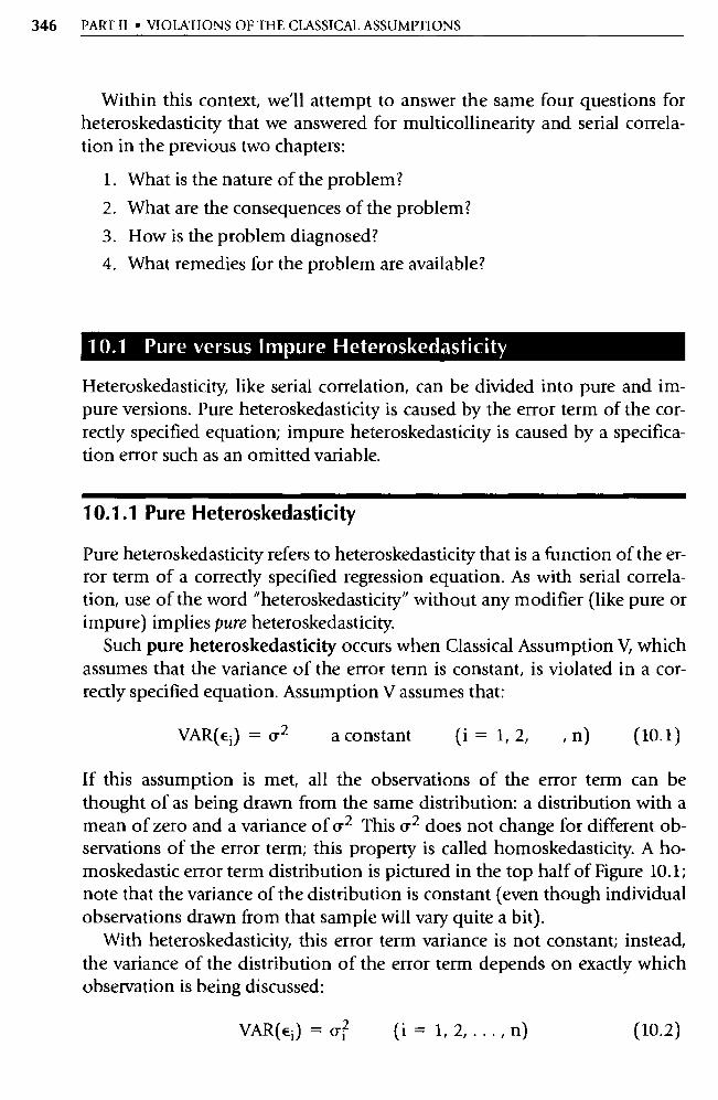
346 PART II • VIOLATIONS OF THE CLASSICAL ASSUMPTIONS
Within this context, we'll attempt to answer the same four questions for heteroskedasticity that we answered for multicollinearity and serial correla-tion in the previous two chapters:
1. What is the nature of the problem?
2. What are the consequences of the problem?
3. How is the problem diagnosed?
4. What remedies for the problem are available?
10.1 Pure versus Impure Heteroskedasticity
Heteroskedasticity, like serial correlation, can be divided into pure and im-pure versions. Pure heteroskedasticity is caused by the error term of the cor-rectly specified equation; impure heteroskedasticity is caused by a specifica-tion error such as an omitted variable.
10.1.1 Pure Heteroskedasticity
Pure heteroskedasticity refers to heteroskedasticity that is a function of the er-ror term of a correctly specified regression equation. As with serial correla-tion, use of the word "heteroskedasticity" without any modifier (like pure or impure) implies pure heteroskedasticity.
Such pure heteroskedasticity occurs when Classical Assumption V, which assumes that the va riance of the error term is constant, is violated in a cor-rectly specified equation. Assumption V assumes that:
VAR(E i) = Q2 a constant (i = 1, 2, , n) (10.1)
If this assumption is met, all the observations of the error term can be thought of as being drawn from the same distribution: a dist ribution with a mean of zero and a variance of 62 This 62 does not change for different ob-servations of the error term; this property is called homoskedasticity. A ho-moskedastic error term distribution is pictured in the top half of Figure 10.1; note that the variance of the distribution is constant (even though individual observations drawn from that sample will vary quite a bit).
With heteroskedasticity, this error term variance is not constant; instead, the variance of the distribution of the error term depends on exactly which observation is being discussed:
VAR(Ei) = 6? (i = 1, 2, . . . , n) (10.2)
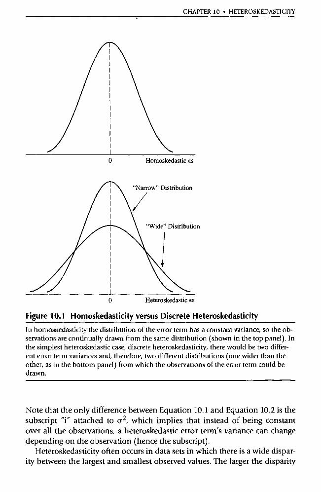
CHAPTER 10 • HETEROSKEDASTICITY
0 Homoskedastic es
0 Heteroskedastic es
Figure 10.1 Homoskedasticity versus Discrete Heteroskedasticity
In homoskedasticity the distribution of the error term has a constant va riance, so the ob-servations are continually drawn from the same distribution (shown in the top panel). In the simplest heteroskedastic case, discrete heteroskedasticity, there would be two differ-ent error term variances and, therefore, two different dist ributions (one wider than the other, as in the bottom panel) from which the observations of the error term could be drawn.
Note that the only difference between Equation 10.1 and Equation 10.2 is the subscript "i" attached to 6 2, which implies that instead of being constant over all the observations, a heteroskedastic error term's variance can change depending on the observation (hence the subscript).
Heteroskedasticity often occurs in data sets in which there is a wide dispar-ity between the largest and smallest observed values. The larger the disparity
348 PART II • VIOLATIONS OF THE CLASSICAL ASSUMPTIONS
between the size of observations in a sample, the larger the likelihood that the error term observations associated with them will have different variances and therefore be heteroskedastic. That is, we'd expect that the error term dis-tribution for very large observations might have a large variance, but the error term distribution for small observations might have a small variance.
In cross-sectional data sets, it's easy to get such a large range between the highest and lowest values of the variables. Recall that in cross-sectional mod-els, the observations are all from the same time period (a given month or year, for example) but are from different entities (individuals, states, or coun-tries, for example). The difference between the size of California's labor force and Rhode Island's, for instance, is quite large (comparable in percentage terms to the difference between the heights of a basketball player and a mouse). Since cross-sectional models often include observations of widely different sizes in the same sample (cross-state studies of the United States usually include California and Rhode Island as individual observations, for example), heteroskedasticity is hard to avoid if economic topics are going to be studied cross sectionally.
Another way to visualize pure heteroskedasticity is to picture a world in which some of the observations of the error term are drawn from much wider distributions than are others. The simplest situation would be that the obser-vations of the error term could be grouped into just two different distribu-tions, "wide" and "narrow." We'll call this simple version of the problem discrete heteroskedasticity. Here, both distributions would be centered around zero, but one would have a larger variance than the other, as indicated in the bottom half of Figure 10.1. Note the difference between the two halves of the figure. With homoskedasticity, all the error term observations come from the same distribution; with heteroskedasticity, they come from different distribu-tions.
Heteroskedasticity takes on many more complex forms. In fact, the num-ber of different models of heteroskedasticity is virtually limitless, and an analysis of even a small percentage of these alternatives would be a huge task. Instead, we'd like to address the general principles of heteroskedasticity by focusing on the most frequently specified model of pure heteroskedasticity, just as we focused on pure, positive, first-order serial correlation in the previ-ous chapter. However, don't let this focus mislead you into concluding that econometricians are concerned only with one kind of heteroskedasticity.
In this model of heteroskedasticity, the variance of the error term is related to an exogenous variable Z i . For a typical regression equation:
Yi = Ro + R1X1i + R2X2i + Ei
the variance of the otherwise classical error term a might be equal to:
(10.3)
CHAPTER 10 • HETEROSKEDASTICITY 349
VAR(Ei) = 62Z1 (10.4)
where Z may or may not be one of the Xs in the equation. The va riable Z is called a proportionality factor because the va riance of the error term changes proportionally to the square of Zi . The higher the value of Z i, the higher the variance of the distribution of the ith observation of the error term. There would be n different distributions, one for each obse rvation, from which the obse rvations of the error term could be drawn depending on the number of different values that Z takes. To see what homoskedastic and heteroskedastic distributions of the error term look like with respect to Z, ex-amine Figures 10.2 and 10.3. Note that the heteroskedastic distribution gets wider as Z increases but that the homoskedastic dist ribution maintains the same width no matter what value Z takes.
What is an example of a proportionality factor Z? How is it possible for an exogenous variable such as Z to change the whole distribution of an error term? Think about a function that relates the consumption of a household to its income. The expenditures of a low income household are not likely to be as variable in absolute value as the expenditures of a high income one be-cause a 10 percent change in spending for a high income family involves a lot more money than a 10 percent change for a low income one. In addition, the proportion of the low income budget that must be spent on necessities is much higher than that of the high income budget. In such a case, the Yi fac-tor would be consumption expenditures and the proportionality factor, Z, would be household income. As household income rose, so too would the variance of the error term of an equation built to explain expenditures. The error term distributions would look something like those in Figure 10.3, where the Z in Figure 10.3 is household income, one of the independent vari-ables in the function.
This example helps emphasize that heteroskedasticity is likely to occur in cross-sectional models because of the large variation in the size of the depen-dent variable involved. An exogenous disturbance that might seem huge to a low income household could seem miniscule to a high income one, for in-stance.
Heteroskedasticity can occur in at least two situations other than a cross-sectional data set with a large amount of variation in the size of the depen-dent variable:
1. Heteroskedasticity can occur in a time-series model with a significant amount of change in the dependent variable. If you were modeling sales of VCRs from 1970 to 1999, it's quite possible that you would
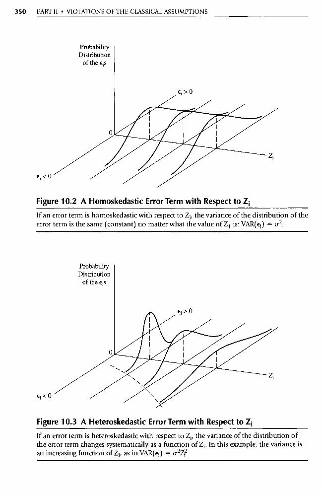
350 PART II • VIOLATIONS OF THE CLASSICAL ASSUMPTIONS
Probability Distribution
of the Eis
Ei <
Figure 10.2 A Homoskedastic Error Term with Respect to Zi
If an error term is homoskedastic with respect to Z i, the variance of the distribution of the error term is the same (constant) no matter what the value of Z 1 is: VAR(€;) = Q2 .
Probability Distribution
of the €is
Ei < 0
Figure 10.3 A Heteroskedastic Error Term with Respect to Z i
If an error term is heteroskedastic with respect to Z ;, the variance of the distribution of the error term changes systematically as a function of Z i . In this example, the variance is an increasing function of Z 1, as in VAR(€;) = Œ2z?
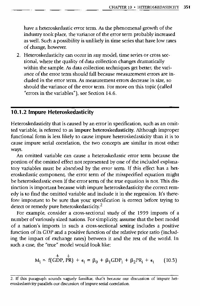
CHAPTER 10 • HETEROSKEDASTICITY 351
have a heteroskedastic error term. As the phenomenal growth of the industry took place, the variance of the error term probably increased as well. Such a possibility is unlikely in time series that have low rates of change, however.
2. Heteroskedasticity can occur in any model, time series or cross sec-tional, where the quality of data collection changes dramatically within the sample. As data collection techniques get better, the vari- ance of the error term should fall because measurement errors are in-cluded in the error term. As measurement errors decrease in size, so should the variance of the error term. For more on this topic (called "errors in the variables"), see Section 14.6.
10.1.2 Impure Heteroskedasticity
Heteroskedasticity that is caused by an error in specification, such as an omit-ted variable, is referred to as impure heteroskedasticity. Although improper functional form is less likely to cause impure heteroskedasticity than it is to cause impure serial correlation, the two concepts are similar in most other ways.
An omitted variable can cause a heteroskedastic error term because the portion of the omitted effect not represented by one of the included explana-tory variables must be absorbed by the error term. If this effect has a het-eroskedastic component, the error term of the misspecified equation might be heteroskedastic even if the error term of the true equation is not. This dis-tinction is important because with impure heteroskedasticity the correct rem-edy is to find the omitted va riable and include it in the regression. It's there-fore impo rtant to be sure that your specification is correct before trying to detect or remedy pure heteroskedasticity. 2
For example, consider a cross-sectional study of the 1999 impo rts of a number of variously sized nations. For simplicity, assume that the best model of a nation's imports in such a cross-sectional setting includes a positive function of its GDP and a positive function of the relative price ratio (includ-ing the impact of exchange rates) between it and the rest of the world. In such a case, the "true" model would look like:
+ + Mi = f(GDP, PR) + Ei = R0 + R 1 GDPi + [32PRi + Ei (10.5)
2. If this paragraph sounds vaguely familiar, that's because our discussion of impure het-eroskedasticity parallels our discussion of impure serial correlation.
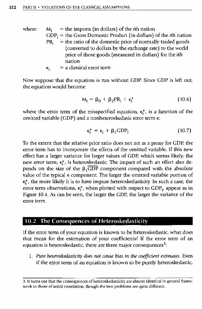
352 PART II • VIOLATIONS OF THE CLASSICAL ASSUMPTIONS
where: M 1 = the impo rts (in dollars) of the ith nation GDPi = the Gross Domestic Product (in dollars) of the ith nation PR; = the ratio of the domestic price of normally traded goods
(converted to dollars by the exchange rate) to the world price of those goods (measured in dollars) for the ith nation
Ei = a classical error term
Now suppose that the equation is run without GDP. Since GDP is left out, the equation would become:
M;= 130 +(32PRi + EI (10.6)
where the error term of the misspecified equation, Ei , is a function of the omitted va riable (GDP) and a nonheteroskedasic error term E:
Ei = Ei + 131 GDP; (10.7)
To the extent that the relative price ratio does not act as a proxy for GDP, the error term has to incorporate the effects of the omitted variable. If this new effect has a larger variance for larger values of GDP, which seems likely, the new error term, e , is heteroskedastic. The impact of such an effect also de-pends on the size of the 13 1 GDP component compared with the absolute value of the typical E component. The larger the omitted variable po rtion of Ei , the more likely it is to have impure heteroskedasticity. In such a case, the error term observations, Ei , when plotted with respect to GDP ;, appear as in Figure 10.4. As can be seen, the larger the GDP, the larger the variance of the error term.
10.2 The Consequences of Heteroskedasticity
If the error term of your equation is known to be heteroskedastic, what does that mean for the estimation of your coefficients? If the error term of an equation is heteroskedastic, there are three major consequences 3 :
1. Pure heteroshedasticity does not cause bias in the coefficient estimates. Even if the error term of an equation is known to be purely heteroskedastic,
3. It turns out that the consequences of heteroskedasticity are almost identical in general frame-work to those of serial correlation, though the two problems are quite different.
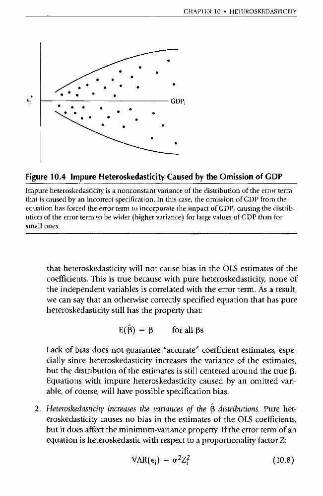
CHAPTER 10 • HETEROSKEDASTICITY
•
GDP;
•
Figure 10.4 Impure Heteroskedasticity Caused by the Omission of GDP
Impure heteroskedasticity is a nonconstant variance of the distribution of the error term that is caused by an incorrect specification. In this case, the omission of GDP from the equation has forced the error term to incorporate the impact of GDP, causing the distrib-ution of the error term to be wider (higher variance) for large values of GDP than for small ones.
that heteroskedasticity will not cause bias in the OLS estimates of the coefficients. This is true because with pure heteroskedasticity, none of the independent variables is correlated with the error term. As a result, we can say that an otherwise correctly specified equation that has pure heteroskedasticity still has the property that:
E0) = (3 for all (3s
Lack of bias does not guarantee "accurate" coefficient estimates, espe-cially since heteroskedasticity increases the variance of the estimates, but the distribution of the estimates is still centered around the true (3. Equations with impure heteroskedasticity caused by an omitted vari-able, of course, will have possible specification bias.
2. Heteroskedasticity increases the variances of the R distributions. Pure het-eroskedasticity causes no bias in the estimates of the OLS coefficients, but it does affect the minimum-variance property. If the error term of an equation is heteroskedastic with respect to a proportionality factor Z:
VAR(ei) = Q2Z; (10.8)
354 PART II • VIOLATIONS OF THE CLASSICAL ASSUMPTIONS
then the minimum-variance po rtion of the Gauss-Markov Theorem cannot be proven because there are other linear unbiased estimators that have smaller variances. This is because the heteroskedastic error term causes the dependent variable to fluctuate in a way that the OLS es-timation procedure attributes to the independent variables. Thus, OLS is more likely to misestimate the true 13 in the face of heteroskedasticity. On balance, the (3s are still unbiased because overestimates are just as likely as underestimates; however, these errors increase the va riance of the distribution of the estimates, increasing the amount that any given estimate is likely to differ from the true 13. (See Figure 10.5.)
3. Heteroskedasticity causes OLS to tend to underestimate the variances (and standard errors) of the coefficients. Heteroskedasticity turns out to in-crease the variances of the 13s in a way that is masked by the OLS esti-mates of them, and OLS nearly always underestimates those variances. 4
As a result, neither the t-statistic nor the F-statistic can be relied on in the face of uncorrected heteroskedasticity. In practice, OLS usually ends up with higher t-scores than would be obtained if the error terms were homoskedastic, sometimes leading researchers to reject null hypothe-ses that shouldn't be rejected.
Why does heteroskedasticity cause this particular pattern of consequences? As Z and the variance of the distribution of the error term increase, so does the probability of drawing a large (in absolute value) observation of the error term. If the pattern of these large observations happens to be positive when one of the independent variables is substantially above average, the OLS (3 for that va riable will tend to be greater than it would have been otherwise. On the other hand, if the pattern of these large error term observations acciden-tally happens to be negative when one of the Xs is substantially above aver-age, then the OLS (3 for that variable will tend to be less than it would have been. Since the error term is still assumed to be independent of all the ex-planatory variables, overestimates are just as likely as underestimates, and the
4. Actually, the OLS estimates of the variance and the standard error of the coefficient estimates Rk are biased, and the bias is negative as long as cr and (X ki — Xk) 2 are positively correlated. The SE(13)s will be underestimated as long as an increase in X is related to an increase in the variance of the error terms. In economic examples, such a positive correlation would almost al-ways be expected in cases in which a sizable correlation is likely to exist. For some va riables, no correlation at all might exist, but a negative correlation would occur quite infrequently. As a re-sult, the statement that OIS underestimates the variances, although a simplification, is almost always true.

R
R
Without Heteroskedasticity
CHAPTER 10 • HETEROSKEDASTICITY 355
Figure 10.5 R Distribution with and without Heteroskedasticity
Heteroskedasticity increases the variance of the 13s, widening the G3 distribution. It does not cause bias, however, so the 13 distribution is centered around the true 13 whether or not there is heteroskedasticity.
OLS estimator is still unbiased in the face of heteroskedasticity. The het-eroskedasticity has caused the j3s to be farther from the true value, however, and so the variance of the distribution of the 13s has increased.
For example, the real interest rate/budget deficit study of Section 9.2.2 could just as well be a hypothetical example of the consequences of het-eroskedasticity. The OLS-estimated t-scores are too high, leading to potential mistakes of inference whenever t-tests are used in heteroskedastic equations. Before we can get rid of heteroskedasticity, however, we must detect it.
10.3 Testing for Heteroskedasticity
Econometricians do not all use the same test for heteroskedasticity because heteroskedasticity takes a number of different forms, and its precise manifes-tation in a given equation is almost never known. The "Z i proportionality factor" approach of this chapter, for example, is only one of many specifica-
356 PART H • VIOLATIONS OF THE CLASSICAL ASSUMPTIONS
tions of the form of heteroskedasticity. As a result, there is no universally agreed upon method of testing for heteroskedasticity; econometrics text-books list as many as eight different methods of such testing.
Because of this wide variety, we'll describe the use of two different tests for heteroskedasticity. Our primary focus will be on the Park test, because it tests precisely the functional form that we use in this chapter to illustrate the problem of pure heteroskedasticity, and the White test, which is more gener-ally used than the Park test. No test for heteroskedasticity can "prove" that heteroskedasticity exists in an equation, though, so the best we can do is to get a general indication of its likelihood.
There's no need to run a heteroskedasticity test for every specification esti-mated, however, so before using any test, it's a good idea to ask the following preliminary questions:
1. Are there any obvious specification errors? If the estimated equation is suspected of having an omitted variable or is about to be rerun for some other specification reason, a test for heteroskedasticity should be delayed until the specification is as good as possible.
2. Is the subject of the research often afflicted with heteroskedasticity? Not only are cross-sectional studies the most likely source of het-eroskedasticity, but some cross-sectional studies (with large variations in the size of the dependent variable, for instance) are more suscepti-ble to heteroskedasticity than others.
3. Finally, does a graph of the residuals show any evidence of het-eroskedasticity? It sometimes saves time to plot the residuals with re-spect to a potential Z proportionality factor. In such cases, the graphs can often show that heteroskedasticity is or is not likely without a test. Figure 10.4 shows an example of what to look for: an expanding (or contracting) range of the residuals.
10.3.1 The Park Test
How do we test for pure heteroskedasticity of the form that we assumed in the previous section? That form, as we outlined in the previous section, is:
VAR(Ei) = Q2Z1
where: E = the error term of the equation being estimated Q2 = the variance of the homoskedastic error term Z = the proportionality factor
CHAPTER 10 • HETEROSKEDASTICITY 357
The Park test s is a formal procedure that attempts to test the residuals for this heteroskedasticity in a manner similar to the way that the Durbin-Watson d statistic tests residuals for serial correlation. The Park test has three basic steps. First, the regression equation is estimated by OLS and the residu-als are calculated. Second, the log of the squared residuals is used as the de-pendent variable of an equation whose sole explanatory variable is the log of the proportionality factor Z. Finally, the results of the second regression are tested to see if there is any evidence of heteroskedasticity.
If there is reason to suspect heteroskedasticity, it's appropriate tip run a Park test. Since the Park test is not run automatically by computer regression packages, you should know how to run the test yourself:
1. Obtain the residuals of the estimated regression equation. The first step is to estimate the equation with OLS and then find the residuals from their estimation:
ei = Yi - Yi = Yi - Ro -- RlXli R2X2i (10.9)
These residuals, which are printed out by most computer regression packages, are the same ones used to calculate the Durbin-Watson d sta-tistic to test for serial correlation.
2. Use these residuals to form the dependent variable in a second regression. In particular, the Park test suggests that you run the following double-log regression:
ln(e?) = a0 + a 1 1nZi + ui (10.10)
where: ei = the residual from the ith observation from Equation 10.9
Zi = your best choice as to the possible proportionality fac-tor (Z)
ui = a classical (homoskedastic) error term 6
5. R. E. Park, "Estimation with Heteroskedastic Error Terms," Econometrica, October 1966, p. 888.
6. One criticism of the Park test is that this error term is not necessarily homoskedastic. See S. M. Goldfeld and R. E. Quandt, Nonlinear Methods in Econometrics (Amsterdam: North-Hol-land Publishing Company, 1972), pp. 93 -94.
358 PART 1I • VIOLATIONS OF THE CLASSICAL ASSUMPTIONS
3. Test the significance of the coefficient of Z in Equation 10.10 with a t-test. The last step is to use the t-statistic to test the significance of 1nZ in explaining ln(e2) in Equation 10.10. If the coefficient of Z is significantly different from zero, this is evidence of heteroskedastic patterns in the residuals with respect to Z; otherwise, heteroskedasticity related to this particular Z is not supported by the evidence in these residuals. However, it's impossi-ble to prove that a particular equation's error terms are homoskedastic.
The Park test is not always easy to use. Its major problem is the identifica-tion of the proportionality factor Z. Although Z is often an explanatory vari-able in the original regression equation, there is no guarantee of that. A par-ticular Z should be chosen for your Park test only after investigating the type of potential heteroskedasticity in your equation. 7 A good Z is a variable that seems likely to vary with the variance of the error term.
For example, in a cross-sectional model of countries or states, a good Z would be one that measured the size of the observation relative to the depen-dent variable in question. For a dependent variable such as gallons of gaso-line consumed, the number of registered drivers or automobiles might be a better measure of size than the population. Although it's difficult to identity the best Z for a particular equation, it's often easier to distinguish good Zs from bad Zs. In the gasoline consumption equation, for example, a bad Z might be the speed limit in the state because, while the speed limit might be important in determining how much gasoline is used, it is unlikely to "cause" any heteroskedasticity. This is because the speed limit in a state does not vary in size in the same way that gasoline consumption does. The states likely to have large error term variances are not also likely to have high speed limits. For more on this fairly thorny issue, see Exercise 2 at the end of the chapter.
10.3.2 An Example of the Use of the Park Test
Let's return to the Woody's Restaurants example of Section 3.2 and test for heteroskedasticity in the residuals of Equation 3.4. Recall that regression ex- plained the number of customers, as measured by the check volume (Y) at a
7 Some econometricians have suggested using the Park test for insight into the form of the het-eroskedasticity. If VAR(e ;) = Œ2Z , then 1n(e;) should be equal to a o + 21nZi plus an error term. Thus the estimate of the coefficient of InZ in the Park test indicates whether the propor-tionality factor should be squared or raised to some other power. For more on this and its im-plications for deciding which form to use to adjust for heteroskedasticity, see R. S. Pindyck and D. L. Rubinfeld, Econometric Models and Econometric Forecasts (New York: McGraw-Hill, 1998), pp. 148-152.
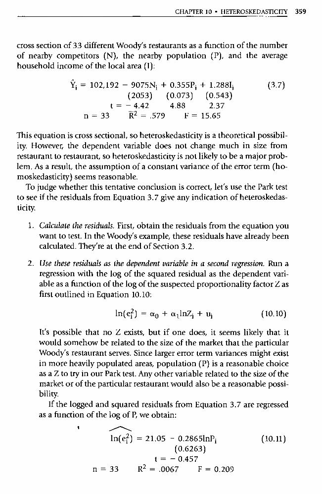
CHAPTER 10 • HETEROSKEDASTICITY 359
cross section of 33 different Woody's restaurants as a function of the number of nearby competitors (N), the nearby population (P), and the average household income of the local area (I):
= 102,192 — 9075Ni + 0.355P; + 1.288I ; (3.7)
(2053) (0.073) (0.543) t = — 4.42 4.88 2.37
n = 33 R2 =.579 F = 15.65
This equation is cross sectional, so heteroskedasticity is a theoretical possibil-ity. However, the dependent variable does not change much in size from restaurant to restaurant, so heteroskedasticity is not likely to be a major prob-lem. As a result, the assumption of a constant variance of the error term (ho-moskedasticity) seems reasonable.
To judge whether this tentative conclusion is correct, let's use the Park test to see if the residuals from Equation 3.7 give any indication of heteroskedas-ticity.
1. Calculate the residuals. First, obtain the residuals from the equation you want to test. In the Woody's example, these residuals have already been calculated. They're at the end of Section 3.2.
2. Use these residuals as the dependent variable in a second regression. Run a regression with the log of the squared residual as the dependent vari-able as a function of the log of the suspected proportionality factor Z as first outlined in Equation 10.10:
ln(e?) = a0 + a 1 1nZi + u; (10.10)
It's possible that no Z exists, but if one does, it seems likely that it would somehow be related to the size of the market that the particular Woody's restaurant se rves. Since larger error term variances might exist in more heavily populated areas, population (P) is a reasonable choice as a Z to try in our Park test. Any other variable related to the size of the market or of the particular restaurant would also be a reasonable possi-bility.
If the logged and squared residuals from Equation 3.7 are regressed as a function of the log of P, we obtain:
In(e?) = 21.05 — 0.28651nP; (0.6263)
t = — 0.457 n = 33 R2 = .0067 F = 0.209

360 PART II • VIOLATIONS OF THE CLASSICAL ASSUMPTIONS
3. Test the significance of a- in Equation 10.10. As can be seen from the cal-culated t-score, there is virtually no measurable relationship between the squared residuals of Equation 3.7 and population. The calculated t-score of —0.457 is quite a bit smaller in absolute value than 2.750, the critical t-value (from Statistical Table B-1) for a two-tailed, one per-cent test. As a result, we would not be able to reject the null hypothesis of homoskedasticity8 -
Ho : a i = 0 HA: a i 2 0
For more practice in the use of the Park test, see Exercise 4 at the end of the chapter.
10.3.3 The White Test
Unfortunately, to use the Park test we must know Z i, the variable suspected of being proportional to the possible heteroskedasticity. Quite often, however, we may want to test the possibility that more than one proportionality factor is involved simultaneously. Less frequently, we might not be able to decide which of a number of possible Z factors to test. In either of these situations, it's unadvisable to run a series of Park tests (one for each possible propor-tionality factor). Instead, it is appropriate to use the White test, one of a fam-ily of such tests.
Like the Park test, the White test y approaches the detection of het-eroskedasticity by running a regression with the squared residuals as the de-pendent variable. This time, though, the right-hand side of the secondary
8. Recall that not being able to reject the null hypothesis of homoskedasticity doesn't prove that the error terms are homoskedastic. In addition, note that this Park test says nothing about other proportionality factors or other forms of heteroskedasticity. Although heteroskedasticity of any kind is unlikely in this example because of the nature of the dependent variable, it's pos-sible to find homoskedasticity with respect to one proportionality factor (or form) but het-eroskeZlasticity with respect to some other proportionality factor (or form). Careful thinking is necessary before a potential Z can be chosen. Running a Park test on every conceivable variable would do little but increase the chance of Type I Error (rejecting the null hypothesis of ho-moskedasticity when it's true).
9. These are a general group of tests based on the Lagrange Multiplier (LM). For more on LM tests, see Section 12.2.
10. Halbert White, "A Heteroskedasticity-Consistent Cova riance Matrix Estimator and a Direct Test for Heteroskedasticity," Econometrica, 1980, pp. 817-838.
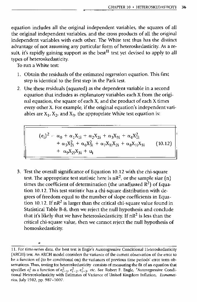
CHAFFER 10 • HETEROSKEDASTICITY 36
equation includes all the original independent variables, the squares of all the original independent variables, and the cross products of all the original independent variables with each other. The White test thus has the distinct advantage of not assuming any particular form of heteroskedasticity. As a re-sult, it's rapidly gaining suppo rt as the best ll test yet devised to apply to all types of heteroskedasticity.
To run a White test:
1. Obtain the residuals of the estimated regression equation. This first step is identical to the first step in the Park test.
2. Use these residuals (squared) as the dependent variable in a second equation that includes as explanatory variables each X from the origi-nal equation, the square of each X, and the product of each X times every other X. For example, if the original equation's independent vari-ables are X 1 , X2, and X3 , the appropriate White test equation is:
(ei) 2 ^ a0 + a1Xli + a2X2i + a3X3i + a4Xli + a5X3i + a6X3i + a7X1iX2i + a8X1iX3i + a9X2iX3i + Ili
(10.12)
3. Test the overall significance of Equation 10.12 with the chi-square test. The appropriate test statistic here is nR 2, or the sample size (n) times the coefficient of determination (the unadjusted R 2) of Equa-tion 10.12. This test statistic has a chi-square distribution with de- grees of freedom equal to the number of slope coefficients in Equa-tion 10.12. If nR2 is larger than the critical chi-square value found in Statistical Table B-8, then we reject the null hypothesis and conclude that it's likely that we have heteroskedasticity. If nR 2 is less than the critical chi-square value, then we cannot reject the null hypothesis of homoskedasticity.
r
11. For time-series data, the best test is Englé s Autoregressive Conditional Heteroskedasticity (ARCH) test. An ARCH model considers the variance of the current observation of the error to be a function of (to be conditional on) the variances of previous time periods' error term ob-servations. Thus, testing for heteroskedasticity consists of measuring the fit of an equation that specifies et as a function of eC 1 , e; 2, et 3 , etc. See Robe rt F. Engle, "Autoregressive Condi-tional Heteroskedasticity with Estimates of Variance of United Kingdom Inflation, Economet-rica, July 1982, pp. 987-1007.
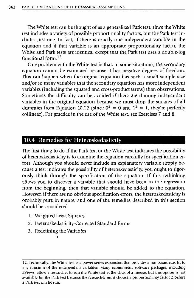
362 PART II • VIOLATIONS OF THE CLASSICAL ASSUMPTIONS
The White test can be thought of as a generalized Park test, since the White test includes a variety of possible proportionality factors, but the Park test in-cludes just one. In fact, if there is exactly one independent variable in the equation and if that va riable is an appropriate proportionality factor, the White and Park tests are identical except that the Park test uses a double-log functional form. 12
One problem with the White test is that, in some situations, the secondary equation cannot be estimated because it has negative degrees of freedom. This can happen when the original equation has such a small sample size and/or so many variables that the secondary equation has more independent variables (including the squared and cross-product terms) than observations. Sometimes the difficulty can be avoided if there are dummy independent variables in the original equation because we must drop the squares of all dummies from Equation 10.12 (since 02 = 0 and 1 2 = 1, they're perfectly collinear). For practice in the use of the White test, see Exercises 7 and 8.
10.4 Remedies for Heteroskedasticity
The first thing to do if the Park test or the White test indicates the possibility of heteroskedasticity is to examine the equation carefully for specification er-rors. Although you should never include an explanatory variable simply be-cause a test indicates the possibility of heteroskedasticity, you ought to rigor-ously think through the specification of the equation. If this rethinking allows you to discover a variable that should have been in the regression from the beginning, then that variable should be added to the equation. However, if there are no obvious specification errors, the heteroskedasticity is probably pure in nature, and one of the remedies described in this section should be considered:
1. Weighted Least Squares
2. Heteroskedasticity-Corrected Standard Errors
3. Redefining the Variables I
12. Technically, the White test is a power series expansion that provides a nonparametric fit to any function of the independent variables. Many econometric software packages, including EViews, allow a researcher to run the White test at the click of a mouse, but this option is not available for the Park test because the researcher must choose a proportionality factor Z before a Park test can be run.
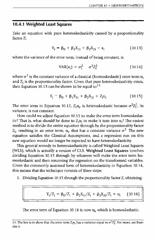
CHAPTER 10 • HETEROSKEDASTICITY
10.4.1 Weighted Least Squares
Take an equation with pure heteroskedasticity caused by a proportionality factor Z:
Yi = Ro + (3 1X11 + i3 2X2i + Ei (10.13)
where the variance of the error term, instead of being constant, is
VAR(Ei) = Q2 0 2Z;
(10.14)
where Q 2 is the constant variance of a classical (homoskedastic) error term u i and Zi is the proportionality factor. Given that pure heteroskedasticity exists,
then Equation 10.13 can be shown to be equal to 13.
Yi—(3o+131X11+(32X21+Ziui (10.15)
The error term in Equation 10.15, Z iui, is heteroskedastic because Π2Z; , its variance, is not constant.
How could we adjust Equation 10.15 to make the error term homoskedas-tic? That is, what should be done to Z iui to make it turn into u i ? The easiest method is to divide the entire equation through by the proportionality factor
resulting in an error term, u i, that has a constant variance cr2 The new equation satisfies the Classical Assumptions, and a regression mn on this new equation would no longer be expected to have heteroskedasticity.
This general remedy to heteroskedasticity is called Weighted Least Squares (WLS), which is actually a version of GLS. Weighted Least Squares involves dividing Equation 10.15 through by whatever will make the error term ho-moskedastic and then rerunning the regression on the transformed variables. Given the commonly assumed form of heteroskedasticity in Equation 10.14, this means that the technique consists of three steps:
1. Dividing Equation 10.15 through the proportionality factor Z, obtaining:
Yi/Zi = 130/Zi + 13 1X1i/Zi + 132X2i/Zi + u i (10.16)
The error term of Equation 10.16 is now u i, which is homoskedastic.
13. The key is to show that the error term Z 1u; has a variance equal to Q 2Z; . For more, see Exer-cise 6.
364 PART II • VIOLATIONS OF THE CLASSICAL ASSUMPTIONS
2. Recalculate the data for the variables to conform to Equation 10.16.
3. Estimate Equation 10.16 with OLS.
This third step in Weighted Least Squares, the estimation of the trans-formed equation, is fairly tricky, because the exact details of how to complete this regression depend on whether the proportionality factor Z is also an ex-planatory variable in Equation 10.13. If Z is not an explanatory variable in Equation 10.13, then the regression to be run in step 3 might seem to be:
Yi/Zi = Ro/Zi + 13 IX1i/Zi + 132X2i/Zi + u i (10.17)
Note, however, that this equation has no constant term. Most OLS computer packages can run such a regression only if the equation is forced through the ori- gin by specifically suppressing the intercept with an instruction to the computer.
As pointed out in Section 7.1, however, the omission of the constant term forces the constant effect of omitted va riables, nonlinearities, and measure-ment error into the other coefficient estimates. To avoid having these con-stant term elements forced into the slope coefficient estimates, one alterna-tive approach to Equation 10.17 is to add a constant term before the transformed equation is estimated. 14 Consequently, when Z is not identical to one of the Xs in the o riginal equation, then we suggest that the following specification be run as step 3 in Weighted Least Squares:
Yi /Zi = a0 + Ro/Zi + R1X1i/Zi + 132X2i/Zi + ui (10.18)
If Z is an explanatory variable in Equation 10.13, then no constant term need be added because one already exists. Look again at Equation 10.17 If Z = X1 (or, similarly, if Z = X2), then one of the slope coefficients becomes the constant term in the transformed equation because X l/Z = 1:
Yi /Zi = Ro/Zi + R 1 + R2X2i/Zi + ui (10.19)
If this form of Weighted Least Squares is used, however, coefficients obtained from an estimation of Equation 10.19 must be interpreted very carefully. No-tice that f3 1 is now the intercept term of Equation 10.19 even though it is a slope coefficient in Equation 10.13 and that 13 0 is a slope coefficient in Equa-tion 10.19, even though it is the intercept in Equation 10.13. As a result, a re-searcher interested in an estimate of the coefficient of X 1 in Equation 10.13 would have to examine the intercept of Equation 10.19, and a researcher in-
14. The suggestion of adding a constant term is also made by Potluri Rao and Roger LeRoy Miller, Applied Econometrics (Belmont, California: Wadsworth, 1971), p. 121, and others. Some authors prefer not to add a constant because Equation 10.18 becomes more difficult to interpret.
CHAPTER 10 • HETEROSKEDASTICITY 365
terested in an estimate of the intercept term of Equation 10.13 would have to examine the coefficient of 1 /Z i in Equation 10.19. The computer will print out 13 0 as a "slope coefficient" and 13 1 as a "constant term" when in reality they are estimates of the opposite coefficients in the original Equation 10.13.
There are three other major problems with using Weighted Least Squares:
1. The job of identifying the proportionality factor Z is, as has been pointed out, quite difficult.
2. The functional form that relates the Z factor to the variance of the er-ror term of the original equation may not be our assumed squared function of Equation 10.14. When some other functional relationship is involved, a different transformation is required. For more on these advanced transformations, see Exercise 12.
3. Sometimes Weighted Least Squares is applied to an equation with im-pure heteroskedasticity. In such cases, it can be shown that the WLS es-timates reduce somewhat the bias from an omitted variable, but the estimates are inferior to those obtained from the correctly specified equation.
10.4.2 Heteroskedasticity-Corrected Standard Errors
The most popular remedy for heteroskedasticity is heteroskedasticity-corrected standard errors, which take a completely different approach to the problem. It focuses on improving the estimation of the SE(13)s without changing the estimates of the slope coefficients. The logic behind this ap-proach is powerful. Since heteroskedasticity causes problems with the SE((3)s but not with the 1j,s, it makes sense to improve the estimation of the SE((3)s in a way that doesn't alter the estimates of the slope coefficients. This differs from our other two remedies because both WLS and reformulating the equa-tion affect the 13s as well as the SE(13)s.
Thus, heteroskedasticity-corrected (HC) standard errors are SE(13)s that have been calculated specifically to avoid the consequences of heteroskedas-ticity. 15 The HC procedure yields an estimator of the standard errors that,
15. For a linear regression model with one independent variable in which both X and Y are measured as deviations from the mean, the HC estimator of the variance of the estimated slope coefficient is
T X2e 2 tt
t= 1
C T
)2,
E X2 t t = 1
where et is the OLS residual for observation t.
366 PART II • VIOLATIONS OF THE CLASSICAL ASSUMPTIONS
while they are biased, are generally more accurate than uncorrected standard errors for large samples in the face of heteroskedasticity. As a result, the HC SE( [',)s can be used in t-tests and other hypothesis tests in most samples with-out the errors of inference potentially caused by heteroskedasticity. Typically, the HC SE(i3)s are greater than the OLS SE(I3)s, thus producing lower t-scores and decreasing the probability that a given estimated coefficient will be signif-icantly different from zero. The technique was suggested by Halbert White in the same a rticle in which he proposed the White test for heteroskedasticity. 16
There are a few problems with using heteroskedasticity-corrected standard errors. First, as mentioned, the technique works best in large samples. Sec-ond, details of the calculation of the HC SE fl3)s are beyond the scope of this text and imply a model that is substantially more general than the basic the-oretical construct, VAR(€) = 0- 2Z; , of this chapter. In addition, not all com-puter regression software packages calculate heteroskedasticity-corrected standard errors.
10.4.3 Redefining the Variables
Another approach to ridding an equation of heteroskedasticity is to go back to the basic underlying theory of the equation and redefine the variables in a way that avoids heteroskedasticity. A redefinition of the variables often is use-ful in allowing the estimated equation to focus more on the behavioral as-pects of the relationship. Such a rethinking is a difficult and discouraging process because it appears to dismiss all the work already done. However, once the theoretical work has been reviewed, the alternative approaches that are discovered are often exciting in that they offer possible ways to avoid problems that had previously seemed insurmountable.
In some cases, the only redefinition that's needed to rid an equation of heteroskedasticity is to switch from a linear functional form to a double-log functional form. The double-log form has inherently less variation than the linear form, so it's less likely to encounter heteroskedasticity. In addition, there are many research topics for which the double-log form is just as theo-retically logical as the linear form. This is especially true if the linear form was chosen by default, as is often the case.
16. Halbert White, "A Heteroskedasticity-Consistent Covariance Matrix Estimator and a Direct Test of Heteroskedasticity," Econometrica, 1980, pp. 817-838. Most authors refer to this method as HCCM, for heteroskedasticity-consistent covariance matrix. Note that Newey-West standard errors, introduced in Section 9.4, also can be used as HC standard errors. Indeed, some econometric software packages, including EViews, provide a choice between the White and Newey-West procedures. Unless otherwise noted, however, HC standard errors should be assumed to be of the White variety.
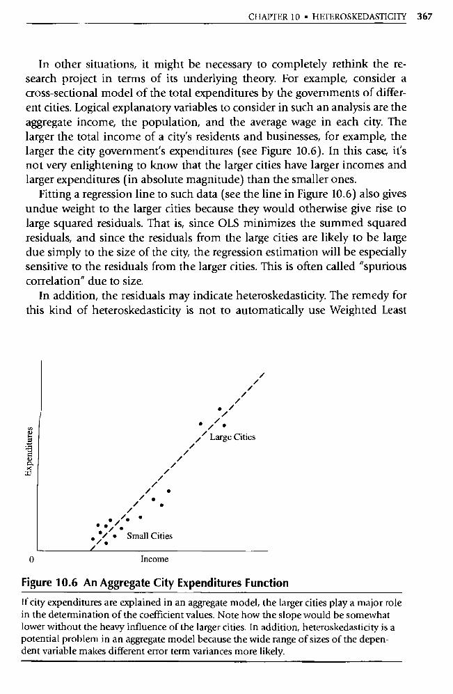
/ /
/ /
• / /
/
• • // Large Cities
/ /
/ / •
/
I . / • • /• •
• •//• •j • Small Cities
CHAPTER 10 • HETEROSKEDASTICITY 367
In other situations, it might be necessary to completely rethink the re-search project in terms of its underlying theory. For example, consider a
cross-sectional model of the total expenditures by the governments of differ-ent cities. Logical explanatory va riables to consider in such an analysis are the aggregate income, the population, and the average wage in each city. The
larger the total income of a city's residents and businesses, for example, the
larger the city government's expenditures (see Figure 10.6). In this case, it's
not very enlightening to know that the larger cities have larger incomes and
larger expenditures (in absolute magnitude) than the smaller ones.
Fitting a regression line to such data (see the line in Figure 10.6) also gives
undue weight to the larger cities because they would otherwise give rise to
large squared residuals. That is, since OLS minimizes the summed squared residuals, and since the residuals from the large cities are likely to be large
due simply to the size of the city, the regression estimation will be especially
sensitive to the residuals from the larger cities. This is often called "spurious
correlation" due to size. In addition, the residuals may indicate heteroskedasticity. The remedy for
this kind of heteroskedasticity is not to automatically use Weighted Least
0 Income
Figure 10.6 An Aggregate City Expenditures Function
If city expenditures are explained in an aggregate model, the larger cities play a major role
in the determination of the coefficient values. Note how the slope would be somewhat
lower without the heavy influence of the larger cities. In addition, heteroskedasticity is a
potential problem in an aggregate model because the wide range of sizes of the depen-dent variable makes different error term variances more likely.

• ^^ ^^
^ ^—
• • • •
• ^'
•
• Large and Small Cities .
▪
•
▪
Given Equal Weight
0
Income Per Capita
Figure 10.7 A per Capita City Expenditures Function
Exp
end i
ture
s Pe
r C
apita
ro
368 PART II • VIOLATIONS OF THE CLASSICAL ASSUMPTIONS
Squares, however, nor is it to throw out the observations from large cities. It
makes sense to consider reformulating the model in a way that will discount
the scale factor (the size of the cities) and emphasize the underlying behav-ior. In this case, per capita expenditures would be a logical dependent vari-able. Such a transformation is shown in Figure 10.7 This form of the equa-tion places New York and Los Angeles on the same scale as, say, Pasadena or
New Brunswick and thus gives them the same weight in estimation. If an ex-planatory variable happened not to be a function of the size of the city, how-ever, it would not need to be adjusted to per capita terms. If the equation in-cluded the average wage of city workers, for example, that wage would not be
divided through by population in the transformed equation.
Note that this transformation is similar in some ways to Weighted Least
Squares, since many variables have been divided by population. The differ-ences are that there is no term equal to the reciprocal of population (as there
is in Weighted Least Squares) and that not all explanatory variables are di-vided by population. For the original equation,
EXPi = (3 0 + 13 1 P013; + 02INCi + 133WAGEi + Ei (10.20)
If city expenditures are explained in a per capita model, then large and small cities have
equal weights. In addition, heteroskedasticity is less likely, because the dependent vari-able does not vary over a wide range of sizes.
CHAPTER 10 • HETEROSKEDASTICITY
the Weighted Least Squares version would be:
EXPi/POPi = p 1 + (3p/POPi + p2INC;/POPi (10.21) + j33WAGEi/POP; + u;
and the directly transformed equation would be
EXPi/POP; = a0 + a 1 INCi/POP; + a2WAGEi + ui (10.22)
where EXP ; refers to expenditures, INC ; refers to income, WAGE ; refers to the average wage, and POP, refers to the population of the ith city. As can be seen, the Weighted Least Squares Equation 10.21 divides through the entire equation by population, but the theoretically transformed one divides only expenditures and income by population. While the directly transformed Equation 10.22 does indeed solve any potential heteroskedasticity in the model, such a solution should be considered incidental to the benefits of rethinking the equation in a way that focuses on the basic behavior being examined.
Note that it's possible that the reformulated Equation 10.22 could have hetero-skedasticity; the error va riances might be larger for the observations having the larger per capita values for income and expenditures than they are for smaller per capita values. Thus, it is legitimate to suspect and test for hetero-skedasticity even in this transformed model. Such heteroskedasticity in the transformed equation is unlikely, however, because there will be little of the variation in size normally associated with heteroskedasticity.
A thoughtful transformation of the variables that corrects for hetero-skedasticity and at the same time avoids the spurious correlation due to size may sometimes be the best approach to solving these problems. Note, how-ever, that unlike with Weighted Least Squares, not every variable in the equa-tion is treated the same. Each variable in a cross-sectional model must be ex-amined for possible transformations that will yield a meaningful and properly interpreted regression equation.
10.5 A More Complete Example
Let's work through a more complete example that involves a cross-sectional data set and heteroskedasticity. In the mid-1970s, the U.S. Department of En-ergy attempted to allocate gasoline to regions, states, and even individual re-tailers on the basis of past usage, changing demographics, and other factors. Underlying these allocations must have been some so rt of model of the usage
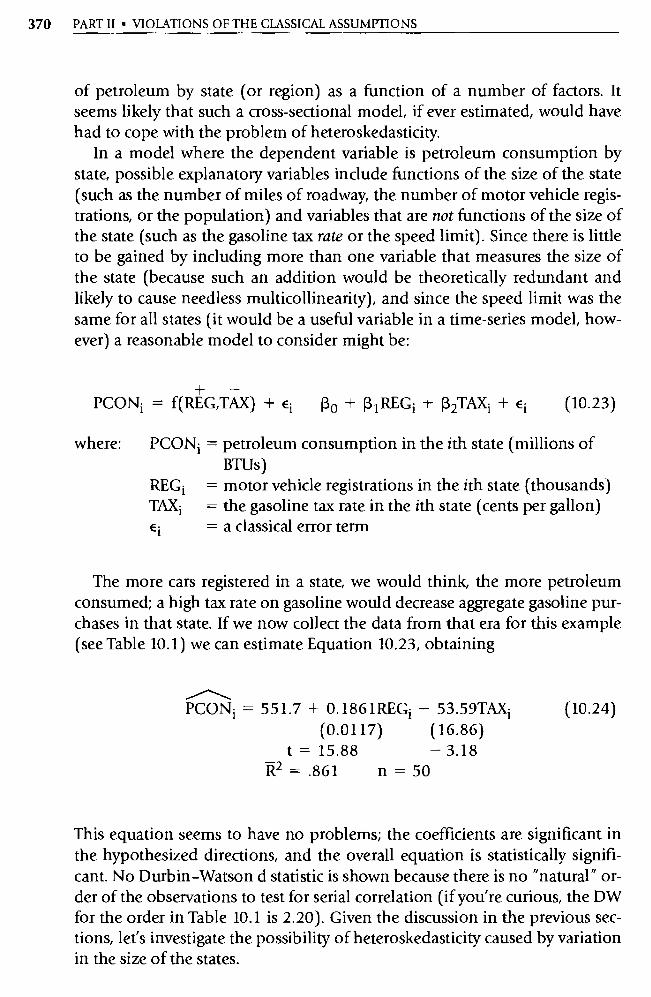
370 PART II • VIOLATIONS OF THE CLASSICAL ASSUMPTIONS
of petroleum by state (or region) as a function of a number of factors. It seems likely that such a cross-sectional model, if ever estimated, would have had to cope with the problem of heteroskedasticity.
In a model where the dependent variable is petroleum consumption by state, possible explanatory variables include functions of the size of the state (such as the number of miles of roadway, the number of motor vehicle regis-trations, or the population) and variables that are not functions of the size of the state (such as the gasoline tax rate or the speed limit). Since there is little to be gained by including more than one variable that measures the size of the state (because such an addition would be theoretically redundant and likely to cause needless multicollinearity), and since the speed limit was the same for all states (it would be a useful variable in a time-series model, how-ever) a reasonable model to consider might be:
+ - PCON; = f(REG,TAX) + E; Ro + R 1 REG ; + 132TAX; + E; (10.23)
where: PCON; = petroleum consumption in the ith state (millions of BTUs)
REG; = motor vehicle registrations in the ith state (thousands) TAX; = the gasoline tax rate in the ith state (cents per gallon) E; = a classical error term
The more cars registered in a state, we would think, the more petroleum consumed; a high tax rate on gasoline would decrease aggregate gasoline pur-chases in that state. If we now collect the data from that era for this example (see Table 10.1) we can estimate Equation 10.23, obtaining
/\ PCON ; = 551.7 + 0.1861REG ; - 53.59TAX;
(0.0117) (16.86) t = 15.88 - 3.18
R2 =.861 n=50
(10.24)
This equation seems to have no problems; the coefficients are significant in the hypothesized directions, and the overall equation is statistically signifi-cant. No Durbin-Watson d statistic is shown because there is no "natural" or-der of the observations to test for serial correlation (if you're curious, the DW for the order in Table 10.1 is 2.20). Given the discussion in the previous sec-tions, let's investigate the possibility of heteroskedasticity caused by variation in the size of the states.

TABLE 10.1 DATA FOR THE PETROLEUM CONSUMPTION EXAMPLE
PCON UHM TAX REG POP e STATE
270 2.2 9 743 1136 62.335 Maine 122 2.4 14 774 948 176.52 New Hampshire
58 0.7 11 351 520 30.481 Vermont 821 20.6 9.9 3750 5 750 101.87 Massachusetts
98 3.6 13 586 953 133.92 Rhode Island 450 10.1 11 2258 3126 67.52 7 Connecticut
1819 36.4 8 8235 17567 163.24 New York 1229 22.2 8 4917 7427 190.83 New Jersey 1200 27.9 11 6725 11879 -13.924 Pennsylvania 1205 29.2 11.7 7636 10772 -140.98 Ohio 650 17.6 11.1 3884 5482 -29.764 Indiana
1198 30.3 7.5 7242 11466 -299.72 Illinois 760 25.1 13 6250 9116 -258.33 Michigan 460 13.8 13 3162 4745 16.446 Wisconsin 503 13.0 13 3278 4133 37.855 Minnesota 371 8.1 13 2346 2906 79.330 Iowa 571 13.9 7 3412 4942 -240.63 Missouri 136 1.6 8 653 672 -108.50 North Dakota 109 1.6 13 615 694 139.52 South Dakota 203 4.3 13.9 1215 1589 170.08 Nebraska 349 8.4 8 2061 2408 -157.58 Kansas 118 1.4 11 415 600 78.568 Delaware 487 9.8 13.5 2893 4270 120.31 Maryland 628 12.4 11 3 705 5485 -23.806 Virginia 192 2.9 10.5 1142 1961 -9.5451 West Virginia 642 17.1 12 4583 6019 -119.64 North Carolina 320 71 13 1975 3227 97.385 South Carolina 677 15.6 7.5 3916 5648 -201.65 Georgia
1459 28.5 8 8335 10466 -215.37 Florida 434 6.9 10 2615 3692 -68.513 Kentucky 482 11.9 9 3381 4656 -216.68 Tennessee 457 13.7 11 3039 3941 -70.842 Alabama 325 6.3 9 1593 2569 -40.877 Mississippi 300 7.4 9.5 1481 2307 -18.235 Arkansas
1417 10.1 8 2800 4383 772.87 Louisiana 451 11.4 6.58 2780 3226 -265.51 Oklahoma
3572 59.9 5 11388 15329 1168.6 Texas 131 2.3 9 758 805 -79.457 Montana 105 2.2 7.5 873 977 -207.25 Idaho 163 1.5 8 508 509 -54.515 Wyoming 323 9.2 9 2502 3071 -212.07 Colorado 192 4.4 11 1193 1367 7.7577 New Mexico 291 8.9 10 2216 2892 -137.25 Arizona 169 5.0 11 1038 1571 13.608 Utah 133 2.4 12 710 876 92.250 Nevada 562 14.8 12 3237 4276 50.895 Washington 364 8.4 8 2075 2668 -145.18 Oregon
2840 62.5 9 17130 24697 -417.81 California 155 1.2 8 319 444 -27.336 Alaska 214 1.3 8.5 586 997 8.7623 Hawaii
Source: 1985 Statistical Abstract (U.S. Department of Commerce), except the residual. Note: Data File = GAS10
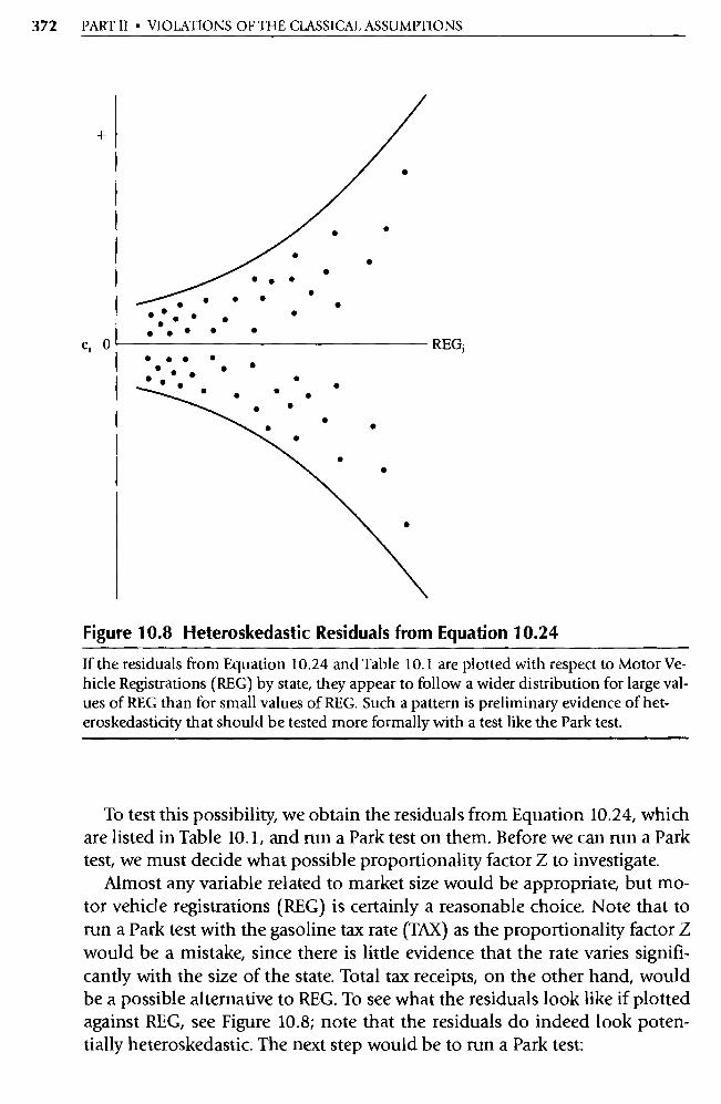
e; 0 REG;
•
•
•
•
•
• • • •
• • • •
• • • • • • • • • •
• •
• •
• • • • • • • •
•• • •
• •
• • • •
• •
•
•
•
•
Figure 10.8 Heteroskedastic Residuals from Equation 10.24
372 PART II • VIOLATIONS OF THE CLASSICAL ASSUMPTIONS
If the residuals from Equation 10.24 and Table 10.1 are plotted with respect to Motor Ve-hicle Registrations (REG) by state, they appear to follow a wider distribution for large val-ues of REG than for small values of REG. Such a pattern is preliminary evidence of het-eroskedasticity that should be tested more formally with a test like the Park test.
To test this possibility, we obtain the residuals from Equation 10.24, which are listed in Table 10.1, and run a Park test on them. Before we can run a Park test, we must decide what possible proportionality factor Z to investigate.
Almost any variable related to market size would be appropriate, but mo-tor vehicle registrations (REG) is certainly a reasonable choice. Note that to run a Park test with the gasoline tax rate (TAX) as the proportionality factor Z would be a mistake, since there is little evidence that the rate varies signifi-cantly with the size of the state. Total tax receipts, on the other hand, would be a possible alternative to REG. To see what the residuals look like if plotted against REG, see Figure 10.8; note that the residuals do indeed look poten-tially heteroskedastic. The next step would be to run a Park test:

CHAPTER 10 • HETEROSKEDASTICITY
ln(e?) = ao + a 1 1nREG; + u; (10.25)
where e; is the residual for the ith state from Equation 10.24, and u ; is a clas-sical (homoskedastic) error term.
If we run this Park test regression, we obtain:
ln(e; ) = 1.650 + 0.9521nREG; (0.308)
t = 3.09 R2 =.148 n = 50 F = 9.533
(10.26)
Since the critical t-value for a 99 percent two-tailed t-test is about 2.7 (inter-polated) in Statistical Table B-1, we can reject the null hypothesis of ho-moskedasticity because the appropriate decision rule is:
Reject H o: a = 0 if I tpARK ^ > 2.7 Do Not Reject H o: if' tpARK I 2.7
Since there appears to be heteroskedasticity in the residuals of Equation 10.24, what should we do? First we think through the specification of the equation in search of an omitted variable. While there are a number of possi-ble ones for this equation, it turns out that all of the ones we tried involve ei-ther significant multicollinearity (as shown in Chapter 8) or do not cure the heteroskedasticity.
As a result, we'll reestimate Equation 10.23 with Weighted Least Squares, using REG as the proportionality factor Z:
PCON;/REG; = Bo/REG; + 13 1 + 132TAXi/REG; + u; (10.27)
which results in the following estimates 17 :
PCON;/REG; = 218.54/REG; + 0.168 — 17.389TAX;/REG; (10.28) (0.014) (4.682)
_ t = 12.27 — 3.71 R2 =.333 n=50
17. Note that we've divided the equation through by REG i. This assumes that the error term ei = Ziui. The coefficient of InREG in the Park test is approximately one, which is evidence that the appropriate functional form may be ei = ui \, but such a transformation should not be
adopted simply on the basis of the Park test coefficient alone. If the underlying theory gives ev-idence in suppo rt of such a change, which is not the case in this example, then we would divide
the equation through by the square root of Zi. For more on this, reread footnote 7.

374 PART II • VIOLATIONS OF THE CLASSICAL ASSUMPTIONS
Compare this result carefully with Equation 10.24. Note that:
1. The coefficient of the reciprocal of REG in Equation 10.28 is really an estimate of the intercept of Equation 10.24, and therefore no t-test is conducted even though the OLS regression program will indicate that it is a slope coefficient.
2. What appears to be the intercept of Equation 10.28 is an estimate of the coefficient of REG in Equation 10.24. Note that this particular esti-mate is quite close in magnitude and significance to the original re-sults in Equation 10.24.
3. The t-score of the coefficient of the proportionality factor, REG, is lower in the Weighted Least Squares estimate than it is in the poten-tially heteroskedastic Equation 10.24. The overall fit is also worse, but this has no particular impo rtance because the dependent variables are different in the two equations.
However, as mentioned in Section 10.4.3, an alternative is to rethink the purpose of the regression and reformulate the variables of the equation to try to avoid heteroskedasticity resulting from spurious correlation due to size. If we were to rethink Equation 10.23, we might decide to attempt to explain per capita petroleum consumption, coming up with:
PCONi/POPi = ^3 p + (3 1 REG i /POPi + 132TAXi + Ei (10.29)
where POP i is the population of the ith state in thousands of people.
We've reformulated the equation in a way similar to Weighted Least
Squares, but we now have an equation that can stand on its own from a theo-retical point of view. If we estimate Equation 10.29, we obtain:
PCONi/POPi = 0.168 + 0.1082REGi/POPi — 0.0103TAXi (0.0716) (0.0035)
t = 1.51 — 2.95 R2 =.165 n=50
(10.30)
If we compare Equation 10.30 with Equations 10.28 and 10.24, we see that
this approach is not necessarily better but quite different. The statistical prop-erties of Equation 10.30, though not directly comparable to the other equa-tions, do not appear as strong as they ought to be, but this is not necessarily
an important factor. Which is better, the unadjusted potentially heteroskedastic equation, the
one derived from Weighted Least Squares, or the reformulated one? It de-
CHAPTER 10 • HETEROSKEDASTICITY 375
pends on the purposes of your research. If your goal is to determine the im-pact of tax rates on gasoline consumption, all three models give virtually the same results in terms of the sign and significance of the coefficient, but the latter two models avoid the heteroskedasticity. If your goal is to allocate pe-troleum in aggregate amounts to states, then the original equation may be just fine. In most cases of severe heteroskedasticity, some remedial action is necessary, but whether Weighted Least Squares or a reformulation is called for depends on the particular equation in question. We generally find that if reformulation makes intuitive sense, it's usually the best remedy to apply, since it more easily avoids the arbitrary process of choosing a Z.
Finally, let's apply the most popular of our remedies, heteroskedasticity-corrected standard errors, to this example. If we start with Equation 10.23 and use White's suggested method for estimating SE((3)s that are minimum variance (for large samples) in the face of heteroskedasticity, we obtain:
PCONi = 551.7 + 0.186REGi 53.59TAXi (10.31) (0.022) (23.90)
t = 8.64 — 2.24 R2 =.86 n=50
Compare Equation 10.31 with Equation 10.24. Note that the slope coeffi-cients are identical, as you'd expect. Also note that the HC SE((3)s are higher than the OLS SE( 3)s, as is usually but not necessarily the case. While the re-sulting t-scores are lower, they are still significantly different from zero in the direction we expected, making Equation 10.31 very appealing indeed.
Is the heteroskedasticity-corrected standard error approach the best one for this example? Most beginning researchers would say yes, because Equa-tion 10.31 has a better overall fit, better t-scores, and easier interpretation than do Equations 10.30 and 10.28. Unfortunately, most experienced re-searchers wouldn't be so sure, in pa rt because the sample size of 50 makes it unlikely that the large sample properties of HC estimation hold in this case. Finally, if t-scores are not being used to test hypotheses or retain variables, as is true in this example, it's not at all clear that any so rt of remedy for het-eroskedasticity is even necessary.
10.6 Summary
1. Heteroskedasticity is the violation of Classical Assumption V that the observations of the error term are drawn from a distribution with a
376 PART II • VIOLATIONS OF THE CLASSICAL ASSUMPTIONS
constant variance. Homoskedastic error term observations are drawn from a distribution that has a constant variance for all observations, and heteroskedastic error term observations are drawn from distribu-tions whose variances differ from different observations. Het-eroskedasticity occurs most frequently in cross-sectional data sets.
2. The variance of a heteroskedastic error term is not equal to 6 2, a con-stant. Instead, it equals u?, where the subscript i indicates that the variance can change from observation to observation. Many different kinds of heteroskedasticity are possible, but a common model is one in which the variance changes systematically as a function of some other variable, a proportionality factor Z:
VAR(E i) = 0- 24
The proportionality factor Z is usually a variable related in some way to the size or accuracy of the dependent variable.
3. Pure heteroskedasticity is a function of the error term of the correctly specified regression equation. Impure heteroskedasticity is caused by a specification error such as an omitted variable.
4. The major consequence of heteroskedasticity is an increase in the variance of the 13s that is masked by an underestimation of the stan-dard errors by OLS. As a result, OLS tends to overestimate t-scores in the face of heteroskedasticity, sometimes leading to errors of infer-ence. Pure heteroskedasticity does not cause bias in the estimates of the 13s themselves.
5. Many tests use the residuals of an equation to test for the possibility of heteroskedasticity in the error terms. The Park test uses a function of these residuals as the dependent va riable of a second regression whose explanatory variable is a function of the suspected proportion-ality factor Z:
ln(e;) =ao +a 1 lnZi +ui
If â 1 is significantly different from zero, then we reject the null hy-pothesis of homoskedasticity.
6. The first step in correcting heteroskedasticity is to check for an omit-ted variable that might be causing impure heteroskedasticity. If the specification is as good as possible, then solutions such as Weighted Least Squares or HC standard errors should be considered.
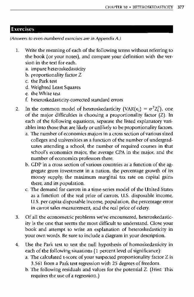
CHAPTER 10 • HETEROSKEDASTICITY 377
Exercises
(Answers to even -numbered exercises are in Appendix A.)
1. Write the meaning of each of the following terms without referring to the book (or your notes), and compare your definition with the ver-sion in the text for each. a. impure heteroskedasticity b. proportionality factor Z c. the Park test d. Weighted Least Squares e. the White test f. heteroskedasticity-corrected standard errors
2. In the common model of heteroskedasticity (VAR(e) = Π2Z?), one of the major difficulties is choosing a proportionality factor (Z). In each of the following equations, separate the listed explanatory vari-ables into those that are likely or unlikely to be proportionality factors. a. The number of economics majors in a cross section of various sized
colleges and universities as a function of the number of undergrad-uates attending a school, the number of required courses in that school's economics major, the average GPA in the major, and the number of economics professors there.
b. GDP in a cross section of various countries as a function of the ag-gregate gross investment in a nation, the percentage growth of its money supply, the maximum marginal tax rate on capital gains there, and its population.
c. The demand for carrots in a time-series model of the United States as a function of the real price of carrots, U.S. disposable income, U.S. per capita disposable income, population, the percentage error in carrot sales measurement, and the real price of celery.
3. Of all the econometric problems we've encountered, heteroskedastic-ity is the one that seems the most difficult to understand. Close your book and attempt to write an explanation of heteroskedasticity in your own words. Be sure to include a diagram in your description.
4. Use the Park test to test the null hypothesis of homoskedasticity in each of the following situations (1 percent level of significance): a. The calculated t -score of your suspected proportionality factor Z is
3.561 from a Park test regression with 25 degrees of freedom. b. The following residuals and values for the potential Z. (Hint: This
requires the use of a regression.)
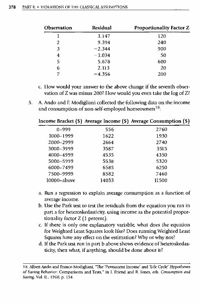
378 PART II • VIOLATIONS OF THE CLASSICAL ASSUMPTIONS
Observation Residual Proportionality Factor Z
1 3.147 120 2 9.394 240 3 -2.344 900 4 -1.034 50 5 5.678 600 6 2.113 20 7 -4.356 200
c. How would your answer to the above change if the seventh obser-vation of Z was minus 200? How would you even take the log of Z?
5. A. Ando and F. Modigliani collected the following data on the income and consumption of non-self-employed homeowners 18 :
Income Bracket ($) Average Income ($) Average Consumption ($)
0-999 556 2760 1000-1999 1622 1930 2000-2999 2664 2740 3000-3999 3587 3515 4000-4999 4535 4350 5000-5999 5538 5320 6000-7499 6585 6250 7500-9999 8582 7460
10000-above 14033 11500
a. Run a regression to explain average consumption as a function of average income.
b. Use the Park test to test the residuals from the equation you ran in part a for heteroskedasticity, using income as the potential propor-tionality factor Z (1 percent).
c. If there is only one explanatory variable, what does the equation for Weighted Least Squares look like? Does running Weighted Least Squares have any effect on the estimation? Why or why not?
d. If the Park test run in pa rt b above shows evidence of heteroskedas-ticity, then what, if anything, should be done about it?
18. Albert Ando and Franco Modigliani, "The 'Permanent Incomé and 'Life Cycle' Hypotheses of Saving Behavior: Comparisons and Tests," in I. Friend and R. Jones, eds. Consumption and Saving, Vol. II., 1960, p. 154.
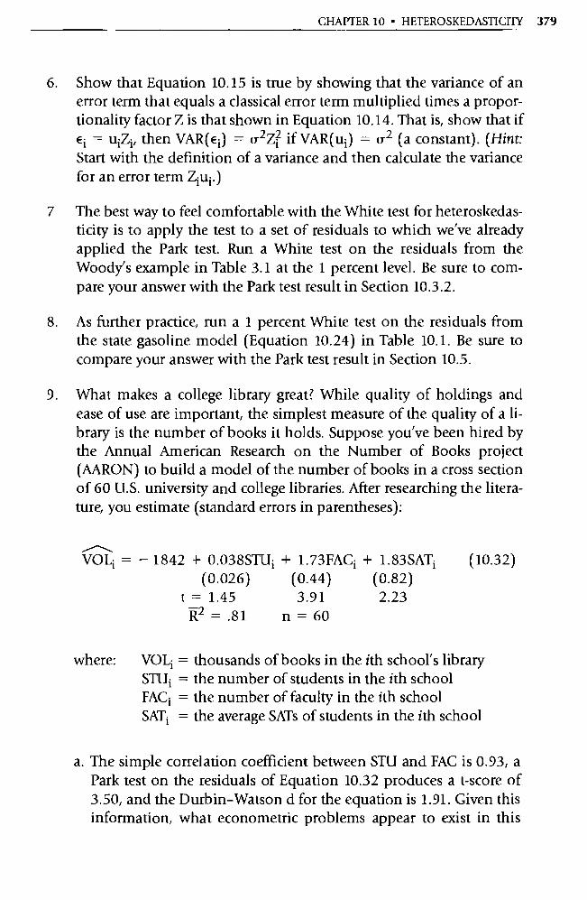
CHAPTER 10 • HETEROSKEDASTICITY 379
6. Show that Equation 10.15 is true by showing that the variance of an error term that equals a classical error term multiplied times a propor-tionality factor Z is that shown in Equation 10.14. That is, show that if Ei = uiZi, then VAR(Ei) = Q2Z1 if VAR(ui) = o-2 (a constant). (Hint: Start with the definition of a va riance and then calculate the variance for an error term Z iui .)
7 The best way to feel comfortable with the White test for heteroskedas-ticity is to apply the test to a set of residuals to which we've already applied the Park test. Run a White test on the residuals from the Woodÿ s example in Table 3.1 at the 1 percent level. Be sure to com-pare your answer with the Park test result in Section 10.3.2.
8. As further practice, run a 1 percent White test on the residuals from the state gasoline model (Equation 10.24) in Table 10.1. Be sure to compare your answer with the Park test result in Section 10.5.
9. What makes a college library great? While quality of holdings and ease of use are important, the simplest measure of the quality of a li-brary is the number of books it holds. Suppose you've been hired by the Annual American Research on the Number of Books project (AARON) to build a model of the number of books in a cross section of 60 U.S. university and college libraries. After researching the litera-ture, you estimate (standard errors in parentheses):
VOLT = - 1842 + 0.038STU i + 1.73FACi + 1.83SATi (10.32)
(0.026) (0.44) (0.82) t = 1.45 3.91 2.23
R2 = .81 n=60
where: VOLT = thousands of books in the ith school's library STUi = the number of students in the ith school FAC T = the number of faculty in the ith school SATi = the average SATs of students in the ith school
a. The simple correlation coefficient between STU and FAC is 0.93, a Park test on the residuals of Equation 10.32 produces a t-score of 3.50, and the Durbin-Watson d for the equation is 1.91. Given this information, what econometric problems appear to exist in this
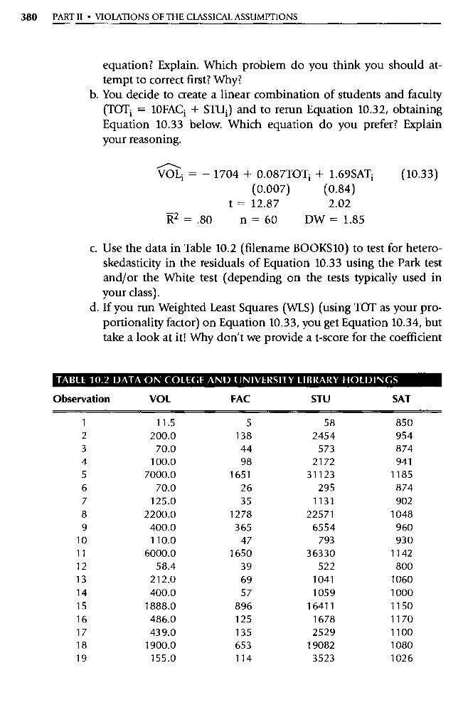
380 PART II • VIOLATIONS OF THE CLASSICAL ASSUMPTIONS
equation? Explain. Which problem do you think you should at-tempt to correct first? Why?
b. You decide to create a linear combination of students and faculty (TOT; = 10FACi + STUi) and to rerun Equation 10.32, obtaining Equation 10.33 below. Which equation do you prefer? Explain your reasoning.
VOLT = — 1704 + 0.087TOTi + 1.69SATi (10.33) (0.007)
(0.84)
t = 12.87
2.02 R2 =.80 n=60
DW — 1.85
c. Use the data in Table 10.2 (filename BOOKS10) to test for hetero-skedasticity in the residuals of Equation 10.33 using the Park test and/or the White test (depending on the tests typically used in your class).
d. If you run Weighted Least Squares (WLS) (using TOT as your pro-portionality factor) on Equation 10.33, you get Equation 10.34, but take a look at it! Why don't we provide a t-score for the coefficient
TABLE 10.2 DATA ON COLEGE AND UNIVERSITY LIBRARY HOLDINGS
Observation VOL FAC STU SAT
1 11.5 5 58 850 2 200.0 138 2454 954 3 70.0 44 573 874 4 100.0 98 2172 941 5 7000.0 1651 31123 1185 6 70.0 26 295 874 7 125.0 35 1131 902 8 2200.0 1278 22571 1048 9 400.0 365 6554 960
10 110.0 47 793 930 11 6000.0 1650 36330 1142 12 58.4 39 522 800 13 212.0 69 1041 1060 14 400.0 57 1059 1000 15 1888.0 896 16411 1150 16 486.0 125 1678 1170 17 439.0 135 2529 1100 18 1900.0 653 19082 1080 19 155.0 114 3523 1026

CHAPTER 10 • HETEROSKEDASTICITY 381
TABLE 10.2 (continued)
Observation VOL FAC STU SAT
20 6.9 11 207 873 21 509.0 346 6781 1097 22 180.0 25 147 990 23 53.0 21 214 920 24 100.0 44 764 900 25 30.0 18 176 1 176 26 157.0 99 3682 930 27 475.0 223 5665 1037 28 613.6 384 4411 960 29 483.6 141 3341 860 30 2500.0 2021 41528 1086 31 142.0 66 1251 1030 32 210.0 73 1036 1000 33 20.0 10 120 1070 34 150.0 94 2344 858 35 300.0 195 2400 1180 36 233.5 70 1416 910 37 235.0 165 4148 1001 38 460.7 316 9738 980 39 1632.0 355 5578 1060 40 93.0 30 505 930 41 263.0 185 3724 1124 42 144.5 101 2387 945 43 770.0 148 1900 1190 44 1700.0 960 16750 1057 45 1100.0 284 2833 1310 46 1900.0 905 15762 1090 47 60.0 55 875 848 48 1200.0 445 6603 1060 49 1600.0 623 14727 1120 50 1289.0 412 11179 1230 51 1666.0 1607 9251 883 52 15.0 26 608 800 53 160.0 48 656 1010 54 200.0 281 3892 980 55 263.0 195 2987 1070 56 487.0 275 5148 1060 57 3300.0 867 11240 1260 58 145.0 37 569 843 59 205.0 28 628 980 60 7377.0 2606 34055 1160
Note: filename BOOKS10
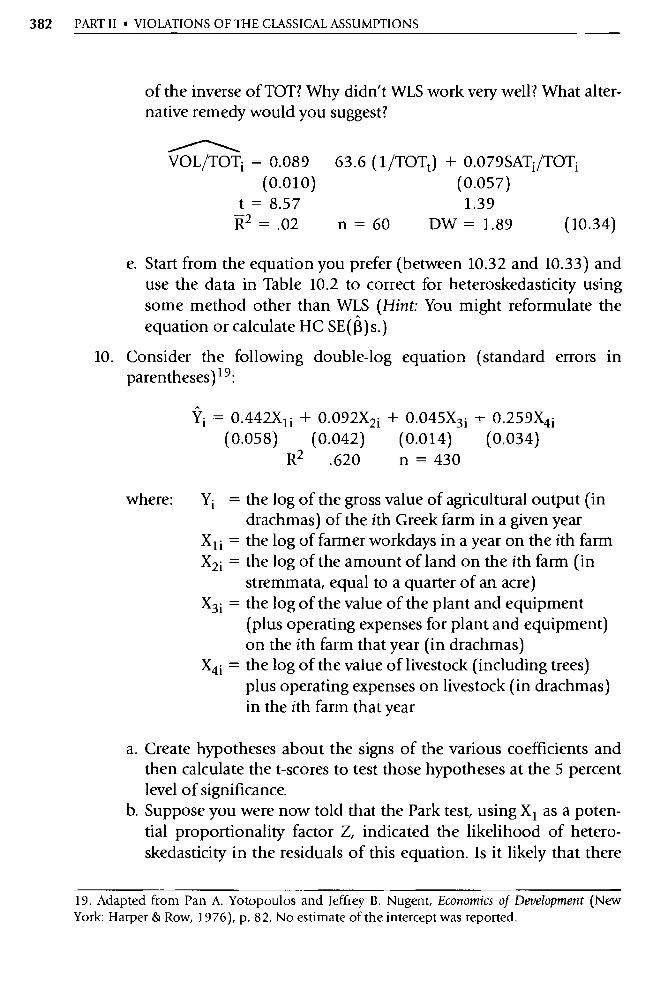
382 PART II ' VIOLATIONS OF THE CLASSICAL ASSUMPTIONS
of the inverse of TOT? Why didn't WLS work very well? What alter-native remedy would you suggest?
VOL/TOTi = 0.089 63.6 (1/TOTt) + 0.079SATi/TOTi (0.010) (0.057)
t = 8.57 1.39 R2 = .02 n = 60 DW = 1.89 (10.34)
e. Start from the equation you prefer (between 10.32 and 10.33) and use the data in Table 10.2 to correct for heteroskedasticity using some method other than WLS (Hint: You might reformulate the equation or calculate HC SE((3)s.)
10. Consider the following double-log equation (standard errors in parentheses) 1 9 :
Yi = 0.442X 11 + 0.092X21 + 0.045X31 + 0.259X41 (0.058) (0.042) (0.014) (0.034)
R2 .620 n = 430
where: Y1 = the log of the gross value of agricultural output (in drachmas) of the ith Greek farm in a given year
X li = the log of farmer workdays in a year on the ith farm X2i = the log of the amount of land on the ith farm (in
stremmata, equal to a qua rter of an acre) X3i = the log of the value of the plant and equipment
(plus operating expenses for plant and equipment) on the ith farm that year (in drachmas)
X4i = the log of the value of livestock (including trees) plus operating expenses on livestock (in drachmas) in the ith farm that year
a. Create hypotheses about the signs of the various coefficients and then calculate the t-scores to test those hypotheses at the 5 percent level of significance.
b. Suppose you were now told that the Park test, using X 1 as a poten-tial proportionality factor Z, indicated the likelihood of hetero-skedasticity in the residuals of this equation. Is it likely that there
19. Adapted from Pan A. Yotopoulos and Jeffrey B. Nugent, Economics of Development (New York: Harper & Row, 1976), p. 82. No estimate of the intercept was reported.
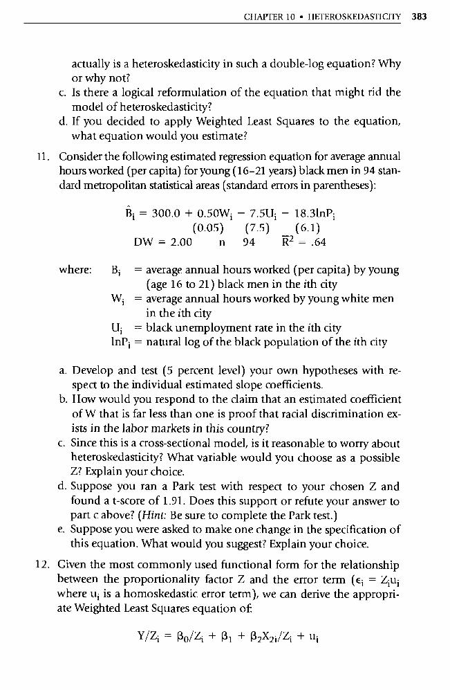
CHAPTER 10 • HETEROSKEDASTICITY 383
actually is a heteroskedasticity in such a double-log equation? Why or why not?
c. Is there a logical reformulation of the equation that might rid the model of heteroskedasticity?
d. If you decided to apply Weighted Least Squares to the equation, what equation would you estimate?
11. Consider the following estimated regression equation for average annual hours worked (per capita) for young (16-21 years) black men in 94 stan-dard metropolitan statistical areas (standard errors in parentheses):
Bi = 300.0 + 0.50W1 - 7.5L1 ; - 18.31nPi (0.05) (7.5) (6.1)
DW = 2.00 n 94 R2 = .64
where: Bi = average annual hours worked (per capita) by young (age 16 to 21) black men in the ith city
Wi = average annual hours worked by young white men in the ith city
= black unemployment rate in the ith city 1nP i = natural log of the black population of the ith city
a. Develop and test (5 percent level) your own hypotheses with re-spect to the individual estimated slope coefficients.
b. How would you respond to the claim that an estimated coefficient of W that is far less than one is proof that racial discrimination ex-ists in the labor markets in this count ry?
c. Since this is a cross-sectional model, is it reasonable to worry about heteroskedasticity? What variable would you choose as a possible Z? Explain your choice.
d. Suppose you ran a Park test with respect to your chosen Z and found a t -score of 1.91. Does this suppo rt or refute your answer to part c above? (Hint: Be sure to complete the Park test.)
e. Suppose you were asked to make one change in the specification of this equation. What would you suggest? Explain your choice.
12. Given the most commonly used functional form for the relationship between the proportionality factor Z and the error term (e i = Ziui
where ui is a homoskedastic error term), we can derive the appropri-ate Weighted Least Squares equation of:
Y/Zi = RO/Zi + 131 + 132X2i/Zi + ui
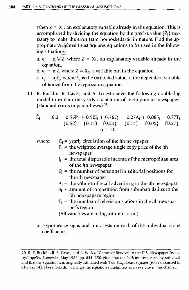
384 PART II • VIOLATIONS OF THE CLASSICAL ASSUMPTIONS
when Z = X 1 , an explanatory variable already in the equation. This is accomplished by dividing the equation by the precise value (Z i ) nec-essary to make the error term homoskedastic in nature. Find the ap-propriate Weighted Least Squares equations to be used in the follow-ing situations: a. Ei ui V Gi
n where Z = X 1 , an explanatory variable already in the
equation. b. Ei = uiZi where Z = X3, a variable not in the equation
c. Ei = uiiri, where Ÿi is the estimated value of the dependent variable
obtained from the regression equation
13. R. Bucklin, R. Caves, and A. Lo estimated the following double-log model to explain the yearly circulation of metropolitan newspapers (standard errors in parentheses) 2°:
Ci — 8.2 — 0.56Pî + 0.90Ii + 0.76Qî + 0.27Aî + 0.08Si — 0.77Tî
(0.58) (0.14) (0.21) (0.14) (0.05) (0.27) n=50
where: Ci = yearly circulation of the ith newspaper Pi = the weighted average single copy price of the ith
newspaper Ii = the total disposable income of the metropolitan area
of the ith newspaper Qi = the number of personnel in editorial positions for
the ith newspaper Ai = the volume of retail advertising in the ith newspaper Si = amount of competition from suburban dailies in the
ith newspaper's region Ti = the number of television stations in the ith newspa-
per's region (All variables are in logarithmic form.)
a. Hypothesize signs and run t-tests on each of the individual slope coefficients.
20. R. E. Bucklin, R. E. Caves, and A. W. Lo, "Games of Survival in the U.S. Newspaper Indus-try," Applied Economics, May 1989, pp. 631-650. Note that the Park test results are hypothetical and that the equation was originally estimated with Two-Stage Least Squares (to he discussed in Chapter 14). These facts don't change the equation's usefulness as an exercise in this chapter.

CHAPTER 10 • HETEROSKEDASTICITY
b. Does heteroskedasticity seem theoretically likely? Test for hetero-skedasticity at the 99 percent level assuming that a Park test with I i
as Z produces a t-score of 3.13. c. Given your responses to pa rts a and b above, what econometric
problems (out of omitted variables, irrelevant variables, incorrect functional form, multicollinearity, serial correlation, and hetero-skedasticity) appear to exist in this equation?
d. If you could suggest just one change in the specification of this equa-tion, what would that change be? Carefully explain your answer.
14. Think back to the Farmer Vin pig growing equation of Exercise 13 in Chapter 9:
Wi = 12+3.5G 1 +7.0Dî -0.25Fi
(1.0) (1.0) (0.10)
t = 3.5 7.0 —2.5
R2 = .70 n = 200 DW=0.50
(10.35)
where: Wi = the percentage weight gain of the ith pig during the six-month experiment
G î = a dummy variable equal to 1 if the ith pig is a male, 0 otherwise
D i = a dummy va riable equal to 1 if the ith pig was fed only at night, 0 if the ith pig was fed only during the day
Fi = the amount of food (pounds) eaten per day by the ith pig
It turns out that this study was estimated originally with the depen-dent variable equal to "pounds gained by the ith pig," but a Park test showed severe heteroskedasticity. (Recall that the sample pigs ranged all the way from pink piglets to ponderous porkers.) The dependent variable was converted to percentage terms in an effo rt to "rethink the equation" and eliminate the heteroskedasticity. Equation 10.35 was the result. a. How theoretically likely is it that there is heteroskedasticity in the
revised equation, Equation 10.35? Explain your answer. b. Suppose that you run a Park test on the residuals of Equation 10.35
and a find a t-score of —6.31 (using the weight of the ith pig as the potential proportionality factor). Do you have heteroskedasticity?
c. The t-score from your Park test in pa rt b above is negative, and yet we've never discussed "negative" or "positive" heteroskedasticity.
386 PART II • VIOLATIONS OF THE CLASSICAL ASSUMPTIONS
What impo rtance, if any, would you attach to the sign of the esti-mated slope coefficient in this Park test?
d. You appear to have heteroskedasticity in both the original and the revised versions of your equation. What should you do? Explain.
15. Let's investigate the possibility of heteroskedasticity in time-series data by looking at a model of the black market for U.S. dollars in Brazil that was studied by R. Dornbusch and C. Pechman. 21 In partic-ular, the authors wanted to know if the Demsetz-Bagehot bid-ask the-ory, previously tested on cross-sectional data from the United States, could be extended to time-series data outside the United States. 22
They estimated the following model on monthly data from Brazil for March 1979 through December 1983:
+ + St = f(It, Vt) + Et Ro + R1It + (3 21n(1 + Vt) + Et (10.36)
where: St = the average daily spread between the bid and asking prices for the U.S. dollar on the Brazilian black mar-ket in month t
It = the average interest rate in month t Vt = the variance of the daily premium between the black
market rate and the official exchange rate for the dol-lar in month t
a. Use the authors' data in Table 10.3 (filename BID 10) to estimate Equation 10.36 and test the residuals for positive first-order serial correlation.
b. If serial correlation appears to exist, reestimate Equation 10.36 us-ing GLS. Do the coefficient estimates change? Which equation do you prefer? Why?
c. The authors noted that S nearly doubled in size during their sam-ple period. Does this make you concerned about the possibility of heteroskedasticity? Why or why not?
21. Rudiger Dombusch and Clarice Pechman, "The Bid-Ask Spread in the Black Market for Dol-lars in Brazil," Journal of Money, Credit and Banking, November 1985, pp. 517-520. The data for this study were not published with the original article but are on the data diskette that accom-panies William F. Lott and Subhash C. Ray, Applied Econometrics: Problems with Data Sets (Fort Worth: D ryden/Harcourt Brace, 1992). The analytical approach of this question also comes from Lott and Ray, pp. 169- 173, and we appreciate permission to use their work.
22. For a review of this literature at the time of Dornbusch and Pechman's research, see Kalman Cohen et al. "Market Makers and the Market Spread: A Review of the Recent Literature," Journal of Financial and Quantitative Studies, November 1979, pp. 813-835.
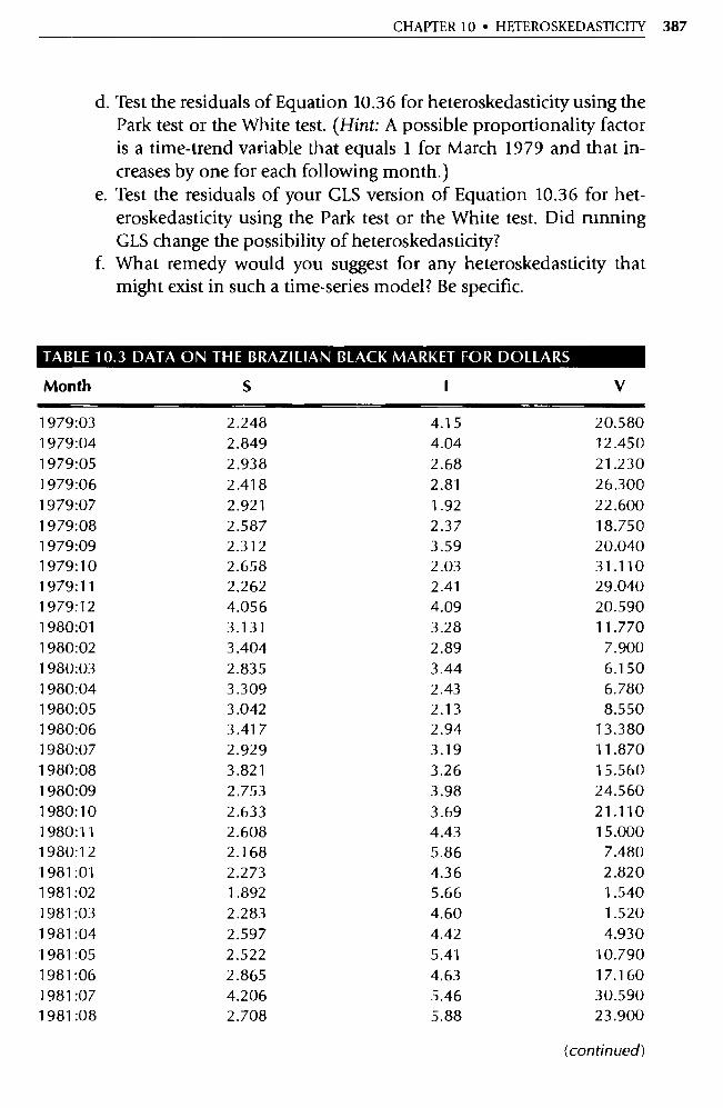
CHAPTER 10 • HETEROSKEDASTICITY 387
d. Test the residuals of Equation 10.36 for heteroskedasticity using the Park test or the White test. (Hint: A possible proportionality factor is a time-trend variable that equals 1 for March 1979 and that in-creases by one for each following month.)
e. Test the residuals of your GLS version of Equation 10.36 for het-eroskedasticity using the Park test or the White test. Did running GLS change the possibility of heteroskedasticity?
f. What remedy would you suggest for any heteroskedasticity that might exist in such a time-series model? Be specific.
TABLE 10.3 DATA ON THE BRAZILIAN BLACK MARKET FOR DOLLARS
Month S V
1979:03 2.248 4.15 20.580 1979:04 2.849 4.04 12.450 1979:05 2.938 2.68 21.230 1979:06 2.418 2.81 26.300 1979:07 2.921 1.92 22.600 1979:08 2.587 2.37 18.750 1979:09 2.312 3.59 20.040 1979:10 2.658 2.03 31.110 1979:11 2.262 2.41 29.040 1979:12 4.056 4.09 20.590 1980:01 3.131 3.28 11.770 1980:02 3.404 2.89 7.900 1980:03 2.835 3.44 6.150 1980:04 3.309 2.43 6.780 1980:05 3.042 2.13 8.550 1980:06 3.417 2.94 13.380 1980:07 2.929 3.19 11.870 1980:08 3.821 3.26 15.560 1980:09 2.753 3.98 24.560 1980:10 2.633 3.69 21.110 1980:11 2.608 4.43 15.000 1980:12 2.168 5.86 7.480 1981:01 2.273 4.36 2.820 1981:02 1.892 5.66 1.540 1981:03 2.283 4.60 1.520 1981:04 2.597 4.42 4.930 1981:05 2.522 5.41 10.790 1981:06 2.865 4.63 17.160 1981:07 4.206 5.46 30.590 1981:08 2.708 5.88 23.900
(continued)
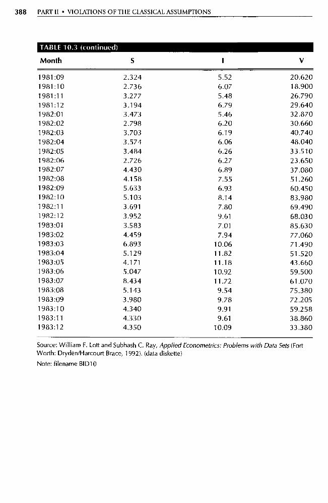
388 PART II • VIOLATIONS OF THE CLASSICAL ASSUMPTIONS
TABLE 10.3 (continued)
Month S I V
1981:09 2.324 5.52 20.620 1981:10 2.736 6.07 18.900 1981:11 3.277 5.48 26.790 1981:12 3.194 6.79 29.640 1982:01 3.473 5.46 32.870 1982:02 2.798 6.20 30.660 1982:03 3.703 6.19 40.740 1982:04 3.574 6.06 48.040 1982:05 3.484 6.26 33.510 1982:06 2.726 6.27 23.650 1982:07 4.430 6.89 37.080 1982:08 4.158 7.55 51.260 1982:09 5.633 6.93 60.450 1982:10 5.103 8.14 83.980 1982:11 3.691 7.80 69.490 1982:12 3.952 9.61 68.030 1983:01 3.583 7.01 85.630 1983:02 4.459 7.94 77.060 1983:03 6.893 10.06 71.490 1983:04 5.129 11.82 51.520 1983:05 4.171 11.18 43.660 1983:06 5.047 10.92 59.500 1983:07 8.434 11.72 61.070 1983:08 5.143 9.54 75.380 1983:09 3.980 9.78 72.205 1983:10 4.340 9.91 59.258 1983:11 4.330 9.61 38.860 1983:12 4.350 10.09 33.380
Source: William F. Lott and Subhash C. Ray, Applied Econometrics: Problems with Data Sets (Fort Wo rth: Dryden/Harcou rt Brace, 1992). (data diskette)
Note: filename BID10
11 CHAPTER
A Regression User's Handbook
11.1 A Regression User's Checklist
11.2 A Regression User's Guide
11.3 Running Your Own Regression Project
11.4 Economic Data
11.5 The Ethical Econometrician
11.6 Summary
11.7 Appendix: The Housing Price Interactive Exercise
The real-world problems that a regression user encounters are not as neatly labeled and compartmentalized as the previous 10 chapters might imply. In-stead, researchers must consider all the possible difficulties in an equation in order to decide which specification and estimation techniques to use. As a re-sult, it's useful to have summaries of the definitions, problems, solutions, and statistical tests that are central to basic single-equation linear regression models. The first two sections of this chapter contain such summaries; al-though you should certainly read these now, we also hope that you'll benefit from using them as a reference whenever you're undertaking econometric research.
The next two sections focus on how to carry out your own regression proj-ect. How might you choose a topic? Where can you go to collect data? What should your research repo rt contain? Although there is no agreed-upon for-mat that all researchers must follow, we still have quite a few practical hints that will make your first independent research project a lot more rewarding.
Unfortunately, no matter how superbly planned or well thought-out your project might be, it's very unusual for a beginning researcher's regression to be "perfect" the first time out. Something always goes wrong!
When this happens, econometrics becomes an art. The core of the prob-lem is that we never know what the true model is. There's a fine line between curve fitting and searching for the truth by formulating and estimating alter-native specifications or using alternative estimating techniques. Some regres-
389
390 PART II • VIOLATIONS OF THE CLASSICAL ASSUMPTIONS
sion results may very well be strictly a product of chance, because the re-searchers might have experimented with a number of models and estimators until they obtained the results that came closest to what they wanted; such an approach is unscientific. On the other hand, it would be foolhardy to go to the opposite extreme and ignore obvious estimation or specification errors in a first regression run; that would also be unscientific. The last three sections of this chapter help beginning researchers strike a balance between these two positions by providing advice on econometric ethics and by giving some hands-on regression experience. The interactive regression exercise in Section 11.7 is a "half-way house" between reading someone else's regression results (and having no input) and doing one's own regression analysis (and getting no feedback). We strongly encourage the reader to take the exercise seriously and work through the example rather than just read it.
11.1 A Regression User's Checklist
Table 11.1 contains a list of the items that a researcher checks when reviewing the output from a computer regression package. Not every item in the check-list will be produced by your computer package, and not every item in your computer output will be in the checklist, but the checklist can be a very use-ful reference. In most cases, a quick glance at the checklist will remind you of the text sections that deal with the item, but if this is not the case, the fairly minimal explanation in the checklist should not be relied on to cover every-thing needed for complete analysis and judgment. Instead, you should look up the item in the index. In addition, note that the actions in the right-hand column are merely suggestions. The circumstances of each individual research project are much more reliable guides than any dogmatic list of actions.
There are two ways to use the checklist. First, you can refer to it as a "glos-sary of packaged computer output terms" when you encounter something in your regression result that you don't understand. Second, you can work your way through the checklist in order, finding the items in your computer out-put and marking them. As with the Regression User's Guide (Table 11.2), the use of the Regression User's Checklist will be most helpful for beginning re-searchers, but we also find ourselves referring back to it once in a while even after years of experience.
Be careful. All simplified tables, like the two in this chapter, must trade completeness for ease of use. As a result, strict adherence to a set of rules is not recommended even if the rules come from one of our tables. Someone

Degrees of freedom df
Estimated coefficient R
tk SE(k)
or
__ Rk tk SE(Rk)
for computer-supplied t-scores or whenever
PH0 = 0
Coefficient of determi-nation
t t-statistic
Rk — PH0
R2
CHAPTER 11 • A REGRESSION USER'S HANDBOOK 391
TABLE 11.1 REGRESSION USER'S CHECKLIST
Symbol
Checkpoint
Reference
Decision
X, Y Data observations
R2 R2 adjusted for degrees
of freedom
Check for errors, espe-
cially outliers, in the
data. Spot check trans-formations of variables. Check means, maxi-mums, and minimums.
n—K-1 >0
n = number of
observations
K = number of explana- tory variables
Compare signs and mag-nitudes to expected
values.
Two-sided test:
H0: 13k = RHo HA: Pk # RHo
One-sided test:
H0: Rk 13H0
HA: 13k > RH o
RH o, the hypothesized f3, is supplied by the re-
searcher, and is often zero.
Measures the degree of overall fit of the model
to the data
Same as R2 . Also at-
tempts to show the con-
tribution of an addi-
tional explanatory
variable.
Correct any errors. If the
quality of the data is poor, may want to avoid
regression analysis or use just OLS.
If n — K — 1 0, equa-
tion cannot be estimated,
and if the degrees of
freedom are low, preci-sion is low. In such a case, try to include more
observations.
If they are unexpected, respecify model if ap-
propriate or assess other
statistics for possible correct procedures.
Reject H 0 if I tk > tc and if the estimate is of
the expected sign.
tc is the critical value of a level of significance and n — K — 1 degrees of freedom.
A guide to the overall fit.
One indication that an explanatory variable is
irrelevant is if the R 2
falls when it is included.
(continued)
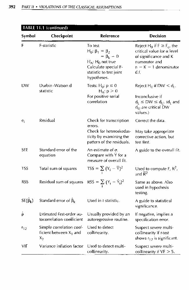
F F-statistic
DW Durbin—Watson d
statistic
Residual
SEE Standard error of the equation
TSS Total sum of squares
RSS Residual sum of squares
SE(K) Standard error of Rk
Estimated first-order au- tocorrelation coefficient
Simple correlation coef-ficient between X 1 and
X2
VIF Variance inflation factor
e i
p
r12
392 PART II • VIOLATIONS OF THE CLASSICAL ASSUMPTIONS
TABLE 11.1 (continued)
Symbol
Checkpoint
Reference
Decision
To test
Ho : 13 1 = R2 = Pk = O
H A : H o not true Calculate special F-
statistic to test joint hypotheses.
Tests: H o : p 0 H A : p > 0
For positive serial
correlation
Check for transcription
errors.
Check for heteroskedas-
ticity by examining the pattern of the residuals.
An estimate of 6. Compare with Y for a
measure of overall fit.
TSS = E (Y i — Y) 2
RSS = E (Yi — Yi) 2
Used in t-statistic.
Usually provided by an autoregressive routine.
Used to detect col l i nearity.
Used to detect multi-
collinearity.
Reject Ho if F >— F, the
critical value for a level
of significance and K
numerator and n — K — 1 denominator d.f.
Reject H o if DW <
Inconclusive if
d L DW d u . (d i_ and
d u are critical DW values.)
Correct the data.
May take appropriate
corrective action, but test first.
A guide to the overall fit.
Used to compute F, R2 ,
and 112
Same as above. Also used in hypothesis testing.
A guide to statistical
significance.
If negative, implies a specification error.
Suspect severe multi-collinearity if t-test
shows r 12 is significant.
Suspect severe multi-
collinearity if VF > 5.
CHAPTER 11 • A REGRESSION USER'S HANDBOOK
who understands the purpose of the research, the exact definitions of the variables, and the problems in the data is much more likely to make a correct judgment than is someone equipped with a set of rules created to apply to a wide variety of possible applications.
11.2 A Regression User's Guide
Table 11.2 contains a brief summary of the major econometric maladies dis-cussed so far in this text. For each econometric problem, we list:
1. Its nature.
2. Its consequences for OLS estimation.
3. How to detect it. 4. How to attempt to get rid of it.
How might you use the guide? If an estimated equation has a particular problem, such as a significant unexpected sign for a coefficient estimate or a correct but insignificant coefficient estimate, a quick glance at the guide can give some idea of what econometric problems might be causing that symp-tom. Both multicollinearity and irrelevant variables can cause regression co-efficients to have insignificant t-scores, for example, and someone who re-membered only one of these potential causes might take the wrong correction action. After some practice, the use of this guide will decrease until it eventually will seem fairly limiting and simplistic. Until then, however, our experience is that those about to undertake their first econometric research can benefit by referring to this guide.
11.3 Running Your Own Regression Project
We believe that econometrics is best learned by doing, not by reading books, listening to lectures, or taking tests. To us, learning the a rt of econometrics has more in common with learning to fly a plane or learning to play golf than it does with learning about history or literature. In fact, we developed the interactive exercises of this chapter and Chapter 8 precisely because of our confidence in learning by doing.
Although interactive exercises are a good bridge between textbook exam-ples and running your own regressions, they don't go far enough. You still need to "get your hands dirty." We think that you should run your own re-gression project before you finish reading this book even if you're not re-

TABLE 11.2 A REGRESSION USER'S GUIDE
What Can Go
What Are the
How Can It Be
How Can It Be Wrong?
Consequences?
Detected?
Corrected?
Omitted Variable The omission of
a relevant
independent
variable
Irrelevant Variable The inclusion of a
variable that
does not belong
in the equation
Bias in the
coefficient
estimates (the (As)
of the included Xs.
Decreased
precision in the
form of higher
standard errors
and lower t-scores.
Theory, significant
unexpected signs,
or surprisingly poor
fits.
1. Theory
2. t-test on â
3. R2 4. Impact on other
coefficients if X
is dropped
Include the left-out
variable or a proxy.
Delete the variable
if its inclusion is not
required by the
underlying theory.
Incorrect Functional Form The functional
form is
inappropriate
Multicollinearity Some of the
independent
variables are
(imperfectly)
correlated
Serial Correlation Observations of
the error term are
correlated, as in:
Et = Pet-1 + ut
Heteroskedasticity The variance of
the error term is
not constant for
all observations,
as in:
VAR(e ; ) = o 2 Z?
Biased and
inconsistent
estimates, poor fit,
and difficult
interpretation.
No biased 13s, but
estimates of the
separate effects of
the Xs are not
reliable, i.e., high
SEs (and low
t-scores).
No biased (3s , but
the variances of the
Rs increase (and
t-scores fall) in a
way not captured
by OLS.
Same as for serial
correlation.
Examine the theory
carefully; think
about the
relationship
between X and Y.
No universally
accepted rule or
test is available.
Use the t-test on
r 12 or the VIF test.
Use Durbin-Watson
d test; if significantly
less than 2, positive
serial correlation
exists.
Plot the spread of
contraction of the
residuals (against
one of the Xs, for
example) or use the
Park or White tests.
Transform the
variable or the
equation to a
different functional
form.
Drop redundant
variables, but to
drop others might
introduce bias. A
combination variable
may be useful, but
often doing nothing
is best.
If impure, add the
omitted variable
or change the
functional form.
Otherwise, consider
Generalized Least
Squares.
If impure, add the
omitted variable.
Otherwise, run a
Weighted Least
Squares or use HC
standard errors.
394

CHAPTER 11 • A REGRESSION USER'S HANDBOOK 395
quired to do so. We're not alone. Some professors substitute a research proj-ect for the final exam as their class's comprehensive learning experience.
Running your own regression project has three major components:
1. Choosing a topic.
2. Applying the six steps in regression analysis to that topic.
3. Writing your research repo rt .
The first and third of these components are the topics of this section. The sec- ond component is covered in Chapter 3 except for data collection, which we cover in Section 11.4.
11.3.1 Choosing a Topic
The purpose of an econometric research project is to use regression analysis to build the best explanatory equation for a particular dependent variable for a particular sample. Often, though, the hardest pa rt is getting started. How can you choose a good topic?
There are at least three keys to choosing a topic. First, try to pick a field that you find interesting and/or that you know something about. If you enjoy working on your project, the hours involved will seem to fly by. In addition, if you know something about your subject, you'll be more likely to make cor-rect specification choices and/or to notice subtle indications of data errors or theoretical problems. A second key is to make sure that data are readily avail-able with a reasonable sample (we suggest at least 25 observations). Nothing is more frustrating than searching through data source after data source in search of numbers for your dependent variable or one of your independent variables, so before you lock yourself into a topic, see if the data are there. The final key is to make sure that there is some substance to your topic. Try to avoid topics that are purely descriptive or virtually tautological in nature. In-stead, look for topics that include a hypothesis or two that you'd like to test.
Perhaps the best place to look for ideas for topics is to review your text-books and notes from previous economics classes or to look over the exam-ples and exercises of the first 10 chapters of this book. Often, you can take an idea from a previous study and update the data to see if the idea can be ap-plied in a different context. Other times, reading an example will spark an idea about a similar or related study that you'd be interested in doing. Don't feel that your topic has to contain an original hypothesis or equation. On your first or second project, it's more impo rtant to get used to the economet-rics than it is to create a publishable masterpiece.
Another way to find a topic is to read through issues of economics jour-nals, looking for a rticle topics that you find interesting and that might be

396 PART II • VIOLATIONS OF THE CLASSICAL ASSUMPTIONS
possible to model. Although this is an excellent way to get ideas, it's also frus-trating, because most current a rticles use econometric techniques that go be-yond those that we've covered so far in this text. As a result, it's often difficult to compare your results to those in the article.
If you get stuck for a topic, go directly to the data sources themselves. That is, instead of thinking of a topic and then seeing if the data are available, look over what data are available and see if they help generate ideas for topics. Quite often, a reference will have data not only for a dependent variable but also for most of the relevant independent variables all in one place, minimiz-ing time spent collecting data.
Once you pick a topic, don't rush out and run your first regression. Re-member, the more time you spend reviewing the literature and analyzing your expectations on a topic, the better the econometric analysis and, ulti-mately, your research repo rt will be. Speaking of your research repo rt
11.3.2 Writing Your Research Report
Once you've finished your research, it's impo rtant to write a repo rt on your results so that others can benefit from what you found out (or didn't find out) or so that you can get feedback on your econometric techniques from someone else. Most good research repo rts have a number of elements in common:
a. A brief introduction that defines the dependent va riable and states the goals of the research.
b. A short review of relevant previous literature and research.
c. An explanation of the specification of the equation (model). This should include explaining why particular independent va riables and functional forms were chosen as well as stating the expected signs of (or other hypotheses about) the slope coefficients.
d. A description of the data (including generated variables), data sources, and any irregularities with the data.
e. A presentation of each estimated specification, using our standard documentation format. If you estimate more than one specification, be sure to explain which one is best (and why).
f. A careful analysis of the regression results that includes a discussion of any econometric problems encountered and complete documentation of all equations estimated and all tests run. (Beginning researchers are well advised to test for every possible econometric problem; with ex-perience, you'll learn to focus on the most likely difficulties.)
CHAPTER 11 • A REGRESSION USER'S HANDBOOK 39;
g. A short summary/conclusion that includes any policy recommenda-tions or suggestions for further research.
h. A bibliography.
i. An appendix that includes all data, all regression runs, and all relevant computer output. Do this carefully; readers appreciate a well-organized and labeled appendix.
We think that the easiest way to write such a research repo rt is to keep a re-search journal as you go along. In this journal, you can keep track of a priori hypotheses, regression results, statistical tests, different specifications you considered, and theoretical analyses of what you thought was going on in your equation. You'll find that when it comes time to write your research re-port, this journal will almost write your paper for you! The alternative to keeping a journal is to wait until you've finished all your econometric work before starting to write your research repo rt, but this runs the risk of forget-ting the thought process that led you to make a particular decision (or some other impo rtant item).
11.4 Economic Data
Before any quantitative analysis can be done, the data must be collected, orga-nized, and entered into a computer. Usually, this is a time-consuming and frustrating task because of the difficulty of finding data, the existence of defin-itional differences between theoretical variables and their empirical counter-parts, and the high probability of data entry errors or data transmission errors. In general, though, time spent thinking about and collecting the data is well spent, since a researcher who knows the data sources and definitions is much less likely to make mistakes using or interpreting regressions run on that data.
11.4.1 What Data to Look For
Before you settle on a research topic, it's good advice to make sure that data for your dependent variable and all relevant independent variables are avail-able. However, checking for data availability means deciding what specific variables you want to study. Half of the time that beginning researchers spend collecting data is wasted by looking for the wrong variables in the wrong places. A few minutes thinking about what data to look for will save hours of frustration later.
For example, if the dependent variable is the quantity of television sets de-manded per year, then most independent variables should be measured an-
398 PART II • VIOLATIONS OF THE CLASSICAL ASSUMPTIONS
nually as well. It would be inappropriate and possibly misleading to define the price of TVs as the price from a particular month. An average of prices over the year (usually weighted by the number of TVs sold per month) would be more meaningful. If the dependent variable includes all TV sets sold re-gardless of brand, then the price would appropriately be an aggregate based on prices of all brands. Calculating such aggregate variables, however, is not sttaightfotwatd. Reseatchers typically make their best eiiotts to compute the respective aggregate variables and then acknowledge that problems still re-main. For example, if the price data for all the various brands are not avail-able, a researcher may be forced to compromise and use the prices of one or a few of the major brands as a substitute for the proper aggregate price.
Another issue is suggested by the TV example. Over the years of the sam-ple, it's likely that the market shares of particular kinds of TV sets have changed. For example, 21-inch color TV sets might have made up a majority of the market in one decade, but 19-inch black and white sets might have been the favo rite 20 years before. In cases where the composition of the mar-ket share, the size, or the quality of the various brands have changed over time, it would make little sense to measure the dependent variable as the number of TV sets because a "TV set" from one year has little in common with a "TV set" from another. The approach usually taken to deal with this problem is to measure the variable in dollar terms, under the assumption that value encompasses size and quality. Thus, we would work with the dol-lar sales of TVs rather than the number of sets sold.
A third issue, whether to use nominal or real variables, usually depends on the underlying theory of the research topic. Nominal (or money) variables are measured in current dollars and thus include increases caused by infla-tion. If theory implies that inflation should be filtered out, then it's best to state the variables in real (constant dollar) terms by selecting an appropriate price deflator, such as the Consumer Price Index, and adjusting the money (or nominal) value by it.
As an example, the appropriate price index for Gross Domestic Product is called the GDP deflator. Real GDP is calculated by multiplying nominal GDP by the ratio of the GDP deflator from the base year to the GDP deflator from the current year:
Real GDP = nominal GDP X (base GDP deflator/current GDP deflator)
In 1994, U.S. nominal GDP was $6891 billion and the GDP deflator 127.0 (for a base year of 1987 = 100), so real GDP wasl:
1. 1995 Economic Repo rt of the President, pp. 274-278.
CHAPTER 11 • A REGRESSION USER'S HANDBOOK
Real GDP = $6891 (100/127.0) = $5426 billion
That is, the goods and services produced in 1994 were worth $6891 billion if 1994 dollars were used but were worth only $5426 billion if 1987 prices were used.
Fourth, recall that all economic data are either time series or cross sec-tional in nature. Since time-series data are for the same economic entity from different time periods, whereas cross-sectional data are from the same time period but for different economic entities, the appropriate definitions of the variables depend on whether the sample is a time series or a cross section.
To understand this, consider the TV set example once again. A time-series model might study the sales of TV sets in the United States from 1960 to 1998, and a cross-sectional model might study the sales of TV sets by state for 1998. The time-series data set would have 39 observations, each of which would refer to a particular year. In contrast, the cross-sectional model data set would have 50 observations, each of which would refer to a particular state. A va riable that might be appropriate for the time-series model might be completely inappro-priate for the cross-sectional model and vice versa; at the very least, it would have to be measured differently. National advertising in a particular year would be appropriate for the time-series model, for example, while advertising in or near each particular state would make more sense for the cross-sectional one.
Finally, learn to be a critical reader of the desc riptions of variables in econometric research. For instance, most readers breezed right through Equa-tion 2.10 on the demand for beef (and the accompanying data in Table 2.2) without asking some vital questions. Where did the data originate? Are prices and income measured in nominal or real terms? Is the price of beef whole-sale or retail? A careful reader would want to know the answers to these ques-tions before analyzing the results of Equation 2.10. (For the record, Yd mea-sures real income, P measures real wholesale prices, and the data come from various issues of Agricultural Statistics, published in Washington, D.C., by the U.S. Department of Agriculture.)
11.4.2 Where to Look for Economic Data
Although some researchers generate their own data through surveys or other techniques, the vast majority of regressions are run on publicly available data. The best sources for such data are government publications and ma-chine-readable data files. In fact, the U.S. government has been called the most thorough statistics-collecting agency in history.
Excellent government publications include the annual Statistical Abstract of the U.S., the annual Economic Report of the President, the Handbook of Labor
400 PART II • VIOLATIONS OF THE CLASSICAL ASSUMPTIONS
Statistics, and Historical Statistics of the U.S. (published in 1975). One of the best places to start with U.S. data is the annual Census Catalog and Guide, which provides overviews and abstracts of data sources and various statistical products as well as details on how to obtain each item. 2 Also quite valuable is the Bureau of Labor Statistics (BLS) Customer Service Guide, which provides details of BLS program areas, products, and on-line access. 3
Consistent international data are harder to come by, but the United Na-tions publishes a number of compilations of figures. The best of these are the U.N. Statistical Yearbook and the U.N. Yearbook of National Account Statistics.
Recently, more and more researchers have started using on-line computer databases to find data instead of plowing through stacks of printed volumes. These on-line databases, available through most college and university li-braries, contain complete series on literally thousands of possible variables. For example, one database, "U.S. Econ.," contains more than 25,000 time-series variables for the U.S. economy. The Directory of Online Databases (New York: Quadra/Elsevier, 1995) contains a complete listing of all available on-line databases. Two of the most useful of these are the "Economic Literature Index," which is an on-line summary of the Journal of Economic Literature, and "Dialog," which provides on-line access to a large number of data sets at a lower cost than many alternatives.
Finally, a huge variety of data is available on the Internet. The best guides to the data available in this rapidly changing world are "Resources For Economists on the Internet," Economagic, and WebEC. 4 Links to these sites and other good sources of data are on the text's website <www.awl.com/studenmund >.
11.4.3 Missing Data
Suppose the data aren't there? What happens if you choose the perfect vari-able and look in all the right sources and can't find the data?
The answer to this question depends on how much data are missing. If a few observations have incomplete data in a cross-sectional study, you usually
2. To obtain this guide, write the Superintendent of Documents, Government Printing Office, Washington, D.C., 20402-9325, or call 202-783-9325 and ask for stock/catalog #C3-163/3.
3. The BLS maintains a 24-hour data hot line (including information on how to order data) at 202-606-7828.
4. On the Web, the resources location is http://econwpa.wustl.edu/EconFAQ.html . You can also access the guide via e-mail by putting GET ECON.FAQ in the subject line of a message to [email protected] . The Economagic location is http://www.economagic.com/. The WebEC location is http://rfe.wustl.edu/Data/index.html.

CHAPTER 11 • A REGRESSION USER'S HANDBOOK 401
can afford to drop these obse rvations from the sample. If the incomplete data are from a time series, you can sometimes estimate the missing value by in-terpolating (taking the mean of adjacent values). Similarly, if one variable is available only annually in an otherwise quarterly model, you may want to consider quarterly interpolations of that variable. In either case, interpolation can be justified only if the variable moves in a slow and smooth manner. Ex-treme caution should always be exercised when "creating" data in such a way (and full documentation is required).
If no data exist for a theoretically relevant variable, then the problem wors-ens significantly. Omitting a relevant variable runs the risk of biased coeffi-cient estimates, as we learned in Chapter 6. After all, how can you hold a vari-able constant if it's not included in the equation? In such cases, most researchers resort to the use of proxy variables.
Proxy variables can sometimes substitute for theoretically desired variables when data on variables are missing. For example, the value of net investment is a variable that is not measured directly in a number of countries. As a result, a researcher might use the value of gross investment as a proxy, the assump-tion being that the value of gross investment is directly proportional to the value of net investment. This proportionality (which is similar to a change in units) is required because the regression analyzes the relationship between changes among variables, rather than the absolute levels of the variables.
In general, a proxy variable is a "good" proxy when its movements corre-spond relatively well to movements in the theoretically correct variable. Since the latter is unobservable whenever a proxy must be used, there is usually no easy way to examine a proxy's "goodness" directly. Instead, the researcher must document as well as possible why the proxy is likely to be a good or bad one. Poor proxies and variables with large measurement errors constitute "bad" data, but the degree to which the data are bad is a matter of judgment by the individual researcher.
11.5 The Ethical Econometrician
One conclusion that a casual reader of this book might draw from the large number of specifications we include is that we encourage the estimation of numerous regression results as a way of insuring the discovery of these best possible estimates.
Nothing could be further from the truth!
As every reader of this book should know by now, our opinion is that the best models are those on which much care has been spent to develop the the-
402 PART II • VIOLATIONS OF THE CLASSICAL ASSUMPTIONS
oretical underpinnings and only a sho rt time is spent pursuing alternative es-timations of that equation. Many econometricians, ourselves included, would hope to be able to estimate only one specification of an equation for each data set. Econometricians are fallible and our data are sometimes im-perfect, however, so it is unusual for a first attempt at estimation to be totally problem free. As a result, two or even more regressions are often necessary to rid an estimation of fairly simple difficulties that perhaps could have been avoided in a world of perfect foresight.
Unfortunately, a beginning researcher usually has little motivation to stop running regressions until he or she likes the way the result looks. If running another regression provides a result with a better fit, why shouldn't one more specification be tested?
The reason is a compelling one. Every time an extra regression is run and a specification choice is made on the basis of fit or statistical significance, the chances of making a mistake of inference increase dramatically. This can hap-pen in at least two ways:
1. If you consistently drop a variable when its coefficient is insignificant but keep it when it is significant, it can be shown, as discussed in Sec-tion 6.4, that you bias your estimates of the coefficients of the equa-tion and of the t-scores.
2. If you choose to use a lag structure, or a functional form or an estima-tion procedure other than OLS, on the basis of fit rather than on the basis of previously theorized hypotheses, you run the risk that your equation will work poorly when it's applied to data outside your sam-ple. If you restructure your equation to work well on one data set, you might decrease the chance of it working well on another.
What might be thought of as ethical econometrics is also in reality good econometrics. That is, the real reason to avoid running too many different specifications is that the fewer regressions you run, the more reliable and more consistently trustworthy are your results. The instance in which profes-sional ethics come into play is when a number of changes are made (differ-ent variables, lag structures, functional forms, estimation procedures, data sets, dropped outliers, and so on), but the regression results are presented to colleagues, clients, editors, or journals as if the final and best equation had been the first and only one estimated. Our recommendation is that all esti-mated equations be reported even if footnotes or an appendix have to be added to the documentation.
We think that there are two reasonable goals for econometricians when es-timating models:
CHAPTER 11 • A REGRESSION USER'S HANDBOOK 403
1. Run as few different specifications as possible while still attempting to avoid the major econometric problems. 5
2. Report honestly the number and type of different specifications esti-mated so that readers of the research can evaluate how much weight to give to your results.
Therefore, the a rt of econometrics boils down to attempting to find the best possible equation in the fewest possible number of regression runs. Only careful thinking and reading before estimating first regression can bring this about. An ethical econometrician is honest and complete in reporting the different specifications and/or data sets used.
11.6 Summary
1. Table 11.1 contains a listing of terms that should be checked when re-viewing the output from a computer regression package.
2. Table 11.2 contains a summary of the nature, consequences, detec-tion, and correction procedures for the various econometric problems covered so far in this text. A review of this table is a good way to pre-pare for the first few attempts at applied regression analysis.
3. The art of econometrics involves finding the best possible equation in the fewest possible number of regression runs. The only way to do this is to spend quite a bit of time thinking through the underlying principles of every research project before the first regression is run.
4. An ethical econometrician is always honest and complete in reporting all the different regressions estimated and/or data sets used before the final results were chosen.
11.7 Appendix: The Housing Price Interactive Exercise
This interactive regression learning exercise is somewhat different from the previous one in Section 8.7 Our goal is still to bridge the gap between text- book and computer, but we feel that if you completed the previous interac-
5. The only exceptions to our recommendation to run as few specifications as possible are scan-ning and sensitivity analysis, described in Section 6.4.5.

404 PART H • VIOLATIONS OF THE CLASSICAL ASSUMPTIONS
tive exercise you should be ready to do the computer work on your own. 6 As a result, this interactive exercise will provide you with a sho rt literature re-view and the data, but you'll be asked to calculate your own estimates. Feed-back on your specification choices will once again be found in the hints in Appendix A.
Since the only difference between this interactive exercise and the first one is that this one requires you to estimate your chosen specification(s) with the computer, our guidelines for interactive exercises will apply:
1. Take the time to look over a portion of the reading list before choosing a specification.
2. Try to estimate as few regression runs as possible.
3. Avoid looking at the hints until after you've reached what you think is your best specification.
We believe that the benefits you get from an interactive exercise are directly proportional to the effo rt you put into it. If you have to delay this exercise until you have the time and energy to do your best, that's probably a good idea.
11.7.1 Building a Hedonic Model of Housing Prices
In the next section, we're going to ask you to specify the independent vari-ables and functional form for an equation whose dependent variable is the price of a house in Southern California. Before making these choices, it's vital to review the housing price literature and to think through the theory behind such models. Such a review is especially impo rtant in this case because the model we'll be building will be hedonic in nature.
What is a hedonic model? Recall that in Section 1.5 we estimated an equa-tion for the price of a house as a function of the size of that house. Such a model is called hedonic because it uses measures of the quality of a product as independent variables instead of measures of the market for that product (like quantity demanded, income, etc.). Hedonic models are most useful when the product being analyzed is heterogeneous in nature because we need to analyze what causes products to be different and therefore to have different prices. With a homogeneous product, hedonic models are virtually useless.
6. If you have not completed the interactive exercise in Section 8.7, we urge you to do so before beginning this one. Instructors interested in additional interactive exercises can find them in our instructor's manual and on the text's internet site <www.awlonline.com/studenmund >.

CHAPTER 11 • A REGRESSION USER'S HANDBOOK 405
Perhaps the most-cited early hedonic housing price study is that of G. Grether and P. Mieszkowski. 7 Grether and Mieszkowski collected a 7-year data set and built a number of linear models of housing price using different combinations of variables. They included square feet of space, the number of bathrooms, and the number of rooms, although the latter turned out to be insignificant. They also included lot size and the age of the house as vari-ables, specifying a quadratic function for the age variable. Most innovatively, they used several slope dummies in order to capture the interaction effects of various combinations of variables (like a hardwood floors dummy times the size of the house).
Peter Linneman 8 estimated a housing price model on data from Los Ange-les, Chicago, and the entire United States. His goal was to create a model that worked for the two individual cities and then to apply it to the nation to test the hypothesis of a national housing market. Linneman did not include any lot characteristics, nor did he use any interaction variables. His only measures of the size of the living space were the number of bathrooms and the number of nonbathrooms. Except for an age variable, the rest of the independent variables were dummies describing quality characteristics of the house and neighborhood. Although many of the dummy variables were quite fickle, the coefficients of age, number of bathrooms, and the number of nonbathrooms were relatively stable and significant. Central air conditioning had a negative, insignificant coefficient for the Los Angeles regression.
K. Ihlanfeldt and J. Martinez-Vasquez investigated sample bias in various methods of obtaining house price data and concluded that the house's sales price is the least biased of all measures. Unfortunately, they went on to esti-mate an equation by starting with a large number of variables and then drop-ping all those that had t-scores below one, almost surely introducing bias into their equation.
7 G. M. Grether and Peter Mieszkowski, "Determinants of Real Estate Values," Journal of Urban Economics, April 1974, pp. 127-146. Another classic a rticle of the same era is J. Kain and J. Quigley, "Measuring the Value of Housing Quality," Journal of American Statistical Association, June 1970.
8. Peter Linneman, "Some Empirical Results on the Nature of Hedonic Price Functions for the Urban Housing Market," Journal of Urban Economics, July 1980, pp. 47-68.
9. Keith Ihlanfeldt and Jorge Martinez-Vasquez, "Alternate Value Estimates of Owner-Occupied Housing: Evidence on Sample Selection Bias and Systematic Errors," Journal of Urban Economics, November 1986, pp. 356-369. Also see E ric Cassel and Robert Mendelsohn, "The Choice of Functional Forms for Hedonic Price Equations: Comment," Journal of Urban Economics, Septem-ber 1985, pp. 135-142.

406 PART II • VIOLATIONS OF THE CLASSICAL ASSUMPTIONS
Finally, Allen Goodman 10 added some innovative variables to an estimate on a national data set. He included measures of specific problems like rats, cracks in the plaster, holes in the floors, plumbing breakdowns, and the level of property taxes. Although the property tax variable showed the capitaliza-tion of low property taxes, as would be expected, the rats variable was in-significant, and the cracks variable's coefficient asserted that cracks signifi-cantly increase the value of a house.
11.7.2 The Housing Price Interactive Exercise
Now that we've reviewed at least a po rtion of the literature, it's time to build your own model. Recall that in Section 1.5, we built a simple model of the price of a house as a function of the size of that house, Equation 1.23:
Pi = 40.0 +0.138Si (1.23)
where: P; = the price (in thousands of dollars) of the ith house Si = the size (in square feet) of the ith house
Equation 1.23 was estimated on a sample of 43 houses that were purchased in the same Southern California town (Monrovia) within a few weeks of each other. It turns out that we have a number of additional independent variables for the data set we used to estimate Equation 1.23. Also available are:
Ni = the quality of the neighborhood of the ith house (1 = best, 4 = worst) as rated by two local real estate agents
Ai = the age of the ith house in years BE = the number of bedrooms in the ith house BA; = the number of bathrooms in the ith house CA; = a dummy variable equal to 1 if the ith house has central air
conditioning, 0 otherwise SP; = a dummy variable equal to 1 if the ith house has a pool, 0
otherwise Y; = the size of the yard around the ith house (in square feet)
Read through the list of variables again, developing your own analyses of the theory behind each variable. What are the expected signs of the coefficients?
10. Allen C. Goodman, "An Econometric Model of Housing Price, Permanent Income, Tenure Choice, and Housing Demand, Journal of Urban Economics, May 1988, pp. 327-353.
CHAPTER 11 • A REGRESSION USER'S HANDBOOK
Which variables seem potentially redundant? Which variables must you in-clude?
In addition, there are a number of functional form modifications that can be made. For example, you might consider a quadratic polynomial for age, as Grether and Mieszkowski did, or you might consider creating slope dummies such as SP•S or CA-S. Finally, you might consider interactive variables that in-volve the neighborhood proxy variable such as N•S or N-BA. What hypothe-ses would each of these imply?
Develop your specification carefully. Think through each variable and/or functional form decision, and take the time to write out your expectations for the sign and size of each coefficient. Don't take the attitude that you should include every possible variable and functional form modification and then drop the insignificant ones. Instead, try to design the best possible hedonic model of housing prices you can the first time around.
Once you've chosen a specification, estimate your equation, using the data in Table 11.3 (page 408), and analyze the result.
1. Test your hypotheses for each coefficient with the t-test. Pay special at-tention to any functional form modifications.
2. Test the overall significance of the equation with the F-test.
3. Decide what econometric problems exist in the equation, testing, if appropriate, for multicollinearity, serial correlation, or heteroskedas-ticity.
4. Decide whether to accept your first specification as the best one or to make a modification in your equation and estimate again. Make sure you avoid the temptation to estimate an additional specification "just to see what it looks like."
Once you've decided to make no further changes, you're finished—con-gratulations! Now turn to the hints for Section 11.7.2 in Appendix A for feed-back on your choices.
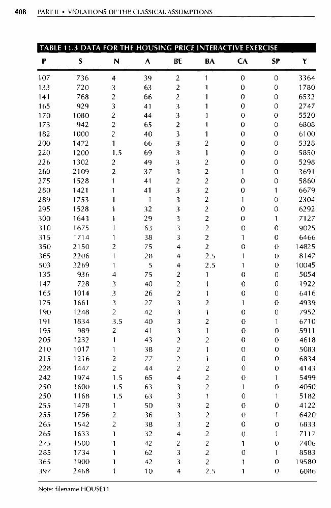
408 PART II • VIOLATIONS OF THE CLASSICAL ASSUMPTIONS
TABLE 11.3 DATA FOR THE HOUSING PRICE INTERACTIVE EXERCISE
P S N A BE BA CA SP Y
107 736 4 39 2 1 0 0 3364 133 720 3 63 2 1 0 0 1780 141 768 2 66 2 1 0 0 6532 165 929 3 41 3 1 0 0 2747 170 1080 2 44 3 1 0 0 5520 173 942 2 65 2 1 0 0 6808 182 1000 2 40 3 1 0 0 6100 200 1472 1 66 3 2 0 0 5328 220 1200 1.5 69 3 1 0 0 5850 226 1302 2 49 3 2 0 0 5298 260 2109 2 37 3 2 1 0 3691 275 1528 1 41 2 2 0 0 5860 280 1421 1 41 3 2 0 1 6679 289 1753 1 1 3 2 1 0 2304 295 1528 1 32 3 2 0 0 6292 300 1643 1 29 3 2 0 1 7127 310 1675 1 63 3 2 0 0 9025 315 1714 1 38 3 2 1 0 6466 350 2150 2 75 4 2 0 0 14825 365 2206 1 28 4 2.5 1 0 8147 503 3269 1 5 4 2.5 1 0 10045 135 936 4 75 2 1 0 0 5054 147 728 3 40 2 1 0 0 1922 165 1014 3 26 2 1 0 0 6416 175 1661 3 27 3 2 1 0 4939 190 1248 2 42 3 1 0 0 7952 191 1834 3.5 40 3 2 0 1 6710 195 989 2 41 3 1 0 0 5911 205 1232 1 43 2 2 0 0 4618 210 1017 1 38 2 1 0 0 5083 215 1216 2 77 2 1 0 0 6834 228 1447 2 44 2 2 0 0 4143 242 1974 1.5 65 4 2 0 1 5499 250 1600 1.5 63 3 2 1 0 4050 250 1168 1.5 63 3 1 0 1 5182 255 1478 1 50 3 2 0 0 4122 255 1756 2 36 3 2 0 1 6420 265 1542 2 38 3 2 0 0 6833 265 1633 1 32 4 2 0 1 7117 275 1500 1 42 2 2 1 0 7406 285 1734 1 62 3 2 0 1 8583 365 1900 1 42 3 2 1 0 19580 397 2468 1 10 4 2.5 1 0 6086
Note: filename HOUSE 11

PART
EXTENSIONS OF THE BASIC
REGRESSION MODEL
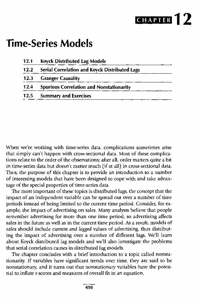
CHAPTER 12 Time-Series Models
12.1 Koyck Distributed Lag Models
12.2 Serial Correlation and Koyck Distributed Lags
12.3 Granger Causality
12.4 Spurious Correlation and Nonstationarity
12.5 Summary and Exercises
When we're working with time-series data, complications sometimes a rise that simply can't happen with cross-sectional data. Most of these complica-tions relate to the order of the observations; after all, order matters quite a bit in time-series data but doesn't matter much (if at all) in cross-sectional data. Thus, the purpose of this chapter is to provide an introduction to a number of interesting models that have been designed to cope with and take advan-tage of the special properties of time-series data.
The most important of these topics is distributed lags, the concept that the impact of an independent variable can be spread out over a number of time periods instead of being limited to the current time period. Consider, for ex-ample, the impact of advertising on sales. Many analysts believe that people remember advertising for more than one time period, so advertising affects sales in the future as well as in the current time period. As a result, models of sales should include current and lagged values of advertising, thus distribut-ing the impact of advertising over a number of different lags. We'll learn about Koyck distributed lag models and we'll also investigate the problems that serial correlation causes in distributed lag models.
The chapter concludes with a brief introduction to a topic called nonsta-tionarity. If va riables have significant trends over time, they are said to be nonstationary, and it turns out that nonstationary variables have the poten-tial to inflate t-scores and measures of overall fit in an equation.
410

CHAPTER 12 • TIME-SERIES MODELS 411
12.1 Koyck Distributed Lag Models
12.1.1 Distributed Lag Models
Ever since we introduced the idea of lags in Section 6.5, we've used lagged in-dependent variables whenever we've expected X to affect Y after a period of time. For example, if the underlying theory has suggested that X 1 affects Y with a one-time-period lag (but X2 has an instantaneous impact on Y) we've used equations like:
Yt - R O + RIX1t- 1 + R2X2t + Et (12.1)
Such lags are called simple lags, and the estimation of R1 with OLS is no more difficult than the estimation of the coefficients of nonlagged equations, except for possible impure serial correlation if the lag is misspecified. Remember, however, that the coefficients of such equations should be interpreted care-fully. For example, 13 2 in Equation 12.1 measures the effect of a one-unit in-crease in this time's X2 on this time's Y holding last time's X1 constant.
A case more complicated than this simple lag model occurs when the im-pact of an independent variable is expected to be spread out over a number of time periods. For example, suppose we're interested in studying the impact of a change in the money supply on GDP. Theoretical and empirical studies have provided evidence that because of rigidities in the marketplace, it takes time for the economy to react completely to a change in the money supply. Some of the effect on GDP will take place in the first qua rter, some more in the second qua rter, and so on. In such a case, the appropriate econometric model would be a distributed lag model:
Yt = ao + RoXt + R 1Xt —1 + R2Xt - 2 + + RpXt_P + Et (12.2)
A distributed lag model explains the current value of Y as a function of cur-rent and past values of X, thus "distributing" the impact of X over a number of time periods. Take a careful look at Equation 12.2. The coefficients j3 0 , R1 ,
and 13 2 through 13p measure the effects of the various lagged values of X on the current value of Y. In most economic applications, including our money supply example, we'd expect the impact of X on Y to decrease as the length of the lag (indicated by the subscript of the [3) increases. That is, although j3 o
might be larger or smaller than [31 , we certainly would expect either [3 0 or 13 1 to be larger in absolute value than 13 6 or 137.

412 PART III • EXTENSIONS OF THE BASIC REGRESSION MODEL
Unfortunately, the estimation of Equation 12.2 with OLS causes a number of problems:
1. The various lagged values of X are likely to be severely multicollinear, making coefficient estimates imprecise.
2. In large part because of this multicollinearity, there is no guarantee that the estimated 13s will follow the smoothly declining pattern that economic theory would suggest. Instead, it's quite typical for the esti-mated coefficients of Equation 12.2 to follow a fairly irregular pattern, for example:
Ro = 0.26 R1 = 0.07 R = 0.17 1:1 3 =— 0.03 R4 = 0.08
3. The degrees of freedom tend to decrease, sometimes substantially, for two reasons. First, we have to estimate a coefficient for each lagged X, thus in-creasing K and lowering the degrees of freedom (n — K — 1) . Second, unless data for lagged Xs outside the sample are available, we have to de-crease the sample size by one for each lagged X we calculate, thus lower-ing the number of observations, n, and therefore the degrees of freedom.
As a result of these problems with OLS estimation of functions like Equa-tion 12.2, called ad hoc distributed lag equations, it's standard practice to use a simplifying assumption to avoid these problems. The most commonly used simplification is the Koyck model.
12.1.2 What Are Koyck Lags?
A Koyck distributed lag model is one that assumes that the coefficients of the lagged variables decrease in a geometric fashion the longer the lag: 1
Ri = 13oXi (12.3)
where i is the length of the lag, 1, 2, p and 0 < X < 1. For example,
P3 — Po'3
If we substitute Equation 12.3 into Equation 12.2 for each coefficient and factor out Ro, we obtain
Yt=ao+ Ro(Xt+XXt_1+X 2Xt-2+X3Xt-3+ ) + Et (12.4)
1. L. M. Koyck, Distributed Lags and Investment Analysis (Amsterdam: North-Holland Publishing Company, 1954).

Rel
ativ
e W
eigh
t of L
agg
ed V
aria
ble
0.5
1.0
CHAPTER 12 • TIME-SERIES MODELS 413
0 1 2 3 4 5
6
7 Time Period of Lag
Figure 12.1 Geometric Weighting Schemes for Various Koyck Lag Models
No matter what X is used, a Koyck distributed lag model has the impact of the indepen-dent variable declining as the length of the lag increases.
Since we have assumed that X is between zero and one, X to the (n + 1)th power is smaller than X to the nth power. As a result, each successive lagged
term has a smaller coefficient than the previous term, 2 For example, if X = 0.2, then Equation 12.4 becomes:
Yt = act + Ro (Xt + 0.2Xt _ 1 + 0.04Xt _ 2 + 0.008Xt _ 3 +
) + Et
(12.5)
because (0.2) 1 = 0.2, (0.2) 2 = 0.04, and so on. As can be seen in Figure 12.1, each successive lagged value does indeed have relatively less weight in deter-mining the current value of Y.
2. One distributed lag model in which the coefficient need not follow this pattern is the Almon polynomial distributed lag model, an estimation procedure for distributed lags that allows the coefficients of the lagged independent variables to follow a variety of continuous patterns as the length of the lag increases. Although coefficients from a simple Koyck model are limited to a steadily decreasing pattern (Figure 12.1), the Almon model can allow coefficients to first increase and then decrease or to change direction more than once. See Shirley Almon, "The Distributed Lag Between Capital Approp riations and Expenditures," Econometrica, 1965, pp. 178-196.
414 PART III • EXTENSIONS OF THE BASIC REGRESSION MODEL
How can we estimate Equation 12.4? As it stands, the equation is nonlin-ear in the coefficients and can't be estimated with OLS. However, with some manipulation, Equation 12.4 can be transformed into an equivalent equa-tion that is linear in the coefficients a0, R0, and X. To see this, multiply both sides of Equation 12.4 by X and lag it once (that is, substitute t - 1 for t in every instance that it appears):
xYt -i - xa0 + 00(XXt -1 + X2Xt -2 + X3Xt -3 + ) + ÂEt -1 (12.6)
Now subtract the resulting equation (Equation 12.6) from Equation 12.4 and rewrite, producing:
Yt= aO+PoXt+AYt_1 + ut (12.7)
where ut = Et — XEt _ 1 and where a 0 = a0 - Xa0 (still a constant). Compare Equation 12.7 with Equation 12.4; the Koyck transformation has changed a distributed lag equation into an equation with a lagged dependent variable, often called an autoregressive equation.
This equation (Equation 12.7) then becomes the estimating equation. OLS can be applied to Equation 12.7 as long as the sample is large enough. How large is "large enough?" Our recommendation, based more on experi-ence than proof, is to aim for a sample size of at least 50 observations. 3 The smaller the sample, the more likely you are to encounter bias. Samples below 25 in size should be avoided entirely, in part because of bias and in pa rt be-cause hypothesis testing becomes untrustworthy.
Koyck distributed lag models have other potentially serious problems. If the original error term Et satisfies all the Classical Assumptions, then the error term in the Koyck model, u t, is almost sure to be serially correlated. In addi-tion, OLS estimation of Equation 12.7 is biased no matter how large the sam-ple. These problems will be discussed in Section 12.2. Also, the presence of a lagged dependent variable as an independent variable forces every other in-dependent variable in the equation to be related to the dependent variable by a declining geometric (Kyock) distributed lag function.
As an example of this latter problem, suppose that we want to build a model of Y that includes a distributed lag of X1 and also includes X2 as an unlagged independent variable. Suppose further that we use the following equation:
3. If ut is well behaved, OLS estimation of Equation 12.7 can be shown to have desirable prop-erties for extremely large samples, but not enough is known about the small sample properties of this model to issue firm sample size guidelines. See H. Doran and W. Griffiths, "Inconsis-tency of the OLS Estimator of the Partial-Adjustment-Adaptive Expectations Model," Journal of Econometrics, 1978, pp. 133-146.

CHAPTER 12 • TIME-SERIES MODELS 4"
Yt ao + RoXlt + XYt -1 + R1X2t + ut (12.8)
The use of the XYt _ 1 term forces both X 1 and X2 to have Koyck distributed lag patterns with respect to Y. Thus, if we don't expect X2 to have lagged effects on Y, a Koyck function is not an appropriate model in this case unless the equation is specifically adjusted to offset this problem.
12.1.3 An Example of Koyck Distributed Lags
As an example of a Koyck distributed lag model, let's look at an aggregate consumption function from a macroeconomic equilibrium GDP model. Many economists argue that, in such a model, consumption is not just an in-stantaneous function of income. Instead, they maintain that current pur-chases of goods and services (CO t) are influenced by past levels of disposable income (YDt _ 1 , YDt _ 2, etc.) as well as current levels of disposable income (YDt):
+ + + COt = f(YDt, YDt_ 1, YDt _ 2, etc.) + ut (12.9)
Such an equation fits well with simple models of consumption, but it only makes sense if the weights given past levels of income decrease as the length of the lag increases. That is, we would expect the coefficient of YD t _ 2 to be less than the coefficient of YD t _ 1 , and so on.
As a result, most econometricians would model Equation 12.9 with a Koyck distributed lag equation:
COt = a0 + 13oYDt + ACOt _ 1 + ut (12.10)
This equation not only fits a simple model of aggregate consumption, but it also is quite close to that suggested by Milton Friedman for his permanent in-come hypothesis. 4 In that hypothesis, Friedman suggested that consumption was based not on current income but instead on the consumer's perception of lifetime income. Consequently, changes in transitory income wouldn't af-fect consumption. Since it's reasonable to hypothesize that perceptions of permanent income are based on past levels of income, the simple Koyck con-sumption model and the more sophisticated permanent income model have similar equations.
4. Milton Friedman, A Theory of the Consumption Function (Princeton, N.l.: P rinceton University Press/National Bureau of Economic Research, 1957). It's interesting to note, however, that Friedman's original function did not include a constant term because of the nature of his de-rivation of permanent income.
416 PART III • EXTENSIONS OF THE BASIC REGRESSION MODEL
To estimate Equation 12.10, we use data from Section 14.3, where we will build a small macro model of the U.S. economy from 1964 through 1994. The OLS estimates of Equation 12.10 for this data set are (standard errors in parentheses):
COt = - 38.11 + 0.52YDt + 0.46COt_ 1
(0.12) (0.12)
t = 4.44 3 . 74 R2 = .998 n = 31 (annual 1964 - 1994)
One way to analyze the coefficients of this equation is to convert the esti-mates back into the format of Equation 12.9 by using the Koyck distributed lag definitions of the individual coefficients, Equation 12.3:
(12.3)
If we substitute Ro = 0.52 and X = 0.46 into Equation 12.3 for i = 1, we ob-tain p i = pox' = (0.52) (0.46) 1 = 0.24. If we continue this process, it turns out that Equation 12.11 is equivalent toy:
COt = - 70.57 + 0.52YDt + 0.24YDt _ 1 + 0.11YDt _ 2 (12.12) + 0.05YDt _ 3 +
As can be seen, the coefficients of YD in Equation 12.12 do indeed smoothly decline as we'd expect in a Koyck distributed lag equation.
To compare this estimate with an OLS estimate of the same equation with-out the Koyck lag format, we'd need to estimate an ad hoc distributed lag equation with the same number of lagged variables:
COt = ao + 13 0YDt + 13 1YDt _ 1 + 132YDt _ 2 + j33YDt _ 3 + Et (12.13)
As expected, the coefficients of the ad hoc estimate do not follow the same smoothly declining pattern:
COt = - 152.8 + 0.93YDt + 0.10YDt _ 1 - 0.05YDt _ 2 - 0.03YDt _ 3
(12.14)
5. Note that the constant term equals 4/(1 - i).
CHAPTER 12 • TIME-SERIES MODELS
How do the coefficients of Equation 12.14 look? As the lag increases, the co-efficients of YD decrease sharply, actually going negative for t 2 and t — 3. Neither economic theory nor common sense leads us to expect this pattern. Such a poor result is due to the severe multicollinearity between the lagged Xs. Most econometricians therefore estimate distributed lag models with a lagged dependent variable simplification scheme like the Koyck function in Equation 12.10.
An interesting interpretation of the results in Equation 12.11 concerns the long-mn multiplier implied by the model. The long-mn multiplier measures the total impact of a change in income on consumption after all the lagged effects have been felt. An estimate of the long-run multiplier can be obtained from Equation 12.11 by calculating k[1/(1 — X)], which in this case equals 0.52[1/(1 — 0.46) ] or 0.96. A sample of this size is likely to encounter small sample bias, however, so we shouldn't overanalyze the results. For more on this data set and the other equations in the model, see Section 14.3. For more on testing and adjusting distributed lag equations like Equation 12.11 for se-rial correlation, let's move on to the next section.
12.2 Serial Correlation and Koyck Distributed Lags
Perhaps the most serious drawback of Koyck lags is the high probability of se-rial correlation. Equations with a lagged dependent variable are more likely to encounter serial correlation than are other equations. To understand why, take a look at a typical Koyck error term from Equation 12.7:
ut = Et ÂE t _ 1
Do you see the problem? This time's error term (u t) is a moving average of Et , so Et _1 affects both u t and ut _ 1 . Since ut and ut _ 1 are affected by the same variable, (Et _ 1 ), they're almost sure to be correlated, violating Classical As-sumption 1V. 6
Compounding this, the consequences, detection, and remedies for serial correlation that we discussed in Chapter 9 are all either incorrect or need to be modified in the presence of a lagged dependent va riable. Since all Koyck dis-tributed lag models include a lagged dependent va riable, a discussion of serial correlation in Koyck models is critical to an understanding of distributed lags.
6. More formally, if we start with u t = Et - AEt _ 1, lag this equation one time period, solve for Et _ 1 , and then substitute back into the o riginal definition of ut, we obtain: ut ^ Et Xut - 1 - X2Et- 2•
In other words, this time's error term u t is a function of last time's error term, u t _ 1.
418 PART III ■ EXTENSIONS OF THE BASIC REGRESSION MODEL
12.2.1 Serial Correlation Causes Bias in Koyck Lag Models
In Section 9.2, we stated that pure serial correlation does not cause bias in the estimates of the coefficients. Unfortunately, the use of a Koyck distributed lag model changes all that. More specifically, if an equation that contains a lagged dependent variable as an independent va riable has a serially corre-lated error term, then OLS estimates of the coefficients of that equation will be biased, even in large samples.
To see where this bias comes from, let's look at an equation with a lagged dependent variable and a serially correlated error term of the type (ut = Et — AEt_ i, called a moving average) found in Koyck distributed lag equations:
T T Yt = ao + (3oXt + xYt — 1 + Et — xEt — 1
Let's also look at Equation 12.15 lagged one time period:
(12.15)
T T Yt— 1 = ao + QoXt— 1 + XYt -2 + Et-1 — XEt -2 (12.16)
What happens when last time period's error term (E t _ 1 ) is positive? In Equa-tion 12.16, the positive Et _1 causes Yt — 1 to be larger than it would have been otherwise (these changes are marked by upward pointing arrows).
Take a look at the right-hand side of Equation 12.15. Every time e t _ 1 is positive, Yt _ 1 will be larger than otherwise. Thus, the two variables are corre-lated and, therefore, so are u t and Yt - 1 . Such a situation violates Classical As-sumption III that the error term is not correlated with any of the explanatory variables. What happens if Et — i is negative? In this case, Yt— i will be lower than it would have been otherwise, so they're still correlated.
The consequences of this correlation include biased estimates, in particu-lar of the coefficient X. In essence, the uncorrected serial correlation acts like an omitted variable (e t _ 1 ) . Since an omitted variable causes bias whenever it is correlated with one of the included independent variables, and since Et _ 1 is correlated with Yt _ 1 , the combination of a lagged dependent variable and serial correlation causes bias in the coefficient estimates.?
Serial correlation in a Koyck lag model also causes estimates of the stan-dard errors of the estimated coefficients and the residuals to be biased. The
7 The reason that pure serial correlation doesn't cause bias in the coefficient estimates of equa-tions that don't include a lagged dependent variable is that the "omitted variable" E t _ 1 isn't correlated with any of the included independent va riables.

CHAFFER 12 • TIME-SERIES MODELS 419
former bias means that hypothesis testing is invalid, even for large samples. The latter bias means that tests based on the residuals, like the Durbin-Watson d test, are potentially invalid.
12.2.2 Testing Koyck Lag Models for Serial Correlation
Until now, we've relied on the Durbin-Watson d test of Section 9.3 to test for serial correlation, but, as mentioned above, the Durbin-Watson d is poten-tially invalid for an equation that contains a lagged dependent variable as an independent va riable. This is because the biased residuals described in the previous paragraph cause the DW d statistic to be biased toward 2. This bias toward 2 means that the Durbin-Watson test sometimes fails to detect the presence of serial correlation in a Koyck (or similar) lag model. 8
The most-used alternative is Durbin's h test, 9 which is a large-sample method of adjusting the Durbin-Watson d statistic to test for first-order serial correlation in the presence of a lagged dependent variable. The equation for Durbin's h statistic is:
h = (1 - 0.5 d)
n (12.17)
(1 n • [S?,])
where: d = the Durbin-Watson statistic n = the sample size S? = the square of the estimated standard error of X, the
estimated coefficient of Yt _
Durbin's h is normally distributed, so a 95 percent two-tailed test implies a critical z-value of 1.96. Therefore, the decision rule is:
If the absolute value of h is greater than 1.96, reject the null hy-pothesis of no first-order serial correlation.
If the absolute value of h is less than 1.96, do not reject the null hypothesis of no first-order serial correlation.
As an example, let's test our Koyck distributed lag aggregate consumption function, Equation 12.11, for serial correlation:
8. The opposite is not a problem. A Durbin-Watson d test that indicates serial correlation in the presence of a lagged dependent va riable, despite the bias toward 2, is an even stronger affirma-tion of serial correlation.
9. J. Durbin, "Testing for Serial Correlation in Least Squares Regression When Some of the Re-gressors Are Lagged Dependent Variables," Econometrica, 1970, pp. 410-421.

420 PART III ■ EXTENSIONS OF THE BASIC REGRESSION MODEL
COt _ 1 = — 38.11 + 0.52YD t + 0.46COt_ 1 (0.12) (0.12)
t = 4.44 3.74 R2 =.998 n = 31 DW = 0.89
Substituting into Equation 12.17, we obtain:
h=(1-0.5•0.89) 31
= 4.15 [1 31(0.12) 2 ]
(12.18)
Since 4.15 > 1.96, we can reject the null hypothesis of no first-order serial correlation and conclude that, as expected, there is indeed significant serial correlation in our consumption function.
Durbin's h test has at least two problems, however. First, the test statistic is undefined in ce rtain circumstances (when n [St] ? 1) because the value under the square root sign in Equation 12.17 is negative. Second, Durbin's h test cannot be used if the model in question has more than one lagged de-pendent variable or if the serial correlation being tested for isn't first order in nature. Although some researchers adjust Durbin's h in these situations, a more satisfactory solution would be to find a test that avoids these two prob-lems altogether while working just as well in the simple case.
One such test is the Lagrange Multiplier test. The Lagrange Multiplier (LM) test is a method that can be used to test for serial correlation in the presence of a lagged dependent va riable by analyzing how well the lagged residuals explain the residuals of the original equation (in an equation that includes all the explanatory variables of the original model). If the lagged residuals are significant in explaining this time's residuals (as shown by the chi-square test), then we can reject the null hypothesis of no serial correla-tion. The Lagrange Multiplier test also is useful as a specification test and as a test for heteroskedasticity and other econometric problems.'°
Using the Lagrange Multiplier to test for serial correlation for a typical Koyck model involves three steps:
1. Obtain the residuals from the estimated equation:
et = Yt — Yt = Yt — ao — RoX1t - 5;Yt -1 (12.19)
10. For example, some readers may remember that the White test of Section 10.3.3 is a Lagrange Multiplier test. For a survey of the various uses to which Lagrange Multiplier tests can be put and a discussion of the LM test's relationship to the Wald and Likelihood Ratio tests, see Robert F. Engle, "Wald, Likelihood Ratio, and Lagrange Multiplier Tests in Econometrics," in Z. Griliches and M. D. Intriligator, eds., Handbook of Econometrics, Volume II (Amsterdam: Elsevier Science Publishers, 1984).

CHAPTER 12 • TIME-SERIES MODELS 42
2. Use these residuals as the dependent variable in an auxiliary equation that includes as independent va riables all those on the right-hand side of the original equation as well as the lagged residuals:
e t = a0 + a 1Xt + a2Yt _ 1 + a3et - 1 + ut (12.20)
3. Estimate Equation 12.20 using OLS and then test the null hypothesis that a3 = 0 with the following test statistic:
LM = n • R2 (12.21)
where n is the sample size and R2 is the unadjusted coefficient of de-termination, both of the auxiliary equation, Equation 12.20. For large samples, LM has a chi-square distribution with degrees of freedom equal to the number of restrictions in the null hypothesis (in this case, one). If LM is greater than the critical chi-square value from Statistical Table B-8, then we reject the null hypothesis that a 3 = 0 and conclude that there is indeed serial correlation in the o riginal equation.
To run an LM test for second-order or higher-order serial correlation, add lagged residuals (e t _ 2 for second order, e t _ 2 and et _ 3 for third order) to the auxiliary equation, Equation 12.20. This latter change makes the null hy-pothesis a3 = a4 = a5 = 0. Such a null hypothesis raises the degrees of free-dom in the chi-square test to three because we have imposed three restric-tions on the equation (three coefficients are jointly set equal to zero). To run an LM test with more than one lagged dependent variable, add the lagged variables (Yt _2, Yt - 3, etc.) to the original equation. For practice with the LM test, see Exercise 6; for practice with testing for higher-order serial correlation, see Exercise 7
12.2.3 Correcting for Serial Correlation in Koyck Models
There are three strategies for attempting to rid a Koyck lag model (or a similar model) of serial correlation: improving the specification, instrumental vari-ables, and modified GLS.
The first strategy is to consider the possibility that the serial correlation could be impure, caused by either omitting a relevant variable or by failing to capture the actual distributed lag pattern accurately. Unfortunately, finding an omitted variable or an improved lag structure is easier said than done, as we've seen in previous chapters. Because of the dangers of sequential specifi-cation searches, this option should be considered only if an alternative speci-fication exists that has a theoretically sound justification.
422 PART III • EXTENSIONS OF THE BASIC REGRESSION MODEL
The second strategy, called instrumental variables, consists of substituting a proxy (an "instrument") for Yt_ 1 in the original equation, thus eliminating the correlation between Y t _ 1 and ut. Although using an instrument is a rea-sonable option that is straightforward in principle, it's not always easy to find a proxy that retains the distributed lag nature of the original equation. For a more complete discussion of instrumental variables, see Section 14.3.
The final solution to serial correlation in Koyck models (or in models with lagged dependent variables and similar error term structures) is to use an iter-ative maximum likelihood technique to estimate the components of the se-rial correlation and then to transform the original equation so that the serial correlation has been eliminated. This technique, which is similar to the GLS procedure outlined in Section 9.4, is not without its complications. In partic-ular, the sample needs to be large, the standard errors of the estimated coeffi-cients potentially need to be adjusted, and the estimation techniques are flawed under some circumstances. 11 In essence, serial correlation causes bias in Koyck distributed lag models, but ridding the equation of that serial corre-lation is not an easy task.
12.3 Granger Causality
One application of ad hoc distributed lag models is to test the direction of causality in economic relationships. Such a test is useful when we know that two variables are related but we don't know which variable causes the other to move. For example, most economists believe that increases in the money supply stimulate GDP, but others feel that increases in GDP eventually lead the monetary authorities to increase the money supply. Who's right?
One approach to such a question of indeterminate causality is to theorize that the two variables are determined simultaneously. We'll address the esti-mation of simultaneous equation models in Chapter 14. A second approach to the problem is to test for what is called "Granger causality."
How can we claim to be able to test for causality? After all, didn't we say in Chapter 1 that even though most economic relationships are causal in na-ture, regression analysis cannot prove such causality? The answer is that we don't actually test for theoretical causality; instead, we test for Granger causality.
11. For more on these complications, see A. C. Harvey, The Econometric Analysis of Time Series (New York: Wiley, 1981), and R. Betancourt and H. Kelejian, "Lagged Endogenous Va riables and Cochrane-Orcutt Procedure," Econometrica, 1981, pp. 1073-1078.
CHAPTER 12 • TIME-SERIES MODELS 423
Granger causality, or precedence, is a circumstance in which one time-series variable consistently and predictably changes before another variable does. 12 If one variable precedes ("Granger causes") another, we still can't be sure that the first variable "causes" the other to change, but we can be fairly sure that the opposite is not the case.
To see this, suppose event A always happens before event B. It's unlikely that B is the cause of A, isn't it? After all, how often does an event that will happen in the future cause an event that has already happened? In such a sit-uation, we can reject the hypothesis that event B causes event A with a fairly high level of confidence.
On the other hand, we still have not shown that event A "causes" B. Prov-ing that people car ry umbrellas around before it rains doesn't prove that car-rying the umbrellas actually causes the rain. All we've shown is that one event preceded or, more specifically, "Granger-caused" the other. Granger causality is important because it allows us to analyze which variable precedes or "leads" the other, and, as we shall see, such leading variables are extremely useful for forecasting purposes. Despite the value of Granger causality, how-ever, we shouldn't let ourselves be lured into thinking that it allows us to prove economic causality in any rigorous way.
There are a number of different tests for Granger causality, and all the vari-ous methods involve distributed lag models in one way or another. 13 Our preference is to use an expanded version of a test originally developed by Granger. Granger suggested that to see if B Granger-caused Y, we should run:
Yt f(Yt _ 1 , Yt -2- Yt -p 1 Bt_ 1, Bt _ 2„ , Bt _ p) + Et (12.22)
and test the null hypothesis that the coefficients of the lagged Bs jointly equal zero. If we can reject this null hypothesis using the F-test, then we have evi-dence that B Granger-causes Y. Note that if p = 1, Equation 12.22 is similar to a Koyck distributed lag model.
12. See C. W. J. Granger, "Investigating Causal Relations by Econometric Models and Cross-Spectral Methods," Econometrica, 1969, pp. 24-36.
13. Perhaps the most famous of these tests is the Sims test: Christopher A. Sims, "Money, Causality, and Income," American Economic Review, 1972, pp. 540-552. Unfortunately, the Sims test has some problems, especially its inability to deal with serially correlated future val-ues of independent va riables. See John Geweke, R. Meese, and W. Dent, "Comparing Alterna-tive Tests of Causality in Temporal Systems," Journal of Econometrics, 1982, pp. 161-194, and Rodney Jacobs, Edward Learner, and Michael Ward, "Difficulties with Testing for Causation," Economic Inquiry, 1979, pp. 401 -413.
424 PART III • EXTENSIONS OF THE BASIC REGRESSION MODEL
For a number of reasons, we recommend running two Granger tests, one in each direction. That is, run Equation 12.22 and also run:
Bt = f(Yt— I , Yt-21 Yt— Bt - 1f Bt-2/ , Bt _ P) + et (12.23)
testing for Granger causality in both directions. If the F-test is significant for Equation 12.22 but not for Equation 12.23, then we can conclude that B Granger-causes Y. For practice with this dual version of the Granger test, see Exercise 8.
12.4 Spurious Correlation and Nonstationarity
One problem with time-series data is that independent va riables can appear to be more significant than they actually are if they have the same underlying trend as the dependent variable. In a country with rampant inflation, for exam-ple, almost any nominal variable will appear to be highly correlated with all other nominal variables. Why? Nominal variables are unadjusted for inflation, so every nominal variable will have a powerful inflationary component. This inflationary component will usually outweigh any real causal relationship, causing nominal variables to appear to be correlated even if they aren't.
Such a problem is an example of spurious correlation, a strong relation-ship between two or more variables that is caused by a statistical fluke or by the nature of the specification of the variables, not by a real underlying causal relationship. If you run a regression in which the dependent variable and one or more independent variables are spuriously correlated, the result is a spuri-ous regression, and the t-scores and overall fit of such spurious regressions are likely to be overstated and untrustworthy.
There are many causes of spurious correlation. In a cross-sectional data set, for example, spurious correlation can be caused by dividing the dependent variable and one independent variable by a third variable that varies consid-erably more than do the first two. The focus of this section, however, will be on time-series data and in particular on spurious correlation caused by non-stationary time series.
12.4.1 Stationary and Nonstationary Time Series
A stationary time series is one whose basic properties don't change over time. In contrast, a nonstationary variable has some so rt of upward or downward trend. For instance, a nominal aggregate va riable for an inflationary count ry
is very likely to be nonstationary but a real per capita version of the same variable in the same count ry might be stationary.
CHAPTER 12 • TIME-SERIES MODELS 425
More formally, a time-series variable, X t, is stationary if:
1. the mean of Xt is constant over time,
2. the variance of X t is constant over time, and
3. the simple correlation coefficient between X t and Xt _ k (also called an autocorrelation function) depends on the length of the lag (k) but on no other variable (for all k). 14
If one or more of these three properties is not met, then X t is nonstationary. If a series is nonstationary, that problem is often referred to as nonstationarity.
Before going on, let's discuss two concepts. First, the autocorrelation func-tions (ACFs) mentioned in property number 3 are not as forbidding as they might seem at first glance. To calculate an autocorrelation function of lag k, compute the simple correlation coefficient between X t and Xt _ k over the n — k such pairs in the data set:
ACF k E
(Xt X) (Xt -
k X)
12.24 ( ) = E (Xt — X) 2
(12.24)
For practice with autocorrelation functions, see Exercise 10 at the end of the chapter. Second, although our definition of a stationary series focuses on sta-tionary and nonstationary variables, it's important to note that error terms (and, therefore, residuals) can also be nonstationary. In fact, we've already had experience with a nonstationary error term. Most cases of heteroskedasticity in time-series data involve an error term with a variance that increases with each time period. Thus, a heteroskedastic error term is also nonstationary!
The major consequence of nonstationarity for regression analysis is spuri-ous correlation that inflates R2 and the t-scores of the nonstationary indepen-dent variables. This occurs because the regression estimation procedure at-tributes to the nonstationary X t changes in Yt that were actually caused by some factor (trend, for example) that also affects X. Thus, the variables move together because of the nonstationarity, increasing R2 and the relevant t-scores. This is especially impo rtant in macroeconometrics, and the litera-ture is dominated by a rticles that examine various macroeconomic series for signs of nonstationarity 15
14.There are a number of different kinds of stationarity. The particular definition we use here is a simplification of the most frequently cited definition, referred to by various authors as a weak, wide-sense, or covariance stationarity.
15. See, for example, C. R. Nelson and C. I. Plosser, "Trends and Random Walks in Macroeco-nomic Time Series: Some Evidence and Implication, Journal of Monetary Economics, 1982, pp. 169-182, and J. Campbell and N. G. Mankiw, "Permanent and Transitory Components in Macroeconomic Fluctuations," American Economic Review, May 1987, pp. 111-117.
426 PART III • EXTENSIONS OF THE BASIC REGRESSION MODEL
12.4.2 Testing for Nonstationarity
How can you tell if a time series is nonstationary? There are at least three ways. The first and easiest test is to visually examine the data. For many time series, a quick glance at the data (or a diagram of the data) will tell you that the mean of a variable is increasing dramatically over time and that the series is nonstationary.
A second, more careful, test is to see if the ACFs for a variable tend to zero as k (the length of the lag) increases, using the t-test of r described in Chapter 5, to see if the ACF is significantly different from 0. If the ACFs tend to zero fairly quickly, the variable is stationary, but if they don't, the variable is non-stationary. For practice in this kind of testing, see Exercise 10.
The third and most popular method of testing for nonstationarity is the Dickey-Fuller test, which examines the hypothesis that the variable in ques-tion has a unit root and, as a result, is likely to benefit from being expressed in first-difference form. 16 To run a Dickey-Fuller test, estimate the following equation:
6Yt = (Yt — Yt - 1) — 13o + 13 1Yt -1 + Et
and run a one-sided t-test on the hypothesis that Ri = 0.
(12.25)
Ho : p i = 0 HA: R1 <0
If R 1 is significantly less than 0, then we can reject the null hypothesis of non-stationarity. On the other hand, recall from Chapter 5 that if we're not able to reject the null hypothesis, we still have not "proven" that Y is nonstationary.
Be careful, however. The standard t-table does not apply to Dickey-Fuller tests; Table 12.1 lists asymptotic (n -a 00) values for t c. For smaller samples, critical t-values are about 60 percent higher (in absolute value) than those in
16. D. A. Dickey and W. A. Fuller, "Distribution of the Estimators for Autoregressive Time-Series with a Unit Root," Journal of the American Statistical Association, 1979, pp. 427-431. The Dickey-Fuller test comes in a variety of forms, including an augmented test to use in cases of a serially correlated error term. The phrase "unit root" refers to the possibility that R 1 = 1 in
Yt = po + 3 1 ,4-1 + et . If (3 1 exactly equals 1, Yt can be characterized by a random walk process, where the change in Y is assumed to be drawn from a distribution with a mean of zero. This process is inherently nonstationary. For more on unit roots, see John Y. Campbell and Pierre Peron, "Pitfalls and Opportunities: What Macroeconomists Should Know About Unit Roots," NBER Macroeconomics Annual (Cambridge: MIT Press, 1991), pp. 141-219.

CHAPTER 12 • TIME-SERIES MODELS
TABLE 12.1 ASYMPTOTIC CRITICAL VALUES FOR THE DICKEY—FULLER TEST
One-Sided Significance Level: .01 .025 .05 10
tc 3.43 3.12 2.86 2.57
Statistical Table B-1. For example, a 2.5 percent one-sided t-test of R1 from Equation 12.25 with 50 degrees of freedom has a critical t-value of 3.22, compared to 2.01 for a standard t-test. 17 For practice in running Dickey-Fuller tests, see Exercise 11.
12.4.3 Adjusting for Nonstationarity
If one of our three tests reveals nonstationarity, what should we do? Some authors attempt to "detrend" an equation by including a time-trend variable (t = 1, 2, T) as an independent variable in the regression, but we urge you not to do so for a number of reasons. 18
Instead, if it's necessary to rid a series of nonstationarity, the traditional practice has been to take a first difference:
AYt = Yt Yt_ 1 (12.26)
and use DYt in place of Yt in the equation. With economic data, taking a first difference usually is enough to convert a nonstationary series to a stationary one, but it's a good habit to test DYt just to make sure. Unfortunately, there are major disadvantages to using first differences to correct for nonstationar-ity. The two most impo rtant of these drawbacks are that using first differences (a) changes the inherent theoretical meaning of the differenced variable, and (b) discards information about the long-run trend in that va riable. As a re-sult, first differences should not be used without weighing the costs and ben-efits of that shift.
17 For adjusted critical t-values for the Dickey-Fuller test, including those in Table 12.1, see J. G. MacKinnon, "Critical Values of Cointegration Tests," in Rob Engle and C. W. J. Granger, eds., Long-Run Economic Relationships: Readings in Cointegration (New York: Oxford University Press, 1991), Chapter 13.
18. See C. R. Nelson and H. Kang, "Pitfalls in the Use of Time as an Explanatory Variable in Re-gression," Journal of Business and Economic Statistics, January 1984, pp. 73-82. An exception to this recommendation is that if both a unit root and a time trend are present, it's impo rtant to in-clude the time trend as an independent va riable when constructing a test statistic for a unit root.
428 PART III • EXTENSIONS OF THE BASIC REGRESSION MODEL
An important alternative to using first differences to correct for nonsta-tionarity is a concept called cointegration. Cointegration consists of matching up the degree of nonstationarity of the variables in an equation in a way that makes the residuals of the equation stationary and rids the equation of any spurious regression results. 19
Consider, for example, the following equation:
Yt =Ro +R1Xt+Et ( 12. 27)
Suppose that both Yt and Xt are nonstationary to the same degree; that is, sup-pose that AYt and AXt are both stationary. In such a situation there's a reason-able possibility that the nonstationarity in the two variables will "cancel each other out," leaving Equation 12.27 as a whole free of nonstationarity. An OLS estimate of Equation 12.27 would not be spurious, given such a situation.
How can you tell if any nonstationarity in an equation is cointegrated? The answer is to test the residuals of the equation for stationarity, using, say, the Dickey-Fuller test. If the residuals are stationary, then we have evidence that the nonstationary variables in the equation are on the same wavelength and that first differences are not necessary. In our example, this would mean estimating Equation 12.27, solving for the residual e t :
e t = Ÿt — Ro — 131Xt (12.28)
and running a test for nonstationarity on e t. Once again, however, the stan-dard t-values do not apply to this application. Instead, adjusted critical t-val-ues developed by Engle and Granger should be used. 20 The values in Statisti-cal Table B-1 are only slightly lower than these adjusted critical t-values, however, so they can be used as rough estimates of the more accurate figures.
12.5 Summary
1. A distributed lag model explains the current value of Y as a function of current and past values of X, thus "distributing" the impact of X over a number of lagged time periods. OLS estimation of distributed lag equations without any constraints (ad hoc distributed lags) en-
19. For more on cointegration, see B. Bhaskara Rau, ed., Cointegration for the Applied Economist (New York: St. Martin's Press, 1994).
20. Rob Engle and C. W. J. Granger, "Co-integration and Error Correction: Representation, Esti-mation and Testing," Econometrica, 1987, pp. 251-276.

CHAPTER 12 • TIME-SERIES MODELS 429
counters problems with multicollinearity, degrees of freedom, and a noncontinuous pattern of coefficients over time.
2. A Koyck distributed lag model avoids these problems by assuming that the coefficients of the lagged independent variables decrease in a geometric fashion the longer the lag (p i = 130X'), where i is the length of the lag and 0 < X < 1. Given this, the Koyck distributed lag equa-tion can be simplified to:
Yt = au+ RoXt+ kYt-1+ut
where ut = Et - ÂEt _ 1 and where Yt _ 1 is a lagged dependent vari-able. Thus, the use of a lagged dependent variable as an independent variable usually implies a Koyck distributed lag model.
3. In small samples, OLS estimates of a Koyck distributed lag model (or a similar model) are biased and have unreliable hypothesis testing properties. Even in large samples, OLS will produce biased estimates of the coefficients of a Koyck (or similar) model if the error term is se-rially correlated.
4. In a Koyck lag (or similar) model, the Durbin-Watson d test some-times can fail to detect the presence of serial correlation because d is biased toward 2. The most-used alternative is Durbin's h test, even though the Lagrange Multiplier test has similar properties and is more generally applicable.
5. Granger causality, or precedence, is a circumstance in which one time-series variable consistently and predictably changes before another variable does. If one variable precedes (Granger-causes) another, we still can't be sure that the first variable "causes" the other to change, but we can be fairly sure that the opposite is not the case.
6. A nonstationary series is one that exhibits a significant trend (for ex-ample in its mean or variance) over time. If the dependent variable and at least one independent variable are nonstationary, a regression is likely to encounter spurious correlation that inflates R 2 and the t-scores of the nonstationary independent variable(s).
7 Nonstationarity can be detected using a number of tests, including vi-sual inspection of the data and the Dickey-Fuller test. The most-used remedy for nonstationarity is converting the series to first differences, but this solution changes the theoretical underpinnings and long-term trend in the series.
430 PART III • EXTENSIONS OF THE BASIC REGRESSION MODEL
Exercises
(Answers to even-numbered exercises are in Appendix A.)
1. Write the meaning of each of the following terms without referring to the book (or your notes), and then compare your definition with the version in the text for each: a. Koyck distributed lag model b. ad hoc distributed lag model c. Durbin's h test d. Lagrange Multiplier (LM) test e. nonstationary series f. Dickey-Fuller test g. autocorrelation function (ACF) h. cointegration
2. Calculate and graph the pattern of the impact of a lagged X on Y as the lag increases for each of the following estimated Koyck distributed lag equations. a. Yt = 13.0 + 12.0Xt + 0.04Y_1 b. Yt = 13.0 + 12.0Xt + 0.08Y_1 c. Yt = 13.0 + 12.0Xt + 2.0Yt _ 1 d. Yt = 13.0 + 12.0Xt - 0.4Yt _ 1 e. Look over your graphs for parts c and d. What X rest riction do they
combine to show the wisdom of?
3. Consider the following equation aimed at estimating the demand for real cash balances in Mexico (standard errors in parentheses):
1nMt = 2.00 - 0.101nRt + 0.701nYt + 0.601nMt- 1 (0.10) (0.35) (0.10)
R2 =.90 DW=1.80 n = 26
where: Mt = the money stock in year t (millions of pesos) Rt = the long-term interest rate in year t (percent) Yt = the real GNP in year t (millions of pesos)
a. What economic relationship between Y and M is implied by the equation?
b. How are Y and R similar in terms of their relationship to M? c. Test for serial correlation in this equation. d. Now suppose you learn that the estimated standard error of the es-
timated coefficient of 1nM t _ 1 is actually 0.30. How does this change your answer to pa rt c above?
CHAPTER 12 • TIME-SERIES MODELS 43
4. Consider the following equation for the determination of wages in the United Kingdom (standard error in parentheses) 21 :
Wt = 8.562 + 0.364Pt + 0.004Pt _ 1 - 2.56Ut
(0.080) (0.072) (0.658)
R2 =.87 n= 19
where: Wt = wages and salaries per employee in year t Pt = the price level in year t Ut = the unemployment in year t
a. Develop and test your own hypotheses with respect to the individ-ual slope coefficients at the 90 percent level.
b. Discuss the theoretical validity of P 1 and how your opinion of that validity has been changed by its statistical significance. Should Pt _ I be dropped from the equation? Why or why not?
c. If Pt _ 1 is dropped from the equation, the general functional form of the equation changes radically? Why?
5. You've been hired to determine the impact of advertising on gross sales revenue for "Four Musketeers" candy bars. Four Musketeers has the same price and more or less the same ingredients as competing candy bars, so it seems likely that only advertising affects sales. You decide to build a distributed lag model of sales as a function of adver-tising, but you're not sure whether an ad hoc or a Koyck distributed lag model is more appropriate.
Using data on Four Musketeers candy bars from Table 12.2, esti-mate both of the following distributed lag equations from 1976-2000 and compare the lag structures implied by the estimated coefficients (Hint: Be careful to use the correct sample.): a. an ad hoc distributed lag model (4 lags) b. a Koyck distributed lag model
6. Test for serial correlation in the estimated Koyck lag equation you got as your answer to Exercise 5b by using: a. Durbin's h test b. The Lagrange Multiplier test
7 Suppose you're building a Koyck distributed lag model and are con-cerned with the possibility that serial correlation, instead of being first order, is second order: u t = f( ut- p ut -2 )•
21. Prices and Earnings in 1951-1969: An Econometric Assessment, United Kingdom Department of Employment, 1971, p. 35.
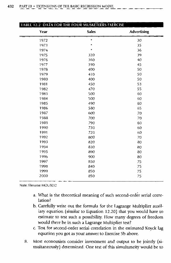
432 PART III • EXTENSIONS OF THE BASIC REGRESSION MODEL
TABLE 12.2 DATA FOR THE FOUR MUSKETEERS EXERCISE
Year Sales Advertising
1972 * 30 1973 * 35 1974 * 36 1975 320 39 1976 360 40 1977 390 45 1978 400 50 1979 410 50 1980 400 50 1981 450 53 1982 470 55 1983 500 60 1984 500 60 1985 490 60 1986 580 65 1987 600 70 1988 700 70 1989 790 60 1990 730 60 1991 720 60 1992 800 70 1993 820 80 1994 830 80 1995 890 80 1996 900 80 1997 850 75 1998 840 75 1999 850 75 2000 850 75
Note: filename MOUSE12
a. What is the theoretical meaning of such second-ordér serial cone-lation?
b. Carefully write out the formula for the Lagrange Multiplier auxil-iary equation (similar to Equation 12.20) that you would have to estimate to test such a possibility. How many degrees of freedom would there be in such a Lagrange Multiplier test?
c. Test for second-order serial correlation in the estimated Koyck lag equation you got as your answer to Exercise 5b above.
8. Most economists consider investment and output to be jointly (si-multaneously) determined. One test of this simultaneity would be to
CHAPTER 12 • TIME-SERIES MODELS 433
see whether one of the variables could be shown to Granger-cause the other. Take the data set from the small macroeconomic model in Table 14.1 and test the possibility that investment (I) Granger-causes GDP (Y) (or vice versa) with a two-sided Granger test with four lagged Xs.
9. Some farmers were interested in predicting inches of growth of corn as a function of rainfall on a monthly basis, so they collected data from the growing season and estimated an equation of the following form:
Gt= Ro + 13 1Rt+ R2Gt -1 + Et
where: GI = inches of growth of corn in month t Rt = inches of rain in month t Et = a normally distributed classical error term
Although the farmers expected a negative sign for 13 2 (they felt that since co rn can only grow so much, if it grows a lot in one month, it won't grow much in the next month), they got a positive estimate in-stead. What suggestions would you have for this problem?
10. Calculate the following autocorrelation functions (ACFs) using the data from the small macroeconomic model in Table 14.1 and then determine which of the variables, if any, you think are nonstationary. Explain your answer. [Hint: To calculate the ACFs on EViews, bring up the data, create the appropriate lagged versions of each va riable (re-membering to adjust for the smaller sample size), and then have the computer calculate the simple correlation coefficient between the variable and itself lagged k times.] a. Y (GDP), using ACFs with k = 2 and k = 6 b. r (the interest rate), using ACFs with k = 2 and k = 6 c. CO (consumption), using ACFs with k = 2 and k = 6 d. I (investment), using ACFs with k = 2 and k = 6
11. Run 2.5 percent Dickey-Fuller tests (of the form in Equation 12.25) for the following variables using the data from the small macroeco-nomic model in Table 14.1 and determine which variables, if any, you think are nonstationary. (Hint: Use 3.22 as your critical t-value.) a. Y (GDP) b. r (the interest rate) c. CO (consumption) d. I (investment)
CHAPTER 13 Dummy Dependent Variable Techniques
13.1 The Linear Probability Model
13.2 The Binomial Logit Model
13.3 Other Dummy Dependent Variable Techniques
13.4 Summary and Exercises
Until now, our discussion of dummy variables has been restricted to dummy independent variables. However, there are many important research topics for which the dependent variable is appropriately treated as a dummy, equal only to zero or one.
In particular, researchers analyzing consumer choice often must cope with dummy dependent variables (also called qualitative dependent variables). For example, how do high school students decide whether to go to college? What distinguishes Pepsi drinkers from Coke drinkers? How can we convince people to commute using public transpo rtation instead of driving? For an econometric study of these topics, or of any topic that involves a discrete choice of some sort, the dependent variable is typically a dummy variable.
In the first two sections of this chapter, we'll present two frequently used ways to estimate equations that have dummy dependent va riables: the linear probability method and the binomial logit model. In the last section, we'll briefly discuss two other useful dummy dependent variable techniques: the binomial probit model and the multinomial logit model.
13.1 The Linear Probability Model
13.1.1 What Is a Linear Probability Model?
The most obvious way to estimate a model with a dummy dependent vari- able is to run OLS on a typical linear econometric equation. A linear proba-
434
CHAPTER 13 • DUMMY DEPENDENT VARIABLE TECHNIQUES 435
bility model is just that, a linear-in-the-coefficients equation used to explain a dummy dependent variable:
Di = Ro + RXi + R2X2i + E i (13.1)
where Di is a dummy variable and the Xs, Pas, and E are typical independent variables, regression coefficients, and an error term, respectively.
For example, suppose you're interested in understanding why some state legislatures voted to ratify the Equal Rights Amendment (ERA) to the Consti-tution and others did not. In such a model, the appropriate dependent vari-able would be a dummy, for example D i equal to one if the ith state ratified the ERA and equal to zero otherwise. If we hypothesize that states with a high percentage of females and a low percentage of Republicans would be likely to have approved the amendment, then a linear probability model of ERA vot-ing by state would be:
Di= Ro+R1Fi+N2Ri+ E i
where: Di = 1 if the ith state ratified the ERA, 0 otherwise Fi = females as a percent of the ith state's population Ri = Republicans as a percent of the ith state's registered voters
The term linear probability model comes from the fact that the right-hand side of the equation is linear, while the expected value of the left side is a probability. Let's discuss more thoroughly the concept that this equation measures a proba-bility. It can be shown that the expected value of D i equals the probability that Di will equal one. 1 If we define P i as the probability that D i equals one, then this is the same as saying that the expected value of D i equals Pi . Since Equation 13.1 specifies this choice as a function of X 11 , X2 i, this can be formally stated as:
E[DiIXli, X21] = Pi (13.2)
We can never observe the probability P i, however, because it reflects the state of mind of a decision maker before a discrete choice is made. After a choice is made, we can observe only the outcome of that choice, and so the dependent
1. The expected value of a va riable equals the sum of the products of each of the possible values the variable can take times the probability of that value occurring. If P i is defined as the proba-bility that D i will equal one, then the probability that D i will equal zero is (1 P i), since Di can take on only two values. Thus, the expected value of Di = Pi 1 + (1 — Pi) • 0 = Pi, the probability that D i equals one.

436 PART III • EXTENSIONS OF THE BASIC REGRESSION MODEL
variable D i can take on the values of only zero or one. Thus, even though the expected value (P i) can be anywhere from zero to one, we can only observe the two extremes (0 and 1) in our dependent va riable (D i).
13.1.2 Problems with the Linear Probability Model
Unfortunately, the use of OLS to estimate the coefficients of an equation with a dummy dependent va riable encounters four major problems:
1. The error term is not normally distributed. Because the dependent variable takes on only two values, the error term is binomial, and Classical As-sumption VII is violated. This flaw makes hypothesis testing unreliable.
2. The error term is inherently heteroshedastic. The variance of ei equals Pi (1 Pi), where P i is the probability that D i equals 1. Since P i can vary from observation to obse rvation, so too can the va riance of ei.
Thus the variance of Ei is not constant, and Classical Assumption V is violated.
3. R2 is not an accurate measure of overall fit. For models with a dummy de-pendent variable, R2 tells us very little about how well the model ex-plains the choices of the decision makers. To see why, take a look at Figure 13.1. D i can equal only 1 or 0, but D i must move in a continu-ous fashion from one extreme to the other. This means that D; is likely to be quite different from D i for some range of Xi . Thus, R2 is likely to be much lower than 1 even if the model actually does an exceptional job of explaining the choices involved. As a result, 1V (or R 2) should not be relied on as a measure of the overall fit of a model with a dummy dependent variable.
4. Di is not bounded by 0 and 1. Since the expected value of D i is a proba-bility, we'd expect D i to be limited to a range of 0 to 1. After all, the prediction that a probability equals 2.6 (or —2.6, for that matter) is al-most meaningless. However, take another look at Equation 13.1. De-pending on the values of the Xs and the (3s, the right-hand side might well be outside the meaningful range. For instance, if all the Xs and 13s in Equation 13.1 equal 2.0, then D i equals 10.0, substantially greater than 1.0.
Luckily, there are potential solutions to the first three problems cited above. First, the nonnormality problem can be ignored in coefficient estimation
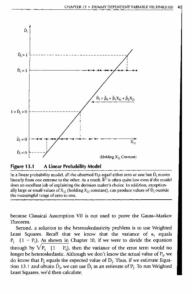
CHAPTER 13 • DUMMY DEPENDENT VARIABLE TECHNIQUES 43
i
• • • • •• • • • • • •
< < Ro + (3 1X 1 i+ RzX2i
X1;
D; <0 (Holding X2 Constant)
Figure 13.1 A Linear Probability Model
In a linear probability model, all the observed D 1s equal either zero or one but D i moves linearly from one extreme to the other. As a result, R 2 is often quite low even if the model does an excellent job of explaining the decision maker's choice. In addition, exception-ally large or small values of X1i (holding X2i constant), can produce values of D ; outside the meaningful range of zero to one.
because Classical Assumption VII is not used to prove the Gauss-Markov Theorem.
Second, a solution to the heteroskedasticity problem is to use Weighted Least Squares. Recall that we know that the variance of Ei equals Pi (1 — Pi) . As shown in Chapter 10, if we were to divide the equation
through by V P1 (1 Pi), then the variance of the error term would no longer be heteroskedastic. Although we don't know the actual value of P i, we do know that P i equals the expected value of D i . Thus, if we estimate Equa-tion 13.1 and obtain D1, we can use D i as an estimate of P i . To run Weighted Least Squares, we'd then calculate:
438 PART III • EXTENSIONS OF THE BASIC REGRESSION MODEL
Zi = V D i (1 — Di) (13.3)
divide Equation 13.1 by Zi, and estimate the new equation with OLS. 2 Third, an alternative to R2 is Rp, the percentage of the obse rvations in the
sample that a particular estimated equation explains correctly. To use this ap-proach, consider a Di ? .5 to predict that D i = 1 and a Di < .5 to predict that D i = 0, compare this prediction with the actual D i, and then compute:
R2 — (13.4) Rp total number of obse rvations (n)
13.4
Since R2 is not used universally, we'll calculate and discuss both R 2 and Rp throughout this chapter.
For most researchers, therefore, the major difficulty with the linear proba-bility model is the unboundedness of the predicted D is. Take another look at Figure 13.1 for a graphical interpretation of the situation. Because of the lin-ear relationship between the X is and Di, D i can fall well outside the relevant range of 0 to 1. Using the linear probability model, despite this unbounded-ness problem, may not cause insurmountable difficulties. In particular, the signs and general significance levels of the estimated coefficients of the linear probability model are often similar to those of the alternatives we will dis-cuss later in this chapter.
One simplistic way to get around the unboundedness problem is to assign D i = 1.0 to all values of D i above one and D i = 0.0 to all negative values. This approach copes with the problem by ignoring it, since an obse rvation for which the linear probability model predicts a probability of 2.0 has been judged to be more likely to be equal to 1.0 than an obse rvation for which the model predicts a 1.0, and yet they are lumped together. What is needed is a systematic method of forcing the D is to range from 0 to 1 in a smooth and meaningful fashion. We'll present such a method, the binomial logit, in Section 13.2.
13.1.3 An Example of a Linear Probability Model
Before moving on to investigate the logit, however, let's take a look at an ex-ample of a linear probability model: a disaggregate study of the labor force participation of women.
number of observations "predicted" correctly
2. Note that when D ; is quite close to 0 or 1, D ; (1 - D ;) is extremely small and X ;/Zi is huge. Also note that when D ; is outside the 0-1 range, D ; (1 - D;) is negative and Z ; is undefined. See R. G. McGilvray, "Estimating the Linear Probability Function," Econometrica, 1970, pp. 775-776. Some researchers arbitrarily drop all such observations to avoid the resulting estima-tion problems. We think that a better alternative is to impose an arbitrary floor, say 0.02, on D ; (1 - D ; ). Either way, WLS is not efficient.

CHAPTER 13 • DUMMY DEPENDENT VARIABLE TECHNIQUES 439
A person is defined as being in the labor force if she either has a job or is actively looking for a job. Thus, a disaggregate (cross-sectional by person) study of women's labor force pa rticipation is appropriately modeled with a dummy dependent variable:
Di = 1 if the ith woman has or is looking for a job, 0 otherwise (not in the labor force)
A review of the literature 3 reveals that there are many potentially relevant independent va riables. Two of the most impo rtant are the marital status and the number of years of schooling of the woman. The expected signs for the coefficients of these variables are fairly straightforward, since a woman who is unmarried and well educated is much more likely to be in the labor force than her opposite:
— + Di = f(Mi, Si) + E i
where: Mi 1 if the ith woman is married and 0 otherwise Si = the number of years of schooling of the ith woman
The data are presented in Table 13.1. The sample size is limited to 30 in order to make it easier for readers to estimate this example on their own. Un-fortunately, such a small sample will make hypothesis testing fairly unreli-able. Table 13.1 also includes the age of the ith woman for use in Exercises 8 and 9. Another typically used va riable, Oi = other income available to the ith woman, is not available for this sample, introducing possible omitted vari-able bias.
If we choose a linear functional form for both independent variables, we've got a linear probability model:
Di = Ro + 13 1 Mi + 132Si + Ei (13.5)
where Ei is an inherently heteroskedastic error term with variance Pi (1 — Pi). If we now estimate Equation 13.5 with the data on the labor force participation of women from Table 13.1, we obtain (standard errors in parentheses):
3. See James P. Smith and Michael P Ward, "Time-Series Growth in the Female Labor Force," Journal of Labor Economics, 1985, pp. 559-590. Smith and Ward include a number of estimated logits in their work.
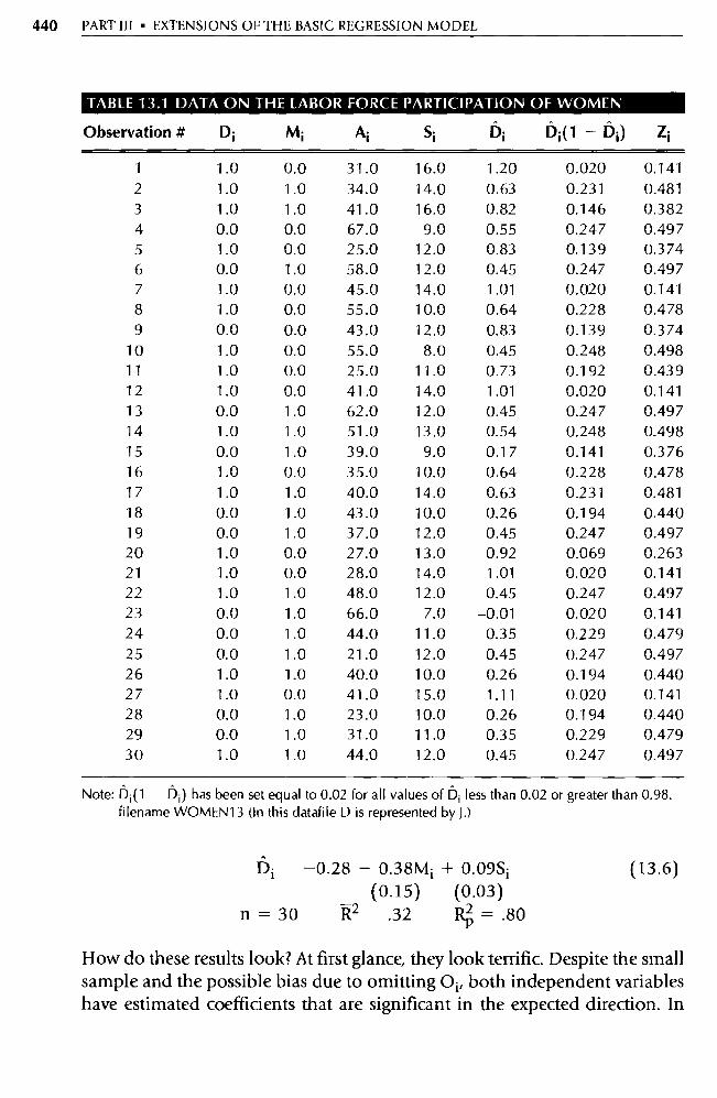
440 PART III • EXTENSIONS OF THE BASIC REGRESSION MODEL
TABLE 13.1 DATA ON THE LABOR FORCE PARTICIPATION OF WOMEN
Observation # Di M ; Ai Si Û; i5 ; ( 1 - D ; ) Z;
1 1.0 0.0 31.0 16.0 1.20 0.020 0.141
2 1.0 1.0 34.0 14.0 0.63 0.231 0.481
3 L0 1.0 41.0 16.0 0.82 0.146 0.382 4 0.0 0.0 67.0 9.0 0.55 0.247 0.497
5 1.0 0.0 25.0 12.0 0.83 0.139 0.3 74
6 0.0 1.0 58.0 12.0 0.45 0.247 0.497 7 1.0 0.0 45.0 14.0 1.01 0.020 0.141
8 1.0 0.0 55.0 10.0 0.64 0.228 0.478
9 0.0 0.0 43.0 12.0 0.83 0.139 0.374
10 1.0 0.0 55.0 8.0 0.45 0.248 0.498 11 1.0 0.0 25.0 11.0 0.73 0.192 0.439 12 1.0 0.0 41.0 14.0 1.01 0.020 0.141 13 0.0 1.0 62.0 12.0 0.45 0.247 0.497 14 1.0 1.0 51.0 13.0 0.54 0.248 0.498
15 0.0 1.0 39.0 9.0 0.17 0.141 0.376 16 1.0 0.0 35.0 10.0 0.64 0.228 0.478 17 1.0 1.0 40.0 14.0 0.63 0.231 0.481 18 0.0 1.0 43.0 10.0 0.26 0.194 0.440 19 0.0 1.0 37.0 12.0 0.45 0.247 0.497 20 1.0 0.0 27.0 13.0 0.92 0.069 0.263 21 1.0 0.0 28.0 14.0 1.01 0.020 0.141 22 1.0 1.0 48.0 12.0 0.45 0.247 0.497 23 0.0 1.0 66.0 7.0 -0.01 0.020 0.141 24 0.0 1.0 44.0 11.0 0.35 0.229 0.479 25 0.0 1.0 21.0 12.0 0.45 0.247 0.497
26 1.0 1.0 40.0 10.0 0.26 0.194 0.440 27 1.0 0.0 41.0 15.0 1.11 0.020 0.141 28 0.0 1.0 23.0 10.0 0.26 0.194 0.440 29 0.0 1.0 31.0 11.0 0.35 0.229 0.479
30 1.0 1.0 44.0 12.0 0.45 0.247 0.497
Note: D ; (1 D ; ) has been set equal to 0.02 for all values of D ; less than 0.02 or greater than 0.98. filename WOMEN13 (In this datafi le D is represented by J.)
Di -0.28 - 0.38Mî + 0.09Si (13.6) (0.15) (0.03)
n= 30 R2 .32 RP= .80
How do these results look? At first glance, they look terrific. Despite the small sample and the possible bias due to omitting O i, both independent variables have estimated coefficients that are significant in the expected direction. In

CHAPTER 13 • DUMMY DEPENDENT VARIABLE TECHNIQUES 441
addition, the R2 of .32 is fairly high for a linear probability model (since D i
equals only 0 or 1, it's almost impossible to get a R 2 much higher than .70). Further evidence of good fit is the fairly high RP of .80, meaning that 80 per-cent of the choices were predicted "correctly" by Equation 13.6.
We need to be careful when we interpret the estimated coefficients in Equation 13.6, however. The slope coefficient in a linear probability model represents the change in the probability that Di equals one caused by a one-unit increase in the independent variable (holding the other independent variables constant). Viewed in this context, do the estimated coefficients still make economic sense? The answer is yes: the probability of a woman partici-pating in the labor force falls by 38 percent if she is married (holding con-stant her schooling). In addition, each year of schooling increases the proba-bility of labor force pa rticipation by 9 percent (holding constant marital status).
However, Equation 13.6 is far from perfect. Recall that the error term is in-herently heteroskedastic, that hypothesis testing is unreliable in such a small sample, that R2 is not an accurate measure of fit, and that one or more rele-vant variables have been omitted. While we can do nothing about some of these problems, there is a solution to the heteroskedasticity problem: Weighted Least Squares (WLS).
To use WLS, we take the D ; from Equation 13.6 and calculate
Z; V D; (1 D i), as in Equation 13.3 [taking care to impose a floor of 0.02 on D i (1 — Di) as suggested in footnote 2.1 We then divide Equation 13.5 through by Z;, obtaining:
Di/Zi = ao + 3(1 /Zi) = R iMi/Zi + 132Si/Zi + u i (13.7)
where u ; is a nonheteroskedastic error term = E i/Zi . Note that since Z i is not an independent variable in Equation 13.6, we have chosen to add a o, a con-stant term, to Equation 13.7 to avoid violating Classical Assumption II (as dis-cussed in Chapter 9). If we now estimate Equation 13.7 with OLS, we obtain:
D Z = 0.18 — 0.21(1 /Zi) — 0.39M; /Zi + 0.08S i/Zi (13.8) (0.15) (0.02)
n=30 R2 =.86 R12, =.83
Let's compare Equations 13.8 and 13.6. Surprisingly, the estimated standard errors of the estimated coefficients are almost identical in the two equations, indicating that at least for this sample the impact of the heteroskedasticity is minimal. The high R2 comes about in part because dividing the entire equa-

442 PART III • EXTENSIONS OF THE BASIC REGRESSION MODEL
tion by the same number (Z i) causes some spurious correlation, especially when some of the Zi values are quite small. As evidence, note that RP is only
slightly higher in Equation 13.8 than in Equation 13.6 even though R 2 jumped from .32 to .86.
To make it easier for the reader to reproduce the WLS procedure, the values
for Di (1 Di) and Zi have been included in Table 13.1. Also included are the D is from Equation 13.6; note that Di is indeed often outside the mean-ingful range of 0 and 1, causing most of the problems cited earlier. To attack
this problem of the unboundedness of Di, however, we need a new estima-tion technique, so let's take a look at one.
13.2 The Binomial Logit Model
To avoid the possibility that a prediction of D i might be outside the probabil-ity interval of 0 to 1, we no longer model D i directly. Instead, we model the ratio Di/ (1 — D i) . This ratio is the likelihood, or odds, 4 of obtaining a suc-cessful outcome (D i = 1). If we take the log of this ratio, we have the left
side of the equation that has become the standard approach to dummy de-pendent variable analysis: the binomial logit.
13.2.1 What Is the Binomial Logit?
The binomial logit is an estimation technique for equations with dummy
dependent variables that avoids the unboundedness problem of the linear
probability model by using a variant of the cumulative logistic function:
D, ^
Di] 0 + RlXli + 132X2i + Ei (13.9)
where D i is a dummy variable. The expected value of D i continues to be Pi , the probability that the ith person will make the choice described by D i = 1. Consequently, the dependent variable of Equation 13.9 can be thought of as the log of the odds that the choice in question will be made.
How does the logit avoid the unboundedness problem of the linear prob-ability model? It turns out that both sides of Equation 13.9 are unbounded. To see this, note that if D i = 1, then the left-side of Equation 13.9 becomes:
4. Odds refer to the ratio of the number of times a choice will be made divided by the number
of times it will not. In today's world, odds are used most frequently with respect to sporting
events, such as horse races, on which bets are made.
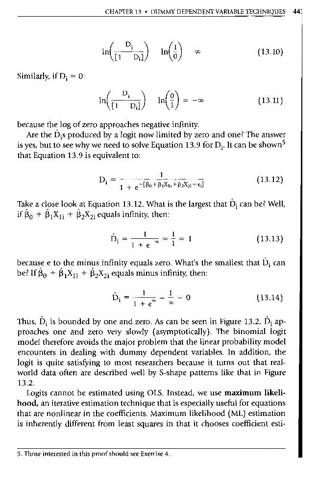
CHAPTER 13 • DUMMY DEPENDENT VARIABLE TECHNIQUES 44:
ln^Cl D1 Dij/ ln \0
(13.10)
Similarly, if D i = 0:
Di ln
[1 D,] 49)1=
-00
because the log of zero approaches negative infinity. Are the D is produced by a logit now limited by zero and one? The answer
is yes, but to see why we need to solve Equation 13.9 for D i . It can be shown 5 that Equation 13.9 is equivalent to:
=
(13.12 ) D' _ 1 + e-E1304
Take a close look at Equation 13.12. What is the largest that D i can be? Well, if Ro + RIXI; + (3 2X21 equals infinity, then:
Di = 1 = 1 1 1 +e — 1
(13.13)
because e to the minus infinity equals zero. What's the smallest that D ; can be? If R0 + RlXli + j32X2i equals minus infinity, then:
Di= 1 „ = 01-0
=0 1 + e
(13.14)
Thus, Di is bounded by one and zero. As can be seen in Figure 13.2, Di ap-proaches one and zero very slowly (asymptotically). The binomial logit model therefore avoids the major problem that the linear probability model encounters in dealing with dummy dependent variables. In addition, the logit is quite satisfying to most researchers because it turns out that real-world data often are described well by S-shape patterns like that in Figure 13.2.
Logits cannot be estimated using OLS. Instead, we use maximum likeli-hood, an iterative estimation technique that is especially useful for equations that are nonlinear in the coefficients. Maximum likelihood (ML) estimation is inherently different from least squares in that it chooses coefficient esti-
5. Those interested in this proof should see Exercise 4.
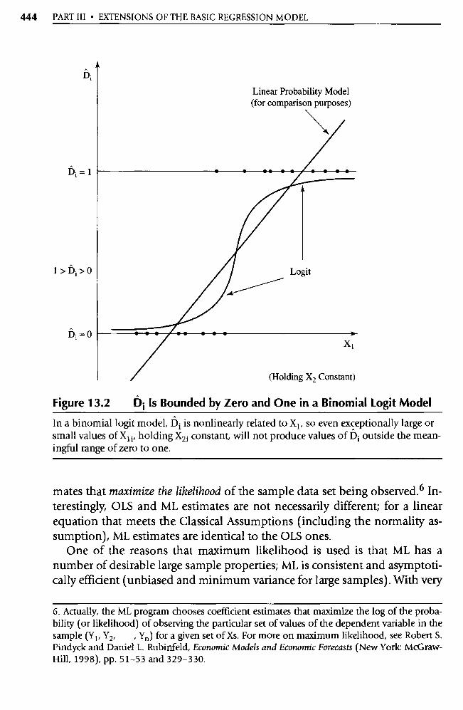
I >D; > 0
Linear Probability Model (for comparison purposes)
Figure 13.2 D i Is Bounded by Zero and One in a Binomial Logit Model
In a binomial logit model, i3 is nonlinearly related to X 1 , so even exceptionally large or small values of X1i, holding X21 constant, will not produce values of D ; outside the mean-ingful range of zero to one.
mates that maximize the likelihood of the sample data set being observed. 6 In-terestingly, OLS and ML estimates are not necessarily different; for a linear equation that meets the Classical Assumptions (including the normality as-sumption), ML estimates are identical to the OLS ones.
One of the reasons that maximum likelihood is used is that ML has a number of desirable large sample properties; ML is consistent and asymptoti-cally efficient (unbiased and minimum va riance for large samples). With very
444 PART III • EXTENSIONS OF THE BASIC REGRESSION MODEL
6. Actually, the ML program chooses coefficient estimates that maximize the log of the proba-bility (or likelihood) of observing the particular set of values of the dependent variable in the sample (Y 1 , Y2, , Yn) for a given set of Xs. For more on maximum likelihood, see Robe rt S. Pindyck and Daniel L. Rubinfeld, Economic Models and Economic Forecasts (New York: McGraw-Hill, 1998), pp. 51-53 and 329-330.

CHAPTER 13 • DUMMY DEPENDENT VARIABLE TECHNIQUES 445
large samples, ML has the added advantage of producing normally distrib-uted coefficient estimates, allowing the use of typical hypothesis testing tech-niques. As a result, sample sizes for logits should be substantially larger than for linear regressions. Some researchers aim for samples of 500 or more.
It's also important to make sure that a logit sample contains a reasonable representation of both alternative choices. For instance, if 98 percent of a sample chooses alternative A and 2 percent chooses B, a random sample of 500 would have only 10 obse rvations that choose B. In such a situation, our estimated coefficients would be overly reliant on the characteristics of those 10 observations. A better technique would be to disproportionately sample from those who choose B. It turns out that using different sampling rates for subgroups within the sample does not cause bias in the slope coefficients of a logit model, 7 even though it might do so in a linear regression.
The maximum likelihood computer program is applied to a logit that has been solved for D i (Equation 13.12), not to a logit solved for the log of the odds (Equation 13.9). This distinction is necessary because, as shown earlier, the left-hand side of Equation 13.9 can be observed only as infinity and neg-ative infinity. Such infinite values make calculations quite difficult.
Once the binomial logit has been estimated, hypothesis testing and econometric analysis can be undertaken in much the same way as for linear equations. When interpreting coefficients, however, be careful to recall that they represent the impact of a one-unit increase in the independent variable in question, holding the other explanatory variables constant, on the log of the odds of a given choice, not on the probability itself (as was the case with the linear probability model).
For instance, P i in Equation 13.9 measures the impact of a one-unit increase in X 1 on the log of the odds of a given choice, holding X2 constant. As a result, the absolute sizes of estimated logit coefficients tend to be quite different from the absolute sizes of estimated linear probability model coefficients for the same variables. Interestingly, as mentioned above, the signs and significance levels of the estimated coefficients from the two models often are similar.
Measuring the overall fit, however, is not quite as straightforward. Recall from Chapter 7 that since the functional form of the dependent va riable has been changed, R2 cannot be used to compare the fit of a logit with an other-wise comparable linear probability model. One way around this difficulty is to use the quasi-R2 approach of Chapter 7 (a nonlinear estimate of R 2) to corn-
7 The constant term, however, needs to be adjusted. Multiply Ro by [1n(p l ) - ln(p2)], where p i is the propo rtion of the observations chosen if D ; = 1 and 132 is the propo rtion of the obser-vations chosen if D i = 0. See G. S. Maddala, Limited-Dependent and Qualitative Variables in Econometrics (Cambridge: Camb ridge University Press, 1983), pp. 90-91.

446 PART III • EXTENSIONS OF THE BASIC REGRESSION MODEL
pare the two fits. However, this quasi-R 2 shares the general faults inherent in using R2 with equations with dummy dependent va riables. A better approach might be to use the percentage of correct predictions, RR, from Equation 13.4.
To allow a fairly simple comparison between the logit and the linear prob-ability model, let's estimate a logit on the same women's labor force partici-pation data that we used in the previous section. The OLS estimate of that model, Equation 13.6, was:
D i = — 0.28 — 0.38Mî + 0.09S i (13.6) (0.15) (0.03)
n=30 R2 =.32 RR= .80
where: Di = 1 if the ith woman is in the labor force, 0 otherwise Mi = 1 if the ith woman is married, 0 otherwise Si = the number of years of schooling of the ith woman
If we estimate a logit on the same data (from Table 13.1) and the same inde-pendent va riables, we obtain 8 :
= — 5.89 — 2.59M1 + 0.69Si (13.15) ' (1.18) (0.31)
t = — 2.19 2.19 n 30 R2 .80 iterations = 5
Let's compare Equations 13.6 and 13.15. As expected, the signs and general significance of the slope coefficients are the same. Note, however, that the ac-tual sizes of the coefficients are quite different because the dependent vari-able is different. The coefficient of M changes from —0.38 to —2.59! Despite these differences, the overall fits are roughly comparable, especially after tak-ing account of the different dependent variables and estimation techniques. In this example, then, the two estimation procedures differ mainly in that the logit does not produce p is outside the range of zero and one.
However, if the size of the sample in this example is too small for a linear probability model, it certainly is too small for a logit, making any in-depth analysis of Equation 13.15 problematic. Instead, we're better off finding an example with a much larger sample.
D i ln [1 D]
8. Equation 13.15 has the log of the odds as its dependent va riable, but the maximum likeli-hood computer estimation program that produces the 13 estimates uses a functional form with Di as the dependent variable (similar to Equation 13.12).
CHAPTER 13 • DUMMY DEPENDENT VARIABLE TECHNIQUES 447
13.2.2 An Example of the Use of the Binomial Logit
For a more complete example of the binomial digit, let's look at a model of the probability of passing the California State Department of Motor Vehicles drivers' license test. To obtain a license, each driver must past a written and a behind-the-wheel test. Even though the tests are scored from 0 to 100, all that matters is that you pass and get your license.
Since the test requires some boning up on traffic and safety laws, driving students have to decide how much time to spend studying. If they don't study enough, they waste time because they have to retake the test. If they study too much, however, they also waste time, because there's no bonus for scoring above the minimum, especially since there is no evidence that doing well on the test has much to do with driving well after the test (this, of course, might be worth its own econometric study).
Recently, two students decided to collect data on test takers in order to build an equation explaining whether someone passed the Department of Motor Vehicles test. They hoped that the model, and in particular the esti-mated coefficient of study time, would help them decide how much time to spend studying for the test. (Of course, it took more time to collect the data and mn the model than it would have taken to memorize the entire traffic code, but that's another story.)
After reviewing the literature, choosing variables, and hypothesizing signs, the students realized that the appropriate functional form was a binomial logit because their dependent variable was a dummy variable:
1 if the ith test taker passed the test on the first try Di =
0 if the ith test taker failed the test on the first try
Their hypothesized equation was:
+ + + + Di = f(A i, H i, E i, C i) + Ei
where: Ai = the age of the ith test taker Hi = the number of hours the ith test taker studied (usually less
than one hour!) Ei = a dummy variable equal to 1 if the ith test taker's primary
language is English, 0 otherwise Ci = a dummy variable equal to 1 if the ith test taker has any col-
lege experience, 0 otherwise
448 PART III • EXTENSIONS OF THE BASIC REGRESSION MODEL
After collecting data from 480 test takers, the students estimated the follow-ing equation:
D. In D ^ = — 1.18 + 0.011Aî + 2.70H1 + 1.62E î + 3.97Cî
[1 _ '
' (0.009) (0.54) (0.34) (0.99) t = 1.23 4.97 4.65 4.00
n = 480 RP = .74 iterations = 5 (13.16)
Note how similar these results look to a typical linear regression result. All the estimated coefficients have the expected signs, and all but one are signifi-cantly different from zero. Remember, though, that the coefficient estimates have different meanings than in a linear regression model. For example, 2.70 is the impact of an extra hour of studying on the log of the odds of passing the test, holding constant the other three independent variables. Note that
RP is .74, indicating that the equation correctly "predicted" almost three quarters of the sample based on nothing but the four variables in Equation 13.16.
And what about the two students? Did the equation help them? How much did they end up deciding to study? They found that given their ages, their college experience, and their English-speaking backgrounds, the ex-pected value of Di for each of them was quite high, even if H i was set equal to zero. So what did they actually do? They studied for a half hour "just to be on the safe side" and passed with flying colors, having devoted more time to passing the test than anyone else in the history of the state.
13.3 Other Dummy Dependent Variable Techniques
Although the binomial logit is the most frequently used estimation tech-nique for equations with dummy dependent variables, it's by no means the only one. In this section, we'll mention two alternatives, the binomial probit and the multinomial logit, that are useful in particular circumstances. Our main goal is to briefly describe these estimation techniques, not to cover them in any detail. 9
9. For more, see G. S. Maddala, Limited Dependent Variables and Qualitative Variables in Econo-metrics (Cambridge: Cambridge University Press, 1983) and T. Amemiya, "Qualitative Re-sponse Models: A Survey," Journal of Economic Literature, 1981, pp. 1483-1536. These surveys also cover additional techniques, like the Tobit model, that are useful with bounded dependent variables or other special situations.
CHAPTER 13 • DUMMY DEPENDENT VARIABLE TECHNIQUES 449
13.3.1 The Binomal Probit Model
The binomial probit model is an estimation technique for equations with
dummy dependent variables that avoids the unboundedness problem of the
linear probability model by using a variant of the cumulative normal distrib-ution.
zi Pi =
" ^
1 too
e-52/2 ds V 2^rr
where: Pi = the probability that the dummy variable Di = 1
Zi = Ro + 13 1X1i + 132X2i s = a standardized normal va riable
(13.17)
As different as this probit looks from the logit that we examined in the pre-vious section, it can be rewritten to look quite familiar:
Zi = F-1 ( Pi) = R o + RlXli + R2X2i (13.18)
where F-1 is the inverse of the normal cumulative distribution function. Pro-bit models typically are estimated by applying maximum likelihood tech-niques to the model in the form of Equation 13.17, but the results often are
presented in the format of Equation 13.18.
The fact that both the logit and the probit are cumulative distributive func-tions means that the two have similar properties. For example, a graph of the
probit looks almost exactly like the logit in Figure 13.2. In addition, the pro-bit has the same requirement of a fairly large sample before hypothesis test-ing becomes meaningful. Finally, t-2 continues to be of questionable value as a measure of overall fit.
From a researcher's point of view, the biggest differences between the two
models are that the probit is based on the cumulative normal dist ribution and that the probit estimation procedure uses more computer time than does
the logit. Since the probit is similar to the logit and is more expensive to run,
why would you ever estimate one? The answer is that since the probit is
based on the normal distribution, it's quite theoretically appealing (because
many economic variables are normally distributed). With extremely large
samples, this advantage falls away, since maximum likelihood procedures
can be shown to be asymptotically normal under fairly general conditions.
For an example of a probit, let's estimate one on the same women's labor
force participation data we used in the previous logit and linear probability
examples (standard errors in parentheses):
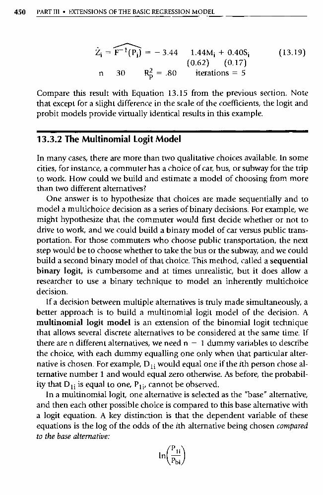
450 PART III • EXTENSIONS OE THE BASIC REGRESSION MODEL
Zi = F-1 (Pi) = - 3.44 1.44Mî + 0.40Si (13.19) (0.62) (0.17)
n 30 RI; = .80 iterations = 5
Compare this result with Equation 13.15 from the previous section. Note that except for a slight difference in the scale of the coefficients, the logit and probit models provide virtually identical results in this example.
13.3.2 The Multinomial Logit Model
In many cases, there are more than two qualitative choices available. In some cities, for instance, a commuter has a choice of car, bus, or subway for the trip to work. How could we build and estimate a model of choosing from more than two different alternatives?
One answer is to hypothesize that choices are made sequentially and to model a multichoice decision as a series of binary decisions. For example, we might hypothesize that the commuter would first decide whether or not to drive to work, and we could build a binary model of car versus public trans-portation. For those commuters who choose public transpo rtation, the next step would be to choose whether to take the bus or the subway, and we could build a second binary model of that choice. This method, called a sequential binary logit, is cumbersome and at times unrealistic, but it does allow a researcher to use a binary technique to model an inherently multichoice decision.
If a decision between multiple alternatives is truly made simultaneously, a better approach is to build a multinomial logit model of the decision. A multinomial logit model is an extension of the binomial logit technique that allows several discrete alternatives to be considered at the same time. If there are n different alternatives, we need n - 1 dummy variables to describe the choice, with each dummy equalling one only when that particular alter-native is chosen. For example, DIi would equal one if the ith person chose al-ternative number 1 and would equal zero otherwise. As before, the probabil-ity that D Ii is equal to one, P Ii, cannot be observed.
In a multinomial logit, one alternative is selected as the "base" alte rnative, and then each other possible choice is compared to this base alternative with a logit equation. A key distinction is that the dependent variable of these equations is the log of the odds of the ith alternative being chosen compared to the base alternative:
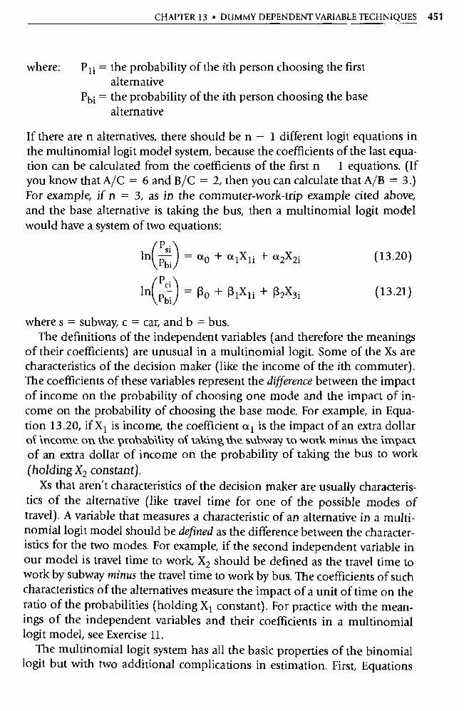
CHAPTER 13 DUMMY DEPENDENT VARIABLE TECHNIQUES 451
where: P 1i = the probability of the ith person choosing the first alternative
Pbi = the probability of the ith person choosing the base alternative
If there are n alternatives, there should be n — 1 different logit equations in the multinomial logit model system, because the coefficients of the last equa-tion can be calculated from the coefficients of the first n 1 equations. (If you know that A/C = 6 and B/C = 2, then you can calculate that A/B = 3.) For example, if n = 3, as in the commuter-work-trip example cited above, and the base alternative is taking the bus, then a multinomial logit model would have a system of two equations:
P. In i = ao + a1X1i + a2X2i (13.20)
Pbi P•
In ci = 130 + R1X1i + R2X3i (13.21) Pbi
where s = subway, c = car, and b = bus. The definitions of the independent variables (and therefore the meanings
of their coefficients) are unusual in a multinomial logit. Some of the Xs are characteristics of the decision maker (like the income of the ith commuter). The coefficients of these variables represent the difference between the impact of income on the probability of choosing one mode and the impact of in-come on the probability of choosing the base mode. For example, in Equa-tion 13.20, if X 1 is income, the coefficient a 1 is the impact of an extra dollar of income on the probability of taking the subway to work minus the impact of an extra dollar of income on the probability of taking the bus to work (holding X2 constant).
Xs that aren't characteristics of the decision maker are usually characteris-tics of the alternative (like travel time for one of the possible modes of travel). A variable that measures a characteristic of an alternative in a multi-nomial logit model should be defined as the difference between the character-istics for the two modes. For example, if the second independent va riable in our model is travel time to work, X2 should be defined as the travel time to work by subway minus the travel time to work by bus. The coefficients of such characteristics of the alte rnatives measure the impact of a unit of time on the ratio of the probabilities (holding X 1 constant). For practice with the mean-ings of the independent variables and their coefficients in a multinomial logit model, see Exercise 11.
The multinomial logit system has all the basic properties of the binomial logit but with two additional complications in estimation. First, Equations

452 PART III • EXTENSIONS OF THE BASIC REGRESSION MODEL
13.20 and 13.21 are estimated simultaneously, 10 so the iterative nonlinear maximum likelihood procedure used to estimate the system is more costly than for the binomial logit. Second, the relationship between the error terms in the equations (Esi and Eci) must be strictly accounted for by using a GLS procedure, a factor that also complicates the estimation procedure. 11
13.4 Summary
1. A linear probability model is a linear-in-the-coefficients equation used to explain a dummy dependent variable (D i). The expected value of D i is the probability that D i equals one (P i).
2. The estimation of a linear probability model with OLS encounters four major problems: a. The error term is not normally distributed. b. The error term is inherently heteroskedastic. c. R2 is not an accurate measure of overall fit. d. The expected value of D i is not limited by 0 and 1.
3. When measuring the overall fit of equations with dummy dependent variables, an alternative to R2 is RP, the percentage of the observa-tions in the sample that a particular estimated equation would have explained correctly.
4. The binomial logit is an estimation technique for equations with dummy dependent variables that avoids the unboundedness problem of the linear probability model by using a variant of the cumulative logistic function:
(
Di ln [1 Dd = Ro + R lXli + 132X2i + Ei
5. The binomial logit is best estimated using the maximum likelihood technique and a large sample. A slope coefficient from a logit mea-sures the impact of a one-unit increase of the independent variable in
10. As with the binomial logit, the maximum likelihood computer package doesn't estimate these precise equations. Instead, it estimates versions of Equations 13.20 and 13.21 that are similar to Equation 13.12.
11. For an interesting and yet accessible example of the estimation of a multinomial logit model, see Kang H. Park and Peter M. Kerr, "Determinants of Academic Performance: A Multi-nomial Logit Approach," The Journal of Economic Education, 1990, pp. 101-111.

CHAPTER 13 • DUMMY DEPENDENT VARIABLE TECHNIQUES 453
question (holding the other explanatory variables constant) on the log of the odds of a given choice.
6. The binomial probit model is an estimation technique for equations with dummy dependent variables that uses the cumulative normal distribution function. The binomial probit has properties quite simi-lar to the binomial logit except that it takes more computer time to estimate than a logit and is based on the normal distribution.
7 The multinomial logit model is an extension of the binomial logit that allows more than two discrete alternatives to be considered si-multaneously. One alternative is chosen as a base alternative, and then each other possible choice is compared to that base alternative with a logit equation.
Exercises
(Answers to even-numbered exercises are in Appendix A.)
1. Write the meaning of each of the following terms without referring to the book (or your notes), and compare your definition with the ver-sion in the text for each: a. linear probability model b. Rp c. binomial logit model d. log of the odds e. binomial probit model f. sequential binary model g. multinomial logit model
2. On graph paper, plot each of the following linear probability models. For what range of Xi is 1 < Di? How about D i < 0? a. D 1 = 0.3+0.1Xi
b.Tî i = 3.0-0.2Xi
c. Di = -1.0 + 0.3Xi
3. Bond ratings are letter ratings (Aaa = best) assigned to firms that is-sue debt. These ratings measure the quality of the firm from the point of view of the likelihood of repayment of the bond. Suppose you've been hired by an arbitrage house that wants to predict Moody's Bond Ratings before they're published in order to buy bonds whose ratings are going to improve. In pa rticular, suppose your firm wants to distin-

454 PART III • EXTENSIONS OF THE BASIC REGRESSION MODEL
guish between A-rated bonds (high quality) and B-rated bonds (medium quality) and has collected a data set of 200 bonds with which to estimate a model. As you arrive on the job, your boss is about to buy bonds based on the results of the following model (standard errors in parentheses):
Yi = 0.70 + 0.05Pî + 0.05PVi — 0.020Di (0.05) (0.02) (0.002)
R2 =.69 DW = 0.50 n = 200
where: Yi = 1 if the rating of the ith bond = A, 0 otherwise Pi = the profit rate of the firm that issues the ith bond PVi = the standard deviation of P i over the last 5 years D i = the ratio of debt to total capitalization of the firm
that issued the ith bond
a. What econometric problems, if any, exist in this equation? b. What suggestions would you have for a rerun of this equation with
a different specification? c. Suppose that your boss rejects your suggestions, saying, "This is the
real world, and I'm sure that my model will forecast bond ratings just as well as yours will." How would you respond? (Hint: Saying, "Okay, boss, you win," is sure to keep your job for you, but it won't get much credit on this question.)
4. Show that the logistic function, D = 1/(1 + e -Z), is indeed equiv-alent to the binomial logit model, ln[D/(1 - D)] = Z, where Z = Ro + R1X1 + 02x2 + E.
5. Plot each of the following binomial logit models. For what range of X i is 1 < Di ? How about D i < 0? (Hint: When you finish, compare your
answers to those for Exercise 2 above.) a. ln[D i/(1 - D i)] = 0.3 + 0.1X1 b. ln[Di/(1 D i)] = 3.0 0.2Xi c. ln[D i/(1 Di)] = - 1.0 + 0.3Xi
6. R. Amatya 12 estimated the following logit model of birth control for 1,145 continuously married women aged 35 to 44 in Nepal:
12. Ramesh Amatya, "Supply-Demand Analysis of Differences in Contraceptive Use in Seven Asian Nations, Late 1970s" (paper presented at the Annual Meetings of the Western Economic Association, 1988, Los Angeles).
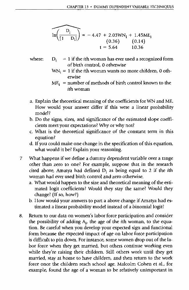
CHAPTER 13 • DUMMY DEPENDENT VARIABLE TECHNIQUES
D. 1n
\\\\ ^
[1 ' Di
] — 4.47 + 2.03WN; + 1.45ME;
(0.36) (0.14)
t = 5.64 10.36
where: D; = 1 if the ith woman has ever used a recognized form of birth control, 0 otherwise
WNi = 1 if the ith woman wants no more children, 0 oth-erwise
ME; = number of methods of birth control known to the ith woman
a. Explain the theoretical meaning of the coefficients for WN and ME. How would your answer differ if this were a linear probability model?
b. Do the signs, sizes, and significance of the estimated slope coeffi-cients meet your expectations? Why or why not?
c. What is the theoretical significance of the constant term in this equation?
d. If you could make one change in the specification of this equation, what would it be? Explain your reasoning.
7 What happens if we define a dummy dependent variable over a range other than zero to one? For example, suppose that in the research cited above, Amatya had defined D ; as being equal to 2 if the ith woman had ever used birth control and zero otherwise. a. What would happen to the size and theoretical meaning of the esti-
mated logit coefficients? Would they stay the same? Would they change? (If so, how?)
b. How would your answers to part a above change if Amatya had es-timated a linear probability model instead of a binomial logit?
8. Return to our data on women's labor force pa rticipation and consider the possibility of adding A ;, the age of the ith woman, to the equa-tion. Be careful when you develop your expected sign and functional form because the expected impact of age on labor force pa rticipation is difficult to pin down. For instance, some women drop out of the la-bor force when they get married, but others continue working even while they're raising their children. Still others work until they get married, stay at home to have children, and then return to the work force once the children reach school age. Malcolm Cohen et al., for example, found the age of a woman to be relatively unimportant in
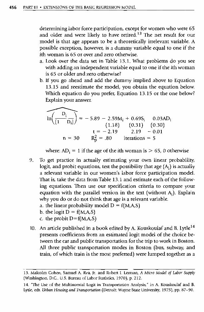
456 PART III • EXTENSIONS OF THE BASIC REGRESSION MODEL
determining labor force pa rticipation, except for women who were 65 and older and were likely to have retired. 13 The net result for our model is that age appears to be a theoretically irrelevant variable. A
possible exception, however, is a dummy variable equal to one if the
ith woman is 65 or over and zero otherwise. a. Look over the data set in Table 13.1. What problems do you see
with adding an independent va riable equal to one if the ith woman
is 65 or older and zero otherwise?
b. If you go ahead and add the dummy implied above to Equation
13.15 and reestimate the model, you obtain the equation below.
Which equation do you prefer, Equation 13.15 or the one below?
Explain your answer.
D.
In ^1 1D^
= — 5.89 — 2.59Mî + 0.69Si 0.03AD i ' (1.18) (0.31) (0.30)
t= —2.19 2.19 — 0.01 n = 30 Rp = . 80 iterations = 5
where: AD i = 1 if the age of the ith woman is > 65, 0 otherwise
9. To get practice in actually estimating your own linear probability,
logit, and probit equations, test the possibility that age (A i) is actually a relevant variable in our women's labor force participation model.
That is, take the data from Table 13.1 and estimate each of the follow-ing equations. Then use our specification criteria to compare your
equation with the parallel version in the text (without A i). Explain why you do or do not think that age is a relevant variable.
a. the linear probability model D = f(M,A,S)
b. the logit D = f(M,A,S) c. the probit D=f(M,A,S)
10. An article published in a book edited by A. Kouskoulaf and B. Lytle 14
presents coefficients from an estimated logit model of the choice be-tween the car and public transpo rtation for the trip to work in Boston. All three public transpo rtation modes in Boston (bus, subway, and
train, of which train is the most preferred) were lumped together as a
13. Malcolm Cohen, Samuel A. Rea, Jr. and Robe rt I. Lerman, A Micro Model of Labor Supply (Washington, D.C.. U.S. Bureau of Labor Statistics, 1970), p. 212.
14. "The Use of the Multinomial Logit in Transpo rtation Analysis," in A. Kouskoulaf and B.
Lytle, eds. Urban Housing and Transportation (Detroit: Wayne State Universi ty, 1975), pp. 87-90.

CHAPTER 13 • DUMMY DEPENDENT VARIABLE TECHNIQUES 457
single alternative to the car in a binomial logit model. The dependent variable was the log of the odds of taking public transpo rtation for the trip to work, so the first coefficient implies that as income rises, the log of the odds of taking public transpo rtation falls, and so on.
Independent Variable Coefficient
Family income (9 categories with 1 = low and 9 = high)
Number employed in the family Out-of-pocket costs (cents) Wait time (tenths of minutes) Walk time (tenths of minutes) In-vehicle travel time (tenths of minutes)
—0.12
—1.09 —3.16
0.18 —0.03 —0.01
The last four variables are defined as the difference between the value of the variable for taking public transpo rtation and its value for taking the car. a. Do the signs of the estimated coefficients agree with your prior ex-
pectations? Which one(s) differ? b. The transpo rtation literature hypothesizes that people would rather
spend time traveling in a vehicle than waiting for or walking to that vehicle. Do the sizes of the estimated coefficients of time suppo rt
this hypothesis? c. Since trains run relatively infrequently, the researchers set wait time
for train riders fairly high. Most trains mn on known schedules, however, so the average commuter learns that schedule and at-tempts to hold down wait time. Does this fact explain any of the unusual results indicated in your answers to pa rts a and b above?
11. Suppose that you want to build a multinomial logit model of how students choose which college to attend. For the sake of simplicity, let's assume that there are only four colleges to choose from: your col-lege (c), the state university (u), the local junior college (j), and the nearby private liberal a rts college (a). Further assume that everyone agrees that the impo rtant variables in such a model are the family in-come (Y) of each student, the average SAT scores of each college (SAT), and the tuition (T) of each college. a. How many equations should there be in such a multinomial logit
system? b. If your college is the base, write out the definition of the dependent
variable for each equation.
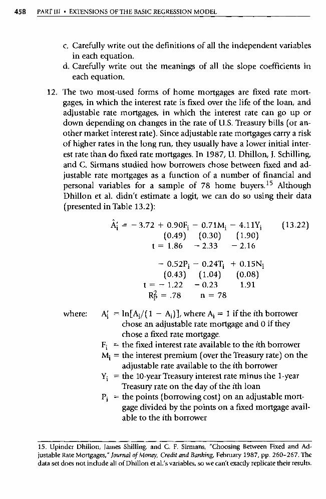
458 PART III • EXTENSIONS OF THE BASIC REGRESSION MODEL
c. Carefully write out the definitions of all the independent variables in each equation.
d. Carefully write out the meanings of all the slope coefficients in each equation.
12. The two most-used forms of home mortgages are fixed rate mort-gages, in which the interest rate is fixed over the life of the loan, and adjustable rate mortgages, in which the interest rate can go up or down depending on changes in the rate of U.S. Treasury bills (or an-other market interest rate). Since adjustable rate mortgages car ry a risk of higher rates in the long run, they usually have a lower initial inter-est rate than do fixed rate mortgages. In 1987, U. Dhillon, J. Schilling, and C. Sirmans studied how borrowers chose between fixed and ad-justable rate mortgages as a function of a number of financial and personal variables for a sample of 78 home buyers.'S Although Dhillon et al. didn't estimate a logit, we can do so using their data (presented in Table 13.2):
A;
= — 3.72 + 0.90Fî — 0.71Mî — 4.11Yî (13.22)
(0.49) (0.30) (1.90)
t = 1.86 —2.33 —2.16
— 0.52Pî — 0.24Tî + 0.15N1
(0.43) (1.04) (0.08)
t = — 1.22 —0.23 1.91 Rp = .78 n=78
where: Ai = ln[A1/ (1 - Ai) ], where Ai = 1 if the ith borrower chose an adjustable rate mortgage and 0 if they chose a fixed rate mortgage.
Fi = the fixed interest rate available to the ith borrower Mi = the interest premium (over the Treasury rate) on the
adjustable rate available to the ith borrower Yi = the 10-year Treasury interest rate minus the 1-year
Treasury rate on the day of the ith loan Pi = the points (borrowing cost) on an adjustable mort-
gage divided by the points on a fixed mortgage avail- able to the ith borrower
15. Upinder Dhillon, James Shilling, and C. F. Sirmans, "Choosing Between Fixed and Ad- justable Rate Mortgages," Journal of Money, Credit and Banking, February 1987, pp. 260-267. The data set does not include all of Dhillon et al.'s va riables, so we can't exactly replicate their results.
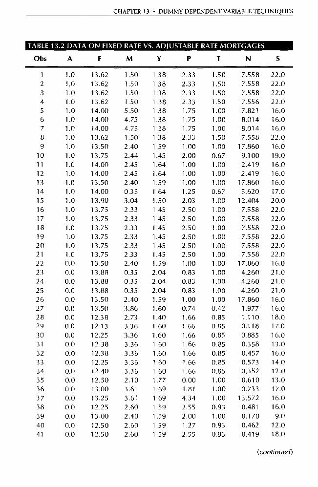
CHAPTER 13 • DUMMY DEPENDENT VARIABLE TECHNIQUES
TABLE 13.2 DATA ON FIXED RATE VS. ADJUSTABLE RATE MORTGAGES
Obs A F M Y P T N S
1 1.0 13.62 1.50 1.38 2,33 1.50 7.558 22.0 2 1.0 13.62 1.50 1.38 2.33 1.50 7.558 22.0 3 1.0 13.62 1.50 1.38 2.33 1.50 7.558 22.0 4 1.0 13.62 1.50 1.38 2.33 1.50 7.556 22.0 5 1.0 14.00 5.50 1.38 1.75 1.00 7.821 16.0 6 1.0 14.00 4.75 1.38 1.75 1.00 8.014 16.0 7 1.0 14.00 4.75 1.38 1.75 1.00 8.014 16.0 8 1.0 13.62 1.50 1.38 2.33 1.50 7.558 22.0 9 1.0 13.50 2.40 1.59 1.00 1.00 17.860 16.0
10 1.0 13.75 2.44 1.45 2.00 0.67 9.100 19.0 11 1.0 14.00 2.45 1.64 1.00 1.00 2.419 16.0 12 1.0 14.00 2.45 1.64 1.00 1.00 2.419 16.0 13 1.0 13.50 2.40 1.59 1.00 1.00 17.860 16.0 14 1.0 14.00 0.35 1.64 1.25 0.67 5.620 17.0 15 1.0 13.90 3.04 1.50 2.03 1.00 12.404 20.0 16 1.0 13.75 2.33 1.45 2.50 1.00 7.558 22.0 17 1.0 13.75 2.33 1.45 2.50 1.00 7.558 22.0 18 1.0 13.75 2.33 1.45 2.50 1.00 7.558 22.0 19 1.0 13.75 2.33 1.45 2.50 1.00 7.558 22.0 20 1.0 13.75 2.33 1.45 2.50 1.00 7.558 22.0 21 1.0 13.75 2.33 1.45 2.50 1.00 7.558 22.0 22 0.0 1 3.50 2.40 1.59 1.00 1.00 17.860 16.0 23 0.0 13.88 0.35 2.04 0.83 1.00 4.260 21.0 24 0.0 13.88 0.35 2.04 0.83 1.00 4.260 21.0 25 0.0 13.88 0.35 2.04 0.83 1.00 4.260 21.0 26 0.0 13.50 2.40 1.59 1.00 1.00 17.860 16.0 27 0.0 13.50 3.86 1.60 0.74 0.42 1.977 1 6.0 28 0.0 12.38 2.73 1.40 1.66 0.85 1.110 18.0 29 0.0 12.13 3.36 1.60 1.66 0.85 0.118 17.0 30 0.0 12.25 3.36 1.60 1.66 0.85 0.885 16.0 31 0.0 12.38 3.36 1.60 1.66 0.85 0.358 13.0 32 0.0 12.38 3.36 1.60 1.66 0.85 0.457 16.0 33 0.0 12.25 3.36 1.60 1.66 0.85 0.573 14.0 34 0.0 12.40 3.36 1.60 1.66 0.85 0.352 12.0 35 0.0 12.50 2.10 1.77 0.00 1.00 0.610 13.0 36 0.0 13.00 3.61 1.69 1.81 1.00 0.733 17.0 37 0.0 13.25 3.61 1.69 4.34 1.00 13.572 16.0 38 0.0 12.25 2.60 1.59 2.55 0.93 0.481 16.0 39 0.0 13.00 2.40 1.59 2.00 1.00 0.170 9.0 40 0.0 12.50 2.60 1.59 1.27 0.93 0.462 12.0 41 0.0 12.50 2.60 1.59 2.55 0.93 0.419 18.0
(continued)
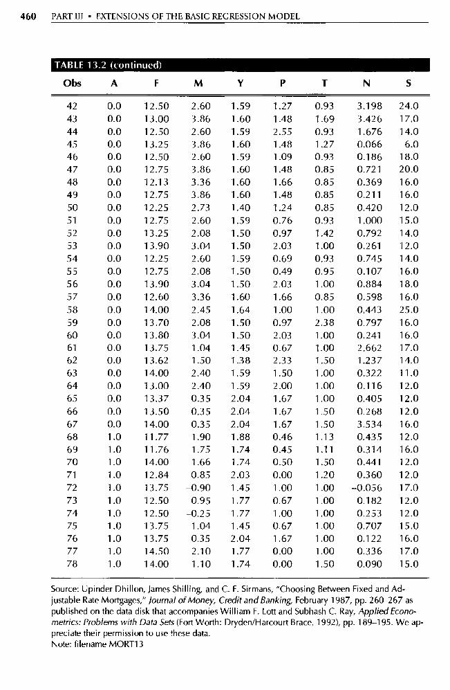
460 PART III • EXTENSIONS OF THE BASIC REGRESSION MODEL
TABLE 13.2 (continued)
Obs A F M Y P T N S
42 0.0 12.50 2.60 1.59 1.27 0.93 3.198 24.0 43 0.0 13.00 3.86 1.60 1.48 1.69 3.426 17.0 44 0.0 12.50 2.60 1.59 2.55 0.93 1.676 14.0 45 0.0 13.25 3.86 1.60 1.48 1.27 0.066 6.0 46 0.0 12.50 2.60 1.59 1.09 0.93 0.186 18.0 47 0.0 12.75 3.86 1.60 1.48 0.85 0.721 20.0 48 0.0 12.13 3.36 1.60 1.66 0.85 0.369 16.0 49 0.0 12.75 3.86 1.60 1.48 0.85 0.211 16.0 50 0.0 12.25 2.73 1.40 1.24 0.85 0.420 12.0 51 0.0 12.75 2.60 1.59 0.76 0.93 1.000 15.0 52 0.0 13.25 2.08 1.50 0.97 1.42 0.792 14.0 53 0.0 13.90 3.04 1.50 2.03 1.00 0.261 12.0 54 0.0 12.25 2.60 1.59 0.69 0.93 0.745 14.0 55 0.0 12.75 2.08 1.50 0.49 0.95 0.107 16.0 56 0.0 13.90 3.04 1.50 2.03 1.00 0.884 18.0 57 0.0 12.60 3.36 1.60 1.66 0.85 0.598 16.0 58 0.0 14.00 2.45 1.64 1.00 1.00 0.443 25.0 59 0.0 13.70 2.08 1.50 0.97 2.38 0.797 16.0 60 0.0 13.80 3.04 1.50 2.03 1.00 0.241 16.0 61 0.0 13.75 1.04 1.45 0.67 1.00 2.662 17.0 62 0.0 13.62 1.50 1.38 2.33 1.50 1.237 14.0 63 0.0 14.00 2.40 1.59 1.50 1.00 0.322 11.0 64 0.0 13.00 2.40 1.59 2.00 1.00 0.116 12.0 65 0.0 13.37 0.35 2.04 1.67 1.00 0.405 12.0 66 0.0 13.50 0.35 2.04 1.67 1.50 0.268 12.0 67 0.0 14.00 0.35 2.04 1.67 1.50 3.534 16.0 68 1.0 11.77 1.90 1.88 0.46 1.13 0.435 12.0 69 1.0 11.76 1.75 1.74 0.45 1.11 0.314 16.0 70 1.0 14.00 1.66 1.74 0.50 1.50 0.441 12.0 71 1.0 12.84 0.85 2.03 0.00 1.20 0.360 12.0 72 1.0 13.75 -0.90 1.45 1.00 1.00 -0.056 17.0 73 1.0 12.50 0.95 1.77 0.67 1.00 0.182 12.0 74 1.0 12.50 -0.25 1.77 1.00 1.00 0.253 12.0 75 1.0 13.75 1.04 1.45 0.67 1.00 0.707 15.0 76 1.0 13.75 0.35 2.04 1.67 1.00 0.122 16.0 77 1.0 14.50 2.10 1.77 0.00 1.00 0.336 17.0 78 1.0 14.00 1.10 1.74 0.00 1.50 0.090 15.0
Source: Upinder Dhillon, James Shilling, and C. F. Sirmans, "Choosing Between Fixed and Ad-justable Rate Mortgages," Journal of Money, Credit and Banking, February 1987, pp. 260-267 as published on the data disk that accompanies William F. Lott and Subhash C. Ray, Applied Econo-metrics: Problems with Data Sets (Fo rt Worth: Dryden/Harcourt Brace, 1992), pp. 189-195. We ap-preciate their permission to use these data. Note: filename MORT13
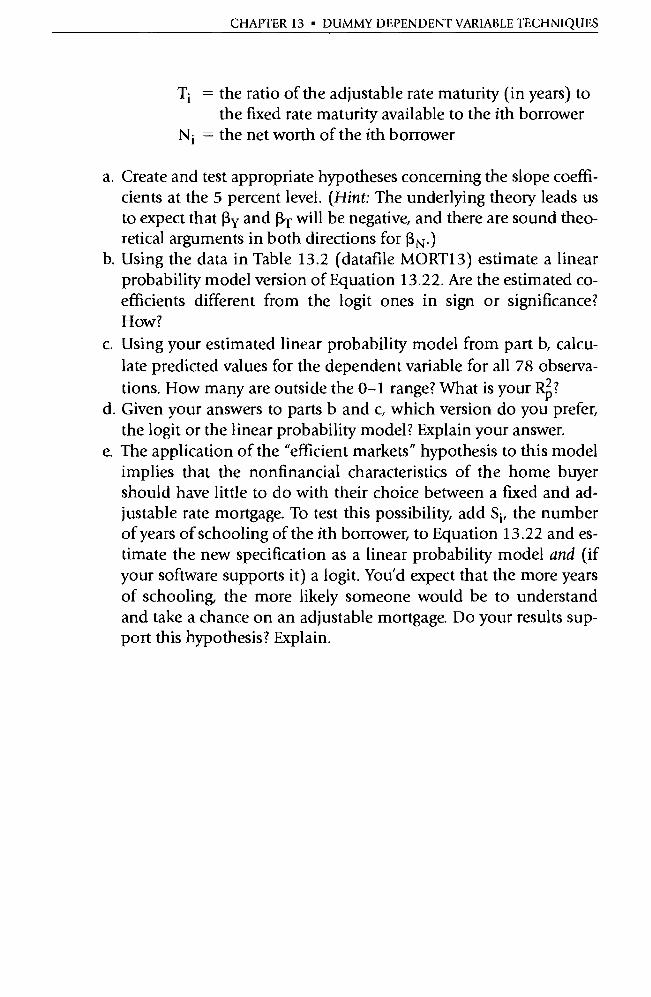
CHAPTER 13 • DUMMY DEPENDENT VARIABLE TECHNIQUES
Ti = the ratio of the adjustable rate maturity (in years) to the fixed rate maturity available to the ith borrower
Ni = the net worth of the ith borrower
a. Create and test appropriate hypotheses concerning the slope coeffi-cients at the 5 percent level. (Hint: The underlying theory leads us to expect that (3 y and (3T will be negative, and there are sound theo-retical arguments in both directions for j3 N .)
b. Using the data in Table 13.2 (datafile MORT13) estimate a linear probability model version of Equation 13.22. Are the estimated co-efficients different from the logit ones in sign or significance? How?
c. Using your estimated linear probability model from pa rt b, calcu-late predicted values for the dependent variable for all 78 observa-tions. How many are outside the 0-1 range? What is your Rp?
d. Given your answers to parts b and c, which version do you prefer, the logit or the linear probability model? Explain your answer.
e. The application of the "efficient markets" hypothesis to this model implies that the nonfinancial characteristics of the home buyer should have little to do with their choice between a fixed and ad-justable rate mortgage. To test this possibility, add S i, the number of years of schooling of the ith borrower, to Equation 13.22 and es-timate the new specification as a linear probability model and (if your software supports it) a logit. You'd expect that the more years of schooling, the more likely someone would be to understand and take a chance on an adjustable mortgage. Do your results sup-port this hypothesis? Explain.
CHAPTER 14 Simultaneous Equations
14.1 Structural and Reduced -Form Equations
14.2 The Bias of Ordinary Least Squares (OLS)
14.3 Two-Stage Least Squares (2SLS)
14.4 The Identification Problem
14.5 Summary and Exercises
14.6 Appendix: Errors in the Variables
Unfortunately, the single-equation models we've covered to date ignore much of the interdependence that characterizes the modern world. Most econometric applications are inherently interdependent or simultaneous in nature, and the best approach to understanding this simultaneity is to explic-itly acknowledge it with feedback loops in our models. This means specifying and estimating simultaneous equations systems instead of looking at just one equation at a time.
The most important models in economics and business are simultaneous in nature. Supply and demand, for example, is obviously simultaneous. To study the demand for chicken without also looking at the supply of chicken is to take a chance on missing impo rtant linkages and thus making signifi-cant mistakes. Virtually all the major approaches to macroeconomics, from Keynesian aggregate demand models to rational expectations schemes, are inherently simultaneous. Even models that appear to be inherently single equation in nature often turn out to be much more simultaneous than you might think. The price of housing, for instance, is dramatically affected by the level of economic activity, the prevailing rate of interest in alternative assets, and a number of other simultaneously determined variables.
All this wouldn't mean much to econometricians if it weren't for the fact that the estimation of simultaneous equations systems with OLS causes a number of difficulties that aren't encountered with single equations. Most important, Classical Assumption III, which states that all explanatory vari-ables should be uncorrelated with the error term, is violated in simultaneous models. Mainly because of this, OLS coefficient estimates are biased in si-
462
CHAPTER 14 • SIMULTANEOUS EQUATIONS
multaneous models. As a result, an alternative estimation procedure called Two-Stage Least Squares is usually employed in such models instead of OLS.
You're probably wondering why we've waited until now to discuss simulta-neous equations if they're so impo rtant in economics and if OLS encounters bias when estimating them. The answer is that the simultaneous estimation of an equation changes every time the specification of any equation in the entire system is changed, so a researcher must be well equipped to deal with specification problems like those of the previous eight chapters. As a result, it does not make sense to learn how to estimate a simultaneous system until you are fairly adept at estimating a single equation.
14.1 Structural and Reduced-Form Equations
Before we can study the problems encountered in the estimation of simulta-neous equations, we need to introduce a few concepts. Readers well versed in the subject are encouraged to skip to Section 14.1.2.
14.1.1 The Nature of Simultaneous Equations Systems
Which came first, the chicken or the egg? This question is impossible to an-swer satisfactorily because chickens and eggs are jointly determined; there is a two-way causal relationship between the variables. The more eggs you have, the more chickens you'll get, but the more chickens you have, the more eggs you'll get. 1 More realistically, the economic world is full of the kind of feed-back effects and dual causality that require the application of simultaneous equations. Besides the supply and demand and simple macroeconomic model examples mentioned above, we could talk about the dual causality of population size and food supply, the joint determination of wages and prices, or the interaction between foreign exchange rates and international trade and capital flows. In a typical econometric equation:
Yt = R O + 13 1X1t + R2X2t + Et {14.1)
a simultaneous system is one in which Y clearly has an effect on at least one of the Xs in addition to the effect that the Xs have on Y.
1. This also depends on how hungry you are, which is a function of how hard you're working, which depends on how many chickens you have to take care of. (Although this chicken/egg ex-ample is simultaneous in an annual model, it would not be truly simultaneous in a quarterly or monthly model because of the time lags involved.)
464 PART III • EXTENSIONS OF THE BASIC REGRESSION MODEL
Such topics are usually modeled by distinguishing between variables that are simultaneously determined (the Ys, called endogenous variables) and those that are not (the Xs, called exogenous variables):
Ylt = ap + a1Y2t + a2X 1t + a3X2t + E 1t (14.2)
Y2t - RO + R1Y lt + R2X3t + Q3X2t + E2t (14.3)
For example, Y 1 and Y2 might be the quantity and price of chicken (respec-tively), X 1 the income of the consumers, X2 the price of beef (beef is a substi-tute for chicken in both consumption and production), and X3 the price of chicken feed. With these definitions, Equation 14.2 would characterize the behavior of consumers of chickens and Equation 14.3 the behavior of sup-pliers of chickens. These behavioral equations are also called structural equa-tions. Structural equations characterize the underlying economic theory be-hind each endogenous variable by expressing it in terms of both endogenous and exogenous variables. Researchers must view them as an entire system in order to see all the feedback loops involved. For example, the Ys are jointly determined, so a change in Y 1 will cause a change in Y2, which will in turn cause Y 1 to change again. Contrast this feedback with a change in X 1 , which will not eventually loop back and cause X 1 to change again. The as and the (3s in the equation are structural coefficients, and hypotheses should be made about their signs just as we did with the regression coefficients of single equations.
Note that a variable is endogenous because it is jointly determined, not just because it appears in both equations. That is, X2, which is the price of beef but could be another factor beyond our control, is in both equations but is still ex-ogenous in nature because it is not simultaneously determined within the chicken market. In a large general equilibrium model of the entire economy, however, such a price va riable would also likely be endogenous. How do you decide whether a particular variable should be endogenous or exogenous? Some variables are almost always exogenous (the weather, for example), but most others can be considered either endogenous or exogenous, depending on the number and characteristics of the other equations in the system. Thus, the distinction between endogenous and exogenous variables usually depends on how the researcher defines the scope of the research project.
Sometimes, lagged endogenous variables appear in simultaneous systems, usually when the equations involved are distributed lag equations (described in Chapter 12). To avoid confusion, predetermined variables are defined to include all exogenous and lagged endogenous variables. "Predetermined" implies that exogenous and lagged endogenous va riables are determined out-

CHAPTER 14 • SIMULTANEOUS EQUATIONS 465
side the system of specified equations or prior to the current period. Endoge-nous variables that are not lagged are not predetermined, because they are jointly determined by the system in the current time period. Therefore, econometricians tend to speak in terms of endogenous and predetermined variables when discussing simultaneous equations systems.
Let's look at the specification of a simple supply and demand model, say for the "cola" soft-drink industry:
QDt = ao + a1Pt + a2X11 + a3X2t + EDt
Qst = Ro + R 1 Pt + 132X3t + Est
Qst
(14.4)
(14.5)
= QDt (equilibrium condition)
where: QDt = the quantity of cola demanded in time period t Qst = the quantity of cola supplied in time period t Pt = the price of cola in time period t X 1t = dollars of advertising for cola in time period t X2t = another "demand-side" exogenous variable (e.g., income
or the prices or advertising of other drinks) X3t — a "supply-side" exogenous va riable (e.g. the price of artifi-
cial flavors or other factors of production) Et = classical error terms (each equation has its own error term,
subscripted "D" and "S" for demand and supply)
In this case, price and quantity are simultaneously determined, but price, one of the endogenous variables, is not on the left side of any of the equa-tions. It's incorrect to assume automatically that the endogenous va riables are those that appear on the left side of at least one equation; in this case, we could have just as easily written Equation 14.5 with price on the left side and quantity supplied on the right side, as we did in the chicken example in Equations 14.2 and 14.3. Although the estimated coefficients would be dif-ferent, the underlying relations would not. Note also that there must be as many equations as there are endogenous variables. In this case, the three en-dogenous variables are QD, Qs, and P.
What would be the expected signs for the coefficients of the price va riables in Equations 14.4 and 14.5? We'd expect price to enter negatively in the de-mand equation but to enter positively in the supply equation. The higher the price, after all, the less quantity will be demanded, but the more quantity will be supplied. These signs would result in the typical supply and demand dia-gram (Figure 14.1) that we're all used to. Look at Equations 14.4 and 14.5

S = Equation 14.5 p i > 0
D = Equation 14.4 al < 0
P
Pe
466 PART III • EXTENSIONS OF THE BASIC REGRESSION MODEL
0 QD = Qs Q
Figure 14.1 Supply and Demand Simultaneous Equations
An example of simultaneous equations that jointly determine two endogenous variables is the supply and demand for a product. In this case, Equation 14.4, the downward-slop-ing demand function, and Equation 14.5, the upward-sloping supply function, intersect at the equilibrium price and quantity for this market.
again, however, and note that they would be identical but for the different predetermined variables. What would happen if we accidentally put a supply-side predetermined variable in the demand equation or vice versa? We'd have a very difficult time identifying which equation was which, and the expected signs for the coefficients of the endogenous variable P would become am-biguous. As a result, we must take care when specifying the structural equa-tions in a system.
14.1.2 Simultaneous Systems Violate Classical Assumption Ill
Recall from Chapter 4 that Classical Assumption III states that the error term and each explanatory variable must be uncorrelated with each other. If there is such a correlation, then the OLS regression estimation program is likely to attribute to the particular explanatory variable any variations in the depen-dent variable that are actually being caused by variations in the error term. The result will be biased estimates.
To see why simultaneous equations violate the assumption of indepen-dence between the error term and the explanatory variables, look again at a
CHAPTER 14 • SIMULTANEOUS EQUATIONS 46;
simultaneous system, Equations 14.2 and 14.3 (repeated with directional
errors) :
T T T Y lt = a0 + alY2t + a2Xit + a3X2t + Elt
T T Y2t — RO + 13 1Y1t + R2X3t + R3X2t + E2t
(14.2)
(14.3)
Let's work through the system and see what happens when one of the error terms increases, holding everything else in the equations constant:
1. If E l increases in a particular time period, Y 1 will also increase due to Equation 14.2.
2. If Y 1 increases, Y2 will also rise2 due to Equation 14.3.
3. But if Y2 increases in Equation 14.3, it also increases in Equation 14.2 where it is an explanatory variable.
Thus, an increase in the error term of an equation causes an increase in an explanatory variable in the same equation: If E l increases, Y 1 increases, and then Y2 increases, violating the assumption of independence between the er-ror term and the explanatory variables.
This is not an isolated result that depends on the particular equations in-volved. Indeed, as you'll find in Exercise 3, this result works for other error terms, equations, and simultaneous systems. All that is required for the viola-tion of Classical Assumption III is that there be endogenous variables that are jointly determined in a system of simultaneous equations.
14.1.3 Reduced-Form Equations
An alternative way of expressing a simultaneous equations system is through the use of reduced-form equations, equations that express a particular en-dogenous variable solely in terms of an error term and all the predetermined (exogenous plus lagged endogenous) variables in the simultaneous system.
The reduced-form equations for the structural Equations 14.2 and 14.3 would thus be:
2. This assumes that R 1 is positive. If 13 1 is negative, Y2 will decrease and there will be a nega-tive correlation between €1 and Y2, but this negative correlation will still violate Classical As-sumption III. Also note that both Equations 14.2 and 14.3 could have Ylt on the left side; if two variables are jointly determined, it doesn't matter which variable is considered dependent and which explanatory, because they are actually mutually dependent. We used this kind of si-multaneous system in the cola model portrayed in Equations 14.4 and 14.5.

468 PART III • EXTENSIONS OF THE BASIC REGRESSION MODEL
Ylt = ^rr0 + 11.1X1t + 7T2X2t + 1T3X3t + vil
Y2t ^ rrr4 + IT5X1t + 76X2t + Ir7X3t + v2t
(14.6)
(14.7)
where the vs are stochastic error terms and the 'rrs are called reduced-form coefficients because they are the coefficients of the predetermined va riables in the reduced-form equations. Note that each equation includes only one
endogenous variable, the dependent variable, and that each equation has ex-actly the same set of predetermined variables. The reduced-form coefficients,
such as it l and 115, are known as impact multipliers because they measure the impact on the endogenous variable of a one-unit increase in the value of
the predetermined variable, after allowing for the feedback effects from the
entire simultaneous system. There are least four reasons for using reduced-form equations:
1. Since the reduced-form equations have no inherent simultaneity, they
do not violate Classical Assumption III. Therefore, they can be estimated
with OLS without encountering the problems discussed in this chapter.
2. The reduced-form coefficients estimated in this way can sometimes be
mathematically manipulated to allow the estimation of the structural
coefficients. That is, estimates of the irs of Equations 14.6 and 14.7 can be used to solve for the as and 13s of Equations 14.2 and 14.3. This method of calculating estimates of the structural coefficients from esti-mates of the reduced-form coefficients is called Indirect Least Squares (ILS). Unfortunately, ILS turns out to be useful only in very limited sit-uations. For more on ILS, see Exercise 4.
3. The interpretation of the reduced-form coefficients as impact multipli-ers means that they have economic meaning and useful applications
of their own. For example, if you wanted to compare a government spending increase with a tax cut in terms of the per dollar impact in
the first year, estimates of the impact multipliers (reduced-form coeffi-cients or 7s) would allow such a comparison.
4. Perhaps most importantly, reduced-form equations play a crucial role
in the estimation technique most frequently used for simultaneous
equations. This technique, Two-Stage Least Squares, will be explained
in Section 14.3.
To conclude, let's return to the cola supply and demand model and specify
the reduced-form equations for that model. (To test yourself, flip back to
Equations 14.4 and 14.5 and see if you can get the right answer before going
on.) Since the equilibrium conditions forces QD to be equal to Qs, we need only two reduced-form equations:

CHAPTER 14 • SIMULTANEOUS EQUATIONS 469
Qt = Ir0 + 1T lXlt + 1T2X2t + 1T3X3t + vlt
Pt = 1r4 + 1T5Xlt + 1T6X2t + 7T7X3t + v2t
(14.8)
(14.9)
Even though P never appears on the left side of a structural equation, it's an endogenous variable and should be treated as such.
14.2 The Bias of Ordinary Least Squares (OLS)
All the Classical Assumptions must be met for OLS estimates to be BLUE; when an assumption is violated, we must determine which of the properties no longer holds. It turns out that applying OLS directly to the structural equations of a simultaneous system, called Direct Least Squares, produces bi-ased estimates of the coefficients. Such bias is called simultaneous equations bias or simultaneity bias.
14.2.1 Understanding Simultaneity Bias
Simultaneity bias refers to the fact that in a simultaneous system, the ex-pected values of the OLS-estimated structural coefficients (13s) are not equal to the true Rs. We are therefore faced with the problem that in a simultane-ous system:
E(R) # R (14.10)
Why does this simultaneity bias exist? Recall from Section 14.1.2 that in si-multaneous equations systems, the error terms (the Es) tend to be correlated with the endogenous variables (the Ys) whenever the Ys appear as explanatory variables. Let's follow through what this correlation means (assuming positive coefficients for simplicity) in typical structural equations like 14.11 and 14.12:
Ylt = Ro + R1Y2t + R2Xt + Elt
Y 2t = ao + aiYit + a2Zt + E2t
(14.11)
(14.12)
Since we cannot obse rve the error term (E 1 ) and don't know when E ll is above average, it will appear as if every time Y 1 is above average, so too is Y2. As a re-sult, the OLS estimation program will tend to attribute increases in Y 1 caused by the error term E 1 to Y2, thus typically overestimating 13 1 . This overestima-tion is simultaneity bias. If the error term is abnormally negative, Ylt is less than it would have been otherwise, causing Y 2t to be less than it would have
470 PART III • EXTENSIONS OF THE BASIC REGRESSION MODEL
been otherwise, and the computer program will attribute the decrease in Y 1 to Y2 , once again causing us to overestimate 13 1 (that is, induce upward bias).
Recall that the causation between Y 1 and Y2 runs in both directions be-cause the two variables are interdependent. As a result, 13 1 , when estimated by OLS, can no longer be interpreted as the impact of Y2 on Y 1 , holding X constant. Instead, (3 1 now measures some mix of the effects of the two en-dogenous variables on each other! In addition, consider 132. It's supposed to be the effect of X on Y 1 holding Y2 constant, but how can we expect Y2 to be held constant when a change in Y 1 takes place? As a result, there is potential bias in all the estimated coefficients in a simultaneous system.
What does this bias look like? It's possible to derive an equation 3 for the expected value of the regression coefficients in a simultaneous system that is estimated by OLS. This equation shows that as long as the error term and any of the explanatory variables in the equation are correlated, then the coeffi-cient estimates will be biased. In addition, it also shows that the bias will have the same sign as the correlation between the error term and the endoge-nous variable that appears as an explanatory variable in that error term's equation. Since that correlation is usually positive in economic and business examples, so is the bias of OLS. The violation of Classical Assumption III will almost always mean bias in the estimation of (3 i . In addition, this bias will usually be positive in economic applications, although the direction of the bias in any given situation will depend on the specific details of the structural equations and the model's underlying theory.
This does not mean that every coefficient from a simultaneous system esti-mated with OLS will be a bad approximation of the true population coeffi-cient; indeed, most researchers use OLS to estimate equations in simultane-ous systems under a number of circumstances. Instead, it's vital at least to consider an alternative to OLS whenever simultaneous equations systems are being estimated. Before we investigate the alternative estimation technique most frequently used (Two-Stage Least Squares), let's look at an example of simultaneity bias.
3. For Equation 14.11, the expected value of 13 simplifies to:
E01) = 13 1 + E[I(Y2t Y2)(E1t)/I(Y2t — 172) 2 ]
In a nonsimultaneous equation, where Y2 and e t are not correlated, the expected value of R1 equals the true f3 i because the expected value of the term X (Y2t Y2) (E n) is zero. If Y2 and e 1 are positively correlated, as would be true in most simultaneous systems in economics, then the expected value of 13 1 is greater than the true p, because the expected value of X (Y2t — Y2) (eft) is positive. In the less likely case that Y2 and e l are negatively correlated, the expected value of (3 1 is less than the true [31.
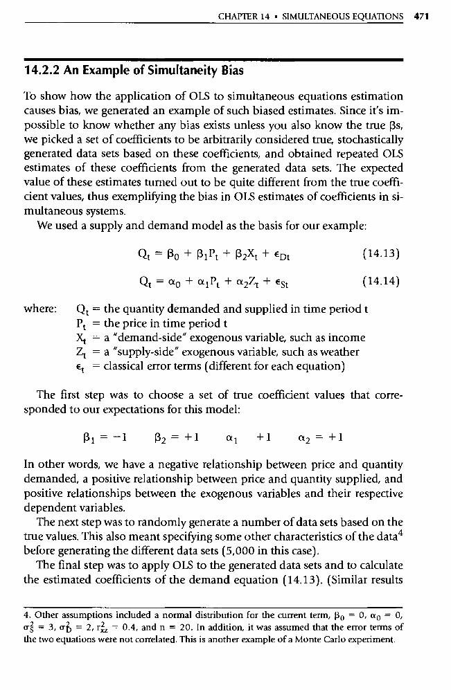
CHAPTER 14 • SIMULTANEOUS EQUATIONS 471
14.2.2 An Example of Simultaneity Bias
To show how the application of OLS to simultaneous equations estimation causes bias, we generated an example of such biased estimates. Since it's im-possible to know whether any bias exists unless you also know the true 13s, we picked a set of coefficients to be arbitrarily considered true, stochastically generated data sets based on these coefficients, and obtained repeated OIS estimates of these coefficients from the generated data sets. The expected value of these estimates turned out to be quite different from the true coeffi-cient values, thus exemplifying the bias in OLS estimates of coefficients in si-multaneous systems.
We used a supply and demand model as the basis for our example:
Qt = Ro +RiPt+ R2Xt + cDt
Qt = ao + a 1 Pt + a2Zt + ESt
(14.13)
(14.14)
where: Qt = the quantity demanded and supplied in time period t Pt = the price in time period t Xt = a "demand-side" exogenous variable, such as income Zt = a "supply-side" exogenous va riable, such as weather
Et = classical error terms (different for each equation)
The first step was to choose a set of true coefficient values that corre-sponded to our expectations for this model:
R 1 = -1 R2 = + 1 a l + 1 a2 + 1
In other words, we have a negative relationship between price and quantity demanded, a positive relationship between price and quantity supplied, and positive relationships between the exogenous variables and their respective dependent variables.
The next step was to randomly generate a number of data sets based on the true values. This also meant specifying some other characteristics of the data 4
before generating the different data sets (5,000 in this case). The final step was to apply OLS to the generated data sets and to calculate
the estimated coefficients of the demand equation (14.13). (Similar results
4. Other assumptions included a normal distribution for the current term, 13 0 = 0, a 0 = 0, cr = 3, QD = 2, r = 0.4, and n = 20. In addition, it was assumed that the error terms of the two equations were not correlated. This is another example of a Monte Carlo experiment.
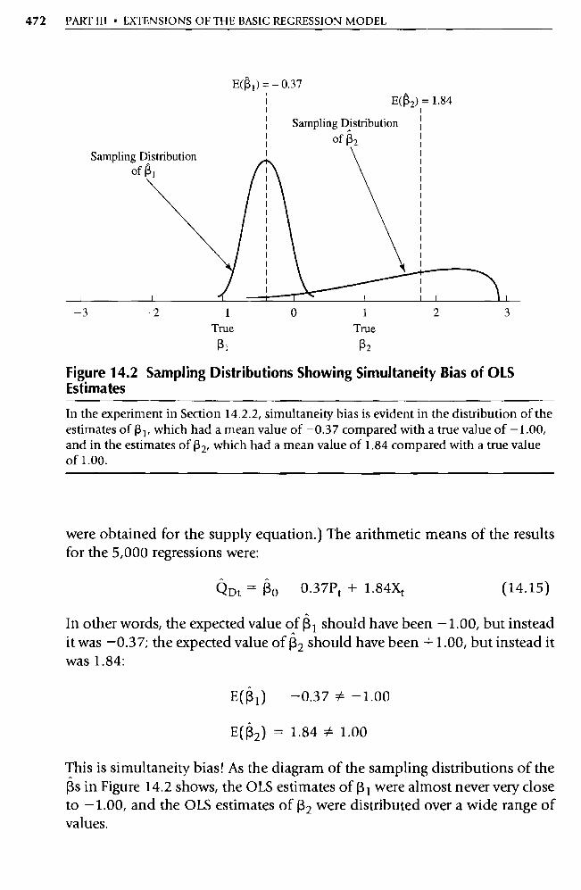
—3 —2 —I True
R 1
0 1 True
13 2
2 3
EA) -- 0.37 E(0 2) = 1.84
Sampling Distribution of R 2
Sampling Distribution of (3 1
472 PART III • EXTENSIONS OF THE BASIC REGRESSION MODEL
Figure 14.2 Sampling Distributions Showing Simultaneity Bias of OLS Estimates
In the experiment in Section 14.2.2, simultaneity bias is evident in the distribution of the estimates of 131, which had a mean value of —0.37 compared with a true value of —1.00, and in the estimates of 132, which had a mean value of 1.84 compared with a true value of 1.00.
were obtained for the supply equation.) The arithmetic means of the results for the 5,000 regressions were:
QDt = Ro 0.37Pt + 1.84Xt (14.15)
In other words, the expected value of j3 1 should have been —1.00, but instead it was —0.37; the expected value of 13 2 should have been +1.00, but instead it was 1.84:
E1) —0.37 * — 1.00
E2) = 1.84 0 1.00
This is simultaneity bias! As the diagram of the sampling dist ributions of the Rs in Figure 14.2 shows, the OLS estimates of (3 1 were almost never very close to —1.00, and the OLS estimates of (32 were distributed over a wide range of values.
CHAPTER 14 • SIMULTANEOUS EQUATIONS 473
The biased estimation in this example did not cause incorrect signs for the majority of the estimates, but any kind of bias is worth avoiding if it is at all possible. The most frequently used method of reducing simultaneity bias is a technique called Two-Stage Least Squares (2SLS).
14.3 Two -Stage Least Squares (2SLS)
Although there are a number of econometric estimation techniques available that help mitigate the bias inherent in the application of OLS to simultane-ous equations systems, the most frequently used alternative to OLS is called Two-Stage Least Squares (2SLS).
14.3.1 What Is Two-Stage Least Squares?
OLS encounters bias in the estimation of simultaneous equations mainly be-cause such equations violate Classical Assumption III, so one solution to the problem is to explore ways to avoid violating that assumption. We could do this if we could find a variable that is:
1. a good proxy for the endogenous variable, and
2. uncorrelated with the error term.
If we then substitute this new variable for the endogenous variable where it appears as an explanatory variable, our new explanatory variable will be uncorrelated with the error term, and Classical Assumption III will be met.
That is, consider Equation 14.16 in the following system:
Yit= Ro +R1Y2t+R2Xt + eft
Yet = ap + a2Yl t + et2Zt + E2t
(14.16)
(14.17)
If we could find a variable that was highly correlated with Y2 but that was un-correlated with e l , then we could substitute this new variable for Y2 on the right side of Equation 14.16, and we'd conform to Classical Assumption III. This new variable is called an instrumental variable. An instrumental variable replaces an endogenous variable (when it is an explanatory variable); it is a good proxy for the endogenous variable and is independent of the error term.
Since there is no joint causality between the instrumental variable and any endogenous variable, the use of the instrumental va riable avoids the violation of Classical Assumption III. The job of finding such a variable is another story,
474 PART III • EXTENSIONS OF THE BASIC REGRESSION MODEL
though. How do we go about finding va riables with these qualifications? For simultaneous equations systems, 2SLS provides an approximate answer.
Two-Stage Least Squares (2SLS) is a method of systematically creating in-strumental variables to replace the endogenous variables where they appear as explanatory variables in simultaneous equations systems. 2SLS does this by running a regression on the reduced form of the right-side endogenous variables in need of replacement and then using the Ÿs (or fitted values) from those reduced-form regressions as the instrumental variables. More specifi-cally, the two-step procedure consists of:
STAGE ONE: Run OLS on the reduced form equations for each of the endogenous variables that appear as explanatory variables in the struc-tural equations in the system.
Since the predetermined (exogenous plus lagged endogenous) variables are uncorrelated with the reduced-form error term, the OLS estimates of the reduced-form coefficients (the -rrs) are unbiased. These 'rrs can then be used to calculate estimates of the endogenous variables 5 :
Y1t = 7T0 + Tf 1 Xt + 'T2Zt
2t = 7T3 + Tr4Xt + 4'1'54
(14.18)
(14.19)
These Ÿs are used as proxies in the structural equations of the simultaneous system.
STAGE TWO: Substitute the reduced form Ys for the Ys that appear on the right side (only) of the structural equations, and then estimate these revised structural equations with OLS.
That is, stage two consists of estimating the following equations with OLS:
Y1t = R 0 + R1Y2t + R2Xt + uIt
Y 2t = a2Ylt + a2Zt + u2t
(14.20)
(14.21)
Note that the dependent variables are still the o riginal endogenous variables and that the substitutions are only for the endogenous variables where they appear on the right-hand side of the structural equations.
5. Because the irs are not uncorrelated with the ES, this procedure produces only approximate instrumental variables that provide consistent (for large samples), but biased (for small sam-ples), estimates of the coefficients of the structural equation (the 3s).
CHAPTER 14 • SIMULTANEOUS EQUATIONS 475
If second-stage equations such as Equations 14.20 and 14.21 are estimated with OLS, the SE( f3)s will be incorrect, so be sure to use your computer's 2SLS estimation procedure.
This description of 2SLS can be generalized to m different simultaneous structural equations. Each reduced-form equation has as explanatory vari-ables every predetermined variable in the entire system of equations. The OLS estimates of the reduced-form equations are used to compute the esti-mated values of all the endogenous variables that appear as explanatory vari-ables in the m structural equations. After substituting these fitted values for the original values of the endogenous independent variables, OLS is applied to each stochastic equation in the set of structural equations.
14.3.2 The Properties of Two-Stage Least Squares
1. 2SLS estimates are still biased in small samples. For small samples, the ex-pected value of a (3 produced by 2SLS is still not equal to the true 13, 7
but as the sample size gets larger, the expected value of the (3 ap-proaches the true (3. As the sample size gets bigger, the variances of both the OLS and the 2SLS estimates decrease. OLS estimates become very precise estimates of the wrong number, and 2SLS estimates be-come very precise estimates of the correct number. As a result, the larger the sample size, the better a technique 2SLS is.
To illustrate, let's look again at the example of Section 14.2. The 2SLS estimate of 13 1 was — 1.25. This estimate is biased, but it's much closer to the truth ((3 1 = 1.00) than is the OLS estimate of — 0.37 We then returned to that example and expanded the data set from 5,000 different samples of size 20 each to 5,000 different samples of 50 observations each. As expected, the average 13 1 for 2SLS moved from — 1.25 to — 1.06 compared to the true value of —1.00. By contrast, the OLS average estimate went from —0.37 to —0.44. Such results are typi-cal; large sample sizes will produce unbiased estimates for 2SLS but bi-ased estimates for OLS.
2. The bias in 2SLS for small samples typically is of the opposite sign of the bias in OLS. Recall that the bias in OLS typically was positive, indicating
6. Most econometric software packages, including EViews, offer such a 2SLS option. For more on this issue, see Exercise 9 and footnote 11 of this chapter.
7 This bias is caused by remaining correlation between the Ys produced by the first-stage re-duced-form regressions and the ES. The effect of the correlation tends to decrease as the sample size increases. Even for small samples, though, it's worth noting that the expected bias due to 2SLS usually is smaller than the expected bias due to OLS.
476 PART III • EXTENSIONS OF THE BASIC REGRESSION MODEL
that a R produced by OLS for a simultaneous system is likely to be greater than the true B. For 2SLS, the expected bias is negative, and thus a R produced by 2SLS is likely to be less than the true R. For any given set of data, the 2SLS estimate can be larger than the OLS estimate, but it can be shown that the majority of 2SLS estimates are likely to be less than the corresponding OLS estimates. For large samples, there is little bias in 2SLS.
Return to the example of Section 14.2. Compared to the true value of —1.00 for (3 1 , the small sample 2SLS average estimate was —1.25, as mentioned above. This means that the 2SLS estimates showed negative bias. The OLS estimates, on the other hand, averaged —0.37; since —0.37 is more positive than —1.00, the OLS estimates exhibited posi-tive bias. Thus, the observed bias due to OLS was opposite the observed bias due to 2SLS, as is generally the case.
3. If the fit of the reduced form equation is quite poor, then 2SLS will not work very well. Recall that the instrumental variable is supposed to be a good proxy for the endogenous variable. To the extent that the fit (as mea-sured by R2) of the reduced-form equation is poor, then the instrumen-tal variable is no longer highly correlated with the original endogenous variable, and there is no reason to expect 2SLS to be effective. As the R2 of the reduced-form equation increases, the usefulness of the 2SLS will increase.
4. If the predetermined variables are highly correlated, 2SLS will not work very well. The first stage of 2SLS includes explanatory variables from differ-ent structural equations in the same reduced-form equation. As a re-sult, severe multicollinearity between explanatory variables from differ-ent structural equations is possible in the reduced-form equations. When this happens, a Y produced by a reduced-form equation can be highly correlated with the exogenous variables in the structural equa-tion. Consequently, the second stage of 2SLS will also show a high de-gree of multicollinearity, and the variances of the estimated coefficients will be high. Thus, the higher the simple correlation coefficient be-tween predetermined variables (or the higher the variance inflation fac-tors), the less precise 2SLS estimates will be.
5. The use of the t-test for hypothesis testing is far more accurate using 2SLS es-timators than it is using OLS estimators. The t-test is not exact for the 2SLS estimators, but it is accurate enough in most circumstances. By con-trast, the biasedness of OLS estimators in simultaneous systems im-plies that its t-statistics are not accurate enough to be relied upon for

CHAPTER 14 • SIMULTANEOUS EQUATIONS 4:
testing purposes. 8 This means that it may be appropriate to use 2SLS even when the predetermined variables are highly correlated.
On balance, then, 2SLS will almost always be a better estimator of the co-efficients of a simultaneous system than OLS will be. The major exception to this general rule is when the fit of the reduced-form equation in question is quite poor for a small sample.
14.3.3 An Example of Two-Stage Least Squares
Let's work through an example of the application of 2SLS to a naive linear Keynesian macroeconomic model of the U.S. economy. We'll specify the fol-lowing system:
Yt = COt + It + Gt + NXt (14.22)
COt = Po + R1YDt + 132C0t-1 + E li (14.23)
YDt =Yt —Tt (14.24)
It — Q 3 + 1:34Yt + R5rt -1 + E2t (14.25)
rt = 136 + 13 7Yt + 13 8M1 + E31 (14.26)
where: Yt = Gross Domestic Product (GDP) in year t COt = total personal consumption in year t It = total gross private domestic investment in year t Gt = government purchases of goods and services in year t NXt = net exports of goods and services (exports minus impo rts)
in year t Tt = taxes (actually equal to taxes, depreciation, corporate prof-
its, government transfers, and other adjustments necessary to convert GDP to disposable income) in year t
rt = the interest rate (yield on commercial paper) in year t Mt = the money supply (narrowly defined) in year t YDt = disposable income in year t
8. In our experiments, OLS estimators rejected the correct null hypothesis more than eight times as often as would have been expected from an unbiased procedure. In contrast, the 2SLS estimators were found to reject a correct null hypothesis only twice as frequently as would have been expected.
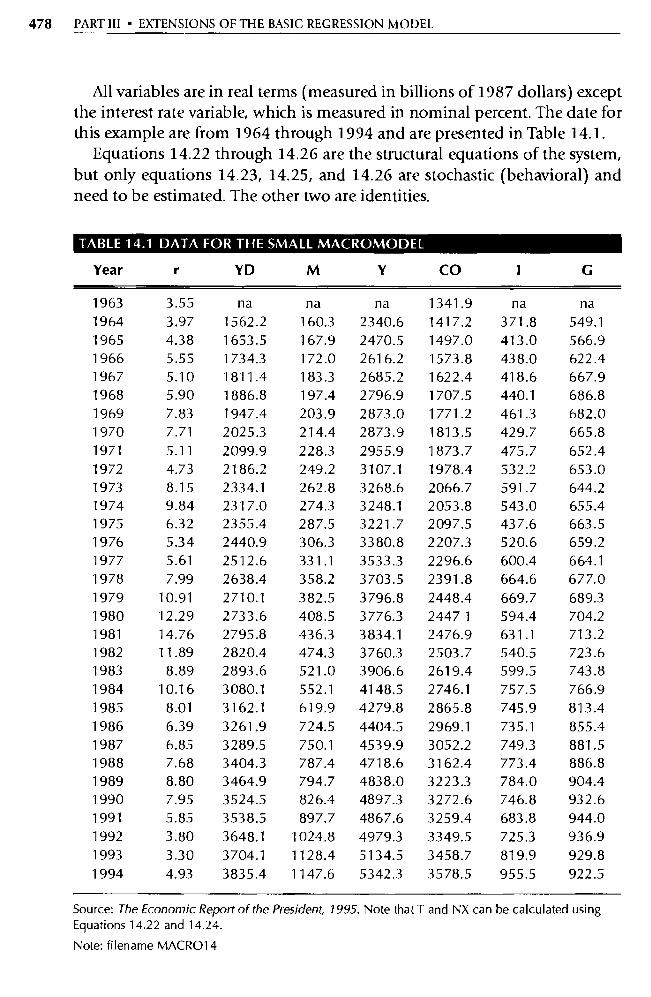
478 PART III • EXTENSIONS OF THE BASIC REGRESSION MODEL
All variables are in real terms (measured in billions of 1987 dollars) except the interest rate variable, which is measured in nominal percent. The date for this example are from 1964 through 1994 and are presented in Table 14.1.
Equations 14.22 through 14.26 are the structural equations of the system, but only equations 14.23, 14.25, and 14.26 are stochastic (behavioral) and need to be estimated. The other two are identities.
TABLE 14.1 DATA FOR THE SMALL MACROMODEL
Year r YD M Y CO 1 G
1963 3.55 na na na 1341.9 na na 1964 3.97 1562.2 160.3 2340.6 1417.2 371.8 549.1 1965 4.38 1653.5 167.9 2470.5 1497.0 413.0 566.9 1966 5.55 1734.3 172.0 2616.2 1573.8 438.0 622.4 1967 5.10 1811.4 183.3 2685.2 1622.4 418.6 667.9 1968 5.90 1886.8 197.4 2796.9 1707.5 440.1 686.8 1969 7.83 1947.4 203.9 2873.0 1771.2 461.3 682.0 1970 7.71 2025.3 214.4 2873.9 1813.5 429.7 665.8 1971 5.11 2099.9 228.3 2955.9 1873.7 475.7 652.4 1972 4.73 2186.2 249.2 3107.1 1978.4 532.2 653.0 1973 8.15 2334.1 262.8 3268.6 2066.7 591.7 644.2 1974 9.84 2317.0 274.3 3248.1 2053.8 543.0 655.4 1975 6.32 2355.4 287.5 3221.7 2097.5 437.6 663.5 1976 5.34 2440.9 306.3 3380.8 2207.3 520.6 659.2 1977 5.61 2512.6 331.1 3533.3 2296.6 600.4 664.1 1978 7.99 2638.4 358.2 3703.5 2391.8 664.6 677.0 1979 10.91 2710.1 382.5 3796.8 2448.4 669.7 689.3 1980 12.29 2733.6 408.5 3776.3 24471 594.4 704.2 1981 14.76 2795.8 436.3 3834.1 2476.9 631.1 713.2 1982 11.89 2820.4 474.3 3760.3 2503.7 540.5 723.6 1983 8.89 2893.6 521.0 3906.6 2619.4 599.5 743.8 1984 10.16 3080.1 552.1 4148.5 2746.1 757.5 766.9 1985 8.01 3162.1 619.9 4279.8 2865M 745.9 813.4 1986 6.39 3261.9 724.5 4404.5 2969.1 735.1 855.4 1987 6.85 3289.5 750.1 4539.9 3052.2 749.3 881.5 1988 7.68 3404.3 787.4 4718.6 3162.4 773.4 886.8 1989 8.80 3464.9 794.7 4838.0 3223.3 784.0 904.4 1990 7.95 3524.5 826.4 4897.3 3272.6 746.8 932.6 1991 5.85 3538.5 897.7 4867.6 3259.4 683.8 944.0 1992 3.80 3648.1 1024.8 4979.3 3349.5 725.3 936.9 1993 3.30 3704.1 1128.4 5134.5 3458.7 819.9 929.8 1994 4.93 3835.4 1147.6 5342.3 3578.5 955.5 922.5
Source: The Economic Report of the President, 1995. Note that T and NX can be calculated using Equations 14.22 and 14.24.
Note: filename MACR014

CHAPTER 14 • SIMULTANEOUS EQUATIONS 479
Stop for a second and look at the system; which variables are endogenous? Which are predetermined? The endogenous variables are those that are jointly determined by the system, namely, Y t, COI, YDt, and It. To see why these four variables are simultaneously determined, note that if you change one of them and follow this change through the system, the change will get back to the original causal variable. For instance, if I t goes up for some rea-son, that will cause Yt to go up, which will feed right back into I t again. They're simultaneously determined.
What about interest rates? Is r t an endogenous variable? The surprising an-swer is that, strictly speaking, r t is not endogenous in this system because r t_ 1
(not rt) appears in the investment equation and r t appears only once in the entire system. Thus, there is no simultaneous feedback through the interest rate in this simple model. Because there is no simultaneity, there is no simul-taneity bias, and OIS can be used to estimate Equation 14.26. In essence, Equation 14.26 is not in the simultaneous system.
Given this answer, which are the predetermined variables? If Equation 14.26 isn't in the simultaneous system, then the predetermined variables are Gt, NXt, Tt, COt_ 1 , and rt_ 1 (but not Mt !). To sum, the simultaneous system has four structural equations, four endogenous variables, and five predeter-mined variables.
What is the economic content of the stochastic structural equations? The consumption function, Equation 14.23, is a Koyck distributed lag consump-tion function of the kind we discussed in Chapter 12. We discussed this exact equation in Section 12.1, going so far as to estimate Equation 14.23 with OIS on data from Table 14.1, and the reader is encouraged to reread that analysis.
The investment function, Equation 14.25, includes simplified multiplier and cost of capital components. The multiplier term R4 measures the stimu-lus to investment that is generated by an increase in GDP. In a Keynesian model, 134 thus would be expected to be positive. On the other hand, the higher the cost of capital, the less investment we'd expect to be undertaken (holding multiplier effects constant), mainly because the expected rate of re-turn on marginal capital investments is no longer sufficient to cover the higher cost of capital. Thus R5 is expected to be negative. It takes time to plan
9. Although this sentence is technically correct, it overstates the case. In pa rticular, there are a couple of circumstances in which an econometrician might want to consider Equation 14.26 to be part of the simultaneous system for theoretical reasons. Such possibilities include GLS mod-els and models where the error terms from various equations are thought to be correlated. For our naive Keynesian model with a lagged interest rate effect, however, the equation is not in the simultaneous system.
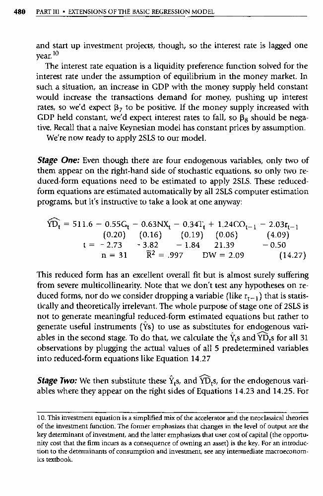
480 PART III • EXTENSIONS OF THE BASIC REGRESSION MODEL
and start up investment projects, though, so the interest rate is lagged one year. 20
The interest rate equation is a liquidity preference function solved for the interest rate under the assumption of equilibrium in the money market. In such a situation, an increase in GDP with the money supply held constant would increase the transactions demand for money, pushing up interest rates, so we'd expect 13 7 to be positive. If the money supply increased with GDP held constant, we'd expect interest rates to fall, so 13 8 should be nega-tive. Recall that a naive Keynesian model has constant prices by assumption.
We're now ready to apply 2SLS to our model.
Stage One: Even though there are four endogenous va riables, only two of them appear on the right-hand side of stochastic equations, so only two re-duced-form equations need to be estimated to apply 2SLS. These reduced-form equations are estimated automatically by all 2SLS computer estimation programs, but it's instructive to take a look at one anyway:
YDt = 511.6 — 0.55Gt — 0.63NXt — 0.34Tt + 1.24COt_ i — 2.03rt_ i (0.20) (0.16) (0.19) (0.06) (4.09)
t = — 2.73 — 3.82 — 1.84 21.39 — 0.50 n = 31 R2 = .997 DW = 2.09 (14.27)
This reduced form has an excellent overall fit but is almost surely suffering from severe multicollinearity. Note that we don't test any hypotheses on re-duced forms, nor do we consider dropping a variable (like r t_ i ) that is statis-tically and theoretically irrelevant. The whole purpose of stage one of 2SLS is not to generate meaningful reduced-form estimated equations but rather to generate useful instruments (Ys) to use as substitutes for endogenous vari-ables in the second stage. To do that, we calculate the Ÿ ts and YDts for all 31 observations by plugging the actual values of all 5 predetermined variables into reduced-form equations like Equation 14.27
Stage Two: We then substitute these Ÿ ts, and YDts, for the endogenous vari- ables where they appear on the right sides of Equations 14.23 and 14.25. For
10. This investment equation is a simplified mix of the accelerator and the neoclassical theories of the investment function. The former emphasizes that changes in the level of output are the key determinant of investment, and the latter emphasizes that user cost of capital (the opportu-nity cost that the firm incurs as a consequence of owning an asset) is the key. For an introduc-tion to the determinants of consumption and investment, see any intermediate macroeconom-ics textbook.
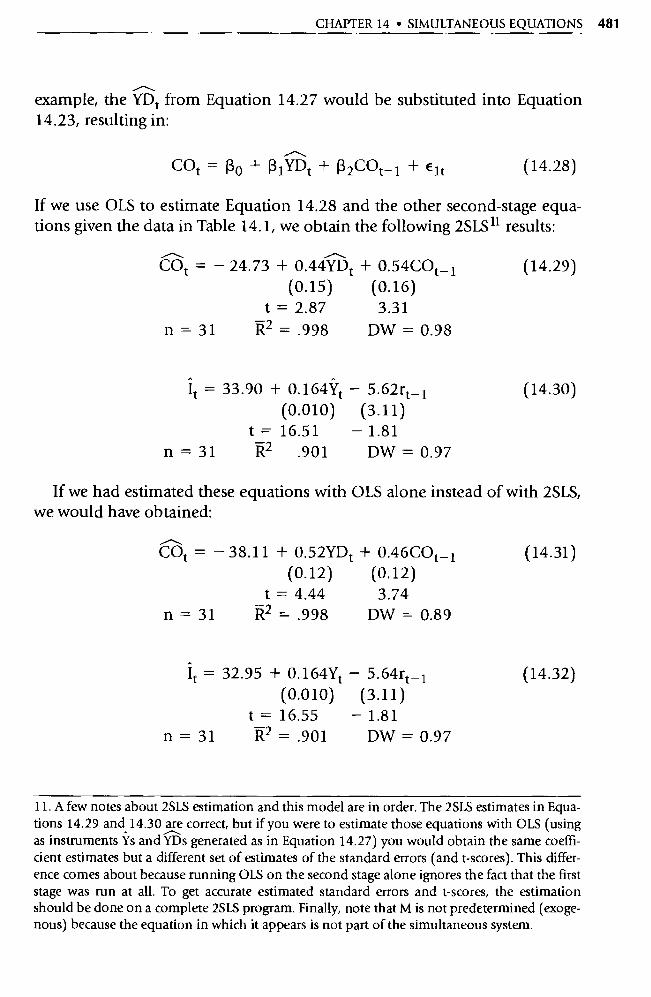
CHAPTER 14 • SIMULTANEOUS EQUATIONS 481
example, the YD t from Equation 14.27 would be substituted into Equation
14.23, resulting in:
COt = Ra + ^3 1YD + R2COt- 1 + Elt ( 1 4.28)
If we use OLS to estimate Equation 14.28 and the other second-stage equa-tions given the data in Table 14.1, we obtain the following 2SLS 11 results:
COt = - 24.73 + 0.44YDt + 0.54COt_
(0.15) (0.16)
t = 2.87 3.31 n = 31 R2 =.998 DW = 0.98
It = 33.90 + 0.164Ÿt - 5.62rt_ 1
(0.010) (3.11) t = 16.51 -1.81
n=31 R2 .901 DW =0.97
(14.29)
(14.30)
If we had estimated these equations with OLS alone instead of with 2SLS, we would have obtained:
COt = - 38.11 + 0.52YDt + 0.46COt_ 1
(0.12) (0.12)
t = 4.44 3.74 n = 31 R2 =.998 DW = 0.89
It = 32.95 + 0.164Yt - 5.64rt _ 1
(0.010) (3.11) t = 16.55 -1.81
n = 31 R2 =.901 DW = 0.97
(14.31)
(14.32)
11. A few notes about 2SLS estimation and this model are in order. The 2SLS estimates in Equa-tions 14.29 and 14.30 are correct, but if you were to estimate those equations with OLS (using as instruments Ys and YDs generated as in Equation 14.27) you would obtain the same coeffi-cient estimates but a different set of estimates of the standard errors (and t-scores). This differ-ence comes about because running OLS on the second stage alone ignores the fact that the first stage was run at all. To get accurate estimated standard errors and t-scores, the estimation should be done on a complete 2SLS program. Finally, note that M is not predetermined (exoge-nous) because the equation in which it appears is not pa rt of the simultaneous system.
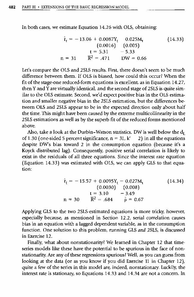
482 PART III • EXTENSIONS OF THE BASIC REGRESSION MODEL
In both cases, we estimate Equation 14.26 with OLS, obtaining:
it = - 13.06 + 0.0087Yt 0.025Mt (0.0016) (0.005)
t = 5.31 - 5.33 n=31 R2 =.471 DW =0.66
(14.33)
Let's compare the OLS and 2SLS results. First, there doesn't seem to be much difference between them. If OLS is biased, how could this occur? When the fit of the stage-one reduced-form equations is excellent, as in Equation 14.27, then Y and Y are virtually identical, and the second stage of 2SLS is quite sim-ilar to the OLS estimate. Second, we'd expect positive bias in the OIS estima-tion and smaller negative bias in the 2SLS estimation, but the differences be-tween OIS and 2SLS appear to be in the expected direction only about half the time. This might have been caused by the extreme multicollinearity in the 2SLS estimations as well as by the superb fit of the reduced forms mentioned above.
Also, take a look at the Durbin-Watson statistics. DW is well below the d L of 1.30 (one-sided 5 percent significance, n = 31, k' 2) in all the equations
despite DW's bias toward 2 in the consumption equation (because it's a Koyck distributed lag). Consequently, positive serial correlation is likely to exist in the residuals of all three equations. Since the interest rate equation (Equation 14.33) was estimated with OLS, we can apply GLS to that equa-tion:
it = - 15.57 + 0.0095Yt - 0.027Mt (0.0030) (0.008)
t = 3.10 - 3.49 n = 30 R2 =.684 p=0.67
(14.34)
Applying GLS to the two 2SLS-estimated equations is more tricky, however, especially because, as mentioned in Section 12.2, serial correlation causes bias in an equation with a lagged dependent variable, as in the consumption function. One solution to this problem, running GLS and 2SLS, is discussed in Exercise 12.
Finally, what about nonstationarity? We learned in Chapter 12 that time-series models like these have the potential to be spurious in the face of non-stationarity. Are any of these regressions spurious? Well, as you can guess from looking at the data (or as you know if you did Exercise 11 in Chapter 12), quite a few of the series in this model are, indeed, nonstationary. Luckily, the interest rate is stationary, so Equations 14.33 and 14.34 are not a concern. In

CHAPTER 14 • SIMULTANEOUS EQUATIONS 483
addition, it turns out that the consumption function is reasonably cointe-grated (see Exercise 15 of this chapter), so Equations 14.29 and 14.31 proba-bly can stand as estimated. Unfortunately, the investment equation suffers from nonstationarity that almost surely results in an inflated t-score for GDP and a low t-score for r t_ 1 (because it is stationary when all the other variables in the equation are nonstationary). In fact, most macromodels encounter sim-ilar problems with the significance (and sometimes the sign) of the interest rate variable in investment equations, at least partially because of the nonsta-tionarity of the other va riables in the equation. Given the tools covered so far in this text, however, there is little we can do to improve the situation.
These caveats aside, this model has provided us with a complete example of the use of 2SLS to estimate a simultaneous system. However, the applica-tion of 2SLS requires that the equation being estimated be "identified," so before we can conclude our study of simultaneous equations, we need to ad-dress the problem of identification.
14.4 The Identification Problem
Two-Stage Least Squares cannot be applied to an equation unless that equa-tion is identified. Before estimating any equation in a simultaneous system, the researcher must address the identification problem. Once an equation is found to be identified, then it can be estimated with 2SLS, but if an equation is not identified (underidentified), then 2SLS cannot be used no matter how large the sample. It's impo rtant to point out that an equation being identified (and therefore capable of being estimated with 2SLS) does not ensure that the resulting 2SLS estimates will be good ones. The question being asked is not how good the 2SLS estimates will be but whether the 2SLS estimates can be obtained at all.
14.4.1 What Is the Identification Problem?
Identification is a precondition for the application of 2SLS to equations in simultaneous systems; a structural equation is identified only when enough of the system's predetermined va riables are omitted from the equation in question to allow that equation to be distinguished from all the others in the system. Note that one equation in a simultaneous system might be identified and another might not.
How could we have equations that we could not identify? To see how, let's consider a supply and demand simultaneous system in which only price and quantity are specified:
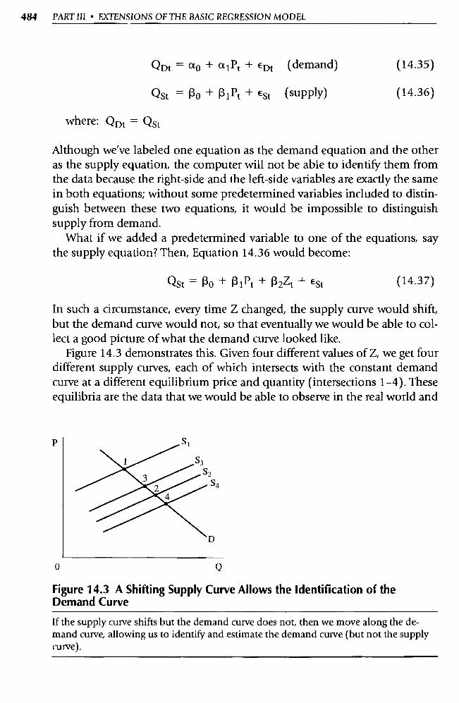
484 PART III • EXTENSIONS OF THE BASIC REGRESSION MODEL
P
QDt = a0 + a l Pt + EDt (demand)
Qst = Ro + 31P1 + Est ( supply)
where: QDt = Qst
(14.35)
(14.36)
Although we've labeled one equation as the demand equation and the other as the supply equation, the computer will not be able to identify them from the data because the right-side and the left-side variables are exactly the same in both equations; without some predetermined variables included to distin-guish between these two equations, it would be impossible to distinguish supply from demand.
What if we added a predetermined va riable to one of the equations, say the supply equation? Then, Equation 14.36 would become:
Qst = Ro + R i Pt + R2Zt + Est (14.37)
In such a circumstance, every time Z changed, the supply curve would shift, but the demand curve would not, so that eventually we would be able to col-lect a good picture of what the demand curve looked like.
Figure 14.3 demonstrates this. Given four different values of Z, we get four different supply curves, each of which intersects with the constant demand curve at a different equilibrium price and quantity (intersections 1-4). These equilibria are the data that we would be able to observe in the real world and
a Q
Figure 14.3 A Shifting Supply Curve Allows the Identification of the Demand Curve
If the supply curve shifts but the demand curve does not, then we move along the de-mand curve, allowing us to identify and estimate the demand curve (but not the supply curve) .

P
CHAPTER 14 • SIMULTANEOUS EQUATIONS 485
o Q
Figure 14.4 If Both the Supply Curve and the Demand Curve Shift, Neither Curve Is Identified
If both the supply curve and the demand curve shift in response to the same variable, then we move from one equilibrium to another, and the resulting data points identify neither curve. To allow such an identification, at least one exogenous factor must cause one curve to shift while allowing the other to remain constant.
are all that we could feed into the computer. As a result, we would be able to identify the demand curve because we left out at least one predetermined variable; when this predetermined variable changed, but the demand curve didn't, the supply curve shifted so that quantity demanded moved along the demand curve and we gathered enough information to estimate the coeffi-cients of the demand curve. The supply curve, on the other hand, remains as much a mystery as ever because its shifts give us no clue whatsoever about its shape. In essence, the demand curve was identified by the predetermined variable that was included in the system but excluded from the demand equation. The supply curve is not identified because there is no such ex-cluded predetermined variable for it.
Even if we added Z to the demand curve as well, that would not identify the supply curve. In fact, if we had Z in both equations, the two would be identical again, and although both would shift when Z changed, those shifts would give us no information about either curve! As illustrated in Figure 14.4, the observed equilibrium prices and quantities would be almost ran-dom intersections describing neither the demand nor the supply curve. That is, the shifts in the supply curve are the same as before, but now the demand curve also shifts with Z. In this case, it's not possible to identify either the de-mand curve or the supply curve. 12
12. An exception would be if you knew the relative magnitudes of the true coefficients of Z in the two equations, but such knowledge is unlikely.
486 PART III • EXTENSIONS OF THE BASIC REGRESSION MODEL
The way to identify both curves is to have at least one predetermined vari-able in each equation that is not in the other, as in:
QDt = ap + a 1 Pt + a2Xt + EDt
Qst = Ro + R 1 Pt + R2Zt + ESt
(14.38)
(14.39)
Now when Z changes, the supply curve shifts, and we can identify the de-mand curves from the data on equilibrium prices and quantities. When X changes, the demand curve shifts, and we can identify the supply curve from the data. Of course, if X and Z are highly correlated, we still have problems of estimation, as mentioned in the previous section.
To sum, identification is a precondition for the application of 2SLS to equations in simultaneous systems. A structural equation is identified only when the predetermined variables are arranged within the system so as to al-low us to use the observed equilibrium points to distinguish the shape of the equation in question. Most systems are quite a bit more complicated than the ones above, however, so econometricians need a general method by which to determine whether equations are identified. The method typically used is the order condition of identification.
14.4.2 The Order Condition of Identification
The order condition is a systematic method of determining whether a partic-ular equation in a simultaneous system has the potential to be identified. If an equation can meet the order condition, then it is identified in all but a very small number of cases. We thus say that the order condition is a neces-sary but not sufficient condition of identification. 13
What is the order condition? Recall that we have used the phrases endoge-nous and predetermined to refer to the two kinds of variables in a simultane-ous system. Endogenous va riables are those that are jointly determined in the system in the current time period. Predetermined variables are exogenous variables plus any lagged endogenous va riables that might be in the model. For each equation in the system, we need to determine:
13. A sufficient condition for an equation to be identified is called the rank condition, but most researchers examine just the order condition before estimating an equation with 2SLS. These re-searchers let the computer estimation procedure tell them whether the rank condition has been met (by its ability to apply 2SLS to the equation). Those interested in the rank condition are en-couraged to consult an advanced econometrics text.
CHAPTER 14 • SIMULTANEOUS EQUATIONS 487
1. The number of predetermined (exogenous plus lagged endogenous) variables in the entire simultaneous system.
2. The number of slope coefficients estimated in the equation in question.
THE ORDER CONDITION: A necessary condition for an equation to be identified is that the number of predetermined (exogenous plus lagged endogenous) variables in the system be greater than or equal to the number of slope coefficients in the equation of interest.
In equation form, a structural equation meets the order condition 14 if:
The number of predetermined va riables ? The number of slope coefficients (in the simultaneous system) (in the equation)
14.4.3 Two Examples of the Application of the Order Condition
Let's apply the order condition to some of the simultaneous equations sys-tems encountered in this chapter. For example, consider once again the cola supply and demand model of Section 14.1.1:
QDt = a0 + a 1 Pt + a2Xit + a3X2t + €Dt
Qst = Ra + R1Pt + R2X3t + ESt
Qst = QDt
(14.4)
(14.5)
Equation 14.4 is identified by the order condition because the number of predetermined variables in the system (three, X1, X2, and X3 ) is equal to the number of slope coefficients in the equation (three, a l , a2, and a3 ). This particular result (equality) implies that Equation 14.4 is exactly identified by the order condition. Equation 14.5 is also identified by the order condition because there still are three predetermined variables in the system, but there are only two slope coefficients in the equation; this condition implies that Equation 14.5 is overidentified. 2SLS can be applied to equations that are
14. A more popular but harder to remember way of stating this condition is that the number of predetermined variables in the system that are excluded from the equation must be greater than or equal to the number of endogenous va riables included in the equation minus one.
488 PART III • EXTENSIONS OF THE BASIC REGRESSION MODEL
identified (which includes exactly identified and overidentified), but not to equations that are underidentified.
A more complicated example is the small macroeconomic model of Sec-tion 14.3.3:
Yt = COt + It + Gt + NXt (14.22)
cot = Ro + RiYDt + 13 2C0t- i + eit (14.23)
YDt=Yt+Tt (14.24)
It =
13 3 + 134Yt + R5rt-1 + E2t (14.25)
As we've noted, there are five predetermined va riables (exogenous plus lagged endogenous) in this system (C t, NXt, Tt, COt_ 1 , and rt_ J. Equation 14.23 has two slope coefficients ((3 1 and (3 2), so this equation is overidentified (5 > 2) and meets the order condition of identification. As the reader can verify, Equation 14.25 also turns out to be overidentified. Since the 2SLS com-puter program did indeed come up with estimates of the (3s in the model, we knew this already. Note that Equations 14.22 and 14.24 are identities and are not estimated, so we're not concerned with their identification properties.
14.5 Summary
1. Most economic and business models are inherently simultaneous be-cause of the dual causality, feedback loops, or joint determination of particular variables. These simultaneously determined variables are called endogenous, and nonsimultaneously determined variables are called exogenous.
2. A structural equation characterizes the theory underlying a particular variable and is the kind of equation we have used to date in this text. A reduced-form equation expresses a particular endogenous variable solely in terms of an error term and all the predetermined (exogenous and lagged endogenous) variables in the simultaneous system.
3. Simultaneous equations models violate the Classical Assumption of independence between the error term and the explanatory va riables because of the feedback effects of the endogenous variables. For ex-ample, an unusually high observation of an equation's error term works through the simultaneous system and eventually causes a high
CHAPTER 14 • SIMULTANEOUS EQUATIONS 489
value for the endogenous variables that appear as explanatory vari-ables in the equation in question, thus violating the assumption of no correlation (Classical Assumption III).
4. If OLS is applied to the coefficients of a simultaneous system, the re-sulting estimates are biased and inconsistent. This occurs mainly be-cause of the violation of Classical Assumption III; the OLS regression package attributes to explanatory variables changes in the dependent variable actually caused by the error term (with which the explanatory variables are correlated).
5. Two-Stage Least Squares is a method of decreasing the amount of bias in the estimation of simultaneous equations systems. It works by sys-tematically using the reduced-form equations of the system to create proxies for the endogenous variables that are independent of the error terms (called instrumental variables). It then runs OLS on the struc-tural equations of the system with the instrumental va riables replacing the endogenous va riables where they appear as explanatory va riables.
6. Two-Stage Least Squares estimates are biased (with a sign opposite that of the OLS bias) but consistent (becoming more unbiased and closer to zero variance as the sample size gets larger). If the fit of the reduced-form equations is poor or if the predetermined variables are highly correlated, then 2SLS will not work very well. The larger the sample size, the better it is to use 2SLS.
7 2SLS cannot be applied to an equation that's not identified. A neces-sary (but not sufficient) requirement for identification is the order condition, which requires that the number of predetermined vari-ables in the system be greater than or equal to the number of slope coefficients in the equation of interest. Sufficiency is usually deter-mined by the ability of 2SLS to estimate the coefficients.
Exercises
(Answers to even-numbered exercises are in Appendix A.)
1. Write the meaning of each of the following terms without referring to the book (or your notes), and compare your definition with the ver-sion in the text for each: a. endogenous variables b. predetermined variables
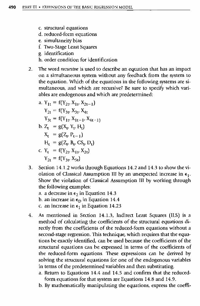
490 PART III • EXTENSIONS OF THE BASIC REGRESSION MODEL
c. structural equations d. reduced-form equations e. simultaneity bias f. Two-Stage Least Squares g. identification h. order condition for identification
2. The word recursive is used to describe an equation that has an impact on a simultaneous system without any feedback from the system to the equation. Which of the equations in the following systems are si-multaneous, and which are recursive? Be sure to specify which vari-ables are endogenous and which are predetermined:
a. `lit = f(Y2 , Xlt , X2t-1)
Yet = f(Y3t, X3t, X4t
Y3t = f(Ylt, Xlt-1f X4t- 1)
b. Zt = g(Xt, Yt, Ht)
Xt — g(Zt , Pt _ 1 )
Ht = g(Zt, Bt, CSt, Dt)
c. Yt = f(Y2t1 X1 , X23
Yet = f(Y3t, X5t)
3. Section 14.1.2 works through Equations 14.2 and 14.3 to show the vi-olation of Classical Assumption III by an unexpected increase in E l . Show the violation of Classical Assumption III by working through the following examples: a. a decrease in E2 in Equation 14.3 b. an increase in ED in Equation 14.4 c. an increase in E 1 in Equation 14.23
4. As mentioned in Section 14.1.3, Indirect Least Squares (ILS) is a method of calculating the coefficients of the structural equations di-rectly from the coefficients of the reduced-form equations without a second-stage regression. This technique, which requires that the equa-tions be exactly identified, can be used because the coefficients of the structural equations can be expressed in terms of the coefficients of the reduced-form equations. These expressions can be derived by solving the structural equations for one of the endogenous va riables in terms of the predetermined variables and then substituting. a. Return to Equations 14.4 and 14.5 and confirm that the reduced-
form equations for that system are Equations 14.8 and 14.9. b. By mathematically manipulating the equations, express the coeffi-
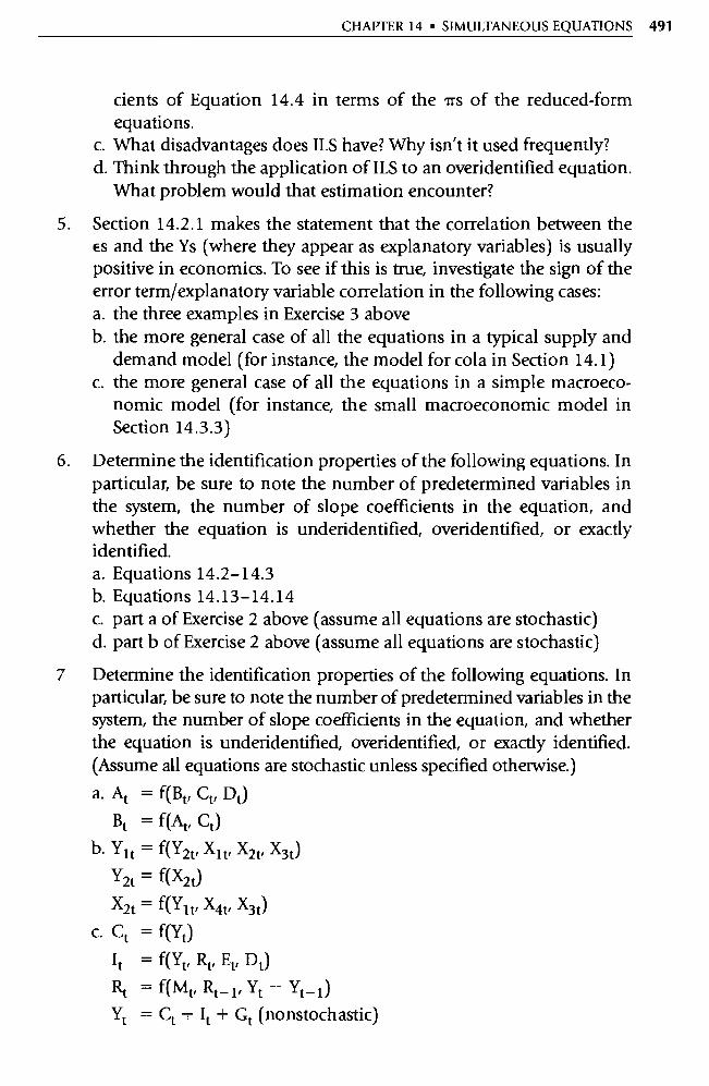
CHAPTER 14 • SIMULTANEOUS EQUATIONS 491
cients of Equation 14.4 in terms of the irs of the reduced-form equations.
c. What disadvantages does ILS have? Why isn't it used frequently? d. Think through the application of ILS to an overidentified equation.
What problem would that estimation encounter?
5. Section 14.2.1 makes the statement that the correlation between the ES and the Ys (where they appear as explanatory variables) is usually positive in economics. To see if this is true, investigate the sign of the error term/explanatory variable correlation in the following cases: a. the three examples in Exercise 3 above b. the more general case of all the equations in a typical supply and
demand model (for instance, the model for cola in Section 14.1) c. the more general case of all the equations in a simple macroeco-
nomic model (for instance, the small macroeconomic model in Section 14.3.3)
6. Determine the identification properties of the following equations. In particular, be sure to note the number of predetermined variables in the system, the number of slope coefficients in the equation, and whether the equation is underidentified, overidentified, or exactly identified. a. Equations 14.2-14.3 b. Equations 14.13- 14.14 c. part a of Exercise 2 above (assume all equations are stochastic) d. part b of Exercise 2 above (assume all equations are stochastic)
7 Determine the identification properties of the following equations. In particular, be sure to note the number of predetermined va riables in the system, the number of slope coefficients in the equation, and whether the equation is underidentified, overidentified, or exactly identified. (Assume all equations are stochastic unless specified otherwise.)
a. At = f(Bt, Ct, Dt) Bt = f(At, Ct)
b. Ylt = f(Y2t, X1 , X2t, X3t)
Y2t = f(X2t)
X2t = f(Y1t/ X4 t, X3t)
C. Ct = f(Yt) It = f(Yt, R , Et, Dt) Rt = f(Mt, Rt-1 , Yt _ Yt- 1)
Yt = Ct + It + Gt (nonstochastic)
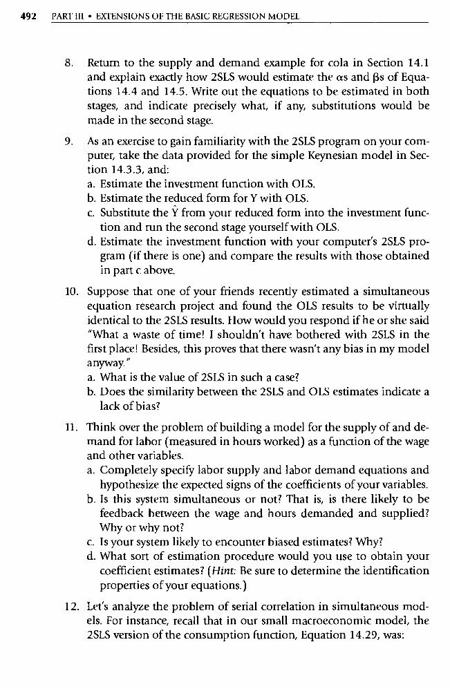
492 PART III • EXTENSIONS OF THE BASIC REGRESSION MODEL
8. Return to the supply and demand example for cola in Section 14.1 and explain exactly how 2SLS would estimate the as and (3s of Equa-tions 14.4 and 14.5. Write out the equations to be estimated in both stages, and indicate precisely what, if any, substitutions would be made in the second stage.
9. As an exercise to gain familiarity with the 2SLS program on your com-puter, take the data provided for the simple Keynesian model in Sec-tion 14.3.3, and: a. Estimate the investment function with OLS. b. Estimate the reduced form for Y with OLS. c. Substitute the Y from your reduced form into the investment func-
tion and run the second stage yourself with OLS. d. Estimate the investment function with your computer's 2SLS pro-
gram (if there is one) and compare the results with those obtained in part c above.
10. Suppose that one of your friends recently estimated a simultaneous equation research project and found the OLS results to be virtually identical to the 2SLS results. How would you respond if he or she said "What a waste of time! I shouldn't have bothered with 2SLS in the first place! Besides, this proves that there wasn't any bias in my model anyway. a. What is the value of 2SLS in such a case? b. Does the similarity between the 2SLS and OLS estimates indicate a
lack of bias?
11. Think over the problem of building a model for the supply of and de-mand for labor (measured in hours worked) as a function of the wage and other variables. a. Completely specify labor supply and labor demand equations and
hypothesize the expected signs of the coefficients of your variables. b. Is this system simultaneous or not? That is, is there likely to be
feedback between the wage and hours demanded and supplied? Why or why not?
c. Is your system likely to encounter biased estimates? Why? d. What sort of estimation procedure would you use to obtain your
coefficient estimates? (Hint: Be sure to determine the identification properties of your equations.)
12. Let's analyze the problem of serial correlation in simultaneous mod-els. For instance, recall that in our small macroeconomic model, the 2SLS version of the consumption function, Equation 14.29, was:
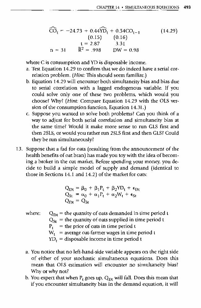
CHAPTER 14 • SIMULTANEOUS EQUATIONS 493
COt = —24.73 + 0.44YDt + 0.54COt _ i
(0.15) (0.16)
t = 2.87 3.31 n = 31 R2 =.998 DW=0.98
(14.29)
where C is consumption and YD is disposable income. a. Test Equation 14.29 to confirm that we do indeed have a serial cor-
relation problem. (Hint: This should seem familiar.) b. Equation 14.29 will encounter both simultaneity bias and bias due
to serial correlation with a lagged endogenous variable. If you could solve only one of these two problems, which would you choose? Why? (Hint: Compare Equation 14.29 with the OLS ver-sion of the consumption function, Equation 14.31.)
c. Suppose you wanted to solve both problems? Can you think of a way to adjust for both serial correlation and simultaneity bias at the same time? Would it make more sense to run GLS first and then 2SLS, or would you rather mn 2SLS first and then GLS? Could they be run simultaneously?
13. Suppose that a fad for oats (resulting from the announcement of the health benefits of oat bran) has made you toy with the idea of becom-ing a broker in the oat market. Before spending your money, you de-cide to build a simple model of supply and demand (identical to those in Sections 14.1 and 14.2) of the market for oats:
QDt = Ro + R1Pt + R2YEit + EDt
Qst = ao + a 1 Pt + a2Wt + ESt QDt = Qst
where: QDt = the quantity of oats demanded in time period t
Qst = the quantity of oats supplied in time period t Pt = the price of oats in time period t Wt = average oat-farmer wages in time period t YDt = disposable income in time period t
a. You notice that no left-hand-side variable appears on the right side of either of your stochastic simultaneous equations. Does this mean that OLS estimation will encounter no simultaneity bias? Why or why not?
b. You expect that when Pt goes up, QDt will fall. Does this mean that if you encounter simultaneity bias in the demand equation, it will
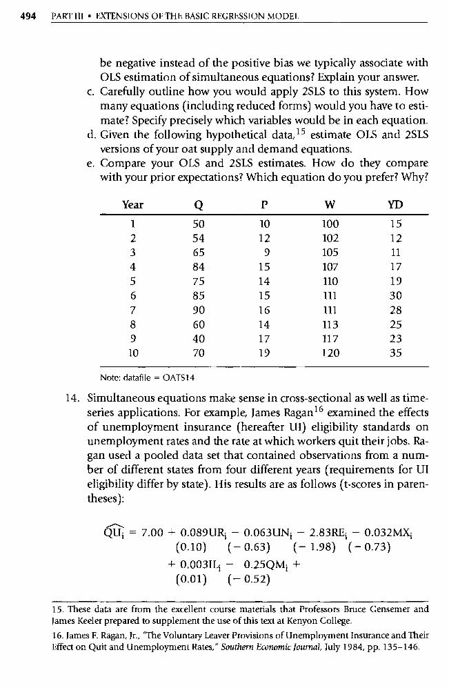
494 PART III ■ EXTENSIONS OF THE BASIC REGRESSION MODEL
be negative instead of the positive bias we typically associate with OLS estimation of simultaneous equations? Explain your answer.
c. Carefully outline how you would apply 2SLS to this system. How many equations (including reduced forms) would you have to esti-mate? Specify precisely which variables would be in each equation.
d. Given the following hypothetical data, 15 estimate OLS and 2SLS versions of your oat supply and demand equations.
e. Compare your OLS and 2SLS estimates. How do they compare with your prior expectations? Which equation do you prefer? Why?
Year Q P W YD
1 50 10 100 15 2 54 12 102 12 3 65 9 105 11 4 84 15 107 17 5 75 14 110 19 6 85 15 111 30 7 90 16 111 28 8 60 14 113 25 9 40 17 117 23 10 70 19 120 35
Note: datafile = OATS14
14. Simultaneous equations make sense in cross-sectional as well as time-series applications. For example, James Ragan 16 examined the effects of unemployment insurance (hereafter UI) eligibility standards on unemployment rates and the rate at which workers quit their jobs. Ra-gan used a pooled data set that contained observations from a num-ber of different states from four different years (requirements for UI eligibility differ by state). His results are as follows (t-scores in paren-theses):
QUi = 7.00 + 0.089URi — 0.063UN i — 2.83REi — 0.032MXi (0.10) (— 0.63) (— 1.98) (— 0.73)
+ 0.003ILi — 0.25QMi + (0.01) (— 0.52)
15. These data are from the excellent course materials that Professors B ruce Gensemer and James Keeler prepared to supplement the use of this text at Kenyon College.
16.James F. Ragan, Jr., "The Voluntary Leaver Provisions of Unemployment Insurance and Their Effect on Quit and Unemployment Rates," Southern Economic Jou rnal, July 1984, pp. 135-146.

CHAPTER 14 • SIMULTANEOUS EQUATIONS 495
UR; = — 0.54 + 0.44QU; + 0.13UN ; + 0.049MX;
(1.01) (3.29) (1.71)
+ 0.56IL; + 0.63QM; +
(2.03) (2.05)
where: QU; = the quit rate (quits per 100 employees) in the ith state
UR; = the unemployment rate in the ith state UN; = union membership as a percentage of nonagricul-
tural employment in the ith state RE; = average hourly earnings in the ith state relative to
the average hourly earnings for the United States IL; = dummy variable equal to 1 if workers in the ith
state are eligible for UI if they are forced to quit a job because of illness, 0 otherwise
QM; = dummy variable equal to 1 if the ith state main-tains full UI benefits for the quitter (rather than lowering benefits), 0 otherwise
MX; = maximum weekly UI benefits relative to average hourly earnings in the ith state
a. Hypothesize the expected signs for the coefficients of each of the explanatory variables in the system. Use economic theory to justify your answers. Which estimated coefficients are different from your expectations?
b. Ragan felt that these two equations would encounter simultaneity bias if they were estimated with OLS. Do you agree? Explain your answer. (Hint: Start by deciding which variables are endogenous and why.)
c. The actual equations included a number of variables not docu-mented above, but the only predetermined variable in the system that was included in the QU equation but not the UR equation was RE. What does this information tell you about the identification properties of the QU equation? The UR equation?
d. What are the implications of the lack of significance of the endoge-nous variables where they appear on the right-hand side of the equations?
e. What, if any, policy recommendations do these results suggest?
15. Return to the consumption function of the small macromodel of Sec-tion 14.3.3 and consider again the issue of cointegration as a possible solution to the problem of nonstationarity.
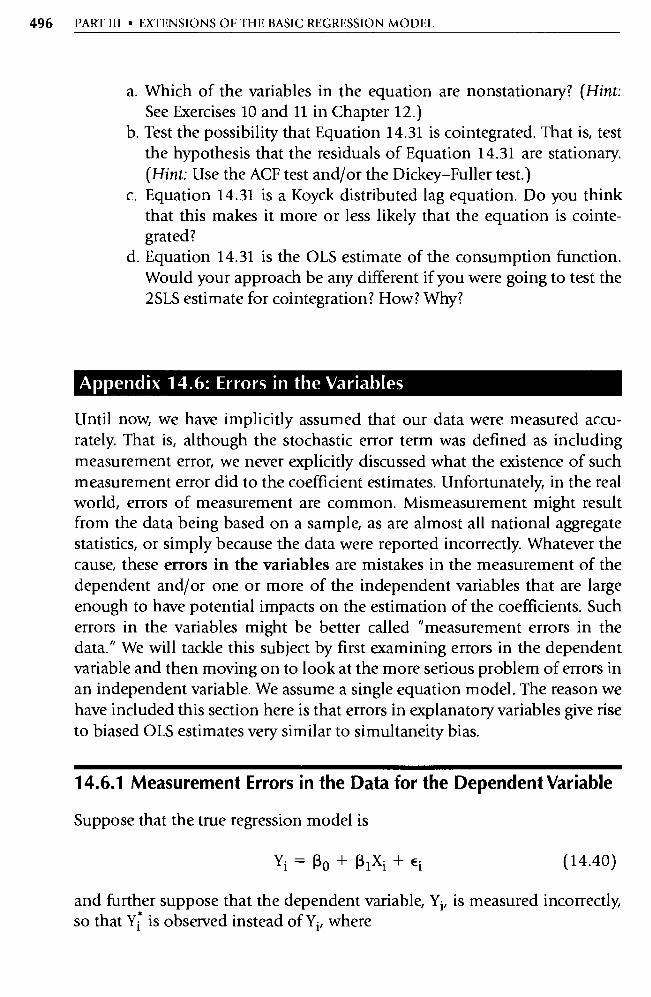
496 PART III • EXTENSIONS OF THE BASIC REGRESSION MODEL
a. Which of the variables in the equation are nonstationary? (Hint: See Exercises 10 and 11 in Chapter 12.)
b. Test the possibility that Equation 14.31 is cointegrated. That is, test the hypothesis that the residuals of Equation 14.31 are stationary. (Hint: Use the ACF test and/or the Dickey-Fuller test.)
c. Equation 14.31 is a Koyck distributed lag equation. Do you think that this makes it more or less likely that the equation is cointe-grated?
d. Equation 14.31 is the OLS estimate of the consumption function. Would your approach be any different if you were going to test the 2SLS estimate for cointegration? How? Why?
Appendix 14.6: Errors in the Variables
Until now, we have implicitly assumed that our data were measured accu-rately. That is, although the stochastic error term was defined as including measurement error, we never explicitly discussed what the existence of such measurement error did to the coefficient estimates. Unfortunately, in the real world, errors of measurement are common. Mismeasurement might result from the data being based on a sample, as are almost all national aggregate statistics, or simply because the data were reported incorrectly. Whatever the cause, these errors in the variables are mistakes in the measurement of the dependent and/or one or more of the independent variables that are large enough to have potential impacts on the estimation of the coefficients. Such errors in the variables might be better called "measurement errors in the data." We will tackle this subject by first examining errors in the dependent variable and then moving on to look at the more serious problem of errors in an independent variable. We assume a single equation model. The reason we have included this section here is that errors in explanatory variables give rise to biased OLS estimates very similar to simultaneity bias.
14.6.1 Measurement Errors in the Data for the Dependent Variable
Suppose that the true regression model is
Yi =RD+l3 1Xi+ e; (14.40)
and further suppose that the dependent va riable, Yi, is measured incorrectly, so that Y; is observed instead of Yi, where
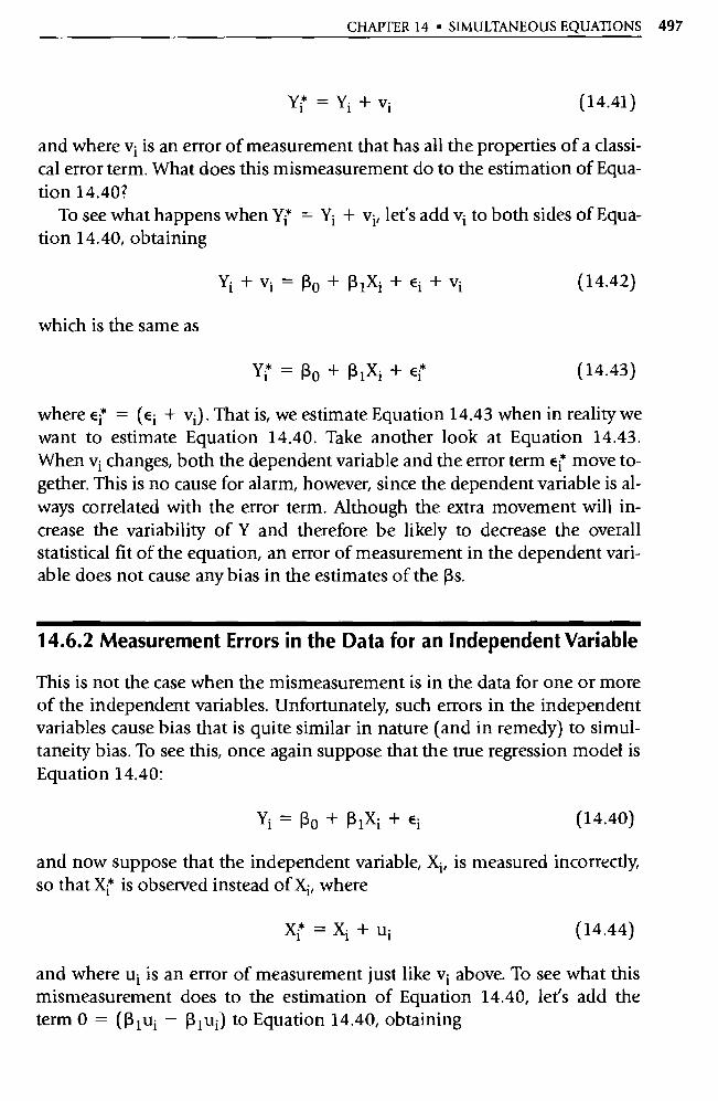
CHAPTER 14 • SIMULTANEOUS EQUATIONS 497
Yi = Yi + vi (14.41)
and where vi is an error of measurement that has all the properties of a classi-cal error term. What does this mismeasurement do to the estimation of Equa-tion 14.40?
To see what happens when Yi = Y i + vi, let's add vi to both sides of Equa-tion 14.40, obtaining
which is the same as
Yi +vi = Ro +R 1 Xi + Ei +vi
Yi*— Ro + R 1Xi + Ei
where Ei = (Ei + vi). That is, we estimate Equation 14.43 when in reality we want to estimate Equation 14.40. Take another look at Equation 14.43. When vi changes, both the dependent variable and the error term Ei move to-gether. This is no cause for alarm, however, since the dependent variable is al-ways correlated with the error term. Although the extra movement will in-crease the variability of Y and therefore be likely to decrease the overall statistical fit of the equation, an error of measurement in the dependent vari-able does not cause any bias in the estimates of the Rs.
14.6.2 Measurement Errors in the Data for an Independent Variable
This is not the case when the mismeasurement is in the data for one or more of the independent variables. Unfortunately, such errors in the independent variables cause bias that is quite similar in nature (and in remedy) to simul-taneity bias. To see this, once again suppose that the true regression model is Equation 14.40:
Yi = Ro + R lxi + Ei (14.40)
and now suppose that the independent variable, X i, is measured incorrectly, so that Xi is observed instead of X i, where
X; =Xi + ui (14.44)
and where u i is an error of measurement just like v i above. To see what this mismeasurement does to the estimation of Equation 14.40, let's add the term 0 = (13 1ui — Rlui) to Equation 14.40, obtaining
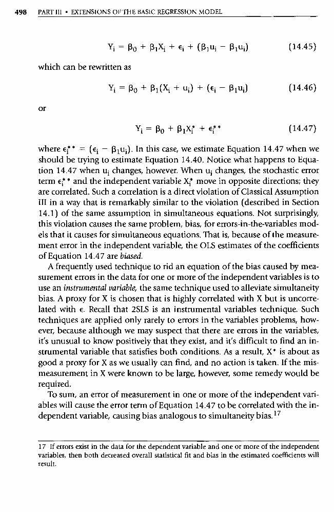
498 PART III • EXTENSIONS OF THE BASIC REGRESSION MODEL
Yi = Ro + R1Xi + Ei (PA - PA)
which can be rewritten as
Yi = Ro + Q 1(Xi + ui) + ( Ei — R lui)
or
Yi= Ro +P1x; + Ei*
(14.45)
(14.46)
(14.47)
where EÎ * = (Ei - 131u0. In this case, we estimate Equation 14.47 when we should be trying to estimate Equation 14.40. Notice what happens to Equa-tion 14.47 when ui changes, however. When u i changes, the stochastic error term Ei * and the independent variable Xi move in opposite directions; they are correlated. Such a correlation is a direct violation of Classical Assumption III in a way that is remarkably similar to the violation (described in Section 14.1) of the same assumption in simultaneous equations. Not surprisingly, this violation causes the same problem, bias, for errors-in-the-variables mod-els that it causes for simultaneous equations. That is, because of the measure-ment error in the independent va riable, the OLS estimates of the coefficients of Equation 14.47 are biased.
A frequently used technique to rid an equation of the bias caused by mea-surement errors in the data for one or more of the independent variables is to use an instrumental variable, the same technique used to alleviate simultaneity bias. A proxy for X is chosen that is highly correlated with X but is uncorre-lated with E. Recall that 2SLS is an instrumental variables technique. Such techniques are applied only rarely to errors in the va riables problems, how-ever, because although we may suspect that there are errors in the variables, it's unusual to know positively that they exist, and it's difficult to find an in-strumental variable that satisfies both conditions. As a result, X* is about as good a proxy for X as we usually can find, and no action is taken. If the mis-measurement in X were known to be large, however, some remedy would be required.
To sum, an error of measurement in one or more of the independent vari-ables will cause the error term of Equation 14.47 to be correlated with the in-dependent variable, causing bias analogous to simultaneity bias. 17
17 If errors exist in the data for the dependent variable and one or more of the independent variables, then both decreased overall statistical fit and bias in the estimated coefficients will result.
1' Forecasting
15.1 What Is Forecasting?
15.2 More Complex Forecasting Problems
15.3 ARIMA Models
15.4 Summary and Exercises
Of the uses of econometrics outlined in Chapter 1, we have discussed fore-casting the least. Accurate forecasting is vital to successful planning, so it's the primary goal of many business and governmental uses of econometrics. For example, manufacturing firms need sales forecasts, banks need interest rate forecasts, and governments need unemployment and inflation rate forecasts.
To many business and government leaders, the words econometrics and forecasting mean the same thing. Such a simplification gives econometrics a bad name because some consulting econometricians overestimate their abil-ity to produce accurate forecasts, resulting in unrealistic claims and unhappy clients. Some of their clients would probably applaud the nineteenth century New York law (luckily unenforced but apparently also unrepealed) that pro-vides that persons "pretending to forecast the future" shall be liable to a $250 fine and/or six months in prison. 1 Although many econometricians might wish that such consultants would call themselves "futurists" or "soothsayers," it's impossible to ignore the importance of econometrics in forecasting in to-day's world.
The ways in which the prediction of future events is accomplished are quite varied. At one extreme, some forecasters use models with hundreds of equations. 2 At the other extreme, quite accurate forecasts can be created with nothing more than a good imagination and a healthy dose of self-confidence.
1. Section 899 of the N.Y. State Criminal Code: the law does not apply to "ecclesiastical bodies acting in good faith and without personal fees.
2. For an interesting comparison of such models, see Ray C. Fair and Robe rt J. Shiller, "Com-paring Information in Forecasts from Econometric Models, American Economic Review, June 1990, pp. 375-389.
CHAPTER
499
500 PART III • EXTENSIONS OF THE BASIC REGRESSION MODEL
Unfortunately, it's unrealistic to think we can cover even a small po rtion of the topic of forecasting in one short chapter. Indeed, there are a number of excellent books and journals on this subject alone. 3 Instead, this chapter is meant to be a brief introduction to the use of econometrics in forecasting. We will begin by using simple linear equations and then move on to investi-gate a few more complex forecasting situations. The chapter concludes with an introduction to a technique, called ARIMA, that calculates forecasts en-tirely from past movements of the dependent variable without the use of any independent variables at all.
15.1 What Is Forecasting?
In general, forecasting is the act of predicting the future; in econometrics, forecasting is the estimation of the expected value of a dependent variable for observations that are not pa rt of the same data set. In most forecasts, the values being predicted are for time periods in the future, but cross-sectional predictions of values for countries or people not in the sample are also com-mon. To simplify terminology, the words prediction and forecast will be used interchangeably in this chapter. (Some authors limit the use of the word fore-cast to out-of-sample prediction for a time series.)
We've already encountered an example of a forecasting equation. Think back to the weight/height example of Section 1.3 and recall that the purpose of that model was to guess the weight of a male customer based on his height. In that example, the first step in building a forecast was to estimate Equation 1.21:
Estimated weighti = 103.4 + 6.38 • Height i (inches over five feet) (1.21)
That is, we estimated that a customer's weight on average equaled a base of 103.4 pounds plus 6.38 pounds for each inch over 5 feet. To actually make the prediction, all we had to do was to substitute the height of the individual whose weight we were trying to predict into the estimated equation. For a male who is 6'1" tall, for example, we'd calculate:
3. See, for example, C. W. J. Granger, Forecasting in Business and Economics (New York: Academic Press, 1980), the Journal of Business Forecasting, Elia Kacapvr, Economic Forecasting: The State of the Art (Armonk: M. E. Sharpe, 1996), and Francis X. Diebold, Elements of Forecasting (Cin-cinati: South Western, 2001).
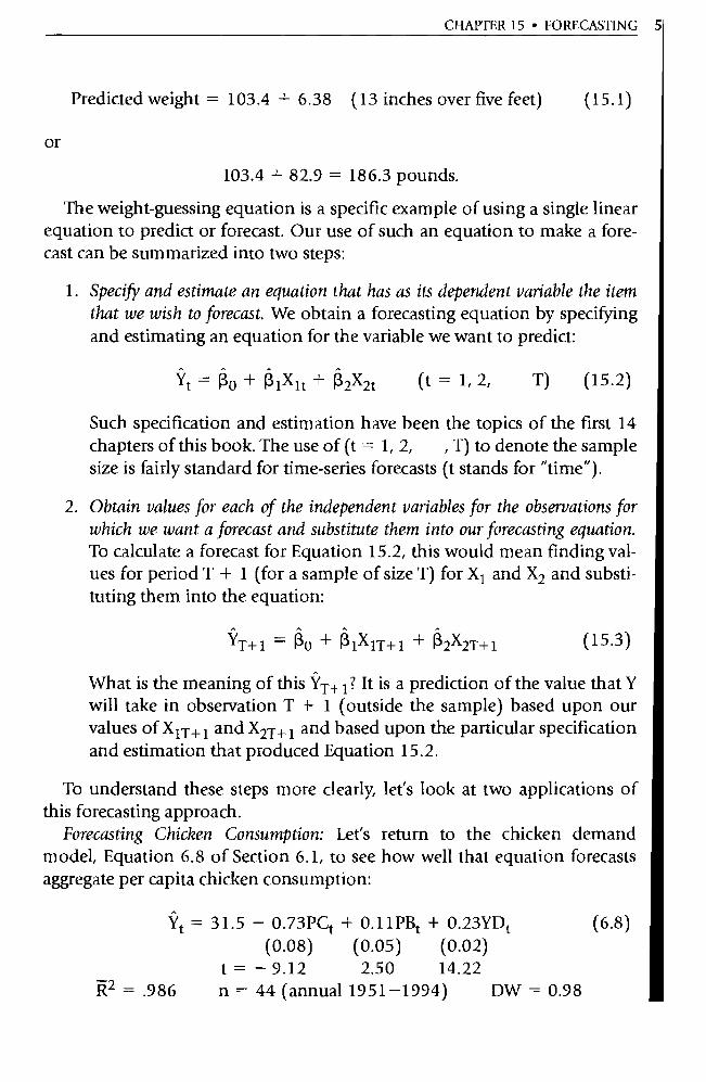
CHAPTER 15 • FORECASTING 5
Predicted weight = 103.4 + 6.38 (13 inches over five feet) (15.1)
or
103.4 + 82.9 = 186.3 pounds.
The weight-guessing equation is a specific example of using a single linear equation to predict or forecast. Our use of such an equation to make a fore-cast can be summarized into two steps:
1. Specify and estimate an equation that has as its dependent variable the item that we wish to forecast. We obtain a forecasting equation by specifying and estimating an equation for the variable we want to predict:
Yt=Oo+O1Xlt+ 02X2t (t = 1,2, T) (15.2)
Such specification and estimation have been the topics of the first 14 chapters of this book. The use of (t = 1, 2, , T) to denote the sample size is fairly standard for time-series forecasts (t stands for "time").
2. Obtain values for each of the independent variables for the observations for which we want a forecast and substitute them into our forecasting equation. To calculate a forecast for Equation 15.2, this would mean finding val-ues for period T + 1 (for a sample of size T) for X 1 and X2 and substi-tuting them into the equation:
YT+1 = PO + O1XlT+1 + 02X2T+1 (15.3)
What is the meaning of this YT+ 1? It is a prediction of the value that Y will take in observation T + 1 (outside the sample) based upon our values of X1T+1 and X2T+1 and based upon the particular specification and estimation that produced Equation 15.2.
To understand these steps more clearly, let's look at two applications of this forecasting approach.
Forecasting Chicken Consumption: Let's return to the chicken demand model, Equation 6.8 of Section 6.1, to see how well that equation forecasts aggregate per capita chicken consumption:
Yt = 31.5 — 0.73PCt + 0.11PBt + 0.23YDt (6.8) (0.08) (0.05) (0.02)
t = — 9.12 2.50 14.22 17Z2 = .986 n = 44 (annual 1951-1994) DW = 0.98
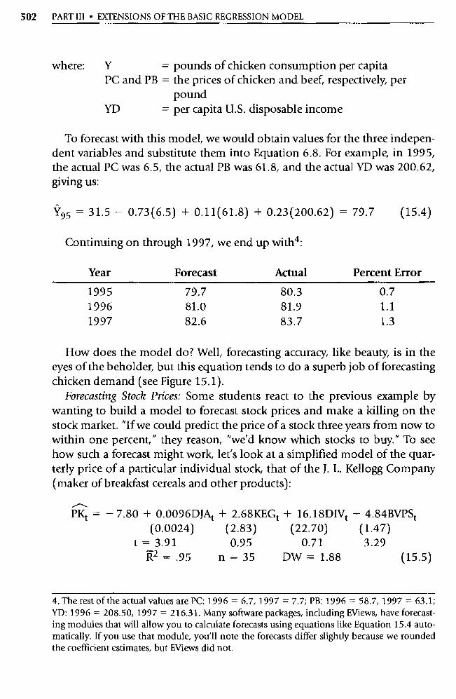
502 PART III • EXTENSIONS OF THE BASIC REGRESSION MODEL
where: Y = pounds of chicken consumption per capita PC and PB = the prices of chicken and beef, respectively, per
pound YD = per capita U.S. disposable income
To forecast with this model, we would obtain values for the three indepen-dent variables and substitute them into Equation 6.8. For example, in 1995, the actual PC was 6.5, the actual PB was 61.8, and the actual YD was 200.62, giving us:
jr‘ 95 = 31.5 — 0.73(6.5) + 0.11(61.8) + 0.23(200.62) = 79.7 (15.4)
Continuing on through 1997, we end up with 4 :
Year Forecast Actual Percent Error
1995 79.7 80.3 0.7 1996 81.0 81.9 1.1 1997 82.6 83.7 1.3
How does the model do? Well, forecasting accuracy, like beauty, is in the eyes of the beholder, but this equation tends to do a superb job of forecasting chicken demand (see Figure 15.1).
Forecasting Stock Prices: Some students react to the previous example by wanting to build a model to forecast stock prices and make a killing on the stock market. "If we could predict the price of a stock three years from now to within one percent," they reason, "we'd know which stocks to buy." To see how such a forecast might work, let's look at a simplified model of the quar-terly price of a particular individual stock, that of the J. L. Kellogg Company (maker of breakfast cereals and other products):
PKt = — 7.80 + 0.0096DJAt + 2.68KECt + 1 6.18DIVt + 4.84BVPS t (0.0024) (2.83) (22.70) (1.47)
t = 3.91 0.95 0.71 3.29 R2 = .95 n = 35 DW = 1.88 (15.5)
4. The rest of the actual values are PC: 1996 = 6.7, 1997 = 7.7; PB: 1996 = 58.7, 1997 = 63.1; YD: 1996 = 208.50, 1997 = 216.31. Many software packages, including EViews, have forecast-ing modules that will allow you to calculate forecasts using equations like Equation 15.4 auto-matically. If you use that module, you'll note the forecasts differ slightly because we rounded the coefficient estimates, but EViews did not.
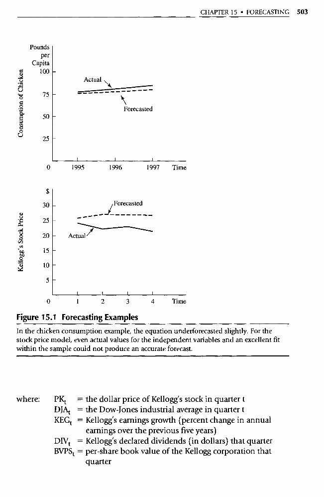
CHAPTER 15 • FORECASTING 503
per Capita
100
75
Actual
Forecasted 50
25
0 1995 1996 1997 Time
30 Forecasted
25
20 Actual
15
10
5
I I I I
0 1 2 3 4 Time
Figure 15.1 Forecasting Examples
Con
sum
ptio
n of
Chi
cken
K
ello
gg's
Sto
ck Pr
ice
In the chicken consumption example, the equation underforecasted slightly. For the stock price model, even actual values for the independent va riables and an excellent fit within the sample could not produce an accurate forecast.
where: PKt = the dollar price of Kellogg's stock in qua rter t DJAt = the Dow-Jones industrial average in qua rter t KEGt = Kellogg's earnings growth (percent change in annual
earnings over the previous five years) DIVt = Kellogg's declared dividends (in dollars) that qua rter BVPSt = per-share book value of the Kellogg corporation that
quarter
504 PART III • EXTENSIONS OF THE BASIC REGRESSION MODEL
The signs of the estimated coefficients all agree with those hypothesized before the regression was run, R 2 indicates a good overall fit, and the Durbin-Watson d statistic indicates that the hypothesis of no positive serial correlation cannot be rejected. The low t-scores for KEG and DIV are caused by multicollinearity (r = .985), but both variables are left in the equation be-cause of their theoretical impo rtance. Note also that most of the variables in the equation are nonstationary, surely causing some of the good fit.
To forecast with Equation 15.5, we collected actual values for all of the in-dependent variables for the next four quarters and substituted them into the right side of the equation, obtaining:
Quarter Foreast Actual Percent Error
1 $26.32 $24.38 8.0 2 27.37 22.38 22.3 3 27.19 23.00 18.2 4 27.13 21.88 24.0
How did our forecasting model do? Even though the R 2 within the sam-ple was .95, even though we used actual values for the independent vari-ables, and even thought we forecasted only four quarters beyond our sam-ple, the model was something like 20 percent off. If we had decided to buy Kellogg's stock based on our forecast, we'd have lost money! Since other at-tempts to forecast stock prices have also encountered difficulties, this doesn't seem a reasonable use for econometric forecasting. Individual stock prices (and many other items) are simply too variable and depend on too many nonquantifiable items to consistently forecast accurately, even if the fore-casting equation has an excellent fit! The reason for this apparent contradic-tion is that equations that worked in the past may or may not work well in the future.
15.2 More Complex Forecasting Problems
The forecasts generated above are unrealistically simple, however, and most actual forecasting involves one or more additional questions. For example:
1. Unknown Xs: It's unrealistic to expect always to know the values for the independent variables outside the sample. For instance, we'll almost never know what the Dow-Jones industrial average will be in the fu-ture when we are making forecasts of the price of a given stock, and yet we assumed that knowledge when making our Kellogg price forecasts.
CHAPTER 15 • FORECASTING 50
What happens when we don't know the values of the independent variables for the forecast period?
2. Serial Correlation: If there is serial correlation involved, the forecasting equation may be estimated with GLS. How should predictions be ad-justed when forecasting equations are estimated with GLS?
3. Confidence Intervals: All the forecasts above were single values, but such single values are almost never exactly right. Wouldn't it be more help-ful if we forecasted an interval within which we were confident that the actual value would fall a certain percentage of the time? How can we develop these confidence intervals?
4. Simultaneous Equations Models: As we saw in Chapter 14, many eco-nomic and business equations are pa rt of simultaneous models. How can we use an independent variable to forecast a dependent variable when we know that a change in value of the dependent variable will change, in turn, the value of the independent variable that we used to make the forecast?
Even a few questions like these should be enough to convince you that fore-casting involves issues that are more complex than implied by Section 15.1.
15.2.1 Conditional Forecasting (Unknown X Values for the Forecast Period)
A forecast in which all values of the independent variables are known with certainty can be called an unconditional forecast, but, as mentioned above, the situations in which one can make such unconditional forecasts are rare. More likely, we will have to make a conditional forecast, for which actual values of one or more of the independent variables are not known. We are forced to obtain forecasts for the independent variables before we can use our equation to forecast the dependent variable, making our forecast of Y conditional on our forecast of the Xs.
One key to an accurate conditional forecast is accurate forecasting of the independent variables. If the forecasts of the independent variables are unbi-ased, using a conditional forecast will not introduce bias into the forecast of the dependent variable. Anything but a perfect forecast of the independent variables will contain some amount of forecast error, however, and so the ex-pected error va riance associated with conditional forecasting typically will be larger than that associated with unconditional forecasting. Thus, one should try to find unbiased, minimum variance forecasts of the independent vari-ables when using conditional forecasting.
506 PART III • EXTENSIONS OF THE BASIC REGRESSION MODEL
To get good forecasts of the independent va riables, take the forecastability of potential independent va riables into consideration when making specifi-cation choices. For instance, when you choose which of two redundant vari-ables to include in ân equation to be used for forecasting, you should choose the one that is easier to forecast accurately. When you can, you should choose an independent variable that is regularly forecasted by someone else (an econometric forecasting firm, for example) so that you don't have to forecast X yourself.
The careful selection of independent variables can sometimes help you avoid the need for conditional forecasting in the first place. This opportunity can arise when the dependent variable can be expressed as a function of lead-ing indicators. A leading indicator is an independent variable the move-ments of which anticipate movements in the dependent variable. The best known leading indicator, the Index of Leading Economic Indicators, is pro-duced each month.
For instance, the impact of interest rates on investment typically is not felt until two or three quarters after interest rates have changed. To see this, let's look at the investment function of the small macroeconomic model of Sec-tion 14.3.3:
It=Po +P1Yt+R2rt -1+ Et (15.6)
where I equals gross investment, Y equals GDP, and r equals the interest rate. In this equation, actual values of r can be used to help forecast IT+ 1 . Note, however, that to predict I T+2, we need to forecast r. Thus, leading indicators like r help avoid conditional forecasting for only a time period or two. For long-range predictions, a conditional forecast is usually necessary.
15.2.2 Forecasting with Serially Correlated Error Terms
Recall from Chapter 9 that pure first-order serial correlation implies that the current observation of the error term e t is affected by the previous error term and an autocorrelation coefficient, p:
et = Pet- 1 + Ut
where ut is a non-serially-correlated error term. Also recall that when serial correlation is severe, one remedy is to run Generalized Least Squares (GLS) as noted in Equation 9.18:
Yt - PYt-I = 13 o( 1 - P) + PI(Xt - PXt-1) + ut (9.18)
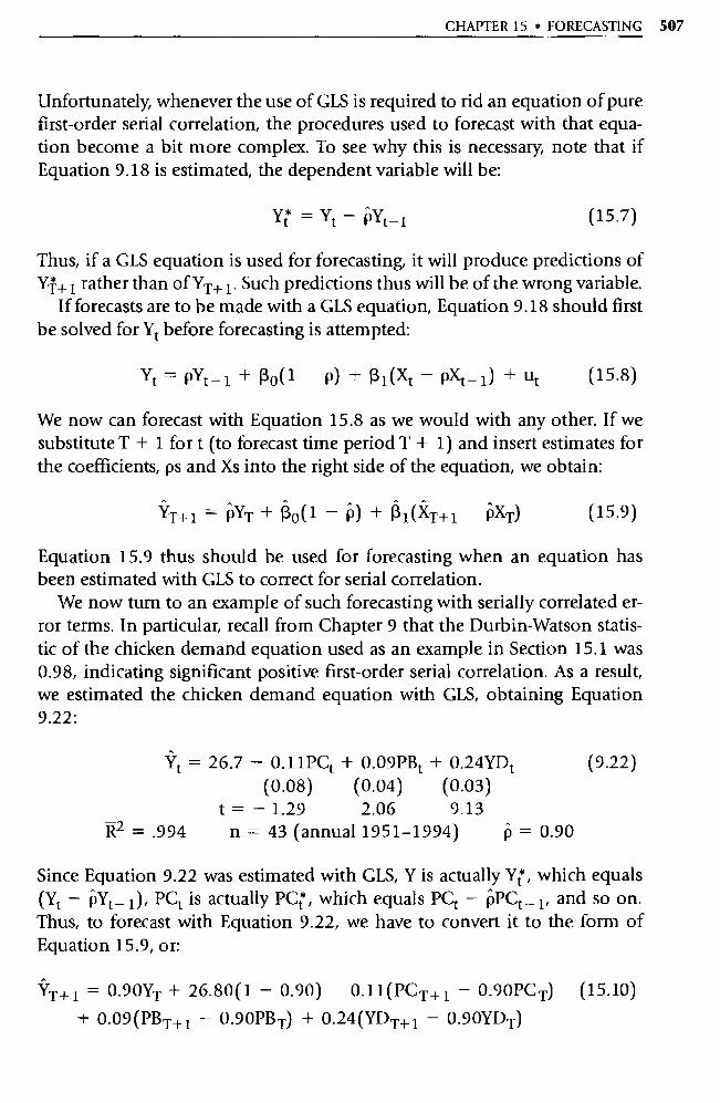
CHAPTER 15 • FORECASTING 507
Unfortunately, whenever the use of GLS is required to rid an equation of pure first-order serial correlation, the procedures used to forecast with that equa-tion become a bit more complex. To see why this is necessary, note that if Equation 9.18 is estimated, the dependent variable will be:
Yt = Yt - PYt-1 (15.7)
Thus, if a GLS equation is used for forecasting, it will produce predictions of YT+ i rather than of YT+ 1. Such predictions thus will be of the wrong variable.
If forecasts are to be made with a GLS equation, Equation 9.18 should first be solved for Yt before forecasting is attempted:
Yt - PYt -1+ 130( 1 P) +R1(Xt - PXt-1) +ut (15.8)
We now can forecast with Equation 15.8 as we would with any other. If we substitute T + 1 for t (to forecast time period T + 1) and inse rt estimates for the coefficients, ps and Xs into the right side of the equation, we obtain:
'1'/T+ PXT) (15.9)
Equation 15.9 thus should be used for forecasting when an equation has been estimated with GLS to correct for serial correlation.
We now turn to an example of such forecasting with serially correlated er-ror terms. In pa rticular, recall from Chapter 9 that the Durbin-Watson statis-tic of the chicken demand equation used as an example in Section 15.1 was 0.98, indicating significant positive first-order serial correlation. As a result, we estimated the chicken demand equation with GLS, obtaining Equation 9.22:
Yt = 26.7 - 0.11PCt + 0.09PBt + 0.24YDt
(0.08) (0.04) (0.03)
t = - 1.29 2.06 9.13 R2 = .994 n = 43 (annual 1951-1994) p = 0.90
(9.22)
Since Equation 9.22 was estimated with GLS, Y is actually Y t*, which equals (Yt - pYt - 1 ), PCt is actually PCt , which equals PCt - pPCt _ 1 , and so on. Thus, to forecast with Equation 9.22, we have to convert it to the form of Equation 15.9, or:
YT+ 1 = 0.90YT + 26.80(1 - 0.90) 0.11(PCT+ 1 - 0.90PC T) (15.10)
+ 0.09(PB T+1 - 0.90PB T) + 0.24(YDT+1 - 0.90YDT)

508 PART III • EXTENSIONS OF THE BASIC REGRESSION MODEL
Substituting the actual values for the independent variables into Equation 15.10, we obtain:
Year Forecast Actual Percent Error
1995 81.9 80.3 2.0 1996 81.8 81.9 0.1 1997 84.0 83.7 0.4
Compare this forecast to that of Equation 15.4. Note that taking serial cor-relation into consideration has improved the forecast dramatically in two of the three years. Indeed, GLS often will provide superior forecasting perfor-mances to OLS in the presence of serial correlation.
Whether to use GLS is not the topic of this section, however. Instead the point is that if GLS is used to estimate the coefficients of an equation, then Equation 15.9 must be used to forecast with the GLS estimates.
15.2.3 Forecasting Confidence Intervals
Until now, the emphasis in this text has been on obtaining point (or single value) estimates. This has been true whether we have been estimating coeffi-cient values or estimating forecasts. Recall, though, that a point estimate is only one of a whole range of such estimates that could have been obtained from different samples (for coefficient estimates) or different independent variable values or coefficients (for forecasts). The usefulness of such point es-timates is improved if we can also generate some idea of the variability of our forecasts. The measure of variability typically used is the confidence interval, which was defined in Section 5.2.4 as the range of values within which the actual value of the item being estimated is likely to fall some percentage of the time (called the level of confidence). This is the easiest way to warn fore-cast users that a sampling distribution exists.
Suppose you are trying to decide how many hot dogs to order for your city's July Fourth fireworks show and that the best point forecast is that you'll sell 24,000 hot dogs. How many hot dogs should you order? If you order 24,000, you're likely to run out about half the time! This is because a point forecast is usually the mean of the distribution of possible sales figures; you will sell more than 24,000 about as frequently as less than 24,000. It would be easier to decide how many dogs to order if you also had a confidence in-terval that told you the range within which hot dog sales would fall 95 per-cent of the time. This is because the usefulness of the 24,000 hot dog forecast changes dramatically depending on the confidence inte rval; an interval of

CHAPTER 15 • FORECASTING 509
22,000 to 26,000 would pin down the likely sales, but an interval of 4,000 to
44,000 would leave you virtually in the dark about what to do. 5 The same techniques we use to test hypotheses can also be adapted to cre-
ate confidence intervals. Given a point forecast, YT+ 1, all we need to generate
a confidence interval around that forecast are t c, the critical t-value (for the
desired level of confidence), and SF, the estimated standard error of the fore-cast:
or, equivalently,
Confidence interval YT+ 1 ± SFtc
YT+ 1 — SFtc 5- YT + 1 T + 1 + SFtc
The critical t-value, t c, can be found in Statistical Table B-1 (for a two-tailed
test with T — K — 1 degrees of freedom). The standard error of the forecast,
SF, for an equation with just one independent variable, equals the square
root of the forecast error variance:
SF— y02/ T _
1 + 1 /T + (XT +1 —
pct — X)2 t=1
(15.13)
where s2
= the estimated variance of the error term
T = the number of obse rvations in the sample XT+ 1 = the forecasted value of the single independent variable
= the arithmetic mean of the observed Xs in the sample. 6
Note that Equation 15.13 implies that the forecast error variance decreases the larger the sample, the more X varies within the sample, and the closer X is
5.The decision as to how many hot dogs to order would also depend on the costs of having the
wrong number. These may not be the same per hot dog for overestimates as they are for under-estimates. For example, if you don't order enough, then you lose the entire retail price of the
hot dog minus the wholesale price of the dog (and bun) because your other costs, like hiring
employees and building hot dog stands, are essentially fixed. On the other hand, if you order
too many, you lose the wholesale cost of the dog and bun minus whatever salvage price you
might be able to get for day-old buns, etc. As a result, the right number to order would depend
on your profit margin and the impo rtance of nonreturnable inputs in your total cost picture.
6. Equation 15.13 is valid whether Yt is in the sample period or outside the sample period, but
it applies only to point forecasts of individual Y ts. If a confidence interval for the expected value of Y, E(Yt), is desired, then the
ccorrect equation to use is:
V SF = s2[1 /T + (XT+I — X) 2 /E(Xt — )02]

510 PART III • EXTENSIONS OF THE BASIC REGRESSION MODEL
0 X XT + 1
Figure 15.2 A Confidence Interval for ŸT+1
A 95 percent confidence interval for ŸT+ 1 includes the range of values within which the actual YT+ 1 will fall 95 percent of the time. Note that the confidence interval widens as XT+ 1 differs more from its within-sample mean, X.
to its within-sample mean. An impo rtant implication is that the farther the X used to forecast Y is from the within-sample mean of the Xs, the wider the confidence interval around the Y is going to be. This can be seen in Figure 15.2, in which the confidence interval actually gets wider as XT+ 1 is farther from X. Since forecasting outside the sample range is common, researchers should be aware of this phenomenon. Also note that Equation 15.13 is for unconditional forecasting. If there is any forecast error in XT+ 1, then the con-fidence interval is larger and more complicated to calculate.
As mentioned above, Equation 15.13 assumes that there is only one inde-pendent variable; the equation to be used with more than one variable is similar but more complicated. Some researchers who must deal with more than one independent variable avoid this complexity by ignoring Equation 15.13 and estimating a confidence interval equal to YT+ 1 ± Sty, where s is the standard error of the equation. Compare this shortcut with Equation 15.13; note that the shortcut confidence interval will work well for large sam-ples and Xs near the within-sample means but will provide only a rough esti-mate of the confidence interval in other cases. At a minimum in such cases,
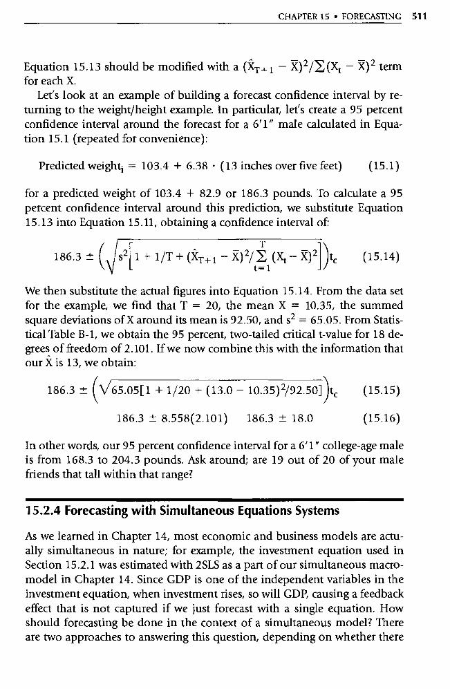
CHAPTER 15 • FORECASTING 511
Equation 15.13 should be modified with a (XT+ 1 — X) 2/I (Xt — X) 2 term for each X.
Let's look at an example of building a forecast confidence interval by re-turning to the weight/height example. In particular, let's create a 95 percent confidence interval around the forecast for a 6'1" male calculated in Equa-tion 15.1 (repeated for convenience):
Predicted weight ; = 103.4 + 6.38. (13 inches over five feet) (15.1)
for a predicted weight of 103.4 + 82.9 or 186.3 pounds. To calculate a 95 percent confidence interval around this prediction, we substitute Equation 15.13 into Equation 15.11, obtaining a confidence interval of:
186.3 ± ( T
1 + 1/T + (XT+1 — )0 2/ E pct — X) 2 tc (15.14) t= 1
We then substitute the actual figures into Equation 15.14. From the data set for the example, we find that T = 20, the mean X = 10.35, the summed square deviations of X around its mean is 92.50, and s 2 = 65.05. From Statis-tical Table B-1, we obtain the 95 percent, two-tailed critical t-value for 18 de-grees of freedom of 2.101. If we now combine this with the information that our X is 13, we obtain:
186.3 ± (V65.o5[1 + 1/20 + (13.0 — 10.35) 2/92.50] tc (15.15)
186.3 ± 8.558(2.101) 186.3 ± 18.0 (15.16)
In other words, our 95 percent confidence interval for a 6'1" college-age male is from 168.3 to 204.3 pounds. Ask around; are 19 out of 20 of your male friends that tall within that range?
15.2.4 Forecasting with Simultaneous Equations Systems
As we learned in Chapter 14, most economic and business models are actu-ally simultaneous in nature; for example, the investment equation used in Section 15.2.1 was estimated with 2SLS as a pa rt of our simultaneous macro-model in Chapter 14. Since GDP is one of the independent variables in the investment equation, when investment rises, so will GDP, causing a feedback effect that is not captured if we just forecast with a single equation. How should forecasting be done in the context of a simultaneous model? There are two approaches to answering this question, depending on whether there
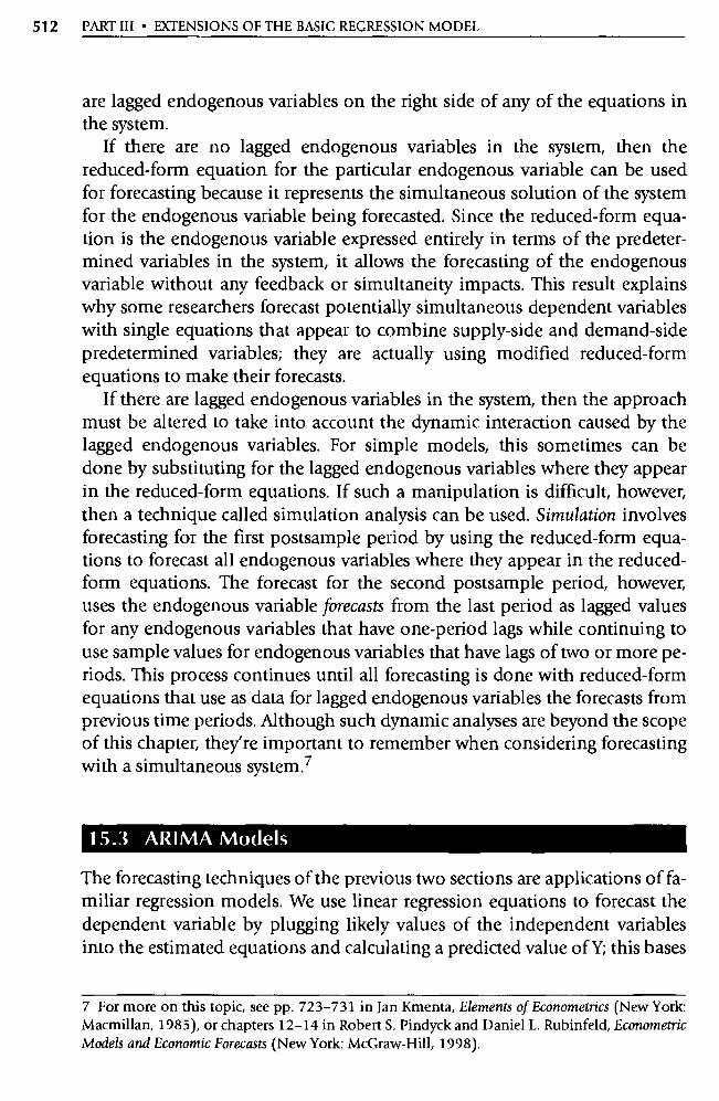
512 PART III • EXTENSIONS OF THE BASIC REGRESSION MODEL
are lagged endogenous variables on the right side of any of the equations in the system.
If there are no lagged endogenous variables in the system, then the reduced-form equation for the particular endogenous variable can be used for forecasting because it represents the simultaneous solution of the system for the endogenous variable being forecasted. Since the reduced-form equa-tion is the endogenous va riable expressed entirely in terms of the predeter-mined variables in the system, it allows the forecasting of the endogenous variable without any feedback or simultaneity impacts. This result explains why some researchers forecast potentially simultaneous dependent variables with single equations that appear to combine supply-side and demand-side predetermined variables; they are actually using modified reduced-form equations to make their forecasts.
If there are lagged endogenous va riables in the system, then the approach must be altered to take into account the dynamic interaction caused by the lagged endogenous variables. For simple models, this sometimes can be done by substituting for the lagged endogenous va riables where they appear in the reduced-form equations. If such a manipulation is difficult, however, then a technique called simulation analysis can be used. Simulation involves forecasting for the first postsample period by using the reduced-form equa-tions to forecast all endogenous va riables where they appear in the reduced-form equations. The forecast for the second postsample period, however, uses the endogenous variable forecasts from the last period as lagged values for any endogenous va riables that have one-period lags while continuing to use sample values for endogenous va riables that have lags of two or more pe-riods. This process continues until all forecasting is done with reduced-form equations that use as data for lagged endogenous variables the forecasts from previous time periods. Although such dynamic analyses are beyond the scope of this chapter, they're impo rtant to remember when considering forecasting with a simultaneous system. 7
15.3 ARIMA Models
The forecasting techniques of the previous two sections are applications of fa-miliar regression models. We use linear regression equations to forecast the dependent variable by plugging likely values of the independent variables into the estimated equations and calculating a predicted value of Y; this bases
7 For more on this topic, see pp. 723-731 in Jan Kmenta, Elements of Econometrics (New York: Macmillan, 1985), or chapters 12-14 in Robe rt S. Pindyck and Daniel L. Rubinfeld, Econometric Models and Economic Forecasts (New York: McGraw-Hill, 1998).
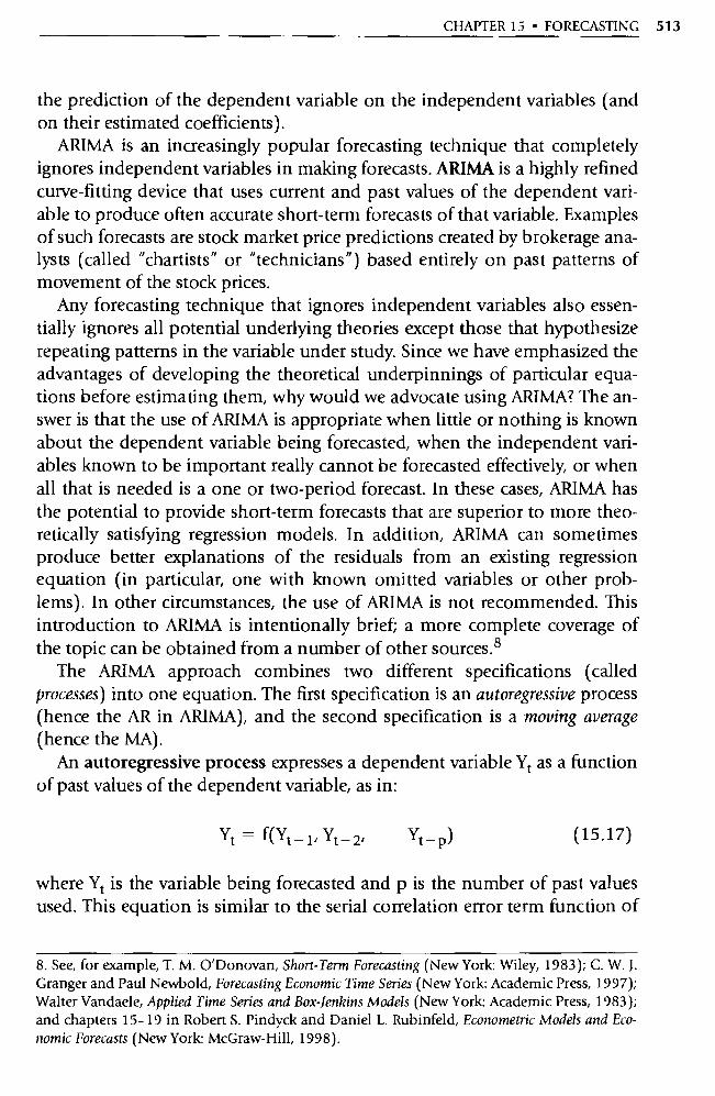
CHAPTER 15 • FORECASTING 513
the prediction of the dependent variable on the independent variables (and on their estimated coefficients).
ARIMA is an increasingly popular forecasting technique that completely ignores independent variables in making forecasts. ARIMA is a highly refined curve-fitting device that uses current and past values of the dependent vari-able to produce often accurate short-term forecasts of that variable. Examples of such forecasts are stock market price predictions created by brokerage ana-lysts (called "chartists" or "technicians") based entirely on past patterns of movement of the stock prices.
Any forecasting technique that ignores independent variables also essen-tially ignores all potential underlying theories except those that hypothesize repeating patterns in the variable under study. Since we have emphasized the advantages of developing the theoretical underpinnings of particular equa-tions before estimating them, why would we advocate using ARIMA? The an-swer is that the use of ARIMA is appropriate when little or nothing is known about the dependent variable being forecasted, when the independent vari-ables known to be impo rtant really cannot be forecasted effectively, or when all that is needed is a one or two-period forecast. In these cases, ARIMA has the potential to provide short-term forecasts that are superior to more theo-retically satisfying regression models. In addition, ARIMA can sometimes produce better explanations of the residuals from an existing regression equation (in particular, one with known omitted variables or other prob-lems). In other circumstances, the use of ARIMA is not recommended. This introduction to ARIMA is intentionally brief; a more complete coverage of the topic can be obtained from a number of other sources. 8
The ARIMA approach combines two different specifications (called processes) into one equation. The first specification is an autoregressive process (hence the AR in ARIMA), and the second specification is a moving average (hence the MA).
An autoregressive process expresses a dependent variable Y t as a function of past values of the dependent variable, as in:
Yt = f(Yt— Yt - 2 , Yt —p ) (1 5. 17 )
where Yt is the variable being forecasted and p is the number of past values used. This equation is similar to the serial correlation error term function of
8. See, for example, T. M. O'Donovan, Short-Term Forecasting (New York: Wiley, 1983); C. W. J. Granger and Paul Newbold, Forecasting Economic Time Series (New York: Academic Press, 1997); Walter Vandaele, Applied Time Series and Box-Jenkins Models (New York: Academic Press, 1983); and chapters 15-19 in Robe rt S. Pindyck and Daniel L. Rubinfeld, Econometric Models and Eco-nomic Forecasts (New York: McGraw-Hill, 1998).
514 PART III • EXTENSIONS OF THE BASIC REGRESSION MODEL
Chapter 9 and to the distributed lag equation of Chapter 12. Since there are p different lagged values of Y in this equation, it is often referred to as a "pth-order" autoregressive process.
A moving-average process expresses a dependent variable Y t as a function of past values of the error term, as in:
Yt f(et-11 Et- 2/ , et—q) (15.18)
where Et is the error term associated with Yt and q is the number of past val-ues of the error term used. Such a function is a moving average of past error terms that can be added to the mean of Y to obtain a moving average of past values of Y. Such an equation would be a qth-order moving-average process.
To create an ARIMA model, we begin with an econometric equation with no independent variables (Y t = Ro + Et) and add to it both the autoregres-sive and moving-average processes:
autoregressive process
Yt = Ro + elYt-1 + e2Yt - 2 + + OpYt-p + Et (15.19)
+ .4)1Et -1 + (1)2Et -2 +
+ kgEt — q
moving-average process
where the Os and the .21)s are the coefficients of the autoregressive and moving-average processes, respectively.
Before this equation can be applied to a time series, however, it must be assumed that the time series is stationary, as defined in Section 12.4. If a series is nonstationary, then steps must be taken to convert the series into a station-ary one before the ARIMA technique can be applied. For example, a nonsta-tionary series can often be converted into a stationary one by taking the first difference of the variable in question:
Yi' = DYt = Yt - Yt - I (15.20)
If the first differences do not produce a stationary series, then first differences of this first-differenced series can be taken. The resulting series is a second-difference transformation:
Yi'* = (AV') = Yi - Yt-1 AYt - °Yt -1 (15.21)
In general, successive differences are taken until the series is stationary. The

CHAPTER 15 • FORECASTING 515
number of differences required to be taken before a series becomes stationary is denoted with the letter d. For example, suppose that GDP is increasing by a fairly consistent amount each year. A plot of GDP with respect to time would depict a nonstationary series, but a plot of the first differences of GDP might depict a fairly stationary series. In such a case, d would be equal to one be-cause one first difference was necessary to convert the nonstationary series into a stationary one.
The dependent variable in Equation 15.19 must be stationary, so the Yin that equation may be Y, Y*, or even Y* *, depending on the variable in ques-tion. 9 If a forecast of Y* or Y* * is made, then it must be converted back into Y terms before its use; for example, if d = 1, then
YT+1 — YT + YT+1 (15.22)
This conversion process is similar to integration in mathematics, so the "I" in ARIMA stands for "integrated. ARIMA thus stands for AutoRegressive Inte-grated Moving Average. (If the original series is stationary and d therefore equals 0, this is sometimes shortened to ARMA.)
As a shorthand, an ARIMA model with p, d, and q specified is usually de-noted as ARIMA (p,d,q) with the specific integers chosen inserted for p, d, and q, as in ARIMA (2,1,1). ARIMA (2,1,1) would indicate a model with two autoregressive terms, one first difference, and one moving-average term:
ARIMA(2,1,1): Yi = po + elYi-1 + e2Yt-2 + Et + ^1Et -1
where Nip = Yt — Yt —1
(15.23)
15.4 Summary
1. Forecasting is the estimation of the expected value of a dependent variable for observations that are not pa rt of the sample data set. Fore-casts are generated (via regressions) by estimating an equation for the
9. If Y in Equation 15.19 is Y*, then Ro represents the coefficient of the linear trend in the orig-inal series, and if Y is Y**, the 13 o represents the coefficient of the second-difference trend in the original series. In such cases, for example Equation 15.23, it's not always necessary that 13 0 be in the model.
516 PART III • EXTENSIONS OF THE BASIC REGRESSION MODEL
dependent variable to be forecasted, and substituting values for each of the independent variables (for the obse rvations to be forecasted) into the equation.
2. An excellent fit within the sample period for a forecasting equation does not guarantee that the equation will forecast well outside the sample period.
3. A forecast in which all the values of the independent va riables are known with certainty is called an unconditional forecast, but if one or more of the independent variables have to be forecasted, it is a condi-tional forecast. Conditional forecasting introduces no bias into the prediction of Y (as long as the X forecasts are unbiased), but increased forecast error variance is virtually unavoidable with conditional fore-casting.
4. If the coefficients of an equation have been estimated with GLS (to correct for pure first-order serial correlation), then the forecasting equation is:
YT+ 1 = PITT = Ro ( 1 — P) + R1(XT+ 1 — PXT)
where p is the coefficient of autocorrelation, rho.
5. Forecasts are often more useful if they are accompanied by a confi-dence interval, which is a range within which the actual value of the dependent variable should fall a given percentage of the time (the level of confidence). This is:
YT+ 1 ± SFtc
where SF is the estimated standard error of the forecast and t c is the critical two-tailed t-value for the desired level of confidence.
6. ARIMA is a highly refined curve-fitting technique that uses current and past values of the dependent variable (and only the dependent variable) to produce often accurate short-term forecasts of that vari-able. The first step in using ARIMA is to make the dependent va riable series stationary by taking d first differences until the resulting trans-formed variable has a constant mean and variance. The ARIMA(p,d,q) approach then combines an autoregressive process (with O1Yt_ 1
terms) of order p with a moving-average process (with (1)1Et_ 1 terms) of order q to explain the dth differenced dependent variable.
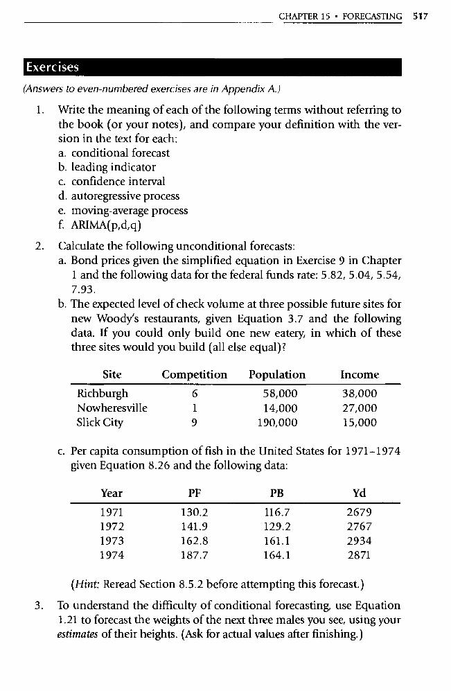
CHAPTER 15 • FORECASTING 517
Exercises
(Answers to even-numbered exercises are in Appendix A.)
1. Write the meaning of each of the following terms without referring to the book (or your notes), and compare your definition with the ver-sion in the text for each: a. conditional forecast b. leading indicator c. confidence interval d. autoregressive process e. moving-average process f. ARIMA(p,d,q)
2. Calculate the following unconditional forecasts: a. Bond prices given the simplified equation in Exercise 9 in Chapter
1 and the following data for the federal funds rate: 5.82, 5.04, 5.54, 7.93
b. The expected level of check volume at three possible future sites for new Woodÿ s restaurants, given Equation 3.7 and the following data. If you could only build one new eatery, in which of these three sites would you build (all else equal)?
Site Competition Population Income
Richburgh 6 58,000 38,000 Nowheresville 1 14,000 27,000 Slick City 9 190,000 15,000
c. Per capita consumption of fish in the United States for 1971-1974 given Equation 8.26 and the following data:
Year PF PB Yd
1971 130.2 116.7 2679 1972 141.9 129.2 2767 1973 162.8 161.1 2934 1974 187.7 164.1 2871
(Hint: Reread Section 8.5.2 before attempting this forecast.)
3. To understand the difficulty of conditional forecasting, use Equation 1.21 to forecast the weights of the next three males you see, using your estimates of their heights. (Ask for actual values after finishing.)
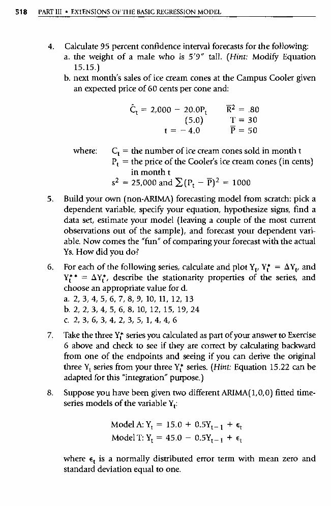
518 PART III • EXTENSIONS OF THE BASIC REGRESSION MODEL
4. Calculate 95 percent confidence interval forecasts for the following: a. the weight of a male who is 5'9" tall. (Hint: Modify Equation
15.15.) b. next month's sales of ice cream cones at the Campus Cooler given
an expected price of 60 cents per cone and:
Ct = 2,000 — 20.0Pt R2 =.80
(5.0)
T=30
t = — 4.0
P = 50
where: Ct = the number of ice cream cones sold in month t Pt = the price of the Cooler's ice cream cones (in cents)
in month t s2 = 25,000 and E (Pt — P) 2 = 1000
5. Build your own (non-ARIMA) forecasting model from scratch: pick a dependent variable, specify your equation, hypothesize signs, find a data set, estimate your model (leaving a couple of the most current observations out of the sample), and forecast your dependent vari-able. Now comes the "fun" of comparing your forecast with the actual Ys. How did you do?
6. For each of the following series, calculate and plot Y t, Yt = AYt, and Yt * = DYt , describe the stationarity properties of the series, and choose an appropriate value for d. a. 2, 3, 4, 5, 6, 7, 8, 9, 10, 11, 12, 13 b. 2, 2, 3, 4, 5, 6, 8, 10, 12, 15, 19, 24 c. 2, 3, 6, 3, 4, 2, 3, 5, 1,4,4,6
7. Take the three Yt series you calculated as pa rt of your answer to Exercise 6 above and check to see if they are correct by calculating backward from one of the endpoints and seeing if you can derive the o riginal three Yt series from your three Yt series. (Hint: Equation 15.22 can be adapted for this "integration" purpose.)
8. Suppose you have been given two different ARIMA(1,0,0) fitted time-series models of the variable Y t :
Model A: Yt = 15.0 + 0.5Yt _ I + Et
Model T: Yt = 45.0 — 0.5Yt _ I + Et
where Et is a normally distributed error term with mean zero and standard deviation equal to one.
CHAPTER 15 • FORECASTING 519
a. The final observation in the sample (time period 96) is Y96 = 31. Determine forecasts for periods 97, 98, and 99 for both models.
b. Suppose you now find out that the actual Y97 was equal to 33. Re-vise your forecasts for periods 98 and 99 to take the new informa-tion into account.
c. Based on the fitted time series and your two forecasts, which model (model A or model T) do you expect to exhibit smoother behavior? Explain your reasoning.
9. Suppose you have been given an ARIMA(1,0,1) fitted time-series model:
Yt =0.0+ 1.0Yt_1 + Et - 0.5Et_1
where Et is a normally distributed error term with mean zero and standard deviation equal to one and where T = 99, Y99 = 27, and where Y99 = 27.5. a. Calculate e 99 . b. Calculate forecasts for Y100 , Y101, and Y102. (Hint: Use your answer
to part a.)
10. You've been hired to forecast Sports Illustrated subscriptions (S) using the following function of GDP (Y) and a classical error term (E):
St = Ro + R tYt + R2St —1 + Et
Explain how you would forecast (out two time periods) with this equation in the following cases: a. If future values of Y are known. (Hint: Be sure to comment on the
functional form of this relationship.) b. If future values of Y are unknown and Sports Illustrated subscrip-
tions are small in comparison to GDP. c. If Sports Illustrated subscriptions are about half of GDP (obviously a
sports-lover's heaven!) and all other components of GDP are known to be stochastic functions of time.
CHAPTER 16 Statistical Principles
16.1 Describing Data
16.2 Probability Distributions
16.3 Sampling
16.4 Estimation
16.5 Hypothesis Tests
16.6 Summary and Exercises
This chapter* reviews the basic statistical principles that underlie the specifi-cation and estimation of econometric models. We start by discussing some simple yet powerful tools for describing data. Then we examine some models that can be used to describe where data come from. The third section looks at how samples can be taken from populations. The fourth and fifth sections explain how a sample can be used to draw inferences about the population from which it came.
16.1 Describing Data
It is very difficult to analyze substantial amounts of data merely by looking at numbers. What sense could we make of pages and pages of a computer print-out showing the gender and height of every student at your school? Instead, most researchers use some simple summary statistics to help understand and interpret data.
16.1.1 Median
The most familiar descriptive statistics are measures of location that describe the center of the data, without telling us whether the data are tightly dus-
* Written by Ga ry Smith of Pomona College. Ga ry is also the author of Statistical Reasoning (McGraw Hill, 1998).
520
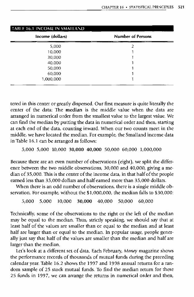
CHAPTER 16 • STATISTICAL PRINCIPLES 521
TABLE 16.1 INCOME IN SMALLAND
Income (dollars) Number of Persons
5,000 2 10,000 1 30,000 1 40,000 1 50,000 1 60,000 1
1,000,000 1
tered in this center or greatly dispersed. Our first measure is quite literally the center of the data: The median is the middle value when the data are arranged in numerical order from the smallest value to the largest value. We can find the median by putting the data in numerical order and then, starting at each end of the data, counting inward. When our two counts meet in the middle, we have located the median. For example, the Smalland income data in Table 16.1 can be arranged as follows:
5,000 5,000 10,000 30,000 40,000 50,000 60,000 1,000,000
Because there are an even number of obse rvations (eight), we split the differ-ence between the two middle obse rvations, 30,000 and 40,000, giving a me-dian of 35,000. This is the center of the income data, in that half of the people earned less than 35,000 dollars and half earned more than 35,000 dollars.
When there is an odd number of obse rvations, there is a single middle ob-servation. For example, without the $1,000,000, the median falls to $30,000:
5,000 5,000 10,000 30,000 40,000 50,000 60,000
Technically, some of the obse rvations to the right or the left of the median may be equal to the median. Thus, strictly speaking, we should say that at least half of the values are smaller than or equal to the median and at least half are larger than or equal to the median. In popular usage, people gener-ally just say that half of the values are smaller than the median and half are larger than the median.
Let's look at a different set of data. Each February, Money magazine shows the performance records of thousands of mutual funds during the preceding calendar year. Table 16.2 shows the 1997 and 1998 annual returns for a ran-dom sample of 25 stock mutual funds. To find the median return for these 25 funds in 1997, we can arrange the returns in numerical order and then,
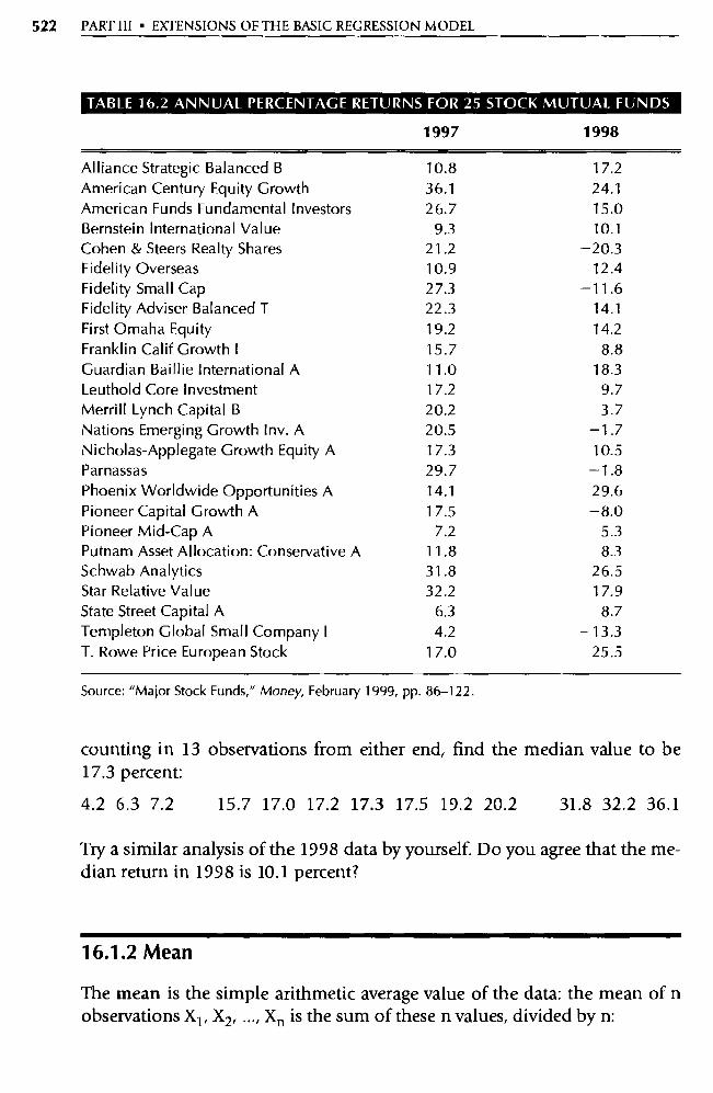
522 PART III • EXTENSIONS OF THE BASIC REGRESSION MODEL
TABLE 16.2 ANNUAL PERCENTAGE RETURNS FOR 25 STOCK MUTUAL FUNDS
1997 1998
Alliance Strategic Balanced B 10.8 17.2
American Century Equity Growth 36.1 24.1 American Funds Fundamental Investors 26.7 15.0 Bernstein International Value 9.3 10.1 Cohen & Steers Realty Shares 21.2 -20.3 Fidelity Overseas 10.9 12.4 Fidelity Small Cap 27.3 -11.6 Fidelity Adviser Balanced T 22.3 14.1 First Omaha Equity 19.2 14.2 Franklin Calif Growth I 15.7 8.8 Guardian Baillie International A 11.0 18.3 Leuthold Core Investment 17.2 9.7 Merrill Lynch Capital B 20.2 3.7 Nations Emerging Growth Inv. A 20.5 -1.7 Nicholas-Applegate Growth Equity A 17.3 10.5 Parnassas 29.7 -1.8 Phoenix Worldwide Opportunities A 14.1 29.6 Pioneer Capital Growth A 17.5 -8.0 Pioneer Mid-Cap A 7.2 5.3 Putnam Asset Allocation: Conservative A 11.8 8.3 Schwab Analytics 31.8 26.5 Star Relative Value 32.2 17.9 State Street Capital A 6.3 8.7 Templeton Global Small Company I 4.2 -13.3 T. Rowe Price European Stock 17.0 25.5
Source: "Major Stock Funds," Money, February 1999, pp. 86-122.
counting in 13 observations from either end, find the median value to be 17.3 percent:
4.2 6.3 7.2 15.7 17.0 17.2 17.3 17.5 19.2 20.2 31.8 32.2 36.1
Try a similar analysis of the 1998 data by yourself. Do you agree that the me-dian return in 1998 is 10.1 percent?
16.1.2 Mean
The mean is the simple arithmetic average value of the data: the mean of n observations X1, X2, ..., Xn is the sum of these n values, divided by n:
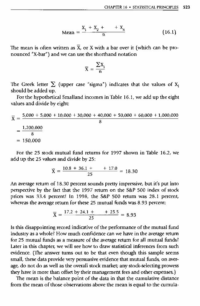
+ Xn
n Xl + X2 +
Mean = (16.1)
CHAPTER 16 • STATISTICAL PRINCIPLES 523
The mean is often written as X, or X with a bar over it (which can be pro-nounced "X-bar") and we can use the shorthand notation
EXi X = n
The Greek letter E (upper case "sigma") indicates that the values of X i should be added up.
For the hypothetical Smalland incomes in Table 16.1, we add up the eight values and divide by eight:
5,000 + 5,000 + 10,000 + 30,000 + 40,000 + 50,000 + 60,000 + 1,000,000 X =
1,200,000 8
= 150,000
For the 25 stock mutual fund returns for 1997 shown in Table 16.2, we add up the 25 values and divide by 25:
X= 10.8+36.1+
25
+ 17.0 = 18.30
An average return of 18.30 percent sounds pretty impressive, but it's put into perspective by the fact that the 1997 return on the S&P 500 index of stock prices was 33.4 percent! In 1998, the S&P 500 return was 28.1 percent, whereas the average return for these 25 mutual funds was 8.93 percent:
X- 17.2+24.1 +
25
+ 25.5 = 8.93
Is this disappointing record indicative of the performance of the mutual fund industry as a whole? How much confidence can we have in the average return for 25 mutual funds as a measure of the average return for all mutual funds? Later in this chapter, we will see how to draw statistical inferences from such evidence. (The answer turns out to be that even though this sample seems small, these data provide very persuasive evidence that mutual funds, on aver-age, do not do as well as the overall stock market; any stock-selecting prowess they have is more than offset by their management fees and other expenses.)
The mean is the balance point of the data in that the cumulative distance from the mean of those observations above the mean is equal to the cumula-
8
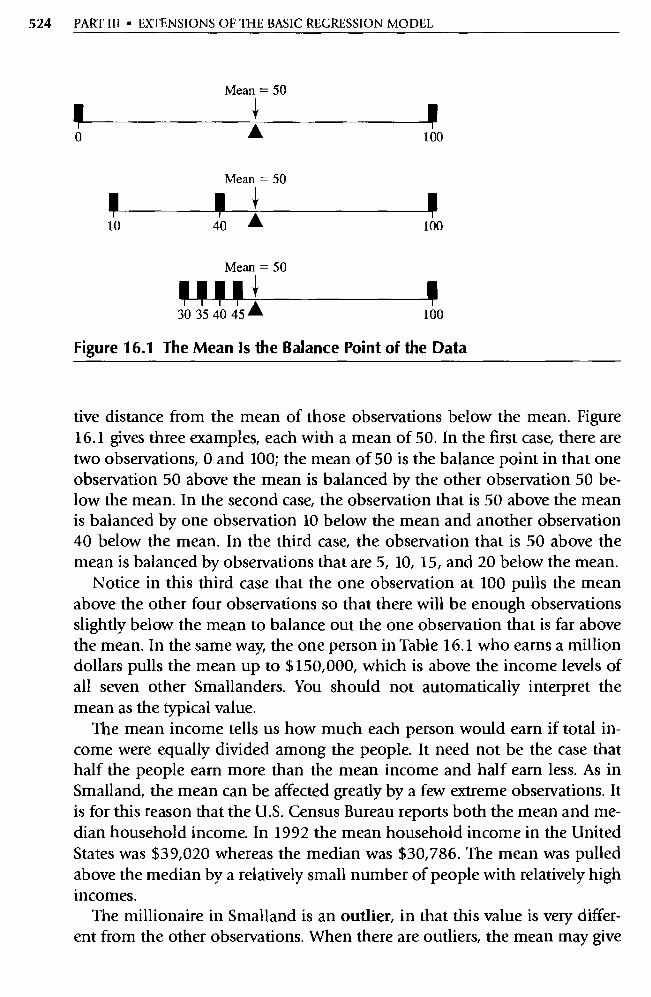
524 PART III • EXTENSIONS OF THE BASIC REGRESSION MODEL
Mean = 50
1!) 100
Mean = 50
10 40 — 100
Mean = 50
i30 35 40 45 100
Figure 16.1 The Mean Is the Balance Point of the Data
tive distance from the mean of those observations below the mean. Figure 16.1 gives three examples, each with a mean of 50. In the first case, there are two observations, 0 and 100; the mean of 50 is the balance point in that one observation 50 above the mean is balanced by the other observation 50 be-low the mean. In the second case, the observation that is 50 above the mean is balanced by one observation 10 below the mean and another observation 40 below the mean. In the third case, the observation that is 50 above the mean is balanced by observations that are 5, 10, 15, and 20 below the mean.
Notice in this third case that the one observation at 100 pulls the mean above the other four observations so that there will be enough observations slightly below the mean to balance out the one observation that is far above the mean. In the same way, the one person in Table 16.1 who earns a million dollars pulls the mean up to $150,000, which is above the income levels of all seven other Smallanders. You should not automatically interpret the mean as the typical value.
The mean income tells us how much each person would earn if total in-come were equally divided among the people. It need not be the case that half the people earn more than the mean income and half earn less. As in Smalland, the mean can be affected greatly by a few extreme observations. It is for this reason that the U.S. Census Bureau repo rts both the mean and me-dian household income. In 1992 the mean household income in the United States was $39,020 whereas the median was $30,786. The mean was pulled above the median by a relatively small number of people with relatively high incomes.
The millionaire in Smalland is an outlier, in that this value is very differ-ent from the other observations. When there are outliers, the mean may give
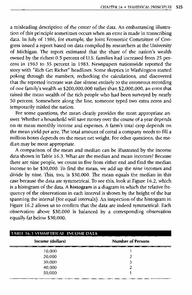
CHAPTER 16 • STATISTICAL PRINCIPLES 525
a misleading description of the center of the data. An embarrassing illustra-tion of this principle sometimes occurs when an error is made in transcribing data. In July of 1986, for example, the Joint Economic Committee of Con-gress issued a repo rt based on data compiled by researchers at the University of Michigan. The report estimated that the share of the nation's wealth owned by the richest 0.5 percent of U.S. families had increased from 25 per-cent in 1963 to 35 percent in 1983. Newspapers nationwide reported the story with "Rich Get Richer" headlines. Some skeptics in Washington started poking through the numbers, rechecking the calculations, and discovered that the reported increase was due almost entirely to the erroneous recording of one family's wealth as $200,000,000 rather than $2,000,000, an error that raised the mean wealth of the rich people who had been surveyed by nearly 50 percent. Somewhere along the line, someone typed two extra zeros and temporarily misled the nation.
For some questions, the mean clearly provides the most appropriate an-swer. Whether a household will save money over the course of a year depends on its mean monthly income and expenses. A farm's total crop depends on the mean yield per acre. The total amount of cereal a company needs to fill a million boxes depends on the mean net weight. For other questions, the me-dian may be more appropriate.
A comparison of the mean and median can be illustrated by the income data shown in Table 16.3. What are the median and mean incomes? Because there are nine people, we count in five from either end and find the median income to be $30,000. To find the mean, we add up the nine incomes and divide by nine. This, too, is $30,000. The mean equals the median in this case because the data are symmetrical. To see this, look at Figure 16.2, which is a histogram of the data. A histogram is a diagram in which the relative fre-quency of the obse rvations in each interval is shown by the height of the bar spanning the interval (for equal intervals). An inspection of the histogram in Figure 16.2 allows us to confirm that the data are indeed symmetrical. Each observation above $30,000 is balanced by a corresponding obse rvation equally far below $30,000.
TABLE 16.3 SYMMETRICAL INCOME DATA
Income (dollars) Number of Persons
10,000 1 2 0, 000 2
30,000 3 40,000 2 50,000 1
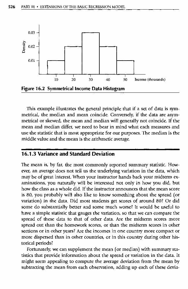
526 PART III • EXTENSIONS OF THE BASIC REGRESSION MODEL
0.03 —
c 0.02 —
^
0.01 —
10 20 30 40 50 Income (thousands)
Figure 16.2 Symmetrical Income Data Histogram
This example illustrates the general principle that if a set of data is sym-metrical, the median and mean coincide. Conversely, if the data are asym-metrical or skewed, the mean and median will generally not coincide. If the mean and median differ, we need to bear in mind what each measures and use the statistic that is most appropriate for our purposes. The median is the middle value and the mean is the arithmetic average.
16.1.3 Variance and Standard Deviation
The mean is, by far, the most commonly reported summary statistic. How-ever, an average does not tell us the underlying va riation in the data, which may be of great interest. When your instructor hands back your midterm ex-aminations, you naturally will be interested not only in how you did, but how the class as a whole did. If the instructor announces that the mean score
is 80, you probably will also like to know something about the spread (or
variation) in the data. Did most students get scores of around 80? Or did
some do substantially better and some much worse? It would be useful to
have a simple statistic that gauges the va riation, so that we can compare the spread of these data to that of other data. Are the midterm scores more
spread out than the homework scores, or than the midterm scores in other
sections or in other years? Are the incomes in one count ry more compact or more dispersed than in other countries, or in this count ry during other his-torical periods?
Fortunately, we can supplement the mean (or median) with summary sta-tistics that provide information about the spread or variation in the data. It
might seem appealing to compute the average deviation from the mean by
subtracting the mean from each observation, adding up each of these devia-
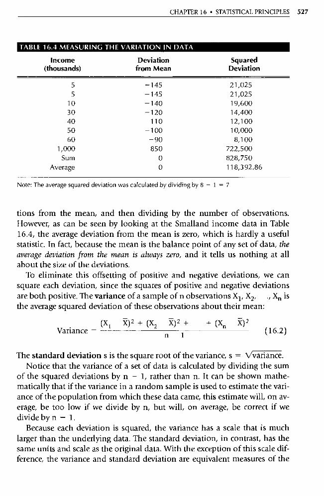
Variance = n 1 (X 1 X) 2 + (X2 X) 2 +
(16.2)
CHAPTER 16 • STATISTICAL PRINCIPLES 527
TABLE 16.4 MEASURING THE VARIATION IN DATA
Income (thousands)
Deviation from Mean
Squared Deviation
5 —145 21,025
5 —145 21,025 10 —140 19,600 30 —120 14,400 40 —110 12,100 50 —100 10,000
60 —90 8,100
1,000 850 722,500
Sum 0 828,750
Average 0 118,392.86
Note: The average squared deviation was calculated by dividing by 8 — 1 = 7
tions from the mean, and then dividing by the number of observations. However, as can be seen by looking at the Smalland income data in Table 16.4, the average deviation from the mean is zero, which is hardly a useful statistic. In fact, because the mean is the balance point of any set of data, the average deviation from the mean is always zero, and it tells us nothing at all about the size of the deviations.
To eliminate this offsetting of positive and negative deviations, we can square each deviation, since the squares of positive and negative deviations are both positive. The variance of a sample of n observations Xi, X2, ., X„ is the average squared deviation of these observations about their mean:
The standard deviation s is the square root of the variance, s = Vvariance. Notice that the va riance of a set of data is calculated by dividing the sum
of the squared deviations by n — 1, rather than n. It can be shown mathe-matically that if the variance in a random sample is used to estimate the vari-ance of the population from which these data came, this estimate will, on av-erage, be too low if we divide by n, but will, on average, be correct if we divide by n — 1.
Because each deviation is squared, the variance has a scale that is much larger than the underlying data. The standard deviation, in contrast, has the same units and scale as the original data. With the exception of this scale dif-ference, the variance and standard deviation are equivalent measures of the
528 PART III • EXTENSIONS OF THE BASIC REGRESSION MODEL
dispersion in a set of data. A data set that has a higher variance than another data set also has a higher standard deviation.
The variance and standard deviation are strongly affected by outliers be-cause of the squaring of deviations from the mean. An alternative measure of the spread of the data is the interquartile range, which is the range encom-passed by the middle half of the data. Even though the interquartile range is more resistant to outliers than is the standard deviation, the standard devia-tion is generally used to gauge the variation in a set of data because of its mathematical tractability and importance in probability and statistics.
Let's look again at the mutual fund returns in Table 16.2. From just staring at the numbers, it is difficult to tell whether there was more dispersion in the 1997 or 1998 returns. The standard deviations answer this question:
10.8+36.1 + + 17.0
1997 . Mean = 25 = 18.30
[10.8 - (18.30)] 2 + + [17.0 - (18.30)] 2
Variance = 25 1
= 74.5833
Standard deviation V74.5833 = 8.64
17.2+24.1 + +25.5
1998: Mean = 25 = 8.93
(17.2 - 8.93) 2 + + (25.5 - 8.93) 2
Variance = 25 1
= 162.9546
Standard deviation = V162.9546 = 12.77
A comparison of the 8.64 and 12.77 percent standard deviations indicates that there was more variation among these fund returns in 1998 than in 1997
The interpretation of the standard deviation is not as easy as is the inter-pretation of the mean. The 18.30 percent average return in 1997 implies that if you had invested an equal amount in each of these 25 funds, your average return would have been 18.30 percent. But what does the 8.64 percent stan-dard deviation mean? A famous theorem and two rules of thumb provide guidance. The remarkable theorem, Chebyshev's inequality, states that in any set of data at least 1 1/k 2 of the data are within k standard deviations of the mean. 1 Using k = 2, at least 1 1/2 2 = 3/4 of the data are within two standard deviations of the mean. The two rules of thumb are that in those cases in which the data have the normal distribution's bell shape, roughly two-thirds of the data are within one standard deviation of the mean and ap-proximately 95 percent are within two standard deviations. Table 16.5 shows
1. This works as long as k > 1.

CHAPTER 16 • STATISTICAL PRINCIPLES 529
TABLE 16.5 THE NUMBER OF MUTUAL FUND RETURNS WITHIN 1 AND 2 STANDARD DEVIATIONS OF THE MEAN
1997 1998
Mean 18.30 8.93
Standard deviation 8.64 12.77 Mean plus or minus 1 standard deviation 9.66 to 26.94 3.84 to 21.70
Fraction of data within 1 standard deviation 17/25 = 0.68 15/25 = 0.60
Mean plus or minus 2 standard deviations 1.02 to 35.58 —16.61 to 34.77
Fraction of data within 2 standard deviations 24/25 = 0.96 24/25 = 0.96
that, overall, 64 percent (32 of 50) of these mutual fund returns are within one standard deviation of the mean and 96 percent (48 of 50) are within two standard deviations.
16.2 Probability Distributions
Although the mean and standard deviation help describe a set of data, they don't do much to help us draw valid statistical inferences from the data. To make such inferences, we often use probability models to describe where the data come from—for example, a medical test that is correct or incorrect, a surveyed person who supports or opposes a particular candidate, an SAT score that is above or below 700. In this section, we will first see how proba-bilities can be used to quantify uncertainty and to help us explain and inter-pret empirical data.
16.2.1 Probability
When we say that a flipped coin has a 0.5 probability of landing with its heads side up, we mean that if this coin were to be flipped an interminable number of times, we anticipate that it will land heads about half the time. More generally, if an event has a probability P of occurring, then the fraction of the times that it occurs in the very long run will be very close to P. Obvi-ously, a probability cannot be negative or larger than one.
A random variable X is a variable whose numerical value is determined by chance, the outcome of a random phenomenon. 2 A discrete random variable,
2. To be mathematically precise, statisticians often use upper-case and lower-case notation to
distinguish between a random variable, which can take on different values, and the actual val-ues that happen to occur. Upper-case notation is used throughout this book for simplicity and convenience.

I I I 1 1 I 6 Number Rolled 1 2 3 4
5
0.20
530 PART III • EXTENSIONS OF THE BASIC REGRESSION MODEL
the subject of this section, has a countable number of possible values, such as 0, 1, and 2; in the next section, we will consider continuous random variables, such as time and distance, which can take on any value in an inte rval. All of the discrete random variables that we will examine have a finite number of outcomes, though there are other discrete variables with an infinite number of countable values. For example, if X is equal to the number of times that a coin will be flipped before a heads is obtained, there is no upper limit on the value of X; nonetheless, X is a discrete variable because its values are obtained by counting. Measures of time and distance, in contrast, are continuous vari-ables; between any two possible values, such as 4.7 and 4.8, there are other possible values, such as 4.75 and 4.76.
A probability distribution P[Xi] for a discrete random variable X assigns probabilities to the possible values X1, X2, and so on. For example, when a fair six-sided die is rolled, there are s ix equally likely outcomes, each with a 1/6 probability of occurring. Figure 16.3 shows this probability distribution.
Probability distributions are scaled so that the total area inside the rectan-gles is equal to 1. A probability distribution looks like a data histogram, but it is conceptually different since it refers to the probabilities of various out-comes occurring, rather than the actual frequencies with which they happen to occur in a particular set of experiments. A probability distribution and data histogram are related by the fact that in the long run, the observed fre-quencies will be very close to the theoretical probabilities.
To illustrate this relationship, we rolled a six-sided die 1000 times. Figure 16.4 shows a data histogram of the results after 100 rolls and after 1000 rolls.
Figure 16.3 Probability Distribution for a Six-Sided Die
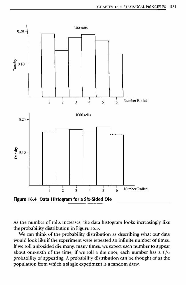
CHAPTER 16 • STATISTICAL PRINCIPLES 531
100 rolls 0.20
^
1 0.10
1 2 3 4
1000 rolls
5 6 Number Rolled
0.20
^
.g 0.10
1 2 1
3 4 5 6 Number Rolled
Figure 16.4 Data Histogram for a Six-Sided Die
As the number of rolls increases, the data histogram looks increasingly like
the probability distribution in Figure 16.3. We can think of the probability distribution as describing what our data
would look like if the experiment were repeated an infinite number of times.
If we roll a six-sided die many, many times, we expect each number to appear
about one-sixth of the time; if we roll a die once, each number has a 1/6
probability of appearing. A probability distribution can be thought of as the
population from which a single experiment is a random draw.
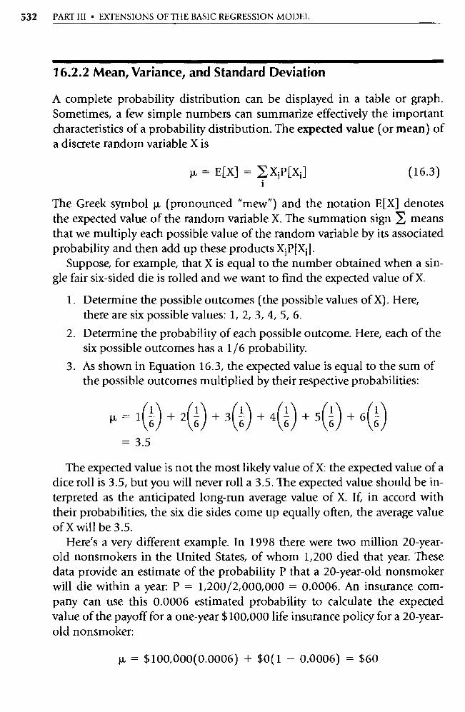
532 PART III • EXTENSIONS OF THE BASIC REGRESSION MODEL
16.2.2 Mean, Variance, and Standard Deviation
A complete probability dist ribution can be displayed in a table or graph. Sometimes, a few simple numbers can summarize effectively the impo rtant characteristics of a probability distribution. The expected value (or mean) of a discrete random variable X is
= E[X] = XiP[Xi] (16.3)
The Greek symbol µ (pronounced "mew") and the notation E[X] denotes the expected value of the random variable X. The summation sign means that we multiply each possible value of the random variable by its associated probability and then add up these products X i PIXi ].
Suppose, for example, that X is equal to the number obtained when a sin-gle fair six-sided die is rolled and we want to find the expected value of X.
1. Determine the possible outcomes (the possible values of X). Here, there are s ix possible values: 1, 2, 3, 4, 5, 6.
2. Determine the probability of each possible outcome. Here, each of the six possible outcomes has a 1/6 probability.
3. As shown in Equation 16.3, the expected value is equal to the sum of the possible outcomes multiplied by their respective probabilities:
1 1 +2 1 +3 1 +4 1
+5 1 +6 1 G G 6 G 6 6
= 3.5
The expected value is not the most likely value of X: the expected value of a dice roll is 3.5, but you will never roll a 3.5. The expected value should be in-terpreted as the anticipated long-run average value of X. If, in accord with their probabilities, the s ix die sides come up equally often, the average value of X will be 3.5.
Here's a very different example. In 1998 there were two million 20-year-old nonsmokers in the United States, of whom 1,200 died that year. These data provide an estimate of the probability P that a 20-year-old nonsmoker will die within a year: P = 1,200/2,000,000 = 0.0006. An insurance com-pany can use this 0.0006 estimated probability to calculate the expected value of the payoff for a one-year $100,000 life insurance policy for a 20-year-old nonsmoker:
µ = $100,000(0.0006) + $0(1 — 0.0006) = $60
CHAPTER 16 • STATISTICAL PRINCIPLES 533
If its probability estimate is accurate, an insurance company can anticipate paying, on average, $60 per policy.
In 1998, the cost for one company's $100,000 one-year life insurance pol-icy for a 20-year-old nonsmoker was $117—roughly twice the expected value of the payoff. If, as anticipated, a fraction 0.0006 of the insured 20-year-old nonsmokers die, the company will collect $117 per policy and pay out, on av-erage, $60 per policy. Roughly half of the money that the insurance company receives will be paid to beneficiaries and half will be retained by the com-pany to cover administrative expenses and provide a profit. This 50 percent benefit-to-premium ratio is representative of many insurance policies.
Pascal and other early probability theorists used probabilities to calculate the expected value of various games of chance and determine which were the most profitable. They assumed that a rational person would choose the course of action with the highest expected value. This expected-value crite-rion is appealing for gambles that are repeated over and over. It makes good sense to look at the long-mn average when there is a long run to average over. Casinos, state lotteries, and insurance companies are very interested in the expected values on the repetitive gambles they offer, because anything with a negative expected value will almost certainly be unprofitable in the long mn.
However, an expected-value criterion is often inappropriate. State lotteries have a positive expected value for the state and, because their gain is our loss, a negative expected value for people who buy lottery tickets. Those who buy lottery tickets are not maximizing expected value. Insurance policies give in-surance companies a positive expected value and insurance buyers a negative expected value. People who buy insurance are not maximizing expected value either. Diversified investments provide yet another example. An expected-value maximizer should invest everything in the single asset with the highest expected value. Individuals and financial institutions that hold dozens or thousands of assets must not be maximizing expected value.
The primary inadequacy of expected-value maximization is that it neglects risk—how certain or uncertain a situation is. An expected value maximizer considers a sure $1 million and a 1 percent chance at $100 million equally attractive because each has an expected value of $1 million. If these alterna-tives were offered over and over, there would be little difference in the long mn because the payoffs from each would almost certainly average close to $1 million per play. But if you get only one chance at this game, the outcome may differ considerably from its expected value, a difference ignored by an expected-value calculation. Much of the uncertainty we face is unique, not repetitive, and the possible divergence between the actual outcome and its expected value is properly described as risk.
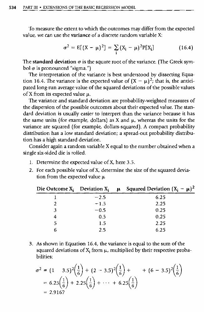
534 PART III • EXTENSIONS OF THE BASIC REGRESSION MODEL
To measure the extent to which the outcomes may differ from the expected
value, we can use the variance of a discrete random va riable X:
0-2 = E[(X - 11) 2] = E (Xi - 0 2P[Xi] (16.4)
The standard deviation Q is the square root of the variance. (The Greek sym-bol if is pronounced "sigma.")
The interpretation of the variance is best understood by dissecting Equa-tion 16.4. The va riance is the expected value of (X — p.) 2; that is, the antici-pated long-run average value of the squared deviations of the possible values
of X from its expected value µ.
The variance and standard deviation are probability-weighted measures of
the dispersion of the possible outcomes about their expected value. The stan-dard deviation is usually easier to interpret than the variance because it has
the same units (for example, dollars) as X and p.,, whereas the units for the
variance are squared (for example, dollars-squared). A compact probability
distribution has a low standard deviation; a spread-out probability distribu-tion has a high standard deviation.
Consider again a random variable X equal to the number obtained when a
single six-sided die is rolled.
1. Determine the expected value of X, here 3.5.
2. For each possible value of X, determine the size of the squared devia-tion from the expected value µ
Die Outcome Xi Deviation Xi µ Squared Deviation (X i — p.) 2
1 —2.5 6.25 2 —1.5 2.25 3 —0.5 0.25 4 0.5 0.25 5 1.5 2.25 6 2.5 6.25
3. As shown in Equation 16.4, the variance is equal to the sum of the squared deviations of Xi from µ,, multiplied by their respective proba-bilities:
0.2 = (1 3.5)0+ (2 — 3.5 )2 G + + (6 — 3.5)2 G
= 6.25 6^
+2.25 ^ +••• +6.25 6 )
= 2.9167
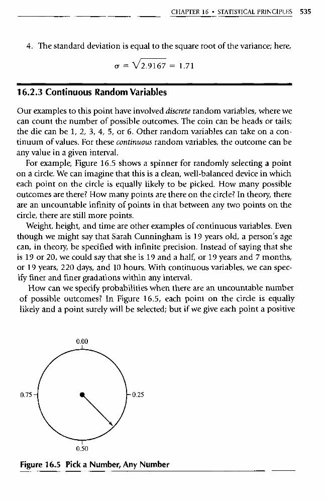
CHAPTER 16 • STATISTICAL PRINCIPLES 535
4. The standard deviation is equal to the square root of the variance; here,
Q= V2.9167= 1.71
16.2.3 Continuous Random Variables
Our examples to this point have involved discrete random variables, where we can count the number of possible outcomes. The coin can be heads or tails; the die can be 1, 2, 3, 4, 5, or 6. Other random variables can take on a con-tinuum of values. For these continuous random variables, the outcome can be any value in a given interval.
For example, Figure 16.5 shows a spinner for randomly selecting a point on a circle. We can imagine that this is a clean, well-balanced device in which each point on the circle is equally likely to be picked. How many possible outcomes are there? How many points are there on the circle? In theory, there are an uncountable infinity of points in that between any two points on the circle, there are still more points.
Weight, height, and time are other examples of continuous variables. Even though we might say that Sarah Cunningham is 19 years old, a person's age can, in theory, be specified with infinite precision. Instead of saying that she is 19 or 20, we could say that she is 19 and a half, or 19 years and 7 months, or 19 years, 220 days, and 10 hours. With continuous variables, we can spec-ify finer and finer gradations within any inte rval.
How can we specify probabilities when there are an uncountable number of possible outcomes? In Figure 16.5, each point on the circle is equally likely and a point surely will be selected; but if we give each point a positive
0.00
0.75 0.25
0.50
Figure 16.5 Pick a Number, Any Number
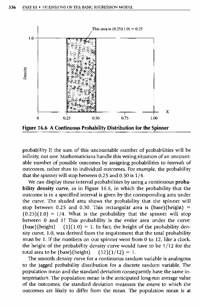
1.00 0 0.25 0.50 0.75
This area is (0.25)(1.0) = 0.25
1.0
1 X
Figure 16.6 A Continuous Probability Distribution for the Spinner
536 PART III • EXTENSIONS OF THE BASIC REGRESSION MODEL
probability P, the sum of this uncountable number of probabilities will be infinity, not one. Mathematicians handle this vexing situation of an uncount-able number of possible outcomes by assigning probabilities to intervals of outcomes, rather than to individual outcomes. For example, the probability that the spinner will stop between 0.25 and 0.50 is 1/4.
We can display these interval probabilities by using a continuous proba-bility density curve, as in Figure 16.6, in which the probability that the outcome is in a specified interval is given by the corresponding area under the curve. The shaded area shows the probability that the spinner will stop between 0.25 and 0.50. This rectangular area is (base) (height) = (0.25) (1.0) = 1/4. What is the probability that the spinner will stop between 0 and 1? This probability is the entire area under the curve: (base) (height) (1) (1.0) = 1. In fact, the height of the probability den-sity curve, 1.0, was derived from the requirement that the total probability must be 1. If the numbers on our spinner went from 0 to 12, like a clock, the height of the probability density curve would have to be 1/12 for the total area to be (base) (height) (12)(1/12) = 1.
The smooth density curve for a continuous random variable is analogous to the jagged probability distribution for a discrete random va riable. The population mean and the standard deviation consequently have the same in-terpretation. The population mean is the anticipated long-run average value of the outcomes; the standard deviation measures the extent to which the outcomes are likely to differ from the mean. The population mean is at
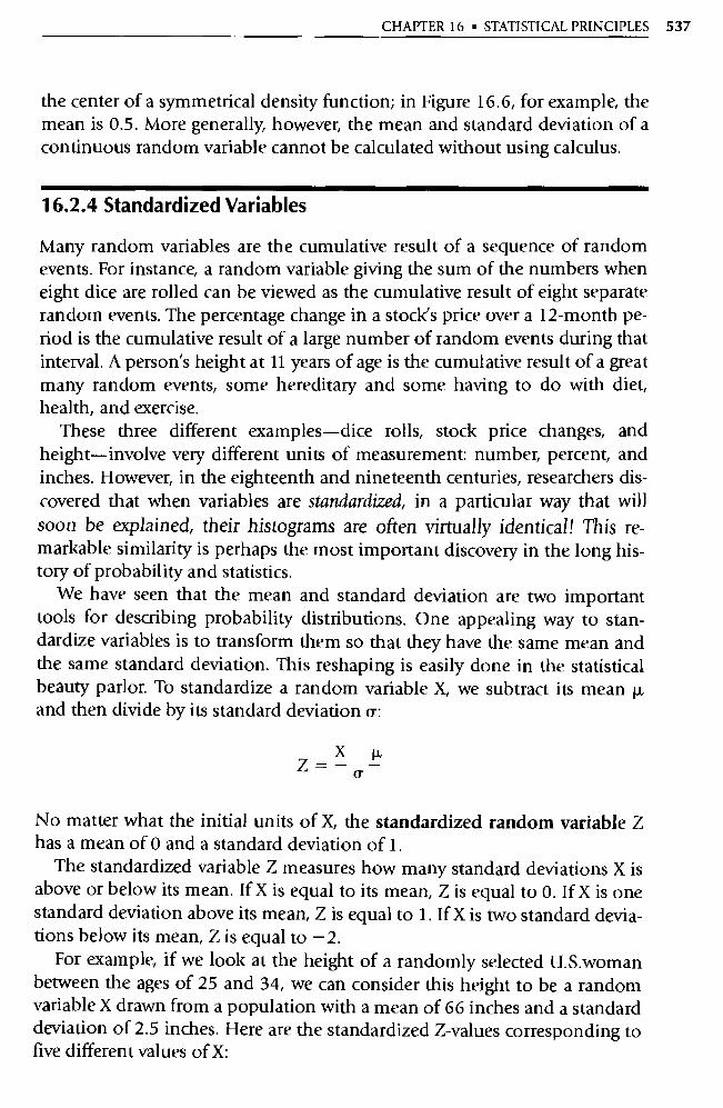
CHAPTER 16 • STATISTICAL PRINCIPLES 537
the center of a symmetrical density function; in Figure 16.6, for example, the mean is 0.5. More generally, however, the mean and standard deviation of a continuous random variable cannot be calculated without using calculus.
16.2.4 Standardized Variables
Many random variables are the cumulative result of a sequence of random events. For instance, a random variable giving the sum of the numbers when eight dice are rolled can be viewed as the cumulative result of eight separate random events. The percentage change in a stock's price over a 12-month pe-riod is the cumulative result of a large number of random events during that interval. A person's height at 11 years of age is the cumulative result of a great many random events, some hereditary and some having to do with diet, health, and exercise.
These three different examples—dice rolls, stock price changes, and height—involve very different units of measurement: number, percent, and inches. However, in the eighteenth and nineteenth centuries, researchers dis-covered that when variables are standardized, in a particular way that will soon be explained, their histograms are often virtually identical! This re-markable similarity is perhaps the most impo rtant discovery in the long his-tory of probability and statistics.
We have seen that the mean and standard deviation are two impo rtant tools for describing probability distributions. One appealing way to stan-dardize variables is to transform them so that they have the same mean and the same standard deviation. This reshaping is easily done in the statistical beauty parlor. To standardize a random variable X, we subtract its mean µ and then divide by its standard deviation 6:
X µ Z= Q
No matter what the initial units of X, the standardized random variable Z has a mean of 0 and a standard deviation of 1.
The standardized variable Z measures how many standard deviations X is above or below its mean. If X is equal to its mean, Z is equal to O. If X is one standard deviation above its mean, Z is equal to 1. If X is two standard devia-tions below its mean, Z is equal to —2.
For example, if we look at the height of a randomly selected U.S.woman between the ages of 25 and 34, we can consider this height to be a random variable X drawn from a population with a mean of 66 inches and a standard deviation of 2.5 inches. Here are the standardized Z-values corresponding to five different values of X:
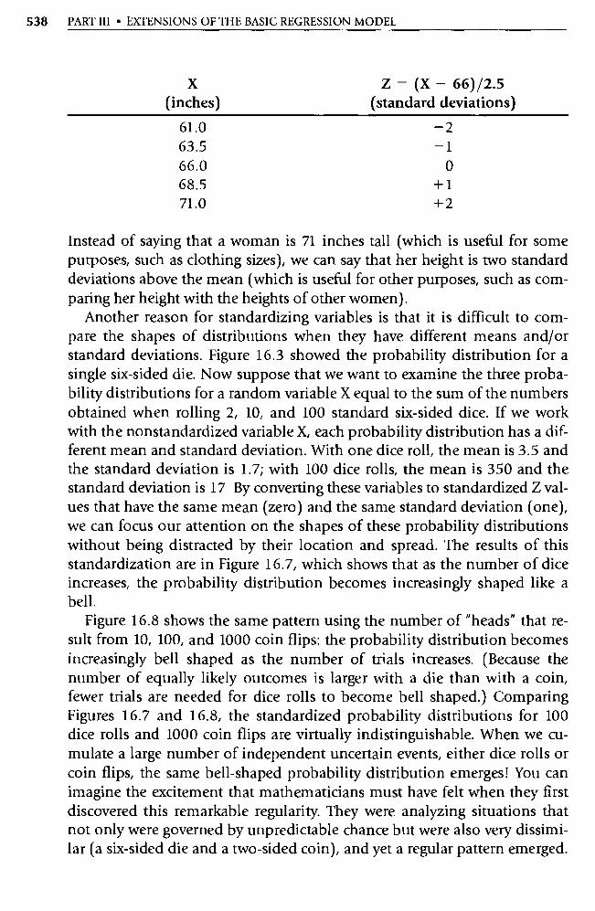
538 PART III • EXTENSIONS OF THE BASIC REGRESSION MODEL
X (inches)
Z = (X — 66) /2.5 (standard deviations)
61.0 —2 63.5 —1 66.0 0 68.5 +1 71.0 +2
Instead of saying that a woman is 71 inches tall (which is useful for some purposes, such as clothing sizes), we can say that her height is two standard deviations above the mean (which is useful for other purposes, such as com-paring her height with the heights of other women).
Another reason for standardizing variables is that it is difficult to com-pare the shapes of distributions when they have different means and/or standard deviations. Figure 16.3 showed the probability distribution for a single six-sided die. Now suppose that we want to examine the three proba-bility distributions for a random variable X equal to the sum of the numbers obtained when rolling 2, 10, and 100 standard six-sided dice. If we work with the nonstandardized variable X, each probability distribution has a dif-ferent mean and standard deviation. With one dice roll, the mean is 3.5 and the standard deviation is 1.7; with 100 dice rolls, the mean is 350 and the standard deviation is 17 By converting these variables to standardized Z val-ues that have the same mean (zero) and the same standard deviation (one), we can focus our attention on the shapes of these probability distributions without being distracted by their location and spread. The results of this standardization are in Figure 16.7, which shows that as the number of dice increases, the probability distribution becomes increasingly shaped like a bell.
Figure 16.8 shows the same pattern using the number of "heads" that re-sult from 10, 100, and 1000 coin flips: the probability distribution becomes increasingly bell shaped as the number of trials increases. (Because the number of equally likely outcomes is larger with a die than with a coin, fewer trials are needed for dice rolls to become bell shaped.) Comparing Figures 16.7 and 16.8, the standardized probability distributions for 100 dice rolls and 1000 coin flips are virtually indistinguishable. When we cu-mulate a large number of independent uncertain events, either dice rolls or coin flips, the same bell-shaped probability distribution emerges! You can imagine the excitement that mathematicians must have felt when they first discovered this remarkable regularity. They were analyzing situations that not only were governed by unpredictable chance but were also very dissimi-lar (a six-sided die and a two-sided coin), and yet a regular pattern emerged.
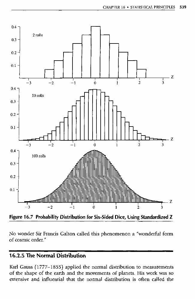
CHAPTER 16 • STATISTICAL PRINCIPLES 539
2 rolls
I r r r r z
—3 —2 —1 0 1 2 3
0.4 —
0.3 —
0.2 —
0.1 —
0.4 —
0.3 —
0.2 —
0.1 —
10 rolls
r r Z
—3 —2 —1 0 1 2 3
0.4 — 100 rolls
r ,
0.3 —
4
0.2 —
J
0.1 —
Z
—3 —2 —1 0 1 2
Figure 16.7 Probability Distribution for Six-Sided Dice, Using Standardized Z
No wonder Sir Francis Galton called this phenomenon a "wonderful form of cosmic order."
16.2.5 The Normal Distribution
Karl Gauss (1777-1855) applied the normal distribution to measurements of the shape of the earth and the movements of planets. His work was so extensive and influential that the normal dist ribution is often called the
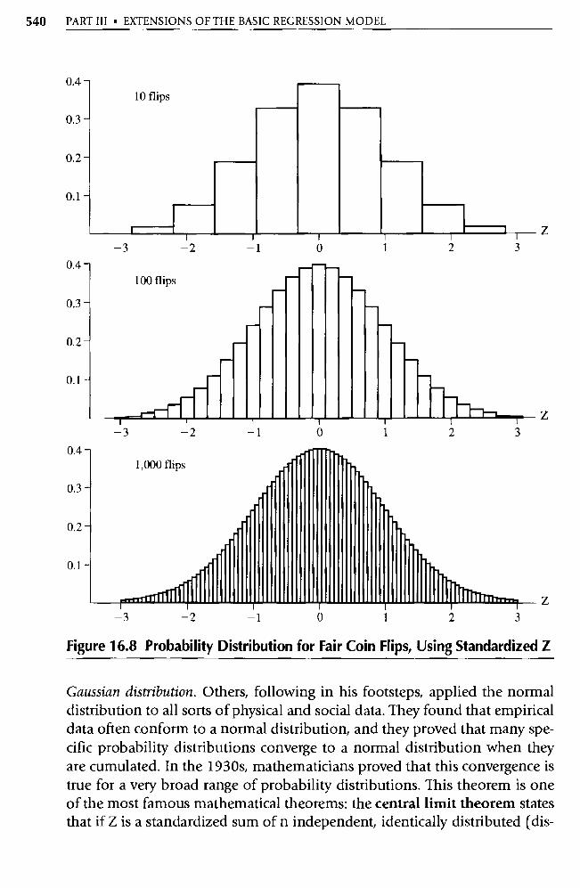
540 PART III • EXTENSIONS OF THE BASIC REGRESSION MODEL
0.4 —
0.3 —
0.2 —
0.1 —
10 flips
I — I Z
0.4 —
0.3 —
0.2 —
0.1 —
—3 —2 —1 0 1 2 3
100 flips
— 3 I i I I i
Z —2 —1 0 1 2 3
0.4 —
0.3 —
0.2 —
0.1 —
1,000 flips
1
i 0
1
2
Z
Figure 16.8 Probability Distribution for Fair Coin Flips, Using Standardized Z
Gaussian distribution. Others, following in his footsteps, applied the normal distribution to all so rts of physical and social data. They found that empirical data often conform to a normal distribution, and they proved that many spe-cific probability distributions converge to a normal distribution when they are cumulated. In the 1930s, mathematicians proved that this convergence is true for a very broad range of probability distributions. This theorem is one of the most famous mathematical theorems: the central limit theorem states that if Z is a standardized sum of n independent, identically distributed (dis-
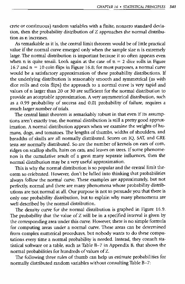
CHAPTER 16 • STATISTICAL PRINCIPLES .541
crete or continuous) random variables with a finite, nonzero standard devia-tion, then the probability distribution of Z approaches the normal distribu-tion as n increases.
As remarkable as it is, the central limit theorem would be of little practical value if the normal curve emerged only when the sample size n is extremely large. The normal distribution is important because it so often appears even when n is quite small. Look again at the case of n = 2 dice rolls in Figure 16.7 and n = 10 coin flips in Figure 16.8; for most purposes, a normal curve would be a satisfactory approximation of these probability distributions. If the underlying distribution is reasonably smooth and symmetrical (as with dice rolls and coin flips) the approach to a normal curve is very rapid and values of n larger than 20 or 30 are sufficient for the normal distribution to provide an acceptable approximation. A very asymmetrical distribution, such as a 0.99 probability of success and 0.01 probability of failure, requires a much larger number of trials.
The central limit theorem is remarkably robust in that even if its assump-tions aren't exactly true, the normal distribution is still a pretty good approx-imation. A normal distribution appears when we examine the weights of hu-mans, dogs, and tomatoes. The lengths of thumbs, widths of shoulders, and breadths of skulls are all normally distributed. Scores on IQ, SAT, and GRE
tests are normally distributed. So are the number of kernels on ears of corn, ridges on scallop shells, hairs on cats, and leaves on trees. If some phenome-non is the cumulative result of a great many separate influences, then the normal distribution may be a very useful approximation.
This is why the normal distribution is so popular and the central limit the-orem so celebrated. However, don't be lulled into thinking that probabilities always follow the normal curve. These examples are approximately, but not perfectly, normal and there are many phenomena whose probability distrib-utions are not normal at all. Our purpose is not to persuade you that there is only one probability distribution, but to explain why many phenomena are well described by the normal distribution.
The density curve for the normal distribution is graphed in Figure 16.9. The probability that the value of Z will be in a specified interval is given by the corresponding area under this curve. However, there is no simple formula for computing areas under a normal curve. These areas can be determined from complex numerical procedures, but nobody wants to do these compu-tations every time a normal probability is needed. Instead, they consult sta-tistical software or a table, such as Table B-7 in Appendix B, that shows the normal probabilities for hundreds of values of Z.
The following three rules of thumb can help us estimate probabilities for normally distributed random variables without consulting Table B-7:
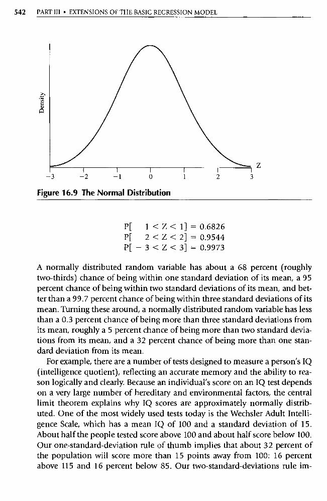
1 2 3
Z
542 PART III • EXTENSIONS OF THE BASIC REGRESSION MODEL
Figure 16.9 The Normal Distribution
P[ 1< Z< 1]= 0.6826 P[ 2 < Z < 2] = 0.9544 P[-3 <Z<3]= 0.9973
A normally distributed random va riable has about a 68 percent (roughly two-thirds) chance of being within one standard deviation of its mean, a 95 percent chance of being within two standard deviations of its mean, and bet-ter than a 99.7 percent chance of being within three standard deviations of its mean. Turning these around, a normally distributed random variable has less than a 0.3 percent chance of being more than three standard deviations from its mean, roughly a 5 percent chance of being more than two standard devia-tions from its mean, and a 32 percent chance of being more than one stan-dard deviation from its mean.
For example, there are a number of tests designed to measure a person's IQ (intelligence quotient), reflecting an accurate memory and the ability to rea-son logically and clearly. Because an individual's score on an IQ test depends on a very large number of hereditary and environmental factors, the central limit theorem explains why IQ scores are approximately normally distrib-uted. One of the most widely used tests today is the Wechsler Adult Intelli-gence Scale, which has a mean IQ of 100 and a standard deviation of 15. About half the people tested score above 100 and about half score below 100. Our one-standard-deviation rule of thumb implies that about 32 percent of the population will score more than 15 points away from 100: 16 percent above 115 and 16 percent below 85. Our two-standard-deviations rule im-

CHAPTER 16 • STATISTICAL PRINCIPLES 543
plies that about 5 percent of the population will score more than 30 points away from 100: 2.5 percent above 130 and 2.5 percent below 70.
16.3 Sampling
The previous sections were concerned with summarizing data. Now we focus on the actual production or collection of empirical data. To draw useful sta-tistical inferences, we must exercise care in gathering the data that will be used to make these inferences. The entire group of items that interests us is called the population. The part of this population that we actually observe is called a sample. Statistical inference involves using the sample to draw con-clusions about the characteristics of the population from which the sample came. In a medical experiment, for example, the population consists of all persons who might use this medication; the sample is the group of people used to test the medication; a possible statistical inference is that people who take the medication tend, on average, to live longer than people who don't.
We use samples to draw inferences about the population because it is of-ten impractical to scrutinize the entire population. If we burn every light bulb that a manufacturer produces to see how long each bulb lasts, all we will have is a large electricity bill and a lot of burnt-out light bulbs. Many tests are not this destructive but are simply too expensive to apply to the en-tire population. Instead, we sample. A light-bulb manufacturer tests a sample of its bulbs. A software company tests a sample of its disks. Medications and opinion polls are administered to a sample of people because it is too expen-sive to test or survey everyone.
16.3.1 Selection Bias
Any sample that differs systematically from the population that it is intended to represent is called a biased sample. Because a biased sample is unrepresen-tative of the population, it gives a distorted picture of the population and may lead to unwarranted conclusions. One of the most common causes of biased samples is selection bias, which occurs when the selection of the sam-ple systematically excludes or underrepresents ce rtain groups. Selection bias often happens when we use a convenience sample consisting of data that are easily collected.
If we are trying to estimate how often people get colds and have a friend who can give us medical records from an elementary school, this is a conve-nience sample with selection bias. If our intended population is people of all ages, we should not use samples that systematically exclude ce rtain ages. Sim-
544 PART III • EXTENSIONS OF THE BASIC REGRESSION MODEL
ilarly, the medical records from a prison, military base, or nursing home are convenience samples with selection bias. Military personnel are in better physical health than those living in nursing homes, and both differ systemat-ically from the population as a whole.
Self-selection bias can occur when we examine data for a group of people who have chosen to be in that group. For example, the accident records of peo-ple who buy collision insurance may be unrepresentative of the population as a whole; maybe they buy insurance because they know that they are accident prone. The physical fitness of joggers may provide a biased estimates of the benefits of jogging most of those who choose to run regularly may be more physically fit than the general population, even before they began running.
16.3.2 Survivor Bias
Retrospective studies look at past data for a contemporaneously selected sam-ple; for example, an examination of the lifetime medical records of 65-year-olds. A prospective study, in contrast, selects a sample and then tracks the members over time. Retrospective studies are notoriously unreliable, and not just because of faulty memories and lost data. When we choose a sample from a current population in order to draw inferences about a past popula-tion, we necessarily exclude members of the past population who are no longer around—an exclusion that causes survivor bias, in that we only look at the survivors. If we examine the medical records of 65 year olds in order to identify the causes of health problems, we overlook those who died before reaching 65 years of age and consequently omit data on some fatal health problems. Survivor bias is a form of selection bias in that the use of retro-spective data excludes pa rt of the relevant population.
Here's another example. Stock market studies sometimes examine histori-cal data for companies that have been selected randomly from the New York Stock Exchange (NYSE). If we restrict our analysis to companies currently listed on the NYSE, our data will be subject to survivor bias because we will ignore companies that were listed in the past, but have subsequently gone bankrupt. If we want to estimate the average return for an investment in NYSE stocks over the past 50 years, and do not consider the stock of any com-pany that went bankrupt, we will overestimate the average return.
16.3.3 Nonresponse Bias
The systematic refusal of some groups to participate in an experiment or to re-spond to a poll is called nonresponse bias. A study is naturally more suspect the fewer the people who bother to respond. In the 1940s, the makers of
CHAPTER 16 • STATISTICAL PRINCIPLES 545
Ipana Tooth Paste boasted that a national survey had found that "Twice as many dentists personally use Ipana Tooth Paste as any other dentifrice prepa-ration. In a recent nationwide survey, more dentists said they recommended Ipana for their patients' daily use than the next two dentifrices combined. " 3
The Federal Trade Commission banned this ad after it learned that less than 1 percent of the dentists surveyed had named the brand of toothpaste they used and that even fewer had named a brand recommended for their patients. 4
16.3.4 The Power of Random Selection
Suppose that we want to estimate the average income of people in our home-town. We could attempt to put together a representative sample by wander-ing around town and carefully selecting people who appear to be "typical," but if we did, we would probably ignore the very rich and the very poor, and end up with a sample that has far less variation than does the population. Our sample would probably be biased, because those we exclude for being "above average" and those we exclude for being "below average" are unlikely to balance each other out perfectly. Worst of all, these biases would depend, in unknowable ways, on our undoubtedly mistaken perception of the "typi-cal" person. We might also be influenced by our preconceived notions of the results we hope to obtain. If we intend to show that these residents are, on average, better off than the citizens of another town, this intention may well influence the people we choose to inte rview.
How do we actually make random selections? Returning to our income study, suppose that we were to inte rview every registered voter. This would be a large sample, but it would have selection bias if there are systematic income differences between those who are and are not registered to vote. Similarly, shoppers at a ce rtain store, owners of ce rtain cars, or members of ce rtain clubs might not be representative of the town as a whole.
Ideally, we would choose a procedure that is equivalent to the following: put each resident's name on a slip of paper, drop these slips into a box, mix thoroughly, and pick names out randomly, just as cards are dealt from a well-shuffled deck. Each person, whether rich or poor, has an equal chance of in-clusion in our sample. In practice, instead of putting pieces of paper into a box, random sampling is usually done through some so rt of numerical iden-tification combined with the random selection of numbers.
3. Earl W. Kintner, A Primer on the Law of Deceptive Practices (New York: Macmillan, 1971), p. 153.
4. Ibid.
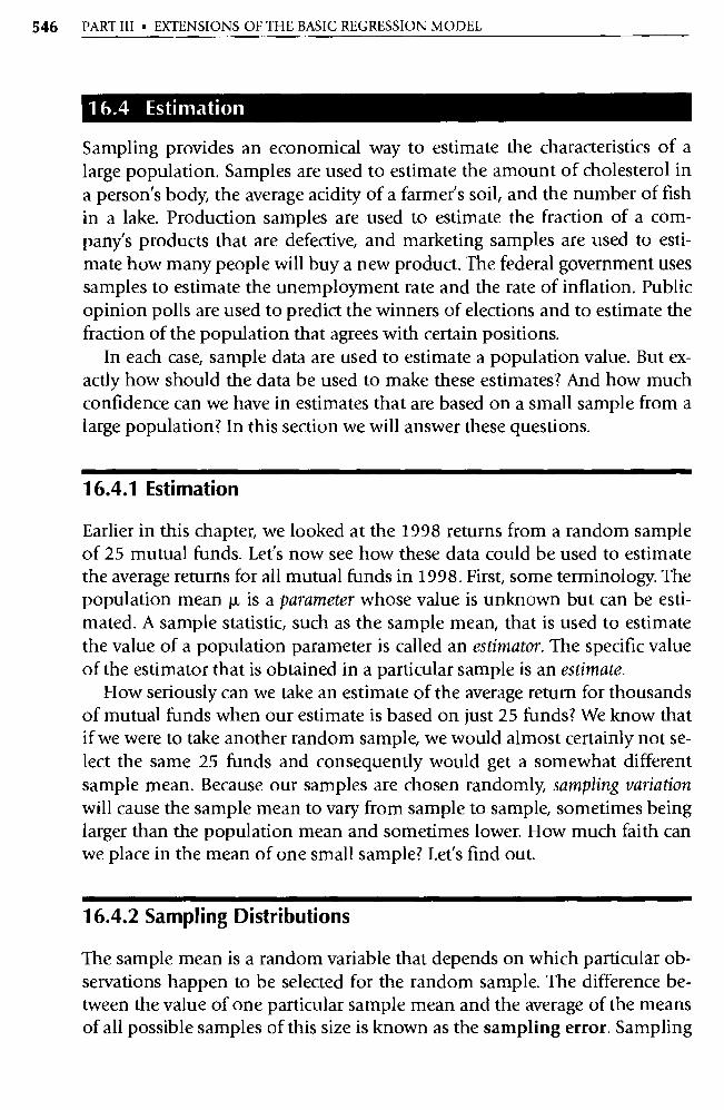
546 PART III • EXTENSIONS OF THE BASIC REGRESSION MODEL
16.4 Estimation
Sampling provides an economical way to estimate the characteristics of a large population. Samples are used to estimate the amount of cholesterol in a person's body, the average acidity of a farmer's soil, and the number of fish in a lake. Production samples are used to estimate the fraction of a com-pany's products that are defective, and marketing samples are used to esti-mate how many people will buy a new product. The federal government uses samples to estimate the unemployment rate and the rate of inflation. Public opinion polls are used to predict the winners of elections and to estimate the fraction of the population that agrees with ce rtain positions.
In each case, sample data are used to estimate a population value. But ex-actly how should the data be used to make these estimates? And how much confidence can we have in estimates that are based on a small sample from a large population? In this section we will answer these questions.
16.4.1 Estimation
Earlier in this chapter, we looked at the 1998 returns from a random sample of 25 mutual funds. Let's now see how these data could be used to estimate the average returns for all mutual funds in 1998. First, some terminology. The population mean µ is a parameter whose value is unknown but can be esti-mated. A sample statistic, such as the sample mean, that is used to estimate the value of a population parameter is called an estimator. The specific value of the estimator that is obtained in a particular sample is an estimate.
How seriously can we take an estimate of the average return for thousands of mutual funds when our estimate is based on just 25 funds? We know that if we were to take another random sample, we would almost certainly not se-lect the same 25 funds and consequently would get a somewhat different sample mean. Because our samples are chosen randomly, sampling variation will cause the sample mean to vary from sample to sample, sometimes being larger than the population mean and sometimes lower. How much faith can we place in the mean of one small sample? Let's find out.
16.4.2 Sampling Distributions
The sample mean is a random variable that depends on which particular ob-servations happen to be selected for the random sample. The difference be-tween the value of one particular sample mean and the average of the means of all possible samples of this size is known as the sampling error. Sampling
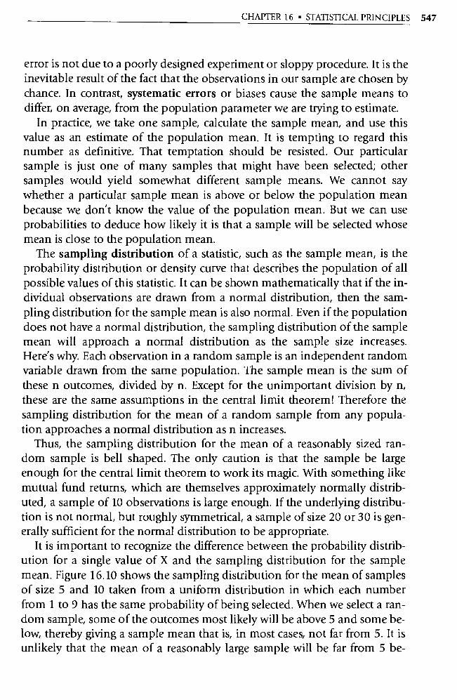
CHAPTER 16 • STATISTICAL PRINCIPLES 547
error is not due to a poorly designed experiment or sloppy procedure. It is the inevitable result of the fact that the observations in our sample are chosen by chance. In contrast, systematic errors or biases cause the sample means to differ, on average, from the population parameter we are trying to estimate.
In practice, we take one sample, calculate the sample mean, and use this value as an estimate of the population mean. It is tempting to regard this number as definitive. That temptation should be resisted. Our particular sample is just one of many samples that might have been selected; other samples would yield somewhat different sample means. We cannot say whether a particular sample mean is above or below the population mean because we don't know the value of the population mean. But we can use probabilities to deduce how likely it is that a sample will be selected whose mean is close to the population mean.
The sampling distribution of a statistic, such as the sample mean, is the probability distribution or density curve that describes the population of all possible values of this statistic. It can be shown mathematically that if the in-dividual observations are drawn from a normal dist ribution, then the sam-pling distribution for the sample mean is also normal. Even if the population does not have a normal distribution, the sampling distribution of the sample mean will approach a normal distribution as the sample size increases. Here's why. Each observation in a random sample is an independent random variable drawn from the same population. The sample mean is the sum of these n outcomes, divided by n. Except for the unimportant division by n, these are the same assumptions in the central limit theorem! Therefore the sampling distribution for the mean of a random sample from any popula-tion approaches a normal dist ribution as n increases.
Thus, the sampling distribution for the mean of a reasonably sized ran-dom sample is bell shaped. The only caution is that the sample be large enough for the central limit theorem to work its magic. With something like mutual fund returns, which are themselves approximately normally distrib-uted, a sample of 10 observations is large enough. If the underlying dist ribu-tion is not normal, but roughly symmetrical, a sample of size 20 or 30 is gen-erally sufficient for the normal distribution to be appropriate.
It is important to recognize the difference between the probability dist rib-ution for a single value of X and the sampling distribution for the sample mean. Figure 16.10 shows the sampling dis tribution for the mean of samples of size 5 and 10 taken from a uniform distribution in which each number from 1 to 9 has the same probability of being selected. When we select a ran-dom sample, some of the outcomes most likely will be above 5 and some be-low, thereby giving a sample mean that is, in most cases, not far from 5. It is unlikely that the mean of a reasonably large sample will be far from 5 be-
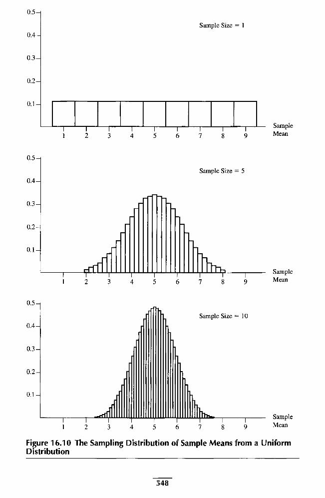
Sample Mean
Sample Size = 5
I I I 7 8 9
0.5
0.4
0.3
0.2
0.1
I I 1 I 1 I 1 2 3 4 5 6
0.5 —
0.4 —
0.3 —
0.2—
0.1 —
I 1 1 1 1 2 3 4 5 6
0.5 —
0.4 —
0.3 —
0.2 —
0.1 —
I I r 6 7 8 9
Sample Mean 5 1 2 4
Sample Mean
L I I
Sample Size = 1
I I I 8 7 9
Sample Size = 10
Figure 16.10 The Sampling Distribution of Sample Means from a Uniform Distribution
548

CHAPTER 16 • STATISTICAL PRINCIPLES 549
cause, for this to occur, the individual outcomes in the sample must repeat-edly be on one side of the population mean. The damping effects of averag-ing many outcomes give the sampling distribution for the sample mean a symmetrical bell shape.
In addition to the general shape of the sampling distribution, we need to know how its mean and standard deviation are related to the mean 1.1, and standard deviation Q of the population from which the individual observa-tions are drawn. It can be shown mathematically that this sampling distribu-tion has a mean equal to µ and a standard deviation equal to if divided by the square root of the sample size n:
Mean of X = µ
Standard deviation of X =
(16.5)
16.4.3 The Mean of the Sampling Distribution
Although we can never know with certainty exactly how close a particular sample mean is to the unknown population mean, we can use the mean and standard deviation of the sampling distribution to gauge the reliability of the sample mean as an estimator of the population mean. A sample statistic is an unbiased estimator of a population parameter if the mean of the sampling distribution of this statistic is equal to the value of the population parameter. Because the mean of the sampling distribution of the sample mean is µ, the sample mean is an unbiased estimator of the population mean.
Unbiased estimators have considerable appeal. It would be discomforting to use an estimator that one knows to be systematically too high or too low. A statistician who uses unbiased estimators can anticipate estimation errors that, over a lifetime, average close to zero. Of course, average performance is not the only thing that counts. A British Lord Justice once summarized his ca-reer by saying that "When I was a young man practicing at the bar, I lost a great many cases I should have won. As I got along, I won a great many cases I ought to have lost; so on the whole justice was done." The conscientious statistician should be concerned with not only how good the estimates are on average, but also how accurate they are in particular cases.
16.4.4 The Standard Deviation of the Sampling Distribution
One way of gauging the accuracy of an estimator is with its standard devia- tion. If an estimator has a large standard deviation, there is a substantial
550 PART III • EXTENSIONS OF THE BASIC REGRESSION MODEL
probability that the estimate will be far from its mean. If an estimator has a small standard deviation, there is a high probability that the estimate will be close to its mean.
Equation 16.5 states that the standard deviation of the sampling distribu-tion for the sample mean is equal to Q divided by the square root of the sam-ple size, n. As the number of obse rvations increases, the standard deviation of the sampling distribution declines. To understand this phenomenon, re-member that the standard deviation is a measure of the uncertainty of the outcome. With a large sample, it is extremely unlikely that all of the observa-tions will be far above the mean of the sampling distribution, and equally improbable that all of the obse rvations will be far below the mean. Instead, it is almost certain that some of the observations will be above the mean and some below, and that the average will be close to the mean of the sampling distribution.
16.4.5 The t-Distribution
The standard deviation of the sampling distribution depends on the value of population standard deviation cr, a parameter that is unknown but can be es-timated. The most natural estimator of Q, the standard deviation of the pop-ulation, is s, the standard deviation of the sample data from this population. The formula for the sample variance was given earlier in Equation 16.2, and the standard deviation s is the square root of the variance.
When the standard deviation of an estimator, such as the sample mean, is itself estimated from the data, this estimated standard deviation is called the estimator's standard error. The standard error of the sample mean is calcu-lated by replacing the unknown parameter s in Equation 16.5 with its esti- mate Q:
standard error of X = s/
The need to estimate the standard deviation creates another source of uncer-tainty in gauging the reliability of the sample mean as an estimator of the population mean.
In 1908, W. S. Gosset figured out how to handle this increased uncertainty when the data are drawn from a normal distribution. Gosset was a statisti-cian employed by the Irish brewery Guinness, which encouraged statistical research but not publication. Because of the importance of his findings, he was able to persuade Guinness to allow his work to be published under the pseudonym "Student" and his calculations became known as the Student's t-distribution.
CHAPTER 16 • STATISTICAL PRINCIPLES 551
aï
has a normal dis tribution. Gosset determined the sampling distribution of the variable that is created when the mean of a sample from a normal distrib-ution is standardized by subtracting and dividing by its standard error:
t=X w
(16.6) s/
The exact distribution of t depends on the sample size, because as the sample size increases, we are increasingly confident of the accuracy of the estimated standard deviation. For an infinite sample, the estimate s will equal the ac-tual value Q, and the distributions of t and Z coincide. With a small sample, s may be either larger or smaller than Q and the distribution of t is conse-quently more dispersed than the distribution of Z.
Table B-1 in Appendix B shows some probabilities for various t-distribu-tions that are identified by the number of degrees of freedom:
degrees of number of number of parameters that freedom observations must be estimated beforehand
Here, we calculate s by using n observations and one estimated parameter (the sample mean); therefore, there are n - 1 degrees of freedom.
There is another way to think about degrees of freedom that is more closely related to the name itself We calculate s from n squared deviations about the sample mean. However, we saw earlier in this chapter that the sum of the deviations about the sample mean is always zero. Thus if we know the values of n - 1 of these deviations, we know the value of the last deviation, too. Only n - 1 deviations are freely determined by the sample.
When the mean of a sample from a normal distribution is standardized by subtracting the mean 1.4 of its sampling distribution and dividing by the stan-dard deviation o-/ \Ai of its sampling distribution, the resulting Z variable
Z= X w
16.4.6 Confidence Intervals
Now we are ready to use the t-distribution and the standard error of the sam-ple mean to measure the reliability of our estimate of the population mean. If we specify a probability, such as a = 0.05, we can use Table B-1 to find the t value t* such that there is a probability a/2 that the value oft will exceed t*, a probability a/2 that the value oft will be less than -t*, and a probability 1 - a that the value oft will be in the interval --t* to t*:
552 PART III • EXTENSIONS OF THE BASIC REGRESSION MODEL
1 — a P[—t* < t < t*]
Using Equation 16.6 and rearranging,
1 — a=P µ— t*^<X<µ +t *^
We can rephrase this probability computation to show the confidence that
we have in using the sample mean to estimate the population mean. If there
is a 1 — a probability that the sample mean will turn out to be within t*
standard errors of the population mean µ, then there is a 1 — a probability
that the interval from
—t* ^ to X+t* ^J
will include the value of µ. Such an interval is called a confidence interval and the 1 — a probability is the interval's confidence level. The shorthand formula for a 1 — a percent confidence interval for the population mean µ is
1 — a confidence interval for µ: X ± t*(-)
(16.7)
There is a 0.95 probability that the sample mean X will be between µ — t*
(standard error of X) and p, + t* (standard error of X), in which case the in-terval X - t* (standard error of X) to X + t* (standard error of X) will en-compass R. There is a 0.05 probability that the sample mean will, by the luck of the draw, turn out to be more than t* (standard error of X) from the popu-lation mean p.., and that the confidence interval will consequently not in-clude µ.
Gosset derived the t-distribution by assuming that the sample data are
taken from a normal distribution. Subsequent research has shown that be-cause of the power of the central limit theorem, confidence intervals based on the t-distribution are remarkably accurate even if the underlying data are not normally distributed, as long as we have at least 15 obse rvations from a roughly symmetrical distribution or at least 30 obse rvations from a clearly asymmetrical distribution. 5 A histogram can be used for a rough symmetry
5. E. S. Pearson and N. W. Please, "Relation Between the Shape of Population Dist ribution and the Robustness of Four Simple Test Statistics," Biometrika, 1975, 62, pp. 223-241; Harry O. Poston, "The Robustness of the One-Sample t-test Over the Pearson System," Journal of Statisti-cal Computation and Simulation, 1979, pp. 133- 149.
CHAPTER 16 • STATISTICAL PRINCIPLES 553
check. Ninety-five percent confidence levels are standard, but there is no compelling reason why we can't use others.
Let's use the 1998 mutual fund data in Table 16.2 to construct a 95 percent confidence interval and a 99 percent confidence interval for the average re-turn for all stock mutual funds in 1998. The sample mean is 8.93 and the standard deviation is 12.7654. The sample size is 25 and there are conse-quently 25 1 24 degrees of freedom. Table B-1 shows that there is a 0.05 probability that the absolute value of t will exceed t* = 2.064 and a 0.01 probability that it will exceed t* = 2.797 Thus,
95% confidence interval for µ = 8.93 ± 2.064 12.7654 _ 8.93 + 5.27
V 25
99% confidence interval for µ = 8.93 ± 2.797 . 12'
./7654 = 8.93 ± 7.14
V
The actual value of the mean return for all stock mutual funds in 1998 was 12 percent, which is inside both of these confidence intervals.
Notice that it is the sample mean that varies from sample to sample, not the population mean. A 95 percent confidence interval for is interpreted as follows: "There is a 0.95 probability that the sample mean will turn out to be sufficiently close to µ so that my confidence interval includes µ. There is a 0.05 probability that the sample mean will happen to be so far from p. that my confidence interval does not include µ." The 0.95 probability refers to the chances that random sampling will result in an interval that includes the fixed parameter µ, not the probability that random sampling will give a value of µ that is inside a fixed confidence interval.
The general procedure for determining a confidence interval for a popula-tion mean is summarized here:
1. Calculate the sample mean. 2. Calculate the standard error of the sample mean by dividing the sam-
ple standard deviation s by the square root of the sample size n. 3. Select a confidence level (such as 95 percent) and look in Table B-1
with n 1 degrees of freedom to determine the t-value t* that corre-sponds to this probability.
4. A confidence interval for the population mean is equal to the sample mean plus or minus t* standard errors of the sample mean:
Confidence interval for µ = X ± t* (standard error of X)
=X±t*( s
554 PART III • EXTENSIONS OF THE BASIC REGRESSION MODEL
16.4.7 Sampling from Finite Populations
A very interesting characteristic of a confidence interval is that it does not de-pend on the size of the population. At first glance, this conclusion may seem surprising. If we are trying to estimate a characteristic of a large population, then there is a natural tendency to believe that a large sample is needed. If there are 25 million items in the population, a sample of 25 includes only one out of every million. How can we possibly obtain a reliable estimate with a sample that looks at only one out of every million items?
A moment's reflection reveals why a confidence interval doesn't depend on whether the population consists of one thousand or one billion items. The chances that the luck of the draw will yield a sample whose mean differs substantially from the population mean depends on the size of the sample and the chances of selecting items that are far from the population mean, not on how many items there are in the population.
16.5 Hypothesis Tests
We've seen how sample data can be used to estimate the value of a popula-tion parameter, such as µ, and determine a confidence interval that gauges the precision of this estimate. Now we will see how sample data can be used to support or refute theories about the value of µ; for example, whether mu-tual funds, on average, beat the market.
16.5.1 A General Framework for Hypothesis Tests
Statistical tests are not as definitive as mathematical proofs, because sample data are subject to sampling error. There is always a chance, however small, that a new sample will discredit a previously confirmed theory. We cannot be absolutely certain of the average return of all mutual funds until we actually calculate it using data for every single fund.
Most theories are potentially vulnerable to reassessment because there never is a final tabulation of all possible data. New experiments and fresh ob-servations continually provide new evidence—data that generally reaffirm previous studies, but occasionally create doubt or even reverse conclusions that were once thought firmly established. Theories are especially fragile in the humanities and social sciences, where there are few data and it is difficult to control for extraneous influences. In the 1960s, economists believed that there was a simple inverse relationship between a nation's unemployment rate and its rate of inflation: when unemployment goes up, inflation goes

CHAPTER 16 • STATISTICAL PRINCIPLES 555
down. In the 1970s, unemployment and inflation both went up, and econo-mists decided that they had overlooked other impo rtant influences, includ-ing inflation expectations.
If we can never be absolutely sure that a theory is true or false, the next best thing might seem to be to make probability statements, such as, "Based on the available data, there is a 0.90 probability that this theory is true." How-ever, a theory isn't true 90 percent of the time; it's either true or it isn't. As a re-sult, statistics has followed another route. Instead of estimating the probabil-ity that a theory is true, based on our observed data, statisticians calculate the reverse probability—that we would observe such data if the theory were true. An understanding of this distinction is crucial to an understanding of the meaning and limitations of hypothesis tests. Hypothesis tests are a proof by statistical contradiction. We calculate the probability of the observed out-come, or a more usual outcome, if the theory were true. If this probability is low, then the data are not consistent with the theory and therefore reject it, what Thomas Huxley called "the great tragedy of science—the slaying of a beautiful hypothesis by an ugly fact." This is a proof by statistical contradic-tion: because these data are unlikely to occur if the theory were true, we reject the theory. Of course, we can never be 100 percent ce rtain, because unlikely events sometimes do happen. Notice, too, that for a theory not to be rejected, it need only be consistent with the data. This is a relatively weak conclusion, because many other theories may also be consistent with the data.
16.5.2 The Null and Alternative Hypotheses
To make these general ideas more concrete, we will consider the performance of stock mutual funds. Our research question is how mutual funds perform, on average, compared with the overall stock market, as measured by the Stan-dard & Poor's index of the stocks of 500 prominent companies. For a proof by statistical contradiction, we make an assumption, called the null hypoth-esis (or Ho), about the population from which the sample is drawn. Typi-cally, the null hypothesis is a "straw assumption" that we anticipate rejecting.
Here, our research question suggests the natural null hypothesis that in any given year, the average return for the entire population of mutual funds is equal to the S&P 500 return. Although we may have initiated this study be-cause we believe that mutual funds systematically underperform or outper-form the market, the way to demonstrate this by statistical contradiction is to see if the evidence rejects the straw hypothesis that their average return is equal to the market return. We will analyze mutual fund performance in 1998 data, when the S&P 500 return was 28.1 percent. Thus our null hypoth-esis is 11 = 28.1.
556 PART III • EXTENSIONS OF THE BASIC REGRESSION MODEL
The alternative hypothesis (usually written as HA or H 1 ) describes the population if the null hypothesis is not true. Here, the natural alternative hy-pothesis is that the population mean is not equal to 28.1:
Ho : µ, = 28.1
HA: it 28.1
This alternative hypothesis is our research question, stated in terms of the value of the population parameter K. Here the alternative hypothesis is two sided, because (even though we might have a hunch about how the study will turn out) we are reluctant to rule out beforehand the possibility that the pop-ulation mean may be either lower or higher than the value specified by the null hypothesis. If, before seeing the data, we could rule out one of these pos-sibilities, the alternative hypothesis would be one sided. If, for example, we
were convinced beforehand that the average mutual fund return could not possibly be greater than the S&P 500 return, the one-sided alternative hy-pothesis would be HA: µ < 28.1.
16.5.3 The Test Statistic and Statistical Significance
Once we have specified the null and alternative hypotheses, we collect and ex-amine our sample data. Table 16.2 shows the 1998 returns for a random sam-ple of 25 mutual funds. As we are concerned with the value of µ, the popula-tion mean return, we calculate the mean of our random sample—because this is what we would use to estimate the value of the population mean. The esti-mator that is used to test the null hypothesis is called the test statistic.
The sample mean for these 25 mutual funds is 8.928 percent, and the standard deviation is 12.765 percent. Does this 8.928 percent average return provide persuasive evidence that the average mutual fund return in 1998 was less than 28.1 percent, or can it be explained by the inevitable variation in the means of small samples drawn from a population with a standard devia-tion estimated to be 12.765 percent?
As explained earlier in this chapter, the sampling distribution for the mean of a random sample from a population with a mean µ and a standard devia-tion cr has a mean µ and a standard deviation equal to Cr divided by the square root of the sample size. Even if the individual obse rvations are not normally distributed, a sample of size 25 should be sufficient to appeal to the central limit theorem. Thus the Z-statistic
Z = X µ
o/VT1
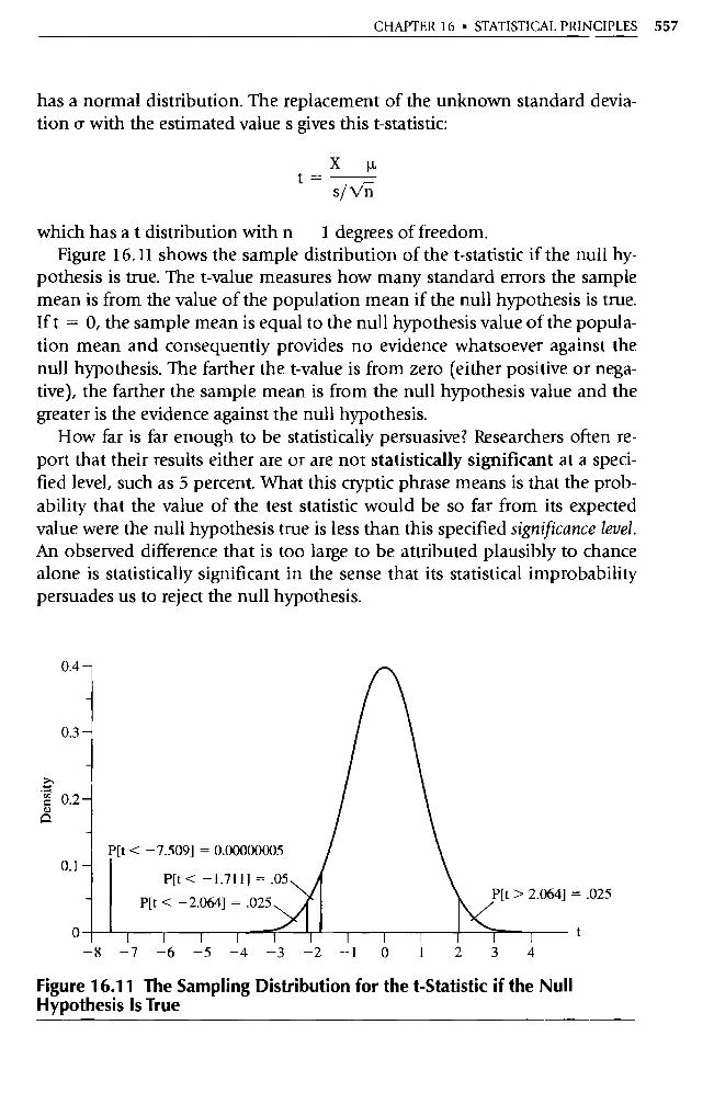
t 0 4 -8 -7 -6 -5 -4 -3 -2 -1 0 1
P[t < - 7.509] = 0.00000005
P[t < -1.711] = .05
P[t < - 2.064] = .025
CHAPTER 16 • STATISTICAL PRINCIPLES 557
has a normal distribution. The replacement of the unknown standard devia-tion 6 with the estimated value s gives this t-statistic:
X µ t=
s/ Vt't
which has a t distribution with n 1 degrees of freedom. Figure 16.11 shows the sample distribution of the t-statistic if the null hy-
pothesis is true. The t-value measures how many standard errors the sample mean is from the value of the population mean if the null hypothesis is true. If t = 0, the sample mean is equal to the null hypothesis value of the popula-tion mean and consequently provides no evidence whatsoever against the null hypothesis. The farther the t-value is from zero (either positive or nega-tive), the farther the sample mean is from the null hypothesis value and the greater is the evidence against the null hypothesis.
How far is far enough to be statistically persuasive? Researchers often re-port that their results either are or are not statistically significant at a speci-fied level, such as 5 percent. What this cryptic phrase means is that the prob-ability that the value of the test statistic would be so far from its expected value were the null hypothesis true is less than this specified significance level. An observed difference that is too large to be attributed plausibly to chance alone is statistically significant in the sense that its statistical improbability persuades us to reject the null hypothesis.
Figure 16.11 The Sampling Distribution for the t-Statistic if the Null Hypothesis Is True
558 PART III • EXTENSIONS OF THE BASIC REGRESSION MODEL
For our mutual fund example, Table B-1 tells us that with n - 1 = 25 1 24 degrees of freedom, there is a 0.025 probability that the t-value will be less than -2.064 and a 0.025 probability that the t-value will be larger than 2.064. These plus-or-minus 2.064 cutoffs for statistical signifi-cance are called the test's critical values. A t-value outside this range is suffi-cient, at the 5 percent level, to reject the null hypothesis that the average re-turn for all mutual funds in 1998 was 28.1 percent.
Notice that because our alternative hypothesis is two sided, we look at t-values that are far from 0 in either direction. If our alternative hypothesis were HA: < 28.1, then we reject the null hypothesis only if the sample mean is sufficiently far below 28.1 to give a sufficiently negative t-value. If the sample mean turns out to be far above 28.1, giving a large positive t-value, we must conclude that an improbable fluke happened. If we say beforehand that µ cannot possibly be above 28.1, we cannot change our mind after seeing the data! If we are willing to be persuaded by the data, then we must initially al-low the alternative hypothesis to be two sided.
If, fully aware of this implicit commitment, we are nonetheless con-vinced that the alternative hypothesis is one sided, then we use only a single critical value (a one-tail test). Table B-1 tells us that with 24 degrees of free-dom, there is a 0.05 probability that the t-value will be less than -1.711; this is consequently the critical value for the one-sided alternative hypothe-sis HA: µ, < 28.1.
In our mutual fund example, the t value is -7.509:
X µ t = S//T
-1
8.928 '28.1
12.765/ V 25
= -7.509
This t-value is far greater in absolute value than the - 2.064 critical value and therefore rejects the null hypothesis that the average return for all mutual funds in 1998 was 28.1 percent.
16.5.4 P-Values
To measure the extent to which our sample mean of 8.928 provides persua-sive evidence against the null hypothesis, we can calculate the probability that the t-value would be so far from 0 if the null hypothesis were true. We don't calculate the probability that t will be exactly equal to -7.509. The

CHAPTER 16 • STATISTICAL PRINCIPLES 559
probability that a continuous variable like t will equal any single number is zero. Instead, we determine the probability that t will be so far (or farther) from zero: P[t < —7.509] = 0.00000005.
The P-value for a test of a null hypothesis about the population mean is the probability, if the null hypothesis is in fact true, that a random sample of this size would yield a sample mean that is this far (or farther) from the value of the population mean assumed by the null hypothesis. A small P-value casts doubt on the null hypothesis.
The P-value can be obtained from statistical software using the t-distribu-tion and is exactly correct if the data come from a normal distribution and, because of the power of the central limit theorem, is an excellent approxima-tion if we have at least 15 observations from a generally symmetrical distrib-ution, or at least 30 observations from a very asymmetrical distribution.
In calculating the P-value, we must take into account whether the alterna-tive hypothesis is one sided or two sided. For a one-sided alternative hypothe-sis, the P-value is the probability that the sample mean would be so far to one side of the null hypothesis population mean. For a two-sided alte rnative hy-pothesis, the P-value is the probability that the test statistic would be so far, in either direction, from the null hypothesis population mean. In our mutual fund example, we repo rt the probability that the sample mean will be 7.509 standard errors or more, in either direction, from 28.1. Because the normal distribution is symmetrical, we double the 0.00000005 probability calculated above and repo rt the two-sided P-value as 2(0.00000005) = 0.0000001.
Because this probability is so slight, sampling error is an unconvincing ex-planation for why the average return in our sample is less than 28.1. A t-value of —7.509 is too improbable to be explained plausibly by the luck of the draw. We have shown, by statistical contradiction, that the average mutual fund return in 1998 was not 28.1 percent.
16.5.5 Using Confidence Intervals
Confidence intervals provide a useful alternative method of reporting the re-sults of a two-sided statistical test. A null hypothesis will be rejected by a two-sided hypothesis test if and only if its value lies outside a corresponding con-fidence inte rval. We can illustrate this equivalence by considering our test of the null hypothesis that the average mutual fund return was 28.1 percent in 1998.
This null hypothesis will be rejected at the 5 percent level if the two-sided P-value is less than 0.05, which requires the sample mean to be more than 2.064 standard errors from 28.1 percent. A 95 percent confidence interval for
560 PART III • EXTENSIONS OF THE BASIC REGRESSION MODEL
µ includes all values that are within 2.064 standard errors of the sample mean. Therefore, a hypothesis test can be conducted by using the sample data to construct a confidence interval and seeing whether the parameter value specified by the null hypothesis is inside this inte rval.
The additional information provided by a confidence interval is a sense of the practical impo rtance of the difference between the parameter value as-sumed by the null hypothesis and the value of the estimator. If we just repo rt
that the P-value is 0.0000001 or that we "found a statistically significant dif-ference at the 5 percent level," readers will not know the actual value of the estimator. In addition to the P-value, we should repo rt a confidence interval.
For our mutual fund example, we saw earlier in this chapter that a 95 per-cent confidence interval is:
95% confidence interval for µ = 8.93 ± 2.064 12.7654
_ 8.93 ± 5.27 V25
As anticipated, the value 28.1 is not inside this confidence interval. Further, we see that the distance of this confidence interval from 28.1 is of consider-able practical importance to investors.
The obse rvation that any value inside a 95 confidence interval would not be rejected at the 5 percent level if tested as a null hypothesis reinforces our earlier remark that not rejecting a null hypothesis is a rather weak conclu-sion. Not rejecting a null hypothesis is not at all the same as proving the null hypothesis to be true. An unrejected null hypothesis is but one of many para-meter values that is consistent with the data. Thus we must be careful to say "the data do not reject the null hypothesis," rather than "the data prove the null hypothesis to be true."
16.5.6 Is It Important?
In testing hypotheses, it is easy to be confused by the distinction between statistical significance and practical importance. A statistically significant re-sult may be of little practical impo rtance. Conversely, a researcher may find a potentially very important result that does not happen to be statistically significant.
Consider the question of whether men or women are more likely to be right handed. A sample of 6,672 people found that 90 percent of the men and 92 percent of the women were right handed. This difference is statisti-cally significant, but unimportant. Or consider the conclusion of two econo-mists studying the effect of inflation on election outcomes. They estimated
CHAPTER 16 • STATISTICAL PRINCIPLES 561
that the inflation issue increased the Republican vote in the 1976 election by 7 percentage points, plus or minus 10 percentage points. Because 0 is inside this interval, they concluded that "in fact, and contrary to widely held views, inflation has no impact on voting behavior." 6 That is not at all what their data show. The fact that they cannot rule out 0 does not prove that 0 is the correct value. Their 95 percent confidence interval does include 0, but it also includes everything from —3 percent to +17 percent. Their best estimate is 7 percent, plus or minus 10 percent, and 7 percent is more than enough to swing most elections one way or another. This result is not statistically signif-icant, but it might be impo rtant.
16.5.7 An Overview of Hypothesis Testing
We can summarize our general procedure as follows.
1. Specify the null hypothesis and whether the alternative hypothesis is one sided or two sided.
2. Use the sample data to estimate the value of the population parameter whose value is specified by the null hypothesis.
3. If this sample statistic is approximately normally distributed, calculate the t-value, which measures how many standard errors the estimate is from the null hypothesis:
Observed statistic — Null hypothesis parameter value Standard error of statistic
For testing a null hypothesis about the value of the population mean, we use the sample mean as our test statistic and calculate this t value:
X µ t=
s/VFn
4. Determine the critical values of t corresponding to the test's selected significance level, and see if the t-value for this sample is outside this range.
5. Report a confidence interval in order to assess the practical importance of the results.
t=
6. F. Arcelus and A. H. Meltzer, "The Effect of Aggregate Economic Va riables on Congressional Elections," American Political Science Review, 1975, 69, pp. 1232-1239.
562 PART III • EXTENSIONS OF THE BASIC REGRESSION MODEL
16.6 Summary
1. Descriptive statistics can often be used to summarize a set of data. The median and mean describe the center of the data, around which the other values are spread. Outliers, values that are very different from the other observations, can pull the mean substantially above or be-low the median. In comparison to the mean, the median is more ro-bust or resistant to outliers.
2. The variance or standard deviation can be used to gauge the spread or variation in the data about its mean. The variance is the average squared deviation of the obse rvations about their mean. The standard deviation is the square root of the variance.
3. The probability that the value of a continuous random variable will be in a specified interval is shown by the corresponding area under a probability density curve. The expected value of a random variable is the anticipated long-run average value of the outcomes. The standard deviation measures the extent to which the outcomes may differ from the expected value; a large standard deviation indicates a great deal of uncertainty, as the outcomes are likely to be far from the expected value.
4. A (discrete or continuous) random variable X is standardized by sub-tracting its mean vi, and then dividing by the standard deviation 6:
Z = (x — µ) /cr
which has a mean of zero and a standard deviation of one. The cen-tral limit theorem explains why so many random variables are ap-proximately normally distributed.
5. A population is the entire group of items that interests us; a sample is the part of the population that we actually obse rve. Statistical infer-ence is used to make inferences about the population from which the sample came. Deliberate attempts to construct representative samples are unwise; instead, statisticians recommend that data be based on a random sample. A selection bias occurs when some members of the population are systematically excluded or underrepresented in the group from which the sample is taken.
6. If a random variable X is normally distributed with a mean µ and standard deviation Q, then the sampling distribution for the mean of

CHAPTER 16 • STATISTICAL PRINCIPLES 563
a random sample of n observations is a normal distribution with a mean µ, and a standard deviation equal to Q divided by the square root of the sample size n. Even if the underlying distribution is not normal, a sufficiently large sample will ensure that the sampling dis-tribution of the sample mean is approximately normal.
7 The sample mean is an unbiased estimator of µ, and a confidence in-terval can be used to gauge the degree of sampling error:
Confidence interval for µ = X ± t* (standard error of X) = X ± t
where s is the sample standard deviation, n is the sample size, and t* is given by a t-distribution with n — 1 degrees of freedom.
8. To conduct a hypothesis test, we specify the null and alternative hy-potheses and then use the sample data to estimate the population pa-rameter whose value is specified by the null hypothesis. For testing a null hypothesis about the value of the population mean, we use the sample mean as our test statistic and calculate this t-value:
X
t= s/V17}
The critical t-values for a specified significance level, such as 5 percent or 1 percent, are given by the t-distribution with n — 1 degrees of freedom. Alternatively, we can determine the P-value.
Exercises
(Answers to even-numbered exercises are in Appendix A)
1. Write the meaning of each of the following terms without referring to the book (or your notes), and compare your definition with the ver-sion in the text for each. a. median b. mean c. histogram d. variance e. standard deviation f. random variable
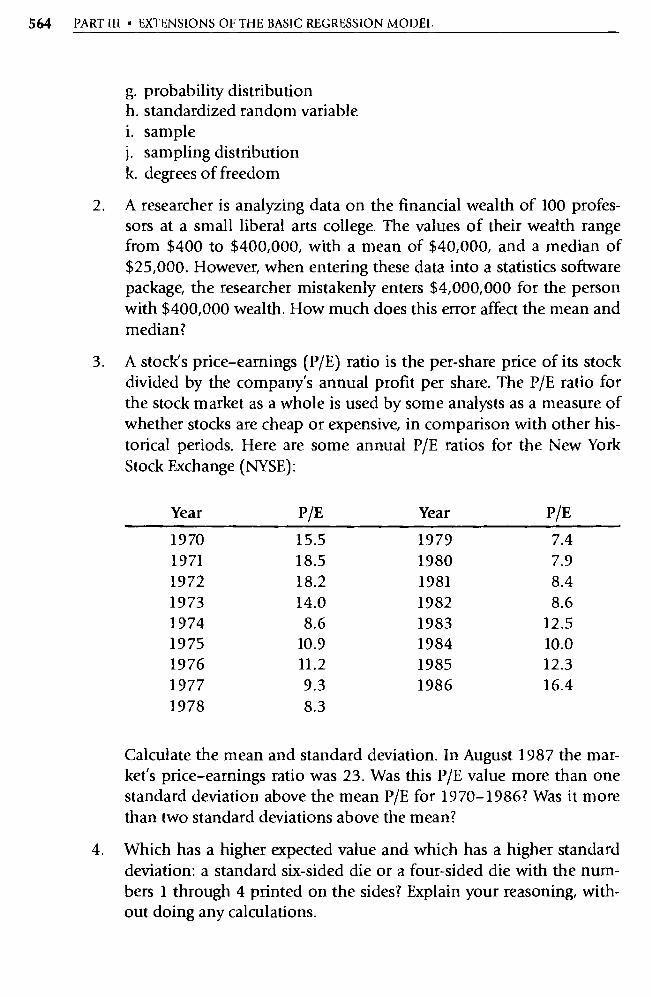
564 PART III • EXTENSIONS OF THE BASIC REGRESSION MODEL
g. probability distribution h. standardized random variable i. sample j. sampling distribution k. degrees of freedom
2. A researcher is analyzing data on the financial wealth of 100 profes-sors at a small liberal a rts college. The values of their wealth range from $400 to $400,000, with a mean of $40,000, and a median of $25,000. However, when entering these data into a statistics so ftware package, the researcher mistakenly enters $4,000,000 for the person with $400,000 wealth. How much does this error affect the mean and median?
3. A stock's price-earnings (P/E) ratio is the per-share price of its stock divided by the company's annual profit per share. The P/E ratio for the stock market as a whole is used by some analysts as a measure of whether stocks are cheap or expensive, in comparison with other his-torical periods. Here are some annual P/E ratios for the New York Stock Exchange (NYSE):
Year P/E Year P/E
1970 15.5 1979 7.4 1971 18.5 1980 7.9 1972 18.2 1981 8.4 1973 14.0 1982 8.6 1974 8.6 1983 12.5 1975 10.9 1984 10.0 1976 11.2 1985 12.3 1977 9.3 1986 16.4 1978 8.3
Calculate the mean and standard deviation. In August 1987 the mar-ket's price-earnings ratio was 23. Was this P/E value more than one standard deviation above the mean P/E for 1970-1986? Was it more than two standard deviations above the mean?
4. Which has a higher expected value and which has a higher standard deviation: a standard six-sided die or a four-sided die with the num-bers 1 through 4 printed on the sides? Explain your reasoning, with-out doing any calculations.
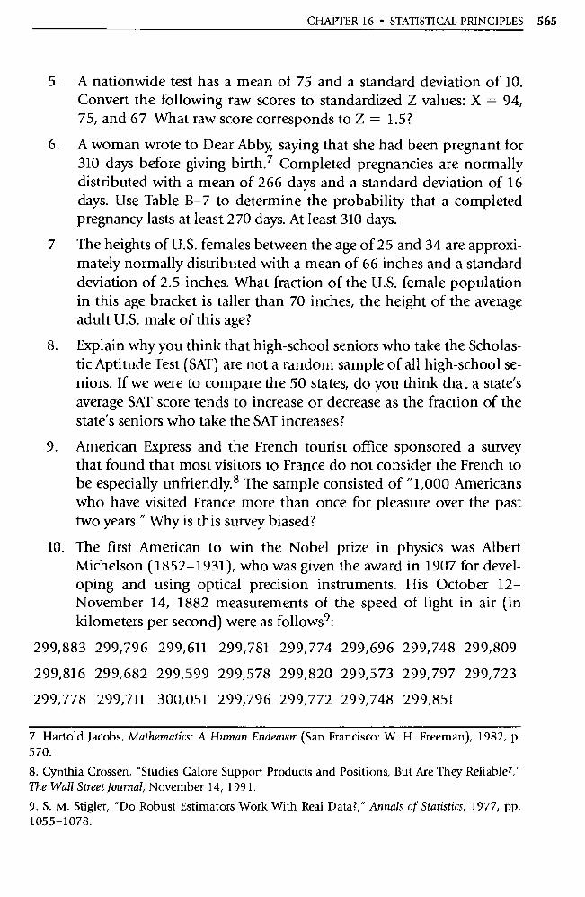
CHAPTER 16 • STATISTICAL PRINCIPLES 565
5. A nationwide test has a mean of 75 and a standard deviation of 10. Convert the following raw scores to standardized Z values: X = 94, 75, and 67 What raw score corresponds to Z = 1.5?
6. A woman wrote to Dear Abby, saying that she had been pregnant for 310 days before giving birth. 7 Completed pregnancies are normally distributed with a mean of 266 days and a standard deviation of 16 days. Use Table B-7 to determine the probability that a completed pregnancy lasts at least 270 days. At least 310 days.
7 The heights of U.S. females between the age of 25 and 34 are approxi-mately normally distributed with a mean of 66 inches and a standard deviation of 2.5 inches. What fraction of the U.S. female population in this age bracket is taller than 70 inches, the height of the average adult U.S. male of this age?
8. Explain why you think that high-school seniors who take the Scholas-tic Aptitude Test (SAT) are not a random sample of all high-school se-niors. If we were to compare the 50 states, do you think that a state's average SAT score tends to increase or decrease as the fraction of the state's seniors who take the SAT increases?
9. American Express and the French tourist office sponsored a survey that found that most visitors to France do not consider the French to be especially unfriendly. 8 The sample consisted of "1,000 Americans who have visited France more than once for pleasure over the past two years." Why is this survey biased?
10. The first American to win the Nobel prize in physics was Albe rt Michelson (1852-1931), who was given the award in 1907 for devel-
oping and using optical precision instruments. His October 12-November 14, 1882 measurements of the speed of light in air (in kilometers per second) were as follows:
299,883 299,796 299,611 299,781 299,774 299,696 299,748 299,809
299,816 299,682 299,599 299,578 299,820 299,573 299,797 299,723
299,778 299,711 300,051 299,796 299,772 299,748 299,851
7 Hartold Jacobs, Mathematics: A Human Endeavor (San Francisco: W. H. Freeman), 1982, p. 570.
8. Cynthia Crossen, "Studies Galore Suppo rt Products and Positions, But Are They Reliable?," The Wall Street Journal, November 14, 1991.
9. S. M. Stigler, "Do Robust Estimators Work With Real Data?," Annals of Statistics, 1977, pp. 1055-1078.

566 PART III • EXTENSIONS OF THE BASIC REGRESSION MODEL
Assuming that these measurements were a random sample from a normal distribution, does a 99 percent confidence interval include the value 299,710.5 that is now accepted as the speed of light?
11. A Wall Street Journal (July 6, 1987) poll asked 35 economic forecasters to predict the interest rate on 3-month Treasury bills in June 1988. These 35 forecasts had a mean of 6.19 and a variance of 0.47 Assum-ing these to be a random sample, give a 95 percent confidence inter-val for the mean prediction of all economic forecasters and then ex-plain why each of these interpretations is or is not correct: a. There is a 0.95 probability that the actual Treasury-bill rate on June
1988 will be in this interval. b. Approximately 95 percent of the predictions of all economic fore-
casters are in this interval.
12. The earlobe test was introduced in a letter to the prestigious New En-gland Journal of Medicine, in which Dr. Sanders Frank reported that 20 of his male patients with creases in their earlobes had many of the risk factors (such as high cholesterol levels, high blood pressure, and heavy cigarette usage) associated with heart disease. For instance, the average cholesterol level for his patients with noticeable earlobe creases was 257 (mg per 100 ml), compared to an average of 215 with a standard deviation of 10 for healthy middle-aged men. If these 20 patients were a random sample from a population with a mean of 215 and a standard deviation of 10, what is the probability their aver-age cholesterol level would be 257 or higher? Explain why these 20 patients may, in fact, not be a random sample.
13. A researcher examined the admissions to a mental health clinic's emergency room on days when the moon was full. 10 For the 12 days with full moons from August 1971 through July 1972, the number of people admitted were
5 13 14 12 6 9 13 16 25 13 14 20
Calculate the t-value for a test of the null hypothesis that these data are a random sample from a normal distribution with a population mean equal to 11.2, the average number of admissions on other days.
10. Sheldon Blackman and Don Catalina, "The Moon and the Emergency Room," Perceptual and Motor Skills, 1973, 37, pp. 624-626.
CHAPTER 16 • STATISTICAL PRINCIPLES 567
14. Use the 1997 data in Table 16.2 to determine the t-value for a test of the null hypothesis that these data were drawn from a population with a mean of 33.4 percent, the return on the S&P 500 index that year.
15. A treatment group was given a cold vaccine while the control group received a placebo. Doctors then recorded the fraction of each group that caught a cold and calculated the two-sided P-value to be 0.08. Ex-plain why you either agree or disagree with each of the interpretations of these results: a. "There is an 8 percent probability that this cold vaccine works." b. "If a randomly selected person takes this vaccine, the chances of
getting sick fall by about 8 percent." c. "These data do not show a statistically significant effect at the 5
percent level; therefore, we are 95 percent certain that this vaccine doesn't work."

A APPENDIX
Answers to Even-Numbered Exercises
Chapter One
1-2. There are four steps to running your first regression on EViews: a. Install EViews: Inse rt the EViews CD-ROM into your computer,
open it (by going to the D: drive po rtion of the "my computer" section of Windows) and then click on "install EViews to disc." If you respond "next" or "yes" when requested, you should eventu-ally get a "successfully installed" message.
b. Start EViews: Return to the D: drive po rtion of the "my com-puter" section of Windows, open EViews (this might require clicking on "EViews 3.1"), and then click on "run.
c. Open the datafile: In order, click on "file," "open, and "work-file." Then browse to the CD-ROM, select the folder "Studen-mund," and click on "HTWT1" and "OK."
d. Run the regression: Type in "LS Y C X" on the top line of EViews, making sure to leave spaces between the variable names. (LS stands for least squares and C stands for constant.) Then hit "en-ter," and the regression result will appear on the screen.
1 -4. a. Customers number 3, 4, and 20; no. b. Weight is determined by more than just height. c. People who decide to play the weight-guessing game may feel
they have a weight that is hard to guess.
1-6. a. The coefficient of L i represents the change in the percentage chance of making a putt when the length of the putt increases by one foot. In this case, the percentage chance of making the putt decreases by 4.1 for each foot longer the putt is.
b. 42.6 percent, yes; 79.5 percent, no (too low); —18.9 percent, no (negative!).
c. One problem is that the theoretical relationship between the length of the putt and the percentage of putts made is almost surely nonlinear in the variables; we'll discuss models appropri-ate to this problem in Chapter 7. A second problem is that the
569
570 APPENDIX A
actual dependent variable is limited by zero and one but the re-gression estimate is not; we'll discuss models appropriate to this problem in Chapter 13.
d. The equations are identical. To convert one to the other, you need to know that Pi = Pi — e i, which is true because e i = Pi Pi (or more generally, e i = Yi
1-8. a. 13y is the change in S caused by a one-unit increase in Y, holding G constant, and 13 G is the change in S caused by a one-unit in-crease in G, holding Y constant.
b. +, c. Yes. Richer states spend at least some of their extra money on ed-
ucation, but states with rapidly growing student populations find it difficult to increase spending at the same rate as the student population, causing spending per student to fall, especially if you hold the wealth of the state constant.
d. Si = —183 + 0.1422Yî — 59.26G î. Note that 59.26 • 10 = 5926 • 0.10, so nothing in the equation has changed except the scale of the coefficient of G.
1-10. a. 19.8: A $1 billion increase in GDP will be associated with an in-crease of $19.80 in the average price of a new house. 7406.6: Technically, the constant term equals the value of the dependent variable when all the independent variables equal zero, but in most cases (as in this one) such a definition has little economic meaning. As we'll learn in Chapters 4 and 7, estimates of the con-stant term should not be relied on for inference.
b. It doesn't matter what letters we use as symbols for the depen-dent and independent variables.
c. You could measure both Pt and Yt in real terms by dividing each observation by the GDP deflator (or the CPI) for that year (and multiplying by 100).
d. The price of houses is determined by the forces of supply and de-mand, and we won't discuss the estimation of simultaneous equations until Chapter 14. In a demand-oriented sense, GDP is probably measuring buying power, which is better represented by disposable income. In a supply-oriented sense, GDP might be standing for costs like wages and the price of materials.
1-12. Linear in the coefficients: a, b, c. Linear in neither: d, e.
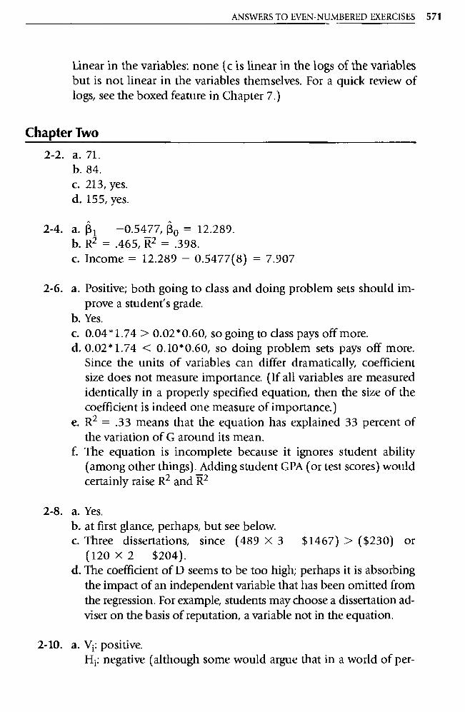
ANSWERS TO EVEN-NUMBERED EXERCISES 571
Linear in the variables: none (c is linear in the logs of the variables but is not linear in the variables themselves. For a quick review of logs, see the boxed feature in Chapter 7.)
Chapter Two
2-2. a. 71. b. 84. c. 213, yes. d. 155, yes.
2-4. a. (3 1 — 0.5477, Ro = 12.289. b. R2 = .465, R2 = .398. c. Income = 12.289 — 0.5477(8) = 7.907
2-6. a. Positive; both going to class and doing problem sets should im-prove a student's grade.
b. Yes. c. 0.04* 1.74 > 0.02 * 0.60, so going to class pays off more. d. 0.02 * 1.74 < 0.10 * 0.60, so doing problem sets pays off more.
Since the units of variables can differ dramatically, coefficient size does not measure impo rtance. (If all variables are measured identically in a properly specified equation, then the size of the coefficient is indeed one measure of impo rtance.)
e. R2 = .33 means that the equation has explained 33 percent of the variation of G around its mean.
f. The equation is incomplete because it ignores student ability (among other things). Adding student GPA (or test scores) would certainly raise R2 and R2
2-8. a. Yes. b. at first glance, perhaps, but see below. c. Three dissertations, since (489 X 3 $1467) > ($230) or
(120 X 2 $204). d. The coefficient of D seems to be too high; perhaps it is absorbing
the impact of an independent va riable that has been omitted from the regression. For example, students may choose a disse rtation ad-viser on the basis of reputation, a va riable not in the equation.
2 - 10. a. Vi : positive. Hi: negative (although some would argue that in a world of per-

572 APPENDIX A
fect information, drivers would take fewer risks if they knew the state had few hospitals). Ci: ambiguous because a high rate of driving citations could indi-cate risky driving (raising fatalities) or zealous police citation policies (reducing risky driving and therefore fatalities).
b. No, because the coefficient differences are small and the data will differ from year to year. We'd be more concerned if the coeffi-cients differed by orders of magnitude or changed sign.
c. Since the equation for 1982 has similar degrees of freedom and a much lower R2, no calculation is needed to know that the equa-tion for 1981 has a higher R 2 . Just to be sure, we calculated R 2
and obtained .652 for 1981 and .565 for 1982.
2-12. a. aE(e2)/aRo = 2 E (Yi — 110 — R1Xi)( -1 ) aI(e2)/aR1 = 2 E(Yi — Ro — R 1Xi)( — R 1Xi )
b. 0 = —2 E(Yi — 13 — R 1 Xi)
0 = —2 13 1 E (Yi — 1-3 0 — 13 1 Xi) (X 1 ) or, rearranging:
EYi — n130+131 Ex; EYiXi = 13o EXi + 131 Ex?
These are the normal equations. c. To get 13 i , solve the first normal equation for 13 0, obtaining
130 = (EYi 13 1 EXi)/n and substitute this value in for 13 0 where it appears in the second normal equation, obtaining
EYiXi = (EYi — 131 EXi)(EXi)/n + I3 1 EX1, which becomes
131 = — EYi EXi)/LnEX; — (EXi)2]. With some al- gebraic manipulation (in part using the fact that EXi = nX), this simplifies to Equation 2.6.
d. To get Equation 2.7, solve the first normal equation for 13 0, using X = E Xi/n.
Chapter Three
3.2. a. D = 1 if graduate student, and D = 0 if undergraduate. b. Yes, for example E = how many exercises (such as this) the stu-
dent did. c. If D is defined as in answer a, then its coefficient's sign would be
expected to be positive. If D is defined as 0 if graduate student, 1 if undergraduate, then the expected sign would be negative.
ANSWERS TO EVEN-NUMBERED EXERCISES 573
d. A coefficient with value of .5 indicates that, all else equal, a graduate student would be expected to earn half a grade point higher than an undergraduate. If there were only graduate students or only under-graduates in lass, the coefficient of D could not be estimated.
3-4. a. There are many possible omitted explanatory variables; for exam-ple, the number of parking spaces near the restaurant.
3-6. a. New P = Old P/1000, so (3 goes from 0.3547 to 354.7 b. 320. c. No.
3-8. a. A male student's GRE subject score in Economics is likely to be 39.7 points higher than a female's, holding constant their GPA and SATs.
b. This result is evidence of, but not proof of, bias. If we were sure that we had the best possible specification (the topic of Chapter 6) and if this result turned out to be statistically significant (the topic of Chapter 5), and if we were able to reproduce this result in other samples, we'd be much closer to a "proof." Even then, there still would be a possibility that some factor other than bias was the cause of these results.
c. Possible variables include the number of upper division econom-ics courses taken, the number of mathematics classes taken, and dummy variables measuring whether the student had taken econometrics or international economics (two fields frequently covered in the test). It's vital that any suggested variable be cross-sectional by student, however.
d. The equation would become GRE ; = 212.1 39.7G ; + 78.9GPA; + 0.203SATM; + 0.110SATV; .
3-10. a. All positive except for the coefficient of F;, which in today's male-dominated movie industry probably has a negative expected sign.
b. Arnold, because $500,000 < ($4,000,000 — $3,027,000). c. Yes, since 200 X 15.4 = $3,080,000 > $1,200,000. d. Yes, since $1,770,000 > $1,000,000. e. Yes, the unexpected sign of the coefficient of B.
Chapter Four
4-2. Pair "c" clearly violates Assumption VI, and pair "a" might violate it for some samples.
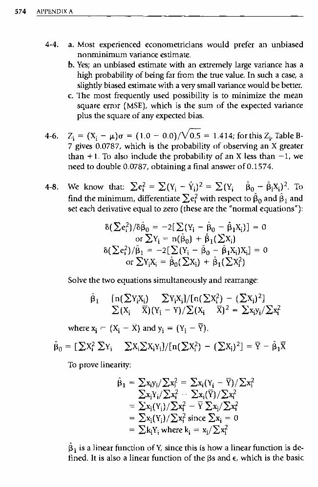
574 APPENDIX A
4-4. a. Most experienced econometricians would prefer an unbiased nonminimum variance estimate.
b. Yes; an unbiased estimate with an extremely large va riance has a high probability of being far from the true value. In such a case, a slightly biased estimate with a very small va riance would be better.
c. The most frequently used possibility is to minimize the mean square error (MSE), which is the sum of the expected variance plus the square of any expected bias.
4-6. Zi = (Xi — µ) Q = ( 1.0 — 0.0)/V0.5 = 1.414; for this Zi, Table B-7 gives 0.0787, which is the probability of observing an X greater than +1. To also include the probability of an X less than —1, we need to double 0.0787, obtaining a final answer of 0.1574.
4-8. We know that: » ei = E (Yi — i(1)2 = E (Yi Ro — R1X1) 2 . To find the minimum, differentiate »e; with respect to Ro and R1 and set each derivative equal to zero (these are the "normal equations"):
8 (Eei)/00 = —2 [E(Y1 — RO — I Xi)] = 0 or EYi = n(R 0) + A1(EXi)
8 (Eei)/0.1 = —2 [E(Yi — Ro — 0.1Xi)Xi] = o or EYiXi = Ro(EXi) + R1(EXi )
Solve the two equations simultaneously and rearrange:
R 1 [n(EYiX1) EYiXi]/[n(EX?) - (EX1) 2 ]
E (Xi X) (Yi - Y) /E (Xi X) 2 = Exiyi/Ex
where xi = (Xi — X) and yi = (Y1 — V).
Rp = [EXi EYi EXiEXiYi]/[n(EX?) — (EXi) 2 ]
To prove linearity:
R1 = Exiyi/Exi = Exi(Yi - Y)/Ex ExiYi/Exi - Exi(Y)/Exi
- Exi(Yi)/Exi - Y Exi/Xx = Exi (Yi)/Ex? since Exi = 0
= EkiYi where ki = xi/Ex
R 1 is a linear function of Y, since this is how a linear function is de- fined. It is also a linear function of the f3s and E, which is the basic

ANSWERS TO EVEN-NUMBERED EXERCISES 575
interpretation of linearity. R1 13 oEki + Ekixi + EkiEi. R o = Y 13 1 (X) where Y = Ro + f (x), which is also a linear
equation.
To prove unbiasedness: R1 = EkiYi Ek1 030 + 131Xi + E i)
= EkiRo+ +EkiEi
Since ki = x;/Ex; _ (Xi — ) /E (X; R) 2, then Eki = 0, Ek? = 1/Ex?, Ikixi = EkiXi = 1. So, 1. 1 = R1 + Ekiei and given the assumptions of Ei, E(13i) = R1 + Eki E(E;) = 131, proving R1 is unbiased.
To prove minimum variance (of all linear unbiased estimators): 13 1 EkiY1 . Since k i = xi/Ex? = (Xi — X)/E (Xi x) 2, R1 is a weighted average of the Ys, and the k i are the weights. To write an expression for any linear estimator, substitute w ; for k; , which are also weights but not necessarily equal to
R 1 = Ew iYi , so E((31) ExiE(Yi) = Ewi(Ro + R1Xi) = RoEwi + R1EwiXi
In order for 13; to be unbiased, Ewi = 0 and EwiXi = 1. The vari-able of 13 1 :
VAR(131`) = VAR EwiYi Ewi VAR Y; = 0-2 Ewe [VAR (Y1) = VAR (E; ) = a- 2 ]
= Q 2L^ (wi — xi/Ex; + xi/Exi) 2 = Q 2 E(wi — xi/Ex? + xi/Exi ) 2 = o-2 E(wi — xi/Exl )2 + 62EXi/(Exl ) 2
+ 20-2E (wi — xi/Ex?) = Q2E(wi — xi/E4)2 + 0-2/(Exi )
The last term in this equation is a constant, so the variance of 13 can be minimized only by manipulating the first term. The first term is minimized only by letting w ; = xi/Ex?, then:
VAR([3f) = (3-2/Exi = VAR 01).
When the least-squares weights, k ;, equal wi, the variance of the lin-
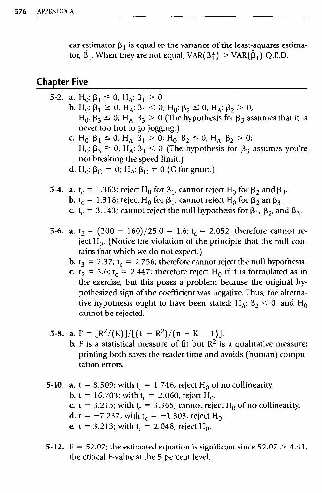
576 APPENDIX A
ear estimator R1 is equal to the variance of the least-squares estima-tor, (3 1 . When they are not equal, VAR(13i) > VAR(K) Q.E.D.
Chapter Five
5-2. a. Ho : (3 1 ^ 0, HA: 131 > 0
b.H0: Pi O , HA: Pi <O; H0 :13 2 _ 0, HA: 13 2 > 0; H0 : (3 3 S 0, HA: (33 > 0 (The hypothesis for 13 3 assumes that it is never too hot to go jogging.)
c. Ho :13 1 0, HA: Pi > O; Ho : (3 2 O, HA: (3 2 > 0;
Ho: (33 ' O, HA: R3 < 0 (The hypothesis for (3 3 assumes you're not breaking the speed limit.)
d. H o : (3G — 0; HA: (3 G 0 (G for grunt.)
5-4. a. tc = 1.363; reject H o for (3 1 , cannot reject H o for (32 and 13 3 . b. tc = 1.318; reject H o for 13 1 , cannot reject H o for R2 an (3 3 . c. tc = 3.143; cannot reject the null hypothesis for (3 1 , 132 , and 133 .
5-6. a. t2 = (200 — 160) /25.0 = 1.6; tc = 2.052; therefore cannot re-ject Ho . (Notice the violation of the principle that the null con-tains that which we do not expect.)
b. t3 = 2.37; tc = 2.756; therefore cannot reject the null hypothesis.
c. t2 = 5.6; tc = 2.447; therefore reject H o if it is formulated as in the exercise, but this poses a problem because the original hy-pothesized sign of the coefficient was negative. Thus, the alterna-tive hypothesis ought to have been stated: HA: 132 < 0, and Ho cannot be rejected.
5-8. a. F = [R2/(K)]/[(1 — R2)/(n — K 1)]. b. F is a statistical measure of fit but R 2 is a qualitative measure;
printing both saves the reader time and avoids (human) compu-tation errors.
5- 10. a. t = 8.509; with tc = 1.746, reject Ho of no collinearity. b. t = 16.703; with tc = 2.060, reject H o . c. t = 3.215; with tc = 3.365, cannot reject H o of no collinearity. d. t = — 7.237; with tc = —1.303, reject Ho.
e. t = 3.213; with tc = 2.048, reject H o .
5 - 12. F = 52.07; the estimated equation is significant since 52.07 > 4.41, the critical F-value at the 5 percent level.

ANSWERS TO EVEN-NUMBERED EXERCISES 577
5-14. a. T: H o : (3T 0, HA: 3T > 0. Reject H o since 1+5.571 > 1.711 and + 5.57 has the sign of HA.
P: Ho : [3p ? 0, HA: (3p < 0. Reject H o since I -2.351 > 1.711 and -2.35 has the sign of HA. A: Ho : j3A 0, HA: (3A > 0. Cannot reject Ho since 1+1.2441 < 1.711. C: H o : f3c ^ 0, HA: Rc > 0. Cannot reject H o since -1.10 < 1.711 or since -1.10 does not have the sign of HA.
b. Reject all null hypotheses. c. Reject null hypotheses for T, J, and S. Cannot reject null hypotheses
for F (since 1-1.471 < 1.645) or B (since 1-1.331 < 1.645 or since - 1.33 does not have the sign of H A).
5 - 16. a. All five tests are one-sided, so to = 1.706 throughout. GDPN: Ho : f3 5- 0, HA: f3 > 0. Reject H o because 16.691 > 1.706
and 6.69 is positive as in HA. CVN: Ho : [3 ? 0, HA: (3 < 0. Reject H o because 1 -2.66 >
1.706 and -2.66 is negative as in HA. PP: Ho : (3 0, HA: (3 > 0. Do not reject H o because 11.191
< 1.706. DPC: Ho: [3 ? 0, HA: (3 < 0. Reject Ho because 1-2.251 >
1.706 and -2.25 is negative as in HA. IPC: Ho : f3 ? 0, HA: f3 < 0. Do not reject H o because 1 - 1.591
< 1.706. b. Reject Ho of no effect because F = 22.35 is larger than the critical
Fe value of 2.59 (interpolated). c. Our confidence interval equation is (3 ± tÊ SE((3), and the 10 per-
cent two-sided to = 1.706 (the same as a one-sided 5 percent t e), so the confidence interval equals (3 ± 1.706 • SE((3), or: GDPN: 1.07 < (3 < 1.79 CVN: -0.98 < f3 < -0.22 PP: -3.13 < < 17.75 DPC: -27.45 < R < -3.81 IPC: -23.59 < R < 0.83
d. Yes. The important signs were as expected and statistically signifi-cant, and the overall fit was good.
e. Little would change: for the first two coefficients, such a specifi-cation change would alter the coefficient sizes but not their signs or significance; for the coefficients of the three dummy variables, even though the coefficient sizes would change dramatically, it's unlikely that their signs and significance would change.
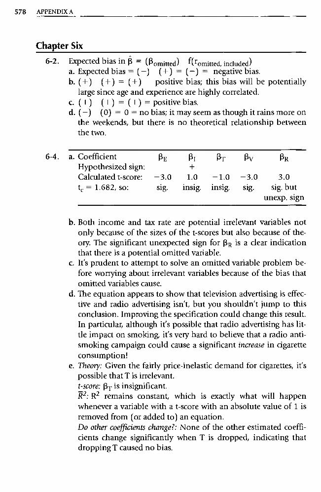
578 APPENDIX A
Chapter S ix
6-2. Expected bias in [3 = (-omitted) f(romitted, included) a. Expected bias = (—) (+) = (—) = negative bias. b. (+) (+) = (+) positive bias; this bias will be potentially
large since age and experience are highly correlated. c. (+) (+) = (+) = positive bias. d. ( —) (0) = 0 = no bias; it may seem as though it rains more on
the weekends, but there is no theoretical relationship between the two.
6-4. a. Coefficient -E -I -T -V -R Hypothesized sign: + Calculated t-score: —3.0 1.0 —1.0 —3.0 3.0 tc = 1.682, so: sig. insig. insig. sig. sig. but
unexp. sign
b. Both income and tax rate are potential irrelevant variables not only because of the sizes of the t-scores but also because of the-ory. The significant unexpected sign for -R is a clear indication that there is a potential omitted variable.
c. It's prudent to attempt to solve an omitted variable problem be-fore worrying about irrelevant variables because of the bias that omitted variables cause.
d. The equation appears to show that television advertising is effec-tive and radio advertising isn't, but you shouldn't jump to this conclusion. Improving the specification could change this result. In particular, although it's possible that radio advertising has lit-tle impact on smoking, it's very hard to believe that a radio anti-smoking campaign could cause a significant increase in cigarette consumption!
e. Theory: Given the fairly price-inelastic demand for cigarettes, it's possible that T is irrelevant. t-score: -T is insignificant. R2 : R2 remains constant, which is exactly what will happen whenever a variable with a t-score with an absolute value of 1 is removed from (or added to) an equation. Do other coefficients change?: None of the other estimated coeffi-cients change significantly when T is dropped, indicating that dropping T caused no bias.

ANSWERS TO EVEN-NUMBERED EXERCISES 579
Conclusion: Based on these four criteria, it's reasonable to con-clude that T is an irrelevant variable.
6-6. a. Coefficient 13 1 13 2 03 04 Hypothesized sign: + + + Calculated t-score: 5.0 1.0 10.0 3.0
tc = 2.485 (1% level), so: sig. insig. sig. unexpected sign
b. The significant unexpected sign of R4 is evidence of a possible omitted variable that is exerting positive bias. The omitted vari-able must either be correlated positively with X4 and have a posi-tive expected coefficient or else be correlated negatively with X4
and have a negative expected coefficient. The fairly low calculated t-score for 13 2 is not strong evidence of a specification error.
c. A second run might add an independent variable that is theoreti-cally sound and that could have caused positive bias in f3.- 4. For example, X5 = the number of "attractions" like movie theaters or shopping malls in the area would have a positive expected coeffi-cient and be positively correlated with the number of nearby competing stores.
6-8. a. Nothing is ce rtain, but the best guess is: X 1 = number of stu-dents, X2 = chain price, X3 = temperature, X4 = Cooler price.
b. X4 has the only negative coefficient, and Cooler price has the only negative expected sign. Number of students (in thousands) should be the most significant and have the largest coefficient. Weather should be the least significant and also have a small co-efficient (since that variable can be the largest in size). X2
chain price by elimination. c. Note that developing hypotheses includes determining the de-
sired level of significance. A possible rerun would be to drop (or reformulate to absolute degrees difference from optimal ham-burger-eating range, if there is such a thing) the weather variable. If there is omitted variable bias, it is positive on 134 (advertising?).
6-10. a. Consumers and producers can react differently to changes in the same variable. For example, price: a rise in price causes con-sumers to demand a lower quantity and producers to supply a greater quantity.

580 APPENDIX A
b. Include variables affecting demand ("demand-side va riables") only in demand equations and va riables affecting supply ("sup-ply-side variables") only in supply equations.
c. Review the literature, decide whether the equation you wish to estimate is a supply or a demand e quation, and, when specifying the model, think carefully about whether an independent vari-able is appropriate for a demand ',or supply equation.
6-12. a. No bias (+ • 0) unless weather patterns indicate a correlation between rainfall and temperature. If it tends to rain more when it's cold, then there would be a small negative bias (+ —) .
b. Positive bias (+ +) . c. Positive bias (+ +) . d. Negative bias (+ —) given a likely negative correlation between
hours studied for the test and hours slept.
6- 14. a. Coefficient RP RL RA RN Hypothesized sign: + + + + Calculated t-score: 3.3 1.5 — 0.6 13.5 tc = 1.677 (approx.), so: sig. insig. insig. sig.
b. The inclusion of N means that the other variables probably should be aimed at differences between the situations of farm women and rural nonfarm women, but they are not, probably because such data are unavailable. Thus, the equation certainly has omitted variables. If they can be found, then L, A, and possi-bly even P might be irrelevant.
c. Add a variable measuring the average income of farm women in the ith state, if possible as a ratio to the average income of rural nonfarm women in the state. Note that this is a sample of states, so suggesting adding a variable relating to specific women would create a mismatch in the data set.
d. Theory: if L is the best proxy available for the relative income of farm women, then it has a strong theoretical basis until the preferred va riable can be found.
t-score: insignificant at the 5 percent level (but significant at the 10 percent level).
R2 : R2 is not given, but it turns out that the deletion of any variable with a t-score greater than one in absolute value will lower R2, in this case not by much.

ANSWERS TO EVEN-NUMBERED EXERCISES 581
Bias: none of the coefficients change significantly. Thus, the four criteria are inconclusive. As long as relative in- come data are unavailable, L probably should be retained.
Chapter Seven
7-2. a. Semilog [where Y = f(lnX)]; as income increases, the sales of shoes will increase, but at a declining rate.
b. Linear (intercept dummy); there is little theory for any other form. c. Semilog (as in part a above) or linear are both justifiable. d. Inverse function [where Y = f(1 /X) ]; as the interest rate gets
higher, the quantity of money demanded will decrease, but even at very high interest rates there still will be some money held to allow for transactions.
e. Quadratic function [where Y = f(X,X 2) ]; as output levels are in-creased, we will encounter diminishing returns to scale.
f. Although functional form should be chosen on the basis of the-ory, one outlier is capable of shifting an estimated quadratic un-reasonably; in such cases, a double-log function might avoid the problem.
7-4. a. Coefficient R 1 (32
Hypothesized sign: + + Calculated t-score: 4.0 2.20 tc = 1.708 at the 5% level, so: Ha : (3 _ 0 can be
rejected for both.
b. It is the sum of the constant effect of omitted independent vari-ables and the nonzero mean of the sample error term observa-tions; it does not mean that salaries (logged) could be negative.
c. For this semilog function, the slopes are (3 1 SALi and 132SALi , which both increase as the Xs rise. This implies that a one-unit change in EDi will cause a (3 1 percent change in SALi, which makes sense for salaries.
d. The Res cannot be compared because the dependent va riables are different. To do so, you would need to calculate a "quasi-R 2."
7-6. a. The Midwest (the fourth region of the count ry). b. Including the omitted condition as a variable will cause the dum-
mies to sum to a constant (1.0). This constant will be perfectly
582 APPENDIX A
collinear with the constant term, and the computer will not be able to estimate the equation.
c. Positive. d. Most correct = III, least correct = I.
7-8. Let PCI i = per capita income in the ith period, GRi = rate of growth in the ith period, and Ei = a classical error term. a. GRi = a0 + a 1 PCI i + a2PCIi + Ei where we'd expect a l > 0
and a2 < 0.
b. A semilog function alone cannot change from positive to nega-tive slope, so it is not appropriate.
c. GRi = 13 0 + 13 1 PCI i + (32 D i + (33D ;PCIi + Ei, where D i = 0 if PCI i <_ $2,000 and D i = 1 if PCIi > $2,000. ($2,000 is an esti-mate of the turning point.)
7 - 10. a. The expected signs are 13 1 , + or ?; R2, + 133, + ; (3 4, + b. ADi/SAi: the inverse form implies that the larger sales are the
smaller will be the impact of advertising on profits. CAP i, ESi, DGi: the semilog functional form implies that as each of these variables increases (holding all others in the equation constant), PR increases at a decreasing rate.
c. 13 2 , 133, and 13 4 all have positive expected signs, so (+) (+) = (+) = positive expected bias on (3 1 if one of the other Xs were omitted.
7-12. a. The estimated coefficients all are in the expected direction, and those for A and S are significant. R 2 seems fairly low, even for a cross-sectional data set of this nature.
b. It implies that wages rise and then fall with respect to age but does not imply perfect collinearity.
c. With a semilog function form (lnY), a slope coefficient repre-sents the percentage change in the dependent variable caused by a one-unit increase in the independent variable (holding con-stant all the other independent variables). Since pay raises are of-ten discussed in percentage terms, such a functional form fre-quently is used to model wage rates and sala ries.
d. It's a good habit to ignore R0 (except to make sure that one ex-ists) even if it looks too large or too small.
e. The poor fit and the insignificant estimated coefficient of union membership are all reasons for being extremely cautious about

ANSWERS TO EVEN-NUMBERED EXERCISES 583
7- 14.
using this regression to draw any conclusions about union mem-bership.
a. Coefficient (3 B RS RD Hypothesized sign: + + Calculated t-score: —0.08 1.85 —1.29 tc = 1.682, so: insig. sig. insig.
The insignificance of âB could be caused by an omitted variable, but it's likely that the interaction variable has "soaked up" the entire effect of beer consumption. Although we cannot reject the null hypothesis or 13 D, we see no reason to consider D to be an ir-relevant variable because of its sound theory and reasonable sta-tistics.
b. The interaction variable is a measure of whether the impact of beer drinking on traffic fatalities rises as the altitude of the city rises. For each unit increase in the multiple of B and A, F rises by 0.011, holding constant all the other independent variables in the equation. Thus, the size of the coefficient has no real intuitive meaning in and of itself.
c. Ho: RBA ^O HA: 3BA > O Reject Ho because 14.051 > tc = 1.682 and 4.05 is positive and thus matches the sign implied by HA.
d. Although there is no ironclad rule (as there is with slope dum-mies) most econometricians include both interaction-term com-ponents as independent variables. The major reason for this prac-tice is to avoid the possibility that an interaction term's
coefficient might be significant only because it is picking up the
effect of the omitted interaction-term component (bias).
e. The exception to this general practice occurs when there is no
reason to expect the interaction-term component to have any
theoretical validity on its own. We prefer Equation 7.27 to 7.26 because we don't believe that altitude typically would be in-cluded as an independent variable in a highway fatality equation.
Of our other three specification criteria, only the increase in R 2 supports considering A to be a relevant variable. However, even
moderate theoretical suppo rt for the inclusion of A on its own would result in our preferring Equation 7.26.
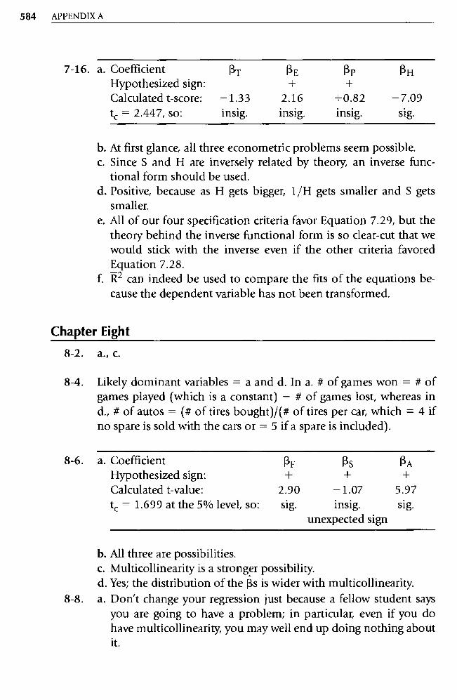
584 APPENDIX A
7- 16. a. Coefficient PT RE RP PH Hypothesized sign: + + Calculated t-score: —1.33 2.16 +0.82 —7.09 tc = 2.447, so: insig. insig. insig. sig.
b. At first glance, all three econometric problems seem possible. c. Since S and H are inversely related by theory, an inverse func-
tional form should be used. d. Positive, because as H gets bigger, 1/H gets smaller and S gets
smaller. e. All of our four specification criteria favor Equation 7.29, but the
theory behind the inverse functional form is so clear-cut that we would stick with the inverse even if the other criteria favored Equation 7.28.
f. R2 can indeed be used to compare the fits of the equations be-cause the dependent variable has not been transformed.
Chapter Eight
8-2. a., c.
8-4. Likely dominant variables = a and d. In a. # of games won = # of games played (which is a constant) — # of games lost, whereas in d., # of autos = (# of tires bought)/(# of tires per car, which = 4 if no spare is sold with the cars or = 5 if a spare is included).
a. Coefficient RF RS RA Hypothesized sign: + + + Calculated t-value: 2.90 —1.07 5.97 tc = 1.699 at the 5% level, so: sig. insig.
unexpected sign sig.
b. All three are possibilities. c. Multicollinearity is a stronger possibility. d. Yes; the distribution of the Rs is wider with multicollinearity.
8 -8. a. Don't change your regression just because a fellow student says you are going to have a problem; in pa rticular, even if you do have multicollinearity, you may well end up doing nothing about it.
8-6.
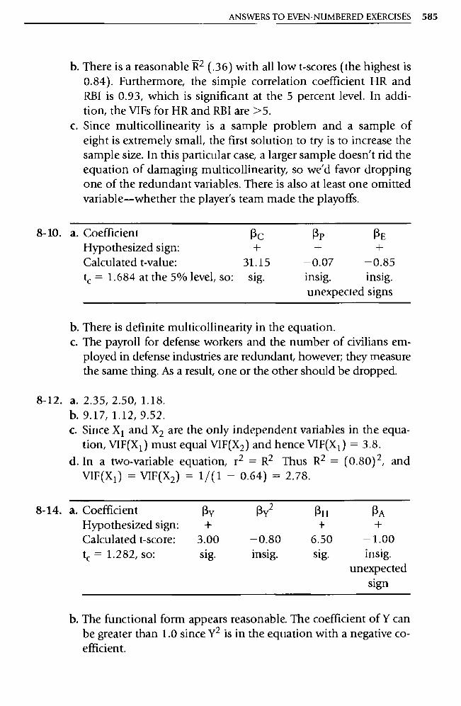
ANSWERS TO EVEN-NUMBERED EXERCISES 585
b. There is a reasonable R2 (.36) with all low t-scores (the highest is 0.84). Furthermore, the simple correlation coefficient HR and RBI is 0.93, which is significant at the 5 percent level. In addi-tion, the VIFs for HR and RBI are >5.
c. Since multicollinearity is a sample problem and a sample of eight is extremely small, the first solution to try is to increase the sample size. In this particular case, a larger sample doesn't rid the equation of damaging multicollinearity, so we'd favor dropping one of the redundant variables. There is also at least one omitted variable—whether the player's team made the playoffs.
8-10. a. Coefficient Pc Rp RE Hypothesized sign: + + + Calculated t-value: 31.15 –0.07 –0.85 tc = 1.684 at the 5% level, so: sig. insig. insig.
unexpected signs
b. There is definite multicollinearity in the equation. c. The payroll for defense workers and the number of civilians em-
ployed in defense industries are redundant, however; they measure the same thing. As a result, one or the other should be dropped.
8-12. a. 2.35, 2.50, 1.18. b. 9.17, 1.12, 9.52. c. Since X 1 and X2 are the only independent variables in the equa-
tion, VIF(X 1 ) must equal VIF(X2 ) and hence VIF(X 1 ) = 3.8.
d. In a two-variable equation, r 2 = R2 Thus R2 = ( 0.80) 2 , and VIF(X 1 ) = VIF(X2 ) = 1/(1 – 0.64) = 2.78.
8-14. a. Coefficient Ry Ry2 PH Hypothesized sign: + + Calculated t-score: 3.00 –0.80 6.50 tc = 1.282, so: sig. insig. sig.
RA +
–1.00 insig.
unexpected sign
b. The functional form appears reasonable. The coefficient of Y can be greater than 1.0 since Y 2 is in the equation with a negative co-efficient.
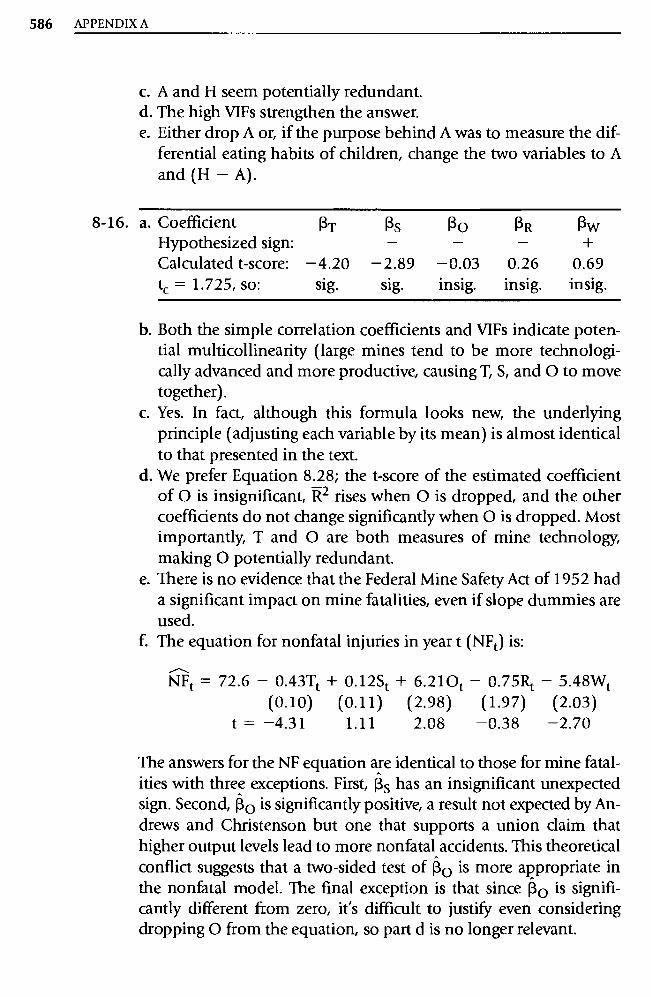
586 APPENDIX A
c. A and H seem potentially redundant. d. The high VIFs strengthen the answer. e. Either drop A or, if the purpose behind A was to measure the dif-
ferential eating habits of children, change the two variables to A and (H — A).
8-16. a. Coefficient PT Ps Ro PR Rw Hypothesized sign: — — — + Calculated t-score: —4.20 —2.89 —0.03 0.26 0.69 tc = 1.725, so: sig. sig. insig. insig. insig.
b. Both the simple correlation coefficients and VIFs indicate poten-tial multicollinearity (large mines tend to be more technologi-cally advanced and more productive, causing T, S, and O to move together).
c. Yes. In fact, although this formula looks new, the underlying principle (adjusting each variable by its mean) is almost identical to that presented in the text.
d. We prefer Equation 8.28; the t-score of the estimated coefficient of O is insignificant, R2 rises when O is dropped, and the other coefficients do not change significantly when O is dropped. Most importantly, T and O are both measures of mine technology, making O potentially redundant.
e. There is no evidence that the Federal Mine Safety Act of 1952 had a significant impact on mine fatalities, even if slope dummies are used.
f. The equation for nonfatal injuries in year t (NF t) is:
NFt = 72.6 — 0.43Tt + 0.12St + 6.21Ot — 0.75Rt — 5.48Wt (0.10) (0.11) (2.98) (1.97) (2.03)
t = —4.31 1.11 2.08 —0.38 —2.70
The answers for the NF equation are identical to those for mine fatal-ities with three exceptions. First, Rs has an insignificant unexpected sign. Second, âo is significantly positive, a result not expected by An-drews and Christenson but one that suppo rts a union claim that higher output levels lead to more nonfatal accidents. This theoretical conflict suggests that a two-sided test of 130 is more appropriate in the nonfatal model. The final exception is that since Ro is signifi-cantly different from zero, it's difficult to justify even considering dropping 0 from the equation, so pa rt d is no longer relevant.
ANSWERS TO EVEN-NUMBERED EXERCISES 587
Hints for Section 8.7.2: The SAT Interactive Regression Learning Exercise:
1. Severe multicollinearity between APMATH and APENG is the only possible problem in this regression. You should switch to the AP linear combination immediately.
2. An omitted variable is a distinct possibility, but be sure to choose the one to add on the basis of theory.
3. Either an omitted or irrelevant va riable is a possibility. In this case, theory seems more important than any mild statistical insignificance.
4. On balance, this is a reasonable regression. We see no reason to worry about theoretically sound variables that have slightly insignif-icant coefficients with expected signs. We're concerned that the co-efficient of GEND seems larger in absolute size than those reported in the literature, but none of the specification alternatives seems re-motely likely to remedy this problem.
S. An omitted variable is a possibility, but there are no signs of bias and this is a fairly reasonable equation already.
6. We'd prefer not to add PREP (since many students take prep courses because they did poorly on their first shots at the SAT) or RACE (be-cause of its redundancy with ESL and the lack of real diversity at Ar-cadia High). If you make a specification change, be sure to evaluate the change with our four specification criteria.
7. Either an omitted or irrelevant variable is a possibility, although GEND seems theoretically and statistically strong.
8. The unexpected sign makes us concerned with the possibility that an omitted variable is causing bias or that PREP is irrelevant. If PREP is relevant, what omission could have caused this result? How strong is the theory behind PREP?
9. This is a case of imperfect multicollinearity. Even though the VIFs are only between 3.8 and 4.0, the definitions of ESL and RACE (and the high simple correlation coe fficient between them) make them seem like redundant variables. Remember to use theory (and not statistical fit) to decide which one to drop.
10. An omitted variable or irrelevant variable is a possibility, but there are no signs of bias and this is a fairly reasonable equation already.
11. Despite the switch to the AP linear combination, we still have an unexpected sign, so we're still concerned with the possibility that an omitted variable is causing bias or that PREP is irrelevant. If PREP is relevant, what omission could have caused this result? How strong is the theory behind PREP?
588 APPENDIX A
12. All of the choices would improve this equation except switching to the AP linear combination. If you make a specification change, be sure to evaluate the change with our four specification criteria.
13. To get to this result, you had to have made at least three suspect specification decisions, and you're running the risk of bias due to a sequential specification search. Our advice is to stop, take a break, review Chapters 6-8, and then try this interactive exercise again.
14. We'd prefer not to add PREP (since many students take prep courses because they did poorly on their first shots at the SAT) or ESL (be-cause of its redundancy with RACE and the lack of real diversity at Arcadia High). If you make a specification change, be sure to evalu-ate the change with our four specification criteria.
15. Unless you drop one of the redundant variables, you're going to continue to have severe multicollinearity.
16. From theory and from the results, it seems as if the decision to switch to the AP linear combination was a waste of a regression mn. Even if there were severe collinearity between APMATH and APENG (which there isn't), the original coefficients are significant enough in the expected direction to suggest taking no action to offset any multicollinearity.
17. On reflection, PREP probably should not have been chosen in the first place. Many students take prep courses only because they did poorly on their first shots at the SAT or because they anticipate do-ing poorly. Thus, even if the PREP courses improve SAT scores, which they probably do, the students who think they need to take them were otherwise going to score worse than their colleagues (holding the other variables in the equation constant). The two ef-fects seem likely to offset each other, making PREP an irrelevant variable. If you make a specification change, be sure to evaluate the change with our four specification criteria.
18. Either adding GEND or dropping PREP would be a good choice, and it's hard to choose between the two. If you make a specification change, be sure to evaluate the change with our four specification criteria.
19. On balance, this is a reasonable regression. We'd prefer not to add PREP (since many students take prep courses because they did poorly on their first shots at the SAT), but the theoretical case for ESL (or RACE) seems strong. We're concerned that the coefficient of GEND seems larger in absolute size than those reported in the liter-ature, but none of the specification alternatives seems remotely likely to remedy this problem. If you make a specification change, be sure to evaluate the change with our four specification criteria.
ANSWERS TO EVEN-NUMBERED EXERCISES 589
Chapter Nine
9-2. a. Reject H 0 of no positive serial correlation (d < d L 1.03). b. Cannot reject H 0 of no positive serial correlation (d > d u = 1.25). c. Inconclusive (d L = 0.98 < d < 1.73 = du). d. Inconclusive (4—du =4— 1.63=2.37<d<4—dL =
4— 1.13=2.87). e. Cannot reject H 0 of no positive serial correlation (d > d u = 1.57). f. Reject H 0 of no serial correlation (d < d L 1.04). g. Inconclusive (d L = 0.90 < d < 1.99 = du).
9-4. a. 03 = 13o( 1 — p), so to get 13 0, divide 03 by (1 — p}. b. To account for the fact that the equation was estimated with GLS.
c. 13 0 = 26.7/(1 — 0.90) = 267 d. The equations are inherently different, and different equations
can have drastically different constant terms, because 13 0 acts as a "garbage collector" for the equation it is in. As a result, we should not analyze the estimated values of the constant term.
9-6. The same test applies, but the inconclusive region has expanded be-cause of the small sample size and the large number of explanatory variables. As a result, even if the DW = 2 you cannot conclude that there is no positive serial correlation.
9-8. a. Except for the first and last observations in the sample, the DW test's ability to detect first-order serial correlation is unchanged.
b. GLS can be applied mechanically to correct for serial correlation, but this procedure generally does not make sense; this time's er-ror term is now hypothesized to be a function of next time's error term.
c. First-order serial correlation in data that have been entered in re-verse chronological order means that this time's error term is a function of next time's error term. This might occur if, for exam-ple, the decision makers accurately predict and adjust to future random events before they occur, which would be the case in a world of rational expectations and perfect information.
9-10. a. Ft = 13.99 0.700RPt + 0.854Pt (1.840) (0.250)
t = —0.38 3.41
R2 = .288 n = 25 DW = 1.248

590 APPENDIX A
b. The relative price coefficient is now insignificant, and the dummy variable is now significant in the unanticipated direction (that is, the Pope's decision significantly increased the fish con-sumption). In addition the DW is inconclusive in testing for se-rial correlation, but the DW of 1.247 is quite close to the d L of 1.21 (for a 10 percent two-sided level of significance). Thus, the omitted variable has not only caused bias, it also has moved the DW d just about into the positive serial correlation range.
c. This exercise is a good example of why it makes sense to search for specification errors before adjusting for serial correlation.
9 - 12. a. Coefficient Hypothesized sign: Calculated t-score: tc = 1.714 at 5 percent, so:
P1nY PPB PPP PD + +
6.6 —2.6 2.7 —3.7 all four are significantly different from zero in the expected direction.
b. With a 5 percent, one-sided test and n 28, k' = 4, the critical values are d L 1.10 and du = 1.75. Since d = 0.94 < 1.10, we can reject the null hypothesis of no positive serial correlation.
c. The probable serial correlation suggests GLS. d. We prefer the GLS equation because we've rid the equation of
much of the serial correlation while retaining estimated coeffi-cients that make economic sense. Note that the dependent vari-ables in the two equations are different, so an improved fit is not evidence of a better equation.
9 - 14. a. Equation 9.26:
Coefficient 13 1 P2 P3 Hypothesized sign: + + + Calculated t-score: 0.76 14.98 1.80 tc = 1.721, so: insig. sig. sig.
Equation 9.27:
Coefficient Pi P2 Hypothesized sign: + + Calculated t-score: 1.44 28.09 tc = 1.717, so: insig. sig.
(Note: The authors explain a positive sign for Psp by stating that

ANSWERS TO EVEN-NUMBERED EXERCISES 591
the Soviet leadership became "more competitive" after 1977, leading the USSR to increase defense spending as SP increased.)
b. All three statistical specification criteria imply that SP is a rele-vant variable: R2 increases when SP is added, SP's coefficient is significantly different from zero, and the other coefficient esti-mates do not change more than one standard error when SP is added. On the other hand, our original expectation was that the sign of Rsp would be negative (an idea supported by the fact that the authors obtained a negative sign for (a sp for the subset of the sample from 1960 to 1976) and that Equation 9.26 therefore has a significant unexpected sign caused by an omitted va riable. No matter which sign you expect, however, SP cannot be considered to be irrelevant.
c. For both equations, DW is far below the critical value for a 5 per-cent one-sided test, so we can reject the null hypothesis of no positive serial correlation. (For Equation 9.26, 0.49 < 1.12, and for Equation 9.27, 0.43 < 1.21.) This result makes us worry that 13sp's t-score might be inflated by serial correlation, making it more likely that SP is an irrelevant variable.
d. Such a small improvement in the DW statistic is no evidence whatsoever that the serial correlation is impure.
e. Just as we suspected, running GLS makes (a sp insignificant, mak-ing it even more likely that SP is an irrelevant variable.
9- 16. a. With a 1 percent, one-sided test and n = 19, k' 1, the critical values are dL = 0.93 and du = 1.13. Since d = 0.48 < 0.93, we can reject the null hypothesis of no positive serial correlation. (Impure serial correlation caused by an incorrect functional form tends to be positive.)
b. See the answer to Exercise 1-6c. c. 1.22 > 1.13, so we can't reject the null hypothesis. d. 9.30, but, as we'll learn in Chapter 13, neither equation is perfect
because the Ps are not limited by zero and one, even though in theory they should be.
Chapter Ten
10 -2. a. LIKELY: the number of professors, the number of undergradu-ates.
b. LIKELY: aggregate gross investment, population. c. LIKELY: U.S. disposable income, population, and, less likely but
still possible, U.S. per capita disposable income.
592 APPENDIX A
10-4. a. At the 1 percent level, t c = 2.787; reject the null hypothesis of ho-moskedasticity.
b. At the 1 percent level, t c = 4.032; t = 1.30, cannot reject null hy-pothesis of homoskedasticity.
c. It depends on the underlying theory that led you to choose Z as a good proportionality factor. If you believe that the absolute value of Z is what makes the variance of E large, then there is no differ-ence between —200 and +200. On the other hand, if you believe that the relative value of Z is important, then you are forced to add a constant (greater than 200) to each Z (which changes the nature of Z) and run the Park test.
10-6. Ei = uiZi, so VAR(Ei) = VAR(uiZi) E[uiZi E(uiZi)] 2 Since ui
is a classical error term, E(u i) = 0 and ui is independent of Z i, so
E(uiZi) = 0 and VAR(E i) E(uiZi ) 2 = E[(u?)(Zl )] = Z?E(u?) _
a-2Z; (since Zi is constant with respect to € i ).
10-8. nR2 = 33.226 > 15.09 = critical chi-square value, so reject H o of homoskedasticity. Thus, both tests agree.
10 - 10. a. Coefficient R1 R2 13 3 R4 Hypothesized sign: + + + + Calculated t-value: 7.62 2.19 3.21 7.62 tc = 1.645 (5% level) so: sig. sig. sig. sig.
b. Some authors suggest the use of a double-log equation to avoid heteroskedasticity because the double-log functional form com-presses the scales on which the variables are measured, reducing a 10-fold difference between two values to a 2-fold difference.
c. A reformulation of the equation in terms of output per acre (well, stremmata) would likely produce homoskedastic error terms.
d. Assuming the heteroskedastic error term is Ei Ziui, where ui is a homoskedastic error term, Z i is the proportionality factor, and Zi = X1 i , then the equation to estimate is:
Yi/Xli
= R0/X1i + R1 + 132X2i/Xii + 133X3i/X1i + R4X4i/X1i + ui
10- 12. a. Yi/ V X1i = ao + 1:30/ V X1i + R1 `' X1i + 132X2i/ v Xli + ui .
b. Yi/X3i = a0 + 130/X3i + + 132X2i/X3i + ui- c. Yi/Yi = a + R0/Yi + 13 1X1i/Yi + R2X2i/Yi + ui.

ANSWERS TO EVEN-NUMBERED EXERCISES 593
10 - 14. a. Heteroskedasticity is still a theoretical possibility. Young pigs are much more likely to grow at a high percentage rate than are old ones, so the variance of the error terms for young pigs might be greater than that of the error terms for old pigs.
b. Yes, I —6.31 is greater than the two-tailed 1 percent t C of 2.576. c. An analysis of the sign of the coefficient can be useful in deciding
how to correct any heteroskedasticity. In this case, the variance of the error term decreases as the proportionality factor increases, so dividing the equation again by weight wouldn't accomplish much.
d. One possibility would be to regroup the sample into three sub-samples by age and return the WLS specification on each. This is an unusual solution, but since the sample is so large, it's a feasible method of obtaining more homogeneous groups of pigs.
Chapter Eleven
Hints for Section 11.7.2: The Housing Price Interactive Exercise: The biggest problem most students have with this interactive exer-cise is that they run far too many different specifications "just to see" what the results look like. In our opinion, all but one or two of the specification decisions involved in this exercise should be made before the first regression is estimated, so one measure of the qual-ity of your work is the number of different equations you estimated. Typically, the fewer the better.
As to which specification to run, most of the decisions involved are matters of personal choice and experience. Our favorite model on theoretical grounds is:
+ — — + + + P = f( S, N, A, A2, Y, CA)
We think that BE and BA are redundant with S. In addition, we can justify both positive and negative coefficients for SP, giving it an ambiguous expected sign, so we'd avoid including it. We would not quibble with someone who preferred a linear functional form for A to our quadratic. In addition, we recognize that CA is quite insignif-icant for this sample, but we'd retain it, at least in pa rt because it gets quite hot in Monrovia in the summer.

594 APPENDIX A
As to interactive va riables, the only one we can justify is between S and N. Note, however, that the proper variable is not S • N but in-stead is S (5 - N), or something similar, to account for the differ-ent expected signs. This variable turns out to improve the fit while being quite collinear (redundant) with N and S.
In none of our specifications did we find evidence of serial cone-lation or heteroskedasticity, although the latter is certainly a possi-bility in such cross-sectional data.
Chapter Twelve
12-2. a. Yt 13.0 + 12.0Xt + 0.48Xt _ i + 0.02Xt _ 2 (smoothly decreasing impact)
b. Yt = 13.0 + 12.0Xt + 0.96Xt _ 1 + 0.08Xt _ 2 + 0.01Xt _3
(smoothly decreasing impact) c. Yt 13.0 + 12.0Xt + 24.0Xt _ i + 48.0Xt _ 2 +
(explosively positive impact) d. Yt ti 13.0 + 12.0Xt - 4.8Xt _ i + 1.92Xt _ 2 -
(damped oscillating impact) e. 0 <X < 1
12-4. a. Coefficient RPt RPt-1 Ru Hypothesized sign: + + Calculated t-value: 4.55 0.06 -3.89 tc. = 1.341, so: sig. insig. sig.
b. The hypothesis being tested here is that the impact of a change in price on wages is distributed over time rather than instantaneous. Such a distributed lag (in this case ad hoc) could occur because of long-term contracts, slowly adapting expectations, and so forth. Pt _ 1 is extremely insignificant in explaining W, but it's not obvious that it should be dropped from the equation. Collinear-ity might be the culprit, or the lag involved may be more or less than a year. In the latter case, it would not be a good idea to test many different lags on the same data set, but if another data set could be developed, such tests (scans) would probably be useful.
c. The equation would no longer be an ad hoc distributed lag.
12-6. a. h = 0.0372 < 1.96 = t c (5 percent two-tailed), so we cannot re-ject the null hypothesis of no serial correlation. (Specific h-values vary because the Durbin-Watson d is so close to 2.0, but H o can never be rejected.)
ANSWERS TO EVEN-NUMBERED EXERCISES 595
b. LM = 0.135 < 3.84 = 5 percent critical chi-square value with one degree of freedom, so we cannot reject the null hypothesis of no serial correlation.
12-8. An F-test with I Granger causing Y, F = [(123157.6 — 71709.2)/4]/ [71709.2/18] = 3.23. Since this observed F-value is greater than the critical F-value of 2.93 (5 percent level with 4 degrees in the nu-merator and 18 degrees in the denominator), we can reject the null hypothesis that the coefficients of the lagged I's are jointly zero.
An F-test Y Granger causing I, F = [(84571.07 31078.5)/4]/ [31078.5/18] = 7.75. Since the observed F-value is greater than the critical F-value of 2.93, we can reject the null hypothesis that the co-efficients of the lagged Y's are equal to zero. Since both null hy-potheses are rejected, we are still unsure whether Y Granger causes I or I Granger causes Y.
12-10. a. Y(GDP) ACF with k = 2: 0.989 (t = 34.30; critical t = 1.703) ACF with k = 6: 0.983 (t = 25.68; critical t = 1.714)
b. r (the interest rate) ACF with k = 2: 0.408 (t = 2.36; critical t = 1.701) ACF with k = 6: 0.015 (t = 0.07; critical t = 1.711)
c. CO (consumption) ACF with k = 2: 0.995 (t = 52.02; critical t = 1.701) ACF with k = 6: 0.989 (t = 32.15; critical t = 1.711)
d. I (investment) ACF with k = 2: 0.773 (t = 6.33; critical t = 1.703) ACF with k = 6: 0.826 (t = 7.04; critical t = 1.714)
All of the variables appear to be nonstationary with the exception of the interest rate variable, r. 5% t-tests on the ACFs for the variables suppo rt this observation.
Chapter Th irteen
13-2. a. Di > 1 if Xi > 7 and Di < 0 if Xi < —3 b. D i > 1 if Xi < 10 and D i < 0 if Xi > 15 c. D i > 1 if Xi > 6.67 and D i < 0 if Xi < 3.33
13-4. Start with ln[D/(1 D)] = Z and take the anti-log, obtaining D/(1 — D) = eZ. Then cross-multiply and multiply out, which gives D = ez — DeZ. Then solve for D = ez/(1 + e z). Finally, mul-tiply the right-hand side by e —z/e —Z, obtaining D = 1/(1 + e—z).
596 APPENDIX A
13 -6. a. WN: The log of the odds that a woman has used a recognized form of birth control is 2.03 higher if she wants no more chil-dren than it is if she wants more children, holding ME constant. ME: A one-unit increase in the number of methods of birth con-trol known to a woman increases the log of the odds that she has used a form of birth control by 1.45, holding WN constant. LPM: If the model were a linear probability model, then each in-dividual slope coefficient would represent the impact of a one-unit increase in the independent variable on the probability that the ith woman had ever used a recognized form of birth control, holding the other independent variable constant.
b. Yes, but we didn't expect RME to be more significant than RWN. c. 13o has no theoretical impo rtance. It's fair to say, however, that in
this particular case the two positive variable-coefficient pairs make it very unlikely indeed that we would observe a positive intercept.
d. We'd add one of a number of potentially relevant variables, for instance the educational level of the ith woman, whether or not the ith woman lives in a rural area, and so on.
13 -8. a. There are only two women in the sample over 65. Because this causes a near singular matrix, many Logit programs, including EViews, will not be able to estimate this equation or will produce estimates quite different from ours.
b. We prefer Equation 13.15 because AD gives every appearance of being an irrelevant variable, at least as measured by the four crite-ria developed in Chapter 6.
13 - 10. a. All signs meet expectations except that of wait time. b. The fact that the estimated coefficient of walk time is larger in ab-
solute value than that of travel time supports this hypothesis, but the large positive coefficient for wait time does not.
c. Yes, if train commuters know train schedules and actually adjust their station arrival to minimize wait time, then setting the wait time for trains high allowed wait time to become a proxy for be-ing the preferred mode of travel in Boston.
13 - 12. a. Coefficient 13F Pm RY 13P RT Hypothesized sign: + — — —
Calculated t -score: 1.86 —2.33 —2.16 —1.22 —0.23 tc = 1.669, so: sig. sig. sig. insig. insig.
ANSWERS TO EVEN-NUMBERED EXERCISES 597
For (3 N, we'd use a two-sided test (H o: (3 N = 0 and HA: (3N 0). Since 1 1 .91 ` < 1.996 (the 5 percent two-sided t e), we cannot reject the null hypothesis of no effect. b. If we estimate a linear probability model, the only change in the
signs and/or significance of the estimated coefficients is that 13 N becomes significantly different from zero:
i5 = -0.07 + 0.16Fî - 0.13Mî - 0.79Yî - 0.09Pî - 0.03Tî + 0.03N i (0.08) (0.05) (0.32) (0.07) (0.19) (0.01)
t = 1.96 -2.64 -2.45 -1.25 -0.18 2.45
c. Two of the 78 predicted values for the dependent variable fall outside the 0-1 range. RP = .744.
d. We prefer the logit in general for theoretical reasons and in this spe-cific case because the linear probability model has two estimates outside the 0-1 range. Less importantly, the logit's RP is better.
e. In the logit, the coefficient of S is 0.024 with a t-score of 0.28, while in the linear probability model, the coefficient of S is 0.0073 with a t-score of 0.47 Thus, neither model can provide evidence that would allow us to reject the efficient markets hypothesis.
Chapter Fourteen
14-2. a. All three equations are simultaneous. Endogenous variables = Ylt, Yet, Y3t Predetermined variables: X1t , X1t-1 , X2t-1 , X3v X4t, X4t-1
b. All three equations are simultaneous. Endogenous variables = Z t, Xt, Ht Predetermined va riables: Yt, Pt _ 1, Bt, CS t, Dt
c. The equations are recursive; solve for Y2 first and use it to get Y 1 .
14-4. a.Pt=7ro+IT1X1t+7T2X2t+1T3X3t+vlt Qst = QDt = IT4 + iî5X1t + ITGX2t + IT7X3t + V2t
b. Step one: Set the two structural quantity equations equal to each other and solve for Pt:
a0 + alPt+a2X1t+a3X2t+EDt = Ro + R1 Pt + R2X3t + ESt
Pt = (Ro - ao)/(a1 - R1) - {a2/(ai - R1)]Xlt
— 0/3/(al - R1))X2t + [R2 /(a1 R1nX3t {
+ (Est - EDt) /(a1 - PO]

598 APPENDIX A
Step two: Compare this equation with the first reduced-form equation in pa rt a:
70 (Ro — ao) /(a1 R1)-
'7 1 = —a2(al — R1)% 72 —a3/(a1 — R1); 7T3 = R2/(al R1)% vlt (Est — EDt)/(a1 — R1)•
Step three: Substitute Pt into the structural QD equation, com-bine like terms, and compare this equation with the second re-duced-form equation in pa rt a:
7.4 = (a1R0 — aoR1) /(al — R1)% 75 = —a213 1/(a1 — 13 1)%
'76 -a313 1/(a 1 - 13 1)% 7r7 = a1R2 /(a1 — R1)% v2t = (alEst — R1EDt) /(a1 R1)•
Step four: Rearrange and solve simultaneously for the as:
ao = 74 — woal; a l = 77/73; a2 =75 — Tr1al; a3 = 76 — 72a1;
c. First, the equation needs to be exactly identified; to see why this is so, try to solve for the Rs of the overidentified Equation 14.5. Second, for equations with more than one or two slope coeffi-cients, it is very awkward and time consuming to use Indirect Least Squares. Third, 2SLS gives the same estimates in this case, and 2SLS is much easier to apply.
14-6. a. There are three predetermined variables in the system, and both equations have three slope coefficients, so both equations are ex-actly identified. (If the model specified that the price of beef was determined jointly with the price and quantity of chicken, then it would not be predetermined, and the equations would be under-identified.)
b. There are two predetermined variables in the system, and both equations have two slope coefficients, so both equations are ex-actly identified.
ANSWERS TO EVEN-NUMBERED EXERCISES 599
c. There are six predetermined variables in the system, and there are three slope coefficients in each equation, so all three equations are overidentified.
d. There are five predetermined variables in the system, and there are three, two, and four slope coefficients in the first, second, and third equations, respectively, so all three equations are overiden-tified.
14-8. Stage one: Apply OLS to the second of the reduced-form equations:
QSt = QDt = 7T0 + TT1Xlt + 1r2X2t + lr3X3t + v1t Pt — 1T4 + 7r 5Xlt + 1T6X2t + 7r7X3t + v2t.
Stage two: Substitute the reduced-form estimates of the endogenous variables for the endogenous variables that appear on the right side of the structural equations. This would give:
QDt = a0 + (1 1 Pt + a2Xlt + a3X2t + uDt
Qst = Ro + R1Pt + 132X3t + ust
To complete stage two, estimate these revised structural equations with OLS.
14-10. a. You don't know that OLS and 2SLS will be the same until the sys-tem is estimated with both.
b. Not necessarily. It indicates only that the fit of the reduced-form equation from stage one is excellent and that Y and Y are virtu-ally identical. Since bias is only a general tendency, it does not show up in every single estimate; indeed, it is possible to have es-timated coefficients in the opposite direction. That is, even though positive bias exists with OLS, an estimated coefficient less than the true coefficient can be produced.
14-12. a. The serial correlation is so severe that it can be detected by the Durbin-Watson d test even though that statistic is biased toward 2. DW=0.98<1.30= di, for n=31,k'= 2 at a 5 percent level of significance.
b. Since the OLS and 2SLS estimates of this equation are similar, and since the serial correlation is quite severe, we'd choose to correct for serial correlation if we could correct for only one problem.
600 APPENDIX A
c. One possibility is a procedure first suggested by Fair.' This in-volves estimating a reduced form for YD t that includes CS t _ 2
and YDt _ 1 on the right-hand side, and then substituting V1-5t into a GLS equation. This approach might be called "2SLS/GLS" since the 2SLS portion of the procedure is carried out before the GLS portion. A second possibility is to include an AR(1) term in a 2SLS model.
14- 14. a. QU: —, +, +, + UR: +,+,+,+,+
b. Yes, since UR and QU are jointly determined in this system. c. This tells us that the UR equation is exactly identified but tells
us nothing about the identification properties of the QU equa-tion.
d. The lack of significance makes us wonder if UR and QU are in-deed simultaneously determined. We should be hesitant to jump to this conclusion, however, because: one, the theory indicates si-multaneity; two, multicollinearity or other specification prob-lems may be causing the insignificance; and three, the pooled cross section/time-series data set makes it difficult to draw infer-ences.
e. Given the above reservations, we should be cautious. However, the results tend to confirm the theory that states interested in lowering their unemployment rates and lowering their budget deficits might consider lowering their unemployment benefits.
Chapter Fifteen
15 -2. a. 73.58; 77.31; 74.92; 63.49 b. 117,276; 132,863; 107,287; Nowheresville c. 14.07; 14.19; 14.52; 14.21
15-4. a. 160.82 ± 17.53 b. 800 ± 344.73
15 -6. a. Yt 1,1,1,1,1,1,1,1,1,1,1 Yt* = 0, 0, 0, 0, 0, 0, 0, 0, 0, 0 (d = 1)
1. R. C. Fair, The Estimation of Simultaneous Equation Models with Lagged Endogenous Vari-ables and First-Order Serially Correlated Errors," Econometrica, 1970, pp. 507-516.
ANSWERS TO EVEN-NUMBERED EXERCISES 601
b . Yt 0, 1, 1, 1, 1, 2, 2, 2, 3, 4, 5 Yt* = 1,0,0,0,1,0,0,1,1, 1(d = 2)
c. lit 1, 3, —3, 1, —2, 1, 2, —4, 3, 0, 2 Yt* = 2,-6,4,-3,3,1,-6,7,- 3,2 (d =0)
15-8. Model A Model T
a. 1997 30.50 29.50
1998 30.25 30.25
1999 30.13 29.87 b. 1998 31.50 28.50
1999 30.75 30.75
c. Model A should exhibit smoother behavior because of the nega-tive coefficient in model T.
15 - 10. a. For period one, this would be an unconditional distributed lag forecast.
St+ i = Ro + R1Yt+ 1 + R2St
For period two, this would become a conditional distributed lag forecast:
St +2 = Ro + R1 Yt +2 + R2St+ 1
b. For both periods, this would be a conditional distributed lag forecast:
k+1 = Ro + 31Yt+ 1 + (3'2t
St +2 Ro + RI 7t +2 + R2St+ 1
c. Here, we'd build a (simultaneous) simulation model using the equations in pa rt b with something like:
Yt a0 +al St +a2Tt +Et
Chapter Sixteen
16 -2. Because these 100 professors have an average financial wealth of $40,000, their total financial wealth must be 100($40,000) = $4,000,000 (thus, the mean is $4,000,000/100 $40,000). If the researcher mistakenly enters $4,000,000 instead of $400,000, total wealth increases to

602 APPENDIX A
$4,000,000 — $400,000 + $4,000,000 = $7,600,000
and average wealth rises to
$7,600,000/100 = $76,000
Such an error has no effect on the median, because it simply causes one high value to be replaced by another. This exercise illustrates the general principle that the median is less sensitive than the mean to measurement errors.
16-4. Because the numbers on each side are equally likely, we can reason directly that a six-sided die has an expected value of 3.5 and a four-sided die has an expected value of 2.5. Because the possibilities are more spread out on the six-sided die (1 through 6 versus 1 through 4), we know that the six-sided die has the larger standard deviation.
16-6. The z values and normal probabilities are:
P[x > 270] = P x µ > 270 - 266
0. 16
P[x > 310] = P x µ> 310 - 266
0. 16
= P[z > 0.25] = 0.4013
= P[z > 2.75] = 0.003
16-8. The high-school seniors who take the SAT are not a random sample because this test is taken by students who intend to go to college; these are generally students with above-average scholastic aptitude. The relationship between the fraction of a state's seniors that takes the SAT and the state's average SAT score is negative. If a small frac-tion of the state's seniors takes the SAT, it will mostly consist of the state's best students. As the fraction of a state's students taking the SAT increases, the group of students that takes the SAT is increas-ingly composed of weaker students, who bring down the state's av-erage SAT.
16 - 10. The mean is 299,756.2174 and the standard deviation is 107.1146. Table B-4 in the appendix shows that with 23 — 1 = 22 degrees of freedom, the appropriate t-value for a 99 percent confidence inter-val is 2.819. A 99 percent confidence interval does include the value 299,710.5 that is now accepted as the speed of light:

ANSWERS TO EVEN-NUMBERED EXERCISES 603
x ± t*( ' V
s 299,756.2174 ± 2.8191
10"
7.^
1146
Vn \ V23
= 299,756.2 ± 63.0
16-12. If x is N[215, 10] then for a random sample of size n = 20
P[x?257]=P X µ 257-215 =P[z?18.8]~0
^ cr/ 10/V20 _
Dr. Frank's patients may choose to be medical patients because they
have heart problems. Any trait they happen to share will then seem-ingly explain the heart disease; however, the standard statistical tests
are not valid if these are not a random sample from the population
of all people with earlobe creases.
16-14. The null hypothesis is that the population mean is 33.4 percent.
The sample mean is 18.300, the standard deviation is 8.636, and the t value is —8.742:
X µ t= "^
s/Vn
_ 18.300 '—
/
33.4
8.636/ V 25
= --8.742

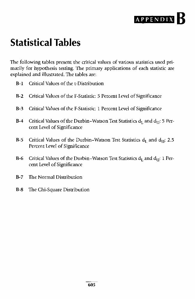
B APPENDIX
Statistical Tables
The following tables present the critical values of various statistics used pri-marily for hypothesis testing. The primary applications of each statistic are explained and illustrated. The tables are:
B-1 Critical Values of the t-Distribution
B-2 Critical Values of the F-Statistic: 5 Percent Level of Significance
B-3 Critical Values of the F-Statistic: 1 Percent Level of Significance
B-4 Critical Values of the Durbin-Watson Test Statistics d L and du : 5 Per-cent Level of Significance
B-5 Critical Values of the Durbin-Watson Test Statistics d L and du: 2.5 Percent Level of Significance
B-6 Critical Values of the Durbin-Watson Test Statistics d L and du : 1 Per-cent Level of Significance
B-7 The Normal Distribution
B-8 The Chi-Square Distribution
605
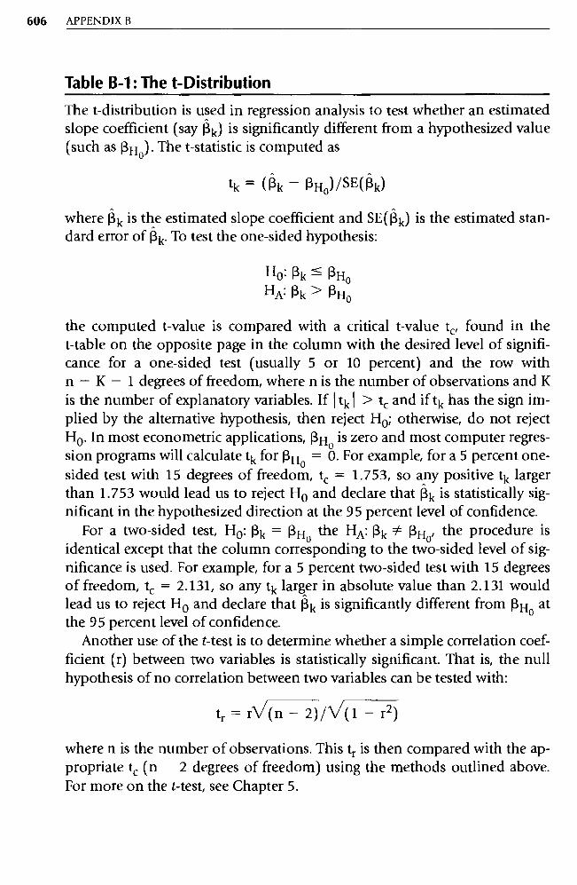
606 APPENDIX B
Table B-1: The t-Distribution
The t-distribution is used in regression analysis to test whether an estimated slope coefficient (say Rk) is significantly different from a hypothesized value (such as 13 H0). The t-statistic is computed as
tk — Ow' Rk — 13H0)/SE(K)
where (3 k is the estimated slope coefficient and SE(R k) is the estimated stan-dard error of j3 k. To test the one-sided hypothesis:
H0: Pk 13H 0
HA: Pk > RH°
the computed t-value is compared with a critical t-value t c, found in the t-table on the opposite page in the column with the desired level of signifi-cance for a one-sided test (usually 5 or 10 percent) and the row with n — K — 1 degrees of freedom, where n is the number of observations and K is the number of explanatory variables. If I tk > t c and if tk has the sign im-plied by the alternative hypothesis, then reject H 0; otherwise, do not reject H0 . In most econometric applications, 13H0 is zero and most computer regres-sion programs will calculate t k for 13 H0 = 0. For example, for a 5 percent one-sided test with 15 degrees of freedom, t c = 1.753, so any positive tk larger than 1.753 would lead us to reject H 0 and declare that Pk is statistically sig-nificant in the hypothesized direction at the 95 percent level of confidence.
For a two-sided test, H 0 : 13k = RHo the HA: Rk # RHo, the procedure is identical except that the column corresponding to the two-sided level of sig-nificance is used. For example, for a 5 percent two-sided test with 15 degrees of freedom, t, = 2.131, so any tk larger in absolute value than 2.131 would lead us to reject H 0 and declare that (3 k is significantly different from 13 H0 at the 95 percent level of confidence.
Another use of the t-test is to determine whether a simple correlation coef-ficient (r) between two variables is statistically significant. That is, the null hypothesis of no correlation between two variables can be tested with:
tr = r\/(n — 2)/V(1 — r 2)
where n is the number of observations. This t r is then compared with the ap-propriate tc (n 2 degrees of freedom) using the methods outlined above. For more on the t-test, see Chapter 5.

STATISTICAL TABLES 607
TABLE B-1 CRITICAL VALUES OF THE t-DISTRIBUTION
Degrees of Freedom
Level of Significance
One Sided: 10% Two Sided: 20%
5% 10%
2.5% 5%
1% 2%
0.5% 1 °/U
1 3.078 6.314 12.706 31.821 63.657 2 1.886 2.920 4.303 6.965 9.925 3 1.638 2.353 3.182 4.541 5.841 4 1.533 2.132 2.776 3.747 4.604 5 1.476 2.015 2.571 3.365 4.032
6 1.440 1 .943 2.447 3.143 3.707 7 1.415 1.895 2.365 2.998 3.499 8 1.397 1.860 2.306 2.896 3.355 9 1.383 1.833 2.262 2.821 3.250 10 1.372 1.812 2.228 2.764 3.169
11 1.363 1.796 2.201 2.718 3.106 12 1.356 1.782 2.179 2.681 3.055 13 1.350 1.771 2.160 2.650 3.012 14 1.345 1.761 2.145 2.624 2.977 15 1.341 1.753 2.131 2.602 2.947
16 1.337 1.746 2.120 2.583 2.921 17 1.333 1.740 2.110 2.567 2.898 18 1 .330 1 .734 2.101 2.552 2.878 19 1.328 1.729 2.093 2.539 2.861 20 1.325 1.725 2.086 2.528 2.845
21 1.323 1.721 2.080 2.518 2.831 22 1.321 1 .717 2.074 2.508 2.819 23 1.319 1.714 2.069 2.500 2.807 24 1.318 1.711 2.064 2.492 2.797 25 1.316 1.708 2.060 2.485 2.787
26 1.315 1.706 2.056 2.479 2.779 27 1.314 1.703 2.052 2.473 2.771
28 1.313 1.701 2.048 2.467 2.763 29 1.311 1.699 2.045 2.462 2.756 30 1.310 1.697 2.042 2.457 2.750
40 1.303 1.684 2.021 2.423 2.704 60 1.296 1 .671 2.000 2.390 2.660 120 1.289 1.658 1.980 2.358 2.617
(Normal) 00 1.282 1.645 1.960 2.326 2.576
Source: Reprinted from Table IV in Sir Ronald A. Fisher, Statistical Methods for Research Workers, 14th ed. (copyright © 1970, University of Adelaide) with permission of Hafner, a Division of the
Macmillan Publishing Company, Inc.
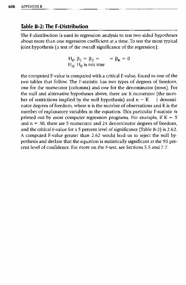
608 APPENDIX B
Table B-2: The F-Distribution
The F-distribution is used in regression analysis to test two-sided hypotheses about more than one regression coefficient at a time. To test the most typical joint hypothesis (a test of the overall significance of the regression):
Ho: R1=R2= = PK = O HA: H o is not true
the computed F-value is compared with a critical F-value, found in one of the two tables that follow. The F-statistic has two types of degrees of freedom, one for the numerator (columns) and one for the denominator (rows). For the null and alternative hypotheses above, there are K numerator (the num-ber of restrictions implied by the null hypothesis) and n — K 1 denomi-nator degrees of freedom, where n is the number of observations and K is the number of explanatory variables in the equation. This particular F-statistic is printed out by most computer regression programs. For example, if K = 5 and n = 30, there are 5 numerator and 24 denominator degrees of freedom, and the critical F-value for a 5 percent level of significance (Table B-2) is 2.62. A computed F-value greater than 2.62 would lead us to reject the null hy-pothesis and declare that the equation is statistically significant at the 95 per-cent level of confidence. For more on the F-test, see Sections 5.5 and 7.7.
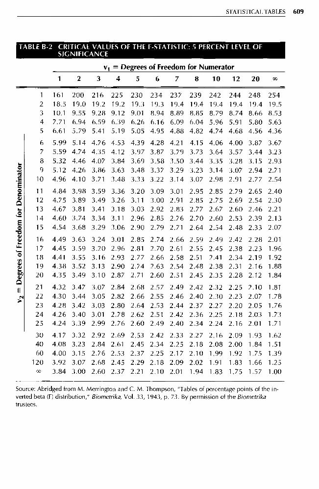
STATISTICAL TABLES 609
TABLE B-2 CRITICAL VALUES OF THE F-STATISTIC: 5 PERCENT LEVEL OF SIGNIFICANCE
y 1 = Degrees of Freedom for Numerator
1 2 3 4 5 6 7 8 10 12 20 00
1 161 200 216 225 230 234 237 239 242 244 248 254 2 18.5 19.0 19.2 19.2 19.3 19.3 19.4 19.4 19.4 19.4 19.4 19.5 3 10.1 9.55 9.28 9.12 9.01 8.94 8.89 8.85 8.79 8.74 8.66 8.53 4 7.71 6.94 6.59 6.39 6.26 6.16 6.09 6.04 5.96 5.91 5.80 5.63 5 6.61 5.79 5.41 5.19 5.05 4.95 4.88 4.82 4.74 4.68 4.56 4.36
6 5.99 5.14 4.76 4.53 4.39 4.28 4.21 4.15 4.06 4.00 3.87 3.67 7 5.59 4.74 4.35 4.12 3.97 3.87 3.79 3.73 3.64 3.57 3.44 3.23 8 5.32 4.46 4.07 3.84 3.69 3.58 3.50 3.44 3.35 3.28 3.15 2.93 9 5.12 4.26 3.86 3.63 3.48 3.37 3.29 3.23 3.14 3.07 2.94 2.71
10 4.96 4.10 3.71 3.48 3.33 3.22 3.14 3.07 2.98 2.91 2.77 2.54
11 4.84 3.98 3.59 3.36 3.20 3.09 3.01 2.95 2.85 2.79 2.65 2.40 12 4.75 3.89 3.49 3.26 3.11 3.00 2.91 2.85 2.75 2.69 2.54 2.30 13 4.67 3.81 3.41 3.18 3.03 2.92 2.83 2.77 2.67 2.60 2.46 2.21 14 4.60 3.74 3.34 3.11 2.96 2.85 2.76 2.70 2.60 2.53 2.39 2.13 15 4.54 3.68 3.29 3.06 2.90 2.79 2.71 2.64 2.54 2.48 2.33 2.07
16 4.49 3.63 3.24 3.01 2.85 2.74 2.66 2.59 2.49 2.42 2.28 2.01 17 4.45 3.59 3.20 2.96 2.81 2.70 2.61 2.55 2.45 2.38 2.23 1.96 18 4.41 3.55 3.16 2.93 2.77 2.66 2.58 2.51 2.41 2.34 2.19 1.92 19 4.38 3.52 3.13 2.90 2.74 2.63 2.54 2.48 2.38 2.31 2.16 1.88 20 4.35 3.49 3.10 2.87 2.71 2.60 2.51 2.45 2.35 2.28 2.12 1.84
21 4.32 3.47 3.07 2.84 2.68 2.57 2.49 2.42 2.32 2.25 2.10 1.81 22 4.30 3.44 3.05 2.82 2.66 2.55 2.46 2.40 2.30 2.23 2.07 1.78 23 4.28 3.42 3.03 2.80 2.64 2.53 2.44 2.37 2.27 2.20 2.05 1.76 24 4.26 3.40 3.01 2.78 2.62 2.51 2.42 2.36 2.25 2.18 2.03 1.73 25 4.24 3.39 2.99 2.76 2.60 2.49 2.40 2.34 2.24 2.16 2.01 1.71
30 4.17 3.32 2.92 2.69 2.53 2.42 2.33 2.27 2.16 2.09 1.93 1.62 40 4.08 3.23 2.84 2.61 2.45 2.34 2.25 2.18 2.08 2.00 1.84 1.51 60 4.00 3.15 2.76 2.53 2.37 2.25 2.17 2.10 1.99 1.92 1.75 1.39
120 3.92 3.07 2.68 2.45 2.29 2.18 2.09 2.02 1.91 1.83 1.66 1.25 x 3.84 3.00 2.60 2.37 2.21 2.10 2.01 1.94 1.83 1.75 1.57 1.00
v2 =
De
gre
es o
f Fre
edo
m f
or
De
nom
ina t
or
Source: Abridged from M. Merrington and C. M. Thompson, "Tables of percentage points of the in-verted beta (F) distribution," Biometrika, Vol. 33, 1943, p. 73. By permission of the Biometrika trustees.
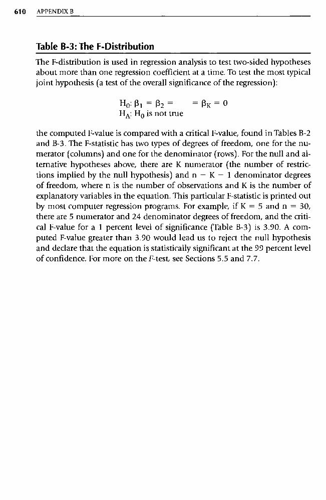
610 APPENDIX B
Table B-3: The F-Distribution
The F-distribution is used in regression analysis to test two-sided hypotheses about more than one regression coefficient at a time. To test the most typical joint hypothesis (a test of the overall significance of the regression):
Ho: Ri = P2 = = PK = °
HA: H o is not true
the computed F-value is compared with a critical F-value, found in Tables B-2 and B-3. The F-statistic has two types of degrees of freedom, one for the nu-merator (columns) and one for the denominator (rows). For the null and al-ternative hypotheses above, there are K numerator (the number of restric-tions implied by the null hypothesis) and n — K — 1 denominator degrees of freedom, where n is the number of observations and K is the number of explanatory variables in the equation. This particular F-statistic is printed out by most computer regression programs. For example, if K = 5 and n = 30, there are 5 numerator and 24 denominator degrees of freedom, and the criti-cal F-value for a 1 percent level of significance (Table B-3) is 3.90. A com-puted F-value greater than 3.90 would lead us to reject the null hypothesis and declare that the equation is statistically significant at the 99 percent level of confidence. For more on the F-test, see Sections 5.5 and 7.7.
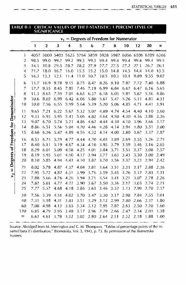
STATISTICAL TABLES 611
TABLE B-3 CRITICAL VALUES OF THE F-STATISTIC: 1 PERCENT LEVEL OF SIGNIFICANCE
vi = Degrees of Freedom for Numerator
1 2 3 4 5 6 7 8 10 12 20 co
1 4052 5000 5403 5625 5764 5859 5928 5982 6056 6106 6209 6366
2 98.5 99.0 99.2 99.2 99.3 99.3 99.4 99.4 99.4 99.4 99.4 99.5 3 34.1 30.8 29.5 28.7 28.2 27.9 27.7 27.5 27.2 271 26.7 26.1 4 21.2 18.0 16.7 16.0 15.5 15.2 15.0 14.8 14.5 14.4 14.0 13.5
5 16.3 13.3 12.1 11.4 11.0 10.7 10.5 10.3 10.1 9.89 9.55 9.02
6 13.7 10.9 9.78 9.15 8.75 8.47 8.26 8.10 7.87 7.72 7.40 6.88 7 12.2 9.55 8.45 7.85 7.46 7.19 6.99 6.84 6.62 6.47 6.16 5.65
8 11.3 8.65 7.59 7.01 6.63 6.37 6.18 6.03 5.81 5.67 5.36 4.86
9 10.6 8.02 6.99 6.42 6.06 5.80 5.61 5.47 5.26 5.11 4.81 4.31
10 10.0 7.56 6.55 5.99 5.64 5.39 5.20 5.06 4.85 4.71 4.41 3.91
11 9.65 7.21 6.22 5.67 5.32 5.07 4.89 4.74 4.54 4.40 4.10 3.60 12 9.33 6.93 5.95 5.41 5.06 4.82 4.64 4.50 4.30 4.16 3.86 3.36 13 9.07 6.70 5.74 5.21 4.86 4.62 4.44 4.30 4.10 3.96 3.66 3.17
14 8.86 6.51 5.56 5.04 4.70 4.46 4.28 4.14 3.94 3.80 3.51 3.00
15 8.68 6.36 5.42 4.89 4.56 4.32 4.14 4.00 3.80 3.67 3.37 2.87
16 8.53 6.23 5.29 4.77 4.44 4.20 4.03 3.89 3.69 3.55 3.26 2.75
17 8.40 6.11 5.19 4.67 4.34 4.10 3.93 3.79 3.59 3.46 3.16 2.65 18 8.29 6.01 5.09 4.58 4.25 4.01 3.84 3.71 3.51 3.37 3.08 2.57
19 8.19 5.93 5.01 4.50 4.17 3.94 3.77 3.63 3.43 3.30 3.00 2.49
20 8.10 5.85 4.94 4.43 4.10 3.87 3.70 3.56 3.37 3.23 2.94 2.42
21 8.02 5.78 4.87 4.37 4.04 3.81 3.64 3.51 3.31 3.17 2.88 2.36 22 7.95 5.72 4.82 4.31 3.99 3.76 3.59 3.45 3.26 3.12 2.83 2.31
23 7.88 5.66 4.76 4.26 3.94 3.71 3.54 3.41 3.21 3.07 2.78 2.26 24 7.82 5.61 4.72 4.22 3.90 3.67 3.50 3.36 3.17 3.03 2.74 2.21 25 7.77 5.57 4.68 4.18 3.86 3.63 3.46 3.32 3.13 2.99 2.70 2.17
30 7.56 5.39 4.51 4.02 3.70 3.47 3.30 3.17 2.98 2.84 2.55 2.01
40 7.31 5.18 4.31 3.83 3.51 3.29 3.12 2.99 2.80 2.66 2.37 1.80
60 7.08 4.98 4.13 3.65 3.34 3.12 2.95 2.82 2.63 2.50 2.20 1.60
120 6.85 4.79 3.95 3.48 3.17 2.96 2.79 2.66 2.47 2.34 2.03 1.38 co 6.63 4.61 3.78 3.32 3.02 2.80 2.64 2.51 2.32 2.18 1.88 1.00
y2 =
Deg
rees
of F
reed
om
fo
r D
eno
min
ato
r
Source: Abridged from M. Merrington and C. M. Thompson, "Tables of percentage points of the in-vertecl beta (F) distribution," Biometrika, Vol. 3, 1943, p. 73. By permission of the Biometrika trustees.
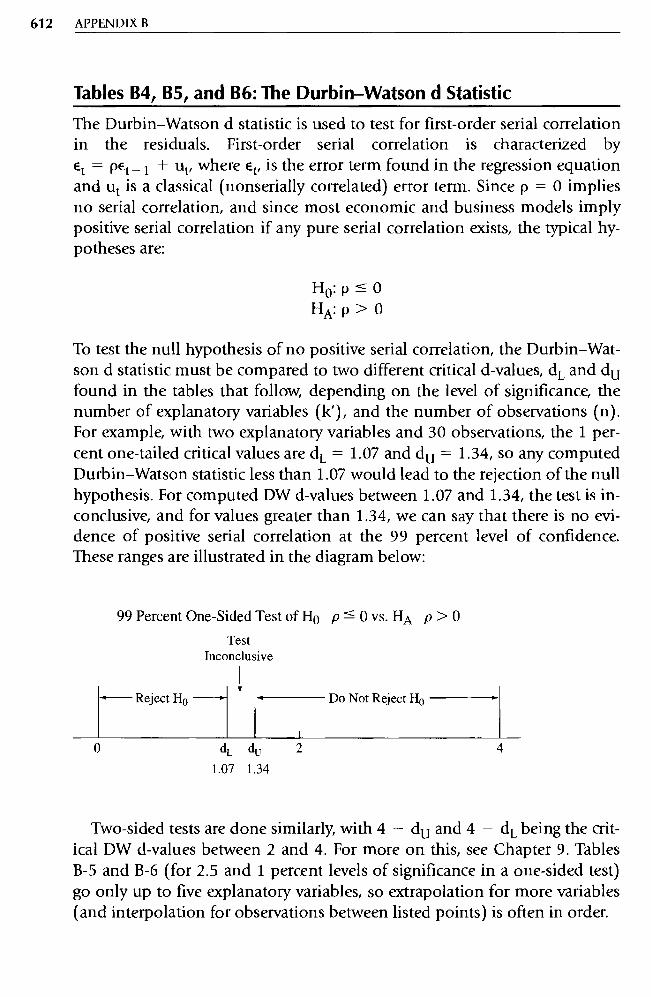
612 APPENDIX B
Tables B4, B5, and B6: The Durbin—Watson d Statistic
The Durbin-Watson d statistic is used to test for first-order serial correlation
in the residuals. First-order serial correlation is characterized by
Et = Pet -1 + u t, where Et, is the error term found in the regression equation and ut is a classical (nonserially correlated) error term. Since p = 0 implies
no serial correlation, and since most economic and business models imply
positive serial correlation if any pure serial correlation exists, the typical hy-potheses are:
Hp:p^O HA: p> 0
To test the null hypothesis of no positive serial correlation, the Durbin-Wat-son d statistic must be compared to two different critical d-values, d L and du found in the tables that follow, depending on the level of significance, the
number of explanatory variables (k'), and the number of observations (n).
For example, with two explanatory variables and 30 observations, the 1 per-cent one-tailed critical values are d L = 1.07 and du = 1.34, so any computed Durbin-Watson statistic less than 1.07 would lead to the rejection of the null
hypothesis. For computed DW d-values between 1.07 and 1.34, the test is in-conclusive, and for values greater than 1.34, we can say that there is no evi-dence of positive serial correlation at the 99 percent level of confidence.
These ranges are illustrated in the diagram below:
99 Percent One-Sided Test of Ho p 0 vs. HA p > 0
Test Inconclusive
Reject Ho
Do Not Reject Ho
dL du 2
1.07 1.34
Two-sided tests are done similarly, with 4 - d u and 4 - d L being the crit-ical DW d-values between 2 and 4. For more on this, see Chapter 9. Tables
B-5 and B-6 (for 2.5 and 1 percent levels of significance in a one-sided test)
go only up to five explanatory variables, so extrapolation for more variables
(and interpolation for observations between listed points) is often in order.
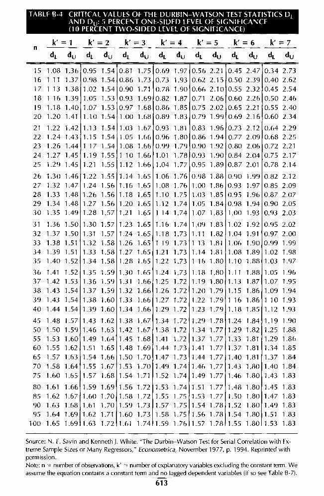
TABLE B-4 CRITICAL VALUES OF THE DURBIN-WATSON TEST STATISTICS D i_ AND D u : 5 PERCENT ONE-SIDED LEVEL OF SIGNIFICANCE (10 PERCENT TWO-SIDED LEVEL OF SIGNIFICANCE)
n k'=1 k'=2 k'=3 k'=4 k'=5 k'=6 k'=7
d i_ du di. du di_ du di_ du d1 du d1 du d1 du
15 1.08 1.36 0.95 1.54 0.81 1.75 0.69 1.97 0.56 2.21 0.45 2.47 0.34 2.73 16 1 11 1.37 0.98 1.54 0.86 1.73 0.73 1.93 0.62 2.15 0.50 2.39 0.40 2.62
17 1 13 1.38 1.02 1.54 0.90 1.71 0.78 1.90 0.66 2.10 0.55 2.32 0.45 2.54
18 1 16 1.39 1.05 1.53 0.93 1.69 0.82 1.87 0.71 2.06 0.60 2.26 0.50 2.46 19 1.18 1.40 1.07 1.53 0.97 1.68 0.86 1.85 0.75 2.02 0.65 2.21 0.55 2.40 20 1.20 1.41 1.10 1.54 1.00 1.68 0.89 1.83 0.79 1.99 0.69 2.16 0.60 2.34
21 1.22 1.42 1.13 1.54 1.03 1.67 0.93 1.81 0.83 1.96 0.73 2.12 0.64 2.29 22 1.24 1.43 1.15 1.54 1.05 1.66 0.96 1.80 0.86 1.94 0.77 2.09 0.68 2.25 23 1.26 1.44 1 17 1.54 1.08 1.66 0.99 1.79 0.90 1.92 0.80 2.06 0.72 2.21
24 1.27 1.45 1.19 1.55 1 10 1.66 1.01 1.78 0.93 1.90 0.84 2.04 0.75 2.17
25 1.29 1.45 1.21 1.55 1.12 1.66 1.04 1.77 0.95 1.89 0.87 2.01 0.78 2.14
26 1.30 1.46 1.22 1.55 1.14 1.65 1.06 1.76 0.98 1.88 0.90 1.99 0.82 2.12 27 1.32 1.47 1.24 1.56 1.16 1.65 1.08 1.76 1.00 1.86 0.93 1.97 0.85 2.09 28 1.33 1.48 1.26 1.56 1.18 1.65 1.10 1.75 1.03 1.85 0.95 1.96 0.87 2.07 29 1.34 1.48 1.27 1.56 1.20 1.65 1.12 1.74 1.05 1.84 0.98 1.94 0.90 2.05 30 1.35 1.49 1.28 1.57 1.21 1.65 1 14 1.74 1.07 1.83 1.00 1.93 0.93 2.03
31 1.36 1.50 1.30 1.57 1.23 1.65 1.16 1.74 1.09 1.83 1.02 1.92 0.95 2.02
32 1.37 1.50 1.31 1.57 1.24 1.65 1.18 1.73 1.11 1.82 1.04 1.91 0.97 2.00 33 1.38 1.51 1.32 1.58 1.26 1.65 1 19 1.73 1 13 1.81 1.06 1.90 0.99 1.99 34 1.39 1.51 1.33 1.58 1.27 1.65 1.21 1.73 1.14 1.81 1.08 1.89 1.02 1.98 35 1.40 1.52 1.34 1.58 1.28 1.65 1.22 1.73 1 16 1.80 1.10 1.88 1.03 1.97
36 1.41 1.52 1.35 1.59 1.30 1.65 1.24 1.73 1.18 1.80 1.11 1.88 1.05 1.96 37 1.42 1.53 1.36 1.59 1.31 1.66 1.25 1.72 1.19 1.80 1.13 1.87 1.07 1.95
38 1.43 1.54 1.37 1.59 1.32 1.66 1.26 1.72 1.20 1.79 1.15 1.86 1.09 1.94
39 1.43 1.54 1.38 1.60 1.33 1.66 1.27 1.72 1.22 1.79 1 16 1.86 1 10 1.93 40 1.44 1.54 1.39 1.60 1.34 1.66 1.29 1.72 1.23 1.79 1.18 1.85 1.12 1.93
45 1.48 1.57 1.43 1.62 1.38 1.67 1.34 1.72 1.29 1.78 1.24 1.84 1.19 1.90 50 1.50 1.59 1.46 1.63 1.42 1.67 1.38 1.72 1.34 1.77 1.29 1.82 1.25 1.88 55 1.53 1.60 1.49 1.64 1.45 1.68 1.41 1.72 1.37 1 .77 1.33 1.81 1.29 1.86 60 1.55 1.62 1.51 1.65 1.48 1.69 1.44 1.73 1.41 1.77 1.37 1.81 1.34 1.85
65 1.57 1.63 1.54 1.66 1.50 1.70 1.47 1.73 1.44 1.77 1.40 1.81 1.37 1.84
70 1.58 1.64 1.55 1.67 1.53 1.70 1.49 1.74 1.46 1.77 1.43 1.80 1.40 1.84
75 1.60 1.65 1.57 1.68 1.54 1.71 1.52 1.74 1.49 1.77 1.46 1.80 1.43 1.83
80 1.61 1.66 1.59 1.69 1.56 1.72 1.53 1.74 1.51 1.77 1.48 1.80 1.45 1.83
85 1.62 1.67 1.60 1.70 1.58 1 .72 1.55 1.75 1.53 1.77 1.50 1.80 1.47 1.83 90 1.63 1.68 1.61 1.70 1.59 1.73 1.57 1.75 1.54 1.78 1.52 1.80 1.49 1.83 95 1.64 1.69 1.62 1.71 1.60 1.73 1.58 1.75 1.56 1.78 1.54 1.80 1.51 1.83
100 1.65 1.69 1.63 1.72 1.61 1.74 1.59 1.76 1.57 1.78 1.55 1 .80 1.53 1.83
Source: N. E. Savin and Kenneth J. White. "The Durbin-Watson Test for Serial Correlation with Ex-treme Sample Sizes or Many Regressors," Econometrica, November 1977, p. 1994. Reprinted with permission. Note: n = number of obse rvations, k' = number of explanatory variables excluding the constant term. We assume the equation contains a constant term and no lagged dependent variables (if so see Table B - 7).
613
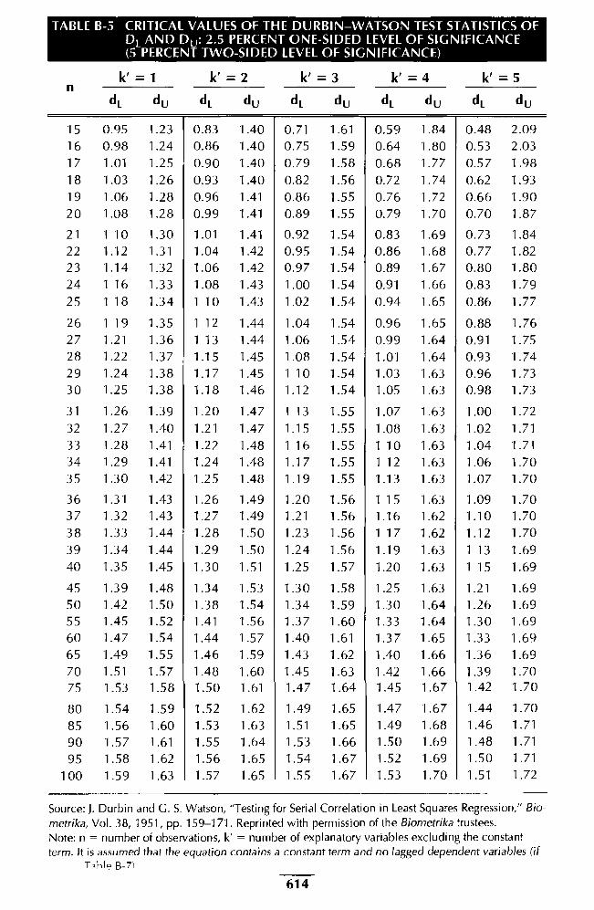
TABLE B-5 CRITICAL VALUES OF THE DURBIN-WATSON TEST STATISTICS OF D i_ AND D u : 2.5 PERCENT ONE-SIDED LEVEL OF SIGNIFICANCE (5 PERCENT TWO-SIDED LEVEL OF SIGNIFICANCE)
k'=1
k' = 2
k' = 3
k ' = 4
k ' = 5 n
d i_ d u d i_ d u d i_ d u d i_ d u
d i_ d u
15 16
17
18 19
20
21 22 23
0.95 0.98
1.01
1.03
1.06 1.08
1 10 1.12 1.14
1.23
1.24
1.25
1.26
1.28 1.28
1.30 1.31 1.32
0.83 0.86
0.90
0.93
0.96 0.99
1.01 1.04 1.06
1.40 1.40
1.40
1.40
1.41 1.41
1.41 1.42 1.42
0.71 0.75
0.79
0.82
0.86 0.89
0.92 0.95 0.97
1.61
1.59
1.58
1.56 1.55
1.55
1.54 1.54 1.54
0.59 0.64
0.68
0.72
0.76 0.79
0.83 0.86
0.89
1.84
1.80
1.77
1.74
1.72 1.70
1.69 1.68 1.67
0.48
0.53
0.57
0.62 0.66
0.70
0.73 0.77 0.80
2.09 2.03
1.98
1.93 1.90
1.87
1.84 1.82 1.80
24 1 16 1.33 1.08 1.43 1.00 1.54 0.91 1.66 0.83 1.79
25 1 18 1.34 1 10 1.43 1.02 1.54 0.94 1.65 0.86 1.77
26 1 19 1.35 1 12 1.44 1.04 1.54 0.96 1.65 0.88 1.76 27 1.21 1.36 1 13 1.44 1.06 1.54 0.99 1.64 0.91 1.75 28 1.22 1 .37 1.15 1.45 1 .08 1.54 1.01 1 .64 0.93 1.74 29 1.24 1 .38 1.17 1 .45 1 10 1.54 1.03 1 .63 0.96 1.73
30 1.25 1.38 1.18 1.46 1.12 1.54 1.05 1.63 0.98 1.73
31 1.26 1.39 1.20 1.47 1 13 1.55 1.07 1.63 1.00 1.72
32 1.27 1.40 1.21 1.47 1.15 1.55 1.08 1.63 1.02 1.71
33 1.28 1.41 1.22 1.48 1 16 1.55 1 10 1.63 1.04 1.71
34 1.29 1.41 1.24 1.48 1.17 1.55 1 12 1.63 1.06 1.70 35 1.30 1.42 1.25 1.48 1.19 1.55 1.13 1.63 1.07 1.70
36 1.31 1.43 1.26 1.49 1.20 1.56 1 15 1.63 1.09 1.70 37 1.32 1.43 1.27 1.49 1.21 1.56 1.16 1.62 1.10 1.70
38 1.33 1.44 1.28 1.50 1.23 1.56 1 17 1.62 1.12 1.70
39 1.34 1.44 1.29 1.50 1.24 1.56 1.19 1.63 1 13 1.69
40 1.35 1.45 1.30 1.51 1.25 1.57 1.20 1.63 1 15 1.69
45 1 .39 1 .48 1.34 1 .53 1 .30 1.58 1.25 1 .63 1.21 1.69 50 1.42 1.50 1.38 1.54 1.34 1.59 1.30 1.64 1.26 1.69 55 1.45 1.52 1 .41 1.56 1.37 1 .60 1.33 1.64 1 .30 1 .69 60 1.47 1.54 1.44 1.57 1.40 1.61 1.37 1.65 1.33 1 .69 65 1.49 1.55 1.46 1.59 1.43 1.62 1.40 1.66 1.36 1.69
70 1.51 1.57 1.48 1.60 1.45 1.63 1.42 1.66 1.39 1.70 75 1.53 1.58 1.50 1.61 1.47 1 .64 1.45 1.67 1 .42 1 .70
80 1.54 1 .59 1.52 1 .62 1.49 1.65 1.47 1 .67 1.44 1.70
85 1.56 1 .60 1.53 1 .63 1.51 1.65 1.49 1 .68 1.46 1.71
90 1.57 1.61 1.55 1.64 1.53 1.66 1.50 1.69 1.48 1.71
95 1.58 1.62 1.56 1.65 1.54 1.67 1.52 1.69 1.50 1.71
100 1.59 1.63 1.57 1.65 1.55 1.67 1.53 1.70 1.51 1.72
Source: J. Durbin and G. S. Watson, "Testing for Serial Correlation in Least Squares Regression," Bio-
metrika, Vol. 38, 1951, pp. 159-171. Reprinted with permission of the Biometrika trustees. Note: n = number of observations, k' = number of explanatory variables excluding the constant term. It is assumed that the equation contains a constant term and no lagged dependent variables (if
T a kIP B-7) .
614
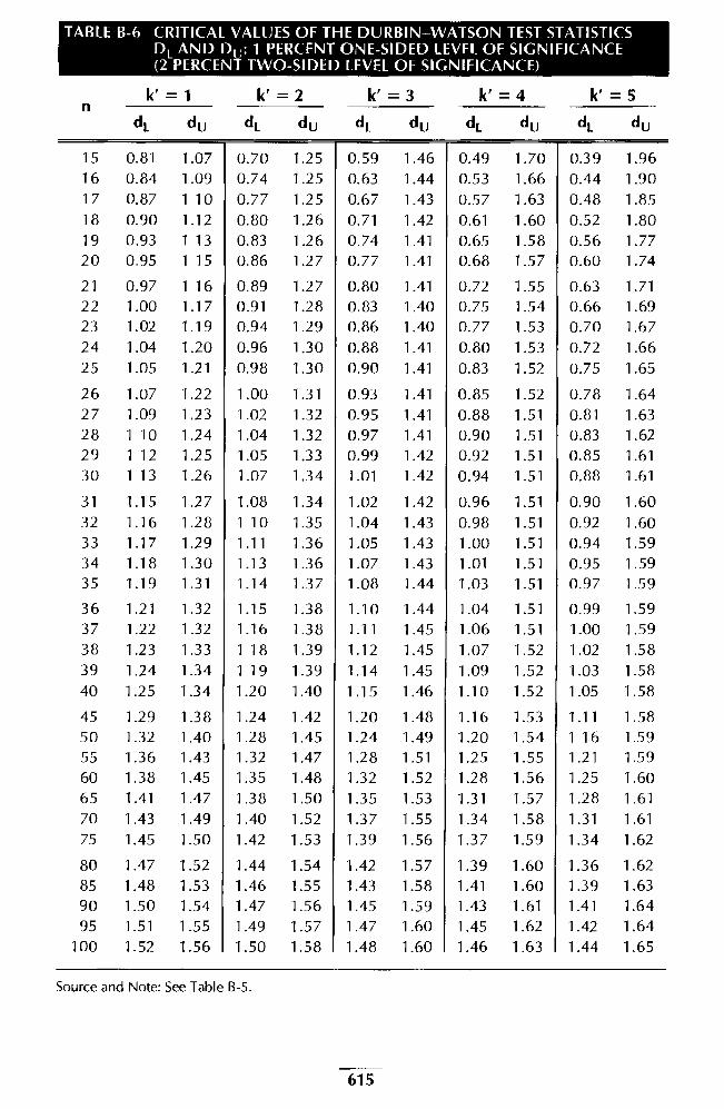
TABLE B-6 CRITICAL VALUES OF THE DURBIN-WATSON TEST STATISTICS D 1 AND Du : 1 PERCENT ONE-SIDED LEVEL OF SIGNIFICANCE (2 PERCENT TWO-SIDED LEVEL OF SIGNIFICANCE)
k'=1
k' = 2
k'=3
k' = 4
k' = 5 n
d i. du di_ d u d i. du d i. du d i. d u
15 0.81 1.07 0.70 1.25 0.59 1.46 0.49 1.70 0.39 1.96 16 0.84 1.09 0.74 1.25 0.63 1.44 0.53 1.66 0.44 1.90 17 0.87 1 10 0.77 1.25 0.67 1.43 0.57 1.63 0.48 1.85 18 0.90 1.12 0.80 1.26 0.71 1.42 0.61 1.60 0.52 1.80 19 0.93 1 13 0.83 1.26 0.74 1.41 0.65 1.58 0.56 1.77 20 0.95 1 15 0.86 1.27 0.77 1.41 0.68 1.57 0.60 1.74
21 0.97 1 16 0.89 1.27 0.80 1.41 0.72 1.55 0.63 1.71 22 1.00 1.17 0.91 1.28 0.83 1.40 0.75 1.54 0.66 1.69 23 1.02 1.19 0.94 1.29 0.86 1.40 0.77 1.53 0.70 1.67 24 1.04 1.20 0.96 1.30 0.88 1.41 0.80 1.53 0.72 1.66 25 1.05 1.21 0.98 1.30 0.90 1.41 0.83 1.52 0.75 1.65
26 1.07 1.22 1.00 1.31 0.93 1.41 0.85 1.52 0.78 1.64 27 1.09 1.23 1.02 1.32 0.95 1.41 0.88 1.51 0.81 1.63 28 1 10 1.24 1.04 1.32 0.97 1.41 0.90 1.51 0.83 1.62 29 1 12 1.25 1.05 1.33 0.99 1.42 0.92 1.51 0.85 1.61 30 1 13 1.26 1.07 1.34 1.01 1.42 0.94 1.51 0.88 1.61
31 1.15 1.27 1.08 1.34 1.02 1.42 0.96 1.51 0.90 1.60 32 1.16 1.28 1 10 1.35 1.04 1.43 0.98 1.51 0.92 1.60 33 1.17 1.29 1.11 1.36 1.05 1.43 1.00 1.51 0.94 1.59 34 1.18 1.30 1.13 1.36 1.07 1.43 1.01 1.51 0.95 1.59 35 1.19 1.31 1.14 1.37 1.08 1.44 1.03 1.51 0.97 1.59
36 1.21 1.32 1.15 1.38 1.10 1.44 1.04 1.51 0.99 1.59 37 1.22 1.32 1.16 1.38 1.11 1.45 1.06 1.51 1.00 1.59 38 1.23 1.33 1 18 1.39 1.12 1.45 1.07 1.52 1.02 1.58 39 1.24 1.34 1 19 1.39 1.14 1.45 1.09 1.52 1.03 1.58 40 1.25 1.34 1.20 1.40 1.15 1.46 1.10 1.52 1.05 1.58
45 1.29 1.38 1.24 1.42 1.20 1.48 1.16 1.53 1.11 1.58 50 1.32 1.40 1 .28 1.45 1.24 1.49 1.20 1 .54 1 16 1.59 55 1.36 1.43 1.32 1.47 1.28 1.51 1.25 1.55 1.21 1.59 60 1.38 1.45 1.35 1.48 1.32 1.52 1.28 1.56 1.25 1.60 65 1.41 1.47 1.38 1.50 1.35 1.53 1.31 1.57 1.28 1.61 70 1.43 1.49 1.40 1.52 1.37 1.55 1.34 1.58 1.31 1.61 75 1.45 1.50 1.42 1.53 1.39 1.56 1.37 1.59 1.34 1.62
80 1.47 1.52 1.44 1.54 1.42 1.57 1.39 1.60 1.36 1.62 85 1.48 1.53 1.46 1.55 1.43 1.58 1.41 1.60 1 .39 1 .63 90 1.50 1.54 1.47 1.56 1.45 1.59 1.43 1.61 1.41 1.64 95 1.51 1.55 1.49 1.57 1.47 1.60 1.45 1.62 1.42 1.64
100 1.52 1.56 1.50 1.58 1.48 1.60 1.46 1.63 1.44 1.65
Source and Note: See Table B-5.
615
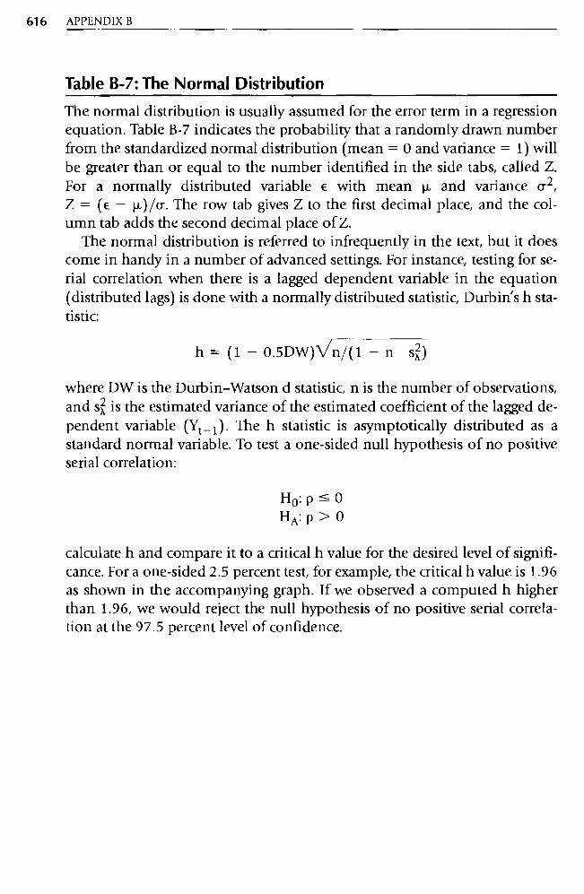
616 APPENDIX B
Table B-7: The Normal Distribution
The normal distribution is usually assumed for the error term in a regression equation. Table B-7 indicates the probability that a randomly drawn number from the standardized normal distribution (mean = 0 and variance = 1) will be greater than or equal to the number identified in the side tabs, called Z. For a normally distributed variable E with mean µ and variance Q 2, Z = (€ - µ)/Q. The row tab gives Z to the first decimal place, and the col-umn tab adds the second decimal place of Z.
The normal distribution is referred to infrequently in the text, but it does come in handy in a number of advanced settings. For instance, testing for se-rial correlation when there is a lagged dependent variable in the equation (distributed lags) is done with a normally distributed statistic, Durbin's h sta-tistic:
h = (1 - 0.5DW) V n/(1 - n s )2,)
where DW is the Durbin-Watson d statistic, n is the number of observations, and s,2, is the estimated variance of the estimated coefficient of the lagged de-pendent variable (Yt_ 1 ) . The h statistic is asymptotically distributed as a standard normal variable. To test a one-sided null hypothesis of no positive serial correlation:
Ho : p<0 HA: p > 0
calculate h and compare it to a critical h value for the desired level of signifi-cance. For a one-sided 2.5 percent test, for example, the critical h value is 1.96 as shown in the accompanying graph. If we observed a computed h higher than 1.96, we would reject the null hypothesis of no positive serial correla-tion at the 97.5 percent level of confidence.


