TYPES OF MOTION OF THE GYROSCOPE* · vector equation à=p, where a is the moment of momentum vector...
28
TYPES OF MOTION OF THE GYROSCOPE* BY A. H. COPELAND 1. Introduction. We can display, by a simple graphical representation, the complete history of all the motions of all gyroscopes which are subject to the following restrictions :f each gyroscope is acted upon by gravity, by a constraint which keeps one point on its axis of symmetry fixed in space, and by no other forces. Furthermore, with the aid of Osgood's intrinsic equations,î we shall be able to include in this history a discussion of some new intrinsic properties of the cone traced in space by the axis of symmetry of such a gyroscope. This cone intersects the unit sphere whose center is at the fixed point, in a curve which we shall call T. We shall describe the pro- perties of this cone in terms of the geodesic curvature, k, of T. The advantage in Osgood's equations lies in the fact that they yield a simple expression for k. We shall also be able to obtain additional properties of the motion from an analysis of the curves T passing near the poles (the north pole being at the top of the unit sphere). By means of these methods, we shall list the proper- ties of the motion more fully than has hitherto been done, exhibit their dependence upon the initial conditions, and show how one type of motion changes into another as the initial conditions are varied continuously. 2. Equations of the motion. In the case of the gyroscope which we are considering, Osgood's equations take the following form:§ (a) Am' = Mgh(sm8)8', (1) (b) Akv2 -Crv= - Mgh(sm28W, (c) Cr = 0, * Presented to the Society, October 29, 1927; received by the editors December 30, 1927. This paper was written in connection with the author's doctorate. t For discussions of the motion of such a gyroscope, see, for example Klein und Sommerfeld, Theorie des Kreisels, Heft II; Appell, Traité de la Mécanique Rationnelle, Tome II, pp. 193-209; Encyklopädie der Mathematischen Wissenschaften, Band IVi, pp. 619—639; or Lamb, Higher Mech- anics, Chap. VIII. % Cf. W. F. Osgood,On the gyroscope, these Transactions, vol. 23 (1922),pp. 240-264. § Cf. Osgood, loc. cit, p. 247, formula (7) and p. 256, formula (1). The term Cm of equation (lb) of this paper is preceded by a minus sign instead of the plus sign in Osgood's article. This change of sign is due to the fact that we have chosen a right-handed instead of a left-handed system of coordinates. 737 License or copyright restrictions may apply to redistribution; see https://www.ams.org/journal-terms-of-use
Transcript of TYPES OF MOTION OF THE GYROSCOPE* · vector equation à=p, where a is the moment of momentum vector...
TYPES OF MOTION OF THE GYROSCOPE*
BY
A. H. COPELAND
1. Introduction. We can display, by a simple graphical representation,
the complete history of all the motions of all gyroscopes which are subject
to the following restrictions :f each gyroscope is acted upon by gravity, by
a constraint which keeps one point on its axis of symmetry fixed in space,
and by no other forces. Furthermore, with the aid of Osgood's intrinsic
equations,î we shall be able to include in this history a discussion of some
new intrinsic properties of the cone traced in space by the axis of symmetry
of such a gyroscope. This cone intersects the unit sphere whose center is at
the fixed point, in a curve which we shall call T. We shall describe the pro-
perties of this cone in terms of the geodesic curvature, k, of T. The advantage
in Osgood's equations lies in the fact that they yield a simple expression for k.
We shall also be able to obtain additional properties of the motion from an
analysis of the curves T passing near the poles (the north pole being at the
top of the unit sphere). By means of these methods, we shall list the proper-
ties of the motion more fully than has hitherto been done, exhibit their
dependence upon the initial conditions, and show how one type of motion
changes into another as the initial conditions are varied continuously.
2. Equations of the motion. In the case of the gyroscope which we are
considering, Osgood's equations take the following form:§
(a) Am' = Mgh(sm8)8',
(1) (b) Akv2 -Crv= - Mgh(sm28W,
(c) Cr = 0,
* Presented to the Society, October 29, 1927; received by the editors December 30, 1927. This
paper was written in connection with the author's doctorate.
t For discussions of the motion of such a gyroscope, see, for example Klein und Sommerfeld,
Theorie des Kreisels, Heft II; Appell, Traité de la Mécanique Rationnelle, Tome II, pp. 193-209;
Encyklopädie der Mathematischen Wissenschaften, Band IVi, pp. 619—639; or Lamb, Higher Mech-
anics, Chap. VIII.% Cf. W. F. Osgood, On the gyroscope, these Transactions, vol. 23 (1922), pp. 240-264.
§ Cf. Osgood, loc. cit, p. 247, formula (7) and p. 256, formula (1). The term Cm of equation
(lb) of this paper is preceded by a minus sign instead of the plus sign in Osgood's article. This
change of sign is due to the fact that we have chosen a right-handed instead of a left-handed system
of coordinates.
737
License or copyright restrictions may apply to redistribution; see https://www.ams.org/journal-terms-of-use
738 A. H. C0PELAND [October
where C is the moment of inertia of the gyroscope about its axis of sym-
metry; A, the moment of inertia about a perpendicular axis through the
fixed point; M, the mass of the gyroscope; h, the distance of the center of
mass from the fixed point; g, the acceleration of gravity; and r, the spin
of the gyroscope about its axis. Likewise, 0 and $ denote, respectively, the
colatitude and longitude of a point, £, which is a trace of the axis of the
gyroscope on the surface of the unit sphere;* k denotes the geodesic curvature
of T at the point £; and v, the velocity of this point. The primes denote dif-
ferentiation with respect to the arc length, s, of T, and the dot denotes dif-
ferention with respect to the time, /. Equations (1) are equivalent to the
vector equation à=p, where a is the moment of momentum vector taken
with respect to the fixed point and p is the resultant moment of the external
forces with respect to the fixed point. Equation (lc) implies that r is a con-
stant. This constant is positive. Equation (la) has the following integral:
(2) î)3 = Do2 + a(u0 — u),
where a = 2Mgh/A and m = cos 8, and where v0 and u0 are respectively the
values of v and u at some time, t0.
In addition to equations (1) and (2), we have the following equations:f
(3) v* = 03 + (sin39)^3,
(4) (1 - M(?)¿o2 + 7(«o - u) = (1 - u*)t
where y = Cr/A, and
(5) Ú3 = (1 - «3)h,3 + a(uo - «)] - [(1 - «o2)¿p + y(uo - «)]a = /(«)•
Equations (4) and (5) define the motion of the gyroscope. If u0 is a root of
f(u), then a solution of these equations is u=u0, ^=fa. It is a familiar
fact that if u0 is a double root of /(«), then this solution satisfies equations
à = p, but that otherwise the solution is extraneous.f When u=u0 and >P — fa,
* The point { is that one of the two traces of the axis on the sphere such that an observer
situated at the fixed point and looking at £ sees the gyroscope rotate in a clockwise sense.
t Equation (3) is a consequence of the fact that the point £ always lies in the surface of the unit
sphere. (Cf. Osgood, loc. cit., p. 247.) Equation (4) is a consequence of the fact that the vector ¡i
is always horizontal and hence the vertical component of the vector a is a constant. Equation (5)
is obtained by combining equations (2), (3), and (4). (For equations (4) and (5), cf. Osgood, loc. cit.,
p. 257, equation (5) ; also Appell, loc. cit., Tome II, p. 196, equations 50,51.)
X The intrinsic equations afford the following simple proof of this fact. If «=«o, then by equation
(2), v is constant, and hence it follows from equation (lb) that k must be constant. Moreover the
value k0 of k obtained by solving this equation, must be equal to the geodesic curvature kc of the
parallel of latitude, «o. O. D. Kellogg (Curvature and the top, these Transactions, vol. 25 (1923),
p. 518, formula 29) has obtained the equation
License or copyright restrictions may apply to redistribution; see https://www.ams.org/journal-terms-of-use

1928] MOTION OF THE GYROSCOPE 739
the gyroscope is said to execute steady precession.* Without loss of gener-
ality, we can assume that u0 is a root oif(u). To see this let us assume that
«o is not a root of/(«). Then, since/(w0) ^ 0 and — 1 ̂ u0 ^ +1 for real motion,
it follows that f(u0) >0. Furthermore,'since /(± 1) g0, then — 1 <«0 < +1
and there exist at least two distinct roots of/(w) in the interval — 1 ¿u^ +1.
Let «i be one of these roots. Since/(«) is a cubic, Ui may be so chosen that it
is a single root and that no other root oif(u) lies between u0 and «i.f Then we
may combine the equations v2 = v02 +a(u0—u) and v? =v02 +a(u0 — Ui) and
obtain the equation
v2 = Vi2 + a(ui — u).
Likewise we may combine the equations (1— m2)^ = (1— Mo2)^o2+7(wo —u)
and (1—«i2)^i= (1—«o2)^o+7(mo —Wi) and obtain the equation
(1 — u2)i = (1 — «i2)^i + 7("i - «)•
Hence we may write
/(«) = (1 - u2)[v? + a(ui - «)] - [(1 - u?)h + 7(«i - m)]2
where — 1 ̂ Wiá +1. Thus we may take the cosine of the colatitude of the
initial point to be «i instead of u0. We can now let u0 play the role of U\,
that is, we can assume that u0 is a root oif(u).
From this point on we shall assume that/(«0) = 0. There is a second root,
«i, of/(w) in the interval — l^Mi^+1, and a third root M2ïï-hl. It is a
familiar fact that T lies completely in the zone bounded by the parallels of
latitude u = ua and u = ui and that, in general, it oscillates between points
of tangency to u0 and to Ui.
3. Graphical representation of gyroscopic motion. Equations (4) and
(5) show that the type of motion is completely determined by the values
«o — kc =-— iM ñapo'— 7^0 + —a I.
But we have also the equation
g(«o) = 2(1 - «tfOlWo2 — T^o + \a],and hence we may write
kg- kc = —- g(«o).2i>o3
It follows that k0 = kc only when g(«o) or ^o vanishes. But t =«i is the only solution of g(u) =0 for
which —1<«< + 1, and hence g(«o)=0 only when «0=«i. If the factor ¿o vanishes then, since
ú=0, t>o=0 and hence v=0. It follows that the moment of momentum vector, a, is constant and
therefore the moment ¡i is zero. But this is only possible if «o= ±1 and if Ms is a double root of /(«).
(Cf. p 745.)* Cf. Lamb, loc. cit., p. 130.
t If «i is a double root and initially u = u¡, then we have seen that the solution is «=«l# This
solution cannot be equivalent to one for which «=«o initially.
License or copyright restrictions may apply to redistribution; see https://www.ams.org/journal-terms-of-use

740 A. H. COPELAND [October
of the parameters u0, fa, a and 7* We shall see that a given situation which
characterizes a type of motion—for example, a change in the sign in the longi-
tudinal velocity—occurs every time T crosses a certain parallel of latitude, u.
If the parameters u0, a, and 7 are held constant and u and fa are allowed to
vary, then the locus of points for which a given situation occurs, is a curve
in the u, ^0-plane. These curves are shown in Figs. I to XL The loci corre-
sponding to points of tangency of T to the parallels of latitude, u0 and «1, are
respectively the straight line u = u0 and the curve u = «i. Since T lies entire!}
within the zone bounded by the parallels of latitude u0 and uh then in a u,
^o-diagram, the points which correspond to real motoin must lie in the region
between the line u — u0 and the curve u = «1. In Figs. I to XI, this region is
indicated by the shading.
The straight line u = uL and the parabolas « = «,- and u = uk are loci
which correspond respectively to points at which the longitudinal velocity,
y¡/, the geodesic curvature, k, and the derivative, k', of k with respect to the
arc length, s, of T, vanish. By studying these loci, we can determine whether
T has waves, loops, or cusps, whether or not it has points of inflection, and
Whether or not its curvature is monotone between points of tangency to the
parallels of latitude, «0 and wx. Only those portions of the curves which lie
in the shaded region correspond to real motion. All of these loci are dependent
upon the values of u0, a, and 7. However, their general character remains
unchanged throughout large ranges in the values of these parameters, so that
the history of gyroscopic motion (which is subject to the restrictions enu-
merated on p. 737) can be represented by means of eleven u, ^o-diagrams
shown in Figs. I to XI, pp. 760-763. These diagrams are classified accord-
ing to whether the quantities D, d, and u0 are positive, negative, or zero,
D and d being defined by the equations
(6) D = 73 - a(l + 1*0), d = 73 - 2a«0.
Since each of the quantities D, d, and «0 may be positive, negative, or
zero, we should expect twenty-seven different cases. However, we have the
inequality d >D, since d—D = (1 — w0) >0. This inequality eliminates twelve
of the twenty-seven possibilities. Of the remaining fifteen, four are eliminated
by the fact that ¿>0 when «0^0.
Let us see how the quantities d and D are related to the motion of the gy-
roscope.
We shall show that the curve u = ui has a single maximum and a single
minimum. If D^O, the maximum occurs when «i= +1 (see Figs. I to VI).
* In this section it will be assumed that —1<«o<-|-1. The case «„= ±1 will be treated in §4.
License or copyright restrictions may apply to redistribution; see https://www.ams.org/journal-terms-of-use

1928] MOTION OF THE GYROSCOPE 741
If a gyroscope be given initial conditions such that D ^ 0 and 4>o has the value
for which Mi is a maximum, then for this value of \¡/0, «i = +1 and the curve V
traced by the gyroscope is bounded merely by the parallel of latitude u0
and the north pole. If D is actually greater than zero, the point $, which
traces T, passes periodically through the north pole. If, however, D is equal
to zero, the point £ approaches but never reaches the north pole. Hence,
when D = 0, t must become infinite as u approaches +1. That is, +1 must
be a double root of f(u). This corresponds in the u, ^o-diagram, to the
fact that the maximum of Ui coincides with the minimum of the curve i^
when D=0 (see Figs. IV, V, VI).
If D<0, then the maximum of «i is less than +1. Hence, for such a value
of D, it is impossible for £ ever to pass through or approach asymptotically
the north pole.
The minimum of u¡ is always — 1. Therefore, no matter what other initial
conditions may be assigned, it is always possible to choose the longitudinal
velocity, ^o, so that £ will pass through the south pole.
A gyroscope executes steady precession on a parallel of latitude, u0,
when and only when u0 is a double root oîf(u). A double root oif(u) corre-
sponds in the u, ^o-diagram, to a point of intersection of the curve u = ui
with the line u = u0. But the curve «i has two, one, or zero intersections with
the line ua according as d is positive, zero, or negative. Hence, there are
two, one, or zero values of the longitudinal velocity ^0 for which the gyro-
scope can execute steady precession on the parallel of latitude, u0, according
as d is positive, zero, or negative.
The equation y = Cr/A shows that the quantities D and d depend upon
the spin of the gyroscope. Thus, if the spin is large, D and d are positive. If
the spin is small, then D is negative. Furthermore, if w0 is positive, the spin
can be taken so small that d is negative. Hence, by a choice of the spin,
we can determine whether the axis of the gyroscope can pass through or
approach asymptotically the north pole, and whether or not the gyroscope
can execute steady precession on the parallel of latitude, Mo-
Let us see what types of motion are possible when we start a given gyro-
scope in such a manner that initially its axis passes through a point of a
parallel of latitude «0, the latitudinal velocity, Ô, is zero, and the spin is so
great that both d and D are positive. This situation corresponds to Figs. I,
II, or III according as w0 is positive, zero, or negative. Let us assume for
définiteness that u0>0.
We shall first take \¡/a equal to zero. In the u, ^0-plane, the points cor-
responding to this motion constitute the segment of the w-axis included be-
tween the line u = u0 and the curve u = ui (see Fig. I). The point (0, u0)
License or copyright restrictions may apply to redistribution; see https://www.ams.org/journal-terms-of-use

742 A. H. COPELAND [October
corresponds to the initial point of the motion. It will be observed that the
lines u = u0 and u = uL intersect in this point. This corresponds to the fact
that both the latitudinal and the longitudinal velocities are zero initially.
Since these initial velocities are both zero, T must be a curve with cusps,
the first cusp occurring at the initial point of the motion and the others
occurring periodically thereafter. The point (0, u0) corresponds to all of
these cusps.
The fact that the curves u = u{ and u = uk pass through the point (0, u0) is
without great significance to this motion; this point cannot correspond to
a point of inflection of T since it corresponds to a cusp. However, the fact
that the curves u = u{ and u = uk do not cut the interior of the segment des-
cribed above, shows that T does not have inflection points and that the
geodesic curvature of T is monotone between points of contact with the
parallels of latitude, u0 and «i.
Next let us take fa small but positive. Since the line u = ul does not enter
the shaded region immediately to the right of the «-axis, it follows that for
motions corresponding to such values of fa, the longitudinal velocity never
vanishes. Furthermore, since the longitudinal velocity is positive when
u is equal to u0, it is always positive. Thus T must be a wavy curve on which
the point £ moves eastward. This fact is indicated in the u, ^o-diagram by
shading which slants to the right. The curves u = ut and u = uk enter the
shaded region to the right of the w-axis and therefore a curve T corresponding
to a small but positive value of fa has points of inflection and its geodesic
curvature is not monotone between points of tangency to the parallels of
latitude u0 and u\.
As we increase fa, we reach a value corresponding to which the curve
u = uk crosses the curve u = Ui and leaves the shaded region. For this value of
fa (and slightly greater values), the curve Y is still wavy and still has points
of inflection but the geodesic curvature of T is now monotone between
points of tangency to the limiting parallels of latitude.
As fais further increased, a value, a/(2y), is reached corresponding to which
the curve u = «< crosses the line u = u0 and leaves the shaded region. For this
value of fa, T no longer has inflection points; it is, however, still a wavy
curve and the geodesic curvature is monotone between points of tangency
to the limiting parallels of latitude. The same is true for slightly greater
values of ^o-
Next we reach the point at which the curve u = ui intersects the straight
line u = u0. For this value of fa, the limiting parallels of latitude, u0 and «i,
coincide, T itself reduces to a parallel of latitude, w0, and the gyroscope exe-
cutes steady precession with positive longitudinal velocity.
License or copyright restrictions may apply to redistribution; see https://www.ams.org/journal-terms-of-use

1928] MOTION OF THE GYROSCOPE 743
If fa is still further increased, we reach a portion of the shaded region
which does not contain the curve u = «,- nor u = uk nor the straight line u = Ul.
For such a value of fa, the curve T is a wavy curve on which £ moves east-
ward, it is without points of inflection and its geodesic curvature is monotone
between points of tangency to the limiting parallels of latitude.
As we proceed further to the right, we reach a point at which the curve
u = Ui crosses the curve u = Ui and reenters the shaded region. Hence we get
again curves T with inflection points. As we proceed still further we reach
a point at which the curve u = uk crosses the line u = ua and reenters the
shaded region. Hence we have again curves T for which the geodesic curva-
ture fails to be monotone between points of tangency to the limiting parallels
of latitude.
When fa = a/y, the line u = uL and the curves u = «i, u = «¿, and u = uk are
concurrent. The curves u = Ui and u = uk leave the shaded region and do not
reenter at any point to the right of a/y. Hence for fa ^ a/y, the curves T
are without points of inflection and their geodesic curvatures are monotone
between points of tangency to their limiting parallels of latitude. The
intersection of the line u = ul with the curve u = Ui corresponds to the fact
that the velocity, v, vanishes. Hence when fa = a/y, T is a curve with cusps.
The line u = Ul enters the shaded region to the right of the line fa = a/y.
Hence the longitudinal velocity vanishes between points of tangency of T
to the limiting parallels of latitude. We shall prove that the longitudinal
velocity changes sign whenever it vanishes, provided the value of u at which
it vanishes lies in the open interval from w0 to Ui. Assuming this to be true,
it follows that the longitudinal velocity is negative at the point of tangency
of T to the parallel of latitude «i since it is positive at the points of tangency
of T to the parallel of latitude u0. Thus T is a curve with loops. This type of
motion is indicated by vertical shading.
If ^o=7/(l+«o), then «i=+l. Moreover, the curve u = ul does not
pass through the point (7/(1 +«o), +1). Hence +1 is a root but not a double
root oif(u). It follows that for this value of fa, F passes periodically through
the north pole. It should be observed that, although ù vanishes, at the north
pole, 0 does not (when D>0). In fact, v must be different from zero at the
north pole, since the contrary assumption leads to the conclusion that +1
is a double root oif(u) when fa=y/(\ +u0).
The line u = uL leaves the shaded region at the point (7/(1+m0), +1)
and does not enter at any point for which ^o>7/(l+«o). It follows that,
except when «0 = «1, for such values of fa, T is a wavy curve on which the
point £ moves eastward. But u0 = «i for only one value of fa greater than
License or copyright restrictions may apply to redistribution; see https://www.ams.org/journal-terms-of-use
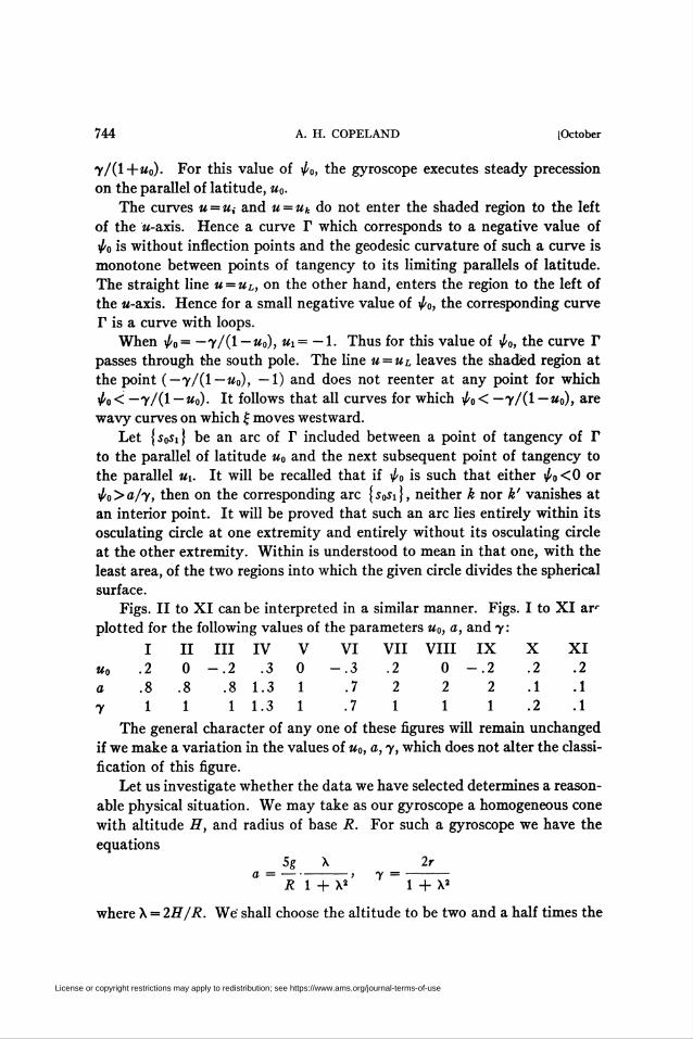
744 A. H. COPELAND [October
7/(1 +Uo). For this value of ^0, the gyroscope executes steady precession
on the parallel of latitude, u0.
The curves u = ut and u = uk do not enter the shaded region to the left
of the «-axis. Hence a curve T which corresponds to a negative value of
4>o is without inflection points and the geodesic curvature of such a curve is
monotone between points of tangency to its limiting parallels of latitude.
The straight line u = ul, on the other hand, enters the region to the left of
the «-axis. Hence for a small negative value of ¿o, the corresponding curve
T is a curve with loops.
When ^0= —7/(1 —«o), «i= —1. Thus for this value of ^0, the curve T
passes through the south pole. The line u = ul leaves the shaded region at
the point (—y/(l—u0), —1) and does not reenter at any point for which
^o< —7/(1 —«0). It follows that all curves for which \f/0< —y/(l—u0), are
wavy curves on which £ moves westward.
Let {soSi} be an arc of T included between a point of tangency of T
to the parallel of latitude u0 and the next subsequent point of tangency to
the parallel «1. It will be recalled that if \¡/<¡ is such that either ^0<0 or
to>a/y, then on the corresponding arc {s0Si}, neither k nor k' vanishes at
an interior point. It will be proved that such an arc lies entirely within its
osculating circle at one extremity and entirely without its osculating circle
at the other extremity. Within is understood to mean in that one, with the
least area, of the two regions into which the given circle divides the spherical
surface.
Figs. II to XI can be interpreted in a similar manner. Figs. I to XI arr
plotted for the following values of the parameters u0, a, and 7:
I II III IV V VI VII VIII IX X XI
«o .2 0 -.2 .3 0 -.3 .2 0 -.2 .2 .2a .8 .8 .8 1.3 1 .7 2 2 2 .1 .1
7 11 1 1.3 1 .7 1 1 1 .2 .1
The general character of any one of these figures will remain unchanged
if we make a variation in the values of u0, a, 7, which does not alter the classi-
fication of this figure.
Let us investigate whether the data we have selected determines a reason-
able physical situation. We may take as our gyroscope a homogeneous cone
with altitude H, and radius of base R. For such a gyroscope we have the
equationsSg X 2r
a = ~-, 7 =-R 1 + X2 1 + X2
where X = 2H/R. We' shall choose the altitude to be two and a half times the
License or copyright restrictions may apply to redistribution; see https://www.ams.org/journal-terms-of-use

1928] MOTION OF THE GYROSCOPE 745
diameter of the base. Then X = 10. In Case XI, a = A, and hence for this
case, the radius of the base of our gyroscope is about 4850 cm.
We do not, however, need to deal with such an enormous gyroscope.
In fact, we can alter the quantities a and y without changing the classifi-
cation of the motion provided we keep u0 and the ratio p = a/y2 fixed. Since
both a and 72 have the dimensions T~2, such an alteration may be brought
about by a change in the unit of time. The effect of such a change, upon
the u, ^o-diagram, is a uniform stretching in the direction of the ^0- axis.
We can now choose X = 10, a = 100, and y = 10/p1'2. We obtain a conical
gyroscope with altitude 24.25 cm. and diameter of base 9.7 cm. In Figs.
I to XI, p varies from about .78 to 10. Hence for the corresponding motions
the gyroscope makes from about 25 to 90 revolutions per second about its
axis.
4. Some exceptional cases. In §3, it was assumed that — 1 <u0 < +1. It
remains to consider the possibilities u0 = ± 1. In order to study these
possibilities, we shall form the function*
/(«) r t
(7) - = («o + u) [vo2 + a(u0 — u) \ — 72(«0 - u) = g(u).«o — u
Since g(u0) = 2u0Vq2 and g(—u0)= — 2u0y2, it follows that g(—l)g0
and g(+l)^0 an(i, since g(+°°) = — °°, there is a root, u\, of g(u) in the
interval — l^Wi^+1, and a root m2^+1. Moreover, u0 = Ui or #2 when
and only when v0 = 0, and ua= — «i or — u2 when and only when 7 = 0.
When «i = «o= ±1 or u2=u0= +1, the equation à=p may be satisfied
by setting v = 0 and u=u0. For, when u= ±1, /x = 0 and, when v = 0 and r
is constant, a is a constant vector. In this case, the axis of the gyroscope
remains vertical.
If 7 = 0, then r = 0 and, if «o= ±1, then \¡/=Q. Thus, if v0¿¿0, the gyros-
cope becomes a plane pendulum.f There are several cases to consider,
namely, if «0= — 1, then either Ui or u2 (or both) is equal to +1, and, if
«o = +1, then Mi = — l and «2 > +1.
First let us take u0 = — 1 and u2 = +1 >uu In this case, the amplitude of
the swing is 20i where cos Oi = «i. Next let us take u0 = — 1 and «i=u2 = +1.
In this case, the angular velocity of the pendulum at the south pole is such
that the pendulum approaches but never reaches the north pole.f Next
* In equation (7) it is assumed that «0= ± 1. If «o^ ±1, then the formula for g(u) =f(u)/(u0—u)
is given by equation (8).
t Cf. Love, Theoretical Mechanics, p. 129.
î Cf. Love, loc. cit., p. 131.
License or copyright restrictions may apply to redistribution; see https://www.ams.org/journal-terms-of-use

746 A. H. COPELAND [October
let us take m0= — 1 and «t= +1 <u2. In this case, the angular velocity of
the pendulum at the south pole is such that the pendulum passes through
the north pole and swings completely around.* Finally, let us take m0 = +1
<u% and Mi = — 1. This case is the same as the case just discussed.
If «o = ± 1 and neither v0 nor y is zero, then — l<ui<+l<u2, and hence
we can interchange the rôles of u0 and «i. That is, this case is equivalent to the
one in which — 1 <m0 < +1.
5. The bounding parallels of latitude. In the u, ^o-diagram, the locus of
points corresponding to points of tangency of T to the parallel of latitude ua,
is the straight line whose equation is u = u0. Since «i is also a root of/(«),
the equation of the curve m = Mi can be obtained by solving the equation
g(u) = 0 where g(u) is defined by the equation
(8) g(u) = /(«)/(«„ - u)
= - a«3 + [(1 - «o2)¿o2 + 72]« + [(1 - «<?)iM«o
+ a — 2(1 - ug)yfa — 72«o].
Likewise, u? is a root of g(u). Solving equation (8), we get
(1 - u0*)fa + 7a - (R(fa)Y>* (1 - uf)fa + 7a + Wo))1'3(9) Ml = -> «2 = -1
2a 2a
where
*(W = (1 - Mo2)V + 2(1 - Mo2)(72 + 2a«o)¿o2 - 8a7(l - u^)fa
+ (74 - 4a73«o + 4a3).
In order to study the nature of the curve u = uu we shall compute its
maxima and minima, treating, for convenience, mx as an implicit function
defined by the equation g(u) = 0 instead of making use of its explicit ex-
pression. Thus
dg_
du, dfa
dfa dgdu
- 2(1 - m|) [(«o + u,)fa -y]=- where v = 1,2.
(1 - Mo2)W - 2a«, + 7s
u = u.
Setting the numerator equal to zero, we obtain the equation u,=y/fa—Uo,
and hence we obtain the following value for g(u,) :
(10) g(y/fa - uo) = -yil-U0i)(fa - ~^-)(fa + -^_Y*. - -)•W \ 1 + «o/ \ 1 — Mo/\ 7 /
* Cf. Love, loc. cit., p. 131.
License or copyright restrictions may apply to redistribution; see https://www.ams.org/journal-terms-of-use

1928] MOTION OF THE GYROSCOPE 747
The roots of this last expression give the values of fa at the extrema of Mi
and M2. The extrema are thus seen to occur at the points
(.11) Pi: (-——» - l\ P.: (—f— > + l\ P3: (-, - - u0).M — Mo / M + m0 / \7 a /
In order to compare the points P2 and P3, we shall write the coordinates
of P3 in the form7 D
P3: '(rl+Uo 7(1 + «o)
where D is defined by equation (6).
When du,/d fa = 0,d2u, d2g_ /dg
du
1 +a/
Hence,
at Pi,
atP2,
at Pa
dfa2 dfa2
d2u, (1 - Mo2)(l - Mo)2
dfa2 72 + a(l - M0)
d2u, _ - (1 - m,?)(1 + M0)2
~dfa?~ Dd2u, 2(1 - Mo3h4
>0;
'' ¿¿o2 a[73+a(l- Mo)]l>
Pi is always a minimum but P2 is a maximum and P3 is a minimum if D is
positive, and P2 is a minimum and P3 is a maximum if D is negative. It
should be observed that dg/du never vanishes at Pi and that it vanishes at P2
and P3 only when D = 0. But, when D = 0,
Mi =
(12)
1 +
where
(13)
i^o-)*i(fa) if fa < a/y,
1 + ( fa-) X2(i¿o) if fa > a/y,
1 + (fa-jMiM Hfa< a/y,
1 + (fa - —)Xi(-Ao) if fa > a/y,
Xi(W = —[(1 - Moh + —(1 - «o2)(^o - a/y) + r(fa)],a 2
X2(W = -[(1 - «oh + -(1 - «o2)(¿o - a/y) - r(fa)],a 2
u2 =
License or copyright restrictions may apply to redistribution; see https://www.ams.org/journal-terms-of-use
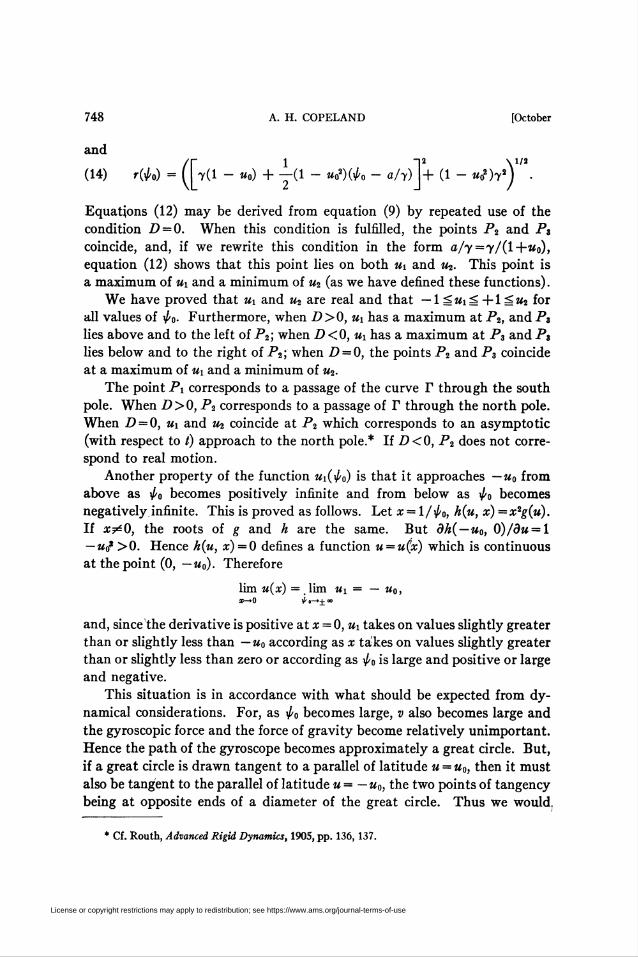
748 A. H. COPELAND [October
and
(14) r(W = ([7(1 - «o) + y(l - «o2)(¿o - a/7)]+ (1 - «o2)72) •
Equations (12) may be derived from equation (9) by repeated use of the
condition D = 0. When this condition is fulfilled, the points P2 and P3
coincide, and, if we rewrite this condition in the form a/y=7/(1 +«o),
equation (12) shows that this point lies on both Mi and u2. This point is
a maximum of ui and a minimum of m2 (as we have defined these functions).
We have proved that «i and u2 are real and that — 1 á«iá +1 ^«2 for
all values of ^0. Furthermore, when D>0,ui has a maximum at P2, and P3
lies above and to the left of P2; when D <0, «i has a maximum at P3 and P3
lies below and to the right of P2 ; when D = 0, the points P2 and P3 coincide
at a maximum of «i and a minimum of u2.
The point Pi corresponds to a passage of the curve V through the south
pole. When D>0,P2 corresponds to a passage of T through the north pole.
When D = 0, Ui and u2 coincide at P2 which corresponds to an asymptotic
(with respect to t) approach to the north pole.* If D<0, P2 does not corre-
spond to real motion.
Another property of the function Wi(iZ'o) is that it approaches — m0 from
above as \¡/0 becomes positively infinite and from below as 4>o becomes
negatively.infinite. This is proved as follows. Let x = l/^o, h(u, x)=x2g(u).
If x^O, the roots of g and h are the same. But dh(—u0, 0)/3m = 1
—wo* >0. Hence h(u, x) = 0 defines a function u = u(x) which is continuous
at the point (0, — u„). Therefore
lim u(x) = , lim «i = — Mo,
and, since the derivative is positive at x = 0, Mi takes on values slightly greater
than or slightly less than — u0 according as x takes on values slightly greater
than or slightly less than zero or according as \¡/0 is large and positive or large
and negative.
This situation is in accordance with what should be expected from dy-
namical considerations. For, as \p0 becomes large, v also becomes large and
the gyroscopic force and the force of gravity become relatively unimportant.
Hence the path of the gyroscope becomes approximately a great circle. But,
if a great circle is drawn tangent to a parallel of latitude u = uQ, then it must
also be tangent to the parallel of latitude u = — m0, the two points of tangency
being at opposite ends of a diameter of the great circle. Thus we would.
* Cf. Routh, Advanced Rigid Dynamics, 1905, pp. 136, 137.
License or copyright restrictions may apply to redistribution; see https://www.ams.org/journal-terms-of-use
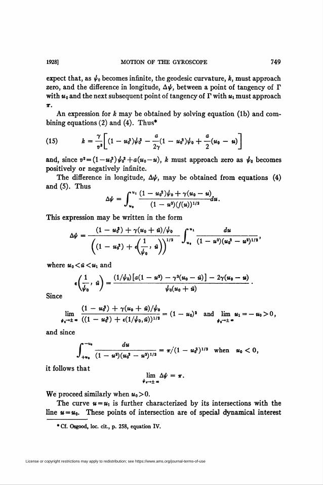
1928] MOTION OF THE GYROSCOPE 749
expect that, as fa becomes infinite, the geodesic curvature, k, must approach
zero, and the difference in longitude, Afa between a point of tangency of T
with Mo and the next subsequent point of tangency of T with Mi must approach
ir.
An expression for k may be obtained by solving equation (lb) and com-
bining equations (2) and (4). Thus*
(15) k = -j(i- uj)M - —(1 - u02)fa + v("o - «)1tr|_ 27 2 J
and, since v2 = (l— u02)fa2+a(u0—u), k must approach zero as fa becomes
positively or negatively infinite.
The difference in longitude, A^, may be obtained from equations (4)
and (5). ThusJ'u> (1 - M02)^o + 7(Mo - m)
-du.(1 - u2)(f(u)Y'2
This expression may be written in the form
(1 - mq2) + 7(m0 + u)/fa /•"•_du_
/ /l _\Y'a Ju, (1-m3)(mo2 -m3)1'3'((l_rf)+ «£„))'
where m0<m<Mi and
/ 1 \ (1/fa) [a(l - m3) - 7a(M0 - m) ] - 27(mo - m)el-—j Ml =-•
\^o / ^o(m0 + M)
Since
r (!-«(?) + 7(«o + ü)/falim -■-= (1 — Mo)3 and lun Mi = — m0 > 0,
#,-*. ((1 - Mo3) + e(l/fa,u)Y>* #,-.±-
and since
du
£!+u, (1 - M3)(Mo2 - M3)1'3
it follows that
= tt/(1 - Mo3)1'3 when m0 < 0,
lim A^ = v.*t-»±«o
We proceed similarly when m0>0.
The curve m = «i is further characterized by its intersections with the
line M = M0. These points of intersection are of special dynamical interest
* Cf. Osgood, loc. cit., p. 258, equation IV.
License or copyright restrictions may apply to redistribution; see https://www.ams.org/journal-terms-of-use

750 A. H. COPELAND [October
since the condition Mi = m0 is necessary and sufficient for steady precession.*
The values of wo at which the curve m = Mi crosses the straight line m = m0 are
given by solving the equation g(u0)=0 for ^o- Thus
7 ± d1'2
(16)2«o
where d is defined by equation (7) and where Mo^O. These values of to
are real and distinct, conjugate imaginary or coincident according as d
is positive, negative, or zero. If m0 = 0 the solution of g(u0) =0 is y0 = a/(2y).
6. Paths for which the longitudinal velocity vanishes. If the path, T,
of the gyroscope is a curve with loops, then the longitudinal velocity, wo,
when m = Mo, must be opposite in sign to the longitudinal velocity, yi, when
when m = mi, and hence y must vanish for some value of u between m0 and
«i. If, at certain points, T has cusps, then, at such points, v must vanish,
since by equation (16), k can be discontinuous only when v = 0. But, when
v vanishes, û and y must both be equal to zero. Hence the character of V
is related to the vanishing or non-vanishing of y.
Iî y = 0, we may solve equation (4) for u and get
wo(17) M = UL(wo) = Mo + (1 - Mo1)— •
7
The equation m = m¿ represents a straight line intersecting the line u = u0
in the point P0: (0, m0). The intersections of m = Ml with the curve m = Mi are
given by solving g(u¿) =0 for y0. Substituting m = m¿ and factoring, we get
riw - ¿o - ««■[*. - jfj [*. + rrj[> - 7}Hence the points of intersection of Ul(wo) with Mi(^0) are Px: (—7/(1—m0),
-1), P2: (7/(1+Mo), +1) and P4: (a/7, m0+(l-M02)a/72). We may write
the coordinates of P4 in the form P4: (7/(1+m0)— Z?/[7(1+m0)], 1 —
D(i —u0)/y2). Hence if ZMO, P4 lies on the curve Mi (y0)when P3 lies on the
curve Mü(^o) and P4 lies on the curve m2(^0) when P3 lies on the curve Ui(4>0),
and, if Z) = 0, P2, P3, and P4 coincide. The line u=Ul is shown in Figs.
I to XLWhen 0<iro<a/y, the line Ul(wo) lies outside of the region between w0
and Mi, since ul lies outside of this region for \p0 small and positive, and does
not cross m0 or Mi between P0 and P4. The line uL lies inside the region be-
tween Mo and Mi between the points P0 and Px and, when D<0, between P2
* Cf. p. 738.
License or copyright restrictions may apply to redistribution; see https://www.ams.org/journal-terms-of-use

1928] MOTION OF THE GYROSCOPE 751
and P4. All other parts of ul lie outside of this region. Hence the values of
fa corresponding to the points of m¿ which lie in this region, are given by the
inequalities*— 7 a y
-Ú fa Û 0 or — ̂ ¿o Ú-1 — m0 7 1 + M0
If fa is such that T is a curve with loops, then we have seen that, for this
value of fa, the point (fa, uL(fa)) must lie in the open region included be-
tween Mo and Ui(fa). The converse is also true; namely, if (fa, UL(fa)) lies
in the open region between u0 and «i, then fa and ¿i have opposite signs and
hence T is a curve with loops. For, by equation (4),
— To^o =- when y = 0,
1 — M3
and thus \¡/ and $ cannot vanish simultaneously when u lies in the open in-
terval between m0 and Mi. Therefore ^ changes sign whenever it vanishes.
But $> vanishes for, at most, one value of u between u0 and Mi, since u = UL{fa)
is a single-valued function. Hence fa and \pi have opposite signs when and
only when (fa, uL{fa) lies between u = w0 and u = uu and consequently when
and only when — 7/(1— M0)<^o<Oora/7<^o<7/(l+M0). It follows that fa
is negative when fa <—7/(1—m0) and positive when —7/(1 —m0)<^o^O.
If D>0, fa is positive when 0^fa<a/y, negative when ff/7<^o<7/(l+M0),
and positive when 7/(1+m0)<^o- If D = Q, \j/i is positive when 0^^0<
7/(1+M0) and when 7/(1+m0)<^o- If D<0, fa is positive when 0 g fa. Con-
sequently ris a wavy curve for which the drift of the motion is westward when
fa < —7/(1 —Mo), and T is a wavy curve for which the drift of the motion is
eastward when D>0 and 0<fa<a/y or 7/(1+m0)<^o, when D = 0 and
0<fa<y/(l+u0) or 7/(1+Mo) <fa, or when D<0 and fa>0. T is a curve
with loops when —y/(l—u0) <fa<0 or a/7<^0<7/(l+«o).
7. Paths having points of inflection. The purpose of this paragraph
is to determine what initial conditions are necessary in order that T may
have points of inflection. At such points, the geodesic curvature, k, must
vanish. But, when k is zero, we may solve equation (15) for u and get
(18) m = M» + (1 - m,?)—(¿o - a/(27)) = Ui(fa).a
The curve m = m< is a parabola with its concave side upward. Only those por-
tions of this parabola which lie in the region between m=m0 and m = Mi
correspond to real motion. The intersections of the curve u{ with the bound-
* The inequality a/y^y/(l—m0) implies D^O.
License or copyright restrictions may apply to redistribution; see https://www.ams.org/journal-terms-of-use

752 A. H. COPELAND [October
ary of this region are obtained by solving the equation g(u{) = 0 for y0 where
-2g(ui) =-(1 - UÍ)(yo - a/y)h(y0),
a(19)
a ayKyo) = (1 - «<Wos - —(1 - «o2)^o2- (72 - au0)y0 + — ■
27 2
We shall study the roots of h(y0). The signs of the coefficients of the
powers of y0 in h(ya) are given in the following scheme:
H-\- when 7a — amo > 0,
-)-\- when 72 — au0 = 0,
H-h + when 72 — öm0 < 0.
In all three cases the number of sign changes is two and therefore (Dy Des-
cartes' rule of signs) the number of positive roots is at most two. If we re-
place yo by —Vo, the signs of the coefficients are given by the following
scheme:-h + when 72 — aua > 0,
-h when 72 — au0 = 0,
-(-when72 — aM0 <0.
Thus in all cases, the number of negative roots is at most one. Since
h(0) = %ay>0 and h(— oo)=— oo, h(y0) must have precisely one negative
root and therefore the other two roots must be either both positive or else
conjugate imaginary. If the roots are real, the question which concerns us
is whether these roots correspond to intersections of m,- with Mi or with u%.
In order to investigate this question we form the function
(20) <KlM = «<GM - «i(W.
We shall show that 0(0) = m0—Mi(0) is positive. The condition $(0)>0
is equivalent to the statement that if the longitudinal velocity on a limiting
circle vanishes, then that circle is the upper limiting circle. Let us denote by
Mo the limiting circle upon which the longitudinal velocity vanishes. Then
v2 = v02 +a(u0—u). But the latitudinal velocity also vanishes when m = m0
and therefore v0 = 0. Thus, if u takes on greater values than m0, v becomes
imaginary, which is impossible. Therefore m0 must be the upper limiting
circle and 0(0) must be positive.*
Since Mi(+oo) = —Mo, it follows that <£(+«>) = +°°- But, since d> is
everywhere continuous, if it has one positive root, it must have a second.
This fact may also be proved directly from the explicit formula for «i(0).
License or copyright restrictions may apply to redistribution; see https://www.ams.org/journal-terms-of-use
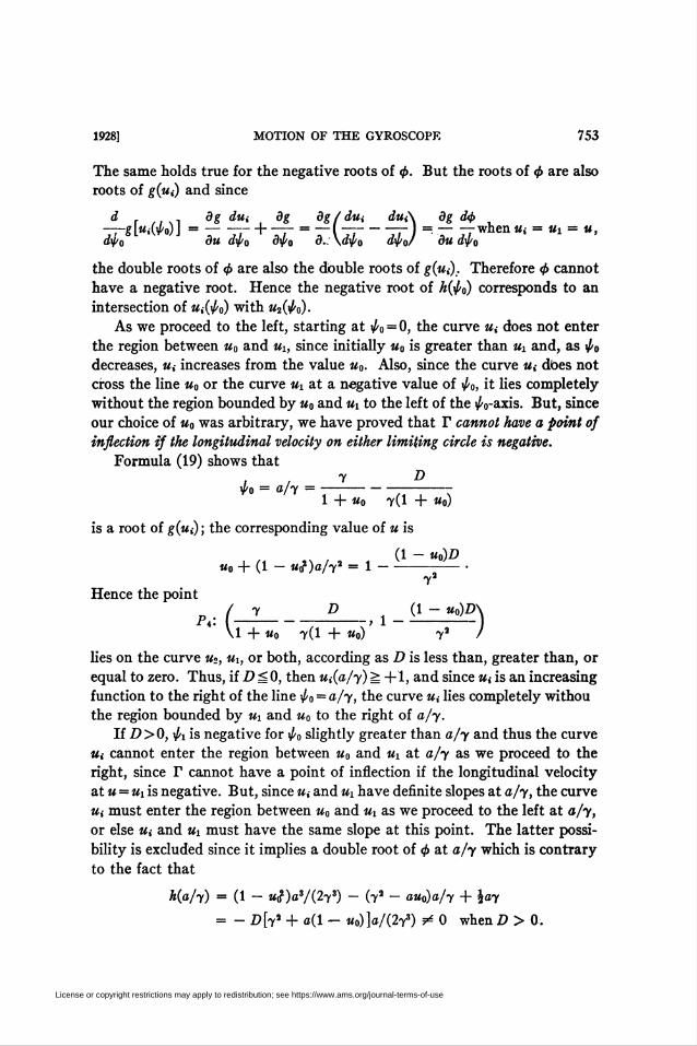
1928] MOTION OF THE GYROSCOPE 753
The same holds true for the negative roots of <f>. But the roots of <¡> are also
roots of g(u{) and since
d . . _ dg dut dg _ dg/dUj duA _dg d<b
dfa du dfa dfa d.: \dfa dfa/ du dfa
the double roots of 0 are also the double roots of g(u¡). Therefore <f> cannot
have a negative root. Hence the negative root of h(fa) corresponds to an
intersection of u{(fa) with u2(fa).
As we proceed to the left, starting at fa = 0, the curve Ui does not enter
the region between u0 and Mi, since initially m0 is greater than Mi and, as fa
decreases, m,- increases from the value u0. Also, since the curve m,- does not
cross the line m0 or the curve Mi at a negative value of fa, it lies completely
without the region bounded by m0 and Mi to the left of the ^0-axis. But, since
our choice of u0 was arbitrary, we have proved that T cannot have a point of
inflection if the longitudinal velocity on either limiting circle is negative.
Formula (19) shows that
/ / y DVo = a/y =-1 + Mo 7(1 + M0)
is a root of #(«,•) ; the corresponding value of u is
(1 - Mo)Z?mo + (1 - «f)o/y* - 1 -
Hence the point72
D (1 - uo)D\-, 1-
+ Mo 7(1 + «o) 7a /
lies on the curve u2, Mi, or both, according as D is less than, greater than, or
equal to zero. Thus, if D g 0, then u,(a/y) = +1, and since m,- is an increasing
function to the right of the line fa = a/y, the curve m, lies completely withou
the region bounded by Mi and m0 to the right of a/y.
If D>0, ¿1 is negative for fa slightly greater than a/y and thus the curve
Ui cannot enter the region between m0 and «1 at a/y as we proceed to the
right, since V cannot have a point of inflection if the longitudinal velocity
at m = Mi is negative. But, since u¡ and Mi have definite slopes at a/y, the curve
Ui must enter the region between m0 and Mi as we proceed to the left at a/y,
or else w< and Mi must have the same slope at this point. The latter possi-
bility is excluded since it implies a double root of <j> at a/y which is contrary
to the fact that
h(a/y) - (1 - uS)az/(2yS) - (73 - au0)a/y + \ay
= - i»[7a + o(l - Uo)]a/(2y3) * 0 when D > 0.
License or copyright restrictions may apply to redistribution; see https://www.ams.org/journal-terms-of-use
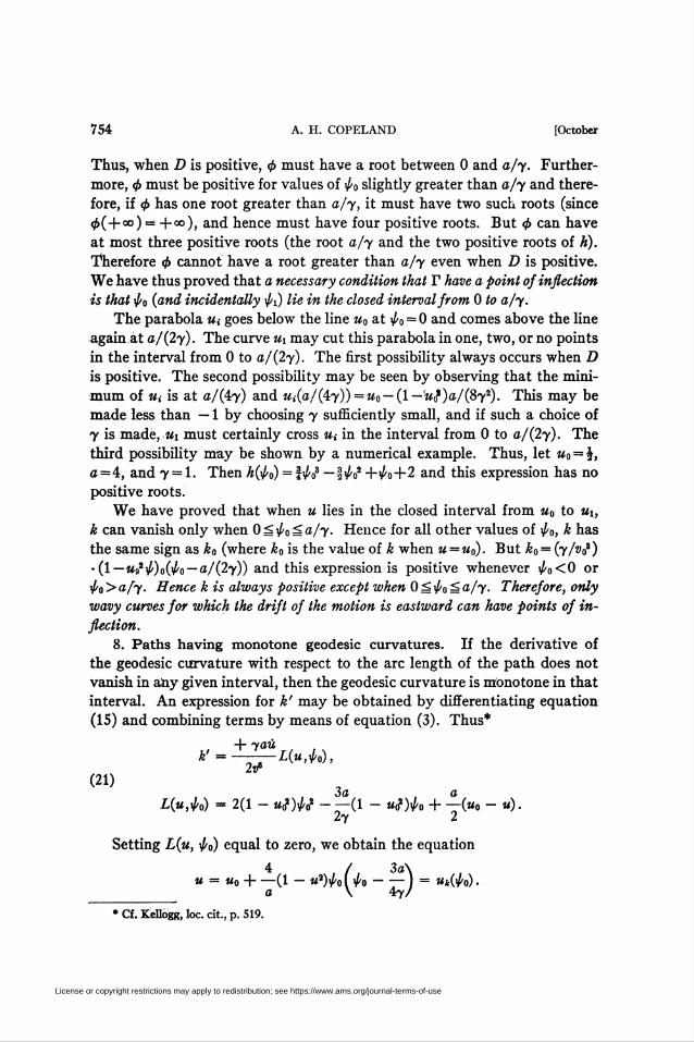
754 A. H. COPELAND [October
Thus, when D is positive, <j> must have a root between 0 and a/y. Further-
more, <f> must be positive for values of y0 slightly greater than a/y and there-
fore, if <f> has one root greater than a/y, it must have two such roots (since
d>(-\-co) = +00), and hence must have four positive roots. But <f> can have
at most three positive roots (the root a/y and the two positive roots of h).
Therefore d> cannot have a root greater than a/y even when D is positive.
We have thus proved that a necessary condition that T have a point of inflection
is that yo (and incidentally yi) lie in the closed interval from 0 to a/y.
The parabola m¿ goes below the line m0 at y0 = 0 and comes above the line
again at a/(2y). The curve M! may cut this parabola in one, two, or no points
in the interval from 0 to a/(2y). The first possibility always occurs when D
is positive. The second possibility may be seen by observing that the mini-
mum of Ui is at a/(47) and Ui(a/(4y)) = uQ — (I —,u0i)a/(8y2). This may be
made less than — 1 by choosing 7 sufficiently small, and if such a choice of
7 is made, Mi must certainly cross m,- in the interval from 0 to a/(2y). The
third possibility may be shown by a numerical example. Thus, let u0 = %,
a = 4, and 7 = 1. Then h(wo) = fwa3 —%w<? +wo+2 and this expression has no
positive roots.
We have proved that when u lies in the closed interval from u0 to Mi,
k can vanish only when 0 g y0 á a/y. Hence for all other values of y0, k has
the same sign as ¿0 (where k0 is the value of k when u = u0). But k0 = (7A08)
•(l—ua2y)0(yo — a/(2y)) and this expression is positive whenever y0<0 or
yo>a/y. Hence k is always positive except when Oíkwoúa/y. Therefore, only
wavy curves for which the drift of the motion is eastward can have points of in-
flection.8. Paths having monotone geodesic curvatures. If the derivative of
the geodesic curvature with respect to the arc length of the path does not
vanish in any given interval, then the geodesic curvature is monotone in that
interval. An expression for k' may be obtained by differentiating equation
(15) and combining terms by means of equation (3). Thus*
+ yaùk'=——L(u,y-o),
2s6(2D
3a aL(u,y0) = 2(1 - Mo2)^2 - — (1 - «<?Wo + —(mo - m).
27 2
Setting L(u, yo) equal to zero, we obtain the equation
4 / 3a\M = M0 H-(1 - M2)^o( WO- —) = Uk(wo) -
a \ 47/
* Cf. Kellogg, loc. cit., p. 519.
License or copyright restrictions may apply to redistribution; see https://www.ams.org/journal-terms-of-use

1928] MOTION OF THE GYROSCOPE 755
Hence k' vanishes when and only when u = uk(fa), u = u0, or u = Ui(fa).
The curve uk(fa) is a parabola which intersects the parabola Ui(fa) in
the points P0: (0, u0) and P4: (a/y, M0+a(l— u$)/y2), and only at these
points. But Po lies on the line u = u0 and P4 lies on the curve u = uxoxu=u2.
Hence k and k' vanish simultaneously (at points corresponding to real mo-
tion) only at the intersections of u,- with m0 and «i. These points of intersec-
tion cannot correspond to points of inflection of the path, since T is
symmetric in any meridian circle through a point of contact with the parallel
of latitude u0 or ux and hence k cannot change sign at such a point. There-
fore, in the m, ̂ o-plane, the points of the parabola u = m< which lie in the open
region included between w0 and Mi, and only these points, correspond to
points of inflection of the path T.
We have proved that the parabola u = Ui(fa) lies inside the shaded re-
gion* between m0 and Mi only when 0^fa^a/y. The same is true for the
parabola uk. This follows from the fact that the portion of uk for which
^o<0 lies in the region bounded on the left by the parabola «,- and on the
right by the ^0-axis. This region, we have seen, does not overlap the region
between u0 and «i. Likewise, the portion of uk for which a/y < fa, lies in the
region bounded on the left by the line fa = a/y and on the right by the para-
bola Ui. This region does not overlap the region between u0 and «i. Conse-
quently, the path V has monotone geodesic curvature between a point of
tangency with u0 and the first subsequent point of tangency with mx (or
vice versa), whenever ^0<0 or a/y < fa. The same is true whenever fa<0
or a/y < faSince L(u, fa) can vanish only when 0^fa^a/y, and since L(u0, fa)
= 2(1 —Uo*)fa(fa—3a/(4y)) is positive whenever ^0<0 or fa>a/y, it follows
that sgn £' = sgn ù whenever fa<0 or fa>a/y.O. D. Kellogg has provedf that if the arc derivative K' of the curvature^,
K, of an arc {sis2} (where Si<s2) of a spherical curve is always positive,
then the arc {sis2} lies entirely within the osculating circle at sh and entirely
without the osculating circle at s2. The curvature, K, is related to the
geodesic curvature, k, by means of the equation
1 + F= K2.
Hence kk' = KK'. But we have proved that, whenever ^0<0 or fa>a/y,
k>0 and sgn £' = sgn u. Therefore, when ^0<0 or fa>a/y, an arc of T
♦ Cf. Figs. I to XI.t Cf. O. D. Kellogg, loc. cit., pp. 509, 521.X The arc {S1S1} is regarded as an arc of a space curve and if is the curvature at a given point
of this arc.
License or copyright restrictions may apply to redistribution; see https://www.ams.org/journal-terms-of-use

756 A. H. COPELAND [October
consisting of a half wave lies entirely within the osculating circle at its point
of tangency with m0, and entirely without the osculating circle at its point
of tangency with uh or entirely within the osculating circle at Mi and entirely
without the osculating circle at m0, according as mx is north or south of m0.
9. The spherical pendulum. When 7 = 0, the gyroscope becomes a spheri-
cal pendulum.* Thus we can discuss the behavior of the spherical pendulum
if we know the nature of the curves «i, uL, Ui, and uk.\
As 7 approaches zero, the point Pi: (—7/(1—m0), —1) approaches the
point (0, —1), the point P2: (7/(1+m0), +1) approaches the point (0, +1),
and the point P3(a/y, y2/(a—u0)) goes out to +00. Hence the line m¿ turns
into coincidence with the M-axis and the curves m¿ and uk degenerate into the
M-axis. Thus we have again the familiar facts that the paths of the spherical
pendulum are always wavy curves and are without inflection points. Í We
have in addition the fact that the curvature of a path of a spherical pendulum
is always monotone between points of tangency to the bounding parallels
of latitude.
The curve m¿ crosses the straight line u0 at the points y0=± (—a/(2u0))112.
These points are real when and only when m0<0. For these values of wo,
the phenomenon of the conical pendulum occurs. When y0 = 0, we have a
plane pendulum.
The curve w,- approaches the straight line — w0 when wo becomes positively
or negatively infinite. Thus, as in the case of the gyroscope, the force of
gravity is relatively unimportant when y0 is large.
10. Curves near the north or south pole. Let us consider a curve passing
through the north pole. For this curve the longitudinal velocity at Mo is
wo=y/(k+Uo). Hence equation (4) reduces to
1 + M
Thus the change in longitude, Aip, between m0 and the north pole is given by
the integralJ»i y du-
u, (1 + u)(a(u - 1*0(1 - «)(«, - m))1'2
This integral may be written in the form
duAy
7 Ç1_«
" (<*(m2 - m))1'2 J„. (1 + m)((m-(a(u2 - m))1'2 Ju, (1 + m)((m - Mo)(m2 - m))1'2
* Cf. Appell, loe. cit., Tome I, pp. 513-524.t These curves are shown in Fig. XII.
I Cf. the photographs of the paths of spherical pendulums (Webster, Dynamics, pp. 50, 51).
License or copyright restrictions may apply to redistribution; see https://www.ams.org/journal-terms-of-use

1928] MOTION OF THE GYROSCOPE 7S7
where m0 < m < 1. ThereforeÎT7
A^ =-(2a(l + mo)(m2 - m))1'3
Next let us find an expression for m2. This is easily done since, when
fa=y/(l+u0), f(u) = (l-u) («o-«) [a(l+M)-273/(l-|-Mo)]. Thus we ob-
tain the expression273
m2 = - 1 +-a(l + Mo)
Substituting this value in the formula for Afa we obtain the equation
A* - y[l - a(\ + Mo)(l + m)/(273)]-1/3.
Furthermore if we set 72 = 2a, then as u0 approaches 1, A\¡/ becomes infinite.
Hence, by a proper choice of a, y and m0, we can make A^ as large as we
please.
If we set fa=y/(l+u0)+h, then, corresponding to any value of h, we
obtain a path T(h). Let us denote by A\J/(h) the change in longitude along
T(h) between m0 and «i. As h approaches zero either through positive or
through negative values, the circle Mi approaches the north pole and the curve
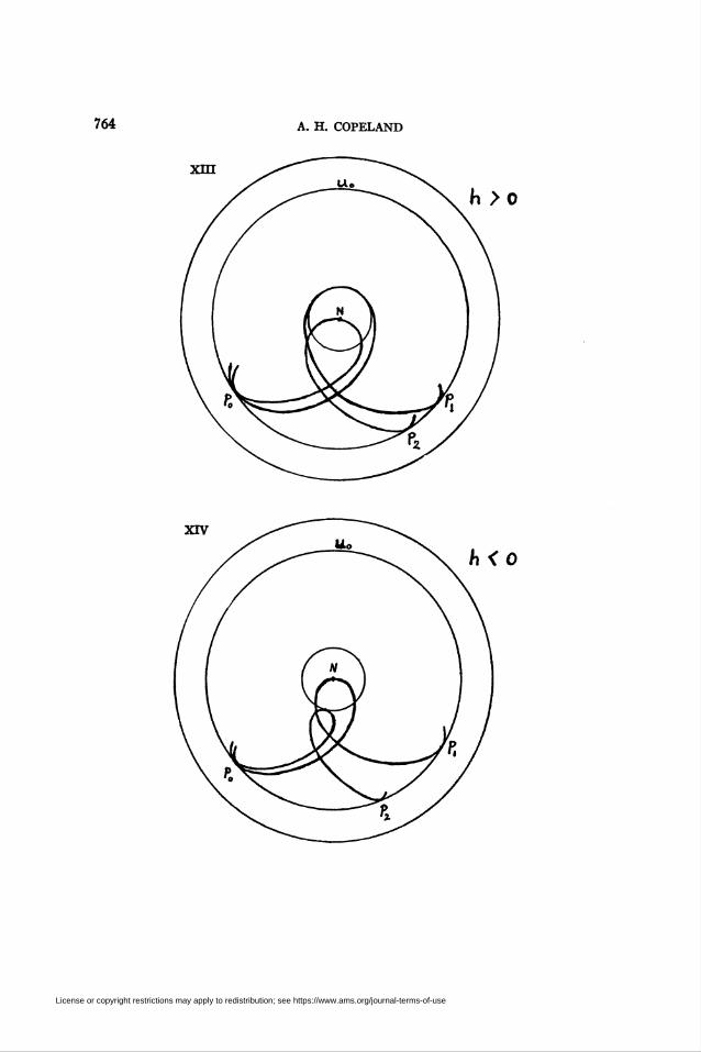
T(h) approaches the limiting curve JT(0). If \h\ is small and h<0, T(h)
is a curve with loops, and if h>0, T(h) is a wavy curve. This situation is
shown in Fig. XIII.
If A>0, then the change in longitude along the curve T(h) from P0 to Pi
is 2A\¡/(h). It is easily seen geometrically that 2A\¡/(h) —2A^(0) differs from
ir by an amount which is numerically equal to the difference in longitude
between Pi and P2. But, as h approaches zero, Pi approaches P2. Therefore,*
lim AiKA) = AfaO) + — ■k-*o+ 2
In a like manner, it may be proved that*
lim A^(â) = AiKO) - — •A-*o 2
* These equations can also be obtained analytically. For we have the equation
= p _ydu_ Ç "1_(1 - ufîhdu_
A*( ' ~ J«0 <1 + «)(o(m-«o)(«i-«)(«í-«))1/2 J«o (1-«2)(o(k-«o)(mi-«)(«*-tí))1'»"
As h approaches zero, «1 approaches +1. Hence
. r*i ydu _ Ç1
h-oJ «o (1 + u)(a(u - «o)(»i - «)(% - »))1/J J »0 (1. + u)(a(u - «,)(1 - u)(u, - «-))•«
= A*(0).
It remains to prove that
License or copyright restrictions may apply to redistribution; see https://www.ams.org/journal-terms-of-use

758 A. H. COPELAND [October
But we have proved that Ay/(0) may be made as large as we please and hence
by choosing \h \ sufficiently small, A\[^(k) may be made as large as we please.*
r «i (1 — u¿)hdu Tlim I -= ± — •A-o J «o (1 - k«)(o(« - «o)(«i - «)(«» - w))1" 2
By means of the substitution u = 1—(1 — Ui)x, we obtain the equation
■ «i (1 - ufthdu
/. «o (1 — «2)(o(m — «o)(«i — «)(«i — m))"*
U-uJHl-uO (1 _ Mo2)dx_i__r~ (i - «0«v,
:rm<
i^J, *[2 - (1 - «i)*](a[(l - Mo)-(l -«0*][(«i - 1) + (1 - «i)*][* - l])1"
x[2-(l-«1)*](a[(l-«,)-(l-«1)*][(«,-l)-l-(l-«i)x][*-l])"»
Furthermore
. u-i^/u-«,) (1 _ Ulf)dx
I. (1 - «ifldx x 1 - »„'
f, 2ï[(x-l)o(l-«o)(«l-l)]1/,' 2 [a(l - «o)(«i - l)]1"
Finally we have to evaluate limju„[A/(l— «i)"1]. In order to obtain a value for this limit, we shall
expand the function Ui=u¡(y/(l+u<,)+h) about the point A=0. But when A=0 (cf. p. 747)
dm „ . dhn (1 - uf)(\ + Ug)1-= 0 and -— =-■-#o <W D
Hence(1 - «¿0(1 + «.)',.
«i = l-—-» + (h(h)
where 0,{h) is an infinitesimal of at least the third order in h. Therefore
A ..* (2Z>)J"lim -; = — lim -
1-0+ (1 - u,)1'1 *-o- (1 - «O1" (1 + «o)(l - »o2)1"
It follows that
/'«i_(1 - u<?)kdu_ /-«i _(1 - u<?)hdu_
u0 (i — u¿)\a{u — «o)(«i — «)(«* — «)•]"* *-*o-J«0 (1—.Mg*)[a(ti—«0)(wi-»)(«f—f)]1"
- jü / 2i> _y/2
™ 2 \o(l+«o)(«,-^Íj/ '
But «i--l+2W[«(l+««)] and D-V-ä(14-»s) and thus
c_??_v=1Va(l + M.)(«.-1)/
Consequently
foii+A,«A) = A*(0) + x/2
andlim A^(Ä) = AiKO) - x/2 •
• In the case of the spherical pendulum, G. H. Halphen proved (cf. Traité des Fonctions Ellip-
tiques, vol. 2,1888, p. 128) that the difference in longitude between successive points of tangency to
limiting circles.is always less than x; and V. Puisseux proved (cf. Journal de Mathématiques, vol.
7 (1842), p. 517) that this difference in longitude is always greater than x/2. Simple proofs of both
theorems are given by A. de Saint Germain in the Bulletin des Sciences Mathématiques, 1896,1898,
1901, and in the Mémoires de l'Académie de Caen, 1901. Cf. also the remark of Kellogg (loc. cit.,
p. 521) concerning this change in longitude in the case of the gyroscope.
License or copyright restrictions may apply to redistribution; see https://www.ams.org/journal-terms-of-use

1928] MOTION OF THE GYROSCOPE 759
Furthermore, by choosing a sufficiently small (or y sufficiently large) we
may make A^(0) differ from ir/2 by an amount which can be made as small
as desired. Thus by first choosing a small and then choosing h<0 and \h \
small, we can make Aip(h) differ from zero by an amount which can be made
arbitrarily small. When h<0, we recall that T is a curve with loops.
At the south pole, fa= —y/(l—u0), and the change in longitude, A^,
is given by the equation
-:-.1 (1-m)[ö(m0 - m)(m + 1)(m2 - m)]1'3
The evaluation of this integral gives the expression
— 7T
A\l/ = t-r— where — 1 < m < Mo.[2a(l - Mo)(m2 - ü)Y'*
But, since M2 = 1+272/[ö(1— m0)], we obtain the equation
x lA<A =-
2 / a(l - mo)(1 - m)\1/31+ —
27 /
Hence —7r/2 < A^- <0, and by a proper choice of a (or 7) A^ may be made to
differ from 0 or —7r/2 by an arbitrarily small amount.
If we let fa= —7/(1— Mo) + h, then corresponding to any value of h, we
obtain a path T(h). If \h \ is small and h>0, T(h) is a curve with loops, and
if h<0, T(h) is a wavy curve westward. This situation is shown in Fig. XIV.
It is easily seen that at the south pole*
lim Afah) = A^(0) + t/2k-o+
andlim Afah) = A^(0) - t/2 •*-»o
But, since —7r/2<A^(0), it follows that when \h\ is sufficiently small
0 < Afah) < ir/2 when A > 0
and- r < Afah) < - */2 when A < 0.
When A>0, A\j/(h) can be made arbitrarily near to either 0 or 7r/2, and when
A<0, A^(A) can be made arbitrarily near to either —x or —ir/2.
* These equations may also be obtained analytically. Cf. footnote p. 757.
Harvard University,
Cambridge, Mass.
License or copyright restrictions may apply to redistribution; see https://www.ams.org/journal-terms-of-use

760 A. H. COPELAND [October
PTS
License or copyright restrictions may apply to redistribution; see https://www.ams.org/journal-terms-of-use

1928] MOTION OF THE GYROSCOPE 761
License or copyright restrictions may apply to redistribution; see https://www.ams.org/journal-terms-of-use

762 A. H. COPELAND [October
A. A. i j.
U: .¿f .;•
I ç L Ni•ft. I o
s / »
^xç"\ V^r^ ̂ \^r*\
7f/~^> ^ J J' V' A v A0 / / //vi o //A
5 I «i il'
License or copyright restrictions may apply to redistribution; see https://www.ams.org/journal-terms-of-use

1928] MOTION OF THE GYROSCOPE 763
License or copyright restrictions may apply to redistribution; see https://www.ams.org/journal-terms-of-use
A. H. COPELAND
h >0
h<0
License or copyright restrictions may apply to redistribution; see https://www.ams.org/journal-terms-of-use