Two Worlds: Abstractions in the Continuous World Rupak Majumdar Max Planck Institute for Software...
59
Two Worlds: Abstractions in the Continuous World Rupak Majumdar Max Planck Institute for Software Systems
-
Upload
clinton-nash -
Category
Documents
-
view
216 -
download
2
Transcript of Two Worlds: Abstractions in the Continuous World Rupak Majumdar Max Planck Institute for Software...

Two Worlds:Abstractions in the Continuous World
Rupak Majumdar
Max Planck Institute for Software Systems

Cyber-Physical Systems
1. Software Controlled interactions
with the physical world
2. Safety Critical
Software a major component:
Boeing 747: ~50ECUs, 4M LOC
ETCS Kernel: ~0.5MLOC
Lexus 2006: ~100 CPUs, ~7M LOC
BMW: ~70-100CPUs, ~100M LOC!

Cyber-Physical Systems
1. Software Controlled interactions
with the physical world
2. Safety Critical
3. Software is the hard part
- Expensive, brittle
- Low productivity, High QA cost
- Major part of development cost
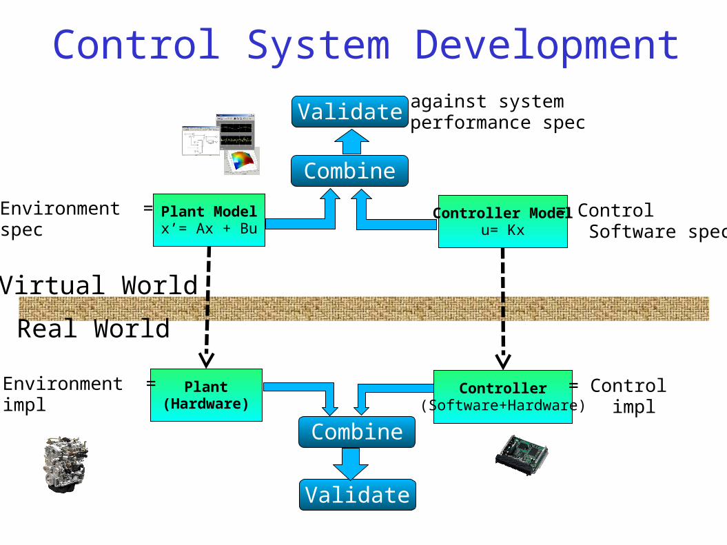
Control System Development
Plant Modelx’= Ax + Bu
Virtual World
Real World
Controller Modelu= Kx
= Control Software spec
Environment = spec
Combine
Validate against systemperformance spec
Plant(Hardware)
Controller(Software+Hardware)
= Control impl
Environment = impl
Combine
Validate
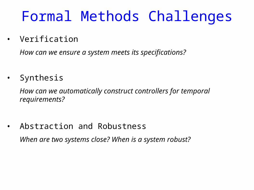
Formal Methods Challenges
• Verification
How can we ensure a system meets its specifications?
• Synthesis
How can we automatically construct controllers for temporal requirements?
• Abstraction and Robustness
When are two systems close? When is a system robust?

This Talk: FM in the Control World
- Proof techniques for verification
- Epsilon-bisimulations and reactive synthesis
- Input-output robustness
- End-to-end arguments

Disclaimer
Tutorial introduction to the field

Continuous Dynamical Systems
f : Dynamics
u : Input from the controller
… assume f is “nice”
Trajectory: Solution of the differential equation
Specification:
Stability: “Under the action of the controller, the dynamics converges to the origin”

Hybrid Dynamical Systems
||
Discrete constraint: - Control task can only run once every k cycles
- The system must reach a sequence of setpoints while avoiding bad states
- LTL specification

Verification Question
||
Given a controller that claims to- Stabilize the system- Satisfy additional discrete constraints
Check the controller works correctly
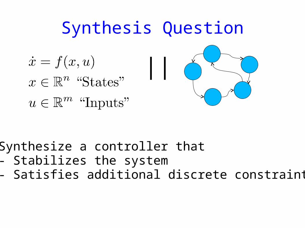
Synthesis Question
||
Synthesize a controller that- Stabilizes the system- Satisfies additional discrete constraints

Formal Methods Perspective
Verification:
Safety Inductive invariants
Liveness Ranking functions
Synthesis:
Controller design Reactive synthesis
Q: How do we apply these techniques to the continuous world?
Verification

CommonalitiesControl Theory
-Safety: Show that system stays in safe states
-Stability: Show that system eventually goes to setpoint
-Techniques: Real Analysis
Formal Methods
-Safety: Show that program stays in safe states
-Liveness: Show that program eventually terminates
-Techniques: (Discrete) Logic

Model
Problem: Ensure no trajectory fromInit reaches Bad

Barriers: B(x)
Init
Bad
The dynamics pushes the stateback at the boundary of the barrier
[PrajnaJadbabaie04]
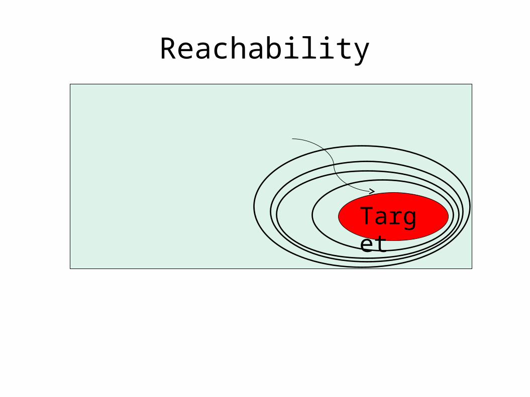
Reachability
Target
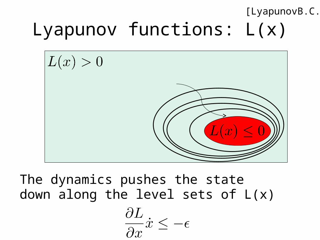
Lyapunov functions: L(x)
The dynamics pushes the statedown along the level sets of L(x)
[LyapunovB.C.]

CommonalitiesControl Theory
-Safety: Show that system stays in safe states
* Barrier certificates
-Stability: Show that system eventually goes to setpoint
* Lyapunov functions
-Techniques: Real Analysis
* Constraints?
Formal Methods
-Safety: Show that program stays in safe states
* Inductive invariants
-Liveness: Show that program eventually terminates
* Rank functions
-Techniques: (Discrete) Logic
* Horn clauses

Barriers/LF to Constraints

Constraints: Polynomials
Assume f(x) is a polynomial
Fix polynomial template for B
Polynomial constraints
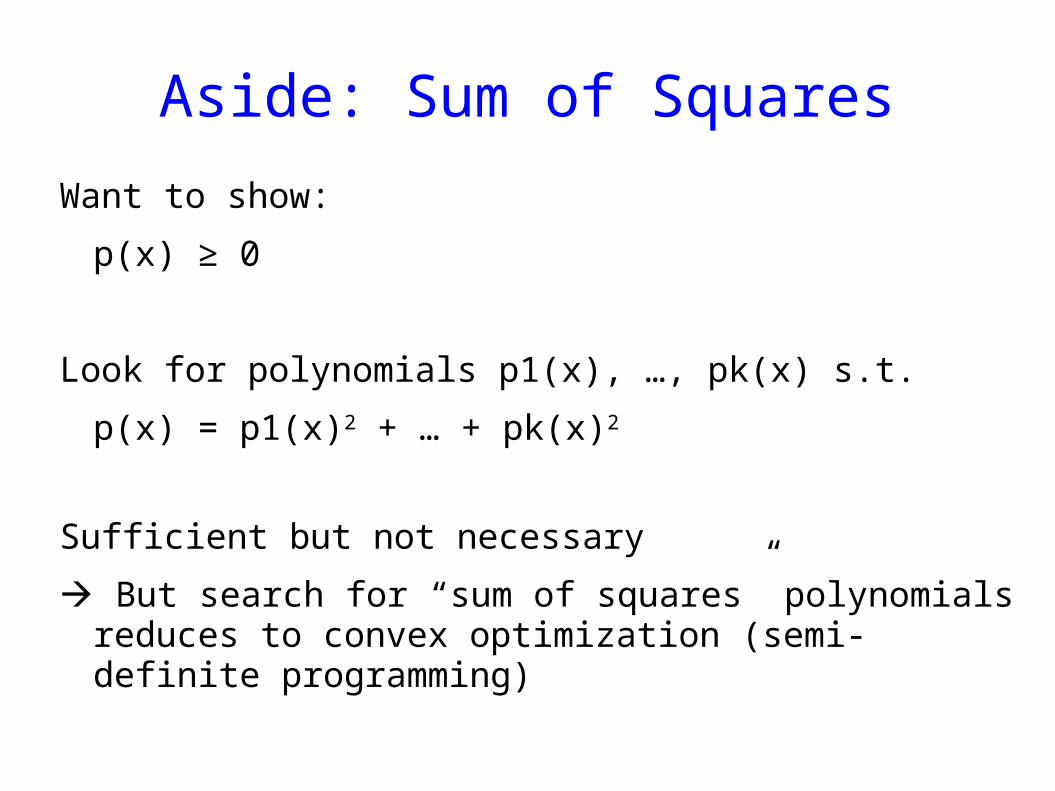
Aside: Sum of Squares
Want to show:
p(x) ≥ 0
Look for polynomials p1(x), …, pk(x) s.t.
p(x) = p1(x)2 + … + pk(x)2
Sufficient but not necessary
But search for “sum of squares” polynomials reduces to convex optimization (semi-definite programming)

Not just Safety/Reachability…
Horn clause formulations carry over:
- LTL, CTL*, ATL* [DimitrovaM]
Idea for LTL:
1.Convert to parity conditions
2.Certificate = Sequence of functions V0,…,Vk
- even i barrier
- odd i Lyapunov function that exits this color

Formal Methods Challenge
1.Design numerically stable and scalable decision procedures for polynomial arithmetic
2.Connect the search for barriers and Lyapunov functions to abstraction-refinement techniques
Synthesis

Continuous system
Controller Synthesis for LTL
Abstraction
Reactive synthesis
Discretecontroller
Refinement
Control input u
?

ε-Bisimulation
(x,y) R means that every trajectory starting from x ∈is matched up to ε by a trajectory from y and vice versa
GirardPappas07,Tabuada

Continuous system
Controller Synthesis for LTL
Abstraction
Reactive synthesis
Discretecontroller
Refinement
Control input u
When do finite bisimulations exist?

Incremental Stability
“Trajectories converge to each other as time progresses”
Incremental asymptotic stability (AS):
|| x(t, x0, u) - y(t, y0, u) || ≤ β (|| x0 – y0 ||, t)
for all u
Incremental input-to-state stability (ISS):
|| x(t, x0, u) - y(t, y0, v) || ≤ β (|| x0 – y0 ||, t) +
γ( || u – v || )
β is KL, γ is K∞
Angeli02
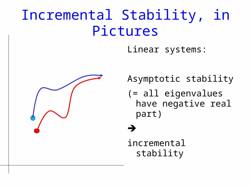
Incremental Stability, in Pictures
Linear systems:
Asymptotic stability
(= all eigenvalues have negative real part)
incremental stability

Transition Systems
Fix a sampling time τ
Transition system:
States: Rn
Labels: Piecewise constant control inputs
Transitions:

Intuition
- Discretize state and input space
- Error accumulated due to discretization cancel out because of incremental stability
x
y
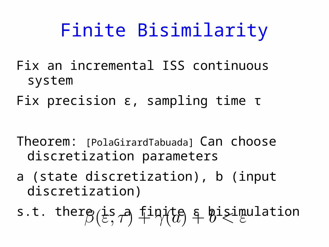
Finite Bisimilarity
Fix an incremental ISS continuous system
Fix precision ε, sampling time τ
Theorem: [PolaGirardTabuada] Can choose discretization parameters
a (state discretization), b (input discretization)
s.t. there is a finite ε bisimulation

Extensions: Stochastic Dynamics
- Extend notions of incremental ISS to stochastic ones
- Finite epsilon-bisimulation (in the sense of expectations) exists for any compact set
ZamaniEfsahaniM.AbateLygeros

Good News/Bad News
- Now discrete synthesis can be applied
- Tool: Pessoa [RoyM.Tabuada]
- (coming up)
- Expensive procedure: exponential in the dimension of the system

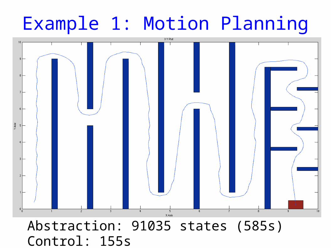
Example 1: Motion Planning

Example 1: Motion Planning
Example 1: Motion Planning
Abstraction: 91035 states (585s)Control: 155s
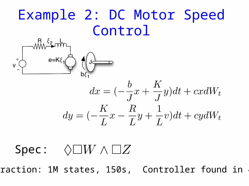
Example 2: DC Motor Speed Control
Spec:
Abstraction: 1M states, 150s, Controller found in 4s
Formal Methods Challenges
1. Better abstractions for bisimulations?
- Using timed automata?
(exponentially succinct representations)
2. Abstraction and refinement for control?

End-to-end Design

Control System Development
Plant Modelx’= Ax + Bu
Virtual World
Real World
Controller Modelu= Kx
= Control Software spec
Environment = spec
Combine
Validate against systemperformance spec
Plant(Hardware)
Controller(Software+Hardware)
= Control impl
Environment = impl
Combine
Validate
Controller Implementations
Physical world and software implementations may not match up
• Resource constraints, finite precision, distributed computation
• Uncertainties in measurements/actuations
How can we ensure that the implemented system correctly implements the controller?
What does correctly mean?
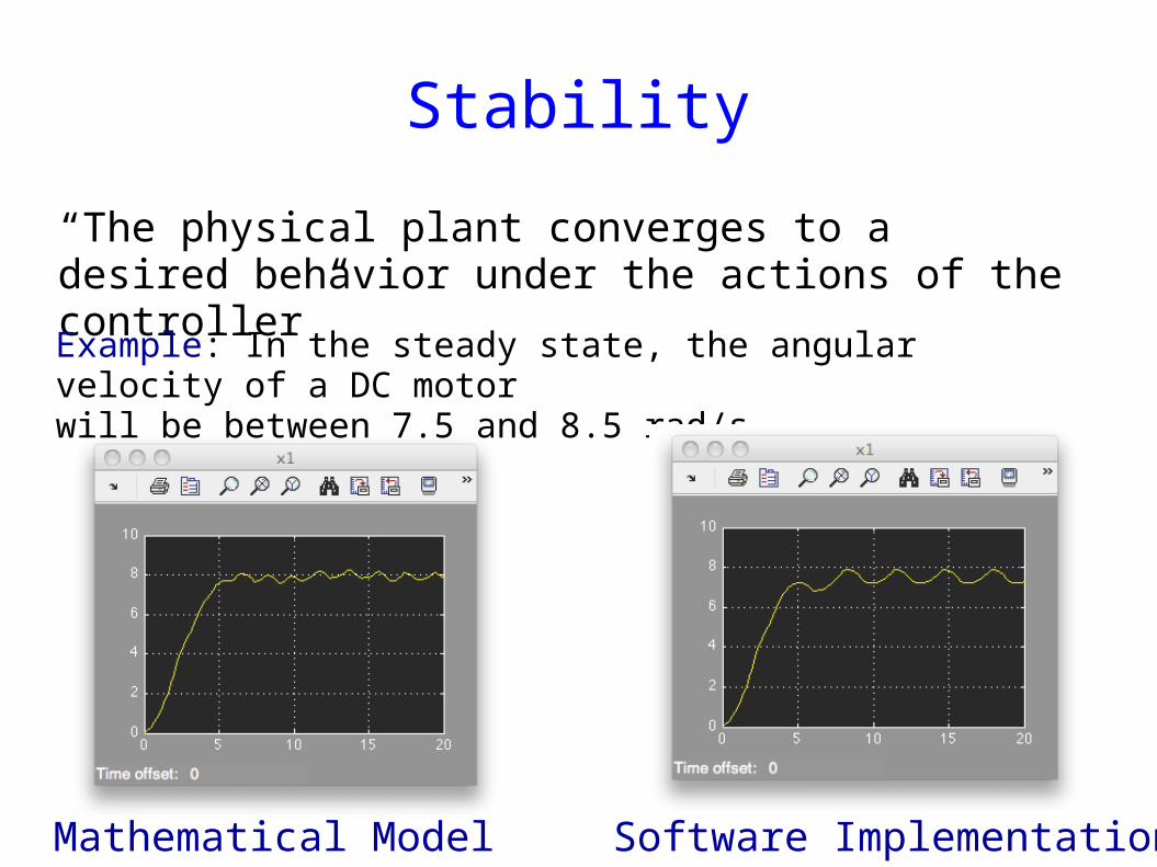
Stability
“The physical plant converges to a desired behavior under the actions of the controller”
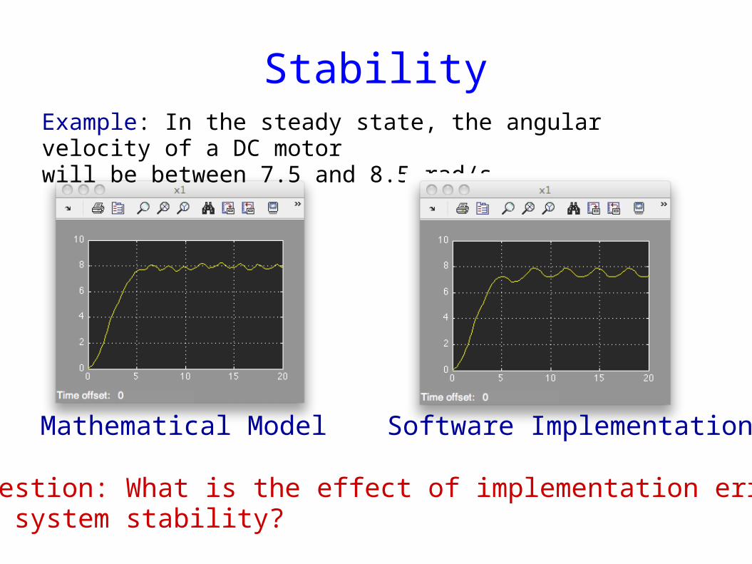
Example: In the steady state, the angular velocity of a DC motor will be between 7.5 and 8.5 rad/s
Mathematical Model Software Implementation
StabilityExample: In the steady state, the angular velocity of a DC motor will be between 7.5 and 8.5 rad/s
Mathematical Model Software Implementation
Question: What is the effect of implementation erroron system stability?

Effects of Implementation Error
Ideal, Mathematical Model Implementation
The software implementation introduces errors due to:- Limited precision arithmetic- Quantization of sensing and actuation- Computation times-…
Can we bound the effect of error on the stability?
ρ
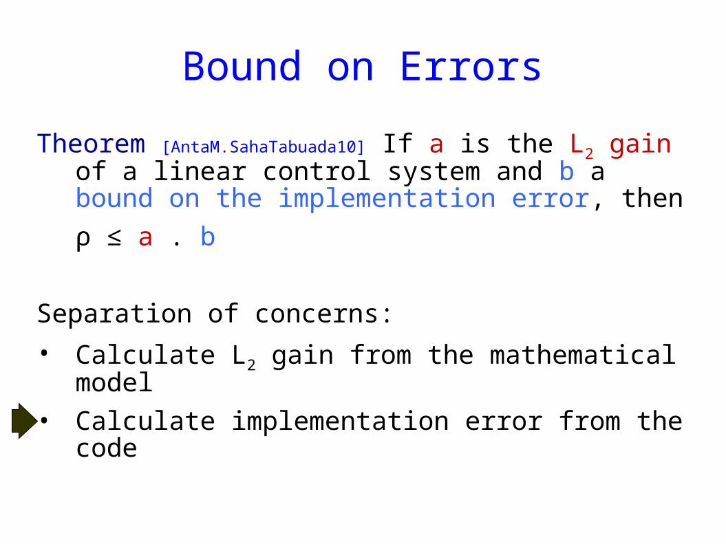
Bound on Errors
Theorem [AntaM.SahaTabuada10] If a is the L2 gain of a linear control system and b a bound on the implementation error, then
ρ ≤ a . b
Separation of concerns:
• Calculate L2 gain from the mathematical model
• Calculate implementation error from the code

Non-linear Systems
System x’ = f(x,u) Controller u = k(x)
Use an ISS Lyapunov function V, and the additional constraint from robust control theory:
∂V/∂x . f(x,k(x)+e) ≤ - λV(x) + σ || e ||
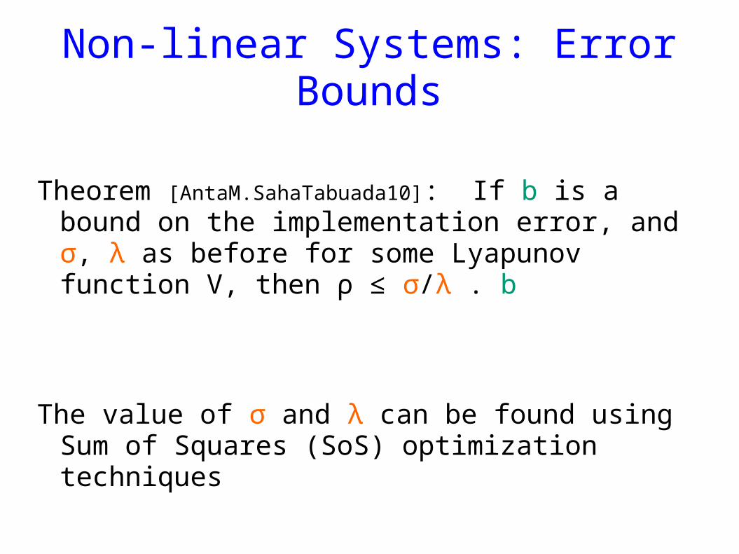
Non-linear Systems: Error Bounds
Theorem [AntaM.SahaTabuada10]: If b is a bound on the implementation error, and σ, λ as before for some Lyapunov function V, then ρ ≤ σ/λ . b
The value of σ and λ can be found using Sum of Squares (SoS) optimization techniques

Error Sources
- Sampling errors: Sampling a function at discrete points
- Quantization errors: Finite precision arithmetic
Assume that sampling errors are negligible (by sampling fast enough)
Focus on quantization errors

Bounding the Error: Finite Precision
• Only consider error due to finite precision
• Target fixed-point implementations
• Each real variable is implemented using n bits, with k bits for the fractional part
n
k

Fixed Point Arithmetic
Can perform arithmetic operations on this representation (using bitshifts and arithmetic)
n
k1
n
k2
n
k1
n
k1
+ +
n
k1

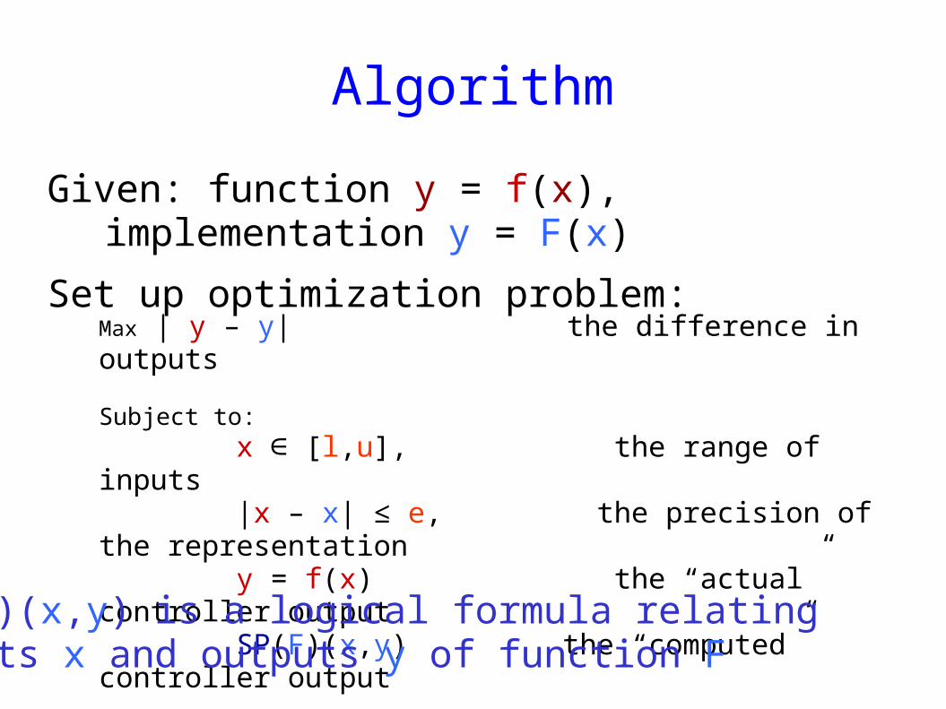
Algorithm
Given: function y = f(x), implementation y = F(x)
Set up optimization problem:
Max | y – y| the difference in outputs
Subject to: x [∈ l,u], the range of inputs |x – x| ≤ e, the precision of the representation y = f(x) the “actual” controller output SP(F)(x,y) the “computed” controller output
SP(F)(x,y) is a logical formula relatinginputs x and outputs y of function F
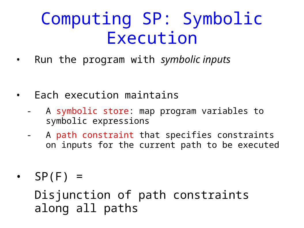
Computing SP: Symbolic Execution
• Run the program with symbolic inputs
• Each execution maintains
- A symbolic store: map program variables to symbolic expressions
- A path constraint that specifies constraints on inputs for the current path to be executed
• SP(F) =
Disjunction of path constraints along all paths

Simulink Model
C code
Instrumented C code
Real-TimeWorkshop
Concolic Execution
Yices+HySat Symbolic constraints
CIL
Implementation
-Implementation of concolic execution with support for numerical operations
-Collect symbolic constraints and relate to control system parameters
-Model fixed-point arithmetic precisely

From Verification to Synthesis
Verification Problem: Given a controller, compute the bound ρ
Synthesis Problem: Find a controller implementation for which the bound is minimized
Search over:
- all implementations of a given controller
- all stabilizing controllers for a fixed budget
ρ

Conclusion
Abstraction + Verification techniques
from computer science
can help
build better systems that
interact with the physical world
Thank Youhttp://www.mpi-sws.org/~rupak/