1

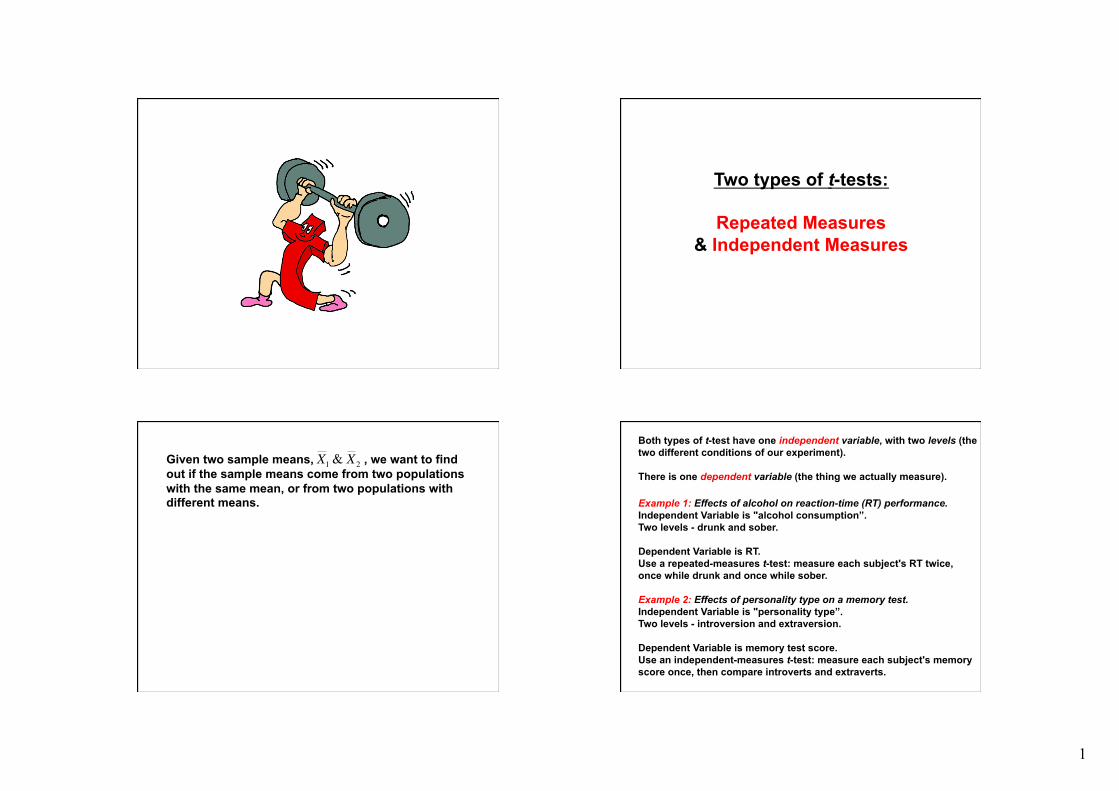
Two types of t-tests:

Repeated Measures & Independent Measures

Given two sample means, , we want to find out if the sample means come from two populations with the same mean, or from two populations with different means.

€

X 1 & X 2

Both types of t-test have one independent variable, with two levels (the two different conditions of our experiment).

There is one dependent variable (the thing we actually measure).

Example 1: Effects of alcohol on reaction-time (RT) performance. Independent Variable is "alcohol consumption”. Two levels - drunk and sober.

Dependent Variable is RT. Use a repeated-measures t-test: measure each subject's RT twice, once while drunk and once while sober.

Example 2: Effects of personality type on a memory test. Independent Variable is "personality type”. Two levels - introversion and extraversion.

Dependent Variable is memory test score. Use an independent-measures t-test: measure each subject's memory score once, then compare introverts and extraverts.

2

POPULATION

N subjects

Level 1 of independent variable A administered

subjects measured on dependent variable B

Compute

Test your hypothesis H0: µ1 – µ2 = 0 H1: µ1 – µ2 ≠ 0

Repeated measures experiment. To examine the effect of variable A on variable B

N subjects are selected from the population

Statistics are computed and hypothesis test carried out to decide if the difference between and is due to sampling variability or effect of A on B.

€

X 1

€

X 2

Level 2 of independent variable A administered

subjects measured on dependent variable B

€

D

The subjects are first given Level 1 of the independent variable A

The same subjects are then given Level 2 of the independent variable A

Subjects are measured on dependent variable B. ( and s1 are computed from these data)

€

X 1

Subjects are measured on dependent variable B. ( and s2 are computed from these data)

€

X 2

€

SD

Rationale behind repeated measures the t-test:

EXAMPLE: Experiment on the effects of alcohol on task performance (time in seconds).

Measure time taken to perform the task for subjects when drunk, and when (same subjects are) sober.

Null hypothesis: alcohol has no effect on time taken: variation between the drunk sample mean and the sober sample mean is due to sampling variation.

i.e. The drunk and sober performance times are samples from the same population.

Quick reminder: Sampling distribution of differences between means

Population level 1 of A with Alcohol

€

X 2

€

X 1. . . . . . . . . . . .

€

X 1

€

X 1

€

X 2

€

X 2

µ1 µ2

frequency of D

€

X 1

€

X 2values of −

€

X 1 − X 2 = D

Population level 2 of A without Alcohol

µD

Condition A Level 1

Condition A Level 2

Participant With Alcohol

Without Alcohol

1 12.4 10.0

2 15.5 14.2

3 17.9 18.0

4 9.7 10.1

5 19.6 14.2

6 16.5 12.1

7 15.1 15.1

8 16.3 12.4

9 13.3 12.7

10 11.6 13.1

Times (in seconds) of participants to complete a motor coordination task

3

the mean difference between scores in our two samples (should be close to zero if there is no difference between the two conditions)

the predicted average difference between scores in our two samples (usually zero, since we assume the two samples don’t differ )

estimated standard error of the mean difference (a measure of how much the mean difference might vary from one occasion to the next).

€

t(observed) =D −µD (hypothesized)

SD

Condition A Level 1

Condition A Level 2

Participant With Alcohol

Without Alcohol

Diff. (D)

1 12.4 10.0 2.4

2 15.5 14.2 1.3

3 17.9 18.0 -0.1

4 9.7 10.1 -0.4

5 19.6 14.2 5.4

6 16.5 12.1 4.4

7 15.1 15.1 0.0

8 16.3 12.4 3.9

9 13.3 12.7 0.6

10 11.6 13.1 -1.5

16.0

€

D∑ =

1. Add up the differences:

2. Find the mean difference: €

D =16∑

€

D =D∑

N=1610

=1.6

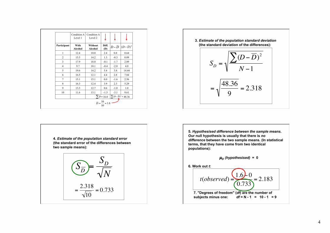
3. Estimate of the population standard deviation (the standard deviation of the differences):

€

SD =(∑ D−D )2

N −1

€

SD =SD

N

4

Condition A Level 1

Condition A Level 2

Participant With Alcohol

Without Alcohol

Diff. (D)

1 12.4 10.0 2.4 0.8 0.64

2 15.5 14.2 1.3 -0.3 0.09

3 17.9 18.0 -0.1 -1.7 2.89

4 9.7 10.1 -0.4 -2.0 4.0

5 19.6 14.2 5.4 3.8 14.44

6 16.5 12.1 4.4 2.8 7.84

7 15.1 15.1 0.0 -1.6 2.56

8 16.3 12.4 3.9 2.3 5.29

9 13.3 12.7 0.6 -1.0 1.0

10 11.6 13.1 -1.5 -3.1 9.61

16.0 48.36

€

D−D

€

(D−D )2

€

D∑ =

€

(D−D )2 =∑

€

D = 1610

=1.6

3. Estimate of the population standard deviation (the standard deviation of the differences):

€

SD =(∑ D−D )2

N −1

€

=48.369

= 2.318

4. Estimate of the population standard error (the standard error of the differences between two sample means):

€

SD =SD

N

€

=2.31810

= 0.733

5. Hypothesised difference between the sample means. Our null hypothesis is usually that there is no difference between the two sample means. (In statistical terms, that they have come from two identical populations):

µD (hypothesised) = 0

6. Work out t:

7. "Degrees of freedom" (df) are the number of subjects minus one: df = N - 1 = 10 - 1 = 9

€

t(observed) =1.6 − 00.733

= 2.183

5

(a)   “Two-tailed test”: if we are predicting a difference between Level 1 and 2; find the critical value of t for a "two-tailed" test. With df = 9, critical value = 2.26.

(b)  “One-tailed test”: if we are predicting that Level 1 is bigger than 2, (or 1 is smaller than 2), find the critical value of t for a "one-tailed" test. For df = 9, critical value = 1.83.

TWO-Tailed: t-observed (2.183) is smaller than t-critical (2.26)

“There is no significant difference between the times taken to complete the task with or without alcohol”

t(9) = 2.183, p > 0.05

ONE-Tailed: t-observed (2.183) is larger than t-critical (1.83)

“The times taken to complete the task is significantly longer with alcohol than without”

t(9) = 2.183, p < 0.05

8. Find t-critical value of t from a table (at the back of statistics books; also on Graham’s website).

0.025 0.025

upper t-critical value

2.26

lower t-critical value

-2.26

two-tailed df = 9

one-tailed df = 9 0.05

t-critical value 1.83

t-observed (2.183) Using SPSS to do a repeated measures t-test

6

Data Entry

Running SPSS (repeated measures t-test) Running SPSS (repeated measures t-test)

7

Running SPSS (repeated measures t-test) Interpreting SPSS output (repeated measures t-test)

POPULATION

Random factors determine which group

N subjects

Group 1: n1 subject

Group 2: n2 subject

Level 1 of independent variable A given to all subjects (n1)

Level 2 of independent variable A given to all subjects (n2)

Group 1 subjects measured on dependent variable B

Group 2 subjects measured on dependent variable B

Compute Error term1

€

X 1

€

X 2Compute

Error term2

Test your hypothesis H0: µ1 – µ2 = 0 H1: µ1 – µ2 ≠ 0

Independent measures experiment. To examine the effect of variable A on variable B

N subjects are selected from the population and split into two groups n1 and n2

n1 + n2 = N

Subjects in each group receive identical treatment except different levels of independent variable A are given to each group

Subjects in each group are measured in the same way on the dependent variable B

Statistics are computed and hypothesis test carried out to decide if the difference between and is due to sampling variability or effect of A on B.

€

X 1

€

X 2

Rationale behind independent measures the t-test:

EXAMPLE: Experiment on the effects of alcohol on task performance (time in seconds).

Measure time taken to perform the task for one set of subjects when drunk, and a different set of subjects when sober.

Null hypothesis: alcohol has no effect on time taken: variation between the drunk sample mean and the sober sample mean is due to sampling variation.

i.e. The drunk and sober performance times are samples from the same population.

8

X1 X2

Participant 1 13.0 Participant 1 11.1

Participant 2 16.5 Participant 2 13.5

Participant 3 16.9 Participant 3 11.0

Participant 4 19.7 Participant 4 9.1

Participant 5 17.6 Participant 5 13.3

Participant 6 17.5 Participant 6 11.7

Participant 7 18.1 Participant 7 14.3

Participant 8 17.3 Participant 8 10.8

Participant 9 14.5 Participant 9 12.6

Participant 10 13.3 Participant 10 11.2

Subject group 1 Subject group 2

the difference between samples means (should be close to zero if there is no difference between the two conditions)

the predicted average difference between scores in our two samples (usually zero, since we assume the two samples don’t differ )

estimated standard error of the difference between means (a measure of how much the difference between means might vary from one occasion to the next).

€

t(observed) =(X 1 − X 2) − (µ1 −µ2)hypothesized

estimatedσX 1−X 2

X1 X2

Participant 1 13.0 Participant 1 11.1

Participant 2 16.5 Participant 2 13.5

Participant 3 16.9 Participant 3 11.0

Participant 4 19.7 Participant 4 9.1

Participant 5 17.6 Participant 5 13.3

Participant 6 17.5 Participant 6 11.7

Participant 7 18.1 Participant 7 14.3

Participant 8 17.3 Participant 8 10.8

Participant 9 14.5 Participant 9 12.6

Participant 10 13.3 Participant 10 11.2

€

X1∑ =164.4

€

X2∑ =118.6

€

X 2 =11.86

€

X 1 =16.44

€

t(observed) =(X 1 − X 2) − (µ1 −µ2)hypothesized

estimatedσX 1−X 2

Step 1

€

X 1 − X 2 = 4.58

Subject group 1 Subject group 2

€

estimatedσX 1−X 2=

(X1 − X 1)∑2

+ (X2 − X 2)2∑

(n1 −1) + (n2 −1)× ( 1

n1+1n2)

€

(X2 − X 2)∑2

= X22 −( X2)

2∑n2

∑

€

(X1 − X 1)∑2

= X12 −( X1)

2∑n1

∑

€

t(observed) =(X 1 − X 2) − (µ1 −µ2)hypothesized

estimatedσX 1−X 2

Step 2

9

X1 (X1)2 X2 (X2)2

Participant 1 13.0 169 Participant 1 11.1 123.21 Participant 2 16.5 272.25 Participant 2 13.5 182.25 Participant 3 16.9 285.61 Participant 3 11.0 121 Participant 4 19.7 388.09 Participant 4 9.1 82.81 Participant 5 17.6 309.76 Participant 5 13.3 176.89 Participant 6 17.5 306.25 Participant 6 11.7 136.89 Participant 7 18.1 327.61 Participant 7 14.3 204.49 Participant 8 17.3 299.29 Participant 8 10.8 116.64 Participant 9 14.5 210.25 Participant 9 12.6 158.76

Participant 10 13.3 176.89 Participant 10 11.2 125.44

Subject group 1 Subject group 2

€

X12∑ = 2745

€

( X1∑ )2 = (164.4)2 = 27027.36

€

X22∑ =1428.38

€

( X2∑ )2 = (118.6)2 =14065.96

Step 2

€

(X2 − X 2)∑2

= X22 −( X2)

2∑n2

∑

€

estimatedσX 1−X 2=

(X1 − X 1)∑2

+ (X2 − X 2)2∑

(n1 −1) + (n2 −1)× ( 1

n1+1n2)

n1 = 10 n2 = 10

€

(X1 − X 1)∑2

= X12 −( X1)

2∑n1

∑

€

= 2745 − 27027.3610

= 2745 − 2702.74 = 42.26

€

=1428.38 − 14065.9610

=1428.38 −1406.6 = 21.78

€

estimatedσX 1−X 2=

42.26 + 21.78(10 −1) + (10 −1)

×110

+110

working out the error term Step 2

€

=64.0418

× 0.2 = 3.558 × 0.2 = 0.711 = 0.843

Step 3

Step 4

Step 5

df = (n1 – 1)+(n2 – 1) = 18

finding t-critical from the table: t-critical = 2.1; df = 18

€

t(observed) =(X 1 − X 2) − (µ1 −µ2)hypothesized

estimatedσX 1−X 2

Frequently µ1 – µ2 = 0

Step 6

Decision: t-observed > t-critical

Therefore reject the null hypothesis

Alcohol has an impact of time taken on the task.

t(18) = 5.429, p < 0.05

€

t(observed) =4.58 − 00.843

= 5.429

Step 7

10

Using SPSS to do a independent measures t-test

Data Entry

Running SPSS (independent measures t-test) Running SPSS (independent measures t-test)

11

Running SPSS (independent measures t-test) Running SPSS (independent measures t-test)

SPSS output (independent measures t-test)