Two Types of Inequality: Inequality Between Persons and ...ftp.iza.org/dp2749.pdf · IZA Discussion...

IZA DP No 2749

Two Types of Inequality Inequality BetweenPersons and Inequality Between Subgroups

Guillermina JassoSamuel Kotz

DI

SC

US

SI

ON

PA

PE

R S

ER

IE

S

Forschungsinstitutzur Zukunft der ArbeitInstitute for the Studyof Labor

April 2007

Two Types of Inequality

Inequality Between Persons and Inequality Between Subgroups

Guillermina Jasso New York University and IZA

Samuel Kotz

George Washington University

Discussion Paper No 2749 April 2007

IZA

PO Box 7240 53072 Bonn

Germany

Phone +49-228-3894-0 Fax +49-228-3894-180

E-mail izaizaorg

Any opinions expressed here are those of the author(s) and not those of the institute Research disseminated by IZA may include views on policy but the institute itself takes no institutional policy positions The Institute for the Study of Labor (IZA) in Bonn is a local and virtual international research center and a place of communication between science politics and business IZA is an independent nonprofit company supported by Deutsche Post World Net The center is associated with the University of Bonn and offers a stimulating research environment through its research networks research support and visitors and doctoral programs IZA engages in (i) original and internationally competitive research in all fields of labor economics (ii) development of policy concepts and (iii) dissemination of research results and concepts to the interested public IZA Discussion Papers often represent preliminary work and are circulated to encourage discussion Citation of such a paper should account for its provisional character A revised version may be available directly from the author

IZA Discussion Paper No 2749 April 2007

ABSTRACT

Two Types of Inequality Inequality Between Persons and Inequality Between Subgroups

Social scientists study two kinds of inequality inequality between persons (as in income inequality) and inequality between subgroups (as in racial inequality) This paper analyzes the mathematical connections between the two kinds of inequality The paper proceeds by exploring a set of two-parameter continuous probability distributions widely used in economic and sociological applications We define a general inequality parameter which governs all measures of personal inequality (such as the Gini coefficient) and we link this parameter to the gap (difference or ratio) between the means of subdistributions In this way we establish that at least in the two-parameter distributions analyzed here and for the case of two nonoverlapping subgroups as personal inequality increases so does inequality between subgroups This general inequality parameter also governs Lorenz dominance Further we explore the connection between subgroup inequality (in particular the ratio of the bottom subgroup mean to the top subgroup mean) and decomposition of personal inequality into between-subgroup and within-subgroup components focusing on an important decomposable measure Theilrsquos MLD and its operation in the Pareto case This allows us to establish that all the quantities in the decomposition are monotonic functions of the general inequality parameter Thus the general inequality parameter captures the ldquodeep structurerdquo of inequality We also introduce a whole-distribution graphical tool for assessing personal and subgroup inequality Substantively this work suggests that in at least some societies characterized by special income distributions whenever inequality disrupts social harmony and social cohesion it attacks on two fronts via subgroup inequality as well as personal inequality JEL Classification C02 C16 D31 D6 I3 Keywords continuous univariate distributions two-parameter distributions

lognormal distribution Pareto distribution power-function distribution Gini coefficient Atkinson measure Theilrsquos MLD coefficient of variation Lorenz curve decomposition of inequality measures between component within component

Corresponding author Guillermina Jasso Department of Sociology New York University 295 Lafayette Street 4th Floor New York NY 10012-9605 USA E-mail gj1nyuedu

We thank Yaw Nyarko and participants at the biennial meeting of the International Society for Justice Research Berlin Germany August 2006 and at the annual Winter Conference of the Methodology Section of the American Sociological Association Yale University March 2007 especially Scott Boorman Thomas DiPrete and Tim F Liao for their valuable comments and we thank the editor and three anonymous referees for their close reading and valuable comments We also gratefully acknowledge New York University and George Washington University for their intellectual and financial support This paper is forthcoming in Sociological Methods and Research

Jencks et al (1972) discuss both types of inequality in the introductory chapter and1

while emphasizing ldquoinequality between individuals not inequality between groupsrdquo (Jencks et al197214) nonetheless introduce pertinent material on race gaps (eg in pp 216-219)

1

1 INTRODUCTION

Discussions of social inequality address two distinct types of inequality inequality

between persons and inequality between subgroups (see inter alia the landmark work by Jencks

et al 1972) The quintessential example of the first type is income inequality and its study has

produced an extensive literature focused on both substantive and methodological aspects (eg

Champernowne and Cowell 1998 Karoly and Burtless 1995 Kleiber and Kotz 2003) The

quintessential examples of the second type are the race earnings gap and the gender earnings gap

and these are examined in a growing substantive literature predominantly in the United States

and the United Kingdom (eg Blau and Kahn 2000 Darity and Mason 1998 Goldin 1990 2006

Harkness 1996 OrsquoNeill 2003 Reskin and Bielby 2005) In the United States the burgeoning

interest in race and gender gaps has been stimulated in part by concern that -- notwithstanding the

almost half century since President John F Kennedy issued the groundbreaking Executive Order

10925 prohibiting discrimination on the basis of ldquorace creed color or national originrdquo (6 March

1961) and signed the Equal Pay Act (10 June 1963) extending to gender the protection against

discrimination -- race and gender may still affect economic chances (US Council of Economic

Advisers 1998ab) These governmental actions although limited to the United States have had a

wider international significance and impact1

In both types of inequality interest centers on inequality with respect to a positive

quantitative variable X such as wages income or wealth The two types differ however in the

entities under assessment While persons are the focal units in the first type the focal units in the

second type are subgroups based on a particular qualitative variable S such as gender race or

nativity Thus inequality between persons refers to inequality in the distribution of X in a set of

persons ndash called personal inequality Inequality between subgroups on the other hand refers to

the discrepancy between the mean (or other measure of central tendency) of X between two

The distinction between qualitative and quantitative characteristics long appreciated in2

mathematics (eg Allen 193810-11) and in statistics and econometrics has since the pioneeringwork of Blau (1974) come to be seen as structuring behavioral and social phenomena in afundamental way The combination of a qualitative and a quantitative characteristic in subgroupinequality provides a further instance of the scope and usefulness of the distinction

2

subgroups of a group (or population) ndash called subgroup inequality Tailored to a specific set of

quantitative and qualitative characteristics the two types of inequality are often called ldquoX

inequalityrdquo ndash eg earnings inequality or wealth inequality ndash and ldquoS X gaprdquo ndash eg gender earnings

gap or nativity wealth gap or race wage gap respectively2

Personal inequality can be defined for a group or population as well as for the subgroups

within the group We refer to personal inequality in a group as plain unmodified ldquopersonal

inequalityrdquo or synonymously as overall inequality We refer to personal inequality in a

subgroup as within-subgroup personal inequality with more particular terms as appropriate for

example bottom-subgroup personal inequality and top-subgroup personal inequality or male

personal inequality and female personal inequality or terms based on particular measures of

inequality such as bottom-subgroup Gini coefficient or top-subgroup Theilrsquos MLD The term

ldquosubgroup inequalityrdquo is always reserved for measures of inequality between subgroups such as

the ratio of the bottom-subgroup mean to the top-subgroup mean

A basic natural question is What is the connection between overall inequality and

subgroup inequality Is one a function (hopefully monotone) of the other Or are both generated

by some other deeper feature of the distribution or population There are several approaches one

can take including investigation of the mechanisms producing the quantitative variable X and its

interplay with the S characteristic Such an approach might explore whether persons who differ

in the S characteristic (say men and women or immigrants and natives) have differential access

to X itself (as when laws prescribe wages by sex or constrain asset accumulation by religion ndash as

in the Middle Ages in Europe say and certain Muslim countries even today) or to the sources of

X (as when education is differentially available on the basis of gender nativity race or religion)

or differ in some X-relevant characteristic (such as language or attachment to the labor force)

The questions concerning the exact connections between personal inequality subgroup3

inequality subgroup-specific means and personal inequality and between-subgroup and within-subgroup components in decomposition are indeed general questions and these concepts andrelations can be applied at any level of generality ndash in various situations For example the groupand its subgroups may as easily be the world and its countries (eg Theil 1979 BerryBourguignon and Morrisson 1983 Schultz 1998 and Firebaugh 2003) as a country and itsnative-born and foreign-born citizens or a social club and its male and female members And inall these cases one can imagine the expanding question of comparisons across groups and overtime ndash albeit only in philosophy or science fiction for comparison across worlds

3

Our approach is more modest yet possibly of larger significance involving greater

generality Because the distribution of any X is subject to the same basic mathematical

underpinnings of probability distributions it is plausible that overall inequality and subgroup

inequality are connected to each other in specified ways Accordingly we investigate the

mathematical relations between overall inequality and subgroup inequality

A further natural question involves the connection between subgroup inequality and

within-subgroup features such as within-subgroup personal inequality and within-subgroup

means These within-subgroup features play vital parts in decomposition of overall inequality

where they appear as the basic ingredients of what are called the between-subgroup component

and the within-subgroup component (Bourguignon 1979 Shorrocks 1980 Das and Parikh 1982

Champernowne and Cowell 1998) As scholarly attention expands from a single population with

subgroups to comparison of many populations each with its own set of subgroups ndash an enterprise

ldquoin its infancyrdquo (Darity and Deshpande 200075) ndash as well as to comparison over time of a

population with subgroups (Tomaskovic-Devey Thomas and Johnson 2005) clear

understanding of the exact connections among all these terms and dimensions becomes all the

more important Analogously to our starting focus on the connection between overall inequality

and subgroup inequality our strategy is to investigate the mathematical relations among the

terms in play3

We begin with specification of a general inequality parameter a property of

mathematically specified distributions defined on the positive support Intuitively we first show

4

that the general inequality parameter governs four measures of overall inequality and next we

show that it also governs measures of subgroup inequality If both overall inequality and

subgroup inequality are functions of the general inequality parameter then we may conclude that

these two distinct types of inequality are presumably manifestations of the same underlying

inequality in a distribution

Next we investigate the operation of the general inequality parameter in the subgroup-

specific terms and their combination into decomposition terms Again but in a more restricted

analysis we show that all these terms are monotonic functions of the general inequality

parameter strengthening the conclusion that all are manifestations of what we may call using

Darity and Deshpandersquos (200077) words the ldquodeep structurerdquo of inequality

In this first foray we impose several restrictions First we work with specific

distributions rather than following a distribution-independent approach Second we focus on

continuous two-parameter distributions investigating three widely used but mathematically quite

simple distributions (lognormal Pareto and power-function) Third the subgroups are defined

as two censored subdistributions Future work should systematically relax these restrictions

assessing for example distributions with more than two parameters or with more than two

subgroups or with overlapping subgroups To the extent that the nonoverlapping-subgroup case

provides a model for many real-world situations ndash from slave and caste societies to societies in

which gender nativity immigration status or rank in an organizational structure predetermine

minimum and maximum earnings or wealth to binational or international work settings in which

different pay scales are used for locals and members of foreign organizations (such as

international joint ventures as well as US news media filmmakers universities think tanks and

military installations abroad) to groups with differentially compensated subgroups (such as

universities with differentially compensated disciplines professional associations with members

from around the world international airlines with pilots under different contracts) -- and that as

well it represents the extreme bound the results reported in this paper may serve as at least a

For example on international joint ventures see Shenkar and Zeira (1987) Leung4

Smith Wang and Sun (1996) and Leung Wang and Smith (2001)

5

benchmark for future studies4

In the analysis of the within-subgroup and decomposition terms we focus on one

inequality measure the ldquosecond measurerdquo proposed by Theil (1967125-127 1979) -- also

known as the mean logarithmic deviation (MLD) ndash and investigate its operation in one of the

three variates mentioned above the Pareto distribution Future work should systematically

analyze the within-subgroup and decomposition terms for the MLD in other distributions and for

other inequality measures

Finally we briefly introduce a whole-distribution graphical tool for assessing inequality

across groups that have subgroups a technique based on the quantile function and its application

to inequality analysis (Jasso 1983b) This technique can be used with both overlapping and

nonoverlapping subgroups there can be any number of subgroups and the subgroup distributions

can have any mean inequality or variate form This technique can be used both with

mathematically specified distributions and with empirical distributions

Section 2 introduces the general inequality parameter and reports its operation in the three

variates ndash lognormal Pareto and power-function ndash showing that measures of overall inequality

are monotonic functions of the general inequality parameter In Section 3 we define two

measures of subgroup inequality one difference-based and the other ratio-based ndash yielding the

absolute gap and the relative gap respectively -- and we show that both measures are also

monotonic functions of the general inequality parameter Section 4 links the Lorenz curve to the

general inequality parameter (showing that the Lorenz curve is a monotonic function of the

general inequality parameter) and to the connection between overall inequality and subgroup

inequality Section 5 investigates the within-subgroup and decomposition terms in the MLD and

analyzes their operation for the Pareto variate the analysis indicates that all the within-subgroup

and decomposition terms are monotonic functions of the general inequality parameter but they

Of course there are other dimensions along which different types of inequality can be5

discerned For example Jasso and Kotz (2007) distinguish between inequality in status andinequality in the characteristics which generate status (such as income) Moreover Liao(2006217) uses the phrase ldquotwo types of inequalityrdquo to refer to the between and withincomponents in a decomposition

For detailed information on these basic distributions see for example Johnson Kotz6

and Balakrishnan (1994 1995) and for applications pertinent to inequality Kleiber and Kotz(2003)

6

differ in their responsiveness to the proportions of the population in the two subgroups Section

6 describes the whole-distribution graphical tool A short note concludes the paper5

2 THE GENERAL INEQUALITY PARAMETER

21 Two-Parameter Continuous Univariate Distributions

Consider a two-parameter continuous univariate distribution defined on the positive

support The two parameters are usually specified as a location parameter (say the mean

median or mode) and either a scale or a shape parameter Table 1 presents the formulas for the

three basic associated functions ndash the probability density function (PDF) cumulative distribution

function (CDF) and quantile function (QF) ndash for the lognormal Pareto and power-function

distributions Figure 1 provides visual illustration The location parameter is specified as the

mean igrave The second parameter is a shape parameter denoted c6

ndash Table 1 about here ndash

ndash Figure 1 about here ndash

22 The Second Parameter c as General Inequality Parameter

We argue that the second parameter c is in fact a general inequality parameter We carry

out two sets of analyses First we examine the formulas for the major measures of overall

inequality in order to assess their relation to the general inequality parameter If the overall

inequality formulas are monotonic functions of c then c is a plausible candidate for general

inequality parameter Second we examine the limit of the quantile function (QF) as c

The idea of a general inequality parameter appears in Jasso (198796) and is rooted both7

in well-known discussions of the shape factor in the Pareto distribution (known as Paretorsquosconstant) as a measure of inequality (eg Cramer 197151-58 Cowell 197795 Kleiber andKotz 200378) and the visual observation that the formulas for many inequality measures inmathematically specified distributions depend on a single parameter (eg Jasso 1982315-318)

7

approaches its low-inequality end If the limit of the QF is the mean then the distribution

becomes degenerate and c is then a fortiori a plausible candidate for general inequality

parameter7

23 The General Inequality Parameter and Measures of Overall Inequality

We focus on four major measures of overall inequality ndash the Gini coefficient one of

Atkinsonrsquos (1970 1975) measures (defined as 1 minus the ratio of the geometric mean to the

arithmetic mean) Theilrsquos (1967125-127 1979) MLD and Pearsonrsquos (1896) coefficient of

variation (CV) Formulas for these measures are well-known (see eg Cowell 1977 Kleiber

and Kotz 2003) Here we provide in Table 2 some convenient formulas for these measures in

both observed and mathematically specified distributions The formulas for mathematically

specified distributions are expressed in terms of the quantile function (QF) and the mean igrave


The lognormal Pareto and power-function variates are quite familiar and the formulas

for the four inequality measures in these variates are well-known (see eg Cowell 1977 Kleiber

and Kotz 2003) Tables 3a and 3b present formulas for Note that in all twelve formulas there

is a single factor namely c which is the second of the two basic parameters in a two-parameter

distribution and the one we are proposing as a general inequality parameter Thus the Gini

coefficient Atkinsonrsquos measure Theilrsquos MLD and the coefficient of variation are all functions

solely of c

ndash Tables 3a and 3b about here ndash

Tables 3a and 3b also provide the first derivatives of each measure of overall inequality

with respect to the parameter c As shown the derivatives of all four measures are in each

variate of the same sign so that the measures of overall inequality are monotonic functions of c

This parameter which operates as general inequality parameter is called by different8

names or appears in alternate forms For example as mentioned above in the Pareto case theparameter c is called Paretorsquos constant and the lognormalrsquos c is often referred to as the standarddeviation of the normal distribution obtained when the lognormal is ldquologgedrdquo

Looking at the formula for the Gini in the lognormal case (Table 3a) observe that as c9

goes to zero the CDF of the unit normal goes to 5 (and 5 times 2 equals one which aftersubtracting one yields zero) Similarly as c goes to infinity the CDF of the unit normal goes toone

8

Figures 2a and 2b present graphs of the four measures of overall inequality as functions of c

As expected from the derivatives the graphs depict the measuresrsquo monotonicity with respect to c

ndash Figures 2a and 2b about here ndash

Thus the parameter c can be interpreted as a general inequality parameter

Aside from monotonicity c operates differently across the variates In the lognormal

case inequality increases as c increases while in the Pareto and power-function inequality

decreases as c increases8

It is also useful to examine the limits of the overall measures of inequality as c

approaches its own limits The Gini coefficient has bounds of zero and one Accordingly in

each variate the formula for the Gini coefficient should approach its two limits as the parameter c

approaches its two limits respectively Consider the lognormal distribution As c approaches

zero the limit of the Gini coefficient is zero and as c goes to infinity the limit of the Gini

coefficient is one9

Proceeding in this manner we find that for each of the three variates the Gini coefficient

approaches its two limits as the parameter c approaches its two limits respectively and so does

the Atkinson measure Theilrsquos MLD and the CV do not have an upper bound and for these we

find that in each of the three variates the two measures approach zero and infinity (their two

limits) as the parameter c approaches its two limits respectively These results provide further

indication that c is a general inequality parameter

The evocative phrase ldquomarch toward equalityrdquo is in wide use See for example the10

chronicle of milestones in the history of US civil rights in the website of the US Department ofState (httpusinfostategovproductspubscivilrtsmarchhtm)

9

(1)

(2)

24 The General Inequality Parameter and the March toward Equality10

Consider the expressions for the quantile functions of the three variates shown in Table

1 Because the location parameter was specified as the arithmetic mean the expressions for the

QF contain the mean (as well as the general inequality parameter c) And because the arithmetic

mean represents equality the expression for the QF in an idealized Equal distribution (also

known as a Dirac distribution or a degenerate distribution) should be the arithmetic mean That

is in a perfectly equal distribution all income amounts are equal and thus at every ldquorelative

rankrdquo the QF is simply the mean

It follows that if c is indeed a general inequality parameter then as c approaches its low-

inequality end or limit the QF should approach the mean In other words denoting the low-

inequality limit by q we have

It is straightforward to show that this is indeed the case in the three variates under

consideration To illustrate we present a formal proposition and proof for the Pareto case

Proposition 1 Limit of the Pareto QF as the Parameter c Approaches Its Low-Inequality

End In the Pareto distribution the limit of the quantile function as c goes to infinity (its low-

inequality end) is equal to the arithmetic mean

Proof The proof of proposition 1 is given in two steps

1 The three constituent factors of the Paretorsquos QF have well-known limits

10

(3)

2 Using the limits in (3) and the fact that the limit of a product(quotient) equals the

product(quotient) of the limits (provided in the case of a quotient that the divisor is not zero)

we immediately obtain the limit for the Pareto case in (2)

Similarly the limit of the power-functionrsquos QF as c goes to infinity (its low-inequality

end) equals the arithmetic mean and the limit of the lognormalrsquos QF as c approaches zero (its

low-inequality end) also equals the arithmetic mean

Thus as the inequality parameter approaches its low-inequality end or limit the

distribution collapses onto a single point the point of equality The parameter c ndash the second

parameter in the two-parameter specifications of the variates ndash is indeed behaving as a general

inequality parameter

Evidently the robustness of the parameter c as general inequality parameter merits further

elucidation

3 SUBGROUP INEQUALITY AND THE GENERAL INEQUALITY PARAMETER

31 Subgroup Inequality in a Population with Two Subgroups

Consider the distribution of X ndash where X is a quantitative variable such as wage earnings

or wealth ndash in a population Suppose now that the persons in the population can be classified

into two subgroups according to a qualitative characteristic such as gender race ethnicity

nativity or religion Each of the two subgroups has an average amount of X Whenever the two

averages differ the two subgroups will be thought to be unequal This condition of subgroup

inequality can be measured in two ways by the difference between the two means and by the

ratio of the smaller mean to the larger While the relative gap may be the more often discussed

11

the absolute gap in income provides complementary information such as a measure of the

discrepancy in purchasing power (Jencks et al 1972216-219)

The objective is to ascertain whether subgroup inequality measured by both the ratio and

difference procedures varies with the general inequality parameter c discussed in the previous

section

32 Censored Subdistribution Structure in a Population with Two Subgroups

We shall now suppose that the two subgroups are nonoverlapping in X ie that the

poorest person in the higher-average subgroup is richer than the richest person in the lower-

average subgroup This is a rather familiar situation across the social sciences where it appears

under a variety of rubrics such as consolidation in Blau (1974632) hierarchy and segmentation

in Hechter (1978) cleavage in Jassorsquos (1983a 1993) conflict model accentuation in Hogg

Terry and White (1995261) and bifurcation in Ridgewayrsquos (1996 2001) status construction

theory

Nonoverlapping subgroups occur in a variety of contexts not only classic slave and caste

societies but also in modern times Seven examples are (1) societies in which the wage for rural

labor is fixed at two amounts one for men and the other for women (2) families in which

childrenrsquos allowances are higher for boys than for girls holding age constant on the rationale

that boys may have higher expenses (such as paying for dates in certain cultural milieus) (3)

firms and organizations in which paygrades are structured so that the lowest pay in one rank is

higher than the highest pay in the adjacent lower rank (4) societies in which inheritance wealth

or access to certain resources such as land ownership or commercial radio operation are

structured by gender nationality nativity or religion (5) construction and farm crews in which

the highest-paid illegal-alien worker is paid less than the lowest-paid legal worker (6) binational

or international work settings in which different pay scales are used for locals and members of

foreign organizations (such as international joint ventures as well as US news media

filmmakers universities think tanks and military installations abroad) and (7) groups with

differentially compensated subgroups (such as universities with differentially compensated

An early example of disjoint monetary value by gender appears in Leviticus (273-4)11

which prescribes the value of a male slave (age 20-60) at fifty shekels and of a female slave (also20-60) at thirty shekels

Note the intriguing contrast between immigration contexts and international joint12

ventures in the first setting the natives earn more while in the second the natives earn less Forfurther discussion of international joint ventures see Shenkar and Zeira (1987) Leung et al(1996) and Leung et al (2001)

Using by now standard terminology (see eg Gibbons 1988355) let censoring refer13

to selection of units by their ranks or percentage (probability) points and let truncation refer toselection of units by values of the variate Thus the truncation point is the value x separating thesubdistributions the censoring point is the percentage point p separating the subdistributions For example the subgroups with incomes less than $20000 or greater than $80000 each form atruncated subdistribution the top 25 percent and the bottom 75 percent of the income distributioneach form a censored subdistribution

12

disciplines professional associations with members from around the world international airlines

with pilots under different contracts) Indeed when one considers the full scope of quantitative

variables in which inequality may be of interest ndash not only wages earnings income and wealth

but also schooling mentoring time received length of prison sentence grades received in school

ndash the examples of nonoverlapping subgroups multiply Moreover nonoverlapping subgroups

arise quickly in immigration contexts to illustrate except in the case where both origin and

destination country speak the same language any function of fluency in the destination-country

language (wages tutoring time time spent on homework experience interpreting) is likely to

generate nonoverlapping subgroups of immigrants and natives 11 12

In this case of nonoverlapping subgroups the distribution generates a censored

subdistribution structure in which the censoring point p corresponds to the boundary between the

two subgroups The proportions in the censored subdistributions are called the subgroup split

The bottom subgroup contains p proportion of the population and the top subgroup has (1 - p)

proportion The phrase ldquosubgroup split prdquo is used as shorthand for ldquosubgroup splitrsquos censoring13

point prdquo

To construct the measures of subgroup inequality it is necessary to derive expressions for

13

the arithmetic means of the censored subdistributions and then embed these into expressions for

the ratio and the difference

33 Measures of Subgroup Inequality

Table 4 presents the ratio and difference measures of subgroup inequality for the three

variates under consideration in this paper As shown all the measures are functions of two

quantities the general inequality parameter c and the censoring point p the difference-based

measures are also functions of the arithmetic mean igrave The ratio-based measure has bounds of 0

and 1 (open at 0 closed at 1) attaining the value of 1 when the two subgroups have identical

means


It is easy to see that the difference-based measures of subgroup inequality are ceteris

paribus increasing in the arithmetic mean igrave In the social sciences it is also important to

investigate the direction of the effects of the proportions in the two subgroups We shall turn to

the subgroup split in section 35 below (after establishing the effect of the general inequality

parameter on subgroup inequality)

34 Effect of the General Inequality Parameter on Subgroup Inequality

Table 4 also provides the first partial derivatives of the two measures of subgroup

inequality with respect to the general inequality parameter c for the three basic variates we

examine Figure 3 presents graphs of the ratio-based measures of subgroup inequality on the

general inequality parameter c for three values of the subgroup split p in each of the variates


Recall now that c operates differently across the three variates ndash higher c associated with

higher inequality in the lognormal and with lower inequality in the Pareto and power-function

Moreover in the difference-based measure of subgroup inequality the larger the measure the

greater the inequality while the behavior is opposite for the ratio-based measure of subgroup

inequality The pattern of signs ndash (1) opposite for the ratio and difference measures and (2)

opposite for the lognormal on the one hand and the Pareto and power-function on the other ndash

14

indicates a consistent effect of c as is evident from the graphs in Figure 3 That is subgroup

inequality seems to be governed by the general inequality parameter Moreover the effects are

exactly in the same direction as in the case of overall inequality namely as the general

inequality parameter moves in the direction of greater inequality subgroup inequality increases

As above the robustness of the parameter c as general inequality parameter merits further

investigation

35 Effect of the Subgroup Split on Subgroup Inequality

As shown above measures of overall inequality are functions of the general inequality

parameter c alone In contrast measures of subgroup inequality are functions not only of c but

also of the subgroup split ndash the proportions in the two subgroups specified by the censoring point

p (as shown in Tables 3a 3b and 4) A natural question arises For given magnitude of c how

does the subgroup split affect subgroup inequality

Figure 4 presents graphs of the ratio-based measures of subgroup inequality on the

subgroup split p for three values of c in each of the three variates We observe that the effect of

the subgroup split on subgroup inequality differs across the three variates in two easily noticeable

ways First the effect of the subgroup split is monotonic in the Pareto and power-function but

not in the lognormal Second the monotonic effect of the subgroup split in the Pareto and

power-function operates in opposite directions ndash in the Pareto the smaller the proportion in the

bottom subgroup the lower the subgroup inequality (higher ratio of bottom-subgroup mean to

top-subgroup mean) while in the power-function the effect is reversed In the lognormal the

effect of the subgroup split traces an inverted-U-shaped curve increasing to a peak in the upper

part of the range and subsequently decreasing


These results make sense if one calls to mind the densities of the three variates (Figure 1)

The Pareto and power-function distributions (of c greater than 1) are almost mirror images of

each other the Pareto with its single mode at the bottom of the range and a long right tail and the

power-function with its single mode at the top of the range and a left tail extending to zero

Analysis of this variate behavior may be useful in studies of the sensitivity of different14

inequality measures to different regions of the distribution as well as in analyses of ldquolatentclassesrdquo based on values of X as in Liao (2007)

15

Thus while in the Pareto case the presence of large chunks of the population in the top subgroup

tempers the effect of the long right tail making the two subgroup means more similar in the

power-function case it is the opposite namely the presence of large chunks of the population in

the bottom subgroup tempers the effect of the left tail and results in the two subgroup means

becoming more similar The lognormal has a mode toward the middle of the range and both a

left tail going to zero and a very long right tail resulting in the nonmonotonicity of the ratio of

the bottom-subgroup mean to the top-subgroup mean relative to the subgroup split p (We

encourage our readers to provide graphical representation of the behavior just described)14

36 Remark on Subgroup Inequality

It follows from the discussion above that subgroup inequality is shaped by three things

the form of the distribution the distributionrsquos general inequality parameter c and the subgroup

split The operation of these three factors has been long known in the study of overall inequality

Now this paper extends the classical work to subgroup inequality in particular to the absolute

gap and relative gap measures Explicit attention to the three factors will assist in interpreting

differences across countries and changes over time in subgroup inequality (as in the questions

addressed by Tomaskovic-Devey Thomas and Johnson 2005 and Darity and Deshpande 2000)

4 THE GENERAL INEQUALITY PARAMETER THE LORENZ CURVE AND

THE LINK BETWEEN OVERALL INEQUALITY AND SUBGROUP INEQUALITY

IN THE LOGNORMAL PARETO AND POWER-FUNCTION VARIATES

Lorenz curves introduced some 100 years ago (Lorenz 1905) provide a convenient

graphical tool for inspecting the amount of inequality in a distribution and comparing it across

two or more distributions The Lorenz curve expresses the proportion of the total amount of X

held by the bottom aacute proportion of the population as a function of aacute (aacute is the same aacute encountered

The quantity aacute can be interpreted in various equivalent ways depending on the15

context For example as the outcome of the CDF it is a probability level as the argument of theQF it is a relative rank and as the argument of the Lorenz curve it is the bottom proportion ofthe population

Table 5 builds on Gastwirth (1972307) who provides a table with the formulas for the16

Lorenz curve in five distributions including the Pareto and the benchmark Equal (Dirac)

16

above as the argument of the quantile function)15

The three variate families described in this paper have the property that their members

possess nonintersecting Lorenz curves Indeed the formulas for the Lorenz curve (reported in

Table 5) show that analogously to the overall inequality and subgroup inequality the Lorenz

curve is also governed by the general inequality parameter As the Lorenz curve is a monotonic

function of c within each variate family different members ndash which differ in c -- possess

nonintersecting Lorenz curves16


To visually represent the operation of the general inequality parameter on Lorenz curves

two sets of graphs are provided Figure 5 presents the usual Lorenz curve representations for the

three variates under study and as before with three cases for each variate The membersrsquo

graphs are nonintersecting and the higher the vertical placement the lower the inequality ndash a

higher curve Lorenz-dominates a lower curve For further illumination we show in Figure 6

graphs of the Lorenz curve formulas plotted on the general inequality parameter c at three

symmetric points in the domain of the Lorenz curve aacute = 25 5 and 75 These graphs show

how the Lorenz curve analogously to the overall inequality and subgroup inequality is governed

by the general inequality parameter

ndash Figures 5 and 6 about here ndash

Equivalently holding the arithmetic mean constant the quantile functions for any pair of

distributions from each family will intersect only once revealing who gains and who loses in a

(4)

Thus in comparisons of distributions of relative income the condition of17

nonintersecting Lorenz curves is also equivalent to the so-called second-order stochasticdominance We express second-order stochastic dominance in terms of the quantile function(QF) rather than the usual cumulative distribution function because the QF has a directinterpretation as the income corresponding to a person of given relative rank leading to furtherresults concerning who wins (or loses) in a shift from one distribution to another

The connection between the quantile function and the Lorenz curve was already known18

to Pietra (1915) and re-appears in Schutz (1951) and Gastwirth (1971) The connection betweenthe Lorenz curve and the Gini coefficient was established by Gini (1914) For further details seeKleiber and Kotz (2003)

17

shift from one member to the other Specifically everyone to the left of the intersection is better-

off in the lower-inequality distribution and everyone to the right of the intersection is better-off

in the higher-inequality distribution17

For example for the Pareto case the intersection of the two QFs is obtained by solving

for the difference between two quantile functions yielding as shown in Jasso (1983b291-293)

where A and B denote the two Pareto distributions and denotes the relative rank (or the

probability level) at which the intersection occurs It can be shown that can occur anywhere

in the interval between ( ) and 1 or approximately between 632 and 1 In a shift from A

to B where B is the lower-inequality distribution everyone to the left of becomes better-off

and everyone to the right becomes worse-off And vice-versa in a shift from B to A

That the Gini and the Lorenz curve are both governed by c and that the Lorenz curve and

the quantile function are tightly linked is not surprising for they are clearly mathematically

connected Indeed the Lorenz curve is the integral of the quantile function (divided by the

mean) and the Gini coefficient is (1 minus 2 times [the integral of the Lorenz curve]) as shown in

expression (4) and Table 2 respectively18

Now suppose that as in Section 3 above there are two nonoverlapping subgroups It

(5)

18

follows that in the within-variate shift from a higher-inequality distribution A to a lower-

inequality distribution B the mean of the upper subgroup (the upper censored subdistribution)

decreases and the mean of the bottom subgroup (the bottom censored subdistribution) is

increased reducing the subgroup inequality Hence the conditions of nonoverlapping subgroups

and nonintersecting Lorenz curves are jointly sufficient for the link between overall inequality

and subgroup inequality

Accordingly in certain mathematically specified distributions there exists a general

inequality parameter which determines all inequality-related aspects including overall inequality

and subgroup inequality as well as Lorenz dominance and stochastic dominance

5 THE CONNECTION BETWEEN THE GENERAL INEQUALITY PARAMETER

SUBGROUP INEQUALITY AND DECOMPOSITION OF OVERALL INEQUALITY

AN ANALYSIS BASED ON THEILrsquoS MLD FOR THE PARETO VARIATE

51 Introducing Decomposition into the Analysis

Our discussion to this point has focused on two types of inequality inequality between

persons ndash personal inequality (or equivalently when defined on all persons in a group or

population overall inequality) ndash and inequality between subgroups ndash subgroup inequality We

have shown that in certain basic mathematically specified distributions both personal inequality

and subgroup inequality are monotonic functions of the general inequality parameter and that as

general inequality increases both personal inequality and subgroup inequality increase We have

also confirmed that Lorenz curve dominance is a monotonic function of the general inequality

parameter

We now introduce into the discussion decomposition of overall inequality into a between-

subgroup component and a within-subgroup component Such decomposition holds the promise

of gauging how much of overall inequality is due to inequality within subgroups and how much

to inequality between subgroups (Theil 1967 1979 Bourguignon 1979 Shorrocks 1980 Das and

Parikh 1982 Jasso 1982321-323 Berry Bourguignon and Morrisson 1983 Champernowne and

Theilrsquos MLD has an additional interesting property It is the negative of the special19

justice index JI1 which summarizes the experience of justice and injustice in a group orpopulation in the special case where each individualrsquos idea of the just reward is perfect equality This special case known as the ldquojustice is equalityrdquo case can be traced to Platorsquos Gorgias (Jasso1980 1999)

19

Cowell 1998 Schultz 1998 Firebaugh 1999 2003 Liao 2006) More generally one would

expect to find a link between one or more elements of the decomposition and the difference-

based or ratio-based measures of subgroup inequality analyzed in this paper Accordingly we

now investigate the mathematical relations among the expanded set of terms encompassing not

only the overall inequality and subgroup inequality but also new decomposition-specific terms

We shall focus on one well-known and appealing inequality measure Theilrsquos MLD

(which combines several useful properties ndash additive decomposability scale invariance and

sensitivity to population shares (Theil 1979 Bourguignon 1979 Shorrocks 1980)) ndash and on one

widely used distributional family the Pareto19

Note that assessing the mathematical relations among the newly expanded set of terms

contributes to addressing what Darity and Deshpande (200077) call the ldquogrand questionsrdquo such

as the relation between overall inequality and subgroup inequality and the relation between

subgroup inequality and within-subgroup personal inequality

52 Theilrsquos MLD Elements of the Decomposition

and the Link to Subgroup Inequality

We begin by collecting in Table 6 the formulas for the MLD and for all the constituent

elements of its decomposition The MLD for a given quantitative variable in a group (or

population) is defined as the average of the log of the ratio of the group mean igrave to each unitrsquos

amount x which for simplicity can be expressed as an expectation and which yields the log of the

ratio of the group mean igrave to the group geometric mean denoted G

In the case investigated in this paper of two nonoverlapping subgroups each subgroup also has

(6)

The argument of the logarithmic function on the lefthand side of the equals sign is the20

reciprocal of the pivotal quantity xigrave the quantity known as the relative amount which arises instatistics and which plays many parts in all the sciences In applications to income it is calledthe relative income (Jasso 1983b) and the income ratio (Firebaugh 1999 2003) in justice theoryit is the comparison ratio under the primitive restrictions (Jasso 1980) and in inequality analysisit appears explicitly in the definitional formulas of many measures of inequality (such as theAtkinson family and the Theil family ndash see for example Cowell 1977155 and Jasso 1982306311) and is embedded in still other inequality measures (Firebaugh 1999 2003)

20

its own igrave G and MLD These are indicated by the two subscripts B for the bottom subgroup

and T for the top subgroup As before p denotes the proportion in the bottom subgroup20


Because X is defined on the positive support its mean and the two subgroup means are

positive The overall MLD and the two subgroup MLDs are also always positive a result

established by classical theorems relating the arithmetic mean to the geometric mean (Hardy

Littlewood and Poacutelya 195216-18) For a positive variable the geometric mean is always less

than or equal to the arithmetic mean with equality obtained when the distribution is Equal

(equivalently Dirac or degenerate)

Table 6 reports the general formula for each subgrouprsquos mean and MLD and the general

formulas for the between component and the within component in the MLD decomposition It is

straightforward to show using properties of logarithms and geometric means that the between

component and the within component sum up to the overall MLD

Two formulas are given for the between and within components the definitional

formulas to the left of the equals sign and to the right of the equals sign new formulas obtained

algebraically which highlight the ratio-based measure of subgroup inequality analyzed in section

3 These formulas show that the subgroup inequality is embedded in both the between

component and the within component of the MLD

The between component has occasionally been used as a proxy for subgroup inequality

Indeed it is designed to capture the portion of the MLD attributable to the inequality between

subgroups However as Darity and Deshpande (200076-77) point out the between component

21

in decompositions usually uses the ratio of the subgroup mean to the overall mean when in fact

the ldquosocially relevant anchorrdquo for the bottom subgroup is not the overall mean but rather the top-

subgroup mean These authors are thus led to the ratio-based measure of subgroup inequality as

a more exact measure of disparity between subgroups than the between component of a

decomposition

53 Theilrsquos MLD in the Pareto Variate

Our first task is to derive for the Pareto variate all the quantities associated with the MLD

decomposition (shown in Table 6) We already have in hand the overall MLD (Table 3b) and

now obtain mathematical expressions for the other terms collecting them in Table 7 There is

one fundamental result in Table 7 along with several surprises


The fundamental result is that all the quantities are functions of the general inequality

parameter c and all but one of the subgroup and decomposition quantities are also functions of

the subgroup split p The main surprises are two First the top-subgroup MLD is identical to the

overall MLD (and independent of the subgroup split p) Second the expression for the ratio-

based subgroup inequality in the Pareto case (Table 4)

is embedded not only in the between and within components (as expected from Table 6) but also

in the bottom-subgroup MLD

Actually the fact that the top-subgroup MLD is the same as the overall MLD should not

be too surprising given that the Pareto curve is known to possess the property that the top-

subgroup mean is a constant multiple of the x value at the censoring point p (Allen 1938407-

408)

Finally we observe that the formulas for the between and within components sum to the

overall MLD

(7)

Sections 54 and 55 ought to be read and analyzed most carefully to arrive at a clear21

picture of the subgroup split and MLD decomposition in the important (pivotal) Pareto family

22

54 The General Inequality Parameter and the MLD Decomposition in the Pareto Case21

We turn now to examine each of the quantities associated with decomposition of the

MLD and their connection to the general inequality parameter c

Subgroup Means and c Partial differentiation of the two subgroup means with respect to

c indicates that holding constant the subgroup split the bottom(top)-subgroup mean is an

increasing(decreasing) function of c Thus as general inequality increases the bottom(top)-

subgroup mean decreases(increases) as shown in panels A and B of Figure 7

ndash Figure 7 about here --

Subgroup MLDs and c Given that the top-subgroup MLD is in this case the same as the

overall MLD it follows that it is a decreasing function of c Partial differentiation of the bottom-

subgroup MLD with respect to c indicates that it is also a decreasing function of c (panels C and

D of Figure 7) Thus as general inequality increases both subgroup MLDs increase

Between Component and c Partial differentiation of the between component shows that

it is a decreasing function of c Consequently as general inequality increases so does the

between component This is indicated in Figure 8 which presents graphs of the overall MLD

and the two components for three subgroup splits


Within Component and c Partial differentiation of the within component also indicates

that it is a decreasing function of c Thus as general inequality increases both the within and

between components increase (Figure 8)

Between Component as a Percentage of Overall MLD It is of interest to consider the

relative sizes of the between and within components Given that they sum up to the overall

MLD either one of them can be expressed as a fraction of the overall MLD We examine the

In a decomposition of the Gini coefficient Liao (2006217-218) uses this measure ndash22

the ratio of the between component to overall inequality ndash as an index of relative stratification

23

between component as a percentage of overall MLD Partial differentiation of this new22

measure implies that it is a decreasing function of c moreover inspection of values and graphs

provided in Figure 9 shows that this measure is almost constant Thus as general inequality

decreases (as c increases) the relative sizes of the between and within components change

trivially with the relative size of the between component decreasing steadily (if mildly)


These results provide further evidence of the operation of the general inequality

parameter In a nutshell the general inequality parameter governs overall inequality and

subgroup inequality as well as the two subgroup means and (at least for the case of the MLD for

the Pareto variate) governs also the two subgroupsrsquo MLDs the between and within components

and the relative sizes of the two components

Recall that the general inequality parameter may encapsulate the ldquodeep structurerdquo of

inequality envisaged by Darity and Deshpande (200077)

55 The Subgroup Split and the MLD Decomposition in the Pareto Case

As we have seen all the subgroup-specific quantities (except the top-subgroup MLD)

depend also on the subgroup split as do the between and within components We shall therefore

examine here the behavior of the relative sizes of the two subgroups

Subgroup Means and p It would seem that both subgroup means should be increasing

functions of the proportion in the bottom subgroup given that as the proportion in the bottom

subgroup increases the bottom(top) subgroup acquires(loses) units with higher(lower) values of

the quantitative variable Partial differentiation of the two subgroup means with respect to p

confirms this conjecture This operation is depicted in panels A and B of Figure 10 which

provides graphs for the subgroup means and MLDs expressed as functions of the subgroup split

(complementing Figure 7 which deals with functions of the general inequality parameter c)

24


Subgroup MLDs and p The top-subgroup MLD is independent of the subgroup split

while the bottom-subgroup MLD is an increasing function of p Thus as the bottom subgroup

gets larger its inequality increases as one would expect in the Pareto case Graphs of the

subgroup MLDs as functions of p appear in panels C and D of Figure 10

Between Component and p Partial differentiation of the between component indicates

that it is a nonmonotonic function of p Figure 11 complementing Figure 8 presents graphs of

the overall MLD and the two components expressed now as functions of p The curves for the

between component indicate that as the proportion in the bottom subgroup increases the between

component first increases reaches a peak and then declines


Within Component and p The within component is a mirror image of the between

component Consequently partial differentiation with respect to p confirms that it is a

nonmonotonic function of p as shown in Figure 11 As the proportion in the bottom subgroup

increases the within component first decreases reaches its nadir and then increases

Between Component as a Percentage of Overall MLD Analogously to the between

component on which it is based this measure is also a nonmonotonic function of p As the

proportion in the bottom subgroup increases this measure increases reaching a peak that is a

function of the general inequality parameter c and then declines (see Figure 12 complementing

Figure 9)


56 Other Features of the MLD Decomposition in the Pareto Case

Relative Sizes of Bottom-Subgroup and Top Subgroup MLDs The top-subgroup MLD is

always larger than the bottom-subgroup MLD but the difference decreases as the subgroup split

p increases The limits of this difference are the overall MLD (as p approaches zero from the

right) and zero (as p approaches 1 from the left) Figure 13 presents graphs of the top-subgroup

and bottom-subgroup MLDs for three members of the Pareto family (with c = 15 2 and 25)

25

As already noted in the Pareto case the top-subgroup MLD is the same as the overall MLD and

(as shown in Figure 2b and discussed earlier) is always a monotonic function of the general

inequality parameter c


Relative Sizes of the Two Components It follows from Figures 8 9 11 and 12 that the

relative size of the components depends on both the general inequality parameter c and the

subgroup split p For subgroup splits roughly between 51-52 and points at the very upper end

in the range of approximately 95-99 the between component is always larger (for all values of

c) As shown in Figure 12 the between component expressed as a percentage of overall MLD is

of inverted-U shape For example the curve corresponding to c of 2 crosses 5 at approximately

p = 514 reaches a peak of about 706 at approximately p = 851 then crosses 5 again at

approximately p = 975

57 Head-to-Head Contrast of the Between Component and Subgroup Inequality

in the Pareto Case

We mentioned above that the between component is sometimes thought of as a gauge of

inequality between subgroups and observed the differences in the formulas of the between

component and the ratio-based subgroup inequality In particular as noted by Darity and

Deshpande (200076) the between component lacks the specificity of the ratio of the bottom-

subgroup mean to the top-subgroup mean as a measure of disparity between subgroups We now

present a ldquohead-to-headrdquo contrast

To begin we obtain a new measure of subgroup inequality defined as one minus the ratio

of the bottom-subgroup mean to the top-subgroup mean

Thus subgroup inequality and the between component are now defined in the same direction ndash

namely the high-inequality end at the left (as c approaches 1 from the right) and the low-

inequality end at the right (as c grows larger tending to infinity) Of course the new measure of

(8)

26

subgroup inequality retains its bounds of 0 and 1

Figure 14 depicts graphs of the between component and the new measure of subgroup

inequality ndash labeled ldquoBetComprdquo and ldquoSubIneqrdquo ndash for three subgroup splits with p = 25 5 and

75 A careful visual analysis shows that while the between component can be much larger than

subgroup inequality in a small region of very high inequality (as c approaches 1 from the right)

for the bulk of the domain of c subgroup inequality is larger than the between component The

discrepancy between them is a function of the subgroup split Both the between component and

the new measure of subgroup inequality have similar convexity


On the basis of Figure 14 neglecting the difference in the two measuresrsquo numerical

values one would have to conclude that both measures capture the essential nature of inequality

between subgroups and as pointed out above both move in the same direction with the general


Evidently both measures also vary with the subgroup split and thus before any

conclusion is reached about their relative performance they should be examined as functions of

p Figure 15 indicates that the two measures now differ substantially While subgroup inequality

is monotonic the between component is nonmonotonic (as follows from our earlier analysis)

The two measures are therefore not interchangeable It would appear that as Darity and

Deshpande (200076) observe the relative gap is a sharper measure of subgroup inequality than

the between component and thus is a serious contender for the measure of choice


Further research on other variates (lognormal power-function etc) would hopefully

elucidate the relation between the between component and the ratio measure of subgroup

inequality

Using the quantile function to assess both personal and subgroup inequality builds on23

work carried out over fifty years ago using the QF to assess personal inequality (see Schutz 1951and for overviews and additional references Jasso 1983b and Chipman 1985)

27

6 WHOLE-DISTRIBUTION GRAPHICAL TOOL

FOR ASSESSING INEQUALITY

So far we have focused on a variety of scalar measures for assessing inequality It is of

interest and importance to also visualize the distribution as a whole and for this purpose the

well-known quantile function (QF) becomes handy The quantile function represents the amount

of a quantitative variable as a function of the relative rank Figure 16 illustrates use of the QF for

the simple case of the Pareto distribution with c = 2 Here there are two nonoverlapping

subgroups each with half of the population Horizontal lines indicate the overall mean (fixed at

10) and the two subgroup means Using the formulas in Table 7 we easily arrive at the values of

5858(14142) for the bottom(top)-subgroup means respectively23


It is highly instructive to visually assess all the important quantities and their

interrelations For example subgroup inequality is the ratio of the lower half-horizontal line to

the upper half-horizontal line The flatness of the curve provides an assessment of the degree of

inequality (the flatter the curve the less the inequality) and consequently the QF provides a gauge

not only of overall inequality but also of inequality within each subgroup

This graphical device is also evidently useful in the general case including overlapping

subgroups as well as subgroup distributions differing in mean general inequality parameter or

the underlying variate Here each subgroup is graphed as though it were the entire distribution

and all subgroup distributions are superimposed on each other Figure 17 illustrates such a case

where both distributions are Paretos the bottom(top) subgroup has a mean of 8(12) and a c of

25(15) Observe that the top subgroup as measured by the mean has poorer persons than the

bottom subgroup (The poorest person in the top subgroup possesses an amount of 4 smaller

than the 48 of the poorest person in the bottom subgroup) This simple example underscores the

28

critical importance of whole-distribution methods


These simple graphs can be refined in several ways For example the curves could cover

an area proportional to population Indeed this graphical tool can be used with any combination

of variates and any number of subgroups (overlapping or not) It can as well be used with

empirical data

Note that if different mechanisms shape the X distribution within subgroups the grouprsquos

distribution will then be a mixture of distributions and its form may obscure the mathematical

representation Fortunately in recent years substantial advances have been made in the theory

and application of mixtures of continuous distributions

7 CONCLUDING NOTE

This paper attempts to clarify the mathematical connection between personal (overall)

inequality and subgroup inequality Using three widely-used two-parameter continuous

univariate distributions and four measures of personal inequality and restricting to the special

case of two nonoverlapping subgroups we find that for the three variates examined both

personal inequality and subgroup inequality are governed by one of the variatersquos two parameters

a parameter to be called the general inequality parameter This same general inequality

parameter also governs Lorenz dominance Further we find (in a restricted analysis involving

one measure of inequality and one variate) that the general inequality parameter governs all the

ldquostatisticsrdquo in a group with subgroups ndash the arithmetic means and the measures of personal

inequality within the subgroups ndash as well as the between and within components in the highly

useful decomposition analysis Thus the general inequality parameter seems to capture the

ldquodeep structurerdquo of inequality

Additional work remains to be done ndash first and foremost finding a distribution-

independent (ldquononparametricrdquo) relation between personal inequality and subgroup inequality

(beyond the connection made in the paper between the relative gap and the ldquostatisticsrdquo of Theilrsquos

29

MLD) and also relaxing the restriction of nonoverlapping subgroups and broadening the analysis

to incorporate also empirical distributions Nevertheless the results reported in this paper are

quite revealing and point in the direction of a unified understanding of the operation of

inequality We arrive at the tentative important conclusion that in a subset of widely used

distributions the same inequality that affects relations between individuals also affects relations

between subgroups

This unitary operation however may be restricted to certain kinds of distributions

exemplified by the mathematically specified two-parameter distributions (examined in this

paper) and by distributions with nonintersecting Lorenz curves For example it is intriguing to

consider that in empirical distributions transfers within subgroup will evidently alter overall

(personal) inequality but leave intact subgroup inequality Such transfers unfortunately violate

the essential element in transfers associated with two-parameter distributions and nonintersecting

Lorenz curves (namely the transfers involve persons at the very ends of the distribution eg

from the richest to the poorest) The tasks ahead are to establish conditions in both

mathematically specified and empirical distributions for the monotone connection between

personal inequality and subgroup inequality and to explore how societal income distributions

ldquojumprdquo from one variate family to another breaking the connection between personal inequality

and subgroup inequality and generating intersecting Lorenz curves

At this point we can conclude that in at least some societies characterized by special

income distributions whenever a population possesses qualitative characteristics which can

generate subgroups -- such as gender (following even the most liberal classifications) and some

other characteristics such as race nativity language or religion ndash increases in inequality may

operate not only on individuals but also on subgroups It is therefore plausible that in such

societies whenever inequality disrupts social harmony and social cohesion it attacks on two

fronts via subgroup inequality as well as personal inequality

30

REFERENCES

Allen Roy G D 1938 Mathematical Analysis for Economists New York St Martinrsquos Press

Atkinson Anthony B 1970 On the Measurement of Inequality Journal of Economic Theory

2244-263

______ 1975 The Economics of Inequality London Oxford

Berry Albert Francois Bourguignon and Christian Morrisson 1983 ldquoThe Level of World

Inequality How Much Can One Sayrdquo Review of Income and Wealth 29217-243

Blau Francine D and Lawrence M Kahn 2000 ldquoGender Differences in Payrdquo Journal of

Economic Perspectives 1475-99

Blau Peter M 1974 ldquoPresidential Address Parameters of Social Structurerdquo American

Sociological Review 39615-635

Bourguignon Francois 1979 ldquoDecomposable Income Inequality Measuresrdquo Econometrica

47901-920

Champernowne David G and Frank A Cowell 1998 Economic Inequality and Income

Distribution Cambridge UK Cambridge University Press

Chipman John 1985 ldquoThe Theory and Measurement of Income Distributionrdquo Advances in

Econometrics 4135-165

Cowell Frank A 1977 Measuring Inequality Techniques for the Social Sciences New York

Wiley

Cramer Jan S 1971 Empirical Econometrics New York Elsevier North-Holland

Darity William A Jr and Ashwini Deshpande 2000 ldquoTracing the Divide Intergroup

Disparity Across Countriesrdquo Eastern Economic Journal 2675-85

______ and Patrick L Mason 1998 ldquoEvidence on Discrimination in Employment Codes of

Color Codes of Genderrdquo Journal of Economic Perspectives 1263-90

Das T and Ashok Parikh 1982 ldquoDecomposition of Inequality Measures and a Comparative

Analysisrdquo Empirical Economics 723-48

Firebaugh Glenn 1999 ldquoEmpirics of World Income Inequalityrdquo American Journal of

31

Sociology 1041597-1630

______ 2003 The New Geography of Global Income Inequality Cambridge MA Harvard

University Press

Gastwirth Joseph L 1971 ldquoA General Definition of the Lorenz Curverdquo Econometrica

391037-1039

______ 1972 The Estimation of the Lorenz Curve and Gini Indexrdquo The Review of Economics

and Statistics 54306-316

Gibbons Jean Dickinson 1988 Truncated Data P 355 in Samuel Kotz Norman L Johnson

and Campbell B Read (eds) Encyclopedia of Statistical Sciences Volume 9 New

York Wiley

Gini Corrado 1914 ldquoSulla Missura della Concentrazione e della Variabilitagrave dei Caratterirdquo

Atti del Reale Istituto Veneto di Scienze Lettere ed Arti 731203-1248

Goldin Claudia 1990 Understanding the Gender Gap An Economic History of American

Women New York NY Oxford University Press

______ 2006 ldquoGender Gaprdquo The Concise Encyclopedia of Economics Library of Economics

and Liberty Retrieved on June 22 2006 from the World Wide Web

httpwwweconliborgLIBRARYEncGenderGaphtml

Harkness Susan 1996 ldquoThe Gender Earnings Gap Evidence from the UKrdquo Fiscal Studies

171-36

Hogg Michael A Deborah J Terry and Katherine M White 1995 ldquoA Tale of Two Theories

A Critical Comparison of Identity Theory with Social Identity Theoryrdquo Social

Psychology Quarterly 58255-269

Jasso Guillermina 1980 A New Theory of Distributive Justice American Sociological

Review 453-32

______ 1982 Measuring Inequality by the Ratio of the Geometric Mean to the Arithmetic

Mean Sociological Methods and Research 10303-326

______ 1983a Social Consequences of the Sense of Distributive Justice Small-Group

32

Applications Pp 243-294 in David M Messick and Karen S Cook (eds) Theories of

Equity Psychological and Sociological Perspectives New York Praeger

______ 1983b Using the Inverse Distribution Function to Compare Income Distributions and

Their Inequality Research In Social Stratification and Mobility 2271-306

______ 1987 Choosing a Good Models Based on the Theory of the Distributive-Justice

Force Advances in Group Processes Theory and Research 467-108

______ 1993 Analyzing Conflict Severity Predictions of Distributive-Justice Theory for the

Two-Subgroup Case Social Justice Research 6357-382

______ 1999 How Much Injustice Is There in the World Two New Justice Indexes

American Sociological Review 64133-168

______ and Samuel Kotz 2007 ldquoA New Continuous Distribution and Two New Families of

Distributions Based on the Exponentialrdquo Statistica Neerlandica 61

Jencks Christopher Marshall Smith Henry Acland Mary Jo Bane David Cohen Herbert

Gintis Barbara Heyns and Stephan Michelson 1972 Inequality A Reassessment of the

Effect of Family and Schooling in America New York NY Basic Books

Johnson Norman L Samuel Kotz and N Balakrishnan 1994 (1995) Continuous Univariate

Distributions Volume 1 (2) Second Edition New York NY Wiley

Karoly Lynn A and Gary Burtless 1995 ldquoDemographic Change Rising Earnings Inequality

and the Distribution of Personal Well-Being 1959-1989rdquo Demography 32379-405

Kleiber Christian and Samuel Kotz 2003 Statistical Size Distributions in Economics and

Actuarial Sciences Hoboken NJ Wiley

Hardy Godfrey H John E Littlewood and George Poacutelya [1934] 1952 Inequalities Second

Edition Cambridge UK Cambridge University Press

Liao Tim Futing 2006 ldquoMeasuring and Analyzing Class Inequality with the Gini Index

Informed by Model-Based Clusteringrdquo Sociological Methodology 36201-224

Leung Kwok Peter B Smith Zhongming Wang and Haifa F Sun 1996 ldquoJob Satisfaction in

Joint Venture Hotels in China An Organizational Justice Analysisrdquo Journal of

33

International Business Studies 27947-962

Leung Kwok Peter B Smith and Zhongming Wang 2001 ldquoJob Attitudes and Organizational

Justice in Joint Venture Hotels in China The Role of Expatriate Managersrdquo

International Journal of Human Resource Management 12926-945

Lorenz Max Otto 1905 ldquoMethods of Measuring the Concentration of Wealthrdquo Journal of the

American Statistical Association 9209-219

OrsquoNeill June 2003 ldquoThe Gender Gap in Earnings Circa 2000rdquo American Economic Review

Papers and Proceedings

Pearson Karl 1896 ldquoMathematical Contributions to the Theory of Evolution III Regression

Heredity and Panmixiardquo Philosophical Transactions of the Royal Society of London

Series A 187253-318

Pietra Gaetano 1915 ldquoDelle Relazioni fra Indici de Variabilitagrave Note I e IIrdquo Atti del Reale

Istituto Veneto di Scienze Lettere ed Arti 74775-804

Reskin Barbara F and Denise D Bielby 2005 ldquoA Sociological Perspective on Gender and

Career Outcomesrdquo Journal of Economic Perspectives 1971-86

Ridgeway Cecilia L 1991 The Social Construction of Status Value Gender and Other

Nominal Characteristics Social Forces 70367-86

______ 2001 ldquoInequality Status and the Construction of Status Beliefsrdquo Pp 323-340 in

Jonathan H Turner (ed) Handbook of Sociological Theory New York Kluwer

AcademicPlenum Press

Schultz T Paul 1998 ldquoInequality in the Distribution of Personal Income in the World How It

Is Changing and Whyrdquo Journal of Population Economics 11307-344

Schutz Robert R 1951 ldquoOn the Measurement of Income Inequalityrdquo American Economic

Review 41107-22

Shenkar Oded and Yoram Zeira 1987 ldquoHuman Resource Management in International Joint

Ventures Directions for Researchrdquo Academy of Management Review 12546-557

Shorrocks Anthony F 1980 ldquoThe Class of Additively Decomposable Inequality Measuresrdquo

34

Econometrica 48613-626

Theil Henri 1967 Economics and Information Theory Amsterdam North-Holland

______ 1979 ldquoWorld Income Inequality and Its Componentsrdquo Economic Letters 299-102

Tomaskovic-Devey Donald Melvin Thomas and Kecia Johnson 2005 ldquoRace and the

Accumulation of Human Capital across the Career A Theoretical Model and Fixed-

Effects Applicationrdquo American Journal of Sociology 11158-89

US Council of Economic Advisers 1998a ldquoAnnual Report of the Council of Economic

Advisersrdquo Chapter 4 ldquoEconomic Inequality Among Racial and Ethnic Groupsrdquo

Available at httpwwwgpoaccessgovusbudgetfy99pdferppdf

______ 1998b ldquoExplaining Trends in the Gender Wage Gaprdquo Available at

httpclinton4naragovWHEOPCEAhtmlgendergaphtml

US Department of State 1998 ldquoMarch Toward Equality Significant Moments in the Civil

Rights Movementrdquo Available at httpusinfostategovproductspubscivilrtsmarchhtm

Table 1 Three Continuous Univariate Distributions and Associated Functional Characteristics

Variate Cumulative DistributionFunction Probability Density Function Quantile Function

Lognormal

Pareto

Power-Function

Notes For all variates other restrictions as indicated The expressions and denote the cumulative distribution functionand the quantile function respectively of the standard normal variate

where erf denotes the error function Inequality is a decreasing function of c for the Pareto and the power-function variates and an increasingfunction of c for the lognormal distribution

Table 2 Some Convenient Formulas for Four Inequality Measures in Observed and Mathematically Specified Distributions

Inequality Measure Observed Distributions Mathematically Specified Distributions

Gini Coefficient

Atkinsonrsquos Measure

Theilrsquos MLD

Pearsonrsquos Coefficient ofVariation

Notes The letters x i and N denote the magnitude of X the absolute rank (arranged in ascending order) and the population size respectively Theletters igrave G and oacute denote the arithmetic mean geometric mean and standard deviation respectively Formulas for mathematically specifieddistributions are expressed in terms of the quantile function (QF) and the mean igrave

Table 3a Personal Inequality as a Function of the General Inequality Parameter c Gini Coefficient and Atkinsonrsquos Measure

Variate

Measures of Personal Inequality

Gini Coefficient Atkinsons Measure

Measure Effect of c Measure Effect of c

Lognormal

Pareto

Power-Function

Notes The expressions and denote the cumulative distribution function (CDF) and the probability density function (PDF) respectivelyof the standard normal variate The PDF is given by

The columns headed ldquoEffect of crdquo provide the first derivative of the inequality measure with respect to c and its sign Inequality is a decreasingfunction of c for the Pareto and the power-function variates and an increasing function of c for the lognormal case Thus both the Gini and Atkinsonmeasures of inequality are increasing functions of the variates general inequality parameter

Table 3b Personal Inequality as a Function of the General Inequality Parameter c Theilrsquos MLD and the Coefficient of Variation

Variate


Theilrsquos MLD Coefficient of Variation


Lognormal

Pareto

Power-Function

Notes The columns headed ldquoEffect of crdquo provide the first derivative of the inequality measure with respect to c and its sign Inequality is adecreasing function of c for the Pareto and the power-function variates and an increasing function of c for the lognormal case Thus both TheilrsquosMLD and the coefficient of variation are increasing functions of the variates general inequality parameter

Table 4 Subgroup Inequality as a Function of the General Inequality Parameter c

Variate

Measures of Subgroup Inequality

DifferenceTop Subgroup Mean - Bottom Subgroup Mean

RatioBottom Subgroup Mean Top Subgroup Mean


Lognormal

Pareto

Power-Function

Notes The terms and denote the cumulative distribution function the probability density function and the quantile function respectively of the standard normal variate The subgroup split is represented by the censoring point p where 0 lt p lt 1 accordingly the proportionin the bottom subgroup is given by p and the proportion in the top subgroup is (1 - p) The columns headed ldquoEffect of crdquo provide the first partialderivative of the inequality measure with respect to c and its sign Inequality is a decreasing function of c for the Pareto and the power-functionvariates and an increasing function of c for the lognormal variate In the difference-based measure of subgroup inequality the larger the measure thegreater the inequality in the ratio-based measure of subgroup inequality the larger the measure the smaller the inequality Thus for both measuressubgroup inequality is an increasing function of the variates general inequality parameter

Table 5 Lorenz Curve as a Function of the General Inequality Parameter c

Variate Lorenz Curve Effect of c

Lognormal

Pareto

Power-Function

Notes The terms and denote the cumulative distribution function theprobability density function and the quantile function respectively of the standard normalvariate The columns headed ldquoEffect of crdquo provide the first partial derivative of the Lorenz curvewith respect to c and its sign Inequality is a decreasing function of c for the Pareto and thepower-function variates and an increasing function of c for the lognormal Thus as the generalinequality parameter moves in the direction of more inequality the Lorenz curve is lower on thegrid

Table 6 Theilrsquos MLD and Its Decomposition

Feature Bottom Subgroup Top Subgroup

Subgroup Mean

Subgroup MLD

Overall MLD

Between Component

Within Component

Notes The subgroup split is represented by the censoring point p where 0 lt p lt 1 accordingly the proportion in the bottom subgroup is given by pand the proportion in the top subgroup is (1 - p) The letters igrave and G denote the arithmetic mean and geometric mean respectively and B and Tdenote the bottom and top subgroups respectively and the operator denotes the expected value

Table 7 Theilrsquos MLD and Its Decomposition in the Pareto Variate


Subgroup Mean

Subgroup MLD

Overall MLD

Between Component

Within Component

Notes Inequality is a decreasing function of c for the Pareto As inequality declines (ie as c increases) both the between component and the withincomponent decline as does the top subgroup mean but the bottom subgroup mean increases

Figure 1 Basic Associated Functions (PDF CDF and QF) in Three ContinuousUnivariate Distributions Arithmetic mean fixed at unity and displayed as either avertical line (PDF and CDF) or horizontal line (QF)

Figure 2a Measures of Overall Inequality Expressed as Functions of the GeneralInequality Parameter c Gini Coefficient and Atkinsonrsquos Measure Inequality is adecreasing function of c for the Pareto and the power-function variates (plots Band C) and an increasing function of c for the lognormal case (plot A) Thus boththe Gini and Atkinson measures of inequality are increasing functions of thevariates general inequality parameter

Figure 2b Measures of Overall Inequality Expressed as Functions of theGeneral Inequality Parameter c Theilrsquos MLD and the Coefficient of Variation Inequality is a decreasing function of c for the Pareto and the power-functionvariates (plots B and C) and an increasing function of c for the lognormal case(plot A) Thus both Theilrsquos MLD and the coefficient of variation are increasingfunctions of the variates general inequality parameter

Figure 3 Subgroup Inequality (Relative Gap Ratio of the Bottom-SubgroupMean to the Top-Subgroup Mean) Expressed as Function of the GeneralInequality Parameter c Each plot presents graphs for three cases defined by threesubgroup splits 25 5 and 75 The higher the vertical placement of the graphthe higher the ratio of the bottom-subgroup mean to the top-subgroup mean ndash thatis the lower the subgroup inequality In the lognormal plot the three curves arevery close and they intersect across the range In the Pareto plot the subgroupsplits are from lowest to highest 75 5 and 25 In the power-function plot thesubgroup splits are from lowest to highest 25 5 75 Thus as will becomeclearer in Figure 4 the effect of the subgroup split on subgroup inequality differsacross the three variates But the effect of the general inequality parameter c isinvariant As general inequality increases so does subgroup inequality

Figure 4 Subgroup Inequality (Relative Gap Ratio of the Bottom-SubgroupMean to the Top-Subgroup Mean) Expressed as Function of the Subgroup Splitp Each plot presents graphs for three cases defined by three values of the generalinequality parameter c = 15 2 and 25 As shown also in Figure 3 the greaterthe general inequality the greater the subgroup inequality But more pointedly inthese plots the effect of the subgroup split on subgroup inequality differs acrossthe three variates In the Pareto and power-function the effect of the subgroupsplit is monotonic but in opposite directions ndash in the Pareto the smaller theproportion in the bottom subgroup the lower the subgroup inequality (higher ratioof bottom-subgroup mean to top-subgroup mean) while in the power-functionthe smaller the proportion in the bottom subgroup the higher the subgroupinequality In the lognormal the effect of the subgroup split is nonmonotonicincreasing to a peak in the upper part of the range subsequently decreasing

Figure 5 Lorenz Curves in Three Variates Each plot presents graphs for threemembers of each variate family defined by three values of the general inequalityparameter c = 15 2 and 25 for the Pareto and power-function variates and 51 and 15 for the lognormal variate

Figure 6 Lorenz Curve Formulas in Three Variates Expressed as Functions ofGeneral Inequality Parameter c Each plot presents graphs for three members ofeach variate family defined by three values in the domain of the Lorenz curve 25 5 and 75

Figure 7 Mean and MLD in the Bottom and Top Subgroups of the ParetoDistribution Expressed as Functions of General Inequality Parameter c Plots forthe two means and the bottom-subgroup MLD each show three curvescorresponding to subgroups splits of 25 5 and 75 The top-subgroup MLD is afunction solely of c hence a single curve appears in panel D The overall mean igravewhich appears in the subgroup means is set to unity

Figure 8 Overall MLD Between Component and Within Component in thePareto Distribution Expressed as Functions of General Inequality Parameter c The overall MLD has the highest curve in each plot The two components arevery similar at p = 5 The between component is smaller than the withincomponent at p = 25 and larger at p = 75

Figure 9 Between Component as Percentage of Overall MLD in the ParetoDistribution Expressed as Function of General Inequality Parameter c for ThreeSubgroup Splits Values of the subgroup split p are 25 5 and 75 All threecurves are monotonically decreasing in c though it is difficult for the naked eye tosee the decrease in the bottom curve

Figure 10 Mean and MLD in the Bottom and Top Subgroups of the ParetoDistribution Expressed as Functions of Subgroup Split p Plots each show threecurves corresponding to values of c of 15 2 and 25 The overall mean igrave whichappears in the subgroup means is set to unity The three graphs for the top-subgroup MLD (panel D) are perfectly flat as that measure is invariant over p

Figure 11 Overall MLD Between Component and Within Component in thePareto Distribution Expressed as Functions of Subgroup Split p The overallMLD has the highest curve in each plot The between and within componentsintersect twice with the between component smaller than the within component tothe left of p approximately equal to 5 and again to the right of a high value of p

Figure 12 Between Component as Percentage of Overall MLD in ThreeMembers of the Pareto Variate Expressed as Function of the Subgroup Split p The Paretos are defined by three values of the general inequality parameter c =15 2 and 25

Figure 13 MLD in the Bottom and Top Subgroups for Three Members of thePareto Variate Family In each plot the top curve depicts the top-subgroup MLDand the bottom curve the bottom-subgroup MLD

Figure 14 ldquoHead-to-Headrdquo Contrast of Between Component and SubgroupInequality in the Pareto Distribution Expressed as Functions of General InequalityParameter c Subgroup inequality is represented by 1 minus the relative gap (1minus the ratio of the bottom-subgroup mean to the top-subgroup mean)

Figure 15 ldquoHead-to-Headrdquo Contrast of Between Component and SubgroupInequality in the Pareto Distribution Expressed as Functions of Subgroup Split p Subgroup inequality is represented by 1 minus the relative gap (1 minus the ratioof the bottom-subgroup mean to the top-subgroup mean)

Figure 16 Pareto Distribution (c = 2) with Two Equally-Sized Subgroups Horizontal lines indicate the overall mean (10) bottom-subgroup mean (5858)and top-subgroup mean (14142)

Figure 17 Two Pareto Distributions ([igrave = 8 c = 25] and [igrave = 12 c = 15]) Horizontal lines indicate the overall mean (10) and the two subgroup means

GJS-IZA-Cov-TwoTypesInequalitypdf

JassoampKotz-Inequality-Text-2007-04-06-IZApdf

JassoampKotz-Inequality-Tabs-2007-04-06pdf

JassoampKotz-Inequality-Figures-2007-04-06pdf

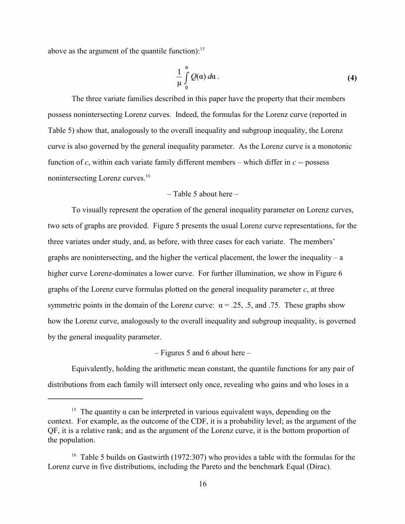
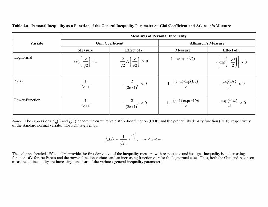
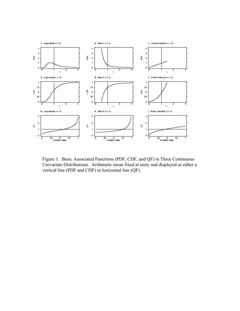
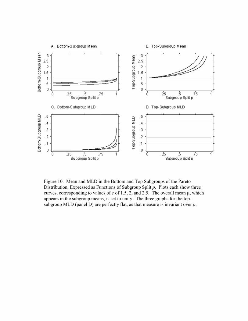
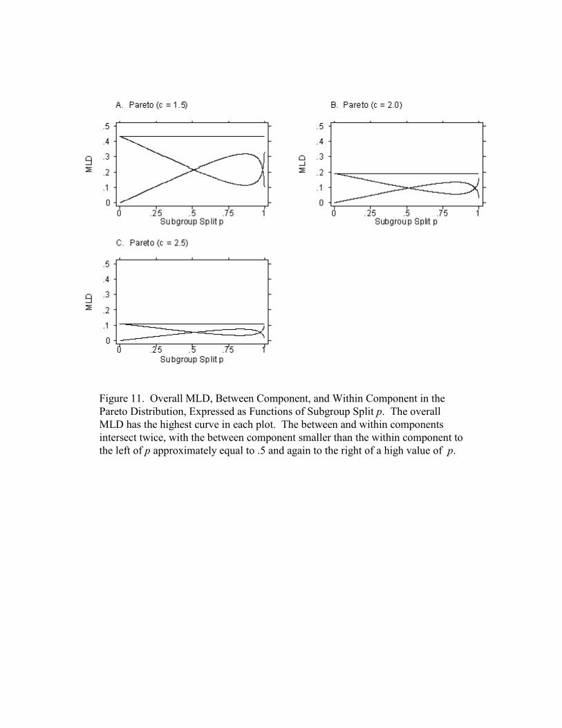
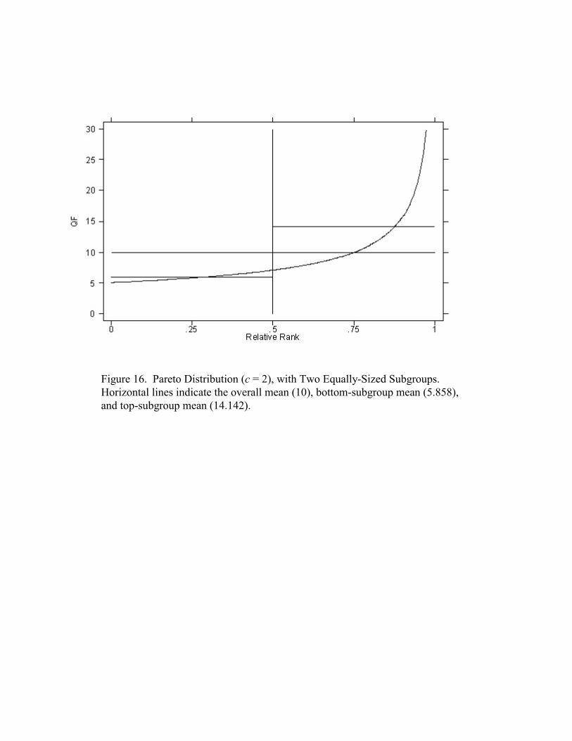
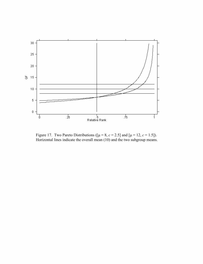Two Types of Inequality

Inequality Between Persons and Inequality Between Subgroups

Guillermina Jasso New York University and IZA

Samuel Kotz

George Washington University

Discussion Paper No 2749 April 2007

IZA

PO Box 7240 53072 Bonn

Germany

Phone +49-228-3894-0 Fax +49-228-3894-180

E-mail izaizaorg

Any opinions expressed here are those of the author(s) and not those of the institute Research disseminated by IZA may include views on policy but the institute itself takes no institutional policy positions The Institute for the Study of Labor (IZA) in Bonn is a local and virtual international research center and a place of communication between science politics and business IZA is an independent nonprofit company supported by Deutsche Post World Net The center is associated with the University of Bonn and offers a stimulating research environment through its research networks research support and visitors and doctoral programs IZA engages in (i) original and internationally competitive research in all fields of labor economics (ii) development of policy concepts and (iii) dissemination of research results and concepts to the interested public IZA Discussion Papers often represent preliminary work and are circulated to encourage discussion Citation of such a paper should account for its provisional character A revised version may be available directly from the author


ABSTRACT








1

1 INTRODUCTION


























2


























3


















terms in play3



4





























5





























6






















7



parameter7
















solely of c









8













coefficient is one9









9

(1)

(2)



















10

(3)












elucidation










11





section








theory





















12















point prdquo


13









means



















14






investigation
























15




























16





















(4)





17

















(5)

18





















parameter








19






















(6)



20






















21





decomposition

















408)


overall MLD

(7)



22


























23

























24




















Figure 9)








25














in the Pareto Case












(8)

26
























inequality



27

























28






empirical data





7 CONCLUDING NOTE
















29






between subgroups




















30

REFERENCES



2244-263









47901-920






Wiley









31



University Press


391037-1039





York Wiley









171-36





Review 453-32




32




























33











Series A 187253-318













Review 41107-22




34
















Lognormal

Pareto

Power-Function





Gini Coefficient


Theilrsquos MLD




Variate




Lognormal

Pareto

Power-Function




Variate




Lognormal

Pareto

Power-Function



Variate





Lognormal

Pareto

Power-Function




Lognormal

Pareto

Power-Function




Subgroup Mean

Subgroup MLD

Overall MLD

Between Component

Within Component




Subgroup Mean

Subgroup MLD

Overall MLD

Between Component

Within Component

























ABSTRACT








1

1 INTRODUCTION


























2


























3


















terms in play3



4





























5





























6






















7



parameter7
















solely of c









8













coefficient is one9









9

(1)

(2)



















10

(3)












elucidation










11





section








theory





















12















point prdquo


13









means



















14






investigation
























15




























16





















(4)





17

















(5)

18





















parameter








19






















(6)



20






















21





decomposition

















408)


overall MLD

(7)



22


























23

























24




















Figure 9)








25














in the Pareto Case












(8)

26
























inequality



27

























28






empirical data





7 CONCLUDING NOTE
















29






between subgroups




















30

REFERENCES



2244-263









47901-920






Wiley









31



University Press


391037-1039





York Wiley









171-36





Review 453-32




32




























33











Series A 187253-318













Review 41107-22




34
















Lognormal

Pareto

Power-Function





Gini Coefficient


Theilrsquos MLD




Variate




Lognormal

Pareto

Power-Function




Variate




Lognormal

Pareto

Power-Function



Variate





Lognormal

Pareto

Power-Function




Lognormal

Pareto

Power-Function




Subgroup Mean

Subgroup MLD

Overall MLD

Between Component

Within Component




Subgroup Mean

Subgroup MLD

Overall MLD

Between Component

Within Component


























1

1 INTRODUCTION


























2


























3


















terms in play3



4





























5





























6






















7



parameter7
















solely of c









8













coefficient is one9









9

(1)

(2)



















10

(3)












elucidation










11





section








theory





















12















point prdquo


13









means



















14






investigation
























15




























16





















(4)





17

















(5)

18





















parameter








19






















(6)



20






















21





decomposition

















408)


overall MLD

(7)



22


























23

























24




















Figure 9)








25














in the Pareto Case












(8)

26
























inequality



27

























28






empirical data





7 CONCLUDING NOTE
















29






between subgroups




















30

REFERENCES



2244-263









47901-920






Wiley









31



University Press


391037-1039





York Wiley









171-36





Review 453-32




32




























33











Series A 187253-318













Review 41107-22




34
















Lognormal

Pareto

Power-Function





Gini Coefficient


Theilrsquos MLD




Variate




Lognormal

Pareto

Power-Function




Variate




Lognormal

Pareto

Power-Function



Variate





Lognormal

Pareto

Power-Function




Lognormal

Pareto

Power-Function




Subgroup Mean

Subgroup MLD

Overall MLD

Between Component

Within Component




Subgroup Mean

Subgroup MLD

Overall MLD

Between Component

Within Component


























2


























3


















terms in play3



4





























5





























6






















7



parameter7
















solely of c









8













coefficient is one9









9

(1)

(2)



















10

(3)












elucidation










11





section








theory





















12















point prdquo


13









means



















14






investigation
























15




























16





















(4)





17

















(5)

18





















parameter








19






















(6)



20






















21





decomposition

















408)


overall MLD

(7)



22


























23

























24




















Figure 9)








25














in the Pareto Case












(8)

26
























inequality



27

























28






empirical data





7 CONCLUDING NOTE
















29






between subgroups




















30

REFERENCES



2244-263









47901-920






Wiley









31



University Press


391037-1039





York Wiley









171-36





Review 453-32




32




























33











Series A 187253-318













Review 41107-22




34
















Lognormal

Pareto

Power-Function





Gini Coefficient


Theilrsquos MLD




Variate




Lognormal

Pareto

Power-Function




Variate




Lognormal

Pareto

Power-Function



Variate





Lognormal

Pareto

Power-Function




Lognormal

Pareto

Power-Function




Subgroup Mean

Subgroup MLD

Overall MLD

Between Component

Within Component




Subgroup Mean

Subgroup MLD

Overall MLD

Between Component

Within Component


























3


















terms in play3



4





























5





























6






















7



parameter7
















solely of c









8













coefficient is one9









9

(1)

(2)



















10

(3)












elucidation










11





section








theory





















12















point prdquo


13









means



















14






investigation
























15




























16





















(4)





17

















(5)

18





















parameter








19






















(6)



20






















21





decomposition

















408)


overall MLD

(7)



22


























23

























24




















Figure 9)








25














in the Pareto Case












(8)

26
























inequality



27

























28






empirical data





7 CONCLUDING NOTE
















29






between subgroups




















30

REFERENCES



2244-263









47901-920






Wiley









31



University Press


391037-1039





York Wiley









171-36





Review 453-32




32




























33











Series A 187253-318













Review 41107-22




34
















Lognormal

Pareto

Power-Function





Gini Coefficient


Theilrsquos MLD




Variate




Lognormal

Pareto

Power-Function




Variate




Lognormal

Pareto

Power-Function



Variate





Lognormal

Pareto

Power-Function




Lognormal

Pareto

Power-Function




Subgroup Mean

Subgroup MLD

Overall MLD

Between Component

Within Component




Subgroup Mean

Subgroup MLD

Overall MLD

Between Component

Within Component
























4





























5





























6






















7



parameter7
















solely of c









8













coefficient is one9









9

(1)

(2)



















10

(3)












elucidation










11





section








theory





















12















point prdquo


13









means



















14






investigation
























15




























16





















(4)





17

















(5)

18





















parameter








19






















(6)



20






















21





decomposition

















408)


overall MLD

(7)



22


























23

























24




















Figure 9)








25














in the Pareto Case












(8)

26
























inequality



27

























28






empirical data





7 CONCLUDING NOTE
















29






between subgroups




















30

REFERENCES



2244-263









47901-920






Wiley









31



University Press


391037-1039





York Wiley









171-36





Review 453-32




32




























33











Series A 187253-318













Review 41107-22




34
















Lognormal

Pareto

Power-Function





Gini Coefficient


Theilrsquos MLD




Variate




Lognormal

Pareto

Power-Function




Variate




Lognormal

Pareto

Power-Function



Variate





Lognormal

Pareto

Power-Function




Lognormal

Pareto

Power-Function




Subgroup Mean

Subgroup MLD

Overall MLD

Between Component

Within Component




Subgroup Mean

Subgroup MLD

Overall MLD

Between Component

Within Component


























5





























6






















7



parameter7
















solely of c









8













coefficient is one9









9

(1)

(2)



















10

(3)












elucidation










11





section








theory





















12















point prdquo


13









means



















14






investigation
























15




























16





















(4)





17

















(5)

18





















parameter








19






















(6)



20






















21





decomposition

















408)


overall MLD

(7)



22


























23

























24




















Figure 9)








25














in the Pareto Case












(8)

26
























inequality



27

























28






empirical data





7 CONCLUDING NOTE
















29






between subgroups




















30

REFERENCES



2244-263









47901-920






Wiley









31



University Press


391037-1039





York Wiley









171-36





Review 453-32




32




























33











Series A 187253-318













Review 41107-22




34
















Lognormal

Pareto

Power-Function





Gini Coefficient


Theilrsquos MLD




Variate




Lognormal

Pareto

Power-Function




Variate




Lognormal

Pareto

Power-Function



Variate





Lognormal

Pareto

Power-Function




Lognormal

Pareto

Power-Function




Subgroup Mean

Subgroup MLD

Overall MLD

Between Component

Within Component




Subgroup Mean

Subgroup MLD

Overall MLD

Between Component

Within Component




























6






















7



parameter7
















solely of c









8













coefficient is one9









9

(1)

(2)



















10

(3)












elucidation










11





section








theory





















12















point prdquo


13









means



















14






investigation
























15




























16





















(4)





17

















(5)

18





















parameter








19






















(6)



20






















21





decomposition

















408)


overall MLD

(7)



22


























23

























24




















Figure 9)








25














in the Pareto Case












(8)

26
























inequality



27

























28






empirical data





7 CONCLUDING NOTE
















29






between subgroups




















30

REFERENCES



2244-263









47901-920






Wiley









31



University Press


391037-1039





York Wiley









171-36





Review 453-32




32




























33











Series A 187253-318













Review 41107-22




34
















Lognormal

Pareto

Power-Function





Gini Coefficient


Theilrsquos MLD




Variate




Lognormal

Pareto

Power-Function




Variate




Lognormal

Pareto

Power-Function



Variate





Lognormal

Pareto

Power-Function




Lognormal

Pareto

Power-Function




Subgroup Mean

Subgroup MLD

Overall MLD

Between Component

Within Component




Subgroup Mean

Subgroup MLD

Overall MLD

Between Component

Within Component


























7



parameter7
















solely of c









8













coefficient is one9









9

(1)

(2)



















10

(3)












elucidation










11





section








theory





















12















point prdquo


13









means



















14






investigation
























15




























16





















(4)





17

















(5)

18





















parameter








19






















(6)



20






















21





decomposition

















408)


overall MLD

(7)



22


























23

























24




















Figure 9)








25














in the Pareto Case












(8)

26
























inequality



27

























28






empirical data





7 CONCLUDING NOTE
















29






between subgroups




















30

REFERENCES



2244-263









47901-920






Wiley









31



University Press


391037-1039





York Wiley









171-36





Review 453-32




32




























33











Series A 187253-318













Review 41107-22




34
















Lognormal

Pareto

Power-Function





Gini Coefficient


Theilrsquos MLD




Variate




Lognormal

Pareto

Power-Function




Variate




Lognormal

Pareto

Power-Function



Variate





Lognormal

Pareto

Power-Function




Lognormal

Pareto

Power-Function




Subgroup Mean

Subgroup MLD

Overall MLD

Between Component

Within Component




Subgroup Mean

Subgroup MLD

Overall MLD

Between Component

Within Component




























8













coefficient is one9









9

(1)

(2)



















10

(3)












elucidation










11





section








theory





















12















point prdquo


13









means



















14






investigation
























15




























16





















(4)





17

















(5)

18





















parameter








19






















(6)



20






















21





decomposition

















408)


overall MLD

(7)



22


























23

























24




















Figure 9)








25














in the Pareto Case












(8)

26
























inequality



27

























28






empirical data





7 CONCLUDING NOTE
















29






between subgroups




















30

REFERENCES



2244-263









47901-920






Wiley









31



University Press


391037-1039





York Wiley









171-36





Review 453-32




32




























33











Series A 187253-318













Review 41107-22




34
















Lognormal

Pareto

Power-Function





Gini Coefficient


Theilrsquos MLD




Variate




Lognormal

Pareto

Power-Function




Variate




Lognormal

Pareto

Power-Function



Variate





Lognormal

Pareto

Power-Function




Lognormal

Pareto

Power-Function




Subgroup Mean

Subgroup MLD

Overall MLD

Between Component

Within Component




Subgroup Mean

Subgroup MLD

Overall MLD

Between Component

Within Component


























9

(1)

(2)



















10

(3)












elucidation










11





section








theory





















12















point prdquo


13









means



















14






investigation
























15




























16





















(4)





17

















(5)

18





















parameter








19






















(6)



20






















21





decomposition

















408)


overall MLD

(7)



22


























23

























24




















Figure 9)








25














in the Pareto Case












(8)

26
























inequality



27

























28






empirical data





7 CONCLUDING NOTE
















29






between subgroups




















30

REFERENCES



2244-263









47901-920






Wiley









31



University Press


391037-1039





York Wiley









171-36





Review 453-32




32




























33











Series A 187253-318













Review 41107-22




34
















Lognormal

Pareto

Power-Function





Gini Coefficient


Theilrsquos MLD




Variate




Lognormal

Pareto

Power-Function




Variate




Lognormal

Pareto

Power-Function



Variate





Lognormal

Pareto

Power-Function




Lognormal

Pareto

Power-Function




Subgroup Mean

Subgroup MLD

Overall MLD

Between Component

Within Component




Subgroup Mean

Subgroup MLD

Overall MLD

Between Component

Within Component
























10

(3)












elucidation










11





section








theory





















12















point prdquo


13









means



















14






investigation
























15




























16





















(4)





17

















(5)

18





















parameter








19






















(6)



20






















21





decomposition

















408)


overall MLD

(7)



22


























23

























24




















Figure 9)








25














in the Pareto Case












(8)

26
























inequality



27

























28






empirical data





7 CONCLUDING NOTE
















29






between subgroups




















30

REFERENCES



2244-263









47901-920






Wiley









31



University Press


391037-1039





York Wiley









171-36





Review 453-32




32




























33











Series A 187253-318













Review 41107-22




34
















Lognormal

Pareto

Power-Function





Gini Coefficient


Theilrsquos MLD




Variate




Lognormal

Pareto

Power-Function




Variate




Lognormal

Pareto

Power-Function



Variate





Lognormal

Pareto

Power-Function




Lognormal

Pareto

Power-Function




Subgroup Mean

Subgroup MLD

Overall MLD

Between Component

Within Component




Subgroup Mean

Subgroup MLD

Overall MLD

Between Component

Within Component
























11





section








theory





















12















point prdquo


13









means



















14






investigation
























15




























16





















(4)





17

















(5)

18





















parameter








19






















(6)



20






















21





decomposition

















408)


overall MLD

(7)



22


























23

























24




















Figure 9)








25














in the Pareto Case












(8)

26
























inequality



27

























28






empirical data





7 CONCLUDING NOTE
















29






between subgroups




















30

REFERENCES



2244-263









47901-920






Wiley









31



University Press


391037-1039





York Wiley









171-36





Review 453-32




32




























33











Series A 187253-318













Review 41107-22




34
















Lognormal

Pareto

Power-Function





Gini Coefficient


Theilrsquos MLD




Variate




Lognormal

Pareto

Power-Function




Variate




Lognormal

Pareto

Power-Function



Variate





Lognormal

Pareto

Power-Function




Lognormal

Pareto

Power-Function




Subgroup Mean

Subgroup MLD

Overall MLD

Between Component

Within Component




Subgroup Mean

Subgroup MLD

Overall MLD

Between Component

Within Component






























12















point prdquo


13









means



















14






investigation
























15




























16





















(4)





17

















(5)

18





















parameter








19






















(6)



20






















21





decomposition

















408)


overall MLD

(7)



22


























23

























24




















Figure 9)








25














in the Pareto Case












(8)

26
























inequality



27

























28






empirical data





7 CONCLUDING NOTE
















29






between subgroups




















30

REFERENCES



2244-263









47901-920






Wiley









31



University Press


391037-1039





York Wiley









171-36





Review 453-32




32




























33











Series A 187253-318













Review 41107-22




34
















Lognormal

Pareto

Power-Function





Gini Coefficient


Theilrsquos MLD




Variate




Lognormal

Pareto

Power-Function




Variate




Lognormal

Pareto

Power-Function



Variate





Lognormal

Pareto

Power-Function




Lognormal

Pareto

Power-Function




Subgroup Mean

Subgroup MLD

Overall MLD

Between Component

Within Component




Subgroup Mean

Subgroup MLD

Overall MLD

Between Component

Within Component
























13









means



















14






investigation
























15




























16





















(4)





17

















(5)

18





















parameter








19






















(6)



20






















21





decomposition

















408)


overall MLD

(7)



22


























23

























24




















Figure 9)








25














in the Pareto Case












(8)

26
























inequality



27

























28






empirical data





7 CONCLUDING NOTE
















29






between subgroups




















30

REFERENCES



2244-263









47901-920






Wiley









31



University Press


391037-1039





York Wiley









171-36





Review 453-32




32




























33











Series A 187253-318













Review 41107-22




34
















Lognormal

Pareto

Power-Function





Gini Coefficient


Theilrsquos MLD




Variate




Lognormal

Pareto

Power-Function




Variate




Lognormal

Pareto

Power-Function



Variate





Lognormal

Pareto

Power-Function




Lognormal

Pareto

Power-Function




Subgroup Mean

Subgroup MLD

Overall MLD

Between Component

Within Component




Subgroup Mean

Subgroup MLD

Overall MLD

Between Component

Within Component
























14






investigation
























15




























16





















(4)





17

















(5)

18





















parameter








19






















(6)



20






















21





decomposition

















408)


overall MLD

(7)



22


























23

























24




















Figure 9)








25














in the Pareto Case












(8)

26
























inequality



27

























28






empirical data





7 CONCLUDING NOTE
















29






between subgroups




















30

REFERENCES



2244-263









47901-920






Wiley









31



University Press


391037-1039





York Wiley









171-36





Review 453-32




32




























33











Series A 187253-318













Review 41107-22




34
















Lognormal

Pareto

Power-Function





Gini Coefficient


Theilrsquos MLD




Variate




Lognormal

Pareto

Power-Function




Variate




Lognormal

Pareto

Power-Function



Variate





Lognormal

Pareto

Power-Function




Lognormal

Pareto

Power-Function




Subgroup Mean

Subgroup MLD

Overall MLD

Between Component

Within Component




Subgroup Mean

Subgroup MLD

Overall MLD

Between Component

Within Component


























15




























16





















(4)





17

















(5)

18





















parameter








19






















(6)



20






















21





decomposition

















408)


overall MLD

(7)



22


























23

























24




















Figure 9)








25














in the Pareto Case












(8)

26
























inequality



27

























28






empirical data





7 CONCLUDING NOTE
















29






between subgroups




















30

REFERENCES



2244-263









47901-920






Wiley









31



University Press


391037-1039





York Wiley









171-36





Review 453-32




32




























33











Series A 187253-318













Review 41107-22




34
















Lognormal

Pareto

Power-Function





Gini Coefficient


Theilrsquos MLD




Variate




Lognormal

Pareto

Power-Function




Variate




Lognormal

Pareto

Power-Function



Variate





Lognormal

Pareto

Power-Function




Lognormal

Pareto

Power-Function




Subgroup Mean

Subgroup MLD

Overall MLD

Between Component

Within Component




Subgroup Mean

Subgroup MLD

Overall MLD

Between Component

Within Component




























16





















(4)





17

















(5)

18





















parameter








19






















(6)



20






















21





decomposition

















408)


overall MLD

(7)



22


























23

























24




















Figure 9)








25














in the Pareto Case












(8)

26
























inequality



27

























28






empirical data





7 CONCLUDING NOTE
















29






between subgroups




















30

REFERENCES



2244-263









47901-920






Wiley









31



University Press


391037-1039





York Wiley









171-36





Review 453-32




32




























33











Series A 187253-318













Review 41107-22




34
















Lognormal

Pareto

Power-Function





Gini Coefficient


Theilrsquos MLD




Variate




Lognormal

Pareto

Power-Function




Variate




Lognormal

Pareto

Power-Function



Variate





Lognormal

Pareto

Power-Function




Lognormal

Pareto

Power-Function




Subgroup Mean

Subgroup MLD

Overall MLD

Between Component

Within Component




Subgroup Mean

Subgroup MLD

Overall MLD

Between Component

Within Component




























17

















(5)

18





















parameter








19






















(6)



20






















21





decomposition

















408)


overall MLD

(7)



22


























23

























24




















Figure 9)








25














in the Pareto Case












(8)

26
























inequality



27

























28






empirical data





7 CONCLUDING NOTE
















29






between subgroups




















30

REFERENCES



2244-263









47901-920






Wiley









31



University Press


391037-1039





York Wiley









171-36





Review 453-32




32




























33











Series A 187253-318













Review 41107-22




34
















Lognormal

Pareto

Power-Function





Gini Coefficient


Theilrsquos MLD




Variate




Lognormal

Pareto

Power-Function




Variate




Lognormal

Pareto

Power-Function



Variate





Lognormal

Pareto

Power-Function




Lognormal

Pareto

Power-Function




Subgroup Mean

Subgroup MLD

Overall MLD

Between Component

Within Component




Subgroup Mean

Subgroup MLD

Overall MLD

Between Component

Within Component
























18





















parameter








19






















(6)



20






















21





decomposition

















408)


overall MLD

(7)



22


























23

























24




















Figure 9)








25














in the Pareto Case












(8)

26
























inequality



27

























28






empirical data





7 CONCLUDING NOTE
















29






between subgroups




















30

REFERENCES



2244-263









47901-920






Wiley









31



University Press


391037-1039





York Wiley









171-36





Review 453-32




32




























33











Series A 187253-318













Review 41107-22




34
















Lognormal

Pareto

Power-Function





Gini Coefficient


Theilrsquos MLD




Variate




Lognormal

Pareto

Power-Function




Variate




Lognormal

Pareto

Power-Function



Variate





Lognormal

Pareto

Power-Function




Lognormal

Pareto

Power-Function




Subgroup Mean

Subgroup MLD

Overall MLD

Between Component

Within Component




Subgroup Mean

Subgroup MLD

Overall MLD

Between Component

Within Component


























19






















(6)



20






















21





decomposition

















408)


overall MLD

(7)



22


























23

























24




















Figure 9)








25














in the Pareto Case












(8)

26
























inequality



27

























28






empirical data





7 CONCLUDING NOTE
















29






between subgroups




















30

REFERENCES



2244-263









47901-920






Wiley









31



University Press


391037-1039





York Wiley









171-36





Review 453-32




32




























33











Series A 187253-318













Review 41107-22




34
















Lognormal

Pareto

Power-Function





Gini Coefficient


Theilrsquos MLD




Variate




Lognormal

Pareto

Power-Function




Variate




Lognormal

Pareto

Power-Function



Variate





Lognormal

Pareto

Power-Function




Lognormal

Pareto

Power-Function




Subgroup Mean

Subgroup MLD

Overall MLD

Between Component

Within Component




Subgroup Mean

Subgroup MLD

Overall MLD

Between Component

Within Component


























20






















21





decomposition

















408)


overall MLD

(7)



22


























23

























24




















Figure 9)








25














in the Pareto Case












(8)

26
























inequality



27

























28






empirical data





7 CONCLUDING NOTE
















29






between subgroups




















30

REFERENCES



2244-263









47901-920






Wiley









31



University Press


391037-1039





York Wiley









171-36





Review 453-32




32




























33











Series A 187253-318













Review 41107-22




34
















Lognormal

Pareto

Power-Function





Gini Coefficient


Theilrsquos MLD




Variate




Lognormal

Pareto

Power-Function




Variate




Lognormal

Pareto

Power-Function



Variate





Lognormal

Pareto

Power-Function




Lognormal

Pareto

Power-Function




Subgroup Mean

Subgroup MLD

Overall MLD

Between Component

Within Component




Subgroup Mean

Subgroup MLD

Overall MLD

Between Component

Within Component
























21





decomposition

















408)


overall MLD

(7)



22


























23

























24




















Figure 9)








25














in the Pareto Case












(8)

26
























inequality



27

























28






empirical data





7 CONCLUDING NOTE
















29






between subgroups




















30

REFERENCES



2244-263









47901-920






Wiley









31



University Press


391037-1039





York Wiley









171-36





Review 453-32




32




























33











Series A 187253-318













Review 41107-22




34
















Lognormal

Pareto

Power-Function





Gini Coefficient


Theilrsquos MLD




Variate




Lognormal

Pareto

Power-Function




Variate




Lognormal

Pareto

Power-Function



Variate





Lognormal

Pareto

Power-Function




Lognormal

Pareto

Power-Function




Subgroup Mean

Subgroup MLD

Overall MLD

Between Component

Within Component




Subgroup Mean

Subgroup MLD

Overall MLD

Between Component

Within Component


























22


























23

























24




















Figure 9)








25














in the Pareto Case












(8)

26
























inequality



27

























28






empirical data





7 CONCLUDING NOTE
















29






between subgroups




















30

REFERENCES



2244-263









47901-920






Wiley









31



University Press


391037-1039





York Wiley









171-36





Review 453-32




32




























33











Series A 187253-318













Review 41107-22




34
















Lognormal

Pareto

Power-Function





Gini Coefficient


Theilrsquos MLD




Variate




Lognormal

Pareto

Power-Function




Variate




Lognormal

Pareto

Power-Function



Variate





Lognormal

Pareto

Power-Function




Lognormal

Pareto

Power-Function




Subgroup Mean

Subgroup MLD

Overall MLD

Between Component

Within Component




Subgroup Mean

Subgroup MLD

Overall MLD

Between Component

Within Component


























23

























24




















Figure 9)








25














in the Pareto Case












(8)

26
























inequality



27

























28






empirical data





7 CONCLUDING NOTE
















29






between subgroups




















30

REFERENCES



2244-263









47901-920






Wiley









31



University Press


391037-1039





York Wiley









171-36





Review 453-32




32




























33











Series A 187253-318













Review 41107-22




34
















Lognormal

Pareto

Power-Function





Gini Coefficient


Theilrsquos MLD




Variate




Lognormal

Pareto

Power-Function




Variate




Lognormal

Pareto

Power-Function



Variate





Lognormal

Pareto

Power-Function




Lognormal

Pareto

Power-Function




Subgroup Mean

Subgroup MLD

Overall MLD

Between Component

Within Component




Subgroup Mean

Subgroup MLD

Overall MLD

Between Component

Within Component
























24




















Figure 9)








25














in the Pareto Case












(8)

26
























inequality



27

























28






empirical data





7 CONCLUDING NOTE
















29






between subgroups




















30

REFERENCES



2244-263









47901-920






Wiley









31



University Press


391037-1039





York Wiley









171-36





Review 453-32




32




























33











Series A 187253-318













Review 41107-22




34
















Lognormal

Pareto

Power-Function





Gini Coefficient


Theilrsquos MLD




Variate




Lognormal

Pareto

Power-Function




Variate




Lognormal

Pareto

Power-Function



Variate





Lognormal

Pareto

Power-Function




Lognormal

Pareto

Power-Function




Subgroup Mean

Subgroup MLD

Overall MLD

Between Component

Within Component




Subgroup Mean

Subgroup MLD

Overall MLD

Between Component

Within Component
























25














in the Pareto Case












(8)

26
























inequality



27

























28






empirical data





7 CONCLUDING NOTE
















29






between subgroups




















30

REFERENCES



2244-263









47901-920






Wiley









31



University Press


391037-1039





York Wiley









171-36





Review 453-32




32




























33











Series A 187253-318













Review 41107-22




34
















Lognormal

Pareto

Power-Function





Gini Coefficient


Theilrsquos MLD




Variate




Lognormal

Pareto

Power-Function




Variate




Lognormal

Pareto

Power-Function



Variate





Lognormal

Pareto

Power-Function




Lognormal

Pareto

Power-Function




Subgroup Mean

Subgroup MLD

Overall MLD

Between Component

Within Component




Subgroup Mean

Subgroup MLD

Overall MLD

Between Component

Within Component
























26
























inequality



27

























28






empirical data





7 CONCLUDING NOTE
















29






between subgroups




















30

REFERENCES



2244-263









47901-920






Wiley









31



University Press


391037-1039





York Wiley









171-36





Review 453-32




32




























33











Series A 187253-318













Review 41107-22




34
















Lognormal

Pareto

Power-Function





Gini Coefficient


Theilrsquos MLD




Variate




Lognormal

Pareto

Power-Function




Variate




Lognormal

Pareto

Power-Function



Variate





Lognormal

Pareto

Power-Function




Lognormal

Pareto

Power-Function




Subgroup Mean

Subgroup MLD

Overall MLD

Between Component

Within Component




Subgroup Mean

Subgroup MLD

Overall MLD

Between Component

Within Component


























27

























28






empirical data





7 CONCLUDING NOTE
















29






between subgroups




















30

REFERENCES



2244-263









47901-920






Wiley









31



University Press


391037-1039





York Wiley









171-36





Review 453-32




32




























33











Series A 187253-318













Review 41107-22




34
















Lognormal

Pareto

Power-Function





Gini Coefficient


Theilrsquos MLD




Variate




Lognormal

Pareto

Power-Function




Variate




Lognormal

Pareto

Power-Function



Variate





Lognormal

Pareto

Power-Function




Lognormal

Pareto

Power-Function




Subgroup Mean

Subgroup MLD

Overall MLD

Between Component

Within Component




Subgroup Mean

Subgroup MLD

Overall MLD

Between Component

Within Component
























28






empirical data





7 CONCLUDING NOTE
















29






between subgroups




















30

REFERENCES



2244-263









47901-920






Wiley









31



University Press


391037-1039





York Wiley









171-36





Review 453-32




32




























33











Series A 187253-318













Review 41107-22




34
















Lognormal

Pareto

Power-Function





Gini Coefficient


Theilrsquos MLD




Variate




Lognormal

Pareto

Power-Function




Variate




Lognormal

Pareto

Power-Function



Variate





Lognormal

Pareto

Power-Function




Lognormal

Pareto

Power-Function




Subgroup Mean

Subgroup MLD

Overall MLD

Between Component

Within Component




Subgroup Mean

Subgroup MLD

Overall MLD

Between Component

Within Component
























29






between subgroups




















30

REFERENCES



2244-263









47901-920






Wiley









31



University Press


391037-1039





York Wiley









171-36





Review 453-32




32




























33











Series A 187253-318













Review 41107-22




34
















Lognormal

Pareto

Power-Function





Gini Coefficient


Theilrsquos MLD




Variate




Lognormal

Pareto

Power-Function




Variate




Lognormal

Pareto

Power-Function



Variate





Lognormal

Pareto

Power-Function




Lognormal

Pareto

Power-Function




Subgroup Mean

Subgroup MLD

Overall MLD

Between Component

Within Component




Subgroup Mean

Subgroup MLD

Overall MLD

Between Component

Within Component
























30

REFERENCES



2244-263









47901-920






Wiley









31



University Press


391037-1039





York Wiley









171-36





Review 453-32




32




























33











Series A 187253-318













Review 41107-22




34
















Lognormal

Pareto

Power-Function





Gini Coefficient


Theilrsquos MLD




Variate




Lognormal

Pareto

Power-Function




Variate




Lognormal

Pareto

Power-Function



Variate





Lognormal

Pareto

Power-Function




Lognormal

Pareto

Power-Function




Subgroup Mean

Subgroup MLD

Overall MLD

Between Component

Within Component




Subgroup Mean

Subgroup MLD

Overall MLD

Between Component

Within Component
























31



University Press


391037-1039





York Wiley









171-36





Review 453-32




32




























33











Series A 187253-318













Review 41107-22




34
















Lognormal

Pareto

Power-Function





Gini Coefficient


Theilrsquos MLD




Variate




Lognormal

Pareto

Power-Function




Variate




Lognormal

Pareto

Power-Function



Variate





Lognormal

Pareto

Power-Function




Lognormal

Pareto

Power-Function




Subgroup Mean

Subgroup MLD

Overall MLD

Between Component

Within Component




Subgroup Mean

Subgroup MLD

Overall MLD

Between Component

Within Component
























32




























33











Series A 187253-318













Review 41107-22




34
















Lognormal

Pareto

Power-Function





Gini Coefficient


Theilrsquos MLD




Variate




Lognormal

Pareto

Power-Function




Variate




Lognormal

Pareto

Power-Function



Variate





Lognormal

Pareto

Power-Function




Lognormal

Pareto

Power-Function




Subgroup Mean

Subgroup MLD

Overall MLD

Between Component

Within Component




Subgroup Mean

Subgroup MLD

Overall MLD

Between Component

Within Component
























33











Series A 187253-318













Review 41107-22




34
















Lognormal

Pareto

Power-Function





Gini Coefficient


Theilrsquos MLD




Variate




Lognormal

Pareto

Power-Function




Variate




Lognormal

Pareto

Power-Function



Variate





Lognormal

Pareto

Power-Function




Lognormal

Pareto

Power-Function




Subgroup Mean

Subgroup MLD

Overall MLD

Between Component

Within Component




Subgroup Mean

Subgroup MLD

Overall MLD

Between Component

Within Component
























34
















Lognormal

Pareto

Power-Function





Gini Coefficient


Theilrsquos MLD




Variate




Lognormal

Pareto

Power-Function




Variate




Lognormal

Pareto

Power-Function



Variate





Lognormal

Pareto

Power-Function




Lognormal

Pareto

Power-Function




Subgroup Mean

Subgroup MLD

Overall MLD

Between Component

Within Component




Subgroup Mean

Subgroup MLD

Overall MLD

Between Component

Within Component


























Lognormal

Pareto

Power-Function





Gini Coefficient


Theilrsquos MLD




Variate




Lognormal

Pareto

Power-Function




Variate




Lognormal

Pareto

Power-Function



Variate





Lognormal

Pareto

Power-Function




Lognormal

Pareto

Power-Function




Subgroup Mean

Subgroup MLD

Overall MLD

Between Component

Within Component




Subgroup Mean

Subgroup MLD

Overall MLD

Between Component

Within Component


























Gini Coefficient


Theilrsquos MLD




Variate




Lognormal

Pareto

Power-Function




Variate




Lognormal

Pareto

Power-Function



Variate





Lognormal

Pareto

Power-Function




Lognormal

Pareto

Power-Function




Subgroup Mean

Subgroup MLD

Overall MLD

Between Component

Within Component




Subgroup Mean

Subgroup MLD

Overall MLD

Between Component

Within Component

























Variate




Lognormal

Pareto

Power-Function




Variate




Lognormal

Pareto

Power-Function



Variate





Lognormal

Pareto

Power-Function




Lognormal

Pareto

Power-Function




Subgroup Mean

Subgroup MLD

Overall MLD

Between Component

Within Component




Subgroup Mean

Subgroup MLD

Overall MLD

Between Component

Within Component

























Variate




Lognormal

Pareto

Power-Function



Variate





Lognormal

Pareto

Power-Function




Lognormal

Pareto

Power-Function




Subgroup Mean

Subgroup MLD

Overall MLD

Between Component

Within Component




Subgroup Mean

Subgroup MLD

Overall MLD

Between Component

Within Component

























Variate





Lognormal

Pareto

Power-Function




Lognormal

Pareto

Power-Function




Subgroup Mean

Subgroup MLD

Overall MLD

Between Component

Within Component




Subgroup Mean

Subgroup MLD

Overall MLD

Between Component

Within Component


























Lognormal

Pareto

Power-Function




Subgroup Mean

Subgroup MLD

Overall MLD

Between Component

Within Component




Subgroup Mean

Subgroup MLD

Overall MLD

Between Component

Within Component


























Subgroup Mean

Subgroup MLD

Overall MLD

Between Component

Within Component




Subgroup Mean

Subgroup MLD

Overall MLD

Between Component

Within Component


























Subgroup Mean

Subgroup MLD

Overall MLD

Between Component

Within Component
























Two Types of Inequality: Inequality Between Persons and ...ftp.iza.org/dp2749.pdf · IZA Discussion...

Documents

Transcript of Two Types of Inequality: Inequality Between Persons and ...ftp.iza.org/dp2749.pdf · IZA Discussion...