1

American Institute of Aeronautics and Astronautics

Two-Step Multi-Physics Analysis of an Annular Linear

Induction Pump for Fission Power Systems

Steven M. Geng1 and Dr. Terry V. Reid1

NASA Glenn Research Center, Cleveland, Ohio, 44135

One of the key technologies associated with fission power systems (FPS) is the annular

linear induction pump (ALIP). ALIPs are used to circulate liquid-metal fluid for transporting

thermal energy from the nuclear reactor to the power conversion device. ALIPs designed and

built to date for FPS project applications have not performed up to expectations. A unique,

two-step approach was taken toward the multi-physics examination of an ALIP using ANSYS

Maxwell 3D and Fluent. This multi-physics approach was developed so that engineers could

investigate design variations that might improve pump performance. Of interest was to

determine if simple geometric modifications could be made to the ALIP components with the

goal of increasing the Lorentz forces acting on the liquid-metal fluid, which in turn would

increase pumping capacity. The multi-physics model first calculates the Lorentz forces acting

on the liquid metal fluid in the ALIP annulus. These forces are then used in a computational

fluid dynamics simulation as (a) internal boundary conditions and (b) source functions in the

momentum equations within the Navier-Stokes equations. The end result of the two-step

analysis is a predicted pump pressure rise that can be compared with experimental data.

Nomenclature

A = surface area

B = magnetic flux density

C1 = activation constant for continuity equation mass source term

C2 = activation constant for momentum equation stress tensor

C3 = activation constant for momentum equation body force source term

C4 = activation constant for energy equation source term

D = displacement field

E = electric field

�⃗� = body force source term

FL = Lorentz force

G = internal energy field

g = gravity

H = magnetic field

𝐼 ̿ = unit tensor

J = current distribution

k = thermal conductivity

= dynamic viscosity

P = pressure

= fluid mass density

charge = electric charge density

Sm, SH = mass source and energy source terms

= electrical conductivity

𝜏̿ = stress tensor

T = temperature

t = time

v⃗⃗ = velocity field

Volslug = slug volume

1 Engineer, Thermal Energy Conversion Branch, 21000 Brookpark Road, M/S 301-2, AIAA Senior Member.

https://ntrs.nasa.gov/search.jsp?R=20170000670 2018-05-30T17:08:55+00:00Z

2

American Institute of Aeronautics and Astronautics

I. Introduction

ission power system (FPS) technology is being developed for use on the surface of the Moon, Mars, or other

moons and planets of our solar system. FPSs are capable of providing good performance at any location, including

those near the poles or other permanently shaded regions, and offer the capability to provide on-demand power at any

time, even at long distances from the Sun. Fission-based systems also offer the potential for outposts, crew, and

science instruments to operate in a power-rich environment.

One of the key technologies associated with the FPS is the annular linear induction pump (ALIP) used to circulate

the liquid-metal fluid that transports thermal energy from the nuclear reactor to the power conversion device. In 2010,

an ALIP developed by the Idaho National Laboratory (INL) was tested under representative space-reactor thermal

operating conditions at NASA’s Marshall Space Flight Center (MSFC) to quantify the pump’s performance1. The

measured performance was below expectations. Illustrations of the ALIP pump are shown in Figure 1. MSFC

conducted performance testing of the ALIP using their test circuit shown in Figure 2. The test circuit consists of the

ALIP, an induction heater, a throttling valve, an electromagnetic flow meter, and a gaseous nitrogen to NaK heat

exchanger. The throttling valve is located downstream of the ALIP (in the test circuit) so that the flow resistance

could be varied.

In 2012, NASA’s Glenn Research Center (GRC) developed a magneto-static finite element model of the ALIP to

gain a better understanding of its functionality, and to independently evaluate design variations that might have

contributed to the performance shortfall2. In 2015, the ALIP model was upgraded to a 3D transient magnetic analysis

which dramatically simplified the post-processing of the model predictions. The magnetic model takes advantage of

ALIP symmetry to reduce computation time.

A full 3D Computational Fluid Dynamics (CFD) model was recently created of the ALIP that, when used in

combination with the magnetic model, could generate pressure rise and flow rate predictions for comparison with the

F

Figure 1. Illustrations of ALIP (Courtesy of Idaho National Lab)

a) Schematic b) Photograph

Figure 2. The ALIP Test Circuit (Courtesy of NASA Marshall Space Flight Center)

3

American Institute of Aeronautics and Astronautics

experimental data. Symmetry is not assumed in the CFD model due to the inhomogenous pressure distribution in the

NaK flow annulus.

The multi-physics ALIP model was validated against experimental data, then used to generate performance

predictions. This paper presents a discussion of the multi-physics (3D transient magnetic and CFD) model of the

ALIP, a comparison of model predictions versus experimental data, and a discussion of several design variations that

could potentially have a positive impact on pump performance.

II. Fission Power System Reference Concept Demonstration

Power is an important consideration when

planning the exploration of planetary surfaces.

Nuclear power is an enabling option for

locations in the solar system where sunlight is

limited. A Fission Surface Power preliminary

reference concept3 was developed, and a full

scale, ¼ power Technology Demonstration Unit

(TDU) was built and tested4 to demonstrate the

system level of readiness (see Figure 3). An

annular linear induction pump (ALIP) was used

to circulate NaK-78 through the loop of the

TDU to transfer thermal energy from the reactor

core simulator to a 12 kWe free-piston Stirling

power convertor. The 12 kWe Stirling

convertor is comprised of two dual-opposed 6

kWe Stirling engines. The core simulator heats

the NaK to 550°C, and as the heated NaK

circulates through the loop, the thermal energy

is transferred to the Stirling convertor through a

pair of heat exchangers. The ALIP must impart

a sufficient pressure rise on the NaK fluid, to

overcome the pressure drop loss produced by

the loop components (piping, core simulator,

and the heat exchangers).

III. Analysis Description

A multi-physics two-step approach was taken to model the ALIP used in the TDU test. The following section

describes the governing equations used by each solver in the various analyses. The application of these equations

occurred in the magnetic and fluid flow solvers (ANSYS MAXWELL® and FLUENT®). The conditions that were

chosen for the calculations were based on data from experimental testing of the ALIP by the NASA Marshall Space

Flight Center.

A. Magnetic Field Analysis

The ANSYS-Maxwell software was used to create a transient magnetic model of the ALIP. The Maxwell software

basically solves the differential form of Maxwell’s equations. The equations include 1) Faraday’s Law of Induction,

2) Gauss’s Law for magnetism, 3) Ampere’s Law, and 4) Gauss’s Law for electricity. The equations are as follows:

∇ × 𝐸 = −𝜕𝐵

𝜕𝑡 (1)

∇ ∙ B = 0 (2)

∇ × 𝐻 = 𝐽 +𝜕𝐷

𝜕𝑡 (3)

∇ ∙ 𝐷 = 𝜌𝑐ℎ𝑎𝑟𝑔𝑒 (4)

(a) Test article (b) CAD Model

Figure 3. Fission Power System (FPS) Technology

Demonstration Unit (TDU).

4

American Institute of Aeronautics and Astronautics

The Maxwell transient field simulator calculates the time-domain magnetic fields in 3D. The source of the

magnetic fields is the 3-phase current flowing through the 12 ALIP coils. The transient field simulator solves for the

magnetic field (H), current distribution (J), and the magnetic flux density (B). Derived quantities such as Lorentz

force acting on the NaK fluid, winding flux linkage, and induced voltage/current in the NaK fluid are calculated from

the basic field equations.

B. Fluid Flow Field Analysis

The flow field analysis involves the solution of the Navier Stokes equations, which include conservation of mass,

momentum and energy. The conservation of mass (5) and conservation of momentum (6) equations are:

𝜕𝜌

𝜕𝑡+ ∇ ∗ (𝜌�⃗⃗�) = 𝑪𝟏𝑆𝑚 (5)

𝜕(𝜌�⃗⃗�)

𝜕𝑡+ ∇ ∗ (𝜌�⃗⃗� �⃗⃗�) = −∇𝑃 + 𝑪𝟐∇ ∗ (𝜏̿) + 𝜌�⃗� + 𝑪𝟑�⃗� (6)

The stress tensor, 𝜏̿, is given by

𝜏̿ = 𝜇 [(∇�⃗⃗� + ∇�⃗⃗�𝑇) −2

3∇ ∗ �⃗⃗�𝐼] (7)

where is the molecular viscosity, I is the unit tensor, and the second term on the right hand side is the effect of

volume dilation. The energy equation (8) is defined by

𝜕(𝜌𝐺)

𝜕𝑡+ ∇ ∗ (�⃗⃗�( 𝜌𝐺 + 𝑝)) = ∇ (𝑘∇𝑇 + ∗ 𝑪𝟐(𝜏̿ ∗ �⃗⃗�)) + 𝑪𝟒𝑆ℎ (8)

In the energy equation, k is the thermal conductivity, while the three terms on the right hand side of the equation

represent energy transfer due to conduction, viscous dissipation, and source/sink terms. It should be noted that there

are source terms on the right-hand side of each of the above equations (Equations 5, 6, & 8). Their coefficients are C1

for mass, C2 and C3 for momentum, and C4 for energy sources. These values are either 0 or 1, depending on which

source terms are used during the analysis. Two different approaches to solving the fluid flow problem were evaluated.

The first approach was assumed to be incompressible and inviscid, C1 = C2 = C3 = C4 = 0 (no viscous or source terms

were used). In the second approach, the Boussinesq hypothesis (density changes due to buoyancy, which are

accounted for in the realizable k- turbulence model) was used so that C1 = C4 = 0 and C2 = C3 = 1 (viscous and source

terms used). These constants are the basis for how the Lorentz forces from the magnetic analysis were handled relative

to the CFD problem. This will be discussed in greater detail in the following section.

IV. Model Description

ANSYS Design Modeler®, Mesher, Maxwell®, and FLUENT® were used to perform these analyses. The analyses

were performed in series.

A. Magnetic Field Model

The 3D transient model is shown in Figure 4. The

components modeled include the Hiperco 50 torpedo, two

Hiperco 50 lamination half stacks, twelve copper coils, and

the NaK-78 fluid contained within the body of the ALIP

pump discretized as 25 individual segments or slugs. The

3D transient model takes advantage of symmetry. Only a

60 degree wedge of the ALIP was modeled to reduce

computation time. Although the model was useful for

calculating the magnetic forces acting on the liquid-metal

contained within the ALIP, the predictions could not be

compared directly with the experimental data.

Three-phase electrical power input is required to

establish a moving magnetic wave down the annulus of the

ALIP. Current amplitude and frequency are inputs for the

Figure 4. 3-D Transient Model of ALIP

NaK-78

Torpedo

CoilsStator

Laminations

Axis of Symmetry

60 °

5

American Institute of Aeronautics and Astronautics

model. Figure 5 shows an example of the model input to simulate a 36 Hz, 18 Ampere (peak) operating condition.

To facilitate numerical stability in the transient solver, the current is ramped-up from zero to full current within two

electrical cycles. Note that the current amplitudes of the three-phase power were not equal. During testing as MSFC,

it was determined that for any given operating condition, the current in phase B (IB) was always greatest, while the

phase A current (IA) was always the smallest with the phase C current (IC) falling in between. The current imbalance

between the three phases was maintained for all model predictions for comparison with the MSFC data.

Figure 5. 3-Phase Current Ramp-up at 36 Hz.

The transient magnetic model of the ALIP calculates the Lorentz forces and B-fields acting on each of the 25 slugs

of NaK-78 fluid, for 5 complete electrical cycles (10 magnetic cycles). The 25 slugs of NaK fluid are shown in Figure

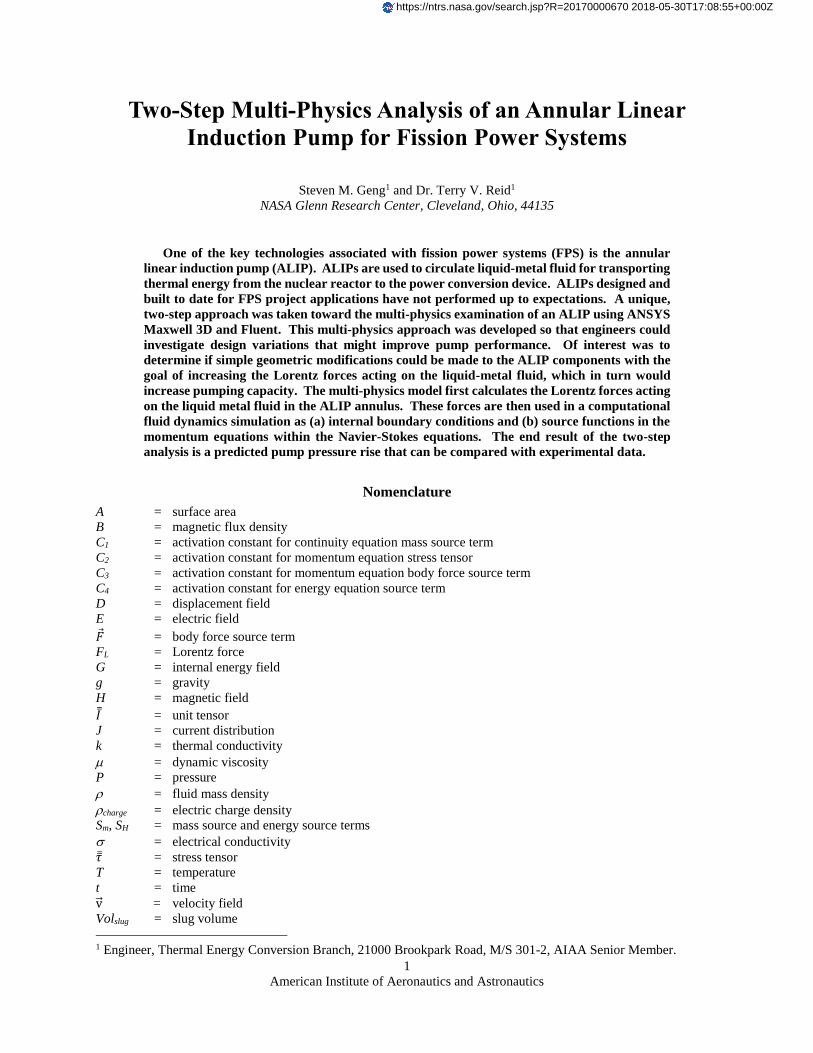
6. Slugs of NaK located adjacent to the stator poles are labeled beginning with the letter “P”. Figures 7 and 8 show

examples of the axial and radial Lorentz forces acting on a NaK slug adjacent to one of the stator poles (P2) over one

electrical cycle, respectively. Note that the negative axial forces shown in Figure 7 oppose the NaK fluid flow in the

pump. The radial forces shown in Figure 8 are always directed radially inward.

0 20 40 60 80 100 120 140

Time (ms)

25

20

15

10

5

0

-5

-10

-15

-20

-25 -25

-20

-15

-10

-5

0

5

10

15

20

25

0 20 40 60 80 100 120 140

Cu

rren

t (A

)

IA IB IC

Figure 6. Section View of ALIP Defining NaK Slugs.

STATOR LAMINATIONS

TORPEDO

P1 S1 P2 S2 P3 S3 P4 S4 P5 S5 P6 S6 P7 S7 P8 S8 P9 S9 P10 S10 P11S11P12S12 P13

NaK

6

American Institute of Aeronautics and Astronautics

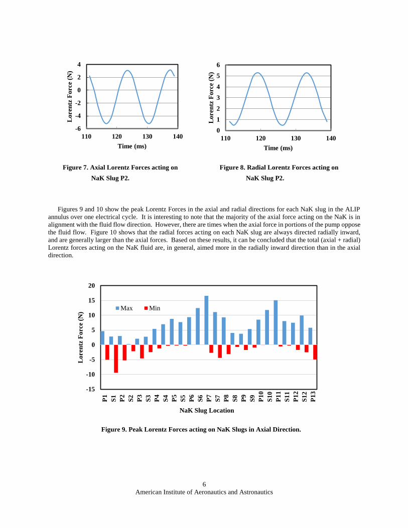
Figures 9 and 10 show the peak Lorentz Forces in the axial and radial directions for each NaK slug in the ALIP

annulus over one electrical cycle. It is interesting to note that the majority of the axial force acting on the NaK is in

alignment with the fluid flow direction. However, there are times when the axial force in portions of the pump oppose

the fluid flow. Figure 10 shows that the radial forces acting on each NaK slug are always directed radially inward,

and are generally larger than the axial forces. Based on these results, it can be concluded that the total (axial + radial)

Lorentz forces acting on the NaK fluid are, in general, aimed more in the radially inward direction than in the axial

direction.

Figure 7. Axial Lorentz Forces acting on Figure 8. Radial Lorentz Forces acting on

NaK Slug P2. NaK Slug P2.

-6

-4

-2

0

2

4

110 120 130 140

Lo

ren

tz F

orc

e (N

)

Time (ms)

0

1

2

3

4

5

6

110 120 130 140

Lo

ren

tz F

orc

e (N

)

Time (ms)

Figure 9. Peak Lorentz Forces acting on NaK Slugs in Axial Direction.

-15

-10

-5

0

5

10

15

20

Lo

ren

tz F

orc

e (N

)

NaK Slug Location

Max Min

P1

S1

P2

S2

P3

S3

P4

S4

P5

S5

P6

S6

P7

S7

P8

S8

P9

S9

P1

0

S1

0

P1

1

S1

1

P1

2

S1

2

P1

3

7

American Institute of Aeronautics and Astronautics

The prototypic ALIP pump used in the TDC test utilizes a hollow torpedo. The transient magnetic analysis was

used to evaluate the torpedo to determine if there was sufficient material to carry the magnetic fields. Figure 11a

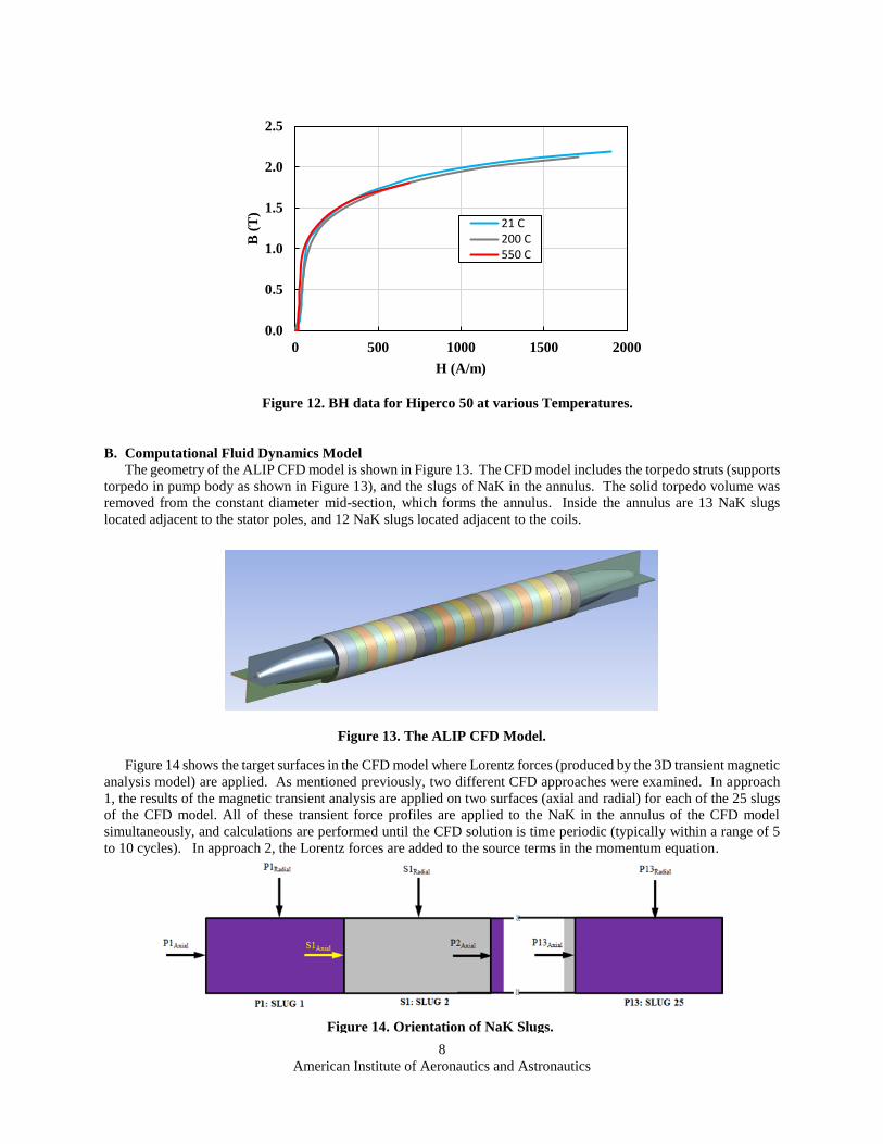
shows the B-field magnitude in the torpedo body at an instant in time. Assuming a torpedo temperature of 550°C,

Figure 11a shows three locations (circled areas) were mild saturation may be occurring. According to GRC Hiperco

50 BH measurements (shown in Figure 12), Hiperco 50 tends to saturate at about 1.8 T at 550°C. The magnetic

analysis was then repeated assuming a solid torpedo. Figure 11b shows that the solid torpedo can eliminate the areas

of saturation.

Figure 10. Peak Lorentz Forces acting on NaK Slugs in Radial Direction

0

10

20

30

40

50

60

P1

S1

P2

S2

P3

S3

P4

S4

P5

S5

P6

S6

P7

S7

P8

S8

P9

S9

P1

0

S1

0

P1

1

S1

1

P1

2

S1

2

P1

3

Lo

ren

tz F

orc

e (N

)

ALIP NaK Slug Location

Max Min

(a) B-field prediction for ALIP configured with hollow torpedo (baseline geometry)

(b) B-field prediction for ALIP configured with solid torpedo

Figure 11. Torpedo B-field Magnitude at Time = 0.134722s

8

American Institute of Aeronautics and Astronautics

B. Computational Fluid Dynamics Model

The geometry of the ALIP CFD model is shown in Figure 13. The CFD model includes the torpedo struts (supports

torpedo in pump body as shown in Figure 13), and the slugs of NaK in the annulus. The solid torpedo volume was

removed from the constant diameter mid-section, which forms the annulus. Inside the annulus are 13 NaK slugs

located adjacent to the stator poles, and 12 NaK slugs located adjacent to the coils.

Figure 14 shows the target surfaces in the CFD model where Lorentz forces (produced by the 3D transient magnetic

analysis model) are applied. As mentioned previously, two different CFD approaches were examined. In approach

1, the results of the magnetic transient analysis are applied on two surfaces (axial and radial) for each of the 25 slugs

of the CFD model. All of these transient force profiles are applied to the NaK in the annulus of the CFD model

simultaneously, and calculations are performed until the CFD solution is time periodic (typically within a range of 5

to 10 cycles). In approach 2, the Lorentz forces are added to the source terms in the momentum equation.

Figure 13. The ALIP CFD Model.

Figure 14. Orientation of NaK Slugs.

Figure 12. BH data for Hiperco 50 at various Temperatures.

0.0

0.5

1.0

1.5

2.0

2.5

0 500 1000 1500 2000

B (

T)

H (A/m)

21 C200 C550 C

9

American Institute of Aeronautics and Astronautics

The difference between the strategies is the method in which the Lorentz forces are applied to the NaK slugs. The

equations that define the Lorentz forces are

�⃗�L = 𝐽 x �⃗⃗� (9)

where

𝐽 = [�⃗⃗� + ( �⃗⃗� x �⃗⃗�)] (10)

The variable J is the current distribution and B is the magnetic field. In approach 1, the Lorentz forces (FL) are

converted to pressures by dividing force by the area of application (P ~ FL/Asurface). The pressures acting on the NaK

slug surfaces are updated every time step. Approach 2 involves adding the Lorentz forces as body force source terms

(�⃗� ~ FL/Volslug) in the momentum equations5. Both strategies were evaluated in terms of ALIP pressure rise, and it

was determined that approach 2 provided results that better matched the measured data. Therefore, the results and

conclusions presented in this paper are based on the approach 2 strategy.

During the beginning stages of the calculations, consideration was given to including the throttling valve, which

is a part of the ALIP test circuit (originally shown in Figure 2). A close-up view of the valve is shown in Figure 15.

Its actual location in the ALIP Test Circuit is 15 to 20 diameters downstream of the ALIP exit and beyond a 90 degree

bend. This valve provides a downstream resistance that affects both the operating pressure and the flow rate. Detailed

measurements were made to determine the relationship between valve position and NaK flow rate. A plot of NaK

flow rate with respect to valve position is shown in Figure 16.

Calculations were performed assuming approach 1 for the ALIP test circuit configured both with and without the

valve. When in place, it is required that the valve be 91.5% closed to produce a volumetric flow rate of ~60 GPM.

The valve placement and resulting predicted NaK fluid velocities are shown in Figure 17. For these predictions, the

valve was placed close to the exit of the computational domain to minimize the size of the mesh. However, when

generating predictions with the valve in place, the separated flow downstream of the valve created an unsettled flow

field that propagated out of the exit boundary in a non-uniform manner, which was deemed undesirable. The

calculations were repeated with the valve removed, and the results were compared in Figure 18. It was discovered

that the inclusion or omission of the valve in the model had no impact on the predicted pressure rise; the valve only

affected the predicted ALIP inlet and outlet pressures. Unfortunately, including the valve in the model required far

more computation time to reach a converged solution. As a result, it was decided to omit the valve from the

simulations.

(a) Rendering (b) Photograph

Figure 15. Throttling Valve used in the ALIP Test Circuit.

(Courtesy of NASA Marshall Space Flight Center)

10

American Institute of Aeronautics and Astronautics

Figure 16. Characteristic Flow Curve of Custom Throttling Valve used in the ALIP Test Circuit.

(Courtesy of NASA Marshall Space Flight Center)

0

1

2

3

4

5

6

0

20

40

60

80

100

2 3 4 5 6 7 8

Flo

w R

ate

(

Lit

ers/

sec)

Flo

w R

ate (G

PM

)

Valve Position (cm) (Zero is Fully Open)

(a) Model (b) Predicted Velocity Vectors

Figure 17. Partially Closed Gate Valve (91.5% closed) in the Computational Domain.

Figure 18. Baseline Predictions (60 GPM) with and without Downstream Valve.

-7.0

3.0

13.0

23.0

33.0

43.0

-50

0

50

100

150

200

250

300

50 70 90

Ma

ss Weig

hte

d P

ressu

re

(psi)

Ma

ss-W

eig

hte

d P

ress

ure

(kP

a)

Cycle Number

-1.5

0.5

2.5

4.5

6.5

-10

0

10

20

30

40

50

50 70 90 110

P0

2 -

P0

1 (p

si)

P0

2 -

P0

1 (

kP

a)

Cycle Number

No

Valve Valve

ΔP

P02 P01

Valve No

Valve

11

American Institute of Aeronautics and Astronautics

V. Results

As mentioned in section IV-B, two CFD approaches were evaluated. Approach 1 (180⁰ model) was used for only

the baseline case. Once it was determined that the predicted pressure rise using this approach was about 15% lower

than the measured value, it was decided to try approach 2. However, approach 2 (180⁰ model) over-predicted the

baseline measured data by 20%. This computational over-prediction was also observed by Maidana5 when using

reduced (< 360⁰) CFD models that assumes symmetry. The approach 2 full 360⁰ model was considered the most

accurate, and as a result, was used to generate the predictions shown in this paper.

Since the multi-physics simulation is computationally time intensive (it takes about a week to simulate a single

test condition), a single flow rate (60 GPM) was chosen for code validation. At the selected validation point, the 3D

multi-physics model predicted a pressure rise of 22.0 kPa (3.2 psi) which was just slightly below (within 3%) of the

measured value of 22.6 kPa (3.28 psi). The 3D multi-physics model was then used to predict the pump performance

over a range of NaK flow rates as shown in Figure 19 and Table I. The predictions were in good agreement with the

experimental data at the mid to high NaK flow rates. The agreement was not quite as good at the low NaK flow

condition. The reason for this discrepancy may be due to the turbulence model being used in the CFD analysis. The

NaK flow may not be fully turbulent at the low flow conditions. In addition, researchers have reported6 that all 2-

equation turbulence models (such as k- and k- turbulence models) experience a reduction in accuracy in the presence

of ‘large’ adverse pressure gradients. They tend to underpredict separation of the boundary layers due to this adverse

pressure gradient. This leads to an underestimation of the effects of viscous-inviscid interaction which generally

produces a performance estimate that is too optimistic for aerodynamic bodies. It is possible to live with this error if

verification and validation indicates that it is not too high, otherwise a more robust turbulence model may be needed.

The multi-physics model was then used to explore ALIP geometric variations in an attempt to improve pump

performance. At the time of this writing, only one design variation was completely modeled: a solid torpedo was

substituted for the baseline hollow torpedo. When the hollow torpedo is replaced with a solid torpedo, the predicted

pump pressure rise is 16% larger. This suggests that replacing the hollow torpedo with a solid torpedo would result

Figure 19. Comparison of Measured and Predicted ALIP Data (100 V, 18 A and 36 Hz)

(Measured Data Courtesy of NASA Marshall Space Flight Center).

1.26 1.76 2.26 2.76 3.26 3.76 4.26 4.76 5.26

0

1

2

3

4

5

6

7

8

0

10

20

30

40

50

60

20 30 40 50 60 70 80 90

Flow Rate ( Liters/sec )

ΔP

( psi )

ΔP

(

kP

a )

Flow Rate ( GPM )

Hollow Torpedo

Solid Torpedo

Measured Data

Table I. Test Matrix Summary

Torpedo

Configuration

Flow Rate Measured ΔP Predicted ΔP %

Difference GPM Liter/sec psi kPa psi kPa

Hollow

28.8 1.82 6.51 44.87 7.45 51.37 14.5

60.0 3.79 3.28 22.61 3.20 22.03 -2.6

82.9 5.23 0.40 2.76 0.38 2.64 -4.4

Solid 60.0 3.79 3.80 26.19 *15.8

* % difference relative to measurement recorded for 60 GPM in baseline ALIP (hollow torpedo) configuration

12

American Institute of Aeronautics and Astronautics

in a modest performance improvement due to an increase in saturation margin. Another design variation that would

be interesting to explore would be to substitute a stepped torpedo for the baseline hollow torpedo. The flow path of

the NaK would still be a smooth annulus since the torpedo is encased inside a stainless steel sleeve. The diameter of

the torpedo adjacent to the coils would be a little bit smaller than the diameter of the torpedo adjacent to the poles of

the stator. The idea here is to encourage the B-field passing through the NaK to flow in a more radial direction, in

hopes of better aligning the Lorentz Forces with the NaK flow direction. With the prototypic ALIP used in the TDU

test, a simple substitution of a stepped torpedo for the hollow torpedo would probably not help since saturation would

still be an issue. The whole ALIP pump would need to be redesigned to allow for a larger diameter torpedo to prevent

B-field saturation.

VI. Conclusion

The multi-physics approach described in this paper was found to be in good agreement with the ALIP experimental

data at the mid to high flow operating conditions. Further model development is necessary to improve ALIP

performance predictions over a wider range of operating conditions. As mentioned in section III-B, the realizable k-

turbulence model was selected for use in the fluid flow analysis. It’s possible that this turbulence model is less

accurate at the pressure gradients encountered at the low NaK flow conditions. Several other turbulence models are

available. Some effort should be applied toward determining the best turbulence model for use in this application.

Based on the results presented in this paper, the prototypic ALIP performance could potentially be improved by

replacing the hollow torpedo with a solid configuration. In future ALIP designs, it might be beneficial to explore the

impact of tailoring the torpedo geometry to better align the Lorentz forces with the NaK flow direction. The methods

described in this paper may be of value in evaluating future ALIP designs.

Acknowledgments

This work was performed for the NASA Enabling Technology Development and Demonstration Program/Fission

Power Systems Project. The opinions expressed are those of the authors and do not necessarily reflect the views of

NASA.

References 1Polzin, K. A., et al, “Performance Testing of a Prototypic Annular Linear Induction Pump for Fission Surface Power,”

NASA/TP-2010-216430, 2010. 2Geng, S. M., Niedra, J. M., Polzin, K. A., “Magnetic Analysis of an Annular Linear Induction Pump for Fission Power

Systems,” Proceedings of the Nuclear and Emerging Technologies for Space 2012 (NETS 2012), CP3033, ANSTD/ANS,

Woodlands, TX, 2012. 3Fission Surface Power Team, “Fission Surface Power System Initial Concept Definition,” NASA/TM-2010-216772, 2010. 4Briggs, M. H., et al, “Fission Surface Power Technology Demonstration Unit Test Results,” Proceedings of the Nuclear and

Emerging Technologies for Space 2016 (NETS 2016), CP6074, ANS, Huntsville, AL, 2016. 5Maidana, C. O., Nieminen, J. E., “Multiphysics Analysis of Liquid Metal Annular Linear Induction Pumps: A Project

Overview,” Proceedings of the Nuclear and Emerging Technologies for Space 2016 (NETS 2016), CP6069, ANS, Huntsville, AL,

2016. 6Bardina, J.E., Huang, P.G., Coakley, T.J., "Turbulence Modeling Validation, Testing, and Development", NASA Technical

Memorandum 110446, 1997.