Two-step Machine Learning Approach for Channel Estimation ...

1

Two-step Machine Learning Approach for

Channel Estimation with Mixed Resolution RF

ChainsBrenda Vilas Boas1,2, Wolfgang Zirwas1, Martin Haardt2

1Nokia Bell Labs Munich, Germany2Ilmenau University of Technology, Germany

Abstract

Massive MIMO is one of the main features of 5G mobile radio systems. However, it often leads to high cost,

size and power consumption. To overcome these issues, the use of constrained radio frequency (RF) frontends has

been proposed, as well as novel precoders, e.g., a multi-antenna, greedy, iterative and quantized precoding algorithm

(MAGIQ). Nevertheless, the best performance of MAGIQ assumes accurate channel knowledge per antenna element,

for example, from uplink sounding reference signals. In this context, we propose an efficient uplink channel estimator

by applying machine learning (ML) algorithms. In a first step a conditional generative adversarial network (cGAN)

predicts the radio channels from a limited set of full resolution RF chains to the rest of the low resolution RF chain

antenna elements. A long-short term memory (LSTM) neural network extracts further phase information from the low

resolution RF chain antenna elements. Our results indicate that our proposed approach is competitive with traditional

Unitary tensor-ESPRIT in scenarios with various closely spaced multipath components (MPCs).

Index Terms

massive MIMO, 1-bit ADC, GAN, LSTM.

I. INTRODUCTION

Consider a massive MIMO system, where every antenna element is connected to a dedicated radio frequency (RF)

chain including a full resolution analog-to-digital converter (ADC). With increasing number of antenna elements, the

energy consumption becomes a serious implementation issue. In this regard, the usage of constrained RF frontends

has been proposed in [1] and later enhanced by suitably adapted downlink multi-user (MU) MIMO precoders,

such as the MAGIQ algorithm [2]. MAGIQ relies on accurate channel state information (CSI), which generally

means one full receiver RF chain per antenna element. Receiver RF chains are less complex than transmiter chains;

however, limiting the uplink receiver complexity is also important to reduce cost and size. Then, a mix of full and

low resolution ADCs can provide a reasonable trade-off between performance and power consumption. Here, we

analyze suitable machine learning (ML) methods to most accurately infer the CSI for the low to the high resolution

RF chains.

January 26, 2021 DRAFT

arX

iv:2

101.

0970

5v1

[ee

ss.S

P] 2

4 Ja

n 20

21

2

Generative adversarial networks (GANs) were first proposed in [3], where a min-max game is played between

two neural networks (NNs), named generator and discriminator networks, aiming to train the generator to output

realistic images from random noise at its input. Since then, many enhancements have been proposed to the pioneering

GAN architecture with most of its success on image reconstruction, image super-resolution, and image domain

translation [4], [5].

For wireless mobile radio systems, GANs are often concerned with physical layer issues like channel modeling

and data augmentation [6], [7]. A conditional GAN (cGAN) is used in [8] to estimate the millimeter wave (mm-

Wave) virtual covariance channel matrix based on prior knowledge of a training sequence. A cGAN and a variational

autoencoder (VAE) GAN are used in [9], [10], but in a context of end-to-end learning where the final objective

is to predict the transmitted symbols, not the wireless channel. The authors in [11], [12] propose fully connected

NNs for the problem of channel estimation for constrained massive MIMO systems with 1-bit ADCs. Their results

are compared with variations of the generalized message passing (GAMP) algorithm. Moreover, [13] proposes two

fully connected NNs for channel estimation in a mixed scenario with full and low resolution ADCs. However, it

concludes that the best strategy is one without taking into account the quantized signals from the low resolution

ADCs due to their distortion and low resolution.

Motivated by the good results of GANs in image to image translation and by the challenge of wireless channel

estimation with low resolution ADCs, in this paper we propose a 2-step ML algorithm to be carried out by the base

station (BS). We first perform channel estimation considering just the full resolution measurements by using the

Pix2Pix GAN architecture [4], which is a type of cGAN. Second, we enhance the channel estimation by acquiring

1-bit measurements and train a long-short term memory (LSTM) NN to improve the reconstruction of the channel

phase. The main contributions of this paper are the combination of cGAN and LSTM for stable channel estimation

in massive MIMO scenarios with mixed resolution ADCs. Moreover, we adopt Unitary tensor-ESPRIT [14] for

super resolution parameter estimation and use this as a baseline for our results.

In this paper, Section II presents our system overview and the wireless channel model, Section III introduces our

proposed method, Section IV presents details about our cGAN, Section V shows the processing performed at the

LSTM, Section VI presents our results, and Section VII concludes our paper.

II. SYSTEM AND CHANNEL MODEL

Figure 1 presents a block diagram of the full resolution RF chains (FRFs) and constrained RF chains (CRFs)

with which the BS is equipped. Analog filters, power amplifiers, local oscillators, and baseband processing units

are available in both types of RF chains. However, they differ with respect to their ADC resolution. We apply

ML methods to tackle the problem of uplink channel estimation for a mixed resolution receiver. Hence, we define

three channel matrices: H is our desired channel, Hce is the input to our first ML instance, and Hc is the input to

Unitary tensor-ESPRIT.

First, we consider the wireless channel H ∈ CM×Nsub of an orthogonal frequency division multiplexing (OFDM)

system in the spatial and frequency domain with Nsub sub-carriers and M antenna elements at the BS.


3

Fig. 1. Overview of the configuration of RF chains at BS for our tackled problem. Even/odd antenna elements are connected to FRFs/CRFs,

respectively.

The channel in each sub-carrier h(n) is modeled as

h(n) =

L∑i=1

αie−j2π (n−1)

NsubτiaF (θi, d,M), (1)

where L is the number of multipath components (MPCs), τi, αi, and θi are, respectively, the delay, complex

amplitude, and direction of arrival (DoA) of each ith MPC. The uniform linear array (ULA) steering vector aF at

the BS is modeled as

aF (θi, d,M) = [1, ejµi , ej2µi , . . . ej(Nant−1)µi ]T , (2)

where µi = 2πλ d cos θi, is the spatial frequency and d = λ

2 is the spacing between the antenna elements.

Equation (2) models a full resolution array steering vector in which each antenna element is connected to one RF

chain, and we use full resolution ADCs. For reduced resolution arrays, we assume that not all antenna elements are

connected to a full resolution RF chain. Without loss of generality, we assume that every odd antenna element is

connected to a low resolution RF chain. Our proposed method first uses only the FRF and ignores the information

from the CRF. Therefore, we assume M ′ = M2 and d′ = λ to derive the constrained wireless channel response

hc(n) per sub-carrier

hc(n) =

L∑i=1

αie−j2π (n−1)

NsubτiaF (θi, d

′,M ′) + z(n), (3)

where z(n) ∈ CN ′ant is zero mean circular symmetric Gaussian noise, and Hc = [hc(0),hc(1), . . . ,hc(Nsub−1)] ∈

CM ′×Nsub . In order to make the dimensionality of Hc equal to the dimensionality of H, Hc is expanded to Hce

by inserting zero row vectors 0 in the odd row antenna positions, then Hce ∈ CM×Nsub .

III. TWO-STEP ML APPROACH FOR CHANNEL ESTIMATION

Figure 2 summarizes our proposed method for channel estimation for massive MIMO systems, where the BS

is equipped with full resolution RF chains for every even and constrained ones for every odd antenna. The first

and second ML instances are highlighted in blue and orange, respectively. Our first ML instance relies only on


4

Fig. 2. Two-step ML approach for channel estimation in massive MIMO scenario with antenna elements connected to mixed resolution RF

chains. Blue and orange highlight the first and second ML steps, respectively.

measurements from the antenna elements connected to full resolution RF chains. Here, we train a cGAN to predict

the channel of the antenna elements with low resolution RF chains and estimate the channel of the antenna elements

with full resolution RF chains. In our second ML instance, we consider the low resolution measurements and the

results from the cGAN as input to a LSTM NN in order to improve the phase accuracy of the channel estimation.

After the LSTM, its phase output is combined with the preprocessed absolute value of the cGAN’s output. This

is our final complex valued channel estimate H in the time domain. Since 1-bit (for real and imaginary parts

separately) quantized signals are similar to quadrature phase shift keying (QPSK) symbols, only phase information

can be extracted from such measurements. Therefore, our second ML instance only aim to improve the phase signal.

The following sections explain in detail how each ML instance operates.

IV. CHANNEL ESTIMATION WITH CGAN

Inspired by the success of cGANs on image to image translation, we employ a similar architecture as the Pix2Pix

application [4] for tackling the problem of channel estimation with mixed resolution RF chains. Figure 3 depicts

the interplay between the two NNs in the cGAN training phase. This section starts by presenting our dataset

preprocessing. In the following, we discuss our cGAN architecture, comment on the adversarial training, and its

optimization function.

A. Dataset preprocesing for cGAN

For the first ML instance of our combined approach, Hce is used as input and H is the desired output or label.

However, DL libraries do not work with complex values. Moreover, the input/output coefficients should be limited

to a known range of values to improve convergence. Therefore, a preprocessing is employed as

• H is normalized by its Frobenius norm, and then multiplied by a scaling factor to increase the range value of

the channel coefficients without changing their statistical distribution.

• H ∈ CM×Nsub is rearranged by concatenating Re{H} and Im{H} in their third dimension.


5

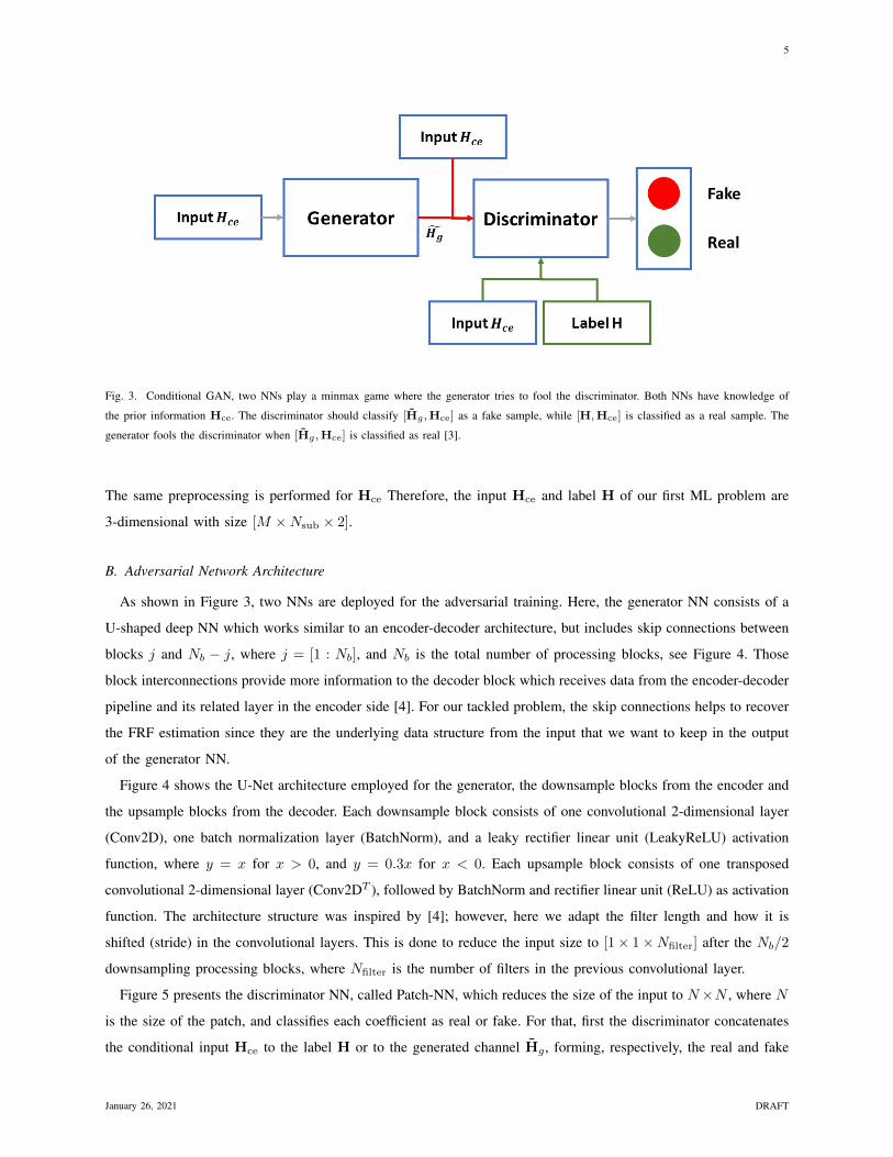
Fig. 3. Conditional GAN, two NNs play a minmax game where the generator tries to fool the discriminator. Both NNs have knowledge of

the prior information Hce. The discriminator should classify [Hg ,Hce] as a fake sample, while [H,Hce] is classified as a real sample. The

generator fools the discriminator when [Hg ,Hce] is classified as real [3].

The same preprocessing is performed for Hce Therefore, the input Hce and label H of our first ML problem are

3-dimensional with size [M ×Nsub × 2].

B. Adversarial Network Architecture

As shown in Figure 3, two NNs are deployed for the adversarial training. Here, the generator NN consists of a

U-shaped deep NN which works similar to an encoder-decoder architecture, but includes skip connections between

blocks j and Nb − j, where j = [1 : Nb], and Nb is the total number of processing blocks, see Figure 4. Those

block interconnections provide more information to the decoder block which receives data from the encoder-decoder

pipeline and its related layer in the encoder side [4]. For our tackled problem, the skip connections helps to recover

the FRF estimation since they are the underlying data structure from the input that we want to keep in the output

of the generator NN.

Figure 4 shows the U-Net architecture employed for the generator, the downsample blocks from the encoder and

the upsample blocks from the decoder. Each downsample block consists of one convolutional 2-dimensional layer

(Conv2D), one batch normalization layer (BatchNorm), and a leaky rectifier linear unit (LeakyReLU) activation

function, where y = x for x > 0, and y = 0.3x for x < 0. Each upsample block consists of one transposed

convolutional 2-dimensional layer (Conv2DT ), followed by BatchNorm and rectifier linear unit (ReLU) as activation

function. The architecture structure was inspired by [4]; however, here we adapt the filter length and how it is

shifted (stride) in the convolutional layers. This is done to reduce the input size to [1× 1×Nfilter] after the Nb/2

downsampling processing blocks, where Nfilter is the number of filters in the previous convolutional layer.

Figure 5 presents the discriminator NN, called Patch-NN, which reduces the size of the input to N×N , where N

is the size of the patch, and classifies each coefficient as real or fake. For that, first the discriminator concatenates

the conditional input Hce to the label H or to the generated channel Hg , forming, respectively, the real and fake


6

Fig. 4. U-Net architecture deployed as the generator including encoder and decoder pipeline and numbering for skip connections.

Fig. 5. Patch-Net architecture deployed for the discriminator.

classes. Then, the input is downsampled by the downsampling blocks which are followed by one zero padding layer,

and one Conv2D with BatchNorm and LeakyReLU activation function. After one zero padding and one Conv2D

layer, the discriminator provides its output of size [N × N × 1]. During the optimization, this output is further

averaged and represented as a scalar value [5].


7

C. Optimization with cGAN

In cGAN, two NNs play a minmax game where the generator tries to fool the discriminator, and it is conditional

because some prior knowledge is provided. Mathematically, the loss function of a cGAN is

LcGAN(G,D) =Ex,y[logD(x, y)]+

Ex,z[log(1−D(x,G(x, z)))],(4)

where the generator G learns to map input data x and random noise z to output data y, G : {x, z} → y, and the

discriminator D tries to recognize the channels generated by G. In order to have the generated output wireless

channels Hg close to the wireless channel labels H, a weighted L2 term

LL2(G) = Ex,y,z[‖y −G(x, z)‖2] (5)

is included on the generator loss function. Therefore, the final optimization objective is

G∗ = arg minG

maxDLcGAN(G,D) + βLL2

, (6)

where β is the weighting factor.

The generator and discriminator NNs are trained together in each epoch. For testing, or inference, only the

generator architecture is used. Therefore, only knowledge of Hce is needed.

V. PHASE IMPROVEMENT WITH LSTM

In this section we enhance the channel estimation based on quantized measurements from constrained RF-chains.

For that purpose, we develop a second ML step based on LSTM to improve the phase of the channel estimated

by our cGAN. This section presents the data preprocessing to obtain the inputs to the LSTM NN, the equations

describing its architecture and comment on the cost function.

A. Data preprocessing for LSTM

After estimating Hg with our first ML instance, we consider the quantized measurements of the antenna elements

with low resolution RF chains, 1-bit ADCs in this case. As the 1-bit RF chains are of low cost and size, we

assume each of the M antennas can perform 1-bit measurements. As our second ML instance operates in the time

domain, the following data manipulation are made: computation of the inverse Fourier transform F−1, profiling

computation [15], random sequence mixture, and 1-bit quantization.

First, the full resolution channel impulse responses (CIRs) Hx ∈ CM×Nsub are computed for the desired, noisy

measurement and predicted signals, respectively, as H = F−1(H), Hz = F−1(H + Z), and Hg = F−1(Hg),

being Z the additive white Gaussian noise. Second, we compute the profiling version of each full resolution signal.

The profiling operation, best described in [15], consists, basically, in oversampling the CIR. At this point, we also

reduce the signal observation window to K < Nsub, so that Hx ∈ CM×K . This windowing is mainly performed

due to the small number of MPCs and their clustering, which leads the CIR to contain relevant power in a limited

number of taps K. Hence, this filtering also limits the impact of noise.


8

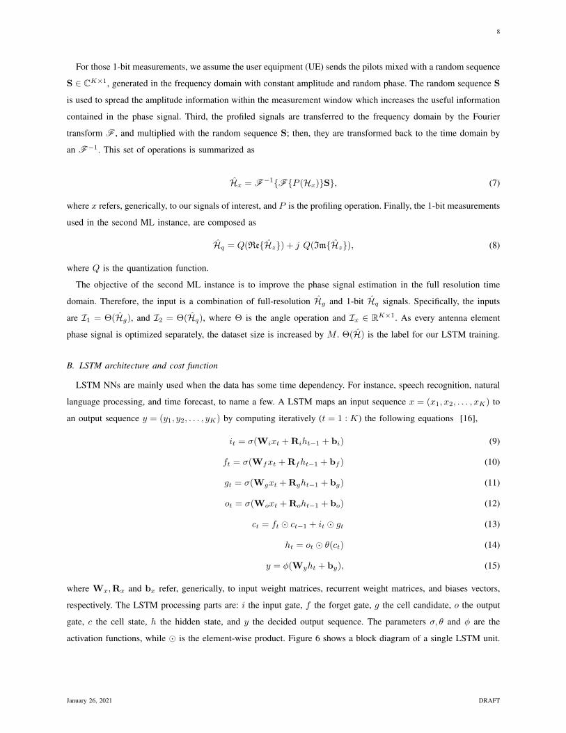
For those 1-bit measurements, we assume the user equipment (UE) sends the pilots mixed with a random sequence

S ∈ CK×1, generated in the frequency domain with constant amplitude and random phase. The random sequence S

is used to spread the amplitude information within the measurement window which increases the useful information

contained in the phase signal. Third, the profiled signals are transferred to the frequency domain by the Fourier

transform F , and multiplied with the random sequence S; then, they are transformed back to the time domain by

an F−1. This set of operations is summarized as

Hx = F−1{F{P (Hx)}S}, (7)

where x refers, generically, to our signals of interest, and P is the profiling operation. Finally, the 1-bit measurements

used in the second ML instance, are composed as

Hq = Q(Re{Hz}) + j Q(Im{Hz}), (8)

where Q is the quantization function.

The objective of the second ML instance is to improve the phase signal estimation in the full resolution time

domain. Therefore, the input is a combination of full-resolution Hg and 1-bit Hq signals. Specifically, the inputs

are I1 = Θ(Hg), and I2 = Θ(Hq), where Θ is the angle operation and Ix ∈ RK×1. As every antenna element

phase signal is optimized separately, the dataset size is increased by M . Θ(H) is the label for our LSTM training.

B. LSTM architecture and cost function

LSTM NNs are mainly used when the data has some time dependency. For instance, speech recognition, natural

language processing, and time forecast, to name a few. A LSTM maps an input sequence x = (x1, x2, . . . , xK) to

an output sequence y = (y1, y2, . . . , yK) by computing iteratively (t = 1 : K) the following equations [16],

it = σ(Wixt + Riht−1 + bi) (9)

ft = σ(Wfxt + Rfht−1 + bf ) (10)

gt = σ(Wgxt + Rght−1 + bg) (11)

ot = σ(Woxt + Roht−1 + bo) (12)

ct = ft � ct−1 + it � gt (13)

ht = ot � θ(ct) (14)

y = φ(Wyht + by), (15)

where Wx,Rx and bx refer, generically, to input weight matrices, recurrent weight matrices, and biases vectors,

respectively. The LSTM processing parts are: i the input gate, f the forget gate, g the cell candidate, o the output

gate, c the cell state, h the hidden state, and y the decided output sequence. The parameters σ, θ and φ are the

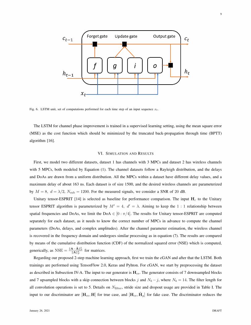
activation functions, while � is the element-wise product. Figure 6 shows a block diagram of a single LSTM unit.


9

Fig. 6. LSTM unit, set of computations performed for each time step of an input sequence xt.

The LSTM for channel phase improvement is trained in a supervised learning setting, using the mean square error

(MSE) as the cost function which should be minimized by the truncated back-propagation through time (BPTT)

algorithm [16].

VI. SIMULATION AND RESULTS

First, we model two different datasets, dataset 1 has channels with 3 MPCs and dataset 2 has wireless channels

with 5 MPCs, both modeled by Equation (1). The channel datasets follow a Rayleigh distribution, and the delays

and DoAs are drawn from a uniform distribution. All the MPCs within a dataset have different delay values, and a

maximum delay of about 163 ns. Each dataset is of size 1500, and the desired wireless channels are parameterized

by M = 8, d = λ/2, Nsub = 1200. For the measured signals, we consider a SNR of 20 dB.

Unitary tensor-ESPRIT [14] is selected as baseline for performance comparison. The input Hc to the Unitary

tensor ESPRIT algorithm is parameterized by M ′ = 4, d′ = λ. Aiming to keep the 1 : 1 relationship between

spatial frequencies and DoAs, we limit the DoA ∈ [0 : π/4]. The results for Unitary tensor-ESPRIT are computed

separately for each dataset, as it needs to know the correct number of MPCs in advance to compute the channel

parameters (DoAs, delays, and complex amplitudes). After the channel parameter estimation, the wireless channel

is recovered in the frequency domain and undergoes similar processing as in equation (7). The results are compared

by means of the cumulative distribution function (CDF) of the normalized squared error (NSE) which is computed,

generically, as NSE =‖A−A‖2F‖A‖2F

for matrices.

Regarding our proposed 2-step machine learning approach, first we train the cGAN and after that the LSTM. Both

trainings are performed using TensorFlow 2.0, Keras and Pyhton. For cGAN, we start by preprocessing the dataset

as described in Subsection IV-A. The input to our generator is Hce. The generator consists of 7 downsampled blocks

and 7 upsampled blocks with a skip connection between blocks j and Nb− j, where Nb = 14. The filter length for

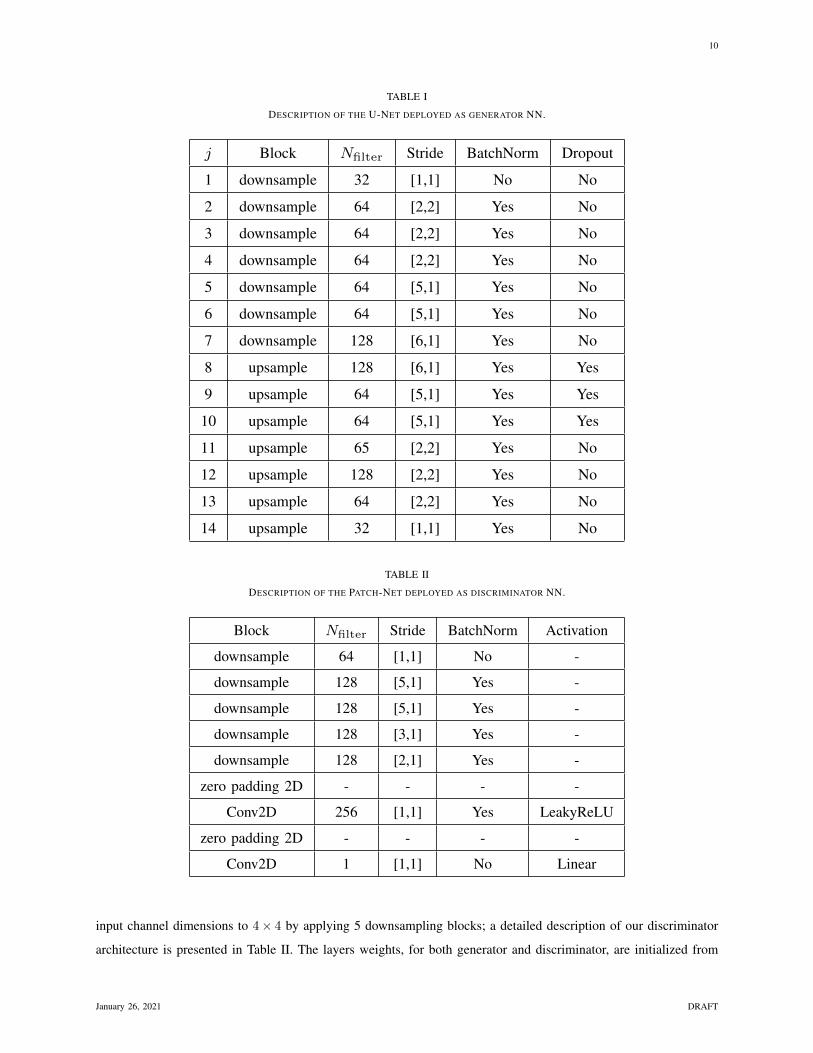
all convolution operations is set to 5. Details on Nfilter, stride size and dropout usage are provided in Table I. The

input to our discriminator are [Hce,H] for true case, and [Hce, Hg] for fake case. The discriminator reduces the


10

TABLE I

DESCRIPTION OF THE U-NET DEPLOYED AS GENERATOR NN.

j Block Nfilter Stride BatchNorm Dropout

1 downsample 32 [1,1] No No

2 downsample 64 [2,2] Yes No






8 upsample 128 [6,1] Yes Yes



11 upsample 65 [2,2] Yes No




TABLE II

DESCRIPTION OF THE PATCH-NET DEPLOYED AS DISCRIMINATOR NN.

Block Nfilter Stride BatchNorm Activation

downsample 64 [1,1] No -

downsample 128 [5,1] Yes -




zero padding 2D - - - -

Conv2D 256 [1,1] Yes LeakyReLU

zero padding 2D - - - -

Conv2D 1 [1,1] No Linear

input channel dimensions to 4× 4 by applying 5 downsampling blocks; a detailed description of our discriminator

architecture is presented in Table II. The layers weights, for both generator and discriminator, are initialized from


11

TABLE III

DESCRIPTION OF THE LSTM NN.

Layer Nfilter Return Sequences Activation

LSTM 10 Yes hyperbolic tangent

LSTM 1 Yes linear

Fig. 7. Channel estimation using cGAN, sample result where x-axis is the number of antennas, y-axis is the number of sub-carriers. The

matrices in the first column are the input Hce with odd antenna elements zeroed, the second column show the ground truth wireless channel

H, and the third column shows the estimated channel Hg after 150 epochs of training.

a normal distribution with zero mean and σ = 0.2 standard deviation. The Adam optimizer [17] with 2 × 10−4

initial learning rate is used for both NNs, and β = 100. The adversarial training runs for 150 epochs, with only

600 dataset samples, 50% from dataset 1, and 50% from dataset 2. The remaining 2400 dataset samples are used

for testing. Figure 7 presents a test sample result for our channel estimation approach employing our cGAN.

After the channel estimation by the cGAN, the second ML instance runs to improve the estimated phase signal.

For this purpose, the dataset is preprocessed as in Subsection V-A, and a two layers LSTM NN is deployed as

described in Table III. The learning rate is set to 2× 10−4, and the gradient descent optimizer is Adam [17]. Then,

the supervised training runs for 50 epochs, using a training dataset with 2400 samples, where 50% are from dataset

1, and 50% are from dataset 2. The remaining 600 combined dataset samples are used for testing.

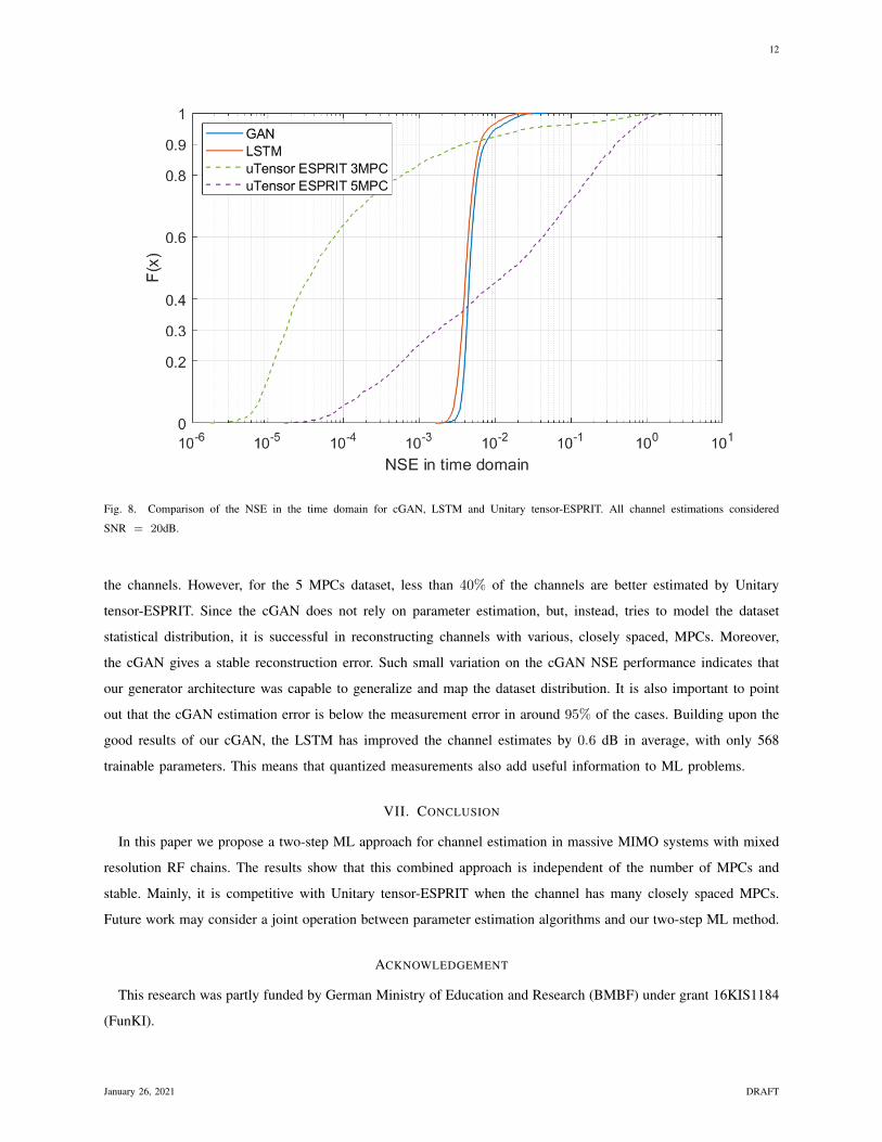
Figure 8 presents the comparison of Unitary tensor-ESPRIT, our cGAN, and LSTM. For Unitary tensor-ESPRIT

at 3 MPC and 5 MPC, there is a large variation on the NSE. This is due to the delay spacing between the MPCs.

For the 3 MPCs dataset, Unitary tensor-ESPRIT has better channel estimation error in slightly more than 90% of


12

Fig. 8. Comparison of the NSE in the time domain for cGAN, LSTM and Unitary tensor-ESPRIT. All channel estimations considered

SNR = 20dB.

the channels. However, for the 5 MPCs dataset, less than 40% of the channels are better estimated by Unitary

tensor-ESPRIT. Since the cGAN does not rely on parameter estimation, but, instead, tries to model the dataset

statistical distribution, it is successful in reconstructing channels with various, closely spaced, MPCs. Moreover,

the cGAN gives a stable reconstruction error. Such small variation on the cGAN NSE performance indicates that

our generator architecture was capable to generalize and map the dataset distribution. It is also important to point

out that the cGAN estimation error is below the measurement error in around 95% of the cases. Building upon the

good results of our cGAN, the LSTM has improved the channel estimates by 0.6 dB in average, with only 568

trainable parameters. This means that quantized measurements also add useful information to ML problems.

VII. CONCLUSION

In this paper we propose a two-step ML approach for channel estimation in massive MIMO systems with mixed

resolution RF chains. The results show that this combined approach is independent of the number of MPCs and

stable. Mainly, it is competitive with Unitary tensor-ESPRIT when the channel has many closely spaced MPCs.

Future work may consider a joint operation between parameter estimation algorithms and our two-step ML method.

ACKNOWLEDGEMENT

This research was partly funded by German Ministry of Education and Research (BMBF) under grant 16KIS1184

(FunKI).


13

REFERENCES

[1] M. Staudacher, G. Kramer, W. Zirwas, B. Panzner, and R. Sivasiva Ganesan, “Optimized Combination of Conventional and Constrained

Massive MIMO Arrays,” in Proceedings of the 21th International ITG Workshop on Smart Antennas (WSA), 2017, pp. 1–4.

[2] A. Nedelcu, F. Steiner, M. Staudacher, G. Kramer, W. Zirwas, R. S. Ganesan, P. Baracca, and S. Wesemann, “Quantized precoding for

multi-antenna downlink channels with MAGIQ,” in Proceedings of the 22nd International ITG Workshop on Smart Antennas (WSA). VDE,

2018, pp. 1–8.

[3] I. Goodfellow, J. Pouget-Abadie, M. Mirza, B. Xu, D. Warde-Farley, S. Ozair, A. Courville, and Y. Bengio, “Generative Adversarial Nets,”

in Advances in neural information processing systems, 2014, pp. 2672–2680.

[4] P. Isola, J.-Y. Zhu, T. Zhou, and A. A. Efros, “Image-to-image translation with conditional adversarial networks,” in Proceedings of the

IEEE conference on computer vision and pattern recognition, 2017, pp. 1125–1134.

[5] C. Ledig, L. Theis, F. Huszar, J. Caballero, A. Cunningham, A. Acosta, A. Aitken, A. Tejani, J. Totz, Z. Wang et al., “Photo-realistic

single image super-resolution using a generative adversarial network,” in Proceedings of the IEEE conference on computer vision and

pattern recognition, 2017, pp. 4681–4690.

[6] Y. Yang, Y. Li, W. Zhang, F. Qin, P. Zhu, and C.-X. Wang, “Generative-adversarial-network-based wireless channel modeling: Challenges

and opportunities,” IEEE Communications Magazine, vol. 57, no. 3, pp. 22–27, 2019.

[7] T. J. O’Shea, T. Roy, and N. West, “Approximating the void: Learning stochastic channel models from observation with variational

generative adversarial networks,” in 2019 International Conference on Computing, Networking and Communications (ICNC). IEEE,

2019, pp. 681–686.

[8] X. Li, A. Alkhateeb, and C. Tepedelenlioglu, “Generative adversarial estimation of channel covariance in vehicular millimeter wave

systems,” in 2018 52nd Asilomar Conference on Signals, Systems, and Computers. IEEE, 2018, pp. 1572–1576.

[9] H. Ye, G. Y. Li, B.-H. F. Juang, and K. Sivanesan, “Channel agnostic end-to-end learning based communication systems with conditional

GAN,” in 2018 IEEE Globecom Workshops (GC Wkshps). IEEE, 2018, pp. 1–5.

[10] A. Smith and J. Downey, “A communication channel density estimating generative adversarial network,” in 2019 IEEE Cognitive

Communications for Aerospace Applications Workshop (CCAAW). IEEE, 2019, pp. 1–7.

[11] M. Y. Takeda, A. Klautau, A. Mezghani, and R. W. Heath, “MIMO Channel Estimation with Non-Ideal ADCS: Deep Learning Versus

GAMP,” in 2019 IEEE 29th International Workshop on Machine Learning for Signal Processing (MLSP). IEEE, 2019, pp. 1–6.

[12] Y. Zhang, M. Alrabeiah, and A. Alkhateeb, “Deep learning for massive MIMO with 1-bit ADCs: When more antennas need fewer pilots,”

IEEE Wireless Communications Letters, 2020.

[13] S. Gao, P. Dong, Z. Pan, and G. Y. Li, “Deep learning based channel estimation for massive MIMO with mixed-resolution ADCs,” IEEE

Communications Letters, vol. 23, no. 11, pp. 1989–1993, 2019.

[14] M. Haardt, F. Roemer, and G. Del Galdo, “Higher-order SVD-based subspace estimation to improve the parameter estimation accuracy in

multidimensional harmonic retrieval problems,” IEEE Transactions on Signal Processing, vol. 56, no. 7, pp. 3198–3213, 2008.

[15] W. Zirwas and M. Sternad, “Profiling of mobile radio channels,” in Proceedings of the 2020 IEEE International Conference on

Communications (ICC), 2020, pp. 1–7.

[16] S. Hochreiter and J. Schmidhuber, “Long short-term memory,” Neural computation, vol. 9, no. 8, pp. 1735–1780, 1997.

[17] D. P. Kingma and J. Ba, “Adam: A method for stochastic optimization,” arXiv preprint arXiv:1412.6980, 2014.


Two-step Machine Learning Approach for Channel Estimation ...

Documents

Transcript of Two-step Machine Learning Approach for Channel Estimation ...