Two-Solid Deposition in Fluid Column using Immersed ...

J. Appl. Comput. Mech., 7(3) (2021) 1814-1825 DOI: 10.22055/JACM.2021.37140.2969

ISSN: 2383-4536 jacm.scu.ac.ir

Published online: July 08 2021

Shahid Chamran

University of Ahvaz

Journal of

Applied and Computational Mechanics

Research Paper

Two-Solid Deposition in Fluid Column using Immersed Boundary-

Lattice Boltzmann Method

M. Rizqie Arbie , Umar Fauzi , Fourier D.E. Latief , Enjang J. Mustopa

Physics of Earth and Complex Systems Division, Department of Physics, Faculty of Mathematics and Natural Sciences, Institut Teknologi Bandung, Jl. Ganesha 10, Bandung, 40132, Indonesia, Email: [email protected]

Received April 13 2021; Revised June 28 2021; Accepted for publication July 07 2021. Corresponding author: M. Rizqie Arbie ([email protected]) © 2021 Published by Shahid Chamran University of Ahvaz

Abstract. Solid deposition in fluid may involve solids with different density and size and may happen in quiescent fluid or rather in counter flow. We perform a numerical investigation on the role of density-ratios, size-ratio, and initial configuration on the settling of two circular solids in a fluid channel with or without counter-flow. Through this study, we show how settling dynamics of two solids can be controlled. Numerical experiment based on a coupled Immersed Boundary-Lattice Boltzmann is employed. It is shown that certain parameter set leads to guided deposition while denser solid leaves the less dense one as time progressing. However, certain parameter set leads to periodic close encounters which is robust in the presence of Poiseuille-like counter-flow. In this case, the separation between two solids is bounded during the deposition.

Keywords: Counter-flow; Density ratio; IBLBM; Initial configuration; Size ratio.

1. Introduction

Solid-fluid transport phenomena has a vast application in industry. Some of them involve suspended nanomaterials as a mean for improving heat convectivity such as in the case of solar energy collector system [1-3]. The nanomaterials are dispersed in water flowing through a tube containing a turbulator. Another study performed by Sheikholeslami and Farshad [4] showed that the presence of suspended nanomaterials contributes to enhance flow convectivity as well as reducing energy loss in such system. Some other application involves larger particles suspended in fluid. Deposition of solids in viscous fluid has been long investigated to understand different aspects that might control the solid-fluid dynamics. Numerous applications in engineering such as powder technology, coating technology and fluidized beds have attracted more attention to investigate dynamics of solids as they settle in viscous fluid that involves solid-solid, solid-fluid, as well as solid-wall interaction. Jayaweera and Mason [5] analyzed the deposition of long thin cylinders as well as flat base cones. The effect of finite boundaries has also been shown to increase drag experienced by settling solids. Brenner [6] showed this effect through a theoretical study on the effect of wall at the proximity of a moving arbitrary solid within two restrictions that drag correction due to the presence of wall for a moving spherical solid is known and the size of the solid is small compared to its distance from the wall.

Several studies also address the influence of solid parameter on the deposition dynamics. Nie et al. [7], for instance, studied the role of density ratio on the dynamics of two circular solids settling in narrow tunnel. They also found that for certain range of small density ratio, repeated Draft-Kissing-Tumbling can also occur. The increasing capacity of computing power has allowed more detail investigation on the dynamics of settling solids. For instance, Glowinski et al. [8] performed a numerical study on particulate flows based on fictitious-domain method. Aidun and Ding [9] used Lattice-Boltzmann Method to investigate the dynamics of two identical circular solids settling in bounded domain.

However, in some engineering applications, such as fluidize beds, solids may settle in pre-existing flow. So, we extend our investigation with the presence of counter-flow. Previously, Arbie et al. [10] considered the case of two disks falling under the influence of gravity through counter-flow to study the role of initial position on the deposition. In this study, we are interested in investigating the change of deposition dynamics through quiescent fluid as well as counter-flow if the two disks have different initial position, density, and size. Several techniques have been developed for performing the simulation of solid-fluid interactions. Mesh-based method such as Finite Element is used by Izadpanahi et al. [11] to study the stress on wing designs in aeroelastic flight. Other study by Mehryan et al. [12] involves the coupling of Finite Element and Arbitrary Lagrangian-Eulerian to study natural convection in a square domain partitioned by a flexible membrane. It is also used to study other solid-fluid interaction such as fluid flow in pipe system (see a review by Ferras et al. [13]). As an alternative, Finite Volume is also widely used such in solid-fluid interaction simulation such as demonstrated by Tuković et al. [14]. On the other hand, meshfree method such as Smoothed Particle Hydrodynamics (SPH) is widely used to avoid grid reconstruction usually encountered in mesh-based methods. Zhang et al. [15] presented a multi-resolution SPH for fluid-solid interaction. For this purpose, we employ Lattice Boltzmann (LB)

Two-Solid Deposition in Fluid Column using Immersed Boundary-Lattice Boltzmann Method

Journal of Applied and Computational Mechanics, Vol. 7, No. 3, (2021), 1814-1825

1815

Method as fluid solver and Immersed Boundary (IB) Method to account the solid-fluid interaction. LB method can be regarded as a low Mach number approximation to the incompressible Navier-Stokes equation [16]. The main ingredient of Lattice Boltzmann Method consists of collision and streaming process. In-depth discussion of these two processes can be found in [17].

Solid dynamics in fluid using the LB method can be done by the Bounce-back procedure [18] which shows a fluctuation on the computed force at solid-fluid interface due to the sudden change of fluid and non-fluid nodes during the solid movement. A coupling between LB and IB can be used to eliminate the sudden change of fluid and non-fluid nodes. Immersed Boundary was first proposed by Peskin [19, 20]. The idea is to use a set of Lagrangian points immersed in fluid as a discrete representation of the solid perimeter while the dynamics of fluids is solved in an Eulerian grid (fixed frame). Force due to solid-fluid interaction is assigned at each IB points. A review on vast applications of IB can be found in Mittal and Iaccarino [21].

Feng and Michaelides [22] introduced the coupling of IB and LB in which the discretized solid surface is considered as a flexible body with high stiffness. Cheng and Zhang [23] computed the IB forces by considering each Lagrangian points as a flexible segment. In this study we employ the coupling procedure proposed by Li et al [24]. IB forces are directly computed from fluid velocity field through a modified spreading procedure proposed by Pinelli et al [25]. The discretized immersed surface is regarded as having the so-called hydrodynamics thickness which prevents fluid from entering the region enclosed by the IB. As mentioned in Peskin [20] and Cheng and Zhang [23], fluid leakage across the discretize IB can be significantly reduced by setting the separation between any two Lagrangian points to be less than half of the spacing of Eulerian grid used to solve the governing equation for fluid. In their work, Pinelli et al [25] emphasize that the hydrodynamics thickness can be best computed by setting the separation between any two Lagrangian points to be equal to the spacing of Eulerian grid. This reduced the number of Lagrangian points and thus reduces computing time.

Through the rest of the article, we describe the employed coupling procedure of IB and LB method. We then briefly explain the governing equation for solid moving in viscous fluid followed by a benchmark. Next, we describe numerical experiments using Immersed Boundary-Lattice Boltzmann (IB-LB) on the deposition dynamics of two solids. We demonstrate the effect of solid density on deposition dynamics for different initial configuration. Then we add numerical experiments on the effect of solid diameter. In some engineering applications, the deposition may be happening in a counter-flow such as in fluidized bed. Therefore, we also consider deposition through a counter-flow which is incorporated in the computational domain by imposing a Poiseuille-like flow as the inflow. The objective of these numerical experiments is to examine important parameters of two-solid deposition dynamics and how robust the resulting dynamics in the presence of counter-flow.

2. Methods

2.1 General description of IB-LB method

Incompressible fluid motion is usually modeled by the following Navier-Stokes

( ) 2u pu u u

tν

ρ

∂ ∇+ ⋅∇ =− + ∇

∂

�

� � �

(1)

where u�

is the velocity field, p is the pressure field, ρ is the fluid density, and ν is the kinematic viscosity of the fluid. Standard numerical procedure to approximate the solution for eq. (1) requires one to solve Poisson equation for pressure field. On the other hand, we can also describe the transportation of fluid mass by considering smaller scale that is by considering the particle distribution function. The evolution of the distribution function is described by the Boltzmann Transport equation. Macroscopic variables such as fluid velocity can be computed once the probability function at a given time is obtained. Pressure field can be obtained from an equation of state which is chosen properly according to the fluid being modeled. The discretization of the Boltzmann Transport equation results in the Lattice Boltzmann (LB) equation. The LB equation can approximate the incompressible Navier-Stokes equation within the low Mach number assumption [16].

In this study, we employ the LB method with Bhatnagar-Gross-Krook (BGK) collision operator with an explicit forcing term. Velocity space is discretized into nine possible directions as shown in Fig. 1 for two-dimensional space (D2Q9 set-up) which results in the following LB equation

( ) ( ) ( ) ( ) ( ), , , , ,eqk k k k k k

tf x e t t t f x t f x t f x t x t t

τ

∆ + ∆ +∆ − = − + ∆ ��

g (2)

where ke�

gives the nine directions ( { }0,1,2, ,8k= … ), ( ),kf x t�

is the particle distribution function for k -th direction at position x�

and time t , ( ),eq

kf x t�

is the equilibrium distribution function, ( ),k x t�

g is the forcing term, and τ is the relaxation time which is related to the viscosity of fluid via the relation ( )1 / 2 / 3tν τ= − ∆ for the D2Q9 set-up. We use the following forcing strategy proposed by Guo et al. [26]

( ) ( )( ) ( )( ) ( ), 1 3 , 9 , ,2k k k k k

tx t e u x t e u x t e F x tω

τ

∆ = − − + ⋅ ⋅

��

g (3)

where F�

is a body force per unit volume acting on the fluid, and kω is the weighting factor for each direction in the discretized velocity space given by

4, 0

91

, 1,2,3,491

, 5,6,7,836

k

k

k

k

ω

== = =

(4)

for the D2Q9 model. Macroscopic fluid density ρ and velocity field u�

are obtained by the following relations

( ) ( )8

0

, ,kk

x t f x tρ=

=∑� �

, (5)

M. Rizqie Arbie et. al., Vol. 7, No. 3, 2021


1816

( ) ( ) ( ) ( )8

0

, , , ,2k k

k

tx t u x t e f x t F x tρ

=

∆= +∑

��

. (6)

We recommend the readers to visit references [17], [24], and [26] for detail discussions on eq. (2) to eq. (6). We use the Immersed Boundary (IB) method to incorporate moving solid in the fluid. The perimeter Γ of the solid is

discretized into a set of Lagrangian points at which forces ( ),IB qF x t��

are assigned where q denotes the q -th Lagrangian point as shown in Fig. 1. The no-slip condition for velocity is enforced on the IB. The assigned forces are spread to the surrounding fluid to obtain forces acting on the fluid ( ),F x t

��

by using the modified spreading procedure proposed by Pinelli et al [25] which is given by

( ) ( ) ( ) ( ), , ,IB q q qF x t F x t x t x x dlε δΓ

= −∫� ��

(7)

where δ is the delta function and dl is the element of length. In this study, this delta function is approximated using the formulation proposed by Roma et al. [27]. The modification from the usual spreading, as in Peskin [20], is the multiplication factor ( ),qx tε

�

called characteristic strip-width to enforce better the no-slip condition at the immersed boundary. In this study, ε is computed at each time step. However, we recommend readers to have a look on Favier et al. [28] regarding the sensitivity of ε computation due to the movement of immersed boundary for rigid and flexible bodies.

For the coupling of IB and LB, we adopt the coupling procedure proposed by Li et al [24]. The idea is to compute the force on each Lagrangian point based on interpolation of velocity field in the vicinity of the Lagrangian point. This is done by applying relation (6) at each IB point which leads to the following relation

( ) ( ) ( ) ( ) ( ) ( )8

0

, , , ,2q q q IB qk k

k

tU x t x t x x dx e f x t x x dx F x tρ δ δ

=

∆ − = − + ∑∫ ∫

� ��

(8)

where ( ),qU x t��

is the fluid velocity at q -the IB point. The no-slip condition on the solid perimeter is imposed by taking ( ),qU x t

��

equals to the velocity of the solid boundary. Therefore, the value of ( ),IB qF x t��

can be obtained from relation (8). In this study, we use the IBLBM program documented in Arbie et al. [10]. Details on the numerical procedures, the governing equation for solid dynamics, and its corresponding time marching procedure can also be found in Arbie et al. [10]. The combination of IB and LB eliminates the necessity to reconstruct the computational grid at each time step as normally done in computational techniques which use body-conformed grid.

2.2 Validation of the IB-LB method

The range of Reynolds number in this study might exceed the one validated in Arbie et al. [10] due to higher solid density and greater diameter. Therefore, we perform a test case of two settling circular solid to simulate Drafting-Kissing-Tumbling process during the deposition. The two solids are initially separated vertically by a distance of 2D where D is the diameter of the two solids. The leading and trailing disks are deviated from the vertical centerline of the tunnel by a distance of +0.004D and -0.004D respectively. We compare the normalized horizontal and vertical velocity component of the two solids with reference results from Favier et al. [28] and Uhlmann [29]. The results show a good agreement as shown in Fig. 2. The comparison is done up to kissing stage. After this stage, the dynamics depend strongly on the chosen collision model and its magnitude. Note that the result by Favier et al. [28] was produced by IB-LB method with different coupling procedure while the results by Uhlmann [29] was produced by a coupling of Central Finite Difference and Immersed Boundary. Figure 2 also shows that the results are consistent for different spatial resolution represented by different lattice unit (LU) per solid diameter. Throughout the study, we use spatial resolution of 60 LU per solid diameter. The benchmark shows the capability of the IB-LB coupling used in this study to simulate a settling phenomenon having Reynolds number (based on solid diameter and maximum vertical velocity) up to 450.

Fig. 1. Schematic illustration of Lattice Boltzmann (LB) and Immersed Boundary (IB) computational discretization. Top left shows the discretization of velocity direction in the D2Q9 LB model for a probability distribution function at a particular position. Top right depicts the IB on fixed rectangular grid where macroscopic fluid variables are computed via the LB equation. The blue dots indicate the IB points. The yellow-shaded area indicates the

influence domain of q-to IB point atqx�

.



1817

(a)

(b)

Fig. 2. Velocity components of two circular solid during settling process with an initial vertical separation of 2D (measured center-to-center): (a)

horizontal velocity, and (b) vertical velocity. Note that vs,max

is the maximum value of the vertical component of solid velocity.

Fig. 3. Different configurations considered in this study. Case I: Two circular solids initially levelled; Case II: Two circular solids initially separated by a

horizontal distance of x∆ and a vertical distance of y∆ measured center-to-center.

3. Effect of solid density

Here, we examine the influence of solid-fluid density ratio on the deposition dynamics for different initial position with and without the presence of counter-flow. The two initial configurations are named as they are named as Case I and Case II. The graphical summary of the two cases considered here are given in Fig. 3. Cases without counter-flow will be denoted as Case Ia and Case Ilia while cases with counter-flow will be denoted as Case IBM and Case IIb. Note that, starting from this point on, the velocity components of each solid is normalized with the computed terminal velocity (denoted by 0v ) of a circular solid (having diameter D = 60 LU) moving downwards under gravity in fluid. The width of the computational domain is taken as 50D to mimic free-falling in a fluid. In this study, both circular solids have densities 1.5 times the density of the surrounding fluid. We then vary the density of one solid to see how it effects the dynamics of the two solids. Here we specify that the two circular solids have similar diameter that is 1 2 60D D D= = = LU. Two vertical boundaries are set at 0x = and 8x D= to make a tunnel of 8D wide. The tunnel configuration will also be used for the next numerical experiments presented through the rest of this article. We will see how the dynamics differs from the one described in Arbie et al. [10].

In our simulation, we set the initial velocity of the fluid as zero everywhere in the computational domain while the initial distribution function is taken to be equal to the equilibrium distribution function, i.e., ( ) ( ), ,eq

k kf x t f x t=� �

. At the two vertical walls, we apply the no-slip condition ( 0u=

�

). We use the standard bounce-back procedure (see [17]) to impose the no-slip condition on each vertical wall. For the upper and bottom boundaries, we also impose the no-slip condition. To guarantee that there is no significant influence of the upper and bottom boundaries, we performed a series of numerical experiments with a variation of initial distance between a circular solid and a wall. We found that a distance of 10D is sufficient to avoid any significant interaction between the solid and the wall. Each simulation is also stopped when one of the solid reaches a distance of 10D from the bottom boundary.



1818

(a)

(b)

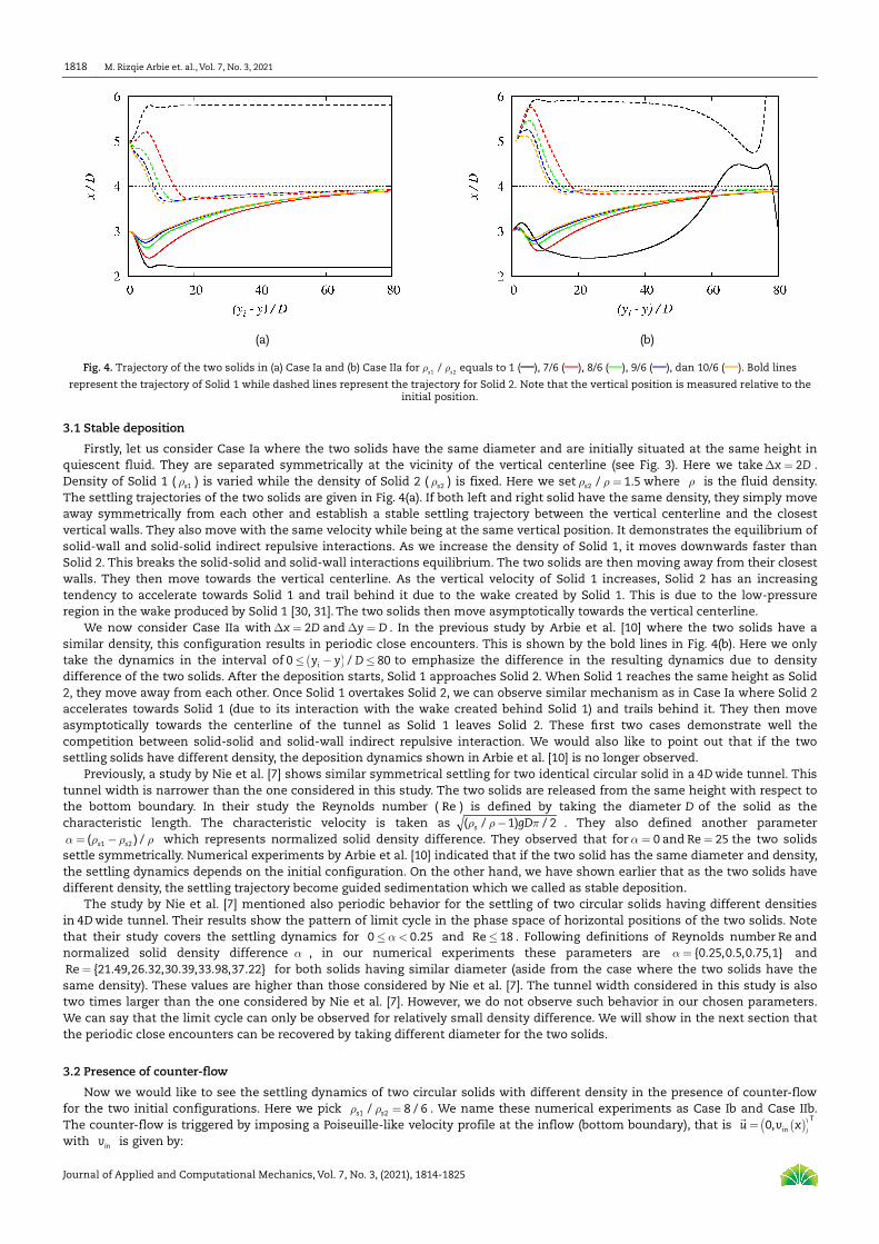
Fig. 4. Trajectory of the two solids in (a) Case Ia and (b) Case IIa for 1 2/

s sρ ρ equals to 1 (──), 7/6 (──), 8/6 (──), 9/6 (──), dan 10/6 (──). Bold lines

represent the trajectory of Solid 1 while dashed lines represent the trajectory for Solid 2. Note that the vertical position is measured relative to the initial position.

3.1 Stable deposition

Firstly, let us consider Case Ia where the two solids have the same diameter and are initially situated at the same height in quiescent fluid. They are separated symmetrically at the vicinity of the vertical centerline (see Fig. 3). Here we take 2x D∆ = . Density of Solid 1 ( 1sρ ) is varied while the density of Solid 2 ( 2sρ ) is fixed. Here we set 2 / 1.5sρ ρ = where ρ is the fluid density. The settling trajectories of the two solids are given in Fig. 4(a). If both left and right solid have the same density, they simply move away symmetrically from each other and establish a stable settling trajectory between the vertical centerline and the closest vertical walls. They also move with the same velocity while being at the same vertical position. It demonstrates the equilibrium of solid-wall and solid-solid indirect repulsive interactions. As we increase the density of Solid 1, it moves downwards faster than Solid 2. This breaks the solid-solid and solid-wall interactions equilibrium. The two solids are then moving away from their closest walls. They then move towards the vertical centerline. As the vertical velocity of Solid 1 increases, Solid 2 has an increasing tendency to accelerate towards Solid 1 and trail behind it due to the wake created by Solid 1. This is due to the low-pressure region in the wake produced by Solid 1 [30, 31]. The two solids then move asymptotically towards the vertical centerline.

We now consider Case IIa with 2x D∆ = and y D∆ = . In the previous study by Arbie et al. [10] where the two solids have a similar density, this configuration results in periodic close encounters. This is shown by the bold lines in Fig. 4(b). Here we only take the dynamics in the interval of ( )0 / 80iy y D≤ − ≤ to emphasize the difference in the resulting dynamics due to density difference of the two solids. After the deposition starts, Solid 1 approaches Solid 2. When Solid 1 reaches the same height as Solid 2, they move away from each other. Once Solid 1 overtakes Solid 2, we can observe similar mechanism as in Case Ia where Solid 2 accelerates towards Solid 1 (due to its interaction with the wake created behind Solid 1) and trails behind it. They then move asymptotically towards the centerline of the tunnel as Solid 1 leaves Solid 2. These first two cases demonstrate well the competition between solid-solid and solid-wall indirect repulsive interaction. We would also like to point out that if the two settling solids have different density, the deposition dynamics shown in Arbie et al. [10] is no longer observed.

Previously, a study by Nie et al. [7] shows similar symmetrical settling for two identical circular solid in a 4Dwide tunnel. This tunnel width is narrower than the one considered in this study. The two solids are released from the same height with respect to the bottom boundary. In their study the Reynolds number ( Re ) is defined by taking the diameter D of the solid as the characteristic length. The characteristic velocity is taken as ( / 1) / 2s gDρ ρ π− . They also defined another parameter

1 2( ) /s sα ρ ρ ρ= − which represents normalized solid density difference. They observed that for 0α = and Re 25= the two solids settle symmetrically. Numerical experiments by Arbie et al. [10] indicated that if the two solid has the same diameter and density, the settling dynamics depends on the initial configuration. On the other hand, we have shown earlier that as the two solids have different density, the settling trajectory become guided sedimentation which we called as stable deposition.

The study by Nie et al. [7] mentioned also periodic behavior for the settling of two circular solids having different densities in 4Dwide tunnel. Their results show the pattern of limit cycle in the phase space of horizontal positions of the two solids. Note that their study covers the settling dynamics for 0 0.25α≤ < and Re 18≤ . Following definitions of Reynolds number Re and normalized solid density difference α , in our numerical experiments these parameters are {0.25,0.5,0.75,1}α = and Re {21.49,26.32,30.39,33.98,37.22}= for both solids having similar diameter (aside from the case where the two solids have the same density). These values are higher than those considered by Nie et al. [7]. The tunnel width considered in this study is also two times larger than the one considered by Nie et al. [7]. However, we do not observe such behavior in our chosen parameters. We can say that the limit cycle can only be observed for relatively small density difference. We will show in the next section that the periodic close encounters can be recovered by taking different diameter for the two solids.

3.2 Presence of counter-flow

Now we would like to see the settling dynamics of two circular solids with different density in the presence of counter-flow for the two initial configurations. Here we pick 1 2/ 8 / 6s sρ ρ = . We name these numerical experiments as Case Ib and Case IIb. The counter-flow is triggered by imposing a Poiseuille-like velocity profile at the inflow (bottom boundary), that is ( )( )0, inu v x=

� T

with inv is given by:



1819

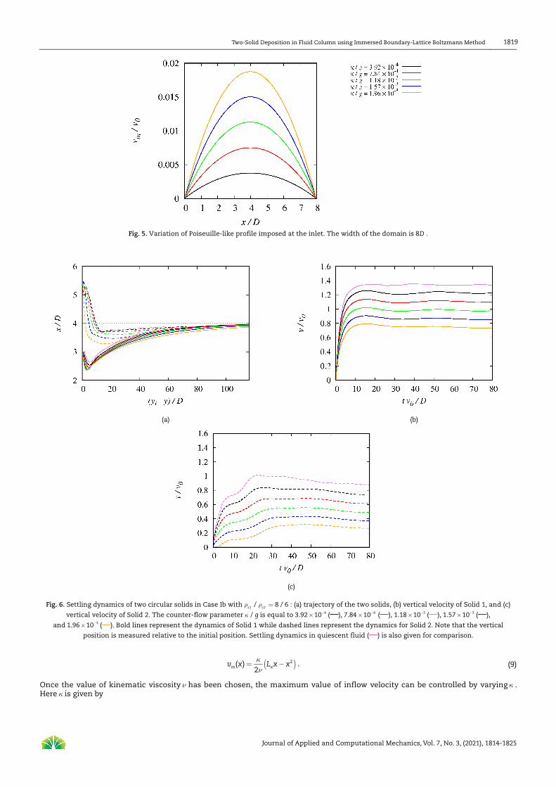
Fig. 5. Variation of Poiseuille-like profile imposed at the inlet. The width of the domain is 8D .

(a)

(b)

(c)

Fig. 6. Settling dynamics of two circular solids in Case Ib with 1 2/ 8 / 6s sρ ρ = : (a) trajectory of the two solids, (b) vertical velocity of Solid 1, and (c)

vertical velocity of Solid 2. The counter-flow parameter / gκ is equal to 43.92 10−× (──), 47.84 10−× (──), 31.18 10−× (──), 31.57 10−× (──),

and 31.96 10−× (──). Bold lines represent the dynamics of Solid 1 while dashed lines represent the dynamics for Solid 2. Note that the vertical

position is measured relative to the initial position. Settling dynamics in quiescent fluid (──) is also given for comparison.

( )2( )2 xinv x L x xκ

ν= − . (9)

Once the value of kinematic viscosity ν has been chosen, the maximum value of inflow velocity can be controlled by varying κ . Here κ is given by



1820

1 pg

yκρ

∂= −

∂ (10)

which gives the upward acceleration to move fluid and is the difference between a pressure gradient and the strength of gravitational acceleration. Here we define a non-dimensional quantity / gκ as parameter to describe the strength of the counter-flow. In this study, we take five different values of / gκ which are given in Fig. 5. The increment of / gκ we use is sufficient to reduce the vertical velocity component of less dense solid by 15% to 20%. This is also due to the additional drag by the confined geometry which has been shown to contribute to the total drag experienced by a solid settling through the confined fluid [32]. Without the confined geometry, the choice of counter-flow might be too weak.

To include the counter-flow, we use the Zou-He boundary condition [33] for velocity at the bottom boundary. On the other hand, the fluid must be able to escape smoothly form the computational domain at the upper boundary. We then apply the Zou-He boundary condition for constant pressure at the upper boundary. The simulation is carried out by letting the imposed counter-flow to be fully developed inside the domain while the two solids are held fixed. The deposition is commenced once the horizontal and vertical force exerted on the two solids by the fluid are constant over time.

The deposition trajectory in the presence of counter-flow for Case Ib with 1 2/ 8 / 6s sρ ρ = is shown in Fig. 6(a). The results show that varying the strength of counter-flow does not give significant change in the settling trajectory of both solids. This is true for all value of / gκ demonstrated here. Based on Fig. 6(b) and (c), we can also say that the presence of counter-flow only causes the two solids to settle slower as the strength of the counter-flow is increased. Figure 6(b) shows also that Solid 1, as the leading one, eventually reaches its terminal velocity. For Solid 2 as the trailing solid, there is an acceleration in the time interval

010 / 20tv D< < as shown in Fig. 6(c). This due to the interaction between Solid 2 and the wake created behind Solid 1. But as the separation between the two solids increases, Solid 2 interacts with decaying wakes produced by Solid 1. Eventually, the vertical velocity of Solid 2 becomes approximately constant. For Case IIb with 1 2/ 8 / 6s sρ ρ = (see Fig. 7(a)), we also observe that there is no significant change in the settling trajectory of each solid due to the increasing strength of counter-flow. Figure 7(b) and (c) also show that the two solids settle with smaller vertical velocity as the strength of the counter-flow is increased. As in Case Ib, Fig. 7(c) shows that Solid 2, as the trailing solid, accelerates in the time interval 010 / 20tv D< < .

(a)

(b)

(c)

Fig. 7. Settling dynamics of two circular solids in Case IIb with 1 2/ 8 / 6s sρ ρ = : (a) trajectory of the two solids, (b) vertical velocity of Solid 1, and (c)

vertical velocity of Solid 2. The counter-flow parameter / gκ is equal to 43.92 10−× (──), 47.84 10−× (──), 31.18 10−× (──), 31.57 10−× (──),

and 31.96 10−× (──). Bold lines represent the dynamics of Solid 1 while dashed lines represent the dynamics for Solid 2. Note that the vertical

position is measured relative to the initial position. Settling dynamics in quiescent fluid (──) is also given for comparison.



1821

(a)

(b)

(c)

(d)

Fig. 8. Variation of normalized center-to-center distance as a function of normalized time for (a) Case Ia and (b) Case IIa as well as the variation of the difference in vertical position between Solid 1 and Solid 2 for (c) Case Ia and (d) Case IIa. The purple line marks the center-to-center distance

of 1.57D .

4. Adding the effect of solid diameter

Here we show that one may recover the periodic close encounters by adding solid diameter difference. We then set 2 12 2D D D= = to observe how solid diameter can affect the settling in Case I and Case II. The initial horizontal separation between Solid 1 and Solid 2 is 4x D∆ = . The density ratio of Solid 2 with the fluid density is 2 / 1.5sρ ρ = . As in previous section, the numerical experiments are performed for different 1 2/s sρ ρ , i.e., by varying the value of 1sρ . Note that since Solid 2 is larger than Solid 1 while density of Solid 1 will be increased, we then set the initial position of Solid 2 higher than Solid 1. We have seen from previous section that density difference may change the periodic close encounters into a stable deposition where less dense solid trails behind the denser one.

The variation of center-to-center distance ( ssl ) between the two solids as a function of time is shown in Fig. 8(a) and (b) while the difference in vertical position of the two solids is given in Fig. 8(c) and (d). The settling trajectory of the two solids is given in Fig. 9. Figure 8(a) depicts the center-to-center distance in Case Ia. For 1 2/ 1s sρ ρ = , Solid 1 trails behind Solid 2 with an increasing distance between the two solids and thus close encounter does not take place. From Fig. 9(a), we can see that Solid 1 trails behind Solid 2 with a damped oscillating trajectory as the two solids settling asymptotically towards the vertical centerline. Figure 8(c) also indicates that Solid 1 settles behind Solid 2. Similar dynamics is also observed in Case IIa as being shown in Fig. 8(b) and (d). The only difference is on the early dynamics due to the difference in initial arrangement for the two cases. As we increase the value of 1 2/s sρ ρ to 7 / 6 , Fig. 8(a) and (b) shows that there is single close encounter in both Case Ia and Case IIa within the time interval of our numerical experiment. After the close encounter there is an increase of separation between the two solids. However, after 0 / 70tv D ≈ , Solid 1 approaches Solid 2 again. From Fig. 9(b), we can identify that Solid 1 performs a damped oscillation as it drifts towards the vertical centerline to approach Solid 2. Again, the settling only differs at the early time due to different initial configuration if compare the result in Fig. 8(c) and (d).

For 1 2/ 8 / 6s sρ ρ = , we observe in Fig. 8(a) and (b) that multiple close encounters take place during the settling process in both Case Ia and Case IIa. Each close encounter leaves a center-to-center distance of 1.57D which is marked by the purple line in the figures. Each close encounter is caused by the interaction between the low-pressure wake produced behind the leading solid as mentioned in previous section. Once the trailing solid enters the wake region, it is accelerated towards the leading particle. As the trailing solid getting close to the leading one, there is a pressure build up in the fluid between the two solids. The closer the two solids are, the larger this pressure. This results in the trailing solid pushes the leading one. So the center-to-center distance increases again. This process takes place periodically and gives the periodic close encounters. The process is depicted in Fig. 9(c) in which the settling trajectory of the two solids forms a periodic curve after the first close encounter. From Fig. 8(c), we can say



1822

that Solid 2 leads the deposition most of the time. Solid 1 only get ahead of Solid 2 for a short period of time during the close encounter. This also holds true for Case IIa as shown in Fig. 8(d) for the multiple close encounters (excluding the early time where Solid 1 is ahead of Solid 2 due to the initial arrangement).

As we set the value of 1 2/s sρ ρ to 9 / 6 , Fig. 8(a) shows that the value ssl for Case Ia is decreasing towards 1.57D . It gives an indication for close encounter to be taking place. However, it requires larger computational domain to observe. We can also see from Fig. 8(c) and 9(d) that Solid 2 trails behind Solid 1 while performing an oscillating movement as the center-to-center distance between them decreases. On the other hand, Fig. 8(b) shows that the value of ssl for Case IIa keeps increasing. This means that the density of Solid 1 is sufficiently large to move fast and leave Solid 2 behind. We can also see from Fig. 9(d) that both solids simply drift towards the vertical centerline as the separation distance between them increases.

(a)

(b)

(c)

(d)

(e)

Fig. 9. Settling trajectories of two circular solids in Case Ia and Case IIa with 2 12D D= for (a) 1 2/ 1

s sρ ρ = , (b) 1 2/ 7 / 6

s sρ ρ = , (c) 1 2/ 8 / 6

s sρ ρ = ,

(d) 1 2/ 9 / 6s sρ ρ = , and (e) 1 2/ 10 / 6

s sρ ρ = in quiescent fluid.



1823

(a)

(b)

Fig. 10. Variation of normalized center-to-center distance as a function of normalized time for (a) Case Ib and (b) Case IIb

with 2 12D D= and 1 2/ 8 / 6s sρ ρ = as the two solids settle through the counter-flow. The purple line marks the center-to-center distance of 1.57D .

For 1 2/ 10 / 6s sρ ρ = , Fig. 8(a) and (b) show that Solid 2 always trails behind Solid 1 with increasing center-to-center distance for

both Case Ia and Case IIa. Solid 1 is always ahead of Solid 2 as shown by Fig. 8(c) and (d). This is an indication that the solid

density ration is large enough to prevent any close encounter. Also, we can see from Fig. 9(e) that the two solids simply move

asymptotically towards the vertical centerline with Solid 1 leading the deposition.

These results demonstrate a dynamic transition from stable deposition (a simple drift towards the vertical centerline as one

solid leaves the other) to periodic close-encounters. When the two solids have identical density and one solid has a diameter

twice as large as the other, the larger one leaves the smaller one. But as the smaller solid has larger density than the bigger one,

we observed dynamics transition to periodic close encounters. If the density ratio between the smaller solid and the larger solid

surpass certain value ( 1 2/ 10 / 6s sρ ρ = in this case), the smaller yet denser one leads ahead with increasing separation distance

between the two solids. These results also indicate that one may keep the separation distance between the two solids below

certain value by adjusting both the density ratio and the size ratio of the two circular solids. In this study, the choice

of 2 12D D= and 1 2/ 8 / 6s sρ ρ = leaves an approximate maximum center-to-center distance of 5.45D between the two solids for both

Case Ia and Case IIa.

In some engineering application, such as fluidized beds, counter-flow may exist. We then perform another test to investigate

whether the presence of periodic close encounters for 2 12D D= and 1 2/ 8 / 6s sρ ρ = is robust if the two solids are settling through a

counter-flow. Now we call the two initial configurations as Case Ib and Case IIb. As in previous section, we use the Poiseuille-like

velocity profile as inflows at the bottom boundary. As in previous section, we run the simulation with the solid at rest first until

the flow inside the domain is fully developed. Once the flow is fully developed, we start the deposition process. The variation of

center-to-center distance between the two solids as a function of time is given in Fig. 10(a) for Case Ib and Fig. 10(b) for Case IIb.

By varying the strength of the counter-flow (parameterized by / gκ ). The multiple close encounters are still observed as shown in

Fig. 10. The distance between the two solids (measured center-to-center) is also still within certain range. For instance,

at 3/ 1.96 10gκ −= × we observe that ssl lies in the range 1.57 5.84ssD l D< < . For 4/ 3.92 10gκ −= × , the multiple encounters we

observe is qualitatively similar to those without counter-flow. Increasing / gκ changes the settling dynamics especially for

large / gκ considered here but the close encounters are still observed.

5. Conclusion

We have performed numerical experiments on the influence of certain physical parameters to the deposition dynamics of two solids in a channel. For two solids initially not levelled, we observe that the multiple close encounters shown by Arbie et al. [10] turn into guided deposition where denser solid leads the deposition. For both initial configurations considered in this study, both solids move asymptotically towards the vertical centerline of the tunnel as the separation distance between them increases. This holds true with the present of counter-flow at least within the range of counter-flow strength considered in this study, that is 4 33.92 10 / 1.96 10 .gκ− −× ≤ ≤ × For the choice 1D D= , 2 2D D= and 1 2/ 1s sρ ρ = where 60D= LU, the larger solid leads the deposition as the smaller one trails behind. At long time, the two solids settle along the vertical centerline. Multiple close encounters is observed as we set 1D D= , 2 2D D= and 1 2/ 8 / 6s sρ ρ = . Once the solid density ratio is set to 1 2/ 10 / 6s sρ ρ = , the denser solid, yet smaller one, leads the deposition and the two solids settle along the vertical centerline at long time. We can conclude that a careful choice of solid size ratio and density ratio may produce the multiple close encounters although the density ratio is larger than the ones studied by Nie et al. [7]. It is also observed that in the presence of counter flow, the spatial distance between the two solids (measured center-to-center) for 1D D= , 2 2D D= and 1 2/ 8 / 6s sρ ρ = is limited on the range 1.57 5.84ssD l D≤ < . The multiple close encounters also appear to be periodic and robust to the present of counter flow at least within the range of counter-flow strength considered in this study. Together with our previous study [6], these numerical experiments show the importance of initial configuration, density ratio, and size ratio (taken to be diameter) to control dynamics and spatial separation of two circular solids during their deposition in narrow channel.



1824

Author Contributions

M. Rizqie Arbie planned the numerical scheme, initiated the project, suggested, and conducted some of the numerical experiments; Umar Fauzi and Fourier D.E. Latief conducted the experiments and analyzed the results together with M. Rizqie Arbie; Enjang J. Mustopa examined the theory validation. The manuscript was written through the contribution of all authors. All authors discussed the results, reviewed, and approved the final version of the manuscript.

Acknowledgments

We thank Julien Favier and Marcus Uhlmann for their permissions to use results in their previous articles as comparison. We would also like to thank the Physics of Earth and Complex Systems research group for the support throughout the research.

Conflict of Interest

The authors declared no potential conflicts of interest with respect to the research, authorship, and publication of this article.

Funding

This research is funded by the P3MI2019 funding program no 1000E/I1.C01/PL/2019 by Institut Teknologi Bandung.

Nomenclature

D Solid diameter inv Vertical component of fluid inflow velocity

ke� Unit direction for velocity space discretization x

� Position

kf Particle distribution function qx� Position of q -th IB point

eqkf Particle distribution function at equilibrium x Horizontal position

F�

Body force per unit volume y Vertical position

IBF�

Body force per unit volume at the IB points iy Initial vertical position

kg Forcing term in LB equation α Normalized solid density difference

g Gravitational acceleration Γ Solid perimeter

xL Tunnel width δ Delta function

yL Tunnel height ε Characteristic strip-width

ssl Center-to-center Distance between two solids κ Upward net acceleration

p Pressure field ν Fluid viscosity

t Time ρ Fluid density

u� Fluid velocity field 1sρ Density of Solid 1

U�

Fluid velocity at the IB points 2sρ Density of Solid 2

su Horizontal component of solid velocity τ Relaxation time

sv Vertical component of solid velocity kω Weighting factor for unit direction in velocity space

References

[1] Sheikholeslami, M., Farshad, S.A., Said, Z., Analyzing Entropy and Thermal Behavior of Nanomaterial through Solar Collector Involving New Tapes, International Communications in Heat and Mass Transfer, 123, 2021, 105190. [2] Sheikholeslami, M., Farshad, S.A., Ebrahimpour, Z., Said, Z., Recent Progress on Flat Plate Solar Collectors and Photovoltaic Systems in the Presence of Nanofluid: a Review, Journal of Cleaner Production, 293, 2021, 126119. [3] Sheikholeslami, M., Jafaryar, M., Said, Z., Alsabery, A.I., Babazadeh, H., Shafee, A., Modification for Helical Turbulator to Augment Heat Transfer Behavior of Nanomaterial via Numerical Approach, Applied Thermal Engineering, 182, 2021, 115935. [4] Sheikholeslami, M., Farshad, S.A., Investigation of Solar Collector System with Turbulator Considering Hybrid Nanoparticles, Renewable Energy, 171, 2021, 1128-1158. [5] Jayaweera, K.O.L.F., Mason, B.J., The Behaviour of Freely Falling Cylinders and Cones in a Viscous Fluid. Journal of Fluid Mechanics, 22, 1965, 709-720. [6] Brenner, H., Effect of Finite Boundaries on the Stokes Resistance of an Arbitrary Particle, Journal of Fluid Mechanics, 12, 1962, 35-48. [7] Nie, D., Lin, J., Gao, Q., Settling Behavior of Two Particles with Different Densities in a Vertical Channel, Computers & Fluids, 156, 2017, 353-367. [8] Glowinski, R., Pan, T.W., Hesla, T.I., Joseph, D.D., Priaux, J., A Distributed Lagrange Multiplier/Fictitious Domain Method for Flows around Moving Rigid Bodies: Application to Particulate Flow, International Journal for Numerical Methods in Fluids, 30, 1999, 1043-1066. [9] Aidun, C.K., Ding, E.J., Dynamics of Particle Sedimentation in a Vertical Channel: Period-Doubling Bifurcation and Chaotic State, Physics of Fluids, 15, 2003, 1612-1621. [10] Arbie, M.R., Fauzi, U., Latief, F.D.E., Dynamics of Two Disks in a Counter-Flow using Immersed Boundary-Lattice Boltzmann Method, Computers & Fluids, 179, 2019, 265-276. [11] Izadpanahi, E., Moshtaghzadeh, M., Radnezhad, H.R., Mardanpour, P., Constructal Approach to Design of Wing Cross-Section for Better Flow of Stresses, AIAA 2020-0275, AIAA Scitech 2020 Forum, 2020. [12] Mehryan, S.A.M., Ghalambaz, M., Ismael, M.A., Chamkha, A.J., Analysis of fluid-solid interaction in MHD natural convection in a square cavity equally partitioned by a vertical flexible membrane, Journal of Magnetism and Magnetic Materials, 424, 2017, 161–173. [13] Ferras, D., Manso, P., Schleiss, A., Covas, D., One-Dimensional Fluid–Structure Interaction Models in Pressurized Fluid-Filled Pipes: A Review, Applied Sciences, 8(10), 2018, 1844. [14] Tuković, Ž., Karač, A., Cardiff, P., Jasak, H., Ivanković, A., OpenFOAM Finite Volume Solver for Fluid-Solid Interaction, Transactions of FAMENA, 42(3), 2018, 1-31. [15] Zhang, C., Rezavand, M., Hu, X., A multi-resolution SPH method for fluid-structure interactions, Journal of Computational Physics, 429, 2021, 110028. [16] He, X., Luo, L.S., Lattice Boltzmann Model for the Incompressible Navier-Stokes Equation, Journal of Statistical Physics, 88, 1997, 927-944. [17] Succi, S., The Lattice Boltzmann Equation: for Fluid Dynamics and Beyond, Oxford University Press, New York, United States of America, 2018. [18] Lallemand, P., Luo, L.S., Lattice Boltzmann Method for Moving Boundaries, Journal of Computational Physics, 184, 2003, 406-421.



1825

[19] Peskin, C.S., Numerical Analysis of Blood Flow in the Heart, Journal of Computational Physics, 25, 1977, 220-252. [20] Peskin, C.S., The Immersed Boundary Method, Acta Numerica, 2002, 11, 479-517. [21] Mittal, R., Iaccarino, G., Immersed Boundary Methods, Annual Review of Fluid Mechanics, 37, 2005, 239-261. [22] Feng, Z.G., Michaelides, E.E., The Immersed Boundary-Lattice Boltzmann Method for Solving Fluid-Particles Interaction Problems, Journal of Computational Physics, 195, 2004, 602-628. [23] Cheng, Y., Zhang, H., Immersed Boundary Method and Lattice Boltzmann Method Coupled FSI Simulation of Mitral Leaflet Flow, Computers & Fluids, 39, 2010, 871-881. [24] Li, Z., Favier, J., D’Ortona, U., Poncet, S., An Immersed Boundary-Lattice Boltzmann Method for Single- and Multi-Component Fluid Flows, Journal of Computational Physics, 304, 2016, 424-440. [25] Pinelli, A., Naqavi, I.Z., Piomelli, U., Favier, J., Immersed-Boundary Methods for General Finite-Difference and Finite-Volume Navier-Stokes Solvers, Journal of Computational Physics, 229, 2010, 9073-9091. [26] Guo, Z., Zheng, C., Shi, B., Discrete Lattice Effects on the Forcing Term in the Lattice Boltzmann Method, Physical Review E, 65, 2002, 046308. [27] Roma, A.M., Peskin, C.S., Berger, M.J., An Adaptive Version of the Immersed Boundary Method, Journal of Computational Physics, 153, 1999, 509-534. [28] Favier, J., Revell, A., Pinelli, A., A Lattice Boltzmann-Immersed Boundary Method to Simulate the Fluid Interaction with Moving and Slender Flexible Objects, Journal of Computational Physics, 261, 2014, 145-161. [29] Uhlmann, M., An Immersed Boundary Method with Direct Forcing for the Simulation of Particulate Flows, Journal of Computational Physics, 209, 2005, 448-476. [30] Dash, S., Lee, T., Two Spheres Sedimentation Dynamics in a Viscous Liquid Column, Computers & Fluids, 123, 2015, 218-234. [31] Derakhshani, S.M., Schott, D.L., Lodewijks, G., Modeling Particle Sedimentation in Viscous Fluids with a Coupled Immersed Boundary Method and Discrete Element Method, Particuology, 31, 2017, 191-199. [32] Ghosh, S., Stockie, J.M., Numerical Simulations of Particle Sedimentation Using the Immersed Boundary Method, Communications in Computational Physics, 18, 2015, 380-416. [33] Zou, Q., He, X., On Pressure and Velocity Boundary Conditions for the Lattice Boltzmann BGK Model, Physics of Fluids, 9, 1997, 1591-1598.

ORCID iD

M. Rizqie Arbie https://orcid.org/0000-0002-1359-8377 Umar Fauzi https://orcid.org/0000-0002-2221-7257 Fourier D.E. Latief https://orcid.org/0000-0002-5448-929X Enjang J. Mustopa https://orcid.org/0000-0002-0769-2164

© 2021 Shahid Chamran University of Ahvaz, Ahvaz, Iran. This article is an open access article distributed under the terms and conditions of the Creative Commons Attribution-NonCommercial 4.0 International (CC BY-NC 4.0 license) (http://creativecommons.org/licenses/by-nc/4.0/).

How to cite this article: Rizqie Arbie M., Fauzi U., Latief F.D.E., Mustopa E.J. Two-Solid Deposition in Fluid Column using Immersed Boundary-Lattice Boltzmann Method, J. Appl. Comput. Mech., 7(3), 2021, 1814–1825. https://doi.org/10.22055/JACM.2021.37140.2969

Publisher’s Note Shahid Chamran University of Ahvaz remains neutral with regard to jurisdictional claims in published maps and institutional affiliations.

Two-Solid Deposition in Fluid Column using Immersed ...

Documents

Transcript of Two-Solid Deposition in Fluid Column using Immersed ...