Two-player interaction in quantum computing:cryptographic primitives & query complexity

These presentee parLoıck Magnin

en vue de l’obtention des grades

Docteur en Sciences, specialite InformatiqueUniversite Paris-Sud 11

et

Docteur en Sciences de l’IngenieurUniversite Libre de Bruxelles

Soutenue le 5 decembre 2011 devant le jury compose de

Alain Denise PresidentPeter Høyer Rapporteur

Pascal Koiran RapporteurAlain Dubus Examinateur

Marc Haelterman ExaminateurJeremie Roland ExaminateurNicolas J. Cerf Directeur de these

Frederic Magniez Directeur de these

A ma famille.

Resume

Cette these etudie deux aspects d’interaction entre deux joueurs dans le modele du calcul etde la communication quantique.

Premierement, elle etudie deux primitives cryptographiques quantiques, des briques de basepour construire des protocoles cryptographiques complexes entre deux joueurs, comme parexemple un protocole d’identification.

La premiere primitive est la “mise en gage quantique”. Cette primitive ne peut pas etrerealisee de maniere inconditionnellement sure, mais il est possible d’avoir une securite lorsqueles deux parties sont soumises a certaines contraintes additionnelles. Nous etudions cetteprimitive dans le cas ou les deux joueurs sont limites a l’utilisation d’etats et d’operationsgaussiennes, un sous-ensemble de la physique quantique central en optique, donc parfaitementadapte pour la communication via fibres optiques. Nous montrons que cette restriction nepermet malheureusement pas la realisation de la mise en gage sure. Pour parvenir a ce resultat,nous introduisons la notion de purification intrinseque, qui permet de contourner l’utilisationdu theoreme de Uhlman, en particulier dans le cas gaussien.

Nous examinons ensuite une primitive cryptographique plus faible, le “tirage faible apile ou face”, dans le modele standard du calcul quantique. Carlos Mochon a donne unepreuve d’existence d’un tel protocole avec un biais arbitrairement petit. Nous donnons uneinterpretation claire de sa preuve, ce qui nous permet de la simplifier et de la raccourcirgrandement.

La seconde partie de cette these concerne l’etude de methodes pour prouver des bornesinferieures dans le modele de la complexite en requete. Il s’agit d’un modele de complexitecentral en calcul quantique dans lequel de nombreux resultats majeurs ont ete obtenus. Dansce modele, un algorithme ne peut acceder a l’entree uniquement qu’en effectuant des requetessur chacune des variables de l’entree. Nous considerons une extension de ce modele dans lequelun algorithme ne calcule pas une fonction, mais doit generer un etat quantique.

Cette generalisation nous permet de comparer les differentes methodes pour prouver desbornes inferieures dans ce modele. Nous montrons d’abord que la methode par adversaire “mul-tiplicative” est plus forte que la methode “additive”. Nous montrons ensuite une reduction dela methode polynomiale a la methode multiplicative, ce qui permet de conclure a la superioritede la methode par adversaire multiplicative sur toutes les autres methodes.

Les methodes par adversaires sont en revanche souvent difficiles a utiliser car elles necessitentle calcul de normes de matrices de tres grandes tailles. Nous montrons comment l’etude dessymetries d’un probleme simplifie grandement ces calculs.

Enfin, nous appliquons ces formules pour prouver la borne inferieure optimale du problemeIndex Erasure, un probleme de generation d’etat quantique lie au celebre probleme Iso-morphisme de Graphes.

v

Abstract

This dissertation studies two different aspects of two-player interaction in the model of quantumcommunication and quantum computation.

First, we study two cryptographic primitives, that are used as basic blocks to constructsophisticated cryptographic protocols between two players, e.g. identification protocols.

The first primitive is “quantum bit commitment”. This primitive cannot be done in anunconditionally secure way. However, security can be obtained by restraining the power of thetwo players. We study this primitive when the two players can only create quantum Gaussianstates and perform Gaussian operations. These operations are a subset of what is allowed byquantum physics, and plays a central role in quantum optics. Hence, it is an accurate modelof communication through optical fibers. We show that unfortunately this restriction doesnot allow secure bit commitment. The proof of this result is based on the notion of “intrinsicpurification” that we introduce to circumvent the use of Uhlman’s theorem when the quantumstates are Gaussian.

We then examine a weaker primitive, “quantum weak coin flipping”, in the standard modelof quantum computation. Mochon has showed that there exists such a protocol with arbitrarilysmall bias. We give a clear and meaningful interpretation of his proof. That allows us to presenta drastically shorter and simplified proof.

The second part of the dissertation deals with different methods of proving lower boundson the quantum query complexity. This is a very important model in quantum complexity inwhich numerous results have been proved. In this model, an algorithm has restricted access tothe input: it can only query individual variables. We consider a generalization of the standardmodel, where an algorithm does not compute a classical function, but generates a quantumstate.

This generalization allows us to compare the strength of the different methods used toprove lower bounds in this model. We first prove that the “multiplicative adversary method”is stronger than the “additive adversary method”. We then show a reduction from the “polyno-mial method” to the multiplicative adversary method. Hence, we prove that the multiplicativeadversary method is the strongest one.

Adversary methods are usually difficult to use since they involve the computation of normsof matrices with very large size. We show how studying the symmetries of a problem canlargely simplify these computations.

Last, using these principles we prove the tight lower bound of the Index Erasure problem.This a quantum state generation problem that has links with the famous Graph Isomorphismproblem.

vii

Acknowledgements

When I started my thesis I knew I would end somewhere one day. I knew I was beginninga journey, but I had no idea how difficult it would be, where it would lead me, and what Iwould end up discovering about sciences and about myself. But I knew I would neither getlost, neither give up, because I was not alone. And I wish here to acknowledge people andorganizations that helped me.

First of all, I want to thank my two supervisors, Frederic Magniez and Nicolas Cerf. Nicolasintroduced me to the fascinating field of quantum cryptography with continuous variables thatI immediately appreciated. Nicolas also taught me the importance of physical intuition overmathematical formalism to explore new territories. He was of constant support and eager tofollow me to discover them. This passion for exploration was also shared by Frederic, and hehelped me to always move forward and discover the greater picture. He helped me to organizemy thoughts and to try to keep a clear mind focused and sharp.

I really appreciated how they both let me a great freedom and encourage me to challengemyself: I was able to choose my research subjects and my coauthors, and discover other way toperform research in the numerous travels they fully supported: USA, Canada, Spain, Japan,Egypt, Singapore, Switzerland. This really was an amazing journey!

I want to acknowledge the support of the Region Ile-de-France for my travels between Parisand Brussels and thus making me feel part of both teams: the Algo group in Paris and theQuIC in Brussels.

In Paris and Brussels, I had a great pleasure to share office, ideas and laughters with Raul,Joachim, Julien, Louis-Philippe, Xavier, Marc, Mathieu, Antoine and Andre.

I also want express my gratitude to all the members of the jury, in particular to PascalKoiran and Peter Høyer, for reading carefully this manuscript and giving to me a very valuablefeedback.

My gratitude goes to all my collaborators. Each of them brought me something and hadfaith in me: Anthony Leverrier, Andris Ambainis, Martin Rotteler, Jeremie Roland, DoritAharonov, Maor Ganz, Iordanis Kerenidis, and of course Nicolas Cerf and Frederic Magniez.

In particular, I want to thank Jeremie Roland again. He was in the same office than mewhen I started my PhD, and I then went to meet him five times in the USA. During twosummers I was intern at NEC Laboratories America under his supervision. These were twomarvelous summers, full of joy and productivity.

Last, I would not be able to finish this thesis without the love and support from my familyand my friends.

ix

List of publications

This dissertation is based on the following publications:

[MMLC10] Loıck Magnin, Frederic Magniez, Anthony Leverrier, and Nicolas J. Cerf.Strong no-go theorem for Gaussian quantum bit commitment. Physi-cal Review A, Rapid communications, 81:010302, 2010. arXiv:0905.3419,doi:10.1103/PhysRevA.81.010302

[ACG+11] Dorit Aharonov, Andre Chailloux, Maor Ganz, Iordanis Kerenidis and LoıckMagnin. A simpler proof of existence of quantum weak coin flipping with arbi-trarily small bias. In submission, 2011.

[AMR+11] Andris Ambainis, Loıck Magnin, Martin Roetteler, and Jeremie Roland.Symmetry-assisted adversaries for quantum state generation. In Proceedings ofthe 26th Annual IEEE Conference on Computational Complexity, pages 167–177,2011. IEEE Computer Society. arXiv:1012.2112, doi:10.1109/CCC.2011.24

[MR11] Loıck Magnin and Jeremie Roland. Quantum adversary lower bounds by poly-nomials. Technical report 2011-TR080, NEC Laboratories America, Inc., 2011

xi

Contents

Resume v

Abstract vii

Acknowledgements ix

List of publications xi

1 Introduction 1

1.1 Quantum disruption in information sciences . . . . . . . . . . . . . . . . . . . . 1

1.1.1 Spooky . . . . . . . . . . . . . . . . . . . . . . . . . . . . . . . . . . . . 1

1.1.2 Surprise . . . . . . . . . . . . . . . . . . . . . . . . . . . . . . . . . . . . 2

1.1.3 Enthusiasm and fear . . . . . . . . . . . . . . . . . . . . . . . . . . . . . 3

1.2 Scope and motivations . . . . . . . . . . . . . . . . . . . . . . . . . . . . . . . . 4

1.2.1 Gaussian quantum key distribution . . . . . . . . . . . . . . . . . . . . . 4

1.2.2 Cryptographic primitives . . . . . . . . . . . . . . . . . . . . . . . . . . 4

1.2.3 Query complexity . . . . . . . . . . . . . . . . . . . . . . . . . . . . . . 5

1.2.4 Outline of this dissertation . . . . . . . . . . . . . . . . . . . . . . . . . 6

1.3 Quantum primitives . . . . . . . . . . . . . . . . . . . . . . . . . . . . . . . . . 7

1.3.1 Bit commitment . . . . . . . . . . . . . . . . . . . . . . . . . . . . . . . 7

1.3.2 Coin flipping . . . . . . . . . . . . . . . . . . . . . . . . . . . . . . . . . 10

1.4 Lower bounds for quantum query complexity . . . . . . . . . . . . . . . . . . . 13

1.4.1 Direct sum and product theorems . . . . . . . . . . . . . . . . . . . . . 13

1.4.2 Adversaries . . . . . . . . . . . . . . . . . . . . . . . . . . . . . . . . . . 14

1.4.3 Polynomial method . . . . . . . . . . . . . . . . . . . . . . . . . . . . . . 15

1.4.4 Quantum state generation problems . . . . . . . . . . . . . . . . . . . . 16

1.4.5 Contributions . . . . . . . . . . . . . . . . . . . . . . . . . . . . . . . . . 16

2 Models of quantum information 21

2.1 Discrete variables . . . . . . . . . . . . . . . . . . . . . . . . . . . . . . . . . . . 21

2.1.1 The Hilbert space Cn . . . . . . . . . . . . . . . . . . . . . . . . . . . . 21

2.1.2 States . . . . . . . . . . . . . . . . . . . . . . . . . . . . . . . . . . . . . 22

2.1.3 Operations . . . . . . . . . . . . . . . . . . . . . . . . . . . . . . . . . . 24

2.2 Continuous variables . . . . . . . . . . . . . . . . . . . . . . . . . . . . . . . . . 25

2.2.1 The Hilbert space L2(Rn) . . . . . . . . . . . . . . . . . . . . . . . . . . 25

2.2.2 States . . . . . . . . . . . . . . . . . . . . . . . . . . . . . . . . . . . . . 26

2.2.3 Operations . . . . . . . . . . . . . . . . . . . . . . . . . . . . . . . . . . 28

2.3 Gaussian model . . . . . . . . . . . . . . . . . . . . . . . . . . . . . . . . . . . . 28

2.3.1 Covariance and symplectic matrices . . . . . . . . . . . . . . . . . . . . 29

2.3.2 Gaussian states . . . . . . . . . . . . . . . . . . . . . . . . . . . . . . . . 29

2.3.3 Gaussian operations . . . . . . . . . . . . . . . . . . . . . . . . . . . . . 31

xii

Contents

2.4 Norms and distinguishability . . . . . . . . . . . . . . . . . . . . . . . . . . . . 32

2.5 Summary . . . . . . . . . . . . . . . . . . . . . . . . . . . . . . . . . . . . . . . 34

I Cryptographic primitives 35

3 Gaussian quantum bit commitment 37

3.1 Intrinsic purifications . . . . . . . . . . . . . . . . . . . . . . . . . . . . . . . . . 37

3.2 No-go theorem . . . . . . . . . . . . . . . . . . . . . . . . . . . . . . . . . . . . 40

3.2.1 Perfectly concealing protocols . . . . . . . . . . . . . . . . . . . . . . . . 41

3.2.2 ε-concealing protocols . . . . . . . . . . . . . . . . . . . . . . . . . . . . 41

3.3 Is physics informational? . . . . . . . . . . . . . . . . . . . . . . . . . . . . . . . 42

3.4 Summary . . . . . . . . . . . . . . . . . . . . . . . . . . . . . . . . . . . . . . . 43

4 Weak coin flipping 45

4.1 Coin flipping and semidefinite programming . . . . . . . . . . . . . . . . . . . . 45

4.1.1 Definitions . . . . . . . . . . . . . . . . . . . . . . . . . . . . . . . . . . 45

4.1.2 Cheating probabilities as SDPs . . . . . . . . . . . . . . . . . . . . . . . 47

4.1.3 Upper bounds on the cheating probabilities via the dual SDPs . . . . . 47

4.2 Point games . . . . . . . . . . . . . . . . . . . . . . . . . . . . . . . . . . . . . . 48

4.2.1 EBM point games . . . . . . . . . . . . . . . . . . . . . . . . . . . . . . 49

4.2.2 Valid point games . . . . . . . . . . . . . . . . . . . . . . . . . . . . . . 55

4.2.3 Time independent point games . . . . . . . . . . . . . . . . . . . . . . . 63

4.2.4 Unbalanced weak coin flipping . . . . . . . . . . . . . . . . . . . . . . . 67

4.3 Summary . . . . . . . . . . . . . . . . . . . . . . . . . . . . . . . . . . . . . . . 67

II Query complexity 69

5 Adversaries and polynomials 71

5.1 Quantum query complexity . . . . . . . . . . . . . . . . . . . . . . . . . . . . . 71

5.2 Adversary methods: general concepts . . . . . . . . . . . . . . . . . . . . . . . . 72

5.2.1 Adversary matrices and progress function . . . . . . . . . . . . . . . . . 73

5.2.2 Effect of oracle calls . . . . . . . . . . . . . . . . . . . . . . . . . . . . . 74

5.3 The different adversary methods . . . . . . . . . . . . . . . . . . . . . . . . . . 76

5.3.1 General additive adversary method . . . . . . . . . . . . . . . . . . . . . 76

5.3.2 Multiplicative adversary method . . . . . . . . . . . . . . . . . . . . . . 78

5.3.3 Intermediate adversary method . . . . . . . . . . . . . . . . . . . . . . . 80

5.4 Comparison of the adversary methods . . . . . . . . . . . . . . . . . . . . . . . 81

5.4.1 Additive versus intermediate . . . . . . . . . . . . . . . . . . . . . . . . 81

5.4.2 intermediate versus multiplicative . . . . . . . . . . . . . . . . . . . . . 82

5.5 Related work . . . . . . . . . . . . . . . . . . . . . . . . . . . . . . . . . . . . . 83

5.6 Relation with the polynomial method . . . . . . . . . . . . . . . . . . . . . . . 84

5.6.1 Polynomial method . . . . . . . . . . . . . . . . . . . . . . . . . . . . . . 85

5.6.2 Max-adversary method . . . . . . . . . . . . . . . . . . . . . . . . . . . 85

5.6.3 Max versus multiplicative . . . . . . . . . . . . . . . . . . . . . . . . . . 86

5.6.4 Polynomial versus max-adversary . . . . . . . . . . . . . . . . . . . . . . 87

xiii

Contents

5.7 Summary . . . . . . . . . . . . . . . . . . . . . . . . . . . . . . . . . . . . . . . 89

6 Applications 916.1 Strong direct product theorem . . . . . . . . . . . . . . . . . . . . . . . . . . . 916.2 Using the representation theory . . . . . . . . . . . . . . . . . . . . . . . . . . . 93

6.2.1 Symmetrization of the circuit . . . . . . . . . . . . . . . . . . . . . . . . 936.2.2 Symmetry of oracle calls . . . . . . . . . . . . . . . . . . . . . . . . . . . 966.2.3 Computing the adversary bounds . . . . . . . . . . . . . . . . . . . . . . 97

6.3 Lower bound for Search . . . . . . . . . . . . . . . . . . . . . . . . . . . . . . 996.4 Lower bounds for Index Erasure . . . . . . . . . . . . . . . . . . . . . . . . . 101

6.4.1 Notations . . . . . . . . . . . . . . . . . . . . . . . . . . . . . . . . . . . 1026.4.2 Proof of the optimal lower bound for Index Erasure . . . . . . . . . . 102

6.5 Summary . . . . . . . . . . . . . . . . . . . . . . . . . . . . . . . . . . . . . . . 112

7 Perspectives 1137.1 Cryptographic primitives . . . . . . . . . . . . . . . . . . . . . . . . . . . . . . 1137.2 Query complexity . . . . . . . . . . . . . . . . . . . . . . . . . . . . . . . . . . . 114

IIIAppendices 115

A Phase-space representation and Wigner function 117A.1 Characteristic and Wigner functions . . . . . . . . . . . . . . . . . . . . . . . . 117A.2 Gaussian states . . . . . . . . . . . . . . . . . . . . . . . . . . . . . . . . . . . . 118A.3 Operations . . . . . . . . . . . . . . . . . . . . . . . . . . . . . . . . . . . . . . 119

B Additional constraint on the dual feasible points 121

C Time independent point game achieving bias ε 123C.1 Overview of the game . . . . . . . . . . . . . . . . . . . . . . . . . . . . . . . . 123C.2 Ladder . . . . . . . . . . . . . . . . . . . . . . . . . . . . . . . . . . . . . . . . . 124C.3 Splits . . . . . . . . . . . . . . . . . . . . . . . . . . . . . . . . . . . . . . . . . 125

Bibliography 127

xiv

1 Introduction

1.1 Quantum disruption in information sciences

The first time that quantum physics poked around information sciences was in 1970 whenStephen Wiesner proposed a scheme for unforgeable “quantum” banknotes. This idea gotmostly ignored and published only in 1983 [Wie83] but inspired the design of quantum keydistribution, one of the greatest success of quantum cryptography.

The other active branch of quantum information takes its root in a proposal by RichardFeynman to use quantum effects to speed up some computational tasks. He actually proposedto use some quantum systems in order to perform efficient simulations of some other quantumsystems for which classical computers seemed unable to do in a reasonable time [Fey82]. Theconsequences of this idea reach much further than the domain of numerical simulation. Whathe proposed is actually another model of computation.

Quantum information brought a new view on many aspects of computer sciences andrevealed unsuspected possibilities.

1.1.1 Spooky

Quantum computation differs from classical computation at its very core level: it does notmanipulate bits, but a quantum equivalent, qubits, that have “spooky” properties. A bit,can takes only two values, that we will denote by |0〉 and |1〉. A randomized algorithm, i.e.an algorithm that will use some random bits as resources, like the Miller-Rabin primality test[Rab80], is mathematically described by a probabilistic bit, that takes value |0〉 with probabilityp and value |1〉 with probability 1− p.

A bit can be compared to an on/off switch that takes only two values 0 or 1, whereasa probabilistic bit will be a dimmer switch that can take all the values between 0and 1.

Quantum bits, or qubits, are a generalization of probabilistic bits: instead of being constrainedin one dimension, they are two-dimensional objects in a space where |0〉 and |1〉 are interpretedas orthonormal vectors, and are described by the superposition α|0〉+β|1〉 with |α|2 + |β|2 = 1.Note that the parameters α and β do not represent probabilities hence can be negative.1

To continue the switch metaphor, a qubit can be compared to a wheel with a markthat one would see from the side. The wheel switch is “1” when the mark is ontop, “0” when the mark is at the bottom. The main difference with the dimmerswitch is that to go from “1” to “0”, there are now two distinct paths depending ifthe wheel turns clockwise or not. (See Figure 1.1)

1actually they are even complex numbers, but we do not discuss it here for the simplicity of the example.

1

1. Introduction

a) 1

0

b) 1

0

c) 1

0

Figure 1.1: a) Schematic representation of an on/off switch on the 1 position. b) Representation of adimmer switch in an intermediate position between 0 and 1. c) Representation of a “quantum wheel”switch. When seen from the side a quantum wheel switch seems identical to a dimmer switch.

Although in many aspects, quantum bits and probabilistic bits seem to have similar behav-iors, they are not equivalent. For example, it is possible to create a

√NOT gate with quantum

bits.

We want to find an operation on the switch that when we applied it twice invertsthe position of the switch. A switch in position 0 will ends up in position 1. After afew thoughts, it is easy to realize that no such operation can exist with deterministor probabilistic switches. But we can create it with a quantum switch: rotate thedisc by an angle of 90. When applied twice, the disc makes a half turn, thusturning a 0 into a 1.

This notation can be extended to strings: a classical string s is denoted by |s〉 and a quantumstring is in general a superposition of classical strings. A quantum string is of the form

∑s αs|s〉

with∑|αs|2 = 1, for example this is a 4-qubit string composed of the superposition of two

4-bit strings: 1/√

2|0000〉+ 1/√

2|1111〉.The most spooky behavior though, is the EPR paradox, named after Einstein, Podolsky

and Rosen who first published about it [EPR35].

Two entangled discs can be represented as two spatially separate discs in the sameposition but it is impossible to describe the positions of the two discs individually.It is only known that they are in the same position. For example the state of thetwo discs after a person made a rotation on one disc is exactly the same as if therotation would have been applied to the other disc.

Einstein, Podolsky and Rosen called this phenomenon a “spooky action at a distance” andeven concluded that we were missing parameters, a hidden variable, in the study of quantumsystems. Bell later showed that this was not the case and that quantum physics defeats one’simagination [Bel64].

This is then not surprising that entanglement is one of the most useful resource in quantumcomputation since the interactions between two players can be enhanced by it.

1.1.2 Surprise

In 1984, Charles Bennett and Gilles Brassard published a quantum key distribution (QKD)protocol in which two parties, usually called Alice and Bob, can communicate over a channel

2

1.1. Quantum disruption in information sciences

with unconditional security if they both have some quantum resources [BB84]. Even if thecomplete proof of the unconditional security took more than two decades to be fully completed[SP00, Ren05], the simplicity of the protocol and the elegance of the ideas behind it werepowerful enough to start the field now known as quantum cryptography. To really understandwhy this announcement was such a surprise, one has to realize that up to that time, uncon-ditional security has been considered as an impossible task to achieve, and the security of theprotocols were always relying on hardness assumptions, e.g. on the hardness of Factoringand Discrete Log, or human trust.

Entanglement A surprising fact about the BB84 protocol is that the interaction betweenAlice and Bob does not use entangled states. Although Ekert proposed another protocol forQKD [Eke91] in which the main resource is entangled states shared between Alice and Bob,this formulation was later shown to be equivalent to the BB84 protocol and the proofs ofsecurity are generally based on this approach. For a recent review on QKD, one could read[SBPC+09].

1.1.3 Enthusiasm and fear

Communication is not the only domain in which quantum resources proved to be powerful;they also play an important role in computation. Undoubtedly the main result in quantumcomputation is the seminal algorithm by Peter Shor to factorize an integer in polynomialtime [Sho94], whereas no classical polynomial time algorithms are known. As an immediateconsequence, anyone with a quantum computer can break all of the current cryptographicprotocols that are based on the hardness assumption of Factoring or Discrete Log. TheFactoring problem is not believed to be in P, but is neither NP-complete nor coNP-complete(unless a cataclysmic collapse of the polynomial hierarchy occurs). Thus we do not know forcertain that a quantum computer is more powerful for factoring integers. Proving the highercomputational power of a quantum computer over a classical one is done by finding separations,i.e. problems for which we can prove that a quantum algorithm exists with lower complexitythan any classical algorithm. Proving separations for time complexity is probably the biggestchallenge in theoretical computer science nowadays. This is why, as a first step, it is interestingto prove separations in more constrained models.

The other major results that shaped up the field is the discovery in 1996 by Lov Groverof an algorithm to find an element in a unordered list [Gro96] quadratically faster than anyclassical algorithm.

Quantum computation also proved to be efficient for evaluating tree formulae. The objec-tive is to evaluate a Boolean formula where the inputs are given by the leaves of a tree, andthe nodes are Boolean gates. Consider for example the balanced NAND-tree formula with Nleaves, (all the branches of the tree have the same size, and the nodes are NAND gates), thedeterministic complexity is Θ(N), the randomized one is Θ(N0.754) [SW86] and the quantumone Θ(N0.5) [FGG08, Amb09].

3

1. Introduction

1.2 Scope and motivations

1.2.1 Gaussian quantum key distribution

Quantum key distribution started to shape up the field of quantum cryptography. There arecurrently many competing protocols, hundreds of papers devoted to prove the security of themany variants, a dozen of teams building hardware to create QKD enabled networks (opticalfibers, quantum memory, repeaters, lasers) for large-scale deployment. In the last decade somestartups started selling QKD devices for some niche markets. As a witness that this field hasgained maturity, some researchers are now trying to hack theses devices, that is finding errorsin the implementation of QKD protocols [GLLL+11].

The theoretical work on perfect QKD protocol is very mature currently, so the effortsare now focused on proposing and analyzing real life schemes. A new set of problems areemerging from this shift of focus, for example how to bypass the low efficiency of single photondetectors. A first answer has been proposed independently by Ralph [Ral99], Hillery [Hil00]and Reid [Rei00] who introduced protocols using continuous variables. This idea comes fromphysicists for whom it is very natural to manipulate quantum systems described by continuousvariables whereas computer scientists are more used to discrete variables. As a matter of fact,many physical quantities are accurately described by continuous variables such as the positionand the momentum of a particle or the amplitude of the electromagnetic field.

The key idea of using continuous variables (CV) and the so-called homodyne detectionthat measures the amplitude of a pulse of light with high accuracy and efficiency whereas allthe previous protocols required photon detectors that are quite inefficient. Nicolas Cerf, MarcLevy and Gilles Van Assche proposed a protocol that uses only Gaussian states [CLVA01] toperformed quantum key distribution, that was later refined by Frederic Grosshans and PhilippeGrangier [GG02]. Gaussian states are a subset of CV states that have many advantages forpractical implementation as for theoretic analysis: they are produced by a laser and can betransmitted using current telecom technologies, they can be easily manipulated in a laboratory,at least for a restricted set of operations, unimaginatively called Gaussian operations, and havea very well defined mathematical formalism. Indeed, Gaussian states can be represented bya “small” number of parameters whereas in general a CV state is characterized by an infinitenumber of parameters. Good introductions to quantum information with continuous variablescan be found in [BvL05, CLP07].

This is how I came to study continuous variables and most noticeably Gaussian variables.Several variations of GG02 have been introduced, one of them in [WLB+04]. During my masterthesis I studied a restricted class of attacks [Mag06] against this protocol, later turned into anarticle [SMGPSC07]. Complete security has subsequently been proved in [GPS07, RC09].

Contrarily to cryptographic purposes for which Gaussian states and operations enableperfect key distribution, Gaussian states and operations are not useful for computational tasks.Indeed they are not universal for quantum computation and can be simulated in polynomialtime with classical computers [BS02, BSBN02].

1.2.2 Cryptographic primitives

Quantum cryptography is not limited to key distribution. Another important task is securetwo-party function evaluation (2PFE). Unlike in QKD the two players, Alice and Bob, do not

4

1.2. Scope and motivations

trust each other. Alice has an input xA and Bob xB and they want to compute f(xA, xB)without revealing their inputs [Yao82].

A popular example is the Millionaire’s problem. Alice and Bob are two millionairesand they want to determine which one is the richest, without revealing how mucheach of them own.

The range of applications to secure two-party function evaluation is gigantic in our Internet era:secure authentication, identification, voting, and function evaluation, to cite a few. In order tocreate protocols for general 2PFE, we use subroutine protocols that perform a restricted classof secure function evaluation. These protocols are then used as building blocks for creatingmore general protocols.

We want to pinpoint that two-party secure computation can be implemented in a totallysecure manner if there is a trusted third party, though it is of crucial importance not to relyon this trick since third parties can be bribed or corrupted. All current cryptography on theInternet is based on trusted third parties, and History shows we cannot rely on them. Thelatest example being the DigiNotar affair. DigiNotar signs identification certificates. When auser visits a website over SSL, the website sends a certificate to prove its authenticity. If thecertificate is signed by a trusted authority, the browser lets its user go. DigiNotar servers gothacked and fraudulent certificates have been issued, that have been actively used to spy onpeople2.

1.2.3 Query complexity

The most studied model in quantum computing other than time is the query complexity model.This model can be described as a two-player interaction. Player A, the algorithm, wants tocompute a function f on an input x known only by Player B, the oracle. The communicationbetween the algorithm and the oracle is strongly constrained: the algorithm can only askquestions of the form “what is the i-th bit of x?” and has to pay a 1$ fee per question (query).In a quantum setting, the queries can be made in superposition. The query complexity ofan algorithm that computes a function f is the amount of money payed by the algorithm tothe oracle. The query complexity of a function f is the minimum over all the algorithms oftheir query complexity, hence the query complexity of an algorithm is an upper bound on thequery complexity of the function. Note that this is a worst-case complexity scenario: we areinterested in the complexity of computing f(x) for every x. This model restricts the design ofalgorithms in a certain way for which we can prove lower bounds. It proved itself extremelyuseful for showing separations and the optimality of certain algorithms, both in classical andquantum computing. For instance, consider the problem of sorting n elements. If an algorithmcan only make comparisons between two elements, then it has to make Ω(n log n) comparisonsto sort them all.

First results in quantum query complexity The first separation came around the same timeas BB84, when David Deutsch exhibited [Deu85] a (very artificial) problem, now known asthe Deutsch’s problem: a quantum computer can solve it in one single query, whereas twoqueries are needed by a classical one. This separation is not dramatic, but was the first one

2http://www.vasco.com/company/press_room/news_archive/2011/news_diginotar_reports_security_

incident.aspx

5

1. Introduction

to be exhibited. It has been generalized by Deutsch and Josza [DJ92] and is now knownin the improved form by Cleve et al. [CEMM98] as the Deutsch-Josza’s problem: theinput is a Boolean string x of length N with the promise that x is either a constant string(all the bits of the string are identical) either balanced (half of them are 0, half of them 1).The goal of the algorithm is to determine which one it is. They show that there is a one-query quantum algorithm that solves it with no error, whereas classically N/2 + 1 queriesare needed. Unfortunately this huge separation does not hold in the probabilistic case whenallowing bounded error, for which the separation is constant.

Similar problems with their quantum algorithms were later introduced, for example theBernstein-Vazirani algorithm [BV97] which is the first exponential separation in query com-plexity between a quantum algorithm and a probabilistic one, or Simon algorithm [Sim97]. Themain tool of Simon algorithm is the Fourier transform over the groups Zk2. Shor’s algorithmfor factoring integers previously mentioned generalizes this idea to Fourier transform over Zn.All of these problems can be seen as instances of a more general problem, called the HiddenSubgroup problem (See e.g. [Joz98]).

Quantum proofs for classical problems Another implication of the study of quantum com-plexity, which will not be considered in this manuscript but is worth mentioning, is the factthat quantum arguments can help understanding classical computing. Some purely classicalresults have quantum proofs much simpler than their classical counterparts ([DdW11] is a goodsurvey on this topic). This is even true by considering continuous variables like the very recentproof of #P completeness of the permanent by Scott Aaronson [Aar11] which uses linear op-tics arguments, in strong contrast with the arithmetic proof in the celebrated paper by Valiant[Val79].

1.2.4 Outline of this dissertation

In this dissertation, we will analyze two-player quantum interaction from two different pointsof view: cryptographic primitives and query complexity. As a matter of fact, even if thesetwo domains may look different, they can be cast in the following very general setting: twoplayers A and B each have an input xA and xB and they want to output a common answeroutput(xA, xB). This output can be a quantum state |ψ(xA, xB)〉, a distribution µ(xA, xB), ora deterministic value f(xA, xB). This thus encompasses quantum state generation problems,computing a function, and even two-party secure function evaluation. This is schematicallyrepresented by the following figure:

Player A Player Bquantum interaction

xA xB

Output(xA, xB)

In Chapter 2, we successively introduce the models of quantum computation that we willconsider in this dissertation, namely discrete variables (the standard model of quantum com-putation), the continuous variables model and its interesting subset: Gaussian variables.

6

1.3. Quantum primitives

Part I is devoted to analyze cryptographic primitives. In this setting, there is no restrictionon the quantum interaction, but some security properties should be satisfied, for example ifone player is dishonest, the outcome should remains correct. We examine two primitives: bitcommitment in Chapter 3 for which we extend the impossibility from the discrete variablemodel to the Gaussian one. We then examine a weaker primitive, weak coin flipping, inChapter 4 and prove the existence of a protocol with arbitrary small bias. These results aresummarized in Section 1.3.

Part II studies lower bounds in quantum query complexity. In this setting, player Arepresents the algorithm, and player B the oracle, the only player to have an input. Thequantum interaction is limited to queries to the oracle. In Chapter 5 we examine the differentmethods used for proving lower bounds on the quantum query complexity and give relationshipsbetween them. Finally in the last Chapter we compute a tight lower bound for a problem calledIndex Erasure. These results are summarized in Section 1.4.

1.3 Quantum primitives

In this dissertation, we are interested in two-party primitives involving dishonest players, with-out the help of a third-party. There is no notion of privacy against an eavesdropper here. Thisis a different setup from key distribution where two honest players are trying to prevent a thirdone to spy on them. We focus our study on two primitives, bit commitment and coin flipping.

1.3.1 Bit commitment

Bit commitment (BC) is a universal primitive in quantum computing. It means that if oneuses a perfectly secure BC protocol, one can do perfectly secure two-party function evaluationfor any function. This situation is rather surprising since BC is not universal in classicalcomputing. However, there exists another primitive, called oblivious transfer, that is universalfor both, classical and quantum computation [BBCS92]. Bit commitment is a protocol thathappens in two steps. In the first one, called the commit phase, Alice commits to a bit to Bobthat she later reveals in the second phase, the revealing phase. A bit commitment protocol issaid to be secure if it prevents both players to cheat, namely, during the revealing phase Alicecannot change the value of the bit she had committed to, and Bob cannot learn informationabout that bit before Alice reveals it. A traditional picture for this protocol is as follows:

Alice locks a secret bit into a safe that she gives to Bob; then, when she wants toreveal her secret, she simply hands over the key of the safe to Bob. The protocolis secure if Bob cannot open the safe without the key, and if Alice cannot changeher secret while Bob has the safe, for example using a remote false bottom system.

Bit commitment is an instance of our model of two-player interaction with two securityproperties: Bob cannot know b at the end of the commit phase, and he outputs b even if Alicecheats.

7

1. Introduction

Alice Bob

Commit

Reveal

b

b

No-go theorem This primitive has been exhaustively studied in classical cryptography, wherethe security relies on unproven computational assumptions [Nao91, Cha87]. The idea of quan-tum bit commitment (QBC) was first introduced by Bennett and Brassard in 1984 [BB84],together with their quantum key distribution protocol. There were hopes that the ideas thatmade QKD possible would also work for QBC, although they also exhibited an attack on thisfirst protocol. In 1993, Brassard et al. proposed a QBC protocol known as BCJL [BCJL93],which was believed to be secure until 1997, when Mayers [May97] and independently Lo andChau [LC97] proved that it was not the case. Their proof involved a reduction of the BCJLprotocol to a purified protocol, which cannot be perfectly secure against both Alice and Bob.A few months later, it has been realized that this reduction is general enough and applies to allQBC protocols. It ruled out the existence of an unconditionally secure QBC protocol. Becauseof the complexity of this reduction, however, it was not universally accepted (see, e.g., [Yue00])until 2007, when d’Ariano et al. provided a complete, formal description of QBC protocolsthat definitely closed the question [DKSW07]. The proof was written for discrete variables,but it appeared that it was also valid for continuous variables. This result is known as theno-go theorem for quantum bit commitment.

This theorem is in fact a lower bound on the relation between the degree of concealmentand bindingness, whereas insecure protocols provide upper bounds. The optimal securityparameter with a quantum bit commitment attaining it have been proven by Chailloux andKerenidis [CK11].

Circumventing the limitations The role of the model of security is a central notion: the no-go theorem is proven under the strong assumption that Alice and Bob have all the resourcesallowed by quantum mechanics. The no-go theorem is not true in other models, for exampleif one uses special relativity [Ken99, Ken11], or difficulties in building the hardware necessaryto perform QBC. This is a very active research area and one of the greatest results are inthe so-called bounded storage [Sch07] and noisy storage models [WST08]. The basic idea isobtained from a key observation: if Bob measures the quantum state he has at the end of thecommit phase, the entanglement between Alice and Bob is broken, thus limiting her ability tocheat. Hence there are protocols for which forcing Bob to make a measurement are secure. Theincentive to measure is done by considering practical implementation constraints, in this casethe difficulty to construct efficient memories. The bounded storage model considers that Bobdoes not have enough memory to store all the qubits exchanged during the committing phase,thus needs to measure the ones he cannot store. The noisy storage model is a refinement ofthe latter: by knowing some practical limitations of the memory, mainly the amount and typeof noise it adds per unit of time, it is possible to bound the amount of information that Bobloses and thus to perform a secure protocol.

8

1.3. Quantum primitives

Contributions We are considering a scenario quite similar to the bounded storage model,based on restraining Alice’s and Bob’s abilities, but the impossibility result remains here. InChapter 3, guided by the ease of implementation of Gaussian variables, we investigate Gaussianquantum bit commitment. The original idea begins with the observation that with currenttechnologies, only Gaussian deterministic operations are easily accessible. Thus, this limitsthe cheating capabilities of dishonest players, and the no-go theorem may not apply with thisadditional restriction. We consider the model in which Alice and Bob have at their disposalonly Gaussian resources. We show that unfortunately the impossibility of bit commitmentremains in this fully Gaussian model.

The result by Mayers, Lo and Chau starts by transforming any protocol into an equivalentprotocol in term of security. Such protocol is non-interactive and happens as follows: first,Alice prepares a bipartite state |ψb〉 if she wants to commit to the bit b, and sends one part toBob as the commit phase. The revealing phase consists of Alice sending the other part of |ψb〉.Thus, as the end of the protocol Bob holds |ψ0〉 if Alice is committed to “0” or |ψ1〉 otherwise.The protocol ends by Bob measuring the state he is holding.

The degree of concealment of the protocol, intuitively the probability that Bob can cheat,is related to Bob’s efficiency to distinguish if he received a part of |ψ0〉 or |ψ1〉. Since Bob doesnot hold the entire state, he only has a partial view on it. We will later formalize this notionby the concept of mixed states. The less distinguishable the partial views of these two parts,the more concealing the protocol. Conversely, the more those partial views are distinguishable,the less Alice can convince Bob of the other outcome. There are different ways to express thedistinguishability of two states (we detail some of them in Section 2.4), one is the fidelity.This is a mathematical function that quantifies how alike two states are. The fidelity of twoidentical states is 1, when they are totally distinguishable the fidelity between them is 0.

The proof of the insecurity is first performed for perfectly concealing protocols. Usingdirect techniques, Mayers, Lo and Chau proved that in this case, Alice has total control overthe outcome of the protocol by applying the right transformation of the qubits she kept. Thegeneral case, not perfectly concealing protocols, is then reduced to the previous one. Themain mathematical tool is Uhlmann’s theorem who states that given two partial views ρ0, ρ1

of two different states, there exist two quantum states |ψ0〉 and |ψ1〉, such that ρ0 and ρ1

are also respectively the partial views of |ψ0〉 and |ψ1〉, and moreover they have the samedistinguishability than |ψ0〉 and |ψ1〉. Those two states are the states that Alice needs toprepare in order to have a successful cheating strategy.

Our proof of the impossibility of Gaussian quantum bit commitment follows the samefootsteps. Using the power of Gaussian formalism, we first prove the perfect case (Section 3.2.1)and we then perform a reduction from the approximate case to the perfect one (Section 3.2.2).This is where our proof differs from the previously published one. We cannot use Uhlmanntheorem for one main reason, contrary to the discrete case, there is no constructive proof ofthe purifications. This has two consequences: we cannot exhibit a cheating strategy in thiscase, we simply have its existence, and we are not able to prove that the cheating strategy isGaussian.

To overcome this problem we introduce a new notion of intrinsic purifications in Section 3.1with the two properties we need: intrinsic purifications of Gaussian states are Gaussian, and thefidelity between two states is roughly the same than the one between their intrinsic purifications(Theorem 3.1). Although our theorem is a bit weaker than Uhlmann’s theorem, we are ableto prove the same level of security than previous proofs.

This work was started during my master thesis [Mag07] and completed with the joint work

9

1. Introduction

of Frederic Magniez, Anthony Leverrier and Nicolas J. Cerf [MMLC10].

1.3.2 Coin flipping

The impossibility result of quantum bit commitment is a bit disappointing since the extrapower offered by quantum physics is of no use there. Happily, we can use it to perform aweaker cryptographic primitive, coin flipping. We say that a primitive P is weaker than Q ifwe can construct a secure protocol for P from a secure protocol for Q. This is why in thisdissertation we focus on weak coin flipping.

Strong and weak Coin flipping comes in two flavors. In a weak coin flipping protocol, Aliceand Bob should flip a coin (or a bit) at distance, it means that all their communications aredone through a (quantum) channel. Originally this primitive has been referred as coin flippingby telephone. Alice wins if the outcome of the protocol is 0, Bob if it is 1. The folkloremetaphor to explain weak CF is the following:

Alice and Bob’s love story has ended and they now live in separate houses. Bothof them want to keep the car, so decide to flip a coin to determine a winner. Bobrefuses to use an attorney to do it, afraid that Alice may bribe him. They decideto flip the coin on the phone.

The protocol is sound if when both players are honest, the probability that each of them winsis 1/2. The bias of the protocol is defined by the excess of probability that one player winswhen the other player follows the protocol (i.e. the other player is honest). The protocol isε-secure if there is the bias is at most ε.

Once again, a weak coin flipping protocol, can be viewed in our model of quantum inter-action. The security property is now that the probability of one of the players to win remainsclose to 1/2 even if he cheats.

Player A Player Bquantum interaction

“Alice wins” with probability 1/2

“Bob wins” with probability 1/2

This primitive is called weak since there are no constraints on the bias when losing, aprotocol can be secure even though Alice could force the outcome to be 1, i.e. Alice decides tolet Bob win. A strong coin flipping protocol adds such a constraint. As a consequence of thisdefinition, weak coin flipping is weaker than strong coin flipping, and thus also weaker than bitcommitment since there is a short reduction from strong coin flipping to BC: Alice randomlypicks a bit a and commits to it. Bob picks a random bit b and publicly announces it, finallyAlice unveils a, and the outcome of the protocol is the random bit a⊕ b.

In the classical setting, coin flipping has first been introduced by Blum [Blu83] and the se-curity of classical protocols relies on computational assumptions, exactly like bit commitment.Without this requirement a cheating player could always decide the outcome of the protocolagainst a honest player.

10

1.3. Quantum primitives

Classical Quantum

Bit commitment 1/2 0.239 + ε

Strong coin flipping 1/2 0.207 + ε

Weak coin flipping 1/2 ε

Table 1.1: Optimal bias for three cryptographic primitives, in classical and quantum settings forunconditional security (no restriction on the model). The parameter ε can be arbitrary small.

Bounds for quantum coin flipping The study of the bias of coin flipping protocols in thequantum setting is particularly interesting. Lo and Chau [LC98] proved the impossibility ofperfect strong coin flipping protocols, that is protocols with bias 0, whether protocols withbias guaranteed to be less than 1/2 (no player can cheat perfectly) exist remained open.

Ambainis proved that a weak coin flipping protocol with bias ε should have a least Ω(log log 1ε )

rounds, thus ruling out the possibility of perfect weak coin flipping. On the positive side, therewere several simple protocols with bias 1/4 [SR01, Amb04, KN04]. Spekkens and Rudolphwere the first ones to have a protocol with a smaller bias since they found a protocol withcheating probability 1/

√2 [SR02]. In a remarkable series of work, Carlos Mochon first discov-

ered protocols with bias 1/6 [Moc05] and even a “protocol” that achieves arbitrarily small bias[Moc07].

The status of the paper by Mochon [Moc07] is quite peculiar. It is an 80-page long paper,extremely technical and never peer-reviewed. Inspired by techniques from Kitaev, Mochonwrites the bias of weak coin flipping protocols as semidefinite programs and their duals. Hethen shows that these duals are equivalent to another model he calls point games. In a laststep he exhibits a point game achieving arbitrarily small bias. There is a way to turn a pointgame into a protocol but Mochon actually never does it, since it is too complicated and theprotocol would have no possibility of practical implementation. Moreover the protocol wouldnot give any intuition on the reason why it performs so well.

For strong coin flipping, Aharonov et al. [ATSVY00] first discovered a protocol with bias0.41, thus showing the superiority of quantum over classical cryptography. This result gotimproved to 1/4 achieved by many protocols [Amb04, SR01, NS03, KN04]. On the lowerbound side, Kitaev [Kit03] proved that no protocol can have a bias smaller than 1/

√2 − 1/2

using semidefinite programming. A simple proof can be found in [ABDR04]. This gap has beenclosed by Chailloux and Kerenidis [CK09] when they showed a classical reduction from anyweak coin flipping with bias ε to a strong coin flipping protocol with bias at most 1

√2−1/2+2ε.

This result reinforced the motivation to have a clearer proof of the possibility of weak coinflipping than the current writing of Mochon. We summarize the tights bounds on the bias forbit commitment, strong and weak coin flipping in classical and quantum settings in Table 1.1.

Contributions Checking the validity of the proof of arbitrary small bias weak CF protocol[Moc07] is beneficiary to the community since it has not been, neither will be, submitted topeer-review. This result was almost not understood at all and the scientific community urgedto see a simpler proof of Mochon’s quantum weak coin flipping.

In Chapter 4 we present an arguably clearer and simpler proof of the existence of quantumweak coin flipping. The original proof is in two parts: first, a model equivalent to weak coin

11

1. Introduction

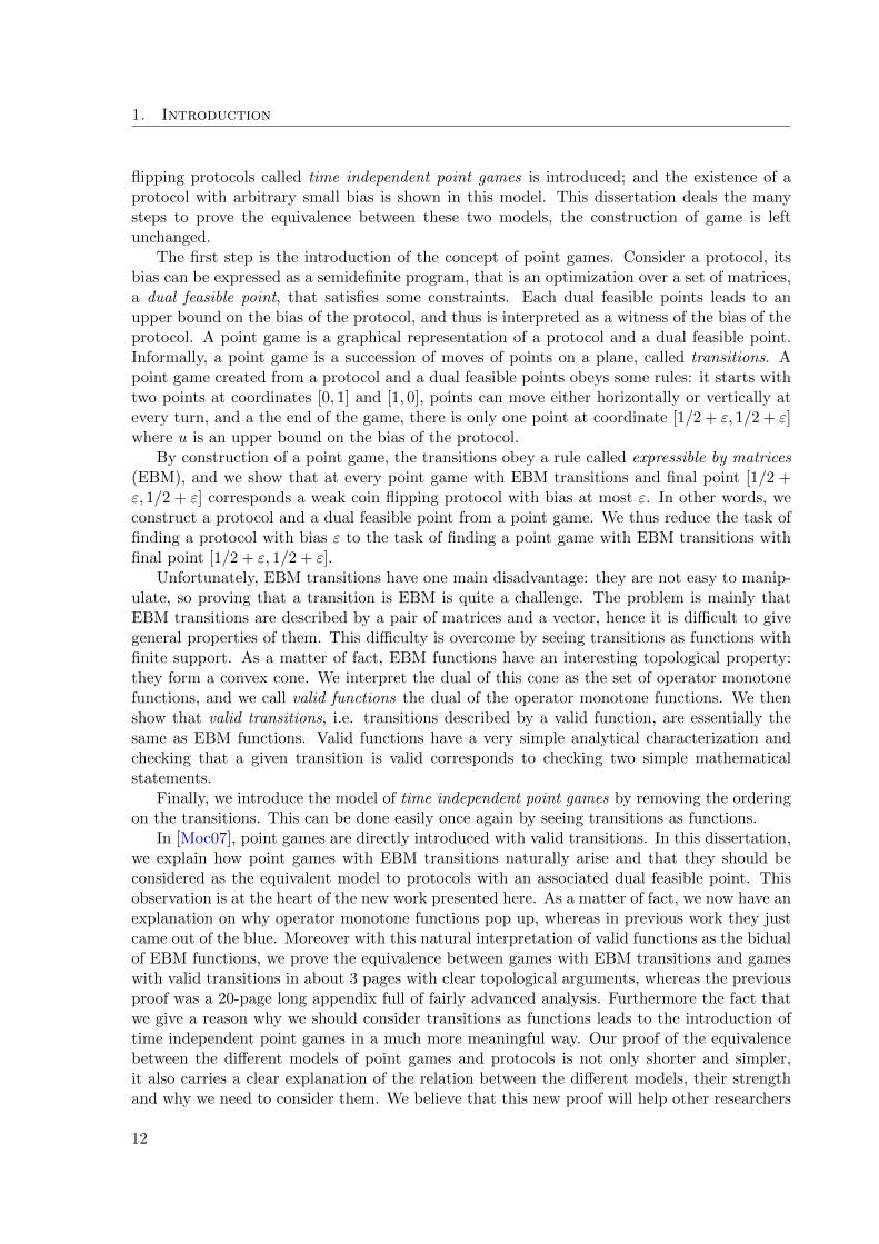
flipping protocols called time independent point games is introduced; and the existence of aprotocol with arbitrary small bias is shown in this model. This dissertation deals the manysteps to prove the equivalence between these two models, the construction of game is leftunchanged.

The first step is the introduction of the concept of point games. Consider a protocol, itsbias can be expressed as a semidefinite program, that is an optimization over a set of matrices,a dual feasible point, that satisfies some constraints. Each dual feasible points leads to anupper bound on the bias of the protocol, and thus is interpreted as a witness of the bias of theprotocol. A point game is a graphical representation of a protocol and a dual feasible point.Informally, a point game is a succession of moves of points on a plane, called transitions. Apoint game created from a protocol and a dual feasible points obeys some rules: it starts withtwo points at coordinates [0, 1] and [1, 0], points can move either horizontally or vertically atevery turn, and a the end of the game, there is only one point at coordinate [1/2 + ε, 1/2 + ε]where u is an upper bound on the bias of the protocol.

By construction of a point game, the transitions obey a rule called expressible by matrices(EBM), and we show that at every point game with EBM transitions and final point [1/2 +ε, 1/2 + ε] corresponds a weak coin flipping protocol with bias at most ε. In other words, weconstruct a protocol and a dual feasible point from a point game. We thus reduce the task offinding a protocol with bias ε to the task of finding a point game with EBM transitions withfinal point [1/2 + ε, 1/2 + ε].

Unfortunately, EBM transitions have one main disadvantage: they are not easy to manip-ulate, so proving that a transition is EBM is quite a challenge. The problem is mainly thatEBM transitions are described by a pair of matrices and a vector, hence it is difficult to givegeneral properties of them. This difficulty is overcome by seeing transitions as functions withfinite support. As a matter of fact, EBM functions have an interesting topological property:they form a convex cone. We interpret the dual of this cone as the set of operator monotonefunctions, and we call valid functions the dual of the operator monotone functions. We thenshow that valid transitions, i.e. transitions described by a valid function, are essentially thesame as EBM functions. Valid functions have a very simple analytical characterization andchecking that a given transition is valid corresponds to checking two simple mathematicalstatements.

Finally, we introduce the model of time independent point games by removing the orderingon the transitions. This can be done easily once again by seeing transitions as functions.

In [Moc07], point games are directly introduced with valid transitions. In this dissertation,we explain how point games with EBM transitions naturally arise and that they should beconsidered as the equivalent model to protocols with an associated dual feasible point. Thisobservation is at the heart of the new work presented here. As a matter of fact, we now have anexplanation on why operator monotone functions pop up, whereas in previous work they justcame out of the blue. Moreover with this natural interpretation of valid functions as the bidualof EBM functions, we prove the equivalence between games with EBM transitions and gameswith valid transitions in about 3 pages with clear topological arguments, whereas the previousproof was a 20-page long appendix full of fairly advanced analysis. Furthermore the fact thatwe give a reason why we should consider transitions as functions leads to the introduction oftime independent point games in a much more meaningful way. Our proof of the equivalencebetween the different models of point games and protocols is not only shorter and simpler,it also carries a clear explanation of the relation between the different models, their strengthand why we need to consider them. We believe that this new proof will help other researchers

12

1.4. Lower bounds for quantum query complexity

understand the ideas behind Mochon’s result.

For the sake of completeness, Appendix C presents Carlos Mochon’s construction of a pointgame achieving an arbitrarily small bias.

This work is a collaboration with Dorit Aharonov, Andre Chailloux, Maor Ganz, andIordanis Kerenidis [ACG+11].

1.4 Lower bounds for quantum query complexity

The query complexity model is also an instance of two-player quantum interaction, where thealgorithm aims to compute a function f on a input x accessible only via queries to the oracle.In this dissertation, we generalize this model by considering algorithms that create a quantumstate |ψx〉.

Algorithm OracleQueries

x

f(x) or |ψx〉

There are two main families of methods to prove lower bounds on the quantum querycomplexity: the adversary methods and the polynomial method. These methods are used toprove lower bounds for computing only a single instance of a function. A related problem ishow the number of queries scales if one wants to compute k independent instances of the samefunction, and will see how to answer that question.

1.4.1 Direct sum and product theorems

The question of the resources needed to compute k instances is interesting and has a very prac-tical importance, for instance for computers that perform very repetitive tasks like web serversthat query their database. For example, in order to decrease the load of the database server,queries from independent and simultaneous users could be combined in smart ways. Roughlyspeaking, direct sum and products theorems are impossibility results on these strategies.

A function is said to obey a direct sum theorem if computing k independent instancesrequires at least Ω(k) times the amount of resources needed for one instance. In general theresources can be time, memory, communication or queries. In this dissertation, we are focusingour study on the latter. Assume that a problem needs T queries to be solved with successprobability σ, then by performing the algorithm k times in parallel, hence using kT queries,the success probability is σk and thus decreases exponentially in k. A direct sum theoremleave the possibility that the success probability could decrease slower than exponentially, andthus there may be some gain to combine the queries. If this is not the case, the function obeysa strong direct product theorem (SDPT), that is the best strategy to compute k independentinstances of the function is simply to repeat the algorithm k times.

There was a plethora of results concerning strong direct product theorems for query com-plexity in 2011! Andrew Drucker showed that the randomized query complexity of any functionobeys a SDPT [Dru11]. Troy Lee and Jeremie Roland using totally different techniques proved

13

1. Introduction

the same result for quantum query complexity [LR11]. Alexander Sherstov proved directproduct for quantum communication complexity and that the polynomial method, a methodto prove lower bounds in the quantum query complexity model, also satisfies a strong directproduct theorem [She11].

1.4.2 Adversaries

The basic idea behind the quantum adversary method and its variations is to define a progressfunction that monotonically changes from an initial value (before any query) to a final value(after the last query), when the algorithm is ready to tell its outcome. The progress functionhas one main property: its value changes only when the oracle is queried. Then, a lower boundon the quantum query complexity of the problem can be obtained by bounding the amount ofprogress done by one query.

Original additive The first adversary method was introduced by Ambainis [Amb00] and wewill refer to it has the original adversary method as a generalization of the “hybrid argu-ment” [BBBV97]. Other adversary methods that are variations on the same principle weresubsequently proposed [HNS08, Amb06, BS04, LM08], but were later proved to be all equiva-lent [SS06]. They all rely on optimizing an adversary matrix Γ assigning non-negative weightsΓxy to different pairs of inputs (x, y) to the problem. Consider two inputs x and y such thatf(x) 6= f(y) and an algorithm computing the function f . The quantum states correspondingto x and y gradually diverge at each step of the algorithm towards their final value f(x) andf(y), i.e. their scalar product decreases. The progress function is defined as the measurementof this divergence as the weighted average of this scalar products, thus a high weight shouldbe put on pairs of functions hard to distinguish.

It was known that this method cannot always be used to prove tight lower bounds on anyproblems, since it is limited by the so-called “certificate complexity barrier” [Zha05, SS06],that is ADV(f) ≤

√C0(f)C1(f) where ADV(f) denotes the best lower bound proved by the

original adversary, and Cb(f) denotes the certificate complexity of f for f(x) = b. Let usconsider the case of the Element Distinctness problem: given a string of length N , areall the letters of the string distinct? For this problem, the original adversary method cannotprove lower bounds better than Ω(N1/2), since the certificate for a negative instance is a pairof positions of two identical letters, and the one for positive instance is the string itself.

General additive method While originally this method only considered non-negative weights,Høyer, Lee and Spalek later showed that negative weights also lead to a lower bound, whichcan actually be stronger in some cases [HLS07]. In particular, they exhibited an examplewhere this general additive method breaks the certificate complexity barrier. A series of work[FGG08, ACR+10, RS08, Rei11, LMR+11] culminated by showing that the general adversarybound is tight for the bounded-error quantum query complexity, thus showing the relevanceof the general additive adversary method.

The general additive adversary method also suffers from one main drawback: it cannotprove lower bounds for very small success probability and thus cannot be used to prove astrong direct product theorem for the quantum query complexity.

Multiplicative method To circumvent it, Robert Spalek introduced the multiplicative ad-versary method [Spa08] that generalizes some previous ad-hoc methods [Amb05, ASdW07].

14

1.4. Lower bounds for quantum query complexity

However, Spalek left unanswered the question of how multiplicative and additive methods re-late in the case of high success probability. Since the multiplicative adversary method canprove lower bounds for small success probability, Spalek has been able to prove that the boundobtained with this method obeys a strong direct product theorem, but he did not answer thekey question, wether or not the quantum query complexity does.

1.4.3 Polynomial method

Method The other main technique to prove lower bounds in the quantum query complexitymodel is the polynomial method introduced by Beals et al. [BBC+01]. Contrarily to theadversary method, the polynomial method can only prove lower bounds for Boolean functions,but has nevertheless achieved tremendous success. One of the most noticeable is, for sure,that the quantum query complexity of a total function cannot be less than q1/6 where q isthe classical query complexity. In other words, there is no exponential separation between therandomized and the quantum query complexity for total functions.

The polynomial method has also been used to prove lower bounds for specific problems,some of them are not very natural like the Ambainis function [Amb06], but it is currentlythe only method from which lower bounds for Element Distinctness and Collision werederived by Scott Aaronson and Yaoyun Shi [Aar02, Shi02, AS04]. Unfortunately, one issuewith those bounds proved by the polynomial method is that they are not very flexible, inthe sense that they cannot be adapted to prove lower bounds on natural variations of theseproblems such that k-Element Distinctness: given a string on some alphabet, is there aletter that appears at least k times?

Other impressive results range from Time-Space trade-offs [KSdW07], lower bounds forAbelian Hidden Subgroup [KNP07] to a strong direct product theorem for lower boundsobtained by the polynomial method [She11].

Relationship with the adversary methods Since the general additive adversary method istight for bounded-error quantum query complexity, it is known that the general additivemethod is stronger than the polynomial method. However an explicit reduction was unknownbefore the work presented in this dissertation.

It was also known that the polynomial method and the original adversary method were notcomparable. Indeed, Aaronson and Shi [AS04] were able to prove a Ω(N2/3) lower bound forElement Distinctness using the polynomial method which breaks the certificate complexitybarrier. On the other hand, it is known that the adversary method can sometimes give betterlower bounds than the polynomial method, in [Amb06] Ambainis exhibits a function withpolynomial degree d and adversary bound Ω(d1.3).

Other cases for which the original adversary bound is stronger than the polynomial boundcan be obtained by considering a weaker kind of oracles. Up to now, we have been consideringevaluation oracles (an oracle returns the value of a letter of the input). It is possible de definea weaker kind of oracles, the test oracles. A query to a test oracle is of the form “Is the i-thletter of x the letter a?” The lower bounds obtained by the polynomial method are the samein both cases. Using this observation, Pierre Phillips demonstrated that some problems areeasier in an “evaluation” model than in a “test” model, and thus that the original additive issometimes stronger than the polynomial method [Phi03].

15

1. Introduction

1.4.4 Quantum state generation problems

Even if one is interested in proving lower bounds for functions, it appears that studying a morecomplex model can actually be very useful. We study a generalization of the query model toinclude problems in which the input is still a black box, however, the output is no longer aclassical value but a quantum state.

An example of quantum state generation problem is Index Erasure. Here the inputis a string x of length N on an alphabet of size M with the promise that all the letters inthe string are different. The task is to prepare the quantum state 1√

N

∑Ni=1 |xi〉 using as few

queries to x as possible. The name “index erasure” came from the observation that while it isstraightforward to prepare the (at first glance perhaps similar looking) state 1√

N

∑Nx=1 |i〉|xi〉

using a single quatum query, it is quite challenging to forget (“erase”) the contents of the firstregister of this state which carries the input (“index”) of the letter.

In particular, quantum state generation has been considered in [AT03] to solve statisti-cal zero knowledge problems, one ultimate goal being to tackle Graph Isomorphism. Thequantum state generation problem resulting from the well-known reduction of Graph Iso-morphism to Index Erasure would be to generate the uniform superposition of all thepermutations of a rigid graph G:

|unif(G)〉 =1√n!

∑π∈Sn

|G permuted by π〉.

By coherently generating this state for two given graphs, one could then use the standardSWAP-test [BCWdW01] to check whether the two states are equal or orthogonal, and thereforedecide whether the graphs are isomorphic or not.

Such a method for solving Graph Isomorphism would be drastically different from morestandard approaches based on the reduction to the Hidden Subgroup problem, and mighttherefore provide a way around serious limitations of the coset state approach [HMR+06]. Asa matter of fact, Graph Isomorphism is quite a mystery in complexity. Like Factoring thisproblem is supposed to be NP-intermediate and reduces to an instance of Hidden Subgroup(however Factoring is an instance of Hidden Subgroup problem (HSP) on the cyclic group,but Graph Isomorphism is an instance of HSP on the symmetric group). But there is noknown polynomial time quantum algorithm for solving Graph Isomorphism.

1.4.5 Contributions

Quantum state generation The chief technical innovation is the extension of the generaladditive and the multiplicative adversary methods to quantum state generation problems inSection 5.3. This provides to us a newer view on the adversary method: instead of gettingfocused on pairs of inputs and their weights in the adversary matrix Γ, we understand thatthe eigenspaces of the adversary matrix Γ are the key. The progress function can now be seenas a function that monitors the progress done by an algorithm, by looking at which subspacesare supporting the internal state of the algorithm. As a by-product we give elementary andarguably more intuitive proofs of the additive and multiplicative methods, contrasting withsome rather technical proofs e.g. in [HLS07, Spa08]. This is a crucial observation to provethat the multiplicative method is stronger than both, the general additive method and thepolynomial method.

16

1.4. Lower bounds for quantum query complexity

Additive versus multiplicative To compare the strength of the additive and multiplicativeadversary methods, we introduce yet another flavor of adversary method which we call inter-mediate adversary method. This method provides lower bounds for quantum state generationproblems as well as for classical problems. The intermediate adversary method is a hybridiza-tion of the additive and multiplicative methods that uses “multiplicative” arguments in an“additive” setup: it is equivalent to the additive method for large success probability, butis also able to prove non-trivial lower-bounds for small success probability, overcoming theconcern [Spa08] that the additive adversary method might fail in this case.

In Section 5.4, we show that for any problem, the intermediate adversary bound lies betweenthe additive and multiplicative adversary bounds, answering Spalek’s open question about therelative power of these methods [Spa08]. By considering the Search problem for exponentiallysmall success probability in Chapter 6, we also conclude that the powers of the three methodsare strictly increasing, since the corresponding lower bounds scale differently as a function ofthe success probability in that regime.

Polynomial versus multiplicative In Section 5.6.4, we give an explicit reduction from thepolynomial method to the multiplicative adversary method. In order to do so, once again anintermediate method, the max-adversary method, yet another type of adversary method whosestrength lies between the polynomial method and the multiplicative method.

Directly inspired by the new interpretation of the progress function, this method does nothave an adversary matrix, but relies on a sequence of subspaces. The idea behind the max-adversary method is the following: define an ordered set of orthogonal subspaces (Sk : 0 ≤ k ≤K) such that any query can only transfer weight from subspace Sk to its immediate neighbors(i.e. Sk−1 and Sk+1) and that the initial state of the algorithm has only overlap on S0. Ifthe final state should have non-zero overlap on subspace ST in order to compute a function faccurately, this implies that T is a lower bound on the quantum query complexity of f .

The reduction from the max-adversary method to the multiplicative adversary methodfollows by considering the multiplicative adversary matrix Γ =

∑k λ

kΠk, where Πk is theprojector on Sk, and showing that the corresponding multiplicative adversary bound tends tothe max-adversary bound when λ → ∞. The reduction from the polynomial method to themax-adversary method is done by showing that we can choose Sk to be a subspace characterizedby polynomials of degree k; more precisely, we choose Sk to be the subspace spanned by thevectors of the Fourier basis of weight k. Let us also note that for any Boolean function, theadversary matrix leading to the same lower bound as the polynomial method does not dependon the function itself. This gives new insight on why the polynomial method does not alwaysprovide tight lower bounds.

If we restrict the progress function of the multiplicative adversary to increase by a factor atmost c per query, the multiplicative bound can be written as a semidefinite program [LR11].The best bound is then obtained by maximizing the value of this semidefinite program overall possible c. The reduction from the general additive to the multiplicative method showsthat the multiplicative bound degrades into the additive bound in the limit c → 1. In con-trast, we can obtain the max-adversary bound by taking the limit c → ∞, which thereforecompletes the picture of the relations between the different lower bound methods in quantumquery complexity (see Fig. 1.2), and shows in particular that all these methods reduce to themultiplicative adversary method.

Our reduction from the polynomial method to the multiplicative adversary method gives

17

1. Introduction

MADVε(f)

ADVε(f)

ADV±ε (f)

ADVmaxε (f)

ADVε(f) degε(f)6=°

¯

¯

¬

­

­®®

Figure 1.2: Relations between the different methods to prove lower bounds for quantum query com-plexity. An arrow from method A to method B implies that any lower bound that can be proved withA can also be proved with B (i.e., B is stronger than A). A solid blue arrow means that the reductionis constructive, i.e., we can obtain a witness for B from a witness for A. ¬ [HLS07] ­ Section 5.4 ®[Rei11, LMR+11] ¯ Section 5.6.4 ° [Zha05, SS06, AS04, Amb06]

new hope to prove lower bounds for problems related to Collision and Element Distinct-ness. Variations of this problem have practical applications in post quantum cryptography,see e.g. recent schemes for secure communications where the security is based on the hardnessof Element Distinctness-type problems [BHK+11].

This work was done in collaboration with Jeremie Roland [AMRR11, MR11].

Applications In Chapter 6 we present two applications of our results. First, we extend thestrong direct product theorem for the multiplicative adversary bound [Spa08] to quantum stategeneration problems (Section 6.1). Since we have clarified the relation between the additiveand multiplicative adversary methods, this also brings us closer to a similar theorem for theadditive adversary method. The most important consequence would be for the quantum querycomplexity of functions, which would therefore also satisfy a strong direct product theoremsince the additive adversary bound is tight in this case [LMR+11].

Secondly we focus on proving lower bounds using the adversary method. As it has beenpreviously pointed out many interesting problems have strong symmetries [Amb05, ASdW07,Spa08]. Section 6.2 shows how studying these symmetries helps to address the two maindifficulties of the usage the adversary method, namely, how to choose a good adversary matrixΓ and how to bound the progress done by one query. Following the automorphism principleof [HLS07], we define the automorphism group G of a problem (function evaluation or quantumstate generation). To do so, we reduce the adversary method from an algebraic problem to thestudy of the representations of the automorphism group G.

Finally, we validate our methodology by proving a lower bound of Ω(√N) for the quantum

query complexity of Index Erasure in Section 6.4 which is tight due to the matching upperbound based on Grover’s algorithm, therefore closing the open problem stated by Shi [Shi02].

18

1.4. Lower bounds for quantum query complexity

To the best of our knowledge, this is the first lower bound directly proved for the querycomplexity of a quantum state generation problem. The previous bound for Index Erasurewas Ω( 5

√N/ logN), proved by a classical reduction to the Set Equality problem [Mid04],

which consists in deciding whether two sets of size N are equal or disjoint or, equivalently,whether two injective functions over a domain of size N have equal or disjoint images.

19

2 Models of quantum information

This Chapter presents two models for encoding quantum information, the standard model usingdiscrete variables (DV), and the so-called continuous variables (CV) model. They share a lotof similarities but are expressed in two different mathematical frameworks: the DV model isin finite dimensional Hilbert spaces, whereas the CV model is in separable infinite dimensionalHilbert spaces.

2.1 Discrete variables

2.1.1 The Hilbert space Cn

The Hilbert space Cn is the vector space of n-dimensional complex column vectors with thecanonical inner product:(

ψ0

...ψn−1

),

(φ0...

φn−1

)7→

n−1∑i=0

ψ∗i φi = (ψ∗0, . . . , ψ∗n−1) ·

(φ0...

φn−1

),

where ψ∗i denotes the complex conjugate of ψi.In quantum mechanics, vectors and inner products are denoted following the Dirac notation.

A column vector ψ ∈ Cn is denoted by the ket |ψ〉 and the complex conjugate row vector ψ∗

by the bra 〈ψ|. As a consequence 〈ψ|φ〉 is the inner product between ψ and φ, |φ〉〈ψ| is theouter product, which is defined as the linear map: |χ〉 7→ 〈ψ|χ〉|φ〉. The projector onto theone-dimensional space spanned by |ψ〉 is thus denoted by |ψ〉〈ψ|.

For i = 0, 1, . . . , n− 1, we denote by |i〉 the vector (0 0 · · · 0 1 0 · · · 0)T where the “1” is inthe i-th position. We have 〈i|j〉 = δi,j , so |i〉, 0 ≤ i ≤ n− 1 is an orthonormal basis of Cn.This basis is called the computational basis of Cn. Thus a vector |ψ〉 can be decomposed onthe computation basis as |ψ〉 =

∑n−1i=0 αi|i〉 with complex probability amplitudes αi. We will

mostly consider spaces whose dimension is a power of 2, and in this case we often alternatebetween writing the index of a vector in the canonical basis in base 10 and in base 2, forexample we could have written the previous decomposition |ψ〉 =

∑x∈0,1logn αx|x〉.

Tensor products For 0 ≤ i ≤ m − 1 and 0 ≤ j ≤ n − 1, the tensor product between|i〉 and |j〉 is the vector |k〉 = |i〉 ⊗ |j〉 of the space Cm ⊗ Cn ∼= Cmn where k = 2ni + j,that is the concatenation of the binary expansion of i and j. For example |010〉 ⊗ |10〉 =|01010〉. The tensor product is extended by bilinearity to the full spaces Cm and Cn by:(∑

i αi|i〉)⊗ (∑

j βj |j〉) =∑

ij αiβj |i〉 ⊗ |j〉 =∑

ij αiβj |i, j〉.

Linear operators Given a Hilbert space H, we denote by L(H) the set of linear operatorson H. When H = Cn, the linear operators are the matrices of size n × n. The adjoint of anoperator A is the operator denoted by A† defined by being the unique linear operator suchthat for all |ψ〉 and |φ〉 of H, 〈A†ψ|φ〉 = 〈ψ|Aφ〉. A Hermitian operator A is its own adjointA = A†. In the case where H = Cn, A is a matrix of size n × n and A† is the transpose of

21

2. Models of quantum information

|1〉

|0〉

|ψ〉β

α

Figure 2.1: Representation (in red) of a qubit |ψ〉 = α|0〉 + β|1〉 when α and β are real values in theplane spanned by the basis vectors |0〉 and |1〉 (in blue).

the complex conjugate of A. Hermitian matrices with non-negative eigenvalues are positivesemidefinite. This defines a partial order on Hermitian matrices: A B if B − A is positivesemidefinite. In particular A 0 means that A is positive semidefinite.

2.1.2 States

A pure one-qubit state is a normalized vector of C2:

|ψ〉 = α|0〉+ β|1〉 with |α|2 + |β|2 = 1.

When α and β are real, it can be easily represented in a real plane, see Figure 2.1. This canbe generalized to states on n qubits:

Definition 2.1 (n-qubit pure state) A n-qubit pure state is a normalized vector of C2n, andcan be written |ψ〉 =

∑x∈0,1n αx|x〉 with

∑x∈0,1n |αx|

2 = 1.

Entanglement Note that all n-qubit pure states |ψ〉 cannot be written as the tensor productbetween two pure states |ψA〉 ⊗ |ψB〉, as for example the state |ψ〉 = 1√

2(|00〉 + |11〉). States

that are not product of two states are called entangled states, in opposition to product states.Entangled states play a crucial role in quantum computing, and we will use entangled statesas the primary resource all along this manuscript. For instance they naturally arise in crypto-graphic primitive, when the state shared by Alice and Bob exhibits correlations between them.This is the quantum generalization of shared randomness when Alice and Bob share a commonprobability distribution.

Mixed states Mixed states are a generalization of pure states and are probabilistic mixturesof pure states, that is a mixed state behaves like a state |ψi〉 with probability pi. A mixed

22

2.1. Discrete variables

state cannot be described by a unit vector anymore, and is represented by a trace-one positivesemidefinite matrix:

ρ =∑i

pi|ψi〉〈ψi|.

This matrix is called a density matrix, and this is how every quantum state is represented:

Definition 2.2 (Density matrix) A n-qubit state ρ is a positive semidefinite matrix of size2n × 2n such that tr(ρ) = 1.

The density matrix of a pure state |ψ〉 is ρ = |ψ〉〈ψ|, and we can easily characterize thedensity matrices of pure state:

Lemma 2.3 ρ is a pure state if and only if tr(ρ2) = 1.

Two different mixtures of pure states can lead to the same density matrix. For example,

one can check that 12 |ψa〉〈ψa|+

12 |ψb〉〈ψb| =

34 |0〉〈0|+

14 |1〉〈1| where |ψa〉 =

√34 |0〉+

√14 |1〉 and

|ψb〉 =√

34 |0〉 −

√14 |1〉. Nevertheless, the density matrix is the most complete description

of a quantum states from a physical point of view since two states with the same densitymatrix are indistinguishable. In particular, since a density matrix ρ in dimension 2 is alwaysdiagonalizable ρ = p|ϕ0〉〈ϕ0|+(1−p)|ϕ1〉〈ϕ1| for 0 ≤ p ≤ 1, any mixed state is indistinguishablefrom a mixture of two pure orthogonal states.

Classical mixture of quantum states and quantum superposition should not be confused.

For instance the state |+〉 = 1√2(|0〉+ |1〉) has a density matrix

(1/2 1/21/2 1/2

)whereas the mixture

12 |0〉〈0|+

12 |1〉〈1| has a density matrix

(1/2 00 1/2

).

Furthermore, we can remark that the states |ψ〉 and eiθ|ψ〉 have the same density matrix,so they are indistinguishable, which means that pure states are defined up to a phase.

Bipartite quantum states Mixed states can be viewed as “parts” of bigger states. Moreformally for a bipartite quantum state, that is a state on more than 1 qubit, the description ofeach possible subsystem is in general a mixed state. The density matrix of a subsystem fromthe density matrix of the global system is computed using the partial trace:

Definition 2.4 (Partial trace) Given two finite-dimensional Hilbert spaces HA and HB, thepartial trace over B is the linear mapping from L(HA ⊗HB) to L(HA) such that:

∀A ∈ L(HA), ∀B ∈ L(HB), trB(A⊗B) = tr(B)A.

The definition of the partial trace gives an explicit formulation only for product states A⊗B,but the linearity condition ensures that this mapping is perfectly defined for all operators inHA ⊗HB.

A mixed state can always been seen as a part of (possibly bigger) pure state:

Lemma 2.5 Let ρ be a n-qubit state. There exist a pure state m-qubit |ψ〉 such that ρ =trB(|ψ〉〈ψ|) with m ≤ 2n.

Such a pure state is called a purification of ρ. As a sketch of a proof, consider a mixedstate ρ written in its diagonal basis ρ =

∑i λi|ψi〉〈ψi| with λi ≥ 0 and

∑i λi = 1. Then

|ψ〉 =∑

i

√λi|ψi〉|ψi〉 is a purification of ρ.

23

2. Models of quantum information

A useful mathematical tool to analyze pure states and their partial trace is the Schmidtdecomposition:

Theorem 2.6 (Schmidt decomposition) Let |ψ〉 be a pure state in C2n ⊗ C2m. There exists anorthonormal basis |ui〉i of C2n and |vj〉j of C2m such that

|ψ〉 =

min(2n,2m)−1∑i=0

√pi|ui〉|vi〉,

with∑

i pi = 1.

Corollary 2.7 Consider a pure bipartite state |ψAB〉 ∈ C2n ⊗ C2n. Its Schmidt decompositionis |ψAB〉 =

∑2n−1i=0

√pi|ui〉|vi〉, thus the two mixed states ρA = trB|ψAB〉〈ψAB| and ρB =

trA|ψAB〉〈ψAB| have the same spectrum pii.

2.1.3 Operations

There are two kinds of operation in quantum mechanics: unitary operations, responsible forthe evolution of the quantum state, and measurements.

Definition 2.8 (Unitary matrix) A unitary matrix U acting on n qubits is a 2n × 2n matrixsuch that UU † = I.

A unitary operation U acts on a state ρ by: ρ 7→ UρU †, and a pure state |ψ〉 by: |ψ〉 7→ U |ψ〉.Quantum evolution shares similarities with stochastic evolution where the latter is modeledby stochastic matrices that preserve the 1-norm of probability distributions, whereas unitariespreserve their 2-norm. Moreover unitary matrices are always invertible, so every quantumcomputation is be reversible. Unlike classical computing it is not possible to compute functionsthat are non 1-to-1, but any function f : 0, 1n → 0, 1m can be converted into a unitaryoperation by appending qubits: |x〉|s〉 7→ |x〉|s⊕f(x)〉 is a reversible operation on m+n qubitswhere ⊕ is the bitwise XOR.

It is sometimes useful to consider a more general type of operation on a quantum state:

Definition 2.9 (CPTP map) Let H1 and H2 be two Hilbert spaces. The linear map E : L(H1)→L(H2) is completely positive trace preserving if for all k ≥ 1, for all positive semidefinitematrix A ∈ L(Ck) ⊗ L(H1), (IL(Ck) ⊗ E)(A) 0 and for all positive semidefinite matrixA ∈ L(H1), tr(E(A)) = tr(A).

However, this does not allow extra power to the model of quantum computation, since aCPTP map can be implemented by a unitary on a larger Hilbert space:

Lemma 2.10 (Stinespring’s dilation) Let E be a completely positive trace preserving map fromL(H1) to L(H2). There exist two Hilbert spaces H′1 and H′2 such that H1 ⊗ H′1 ∼= H2 ⊗ H′2,a unitary U acting on H1 ⊗ H′1 and a pure state |ϕ〉 ∈ H′1 such that ∀ρ ∈ L(H1), E(ρ) =trH′2 [U(ρ⊗ |ϕ〉〈ϕ|)U †].

Measurement The projective measurement of a n-qubit pure state is defined by an orthonor-mal basis |ψi〉 of C2n . After the measurement, a state |ψ〉 will be transformed into |ψi〉 withprobability |〈ψ|ψi〉|2. This phenomenon is referred to as the “collapse of the wave function”.

To extend this notion of measure to mixed states and partial measurements, a more generalframework is for analyzing measurements is the following one:

24

2.2. Continuous variables

Definition 2.11 (Positive Operator Valued Measure) A POVM is a finite set of Hermitianpositive semidefinite operators Ei such that

∑iEi = IH. The value of the measure of a state

ρ ∈ B(H) is “i” with probability tr[Eiρ], the resulting state is ρ′ = MiρMi

tr(MiρMi)with Mi = E

1/2i .

Physicists tend to use a slightly different and weaker point of view on measurement throughthe notion of observable

Definition 2.12 (Observable) Let M be a Hermitian matrix that can be diagonalized M =∑m∈sp(M) Π[m]. The value of the measurement of a state ρ using the observable M is “m”

with probability tr[Π[m]ρ] and the resulting state is ρ′ = Π[m]ρΠ[m]

tr(Π[m]ρΠ[m]).

2.2 Continuous variables

Although we will not deal with physical implementations of qubits in the manuscript, oneshould never forget a qubit is encoded into two levels of one degree of liberty of a quantumstate, like the spin of an electron or the polarization of a photon. However, quantum statescan usually have more degrees of liberty and many more levels in them. Indeed, all elementaryquantum systems cannot be represented by finite dimensional Hilbert spaces; e.g. position andmomentum of a particle or the amplitude of an electromagnetic (EM) field. Let us insist thata qubit is a density matrix on a 2-dimensional Hilbert space, and that this Hilbert space canbe embedded into another Hilbert space that can be infinite dimensional, see e.g. [GKP01].

The content of this section is to give a clear mathematical model for continuous variablesystems, their evolution and their measurements.

2.2.1 The Hilbert space L2(Rn)

Let us first recall the definition of the Hilbert space L2(R). This is the quotient space L2(R)/ ∼where ∼ is the equivalence relation: two function ψ and φ are equivalent if they are equal almosteverywhere, and L2(R) = φ : R → C |

∫R |φ(x)|2dx < ∞ is the set of square integrable

functions. For any functions φ, ψ in L2(R), the canonical inner product on this space is definedby:

(ψ, φ) =

∫Rψ∗(x)φ(x)dx,

where ψ∗ is the complex conjugate of ψ and the norm associated to it is:

‖φ‖ =√

(φ, φ).

When a tensor product structure is involved, we will abuse notations between the two isomor-phic spaces L2(Rn) ∼= L2(R)⊗n.

One of the main property of L2(Rn) is that it admits a countable basis:

Definition 2.13 (Hilbert basis, separable Hilbert space) A Hilbert basis of an infinite-dimensionalHilbert space H is a countable set of orthonormal vectors |vi〉, i ∈ N such that the spacespanned by finite linear combinations of |vi〉 is dense in H. A Hilbert space with a Hilbert basisis separable.

As a consequence, all separable Hilbert spaces are isomorphic, in particular L2 and `2, theHilbert space of square-summable sequences. In this manuscript, we will exclusivity use L2

25

2. Models of quantum information

since we want to capture the “continuous” nature of the electromagnetic field that is moreeasily expressed in this setting. From now on, all the Hilbert spaces we will use are separable.

The Dirac notation can also be used in this case. A function ψ of L2 is denoted by the ket|ψ〉 and the linear form φ ∈ L2 7→

∫Rn ψ

∗(x)φ(x)dx by |ψ〉. Please note that there are otherlinear form that the ones generated by functions of L2 such as Dirac distributions, but we willcarefully avoid to use them in this manuscript since it can lead to errors. The inner producton L2 between ψ and φ can thus be denoted by 〈ψ|φ〉 and the linear map |χ〉 7→ 〈ψ|χ〉|φ〉 by|φ〉〈ψ|.

Contrarily to the finite dimensional case, all linear operators on a infinite-dimensionalseparable Hilbert space H do not have an adjoint, but bounded linear operator do. A linearoperator A is bounded if for all vector |u〉 of H, the norm ‖A|u〉‖ is finite. This restriction willnot cause any problems, since unitaries and density operators are all bounded.

2.2.2 States

When dealing with infinite dimensional Hilbert spaces to study quantum systems, we are ina territory controlled by physicists, and the vocabulary is often dictated by historical andempirical reasons. For example an infinite dimensional state is often called a mode even ifits physical support is not a mode of an electromagnetic field, and conversely the observableassociated to the amplitude of an EM field is called position observable since the equationgoverning it is mathematically identical to the one of the position of a particle.

Definition 2.14 (CV states, modes) A pure n-mode state is a vector of L2(Rn) of norm 1.

Contrarily to the finite dimensional case, the trace and the partial trace of an operator donot necessarily exist, this is why we will restrict ourselves to a smaller class of operators forwhich we can define the trace:

Definition 2.15 (Compact, trace-class operators, trace) An operator A on a separable Hilbertspace H is said compact if it can be written

A =

∞∑n=0

λn|an〉〈bn|,

where the λn is a converging sequence of positive real numbers of limit 0, |an〉 and |bn〉 aretwo Hilbert basis of H. The operator is trace-class if

∞∑n=0

λn <∞.

The Banach space of trace-class operators on H is denoted T (H), and the trace is the linearfunctional from T (H) to R defined by:

tr(A) =

∞∑k=0

〈ψk|A|ψk〉,

where |ψk〉 is any Hilbert basis of H.

26

2.2. Continuous variables

Properties of trace-class operators

• If A and B are trace-class, then AB and BA are also trace-class.

• If A is trace-class, then A† is trace-class.

This definition of the trace is the correct notion since the usual properties of the trace formatrices are also true for operators of T (H): tr(AB) = tr(BA) and the trace does not dependof the choice of the basis. It is also straightforward to extend this definition to the partialtrace of trace-class operators:

Definition 2.16 (Partial trace) Given two separable Hilbert spaces HA and HB, the partialtrace over B is the linear mapping from T (HA ⊗HB) to T (HA) such that by:

∀A ∈ T (HA), B ∈ T (HB), trB(A⊗B) = tr(B)A.

A state with n modes will thus be represented by a density operator, the CV analog of thedensity matrix:

Definition 2.17 (n-mode state) A n-mode state ρ is a positive semidefinite trace-class operatorof L2(Rn) such that tr(ρ) = 1. The density operator ρ of pure state |ψ〉 is ρ = |ψ〉〈ψ|.Lemma 2.18 A state ρ is pure if and only if tr(ρ2) = 1.

Since density operators are compact Hermitian operators, we can diagonalize them in avery similar manner than matrices: they have a discrete spectrum of real positive numbers:

Theorem 2.19 (Spectral Theorem) Let A be a compact positive semidefinite Hermitian operatoron L2. There exists a sequence λn of real positive numbers converging to 0, and a Hilbert basis|an〉 of L2 such that:

A =∑n

λn|an〉〈an|.

When dealing with continuous variable states, it is often easier to use a different formal-ism than the one introduced here, the phase space formalism which is briefly introduced inAppendix A. The special case of Gaussian states in phase space is the focus of Section 2.3.Nevertheless, some operations are more easily done in the state space using a Hilbert basis.The most famous Hilbert basis is probably the Fourier basis, but this basis will be of no use inthis work, instead we will the Fock basis which is of terrific importance, since the most usefulGaussian states can be easily expressed in it.

Definition 2.20 (Fock states) For all integer k ∈ N, we define the k-th Fock state |k〉 by thefunction

|k〉 : x 7→(π1/22kk!

)− 12Hk(x)e−

x2

2 ,

where Hk is the k-th Hermite polynomial defined by: Hk : x 7→ (−1)kex2 dk

dxke−x

2.

Theorem 2.21 (Fock Basis) The set of Fock states is a Hilbert basis of L2(R).

This definition can seem a bit arid, but those states are the eigenstates of the harmonicoscillator, one of the most basic model in quantum mechanics. Moreover the state |k〉 repre-sents number state of exactly k coherent photons produced by a laser. In realistic settings,

27

2. Models of quantum information

lasers produce Gaussian states that are superposition of Fock states according to a Poissondistribution. We will decompose some of the Gaussian states in the Fock basis in Section 2.3.2.

When dealing with n modes, we use bold notation to denote a n-index i = i1 . . . in ∈ Nn.The set |i〉, i ∈ Nn defined by |i〉 = |i1〉 · · · |in〉 will be also called the Fock basis of L2(Rn).

2.2.3 Operations

According to the axioms of quantum mechanics, the states will evolve with unitary operations:

Definition 2.22 (Unitary operator) An operator U acting a Hilbert space H is unitary if UU † =U †U = IH.

We emphasize that contrary to the finite case, the existence of a right inverse does not implythe existence of a left inverse. For example, given a Hilbert basis |φk〉, the shift operatorS : |φk〉 7→ |φk+1〉 has a left inverse, but no right inverse.

Measurements on the other hand are far more complex with continuous variables andexpressed in the formalism of “observables”. An observable is simply an Hermitian operatorand can have discrete or continuous spectrum, being bounded or not. We do not introduce thegeneral case here but we give a straightforward generalization of Definition 2.12

Definition 2.23 (Observable with discrete spectrum) A Hermitian operator M is an observablewith discrete spectrum if there exists a countable set of projectors Π[m] such that M =∑

mmΠ[m]. Measuring a state ρ with M will result to outcome “m” with probability tr[Π[m]ρ].

The resulting state is ρ′ = Π[m]ρΠ[m]

tr[Π[m]ρΠ[m]].

The other fundamental case, that has no discrete equivalent, comes from using an observ-able with a fully continuous spectrum. Phase space is the best formalism to describe such ameasurement, but we nonetheless give the definition of one of them, the position measurement:

Definition 2.24 (Position observable) Let ρ =∑

m,n ρm,n|m〉〈n| be a one-mode state. Theoutcome of measuring ρ with the position observable and error ∆ is x0 with probability

∑m,n

ρm,n

∫ x0+∆

x0−∆n(x)m(x)dx,

where m and n are the m-th and n-th Fock functions.

We did not specify the resulting state after the measurement since we will never considerit in this dissertation, and in practical implementations this measurement is destructive: thelight is absorbed by the measurement apparatus.

In the limit ∆→ 0, this measurement appears to be fully continuous, thus giving the namecontinuous variables to quantum state expressed in infinite dimensional Hilbert spaces. In thelaboratory, this measure can be perform efficiently for very small ∆, which is why this measureis the very root of considering CV state as a resource in quantum computing. Indeed whenconsidering light pulses, this correspond to measuring their amplitude.

2.3 Gaussian model

In this dissertation, we restrict ourselves to a class of continuous variables states and operationscalled Gaussian states and Gaussian operations. In this Section, we introduce their formalism

28

2.3. Gaussian model

based on covariance and symplectic matrices. This is quite different from the previous sectionssince the states and operations are considered from a different point of view, called the phasespace and not from the Hilbert space L2(Rn) which is called the state space. We present afirst connexion between the two formalisms by giving the decomposition of some of the usualGaussian states in the Fock basis. The formal construction of the phase space and why statesare described by covariance matrices is postponed to Appendix A since this is not needed forunderstanding the results presented in this manuscript.

2.3.1 Covariance and symplectic matrices

In this Section, we introduce the two mathematical objects at the heart of the study of Gaussianstates and operations, covariance and symplectic matrices.

Definition 2.25 (Covariance matrix) A covariance matrix is a 2n× 2n real symmetric positivesemi-definite matrix.

Definition 2.26 (Symplectic matrix) A symplectic matrix is a 2n×2n real matrix that satisfies

SΩST = Ω,

where Ω is the block diagonal matrix Ω =

(0 1−1 0

)⊕n.

Properties of symplectic matrices:

• If S and T are symplectic, ST and TS are also symplectic;

• If S is symplectic, S is invertible and S−1 = −ΩSTΩ;

• detS = 1;

• Ω is symplectic and Ω−1 = ΩT = −Ω.

Covariance matrices can be “diagonalized” by the action of symplectic matrices. Of course,this is not a diagonalization in the usual sense since symplectic matrices are not unitary ingeneral.

Theorem 2.27 (Williamson’s decomposition [SCS99]) Let γ be a covariance matrix. Thereexists a symplectic matrix S and a diagonal matrix D = diag(ν1, ν1, ν2, ν2 . . . , νn, νn) suchthat:

νi ≥ 0 and γ = SDST .

The νi are called the symplectic values of γ and are independent of S up to a permutation.

2.3.2 Gaussian states

Definitions Let us now make the connection between covariance matrices and Gaussian states.

Definition 2.28 (Gaussian state) An n-mode Gaussian state is described by a 2n-dimensionalreal vector µ called the mean vector and 2n × 2n covariance matrix γ with the additionalconstraint γ + iΩ 0.

29

2. Models of quantum information

As a consequence a Gaussian state is described by less than n2 real parameters. This isin strong contrast with general CV states for which each mode can require an infinite numberof parameters. It is also noteworthy that the set of Gaussian states does not have a linearstructure: the superposition of Gaussian states is in general not a Gaussian state.

Informally, covariance matrices play a role quite similar to the one played by density opera-tors in state space, and the symplectic values the one of eigenvalues. The condition γ+ iΩ 0is in fact a condition on the symplectic values implies that all the symplectic values are at leastone. To continue further this analogy, there is a characterization of pure Gaussian states quitesimilar to Lemma 2.18 and Lemma 2.3:

Lemma 2.29 (Symplectic values of a Gaussian state) The symplectic values of a Gaussian stateare greater or equal to 1. They are all equal to one if and only if the state is pure.

Some Gaussian states Some Gaussian states play extremely important roles, such as thethermal states which are mixed Gaussian states and can be compared to totally mixed statesof one qubit, and the two-mode squeezed states that are the Gaussian equivalent of EPR pairson two qubits.

Definition 2.30 (Coherent and thermal states)

• A thermal state of variance ν is a one-mode state with µ = (0, 0) and γ = νI with ν ≥ 1.

• A coherent state |α〉 is a pure one-mode state with µ = 1√2(<(α), Im(α)) and γ = I2.

• The vacuum state is the Fock state |0〉. It is a special case of coherent state (centered inµ = (0, 0)) and thermal state of variance ν = 1.

One other state plays a central role in the study of Gaussian states, the two-mode squeezedstate, since it is the Gaussian equivalent of the EPR pair. A two-mode squeezed state ofsqueezing r is the Gaussian state of mean vector µ = (0, 0, 0, 0) and covariance matrix:

ν 0√ν2 − 1 0

0 ν 0 −√ν2 − 1√

ν2 − 1 0 ν 0

0 −√ν2 − 1 0 ν

with the variance ν = cosh(2r).

The partial trace of Gaussian states can also be expressed in a very simple way in phasespace

Theorem 2.31 (Partial trace of a Gaussian state) Let ρAB be a bipartite Gaussian state with

n+m modes. It is described by a 2n× 2m covariance matrix γAB =

(γA CCT γB

)and a mean

vector µ = µA ⊕ µB ∈ R2n+2m, then the state ρA = trB(ρAB) is described by the covariancematrix γA and the mean vector µA.

This proves that the mixed state obtained by tracing out one of the mode of a two-modesqueezed state of squeezing r is a thermal state of variance ν = cosh(2r), thus making theconnection with totally mixed states.

30

2.3. Gaussian model

Relation with the Fock basis Although it is difficult to write any Gaussian state in the Fockbasis, we know the expansion of these examples. A coherent state |α〉 can be written as:

|α〉 = e−|α|22

∞∑i=0

αi√i!|i〉,

a two-mode squeezed state with squeezing r as:

|TMS(r)〉 = (cosh(r))−1/2∑

tanh(r)i|i〉|i〉, (2.1)

and as a consequence a thermal state of variance ν = cosh(2r) as:

ρth(ν) =

∞∑i=0

(ν − 1

ν + 1

)i|i〉〈i|. (2.2)

2.3.3 Gaussian operations

Definition 2.32 (Gaussian operation) A Gaussian operation is a linear map that maps anyGaussian state into a Gaussian state.

This definition is not quite useful since it does not give a characterization of Gaussianoperations in phase space. For unitary operation, there exist a simple characterization inphase space [Fiu01]:

Lemma 2.33 The set of Gaussian unitaries acting on n modes is in one-to-one correspondencewith the set (S, d) for all 2n× 2n symplectic matrix S and real vector d of R2n.

In Appendix A, we explain how a Gaussian unitary acts on any CV state in phase space.This has a very simple formulation when considering only Gaussian states:

Corollary 2.34 Let ρ be a Gaussian state with covariance matrix γ and mean vector µ anda Gaussian unitary U described in phase space by a symplectic matrix S and a displacementvector d, then the action of U in phase space is:

(γ, µ) 7→ (SγST , Sµ+ d).

Normal mode decomposition One of the main mathematical tool for analyzing bipartiteGaussian states, is the normal mode decomposition [BR03], which is the Gaussian equivalentof the Schmidt decomposition:

Theorem 2.35 (Normal form) Let γAB be the covariance matrix of a pure bipartite Gaussianstate. γAB can be decomposed:

(SA ⊕ SB)γAB(STA ⊕ STB) =

(D

√D2 − IZn√

D2 − IZn D

)(2.3)

where D is the diagonal matrix of the symplectic values of γA, Zn =(

1 00 −1

)⊕n, and SA and

SB are two symplectic matrix acting respectively on Alice’s and Bob’s modes.

Physically, this theorem states if Alice and Bob share n modes of a pure Gaussian state, byapplying local Gaussian unitary operations only, they can transfer it into n shared two-modesqueezed states.

31

2. Models of quantum information

2.4 Norms and distinguishability

This section introduces different norms that are used in this manuscript and focuses on howto use them for distinguishing states. Distinguishability between states has been extensivelystudied by Christopher A. Fuchs [Fuc96]. All the notions defined here are valid for separableHilbert spaces, finite or infinite dimensional, this is why we omit to specify the dimensions.

First, the measure induced by the scalar product on the linear operator is the operatornorm, sometimes called the spectral norm:

Definition 2.36 (Operator norm) Let A ∈ B(H). The operator norm of A is defined by:

‖A‖ = sup|v〉

‖A|v〉‖‖|v〉‖

.

This norm appears quite naturally in many derivations, but does not have an operationalmeaning for distinguishability. This is why the trace norm is used:

Definition 2.37 (Trace norm) Let A ∈ T (H), its trace norm is:

‖A‖tr = tr√A†A.

The trace norm gives the optimal probability p of distinguishing two equiprobable states ρand σ:

p =1

2+

1

4‖ρ− σ‖tr .

It is sometimes easier to define the trace distance between two states ρ and σ by

Dtr(ρ, σ) =1

2‖ρ− σ‖tr .

The constant 1/2 is chosen so that two orthogonal states have distance 1.When dealing with trace norm, we will use the following lemmata:

Lemma 2.38 (Holder’s inequality) For any A,B ∈ T (H), we have ‖AB‖tr ≤ ‖A‖F · ‖B‖F,

where ‖A‖F is the Frobenius norm defined by: ‖A‖F =√

tr(A†A).

Lemma 2.39 For any A,B ∈ T (H), we have tr(AB) ≤ ‖A‖ · ‖B‖tr.

Lemma 2.40 For any A,B Hermitian positive definite, we have∥∥∥A 1

2BA12

∥∥∥ =∥∥∥A 1

2B12

∥∥∥2=∥∥∥B 1

2A12

∥∥∥2, and

∥∥∥A 12B−

12

∥∥∥2= minc such that A cB.

The other quantity that we will often use when dealing with distinguishability of two statesis the fidelity.

Definition 2.41 (Fidelity) The fidelity between to quantum states ρ and σ is defined by:

F(ρ, σ) = tr√√

ρσ√ρ.

When dealing with pure states, the fidelity is sometimes called the “transition probability”(see e.g. [Uhl76]), the term fidelity seems to come from an article by Josza [Joz94], but heuses the square of this quantity, since it can be understood as a probability. However in their

32

2.4. Norms and distinguishability

book, Nielsen and Chuang [NC04] used this definition and has been used since in the computerscience community. Physicists tend to use the original definition.1

The fidelity and the trace norm have some useful properties in common: they are symmetric,invariant under the action of unitary operations, and simpler expression for pure states ρ =|ψ〉〈ψ| and σ = |φ〉〈φ| can be derived:

F(ρ, σ) = |〈ψ|φ〉| and ‖ρ− σ‖tr = 2√

1− |〈ψ|φ〉|.

Fidelity and trace distance also capture the fact that it is more difficult to distinguish mixedstates than their purifications. Let |ψ〉 and |φ〉 be two bipartite pure states in T (HA ⊗ HB)and ρA = trB(|ψ〉〈ψ|) and σA = trB(|φ〉〈φ|) their partial traces over HB then:

F(ρA, σA) ≥ F(|ψ〉〈ψ|, |φ〉〈φ|) and Dtr(ρA, σA) ≤ Dtr(|ψ〉〈ψ|, |φ〉〈φ|).

The first inequality can always be saturated, this is the content of Uhlmann’s theorem:

Theorem 2.42 (Uhlmann’s theorem) Let ρ and σ be two quantum states and |ψ〉 a purificationof ρ. Then

F(ρ, σ) = max|ϕ〉|〈ψ|ϕ〉| ,

where the maximum is taken over all purifications |ϕ〉 of σ.

There is a first proof of the theorem in [Uhl76] for discrete variables as well as for continuousvariables. This proof is difficult to read and is non constructive. Richard Jozsa gave a simpleconstructive proof for the discrete variable case [Joz94]. To the best of our knowledge there isno continuous variable equivalent.

As written above, fidelity and trace distance have a strong relationship. It is possible tohave a formal statement:

Lemma 2.43 Let ρ and σ two quantum states. Then

1−F(ρ, σ) ≤ Dtr(ρ, σ) ≤√

1−F(ρ, σ)2.

Quantum Chernoff bound and Bhattacharyya bound The quantum Chernoff bound [ACMT+07]is an upper bound on the minimal error done when distinguishing between two states whenthere are k copies of them and reads,

Perr ≤1

2

(inf

0<s<1tr[ρsσ1−s])k .

The Bhattacharyya bound [Kai67, PL08] is the special case s = 1/2 of the Chernoff bound. Inthis manuscript, we will only consider that bound when k = 1, and by writing Perr in term oftrace distance, we get:

Lemma 2.44 (Bhattacharyya bound) For all state ρ and σ:

1−Dtr(ρ, σ) ≤ tr[√ρ√σ].

1and they are probably right, but the primary focus of this dissertation is mostly computer scientists whoare used to the definition introduced here.

33

2. Models of quantum information

2.5 Summary

In this Chapter, we gave a quick overview of the standard model of quantum computing in afinite-dimensional Hilbert space. We then extended it to continuous variables by consideringthe separable Hilbert space of square integrable functions. We underlined a few key differences,like the necessity to restrict ourselves to trace-class operators and the existence of “continuous”measurements.

We then focused on a subclass of CV states, called Gaussian states and their formalismcoming from an formalism in another space. Gaussian states that can be concisely describedby covariance matrices and Gaussian unitaries by symplectic matrices.

Let us summarize an informal connection between CV states in state space and Gaussianstates in phase space (for clarity the mean vector of Gaussian states is omitted)

n qubits n modes n Gaussian modes

Basis |x〉, x ∈ 0, 1n |i〉, i ∈ Nn no basis

State density matrix density operator covariance matrix

Size 2n × 2n infinite dimensional 2n× 2n

Eigenvalues∑2n

i=1 λi = 1, λi ≥ 0∑∞

i=1 λi = 1, λi ≥ 0 (ν1, ν1, ν2, ν2, · · · , νn, νn), νi ≥ 1

Unitary UU † = I UU † = U †U = I SΩST = Ω

Acts by ρ 7→ UρU † ρ 7→ UρU † γ 7→ SγST

We finally examined two different notions to quantify the distinguishability between twostates, the trace distance and the fidelity.

34

Part I

Cryptographic primitives

35

3 Gaussian quantum bit commitment

In this Chapter, we address quantum bit commitment protocols with continuous variables, andexplore whether such protocols may be found secure when both parties are restricted to useGaussian states and operations. We answer by the negative in Section 3.2. The main ingredientof the proof is the introduction of what we call intrinsic purifications that are introduced andstudied in the first Section.

At the heart of the impossibility proof of quantum bit commitment lies Uhlmann’s theorem(Theorem 2.42). For Gaussian quantum bit commitment, one would need a Gaussian versionof this theorem, namely that if two Gaussian states have a certain fidelity between them,then there are two Gaussian purifications of them with the same fidelity. We do not resolvethe question of stating if such theorem exists or not. As a matter of fact this question seemsextremely difficult to answer. However an approximate version of Uhlmann is sufficient to provethe no-go theorem. This is the strategy we are following in this Chapter. By relaxing slightlythe condition on the fidelity (we do not require that the fidelity of the purifications is exactlythe same than the mixed states, but close enough) we can construct Gaussian purifications.Our approach is even a bit more general and it is called intrinsic purifications.

Moreover, the use of intrinsic purifications instead of Uhlmann’s theorem allows us toprovide a constructive attack for any CV QBC protocol, whereas constructive attacks werepreviously known for finite dimensions only.

3.1 Intrinsic purifications

In this Chapter, A∗ (resp. AT ) denotes the complex conjugate (resp. the transpose) of anylinear operator A relatively to the Fock basis, defined as 〈i|A∗|j〉 = 〈i|A|j〉∗ and 〈i|AT |j〉 =〈j|A|i〉.

This section is devoted to prove the following theorem:

Theorem 3.1 For all n-mode state ρ there exists a 2n-mode purification |ψ(ρ)〉 of ρ such that:

• If ρ is a Gaussian state, then |ψ(ρ)〉 is also a Gaussian state,

• For every n-mode states ρ0 and ρ1, we have

1−√

1−F(ρ0, ρ1)2 ≤ F(|ψ(ρ0)〉〈ψ(ρ0)|, |ψ(ρ1)〉〈ψ(ρ1)|

).

The proof of the theorem is based on the notion of intrinsic purifications :

Definition 3.2 (Intrinsic purifications) Let ρ be an n-mode state and U be a diagonalization ofρ in the Fock basis, that is, U is a unitary operator such that 〈i|U †ρU |j〉 = pi δij, where δij isthe Kronecker delta. We then define an intrinsic purification |ψ〉 of ρ as

|ψ〉 = (U∗ ⊗ U)∑i

√pi|i〉|i〉.

37

3. Gaussian quantum bit commitment

Note that this purification is not uniquely defined, since there exist many diagonalizations ofa state, one can for example permute the ordering of the extra modes. Contrary to Uhlmann’spurifications for which it is not known wether they can be Gaussian for Gaussian states, wecan make a statement for intrinsic purifications:

Lemma 3.3 A Gaussian state has a Gaussian intrinsic purification.

Proof. By Williamson’s decomposition (Theorem 2.27), there exists a Gaussian unitary V suchthat V ρV † is a tensor product of n thermal states with variances νk, i.e. it can be written inthe Fock basis by tensoring Equation (2.2):

V ρV † =

n⊗k=1

∞∑i=0

(νk − 1

νk + 1

)i|i〉〈i| =

∑i∈Nk

pi|i〉〈i|,

with pi =∏nk=1

(νk−1νk+1

)ik. The unitary V is a diagonalization of ρ in the Fock basis.

Our goal is to show that the state

(V ∗ ⊗ V )∑i∈Nk

√pi|i〉|i〉

is Gaussian. First of all, according to Equation (2.1), the state∑

i∈Nk√pi|i〉|i〉 is a two-mode

squeezed state, so is Gaussian. Since V comes from the Williamson’s decomposition, V is alsoGaussian. The remaining piece is to prove that V ∗ is also Gaussian.

V ∗ is Gaussian Our strategy is look at the action on V ∗ on any Gaussian state, and showit corresponds to apply a certain symplectic matrix in phase space. Let us take an arbitraryn-mode Gaussian state τ with covariance matrix γτ and mean vector µτ . Let us also denotethe action of V by its symplectic matrix S and displacement vector d.

Define Zn =⊕n

k=1 Z =⊕n

k=1

(1 00 −1

). We want to show that applying V ∗ to τ is equivalent

to applying the symplectic matrix ZnSZn and the displacement Znd in phase space. First,remark that V ∗ = (V †)T and observe that V ∗τV ∗

†= (V τTV †)T .

The transposition relatively to the Fock basis has a simple expression in phase space forGaussian states [Sim00]: let σ be a Gaussian state with covariance matrix γσ and mean vectorµσ, then σT is a Gaussian state with covariance matrix ZnγσZn and mean vector Znµσ.

As a consequence, we get

τT is described by ZnγτZn and Znµτ

V τTV † is described by (SZn)γτ (ZnST ) and (SZn)µτ − d

V ∗τTV ∗†

is described by (ZnSZn)γτ (ZnSZn)T and (ZnSZn)µτ − Znd

Finally, we can conclude that (ZnSZn) is a symplectic matrix, even though Zn is not. Firstremark that ZnΩZn = −Ω, this leads us to:

(ZnSZn)Ω(ZnSZn)T = Ω.

38

3.1. Intrinsic purifications

Proof of Theorem 3.1. Let |ψ0〉 = (U∗0 ⊗U0)∑

i

√pi|i〉|i〉 be an intrinsic purification of ρ0 and

|ψ1〉 = (U∗1 ⊗ U1)∑

i

√qi|i〉|i〉 an intrinsic purification of ρ1. According to the Bhattacharyya

bound, we have

1−√

1−F(ρ0, ρ1)2 ≤ tr[√ρ0√ρ1],

so proving that

tr[√ρ0√ρ1] = F

(|ψ0〉〈ψ0|, |ψ1〉〈ψ1|

),

will conclude the proof. This equality is a property of intrinsic purifications.

Let us compute tr[√ρ0√ρ1] by taking the trace in the basis U0|k〉k:

tr[√ρ0√ρ1] = tr

U0

∑i

√pi|i〉〈i|U †0U1

∑j

√qj|j〉〈j|U †1

=∑i,j,k

√piqj (〈k|U †0)U0|i〉〈i|U †0U1|j〉〈j|U †1(U0|k〉)

=∑i,j

√piqj〈i|U †0U1|j〉〈j|U †1U0|i〉

=∑i,j

√piqj

∣∣∣〈i|U †0U1|j〉∣∣∣2

On the other hand:

F(|ψ0〉〈ψ0|, |ψ1〉〈ψ1|) = |〈ψ0|ψ1〉| =

∣∣∣∣∣∣∑i,j

√piqj 〈i|(U †0U1)∗|j〉〈i|U †0U1|j〉

∣∣∣∣∣∣ .According to the definition of the conjugation relatively to the Fock basis, we can concludethat

tr(√ρ0√ρ1) = F(|ψ0〉〈ψ0|, |ψ1〉〈ψ1|).

This proof holds for any intrinsic purifications, so in particular, if ρ0 and ρ1 are Gaussianstates, we can choose |ψ0〉 and |ψ1〉 to be Gaussian.

This theorem can also be reformulated using the trace distance instead of the fidelity:

Corollary 3.4 Given two n-mode states ρ0 and ρ1, there exist 2n-mode purifications |ψ0〉 of ρ0

and |ψ1〉 of ρ1 such that

Dtr(|ψ0〉〈ψ0|, |ψ1〉〈ψ1|) ≤√

2Dtr(ρ0, ρ1)

Moreover, if ρ0 and ρ1 are Gaussian states, so are their purifications |ψ0〉 and |ψ1〉.

39

3. Gaussian quantum bit commitment

Relation to Uhlmann’s theorem Our theorem is weaker than Uhlmann’s theorem whenstated in term of fidelity, but not in term of trace distance like in Corollary 3.4. However,our theorem has some advantages. First, our proof is constructive, whereas Uhlmann is notconstructive for CV states, and secondly, we are able to prove the Gaussianity of the purifi-cations, which was our first motivation. Another consequence that we reflected in the term“intrinsic” is that the purifications do not depend of both states ρ0 and ρ1. Thus we canpurified several close states, and guarantee that their purification will also be close:

Corollary 3.5 Let ρ1, . . . , ρt be t quantum states, and note di,j the trace distance between ρiand ρj. Then, for all i ∈ [t], there exists purification |ψi〉 of ρi such that

∀i, j ∈ [t],1

2‖|ψi〉〈ψi| − |ψj〉〈ψj |‖tr ≤

√2di,j .

Moreover, if ρ1, . . . , ρt are Gaussian states, the purifications are also Gaussian.

3.2 No-go theorem

In [May97, LC97] it has been shown that any QBC protocol, no matter how complicated arethe commit and the reveal phases is equivalent to a purified protocol in terms of security.

Definition 3.6 (Purified quantum bit commitment protocol) A purified quantum bit commitmentprotocol is an interactive protocol between two players Alice and Bob with two phases:

Commit phase Alice encodes her bit b into a pure bipartite state |ψb〉 and sends one half to Bob.At the end of the committing phase, Bob holds either ρ0 = trA|ψ0〉〈ψ0| or ρ1 = trA|ψ1〉〈ψ1|if Alice wants to commit to 0 or 1, respectively.

Reveal phase Alice sends the other half of |ψb〉.

The reduction is done by remarking that all the measurements happening during eachof the phases can be postponed to the end of the phases. When a full protocol involves onlyGaussian states and Gaussian operations, the purified protocol uses only Gaussian states. Thisis why we will consider that |ψb〉 are Gaussian states from now on, and we will show that sucha protocol is insecure, more precisely, we will show that the more concealing the protocol, themore powerful the cheating strategies.

Definition 3.7 (ε-concealing) The protocol is referred to as ε-concealing if ‖ρ0 − ρ1‖tr ≤ 2ε,which means that Bob cannot learn the value of b, except with probability ε

Definition 3.8 (δ-cheating strategy) In a δ-cheating strategy, Alice sends a state ρ] in thecommitting phase and then decides to follow a strategy leading to a final state of her choice,|ψ]0〉 or |ψ]1〉, so that Bob should not be able to distinguish this strategy from a honest strategy

with a probability greater than δ. This means that∥∥ρ] − ρb∥∥tr

≤ 2δ and∥∥∥ψ]b − ψb∥∥∥

tr≤ 2δ.

Now, let us state our main result:

Theorem 3.9 Given any ε-concealing Gaussian quantum bit commitment protocol to Bob,there exists a Gaussian

√2ε-cheating strategy for Alice.

Here, we will only consider the simple strategy in which ρ] = ρ0 and |ψ]0〉 = |ψ0〉. Thus,

|ψ]1〉 will correspond to Alice initially committing to a zero and then cheating so to make it

40

3.2. No-go theorem

a one. This is sufficient to prove the no-go theorem. Without loss of generality, we will alsoconsider that |ψb〉 are 2n-mode states and ρb are n-mode states.

3.2.1 Perfectly concealing protocols

Let us first have a look at what happens when the protocol is perfectly concealing. In this caseAlice has a perfect cheating strategy.

Lemma 3.10 Let |ψ0〉 and |ψ1〉 be 2n-mode Gaussian states such that trA|ψ0〉〈ψ0| = trA|ψ1〉〈ψ1|.There exists a Gaussian unitary operator U acting on n modes such that (U ⊗ I)|ψ0〉 = |ψ1〉,where I is the identity on n modes.

Proof. For b ∈ 0, 1, denote by µb =(µAbµBb

)and γb =

(γAb CbCTb γBb

)the covariance matrix and

mean vector of |ψb〉. According to Theorem 2.31, the condition trA|ψ0〉〈ψ0| = trA|ψ1〉〈ψ1|implies that µB0 = µB1 and γB0 = γB1 .

As a consequence, γA0 and γA1 have the same symplectic spectra, so that, by applying thenormal mode decomposition on γ0 and γ1 we know that there exist symplectic matrices Sjbsuch that:

γ0 = (SA0 ⊕ SB0 )γ0(SA0 ⊕ SB0 )t,

γ1 = (SA1 ⊕ SB1 )γ1(SA1 ⊕ SB1 )t,

where γb =(Db dd Db

). The matrices D0 and D1 are diagonal matrices with the same values. It

is then possible to choose the symplectic matrices Sjb such that D0 = D1, hence γ0 = γ1 = γ.The symplectic matrix S] = SA1 (SA0 )−1 ⊕ I2n transforms γ0 into γ1 by acting on Alice’s modesonly. Similarly, the displacement µ1 − S]µ0 transforms µ0 into µ1 by acting on Alice’s sideonly, which proves Lemma 3.10.

The previous theorem is exactly what we needed to prove the no-go theorem for perfectlyconcealing protocol. Alice’s cheating strategy is well-known, she first starts the protocol as shewanted to commit to 0, and she simply applies an appropriate unitary operation to her half of|ψb〉 between the two stages of the protocol if she decides to actually reveal 1. This allows herto convert |ψ0〉 into |ψ1〉. In the case of Gaussian QBC, Lemma 3.10 implies that this cheatingunitary is Gaussian.

3.2.2 ε-concealing protocols

We now investigate the realistic case where the protocol is not perfectly concealing, which willfinally lead us to the proof of Theorem 3.9. This proof is a reduction to the perfectly concealingcase that is done using intrinsic purifications. (See Figure 3.1)

Proof of Theorem 3.9. We want to find an explicit Gaussian√

2ε-cheating strategy for Aliceagainst a ε-concealing QBC protocol. In the first stage of the protocol, Alice creates the state|ψ0〉 and sends ρ0 to Bob. In the second stage, if Alice wants to reveal the bit 0, she sendsher half of |ψ0〉 to Bob, while if she decides to reveal the bit 1, she applies a Gaussian unitary

operation to her half of |ψ0〉, mapping it to |ψ]1〉, and then sends it to Bob.As a consequence of Lemma 3.1, there exist Gaussian purifications |φ0〉 of ρ0 and |φ1〉 of

ρ1 such that D(φ0, φ1) ≤√

2D(ρ0, ρ1). Moreover |ψ0〉 and |φ0〉 (resp. |ψ1〉 and |φ1〉) are

41

3. Gaussian quantum bit commitment

ρ0

|ψ0〉 |ψ]1〉|ψ]1〉

ρ1

|ψ1〉

trA trA trA

Dtr ≤ ε

Dtr ≤√

2εUA ⊗ IB

Figure 3.1: Overview of the proof. Square represent pure states, circles mixed state. The thick arrowdenotes the action of a unitary, the thin arrows tracing over Alice’s modes and the “snake” arrow isused to indicate the trace distance.

two Gaussian purifications of the same Gaussian state ρ0 (resp. ρ1), so that, according toLemma 3.10, there exists a Gaussian unitary operator U0 (resp. U1) such that (U0 ⊗ I)|ψ0〉 =

|φ0〉 (resp. (U1 ⊗ I)|ψ1〉 = |φ1〉). We note |ψ]1〉 = (U−11 U0 ⊗ I)|ψ0〉 = (U−1

1 ⊗ I)|φ0〉. By

unitary invariance of the trace distance, one has D(ψ]1, ψ1) = D(φ0, φ1). Thus, for ε-concealing

protocols, we have D(ψ]1, ψ1) ≤√

2ε.

We have thus obtained a stronger result than the standard no-go theorem since we haveshown that QBC remains impossible even if Alice and Bob are restricted to manipulate Gaus-sian states. Although Lemma 3.1 can be seen as a weak version of Uhlmann’s theorem in thesense that the intrinsic purification does not reach Uhlmann’s bound, it is sufficient here be-cause the quantities of interest in terms of guessing probability are not changed. Interestingly,the question of whether the purifications that saturate Uhlmann’s bound could both be chosenGaussian if the states are Gaussian is still open (although partial results in this direction havebeen obtained in [MM07]). Note also that we have an explicit construction of Alice’s cheatingpurifications for any CV QBC protocol, Gaussian or not. This is done by noting that theGaussian constraint can be relaxed in the proof of Lemma 3.1, and that Lemma 3.10 can bereplaced by the usual Schmidt decomposition.

3.3 Is physics informational?

With the emergence of computers, devices that manipulate information, the concept that“information is physical” got widely accepted and formulated in a series of papers by Landauer(e.g. see [Lan92]). But in recent years, this concept got challenged [Fuc01, Fuc02, Bra05]and presented as the Fuchs-Brassard conjecture. This conjecture tries to build the theory ofquantum physics on axioms from information theory instead of mechanics. Fuchs and Brassardconjectured that a theory in which key distribution is possible, and bit commitment is not is thetheory of quantum physics. It was later proven wrong, but Clifton et al. proved instead that theassumptions of no-signalling, no-broadcasting, and the impossibility of bit commitment makeit work within the framework of C∗-algebras [CBH03]. This is known as the CBH theorem.

One of the consequence of this strong no-go theorem is that it provides us with a natural andelegant counter-example of the Brassard and Fuchs conjecture as well as another input on theimportance of the C∗-algebra framework for CBH. As a matter of fact, consider the subset ofquantum mechanics where only Gaussian states and operations are allowed. As a result of our

42

3.4. Summary

no-go theorem, this Gaussian model forbids bit commitment while it allows unconditional secretkey distribution [RC09]. Interestingly, however, it is strictly included in quantum mechanicssince, for instance, Bell inequalities cannot be violated with Gaussian states and measurements.This is in contradiction with the Brassard-Fuchs conjecture. Furthermore, according to theCBH theorem [CBH03], quantum mechanics can be rederived from the sole assumptions thatsignaling, broadcasting, and bit commitment are impossible in Nature. While this idea is veryappealing, the Gaussian model again provides a natural counter-example to it.

The reason is that the CBH theorem actually requires the further assumption that thephysical description of Nature is done within the framework of C∗-algebras. Although Smolin[Smo05] and latter Spekkens [Spe07] found toy models compatible with CBH but distinct fromquantum mechanics, our counter-example is physically grounded.

3.4 Summary

We have addressed continuous variable quantum bit commitment, and have proved a strongversion of the standard no-go theorem in which Alice and Bob are restricted to Gaussian statesand operations. The main technical innovation of our proof is the introduction of “intrinsicpurifications”, for which we are able to prove a Gaussian analog to Uhlmann’s theorem.

43

4 Weak coin flipping

The Chapter aims at proving the existence of a way coin flipping protocol with arbitrarilysmall bias. More precisely we study a model called time independent point game. We showthat a time independent point game is equivalent to weak quantum coin flipping protocol anda witness on its bias. The construction of a time independent point game leading to a protocolwith arbitrarily small bias is presented in Appendix C. This construction is due to CarlosMochon [Moc07].

To prove the equivalence between a time independent point game and a protocol witha witness on its bias, we consider different intermediate models. Let us give a big pictureoverview of this Chapter. Section 4.1 formally introduces coin flipping protocols and theirbias. We also show that the optimal bias of a protocol can be expressed as a semidefiniteprogram, and that the points in this dual, dual feasible points are a witness on the bias ofthis protocol. In Section 4.2, we show the equivalence between a protocol and its dual feasiblepoints on one side, and a point game on the other side. Roughly speaking, a point game is agame composed of succession of moves of points, called transitions. The game ends when onlyone point remains. We prove that the coordinates of that final point gives an upper bound onthe cheating probabilities. Thus finding a point game with final point [1/2+ε, 1/2+ε] gives usthe existence of a quantum weak coin flipping protocol with bias ε. We consider 3 variations ofpoint games, namely point games with EBM transitions, valid transitions and time independentpoint games, each model being a little bit easier to manipulate mathematically. We summarizethe succession of models in Figure 4.1.

4.1 Coin flipping and semidefinite programming

4.1.1 Definitions

The role of the next couple of definitions is to formally define weak coin flipping protocols.

Definition 4.1 (Coin flipping protocol) For n even, an n-message coin flipping protocol betweentwo players, Alice and Bob, is described by:

Protocol

Dual

Feasible

Point

Point game

with EBM

transitions

Point game

with valid

transitions

Time

independent

point game

4.374.134.114.4

Figure 4.1: The succession of models we will consider. An arrow from model A to model B means thatproving the existence of an ε biased protocol in A implies the existence of an ε+ ε′ biased protocol inB (for all ε, ε′ > 0). The numbers on top of the arrows refer to the theorem proving that reduction.

45

4. Weak coin flipping

• Three Hilbert spaces A,B corresponding to Alice and Bob private workspaces (Bob doesnot have any access to A and Alice to B), and a message space M.

• An initial product state |ψ0〉 = |ψA,0〉 ⊗ |ψM,0〉 ⊗ |ψB,0〉 ∈ A ⊗M⊗B.

• A set of n unitaries U1, . . . , Un acting on A⊗M⊗ B, with Ui = UA,i ⊗ IB for i odd,and Ui = IA ⊗ UB,i for i even.

• A set of honest states |ψi〉, i ∈ [n] defined by |ψi〉 = UiUi−1 · · ·U1|ψ0〉.

• A set of n projectors E1, . . . , En acting on A⊗M⊗B, with Ei = EA,i ⊗ IB for i odd,and Ei = IA ⊗ EB,i for i even, such that Ei|ψi〉 = |ψi〉.

• Two final POVM

Π(0)A ,Π

(1)A

acting on A and

Π

(0)B ,Π

(1)B

acting on B.

The protocol is the following:

1. In the beginning, Alice holds |ψA,0〉|ψM,0〉 and Bob |ψB,0〉.

2. For i = 1 to n:— If i is odd, Alice applies Ui and measures the resulting state with the POVM Ei, I−Ei. On the first outcome, Alice sends the message qubits to Bob; on the second outcome,she ends the protocol by outputting “0”, i.e. Alice declares herself winner.— If i is even, Bob applies Ui and measures the resulting state with the POVM Ei, I−Ei. On the first outcome, Bob sends the message qubits to Alice; on the second outcome,he ends the protocol by outputting “1”, i.e. Bob declares himself winner.

3. Alice and Bob measure their part of the state with the final POVM and output the outcomeof their measurements. Alice wins on outcome “0” and Bob on outcome “1”.

Definition 4.2 (Weak coin flipping protocol with bias ε) A weak coin flipping protocol with biasε is a coin flipping protocol with the following properties:

• Correctness: When both players are honest, Alice and Bob’s outcomes are always thesame:Π

(0)A ⊗ IM ⊗Π

(1)B |ψn〉 = Π

(1)A ⊗ IM ⊗Π

(0)B |ψn〉 = 0.

• Balanced: When both players are honest, they win with probability 1/2:

PA =∥∥∥Π

(0)A ⊗ IM ⊗Π

(0)B |ψn〉

∥∥∥2= 1

2 and PB =∥∥∥Π

(1)A ⊗ IM ⊗Π

(1)B |ψn〉

∥∥∥2= 1

2 .

• ε biased: When Alice is honest, the probability that both players agree on Bob winningis P ∗B ≤ 1/2 + ε. And conversely, if Bob is honest, the probability that both players agreeon Alice winning is P ∗A ≤ 1/2 + ε.

The definition of a weak coin flipping protocol differs from the usual one in the fact thatwe added the projections Ei. The goal of these projections is to catch if the other playeris cheating since they do not change the honest states. Intuitively they can only decrease thebias compared to a protocol without them. This can be proved, but it is not necessary in ourcase since we will directly prove upper bounds on the cheating probabilities for this specifictype of protocols.

46

4.1. Coin flipping and semidefinite programming

4.1.2 Cheating probabilities as SDPs

The cheating probabilities P ∗A and P ∗B cannot be easily computed from the definitions above.Kitaev showed that they can be expressed as semidefinite programs (SDP) [Kit03] and a writtenproof can be found in [ABDR04].

Fix a weak coin flipping protocol, and assume that Alice is honest. We describe a semidefi-nite program with variables the states ρAM,i, ie. the states at round i after Bob’s workspace istraced out. The probability that Bob wins is the probability that Alice outputs “1” when apply-

ing the POVM

Π(0)A ,Π

(1)A

to her part of the final state, or equivalently tr((Π

(1)A ⊗IM)ρAM,n).

Since Alice is honest, the state in her workspace is not arbitrary, but rather satisfies someconstraints. In the beginning of the protocol, Alice held the state trM(ρAM,0) = |ψA,0〉〈ψA,0|.Moreover, the evolution of Alice’s state is only due to her own actions, namely trM(ρAM,i) =

trM(ρAM,i−1) if i is even and trM(ρAM,i) = trM(EiUiρAM,i−1U†i Ei) if i is odd. Bob’s cheating

probability is the maximum over all his strategies, i.e. over all states ρAM,i that satisfy theseconstraints.

The evolution of the states ρAM,i is not unitary due to the presence of the projections,

so they are not necessary normalized. However tr((Π(1)A ⊗ I)ρAM,n) represents the probability

that Alice and Bob agree on Bob winning when Alice is honest. If Bob got caught cheatingby the projections, Alice already declared herself the winner. The non-normalization of thestates ρAM,i reflects the probability that the protocol ended prematurely by one of the playersdeclaring oneself winner.

This reasoning leads to the following two semidefinite programs:

Theorem 4.3 (Primal)

P ∗B = max tr((Π(1)A ⊗ I)ρAM,n) over all ρAM,i satisfying the constraints:

• trM(ρAM,0) = trMB(|ψ0〉〈ψ0|) = |ψA,0〉〈ψA,0|,

• for i odd, trM(ρAM,i) = trM(EiUiρAM,i−1U†i Ei),

• for i even, trM(ρAM,i) = trM(ρAM,i−1).

P ∗A = max tr((I⊗Π(0)B )ρMB,n) over all ρBM,i satisfying the constraints:

• trM(ρMB,0) = trAM(|ψ0〉〈ψ0|) = |ψB,0〉〈ψB,0|,

• for i even trM(ρMB,i) = trM(EiUiρMB,i−1U†i Ei),

• for i odd trM(ρMB,i) = trM(ρMB,i−1).

4.1.3 Upper bounds on the cheating probabilities via the dual SDPs

We wish to prove upper bounds on the cheating probabilities P ∗A and P ∗B. Using the primal isnot suitable for this task since the cheating probabilities are defined by a maximization: anyset of matrices ρi that satisfies the constraints will lead to a lower bound on the cheatingprobabilities. We circumvent this problem by dualizing these SDPs.

Theorem 4.4 (Dual)P ∗B = min tr(ZA,0|ψA,0〉〈ψA,0|) over all ZA,i under the constraints:

¬ ∀i, ZA,i 0,

47

4. Weak coin flipping

­ for i odd, ZA,i−1 ⊗ IM U †A,iEA,i(ZA,i ⊗ IM)EA,iUA,i,

® for i even, ZA,i−1 = ZA,i,

¯ ZA,n = Π(1)A ,

P ∗A = min tr(ZB,0|ψB,0〉〈ψB,0|) over all ZB,i under the constraints:

¬ ∀i, ZB,i 0,

­ for i even IM ⊗ ZB,i−1 U †B,iEB,i(IM ⊗ ZB,i)EB,iUB,i,

® for i odd, ZB,i−1 = ZB,i,

¯ ZB,n = Π(0)B ,

A proof of this theorem can be found in [Kit03, ABDR04].Let us now add one more constraint on the above dual SDPs:

° ZA,0|ψA,0〉 = β|ψA,0〉 i.e. |ψA,0〉 is an eigenvector of ZA,0 with eigenvalue β > 0,

° ZB,0|ψB,0〉 = α|ψB,0〉 i.e. |ψB,0〉 is an eigenvector of ZB,0 with eigenvalue α > 0.

Definition 4.5 (Dual feasible point) A dual feasible point is a set of matrices Z0, . . . , Znwith Zi = ZA,i ⊗ IM ⊗ ZB,i satisfying conditions ¬ to °.

Notice that tr(ZA,0|ψA,0〉〈ψA,0|) = β and tr(ZB,0|ψB,0〉〈ψB,0|) = α and hence

Corollary 4.6 Let Zi be a dual feasible point of a protocol, then P ∗A ≤ α and P ∗B ≤ β.

Note that since we imposed a new constraint on the dual SDP, we may only be able to finda dual feasible point with larger values of α and β than before. However, we will show thatstill, we can make these values arbitrarily close to 1/2. Moreover, one can, in fact, show thatP ∗A = inf α and P ∗B = inf β where the infimum is taken over all dual feasible points (see proofin Appendix B); therefore, we have not changed the value of the optimization problem.

Every dual feasible point produces an upper bound on the cheating probability: P ∗A ≤ αand P ∗B ≤ β. This is the magic of duality, a maximization problem has been turned into aminimization one.

Notice also that the dualization reversed the time ordering of the protocol. The primalformulation sets constraints on the evolution of ρi to ρi+1 from a fixed state ρ0, whereas in thedual formulation the initial constraint is on Zn and the evolution concerns how Zi is relatedto Zi−1.

4.2 Point games

In the previous section we saw that we can upper bound the cheating probability of any weakcoin flipping protocol by looking at the dual SDP formulation of the protocol and by providing adual feasible point, namely a set of matrices Z0, . . . , Zn that satisfies a number of conditions.One can think of these matrices as a witness of the security of the protocol. However, it is notclear how to construct a protocol and, moreover, its dual feasible point.

Here, our goal is to find a graphical representation of a protocol together with its dualfeasible point that will be easier to manipulate. This is the reason we introduce point games.

48

4.2. Point games

In high level, a point game is a set of points on a 2-dimensional plane together with a sequenceof transitions between them. Instead of defining a point game at this point, we see how aprotocol with cheating probabilities P ∗A ≤ α and P ∗B ≤ β and a dual feasible point naturallygives rise to what we call a point game expressible by matrices with final point [β, α]. Moreimportantly, we will show that the reverse implication is also true and hence we will reducethe task of finding a coin flipping protocol and its dual feasible point to finding a point gameexpressible by matrices (EBM point game).

4.2.1 EBM point games

The dual SDP formulation of a coin flipping protocol enables us to calculate an upper boundon the cheating probabilities of Alice and Bob by finding a dual feasible point, i.e. a setof positive definite matrices Z0, . . . , Zn, with Zi = ZA,i ⊗ IM ⊗ ZB,i that satisfy a set ofconditions. Then, the cheating probabilities of Alice and Bob are bounded by tr(ZA,0ρA,0) = αand tr(ZB,0ρB,0) = β, where ρA,0 = |ψA,0〉〈ψA,0| = trMB|ψ0〉〈ψ0| and ρB,0 = |ψB,0〉〈ψB,0| =trAM|ψ0〉〈ψ0| are the initial states of the protocol.

In fact, we need to be looking at the two cheating probabilities at the same time and hencewe will be interested in their product (similar to Kitaev’s lower bound for strong coin flipping)tr(ZA,0ρA,0) · tr(ZB,0ρB,0) = tr(ZA,0 ⊗ IM ⊗ ZB,0|ψ0〉〈ψ0|). Note that this equality holds onlybecause the state |ψ0〉 is a product state and it does not hold for the matrices Zi and states|ψi〉 that correspond to the intermediate rounds of the protocol.

Nevertheless, the quantity ZA,i ⊗ IM ⊗ ZB,i|ψi〉〈ψi| is exactly what we will represent as aset of points. In high level, for each pair of eigenspaces of ZA,i and ZB,i with correspondingeigenvalues zA,i and zB,i we define a point [zA,i, zB,i] with weight equal to the projection of |ψi〉on this pair of eigenspaces. When |ψi〉 is a unit vector, then this is a probability distribution.More formally,

Definition 4.7 (prob) Let Z be a positive semidefinite matrix and note Π[z] the projector on theeigenspace of eigenvalue z ∈ sp(Z). We then have Z =

∑z zΠ

[z]. Let |ψ〉 be a (not necessarilyunit) vector. We define prob[Z,ψ] as a function with finite support from [0,∞)→ [0,∞) by:

prob[Z,ψ](z) =

〈ψ|Π[z]|ψ〉 if z ∈ sp(Z)

0 otherwise.

If Z = ZA ⊗ IM ⊗ ZB, using the same notation, we define prob[ZA, ZB, ψ] as a 2-variatefunction with finite support from [0,∞)× [0,∞)→ [0,∞) by:

prob[ZA, ZB, ψ](zA, zB) =

〈ψ|Π[zA] ⊗ IM ⊗Π[zB ]|ψ〉 if (zA, zB) ∈ (Sp(ZA), Sp(ZB))

0 otherwise.

Hence, for every i, the positive semidefinite matrix Zi = ZA,i ⊗ IM ⊗ ZB,i and the honestjoint state |ψi〉 define the function pn−i = prob[ZA,i, ZB,i, ψi] with finite support.

Notice that we have reversed the order of the protocol since this is a representation of thedual. The function p0 represents the final state of the protocol, and pn the protocol beforeany message. In other words, we have interpreted the dual feasible solution together with thehonest states of the protocol as a sequence of functions with finite support p0, p1, . . . , pn.

A function with finite support can be equivalently represented by weighted points. Eachvalue (zA,i, zB,i) in the support of the function is represented by a point of coordinates [zA,i, zB,i]with weight 〈ψi|Π[zA,i] ⊗ IM ⊗ Π[zB,i]|ψi〉. More formally, we denote by [x0, y0] the function

49

4. Weak coin flipping

with finite support defined by (x, y) 7→ δx,x0δy,y0 . This function is graphically represented bya point of coordinates [x0, y0] with weight 1. Then, the “point notation” of prob[ZA,i, ZB,i, ψi]is

prob[ZA,i, ZB,i, ψi] =∑

(zA,i,zB,i)∈(sp(ZA,i),sp(ZB,i))

〈ψi|Π[zA,i] ⊗ IM ⊗Π[zB,i]|ψi〉 [zA,i, zB,i].

We can now interpret the initial and final condition of the dual SDP in the language ofpoint games and get:

p0 = prob[ZA,n, ZB,n, ψn] = prob[Π(1)A ,Π

(0)B , ψn] =

1

2[1, 0] +

1

2[0, 1]

pn = prob[ZA,0, ZB,0, ψ0] = 1[β, α].

Recall that we added an extra condition in Theorem 4.4, namely that |ψA,0〉 is an eigenstateof ZA,0. This condition ensures us that the game ends with one final point, and not severalpoints.

The only thing that remains is to interpret the dual SDP condition for the intermediateround i in the language of point games, which will tell us how the points can move on theplane, in other words what type of transitions (pn−i → pn−i+1) are allowed in our game.

Let us assume that i is odd. We know that the function pn−i (resp. pn−i+1) correspondsto the matrix Zi (resp. Zi−1) and the state |ψi〉 (resp. |ψi−1〉). Since i is odd, the conditionsof the dual SDP state that ZB,i = ZB,i−1 and also |ψi〉 = EA,iUA,i ⊗ IB|ψi−1〉. We claim thatthis implies that the points only move horizontally and moreover, the total weight on everyhorizontal line remains unchanged (thus so does the total weight).

We have

pn−i+1 =∑

(zA,i−1,zB,i−1)

〈ψi−1|Π[zA,i−1] ⊗ IM ⊗Π[zB,i−1]|ψi−1〉 [zA,i−1, zB,i−1].

For pn−i, we have

pn−i =∑

(zA,i,zB,i−1)

〈ψi|Π[zA,i] ⊗ IM ⊗Π[zB,i−1]|ψi〉 [zA,i, zB,i−1]

=∑

(zA,i,zB,i−1)

〈ψi−1|U †A,iEA,i(Π[zA,i] ⊗ IM)EA,iUA,i ⊗Π[zB,i−1]|ψi−1〉 [zA,i, zB,i−1].

First, notice that sp(ZB,i) = sp(ZB,i−1) and hence the possible values for the secondcoordinate of the points remain the same. Second, the sum of the weights of the points in eachhorizontal line with second coordinate zB,i−1 remains the same and equal to 〈ψi−1|IA ⊗ IM ⊗Π[zB,i−1]|ψi−1〉. Note also that for every zB,i−1, i.e. for every horizontal line, we can define thefunctions

pn−i+1(·, zB,i−1) = prob[ZA,i−1 ⊗ IM ⊗Π[zB,i−1], ψi−1],

pn−i(·, zB,i−1) = prob[U †A,iEA,i(ZA,i ⊗ IM)EA,iUA,i ⊗Π[zB,i−1], ψi−1],

and from the dual SDP condition we have ZA,i−1⊗IM⊗Π[zB,i−1] U †A,iEA,i(ZA,i⊗IM)EA,iUA,i⊗Π[zB,i−1]. Similarly, for i even, the points move only vertically and the total weight on everyvertical line remains unchanged.

50

4.2. Point games

We are now ready to define our point game. In plain words, a point game is a sequenceof moves of weighted points. It starts with two points with weight 1/2 at coordinates [1, 0]and [0, 1]. Odd transitions are called horizontal transitions since the points seem to movehorizontally, in the sense that the sum of the weights of the points on any horizontal lineremains unchanged. Even transitions are called vertical transitions. At the end of the game,only one final point remains with weight 1 at coordinates [β, α]. More formally,

Definition 4.8 (EBM line transition) Let l, r : [0,∞) → [0,∞) be two functions with finitesupports. The line transition l → r is expressible by matrices (EBM) if there exist pos-itive semidefinite matrices 0 X Y and a (not necessarily unit) vector |ψ〉 such thatl = prob[X,ψ] and r = prob[Y, ψ].

We have already seen that any protocol and dual feasible point give rise only to EBM linetransitions.

Definition 4.9 (EBM transition) Let p, q : [0,∞) × [0,∞) → [0,∞) be two functions withfinite supports. The transition p → q is an EBM horizontal transition if for all y ∈ [0,∞),p(·, y)→ q(·, y) is an EBM line transition, and an EBM vertical transition if for all x ∈ [0,∞),p(x, ·)→ q(x, ·) is an EBM line transition.

Definition 4.10 (EBM point game) An EBM point game is a sequence of functions p0, p1, · · · , pnwith finite support such that:

• p0 = 1/2[0, 1] + 1/2[1, 0];

• For all even i, pi → pi+1 is an EBM vertical transition;

• For all odd i, pi → pi+1 is an EBM horizontal transition;

• pn = 1[β, α].

We saw that a protocol with cheating probabilities P ∗A ≤ α and P ∗B ≤ β and a dual feasiblepoint give rise to an EBM point game with final point [β, α]. Our goal is to show the reverseimplication, namely that any EBM point game with final point [β, α] implies the existence ofa protocol with cheating probabilities P ∗A ≤ α and P ∗B ≤ β.

Theorem 4.11 (EBM to Protocol) From any EBM point game with final point [β, α], we canconstruct a weak coin flipping protocol with cheating probabilities P ∗A ≤ α and P ∗B ≤ β.

Proof. Consider an EBM point game with transitions p0 → p1 → · · · → pn = [β, α] and letus define the sets of all possible first and second coordinates zA and zB of all the points thatappear in the game:

SA = zA ≥ 0 | ∃i ∈ 0, . . . , n, ∃zB ≥ 0, pi(zA, zB) > 0 ,SB = zB ≥ 0 | ∃i ∈ 0, . . . , n, ∃zA ≥ 0, pi(zA, zB) > 0 .

We wish to find a protocol (honest states, unitaries, projections) and a dual feasible point thatguarantees that in this protocol Alice’s and Bob’s cheating probabilities are upper-boundedby α and β respectively. The idea is the following: every point [zA, zB] of the game will berepresented as an orthogonal state |0, zA〉|zA, zB〉|zB, 0〉 ∈ A ⊗M⊗B, where

A = span|b, zA〉, b ∈ 0, 1, zA ∈ SA,M = A′ ⊗ B′ = span|zA, zB〉, zA ∈ SA, zB ∈ SB,B = span|zB, b〉, b ∈ 0, 1, zB ∈ SB.

51

4. Weak coin flipping

The honest state |ψi〉 of the protocol at round i will be

|ψi〉 =∑

zA∈SA,zB∈SB

√pn−i(zA, zB)|0, zA〉|zA, zB〉|zB, 0〉.

The message space M contains the states that correspond to all the points of the gameso that both players have alternate access to them and can manipulate their amplitudes byapplying a unitary operation. The role of the unitary Ui is to transform the state |ψi−1〉to the state |ψi〉, in other words Ui|ψi−1〉 = |ψi〉. Moreover, we need to ensure that whenAlice (resp. Bob) applies a unitary, then it corresponds to a horizontal (resp. vertical) linetransition; in other words that the sum of the squares of the amplitudes of the states witha fixed second (resp. first) coordinate remains unchanged. The way to achieve this, is toforce Alice to perform a unitary on the message space and her workspace which only usesthe second coordinate of the points as a control (similarly we need to force Bob to perform aunitary which only uses the first coordinate of the points as a control). For this reason, Alice(resp. Bob) keeps a copy of the first (resp. second) coordinate of the points and each has aqubit that becomes 1 (via the unitary operation) when they catch the other player cheating,ie. not using the coordinate only as control. We define the cheating detection projectionsEA,i = EA =

∑zA|0, zA, zA〉〈0, zA, zA| ⊗ IB and EB,i = EB =

∑zB|0, zB, zB〉〈0, zB, zB| ⊗ IA

that allow Alice and Bob to prematurely end the protocol and declare themselves winner. Notethat these projections leave the honest states invariant.

It remains to find the unitaries Ui and the matrices Zi. Let us assume that i is odd(similarly for i even), hence the transition pn−i → pn−i+1 is horizontal; that is Alice appliesthe unitary Ui = UA,i ⊗ IB. Since we want this unitary to use the second coordinate only as

control we have UA,i =∑

zBU

(zB)A,i ⊗ |zB〉〈zB|. Define the (non-normalized) states |ψ(zB)

i−1 〉 =∑zA∈SA

√pn−i+1(zA, zB)|0, zA, zA〉. Then in order to have Ui|ψi−1〉 = |ψi〉, we need that

U(zB)A,i |ψ

(zB)i−1 〉 = |ψ(zB)

i 〉.We find the unitaries U

(zB)A,i for i = 1, . . . , n and a single matrix ZA(= ZA,1 = · · · = ZA,n−1)

by expressing each EBM line transition pn−i(·, zB)→ pn−i+1(·, zB) as prob[X,ψ]→ prob[Y, ψ],where the matrices X,Y and the state |ψ〉 satisfy the properties of the following lemma:

Lemma 4.12 Let l → r be an EBM line transition and denote by supp(l) and supp(r) thesupports of l and r respectively. Let S be a set such that supp(l)∪supp(r) ⊆ S and Λ > maxz :z ∈ S. Given a set of orthonormal vectors |z〉, z ∈ S, there exists a family of |S| orthonormalvectors |ϕ(z)〉, z ∈ S in the 2|S|2-dimensional space span|b, z, z′〉, b ∈ 0, 1, z, z′ ∈ Ssuch that

• the state |ψ〉 =∑

z

√r(z)|0, z, z〉 can be expressed as |ψ〉 =

∑z

√l(z)|ϕ(z)〉,

• l = prob[X,ψ] and r = prob[Y, ψ], with

Y =∑z∈S

z|0, z, z〉〈0, z, z|+ Λ∑z∈S|1, z, z〉〈1, z, z| and X =

∑z∈S

z|ϕ(z)〉〈ϕ(z)|.

We defer the proof of this lemma to the end of the section.

52

4.2. Point games

For each zB ∈ SB and each EBM line transition pn−i(·, zB) → pn−i−1(·, zB), we applyLemma 4.12 with S = SA. This defines

X(zB)i =

∑zA∈SA

zA|ϕ(zB)i (zA)〉〈ϕ(zB)

i (zA)|

Y =∑zA∈SA

zA|0, zA, zA〉〈0, zA, zA|+ Λ∑zA∈SA

|1, zA, zA〉〈1, zA, zA|

|ψ(zB)i−1 〉 =

∑zA∈SA

√pn−i+1(zA, zB)|0, zA, zA〉 =

∑zA

√pn−i(zA, zB)|ϕ(zB)

i (zA)〉

We can now define the unitary U(zB)A,i by its action on a subspace of A⊗A′:

U(zB)A,i : |ϕ(zB)

i (zA)〉 7→ |0, zA, zA〉.

We complete U(zB)A,i so that it is a unitary on A⊗A′. Note that we have:

U(zB)A,i

∑zA

√pn−i+1(zA, zB)|0, zA, zA〉 = U

(zB)A,i

∑zA

√pn−i(zA, zB)|ϕ(zB)

i (zA)〉

=∑zA

√pn−i(zA, zB)|0, zA, zA〉.

and thus have Ui|ψi−1〉 = |ψi〉. Moreover, by the definition of the unitary and the cheatingdetection projection, we can see that indeed Bob is forced to use the first coordinate only ascontrol.

Last, we define ZA =∑

zA∈SA zA|0, zA〉〈0, zA| + Λ∑

zA∈SA |1, zA〉〈1, zA|. We need to verifythat the ZA’s we defined are a dual feasible point. According to the constraints of the dual,

we pick ZA,n = Π(1)A = |0, 1〉〈0, 1|. Since the initial points of the point game are [0, 1] and [1, 0],

then 1 is an eigenvalue of ZA, so we have Π(1)A ZA, i.e. ZA,n ZA,n−1. For i = 0, . . . , n−1,

we have

U †A,iEA(ZA ⊗ IM)EAUA,i = U †A,i

(∑zA

zA|0, zA, zA〉〈0, zA, zA| ⊗∑zB

|zB〉〈zB|

)UA,i

=∑zB

∑zA

zAU(zB)†A,i |0, zA, zA〉〈0, zA, zA|U

(zB)A,i ⊗ |zB〉〈zB|

=∑zB

X(zB)i ⊗ |zB〉〈zB|

Y ⊗ IB′

=

∑zA∈SA

zA|0, zA, zA〉〈0, zA, zA|+ Λ|1, zA, zA〉〈1, zA, zA|

⊗ IB′

∑zA,z

′A∈SA

zA|0, zA, z′A〉〈0, zA, z′A|+ Λ|1, zA, z′A〉〈1, zA, z′A|

⊗ IB′

= ZA ⊗ IM.

53

4. Weak coin flipping

To see that the first inequality is correct, consider a state |ζ〉 inA⊗M, |ζ〉 =∑

zB|ζzB 〉|zB〉. We

get 〈ζ|(∑

zBX

(zB)i ⊗ |zB〉〈zB|

)|ζ〉 =

∑zB〈ζzB |X

(zB)i |ζzB 〉 ≤

∑zB〈ζzB |Y |ζzB 〉 = 〈ζ|Y ⊗ IB′ |ζ〉

by Lemma 4.12, hence∑

zBX

(zB)i ⊗ |zB〉〈zB| Y ⊗ IB′ .

We remark that by the definition of the honest states, the projections, the unitaries andthe dual feasible point, we have shown that any EBM line transition can be expressed as

pn−i+1(·, zB) = prob[ZA ⊗ IA′ , ψ(zB)i−1 ] = prob[ZA ⊗ IM ⊗Π[zB ], ψi−1],

pn−i(·, zB) = prob[U(zB)†A,i EA(ZA ⊗ IA′)EAU zBA,i, ψ

(zB)i−1 ]

= prob[U †A,iEA(ZA ⊗ IM)EAUA,i ⊗Π[zB ], ψi−1].

This is precisely the type of EBM line transitions that arose when we started from a protocoland a dual feasible point.

Proof of Lemma 4.12. Let l → r be an EBM line transition, so by definition there exist twopositive semidefinite matrices X0 Y0 and a vector |ψ0〉 such that l = prob[X0, ψ0] andr = prob[Y0, ψ0]. We will now make a succession of transformations to X0, Y0 and |ψ0〉 in orderto show that they can satisfy the properties of the Lemma.

Notice that the size of the matrices X0 and Y0 is unknown. We first see that we can decreasetheir size to at most |S|. We start by diagonalizing X0 and Y0:

X0 =∑x

xΠ[x]X0

and Y0 =∑y

yΠ[y]Y0.

To remove the multiplicities of the eigenvalues, we go into the Hilbert space H, spanned by

Π[x]X0|ψ0〉,Π[y]

Y0|ψ0〉. This space has dimension at most |supp(p) ∪ supp(q)| ≤ |S|. We define

the new |ψ〉 = ΠH|ψ0〉 as the projection of |ψ0〉 on H and the matrices X and Y by

X =∑x

xΠ[x]X and Y =

∑y

yΠ[y]Y ,

where Π[x]X is the projector onto the one-dimensional space spanned by Π

[x]X0|ψ0〉 and Π

[y]Y is the

projector onto the one-dimensional space spanned by Π[y]Y0|ψ0〉. These matrices have size at

most |S|. By construction, the matrices X, Y and the vector |ψ〉 satisfy the four properties

• X Y ,

• l = prob[X,ψ] and r = prob[Y, ψ],

• The eigenvalues of X are in supp(l) with multiplicity 1,

• The eigenvalues of Y are in supp(r) with multiplicity 1.

Then, we will append the values in S that are not yet into the spectra of X and Y . This isdone by increasing the dimension of the matrices and the vector |ψ〉 by the following algorithm:For each z in S do:

• if z is in the spectrum of X but not Y , X ← X ⊕ [0] and Y ← Y ⊕ [z];

54

4.2. Point games

• if z is in the spectrum of Y but not X, X ← X ⊕ [z] and Y ← Y ⊕ [Λ];

• if z is neither in the spectrum of X nor Y , X ← X ⊕ [z] and Y ← Y ⊕ [z].

The output of this algorithm are matrices of size less or equal to 2 |S|. We append extra 0 toX and extra Λ to Y until they have exactly size 2 |S|. We also increase the dimension of |ψ〉by appending 0’s.

We have constructed two matrices 0 X Y and a vector |ψ〉 of dimension 2 |S| suchthat l = prob[X,ψ] and r = prob[Y, ψ]. Moreover the spectrum of X is exactly 0∪S and allnon zero eigenvalues have multiplicity one; the spectrum of Y is exactly S ∪ Λ and all theeigenvalues in S have multiplicity one. Thus, they can be decomposed as:

X =∑z∈S

z|uz〉〈uz| and Y =∑z∈S

z|vz〉〈vz|+ ΛP,

where the |uz〉 and |vz〉 are orthonormal families of vectors and P is the projector ontothe complement of span|vz〉.

We now increase the size of X, Y , and |ψ〉 by appending 0’s to all of them until they reachsize 2|S|2. In particular, we can write X =

∑z∈S z|u′z〉〈u′z| and Y =

∑z∈S z|v′z〉〈v′z| + ΛP ′

where |u′z〉 = |uz〉 ⊗ |0S〉, |v′z〉 = |vz〉 ⊗ |0S〉, and P ′ = P ⊗ |0S〉〈0S |. As a consequence, P ′

is a projector on a |S|-dimensional subspace of the 2|S|2-dimensional space. Then, let U bea unitary that maps |v′z〉 to |0, z, z〉 and sends P ′ to

∑z |1, z, z〉〈1, z, z| (Such unitary exists

since P ′ is a projector onto a space of size |S| orthogonal to the space spanned by the vectors|u′z〉, z ∈ S). We define |ϕ(z)〉 = Ueiθz |u′z〉 so that applying U to X, Y , and |ψ〉 leads to:

X =∑z∈S

z|ϕ(z)〉〈ϕ(z)| ; Y =∑z∈S

z|0, z, z〉〈0, z, z|+ Λ|1, z, z〉〈1, z, z| and |ψ〉 =∑z

√l(z)|ϕ(z)〉.

4.2.2 Valid point games

Here is where we stand now: we have defined points games as a sequence of EBM transitions,starting at points 1/2[0, 1] + 1/2[1, 0] and ending at some point [β, α]. We have also shownthat for each point game with final point [β, α], we can construct a balanced weak coin flippingprotocol with cheating probabilities P ∗A ≤ α and P ∗B ≤ β. Our goal is thus to find a pointgame with final point [1

2 + ε, 12 + ε] for any ε > 0.

This task is quite a challenge and the formalism of EBM transitions (prob functions, ma-trices, vectors) is not very practical. As a matter of fact, to check that a transition is EBM,we need to check an existence property. The strategy we are following in this section is to turnthe existential definition of EBM transitions into a universal characterization. The way wewish to accomplish that is by seeing the set of EBM transitions as a dual of another set. Thisis the main idea, however reality is a bit more complicated.

First, we change our point of view and we see the EBM line transitions as functions. Inother words, instead of considering a line transition l → r, we will manipulate the functionwith finite support h = r − l.

We will see in this section how the bidual of EBM functions allows us to define validfunctions (and thus valid transitions). Unfortunately, the set of valid functions is a supersetof the set of EBM functions, which means that all valid transitions are not necessarily EBM

55

4. Weak coin flipping

transitions. The main problem comes from the fact that the set of EBM functions is not closedwhile the set of valid functions is. On the other hand, valid transitions are much nicer towork with since they have a very simple characterization, as we will see in Section 4.2.2. Thesolution comes from the fact that even though not all valid transitions are EBM transitions,they can all be approximated by EBM transitions.

Theorem 4.13 (Valid to EBM) Given a point game with valid transitions and final point [β, α]and any ε > 0, there is a point game with EBM transitions and final point [β + ε, α+ ε].

Hence our goal has become to find a point game with valid transitions and final point[12 + ε, 1

2 + ε] for any ε > 0. The following subsections are devoted to proving the abovetheorem.

EBM functions and EBM functions on [0,Λ]

Let us first describe the topological space we will be working in. This is the set V of functionsfrom [0,∞) to R with finite support. V is an infinite dimensional vector space spanned by thecanonical basis [x]x∈[0,∞) where [x](y) = δx,y is the Kronecker delta function. Each elementv of V can be written as v =

∑x v(x)[x]. The usual norm on this space is the 1-norm, which

is defined for any v =∑

x v(x)[x] as ‖v‖1 =∑

x |v(x)|.We now define the set K of EBM functions.

Definition 4.14 (K, EBM functions) A function h : [0,∞)→ R with finite support is an EBMfunction if the line transition h− → h+ is expressible by matrices (EBM), where h+ : [0,∞)→[0,∞) and h− : [0,∞) → [0,∞) denotes respectively the positive and the negative part of h(h = h+ − h−). We denote by K the set of EBM functions.

We would like to better characterize the set K. It is known, that for any closed convexcone C ⊂ V , we can define the space V ′ as the space of continuous functions from V to R andthe dual cone C∗ of C as

C∗ = Φ ∈ V ′, ∀h ∈ C,Φ(h) ≥ 0

Since C is a closed convex cone, C can be recovered from the dual cone (C∗)∗ of C∗ as follows

Proposition 4.15 ([DR09]) If C is a closed convex cone then

C = h ∈ V, ∀Φ ∈ C∗,Φ(h) ≥ 0

This provides a universal characterization of the set C.

We can show that K is a convex cone, but unfortunately it is not closed. However, if werestrict the support of elements of K to be on the closed interval [0,Λ], then the resulting setis a closed convex cone.

Definition 4.16 (KΛ) A function h : [0,Λ)→ R with finite support is an EBM function withsupport on [0,Λ] if the line transition h− → h+ is expressible by matrices with spectrum in[0,Λ], where h+ and h− denotes respectively the positive and the negative part of h. We denoteby KΛ the set of EBM functions with support on [0,Λ].

Note that when we restrict the spectrum of the matrices in the above definition to [0,Λ],then the support of the corresponding function is also in [0,Λ].

The proof that KΛ is a closed convex cone follows from Lemma 4.17 and 4.18.

56

4.2. Point games

Lemma 4.17 For any Λ > 0, KΛ is a convex cone.

Proof. Fix Λ > 0. Let g, h ∈ KΛ, so g− → g+ and h− → h+ are two EBM line transitions,i.e. we can write them as: g− = prob[Xg, ψg], g

+ = prob[Yg, ψg], h− = prob[Xh, ψh] and

h+ = prob[Yh, ψh]. (note that the dimensions of Xg and Yg are not necessarily the same as theones of Xh and Yh)

KΛ is a cone since for all λ ≥ 0, λg = λg+ − λg− = prob[Yg,√λ|ψg〉] − prob[Xg,

√λ|ψg〉]

and hence λg− → λg+ is expressible by matrices with spectra in in [0,Λ].Let us finally show KΛ is convex. It is enough to prove that g + h ∈ KΛ. Construct

X = Xg ⊕Xh =

[Xg 00 Xh

], Y = Yg ⊕ Yh =

[Yg 00 Yh

]and |ψ〉 = |ψg〉 ⊕ |ψh〉 =

[ψgψh

]. We now

have

g− + h− = prob[X,ψ] and g+ + h+ = prob[Y, ψ].

Since we also have that sp(X), sp(Y ) ⊂ [0,Λ], we can conclude that KΛ is convex.

Lemma 4.18 For any Λ > 0, KΛ is closed.

Proof. Fix Λ > 0. Let tii∈N be a converging sequence of functions in KΛ, and denotethe limit of this sequence t = limi→∞ ti. The rest of the proof is devoted to show thatt ∈ KΛ. Denote t =

∑x t(x)[x] and S the support of t, that is the set S = x : t(x) 6= 0.

Note that t is an element of V so t has finite support. Since the ti are EBM, we writeti = prob[Yi, ψi]−prob[Xi, ψi], with 0 Xi Yi. Each of the Xi’s and Yi’s can be diagonalized:

Xi =∑x(i)

x(i)Π[x(i)] and Yi =∑y(i)

y(i)Π[y(i)],

where Π[x(i)] is the projector onto the eigenspace of Xi with eigenvalue x(i). Since there willbe no confusion, we drop the exponent (i) from now on. Let us define the matrices:

Ai =∑x∈S

xΠ[x] +∑x/∈S

0 ·Π[x] and Bi =∑y∈S

yΠ[y] +∑y/∈S

Λ ·Π[y].

First note that we immediately have 0 Ai Xi Yi Bi so we can define an EBMfunction t′i = prob[Bi, ψi]− prob[Ai, ψi]. The dimension of the matrices Ai are not necessarilyidentical, but this is not a problem. As done in the proof of Lemma 4.12 (“getting rid of themultiplicities” and “appending the missing eigenvalues”), we construct the positive semidefinitematrices A′i, B

′i of size s = 2 |S| and the vectors |ψ′i〉 also of dimension s such that t′i =

prob[B′i, ψ′i]−prob[A′i, ψ

′i]. Notice also that the spectra of the A′i and the B′i are in the interval

[0,Λ].We show that limi→∞ t

′i = t. We write each ti as ti = ui + vi, where ui =

∑x∈S ti(x)[x]

and vi =∑

x/∈S ti(x)[x]. Let εi =∑

x/∈S ti(x). Since limi→∞ ti = t, we have limi→∞ εi = 0.Our construction of t′i implies that t′i = ui + ε+

i [Λ] − ε−i [0] with ε+i + ε−i = εi. This means

in particular that ‖t′i − ti‖1 ≤ εi. Since limi→∞ εi = 0 and limi→∞ ti = t, we conclude thatlimi→∞ t

′i = t.

We will now show that the limit of the sequence t′ii∈N is an element t′ ∈ KΛ which willconclude the proof. We consider the sequence of triplets (A′i, B′i, |ψ′i〉)i∈N. Let Xs

Λ the setof positive semidefinite matrices with spectrum in [0,Λ] and Y s the set of quantum states of

57

4. Weak coin flipping

dimension s. An element of the sequence is an element of XsΛ ×Xs

Λ × Y s. Since XsΛ and Y s

are two compact sets, XsΛ × Xs

Λ × Y s is also a compact set. This means that our sequenceof triplets has an accumulation point (A′, B′, |ψ′〉) even if this sequence does not necessarilyconverge.

Let us now define t′ = prob[B′, ψ′]− prob[A′, ψ′]. Since 0 A′ B′, we have t′ ∈ KΛ. Wecan also see that t′ is an accumulation point of the sequence t′ii. Since the sequence of t′i’sconverges to t, we conclude that t = t′ and t ∈ KΛ.

We proved that KΛ is a convex cone. From Proposition 4.15, we have

Proposition 4.19 KΛ = h,∀Φ ∈ K∗Λ,Φ(h) ≥ 0

We now go back to the language of transitions and provide a characterization of an EBMline transition on [0,Λ] (ie. a line transition expressible by matrices with spectra on [0,Λ]).

Proposition 4.20 Let l, r : [0,Λ] → [0,∞) be two functions with finite support on [0,Λ]. Theline transition l→ r is EBM on [0,Λ] if and only if ∀Φ ∈ K∗Λ,Φ(r − l) ≥ 0.

Proof. The forward direction follows immediately from Proposition 4.19. We now prove theopposite direction. This direction is immediately true from Proposition 4.19 if l and r havedisjoint supports. We show that this still holds in the general case. Let l, r two non negativefunctions with finite support on [0,Λ] such that ∀Φ ∈ K∗Λ,Φ(r − l) ≥ 0. Let l = l′ + ξ andr = r′ + ξ where ξ is a positive function and l′ and r′ have disjoint supports and are nonnegative.

For any Φ ∈ K∗Λ, we have Φ(r′ − l′) = Φ(r − l) ≥ 0 hence r′ − l′ ∈ KΛ which means thatl′ → r′ is an EBM line transition on [0,Λ]. In a similar flavor than in Lemma 4.17, we canappend ξ to the EBM transition such that l′ + ξ → r′ + ξ is EBM on [0,Λ]. We conclude thatl→ r is EBM on [0,Λ].

EBM transitions and operator monotone functions

From the previous Proposition we have that a line transition l → r is EBM on [0,Λ] if ∀Φ ∈K∗Λ,Φ(r − l) ≥ 0. It is now the time to explicitly characterize the set K∗Λ. Recall that

K∗Λ = Φ ∈ V ′, ∀h ∈ KΛ,Φ(h) ≥ 0

There is a bijective mapping between Φ and fΦ where fΦ is a function on reals such thatΦ([x]) = fΦ(x). This gives us by linearity of Φ that for a function h =

∑x h(x)[x] we have

Φ(∑

x h(x)[x]) =∑

x h(x)fΦ(x). With this mapping, we can see elements of K∗Λ as functionson reals.

We will show that up to this mapping, the set K∗Λ is the set of operator monotone functionson [0,Λ], which we define below.

Definition 4.21 (Operator monotone function) A function f : [0,Λ]→ R is operator monotoneon [0,Λ] if for all positive semidefinite matrices X Y with spectrum on [0,Λ], we havef(X) f(Y ).

A function f : [0,∞) → R is operator monotone if for all positive semidefinite matricesX Y , we have f(X) f(Y ).

Operator monotone functions have an analytic characterization:

58

4.2. Point games

Lemma 4.22 ([Bha97]) Any operator monotone function f : [0,∞)→ R can be written as

f(t) = c0 + c1t+

∫ +∞

0

λt

λ+ tdw(λ)

for a measure w satisfying∫ +∞

0λ

1+λdw(λ) < +∞.Any operator monotone function f : [0,Λ]→ R can be written as

f(t) = c0 + c1t+

∫λt

λ+ tdw(λ)

with the integral ranging over λ ∈ (−∞,−Λ) ∪ (0,+∞).

Lemma 4.23 Φ ∈ K∗Λ ⇔ fΦ is operator monotone on [0,Λ].

Proof. Forward implication. We first notice that Φ ∈ K∗Λ implies

∀h ∈ KΛ,∑x

fΦ(x)h(x) ≥ 0. (4.1)

This is immediate from the definition of fΦ. We now prove that a function f with finitesupport on [0,Λ] satisfies (4.1) if and only if f is operator monotone on [0,Λ]. The proof ofthis equivalence is based on the following observation:∑x∈sp(X)

f(x) prob[X,ψ](x) =∑

x∈sp(X)

f(x)〈ψ|Π[x]|ψ〉 =∑

x∈sp(X)

〈ψ|f(x)Π[x]|ψ〉 = 〈ψ|f(X)|ψ〉.

Then,

∀h ∈ KΛ,∑x

f(x)h(x) ≥ 0

⇔ ∀|ψ〉, ∀ 0 X Y with sp(X), sp(Y ) ⊂ [0,Λ],∑x

f(x) (prob[Y, ψ](x)− prob[X,ψ](x)) ≥ 0

⇔ ∀|ψ〉, ∀ 0 X Y with sp(X), sp(Y ) ⊂ [0,Λ], 〈ψ|f(X)|ψ〉 ≤ 〈ψ|f(Y )|ψ〉⇔ ∀ 0 X Y with sp(X), sp(Y ) ⊂ [0,Λ], f(X) f(Y )

⇔ f is operator monotone on [0,Λ]

For the reverse implication, consider a pair (fΦ,Φ) where fΦ is a function with finite supporton [0,Λ] and Φ is its associated function in V ′. Hence by the previous series of equivalence,we have ∀h ∈ KΛ, Φ(h) ≥ 0. In order to prove that Φ ∈ K∗Λ we need to show that Φ iscontinuous. Since fΦ is operator monotone on [0,Λ], fΦ is increasing and ∀x ∈ [0,Λ], fΦ(x) ∈[fΦ(0), fΦ(Λ)], which means that ‖fΦ‖∞ < +∞. Thus, for any h =

∑x h(x)[x], we have

Φf (h) =∑

x h(x)fΦ(x) ≤ ‖h‖1 ‖fΦ‖∞, and hence Φ is continuous.

Using Lemma 4.23 and Proposition 4.20, we have the following characterization of EBMline transitions on [0,Λ].

Proposition 4.24 Let l, r : [0,Λ] → [0,∞) be two functions with finite support on [0,Λ]. Theline transition l→ r is EBM on [0,Λ] if and only if ∀f : [0,Λ]→ R operator monotone on [0,Λ],∑

x f(x)l(x) ≤∑

x f(x)r(x).

59

4. Weak coin flipping

From the above proposition and Lemma 4.22, we have the following corollary

Corollary 4.25 Let l, r : [0,Λ]→ [0,∞) be two functions with finite support on [0,Λ]. The linetransition l→ r is EBM on [0,Λ] if and only if∑x

l(x) =∑x

r(x) ;∑x

x(r(x)− l(x)) ≥ 0 ; ∀λ ∈ (−∞,−Λ] ∪ (0,∞),∑x

λx(r(x)− l(x))

λ+ x≥ 0

Valid and strictly valid transitions

In the previous section, we gave a characterization of EBM line transitions on [0,Λ] in termsof functions which are operator monotone on [0,Λ]. However, it is still not easy to manipulatethis type of functions. Hence, we define a superset of EBM transitions, this time in terms ofoperator monotone functions (on [0,∞)).

Definition 4.26 (Valid line transition) Let l, r : [0,∞) → [0,∞) be two functions with finitesupports. The line transition l → r is valid if for every operator monotone function f :[0,∞)→ R, we have

∑x∈supp(l) f(x)l(x) ≤

∑x∈supp(r) f(x)r(x).

Definition 4.27 (Valid transition) Let p, q : [0,∞) × [0,∞) → [0,∞) be two functions withfinite supports. The transition p → q is a valid horizontal transition if for all y ∈ [0,∞) thep(·, y) → q(·, y) is a valid line transition, and a valid vertical transition if for all x ∈ [0,∞)the p(x, ·)→ q(x, ·) is a valid line transition.

On the positive side, there is a simple way to verify whether a line transition is valid ornot using the following Lemma:

Lemma 4.28 Let l and r be two positive functions with finite support. l → r is a valid linetransition if and only if

∑x l(x) =

∑x r(x) and for all λ > 0,

∑x−1λ+xr(x) ≥

∑x−1λ+x l(x).

Proof. An immediate consequence of Lemma 4.22 and the definition of valid line transitions isthat l→ r is a valid line transition if and only if

¶∑

x r(x) =∑

x l(x)

· for all λ > 0,∑

xλxλ+xr(x) ≥

∑x

λxλ+x l(x),

¸∑

x x · r(x) ≥∑

x x · l(x).

Condition ¸ is implied by condition · in the limit λ→∞. Moreover, for all λ > 0 we have:∑x

λx

λ+ xr(x) ≥

∑x

λx

λ+ xl(x)⇐⇒

∑x

(1 +

−λλ+ x

)r(x) ≥

∑x

(1 +

−λλ+ x

)l(x)

⇐⇒∑x

−1

λ+ xr(x) ≥

∑x

−1

λ+ xl(x)

by using property ¶.

On the negative side, these transitions are indeed not necessarily EBM transitions. Tocircumvent this problem, we proceed as follows:

1. We consider a restriction of valid transitions, which we call strictly valid transitions andwe show that such transitions are EBM transitions

60

4.2. Point games

2. From a point game with valid transitions and final point [β, α], we construct a pointgame with strictly valid transitions - and hence with EBM transitions - with final point[β + ε, α+ ε], for all ε > 0.

Last, in the following Section, we will present a point game with valid transitions with finalpoint [1

2 + ε, 12 + ε] for any ε > 0 which will, finally, imply the existence of a weak coin flipping

protocol with arbitrarily small bias.

Strictly valid transitions

Definition 4.29 (Strictly valid line transition) Let l, r : [0,∞) → [0,∞) be two functions withfinite supports. The line transition l→ r is strictly valid if it is a valid line transition and forevery non-constant operator monotone function f : [0,∞)→ R, we have

∑x∈supp(l) f(x)l(x) <∑

x∈supp(r) f(x)r(x).

Using the characterization of operator monotone functions described in Lemma 4.22 andthe same reasoning as in Lemma 4.28, we have

Corollary 4.30 Let l, r : [0,∞) → [0,∞) be two functions with finite supports. The linetransition l→ r is strictly valid if∑

x

l(x) =∑x

r(x) ;∑x

x(r(x)− l(x)) > 0 ; ∀λ > 0,∑x

λx(r(x)− l(x))

λ+ x> 0.

or equivalently if∑x

l(x) =∑x

r(x) ; ∀λ > 0,∑x

−1

λ+ xr(x) >

∑x

−1

λ+ xl(x).

Definition 4.31 (Strictly valid transition) Let p, q : [0,∞) × [0,∞) → [0,∞) be two functionswith finite supports. The transition p → q is a strictly valid horizontal transition if for ally ∈ [0,∞) with

∑x p′i(x, y) =

∑x p′i+1(x, y) > 0 the p(·, y) → q(·, y) is a strictly valid line

transition, and a strictly valid vertical transition if for all x ∈ [0,∞) with∑

y p′i(x, y) =∑

y p′i+1(x, y) > 0 the p(x, ·)→ q(x, ·) is a strictly valid line transition.

Using Corollary 4.30, we can show the following

Lemma 4.32 Any strictly valid transition is an EBM transition.

Proof. We prove that for any strictly valid line transition, there exists a Λ > 0 such that thetransition is an EBM line transition on [0,Λ] and hence an EBM line transition. The proofeasily extends to horizontal and vertical transitions.

Let l→ r be a striclty valid line transition. The conditions of Corollary 4.30 are very closeto the conditions in Corollary 4.25. We just need to show that there exists a Λ such that

∀λ < −Λ,∑x

λx h(x)

λ+ x≥ 0

We have

limλ→−∞

∑x

λx h(x)

λ+ x=∑x

x h(x) > 0.

61

4. Weak coin flipping

If we consider∑

xλx h(x)λ+x as a function of λ, we have by continuity that there exists a Λ > 0

such that

∀λ < −Λ,∑x

λx h(x)

λ+ x> 0,

which proves the Lemma.

Approximating valid transitions with strictly valid transitions

Lemma 4.33 Fix ε > 0. Given a point game with 2m valid transitions and final point [β, α],there exists a point game with 2m strictly valid transitions and final point [β + ε, α+ ε].

Proof. Consider a game with valid transitions p0 → p1 → · · · → p2m. We will construct a newgame with strictly valid transitions p′0 → p′1 → · · · → p′2m. The idea to ensure strict validity,is to shift each point by an extra ε/m to the right for horizontal transitions and to the top forvertical transitions. After 2m transitions (m horizontal and m vertical), the final point willthen be [β + ε, α+ ε] as desired.

For all i 6= 0 and ∀(x, y) ∈ supp(pi), we define the shifted points as:

p′i(x+ iε/m, y + (i− 1)ε/m) = pi(x, y) if i is odd,

p′i(x+ (i− 1)ε/m, y + iε/m) = pi(x, y) if i is even.

Fix i even. We prove that the transition p′i → p′i+1 is a strictly valid horizontal transition byshowing that for all y ∈ [0,∞) with

∑x p′i(x, y) =

∑x p′i+1(x, y) > 0 and for all non-constant

operator monotones functions we have:∑x∈supp(p′i+1)

p′i+1(x, y)f(x) =∑

x∈supp(p′i+1)

pi+1(x− (i+ 1)ε/m, y − iε/m)f(x)

=∑

x∈supp(pi+1)

pi+1(x, y − iε/m)f(x+ (i+ 1)ε/m)

≥∑

x∈supp(pi)

pi(x, y − iε/m)f(x+ (i+ 1)ε/m)

=∑

x∈supp(pi)

p′i(x+ (i− 1)ε/m, y)f(x+ (i+ 1)ε/m)

=∑

x∈supp(p′i)

p′i(x, y)f(x+ 2ε/m)

>∑

x∈supp(p′i)

p′i(x, y)f(x)

The first inequality follows from the validity of the transition pi → pi+1 and by noticing that iff(x) is an operator monotone function in x then f(x+(i+1)ε/m) is also an operator monotonefunction in x. The second strict inequality follows from the fact that every no constant operatormonotone function is strictly increasing. A similar proof holds for vertical transitions.

62

4.2. Point games

Examples of valid line transitions

Point raise The transition w[x]→ w[x′] with x′ ≥ x is a valid line transition.

We want to show that for all operator monotone functions f , wf(x) ≤ wf(x′)if and onlyif x′ ≥ x. By taking f(x) = x, we see that the condition is necessary. It is also sufficient sinceevery operator monotone function is increasing.

Point merge The transition w1[x1] + w2[x2] → (w1 + w2)[x3] is valid if and only if x3 ≥w1x1+w2x2w1+w2

.

We want to show that for every operator monotone function, w1f(x1) + w2f(x2) ≤ (w1 +w2)[x3] when x3 ≥ w1x1+w2x2

w1+w2. By taking f(x) = x, the above condition is necessary. This

condition is also sufficient because operator monotone functions are concave.

Point split The transition w[x] → w1[x1] + w2[x2] with w = w1 + w2 is valid if and only ifwx ≥

w1x1

+ w2x2

.

We want to show that for every operator monotone function, wf(x) ≤ w1f(x1) +w2f(x2).By considering the function f(x) = − 1

λ+x and by considering the case where λ → 0, we have−wx ≤ −

w1x1− w2

x2which shows that the above condition is necessary.

We now show that the above condition is also sufficient. Assume that wx ≥

w1x1

+ w2x2

. We

want to verify that wf(x) ≤ w1f(x1) + w2f(x2) for f(x) = − 1λ+x . Let q = 1

x , q′i = 1

xi. Let a

function g(t) = − t1+λt . We have − 1

λ+x = g(w) and − 1λ+xi

= g(wi). This gives us

wf(x) = g(q) ≤ g(w1q1 + w2q2

w1 + w2) ≤ w1g(q1) + w2g(q2) = w1f(x1) + w2f(x2)

The first inequality holds because g is decreasing and the second inequality holds because g isconvex. The special case of f(x) = x follows by considering the limit λ→∞ when consideringfunction f(x) = λx

λ+x = λ(1 + λ · −1λ+x).

A last property that will be useful later on is that no valid point game puts any weight onthe point [0, 0].

Lemma 4.34 A point game with valid transitions has no transition involving the point [0, 0].

Proof. It is sufficient to prove that there is no valid line transition l→ w[0] + (1−w)r where land r are positive functions with finite support and l(0) = r(0) = 0. By contradiction, assumethere exists such transition. In that case the second condition of Lemma 4.28 implies that forall λ > 0, we have (1 − w)

∑x−λλ+xr(x) − w ≥

∑x−λλ+x l(x). The contradiction is obtained by

taking the limit λ→ 0.

4.2.3 Time independent point games

In the previous subsections, we showed that if there exists a point game with valid transitionsand final point [1/2 + ε, 1/2 + ε] for any ε > 0, then there exists a weak coin flipping protocolwith arbitrarily small bias. We now introduce the last model, namely time independent pointgames (TIPG).

63

4. Weak coin flipping

As its name suggests, the idea behind a time independent point game is to remove the timeordering of the transitions.In order to formally define time independent point games, we firstextend the definition of valid functions, to 2-variable functions:

Definition 4.35 (Valid horizontal and vertical function) Let t : [0,∞)× [0,∞)→ R be a functionwith finite support.

• t is a valid horizontal function if for all y ≥ 0, t(·, y) is a valid function;

• t is a valid vertical function if for all x ≥ 0, t(x, ·) is a valid function.

The previous discussion leads to the following definition:

Definition 4.36 (Time independent point game) A time independent point game is a validhorizontal function h and a valid vertical function v such that

h+ v = 1[β, α]− 1

2[0, 1]− 1

2[1, 0].

We call the point [β, α] the final point of the game.

The interest of this model in comparison to point games with valid transitions is obvious:we only need to find two valid functions, instead of a sequence with an appropriate order. Evensimpler, since h+ v = 0 almost everywhere (except in [0, 1], [1, 0], and [β, α]), it is enough tofind a single valid function.

It is easy to construct a time independent point game with final point [β, α] from a pointgame with valid transitions and final point [β, α]. As a matter of fact, h is the sum of thefunctions representing all the valid horizontal transitions, and v the sum of all the functionsrepresenting the vertical transitions. More interestingly, the reverse also holds:

Theorem 4.37 (TIPG to valid point games) Assume there exists a time independent game witha valid horizontal function h and a valid vertical function v such that h+v = 1[β, α]− 1

2 [0, 1]−12 [1, 0]. Then, for all ε > 0, there exists a valid point game with final point [β + ε, α+ ε].

Before we prove the above theorem let us define transitively valid transitions.

Definition 4.38 (Transitively valid transition) Let p, q : [0,∞)×[0,∞)→ [0,∞) be two functionswith finite support. The transition p→ q is transitively valid if there exists a sequence of validtransitions p0 → p1, p1 → p2, · · · , pm−1 → pm such that p = p0 and q = pm.

Proof (Theorem 4.37). We will show that for every ε > 0 the transition 12 [0, 1] + 1

2 [1, 0] →1[β+ε, α+ε] is transitively valid, which implies the theorem. Let us write v = v+−v−, wherev+ and v− are positive functions with disjoint supports and h = h+ − h−, where h+ and h−

are again positive functions with disjoint supports. We first show the following

Lemma 4.39 12 [0, 1] + 1

2 [1, 0] + v− → [β, α] + v− is transitively valid.

Proof. By definition of v and h, v− → v+ is a valid vertical transition and h− → h+ is a validhorizontal transition. By adding the fixed points 1

2 [0, 1] + 12 [1, 0] to the transition v− → v+,

we have that

1

2[0, 1] +

1

2[1, 0] + v− → 1

2[0, 1] +

1

2[1, 0] + v+

64

4.2. Point games

is a valid vertical transition. Let us now show that

1

2[0, 1] +

1

2[1, 0] + v+ → [β, α] + v−

is a valid horizontal transition. First, remark that h+v = (h+−h−)+(v+−v−) = −(12 [0, 1]+

12 [1, 0]) + [β, α] implies

1

2[0, 1] +

1

2[1, 0] + v+ = [β, α] + h− − h+ + v−.

Define the function with finite support ζ = [β, α]− h+ + v−. ζ is a positive function: the onlyplace where ζ could be negative is on the support of h+. But ζ+h− = 1

2 [0, 1]+ 12 [1, 0]+v+ is non

negative and supp(h+)∩ supp(h−) = ∅ so ζ is non negative. This gives us ζ + h− → ζ + h+ =[β, α] + v− is a valid horizontal transition since h− → h+ is a valid horizontal transition andζ is non negative. This shows that 1

2 [0, 1] + 12 [1, 0] + v− → [β, α] + v− is transitively valid.

Our goal now is to get rid of this v− function. We first show how to reduce the weightassociated to v− in the transition.

Lemma 4.40 Suppose we have a transitively valid transition p+ξ → q+ξ, then for any ε > 0,the transition p+ εξ → q + εξ is transitively valid.

Proof. First we remark that if p′ → q′ is a transitively valid transition and ζ : [0,∞)×[0,∞)→[0,∞) is a positive function with finite support, then p′+ ζ → q′+ ζ is also a transitively validtransition. Pick ε′ the inverse of an integer such that ε > ε′ > 0, we write

p+ ε′ξ = (1− ε′)p+ ε′ (p+ ξ)

→ (1− ε′)p+ ε′ (q + ξ) = (p+ ε′ξ) + ε′(q − p),

where we used p′ = ε′(p+ ξ), q′ = ε′(q + ξ) and ζ = (1− ε′)p. By repeating this process 1/ε′

times, and adding on both side (ε − ε′)ξ, we obtain that the transition p + εξ → q + εξ istransitively valid.

From this Lemma, we have that ∀ε > 0, the following transition is transitively valid

1

2[0, 1] +

1

2[1, 0] + εv− → [β, α] + εv− (4.2)

We will now see how to create this tiny part εv− by removing some weight from the points[0, 1] and [1, 0].

First note that by Lemma 4.34, v−(0, 0) = 0. Now let

m = min(x,y)∈supp(v−)

maxx, y.

Then, we have v−(x, y) > 0 =⇒ x ≥ m or y ≥ m. From the previous remark, we have thatm > 0. Then, by doing point raises, we have that there exists a, b ≥ 0 such that the transition

a[0,m] + b[m, 0]→ v− (4.3)

is transitively valid. This gives∑

x,y v−(x, y) = a+ b.

65

4. Weak coin flipping

Let us now assume that m < 1 (in fact, the case m ≥ 1 is simpler and we will consider it

afterwards). Let mx,my such that [0, 1]→ ama+b [0,m]+ b+a(1−m)

a+b [0,my] and [1, 0]→ bma+b [m, 0]+

a+b(1−m)a+b [mx, 0] are valid line transitions (such mx,my always exist). For any δ > 0, the

transition

1

2[0, 1] +

1

2[1, 0]→1− δ

2[0, 1] +

δam

2(a+ b)[0,m] +

δ(b+ a(1−m))

2(a+ b)[0,my]

+1− δ

2[1, 0] +

δbm

2(a+ b)[m, 0] +

δ(a+ b(1−m))

2(a+ b)[mx, 0]

is transitively valid by definition of mx and my. Using Equation (4.3), we get that the followingtransition is transitively valid:

1

2[0, 1] +

1

2[1, 0]→1− δ

2[0, 1] +

1− δ2

[1, 0] +δm

2(a+ b)v−

+δ(b+ a(1−m))

2(a+ b)[0,my] +

δ(a+ b(1−m))

2(a+ b)[mx, 0].

Using Lemma 4.40 and Equation 4.2, we have that (1−δ)(

12 [0, 1] + 1

2 [1, 0] + δm2(1−δ)(a+b)v

−)→

(1− δ)(

[β, α] + δm2(1−δ)(a+b)v

−)

is transitively valid. This gives that:

1

2[0, 1] +

1

2[1, 0]→ (1− δ)[β, α] +

δm

2(a+ b)v− +

δ(b+ a(1−m))

2(a+ b)[0,my] +

δ(a+ b(1−m))

2(a+ b)[mx, 0]

is transitively valid. Let ξ = m2(a+b)v

−+ b+a(1−m)2(a+b) [0,my]+

a+b(1−m)2(a+b) [mx, 0]. The above transition

can be rewritten as 12 [1, 0] + 1

2 [0, 1]→ (1− δ)[β, α] + δξ. This holds for any δ > 0.For m ≥ 1, we start by considering the raises [0, 1] → [0,m] and [1, 0] → [m, 0] and then

continue as above.Our last goal is to get rid of this δξ. To do this, we use the following Lemma.

Lemma 4.41 Given ε > 0 and a function ξ : [0,∞)× [0,∞)→ [0,∞) with finite support and∑(x,y)∈supp(ξ) ξ(x, y) = 1, there exists 0 < δ < 1 such that (1− δ)[β, α] + δξ → [β + ε, α+ ε] is

transitively valid.

Proof. By point raising, there exist values nx and ny such that ξ → [nx, ny] is transitivelyvalid. Moreover, by further point raising, we can have nx > β + ε and ny > α+ ε. We pick δand δ′ such that the following two line transitions are valid:

δ′[nx, α] + δ[nx, ny]→ (δ + δ′)[nx, α+ ε],

(1− δ − δ′)[β, α+ ε] + (δ′ + δ)[nx, α+ ε]→ [β + ε, α+ ε].

This is possible by taking δ, δ′ > 0 that satisfy δ′α+ δny = (δ + δ′)(α+ ε) and (1− δ − δ′)β +(δ′ + δ)nx = β + ε. We conclude that

(1− δ)[β, α] + δξ → (1− δ)[β, α] + δ[nx, ny] is transitively valid

→ (1− δ − δ′)[β, α] + δ′[nx, α] + δ[nx, ny] is a valid point raise

→ (1− δ − δ′)[β, α] + (δ′ + δ)[mx, α+ ε] is a valid merge

→ (1− δ − δ′)[β, α+ ε] + (δ′ + δ)[mx, α+ ε] is a valid point raise

→ [β + ε, α+ ε] is a valid merge.

66

4.3. Summary

This concludes the proof of the theorem.

4.2.4 Unbalanced weak coin flipping

Unbalanced weak coin flipping is a generalization of the balanced version in which when bothplayers are honest Alice wins with probability PA and Bob with probability PB = 1 − PA asdefined in Definition 4.2, but we do not impose any longer that PA = PB = 1/2. All the pointgame formalism can be easily extended to handle unbalanced coin flipping. The initial pointsare then PA[1, 0] + PB[0, 1] and we aim to have a final point 1[β, α] = 1[PB + ε, PA + ε]. Asshown in [CK09], the existence of ε-biased unbalanced coin flipping implies the existence of an1/√

2−1/2+2ε-biased unbalanced coin flipping for all ε by composition of balanced protocols.

4.3 Summary

The objective of this Chapter is to prove the existence of weak coin flipping protocol witharbitrarily small bias. We have shown that this task can be reduced to finding a time indepen-dent point game with final point [1/2 + ε, 1/2 + ε]. Such game has already been constructedby Carlos Mochon (see Appendix C). Our major contribution is a strong clarification on therelationship between transitions expressible by matrices and valid transitions. The proof pre-sented in this dissertation that strictly valid transitions are EBM is also totally new and usestopological arguments.

67

Part II

Query complexity

69

5 Adversaries and polynomials

This Chapter is devoted to the different methods used to prove lower bounds in the quantumquery complexity model. The main result is that the multiplicative adversary method isstronger than any other known method, in particular the general additive method and thepolynomial method. The key to prove this result is generalizing all the methods to be ableto prove lower bounds on the query complexity of quantum state generation, and not simplyclassical functions. The methods then take a particularly nice geometric simplifications andsimpler mathematical formulations that are thus used to compare their respective powers. Wefirst introduce the notion of quantum query complexity for state generation before generalizingthe methods.

5.1 Quantum query complexity

The query complexity model is a model of computation where the input of the a problem P, astring x of length N over an alphabet ΣO, can be accessed only through an oracle Ox.We willconsider two types of oracles. A register oracle acts on two registers, the input register I andthe output register O, as:

|i〉I |s〉OOx−→ |i〉I |s⊕ xi〉O,

where i ∈ [N ], s, xi ∈ ΣO and ⊕ denotes the bitwise XOR.When ΣO = 0, 1, it is also possible to consider a phase oracle

∀i, b ∈ 0, 1, |i〉|b〉 7→ (−1)bxi |i〉|b〉.

We denote by F the set of all possible inputs x that can be encoded into the oracle. Wewill consider three types of problems P, a classical one and two quantum ones:

Function evaluation Given an oracle Ox, compute the classical output P(x). The successprobability of an algorithm A solving P is minx∈F Pr[A(x) = P(x)], where A(x) is theclassical output of the algorithm on oracle x.

Coherent quantum state generation Given an oracle Ox, generate a quantum state |P(x)〉 =|ψx〉 in some target register T , and reset all other registers to a default state |0〉. Let|ψTx 〉 be the final state of an algorithm A on oracle x, where <(〈ψTx |(|ψx〉|0〉)) ≥

√1− εx,

where <(z) denotes the real part of the complex number z. Then, the success probabilityof A is given by minx∈F (1− εx).

Non-coherent quantum state generation Given an oracle Ox, generate a quantum state|P(x)〉 = |ψx〉 in some target register T , while some x-dependent junk state may begenerated in other registers. The success probability of an algorithm A solving P isgiven by minx∈F

∥∥Π|ψx〉|ψTx 〉∥∥2

, where |ψTx 〉 is the final state of the algorithm and Π|ψx〉is the projector on |ψx〉.

71

5. Adversaries and polynomials

A U0

OxU1

OxUt

OxUT

|0〉I

|0〉O

|0〉W

|ψ1x〉 |ψtx〉

Figure 5.1: Schematic representation of a quantum algorithm that make use of an oracle Ox, an inputregister I, an output register O, and a register W for work space.

Definition 5.1 (Query complexity) Fix one oracle and ε ≥ 0. The query complexity Qε(P) isthe minimum number of queries to the oracle necessary to solve P with error probability ε overall possible algorithms.

The two different model of oracle, phase oracle and register oracle, lead to equivalentnotions of asymptotic query complexity (up to a constant), so we usually do not specify whichone is used.

5.2 Adversary methods: general concepts

Before examining the differences between all the variations of the adversary method in thenext Section, let us review the elements that are common in all of them.

Let us note that computing a function is a special case of non-coherent quantum stategeneration, where all states |P(x)〉 are computational basis states. Indeed, no coherence isneeded since the state is in this case measured right after its generation. However, whenthe quantum state generation is used as a subroutine in a quantum algorithm for anotherproblem, coherence is typically needed to allow interferences between different states. Thisis in particular the case for solving Set Equality via reduction to Index Erasure, andsimilarly to solve Graph Isomorphism via the quantum state generation approach, sincecoherence is required to implement the SWAP-test.

Without loss of generality we can consider the algorithm as being a circuit C consistingof a sequence of unitaries U0, . . . , UT and oracle calls Ox acting on the “algorithm” Hilbertspace A. Decomposing A into three registers, the input register I and output register O forthe oracle, as well as an additional workspace register W, the circuit may be represented as inFig. 5.1.

At the end of the circuit, a target register T holds the output of the algorithm. In theclassical case, this register is measured to obtain the classical output, the string A(x). In thequantum case, it holds the output state A(x) (not necessarily pure).

In both cases, for a fixed algorithm, we note |ψtx〉 the state of the algorithm after the t-th query. The idea behind the adversary methods is to consider that x is in fact an inputto the oracle. We therefore introduce a function register F holding this input, and define asuper-oracle O acting on registers I ⊗ O ⊗ F as

|i〉I |s〉O|x〉FO−→ |i〉I |s⊕ xi〉O|x〉F .

We see that when the function register F is in state |x〉, O acts on I ⊗O just as Ox. Suppose,just for the sake of analyzing the algorithm, that we prepare register F in the state |α〉 =

72

5.2. Adversary methods: general concepts

A U0

O

U1

O

Ut

O

UT

|α〉F

|0〉I

|0〉O

|0〉W

ρT

|Ψ1〉

ρ1

|Ψt〉

ρt

Figure 5.2: Schematic representation of a quantum algorithm that makes use of an oracle Of , an inputregister I, an output register O, a registerW for work space, and a virtual register F holding the inputof the problem.

∑x∈F√αx|x〉 (with αx ≥ 0), a superposition over the elements of F , and that we apply the

same circuit as before, by replacing each call to Ox by a call to O. Intuitively, each oracle callintroduces more entanglement between this new register and the algorithm register. The stateof this new circuit after the t-th query is (see Figure 5.2)

|Ψt〉 =∑x∈F

√αx|ψtx〉A|x〉F .

Note that only oracle calls can modify the state of the function register F , since all othergates only affect the algorithm register A = I ⊗O ⊗W. After the t-th query, the state in thefunction register can be written as:

ρt = trA|Ψt〉〈Ψt| =∑x,x′∈F

√αxαx′〈ψtx′ |ψtf 〉|x〉〈x′|.

The general idea of all adversary methods is to study the evolution of the algorithm by lookingat ρt. The algorithm starts with the state ρ0 = |α〉〈α| and ends in a state ρT .

5.2.1 Adversary matrices and progress function

The adversary method studies how fast ρt can change from ρ0 to ρT . We introduce a progressfunction in order to do so.

Definition 5.2 (Adversary, progress function) An adversary is a couple (Γ, |α〉) where Γ, theadversary matrix, is a Hermitian matrix such that tr[Γ|α〉〈α|] = 1, and |α〉, the adversarystate, is a pure state. An additive adversary matrix also satisfies −I Γ I (i.e., ‖Γ‖ = 1),while a multiplicative adversary matrix satisfies Γ I. In both cases, the progress function isdefined as W t = tr

[Γρt].

In order to analyze the variation of the progress function, let us define the action of anoracle in terms of matrices.

Definition 5.3 (Di) For a register oracle we define Di as the (0-1)-matrix

Di =∑

x,x′:xi=x′i

|x〉〈x′|,

73

5. Adversaries and polynomials

Ox ⊕ O−1x

|i〉

|0〉

|s〉

|i〉

|0〉

|s⊕ xi〉

|i〉

|xi〉 |xi〉

Figure 5.3: Schematic representation on the simulation of one register oracle (in gray) by one computingoracle call, a |ΣO| XOR gates and one uncomputing oracle call (in white).

and for a phase oracle as the −1, 1-valued matrix

Di =∑x,x′

(−1)xi+x′i |x〉〈x′|.

Recall that the Hadamard product (entrywise product) between two matrices is denotedby . We will show that the Hadamard product is closely related to oracle calls.

Definition 5.4 (Γi) For any adversary matrix Γ, we denote by Γi the matrix Γ Di.

For the rest of this Section, we only consider register oracles. Consider now that the inputregister is in a state |i〉, the oracle acts on the function register as the Hadamard product,denoted by , with Di. It is easy to check that this Hadamard product is a CPTP-map.

Fact 5.5 The map γ 7→ γDi is a CPTP-map and γDi =∑

y ΠiyγΠi

y with Πiy =

∑x:xi=y

|x〉〈x|.

5.2.2 Effect of oracle calls

The basic idea of all adversary methods is to bound how much the value of the progress functioncan change by one oracle call. To study the action of one oracle call, we isolate the registersI and O holding the input and output of the oracle from the rest of the algorithm register.Without loss of generality, we may assume that for any oracle call, the output register O is inthe state |0〉O (computing oracle call) or |xi〉O (uncomputing oracle call). Indeed, an oracle callfor any other state |s〉O may be simulated by one computing oracle call, O(log |ΣO|) XOR gatesand one uncomputing oracle call (See Figure 5.3). Therefore, this assumption only increasesthe query complexity by a factor at most 2.

Let us consider the action of the (t + 1)-th register oracle call, which we assume to be ofcomputing type (uncomputing oracle calls are treated similarly). Just before the (t + 1)-thoracle call, the state can be written as:

|Ψt〉 =∑x,i

√αx|ψtx,i〉W |i〉I |0〉O|x〉F ,

with |ψtx,i〉 being non-normalized states. Let us consider the reduced density matrix ρt =trW |Ψt〉〈Ψt|:

ρt =∑x,x′

√αxαx′

∑i,i′

〈ψtx,i|ψtx′,i′〉|i′〉〈i|

⊗ |0〉〈0| ⊗ |x′〉〈x|. (5.1)

74

5.2. Adversary methods: general concepts

and note that ρt = trIO[ρt].

Lemma 5.6 Let the t-th oracle call be of computing-type. Then, W t = tr[Υρt

]and W t+1 =

tr[Υ′ρt

], where

Υ =∑i

|i〉〈i| ⊗∑y

|y〉〈y| ⊗ Γ =⊕i,y

Γ, (5.2)

Υ′ =∑i

|i〉〈i| ⊗∑y

|y〉〈y| ⊗ Γi =⊕i,y

Γi. (5.3)

Note that for uncomputing oracle calls, it suffices to swap the roles of ρt and ρt+1.

Proof. Recall that the progress function is defined by W t = tr[Γρt]. From the definition ofΥ and from the fact that ρt = trIO

[ρt], we get W t = tr

[Υρt

]. Let us now consider what

happens after one oracle call. An oracle call acts on the registers I ⊗ O ⊗ F as the operator

O =∑i

|i〉〈i|∑x,s

|xi ⊕ s〉〈s| ⊗ |x〉〈x|.

Before a computing oracle call, the output register O is in the state |0〉, as in Equation (5.1).Therefore, the state ρt+1 = OρtO† just after the (t+ 1)-th oracle call is

ρt+1 =∑

x,x′,i,i′

√αxαx′〈ψtx,i|ψtx′,i′〉|i′〉〈i| ⊗ |x′i′〉〈xi| ⊗ |x′〉〈x|

and

ρt+1 = trIO[ρt+1

]=∑i

ρti Di, (5.4)

where

ρti =∑x,x′

√αxαx′〈ψtx,i|ψtx′,i〉|x′〉〈x|. (5.5)

Combining Equation (5.1) with Equation (5.3) we have:

tr[Υ′ρt

]=

∑x,x′,i,i′

√αxαx′tr

[〈ψtx,i|ψtx′,i′〉|i′〉〈i| ⊗ |0〉〈0| ⊗ Γi|x′〉〈x|

]

=∑i

tr

Γi∑x,x′

√αxαx′〈ψtx,i|ψtx′,i〉|x′〉〈x|

=∑i

tr[Γiρ

ti

]by Equation (5.5)

=∑i

tr[(Γ Di)ρ

ti

]=∑i

tr[Γ(ρti Di)

]using Fact 5.5 and tr(AB) = tr(BA)

= tr[Γρt+1

]by Equation (5.4).

Notice that the action of querying i on ρt is the CPTP map ρ 7→ ρt+1 = ρ Di.

75

5. Adversaries and polynomials

5.3 The different adversary methods

We first review the two main methods, namely the general additive and the multiplicativemethods. These methods differ in two key points: firstly, the additive method bounds theabsolute variation of the progress functions, whereas the multiplicative method bounds therelative progress done by one query; secondly the additive method imposes more conditions onthe adversary matrix than the multiplicative method.

Then, we introduce the intermediate method, that is bound the absolute progress doneby one query (additively) but uses the same conditions on the adversary matrices than themultiplicative method. We will later use this intermediate method as a “bridge” between thetwo other to compare their respective powers.

Moreover, we directly consider the case of quantum state generation since this formalismis the technical key in the proof of our main theorem. On of the main difference betweengenerating a quantum state and a classical value is that the quantum state may be entangledwith the environment. The query complexity should not depend of the state of the environmentthat we capture in a junk matrix. This is the role of the next couple of definitions.

To differentiate between the different methods, we will from now on denote additive ad-versary matrices by Γ and multiplicative adversary matrices by Γ. For the statement of thetheorem, we will also need the following notions.

Definition 5.7 (Gram matrix) A Gram matrix M of size |F | × |F | is a positive semidefinitematrix whose all diagonal entries are 1 (M I = I). Equivalently, there exists a set vk : k ∈[|F |] of unit-length vectors such that Mk,l = 〈vk|vl〉.Definition 5.8 (ρ, junk matrix) For a quantum state generation problem P such that |P(x)〉 =|ψx〉, and a adversary state |α〉, we denote by ρ the target matrix

ρ =∑x,x′∈F

√αxαx′〈ψx|ψx′〉|x′〉〈x|.

In the non-coherent case, we call junk matrix any Gram matrix M . In the coherent case wecall junk matrix, the matrix J (the all-one matrix).

5.3.1 General additive adversary method

Theorem 5.9 (Additive adversary method) Let P be a problem, and (Γ, |α〉) be an additive

adversary such that tr[Γ(ρ M)

]= 0 for any junk matrix M . Then,

Qε(P) ≥ 1− C(ε)

maxi

∥∥∥Γi − Γ∥∥∥ where C(ε) = ε+ 2

√ε(1− ε).

Proof. Consider an algorithm that solves P with probability at least 1 − ε in T queries. Bydefinition of Γ, the initial value of the progress function is W 0 = 1. We now bound the decreaseof the progress function for each query. We have from Lemma 5.6∣∣∣W t+1 − W t

∣∣∣ =∣∣∣tr[(Υ′ − Υ)ρt]

∣∣∣ ≤ ∥∥∥Υ′ − Υ∥∥∥ = max

i

∥∥∥Γi − Γ∥∥∥.

To conclude, we need to upper-bound the value of the progress function at the end of thealgorithm. Let us prove that W T ≤ C(ε). Let |ψx〉 be the state to be generated when the

76

5.3. The different adversary methods

input is x (in particular, for a classical problem this will just be a computational basis stateencoding the output of the function). The final state is:

|ΨT 〉 =∑x∈F

√αx[√

1− εx|ψx, junkx〉+√εx|errx〉

]|x〉,

where |junkx〉 is the default state |0〉 for a coherent quantum state generation problem, andany state otherwise. Since the algorithm has success probability 1− ε, we have 0 ≤ εx ≤ ε, ∀xand the final state can be rewritten as:

|ΨT 〉 =∑x∈F

√αx[√

1− ε|ψx, junkx〉+√ε|errorx〉

]|x〉,

where |errorx〉 is the (non-normalized) vector√

1−εx−√

1−ε√ε

|ψx, junkx〉+√

εxε |errx〉.

Tracing over everything but the last register, we have

ρT = (1− ε)(ρ Mjunk

)+ ετ +

√ε(1− ε)(σ + σ†),

where

Mjunk =∑x,x′∈F

〈junkx|junkx′〉|x′〉〈x|,

τ =∑x,x′∈F

√αxαx′〈errorx|errorx′〉|x′〉〈x|,

σ =∑x,x′∈F

√αxαx′〈ψx, junkx|errorx′〉|x′〉〈x|.

By assumption on Γ, we have tr[Γ(ρ Mjunk)

]= 0. Moreover, according to Lemma 2.39 we

have tr[ΓA]≤ ‖Γ‖ ‖A‖tr = ‖A‖tr for any operator A, so that

W T = (1− ε)tr[Γ(ρ Mjunk)

]+ εtr

[Γτ]

+√ε(1− ε)tr

[Γ(σ + σ†)

]≤ ε ‖τ‖tr +

√ε(1− ε)

∥∥∥σ + σ†∥∥∥

tr.

It remains to show that ‖τ‖tr ≤ 1 and∥∥σ + σ†

∥∥tr≤ 2. Let us define the following matrices:

A =∑x∈F

√αx|ψx, junkx〉〈x|, B =

∑x∈F

√αx|errorx〉〈x|.

Then, we have σ = (A†B)t and therefore∥∥σ + σ†

∥∥tr≤ 2 ‖σ‖tr = 2

∥∥A†B∥∥tr≤ 2 ‖A‖F · ‖B‖F ≤

2, where we have used Holder’s inequality (Lemma 2.38) and the fact that ‖A‖F = 1 since|ψx, junkx〉 is normalized, ‖B‖F ≤ 1, and 〈errorx|errorx〉 = 1

ε

(2− ε− 2

√1− ε

√1− εx

)≤ 1

for εx ≤ ε. Similarly, we have τ = (B†B)t and therefore ‖τ‖tr ≤ ‖B‖2F ≤ 1.

For classical problems, we now prove that our method generalizes [HLS07]. Indeed, ourcondition on the adversary matrix is different, which allows us to also deal with quantumproblems. However, for function evaluation the following lemma shows that the usual conditionimplies our modified condition. Let P(x) be the function to be computed.

77

5. Adversaries and polynomials

Lemma 5.10 tr[Γ(ρ M)

]= 0 for any matrix M if and only if Γxx′ = 0 for any x, x′ such

that P(x) = P(x′).

Proof. Let Γ be such that tr[Γ(ρ M)

]= 0 for any matrix M , and x0, x

′0 be such that

P(x0) = P(x′0). Choosing M such that Mx0x′0= 1 and Myy′ = 0 for any other element, we

have ρ M = √αx0αx′0M and therefore Γx0x′0 = 0.

For the other direction, we obtain for any matrix M

tr[Γ(ρ M)

]=∑x,x′∈F

√αxαx′Γxx′〈P(x)|P(x′)〉Mxx′ = 0

since Γxx′ = 0 whenever P(x) = P(x′), and 〈P(x)|P(x′)〉 = 0 whenever P(x) 6= P(x′).

5.3.2 Multiplicative adversary method

The original adversary method can only prove a lower bound when C(ε) < 1, that is, when thesuccess probability 1−ε > 4

5 . For smaller success probability, we need to prove a stronger boundon the final value of the progress function W T . Recall that this one of the main differencescompared to the additive method. Since it is slightly more complicated than for the additivemethod, we first need to introduce the notion of overlap on the bad subspace:

Definition 5.11 (Good and bad multiplicative subspaces) Let Γ be a multipliative adversarymatrix and fix a threshold λ > 1. The eigenspaces of Γ are split into two spaces: the goodsubspace Vgood is the direct sum of the eigenspaces of Γ with eigenvalues larger than λ, and thebad subspace Vbad is the direct sum of the eigenspaces of Γ with eigenvalues strictly smallerthan λ. The projector on the bad subspace is denoted by Πbad.

Since the state of the algorithm ρT starts by being ρ0 = |α〉〈α|, it only has support on thebad subspace. Intuitively, ρ should have a small support on it. This is quantified by

Definition 5.12 (Overlap on the bad subspace) Let P be a problem, (Γ, |α〉) be an adversary(additive or multiplicative), and λ a threshold. The overlap of ρ on the bad subspace setdefined by η = minM tr [Πbad(ρ M)] over all junk matrix M .

We can now state the multiplicative adversary method in a similar manner than the generaladditive adversary method:

Theorem 5.13 (Multiplicative adversary method) Let P be a problem, (Γ, |α〉) be a multiplicativeadversary, and λ > 1 a threshold. Denote by η the overlap of ρ on the bad subspace. Ifη ≤ 1− ε, then we have:

Qε(P) ≥ logK(η, λ, ε)

log max

∥∥∥∥Γ12i Γ−

12

∥∥∥∥2

,

∥∥∥∥Γ12 Γ− 1

2i

∥∥∥∥2

: ∀i ∈ ΣI

,

where K(η, λ, ε) = 1 + (λ− 1)(√

1− ε−√η)2.

Proof. Consider an algorithm that solves P with probability at least 1 − ε in T queries. Asdone in the previous proof, the initial value of the progress function is W 0 = 1.

78

5.3. The different adversary methods

In this case we do not bound the difference of the progress function between two queries,but its quotient. From Fact 5.5, we note that Υ and Υ′ are positive semidefinite. Then, usingLemma 5.6, we have

W t+1

W t=

tr[Υ′ρt

]tr [Υρt]

=tr[Υ′

12 Υ−

12 Υ

12 ρtΥ

12 Υ−

12 Υ′

12

]tr[Υ

12 ρtΥ

12

] =tr[Υ−

12 Υ′Υ−

12 Υ

12 ρtΥ

12

]tr[Υ

12 ρtΥ

12

]≤∥∥∥Υ−

12 Υ′Υ−

12

∥∥∥ by to Lemma 2.39 and since tr[Υ12 ρtΥ

12 ] =

∥∥∥Υ12 ρtΥ

12

∥∥∥tr

=∥∥∥Υ′

12 Υ−

12

∥∥∥2by Lemma 2.40

=

∥∥∥∥∥∥⊕i,y

Γ12i Γ−

12

∥∥∥∥∥∥2

= maxi

∥∥∥∥Γ12i Γ−

12

∥∥∥∥2

.

If the (t+1)-th oracle call is of uncomputing type, we similarly obtain W t+1

W t ≤ maxx

∥∥∥∥Γ12 Γ− 1

2i

∥∥∥∥2

.

The second part of the proof is upper-bounding the final value of the progress function.Recall that by assumption, |ΨT 〉 can be written

|ΨT 〉 =∑x∈F

√αx[√

1− ε|ψx, junkx〉+√ε|errorx〉

]|x〉.

The state |Ψ〉 =∑

x∈F√αx|ψx, junkx〉|f〉 satisfies |〈Ψ|ΨT 〉| ≥

√1− ε, and trA|Ψ〉〈Ψ| = ρ

Mjunk. Let β =∥∥Πgood|ΨT 〉

∥∥2, |Ψgood〉 = Πgood|ΨT 〉/

√β and |Ψbad〉 = Πbad|ΨT 〉/

√1− β, so

that

√1− ε ≤ |〈Ψ|ΨT 〉| =

√β |〈Ψ|Ψgood〉|+

√1− β |〈Ψ|Ψbad〉|

≤√β ‖Πgood|Ψ〉‖+

√1− β ‖Πbad|Ψ〉‖

≤√β +

√1− β

√tr [Πbad(ρ Mjunk)]

≤√β +√η.

Since η ≤ 1−ε, we obtain that β ≥ (√

1− ε−√η)2. We are now ready to bound W T = tr(ΓρT ),where

ρT = βρgood + (1− β)ρbad +√β(1− β) [trA(|Ψgood〉〈Ψbad|) + trA(|Ψbad〉〈Ψgood|)] .

Since tr(Γρgood) ≥ λ, tr(Γρbad) ≥ 1, and the off-diagonal terms are zero, we have

WT = β tr(Γρgood) + (1− β) tr(Γρbad) (5.6)

≥ 1 + (λ− 1)β ≥ 1 + (λ− 1)(√

1− ε−√η)2. (5.7)

The lower bound on the query complexity is a consequence of(max

∥∥∥∥Γ12i Γ−

12

∥∥∥∥2

,

∥∥∥∥Γ12 Γ− 1

2i

∥∥∥∥2

: ∀i ∈ ΣI

)T≥ K(η, λ, ε).

79

5. Adversaries and polynomials

For classical problems (function evaluation), we can use the following lemma:

Lemma 5.14 Let Πbad be the projector on Vbad, Πz =∑P(x)=z |x〉〈x|, and assume that

‖ΠzΠbad‖2 ≤ η for any z. Then, tr [Πbad(ρ M)] ≤ η for any junk matrix M .

Proof. For any junk matrix M , let us define the following purification of ρ M ,

|ψM 〉 =∑x∈F

√αx|P(x)〉|Mx〉|x〉,

where |Mx〉 are normalized states such that 〈Mx|Mx′〉 = 〈x|M |x′〉. Let us also consider theoperator P =

∑z |z〉〈z| ⊗ Ijunk ⊗Πz. Then, we have P |ψM 〉 = |ψM 〉, so that

tr[Πbad(ρ M)

]=∥∥Πbad|ψM 〉

∥∥2=∥∥ΠbadP |ψM 〉

∥∥2 ≤ ‖ΠbadP‖2 = maxz‖ΠbadΠz‖2 ≤ η.

This implies that our method is an extension of Spalek’s original multiplicative adversarymethod [Spa08].

5.3.3 Intermediate adversary method

We now introduce the intermediate adversary method:

Definition 5.15 (Good and bad additive subspaces) Let Γ be an additive adversary matrix andfix a threshold 0 < λ < 1. The eigenspaces of Γ are split into two categories: the good subspaceVgood is the direct sum of the eigenspaces of Γ with eigenvalues smaller than λ, and the bad

subspace Vbad is the direct sum of the eigenspaces of Γ with eigenvalues strictly larger than λ.The projector on the bad subspace is denoted by Πbad.

Theorem 5.16 (Intermediate adversary method) Let P be a problem, (Γ, |α〉) be an additiveadversary, and 0 < λ < 1 be a threshold. Denote by η the overlap of ρ on the bad subspace.If η ≤ 1− ε, then we have:

Qε(P) ≥ K(η, λ, ε)

maxi

∥∥∥Γi − Γ∥∥∥ where K(η, λ, ε) = (1− λ)(

√1− ε−√η)2.

Proof. The proof to bound the progress done by query is identical to the proof used for thegeneral additive method, and the proof to lower-bound the final value of the progress function isidentical to the proof of the multiplicative method up to Equation (5.6). Since tr(Γρgood) ≤ λ,

tr(Γρbad) ≤ 1, and the off-diagonal terms are zero, we have

W T = β tr(Γρgood) + (1− β) tr(Γρbad) (5.8)

≤ 1− (1− λ)β ≤ 1− (1− λ)(√

1− ε−√η)2. (5.9)

Note that since the condition on the adversary matrix is very similar as for the multiplicativeadversary, we can also use an analogue of Lemma 5.14 to choose the adversary matrix in thespecial case of classical problems.

80

5.4. Comparison of the adversary methods

5.4 Comparison of the adversary methods

Definition 5.17 We define the additive adversary bound and the intermediate adversarybound respectively as

ADV±ε (P) = maxΓ,|α〉

1− C(ε)

maxi

∥∥∥Γ− Γi

∥∥∥ and ADVε(P) = maxΓ,|α〉,λ

K(η, λ, ε)

maxi

∥∥∥Γ− Γi

∥∥∥where, for ADV±, the maximum is taken over additive adversary (Γ, |α〉) such that

tr[Γ(ρ M)

]= 0 for any junk matrix M , while for ADV it is taken over all additive adver-

sary matrices. Finally, we define the multiplicative adversary bound as

MADVε(P) = supλ>1

MADV(λ)ε (P) where MADV(λ)

ε (P) = supΓ,|α〉

logK(η,λ,ε)

log max

∥∥∥∥Γ12i Γ−

12

∥∥∥∥2,∥∥∥∥Γ12 Γ− 1

2i

∥∥∥∥2:∀i∈ΣI

,

and the supremum is taken over all multiplicative adversary (Γ, |α〉).Remark 5.18 (Alternate formulation) Moreover, using Lemma 2.40, the multiplicative adver-sary bound can be rewritten:

MADVcε(P) = sup

Γ,|α〉

logK(η, λ, ε)

log c,

MADVε(P) = supc>1

MADVcε(P),

where c satisfies Γi cΓ for all i ∈ ΣI . There is a implicit relation between c, λ and η that wedo not specify in this dissertation. We will use this alternate form later on.

In this Section, we show that the three methods are progressively stronger (the two in-equalities are proved independently in the next two sections).

Theorem 5.19 MADVε(P) ≥ ADVε(P) ≥ ADV±ε (P)/60.

In a nutshell, the multiplicative adversary bound is larger than the intermediate one sincebounding the relative progress is more subtle than the absolute progress; and the intermediateadversary bound is larger than the general additive since the condition on the adversary matrixis more tight.

5.4.1 Additive versus intermediate

We show that the intermediate adversary method is at least as strong as the original additiveone (up to a constant factor).

Lemma 5.20 ADVε(P) ≥ ADV±ε (P)/60.

The proof of this lemma relies on the following.

Lemma 5.21 Let (Γ, |α〉) be an additive adversary such that tr[Γ(ρ M)

]= 0 for any junk

matrix M . Then, for any λ, ε such that ε1−ε ≤ λ ≤ 1, we have

K(η, λ, ε) > (1− λ)

(√

1− ε− 1√1 + λ

)2

.

81

5. Adversaries and polynomials

Proof. From the definition of K(η, λ, ε), it suffices to show that tr [Πbad(ρ M)] < 1/(1 +

λ) for any junk matrix M . Let pbad = tr [Πbad(ρ M)] =∥∥Πbad|ψM 〉

∥∥2, where |ψM 〉 is

defined as above. Let us also define the states |ψbad〉 = Πbad|ψM 〉/√pbad and |ψgood〉 =

Πgood|ψM 〉/√

1− pbad, so that |ψM 〉 =√pbad|ψbad〉 +

√1− pbad|ψgood〉. From the properties

of the additive adversary matrix Γ, we have

0 = tr[Γ(ρ M)

]= tr

[Γ|ψM 〉〈ψ

M |]

= pbadtr[Γ|ψbad〉〈ψbad|

]+ (1− pbad)tr

[Γ|ψgood〉〈ψgood|

]> pbadλ+ (1− pbad)(−1) = (λ+ 1)pbad − 1.

This implies that pbad < 1/(1 + λ).

Proof of Lemma 5.20. This is immediate for ε ≥ 1/5 as in this case, we have ADV±ε (P) = 0.Therefore, it suffices to show that for any additive adversary (Γ, |α〉) and any ε < 1/5, we havemaxλ K(η, λ, ε) ≥ (1− ε− 2

√ε(1− ε))/60. Let

λ =

(4

1− ε

)1/3

− 1,

and note that ε1−ε ≤ λ ≤ 1 when 0 ≤ ε ≤ 1/2. By Lemma 5.21, we then have

maxλ

K(η, λ, ε) ≥ 1− 2ε− 3(2− 2ε)2/3 + 3(2− 2ε)1/3 ≥ (1− ε− 2√ε(1− ε))/60,

for any 0 ≤ ε ≤ 1/2.

5.4.2 intermediate versus multiplicative

We now show that the multiplicative adversary method is at least as strong as the intermediateone.

Lemma 5.22 limλ→1 MADV(λ)ε (P) ≥ ADVε(P).

Using the alternate form of the multiplicative bound, it can be shown that this lemmareads, limc→1 MADVc

ε(P) ≥ ADVε(P).

Proof. Let (Γ, |α〉) be the additive adversary achieving ADVε(P). Therefore, we have

ADVε(P) =K(η, λ, ε)

maxi

∥∥∥Γ− Γi

∥∥∥ .Let Γ(γ) = I + γ(I − Γ). Since tr(Γ|α〉〈α|) = 1 and

∥∥∥Γ∥∥∥ ≤ 1, we see that for any γ > 0, Γ(γ)

is definite positive with Γ(γ) I and tr(Γ(γ)|α〉〈α|) = 1, therefore it is a valid multiplicativeadversary matrix. Moreover, Γ has eigenvalue at least λ = 1 + γ(1− λ) over Vgood. Therefore,K(η, λ(γ), ε) = 1 + γK(η, λ, ε) and, by definition of the multiplicative adversary bound,

MADVε(P) ≥ supγ>0

ln[1 + γK(η, λ, ε)

]ln max

∥∥∥∥Γ12i (γ)Γ−

12 (γ)

∥∥∥∥2

,

∥∥∥∥Γ12 (γ)Γ

− 12

i (γ)

∥∥∥∥2

: ∀i ∈ ΣI

.

82

5.5. Related work

We show that in the limit γ → 0+, the argument of the supremum is just ADVε(P), whichimplies the lemma. For the numerator, we immediately have

ln[1 + γK(η, λ, ε)

]= γK(η, λ, ε) + O

(γ2).

Also, since Γi(γ) = I + γ(I− Γi), we have∥∥∥∥Γ12i (γ)Γ−

12 (γ)

∥∥∥∥2

=∥∥∥I +

γ

2(Γ− Γi)

∥∥∥2+ O

(γ2),∥∥∥∥Γ

12 (γ)Γ

− 12

i (γ)

∥∥∥∥2

=∥∥∥I− γ

2(Γ− Γi)

∥∥∥2+ O

(γ2).

Therefore, we have for the denominator

L(γ, i)def= ln max

∥∥∥∥Γ12i (γ)Γ−

12 (γ)

∥∥∥∥2

,

∥∥∥∥Γ12 (γ)Γ

− 12

i (γ)

∥∥∥∥2

= γ∥∥∥Γ− Γi

∥∥∥+ O(γ2).

Since limγ→0+ L(γ, i) exists for all i ∈ ΣI and there are only a finite number of possible i, wecan swap lim and max, which finally implies that:

limγ→0

ln[1 + γK(η, λ, ε)

]ln max

∥∥∥∥Γ12i (γ)Γ−

12 (γ)

∥∥∥∥2

,

∥∥∥∥Γ12 (γ)Γ

− 12

i (γ)

∥∥∥∥2

: ∀i ∈ ΣI

= ADVε(P).

5.5 Related work

In a follow-up work, Troy Lee and Jeremie Roland simplified and improved the understandingof the adversary methods. First, they separated the dependency of the adversary state |α〉from the density matrix ρt. As a matter of fact, for every t, the state of the algorithm can bedecomposed:

ρt = M t |α〉〈α|,

where M t is the Gram matrix [M t]xx′ = 〈ψtx|ψtx′〉. Since tr[Γ(ρt)] = tr[Γ(M t |α〉〈α|)] =tr[(Γ |α〉〈α|)M t], the dependency in |α〉 can be transferred to the adversary matrix. As aconsequence, instead of defining the progress function for a state ρt that depends of somearbitrary state |α〉, it is possible to express it as a Gram matrix whose coefficients dependsonly on the problem. An algorithm start with the Gram matrix M0 = J, the all-one matrix,and in the zero-error case ends with the Gram matrix M =

∑x,x′〈ψx′ |ψx〉|x〉〈x′|. Since Gram

matrix are Hermitian positive semidefinite, we still call them “states of the algorithm” even ifthey are not normalized.

Using the alternate formulation of the multiplicative adversary bound, and the previousremark, Lee and Roland gave a beautiful formulation of the multiplicative adversary bound inthe zero-error case:

MADVc0(M) =

1

ln cmaxΓ0

log tr[ΓM] : tr[ΓJ] = 1, Γ Di cΓ, ∀i ∈ ΣI

,

MADV0(M) = supc>1

MADVc0(M).

83

5. Adversaries and polynomials

Since we now only impose to the adversary matrix to be positive semidefinite in this setup,we denote it by Γ in order to avoid confusions. For the general additive and the intermediatemethod, the dependency in |α〉 cannot be completely removed.

They also revisited the output condition of an algorithm. Consider an algorithm thatproduces a Gram matrix N . What are the conditions that N should satisfy in order to solve Pwith probability larger than 1−ε? It can be shown1 that the original additive method considersas output states, any state N such that ‖N −M‖∞ ≤ 2

√ε, and the general additive method

the states such that γ2(N − M) ≤ 2√ε. Troy Lee and Jeremie Roland interpreted the

intermediate method and the multiplicative methods as using yet another output condition,based on the classical fidelity between the probability distributions of measuring N and M

with the observable Γ.They even found the optimal output condition that the final Gram matrix of an algorithm

should obeys to solve a problem with error ε. This condition involves the Hadamard productfidelity:

Definition 5.23 (Hadamard product fidelity) The Hadamard product fidelity FH(A,B) betweentwo Gram matrices A and B is defined by:

FH(A,B) = min|α〉:‖|α〉‖=1

F(A |α〉〈α|, B |α〉〈α|).

When the Gram matrices are given by their vectors, computing the Hadamard productfidelity can be expressed by a maximization over unitaries:

Claim 5.24 ([LR11]) Let |ax〉, |bx〉 be two sets of vectors, and A,B their correspondingGram matrices. We have

maxV

minx<(〈ax|V |bx〉) = FH(A,B),

where the maximization is taken over all unitaries V .

Lemma 5.25 ([LR11]) Let M be a target state of a problem P, An algorithm with final stateMT solve P with error at most ε if and only if FH(MT ,M) ≥

√1− ε.

As a consequence, in the approximate case, the multiplicative bound have also a verybeautiful formulation:

MADVε(M) = min

N

MADV0(N) : FH

(M, N

)≥√

1− ε, N 0, N I = I.

For the rest of this chapter, we will now use this definition since separating the outputcondition from the adversary matrix will be helpful.

5.6 Relation with the polynomial method

In this section we show an explicit reduction from the polynomial method to the multiplicativeadversary. The polynomial has a more restrictive scope than the adversary method. Weconsider only the case of function evaluation, and more precisely Booleans functions. Tomainstream the notations we will use f to denote P. We also consider only inputs that arebinary strings of size n.

Even with those restrictions, considering state generation as intermediate steps will simplifythe proof.

1Personnal communication with Troy Lee and Jeremie Roland.

84

5.6. Relation with the polynomial method

5.6.1 Polynomial method

Definition 5.26 (Approximate degree) For any ε ≥ 0, the approximate degree degε(f) of afunction f : 0, 1n → R is defined as:

degε(f) = minpdeg(p) : ∀x ∈ 0, 1n, |f(x)− p(x)| ≤ ε ,

where the minimum is over n-variate polynomials p : Rn → R.

Theorem 5.27 (Polynomial method [BBC+01]) If f is a Boolean function, then Qε(f) ≥Ω(

degε(f))

.

To compare the polynomial bound and the multiplicative adversary bound, we introduce themax-adversary method, that is, once again, an intermediate method between the polynomialmethod and the multiplicative method. The main idea behind this method is to rewrite thepolynomial method with a progress function: this progress function can increase by at mostone at each query, exactly as the degree of the coefficients in the polynomial method.

5.6.2 Max-adversary method

Let us introduce a new adversary method that we call max-adversary method. The basic ideais to define an ordered set of orthogonal subspaces (Sk : 0 ≤ k ≤ K) such that any querycan only transfer weight from subspace Sk to its immediate neighbors, i.e. on subspace Sk′ if|k − k′| ≤ 1. In that case, if the initial Gram matrix J only has overlap on S0 and the finalGram matrix M has non-zero overlap on a subspace Sk0 , then k0 is a lower bound on thequery complexity of M. This leads to the following adversary bound.

Definition 5.28 (Max-adversary bound) Let M be a Gram matrix specifying a quantum stategeneration problem. The zero-error max-adversary bound is:

ADVmax0 (M) = max

P

k0 : tr(Πk0M

t) 6= 0,

where the maximization is over ordered sets of projectors P = (Πk : 0 ≤ k ≤ K) satisfying the3 following constraints:

·

k Πk = IC2n ,

­ tr(Π0J) = 2n,

® ∀i ∈ [1, n],∀k, k′ such that |k − k′| > 1,

Πk′(Πk Di) = 0(Πk Di)Πk′ = 0

.

The bounded-error bound is defined as:

ADVmaxε (M) = min

N

ADVmax

0 (N) : FH(M, N

)≥√

1− ε, N 0, N I = I.

The name max -adversary comes from the fact that we define the progress function as theindex of the maximal eigenspace on which M t has support, whereas in all the other adversarymethods, the progress function is defined as an average over those indices.

Theorem 5.29 (Max-adversary) Qε(M) ≥ ADVmax

ε (M).

85

5. Adversaries and polynomials

Proof. We track the change of a progress function

W [M t] = maxk

k : tr[ΠkM

t] 6= 0.

By condition ­, the first Gram matrix M0 = J has only support on S0, so its initial value is0. The final value is ADVmax

ε (M). It suffices to show that one query increases the progressfunction by at most one.

Similarily to Equation (5.5), we decompose M t =∑

iMti . This means that M t

i is thereduced Gram matrix corresponding to the part of the state where the bit xi is queried. Recallthat after the t-th query, the Gram matrix of the algorithm will be M t+1 =

∑iM

ti Di. Let

k0 = W [M t]. Remark that for all i, W [M ti ] is positive, thus by definition of k0, we also have

W [M ti ] ≤ k0. Hence it is sufficient to prove that for all k > k0 + 1, we have tr[ΠkM

ti ] = 0 to

conclude the proof. Fix 0 ≤ k ≤ K, we get:

tr[Πk(Mti Di)] = tr[(Πk Di)M

ti ] =

∑l,m≤k0

tr[(Πk Di)ΠlMtiΠm].

The last equality holds since M ti has no support on the spaces Sk for k > k0 by definition of

k0. This quantity is null for all k > k0 + 1, therefore the progress function can increase by atmost one per query.

5.6.3 Max versus multiplicative

We have previously shown that in the limit c → 1, the multiplicative adversary boundMADVc

0(M) is at least as strong as the additive adversary bound ADV±(M). Here, weshow that the max-adversary bound can be obtained by taking the limit c→∞.

There is a good intuitive explanation to this fact. Recall that the progress functiontr[ΓM t] =

∑λktr[ΠkM

t] is the average weighted by the λk of M t on the spaces spannedby the Πk, whereas the max-adversary is simply the maximum of the index of those spaces,thus by taking weights that are increase exponentially, the average is then quite close to themaximum.

Theorem 5.30 For any ε ≥ 0 and any Gram matrix M, we have

limc→∞

MADVc0(M) ≥ ADVmax

0 (M).

This theorem is for the zero-error case, but since the ε-error case can be obtained for bothbounds using the same optimization, we immediately obtain the following corollary.

Corollary 5.31 For any ε ≥ 0 and any Gram matrix M,

MADVε(M) ≥ ADVmax

ε (M).

Proof of Theorem 5.30. Let Πk be a set of projectors such that T = ADVmax0 (M). There-

fore, we have tr(Π0J) = 2n and tr(ΠTM) 6= 0. We construct the multiplicative adversary

matrix

Γ =1

2n

∑k

λkΠk,

86

5.6. Relation with the polynomial method

for some λ > 1 (we will later take the limit λ → ∞). Then Γ satisfies tr(ΓJ) = 1 andtr(ΓM) ≥ λT pT > 0, where we have defined pT = tr(ΠTM

)/2n > 0.

We now show that for c = 3λ, we have ΓDi cΓ for all i. We recall that for a phase oracleDi =

∑x,x′(−1)xi+x

′i |x〉〈x′|, and for any matrix A, A Di = UiAU

†i where Ui is the diagonal

unitary matrix Ui =∑

x(−1)xi |x〉〈x|. Let us first observe that ∀k ∈ [1,K − 1], UiΠkUi haseigenvalues at most one and support only on the spaces spanned by Πk−1, Πk, and Πk−1. As aconsequence we have λkUiΠkUi λk(Πk−1 +Πk+Πk+1) λ

(λk−1Πk−1 + λkΠk + λk+1Πk+1

).

The cases k = 0 and k = K are handled in a similar manner. We also observe that Πk Di

and Πk+3 Di have no overlap, thus Γj =∑bK/3c

k=0 λ3k+jUiΠ3k+jUi λΓ. By decomposingΓ = Γ0 + Γ1 + Γ2 we get:

∀i ∈ [n], Γ Di 3λ · Γ.

Combining everything, we have:

MADVc0(M) ≥ log tr[ΓM]

log c≥ T · log(c/3)

log c+

log pTlog c

−−−→c→∞

T.

5.6.4 Polynomial versus max-adversary

This section compares the bounds obtained by the polynomial method and the max-adversarymethod. The common point between these two methods is that they both have a quantitythat increases by at most one per query. For the max-adversary method, this quantity is theprogress function; and for the polynomial method, it is the degree of the amplitudes of thebasis states (see proof of the polynomial method [BBC+01]). The proof makes a formal linkbetween these two quantities by defining spaces Sk characterizing polynomial of degree k withvery little Fourier analysis on the Boolean cube.

For a Boolean function f , let us define the 1,−1-valued function ϕ : 0, 1n → 1,−1 :x → (−1)f(x). There are two natural quantum state generation problems associated to f ,corresponding to the Gram matrices

F =∑x,x′

δf(x),f(x′)|x〉〈x′| and Φ =∑x,x′

ϕ(x)ϕ(x′)|x′〉〈x|.

Indeed, generating the Gram matrix F non-coherently is exactly the same problem as comput-ing f , while generating the Gram matrix Φ coherently corresponds to computing the functionin the phase, i.e., we need to generate the state ϕ(x)|0〉. The bounded-error complexities ofthese problems are closely related:

Claim 5.32 ([LR11]) Q(1−√

1−ε)/2+ε/4(f) ≤ Qε(Φ) ≤ 2Q(1−√

1−ε)/2(f).

We insist that the problem corresponding to compute f is an incoherent quantum stategeneration problem, whereas computing f “in the phase” corresponds to the coherent stategeneration problem of the Gram matrix Φ.

This implies that to prove lower bounds on the bounded-error query complexity of f ,it is sufficient to prove lower bounds on the query complexity of the related quantum stategeneration problem Φ, and this is precisely the approach that we will use in this section.

87

5. Adversaries and polynomials

Theorem 5.33 Let f be a Boolean function and Φ be the Gram matrix corresponding to com-puting f in the phase. For any 0 ≤ ε < 1/2, we have

ADVmaxε (Φ) ≥ degε(f).

Combined with Claim 5.32 this immediately implies the polynomial lower bound as corol-lary.

Corollary 5.34 Q(1−√

1−ε)/2(f) ≥ degε(f)2 .

The proof of Theorem 5.33 relies on the following property of the Hadamard product fidelityFH . Recall that <(z) denotes the real part of the complex z.

Claim 5.35 Let f be a Boolean function and Φ be the corresponding phase matrix. Then, forany Gram matrix N such that FH(N,Φ) ≥

√1− ε , we have

∣∣<(Nx,x′)− Φx,x′∣∣ ≤ 2ε for all

x, x′.

Proof. By Claim 5.24, there exists a set of unit vectors |nx〉 such that for all x, x′, we haveNx,x′ = 〈nx|nx′〉 and <〈nx|ϕ(x)|0〉 ≥

√1− ε. For each x, let us define the scalar εx such that

<〈nx|0〉 = ϕ(x)√

1− εx and the vector |ex〉 = |nx〉 − ϕ(x)√

1− εx|0〉. Therefore, we have bydefinition

|nx〉 = ϕ(x)√

1− εx|0〉+ |ex〉,

where <〈0|ex〉 = 0 and ‖|ex〉‖ =√εx ≤

√ε. Finally, this implies

ϕ(x)ϕ(x′)<〈nx|nx′〉 =√

(1− εx)(1− εx′) + ϕ(x)ϕ(x′)<〈ex|ex′〉 ≥ 1− 2ε,

and in turn |<〈nx|nx′〉 − ϕ(x)ϕ(x′)| ≤ 2ε.

The other main ingredient of the proof is basic properties of the Fourier basis on theBoolean cube (see e.g. [dW08]).

Definition 5.36 (Fourier basis) For every subset S ⊆ [n], we denote by |χS〉 the Fourier state

|χS〉 =1√2n

∑x∈0,1n

(−1)S·x|x〉,

where S · x is the inner product of S and x when both are seen as vectors of C2n, i.e. S · x =∑i∈S xi. The set |χS〉, S ⊆ [n] is an orthonormal basis of C2n.

Lemma 5.37 The set Πk where Πk =∑

S:|S|=k |χS〉〈χS | satisfies the 3 properties in Defini-tion 5.28.

Observe that this set is independent of any function f . This will lead to the fact thatthere exists a fixed multiplicative adversary matrix independent of the problem such that themultiplicative bound obtained by using this matrix is as stronger than the polynomial method.

Proof. The set Πk satisfies conditions ¬ and ­. Let us show that it also satisfies condition®. For any l ∈ [n− 1] and i ∈ [n], we have

Πl Di =1

2n

∑S:|S|=l

∑x,x′

(−1)S·(x+x′)+xi+x′i |x〉〈x′| =∑

S:|S|=l+1i∈S

|χS〉〈χS |+∑

S:|S|=l−1i 6∈S

|χS〉〈χS |.

88

5.7. Summary

We also have Π0 Di = |χi〉〈χi| and Πn Di = |χ[n]\i〉〈χ[n]\i|. Condition ® is thenenforced.

We are now ready to prove that this adversary method leads to the same lower bound asthe polynomial method.

Proof of Theorem 5.33. Recall that we associate to any Boolean function f the −1, 1-valuedfunction defined by ϕ(x) = (−1)f(x) = 1− 2f(x). We then have deg(ϕ) = deg(f).

We denote by |ϕ〉 =∑

x(−1)f(x)|x〉 the non-normalized quantum state representing thefunction ϕ. For all S ⊆ [n], the S-indexed Fourier coefficient ϕ(S) of the function ϕ is definedby ϕ(S) = 〈χS |ϕ〉. They have the property that ϕ(S) = 0 if S has more elements than deg(ϕ).Hence, |ϕ〉 in the Fourier basis reads

|ϕ〉 =∑

S:|S|≤deg(ϕ)

ϕ(S)|χS〉 =∑

S:|S|≤deg(f)

ϕ(S)|χS〉.

. For the problem of computing the function f in the phase, the final Gram matrix is Φ = |ϕ〉〈ϕ|,hence tr(ΠdΦ) 6= 0 for d = deg(f) (see e.g. [dW08]), which immediately proves the theorem inthe special case ε = 0 since this implies that ADVmax

0 (Φ) ≥ deg(f).Let us now fix ε > 0. We now show that for any Gram matrix N such that FH(N,Φ) ≥√

1− ε, there exists T ≥ degε(f) such that tr(ΠTN) 6= 0, which implies the theorem by defi-nition of ADVmax

ε (Φ). Let N be any such matrix. Fix x0 ∈ 0, 1n and define the multilinearpolynomial p by

p(x) = ϕ(x0)<〈nx|nx0〉.

By Claim 5.35, we have |<(〈nx|nx0〉 − ϕ(x0)ϕ(x0))| ≤ 2ε for any x, therefore maxx |ϕ(x)− p(x)| ≤2ε. As a consequence the polynomial q = (1+p)/2 is an ε-approximation of f since ϕ = 1−2f .

Let T = maxk k : tr(ΠkN) 6= 0. Then, the matrixN can be written asN =∑

S,S′ αS,S′ |χS〉〈χS′ |where the sum is over all the sets of size at most T . Then the coefficient

Nx0,x =∑S

(∑S′

αS,S′χS(x0)

)χS′(x)

is a polynomial of degree at most T in x, and so is p. Thus

degε(f) ≤ T = maxkk : tr(ΠkN) 6= 0 ,

that is, there exists T ≥ degε(f) such that tr(ΠTN) 6= 0.

5.7 Summary

We extended the multiplicative adversary method and the general adversary method to quan-tum state generation problems which is a generalization of their usual scope: computing func-tions. This generalization gives a clearer view on the adversary methods by considering thatone should put weight on spaces instead of on pairs of inputs. This was used to prove that themultiplicative adversary is stronger that the general additive (by introducing another inter-mediate method: the intermediate adversary method). Considering quantum state generationproblems was also very useful to give an explicit reduction from the polynomial method to themultiplicative method.

89

6 Applications

6.1 Strong direct product theorem

In this section we extend Spalek’s strong direct product theorem [Spa08] to quantum stategeneration problems. We prove that for any problem which accepts a multiplicative adversary

bound MADV(λ)ε (P), if one wants to solve P(k), i.e., k independent instances of P, using less

than O(k) times the number of queries necessary to solve one instance with error ε, then thesuccess probability for P(k) is exponentially small in k.

Theorem 6.1 (Strong direct product) For any ε > 0 and λ > 1 there exist a constant 0 < s < 1and two integers k0, κ such that for any problem P and k > k0:

MADV(λ)

1−sk(P(k)) ≥ k

κ·MADV(λ)

ε (P).

Proof. This proof closely follows the footsteps of the one by Spalek in [Spa08, Section 5], whichdealt with the special case of computing functions. Let us assume that the multiplicativeadversary bound for P with threshold λ is obtained by the adversary (Γ, |α〉). For P(k), we

construct an adversary (Γ′ = Γ⊗k, |α′〉 = |α〉⊗k) and set the threshold at value λ′ = λkκ , where

κ is an integer that will be fixed later.

First of all we observe that maxi∈ΣI ,j∈[k]

∥∥∥∥Γ′ 12i,jΓ′− 1

2

∥∥∥∥ = maxi∈ΣI

∥∥∥∥Γ12i Γ−

12

∥∥∥∥ where j is the

index of the queried oracle and Γ′i,j = Γ′ (Jj−1⊗Di⊗ Jk−j), J being the all-one matrix of size|F | × |F |. The proof follows by noting that for all i ∈ ΣI and for all j ∈ [k] we have

Γ′ 12i,jΓ′− 1

2 =

(Γ

12⊗j−1

⊗ Γ12i ⊗ Γ

12⊗k−j

)(Γ−

12⊗j−1

⊗ Γ−12 ⊗ Γ−

12⊗k−j

)= I⊗j−1 ⊗ Γ

12i Γ−

12 ⊗ I⊗k−j .

The same calculation holds for the uncomputing oracle: Γ′− 1

2i,j Γ′

12 = I⊗j−1 ⊗ Γ

− 12

i Γ12 ⊗ I⊗k−j .

Let us now find an upper bound of maxM tr[Π′bad(ρ M)]. The “bad” subspace V ′bad forthe problem P(k) is defined by the direct sum of eigenspaces of Γ⊗k with eigenvalue at mostλ′ = λk/κ. While, we do not have in general V ′bad ⊂ V ⊗kbad nor V ⊗kbad ⊂ V ′bad, we know that V ′bad

is a subspace of the direct sum of spaces⊗k

j=1 Vvj where v ∈ good, badk and the number

of good subspaces |v| is at most kκ . Indeed, any other eigenspace of Γ′ has eigenvalue at least

1(κ−1)k/κλk/κ = λ′ since the eigenvalues of Γ are greater than 1, and those associated to goodsubspaces are greater than λ > 1. Therefore, the projector Π′bad on the bad subspace is such

that Π′bad = Π′bad ·(⊕

v:|v|<k/κ⊗

j Πvj

). Let us consider a junk matrix M ′ for P(k). Such a

matrix can be written as M ′ =∑

lml⊗k

j=1Mj,l where∑

lml = 1, and each Mj,l is a junk

91

6. Applications

matrix for P.

tr[Π′bad(ρ⊗k M ′)] ≤

∑v:|v|<k/κ

∑l

mltr

k⊗j=1

Πvj (ρ Mjl)

=

∑v:|v|<k/κ

∑l

ml

∏j

tr[Πvj (ρ Mjl)]

≤∑

v:|v|<k/κ

∑l

mlη(κ−1)k/κ

= η(κ−1)k/κ∑

v:|v|<k/κ

1

≤ η(κ−1)k/κ(κe)k/κ

≤[(κe)1/κη(κ−1)/κ

]k≤ η′k,

where η′ = (κe)1/κ(1− ε)(κ−1)/κ, and we choose a large enough integer κ so that η′ < 1 (this is

always possible as 1− ε < 1). Let us also define the constant ζ ′ =(

1+(λ−1)(1−ε)λ

)1/κand note

that ζ ′ < 1 since λ > 1 and 1− ε < 1. Therefore, for large enough k0, there exists a constant0 < s < 1 such that for all k ≥ k0, ζ

′k/2 + η′k/2 ≤ sk/2. For such k’s, we choose ε′ = 1 − sk.With these choices, we have

K(η′, λ′, ε′) = 1 + (λ′ − 1)(√

1− ε′k/2 − η′k/2) ≥ 1 + (λ′ − 1)ζ ′k

≥ 1 + (1− λ−k/κ)K(η, λ, ε)k/κ ≥ K(η, λ, ε)k/κ,

where we used the fact that K(η, λ, ε) = 1 + (λ − 1)(√

1− ε − √η)2 ≤ λζ ′κ ≤ λ. Combiningeverything, we then have

k

κ·MADVε(P) =

lnK(η, λ, ε)k/κ

ln max

∥∥∥∥Γ12i Γ−

12

∥∥∥∥2

,

∥∥∥∥Γ12 Γ− 1

2i

∥∥∥∥2

: ∀i ∈ ΣI

≤ lnK(η′, λ′, ε′)

ln max

∥∥∥∥Γ′ 12i Γ′−

12

∥∥∥∥2

,

∥∥∥∥Γ′12 Γ′− 1

2i

∥∥∥∥2

: ∀i ∈ ΣI

≤ MADVε′(P(k)).

Let us note that while we have proved that the multiplicative adversary method is strongerthan the additive one, we cannot directly conclude that this strong direct product theoremalso applies to the additive bound, in particular we cannot conclude that the bounded-errorquantum query complexity of any function obeys a strong direct product theorem. This isbecause we can only prove that the multiplicative adversary method becomes stronger in thelimit of λ going to 1, while in the same limit the constant s in the theorem also goes to 1.Therefore, this only implies a direct sum theorem for the additive adversary bound.

92

6.2. Using the representation theory

However, we made a significant step towards a proof that the quantum query complexityobeys a strong direct product theorem. In the special of functions, Troy Lee and JeremieRoland filled up the missing part of the proof [LR11]. They overcame the issue by usingthe alternate formulation of the multiplicative bound (see Remark 5.18). More precisely they

showed that there exists c0(ε) > 1 such that for all c < c0(ε), MADV(c)ε (P) ≥ ADV±ε (P)/60

for any problem P. The question wether the quantum query complexity obeys a SDPT forquantum state generation problems remains opened.

6.2 Using the representation theory

There are two main challenges to derive an adversary bound: first, one needs to find an optimal

adversary, and then to compute the norm of Γi − Γ in an additive setting or Γ1/2Γ−1/2i for the

multiplicative bound.In this section we study how we can leverage the symmetries of a problem in order to

simplify these two tasks. This leads to a very elegant solution when a natural representationof its automorphism group is multiplicity-free. We recall that the set of inputs of length Nover an alphabet of size M is denoted by F .

6.2.1 Symmetrization of the circuit

In this section we will study how the symmetries of the problem can help choosing the adversarymatrix and in turn obtain the lower bounds. Let us consider permutations (π, τ) ∈ SN × SMacting on x ∈ F as

∀i ∈ ΣI , xπ,τ (i) = τ(xπ(i)).

Definition 6.2 (Automorphism group of P) We call a group G ⊆ SN × SM an automorphismgroup of a problem P if

• For any (π, τ) ∈ G and x ∈ F , we have xπ,τ ∈ F .

• For any (π, τ) ∈ G, there exists a unitary Vπ,τ such that Vπ,τ |P(x)〉 = |P(xπ,τ )〉 for allx ∈ F .

Note that from an oracle for x, it is easy to simulate an oracle for xπ,τ by prefixing andappending the necessary permutations on the input and output registers. Consider for examplea computing oracle call. Then, Oxπ,τ acts on |i〉|0〉 just as (π−1 ⊗ τ)Of (π ⊗ I).

Therefore, if (π, τ) is an element of an automorphism G of P, we can solve the problemwith oracle x in the following indirect way:

1. Solve the problem for xπ,τ , which will prepare a state close to |P(xπ,τ )〉.

2. Apply V †π,τ to map this state to a state close to |P(x)〉.

Since we want the algorithm to work just as well for any possible x, we can use this propertyto symmetrize the circuit. The idea is to solve the algorithm for x by solving it for xπ,τ for allpossible (π, τ) ∈ G simultaneously in superposition. Just as we considered |x〉 as an additionalinput to the circuit, we can also use the same mathematical trick and consider |π, τ〉 as anotherinput. We then run the algorithm on the superposition 1√

|G|

∑(π,τ)∈G |π, τ〉. Note that we can

93

6. Applications

assume without loss of generality that the best algorithm for P is symmetrized. Indeed, for anyalgorithm for P with success probability p and query complexity T , the symmetrized versionwill have the same query complexity and a success probability at least p. For the same reason,we can also assume that the optimal adversary matrix satisfies a similar symmetry, in thefollowing sense:

Lemma 6.3 For all (π, τ) ∈ G, let Uπ,τ be the unitary that maps |x〉 to |xπ,τ 〉. Then, we can

assume without loss of generality that the optimal adversary matrix Γ satisfies Uπ,τΓU †π,τ = Γfor any (π, τ) ∈ G.

Proof. Let Γ be an adversary matrix that does not satisfy this property, and |α〉 =∑

x

√αx|x〉

be one of its eigenstates with eigenvalue 1.. We have Γ|α〉 = |α〉, so in particular the conditiontr[Γ|α〉〈α|] = 1. Let

αx =1

|G|∑

(π,τ)∈G

αxπ,τ

and let us consider the following states and matrices

|α〉 =∑x

√αx|x〉, |α〉 =

∑x

1√αx|x〉,

Γ =1

|G|∑

(π,τ)∈G

Uπ,τ (Γ |α〉〈α| |α〉〈α|)U †π,τ , M =∑x,x′

〈P(x)|P(x′)〉 |x′〉〈x|.

Let us note that any of the matrices |α〉〈α|, |α〉〈α|, Γ and M satisfy the required symmetry

under the action of G, i.e., Uπ,τ ΓU †π,τ = Γ for any (π, τ) ∈ G, and similarly for the othermatrices. For |α〉〈α|, |α〉〈α| and Γ, it follows directly from their definition and the fact thatαxπ,τ = αx for any (π, τ) ∈ G, while for M, it follows from the definition of the automorphismgroup: for any (π, τ) ∈ G, we have

Uπ,τMU †π,τ =

∑x,x′

〈P(x)|P(x′)〉 |x′π,τ 〉〈xπ,τ | =∑x,x′

〈P(xπ−1,τ−1

)|P(x′π−1,τ−1

)〉 |x′〉〈x|

=∑x,x′

〈P(x)|Vπ,τV †π,τ |P(x′)〉 |x′〉〈x| = M.

Recall that we can assume without loss of generality that the optimal algorithm is symmetrized.In that case, the states |ψtx〉 of the algorithm satisfy 〈ψtxπ,τ |ψtx′π,τ 〉 = 〈ψtx|ψtx′〉 for any (π, τ) ∈ Gat any time t. Therefore, the Gram matrix

M t =∑x,x′

〈ψtx|ψtx′〉|x′〉〈x|

also satisfies the symmetry Uπ,τMtU †π,τ = Γ for any (π, τ) ∈ G at any time t.

We now show that using the adversary matrix Γ with initial state |α〉 yields adversarybounds that are at least as strong as those obtained from Γ with initial state |α〉. Intuitively,this follows from the fact that this choice leads to the same progress function for symmetrized

94

6.2. Using the representation theory

algorithms. Indeed, for ρt = M t |α〉〈α|, we have

tr[Γρt]

=1

|G|∑

(π,τ)∈G

tr[Uπ,τ (Γ |α〉〈α| |α〉〈α|)U †π,τ (M t |α〉〈α|)

]=

1

|G|∑

(π,τ)∈G

tr[(Γ |α〉〈α| |α〉〈α|)U †π,τ (M t |α〉〈α|)Uπ,τ

]= tr

[(Γ |α〉〈α| |α〉〈α|)(M t |α〉〈α|)

]= tr

[Γ(M t |α〉〈α|)

]= tr

[Γρt]

(6.1)

where we used the fact that |α〉〈α| |α〉〈α| = J, the all-one matrix.Let us now show more explicitly that this implies that the additive bound obtained from Γ

is at least as strong as that obtained from Γ (the cases of the intermediate and multiplicativebounds are treated similarly). First, since ρ0 = |α〉〈α| and ρ0 = |α〉〈α|, we immediately obtainfrom Equation (6.1) that tr

[Γ|α〉〈α|

]= tr [Γ|α〉〈α|] = 1. Moreover, ‖Γ‖ ≤ 1 is equivalent to

−I Γ I and therefore implies

Γ I =⇒ Γ |α〉〈α| |α〉〈α| I |α〉〈α| |α〉〈α|

=⇒ 1

|G|∑

(π,τ)∈G

Uπ,τ (Γ |α〉〈α| |α〉〈α|)U †π,τ 1

|G|∑

(π,τ)∈G

Uπ,τ (I |α〉〈α| |α〉〈α|)U †π,τ

=⇒ Γ I. (6.2)

Similarly, Γ −I implies Γ −I, and therefore∥∥Γ∥∥ ≤ 1. Together with the fact that

tr[Γ|α〉〈α|

]= 1, this implies that

∥∥Γ∥∥ = 1 and Γ|α〉 = |α〉.

Second, we need to show that if Γ satisfies tr [Γ(ρ M)] = 0 for any junk matrix M , thesame applies for Γ and ρ = M |α〉〈α|. Following the same argument as for Equation (6.1),we have

tr[Γ(ρ M)

]= tr

[(Γ |α〉〈α| |α〉〈α|)(M |α〉〈α| M)

]= tr

[Γ(M |α〉〈α| M)

]= tr

[Γ(ρ M)

]= 0,

where M = 1|G|∑

(π,τ)∈G Uπ,τMU †π,τ is the symmetrized version of M , which is also a junkmatrix.

Third, we need to show that maxi ‖Γ− Γi‖ ≤ c implies the same condition for Γ andΓi = Γ Di. Recall from Fact 5.5 that Γi =

∑y Πi

yΓΠiy, and similarly for Γi. By definition of

Πiy, we have Uπ,τΠi

yU†π,τ = Π

π−1(i)τ(y) and in turn

Γi =1

|G|∑y

∑(π,τ)∈G

ΠiyUπ,τ (Γ |α〉〈α| |α〉〈α|)U †π,τΠi

y

=1

|G|∑y

∑(π,τ)∈G

Uπ,τΠπ(i)τ−1(y)

(Γ |α〉〈α| |α〉〈α|)Ππ(i)τ−1(y)

U †π,τ

=1

|G|∑

(π,τ)∈G

Uπ,τ (Γπ(i) |α〉〈α| |α〉〈α|)U †π,τ

Since maxi ‖Γ− Γi‖ ≤ c can be rewritten as −c I Γ− Γi c I, we have, following the sameargument as for Equation (6.2),

Γ− Γπ(i) c I⇔ (Γ− Γπ(i)) |α〉〈α| |α〉〈α| c I |α〉〈α| |α〉〈α|⇒ Γ− Γi c I.

95

6. Applications

Similarly, we also have Γ− Γi −c I and therefore∥∥Γ− Γi

∥∥ ≤ c for every i in ΣI .

Note that the mapping U : (π, τ) 7→ Uπ,τ defines a representation of the automorphismgroup G and that Lemma 6.3 implies that Γ commutes with Uπ,τ for any (π, τ) ∈ G. Thismeans that the matrices Uπ,τ and Γ block-diagonalize simultaneously in a common basis, whereeach block corresponds to a different irrep of G in U . From now on, we will consider the specialcase where U is multiplicity-free. This happens for different interesting problems, such as t-fold search [ASdW07, Spa08] and Index Erasure (see Section 6.4), as a consequence ofthe following lemma.

Lemma 6.4 If, for any x, x′ ∈ F , there exists (π, τ) ∈ G such that x′ = xπ,τ and x′π,τ = x,then U is multiplicity-free.

Proof. Let us consider the set of matrices M = A ∈ C|F |×|F | : ∀(π, τ) ∈ G, Uπ,τAU †π,τ = A.It is easy to see that for any A,B ∈ M, we have AB ∈ M, therefore M defines an algebra.Note that U is multiplicity-free if and only if M is commutative, in which case all matricesin M diagonalize in a common basis [Cam99, page 65]. For any matrix A ∈ M, we have

At = A since there exists (π, τ) ∈ G such that 〈f |A|g〉 = 〈f |Uπ,τAU †π,τ |g〉 = 〈g|A|x〉. Thisimmediately implies that for any A,B ∈ M, we have AB = (AB)t = BtAt = BA, thereforeM is a commutative algebra. (More precisely, M is a Bose-Mesner algebra associated to anassociation scheme [Bai04])

6.2.2 Symmetry of oracle calls

Recall that oracle calls are closely related to the Hadamard product with Di. We show thatthe invariance of Γ under the action of a group G implies the invariance of Γi = Γ Di underthe action of the subgroup Gi of G that leaves i invariant.

Lemma 6.5 For any i ∈ ΣI and y ∈ ΣO, let us define the following subgroups of G

Giy = (π, τ) ∈ G : π(i) = i, τ(y) = y,Gi = (π, τ) ∈ G : π(i) = i.

Then Πiy satisfies Uπ,τΠi

yU†π,τ = Πi

y for any (π, τ) ∈ Giy, and Γi satisfies Uπ,τΓiU†π,τ = Γi for

any (π, τ) ∈ Gi.

Proof. Recall that by definition of Πiy, we have Uπ,τΠi

yU†π,τ = Π

π−1(i)τ(y) for any (π, τ) ∈ G. This

immediately implies the first part of the lemma for (π, τ) ∈ Giy. Moreover, Fact 5.5 and

Lemma 6.3 imply that Uπ,τΓiU†π,τ = Γπ−1(i) for any (π, τ) ∈ G. This implies the second part

of the lemma for (π, τ) ∈ Gi.

Since U is a representation of G, it is also a representation of the subgroup Gi. However,even if U is multiplicity-free with respect to G, it is typically not with respect to Gi. Indeed,when restricting G to Gi, multiplicities can happen due to two different mechanisms. First, anirrep can become reducible, and one of the new smaller irreps can be a copy of another irrep.Secondly, two irreps that are different for G could be the same when we restrict to the elementsof Gi. Let us identify an irrep of Gi by three indices (k, l,m): the first index identifies theirrep k of G from which it originates, the second index identifies the irrep l of Gi, and the lastindex allows to discriminate betwen different copies of the same irrep of Gi. For example, two

96

6.2. Using the representation theory

irreps having the same index l but different indices k are two copies of the same irrep of Gioriginating from different irreps of G. Also, we denote by Vk,l,m the subspace spanned by irrep(k, l,m). These subspaces are such that

⊕l,m Vk,l,m = Vk, where Vk is the subspace spanned

by the irrep k of G (we assume that Vk,l,m is empty if (k, l,m) does not correspond to a validirrep). In the following, it will also be useful to define Wl =

⊕k,m Vk,l,m which is sometimes

called the isotypical component corresponding to l [Ser77].

Lemma 6.6 Let U be multiplicity-free for G. Then, Γ can be written as Γ =∑

k γkΠk, wherek indexes the irreps of G and Πk is the projector onto the space Vk spanned by the irrep k.Also, Γi block-diagonalizes as Γi =

∑l Γ

li, where l indexes the irreps of Gi, and, for each l, Γli

is a matrix on the isotypical component Wl =⊕

k,m Vk,l,m of l. Moreover, Γli can be written as

Γli =∑

k1,m1,k2,m2

γlx;k1m1;k2m2Πlk1m1←k2m2

,

where dl is the dimension of irrep l, Πlk1m1←k2m2

is the “transporter” from Vk2,l,m2 to Vk1,l,m1,i.e., the operator that maps any state in Vk2,l,m2 to the corresponding state in Vk1,l,m1, and

γlx;k1m1;k2m2=

1

dltr[ΓiΠ

lk2m2←k1m1

].

Proof. This directly follows from Lemmas 6.3 and 6.5 using the canonical decomposition ofthe representation U [Ser77].

6.2.3 Computing the adversary bounds

Lemma 6.6 tells us how to choose the adversary matrix: it suffices to assign weights γk toeach irrep k of G, i.e., Γ =

∑k γkΠk. Moreover, it also implies that computing the associated

adversary bounds boils down to bounding for each irrep l of Gi the norm of a small ml ×ml

matrix, where ml is the multiplicity of irrep l.

Theorem 6.7 Let U be multiplicity-free for G. Then, we have∥∥∥Γi − Γ∥∥∥ = max

l

∥∥∥∆li

∥∥∥ , ∥∥∥∥Γ12i Γ−

12

∥∥∥∥2

= maxl

∥∥∥∆li

∥∥∥ , ∥∥∥∥Γ12 Γ− 1

2i

∥∥∥∥2

= maxl

∥∥∥(∆li)−1∥∥∥ ,

where the maximums are over irreps l of Gi. For each irrep l, ∆li and ∆l

i are ml×ml matrices,where ml is the multiplicity of l for Gi, with elements labeled by the different copies of the irrepand such that

(∆li)k1m1,k2m2 =

1

dl

∑k,y

γktr[ΠiyΠkΠ

iyΠ

lk2m2←k1m1

]− γk1δk1,m1;k2,m2

(∆li)k1m1,k2m2 =

1

dl

∑k,y

γk√γk1γk2

tr[ΠiyΠkΠ

iyΠ

lk2m2←k1m1

].

Proof. Γ and Γi block-diagonalize in the spaces spanned by the irreps (k, l,m) of Gi, thisimplies that ‖Γi − Γ‖ = maxl

∥∥Γli − Γl∥∥ where

Γl =⊕k,m:

(k,l,m)∈U

γkIdl = Idl ⊗

⊕k,m:

(k,l,m)∈U

γk|k, l,m〉〈k, l,m|

.

97

6. Applications

and Lemma 6.6 gives us:

Γli − Γl = Idl ⊗

∑k1,m1k2,m2

(1

dltr[ΓiΠ

lk2m2←k1m1

]− γk1δk1,m1;k2,m2

)︸ ︷︷ ︸

(∆li)k1m1,k2m2

|k1, l,m1〉〈k2, l,m2|

.

The multiplicative case is handled similarly after noting that

∥∥∥∥Γ12i Γ−

12

∥∥∥∥2

=∥∥∥Γ−

12 ΓiΓ

− 12

∥∥∥ which

leads to

(Γl)−12 Γli(Γ

l)−12 = Idl ⊗

∑k1,m1k2,m2

1dl

tr[ΓiΠ

lk2m2←k1m1

]√γk1γk2︸ ︷︷ ︸

(∆li)k1m1,k2m2

|k1, l,m1〉〈k2, l,m2|

.

We see that to obtain the adversary bounds, we need to compute the traces of productsof four operators. Since Giy is a subgroup of both G and Gi, each of these operators can bedecomposed into a sum of projectors onto irreps of Giy (or transporters from and to theseirreps). To compute these traces, we can use the following lemma, which shows that it issufficient to compute the traces of products of two projectors onto irreps of Giy.

Lemma 6.8 Let λ, µ, ν1, ν2 denote irreps of Giy. If any of µ, ν1 or ν2 is not isomorphic to λ,then tr [ΠλΠµΠλΠν1←ν2 ] = 0. Otherwise, we have

tr [ΠλΠµΠλΠν1←ν2 ] =1

dtr [ΠλΠµ] · tr [ΠλΠν1←ν2 ] ,

|tr [ΠλΠν1←ν2 ]| =√

tr [ΠλΠν1 ] · tr [ΠλΠν2 ],

where d is the dimension of the representation λ.

Proof. If two irreps are not isomorphic to each other, they belong to different isotypical sub-spaces of U , and therefore the product of their projectors (or transporters) is zero. Let usnow assume that all the irreps are isomorphic to λ, and therefore belong to the same isotyp-

ical subspace. Then, we can define isomorphic bases |j〉j∈[d], |ψj〉j∈[d], |φ(1)j 〉j∈[d] and

|φ(2)j 〉j∈[d] for the subspaces spanned by irreps λ, µ, ν1 and ν2, respectively, such that

Πλ =

d∑j=1

|j〉〈j|, Πµ =

d∑j=1

|ψj〉〈ψj |, Πν1←ν2 =

d∑j=1

|φ(1)j 〉〈φ

(2)j |.

Let us also choose a basis |j, j′〉(j,j′)∈[d]×[m] for the whole (d × m)-dimensional isotypicalsubspace, m being the multiplicity of the irreps. Without loss of generality, we may choosethis basis such that |j, 1〉j∈[d] = |j〉j∈[d] corresponds to λ itself, and, for any j′ 6= 1,

98

6.3. Lower bound for Search

|j, j′〉j∈[d] corresponds to a copy of λ. Since λ, µ, ν1 and ν2 are isomorphic, there exist

coefficients αj′j′∈[m], β(1)j′ j′∈[m] and β(2)

j′ j′∈[m] such that

|ψj〉 =

m∑j′=1

αj′ |j, j′〉, |φ(1)j 〉 =

m∑j′=1

β(1)j′ |j, j

′〉, |φ(2)j 〉 =

m∑j′=1

β(2)j′ |j, j

′〉.

We now have

tr [ΠλΠµΠλΠν1←ν2 ] =d∑j=1

〈j|ψj〉〈ψj |j〉〈j|φ(1)j 〉〈φ

(2)j |j〉

= d · 〈1|ψ1〉〈ψ1|1〉〈1|φ(1)1 〉〈φ

(2)1 |1〉

=1

d

d∑i=1

〈j|ψj〉〈ψj |j〉 ·d∑j=1

〈j|φ(1)j 〉〈φ

(2)j |j〉

=1

dtr [ΠλΠµ] · tr [ΠλΠν1←ν2 ] .

Similarly, we also have

tr [ΠµΠν1←ν2 ] · tr [ΠµΠν2←ν1 ] =

d∑j=1

〈j|φ(1)j 〉〈φ

(2)j |j〉 ·

d∑j=1

〈j|φ(2)j 〉〈φ

(1)j |j〉

= d2 · 〈1|φ(1)1 〉〈φ

(2)1 |1〉〈1|φ

(2)1 〉〈φ

(1)1 |1〉

=d∑j=1

〈j|φ(1)j 〉〈φ

(1)j |j〉 ·

d∑j=1

〈j|φ(2)j 〉〈φ

(2)j |j〉

= tr [ΠµΠν1 ] · tr [ΠµΠν2 ] .

6.3 Lower bound for Search

In this Section, we consider Grover’s Search problem [Gro96], which we denote Searchn:Given a string x ∈ 0, 1n with the promise that there exists a unique i such that xi = 1, findthis index. We can show that the inequalities in Theorem 5.19 are strict.

Theorem 6.9 For any 0 < ε < 1− 1n , we have

ADV±ε (Searchn) = Ω(

(1− ε− 2√ε(1− ε))

√n)

ADVε(Searchn) = Ω((√

1− ε− 1/√n)2√n

)MADVε(Searchn) = Ω

((√

1− ε− 1/√n)√n).

In particular, for ε > 1/5, we have MADVε(Searchn) > ADVε(Searchn) > ADV±ε (Searchn).

In order to illustrate our method, we will use representation theory to compute the adver-sary bounds, even though this is not really necessary for such a simple problem. The Ω(

√n)

99

6. Applications

lower bound for large success probability is well-known (see e.g [BBBV97]), and the case ofsmall success probability has been studied in [Amb05, Spa08] using the multiplicative adver-sary method. The fact that a non-trivial bound can also be found in this regime using anadditive adversary method (our intermediate method) is new to the present work.

Proof. Let us denote by x(j) the oracle that marks element j, that is, x(j)i = 1 if i = j and 0

otherwise. Let us consider the symmetric group Sn acting on x as xπi = x(π(i)). This groupforms an automorphism for Searchn, and the associated representation U corresponds to thenatural representation acting on [n]. This representation decomposes into two irreps, the one-dimensional trivial representation on V0 = Span|α〉, where |α〉 = (1/

√n)∑

j |x(j)〉, and an

(n− 1)-dimensional irrep on V1 = V ⊥0 . Following Lemma 6.3, we set Γ = Π0 + γΠ1.

Let us now fix some input i ∈ [n] to the oracle (by symmetry, the calculation will be thesame for any i). When restricting G to Gi = π ∈ G : π(i) = i, the second representationsplits into two irreps, the first one being a second copy of the trivial representation, now actingon V1,0 = Span|αi〉, where |αi〉 = (|α〉 −

√n|x(i)〉)/

√n− 1. Following our convention, we

index the three irreps of Gi with labels (k, l) as (0, 0), (1, 0) and (1, 1) (no need for a thirdindex as each irrep of Gi appears only once in a given irrep of G). Since we have one irrepwith multiplicity two, and one irrep with multiplicity one, the matrix Γi will block-diagonalizeinto two blocks: one 2× 2 block Γ0

i on V0 ⊕ V1,0, and one (n− 2)× (n− 2) block Γ1i on V1,1.

Only the block corresponding to the trivial representation l = 0 is relevant. Indeed, sincethe other representation has multiplicity 1, the corresponding block is characterized by a singlescalar, and it is straightforward to check that ∆1

i = 0 and ∆1i = 1, so that the maximum in

Theorem 6.7 will not be achieved by this block.

Let us now consider the other representation, corresponding to a 2 × 2 block. In order tocompute matrices ∆0

i , and ∆0i , we first compute Π0 Di and Π1 Di using Fact 5.5. In the

basis |α〉, |αi〉, we obtain

Π0 Di =

(1− 2β2(1− β2) β

√1− β2(1− 2β2)

β√

1− β2(1− 2β2) 2β2(1− β2)

),

where β = 1/√n, and therefore Π1 Di = I − Π0 Di. For the additive adversary methods,

we then obtain from Theorem 6.7

∆0i = (1− γ)β

√1− β

(−2β

√1− β2 1− 2β2

1− 2β2 2β√

1− β2

).

The matrix has eigenvalues ±1, so that∥∥∥∆0

i

∥∥∥ = (1− γ)β√

1− β.

For the usual additive adversary method, we need to choose γ such that tr(Γ(ρ M)) = 0for any junk matrix M . Here, ρ = I/n, therefore this condition reduces to tr(Γ) = 0, which is

satisfied for γ = −1/(n−1). This yields∥∥∥∆0

i

∥∥∥ = 1/√n− 1, and therefore ADV±ε (Searchn) =

(1− ε− 2√ε(1− ε))

√n− 1, which is Ω(

√n) for ε < 1/5, but negative otherwise.

For the intermediate adversary method, we can choose λ = γ, so that Vbad = V0 and η =1/n. This implies that as soon as ε < 1−1/n, we have a non-trivial bound ADVε(Searchn) =(√

1− ε− 1/√n)2√n− 1.

100

6.4. Lower bounds for Index Erasure

For the multiplicative adversary method, we choose γ > 1 and λ = γ, so that Vbad = V0

and η = 1/n. We then obtain similarly

∆0i =

(1 + 2(γ − 1)β2(1− β2) −γ−1√

γ β√

1− β2(1− 2β2)

−γ−1√γ β√

1− β2(1− 2β2) 1− 2γ−1γ β2(1− β2)

)

=

(1 −γ−1√

γ β

−γ−1√γ β 1

)+ O

(β2).

For a 2 × 2 matrix(a bc d

), Gershgorin circle theorem states the eigenvalues lie in [b −

|a|, b + |a|] ∪ [d − |c|, d + |c|]. In our case, the eigenvalues of

(1 − γ−1√

γβ

− γ−1√γβ 1

)lie in the range

[1− γ−1√γn , 1 + γ−1√

γn ], so that

MADV(Searchn) ≥ log[1 + (γ − 1)ζ2]

log[1 + (γ − 1)/√γn]

,

where ζ =√

1− ε − 1/√n. In the limit γ → 1+, we obtain the same bound as for the

intermediate adversary method. However, for γ = 1 + 1/ζ2, we obtain

MADV(Searchn) ≥ (log 2) ·√γn

γ − 1= Ω

((√

1− ε− 1/√n)√n),

where we have used the fact that log(1 + x) ≤ x.

6.4 Lower bounds for Index Erasure

We recall the definition of Index Erasure:

Definition 6.10 (Index Erasure) Let x be a string of length N on an alphabet of size M > Nwith distinct letters, that is xi 6= xj if i 6= j. Index Erasure is the problem of coherentlygenerating the quantum state

|ψx〉 =1√N

N∑i=1

|xi〉.

The goal of this section is to prove the optimal quantum query complexity of this problem:

Theorem 6.11 For any ε < 1− NM , we have Qε(Index Erasure) = Θ(

√N).

The upper bound has been proved by Shi [Shi02], we focus our work on the lower bound.The proof is rather long and takes the whole Section 6.4.2. Note that in general, we can seethe input x as function i 7→ xi, and in the case of Index Erasure as an injective functionfrom [N ] to [M ]. Since it is easier to speak about “injective functions from [N ] to [M ]” than“strings of length N with distinct letters over an alphabet of size M”, we will mostly use thisterminology.

101

6. Applications

6.4.1 Notations

We will consider irreps of the symmetric group SN , i.e., Young diagrams and denote them byλN , λ

+N , . . . . Note that since a diagram λN necessarily contains N boxes, it is fully determined

by its part λ below the first row, as we know that its first row must contain N − |λ| boxes,where |λ| is the number of boxes below the first row. This will lighten the notations. Thedimension of the space spanned by an irrep of the symmetric group can be easily computed:

Lemma 6.12 (Hook-length formula [Sag01]) For any Young diagram λ corresponding to anirrep of SN , the dimension of the space spanned by this irrep is:

dNλ =N !∏

(i,j)∈λ hN (i, j),

where hN (i, j) = |(i, j′) ∈ λN : j′ > j ∪ (i′, j) ∈ λN : i′ ≥ i| is the hook-length.

More precisely, we will use the Hook-length formula to show that:

Lemma 6.13 For |λ| ≤√N , we have:

dNλNdN−1

λ

= O

(1

N

).

Proof.

dNλNdN−1

λ

=N !

N(N − 1)!

H(λ)

H(λ)

∏i:(i,1)∈λN−1

hN (i, 1)− 1

hN (i, 1),

where H(λ) denotes the product of the Hook-length of the boxes below the first row. Theother product is maximized when the Hook-lengths are small, i.e. when the Young diagramshave only two rows. It leads to:

dNλNdN−1

λ

≤N−2|λ|∏i=2

(1− 1

i

) N−|λ|+1∏i=N−2|λ|+2

(1− 1

i

)=

1

N − 2 |λ|N − 2 |λ|+ 1

N − |λ|+ 1= O

(1

N

)

since |λ| ≤√N .

6.4.2 Proof of the optimal lower bound for Index Erasure

Let (π, τ) ∈ SN×SM act on the set F of injective functions from [N ] to [M ] (with M ≥ N2) bymapping x to xπ,τ . Since we can obtain the state |ψx〉 from |ψxπ,τ 〉 by applying the permutationτ−1 on the target register, the whole group G = SN × SM defines an automorphism group forthe problem.

Proof road map This proof is an illustration of the method we developed in Section 6.2, andthus relies heavily on the representation theory of the automorphism group SN × SM .

First of all, we ensure that the irreps of the representation corresponding to the action G onthe set of injective functions is multiplicity-free by using the necessary condition of Lemma 6.4.The irreps of the symmetric group SN are represented by Young diagrams with N boxes (seee.g. [Sag01]), so the irreps of G are represented by pairs of Young diagrams with respectively

102

6.4. Lower bounds for Index Erasure

N and M boxes. We show that most of the irreps do not even occur in this representation.More precisely that only the irreps whose Young diagram for SN is included into the one forSM appear.

Secondly, we decompose ρ0 and ρ in the basis corresponding to those irreps. Since theIndex Erasure problem is totally symmetric by permutation of the outputs, we choose |α〉 asthe uniform superposition over the set of injective functions, thus ρ0 = |α〉〈α| as support onlyon the space V0 corresponding to the trivial irrep which is represented by the pair of Youngdiagrams respectively with only one row of N boxes and M boxes. Meanwhile, we show thatρ has overlap on two spaces: V0 the one corresponding to the trivial irrep, and mostly on V1,the space corresponding to the Young diagrams (λN , λM ) where λN has only one row of Nboxes, and λM has two rows with respectively M − 1 and 1 boxes (See Figure 6.1).

Since we start from state ρ0 and we want to reach the state ρ which has a large weightover the space V1, the strategy for the lower bound is to show that it is hard to transfer weightfrom V0 to V1. More precisely, we divide all irreps (and by consequence their correspondingsubspaces) into two sets: one set of bad irreps containing all irreps represented by diagrams(λN , λM ) where λN and λM only differ in their first row, and one set of good irreps containingall the other irreps (see Figure 6.2). According to Lemma 6.5, we pick the adversary matrix Γdiagonal in the basis of the irreps of the representation. We also choose the eigenvalues of Γto be 0 on the good irrep so that the progress function for ρ is small.

The last step uses Theorem 6.7. We show that three different cases arise for the matrices∆li, and we handle them separately.

Multiplicities of representations Let us show that the representation U corresponding to theaction of G on the set of injective functions F is multiplicity-free by using Lemma 6.4. We needto show that for any pair of functions x, x′ ∈ F , there exists permutations (π, τ) ∈ SM × SNsuch that xπ,τ = x′ and x′π,τ = x. We first construct a permutation π acting on the input set.We denote by Px (resp. Px′) the preimage of the set Im(x)∩ Im(x′) by the function x (resp. bythe function x′). We call chain of length l + 1 a sequence of inputs i0 → i1 → · · · → il−1 → ilsuch that xi0 = x′i1 , xi1 = x′i2 , . . . , xil−1

= x′il . We only consider maximal chains, that is, chainsthat cannot be made longer by prepending or appending another chain. There are two typesof maximal chains: the paths such that i0 ∈ Px\Px′ , i1, . . . , il−1 ∈ Px ∪ Px′ and il ∈ Px′\Px;and the cycles such that all the elements are in Px ∩ Px′ and i0 = il. The maximal chains area partition of Px ∪Px′ . We define the permutation π on each chain by π(ij) = il−j , and for allj 6∈ Px ∪ Px′ , π(j) = i.

We define the permutation τ by:

τ :

∀i ∈ [N ], τ(xπ(j)) = x′i∀i ∈ [N ], τ(x′π(j)) = xi

∀y 6∈ Im(x) ∪ Im(x′), τ(y) = y

The two first equations would imply that xπ,τ = x′ and x′π,τ = x, but we need to check thatthey are consistent.

This is immediately the case for all y /∈ Im(x) ∩ Im(x′), therefore it remains to showthat they are equivalent for y ∈ Im(x) ∩ Im(x′). Let us consider such an output y, in whichcase there is a chain including inputs ij and ij+1 such that y = xij = x′ij+1

. By definition

of π, the same chain then also includes the inputs π(ij+1) and π(ij), and we can define anoutput y′ as y′ = xπ(ij+1) = x′π(ij)

. Therefore, the first equation in the definition of τ leads to

103

6. Applications

a)

×N boxes M boxes b)

×N boxes M − 1 boxes

Figure 6.1: We use N = 10 and M = 15. a) Young diagrams corresponding to the one-dimensionalspace V0. The initial state ρ0 is the projector over V0 ; b) Young diagrams corresponding to the (M−1)-dimensional space V1. The target state ρ has a large overlap (1 −N/M) with the completely mixedstate over V1.

τ(y′) = τ(xπ(ij+1)) = x′ij+1= y while the second equations leads to τ(y′) = τ(x′π(ij)

) = xij = y,

i.e., both equations are consistent. By Lemma 6.4, this concludes the proof that the irreps inU have multiplicity 0 or 1.

Let us now show that many irreps do not appear at all. Recall that irreps of G = SN ×SMcan be represented by pairs of Young diagrams (λN , λM ), where λN has N boxes, and λMhas M boxes [Sag01]. We show that only irreps where the diagram λN is contained in thediagram λM can appear. We show this by induction on M , starting from M = N . For thebase case, the set of injective functions F is isomorphic to the set of permutations in SN , and(π, τ) ∈ SN ×SN acts on a permutation σ as τσπ. Therefore, the only irreps which occur in Uare those where the two diagrams are the same, that is, λN = λM . When extending the rangeof functions in F from M to M + 1, we induce irreps of SN × SM to irreps of SN × SM+1 byadding an extra box on the diagram corresponding to SM . Since we start from a case wherethe two diagrams are the same, we can only obtain pairs of diagrams (λN , λM ) where λN iscontained inside λM .

Initial and target states The initial state is ρ0 = |xπ,τ 〉〈xπ,τ |, where |xπ,τ 〉 = 1√|F |

∑x∈F |x〉 is

the superposition over all injective functions, which is invariant under any element (π, τ) ∈ G.Therefore, it corresponds to the trivial one-dimensional irrep of SN × SM , represented by apair of diagrams (λN , λM ) where both diagrams contain only one row of N and M boxes,respectively (see Figure 6.1). Let V0 = Span|xπ,τ 〉 be the corresponding one-dimensionalsubspace. We now show that the target state ρ is a mixed state over V0 ⊕ V1, whereV1 = Span|φy〉 : y ∈ [M ] is the (M − 1)-dimensional subspace spanned by states |φy〉 =√

1− (N/M)|ψy〉 −√N/M |ψy〉, |ψy〉 being the uniform superposition over functions x such

that y ∈ Im(x), and |ψy〉 the uniform superposition over functions x such that y /∈ Im(x). Thissubspace corresponds to the irrep represented by diagrams (λN , λM ) where λN contains onlyone row of N boxes, and λM has M − 1 boxes on the first row and one box on the second (seeFigure 6.1). We have for the target state

ρ =1

F

∑x,x′∈F

〈ψx|ψx′〉|x′〉〈x| =1

F

∑x,x′∈F

|Im(x) ∩ Im(x′)|N

|x′〉〈x|

=1

M

M∑y=1

|ψy〉〈ψy| =N

M|xπ,τ 〉〈xπ,τ |+

(1− N

M

)1

M

M∑y=1

|φy〉〈φy|

=N

Mρ0 +

(1− N

M

)ρ1,

where ρ0 and ρ1 are the maximally mixed states over V0 and V1, respectively.

104

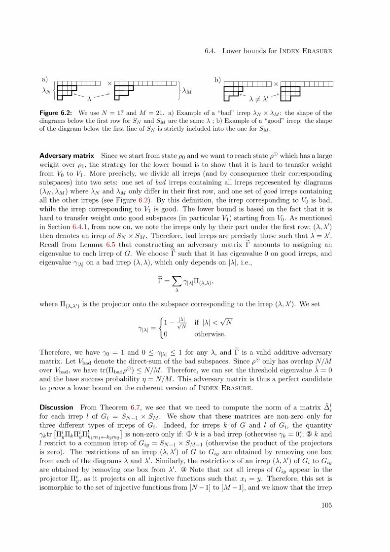
6.4. Lower bounds for Index Erasure

a) ×λN λM

λ

b) ×

λ 6= λ′

Figure 6.2: We use N = 17 and M = 21. a) Example of a “bad” irrep λN × λM : the shape of thediagrams below the first row for SN and SM are the same λ ; b) Example of a “good” irrep: the shapeof the diagram below the first line of SN is strictly included into the one for SM .

Adversary matrix Since we start from state ρ0 and we want to reach state ρ which has a largeweight over ρ1, the strategy for the lower bound is to show that it is hard to transfer weightfrom V0 to V1. More precisely, we divide all irreps (and by consequence their correspondingsubspaces) into two sets: one set of bad irreps containing all irreps represented by diagrams(λN , λM ) where λN and λM only differ in their first row, and one set of good irreps containingall the other irreps (see Figure 6.2). By this definition, the irrep corresponding to V0 is bad,while the irrep corresponding to V1 is good. The lower bound is based on the fact that it ishard to transfer weight onto good subspaces (in particular V1) starting from V0. As mentionedin Section 6.4.1, from now on, we note the irreps only by their part under the first row; (λ, λ′)then denotes an irrep of SN × SM . Therefore, bad irreps are precisely those such that λ = λ′.Recall from Lemma 6.5 that constructing an adversary matrix Γ amounts to assigning aneigenvalue to each irrep of G. We choose Γ such that it has eigenvalue 0 on good irreps, andeigenvalue γ|λ| on a bad irrep (λ, λ), which only depends on |λ|, i.e.,

Γ =∑λ

γ|λ|Π(λ,λ),

where Π(λ,λ′) is the projector onto the subspace corresponding to the irrep (λ, λ′). We set

γ|λ| =

1− |λ|√

Nif |λ| <

√N

0 otherwise.

Therefore, we have γ0 = 1 and 0 ≤ γ|λ| ≤ 1 for any λ, and Γ is a valid additive adversarymatrix. Let Vbad denote the direct-sum of the bad subspaces. Since ρ only has overlap N/Mover Vbad, we have tr(Πbadρ

) ≤ N/M . Therefore, we can set the threshold eigenvalue λ = 0and the base success probability η = N/M . This adversary matrix is thus a perfect candidateto prove a lower bound on the coherent version of Index Erasure.

Discussion From Theorem 6.7, we see that we need to compute the norm of a matrix ∆li

for each irrep l of Gi = SN−1 × SM . We show that these matrices are non-zero only forthree different types of irreps of Gi. Indeed, for irreps k of G and l of Gi, the quantityγktr

[ΠiyΠkΠ

iyΠ

lk1m1←k2m2

]is non-zero only if: ¬ k is a bad irrep (otherwise γk = 0); ­ k and

l restrict to a common irrep of Giy = SN−1 × SM−1 (otherwise the product of the projectorsis zero). The restrictions of an irrep (λ, λ′) of G to Giy are obtained by removing one boxfrom each of the diagrams λ and λ′. Similarly, the restrictions of an irrep (λ, λ′) of Gi to Giyare obtained by removing one box from λ′. ® Note that not all irreps of Giy appear in theprojector Πi

y, as it projects on all injective functions such that xi = y. Therefore, this set isisomorphic to the set of injective functions from [N −1] to [M −1], and we know that the irrep

105

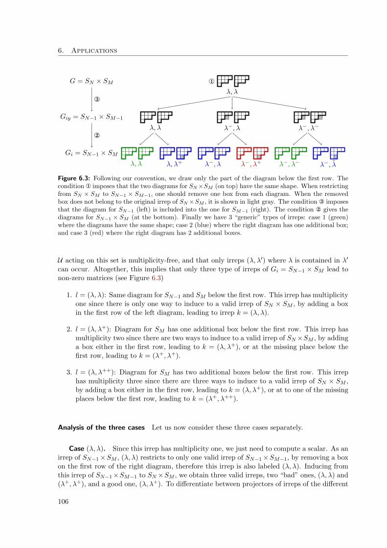
6. Applications

Gi = SN−1 × SMλ, λ λ, λ+ λ−, λ λ−, λ+ λ−, λ− λ−, λ

Giy = SN−1 × SM−1

λ, λ λ−, λ λ−, λ−

G = SN × SMλ, λ

¬

®

­

Figure 6.3: Following our convention, we draw only the part of the diagram below the first row. Thecondition ¬ imposes that the two diagrams for SN×SM (on top) have the same shape. When restrictingfrom SN × SM to SN−1 × SM−1, one should remove one box from each diagram. When the removedbox does not belong to the original irrep of SN ×SM , it is shown in light gray. The condition ® imposesthat the diagram for SN−1 (left) is included into the one for SM−1 (right). The condition ­ gives thediagrams for SN−1 × SM (at the bottom). Finally we have 3 “generic” types of irreps: case 1 (green)where the diagrams have the same shape; case 2 (blue) where the right diagram has one additional box;and case 3 (red) where the right diagram has 2 additional boxes.

U acting on this set is multiplicity-free, and that only irreps (λ, λ′) where λ is contained in λ′

can occur. Altogether, this implies that only three type of irreps of Gi = SN−1 × SM lead tonon-zero matrices (see Figure 6.3)

1. l = (λ, λ): Same diagram for SN−1 and SM below the first row. This irrep has multiplicityone since there is only one way to induce to a valid irrep of SN × SM , by adding a boxin the first row of the left diagram, leading to irrep k = (λ, λ).

2. l = (λ, λ+): Diagram for SM has one additional box below the first row. This irrep hasmultiplicity two since there are two ways to induce to a valid irrep of SN×SM , by addinga box either in the first row, leading to k = (λ, λ+), or at the missing place below thefirst row, leading to k = (λ+, λ+).

3. l = (λ, λ++): Diagram for SM has two additional boxes below the first row. This irrephas multiplicity three since there are three ways to induce to a valid irrep of SN × SM ,by adding a box either in the first row, leading to k = (λ, λ+), or at to one of the missingplaces below the first row, leading to k = (λ+, λ++).

Analysis of the three cases Let us now consider these three cases separately.

Case (λ, λ). Since this irrep has multiplicity one, we just need to compute a scalar. As anirrep of SN−1×SM , (λ, λ) restricts to only one valid irrep of SN−1×SM−1, by removing a boxon the first row of the right diagram, therefore this irrep is also labeled (λ, λ). Inducing fromthis irrep of SN−1×SM−1 to SN ×SM , we obtain three valid irreps, two “bad” ones, (λ, λ) and(λ+, λ+), and a good one, (λ, λ+). To differentiate between projectors of irreps of the different

106

6.4. Lower bounds for Index Erasure

a)

SN−1 × SM−1

SN−1 × SM

SN × SM

λ, λ

λ, λ

λ, λ λ+, λ

λ, λ+

λ, λ+ λ+, λ+

b)

SN−1 × SM−1

SN × SM−1

SN × SM

λ, λ

λ, λ

λ, λ λ, λ+

λ+, λ

λ+, λ λ+, λ+

Figure 6.4: a) Justification of Equation (6.3). The irrep (λ, λ) of SN−1 × SM only induces to oneirrep of SN × SM , since the other possible irrep is invalid (diagram λ+ is not contained inside λ). b)Justification of Equation (6.4), using a similar argument.

groups, we will from now on use superscripts (for example ΠN,Mλ,λ denotes a projector on the

irrep (λ, λ) of SN × SM ). We therefore have from Theorem 6.7

∆λ,λi =

γ|λ|

dN−1,Mλ,λ

∑y

tr[ΠiyΠ

N,Mλ,λ Πi

yΠN−1,Mλ,λ

]+

γ|λ|+1

dN−1,Mλ,λ

∑y,λ+

tr[ΠiyΠ

N,Mλ+,λ+

ΠiyΠ

N−1,Mλ,λ

]− γ|λ|

=Mγ|λ|

dN−1,Mλ,λ dN−1,M−1

λ,λ

· tr[ΠN−1,M−1λ,λ ΠN,M

λ,λ

]· tr[ΠN−1,M−1λ,λ ΠN−1,M

λ,λ

]+

Mγ|λ|+1

dN−1,Mλ,λ dN−1,M−1

λ,λ

∑λ+

tr[ΠN−1,M−1λ,λ ΠN,M

λ+,λ+

]· tr[ΠN−1,M−1λ,λ ΠN−1,M

λ,λ

]− γ|λ|,

where we have used Lemma 6.8 and the fact that all terms in the sum over y are equal bysymmetry.

From Figure 6.4, we see that

tr[ΠN−1,M−1λ,λ ΠN,M

λ,λ

]= tr

[ΠN−1,M−1λ,λ ΠN−1,M

λ,λ

], (6.3)

tr[ΠN−1,M−1λ,λ ΠN,M

λ+,λ+

]= tr

[ΠN−1,M−1λ,λ ΠN,M−1

λ+,λ

], (6.4)

since the only way for (λ, λ) as an irrep of SN × SM to restrict to (λ, λ) as an irrep of SN−1 ×SM−1 is to first restrict to (λ, λ) as an irrep of SN−1×SM , and similarly for (λ+, λ+). Therefore,we only have two traces to compute. For the first one, we consider the maximally mixed stateρN−1,M−1λ,λ over the corresponding irrep. By inducing from SM−1 to SM we find that its overlap

over the irrep (λ, λ) of SN−1 × SM is given by

tr[ρN−1,M−1λ,λ ΠN−1,M

λ,λ

]=

dN−1,Mλ,λ

MdN−1,M−1λ,λ

=dMλ

MdM−1λ

.

For the second term, we use the fact that∑

λ+ ΠN,M−1λ+,λ

= I−ΠN,M−1λ,λ ,∑

λ+

tr[ρN−1,M−1λ,λ ΠN,M−1

λ+,λ

]= 1− tr

[ρN−1,M−1λ,λ ΠN,M−1

λ,λ

]= 1−

dNλNdN−1

λ

,

107

6. Applications

and finally

∆λ,λi = γ|λ|

dMλMdM−1

λ

+ γ|λ|+1

(1−

dNλNdN−1

λ

)− γ|λ|

=1√N

+ O

(1

N+

1

M

),

where we have used Lemma 6.13.

Case (λ, λ+). This irrep has multiplicity two, so we need to compute a 2× 2 matrix. Let(λ, λ+, 1) denote the copy of (λ, λ+) irrep of SN−1 × SM which is inside the (λ+, λ+) irrepof SN × SM . Let (λ, λ+, 2) denote the copy of (λ, λ+) irrep of SN−1 × SM which is inside

the (λ, λ+) irrep of SN × SM . Let the first row and the first column of ∆λ,λ+

i be indexed by(λ, λ+, 1) and the second row and the second column be indexed by (λ, λ+, 2).

An irrep (λ, λ+) of SN−1 × SM restricts to two valid irreps of SN−1 × SM−1: (λ, λ) and(λ, λ+). Those two irreps can be induced to the following bad irreps of SN × SM : (λ, λ) andany irrep (λ′, λ′) which has one more square below the first row than λ. (λ′ may be equal ordifferent from λ+.)

For brevity, we denote ∆λ,λ+

i simply by ∆. Since (λ, λ+, 1) is contained inside a bad irrepof SN × SM , we have

∆1,1 =γ|λ|

dN−1,Mλ,λ+

∑y

tr[ΠiyΠ

N,Mλ,λ Πi

yΠN−1,Mλ,λ+,1

]+

γ|λ|+1

dN−1,Mλ,λ+

∑λ′

∑y

tr[ΠiyΠ

N,Mλ′,λ′Π

iyΠ

N−1,Mλ,λ+,1

]− γ|λ|+1

=Mγ|λ|

dN−1,Mλ,λ+

dN−1,M−1λ,λ

tr[ΠN−1,M−1λ,λ ΠN,M

λ,λ

]tr[ΠN−1,M−1λ,λ ΠN−1,M

λ,λ+,1

]+

Mγ|λ|+1

dN−1,Mλ,λ+

dN−1,M−1λ,λ

(∑λ′

tr[ΠN−1,M−1λ,λ ΠN,M

λ′,λ′

])tr[ΠN−1,M−1λ,λ ΠN−1,M

λ,λ+,1

]+

Mγ|λ|+1

dN−1,Mλ,λ+

dN−1,M−1λ,λ+

tr[ΠN−1,M−1λ,λ+

ΠN,Mλ+,λ+

]tr[ΠN−1,M−1λ,λ+

ΠN−1,Mλ,λ+,1

]− γ|λ|+1

We start by evaluating the sum ∑λ′

tr[ΠN−1,M−1λ,λ ΠN,M

λ′,λ′

].

We consider the maximally mixed state ρN−1,M−1λ,λ over the corresponding irrep of SN−1×SM−1.

By inducing λ from SN−1 to SN , we find that the dimension of the induced representation isNdN−1

λ and the induced representation decomposes into irrep λ of SN , with dimension dNλ andirreps λ′. Therefore, ∑

λ′

tr[ΠN,Mλ′,λ′ ρ

N−1,M−1λ,λ

]= 1−

dNλNdN−1

λ

≤ 1− 1

N(6.5)

where the inequality follows by comparing the hook-length formulas of dNλ and dN−1λ . Similarly,

we have

tr[ΠN,Mλ,λ ρN−1,M−1

λ,λ

]= O

(1

N

). (6.6)

108

6.4. Lower bounds for Index Erasure

We now evaluate a similar quantity for ρN−1,M−1λ,λ+

. By inducing λ+ from SM−1 to SM , we find

that the dimension of the induced representation is MdM−1λ+

and the induced representationdecomposes into irrep λ+ of SM , with dimension dMλ and irreps λ++ which have one moresquare below the first row than λ+. Therefore,

tr[ΠN,Mλ+,λ+

ρN−1,M−1λ,λ+

]=

dMλMdM−1

λ

= O

(1

M

). (6.7)

By using Equations (6.5), (6.6) and (6.7), we have

∆1,1 =Mγ|λ|+1

dN−1,Mλ,λ+

tr[ΠN−1,M−1λ,λ ΠN−1,M

λ,λ+,1

]+ O

(1

N

)− γ|λ|+1. (6.8)

We havetr[ΠN−1,M−1λ,λ ΠN−1,M

λ,λ+,1

]= tr

[ΠN−1,M−1λ,λ ΠN,M

λ+,λ+

]because the other irreps of SN−1 × SM contained in the irrep (λ+, λ+) of SN × SM have nooverlap with the irrep (λ, λ) of SN−1 × SM−1. Let ρN−1,M−1

λ,λ be the completely mixed stateover (λ, λ). Then,

tr[ΠN−1,M−1λ,λ ΠN,M

λ+,λ+

]= dN−1,M−1

λ,λ tr[ΠN,Mλ+,λ+

ρN−1,M−1λ,λ

]= dN−1,M−1

λ,λ

dNλ+

NdN−1λ

.

Here, the second equality follows by inducing λ from SN−1 to SN . We have

dN−1,M−1λ,λ

dNλ+

NdN−1λ

= dN−1λ dM−1

λ

dNλ+

NdN−1λ

=dM−1λ dNλ+

N.

By matching up the terms in hook-length formulas, we have

dM−1λ dNλ+ =

(1 + O

(1

N

))N

MdN−1λ dMλ+ . (6.9)

Therefore,

tr[ΠN−1,M−1λ,λ ΠN,M

λ+,λ+

]=

(1 + O

(1

N

))dN−1,Mλ,λ+

M(6.10)

and

∆1,1 = O

(1

N

)Similarly to Equation (6.8), we have

∆2,2 =Mγ|λ|+1

dN−1,Mλ,λ+

tr[ΠN−1,M−1λ,λ ΠN−1,M

λ,λ+,2

]+ O

(1

N

). (6.11)

We have

tr[ΠN−1,M−1λ,λ ΠN−1,M

λ,λ+,2

]= tr

[ΠN−1,M−1λ,λ ΠN,M

λ,λ+

]= dN−1,M−1

λ,λ tr[ΠN,Mλ,λ+

ρN−1,M−1λ,λ

],

109

6. Applications

because the other irreps of SN−1 × SM contained in the irrep (λ, λ+) of SN × SM have nooverlap with the irrep (λ, λ) of SN−1 × SM−1.

By inducing λ from SM−1 to SM , we get

tr[ΠN,Mλ,λ+

ρN−1,M−1λ,λ

]+ tr

[ΠN,Mλ+,λ+

ρN−1,M−1λ,λ

]=

dMλ+

MdM−1λ

. (6.12)

By inducing λ from SN−1 to SN , we get

tr[ΠN,Mλ+,λ+

ρN−1,M−1λ,λ

]=

dNλ+

NdN−1λ

. (6.13)

By subtracting Equation (6.13) from Equation (6.12), we get

tr[ΠN−1,M−1λ,λ ΠN,M

λ,λ+

]=dMλ+d

N−1λ

M−dNλ+d

M−1λ

N.

Because of Equation (6.9),

tr[ΠN−1,M−1λ,λ ΠN,M

λ,λ+

]= O

(dMλ+d

N−1λ

MN

). (6.14)

By substituting this into Equation (6.11), we get ∆2,2 = O(

1N

).

Last, we have to bound ∆1,2 and ∆2,1. Similarly to Equation (6.8), we have

∆i,j =Mγ|λ|+1

dN−1,Mλ,λ+

tr[ΠN−1,M−1λ,λ ΠN−1,M

λ,λ+,i←j

]+ O

(1

N

).

By using Lemma 6.8 and Equations (6.10) and (6.14), we get

∆i,j = O

(1√N

).

We have shown that ∆i,j = O(

1√N

)for all i, j. Therefore, ‖∆‖ = O

(1√N

).

Case (λ, λ++). This irrep of SN−1 × SM has multiplicity three, so we need to bound theelements of a 3 × 3 matrix. Let (λ, λ++, 1) denote the copy of the irrep that lies inside theirrep (λ, λ++) of (SN × SM ), (λ, λ++, 2) be the copy that lies inside the irrep (λ+, λ++) of(SN × SM ), and (λ, λ++, 3) be the copy that lies inside the irrep (λ′+, λ++) of (SN × SM ),where λ+ and λ′+ correspond to the two different ways a box can be added to λ. Since thesetwo last copies have exactly the same structure, they can be treated similarly and we reallyneed to compute only 4 different matrix elements (2 diagonal elements and 2 non-diagonalelements). Let us also note that none of these copies are contained in bad irreps of SN × SM .

Let us now denote ∆λ,λ++

i by ∆, and index the rows and columns of this matrix by thethree copies of the irrep. Note that the irrep (λ, λ++) of SN−1 × SM restricts to three validirreps of SN−1 × SM−1: (λ, λ++), (λ, λ+) and (λ, λ′+). Also only these last two irreps induce

110

6.4. Lower bounds for Index Erasure

to bad irreps of SN × SM , (λ+, λ+) and (λ′+, λ′+), respectively. Therefore, we have for thefirst diagonal element

∆1,1 =γ|λ|+1

dN−1,Mλ,λ++

∑y

tr[ΠiyΠ

N,Mλ+,λ+

ΠiyΠ

N−1,Mλ,λ++,1

]+ tr

[ΠiyΠ

N,M

λ′+,λ′+ΠiyΠ

N−1,Mλ,λ++,1

]

=2Mγ|λ|+1d

N−1,M−1λ,λ+

dN−1,Mλ,λ++

tr[ΠN,Mλ+,λ+

ρN−1,M−1λ,λ+

]· tr[ΠN−1,Mλ,λ++,1

ρN−1,M−1λ,λ+

].

Studying as before the overlap of ρN−1,M−1λ,λ+

over the irreps of SN × SM , we obtain for the twotraces

tr[ΠN,Mλ+,λ+

ρN−1,M−1λ,λ+

]≤

dMλ+

MdM−1λ+

, (6.15)

tr[ΠN−1,Mλ,λ++,1

ρN−1,M−1λ,λ+

]= tr

[ΠN,Mλ,λ++ρ

N−1,M−1λ,λ+

]≤

dNλ+

NdN−1λ+

, (6.16)

and in turn

∆1,1 ≤2Mγ|λ|+1d

Nλ+d

Mλ+

NdN−1λ+

dMλ++

= O

(1

MN

).

For the second diagonal element, we find similarly

∆2,2 =γ|λ|+1

dN−1,Mλ,λ++

∑y

tr[ΠiyΠ

N,Mλ+,λ+

ΠiyΠ

N−1,Mλ,λ++,2

]+ tr

[ΠiyΠ

N,M

λ′+,λ′+ΠiyΠ

N−1,Mλ,λ++,2

]

=Mγ|λ|+1d

N−1,M−1λ,λ+

dN−1,Mλ,λ++

tr[ΠN,Mλ+,λ+

ρN−1,M−1λ,λ+

]·

tr[ΠN−1,Mλ,λ++,2

ρN−1,M−1λ,λ+

]+ tr

[ΠN−1,Mλ,λ++,2

ρN−1,M−1

λ,λ′+

]≤

2γ|λ|+1dMλ+

dMλ++

= O

(1

M

),

where we have used Equation (6.16) and the fact that the other overlaps are at most 1.Using exactly the same arguments, we find for the non-diagonal elements

|∆1,2| ≤2γ|λ|+1d

Mλ+

dMλ++

√dNλ+

NdN−1λ+

= O

(1

M√N

),

|∆2,3| ≤2γ|λ|+1d

Mλ+

dMλ++

= O

(1

M

).

Since the irreps (λ, λ++, 2) and (λ, λ++, 3) are of the same type, we also have ∆3,3 = O(1/M)

and ∆1,3 = O(

1/(M√N))

. Therefore, all elements of ∆ are at most O(1/M), so that ‖∆‖ =

O(1/M).

Finally, since the matrices corresponding to all irreps have norm at most O(

1/√N)

, we

have from Theorem 6.7 that∥∥∥Γi − Γ

∥∥∥ = O(

1/√N)

, and in turn

Qε(Index Erasure) = Ω(

(√

1− ε−√N/M)2

√N).

111

6. Applications

6.5 Summary

In this Chapter, we showed that the multiplicative adversary bound satisfies a strong directproduct even for quantum state generation problems. We also examined how to use theadversary methods on specific problems, in particular we gave simple expressions when theautomorphism group of a function is multiplicity-free. We then applied these formulas to re-derived the bounds for Search, (which gives an illustration of the differences between theadversary methods) and a tight lower bound for Index Erasure.

112

7 Perspectives

7.1 Cryptographic primitives

The quest is now to find practical schemes for implementing quantum primitives. Bit commit-ment and coin flipping face different challenges: indeed, we are interested in secure quantum bitcommitment based on “reasonable” assumptions. In this manuscript we unfortunately provedthat the physically grounded restriction to Gaussian states and Gaussian operations does notallow security. Let us give two other approaches that could lead to secure bit commitmentunder restrictions.

Gaussian bounded/noisy-storage model In a recent series of work, bit commitment andoblivious transfer have been shown to been secure when both player have bounded or deficientmemories [DFSS08, WW08, WST08]. However, the proposed protocols involve qubits, singlephoton source and single photon detectors. Following the footsteps of quantum key distribu-tion, proposing protocols with Gaussian variables could lead to efficient protocols. It appearsthat the study of security of such protocols requires new ideas. For example what is the gooddefinition of “bounded” memory for continuous variables? If one tries to limit the numberof modes, each of them being described by an infinite-dimensional vector, the overall Hilbertspace is still unbounded, thus no real limitation is achieved. In these models, security canbe proved by using a strong converse Shannon coding theorem [KW09]. Very few results areknown in the continuous case, even for Gaussian channels. Such results would have strongimpacts in the study of continuous variables cryptography.

Almost Gaussian bit commitment To go beyond Gaussian bit commitment we wish to findanother model, with physical significance, that allows bit commitment. Mandilara and Cerf[MC11] proposed an extension to the Gaussian model by allowing a non-Gaussian gate (inthis case photon subtraction) that only succeeds with bounded probability. They introduceda protocol which is more a proof-of-concept than a proposal for an actual protocol and provedas a first step that it is secure against Gaussian attacks. The full study of the security remainsto be done and this idea deserves to be pushed further.

Let us point out that adding any non-Gaussian gate to Gaussian computation makes ituniversal for quantum computing [LB99]. This leads to the following extension: consider aset of gates that is not universal for quantum computing (e.g. Clifford operation for discretevariables, Gaussian operations for continuous variables) and one extra gate that makes the setuniversal (CNOT for DV, cubic gate for CV) but which can only be implemented with boundedprobability. Can one construct a secure bit commitment protocol in this setting? The idea isthat when preparing states, the probabilistic gate can be repeated as long a desired, but notwhen trying to cheat. Such a model is strongly grounded for the CV case and might also berelevant in the DV one.

Weak coin flipping The situation is quite different for weak coin flipping. If one tries toconstruct a protocol directly from the point games, it will be ridiculous in term of resources

113

7. Perspectives

(qubits, circuit size, and number of rounds). Finding protocols with more constrained resourcesseems the next step. In particular, the recursive structure of the ladder seems to imply thatsuch protocols may exist. Another direction is to prove better bounds on the number of roundsneeded to achieve a bias ε than the current lower bound of log log 1/ε [Amb04]. Only whensuch protocols will be discovered, it will be interesting to study practical questions that arisefrom implementation: detector efficiency, loss in the communication channel, imperfection ofmemories, etc. It would also be interesting to know if the proof of arbitrary small bias can stillbe adapted to take care of these effects, or if it will stay a Grail for unconditional security.

7.2 Query complexity

We proved that the multiplicative method is the strongest method we currently have to provelower bounds for the quantum query complexity. Nevertheless this method is quite challengingto use, this is why we gave an easier formulation in term of representation theory when problemsare multiplicity free.

Graph Isomorphism We extended the adversary methods to prove lower bounds for quantumstate generation problems and demonstrated the power of our method by proving a tight lowerbound for Index Erasure. This did not specifically address Graph Isomorphism since anexponential lower bound was already known using this approach. However we now have atour disposal a powerful new tool to rule out many more “state generation” approaches in thequery complexity model. The next step is to consider more powerful approaches than IndexErasure for which we did not assume any structure to the problem. One elegant solutionwould be to prove lower bounds for the Component Superposition problem introduced in[Lut11]. This would have implication for Graph Isomorphism as well as on the study ofcounterfeiting quantum money [FGH+10].

Lower bound for Element Disctinctness The optimal lower bounds for Element Distinct-ness and Collision have been proved by the polynomial method [AS04]. Unfortunately itis not know how to extend those proofs to related problems like k-Element Distinctness.The reduction from the polynomial method to the multiplicative adversary method offers anew hope to prove those lower bounds. The first step is naturally to reprove the bound forElement Distinctness using the adversary method, and in a second step to generalize it.

Time-space tradeoff for Element Distinctness We made a significant step in proving thatthe quantum query complexity obeys a strong direct product theorem, the proof has thenbeen completed in [LR11]. However this proof holds only for functions and not for quantumstate generation problems. One possible application of this theorem is for proving a time-spacetradeoff for Element Distinctness. Indeed, such tradeoff for multi output problems, suchas Sorting, were proved using SDPTs. The k independent instances of a function f areencoded in Sorting such that the k outputs can be deduced from the sorted array. Then thespace constraint combined to the SDPT gives the time-space tradeoff. For a decision problemhowever, such as Element Distinctness, this approach fails. One needs a measure on theprogress based on the intermediate quantum states. We hope our approach can contribute tothis quest.

114

Part III

Appendices

115

A Phase-space representation and Wigner function

In this Appendix we introduce another description of continuous variables states and operation:the phase-space description. This gives a formal justification to the introduction of covarianceand symplectic matrices for Gaussian states.

A.1 Characteristic and Wigner functions

Definition A.1 (The operators X and P ) For j ∈ [n], define the operators Xj , Pj : L2(Rn) →CRn that act on a function ψ ∈ L2(Rn) by

• ∀(x1, . . . , xn) ∈ Rn, Xj [ψ](x1, . . . , xn) = xjψ(x1, . . . , xn),

• ∀(x1, . . . , xn) ∈ Rn, Pj [ψ](x1, . . . , xn) = −i ∂ψ∂xj (x1, . . . , xn).

Definition A.2 (Characteristic function) Let ξ = (α1, β1, . . . , αn, βn) ∈ R2n. Define the Weyloperator Vξ on L2(Rn) by:

Vξ = exp

n∑i=1

αiXi + βiPi

.

The characteristic function of a trace-class operator A is

χA : ξ 7→ tr[AVξ].

The Weyl operator, is sometimes called the displacement operator. For example let |ψ〉 ∈L2(R), then V(α,0)|ψ〉 is the function: x 7→ ψ(x − α). Consider another example: let ρ bea density operator on n modes, and ζ a 2n-dimensional vector, the χ

VζρV†ζ

(ξ) = χρ(ξ − ζ).

Details of these derivations can be found in [GPS07].

The vector ξ belongs to a 2n-dimensional real space called the phase-space. The phase-space is actually a good model to analyze CV systems since any trace-class operator can bereconstructed from its characteristic function, this is the Weyl-Wigner isomorphism:

A =1

(2π)n

∫χA(−ξ)Vξdξ.

Though all the computations in the phase-space can be done using the characteristic function,it is often easier to use the Wigner function which is its Fourier transform:

WA(ξ) =1

(2π)n

∫χA(ζ) exp

iξTΩζ

dζ,

where Ω =

(0 1−1 0

)⊕n.

117

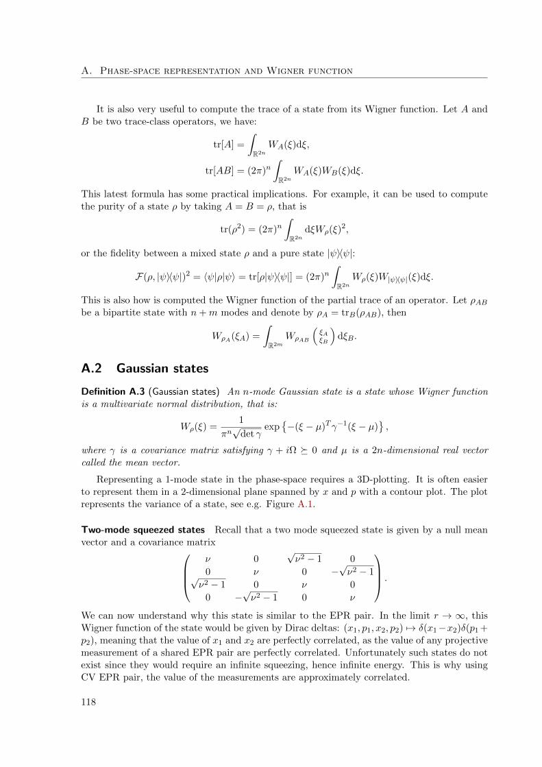
A. Phase-space representation and Wigner function

It is also very useful to compute the trace of a state from its Wigner function. Let A andB be two trace-class operators, we have:

tr[A] =

∫R2n

WA(ξ)dξ,

tr[AB] = (2π)n∫R2n

WA(ξ)WB(ξ)dξ.

This latest formula has some practical implications. For example, it can be used to computethe purity of a state ρ by taking A = B = ρ, that is

tr(ρ2) = (2π)n∫R2n

dξWρ(ξ)2,

or the fidelity between a mixed state ρ and a pure state |ψ〉〈ψ|:

F(ρ, |ψ〉〈ψ|)2 = 〈ψ|ρ|ψ〉 = tr[ρ|ψ〉〈ψ|] = (2π)n∫R2n

Wρ(ξ)W|ψ〉〈ψ|(ξ)dξ.

This is also how is computed the Wigner function of the partial trace of an operator. Let ρABbe a bipartite state with n+m modes and denote by ρA = trB(ρAB), then

WρA(ξA) =

∫R2m

WρAB

(ξAξB

)dξB.

A.2 Gaussian states

Definition A.3 (Gaussian states) An n-mode Gaussian state is a state whose Wigner functionis a multivariate normal distribution, that is:

Wρ(ξ) =1

πn√

det γexp

−(ξ − µ)Tγ−1(ξ − µ)

,

where γ is a covariance matrix satisfying γ + iΩ 0 and µ is a 2n-dimensional real vectorcalled the mean vector.

Representing a 1-mode state in the phase-space requires a 3D-plotting. It is often easierto represent them in a 2-dimensional plane spanned by x and p with a contour plot. The plotrepresents the variance of a state, see e.g. Figure A.1.

Two-mode squeezed states Recall that a two mode squeezed state is given by a null meanvector and a covariance matrix

ν 0√ν2 − 1 0

0 ν 0 −√ν2 − 1√

ν2 − 1 0 ν 0

0 −√ν2 − 1 0 ν

.

We can now understand why this state is similar to the EPR pair. In the limit r → ∞, thisWigner function of the state would be given by Dirac deltas: (x1, p1, x2, p2) 7→ δ(x1−x2)δ(p1 +p2), meaning that the value of x1 and x2 are perfectly correlated, as the value of any projectivemeasurement of a shared EPR pair are perfectly correlated. Unfortunately such states do notexist since they would require an infinite squeezing, hence infinite energy. This is why usingCV EPR pair, the value of the measurements are approximately correlated.

118

A.3. Operations

x

p

|α〉

<α/√

2

Imα/√

2

1|0〉v

ρth(v)

Figure A.1: Phase-space representations of the vacuum state |0〉, a coherent state centered on α and athermal state of variance v. The diameter of the circles represent the variance of the Wigner function.

A.3 Operations

Gaussian unitary Let ρ be a n-mode Gaussian state and U be Gaussian unitary acting on nmodes and characterized by a symplectic matrix S and a displacement vector d, then for allξ ∈ R2n:

WUρU†(ξ) = Wρ(ST ξ − d).

Homodyne measurement The homodyne measurement of one mode is the measurement ofthe value of one quadrature of this mode (x or p). Since these values are continuous, theoutcomes of the measurement are given by a continuous probability distribution P whichcorresponds the marginal of the Wigner function over the other quadrature:

P (x) =

∫RW (x, p)dp.

Partial measurement When considering multimode states, the partial measurement of someof the mode is a Gaussian operation. Consider a bipartite Gaussian state with covariance ma-

trix γAB =

(γA CCT γB

)and a mean vector µ = µA⊕µB. Denote by µm = (x1, 0, x2, 0, . . . , xnB , 0)

the values of the homodyne measurements on the “B” modes, then the resulting state on Aconditionally on the outcome µB on B is described a covariance matrix

γA − C(∆γB∆)−1CT

where ∆ =

(1 00 0

)⊕nBand the inverse is taken only on the range of the matrix. The mean

vector reads,

C(∆γB∆)−1CT (µm − µB) + µA.

119

B Additional constraint on the dual feasible points

Lemma B.1 P ∗A = inf α and P ∗B = inf β where the infinimum is taken over all dual feasiblepoints.

The difference between this lemma and Theorem 4.4, is the condition ° of that the dualfeasible points should obey. We will now prove that for all set of matrices ZA,i that satisfythe constraints ¬ to ¯ and all ε > 0, there exists a set of matrices Z ′A,i that satisfy theconstraints ¬ to ° with α = tr(Z ′A,0ρ0) = tr(ZA,0ρ0) + ε.

Fix ZA,0, . . . , ZA,n a set of matrices that satisfies the constraints ¬ to ¯ and ε > 0. Theproof relies on the following fact: there exists Λ > 0 such that:

Z ′A,0 = (〈ψA,0|ZA,0|ψA,0〉+ ε)|ψA,0〉〈ψA,0|+ Λ(I− |ψA,0〉〈ψA,0|) ZA,0.

For all i > 0, define Z ′A,i = ZA,i. We now prove that the set of matrices Z ′A,0, . . . , Z ′A,nsatisfies the constraints 1) to 6). Since |ψA,0〉 is an eigenvector of Z ′A,0 of the eigenvalue α =tr(ZA,0ρ0) + ε, the constraint 6) is satisfied. Moreover, Z ′A,0 ZA,0 so Z ′A,0⊗ IM ZA,0⊗ IMso constraint 2) is also satisfied. (All the other constraints involves only matrices Z ′A,i for i > 0so they are satisfied by definition of the Z ′A,i.

The only one thing left to do is to prove the previous claim, that is for a well chosen Λ, wehave Z ′A,0 ZA,0. Let |φ〉 a vector in A, then it can be decomposed as |φ〉 = a|ψA,0〉+ b|ψ⊥〉where 〈ψA,0|ψ⊥〉 = 0. We can restrict ourselves to b ∈ R and |a|2 + |b|2 = 1, thus we have:

〈φ|Z ′A,0 − ZA,0|φ〉 = |a|2 ε+ |b|2 (Λ− 〈ψ⊥|ZA,0|ψ⊥〉)− 2b<(a〈ψ⊥|ZA,0|ψA,0〉) (B.1)

This expression is always non negative for a Λ big enough that we will explicit later on. ThisΛ is independent of |φ〉, i.e. a, b and |ψ⊥〉. We have the following cases:

• a = 0. We want Λ ≥ 〈ψ⊥|ZA,0|ψ⊥〉 for all |ψ⊥〉. This is possible by choosing Λ ≥ ‖ZA,0‖.Let us assume now assume that a 6= 0.

• a 6= 0. Let us see Equation (B.1) as a polynomial in b. The leading coefficient beingnon negative, we need to show that the discriminant is negative for Λ large enough.The discriminant reads 4<(a〈ψ⊥|ZA,0|ψA,0〉)2 − 4 |a|2 ε(Λ − 〈ψ⊥|ZA,0|ψ⊥〉). Since forany complex number x, <(x) ≤ |x|, it is sufficient to prove that for Λ large enough

we have, |a|2∣∣〈ψ⊥|ZA,0|ψA,0〉∣∣2 − |a|2 ε(Λ − 〈ψ⊥|ZA,0|ψ⊥〉) ≤ 0. Since a 6= 0, we want

Λ ≥ 1ε (∣∣〈ψ⊥|ZA,0|ψA,0〉∣∣2 − 〈ψ⊥|ZA,0|ψ⊥〉). This is done by choosing Λ ≥ ‖ZA,0‖2 /ε.

Choosing Λ such that Λ ≥ ‖ZA,0‖ and Λ ≥ ‖ZA,0‖2 /ε concludes the proof.

121

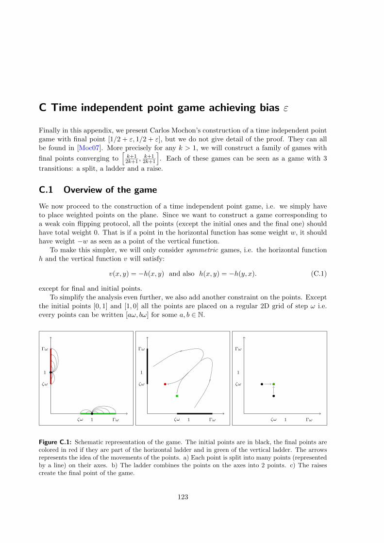
C Time independent point game achieving bias ε

Finally in this appendix, we present Carlos Mochon’s construction of a time independent pointgame with final point [1/2 + ε, 1/2 + ε], but we do not give detail of the proof. They can allbe found in [Moc07]. More precisely for any k > 1, we will construct a family of games with

final points converging to[k+12k+1 ,

k+12k+1

]. Each of these games can be seen as a game with 3

transitions: a split, a ladder and a raise.

C.1 Overview of the game

We now proceed to the construction of a time independent point game, i.e. we simply haveto place weighted points on the plane. Since we want to construct a game corresponding toa weak coin flipping protocol, all the points (except the initial ones and the final one) shouldhave total weight 0. That is if a point in the horizontal function has some weight w, it shouldhave weight −w as seen as a point of the vertical function.

To make this simpler, we will only consider symmetric games, i.e. the horizontal functionh and the vertical function v will satisfy:

v(x, y) = −h(x, y) and also h(x, y) = −h(y, x). (C.1)

except for final and initial points.To simplify the analysis even further, we also add another constraint on the points. Except

the initial points [0, 1] and [1, 0] all the points are placed on a regular 2D grid of step ω i.e.every points can be written [aω, bω] for some a, b ∈ N.

ζω

1

Γω

ζω 1 Γω

ζω

1

Γω

ζω 1 Γω

ζω

1

Γω

ζω 1 Γω

Figure C.1: Schematic representation of the game. The initial points are in black, the final points arecolored in red if they are part of the horizontal ladder and in green of the vertical ladder. The arrowsrepresents the idea of the movements of the points. a) Each point is split into many points (representedby a line) on their axes. b) The ladder combines the points on the axes into 2 points. c) The raisescreate the final point of the game.

123

C. Time independent point game achieving bias ε

We will consider a 3 step game:

Split: The point [0, 1] will be split into points on the vertical axis between the position ζω andΓω. (same treatment for [1, 0]). See a) in Figure C.1.

Ladder of width k: This transition mixed the points on the axes and has two final points inposition [ζω − kω, ζω] and [ζω, ζω − kω]. See b) in Figure C.1.

Raises The two points are raised into a final point [ζω, ζω]. See c) in Figure C.1.

More formally the game will be:

1

2[0, 1] +

1

2[1, 0]

split−→Γ∑j=ζ

split(j)[0, jω] +

Γ∑j=ζ

split(j)[jω, 0] (C.2)

ladder−→ 1

2[ζω − kω, ζω] +

1

2[ζω, ζω − kω] (C.3)

raises−→ 1[ζω, ζω]

C.2 Ladder

A ladder of width k is a repetitive pattern along the main diagonal for h and v, with 2k + 1points on each level. A rung in the ladder, is the horizontal part of it, i.e.

∑x h(x, y) for some

y. As previously discussed we will consider a symmetric ladder. Equation C.1 implies thatthere are no point on the main diagonal: ∀z, h(z, z) = v(z, z) = 0. If h is valid function, thenv will be valid too. This is why we focus our attention on the horizontal part of the ladder.

The ladder have rungs from height z∗ = ζω to Γω, each rung will have 2k points centered onthe diagonal and one point on the y-axis. More formally for ζ < j0 < Γ, the x-axis coordinateof the points of the rung at height j0ω are

0, (j0 − k)ω, (j0 − k + 1)ω, . . . , (j0 − 1)ω, (j0 + 1)ω, . . . , (j0 + k − 1)ω, (j0 + k)ω . (C.4)

Some principles governing the ladder are represented in Figure C.2. First in a), we give aschematic representation of all the points defined in (C.4) that are the horizontal part of theladder. The vertical part is constructed using the symmetry relation (C.1) we imposed. Both,the horizontal part and the vertical part of the ladder are represented in Figure b). All thepoints that are located on the overlap of the two parts of the ladder have total weight 0. Therea then only a few remaining points: the initial points on the axes, the final points in [ζω] and4 “triangles”.

To choose the weight on the point of the ladder, we use the following lemma that isextremely useful to construct valid functions:

Lemma C.1 ([Moc07]) Let x1, . . . , x2k+1 ∈ R+ be different points, f ∈ R [X] be a real polyno-mial such that:

• the absolute value of its leading coefficient is 1,

• deg(f) ≤ 2k − 1,

• ∀λ < 0, f(λ) > 0,

124

C.3. Splits

ζω

1

Γω

ζω 1 Γω

ζω

1

Γω

ζω 1 Γω

ζω

1

Γω

ζω 1 Γω

Figure C.2: Schematic construction of the ladder. a) The horizontal part of the ladder. b) Superpositionof the horizontal part and the vertical part of the ladder. By symmetry, the sum of the weights of thepoint in the overlap is 0. Except the final points, the weights of the points in the 4 “triangle” with nooverlap will be set to 0 by truncation. c) All the points actually involved in the ladder transition

then ∀C > 0 the function hrung defined by:

hrung =

2k+1∑i=1

−C · f(xi)∏j 6=i

(xj − xi)[xi] (C.5)

is a valid function.

This is how we get rid of the 4 “triangles”. We use the previous lemma in order to putweights on the points in the ladder, except the one in the triangle, that is we impose thepolynomial to be 0 on these points. There is then only on way (up to a constant C) to set upweights on the ladder, and the horizontal function is thus:

hlad =Γ∑j=ζ

−C · f(0, jω)∏kl=−k[(j + l)ω]

[0, jω] +k∑

i=−ki 6=0

C · f((j + i)ω, jω)

((j + i)ω)(jω)∏l 6=il 6=0

[ω(l − i)][(j + i)ω, jω]

, (C.6)

where f is the polynomial defined by its zeros being on the points in the “triangles”:

f(x, y) = (−1)k+1k−1∏i=1

(z∗ − iω − x) (z∗ − iω − y)k∏i=1

(Γω + iω − x) (Γω + iω − y) .

C.3 Splits

Notice that Equation (C.6) also defines the weight on the points of the splits:

split(j) =C · f(0, jω)∏kl=−k[(j + l)ω]

.

125

C. Time independent point game achieving bias ε

The last remaining part is to check that the splits are valid. More precisely, we show thatthe ladder is high enough, and the steps ω small enough, the splits are strictly valid for allz∗ > k+1

2k+1 .

Lemma C.2 (The splits are strictly valid [Moc07]) We can chose ω and Γ such that if z∗ > k+12k+1 ,

the functions

hsplit =Γ∑j=ζ

split(j)[jω, 0]− 1

2[1, 0] and vsplit =

Γ∑j=ζ

split(j)[0, jω]− 1

2[0, 1]

are strictly valid functions for

C =1

2·

Γ∑j=ζ

−f(0, jω)k∏

l=−kω (j + l)

−1

.

126

Bibliography

[Aar02] Scott Aaronson. Quantum lower bound for the collision problem. In Proceedingsof the 34th Annual ACM Symposium on Theory of Computing, pages 635–642.ACM, 2002. arXiv:quant-ph/0111102, doi:10.1145/509907.509999. [1.4.3]

[Aar11] Scott Aaronson. A linear-optical proof that the permanent is #P-hard. InProceedings of the Royal Society A. Royal Society Publishing, 2011. arXiv:

1109.1674, doi:10.1098/rspa.2011.0232. [1.2.3]

[ABDR04] Andris Ambainis, Harry Buhrman, Yevgenity Dodis, and Hein Rorig. Multipartyquantum coin flipping. In Proceedings of the 19th IEEE Annual Conferenceon Computational Complexity, pages 250–259. IEEE Computer Society, 2004.arXiv:quant-ph/0304112, doi:10.1109/CCC.2004.19. [1.3.2, 4.1.2, 4.1.3]

[ACG+11] Dorit Aharonov, Andre Chailloux, Maor Ganz, Iordanis Kerenidis, and LoıckMagnin. A simple(r) proof of existence of quantum weak coin flipping witharbitrarily small bias. In submission, 2011. [1.3.2]

[ACMT+07] K. M. R. Audenaert, J. Calsamiglia, R. Munoz-Tapia, E. Bagan, Ll. Masanes,Antonio Acın, and Frank Verstraete. Discriminating states: the quantum Cher-noff bound. Physical Review Letters, 98(16):160501, 2007. arXiv:quant-ph/

0610027, doi:10.1103/PhysRevLett.98.160501. [2.4]

[ACR+10] Andris Ambainis, Andrew M. Childs, Ben W. Reichardt, Robert Spalek, andShengyu Zhang. Any AND-OR formula of size N can be evaluated in timeN1/2+o(1) on a quantum computer. SIAM Journal on Computing, 39(6):2513–2530, 2010. doi:10.1137/080712167. [1.4.2]

[Amb00] Andris Ambainis. Quantum lower bounds by quantum arguments. In Proceedingsof the 32nd Annual ACM Symposium on Theory of Computing, pages 636–643.ACM, 2000. arXiv:quant-ph/0002066, doi:10.1145/335305.335394. [1.4.2]

[Amb04] Andris Ambainis. A new protocol and lower bounds for quantum coin flipping.Journal of Computer and System Sciences, 68:398–416, 2004. arXiv:quant-ph/0204022, doi:10.1016/j.jcss.2003.07.010. [1.3.2, 7.1]

[Amb05] Andris Ambainis. A new quantum lower bound method with an application tostrong direct product theorem for quantum search. 2005. arXiv:quant-ph/

0508200. [1.4.2, 1.4.5, 6.3]

[Amb06] Andris Ambainis. Polynomial degree vs. quantum query complexity. Jour-nal of Computer and System Sciences, 72(2):220–238, 2006. arXiv:quant-ph/

0305028, doi:10.1016/j.jcss.2005.06.006. [1.4.2, 1.4.3, 1.4.3, 1.2]

127

Bibliography

[Amb09] Andris Ambainis. Quantum algorithms for formula evaluation. Survey presentedat the NATO Advanced Research Workshop on Quantum Cryptography andComputing: Theory and Implementation, 2009. arXiv:1006.3651. [1.1.3]

[AMRR11] Andris Ambainis, Loıck Magnin, Martin Roetteler, and Jeremie Roland.Symmetry-assisted adversaries for quantum state generation. In Proceedingsof the 26th Annual IEEE Conference on Computational Complexity, pages 167–177, San Jose, CA, USA, 2011. IEEE Computer Society. arXiv:1012.2112,doi:10.1109/CCC.2011.24. [1.4.5]

[AS04] Scott Aaronson and Yaoyun Shi. Quantum lower bounds for the collision andthe element distinctness problems. Journal of the ACM, 51(4):595–605, 2004.doi:10.1145/1008731.1008735. [1.4.3, 1.4.3, 1.2, 7.2]

[ASdW07] Andris Ambainis, Robert Spalek, and Ronald de Wolf. A new quantum lowerbound method with applications to direct product theorems and Time-Spacetradeoffs. Algorithmica, 55(3):422–461, 2007. arXiv:quant-ph/0511200, doi:10.1007/s00453-007-9022-9. [1.4.2, 1.4.5, 6.2.1]

[AT03] Dorit Aharonov and Amnon Ta-Shma. Adiabatic quantum state generation andstatistical zero knowledge. In Proceedings of the 35th Annual ACM Symposiumon Theory of Computing, pages 20–29. ACM, 2003. arXiv:quant-ph/0301023,doi:10.1145/780542.780546. [1.4.4]

[ATSVY00] Dorit Aharonov, Amnon Ta-Shma, Umesh V. Vazirani, and Andrew C. Yao.Quantum bit escrow. In Proceedings of the 32d annual ACM Symposium onTheory of Computing, pages 705–714. ACM, 2000. arXiv:quant-ph/0004017,doi:10.1145/335305.335404. [1.3.2]

[Bai04] Rosemary Bailey. Associations schemes: designed experiments, algebra, andcombinatorics, volume 84 of Cambridge studies in advanced mathematics. Cam-bridge University Press, 2004. [6.2.1]

[BB84] Charles H. Bennett and Gilles Brassard. Quantum cryptography: Pub-lic key distribution and coin tossing. In Proceedings of the IEEE Interna-tional Conference on Computers, Systems, and Signal Processing, page 175,1984. Available from: http://www.research.ibm.com/people/b/bennetc/

bennettc198469790513.pdf. [1.1.2, 1.3.1]

[BBBV97] Charles H. Bennett, Ethan Bernstein, Gilles Brassard, and Umesh Vazi-rani. Strengths and weaknesses of quantum computing. SIAM Journal onComputing, 26(5):1510–1523, 1997. arXiv:quant-ph/9701001, doi:10.1137/S0097539796300933. [1.4.2, 6.3]

[BBC+01] Robert Beals, Harry Buhrman, Richard Cleve, Michele Mosca, and Ronaldde Wolf. Quantum lower bounds by polynomials. Journal of the ACM, 48:778–797, 2001. arXiv:quant-ph/9802049, doi:10.1145/502090.502097. [1.4.3, 5.27,

5.6.4]

128

Bibliography

[BBCS92] Charles Bennett, Gilles Brassard, Claude Crepeau, and Marie-Helene Sku-biszewska. Practical quantum oblivious transfer. In Proceedings of the 11thAnnual International Cryptology Conference on Advances in Cryptology, volume576 of Lecture Notes in Computer Science, pages 351–366. Springer Berlin / Hei-delberg, 1992. Available from: www.cs.mcgill.ca/~crepeau/PS/BBCS92.ps.[1.3.1]

[BCJL93] Gilles Brassard, Claude Crepeau, Richard Jozsa, and David Langlois. A quan-tum bit commitment scheme provably unbreakable by both parties. In Proceed-ing of the 34th Annual IEEE Symphosium on Foundations of Computer Science,pages 42–52, 1993. Available from: crypto.cs.mcgill.ca/~crepeau/COMP647/2007/TOPIC04/BCJL93.pdf, doi:10.1109/SFCS.1993.366851. [1.3.1]

[BCWdW01] Harry Buhrman, Richard Cleve, John Watrous, and Ronald de Wolf. Quantumfingerprinting. Physical Review Letters, 87:167902, 2001. arXiv:quant-ph/

0102001, doi:10.1103/PhysRevLett.87.167902. [1.4.4]

[Bel64] John S. Bell. On the Einstein Podolsky Rosen paradox. Physics, 1(3):195–200,1964. [1.1.1]

[Bha97] Rajendra Bhatia. Matrix analysis, volume 169 of Graduate texts in mathematics.Springer-Verlag, 1997. [4.22]

[BHK+11] Gilles Brassard, Peter Høyer, Kassem Kalach, Marc Kaplan, Sophie Laplante,and Louis Salvail. Merkle puzzles in a quantum world. In Proceedings of the 31stInternational Cryptology Conference, volume 6841 of Lecture Notes in ComputerScience, pages 391–410. Springer Berlin / Heidelberg, 2011. arXiv:1108.2316,doi:10.1007/978-3-642-22792-9_22. [1.4.5]

[Blu83] Manuel Blum. Coin flipping by telephone a protocol for solving impossibleproblems. SIGACT News, 15:23–27, 1983. doi:10.1145/1008908.1008911.[1.3.2]

[BR03] Alonso Botero and Benni Reznik. Modewise entanglement of Gaussian states.Physical Review A, 67(5):052311, 2003. arXiv:quant-ph/0209026, doi:10.

1103/PhysRevA.67.052311. [2.3.3]

[Bra05] Gilles Brassard. Is information the key? Nature Physics, 1(1):2–4, 2005. arXiv:10.1038/nphys134. [3.3]

[BS02] Stephen D. Bartlett and Barry C. Sanders. Efficient classical simulation ofoptical quantum information circuits. Physical Review Letters, 89:207903, 2002.doi:10.1103/PhysRevLett.89.207903. [1.2.1]

[BS04] Howard Barnum and Michael Saks. A lower bound on the quantum querycomplexity of read-once functions. Journal of Computer and System Sciences,69(2):244–258, 2004. arXiv:quant-ph/0201007, doi:10.1016/j.jcss.2004.02.002. [1.4.2]

129

Bibliography

[BSBN02] Stephen D. Bartlett, Barry C. Sanders, Samuel L. Braunstein, and Kae Nemoto.Efficient classical simulation of continuous variable quantum information pro-cesses. Physical Review Letters, 88(9):097904, 2002. arXiv:quant-ph/0109047,doi:10.1103/PhysRevLett.88.097904. [1.2.1]

[BV97] Ethan. Bernstein and Umesh V. Vazirani. Quantum complexity the-ory. SIAM Journal on Computing, 26(5):1411–1473, 1997. Avail-able from: www.cs.berkeley.edu/~vazirani/pubs/bv.ps, doi:10.1137/

S0097539796300921. [1.2.3]

[BvL05] Samuel L. Braunstein and Peter van Loock. Quantum information with con-tinuous variables. Reviews of Modern Physics, 77:513–577, 2005. arXiv:

quant-ph/0410100, doi:10.1103/RevModPhys.77.513. [1.2.1]

[Cam99] Peter James Cameron. Permutation Groups, volume 45 of London MathematicalSociety Student Texts. Cambridge University Press, 1999. [6.2.1]

[CBH03] Rob Clifton, Jeffrey Bub, and Halvorson Hans. Characterizing quantum theoryin terms of information-theoretic constraints. Found. Phys, 33(11):1561–1591,2003. arXiv:quant-ph/0211089, doi:10.1023/A:1026056716397. [3.3]

[CEMM98] Richard Cleeve, Artur Ekert, Chiara Macchiavello, and Michele Mosca. Quan-tum algorithms revisited. In Proceedings of the Royal Society A, volume 454,pages 339–354, 1998. arXiv:quant-ph/9708016, doi:10.1098/rspa.1998.

0164. [1.2.3]

[Cha87] David Chaum. Demonstrating that a public predicate can be satisfied withoutrevealing any information about how. In Proceedings on Advances in cryptol-ogy, pages 195–199. Springer-Verlag, 1987. Available from: http://crypto.cs.mcgill.ca/~crepeau/COMP647/2007/TOPIC05/Chaum.pdf. [1.3.1]

[CK09] Andre Chailloux and Iordanis Kerenidis. Optimal quantum strong coin flipping.In Proceeding of the 44th Annual IEEE Symposium on Foundations of ComputerScience, pages 527–533. IEEE Computer Society, 2009. arXiv:arXiv:0904.

1511, doi:10.1109/FOCS.2009.71. [1.3.2, 4.2.4]

[CK11] Andre Chailloux and Iordanis Kerenidis. Optimal bounds for quantum bit com-mitment. In Proceedings of the 52nd Annual IEEE Symposium on Foundationsof Computer Science. IEEE Computer Society, 2011. arXiv:1102.1678. [1.3.1]

[CLP07] Nicolas J. Cerf, Gerd Leuchs, and Eugene S. Polzik, editors. Quantum informa-tion with continuous variables of atoms and light. Imperial College Press, 2007.[1.2.1]

[CLVA01] Nicolas J. Cerf, Marc Levy, and Gilles Van Assche. Quantum distribution ofgaussian keys using squeezed states. Physical Review A, 63:052311, 2001. arXiv:quant-ph/0008058, doi:10.1103/PhysRevA.63.052311. [1.2.1]

[DdW11] Andrew Drucker and Ronald de Wolf. Quantum Proofs for Classical Theorems.Number 2 in Graduate Surveys. Theory of Computing Library, 2011. doi:

10.4086/toc.gs.2011.002. [1.2.3]

130

Bibliography

[Deu85] David Deutsch. Quantum theory, the Church-Turing principle and the universalquantum computer. In Proceedings of the Royal Society A, volume 400, pages97–117, 1985. Available from: http://www.cs.berkeley.edu/~christos/

classics/Deutsch_quantum_theory.pdf, doi:10.1098/rspa.1985.0070.[1.2.3]

[DFSS08] Ivan B. Damgard, Serge Fehr, Louis Salvail, and Christian Schaffner. Cryptog-raphy in the bounded quantum-storage model. SIAM J. Comput., 37(6):1865–1890, 2008. arXiv:quant-ph/0508222, doi:10.1109/SFCS.2005.30. [7.1]

[DJ92] David Deutsch and Richard Jozsa. Rapid solution of problems by quantumcomputation. In Mathematical and Physical Sciences, volume 439, pages 553–558. The Royal Society, 1992. doi:10.1098/rspa.1992.0167. [1.2.3]

[DKSW07] Giacomo Mauro D’Ariano, Dennis Kretschmann, Dirk Schlingemann, and Rein-hard F. Werner. Reexamination of quantum bit commitment: The possible andthe impossible. Physical Review A, 76:032328, 2007. arXiv:quant-ph/0605224,doi:10.1103/PhysRevA.76.032328. [1.3.1]

[DR09] Asen L. Dontchev and R. Tyrrell Rockafellar. Implicit functions and solutionmappings: a view from variational analysis. Springer Monographs in Mathe-matics. Springer, 2009. [4.15]

[Dru11] Andrew Drucker. Improved direct product theorems for randomized query com-plexity. In Proceedings of the 26th Annual IEEE Conference on ComputationComplexity, pages 1–11. IEEE Computer Society, 2011. arXiv:1005.0644,doi:10.1109/CCC.2011.29. [1.4.1]

[dW08] Ronald de Wolf. A Brief Introduction to Fourier Analysis on the Boolean Cube.Number 1 in Graduate Surveys. Theory of Computing Library, 2008. doi:

10.4086/toc.gs.2008.001. [5.6.4, 5.6.4]

[Eke91] Artur K. Ekert. Quantum cryptography based on Bell’s theorem. PhysicalReview Letters, 67:661–663, 1991. doi:10.1103/PhysRevLett.67.661. [1.1.2]

[EPR35] Albert Einstein, Boris Podolsky, and Nathan Rosen. Can quantum-mechanicaldescription of physical reality be considered complete? Physical Review, 47:777–780, 1935. doi:10.1103/PhysRev.47.777. [1.1.1]

[Fey82] Richard Feynman. Simulating physics with computers. International Journal ofTheoretical Physics, 21:467–488, 1982. doi:10.1007/BF02650179. [1.1]

[FGG08] Edward Farhi, Jeffrey Goldstone, and Sam Gutmann. A quantum algorithmfor the Hamiltonian NAND tree. Theory of Computing, 4(1):169–190, 2008.arXiv:quant-ph/0702144, doi:10.4086/toc.2008.v004a008. [1.1.3, 1.4.2]

[FGH+10] Edward Farhi, David Gosset, Avinatan Hassidim, Andrew Lutomirski, and Pe-ter W. Shor. Quantum money from knots. Technical Report MIT-CTP-4146,Massachusetts Institute of Technology, 2010. arXiv:1004.5127. [7.2]

131

Bibliography

[Fiu01] Jaromır Fiurasek. Optical implementation of continuous-variable quantumcloning machines. Physical Review Letters, 86(21):4942–4945, 2001. arXiv:

quant-ph/0012048, doi:10.1103/PhysRevLett.86.4942. [2.3.3]

[Fuc96] Christopher Alexander Fuchs. Distinguishability and Accessible Informationin Quantum Theory. PhD thesis, University of New Mexico, 1996. arXiv:

quant-ph/9601020. [2.4]

[Fuc01] Christopher Alexander Fuchs. Notes on a Paulian idea: Foundations, histor-ical, anecdotal and forward-looking thoughts on the quantum. 2001. arXiv:

quant-ph/0105039. [3.3]

[Fuc02] Christopher Alexander Fuchs. Quantum mechanics as quantum information(and only a little more). 2002. arXiv:quant-ph/0205039. [3.3]

[GG02] Frederic Grosshans and Philippe Grangier. Continuous variable quantum cryp-tography using coherent states. Physical Review Letters, 88(5):057902, 2002.doi:10.1103/PhysRevLett.88.057902. [1.2.1]

[GKP01] Daniel Gottesman, Alexei Kitaev, and John Preskill. Encoding a qubit in anoscillator. Physical Review A, 64(012310), 2001. doi:10.1103/PhysRevA.64.

012310. [2.2]

[GLLL+11] Ilja Gerhardt, Qin Liu, Antia Lamas-Linares, Johannes Skaar, Christian Kurt-siefer, and Vadim Makarov. Perfect eavesdropping on a quantum cryptogra-phy system. Nature Communication, 2:349, 2011. arXiv:1011.0105, doi:

10.1038/ncomms1348. [1.2.1]

[GPS07] Raul Garcıa-Patron Sanchez. Quantum Information with Optical ContinuousVariables: from Bell Tests to Key Distribution. PhD thesis, Universite Libre deBruxelles, 2007. [1.2.1, A.1]

[Gro96] Lov K. Grover. A fast quantum mechanical algorithm for database search.In Proceedings of the 28th Annual ACM Symposium on Theory of Computing,pages 212–219. ACM, 1996. arXiv:quant-ph/9605043, doi:10.1145/237814.237866. [1.1.3, 6.3]

[Hil00] Mark Hillery. Quantum cryptography with squeezed states. Physical ReviewA, 61:022309, 2000. arXiv:quant-ph/9909006, doi:10.1103/PhysRevA.61.

022309. [1.2.1]

[HLS07] Peter Høyer, Troy Lee, and Robert Spalek. Negative weights make adversariesstronger. In Proceedings of the 39th Annual ACM Symposium on Theory ofComputing, pages 526–535. ACM, 2007. doi:10.1145/1250790.1250867. [1.4.2,

1.4.5, 1.2, 1.4.5, 5.3.1]

[HMR+06] Sean Hallgren, Cristopher Moore, Martin Rotteler, Alexander Russell, andPranab Sen. Limitations of quantum coset states for graph isomorphism. InProceedings of the 38th Annual ACM Symposium on Theory of Computing,pages 604–617. ACM, 2006. arXiv:quant-ph/0511148, doi:10.1145/1132516.1132603. [1.4.4]

132

Bibliography

[HNS08] Peter Høyer, Jan Neerbek, and Yaoyun Shi. Quantum complexities of orderedsearching, sorting, and element distinctness. Algorithmica, 34(4):429–448, 2008.arXiv:quant-ph/0102078, doi:10.1007/s00453-002-0976-3. [1.4.2]

[Joz94] Richard Jozsa. Fidelity for mixed quantum states. Journal of Modern Optics,41:2315–2324, 1994. doi:10.1080/09500349414552171. [2.4, 2.4]

[Joz98] Richard Jozsa. Quantum algorithms and the Fourier transform. In Proceedingsof the Royal Society A, volume 454, pages 323 – 337. Royal Society Publishing,1998. arXiv:quant-ph/9707033, doi:10.1098/rspa.1998.0163. [1.2.3]

[Kai67] T. Kailath. The divergence and Bhattacharyya distance measures in signalselection. IEEE Transactions on Communication Technology, 15(1):52–60, 1967.doi:10.1109/TCOM.1967.1089532. [2.4]

[Ken99] Adrian Kent. Unconditional secure bit commitment. Physical ReviewLetters, 83(7):1447–1450, 1999. arXiv:quant-ph/9810068, doi:10.1103/

PhysRevLett.83.1447. [1.3.1]

[Ken11] Adrian Kent. Unconditionally secure bit commitment by transmitting measure-ment outcomes. 2011. arXiv:1108.2879. [1.3.1]

[Kit03] Alexei Kitaev. Quantum coin-flipping. Talk at the 6th workshop on QuantumInformation Processing, 2003. [1.3.2, 4.1.2, 4.1.3]

[KN04] Iordanis Kerenidis and Ashwin Nayak. Weak coin flipping with small bias. In-formation Processing Letters, 89(3):131 – 135, 2004. arXiv:quant-ph/0206121,doi:10.1016/j.ipl.2003.07.007. [1.3.2]

[KNP07] Pascal Koiran, Vincent Nesme, and Natacha Portier. The quantum query com-plexity of the Abelian hidden subgroup problem. Theoretical Computer Science,380(1-2):115 – 126, 2007. doi:10.1016/j.tcs.2007.02.057. [1.4.3]

[KSdW07] Hartmut Klauck, Robert Spalek, and Ronald de Wolf. Quantum and classi-cal strong direct product theorems and optimal time-space tradeoffs. SIAMJournal on Computing, 36(5):1472–1493, 2007. arXiv:quant-ph/0402123,doi:10.1137/05063235X. [1.4.3]

[KW09] Robert Konig and Stephanie Wehner. A strong converse for classical chan-nel coding using entangled inputs. Physical Review Letters, 103:070504, 2009.arXiv:0903.2838, doi:10.1103/PhysRevLett.103.070504. [7.1]

[Lan92] R. Landauer. Information is physical. In Proceedings of the workshop on Physicsand Computation, pages 1 – 4, 1992. doi:10.1109/PHYCMP.1992.615478. [3.3]

[LB99] Seth Lloyd and Samuel L. Braunstein. Quantum computation over continuousvariables. Physical Review Letters, 82(8):1784–1787, 1999. arXiv:quant-ph/

9810082, doi:10.1103/PhysRevLett.82.1784. [7.1]

[LC97] Hoi-Kwong Lo and H. F. Chau. Is quantum bit commitment really possible?Physical Review Letters, 78(17):3410–3413, 1997. arXiv:quant-ph/9603004,doi:10.1103/PhysRevLett.78.3410. [1.3.1, 3.2]

133

Bibliography

[LC98] Hoi-Kwong Lo and H.F. Chau. Why quantum bit commitment and ideal quan-tum coin tossing are impossible. Physica D: Nonlinear Phenomena, 120:177 –187, 1998. arXiv:quant-ph/9711065, doi:10.1016/S0167-2789(98)00053-0.[1.3.2]

[LM08] Sophie Laplante and Frederic Magniez. Lower bounds for randomized and quan-tum query complexity using Kolmogorov arguments. SIAM Journal on Comput-ing, 38(1):46–62, 2008. arXiv:quant-ph/0311189, doi:10.1137/050639090.[1.4.2]

[LMR+11] Troy Lee, Rajat Mittal, Ben W. Reichardt, Robert Spalek, and Mario Szegedy.Quantum query complexity of state conversion. In Proceedings of the 52ndAnnual IEEE Symposium on Foundations of Computer Science. IEEE ComputerSociety, 2011. To appear. arXiv:1011.3020. [1.4.2, 1.2, 1.4.5]

[LR11] Troy Lee and Jeremie Roland. A strong direct product theorem for quantumquery complexity. 2011. arXiv:1104.4468. [1.4.1, 1.4.5, 5.24, 5.25, 5.32, 6.1, 7.2]

[Lut11] Andrew Lutomirski. Component mixers and a hardness result for counterfeitingquantum money. Technical Report MIT-CTP 4279, Massachusetts Institute ofTechnology, 2011. arXiv:1107.0321. [7.2]

[Mag06] Loıck Magnin. Cryptographie avec des variables continues. Master’s thesis,Ecole Normale Superieure de Lyon, 2006. [1.2.1]

[Mag07] Loıck Magnin. Mise en gage quantique avec des variables continues. Master’sthesis, Ecole Normale Superieure de Lyon, 2007. [1.3.1]

[May97] Dominic Mayers. Unconditionally secure quantum bit commitment is impossible.Physical Review Letters, 78:3414, 1997. arXiv:quant-ph/9605044v2, doi:10.1103/PhysRevLett.78.3414. [1.3.1, 3.2]

[MC11] Aikatarini Mandilara and Nicolas J. Cerf. Quantum bit commitment underGaussian constraints. 2011. arXiv:1105.2140. [7.1]

[Mid04] Gatis Midrijanis. A polynomial quantum query lower bound for the set equalityproblem. In Josep Diaz, Juhani Karhumaki, Arto Lepisto, and Donald Sannella,editors, Automata, Languages and Programming, volume 3142 of Lecture Notesin Computer Science, pages 29–41. Springer Berlin / Heidelberg, 2004. arXiv:

quant-ph/0401073, doi:10.1007/978-3-540-27836-8_83. [1.4.5]

[MM07] Paulina Marian and Tudor A. Marian. Optimal purifications and fidelity fordisplaced thermal states. Physical Review A, 76(5):054307, 2007. arXiv:0706.3204, doi:10.1103/PhysRevA.76.054307. [3.2.2]

[MMLC10] Loıck Magnin, Frederic Magniez, Anthony Leverrier, and Nicolas J. Cerf. Strongno-go theorem for Gaussian quantum bit commitment. Physical Review A,81:010302, 2010. arXiv:0905.3419, doi:10.1103/PhysRevA.81.010302. [1.3.1]

[Moc05] Carlos Mochon. Large family of quantum weak coin-flipping protocols. Phys-ical Review A, 72:022341, 2005. arXiv:quant-ph/0502068, doi:10.1103/

PhysRevA.72.022341. [1.3.2]

134

Bibliography

[Moc07] Carlos Mochon. Quantum weak coin flipping with arbitrary small bias. 2007.arXiv:quantum-ph/0711.4114. [1.3.2, 1.3.2, 4, C, C.1, C.2]

[MR11] Loıck Magnin and Jeremie Roland. Quantum adversary lower bounds by poly-nomials. Technical Report 2011-TR080, NEC Laboratories America, 2011. [1.4.5]

[Nao91] Moni Naor. Bit commitment using pseudorandomness. Journal of Cryptology,4(2):151–158, 1991. Available from: http://crypto.cs.mcgill.ca/~crepeau/COMP647/2007/TOPIC06/Naor-bit.pdf, doi:10.1007/BF00196774. [1.3.1]

[NC04] Michael A. Nielsen and Isaac L. Chuang. Quantum Computation and Quan-tum Information. Cambridge Series on Information and the Natural Sciences.Cambridge University Press, 1st edition, 2004. [2.4]

[NS03] Ashwin Nayak and Peter W. Shor. Bit-commitment-based quantum coin flip-ping. Physical Review A, 67:012304, 2003. arXiv:quant-ph/0206123, doi:

10.1103/PhysRevA.67.012304. [1.3.2]

[Phi03] Pierre Phillips. Bornes inferieures en calcul quantique: Methode par adversairevs. methode des polynomes. Master’s thesis, Ecole Normale Superieure de Lyon,2003. Available from: http://www.lri.fr/~magniez/PAPIERS/philipps03.

ps.gz. [1.4.3]

[PL08] Stefano Pirandola and Seth Lloyd. Computable bounds for the discriminationof Gaussian states. Physical Review A, 78(01):012331, 2008. arXiv:0806.1625,doi:10.1103/PhysRevA.78.012331. [2.4]

[Rab80] Michael O. Rabin. Probabilistic algorithm for testing primality. Journal ofNumber Theory, 12(1):128 – 138, 1980. doi:10.1016/0022-314X(80)90084-0.[1.1.1]

[Ral99] Tim C. Ralph. Continuous variable quantum cryptography. Physical ReviewA, 61:010303, 1999. arXiv:quant-ph/9907073, doi:10.1103/PhysRevA.61.

010303. [1.2.1]

[RC09] Renato Renner and J. Ignacio Cirac. A de Finetti representation theoremfor infinite dimensional quantum systems and applications to quantum cryp-tography. Physical Review Letters, 102(11):110504, 2009. arXiv:0809.2243,doi:10.1103/PhysRevLett.102.110504. [1.2.1, 3.3]

[Rei00] Margaret D. Reid. Quantum cryptography with a predetermined key, us-ing continuous-variable Einstein-Podolsky-Rosen correlations. Physical ReviewA, 62:062308, 2000. Available from: http://link.aps.org/doi/10.1103/

PhysRevA.62.062308, arXiv:quant-ph/9909030, doi:10.1103/PhysRevA.

62.062308. [1.2.1]

[Rei11] Ben W. Reichardt. Reflections for quantum query algorithms. In Proceedings ofthe 22nd ACM-SIAM Symposium on Discrete Algorithms, pages 560–569, 2011.arXiv:1005.1601. [1.4.2, 1.2]

135

Bibliography

[Ren05] Renato Renner. Security of Quantum Key Distribution. PhD thesis, ITH Zurich,2005. arXiv:quant-ph/0512258. [1.1.2]

[RS08] Ben W. Reichardt and Robert Spalek. Span-program-based quantum algorithmfor evaluating formulas. In Proceedings of the 40th Annual ACM Symposiumon Theory of Computing, pages 103–112. ACM, 2008. arXiv:0710.2630, doi:10.1145/1374376.1374394. [1.4.2]

[Sag01] Bruce E. Sagan. The Symmetric Group Representations, Combinatorial Algo-rithms, and Symmetric Functions, volume 203 of Graduate texts in mathematics.Springer-Verlag, 2 edition, 2001. [6.12, 6.4.2, 6.4.2]

[SBPC+09] Valerio Scarani, Helle Bechmann-Pasquinucci, Nicolas J. Cerf, Miloslav Dusek,Norbert Lutkenhaus, and Momtchil Peev. The security of practical quantumkey distribution. Reviews of Modern Physics, 81:1301–1350, 2009. arXiv:0802.4155, doi:10.1103/RevModPhys.81.1301. [1.1.2]

[Sch07] Christian Schaffner. Cryptography in the Bounded Quantum-Storage Model. PhDthesis, University of Arhus, 2007. [1.3.1]

[SCS99] R. Simon, S. Chaturvedi, and V. Srinivassan. Congruences and canonical formsfor a positive matrix: Application to the schweinler-wigner extremum principle.J. Math. Phys, 40:3632–3642, 1999. arXiv:math-ph/9811003, doi:10.1063/1.532913. [2.27]

[Ser77] Jean-Pierre Serre. Linear Representations of Finite Groups, volume 42 of Grad-uate texts in mathematics. Springer-Verlag, 1977. [6.2.2, 6.2.2]

[She11] Alexander A. Sherstov. Strong direct product theorems for quantum commu-nication and query complexity. In Proceedings of the 43rd Annual ACM Sym-posium on Theory of Computing, pages 41–50. ACM, 2011. arXiv:1011.4935,doi:10.1145/1993636.1993643. [1.4.1, 1.4.3]

[Shi02] Yaoyun Shi. Quantum lower bounds for the collision and the element distinctnessproblems. In Proceedings of the 43rd Annual IEEE Symposium on Foundationsof Computer Science, pages 513–519. IEEE Computer Society, 2002. The IndexErasure problem is introduced in the arXiv version only. arXiv:quant-ph/

0112086, doi:10.1109/SFCS.2002.1181975. [1.4.3, 1.4.5, 6.4]

[Sho94] Peter W. Shor. Algorithms for quantum computation: discrete logarithms andfactoring. In Proceedings of the 35th Annual IEEE Symposium on Foundationsof Computer Science, pages 124 –134. IEEE Computer Society, 1994. arXiv:

quant-ph/9508027, doi:10.1109/SFCS.1994.365700. [1.1.3]

[Sim97] Daniel R. Simon. On the power of quantum computation. SIAM Journal onComputing, 26:1474–1483, 1997. doi:10.1137/S0097539796298637. [1.2.3]

[Sim00] R. Simon. Peres-horodecki separability criterion for continuous variable systems.Physical Review Letters, 84:2726–2729, 2000. arXiv:quant-ph/9909044, doi:10.1103/PhysRevLett.84.2726. [3.1]

136

Bibliography

[SMGPSC07] Jimmy Sudjana, Loıck Magnin, Raul Garcıa-Patron Sanchez, and Nicolas J.Cerf. Tight bounds on the eavesdropping of a continuous-variable quantum cryp-tographic protocol with no basis switching. Physical Review A, 76(5):052301,2007. arXiv:quant-ph/0706.4283, doi:10.1103/PhysRevA.76.052301. [1.2.1]

[Smo05] John A. Smolin. Can quantum cryptography imply quantum mechanics? Jour-nal on Quantum Information and Computation, 05(2):161–169, 2005. arXiv:

quant-ph/0310067. [3.3]

[SP00] Peter W. Shor and John Preskill. Simple proof of security of the BB84 quantumkey distribution protocol. Physical Review Letters, 85:441–444, 2000. arXiv:

quant-ph/0003004, doi:10.1103/PhysRevLett.85.441. [1.1.2]

[Spa08] Robert Spalek. The multiplicative quantum adversary. In Proceedings of the23rd Annual IEEE Conference on Computational Complexity, pages 237–248.IEEE Computer Society, 2008. arXiv:quant-ph/0703237, doi:10.1109/CCC.2008.9. [1.4.2, 1.4.5, 1.4.5, 1.4.5, 5.3.2, 6.1, 6.1, 6.2.1, 6.3]

[Spe07] Robert W. Spekkens. Evidence for the epistemic view of quantum states: Atoy theory. Physical Review A, 75(3):032110, 2007. arXiv:quant-ph/0401052,doi:10.1103/PhysRevA.75.032110. [3.3]

[SR01] R. W. Spekkens and Terry Rudolph. Degrees of concealments and bindingnessin quantum bit commitment protocols. Physical Review A, 65(01):012310, 2001.arXiv:quant-ph/0106019, doi:10.1103/PhysRevA.65.012310. [1.3.2]

[SR02] R. W. Spekkens and Terry Rudolph. Quantum protocol for cheat-sensitiveweak coin flipping. Physical Review Letters, 89:227901, 2002. arXiv:quant-ph/0202118, doi:10.1103/PhysRevLett.89.227901. [1.3.2]

[SS06] Robert Spalek and Mario Szegedy. All quantum adversary methods are equiv-alent. Theory of Computing, 2(1):1–18, 2006. Available from: http://

www.theoryofcomputing.org/articles/v002a001, doi:10.4086/toc.2006.

v002a001. [1.4.2, 1.2]

[SW86] Michael Saks and Avi Wigderson. Probabilistic boolean decision trees and thecomplexity of evaluating game trees. In Proceedings of the 27th Annual Sympo-sium on Foundations of Computer Science, pages 29–38, 1986. Available from:www.math.ias.edu/~avi/PUBLICATIONS/MYPAPERS/SW86/SW86.pdf, doi:10.

1109/SFCS.1986.44. [1.1.3]

[Uhl76] Armin Uhlmann. The “transition probability” in the state space of a ∗-algebra.Reports on Mathematical Physics, 9:273–279, 1976. Available from: http://

www.physik.uni-leipzig.de/~uhlmann/PDF/Uh76a.pdf. [2.4, 2.4]

[Val79] Leslie G. Valiant. The complexity of computing the permanent. TheoreticalComputer Science, 8(2):189 – 201, 1979. doi:10.1016/0304-3975(79)90044-6.[1.2.3]

[Wie83] Stephen Wiesner. Conjugate coding. SIGACT News, 15:78–88, 1983. doi:

10.1145/1008908.1008920. [1.1]

137

Bibliography

[WLB+04] Christian Weedbrook, Andrew M. Lance, Warwick P. Bowen, Thomas Symul,Timothy C. Ralph, and Ping Koy Lam. Quantum cryptography without switch-ing. Physical Review Letters, 93:170504, 2004. doi:10.1103/PhysRevLett.93.170504. [1.2.1]

[WST08] Stephanie Wehner, Christian Schaffner, and Barbara M. Terhal. Cryptographyfrom noisy storage. Physical Review Letters, 100:220502, 2008. arXiv:0711.

2895, doi:10.1103/PhysRevLett.100.220502. [1.3.1, 7.1]

[WW08] Stephanie Wehner and Jurg Wullschleger. Composable security in the bounded-quantum-storage model. In Proceedings of the 35th International Colloquium onAutomata, Languages and Programming, pages 604–615. Springer-Verlag, 2008.arXiv:0709.0492, doi:10.1007/978-3-540-70583-3_49. [7.1]

[Yao82] Andrew C. Yao. Protocols for secure computations. In Proceedings of the 23rdAnnual Symposium on Foundations of Computer Science, pages 160–164. IEEEComputer Society, 1982. Available from: http://www.cs.wisc.edu/areas/

sec/yao1982-ocr.pdf, doi:10.1109/SFCS.1982.88. [1.2.2]

[Yue00] Horace P. Yuen. Unconditionally secure quantum bit commitment is possible.2000. arXiv:quantum-ph/0006109v7. [1.3.1]

[Zha05] Shengyu Zhang. On the power of Ambainis lower bounds. Theoretical Com-puter Science, 339(2):241–256, 2005. arXiv:quant-ph/0311060, doi:10.1016/j.tcs.2005.01.019. [1.4.2, 1.2]

138