
Two new algorithms for UMTS access network topology design
19
O.R. Applications Two new algorithms for UMTS access network topology design Alp ar J€ uttner a,b, * , Andr as Orb an a , Zolt an Fiala a a Ericsson Research Hungary, Laborc u.1, Budapest H-1037, Hungary b Communication Networks Laboratory, Department of Operations Research, E€ otv€ os University, P azm any P eter s et any 1/C, Budapest H-1117, Hungary Received 25 May 2001; accepted 28 November 2003 Available online 27 February 2004 Abstract Present work introduces two network design algorithms for planning UMTS (Universal Mobile Telecommunication System) access networks. The task is to determine the cost-optimal number and location of the Radio Network Con- troller nodes and their connections to the Radio Base Stations (RBS) in a tree topology according to a number of planning constraints. First, a global algorithm to this general problem is proposed, which combines a metaheuristic technique with the solution of a specific b-matching problem. It is shown how a relatively complex algorithm can be performed within each step of a metaheuristic method still in reasonable time. Then, another method is introduced that is able to plan single RBS-trees. It can also be applied to make improvements on each tree created by the first algorithm. This approach applies iterative local improvements using branch-and-bound with Lagrangian lower bound. Eventually, it is demonstrated through a number of test cases that these algorithms are able to reduce the total cost of UMTS access networks, also compared to previous results. Ó 2004 Elsevier B.V. All rights reserved. Keywords: Telecommunication; Metaheuristics; UMTS; Facilities planning and design; Lagrange-relaxation 1. Introduction UMTS [22,25], stands for Universal Mobile Telecommunication System; it is a member of the ITUÕs IMT-2000 global family of third-generation (3G) mobile communication systems. UMTS will play a key role in creating the future mass market for high quality wireless multimedia communica- tions, serving expectedly 2 billion users worldwide by the year 2010. One part of the UMTS network will be built upon the transport network of todayÕs significant 2G mobile systems [15], but to satisfy the needs of the future Information Society new network architectures are also required. Since UMTS aims to provide high bandwidth data, video or voice transfer, the radio stations communicating with * Corresponding author. Address: Ericsson Research Hun- gary, Laborc u.1, Budapest H-1037, Hungary. Tel.: +36-1-437- 7262; fax: +36-1-437-7767. E-mail addresses: [email protected] (A. J€ uttner), [email protected] (A. Orb an), zoltan.fi[email protected] icsson.se (Z. Fiala). 0377-2217/$ - see front matter Ó 2004 Elsevier B.V. All rights reserved. doi:10.1016/j.ejor.2003.11.027 European Journal of Operational Research 164 (2005) 456–474 www.elsevier.com/locate/dsw
-
Upload
alpar-juettner -
Category
Documents
-
view
213 -
download
0
Transcript of Two new algorithms for UMTS access network topology design
European Journal of Operational Research 164 (2005) 456–474
www.elsevier.com/locate/dsw
O.R. Applications
Two new algorithms for UMTS access networktopology design
Alp�ar J€uttner a,b,*, Andr�as Orb�an a, Zolt�an Fiala a
a Ericsson Research Hungary, Laborc u.1, Budapest H-1037, Hungaryb Communication Networks Laboratory, Department of Operations Research, E€otv€os University,
P�azm�any P�eter s�et�any 1/C, Budapest H-1117, Hungary
Received 25 May 2001; accepted 28 November 2003
Available online 27 February 2004
Abstract
Present work introduces two network design algorithms for planning UMTS (Universal Mobile Telecommunication
System) access networks. The task is to determine the cost-optimal number and location of the Radio Network Con-
troller nodes and their connections to the Radio Base Stations (RBS) in a tree topology according to a number of
planning constraints. First, a global algorithm to this general problem is proposed, which combines a metaheuristic
technique with the solution of a specific b-matching problem. It is shown how a relatively complex algorithm can be
performed within each step of a metaheuristic method still in reasonable time. Then, another method is introduced that
is able to plan single RBS-trees. It can also be applied to make improvements on each tree created by the first algorithm.
This approach applies iterative local improvements using branch-and-bound with Lagrangian lower bound. Eventually,
it is demonstrated through a number of test cases that these algorithms are able to reduce the total cost of UMTS access
networks, also compared to previous results.
� 2004 Elsevier B.V. All rights reserved.
Keywords: Telecommunication; Metaheuristics; UMTS; Facilities planning and design; Lagrange-relaxation
1. Introduction
UMTS [22,25], stands for Universal MobileTelecommunication System; it is a member of the
ITU�s IMT-2000 global family of third-generation
* Corresponding author. Address: Ericsson Research Hun-
gary, Laborc u.1, Budapest H-1037, Hungary. Tel.: +36-1-437-
7262; fax: +36-1-437-7767.
E-mail addresses: [email protected] (A. J€uttner),
[email protected] (A. Orb�an), [email protected]
icsson.se (Z. Fiala).
0377-2217/$ - see front matter � 2004 Elsevier B.V. All rights reserv
doi:10.1016/j.ejor.2003.11.027
(3G) mobile communication systems. UMTS will
play a key role in creating the future mass market
for high quality wireless multimedia communica-tions, serving expectedly 2 billion users worldwide
by the year 2010.
One part of the UMTS network will be built
upon the transport network of today�s significant
2G mobile systems [15], but to satisfy the needs of
the future Information Society new network
architectures are also required. Since UMTS aims
to provide high bandwidth data, video or voicetransfer, the radio stations communicating with
ed.

A. J€uttner et al. / European Journal of Operational Research 164 (2005) 456–474 457
the mobile devices of the end-users should beplaced more dense to each other, corresponding to
the higher frequency needed for the communica-
tion. In the traditional star topology of the radio
stations, i.e. all the radio stations are directly
connected to the central station, this would in-
crease the number of expensive central stations as
well. To solve this problem, UMTS allows a con-
strained tree topology of the base stations, per-mitting to connect them to each other and not only
to the central station. This new architecture re-
quires new planning methods as well.
As shown in Fig. 1 the UMTS topology can be
decomposed into two main parts: the core network
and the access network. The high-speed core net-
work based on e.g. ATM technology connects the
central stations of the access network. These con-nections are generally realized with high-capacity
optical cables. In this paper the focus is on plan-
ning the access network, the design of the core
network is beyond the scope. The reader is referred
to e.g. [21] on this topic.
The access network consists of a set of Radio
Base Stations (RBS nodes) and some of them are
provided with Radio Network Controllers (RNCnodes). The RBSs communicate directly with the
mobile devices of the users, like mobile phones,
mobile notebooks, etc., collect the traffic of a small
region and forward it to the RNC they belong to
using the so-called access links, that are typically
microwave radio links with limited length (longer
length connections can be realized using repeaters,
but at higher cost). In traditional GSM configu-
CORE NETWORK
RBS
RNC
R
A B
inter–RNC andcore network links
access links
Fig. 1. UMTS topology.
ration the RBSs are connected directly to an RNCstation limiting the maximum number of RBSs
belonging to a certain RNC. To overcome this
limitation the UMTS technology makes it possible
for an RBS to connect to another RBS instead of
its RNC. However RBSs have no routing capabil-
ity, they simply forward all the received data to-
ward their corresponding RNC station, therefore
all traffic from an RBS goes first to the RNCcontrolling it. For example if a mobile phone in
region A in Fig. 1 wants to communicate with a
device in region B, their traffic will be sent through
the RNC R. Only the RNC station is responsible
for determining the correct route for that amount
of traffic. It follows that the RBSs should be con-
nected to the RNC in a tree topology. (There are
research initiatives to provide some low-levelrouting capability for the RBSs and to allow
additional links between RBSs, which may increase
the reliability of the network. These developments
are quite in early stage, hence we only deal with tree
topology.) As a consequence, the access network
can be divided into independent trees of RBSs,
each rooted at an RNC. These trees are called
Radio Network Subsystems (RNS). Furtheradvantage of the tree topology compared to the
star topology is that the links can become shorter,
which on one hand reduces the cost of the links, on
the other hand it may require less repeaters in the
network.
Moreover, there are some additional links
connecting the RNCs to each other (inter-RNC
links) and to the core network. The planning ofthese links are beyond the scope of this paper.
For technical reasons the following strict
topology constraints have to be taken into ac-
count:
• The limited resources of the RBS stations and
the relatively low bandwidth of the access links
cause considerable amount of delay in the com-munication. In order to reduce this kind of
delay, the maximum number of the access links
on a routing path is kept under a certain
amount by limiting the depth of a tree to a
small predefined value. This limit is denoted
by ltree in our model. Currently, the usual value
of ltree is 3.

458 A. J€uttner et al. / European Journal of Operational Research 164 (2005) 456–474
• The degree of an RBS is also constrained. One
simple reason is that the commercial devices
have only limited number of ports. Another rea-
son is that too many close RBSs can cause inter-
ference problems in their radio interface if their
connections are established through microwave
links. Moreover the capacity of an RBS device
also limits the number of connectable RBSs.Therefore in our model there can be at most
dRBS RBSs connected directly to another RBSs
on a lower level. It is typically a low value,
dRBS ¼ 2 in the currently existing devices.
• The degree of RNCs (the number of RBSs con-
nected directly to a certain RNCs) is also lim-
ited for similar reasons, it is at most dRNC.
Generally dRNC � dRBS.
The planning task investigated in the present
paper is to plan cost-optimal access network, that is
to determine the optimal number and location of
the RNCs and to find the connections of minimal
cost between RNCs and RBSs satisfying all the
topological restrictions.
The cost of a UMTS access network is com-posed of two variable factors: the cost of the RNC
stations and the cost of the links. For the exact
definitions see Section 2.
Unfortunately, this planning problem is NP-
hard. The problem of finding a minimal weight
two-depth rooted tree in a weighted graph can be
reduced to this problem. Moreover, the problem
remains NP-hard even in the special case ofplanning a single tree with a fixed RNC node. See
Appendix A for the proof of this claim.
A general UMTS network may contain even
about 1000 RBSs, a powerful RNC device controls
approximately at most 200–300 RBSs. This large
number of network nodes indicates that the plan-
ning algorithms have to be quite fast in order to
get acceptable results.One possible approach to the problem de-
scribed above would be to divide the set of input
nodes into clusters and then create a tree with one
RNC in each cluster. However, this ‘‘two-stage’’
solution has some significant drawbacks: first, it is
very hard to give a good approximation to the cost
of a cluster without knowing the exact connec-
tions. Second, it would also be a strong restriction
to the algorithm searching for connections to workin static clusters of nodes created in the beginning.
For these reasons a ‘‘one-stage’’ approach is
introduced: an algorithm which creates a number
of independent trees with connections simulta-
neously. The proposed method called Global is
based on a widely used metaheuristic technique
called Simulated Annealing. However, it is not
straightforward to apply Simulated Annealing tothis problem, since the state space is very large and
a reasonable neighborhood-relationship is hard to
find. To overcome these problems a combination
of the Simulated Annealing and a specific b-matching algorithm is proposed. To make this
method efficient it will be shown how the relatively
complex and time-consuming b-matching method
can be performed within each step of a metaheu-ristic process in still acceptable time.
Then, a Lagrangian relaxation based lower
bound computation method is presented for the
problem of designing a single tree with predefined
RNC node. Using this lower bound a branch-and-
bound method is proposed to compute the theo-
retical optimal solution to this problem for smaller
but still considerable large number of nodes.For bigger single-tree design tasks, a second
heuristic method called Local is proposed based on
an effective combination of a local search tech-
nique and the branch-and-bound procedure
above. This Local algorithm can be used effectively
either in circumstances when only a single tree
should be designed or to improve each trees pro-
vided by the Global algorithm.
1.1. Related work
Similar problems have already been examined
by several authors, using different notations
according to the origin of their optimization tasks.
By adding a new virtual root node r to the
underlying graph and connecting the possibleRNC nodes to r the problem transforms to the
planning problem of a single rooted spanning tree
with limited depth and with inhomogeneous degree
constraints. There are some papers in the literature
dealing with planning of a minimal cost spanning
tree with either of the above constraints (see e.g.

RBS
RNC
0. level
1. level
2. level
3. level
Fig. 2. Logical structure of the network.
A. J€uttner et al. / European Journal of Operational Research 164 (2005) 456–474 459
[2,18,19]), but finding an algorithm handling bothrequirements is still a challenge.
On the other hand, our problem can be con-
sidered as a version of facility location problems.
The problem of facility location is to install some
‘‘facilities’’ at some of the possible places, so that
they will be able to serve a number of ‘‘clients’’.
The objective is usually to minimize the sum of
distances between the clients and the correspond-ing facilities while satisfying some side constraints,
e.g. the number or capacity of facilities is limited.
See e.g. [8,20] for more details on facility location
problems and on the known algorithmic ap-
proaches.
Facility location problems give a good model to
the planning task of traditional GSM access net-
work topology, for it requires the design of one-level concentrators (for the star concentrator
location problem see e.g. [10]). The case of multi-
level concentrators is also studied in the literature,
though less extensively. [11,23] examined the
problem similar to ours, but without depth and
degree constraint and with capacity dependent
cost functions. [5] discusses the case of two-level
concentrators, also without degree constraints.Finally, our problem can also be considered as
an extension of the so-called hub location prob-
lem. In this scenario we have a given set of nodes
communicating with each other and the amount of
the traffic between the node pairs is given by a
traffic matrix. Instead of installing a link between
every pair of nodes, each node is connected to only
a single special node called hub. The hubs are fullyinterconnected, so the traffic flow between two
nodes is realized on a path of length three, where
the two intermediate nodes are hubs. The task is to
find an optimal placement of hubs, where the cost
is composed of the cost of the hubs and the
capacity dependent cost of the links. There are
several papers examining hub location problems
with various side constraints and optimizationobjectives. A good review on this topic can be
found e.g. in [17].
A previous method that is able to a give solu-
tion to the problem presented in this paper can be
found in [14]. This algorithm called TreePlan finds
the number and the places of the RNC devices by
Simulated Annealing metaheuristic and connects
the nodes to the RNSs using an extension of Prim�sspanning tree algorithm, which respects the topo-
logical requirements on the tree. This algorithm
was used as a reference method in our experi-
mental tests.
The rest of the paper is organized as follows.
First, in Section 2 the exactly defined planning
problem is introduced. Then, in Section 3 the
Global algorithm for the general problem is de-scribed in detail. In Section 4 the Local method is
introduced for planning a single tree with one
RNC. Section 5 shows the results of test cases of
both algorithms also compared to former solu-
tions. Finally, Appendix A gives a short proof of
the NP-completeness of the problem in the spe-
cial case when only a single tree with a given RNC
node is planned.
2. Problem definition and notations
The access network is modeled as a directed
graph GðN ;EÞ, where N is the set of the RBSs. For
each feasible solution there exists a natural one to
one mapping of the set of links to the set of edges.Each edge in E corresponds to a link between its
ends and directed toward the corresponding RNC.
On the other hand, this set E of directed edges
determines the set of RNCs as well: a node is RNC
if and only if it has no outgoing edge.
In order to illustrate the logical structure of the
network the notion of the level of nodes is intro-
duced (Fig. 2). Let all RNC nodes be on level 0,and let the level of an RBS station be the number
of edges of the path that connects it to its con-
trolling RNC. The level of a link is defined as the

Table 1
Some important notations
N the set of RBSs
E the set of links
n the number of network nodes
ltree the maximal depth of the trees
LEi , Li the set of nodes on the ith level of the
graph
Ei the set of links on the ith level of the graph
lEðvÞ, lðvÞ the level of the node vlEðeÞ, lðeÞ the level of the edge edRBS the maximal degree of an RBS
dRNC the maximal degree of an RNC
costRNC the cost of an RNC
460 A. J€uttner et al. / European Journal of Operational Research 164 (2005) 456–474
level of its end on the greater level-number. Someother important notations used in this paper is
shown in Table 1.
The input of the examined planning problem
consists of the set N of RBSs, the cost function clinkof the links (described later), the installation cost
costRNC of the RNCs and the constraints dRNC,
dRBS and ltree. Moreover we are given the set RR of
places of required RNCs and the set RP of placesof possible RNCs. (It is useful since in many
practical cases already existing networks should be
extended.)
The set E of links is a feasible solution to this
input if
• E forms a set of disjoint rooted trees, which
cover the whole set N ,• the depth of each tree is at most ltree,• the degree of the root of each tree is at most
dRNC,
• the in-degree of each other node is at most dRBS,
• RR � LE0 � RP .
The total cost of the network is composed of the
following factors.
• The cost of the RNC stations. The cost of one
RNC, costRNC, means the installation cost of
that particular RNC. This constant may con-
tain other factors as well, e.g. the cost of the
links between the RNCs can be included,
assuming that it has a nearly constant addi-
tional cost for every RNC.
• The cost of the access links. In this model the
cost clinkði; j; lÞ of a link depends on its end-
points i and j and its level l. A possible further
simplification is to assume that clinkði; j; lÞ ¼fl � clinkði; jÞ, where fl is a constant factor repre-
senting the weight of level l.
This kind of link–cost function has two appli-cations. First, since access links closer to the RNC
aggregate more traffic, this is an elementary way to
model the capacity dependent costs by giving
higher cost on the lower levels. Second, it can be
used to prohibit the usage of some links on some
levels by setting their cost to an extremely large
value. Also, it makes it possible to force a node to
be on a predefined level.So, the task is to find a feasible connection E
minimizing the total cost
jLE0 j � costRNC þ
XðijÞ2E
clinkði; j; lEððijÞÞÞ: ð1Þ
3. The Global algorithm
The aim of this algorithm is to find the optimum
places of the RNC nodes (i.e. to decide which RBSs
should be equipped with RNC devices) and to
connect each RBS to an RNC directly or indirectly
as described in Section 2. The basic idea of the
proposed approach is the following.
Assuming that the level lðvÞ is known for each
node v, the theoretically minimal cost can bedetermined for that given level-distribution (see
Section 3.2). The algorithm considers a series of
such distributions, determines the cost for each of
them and uses some metaheuristic method to reach
the final solution. From among the wide range of
metaheuristic methods existing in the literature,
Simulated Annealing was chosen for this purpose,
but some other local search methods could also beused, e.g. the so-called Tabu Search method [1,12].
3.1. Using Simulated Annealing
In this section the application of Simulated
Annealing [1,16] to the problem is illustrated. To
use Simulated Annealing to a specific optimization

Fig. 3. Structure of the Simulated Annealing algorithm.
A. J€uttner et al. / European Journal of Operational Research 164 (2005) 456–474 461
problem, an appropriate state space S corre-sponding to the possible feasible solutions, a
neighborhood-relation between the states and a
cost function of each state should be selected. The
role of neighborhood-relation is to express the
similarity between the elements of the state space.
The neighborhood of a state s is typically defined
as the set of the states that can be obtained by
making some kind of local modifications on s.Then the Simulated Annealing generates a se-
quence of feasible solutions s0; s1; . . . , approachingto a suboptimal solution as follows. It starts with
an arbitrary initial state s0. In each iteration it
chooses a random neighbor siþ1 of the last solution
si and calculates its cost cðsiþ1Þ, then decides
whether it accepts this new solution or rejects it
(i.e. siþ1 :¼ si). This iteration is repeated until acertain stop condition fulfills.
If the cost of the new state cðsiþ1Þ is lower thancðsiÞ, the new state is always accepted. If it is
higher then it is accepted with a given probability
Paccept determined by the value of the deterioration
and a global system variable, the so called tem-
perature T of the system. In this case Paccept is alsopositive, however, it is an exponentially decreasingfunction of cost deterioration.
In general, the state siþ1 is accepted with prob-
ability
Paccept ¼ min 1; exp
��� cðsiþ1Þ � cðsiÞ
Ti
��:
The temperature decreases exponentially during
the execution, i.e the temperature Ti in the ithiteration is given by
Ti ¼ Ti�1 � fact; T0 ¼ const:;
where fact is the so called decreasing factor, which
is a number close to 1, typically 0.99–0.9999. The
values T0 and fact are declared in the beginning of
the algorithm. The short pseudo-code in Fig. 3
illustrates the framework of Simulated Annealing.
For an effective Simulated Annealing the fol-lowing criteria should be met. The state space to be
searched should be possibly small; each state
should have lot of (meaningful) neighborhoods,
allowing to reach the optimum in a low number of
steps; the cost of a state should be determined
relatively fast.
None of these criteria can be fulfilled easily in
case of this planning problem. The most obvious
idea for the state space would be the set of all
feasible connections. Two such connections wouldbe neighbors, if they can be reached from each
other by changing one edge. This solution violates
the first two criteria: the state space is very large,
and because of the topological constraints, each
state has only few neighbors and there are a lot of
local minima. Although the cost of a state can be
calculated easily, since the exact connections are
given in every state, this solution is not usable.Instead, we propose following idea.
The state space of Simulated Annealing is the
set of all possible distributions of the nodes on the
different levels of the graph. Thus a given distri-
bution can be represented as an n-dimensional
integer vector s inS. (Note that the distribution of
an arbitrary state i is denoted by si.)
D ¼ f0; 1; 2; . . . ; ltreeg; S ¼ Dn; s 2 S:
The state space with this selection will be much
smaller than in the previous case.

462 A. J€uttner et al. / European Journal of Operational Research 164 (2005) 456–474
Two level-distributions are neighbors if theycan be reached from each other trough one of the
following slight modifications of the current dis-
tribution:
• moving an arbitrary node onto an adjacent level
upwards or downwards,
• swapping an arbitrary RNC with an arbitrary
RBS, that is, moving an RNC to another site.
The price for the smaller state space is that the
calculation of the cost of a state becomes more
difficult. Section 3.2 shows how the cost cðsiÞ of agiven state si 2 S can be calculated.
The initial state s0 of the Simulated Annealing
algorithm can be any feasible state. Such a state
can be constructed easily by setting each possiblenodes to RNC and connecting the other nodes
arbitrarily fulfilling the criteria defined in Section
2. The fact that there exists no feasible solution at
all can be detected, as well.
3.2. Finding the exact cost for a given level-
distribution si
Let us assume that the distribution of the nodes
on different levels is known. In order to find the
optimal connections for this given distribution, the
connections between the adjacent levels have to be
determined. The main observation is that the con-
nections of the different levels to their parents are
independent, so the task of connecting the nodes of
a certain level can be performed separately for eachlevel. (As there are ltree adjacent level-pairs, the
algorithm described now has to be run ltree times in
each step of the Simulated Annealing process.)
Generally, for each adjacent level-pair (Li and
Liþ1, i ¼ 0; . . . ; ltree � 1) a connection has to be
found so that
• all nodes in set Liþ1 are covered,• the maximal degree k of the nodes in set Li is gi-
ven. As already mentioned, k ¼ dRNC if i ¼ 0,
k ¼ dRBS if i > 0.
This can be formulated as a special b-matching
problem, which can be solved in strongly polyno-
mial time [3,6].
3.2.1. Bipartite b-matching
A bipartite b-matching problem is the general
minimal-cost matching problem, where there is a
predefined lower bound lowðvÞ and upper bound
uppðvÞ for the degree of each node v in a bipartite
graph.
Definition 3.1. Let GðV ;EÞ be a bipartite graphand let low, upp: V ! N be two predefined func-
tions on the set of nodes. A subgraph M of G is
called b-matching if lowðvÞ6 degM ðvÞ6 uppðvÞ foreach v 2 V .
Obviously, our case is a special b-matching
problem with lowðvÞ ¼ 1 and uppðvÞ ¼ 1 for each
node v 2 Liþ1 and lowðwÞ ¼ 0 and uppðwÞ ¼ k foreach node w 2 Li.
3.2.2. The solution of the b-matching problem
As it was mentioned above, the problem of
finding the cost of a given level-distribution can be
reduced to a specific b-matching problem. In this
section the solution of this b-matching problem is
outlined. The detailed description of this method isskipped and only its main idea and the definition
of the used notions is sketched in order to show
how the b-matching algorithm can be accelerated
significantly when it is called with a series of inputs
such that each input only slightly differs from the
previous one.
Let a bipartite graph G ¼ ðLi;Liþ1;Eiþ1Þ, a cost
function c : Eiþ1 ! RP 0 and a degree bound k ofthe nodes Li be given.
Definition 3.2. A subset M of Eiþ1 is called partialmatching if the degree of each node in Li is at most
k and in Liþ1 at most 1. A partial matching is called
full matching if the degree of each node in Liþ1 is
exactly 1.
Thus, the aim is to find a c-minimal full
matching. Of course, it can be supposed that
k � jLijP jLiþ1j, otherwise there cannot be a full
matching.
Definition 3.3. For a partial matching M a path
P ¼ fe1; e2; . . . ; e2tþ1g is called M-alternating, if

A. J€uttner et al. / European Journal of Operational Research 164 (2005) 456–474 463
e2i 2 M for all i ¼ 1; 2; . . . ; t and e2iþ1 62 M for all
i ¼ 0; 1; . . . ; t.
Definition 3.4. A node v 2 Li is called saturated if
the degree of v in M is maximal, that is if
degM ðvÞ ¼ k. A node v 2 Liþ1 is saturated if Mcovers it, that is if degM ðvÞ ¼ 1.
The most important property of M-alternating
path is that if there exists an M-alternating path Pbetween two non-saturated nodes, then a partial
matching with one more edge can be found by
‘‘flipping’’ the edges of the path P . More exactly
M 0 :¼ ðM n PÞ [ ðP nMÞ is again a partial match-
ing and jM 0j ¼ jM j þ 1. It also holds that if a
partial matching is not maximal, then it can beextended through alternating paths.
Definition 3.5. A real function pðuÞ defined for
each node u 2 Li [ Liþ1 is called a node potential:
p : Li [ Liþ1 ! R:
A given p is called c-feasible or simply feasible if
pðvÞ6 0 8v 2 Li ð2Þ
and the condition
pðxÞ þ pðyÞ6 cxy ð3Þholds for every edge ðx; yÞ 2 Eiþ1. If inequality (3)
is actually an equation, the edge ðx; yÞ 2 Eiþ1 is
called an equality edge. Let Epiþ1 � Eiþ1 denote the
set of all equality edges with respect to the po-
tential p.
The following theorem is also fundamental in
matching theory.
Theorem 3.1. A full matching M is c-minimal if andonly if there exists a feasible potential p for whichall edges in M are equality edges.
The algorithm is based on this theorem. It
stores a feasible potential p and a partial
matching M � Epiþ1, i.e. a partial matching hav-
ing only equality edges. If M is a full matching
then it is optimal. If it is not, then in each
iteration the algorithm either finds a partial
matching having one more edges or ‘‘improves’’the potential p.
The algorithm finds an optimal full matching in
Oðn3Þ steps in full bipartite graphs.
3.2.3. Acceleration of the algorithm
The b-matching algorithm described in Section
3.2 should be run in each step of the Simulated
Annealing for all adjacent level-pairs. Because thecomplexity of the b-matching algorithm is Oðn3Þthis process is quite time-consuming. This section
introduces an idea to accelerate the whole algo-
rithm significantly, so that it can solve even large
inputs in acceptable time.
Considering that in each transition only a
minor part of the level-distribution changes,
therefore a significant part of the former connec-tions can be reused in the next step. The possible
changes are:
• a node is deleted,
• a new node is added,
• a node is moved from the set Li to Liþ1 or vice
versa.
The idea is, that after making a modification to
the level-distribution, a better initial potential pand initial partial matching M can be used in-
stead of the zero potential and the empty
matching.
If a node is deleted, the previous potential re-
sulted by the algorithm remains feasible so it does
not need to be modified. If a new node v is added, itis easy to find an appropriate potential pðvÞ for thisnew node in such a way that (2) and (3) hold.
Moving a node is a combination of a deletion and
an addition. Furthermore, a significant part of Mcan be reused, too, only the edges which ceased to
be equality edges after the modification must be
deleted.
These improved initial values make it possibleto reduce the running time efficiently, since there is
no need to calculate all connections again from the
beginning. Section 5 shows that this acceleration
makes the algorithm significantly faster, nearly
squarewise to the number of input nodes. It en-
ables us to run the quite difficult b-matching

464 A. J€uttner et al. / European Journal of Operational Research 164 (2005) 456–474
algorithm in each step of the Simulated Annealingprocess.
4. The single-tree problem
In practical planning problems it is often the
case that––for geographical, political or eco-
nomical reasons––the exact number and locationof the RNC nodes and the set of RBSs
belonging to them is already known in the
beginning.
For these reasons in this section we discuss the
special problem where only one fixed RNC and a
set of RBS nodes are given. Of course the Global
algorithm can solve this special case, as well, but
an alternative method called Local algorithm,which finds remarkably better solutions, is intro-
duced. Although this algorithm is slightly slower
than the Global algorithm, it is efficient for about
200–300 nodes, which is the typical number of
RBSs controlled by one RNC.
The Local algorithm is based on a branch-and-
bound method that finds the exact optimal solution
for smaller inputs (40–50 nodes). To sum up, theLocal algorithm can be used for the following
purposes.
• Planning a tree of RBSs belonging to a fixed
RNC.
• Improving the trees created by an arbitrary pre-
vious algorithm.
• Determining the real optimum for smaller in-puts.
The simplified single-tree problem can be formu-
lated as follows.
A single RNC and n� 1 RBSs are given by
their coordinates. Note that the problem of posi-
tioning the RNC is omitted in this model. The task
of the algorithm is to connect all the RBSs directlyor indirectly to the RNC. These connections
should build a tree rooted in the RNC. This tree
has the following characteristics.
• The depth of the tree can be at most ltree.• The in-degree of RBSs can be at most dRBS.
• The degree of the RNC is at most dRNC.
We remark that this simplified optimization
problem is still NP-hard (see Appendix A for the
proof).
In the next section the branch-and-bound
algorithm is described that finds the optimal
solution for smaller inputs and then it will be
shown how it can help to solve the problem for
larger inputs.
4.1. Finding the optimal solution
The well-known branch-and-bound method is
used to find the optimal solution to the problem.
The efficiency of the branch-and-bound method
mainly depends on the algorithm that computes a
lower bound to the problem. It must run fastand––what is more substantial––it should give
tight bounds.
The most commonly used techniques are based
on some kind of relaxation. The problem is for-
mulated as an ILP problem, and some conditions
are relaxed.
One possible way to relax the problem is LP-
relaxing. In this case we work with the LP versionof the given ILP-formulation by allowing also
non-integer solutions, and compute a lower bound
for the original ILP optimization problem. The LP
problem can be solved efficiently, e.g. using the
simplex method. A lot of software packages can do
it automatically, the bests (e.g. CPLEX) use many
deep techniques to improve the running time of the
branch-and-bound algorithms [7]. Unfortunately,in our case these packages fail to find an optimal
solution even for inputs having only 15 nodes. The
reason is twofold. Firstly, the ILP-formulation of
the problem needs too many variables. Secondly,
in this case, there is quite a large gap between the
optimal solution and the lower bound provided by
the LP-relaxation.
In order to solve the problem for larger inputstwo substantial improvements of this technique
are presented.
• First, Lagrange-relaxation is used instead of
LP-relaxation. In this case it provides signifi-
cantly tighter lower bounds.
• The other improvement is that we seek with
branch-and-bound not for the exact connec-
A. J€uttner et al. / European Journal of Operational Research 164 (2005) 456–474 465
tions but only for the levels of nodes. This
significantly reduces the number of the decision
variables. After that the optimal connections
can be computed as described in Section 3.2.2.
These techniques enable to find the optimal
solution of practical examples having up to 50–60
nodes. In case of 20–30 nodes the algorithm is veryfast, it terminates usually within some seconds and
at most in some minutes.
In the following the problem is formulated as
an ILP program, its Lagrange-relaxation is intro-
duced and finally the branch-and-bound technique
is described. For the sake of simplicity we examine
the case when ltree ¼ 3 and dRBS ¼ 2, but it is
straightforward to extend it to the general one.
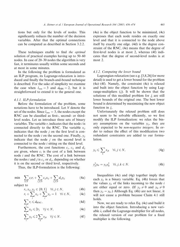
4.1.1. ILP-formulation
Before the formulation of the problem, some
notations have to be introduced. Let N denote the
set of the nodes. Since ltree ¼ 3, the nodes except the
RNC can be classified as first-, second- or third-
level nodes. Let us introduce three sets of binary
variables. The variable ri indicates that the node i isconnected directly to the RNC. The variable xijindicates that the node j on the first level is con-
nected to the node i on the second one. Finally, yijindicate that the node j on the second level is
connected to the node i sitting on the third level.
Furthermore, the cost functions ci, cij and dijare given, where ci is the cost of a link between
node i and the RNC. The cost of a link betweenthe nodes i and j is cij or dij, depending on whether
it is on the second or third level, respectively.
Thus, the ILP-formulation is the following:
minXi2N
ciri þXi;j2N
cijxij þXi;j2N
dijyij ð4aÞ
subject to
ri; xij; yij 2 f0; 1g 8i; j 2 N ; ð4bÞri þ
Xj
xij þXj
yij ¼ 1 8i 2 N ; ð4cÞXi
ri 6 dRNC; ð4dÞXi
xij 6 2rj 8j 2 N ; ð4eÞXi
yij 6 2X
xjk 8j 2 N : ð4fÞ
k(4a) is the object function to be minimized, (4c)
expresses that each node resides on exactly one
level and that it is connected to the node above
itself by exactly one edge. (4d) is the degree con-
straint of the RNC, (4e) means that the degree of
first-level nodes is at most 2, whereas (4f) indi-
cates that the degree of second-level nodes is at
most 2.
4.1.2. Computing the lower bound
Lagrangian-relaxation (see e.g. [3,8,26] for more
detail) is used to get a lower bound for the problem
(4a)–(4f). Namely, the constraint (4c) is relaxed
and built into the object function by using Lag-
range-multipliers (k). It will be shown that the
solutions of this modified problem for k are stilllower bounds of the original one. The best lower
bound is determined by maximizing the new object
function in k.Unfortunately the relaxed problem still does
not seem to be solvable efficiently, so we first
modify the ILP formalization: we relax the bin-
ary assumptions on the variables yij, they are
only expected to be non-negative integers. In or-der to reduce the effect of this modification two
redundant constraints are added to our formu-
lation.
yij 6Xk
xjk 8i; j 2 N ; ð4gÞ
y2jiyki ¼ yjiy2ki 8i; j; k 2 N : ð4hÞ
Inequalities (4c) and (4g) together imply that
each yij is a binary variable. Eq. (4h) forces that
the values yji of the links incoming to the node iare either equal or zero. (If yji 6¼ 0 and yki 6¼ 0
then yji ¼ yki.) Although Eq. (4h) are not linear, itwill not cause a problem because Claim 4.1 still
holds.
Now, we are ready to relax Eq. (4c) and build it
into the object function. Introducing a new vari-
able ki called the Lagrange-multiplier for all nodes,
the relaxed version of our problem for a fixed
multiplier is the following.

466 A. J€uttner et al. / European Journal of Operational Research 164 (2005) 456–474
LðkÞ :¼ minXi2N
ciri þXi;j2N
cijxij þXi;j2N
dijyij
þXi2N
ki ri
þXj2N
xij þXj2N
yij
!�Xi2N
ki;
ð5aÞri; xij 2 f0; 1g; yij 2 Z 8i; j 2 N ; ð5bÞyij P 0 8i; j 2 N ; ð5cÞXi
ri 6 dRNC; ð5dÞXi2N
xij 6 2rj 8j 2 N ; ð5eÞXi2N
yij 6 2Xk2N
xjk 8j 2 N ; ð5fÞ
yij 6Xk
xjk 8i; j; ð5gÞ
y2jiyki ¼ yjiy2ki 8i; j; k: ð5hÞ
In spite of the non-linear constraint (5h), the
following statement, which is well-known for the
linear case, still holds with the usual proof.
1 Note that we just relaxed the constraint that guarantees
that every node will be connected to another node or to the
RNC, so we can reach the cost Kk if none of them are
connected. Therefore LðkÞ should be possibly less than Kk.
Claim 4.1. For any vector k of the Lagrange mul-tipliers, LðkÞ is a lower bound of the original prob-lem.
Proof. Let rki , xkij, ykij be an optimal solution of
system (5b)–(5h) and r�i , x�ij, y�ij be an optimal
solution to system (4b)–(4f). Then
LðkÞ ¼Xi
cirki þXij
cijxkij þXij
dijykij
þXi
ki rki
þXj
xkij þXj
ykij � 1
!
6
Xi
cir�i þXij
cijx�ij þXij
dijy�ij
þXi
ki r�i
þXj
x�ij þXj
y�ij � 1
!
¼Xi
cir�i þXij
cijx�ij þXij
dijy�ij
proves the claim. h
An easy computation shows that the objectfunction (5a) is equal to
minXi
cki ri þXij
ckijxij þXij
dkijyij þ Kk; ð6Þ
where cki :¼ ci þ ki, ckij :¼ cij þ ki, d
kij :¼ dij þ ki and
Kk :¼ �P
i ki.
Claim 4.2. The optimal solution can be chosen insuch a way that there are at most two incomingedges with non-zero y variable for each node j 2 N .
Proof. Obviously, it is not worth setting the yijnon-zero if its cost is not less than zero. If there is
only one edge with negative cost then the best we
can do is to set the corresponding y variable toPk xjk, otherwise the best solution is to set the y
variables of the two edges having most negative
cost toP
k xjk. h
Now let us discuss the problem of computing
LðkÞ for a fixed k value. First let suppose that
dRNC ¼ 1. Observe that
• if the modified cost cki of a first-level node is neg-ative, 1 we connect it in order to minimize the
object function,• even if its modified cost is positive, it may be
advantageous to connect it, if we can link it
with two second-level nodes, so that the modi-
fied total cost of these three nodes is negative,
• finally, we can connect it if we find two second-
level nodes so that there are third-level nodes,
where the modified cost of the whole set of
nodes is negative.
This idea leads to the following algorithm.
(Note that here we work in the reverse direction.)
1. For each node j let i1 and i2 be the two nodes
for which the values dki1j and dk
i2j are the most
negative ones.
Let aj :¼ minf0; dki1jg þminf0; dk
i2jg.

A. J€uttner et al. / European Journal of Operational Research 164 (2005) 456–474 467
2. Again, for each node j let i1 and i2 be the two
nodes for which the values cki1j þ ai1 and
cki2j þ ai2 are the most negative ones.
Then let
bj :¼ minf0; cki1j þ ai1g þminf0; cki2j þ ai2g:
3. The cost of the optimal solution to problem
(5a)–(5h) is
LðkÞ :¼Xi
minf0; bi þ cki g þ Kk: ð7Þ
If dRNC < n the algorithm is the same except
that in (7) we have to sum only the dRNC smallest
(most negative) values of minf0; bi þ cki g.To obtain the best lower bound we have to look
for the vector k which maximizes the function
LðkÞ. That is, we are looking for the value
L� :¼ maxk
LðkÞ: ð8Þ
Since the function LðkÞ is concave (it can beseen from (5a) that LðkÞ is the minimum of some
k-linear functions), the well-known subgradient
method can be used to find its maximum. The
details are omitted, the reader can find a good
introduction to this method for example in
[3,4,8].
In order to be able to apply the branch-and-
bound method we need to solve a modified versionof this problem where the depth of some nodes is
predefined. Even this case can be handled easily,
because for example if the depth of a node i must
be equal to 2, then it means that the variables ri, yikand xki must be avoided for all k. This can be
performed by setting their corresponding costs to a
sufficiently large value. The other cases can be
handled similarly.It is also mentioned that if all node levels are
fixed, then the lower bound given by the previous
algorithm is tight, that is, it is actually equal to the
optimal solution to the problem (4a)–(4f). It fol-
lows from the fact that in this case the problem
reduces to two separate b-matching problems, for
which total unimodularity holds [24], so the opti-
mal object function value is equal to the value ofthe LP-relaxed version of the problem (4a)–(4f)
and in case of LP-programs the Lagrange-relaxa-tion gives the optimal solution.
4.1.3. Branch-and-bound
This section describes our implementation of
the branch-and-bound method. Readers who are
not familiar with this technique are referred to e.g.
[3,8,26].
A set system ðN1;N2;N3Þ is called partial level-
distribution if Ni � N , i 2 f1; 2; 3g are disjoint
subsets of the nodes. For this partial level-distri-
bution, let LN1;N2;N3 denote the computed
Lagrangian lower bound, when each node in Ni is
fixed on level i.The core of this method is the recursive proce-
dure called SingleTree, the input of which are the
subsets N1, N2, N3 and a bounding number B. Theprocedure either states that there is no solution
cheaper than B for this partial level-distribution or
it returns an optimal solution.
Of course, the optimal solution can be obtained
by calling SingleTree with the empty level-distri-
bution ð;; ;; ;Þ and B ¼ 1.
The procedure SingleTree works as follows
(Fig. 4). First, we choose a node j 2 N n ðN1 [ N2
[ N3Þ, we fix it onto every level and compute the
corresponding lower bounds, that is we determine
the values L1 ¼ LN1[j;N2;N3 , L2 ¼ LN1;N2[j;N3 and
L3 ¼ LN1;N2;N3[j . Then we examine these partial le-
vel-distributions in decreasing order according to
their lower bounds. For each level-distribution, if
the lower bound is less than B, we fix the node jon the corresponding level and call SingleTree withthe new Ni sets. If it returns a new solution, then
we update B with the cost of this solution and
repeat this with the other level-distributions. Fi-
nally, if some of these three calls of SingleTree
return a solution, we return the best one, else we
state that there is no solution with cost less than B.We also keep an eye on the number of nodes on
each level, and if the topological constraintsare not fulfilled, we go to the next step automati-
cally.
An easy modification of this method enables to
give an approximation algorithm to our problem.
The idea is to skip a possible partial fixing not only
if the lower bound is worse than the best solution
but also if they are close enough to each other.

Fig. 4. The SingleTree algorithm.
468 A. J€uttner et al. / European Journal of Operational Research 164 (2005) 456–474
Namely an error factor err is introduced and a
partial fixing is examined only if the corresponding
lower bound is less than 11þerr B. This ensures that
the resulted solution is worse at most by the factor
err than the optimum.
4.2. The local algorithm
The main idea of the algorithm is the principle
of ‘‘divide et impera’’. The heart of the algorithm
is the optimizer routine of the previous section
which is able to find the theoretical optimum for
small networks. So in each step we select a subset
of nodes, find the optimal solution for this sub-
problem and get near the global optimum itera-
tively.This idea is also motivated by the geometrical
fact that the connections of distant nodes do not
affect each other significantly, i.e. every node is
probably linked to a nearby one. Therefore it is a
good approximation of the optimum if the con-
nections of small subsets of close RBSs are deter-
mined independently.
The algorithm begins with an initial solution
and in every step it forms a group of RBSs (H ),
finds the optimal connections for H and ap-
proaches the global optimum by cyclical local
optimization. In Fig. 5 the result of the first step
can be seen. In the general step we choose the nextsubset according to a strategy described in Section
4.2.2 and make corrections to it. The algorithm
terminates if it could not improve the network
through a whole cycle.
This method is an effective implementation of
the so-called best local improvement method [1]. In
this problem the state space is the possible set of
connections. Two states A and B are adjacent, if wecan reach B from A by changing the connections
inside the set H . Note that this local search method
does not use elementary steps, it makes rather
complex improvement to the graph. Since the
typical size of H is 20–25 nodes, the number of

3
7
2
4
5
6
1
Fig. 6. The selection of H .
Fig. 5. The first step of the Local algorithm. In this example it
is assumed that dRNC is high enough to put every node in L1 in
the initial solution.
A. J€uttner et al. / European Journal of Operational Research 164 (2005) 456–474 469
possible connections inside H is about 1020, i.e.
each state has a huge number of adjacent states.
Therefore a local optimum can be reached fromevery state in few steps. The power of the algo-
rithm is that in spite of the large number of
neighbors the optimizer function chooses the best
one in each step.
4.2.1. Finding an initial solution
The algorithm can be utilized to improve the
solution given by a previous one, hence in this casethe starting solution is given. However, the algo-
rithm can also work independently, so it should be
capable of finding an initial solution satisfying the
conditions.
• The easiest way to do that is to put dRNC ran-
domly chosen RBSs in the set L1, dRNC � dRBS
randomly chosen ones in set L2, etc. This trivialsolution satisfies the constraints.
• A more sophisticated way to find an initial solu-
tion is the following: as described in Section
4.1.3 the core optimizer can be configured to re-
turn the theoretical optimum or work with a
predefined error rate (err). If err is high enough,
the optimization becomes very fast, but of
course less effective. So by setting the error ratehigh in the first cycle (i.e. until every RBS is at
least once picked in H ) we could quickly find
a considerably better starting solution than the
previously mentioned trivial one.
2 Of course the RNC is always in H .
4.2.2. Selection of HIn each step of the algorithm a new set H is
selected and given as input for the optimizer. On
the one hand, H should consist of close RBSs, on
the other hand, it should contain whole subtrees
only 2, each rooting in a first-level RBS. This is
important because during optimization the con-nections in H will be changed, so otherwise it
would be possible to make unconnected RBSs.
To satisfy these conditions we select adjacent
subtrees of the current network rooting in a first-
level node until a predefined upper bound (hmax)
for the size of H has been reached. The first-level
RBSs are ordered according to their location
(clockwise around the RNC). An example for sucha selection can be seen in Fig. 6. The selection
starts in every step with another first-level node,
which guarantees the variety of H .
Since the core optimizer solves an NP-hard
problem, its speed is very sensitive to the size of its
input, i.e. jH j. Choosing the parameter hmax at the
beginning of the algorithm, we can set an upper
bound for jH j. Of course the higher jH j is, thebetter the result will be, but the slower the algo-
rithm becomes.
5. Numerical results
In our empirical tests we used the TreePlan
algorithm [13,14] as a reference method since toour knowledge this is the only method in the

Table 3
Results of the Global algorithm with different dRNC values
n dRNC Cost Time
700 100 30,658 21 minutes
03 seconds
700 50 30,658 18 minutes
38 seconds
700 25 30,737 18 minutes
37 seconds
700 10 31,506 19 minutes
24 seconds
700 5 36,956 17 minutes
16 seconds
700 3 45,263 15 minutes
13 seconds
700 2 56,437 14 minutes
21 seconds
700 1 80,860 15 minutes
25 seconds
470 A. J€uttner et al. / European Journal of Operational Research 164 (2005) 456–474
literature that is able to solve problems similar toours.
First the Global algorithm was executed on
several test cases, then in a second phase the Local
algorithm was used to improve the results of the
Global algorithm. (Note that the Local algorithm
can also be used to re-design the trees of any
planning algorithms, e.g. the Global algorithm.)
Both results were compared with TreePlan.Although our algorithms can work with arbi-
trary parameters, the values dRBS ¼ 2 and ltree ¼ 3
are fixed in our test cases, for these values are
currently accepted in the UMTS architecture. The
cost of an RNC node, costRNC was set to 500
during all tests, and length proportional link cost
function was used. In order to be able to compare
the numerical results to those of TreePlan, dRNC
was set to 1 in the comparative test cases. After
these we present some tests on the Global algo-
rithm with different dRNC values.
The Global algorithm terminates if there is no
new state accepted during a predefined number of
iterations (K) in the simulated annealing. This
frees the tester to explicitly set the number of
iterations in the simulated annealing for differentinitial temperature and decreasing factor values. In
the following results the decreasing factor fact was
set to 0.9995, the initial temperature T0 was 20,000and K was set to 2000.
The results of our tests can be seen in Table 2.
The first column is the size of the network, then the
total network cost planned by TreePlan and by the
Global algorithm is compared. The fourth columncontains the number of iterations made by the
Global algorithm. In the sixth column the
improvement of the Local algorithm on the Global
Table 2
Results of the algorithms (with dRNC ¼ 1) compared with TreePlan
n TreePlan Global Iteration G
T
100 4736 4363 19,880 7.
200 9048 8757 20,905 3.
300 13,534 13,274 20,879 2.
400 18,389 18,040 19,439 1.
500 23,037 21,943 22,772 4.
600 27,533 26,662 29,872 3.
1000 45,686 43,916 28,596 3.
algorithm can be seen, and finally the totalimprovement vs. TreePlan.
In all of the test cases the Global algorithm
alone can reduce the cost of the UMTS network;
moreover the Local algorithm was able to make
further improvements on the trees in every test.
The size of these trees varied from 35 to 200,
showing that the Local algorithm is appropriate
for practical sized problems. As we expected thebest results can be found by the combination of the
two new methods, which gave an improvement of
6–7%, in extreme cases even of 12% compared to
the former approach, TreePlan.
Table 3 contains the cost of the same network
of size 700 with different dRNC values planned by
the Global algorithm. Naturally the cost of the
network should be monotonously increasing withthe decrease of dRNC, as the search space is more
lobal vs.
reePlan (%)
Global+Local Global+Local vs.
TreePlan (%)
9 4168 12.0
2 8485 6.2
0 12,747 5.8
9 17,005 7.5
7 21,293 7.6
2 25,759 6.4
9 42,645 6.7

0
50
100
150
200
250
300
350
100 200 300 400 500 600 700 800 900 1000 1100
t(m
s)
n
time/iterationf(n)
Fig. 7. The circles indicate the execution times of a single
iteration of the Global algorithm. The dotted line shows the
function f ðnÞ ¼ 5:588� 10�5 � n2:24.
Table 4
The percentage of the difference between the lower bound and
the result of the Local algorithm
n AVG (%) MIN (%) MAX (%)
25 2.60 1.01 8.04
50 5.88 4.35 7.65
75 5.42 3.79 8.55
100 6.44 5.35 8.36
150 6.87 5.89 8.35
200 6.79 5.87 7.83
Table 5
Comparing the Local algorithm with hmax ¼ 21 to the optimum
for small inputs
N Optimum Local algorithm
40 1190.8 1190.8
40 1244.9 1244.9
40 1232.3 1232.3
40 1209.9 1216.3
50 1668.0 1677.1
A. J€uttner et al. / European Journal of Operational Research 164 (2005) 456–474 471
constrained. The results clearly reflect this char-
acteristic.
The execution times of the Global algorithm ona 400 MHz PC under SuSe Linux 7.1 can be seen
in Fig. 7. (On the x-axis the number of nodes, on
the y-axis the execution time of an iteration in
milliseconds can be seen.) The figure indicates that
the running time is approx. Oðn2:24Þ. Since the b-matching algorithm is an Oðn3Þ method, the
acceleration of the algorithm in Section 3.2.3 is
significant. Note that just scanning the input re-quires Oðn2Þ time.
The number of iterations highly depends on the
initial parameters and the termination criterion of
the Simulated Annealing. In case of the above tests
the number of iterations was in the range of 20–
30.000. Of course, our algorithms are slower than
the former approach according to the more com-
plex computation. However, in a typical networkdesign process one would run the planning algo-
rithm a couple of times only, hence an execution
time of about 2.5 hours for a network with 1000
nodes (which is the size of usual UMTS networks)
should be acceptable.
We also tested the Local algorithm separately.
The subgradient method applied in the tests was as
in e.g. [8]. Our objective was to estimate the dif-ference of the results of the Local algorithm and
the optimum. Therefore we calculated the lower
bound of several test instances as described in
Section 4.1.2 and compared it to the result of the
Local algorithm. We considered four problem sizeseach with 10 different networks. Table 4 presents
the average/minimum/maximum difference be-
tween the lower bound and the Local algorithm
with hmax ¼ 24. This means, that the Local algo-
rithm gives around 5–7% approximation of the
optimum value in average for practical examples
of 25–200 nodes.
Following test shows, that in small problemsthe actual difference is even smaller. Namely one
may sets hmax to n to get the global optimum. This
is of course feasible for smaller n values only.
Table 5 shows the results of comparing the Local
algorithm with hmax ¼ 21 with the optimum value
– also computed with the Local algorithm with
hmax ¼ n. The table shows four different networks
with 40 nodes and one network with 50 nodes. Onecan clearly see that for small inputs the Local
algorithm gives almost always optimum.
The local algorithm can also handle the dRNC
constraint, however this has only theoretical
importance. Since the input of the Local algorithm
is only one RNC, the
dRNC PnPltree�1
i¼0 diRBS
& ’
472 A. J€uttner et al. / European Journal of Operational Research 164 (2005) 456–474
must hold (here the denominator equals to the
maximum number of nodes in a subtree rooting in
a first-level node). The Local algorithm without an
RNC degree constraint plans a network with RNC
degree just slightly above the lower bound. For
instance in a network of 100 nodes (with dRBS ¼ 2,
ltree ¼ 3) dRNC P 15 must hold, and the Local
algorithm without any RNC degree constraintreturns a network with RNC degree equals to 16.
6. Conclusion
In this paper two new algorithms were intro-
duced for planning UMTS access networks. The
first one––relying on a combination of the Simu-lated Annealing heuristic and a specific b-matching
problem––plans global UMTS access networks,
the second one––which uses Lagrangian lower
bound with branch-and-bound––is able to plan a
single tree or make corrections to existing UMTS
trees. It has been also demonstrated by a number
of test cases how these methods can reduce the
total cost of UMTS networks.Nevertheless, some basic simplifications con-
cerning the capacity dependent part of the cost
functions were proposed. The more proper con-
sideration of this cost factor of UMTS access
networks is the next direction of further research.
RNC
Acknowledgements
The authors would like to thank to Zolt�anKir�aly for his useful ideas and also to Tibor Cin-
kler, Andr�as Frank, G�aborMagyar, �Aron Szentesi,
Bal�azs Szviatovszki and the anonymous referees
for their valuable suggestions and comments.
ai ci
ei
f i
bi di
1
Xi
H
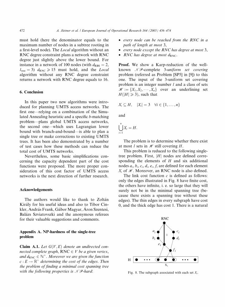
Fig. 8. The subgraph associated with each set Xi.
Appendix A. NP-hardness of the single-tree
problem
Claim A.1. Let GðV ;EÞ denote an undirected con-nected complete graph, RNC 2 V be a given vertex,and dRNC 2 Nþ. Moreover we are given the functionc : E ! Rþ determining the cost of the edges. Thenthe problem of finding a minimal cost spanning treewith the following properties is NP-hard:
• every node can be reached from the RNC in apath of length at most 3,
• every node except the RNC has degree at most 3,• RNC has degree at most dRNC.
Proof. We show a Karp-reduction of the well-
known NP-complete 3-uniform set coveringproblem (referred as Problem [SP5] in [9]) to thisone. The input of the 3-uniform set covering
problem is an integer number l and a class of sets
H :¼ fX1;X2; � � � ;Xng over an underlining set
HðjH jP 3Þ, such that
Xi � H ; jXij ¼ 3 8i 2 f1; . . . ; ng
and
[ni¼1
Xi ¼ H :
The problem is to determine whether there exist
at most l sets in H still covering H .
This problem is reduced to the following single-
tree problem. First, jH j nodes are defined corre-
sponding the elements of H and six additionalnodes ai, bi, ci, di, ei, fi are defined for each element
Xi of H. Moreover, an RNC node is also defined.
The link cost function c is defined as follows:
only the edges illustrated in Fig. 8 have finite cost,
the others have infinite, i. e. so large that they will
surely not be in the minimal spanning tree (be-
cause there exists a spanning tree without these
edges). The thin edges in every subgraph have cost0, and the thick edge has cost 1. There is a natural

Fig. 9. Spanning tree with cost r. (a) The part of the spanning tree belonging to the Xi sets not in the minimal covering set. The cost is 0.
(b) The part of the spanning tree belonging to the Xi sets in the minimal covering set. The cost is 1.
A. J€uttner et al. / European Journal of Operational Research 164 (2005) 456–474 473
one to one mapping between the sets Xi and the
thick edges. Obviously the cost of a spanning tree
in G arises only from thick edges, i.e. it is always
an integer number.
It is going to be shown that the cost of the
minimal cost spanning tree satisfying the abovecriteria is equal to the minimal number of sets
covering H completely.
A trivial observation is, that every path of
length at most 3 between a vertex v 2 H and the
RNC must contain exactly one thick edge. Fur-
thermore, through a particular thick edge at most
the vertices of its set Xi can be reached through
paths of length at most three. As a consequence ofthese, the sets corresponding to the thick edges of a
given feasible tree will cover all vertices in H .
On the other hand, let us suppose that
Xi1 [ Xi2 [ � � �Xir ¼ H . To prove the other direc-
tion, we show a spanning tree with cost r. In each
subgraph belonging to a set Xi a subtree is con-
structed according to Fig. 9(a) or (b) with cost 0 or
1 depending on whether the set Xi is among thecovering ones.
The union of these subtrees covers every vertex
in G, since the covering set covers every vertex in Hand the V n H vertices are covered by the subtrees
in both cases. It may happens that this union
contains cycles, but by simply neglecting the
superfluous edges a spanning tree is obtained with
cost at most r. h
References
[1] E Aarts, J.K. Lenstra, Local Search in Combinatorial
Optimization, John Wiley & Sons, Inc., 1997.
[2] N.R. Achuthan, L. Caccetta, J.F. Geelen, Algorithms for
the minimum weight spanning tree with bounded diameter
problem, Optimization: Techniques and Applications
(1992) 297–304.
[3] R.K. Ahuja, T.L. Magnanti, J.B. Orlin, Network Flows,
Prentice Hall, 1993.
[4] M.S. Bazaraa, H.D. Sherali, C.M. Shetty, Nonlinear
Programming––Theory and Algorithms, John Wiley &
Sons, Inc., 1993.
[5] P. Chardaire, Upper and lower bounds for the two-level
simple plant location problem, Annals of Operations
Research (1998).
[6] W.J. Cook, W. H. Cunningham, W. Puleyblank, A.
Schrijver, Combinatorial Optimization, Wiley-Interscience
Series in Discrete Mathematics and Optimization.
[7] ILOG CPLEX 7.1 User�s Manual, ILOG, 2001.
[8] M.S. Daskin, Network and Discrete Location, John Wiley
& Sons, Inc., 1995.
[9] M.R. Garey, D.S. Johnson, Computers and Intractabil-
ity––A Guide to the Theory of NP-Completeness, W.H.
Freeman and Company, New York, 1979.
[10] B. Gavish, Topological design of telecommunication net-
works––local access design methods, Annals of Operations
Research 33 (1991) 17–71.
[11] A. Girard, B. Sanso, L. Dadjo, A tabu search algorithm for
access network design, Annals of Operations Research 106
(2001) 229–262.
[12] F. Glover, Tabu Search––part I and II, ORSA Journal on
Computing 1 (3) (1989), and 2 (1) (1990).
[13] J. Harmatos, A. J€uttner, �A. Szentesi, Cost-Based UMTS
Transport Network Topology Optimization, ICCC 99,
Japan, Tokyo, September, 1999.

474 A. J€uttner et al. / European Journal of Operational Research 164 (2005) 456–474
[14] J. Harmatos, �A. Szentesi, I. G�odor, Planning of Tree-
Topology UMTS Terrestrial Access Networks, PIMRC
2000, England, London, September 18–21.
[15] P. Kallenberg, Optimization of the Fixed Part GSM
Networks Using Simulated Annealing, Networks 98,
Sorrento, October 1998.
[16] S. Kirkpatrick, C.D. Gelatt Jr., M.P. Vecchi, Optimization
by simulated annealing, Science 220 (1983) 671–680.
[17] J.G. Klincewicz, Hub location in backbone/tributary net-
work design: A review, Location Science 6 (1998) 307–335.
[18] N. Deo, N. Kumar, Constrained spanning tree problems,
in: Approximate Methods and Parallel Computation in
Network Design: Connectivity and Facilities Location,
DIMACS Workshop April 28–30, 1997, pp. 191–219.
[19] N. Deo, N. Kumar, Computation of constrained spanning
trees: A unified approach, in: P.M. Pardalos, D.W. Hearn,
W.W. Hager (Eds.), Network Optimization, Springer-
Verlag, 1997.
[20] Z. Drezner (Ed.), Facility Location: A Survey of Applica-
tions and Methods, Springer-Verlag, 1995.
[21] B.G. Marchent, Third Generation Mobile Systems for the
Support of Mobile Multimedia based on ATM Transport,
tutorial presentation, 5th IFIP Workshop, Ilkley, July
1997.
[22] T. Ojanper€a, R. Prasad, Wideband CDMA for Third
Generation Mobile Communication, Artech House Pub-
lishers, 1998.
[23] G.M. Schneider, M.N. Zastrow, An algorithm for design
of multilevel concentrator networks, Computer Networks
6 (1982) 1–11.
[24] A. Schrijver, Theory of Linear and Integer Programming,
John Wiley & Sons, Inc., 1998.
[25] The Path towards UMTS––Technologies for the Informa-
tion Society, UMTS Forum, 1998.
[26] L.A. Wolsey, Integer Programming, John Wiley & Sons,
Inc., 1998.


![A Performance Comparison of Wireless Multi-Hop Network ... · formulation of topology control algorithms to ensure optimum network connectivity [5, 6, 7]. The topology control algorithms](https://static.fdocuments.in/doc/165x107/5f0551777e708231d4125ebb/a-performance-comparison-of-wireless-multi-hop-network-formulation-of-topology.jpg)


![Algorithms for Fault-Tolerant Topology in Heterogeneous ...jie/hra_tpds[1].pdfAlgorithms for Fault-Tolerant Topology in Heterogeneous Wireless Sensor Networks ∗ Mihaela Cardei, Shuhui](https://static.fdocuments.in/doc/165x107/6001e33d2ef182623963a619/algorithms-for-fault-tolerant-topology-in-heterogeneous-jiehratpds1pdf.jpg)

